Broader Benefits of Infrastructure - final

1

THE BROADER BENEFITS OF TRANSPORTATION INFRASTUCTURE

Ian Sue Wing, William P. Anderson and T.R. Lakshmanan Boston University Center for Transportation Studies

Abstract

Assessments of the economic benefits of transportation infrastructure investments are critical to good policy decisions. At present, most such assessments are based of two types of studies: micro-scale studies in the form of cost-benefit analysis (CBA) and macro-scale studies in the form of national or regional econometric analysis. While the former type takes a partial equilibrium perspective and may therefore miss broader economic benefits, the latter type is too widely focused to provide much guidance concerning specific infrastructure projects or programs. Intermediate (meso-scale) analytical frameworks, which are both specific with respect to the infrastructure improvement in question and comprehensive in terms of the range of economic impacts they represent, are needed. This paper contributes to the development of meso-scale analysis via the specification of a computable general equilibrium (CGE) model that can assess the broad economic impact of improvements in transportation infrastructure networks. The model builds on recent CGE formulations that seek to capture the productivity penalty on firms and the utility penalty on households imposed by congestion (Meyers and Proost, 1997; Conrad, 1997) and others that model congestion via the device of explicit household time budgets (Parry and Bento, 2001, 2002). The centerpiece of our approach is a representation of the process through which markets for non-transport commodities and labor create derived demands for freight, shopping and commuting trips. Congestion, which arises due to a mismatch between the derived demand for trips and infrastructure capacity, is modeled as increased travel time along individual network links. Increased travel time impinges on the time budgets of households and reduces the ability of transportation service firms to provide trips using given levels of inputs. These effects translate into changes in productivity, labor supply, prices and income. A complete algebraic specification of the model is provided, along with details of implementation and a discussion of data resources needed for model calibration and application in policy analysis.

1. INTRODUCTION

Most contemporary assessments of the economic effects of transportation infrastructure

investments fall into two major categories, one at the micro-scale and the other at the macro-scale. Micro-

scale assessments follow the procedures of cost-benefit analysis (CBA). They use information on the

likely outcomes of a proposed project – its effect on travel times, traffic flows, emissions, accidents, etc. –

to estimate a pecuniary value of its lifetime benefit. That benefit estimate is then contrasted with lifetime

2

project costs to determine whether it is economically productive. Such ex ante analyses are often required

as a justification for devoting public funds to a proposed project. (For a review see Mackie and Nellthorp,

2001.)

Macro-scale studies include econometric analyses that relate the aggregate investment in (or stock

of) transportation infrastructure to economy-wide measures of economic performance. For the most part,

they specify production or cost functions in which public infrastructure is regarded as an input to

production by private firms in a region or nation. The estimated production and cost functions provide

evidence of the contribution that infrastructure investment makes towards augmenting the productivity of

private firms and, in some cases, make it possible to calculate a rate of return on aggregate infrastructure

investment. (For a review see Lakshmanan and Anderson, 2002.)

The two approaches are complementary. Micro-scale analyses have the advantage of being able

to measure the impacts of adding or improving a specific infrastructure element, but the scope of their

economic assessment is limited to effects on users of the element in question or closely related elements

and to firms and individuals in its immediate locale. The macro-scale analyses capture a broader range of

economic impacts, but they treat infrastructure investment as a homogenous good (measured in dollars or

network miles.) and are therefore of little use for assessing the worth of specific investments. Further, the

macro-scale approach sheds little, if any, light on the mechanisms that drive the observed economic

impacts.

To provide a more complete picture of the economic impacts of infrastruture, an intermediate

level of analysis is needed. For convenience, we refer to this level as “meso-scale,” although models in

this category might be applied at a variety of geographical scales. We define three requisites for models

in this class.

1. Unlike macro-scale analyses they should incorporate information about specific additions or

improvements to transportation infrastructure networks (although not necessarily at the level of detail

found in micro-scale analyses.)

3

2. They should trace the economic processes that are triggered by infrastructure improvements. (As we

will explain below, these may take the form of static general equilibrium effects or dynamic

developmental effects.)

3. Finally, in order to assess the relative magnitude of different economic mechanisms and to inform

policy, they should be amenable to empirical implementation using data that are either available or

obtainable at reasonable cost.

As a contribution toward the development of meso-scale analyses, we introduce a computable

general equilibrium (CGE) model that incorporates a number of novel mechanisms for tracing the effects

of additions to the capacity of a transport network through the broader economy. Infrastructure

investments are modeled as reducing travel times over links in a network. The key novelty is to

incorporate travel time explicitly in the utility and profit maximization problems of households and firms.

For households, travel time for commuting and consumption activities enters a time budget that also

includes time devoted to work and leisure. For firms providing transportation services, travel time affects

the number of trips that can be provided by a given stock of vehicles, which in turn affects the prices of

intermediate and final goods.

The remainder of the paper is organized as follows. Sections 2 and 3 discuss the broad economic

impacts of transportation infrastructure and the state of the art in assessing those impacts. Section 4

reviews the relatively brief literature on assessing economic impacts of infrastructure investment with a

CGE framework. Section 5 constitutes the meat of the paper, presenting an overview of our model, a

complete algebraic specification, details of implementation and a discussion of data needs. Section 6

provides a discussion and summary.

2. CONTEXT: THE BROADER ECONOMIC IMPACTS OF INFRASTRUCTURE INVESTMENT

4

The role of transportation infrastructure in the economy is multifaceted and plays out over a long period

of time. It is unlikely that any modeling framework can capture all possible mechanisms. For our purpose,

it is useful to make a distinction between two classes of economic impacts, which we call static general

equilibrium impacts and dynamic developmental impacts. Static general equilibrium impacts comprise a

broad range of effects coursing through the economy consequent on the time and monetary savings

induced by the infrastructure improvements. Such temporal and monetary savings alter, in turn, the

marginal costs of transport producers, individuals’ mobility and the demand for goods and services in the

context of lowered congestion. As these changes ripple through the market mechanisms, endogenous

changes occur in employment, output, and incomes. Dynamic developmental impacts ensue from the

mechanisms set in motion when transport infrastructure improvements activate a variety of interacting

processes that yield over time many sectoral, spatial, and regional effects which augment productivity.

They produce transformations in the structure and pattern of the economy – such as changes in the spatial

pattern of production; creation of new industries and inter-industry linkages; changes in the lifestyles and

preferences of households; and the evolution of institutions and markets. While static general equilibrium

impacts arise from the actions of a well-defined set of economic agents through the medium of markets,

dynamic developmental impacts involve complex interactions of economic, social, cultural and

institutional factors and are more idiosyncratic in nature. We therefore attempt to capture only the former

category of impacts in the CGE model.

General equilibrium effects occur within a system of market relationships that is stable and

relatively well understood. Most economic activities require some movement of goods and people.

Production requires the movement of intermediate inputs to the production site, the movement of workers

back and forth between their homes and places of employment (commuting) and the movement of

finished goods to market. Consumption activities also require movement as in the case of household trips

for shopping and recreation. To the extent that improvements to transportation infrastructure reduce the

cost of movement of goods and people, they affect the levels of economic activity in all parts of the

economy.

5

A number of general equilibrium mechanisms are described in detail below. But for the purpose

of illustration, consider the effect of infrastructure on employment. Most transportation analyses start with

the explicit or implicit assumption that the number of people who commute to work over a given network

is fixed. In an economy like the US, however, labor supply is by no means perfectly inelastic because

significant segments of the population, such as mothers with children and individuals past the normal

retirement age, face decisions as to whether to enter or remain in the labor force. Labor supply is normally

associated with the wage, but since commuting represents a significant cost of labor force participation,

infrastructure improvements could entice more people to work. Of course, in a general equilibrium

framework this would represent a shift in the labor supply function, which in turn would affect the

equilibrium wage and employment level.

A peculiar aspect of transportation infrastructure investments is that the cost reductions they

generate are often realized in time savings rather than monetary savings. Returning to the commuting

example, a road expansion that relieves congestion might have a minor effect on a commuter’s out of

pocket cost (e.g. lower fuel costs due to efficiency improvements that stem from changes in the driving

cycle) but a major effect on commuting time. Time is a scarce resource for any potential worker, so less

time spent commuting means more time is available for work, leisure, consumption activities, childcare,

etc. Thus, in assessing the general equilibrium impacts of transportation infrastructure, the household time

budget is as important as the household expenditure budget. Depending on the magnitude of the wage

relative to the marginal utility of leisure, the impact of the decrease in commuters’ time costs on the labor

supply may be larger than that of their pecuniary savings.

A general equilibrium perspective on transportation infrastructure recognizes that reductions in

the pecuniary and time costs of transportation can lead to increases in the levels of various economic

activities and thereby to increased derived demand for transportation services. Thus, induced traffic flows

are a natural outcome of market mechanisms. To many transportation analyses, such flows are seen as

negating benefits from transportation infrastructure. A project whose congestion reduction effect

disappears due to increased traffic within a few years of its implementation is seen as a failure. This point

6

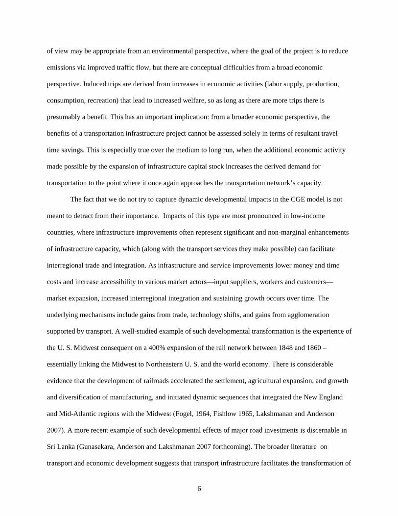
of view may be appropriate from an environmental perspective, where the goal of the project is to reduce

emissions via improved traffic flow, but there are conceptual difficulties from a broad economic

perspective. Induced trips are derived from increases in economic activities (labor supply, production,

consumption, recreation) that lead to increased welfare, so as long as there are more trips there is

presumably a benefit. This has an important implication: from a broader economic perspective, the

benefits of a transportation infrastructure project cannot be assessed solely in terms of resultant travel

time savings. This is especially true over the medium to long run, when the additional economic activity

made possible by the expansion of infrastructure capital stock increases the derived demand for

transportation to the point where it once again approaches the transportation network’s capacity.

The fact that we do not try to capture dynamic developmental impacts in the CGE model is not

meant to detract from their importance. Impacts of this type are most pronounced in low-income

countries, where infrastructure improvements often represent significant and non-marginal enhancements

of infrastructure capacity, which (along with the transport services they make possible) can facilitate

interregional trade and integration. As infrastructure and service improvements lower money and time

costs and increase accessibility to various market actors—input suppliers, workers and customers—

market expansion, increased interregional integration and sustaining growth occurs over time. The

underlying mechanisms include gains from trade, technology shifts, and gains from agglomeration

supported by transport. A well-studied example of such developmental transformation is the experience of

the U. S. Midwest consequent on a 400% expansion of the rail network between 1848 and 1860 –

essentially linking the Midwest to Northeastern U. S. and the world economy. There is considerable

evidence that the development of railroads accelerated the settlement, agricultural expansion, and growth

and diversification of manufacturing, and initiated dynamic sequences that integrated the New England

and Mid-Atlantic regions with the Midwest (Fogel, 1964, Fishlow 1965, Lakshmanan and Anderson

2007). A more recent example of such developmental effects of major road investments is discernable in

Sri Lanka (Gunasekara, Anderson and Lakshmanan 2007 forthcoming). The broader literature on

transport and economic development suggests that transport infrastructure facilitates the transformation of

7

low-income economies from subsistence to commercial agriculture, the development of basic, transport-

intensive industries and the growth of cites (Haynes and Button, 2001).

It would be a mistake to think that developmental impacts occur only at an early stage of

economic development. Even in a mature economy, transportation infrastructure improvements might

promote structural changes such as increased decentralization or agglomeration of economic activity;

changes in the way business enterprises conduct operations such as inventory management, logistics and

other practices; enhanced opportunities for face-to-face interaction; and a range of new recreational

opportunities (Anderson and Lakshmanan, 2007.) These impacts, which affect the long-term evolution of

the economy, are difficult to measure and even more difficult to predict. Nevertheless they are important,

and a better understanding of developmental effects should lead to better decision-making on

transportation infrastructure.

3. CONVENTIONAL METHODS OF IMPACT ASSESSMENT

As we have stated earlier, current methods of impact assessment include the micro-scale CBA

and macro-scale econometric studies. CBA is nearly universal as a means of assessing the desirability of

specific projects. Conceptually, economic benefits are assessed as the consumer surplus, defined in

relation to the demand curve for the infrastructure facility in question. The effect of the infrastructure

improvement is represented as a rightward shift in the infrastructure supply curve, which results in a fall

in the price of using the facility—usually defined in units of time as opposed to money—for any given

level of demand. The associated economic benefit thus has two components: one based on the cost

savings enjoyed by the number of travelers who used the facility prior to the improvement, and a second

representing the benefits to new travelers who now choose to use the facility because of its lower price.

8

Since the benefit is calculated in terms of time savings, it is necessary to apply a value of time to

recast the total benefit in monetary terms so that it can be compared against the project’s cost. Benefits

may also be adjusted for the value of environmental externalities and traffic accidents. Since benefits

accrue annually over the lifetime of the facility and most costs are incurred at the beginning of its

lifetime, present values of the flows of benefits and costs are calculated to make them comparable.

In practice, the result of CBA can be highly sensitive to the assumed value of time and discount

rates. If these values are accurate, however, the beauty of CBA lies in the theoretical argument that

consumer surplus, which is a measure of travelers willingness-to-pay, captures the full range of economic

benefits.1 For example, other measurable benefits, such as property appreciation near the improved

facility, are chiefly outcomes of reduced travel time so including them in benefit calculation constitutes

double-counting (Forkenbrock and Foster, 1990).

Even proponents of CBA concede that there are broader economic impacts that are not captured,

but argue that the magnitude of these impacts for any particular project is probably small (Mackie and

Nellthorp, 2001). But such impacts summed across a number projects may be substantial, which suggests

that CBA is more appropriate for assessing individual projects than for assessing a program of

infrastructure spending. As an indication that certain broader impacts are excluded from CBA results,

notice that economic benefits are measured almost exclusively in terms of time savings. As we noted

earlier, general equilibrium benefits can accrue even in the absence of time savings.

To the extent that an infrastructure spending program significantly influences relative prices, its

effects are likely to be felt in markets that are removed from those under the narrow consideration of

micro-level CBA. (e.g., consider the impacts on West-coast commodity markets of a significant

infrastructure investment at the Port of Long Beach.) In such cases, analysis which (i) ignores changes in

prices by treating the latter as strictly exogenous and (ii) considers only those impacts which are spatially

or temporally proximate—or confined to transportation or related sectors—may well fail to fully account

1 The theoretical justification rests on the assumption of perfect competition. Venables and Gasiorek (1999) develop a theoretical framework for assessing impacts under the assumption of monopolistic competition.

9

for the benefits of the investment in question. In traditional CBA the issue boils down to the conditions

under which the value of time is a theoretically valid measure of for the monetary impacts of these myriad

inter-market adjustments, and the extent to which these conditions are likely to be satisfied in practice.

Macro-scale assessments of the economic impact of productivity analysis generally take the form

of production and cost functions in which transportation infrastructure is included as an argument on the

right-hand-side. (For a review see Lakshmanan and Anderson, 2002.) Despite their rigorous grounding in

economic theory, there is a “black-box” quality about them because public capital does not function like

private capital in the production technology. For example, no firm has exclusive use of a highway, and for

any firm one might consider, there are large segments of the highway network that it does not use at all.

Still, a firm might benefit from a highway that it does not use directly via the indirect means of reduced

input costs. Clearly the mechanisms by which private productivity is enhanced by transportation

infrastructure are varied and complex. Thus, a positive output elasticity tells us that some economic

benefit is occurring, but sheds little light on the underlying mechanisms (Anderson and Lakshmanan,

2007). In particular, it is often very difficult to discern how much of the observed impact is due to

developmental as opposed to general equilibrium influences.

A further limitation of macro-level studies is that they treat transportation infrastructure as a

homogeneous good that can be measured in dollar terms. Such a measurement has some validity in the

case of private capital, because it is not unreasonable to assume that the value of a capital good reflects its

competitively determined marginal revenue product. In the case of transportation infrastructure, which is

allocated via mechanisms that are likely to emphasize distributional goals or political expediency over

economic efficiency, such an assumption is questionable. It is highly likely that investments of some

types and in some locations are more productive than others.

In short, the results of macro-studies point to an important relationship between public capital and

private productivity, but provide little in the way of either explanation or policy guidance.

10

4. A REVIEW OF GENERAL EQUILIBRIUM ANALYSES OF CONGESTION

We focus our attention on two sets of simulation studies, which develop models of the interplay

between infrastructure and congestion at the level of the aggregate economy. The first, by Mayeres and

Proost (1997), Conrad, 1997 and Conrad and Heng (2000), define an explicit index of congestion (Z),

modeled a function of the level of utilization of aggregate transportation infrastructure or capacity, where

the latter is expressed in terms of either aggregate transport activity or the size of the vehicle capital stock.

Congestion incurs a productivity penalty on firms and a utility penalty on consumers. The former

manifests itself through the reduced speed with which firms are able to ship their goods to market, while

the latter does do via the diminished quality of transport services consumed by households. The second

set of studies (Parry and Bento, 2001; 2002) model congestion through the device of an explicit

household time budget. Increases in travel times with the expansion of transport activity cause a reduction

in labor supply and the consumption of both leisure and services of transport producers.

Mayeres and Proost (1997) construct a stylized applied general equilibrium model which captures

the essence of the congestion problem without simulating the process by which infrastructure spending

affects the value of time. They consider a simple economy made up of a utility-maximizing representative

household and two representative firms, summarized algebraically as follows:

, , ,max ( , ; )

P

PC q R

U C Z qξ−Λ

Λ (MP1)

subject to:

1 1, )(P FC q R Z f h qϖ−+ + ≤ (MP2)

qF = f2(h2) (MP3)

1 2h h H+ Λ≤+ (MP4)

1.51/[1 ( ) /( )]P FZ q q CAP R= − + + (MP5)

11

In eq. (MP1) the household derives utility (U) from consumption of a final good (C), passenger

transport (qP) and leisure (Λ). Eq. (MP2) says that firm 1 combines inputs of labor (h1) and freight

transportation (qF) according to the production function f1 to produce the final good, which may be

consumed directly, allocated to passenger transport services, or used to create new transport infrastructure

(R). Firm 2 produces freight transportation services from labor (h2) according to the production function f2

in (MP3), and the household’s labor endowment (H) constrains labor-leisure choice in (MP4): Eq. (MP5)

specifies how the imbalance between aggregate transport activity and infrastructure capacity (CAP) gives

rise to congestion according to a capacity restraint function based on Evans (1992). In turn, Z adversely

influences both the productivity of the final goods producer and the quality of passenger transport enjoyed

by the household, according to the elasticities ξ and ϖ, respectively. Infrastructure investment alleviates

congestion by expanding transit capacity, though at the cost of reduced consumption.

Conrad (1997) and Conrad and Heng (2002) apply these ideas in the context of a large-scale

recursive-dynamic CGE model (GEM-E3). They elaborate the mechanisms underlying eq. (MP5) by

developing an explicit model of the influence of aggregate infrastructure on the utilization of vehicle

capital stocks. Their economy is made up of a representative utility-maximizing household and j = 1, ...,

J, Tr firms, where firm Tr is a producer of transportation services. Firms’ capital stocks are partitioned

into intersectorally mobile “jelly” capital (kj) and transportation capital (ktj), which represents vehicles

and is a fixed factor. In the simplest version of their model the aggregate quantity of transportation

infrastructure (KI) is constant, and its divergence from the socially optimal level (KI*) is responsible for

congestion which reduces the productivity of kt:

1max ( ,..., ; )j

J TrC

U C C Z Cξ− (CH1)

subject to

, 1, ,( , ..., ; , , )e

v j j j I j j j jv

X C f X X h k kt+ ≤∑ (CH2)

e

j jkt kt Z ϖ−= (CH3)

12

0 exp( / )j jkt kt a KI−= (CH4)

*

1 1exp j

j

Z aKI KI

ω= − − ∑ , 1j

j

ω =∑ (CH5)

jj

H h=∑ , (CH6)

jj

K k=∑ . (CH7)

KI fixed (CH8)

* /KT KI

j j

j

KI kt Pκ π≈ ∑ (CH9)

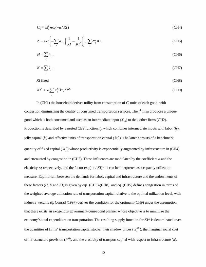
In (CH1) the household derives utility from consumption of Cj units of each good, with

congestion diminishing the quality of consumed transportation services. The jth firm produces a unique

good which is both consumed and used as an intermediate input (Xi, j) to the i other firms (CH2).

Production is described by a nested CES function, fj, which combines intermediate inputs with labor (hj),

jelly capital (kj) and effective units of transportation capital (e

jkt ). The latter consists of a benchmark

quantity of fixed capital ( 0

jkt ) whose productivity is exponentially augmented by infrastructure in (CH4)

and attenuated by congestion in (CH3). These influences are modulated by the coefficient a and the

elasticity ϖ, respectively, and the factor exp(–a / KI) < 1 can be interpreted as a capacity utilization

measure. Equilibrium between the demands for labor, capital and infrastructure and the endowments of

these factors (H, K and KI) is given by eqs. (CH6)-(CH8), and eq. (CH5) defines congestion in terms of

the weighted average utilization rate of transportation capital relative to the optimal utilization level, with

industry weights ωj. Conrad (1997) derives the condition for the optimum (CH9) under the assumption

that there exists an exogenous government-cum-social planner whose objective is to minimize the

economy’s total expenditure on transportation. The resulting supply function for KI* is denominated over

the quantities of firms’ transportation capital stocks, their shadow prices (KT

jπ ), the marginal social cost

of infrastructure provision (PKI), and the elasticity of transport capital with respect to infrastructure (κ).

13

This approach has the advantage of being straightforward to numerically parameterize.2 However,

its main limitation is that it does not explicitly relate congestion to investment in infrastructure and the

value of time (e.g., the Lagrange multiplier on eq. (MP4)), whose role in CBA is to indicate when the

marginal benefits of alleviating the former exceed the marginal costs of the latter. The relevant

mechanism is captured by the second set of studies, which model the production of travel as requiring

inputs of time, which explicitly enter into a household time budget constraint.

Parry and Bento (2001) emphasize the impact of substitution among differentially congested

modes of travel on time expenditures. Theirs is a stylized model of commuting—production is modeled in

the simplest possible way and freight transport is not considered. The economy is made up of a utility-

maximizing household, a final goods producer and three transport firms (indicated by the subscript m),

each of which corresponds to a particular mode: congested roads (R), public transit (P) and non-congested

roads (F).

, , , ,max ( , )

R P FC q q qU C

ΛΛ (PB1)

subject to:

min( , )mm

C X H Q+ ≤∑ (PB2)

( , , )R P FQ f q q q= (PB3)

1 2

min( / , / ) ,

min[ / , ( /, ) ]m m m m

m

m m m m m

X T m P Fq

X D T q m Rd d

ν τ

ν τ

=

=

= −

(PB4)

mm

H T TΛ+ ≤+ ∑ (PB5)

The household derives utility from consumption of the final good and leisure, (PB1). Eq. (PB2)

says that the output of the final goods firm is produced from labor and aggregate transportation services

(Q) according to a fixed-coefficients technology, and can either be consumed or allocated to intermediate 2 The main empirically-derived inputs employed by Conrad-Heng are benchmark estimates of the transportation and infrastructure capital stocks, the aggregate cost of congestion, and the elasticity of congestion with respect infrastructure spending, which, along with assumed industry weights, ωj, permits the a parameter in the congestion function to be calibrated.

14

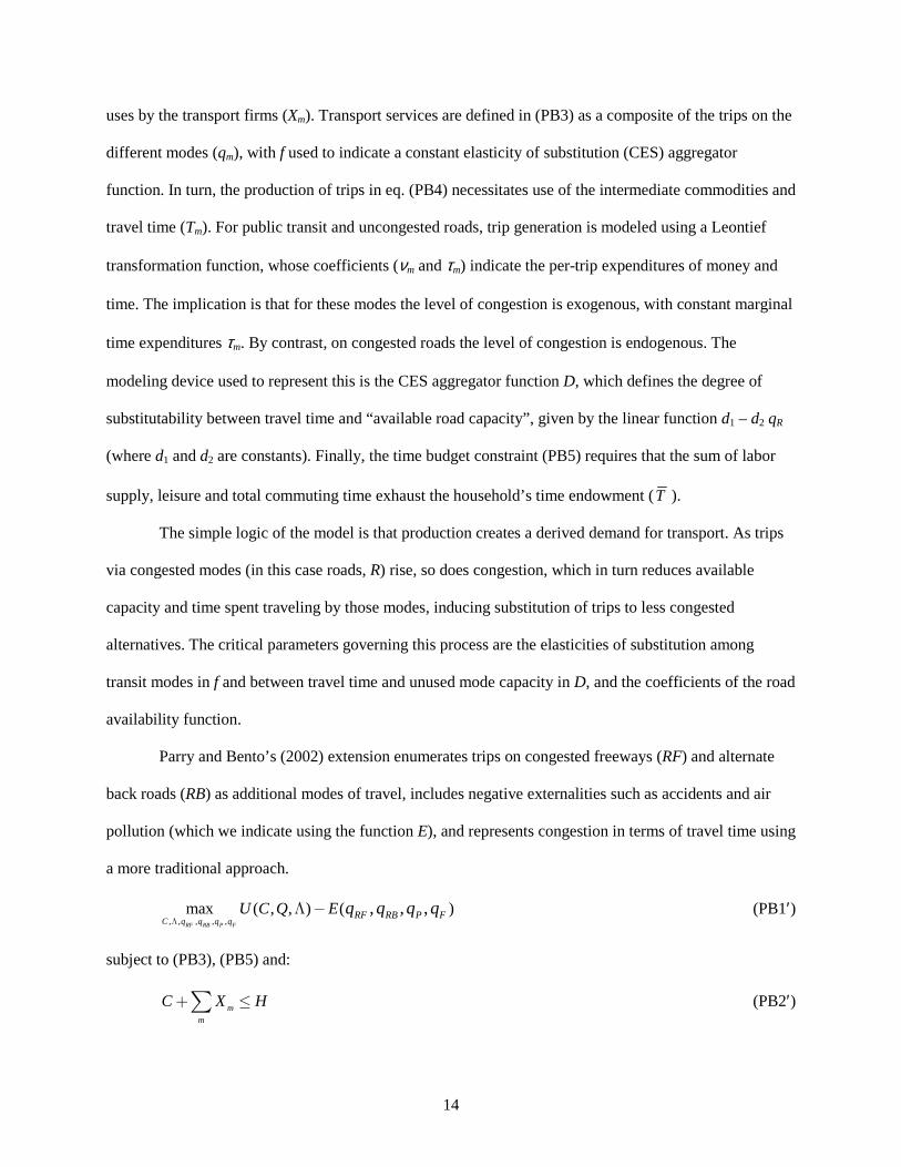
uses by the transport firms (Xm). Transport services are defined in (PB3) as a composite of the trips on the

different modes (qm), with f used to indicate a constant elasticity of substitution (CES) aggregator

function. In turn, the production of trips in eq. (PB4) necessitates use of the intermediate commodities and

travel time (Tm). For public transit and uncongested roads, trip generation is modeled using a Leontief

transformation function, whose coefficients (νm and τm) indicate the per-trip expenditures of money and

time. The implication is that for these modes the level of congestion is exogenous, with constant marginal

time expenditures τm. By contrast, on congested roads the level of congestion is endogenous. The

modeling device used to represent this is the CES aggregator function D, which defines the degree of

substitutability between travel time and “available road capacity”, given by the linear function d1 – d2 qR

(where d1 and d2 are constants). Finally, the time budget constraint (PB5) requires that the sum of labor

supply, leisure and total commuting time exhaust the household’s time endowment (T ).

The simple logic of the model is that production creates a derived demand for transport. As trips

via congested modes (in this case roads, R) rise, so does congestion, which in turn reduces available

capacity and time spent traveling by those modes, inducing substitution of trips to less congested

alternatives. The critical parameters governing this process are the elasticities of substitution among

transit modes in f and between travel time and unused mode capacity in D, and the coefficients of the road

availability function.

Parry and Bento’s (2002) extension enumerates trips on congested freeways (RF) and alternate

back roads (RB) as additional modes of travel, includes negative externalities such as accidents and air

pollution (which we indicate using the function E), and represents congestion in terms of travel time using

a more traditional approach.

, , , , ,max ( , , ) ( ), , ,RF RB P FC q q q q

RF RB P FU C Q E q q q qΛ

Λ − (PB1′)

subject to (PB3), (PB5) and:

mm

C X H+ ≤∑ (PB2′)

15

Xm = νm qm (PB6)

Tm = τm qm (PB7)

0 4[1 0.15( / ) ]m m m mq CAPτ τ= + , m = RF, RB (PB9)

Aggregate transportation services are now included as an additional argument in the household’s

utility function, along with non-congestion externalities (PB1′). As before, the sole factor of production is

labor, whose supply is traded off against leisure and travel according to the time budget constraint (PB5).

Here, however, (PB2′) assumes that each unit of labor produces one unit of the final good, which can be

consumed or used to pay for trips, whose transformation into aggregate transport services follows (PB3).

As in (PB4), trips incur fixed marginal pecuniary costs (PB6), but marginal expenditures of time (PB7)

which increase with congestion. Eq. (PB10) defines the latter relationship using the classic Bureau of

Public Roads (BPR) capacity restraint formula.

In both Parry-Bento models, the Lagrange multiplier on eq. (PB5) represents the “true” marginal

utility of time, which takes into account the general equilibrium interactions among the labor supply, the

consumption of the final good and leisure, and the supply-demand balance for trips by different modes.

Nevertheless, the value of time which emerges from this analysis still does not completely account for the

channels through which congestion’s effects are felt. In particular, the simple representation of production

fails to capture the way in which travel delays impact firms or may themselves be exacerbated by the

shipment of finished goods to retail markets or households’ retail purchasing behavior.

Likewise, the specification of substitution possibilities in transportation is simplistic. The Parry-

Bento models are “maquettes” which resolve only a few, very aggregate modes of travel and can afford to

rely on synthetic benchmark distributions of trips.3 In section 5.2.5 we caution that moving to the use of

real-world data to numerically calibrate the aggregator functions for transportation services may be quite

3 Parry and Bento (2001) distribute trips equally among modes, while in Parry and Bento (2001) trips are allocated 33 percent to each of peak-period freeway and public transit and 17 percent each to back roads and off-peak freeway travel.

16

involved. The remainder of the paper addresses these issues and examines their implications for

constructing large-scale transport-focused CGE models.

5. A HYBRID MESO-MACRO APPROACH

Our proposed approach is a hybrid one which seeks to capture meso-level details of

infrastructure, congestion and transport within the traditional framework of a macro-level CGE model.

We consider a static economy with N representative profit-maximizing firms, each of which produces a

single, distinct commodity. Firms and commodities come in two varieties, I non-transport producers and

their associated goods and services, which we index using the subscript i = 1, ..., I, and M transport or

logistics firms and their associated services, which we index with the subscript m = 1, ..., M. To

distinguish between firms and the goods which they produce, we introduce the subscript j = 1, ..., I to

enumerate non-transport producers. Furthermore, we define the set of transport producers in such a way

that each firm corresponds to a single disaggregate mode of transit, e.g., rail as well as truck freight

shippers, air passenger and freight travel, own-supplied passenger road travel using private vehicles,

purchased local/interurban passenger transit by road and rail, etc. Non-transport firms supply goods and

services to satisfy the intermediate demands of other firms as well as the final demands of households.

Transportation firms provide freight transport services to the non-transport firms and passenger transport

services to households. Households in the economy are modeled as a representative utility-maximizing

agent who owns the factors of production (hours of labor, H, and capital, K) and rents them out to the

firms in exchange for factor payments which finance the consumption of commodities.

The centerpiece of our approach is a representation of the process though which the operation of

markets for non-transport commodities and labor creates derived demands for transportation. In

particular, we assume that:

17

(a) Each unit of non-transport commodity requires freight trips to be shipped to sources of intermediate

or final demand.

(b) The representative agent’s final purchases of these goods and services require retail shopping trips in

order for them to be converted into utility, and

(c) The agent’s rental of labor to firms requires commuting trips.

The three kinds of mobility are distinguished using the superscripts TF, TC and TH, respectively.

We assume that households face two budget constraints, a pecuniary constraint that commodity

purchases not exceed factor income, and a temporal constraint that the duration of travel for shopping and

commuting, hours of work and leisure not exceed an aggregate endowment of time. The latter sets up a

tension between travel time expenditures for the purposes of consumption and income generation. For

households to increase their consumption they need more income, which in the short run can only be

obtained by renting additional hours of labor to firms, with the possible side-effect of more and/or longer

journeys to work. However, their ability to earn is constrained by the fact that consuming more non-

transport goods requires additional retail trips, and concomitant expenditures of time.

Firms do not have explicit time budgets, nevertheless we assume that time constraints influence

production in an implicit fashion. We treat non-transport firms as “mills”, whose products are

manufactured using labor, capital and intermediate inputs from other non-transport firms. In order for

these products to be consumed they must be shipped to markets, which creates a demand for trips

supplied by the transportation firms. A key feature of the model is that the latter firms do not produce

trips directly. Rather, their outputs take the form of generalized transportation services such as vehicles

operated on the road, trains on tracks, planes in the air, etc.—whose capacity is determined by the firms’

stocks of transportation capital (i.e., vehicles). This allows us to model the mechanism by which

congestion imposes a productivity penalty on firms: speed, which along any given segment of the

transportation network is equivalent to the inverse of the travel time, is necessary to transform these

services into trips. Thus, given a certain capacity to produce transport services, increases in travel time

translate into fewer trips. Other things equal, the main consequence is a fall in the productivity of inputs

18

to transportation and in rise in the average cost of trips, a decline in movements of passengers and non-

transport goods, and a reduction in production and consumption.

These devices allow us to model the impacts of congestion in a novel way. Congestion is the

increase in travel time arising out of the imbalance between the aggregate derived demand for mobility

and the capacity of the stock of transportation infrastructure to support the desired flux of trips. Our way

of representing travel admits three channels through which congestion may exert a drag on activity,

corresponding to (a)-(c), above:

• An increase in the duration of households’ retail trips per unit of consumption, which attenuates

consumption through the time budget constraint. Depending on the relevant elasticities, the time spent

on work or leisure may rise or fall as well, but the standard result is a decline in utility.

• A reduction in average productivity of transport-producers. Because congestion increases the duration

of freight trips of a given distance, it reduces the number of trips which transport producers can

supply with a given fleet of vehicles. The consequent dissipation of operating time—and thus

revenue—drives a wedge between the marginal cost of each transportation firm’s output and the unit

value of its trips consumed by firms and households, much like a tax.

• Dissipation of time in commuting, acting through the time budget constraint to reduce the economy’s

aggregate labor supply. This effect is similar to a tax on labor.

To effectively inform traditional microeconomic cost benefit analysis, any attempt to capture

these influences using top-down economy-wide models must address a number of issues. First,

considering the impacts of congestion in the aggregate will yield limited insights, as typically only a

fraction of the links in an economy’s transport network will be congested. These are the ones which are

candidates for infrastructure projects. Following from this observation, a second consideration is that trips

should be thought of as differentiated commodities, whose equilibrium allocation among network links

will be a function of transport producers’ marginal costs, firms and households’ demands for goods and

passenger mobility, and the distribution of travel times/congestion. In general, infrastructure investments

that are sufficiently large will give rise to simultaneous non-marginal changes in all of these variables, the

19

character of which will depend on both magnitude of the investments and their location on the network.

Finally, in order to properly capture the dissipative effect of congestion, a distinction needs to be made

between the production of transport services and the consumption of the trips which they make possible.

Logistics and passenger transport firms will allocate their outputs to the network segments which yield

the highest marginal revenue, while households and non-transport firms will allocate their demand for

trips to links with the lowest marginal cost. The key challenge is therefore to develop a computationally

tractable way of modeling the equilibrium between the supply-side transformation of transport services to

trips and the demand-side aggregation of trips into passenger and freight movements so as to resolve the

substitution of trips from congested links to uncongested alternatives.

The simplest way of doing this is to keep the spatial details of the network structure to a

minimum. Our strategy is to assume the existence of a generic transport network with l = 1, ..., L links,

amongst which trips generated by the m transport producers are allocated in a competitive fashion. This

choice allows us to specify a top-down model of intermediate complexity which is able to capture the

macroeconomic feedbacks which affect—and are affected by—Wardropian equilibria, while serving as a

bridge to more disaggregate network equilibrium models (e.g., Ferris et al, 1999). We make the key

simplifying assumption that trips across different mode-link alternatives are imperfect substitutes, with

differing marginal costs to transport consumers and differing marginal revenues to transport producers.

Thus, when non-transport firms ship their product to market, or households supply labor or consume a

particular commodity, each of these actors simultaneously chooses travel distances/routes and modes by

allocating trips over l and m so as to minimize total transportation expenditure. Symmetrically, each

logistics or passenger transport firm simultaneously chooses travel distances/routes and payloads by

allocating the transportation services it produces to trips by l and j in the case of freight, l and i in the case

of retail shopping, and just l in the case of commuting, so as to maximize revenue.

We operationalize these ideas by specifying transportation demands as constant elasticity of

substitution (CES) functions of trips by mode. Thus, freight transport demand by the jth firm, TF

jQ , is

20

modeled as a CES aggregate of the trips, , ,

TF

j l mq , made by transport mode m on network link l to ship j’s

product to intermediate and final consumers. Similarly, we model the aggregate household demand for

transportation to consume the ith commodity, TC

iQ , as a CES function of the retail trips, , ,

TC

i l mq , across all

combinations of transit modes and links, and the aggregate demand for transportation to supply labor,

QTH, as a CES function of the various mode-and link-specific commuting trips, ,

TH

l mq . We use the same

device on the supply side, specifying the trips undertaken by each transport producer as a constant

elasticity of transformation (CET) expansion of that firm’s output. Thus, firm m’s trips , ,

TF

j l mq , , ,

TC

i l mq and

,

TH

l mq are modeled as a CET function of the aggregate supply of transportation services by mode, Ym. Parry

and Bento (2001) note that the ability to substitute between transport modes mitigates the cost of reducing

congestion. Our assumption that households and firms substitute among both transport modes and

network segments means that the elasticities in the aforementioned CES and CET functions will likely be

a key influence on the marginal benefit of investments to increase the capacity of congested links.

The attractive feature of this formulation is that it automatically generates different levels of

congestion for each transport mode and network link. Congestion is a function of the total flux of trips

generated by each mode across a given link,

( ), , , , , ,

TC TF TH

l m i l m i l m l mi

q q qϑ = + +∑ , (1)

and the design capacity of the particular segment, CAPl, m, such that as ,l mϑ exceeds CAPl, m, travel time on

that link, τl, m, increases rapidly. A convenient representation of this phenomenon is the BPR formula

(PB9):

( )( )40

, , , ,1 0.15 /l m l m l m l mCAPτ τ ϑ= + , (2)

in which 0

,l mτ is the mode- and link-specific free-flow travel time.

21

The dependence of capacity on infrastructure investment is an exogenous input to the model that

must be developed from the existing characteristics of the transit network, the links which are candidates

for improvement, and the projected changes in traffic flows resulting from the proposed project. Eqs. (1)

and (2) establish the crucial connection between household trips to consume goods or commute back and

forth to work, and the trips undertaken by logistics firms to deliver commodities. Growth in any one type

of transportation adds to the total flux of trips across the transport network, raising trip times, and

inducing economic actors to re-allocate trips to less congested mode-link alternatives, as well as cut back

on overall travel. As mentioned above, the consequence of this is a decline in both the quantity of labor

supplied to producers and the goods and services consumed by households. In this way infrastructure

capacity acts as a fundamental brake on the expansion of economic activity.

5.1. Algebraic Summary of the CGE model

We begin with a description of the households in our simulated economy. We assume the

existence of a representative agent whose utility is represented by the nested CES function shown in

Figure 1A. At the top level of the nesting hierarchy, the agent obtains utility (U) from non-transport

consumer commodities (iC ) and leisure (Λ), with elasticity of substitution σU and technical coefficients

αi and αΛ:

( )/( 1)

( 1) / ( 1) /ˆU U

U UU U

i ii

U Cσ σ

σ σ σ σα α−

− −Λ= + Λ

∑ . (3)

The second level of the utility hierarchy describes how the demands for commodities create derived

demands for personal transportation. We specify each unit of delivered commodity as a CES composite of

transportation services, TC

iQ (i.e., trips for the purpose of retail purchases), and the relevant commodity

( iCɶ ) whose consumption necessitates transport expenditures, with elasticity of substitution C

iσ < 1 and

technical coefficients TC

iβ and C

iβ :

22

( ) ( )( ) /( 1)( 1) / ( 1) /ˆ

C CC C C C i ii i i iTC TC C

i i i i iC Q Cσ σ

σ σ σ σβ β

−− −

= + ɶ . (4)

Each retail commodity is itself a composite of the goods and services actually being purchased by

consumers and freight transportation services, which we discuss in more detail below. Note that eq. (4)

implicitly captures Lakshmanan and Hua’s (1983) distinction between discretionary and non-

discretionary transportation: while travel is a necessary input to consumption ( C

iσ < 1) the actual quantity

of travel undertaken by households is discretionary. Consequently, our formulation captures the ability of

consumers to substitute passenger travel (TC

iQ ) for the freight transportation component of iCɶ , e.g., by

opting to travel to retail outlets to purchase goods versus having them delivered directly to the consumer’s

place of residence. At the lowest level of the hierarchy the transportation services necessary to consume

good i are a CES composite of the shopping trips (, ,

TC

i l mq ) which occur on each link of the transport

network and mode of transit:

( )/( 1)

( 1) /

, , , ,

TC TCi iTC TC

i iTC TC TC

i i m l i m ll m

Q qσ σ

σ σγ

−−

= ∑∑ . (5)

Here TC

iσ is the substitution elasticity and , ,

TC

i l mγ are technical coefficients which indicate how the retail

trips associated with each commodity are distributed across mode-link alternatives in the benchmark data

used to calibrate the model.

Households’ rental of their factor endowments is modeled in a similar fashion. We assume that

transport services are not necessary to supply capital to firms. However, to supply H units of labor the

agent must utilize transportation services, QTH (i.e., trips for the purpose of commuting). Accordingly, the

aggregate supply of labor (Hɶ ) is modeled as a CES composite, with elasticity σH and coefficients βTH

and βH:

( )( ) /( 1)( 1) / ( 1) /

H HH H

H HTH TH HH Q Hσ σ

σ σ σ σβ β−

− −= +ɶ . (6)

23

As with retail trips, we model QTH as a CES composite of the commuting trips (,

TH

l mq ) by each network link

and transit mode, with elasticity σTH and mode-link coefficients ,TH

l mγ :

( )/( 1)

( 1) /

, ,

TH TH

TH TH

TH TH TH

l m l ml m

Q qσ σ

σ σγ

−−

= ∑∑ . (7)

The representative agent’s budget constraint mandates that the value of consumption at retail

goods prices (iPɶ ) exhaust the income from factor rentals:

i ii

PC H rKθ≤ +∑ ɶɶ , (8)

where θ denotes the marginal utility of time—i.e., the wage net of the marginal cost of commuting, and r

is the capital rental rate. The agent’s time constraint mandates that the total expenditure of time on trips

for retail consumption and commuting (summed over all network links and modes), plus labor and leisure

time, exhaust the agent’s endowment of time, given by T :

, , , ,

TC TL

l m i l m l ml m i

q q H Tτ + + + Φ ≤

∑∑ ∑ . (9)

The key variable in this expression is τl,m, the average trip time on each network segment, which by (1)

and (2) reflects the tension between the total flux of trips on that segment and its capacity.

The organization of production is shown in panels B and C Figure 1. In panel B, the output of

each of the j non-transport firms (Yj) is modeled using a CES production function denominated over

inputs of intermediate commodities (,i j

Xɶ ), labor (j

hɶ ) and capital (kj):

/( 1)( 1) / ( 1) / ( 1) /

, , , ,

NT NTj j

NT NT NT NT NT NTj j j j j jNT NT NT

j i j i j H j j K j ji

Y X h kσ σ

σ σ σ σ σ σδ δ δ−

− − −= + + ∑ ɶɶ , (10)

with substitution elasticity NT

jσ and distribution parameters δNT. Similar to the households, the supply of

commodities creates a derived demand for transportation services. We assume that the delivery of TF

iχ

units of commodity i to intermediate and final users requires a unit of freight transportation services

24

( TF

iQ ). As a result, the supply of non-transport commodities are a Leontief composite of produced

commodities and transportation:

( )min ,TF TF

i i i iY Q Yχ=ɶ . (11)

In turn, freight transport is a CES composite of delivery trips (, ,

TF

j l mq ) by network link and transit mode:

( )/( 1)

( 1) /

, , , ,

TF TFj jTF TF

j jTF TF TF

j j l m j l ml m

Q qσ σ

σ σγ

−−

= ∑∑ , (12)

with elasticity TF

jσ and mode-link coefficients , ,

TF

j l mγ .

The production function for the m transportation services is illustrated in panel C, and is

essentially the same as that for non-transport commodities:

/( 1)

( 1) / ( 1) / ( 1) /

, , , ,

T Tm m

T T T T T Tm m m m m mT T T

m i m i m H m m K m mi

Y X h kσ σ

σ σ σ σ σ σδ δ δ−

− − −= + + ∑ ɶɶ , (13)

with substitution elasticity T

mσ and distribution parameters δT. However, to translate between transport

producers’ outputs and the trips necessary to deliver passengers and freight along each link, we use the

following CET formulation with transformation elasticity Tmψ and distribution parameters :

( ) ( ) ( )/( 1)

( 1) / ( 1) / ( 1) /1

, , , , , , , , , , ,

T Tm m

T T T T T Tm m m m m mTF TF TC TC TH TH

m l m j l m j l m i l m i l m l m l ml j i

Y Z q q q

ψ ψψ ψ ψ ψ ψ ψ

µ µ µ−

− − −−= ⋅ + +

∑ ∑ ∑ (14)

The variable Zl, m is particularly important. It is a link-specific productivity penalty which is a function of

each link’s average travel time in (2), and is intended to capture the adverse impact of congestion on the

ability of transport firms to translate service outputs into movements of goods and passengers. Thus, the

more congested a given link, the more units of Ym necessary to generate an additional trip on that link,

reducing the average and marginal productivity of the inputs to (13).

The model is closed by specifying market clearance conditions for the supply of composite non-

transport commodities:

25

,i j iij

X CY +=∑ ɶɶɶ , (15)

and the representative agent’s primary factor endowments:

j mj m

H h h= +∑ ∑ɶ ɶ , (16)

j mj m

K k k= +∑ ∑ . (17)

In the next section we go on to elaborate how the foregoing elements may be used to develop an

operational CGE model.

5.2. Implementational Details

Walrasian general equilibrium prevails when the price of commodities equals their marginal cost

of production with firms earning zero profits, there is zero excess demand for commodities and factors,

and consumer’ income equals their expenditure. These conditions form the basis for CGE models in a

complementarity format, which specify the economy as a vector of zero profit, market clearance, income

balance, and auxiliary equations. Each equation is paired with an associated dual variable with respect to

which it exhibits complementary slackness (see, e.g., Rutherford, 1995; Sue Wing, 2004):

1. Zero profit conditions for firms and households. These specify the equilibrium between commodity

prices and firms’ unit cost functions, and between the marginal utility of income and the aggregate

expenditure function. They complementary to the activity levels of firms and the utility level of the

representative agent.

2. Market clearance conditions for commodities and factors. These specify the equilibrium between the

aggregate demands for commodities and factors—which are functions of prices and activity levels,

and their aggregate supplies—typically indicated by firms’ activity levels and households’ factor

endowments. They are complementary to commodity and factor prices.

26

3. Income balance conditions. These specify the equilibrium between the value of households’

expenditures and the value of their income, and are complementary to the income levels of the

households.

4. Auxiliary equations. These typically represent some sort of constraint on the economy that is a

function of both an auxiliary variable and other endogenous variables, which requires them to be

solved for along with the remaining variables. They are complementary to the auxiliary variable..

Henceforth we use the shorthand symbol “⊥”to represent these complementary relationships.

5.2.1 Zero Profit Conditions and Associated Demand Functions

As before, we begin with the households in the economy. Recasting the representative agent’s

utility maximization problem as a dual expenditure minimization permits us to solve for the unit

expenditure function, ε, dual to (3):

1/(1 )

1 1ˆU

U U U U

i ii

Pσ

σ σ σ σθε α α−

− −Φ= +

∑ , ⊥ U (18)

where iP is the price of the ith consumption good-transport services aggregate, and θ is the value of time.

This expression can be thought of as a zero-profit condition for the “production” of a utility good, to

which aggregate utility is the complementary activity variable. By Shepard’s Lemma, the derivatives of

the zero-profit condition with respect to the prices of the inputs yields the conditional input demands.

Accordingly, final demands for commodities and leisure are given by:

ˆ ˆU U U

i i iC P Uσ σ σα ε−= , (19)

U U U

Uσ σ σα θ ε−ΦΦ = , (20)

Cost minimization in the aggregation of transport services and physical goods in eq. (4) gives rise

to the following zero profit condition, which is the unit cost function for ˆiC :

( ) ( ) ( )( )1/(1 )1 1ˆ

CC C C iCi i i

iTC TC C

i i i i iP P Pσ

σ σ σ σβ β−

− −= + ɶ , ⊥ ˆiC (21)

27

where TC

iP and iPɶ are the consumer prices of retail mobility and final commodity sales associated with

good i. The conditional demands for these inputs are given by:

( ) ( ) ˆˆC C

CTC TC

i i

TC

i i iP P CQσ σ σβ

−= , (22)

( ) ( ) ˆˆC C C

C

ii i i iC P P Cσ σ σβ

−=ɶ ɶ . (23)

Similarly, the unit cost function arising from cost-minimizing aggregation of labor hours and commuting

to produce supplied labor in (6) is:

( ) ( ) ( )( )1/(1 )1 1

HH H H

HTH TH Hw Pσ

σ σ σ σβ β θ−

− −= +ɶ , ⊥ Hɶ (24)

where wɶ is the wage and PTH is the marginal cost of commuting trips. Then, the conditional demands for

trips and aggregate labor are given by:

( ) ( )H H

HTH TH THQ P w Hσ σ σβ

−= ɶɶ , (25)

( )H

H HHH w Hσ σ σβ θ −= ɶɶ . (26)

The zero profit conditions corresponding to the cost-minimizing allocation of trips by mode and

link in eqs. (5) and (7) are

( ) ( )1/(1 )

1

, , , ,

TCiTC TC

i iTC TC TC

i i l m i l ml m

P pσ

σ σγ

−−

= ∑∑ , ⊥ TC

iQ (27)

( ) ( )1/(1 )

1

, ,

TH

TH TH

TH TH TH

l m l ml m

P pσ

σ σγ

−−

= ∑∑ , ⊥ THQ (28)

where , ,

TC

i l mp and ,

TH

l mp are the marginal costs of trips on a given mode-link alternative incurred by the

representative agent in order to consume good i and journey to work, respectively. The associated

conditional demands for trips by link, mode and commodity are:

( ) ( ) ( ), , , , , ,

TC TC TCi i iTC TC TC TC TC

i l m i l m i l m i iq p P Qσ σ σ

γ−

= , (29)

28

( ) ( ) ( ), , ,

TH TH TH

TH TH TH TH TH

l m l m l mq p P Qσ σ σ

γ−

= . (30)

Turning now to the firms in the economy, cost minimization by producers of non-transportation

goods and services in eq. (10) results in the following zero-profit condition:

( ) ( ) ( )1/(1 )

1 1 1

, , ,

NTjNT NT NTNT NT NT

j j jj j jNT NT NT

j i j i H j K ji

P P w rσ

σ σ σσ σ σδ δ δ−

− − −= + + ∑ ɶ ɶ , ⊥ Yj (31)

where Pj is the producer price of each non-transport commodity and r is the capital rental rate. The zero-

profit condition for logistics firms in eq. (13) takes a somewhat different form, owing to the CET

specification of production. In particular, transportation services are not traded, and so do not have an

explicit price within the model. Producers therefore equate the marginal revenue from revenue-

maximizing allocation of trips in (14) to the marginal cost from cost-minimizing transport service

production in (13):

( ) ( ) ( ) ( ) ( ) ( )1/(1 )

1 1 1

, , , , , , , , , , , , ,

Tm

T T T T T Tm m m m m mTF TF TC TC TH TH

j l m l m j l m i l m l m i l m l m l m l ml j i

Z p Z p Z p

ψψ ψ ψ ψ ψ ψ

µ µ µ−

− − −+ +

∑ ∑ ∑

( ) ( ) ( )1/(1 )

1 1 1

, , ,

TmT T T

T T Tm m m

m m mT T T

i m i H m K mi

P w rσ

σ σ σσ σ σδ δ δ−

− − −+ + = ∑ ɶ ɶ ⊥ Ym (32)

The left-hand side of the foregoing expression clearly demonstrates that the impact of congestion is

identical to a tax on trips that is differentiated by link. This result turns out to be very useful, because it

enables the level of congestion, Zl, m, to be modeled as an endogenous, nonlinear tax. We elaborate on this

point below.

The associated conditional demands for inputs of intermediate commodities, labor and capital are

found by applying Shepard’s lemma to the right-hand sides of (31) and (32):

( ) ( ) ( ), ,

NT NTNTj jjNT

i j i j i j jX P P Yσ σσδ −

=ɶ ɶ , (33)

( ) ( ) ( ) ( ) ( )1

1 1 1

, , , , ,

/( )T Tm mT T T TT T T T

m m m mm m m mT T T T

i m i m i i m i H m K mi

mX P P w Yrσ σ

σ σ σ σσ σ σ σδ δ δ δ−

− − − −= + + ∑ɶ ɶ ɶ ɶ , (34)

29

( ) ( ),

NT NTNTj jjNT

j H j j jh w P Yσ σσδ −=ɶ ɶ , (35)

( ) ( ) ( ) ( )1

1 1 1

, , , ,

/( )T Tm mT T T T

T T T Tm m m m

m m m mT T T T

m H m i m i H m K mi

mh w P w Yrσ σ

σ σ σ σσ σ σ σδ δ δ δ−

− − − −= + + ∑ɶ ɶɶ ɶ , (36)

( ) ( ),

NT NTNTj jjNT

j K j j jk r P Yσ σσδ −= , (37)

( ) ( ) ( ) ( )1

1 1 1

, , , ,

/( )T Tm mT T T T

T T T Tm m m m

m m m mT T T T

m K m i m i H m K mi

mk r P w Yrσ σ

σ σ σ σσ σ σ σδ δ δ δ−

− − − −= + + ∑ ɶ ɶ . (38)

As well, the associated conditional supplies for trips are found by invoking Shepard’s lemma on the left-

hand side of (32):

( ) ( ) ( ) ( ) ( )1

1 1 1 1

, , , , , , , , , ,

/( )T Tm mT T T T T

T T T Tm m m m m

m m m mTF TF TF T T T

j l m l m j l m j l m i m i H m K mi

mq p P w YZ rψ σ

ψ ψ σ σ σψ σ σ σµ δ δ δ−

−− − − −= + + ∑ ɶ ɶ ,(39)

( ) ( ) ( ) ( ) ( )1

1 1 1 1

, , , , , , , , , ,

/( )T Tm mT T T T T

T T T Tm m m m m

m m m mTC TC TC T T T

i l m l m i l m i l m i m i H m K mi

mq Z p P w Yrψ σ

ψ ψ σ σ σψ σ σ σµ δ δ δ−

−− − − −= + + ∑ ɶ ɶ ,(40)

( ) ( ) ( ) ( ) ( )1

1 1 1 1

, , , , , , ,

/( )T Tm mT T T T T

T T T Tm m m m m

m m m mTH TH TH T T T

l m l m l m l m i m i H m K mi

mq Z p P w Yrψ σ

ψ ψ σ σ σψ σ σ σµ δ δ δ−

−− − − −= + + ∑ ɶ ɶ . (41)

The zero profit condition corresponding to the cost-minimizing allocation of freight trips by mode

and link in eq (12) is:

( ) ( )1/(1 )

1

, , , ,

TFjTF TF

j jTF TF TF

j j l m j l ml m

P pσ

σ σγ

−−

= ∑∑ , ⊥ TF

jQ (42)

The associated conditional demands for freight trips by link, mode and commodity are:

( ) ( ) ( ), , , , , ,

TF TF TFj j jTF TF TF TF TF

j l m j l m j l m j jq p P Qσ σ σ

γ−

= . (43)

Finally, using eq. (11), the consumer price of non-transport commodities, iPɶ , is given by the

following zero-profit condition:

/TF TF

i i i iP P Pχ= +ɶ , ⊥ iYɶ (44)

30

whose first term indicates the transportation margin. The associated demands are

/TF TF

i i iQ Y χ= ɶ , (45)

i iY Y= ɶ . (46)

5.2.2 Market Clearance Conditions

Substituting eqs. (35), (36) and (46) into (16) and (37), (38) and (46) into (17) yields the supply-

demand balances for labor and capital

( ) ( ),

NT NTNTj jjNT

H j j jj

H w P Yσ σσδ −=∑ɶ ɶ

( ) ( ) ( ) ( )/(1 )

1 1 1

, , , ,

T Tm mT T T T

T T T Tm m m m

m m m mT T T T

H m i m i H m K m mm i

w P w r Yσ σ

σ σ σ σσ σ σ σδ δ δ δ−

− − − −+ + +

∑ ∑ ɶɶ ɶ , ⊥ wɶ (47)

( ) ( ),

NT NTNTj jjNT

K j j jj

K r P Yσ σσδ −=∑

( ) ( ) ( ) ( )/(1 )

1 1 1

, , , ,

T Tm mT T T T

T T T Tm m m m

m m m mT T T T

K m i m i H m K m mm i

r P w r Yσ σ

σ σ σ σσ σ σ σδ δ δ δ−

− − − −+ + +

∑ ∑ ɶ ɶ . ⊥ r (48)

Substituting eqs. (33), (34) and (46) into (15) yields the market clearance condition for delivered non-

transport commodities:

( ) ( ) ( ),

NT NTNTj jjNT

i i j i j jj

Y P P Yσ σσδ −

=∑ɶ ɶ

( ) ( ) ( ) ( ) ( ),ˆˆ

T UT UT Um m m C

i

T

i m i m m i i im

P P Y P P Cσ σσ σσ σβδ

− −+ +∑ ɶ ɶ , ⊥ iPɶ (49)

while the corresponding equation for non-transport firms’ outputs is given by (46):

i iY Y= ɶ . ⊥ Pi (46′)

We note that a similar condition for the services produced by transportation firms (Ym) does not exist, as

we assume that there are only markets for trips.

The balance between supply and demand for the final use of the commodity-retail transport

aggregate is given by (19), and is complementary to the composite final commodity price:

ˆ ˆU U U

i i iC P Uσ σ σα ε−= , ⊥ iP (19′)

31

which enables us to specify analogous conditions for the retail, commuting and freight mobility

aggregates, given by (22), (25) and (45):

( ) ( ) ˆˆC C

CTC TC

i i

TC

i i iP P CQσ σ σβ

−= , ⊥ TC

iP (22′)

( ) ( )H H

HTH TH THQ P w Hσ σ σβ

−= ɶɶ , ⊥ THP (25′)

/TF TF

j j jQ Y χ= ɶ . ⊥ TF

jP (45′)

Supply-demand equilibria for trips, which are complementary to mode- and link-specific

marginal trip costs, are found by equating (27) and (39), (28) and (40), and (43) and (41):

( ) ( ) ( ) ( ) ( )1

1 1 1 1

, , , , , , , ,

/( )T Tm mT T T T T

T T T Tm m m m m

m m m mTF TF T T T

l m j l m j l m i m i H m K mi

mp P w YZ rψ σ

ψ ψ σ σ σψ σ σ σµ δ δ δ−

−− − − −+ + ∑ ɶ ɶ

( ) ( ) ( ), , , ,

TF TF TFj j jTF TF TF TF

j l m j l m j jp P Qσ σ σ

γ−

= , ⊥ , ,

TF

j l mp (50)

( ) ( ) ( ) ( ) ( )1

1 1 1 1

, , , , , , , ,

/( )T Tm mT T T T T

T T T Tm m m m m

m m m mTC TC T T T

l m i l m i l m i m i H m K mi

mp P w YZ rψ σ

ψ ψ σ σ σψ σ σ σµ δ δ δ−

−− − − −+ + ∑ ɶ ɶ

( ) ( ) ( ), , , ,

TC TC TCi i iTC TC TC TC

i l m i l m i ip P Qσ σ σ

γ−

= , ⊥ , ,

TC

i l mp (51)

( ) ( ) ( ) ( ) ( )1

1 1 1 1

, , , , , ,

/( )T Tm mT T T T T

T T T Tm m m m m

m m m mTH TH T T T

l m l m l m i m i H m K mi

mp P w YZ rψ σ

ψ ψ σ σ σψ σ σ σµ δ δ δ−

−− − − −+ + ∑ ɶ ɶ

( ) ( ) ( ), ,

TH TH TH

TH TH TH TH

l m l mp P Qσ σ σ

γ−

= . ⊥ ,

TH

l mp (52)

A particularly attractive feature of the model is the fact that the value of time exhibits

complementary slackness with respect to the representative agent’s time budget constraint. The associated

market clearance condition is derived by substituting eqs. (19), (29) and (30) into the representative

agent’s time budget constraint, (9):

( ) ( ) ( ) ( ) ( ) ( ), , , , , , ,

TC TC TC TH TH THi i iTC TC TC TC TH TH TH TH

l m i l m i l m i i l m l ml m i

p P Q p P Qσ σ σ σ σ σ

τ γ γ− −

+

∑∑ ∑

( )H

H H U U UH w H U Tσ σ σ σ σ σβ θ α θ ε− −

Φ+ + ≤ɶɶ . ⊥ θ (53)

32

Because θ is the Lagrange multiplier on a constraint which take into account the fully endogenous price,

supply and demand responses across the entire spectrum of markets in the economy (as opposed to just

transportation), it represents the true general equilibrium value of time.

The final market clearance condition is a placeholder equation that specifies the quantity of

“utility goods” as the ratio of the representative agent’s aggregate income, Ω, to the unit expenditure

index. This expression is complementary to unit expenditure:

U = Ω / ε. ⊥ ε (54)

5.2.3 Income Balance Conditions and Auxiliary Variables

Income-expenditure balance is defined by the representative agent’s money budget constraint,

(8), which is complementary to aggregate income:

i i

i

PC H rKθ≤ +∑ ɶɶ . ⊥ Ω (8′)

The auxiliary variables in the model are the average trip times by mode and link (τl, m) in eq. (53) and the

congestion penalty parameter (Zl, m) in eqs. (32) and (50)-(52). Assuming that Zl, m can be expressed as a

parametric function of τl, m (e.g., as in Mayeres and Proost, 1997), we may specify two auxiliary equations

complementary to these variables:

( ) 4

, , , , ,0

, ,

,

1 0.15

TC TF TH

i l m i l m l mi

l m l m

l m

q q q

τ τκ

+ += +

∑, ⊥ τl, m (55)

Zl, m(τl, m). ⊥ Zl, m (56)

5.2.4 General Equilibrium in Complementarity Format

Given the above, we can now specify the general equilibrium of the economy as follows:

• 3 + 5I + M zero profit equations (18), (21), (24), (27)-(28), (31)-(32), (42) and (44) in as many

unknown activity variables (U, ˆiC , Hɶ , TC

iQ , THQ , Yj, Ym, iYɶ , TF

jQ ).

33

• 5 + 5I + (1 + 2I) (L × M) income balance equations (19′), (22′), (25′), (45′)-(46′), and (47)-(54), in as

many unknown price variables (iP , TC

iP , THP , TF

jP , Pi, wɶ , r, iPɶ , , ,

TF

j l mp , , ,

TC

i l mp , ,

TH

l mp , θ, ε).

• A single income balance condition (8′) in one unknown income level (Ω), and

• The 2(L × M) auxiliary constraints (55) and (56) in as many unknown auxiliary variables (τl, m, Z l, m).

The CGE model consists of the paired, stacked vectors of 9 + 10I + M + (3 + 2I) (L × M)

variables, b = vec[U, ˆiC , Hɶ , TC

iQ , THQ , Yj, Ym, iYɶ , TF

jQ , iP , TC

iP , THP , TF

jP , Pi, wɶ , r, iPɶ , , ,

TF

j l mp , , ,

TC

i l mp ,

,

TH

l mp , θ, ε, Ω, τl, m, Z l, m], and 9 + 10I + M + (3 + 2I) (L × M) equations (18), (21), (24), (27)-(28), (31)-

(32), (42)-(44), (19′), (22′), (25′), (45′)-(46′), (47)-(54), (8′), (55)-(56), which we denote Ξ(b). The latter

is the excess demand correspondence of the economy. By setting up the model in this way, the economy

can be cast as a square system of nonlinear inequalities known as a mixed complementarity problem

(Ferris and Pang, 1997; Ferris and Kanzow, 2002):

Ξ(b) ≥ 0, b ≥ 0, b′ Ξ(b) = 0,

which is straightforward to express and solve using computational tools such as the MPSGE subsystem

(Rutherford, 1999) for GAMS (Brooke et al, 1998) in conjunction with the PATH solver (Dirkse and

Ferris, 1995).

5.2.5 Data and Calibration

Numerical solution of the model requires that values be specified for the parameters of the excess

demand correspondence, Ξ. This procedure, known as calibration, is likely to be especially challenging

given that it requires the integration of economic and transportation data which are often incommensurate.

Calibrating the purely macroeconomic, non-transport related components of the CGE model is a

fairly simple task, involving the selection of values for the elasticities σU, NT

jσ and T

mσ based on empirical

estimates, and the computation of values for the coefficients αi, αΛ, δNT and δT using a national- or

regional-level social accounting matrix (SAM). (For details see, e.g., Sue Wing, 2004.) We anticipate that

it will be somewhat more difficult to find econometric estimates for, or calibrate using related empirical

34

studies, values for the substitution elasticities C

iσ , or to infer values for the coefficients TF

jχ , TC

iβ and C

iβ

from data on freight transport margins. And since published estimates for the elasticities TC

iσ , TF

jσ , TC

iσ ,

T

mψ do not exist, developing the data and econometric procedures to estimate these parameters will likely

involve a large amount of effort. A rough-and-ready way to proceed is to set up the model using the

values in the range assumed by Parry and Bento (2001, 2002), and perform sensitivity analysis.

Calibrating the coefficients , ,

TF

j l mγ , , ,

TC

i l mγ , ,

TH

l mγ , , ,

TF

j l mµ , , ,

TC

i l mµ and ,

TH

l mµ in the trip aggregation and

transformation functions is likely to be a significant undertaking. The key difficulty lies in defining the

topology of the transport network and associated traffic flows at a geographic scale for which there are

published inter-industry economic accounts. Although survey data on commuting and freight traffic flows

are readily available at the level of metropolitan statistical areas (MSAs), input-output data are rarely

tabulated at such a fine spatial scale. At the opposite extreme, while it is straightforward to construct an

aggregate CGE model using a SAM constructed from the transportation satellite account make and use

tables (Fang et al, 2000), for modes of surface travel such as commuting or retail shopping which are

important contributors to congestion, it is not obvious how to represent major congested network links at

such a highly aggregate scale.

Thus, apart from the normative question of what is the most appropriate geographic scale at

which our model should be specified, data constraints dictate the practical necessity of structuring a

reduced-form representation of the transportation network so that it is both sufficiently simple to calibrate

the γ and µ parameters and able to be matched to a regional SAM. At the current stage of this research,

the most promising source of economic data would seem to be county-level SAMs developed by

IMPLAN which are coterminous with MSAs that straddle major transportation corridors in the eastern

U.S.

35

6. DISCUSSION AND SUMMARY

Provision of transportation infrastructure is one of the most visible, vital and costly ways in which

the public sector contributes to the private economy. Yet decisions about the levels and allocations of

transportation infrastructure investments must currently be made with incomplete information about their

economic impacts. Analytical tools are limited to micro-scale analyses, which may not capture the full

range of economic benefits induced by a project or program, and macro-scale analyses, which are too

broadly defined to provide guidance on the relative benefits of specific projects and programs. The

situation calls for analytical tools defined as a “meso-level” that can provide impacts assessments that are

both comprehensive and capable of representing specific expansions of infrastructure capacity, following

the three criteria we define in the introduction. This paper contributes to the development of such tools by

specifying a CGE model that is specifically designed to assess the broader economic impacts of

transportation infrastructure investments.

The model specified above draws on the limited CGE literature on transportation

infrastructure – especially the household time budgets of Parry and Bento (2001, 2002). It goes beyond

existing models both in terms of its technical specification and its overall scope. It specifies a set of

derived demands for transportation services that arise from production, consumption and labor supply

activities. It represents transportation infrastructure as a set of capacitated mode-link combinations on

which flows are assigned and congestion is modeled as increases in travel time. By embedding travel time

explicitly in the determination of household utilities and the prices and quantities of commodities

produced in the economy, it incorporates in the model the phenomenon of congestion that is based on a

comprehensive, endogenous definition of the value of time.

Existing CGE models designed for the analysis of transportation infrastructure can, for the most

part, be classified s maquettes – that is, simplified or scaled down models designed to make rough

estimates of relative magnitudes or as steps toward the creation of more comprehensive models. By

contrast, the model specified above is intended as a practical tool for policy analysis. There are, however,

36

significant hurdles to overcome before it can be made operational, including defining an appropriate

geographical scale for its application, an appropriate level of detail for the set of mode-link combinations

and appropriate data and parameters for calibration.

The question that naturally arises is whether it is worth the effort. To some extent this comes

down to the empirical question of whether the broader economic benefits captured in the CGE model are

of significant magnitude relative to the more direct effects captured in CBA. But looking beyond the

“bottom line” of aggregate benefits, the CGE model generates a range of information that cannot be

obtained from existing models such as whether the benefits of a capacity expansion accrue mostly to

firms or households, whether household benefits are mostly in consumption activities or commuting and

whether some industries benefit more than others. Such information may be useful in assessing whether

specific objectives that policy makers attach to a project are likely to be met. Also, the CGE specification

is especially well-suited to assessing the impact of infrastructure programs because the implementation of

two or more capacity expansions can be modeled simultaneously. This will be useful in identifying

complementarities among projects by seeing, for example, whether the benefits of projects A and B

implemented simultaneously exceed the sum of the benefits of A and B implemented independently.

Ultimately, the value of a model such as the one we have specified lies in its laying bare a

plausible set of economy-wide interactions that are triggered by an improvement in transportation

infrastructure. In other words, it is an attempt to move beyond “black box” and “bottom line” approaches

to policy models to an approach that explains rather than just captures economic impacts. Naturally,

laying the underlying mechanisms bare opens the door to criticism based on underlying assumptions –

especially as regards market imperfections. Furthermore, we recognize that there are a range of dynamic,

developmental impacts that the model does not include. Still, we believe that specifying and calibrating

our model is a useful step toward a better understanding of the economy-wide consequences of

transportation infrastructure in the economy.

37

REFERENCES

1. Anderson, William P. and T.R. Lakshmanan, (2007) Infrastructure and Productivity: What are the

Underlying Mechanisms?” (eds) Charlie Karlsson, William P. Anderson, Börje Johansson, and

Kiyoshi Kobayashi. in The Management and Measurement of Infrastructure: Performance, Efficiency

and Innovation. Edward Elgar, UK.

2. Brooke, A., D. Kendrick, A. Meeraus and R. Raman (1998). GAMS: A User's Guide, Washington

DC: GAMS Development Corp.

3. Dirkse, S.P. and M.C. Ferris (1995). The PATH Solver: A Non-Monotone Stabilization Scheme for

Mixed Complementarity Problems, Optimization Methods and Software 5: 123-156.

4. Evans, A.W. (1992). Road congestion pricing: When is it a good policy? Journal of Transport

Economics and Policy 26: 213-43.

5. Fang, B., X. Han, S. Okubo and A.M. Lawson (2000). U.S. Transportation Satellite Accounts for

1996, Survey of Current Business 80: 14-22.

6. Ferris, M.C. and C. Kanzow (2002). Complementarity and Related Problems, in P.M. Pardalos and

M.G.C. Resende (eds.), Handbook of Applied Optimization, New York: Oxford University Press,

514-530.

7. Ferris, M.C., A. Meeraus and T.F. Rutherford (1999). Computing Wardropian Equilibria in a

Complementarity Framework, Optimization Methods and Software 10: 669-685.

8. Ferris, M.C. and J.S. Pang (1997). Engineering and Economic Applications of Complementarity

Problems, SIAM Review 39(4): 669-713.

9. Fishlow, Albert (1965). American Railroads and the Transformation of the Antebellum Economy,

Harvard University Press, Cambridge, MA.

10. Fogel, , R.W. (1964) Railroads and American Economic Growth: essays in econometric history, John

Hopkins University Press, Baltimore.

38

11. Forkenbrock, D.J. and N.S. Foster (1990) Economic benefits of corridor investment projects,

Transportation Research, 24A(3): 303-312.

12. Gunasekara, K., W.P. Anderson, and T. R. Lakshmanan (2007 forthcoming) “Highway Induced

Development: Evidence from Sri Lanka”, World Development.

13. Haynes, Kingsley and Kenneth J. Button (2001) Transportation systems and economic development,

Chapter 16 in Kenneth.J. Button and David.A. Hensher (eds.) Handbook of Transportation Systems

and Traffic Control, Amsterdam:Pergamon

14. Lakshmanan, T.R. and W. Anderson, 2002. A White Paper on “Transportation Infrastructure, Freight

Services Sector, and Economic Growth”, prepared for the U.S. Department of Transportation, Federal

Highway Administration.

15. Lakshmanan, T.R. and W. Anderson, 2007, “Transport’s Role in Regional Integration Processes”

Market Access, Trade in Transport Services and Trade Facilitation, Round Table 134. OECD-

ECMT, Paris, pp. 45-71.

16. Lakshmanan, T.R. and C.-I. Hua (1983). A Temporal-Spatial Theory of Consumer Behavior,

Regional Science and Urban Economics 13: 341-361.

17. Mackie, Peter and John Nellthorp (2001) Cost-benefit analysis in transport, Chapter 10 in Kenneth.J.

Button and David.A. Hensher (eds.) Handbook of Transportation Systems and Traffic Control,

Amsterdam: Pergamon.

18. Mayeres, I. and S. Proost (1997). Optimal Tax and Public Investment Rules for Congestion Type of

Externalities, Scandinavian Journal of Economics 99(2): 261-279.

19. Parry, I.W.H. and A.M. Bento (2001). Revenue Recycling and the Welfare Effects of Road Pricing,

Scandinavian Journal of Economics 103: 645-671.

20. Parry, I.W.H. and A.M. Bento (2002). Estimating the Welfare Effect of Congestion Taxes: The

Critical Importance of other Distortions within the Transport System, Journal of Urban Economics

51: 339-365.

39

21. Rutherford, T.F. (1995). Extensions of GAMS for Complementarity Problems Arising in Applied

Economic Analysis, Journal of Economic Dynamics and Control 19(8): 1299-1324.

22. Rutherford, T.F. (1999). Applied General Equilibrium Modeling with MPSGE as a GAMS

Subsystem: An Overview of the Modeling Framework and Syntax, Computational Economics 14: 1-

46.

23. Sue Wing, I. (2004). Computable General Equilibrium Models and Their Use in Economy-Wide

Policy Analysis, MIT Joint Program on the Science & Policy of Global Change Technical Note No.

6, Cambridge MA.

24. Venables, Anthony J. and Michael Gasiorek (1999) Welfare Implication of Transport Improvement in

the Presence of Market Failure, Report to the Standing Committee on Trunk Road Assessment,

London: Department of Environment Transportation and the Regions.

40

Figure 1. Nested CES Utility and Production Functions Used in the Model

A. Utility

B. Production: Non-Transport Firms (i ∈ I)

C. Production: Transportation Firms (m ∈ M)

Notes: U = utility; Λ = leisure; ˆiC = consumption goods-retail mobility composite; iCɶ = consumption

goods-freight mobility composite; TC

iQ = retail mobility; σU, C

iσ = goods-leisure and transport-goods,

substitution elasticities; jYɶ = delivered non-transport goods; Yj = non-transport goods production; Ym =

transport services production; TF

jQ = freight mobility; ,i jXɶ , ,i mXɶ = intermediate inputs; jhɶ , mhɶ = labor

inputs; kj, km = capital inputs; NT

jσ , T

mσ = firm input substitution elasticities; , ,

TF

j l mq , , ,

TC

i l mq , ,

TH

l mq = freight,

retail and commuting trips; T

mψ = elasticity of transformation of transport services into trips; TF

jσ , TC

iσ , THσ = freight, retail and commuting trip mode-link substitution elasticities.

U

Λ

iCɶ

σU

C

iσ

TC

iQ TC

iσ ← , ,

TC

i l mq →

← ˆiC →

NT

jσ

jYɶ

Yj

kj

σ = 0 TF

jQ

jhɶ ← ,i jXɶ →

← , ,

TF

j l mq →

TF

jσ

T

mσ

Ym

km

T

mψ

mhɶ ← ,i mXɶ →

← , ,

TF

j l mq → ← , ,

TC

i l mq → ← ,

TH

l mq →