Broadband analysis of microstrip patch antenna using …sandeepkumar2006.tripod.com/FDTD3DPatchAntenna.pdfBroadband analysis of microstrip patch antenna using 3D FDTD - UPML Srikumar

Broadband analysis of microstrip patch antenna using 3D FDTD - UPML

Srikumar Sandeep ECEN 5134- Term paper

University of Colorado at Boulder

Abstract – This paper presents the analysis of microstrip patch antenna using the three dimensional Finite Difference Time Domain (FDTD) method. The derivation and implementation of the three dimensional FDTD method is described. This is done along with the implementation of an artificial absorbing boundary medium known as the Uniaxial Perfectly Matched Layer (UPML). This medium enables to limit the computational domain required for simulation. This is followed by the broadband analysis of a microstrip line fed rectangular patch antenna using Gaussian pulse excitation. The broadband analysis is used to estimate the return loss of the line fed antenna. The results are compared with the solution obtained from Ansoft planar EM simulator. Furthermore, the input resistance and reactance of the antenna near resonance are estimated.

I .INTRODUCTION

Microstrip patch antennas are low – profile antennas that are simple and inexpensive to manufacture. They are mechanically robust and are conformable to planar and nonplanar surfaces. One of the main features of the microstrip antenna is the extremely narrow frequency bandwidth. Several methods exist for the analysis of microstrip antennas. They can be classified as the Transmission Line Model (TLM), cavity model and full wave models. Finite Element Method (FEM), FDTD, Integral Equation – Method of Moment (IE – MoM) are some of the prominent full wave models. The primary advantage of FDTD over other full-wave models is that, FDTD being a time domain method allows broadband analysis of the antenna by Gaussian pulse excitation. The antenna characteristics over a wide frequency range can be obtained by taking the Fourier transform of the FDTD simulation results obtained when a wideband Gaussian pulse is used as an excitation. Moreover, most of widely used electromagnetic simulation software's use frequency domain methods like FEM. The disadvantages of the FDTD are high memory and computational requirements. Since the computational power will continue to grow exponentially in the future, this drawback will become less significant.

FDTD has received tremendous attention in the literature recently. FDTD has been used to simulate and analyze a plethora of electromagnetic problems ranging from antennas, microwave wave circuits, electromagnetic compatibility (EMC) issues, bioelectromagnetics, electromagnetic scattering to novel materials and nanophotonics [2]. In this paper, we explore the analysis of microstrip patch antennas using FDTD. The technique described in this paper can be used to analyze other planar microwave circuits such as filters, hybrids, impedance transformers etc. FDTD analysis of microstrip antennas can be found in [3] – [5]. But most of these papers use either Berenger’s PML or Mur Absorbing Boundary Conditions (ABC) for terminating the computational domain. In this paper, we use the UPML as the absorbing boundary to terminate the computational domain. UPML is superior in performance to either Berenger’s PML or Mur ABC.

II. FINITE DIFFERENCE TIME DOMAIN (FDTD) METHOD

The Finite Difference Time Domain (FDTD) method is a computational electromagnetic method that can be used to simulate any electromagnetic problem. In the FDTD method, Maxwell’s curl equations are converted to their corresponding scalar Partial Differential Equations (PDE). This is followed by the discretization of space and time domain. Central difference approximations are applied to the scalar Partial Differential Equations (PDE) with respect to the discretized time and space domain. This will result in discrete equations for each field component, which can be used to evaluate these field components. These equations are called update equations or time – stepping equations. The update equation for a particular field component can be defined as the discrete equation that expresses the future value of the same field component using previous value of the same field component and the spatial derivatives of other field components at the present time. A. Three dimensional FDTD formulation One of the most important considerations in FDTD simulation is that of Absorbing Boundary Conditions

(ABC). In solving electromagnetic wave problems, it is assumed that geometries of interest are defined in an open region, i.e. only the geometries of interest are the scattering objects present. But computational resources are limited and hence the spatial domain needs to be truncated in such way that there are no wave reflections from the boundaries. Such boundary conditions are called ABCs. The Uniaxial Perfectly Matched Layer (UPML) is the most efficient of the ABC’s available in literature [2]. The computational domain will be surrounded by the UPML, which will absorb waves of any polarization, angle of incidence and frequency. In FDTD – UPML formulation, the entire spatial domain is assumed to be an anisotropic medium [2]. Maxwell’s curl equations in the anisotropic medium can be expressed as follows ∇ × 𝐻𝐻���⃗ = 𝑗𝑗𝑗𝑗𝑗𝑗�̿�𝑠𝐸𝐸��⃗ ∇ × 𝐸𝐸��⃗ = −𝑗𝑗𝑗𝑗𝑗𝑗�̿�𝑠𝐻𝐻���⃗ (1) where 𝐸𝐸��⃗ , 𝐻𝐻���⃗ are the electric and magnetic field intensity vectors with components in phasor form and �̿�𝑠 is the diagonal tensor given by (2).

�̿�𝑠 =

⎣⎢⎢⎢⎡𝑠𝑠𝑦𝑦 𝑠𝑠𝑧𝑧𝑠𝑠𝑥𝑥

0 0

0 𝑠𝑠𝑥𝑥𝑠𝑠𝑧𝑧𝑠𝑠𝑦𝑦

0

0 0 𝑠𝑠𝑥𝑥𝑠𝑠𝑦𝑦𝑠𝑠𝑧𝑧 ⎦⎥⎥⎥⎤

(2)

In (2), 𝑠𝑠𝑥𝑥 , 𝑠𝑠𝑦𝑦 and 𝑠𝑠𝑧𝑧 are the relative complex permittivities along x, y and z directions. They are given by (3). 𝑠𝑠𝑥𝑥 = 𝜅𝜅𝑥𝑥 + 𝜎𝜎𝑥𝑥

𝑗𝑗𝑗𝑗𝑗𝑗

𝑠𝑠𝑦𝑦 = 𝜅𝜅𝑦𝑦 + 𝜎𝜎𝑦𝑦𝑗𝑗𝑗𝑗𝑗𝑗

𝑠𝑠𝑧𝑧 = 𝜅𝜅𝑧𝑧 + 𝜎𝜎𝑧𝑧𝑗𝑗𝑗𝑗𝑗𝑗

(3) The first equation of (1) is a vector PDE and hence it can be expanded into three scalar PDEs as below.

⎣⎢⎢⎢⎡𝜕𝜕𝐻𝐻𝑧𝑧����𝜕𝜕𝑦𝑦

− 𝜕𝜕𝐻𝐻𝑦𝑦����

𝜕𝜕𝑧𝑧𝜕𝜕𝐻𝐻𝑥𝑥����𝜕𝜕𝑧𝑧

− 𝜕𝜕𝐻𝐻𝑧𝑧����𝜕𝜕𝑥𝑥

𝜕𝜕𝐻𝐻𝑦𝑦����

𝜕𝜕𝑥𝑥− 𝜕𝜕𝐻𝐻𝑥𝑥����

𝜕𝜕𝑦𝑦 ⎦⎥⎥⎥⎤

= 𝑗𝑗𝑗𝑗𝑗𝑗

⎣⎢⎢⎢⎡𝑠𝑠𝑦𝑦 𝑠𝑠𝑧𝑧𝑠𝑠𝑥𝑥

0 0

0 𝑠𝑠𝑥𝑥𝑠𝑠𝑧𝑧𝑠𝑠𝑦𝑦

0

0 0 𝑠𝑠𝑥𝑥𝑠𝑠𝑦𝑦𝑠𝑠𝑧𝑧 ⎦⎥⎥⎥⎤

�𝐸𝐸𝑥𝑥���𝐸𝐸𝑦𝑦���

𝐸𝐸𝑧𝑧���� (4)

The electric flux density components are related to the electric field intensity components as shown in (5).

𝐷𝐷𝑥𝑥���� = 𝑗𝑗 𝑠𝑠𝑧𝑧𝑠𝑠𝑥𝑥𝐸𝐸𝑥𝑥���

𝐷𝐷𝑦𝑦���� = 𝑗𝑗 𝑠𝑠𝑥𝑥𝑠𝑠𝑦𝑦𝐸𝐸𝑦𝑦���

𝐷𝐷𝑧𝑧��� = 𝑗𝑗 𝑠𝑠𝑦𝑦𝑠𝑠𝑧𝑧𝐸𝐸𝑧𝑧��� (5)

Substituting (5) in (4) results in (6)

⎣⎢⎢⎢⎡𝜕𝜕𝐻𝐻𝑧𝑧����𝜕𝜕𝑦𝑦

− 𝜕𝜕𝐻𝐻𝑦𝑦����

𝜕𝜕𝑧𝑧𝜕𝜕𝐻𝐻𝑥𝑥����𝜕𝜕𝑧𝑧

− 𝜕𝜕𝐻𝐻𝑧𝑧����𝜕𝜕𝑥𝑥

𝜕𝜕𝐻𝐻𝑦𝑦����

𝜕𝜕𝑥𝑥− 𝜕𝜕𝐻𝐻𝑥𝑥����

𝜕𝜕𝑦𝑦 ⎦⎥⎥⎥⎤

= 𝑗𝑗𝑗𝑗 �𝑠𝑠𝑦𝑦 0 00 𝑠𝑠𝑧𝑧 00 0 𝑠𝑠𝑥𝑥

� �𝐷𝐷𝑥𝑥����𝐷𝐷𝑦𝑦����

𝐷𝐷𝑧𝑧���� (6)

The PDEs in (6) are in frequency domain. They are converted to time domain, by using the transformation, 𝑗𝑗𝑗𝑗 → 𝜕𝜕

𝜕𝜕𝜕𝜕. This is followed by

substituting (3) in (6). The resultant time – domain PDEs relating magnetic field intensity components and electric flux density components are as follows.

⎣⎢⎢⎢⎡𝜕𝜕𝐻𝐻𝑧𝑧𝜕𝜕𝑦𝑦

− 𝜕𝜕𝐻𝐻𝑦𝑦𝜕𝜕𝑧𝑧

𝜕𝜕𝐻𝐻𝑥𝑥𝜕𝜕𝑧𝑧

− 𝜕𝜕𝐻𝐻𝑧𝑧𝜕𝜕𝑥𝑥

𝜕𝜕𝐻𝐻𝑦𝑦𝜕𝜕𝑥𝑥

− 𝜕𝜕𝐻𝐻𝑥𝑥𝜕𝜕𝑦𝑦 ⎦⎥⎥⎥⎤

= 𝜕𝜕𝜕𝜕𝜕𝜕�𝜅𝜅𝑦𝑦 0 00 𝜅𝜅𝑧𝑧 00 0 𝜅𝜅𝑥𝑥

� �𝐷𝐷𝑥𝑥𝐷𝐷𝑦𝑦𝐷𝐷𝑧𝑧� +

1𝑗𝑗�𝜎𝜎𝑦𝑦 0 00 𝜎𝜎𝑧𝑧 00 0 𝜎𝜎𝑥𝑥

� �𝐷𝐷𝑥𝑥𝐷𝐷𝑦𝑦𝐷𝐷𝑧𝑧� (7)

The second equation of (1) can be treated similarly leading to (8).

⎣⎢⎢⎢⎡𝜕𝜕𝐸𝐸𝑧𝑧𝜕𝜕𝑦𝑦

− 𝜕𝜕𝐸𝐸𝑦𝑦𝜕𝜕𝑧𝑧

𝜕𝜕𝐸𝐸𝑥𝑥𝜕𝜕𝑧𝑧

− 𝜕𝜕𝐸𝐸𝑧𝑧𝜕𝜕𝑥𝑥

𝜕𝜕𝐸𝐸𝑦𝑦𝜕𝜕𝑥𝑥

− 𝜕𝜕𝐸𝐸𝑥𝑥𝜕𝜕𝑦𝑦 ⎦⎥⎥⎥⎤

= − 𝜕𝜕𝜕𝜕𝜕𝜕�𝜅𝜅𝑦𝑦 0 00 𝜅𝜅𝑧𝑧 00 0 𝜅𝜅𝑥𝑥

� �𝐵𝐵𝑥𝑥𝐵𝐵𝑦𝑦𝐵𝐵𝑧𝑧� −

1𝑗𝑗�𝜎𝜎𝑦𝑦 0 00 𝜎𝜎𝑧𝑧 00 0 𝜎𝜎𝑥𝑥

� �𝐵𝐵𝑥𝑥𝐵𝐵𝑦𝑦𝐵𝐵𝑧𝑧� (8)

Thus (7) and (8) are time – domain PDEs relating magnetic field intensity to electric flux density and electric field intensity to magnetic flux density respectively. It should be noted that in (7) and (8), the quantities are in time – domain, and hence they are represented without bar. Using (5), we can derive time – domain PDEs relating electric field intensity components to electric flux density components. The first equation of (5) is expanded as follows.

�𝜅𝜅𝑥𝑥 + 𝜎𝜎𝑥𝑥

𝑗𝑗𝑗𝑗𝑗𝑗�𝐷𝐷𝑥𝑥���� = 𝑗𝑗 �𝜅𝜅𝑧𝑧 + 𝜎𝜎𝑧𝑧

𝑗𝑗𝑗𝑗𝑗𝑗� 𝐸𝐸𝑥𝑥��� (9)

Multiplying both sides of (8) by 𝑗𝑗𝑗𝑗 and transforming to time – domain leads to (10). A similar treatment of the remaining equations in (5) will result in (11) and (12). 𝜕𝜕𝜕𝜕𝜕𝜕

(𝜅𝜅𝑥𝑥𝐷𝐷𝑥𝑥) + 𝜎𝜎𝑥𝑥𝑗𝑗𝐷𝐷𝑥𝑥 = 𝑗𝑗 � 𝜕𝜕

𝜕𝜕𝜕𝜕(𝜅𝜅𝑧𝑧𝐸𝐸𝑥𝑥) + 𝜎𝜎𝑧𝑧

𝑗𝑗𝐸𝐸𝑥𝑥� (10)

𝜕𝜕𝜕𝜕𝜕𝜕�𝜅𝜅𝑦𝑦𝐷𝐷𝑦𝑦�+ 𝜎𝜎𝑦𝑦

𝑗𝑗𝐷𝐷𝑦𝑦 = 𝑗𝑗 � 𝜕𝜕

𝜕𝜕𝜕𝜕�𝜅𝜅𝑥𝑥𝐸𝐸𝑦𝑦� + 𝜎𝜎𝑥𝑥

𝑗𝑗𝐸𝐸𝑦𝑦�(11)

𝜕𝜕𝜕𝜕𝜕𝜕

(𝜅𝜅𝑧𝑧𝐷𝐷𝑧𝑧) + 𝜎𝜎𝑧𝑧𝑗𝑗𝐷𝐷𝑧𝑧 = 𝑗𝑗 � 𝜕𝜕

𝜕𝜕𝜕𝜕�𝜅𝜅𝑦𝑦𝐸𝐸𝑧𝑧� + 𝜎𝜎𝑦𝑦

𝑗𝑗𝐸𝐸𝑧𝑧� (12)

Similarly time – domain PDEs relating magnetic field intensities and flux densities can be derived from their constitutive relations. They are given by (13), (14) and (15). 𝜕𝜕𝜕𝜕𝜕𝜕

(𝜅𝜅𝑥𝑥𝐵𝐵𝑥𝑥) + 𝜎𝜎𝑥𝑥𝑗𝑗𝐵𝐵𝑥𝑥 = 𝑗𝑗 � 𝜕𝜕

𝜕𝜕𝜕𝜕(𝜅𝜅𝑧𝑧𝐻𝐻𝑥𝑥) + 𝜎𝜎𝑧𝑧

𝑗𝑗𝐻𝐻𝑥𝑥� (13)

𝜕𝜕𝜕𝜕𝜕𝜕�𝜅𝜅𝑦𝑦𝐵𝐵𝑦𝑦�+ 𝜎𝜎𝑦𝑦

𝑗𝑗𝐵𝐵𝑦𝑦 = 𝑗𝑗 � 𝜕𝜕

𝜕𝜕𝜕𝜕�𝜅𝜅𝑥𝑥𝐻𝐻𝑦𝑦� + 𝜎𝜎𝑥𝑥

𝑗𝑗𝐻𝐻𝑦𝑦�(14)

𝜕𝜕𝜕𝜕𝜕𝜕

(𝜅𝜅𝑧𝑧𝐵𝐵𝑧𝑧) + 𝜎𝜎𝑧𝑧𝑗𝑗𝐵𝐵𝑧𝑧 = 𝑗𝑗 � 𝜕𝜕

𝜕𝜕𝜕𝜕�𝜅𝜅𝑦𝑦𝐻𝐻𝑧𝑧� + 𝜎𝜎𝑦𝑦

𝑗𝑗𝐻𝐻𝑧𝑧� (15)

B. Discretization of space and time domain Spatial discretization is done by dividing the computational space into cuboidal cells called Yee – cells. The Yee – cell is shown in figure 1.

Figure 1. Electric and magnetic field vector components in a Yee – cell. From figure 1, it can be seen that electric field components are located at Yee – cell edge centers and magnetic field components are located at face

centers. The computation space is assumed to be filled with a number of Yee – cells. Each Yee – cell is identified by the spatial discretization indices (𝑖𝑖, 𝑗𝑗, 𝑘𝑘). The indices (𝑖𝑖, 𝑗𝑗, 𝑘𝑘) are mapped to the physical space as per the following relation. (𝑖𝑖, 𝑗𝑗, 𝑘𝑘) → (𝑖𝑖∆𝑥𝑥, 𝑗𝑗∆𝑦𝑦, 𝑘𝑘∆𝑧𝑧) (16) where ∆𝑥𝑥,∆𝑦𝑦 and ∆𝑧𝑧 are the dimensions of the Yee – cell along the x, y and z axis respectively. Temporal discretization is done by dividing the time axis into segments of duration ∆𝜕𝜕 each. The temporal discretization index n corresponds to the real time, 𝑛𝑛∆𝜕𝜕. In order to apply central difference approximations to the differential equations, the magnetic and electric field vector components are assigned to the discrertized space and time domain, in such a way that they are interleaved in both space and time. Spatial interleaving can be seen in figure. In order to have temporal interleaving, electric field / electric flux components are evaluated at . .𝑛𝑛∆𝜕𝜕, (𝑛𝑛 +1)∆𝜕𝜕.. and magnetic field / magnetic flux components are evaluated at . (𝑛𝑛 − 0.5)∆𝜕𝜕, (𝑛𝑛 + 0.5)∆𝜕𝜕...For convenience we will use a shorthand notation to represent the field components at a particular time. Two examples of this notation are given below. �𝐸𝐸𝑧𝑧 |𝑖𝑖 ,𝑗𝑗 ,𝑘𝑘+0.5

𝑛𝑛 → 𝐸𝐸𝑧𝑧(𝑖𝑖∆𝑥𝑥, 𝑗𝑗∆𝑦𝑦, 𝑘𝑘∆𝑧𝑧 + 0.5∆𝑧𝑧 ;𝑛𝑛∆𝜕𝜕) �𝐻𝐻𝑦𝑦 �𝑖𝑖+0.5,𝑗𝑗 ,𝑘𝑘+0.5

𝑛𝑛+0.5 → 𝐻𝐻𝑦𝑦 (𝑖𝑖∆𝑥𝑥 + 0.5∆𝑥𝑥, 𝑗𝑗∆𝑦𝑦, 𝑘𝑘∆𝑧𝑧 +0.5∆𝑧𝑧 ;𝑛𝑛∆𝜕𝜕 + 0.5∆𝜕𝜕) (17) C. Derivation of FDTD update equations The three dimensional FDTD is implemented using 12 update equations. They are for 𝐷𝐷𝑥𝑥 ,𝐷𝐷𝑦𝑦 ,𝐷𝐷𝑧𝑧 ,𝐸𝐸𝑥𝑥 ,𝐸𝐸𝑦𝑦 ,𝐸𝐸𝑧𝑧 ,𝐵𝐵𝑥𝑥 ,𝐵𝐵𝑦𝑦 ,𝐵𝐵𝑧𝑧 ,𝐻𝐻𝑥𝑥 ,𝐻𝐻𝑦𝑦 ,𝐻𝐻𝑧𝑧 . In this section, the derivation of update equations for 𝐷𝐷𝑥𝑥 and 𝐸𝐸𝑥𝑥 are shown. The rest of the equations can be derived in the same way. The figure 1 and the shorthand notation in (17), should be used to understand the derivation of these update equations. The starting point for the derivation of update equations are the continuous time PDEs given by (7), (8), (10) – (12), (13) – (15). The equations (7), (8) are used for the derivation of electric and magnetic flux density update equations respectively. (10) – (12), (13) – (15) are used for the derivation of electric and magnetic field intensity update equations. In order to derive 𝐷𝐷𝑥𝑥 update equation, we use the first row of (7). The first row of (7) is given by (18). 𝜕𝜕𝐻𝐻𝑧𝑧𝜕𝜕𝑦𝑦

− 𝜕𝜕𝐻𝐻𝑦𝑦𝜕𝜕𝑧𝑧

= 𝜅𝜅𝑦𝑦𝜕𝜕𝜕𝜕𝜕𝜕

(𝐷𝐷𝑥𝑥) + 𝜎𝜎𝑦𝑦𝑗𝑗𝐷𝐷𝑥𝑥 (18)

From (18), it is obvious that future value of 𝐷𝐷𝑥𝑥 , depends on the past value of 𝐷𝐷𝑥𝑥 and the spatial derivatives of 𝐻𝐻𝑦𝑦 ,𝐻𝐻𝑧𝑧 at the current time. The 𝐷𝐷𝑥𝑥 update equation will be used to evaluate, the future value of 𝐷𝐷𝑥𝑥 , i.e. 𝐷𝐷𝑥𝑥 |𝑖𝑖+0.5,𝑗𝑗 ,𝑘𝑘

𝑛𝑛+1 . This will depend on the previous value of 𝐷𝐷𝑥𝑥 , i.e. 𝐷𝐷𝑥𝑥 |𝑖𝑖+0.5,𝑗𝑗 ,𝑘𝑘

𝑛𝑛 and the spatial derivatives of 𝐻𝐻𝑧𝑧 ,𝐻𝐻𝑦𝑦 at the current time, i.e. n + 0.5 .The spatial derivatives of 𝐻𝐻𝑧𝑧 , 𝐻𝐻𝑦𝑦 are obtained around the position of 𝐷𝐷𝑥𝑥 , i.e. the same position of 𝐸𝐸𝑥𝑥 in figure 1. The spatial derivatives approximated in such a way using central difference approximation are as follows. 𝜕𝜕𝐻𝐻𝑧𝑧𝜕𝜕𝑦𝑦

= 𝐻𝐻𝑧𝑧 |𝑖𝑖+0.5,𝑗𝑗+0.5,𝑘𝑘

𝑛𝑛+0.5 − 𝐻𝐻𝑧𝑧 |𝑖𝑖+0.5,𝑗𝑗−0.5,𝑘𝑘𝑛𝑛+0.5

∆𝑦𝑦

𝜕𝜕𝐻𝐻𝑦𝑦𝜕𝜕𝑧𝑧

= 𝐻𝐻𝑦𝑦 |𝑖𝑖+0.5,𝑗𝑗 ,𝑘𝑘+0.5

𝑛𝑛+0.5 − 𝐻𝐻𝑦𝑦 |𝑖𝑖+0.5,𝑗𝑗 ,𝑘𝑘−0.5𝑛𝑛+0.5

∆𝑧𝑧 (19)

In (18), the time derivative of 𝐷𝐷𝑥𝑥 is replaced with the central difference approximation of the derivative around current time n + 0.5. This is given by 𝜕𝜕𝐷𝐷𝑥𝑥𝜕𝜕𝜕𝜕

= 𝐷𝐷𝑥𝑥 |𝑖𝑖+0.5,𝑗𝑗 ,𝑘𝑘

𝑛𝑛+1 − 𝐷𝐷𝑥𝑥 |𝑖𝑖+0.5,𝑗𝑗 ,𝑘𝑘𝑛𝑛

∆𝜕𝜕 (20)

The last term on the right hand side of (18), denotes the value of 𝐷𝐷𝑥𝑥 at the current time, i.e. 𝐷𝐷𝑥𝑥 |𝑖𝑖+0.5,𝑗𝑗 ,𝑘𝑘

𝑛𝑛+0.5 . Since we evaluate the values of 𝐷𝐷𝑥𝑥 at . .𝑛𝑛∆𝜕𝜕, (𝑛𝑛 +1)∆𝜕𝜕.., 𝐷𝐷𝑥𝑥 |𝑖𝑖+0.5,𝑗𝑗 ,𝑘𝑘

𝑛𝑛+0.5 is substituted by the following approximation.

𝐷𝐷𝑥𝑥 |𝑖𝑖+0.5,𝑗𝑗 ,𝑘𝑘𝑛𝑛+0.5 =

𝐷𝐷𝑥𝑥 |𝑖𝑖+0.5,𝑗𝑗 ,𝑘𝑘𝑛𝑛 +𝐷𝐷𝑥𝑥 |𝑖𝑖+0.5,𝑗𝑗 ,𝑘𝑘

𝑛𝑛+1

2 (21)

Substituting (19), (20) and (21) in (18) will result in the 𝐷𝐷𝑥𝑥 update equation as shown below. 𝐷𝐷𝑥𝑥 |𝑖𝑖+0.5,𝑗𝑗 ,𝑘𝑘

𝑛𝑛+1 = 𝐶𝐶1𝐷𝐷𝑥𝑥.𝐷𝐷𝑥𝑥 |𝑖𝑖+0.5,𝑗𝑗 ,𝑘𝑘𝑛𝑛 +

𝐶𝐶2𝐷𝐷𝑥𝑥. �𝐻𝐻𝑧𝑧 |𝑖𝑖+0.5,𝑗𝑗+0.5,𝑘𝑘

𝑛𝑛+0.5 − 𝐻𝐻𝑧𝑧 |𝑖𝑖+0.5,𝑗𝑗−0.5,𝑘𝑘𝑛𝑛+0.5

∆𝑦𝑦−

𝐻𝐻𝑦𝑦 |𝑖𝑖+0.5,𝑗𝑗 ,𝑘𝑘+0.5

𝑛𝑛+0.5 − 𝐻𝐻𝑦𝑦 |𝑖𝑖+0.5,𝑗𝑗 ,𝑘𝑘−0.5𝑛𝑛+0.5

∆𝑧𝑧�

𝐶𝐶1𝐷𝐷𝑥𝑥 = �2𝑗𝑗𝜅𝜅𝑦𝑦− 𝜎𝜎𝑦𝑦∆𝜕𝜕2𝑗𝑗𝜅𝜅𝑦𝑦+ 𝜎𝜎𝑦𝑦∆𝜕𝜕

�

𝐶𝐶2𝐷𝐷𝑥𝑥 = � 2𝑗𝑗∆𝜕𝜕

2𝑗𝑗𝜅𝜅𝑦𝑦+ 𝜎𝜎𝑦𝑦Δ𝜕𝜕� (22)

Similar to the derivation of 𝐷𝐷𝑥𝑥 update equation, update equations for 𝐷𝐷𝑦𝑦 ,𝐷𝐷𝑧𝑧 ,𝐵𝐵𝑥𝑥 ,𝐵𝐵𝑦𝑦 and 𝐵𝐵𝑧𝑧 can be derived. In order to derive 𝐸𝐸𝑥𝑥 update equation, (10) is used. The left hand side of (10) is substituted with

(20) and (21). The right hand side of (10) is substituted with (23) and (24). 𝜕𝜕𝐸𝐸𝑥𝑥𝜕𝜕𝜕𝜕

= 𝐸𝐸𝑥𝑥 |𝑖𝑖+0.5,𝑗𝑗 ,𝑘𝑘

𝑛𝑛+1 − 𝐸𝐸𝑥𝑥 |𝑖𝑖+0.5,𝑗𝑗 ,𝑘𝑘𝑛𝑛

∆𝜕𝜕 (23)

𝐸𝐸𝑥𝑥 |𝑖𝑖+0.5,𝑗𝑗 ,𝑘𝑘𝑛𝑛+0.5 =

𝐸𝐸𝑥𝑥 |𝑖𝑖+0.5,𝑗𝑗 ,𝑘𝑘𝑛𝑛 +𝐸𝐸𝑥𝑥 |𝑖𝑖+0.5,𝑗𝑗 ,𝑘𝑘

𝑛𝑛+1

2 (24)

This will result in 𝐸𝐸𝑥𝑥 update equation as follows. 𝐸𝐸𝑥𝑥 |𝑖𝑖+0.5,𝑗𝑗 ,𝑘𝑘

𝑛𝑛+1 = 𝐶𝐶1𝐸𝐸𝑥𝑥.𝐷𝐷𝑥𝑥 |𝑖𝑖+0.5,𝑗𝑗 ,𝑘𝑘𝑛𝑛+1 − 𝐶𝐶2𝐸𝐸𝑥𝑥.𝐷𝐷𝑥𝑥 |𝑖𝑖+0.5,𝑗𝑗 ,𝑘𝑘

𝑛𝑛

+ 𝐶𝐶3𝐸𝐸𝑥𝑥.𝐸𝐸𝑥𝑥|𝑖𝑖+0.5,𝑗𝑗,𝑘𝑘𝑛𝑛

𝐶𝐶1𝐸𝐸𝑥𝑥 = � 2𝑗𝑗𝜅𝜅𝑥𝑥+ 𝜎𝜎𝑥𝑥Δ𝜕𝜕𝑗𝑗(2𝑗𝑗𝜅𝜅𝑧𝑧+ 𝜎𝜎𝑧𝑧Δ𝜕𝜕)�

𝐶𝐶2𝐸𝐸𝑥𝑥 = � 2𝑗𝑗𝜅𝜅𝑥𝑥− 𝜎𝜎𝑥𝑥Δ𝜕𝜕

𝑗𝑗(2𝑗𝑗𝜅𝜅𝑧𝑧+ 𝜎𝜎𝑧𝑧Δ𝜕𝜕)� 𝐶𝐶2𝐸𝐸𝑥𝑥 = �2𝑗𝑗𝜅𝜅𝑧𝑧− 𝜎𝜎𝑧𝑧Δ𝜕𝜕

2𝑗𝑗𝜅𝜅𝑧𝑧+ 𝜎𝜎𝑧𝑧Δ𝜕𝜕� (25)

Similar to the derivation of 𝐸𝐸𝑥𝑥 update equation, update equations for 𝐸𝐸𝑦𝑦 ,𝐸𝐸𝑧𝑧 ,𝐻𝐻𝑥𝑥 ,𝐻𝐻𝑦𝑦 and 𝐻𝐻𝑧𝑧 can be derived. All the 12 update equations were carefully derived and are given in appendix I for reference. D. Computer implementation of FDTD FDTD is implemented in software by iterating the 12 update equations given in appendix I. In each iteration, the flux / field components in the entire computational space are updated. For instance, the updating of the components can be in this order, D, E, B, H. The computational space is divided into two regions, the inner problem space and the UPML region surrounding the problem space. The UPML is terminated by Perfect Electric Conductor (PEC) on all the six sides. Figure 2, shows the cross – sectional view of the computational domain in a constant y plane. The problem space, UPML and PEC boundary can be seen. In figure 2, it should be noted that the UPML region is divided into different regions. These are the 𝑥𝑥𝑚𝑚𝑖𝑖𝑛𝑛 , 𝑥𝑥𝑚𝑚𝑚𝑚𝑥𝑥 , 𝑧𝑧𝑚𝑚𝑖𝑖𝑛𝑛 ,𝑧𝑧𝑚𝑚𝑚𝑚𝑥𝑥 UPML slabs and the corner regions. A cross – sectional cut of the domain in a constant z plane will show 𝑦𝑦𝑚𝑚𝑖𝑖𝑛𝑛 ,𝑦𝑦𝑚𝑚𝑚𝑚𝑥𝑥 UPML regions. Corner UPML regions are the overlap of two or more UPML slabs. There will be 4 corner regions near the vertices of the computational domain, where x, y an z UPML slabs overlap (i.e. overlap of three UPML regions). In FDTD, different materials are modeled by varying the values of 𝜅𝜅𝑥𝑥 , 𝜅𝜅𝑦𝑦 , 𝜅𝜅𝑧𝑧 ,𝜎𝜎𝑥𝑥 ,𝜎𝜎𝑦𝑦 ,𝜎𝜎𝑧𝑧 . The computational space will be divided into Yee – cells. Each Yee – cell will have its corresponding constitutive parameters. The variations of 𝜅𝜅 and 𝜎𝜎 in

different regions of the computational domain are given below. Problem space : Isotropic materials in problem space are modeled by allowing 𝜅𝜅𝑥𝑥 = 𝜅𝜅𝑦𝑦 = 𝜅𝜅𝑧𝑧 = 1, 𝜎𝜎𝑥𝑥 = 𝜎𝜎𝑦𝑦 = 𝜎𝜎𝑥𝑥 = 𝜎𝜎𝑚𝑚𝑚𝑚𝜕𝜕 , where 𝜎𝜎𝑚𝑚𝑚𝑚𝜕𝜕 is the conductivity of the material. Furthermore, 𝑗𝑗 in all the update equations should be multiplied by the 𝑗𝑗𝑟𝑟 of the corresponding Yee – cell, i.e. the 𝑗𝑗𝑟𝑟 of the material. 𝑥𝑥𝑚𝑚𝑖𝑖𝑛𝑛 , 𝑥𝑥𝑚𝑚𝑚𝑚𝑥𝑥 UPML slabs : 𝜎𝜎𝑦𝑦 = 𝜎𝜎𝑧𝑧 = 0, 𝜅𝜅𝑦𝑦 = 𝜅𝜅𝑧𝑧 =1. 𝜎𝜎𝑥𝑥 , 𝜅𝜅𝑥𝑥 varies. 𝑦𝑦𝑚𝑚𝑖𝑖𝑛𝑛 ,𝑦𝑦𝑚𝑚𝑚𝑚𝑥𝑥 UPML slabs : 𝜎𝜎𝑥𝑥 = 𝜎𝜎𝑧𝑧 = 0, 𝜅𝜅𝑥𝑥 = 𝜅𝜅𝑧𝑧 =1. 𝜎𝜎𝑦𝑦 , 𝜅𝜅𝑦𝑦 varies. 𝑧𝑧𝑚𝑚𝑖𝑖𝑛𝑛 , 𝑧𝑧𝑚𝑚𝑚𝑚𝑥𝑥 UPML slabs : 𝜎𝜎𝑥𝑥 = 𝜎𝜎𝑦𝑦 = 0, 𝜅𝜅𝑥𝑥 = 𝜅𝜅𝑦𝑦 =1. 𝜎𝜎𝑧𝑧 , 𝜅𝜅𝑧𝑧 varies. Corner UPML regions : Depending on which UPML slabs are overlapping, a combination of two or more of the UPML slab conditions should be used. For instance, when all the UPML slabs overlap in the corners near the computational space vertices, 𝜎𝜎𝑥𝑥 ,𝜎𝜎𝑦𝑦 ,𝜎𝜎𝑧𝑧 , 𝜅𝜅𝑥𝑥 , 𝜅𝜅𝑦𝑦 , 𝜅𝜅𝑧𝑧 will vary. For the corners in figure 2, only 𝜎𝜎𝑦𝑦 ,𝜎𝜎𝑧𝑧 , 𝜅𝜅𝑦𝑦 , 𝜅𝜅𝑧𝑧 varies.

Figure 2. Cross sectional view of the computational space in a plane parallel to XZ plane.

In order to obtain gradual attenuation of any wave incident on the UPML, the parameters 𝜎𝜎 and 𝜅𝜅 are geometrically graded along the normal axes of the UPML regions. These normal axis directions of each UPML slab is shown as arrows in figure 2. The geometric grading equations are given by

𝜎𝜎𝑥𝑥 ,𝑦𝑦 ,𝑧𝑧(𝑢𝑢) = �𝑔𝑔1Δ�

𝑢𝑢𝜎𝜎0 (26)

𝜅𝜅𝑥𝑥 ,𝑦𝑦 ,𝑧𝑧(𝑢𝑢) = �𝑔𝑔1Δ�

𝑢𝑢 (27)

where u is the normal distance between the point where the parameter is calculated and the UPML - problem space boundary. Δ is the spatial discretization interval, i.e. Δ𝑥𝑥 = Δ𝑦𝑦 = Δ𝑧𝑧 = Δ. 𝑔𝑔,𝜎𝜎𝑜𝑜 are constants. It should be noted that 𝜎𝜎, 𝜅𝜅 are calculated at the location of the field component. For instance, 𝜎𝜎, 𝜅𝜅 for the update equations of 𝐻𝐻𝑥𝑥 ,𝐸𝐸𝑧𝑧 of the same Yee – cell will be different. This is because the two field components are at different locations in the same Yee – cell. Since the exterior of the UPML is a PEC layer, the tangential electric field components on this surface will be zero. From figure 1, it can be seen that 𝐸𝐸𝑥𝑥 ,𝐸𝐸𝑦𝑦 and 𝐸𝐸𝑧𝑧 on the PEC surface will be zero. This zero electric field condition acts as the stopping criterion for the FDTD update equation loops in software. E. Precision and stability of FDTD method The precision and algorithmic stability of the FDTD method is governed by the value of Δ𝑥𝑥,Δ𝑦𝑦,Δ𝑧𝑧 and Δ𝜕𝜕. In this paper, we will be using cubical Yee – cells, so Δ𝑥𝑥 = Δ𝑦𝑦 = Δ𝑧𝑧 = Δ. In order to minimize dispersive effects, (28) should be satisfied [2]. Δ ≤ 𝜆𝜆𝑚𝑚𝑖𝑖𝑛𝑛

10 (28)

where 𝜆𝜆𝑚𝑚𝑖𝑖𝑛𝑛 is the minimum wavelength corresponding to the maximum frequency of simulation. The time discretization interval, Δ𝜕𝜕 is determined by the Courant condition [2], given by (29). Δ𝜕𝜕 ≤ ∆

𝑐𝑐𝑜𝑜√𝑛𝑛 (29)

where n is the dimension of the FDTD formulation and 𝑐𝑐𝑜𝑜 is the velocity of light in vacuum. For 3D simulation, it is usual practice to use, ∆𝜕𝜕 = ∆ 2𝑐𝑐𝑜𝑜⁄ .

III. BROADBAND ANALYSIS USING FDTD

Three dimensional FDTD with UPML ABC was implemented in C++. The main objective was to simulate the rectangular patch antenna shown in figure 3. The code is given in appendix II. The code can be used with update equations in appendix I, to gain a clear understanding. The length of the antenna, 𝐿𝐿 = 16.2 𝑚𝑚𝑚𝑚 and width, 𝑊𝑊 = 12.45 𝑚𝑚𝑚𝑚. The height of the substrate h = 0.795 mm and substrate dielectric constant is 2.2. The simulation results can be used to obtain 𝑆𝑆11(𝑑𝑑𝐵𝐵) vs. frequency of this

Problem space

z

x

xmaxUPML slab

zmax UPML slab

zmin UPML slab

xmin UPML slab

Corner

Corner Corner

Corner

PEC boundary y

antenna. Port 1 is the port represented by the terminal plane (TP) in figure 3.

Figure 3. Microstrip line fed rectangular patch antenna (not to scale)

A. FDTD simulation details The spatial discretization interval used was ∆ =0.265 𝑚𝑚𝑚𝑚. Using this interval all the relevant dimensions of the antenna in figure 3 can be represented by integer number of cells. By using (28), it can be seen that this value of ∆ will allow the use of high excitation frequencies without causing numerical dispersion. The maximum excitation frequency can easily be more than 50 GHz. The temporal discretization interval is calculated using the Courant condition listed in section II.E. The ∆𝜕𝜕 used for simulation is 0.441 ps. The UPML parameters 𝑔𝑔,𝜎𝜎𝑜𝑜 given in (26), (27) are found after performing several simulations. They are chosen so that reflection from the problem space – UPML boundary is very low. The following values were found suitable: 𝑔𝑔 = 1.4,𝜎𝜎𝑜𝑜 = 0.5. The number of UPML layers used was 19. Few results of the UPML experiments are given in Appendix III. The size of the problem space was 70 x 150 x 16 cells. Since there are 19 layers of UPML adjoining each of the six faces of the problem space, the total size of the computational space is 106 x 186 x 52 cells. From appendix I, it can be seen that there are a total of 30 update equation coefficients. In addition to this, there are 12 field / flux components. Therefore the code needs 42 three dimensional matrices, where each matrix is of size 106 x 186 x 52. A floating point number requires 8 bytes of memory for storage. Hence the total amount of RAM required for the

simulation was around 330 MB. The simulation environment was Win32 – x86. The microstrip antenna is modeled by modifying the constitutive parameters corresponding to the Yee – cells. The procedure was explained in section II . D. The conductor used as microstrip and ground plane is Copper (𝜎𝜎 = 5.8𝑒𝑒7). It should be noted that ground plane fills the entire computational XY plane and the substrate fills the entire problem – space XY plane. The ground plane is one cell thick, while the substrate is 3 cells thick, i.e 3 cells along the Z direction. B. Estimation of 𝑆𝑆11

In this section, the procedure used for estimating 𝑆𝑆11 is outlined. Port 1 is associated with the terminal plane (TP) in figure 3. 𝑆𝑆11 can be defined as follows.

𝑆𝑆11(𝑓𝑓) = 𝑉𝑉𝑟𝑟𝑒𝑒𝑓𝑓(𝑓𝑓)

𝑉𝑉𝑖𝑖𝑛𝑛𝑐𝑐 (𝑓𝑓) = 𝐸𝐸𝑟𝑟𝑒𝑒𝑓𝑓(𝑓𝑓)

𝐸𝐸𝑖𝑖𝑛𝑛𝑐𝑐 (𝑓𝑓) (30) The estimation of 𝑆𝑆11 consists of two parts. The objective of the first part is just to sample the incident wave at the terminal plane. In this part, only the microstrip feed line is used. The feed line will extend from 𝑦𝑦 = 0 at one end to 𝑦𝑦 = 𝑦𝑦𝑚𝑚𝑚𝑚𝑥𝑥 at the other end. At both ends the strip will extend into the UPML regions and touch the PEC boundary. If the strip is not extended into UPML, the microstrip discontinuity will result in reflection. The incident wave simulation setup is shown in figure 4. In figure 4, it should be noted that the ground plane extends throughout the XY plane, while the feed line is only 9 cells wide on the XY plane. SP TP Figure 4. Incident wave simulation setup

𝑗𝑗𝑟𝑟 = 2.2 0.795 mm

12.45 mm

16.2 mm

2.385 mm

7.945 mm

TP

SP

y

UPML

Substrate

Feed line

Ground plane

x z

z

y x

22 mm

Since we are interested in the broadband response of the patch antenna, the excitation source used should be a broadband pulse. A very narrow Gaussian pulse will approximate a time domain impulse function. Therefore the response we obtain from FDTD will approximate impulse response. The frequency response can be obtained by taking the Fourier transform of the response. The excitation pulse that is used for the simulation is a Gaussian pulse of the functional form given below.

𝐸𝐸𝑧𝑧(𝜕𝜕) = 𝑒𝑒𝑥𝑥𝑒𝑒−��𝜕𝜕−𝜕𝜕𝑜𝑜𝜕𝜕𝑤𝑤

�2� (31)

The Fourier transform of a time – domain Gaussian function is Gaussian in functional form. The lower the value of 𝜕𝜕𝑤𝑤 , larger the frequency bandwidth of the pulse. The system is excited by adding (31) to all the 𝐸𝐸𝑧𝑧 components under the feed line strip in the source plane. Source plane is denoted by SP in figures 3 and 4. The SP is placed 4 cells away from the UPML – problem space boundary. The values used for the simulation are: 𝜕𝜕𝑜𝑜 = 120∆𝜕𝜕, 𝜕𝜕𝑤𝑤 = 30∆𝜕𝜕. The idea is to generate a TEM wave under the strip which has a Gaussian time signature. For estimating 𝑆𝑆11 , the incident wave at the terminal plane (TP) is sampled, after excitation at the the source plane. TP is located at about 10 cells away from SP. The transverse field components, i.e. 𝐸𝐸𝑧𝑧 ,𝐻𝐻𝑥𝑥were sampled. It was found that there is significant distortion in the 𝐸𝐸𝑧𝑧 field. This is because of the simple source condition that is used. In FDTD, to generate a plane wave, the Total field / Scattered field (TF / SF) formulation is used. By using TF / SF a clean Gaussian plane wave can be generated. However, 𝐻𝐻𝑥𝑥 sampled at the terminal plane showed considerably less distortion. The incident wave at TP is shown in figure 5.

Figure 5. Incident wave at the terminal plane with only the microstrip feed line.

From figure 5, it can be seen that there is some distortion after the trailing edge of the Gaussian pulse. It can be noticed that once pulse has through the terminal plane, the field is nearly zero. This is because of the UPML, which will absorb the pulse. This shows the effectiveness of the UPML. In the second part, the simulation model is the structure shown in figure 3. From figure 3, it can be seen that the length of the feed line from the UPML – problem space boundary to the edge of the patch antenna is 22 cm. The other end of the feed line is extended into the UPML till it touched PEC boundary at y = 0. This will make sure that the only reflection is from that of the patch antenna. The simulation result is shown in figure 6. By comparing figure 6 with 5, it can be seen that after 500 time steps, the incident wave simulation field is nearly zero. That means the pulse has passed the terminal plane. On the other hand, from figure 6, it can be seen that after 500 steps, there is a reflected wave due to microstrip discontinuities. The reflected wave will be completely absorbed by the UPML at the y = 0 end of the feed line. After about 3500 time steps, the terminal plane field settled down to zero. The reflected wave can be obtained by subtracting the incident wave from the total wave. This is depicted in figure 7. Since we know the incident and reflected waves at the terminal plane, 𝑆𝑆11 can be found out as follows.

𝑆𝑆11(𝑓𝑓) = 𝐻𝐻𝑟𝑟𝑒𝑒𝑓𝑓(𝑓𝑓)

𝐻𝐻𝑖𝑖𝑛𝑛𝑐𝑐 (𝑓𝑓) = 𝐹𝐹𝑇𝑇�𝐻𝐻𝑟𝑟𝑒𝑒𝑓𝑓(𝜕𝜕)�

𝐹𝐹𝑇𝑇{𝐻𝐻𝑖𝑖𝑛𝑛𝑐𝑐 (𝜕𝜕)} (32) 𝑆𝑆11 (𝑑𝑑𝐵𝐵) can be calculated using (33). 𝑆𝑆11 (𝑑𝑑𝐵𝐵) = 10 log(|𝑆𝑆11|) (33)

Figure 6. Total wave at the terminal plane with the microstrip patch antenna.

Source distortion

Figure 7. Reflected wave at the terminal plane with the microstrip patch antenna.

MATLAB Fast Fourier Transform (FFT) was used to evaluate (32). Zero padding was used to increase the frequency resolution. MATLAB code written for this purpose is given in appendix IV. The estimated 𝑆𝑆11 (𝑑𝑑𝐵𝐵) is plotted against frequency in figure 8. In order to validate the result obtained by FDTD simulation, Ansoft planar EM simulator was used to simulate the patch antenna of figure 3. The 𝑆𝑆11(𝑑𝑑𝐵𝐵) obtained by this simulation is also shown in figure 7. It can be seen that there is a reasonable match between the results, especially the frequencies at which resonance occurs. A better result can be obtained if there was no source distortion that is seen in figure 5. In order to remove this distortion, more advanced incident source models should be used. In figure 7, only frequencies above 5 GHz are shown. This is because of the erroneous results obtained from FDTD simulation at frequencies below 5 GHz, which can be attributed to source distortion. Three dimensional plots of the patch antenna simulation are given in figure 9.

Figure 8. 𝑆𝑆11(𝑑𝑑𝐵𝐵) vs. frequency (GHz) of the rectangular patch antenna.

C. Microstrip antenna resonant frequencies Cavity model of microstrip antennas can be used to obtain approximate values of resonant frequencies. For a microstrip antenna with 𝐿𝐿 > 𝑊𝑊 > ℎ , the dominant mode is 𝑇𝑇𝑇𝑇010 and its resonant frequency is given by (34). (𝑓𝑓𝑟𝑟)010 = 𝑣𝑣𝑜𝑜

2𝐿𝐿√𝑗𝑗𝑟𝑟 (34)

where 𝑣𝑣𝑜𝑜 is the velocity of light in free space. This value can be evaluated as (𝑓𝑓𝑟𝑟)010 = 6.25 GHz. This resonance frequency can be seen in the planar EM solution result of figure 8. However from figure 7, it can be noticed that 𝑆𝑆11(𝑑𝑑𝐵𝐵) is not low enough at this resonant frequency. Hence the operating resonance of this antenna is the next resonance. From figure 8, it can be seen that the operating resonance of the antenna is about 7.8 GHz. Both the FDTD and Ansoft planar EM simulation confirms this. The higher order mode after the dominant mode is 𝑇𝑇𝑇𝑇020 . The resonant frequency for this mode is given below. (𝑓𝑓𝑟𝑟)020 = 𝑣𝑣𝑜𝑜

2𝑊𝑊√𝑗𝑗𝑟𝑟 (35)

This value is evaluated as (𝑓𝑓𝑟𝑟)020 = 8.1 GHz. This is slightly different from the estimated value of 7.8 GHz. This may be because the cavity model which is used to derive (35) is an approximate model. The Ansoft simulation and FDTD simulation as full wave models and gives much more accurate results. Microstrip antennas resemble dielectric filled rectangular cavities and hence they exhibit higher order resonances. These resonant frequencies can be seen in figure 8 at frequencies higher than 7.8 GHz. D. Estimation of antenna input impedance around

resonance In this section, the input impedance of the patch

antenna around resonance is estimated. In the last section, we estimated the 𝑆𝑆11 at the terminal plane. Input impedance at the terminal plane is given by (36). 𝑍𝑍𝑖𝑖𝑛𝑛𝑇𝑇𝑇𝑇 = 𝑍𝑍𝑜𝑜 �

1+ 𝑆𝑆111− 𝑆𝑆11

� (36) where 𝑍𝑍𝑜𝑜 = 50 Ω is the characteristic impedance of the feed line. The input impedance around the resonant frequency of 7.8 GHz was estimated. The input resistance and reactance versus frequency are shown in figure 10 and 11. From figure 10, it can be seen that at the resonant frequency of 7.8 GHz, the input resistance is about 46 Ω.

n = 60 n = 100

n = 200 n = 300

Figure 9 . Microstrip patch antenna simulation : Three dimensional plots of 𝐻𝐻𝑥𝑥 in the computational space at different times

This is close to feed line characteristic impedance of 50 Ω resulting in low value of 𝑆𝑆11 . From figure 11, it can be noticed that input reactance at the resonant frequency is zero. This is typical for resonance. Once we know the input impedance at the terminal plane, the input impedance of the antenna, i.e. the input impedance at the antenna – feed line junction can be found out using the transmission line impedance transformation equation. The antenna input impedance, 𝑍𝑍𝑖𝑖𝑛𝑛 can be evaluated as follows.

𝑍𝑍𝑖𝑖𝑛𝑛 = 𝑍𝑍𝑜𝑜 �𝑍𝑍𝑖𝑖𝑛𝑛𝑇𝑇𝑇𝑇 − 𝑗𝑗𝑍𝑍𝑜𝑜𝜕𝜕𝑚𝑚𝑛𝑛𝑡𝑡𝑡𝑡𝑍𝑍𝑜𝑜−𝑗𝑗𝑍𝑍𝑖𝑖𝑛𝑛

𝑇𝑇𝑇𝑇 𝜕𝜕𝑚𝑚𝑛𝑛𝑡𝑡𝑡𝑡� (37)

where 𝑍𝑍𝑜𝑜 is the characteristic impedance of the microstrip feed line.

Figure 10. Input resistance vs. frequency (GHz) for the line fed rectangular patch antenna

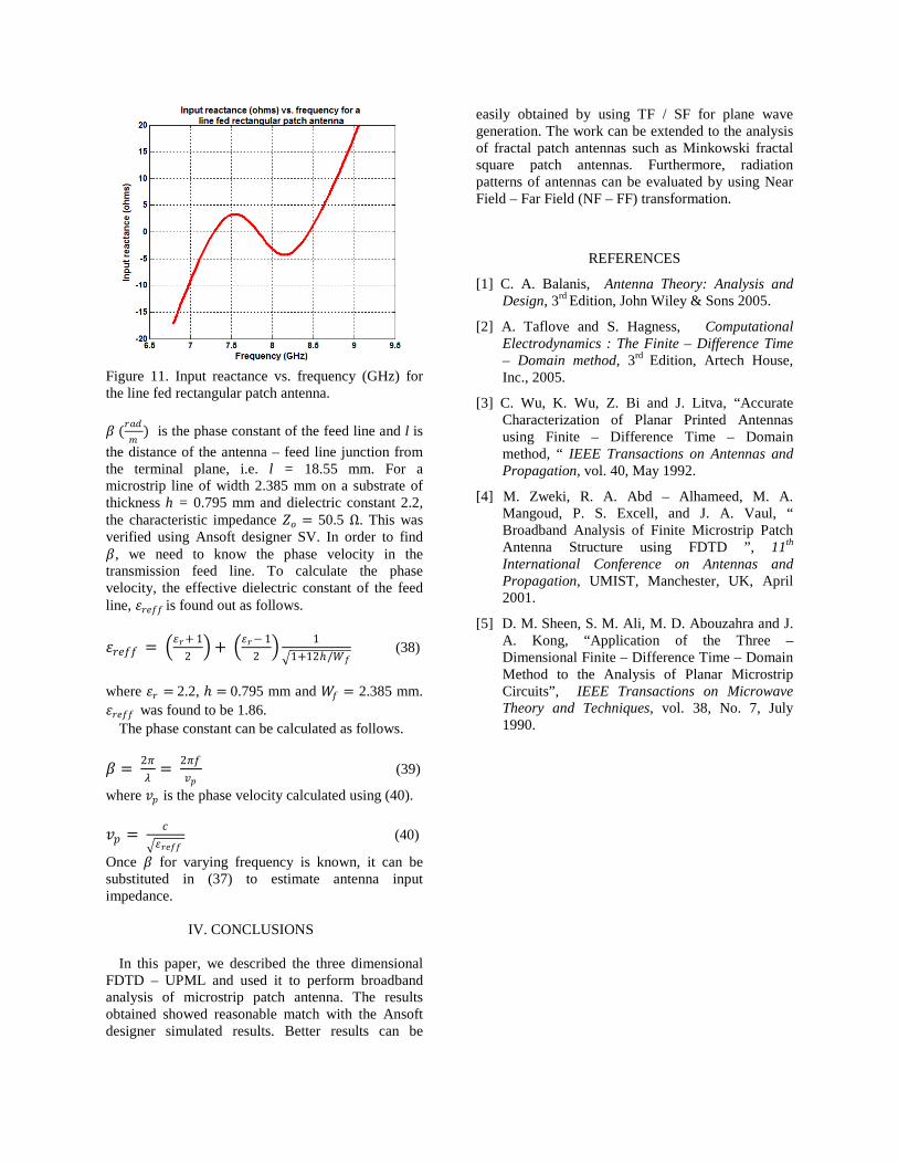
Figure 11. Input reactance vs. frequency (GHz) for the line fed rectangular patch antenna. 𝑡𝑡 (𝑟𝑟𝑚𝑚𝑑𝑑

𝑚𝑚) is the phase constant of the feed line and l is

the distance of the antenna – feed line junction from the terminal plane, i.e. l = 18.55 mm. For a microstrip line of width 2.385 mm on a substrate of thickness h = 0.795 mm and dielectric constant 2.2, the characteristic impedance 𝑍𝑍𝑜𝑜 = 50.5 Ω. This was verified using Ansoft designer SV. In order to find 𝑡𝑡, we need to know the phase velocity in the transmission feed line. To calculate the phase velocity, the effective dielectric constant of the feed line, 𝑗𝑗𝑟𝑟𝑒𝑒𝑓𝑓𝑓𝑓 is found out as follows. 𝑗𝑗𝑟𝑟𝑒𝑒𝑓𝑓𝑓𝑓 = �𝑗𝑗𝑟𝑟+ 1

2�+ �𝑗𝑗𝑟𝑟− 1

2� 1�1+12ℎ/𝑊𝑊𝑓𝑓

(38)

where 𝑗𝑗𝑟𝑟 = 2.2, ℎ = 0.795 mm and 𝑊𝑊𝑓𝑓 = 2.385 mm. 𝑗𝑗𝑟𝑟𝑒𝑒𝑓𝑓𝑓𝑓 was found to be 1.86. The phase constant can be calculated as follows. 𝑡𝑡 = 2𝜋𝜋

𝜆𝜆= 2𝜋𝜋𝑓𝑓

𝑣𝑣𝑒𝑒 (39)

where 𝑣𝑣𝑒𝑒 is the phase velocity calculated using (40). 𝑣𝑣𝑒𝑒 = 𝑐𝑐

�𝑗𝑗𝑟𝑟𝑒𝑒𝑓𝑓𝑓𝑓 (40)

Once 𝑡𝑡 for varying frequency is known, it can be substituted in (37) to estimate antenna input impedance. IV. CONCLUSIONS In this paper, we described the three dimensional FDTD – UPML and used it to perform broadband analysis of microstrip patch antenna. The results obtained showed reasonable match with the Ansoft designer simulated results. Better results can be

easily obtained by using TF / SF for plane wave generation. The work can be extended to the analysis of fractal patch antennas such as Minkowski fractal square patch antennas. Furthermore, radiation patterns of antennas can be evaluated by using Near Field – Far Field (NF – FF) transformation.

REFERENCES

[1] C. A. Balanis, Antenna Theory: Analysis and Design, 3rd Edition, John Wiley & Sons 2005.

[2] A. Taflove and S. Hagness, Computational Electrodynamics : The Finite – Difference Time – Domain method, 3rd Edition, Artech House, Inc., 2005.

[3] C. Wu, K. Wu, Z. Bi and J. Litva, “Accurate Characterization of Planar Printed Antennas using Finite – Difference Time – Domain method, “ IEEE Transactions on Antennas and Propagation, vol. 40, May 1992.

[4] M. Zweki, R. A. Abd – Alhameed, M. A. Mangoud, P. S. Excell, and J. A. Vaul, “ Broadband Analysis of Finite Microstrip Patch Antenna Structure using FDTD ”, 11th International Conference on Antennas and Propagation, UMIST, Manchester, UK, April 2001.

[5] D. M. Sheen, S. M. Ali, M. D. Abouzahra and J. A. Kong, “Application of the Three – Dimensional Finite – Difference Time – Domain Method to the Analysis of Planar Microstrip Circuits”, IEEE Transactions on Microwave Theory and Techniques, vol. 38, No. 7, July 1990.

Appendix I : 3D FDTD – UPML update equations 1. 𝑫𝑫𝒙𝒙 update equation

𝐷𝐷𝑥𝑥 |𝑖𝑖+0.5,𝑗𝑗 ,𝑘𝑘𝑛𝑛+1 = 𝐶𝐶1𝐷𝐷𝑥𝑥.𝐷𝐷𝑥𝑥 |𝑖𝑖+0.5,𝑗𝑗 ,𝑘𝑘

𝑛𝑛 + 𝐶𝐶2𝐷𝐷𝑥𝑥. �𝐻𝐻𝑧𝑧 |𝑖𝑖+0.5,𝑗𝑗+0.5,𝑘𝑘

𝑛𝑛+0.5 − 𝐻𝐻𝑧𝑧 |𝑖𝑖+0.5,𝑗𝑗−0.5,𝑘𝑘𝑛𝑛+0.5

∆𝑦𝑦−

𝐻𝐻𝑦𝑦 |𝑖𝑖+0.5,𝑗𝑗 ,𝑘𝑘+0.5𝑛𝑛+0.5 − 𝐻𝐻𝑦𝑦 |𝑖𝑖+0.5,𝑗𝑗 ,𝑘𝑘−0.5

𝑛𝑛+0.5

∆𝑧𝑧�

𝐶𝐶1𝐷𝐷𝑥𝑥 = �2𝑗𝑗𝜅𝜅𝑦𝑦− 𝜎𝜎𝑦𝑦∆𝜕𝜕2𝑗𝑗𝜅𝜅𝑦𝑦+ 𝜎𝜎𝑦𝑦∆𝜕𝜕

� 𝐶𝐶2𝐷𝐷𝑥𝑥 = � 2𝑗𝑗∆𝜕𝜕2𝑗𝑗𝜅𝜅𝑦𝑦+ 𝜎𝜎𝑦𝑦Δ𝜕𝜕

�

2. 𝑫𝑫𝒚𝒚 update equation

𝐷𝐷𝑦𝑦 |𝑖𝑖 ,𝑗𝑗+0.5,𝑘𝑘𝑛𝑛+1 = 𝐶𝐶1𝐷𝐷𝑦𝑦.𝐷𝐷𝑦𝑦 |𝑖𝑖 ,𝑗𝑗+0.5,𝑘𝑘

𝑛𝑛 + 𝐶𝐶2𝐷𝐷𝑦𝑦. �𝐻𝐻𝑥𝑥 |𝑖𝑖 ,𝑗𝑗+0.5,𝑘𝑘+0.5

𝑛𝑛+0.5 − 𝐻𝐻𝑥𝑥 |𝑖𝑖 ,𝑗𝑗+0.5,𝑘𝑘−0.5𝑛𝑛+0.5

∆𝑧𝑧−

𝐻𝐻𝑧𝑧 |𝑖𝑖+0.5,𝑗𝑗+0.5,𝑘𝑘𝑛𝑛+0.5 − 𝐻𝐻𝑧𝑧 |𝑖𝑖−0.5,𝑗𝑗+0.5,𝑘𝑘

𝑛𝑛+0.5

∆𝑥𝑥�

𝐶𝐶1𝐷𝐷𝑦𝑦 = �2𝑗𝑗𝜅𝜅𝑧𝑧− 𝜎𝜎𝑧𝑧∆𝜕𝜕2𝑗𝑗𝜅𝜅𝑧𝑧+ 𝜎𝜎𝑧𝑧∆𝜕𝜕

� 𝐶𝐶2𝐷𝐷𝑦𝑦 = � 2𝑗𝑗∆𝜕𝜕2𝑗𝑗𝜅𝜅𝑧𝑧+ 𝜎𝜎𝑧𝑧Δ𝜕𝜕

�

3. 𝑫𝑫𝒛𝒛 update equation 𝐷𝐷𝑧𝑧 |𝑖𝑖 ,𝑗𝑗 ,𝑘𝑘+0.5

𝑛𝑛+1 = 𝐶𝐶1𝐷𝐷𝑧𝑧.𝐷𝐷𝑧𝑧 |𝑖𝑖 ,𝑗𝑗 ,𝑘𝑘+0.5𝑛𝑛 + 𝐶𝐶2𝐷𝐷𝑧𝑧. �

𝐻𝐻𝑦𝑦 |𝑖𝑖+0.5,𝑗𝑗 ,𝑘𝑘+0.5𝑛𝑛+0.5 − 𝐻𝐻𝑦𝑦 |𝑖𝑖−0.5,𝑗𝑗 ,𝑘𝑘+0.5

𝑛𝑛+0.5

∆𝑥𝑥−

𝐻𝐻𝑥𝑥 |𝑖𝑖 ,𝑗𝑗+0.5,𝑘𝑘+0.5𝑛𝑛+0.5 − 𝐻𝐻𝑥𝑥 |𝑖𝑖 ,𝑗𝑗−0.5,𝑘𝑘+0.5

𝑛𝑛+0.5

∆𝑦𝑦�

𝐶𝐶1𝐷𝐷𝑧𝑧 = �2𝑗𝑗𝜅𝜅𝑥𝑥− 𝜎𝜎𝑥𝑥∆𝜕𝜕2𝑗𝑗𝜅𝜅𝑥𝑥+ 𝜎𝜎𝑥𝑥∆𝜕𝜕

� 𝐶𝐶2𝐷𝐷𝑧𝑧 = � 2𝑗𝑗∆𝜕𝜕2𝑗𝑗𝜅𝜅𝑥𝑥+ 𝜎𝜎𝑥𝑥Δ𝜕𝜕

�

4. 𝑬𝑬𝒙𝒙 update equation 𝐸𝐸𝑥𝑥 |𝑖𝑖+0.5,𝑗𝑗 ,𝑘𝑘

𝑛𝑛+1 = 𝐶𝐶1𝐸𝐸𝑥𝑥.𝐸𝐸𝑥𝑥 |𝑖𝑖+0.5,𝑗𝑗 ,𝑘𝑘𝑛𝑛 + 𝐶𝐶2𝐸𝐸𝑥𝑥.𝐷𝐷𝑥𝑥 |𝑖𝑖+0.5,𝑗𝑗 ,𝑘𝑘

𝑛𝑛+1 − 𝐶𝐶3𝐸𝐸𝑥𝑥.𝐷𝐷𝑥𝑥 |𝑖𝑖+0.5,𝑗𝑗 ,𝑘𝑘𝑛𝑛

𝐶𝐶1𝐸𝐸𝑥𝑥 = �2𝑗𝑗𝜅𝜅𝑧𝑧−𝜎𝜎𝑧𝑧Δ𝜕𝜕2𝑗𝑗𝜅𝜅𝑧𝑧+𝜎𝜎𝑧𝑧Δ𝜕𝜕

� 𝐶𝐶2𝐸𝐸𝑥𝑥 = � 2𝑗𝑗𝜅𝜅𝑥𝑥+ 𝜎𝜎𝑥𝑥Δ𝜕𝜕𝑗𝑗(2𝑗𝑗𝜅𝜅𝑧𝑧+ 𝜎𝜎𝑧𝑧Δ𝜕𝜕)

� 𝐶𝐶3𝐸𝐸𝑥𝑥 = � 2𝑗𝑗𝜅𝜅𝑥𝑥− 𝜎𝜎𝑥𝑥Δ𝜕𝜕𝑗𝑗(2𝑗𝑗𝜅𝜅𝑧𝑧+ 𝜎𝜎𝑧𝑧Δ𝜕𝜕)

�

5. 𝑬𝑬𝒚𝒚 update equation

𝐸𝐸𝑦𝑦 |𝑖𝑖 ,𝑗𝑗+0.5,𝑘𝑘𝑛𝑛+1 = 𝐶𝐶1𝐸𝐸𝑦𝑦.𝐸𝐸𝑦𝑦 |𝑖𝑖 ,𝑗𝑗+0.5,𝑘𝑘

𝑛𝑛 + 𝐶𝐶2𝐸𝐸𝑦𝑦.𝐷𝐷𝑦𝑦 |𝑖𝑖 ,𝑗𝑗+0.5,𝑘𝑘𝑛𝑛+1 − 𝐶𝐶3𝐸𝐸𝑦𝑦.𝐷𝐷𝑦𝑦 |𝑖𝑖 ,𝑗𝑗+0.5,𝑘𝑘

𝑛𝑛

𝐶𝐶1𝐸𝐸𝑦𝑦 = �2𝑗𝑗𝜅𝜅𝑥𝑥−𝜎𝜎𝑥𝑥Δ𝜕𝜕2𝑗𝑗𝜅𝜅𝑥𝑥+𝜎𝜎𝑥𝑥Δ𝜕𝜕

� 𝐶𝐶2𝐸𝐸𝑦𝑦 = � 2𝑗𝑗𝜅𝜅𝑦𝑦+ 𝜎𝜎𝑦𝑦Δ𝜕𝜕𝑗𝑗(2𝑗𝑗𝜅𝜅𝑥𝑥+ 𝜎𝜎𝑥𝑥Δ𝜕𝜕)

� 𝐶𝐶3𝐸𝐸𝑦𝑦 = � 2𝑗𝑗𝜅𝜅𝑦𝑦− 𝜎𝜎𝑦𝑦Δ𝜕𝜕𝑗𝑗(2𝑗𝑗𝜅𝜅𝑥𝑥+ 𝜎𝜎𝑥𝑥Δ𝜕𝜕)

�

6. 𝑬𝑬𝒛𝒛 update equation 𝐸𝐸𝑧𝑧 |𝑖𝑖 ,𝑗𝑗 ,𝑘𝑘+0.5

𝑛𝑛+1 = 𝐶𝐶1𝐸𝐸𝑧𝑧.𝐸𝐸𝑧𝑧 |𝑖𝑖 ,𝑗𝑗 ,𝑘𝑘+0.5𝑛𝑛 + 𝐶𝐶2𝐸𝐸𝑧𝑧.𝐷𝐷𝑧𝑧 |𝑖𝑖 ,𝑗𝑗 ,𝑘𝑘+0.5

𝑛𝑛+1 − 𝐶𝐶3𝐸𝐸𝑧𝑧.𝐷𝐷𝑧𝑧 |𝑖𝑖 ,𝑗𝑗 ,𝑘𝑘+0.5𝑛𝑛

𝐶𝐶1𝐸𝐸𝑧𝑧 = �2𝑗𝑗𝜅𝜅𝑦𝑦−𝜎𝜎𝑦𝑦Δ𝜕𝜕2𝑗𝑗𝜅𝜅𝑦𝑦+𝜎𝜎𝑦𝑦Δ𝜕𝜕

� 𝐶𝐶2𝐸𝐸𝑧𝑧 = � 2𝑗𝑗𝜅𝜅𝑧𝑧+ 𝜎𝜎𝑧𝑧Δ𝜕𝜕𝑗𝑗�2𝑗𝑗𝜅𝜅𝑦𝑦+ 𝜎𝜎𝑦𝑦Δ𝜕𝜕�

� 𝐶𝐶3𝐸𝐸𝑧𝑧 = � 2𝑗𝑗𝜅𝜅𝑧𝑧− 𝜎𝜎𝑧𝑧Δ𝜕𝜕𝑗𝑗�2𝑗𝑗𝜅𝜅𝑦𝑦+ 𝜎𝜎𝑦𝑦Δ𝜕𝜕�

�

7. 𝑩𝑩𝒙𝒙 update equation 𝐵𝐵𝑥𝑥 |𝑖𝑖 ,𝑗𝑗+0.5,𝑘𝑘+0.5

𝑛𝑛+1.5 = 𝐶𝐶1𝐵𝐵𝑥𝑥.𝐵𝐵𝑥𝑥 |𝑖𝑖 ,𝑗𝑗+0.5,𝑘𝑘+0.5𝑛𝑛+0.5 − 𝐶𝐶2𝐵𝐵𝑥𝑥. �

𝐸𝐸𝑧𝑧 |𝑖𝑖 ,𝑗𝑗+1,𝑘𝑘+0.5𝑛𝑛+1 − 𝐸𝐸𝑧𝑧 |𝑖𝑖 ,𝑗𝑗 ,𝑘𝑘+0.5

𝑛𝑛+1

∆𝑦𝑦−

𝐸𝐸𝑦𝑦 |𝑖𝑖 ,𝑗𝑗+0.5,𝑘𝑘+1𝑛𝑛+1 − 𝐸𝐸𝑦𝑦 |𝑖𝑖 ,𝑗𝑗+0.5,𝑘𝑘

𝑛𝑛+1

∆𝑧𝑧�

𝐶𝐶1𝐵𝐵𝑥𝑥 = �2𝑗𝑗𝜅𝜅𝑦𝑦− 𝜎𝜎𝑦𝑦∆𝜕𝜕2𝑗𝑗𝜅𝜅𝑦𝑦+ 𝜎𝜎𝑦𝑦∆𝜕𝜕

� 𝐶𝐶2𝐵𝐵𝑥𝑥 = � 2𝑗𝑗∆𝜕𝜕2𝑗𝑗𝜅𝜅𝑦𝑦+ 𝜎𝜎𝑦𝑦Δ𝜕𝜕

�

8. 𝑩𝑩𝒚𝒚 update equation

𝐵𝐵𝑦𝑦 |𝑖𝑖+0.5,𝑗𝑗 ,𝑘𝑘+0.5𝑛𝑛+1.5 = 𝐶𝐶1𝐵𝐵𝑦𝑦.𝐵𝐵𝑦𝑦 |𝑖𝑖+0.5,𝑗𝑗 ,𝑘𝑘+0.5

𝑛𝑛+0.5 − 𝐶𝐶2𝐵𝐵𝑦𝑦. �𝐸𝐸𝑥𝑥 |𝑖𝑖+0.5,𝑗𝑗 ,𝑘𝑘+1

𝑛𝑛+1 − 𝐸𝐸𝑥𝑥 |𝑖𝑖+0.5,𝑗𝑗 ,𝑘𝑘𝑛𝑛+1

∆𝑧𝑧−

𝐸𝐸𝑧𝑧 |𝑖𝑖+1,𝑗𝑗 ,𝑘𝑘+0.5𝑛𝑛+1 − 𝐸𝐸𝑧𝑧 |𝑖𝑖 ,𝑗𝑗 ,𝑘𝑘+0.5

𝑛𝑛+1

∆𝑥𝑥�

𝐶𝐶1𝐵𝐵𝑦𝑦 = �2𝑗𝑗𝜅𝜅𝑧𝑧− 𝜎𝜎𝑧𝑧∆𝜕𝜕2𝑗𝑗𝜅𝜅𝑧𝑧+ 𝜎𝜎𝑧𝑧∆𝜕𝜕

� 𝐶𝐶2𝐵𝐵𝑦𝑦 = � 2𝑗𝑗∆𝜕𝜕2𝑗𝑗𝜅𝜅𝑧𝑧+ 𝜎𝜎𝑧𝑧Δ𝜕𝜕

�

9. 𝑩𝑩𝒛𝒛 update equation 𝐵𝐵𝑧𝑧 |𝑖𝑖+0.5,𝑗𝑗+0.5,𝑘𝑘

𝑛𝑛+1.5 = 𝐶𝐶1𝐵𝐵𝑧𝑧.𝐵𝐵𝑧𝑧 |𝑖𝑖+0.5,𝑗𝑗+0.5,𝑘𝑘𝑛𝑛+0.5 − 𝐶𝐶2𝐵𝐵𝑧𝑧. �

𝐸𝐸𝑦𝑦 |𝑖𝑖+1,𝑗𝑗+0.5,𝑘𝑘𝑛𝑛+1 − 𝐸𝐸𝑦𝑦 |𝑖𝑖 ,𝑗𝑗+0.5,𝑘𝑘

𝑛𝑛+1

∆𝑥𝑥−

𝐸𝐸𝑥𝑥 |𝑖𝑖+0.5,𝑗𝑗+1,𝑘𝑘𝑛𝑛+1 − 𝐸𝐸𝑥𝑥 |𝑖𝑖+0.5,𝑗𝑗 ,𝑘𝑘

𝑛𝑛+1

∆𝑦𝑦�

𝐶𝐶1𝐵𝐵𝑧𝑧 = �2𝑗𝑗𝜅𝜅𝑥𝑥− 𝜎𝜎𝑥𝑥∆𝜕𝜕2𝑗𝑗𝜅𝜅𝑥𝑥+ 𝜎𝜎𝑥𝑥∆𝜕𝜕

� 𝐶𝐶2𝐵𝐵𝑧𝑧 = � 2𝑗𝑗∆𝜕𝜕2𝑗𝑗𝜅𝜅𝑥𝑥+ 𝜎𝜎𝑥𝑥Δ𝜕𝜕

� 10. 𝑯𝑯𝒙𝒙 update equation

𝐻𝐻𝑥𝑥 |𝑖𝑖 ,𝑗𝑗+0.5,𝑘𝑘+0.5𝑛𝑛+1.5 = 𝐶𝐶1𝐻𝐻𝑥𝑥.𝐻𝐻𝑥𝑥 |𝑖𝑖 ,𝑗𝑗+0.5,𝑘𝑘+0.5

𝑛𝑛+0.5 + 𝐶𝐶2𝐻𝐻𝑥𝑥.𝐵𝐵𝑥𝑥 |𝑖𝑖 ,𝑗𝑗+0.5,𝑘𝑘+0.5𝑛𝑛+1.5 − 𝐶𝐶3𝐻𝐻𝑥𝑥.𝐵𝐵𝑥𝑥 |𝑖𝑖 ,𝑗𝑗+0.5,𝑘𝑘+0.5

𝑛𝑛+0.5

𝐶𝐶1𝐻𝐻𝑥𝑥 = �2𝑗𝑗𝜅𝜅𝑧𝑧−𝜎𝜎𝑧𝑧Δ𝜕𝜕2𝑗𝑗𝜅𝜅𝑧𝑧+𝜎𝜎𝑧𝑧Δ𝜕𝜕

� 𝐶𝐶2𝐻𝐻𝑥𝑥 = � 2𝑗𝑗𝜅𝜅𝑥𝑥+ 𝜎𝜎𝑥𝑥Δ𝜕𝜕𝑗𝑗(2𝑗𝑗𝜅𝜅𝑧𝑧+ 𝜎𝜎𝑧𝑧Δ𝜕𝜕)

� 𝐶𝐶3𝐻𝐻𝑥𝑥 = � 2𝑗𝑗𝜅𝜅𝑥𝑥− 𝜎𝜎𝑥𝑥Δ𝜕𝜕𝑗𝑗(2𝑗𝑗𝜅𝜅𝑧𝑧+ 𝜎𝜎𝑧𝑧Δ𝜕𝜕)

�

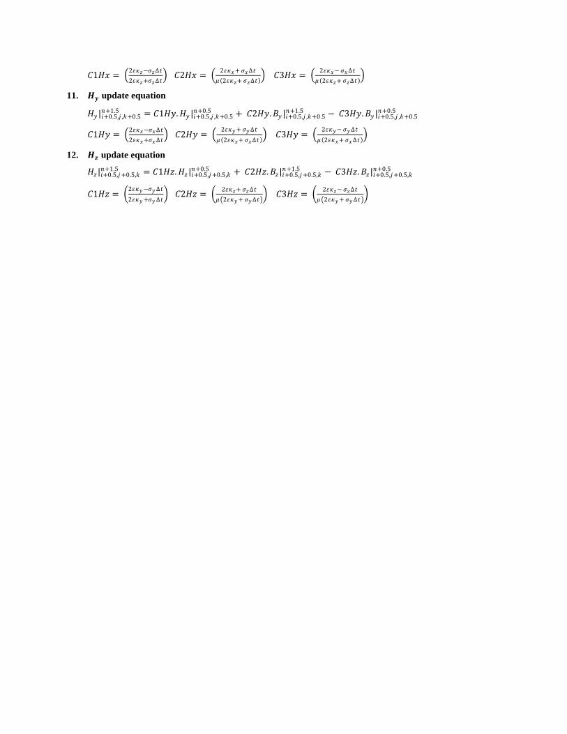
11. 𝑯𝑯𝒚𝒚 update equation

𝐻𝐻𝑦𝑦 |𝑖𝑖+0.5,𝑗𝑗 ,𝑘𝑘+0.5𝑛𝑛+1.5 = 𝐶𝐶1𝐻𝐻𝑦𝑦.𝐻𝐻𝑦𝑦 |𝑖𝑖+0.5,𝑗𝑗 ,𝑘𝑘+0.5

𝑛𝑛+0.5 + 𝐶𝐶2𝐻𝐻𝑦𝑦.𝐵𝐵𝑦𝑦 |𝑖𝑖+0.5,𝑗𝑗 ,𝑘𝑘+0.5𝑛𝑛+1.5 − 𝐶𝐶3𝐻𝐻𝑦𝑦.𝐵𝐵𝑦𝑦 |𝑖𝑖+0.5,𝑗𝑗 ,𝑘𝑘+0.5

𝑛𝑛+0.5

𝐶𝐶1𝐻𝐻𝑦𝑦 = �2𝑗𝑗𝜅𝜅𝑥𝑥−𝜎𝜎𝑥𝑥Δ𝜕𝜕2𝑗𝑗𝜅𝜅𝑥𝑥+𝜎𝜎𝑥𝑥Δ𝜕𝜕

� 𝐶𝐶2𝐻𝐻𝑦𝑦 = � 2𝑗𝑗𝜅𝜅𝑦𝑦+ 𝜎𝜎𝑦𝑦Δ𝜕𝜕𝑗𝑗(2𝑗𝑗𝜅𝜅𝑥𝑥+ 𝜎𝜎𝑥𝑥Δ𝜕𝜕)

� 𝐶𝐶3𝐻𝐻𝑦𝑦 = � 2𝑗𝑗𝜅𝜅𝑦𝑦− 𝜎𝜎𝑦𝑦Δ𝜕𝜕𝑗𝑗(2𝑗𝑗𝜅𝜅𝑥𝑥+ 𝜎𝜎𝑥𝑥Δ𝜕𝜕)

�

12. 𝑯𝑯𝒛𝒛 update equation 𝐻𝐻𝑧𝑧 |𝑖𝑖+0.5,𝑗𝑗+0.5,𝑘𝑘

𝑛𝑛+1.5 = 𝐶𝐶1𝐻𝐻𝑧𝑧.𝐻𝐻𝑧𝑧 |𝑖𝑖+0.5,𝑗𝑗+0.5,𝑘𝑘𝑛𝑛+0.5 + 𝐶𝐶2𝐻𝐻𝑧𝑧.𝐵𝐵𝑧𝑧 |𝑖𝑖+0.5,𝑗𝑗+0.5,𝑘𝑘

𝑛𝑛+1.5 − 𝐶𝐶3𝐻𝐻𝑧𝑧.𝐵𝐵𝑧𝑧 |𝑖𝑖+0.5,𝑗𝑗+0.5,𝑘𝑘𝑛𝑛+0.5

𝐶𝐶1𝐻𝐻𝑧𝑧 = �2𝑗𝑗𝜅𝜅𝑦𝑦−𝜎𝜎𝑦𝑦 Δ𝜕𝜕2𝑗𝑗𝜅𝜅𝑦𝑦+𝜎𝜎𝑦𝑦 Δ𝜕𝜕

� 𝐶𝐶2𝐻𝐻𝑧𝑧 = � 2𝑗𝑗𝜅𝜅𝑧𝑧+ 𝜎𝜎𝑧𝑧Δ𝜕𝜕𝑗𝑗�2𝑗𝑗𝜅𝜅𝑦𝑦+ 𝜎𝜎𝑦𝑦Δ𝜕𝜕�

� 𝐶𝐶3𝐻𝐻𝑧𝑧 = � 2𝑗𝑗𝜅𝜅𝑧𝑧− 𝜎𝜎𝑧𝑧Δ𝜕𝜕𝑗𝑗�2𝑗𝑗𝜅𝜅𝑦𝑦+ 𝜎𝜎𝑦𝑦Δ𝜕𝜕�

�

Appendix II : C++ code for 3D FDTD - UPML simulation of microstrip patch antenna /* Fdtd3D.cpp : 3D FDTD + UPML Author : Srikumar Sandeep 1) E,D vectors on yee cell edge centres and H,B vectors on Yee cell face centres. Ex[i + 0.5][j][k], Ey[i][j + 0.5][k], Ez[i][j][k + 0.5] Dx[i + 0.5][j][k], Dy[i][j + 0.5][k], Dz[i][j][k + 0.5]

Hx[i][j + 0.5][k + 0.5], Hy[i + 0.5][j][k + 0.5], Hz[i + 0.5][j + 0.5][k] Bx[i][j + 0.5][k + 0.5], By[i + 0.5][j][k + 0.5], Bz[i + 0.5][j + 0.5][k]

2) Constitutive parameter matrices epsr [XCELLS] [YCELLS] [ZCELLS] sigma[XCELLS] [YCELLS] [ZCELLS] */ #include "iostream.h" #include "math.h" #include "stdlib.h" #include "fstream.h" #define PL 19 //Number of PML layers. #define PSX 70 //Number of yee cells in problem space along x-direction #define PSY 150 //Number of yee cells in problem space along y-direction #define PSZ 16 //Number of yee cells in problem space along z-direction #define XCELLS PSX + (2 * PL) //Total number of yee cells along x-direction #define YCELLS PSY + (2 * PL) //Total number of yee cells along y-direction #define ZCELLS PSZ + (2 * PL) //Total number of yee cells along z-direction typedef double*** MatPtr; //3D matrix const double muo = 12.5664e-7; const double epso = 8.85e-12; const double CuSigma = 5.8e78; //Matrices MatPtr epsr, sigma; MatPtr Dx,Dy,Dz,Bx,By,Bz,Ex,Ey,Ez,Hx,Hy,Hz; MatPtr C1Dx,C2Dx,C1Dy,C2Dy,C1Dz,C2Dz; MatPtr C1Bx,C2Bx,C1By,C2By,C1Bz,C2Bz; MatPtr C1Ex,C2Ex,C3Ex,C1Ey,C2Ey,C3Ey,C1Ez,C2Ez,C3Ez; MatPtr C1Hx,C2Hx,C3Hx,C1Hy,C2Hy,C3Hy,C1Hz,C2Hz,C3Hz; //Function prototypes void CreateAllMatrices(); void DeleteAllMatrices(); void CreateMatrix(MatPtr&,int dimx,int dimy,int dimz); void DeleteMatrix(MatPtr, int dimx,int dimy,int dimz); void FillUpdateEqnConstantMatrices(double g, double sigmao,double dt); void main() { cout<<"--------------FDTD 3D simulator--------------------\n"; //T - Number of time steps //i,j,k - x,y,z direction yee cell index //n - Temporal index int T = 5000;

int i,j,k,n; //Text files to write the simulation data ofstream Ezfile,Hxfile; Ezfile.open("Ezfile.txt"); Hxfile.open("Hxfile.txt"); //dx, dy, dz ,dt – Spatial and temporal discretization interval double dx,dy,dz,dt; //UPML parameters double g = 1.4; double sigmao = 0.5; // Source plane at j = SP // Terminal plane at j = TP // GP – Ground plane location at k = PL + 1 int SP = 22; int TP = 32; int GP = PL + 1; //Initiliazation of discretization interval dx = 0.000265; dy = 0.000265; dz = 0.000265; dt = dz/(6e8); // Create all the 3D matrices and initialize the elements to zero // matrices include field / flux components and precomputed update equation // coefficients CreateAllMatrices(); //Fill the constitutive parameter matrices for(i = 0;i < XCELLS;i++) { for(j = 0;j < YCELLS;j++) { for(k = 0;k < ZCELLS;k++) { epsr [i][j][k] = 1.0; sigma[i][j][k] = 0.0; //Ground plane at k = 17 //Ground plane extends throughout the entire XY plane if(k == GP && i >= 0 && i < XCELLS && j >= 0 && j < YCELLS) { sigma[i][j][k] = Cusigma; } //3 layers of substrate corresponding to substrate //thickness = 0.795 mm. The substrate extends in the whole

//XY plane of the problem space. But does not extend into //UPML

if((k == GP + 1 || k == GP + 2 || k == GP + 3) && i >= PL && i < XCELLS - PL && j >= PL && j < YCELLS - PL)

{ epsr[i][j][k] = 2.2; } //Feed line width is 9dx //Feed line is 8dx offset from the edge of the patch

//i.e it starts from i = 35 if(k == GP + 4) { if(i >= 35 && i <= 43) {

//For incident wave simulation : j >=0 && j <= //YCELLS – 1 //For patch antenna simulation : j >= 0 && j //<= 102

if(j >= 0 && j <= 102) { sigma[i][j][k] = CuSigma; } } } //Patch antenna if(k == GP + 4) { //The width of patch = 12.45 mm = 47dx if(i >= 27 && i <= 73) { //The length of patch = 16 mm = 60 dx if(j >= 102 && j <= 162) { sigma[i][j][k] = CuSigma; } } } } } } //Precomputer update equation coefficient matrices FillUpdateEqnConstantMatrices(g,sigmao,dt); //Temp variables to hold previous field values and field differential values. double Dxo,Exo,Dyo,Eyo,Dzo,Ezo; double dHx,dHy,dHz; double Hxo,Hyo,Hzo,Bxo,Byo,Bzo; double dEx,dEy,dEz; //----------------------FDTD update loop starts here--------------------------- for(n = 0;n < T;n++) { //to = 4T double temp = -1*(((n*dt - 120*dt)*(n*dt - 120*dt))/(30*30*dt*dt)); double source = exp(temp); double Ezinc = source; /*Dx,Ex update Dx,Ex[XCELLS][YCELLS + 1][ZCELLS + 1] Dx,Ex at j = 0 or j = YCELLS or k = 0 or k = ZCELLS are on the PEC surface. So they are zero and need not be calculated. */ for(i = 0;i < XCELLS;i++) { for(j = 1;j < YCELLS;j++) { for(k = 1;k < ZCELLS;k++) { Dxo = Dx[i][j][k]; Exo = Ex[i][j][k];

//Dx update equation dHz = (Hz[i][j][k] - Hz[i][j - 1][k]) / dy; dHy = (Hy[i][j][k] - Hy[i][j][k - 1]) / dz; Dx[i][j][k] = C1Dx[i][j][k] * Dxo + C2Dx[i][j][k] * (dHz - dHy); //Ex update equation Ex[i][j][k] = C2Ex[i][j][k] * Dx[i][j][k] - C3Ex[i][j][k] * Dxo + C1Ex[i][j][k] * Exo; } } } /*Dy,Ey update Dy,Ey[XCELLS + 1][YCELLS][ZCELLS + 1] Dy,Ey at i = 0 or i = XCELLS or k = 0 or k = ZCELLS are on the PEC surface. So they are zero and need not be calculated. */ for(i = 1;i < XCELLS;i++) { for(j = 0;j < YCELLS;j++) { for(k = 1;k < ZCELLS;k++) { Dyo = Dy[i][j][k]; Eyo = Ey[i][j][k]; //Dy update equation dHx = (Hx[i][j][k] - Hx[i][j][k - 1]) / dz; dHz = (Hz[i][j][k] - Hz[i - 1][j][k]) / dx; Dy[i][j][k] = C1Dy[i][j][k] * Dyo + C2Dy[i][j][k] * (dHx - dHz); //Ey update equation Ey[i][j][k] = C2Ey[i][j][k] * Dy[i][j][k] - C3Ey[i][j][k] * Dyo + C1Ey[i][j][k] * Eyo; } } } //Dz,Ez update for(i = 1;i < XCELLS;i++) { for(j = 1;j < YCELLS;j++) { for(k = 0;k < ZCELLS;k++) { Dzo = Dz[i][j][k]; Ezo = Ez[i][j][k]; //Dy update equation dHx = (Hx[i][j][k] - Hx[i][j - 1][k]) / dy; dHy = (Hy[i][j][k] - Hy[i - 1][j][k]) / dx; Dz[i][j][k] = C1Dz[i][j][k] * Dzo + C2Dz[i][j][k] * (dHy - dHx); //Ez update equation Ez[i][j][k] = C2Ez[i][j][k] * Dz[i][j][k]

- C3Ez[i][j][k] * Dzo + C1Ez[i][j][k] * Ezo;

//Excitation of the all Ez components under the feed //line microstrip at j = Source plane if(j == SP && i >= 35 && i <= 43 && k >= GP + 1 && k

<= GP + 3) { Ez[i][j][k] += Ezinc; } } } } //Write simulation data to text file Hxfile<<Hx[39][TP][GP + 2]<<"\n"; Ezfile<<Ez[35][TP][GP + 2]<<"\n"; //Hx,Bx update for(i = 0;i < XCELLS;i++) { for(int j = 0;j < YCELLS;j++) { for(int k = 0;k < ZCELLS;k++) { Hxo = Hx[i][j][k]; Bxo = Bx[i][j][k]; dEz = (Ez[i][j + 1][k] - Ez[i][j][k]) / dy; dEy = (Ey[i][j][k + 1] - Ey[i][j][k]) / dz;

Bx[i][j][k] = C1Bx[i][j][k] * Bxo - C2Bx[i][j][k] * (dEz - dEy); Hx[i][j][k] = C1Hx[i][j][k] * Hxo + C2Hx[i][j][k] * Bx[i][j][k] - C3Hx[i][j][k] * Bxo;

} } } //Hy,By update for(i = 0;i < XCELLS;i++) { for(int j = 0;j < YCELLS;j++) { for(int k = 0;k < ZCELLS;k++) { Hyo = Hy[i][j][k]; Byo = By[i][j][k]; dEx = (Ex[i][j][k + 1] - Ex[i][j][k]) / dz; dEz = (Ez[i + 1][j][k] - Ez[i][j][k]) / dx;

By[i][j][k] = C1By[i][j][k] * Byo - C2By[i][j][k] * (dEx - dEz); Hy[i][j][k] = C1Hy[i][j][k] * Hyo + C2Hy[i][j][k] * By[i][j][k] - C3Hy[i][j][k] * Byo;

} }

} //Hz,Bz update for(i = 0;i < XCELLS;i++) { for(int j = 0;j < YCELLS;j++) { for(int k = 0;k < ZCELLS;k++) { Hzo = Hz[i][j][k]; Bzo = Bz[i][j][k]; dEy = (Ey[i + 1][j][k] - Ey[i][j][k]) / dx; dEx = (Ex[i][j + 1][k] - Ex[i][j][k]) / dy;

Bz[i][j][k] = C1Bz[i][j][k] * Bzo - C2Bz[i][j][k] * (dEy - dEx); Hz[i][j][k] = C1Hz[i][j][k] * Hzo + C2Hz[i][j][k] * Bz[i][j][k] - C3Hz[i][j][k] * Bzo;

} } } } DeleteAllMatrices(); Hxfile.close(); Ezfile.close(); } //------------------------------------------------------------------------------------ void FillUpdateEqnConstantMatrices(double g, double sigmao, double dt) { double Dx_ky,Dx_sigmay,Dy_kz,Dy_sigmaz,Dz_kx,Dz_sigmax; double Bx_ky,Bx_sigmay,By_kz,By_sigmaz,Bz_kx,Bz_sigmax; double Ex_kx,Ex_sigmax,Ex_kz,Ex_sigmaz,Ey_ky,Ey_sigmay, Ey_kx,Ey_sigmax,Ez_kz,Ez_sigmaz,Ez_ky,Ez_sigmay; double Hx_kx,Hx_sigmax,Hx_kz,Hx_sigmaz,Hy_ky,Hy_sigmay, Hy_kx,Hy_sigmax,Hz_kz,Hz_sigmaz,Hz_ky,Hz_sigmay; //C1Dx,C2Dx,C1Ex,C2Ex,C3Ex for(int i = 0;i < XCELLS; i++) { for(int j = 1;j < YCELLS; j++) { for(int k = 1;k < ZCELLS; k++) { Dx_ky = 1; Dx_sigmay = sigma[i][j][k]; Ex_kx = 1; Ex_sigmax = sigma[i][j][k]; Ex_kz = 1; Ex_sigmaz = sigma[i][j][k]; //Dx_ky,Dx_sigmay if(j < PL) { Dx_ky = pow(g,PL - j); Dx_sigmay = sigmao * Dx_ky; } else if (j >= PL + PSY) {

Dx_ky = pow(g,j - PL - PSY); Dx_sigmay = sigmao * Dx_ky; } //Ex_kx, Ex_sigmax if(i < PL) { Ex_kx = pow(g,PL - i - 0.5); Ex_sigmax = sigmao * Ex_kx; } else if(i >= PL + PSX) { Ex_kx = pow(g,i - PL - PSX + 0.5); Ex_sigmax = sigmao * Ex_kx; } //Ex_kz,Ex_sigmaz if(k < PL) { Ex_kz = pow(g,PL - k); Ex_sigmaz = sigmao * Ex_kz; } else if(k >= PL + PSZ) { Ex_kz = pow(g,k - PL - PSZ); Ex_sigmaz = sigmao * Ex_kz; } //C1Dx,C2Dx

C1Dx[i][j][k] = (2 * epso * epsr[i][j][k] * Dx_ky - Dx_sigmay * dt)/(2 * epso * epsr[i][j][k] * Dx_ky + Dx_sigmay * dt); C2Dx[i][j][k] = (2 * epso * epsr[i][j][k] * dt) /(2 * epso * epsr[i][j][k] * Dx_ky + Dx_sigmay * dt);

//C1Ex,C2Ex,C3Ex,C1Ey,C2Ey,C3Ey,C1Ez,C2Ez,C3Ez

C1Ex[i][j][k] = (2 * epso * epsr[i][j][k] * Ex_kz - Ex_sigmaz * dt) /(2* epso * epsr[i][j][k] * Ex_kz + Ex_sigmaz * dt); C2Ex[i][j][k] = (2 * epso * epsr[i][j][k] * Ex_kx + Ex_sigmax * dt)/((2 * epso * epsr[i][j][k] * Ex_kz + Ex_sigmaz * dt)* epso * epsr[i][j][k]); C3Ex[i][j][k] = (2 * epso * epsr[i][j][k] * Ex_kx - Ex_sigmax * dt)/((2 * epso * epsr[i][j][k] * Ex_kz + Ex_sigmaz * dt)* epso * epsr[i][j][k]);

} } } //C1Dy,C2Dy,C1Ey,C2Ey,C3Ey for(i = 1;i < XCELLS; i++) { for(int j = 0;j < YCELLS; j++) { for(int k = 1;k < ZCELLS; k++) { Dy_kz = 1; Dy_sigmaz = sigma[i][j][k]; Ey_ky = 1;

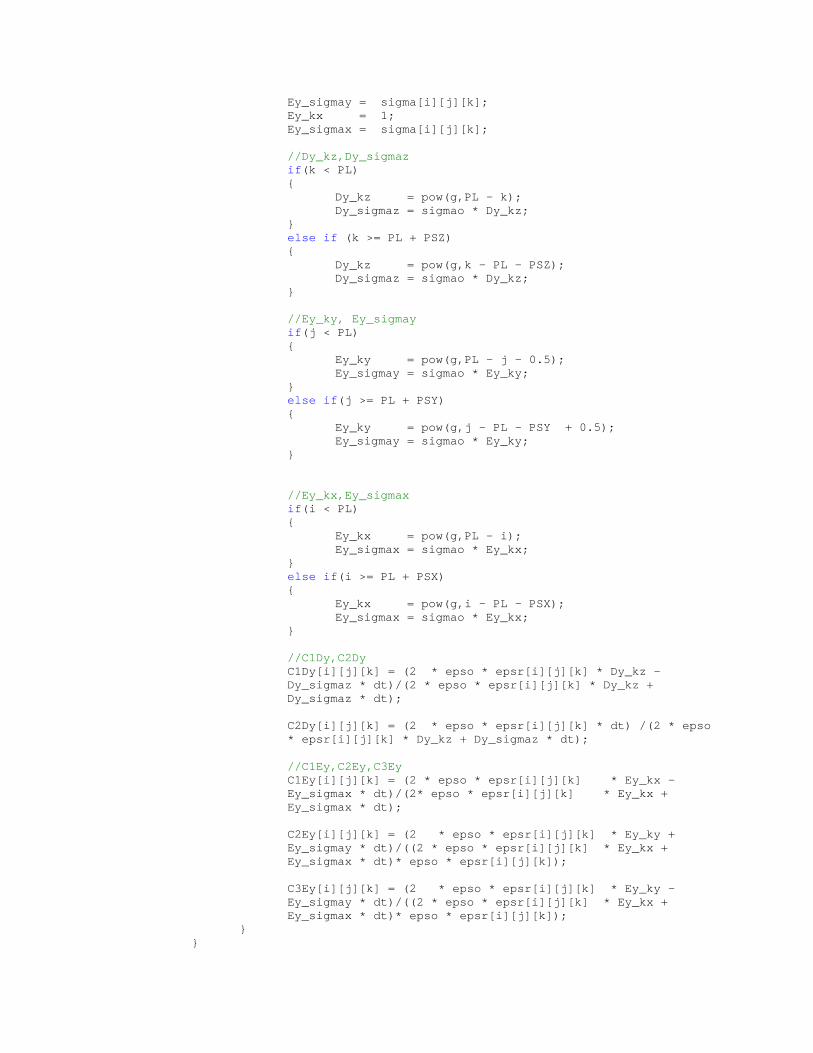
Ey_sigmay = sigma[i][j][k]; Ey_kx = 1; Ey_sigmax = sigma[i][j][k]; //Dy_kz,Dy_sigmaz if(k < PL) { Dy_kz = pow(g,PL - k); Dy_sigmaz = sigmao * Dy_kz; } else if (k >= PL + PSZ) { Dy_kz = pow(g,k - PL - PSZ); Dy_sigmaz = sigmao * Dy_kz; } //Ey_ky, Ey_sigmay if(j < PL) { Ey_ky = pow(g,PL - j - 0.5); Ey_sigmay = sigmao * Ey_ky; } else if(j >= PL + PSY) { Ey_ky = pow(g,j - PL - PSY + 0.5); Ey_sigmay = sigmao * Ey_ky; } //Ey_kx,Ey_sigmax if(i < PL) { Ey_kx = pow(g,PL - i); Ey_sigmax = sigmao * Ey_kx; } else if(i >= PL + PSX) { Ey_kx = pow(g,i - PL - PSX); Ey_sigmax = sigmao * Ey_kx; } //C1Dy,C2Dy

C1Dy[i][j][k] = (2 * epso * epsr[i][j][k] * Dy_kz - Dy_sigmaz * dt)/(2 * epso * epsr[i][j][k] * Dy_kz + Dy_sigmaz * dt);

C2Dy[i][j][k] = (2 * epso * epsr[i][j][k] * dt) /(2 * epso * epsr[i][j][k] * Dy_kz + Dy_sigmaz * dt);

//C1Ey,C2Ey,C3Ey

C1Ey[i][j][k] = (2 * epso * epsr[i][j][k] * Ey_kx - Ey_sigmax * dt)/(2* epso * epsr[i][j][k] * Ey_kx + Ey_sigmax * dt);

C2Ey[i][j][k] = (2 * epso * epsr[i][j][k] * Ey_ky + Ey_sigmay * dt)/((2 * epso * epsr[i][j][k] * Ey_kx + Ey_sigmax * dt)* epso * epsr[i][j][k]); C3Ey[i][j][k] = (2 * epso * epsr[i][j][k] * Ey_ky - Ey_sigmay * dt)/((2 * epso * epsr[i][j][k] * Ey_kx + Ey_sigmax * dt)* epso * epsr[i][j][k]);

} }

} //C1Dz,C2Dz,C1Ez,C2Ez,C3Ez for(i = 1;i < XCELLS; i++) { for(int j = 1;j < YCELLS; j++) { for(int k = 0;k < ZCELLS; k++) { Dz_kx = 1; Dz_sigmax = sigma[i][j][k]; Ez_kz = 1; Ez_sigmaz = sigma[i][j][k]; Ez_ky = 1; Ez_sigmay = sigma[i][j][k]; //Dz_kx,Dz_sigmax if(i < PL) { Dz_kx = pow(g,PL - i); Dz_sigmax = sigmao * Dz_kx; } else if (i >= PL + PSX) { Dz_kx = pow(g,i - PL - PSX); Dz_sigmax = sigmao * Dz_kx; } //Ez_kz, Ez_sigmaz if(k < PL) { Ez_kz = pow(g,PL - k - 0.5); Ez_sigmaz = sigmao * Ez_kz; } else if(k >= PL + PSZ) { Ez_kz = pow(g,k - PL - PSZ + 0.5); Ez_sigmaz = sigmao * Ez_kz; } //Ez_ky,Ez_sigmay if(j < PL) { Ez_ky = pow(g,PL - j); Ez_sigmay = sigmao * Ez_ky; } else if(j >= PL + PSY) { Ez_ky = pow(g,j - PL - PSY); Ez_sigmay = sigmao * Ez_ky; } //C1Dz,C2Dz

C1Dz[i][j][k] = (2 * epso * epsr[i][j][k] * Dz_kx - Dz_sigmax * dt) /(2 * epso * epsr[i][j][k] * Dz_kx + Dz_sigmax * dt); C2Dz[i][j][k] = (2 * epso * epsr[i][j][k] * dt) /(2 * epso * epsr[i][j][k] * Dz_kx + Dz_sigmax * dt);

//C1Ez,C2Ez,C3Ez

C1Ez[i][j][k] = (2 * epso * epsr[i][j][k] * Ez_ky - Ez_sigmay * dt)/(2* epso * epsr[i][j][k] * Ez_ky + Ez_sigmay * dt);

C2Ez[i][j][k] = (2 * epso * epsr[i][j][k] * Ez_kz + Ez_sigmaz * dt)/((2 * epso * epsr[i][j][k] * Ez_ky + Ez_sigmay * dt) * epso * epsr[i][j][k]); C3Ez[i][j][k] = (2 * epso * epsr[i][j][k] * Ez_kz - Ez_sigmaz * dt)/((2 * epso * epsr[i][j][k] * Ez_ky + Ez_sigmay * dt)* epso * epsr[i][j][k]);

} } } //C1Bx,C2Bx,C1Hx,C2Hx,C3Hx for(i = 0;i < XCELLS;i++) { for(int j = 0;j < YCELLS;j++) { for(int k = 0;k < ZCELLS;k++) { Bx_ky = 1; Bx_sigmay = sigma[i][j][k]; Hx_kx = 1; Hx_sigmax = sigma[i][j][k]; Hx_kz = 1; Hx_sigmaz = sigma[i][j][k]; //Bx_ky,Bx_sigmay if(j < PL) { Bx_ky = pow(g,PL - j - 0.5); Bx_sigmay = sigmao * Bx_ky; } else if(j >= PL + PSY) { Bx_ky = pow(g,j - PL - PSY + 0.5); Bx_sigmay = sigmao * Bx_ky; } //} //Hx_kx,Hx_sigmax if(i < PL) { Hx_kx = pow(g,PL - i); Hx_sigmax = sigmao * Hx_kx; } else if(i >= PL + PSX) { Hx_kx = pow(g,i - PL - PSX); Hx_sigmax = sigmao * Hx_kx; } //Hx_kz,Hx_sigmaz if(k < PL) { Hx_kz = pow(g,PL - k - 0.5); Hx_sigmaz = sigmao * Hx_kz; } else if(k >= PL + PSZ) {

Hx_kz = pow(g,k - PL - PSZ + 0.5); Hx_sigmaz = sigmao * Hx_kz; } //C1Bx,C2Bx,C1By,C2By,C1Bz,C2Bz

C1Bx[i][j][k] = (2 * epso * epsr[i][j][k] * Bx_ky - Bx_sigmay * dt)/(2 * epso * epsr[i][j][k] * Bx_ky + Bx_sigmay * dt);

C2Bx[i][j][k] = (2 * epso * epsr[i][j][k] * dt)

/(2 * epso * epsr[i][j][k] * Bx_ky + Bx_sigmay * dt); //C1Hx,C2Hx,C3Hx,C1Hy,C2Hy,C3Hy,C1Hz,C2Hz,C3Hz

C2Hx[i][j][k] = (2 * epso * epsr[i][j][k] * Hx_kx + Hx_sigmax * dt)/((2 * epso * epsr[i][j][k] * Hx_kz + Hx_sigmaz * dt)* muo );

C3Hx[i][j][k] = (2 * epso * epsr[i][j][k] * Hx_kx - Hx_sigmax * dt)/((2 * epso * epsr[i][j][k] * Hx_kz + Hx_sigmaz * dt)* muo ); C1Hx[i][j][k] = (2 * epso * epsr[i][j][k] * Hx_kz - Hx_sigmaz * dt) /(2* epso * epsr[i][j][k] * Hx_kz + Hx_sigmaz * dt);

} } } //C1By,C2By,C1Hy,C2Hy,C3Hy for(i = 0;i < XCELLS;i++) { for(int j = 0;j < YCELLS;j++) { for(int k = 0;k < ZCELLS;k++) { By_kz = 1; By_sigmaz = sigma[i][j][k]; Hy_ky = 1; Hy_sigmay = sigma[i][j][k]; Hy_kx = 1; Hy_sigmax = sigma[i][j][k]; //By_kz,By_sigmaz if(k < PL) { By_kz = pow(g,PL - k - 0.5); By_sigmaz = sigmao * By_kz; } else if(k >= PL + PSZ) { By_kz = pow(g,k - PL - PSZ + 0.5); By_sigmaz = sigmao * By_kz; } //Hy_ky,Hy_sigmay if(j < PL) { Hy_ky = pow(g,PL - j); Hy_sigmay = sigmao * Hy_ky; } else if(j >= PL + PSY)

{ Hy_ky = pow(g,j - PL - PSY); Hy_sigmay = sigmao * Hy_ky; } //} //Hy_kx,Hy_sigmax if(i < PL) { Hy_kx = pow(g,PL - i - 0.5); Hy_sigmax = sigmao * Hy_kx; } else if(i >= PL + PSX) { Hy_kx = pow(g,i - PL - PSX + 0.5); Hy_sigmax = sigmao * Hy_kx; } //C1By,C2By

C1By[i][j][k] = (2 * epso * epsr[i][j][k] * By_kz - By_sigmaz * dt)/(2 * epso * epsr[i][j][k] * By_kz + By_sigmaz * dt);

C2By[i][j][k] = (2 * epso * epsr[i][j][k] * dt) /(2 * epso * epsr[i][j][k] * By_kz + By_sigmaz * dt);

//C1Hy,C2Hy,C3Hy

C2Hy[i][j][k] = (2 * epso * epsr[i][j][k] * Hy_ky + Hy_sigmay * dt)/((2 * epso * epsr[i][j][k] * Hy_kx + Hy_sigmax * dt)* muo );

C3Hy[i][j][k] = (2 * epso * epsr[i][j][k] * Hy_ky - Hy_sigmay * dt)/((2 * epso * epsr[i][j][k] * Hy_kx + Hy_sigmax * dt)* muo ); C1Hy[i][j][k] = (2 * epso * epsr[i][j][k] * Hy_kx - Hy_sigmax * dt)/(2* epso * epsr[i][j][k] * Hy_kx + Hy_sigmax * dt);

} } } //C1Bz,C2Bz,C1Hz,C2Hz,C3Hz for(i = 0;i < XCELLS;i++) { for(int j = 0;j < YCELLS;j++) { for(int k = 0;k < ZCELLS;k++) { Bz_kx = 1; Bz_sigmax = sigma[i][j][k]; Hz_kz = 1; Hz_sigmaz = sigma[i][j][k]; Hz_ky = 1; Hz_sigmay = sigma[i][j][k]; //Bz_kx,Bz_sigmax if(i < PL) { Bz_kx = pow(g,PL - i - 0.5); Bz_sigmax = sigmao * Bz_kx; } else if(i >= PL + PSX)

{ Bz_kx = pow(g,i - PL - PSX + 0.5); Bz_sigmax = sigmao * Bz_kx; } //Hz_kz,Hz_sigmaz if(k < PL) { Hz_kz = pow(g,PL - k); Hz_sigmaz = sigmao * Hz_kz; } else if(k >= PL + PSZ) { Hz_kz = pow(g,k - PL - PSZ); Hz_sigmaz = sigmao * Hz_kz; } //Hz_ky,Hz_sigmay if(j < PL) { Hz_ky = pow(g,PL - j - 0.5); Hz_sigmay = sigmao * Hz_ky; } else if(j >= PL + PSY) { Hz_ky = pow(g,j - PL - PSY + 0.5); Hz_sigmay = sigmao * Hz_ky; } //} //C1Bz,C2Bz

C1Bz[i][j][k] = (2 * epso * epsr[i][j][k] * Bz_kx - Bz_sigmax * dt)/(2 * epso * epsr[i][j][k] * Bz_kx + Bz_sigmax * dt); C2Bz[i][j][k] = (2 * epso * epsr[i][j][k] * dt) /(2 * epso * epsr[i][j][k] * Bz_kx + Bz_sigmax * dt);

//C1Hz,C2Hz,C3Hz

C2Hz[i][j][k] = (2 * epso * epsr[i][j][k] * Hz_kz + Hz_sigmaz * dt)/((2 * epso * epsr[i][j][k] * Hz_ky + Hz_sigmay * dt)* muo ); C3Hz[i][j][k] = (2 * epso * epsr[i][j][k] * Hz_kz - Hz_sigmaz * dt)/((2 * epso * epsr[i][j][k] * Hz_ky + Hz_sigmay * dt)* muo ); C1Hz[i][j][k] = (2 * epso * epsr[i][j][k] * Hz_ky - Hz_sigmay * dt)/(2* epso * epsr[i][j][k] * Hz_ky + Hz_sigmay * dt);

} } } } void CreateAllMatrices() { //Create the parameter matrices CreateMatrix(epsr, XCELLS,YCELLS,ZCELLS); CreateMatrix(sigma,XCELLS,YCELLS,ZCELLS);

//Field matrices CreateMatrix(Dx,XCELLS,YCELLS + 1,ZCELLS + 1); CreateMatrix(Dy,XCELLS + 1,YCELLS,ZCELLS + 1); CreateMatrix(Dz,XCELLS + 1,YCELLS + 1,ZCELLS); CreateMatrix(Ex,XCELLS,YCELLS + 1,ZCELLS + 1); CreateMatrix(Ey,XCELLS + 1,YCELLS,ZCELLS + 1); CreateMatrix(Ez,XCELLS + 1,YCELLS + 1,ZCELLS); CreateMatrix(Bx,XCELLS,YCELLS,ZCELLS); CreateMatrix(By,XCELLS,YCELLS,ZCELLS); CreateMatrix(Bz,XCELLS,YCELLS,ZCELLS); CreateMatrix(Hx,XCELLS,YCELLS,ZCELLS); CreateMatrix(Hy,XCELLS,YCELLS,ZCELLS); CreateMatrix(Hz,XCELLS,YCELLS,ZCELLS); //Create the update eqn constant matrices CreateMatrix(C1Dx,XCELLS,YCELLS + 1,ZCELLS + 1); CreateMatrix(C2Dx,XCELLS,YCELLS + 1,ZCELLS + 1); CreateMatrix(C1Dy,XCELLS + 1,YCELLS,ZCELLS + 1); CreateMatrix(C2Dy,XCELLS + 1,YCELLS,ZCELLS + 1); CreateMatrix(C1Dz,XCELLS + 1,YCELLS + 1,ZCELLS); CreateMatrix(C2Dz,XCELLS + 1,YCELLS + 1,ZCELLS); CreateMatrix(C1Bx,XCELLS,YCELLS,ZCELLS); CreateMatrix(C2Bx,XCELLS,YCELLS,ZCELLS); CreateMatrix(C1By,XCELLS,YCELLS,ZCELLS); CreateMatrix(C2By,XCELLS,YCELLS,ZCELLS); CreateMatrix(C1Bz,XCELLS,YCELLS,ZCELLS); CreateMatrix(C2Bz,XCELLS,YCELLS,ZCELLS); CreateMatrix(C1Ex,XCELLS,YCELLS + 1,ZCELLS + 1); CreateMatrix(C2Ex,XCELLS,YCELLS + 1,ZCELLS + 1); CreateMatrix(C3Ex,XCELLS,YCELLS + 1,ZCELLS + 1); CreateMatrix(C1Ey,XCELLS + 1,YCELLS,ZCELLS + 1); CreateMatrix(C2Ey,XCELLS + 1,YCELLS,ZCELLS + 1); CreateMatrix(C3Ey,XCELLS + 1,YCELLS,ZCELLS + 1); CreateMatrix(C1Ez,XCELLS + 1,YCELLS + 1,ZCELLS); CreateMatrix(C2Ez,XCELLS + 1,YCELLS + 1,ZCELLS); CreateMatrix(C3Ez,XCELLS + 1,YCELLS + 1,ZCELLS); CreateMatrix(C1Hx,XCELLS,YCELLS,ZCELLS); CreateMatrix(C2Hx,XCELLS,YCELLS,ZCELLS); CreateMatrix(C3Hx,XCELLS,YCELLS,ZCELLS); CreateMatrix(C1Hy,XCELLS,YCELLS,ZCELLS); CreateMatrix(C2Hy,XCELLS,YCELLS,ZCELLS); CreateMatrix(C3Hy,XCELLS,YCELLS,ZCELLS); CreateMatrix(C1Hz,XCELLS,YCELLS,ZCELLS); CreateMatrix(C2Hz,XCELLS,YCELLS,ZCELLS); CreateMatrix(C3Hz,XCELLS,YCELLS,ZCELLS); } void DeleteAllMatrices() { //Delete the constitute parameter matrices DeleteMatrix(epsr ,XCELLS,YCELLS,ZCELLS); DeleteMatrix(sigma,XCELLS,YCELLS,ZCELLS); //Delete the field component matrices DeleteMatrix(Dx,XCELLS,YCELLS + 1,ZCELLS + 1); DeleteMatrix(Dy,XCELLS + 1,YCELLS,ZCELLS + 1);

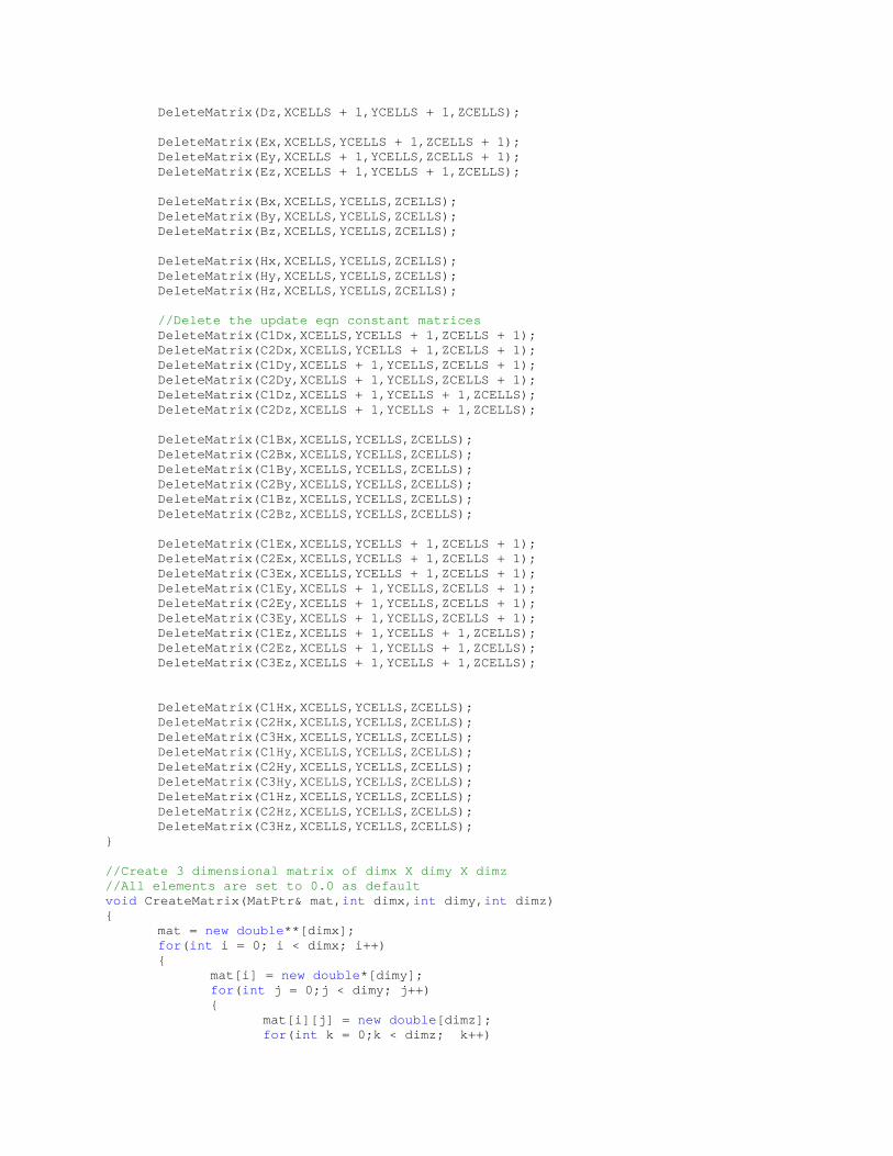
DeleteMatrix(Dz,XCELLS + 1,YCELLS + 1,ZCELLS); DeleteMatrix(Ex,XCELLS,YCELLS + 1,ZCELLS + 1); DeleteMatrix(Ey,XCELLS + 1,YCELLS,ZCELLS + 1); DeleteMatrix(Ez,XCELLS + 1,YCELLS + 1,ZCELLS); DeleteMatrix(Bx,XCELLS,YCELLS,ZCELLS); DeleteMatrix(By,XCELLS,YCELLS,ZCELLS); DeleteMatrix(Bz,XCELLS,YCELLS,ZCELLS); DeleteMatrix(Hx,XCELLS,YCELLS,ZCELLS); DeleteMatrix(Hy,XCELLS,YCELLS,ZCELLS); DeleteMatrix(Hz,XCELLS,YCELLS,ZCELLS); //Delete the update eqn constant matrices DeleteMatrix(C1Dx,XCELLS,YCELLS + 1,ZCELLS + 1); DeleteMatrix(C2Dx,XCELLS,YCELLS + 1,ZCELLS + 1); DeleteMatrix(C1Dy,XCELLS + 1,YCELLS,ZCELLS + 1); DeleteMatrix(C2Dy,XCELLS + 1,YCELLS,ZCELLS + 1); DeleteMatrix(C1Dz,XCELLS + 1,YCELLS + 1,ZCELLS); DeleteMatrix(C2Dz,XCELLS + 1,YCELLS + 1,ZCELLS); DeleteMatrix(C1Bx,XCELLS,YCELLS,ZCELLS); DeleteMatrix(C2Bx,XCELLS,YCELLS,ZCELLS); DeleteMatrix(C1By,XCELLS,YCELLS,ZCELLS); DeleteMatrix(C2By,XCELLS,YCELLS,ZCELLS); DeleteMatrix(C1Bz,XCELLS,YCELLS,ZCELLS); DeleteMatrix(C2Bz,XCELLS,YCELLS,ZCELLS); DeleteMatrix(C1Ex,XCELLS,YCELLS + 1,ZCELLS + 1); DeleteMatrix(C2Ex,XCELLS,YCELLS + 1,ZCELLS + 1); DeleteMatrix(C3Ex,XCELLS,YCELLS + 1,ZCELLS + 1); DeleteMatrix(C1Ey,XCELLS + 1,YCELLS,ZCELLS + 1); DeleteMatrix(C2Ey,XCELLS + 1,YCELLS,ZCELLS + 1); DeleteMatrix(C3Ey,XCELLS + 1,YCELLS,ZCELLS + 1); DeleteMatrix(C1Ez,XCELLS + 1,YCELLS + 1,ZCELLS); DeleteMatrix(C2Ez,XCELLS + 1,YCELLS + 1,ZCELLS); DeleteMatrix(C3Ez,XCELLS + 1,YCELLS + 1,ZCELLS); DeleteMatrix(C1Hx,XCELLS,YCELLS,ZCELLS); DeleteMatrix(C2Hx,XCELLS,YCELLS,ZCELLS); DeleteMatrix(C3Hx,XCELLS,YCELLS,ZCELLS); DeleteMatrix(C1Hy,XCELLS,YCELLS,ZCELLS); DeleteMatrix(C2Hy,XCELLS,YCELLS,ZCELLS); DeleteMatrix(C3Hy,XCELLS,YCELLS,ZCELLS); DeleteMatrix(C1Hz,XCELLS,YCELLS,ZCELLS); DeleteMatrix(C2Hz,XCELLS,YCELLS,ZCELLS); DeleteMatrix(C3Hz,XCELLS,YCELLS,ZCELLS); } //Create 3 dimensional matrix of dimx X dimy X dimz //All elements are set to 0.0 as default void CreateMatrix(MatPtr& mat,int dimx,int dimy,int dimz) { mat = new double**[dimx]; for(int i = 0; i < dimx; i++) { mat[i] = new double*[dimy]; for(int j = 0;j < dimy; j++) { mat[i][j] = new double[dimz]; for(int k = 0;k < dimz; k++)

{ mat[i][j][k] = 0.0; } } } } //Delete the 3 D matrix. Free the memory void DeleteMatrix(MatPtr mat,int dimx,int dimy,int dimz) { for(int i = 0;i < dimx;i++) { for(int j = 0;j<dimy;j++) { free(mat[i][j]); } free(mat[i]); } free(mat); }

Appendix III : UPML experiments

Gaussian source at one end and Hx is sampled near the other end (near the UPML at the other end). The figures show the incident Gaussian and the reflection from the UPML – problem space boundary for varying values of UPML parameters.

-0.0001

-0.00005

0

0.00005

0.0001

0.00015

0.0002

0.00025

0 200 400 600 800 1000 1200 1400 1600 1800

Series1

-0.0001

-0.00005

0

0.00005

0.0001

0.00015

0.0002

0.00025

0 200 400 600 800 1000 1200 1400 1600 1800

Series1

-0.0001

-0.00005

0

0.00005

0.0001

0.00015

0.0002

0.00025

0 200 400 600 800 1000 1200 1400 1600

Series1

𝑷𝑷𝑷𝑷𝑷𝑷 𝒍𝒍𝒍𝒍𝒚𝒚𝒍𝒍𝒍𝒍𝒍𝒍 = 𝟏𝟏𝟏𝟏

𝒈𝒈 = 𝟏𝟏.𝟒𝟒,𝝈𝝈𝒐𝒐 = 𝟎𝟎.𝟎𝟎𝟏𝟏

𝑷𝑷𝑷𝑷𝑷𝑷 𝒍𝒍𝒍𝒍𝒚𝒚𝒍𝒍𝒍𝒍𝒍𝒍 = 𝟏𝟏𝟏𝟏

𝒈𝒈 = 𝟏𝟏.𝟒𝟒,𝝈𝝈𝒐𝒐 = 𝟎𝟎.𝟏𝟏

𝑷𝑷𝑷𝑷𝑷𝑷 𝒍𝒍𝒍𝒍𝒚𝒚𝒍𝒍𝒍𝒍𝒍𝒍 = 𝟏𝟏𝟏𝟏

𝒈𝒈 = 𝟏𝟏.𝟒𝟒,𝝈𝝈𝒐𝒐 = 𝟎𝟎.𝟓𝟓

Appendix IV : MATLAB code to evaluate 𝑺𝑺𝟏𝟏𝟏𝟏 from simulation results %Total -> Simulation data from the microstrip patch simulation %Incident -> Simulation data from the incident wave simulation %Size of Total and Incident is 4000 dt = 0.265 / 6e8; Ref = Total - Incident; %Zero padding to increase frequency resolution Incident = [Incident zeros(1,46000)]; Ref = [Ref zeros(1,46000)]; reffft = fft(ref); incfft = fft(Incident); S11 = reffft ./ incfft; k = 0 : 450; plot(k/(50000*dt*1e9),10*log10(abs(S11(k + 1))) ); xlabel('Frequency (GHz)'); ylabel('S11 (dB)');