UK NEA Economic Analysis Report Recreational Values of Ecosystems: Antara et al. 2011 1 Economic Assessment of the Recreational Value of Ecosystems in Great Britain 1 Report to the Economics Team of the UK National Ecosystem Assessment The Centre for Social and Economic Research on the Global Environment (CSERGE), University of East Anglia May 2011 Authors: Antara Sen, Amii Darnell, Andrew Crowe, Ian Bateman, Paul Munday and Jo Foden 1 We would like to thank the Monitor of the Engagement with the Natural Environment (MENE) teams at Natural England, Defra and the Forestry Commission, Luke Brander at IVM Amsterdam, the NEA Economics group members, NEA Scenarios team at the University of Nottingham and Natural England and their contractor TNS for sharing their data with us.

Welcome message from author
This document is posted to help you gain knowledge. Please leave a comment to let me know what you think about it! Share it to your friends and learn new things together.
Transcript

UK NEA Economic Analysis Report Recreational Values of Ecosystems: Antara et al. 2011
1
Economic Assessment of the Recreational Value of Ecosystems in Great
Britain1
Report to the Economics Team of the UK National Ecosystem Assessment
The Centre for Social and Economic Research on the Global Environment
(CSERGE), University of East Anglia
May 2011
Authors:
Antara Sen, Amii Darnell, Andrew Crowe, Ian Bateman, Paul Munday and Jo
Foden
1 We would like to thank the Monitor of the Engagement with the Natural Environment (MENE) teams at
Natural England, Defra and the Forestry Commission, Luke Brander at IVM Amsterdam, the NEA Economics
group members, NEA Scenarios team at the University of Nottingham and Natural England and their contractor
TNS for sharing their data with us.

UK NEA Economic Analysis Report Recreational Values of Ecosystems: Antara et al. 2011
2
1. Introduction
Outdoor recreation forms one of the major leisure activities for most of the population in
Great Britain. According to the most recent figures published by Natural England, even just
focussing upon English recreational behaviour, there are around 2,858 million visits made
every year involving a direct expenditure of some £20.4 billion per annum. Considering the
location of these visits, research undertaken by Natural England shows that “during a 12
month period, 64% of adults had visited a town/city with 62% visiting a seaside town/city,
59% visited the countryside and 37% had visited the seaside coast. Across England as a
whole, 40% had visited a wood/forest in the past year. A quarter (25%) of people had visited
a stretch of inland ‘water with boats’ whilst just under a fifth (18%) had taken a trip to ‘water
without boats’.’’
While the majority of outdoor recreation involves informal activities such as walking, nature
watching and picnicking, some more distinct activities deserve mention. For example,
angling is a major pastime for about 1 million licensed anglers in England and Wales.
Licensed anglers fished about a total of 30 million days during 2005, about 26 million for
course fishing and 4 million for game (salmon and trout) fishing (Environment Agency,
2009). Recreational fishing involves an estimated expenditure of about £1,000 million per
year in England and Wales2. The economic gross value added from an additional 1000 days
of course fishing is estimated at £15,000-19,000, varying according to region (Environment
Agency, 2009).
While specific activities are clearly important, it is the general, informal activities which form
the bulk of ecosystem service related recreation. Clearly these outdoor visits generate
substantial recreational value and it is likely that changes to the natural environment would
affect those values. Such changes in recreational values should be considered within
environmental policy and decision making institutions. Here one of the major problems
facing assessment is that the outdoor recreation values generated by any given resource are
likely to vary substantially depending upon the spatial context. Put simply, the same resource
located in different areas will generate very different numbers of visits and values.
In order to overcome this difficulty and generate valuations for the NEA, we develop and
implement a novel methodology in this paper that can be used as a general tool for recreation
planning and decision making. This novel methodology combines the spatial analytic
capabilities of a geographic information system (GIS) with new data obtained from the
Monitor of the Engagement with the Natural Environment (MENE) survey to model how the
distribution of natural environment and urban resources interact with population distribution
in determining recreational visit flows3.
The methodology developed for our analysis consists of three basic elements. These are
described below:
2 To clarify, this statement refers to expenditure, not to net economic value in terms of willingness to pay. 3 The Monitor of the Engagement with the Natural Environment (MENE) survey was recently released by
Natural England, Defra and the Forestry Commission. This is a major new database intended to provide baseline
and trend information on how people use the natural environment in England. It provides an unrivalled source of
data and our present analysis is, as far as we are aware, the first major empirical use of the MENE survey.

UK NEA Economic Analysis Report Recreational Values of Ecosystems: Antara et al. 2011
3
(i) A site prediction model (SPM): Normally the location of existing and policy
intended recreation sites is known via secondary sources. However, the economic
analysis of the NEA Scenarios described in Section 4 of this report extends to
future worlds where such locations are unknown. To address this problem, we
need a method to determine the location of potential recreational sites in new
states of the world. The site prediction model achieves this by taking information
from the MENE survey on the location of outdoor recreational sites and examines
how these are related to: (i) the type of natural resources at that site (ii) the
distribution of population around that site and (iii) the travel distance to the site.
While the location of sites is known for England via the MENE survey, this
model also allows us to predict the spatial distribution of sites for the rest of Great
Britain using the model fit on England. This method avoids reliance upon
secondary sources for this information, which is liable to omit informal recreation
sites which are not officially recorded as such but may generate a large proportion
of overall trip numbers.
(ii) A trip generation function (TGF): The trip generation function models the factors
determining the number of visits from each UK Census Lower Super Output Area
(LSOA) to any given recreational site4. The analysis takes information on the
location of both LSOAs and recreational sites from the MENE survey. The outset
point is defined as the point from where the respondents start their journey in
order to visit the recreational sites. Since our analysis is restricted to day trips
only, outset point for most of the respondents is given by their residential
location. However, for simplicity, we assume that all respondents start their
journey from the population-weighted centroid of the LSOA to which they
belong. We examine the accessibility of environmental characteristics within and
around these LSOA outset locations in order to assess the availability of
substitutes which may divert potential visitors away from any given site.
Allowance is also made for the population of each LSOA and its socio-economic
and demographic characteristics as these may affect the propensity to undertake
visits. We also incorporate measures of the environmental characteristics of sites
(which could be taken either directly from MENE or from the predictions of the
site prediction model) and their surroundings so as to assess their attractiveness to
potential visitors.
(iii) A trip valuation meta-analysis (MA): Once we know where sites are located via
the site prediction model and the number of visits to each of those sites via the
trip generation function, we then seek to determine the value of those visits. This
stage in the study re-analyses nearly 200 previous estimates of the value of a
recreational visit, examining the influence of the environmental characteristics of
visited sites and the differences in the methods used to generate those value
estimates.
4 LSOAs are small areas of around 400 to 600 households which, particularly in urban areas, mean that the
influence of residential location on visits made can be accurately modelled. We used population weighted
LSOA centroids as the outset point for our analysis. Further details regarding LSOAs are available at:
http://www.neighbourhood.statistics.gov.uk/dissemination/Info.do?page=aboutneighbourhood/geography/super
outputareas/soa-intro.htm. For our modelling of Scottish outset areas we used the Census Data Zone (DZ) unit.

UK NEA Economic Analysis Report Recreational Values of Ecosystems: Antara et al. 2011
4
Once the site prediction model is estimated using data for England taken from MENE survey,
it is then used to generate the predicted number of potential recreational sites in each 5km
square cell of Great Britain. The trip generation function is used to estimate the predicted
number of visits per week to a site in each of the 5km square cells. By weighting the
estimated number of visits per week by the number of sites per cell (as predicted by the site
prediction model) we get a sense of the spatial distribution of visits. However, adjustments
have to be made for the sampling strategy of the MENE survey. The MENE survey is well
designed for extrapolation, with households from all areas of the country being sampled at all
periods across the year, thus avoiding spatial and temporal biases. However, of course, only a
subset of households can and are interviewed, and even these households are asked only
about the trips that they make during the week prior to the interview. One of these trips is
then randomly selected by the interviewer and the respondent is asked to give detailed
information regarding this visit including outset and destination location. Any extrapolation
process therefore has to make allowance for these sampling characteristics. The requisite
adjustments are calibrated by official estimates of the total annual number of outdoor visits to
all sites obtained from the MENE survey. Once we make these adjustments we obtain an
estimate of the annual predicted number of visits to each 5km cell allowing for both the
number of sites and number of visits to those sites.
The final step of our assessment is to value these predicted visits. Our meta analysis allows
the value of a visit to vary according to the habitat type characteristics of the visited site. We
assume that these characteristics can be proxied by information on the physical environment
of the 5km cell into which a site falls. This allows us to generate a site specific value per
person per visit for each trip. Multiplying this by the predicted number of trips to each site in
that cell allows us to estimate its annual recreation value. The annual recreation values vary
according to the natural environment of the area, the availability of substitutes, the transport
infrastructures and the distribution and characteristics of the population in and around that
area and hence are spatially varied. These recreation values provide a useful input to
environmental policy and decision making especially in situations where we need to ensure
an efficient allocation of scare resources. Furthermore, these values can be aggregated across
any desired spatial unit up to and including country-level to provide an estimate of total
annual recreational value under any given state of the world. Analyses of policy change or
future scenarios can then be undertaken by applying our site prediction model, trip generation
function and meta-analysis models to the various land use and population distributions
envisioned under those policies or scenarios. Figure 1 provides a schematic overview of the
methodology developed for this analysis.

UK NEA Economic Analysis Report Recreational Values of Ecosystems: Antara et al. 2011
5
Figure 1: Schematic representation of the recreation valuation model.
The schematics shown above allow us to predict where recreational sites are located, how
many visits these sites generate and the value of those visits. Importantly, for decision
making purposes, the models allow us to vary policy relevant elements of the analysis to
examine their impacts on recreational values. Thus, for example, we can examine how new
Predicted visits
to any
specified site
Predicted
number of
sites
Predicted number
of annual visits to
all predicted sites
Predicted total
annual value of
visits to sites
Meta-analysis of
habitat specific
recreational values
Site
prediction
model
Trip
generation
function
Model
Output
s
Baseline land
use &
population
Scenario land
use &
population
Recreation
survey data
(MENE)
Data on total
recreational visit
numbers used for
calibration
Inputs
Key:

UK NEA Economic Analysis Report Recreational Values of Ecosystems: Antara et al. 2011
6
land use scenarios would alter the environmental characteristics of potential sites, making
them more or less attractive to visitors and enhancing or degrading the value of any visits
made.
This report is organized as follows. Section 2 describes the data that we use for our analysis.
Section 3 describes the site prediction model, trip generation function and meta-analysis
models and the empirical methodologies underpinning these models. Section 4 applies the
methodology developed in this report for predicting the pattern and value of recreational day
visits in Great Britain under the full range of population and land use change scenarios
developed by the NEA scenarios team. These predictions are compared with the baseline year
2000 to estimate the changes in recreation values under each of the scenarios. Section 5
concludes with a case study which demonstrates the versatility of our methodology.
2. Data
The most crucial and novel source of data used in our analysis is the Monitor of the
Engagement with the Natural Environment (MENE) survey data which was recently released
by Natural England, Defra and the Forestry Commission. The data for MENE was provided
by a year long, in-house, face-to-face survey. Respondents were asked about the number of
visits that they had made seven days prior to the day of their interview. One of these trips was
then randomly selected by the interviewer and the respondent was asked to give detailed
information regarding this visit including destination location. This information on
destination location was then recorded alongside information on the outset location providing
the vital information required for our analysis. MENE survey results were published in
September 2010 and have been used for economic analysis for the first time in this report.
The methodology developed for this study is applied not only to England where the survey
data was gathered, but throughout Great Britain (See Section 4 below)5. A detailed
description of the methodology underlining the GIS-based calculation of location and travel
time variables is provided below. In summary the GIS methodology entails the following
steps:
• Respondent home and visited site locations are obtained from the MENE survey
database
• The environmental characteristics for both the visited site and its surroundings are
defined and data is obtained using the Land Cover map 2000, provided by the Centre
for Ecology and Hydrology (CEH), Wallingford, UK
5 There is an implicit assumption here that the preferences of English respondents can be generalised across
Great Britain. While we see no clear cultural case against this assumption one concern is whether the
environmental characteristics of England embrace the diversity of Great Britain. Generally this is not
thought to be a problem. Perhaps the weakest element of this assumption is in regard to mountains. England
contains a considerably lower density of such environments and does not contain any of the high peaks of
Wales and none of the major mountains of Scotland. Obviously it would be ideal to have comparable data
from all UK nations. However, perhaps surprisingly, information on both outset and destination location is
not collected in surveys other than MENE. Note that while our application considers all of Great Britain it
could readily be applied throughout the UK or further afield provided that sufficient data is available.

UK NEA Economic Analysis Report Recreational Values of Ecosystems: Antara et al. 2011
7
• GIS is used to calculate travel times via the full road network between all potential
outset points (LSOAs) and both potential and actual destination sites
• Potential substitute sites are defined including measures of the density of different
land use and habitat types around each potential outset point using GIS
• Socio-economic and demographic variables describing each LSOA are obtained from
the UK Census database 2001.
From the original MENE dataset of 48,514 respondents, we omit 5,305 respondents due to
incomplete location information. We omit a further 751 respondents as they were on holiday
during the interview period (only day trippers are considered in our analysis).6 An analysis of
potential “edge-effects” is undertaken to examine whether those who live near the England-
Scotland border and the England-Wales border appear to have lower than expected visit rates.
Such a pattern is possible given that the visits made by these people to locations outside
England (i.e. to Scotland or Wales) are truncated. The truncation occurs since the MENE
survey reports information on visits made to recreational sites located in England only. Our
analysis indicates that a small number of respondents (approximately 150 people) are affected
in this way and these are also omitted from further analysis. Of the remainder, some 27,593
respondents did not take a visit during the seven days preceding the survey although these
respondents are retained within our subsequent analysis in order to adjust the model estimates
for these valid zero visit observations. The destination sites are identified on the basis of the
MENE questionnaire which required the respondent to name the actual place(s) that he
visited seven days prior to the interview. This locational information is verified by the
interviewer using a variety of secondary sources like internet search engines, online mapping
websites etc. Once the interviewer has successfully identified and verified the destination
location, he adds the grid references corresponding to each of the destination sites in the form
of Eastings and Northings and includes this information in the survey data files7. We identify
8,292 distinct destination sites, each having a 1 km square grid reference from these survey
data files. Figure 2 maps the location of LSOA outset areas and destination sites.
6 Subsequent investigations further restricted our analysis to the more than 90% of day trip journeys with a one-
way duration of 60 minutes or less. This restriction was imposed to avoid the very large number of zero visit
outset locations imputed when we permit our analysis to allow day trip visits from any outset to any
destination across the entire country. 7 Eastings and Northings are geographic Cartesian coordinates for any point. Easting refers to the x-coordinate
and Northing refers to the y-coordinate

UK NEA Economic Analysis Report Recreational Values of Ecosystems: Antara et al. 2011
8
Figure 2: Distribution of day trip visitor outset locations (left hand panel) and destination
sites (right hand panel).
The environmental characteristics of sites are defined by linking their 1 km square grid cell
locations to habitat proportions derived from the 25m resolution UK-wide Land Cover Map
2000 data (Fuller, et al., 2002)8. This dataset is used for its coverage and availability. Habitat
categories in the Land Cover map were reclassified in order to be consistent with the NEA
habitat categories. Thus the habitat categories that we consider in our analysis are (1)
broadleaved woodland; (2) coniferous woodland; (3) coast (littoral and supra littoral); (4)
enclosed farmland; (5) freshwater body; (6) mountain, moorland and heathlands; (7) estuary
(sub littoral); (8) semi-natural grassland; and (9) urban and suburban. Percentages of each
habitat type in each 1 km square cell are calculated and used to define sites for the estimation
of the trip generation function9. For prediction across Great Britain, habitat proportions are
calculated at a 5 km grid square resolution.
Travel times between outset and destination locations are calculated for all of Great Britain
predominantly using the Ordnance Survey Meridian road network. Average road speeds are
taken from Jones et al. (2010). The study by Jones et al., (2010) discriminate between road
types (motorway, A-road, B-road and minor road), as well as between urban and rural
contexts. The road network is converted into a regular grid of 100 × 100 metre cells with each
cell containing a value corresponding to travel-time-per-unit distance. Allowances for
locations off the regular road grid are made using adjustments for walking speed (Jones et al.,
8 LCM2000 is provided by the Centre for Ecology and Hydrology (CEH), Wallingford, UK. The procedure that
we use here employs a substantially greater degree of spatial accuracy than that used by the NEA Scenarios
team. As a result of this, the Site Prediction Model and Trip Generation Function models reported in Section
3 below had to be re-estimated using the simplified land use map employed by the NEA Scenarios team
before they could be applied to value those scenarios (see Section 4 below for the re-estimated models). 9 This was undertaken using ESRI’s ArcGIS Zonal Statistics facility.

UK NEA Economic Analysis Report Recreational Values of Ecosystems: Antara et al. 2011
9
2002).The resultant travel time map is used to calculate the minimum travel time between
any outset location and any destination site10
. An example of the resulting travel time surface
or the impedance surface for a single destination is given in Figure 3.
Figure 3: Impedance surface (left hand panel) and estimated travel time bands (right hand
panel) for potential outset locations around a single recreational visit site near to Pickering in
the North York Moors
The number of visits to a specific site from some given outset location will be lower when
that outset area is well served by other local substitute sites. Ignoring the impact of substitutes
is likely to inflate the attractiveness of more distant sites. To allow for this fact the
availability of substitute resources around each potential outset location across the country is
assessed. This was achieved by defining circular areas around each LSOA and calculating the
percentage of each land use and habitat type in that area11
. This measure of substitute
availability is then included within the trip generation function. The radius of these circles is
varied and the analysis repeated to identify the optimal size of surrounding area for capturing
this substitution effect12
.
10 An essential simplification for the Trip Generation Function analysis is that all visitors are assumed to start
their journey from the population-weighted centroid of their home LSOA and to travel using the shortest
time route to their chosen destination site the location of which is taken to be the geometric centroid of the 1
km grid square containing that site. A similar approach was used for the Site Prediction Model analysis
although here 5km grid square centroids were used for the location of destination sites. Bateman et al.,
(1999) show that actual and GIS predicted routes are highly correlated and the latter provides a strong
predictor of the former for modelling purpose. The calculations needed for this analysis were undertaken
using the ‘Cost Distance’ (impedance surface) command in ESRI ArcGIS. 11 Zonal Statistics ++, a module of the ‘Hawths Tools’ plug-in for ArcGIS (Beyer, 2004), is used to count the
cells entirely within the search radius that are of a particular substitute type. These are converted into
percentages of the total circle area (25 m cells entirely within the search radius). 12
Radii of 1, 2.5, 5 and 10 km are used for defining substitution availability measures around outset locations.
Resultant measures are used within a variety of model specifications including travel time from the

UK NEA Economic Analysis Report Recreational Values of Ecosystems: Antara et al. 2011
10
Previous research suggests that visit rates vary across LSOAs depending in part upon the
socio-economic and demographic characteristics of those areas (Jones et al., 2010). To allow
for this possibility, such characteristic data is obtained for all LSOAs from the UK Census
with income variables being obtained from Experian data13
. Comparable statistics for the rest
of Great Britain is also obtained for purposes of prediction.
As noted above, we expect that the probability of recreation sites being located in an area is
in part a function of the size and distribution of the local population. To include this factor
within the site prediction model, a spatially weighted measure of the population around any
point is calculated by first taking a 1km grid square map of population and aggregating this
up to the 5km grid resolution as used by the site prediction model. Population from outside
any ‘focal’ 5km square is likely to have a non-zero but diminishing probability of visiting a
site in that cell. As there is no theoretical guidance regarding the exact form of this
relationship it can be determined through purely empirical means. To investigate this we first
define a population weight (w) as the following inverse power function:
� � �
��
Where w = population weight
d = distance from focal cell14
y = empirically determined exponent
As can be seen, w is defined so that populations at a greater distance from a given location
site have a diminishing impact on the probability of that location being a recreational site.
The larger the value of the exponent (y) the faster this diminishment occurs. Our empirical
analysis suggests that a good fit to the data on actual site locations can be found by a site
prediction model containing two versions of this weight, the first with y=1 and the second
with y=2. This was improved further by constraining values of w lower than 0.125 to be zero.
Figure 4 illustrates the resultant weight functions.
population-weighted centroid of each LSOA to the nearest substitute site and interactions between travel
time and the proportion of the above circles taken up by substitutes. An AIC criterion comparison of
different models indicate that a measure of the density of each land use/habitat type within a 10km radius of
the LSOA population weighted centroids provides the best fit to the MENE visitation data. 13
This of course assumes that LSOA statistics can be used as valid estimates for the households interviewed in
the MENE survey. Note that UK Census 2001 data are used for all socio-demographic variables but that the
2009 Experian data on income is employed. Experian data is held at MIMAS, University of Manchester. 14
distance (d) is defined as d = (centroid distance from focal cell centroid (in metres)+ 5000)/5000 so that a
maximum weighting of 1 is given to the population of the focal cell.

UK NEA Economic Analysis Report
Figure 4: Weight function relating population to the probability of recreational sites over
increasing distance to that potential site. Exponent values of 1 and 2 and dotted line
indicating cut-off value of 0.125 are empirically determined.
3. Empirical Methodology
3.1 The site prediction model (SPM
The first element of our analysis seeks to predict the likely location o
While such a predictive analysis is clearly unnecessary where
planned recreational sites are known,
data area of England, and application of our
NEA Scenarios.
Two broad factors are postulated as determinants of recreational site location:
• the nature of any potential destination site (e.g. its environmental and land use
characteristics);
• availability of population around that site.
We assume that yi which is the number of
hence a count variable follows a
distribution is basically a Poisson distribution with an o
follows a gamma distribution with mean 1 and variance
yi ~ Poisson (µi*) where µi*= exp (
parameter. We consider the negative binomial model specification since the conditional
variance of yi is found to be greater than its conditional mean so that the data is
overdispersed. If the mean structure is correctly specified but there is overdispersion then the
estimates from the Poisson regression model are consistent but inefficient (Gourieroux et.
Recreational Values of Ecosystems:
11
: Weight function relating population to the probability of recreational sites over
increasing distance to that potential site. Exponent values of 1 and 2 and dotted line
off value of 0.125 are empirically determined.
SPM)
The first element of our analysis seeks to predict the likely location of recreational sites.
While such a predictive analysis is clearly unnecessary where the location of existing or
planned recreational sites are known, it is required both for extrapolation beyond the base
application of our models to the new worlds envisioned within the
ulated as determinants of recreational site location:
the nature of any potential destination site (e.g. its environmental and land use
availability of population around that site.
which is the number of observed visited sites in each 5 km square cell
follows a negative binomial distribution. The negative binomial
distribution is basically a Poisson distribution with an omitted variable υi, such that e
follows a gamma distribution with mean 1 and variance α.
exp (xiβ +υi) and eυi
~Gamma (1/α, α); α is the overdispersion
We consider the negative binomial model specification since the conditional
is found to be greater than its conditional mean so that the data is
overdispersed. If the mean structure is correctly specified but there is overdispersion then the
estimates from the Poisson regression model are consistent but inefficient (Gourieroux et.
Recreational Values of Ecosystems: Antara et al. 2011
: Weight function relating population to the probability of recreational sites over
increasing distance to that potential site. Exponent values of 1 and 2 and dotted line
f recreational sites.
the location of existing or
is required both for extrapolation beyond the base-
to the new worlds envisioned within the
the nature of any potential destination site (e.g. its environmental and land use
ited sites in each 5 km square cell and
. The negative binomial
, such that eυi
is the overdispersion
We consider the negative binomial model specification since the conditional
is found to be greater than its conditional mean so that the data is
overdispersed. If the mean structure is correctly specified but there is overdispersion then the
estimates from the Poisson regression model are consistent but inefficient (Gourieroux et.al.,

UK NEA Economic Analysis Report Recreational Values of Ecosystems: Antara et al. 2011
12
1984). The standard errors resulting from the Poisson model are also biased downwards as a
result of overdispersion. The negative binomial model is an extension of the Poisson model
that adds a parameter which allows the conditional variance of yi to exceed its conditional
mean. Likelihood ratio tests indicate that over dispersion parameter (α) is statistically
significant, justifying our choice of the negative binomial model reported below.
The data drawn from across the entirety of England provides a good deal of variation in both
of these dimensions. An analysis of competing model specifications resulted in our best-
fitting Site Prediction Model as reported in Table 1. This model sets enclosed farmland as the
base land use category so that the coefficients on the other land uses gives us their influence
relative to the base case.
Table 1: Site Prediction model: Predicting the number of recreation sites in each 5km square
Coefficients t-stat p-value
% of coast in cell 0.00769**
(2.603) 0.009
% of freshwater in cell 0.0651***
(6.128) 0.000
%of semi-natural grass in cell 0.00545** (3.151) 0.002
% of mountains& heath in cell -0.0149***
(-4.949) 0.000
% of estuary & ocean in cell 0.0134***
(12.27) 0.000
% of urban area in cell 0.0543***
(32.07) 0.000
% of coniferous forests in cell -0.00631 (-1.461) 0.144
%of broadleaved forests in cell 0.0267***
(10.24) 0.000
weighted pop density (y=1) 0.000000417***
(5.541) 0.000
weighted pop density (y=2) -0.00000486***
(-9.103) 0.000
Constant -0.805*** (-20.62)
Log alpha -0.644***
(-12.22)
Observations 5497
Notes: Dependent variable is number of visited MENE sites in a 5 km cell. Data is for England.
Base category land use is enclosed farmland
Significance levels: * p < 0.05,
** p < 0.01,
*** p < 0.001
The above SPM is estimated using a negative binomial model with robust standard errors.
The number of observations refers to the number of 5 km square grid cells in England on which the
estimation was based. This is less than the number of sites in the MENE dataset due to multiple sites
falling within the same grid square.
Because of the negative binomial form of the model the magnitudes of the coefficients cannot
be directly interpreted as the marginal effects of their influence on the number of visited sites.
However, their signs do allow simple interpretation of the direction of their effects. To
interpret the coefficients on the land use variables we need to recall that these show the
differences in effect from the baseline which is set as enclosed farmland. Given this fact, a
positive coefficient shows a land use or habitat which is more likely to yield recreational sites
than does enclosed farmland (and the opposite applies for negative coefficients). This means
that coastal, freshwater, semi-natural grassland, estuary, broadleaf and even urban areas yield
a higher number of recreation sites than enclosed farmland. One clear exception is mountains
moors and heathlands. While such habitats yield high quality recreational experiences (as
evidenced in our subsequent trip generation function and meta-analysis models), they are
characterised by few access points relative to their size. Interestingly, coniferous forests are
found to be insignificantly different from enclosed farmland in terms of site probability, a
result which is in stark contrast to the positive and significant effects found for broadleaf
woodland. The coefficients for the weighted population density variables indicate a

UK NEA Economic Analysis Report Recreational Values of Ecosystems: Antara et al. 2011
13
significant positive but marginally diminishing impact on the expected count of recreational
sites. In other words locations near to populations are more likely to yield recreational sites
than those further away.
The estimated site prediction model described above is now used to generate a predicted
count of potential recreational sites in each 5km square cell of Great Britain. This count for
each cell is divided by the total predicted count of sites for Great Britain to generate a weight
for each cell. This weight for each cell is used in conjunction with the output from the trip
generation function to estimate the total number of visits to each cell.
3.2 The trip generation function (TGF)
The trip generation function predicts the number of visits made from each outset location to
any given recreational site (whether observed or predicted from the site prediction model) as
a function of: the travel time to the site (in minutes), the accessibility of other potential
substitute recreational areas near to outset locations, socio-economic and demographic
characteristics of population in the outset area and the land use and habitat characteristics of
the potential destination site15
.
The multilevel Poisson regression model is used to estimate the trip generation function. The
choice of this model is motivated by nature of the data. First, since the dependent variable
which is the number of visits from an outset area to any given recreational site is a count, we
assume that it follows a Poisson distribution. Second, since the nature of the data is
hierarchical, i.e., the data have a nested structure we use a multilevel poisson regression
model instead of the standard Poisson regression model. A two level structure is assumed
where the outset zones (level 1) are nested within sites (level 2). The basic assumption of the
multilevel model is that the dependent variable, viz, the number of visits, is influenced by a
variety of factors which operate at both the outset as well as the site levels. We control for
some of these factors by including them explicitly in our regression model. For example, we
include habitat proportions for each site as controls in the model. However, there may still
exist certain unobserved factors that influence visit numbers. For example, a woodland site
may be more attractive to visitors than other woodland sites because of a biking trail at that
site. If this is the case then we can no longer assume independence of the regression residuals.
Failure to account for this intra-unit correlation will lead to an underestimation of the
standard errors and inefficient parameter estimates.
The multilevel Poisson model that we estimate is basically a random effects Poisson model in
which the site-specific error terms follow a multivariate normal distribution (Rabe-Hesketh
and Skrondal 2008 pp 381). The model is estimated using maximum likelihood techniques
where the marginal likelihood is approximated by numerical integration methods, viz, the
Gauss-Hermite adaptive quadrature method.
The estimating equation for the trip generation function is as follows:
ln (yij) =γ00+γ01Wj+γ10Xij+u0j+rij
15 This is defined as each LSOA within 60 minutes one way travel of a potential site.

UK NEA Economic Analysis Report Recreational Values of Ecosystems: Antara et al. 2011
14
where i denotes outset areas and j denotes sites and yij is the number of visits from a specified
small area Census unit i (LSOA in England and Wales; DZ in Scotland) to a specified site j.
The fixed part of the model consists of Wj (which includes variables that describe site
characteristics) and Xij (which include variables that describe the outset area characteristics).
The random part of the model consists of u0j (the site-specific random intercept term and
hence captures the unobserved heterogeneity between different sites) and rij (the usual error
term). The random effects u0j are assumed to be normally distributed with mean zero and
variance σ2u. The table below reports the best-fitting trip generation function.
Table 2: Trip generation function: Predicting visit numbers from an outset location to a site
destination
Coefficient t-stat
Travel time from a LSOA/DZ to a site -0.0594***
(-106.3)
Coast substitute availability -0.0115***
(-4.156)
Urban substitute availability -0.0211*** (-32.99)
Freshwater substitute availability -0.0633***
(-5.109)
Grassland substitute availability -0.0225***
(-10.16)
Woodland substitute availability -0.0168***
(-8.446)
Other marine substitute availability 0.000710 (0.738)
Mountain substitute availability 0.0148***
(3.725)
% of coast in site 0.00940***
(6.504)
% urban in site -0.00219***
(-4.464)
% of freshwater in site 0.0102*** (4.220)
% of grasslands in site 0.00158 (1.343)
% of woodlands in site 0.00286**
(2.948)
% of estuary and ocean in site -0.0156***
(-11.89)
% of mountain & heath in site 0.0226*** (10.54)
% non-white ethnicity -0.00580***
(-6.537)
% Retired 0.00642***
(3.678)
Median Household Income 0.00000874***
(9.414)
Total Population of outset area 0.000225*** (5.899)
Constant -3.195***
(-37.84)
lnsig2u
Constant -0.737***
(-21.76)
Observations 4141089
Notes: The dependent variable is the number of visits from a specified small area Census unit (LSOA in
England and Wales; DZ in Scotland) to a specified site.
t-stat is given beside the coefficients in parenthesis * p < 0.05,
** p < 0.01,
*** p < 0.001
The substitute availability variables are calculated as the percentage of a specified land use type within
a 10km radius of the outset point.
Enclosed farmland is set as the base case for both the ‘substitute availability’ and ‘site’ characteristic
variables. * p < 0.05,
** p < 0.01,
*** p < 0.001
Note: lnsig2u = natural logarithm of the variance of the random intercept term in the multilevel model.
The random intercept term captures the unobserved heterogeneity between the different sites.
Estimated using a Multilevel Poisson regression model
Examining the relationships captured in the trip generation function we see that by far the
most powerful predictor of visits from an outset area to a potential visit site is the travel time
involved. Here the highly significant negative coefficient shows that as travel time increases
the number of visits falls. This is an important result as it underlines the vital importance of
space in optimal decision making-location is a major driver of value. The impact of the

UK NEA Economic Analysis Report Recreational Values of Ecosystems: Antara et al. 2011
15
availability of substitutes is also strongly in line with prior expectations with all substitutes
working to reduce visits to more distant sites with the exception of mountains where (as
discussed previously) access to sites is limited by the available road infrastructure relative to
the size of such areas16
. A set of variables is included in the trip generation function to
describe the attractiveness of land use and habitat type across different potential visit sites.
By specifying all site habitat variables to contrast with a baseline of enclosed farmland we
see that most of the habitat types exert a positive impact upon visits (i.e. they are considered
more attractive than enclosed farmlands). Mountains, coasts, freshwater sites and woodlands
exert significant positive effects in attracting visitors. Notice that while mountainous outset
locations are associated with a low substitute availability effect, nevertheless they have a
positive effect as destinations for visits from other areas. A set of socio-economic and
demographic variables pertaining to the population in the outset area are also included in the
trip generation function. We observe significantly higher levels of engagement in recreation
from retired and richer populations and lower engagement amongst ethnic groups.
The estimated trip generation function allows us to predict the number of visitors that would
arrive at a site located in any given 5km square cell of Great Britain. However, as we have
already seen from the site prediction model analysis, the distribution of sites across the
country is far from uniform. Therefore by multiplying the predictions of visit counts in a
given cell (obtained from the trip generation function) by the expected number of sites in that
cell (obtained from the site prediction model analysis) we obtain an estimate of the total
number of visits in each grid square which is fully adjusted for the characteristics and
location of that cell. The resulting spatial distribution of predicted visits can readily be
mapped for decision support purposes or aggregated up to any desired area including country
or Great Britain level. However, we now need to allow for the fact that the characteristics of
sites may influence the value of any predicted visits. For this we turn to the meta-analysis
model.
3.3 The valuation meta-analysis (MA)
The literature on the valuation of outdoor recreation activities is substantial and a review of
this literature reveals some 193 value estimates within 98 relevant studies17
. We conduct a
meta-analysis of these studies and explain the value estimates as a function of both the
resources that they are concerned with and to various variables which describe the study
characteristics and populations used to provide these estimates. To improve comparability
across studies all the value estimates from non-UK studies are adjusted using purchasing
power parity data and all estimates are converted to common GBP (2010) prices.18
The estimating equation for the meta-analysis is as follows:
ln(yi)= β0+β1(habitat type)i + β2 (study)i + β3 (valuation unit)i +β4 (valuation method)i
+β5(study country)i +εi
16
Note that the other marine category does not include coast and generally picks up the effect of less accessible
marine areas. But this is insignificantly different from the enclosed farmland base category. 17
References for the studies used in the meta-analysis can be obtained from the author upon request. 18
We use the purchasing power parity (PPP) adjusted exchange rates listed in the Penn World Table for the
conversion (http://pwt.econ.upenn.edu/). Using the GDP deflator for the UK (http://www.hm-
treasury.gov.uk/data_gdp_guide.htm) we then convert all the values to 2009 prices.

UK NEA Economic Analysis Report Recreational Values of Ecosystems: Antara et al. 2011
16
where yi is recreational value (willingness to pay/consumer surplus value), habitat type is the
land use type of the recreational site valued, study is the characteristics of the valuation study,
valuation unit is the unit in which the original study records the recreational value estimates,
valuation method is the method used for the valuation of the good, study country is the
characteristics of the country in which the recreational site is located and εi is the error term
specific to study j.
The OLS regression results are presented in Table 3 below. Since the Breusch-Pagan test for
heteroskedasticity indicates that the model is heteroskedastic we estimate the model using the
Huber-White-adjusted standard errors. The coefficients of the above semi-log regression
model measure the relative change in recreational values for any given absolute change in the
value of the explanatory variables. For explanatory variables which are expressed as
logarithms, viz, population density and the sample size, the coefficients are interpreted as the
percentage change in recreational values given a small percentage change in the explanatory
variables. The adjusted R2 value is 0.75 which implies that about three quarters of the
variation in recreational values is explained by variation in the explanatory variables included
in the meta-analysis model.
Since the meta-analysis dataset consist of some studies which report multiple value estimates,
we re-estimate the above model using cluster-robust standard errors. Each study is considered
to be a cluster. The cluster-robust standard errors adjust for within-study correlation of value
estimates but assume zero correlation across different studies. The regression results for this
model are not reported in this report but are available from the author. The model estimates
using the cluster-robust standard errors, as expected, remain the same when compared to the
model estimates using the Huber-White-adjusted standard errors, with changes pertaining to
the standard errors alone19
.
19
Some of the variables viz, Grasslands, farm & woods, use value only and Open-ended format become
statistically insignificant when we move from the OLS model estimated using the Huber-White-adjusted
standard errors to the OLS model estimated using cluster-robust standard errors.

UK NEA Economic Analysis Report Recreational Values of Ecosystems: Antara et al. 2011
17
Table 3: Meta-analysis (MA) model of recreational value estimates (£, 2010)
Variable Variable definition Coefficient t-stat
Good characteristics1
Mountains & heathlands 1 if recreational site valued is mountain or heath; 0 otherwise 1.771* (1.834)
Grasslands, farm & woods 1 if recreational site valued is Grasslands, farm and woodlands; 0 otherwise 0.579* (1.886)
Freshwater, marine &coastal 1 if recreational site valued is Freshwater, marine &coastal; 0 otherwise 0.222 (0.763)
Designated site 1 if recreational site is holds some official designation; 0 otherwise 0.0225 (0.121)
Study characteristics
Published 1 if study published in peer-reviewed journal or book; 0 otherwise 0.133 (0.468)
Survey year Discrete variable: 1 = published in 1975, to 29 = published in 2008 0.0360 (1.364)
Log sample size Logarithm of sample size -0.493** (-2.143)
in-person interview 1 if survey mode is in-person; 0 otherwise 0.130 (0.469)
Use value only 1 if use value study; 0 otherwise 0.372* (1.787)
Substitutes considered 1 if substitute sites included in the valuation study; 0 otherwise -0.117 (-0.570)
Valuation unit2
Per household per year 1 if value in terms of per household per year; 0 otherwise 2.825**** (8.583)
Per person per year 1 if value in terms of per person per year; 0 otherwise 2.090**** (6.251)
Other valuation unit 1 if value in terms of per household/person, per day/ month; 0 otherwise 2.101**** (4.648)
Valuation method3
RPM & mixed valuation 1 = revealed preference or mixed valuation methods; 0 otherwise 1.494** (2.335)
Open-ended format 1 = stated preference using open-ended WTP elicitation format; 0 otherwise -0.363* (-1.838)
Payment vehicle-tax 1 = payment vehicle is a tax; 0 otherwise 0.351 (1.316)
Study country characteristics
Log of population density Population density of state/country in which the site is located 0.360 (1.206)
Non-UK countries4
1 = study conducted overseas; 0 otherwise (UK) 1.193*** (3.215)
Constant -0.110 (-0.123)
Observations 193
Dependent variable is logarithm of recreational value (WTP or consumer surplus) (£, 2010)
1. Omitted land use base case = urban environments
2. Base case for valuation units is per person per visit
3. Base case for valuation method is close-ended stated preference methods
4. Non-UK countries considered: North America, Western Europe, Australia and New Zealand.
Estimated using OLS with Huber White standard errors * p < 0.10, ** p < 0.05, *** p < 0.01, **** p < 0.001

UK NEA Economic Analysis Report Recreational Values of Ecosystems: Antara et al. 2011
18
The estimated model detailed in Table 3 conforms well to prior expectations. Most of the
methodological variables are statistically insignificant which suggests that framing issues
observed in many individual studies may be less of a problem when studies are pooled
within a meta-analysis. Interestingly, although the site prediction model highlights that
mountain areas provide a lower density of recreational sites, the meta-analysis model
suggests that visits that are made to such areas yield relatively high per visit values.
The methodology developed in Sections 2 and 3 is flexible and can be readily applied to a
variety of policy questions. In Section 4 below we apply the method to valuing the
variety of changes envisioned in the NEA scenarios. However, this approach can also be
applied to more commonplace decision contexts such as the simple question of how to
optimise the recreation value generated by a limited budget. Such a question is addressed
in Section 5 of this report so as to demonstrate the versatility of the methodology.
4. NEA Scenario Analyses
This section applies the methodology developed above for predicting the pattern and
value of recreational day visits in Great Britain under different scenarios. These
predictions are compared with the pattern and value of visits for the year 2000 (taken to
be the baseline by the NEA scenarios team) to calculate the changes in recreation values
under each scenario.
4.1 Methodology: Although we follow the basic methodology outlined in the previous
sections we have had to make a few adjustments in order to extend that approach to the
valuation of recreation under the NEA Scenarios, as follows:
• LSOA/DZ populations were calculated for 2060 in accordance with the
population trends envisaged by the NEA Scenarios
• The NEA Scenarios team employ a 1km grid resolution to define their maps of
the baseline and scenario land use whereas we employ a 25metre resolution map
in our development of the methods described in Sections 2 and 3 above. For
consistency we re-estimate site prediction model (SPM) and trip generation
function (TGF) using map information from the NEA Scenarios team (including
recalculation of the explanatory variables used in those models). These re-
estimated models are reported as Tables 4 and 5. Comparison with the models
reported in Section 3 above shows that these are more or less similar with
relatively minor changes in parameter values.

UK NEA Economic Analysis Report Recreational Values of Ecosystems: Antara et al. 2011
19
Table 4: Site probability model (SPM)20
: Predicting the number of recreation sites in each 5km grid square
Coefficients t-stat
% of coast in cell 0.0210**
(2.699)
% of freshwater in cell 0.0613***
(6.160)
% of grasslands in cell 0.00490**
(3.220)
% of mountains and heath in cell -0.0169***
(-5.267)
% of other marine in cell 0.0110***
(11.16)
%of urban in cell 0.0542***
(32.17)
% of coniferous forests in cell -0.00582 (-1.358)
% of broadleaved forests in cell 0.0267***
(10.29)
weighted pop density (y=1) in cell21
0.000000407***
(5.407)
weighted pop density (y=2) in cell -0.00000460***
(-8.695)
Constant -0.811***
(-20.40)
Log alpha
Constant -0.627***
(-12.04)
Observations 5526
The dependent variable is the number of visited MENE sites in a 5 km cell.
For full definition of variables and discussion of relationships see the NEA Economics chapter * p < 0.05,
** p < 0.01,
*** p < 0.001
The model is estimated using a negative binomial model with robust standard errors.
Table 5: Trip generation function (TGF): Predicting the number of day visits to a site
Coefficients t-stat
Travel time from LSOA to site -0.0628***
(-110.6)
Coast substitute availability -0.0233* (-2.151)
Urban substitute availability -0.0219***
(-34.75)
Freshwater substitute availability -0.0827***
(-6.349)
Grasslands substitute availability -0.0215***
(-9.797)
Woodland substitute availability -0.0177***
(-8.887)
Sea/ocean substitute availability -0.00198* (-2.164)
Mountain substitute availability 0.0120**
(2.971)
%coast in site 0.0226***
(11.12)
%urban in site -0.00222***
(-4.617)
%freshwater in site 0.0113***
(4.812)
% grasslands in site 0.00160 (1.477)
%woodlands in site 0.00364***
(3.896)
%of sea in site 0.0233***
(9.804)
%mountain/heath in site 0.0181***
(7.980)
% non-white ethnicity -0.00546***
(-6.162)
% retired 0.00645***
(3.661)
Median Household Income 0.0000104***
(11.19)
Total Population of outset area 0.000227***
(5.902)
Constant -3.101***
(-36.30)
lnsig2u
Constant -0.912***
(-25.47)
Observations 4047387
The dependent variable is the number of visits from an LSOA/DZ to a site * p < 0.05,
** p < 0.01,
*** p < 0.001.
The above model is estimated using a multilevel Poisson regression model
20
Tests indicate that the overdispersion parameter (alpha) is significant, justifying our choice of the
negative binomial model. 21
Weighted population density variables (weights=1.0 and 2.0) are only included in the model based on
statistical significance

UK NEA Economic Analysis Report Recreational Values of Ecosystems: Antara et al. 2011
20
4.2 Distribution and value of recreational visits under the Baseline
In order to establish a comparative baseline for our subsequent scenario analysis we take
data from the most recent UK Census (2001) on the distribution and socioeconomic and
demographic characteristics of the population, and combine this with the most recent
CEH land use map (2000), Ordnance Survey information on the road network and data on
travel times (Jones et al., 2010). This allows us to generate the range of variables required
for the site prediction model and trip generation function analyses including the
characteristics of outset locations and potential destination sites, travel times, substitute
availability, etc.
Estimation of the site prediction model provides us with the predicted distribution of sites
across Great Britain under the baseline conditions, as illustrated in the left hand panel of
Figure 5. As per expectations, the immediate observation regarding this distribution is
that it reflects at least in some noticeable part, variation in population density across the
country. However, there are also noticeable influences from variation in land use type.
This is perhaps most clearly seen in areas such as the south-west of England and the
western coastal areas of Wales where, despite relatively low populations, site probability
remains significant. Population pressures become the dominant factor when we consider
the baseline predictions of the trip generation function as illustrated in the central panel of
Figure 5. This predicts the number of visitors that there would be to each grid cell on the
assumption that it does indeed contain a recreational site. Here the decay in visit rates
away from population centres clearly demonstrates the vital importance of placing
recreational sites in areas which are readily accessible to large numbers of people. The
right hand panel of Figure 5 combines the information given in both of the previous
analyses to adjust the trip generation function predictions for the probability of sites given
by the site prediction model. Note that we have also at this stage adjusted from the
sample data given in the central figure, to the entire population of Great Britain (Section
1 above discusses this adjustment). Hence the distribution in the right hand panel shows
us the estimated total number of visits to each grid cell per annum.

UK NEA Economic Analysis Report Recreational Values of Ecosystems: Antara et al. 2011
21
Figure 5: The Baseline distribution of sites (LHS), predicted number of day visits
(unadjusted for sample size) to sites (centre) and the estimated total number of
recreational day visits per annum across Great Britain (RHS; adjusted for sample size).
The resulting distribution conforms strongly to prior expectations. Visit numbers reflect
the very strong influence of travel time and associated costs. However, the land use and
habitat types of each area clearly exert their influence. For example, prized landscapes
such as large areas of south-west England, the north Norfolk coast, the western coast of
Wales and the border areas of Scotland down into the Lakes all exert a pull on visitors
which overcomes the fact that they have relatively low resident populations.
The total annual visitor numbers described in the RHS panel of Figure 5 can then be fed
into the meta-analysis model to convert visitor numbers into values, taking into account
the land use and habitat characteristics of each visited site and their corresponding
specific values. Figure 6 maps the resultant values obtained from this analysis. The
distribution is similar to but not identical with that shown in the final panel of Figure 5
due to the different per visit values attached to visits in different habitat types. This is
perhaps most noticeable in areas such as the Scottish highlands where, although the
number of visits is low relative to the vast numbers around major conurbations,
nevertheless the high per visit values attached to such habitats boosts up the recreational
value of such areas. Table 6 presents a few descriptive statistics regarding the number of
visits and their value in the Baseline situation

UK NEA Economic Analysis Report Recreational Values of Ecosystems: Antara et al. 2011
22
Figure 6: Total value of annual predicted visits (£’000) in the Baseline scenario
Table 6: Predicted total annual visit numbers and their total value: Great Britain and its
constituent countries for the Baseline period (‘000)
Great Britain England Scotland Wales Predicted visit per annum
Mean (No. per 5km cell) 394 559 130 94
Median (No. per 5km cell) 72 133 12 24
Country total 3,231,000 2,860,000 290,000 81,000
Value of predicted visit per annum
Mean (£/5km cell) 1,223 1,732 414 303
Median (£/5km cell) 241 436 44 79
Country total (£) 10,040,000 8,854,000 926,000 260,000

UK NEA Economic Analysis Report Recreational Values of Ecosystems: Antara et al. 2011
23
4.3 Description of the NEA Scenarios
The scenarios envisaged by the NEA scenarios team are not the product of a modelling
exercise in which trends are extrapolated and estimates of the future produced. Rather,
the scenarios are hypothetical future worlds drawn in major part from a process of
interaction with relevant agencies and do not reflect the consequences of policy
implementations, market shifts or environmental changes.
The following paragraphs present a concise overview of the NEA scenarios. In each case,
changes are calculated between a baseline (set as the situation in 2000) and the envisioned
state of Great Britain in 2060 under the six NEA Scenarios.
• Go with the Flow (GF) essentially follows today’s socio-political, economic
trends and results in a future Britain that is roughly based on today's ideals with
some leaning towards improving the environmental and sustainability
performance of the UK. Current ideas being developed in academic, government
and the media about the way forward for the UK environment have been adopted.
Environmental improvements are still important in the governments vision for a
future UK, but the public are less keen on adopting many global or national
environmental standards (business and industry even less so). This stand-off
continues to dominate and a lot of environmental progress is hindered. It is
important to note that this scenario does not conform to that usually used as a
baseline in an economic analysis. Typically an economic analysis would define a
baseline case under which existing trends and expected shifts are modelled to
generate an estimate of how the world might look in the absence of particular
policy changes. Economists typically refer to these as ‘business as usual’ or ‘do-
nothing’ baselines. Other scenarios which embody such drivers such as policy
change can then be analysed to assess their likely impact on recreational values.
This is not the case here and economists or other decision makers should not infer
that the GF scenario is a ‘do-nothing’ baseline. The present approach is justified
by noting both that it refers to a very long time horizon over which modelling
would be problematic and that the scenarios listed here are to some extent either
aspirational or embody fears about the future.
• Green and Pleasant Land (GPL) is a storyline where the conservation of
biodiversity and landscape are the dominant driving forces. Whilst it is recognised
that biodiversity often provides essential benefits to society, its intrinsic value is
accorded a pre-eminence in policy and legislation. A preservationist attitude arises
because the UK can afford to look after its own backyard without diminishing
standards of living. Tourism and leisure is consequently boosted by this drive and
increases its share of overall UK GDP – and by the decline in popularity of many
of late-20th century holiday destinations because of climate change (e.g., France,
Spain and Italy). The countryside is very much a managed, cultural landscape but
the focus is now on trying to maintain, protect and improve the aesthetic appeal.
In general, landscape preservation often coincides with biodiversity conservation
although one major source of conflict is between the importance of recognising
habitat and ecosystem change and the preservation of landscapes.

UK NEA Economic Analysis Report Recreational Values of Ecosystems: Antara et al. 2011
24
• Local Stewardship (LS) has elements of National Security but is more
environmentally benign under this scenario and although localism is a dominant
paradigm, society is less nationalistic. Political power is devolved and many
major issues are decided at a regional or local level (except crucial national
aspects like defence); local timber and energy production is encouraged and there
is great pride the numerous local food products. This scenario focuses on
optimising resources and consumption is reduced to more sustainable (and
healthy) levels - GDP is low but sustainable. The ‘Tragedy of the Commons’
would not be recognised in the UK; societal equity fits alongside environmental
equity. People travel less and depend more on local resources; more of our food
and leisure activities take place in the immediate locale. Technological
development occurs in localised areas due to private innovation and a government
initiative for developing sustainable technology. The implementation of the
sustainable management of resources is a priority and society relies less on
technological innovation. Low carbon economies spring up and there is greater
use of alternative economies such as LETS (Local Exchange Trading Systems)
schemes. Through local specialisation the UK becomes less homogenised -
landscape become more distinct and even local economies vary considerably.
Social and environmental regulation has advanced though, particularly in workers
welfare and rights and in environmental protection. Although economic growth is
slower compared to other storylines, the economy is more stable.
• Under the National Security (NS) scenario UK industry is protected from foreign
investors and imports. Trade barriers and tariffs are increased to protect jobs and
livelihoods in the UK; immigration is also very tightly controlled. Technological
development is state funded and many industries are subsidised by the state
(including agriculture). Food, fuel, timber and mineral resources are prioritised
over biodiversity conservation. Climate change results in increases in global
energy prices forcing many countries to attempt greater self-sufficiency (and
efficiency) in many of their core industries. Britain is no exception and
agricultural and other primary industries ‘optimise’ (rather than intensify)
accordingly.
• In the Nature at Work (NW) scenario the conservation of biodiversity as an end in
itself is less of a priority compared to maintaining and enhancing the output of
ecosystem services. Adapting to climate change is also a priority, which means
that some non-native species are introduced to provide food, energy or shade. A
campaign of promoting ecosystem services in multifunctional landscapes as
essential to maintaining the quality of life in the UK is now embedded in all walks
of society (primary schooling all the way to large industry). Society accepts that
some trade-offs have to be made and as a result becomes more environmentally
aware. Habitat restoration and creation is seen as an important component of this
campaign but the explicit conservation of species is sometimes overruled by a
‘greater’ ecosystem service benefit; this sometimes results in habitat conversion
(e.g., semi-natural grassland to woodland). As well as carbon mitigation, an
important focus is the enhancement of societies’ resilience to climate change
through ‘ecosystem-based adaptation’. Modern technology is used were
appropriate though and even genetically modified biotechnology is adopted if it

UK NEA Economic Analysis Report Recreational Values of Ecosystems: Antara et al. 2011
25
can be shown to enhance ecosystem service provision. This includes the use of
drought-tolerant crops to maintain production and reduce soil erosion. ‘Optimal
Service Provision’ is important and many ecosystem services in the landscape are
a result of careful examination of the trade-offs through scientific and community
review.
• In the World Markets (WM) storyline unfettered economic growth through the
complete liberalisation of trade is the main goal. International trade barriers
dissolve, agriculture subsidies disappear and farming, for example, is now
industrial and large-scale. Consumption in society is high which results in greater
resource use and imports. There is competition for land and this coupled with
reduced rural and urban planning regulations on housing, agriculture and industry
mean that biodiversity is often the loser. Technological development in all
industries is mainly privately funded but nevertheless is burgeoning. Food is
cheap and plentiful but of low quality. As in land-based food production, food
supplies from the seas are equally seen as source for exploitation without recourse
to any sustainable management. Fish stocks plummet and a few species are wiped
out. Most fish is imported from Asia. Desalination plants are built in areas on the
east coast to meet water demand for the south and eastern counties. ‘Home-
grown’ fossil fuel energy production is declining and has been overtaken by
imports of gas from abroad and privately funded nuclear industry in the UK.
Consequently, coastal areas are built upon to accommodate power plants and gas
pipeline stations. Supplies of other ecosystem services increasingly become
privatised.

UK NEA Economic Analysis Report Recreational Values of Ecosystems: Antara et al. 2011
26
Table 7: Mean land use coverage & population figures for Great Britain: Year 2000 Baseline and NEA 2060 Scenarios
Land use
Baseline
GF-H
GF-L
GPL-H
GPL-L
LS-H
LS-L
NS-H
NS-L
NW-H
NW-L
WM-H
WM-L
% coast
0.48
0.44
0.47
0.47
0.47
0.44
0.47
0.41
0.44
0.45
0.46
0.42
0.45
% freshwater
0.77
1.95
0.90
1.54
1.51
1.82
0.77
1.63
0.77
2.12
1.69
1.62
0.78
% grasslands
15.9
18.34
17.64
25.3
22.1
21.9
21.5
8.42
8.15
20.20
20.03
13.7
13.28
% mountains &
heathlands
13.8
15.04
14.75
14.62
14.82
14.22
14.06
8.16
8.02
16.6
15.6
11.7
11.5
% other marine
7.08
7.12
7.09
7.09
7.09
7.12
7.09
7.09
7.08
7.11
7.11
7.46
7.35
% urban
6.72
7.61
8.06
6.74
6.71
6.36
6.50
6.95
6.81
6.61
6.72
14.3
14.57
% conifer wood
5.32
4.23
4.23
3.82
3.77
4.77
4.77
18.91
18.2
8.54
8.79
6.18
5.01
% broadleaved
wood
6.34
9.76
9.37
11.06
11.94
7.69
6.73
6.40
7.21
10.57
10.57
5.25
5.75
% enclosed
farmlands
43.5
35.5
37.49
29.25
31.53
36.6
38.06
42.04
43.22
27.75
28.85
39.32
41.2
LSOA mean
population
1518
1781
1781
1543
1543
1524
1524
1660
1660
1612
1612
1831
1831
Change in total
real income
0
+1.5%
+1.5%
+2%
+2%
+0.5%
+0.5%
+1%
+1%
+3%
+3%
+2%
+2%
Change in
proportion retired
0
+20%
+20%
+22%
+22%
+19.5%
+19.5%
+19.5%
+19.5%
+20%
+20%
+21%
+21%
Notes: Cells are shaded so as to indicate the magnitude of change from the 2000 Baseline under each of the NEA Scenarios. Unshaded cells indicate that there is no significant change; Green cells indicate
significant increases over the Baseline (with darker tones indicating more substantial increases); Red cells indicate significant reductions from the Baseline (with darker tones indicating more substantial
reductions).

UK NEA Economic Analysis Report Recreational Values of Ecosystems: Antara et al. 2011
27
Table 7 above presents the average land use coverage and population figures for Great Britain
for the baseline year 2000 and the various NEA 2060 Scenarios All of these scenarios have
been further modified according to two different responses to climate change taken from the
simplified UKCIP-09 Low and High Emissions Scenarios for 2050-2079. In sum then, we
assess changes to all five of our ecosystem service related goods under twelve scenarios.
Recall that the GF scenario is not a conventional economic ‘business as usual’ baseline in that
it does not attempt to model future trends based upon best available data (on policy and
market trends and environmental change forecasts) but is rather a product of the ideologies
summarised in the discussion given above. As such it does not constitute an acceptable
baseline for comparison with other scenarios. Consequently all economic analyses in this
report compare the situation envisioned in 2060 under each of the above scenarios with a
consistent baseline for the year 2000. The valuation of changes under each scenario informs
decision analysts of the trade-offs across the set of goods under consideration. Such
information is clearly an important input to decision making.
4.4 Recreation valuation changes under the NEA Scenarios While Sections 2 and 3
discusses the development and estimation of our underlying models in some detail, it does not
discuss their use within scenario analyses at any length. Therefore in this section we first
describe a single such analysis in some detail. That methodology is then simply iterated to
generate results for the remaining scenarios. Our more detailed discussions concern the
estimation of values generated by moving from the Baseline situation to that envisaged under
the high emissions variant of the Green and Pleasant Land (GPL-H) scenario.
The NEA Scenarios team envision the GPL-H scenario as one in which conservation of
biodiversity and landscape are the dominant driving forces. There are substantial relative
increases in broadleaved woodland, freshwater and grassland habitats and declines in
coniferous woodland and enclosed farmland. Although overall population increase is modest,
the proportion retired increases more than under any other scenario and incomes also rise
substantially. Taken together these factors are expected to play out through the site prediction
model and the trip generation function models to increase both the number and value of
recreational visits. This is indeed what our analysis reveals as illustrated in Figure 7 which
reworks the format of Figure 5, although now for the GPL-H scenario. The maps are now
coloured such that decreases from the baseline are shown in red and increases are coloured in
green. In both cases darker tones indicate more substantial changes from the Baseline.
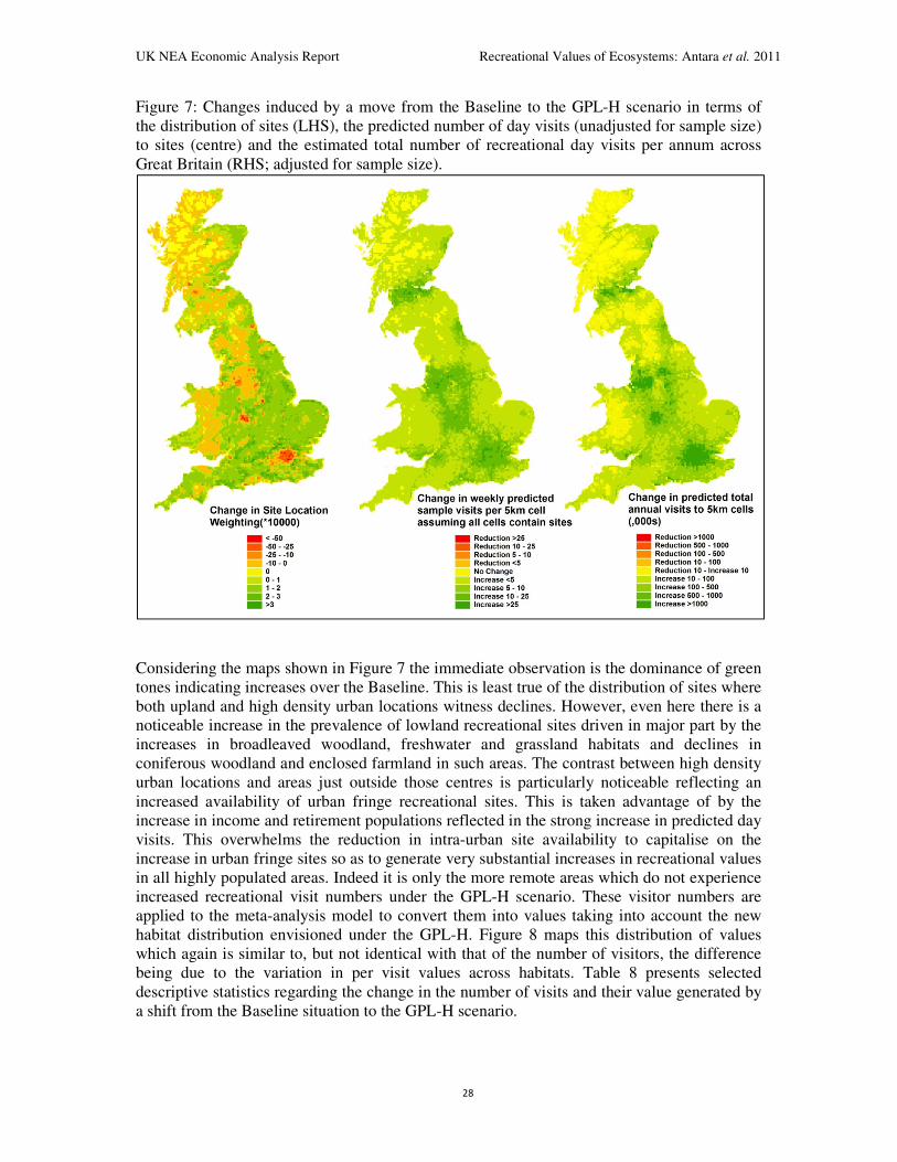
UK NEA Economic Analysis Report Recreational Values of Ecosystems: Antara et al. 2011
28
Figure 7: Changes induced by a move from the Baseline to the GPL-H scenario in terms of
the distribution of sites (LHS), the predicted number of day visits (unadjusted for sample size)
to sites (centre) and the estimated total number of recreational day visits per annum across
Great Britain (RHS; adjusted for sample size).
Considering the maps shown in Figure 7 the immediate observation is the dominance of green
tones indicating increases over the Baseline. This is least true of the distribution of sites where
both upland and high density urban locations witness declines. However, even here there is a
noticeable increase in the prevalence of lowland recreational sites driven in major part by the
increases in broadleaved woodland, freshwater and grassland habitats and declines in
coniferous woodland and enclosed farmland in such areas. The contrast between high density
urban locations and areas just outside those centres is particularly noticeable reflecting an
increased availability of urban fringe recreational sites. This is taken advantage of by the
increase in income and retirement populations reflected in the strong increase in predicted day
visits. This overwhelms the reduction in intra-urban site availability to capitalise on the
increase in urban fringe sites so as to generate very substantial increases in recreational values
in all highly populated areas. Indeed it is only the more remote areas which do not experience
increased recreational visit numbers under the GPL-H scenario. These visitor numbers are
applied to the meta-analysis model to convert them into values taking into account the new
habitat distribution envisioned under the GPL-H. Figure 8 maps this distribution of values
which again is similar to, but not identical with that of the number of visitors, the difference
being due to the variation in per visit values across habitats. Table 8 presents selected
descriptive statistics regarding the change in the number of visits and their value generated by
a shift from the Baseline situation to the GPL-H scenario.

UK NEA Economic Analysis Report Recreational Values of Ecosystems: Antara et al. 2011
29
Figure 8: Total value of annual predicted visits (£’000) under the GPL-H scenario
Table 8: Changes in the predicted total annual visit numbers and their total value arising from
a move from the Baseline situation to the GPL-H scenario: Great Britain and its constituent
countries (‘000).
Great Britain England Scotland Wales
Predicted visit per annum
Mean (No. per 5km cell) 199 277 77 54
Median (No. per 5km cell) 49 85 8 14
Country total 1,636,000 1,417,000 173,000 46,000
Value of predicted visit per annum
Mean (£/5km cell) 628 871 249 173
Median (£/5km cell) 163 279 28 47
Country total (£) 5,156,000 4,451,000 556,000 149,000
Note: all changes are positive under this scenario analysis.
Inspection of Table 8 confirms the message of Figure 8, that the GPL-H scenario delivers a
substantial increase in recreation values over the Baseline. We now repeat this analysis for
each of the scenarios with the resulting distribution of values being mapped in Figure 9 for
their low emission variants while Figure 10 repeats this for the high emission scenarios.

UK NEA Economic Analysis Report Recreational Values of Ecosystems: Antara et al. 2011
30
Figure 9: Total recreational value changes from the Baseline to all low emissions scenarios
Note: Scenarios are as follows:
GF = Go with the Flow
GPL = Green and Pleasant Land
LS = Local Stewardship
NS = National Security
NW = Nature at Work
WM = World Markets

UK NEA Economic Analysis Report Recreational Values of Ecosystems: Antara et al. 2011
31
Figure 10: Total recreational value changes from the Baseline to all high emissions scenarios
Note: Scenarios are as follows:
GF = Go with the Flow
GPL = Green and Pleasant Land
LS = Local Stewardship
NS = National Security
NW = Nature at Work
WM = World Markets
In general the maps shown in figures 9 and 10 are dominated by increases in visit values. The
NW scenario displays the most substantial increases in the value of visits for large areas of
GB both at high and low emissions. These gains are followed by those under the GPL
scenario which are a little higher than those under GF. In both of these scenarios, large
increases are seen in and around urban areas, while more rural areas see smaller increases in
the annual value of visits. The NS scenario also shows a similar geographic pattern to GF and
GPL, but with some areas, such as the Scottish Highlands and the Pennines, experiencing a
reduction in the predicted annual value of visits. Larger predicted reductions are seen under
the LS scenarios, particularly in the area south and west of London and in the urban centres,
although London itself shows a substantial increase in the value of visits. The WM scenarios
probably show the greatest difference both in comparison to the other scenarios and also in

UK NEA Economic Analysis Report Recreational Values of Ecosystems: Antara et al. 2011
32
the response to high and low emissions. In both high and low scenarios London shows a very
large decrease in value of visits with similar decreases in predicted visit value also seen in
other urban centres across the country. However, in the low emissions scenario the urban
areas outside of London are expected to experience an increase in the value of visits. In all
cases the remote uplands of Scotland, because of their inaccessibility, remain unvisited and
show no change in value.
Table 9 summarises the national level changes in value arising between the baseline and each
of the scenarios. At this national level all of the scenarios generate increases in the annual
value of visits except for the WM-high emissions scenario. In general, we find large gains
under the NW, GPL and GF scenarios and moderate increases for the LS scenario.

UK NEA Economic Analysis Report Recreational Values of Ecosystems: Antara et al. 2011
33
Table 9: Total (million £) and per capita (£) value of predicted annual visits in the baseline period and changes in total and per capita
value of predicted annual visit under the various scenarios
Region
Baseline
(million
£)
GF
(million £)
GPL
(million £)
LS
(million £)
NS
(million £)
NW
(million £)
WM
(million £)
high low high low high low high low High low high low
England 8854 3624 5048 4451 5327 898 1400 3061 4125 21084 21428 -678 4398
Scotland 926 370 488 556 602 162 84 189 249 2262 2190 -61 517
Wales 260 127 174 149 174 38 52 94 119 568 547 -84 122
Great
Britain 10040 4121 5711 5156 6103 1098 1535 3344 4493 23914 24165 -823 5037
Great Britain
population
(millions)
55.4 62.8 62.8 65.6 65.6 74.5 74.5 67.5 67.5 62.0 62.0 72.4 72.4
Great Britain
per capita
values (£
p.a.)
181 14 36 61 76 -1 6 17 34 337 341 -57 21
Note: Scenarios are as follows:
GF = Go with the Flow
GPL = Green and Pleasant Land
LS = Local Stewardship
NS = National Security
NW = Nature at Work
WM = World Markets

UK NEA Economic Analysis Report
The last row of Table 9 divides the G
scenario by the Great Britain population to obtain per capita values. These adjust the national
level results for the increases in population envisioned to occur, at different rates, under
scenarios. While the NW scenario yields the highest per capita value, this analysis
substantially differentiates the GPL and
former more than double the value of the latter.
5. Case Study
Our case study considers a simple scenario in which a policy maker has the funds to convert a
single area of farmland into recreational forest and wants to know where best to locate that
forest. For this simple illustration we bypass the site prediction model (SPM
of use when we seek to transfer findings outside England to the rest of the UK (a stage
considered in the Valuing Changes in Ecosystem Services chapter). Therefore we omit this
stage and move straight on to applying
generation function reported in Table 2 shows that woodland is significantly more attractive
to recreational visitors than enclosed farmland (the base case for that model). However, the
strong influence of travel time shows that
further away a site is from an outset location. This is illustrated in Figure 1
shows the predicted visitor rates for each of these land uses at different travel times.
Figure 11: TGF predictions: Travel time impacts on visit rate for woodland and farmland sites
Source: Sen. et al (2011) and the SEER project.
Figure 11 demonstrates not only that woodlands attract more visitors than farmland, but also
that there is a strong distance decay in these visit rates. This means that
will significantly determine the number of visitors they attract. We apply our methodology to
examine how the recreational values created by converting enclosed farmland to woodland
will vary depending upon the location of that conversion. For simplicity we illustrate this by
considering the consequences of placing our new forest in ten randomly chosen locations
across the North Humberside area illustrated in Figure
Recreational Values of Ecosystems:
34
divides the Great Britain level values under the Baseline and each
population to obtain per capita values. These adjust the national
level results for the increases in population envisioned to occur, at different rates, under
scenarios. While the NW scenario yields the highest per capita value, this analysis
substantially differentiates the GPL and GF findings showing that, on a per person basis, the
former more than double the value of the latter.
considers a simple scenario in which a policy maker has the funds to convert a
single area of farmland into recreational forest and wants to know where best to locate that
forest. For this simple illustration we bypass the site prediction model (SPM), which is mainly
of use when we seek to transfer findings outside England to the rest of the UK (a stage
considered in the Valuing Changes in Ecosystem Services chapter). Therefore we omit this
straight on to applying the trip generation function. The estimated
reported in Table 2 shows that woodland is significantly more attractive
to recreational visitors than enclosed farmland (the base case for that model). However, the
strong influence of travel time shows that both land uses become relatively less attractive the
further away a site is from an outset location. This is illustrated in Figure 11 below
shows the predicted visitor rates for each of these land uses at different travel times.
predictions: Travel time impacts on visit rate for woodland and farmland sites
et al (2011) and the SEER project.
demonstrates not only that woodlands attract more visitors than farmland, but also
decay in these visit rates. This means that the location of sites
significantly determine the number of visitors they attract. We apply our methodology to
examine how the recreational values created by converting enclosed farmland to woodland
ry depending upon the location of that conversion. For simplicity we illustrate this by
considering the consequences of placing our new forest in ten randomly chosen locations
across the North Humberside area illustrated in Figure 12. If we were undertakin
Recreational Values of Ecosystems: Antara et al. 2011
level values under the Baseline and each
population to obtain per capita values. These adjust the national
level results for the increases in population envisioned to occur, at different rates, under all
scenarios. While the NW scenario yields the highest per capita value, this analysis
findings showing that, on a per person basis, the
considers a simple scenario in which a policy maker has the funds to convert a
single area of farmland into recreational forest and wants to know where best to locate that
), which is mainly
of use when we seek to transfer findings outside England to the rest of the UK (a stage
considered in the Valuing Changes in Ecosystem Services chapter). Therefore we omit this
. The estimated trip
reported in Table 2 shows that woodland is significantly more attractive
to recreational visitors than enclosed farmland (the base case for that model). However, the
both land uses become relatively less attractive the
1 below which
shows the predicted visitor rates for each of these land uses at different travel times.
predictions: Travel time impacts on visit rate for woodland and farmland sites
demonstrates not only that woodlands attract more visitors than farmland, but also
the location of sites
significantly determine the number of visitors they attract. We apply our methodology to
examine how the recreational values created by converting enclosed farmland to woodland
ry depending upon the location of that conversion. For simplicity we illustrate this by
considering the consequences of placing our new forest in ten randomly chosen locations
. If we were undertaking a formal

UK NEA Economic Analysis Report Recreational Values of Ecosystems: Antara et al. 2011
35
review of such a scheme then this process would be iterated for all potential sites across the
entire area (a process which is rapid and straightforward given modern computing speeds) so
as to identify the optimal location for such a scheme.
Figure 12: Location map for ten randomly assigned land use change locations
Source: Sen. et al (2011) and the SEER project.
For each of the randomly chosen land use conversion sites we calculate the various
substitution measures needed for the TGF. These are added to data on site characteristics and
the socio-economic and demographic variables included in that model. Applying our TGF
visit rates to each location, first under its present agricultural land use and then under
woodland, we can estimate the change in visit numbers generated by the land conversion
policy. The final stage of our analysis is to use the meta-analysis model to value predicted
visits to each site under the current land use which is farmland and under the change in land
use which is woodland.
Table 10 presents results from the above illustrative analysis. As can be seen, in each of the
ten locations considered, the number of visits increases when the land is converted into
woodland. However, the magnitude of this change and the value they generate varies
substantially across locations. Site P9 yields the highest increase in value from this change in
land use while site P4 provides the lowest value. Clearly incorporating spatial variation into
decision making is a vital aid to efficient resource allocation, particularly in a time of
austerity.
Under a cost-effectiveness analysis this would conclude our assessment. However, a full
economic cost-benefit analysis would supplement this recreational value with the other
market and non-market benefits generated and set this against the costs of each scheme in
each location. Because costs such as the loss of agricultural output values will also vary
spatially, it is not necessarily the case that the site which generates the highest recreational
value is necessarily the optimal location for such land use conversion. Nevertheless, given the
prevailing shadow value of agriculture it seems very likely that many of these sites, if chosen,
would pass benefit-cost tests (although note that there is a substitution effect here; once one

UK NEA Economic Analysis Report Recreational Values of Ecosystems: Antara et al. 2011
36
new site is created this forms a substitute for, and lowers the value of, any other proposed site
in the vicinity – our methodology can readily be automated to permit the capture of such
effects within the decision analysis system). Why then do such sites not presently exist? This
is, in part, a reflection of market failure; at present land users are not compensated for the
recreational and other non-market benefits they provide and hence such services are, from a
social optimality perspective, under supplied. It is the task of government to address such
market failures through incentives or other mechanisms (including the removal of market
imperfections and distortions which perversely often reinforce the problems of missing
markets for environmental goods).

UK NEA Economic Analysis Report Recreational Values of Ecosystems: Antara et al. 2011
37
Table 10: Predicted increase in recreational visits and valuations at alternative sites conversion from farmland to woodland (£/year, 2010 prices)
Site No. → P0 P1 P2 P3 P4
Description Very remote site but near to rural
A road Close to York
A little remote and with substitutes like P7 nearer to York
Slightly further from Middlesbrough than site P8
Very remote and with no nearby major roads
Travel Bands (min)
Extra Visits (per
annum)
Value of Extra Visits
(£ per annum)
Extra Visits (per
annum)
Value of Extra Visits (£ per annum)
Extra Visits (per
annum)
Value of Extra Visits (£ per annum)
Extra Visits (per
annum)
Value of Extra Visits (£ per annum)
Extra Visits (per
annum)
Value of Extra Visits (£ per annum)
1 0 0 0 0 0 0 0 0 0 0
5 0 0 0 0 0 0 0 0 0 0
10 0 0 195 643 0 0 0 0 0 0
20 162 537 541 1788 0 0 595 1967 0 0
30 241 796 3159 10444 90 298 451 1492 0 0
40 201 664 602 1991 251 830 1004 3318 33 111
50 931 3076 1042 3445 875 2891 958 3168 28 92
60 709 2342 1671 5523 290 957 822 2719 67 222
Total 2243 7414 7210 23834 1506 4977 3831 12664 129 425
Site No. → P5 P6 P7 P8 P9
Description Midway between York & Leeds
with good road links Remote site but near to rural A
road Very close to York
Quite near Middlesbrough but no main road link
Midway between York & Leeds with excellent motorway links
Travel Bands (min)
Extra Visits (per
annum)
Value of Extra Visits (£ per annum)
Extra Visits (per
annum)
Value of Extra Visits (£ per annum)
Extra Visits (per
annum)
Value of Extra Visits (£ per annum)
Extra Visits (per
annum)
Value of Extra Visits (£ per annum)
Extra Visits (per
annum)
Value of Extra Visits (£ per annum)
1 0 0 0 0 0 0 0 0 165 545
5 0 0 261 862 0 0 0 0 130 431
10 0 0 292 965 584 1930 0 0 0 0
20 1028 3398 271 894 2705 8942 866 2862 1948 6438
30 3581 11836 361 1194 2046 6764 301 995 4574 15119
40 4601 15209 402 1327 719 2378 1389 4590 4852 16039
50 4643 15349 996 3291 1740 5752 968 3199 4718 15595
60 2183 7215 590 1949 1914 6326 1091 3608 3372 11148
Total 16036 53008 3171 10483 9708 32092 4614 15253 19759 65315
Source: Sen. et al (2011) and the SEER project.

UK NEA Economic Analysis Report Recreational Values of Ecosystems: Antara et al. 2011
38
References
Bateman, I. J., Brainard, J. S., Lovett, A. A., and Garrod, G. D., 1999. The impact of
measurement assumptions upon individual travel cost estimates of consumer surplus: a GIS
analysis. Regional Environmental Change, 1, 24—30.
Bateman, I., and Jones, A., 2003. Contrasting Conventional with Multi-Level Modelling
Approaches to Meta-Analysis: Expectation Consistency in U.K. Woodland Recreation
Values, Land Economics, 79, 235-258
Beyer, H.L., 2004, Hawths Analysis Tools for ArcGIS, Available at
http://www.spatialecology.com/htools
England Leisure Visits Survey, 2005. Natural England
Gourieroux, C., Montfort, A., and Trognon, A. (1984). Pseudo maximum likelihood methods:
Applications to Poisson models. Econometrica, 52,701-720
Jones, A., Bateman, I., and Wright, J., 2002. Estimating arrival numbers and values for
informal recreational use of British woodlands. Final report submitted to the Forestry
Commission.
Jones, A., Wright, J., Bateman, I., and Schaafsma, M., 2010. Estimating arrival numbers for
informal recreation: a geographical approach and case study of British woodlands,
Sustainability, 2, 684-701
Monitor of Engagement with the Natural Environment, 2010: The national survey on people
and the natural environment - Annual Report from the 2009-10 survey, NECR049 –Natural
England
Rabe-Hesketh, R., and Skrondal, A., 2008. Multilevel and Longitudinal Modelling using
Stata, Second edition.
Sen, A., Darnell, A., Munday, P., Crowe. A. and Bateman, I.J. (2010) Economic Assessment
of the Recreational Value of UK Ecosystems, Report to the Economics Team of the UK
National Ecosystem Assessment, University of East Anglia.
Sen, A., Darnell, A., Crowe, A., Bateman, I.J. and Munday, P. (2011) Economic Assessment
of the Value of Open-Access Recreation in UK Ecosystems: A Scenario Analysis, Report to
the UK National Ecosystem Assessment, Centre for Social and Economic Research on the
Global Environment (CSERGE), School of Environmental Sciences, University of East
Anglia.
Related Documents