Bridging Minimum Bias and Maximum Likelihood Methods through Weighted Equation

367

Bridging Minimum Bias and Maximum Likelihood Methods through Weighted Equation

Noriszura Ismail and Abdul Aziz Jemain

Abstract In classification ratemaking, the multiplicative and additive models derived by actuaries are based on two common methods; minimum bias and maximum likelihood. These models are already considered as established and standard, particularly in automobile and general liability insurance. This paper aims to identify the relationship between both methods by rewriting the equations of both minimum bias and maximum likelihood as a weighted equation. The weighted equation is in the form of a weighted difference between observed and fitted rates. The advantage of having the weighted equation is that the solution can be solved using regression model. Compared to the classical method introduced by Bailey and Simon (1960), the regression model provides an improved and simplified programming algorithm. In addition, the parameter estimates could also be rewritten as a weighted solution; for multiplicative model the solution can be written in the form of a weighted proportion whereas for additive model, the form is of a weighted difference. In this paper, the weighted equation will be applied on three types of classification ratemaking data; ship damage incidents data of McCullagh and Nelder (1989), data from Bailey and Simon (1960) on Canadian private automobile liability insurance and UK private car motor insurance data from Coutts (1984). Keywords: Classification ratemaking; Minimum bias; Maximum likelihood; Multiplicative; Additive.

1. INTRODUCTION

In order to determine pure premium rates in casualty insurance, actuaries have to fulfil two requirements. First, they have to ensure that the insurer will receive premiums at a level adequate to cover losses and expenses. Next, they have to allocate premiums “fairly” between insureds, i.e., high risk insured should pay higher premium. For the first requirement, actuaries are required to adjust the overall level of premiums, taking into account short-term economic effects such as inflation, and other external factors such as government regulation, that can be dealt with minimum statistical analysis. However, for the second requirement, the relative premium levels need to be determined. At this stage, statistical modelling and actuarial judgement are important and actuaries can achieve this by using classification ratemaking.

The goal of classification ratemaking is to group homogeneous risks and charge each group a premium to commensurate with the expected average loss. Failure to achieve this goal may lead to adverse selection to insureds and economic losses to insurers. The risks may be categorized according to rating factors; for instance in auto insurance, driver’s gender,


368 Casualty Actuarial Society Forum, Spring 2005

claim experience, and location, or vehicle’s make, capacity and year, can be considered as rating factors.

Among the pioneer studies of classification ratemaking, Bailey and Simon (1960) compared the systematic bias of multiplicative and additive models. Following their work, a few studies focusing and debating on additive and multiplicative models were published. Bailey (1963) compared multiplicative and additive models by producing two statistical criteria, namely the minimum chi-squares and the average absolute difference. Freifelder (1986) predicted the pattern of over and under estimation of multiplicative and additive models if true models are misspecified. Jee (1989) compared the predictive accuracy of multiplicative and additive models, and Holler et al. (1999) compared the initial values sensitivity of multiplicative and additive models.

In addition, researchers of classification ratemaking also suggested various statistical procedures to estimate the model parameters. Bailey and Simon (1960) suggested the minimum chi-squares, Bailey (1963) used the zero bias, Jung (1968) produced a heuristic method for minimum modified chi-squares, Ajne (1975) suggested the method of moments, Chamberlain (1980) used the weighted least squares, Coutts (1984) produced the method of orthogonal weighted least squares with logit transformation, Harrington (1986) suggested the maximum likelihood method for models with functional form, and Brockmann and Wright (1992) used the generalized linear models with Poisson error structure for claim frequency and Gamma error structure for claim severity. With the development of computing packages in the recent years, various statistical packages were also suggested and used, including GLIM by Brown (1988) and SAS by Holler et al. (1999) and Mildenhall (1999).

Based on the literature review, most researchers studied classification ratemaking in terms of two main perspectives; the models of multiplicative vs. additive, and the methods of minimum bias vs. maximum likelihood; using a variety of criteria, namely biasness, interaction terms, goodness of fit, initial value sensitivity and prediction accuracy. This paper differs such that it tries to bridge both methods via a weighted equation. This author believes that the weighted equation makes understanding the similarities and differences between both methods an easier task.

The objective of this paper is to bridge minimum bias and maximum likelihood methods by rewriting their equations as a weighted equation. The weighted equation can be written in the form of a weighted difference between observed and fitted rates. The advantage of


Casualty Actuarial Society Forum, Spring 2005 369

having the weighted equation is that the solution can be solved using regression model. Compared to the classical method introduced by Bailey and Simon (1960), the regression model provides an improved and simplified programming algorithm. In addition, the parameter estimates could also be rewritten as a weighted solution; for multiplicative model it is in the form of a weighted proportion whereas for additive model, the form is of a weighted difference. In this paper, the weighted equation will be applied on three types of classification ratemaking data; ship damage incidents data of McCullagh and Nelder (1989), data from Bailey and Simon (1960) on Canadian private automobile liability insurance and UK private car motor insurance data from Coutts (1984).

Rewriting the equations of minimum bias and maximum likelihood as a weighted equation has its own advantages; the mathematical concept of the weighted equation is simpler, hence providing an easier understanding, particularly for insurance practitioners; the weighted equation allows the usage of regression model as an alternative programming algorithm to calculate the parameter estimates; the weighted equation provides a basic step to further understand the more complex distributions, primarily the distributions involving dispersion parameter; the weights of the parameter solution shows that each of multiplicative and additive models has similar solution; and finally, the weights of the parameter solution also shows that models with larger sample size and number of parameter have slower convergence.

2. CLASSIFICATION RATEMAKING

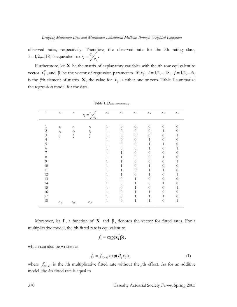
In casualty insurance, the risk premium, i.e., the premium excluding expenses, is equal to the product of claim frequency and severity. Classification ratemaking is the statistical procedure that classifies risks in claim frequency and severity models into groups of homogeneous risks, categorized by the rating factors. In this study, classification ratemaking is used to estimate claim frequency rates, expressed in terms of frequency per unit of exposure. For instance, the exposure unit used for auto insurance is based on a car-year unit. Consider a regression model with n observations of claim frequency rates and p explanatory variables inclusive of intercept and dummy variables. Next, consider a data of frequency rates involving three rating factors, each respectively with three, two and three rating classes. Thus, this data has a total of 18=n observed rates with 6=p explanatory variables. In addition, let c , e and r denote the vectors for claim counts, exposures and



observed rates, respectively. Therefore, the observed rate for the ith rating class, 18,...,2,1=i , is equivalent to

i

ii ecr = .

Furthermore, let X be the matrix of explanatory variables with the ith row equivalent to vector T

ix , and β be the vector of regression parameters. If ijx , 18,...,2,1=i , 6,...,2,1=j , is the ijth element of matrix X , the value for ijx is either one or zero. Table 1 summarize the regression model for the data.

Table 1. Data summary

i ci ei

i

ii ecr = xi1 xi2 xi3 xi4 xi5 xi6

1 2 3 4 5 6 7 8 9 10 11 12 13 14 15 16 17 18

c1 c2

c18

e1 e2

e18

r1 r2

r18

1 1 1 1 1 1 1 1 1 1 1 1 1 1 1 1 1 1

0 0 0 0 0 0 1 1 1 1 1 1 0 0 0 0 0 0

0 0 0 0 0 0 0 0 0 0 0 0 1 1 1 1 1 1

0 0 0 1 1 1 0 0 0 1 1 1 0 0 0 1 1 1

0 1 0 0 1 0 0 1 0 0 1 0 0 1 0 0 1 0

0 0 1 0 0 1 0 0 1 0 0 1 0 0 1 0 0 1

Moreover, let f , a function of X and β , denotes the vector for fitted rates. For a multiplicative model, the ith fitted rate is equivalent to

)exp( βxTi=if ,

which can also be written as

)exp()( ijjjii xff β−= , (1)

where )( jif − is the ith multiplicative fitted rate without the jth effect. As for an additive model, the ith fitted rate is equal to



βxTi=if ,

which can also be written as

ijjjii xff β+= − )( , (2)

where )( jif − is the ith additive fitted rate without the jth effect. Thus, the objective of classification ratemaking is to have the fitted rates, if , be as close as possible to the observed rates, ir , for all i.

3. MINIMUM BIAS

Bailey and Simon (1960) were among the pioneer researchers that consider bias in classification ratemaking and introduced the minimum bias method. They proposed a famous list of four criteria for an acceptable set of classification rates:

i. It should reproduce experience for each class and overall, i.e., be balanced for each class and overall.

ii. It should reflect the relative credibility of the various classes.

iii. It should provide minimum amount of departure from the raw data.

iv. It should produce a rate for each class of risks which is close enough to the experience so that the differences could reasonably be caused by chance.

3.1 Bailey Zero Bias Bailey and Simon (1960) proposed a suitable test for Criterion (i) by calculating,

∑∑

iii

iii

re

fe, (3)

for each j and total. A set of rates is balanced, i.e., zero bias, if equation (3) equals 1.00. Automatically, zero bias for each class implies zero bias overall.

From this test, Bailey (1963) derived a minimum bias model by setting the average difference between observed and fitted rates to be equal to zero. The zero bias equation for each j can be written in the form of a weighted difference between observed and fitted rates,

0)( =−∑i

iii frw , (4)



where iw is equal to iji xe .

Substituting (1) into (4), the zero bias equation for multiplicative model become

∑∑ −=i

ijijjjiii

ijii xxfexre )exp()( β .

Since ijx is either one or zero, the solution for each j could be obtained and written in the form of a weighted proportion of observed over multiplicative fitted rates without the jth effect,

∑−

=i ji

iij f

rv

)(

)exp(β , (5)

where iv is the normalized weight of i

ii

z

z∑ and iz is ( )i i j ije f x− .

For additive model, the zero bias equation after substituting (2) into (4) is

( )( ) ( )i i i j ij i j ij iji i

e r f x e x xβ−− =∑ ∑ .

Again, since ijx is either one or zero, the solution for each j could be obtained. However, for additive model, it is in term of a weighted difference between observed and additive fitted rates without the jth effect,

jβ ( )( )i i i ji

v r f −= −∑ , (6)

where iv is i

ii

z

z∑ and iz is i ije x .

3.2 Minimum Chi-Squares Bailey and Simon (1960) also suggested the 2χ statistics as an appropriate test for Criterion (iv),

2 2( )ii i

i i

er f

fχ = −∑ .

The same test is also suitable for Criterion (ii) and (iii) as well.



By minimizing the 2χ statistics, another minimum bias model was derived. For each j, the minimum χ2 equation could be written in the form of a weighted difference between observed and fitted rates,

2

( ) 0i i iij

w r fχβ

∂ = − =∂ ∑ , (7)

where iw is 2

( )i i i i

i j

e r f f

f β+ ∂

∂.

For multiplicative model,

ijij

i xff

=∂∂β

, (8)

whereas in additive model,

ij

j

i xf

=∂∂β

. (9)

If multiplicative model is chosen, by substituting (1) and (8) into (7), the parameter solution is equivalent to

( )

exp( ) ij i

i i j

rvf

β−

=∑ , (10)

where iv is i

ii

z

z∑ and iz is ( )i i i ije r f x+ .

For additive model, the parameter solution after substituting (2) and (9) into (7) is

( )( )j i i i ji

v r fβ −= −∑ , (11)

where iv is i

ii

z

z∑ and iz is

2

( )i i iij

i

e r fx

f

+ .



4. MAXIMUM LIKELIHOOD

Assume that the ith claim frequency count, i i ic e r= , comes from a distribution whose probability density function is ( ; )i ig c f . A maximum likelihood method maximizes the likelihood function,

( ; )i ii

L g c f= ∏ ,

or equivalently, the log likelihood function,

( )log log ( ; )i ii

L g c f= =∑ .

Thus, the parameter solution can be obtained by setting 0jβ

∂ =∂

for each j.

4.1 Normal Distribution If i i ic e r= is assumed to follow Normal distribution with mean i ie f , ( ; )i ig c f can be written as

( )2

2

1 1( ; ) exp

22i i i i i ig c f e r e f

σσ π = − −

.

Hence, the likelihood equation for each j is equivalent to

jβ

∂∂

= ( ) 0i i ii

w r f− =∑ , (12)

where iw is 2 ii

j

fe

β∂∂

.

Assuming multiplicative model, the solution after substituting (1) and (8) into (12) is

exp( )jβ( )

ii

i i j

rv

f −

=

∑ , (13)

where iv is i

ii

z

z∑ and iz is 2 2

( )i i j ije f x− .

For additive model, by substituting (2) and (9) into (12), the parameter solution is equivalent to



jβ ( )( )i i i ji

v r f −= −∑ , (14)

where iv is i

ii

z

z∑ and iz is 2

i ije x .

4.2 Poisson Distribution The same weighted equation could also be used to show that Poisson multiplicative is actually equivalent to zero bias multiplicative, derived by Bailey (1963). If i i ic e r= is assumed to have Poisson distribution with mean i ie f , the probability density function is

exp( )( )( ; )

( )!

i ie ri i i i

i ii i

e f e fg c f

e r

−= .

As a result, for each j, the likelihood equation is equal to

jβ

∂∂

= ( ) 0i i ii

w r f− =∑ , (15)

where iw is i i

i j

e f

f β∂∂

.

Substituting (1) and (8) into (15) for multiplicative model, the parameter solution can be written as

exp( )jβ( )

ii

i i j

rvf −

=∑ ,

where iv is i

ii

z

z∑ and iz is ( )i i j ije f x− . This solution is equivalent to zero bias multiplicative

shown by (5).

If additive model is chosen, by substituting (2) and (9) into (15), the parameter solution is equal to

( )( )j i i i ji

v r fβ −= −∑ , (16)

where iv is i

ii

z

z∑ and iz is i

iji

ex

f.



4.3 Binomial Distribution Assuming i i ic e r= comes from Binomial distribution with mean i ie f , ( ; )i ig c f can be written as

( ; ) (1 )i i ici e ci i i i

i

eg c f f f

c−

= −

.

For each j, the likelihood equation is equivalent to

jβ

∂∂

= ( ) 0i i ii

w r f− =∑ , (17)

where iw is (1 )

i i

i i j

e f

f f β∂

− ∂.

Using multiplicative model, the solution after substituting (1) and (8) into (17) is

exp( )jβ( )

ii

i i j

rv

f −

=

∑ , (18)

where iv is i

ii

z

z∑ and iz is ( )

1i i j

iji

e fx

f−

−.

If additive model is chosen, by substituting (2) and (9) into (17), the solution can be written as

( )( )j i i i ji

v r fβ −= −∑ , (19)

where iv is i

ii

z

z∑ and iz is

(1 )i

iji i

ex

f f−.

4.4 Negative Binomial Distribution The advantage of using the weighted equation is that it can be used as an introductory step to understand the fitting procedure of a distribution with dispersion parameter. If the dependent variable, iC , is a count with mean ( )i iE C µ= , a standard statistical procedure is to fit the data with Poisson distribution using multiplicative model. However, if overdispersion is detected in the data, i.e., ( ) ( )i iVar C E C> , the parameter estimates for standard Poisson are still consistent, but inefficient. As an alternative, the standard overdispersion model is the Negative Binomial distribution with multiplicative model. If iC



is distributed as Negative Binomial ( ; )i aµ , the probability density function is (Lawless, 1987),

1

1

1

( ) 1( ; , )

! ( ) 1 1

i ac

i a ii i

i i ia

c ag c a

c a a

µµµ µ

Γ += Γ + +

,

and the mean and variance are

( )i iE C µ= ,

( ) (1 )i i iVar C aµ µ= + ,

where a is the dispersion parameter. Since 0a ≥ and 0iµ ≥ for all i, the distribution allows for overdispersion.

For our classification ratemaking example, i i ic e r= and i i ie fµ = . Thus, the likelihood equation can also be written as

( ) 0i i iij

w r fβ∂ = − =

∂ ∑ , (20)

where iw is (1 )

i i

i i i j

e f

f ae f β∂

+ ∂. Notice that the weight for Poisson (15) is a special case of

the weight for Negative Binomial (20), when the dispersion parameter, a , is equal to zero.

Assuming multiplicative model, by substituting (1) and (8) into (20), the parameter solution is

exp( )jβ( )

ii

i i j

rv

f −

=

∑ , (21)

where iv is i

ii

z

z∑ and iz is ( )

1i i j

iji i

e fx

ae f−

+.

For additive model, the parameter solution after substituting (2) and (9) into (20) is equal to

( )( )j i i i ji

v r fβ −= −∑ , (22)

where iv is i

ii

z

z∑ and iz is

(1 )i

iji i i

ex

f ae f+.



4.5 Generalized Poisson Distribution

Another alternative for overdispersion is to use the Generalized Poisson distribution. The advantage of using Generalized Poisson distribution is that it can be used for both overdispersion, i.e., ( ) ( )i iVar C E C> , as well as underdispersion, i.e., ( ) ( )i iVar C E C< . If

iC is assumed to follow Generalized Poisson distribution, ( ; , )i ig c aµ can be written as (Wang and Famoye, 1997),

1(1 ) (1 )( ; , ) exp

1 ! 1

ii

c ci i i i

i ii i i

ac acg c a

a c a

µ µµµ µ

− + += − + + ,

with mean and variance,

( )i iE C µ= , 2( ) (1 )i i iVar C aµ µ= + .

Since 0a ≥ or 0a ≤ , the distribution allows for either overdispersion or underdispersion. Assuming i i ic e r= and i i ie fµ = , the likelihood equation is

( ) 0i i iij

w r fβ∂ = − =

∂ ∑ , (23)

where iw is 2(1 )

i i

i i i j

e f

f ae f β∂

+ ∂. Again, the weight for Poisson (15) is a special case of the

weight for Generalized Poisson (23), when the dispersion parameter, a , is equal to zero.

Substituting (1) and (8) into (23) for multiplicative model, the parameter solution is

exp( )jβ( )

ii

i i j

rv

f −

=

∑ , (24)

where iv is i

ii

z

z∑ and iz is ( )

2(1 )i i j

iji i

e fx

ae f−

+.

For additive model, by substituting (2) and (9) into (23), the parameter solution can be written as

( )( )j i i i ji

v r fβ −= −∑ , (25)



where iv is i

ii

z

z∑ and iz is

2(1 )i

iji i i

ex

f ae f+.

5. OTHER MODELS

5.1 Least Squares The same weighted equation could also be extended to other error functions as well. Define the sum squares error as (Brown, 1988),

22( )

( )i i i ii i i

i ii

e r e fS e r f

e

−= = −∑ ∑ .

So, the least squares equation can be written as

j

S

β∂∂

= ( ) 0i i ii

w r f− =∑ , (26)

where iw is ii

j

fe

β∂∂

.

Substituting (1) and (8) into (26) for multiplicative model, the parameter solution is

( )

exp( ) ij i

i i j

rvf

β−

=∑ , (27)

where iv is i

ii

z

z∑ and iz is 2

( )i i j ije f x− .

Extending this equation to least squares with additive model, it can be shown that least squares additive is equivalent to zero bias additive, derived by Bailey (1963). The parameter solution after substituting (2) and (9) into (26) is equivalent to

( )( )j i i ji

v r fβ −= −∑ ,

where ii

ii

zv

z=∑

and i i ijz e x= . This solution is equivalent to the zero bias additive shown

by (6).



5.2 Minimum Modified Chi-Squares If the function of error is a modified χ2 statistics which is defined as,

2 2mod ( )i

i ii i

er f

rχ = −∑ ,

the equation for minimum modified χ2 is equivalent to

2mod

j

χβ

∂∂

= ( ) 0i i ii

w r f− =∑ , (28)

where iw is i i

i j

e f

r β∂∂

.

For multiplicative model, by substituting (1) and (8) into (28), the parameter solution can be written as

( )

exp( ) ij i

i i j

rvf

β−

=∑ , (29)

where iv is i

ii

z

z∑ and iz is

2( )i i j

i iji

e fz x

r−= .

Substituting (2) and (9) into (28) for additive model, the parameter solution is

( )( )j i i ji

v r fβ −= −∑ , (30)

where iv is i

ii

z

z∑ and iz is i

iji

ex

r.

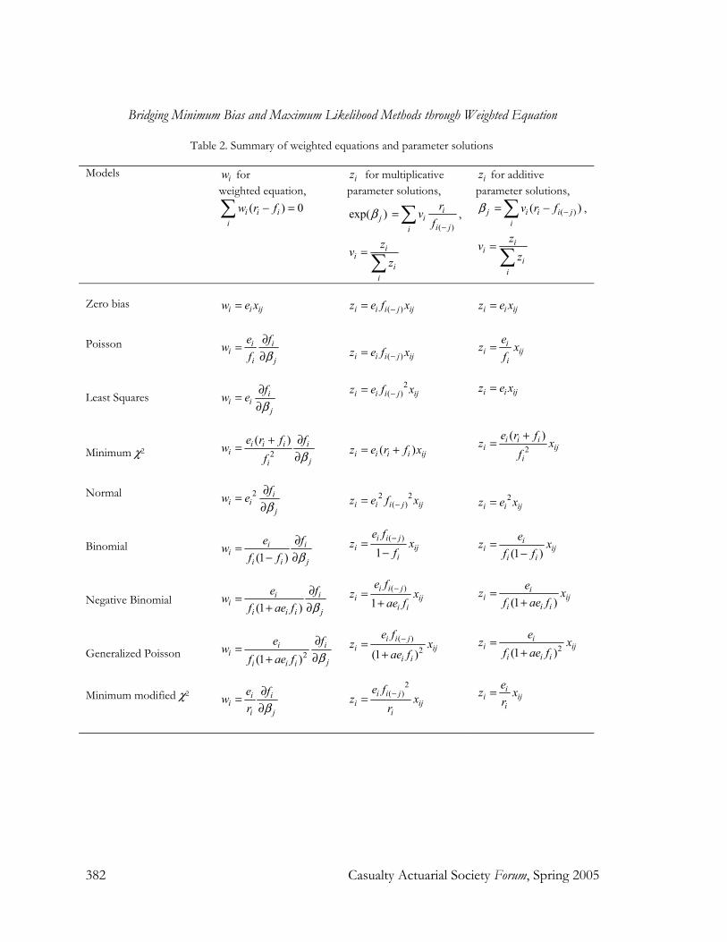
Table 2 summarizes the weighted equations and parameter solutions for all of the models discussed above. From the table, the following conclusions can be made:

i. For additive models, the zero bias and least squares are equivalent.

ii. For multiplicative models, the zero bias and Poisson are equal.

iii. The weighted equation, which is in the form of a weighted difference between observed and fitted rates, show that all models are similar; each model is distinguished only by its weight.

iv. The weights in the parameter solutions show that each of multiplicative and additive models is expected to produce similar parameter estimates.



6. MODEL PROGRAMMING

6.1 Classical Method The classical iterative method for finding parameter solutions was first introduced by Bailey and Simon (1960). This method solves the parameter individually for each j. In the first iteration, vector of initial values, (0)β , are needed to calculate the vector of next parameter estimates, (1)β . The process of iteration is then repeated until all solutions converge.



Table 2. Summary of weighted equations and parameter solutions

Models iw for

weighted equation, ( ) 0i i i

i

w r f− =∑

iz for multiplicative parameter solutions,

exp( )jβ( )

iii ji

rvf −

=∑ ,

ii

ii

zv

z=∑

iz for additive parameter solutions,

jβ ( )( )i i i ji

v r f −= −∑ ,

ii

ii

zv

z=∑

Zero bias Poisson Least Squares Minimum χ2 Normal Binomial Negative Binomial Generalized Poisson Minimum modified χ2

i i ijw e x=

i i

ii j

e fw

f β∂

=∂

i

i ij

fw e

β∂

=∂

2

( )i i i ii

ji

e r f fw

f β+ ∂

=∂

2 i

i ij

fw e

β∂

=∂

(1 )i i

ii i j

e fw

f f β∂

=− ∂

(1 )i i

ii i i j

e fw

f ae f β∂

=+ ∂

2(1 )i i

iji i i

e fw

f ae f β∂

=∂+

i i

ii j

e fw

r β∂

=∂

( )i i i j ijz e f x−=

( )i i i j ijz e f x−=

2( )i i i j ijz e f x−=

( )i i i i ijz e r f x= +

2 2( )i i i j ijz e f x−=

( )

1i i j

i iji

e fz x

f−=

−

( )

1i i j

i iji i

e fz x

ae f−=

+

( )

2(1 )

i i ji ij

i i

e fz x

ae f

−=+

2

( )i i ji ij

i

e fz x

r−=

i i ijz e x=

i

i iji

ez x

f=

i i ijz e x=

2

( )i i ii ij

i

e r fz x

f

+=

2i i ijz e x=

(1 )i

i iji i

ez x

f f=

−

(1 )i

i iji i i

ez x

f ae f=

+

2(1 )i

i iji i i

ez x

f ae f=

+

i

i iji

ez x

r=



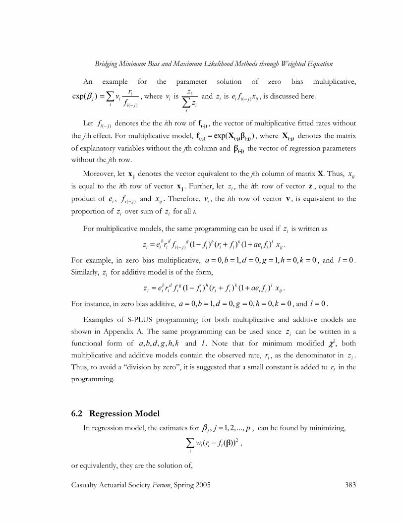
An example for the parameter solution of zero bias multiplicative,

exp( )jβ( )

ii

i i j

rvf −

=∑ , where iv is i

ii

z

z∑ and iz is ( )i i j ije f x− , is discussed here.

Let ( )i jf − denotes the the ith row of (-j)f , the vector of multiplicative fitted rates without the jth effect. For multiplicative model, exp( )=(-j) (-j) (-j)f X β , where (-j)X denotes the matrix of explanatory variables without the jth column and (-j)β the vector of regression parameters without the jth row.

Moreover, let jx denotes the vector equivalent to the jth column of matrix X. Thus, ijx is equal to the ith row of vector jx . Further, let iz , the ith row of vector z , equal to the product of ie , )( jif − and ijx . Therefore, iv , the ith row of vector v , is equivalent to the proportion of iz over sum of iz for all i.

For multiplicative models, the same programming can be used if iz is written as

( ) (1 ) ( ) (1 )b d g h k li i i i j i i i i iz e r f f r f ae f−= − + + ijx .

For example, in zero bias multiplicative, 0,0,1,0,1,0 ====== khgdba , and 0=l . Similarly, iz for additive model is of the form,

lii

kii

hi

gi

di

bii faefrffrez )1()()1( ++−= ijx .

For instance, in zero bias additive, 0,0,0,0,1,0 ====== khgdba , and 0=l .

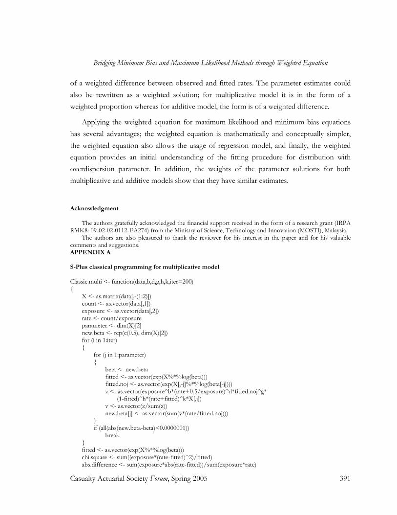
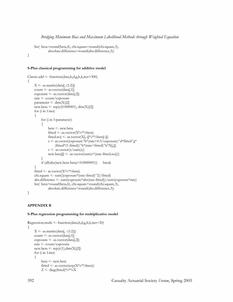
Examples of S-PLUS programming for both multiplicative and additive models are shown in Appendix A. The same programming can be used since iz can be written in a functional form of , , , , ,a b d g h k and l . Note that for minimum modified χ2, both multiplicative and additive models contain the observed rate, ir , as the denominator in iz . Thus, to avoid a “division by zero”, it is suggested that a small constant is added to ir in the programming.

6.2 Regression Model In regression model, the estimates for , 1, 2,...,j j pβ = , can be found by minimizing,

2( ( ))i i ii

w r f−∑ β ,

or equivalently, they are the solution of,



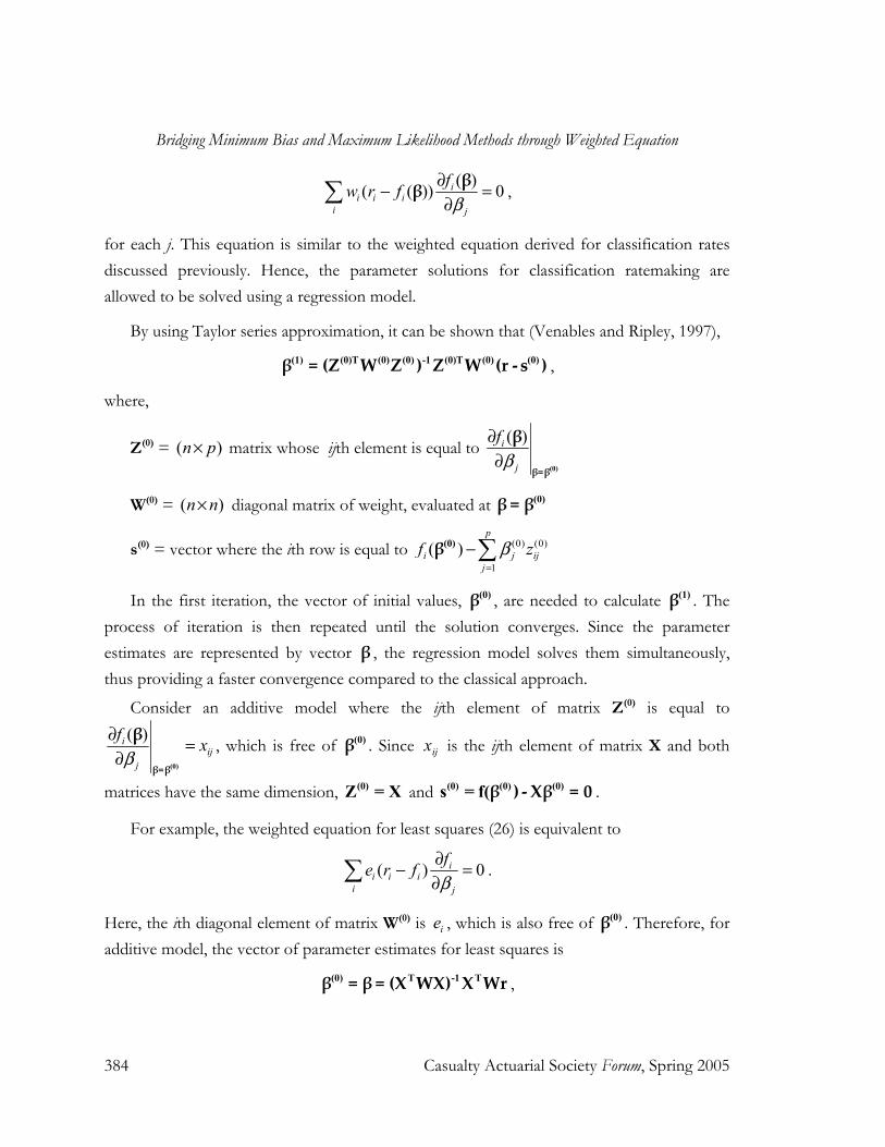
( )( ( )) 0ii i i

i j

fw r f

β∂− =∂∑ ββ ,

for each j. This equation is similar to the weighted equation derived for classification rates discussed previously. Hence, the parameter solutions for classification ratemaking are allowed to be solved using a regression model.

By using Taylor series approximation, it can be shown that (Venables and Ripley, 1997), (1) (0)T (0) (0) -1 (0)T (0) (0)β = (Z W Z ) Z W (r - s ) ,

where,

Z(0) = ( )n p× matrix whose ijth element is equal to ( )i

j

f

β∂∂

(0)β=β

β

W(0) = ( )n n× diagonal matrix of weight, evaluated at (0)β = β

s(0) = vector where the ith row is equal to (0) (0)

1

( )p

i j ijj

f zβ=

−∑(0)β

In the first iteration, the vector of initial values, (0)β , are needed to calculate (1)β . The process of iteration is then repeated until the solution converges. Since the parameter estimates are represented by vector β , the regression model solves them simultaneously, thus providing a faster convergence compared to the classical approach.

Consider an additive model where the ijth element of matrix Z(0) is equal to ( )i

ijj

fx

β∂ =∂

(0)β=β

β , which is free of (0)β . Since ijx is the ijth element of matrix X and both

matrices have the same dimension, (0)Z = X and (0) (0) (0)s = f(β ) - Xβ = 0 .

For example, the weighted equation for least squares (26) is equivalent to

( ) 0ii i i

i j

fe r f

β∂− =∂∑ .

Here, the ith diagonal element of matrix W(0) is ie , which is also free of (0)β . Therefore, for additive model, the vector of parameter estimates for least squares is

(0) T -1 Tβ = β = (X WX) X Wr ,



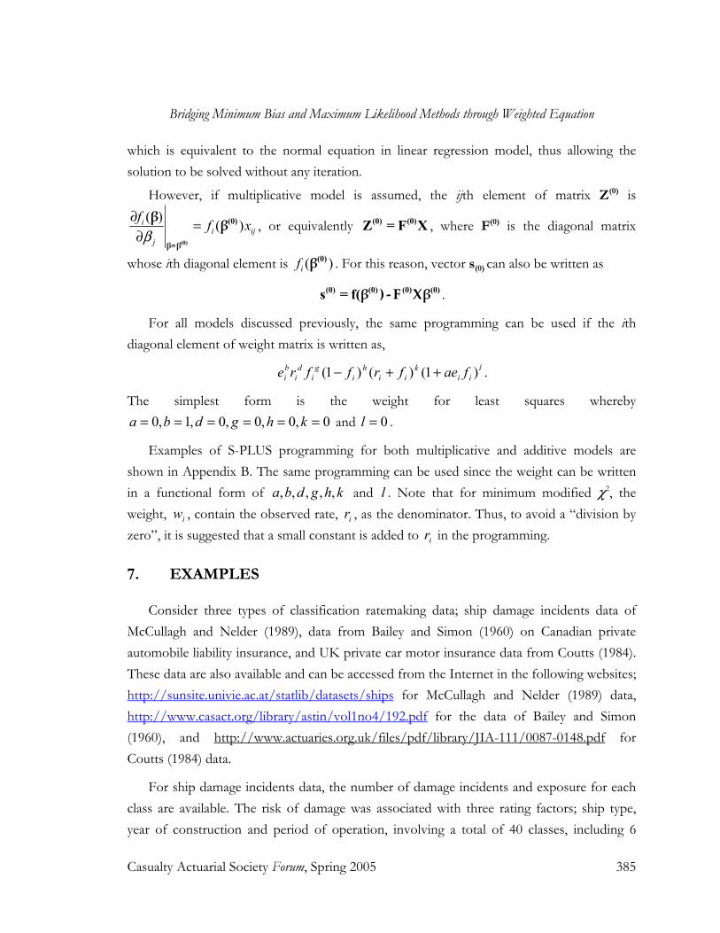
which is equivalent to the normal equation in linear regression model, thus allowing the solution to be solved without any iteration.

However, if multiplicative model is assumed, the ijth element of matrix Z(0) is ( )

( )ii ij

j

ff x

β∂ =∂

(0)

(0)

β=β

β β , or equivalently (0) (0)Z = F X , where F(0) is the diagonal matrix

whose ith diagonal element is ( )if(0)β . For this reason, vector s(0) can also be written as

(0) (0) (0) (0)s = f(β ) - F Xβ .

For all models discussed previously, the same programming can be used if the ith diagonal element of weight matrix is written as,

lii

kii

hi

gi

di

bi faefrffre )1()()1( ++− .

The simplest form is the weight for least squares whereby 0,0,0,0,1,0 ====== khgdba and 0=l .

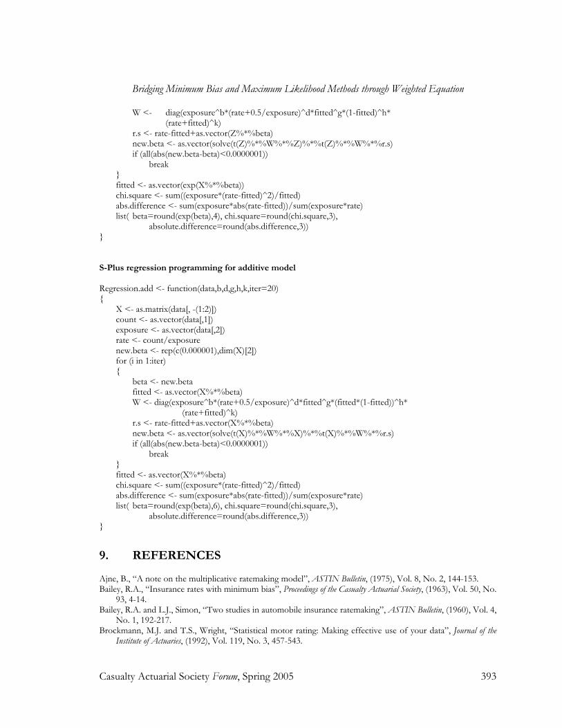
Examples of S-PLUS programming for both multiplicative and additive models are shown in Appendix B. The same programming can be used since the weight can be written in a functional form of , , , , ,a b d g h k and l . Note that for minimum modified χ2, the weight, iw , contain the observed rate, ir , as the denominator. Thus, to avoid a “division by zero”, it is suggested that a small constant is added to ir in the programming.

7. EXAMPLES

Consider three types of classification ratemaking data; ship damage incidents data of McCullagh and Nelder (1989), data from Bailey and Simon (1960) on Canadian private automobile liability insurance, and UK private car motor insurance data from Coutts (1984). These data are also available and can be accessed from the Internet in the following websites; http://sunsite.univie.ac.at/statlib/datasets/ships for McCullagh and Nelder (1989) data, http://www.casact.org/library/astin/vol1no4/192.pdf for the data of Bailey and Simon (1960), and http://www.actuaries.org.uk/files/pdf/library/JIA-111/0087-0148.pdf for Coutts (1984) data.

For ship damage incidents data, the number of damage incidents and exposure for each class are available. The risk of damage was associated with three rating factors; ship type, year of construction and period of operation, involving a total of 40 classes, including 6



classes with zero exposure. For Canadian private automobile liability insurance data, the number of claims incurred and exposure for each class are available. Two rating factors are considered; class and merit ratings, involving a total of 20 classes. Finally, for UK private car motor insurance data, the incurred claim count and exposure for each class are available. Four rating factors are considered; coverage, vehicle age, vehicle group and policyholder age, involving a total of 120 classes.

Bailey and Simon (1960) also suggested the average absolute difference as a suitable test for Criterion (iii),

i i ii

i ii

e r f

e r

−∑∑

.

Therefore, the χ2 statistics, a test for Criterion (iv), and the average absolute difference, a test for Criterion (iii), will be calculated for all models. Table 3, Table 4 and Table 5 show the parameter estimates, χ2 statistics and average absolute difference for the models discussed above.



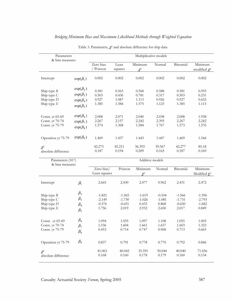
Table 3. Parameters, χ2 and absolute difference for ship data

Parameters & bias measures

Multiplicative models

Zero bias / Poisson

Least squares

Minimum χ2

Normal Binomial Minimum modified χ2

Intercept Ship type B Ship type C Ship type D Ship type E Const. yr 65-69 Const. yr 70-74 Const. yr 75-79 Operation yr 75-79 χ2 absolute difference

)exp( 1β

)exp( 2β)exp( 3β)exp( 4β)exp( 5β

)exp( 6β)exp( 7β)exp( 8β

)exp( 9β

0.002

0.581 0.503 0.927 1.385

2.008 2.267 1.574

1.469

42.275 0.187

0.002

0.563 0.436 1.087 1.384

2.071 2.157 1.368

1.437

45.211 0.194

0.002

0.568 0.781 1.113 1.575

2.040 2.242 1.584

1.443

36.393 0.209

0.002

0.588 0.317 0.926 1.123

2.038 2.395 1.767

1.447

59.567 0.165

0.002

0.581 0.503 0.927 1.385

2.008 2.267 1.573

1.469

42.277 0.187

0.002

0.593 0.231 0.652 1.113

1.938 2.242 1.576

1.544

85.18 0.169

Parameters (10-3) & bias measures

Additive models

Zero bias/ Least squares

Poisson Minimum χ2

Normal Binomial Minimum Modified χ2

Intercept Ship type B Ship type C Ship type D Ship type E Const. yr 65-69 Const. yr 70-74 Const. yr 75-79 Operation yr 75-79 χ2 absolute difference

1β 2β

3β

4β

5β 6β

7β

8β 9β

2.665

-1.821 -2.149 -0.376 1.756

1.094 1.536 0.453

0.837

41.063 0.168

2.430

-1.565 -1.730 -0.651 2.019

1.055 1.604 0.714

0.791 40.042 0.160

2.477

-1.619 -1.026 0.433 2.932

1.097 1.661 0.747

0.778

35.591 0.178

0.962

-0.104 -1.081 0.868 2.650

1.108 1.657 0.968

0.770 50.044 0.179

2.431

-1.566 -1.731 -0.650 2.017

1.055 1.603 0.713

0.792

40.040 0.160

2.472

-1.596 -2.793 -1.682 0.849

1.003 1.323 0.665

0.846

71.436 0.154



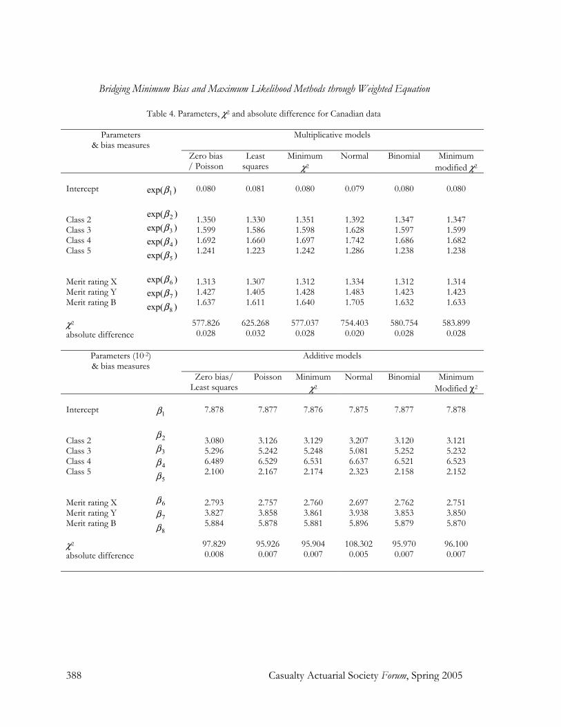
Table 4. Parameters, χ2 and absolute difference for Canadian data



Zero bias / Poisson

Least squares

Minimum χ2


Intercept Class 2 Class 3 Class 4 Class 5 Merit rating X Merit rating Y Merit rating B χ2 absolute difference

)exp( 1β



0.080

1.350 1.599 1.692 1.241

1.313 1.427 1.637

577.826 0.028

0.081

1.330 1.586 1.660 1.223

1.307 1.405 1.611

625.268 0.032

0.080

1.351 1.598 1.697 1.242

1.312 1.428 1.640

577.037 0.028

0.079

1.392 1.628 1.742 1.286

1.334 1.483 1.705

754.403 0.020

0.080

1.347 1.597 1.686 1.238

1.312 1.423 1.632

580.754 0.028

0.080

1.347 1.599 1.682 1.238

1.314 1.423 1.633

583.899 0.028


Additive models


Poisson Minimum χ2


Intercept Class 2 Class 3 Class 4 Class 5 Merit rating X Merit rating Y Merit rating B χ2 absolute difference

1β 2β

3β

4β

5β 6β

7β

8β

7.878

3.080 5.296 6.489 2.100

2.793 3.827 5.884

97.829 0.008

7.877

3.126 5.242 6.529 2.167

2.757 3.858 5.878

95.926 0.007

7.876

3.129 5.248 6.531 2.174

2.760 3.861 5.881

95.904 0.007

7.875

3.207 5.081 6.637 2.323

2.697 3.938 5.896

108.302 0.005

7.877

3.120 5.252 6.521 2.158

2.762 3.853 5.879

95.970 0.007

7.878

3.121 5.232 6.523 2.152

2.751 3.850 5.870

96.100 0.007



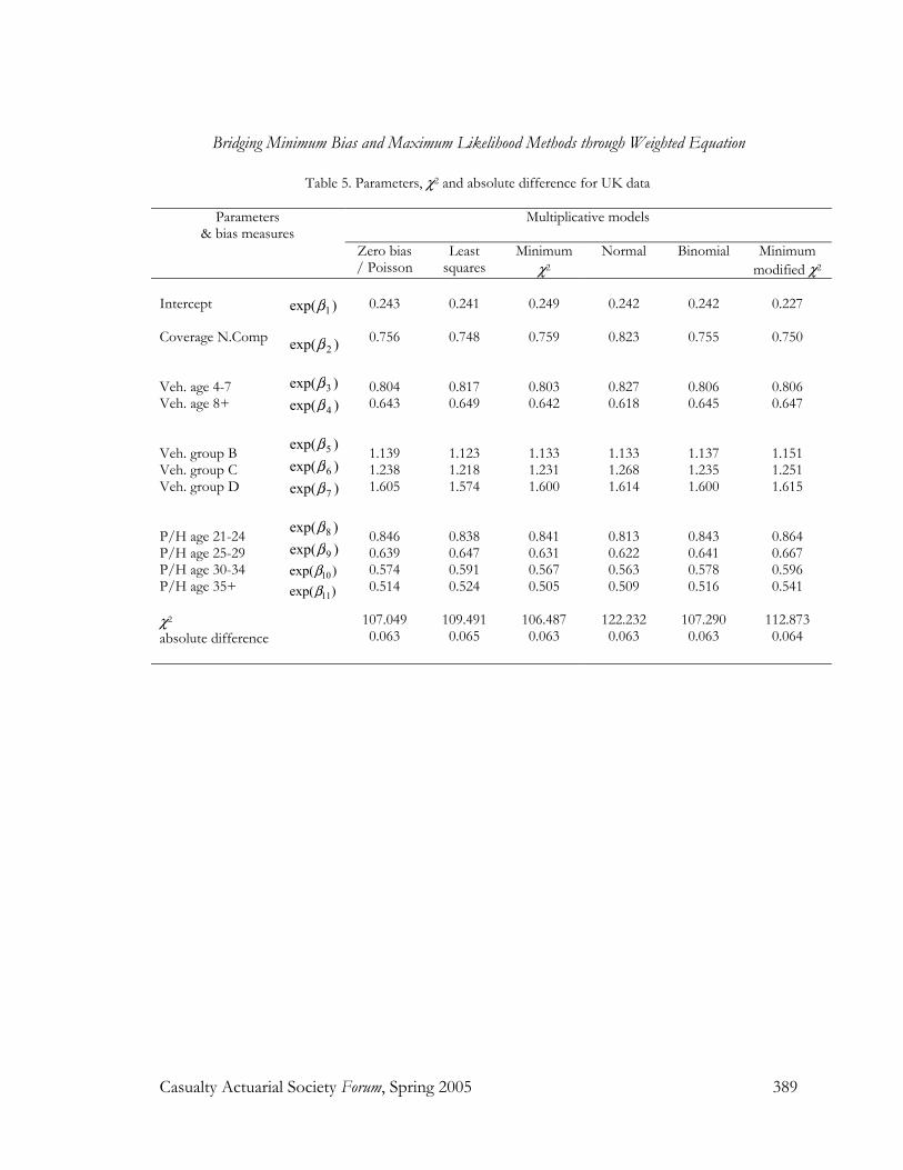
Table 5. Parameters, χ2 and absolute difference for UK data



Zero bias / Poisson

Least squares

Minimum χ2


Intercept Coverage N.Comp Veh. age 4-7 Veh. age 8+ Veh. group B Veh. group C Veh. group D P/H age 21-24 P/H age 25-29 P/H age 30-34 P/H age 35+ χ2 absolute difference

)exp( 1β

)exp( 2β

)exp( 3β)exp( 4β



0.243

0.756

0.804 0.643

1.139 1.238 1.605

0.846 0.639 0.574 0.514

107.049 0.063

0.241

0.748

0.817 0.649

1.123 1.218 1.574

0.838 0.647 0.591 0.524

109.491 0.065

0.249

0.759

0.803 0.642

1.133 1.231 1.600

0.841 0.631 0.567 0.505

106.487 0.063

0.242

0.823

0.827 0.618

1.133 1.268 1.614

0.813 0.622 0.563 0.509

122.232 0.063

0.242

0.755

0.806 0.645

1.137 1.235 1.600

0.843 0.641 0.578 0.516

107.290 0.063

0.227

0.750

0.806 0.647

1.151 1.251 1.615

0.864 0.667 0.596 0.541

112.873 0.064



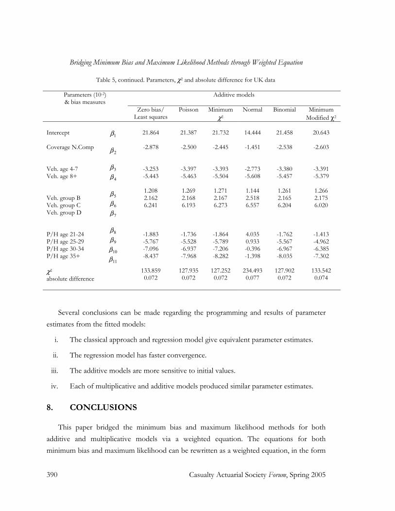
Table 5, continued. Parameters, χ2 and absolute difference for UK data


Additive models


Poisson Minimum χ2


Intercept Coverage N.Comp Veh. age 4-7 Veh. age 8+ Veh. group B Veh. group C Veh. group D P/H age 21-24 P/H age 25-29 P/H age 30-34 P/H age 35+ χ2 absolute difference

1β 2β 3β

4β 5β

6β

7β 8β

9β

10β

11β

21.864

-2.878

-3.253 -5.443

1.208 2.162 6.241

-1.883 -5.767 -7.096 -8.437

133.859 0.072

21.387

-2.500

-3.397 -5.463

1.269 2.168 6.193

-1.736 -5.528 -6.937 -7.968

127.935 0.072

21.732

-2.445

-3.393 -5.504

1.271 2.167 6.273

-1.864 -5.789 -7.206 -8.282

127.252 0.072

14.444

-1.451

-2.773 -5.608

1.144 2.518 6.557

4.035 0.933 -0.396 -1.398

234.493 0.077

21.458

-2.538

-3.380 -5.457

1.261 2.165 6.204

-1.762 -5.567 -6.967 -8.035

127.902 0.072

20.643

-2.603

-3.391 -5.379

1.266 2.175 6.020

-1.413 -4.962 -6.385 -7.302

133.542 0.074

Several conclusions can be made regarding the programming and results of parameter estimates from the fitted models:

i. The classical approach and regression model give equivalent parameter estimates.

ii. The regression model has faster convergence.

iii. The additive models are more sensitive to initial values.

iv. Each of multiplicative and additive models produced similar parameter estimates.

8. CONCLUSIONS

This paper bridged the minimum bias and maximum likelihood methods for both additive and multiplicative models via a weighted equation. The equations for both minimum bias and maximum likelihood can be rewritten as a weighted equation, in the form



of a weighted difference between observed and fitted rates. The parameter estimates could also be rewritten as a weighted solution; for multiplicative model it is in the form of a weighted proportion whereas for additive model, the form is of a weighted difference.

Applying the weighted equation for maximum likelihood and minimum bias equations has several advantages; the weighted equation is mathematically and conceptually simpler, the weighted equation also allows the usage of regression model, and finally, the weighted equation provides an initial understanding of the fitting procedure for distribution with overdispersion parameter. In addition, the weights of the parameter solutions for both multiplicative and additive models show that they have similar estimates.

Acknowledgment The authors gratefully acknowledged the financial support received in the form of a research grant (IRPA RMK8: 09-02-02-0112-EA274) from the Ministry of Science, Technology and Innovation (MOSTI), Malaysia. The authors are also pleasured to thank the reviewer for his interest in the paper and for his valuable comments and suggestions. APPENDIX A S-Plus classical programming for multiplicative model Classic.multi <- function(data,b,d,g,h,k,iter=200) { X <- as.matrix(data[,-(1:2)]) count <- as.vector(data[,1]) exposure <- as.vector(data[,2]) rate <- count/exposure parameter <- dim(X)[2] new.beta <- rep(c(0.5), dim(X)[2]) for (i in 1:iter) { for (j in 1:parameter) { beta <- new.beta fitted <- as.vector(exp(X%*%log(beta))) fitted.noj <- as.vector(exp(X[,-j]%*%log(beta[-j]))) z <- as.vector(exposure^b*(rate+0.5/exposure)^d*fitted.noj^g* (1-fitted)^h*(rate+fitted)^k*X[,j]) v <- as.vector(z/sum(z)) new.beta[j] <- as.vector(sum(v*(rate/fitted.noj))) } if (all(abs(new.beta-beta)<0.0000001)) break } fitted <- as.vector(exp(X%*%log(beta))) chi.square <- sum((exposure*(rate-fitted)^2)/fitted) abs.difference <- sum(exposure*abs(rate-fitted))/sum(exposure*rate)



list( beta=round(beta,4), chi.square=round(chi.square,3), absolute.difference=round(abs.difference,3)) } S-Plus classical programming for additive model Classic.add <- function(data,b,d,g,h,k,iter=300) { X <- as.matrix(data[,-(1:2)]) count <- as.vector(data[,1]) exposure <- as.vector(data[,2]) rate <- count/exposure parameter <- dim(X)[2] new.beta <- rep(c(0.000001), dim(X)[2]) for (i in 1:iter) { for (j in 1:parameter) { beta <- new.beta fitted <- as.vector(X%*%beta) fitted.noj <- as.vector(X[,-j]%*%beta[-j]) z <- as.vector(exposure^b*(rate+0.5/exposure)^d*fitted^g* (fitted*(1-fitted))^h*(rate+fitted)^k*X[,j]) v <- as.vector(z/sum(z)) new.beta[j] <- as.vector(sum(v*(rate-fitted.noj))) } if (all(abs(new.beta-beta)<0.0000001)) break } fitted <- as.vector(X%*%beta) chi.square <- sum((exposure*(rate-fitted)^2)/fitted) abs.difference <- sum(exposure*abs(rate-fitted))/sum(exposure*rate) list( beta=round(beta,6), chi.square=round(chi.square,3), absolute.difference=round(abs.difference,3)) } APPENDIX B S-Plus regression programming for multiplicative model Regression.multi <- function(data,b,d,g,h,k,iter=20) { X <- as.matrix(data[, -(1:2)]) count <- as.vector(data[,1]) exposure <- as.vector(data[,2]) rate <- count/exposure new.beta <- rep(c(1),dim(X)[2]) for (i in 1:iter) { beta <- new.beta fitted <- as.vector(exp(X%*%beta)) Z <- diag(fitted)%*%X



W <- diag(exposure^b*(rate+0.5/exposure)^d*fitted^g*(1-fitted)^h* (rate+fitted)^k) r.s <- rate-fitted+as.vector(Z%*%beta) new.beta <- as.vector(solve(t(Z)%*%W%*%Z)%*%t(Z)%*%W%*%r.s) if (all(abs(new.beta-beta)<0.0000001)) break } fitted <- as.vector(exp(X%*%beta)) chi.square <- sum((exposure*(rate-fitted)^2)/fitted) abs.difference <- sum(exposure*abs(rate-fitted))/sum(exposure*rate) list( beta=round(exp(beta),4), chi.square=round(chi.square,3), absolute.difference=round(abs.difference,3)) } S-Plus regression programming for additive model Regression.add <- function(data,b,d,g,h,k,iter=20) { X <- as.matrix(data[, -(1:2)]) count <- as.vector(data[,1]) exposure <- as.vector(data[,2]) rate <- count/exposure new.beta <- rep(c(0.000001),dim(X)[2]) for (i in 1:iter) { beta <- new.beta fitted <- as.vector(X%*%beta) W <- diag(exposure^b*(rate+0.5/exposure)^d*fitted^g*(fitted*(1-fitted))^h* (rate+fitted)^k) r.s <- rate-fitted+as.vector(X%*%beta) new.beta <- as.vector(solve(t(X)%*%W%*%X)%*%t(X)%*%W%*%r.s) if (all(abs(new.beta-beta)<0.0000001)) break } fitted <- as.vector(X%*%beta) chi.square <- sum((exposure*(rate-fitted)^2)/fitted) abs.difference <- sum(exposure*abs(rate-fitted))/sum(exposure*rate) list( beta=round(exp(beta),6), chi.square=round(chi.square,3), absolute.difference=round(abs.difference,3)) }

9. REFERENCES

Ajne, B., “A note on the multiplicative ratemaking model”, ASTIN Bulletin, (1975), Vol. 8, No. 2, 144-153. Bailey, R.A., “Insurance rates with minimum bias”, Proceedings of the Casualty Actuarial Society, (1963), Vol. 50, No.

93, 4-14. Bailey, R.A. and L.J., Simon, “Two studies in automobile insurance ratemaking”, ASTIN Bulletin, (1960), Vol. 4,

No. 1, 192-217. Brockmann, M.J. and T.S., Wright, “Statistical motor rating: Making effective use of your data”, Journal of the

Institute of Actuaries, (1992), Vol. 119, No. 3, 457-543.



Brown, R.L., “Minimum bias with generalized linear models”, Proceedings of the Casualty Actuarial Society, (1988), Vol. 75, No. 143, 187-217.

Chamberlain, C., 1980, “Relativity pricing through analysis of variance”, Discussion Paper Program of the Casualty Actuarial Society, (1980), 4-24.

Coutts, S.M., “Motor insurance rating, an actuarial approach”, Journal of the Institute of Actuaries, (1984), Vol. 111, 87-148.

Freifelder, L., “Estimation of classification factor relativities: A modelling approach”, Journal of Risk and Insurance, (1986), Vol. 53, 135-143.

Harrington, S.E., 1986, “Estimation and testing for functional form in pure premium regression models”, ASTIN Bulletin, (1986), Vol. 16, 31-43.

Holler, K.D., D., Sommer, and G., Trahair, “Something old, something new in classification ratemaking with a novel use of GLMs for credit insurance”, Forums of the Casualty Actuarial Society, (1999), Winter, 31-84.

Jee, B., “A comparative analysis of alternative pure premium models in the automobile risk classification system”, Journal of risk and insurance, (1989), Vol. 56, 434-459.

Jung, J., “On automobile insurance ratemaking”, ASTIN Bulletin, (1968), Vol. 5, No. 1, 41-48. Lawless, J.F., “Negative binomial and mixed Poisson regression”, The Canadian Journal of Statistics, (1987), Vol.

15, No. 3, 209-225. McCullagh, P., and J.A., Nelder, Generalized Linear Models (2nd Edition), (1989), Chapman and Hall, London. Mildenhall, S.J., 1999, “A systematic relationship between minimum bias and generalized linear models”,

Proceedings of the Casualty Actuarial Society, (1999), Vol. 86. No. 164, 393-487. S-PLUS 2000, Guide to Statistics, Vol 1, MathSoft. Inc., Seattle. Venables, W.N., and B.D., Ripley, Modern Applied Statistics with S-PLUS (2nd Edition), (1997), Springer-Verlag,

New York. Wang, W., and F., Famoye, F., “Modeling household fertility decisions with generalized Poisson regression”,

Journal of Population Economics, (1997), Vol. 10, 273-283. Biographies of Authors Noriszura Ismail is a lecturer in National University of Malaysia since July 1993, teaching Actuarial Science courses. She received her MSc. (1993) and BSc. (1991) in Actuarial Science from University of Iowa, and is now currently pursuing her PhD in Statistics. She has presented several papers in Seminars, including those locally and in South East Asia, and published several papers in local and Asian Journals. Abdul Aziz Jemain is an Associate Professor in National University of Malaysia, teaching in Statistics Department since 1982. He received his MSc. (1982) in Medical Statistics from London School of Hygiene and Tropical Medicine and PhD (1989) in Statistics from University of Reading. He has written several articles, including local and international Proceedings and Journals, and co-authors several local books.

Bridging Minimum Bias and Maximum Likelihood Methods through Weighted Equation

Documents