To be presented to Inside Financial Markets: Knowledge and Interaction Patterns in Global Markets, Konstanz, 15-18 May 2003 An Equation and its Worlds: Bricolage, Exemplars, Disunity and Performativity in Financial Economics Donald MacKenzie April 2003 Author’s address: School of Social & Political Studies University of Edinburgh Adam Ferguson Building Edinburgh EH8 9LL [email protected]

Welcome message from author
This document is posted to help you gain knowledge. Please leave a comment to let me know what you think about it! Share it to your friends and learn new things together.
Transcript

To be presented to Inside Financial Markets: Knowledge and Interaction Patterns in Global Markets, Konstanz, 15-18 May 2003
An Equation and its Worlds:
Bricolage, Exemplars, Disunity
and Performativity in Financial Economics
Donald MacKenzie
April 2003
Author’s address: School of Social & Political Studies University of Edinburgh Adam Ferguson Building Edinburgh EH8 9LL [email protected]
2
An Equation and its Worlds:
Bricolage, Theoretical Commitment, Disunity
and Performativity in Financial Economics
Abstract This paper describes and analyzes the history of the fundamental equation of
modern financial economics: the Black-Scholes (or Black-Scholes-Merton) option
pricing equation. In that history, several themes of potentially general importance
are revealed. First, the key mathematical work was not rule-following but bricolage,
creative tinkering. Second, it was, however, bricolage guided by the goal of finding a
solution to the problem of option pricing analogous to existing exemplary solutions,
notably the Capital Asset Pricing Model, which had successfully been applied to
stock prices. Third, the central strands of work on option pricing, although all
recognisably ‘orthodox’ economics, were not unitary. There was significant
theoretical disagreement amongst the pioneers of option pricing theory; this
disagreement, paradoxically, turns out to be a strength of the theory. Fourth, option
pricing theory has been performative. Rather than simply describing a pre-existing
empirical state of affairs, it altered the world, in general in a way that made itself
more true.
3
Economics and economies are becoming a major focus for social studies of science.
Historians of economics such as Philip Mirowski and the small number of
sociologists of economics such as Yuval Yonay have been applying ideas from
science studies with increasing frequency in the last decade or so.1 Established
science-studies scholars such as Knorr Cetina and newcomers to the field such as
Izquierdo, Lépinay, Millo and Muniesa have begun detailed, often ethnographic,
work on economic processes, with a particular focus on the financial markets.2
1 See, for example, Philip Mirowski, More Heat than Light (Cambridge: Cambridge University Press,
1989); Mirowski, Machine Dreams: Economics Becomes a Cyborg Science (Cambridge: Cambridge
University Press, 2002); Matthias Klaes, ‘The History of the Concept of Transaction Costs: Neglected
Aspects’, Journal of the History of Economic Thought, Vol. 22 (2000), 191-216; Esther-Mirjam Sent, The
Evolving Rationality of Rational Expectations (Cambridge: Cambridge University Press, 1998); E. Roy
Weintraub, Stabilizing Dynamics: Constructing Economic Knowledge (Cambridge: Cambridge University
Press, 1991); Yuval P. Yonay, ‘When Black Boxes Clash: Competing Ideas of What Science is in
Economics, 1924-39’, Social Studies of Science, Vol. 24 (1994), 39-80; Yonay and Daniel Breslau,
‘Economic Theory and Reality: A Sociological Perspective on Induction and Inference in a Deductive
Science’ (typescript, August 2001).
2 See, for example, Karin Knorr Cetina and Urs Bruegger, ‘The Virtual Societies of Financial Markets’,
American Journal of Sociology, Vol. 107 (2002), 905-51; A. Javier Izquierdo M., ‘El Declive de los
Grandes Números: Benoit Mandelbrot y la Estadística Social’ Empiria: Revista de Metodología de
Ciencias Sociales, Vol. 1 (1998), 51-84; Izquierdo, ‘Reliability at Risk: The Supervision of Financial
Models as a Case Study for Reflexive Economic Sociology’, European Societies, Vol. 3 (2001), 69-90;
Vincent Lépinay, ‘How Far Can We Go in the Mathematization of Commodities’, International

4
Actor-network theorist Michel Callon has conjoined the two concerns by arguing
that an intrinsic link exists between studies of economics and of economies. The
Workshop, Culture(s) of Financial Markets, Bielefeld, Germany, 10-11 November 2000; Lépinay and
Fabrice Rousseau, ‘Les Trolls sont-ils Incompétents? Enquête sur les Financiers Amateurs’, Politix,
Vol. No. 52 13, (2000), 73-97; Donald MacKenzie, ‘Physics and Finance: S-Terms and Modern Finance
as a Topic for Science Studies’, Science Technology & Human Values Vol. 26 (2001), 115-144; Yuval
Millo, ‘How to Finance the Floor? The Chicago Commodities Markets Ethos and the Black-Scholes
Model‘, forthcoming; Fabian Muniesa, ‘Performing Prices: The Case of Price Discovery Automation
in the Financial Markets’, in Herbert Kalthoff, Richard Rottenburg, and Hans-Jürgen Wagener (eds),
Okönomie und Gesellschaft, Jahrbuch 16. Facts and Figures: Economic Representations and Practices
(Marburg: Metropolis 2000), 289-312; Fabian Muniesa, ‘Un Robot Walrasien: Cotation Electronique et
Justesse de la Découverte des Prix’, Politix, Vol. No. 52 13, (2000) 121-54; Alex Preda, ‘On Ticks and
Tapes: Financial Knowledge, Communicative Practices, and Information Technologies on 19th
Century Markets’, Columbia Workshop on Social Studies of Finance, 3-5 May 2002. This body of
work of course interacts with a preexisting tradition of the sociology, and anthropology of financial
markets. See, for example, Mitchel Y. Abolafia, Making Markets: Opportunism and Restraint on Wall
Street (Cambridge, Mass.: Harvard University Press, 1996); Abolafia, ‘Markets as Cultures: An
Ethnographic Approach’, in Michel Callon (eds) The Laws of the Markets (Oxford: Blackwell, 1998), 69-
85; Patricia Adler and Peter Adler (eds), The Social Dynamics of Financial Markets (Greenwich, Conn.:
JAI Press, 1984); Wayne E. Baker, ‘The Social Structure of a National Securities Market’, American
Journal of Sociology, Vol. 89 (1984), 775-811; Ellen Hertz, The Trading Crowd: An Ethnography of the
Shanghai Stock Market (Cambridge: Cambridge University Press, 1998); Charles W. Smith, Success and
Survival on Wall Street: Understanding the Mind of the Market (Lanham, Maryland: Rowman &
Littlefield 1999).

5
economy is not an independent object that economics observes, argues Callon.
Rather, the economy is performed by economic practices. Accountancy and
marketing are among the more obvious such practices, but, claims Callon, economics
in the academic sense plays a vital role in constituting and shaping modern
economies.3
This article contributes to the emergent science studies literature on
economics and economies by way of a historical case study of option† pricing theory
(terms marked † are defined in the glossary in table 1). The theory is a ‘crown jewel’
of modern economics – ‘when judged by its ability to explain the empirical data,
option pricing theory is the most successful theory not only in finance, but in all of
economics’4 – and their work on the topic won two leading contributors, Robert C.
Merton and Myron Scholes, a Nobel Prize. Over the last three decades, option
theory has become a vitally important part of financial practice. As recently as 1970,
the market in derivatives† such as options was tiny; indeed, many modern
derivatives were illegal. By December 2001, derivatives contracts totaling $134.7
trillion were outstanding worldwide, a sum equivalent to around $22,000 for every
3 Michel Callon (ed.), The Laws of the Markets (Oxford: Blackwell, 1998).
4 Stephen A. Ross, ‘Finance’, in John Eatwell et al. (eds), The New Palgrave: A Dictionary of Economics
(London: Macmillan, 1987), Vol. 2, 332-26, at 332.

6
human being on earth.5 Because of its centrality to this huge market, the equation
that is my focus here, the Black-Scholes option pricing equation, may be ‘the most
widely used formula, with embedded probabilities, in human history’.6
Attention in this paper is primarily on the detailed, mathematical history of
the Black-Scholes equation.7 Its interaction with market practices is described
elsewhere,8 although the issue of performativity means that the two aspects of the
5 Data from Bank for International Settlement, www.bis.org. These figures are adjusted for the most
obvious forms of double-counting, but still arguably exaggerate the economic significance of
derivatives markets. Swaps, for example, are measured by notional principal, when this is not in fact
exchanged. The Bank’s estimate of total gross market value of $3.8 trillion may be a more realistic
measure, although it is based only on the over-the-counter (direct institution-to-institution) market.
Even this, though, is equivalent to a not-inconsiderable $600 for every person on earth.
6 Mark Rubinstein, ‘Implied Binomial Trees’, Journal of Finance, Vol. 49 (1994), 771-818, at 772.
7 Aside from the recollections of Black and Scholes themselves (cited below), the main existing history
is Peter L. Bernstein, Capital Ideas: The Improbably Origins of Modern Wall Street (New York: Free Press,
1992), chapter 11. This is a fine study, but eschews detailed mathematical exposition. More
mathematical, but unfortunately somewhat Whiggish (see below), is Edward J. Sullivan and Timothy
M. Weithers, ‘The History and Development of the Option Pricing Formula’, Research in the History of
Economic Thought and Methodology, Vol. 12 (1994), 31-43.
8 Donald MacKenzie and Yuval Millo ‘Constructing a Market, Performing Theory: the Historical
Sociology of a Financial Derivatives Exchange’, American Journal of Sociology, forthcoming. This
article is available at http://www.ed.ac.uk/sociol/Research/Staff/mcknz.htm
7
equation’s history are tightly linked and market practices will be touched on here
briefly. Four themes will emerge. I would not describe them as ‘findings’, because
of the limitations on what can be inferred from a single historical case-study, but
they may be of general significance. The first is bricolage. Creative scientific practice
is typically not the following of set rules of method: it is, in Lynch’s words,
‘particular courses of action with materials to hand’. While this has been
documented in overwhelming detail by ethnographic studies of laboratory science,
this case-study suggests it may also be the case in a deductive, mathematical science.
Economists – at least the particular economists focused on here – are also bricoleurs.9
They are not, however, random bricoleurs, and the role of existing exemplary
is the second theme to emerge. Ultimately, of course, this is a Kuhnian theme. As is
well known (at least) two quite distinct meanings of the key term ‘paradigm’ can be
found in Kuhn’s work. One – by far the dominant one in how Kuhn’s work was
taken up by others – is the ‘entire constellation of beliefs, values, techniques, and so
on shared by the members of a given [scientific] community’. The second – rightly
9 Bricoleur is French for odd-job person. The metaphor was introduced to the social sciences by
Claude Lévi-Strauss, The Savage Mind (London: Weidenfeld & Nicolson, 1966). Its appropriateness to
describe science is argued in Barry Barnes, Scientific Knowledge and Sociological Theory (London:
Routledge & Kegan Paul, 1974), chapter 3. The quotation is from Michael Lynch, Art and Artifact in
8
described by Kuhn as ‘philosophically ... deeper’ – is the exemplar, the problem-
solution that is accepted as successful and that is creatively drawn upon to solve
further problems.10 The role of the exemplar will become apparent here in the
contrast between the work of Black and Scholes and that of mathematician and
arbitrageur† Edward O. Thorp. Amongst those who worked on option pricing prior
to Black and Scholes, Thorp’s work is closest to theirs. However, while Thorp was
seeking market inefficiencies to exploit, Black and Scholes were seeking a solution to
the problem of option pricing analogous to an existing exemplary solution, the
Capital Asset Pricing Model. This was not just a general inspiration: in his detailed
mathematical work, Fischer Black drew directly on a previous mathematical analysis
on which he had worked with the Capital Asset Pricing Model’s co-developer, Jack
Treynor.
As Peter Galison and others have pointed out, the key shortcoming in the
view of the ‘paradigm’ as ‘constellation of beliefs, values, techniques, and so on’ is
that it overstates the unity and coherence of scientific fields. Nowhere is this more
Laboratory Science: A Study of Shop Work and Shop Talk in a Research Laboratory (London: Routledge &
Kegan Paul, 1985), 5.
10 Thomas S. Kuhn, The Structure of Scientific Revolutions (Chicago: Chicago University Press, second
edition, 1970), 175. On the greater philosophical depth of the exemplar, see Barry Barnes, T.S. Kuhn
and Social Science (London and Basingstoke: Macmillan, 1982).
9
true than when outsiders discuss ‘orthodox’ neoclassical economics, and the nature
of economic orthodoxy is the third theme explored here. Black, Scholes, Merton,
several of their predecessors, and most of those who subsequently worked on option
pricing were all (with some provisos in the case of Black, to be discussed below)
recognizably ‘orthodox’ economists. As others studying different areas of economics
have found, however, orthodoxy seems not to be a single unitary doctrine,
substantive or methodological. For example, Robert C. Merton, the economist
whose name is most closely yoked to those of Black and Scholes, did not accept the
original version of the Capital Asset Pricing Model, the apparent pivot of their
derivation, and himself reached the Black-Scholes equation by drawing on different
intellectual resources. Black, in turn, never found Merton’s derivation entirely
compelling, and continued to champion the derivation based on the Capital Asset
Pricing Model. So no unitary ‘constellation of beliefs, values, techniques, and so on’
can be found. Economic ‘orthodoxy’ is a reality – attend conferences of economists
who feel excluded by it, and one is left in no doubt on that – but it is a reality that
should perhaps be construed as a cluster of family resemblances that arises from
imaginative bricolage drawing on an only partially overlapping set of existing
exemplary solutions. It is an ‘epistemic culture’, not a catechism.11
11 Peter Galison and David J. Stump (eds), The Disunity of Science: Boundaries, Contexts, and Power
(Stanford, Calif.: Stanford University Press, 1996); Galison, Image and Logic: A Material Culture of
Microphysics (Chicago: University of Chicago Press, 1997); Yonay and Breslau, op. cit. note 1; Philip
10
A major aspect of Galison’s critique of the Kuhnian paradigm conceived as
all-embracing ‘constellation’ is his argument that diversity is a source of robustness,
not a weakness. Though his topic is physics, the same appears true of economics.
Philip Mirowski and Wade Hands, describing the emergence of modern economic
orthodoxy in the postwar U.S., put the point as follows:
Rather than saying it [neoclassicism] simply chased out the competition –
which it did, if by “competition” one means the institutionalists, Marxists,
and Austrians – and replaced diversity with a single monolithic
homogeneous neoclassical strain, we say it transformed itself into a more
robust ensemble. Neoclassical demand theory gained hegemony by going
from patches of monoculture in the interwar period to an interlocking
competitive ecosystem after World War II. Rather than presenting itself as
Mirowski and D. Wade Hands, ‘A Paradox of Budgets: The Postwar Stabilization of American
Neoclassical Demand Theory’, in Mary S. Morgan and Malcolm Rutherford (eds), From Interwar
Pluralism to Postwar Neoclassicism, Annual Supplement to History of Political Economy, Vol. 30 (London:
Duke University Press 1998), 260-92; Mirowski, op. cit. note 1 (2002). The term ‘epistemic culture’ is
of course Knorr Cetina’s: see Karin Knorr Cetina, Epistemic Cultures: How the Sciences make Knowledge
(Cambridge, Mass.: Harvard University Press, 1999).
11
a single, brittle, theoretical strand, neoclassicism offered a more flexible,
and thus resilient skein ...12
That general characterization, we shall see, appears to hold for the particular case of
option pricing theory.
The final theme explored here, and in the counterpart paper referred to
above,13 is performativity. As we shall see, there is at least qualified support here for
Callon’s conjecture, albeit in a case that is favourable to the conjecture, since option
pricing theory was chosen for examination in part because it seemed a plausible case
of performativity. Option pricing theory did not simply describe a pre-existing
world, but helped create a world of which the theory was a truer reflection. Inter
alia, this makes its history a matter of more than technical interest. Option pricing
theory is one thread in the radical changes in the world’s financial markets over the
past three decades, changes that have had considerable consequences for economies
and the wider societies and polities in which they are embedded. The history of
option pricing theory is thus part (a small but not an insignificant part) of the history
of our times.
12 Mirowski and Hands, op. cit. note 11, 289.
13 MacKenzie and Millo, op. cit. note 8.

12
‘Too much on finance!’
Options are old instruments, but until the 1970s age had not brought them
respectability. Puts† and calls† on the stock of the Dutch East India Company were
being bought and sold in Amsterdam when de la Vega discussed its stock market in
1688,14 and options were subsequently widely traded in Paris, London, New York and
other financial centres. They frequently came under suspicion, however, as vehicles for
speculation. Because the cost of an option was typically much less than that of the
underlying stock, a speculator who anticipated price rises could profit considerably by
buying calls, or benefit from falls by buying puts, and such speculation was often
regarded as manipulative and/or destabilizing. Indeed, options were often seen
simply as gambling, as betting on stock price movements. In Britain, options were
banned from 1734 and again from 1834, and in France from 1806, although these bans
were widely flouted. Several American states, beginning with Illinois in 1874, also
outlawed options. Although the main target in the U.S. was options on agricultural
commodities, options on securities were often banned as well.15
14 Joseph de la Vega, Confusion de Confusiones, trans. Hermann Kellenbenz (Boston: Baker Library,
Harvard Graduate School of Business Administration, 1957).
15 Ranald C. Michie, The London Stock Exchange: A History (Oxford: Oxford University Press, 1999), 22
and 49; Alex Preda, ‘The Rise of the Popular Investor: Financial Knowledge and Investing in England
and France, 1840-1880’, Sociological Quarterly, Vol. 42 (2001), 205-32, at 214; Richard J. Kruizenga, Put
and Call Options: A Theoretical and Market Analysis (PhD thesis, MIT, 1956), chapter 2. On options

13
Options’ dubious reputation did not prevent serious interest in them. In 1877,
for example, the London broker Charles Castelli, who had been ‘repeatedly called upon
to explain the various processes’ involved in buying and selling options, published a
booklet explaining them, directed apparently at his fellow market professionals rather
than popular investors. He concentrated primarily on the profits that could be made
by the purchaser, and discussed only in passing how options were priced, noting that
prices tended to rise in periods of what we would now call high volatility.† His booklet
ended – in a nice corrective for those who believe the late twentieth century’s financial
globalization to be a novelty – with an example of how options had been used in bond
arbitrage† between the London Stock Exchange and the Constantinople Bourse to
capture the high contango rate prevailing in Constantinople in 1874.16
trading in France, see, e.g., anon., Manuel du Spéculateur à la Bourse (Paris: Garnier, second edition,
1855).
16 Charles Castelli, the Theory of ‘Options’ in Stocks and Shares (London: Mathieson, 1877), 2, 7-8, and
74-77. ‘Contango’ was the premium paid by the buyer of a security to its seller in return for
postponing payment from one settlement date to the next. On literature directed at popular
investors, see Preda, op. cit. note N. The scale of operations described by Castelli, and his use,
without explanation, of terms such as ‘contango’, suggest a specialized rather than lay readership.
For other nineteenth-century analyses of options, see Alex Preda, ‘Pricing Elusiveness: Louis
Bachelier’s Theory of Speculation and the Popular “Science of the Market”’, International Workshop
on Culture(s) of Financial Markets, Bielefeld, 10-11 November, 2000.
14
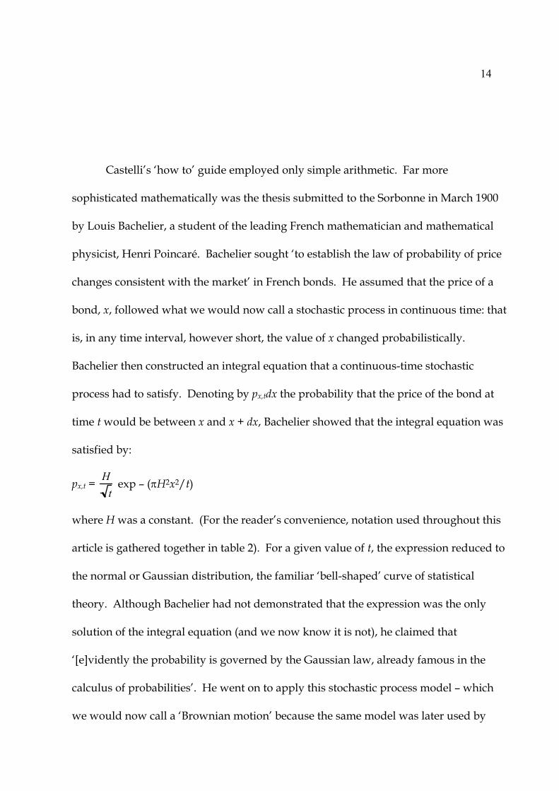
Castelli’s ‘how to’ guide employed only simple arithmetic. Far more
sophisticated mathematically was the thesis submitted to the Sorbonne in March 1900
by Louis Bachelier, a student of the leading French mathematician and mathematical
physicist, Henri Poincaré. Bachelier sought ‘to establish the law of probability of price
changes consistent with the market’ in French bonds. He assumed that the price of a
bond, x, followed what we would now call a stochastic process in continuous time: that
is, in any time interval, however short, the value of x changed probabilistically.
Bachelier then constructed an integral equation that a continuous-time stochastic
process had to satisfy. Denoting by px,tdx the probability that the price of the bond at
time t would be between x and x + dx, Bachelier showed that the integral equation was
satisfied by:
px,t = Ht
exp – (πH2x2/t)
where H was a constant. (For the reader’s convenience, notation used throughout this
article is gathered together in table 2). For a given value of t, the expression reduced to
the normal or Gaussian distribution, the familiar ‘bell-shaped’ curve of statistical
theory. Although Bachelier had not demonstrated that the expression was the only
solution of the integral equation (and we now know it is not), he claimed that
‘[e]vidently the probability is governed by the Gaussian law, already famous in the
calculus of probabilities’. He went on to apply this stochastic process model – which
we would now call a ‘Brownian motion’ because the same model was later used by
15
others as a model of the path followed by a minute particle subject to random collisions
– to various problems in the determination of the strike† price of options, the
probability of their exercise and the probability of their profitability, showing a
reasonable fit between predicted and observed values.17
When Bachelier’s work was ‘rediscovered’ by Anglo-Saxon authors in the 1950s,
it was regarded as a stunning anticipation both of the modern theory of continuous-
time stochastic processes and of late twentieth century finance theory. For example,
the translator of his thesis, option theorist A. James Boness, noted that Bachelier’s
model anticipated Einstein’s stochastic model of Brownian motion.18 Bachelier’s
contemporaries, however, were less impressed. While modern accounts of the neglect
17 L. Bachelier, ‘Théorie de la Spéculation’, Annales de l’École Normale Supérieure, series 3, Vol. 17
(1900), 21-86, at 21, 35 and 37; the quotations are from the English translation by A. James Boness,
‘Theory of Speculation’, in Paul H. Cootner (ed.), The Random Character of Stock Market Prices
(Cambridge, Mass.: MIT Press, 1964), 17-78, at 17, 28-29, and 31. See also Edward J. Sullivan and
Timothy M. Weithers, ‘Louis Bachelier: The Father of Modern Option Pricing Theory’, Journal of
Economic Education, Vol. 22 (1991), 165-71. In the French market studied by Bachelier, option prices
were fixed and strike prices variable (the reverse of the situation studied by the American authors
discussed below), hence Bachelier’s interest in the determination of strike prices rather than option
prices.
18 Boness, op. cit. note 17, 77. For the story of the rediscovery, see Peter L. Bernstein, Capital Ideas: The
Improbable Origins of Modern Wall Street (New York: Free Press, 1992), 18-23.
16
of his work are overstated, the modesty of Bachelier’s career in mathematics – he was
57 before he achieved a full professorship, at Besançon rather than in Paris – seems due
in part to his peers’ doubts about his rigour and their lack of interest in his subject
matter, the financial markets. ‘Too much on finance!’ was the private comment on
Bachelier’s thesis by the leading French probability theorist, Paul Lévy. Nor is there
any evidence that either practitioners of finance or economists of the period took up
Bachelier’s work.19
19 Jean-Michel Courtault, Yuri Kabanov, Bernard Bru, Pierre Crépel, Isabelle Lebon and Arnaud le
Marchand, ‘Louis Bachelier on the Centenary of Théorie de la Spéculation’, Mathematical Finance, Vol. 10
(2000), 341-53; see ibid., 346, for the translated quotation from Lévy’s notebook.
17
Option and Warrant Pricing in the 1950s and 1960s
The continuous-time random walk, or Brownian motion, model of stock market
prices became prominent in economics only from the late 1950s onwards, and did so,
furthermore, with an important technical modification, introduced to finance by Paul
Samuelson, MIT’s renowned mathematical economist, and independently by statistical
astronomer M.F.M. Osborne. On Bachelier’s model, there was a non-zero probability
of prices becoming negative. When Samuelson, for example, learned of Bachelier’s
model, ‘I knew immediately that couldn’t be right for finance because it didn’t respect
limited liability’: a stock price could not become negative. So Samuelson and Osborne
assumed not Bachelier’s ‘arithmetic’ Brownian motion, but a ‘geometric’ Brownian
motion, or log-normal† random walk, in which prices could not become negative.20
Though it initially struck many non-academic practitioners as bizarre to posit
that stock price movements were random, the random-walk model became a key
aspect of what has become known as the ‘efficient market hypothesis’. All today’s
information is already incorporated in today’s prices, argued the growing number of
financial economists: if it is knowable that the price of a stock will rise tomorrow, it
20 Paul Samuelson, interviewed by author, Cambridge, Mass., 3 November 1999; M.F.M. Osborne,
‘Brownian Motion in the Stock Market’, Operations Research, Vol. 7 (1959), 145-73.

18
would already have risen today. Stock price changes are influenced only by new
information, which, by virtue of being new, is unpredictable or ‘random’.21
Like Bachelier, a number of researchers in the late 1950s’ and 1960’s U.S. saw the
possibility of drawing on the random walk model to study option pricing. Typically,
they studied not the prices of options in general but those of warrants.† Options had
nearly been banned in the U.S. after the Great Crash of 1929,22 and were traded only in
a small, illiquid, ad hoc market based in New York. Researchers could in general obtain
only brokers’ price quotations from that market, not the actual prices at which options
were bought and sold, and the absence of robust price data make options unattractive
as an object of study. Warrants, on the other hand, were traded in more liquid,
organized markets, particularly the American Exchange, and their market prices were
available.
To Case Sprenkle, a graduate student in economics at Yale University in the late
1950s, warrant prices were interesting because of what they might reveal about
investors’ attitudes to and expectations about risk levels. Let x* be the price of a stock
21 For the sake of brevity, this paragraph simplifies complex historical and conceptual developments.
For an excellent popular history, see Bernstein, op. cit. note N; the key early papers are collected in
Cootner, op. cit. note 17.
22 Herbert Filer, Understanding Put and Call Options (New York: Crown, 1959).
19
on the expiration† date of a warrant. A warrant is a form of call option: it gives the
right to purchase the underlying stock at strike price, c. At expiration, the warrant will
therefore be worthless if x* is below c, since exercising the warrant would be more
expensive than simply buying the stock on the market. If x* is higher than c, the
warrant will be worth the difference. So its value will be:
0 if x*<c
x* - c if x*≥c
Of course, the stock price x* is not known in advance, so to calculate the expected value
of the warrant at expiration Sprenkle had to ‘weight’ these final values by f(x*), the
probability distribution of x*. He used the standard integral formula for the expected
value of a continuous random variable, obtaining the following expression for the
warrant’s expected value at expiration:
c
∞∫ (x* - c) f(x*) dx*
To evaluate this integral, Sprenkle assumed that f(x*) was log-normal (by the late 1950s,
that assumption was ‘in the air’, he recalls), and that the value of x* expected by an
investor was the current stock price x multiplied by a constant, k. The above integral
expression for the warrant’s expected value became:
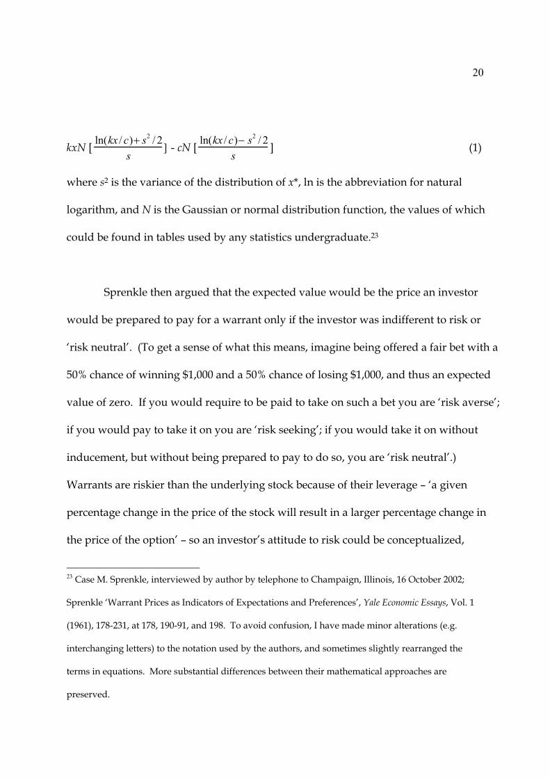
20
kxN [ ln(kx / c)+ s2 / 2s
] - cN [ ln(kx / c)− s2 / 2s
] (1)
where s2 is the variance of the distribution of x*, ln is the abbreviation for natural
logarithm, and N is the Gaussian or normal distribution function, the values of which
could be found in tables used by any statistics undergraduate.23
Sprenkle then argued that the expected value would be the price an investor
would be prepared to pay for a warrant only if the investor was indifferent to risk or
‘risk neutral’. (To get a sense of what this means, imagine being offered a fair bet with a
50% chance of winning $1,000 and a 50% chance of losing $1,000, and thus an expected
value of zero. If you would require to be paid to take on such a bet you are ‘risk averse’;
if you would pay to take it on you are ‘risk seeking’; if you would take it on without
inducement, but without being prepared to pay to do so, you are ‘risk neutral’.)
Warrants are riskier than the underlying stock because of their leverage – ‘a given
percentage change in the price of the stock will result in a larger percentage change in
the price of the option’ – so an investor’s attitude to risk could be conceptualized,
23 Case M. Sprenkle, interviewed by author by telephone to Champaign, Illinois, 16 October 2002;
Sprenkle ‘Warrant Prices as Indicators of Expectations and Preferences’, Yale Economic Essays, Vol. 1
(1961), 178-231, at 178, 190-91, and 198. To avoid confusion, I have made minor alterations (e.g.
interchanging letters) to the notation used by the authors, and sometimes slightly rearranged the
terms in equations. More substantial differences between their mathematical approaches are
preserved.
21
Sprenkle suggested, as the price Pe he or she was prepared to pay for leverage. A risk-
seeking investor would pay a positive price, and a risk-averse investor a negative one:
that is, a levered asset would have to offer an expected rate of return sufficiently higher
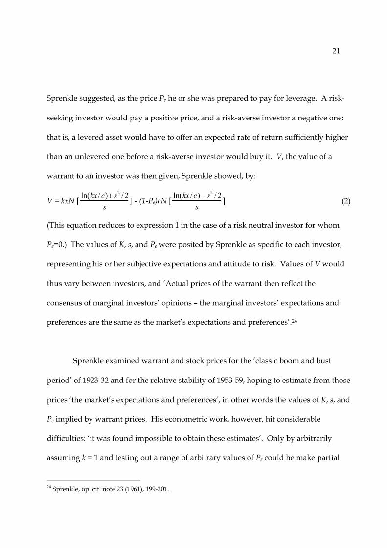
than an unlevered one before a risk-averse investor would buy it. V, the value of a
warrant to an investor was then given, Sprenkle showed, by:
V = kxN [ ln(kx / c)+ s2 / 2s
] - (1-Pe)cN [ ln(kx / c)− s2 / 2s
] (2)
(This equation reduces to expression 1 in the case of a risk neutral investor for whom
Pe=0.) The values of K, s, and Pe were posited by Sprenkle as specific to each investor,
representing his or her subjective expectations and attitude to risk. Values of V would
thus vary between investors, and ‘Actual prices of the warrant then reflect the
consensus of marginal investors’ opinions – the marginal investors’ expectations and
preferences are the same as the market’s expectations and preferences’.24
Sprenkle examined warrant and stock prices for the ‘classic boom and bust
period’ of 1923-32 and for the relative stability of 1953-59, hoping to estimate from those
prices ‘the market’s expectations and preferences’, in other words the values of K, s, and
Pe implied by warrant prices. His econometric work, however, hit considerable
difficulties: ‘it was found impossible to obtain these estimates’. Only by arbitrarily
assuming k = 1 and testing out a range of arbitrary values of Pe could he make partial
24 Sprenkle, op. cit. note 23 (1961), 199-201.

22
progress. His theoretically-derived formula for the value of a warrant depended on
parameters whose empirical values were extremely problematic to determine.25
The same difficulty hit the most sophisticated theoretical analysis of warrants
from this period, by Paul Samuelson in collaboration with the MIT mathematician
Henry P. McKean, Jr. McKean was a world-class specialist in stochastic calculus, the
theory of stochastic processes in continuous time, which in the years after Bachelier’s
work had burgeoned into a key domain of modern probability theory. Even with
McKean’s help, however, Samuelson’s model (which space constraints prevent me
describing in detail) also depended, like Sprenkle’s, on parameters that seemed to have
no straightforward empirical referents: rα, the expected rate of return on the underlying
stock, and rβ, the expected return on the warrant.26 A similar problem was encountered
in the somewhat simpler work of University of Chicago PhD student, A. James Boness.
He made the simplifying assumption that option traders are risk-neutral, but his
25 Sprenkle, op. cit. note 23 (1961), 204 and 212-13.
26 Paul A. Samuelson, ‘Rational Theory of Warrant Pricing’, Industrial Management Review, Vol. 6, No.
2 (Spring 1965), 13-32; Henry P. McKean, Jr., ‘Appendix: A Free Boundary Problem for the Heat
Equation arising from a Problem of Mathematical Economics’, ibid., 32-39.
23
formula also involved rα, which he could estimate only indirectly by finding the value
that minimized the difference between predicted and observed option prices.27
27 A. James Boness, ‘Elements of a Theory of Stock-Option Value’, Journal of Political Economy, Vol. 72
(1964), 163-175.
24
‘The greatest gambling game on earth’
Theoretical analysis of warrant and option prices thus seemed always to lead
to formulae involving parameters that were difficult or impossible to estimate. An
alternative approach was to eschew a priori models and to study the relationship
between warrant and stock prices empirically. The most influential work of this
kind was conducted by Sheen Kassouf. After a mathematics degree from Columbia
University, Kassouf set up a successful technical illustration firm. He was fascinated
by the stock market and a keen, if not always successful, investor. In 1961, he
wanted to invest in the defence company Textron, but could not decide between
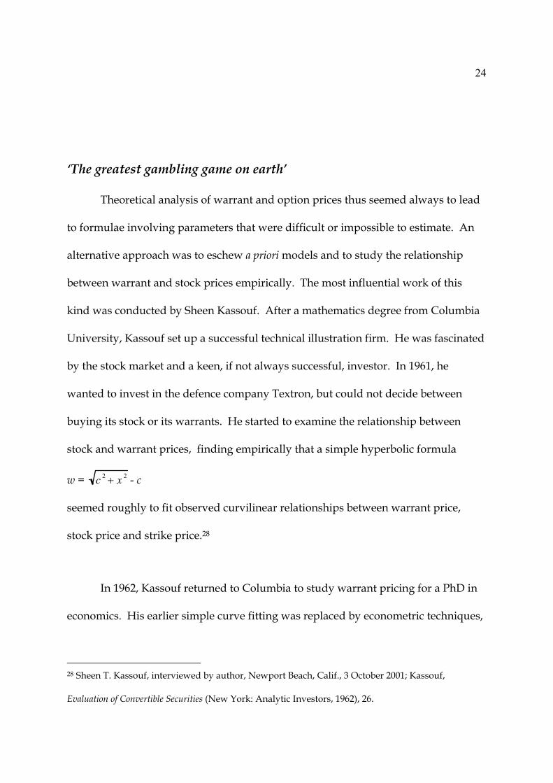
buying its stock or its warrants. He started to examine the relationship between
stock and warrant prices, finding empirically that a simple hyperbolic formula
w = c 2 + x 2 - c
seemed roughly to fit observed curvilinear relationships between warrant price,
stock price and strike price.28
In 1962, Kassouf returned to Columbia to study warrant pricing for a PhD in
economics. His earlier simple curve fitting was replaced by econometric techniques,
28 Sheen T. Kassouf, interviewed by author, Newport Beach, Calif., 3 October 2001; Kassouf,
Evaluation of Convertible Securities (New York: Analytic Investors, 1962), 26.

25
especially regression analysis, and he posited a more complex relationship
determining warrant prices:
w/c = [(x/c)z + 1]1/z – 1 (3)
where z was an empirically-determined function of the stock price, exercise price,
stock price ‘trend’, time to expiration, stock dividend, and the extent of the dilution
of existing shares that would occur if all warrants were exercised.29
Kassouf’s interest in warrants was not simply academic: he wanted ‘to make
money’ trading them.30 He had rediscovered, even before starting his PhD, an old
form of securities arbitrage†.31 Warrants and the corresponding stock tended to
move together: if the stock price rose, then so did the warrant price; if the stock fell,
so did the warrant. So one could be used to offset the risk of the other. If, for
example, warrants seemed overpriced relative to the corresponding stock, one could
short sell† them, hedging the risk by buying some of the stock. Trading of this sort,
29 Kassouf interview, op. cit. note 28; Sheen T. Kassouf, A Theory and an Econometric Model for Common
Stock Purchase Warrants (Brooklyn, N.Y.: Analytical Publishers, 1965). Stock price ‘trend’ was
measured by ‘the ratio of the present price to the average of the year’s high and low’ (ibid., 50).
30 Kassouf interview, op. cit. note 28.
31 Meyer H. Weinstein, Arbitrage in Securities (New York: Harper, 1931), 84 and 142-45.
26
conducted by Kassouf in parallel with his PhD research, enabled him ‘to more than
double $100,000 in just four years’.32
In 1965, fresh from his PhD, Kassouf was appointed to the faculty of the
newly established Irvine campus of the University of California. There, he was
introduced to mathematician Edward O. Thorp. Alongside research in functional
analysis and probability theory, Thorp had a long-standing interest in casino games.
While at MIT in 1959-61 he had collaborated with the celebrated information theorist
Claude Shannon on a tiny, wearable, analog computer system to predict where the
ball would be deposited on a roulette wheel. Thorp went on to devise the first
effective methods for beating the casino at blackjack, by keeping track of cards that
had already been dealt and thus identifying situations favourable to the player.33
Thorp and Shannon’s use of their wearable roulette computer was limited by
frequently broken wires, but card-counting was highly profitable. In the MIT spring
recess in 1961, Thorp travelled to Nevada equipped with a hundred $100 bills
32 Edward O. Thorp and Sheen T. Kassouf, Beat the Market: A Scientific Stock Market System (New York:
Random House, 1967), 32
33 Edward O. Thorp, interviewed by author, Newport Beach, Calif., 1 October 2001; Thorp, ‘A
Favorable Strategy for Twenty-One’, Proceedings of the National Academy of Sciences, Vol. 47 (1961), 110-
12. See also Dan Tudball, ‘In for the Count’, Willmot, September 2002, 24-35.

27
provided by two millionaires with an interest in gambling. After thirty hours of
blackjack, Thorp’s $10,000 had become $21,000. He went on to devise, with
computer scientist William E. Walden of the nuclear weapons laboratory at Los
Alamos, a method for identifying favourable side bets in the version of baccarat
played in Nevada. Thorp found, however, that beating the casino had
disadvantages as a way of making money. At a time when U.S. casinos were
controlled largely by organized criminals, there were physical risks: while Thorp
was playing baccarat in 1964, he was rendered almost unconscious by knock-out
drops added to his coffee. The need to travel to places where gambling was legal
was a further disadvantage to an academic with a family.34
Increasingly, Thorp’s attention switched to the financial markets. ‘The
greatest gambling game on earth is the one played daily through the brokerage
houses across the country’, Thorp told the readers of the hugely successful book
describing his card-counting methods.35 But could the biggest of casinos succumb to
Thorp’s mathematical skills? Predicting stock prices seemed too daunting: ‘there is
an extremely large number of variables, many of which I can’t get any fix on’.
However, he realized that ‘I can eliminate most of the variables if I think about
warrants versus common stock’. Thorp began to sketch graphs of the observed
34 Thorp interview, op. cit. note 33.
35 Edward O. Thorp, Beat the Dealer (New York: Vintage, 1966), 59-74, 94 and 182.

28
relationships between stock and warrant prices, and meeting Kassouf provided him
with a formula (equation 3 above) for these curves.36
In their 1967 book, Beat the Market, Thorp and Kassouf explained graphically
the relationship between the price of a warrant, w, and of the underlying common
stock, x (see figure 1). No warrant should ever cost more than the underlying stock,
since it is simply an option to buy the latter, and this constraint yielded a ‘maximum
value line’. At expiration, as Sprenkle had noted, a warrant would be worthless if
the stock price, x, was less than the strike price, c; otherwise it would be worth the
difference (x – c). If, at any time, w < x – c, an instant arbitrage profit could be made
by buying the warrant and exercising it (at a cost of w + c) and selling the stock thus
acquired for x. So the warrant’s value at expiration was also a ‘minimum value’ for
it at any time. As expiration approached, the ‘normal price curves’ expressing the
value of a warrant dropped closer to its value at expiration.
These ‘normal price curves’ could then be used to identify overpriced and
underpriced warrants.37 The former could be sold short, and the latter bought, with
36 Thorp interview, op. cit. note 33. Despite the number of variables involved, Thorp was later to
enjoy considerable success in ‘statistical arbitrage’ of stock prices.
29
the resultant risks hedged by taking a position in the stock (buying stock if warrants
had been sold short; selling stock short if warrants had been bought). The
appropriate size of hedge, Thorp and Kassouf explained, was determined by ‘the
slope of the normal price curve at our starting position’. If that slope were, say, 1:3,
as it roughly is at point (A,B) in figure 1, the appropriate hedge ratio was to buy one
unit of stock for every three warrants. Any movements along the normal price curve
caused by small stock price fluctuations would then have little effect on the value of
the overall position, because the loss or gain on the warrants would be balanced by a
nearly equivalent gain or loss on the stock.38 Larger stock price movements could of
course lead to a shift to a region of the curve in which the slope differed from 1:3,
and in their investment practice both Thorp and Kassouf adjusted their hedges when
that happened.39
Initially, Thorp relied upon Kassouf’s empirical formula for warrant prices
(equation 3 above): as he says, ‘it produced ... curves qualitatively like the actual
warrant curves’. Yet he was not entirely satisfied with it: ‘quantitatively, I think we
37 The curves are of course specific to an individual warrant, but as well as providing their readers
with Kassouf’s formula for calculating them Thorp and Kassouf provided ‘average’ curves based on
the prices of 1964-66: op. cit. note 32, 78-79.
38 Thorp and Kassouf, op. cit. note 32, 82.

30
both knew that there was something more that had to happen’. He began his
investigation of that ‘something’ in the same way as Sprenkle – applying the log-
normal distribution to work out the expected value of a warrant at expiration –
reaching a formula equivalent to Sprenkle’s (equation 1 above).40
Like Sprenkle’s, Thorp’s formula for the expected value of a warrant involved
the expected increase in the stock price, which there was no straightforward way to
estimate. He decided to approximate it by assuming that the expected value of the
stock rose at the riskless† rate of interest: he had no better estimate, and he ‘didn’t
think that enormous errors would necessarily be introduced’ by the approximation.
Thorp found that the resultant equation was plausible – ‘I couldn’t find anything
wrong with its qualitative behavior and with the actual forecast it was making’ – and
in 1967 he started to use it to identify grossly overpriced options to sell. It was
formally equivalent to the Black-Scholes formula for a call option (equation 5 below),
except for one feature: unlike Black and Scholes, Thorp did not discount† the
expected value of the option at expiration back to the present. In the warrant
markets he was used to, the proceeds of the short sale of a warrant were retained in
39 Edward O. Thorp, ‘What I knew and when I knew it Part 1’, Willmot, September 2002, 44-45, at 45;
Kassouf interview, op. cit. note 28.
40 Thorp interview; E.O. Thorp, ‘Optional Gambling Systems for Favorable Games’, Review of the
International Statistical Institute, Vol. 37 (1969), 273-281.

31
their entirety to the broker, and were not available immediately to the seller as Black
and Scholes assumed.41 It was a relatively minor difference: when Thorp read Black
and Scholes, he was able quickly to see why the two formulae differed and to add to
his formula the necessary discount† factor to make them identical.42 In the
background, however, lay more profound differences of approach.
Black and Scholes
In 1965, Fischer Black, with a Harvard PhD in what was in effect artificial
intelligence,43 joined the operations research group of the consultancy firm, Arthur D.
Little, Inc. There, Black met Jack Treynor, a financial specialist at Little. Treynor had
developed, though had not published, what later became known as the Capital Asset
Pricing Model (also developed, independently, by academics William Sharpe, John
41 Thorp interview, op. cit. note 33; Edward Thorp, ‘Extensions of the Black-Scholes Option Model’,
Proceedings of the 39th Session of the International Statistical Institute, Vienna, Austria, August 1973, 522-29.
As Thorp explained (ibid., 526) ‘to sell warrants short [and] buy stocks, and yet achieve the riskless
rate of return r requires a higher warrant short sale price than for the corresponding call [option]’
under the Black-Scholes assumptions. Thorp had also been selling options in the New York market,
where the seller did receive the sale price immediately (minus ‘margin’ retained by the broker), but
the price discrepancies he was exploiting were gross (so gross he felt able to proceed without hedging
in stock), and thus the requisite discount factor was not a salient consideration.
42 Thorp, op. cit. note 39.
43 Fischer Black, A Deductive Question Answering System (PhD thesis: Harvard University, 1964).
32
Lintner, and Jan Mossin).44 It was Black’s (and also Scholes’s) use of this model that
decisively differentiated their work from the earlier research on option pricing.
The Capital Asset Pricing Model provided a systematic account of the ‘risk
premium’: the additional return that investors demand for holding risky assets.
That premium, Treynor pointed out, could not depend simply on the ‘sheer
magnitude of the risk’, because some risks were ‘insurable’: they could be
minimized by diversification, by spreading one’s investments over a broad range of
companies.45 What could not be diversified away, however, was the risk of general
market fluctuations. By reasoning of this kind, Treynor showed (and the other
developers of the model also demonstrated) that a capital asset’s risk premium
should be proportional to its β, its covariance with the general level of the market,
44 Jack Treynor, interviewed by author, Palos Verdes Estates, Calif., 3 October 2001; Treynor, ‘Toward
a Theory of Market Value of Risky Assets’ (typescript rough draft, undated but c. 1961, Papers-
Treynor file, Box 56, Fischer Black papers, MIT Archives, MC505); William F. Sharpe, ‘Capital Asset
Prices: A Theory of Market Equilibrium under Conditions of Risk’, Journal of Finance, Vol. 19 (1964),
425-442; John Lintner, ‘Security Prices, Risk, and Maximal Gains from Diversification’, Journal of
Finance, Vol. 20 (1965), 587-615; Jan Mossin, ‘Equilibrium in a Capital Asset Market’, Econometrica,
Vol. 34 (1966), 768-783. Treynor’s typescript draft was eventually published in Robert A. Korajczyk
(ed.), Asset Pricing and Portfolio Performance: Models, Strategy and Performance Metrics (London: Risk
Books, 1999), 15-22.
45 Treynor, ‘Toward a Theory’, op. cit. note 44, typescript 13-14, published version, 20.
33
divided by the variance of the market. An asset whose β was zero, in other words an
asset the price of which was uncorrelated with the overall level of the market, had no
risk premium (any specific risks involved in holding it could be diversified away),
and investors in it should earn only r, the riskless rate of interest. As the asset’s β
increased, so should its risk premium.
The Capital Asset Pricing Model was an elegant piece of theoretical reasoning.
Its co-developer Treynor became Black’s mentor in what was for Black the new field
of in finance, so it is not surprising that when Black began his own work in finance it
was by trying to apply the model to a range of assets other than shares (which had
been its main initial field of application). Also important as a resource for Black’s
research was a specific piece of joint work with Treynor on how companies should
value cash flows in making their investment decisions. This was the problem that
had most directly inspired Treynor’s development of the Capital Asset Pricing
Model, and the aspect of it on which Black and Treynor collaborated had involved
Treynor writing an expression for the change in the value of a cash flow in a finite,
short time interval ∆t; expanding the expression using the standard calculus
technique of Taylor expansion; taking expected values; dropping the terms of order
∆t2 and higher; dividing by ∆t; and letting ∆t tend to zero so that the finite difference
equation became a differential equation. Treynor’s original version of the latter was
in error because he had left out a second derivative that did not vanish, but Black
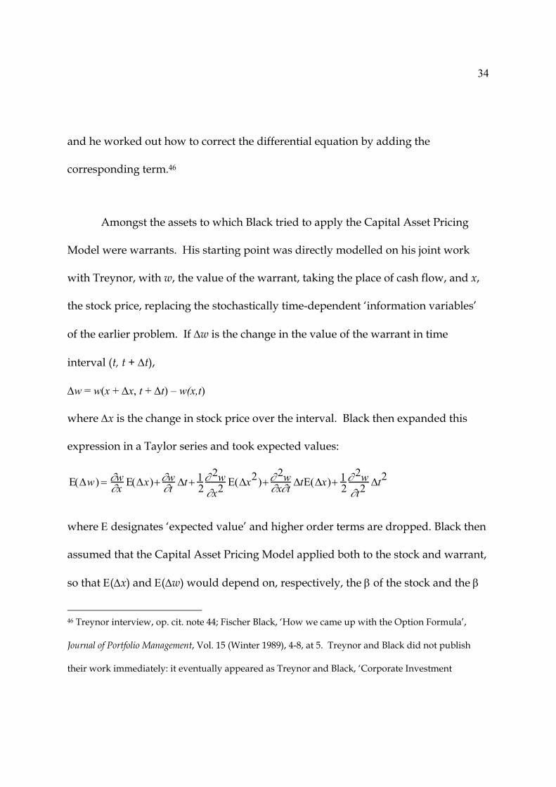
34
and he worked out how to correct the differential equation by adding the
corresponding term.46
Amongst the assets to which Black tried to apply the Capital Asset Pricing
Model were warrants. His starting point was directly modelled on his joint work
with Treynor, with w, the value of the warrant, taking the place of cash flow, and x,
the stock price, replacing the stochastically time-dependent ‘information variables’
of the earlier problem. If ∆w is the change in the value of the warrant in time
interval (t, t + ∆t),
∆w = w(x + ∆x, t + ∆t) – w(x,t)
where ∆x is the change in stock price over the interval. Black then expanded this
expression in a Taylor series and took expected values:
Ε(∆w) = ∂w∂x Ε(∆x)+∂w∂t ∆t+
12∂ 2w∂x2
Ε(∆x2)+∂2w
∂x∂t ∆tΕ(∆x)+ 12∂ 2w∂t2
∆t2
where Ε designates ‘expected value’ and higher order terms are dropped. Black then
assumed that the Capital Asset Pricing Model applied both to the stock and warrant,
so that Ε(∆x) and Ε(∆w) would depend on, respectively, the β of the stock and the β
46 Treynor interview, op. cit. note 44; Fischer Black, ‘How we came up with the Option Formula’,
Journal of Portfolio Management, Vol. 15 (Winter 1989), 4-8, at 5. Treynor and Black did not publish
their work immediately: it eventually appeared as Treynor and Black, ‘Corporate Investment
35
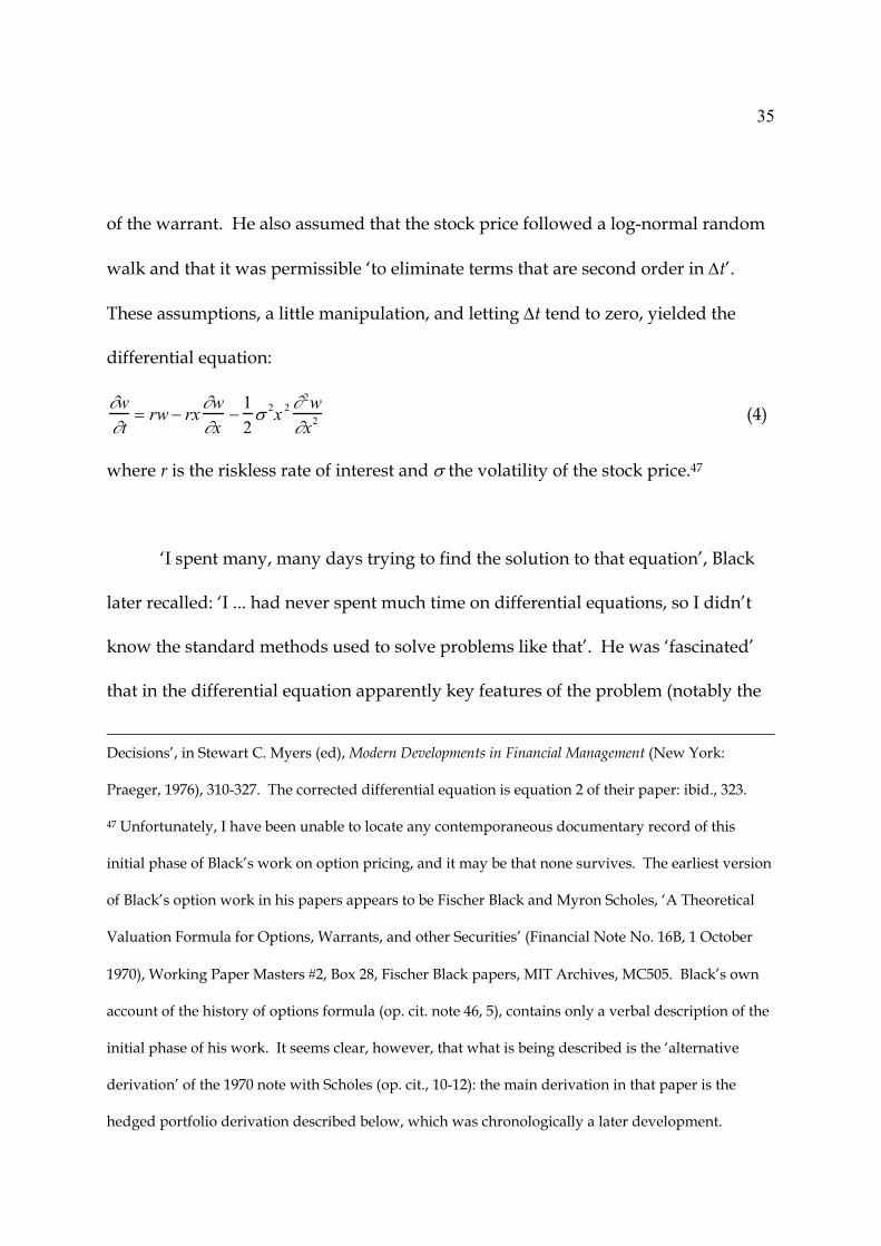
of the warrant. He also assumed that the stock price followed a log-normal random
walk and that it was permissible ‘to eliminate terms that are second order in ∆t’.
These assumptions, a little manipulation, and letting ∆t tend to zero, yielded the
differential equation:
∂w∂t
= rw − rx ∂w∂x
−12σ 2x 2 ∂ 2w
∂x2 (4)
where r is the riskless rate of interest and σ the volatility of the stock price.47
‘I spent many, many days trying to find the solution to that equation’, Black
later recalled: ‘I ... had never spent much time on differential equations, so I didn’t
know the standard methods used to solve problems like that’. He was ‘fascinated’
that in the differential equation apparently key features of the problem (notably the
Decisions’, in Stewart C. Myers (ed), Modern Developments in Financial Management (New York:
Praeger, 1976), 310-327. The corrected differential equation is equation 2 of their paper: ibid., 323.
47 Unfortunately, I have been unable to locate any contemporaneous documentary record of this
initial phase of Black’s work on option pricing, and it may be that none survives. The earliest version
of Black’s option work in his papers appears to be Fischer Black and Myron Scholes, ‘A Theoretical
Valuation Formula for Options, Warrants, and other Securities’ (Financial Note No. 16B, 1 October
1970), Working Paper Masters #2, Box 28, Fischer Black papers, MIT Archives, MC505. Black’s own
account of the history of options formula (op. cit. note 46, 5), contains only a verbal description of the
initial phase of his work. It seems clear, however, that what is being described is the ‘alternative
derivation’ of the 1970 note with Scholes (op. cit., 10-12): the main derivation in that paper is the
hedged portfolio derivation described below, which was chronologically a later development.

36
stock’s β and thus its expected return, a pervasive feature in earlier theoretical work
on option pricing) no longer appeared. ‘But I was still unable to come up with the
formula. So I put the problem aside and worked on other things’.48
In the autumn of 1968, however, Black (still working for Arthur D. Little in
Cambridge, Mass.) met Myron Scholes, a young researcher who had just joined the
finance group in MIT’s Sloan School of Management. The pair teamed up with
finance scholar Michael Jensen to test the Capital Asset Pricing Model (still largely a
theoretical postulate) empirically. Simultaneously, through supervising two MIT
Master’s dissertations on the topic, Scholes became interested in warrant pricing.
Scholes’s 1970 PhD thesis involved the analysis of securities as potential substitutes
for each other, with the potential for arbitrage ensuring that securities whose risks
are alike will offer similar expected returns.49 Scholes’s PhD adviser, Merton H.
Miller, had introduced this form of theoretical argument – ‘arbitrage proof’ – in what
by 1970 was already seen as classic work with Franco Modigliani.50 Scholes started
to investigate whether similar reasoning could be applied to warrant pricing, and
48 Black, op. cit. note 46, 5-6.
49 Myron S. Scholes, interviewed by author, San Francisco, 15 June 2000; Scholes, A Test of the
Competitive Market Hypothesis: The Market for New Issues and Secondary Offerings (PhD thesis,
University of Chicago, 1970).
50 Franco Modigliani and Merton H. Miller, ‘The Cost of Capital, Corporation Finance and the Theory
of Investment’, American Economic Review, Vol. 48 (1958), 261-97.

37
began to consider the hedged portfolio formed by buying warrants and short selling
the underlying stock.51
The hedged portfolio had been the central idea of Thorp and Kassouf’s Beat
the Market, though Scholes had not yet read the book.52 Scholes’s goal, in any case,
was different. Thorp and Kassouf’s hedged portfolio was designed to earn high
returns with low risk in real markets. Scholes’s was a theoretical artifact. He wanted
a portfolio with a β of zero: that is, with no correlation with the overall level of the
market. If such a portfolio could be created, the Capital Asset Pricing Model implied
that it would earn, not high returns, but only the riskless rate of interest, r. It would
thus not be an unduly enticing investment, but knowing the rate of return on the
hedged portfolio might solve the problem of warrant pricing.
What Scholes could not work out, however, was how to construct a zero-β
portfolio. He could see that the quantity of shares that had to be sold short must
change with time and with changes in the stock price, but he could not see how to
determine that quantity. He ‘thought about it empirically’, but decided ‘that doesn’t
do it’, and tried unsuccessfully to solve the problem analytically. Like Black, Scholes
51 Scholes interview, op. cit. note 49; Myron S. Scholes, ‘Derivatives in a Dynamic Environment’, in
Les Prix Nobel 1997 (Stockholm: Almquist & Wicksell, 1998), 475-502, at 480.
52 Thorp and Kassouf, op. cit. note 32; Scholes interview, op. cit. note 49.
38
was stymied: ‘I put it [the warrant pricing problem] away’.53 Then, in ‘the summer
or early fall of 1969’, Scholes told Black of his efforts, and Black described the
different approach he had taken, in particular showing Scholes the Taylor series
expansion of the warrant price. The two men then found how to construct a zero-β
portfolio. If the stock price changed by ∆x, the option price would alter by ∂w∂x ∆x. So
the necessary hedge was to short sell a quantity ∂w∂x of stock for every warrant held.
This was the same conclusion Thorp and Kassouf had arrived at: ∂w∂x is their hedging
ratio, the slope of the curve of w plotted against x as in figure 1.54
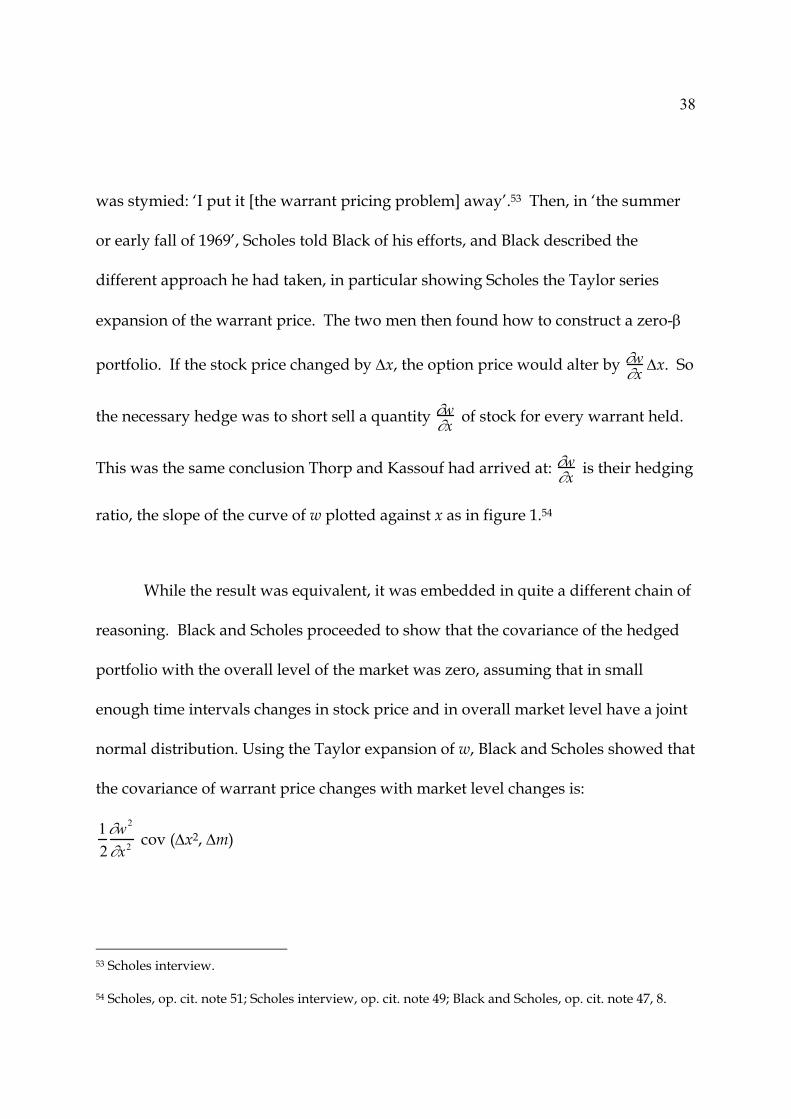
While the result was equivalent, it was embedded in quite a different chain of
reasoning. Black and Scholes proceeded to show that the covariance of the hedged
portfolio with the overall level of the market was zero, assuming that in small
enough time intervals changes in stock price and in overall market level have a joint
normal distribution. Using the Taylor expansion of w, Black and Scholes showed that
the covariance of warrant price changes with market level changes is:
12∂w2
∂x2 cov (∆x2, ∆m)
53 Scholes interview.
54 Scholes, op. cit. note 51; Scholes interview, op. cit. note 49; Black and Scholes, op. cit. note 47, 8.
39
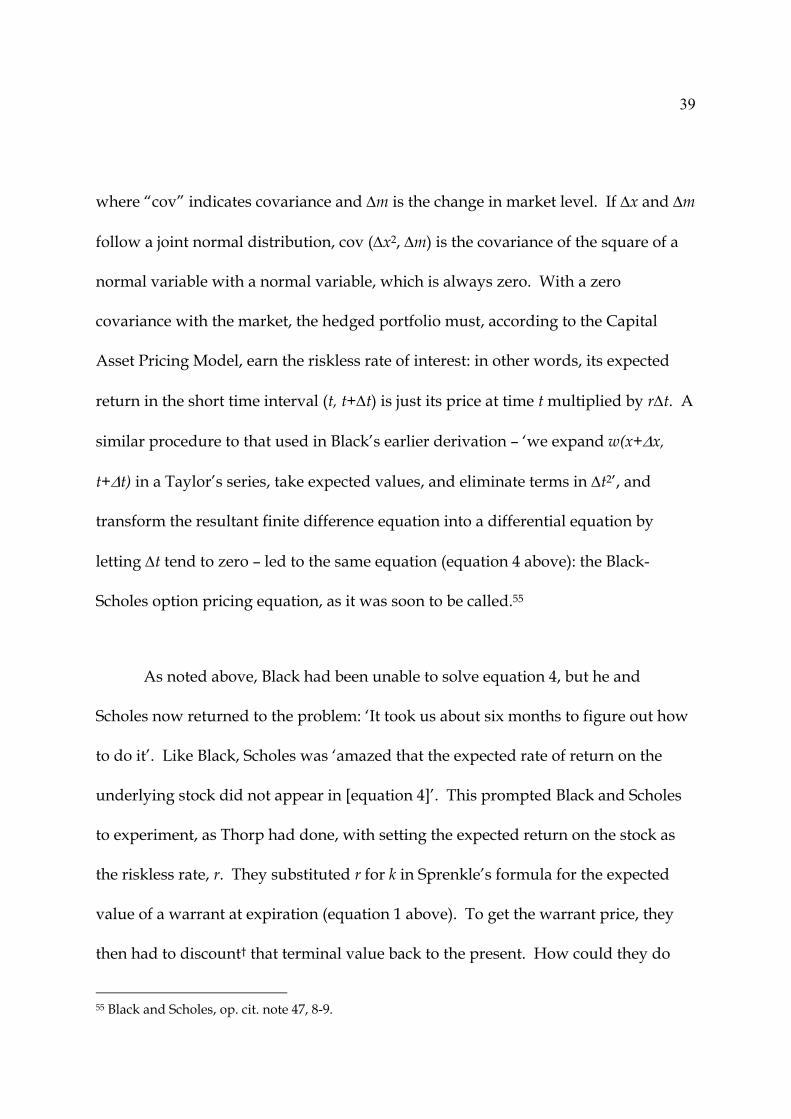
where “cov” indicates covariance and ∆m is the change in market level. If ∆x and ∆m
follow a joint normal distribution, cov (∆x2, ∆m) is the covariance of the square of a
normal variable with a normal variable, which is always zero. With a zero
covariance with the market, the hedged portfolio must, according to the Capital
Asset Pricing Model, earn the riskless rate of interest: in other words, its expected
return in the short time interval (t, t+∆t) is just its price at time t multiplied by r∆t. A
similar procedure to that used in Black’s earlier derivation – ‘we expand w(x+∆x,
t+∆t) in a Taylor’s series, take expected values, and eliminate terms in ∆t2’, and
transform the resultant finite difference equation into a differential equation by
letting ∆t tend to zero – led to the same equation (equation 4 above): the Black-
Scholes option pricing equation, as it was soon to be called.55
As noted above, Black had been unable to solve equation 4, but he and
Scholes now returned to the problem: ‘It took us about six months to figure out how
to do it’. Like Black, Scholes was ‘amazed that the expected rate of return on the
underlying stock did not appear in [equation 4]’. This prompted Black and Scholes
to experiment, as Thorp had done, with setting the expected return on the stock as
the riskless rate, r. They substituted r for k in Sprenkle’s formula for the expected
value of a warrant at expiration (equation 1 above). To get the warrant price, they
then had to discount† that terminal value back to the present. How could they do
55 Black and Scholes, op. cit. note 47, 8-9.
40
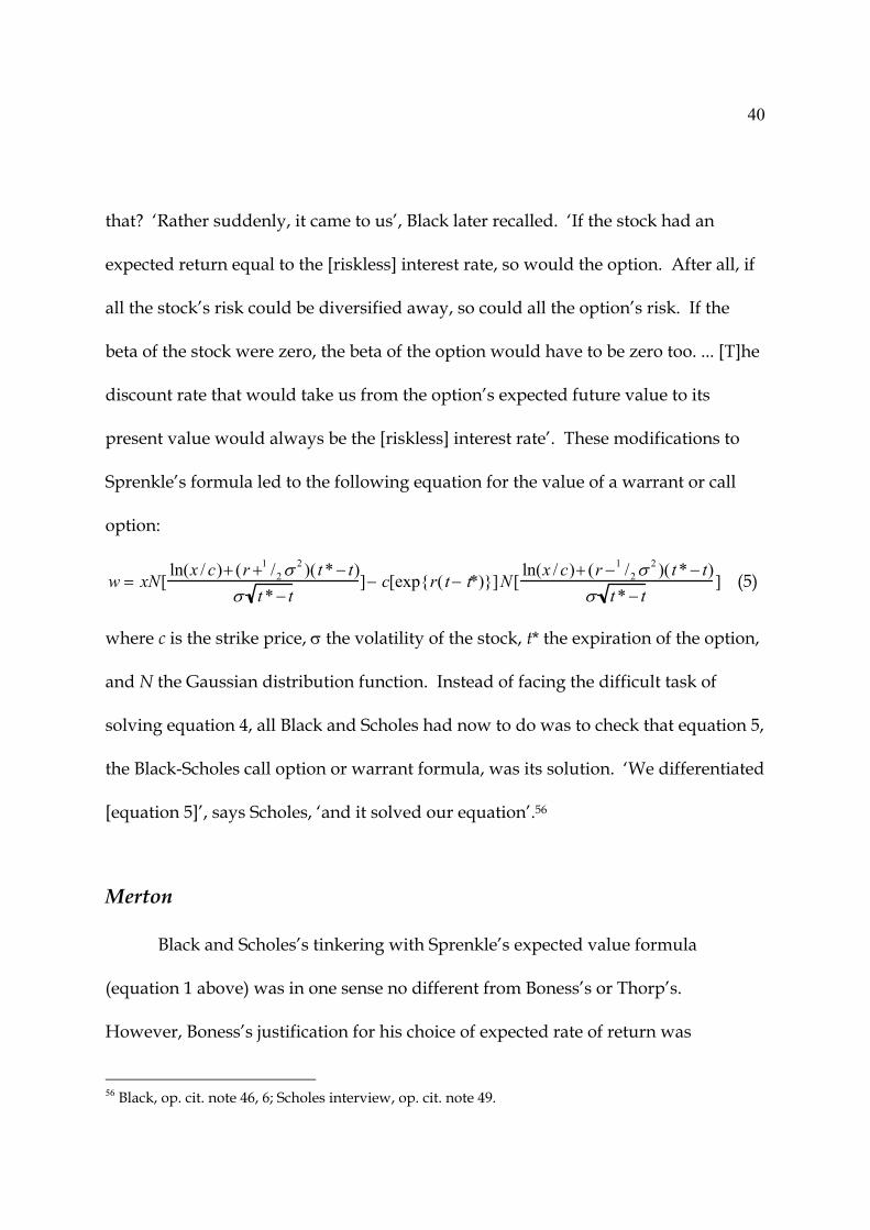
that? ‘Rather suddenly, it came to us’, Black later recalled. ‘If the stock had an
expected return equal to the [riskless] interest rate, so would the option. After all, if
all the stock’s risk could be diversified away, so could all the option’s risk. If the
beta of the stock were zero, the beta of the option would have to be zero too. ... [T]he
discount rate that would take us from the option’s expected future value to its
present value would always be the [riskless] interest rate’. These modifications to
Sprenkle’s formula led to the following equation for the value of a warrant or call
option:
w = xN[ln(x / c)+ (r +1 /2σ
2 )( t* − t)σ t* − t
]− c[exp{r( t− t*)}]N[ln(x / c)+ (r −1 /2σ
2 )( t* − t)σ t* − t
] (5)
where c is the strike price, σ the volatility of the stock, t* the expiration of the option,
and N the Gaussian distribution function. Instead of facing the difficult task of
solving equation 4, all Black and Scholes had now to do was to check that equation 5,
the Black-Scholes call option or warrant formula, was its solution. ‘We differentiated
[equation 5]’, says Scholes, ‘and it solved our equation’.56
Merton
Black and Scholes’s tinkering with Sprenkle’s expected value formula
(equation 1 above) was in one sense no different from Boness’s or Thorp’s.
However, Boness’s justification for his choice of expected rate of return was
56 Black, op. cit. note 46, 6; Scholes interview, op. cit. note 49.

41
empirical – he chose ‘the rate of appreciation most consistent with market prices of
puts and calls’ – while Thorp freely admits he ‘guessed’ that the right thing to do
was to set the stock’s rate of return equal to the riskless rate: it was ‘guesswork not
proof’.57 Black and Scholes on the other hand, could prove mathematically that their
call option formula (equation 5) was a solution to their differential equation
(equation 4), and the latter had a clear theoretical justification.
It was a justification apparently intimately bound up with the Capital Asset
Pricing Model. Not only was the model drawn on explicitly in the equation’s
derivation, but it also assuaged Scholes’s doubts about the mathematical rigour of
what he and Black were doing. Like all others working on the problem in the 1950s
and 1960s (with the exception of Samuelson, McKean, and Merton), Black and
Scholes used ordinary calculus – Taylor series expansion, and so on – but in a
context in which x, the stock price, was known to vary stochastically. ‘I was worried
that we were taking derivatives on things that are stochastic’, says Scholes. Neither
he nor Black knew the mathematical theory needed to do calculus rigorously in a
stochastic environment, but the ideas of the hedged portfolio and Capital Asset
Pricing Model provided an economic justification for what might otherwise have
seemed dangerously unrigorous mathematics. ‘According to our economic logic, at
the time’, says Scholes, ‘our solution was exact if the CAPM [Capital Asset Pricing
57 Boness, op. cit. note 27, 170; Thorp interview, op. cit. note 33.

42
Model] was true in continuous time. Essentially, ... we showed that if time was
small enough and you took the CAPM framework and had any residual, it would
have an expected value of zero. That’s because it could be diversified away. In a
large portfolio it would have no economic importance’.58
As noted above, Black had been a close colleague of the Capital Asset Pricing
Model’s co-developer, Treynor, while Scholes had done his graduate work at the
University of Chicago, one of the two main sites of financial economics, where the
model was also ‘quite highly regarded’.59 However, at the other main site, MIT, the
original version of the Capital Asset Pricing Model was regarded much less
positively. The model rested upon the ‘mean-variance’ view of portfolio selection:
that investors could be modelled as guided only by their expectations of the returns
on investments and their risks as measured by the expected standard deviation or
variance of returns. Unless returns followed a joint normal distribution (which was
regarded as ruled out, because it would imply, as noted above, a non-zero
probability of negative prices), mean-variance analysis seemed to rest upon a
specific form of ‘utility function’ (the function that characterizes the relationship
between an investor’s wealth, y, and his or her preferences). Mean-variance analysis
58 Scholes interview, op. cit. note 49.
59 Scholes interview, op. cit. note 49.

43
seemed to imply that investors’ utility functions were quadratic: that is, they
contained only terms in y and y2.
For MIT’s Paul Samuelson, the assumption of quadratic utility was over-
specific (one of his earliest contributions to economics had been his ‘revealed
preference’ theory, designed to eliminate the non-empirical aspects of utility
analysis) and a ‘bad ... representation of human behaviour’.60 Seen from Chicago,
Samuelson’s objections were ‘quibbles’61 when set against the virtues of the Capital
Asset Pricing Model: ‘he’s got to remember what Milton Friedman said – “Never
60 Paul A. Samuelson, ‘A Note on the Pure Theory of Consumer’s Behaviour’, Economica, Vol. 5 (1938),
61-71; Samuelson, interviewed by author, Cambridge, Mass., 3 November 1999. A quadratic utility
function has the form U(y) = l + my + ny2, where l, m, and n are constant. n must be negative if, as
will in general be the case, ‘the investor prefers smaller standard deviation to larger standard
deviation (expected return remaining the same)’, and negative n implies that above a threshold value
utility will diminish with increasing wealth: Harry Markowitz, Portfolio Selection: Efficient
Diversification of Investments (New Haven, Conn.: Yale University Press, 1959), 288. Markowitz’s
position is that while quadratic utility cannot reasonably be assumed, a quadratic function centred on
expect return is a good approximation to a wide range of utility functions: see H. Levy and H.M.
Markowitz, ‘Approximating Expected Utility by a Function of Mean and Variance’, American
Economic Review, Vol. 69 (1979), 308-317.
61 Eugene Fama, interviewed by author, Chicago, 5 November 1999.
44
mind about assumptions. What counts is, how good are the predictions?”’62
Nevertheless, they were objections that weighed heavily with Robert C. Merton. Son
of the social theorist and sociologist of science Robert K. Merton, he switched in
autumn 1967 from graduate work in applied mathematics at the California Institute
of Technology to study economics at MIT. He had been an amateur investor since
aged 10 or 11, had graduated from stocks to options and warrants, and came to
realize ‘that I had a much better intuition and “feel” into economic matters than
physical ones’. In spring 1968, Samuelson appointed the mathematically-talented
young Merton as his research assistant, even allocating him a desk inside his MIT
office.63
It was not simply a matter of Merton finding the assumptions underpinning
the standard Capital Asset Pricing Model ‘objectionable’. At the centre of his work
was the effort to replace simple ‘one-period’ models of that kind with more
sophisticated ‘continuous-time’ models. In the latter, not only did the returns on
assets vary in a continuous stochastic fashion, but individuals took decisions about
62 Merton Miller, interviewed by author, Chicago, 5 November 1999. Miller’s reference is to Milton
Friedman, ‘The Methodology of Positive Economics’, in Friedman, Essays in Positive Economics
(Chicago: University of Chicago Press, 1953), 3-43.

45
portfolio selection (and also consumption) continuously, not just at a single point in
time. In any time interval, however short, individuals could change the composition
of their investment portfolios. Compared with ‘discrete-time’ models, ‘the
continuous time models are mathematically more complex’, says Merton. He
quickly became convinced, however, that ‘the derived results of the continuous-time
models were often more precise and easier to interpret than their discrete-time
counterparts’. His ‘intertemporal’ capital asset pricing model, for example, did not
necessitate the ‘quadratic utility’ assumption of the original.64
With continuous-time stochastic processes at the centre of his work, Merton
felt the need not just to make ad hoc adjustments to standard calculus but to learn
stochastic calculus. It was not yet part of economists’ mathematical repertoire (it
was above all Merton who introduced it), but by the late 1960s a number of textbook
treatments by mathematicians had been published, and Merton used these to teach
himself the subject. He rejected as unsuitable the ‘symmetrized’ formulation of
stochastic integration by R.L. Stratonovich: it was easier to use for those with
63 Robert C. Merton, interviewed by author, Cambridge, Mass., 2 November 1999; Merton,
Applications of Option-Pricing Theory: Twenty-Five Years Later (Boston: Harvard Business School, 1998),
15-16.

46
experience only of ordinary calculus, but when applied to prices it in effect allowed
investors an illegitimate peek into the future. Merton chose instead the original
1940s’ definition of the stochastic integral by the Japanese mathematician, Kiyosi Itô,
and Itô’s associated apparatus for handling stochastic differential equations.65
Amongst the problems on which Merton worked, both with Samuelson and
independently, was warrant pricing, and the resultant work formed two of the five
chapters of his September 1970 PhD thesis.66 Black and Scholes read the 1969 paper
in which Samuelson and Merton described their joint work, but did not immediately
tell them of the progress they had made: there was ‘friendly rivalry between the two
64 Robert Cox Merton, Analytical Optimal Control Theory as Applied to Stochastic and Non-Stochastic
Economics (PhD thesis: MIT, 1970), 2 and 48; Merton, op. cit. note 63 (1998), 18-19; Merton, ‘An
Intertemporal Capital Asset Pricing Model’, Econometrica, Vol. 41 (1973), 867-87.
65 Merton interview, op. cit. note 63. Merton drew particularly on D.R. Cox and H.D. Miller, The
Theory of Stochastic Processes (London: Methuen, 1965) and H.J. Kushner, Stochastic Stability and Control
(New York: Academic Press, 1967). For Stratonovich’s work, see R.L. Stratonovich, ‘A New
Representation for Stochastic Integrals and Equations’, SIAM Journal of Control, Vol. 4 (1966), 362-371,
and Stratonovich, Conditional Markov Processes and their Application to the Theory of Optimal Control
(New York: Elsevier, 1968), chapter 2. For Itô’s work, see Daniel W. Stroock and S.R.S.
Varadhan(eds), Kiyosi Itô: Selected Papers (New York: Springer, 1987).
66 Merton, op. cit. note 64 (PhD), chapters 4 and 5; Paul A. Samuelson and Robert C. Merton, ‘A
Complete Model of Warrant Pricing that Maximizes Utility’, Industrial Management Review, Vol. 10
(1969), 17-46.
47
teams’, says Scholes. In the early autumn of 1970, however, Scholes did discuss with
Merton his work with Black. The former immediately appreciated that this work
was a ‘significant “break-through”’ ( it was Merton, for example, who christened
equation 4 the ‘Black-Scholes’ equation). Given Merton’s critical attitude to the
Capital Asset Pricing Model, however, it is also not surprising that he also believed
that ‘such an important result deserves a rigorous derivation’, not just the
‘intuitively appealing’ one Black and Scholes had provided.67 In particular, Merton
was ‘not convinced ... that the covariance between the market return and the return
on the hedged portfolio would actually be zero’, recalls Scholes. ‘What I sort of
argued with them [Black and Scholes]’, says Merton, ‘was, if it depended on the
[Capital] Asset Pricing Model, why is it when you look at the final formula [equation
4] nothing about risk appears at all? In fact, it’s perfectly consistent with a risk-
neutral world’.68
So Merton set to work applying his continuous-time model and Itô calculus to
the Black-Scholes hedged portfolio. ‘I looked at this thing’, says Merton, ‘and I
realized that if you did ... dynamic trading ... if you actually [traded] literally
continuously, then in fact, yeah, you could get rid of the risk, but not just the
67 Scholes, op. cit. note 51, 483; Robert C. Merton, ‘Theory of Rational Option Pricing’, Bell Journal of
Economics and Management Science, Vol. 4 (1973), 141-83, at 142 and 161-62.
68 Scholes interview, op. cit. note 49; Merton interview, op. cit. note 63.
48
systematic risk, all the risk’. Not only did the hedged portfolio have zero β in the
continuous-time limit (Merton’s initial doubts on this point were assuaged), ‘but you
actually get a zero sigma’: that is, no variance of return on the hedged portfolio. So
the hedged portfolio can earn only the riskless rate of interest, ‘not for the reason of
[the Capital] Asset Pricing Model but ... to avoid arbitrage, or money machine’: a
way of generating certain profits with no net investment. For Merton, then, the ‘key
to the Black-Scholes analysis’ was an assumption Black and Scholes did not initially
make: continuous trading, the capacity to adjust a portfolio at all times and
instantaneously. ‘[O]nly in the instantaneous limit are the warrant price and stock
price perfectly correlated, which is what is required to form the “perfect” hedge’.69
Black and Scholes were not initially convinced of the correctness of Merton’s
approach. ‘We always worried you couldn’t do this continuous-time hedging’, says
Scholes, and in the second draft of their paper on option pricing Black and Scholes
even claimed that Merton’s ‘assumptions are inconsistent with equilibrium in the
69 Merton interview op. cit. note 63; Robert C. Merton, ‘Appendix: Continuous-Time Speculative
Processes’, in Richard H. Day and Stephen M. Robinson (eds), Mathematical Topics in Economic Theory
and Computation (Philadelphia: Society for Industrial and Applied Mathematics, 1972), 34-42, at 38.
49
asset markets’.70 Merton, in turn, told Fischer Black in 1972 that ‘I ... do not
understand your reluctance to accept that the standard form of CAPM [Capital Asset
Pricing Model] just does not work’.71 Despite this disagreement, Black and Scholes
used what was essentially Merton’s revised form of their derivation in the final,
published version of their paper, though they also preserved Black’s original
derivation, which drew directly on the Capital Asset Pricing Model. Scholes
appreciated the greater mathematical rigour of Merton’s use of stochastic calculus:
‘the [stochastic] calculus made it a much more solid proof than our proof’. Black,
however, was never entirely convinced, telling a 1989 interviewer that ‘I’m still more
fond’ of the Capital Asset Pricing Model derivation: ‘[T]here may be reasons why
arbitrage is not practical, for example trading costs’. (If trading incurs even tiny
transaction costs, continuous adjustment of a portfolio is infeasible). Merton’s
derivation ‘is more intellectual[ly] elegant but it relies on stricter assumptions, so I
don’t think it’s really as robust’.72
70 Scholes interview, note, op. cit. note 49; Fischer Black and Myron Scholes, ‘Capital Market
Equilibrium and the Pricing of Corporate Liabilities’ (Financial Note No 16C, January 1971), Working
Paper Master #2, Box 28, Fischer Black papers, MIT Archives, MC505, at 20.
71 Robert C. Merton to Fischer Black, 28 February 1972, Merton, Robert file, Box 14, Fischer Black
papers, MIT Archives MC505.
72 Fischer Black and Myron Scholes, ‘The Pricing of Options and Corporate Liabilities’, Journal of
Political Economy, Vol. 81 (1973), 637-654; Scholes interview, op. cit. note 49; Fischer Black interviewed
50
Black, indeed, came to express doubts even about the central intuition of
orthodox financial economics, that modern capital markets were efficient (in other
words that prices in them incorporate all known information). Efficiency held, he
suggested, only in a diluted sense: ‘we might define an efficient market as one in
which price is within a factor of 2 of value’. Black noted that this position was
intermediate between that of Merton, who defended the efficient market hypothesis,
and that of ‘behavioural’ finance theorist Robert Shiller: ‘Deviations from efficiency
seem more significant in my world than in Merton’s, but much less significant in my
world than in Shiller’s’.73
by Zvi Bodie, July 1989. I’m grateful to Prof. Bodie for a copy of the transcript of this unpublished
interview.
73 Fischer Black, ‘Noise’, Journal of Finance, Vol. 41 (1986), 529-43, at 533. For Merton’s views on the
efficient market hypothesis, see Robert C. Merton ‘On the Current State of the Stock Market
Rationality Hypothesis’, in R. Dornbusch, S. Fischer and J. Bossons (eds), Macroeconomics and Finance:
Essays in Honor of Franco Modigliani (Cambridge, Mass.: MIT Press, 1987), 93-124. For Shiller’s views,
see Robert J. Shiller, Market Volatility (Cambridge, Mass.: MIT Press, 1989).

51
The Equation and the World
It was not immediately obvious to all that what Black, Scholes and Merton
had done was a fundamental breakthrough. The Journal of Political Economy
originally rejected Black and Scholes’s paper because option pricing seemed to its
editor to be too specialized a topic to merit publication in a general economic
journal, and the paper was also rejected by the Review of Economics and Statistics.74
True, financial economists quickly saw the elegance of the Black-Scholes solution.
All the parameters in equations 4 and 5 seemed readily observable empirically: there
were none of the intractable estimation problems of earlier theoretical solutions.
That alone, however, does not account for the wider impact of the Black-Scholes-
Merton work. It does not explain, for example, how a paper originally rejected by an
economic journal as too specialized should win a Nobel prize in economics. (Scholes
and Merton were awarded the prize in 1997; Black died in 1995).
74 Robert J. Gordon to Fischer Black, 24 November 1970, Journal of Political Economics [sic] file, Box
13, Fischer Black papers, MIT Archives, MC505; Scholes interview, op. cit. note N.
52
That the world came to embrace the Black-Scholes equation is in part because
the equation (unlike, for example, Bachelier’s work) changed the world.75 This is so
in four senses. First, the Black-Scholes equation altered how options were priced.
After constructing their call-option pricing formula (equation 5 above), Black and
Scholes tested its empirical validity for the ad hoc New York options market, using a
broker’s diaries in which were ‘recorded all option contracts written for his
customers’. They found only an approximate fit: ‘ in general writers [the sellers of
options] obtain favorable prices, and ... there tends to be a systematic mispricing of
options as a function of the variance of returns of the stock’. A more organized,
continuous options exchange was established in Chicago in 1973, but Scholes’s
student Dan Galai also found that prices there initially differed from the Black-
Scholes model, indeed to a greater extent than in the New York market.76
By the latter half of the 1970s, however, discrepancies between patterns of
option pricing in Chicago and the Black-Scholes model diminished to the point of
economic insignificance (the ad hoc New York market quickly withered after Chicago
75 See Robert A. Jarrow, ‘In Honor of the Nobel Laureates Robert C. Merton and Myron S. Scholes: A
Partial Differential Equation that Changed the World’, Journal of Economic Perspectives, Vol. 13 (1999),
229-48, though Jarrow has in mind a sense of ‘changed the world’ weaker than performativity.
53
opened). The reasons are various, but they include the use of the Black-Scholes
model as a guide to arbitrage. Black set up a service selling sheets of theoretical
option prices to market participants (see figure 2). Options market makers† used the
model to identify relative over-priced and under-priced options on the same stock,
sold the former and hedged their risk by buying the latter. In so doing, they altered
patterns of pricing in a way that increased the validity of the model’s predictions, in
particular helping the model to pass its key econometric test: that the implied†
volatility of all options on the same stock with the same expiration should be
identical.77
The second world-changing, performative aspect of the Black-Scholes-Merton
work was deeper than its use in arbitrage. In its mathematical assumptions, the
equation embodied a world, so to speak. (From this viewpoint, the differences
between the Black-Scholes world and Merton’s world are less important than their
commonalities.) In the final published version of their option pricing paper in 1973,
Black and Scholes spelled out these assumptions, which included not just the basic
assumption that the ‘stock price follows a [lognormal] random walk in continuous
76 Fischer Black and Myron Scholes, ‘The Valuation of Option Contracts and a Test of Market
Efficiency’, Journal of Finance, Vol. 27 (1972), 399-417, at 403 and 413; Dan Galai, ‘Tests of Market
Efficiency of the Chicago Board Options Exchange’, Journal of Business, Vol. 50 (1977), 168-97.
77 See MacKenzie and Millo, op. cit. note 8.
54
time’, but also assumptions about market conditions: that there are ‘no transaction
costs in buying or selling the stock or the option’; that it is ‘possible to borrow any
fraction of the price of a security to buy it or to hold it’, at the riskless rate of interest;
and that these are ‘no penalties to short selling’.78
In 1973, these assumptions about market conditions were wildly unrealistic.
Transaction costs were high everywhere. Investors could not purchase stock entirely
on credit – in the U.S. this was banned by the Federal Reserve’s famous ‘Regulation
T’ – and such loans would be at a rate of interest in excess of the riskless rate. Short
selling was legally constrained and financially penalized: stock lenders retained the
proceeds of a short sale as collateral for the loan, and refused to pass on all (or
sometimes any) of the interest earned on those proceeds.79
Since 1973, however, the Black-Scholes-Merton assumptions have become,
while still not completely realistic, a great deal more so.80 In listing these
assumptions, Black and Scholes wrote: ‘we will assume “ideal conditions” in the
market for the stock and for the option’.81 Of course, ‘ideal’ here means simplified
78 Black and Scholes, op. cit. note 72, 640.
79 Thorp interview, op. cit. note 33.
80 See MacKenzie and Millo, op. cit. note 8.
81 Black and Scholes, op. cit. note 72, 640.
55
and thus mathematically tractable, like the physicist’s frictionless surface: non-zero
transaction costs and constraints on borrowing and short selling hugely complicate
the option pricing problem. ‘Ideal’, however, also connotes the way things ought to
be. This was not Black and Scholes’s intended implication: neither was an activist in
relation to the politics of markets. From the early 1970s onwards, however, an
increasingly influential number of economists and others were activists for the ‘free
market’ ideal.
Their activities (along with other factors, such as the role of technological
change in reducing transaction costs) helped make the world embodied in the Black-
Scholes-Merton assumptions about market conditions more real. In this process, the
Black-Scholes-Merton model played both a general and a specific role. It helped
legitimize options trading, and thus helped the Chicago Board Options Exchange
and other U.S. options exchanges to grow, prosper, and become more efficient. The
Chicago exchange’s counsel recalls:
Black-Scholes was really what enabled the exchange to thrive. ... [I]t gave a
lot of legitimacy to the whole notions of hedging and efficient pricing,
whereas we were faced, in the late 60s-early 70s with the issue of
gambling. That issue fell away, and I think Black-Scholes made it fall
away. It wasn’t speculation or gambling, it was efficient pricing. I think

56
the SEC [Securities and Exchange Commission] very quickly thought of
options as a useful mechanism in the securities markets and it’s probably –
that’s my judgement – the effects of Black-Scholes. [Soon] I never heard
the word ‘gambling’ again in relation to options.82
More specifically, the Black-Scholes equation was used to free hedging by options
market makers† from the constraints of Regulation T. So long as their stock positions
were close to the theoretical hedging ratio (∂w∂x ), they were allowed to construct such
hedges using entirely borrowed funds.83 It was a delightful loop of performativity:
the model being used to make one of its key assumptions a reality.
Third, the Black-Scholes-Merton solution to the problem of option pricing
became paradigmatic in the deeper Kuhnian sense of ‘exemplary solution,’ indeed
more deeply so than the Capital Asset Pricing Model.84 The Black-Scholes-Merton
analysis provided a range of intellectual resources for those tackling problems of
pricing derivatives of all kinds. Amongst those resources were the idea of perfect
hedging (or of a ‘replicating portfolio’, a portfolio whose returns would exactly
match those of the derivative in all states of the world); no-arbitrage pricing (deriving
82 Burton R. Rissman, interviewed by author, Chicago, 9 November 1999.
83 Millo, op. cit. note 2.
84 Kuhn, op. cit. note 10, 175.

57
prices from the argument that the only patterns of pricing that can be stable are those
that give rise to no arbitrage opportunities); and a striking example of the use in
economics of Itô’s stochastic calculus, especially of the basic result known as ‘Itô’s
lemma’, the stochastic equivalent of Taylor expansion, which serves inter alia as a
‘bridging result’, allowing those trained only in ordinary calculus to perform at least
some manipulations in Itô calculus. Open any textbook of modern mathematical
finance, and one finds multiple uses of these ideas.85 These uses are creative
solutions to problems of sometimes great difficulty, not rote applications of these
ideas – a paradigm is a resource, not a rule – but the family resemblance to the Black-
Scholes-Merton solution is clear. In the words of option trader and theorist Nassim
Taleb, far from an uncritical admirer of the Black-Scholes-Merton work, ‘most
everything that has been developed in modern finance since 1973 is but a footnote on
the BSM [Black-Scholes-Merton] equation’.86
The capacity to generate theoretical prices – not just for what soon came to be
called the ‘vanilla’ options analyzed by Black, Scholes, and Merton but for a wide
range of often exotic derivatives – played a vital role in the emergence of the modern
85 E.g. John C. Hull, Options, Futures, & Other Derivatives (Upper Saddle River, N.J.: Prentice Hall,
fourth edition, 2000).
86 Nassim Taleb, ‘How the Ought became the Is’, Futures & OTC World Supplement, The Risk Tamers:
Celebrating the First Quarter Century of Black-Scholes-Merton (June 1998), 35-36, at 35.

58
derivatives markets, especially when, as was the case with the original Black-Scholes-
Merton analysis, the theoretical argument that generated prices also generated rules
for hedging the risk of involvement in such derivatives. I have already touched on
its role in legitimizing the emergence of organized derivatives exchanges, but it was
at least equally important in the growth of what is known as the ‘over-the-counter’
(direct, institution-to-institution) market, the overall volume of which is now larger.
(In December 2001, the over-the-counter market accounted for 82.5% of total notional
value of derivatives contracts outstanding globally.87) Many of the instruments
traded in this market are highly specialized, and sometimes no liquid market, or
easily observable market price, exists for them. Both the vendors of them (most
usually investment banks) and at least the more sophisticated purchasers of them
can, however, often calculate theoretical prices, and thus have a benchmark ‘fair’
price. The Black-Scholes-Merton analysis and subsequent developments of it are also
central to the capacity of an investment bank to operate at large scale in this market.
They enable the risks involved in derivatives portfolios to be decomposed
mathematically. Many of these risks are mutually offsetting, so the residual risk that
requires hedged is often quite small in relation to the overall portfolio. Major
investment banks can thus ‘operate on such a scale that they can provide liquidity as
87 Data from Bank for International Settlements, www.bis.org
59
if they had no transaction costs’.88 So the Black-Scholes-Merton assumption of zero
transaction costs is now close to true for major investment banks – in part because the
use of that theory and its developments by those banks allows them to manage their
portfolios in a way which minimizes transaction costs.
Fourth, option pricing theory allowed a reconceptualization of risk that is only
beginning to be recognized in the burgeoning literature on ‘risk society’.89 Since
1973, a wide range of situations involving uncertainty have been reconceptualized as
involving implicit options. Closest to traditional finance is the application of option
theory to corporate liabilities such as bonds. Black and Scholes pointed out that
when a corporation’s bonds mature its shareholders can either repay the principal
(and own the corporation free of bond liabilities) or default (and thus pass the
corporation’s assets to the bond holders).90 A corporation’s bond holders have thus
in effect sold a call option to its shareholders. This kind of reasoning allows, for
example, calculation of implicit probabilities of bankruptcy. More generally, many
88 Taleb, op. cit. note 86, 36; see also Hull, op. cit. note 85, 54, on the extent to which typical
assumptions of finance theory are true of major investment banks.
89 The founding text of this literature is Ulrich Beck, Risk Society: Towards a New Modernity (London:
Sage, 1992). For one of the few treatments bringing financial risk (but not option theory) into the
discussion, see Stephen Green, ‘Negotiating with the Future: The Culture of Modern Risk’ in Global
Financial Markets’, Environment and Planning D: Society and Space, Vol. 18 (2000), 77-89.
90 Black and Scholes, op. cit. note 72, 649-652.

60
insurance contracts have at least some of the structure of put options, and this way of
thinking has facilitated the growing integration of insurance and derivatives trading
(such as the sale of ‘hurricane bonds’ as a marketized form of reinsurance). Even
areas that at first sight seem unlikely candidates for rethinking as involving implicit
options have been conceptualized in this way: for example, professorial tenure,
pharmaceuticals innovation, and decisions about the production of film sequels. 91 In
the case of film sequels, for instance, it is cheaper to make a sequel at the same time
as the original, but postponing the sequel grants a valuable option not to make it:
option theory can be used to calculate which is better. Option pricing theory has
altered how risk is conceptualized, by practitioners as well as by theorists.
Conclusion: Bricolage, Exemplars, Disunity and Performativity
The importance of bricolage in the history of option pricing theory, especially
in Black’s and Scholes’s work, is clear. They followed no rules, no set methodology,
but worked in a creatively ad hoc fashion. Their mathematical work can indeed be
seen as Lynch’s ‘particular courses of action with materials to hand’92 – in this case,
conceptual materials. Consider, for example, Black and Scholes’s use of Sprenkle’s
work. The latter would rate scarcely a mention in a “Whig” history of option pricing:
91 For a useful survey, see Merton, op. cit. note 63.
92 Lynch, op. cit. note 9, 5.

61
his model is, for example, dismissed in a footnote in Sullivan and Weithers’ history
as possessing ‘serious drawbacks’.93 True, central to Sprenkle’s work was the hope
that analyzing option pricing would reveal investors’ attitudes to risk, a goal that in
the Black-Scholes-Merton analysis (which implies that options are priced as if all
investors are entirely risk-neutral) is not achievable. Yet, as we have seen, Black and
Scholes’s tinkering with Sprenkle’s equation was the key step in their finding a
solution to their differential equation, and ‘tinkering’ is indeed the right word.94
It was, however, tinkering inspired by an existing exemplar, the Capital Asset
Pricing Model. Here, the contrast with Thorp is revealing. He was far better-trained
mathematically than Black and Scholes were, and had extensive experience of
trading options (especially warrants), when they had next to none. He and Kassouf
also conceived of a hedged portfolio of stock and option (with the same hedging
ratio, ∂w∂x ), and, unlike Black and Scholes, had implemented approximations to such
hedged portfolios in their investment practice. Thorp had even tinkered in
essentially the same way as Black and Scholes with an equation equivalent to
Sprenkle’s (equation 1 above). But while Black and Scholes were trying to solve the
option pricing problem by applying the Capital Asset Pricing Model, Thorp had little
93 Sullivan and Weithers, op. cit. note 7, 41.
94 It is used in a one-sentence summary of Black’s own history (op. cit. note 46, 4), but the summary is
probably an editorial addition, not Black’s own.

62
interest in it: he was aware of it, but not ‘at the expert level’.95 Indeed, for him the
proposition (central to the mathematics of black and Scholes, and in a different way
to Merton’s analysis as well) that a properly hedged portfolio could earn only the
riskless rate would have stood in direct contradiction to his empirical experience. He
and Kassouf were regularly earning far more than that from their hedged portfolios.
For Thorp, then, to have put forward Black and Scholes’s or Merton’s central
argument would have involved overriding what he knew of empirical reality. For
Scholes (trained as he was in Chicago economics), and even for Black (despite his
doubts as to the precise extent to which markets were efficient), it was reasonable to
postulate that markets would not allow money-making opportunities like a zero-β
(or, in Merton’s version, zero-risk) portfolio that earned more than the riskless rate.
Thorp, however, was equally convinced that such opportunities could be found in the
capital markets. The ‘conventional wisdom’ had been that ‘you couldn’t beat the
casino’: in the terminology of economics, that ‘the casino markets were efficient’.
Thorp had showed this was not true, ‘so why should I believe these people who are
saying the financial markets are efficient?’96
95 Edward O. Thorp, email message to author, 19 October 2001.
96 Thorp interview, op. cit. note 33.
63
Theoretical commitment was thus important to the development of option
pricing. It was not, however, commitment to the literal truth of economics’s models.
Black and Scholes, for example, knew (indeed, in their collaboration with Jensen97
they showed) that the Capital Asset Pricing Model’s empirical accuracy was
questionable. That, however, did not stop them regarding the model as identifying
an economic process of great importance. Nor, crucially, did it deter them from
using the model as a resource with which to solve the option pricing problem.
Similarly, neither they, nor Merton, mistook their option model for a representation
of reality. Black, for example, delighted in pointing out ‘The Holes in Black-Scholes’:
economically consequential ways in which the model’s assumptions were
unrealistic.98 For Black, Scholes, and Merton – like the economists studied by Yonay
and Breslau – a model had to be simple enough to be mathematically tractable, yet
rich enough to capture the economically most important aspects of the situations
modelled.99 Models were resources, not (in any simple sense) representations: ways
of understanding and reasoning about economic processes, not descriptions of
reality.
97 Fischer Black, Michael C. Jensen and Myron Scholes, ‘The Capital Asset Pricing Model: Some
Empirical Tests’ in Jensen (ed.), Studies in the Theory of Capital Markets (New York: Praeger, 1972), 79-
121.
98 Fischer Black, ‘The Holes in Black-Scholes’, Risk, Vol. 1 (4) (March 1988), 30-32.
99 Yonay and Breslau, op. cit. note 1.

64
Nor were the theoretical inspirations and commitments of option pricing
theorists unitary. Black-Scholes-Merton option pricing theory is central to the
‘orthodox’ modern economic analysis of financial markets. But that does not mean
that Black, Scholes, and Merton adhered to the same theoretical viewpoint. They
disagreed, for example, on the validity of the original form of the Capital Asset
Pricing Model. As we have seen, Merton considered the original derivations of the
Black-Scholes equation unrigorous; Black remained to a degree a sceptic as to the
virtues of Merton’s derivation. Nor did this kind of disagreement end in 1973. For
example, to Michael Harrison, an operations researcher (and essentially an applied
mathematician) at Stanford University, the entire body of work in option pricing
theory prior to the mid-1970s was insufficiently rigorous. Harrison and his colleague
David Kreps asked themselves, ‘Is there a Black-Scholes theorem?’ From the
viewpoint of the ‘theorem-proof culture ... I [Harrison] was immersed in’ there was
not. So they set to work to formulate and prove such a theorem, a process that
eventually brought to bear modern ‘Strasbourg’ martingale theory (an advanced and
previously a rather ‘pure’ area of probability theory).100
100 J. Michael Harrison, interviewed by author, Stanford, Calif., 8 October 2001; J. Michael Harrison
and David M. Kreps, ‘Martingales and Arbitrage in Multiperiod Securities Markets’, Journal of
Economic Theory, Vol. 20 (1979), 381-408. The first derivation of the Black-Scholes formula that
Harrison and Kreps would allow as reasonably rigorous is in Robert C. Merton, ’On the Pricing of
65
Divergences of this kind might seem to be a source of weakness. In the case of
option pricing theory, however, they are a source of strength, even more directly so
than in the more general case discussed by Mirowski and Hands.101 If the Black-
Scholes equation could be derived in only one way, it would be a fragile piece of
reasoning. But it can be derived in several: not just in the variety of ways described
above, but also, for example, as a limit case of the later finite-time Cox, Ross,
Rubinstein model. 102 Plug the lognormal random walk and the specific features of
option contracts into Harrison and Kreps’s martingale model, and Black-Scholes
again emerges. Diversity indeed yields robustness. For example, as Black pointed
out, defending the virtues of the original derivation from the Capital Asset Pricing
Model, it ‘might still go through’ even if the assumptions of the arbitrage-based
derivation failed.103
Contingent Claims and the Modigliani-Miller Theorem’, Journal of Financial Economics, Vol. 5 (1977),
241-49. This latter paper explicitly responds to queries that had been raised about the original
derivation. For example, C.W. Smith, Jr., ‘Option-Pricing: A Review’, Journal of Financial Economics,
Vol. 3 (1976), 3-51, at 23, notes that the option price, w, is, in the original work, assumed but not
proved ‘to be twice differentiable everywhere’.
101 Mirowski and Hands, op. cit. note 11, 288-89.
102 John C. Cox, Stephen A. Ross, and Mark Rubinstein, ‘Option Pricing: A Simplified Approach’,
Journal of Financial Economics 7 (1979), 229-63.
103 Black interviewed by Bodie, op. cit. note 72.
66
This rich diversity of ways of deriving the Black-Scholes equation may prompt
in the reader a profoundly unsociological thought: perhaps the equation is simply
true? This is where this article’s final theme, performativity, is relevant. As an
empirical description of patterns of option pricing, the equation started out as only a
rough approximation, but then pricing patterns altered in a way that made it more
true. In part, this was because the equation was used in arbitrage. In part, it was
because the hypothetical world embedded in the equation (perhaps especially in
Merton’s continuous-time derivation of it) has been becoming more real, at least in
the core markets of the Euro-American world. As Robert C. Merton, in this context
appropriately the son of Robert K. Merton (with his sensitivity to the dialectic of the
social world and knowledge of that world), puts it, ‘reality will eventually imitate
theory’.104
Perhaps, though, the reader’s suspicion remains: that this talk of
performativity is just a fancy way of saying that the Black-Scholes equation is the
correct way to price options, but market practitioners only gradually learned that.
104 Robert C. Merton, Continuous-Time Finance (Malden, Mass.: Blackwell, 1992), 470. See, e.g., Robert
K. Merton, ‘The Unanticipated Consequences of Purposive Social Action’, American Sociological
Review, Vol. 1 (1936), 894-904, and Robert K. Merton, ‘The Self-Fulfilling Prophecy’, in Merton, Social
Theory and Social Structure (New York: Free Press, 1949), 179-95.
67
Not so. The phase of increasing empirical accuracy of the Black-Scholes equation has
been followed by a phase, since 1987, in which the fit of the empirical prices to the
model has again deteriorated.105 The reasons are complex, still somewhat unclear
(although the 1987 stock market crash is plainly the pivotal event), and cannot be
discussed here.106 What is, however, clear is that the Black-Scholes equation’s
relations to the world are not those of an unequivocally correct representation.
Financial economics is a world-making, not just a world-describing, enterprise, and
its world-making aspects interact with, sometimes contend with, and are altered by
many other factors and events. These processes are ‘big’ – they help shape the
economic history of high modernity – but they are also inscribed in the ‘small,’ in the
equations of financial economics and in how those equations stand in respect to the
markets they both partially reflect and also perform.
105 See, above all, Rubinstein, op. cit. note 6.
106 See MacKenzie and Millo, op. cit. note 8.

68
Arbitrage; arbitrageur Trading that seeks to profit from price discrepancies; a trader who seeks to do so.
Call See option. Derivative An asset, such as a future or option, the value of which
depends on the price of another, “underlying,” asset. Discount to calculate the amount by which future payments
must be reduced to give their present value. Expiration See option. Future An exchange-traded contract in which one party
undertakes to buy, and the other to sell, a set quantity of an asset at a set price on a given future date.
Implied volatility the volatility of a stock or index consistent with the price of options on the stock or index.
Log-normal A variable is log-normally distributed if its natural logarithm is normally distributed.
Market maker In the options market, a market participant who trades on his/her own account, is obliged continuously to quote prices at which he/she will buy and sell options, and is not permitted to execute customer orders.
Option A contract that gives the right, but not obligation, to buy (“call”) or sell (“put”) an asset at a given price (the “strike price”) on, or up to, a given future date (the “expiration”).
Put See option. Riskless rate the rate of interest paid by a lender who creditors are certa
will not default. Short selling Borrowing an asset, selling it, and later repurchasing
and returning it. Strike price See option. Swap A contract to exchange two income streams, e.g. fixed-
rate and floating-rate interest on the same notional principal sum.
Volatility The extent of the fluctuations of a price, conventionally measured by its annualized standard deviation.
Warrant A call option issued by a corporation on its own shares. Its exercise typically leads to the creation of new shares rather than the transfer of ownership of existing shares.
Table 1. Terminology.
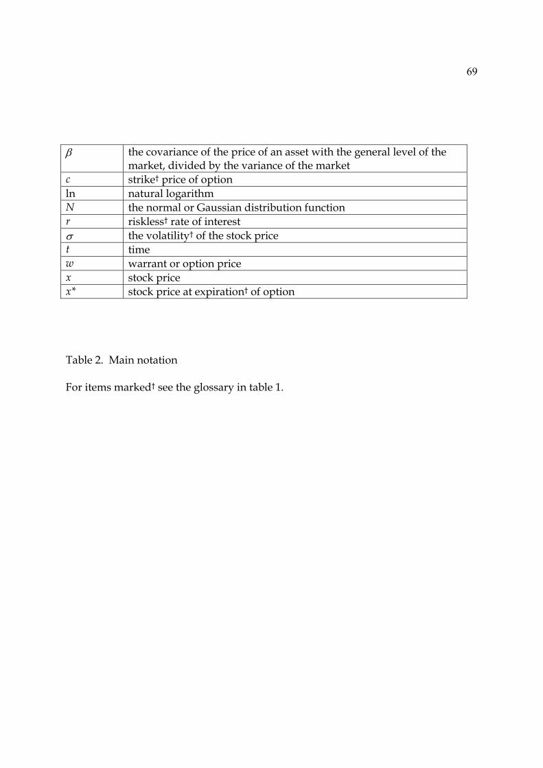
69
β the covariance of the price of an asset with the general level of the
market, divided by the variance of the market c strike† price of option ln natural logarithm N the normal or Gaussian distribution function r riskless† rate of interest σ the volatility† of the stock price t time w warrant or option price x stock price x* stock price at expiration† of option Table 2. Main notation For items marked† see the glossary in table 1.
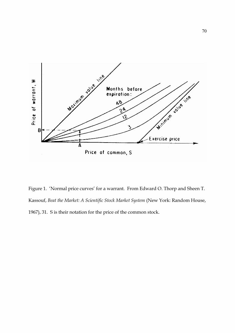
70
Figure 1. ‘Normal price curves’ for a warrant. From Edward O. Thorp and Sheen T.
Kassouf, Beat the Market: A Scientific Stock Market System (New York: Random House,
1967), 31. S is their notation for the price of the common stock.
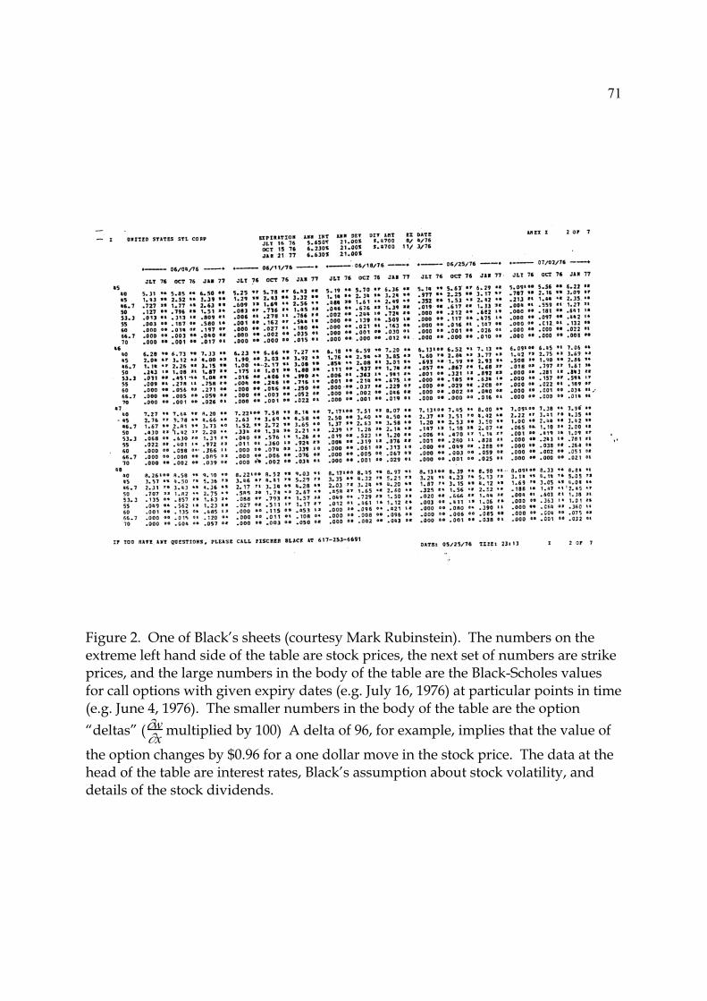
71
Figure 2. One of Black’s sheets (courtesy Mark Rubinstein). The numbers on the extreme left hand side of the table are stock prices, the next set of numbers are strike prices, and the large numbers in the body of the table are the Black-Scholes values for call options with given expiry dates (e.g. July 16, 1976) at particular points in time (e.g. June 4, 1976). The smaller numbers in the body of the table are the option “deltas” (∂w∂x multiplied by 100) A delta of 96, for example, implies that the value of
the option changes by $0.96 for a one dollar move in the stock price. The data at the head of the table are interest rates, Black’s assumption about stock volatility, and details of the stock dividends.
Related Documents


