Breakthrough in Noise Greatly reduce Figure … · IFA 2nd LO IF BPF 2nd IFA ... Pin Pout amplifier gain. Noise Figure Seminar January, 2008 Some Y-Factor Measurement Assumptions

Noise Figure Seminar

January, 2008

David Ballo

Product Marketing EngineerComponent Test Division

June, 2008

Breakthrough in Noise

Figure Measurement

Technique

Greatly reduce systematic errors

while simplifying measurement setups


January, 2008

Agenda

• Overview of Noise Figure

• Noise Figure Measurement Techniques

• Accuracy Limitations

• PNA-X’s Unique Approach

DUT

So/No

Si/Ni

Gain


January, 2008

Why Do We Care About Noise?

• Noise causes system impairments

• Degrades image quality of TV, voice quality of cell phone

• Limits range of radar systems

• Causes increased bit-error rate in digital systems

• How can we improve system signal-to-noise ratio (SNR)?

• Increase transmitter power (need larger antennas

and/or bigger, more powerful amplifiers)

• Decrease path loss (this may not be in our control)

• Lower receiver-contributed noise (LNA at front end is critical)

• Generally easier and less

expensive to decrease receiver noise than

increase transmitter powerI

Q


January, 2008

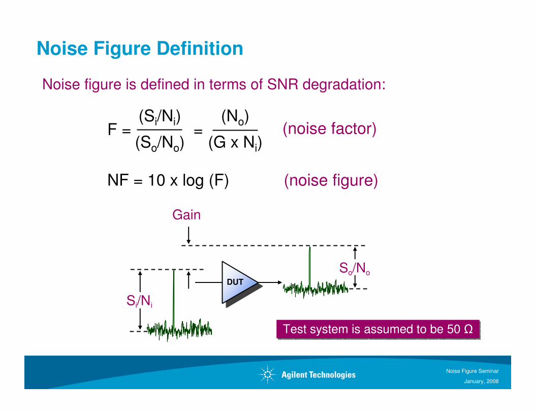
Noise Figure Definition

Noise figure is defined in terms of SNR degradation:

F =(So/No)

(Si/Ni)=

(No)

(G x Ni)(noise factor)

NF = 10 x log (F) (noise figure)

DUT

So/No

Si/Ni

Gain

Test system is assumed to be 50 ΩTest system is assumed to be 50 Ω


January, 2008

Effective Noise Temperature

• Available noise power of a passive termination = kTB

• k is Boltzmann’s constant (1.38 x 10-23 J/K)

• kTB = -174 dBm in a 1 Hz bandwidth

• For a given system bandwidth, noise is related to temperature

• Amount of noise produced by a device can be expressed as

an equivalent noise temperature (e.g., 15 dB ENR => 8880K)

• Noise factor can be expressed as effective input noise temperature

• Not the physical temperature of the input termination

• Theoretical temperature of input termination connected to a noiseless device resulting in the same output noise power

Te = 290 x (F-1)


January, 2008

Effective Temperature Versus Noise Figure

1.00

10.00

100.00

1000.00

0.0 0.5 1.0 1.5 2.0 2.5 3.0 3.5 4.0 4.5 5.0

NF (dB)

Te (

K)


January, 2008

Importance of Noise Figure Accuracy – R&D

AMPBPFCOHO

STALO Receiver

Protection

Pulse

Modulator

PRF

Generator

Frequency

Agile LO

DUPLEXORPREDRIVER

AMP

RFBPF

PULSED

POWERTx

LNA

IF

BPF

0o SPLITTER

ADC

ADC

ANTENNATRANSMITTER / EXCITER

Digital Signal

Processor

(range and Doppler FFT)

Radar Data

Processor

(tracking loops, etc.)

90oCOHO

S/H

S/H

LIMITER

LPF

LPF

BB AMP

BB AMP

LPF

MMI

RECEIVER /

SIGNAL PROCESSOR

1st

IFA

2nd LO

IF

BPF

2nd

IFA

• Many systems have transmit and receive sections

• System designer optimizes size, weight, cost, performance

• Improved measurement accuracy results in smaller guard bands

• Tighter specificationson LNA means

lower-power

transmit amplifiers

Radar example


January, 2008

Importance of Noise Figure Accuracy – Mfg

• Improved measurement accuracy results in smaller guard bands

• Smaller guard bands yields better component specifications

• Better specifications means more competitive products

• More competitive products command higher prices or attain higher

market share


January, 2008

Agilent’s Noise Figure Legacy

340A

1958

8970

1980

PSA with NF

2002

ESA with NF

2003PNA-X with NF

2007 MXA, EXA with NF

2007

8560/90 with NF

1995

85120

1999

NFA

2000

Nearly 50 years of Leadership

NEW!NEW!NEW!NEW!


January, 2008

Agenda





DUT

So/No

Si/Ni

Gain


January, 2008

Noise Figure Measurement Techniques

• Y-factor (hot/cold source)

• Used by NFA and SA-based solutions

• Uses noise source with a specified “excess noise ratio” (ENR)

• Cold source (direct noise)

• Used by vector network analyzers (VNAs)

• Uses cold (room temperature) termination only

• Allows single connection S-parameters and noise figure (and more)

+28V

Excess noise ratio (ENR) =K

TT coldhot

290

−

Diode off ⇒ Tcold

Diode on ⇒ Thot

Noise source346C 10 MHz – 26.5 GHz


January, 2008

Y-Factor Technique

Thot (on)

Tcold (off)

Pout (hot)= kBGa(Thot + Te)

Pout (cold)= kBGa(Tcold + Te)

Pout (hot)

Pout (cold)

Y =Thot – Y x Tcold

Y – 1Te =

Noise Receiver

Te

290Fsys = 1+

Calibration:

Noise Receiver

DUT

FDUT = Fsys –Frcv - 1

Ga DUT

Y-factor yields gain and noise figureY-factor yields gain and noise figure

Unknown variables


January, 2008

Graphical Representation of Y-Factor Technique

Noise Power Out

No

ise

Po

we

r In

Pout (cold) Pout (hot)

Pin (cold)

Pin (hot)

DUT

Noise added by amplifier

=∆

∆

Pin

Poutamplifier gain


January, 2008

Some Y-Factor Measurement Assumptions

Ga (available gain) is a function of S11, S22 and ΓsGa (available gain) is a function of S11, S22 and Γs

True only if S11 and S22 are <<1

Γsrc (hot) = Γsrc(cold)

Frcv = Frcv

Ga (DUT) =Po (hot-sys) – Po (cold sys)

po (hot rcv) – Po (cold rcv)

Γo (DUT) Γsrc(no noise-parameter effects of receiver)

(source match of noise source does not change)

Noise ReceiverDUTΓsrc Γo (DUT)


January, 2008

Four Examples Of Y-Factor Measurements

What you want for good NF accuracy!

Noise source

Noise source

Automated multi-instrument

(ATE) environment

On-wafer environment

On-wafer multi-instrument

(ATE) environment

1 2

3 4

Noise source Noise source


January, 2008

Cold Noise Technique

Pout= kBGa(Tcold + Te)

Pout

kToBGa

Fsys =

Noise ReceiverDUT

Calibration:

Noise Receiver

FDUT = Fsys –Frcv - 1

GDUT

Need to know available gain very accurately

(Ga is function of S11, S22 and Γs)

Need to know available gain very accurately

(Ga is function of S11, S22 and Γs)

Unknown variable


January, 2008

Graphical Representation of Cold Source Technique

Noise Power Out

No

ise

Po

we

r In

Pout (cold)

Pin (cold)

DUT

Noise added by amplifier

Known gain of amplifier


January, 2008

Agenda






January, 2008

Sources of Measurement Uncertainty

• Several contributors to measurement uncertainty

(some are small, some are large)

• Common contributors:

• Instrument uncertainty

• ENR uncertainty

• Jitter (related to bandwidth and measurement time)

• Noise-parameter effects (noise figure versus source match)

• Drift (primarily due to temperature)

• Unique contributors

• Mismatch errors (primarily Y-factor)

• S-parameter uncertainty (cold source)

• Uncertainty calculator can estimate combined effect


January, 2008

Y-Factor Uncertainty Model

Noise Receiver

DUT Noise Receiver

ENR uncertainty

Mismatch

Noise

parameters

• Jitter• Instrument uncertainty

Noise

parameters

Noise

parameters

• Jitter

• Instrument uncertainty

CalibrationCalibration

MeasurementMeasurement

Mismatch Mismatch

ENR uncertainty

DRIFT


January, 2008

Cold-Source Uncertainty Model

DUT Noise Receiver

S-parameter uncertainty

• Jitter• Dynamic accuracy

• S11 uncertainty

CalibrationCalibration

MeasurementMeasurement

Γ uncertainty

Tuner

Noise Receiver• Jitter

• Dynamic accuracy

ENR uncertainty

VNA

ECalTuner

VNA

Tuner

S-parameter uncertainty Γ uncertainty

Noise Receiver• Jitter• Dynamic accuracy

DRIFT


January, 2008

• Plots of noise figure circles versus impedance (at one frequency)

• Fmin is lowest noise figure and occurs at Γopt

• F changes with Γs

• F changes with device bias

Noise Parameters

Fmin at Γopt

Increasing noise figure

Increasing noise figure

frequency


January, 2008

Two-Port Noise Models

There are multiple ways to represent noisy two-port networks

Z

+ -

e1

+

-

+-

e2

I1

V1

I2

V2

V1 = Z11I1 + Z12I2 + e1

V2 = Z21I1 + Z22I2 + e2

Y+

-

I1

V1

I2

V2

i1 i2

I1 = Y11V1 + Y12V2 + i1

I2 = Y21V1 + Y22V2 + i2

ABCD

+ -e

+

-

I1

V1

I2

V2

iI1 = AV2 + BI2 + i

V1 = CV2 + DI2 + e

Contributes to

noise figure

Contributes

to gain

Noise sources are generally

independent, with varying

degrees of correlation

Noise sources are generally

independent, with varying

degrees of correlation


January, 2008

Noise Correlation

ABCD

+ -

e

+

-

I1

V1

I2

V2

i

e noise

i noise

Full correlation

ABCD

+ -

e

+

-

I1

V1

I2

V2

i

e noise

i noise

No correlation

If the noise sources are

correlated, some input impedance

will cause maximum cancellation

and minimum noise figure


January, 2008

Two-Port Noise Wave Model

a1

b1 a2

b2

[S]bn1

bn2

11 11 12 1

22 21 22 2

n

n

bb s s a

bb s s a

= +

2 *

1 1 2 11 12

2*21 22

2 1 2

C

= =

n n n

s

n n n

b b b cs cs

cs csb b b

Noise correlation matrix

a1

b1

b2

a2

b1n

S11 S22

S12

S21

1

1

b2n


January, 2008

Noise Correlation Matrix in Terms of Noise Parameters

( ) ( ) ( )( )

( )( )

2

2 11 11

min 11 21 min 112 2

0 0

2

211

21 min 11 21 min2 2

0 0

1 4 141 1 1

1 1

4 1 41 1

1 1

opt n opt optn

opt opt

n opt opt n opt

opt opt

s R sRF s s F s

Z Z

R s Rs F s s F

Z Z

− Γ Γ − Γ − − + − − + Γ + Γ

= Γ − Γ Γ − − − + Γ + Γ

sC


January, 2008

Noise Parameters

2

si sYn

e

ni

Noiseless two-port

( )

2

2

min min 2 20

4

1 1

Γ − Γ = + − = +

+ Γ − Γ

opt sn ns opt

s opt s

R RF F Y Y F

G Z

2

si s

YNoisy

two-port

Noise figure varies

as a function of

source impedance

Noise figure varies

as a function of

source impedance

Four noise parameters: Fmin, Rn, Γopt (mag), Γopt (phase)


January, 2008

The Problem with Measuring Noise Figure

• NFA and other analyzers measure NF in a nominal 50-ohm

environment

• Noise parameter analysis shows us that NF varies with source

impedance (Γs)

• Test systems don’t have perfect 50-ohm source impedances

• Conventional noise figure systems

introduce significant error due to

non-ideal source match

Noise source

VNA


January, 2008

Comparing Accuracy of Two Methods

• Noise parameter effect present for both methods

• Y-factor

• Noise source directly to DUT: good source match

• Noise source in ATE or probe situation: poor source match

• Cold source

• Without source correction: poor source match

• With source correction: excellent effective source match


January, 2008

Agenda





DUT

So/No

Si/Ni

Gain


January, 2008

N5242A Option 029 for Noise Figure Measurements

• Measure key amplifier parameters up

to 26.5 GHz with a single connection(e.g. S-parameters, noise figure, compression, IMD, harmonics)

• Achieve the highest measurement accuracy of any solution on the market

• Typically 4 to 10 times faster than the NFA

ECal module used as an impedance tuner to remove the effects of imperfect system source match


January, 2008

2-Port PNA-X Options 219, 224, 029

Test port 1 Test port 2

R2

35 dB

65 dB

65 dB

Rear panel

A

35 dB

B

Source 2

Output 1Source 2

Output 2

Noise receivers

10 MHz -3 GHz

3 - 26.5 GHz

DUT

Pulse generators

RF jumpers

Receivers

Mechanical switch

Source 1

OUT 2OUT 1

Pulsemodulator

LO

To

receivers

R1

OUT 1 OUT 2

Pulsemodulator

J11 J10 J9 J8 J7 J2 J1+28V


January, 2008

PNA-X’s Unique Source-Corrected Technique

(Z1, F1), (Z2, F2), …

• PNA-X varies source match around 50 ohms using an ECal module (source-pull technique)

• With resulting impedance/noise-figure pairs and vector error terms, very accurate 50-ohm noise figure (NF50) can be calculated

• Each impedance state is measured versus frequency

frequency

Z’s measured during cal

F’s measured with DUT


January, 2008

Noise Figure Uncertainty Example (ATE Setup)

2.000

2.500

3.000

3.500

4.000

4.500

0.5 2.5 4.5 6.5 8.5 10.5 12.5 14.5 16.5 18.5 20.5 22.5 24.5 26.5

GHz

NF

(d

B)

PNA-X

Y-factor with noise source connected to DUT via switch matrix

Amplifier:Gain = 15 dB

Input/output match = 10 dB

NF = 3 dBGamma opt = 0.27 ∠ 0o

Fmin = 2.7 dBRn = 12 – 33

0.2 dB

0.75 dB

0.5 dBY-factor with noise source

directly at DUT input

* Note: this example ignores drift contribution


January, 2008

Uncertainty Breakdown (ATE Setup)

PNA-X with ATE network

Y-factor with ATE network

Y-factor with noisesource connected to DUT

Uncertainty contributors

To

tal un

ce

rta

inty

EN

R u

nce

rta

inty

Mis

ma

tch

DU

T n

ois

e/

Γs

inte

raction

S-p

ara

me

ter

Jitte

r

Notes:Gain = 15 dB (4.5 GHz)NF = 3 dBInput/output match = 10 dBFmin = 2.8 dB

Gopt = 0.27+j0Rn = 37Noise source = 346C97% confidence

dB

Due to imperfect 50-ohm source match


January, 2008

Noise Figure Uncertainty Example (Wafer Setup)

PNA-X

Y-factor with noise source connected to DUT input

Y-factor with noise source connected to DUT via switch matrix


Input/output match = 10 dBNF = 3 dB

Gamma opt = 0.268 ∠ 0o

Fmin = 1.87 dBRn = 12 – 33

Wave model correlation = 50%

2.000

2.500

3.000

3.500

4.000

4.500

0.5 2.5 4.5 6.5 8.5 10.5 12.5 14.5 16.5 18.5 20.5 22.5 24.5 26.5

GHz

NF

(d

B)

PNA-X

Y-factor with noise source connected to probe input

Y-factor with noise source connected to probe via switch matrix


Input/output match = 10 dB

NF = 3 dBGamma opt = 0.27 ∠ 0o

Fmin = 2.7 dBRn = 12 – 33

0.3 dB

1.1 dB

0.75 dB

* Note: this example ignores drift contribution


January, 2008

Uncertainty Breakdown (Wafer Setup)

Tota

l U

nce

rta

inty

EN

R U

nce

rta

inty

Mis

ma

tch

No

ise P

ara

mete

rs

S-p

ara

me

ters

Jitte

r

Wave

Y-Factor0

0.2

0.4

0.6

0.8

1

1.2

1.4

1.6

1.8

97% Confidence (dB)

Uncertainty Contributor

On Wafer 15 dB amp with 3 dB Noise figure at 4.5 GHz

(Fmin = 2.8 dB, Gopt = 0.27 +j0, Rn = 37.4)

Wave

Y-Factor

PNA-X


January, 2008

Example NF Measurements

0

1

2

3

4

5

0 5 10 15 20 25

Frequency (GHz)

Noise Figure (dB) PNA-X method using source correction

Traditional Y-factor technique


January, 2008

NF Comparison in Pseudo ATE environment

DUT

12” cable

DUT

12” cable

PNA-X cal and measurement planes

Noise source (measurement) NFA

Loss comp:

4 GHz - 0.30 dB

6 GHz – 0.38 dB


January, 2008

Speed Comparison: PNA-X Versus Y-Factor

Noise Figure Speed Benchmarks

10 MHz - 26.5 GHz

0

5

10

15

20

25

30

35

40

45

11 51 101 201

Points

Seco

nd

s

NFA

PSA

EXA

PNA-X

1.4x* 4.2x* 6.8x*

10x*

* PNA-X sweep-speed improvement compared to the NFA


January, 2008

Calibration Procedure

• Calibration uses sinusoidal and noise sources, plus cold terminations

• Calibration sequence for simplest case (insertable)1. Connect noise source to port 2

– Measure hot and cold noise power

– Measure hot and cold match of noise source

2. Connect through (ports 1 and 2)

– Measure gain differences between 0, 15, 30 dB stages

– Measure load match of noise receivers

– Measure Γs values of ECal used as impedance tuner

– Measure receiver noise power with different tuner Γs values (mechanical cal only)

3. Connect calibration standards (ports 1 and 2)

– Measure normal S-parameter terms

– Measure receiver noise power with different Γs values (use ECal or mechanical standards)

• Non-insertable cases require extra steps

– additional 1-port calibration to account for adapter if noise source is non-insertable

– additional S-parameter cal steps for non-insertable DUTs


January, 2008

Calibrating On Wafer

1-port cal

2-port cal

1 2

3

Embed this section to move noise-cal

reference plane to 2-port-cal reference plane


January, 2008

Comparison Between Gain Settings

Value of attenuator

after amplifier


January, 2008

Measuring Attenuators

20 dB attenuator 40 dB attenuator


January, 2008

Summary

• Y-factor method offers reasonable accuracy

when noise source is connected directly to DUT

• Source-corrected cold-source technique:

• Offers best accuracy in all cases

• Works well in fixtured, on-wafer, and ATE environments

• Is 1.4 to 10 times faster than NFA

• PNA-X offers highest accuracyas well as speed and convenienceof single connection to DUT for a

variety of amplifier measurements

Breakthrough in Noise Greatly reduce Figure … · IFA 2nd LO IF BPF 2nd IFA ... Pin Pout amplifier gain. Noise Figure Seminar January, 2008 Some Y-Factor Measurement Assumptions

Documents