Braneworld dynamics of inflationary cosmologies with exponential potentials

arX

iv:g

r-qc

/020

4059

v1 1

8 A

pr 2

002

Braneworld Dynamics of Inflationary Cosmologies with Exponential Potentials

Naureen Goheer1 and Peter K. S. Dunsby1,2

1. Department of Mathematics and Applied Mathematics,

University of Cape Town, 7701 Rondebosch, Cape Town, South Africa and

2. South African Astronomical Observatory, Observatory 7925, Cape Town, South Africa.

In this work we consider Randall - Sundrum brane -world type scenarios, in which the spacetimeis described by a five - dimensional manifold with matter fields confined in a domain wall or three-brane. We present the results of a systematic analysis, using dynamical systems techniques, ofthe qualitative behaviour of Friedmann - Lemaıtre -Robertson - Walker type models, whose matteris described by a scalar field with an exponential potential. We construct the state spaces for thesemodels and discuss how their structure changes with respect to the general - relativistic case, inparticular, what new critical points appear and their nature and the occurrence of bifurcation.

I. INTRODUCTION

String and membrane theories are considered to bepromising candidates for a unified theory of all forcesand particles in Nature. Since a consistent constructionof a quantum string theory is only possible in more thanfour spacetime dimensions we are compelled to compact-ify any extra spatial dimensions to a finite size or, alter-natively, find a mechanism to localize matter fields andgravity in a lower dimensional submanifold.

Motivated by orbifold compactification of higher di-mensional string theories in particular the dimensionalreduction of eleven - dimensional supergravity introducedby Horava and Witten [1, 2], Randall and Sundrumshowed that for non - factorisable geometries in five di-mensions there exists a single massless bound state con-fined in a domain wall or three - brane [3]. This boundstate is the zero mode of the Kaluza - Klein dimensionalreduction and corresponds to the four - dimensional gravi-ton. This scenario may be described by a model consist-ing of a five - dimensional Anti - de Sitter space (knownas the bulk) with an embedded three - brane on whichmatter fields are confined and Newtonian gravity is effec-tively reproduced on large - scales. A discussion of earlierwork on Kaluza - Klein dimensional reduction and matterlocalization in a four - dimensional manifold of a higher -dimensional non - compact spacetime can be found in [4].

Gravity on the brane can be described by the standardEinstein equations modified by two additional terms, onequadratic in the energy - momentum tensor and the otherrepresenting the electric part of the five - dimensionalWeyl tensor.

Following an approach to the study of homogeneouscosmological models with a cosmological constant firstintroduced by by Goliath and Ellis [5] (see also [6]for a detailed discussion of the dynamical systems ap-proach to cosmology), Campus and Sopuerta have re-cently studied the complete dynamics of Friedmann -Lemaıtre - Robertson -Walker (FLRW) and the Bianchitype I and V cosmological models with a barotropic equa-tion of state, taking into account effects produced by thecorrections to the Einstein Field Equations [7].

Their analysis led to the discovery of new critical points

corresponding to the Binetruy -Deffayet - Langlois (BDL)models [8], representing the dynamics at very high en-ergies, where effects due to the extra dimension becomedominant. These solutions appear to be a generic featureof the state space of more general cosmological models.They also showed that the state space contains new bifur-cations, demonstrating how the dynamical character ofsome of the critical points changes relative to the general -relativistic case. Finally, they showed that for modelssatisfying all the ordinary energy conditions and causal-ity requirements the anisotropy is negligible near the ini-tial singularity, a result first demonstrated by Maartenset. al. [9].

In this paper we extend their work to the case wherethe matter is described by a dynamical scalar field φ withan exponential potential V (φ) = exp(bφ). This workbuilds on earlier results obtained by Burd and Barrow[10] and Haliwell [11] who considered the dynamics ofthese models in standard general relativity (GR). Vanden Hoogen et. al. and Copeland et. al. have alsoconsidered the GR dynamics of exponential potentialsin the context of Scaling Solutions in FLRW spacetimescontaining an additional barotropic perfect fluid [12, 13].

It is worth mentioning that Exponential potentials aresomewhat more interesting in the brane - world scenario,since the high - energy corrections to the Friedmann equa-tion allow for inflation to take place with potentials or-dinarily too steep to sustain inflation [14].

II. PRELIMINARIES

In what follows we summarise the geometric frameworkused analyse the brane - world scenario in the cosmologi-cal context.

A. Basic equations of the brane - world

In Randall - Sundrum brane - world type scenarios mat-ter fields are confined in a three - brane embedded in afive - dimensional spacetime (bulk). It is assumed that

the metric of this spacetime, g(5)AB, obeys the Einstein

2

equations with a negative cosmological constant Λ(5)

[15, 16, 17])

G(5)AB = −Λ(5)g

(5)AB + κ2

(5)δ(χ) [−λ gAB + TAB] , (1)

where G(5)AB is the Einstein tensor, κ(5) denotes the five -

dimensional gravitational coupling constant and TAB

represents the energy - momentum tensor of the matterwith the Dirac delta function reflecting the fact that mat-ter is confined to the spacelike hypersurface x4 ≡ χ = 0(the brane) with induced metric gAB and tension λ.

Using the Gauss - Codacci equations, the Israel junc-tion conditions and the Z2 symmetry with respect to thebrane the effective Einstein equations on the brane are

Gab = −Λgab + κ2Tab + κ4(5)Sab − Eab , (2)

where Gab is the Einstein tensor of the induced metricgab. The four - dimensional gravitational constant κ andthe cosmological constant Λ can be expressed in termsof the fundamental constants in the bulk (κ(5), Λ(5)) andthe brane tension λ [21].

As mentioned in the introduction, there are two cor-rections to the general - relativistic equations. Firstly Sab

represent corrections quadratic in the matter variablesdue to the form of the Gauss - Codacci equations:

Sab = 112TTab − 1

4TacTbc + 1

24gab

[

3T cdTcd − T 2]

. (3)

Secondly Eab, corresponds to the “electric” part of the

five - dimensional Weyl tensor C(5)ABCD with respect to the

normals, nA (nAnA = 1), to the hypersurface χ = 0, thatis

EAB = C(5)ACBDnCnD , (4)

representing the non - local effects from the free gravita-tional field in the bulk. The modified Einstein equations(2) together with the conservation of energy -momentumequations ∇aTab = 0 lead to a constraint on Sab and Eab:

∇a(Eab − κ4(5)Sab) = 0 . (5)

We can decompose Eab into its ineducable parts relativeto any timelike observers with 4 - velocity ua (uaua =−1):

Eab = −(

κ(5)

κ

)4[

(uaub + 13hab)U + 2u(aQb) + Pab

]

,

(6)where

Qaua = 0 , P(ab) = Pab , Paa = 0 , Pabu

b = 0 . (7)

Here U has the same form as the energy -momentum ten-sor of a radiation perfect fluid and for this reason is re-ferred to as the “dark” energy density of the Weyl fluid.Qa is a spatial and Pab is a spatial, symmetric and trace -free tensor. Qa and Pab are analogous to the usual energyflux vector qa and anisotropic stress tensor πab in General

Relativity. The constraint equation (5) leads to evolutionequations for U and Qa, but not for Pab (see [17]).

The above equations correspond to the general situa-tion. In what follows we restrict our analysis to the casewhere Eab = 0 so the brane is conformally flat. Suchbulk spacetimes admit FLRW brane -world models withvanishing non - local energy density (U = 0).

B. Scalar field dynamics on the brane

Relative to a normal congruence of curves with tangentvector

ua = −∇aφ

φ, uaua = −1 , (8)

the energy - momentum tensor Tµν for a scalar field takesthe form of a perfect fluid (See page 17 in [18] for details):

Tµν = ρuµuν + phµν , (9)

with

ρ =1

2φ2 + V (φ) (10)

and

p =1

2φ2 − V (φ) . (11)

where φ is the momentum density of the scalar field andV (φ) is its potential energy. If the scalar field is notminimally coupled this simple representation is no longervalid, but it is still possible to have an imperfect fluidform for the energy -momentum tensor [19].

Substituting for ρ and p from (10) and (11) into theenergy conservation equation

ρ + Θ(ρ + p) = 0 , (12)

leads to the 1+3 form of the Klein -Gordon equation

φ + Θφ + V ′(φ) = 0 , (13)

an exact ordinary differential equation for φ once thepotential has been specified. It is convenient to relate pand ρ by the index γ defined by

p = (γ − 1)ρ ⇔ γ =p + ρ

ρ=

φ2

ρ. (14)

This index would be constant in the case of a simple one -component fluid, but in general will vary with time in thecase of a scalar field:

γ = Θγ(γ − 2) − 2γV ′

φ. (15)

Notice that this equation is well-defined even for φ → 0,

since γ

φ= φ

ρ .

3

The dynamics of FLRW models imposed by the modi-fied Einstein equations are governed by the Raychaudhuriand Friedmann equations

H = −H2 − 3γ − 2

6κ2ρ

[

1 +3γ − 1

3γ − 2

ρ

λ

]

, (16)

H2 =1

3κ2ρ

(

1 +ρ

2λ

)

− 1

63R , (17)

together with the Klein Gordon equation (13) above. 3Rdenotes the scalar curvature of the hypersurfaces orthog-onal to the the fluid 4 - velocity (8) and can be expressedin terms of the scale factor via 3R = 6k

a2 where as usualk = 0,±1 determines whether the model is flat, open orclosed.

III. DYNAMICAL SYSTEMS ANALYSIS FOR

EXPONENTIAL POTENTIALS

In the following analysis we extend recent work pre-sented by Campus and Sopuerta [7] to the case where thematter is described by a dynamical scalar field φ with aself - interacting potential V (φ) = exp(bφ), where b ≤ 0and consider only models which have negligible non - localenergy density U and cosmological constant Λ. Althoughthe full dynamics are described by the equations pre-sented in the previous section, it is useful to re - writethese equations in terms of a set of dimensionless expan-sion normalized variables. In order to get compact statespaces it is convenient to consider two different cases (i)3R ≤ 0 (k = 0 or k = −1) and (ii) 3R ≥ 0 (k = 0 ork = 1). In case (i) the appropriate variables are

Ωρ ≡ κ2ρ

3H2, Ωk ≡ −

3R

6H2= − k

a2, Ωλ ≡ κ2ρ2

6λH2, (18)

leading via equation (17) to very simple expression of theFriedmann constraint:

Ωρ + Ωk + Ωλ = 1 . (19)

We introduce a dimensionless time variable by

′ ≡ 1

|H |d

dt, (20)

where |H | is the absolute value of H . It follows that

H ′ = −ǫ(1 + q)H , (21)

where ǫ is the sign of H and q is the usual decelerationparameter defined by

q = − 1

H2

a

a. (22)

It is clear that ǫ = 1 corresponds to models which areexpanding while ǫ = −1 correspond to models which arecontracting.

Using the above definitions, the dynamics for open andflat models are described by the following system of equa-tions

Ω′

k = ǫ[(3γ − 2)(1 − Ωk) + 3γΩλ]Ωk , (23)

Ω′

λ = ǫ[3γ(Ωλ − Ωk − 1) + 2Ωk]Ωλ .

In case (ii) it is necessary to normalise using

D ≡√

H2 + 163R (24)

instead of the Hubble function H , so the dimensionlessvariables for this case are given by

Q ≡ H

D, Ωρ ≡ κ2ρ

3D2Ωλ ≡ κ2ρ2

6λD2(25)

and the Friedmann constraint is

Ωρ + Ωλ = 1 . (26)

The appropriate dimensionless time derivative is definedvia

′ ≡ 1

D

d

dt(27)

so the dynamical equations for closed models become

Q′ = [1 − 3

2γ(1 + Ωλ)](1 − Q2) , (28)

Ω′

λ = 3γQ(Ωλ − 1)Ωλ .

Notice that in (23), (28) we have already included theconstraint (19), (26) in order to keep the dimensionalityof the state space as low as possible. The evolution of Ωρ,

Ωρ can easily be recovered from the Friedmann equation.We have to add a third equation to (23), (28) respec-

tively in order to describe the dynamics of the scalar fieldφ. It turns out, that the equation of state parameter γinstead of φ, is a the preferred coordinate, since it is bothbounded by causality requirements (0 ≤ γ ≤ 2) and isdimensionless.

For open models (case (i)), we find using (15) that theevolution of γ is determined by

γ′ = ǫ√

3γ(γ − 2)[√

3γ + ǫ sgn(φ)b√

1 − Ωk − Ωλ] (29)

where sgn(φ) is the sign of φ. We can see from (29) that

we only need to consider the case φ ≥ 0, since the caseφ ≤ 0 can be recovered from the former by time reversal;simultaneously changing the sign of φ and H results inan overall change of sign of γ′. From (23), we see thatthis transformation also changes the sign of Ω′

k and Ω′

λ,

which means that φ → −φ corresponds to time reversalτ → −τ .

In the closed case, we find that

γ′ =√

3γ(γ − 2)[√

3γQ + sgn(φ)b

√

1 − Ωλ] (30)

4

and again we can easily see from (30) and (28) that φ →−φ corresponds to time reversal τ → −τ . Therefore inthe following analysis we restrict ourselves to the caseφ ≥ 0.

So in summary, the resulting dynamical equations wehave to analyse are

γ′ = ǫ√

3γ(γ − 2)[√

3γ + ǫ b√

1 − Ωk − Ωλ] , (31)

Ω′

k = ǫ[(3γ − 2)(1 − Ωk) + 3γΩλ]Ωk ,

Ω′

λ = ǫ[3γ(Ωλ − Ωk − 1) + 2Ωk]Ωλ

for the open case and

γ′ =√

3γ(γ − 2)[√

3γQ + b

√

1 − Ωλ] , (32)

Q′ = [1 − 3

2γ(1 + Ωλ)](1 − Q2) ,

Ω′

λ = 3γQ(Ωλ − 1)Ωλ

for the closed case.Notice that in the open sector, the cosmological con-

stant - like subset γ = 0, the stiff -matter - subset γ = 2,the flat subset Ωk = 0, the GR subset Ωλ = 0 and thevacuum subset Ωk + Ωλ = 1 are invariant sets. Analo-gously, the closed sector has the invariant sets γ = 0, 2,the flat subset Q = ±1, the GR subset Ωλ = 0 and thevacuum subset Ωλ = 1.

IV. ANALYSIS OF THE DYNAMICAL SYSTEM

In order to analyse the dynamical systems (31) and(32), we will use for the most part the standard methodof linearising the dynamical equations around any equi-librium points. One can easily see that because of theγ′ - equation, the linearisation matrix (the Jacobian), isnot well - defined for certain values of (γ, Ωk, Ωλ) if b 6= 0.Indeed, if b 6= 0 and γ = 0 or b 6= 0 and Ωk + Ωλ = 1(Ωλ = 1), the Jacobian diverges. This means that wecannot linearise the dynamical equations in the neigh-bourhood of these points. Instead, we will have to con-sider the full non - linear equations and study the be-haviour of small perturbations away from these problem-atic equilibrium points.

Furthermore the fact that we are dealing with a non -linear system is also important in cases, where the dy-namical equations can be linearised. Whenever the linearterms are not dominant, the peculiar behaviour of non -linear systems becomes visible. We then have to analysethe dynamical equations with additional caution. If forexample an eigenvalue of the linearised system vanishesat an equilibrium point, which means that the first or-der terms of the dynamical equation vanishes, we have tostudy the higher order terms in a perturbative analysisaround that point.

Notice that the dynamical systems (31) and (32) matchat the k = 0 plane (the flat subspace). If we analysecritical points that lie in the flat subspace by studying

small perturbations out of that surface, i.e. where (31)differs from (32), it is necessary to do the analysis inboth coordinate systems and check, whether the resultsagree. If they don’t, this means that small perturbationsaround the critical point will evolve differently, depend-ing on whether they enter the closed or the open sector.In our analysis we have checked this carefully. In only

one case (F2/3+ ) the higher order terms were dominant

and of different sign, depending on which sector was en-tered. This will be commented on below. In all the othercases, the behaviour of the perturbations did not dependon the sector they entered [22].

A. Models with Non - positive Spatial Curvature

The dynamical system (31) has 5 hyperbolic critical

points corresponding to the flat FLRW universe Fb2/3+

with γ = b2

3 and a(t) = t2/b2 [23]; the flat FLRW uni-

verse F 2ǫ with stiff matter and a(t) = t1/3; the Milne

universe M2ǫ with stiff matter and a(t) = t; a flat non -

general - relativistic model m2ǫ with γ = 2, which has been

discussed in [7]; and a set of universe models X2/3+ (b) with

γ = 2/3 and curvature Ωk = 1 − 2/b2 depending on thevalue of b. The critical points, their coordinates in statespace and their eigenvalues is given in Table I below. InTable II we give the corresponding eigenvectors. Notice

that Fb2/3+ only occurs for 0 ≤ b2 ≤ 6, and X

2/3+ (b) for

b2 ≥ 2 only. Both only occur in the expanding sectorǫ = 1.

We further find the non - hyperbolic critical points M0ǫ

and m0ǫ(Ωλ), where the former describes the Milne uni-

verse with γ = 0 and the latter is a line of non - general -relativistic critical points with γ = 0 including the flatFLRW model with constant energy density. The Ja-cobian of the dynamical system (31) at both M0

ǫ andm0

ǫ(Ωλ) diverges for b 6= 0, which means that the dy-namical system cannot be linearised around these pointsfor arbitrary positive values of b2.

For b = 0, the Jacobian is well - defined for bothM0

ǫ and m0ǫ(Ωλ), and the eigenvalues and correspond-

ing eigenvectors are given in Tables I, II. For Ωλ 6= 1, theJacobian around m0

ǫ(Ωλ) can still be evaluated even forb 6= 0. The results from taking the limits γ, Ωk → 0 areincluded in Table I.

If Ωλ = 1 and b2 > 0, we have to look at thenon - linear system (31) and study small perturbationsx(τ), y(τ), z(τ) about the equilibrium point m0

ǫ(Ωλ = 1).That means we evaluate (31) at (γ, Ωk, Ωλ) = (x, y, 1−z),where 0 < x(τ), y(τ), z(τ) ≪ 1.

Up to first order, (31) becomes

x′ = −6ǫx − 2√

3b√

x√

z − y) ,

y′ = −2ǫy ,

z′ = −2ǫy .

5

TABLE I: This table gives the coordinates and eigenvalues of the critical points with non - positive spatial curvature. We have

defined ψ =√

8b2

− 3.

Model Coordinates Eigenvalues

m0ǫ(Ωλ 6= 1) for b = 0 (0, 0,Ωλ) −2ǫ(3, 1, 0)

m0ǫ(Ωλ 6= 1) for b 6= 0 (0, 0,Ωλ) (∞,−2ǫ, 0)

F2ǫ (2, 0, 0) (6ǫ+

√6b, 4ǫ,−6ǫ)

M2ǫ (2, 1, 0) 2ǫ(3,−2,−5)

m2ǫ (2, 0, 1) 2ǫ(3, 5, 3)

Fb2/3+ ( b2

3, 0, 0) ( b2

2− 3, b2 − 2,−b2)

X2/3+ (b) ( 2

3, 1 − 2

b2, 0) (−1 − ψ,−1 + ψ,−2)

For y = z or b = 0, this can be solved to give

x = x0e−6ǫτ ,

y = y0e−2ǫτ ,

z = z0 + y0e−2ǫτ .

For y 6= z and b 6= 0, we find

x = 3b2z0(τ − τ0)2 ,

y = y0e−2ǫτ ,

z = z0 + y0e−2ǫτ ,

where x0, y0 and z0 are positive constants of integration(initial values).

This demonstrates, that for b 6= 0, m0+(Ωλ = 1) is

an unstable saddle point (to be precise, it is a line ofsaddles, since z is stationary), whereas the contractingmodel m0

−(Ωλ = 1) remains a source (actually a line ofsources) for all b.

In the same way, we analyse the nature of thepoint M0

ǫ . Here, we find that the perturbed system(γ, Ωk, Ωλ) = (x, 1 − y, z) becomes up to first order

x′ = −6ǫx − 2√

3b√

x√

y − z ,

y′ = 2ǫy ,

z′ = 2ǫz .

If z = y or b = 0, this can be solved to give

x = x0e−6ǫτ ,

y = y0e2ǫτ ,

z = z0e2ǫτ ,

where of course y0 = z0 in the case y = z.For z 6= y and b 6= 0, the perturbations behave like

x = 3b2(y0 − z0)(ǫeǫτ + const)2 ,

y = y0e2ǫτ ,

z = z0e2ǫτ .

Notice that the Friedmann constraint (19) translatesinto 0 ≤ y − z ≤ 1, therefore in particular y0 − z0 ≥ 0.

Since we are looking at small perturbations 0 < x(τ) ≪1, we conclude that the constant of integration is positive

for ǫ = −1, whereas const < 0 for ǫ = 1. This shows, thatM0

ǫ is a saddle for all values of b. It should be realisedthat for b 6= 0, the dynamics around the expanding modelM0

+ are reflecting the non - linearity of the system: x isdecreasing until eτ = −const, but then the system isrepelled since x increases for −const < eτ < ∞.

Table III below summarizes the dynamical character ofthe critical points with non - positive spatial curvature.

Note that if one of the eigenvalues in Table I vanishes,this just means that the lowest order terms vanish. Thisis very different to what happens in the case of systems oflinear differential equations, where vanishing eigenvaluesindicate lines of critical points. For a non - linear systemto contain a line of critical points, we need small per-turbations away from the critical point to be stationaryin one direction. We found an example of that case inthe analysis of m0

ǫ (Ωλ) above. Since we are dealing witha non - linear system here, vanishing eigenvalues only in-dicate that it is not sufficient to look at the linearisedequations, i.e. to study the eigenvalues and eigenvectorsof the Jacobian. Instead, we carried out a perturbativeanalysis of the kind that we have presented above whenanalyzing M0

ǫ and m0ǫ(Ωλ). Including the higher order

contributions, we obtained the results presented in Ta-bles III and VI.

B. Models with Positive Spatial Curvature

We now analyse the dynamical system (32), which de-scribes flat or closed models. In addition to the criti-cal points corresponding to the flat models F

b2/3+ , F 2

ǫ ,

m0ǫ(Ωλ) and m2

ǫ , we find a maximally non - general -relativistic Einstein universe - like model E1/3 with γ =1/3, k = 1 and H = 0, which for b = 0 degenerates into a

line (hyperbola) of critical points E(Ωλ) with γ ∈ [13 , 23 ].

For 0 ≤ b2 ≤ 2, we also find the model X2/3+ (b), which

has γ = 2/3 and Q = ∓b/√

2. A summary of all thesecritical points, their coordinates in state space and theireigenvalues can be found in Table IV below. The corre-sponding eigenvectors are given in Table V.

In order to analyse the nature of m0ǫ (Ωλ), we have to

study the first order perturbations around the point, asshown in detail in the previous section. We find here, that

6

TABLE II: Eigenvalues and eigenvectors of the critical points with non-positive spatial curvature 3R ≤ 0. We have defined

ψ =√

8b2

− 3. Notice that the first eigenvector of second row is (−6ǫ−√

3b√

1−Ωλ

γ, 0, 3ǫΩλ(Ωλ − 1)) −→ (1, 0, 0) as γ → 0 for

Ωλ 6= 1.

Model Eigenvalues Eigenvectorsm0

ǫ(Ωλ 6= 1) for b = 0 ǫ(−6,−2, 0) (2, 0,Ωλ(1 − Ωλ)), (0, 1,−Ωλ), (0, 0, 1)m0

ǫ(Ωλ 6= 1) for b 6= 0 (∞,−2ǫ, 0) (1, 0, 0), (0,−1,Ωλ), (0, 0, 1)

F2ǫ (6ǫ +

√6b, 4ǫ,−6ǫ) (1, 0, 0), (0, 1, 0), (0, 0, 1)

m2ǫ 2ǫ(3, 5, 3) (1, 0, 0), (0, 1,−1), (0, 0, 1) a

M2ǫ 2ǫ(3,−2,−5) (1, 0, 0), (0, 1, 0), (0, 1,−1)

Fb2/3+ ( b2

2− 3, b2 − 2,−b2) (1, 0, 0), ( b2

2( b2

3− 2), b2

2+ 1, 0), (b2(1 − b2

6), 0, 3( b2

2− 1))

X2/3+ (b) (−1 − ψ,−1 + ψ,−2) (− 2

3b2, 1 − ψ, 0), (− 2

3b2, 1 + ψ, 0), (−2, 3(1 − 2

b2),−3(1 − 2

b2))

aWe can use any two linearly independent vectors in the Ωk = 0-

plane as first and third eigenvectors; we have chosen the ones above

for convenience.

the behaviour of the perturbed system agrees to leadingorder with the results obtained in section IVA.

Notice that the Jacobian of the dynamical systemaround the equilibrium point corresponding to the staticmodel E1/3 is not well - defined for b 6= 0 however wecan extract the eigenvalues using a limiting procedure.The results are given in Table IV. Since the third eigen-value vanishes, it is not sufficient to analyse the linearisedequations at that point, unless we remain in the invari-ant subset Ωλ = 1, in which E1/3 appears as a saddlewith the two eigenvectors given in Table V. A study ofthe full perturbed equations around E1/3 confirms, thatthis point is a saddle however it has a more complicatedbehaviour out of the Ωλ - plane; to second order, the sys-tem will be repelled in the Ωλ - direction in the expandingsector (Q ≥ 0) , while in the collapsing sector (Q ≤ 0),it is attracted in that direction.

The dynamical character of all the critical points withnon - negative spatial curvature is summarized in TableVI.

V. THE STRUCTURE OF THE STATE SPACE

With the information we have obtained in the lastsection about the equilibrium points of the dynamicalsystem, we can now analyse the structure of the statespace. The whole state space is obtained by matchingthe dynamical systems (31) and (32). It consists of threepieces corresponding to the collapsing open models, theclosed models and the expanding open models, matchedtogether at the corresponding flat boundaries.

As mentioned above, the state space has the invariantsubsets γ = 0, 2; Ωk = 0 ⇔ Q = ±1; Ωλ, Ωλ = 0 andΩk + Ωλ, Ωλ = 1.

The bottom planes in Figures 1 - 9 correspond to GR,while top planes represent the vacuum boundaries.

Since the eigenvalues of the equilibrium points in gen-eral depend on the parameter b, the nature of these criti-cal points varies with b. Furthermore, some of the critical

points (Fb2/3+ , X

2/3+ ) will also move in state space as b2

increases, since their coordinates are also functions of b.We also find critical points, which only appear for b = 0and then disappear, as we increase b2.

For certain values of b, some of the eigenvalues passthrough zero. At these values of b, the state space is“torn” in that it undergoes topological changes. In con-trast to the model that [7] analysed, the appearance ofsuch bifurcations in our model does not coincide with theappearance of lines of critical points. This a consequenceof the fact, that in our inflationary model, the criticalpoints are moving in state space. Bifurcations appear,when two of the equilibrium points merge, which occursat b2 = 0, 2, 6. These are the same parameter values asin GR [10, 11]. This was to be expected, since the onlypoints moving in state space and causing these bifurca-tions, are the ones corresponding to the general relativis-

tic models Fb2/3+ , X

2/3+ . For this reason the occurrence of

bifurcations is restricted to the GR - subspace. Thereforethe dynamics of these bifurcations will only be discussedin section VA.

Since the collapsing open sector remains unchangedwith varying parameter value b, we do not include thatsector in the different portraits of state space. The wholestate space can be obtained by matching Fig. 1 to Fig.2 - Fig. 9.

A. The GR - subspace

As discussed above, the subset Ωλ, Ωλ = 0 is the in-variant submanifold of the full state space correspond-ing to GR. In this section, we will discuss the stabilityof the general relativistic equilibrium points within theGR - subspace. In the next section, we will discuss thebrane -world - modifications of these general relativisticresults due to the additional degrees of freedom Ωλ, Ωλ,and also the additional non - general relativistic equilib-rium points.

It is worth mentioning that although the GR -

7

TABLE III: Dynamical character of the critical points with non - positive spatial curvature.

Model b = 0 0 < b2 < 2 b2 = 2 2 < b2 < 83

b2 = 83

83< b2 < 6 b2 = 6 b2 > 6

m0+(Ωλ) line of sinks line of saddles line of saddles line of saddles line of saddles line of saddles line of saddles line of saddles

m0−

(Ωλ) line of sources line of sources line of sources line of sources line of sources line of sources line of sources line of sourcesM0

ǫ saddle saddle saddle saddle saddle saddle saddle saddleM2

ǫ saddle saddle saddle saddle saddle saddle saddle saddleF2

+ saddle saddle saddle saddle saddle saddle saddle saddleF2

−saddle saddle saddle saddle saddle saddle saddle saddle

m2+ source source source source source source source source

m2−

sink sink sink sink sink sink sink sink

Fb2/3+ line of sinks sink saddle a saddle saddle saddle saddle -

X2/3+ (b) − - saddle a sink sink spiral sink spiral sink spiral sink

aNotice that this point is an attractor for all open or flat models,

while it is a repeller for all closed models.

submanifold has been discussed in detail by Burd andBarrow [10] and Halliwell [11], their analysis is some-what incomplete, since the state space they consideredwas non - compact. The variables they chose to describethe inflationary dynamics of homogeneous isotropic mod-els were φ′, α′. Here α relates to the scale factor a(τ) bya(τ) = eα(τ), and the potential has been absorbed intothe time derivative by rescaling the time variable t → τby d

dτ = ′ = V −1/2 ddt . We find that these coordinates

relate to our expansion normalized variables via the fol-lowing transformations:

(α′)2 =2

3

1

(2 − γ)(1 − Ωk),

(φ′)2 =2γ

2 − γ,

for γ 6= 2, Ωk 6= 1. We can see that

α′ → ∞ ⇔ Ωk → 1 ⇔ Ωρ → 0 (33)

and

φ′ → ∞ ⇔ γ → 2 . (34)

This means, that we have compactified the state spaceby mapping φ′ ∈ [0,∞] −→ γ ∈ [0, 2] and α′ ∈ [0,∞] −→Ωk ∈ [0, 1]. In this way we have extended the work thathas been done on inflationary models with exponentialpotentials in the general relativistic context. We find

that X2/3+ , F

b2/3+ correspond to the critical points I, II in

[10]. In addition, we obtain the new critical points F 2ǫ ,

M0ǫ and M2

ǫ corresponding to a FLRW universe with stiffmatter and a Milne universe with γ = 0 or stiff matterγ = 2 respectively.

Notice that we also find the new equilibrium point F 0ǫ .

The reason is that we are using γ to describe the dynam-ics of the scalar field φ, which essentially is a functionof φ2 instead of φ. Therefore our γ - equation is homo-geneous in φ, whereas the dynamical equation for φ isinhomogeneous in φ.

It might seem surprising, that we find a critical pointat φ = 0, whereas there is no equilibrium point at φ = 0

in [10]. The reason for this is, that we are describing dif-ferent physical quantities; although the equation of statedoes not change as φ → 0 (γ = 0), φ does change as

φ → 0 , (φ, φ′′ 6= 0).

The collapsing FLRW model with stiff matter found inthis analysis is of particular interest, since for all valuesof b, F 2

− is the future attractor for all collapsing open andsome of the closed models within the GR - subspace. F 0

−

is the past attractor for the whole collapsing open andparts of the closed sector for all b.

Notice that the dynamics of the collapsing open sectordoes not depend on the parameter value b. The dynam-ics of this sector is constrained by the fact, that for allmodels in this sector, the flat FLRW model with constantenergy density is the past attractor, and the flat FLRWmodel with stiff matter is the future attractor (see FIG1).

Having said that, we will now discuss the more com-plicated dynamics of the closed and the expanding openmodels for the different ranges of the parameter value b.

At b = 0, we find a bifurcation of the state space,since for this value of b, the equilibrium points E1/3 and

X2/3+ (b), as well as F 0

+ and Fb2/3+ coincide. All expanding

open models are attracted to F 0+. All closed models will

evolve into either F 2− or F 0

+, depending on the initialconditions. At γ = 2/3, the Einstein universe appears asan unstable saddle point (see FIG 2).

As b2 increases, the Einstein universe disappears. In-

stead, we find the saddle point X2/3+ (b), which moves in

Q - direction as b2 is increases, remaining a saddle until itreaches the flat sector Q = 1 at b2 = 2. There it merges

with expanding FLRW model Fb2/3+ . For 0 < b2 < 2,

Fb2/3+ is a sink moving along the γ - axis. All open and

some of the closed models are attracted to this solution(see FIG 3).

At b2 = 2, the models X2/3+ (b) and F

b2/3+ merge, which

causes a bifurcation of the state space. The nature of thetwo merging critical points is significantly changed at this

value of b. The flat solution X2/3+ (b = −

√2) = F

2/3+ is

8

TABLE IV: Coordinates and eigenvalues of the critical points with non - negative spatial curvature. We have defined χ =√

8−3b2

2, φ =

√

Ω2λ + 3Ωλ + 1

Model Coordinates Eigenvalues

mǫ(Ωλ 6= 1) for b = 0 (0, 1, Ωλ) −2ǫ(3, 1, 0)

m0ǫ(Ωλ 6= 1) for b 6= 0 (0, 1, Ωλ) (∞,−2ǫ, 0)

F2ǫ (2, ǫ, 0) (6ǫ +

√6b, 4ǫ,−6ǫ)

m2ǫ (2, ǫ, 1) 2ǫ(3, 5, 3)

Fb2/3+ ( b2

3, 1, 0) ( b2

2− 3, b2 − 2,−b2)

X2/3+ (b) ( 2

3,− b

√

2, 0) ( b

√

2− χ, b

√

2+ χ,

√2b)

E1/3 ( 13, 0, 1) (

√5,−

√5, 0)

E(Ωλ) for b = 0 ( 2

3(1+Ωλ), 0, Ωλ) ( 2

1+Ωλ

φ,− 2

1+Ωλ

φ, 0)

an attractor for all open or flat models, but a repeller forall closed models (see FIG 4). This behaviour has beenobserved by [10]. At this value of b2, the two merging

critical points swap their nature: for all b2 ≥ 2, X2/3+ (b)

will be a sink, while Fb2/3+ will be a saddle (see FIGS

5 - 9).

As b is further increased (2 < b2 < 6), Fb2/3+ moves

further along the γ - axis. It is now a saddle for all mod-els. All flat models are attracted, whereas all open or

closed models are repelled. X2/3+ (b) has now entered the

open sector and moves further to the Ωk = 1 boundary.

X2/3+ (b) is a node sink for all 2 < b2 < 8/3 and a spiral

sink for 8/3 < b2 < ∞. For all b2 ≥ 2, F 2− is the future

attractor for all closed models and X2/3+ (b) the future

attractor for all expanding open models (see FIGS 5 - 7).

At b2 = 6, we find another bifurcation of the state

space. The two points Fb2/3+ and F 2

+ merge. This turnsF 2

+ from a source into a saddle (see FIG. 8). For b2 ≥ 6,all open or closed models are still repelled from F 2

+, butall flat models are now attracted. In the limit b2 → ∞,

the future attractor for the open sector, X2/3+ (b) ap-

proaches the vacuum solution Ωρ → 0 with γ = 2/3 (seeFIG 9).

B. Higher dimensional effects

The question we will now discuss is how the behaviourof the dynamical system describing GR is changed withinthe brane - world context. In particular, do the additionaldegree of freedom Ωλ, Ωλ change the stability of the gen-eral relativistic models, and are there new non - generalrelativistic stable equilibrium points?

We will first answer the second question. In additionto the general relativistic points, we have found the non -general - relativistic equilibrium points m2

ǫ and the linesm0

ǫ(Ωλ). We can solve the Friedmann equation at thesepoints to determine their behaviour in detail. At m0

ǫ , theenergy density is constant ρ(t) = ρ0, and we can easily

integrate the Friedmann equation to find

a(t) ∼ eǫ√

Λ/3 t , (35)

where Λ = κ2ρ0(1 + ρ0

2λ ) behaves like a modified cosmo-logical constant.

For m2+, the scale factor is given by

a(t) = (t − tBB)1/6(t + tBB)1/6 . (36)

where tBB = 1/√

6κ2λ is the Big Bang time. Asexplained in detail in [7], this model corresponds tothe Binetruy - Deffayet - Langlois (BDL) solution [8] withscale factor a(t) = (t − tBB)1/6. The solution for m2

− isgiven by time reversal and tBB should now be identifiedas the Big Crunch time.

At b = 0, we also observe, that the general - relativisticEinstein universe has non - general - relativistic ana-logues. We find a whole line of Einstein universe - likestatic equilibrium points E(Ωλ) extending in the Ωλ di-rection. For b2 > 0, the line collapses to the non -general - relativistic Einstein saddle E1/3 in the Ωλ = 1

subset, and the general relativistic model X2/3+ (b).

We now study the dynamical character of these non -general - relativistic equilibrium points. We find that inthe full state space, m2

− instead of F 2− is the future at-

tractor for all collapsing open models and some of theclosed models. This means, that within the brane -worldcontext, FLRW with stiff matter changes from a stablesolution into a unstable saddle. F 0

− remains a past at-tractor for the collapsing open and parts of the closedsector, but now there is a whole line m0

−(Ωλ) of sources

extending in Ωλ direction. The same applies to the cor-responding expanding models: the sink/saddle F 0

+ is aone - element subset of the line of sinks/saddles m0

+(Ωλ).This means, that for b = 0, the future attractor of theexpanding open and some of the closed models is notnecessarily F 0

+, but instead any of the points m0+(Ωλ)

depending on the initial conditions. For b2 > 0, m0+(Ωλ)

including F 0+ turns into a line of saddles.

For b > 0 the models m0+(Ωλ) represent high energy

inflationary models with exponential potentials (whichare too steep to inflate in GR) [13]. The fact that they

9

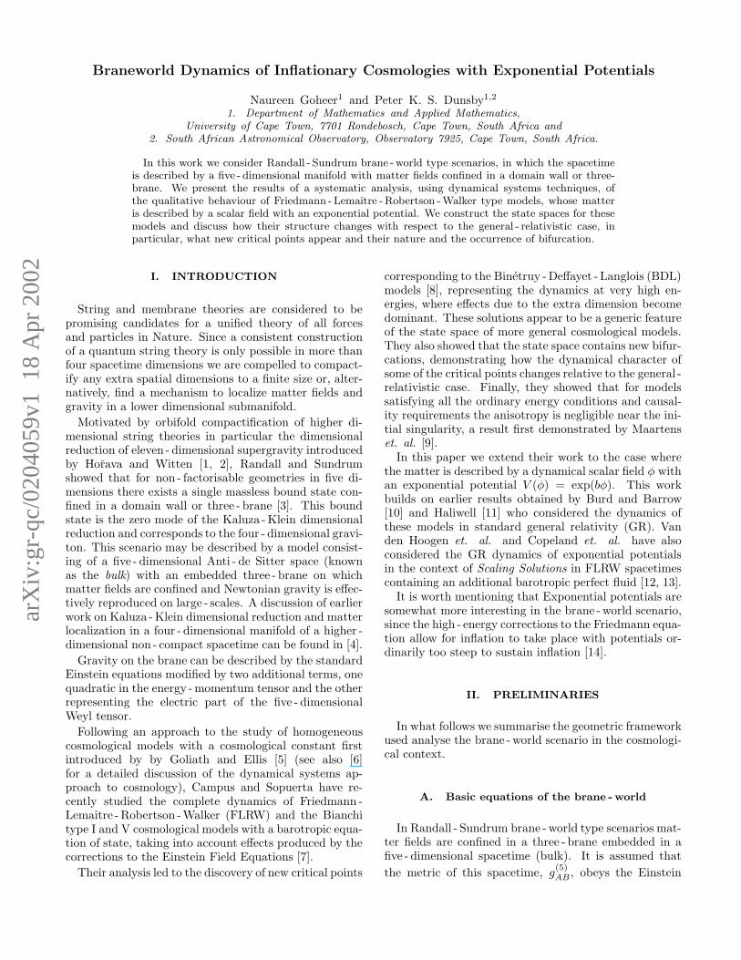
TABLE V: Eigenvalues and eigenvectors of the critical points with non-negative spatial curvature 3R ≥ 0. We have defined

χ =

√

8−3b2

2, φ =

√

Ω2λ + 3Ωλ + 1. Notice that the first eigenvector of second row is (−6ǫ −

√3b

√

1−Ωλ

γ, 0, 3Ωλ(Ωλ − 1)) −→

(1, 0, 0) as γ → 0 for Ωλ 6= 1.

Model Eigenvalues Eigenvectors

m0ǫ(Ωλ 6= 1) for b = 0 ǫ(−6,−2, 0) (2, 0, Ωλ(1 − Ωλ)), (0, 1, 0), (0, 0, 1)

m0ǫ(Ωλ 6= 1) for b 6= 0 (∞,−2ǫ, 0) (1, 0, 0), (0, 1, 0), (0, 0, 1)

F2ǫ (6ǫ +

√6b, 4ǫ,−6ǫ) (1, 0, 0), (0, 1, 0), (0, 0, 1)

m2ǫ 2ǫ(3, 5, 3) (1, 0, 0), (0, 1, 0), (0, 0, 1) a

Fb2/3+ ( b2

2− 3, b2 − 2,−b2) (1, 0, 0), (b2( b2

3− 2), b2

2+ 1, 0), (b2(1 − b2

6), 0, 3( b2

2− 1))

X2/3+ (b) ( b

√

2− χ, b

√

2+ χ,

√2b) ( 8

3, b√

2+ χ, 0), ( 8

3, b√

2− χ, 0), (2, 3

2√

2b(1 − b2

2), 3(1 − b2

2))

E1/3 (√

5,−√

5, 0) (√

5,−3, 0), (√

5, 3, 0),−E(Ωλ) for b = 0 ( 2

1+Ωλ

φ,− 2

1+Ωλ

φ, 0) (− 4+6Ωλ

3(1+Ωλ), φ, Ωλ(Ωλ − 1)), ( 4+6Ωλ

3(1+Ωλ), φ,−Ωλ(Ωλ − 1)), (1, 0,− 3

2(1 + Ωλ)2)

aWe can use any two linearly independent vectors in the Ωk = 0-

plane as first and third eigenvectors; we have chosen the ones above

for convenience.

are all unstable (saddle points) reflects the fact that steep

inflation ends naturally, since as the energy drops belowthe brane tension the condition for inflation no longerholds.

Finally let us consider whether the stability of the most

interesting equilibrium points Fb2/3+ and X

2/3+ is changed

by the higher - dimensional degrees of freedom. From Ta-bles V, VI, we can see that the third eigenvalues (corre-sponding to eigenvectors pointing out of the GR - plane)

are negative for all b 6= 0. That means, if Fb2/3+ , X

2/3+ was

a sink in GR, it will remain a sink in the brane -worldscenario.

VI. DISCUSSION AND CONCLUSION

In this paper we extend recent work by Campos andSopuerta [7] to the case where the matter is described bya dynamical scalar field φ with an exponential potential.By using expansion normalised variables which compact-ifies the state space we built on earlier results due to Burdand Barrow [10] and Halliwell [11] for the case of GR andexplored the effects induced by higher dimensions in thebrane - world scenario.

As in [7] we obtain the equilibrium point correspondingto the BDL model (m±) [8] which dominates the dynam-ics at high energies (near the Big Bang and Big Crunch),where the extra - dimension effects become dominant sup-porting the claim that this solution is a generic featureof the state space of more general cosmological models inthe brane - world scenario.

We emphasise again that here, unlike in the analysisby Campos and Sopuerta [7], γ is a dynamical variable.

Fixing γ to be a constant corresponds to looking at theγ = const. slices of the full state space. This obviouslyonly makes sense for the invariant sets γ = 0 and γ = 2.The important point is, that even if we want to anal-yse the dynamical character of the de Sitter and Milnemodels in the γ = 0 - plane, we have to bear in mind thedynamical character of γ. Unlike in [7], we have to studyperturbations away from the plane. This makes thesemodels much more interesting in the presence of an ex-ponential potential, since the dynamics are not reducedto the plane γ = 0. In fact, unless b = 0, we find that theplane γ = 0 is unstable. Small perturbations out of thatplane will in general be enhanced, i.e. even for initialconditions with negligible γ, the system will in generalevolve towards γ = 2/3 or γ = 2. Notice that orbits con-fined to the γ = 0 plane evolve towards the expanding deSitter models m0

+(Ωλ) or the contracting Milne universeM0

− for all values of b.

Finally we note that we did not find any new bifur-cations in this simple brane - world scenario because weconsider only the case U = 0. In the next paper in this se-ries [20] we will analyse both the effects of the non - localenergy density U on the FLRW brane -world dynamicsand look at homogeneous and anisotropic models withan exponential potential.

Acknowledgments: We would like to thank RoyMaartens and Varun Sahni for very useful discussionsduring the Cape Town Cosmology Meeting in July 2001.We also thank Toni Campos and Carlos Souperta forcomments and suggestions for future work. This workhas been funded by the National Research Foundation(SA) and a UCT international postgraduate scholarship.

[1] P. Horava and E. Witten, Nucl. Phys. B460, 506 (1996). [2] P. Horava and E. Witten, Nucl. Phys. B475, 94 (1996).

10

TABLE VI: Dynamical character of the critical points with non - negative spatial curvature.

Model b = 0 0 < b2 < 2 b2 = 2 2 < b2 < 6 b2 = 6 b2 > 6

m0+(Ωλ) line of sinks line of saddles line of saddles line of saddles line of saddles line of saddles

m0−

(Ωλ) line of sources line of sources line of sources line of sources line of sources line of sourcesF2

+ saddle saddle saddle saddle saddle saddleF2

−saddle saddle saddle saddle saddle saddle

m2+ source source source source source source

m2−

sink sink sink sink sink sink

Fb2/3+ line of sinks sink saddle a saddle saddle -

X2/3+ (b) line of saddles saddle saddle a - - -

E1/3 saddle saddle saddle saddle saddle saddle

E(Ωλ) for b = 0 line of saddles - - - - -

aNotice that this point is an attractor for all open or flat models,

while it is a repeller for all closed models.

[3] L. Randall and R. Sundrum, Phys. Rev. Lett. 83, 4690(1999).

[4] V. A. Rubakov and M. E. Shaposhnikov, Phys. Lett. B125, 136 (1983); M. Visser, ibid. 159, 22 (1985); E.J. Squires, ibid. 167, 286 (1986); M. Gell -Mann andB. Zwiebach, Nucl. Phys. B260, 569 (1985); H. Nico-lai and C. Wetterich, Phys. Lett. B 150, 347 (1985); M.Gogberashvili, Mod. Phys. Lett. A 14, 2025 (1999). K.Akama, in Lectures in Physics, Vol. 176, edited by K.Kikkawa, N. Nakanishi, and H. Nariai (Springer Verlag,New York, 1982).

[5] M. Goliath and G. F. R. Ellis, Phys. Rev. D 60, 023502(1999).

[6] J. Wainwright and G. F. R. Ellis, Dynamical systems

in cosmology (Cambridge University Press, Cambridge,1997).

[7] A. Campos and C. F. Sopuerta, Phys. Rev. D 63, 104012(2001).

[8] P. Binetruy, C. Deffayet, and D. Langlois, Nucl. Phys.

B565, 269 (2000).[9] R. Maartens. V. Sahni and T. D. Saini, Phys. Rev. D 63,

063509 (2001).[10] A. D. Burd and John D. Barrow, Nucl. Phys. B308, 929

(1988).

[11] J. J. Halliwell, Phys. Lett. B 185, no.3,4 (1987).[12] R. J. van den Hoogen, A. A. Coley and D. Wands, Class.

Quantum Grav. 16, 1843 (1999)[13] E. J. Copeland, A. R. Liddle and D. Wands, Phys. Rev.

D 57, 4686 (1998).[14] E. J. Copeland, A. R. Liddle and J. E. Lidsey, astro-

ph/000642.[15] T. Shiromizu, K. Maeda, and M. Sasaki, Phys. Rev. D

62, 024012 (2000).[16] M. Sasaki, T. Shiromizu, and K. Maeda, Phys. Rev. D

62, 024008 (2000).[17] R. Maartens, Phys. Rev. D 62, 084023 (2000).[18] M. Bruni, G. F. R. Ellis and P. K. S. Dunsby Class.

Quant. Gravity 9, 921 (1991).[19] M. S. Madsen, Class. Quantum Grav., 5, 627 (1988).[20] N. Goheer and P. K. S. Dunsby, In Preparation (2002).[21] In order to recover conventional gravity on the brane λ

must be assumed to be positive.[22] Note however that even if the eigenvalues are the same

in the closed and open sectors, the eigenvectors pointingout of the Ωk = 0 plane into these two different sectorsare not necessarily parallel.

[23] If b2 = 6, ǫ = 1, this point is actually non - hyperbolic.That case will be discussed in detail below.

11

Ωλ

Ω

0

F2

2m

−

−

λΩ−m ( )0

M

M 2−

−

k

γ

FIG. 1: State space for the collapsing open FLRW models, ǫ = −1, 3R ≤ 0. The bottom plane Ωλ = 0 corresponds to generalrelativity. The top surface Ωk + Ωλ = 1 corresponds to vacuum Ωρ = 0. The equilibrium points M0

−, M2−, F

2−, m

2−, m

0−(Ωλ)

describe the Milne universe with γ = 0 / stiff matter, the flat FLRW model with stiff matter, the non-general-relativistic BDLmodel with stiff matter and a line of non-general-relativistic models with constant energy density (including the flat FLRWmodel with γ = 0). We are only drawing the trajectories in the invariant planes, from which the whole dynamics can bededuced. The structure of this part of the whole state space does not change with the parameter value b. The full state spacecan be obtained by matching this section to FIG. 2 - FIG. 9.

M+0

λΩ~

+F2

M+2

F+2

+2m

γ

Q Ωk

Ωλ

F−2

~λΩE( )

+

+~

λΩ + λΩm ( )

λΩ−m ( )0

m ( )0

2m

0

m2−

γ

FIG. 2: State space for the FLRW models with non-negative spatial curvature 3R ≥ 0, ǫ = ±1 (on the left) and the expandingFLRW models with non-positive spatial curvature, 3R ≤ 0, ǫ = 1 (on the right) for b = 0 (a bifurcation). In the left part ofthe figure, which describes the closed models, the plane Q = 0 differentiates between the expanding sector Q ≥ 0, ǫ = 1 andthe collapsing sector Q ≤ 0, ǫ = −1. As in FIG. 1, the bottom plane corresponds to GR, whereas the top surfaces representthe vacuum solutions. We only give the trajectories on the invariant planes, from which the whole dynamics can be deduced.The critical points F 2

ǫ , m2ǫ , m

0ǫ(Ωλ), E(Ωλ) correspond to the flat FLRW model with stiff matter, the non-general-relativistic

BDL model with stiff matter, a line of non-general relativistic model with constant energy density (including the flat FLRWmodel with γ = 0) and a line of static Einstein universes with 1/3 ≤ γ ≤ 2/3.

12

M+0

λΩ~

+F2

M+2

F+2

+2m

E1/3

F+b /3 F+

b /3

X+2/3

Q

Ωλ

Ωk

γγF−2

2−m

+~

λΩ

+

+0

λΩ

λΩ−~m ( )0

m ( )0

2

m ( )

m

2 2

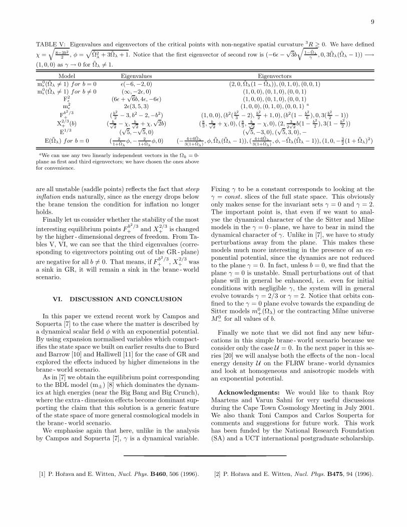
FIG. 3: State space for the FLRW models with 0 < b2 < 2. The line of Einstein universes in the closed sector of the state space

has collapsed into the non-general-relativistic Einstein model E1/3 and the general-relativistic model X2/3+ , which is expanding

and moving towards the expanding flat subspace Q = 1, (ǫ = 1) as b2 is increasing. The equilibrium point Fb2/3+ corresponds

to a flat FLRW model with γ = b2/3. See the captions of FIG. 1, FIG. 2 for more details.

M+0

λΩ~

+F2

M+2

F+2

+2m

E1/3

2−m

F+b /3

F+b /3

X+2/3

Q

Ωλ

Ωk

γγF−2

+ λΩ+~

λΩ

+

λΩ−m ( )~0

m ( )0 m ( )0

2m

2

2=

FIG. 4: State space for the FLRW models with b2 = 2 (a bifurcation). The equilibrium point X2/3+ has reached the flat

subspace, where it merges with Fb2/3+ . This causes the bifurcation; the nature of the two critical points will be swapped as they

are moving on (see FIG. 5 - 9). All open and flat models are attracted to this point X2/3+ = F

b2/3+ , whereas all closed models

are repelled. See the captions of FIG. 1, FIG. 2 for more details.

13

F+b /3

M+0

λΩ~

+F2

M+2

X+2/3

F+2

+2m

E1/3

2−m

F+b /3

Q

Ωλ

Ωk

γγF−2

+ λΩ+~

λΩ

+

λΩ−m ( )~0

m ( )0 m ( )0

2m

22

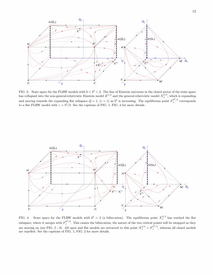
FIG. 5: State space for the FLRW models with 2 < b2 < 8/3. X2/3+ has entered the open sector and turned into a node sink.

Fb2/3+ is now an unstable saddle for all models. See the captions of FIG. 1, FIG. 2 for more details.

F+b /3 F+

b /3

M+0

λΩ~

+F2

M+2

X+2/3

F+2

+2m

E1/3

Q Ωk

γγ

~ λΩ

F−2

2−m

λΩ−

+~

λΩm ( ) + λΩ0

+0m

m ( )0

m ( )0

2 2

FIG. 6: State space for the FLRW models with b2 = 8/3. The node sink X2/3+ is turning into a spiral sink; the structure of

the state space has not changed. See the captions of FIG. 1, FIG. 2 for more details.

14

M+0

λΩ~

+F2

M+2

F+2

+2m

E1/3

2−m

F+b /3

F+b /3

X+2/3

Q

Ωλ

Ωk

γγF−2

+ λΩ+~

λΩ

+

λΩ−m ( )~0

m ( )0 m ( )0

2m

22

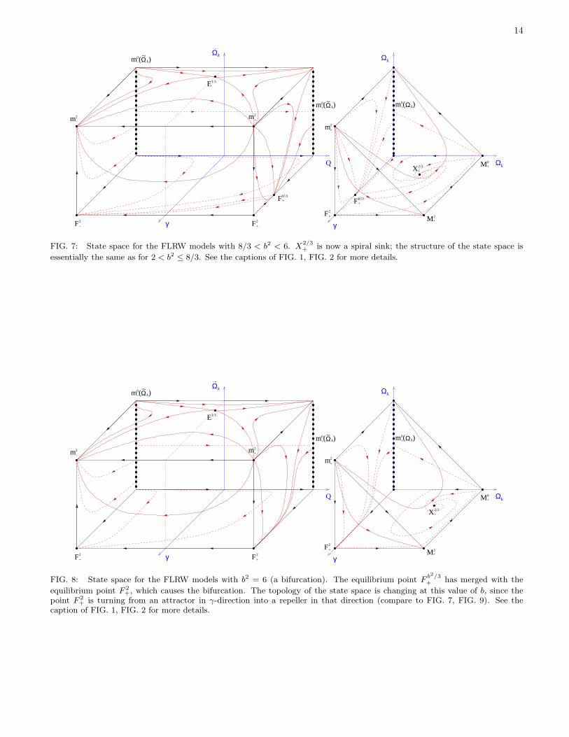
FIG. 7: State space for the FLRW models with 8/3 < b2 < 6. X2/3+ is now a spiral sink; the structure of the state space is

essentially the same as for 2 < b2 ≤ 8/3. See the captions of FIG. 1, FIG. 2 for more details.

M+0

λΩ~

+F2

M+2

F+2

+2m

E1/3

2−m

X+2/3

γ

Q

Ωλ

Ωk

γF−2

+ λΩ+~

λΩ

+

λΩ−m ( )~0

m ( )0 m ( )0

2m

FIG. 8: State space for the FLRW models with b2 = 6 (a bifurcation). The equilibrium point Fb2/3+ has merged with the

equilibrium point F 2+, which causes the bifurcation. The topology of the state space is changing at this value of b, since the

point F 2+ is turning from an attractor in γ-direction into a repeller in that direction (compare to FIG. 7, FIG. 9). See the

caption of FIG. 1, FIG. 2 for more details.

15

M+0

λΩ~

+F2

M+2

F+2

+2m

E1/3

2−m

X+2/3

γ

Q

Ωλ

Ωk

γF−2

+ λΩ+~

λΩ

+

λΩ−m ( )~0

m ( )0 m ( )0

2m

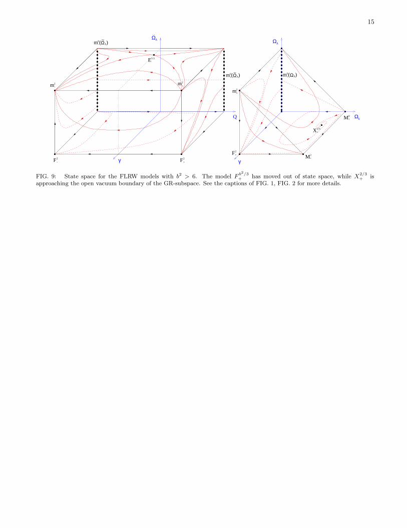
FIG. 9: State space for the FLRW models with b2 > 6. The model Fb2/3+ has moved out of state space, while X

2/3+ is

approaching the open vacuum boundary of the GR-subspace. See the captions of FIG. 1, FIG. 2 for more details.

+

SFF

−

S

m −

S

Ωρ~ =0

Ω~ ρ =0

Ω~ ρ =0

Q

Ωλ

Ωk

γγ

λΩ~

m +

S