Brane dimers and quiver gauge theories

arX

iv:h

ep-t

h/05

0411

0v2

30

Jun

2005

Preprint typeset in JHEP style. - HYPER VERSION MIT-CTP-3619

hep-th/0504110

Brane Dimers and Quiver Gauge Theories

Sebastian Franco1, Amihay Hanany1, Kristian D. Kennaway2, David Vegh1, Brian Wecht1

1 Center for Theoretical Physics, Massachusetts Institute of Technology,

Cambridge, MA 02139, USA.∗

2 Department of Physics, University of Toronto,

Toronto, ON M5S 1A7, CANADA.†

Abstract: We describe a technique which enables one to quickly compute an infinite num-

ber of toric geometries and their dual quiver gauge theories. The central object in this

construction is a “brane tiling,” which is a collection of D5-branes ending on an NS5-brane

wrapping a holomorphic curve that can be represented as a periodic tiling of the plane. This

construction solves the longstanding problem of computing superpotentials for D-branes

probing a singular non-compact toric Calabi-Yau manifold, and overcomes many difficulties

which were encountered in previous work. The brane tilings give the largest class of N = 1

quiver gauge theories yet studied. A central feature of this work is the relation of these tilings

to dimer constructions previously studied in a variety of contexts. We do many examples of

computations with dimers, which give new results as well as confirm previous computations.

Using our methods we explicitly derive the moduli space of the entire Y p,q family of quiver

theories, verifying that they correspond to the appropriate geometries. Our results may be

interpreted as a generalization of the McKay correspondence to non-compact 3-dimensional

toric Calabi-Yau manifolds.

∗Research supported in part by the CTP and the LNS of MIT and the U.S. Department of Energy under

cooperative agreement #DE-FC02-94ER40818. AH is also supported in part by the BSF American–Israeli

Bi–National Science Foundation and a DOE OJI award. BW is supported in part by National Science

Foundation Grant beas PHY-00-96515. DV is supported by the MIT Praecis Presidential Fellowship.†K.K. is supported by NSERC.

http://arXiv.org/abs/hep-th/0504110v2

Contents

1. Introduction 2

2. Brane tilings and quivers 8

2.1 Unification of quiver and superpotential data 12

3. Dimer model technology 15

4. An explicit correspondence between dimers and GLSMs 18

4.1 A detailed example: the Suspended Pinch Point 22

5. Massive fields 24

6. Seiberg duality 26

6.1 Seiberg duality as a transformation of the quiver 26

6.2 Seiberg duality as a transformation of the brane tiling 27

6.3 Seiberg duality acting on the Kasteleyn matrix 30

7. Partial resolution 32

8. Different toric superpotentials for a given quiver 35

9. Examples 37

9.1 Del Pezzo 2 37

9.2 Pseudo del Pezzo 5 41

9.3 Tilings for infinite families of gauge theories 42

9.3.1 Y p,q tilings 43

9.3.2 Y 3,1 with double impurity 47

9.3.3 Xp,q tilings 48

10. Conclusions 50

1

1. Introduction

Shortly after the discovery of the importance of D-branes in string theory, it became clear

that they provide a deep connection between algebra and geometry. This is realized in string

theory in the following way: the D-brane, a physical object in spacetime, probes the geometry

in which it lives, and the properties of spacetime fields are reflected in its worldvolume gauge

theory. On the other hand, the D-brane has fundamental strings ending on it, thus giving

rise to gauge quantum numbers which enumerate the possible ways strings can end on the

brane when it is embedded in the given singular geometry. This fact leads to a pattern

of algebraic relations, which are conveniently encoded in terms of algebraic quantities like

Dynkin diagrams and, more generally, quiver gauge theories.

One simple example is given by a collection of N parallel D-branes; these have funda-

mental strings stretching between them and are in one-to-one correspondence with Dynkin

diagrams of type AN−1. Branes are mapped to nodes in the Dynkin diagrams and funda-

mental strings are mapped to lines. Placing this configuration on a circle leads to an affine

Dynkin diagram AN−1, where the imaginary root is mapped to a fundamental string encir-

cling the compact direction. Many more examples of this type lead to a beautiful relationship

between branes and Lie algebras.

When D-branes in Type II string theory are placed on an ALE singularity of ADE type,

the gauge theory living on them is encoded by an affine ADE Dynkin diagram. Here, frac-

tional branes are mapped to nodes in the Dynkin diagram while strings stretching between

the fractional branes are mapped to lines in the Dynkin diagram. The gauge theory living

on the branes has 8 supercharges, since the ALE singularity breaks one half of the supersym-

metry while the D-branes break a further half. With this amount of supersymmetry (N = 2

in four dimensions), it is enough to specify the gauge group and the matter content in order

to fix the Lagrangian of the theory uniquely. As above, we see that this gauge theory also

realizes the relationship between algebra and geometry: on the algebra side, we have the

Dynkin diagram, and on the geometry side there is a moduli space of vacua which is the ADE

type singularity. This connection between the Lie algebras of affine Dynkin diagrams and

the geometry of ALE spaces is known as the McKay correspondence [1]. This relation was

first derived in the mathematics literature and later – with the help of D-branes – became

an important relation in string theory.

The McKay correspondence can be realized in other ways in string theory. One example

which will be important to us in this paper is the configuration of NS5-branes and D-branes

stretching between them which was studied in [2]. A collection of N NS5-branes with D-

branes stretching between them results in a gauge theory on the D-branes which turns

2

out to be encoded by an AN−1 Dynkin diagram. Here, NS5-branes are mapped to lines

while D-branes stretching between NS5-branes are mapped to nodes in the quiver gauge

theory. Putting this configuration on a circle leads to an affine version of this correspondence

AN−1; the imaginary root now corresponds to a D-brane which wraps the circle. This

correspondence is very similar to the D-brane picture which was presented above and indeed,

using a chain of S- and T- dualities, one can get from one configuration of branes to the

other, while keeping the algebraic structure the same. Furthermore, the gauge theory living

on a D-brane stretched between NS5-branes is very similar to the gauge theory living on a

D-brane that probes an AN−1 singularity. Indeed, as first observed in [3], the collection of

N NS5-branes on a circle is T-dual to an ALE singularity of type AN−1 with one circular

direction. A detailed study of this correspondence was performed in [4].

Many attempts at generalizing the McKay correspondence from a 2 complex dimensional

space to a 3 complex dimensional space have been made in the literature [5, 6, 7, 8, 9, 10].

From the point of view of branes in string theory it is natural to extend the 2-dimensional

correspondence stated above from D-branes probing a 2-dimensional singular manifold to

a collection of D-branes probing a 3 dimensional singular Calabi-Yau (CY) manifold [11].

A few qualitative features are different in this case. First, the supersymmetry of the gauge

theory living on the D-brane is now reduced to 4 supercharges. This implies that gauge fields

and matter fields are not enough to uniquely determine the Lagrangian of the theory, and

one must also specify a superpotential which encodes the interactions between the matter

fields.

This is an important observation: any attempt at stating the 3-dimensional McKay

correspondence must incorporate the superpotential, which was uniquely constrained in the

2-dimensional case. Second, the matter multiplets in theories with 4 supercharges are chiral

and therefore have a natural orientation. In the theories with 8 supercharges, for every

chiral multiplet there is another chiral multiplet with an opposite orientation, transforming

together in a hypermultiplet. Therefore, an overall orientation is not present in a theory

with 8 supercharges. We conclude that the 3-dimensional McKay correspondence requires

information about these orientations, absent in the 2-dimensional case.

Studying the first few examples for the 3-dimensional McKay correspondence (the sim-

plest of which is the orbifold C3/Z3), it became clear that the objects which replace the

Dynkin diagrams are quivers with oriented arrows [12]. For these objects, nodes represent

gauge groups, oriented arrows between two nodes represent bifundamental chiral multiplets,

and certain closed paths in the quiver (which represent gauge-invariant operators) represent

terms in the superpotential. It is important to note that only a subset of all closed paths

3

on the quiver appears in the superpotential, and finding which particular subset is selected

for the quiver associated to a given toric singularity is a difficult task. This difficulty will be

greatly simplified with the results of this paper.

Since we will be using quivers throughout this work, it will be useful to briefly recall

what is currently known about the theories we can study via string theory. The first known

examples of quiver theories obtained from string theory were those dual to C3/Γ, where Γ

is any discrete subgroup of SU(3) [13, 14]. The most common examples of this type take

Γ = Zn or Γ = Zn × Zm. These theories are easy to construct, since it is straightforward

to write down an orbifold action on the coordinates of C3. If |Γ| = k, then there are k

nodes in the dual quiver and a bifundamental for each orbifold action on C3 that connects

different regions of the covering space. These orbifold theories may be described torically

in a straightforward manner. It was then realized that partial resolution of these orbifold

spaces corresponds to Higgsing the quivers; in this manner, people were able to obtain many

different quiver theories and their dual toric geometries [15, 16, 17]. For a good review of

toric geometry, see [18, 19].

It was not long before a general algorithm for deriving toric data from a given quiver

was found; this procedure is usually called “The Forward Algorithm” [15]. Although the

procedure is well-understood, it is computationally prohibitive for quivers with more than

approximately ten nodes. The Forward Algorithm, in addition to providing the toric data

for a given quiver theory, also gives the relative multiplicities of the gauged linear sigma

model (GLSM) fields in the related sigma model [20]. However, the same problem applies

here as well: the toric diagrams and their associated multiplicities are difficult to derive for

large quivers.

In recent months there has been much progress in the arena of gauge theories dual

to toric geometries. Gauntlett, Martelli, Sparks, and Waldram [21] found an infinite class

of Sasaki-Einstein (SE) metrics; previous to their work, only two explicit SE metrics were

known. These metrics are denoted Y p,q and depend only on two integers p and q, where

0 < q < p. In related work, Martelli and Sparks [22] found the toric descriptions of the Y p,q

theories, and noted that some of these spaces were already familiar, although their metrics

had not previously been known. One of the simplest examples is Y 2,1, which turns out to be

the SE manifold which is the base of the complex cone over the first del Pezzo surface. The

R-charges for Y 2,1 were computed in [23] and shown to agree exactly with the geometrical

computation done using the metric found in [22]. More progress was made when the gauge

theory duals of the Y p,q spaces were found [24], providing an infinite class of AdS/CFT dual

pairs. These theories have survived many nontrivial checks of the AdS/CFT correspondence,

4

such as central charge and R-charge computations from volume calculations on the string

side and a-maximization [25] on the gauge theory side. Inspired by these gauge theories,

there have since been many new and startling checks of AdS/CFT, such as the construction

of gravity duals for cascading RG flows [26]. Thus, there has been remarkable progress

recently in the study of toric Calabi-Yau manifolds and their dual gauge theories; however,

a general procedure for constructing the dual to a given CY is still unknown. In this work,

we will shed some light on this problem.

One of the results of the present work is that the ingredients required to uniquely define

an N = 1 quiver gauge theory – gauge groups, chiral matter fields, and superpotential terms

– may be represented in terms of nodes, lines and faces of a single object, which is the

quiver redrawn as a planar graph on the torus (for the quiver theories corresponding to toric

singularities). This point will be crucial in the construction of the quiver gauge theory using

dimers, as will be discussed in detail in section 3.

One may also ask how these theories may be constructed in string theory by using

branes, as explained above for the case of theories with 8 supercharges. A key observation

is that if a collection of m NS5-branes is T-dual to an orbifold C3/Zm, then a collection of

m NS5-branes intersecting with n NS5′-branes with both sets of NS5-branes sharing 3+1

space-time directions, is equivalent under two T-dualities to an orbifold singularity of type

C3/(Zm × Zn). When D3-brane probes are added over the orbifold, they are mapped to

D5-branes suspended between the NS5-branes on the T-dual configuration. Indeed, a study

of these theories using the Brane Box Models of [27] was done in [28]. Another important

development in the brane construction of quiver gauge theories with 4 supercharges was

made in [29] where it was realized that the quiver gauge theories which live on D-branes

probing the conifold and its various orbifolds are constructed by “Brane Diamonds.” Brane

diamonds were also applied to the study of gauge theories for D-branes probing complex

cones over del Pezzo surfaces [30].

In the present paper, we consider a more intricate configuration of branes. First, we take

an NS5-brane which extends in the 0123 directions and wraps a complex curve f(x, y) = 0,

where x and y are holomorphic coordinates in the 45 and 67 directions, respectively. We

typically depict this by drawing this curve in the 4 and 6 directions, where it looks like a

network that separates the plane into different regions, i.e. a tiling3. We do not explicitly

write down the equation for this curve, but do note that a requirement of our construction

is that the tiling of the 46 plane is such that all polygons have an even number of sides.

The 4 and 6 directions are compact, forming a torus, and we take the D5 branes to be finite

3Related work, on how to tile a domain wall with lower-dimensional domain walls, was done in [31].

5

in these directions (but extended in the 0123 directions) and bounded by the curve which

is wrapped by the NS5-brane. As above, this brane configuration results in a quiver gauge

theory living on the D5-branes. The rules for computing this quiver theory turn out to follow

similar guidelines to those in the constructions mentioned above: gauge groups are faces of

the intersecting brane configuration, bifundamental fields arise across NS5-branes which are

lines in the brane configuration, and superpotential terms show up as vertices.

It is important to note that the Brane Box Models were formulated using periodic square

graphs for encoding the rules of the quiver gauge theory, but it will become clear in this paper

that the correct objects to use to recover that construction are hexagonal graphs, and in fact

the brane boxes are recovered in a degenerate limit in which two opposite edges of the

hexagons are reduced to zero length.

We observe that in both the brane box and diamond constructions, the brane config-

urations are related to the quiver gauge theory in the following sense: faces in the brane

configuration are mapped to nodes in the quiver, lines are mapped to orthogonal lines and

nodes are mapped to faces. The statement of this duality will be formulated precisely in

Section 2.1, and will prove to be a very powerful tool in generalizing these constructions to a

larger class of quiver gauge theories (those whose moduli space describe non-compact toric

CY 3-folds).

Thus, we find that it is possible to encode all the data necessary to uniquely specify

an N = 1 quiver gauge theory in a tiling of the plane. The dual graph is then essentially

the quiver theory, written in such a way as to encode the superpotential data as well. As we

will now see, however, this tiling encodes much more than just the quiver theory – it also

encodes the dual toric geometry! The central object for deriving the toric geometry is the

dimer, which we now explain.

Since we have taken our brane tiling to consist of polygons with an even number of sides,

and all cycles of our periodic graph have even length, it is always possible to color the nodes

of the graph with two different colors (say, black and white) in such a way that any given

black node is adjacent only to white nodes, and vice versa. Such graphs are well-known in

condensed matter physics, where the links between black nodes and white nodes are called

dimers; one may think of a substance formed out of two different type of atoms (e.g. a

salt), where a dimer is just an edge of the lattice with a different atom at each end. One

can allow bonds between adjacent atoms to break and then re-form in a possibly different

configuration; the statistical mechanics of such systems has been extensively studied.

Recently, dimers have shown up in the context of string theory on toric Calabi-Yau

manifolds. In [32], the authors propose a relationship between the statistical mechanics of

6

dimer models and topological strings on a toric non-compact Calabi-Yau. The relationship

between toric geometry and dimer models was developed further in [33], where it was shown

how it is possible to obtain toric diagrams and GLSM multiplicities via dimer techniques. In

general, however, we expect that one should be able to derive the quiver gauge theory dual

to any given toric geometry. This is the purpose of the present work, to describe how dimer

technology may be used to efficiently derive both the quiver theory and the toric geometry,

thus giving a fast and straightforward way of deriving AdS/CFT dual pairs.

We can now state that the 3-dimensional McKay correspondence is represented in string

theory as a physical brane configuration of an NS5-brane spanning four dimensions and

wrapping an holomorphic curve on four other dimensions, and D5-branes. Alternatively, we

can use a twice T-dual (along the 4 and 6 directions) description: the McKay correspondence

is realized by the quiver gauge theory that lives on D-branes probing toric CY 3-folds. As

a byproduct of these two equivalent representations we can argue that it is possible to find

NS5-brane configurations that are twice T-dual to these toric singular CY manifolds. One

removes the D-branes and ends up with NS5-branes on one side and singular geometries on

the other.

The outline of this paper is as follows. In Section 2, we summarize the basic features

of our construction, and establish the relationship between brane tilings and quiver gauge

theories. We explain the brane construction that leads to the quiver theory, and detail how

it is possible to read off all relevant data about the quiver theory from the brane tiling. We

derive an interesting identity for which the brane tiling perspective provides a simple proof.

We illustrate these ideas with a simple example, Model I of del Pezzo 3. Additionally, we

describe a new object, the “periodic quiver,” which is the dual graph to the brane tiling and

neatly summarizes the quiver and superpotential data for a given gauge theory.

In Section 3, we describe the utility of the dimer model and review the relationship

between dimers and toric geometries. We begin by summarizing relevant facts about dimer

models which we will use repeatedly throughout the paper. The central object in any compu-

tation is the Kasteleyn matrix, which is a weighted adjacency matrix that is easy to derive.

We do a simple computation as an example, which illustrates the basic techniques required

to compute the toric geometry related to any given brane tiling.

Section 4 provides the relationship between dimers and fields in the related gauged linear

sigma model. We review the relationship of toric geometries to GLSMs, and describe how the

dimer model allows one to compute multiplicities of GLSM. These techniques are illustrated

with an example, that of the Suspended Pinch Point (SPP) [34].

Section 5 briefly describes how massive fields arise via the brane tiling description, and

7

comments on the process of integrating out these fields from the perspective of both the

brane tiling and the Kasteleyn matrix. Section 6 talks about Seiberg duality from three

complementary perspectives: the brane tiling, the quiver, and the Kasteleyn matrix. We

illustrate these viewpoints with F0 as an example.

Section 7 gives two descriptions of the process of partial resolution of orbifold singu-

larities, both from the brane tiling and quiver perspectives. In Section 8, we describe how

one may construct brane tilings which produce identical quivers but different superpoten-

tials; this is illustrated via the quiver from Model II of dP3. In Section 9, we present many

different examples of brane tilings, and compute the Kasteleyn matrix and dual toric geom-

etry in each example. These computations duplicate known results, as well as generate new

ones. Most notably, we find that toric diagrams with specified GLSM multiplicities are not

in one-to-one correspondence with toric phases of quiver gauge theories, as had previously

been suspected. This computation is done for Pseudo del Pezzo 5, where we find two toric

phases with identical GLSM multiplicities. Finally, in Section 10, we briefly conclude and

present some suggestions for further study.

2. Brane tilings and quivers

In this section we introduce the concept of brane tilings. They are Type IIB configurations

of NS5 and D5-branes that generalize the brane box [28] and brane diamond [29] construc-

tions and are dual to gauge theories on D3-branes transverse to arbitrary toric singularities.

From now on, we proceed assuming that the dual geometry is toric and introduce the relevant

brane configurations. The reason for the requirement that the corresponding singularities

are toric will become clear in this and subsequent sections.

In our construction, the NS5-brane extends in the 0123 directions and wraps a holo-

morphic curve embedded in the 4567 directions (the 46 directions are taken to be compact).

D5-branes span the 012346 directions and stretch inside the holes in the NS5 skeleton like

soap bubbles. The D5-branes are bounded by NS5-branes in the 46 directions, leading to a

3+1 dimensional theory in their world-volume at low energies. The branes break supersym-

metry to 1/8 of the original value, leading to 4 supercharges, i.e. N = 1 in four dimensions.

In principle, there can be a different number of D5-branes NI in each stack. This would

lead to a product gauge group∏

I SU(NI). Strings stretching between D5-branes in a given

stack give rise to the gauge bosons of SU(NI) while strings connecting D5-branes in adja-

cent stacks I and J correspond to states in the bifundamental of SU(NI) × SU(NJ ). We

will restrict ourselves to the case NI = N for all I. Theories satisfying this restriction on

8

the ranks were dubbed toric phases in [20], We should emphasize though, that there are

quivers that are dual to toric geometries but that do not satisfy this condition.

It is worthwhile here to note a few properties of NS5-branes that are relevant for this

construction. As is well-known, an NS5-brane backreacts on its surrounding spacetime to

create a throat geometry. When we have two sets of D5-branes ending on different sides of the

NS5-brane, the throat separates the two sets of branes. The D-branes may then only interact

via fundamental strings stretching between them; these are the bifundamentals in the quiver

gauge theory. Initially it might seem like there are two conjugate bifundamentals which pair

up to form hypermultiplets, but in this case, where the NS5-brane wraps a holomorphic

curve, the orientation of the NS5-brane projects one of these out of the massless spectrum

[35]. Thus the resulting quiver theory will generically have arrows pointing in only one

direction (it is easy to get quivers with bidirectional arrows as well, but these will instead

come from strings stretching across different NS5-branes rather than both orientations across

the same NS5-brane).

The important physics is captured by drawing the brane tiling in the 46 plane. The

NS5-branes wrap a holomorphic curve, the real section of which is a graph G in the 46

plane, which we will later show must be bipartite. A graph is bipartite when its nodes can

be colored in white and black, such that edges only connect black nodes to white nodes and

vice versa. By construction, G is Z2-periodic under translations in the 46 plane since these

directions are taken to be compact. We will see in the next section that the existence of G

is associated to the duality between quiver gauge theories and dimer models.

Given a brane tiling, it is straightforward to derive its associated quiver gauge theory.

The brane tiling encodes both the quiver diagram and the superpotential, which can be

constructed according to the dictionary given in Table 1 (see the following section). Con-

versely, we can use this set of rules to construct a brane tiling from a given quiver with a

superpotential. In the following section we will make this correspondence precise.

Several interesting consequences follow naturally from this simple set of rules. Some of

them are well known, while others are new. The fact that the graphs under consideration

are bipartite implies that each edge has a black and a white endpoint. Edges correspond to

bifundamental fields while nodes indicate superpotential terms, with their sign determined

by the color of the node. Thus, we conclude that each bifundamental field appears exactly

twice in the superpotential, once with a plus and once with a minus sign. We refer to this

as the toric condition and it follows from the underlying geometry being an affine toric

variety [20].

The total number of nodes inside a unit cell is even (there are equal numbers of black

9

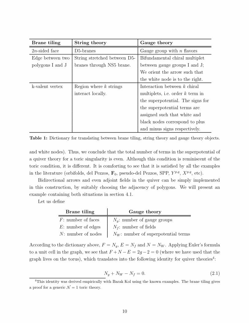
Brane tiling String theory Gauge theory

2n-sided face D5-branes Gauge group with n flavors

Edge between two String stretched between D5- Bifundamental chiral multiplet

polygons I and J branes through NS5 brane. between gauge groups I and J;

We orient the arrow such that

the white node is to the right.

k-valent vertex Region where k strings Interaction between k chiral

interact locally. multiplets, i.e. order k term in

the superpotential. The signs for

the superpotential terms are

assigned such that white and

black nodes correspond to plus

and minus signs respectively.

Table 1: Dictionary for translating between brane tiling, string theory and gauge theory objects.

and white nodes). Thus, we conclude that the total number of terms in the superpotential of

a quiver theory for a toric singularity is even. Although this condition is reminiscent of the

toric condition, it is different. It is comforting to see that it is satisfied by all the examples

in the literature (orbifolds, del Pezzos, F0, pseudo-del Pezzos, SPP, Y p,q, Xp,q, etc).

Bidirectional arrows and even adjoint fields in the quiver can be simply implemented

in this construction, by suitably choosing the adjacency of polygons. We will present an

example containing both situations in section 4.1.

Let us define

Brane tiling Gauge theory

F : number of faces Ng: number of gauge groups

E: number of edges Nf : number of fields

N : number of nodes NW : number of superpotential terms

According to the dictionary above, F = Ng, E = Nf and N = NW . Applying Euler’s formula

to a unit cell in the graph, we see that F +N −E = 2g−2 = 0 (where we have used that the

graph lives on the torus), which translates into the following identity for quiver theories4:

Ng + NW − Nf = 0. (2.1)

4This identity was derived empirically with Barak Kol using the known examples. The brane tiling gives

a proof for a generic N = 1 toric theory.

10

The geometric intuition we gain when using brane tilings make the derivation of this remark-

able identity straightforward.

It is interesting to point out here that the Euler formula has another interpretation. Let

us assign an R-charge to each bifundamental field in the quiver, i.e. to each edge in the brane

tiling. At the IR superconformal fixed point, we know that each term in the superpotential

must satisfy ∑

i∈edges around node

Ri = 2 for each node (2.2)

where the sum is over all edges surrounding a given node. We can sum over all the nodes in

the tiling, each of which corresponds to a superpotential term, to get∑

edges,nodes R = 2N .

Additionally, the beta function for each gauge coupling must vanish,

2 +∑

i∈edges around face

(Ri − 1) = 0 for each face (2.3)

where the sum is over all edges surrounding a given face. But we can now sum this over all

the faces in the tiling to get 2F +2N −2E = 0, where we have used the fact that the double

sum hits every edge twice, and (2.2). The sums∑

edges,nodes R and∑

edges,faces R are equal

because each double sum has the R-charge of each bifundamental contributing twice. Thus

we see that the requirements that the superpotential have R(W ) = 2 and the beta functions

vanish (i.e. that the theory is superconformal in the IR) imply that the Euler characteristic

of the tiling is zero. This condition is the analog of a similar condition for superconformal

quivers discussed in [36, 37]. Conversely we see that, in the case in which the ranks of all

gauge groups are equal, the construction of tilings over Riemann surfaces different from a

torus leads to non-conformal gauge theories.

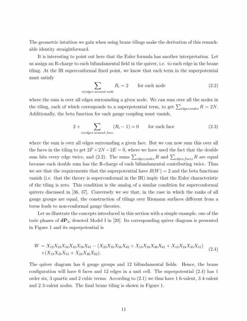
Let us illustrate the concepts introduced in this section with a simple example, one of the

toric phases of dP3, denoted Model I in [20]. Its corresponding quiver diagram is presented

in Figure 1 and its superpotential is

W = X12X23X34X45X56X61 − (X23X35X56X62 + X13X34X46X61 + X12X24X45X51)

+(X13X35X51 + X24X46X62).(2.4)

The quiver diagram has 6 gauge groups and 12 bifundamental fields. Hence, the brane

configuration will have 6 faces and 12 edges in a unit cell. The superpotential (2.4) has 1

order six, 3 quartic and 2 cubic terms. According to (2.1) we thus have 1 6-valent, 3 4-valent

and 2 3-valent nodes. The final brane tiling is shown in Figure 1.

11

35 56 6223−X X X X

6 1

4 3

25

1

2 6

53

4

6 1

4 3

256 1

4 3

25

6 1

4 3

25

6 1

4 3

25

6 1

4 3

25

6 1

4 3

25

Figure 1: A finite region in the infinite brane tiling and quiver diagram for Model I of dP3. We

indicate the correspondence between: gauge groups ↔ faces, bifundamental fields ↔ edges and

superpotential terms ↔ nodes.

2.1 Unification of quiver and superpotential data

An N = 1 quiver gauge theory is described by the following data: a directed graph represent-

ing the gauge groups and matter content, and a set of closed paths on the graph representing

the gauge invariant interactions in the superpotential. An equivalent way to characterise this

data is to view it as defining a CW-complex; in other words, we may take the superpotential

terms to define the 2-dimensional faces of the complex bounded by a given set of edges and

vertices (the 1-skeleton and 0-skeleton of the complex). Thus, the quiver and superpotential

may be combined into a single object, a planar tiling of a 2-dimensional (possibly singular)

space. Toric quiver theories, as we will see, are defined by planar tilings of the 2-dimensional

torus.

This is a key observation. Given the presentation of the quiver data (quiver graph and

superpotential) as a planar graph tiling the torus, the bipartite graph appearing in the dimer

model (the brane construction of the previous section) is nothing but the planar dual of this

graph! Moreover, as we have argued, this dual presentation of the quiver data is physical, in

that it appears directly in string theory as a way to construct the 3 + 1-dimensional quiver

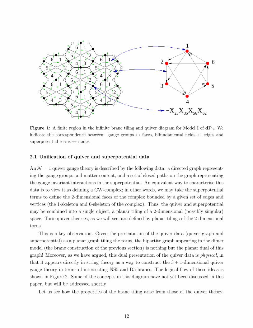
gauge theory in terms of intersecting NS5 and D5-branes. The logical flow of these ideas is

shown in Figure 2. Some of the concepts in this diagram have not yet been discussed in this

paper, but will be addressed shortly.

Let us see how the properties of the brane tiling arise from those of the quiver theory.

12

Periodic quiver

Toric diagram

with multiplicitiesQuiver gauge theory

faces =superpotential terms

dual graph

Forward algorithm

det[Kasteleyn matrix]

(partial resolution)Inverse algorithm

Brane tiling

Figure 2: The logical flowchart.

We will show that we can think of the superpotential and quiver together as a tiling of a

two-dimensional surface, where bifundamentals are edges, superpotential terms are faces,

and gauge groups are nodes. We refer to this as the “periodic quiver” representation. The

toric condition, which states that each matter field appears in precisely two superpotential

terms of opposite sign, means that the faces all glue together in pairs along the common

edges. Since every field is represented exactly twice in the superpotential, this tiling has

no boundaries. Thus, the quiver and its superpotential may be combined to give a tiling

of a Riemann surface without boundary; this periodic quiver gives a discretization of the

torus. Since the Euler characteristic of the quiver is zero for toric theories (as discussed in

the previous section), the quiver and superpotential data are equivalent to a planar tiling of

the two-dimensional torus. See Figure 5 of [15] for an early example of a periodic quiver.

This tiling has additional structure. The toric condition implies that adjacent faces of

the tiling may be labelled with opposite signs according to the sign of the corresponding

term in the superpotential. Thus, under the planar duality the vertices of the dual graph

may be labelled with opposite signs; this is the bipartite property of the dimer model. Since

the periodic quiver is defined on the torus, the dual bipartite graph also lives on the torus.

Anomaly cancellation of the quiver gauge theory is represented by the balancing of all

incoming and outgoing arrows at every node of the quiver. In the dual graph, bipartiteness

means that the edges carry a natural orientation (e.g. from black to white). This induces

an orientation for the dual edges, which transition between adjacent faces of the brane tiling

(vertices of the planar quiver). For example, these dual arrows point in a direction such

that, looking at an arrow from its tail to its head, the black node is to the left and the

white node is to the right (this is just a convention and the opposite choice is equivalent by

13

charge conjugation). Arrows around a face in G alternate between incoming and outcoming

arrows of the quiver; this is how anomaly cancellation is manifested in the brane tiling

picture. Alternatively, we can say that arrows “circulate” clockwise around white nodes and

counterclockwise around black nodes.

81

10

2 +−

+

+−

+

−

−9

+−+

−

+

−

A B

CD

73

3 7

6 6

1212

11

11 4

4

+

55

−

B

CD

A

113

7

981

12

5

4

2

106

5

73

411

12

6

Planar

quiver

Quiver

5,9

2,4

6,10

1,37,8,11,12

A

D C

B

Dual graph

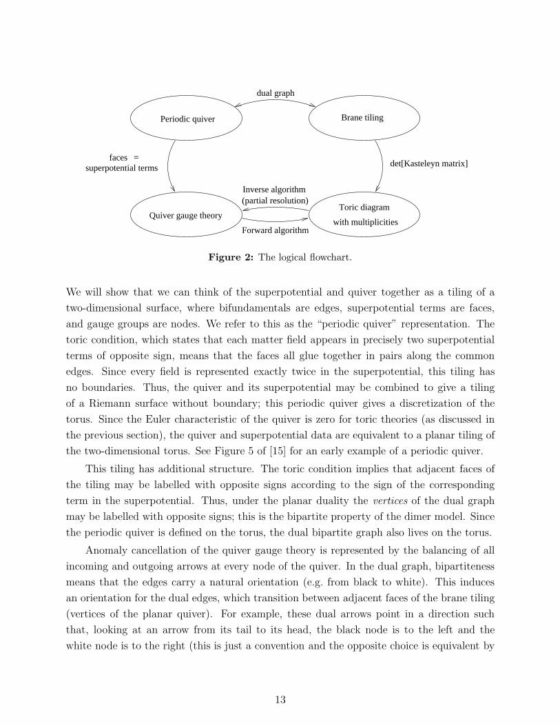
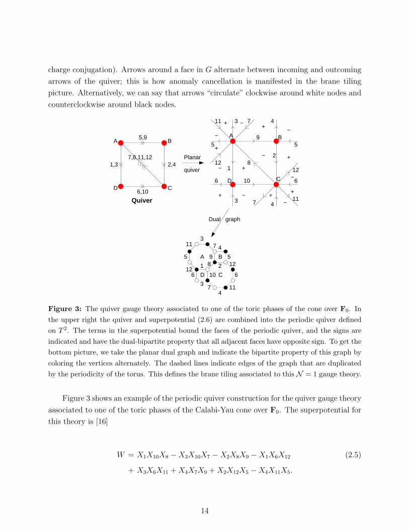
Figure 3: The quiver gauge theory associated to one of the toric phases of the cone over F0. In

the upper right the quiver and superpotential (2.6) are combined into the periodic quiver defined

on T 2. The terms in the superpotential bound the faces of the periodic quiver, and the signs are

indicated and have the dual-bipartite property that all adjacent faces have opposite sign. To get the

bottom picture, we take the planar dual graph and indicate the bipartite property of this graph by

coloring the vertices alternately. The dashed lines indicate edges of the graph that are duplicated

by the periodicity of the torus. This defines the brane tiling associated to this N = 1 gauge theory.

Figure 3 shows an example of the periodic quiver construction for the quiver gauge theory

associated to one of the toric phases of the Calabi-Yau cone over F0. The superpotential for

this theory is [16]

W = X1X10X8 − X3X10X7 − X2X8X9 − X1X6X12 (2.5)

+ X3X6X11 + X4X7X9 + X2X12X5 − X4X11X5.

14

3. Dimer model technology

Given a bipartite graph, a problem of interest to physicists and mathematicians is to count

the number of perfect matchings of the graph. A perfect matching of a bipartite graph is

a subset of edges (“dimers”) such that every vertex in the graph is an endpoint of precisely

one edge in the set. A dimer model is the statistical mechanics of such a system, i.e. of

random perfect matchings of the graph with assigned edge weights. As discussed in the

previous section, we are interested in dimer models associated to doubly-periodic graphs,

i.e. graphs defined on the torus T 2. We will now review some basic properties of dimers; for

additional review, see [33, 38].

Many important properties of the dimer model are governed by the Kasteleyn matrix

K(z, w), a weighted, signed adjacency matrix of the graph with (in our conventions) the rows

indexed by the white nodes, and the columns indexed by the black nodes. It is constructed

as follows:

To each edge in the graph, multiply the edge weight by ±1 so that around every face

of the graph the product of the edge weights over edges bounding the face has the following

sign

sign(∏

i

ei) =

{+1 if (# edges) = 2 mod 4

−1 if (# edges) = 0 mod 4(3.1)

It is always possible to arrange this [39].

The coloring of vertices in the graph induces an orientation to the edges, for example the

orientation “black” to “white”. This orientation corresponds to the orientation of the chiral

multiplets of the quiver theory, as discussed in the previous section. Now construct paths

γw, γz in the dual graph (i.e. the periodic quiver) that wind once around the (0, 1) and (1, 0)

cycles of the torus, respectively. We will refer to these fundamental paths as flux lines. In

terms of the periodic quiver, the paths γ pick out a subset of the chiral multiplets whose

product is gauge-invariant and forms a closed path that winds around one of the fundamental

cycles of the torus. For every such edge (chiral multiplet) in G crossed by γ, multiply the

edge weight by a factor of w or 1/w (respectively z, 1/z) according to the relative orientation

of the edges in G crossed by γ.

The adjacency matrix of the graph G weighted by the above factors is the Kasteleyn

matrix K(z, w) of the graph. The determinant of this matrix P (z, w) = det K is a Laurent

polynomial (i.e. negative powers may appear) called the characteristic polynomial of the

dimer model

15

P (z, w) =∑

i,j

cijziwj. (3.2)

This polynomial provides the link between dimer models and toric geometry [33].

Given an arbitrary “reference” matching M0 on the graph, for any matching M the

difference M − M0 defines a set of closed curves on the graph in T 2. This in turn defines a

height function on the faces of the graph: when a path in the dual graph crosses the curve,

the height is increased or decreased by 1 according to the orientation of the crossing. A

different choice of reference matching M0 shifts the height function by a constant. Thus,

only differences in height are physically significant.

In terms of the height function, the characteristic polynomial takes the following form:

P (z, w) = zhx0why0

∑chx,hy

(−1)hx+hy+hxhyzhxwhy (3.3)

where chx,hyare integer coefficients that count the number of paths on the graph with height

change (hx, hy) around the two fundamental cycles of the torus.

The overall normalization of P (z, w) is not physically meaningful: since the graph does

not come with a prescribed embedding into the torus (only a choice of periodicity), the paths

γz,w winding around the primitive cycles of the torus may be taken to cross any edges en

route. Different choices of paths γ multiply the characteristic polynomial by an overall power

ziwj, and by an appropriate choice of path P (z, w) can always be normalized to contain only

non-negative powers of z and w.

The Newton polygon N(P ) is a convex polygon in Z2 generated by the set of integer

exponents of the monomials in P . In [33], it was conjectured that the Newton polygon can

be interpreted as the toric diagram associated to the moduli space of the quiver gauge theory,

which by assumption is a non-compact toric Calabi-Yau 3-fold. In the following section, we

will prove that the perfect matchings of the dimer model are in 1-1 correspondence with the

fields of the gauged linear sigma model that describes the probed toric geometry.

The connection between dimer models and toric geometry was explored in [33]. In that

paper the action of orbifolding the toric singularity was understood in terms of the dimer

model: the orbifold action by Zm × Zn corresponds to enlarging the fundamental domain

of the graph by m × n copies, and non-diagonal orbifold actions correspond to a choice of

periodicity of the torus, i.e. an offset in how the neighboring domains are adjoined. Further-

more, results analogous to the Inverse Algorithm were developed for studying arbitrary toric

singularities and their associated quiver theories. The present paper derives and significantly

extends the results of [33], and places them into the context of string theory.

16

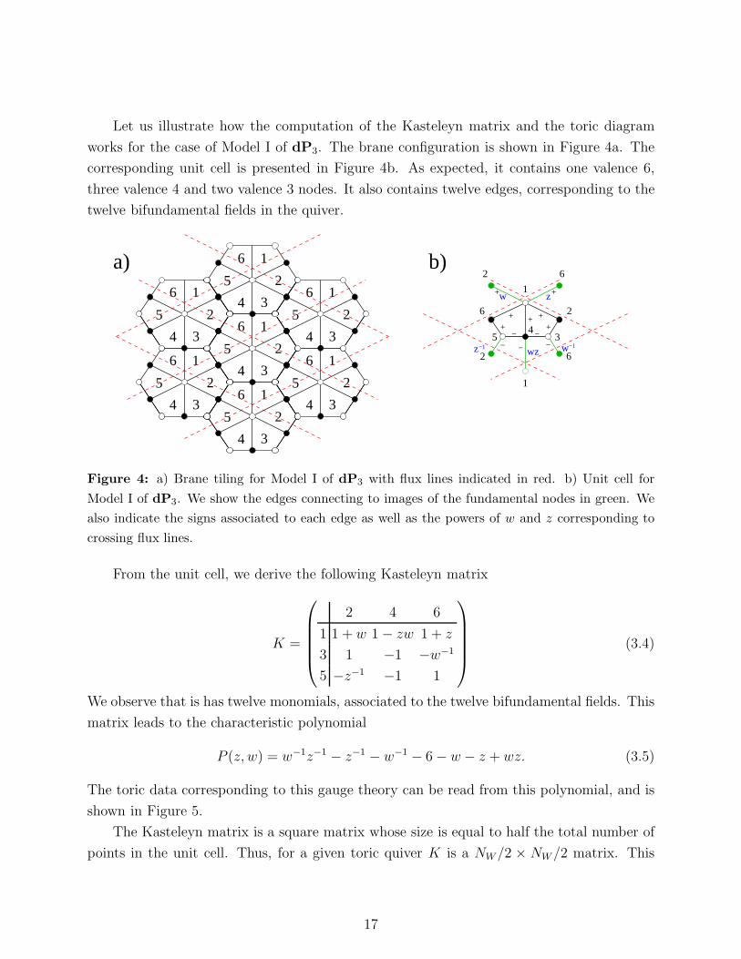
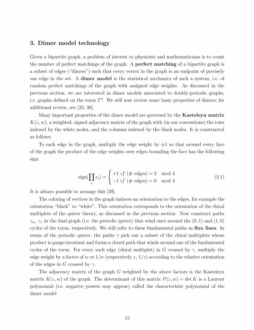
Let us illustrate how the computation of the Kasteleyn matrix and the toric diagram

works for the case of Model I of dP3. The brane configuration is shown in Figure 4a. The

corresponding unit cell is presented in Figure 4b. As expected, it contains one valence 6,

three valence 4 and two valence 3 nodes. It also contains twelve edges, corresponding to the

twelve bifundamental fields in the quiver.

6 1

4 3

25

6 1

4 3

25

6 1

4 3

25

6 1

4 3

25

6 1

4 3

25

6 1

4 3

25

6 1

4 3

25

w−1z−1

b)a)62

5 3

62

1

1

6 2

4

w z

wz

+ +

+ ++++

− −

−− −

Figure 4: a) Brane tiling for Model I of dP3 with flux lines indicated in red. b) Unit cell for

Model I of dP3. We show the edges connecting to images of the fundamental nodes in green. We

also indicate the signs associated to each edge as well as the powers of w and z corresponding to

crossing flux lines.

From the unit cell, we derive the following Kasteleyn matrix

K =

2 4 6

1 1 + w 1 − zw 1 + z

3 1 −1 −w−1

5 −z−1 −1 1

(3.4)

We observe that is has twelve monomials, associated to the twelve bifundamental fields. This

matrix leads to the characteristic polynomial

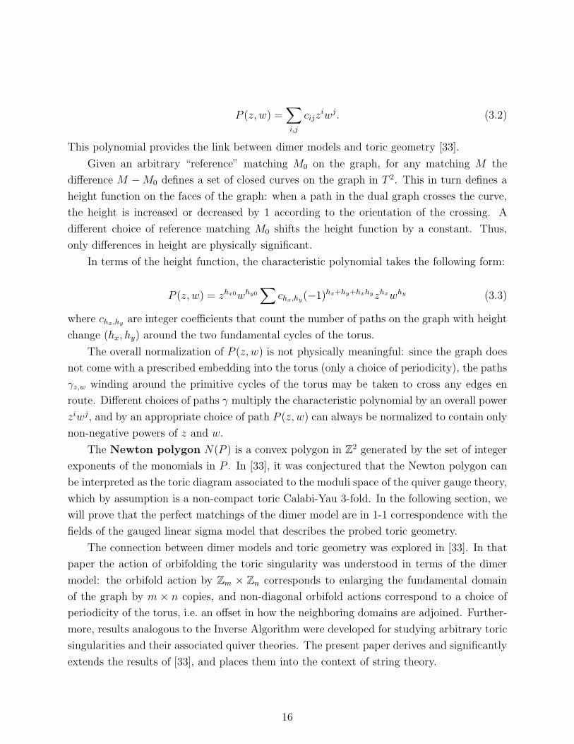
P (z, w) = w−1z−1 − z−1 − w−1 − 6 − w − z + wz. (3.5)

The toric data corresponding to this gauge theory can be read from this polynomial, and is

shown in Figure 5.

The Kasteleyn matrix is a square matrix whose size is equal to half the total number of

points in the unit cell. Thus, for a given toric quiver K is a NW /2 × NW /2 matrix. This

17

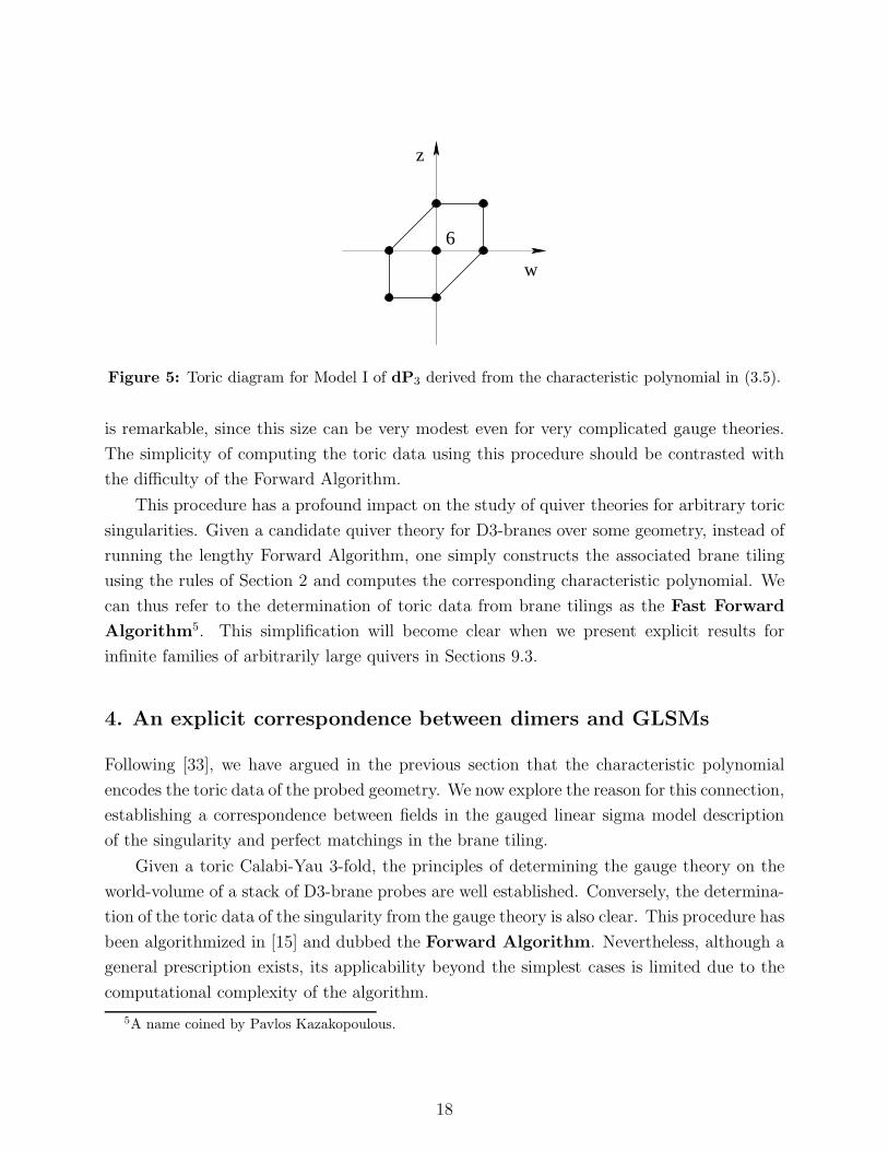
6

w

z

Figure 5: Toric diagram for Model I of dP3 derived from the characteristic polynomial in (3.5).

is remarkable, since this size can be very modest even for very complicated gauge theories.

The simplicity of computing the toric data using this procedure should be contrasted with

the difficulty of the Forward Algorithm.

This procedure has a profound impact on the study of quiver theories for arbitrary toric

singularities. Given a candidate quiver theory for D3-branes over some geometry, instead of

running the lengthy Forward Algorithm, one simply constructs the associated brane tiling

using the rules of Section 2 and computes the corresponding characteristic polynomial. We

can thus refer to the determination of toric data from brane tilings as the Fast Forward

Algorithm5. This simplification will become clear when we present explicit results for

infinite families of arbitrarily large quivers in Sections 9.3.

4. An explicit correspondence between dimers and GLSMs

Following [33], we have argued in the previous section that the characteristic polynomial

encodes the toric data of the probed geometry. We now explore the reason for this connection,

establishing a correspondence between fields in the gauged linear sigma model description

of the singularity and perfect matchings in the brane tiling.

Given a toric Calabi-Yau 3-fold, the principles of determining the gauge theory on the

world-volume of a stack of D3-brane probes are well established. Conversely, the determina-

tion of the toric data of the singularity from the gauge theory is also clear. This procedure has

been algorithmized in [15] and dubbed the Forward Algorithm. Nevertheless, although a

general prescription exists, its applicability beyond the simplest cases is limited due to the

computational complexity of the algorithm.

5A name coined by Pavlos Kazakopoulous.

18

Let us review the main ideas underlying the Forward Algorithm (for a detailed descrip-

tion and explicit examples, we refer the reader to [15]). The starting point is a quiver with r

SU(N) gauge groups and bifundamentals Xi, i = 1, . . . , m, together with a superpotential.

The toric data that describes the probed geometry is computed using the following steps:

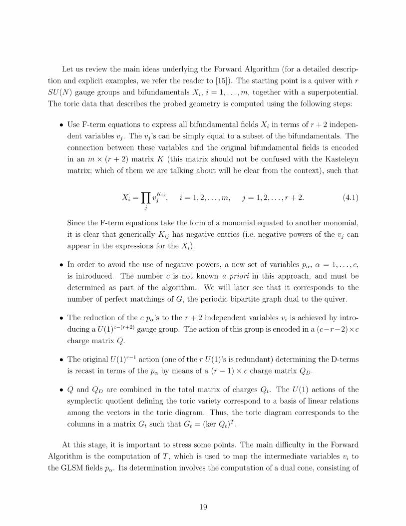
• Use F-term equations to express all bifundamental fields Xi in terms of r + 2 indepen-

dent variables vj . The vj ’s can be simply equal to a subset of the bifundamentals. The

connection between these variables and the original bifundamental fields is encoded

in an m × (r + 2) matrix K (this matrix should not be confused with the Kasteleyn

matrix; which of them we are talking about will be clear from the context), such that

Xi =∏

j

vKij

j , i = 1, 2, . . . , m, j = 1, 2, . . . , r + 2. (4.1)

Since the F-term equations take the form of a monomial equated to another monomial,

it is clear that generically Kij has negative entries (i.e. negative powers of the vj can

appear in the expressions for the Xi).

• In order to avoid the use of negative powers, a new set of variables pα, α = 1, . . . , c,

is introduced. The number c is not known a priori in this approach, and must be

determined as part of the algorithm. We will later see that it corresponds to the

number of perfect matchings of G, the periodic bipartite graph dual to the quiver.

• The reduction of the c pα’s to the r + 2 independent variables vi is achieved by intro-

ducing a U(1)c−(r+2) gauge group. The action of this group is encoded in a (c−r−2)×c

charge matrix Q.

• The original U(1)r−1 action (one of the r U(1)’s is redundant) determining the D-terms

is recast in terms of the pα by means of a (r − 1) × c charge matrix QD.

• Q and QD are combined in the total matrix of charges Qt. The U(1) actions of the

symplectic quotient defining the toric variety correspond to a basis of linear relations

among the vectors in the toric diagram. Thus, the toric diagram corresponds to the

columns in a matrix Gt such that Gt = (ker Qt)T .

At this stage, it is important to stress some points. The main difficulty in the Forward

Algorithm is the computation of T , which is used to map the intermediate variables vi to

the GLSM fields pα. Its determination involves the computation of a dual cone, consisting of

19

vectors such that ~K · ~T ≥ 0. The number of operations involved grows drastically with the

“size” (i.e. the number of nodes and bifundamental fields) of the quiver. The computation

becomes prohibitive even for quivers of moderate complexity. Thus, one is forced to appeal

to alternative approaches such as (un-)Higgsing [40]. Perhaps the most dramatic examples

of this limitation are provided by recently discovered infinite families of gauge theories for

the Y p,q [24] and Xp,q [41] singularities. The methods presented in this section will enable

us to treat such geometries. This also represents a significant improvement over the brute

force methods of [33], since the relevant brane tiling may essentially be written down directly

from the data of the quiver theory.

It is natural to ask whether the possibility of associating dimer configurations to a gauge

theory, made possible due to the introduction of brane tilings, can be exploited to find

a natural set of variables playing the role of the pα’s, overcoming the main intricacies of

the Forward Algorithm. This is indeed the case, and we now elaborate on the details of

the dimer/GLSM correspondence. The fact that the GLSM multiplicities are counted

by the cij coefficients in the characteristic polynomial provides some motivation for the

correspondence.

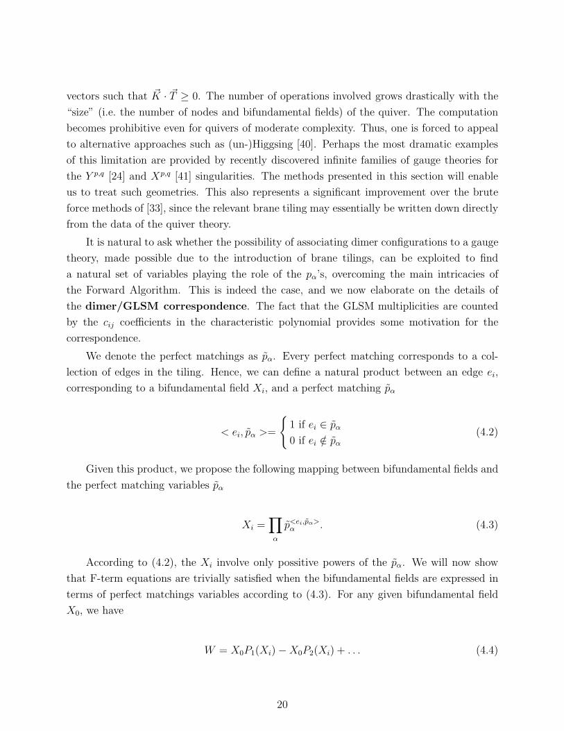
We denote the perfect matchings as pα. Every perfect matching corresponds to a col-

lection of edges in the tiling. Hence, we can define a natural product between an edge ei,

corresponding to a bifundamental field Xi, and a perfect matching pα

< ei, pα >=

{1 if ei ∈ pα

0 if ei /∈ pα

(4.2)

Given this product, we propose the following mapping between bifundamental fields and

the perfect matching variables pα

Xi =∏

α

p<ei,pα>α . (4.3)

According to (4.2), the Xi involve only possitive powers of the pα. We will now show

that F-term equations are trivially satisfied when the bifundamental fields are expressed in

terms of perfect matchings variables according to (4.3). For any given bifundamental field

X0, we have

W = X0P1(Xi) − X0P2(Xi) + . . . (4.4)

20

where we have singled out the two terms in the superpotential that involve X0. P1(Xi) and

P2(Xi) represent products of bifundamental fields. The F-term equation associated to X0

becomes

∂X0W = 0 ⇔ P1(Xi) = P2(Xi). (4.5)

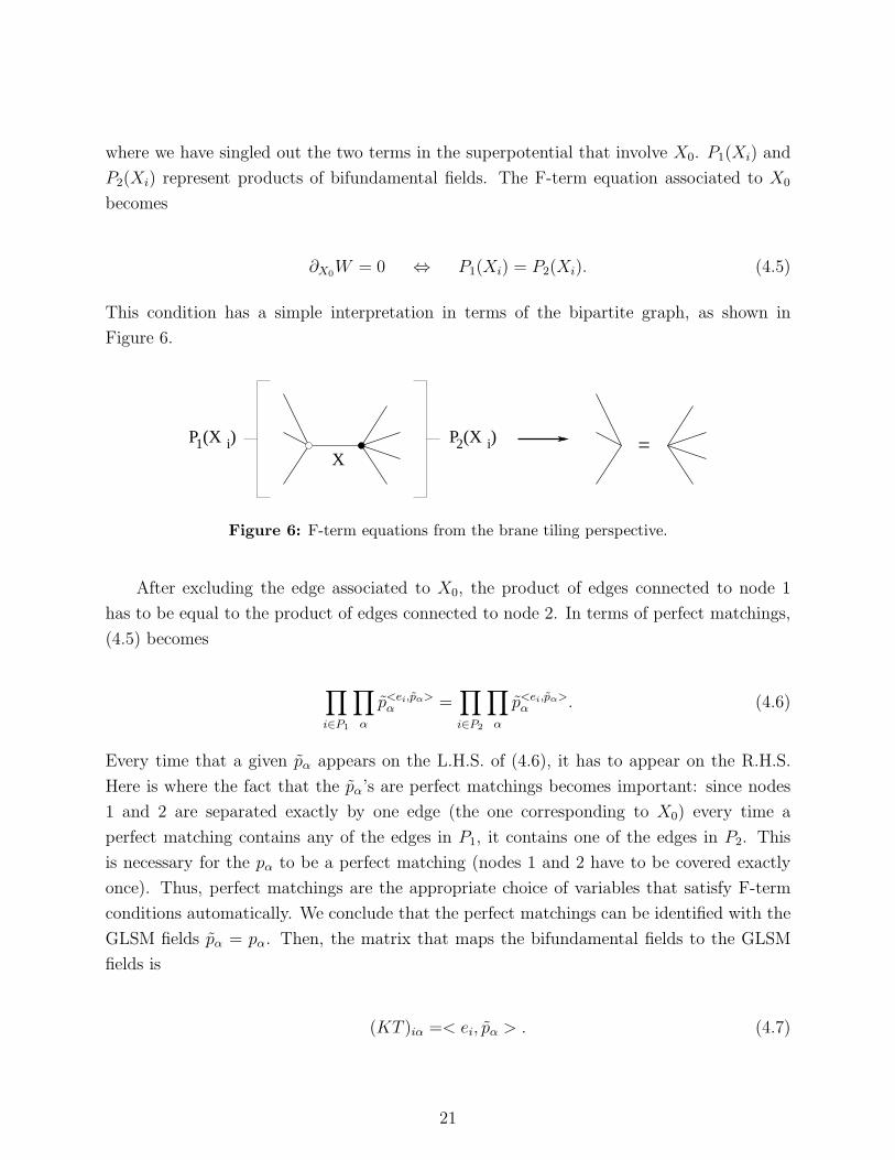
This condition has a simple interpretation in terms of the bipartite graph, as shown in

Figure 6.

P (X )1 iX

P (X )2 i =

Figure 6: F-term equations from the brane tiling perspective.

After excluding the edge associated to X0, the product of edges connected to node 1

has to be equal to the product of edges connected to node 2. In terms of perfect matchings,

(4.5) becomes

∏

i∈P1

∏

α

p<ei,pα>α =

∏

i∈P2

∏

α

p<ei,pα>α . (4.6)

Every time that a given pα appears on the L.H.S. of (4.6), it has to appear on the R.H.S.

Here is where the fact that the pα’s are perfect matchings becomes important: since nodes

1 and 2 are separated exactly by one edge (the one corresponding to X0) every time a

perfect matching contains any of the edges in P1, it contains one of the edges in P2. This

is necessary for the pα to be a perfect matching (nodes 1 and 2 have to be covered exactly

once). Thus, perfect matchings are the appropriate choice of variables that satisfy F-term

conditions automatically. We conclude that the perfect matchings can be identified with the

GLSM fields pα = pα. Then, the matrix that maps the bifundamental fields to the GLSM

fields is

(KT )iα =< ei, pα > . (4.7)

21

4.1 A detailed example: the Suspended Pinch Point

Let us illustrate the simplifications achieved by identifying GLSM fields with perfect match-

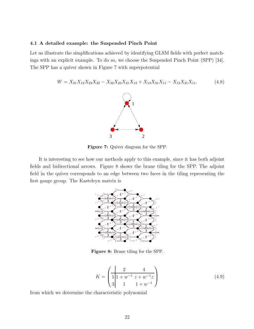
ings with an explicit example. To do so, we choose the Suspended Pinch Point (SPP) [34].

The SPP has a quiver shown in Figure 7 with superpotential

W = X21X12X23X32 − X32X23X31X13 + X13X31X11 − X12X21X11. (4.8)

1

3 2

Figure 7: Quiver diagram for the SPP.

It is interesting to see how our methods apply to this example, since it has both adjoint

fields and bidirectional arrows. Figure 8 shows the brane tiling for the SPP. The adjoint

field in the quiver corresponds to an edge between two faces in the tiling representing the

first gauge group. The Kasteleyn matrix is

3

1

3

3

1 3

13

1 3

1 3

1

11

13

1

3

3

1

2

2

22

2

22

22

2

Figure 8: Brane tiling for the SPP.

K =

2 4

1 1 + w−1 z + w−1z

3 1 1 + w−1

(4.9)

from which we determine the characteristic polynomial

22

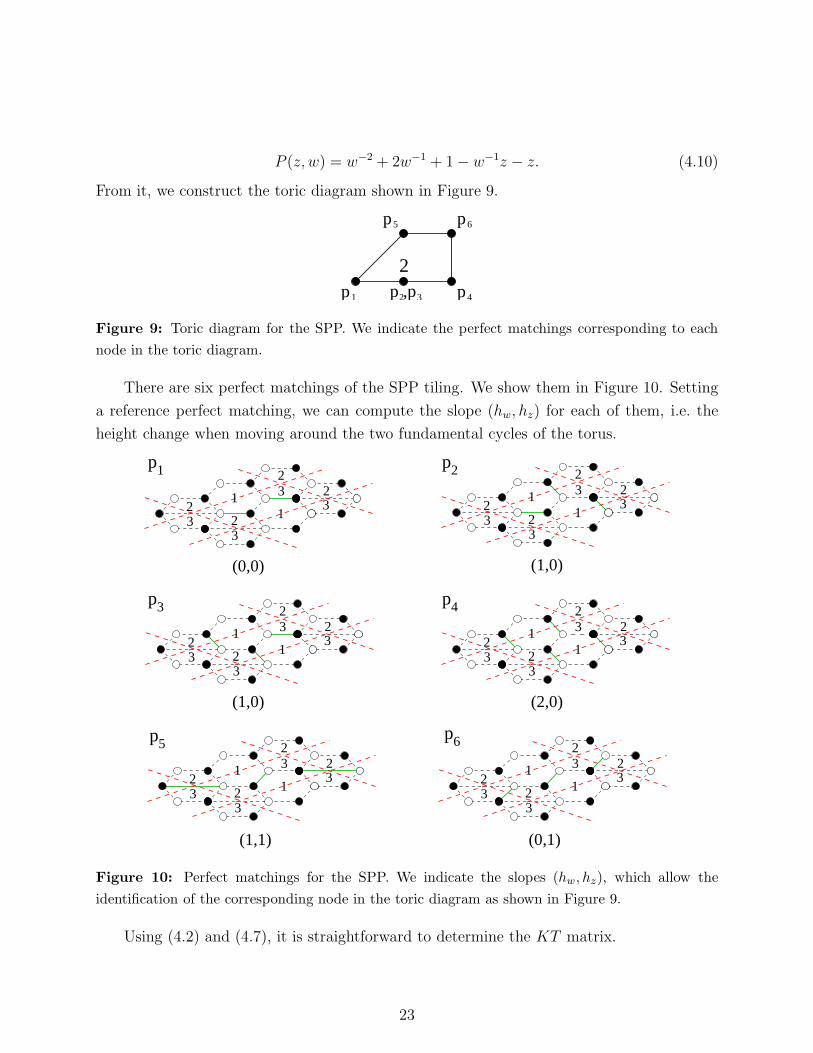
P (z, w) = w−2 + 2w−1 + 1 − w−1z − z. (4.10)

From it, we construct the toric diagram shown in Figure 9.

4

65

1 p

pp

p 2 3p ,p

2

Figure 9: Toric diagram for the SPP. We indicate the perfect matchings corresponding to each

node in the toric diagram.

There are six perfect matchings of the SPP tiling. We show them in Figure 10. Setting

a reference perfect matching, we can compute the slope (hw, hz) for each of them, i.e. the

height change when moving around the two fundamental cycles of the torus.

p43p

2pp1

5p p6

(2,0)(1,0)

(1,0)(0,0)

(1,1) (0,1)

32

2

223

3

1

31

32

2

223

3

1

31

32

2

223

3

1

3132

2

223

3

1

31

32

2

223

3

1

31

32

2

223

3

1

31

Figure 10: Perfect matchings for the SPP. We indicate the slopes (hw, hz), which allow the

identification of the corresponding node in the toric diagram as shown in Figure 9.

Using (4.2) and (4.7), it is straightforward to determine the KT matrix.

23

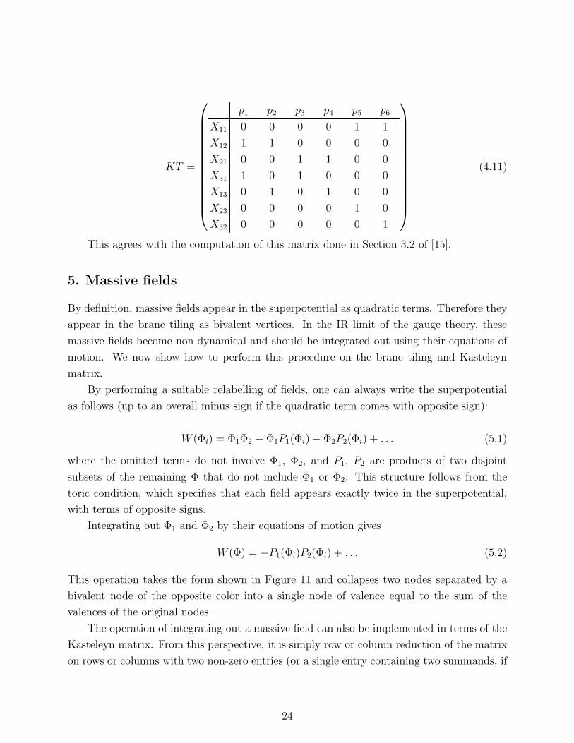
KT =

p1 p2 p3 p4 p5 p6

X11 0 0 0 0 1 1

X12 1 1 0 0 0 0

X21 0 0 1 1 0 0

X31 1 0 1 0 0 0

X13 0 1 0 1 0 0

X23 0 0 0 0 1 0

X32 0 0 0 0 0 1

(4.11)

This agrees with the computation of this matrix done in Section 3.2 of [15].

5. Massive fields

By definition, massive fields appear in the superpotential as quadratic terms. Therefore they

appear in the brane tiling as bivalent vertices. In the IR limit of the gauge theory, these

massive fields become non-dynamical and should be integrated out using their equations of

motion. We now show how to perform this procedure on the brane tiling and Kasteleyn

matrix.

By performing a suitable relabelling of fields, one can always write the superpotential

as follows (up to an overall minus sign if the quadratic term comes with opposite sign):

W (Φi) = Φ1Φ2 − Φ1P1(Φi) − Φ2P2(Φi) + . . . (5.1)

where the omitted terms do not involve Φ1, Φ2, and P1, P2 are products of two disjoint

subsets of the remaining Φ that do not include Φ1 or Φ2. This structure follows from the

toric condition, which specifies that each field appears exactly twice in the superpotential,

with terms of opposite signs.

Integrating out Φ1 and Φ2 by their equations of motion gives

W (Φ) = −P1(Φi)P2(Φi) + . . . (5.2)

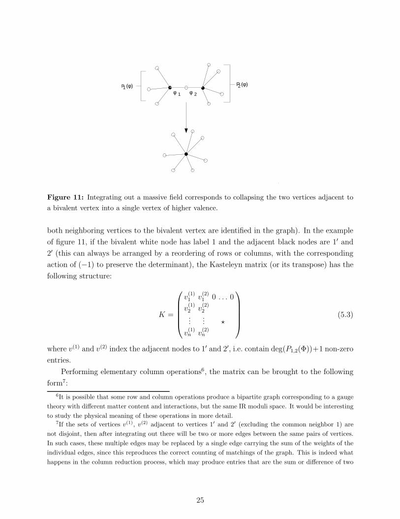
This operation takes the form shown in Figure 11 and collapses two nodes separated by a

bivalent node of the opposite color into a single node of valence equal to the sum of the

valences of the original nodes.

The operation of integrating out a massive field can also be implemented in terms of the

Kasteleyn matrix. From this perspective, it is simply row or column reduction of the matrix

on rows or columns with two non-zero entries (or a single entry containing two summands, if

24

φ 1 φ 2

P1 (φ P2 (φ) )

Figure 11: Integrating out a massive field corresponds to collapsing the two vertices adjacent to

a bivalent vertex into a single vertex of higher valence.

both neighboring vertices to the bivalent vertex are identified in the graph). In the example

of figure 11, if the bivalent white node has label 1 and the adjacent black nodes are 1′ and

2′ (this can always be arranged by a reordering of rows or columns, with the corresponding

action of (−1) to preserve the determinant), the Kasteleyn matrix (or its transpose) has the

following structure:

K =

v(1)1 v

(2)1 0 . . . 0

v(1)2 v

(2)2

...... ⋆

v(1)n v

(2)n

(5.3)

where v(1) and v(2) index the adjacent nodes to 1′ and 2′, i.e. contain deg(P1,2(Φ))+1 non-zero

entries.

Performing elementary column operations6, the matrix can be brought to the following

form7:

6It is possible that some row and column operations produce a bipartite graph corresponding to a gauge

theory with different matter content and interactions, but the same IR moduli space. It would be interesting

to study the physical meaning of these operations in more detail.7If the sets of vertices v(1), v(2) adjacent to vertices 1′ and 2′ (excluding the common neighbor 1) are

not disjoint, then after integrating out there will be two or more edges between the same pairs of vertices.

In such cases, these multiple edges may be replaced by a single edge carrying the sum of the weights of the

individual edges, since this reproduces the correct counting of matchings of the graph. This is indeed what

happens in the column reduction process, which may produce entries that are the sum or difference of two

25

K =

1 0 0 . . . 0

v(1)2 /v

(1)1 v

(2)2 v

(1)1 − v

(1)2 v

(2)1

...... ⋆

v(1)n /v

(1)1 v

(2)n v

(1)1 − v

(1)n v

(2)1

(5.4)

and therefore can be reduced in rank without changing the determinant, by deleting the first

row and column, giving the reduced Kasteleyn matrix

K =

v(2)2 v

(1)1 − v

(1)2 v

(2)1 ⋆ ⋆ . . .

... ⋆ ⋆ . . .

v(2)n v

(1)1 − v

(1)n v

(2)1 ⋆ ⋆ . . .

(5.5)

corresponding to the graph with bivalent vertex deleted.

6. Seiberg duality

6.1 Seiberg duality as a transformation of the quiver

We now discuss how one can understand Seiberg duality from the perspective of the brane

tilings. To motivate our construction, let us first recall what happens to a quiver theory

when performing Seiberg duality at a single node. This was first done for orbifold quivers

in [42]. Recall first that since Seiberg duality takes a given gauge group SU(Nc) with Nf

fundamentals and Nf anti-fundamentals to SU(Nf − Nc), if we want the dual quiver to

remain in a toric phase, we are only allowed to dualize on nodes with Nf = 2Nc. Dualizing

on such a node (call it I) is straightforward, and is done as follows:

• To decouple the dynamics of node I from the rest of the theory, the gauge couplings

of the other gauge groups and superpotential should be scaled to zero. The fields

corresponding to edges in the quiver that are not adjacent to I decouple, and the

edges between I and other nodes reduce from bifundamental matter to fundamental

matter transforming under a global flavor symmetry group. This reduces the theory to

the SQCD-like theory with 2Nc flavors and additional gauge singlets, to which Seiberg

duality may be applied.

• Next, reverse the direction of all arrows entering or exiting the dualized node. This is

because Seiberg duality requires that the dual quarks transform in the conjugate flavor

non-zero entries.

26

representations to the originals, and the other end of each bifundamental transforms

under a gauge group which acts as an effective flavor symmetry group. Because we want

to describe our theory with a quiver, we perform charge conjugation on the dualized

node to get back bifundamentals. This is exactly the same as reversing the arrows in

the quiver.

• Next, draw in Nf bifundamentals which correspond to composite (mesonic) operators

that are singlets at the dualized node I and carry flavor indices in the pairs nodes

connected to I. This is just the usual QiQj → M j

i “electric quark → meson” map of

Seiberg duality, but since each flavor group becomes gauged in the full quiver theory,

the Seiberg mesons are promoted to fields in the bifundamental representation of the

gauge groups.

• In the superpotential, replace any composite singlet operators with the new mesons,

and write down new terms corresponding to any new triangles formed by the operators

above. It is possible that this will make some fields massive (e.g. if a cubic term

becomes quadratic), in which case the appropriate fields should then be integrated

out.

6.2 Seiberg duality as a transformation of the brane tiling

By writing the action of Seiberg duality in the periodic quiver picture, one may derive the

corresponding transformation on the dual brane tiling. This operation may be encoded in a

transformation on the Kasteleyn matrix of the graph, and the recursive application of Seiberg

duality may be implemented by computer to traverse the Seiberg duality tree [43, 44] and

enumerate all toric phases 8.

Consider a node in the periodic quiver. For the toric phases of the quiver all nodes in

the quiver correspond to gauge groups of equal rank. If the node has 2 incoming arrows (and

therefore 2 outgoing arrows by anomaly cancellation, for a total of 4 arrows), then for this

gauge group Nf = 2Nc, and Seiberg duality maps

Nc 7→ Nc = Nf − Nc = Nc (6.1)

8Assuming this graph is connected. In fact, this is not allways the case and it is possible for the toric

phases to appear in disconnected (i.e. connected by non-toric phases) regions of the duality tree. A simple

example of this situation is given by the duality tree of dP1. This tree is presented in [43], where the

connected toric components where denoted “toric islands”. In addition, it is interesting to see that if the

theory is taken out of the conformal point by the addition of fractional branes, the cascading RG flow can

actually “migrate” among these islands [45].

27

so after the duality the theory remains in a toric phase.

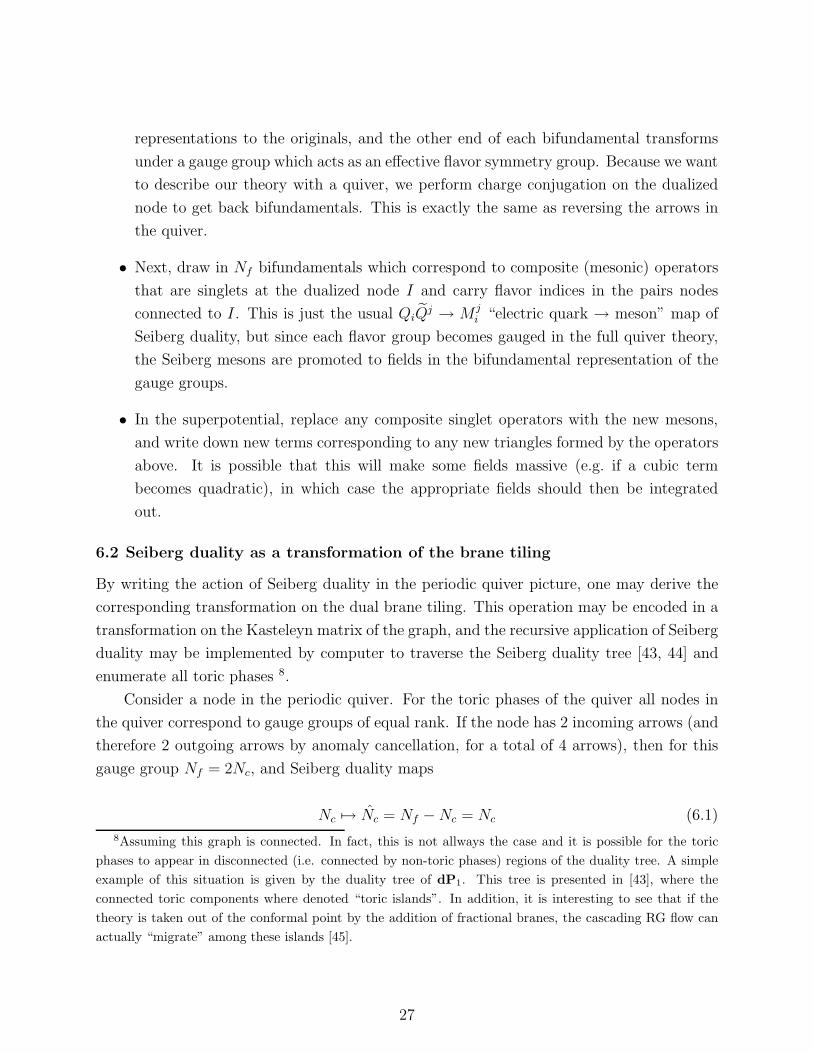
At such a node V , a generic quiver can be represented as in Figure 12. The 4 faces Fi

adjacent to V share an edge with their adjacent faces, and contain some number of additional

edges.

+

+

+

−

− −

−

+

−

−

++

Figure 12: The action of Seiberg duality on a periodic quiver to produce another toric phase of

the quiver. Also marked are the signs of superpotential terms, showing that the new terms (faces)

are consistent with the pre-existing 2-coloring of the global graph.

The neighboring vertices to V are not necessarily all distinct (they may be identified

by the periodicity of the torus on which the quiver lives). However by the periodic quiver

construction, if there are multiple fields in the quiver connecting the same two vertices, these

appear as distinct edges in the periodic quiver.

Note that the new mesons can only appear between adjacent vertices in the planar quiver,

because the edges connecting opposing vertices do not have a compatible orientation, so they

cannot form a holomorphic, gauge-invariant combination. There are indeed 4 such arrows

that can be drawn on the quiver corresponding to the 2 × 2 = 4 Seiberg mesons.

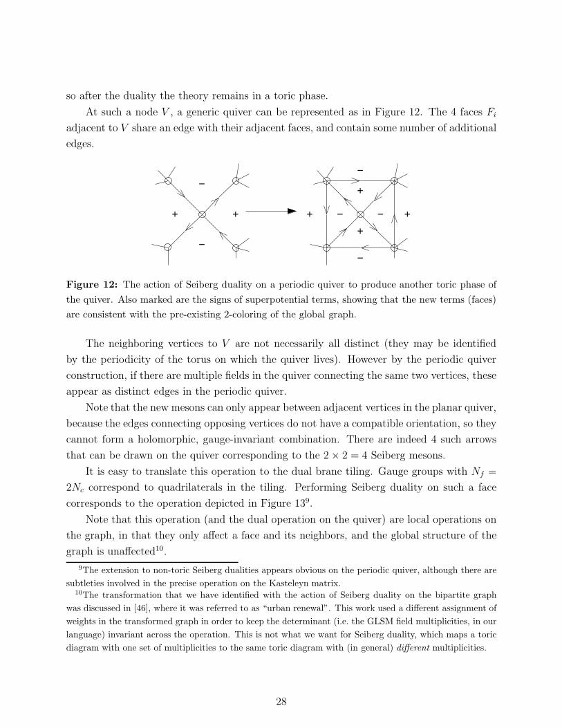
It is easy to translate this operation to the dual brane tiling. Gauge groups with Nf =

2Nc correspond to quadrilaterals in the tiling. Performing Seiberg duality on such a face

corresponds to the operation depicted in Figure 139.

Note that this operation (and the dual operation on the quiver) are local operations on

the graph, in that they only affect a face and its neighbors, and the global structure of the

graph is unaffected10.

9The extension to non-toric Seiberg dualities appears obvious on the periodic quiver, although there are

subtleties involved in the precise operation on the Kasteleyn matrix.10The transformation that we have identified with the action of Seiberg duality on the bipartite graph

was discussed in [46], where it was referred to as “urban renewal”. This work used a different assignment of

weights in the transformed graph in order to keep the determinant (i.e. the GLSM field multiplicities, in our

language) invariant across the operation. This is not what we want for Seiberg duality, which maps a toric

diagram with one set of multiplicities to the same toric diagram with (in general) different multiplicities.

28

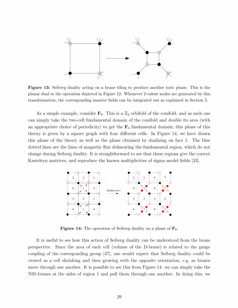
Figure 13: Seiberg duality acting on a brane tiling to produce another toric phase. This is the

planar dual to the operation depicted in Figure 12. Whenever 2-valent nodes are generated by this

transformation, the corresponding massive fields can be integrated out as explained in Section 5.

As a simple example, consider F0. This is a Z2 orbifold of the conifold, and as such one

can simply take the two-cell fundamental domain of the conifold and double its area (with

an appropriate choice of periodicity) to get the F0 fundamental domain; this phase of this

theory is given by a square graph with four different cells. In Figure 14, we have drawn

this phase of the theory as well as the phase obtained by dualizing on face 1. The blue

dotted lines are the lines of magnetic flux delineating the fundamental region, which do not

change during Seiberg duality. It is straightforward to see that these regions give the correct

Kasteleyn matrices, and reproduce the known multiplicities of sigma model fields [33].

Dualize on 1

��

��

��

��

��

��

��

��

��

��

��

��

��

��

��

��

��

��

��

��

��

��

��

��

��

��

��

��

��

��

��

��

��

��

1

1

2

2 3

33

3

4 4

44

1

1

2

2 3

33

3

4 4

44 1

2

1

2

��

Figure 14: The operation of Seiberg duality on a phase of F0.

It is useful to see how this action of Seiberg duality can be understood from the brane

perspective. Since the area of each cell (volume of the D-brane) is related to the gauge

coupling of the corresponding group [47], one would expect that Seiberg duality could be

viewed as a cell shrinking and then growing with the opposite orientation, e.g. as branes

move through one another. It is possible to see this from Figure 14: we can simply take the

NS5-branes at the sides of region 1 and pull them through one another. In doing this, we

29

generate the diagonal lines. Since we are in a toric phase with Nf = 2Nc, the ranks of the

gauge groups do not change in this crossing operation and no new branes are created.

6.3 Seiberg duality acting on the Kasteleyn matrix

Since the Kasteleyn matrix encodes all of the information about the graph, it is possible to

implement the transformation of Seiberg duality directly in terms of the matrix. The first

step is to identify the candidate (quadrilateral) faces to be dualized. These form a square in

the Kasteleyn matrix, e.g. :

K =

⋆ a ⋆ . . . b

⋆ ⋆ ⋆ . . . ⋆...

......

...

⋆ c ⋆ . . . d

⋆ ⋆ ⋆ . . . ⋆

(6.2)

However not all such squares represent the boundary of a face, e.g. on small enough graphs

there can be a closed path of 4 edges which winds around the torus (for a closed cycle of

4 edges there are no other possibilities, as there is no room for additional “internal” edges

that would allow the cycle to have zero winding but not bound a face of the graph). The

way to distinguish these cases is to use the magnetic flux through the cycle; if the cycle has

no net winding around the torus then the flux lines γz, γw must each cross the cycle twice:

once to enter and once to leave. Depending on the orientation with which they cross the

edges (which depends on the choice of paths γ and is therefore not invariant), they may each

contribute z or 1/z (similarly w or 1/w), but it is invariantly true that the product of the

edges must have even degree in both z and w. Conversely, a path with net winding around

the torus will have odd degree in one or both of z and w.

Having identified the four edges forming the quadrilateral to be dualized, we wish to

implement the transformation on the underlying graph depicted in Figure 13. This requires

the addition of 2 white and 2 black nodes to the graph, increasing the rank of the adjacency

matrix by 2. The large square is removed from the graph by setting to zero the four edges

a, b, c, d found previously, the smaller square is added in by setting to non-zero the weights

in the new 2 × 2 diagonal block, and the new smaller square is connected to the rest of the

graph by adding non-zero elements to the 2 × n and n × 2 blocks in the rows and columns

corresponding to the removed entries.

Since the new square has opposite orientation with respect to the large square, the power

of z and w along the edges must be inverted. This may change the normalization of the

30

determinant, so to correct this we can rescale a row by zdz and a column by wdw , where

dw,z = degw,z abcd. Finally, since the graph transformation adds 2 additional edges to each

of the 4 faces adjacent to the square, each of these faces must gain an additional minus sign

on one of the new edges bounding it, in order to satisfy the sign rules discussed in section 3.

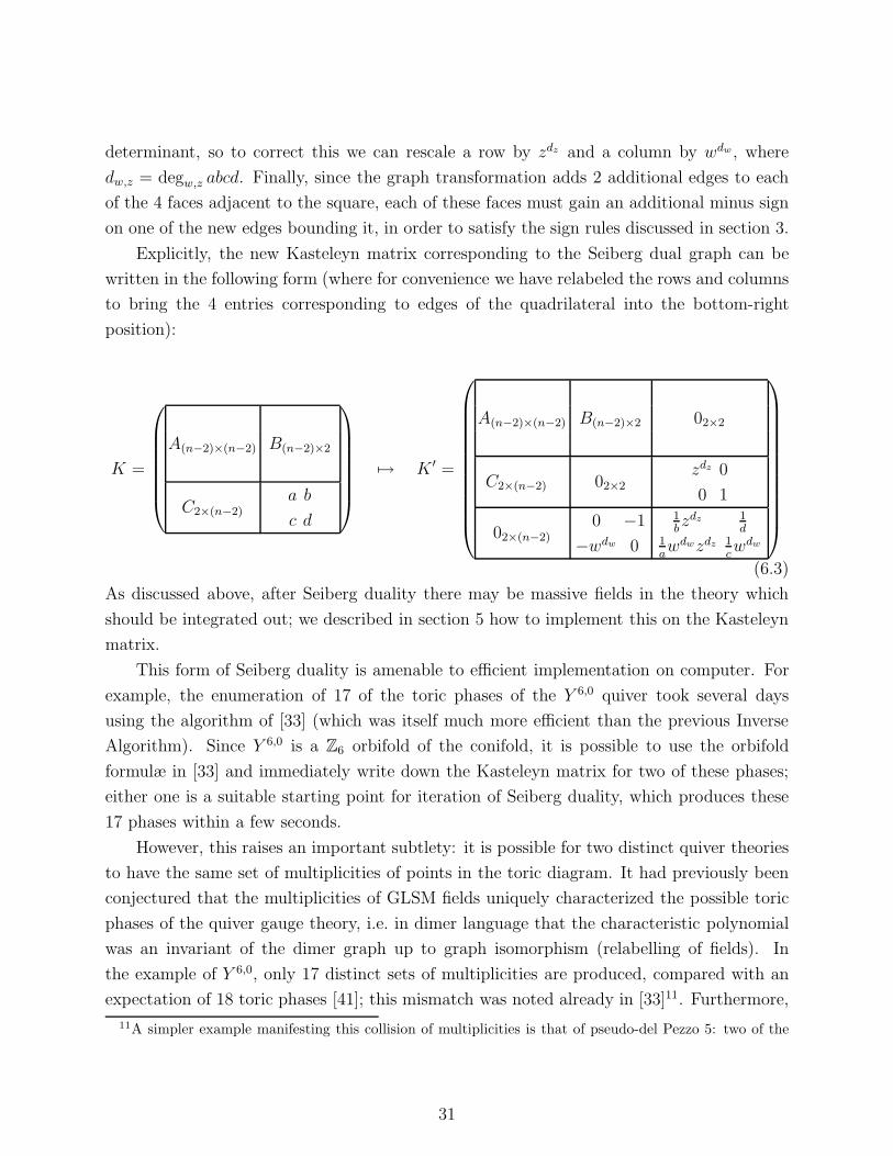
Explicitly, the new Kasteleyn matrix corresponding to the Seiberg dual graph can be

written in the following form (where for convenience we have relabeled the rows and columns

to bring the 4 entries corresponding to edges of the quadrilateral into the bottom-right

position):

K =

A(n−2)×(n−2) B(n−2)×2

C2×(n−2)a b

c d

7→ K ′ =

A(n−2)×(n−2) B(n−2)×2 02×2

C2×(n−2) 02×2zdz 0

0 1

02×(n−2)

0 −1

−wdw 0

1bzdz 1

d1awdwzdz 1

cwdw

(6.3)

As discussed above, after Seiberg duality there may be massive fields in the theory which

should be integrated out; we described in section 5 how to implement this on the Kasteleyn

matrix.

This form of Seiberg duality is amenable to efficient implementation on computer. For

example, the enumeration of 17 of the toric phases of the Y 6,0 quiver took several days

using the algorithm of [33] (which was itself much more efficient than the previous Inverse

Algorithm). Since Y 6,0 is a Z6 orbifold of the conifold, it is possible to use the orbifold

formulæ in [33] and immediately write down the Kasteleyn matrix for two of these phases;

either one is a suitable starting point for iteration of Seiberg duality, which produces these

17 phases within a few seconds.

However, this raises an important subtlety: it is possible for two distinct quiver theories

to have the same set of multiplicities of points in the toric diagram. It had previously been

conjectured that the multiplicities of GLSM fields uniquely characterized the possible toric

phases of the quiver gauge theory, i.e. in dimer language that the characteristic polynomial

was an invariant of the dimer graph up to graph isomorphism (relabelling of fields). In

the example of Y 6,0, only 17 distinct sets of multiplicities are produced, compared with an

expectation of 18 toric phases [41]; this mismatch was noted already in [33]11. Furthermore,

11A simpler example manifesting this collision of multiplicities is that of pseudo-del Pezzo 5: two of the

31

extending the set of data considered to include the set of orders of terms in the superpotential

(which can be read off from the Kasteleyn matrix independently of the field labelling), and

the set of neighboring toric phases that are reachable under Seiberg duality, still only distin-

guishes 17 distinct phases. By writing down the brane tilings explicitly and reconstructing

the quivers12, we were able to isolate the “missing” 18th phase and confirm that it indeed

has the same toric diagram with multiplicities as one of the remaining 17, but is nonetheless

a distinct quiver theory that is not equivalent under field redefinition. In addition, these two

phases have the same superpotential orders and Seiberg duality neighbors. In Section 9.2, we

will present a similar example in which two gauge theories produce the same toric diagram

and multiplicities, although in that case the superpotentials will have different orders and

numbers of terms.

How can we understand this situation? It is a known result in mathematics that the

characteristic polynomial (in the usual linear algebra sense) of the adjacency matrix of a

graph does not uniquely characterize the graph up to isomorphism: there may be two distinct

graphs with the same characteristic polynomial. The determinant of the Kasteleyn matrix of

the graph is essentially a double characteristic polynomial (due to the block structure of the

matrix, as explained in [33]), so the result explains the observed non-uniqueness of GLSM

multiplicities of the toric quivers. Similarly, it is believed that there exists no invariant of

a graph up to isomorphism that distinguishes between all non-isomorphic graphs. In other

words, the only invariant of a graph that characterizes it uniquely is the graph itself, and in

order to distinguish between the pathological cases where the would-be-invariants fail, one

must resort to explicit testing of graph isomorphism, which is an expensive (non-polynomial)

operation. Thus, the enumeration of toric phases by testing graph invariants such as the

characteristic polynomial can only produce a lower bound on the number of phases, and

in general there may be phases (or even entire regions of the toric duality graph) that are

missed by this counting.

7. Partial resolution

Many of the first known examples of gauge theories dual to toric geometries were described

by embedding them in orbifolds [15, 16, 17]. For example, partial resolutions of C3/Z3 ×Z3

give the first three del Pezzo theories and F0, among others. Partially resolving the orbifold

singularity corresponds to turning on Fayet-Iliopoulos terms in the dual gauge theory, which

four toric phases of this theory have the same multiplicities, as we discuss in section 9.12This work was done in conjunction with P. Kazakopoulos.

32

by the D-flatness conditions gives vacuum expectation values to bifundamental fields. These

vevs then reduce the rank of the gauge group via the Higgs mechanism. From the standpoint

of the toric diagram, this is simply removing an external point. Doing so decreases the area

of the toric diagram, and consequently decreases the number of gauge groups in the dual

superconformal theory.

It is straightforward to see how Higgsing operates from the perspective of the dimer

models. We give a non-zero vev to a bifundamental field, which reduces the two gauge group

factors under which the bifundamental is charged to the diagonal combination. Hence,

Higgsing is nothing more than the removal of an edge from the fundamental region of the

graph, which causes two faces of the graph to become one.

This method was used in [33] to obtain the bipartite graphs corresponding to an arbitrary

toric singularity, but the algorithm presented was computationally expensive since it was

unknown how to identify the desired Higgsing in the quiver side. Using the duality between

the quivers and brane tilings, it is straightforward to identify the edge of the bipartite graph

to be removed that corresponds to the Higgsing of any given field in the quiver. Thus, the

relations between quiver theories under Higgsing may be easily followed on the dual brane

tiling, avoiding any computational difficulties.

Let us begin with Model I of dP3, since we have already studied this tiling in a previous

section. Since this model is perfectly symmetric and contains only single bifundamental

field between any two gauge groups, giving a vev to any field should result in the same

theory. This theory is dP2, which has five nodes in its quiver. One can easily check that

removing any edge from this tiling for dP3 results in the expected gauge theory. Figure 15

illustrates this process: removing the edge between regions 5 and 6 is equivalent to removing

the bifundamental between the corresponding nodes.

The example of taking Model I of dP3 to one of the two toric phases of dP2 (called

Model II in [20]) is particularly simple, since no fields acquire a mass when X56 gets a vev.

It is not any more difficult to see what happens when bifundamentals do become massive, as

we can see by considering the dP2 example. We know that the dP2 theory can be Higgsed

to either dP1 or F0; this corresponds to giving a vev to X34 (or equivalently X12 by the

symmetry of the quiver) or X23, respectively. In the brane tiling, we delete the edge between

regions 2 and 3 of the tiling. This puts an isolated node between the two regions. As per our

discussion in Section 5, we then simply collapse those two edges to a point, which corresponds

to integrating out the fields X35 and X52. See Figure 16.

We expect from string theory that we may embed any toric quiver in an appropriately

large Abelian orbifold theory of the form C3/Zm×Zn. The tiling for C3/Zm×Zn is hexagonal,

33

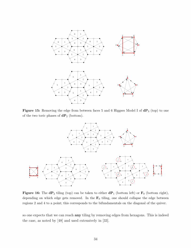
5

��

��

��

��

��

��

��

��

��

��

��

��

��

��

��

��

��

��

��

��

��

��

��

��

��

��

��

��

��

��

��

��

��

��

��

��

��

��

��

��

��

��

��

��

��

��

��

��

��

��

��

��

��

��

��

��

��

��

��

��

��

��

��

��

��

��

��

��

��

��

��

��

��

��

��

��

��

��

��

��

��

��

��

��

��

��

��

��

��

��

��

��

��

��

��

��

��

��

��

��

��

��

��

��

��

��

��

��

��

��

��

��

��

��

��

��

��

��

��

��

��

��

��

��

��

��

1

2

34

5

6

1

11

2

22

3

33

4

44

5

5

5

6

6

6

��

��

��

��

��

��

��

��

��

��

��

��

��

��

��

��

��

��

��

��

��

��

��

��

��

��

��

��

��

��

��

��

��

��

��

��

��

��

��

��

��

��

��

��

��

��

��

��

��

��

��

��

��

��

��

��

��

��

��

��

��

��

��

��

��

��

��

��

��

��

��

��

��

��

��

��

��

��

��

��

��

��

��

��

��

��

��

��

��

��

��

��

��

��

��

��

��

��

��

��

��

��

��

��

��

��

��

��

��

��

��

��

��

��

��

1

2

34

1

11

2

22

3

33

4

44

5

5

5

5

5 6

2

4

3

1

1

23

4

��

��

Figure 15: Removing the edge from between faces 5 and 6 Higgses Model I of dP3 (top) to one

of the two toric phases of dP2 (bottom).

4

��

��

��

��

��

��

��

��

��

��

��

��

��

��

��

��

��

��

��

��

��

��

��

��

��

��

��

��

��

��

��

��

��

��

��

��

��

��

��

��

��

��

��

��

��

��

��

��

��

��

��

��

��

��

��

��

��

��

��

��

��

��

��

��

��

��

��

��

��

��

��

��

��

��

��

��

��

��

��

��

��

1

2

34

1

11

2

22

3

33

4

44

5

5

5

5 1

23

4

5

1 2

34

1 2

34

��

��

��

��

��

��

��

��

��

��

��

��

��

��

��

��

��

��

��

��

��

��

��

��

��

��

��

��

��

��

��

��

��

��

��

��

��

��

��

��

��

��

��

��

��

��

��

��

��

��

��

��

��

��

��

��

��

��

��

��

��

��

��

��

��

��

��

��

��

��

��

��

��

��

��

��

��

��

��

��

��

��

��

��

��

��

��

��

��

��

��

��

��

��

��

��

��

��

��

��

��

��

��

��

��

��

��

��

��

��

��

��

��

��

��

��

��

��

��

��

��

��

��

��

��

��

��

��

��

��

��

��

��

��

��

��

��

��

��

��

��

��

��

��

��

��

��

��

��

��

��

��

��

��

��

��

��

��

��

��

��

��

��

��

��

��

��

��

��

��

��

��

��

��

��

��

��

��

��

��

��

��

��

��

��

��

��

��

��

��

��

��

��

��

��

��

��

��

��

��

��

��

��

��

��

��

��

1

2

1

11

2

22

1

1

11

3

4

4

43

3

3

4

3

2

4

32

4

32

4

32

��

Figure 16: The dP2 tiling (top) can be taken to either dP1 (bottom left) or F0 (bottom right),

depending on which edge gets removed. In the F0 tiling, one should collapse the edge between

regions 2 and 4 to a point; this corresponds to the bifundamentals on the diagonal of the quiver.

so one expects that we can reach any tiling by removing edges from hexagons. This is indeed

the case, as noted by [48] and used extensively in [33].

34

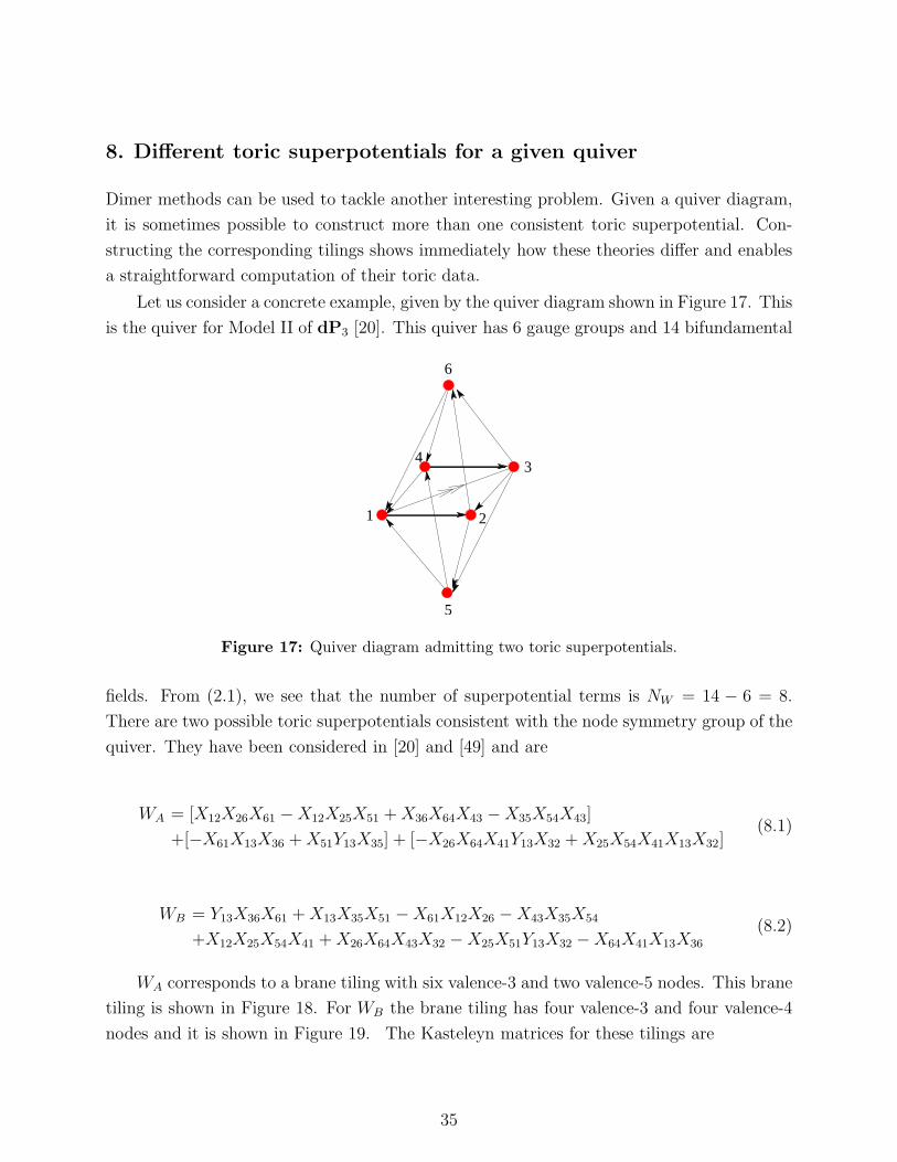
8. Different toric superpotentials for a given quiver

Dimer methods can be used to tackle another interesting problem. Given a quiver diagram,

it is sometimes possible to construct more than one consistent toric superpotential. Con-

structing the corresponding tilings shows immediately how these theories differ and enables

a straightforward computation of their toric data.

Let us consider a concrete example, given by the quiver diagram shown in Figure 17. This

is the quiver for Model II of dP3 [20]. This quiver has 6 gauge groups and 14 bifundamental

2

43

1

5

6

Figure 17: Quiver diagram admitting two toric superpotentials.

fields. From (2.1), we see that the number of superpotential terms is NW = 14 − 6 = 8.

There are two possible toric superpotentials consistent with the node symmetry group of the

quiver. They have been considered in [20] and [49] and are

WA = [X12X26X61 − X12X25X51 + X36X64X43 − X35X54X43]

+[−X61X13X36 + X51Y13X35] + [−X26X64X41Y13X32 + X25X54X41X13X32](8.1)

WB = Y13X36X61 + X13X35X51 − X61X12X26 − X43X35X54

+X12X25X54X41 + X26X64X43X32 − X25X51Y13X32 − X64X41X13X36

(8.2)

WA corresponds to a brane tiling with six valence-3 and two valence-5 nodes. This brane

tiling is shown in Figure 18. For WB the brane tiling has four valence-3 and four valence-4

nodes and it is shown in Figure 19. The Kasteleyn matrices for these tilings are

35

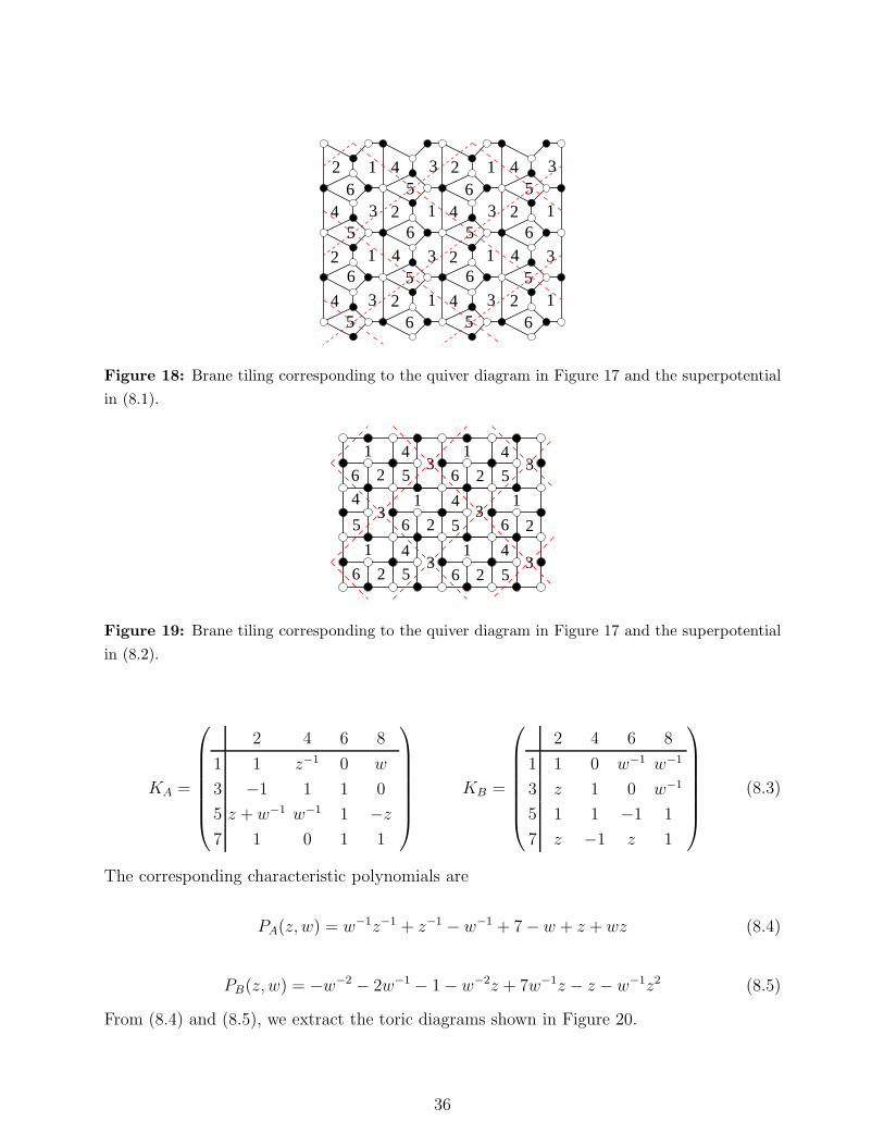
5

6

6

5

3

1

3

15

6

6

5

3

1

3

1

4

2

2

4

3

1

3

1

5

6

5

62

4

2

4

4

2

23

1

3

1 4

5

6

5

62

4

2

4

Figure 18: Brane tiling corresponding to the quiver diagram in Figure 17 and the superpotential

in (8.1).

34

1 43

26

35

1

6 2 5

4

6 2

31

6 2 53

4

65 2

141

6 2 53

41

5

Figure 19: Brane tiling corresponding to the quiver diagram in Figure 17 and the superpotential

in (8.2).

KA =

2 4 6 8

1 1 z−1 0 w

3 −1 1 1 0

5 z + w−1 w−1 1 −z

7 1 0 1 1

KB =

2 4 6 8

1 1 0 w−1 w−1

3 z 1 0 w−1

5 1 1 −1 1

7 z −1 z 1

(8.3)

The corresponding characteristic polynomials are

PA(z, w) = w−1z−1 + z−1 − w−1 + 7 − w + z + wz (8.4)

PB(z, w) = −w−2 − 2w−1 − 1 − w−2z + 7w−1z − z − w−1z2 (8.5)

From (8.4) and (8.5), we extract the toric diagrams shown in Figure 20.

36

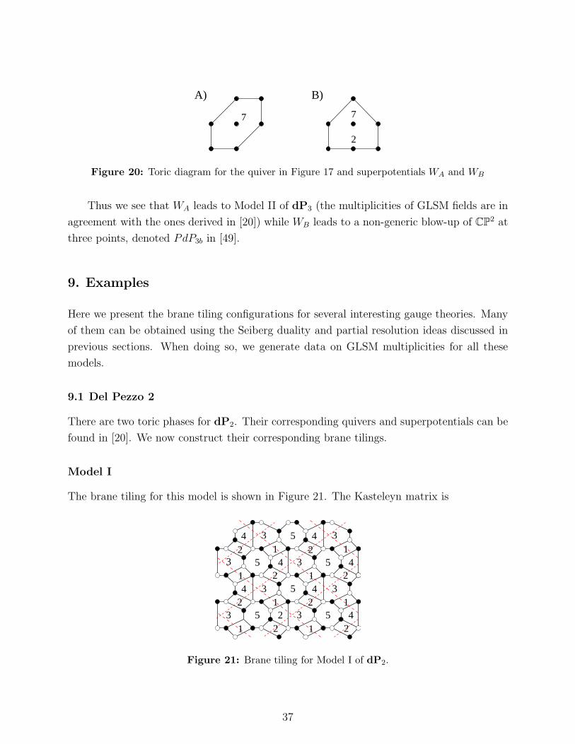
7

2

A) B)

7

Figure 20: Toric diagram for the quiver in Figure 17 and superpotentials WA and WB

Thus we see that WA leads to Model II of dP3 (the multiplicities of GLSM fields are in

agreement with the ones derived in [20]) while WB leads to a non-generic blow-up of CP2 at

three points, denoted PdP3b in [49].

9. Examples

Here we present the brane tiling configurations for several interesting gauge theories. Many

of them can be obtained using the Seiberg duality and partial resolution ideas discussed in

previous sections. When doing so, we generate data on GLSM multiplicities for all these

models.

9.1 Del Pezzo 2

There are two toric phases for dP2. Their corresponding quivers and superpotentials can be

found in [20]. We now construct their corresponding brane tilings.

Model I

The brane tiling for this model is shown in Figure 21. The Kasteleyn matrix is

25

5 5

5

5

5

2

2 2

2

22

2

2

2

1

1

1

1

1

1

1

14

44

4

4

443

3

3

3

3

3

3

3

Figure 21: Brane tiling for Model I of dP2.

37

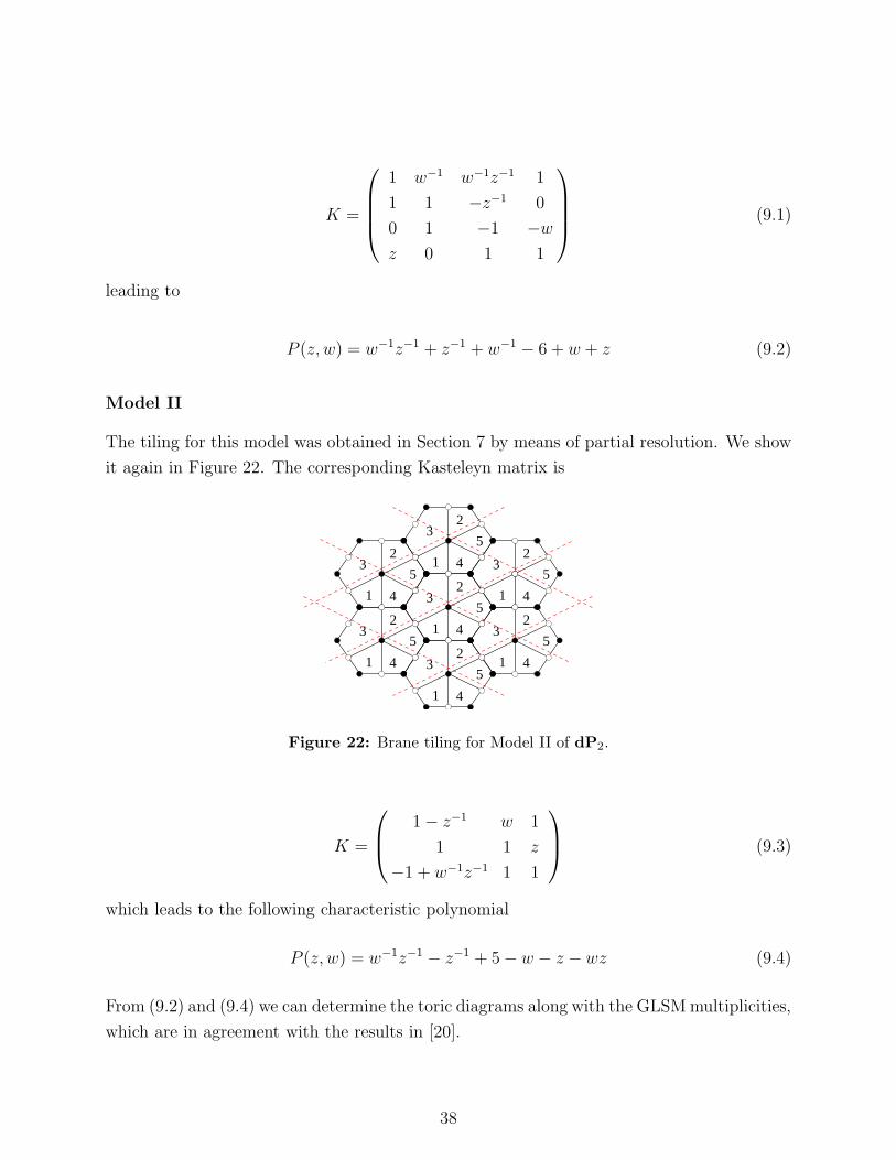
K =

1 w−1 w−1z−1 1

1 1 −z−1 0

0 1 −1 −w

z 0 1 1

(9.1)

leading to

P (z, w) = w−1z−1 + z−1 + w−1 − 6 + w + z (9.2)

Model II

The tiling for this model was obtained in Section 7 by means of partial resolution. We show

it again in Figure 22. The corresponding Kasteleyn matrix is

2

4

5

1

3

2

4

5

1

3

2

4

5

1

3

2

4

5

1

3

2

4

5

1

32

4

5

1

3

2

4

5

1

3

Figure 22: Brane tiling for Model II of dP2.

K =

1 − z−1 w 1

1 1 z

−1 + w−1z−1 1 1

(9.3)

which leads to the following characteristic polynomial

P (z, w) = w−1z−1 − z−1 + 5 − w − z − wz (9.4)

From (9.2) and (9.4) we can determine the toric diagrams along with the GLSM multiplicities,

which are in agreement with the results in [20].

38

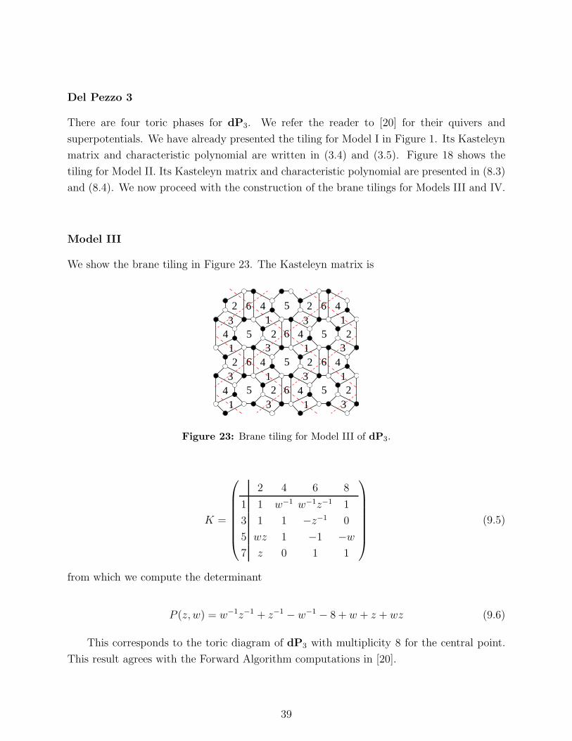
Del Pezzo 3

There are four toric phases for dP3. We refer the reader to [20] for their quivers and

superpotentials. We have already presented the tiling for Model I in Figure 1. Its Kasteleyn

matrix and characteristic polynomial are written in (3.4) and (3.5). Figure 18 shows the

tiling for Model II. Its Kasteleyn matrix and characteristic polynomial are presented in (8.3)

and (8.4). We now proceed with the construction of the brane tilings for Models III and IV.

Model III

We show the brane tiling in Figure 23. The Kasteleyn matrix is

2 4

4 2

42

24

2

4 2

42

24

46 5 63 1 3 1

65 51 3 1 3

6 5 63 1 3 1

5 6 51 3 1 3

Figure 23: Brane tiling for Model III of dP3.

K =

2 4 6 8

1 1 w−1 w−1z−1 1

3 1 1 −z−1 0

5 wz 1 −1 −w

7 z 0 1 1

(9.5)

from which we compute the determinant

P (z, w) = w−1z−1 + z−1 − w−1 − 8 + w + z + wz (9.6)

This corresponds to the toric diagram of dP3 with multiplicity 8 for the central point.

This result agrees with the Forward Algorithm computations in [20].

39

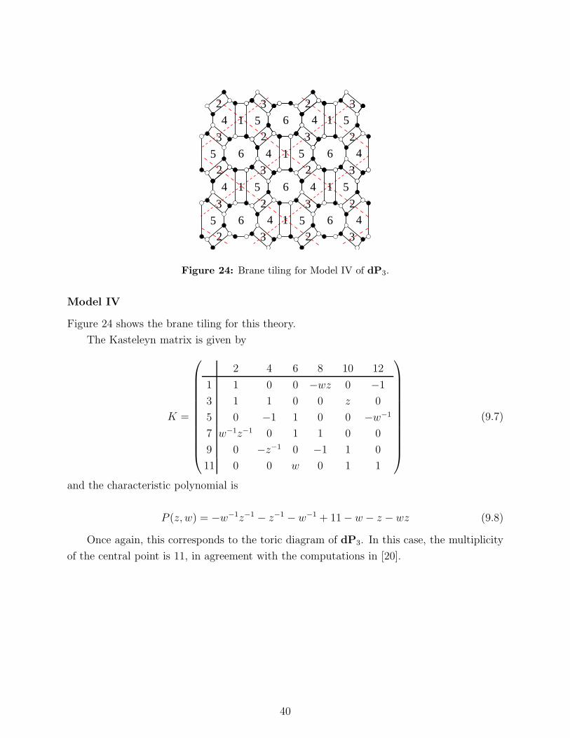
1

1

1

1

1 6

1

2 3 2 34 5 6 4 5

3 2 3 2

65 4 5 4

2 3 2 3

4 5 4 5

3 2 3 2

5 6 4 5 6 4

2 3 2 3

6

Figure 24: Brane tiling for Model IV of dP3.

Model IV

Figure 24 shows the brane tiling for this theory.

The Kasteleyn matrix is given by

K =

2 4 6 8 10 12

1 1 0 0 −wz 0 −1

3 1 1 0 0 z 0

5 0 −1 1 0 0 −w−1

7 w−1z−1 0 1 1 0 0

9 0 −z−1 0 −1 1 0

11 0 0 w 0 1 1

(9.7)

and the characteristic polynomial is

P (z, w) = −w−1z−1 − z−1 − w−1 + 11 − w − z − wz (9.8)

Once again, this corresponds to the toric diagram of dP3. In this case, the multiplicity

of the central point is 11, in agreement with the computations in [20].

40

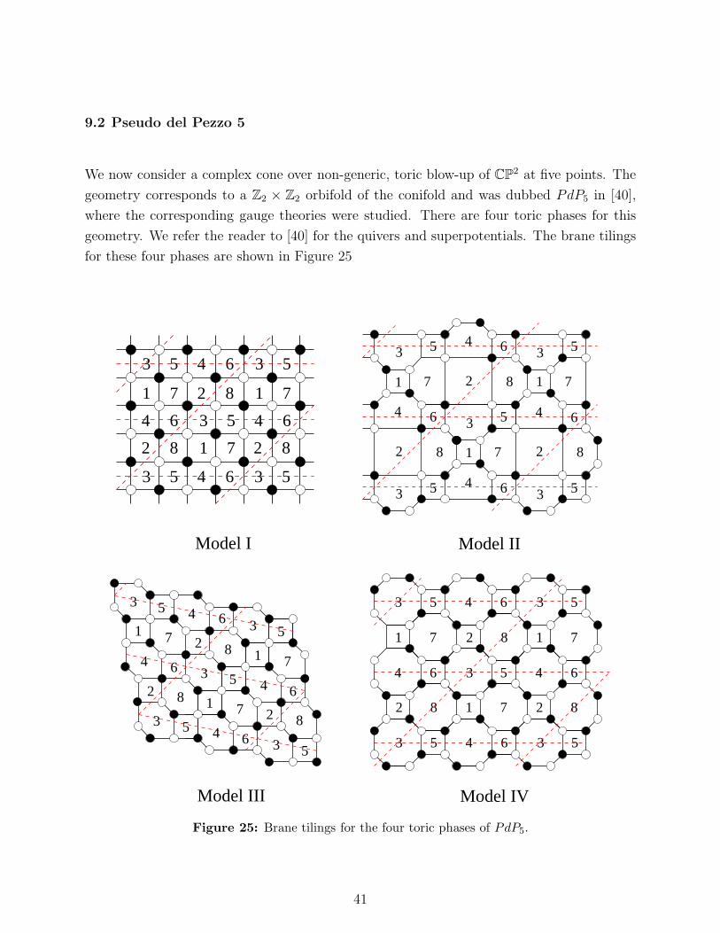
9.2 Pseudo del Pezzo 5

We now consider a complex cone over non-generic, toric blow-up of CP2 at five points. The

geometry corresponds to a Z2 × Z2 orbifold of the conifold and was dubbed PdP5 in [40],

where the corresponding gauge theories were studied. There are four toric phases for this

geometry. We refer the reader to [40] for the quivers and superpotentials. The brane tilings

for these four phases are shown in Figure 25

364 5 64

821 7

82

82

643 5 3 5

643 5 3 5

711 7

5364

2 8 1 7

2 8 1 7

536453

536453

4 6

2 8

2 82 18 7

3 5 4 6

3 5

3 5

1 7

3 5 3 5

1 7

4 6 4 6

12 8

71 7

5364

53

4 6 3 5 4 62 8 1 7 2 83 5 4 6 3 5

Model IIModel I

Model III Model IV

1 7

64

2 8

Figure 25: Brane tilings for the four toric phases of PdP5.

41

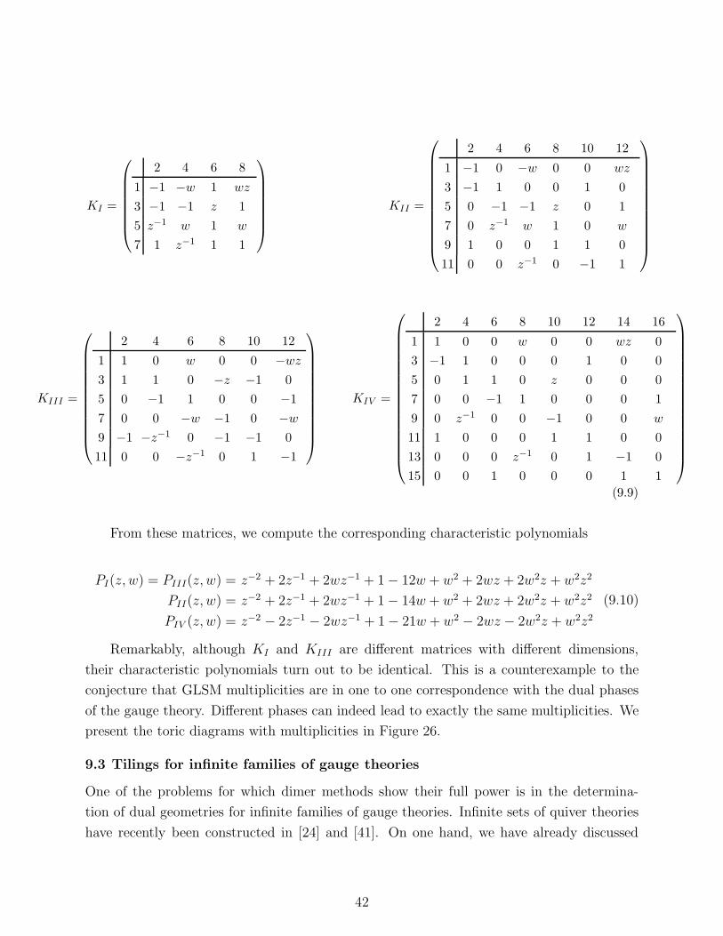
KI =

2 4 6 8

1 −1 −w 1 wz

3 −1 −1 z 1

5 z−1 w 1 w

7 1 z−1 1 1

KII =

2 4 6 8 10 12

1 −1 0 −w 0 0 wz

3 −1 1 0 0 1 0

5 0 −1 −1 z 0 1

7 0 z−1 w 1 0 w

9 1 0 0 1 1 0

11 0 0 z−1 0 −1 1

KIII =

2 4 6 8 10 12

1 1 0 w 0 0 −wz

3 1 1 0 −z −1 0

5 0 −1 1 0 0 −1

7 0 0 −w −1 0 −w

9 −1 −z−1 0 −1 −1 0

11 0 0 −z−1 0 1 −1

KIV =

2 4 6 8 10 12 14 16

1 1 0 0 w 0 0 wz 0

3 −1 1 0 0 0 1 0 0

5 0 1 1 0 z 0 0 0

7 0 0 −1 1 0 0 0 1

9 0 z−1 0 0 −1 0 0 w

11 1 0 0 0 1 1 0 0

13 0 0 0 z−1 0 1 −1 0

15 0 0 1 0 0 0 1 1

(9.9)

From these matrices, we compute the corresponding characteristic polynomials

PI(z, w) = PIII(z, w) = z−2 + 2z−1 + 2wz−1 + 1 − 12w + w2 + 2wz + 2w2z + w2z2

PII(z, w) = z−2 + 2z−1 + 2wz−1 + 1 − 14w + w2 + 2wz + 2w2z + w2z2

PIV (z, w) = z−2 − 2z−1 − 2wz−1 + 1 − 21w + w2 − 2wz − 2w2z + w2z2

(9.10)

Remarkably, although KI and KIII are different matrices with different dimensions,

their characteristic polynomials turn out to be identical. This is a counterexample to the

conjecture that GLSM multiplicities are in one to one correspondence with the dual phases

of the gauge theory. Different phases can indeed lead to exactly the same multiplicities. We

present the toric diagrams with multiplicities in Figure 26.

9.3 Tilings for infinite families of gauge theories

One of the problems for which dimer methods show their full power is in the determina-

tion of dual geometries for infinite families of gauge theories. Infinite sets of quiver theories

have recently been constructed in [24] and [41]. On one hand, we have already discussed

42

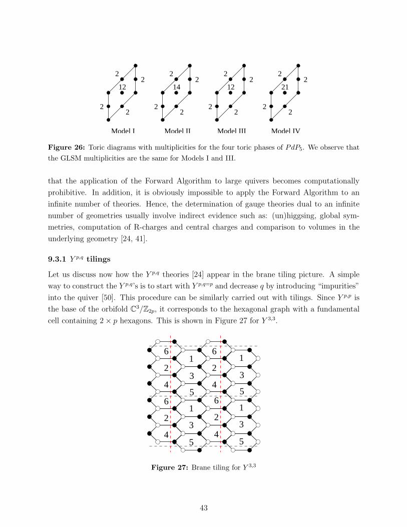
142

22

2

122

22

2

212

22

2

Model II

122

22

2

Model I Model III Model IV

Figure 26: Toric diagrams with multiplicities for the four toric phases of PdP5. We observe that

the GLSM multiplicities are the same for Models I and III.

that the application of the Forward Algorithm to large quivers becomes computationally

prohibitive. In addition, it is obviously impossible to apply the Forward Algorithm to an

infinite number of theories. Hence, the determination of gauge theories dual to an infinite

number of geometries usually involve indirect evidence such as: (un)higgsing, global sym-

metries, computation of R-charges and central charges and comparison to volumes in the

underlying geometry [24, 41].

9.3.1 Y p,q tilings

Let us discuss now how the Y p,q theories [24] appear in the brane tiling picture. A simple

way to construct the Y p,q’s is to start with Y p,q=p and decrease q by introducing “impurities”

into the quiver [50]. This procedure can be similarly carried out with tilings. Since Y p,p is

the base of the orbifold C3/Z2p, it corresponds to the hexagonal graph with a fundamental

cell containing 2 × p hexagons. This is shown in Figure 27 for Y 3,3.

5

3

1

5

3

1

5

3

1

5

3

1

6

4

2

6

2

4

6

2

4

6

2

4

Figure 27: Brane tiling for Y 3,3

43

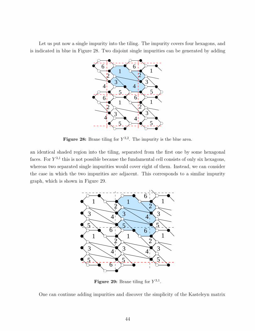
Let us put now a single impurity into the tiling. The impurity covers four hexagons, and

is indicated in blue in Figure 28. Two disjoint single impurities can be generated by adding

6

45

1

5

1

5

1

5

12

23

3 3

3

6

2

2

4

6 6

44

Figure 28: Brane tiling for Y 3,2. The impurity is the blue area.

an identical shaded region into the tiling, separated from the first one by some hexagonal

faces. For Y 3,1 this is not possible because the fundamental cell consists of only six hexagons,

whereas two separated single impurities would cover eight of them. Instead, we can consider

the case in which the two impurities are adjacent. This corresponds to a similar impurity

graph, which is shown in Figure 29.

1

5

23

61

5

3 4

5

3 4

12

6

5

3 4

12

6

61 1

5 5

23 4 3

Figure 29: Brane tiling for Y 3,1.

One can continue adding impurities and discover the simplicity of the Kasteleyn matrix

44

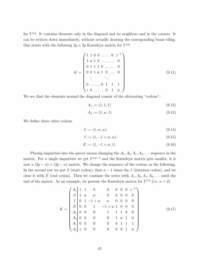
for Y p,q. It contains elements only in the diagonal and its neighbors and in the corners. It

can be written down immediately, without actually drawing the corresponding brane tiling.

One starts with the following 2p × 2p Kasteleyn matrix for Y p,p.

K =

1 1 0 0 . . . . 0 z−1

1 w 1 0 . . . . . . . . 0

0 1 1 1 0 . . . . . . 0

0 0 1 w 1 0 . . . 0...

. . .

0 . . . . . . 0 1 1 1

z 0 . . . . . 0 1 w

(9.11)

We see that the elements around the diagonal consist of the alternating “codons”:

A1 := (1, 1, 1) (9.12)

A2 := (1, w, 1) (9.13)

We define three other codons

S := (1, w, w) (9.14)

I := (1,−1 + w, w) (9.15)

E := (1,−1 + w, 1) (9.16)

Placing impurities into the quiver means changing the A1, A2, A1, A2, . . . sequence in the

matrix. For n single impurities we get Y p,p−n and the Kasteleyn matrix gets smaller, it is

now a (2p − n) × (2p − n) matrix. We change the sequence of the codons as the following.

In the second row we put S (start codon), then n − 1 times the I (iteration codon), and we

close it with E (end codon). Then we continue the series with A1, A2, A1, A2, . . . until the

end of the matrix. As an example, we present the Kasteleyn matrix for Y 5,3 (i.e. n = 2)

K =

A1 1 1 0 0 0 0 0 z−1

S 1 w w 0 0 0 0 0

I 0 1 −1 + w w 0 0 0 0

E 0 0 1 −1 + w 1 0 0 0

A1 0 0 0 1 1 1 0 0

A2 0 0 0 0 1 w 1 0

A1 0 0 0 0 0 1 1 1

A2 z 0 0 0 0 0 1 w

(9.17)

45

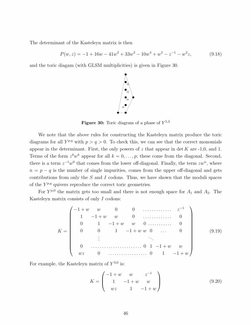
The determinant of the Kasteleyn matrix is then

P (w, z) = −1 + 16w − 41w2 + 33w3 − 10w4 + w5 − z−1 − w2z, (9.18)

and the toric diagam (with GLSM multiplicities) is given in Figure 30.

10

33

41

16

Figure 30: Toric diagram of a phase of Y 5,3

We note that the above rules for constructing the Kasteleyn matrix produce the toric

diagrams for all Y p,q with p > q > 0. To check this, we can see that the correct monomials

appear in the determinant. First, the only powers of z that appear in det K are -1,0, and 1.

Terms of the form z0wk appear for all k = 0, . . . , p; these come from the diagonal. Second,

there is a term z−1w0 that comes from the lower off-diagonal. Finally, the term zwn, where

n = p − q is the number of single impurities, comes from the upper off-diagonal and gets

contributions from only the S and I codons. Thus, we have shown that the moduli spaces

of the Y p,q quivers reproduce the correct toric geometries.

For Y p,0 the matrix gets too small and there is not enough space for A1 and A2. The

Kasteleyn matrix consists of only I codons:

K =

−1 + w w 0 0 . . . . . . . . . . . . . z−1

1 −1 + w w 0 . . . . . . . . . . . . . 0

0 1 −1 + w w 0 . . . . . . . . . . . 0

0 0 1 −1 + w w 0 . . . 0...

. . .

0 . . . . . . . . . . . . . . . . . . . . . . . 0 1 −1 + w w

wz 0 . . . . . . . . . . . . . . . . . . 0 1 −1 + w

(9.19)

For example, the Kasteleyn matrix of Y 3,0 is:

K =

−1 + w w z−1

1 −1 + w w

wz 1 −1 + w

(9.20)

46

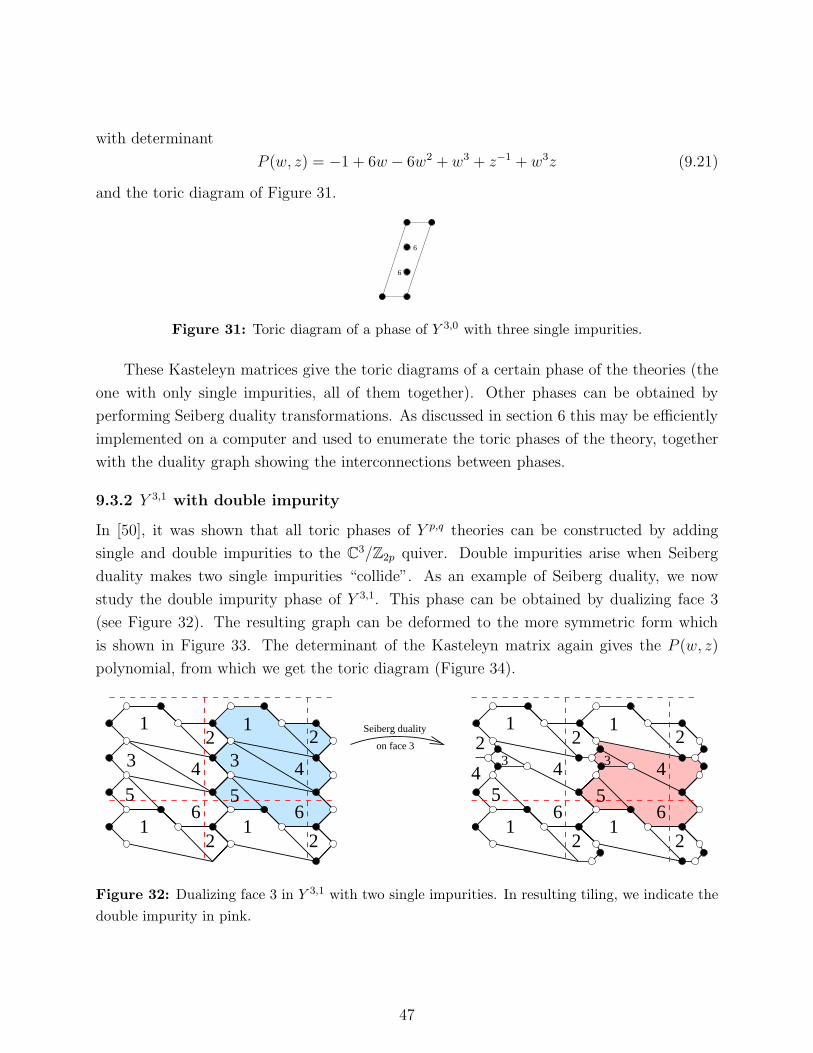
with determinant

P (w, z) = −1 + 6w − 6w2 + w3 + z−1 + w3z (9.21)

and the toric diagram of Figure 31.

6

6

Figure 31: Toric diagram of a phase of Y 3,0 with three single impurities.

These Kasteleyn matrices give the toric diagrams of a certain phase of the theories (the

one with only single impurities, all of them together). Other phases can be obtained by

performing Seiberg duality transformations. As discussed in section 6 this may be efficiently

implemented on a computer and used to enumerate the toric phases of the theory, together

with the duality graph showing the interconnections between phases.

9.3.2 Y 3,1 with double impurity

In [50], it was shown that all toric phases of Y p,q theories can be constructed by adding

single and double impurities to the C3/Z2p quiver. Double impurities arise when Seiberg

duality makes two single impurities “collide”. As an example of Seiberg duality, we now

study the double impurity phase of Y 3,1. This phase can be obtained by dualizing face 3

(see Figure 32). The resulting graph can be deformed to the more symmetric form which

is shown in Figure 33. The determinant of the Kasteleyn matrix again gives the P (w, z)

polynomial, from which we get the toric diagram (Figure 34).

1

5

23

12

12

5

3

12

Seiberg duality

on face 3

1

5

2

12

12

5

122

44 44 4

66 6 6

33

Figure 32: Dualizing face 3 in Y 3,1 with two single impurities. In resulting tiling, we indicate the

double impurity in pink.

47

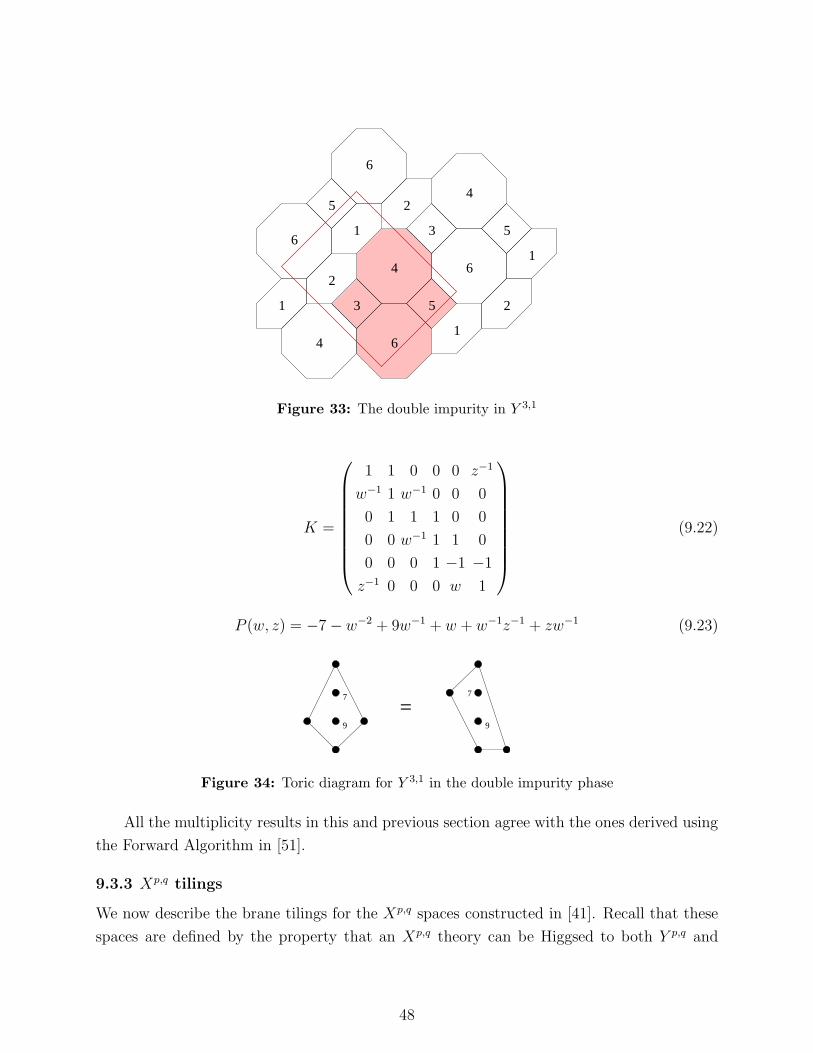
3

3

4

4

4

5

5

5

6

6

6

6

1

1

1

1

2

2

2

Figure 33: The double impurity in Y 3,1

K =

1 1 0 0 0 z−1

w−1 1 w−1 0 0 0

0 1 1 1 0 0

0 0 w−1 1 1 0

0 0 0 1 −1 −1

z−1 0 0 0 w 1

(9.22)

P (w, z) = −7 − w−2 + 9w−1 + w + w−1z−1 + zw−1 (9.23)

7

9 9

7

=

Figure 34: Toric diagram for Y 3,1 in the double impurity phase

All the multiplicity results in this and previous section agree with the ones derived using

the Forward Algorithm in [51].

9.3.3 Xp,q tilings

We now describe the brane tilings for the Xp,q spaces constructed in [41]. Recall that these

spaces are defined by the property that an Xp,q theory can be Higgsed to both Y p,q and

48

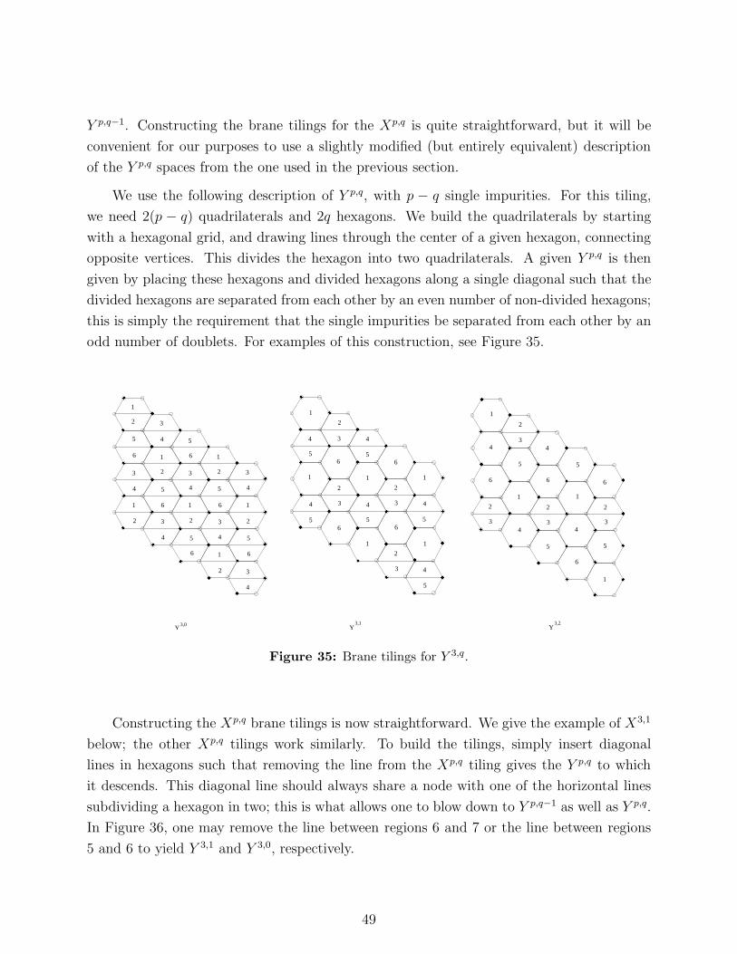
Y p,q−1. Constructing the brane tilings for the Xp,q is quite straightforward, but it will be

convenient for our purposes to use a slightly modified (but entirely equivalent) description

of the Y p,q spaces from the one used in the previous section.

We use the following description of Y p,q, with p − q single impurities. For this tiling,

we need 2(p − q) quadrilaterals and 2q hexagons. We build the quadrilaterals by starting

with a hexagonal grid, and drawing lines through the center of a given hexagon, connecting

opposite vertices. This divides the hexagon into two quadrilaterals. A given Y p,q is then

given by placing these hexagons and divided hexagons along a single diagonal such that the

divided hexagons are separated from each other by an even number of non-divided hexagons;

this is simply the requirement that the single impurities be separated from each other by an

odd number of doublets. For examples of this construction, see Figure 35.

��

��

��

��

��

��

��

��

��

��

��

��

��

��

��

��

��

��

��

��

��

��

��

��

��

��

��

��

��

��

��

��

��

��

��

��

��

��

��

��

��

��

��

��

��

��

��

��

��

��

��

��

��

��

��

��

��

��

��

��

��

��

��

��

��

��

��

��

��

��

��

��

��

��

��

��

��

��

��

��

��

��

��

��

��

��

��

��

��

��

��

��

��

��

��

��

Y3,2

Y3,1

Y3,0

��

��

��

��

��

��

��

��

��

��

��

��

��

��

��

��

��

��

��

��

��

��

��

��

��

��

��

��

��

��

��

��

��

��

��

��

��

��

��

��

��

��

��

��

��

1

2 3

4 5

6 11

2 23 33

5

6

4 4 45 5

6 611 1

2 2 233

4 45

6

5

61

2 3

4

1

2

3 4

56

111

6

1 1

66

4

5

2

3

2

2

3

3

44 4

5 5 5

4

5

1

2

34

5

6

1

2

34

5

6

1

2

3

1

4

5

2

3

6

5

6

4

Figure 35: Brane tilings for Y 3,q.

Constructing the Xp,q brane tilings is now straightforward. We give the example of X3,1

below; the other Xp,q tilings work similarly. To build the tilings, simply insert diagonal

lines in hexagons such that removing the line from the Xp,q tiling gives the Y p,q to which

it descends. This diagonal line should always share a node with one of the horizontal lines

subdividing a hexagon in two; this is what allows one to blow down to Y p,q−1 as well as Y p,q.

In Figure 36, one may remove the line between regions 6 and 7 or the line between regions

5 and 6 to yield Y 3,1 and Y 3,0, respectively.

49

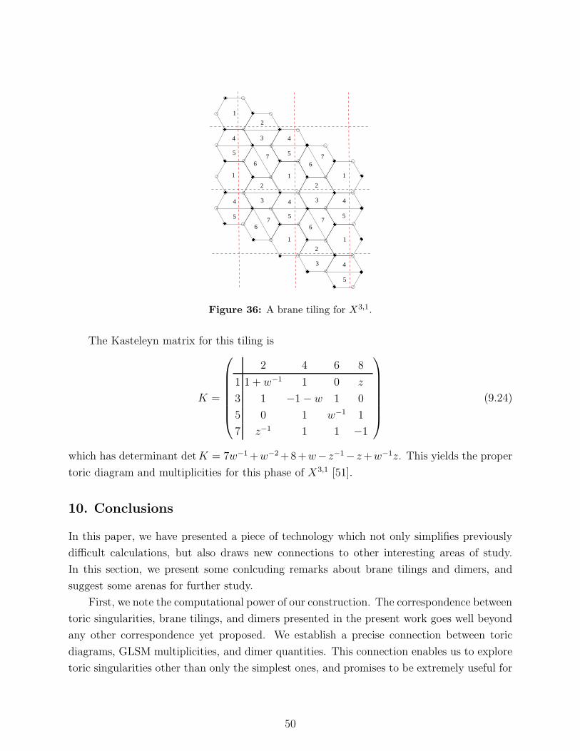
7

��

��

��

��

��

��

��

��

��

��

��

��

��

��

��

��

��

��

��

��

��

��

��

��

��

��

��

��

��

��

��

��

��

��

��

��

��

��

��

��

��

��

��

1

2

3 4

5

111

1 1

4

5

2

3

2

2

3

3

44 4

5 5 5

4

5

66

6 6

77

7

Figure 36: A brane tiling for X3,1.

The Kasteleyn matrix for this tiling is

K =

2 4 6 8

1 1 + w−1 1 0 z

3 1 −1 − w 1 0

5 0 1 w−1 1

7 z−1 1 1 −1

(9.24)

which has determinant det K = 7w−1 +w−2 +8+w−z−1−z +w−1z. This yields the proper

toric diagram and multiplicities for this phase of X3,1 [51].

10. Conclusions

In this paper, we have presented a piece of technology which not only simplifies previously

difficult calculations, but also draws new connections to other interesting areas of study.

In this section, we present some conlcuding remarks about brane tilings and dimers, and

suggest some arenas for further study.

First, we note the computational power of our construction. The correspondence between

toric singularities, brane tilings, and dimers presented in the present work goes well beyond

any other correspondence yet proposed. We establish a precise connection between toric

diagrams, GLSM multiplicities, and dimer quantities. This connection enables us to explore

toric singularities other than only the simplest ones, and promises to be extremely useful for

50

the future study of toric geometries. We further emphasize here that the central object in

our construction, the brane tiling, is a physical object constructed out of NS5-branes and

D5-branes in Type IIB string theory, and not just a mathematical tool.

Previous to our work, it had been suspected that there was a one-to-one correspondence

between toric geometries with specified GLSM multiplicites and toric phases of the quiver

gauge theory. The increased computational power provided by the brane tiling has enabled

us to show that there is a relatively simple counterexample to this conjecture, that of Pseudo

del Pezzo 5. We find that in fact there are examples where the only way of distinguishing

two phases is by checking graph isomorphism, i.e. there exists no simpler characterisation of

the graph other than the graph itself.

The operation of Seiberg duality on a quiver theory is straightforward, although it be-

comes extremely cumbersome to implement it many times. The dimer model allows us to

encode Seiberg duality as an operation on the Kasteleyn matrix. In many cases this provides

an extremely efficient way of enumerating all toric phases of a quiver theory, as long as one

has at least one phase of the quiver theory to start with. It is an interesting question whether

or not one can explore even non-toric theories via Seiberg duality.

In recent work [52], a geometrical method was given for performing a-maximization [25]

purely in terms of toric data, without needing to know the explicit Calabi-Yau metric on

the toric space. This method involved the use of a Monge-Ampere equation to extremise

a certain function. It is interesting to note that the solution to a Monge-Ampere equation

also appears in the dimer model literature [48], where it is related to the extremization

of the surface tension functional that determines the asymptotic shape (limit curve) of a

random matching of many copies of the fundamental domain of a bipartite graph. It would

be fascinating to determine whether or not these two extremization problems are related.

In general, there are many different properties of dimer models that have been studied

in the mathematics literature. It is undoubtedly worth exploring this literature in depth,

since there are surely many additional connections one can draw between the mathematics

and physics of dimers. In particular, the mathematical literature has different examples of

partition functions it is possible to define on a dimer model. Could some of these quantities

be related to e.g. a central charge for the quiver gauge theory, and is it possible to prove the

a-theorem for even the simple example of Higgsing?

The limit curve of the dimer model is related to the geometry that is mirror to the toric

Calabi-Yau cone. This mirror geometry encodes the quantum corrections from worldsheet

instantons to the classical geometry of the toric CY, and provides a point of contact between

dimer models and topological string theory [32]. It would be interesting to investigate this

51

connection in more detail.

One important gap in our understanding of the brane tiling/dimer correspondence is the

string theoretic meaning of the perfect matchings. We proved in section 4 that introducing

the dimer model on the bipartite graph of the brane tiling is the correct thing to do to

compute the moduli space of the quiver theory, but we do not currently understand the

mechanism that produces these perfect matchings in the string theory construction of the

brane tiling in terms of 5-branes and strings.

Finally, we note that in this paper, we do not discuss at all the problem of starting with

a given toric geometry and deriving the brane tiling from that. Ideally, one would like to be

able to do this, since there would then be a direct link to the dual SCFT from any given toric

geometry. In fact there has been recent progress on this, and we may say with confidence

that it is possible to derive the brane tiling related to any toric Calabi-Yau [53].

Acknowledgements: We would like to thank V. Braun, J. de Boer, R. Dijkgraaf,

A. Dunn, Y.-H. He, P. Kazakopoulos, T. Faulkner, A. Uranga and J. Walcher for helpful

discussions.

References

[1] J. McKay, Graphs, singularities, and finite groups, Pure Math. 37 (1980) 183–186.

[2] A. Hanany and E. Witten, Type IIB superstrings, BPS monopoles, and three-dimensional

gauge dynamics, Nucl. Phys. B492 (1997) 152–190, [hep-th/9611230].

[3] H. Ooguri and C. Vafa, Two-dimensional black hole and singularities of CY manifolds, Nucl.

Phys. B463 (1996) 55–72, [hep-th/9511164].

[4] A. Karch, D. Lust, and D. J. Smith, Equivalence of geometric engineering and

Hanany-Witten via fractional branes, Nucl. Phys. B533 (1998) 348–372, [hep-th/9803232].

[5] Y. Ito and M. Reid, The McKay correspondence for finite subgroups of SL(3, C),

alg-geom/9411010.

[6] M. Reid, McKay correspondence, alg-geom/9702016.

[7] S. Govindarajan and T. Jayaraman, D-branes, exceptional sheaves and quivers on Calabi-Yau

manifolds: From Mukai to McKay, Nucl. Phys. B600 (2001) 457–486, [hep-th/0010196].

[8] A. Tomasiello, D-branes on Calabi-Yau manifolds and helices, JHEP 02 (2001) 008,

[hep-th/0010217].

52

http://xxx.lanl.gov/abs/hep-th/9611230



http://xxx.lanl.gov/abs/alg-geom/9411010

http://xxx.lanl.gov/abs/alg-geom/9702016



[9] P. Mayr, Phases of supersymmetric D-branes on Kaehler manifolds and the McKay

correspondence, JHEP 01 (2001) 018, [hep-th/0010223].

[10] W. Lerche, P. Mayr, and J. Walcher, A new kind of McKay correspondence from non-Abelian

gauge theories, hep-th/0103114.

[11] M. R. Douglas, B. R. Greene, and D. R. Morrison, Orbifold resolution by D-branes, Nucl.

Phys. B506 (1997) 84–106, [hep-th/9704151].

[12] M. R. Douglas and G. W. Moore, D-branes, quivers, and ALE instantons, hep-th/9603167.

[13] A. E. Lawrence, N. Nekrasov, and C. Vafa, On conformal field theories in four dimensions,

Nucl. Phys. B533 (1998) 199–209, [hep-th/9803015].

[14] A. Hanany and Y.-H. He, Non-Abelian finite gauge theories, JHEP 02 (1999) 013,

[hep-th/9811183].

[15] B. Feng, A. Hanany, and Y.-H. He, D-brane gauge theories from toric singularities and toric

duality, Nucl. Phys. B595 (2001) 165–200, [hep-th/0003085].

[16] B. Feng, A. Hanany, and Y.-H. He, Phase structure of D-brane gauge theories and toric

duality, JHEP 08 (2001) 040, [hep-th/0104259].

[17] C. E. Beasley and M. R. Plesser, Toric duality is Seiberg duality, JHEP 12 (2001) 001,

[hep-th/0109053].

[18] W. Fulton, Introduction to Toric Varieties. Princeton University Press, 1993.

[19] N. C. Leung and C. Vafa, Branes and toric geometry, Adv. Theor. Math. Phys. 2 (1998)

91–118, [hep-th/9711013].

[20] B. Feng, S. Franco, A. Hanany, and Y.-H. He, Symmetries of toric duality, JHEP 12 (2002)

076, [hep-th/0205144].

[21] J. P. Gauntlett, D. Martelli, J. Sparks, and D. Waldram, Sasaki-Einstein metrics on s2 × s3,

Adv. Theor. Math. Phys. 8 (2004) 711–734, [hep-th/0403002].

[22] D. Martelli and J. Sparks, Toric geometry, Sasaki-Einstein manifolds and a new infinite

class of AdS/CFT duals, hep-th/0411238.

[23] M. Bertolini, F. Bigazzi, and A. L. Cotrone, New checks and subtleties for AdS/CFT and

a-maximization, JHEP 12 (2004) 024, [hep-th/0411249].

[24] S. Benvenuti, S. Franco, A. Hanany, D. Martelli, and J. Sparks, An infinite family of

superconformal quiver gauge theories with Sasaki-Einstein duals, hep-th/0411264.

53
















[25] K. Intriligator and B. Wecht, The exact superconformal r-symmetry maximizes a, Nucl.

Phys. B667 (2003) 183–200, [hep-th/0304128].

[26] C. P. Herzog, Q. J. Ejaz, and I. R. Klebanov, Cascading RG flows from new Sasaki-Einstein

manifolds, JHEP 02 (2005) 009, [hep-th/0412193].

[27] A. Hanany and A. Zaffaroni, On the realization of chiral four-dimensional gauge theories

using branes, JHEP 05 (1998) 001, [hep-th/9801134].

[28] A. Hanany and A. M. Uranga, Brane boxes and branes on singularities, JHEP 05 (1998) 013,

[hep-th/9805139].

[29] M. Aganagic, A. Karch, D. Lust, and A. Miemiec, Mirror symmetries for brane configurations

and branes at singularities, Nucl. Phys. B569 (2000) 277–302, [hep-th/9903093].

[30] B. Feng, A. Hanany, Y.-H. He, and A. M. Uranga, Toric duality as Seiberg duality and brane

diamonds, JHEP 12 (2001) 035, [hep-th/0109063].

[31] D. Bazeia and F. A. Brito, Pattern formation through the entrapment of a network of domain

walls, Phys. Rev. D62 (2000) 101701, [hep-th/0005045].

[32] A. Okounkov, N. Reshetikhin, and C. Vafa, Quantum Calabi-Yau and classical crystals,

hep-th/0309208.

[33] A. Hanany and K. D. Kennaway, Dimer models and toric diagrams, hep-th/0503149.

[34] D. R. Morrison and M. R. Plesser, Non-spherical horizons. i, Adv. Theor. Math. Phys. 3

(1999) 1–81, [hep-th/9810201].

[35] S. Elitzur, A. Giveon, D. Kutasov, E. Rabinovici, and G. Sarkisian, D-branes in the

background of NS fivebranes, Int. J. Mod. Phys. A16 (2001) 880–890.

[36] K. Intriligator and B. Wecht, Baryon charges in 4d superconformal field theories and their

AdS duals, Commun. Math. Phys. 245 (2004) 407–424, [hep-th/0305046].

[37] S. Benvenuti and A. Hanany, New results on superconformal quivers, hep-th/0411262.

[38] R. Kenyon, An introduction to the dimer model, math.CO/0310326.

[39] P. Kasteleyn, Graph theory and crystal physics, in Graph theory and theoretical physics,

pp. 43–110. Academic Press, London, 1967.

[40] B. Feng, S. Franco, A. Hanany, and Y.-H. He, Unhiggsing the del Pezzo, JHEP 08 (2003)

058, [hep-th/0209228].

54













http://xxx.lanl.gov/abs/math.CO/0310326


[41] A. Hanany, P. Kazakopoulos, and B. Wecht, A new infinite class of quiver gauge theories,

hep-th/0503177.

[42] M. Schmaltz, Duality of non-supersymmetric large n gauge theories, Phys. Rev. D59 (1999)

105018, [hep-th/9805218].

[43] S. Franco, A. Hanany, Y.-H. He, and P. Kazakopoulos, Duality walls, duality trees and

fractional branes, hep-th/0306092.

[44] S. Franco, A. Hanany, and Y.-H. He, A trio of dualities: Walls, trees and cascades, Fortsch.

Phys. 52 (2004) 540–547, [hep-th/0312222].

[45] S. Franco, Y.-H. He, C. Herzog, and J. Walcher, Chaotic duality in string theory, Phys. Rev.

D70 (2004) 046006, [hep-th/0402120].

[46] J. Propp, Generalized domino-shuffling, math.CO/0111034.

[47] A. Hanany, M. J. Strassler, and A. M. Uranga, Finite theories and marginal operators on the

brane, JHEP 06 (1998) 011, [hep-th/9803086].

[48] R. Kenyon, A. Okounkov, and S. Sheffield, Dimers and amoebae, math-ph/0311005.

[49] B. Feng, Y.-H. He, and F. Lam, On correspondences between toric singularities and (p, q)-

webs, Nucl. Phys. B701 (2004) 334–356, [hep-th/0403133].

[50] S. Benvenuti, A. Hanany, and P. Kazakopoulos, The toric phases of the Y (p, q) quivers,

hep-th/0412279.

[51] A. Dunn and A. Hanany. Unpublished work.

[52] D. Martelli, J. Sparks, and S. T. Yau, The geometric dual of a-maximisation for toric Sasaki-

Einstein manifolds, hep-th/0503183.

[53] A. Hanany and D. Vegh. Work in progress.

55






http://xxx.lanl.gov/abs/math.CO/0111034


http://xxx.lanl.gov/abs/math-ph/0311005




Brane dimers and quiver gauge theories

Documents