Brain MRI denoizing and segmentation based on improved adaptive nonlocal means

Brain MRI Denoizing and Segmentation Based onImproved Adaptive Nonlocal Means

Muhammad Aksam Iftikhar,* Abdul Jalil, Saima Rathore, Ahmad Ali, Mutawarra Hussain

Department of Computer and Information Sciences, Pakistan Institute of Engineering andApplied Sciences, Islamabad, Pakistan

Received 8 February 2013; revised 26 March 2013; accepted 19 April 2013

ABSTRACT: Denoizing of magnetic resonance (MR) brain images

has been focus of numerous studies in the past. The performance ofsubsequent stages of image processing, in automated image analy-sis, is substantially improved by explicit consideration of noise. Non-

local means (NLM) is a popular denoizing method which exploitsusual redundancy present in an image to restore noise free image. It

computes restored value of a pixel as weighted average of candidatepixels in a search window. In this article, we propose an improvedversion of the NLM algorithm which is modified in two ways. First, a

robust threshold criterion is introduced, which helps selecting suita-ble pixels for participation in the restoration process. Second, the

search window size is made adaptive using a window adaptation testbased on the proposed threshold criterion. The modified NLM algo-rithm is named as improved adaptive nonlocal means (IANLM). An

alternate implementation of IANLM is also proposed which exploitsthe image smoothness property to yield better denoizing perform-

ance. The computational burden is reduced significantly due to pro-posed modifications. Experiments are performed on simulated andreal brain MR images at various noise levels. Results indicate that the

proposed algorithm produces not only better denoizing results (quan-titatively and qualitatively), but is also computationally more efficient.Moreover, the proposed technique is incorporated in an already pro-

posed segmentation framework to check its validity in the practicalscenario of segmentation. Improved segmentation results (quantita-

tive and qualitative) verify the practical usefulness of the proposedalgorithm in real world medical applications. VC 2013 Wiley Periodi-

cals, Inc. Int J Imaging Syst Technol, 23, 235–248, 2013; Published online in

Wiley Online Library (wileyonlinelibrary.com). DOI: 10.1002/ima.22057

Key words: nonlocal means; adaptive; denoizing; brain MRI;

segmentation

I. INTRODUCTION

Brain MR Image analysis is a common medical practice to diagnose

various brain diseases such as tumor, multiple sclerosis, Alzhiemer’s

disease, and so on. The study of different brain tissues, such as cere-

brospinal fluid (CSF), gray matter (GM), and white matter (WM), is

central to computer-aided diagnosis and analysis. The brain MR

images are processed in several stages during such computer-aided

analysis. However, the images acquired by MR imaging equipment

may undergo different types of degradations which hinder the subse-

quent processing stages. These degradations may be caused by sev-

eral factors such as operator error and limitations imposed by the

imaging equipment. Noise is a common degradation, which signifi-

cantly deteriorates the MR image quality. This inherent noise should

be removed for effective results prior to subsequent image processing

stages.

The type of noise present in MR images is usually Rician (Gudb-

jartsson et al., 1995; Macovski, 1996), which is known to be difficult

to remove as compared to other types of noise (Coupe et al., 2008).

Various techniques have been applied to attack the problem of noise

including anisotropic diffusion (Gerig et al., 1992), wavelet-based

techniques (Nowak, 1999), and others (Bankman, 2000). Among

these techniques, NLM (Buades et al., 2005) has drawn the interest

of many researchers due to its superior denoizing and detail preserva-

tion characteristics. It is a nonlocal neighborhood averaging algo-

rithm, based on weighted average of pixels within a large search

window. The term nonlocal is attributed to the larger size search win-

dow as compared to smaller window size of traditional local neigh-

borhood based approaches. The NLM algorithm is not only effective

in removing noise from image but also preserves fine image details.

It is similar in approach to Yaroslavsky (1985) work which involves

gray level similarity computation between a noisy pixel and its

neighbors rather than spatial similarity. However, NLM employs

similarity between neighboring windows of pixels (called patches)

instead of pixels themselves. This idea of patch comparison is

inspired by Discrete Universal Denoizing (DUDE) algorithm

(Ordentlich et al., 2003). Images in practice usually contain much re-

dundancy in their local structures. Because of such redundancy, the

patch of a noisy pixel is expected to be close to the patch of another

pixel in a search area. Hence, the pixel of interest can be restored by

weighted averaging of pixels with similar patches.

Several modifications have been made to the classical NLM algo-

rithm to improve its denoizing performance and computational

Correspondence to: Muhammad Aksam Iftikhar;e-mail: [email protected]

Grant sponsor: PIEAS-administered Endowment Fund (provided by Higher Edu-cation Commission Pakistan, for Higher eductation and R&D in IT and TelecomSector).

VC 2013 Wiley Periodicals, Inc.

efficiency. Yan et al. (2012) improved the denoizing performance of

NLM by increasing the number of suitable candidate pixels to be

included in restoring the value of a particular pixel. Their work was

based on a preprocessing step of classifying the pixels in input image

into similar clusters. The method in Liu et al. (2008) presents a ro-

bust and fast variant of NLM that incorporates the concept of Lapla-

cian pyramid into classical NLM.

A substantial contemporary literature deals with brain MRI deno-

izing. In Manjon et al. (2008), authors applied NLM to brain MR

images to obtain optimal parameters of the algorithm. In Aksam

et al. (2012), parameters optimization for brain MRI denoizing using

NLM has been achieved by employing Genetic Algorithm. In Coupe

et al. (2008), authors presented a fast and effective method for 3D

brain MRI denoizing based on voxel pre-selection and a block-wise

implementation. The work of Vega et al. (2012) is based on compar-

ing features of patches instead of their intensities. This salient feature

matching approach leads to fast and improved denoizing, as verified

by brain MR data denoizing, achieved by using this method. In Gal

et al. (2010), authors proposed dynamic NLM algorithm adopted to

the special nature of dynamic contrast-enhanced (DCE) magnetic

resonance images. Spatially varying noise level is handled in Manjon

et al. (2010), where authors introduced an adaptive nonlocal means

algorithm, taking into account the local noise level. Some authors

have also studied the effect of the search window size of the NLM

algorithm (Salmon, 2010; Thaipanich et al., 2010). In Salmon

(2010), the two parameters of the NLM algorithm, namely the search

window size and central patch weight, have been studied. In Thaipa-

nich et al. (2010), the search window size is made adaptive for differ-

ent region types in the image. This work is similar to the one

presented in this article, in the sense that search window size is made

adaptive. However, our approach considers a robust threshold crite-

rion based adaptive search window, which is independent of the

region type. The implementation of our proposed algorithm is also

novel and complementary to the proposed approach (see Section III).

Image segmentation is usually a subsequent processing step in an

automated image analysis application. It has found several applica-

tion in the field of medical imaging (Kwon et al., 2003; Saha et al.,

2011; Hassan et al. 2012). Robust MR image segmentation can be

obtained by embedding the nonlocal information into fuzzy segmen-

tation framework. In Zhao et al. (2011), for example, a nonlocal spa-

tial constraint term is added to the objective function of classical

fuzzy c-means clustering. Similarly, a weighted image patch-based

FCM is proposed in Ji et al. (2012) which replaces image pixels with

patches and constructs a weighing scheme in the clustering process

based on these patches. Another nonlocal fuzzy c-means algorithm is

proposed specifically for details preservation in synthetic aperture ra-

dar (SAR) images (Feng et al., 2013). In this approach, a new image

is generated which is more robust to multiplicative speckle noise

present in MR images. The new image is generated based on nonlo-

cal information and rectified edge parts are located using coefficient

of variation and orientation based statistics. The nonlocal framework

embedded in above approaches enhances to a great extent their

robustness to noise.

In this article, we present an improved variant of the classical

NLM algorithm. The improvement is two-fold. First, while denoiz-

ing a particular pixel, we consider only those pixels in its neighbor-

hood which have similarity weights greater than a particular

threshold—the so-called robust threshold criterion. Second, the

search window size is made adaptive for each pixel. To better exploit

the image smoothness property, an alternate traversal mechanism of

the search window is proposed instead of conventional row/column

wise traversal. These modifications to the classical NLM algorithm

give rise to Improved Adaptive NLM (IANLM), which is not only

more robust to noise, but is also computationally more efficient. The

proposed algorithm is also used in a segmentation framework pre-

sented in Zhao et al. (2011), which served to verify the practical

applicability of the algorithm in real world applications. The results

of denoizing and segmentation, compared to classical NLM, verify

the effectiveness and efficiency of IANLM.

The remainder of this article is organized as follows. Section II

describes the NLM algorithm and introduces a few notations to be

used in the text. Section III presents the proposed scheme and its

novel implementation. Comparative results of different denoizing

schemes, applied to simulated and real brain MR images, are pre-

sented in Section IV. Practical usefulness of the proposed scheme is

validated in Section V by integrating it into a segmentation frame-

work. Finally, Section VI concludes the article. Various abbrevia-

tions have been used throughout the text to refer to different terms.

Table I describes these abbreviations and corresponding terms for

reference purpose. In our denoizing and segmentation experiments,

simulated brain MR images are corrupted by Rician noise of various

levels (percentages). However, signal-to-noise ratio (SNR) is a con-

venient way of specifying the amount of noise in an image. There-

fore, we also relate noise percentage to average SNR for simulated

brain MR images in Table II.

II. PRELIMINARIES

A. Notations. The NLM algorithm involves different elements

and parameters. It is useful to set up a nomenclature for these elements

which may be used consistently throughout the text. We introduce the

following notations to formally describe different elements in NLM

procedure. Note the bold-face notation to identify a vector.

X2 The input image, in 2D space, of size MxN.

yi Intensity value observed at input image pixel i.

xi Intensity value restored by NLM filter for pixel i.xi’ Intensity value restored by IANLM filter for pixel i.s Radius of the search window.

Si Set of pixels belonging to search window around pixel i,

where |Si| 5 (2s 1 1)2.

p Radius of an image patch.

Pi Set of pixels belonging to patch of pixel i, where |Pi| 5 (2p 1 1)2.

y(Pi) Intensity values observed at each pixel in Pi i.e.

y(Pi) 5 (y(1)(Pi), y(1)(Pi),…,y(|Pi|)(Pi)).

h Smoothing parameter; controls tradeoff between edge

preservation and noise removal.

k Scaling parameter; used to scale the smoothing parameter

for a particular application.

r Sigma; the standard deviation of noise

wij Similarity weight between pixel i and j, used when restoring

the value of pixel i.

wh Threshold value used in robust threshold criterion of IANLM.

Nf Desired number of pixels(patches) satisfying the threshold criterion.

B. NLM Filter. The denoizing in NLM algorithm relies on a

weight function that computes similarity between neighboring win-

dows of noisy pixels. For each pixel i in the image, its local neigh-

borhood (patch) is compared with that of every pixel j in a search

window of size |Si| (radius s). The local neighborhood of pixel i is

referred as patch (Pi) of pixel i throughout the following text. This

236 Vol. 23, 235–248 (2013)

similarity comparison, between two patches Pi and Pj, is made in

terms of Euclidean distance of corresponding intensity values in

patches which has been proven to be reliable enough as a distance

measure (Coupe et al., 2008). The similarity is measured by a weight

term, expressed in the following equation.

wij51

Zie2

||yðPiÞ2yðPj Þ||22

� �h2 (1)

where y(Pi) and y(Pj) represent intensity values observed at pixels

contained within patch Pi and Pj, respectively. The factor h is a

tradeoff parameter that controls balance between the noise removal

and detail preserving capabilities of the algorithm. Higher the value

of h, more noise will be removed. However, a too high value may

introduce undesirable blurring. Similarly, a very low value may not

be able to remove noise completely and leave undesirable artifacts in

the image. Hence, this parameter is related to the amount of noise in

the image and is normally used with a scaling parameter, that is,

h 5 kr, where r is the noise level. According to NLM, the restored

value xi of pixel i is computed as in following equation.

xi5Xj2Si

wijyj subject toXj2Si

wij51 and wij 2 0; 1½ � (2)

where Si is a search window around pixel i and xi is the NLM-

restored value for pixel i. The two constraints specify that weight wij

lies between 0 and 1 and the sum of weights over a particular win-

dow equals 1. The constraints are satisfied due to the normalization

factor Zi in Eq. (1), computed as follows.

Zi5Xj2Si

e2

||yðPiÞ2yðPj Þ||22

� �h2 (3)

III. PROPOSED SCHEME

The conventional NLM algorithm involves a few parameters which

need to be tuned for a particular application. The search window size sis an important parameter which is critical both in terms of denoizing

performance and computational efficiency. Larger value of s may

increase the performance, as more similar patches can be found in a

larger search area. However, a window size greater than a certain

value may stop yielding better performance (Salmon, 2010). Con-

versely, the larger the window size more will be the computational

burden. Hence, a suitable window size is always desirable for better

denoizing. In this section, we propose a variant of conventional NLM,

named as improved adaptive nonlocal means (IANLM), by making

the search window size adaptive based on a robust threshold criterion.

A. Improved Adaptive Nonlocal Means Denoizing. We

have proposed two valuable modifications to the conventional NLM

algorithm. First, pixel j, in neighborhood of pixel i, participate in the

restoration process of pixel i, only if it satisfies a robust threshold cri-

terion. The criterion states that a pixel (patch) j is considered only if

weight wij>wh, where wh is a weight threshold. We call the pixel

(patch), which satisfies the threshold criterion, as the fit pixel (patch).

Second, the window size is made adaptive based on this threshold

criterion. In particular, the process of patch comparison is terminated

as soon as we have Nf fit pixels (patches) available within current

search window which satisfy the robust threshold criterion. Hence,

both the modifications are complementary to each other. Restoration

of a particular pixel in IANLM is shown, graphically, in Figure 1.

Mathematically, the process of denoizing in IANML is formu-

lated slightly different from NLM, and is given in Eq. (4).

x0i5Xj2N�i

wijyj subject toXj2N�i

wij51 and wij 2 0; 1½ � (4)

where xi0 is the IANLM-restored value for pixel i and N�i � Si is the

set of pixels around pixel i, satisfying following constraints.

Table I. Abbreviations used in the text.

Abbreviation Text

MRI Magnetic resonance imaging

WM White matter

GM Gray matter

CSF Cerebrospinal fluid

DCE Dynamic contrast enhanced

NLM Non-local means

IANLM Improved adaptive non-local means

PSNR Peak signal to noise ratio

RMSE Root mean square error

FE Function evaluations

SA Segmentation accuracy

DC Dice coefficient

FCM Fuzzy c-means

SFCM Spatial fuzzy c-means

FLICM Fuzzy local information c-means

FCM_NLS Fuzzy c-means with non-local spatial information

FCM_INLS Fuzzy c-means with improved non-local spatial information

Table II. Performance comparison in terms of PSNR.

Noise % 1 2 3 4 5 6 7 8 9

SNR 31.11 27.33 25.78 21.53 19.08 17.52 16.06 14.95 13.82

Figure 1. Graphical illustration of restoration process of pixel iin IANLM.

Vol. 23, 235–248 (2013) 237

� Robust threshold criterion: wij>wh, where wh is the weight

threshold and related to the amount of noise present in the

image.

� Window adaptation test: jN�i j � Nf , where Nf is the desired

number of fit patches which satisfy the robust threshold crite-

rion and is application dependent.

The algorithm introduces two new parameters i.e. wh and Nf,

while relaxing the search window size parameter of conventional

NLM. Search window size is treated in IANLM as the maximum

search window size, that is, the maximum size of window that should

be searched adaptively. The parameter wh is related to the amount of

noise in the image and can be set empirically or as a function of

noise level in the image. The suitable value of the parameter Nf is

application specific. However, as we will see in Section IV.C.1, the

proposed technique is not much sensitive to this parameter if we

assign it a sufficiently high value.

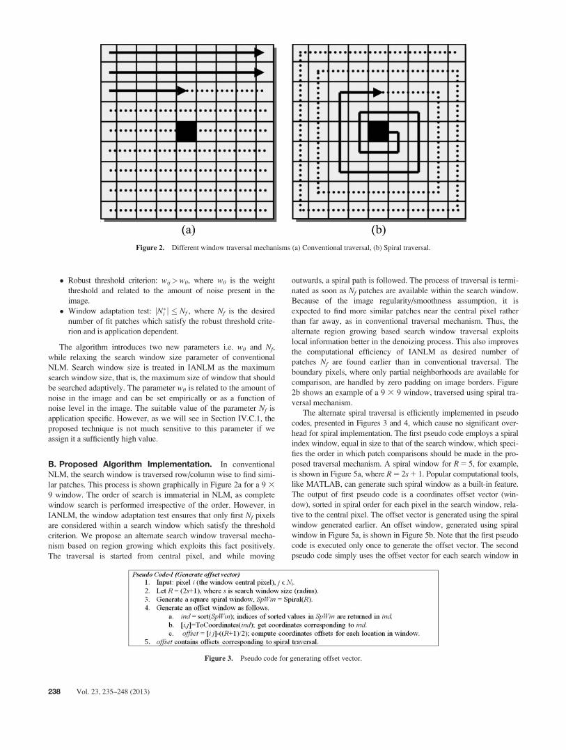
B. Proposed Algorithm Implementation. In conventional

NLM, the search window is traversed row/column wise to find simi-

lar patches. This process is shown graphically in Figure 2a for a 9 3

9 window. The order of search is immaterial in NLM, as complete

window search is performed irrespective of the order. However, in

IANLM, the window adaptation test ensures that only first Nf pixels

are considered within a search window which satisfy the threshold

criterion. We propose an alternate search window traversal mecha-

nism based on region growing which exploits this fact positively.

The traversal is started from central pixel, and while moving

outwards, a spiral path is followed. The process of traversal is termi-

nated as soon as Nf patches are available within the search window.

Because of the image regularity/smoothness assumption, it is

expected to find more similar patches near the central pixel rather

than far away, as in conventional traversal mechanism. Thus, the

alternate region growing based search window traversal exploits

local information better in the denoizing process. This also improves

the computational efficiency of IANLM as desired number of

patches Nf are found earlier than in conventional traversal. The

boundary pixels, where only partial neighborhoods are available for

comparison, are handled by zero padding on image borders. Figure

2b shows an example of a 9 3 9 window, traversed using spiral tra-

versal mechanism.

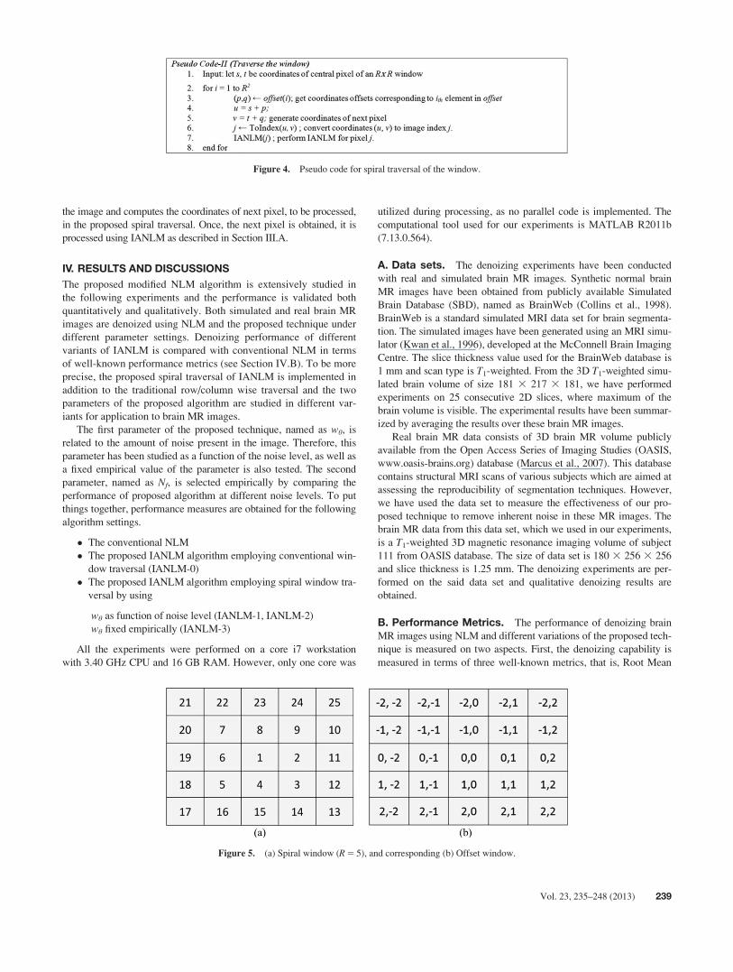
The alternate spiral traversal is efficiently implemented in pseudo

codes, presented in Figures 3 and 4, which cause no significant over-

head for spiral implementation. The first pseudo code employs a spiral

index window, equal in size to that of the search window, which speci-

fies the order in which patch comparisons should be made in the pro-

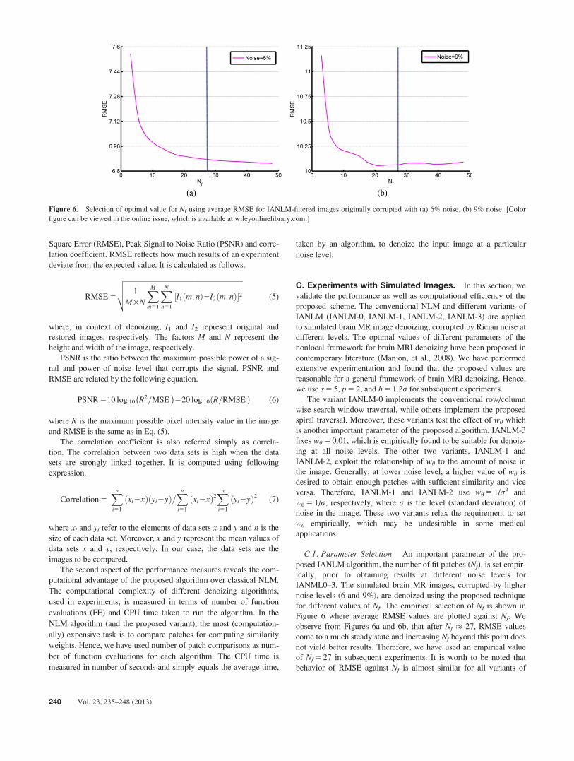
posed traversal mechanism. A spiral window for R 5 5, for example,

is shown in Figure 5a, where R 5 2s 1 1. Popular computational tools,

like MATLAB, can generate such spiral window as a built-in feature.

The output of first pseudo code is a coordinates offset vector (win-

dow), sorted in spiral order for each pixel in the search window, rela-

tive to the central pixel. The offset vector is generated using the spiral

window generated earlier. An offset window, generated using spiral

window in Figure 5a, is shown in Figure 5b. Note that the first pseudo

code is executed only once to generate the offset vector. The second

pseudo code simply uses the offset vector for each search window in

Figure 2. Different window traversal mechanisms (a) Conventional traversal, (b) Spiral traversal.

Figure 3. Pseudo code for generating offset vector.

238 Vol. 23, 235–248 (2013)

the image and computes the coordinates of next pixel, to be processed,

in the proposed spiral traversal. Once, the next pixel is obtained, it is

processed using IANLM as described in Section III.A.

IV. RESULTS AND DISCUSSIONS

The proposed modified NLM algorithm is extensively studied in

the following experiments and the performance is validated both

quantitatively and qualitatively. Both simulated and real brain MR

images are denoized using NLM and the proposed technique under

different parameter settings. Denoizing performance of different

variants of IANLM is compared with conventional NLM in terms

of well-known performance metrics (see Section IV.B). To be more

precise, the proposed spiral traversal of IANLM is implemented in

addition to the traditional row/column wise traversal and the two

parameters of the proposed algorithm are studied in different var-

iants for application to brain MR images.

The first parameter of the proposed technique, named as wh, is

related to the amount of noise present in the image. Therefore, this

parameter has been studied as a function of the noise level, as well as

a fixed empirical value of the parameter is also tested. The second

parameter, named as Nf, is selected empirically by comparing the

performance of proposed algorithm at different noise levels. To put

things together, performance measures are obtained for the following

algorithm settings.

� The conventional NLM

� The proposed IANLM algorithm employing conventional win-

dow traversal (IANLM-0)

� The proposed IANLM algorithm employing spiral window tra-

versal by using

wh as function of noise level (IANLM-1, IANLM-2)

wh fixed empirically (IANLM-3)

All the experiments were performed on a core i7 workstation

with 3.40 GHz CPU and 16 GB RAM. However, only one core was

utilized during processing, as no parallel code is implemented. The

computational tool used for our experiments is MATLAB R2011b

(7.13.0.564).

A. Data sets. The denoizing experiments have been conducted

with real and simulated brain MR images. Synthetic normal brain

MR images have been obtained from publicly available Simulated

Brain Database (SBD), named as BrainWeb (Collins et al., 1998).

BrainWeb is a standard simulated MRI data set for brain segmenta-

tion. The simulated images have been generated using an MRI simu-

lator (Kwan et al., 1996), developed at the McConnell Brain Imaging

Centre. The slice thickness value used for the BrainWeb database is

1 mm and scan type is T1-weighted. From the 3D T1-weighted simu-

lated brain volume of size 181 3 217 3 181, we have performed

experiments on 25 consecutive 2D slices, where maximum of the

brain volume is visible. The experimental results have been summar-

ized by averaging the results over these brain MR images.

Real brain MR data consists of 3D brain MR volume publicly

available from the Open Access Series of Imaging Studies (OASIS,

www.oasis-brains.org) database (Marcus et al., 2007). This database

contains structural MRI scans of various subjects which are aimed at

assessing the reproducibility of segmentation techniques. However,

we have used the data set to measure the effectiveness of our pro-

posed technique to remove inherent noise in these MR images. The

brain MR data from this data set, which we used in our experiments,

is a T1-weighted 3D magnetic resonance imaging volume of subject

111 from OASIS database. The size of data set is 180 3 256 3 256

and slice thickness is 1.25 mm. The denoizing experiments are per-

formed on the said data set and qualitative denoizing results are

obtained.

B. Performance Metrics. The performance of denoizing brain

MR images using NLM and different variations of the proposed tech-

nique is measured on two aspects. First, the denoizing capability is

measured in terms of three well-known metrics, that is, Root Mean

Figure 5. (a) Spiral window (R 5 5), and corresponding (b) Offset window.

Figure 4. Pseudo code for spiral traversal of the window.

Vol. 23, 235–248 (2013) 239

Square Error (RMSE), Peak Signal to Noise Ratio (PSNR) and corre-

lation coefficient. RMSE reflects how much results of an experiment

deviate from the expected value. It is calculated as follows.

RMSE 5

ffiffiffiffiffiffiffiffiffiffiffiffiffiffiffiffiffiffiffiffiffiffiffiffiffiffiffiffiffiffiffiffiffiffiffiffiffiffiffiffiffiffiffiffiffiffiffiffiffiffiffiffiffiffiffiffiffiffiffiffiffiffiffiffiffiffiffi1

M3N

XM

m51

XN

n51

I1 m; nð Þ2I2 m; nð Þ½ �2

vuut (5)

where, in context of denoizing, I1 and I2 represent original and

restored images, respectively. The factors M and N represent the

height and width of the image, respectively.

PSNR is the ratio between the maximum possible power of a sig-

nal and power of noise level that corrupts the signal. PSNR and

RMSE are related by the following equation.

PSNR 510 log 10 R2=MSE� �

520 log 10 R=RMSEð Þ (6)

where R is the maximum possible pixel intensity value in the image

and RMSE is the same as in Eq. (5).

The correlation coefficient is also referred simply as correla-

tion. The correlation between two data sets is high when the data

sets are strongly linked together. It is computed using following

expression.

Correlation 5Xn

i51

xi2�xð Þ yi2�yð Þ=Xn

i51

xi2�xð Þ2Xn

i51

yi2�yð Þ2 (7)

where xi and yi refer to the elements of data sets x and y and n is the

size of each data set. Moreover, �x and �y represent the mean values of

data sets x and y, respectively. In our case, the data sets are the

images to be compared.

The second aspect of the performance measures reveals the com-

putational advantage of the proposed algorithm over classical NLM.

The computational complexity of different denoizing algorithms,

used in experiments, is measured in terms of number of function

evaluations (FE) and CPU time taken to run the algorithm. In the

NLM algorithm (and the proposed variant), the most (computation-

ally) expensive task is to compare patches for computing similarity

weights. Hence, we have used number of patch comparisons as num-

ber of function evaluations for each algorithm. The CPU time is

measured in number of seconds and simply equals the average time,

taken by an algorithm, to denoize the input image at a particular

noise level.

C. Experiments with Simulated Images. In this section, we

validate the performance as well as computational efficiency of the

proposed scheme. The conventional NLM and different variants of

IANLM (IANLM-0, IANLM-1, IANLM-2, IANLM-3) are applied

to simulated brain MR image denoizing, corrupted by Rician noise at

different levels. The optimal values of different parameters of the

nonlocal framework for brain MRI denoizing have been proposed in

contemporary literature (Manjon, et al., 2008). We have performed

extensive experimentation and found that the proposed values are

reasonable for a general framework of brain MRI denoizing. Hence,

we use s 5 5, p 5 2, and h 5 1.2r for subsequent experiments.

The variant IANLM-0 implements the conventional row/column

wise search window traversal, while others implement the proposed

spiral traversal. Moreover, these variants test the effect of wh which

is another important parameter of the proposed algorithm. IANLM-3

fixes wh 5 0.01, which is empirically found to be suitable for denoiz-

ing at all noise levels. The other two variants, IANLM-1 and

IANLM-2, exploit the relationship of wh to the amount of noise in

the image. Generally, at lower noise level, a higher value of wh is

desired to obtain enough patches with sufficient similarity and vice

versa. Therefore, IANLM-1 and IANLM-2 use wu 5 1/r2 and

wu 5 1/r, respectively, where r is the level (standard deviation) of

noise in the image. These two variants relax the requirement to set

wh empirically, which may be undesirable in some medical

applications.

C.1. Parameter Selection. An important parameter of the pro-

posed IANLM algorithm, the number of fit patches (Nf), is set empir-

ically, prior to obtaining results at different noise levels for

IANML0–3. The simulated brain MR images, corrupted by higher

noise levels (6 and 9%), are denoized using the proposed technique

for different values of Nf. The empirical selection of Nf is shown in

Figure 6 where average RMSE values are plotted against Nf. We

observe from Figures 6a and 6b, that after Nf � 27, RMSE values

come to a much steady state and increasing Nf beyond this point does

not yield better results. Therefore, we have used an empirical value

of Nf 5 27 in subsequent experiments. It is worth to be noted that

behavior of RMSE against Nf is almost similar for all variants of

Figure 6. Selection of optimal value for Nf using average RMSE for IANLM-filtered images originally corrupted with (a) 6% noise, (b) 9% noise. [Color

figure can be viewed in the online issue, which is available at wileyonlinelibrary.com.]

240 Vol. 23, 235–248 (2013)

IANLM. However, for simplicity, results are shown only for

IANLM-1 in Figure 6.

C.2. Performance Analysis. In this section, we denoize simu-

lated brain MRI data, corrupted by various noise levels, using NLM,

IANLM-0, IANLM-1, IANLM-2, and IANLM-3. The performance

measures are obtained in terms of PSNR, RMSE and correlation at

nine different noise levels. The denoizing process is carried out 20

times by adding certain amount of noise to each image slice and av-

erage results, over all slices, are presented in Tables III and IV and

Figure 7 for each noise level.

Quantitative results in Tables III and IV show superiority of

IANLM algorithm over conventional NLM at all noise levels. The

proposed implementation of the algorithm also outperforms the con-

ventional implementation (IANLM-0) with exception of a few lower

noise levels. Conventional traversal based scheme IANLM-0 per-

forms poorly at higher noise levels as compared to spiral traversal

based IANLM schemes. Similar conclusion is drawn from the results

obtained in terms of correlation measure, which are shown graphi-

cally in Figure 7. The performance of IANLM-1 and IANLM-3 sur-

passes other techniques at all noise levels in terms of correlation

Table IV. Performance comparison in terms of RMSE.

Noise (%)

RMSE

NLM IANLM-0 IANLM-1 IANLM-2 IANLM-3

1 2.98 6 0.02 1.59 6 0.01 1.75 6 0.01 1.77 6 0.01 1.63 6 0.01

2 3.62 6 0.02 2.87 6 0.01 2.94 6 0.01 3.10 6 0.01 2.75 6 0.01

3 4.37 6 0.03 3.89 6 0.02 3.92 6 0.02 4.26 6 0.02 3.79 6 0.02

4 5.26 6 0.03 4.88 6 0.03 4.87 6 0.03 5.23 6 0.03 4.82 6 0.03

5 6.22 6 0.04 5.92 6 0.03 5.86 6 0.03 6.13 6 0.03 5.86 6 0.03

6 7.23 6 0.04 7.05 6 0.04 6.90 6 0.04 7.04 6 0.04 6.91 6 0.03

7 8.26 6 0.04 8.29 6 0.04 7.96 6 0.04 8.01 6 0.05 7.99 6 0.05

8 9.31 6 0.06 9.60 6 0.06 8.99 6 0.05 8.98 6 0.05 9.01 6 0.05

9 10.38 6 0.05 10.93 6 0.06 10.06 6 0.05 10.04 6 0.05 10.07 6 0.05

Table III. Performance comparison in terms of PSNR.

Noise

(%)

PSNR

NLM IANLM-0 IANLM-1 IANLM-2 IANLM-3

1 38.66 6 0.05 44.11 6 0.04 43.29 6 0.04 43.18 6 0.04 43.88 6 0.04

2 36.96 6 0.06 38.99 6 0.05 38.78 6 0.04 38.32 6 0.04 39.36 6 0.04

3 35.32 6 0.05 36.33 6 0.05 36.26 6 0.04 35.55 6 0.05 36.57 6 0.05

4 33.72 6 0.05 34.37 6 0.05 34.38 6 0.05 33.76 6 0.05 34.47 6 0.05

5 32.26 6 0.05 32.68 6 0.04 32.77 6 0.05 32.38 6 0.05 32.77 6 0.05

6 30.95 6 0.05 31.17 6 0.05 31.36 6 0.05 31.17 6 0.05 31.34 6 0.04

7 29.79 6 0.05 29.76 6 0.05 30.11 6 0.05 30.06 6 0.05 30.09 6 0.05

8 28.75 6 0.05 28.49 6 0.05 29.06 6 0.05 29.07 6 0.05 29.04 6 0.05

9 27.81 6 0.05 27.36 6 0.05 28.08 6 0.05 28.10 6 0.04 28.08 6 0.05

Figure 7. Performance comparison in terms of Correlation measure. [Color figure can be viewed in the online issue, which is available at

wileyonlinelibrary.com.]

Vol. 23, 235–248 (2013) 241

measure. However, conventional traversal based IANLM-0 performs

poorly at higher noise levels.

Among three spiral traversal based variants of IANLM, we rec-

ommend IANLM-1 for two reasons. First, the performance of

IANLM-1 is superior as compared to IANLM-2 at almost all noise

levels. Second, IANLM-1 is preferable over IANLM-3, as it elimi-

nates the need to empirically adjust the value of wh. Therefore, we

will be using IANLM-1 to demonstrate the results of subsequent

experiments and it will be called simply as IANLM.

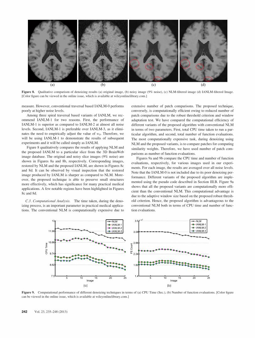
Figure 8 qualitatively compares the results of applying NLM and

the proposed IANLM to a particular slice from the 3D BrainWeb

image database. The original and noisy slice images (9% noise) are

shown in Figures 8a and 8b, respectively. Corresponding images,

restored by NLM and the proposed IANLM, are shown in Figures 8c

and 8d. It can be observed by visual inspection that the restored

image produced by IANLM is sharper as compared to NLM. More-

over, the proposed technique is able to preserve small structures

more effectively, which has significance for many practical medical

applications. A few notable regions have been highlighted in Figures

8c and 8d.

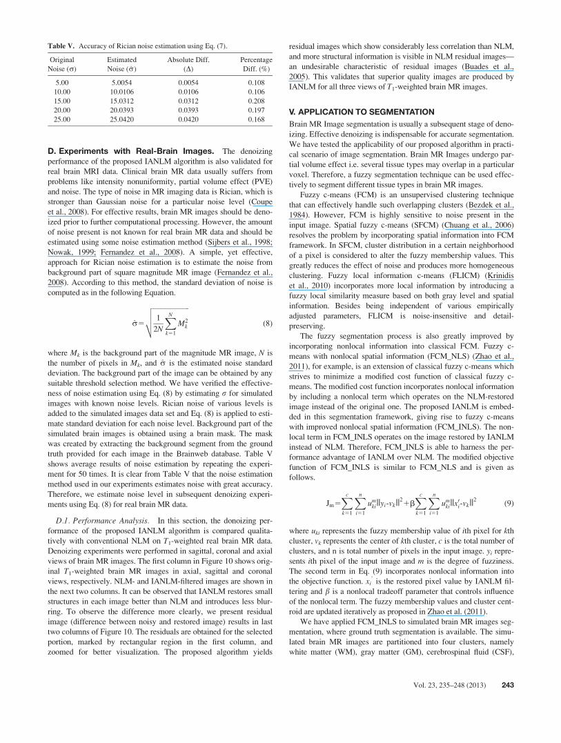
C.3. Computational Analysis. The time taken, during the deno-

izing process, is an important parameter in practical medical applica-

tions. The conventional NLM is computationally expensive due to

extensive number of patch comparisons. The proposed technique,

conversely, is computationally efficient owing to reduced number of

patch comparisons due to the robust threshold criterion and window

adaptation test. We have compared the computational efficiency of

different variants of the proposed algorithm with conventional NLM

in terms of two parameters. First, total CPU time taken to run a par-

ticular algorithm, and second, total number of function evaluations.

The most computationally expensive task, during denoizing using

NLM and the proposed variants, is to compare patches for computing

similarity weights. Therefore, we have used number of patch com-

parisons as number of function evaluations.

Figures 9a and 9b compare the CPU time and number of function

evaluations, respectively, for various images used in our experi-

ments. For each image, the results are averaged over all noise levels.

Note that the IANLM-0 is not included due to its poor denoizing per-

formance. Different variants of the proposed algorithm are imple-

mented using the pseudo code described in Section III.B. Figure 9a

shows that all the proposed variants are computationally more effi-

cient than the conventional NLM. This computational advantage is

due to the adaptive window size based on the proposed robust thresh-

old criterion. Hence, the proposed algorithm is advantageous to the

conventional NLM both in terms of CPU time and number of func-

tion evaluations.

Figure 8. Qualitative comparison of denoizing results (a) original image, (b) noisy image (9% noise), (c) NLM-filtered image (d) IANLM-filtered Image.

[Color figure can be viewed in the online issue, which is available at wileyonlinelibrary.com.]

Figure 9. Computational performance of different denoizing techniques in terms of (a) CPU Time (Sec.), (b) Number of function evaluations. [Color figure

can be viewed in the online issue, which is available at wileyonlinelibrary.com.]

242 Vol. 23, 235–248 (2013)

D. Experiments with Real-Brain Images. The denoizing

performance of the proposed IANLM algorithm is also validated for

real brain MRI data. Clinical brain MR data usually suffers from

problems like intensity nonuniformity, partial volume effect (PVE)

and noise. The type of noise in MR imaging data is Rician, which is

stronger than Gaussian noise for a particular noise level (Coupe

et al., 2008). For effective results, brain MR images should be deno-

ized prior to further computational processing. However, the amount

of noise present is not known for real brain MR data and should be

estimated using some noise estimation method (Sijbers et al., 1998;

Nowak, 1999; Fernandez et al., 2008). A simple, yet effective,

approach for Rician noise estimation is to estimate the noise from

background part of square magnitude MR image (Fernandez et al.,

2008). According to this method, the standard deviation of noise is

computed as in the following Equation.

r̂5

ffiffiffiffiffiffiffiffiffiffiffiffiffiffiffiffiffiffiffiffiffi1

2N

XN

k51

M2k

vuut (8)

where Mk is the background part of the magnitude MR image, N is

the number of pixels in Mk, and r̂ is the estimated noise standard

deviation. The background part of the image can be obtained by any

suitable threshold selection method. We have verified the effective-

ness of noise estimation using Eq. (8) by estimating r for simulated

images with known noise levels. Rician noise of various levels is

added to the simulated images data set and Eq. (8) is applied to esti-

mate standard deviation for each noise level. Background part of the

simulated brain images is obtained using a brain mask. The mask

was created by extracting the background segment from the ground

truth provided for each image in the Brainweb database. Table V

shows average results of noise estimation by repeating the experi-

ment for 50 times. It is clear from Table V that the noise estimation

method used in our experiments estimates noise with great accuracy.

Therefore, we estimate noise level in subsequent denoizing experi-

ments using Eq. (8) for real brain MR data.

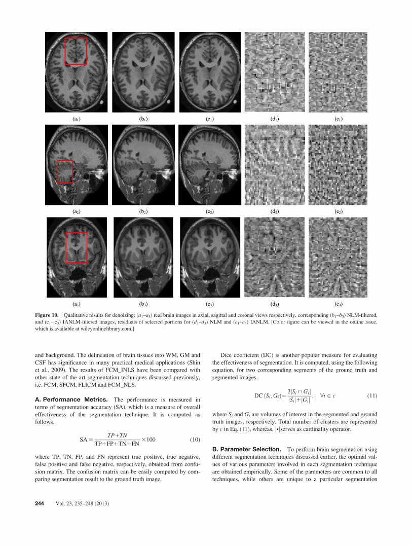
D.1. Performance Analysis. In this section, the donoizing per-

formance of the proposed IANLM algorithm is compared qualita-

tively with conventional NLM on T1-weighted real brain MR data.

Denoizing experiments were performed in sagittal, coronal and axial

views of brain MR images. The first column in Figure 10 shows orig-

inal T1-weighted brain MR images in axial, sagittal and coronal

views, respectively. NLM- and IANLM-filtered images are shown in

the next two columns. It can be observed that IANLM restores small

structures in each image better than NLM and introduces less blur-

ring. To observe the difference more clearly, we present residual

image (difference between noisy and restored image) results in last

two columns of Figure 10. The residuals are obtained for the selected

portion, marked by rectangular region in the first column, and

zoomed for better visualization. The proposed algorithm yields

residual images which show considerably less correlation than NLM,

and more structural information is visible in NLM residual images—

an undesirable characteristic of residual images (Buades et al.,

2005). This validates that superior quality images are produced by

IANLM for all three views of T1-weighted brain MR images.

V. APPLICATION TO SEGMENTATION

Brain MR Image segmentation is usually a subsequent stage of deno-

izing. Effective denoizing is indispensable for accurate segmentation.

We have tested the applicability of our proposed algorithm in practi-

cal scenario of image segmentation. Brain MR Images undergo par-

tial volume effect i.e. several tissue types may overlap in a particular

voxel. Therefore, a fuzzy segmentation technique can be used effec-

tively to segment different tissue types in brain MR images.

Fuzzy c-means (FCM) is an unsupervised clustering technique

that can effectively handle such overlapping clusters (Bezdek et al.,

1984). However, FCM is highly sensitive to noise present in the

input image. Spatial fuzzy c-means (SFCM) (Chuang et al., 2006)

resolves the problem by incorporating spatial information into FCM

framework. In SFCM, cluster distribution in a certain neighborhood

of a pixel is considered to alter the fuzzy membership values. This

greatly reduces the effect of noise and produces more homogeneous

clustering. Fuzzy local information c-means (FLICM) (Krinidis

et al., 2010) incorporates more local information by introducing a

fuzzy local similarity measure based on both gray level and spatial

information. Besides being independent of various empirically

adjusted parameters, FLICM is noise-insensitive and detail-

preserving.

The fuzzy segmentation process is also greatly improved by

incorporating nonlocal information into classical FCM. Fuzzy c-

means with nonlocal spatial information (FCM_NLS) (Zhao et al.,

2011), for example, is an extension of classical fuzzy c-means which

strives to minimize a modified cost function of classical fuzzy c-

means. The modified cost function incorporates nonlocal information

by including a nonlocal term which operates on the NLM-restored

image instead of the original one. The proposed IANLM is embed-

ded in this segmentation framework, giving rise to fuzzy c-means

with improved nonlocal spatial information (FCM_INLS). The non-

local term in FCM_INLS operates on the image restored by IANLM

instead of NLM. Therefore, FCM_INLS is able to harness the per-

formance advantage of IANLM over NLM. The modified objective

function of FCM_INLS is similar to FCM_NLS and is given as

follows.

Jm5Xc

k51

Xn

i51

umki||yi-vk ||

21bXc

k51

Xn

i51

umki||x

0i-vk ||

2(9)

where uki represents the fuzzy membership value of ith pixel for kth

cluster, vk represents the center of kth cluster, c is the total number of

clusters, and n is total number of pixels in the input image. yi repre-

sents ith pixel of the input image and m is the degree of fuzziness.

The second term in Eq. (9) incorporates nonlocal information into

the objective function. xi’ is the restored pixel value by IANLM fil-

tering and b is a nonlocal tradeoff parameter that controls influence

of the nonlocal term. The fuzzy membership values and cluster cent-

roid are updated iteratively as proposed in Zhao et al. (2011).

We have applied FCM_INLS to simulated brain MR images seg-

mentation, where ground truth segmentation is available. The simu-

lated brain MR images are partitioned into four clusters, namely

white matter (WM), gray matter (GM), cerebrospinal fluid (CSF),

Table V. Accuracy of Rician noise estimation using Eq. (7).

Original

Noise (r)

Estimated

Noise (r̂)

Absolute Diff.

(D)

Percentage

Diff. (%)

5.00 5.0054 0.0054 0.108

10.00 10.0106 0.0106 0.106

15.00 15.0312 0.0312 0.208

20.00 20.0393 0.0393 0.197

25.00 25.0420 0.0420 0.168

Vol. 23, 235–248 (2013) 243

and background. The delineation of brain tissues into WM, GM and

CSF has significance in many practical medical applications (Shin

et al., 2009). The results of FCM_INLS have been compared with

other state of the art segmentation techniques discussed previously,

i.e. FCM, SFCM, FLICM and FCM_NLS.

A. Performance Metrics. The performance is measured in

terms of segmentation accuracy (SA), which is a measure of overall

effectiveness of the segmentation technique. It is computed as

follows.

SA 5TP1TN

TP1FP1TN1FN3100 (10)

where TP, TN, FP, and FN represent true positive, true negative,

false positive and false negative, respectively, obtained from confu-

sion matrix. The confusion matrix can be easily computed by com-

paring segmentation result to the ground truth image.

Dice coefficient (DC) is another popular measure for evaluating

the effectiveness of segmentation. It is computed, using the following

equation, for two corresponding segments of the ground truth and

segmented images.

DC Si;Gið Þ5 2jSi \ GijjSij1jGij

; 8i 2 c (11)

where Si and Gi are volumes of interest in the segmented and ground

truth images, respectively. Total number of clusters are represented

by c in Eq. (11), whereas, j•jserves as cardinality operator.

B. Parameter Selection. To perform brain segmentation using

different segmentation techniques discussed earlier, the optimal val-

ues of various parameters involved in each segmentation technique

are obtained empirically. Some of the parameters are common to all

techniques, while others are unique to a particular segmentation

Figure 10. Qualitative results for denoizing: (a1–a3) real brain images in axial, sagittal and coronal views respectively, corresponding (b1–b3) NLM-filtered,

and (c1- c3) IANLM-filtered images, residuals of selected portions for (d1–d3) NLM and (e1–e3) IANLM. [Color figure can be viewed in the online issue,

which is available at wileyonlinelibrary.com.]

244 Vol. 23, 235–248 (2013)

technique. The degree of fuzziness (m) and number of clusters (c),

for example, are assigned the same values for all techniques, that is,

4 and 2, respectively. However, in case of SFCM and FLICM, a local

window size parameter (Nwin) is required which is empirically

selected to be 5 and 3 (i.e., 5 3 5 and 3 3 3 window), respectively.

The segmentation techniques FCM_NLS and FCM_INLS require

images to be denoized first using NLM and IANLM, respectively.

For denoizing, common parameters (s, p, and h) of NLM and

IANLM and unique parameters of IANLM (Nf and wh) assume same

values as used for simulated brain MRI denoizing in Section IV.C.

An important parameter, critical to the segmentation performance

in FCM_NLS and FCM_INLS, is the nonlocal tradeoff parameter

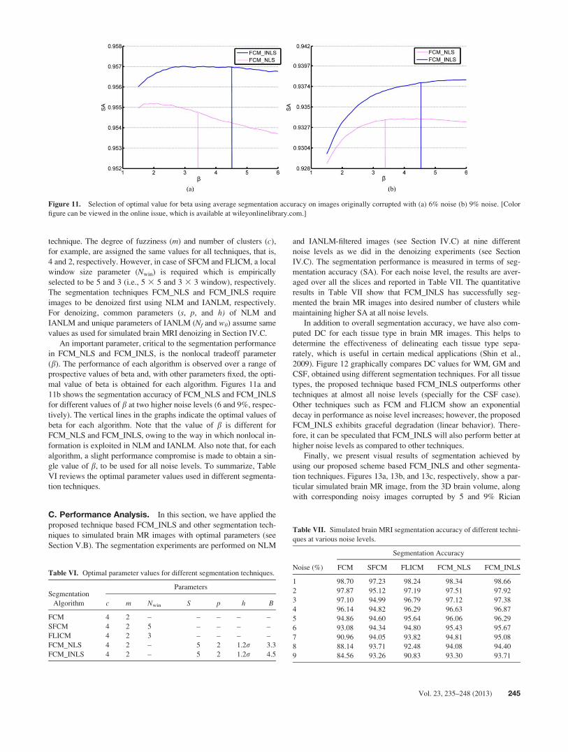
(b). The performance of each algorithm is observed over a range of

prospective values of beta and, with other parameters fixed, the opti-

mal value of beta is obtained for each algorithm. Figures 11a and

11b shows the segmentation accuracy of FCM_NLS and FCM_INLS

for different values of b at two higher noise levels (6 and 9%, respec-

tively). The vertical lines in the graphs indicate the optimal values of

beta for each algorithm. Note that the value of b is different for

FCM_NLS and FCM_INLS, owing to the way in which nonlocal in-

formation is exploited in NLM and IANLM. Also note that, for each

algorithm, a slight performance compromise is made to obtain a sin-

gle value of b, to be used for all noise levels. To summarize, Table

VI reviews the optimal parameter values used in different segmenta-

tion techniques.

C. Performance Analysis. In this section, we have applied the

proposed technique based FCM_INLS and other segmentation tech-

niques to simulated brain MR images with optimal parameters (see

Section V.B). The segmentation experiments are performed on NLM

and IANLM-filtered images (see Section IV.C) at nine different

noise levels as we did in the denoizing experiments (see Section

IV.C). The segmentation performance is measured in terms of seg-

mentation accuracy (SA). For each noise level, the results are aver-

aged over all the slices and reported in Table VII. The quantitative

results in Table VII show that FCM_INLS has successfully seg-

mented the brain MR images into desired number of clusters while

maintaining higher SA at all noise levels.

In addition to overall segmentation accuracy, we have also com-

puted DC for each tissue type in brain MR images. This helps to

determine the effectiveness of delineating each tissue type sepa-

rately, which is useful in certain medical applications (Shin et al.,

2009). Figure 12 graphically compares DC values for WM, GM and

CSF, obtained using different segmentation techniques. For all tissue

types, the proposed technique based FCM_INLS outperforms other

techniques at almost all noise levels (specially for the CSF case).

Other techniques such as FCM and FLICM show an exponential

decay in performance as noise level increases; however, the proposed

FCM_INLS exhibits graceful degradation (linear behavior). There-

fore, it can be speculated that FCM_INLS will also perform better at

higher noise levels as compared to other techniques.

Finally, we present visual results of segmentation achieved by

using our proposed scheme based FCM_INLS and other segmenta-

tion techniques. Figures 13a, 13b, and 13c, respectively, show a par-

ticular simulated brain MR image, from the 3D brain volume, along

with corresponding noisy images corrupted by 5 and 9% Rician

Figure 11. Selection of optimal value for beta using average segmentation accuracy on images originally corrupted with (a) 6% noise (b) 9% noise. [Color

figure can be viewed in the online issue, which is available at wileyonlinelibrary.com.]

Table VII. Simulated brain MRI segmentation accuracy of different techni-

ques at various noise levels.

Segmentation Accuracy

Noise (%) FCM SFCM FLICM FCM_NLS FCM_INLS

1 98.70 97.23 98.24 98.34 98.66

2 97.87 95.12 97.19 97.51 97.92

3 97.10 94.99 96.79 97.12 97.38

4 96.14 94.82 96.29 96.63 96.87

5 94.86 94.60 95.64 96.06 96.29

6 93.08 94.34 94.80 95.43 95.67

7 90.96 94.05 93.82 94.81 95.08

8 88.14 93.71 92.48 94.08 94.40

9 84.56 93.26 90.83 93.30 93.71

Table VI. Optimal parameter values for different segmentation techniques.

Segmentation

Algorithm

Parameters

c m Nwin S p h B

FCM 4 2 – – – – –

SFCM 4 2 5 – – – –

FLICM 4 2 3 – – – –

FCM_NLS 4 2 – 5 2 1.2r 3.3

FCM_INLS 4 2 – 5 2 1.2r 4.5

Vol. 23, 235–248 (2013) 245

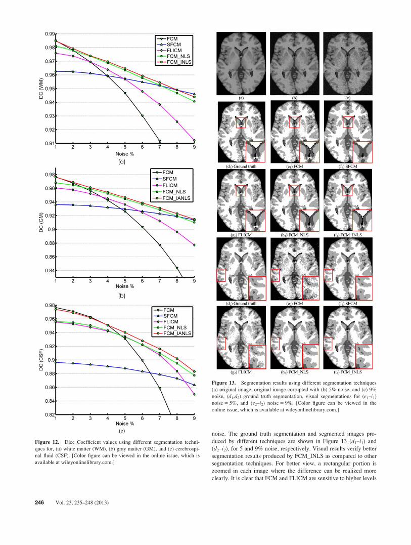
noise. The ground truth segmentation and segmented images pro-

duced by different techniques are shown in Figure 13 (d1–i1) and

(d2–i2), for 5 and 9% noise, respectively. Visual results verify better

segmentation results produced by FCM_INLS as compared to other

segmentation techniques. For better view, a rectangular portion is

zoomed in each image where the difference can be realized more

clearly. It is clear that FCM and FLICM are sensitive to higher levels

Figure 12. Dice Coefficient values using different segmentation techni-

ques for, (a) white matter (WM), (b) gray matter (GM), and (c) cerebrospi-

nal fluid (CSF). [Color figure can be viewed in the online issue, which is

available at wileyonlinelibrary.com.]

Figure 13. Segmentation results using different segmentation techniques

(a) original image, original image corrupted with (b) 5% noise, and (c) 9%

noise, (d1,d2) ground truth segmentation, visual segmentations for (e1–i1)

noise 5 5%, and (e2–i2) noise 5 9%. [Color figure can be viewed in the

online issue, which is available at wileyonlinelibrary.com.]

246 Vol. 23, 235–248 (2013)

of noise, while SFCM results in over-segmentation at various points

in the image. Similarly, FCM_INLS produces better results than

FCM_NLS as evident from the zoomed portions in Figure 13 (h1, i1)

and (h2, i2). Hence, overall, the segmentation produced by

FCM_INLS is much closer to the ground truth.

VI. CONCLUSION

Nonlocal means is a classical denoizing technique of effective image

restoration being used in many practical application. The restoration

process is based on similarity weights computed from image patches.

In this research, we have proposed a novel variant of NLM by intro-

ducing two complementary modifications. First, a robust threshold

criterion is introduced, which helps selecting suitable pixels for par-

ticipation in the restoration process. Second, the window size is

made adaptive based on a window adaptation test. Hence, the pro-

posed variant is named as improved adaptive nonlocal means

(IANLM). To better exploit local information in the proposed

scheme, an alternate implementation of IANLM is proposed. The

validation of the proposed scheme is performed by denoizing syn-

thetic and real brain MR data. After denoizing synthetic brain

images, performance results, in terms of PSNR, RMSE and correla-

tion, and computational measures, in terms of CPU time and number

of function evaluations, are obtained for classical NLM and different

IANLM-based denoizing schemes. The results verify that IANLM

not only performs denoizing more effectively, but is also computa-

tionally efficient. Real clinical brain MR images are also denoized

using NLM and IANLM. Qualitative comparison of denoized images

and corresponding residuals verify superiority of IANLM for real

images as well. Finally, the proposed scheme is also incorporated

into a segmentation framework to verify its practical applicability.

The segmentation performance is compared in terms of segmentation

accuracy and DICE coefficient. The proposed scheme-based segmen-

tation technique outperformed all other techniques. Hence, the pro-

posed algorithm can be used reliably in practical medical

applications.

ACKNOWLEDGMENTS

The authors like to express their appreciation for McConnell Brain

Imaging Center (BIC) of the Montreal Neurological Institute, for

publicly sharing the simulated brain MR data (http://www.bic.m-

ni.mcgill.ca/brain-web). They also like to acknowledge Randy

Buckner, Daniel Marcus, and Washington University Alzheimer’s

Disease Research Center for sharing Open Access Series of Imag-

ing Studies (OASIS, www.oasis-brains.org) real brain MRI data-

base.

REFERENCES

M. Aksam, S. Rathore, and A. jalil, Parameter Optimization for Non-Local

De-noising using Elite GA, International Multitopic Conference, Islamabad,

Pakistan, 2012.

I. Bankman, Handbook of medical imaging: Processing and analysis, Aca-

demic Press, New York, 2000.

J.C. Bezdek, R. Ehrlich, and W. Full, FCM: The Fuzzy C-Means clustering

algorithm, Comput Geosci 10 (1984), 191–203.

A. Buades, B. Coll, and J.M. Morel, A review of image denoising algo-

rithms with a new one, Multiscale Model Simul 4 (2005), 490–530.

K.S. Chuang, H.L. Tzeng, S. Chen, J. Wu, and T.J. Chen, Fuzzy c-means

clustering with spatial information for image segmentation, Comput Med

Imaging Graphics 30 (2006), 9–15.

D.L. Collins, A.P. Zijdenbos, V. Kollokian, J.G. Sled, N.J. Kabani, C.J.

Holmes, and A.C. Evans, Design and construction of a realistic digital brain

phantom, IEEE Trans Med Imaging 17 (1998), 463–468.

P. Coupe, P. Yger, S. Prima, P. Hellier, C. Kervrann, and C. Barillot, An

optimized blockwise nonlocal means denoising filter for 3-D magnetic reso-

nance images, IEEE Trans Med Imaging 27 (2008), 425–441.

J. Feng, L.C. Jiao, X. Zhang, M. Gong, and T. Sun, Robust non-local fuzzy

c-means algorithm with edge preservation for SAR image segmentation,

Signal Process 93 (2013), 487–499.

S.A. Fernandez, C.A. Lopez, and C.F. Westin, Noise and signal estimation

in magnitude MRI and Rician distributed images: A LMMSE approach,

IEEE Trans Image Process 17 (2008), 1383–1398.

Y. Gal, A.J.H. Mehnert, A.P. Bradley, K. McMahon, D. Kennedy, and S.

Crozier, Denoising of dynamic contrast-enhanced mr images using dynamic

nonlocal means, IEEE Trans Med Imaging 29 (2010), 302–310.

G. Gerig, O. K€ubler, R. Kikinis, and F. Jolesz, Nonlinear anisotropic fitering

of MRI data, IEEE Trans Med Imaging 11 (1992), 221–232.

H. Gudbjartsson and S. Patz, The rician distribution of noisy MRI data,

Magn Reson Med 34 (1995), 910–914.

M. Hassan, A. Chaudhr, A. Khan, and J.Y. Kim, Carotid artery image seg-

mentation using modified spatial fuzzy c-means and ensemble clustering,

Comput Methods Prog Biomed 108 (2012), 1261–1276.

Z. Ji, Y. Xia, Q. Chen, Q. Sun, D. Xia, and D.D. Feng, Fuzzy c-means clus-

tering with weighted image patch for image segmentation, Appl Soft Com-

put 12 (2012), 1659–1667.

S. Krinidis and V. Chatzis, A robust fuzzy local information C-means clus-

tering algorithm, IEEE Trans Image Process 19 (2010), 1328–1337.

R.K.S. Kwan, A.C. Evans, and G.B. Pike, An Extensible MRI Simulator for

Post-Processing Evaluation, Visualization in Biomedical Computing, Lec-

ture Notes in Computer Science, Springer-Verlag, Hamburg, Germamy,

1996, pp. 135–140.

M.J. Kwon, Y.J. Han, I.H. Shin, and H.W. Park, Hierarchical fuzzy segmen-

tation of brain MR images, Int J Imaging Syst Technol 13 (2003), 115–125.

Y.L. Liu, J. Wang, X. Chen, Y.W. Guo, Q.S. Peng, A robust and fast non-

local means algorithm for image denoising, J Comput Sci Technol 23

(2008), 270–279.

A. Macovski, Noise in MRI, Magn Reson Med 36 (1996), 494–497.

J.V. Manjon, J.C. Caballero, J.J. Lull, G.G. Marti, L.M. Bonmati, and M.

Robles, MRI denoising using non-local means, Med Image Anal 12 (2008),

514–523.

J.V. Manjon, P. Coupe, L.M. Bonmat�ı, D.L. Collins, and M. Robles, Adapt-

ive non-local means denoising of mr images with spatially varying noise

levels, J Magen Reson Imaging 31 (2010), 192–203.

D.S. Marcus, T.H. Wang, J. Parker, J.G. Csernansky, J.C. Morris, and R.L.

Buckner, Open access series of imaging studies (OASIS): Cross-sectional

MRI data in young, middle aged, nondemented, and demented older adults,

J Cogn Neurosci 19 (2007), 1498–1507.

R.D. Nowak, Wavelet-based rician noise removal for magnetic resonance

imaging, IEEE Trans on Image Process 8 (1999), 1408–1419.

E. Ordentlich, G. Seroussi, S. Verdu, M. Weinberger, T. Weissman, A dis-

crete universal denoiser and its application to binary images, IEEE Interna-

tional Conference on Image Processing, Barcelona, Spain, 2003, pp. 117–

120.

S. Saha and U. Maulik, A new line symmetry distance based automatic clus-

tering technique: Application to image segmentation, Int J Imaging Syst

Technol 21 (2011), 86–100.

Vol. 23, 235–248 (2013) 247

J. Salmon, On two parameters for denoising with Non-Local Means, Signal

Process Lett 17 (2010), 269–272.

J. Sijbers, A.J.D. Dekker, D.V. Dyck, and E. Raman, Estimation of signal

and noise from Rician distributed data, Proceedings of the International

Conference on Signal Processing and Communications, Gran Canaria,

Spain, 1998, 140–142.

W. Shin, G. Xiujuan, H. Gu, and Y. Yang, Brain Tissue Segmentation using

Fast T1 Mapping, Proceedings of the International Society for Magnetic

Resonance in Medicine, Honolulu, Hawaii, 2009.

T. Thaipanich and C.C.J. Kuo, An Adaptive Nonlocal Means Scheme for

Medical Image Denoising, Proceedings of SPIE., Medical Imaging, San

Diego, California, 2010.

A.T. Vega, V.G. Perez, S.A. Fernandez, and C.F. Westin, Efficient and ro-

bust nonlocal means denoising of MR data based on salient features match-

ing, Comput Methods Prog Biomed 105 (2012), 131–144.

R. Yan, L. Shao, S.D. Cvetkovic, and J. Klijn, Improved nonlocal means

based on pre-classification and invariant block matching, J Display Technol

8 (2012), 212–218.

L. Yaroslavsky, Digital picture processing, an introduction, Springer-Ver-

lag, Berlin, 1985.

F. Zhao, L. Jiao, and H. Liu, Fuzzy c-means clustering with non local spatial

information for noisy image segmentation, Front Comput Sci China 5

(2011), 45–56.

248 Vol. 23, 235–248 (2013)