Brain Lobes Revealed by Spectral Clustering

Brain lobes revealed by spectral clustering

Julien LefevreAix-Marseille Universite

CNRS, ENSAMUniversite de Toulon

LSIS UMR 729613397 Marseille, France

[email protected]

Guillaume AuziasAix-Marseille Universite

CNRSINT UMR 7289

13385 Marseille, [email protected]

David GermanaudUMR663, NeuroSpin, INSERM

Universite Paris DescartesCEA, Gif/Yvette, France

Service de Neuropediatrie, Hopital Robert DebreAPHP - Universite Paris Diderot, Paris, France

[email protected]

Abstract—The cortical surface is composed of a mosaic ofdistinct regions that are functionally or micro-anatomically homo-geneous. Parcellating the cortical surface into few lobes is a com-mon approach in neuroimaging resulting from a long tradition inphysiology. However, defining such subregions consistent acrosssubjects is more difficult. If macro-anatomical landmarks such ascentral sulcus and parieto-occipital sulcus are clear boundariesbetween distinct lobes, appropriate separators still have to bedefined e.g. in the posterior temporal lobe. Several approacheshave been proposed, but they are all built from supervisedinformation in general from manually defined segmentation ontoan atlas brain. However, some of the boundaries imposed in suchatlas actually rely on ad hoc approaches rather than anatomicalor functional considerations regarding the underlying structureof the cortex. In this work, we propose an original techniquethat allows to define a parcellation of the cortical surface basedon its intrinsic properties with no a priori information. Ourapproach is based on spectral clustering applied to the firsteigenfunctions of Laplace-Beltrami Operator of the cortical mesh.We demonstrate a good reproducibility of clusters across subjectsas well as striking visual similarities between our segmentationand traditional lobar parcellation.

I. INTRODUCTION

Most of neuroimaging studies rely on the localisation-ism paradigm that postulates existence of brain regions withspecific functions. This segregated vision is the result of along history in neuroanatomy. Gratiolet (1854) was the first topropose a segmentation of primate cortex in four lobes, frontal,parietal, temporal and occipital based on anatomical considera-tions and identification of reproducible patterns of folds acrossdifferent species [1]. This division is still used today even iffiner levels of brain parcellation have been defined throughmicroscopic organization (Broadman areas, 1909) or by usinggyral based regions delimited by sulci, i.e. fundus of brainfolds [2], [3], [4]. Such parcellations are of great interest formorphometric or functional studies in 3D or on the corticalsurface. They can be considered as a coarser resolution forbrain information that allows a better matching of differentanatomies [5]. Anatomy-based parcellation are mostly builtfrom supervised information. In [3], [4] cortical surfaces areregistered on an atlas with FreeSurfer software then labelledwith 32 and 74 regions respectively. The approach proposedin [2] can be viewed as a semi-supervised one since surfaceparcels are obtained from Voronoi diagrams and informationpropagation from labeled sulci.To our knowledge there are no unsupervised methods allowingto segregate a cortical surface into lobes or more parcels. Thus

a full unsupervised solution to this problem would consistin finding reproducible segmentations only through globalgeometric shape invariants. The field of computer graphics isa good source of inspiration with a huge literature on meshsegmentation or mesh clustering (see [6] for a review). Inparticular spectral clustering methods have been popularizedin the case of meshes [7], [8] even if it is mainly used inthe case of general graphs [9]. These approaches rely on thedescription of shapes or surfaces through eigenfunctions ofLaplace-Beltrami Operator (L.B.O.) associated to the domainof interest. In one dimension, these eigenfunctions correspondactually to sine and cosine functions with increasing spatialfrequencies. If the surface is a square, eigenfunctions areproducts of previous one dimensional modes along the twodimensions. When harmonic analysis is used on signals (e.g.time-frequency analysis) or images (e.g. filtering), emphasis isnot put on the modes by themselves because of their simpleparametric expressions. However L.B.O. encodes importantinformation on the geometry of the surface, for instance itseigenvalues (or spectrum) correspond to spatial frequencies.The famous problem of ”hearing the shape of a drum” [10]has had a negative answer : different surfaces can have thesame spectrum [11]. Other shape descriptors built on L.B.O.eigenfunctions have been proposed in [12] by counting thenodal domains and they have demonstrated a better discrimina-tive power to distinguish brain structures. L.B.O eigenfunctionhave also been used to describe the cortical folding patterns atvarious scales [13]. In [14] the 2 first L.B.O. eigenfunctionsallow to define a feature space for the sulci recognitionproblem.In the present work we propose an approach that serves two

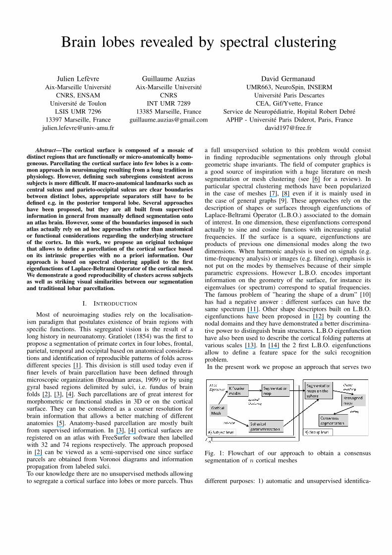
Fig. 1: Flowchart of our approach to obtain a consensussegmentation of n cortical meshes

different purposes: 1) automatic and unsupervised identifica-

tion of relevant brain parcels, 2) demonstration of a strongrelationships between first L.B.O. eigenfunctions associatedto low spatial frequencies and anatomical landmarks such asCentral Sulcus (C.S.) and Parieto-Occipital Sulcus (P.O.S.). Forthis we propose first an individual segmentation strategy basedon spectral clustering. Next the HIP-HOP parameterization[15] allows to project every segmentation maps on a samespherical domain. Last we propose a simple way to match thedifferent clusters in order to build a consensus segmentation.The different steps are summarized in the flowchart on Fig. 1.

II. METHODS

A. Fourier modes

We consider an ideal continuous cortical surface S, itsmetric tensor g(·, ·) and the space of the square integrablefunctions L2(S) = {u : S → R /

∫S u

2 < +∞} with itscanonical scalar product < u, v >=

∫S uv. The Laplace-

Beltrami operator (LBO denoted by ∆S ) has a basis oforthonormal eigenfunctions φ0, φ1, ... in L2(S) which satisfy:

−∆Sφi = λiφi. (1)

where λ0 = 0 ≤ λ1 ≤ λi.... This sequence is called spectrum.A more detailed introduction on LBO can be found forinstance in [16]. In the following, eigenfunctions φi willbe called Fourier modes which allows a more intuitiveunderstanding of the underlying concepts.

It is possible to compute eigenfunctions on a mesh S thatapproximates S using a weak formulation of the eigenvalueproblem and the finite elements method. If u and λ aresolutions of −∆Su = λu then:∫

Sg(∇u,∇v) = λ

∫Suv , ∀v ∈ L2(S). (2)

We use the finite elements method to derive a matrix ex-pression of this weak formulation. We consider the mesh Scomposed of N vertices. For each vertex i of the mesh we havea function wi : S → R which is continuous, linear on eachtriangle of the mesh and satisfying the property wi(j) = δij .Any function continuous and linear on each triangle can bedecomposed on this basis u =

∑Ni=1 uiwi where ui are real

coefficients. So the equation (2) can be rewritten in the discretesetting, taking v = wj for all j = 1..N . And the discretizedproblem becomes to find a vector U = (ui)i=1..N and a scalarλ such that:

GU = λMU, (3)

with the stiffness and mass matrices given by :

G =

(∫S∇wi · ∇wj

)i,j=1..N

(4)

M =

(∫Swiwj

)i,j=1..N

(5)

More details on the computation of these two matrices aregiven in [17]. The eigenvalue problem (3) can be solvedfor example with the Lanczos method as implemented inARPACK. Fig. 2 represents the five first non-trivial Fouriermodes where color encodes the sign (positive in yellow/redand negative in blue).

B. Spectral clustering

The general idea behind spectral clustering consists inusing a clustering algorithm (K-means in general) on theK first eigenvectors of a matrix built upon similaritiesbetween points [9], [18]. This class of methods starts fromlocal information (pairwise comparisons) to infer a globalpartitioning of data. There are theoretical results on the goodidentification of clusters through this algorithm [9] even iffundamental limitations exist when clusters to be identifiedhave very different scales [19].There are many ways to choose the matrix and graph laplacianmatrices are often used because of good properties (positiveand semi-definite) which guarantee non-negative eigenvalues.In our case, Fourier modes computed from a finite elementmethod at order p are natural candidates as inputs of a spectralclustering algorithm since they reflect the geometry of theoriginal surface and offer two extra advantages: no need ofparameters tuning for a Gaussian kernel (scale parameter) andonly the p-neighborhood (p = 1 in practice) is necessary tocompute the pairwise similarity between the points.

Our algorithm to obtain a parcellation of a brain in Kclusters is the following:

Algorithm 1 Cortical surface parcellation

Require: integer K, mesh defined bynV × 3 array of points VnT × 3 array of triangles T

1: Compute matrices G and M with Eq. 4 and 52: Find K first eigenvectors X(:,1),...,X(:,K) of GX=λ MX3: Apply K-means clustering to the nV× K array X to get

an nV × 1 array labels4: return labels

So the labels array obtained by the algorithm allowsto define surface patches and can be visualized directly as atexture on the surface (see Fig 4). We can observe that eachof the K resulting patches obtained by the previous algorithmis connected, i.e. every vertex can be linked to another vertexof the same patch by a path. To our knowledge this empiricalresult does not seem to be the consequence of a known theoremand it could be worth investigating the general case for anykind of graphs or even just genus 0 graphs.

C. Cluster matching

1) Surface parameterization with ”HIP-HOP”: We presenthere a parameterization method that will allow to evaluate thereproducibility of cortical segmentations in K surface patchesacross a group of subjects. We use a recent model-drivenharmonic parameterization of the cortical surface called ”HIP-HOP” [15]. This approach allows to find a bijective mapping hbetween any surface point not in the insula I nor in the corpuscallosum C and two coordinates in a rectangle of prescribeddimensions: h : S \ {C ∪ I} −→ [0, L]× [0, w] with two softconstraints:

• Angles must be conserved between the original surfaceand the rectangle.

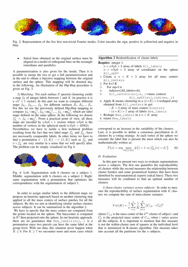
Fig. 2: Representation of the five first non-trivial Fourier modes. Color encodes the sign, positive in yellow/red and negative inblue.

• Sulcal lines obtained on the original surface must bealigned on a model of orthogonal lines on the rectangle(meridians and parallels).

A parameterization is also given for the insula. Then it ispossible to merge the two to get a full parameterization andat the end to obtain a bijective mapping between the originalsurface and the sphere. This mapping will be denoted mSin the following. An illustration of the Hip-Hop procedure isgiven on Fig. 3.

2) Matching: For each surface S spectral clustering yieldsa map fS of integer labels between 1 and K (in practice it isa nV × 1 vector). In this part we want to compare differentmaps fS1 , fS2 ,..., fSn for different surfaces S1, S2,..., Sn.For this we use the previously defined Hip-Hop mapping tocompare fS1 ◦m−1S1 , fS2 ◦m−1S2 ,..., fSn ◦m−1Sn , which are labelmaps defined on the same sphere. In the following we denotef ′Si = fSi ◦m−1Si . From a practical point of view, all thesemaps are encoded by nSph × 1 vectors where nSph is thenumber of vertices in the spherical mesh (nSph = 40962).Nevertheless we have to tackle a first technical problemresulting from the fact that two label maps f ′Si and f ′Sj , havenot necessarily comparable labels. In other terms we have tofind a permutation σ : {1,K} −→ {1,K} such as f ′Si andσ ◦ f ′Sj are very similar in a sense that we will specify after.The problem can be simply visualized on Fig 4.

Fig. 4: Left: Segmentation with 6 clusters on a subject 1.Middle: segmentation with 6 clusters on a subject 2. Right:same segmentation with a permutation that optimizes thecorrespondence with the segmentation of subject 1.

In order to assign similar labels to the different maps wepropose an heuristic approach based on another clustering stepapplied to all the mass centers of surface patches for all thesubjects. By this we aim at identifying similar surface clustersacross subjects. It can be summarized in the algorithm 2.We have to specify that the mass centers are computed from

the points located on the sphere. The barycenter is computedin R3 then projected onto the sphere. In our heuristic approach,there are no guarantees that New_labels(suj,.) is apermutation since two parcels can have the same label at thegroup level. With our data, this situation never happen whenK ≤ 6. For K ≥ 7 we encounter more and more cases which

Algorithm 2 Reidentification of cluster labels

Require: integer Kn× nSph× 3 array of labels All_labelsn × nSph × 3 array of coordinates on the sphereAll_sphV

1: Create a n × K × 3 array for all mass centersAll_centers

2: For k=1:K3: For suj=1:n4: indices=(All labels==k)5: All_centers(suj,k,.)=mass centers(

All_sphV(suj,indices,.))6: Apply K-means clustering to a (n∗K)×3 reshaped array

obtained from All_centers to get:- K × 3 array of mass centers Kcenters- (n ∗K)× 1 array of labels New_labels

7: Reshape New_labels in a n×K array8: return New_labels

correspond to an increase in the variability of the clusters.Last, it is possible to define a consensus parcellation in Kclusters by a voting strategy. At each vertex of the sphere weconsider the label that is present the most which can also bemathematically written as:

F(x) = arg maxk∈[|1,K|]

#{i = 1..n/f ′Si(x) = k/

}(6)

D. Evaluation

In this part we present two ways to evaluate segmentationsacross n subjects. The first one quantifies the reproducibilityof clusters while the second measures the relationship betweencluster borders and some geometrical features that have beenidentified by neuroanatomical experts (sulcal lines). These twomeasures will be combined to find an optimal number ofclusters.

1) Intra-cluster variance across subjects: In order to mea-sure the reproducibility of surface segmentation with K clus-ters we compute the sum of intra-cluster variance:

V ar(K) =1

n

n∑i=1

1

K

K∑k=1

||Ci,k − Ck||2

where Ci,k is the mass center of the kth cluster of subject i andCk is the projected mass center of Ci,k when i varies acrossall the subjects. It is important to mention that this measureis not the within-cluster sum of squares at the individual levelthat is minimized in K-means algorithm. Our measure takesinto account all the partitions for the n subjects.

Fig. 3: Left and middle: external and internal faces of a cortical surface with sulcal lines superimposed: blue colors representparallels while red/yellow/orange stand for meridians. Insula and Corpus Callosum are depicted in dark red (left and middle).Right: Mapping of the previous surface onto the sphere through HIP-HOP parameterization.

2) Geometrical measurements: We consider M anatomicallandmarks that will be compared to cluster borders. In particu-lar, Central Sulcus (C.S.) and Parieto-Occipital Sulcus (P.O.S.)are very important landmarks since they are considered as hardborders between lobes ( M = 2 in the following). For eachdiscrete sulcal line lm we can define a mean distance to theboundaries of the segmentation maps Bi:

Dist(lm, fSi) =1

#lm

∑p∈lm

d(p,Bi) (7)

where d(., .) is the euclidian distance between a point and aset. Bi can be simply computed through the graph laplacian L[6] of the mesh:

Bi ={x ∈ Si/LfSi(x) 6= 0

}This property is obvious since in the interior of one cluster,a vertex and its neighbors share the same information in themap fSi so LfSi(x) = 0. Then we can derive a global measurereflecting the adequacy between anatomy and a segmentationin K clusters:

D(K) =1

n

n∑i=1

1

M

1

Area(Si)

M∑m=1

Dist(lm, fSi)2 (8)

In this measure distances for each subject are normalized bythe area of the surface Si in order to make D(K) comparableto V ar(K).

3) Number of clusters: A natural question can be addressedregarding the optimal number of clusters representing thegroup of subjects. In our case this issue is different fromfinding the optimal number of clusters at the individual levelwith indices like Akaike Information Criterion or Gap statis-tics. Indeed we want to discover a posteriori that there arereproducibility among the group of n subjects with the samenumber of clusters for each. This reproducibility must take intoaccount the total explained variance, represented in V ar(K)but also the criterion that is not directly used in the clusteringprocess D(K) and that reflects the supervised validation of ourapproach. The two measures are directly comparable thanks tothe normalization of D(K). We can obtain an optimal value ofK as the one for which (V ar(K), D(K)) is the closest pointto the origin.

III. RESULTS

A. Data

We have tested our approach on the group of n = 62healthy subjects previously used in [15]. At the momentwe have only examined the left hemispheres of their brainssegmented from T1-weighted MRI with FreeSurfer software1. Each individual cortical meshes is composed of a hundredthousand points. Lines of Central Sulcus and Parieto-OccipitalSulcus were traced manually by an expert with BrainVisapainting tool SurfPaint [20].

B. Robustness of clustering

We have applied our methodology for different values ofK varying from 2 to 10. The two first pictures on Fig. 5are reflecting two opposite behavior for the measurements.When the number of clusters increases the variability acrossthe group grows as well while the distance between the tworeference sulci and the cortical segmentation tends to diminishthen stabilize. If we examine the third picture on Fig. 5 wecan conclude that clustering with K = 6 is the good tradeoffbetween variability across subjects and supervised validationin terms of anatomical information.

C. Group level

It is possible to visualize on the sphere the consensussegmentation for different values of K on Fig. 6 with a visualimpression that is in accordance with the measure V ar(K).It is also possible to display a consensus segmentation for theoptimal value previously found K = 6 and to represent it onan average surface built from the 62 subjects, see Fig. 8. At thebottom of the figure we can see the average supervised lobarsegmentation obtained with FreeSurfer software. We find agood visual correspondence regarding frontal lobe (Dark bluewith F.S., light blue + dark blue with our approach), parietallobe (gray in both cases), occipital lobe (orange), temporallobe (red). Insula (light blue) and corpus callosum (yellow) areidentified with Freesurfer but not with our approach: insula isdivided in four parts while corpus callosum is included in a big

1http://surfer.nmr.mgh.harvard.edu/fswiki/FreeSurferWiki

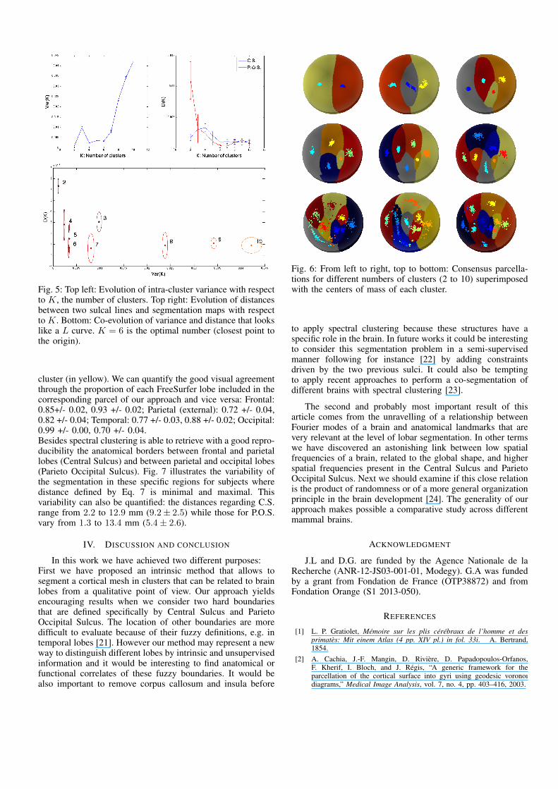
Fig. 5: Top left: Evolution of intra-cluster variance with respectto K, the number of clusters. Top right: Evolution of distancesbetween two sulcal lines and segmentation maps with respectto K. Bottom: Co-evolution of variance and distance that lookslike a L curve. K = 6 is the optimal number (closest point tothe origin).

cluster (in yellow). We can quantify the good visual agreementthrough the proportion of each FreeSurfer lobe included in thecorresponding parcel of our approach and vice versa: Frontal:0.85+/- 0.02, 0.93 +/- 0.02; Parietal (external): 0.72 +/- 0.04,0.82 +/- 0.04; Temporal: 0.77 +/- 0.03, 0.88 +/- 0.02; Occipital:0.99 +/- 0.00, 0.70 +/- 0.04.Besides spectral clustering is able to retrieve with a good repro-ducibility the anatomical borders between frontal and parietallobes (Central Sulcus) and between parietal and occipital lobes(Parieto Occipital Sulcus). Fig. 7 illustrates the variability ofthe segmentation in these specific regions for subjects wheredistance defined by Eq. 7 is minimal and maximal. Thisvariability can also be quantified: the distances regarding C.S.range from 2.2 to 12.9 mm (9.2± 2.5) while those for P.O.S.vary from 1.3 to 13.4 mm (5.4± 2.6).

IV. DISCUSSION AND CONCLUSION

In this work we have achieved two different purposes:First we have proposed an intrinsic method that allows tosegment a cortical mesh in clusters that can be related to brainlobes from a qualitative point of view. Our approach yieldsencouraging results when we consider two hard boundariesthat are defined specifically by Central Sulcus and ParietoOccipital Sulcus. The location of other boundaries are moredifficult to evaluate because of their fuzzy definitions, e.g. intemporal lobes [21]. However our method may represent a newway to distinguish different lobes by intrinsic and unsupervisedinformation and it would be interesting to find anatomical orfunctional correlates of these fuzzy boundaries. It would bealso important to remove corpus callosum and insula before

Fig. 6: From left to right, top to bottom: Consensus parcella-tions for different numbers of clusters (2 to 10) superimposedwith the centers of mass of each cluster.

to apply spectral clustering because these structures have aspecific role in the brain. In future works it could be interestingto consider this segmentation problem in a semi-supervisedmanner following for instance [22] by adding constraintsdriven by the two previous sulci. It could also be temptingto apply recent approaches to perform a co-segmentation ofdifferent brains with spectral clustering [23].

The second and probably most important result of thisarticle comes from the unravelling of a relationship betweenFourier modes of a brain and anatomical landmarks that arevery relevant at the level of lobar segmentation. In other termswe have discovered an astonishing link between low spatialfrequencies of a brain, related to the global shape, and higherspatial frequencies present in the Central Sulcus and ParietoOccipital Sulcus. Next we should examine if this close relationis the product of randomness or of a more general organizationprinciple in the brain development [24]. The generality of ourapproach makes possible a comparative study across differentmammal brains.

ACKNOWLEDGMENT

J.L and D.G. are funded by the Agence Nationale de laRecherche (ANR-12-JS03-001-01, Modegy). G.A was fundedby a grant from Fondation de France (OTP38872) and fromFondation Orange (S1 2013-050).

REFERENCES

[1] L. P. Gratiolet, Memoire sur les plis cerebraux de l’homme et desprimates: Mit einem Atlas (4 pp. XIV pl.) in fol. 33i. A. Bertrand,1854.

[2] A. Cachia, J.-F. Mangin, D. Riviere, D. Papadopoulos-Orfanos,F. Kherif, I. Bloch, and J. Regis, “A generic framework for theparcellation of the cortical surface into gyri using geodesic voronoıdiagrams,” Medical Image Analysis, vol. 7, no. 4, pp. 403–416, 2003.

Fig. 7: Two first pictures: zoom on the Central Sulcus (white)of two subjects for which the distance between C.S. and theborder of clusters is minimal and maximal respectively. Twolast pictures: the same for Parieto-Occipital Sulcus (blue).

Fig. 8: Top: Unsupervised consensus segmentation for K = 6,external and internal view. Bottom: Consensus segmentationobtained with Freesurfer on the group of subjects. See text formore details.

[3] R. S. Desikan, F. Segonne, B. Fischl, B. T. Quinn, B. C. Dickerson,D. Blacker, R. L. Buckner, A. M. Dale, R. P. Maguire, B. T. Hymanet al., “An automated labeling system for subdividing the humancerebral cortex on mri scans into gyral based regions of interest,”Neuroimage, vol. 31, no. 3, pp. 968–980, 2006.

[4] C. Destrieux, B. Fischl, A. Dale, and E. Halgren, “Automatic par-cellation of human cortical gyri and sulci using standard anatomicalnomenclature,” Neuroimage, vol. 53, no. 1, pp. 1–15, 2010.

[5] B. Thirion, G. Flandin, P. Pinel, A. Roche, P. Ciuciu, and J.-B. Poline,

“Dealing with the shortcomings of spatial normalization: Multi-subjectparcellation of fmri datasets,” Human brain mapping, vol. 27, no. 8,pp. 678–693, 2006.

[6] A. Shamir, “A survey on mesh segmentation techniques,” in Computergraphics forum, vol. 27, no. 6. Wiley Online Library, 2008, pp. 1539–1556.

[7] R. Liu and H. Zhang, “Segmentation of 3d meshes through spectralclustering,” in Computer Graphics and Applications, 2004. PG 2004.Proceedings. 12th Pacific Conference on. IEEE, 2004, pp. 298–305.

[8] H. Zhang and R. Liu, “Mesh segmentation via recursive and visuallysalient spectral cuts,” in Proc. of vision, modeling, and visualization.Citeseer, 2005, pp. 429–436.

[9] A. Y. Ng, M. I. Jordan, Y. Weiss et al., “On spectral clustering: Analysisand an algorithm,” Advances in neural information processing systems,vol. 2, pp. 849–856, 2002.

[10] M. Kac, “Can one hear the shape of a drum?” The american mathe-matical monthly, vol. 73, no. 4, pp. 1–23, 1966.

[11] C. Gordon, D. L. Webb, and S. Wolpert, “One cannot hear the shape ofa drum,” Bulletin of the American Mathematical Society, vol. 27, no. 1,pp. 134–138, 1992.

[12] R. Lai, Y. Shi, I. Dinov, T. Chan, and A. Toga, “Laplace-beltrami nodalcounts: A new signature for 3d shape analysis,” in IEEE InternationalSymposium on Biomedical Imaging: From Nano to Macro, ISBI’09,2009, pp. 694–697.

[13] D. Germanaud, J. Lefevre, R. Toro, C. Fischer, and J. Dubois, “Largeris twistier: Spectral analysis of gyrification (spangy) applied to adultbrain size polymorphism,” NeuroImage, vol. 63, pp. 1257–1272, 2012.

[14] Y. Shi, I. Dinov, and A. W. Toga, “Cortical shape analysis in the laplace-beltrami feature space,” in Medical Image Computing and Computer-Assisted Intervention–MICCAI 2009. Springer, 2009, pp. 208–215.

[15] G. Auzias, J. Lefevre, A. Le Troter, C. Fisher, M. Perrot, J. Regis, andO. Coulon, “Model-driven harmonic parameterization of the corticalsurface: Hip-hop,” IEEE, transaction on medical imaging, vol. 32, no. 5,pp. 873–887, 2013.

[16] M. Berger, A panoramic view of Riemannian geometry. SpringerVerlag, 2003.

[17] M. Desbrun, M. Meyer, S. P., and A. Barr, “Implicit fairing of irregularmeshes using diffusion and curvature flow,” in Proceedings of the 26thannual conference on Computer graphics and interactive techniques,1999, pp. 317–324.

[18] U. Von Luxburg, “A tutorial on spectral clustering,” Statistics andcomputing, vol. 17, no. 4, pp. 395–416, 2007.

[19] B. Nadler and M. Galun, “Fundamental limitations of spectral cluster-ing,” in Advances in Neural Information Processing Systems, 2006, pp.1017–1024.

[20] A. Le Troter, D. Riviere, and O. Coulon, “An interactive sulcal fundieditor in brainvisa,” in Proc. Org. Human Brain Mapp. Conf., 2011,p. 61.

[21] J.-J. Kim, B. Crespo-Facorro, N. C. Andreasen, D. S. O’Leary,B. Zhang, G. Harris, and V. A. Magnotta, “An mri-based parcellationmethod for the temporal lobe,” Neuroimage, vol. 11, no. 4, pp. 271–288,2000.

[22] Z. Lu and M. A. Carreira-Perpinan, “Constrained spectral clusteringthrough affinity propagation,” in Computer Vision and Pattern Recog-nition, 2008. CVPR 2008. IEEE Conference on. IEEE, 2008, pp. 1–8.

[23] O. Sidi, O. van Kaick, Y. Kleiman, H. Zhang, and D. Cohen-Or,“Unsupervised co-segmentation of a set of shapes via descriptor-spacespectral clustering,” in ACM Transactions on Graphics (TOG), vol. 30,no. 6. ACM, 2011, p. 126.

[24] R. Toro, “On the possible shapes of the brain,” Evolutionary Biology,vol. 39, no. 4, pp. 600–612, 2012.