Brain Age as a measure of neurocognitive disorders

Page 1

THESEDEDOCTORA

TNNT:2021UPA

SG101

Building clinical biomarkers from cerebralelectrophysiology: Brain Age as a

measure of neurocognitive disordersConstruction de biomarqueurs cliniques à partir de

l’electrophysiologie cérébrale : l’Age du Cerveau commemesure des troubles neurocognitifs

Thèse de doctorat de l’université Paris-Saclay

École doctorale n◦ 580, Sciences et Technologies de l’Information et dela Communication (STIC)

Spécialité de doctorat : Traitement du signal et des imagesGraduate School : Informatique et sciences du numérique

Référent : Faculté des sciences d’Orsay

Thèse préparée dans l’unité de recherche Inria Saclay-Île-de-France(Université Paris-Saclay, Inria), sous la direction de Alexandre GRAMFORT,Directeur de recherche, la co-direction de Etienne GAYAT, Professeur des

universités - praticien hospitalier, le co-encadrement de Denis A.ENGEMANN,Chercheur

Thèse soutenue à Paris-Saclay, le 15 décembre 2021, par

David SABBAGH

Composition du jurySylvain CHEVALLIER PrésidentMaître de conférences, HDR, Université de Ver-sailles St-QuentinFabien LOTTE Rapporteur & ExaminateurDirecteur de Recherche, Inria BordeauxKarim JERBI Rapporteur & ExaminateurProfesseur agrégé, Université de MontréalVadim NIKULIN ExaminateurProfesseur, Max Planck Institute LeipzigAlexandre GRAMFORT Directeur de thèseDirecteur de Recherche, Université Paris-Saclay

Page 2

Title: Building clinical biomarkers from cerebral electrophysiology: Brain Age as a measure of neu-rocognitive disordersKeywords: Machine learning, Neuroimaging, MEG, EEG, Riemannian manifold, Biomarker

Abstract: Neurodegenerative diseases are amongthe top causes of worldwide mortality. Unfortu-nately, early diagnosis is challenging as it requiresa frequently too late indication of biomedical examand dedicated laboratory equipments. It also oftenrelies on research-based predictive measures suffer-ing from selection bias. This thesis investigates apromising solution to tackle these problems: a ro-bust method to build predictive biological markersfrom M/EEG brain signals, directly usable in theclinic, and validated against neurocognitive disor-ders following general anaesthesia.

In a first (theoretical) contribution [Sab+19],we benchmarked M/EEG regression models thatcould learn from between-channels covariance ma-trices as a compact summary of spatial distribu-tion of power of high-dimensional brain M/EEGsignal. Mathematical analysis identified differentmodels supporting perfect prediction under idealcircumstances when the outcome is either linear orlog-linear in the source power. These models arebased on the mathematically principled approachesof supervised spatial filtering and projection withRiemannian geometry, and enjoy optimal predic-tion guarantees without the need of costly sourcelocalization. Our simulation-based findings wereconsistent with the mathematical analysis and sug-gested that these regression algorithms were robustacross data generating scenarios and model viola-tions. This study suggested that the Riemannianmethods have the potential to support automatedlarge-scale analysis of M/EEG data in the absenceof MRI scans, which is one condition to be practi-cally used in the clinic for biomarker development.

In a second (empirical) contribution [Sab+20],we validated our predictive modeling frame-work with several publicly available neuroimagingdatasets and showed it can be used to learn thesurrogate biomarker of brain age from research-grade M/EEG signals, without source localiza-tion and with minimal pre-processing. Our re-

sults demonstrate that our Riemannian data-drivenmethod does not fall far behind the gold-standardsource localization methods with biophysical pri-ors, that depend on manual data processing, thecostly availability of anatomical MRI images andspecialized knowledge in M/EEG source modeling.Subsequent large-scale empirical analysis providedevidence that brain age derived from MEG cap-tures unique information related to neuronal ac-tivity that was not explained by anatomical MRI.They also suggested that, consistent with simula-tions, Riemannian methods are generally a goodbet across a wide range of settings with consider-able robustness to different choices of preprocess-ing including minimalistic preprocessing. The goodperformance obtained on MEG was also reachedwith research-grade clinical EEG.

In a third (clinical) contribution [Sab+21, inprep.], we validated the concept of M/EEG-derivedbrain age directly in the operating rooms of Lari-boisière hospital in Paris, from monitoring-gradeclinical EEG during the particular period of generalanaesthesia. We validated our EEG-based brainage measure against intra-operative complicationsand brain health in anaesthesia population with apotential link to postoperative cognitive dysfunc-tions, unveiling it as a promising clinical biomarkerof neurocognitive disorders. We also showed thatthe drug critically impacts brain age prediction anddemonstrated the robustness applicability of ourapproach across different types of drugs.

By combining concepts previously investigatedseparately, our contribution demonstrates theclinical relevance of EEG-brain-age in revealingpathologies of brain function and obtaining brainhealth assessments in situations where MRI scanscannot be conducted. It also provides early evi-dence that anaesthesia-based modeling has the po-tential to help biomarker discovery and eventuallyrevolutionize preventive medicine.

Page 3

Titre : Construction de biomarqueurs cliniques à partir de l’electrophysiologie cérébrale : l’Age duCerveau comme mesure des troubles neurocognitifsMots clés : Apprentissage statistique, Imagerie cérébrale, MEG, EEG, Variétés riemanniennes, Bio-marqueur

Résumé : Les maladies neurodégénératives fi-gurent parmi les principales causes de mortalitédans le monde. Malheureusement, leur diagnosticprécoce nécessite un examen médical prescrit sou-vent trop tardivement et des équipements de la-boratoire dédiés. Il repose aussi fréquemment surdes mesures prédictives souffrant d’un biais de sé-lection. Cette thèse présente une solution promet-teuse à ces problèmes : une méthode robuste, di-rectement utilisable en clinique, pour construiredes biomarqueurs prédictifs à partir des signauxcérébraux M/EEG, validés contre les troubles neu-rocognitifs apparaissant après une anesthésie gé-nérale.

Dans une première contribution (théo-rique) [Sab+19], nous avons évalué des modèles derégression capables d’apprendre des biomarqueursà partir des matrices de covariance de signauxM/EEG. Notre analyse mathématique a identi-fié différents modèles garantissant une prédictionparfaite dans des circonstances idéales, lorsque lacible est une fonction (log-)linéaire en la puis-sance des sources cérébrales. Ces modèles, baséssur les approches mathématiques de filtrage spa-tial supervisé et de géométrie riemannienne, per-mettent une prédiction optimale sans nécessiterune coûteuse localisation des sources. Nos simu-lations confirment cette analyse mathématique etsuggèrent que ces algorithmes de régression sontrobustes à travers les mécanismes de génération dedonnées et les violations de modèles. Cette étudesuggère que les méthodes riemanniennes sont desméthodes de choix pour l’analyse automatisée àgrande échelle des données M/EEG en l’absenced’IRM, condition importante pour pouvoir déve-lopper des biomarqueurs cliniques.

Dans une deuxième contribution (empi-rique) [Sab+20], nous avons validé nos modèlesprédictifs sur plusieurs ensembles de données deneuro-imagerie et avons montré qu’ils peuvent êtreutilisé pour apprendre l’âge du cerveau à partirde signaux cérébraux M/EEG, sans localisation desources, et avec un prétraitement minimal des don-

nées. De plus, la performance de notre méthoderiemannienne est proche de celle des méthodes deréférence nécessitant une localisation de sources etdonc un traitement manuel des données, la dispo-nibilité d’images IRM anatomiques et une expertiseen modélisation de sources M/EEG. Une analyseempirique à grande échelle a ensuite permis de dé-montrer que l’âge du cerveau dérivé de la MEGcapture des informations uniques liées à l’activiténeuronale et non expliquées par l’IRM anatomique.Conformément aux simulations, ces résultats sug-gèrent également que l’approche riemannienne estune méthode pouvant s’appliquer dans un largeéventail de situations, avec une robustesse consi-dérable aux différents choix de prétraitement, ycompris minimaliste. Les bonnes performances ob-tenues avec la MEG ont ensuite été répliquées avecdes EEGs de qualité recherche.

Dans une troisième contribution (cli-nique) [Sab+21, en préparation], nous avons validéle concept d’âge cérébral directement au bloc opé-ratoire de l’hôpital Lariboisière à Paris, à partird’EEG de qualité clinique recueillis pendant la pé-riode de l’anesthésie générale. Nous avons évaluénotre mesure de l’âge cérébral comme prédicteurde complications peropératoires liées aux dysfonc-tions cognitives post opération, validant ainsi l’âgedu cerveau comme un biomarqueur clinique pro-metteur des troubles neurocognitifs. Nous avonségalement montré que le sédatif utilisé a un impactimportant sur la prédiction de l’âge du cerveau etavons démontré la robustesse de notre approche àdifférents types de médicaments.

Combinant des concepts précédemment étu-diés séparément, notre contribution démontre lapertinence clinique de la notion d’âge du cerveauprédit à partir de l’EEG pour révéler les patholo-gies des fonctions cérébrales dans des situations oùl’IRM ne peut pas être réalisée. Ces résultats four-nissent également une première preuve que l’anes-thésie générale est une période propice à la décou-verte de biomarqueurs cérébraux, avec un impactpotentiel profond sur la médecine préventive.

3

Page 4

Acknowledgement

This thesis is the result of an incredible intellectual journey that began 3 years agowhen I first met my future PhD advisor, Denis, during this cold and snowy winternight on the Plateau de Saclay. We didn’t know it by then but it was the beginningof a sensational scientific ride. I don’t have the words to express my gratitude to himfor his kindness during these 3 years, his daily care and his generosity. I was verylucky to meet him: his unfaltering enthusiasm made this thesis an unforgettablelearning experience. Then two other advisors quickly joined the adventure.

To Alex I extend my deepest gratitude for welcoming me to his lab, and supportingme through the challenges of this project. I can only imagine his surprise to seethis 43 years old guy at the time approaching him to pursue a PhD. I thank himvery much for not having laughed at me and for his trust. His pragmatism, scientificrigour, attention to detail and dedication to the open source software communitywill continue to inspire me for years to come.

To Etienne I am also particularly grateful, for his faith in the project and so kindlyand so humbly welcoming me in his team of medical doctors. His double training inmedicine and statistics made him the perfect guide and bridge to the clinical world.Denis, Alex and Etienne have been the mentors any PhD student could dream of.None of this could have been possible without their competence, their benevolence,kindness, and availability.

I feel also very indebted to my collaborators from which I learnt so much. To PierreAblin at Inria on the mathematical aspects of this work: I will always remember theintensity of our sprint against the NeurIPS deadline. To Fabrice Vallée, Jona Joachim,Jerome Cartailler and Cyril Touchard at AP-HP: it is rare to meet a team of medicaldoctors so open to external collaborations and enthusiastic about what mathematicsand compute science can bring to the practice of medicine. They made me realizehow little I know on what ultimately matters the most.

I also want to thank my colleagues in the Parietal team at Inria. Their comradeshipand support made my time so much pleasant. On account of his leader, BertrandThirion, Parietal is more than a team, it’s a culture in which I grew naturally. Inparticular I feel very lucky for meeting Valentin, Hicham, Maëliss and Hubert,who became my friends. Writing this acknowledgment makes me realize that this

i

Page 5

scientific endeavour was ultimately a human adventure. To all these people: you arewhat I will remember the most from these 3 years.

On a more personal note, I am incredibly grateful beyond words to my family andmy friends for their unconditional affection since the beginning and their unfailingsupport. To my love, Virginie, who supports me in every moment: it is her dailylove and intelligence that gives me the courage and the strength to face the excitingchallenges of my life. And finally, to my two little girls Ava and Lisa. You’re too littleto even understand these words but big in your ability to wonder, laugh and love.Let this thesis be a testimony of the power of will. Never ever let anyone tell youwhat you can or can’t do. This thesis is for you.

David Sabbagh

Paris, December 2021

Page 6

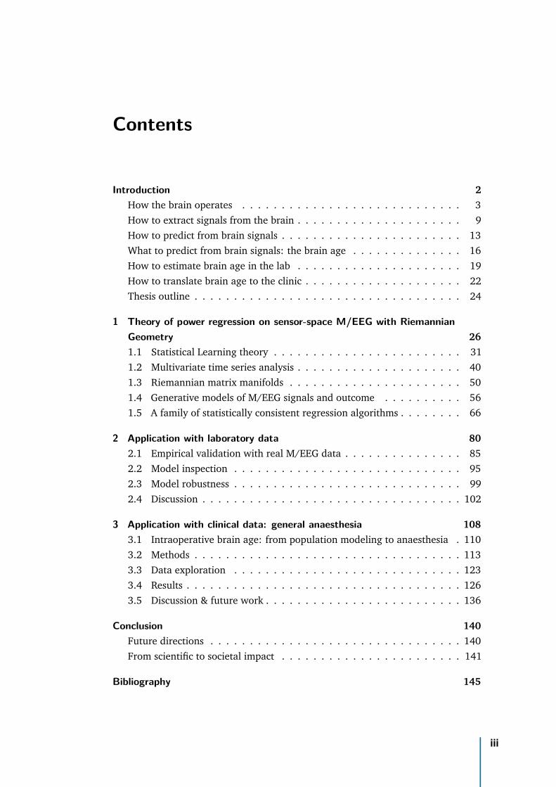
Contents

Introduction 2How the brain operates . . . . . . . . . . . . . . . . . . . . . . . . . . . . 3How to extract signals from the brain . . . . . . . . . . . . . . . . . . . . . 9How to predict from brain signals . . . . . . . . . . . . . . . . . . . . . . . 13What to predict from brain signals: the brain age . . . . . . . . . . . . . . 16How to estimate brain age in the lab . . . . . . . . . . . . . . . . . . . . . 19How to translate brain age to the clinic . . . . . . . . . . . . . . . . . . . . 22Thesis outline . . . . . . . . . . . . . . . . . . . . . . . . . . . . . . . . . . 24

1 Theory of power regression on sensor-space M/EEG with RiemannianGeometry 261.1 Statistical Learning theory . . . . . . . . . . . . . . . . . . . . . . . . 311.2 Multivariate time series analysis . . . . . . . . . . . . . . . . . . . . . 401.3 Riemannian matrix manifolds . . . . . . . . . . . . . . . . . . . . . . 501.4 Generative models of M/EEG signals and outcome . . . . . . . . . . 561.5 A family of statistically consistent regression algorithms . . . . . . . . 66

2 Application with laboratory data 802.1 Empirical validation with real M/EEG data . . . . . . . . . . . . . . . 852.2 Model inspection . . . . . . . . . . . . . . . . . . . . . . . . . . . . . 952.3 Model robustness . . . . . . . . . . . . . . . . . . . . . . . . . . . . . 992.4 Discussion . . . . . . . . . . . . . . . . . . . . . . . . . . . . . . . . . 102

3 Application with clinical data: general anaesthesia 1083.1 Intraoperative brain age: from population modeling to anaesthesia . 1103.2 Methods . . . . . . . . . . . . . . . . . . . . . . . . . . . . . . . . . . 1133.3 Data exploration . . . . . . . . . . . . . . . . . . . . . . . . . . . . . 1233.4 Results . . . . . . . . . . . . . . . . . . . . . . . . . . . . . . . . . . . 1263.5 Discussion & future work . . . . . . . . . . . . . . . . . . . . . . . . . 136

Conclusion 140Future directions . . . . . . . . . . . . . . . . . . . . . . . . . . . . . . . . 140From scientific to societal impact . . . . . . . . . . . . . . . . . . . . . . . 141

Bibliography 145

iii

Page 7

Introduction

ContentsHow the brain operates . . . . . . . . . . . . . . . . . . . . . . . . . . 3

How to extract signals from the brain . . . . . . . . . . . . . . . . . . 9

How to predict from brain signals . . . . . . . . . . . . . . . . . . . . . 13

What to predict from brain signals: the brain age . . . . . . . . . . . . 16

How to estimate brain age in the lab . . . . . . . . . . . . . . . . . . . 19

How to translate brain age to the clinic . . . . . . . . . . . . . . . . . . 22

Thesis outline . . . . . . . . . . . . . . . . . . . . . . . . . . . . . . . . 24

What reveals the most about us? Is it the colour of our eyes, our heart beats, ourblood pressure, our clicks on a webpage? Even though all of this reveals somepart of us, there is one single organ that contains all the information about ourthoughts, our feelings, our memory, our actions: this is our brain. The billions ofinterconnected cells that compose our brain, firing at hectic pace, are literally ourperception, our thinking, our emotions, our memories and ultimately define who weare. If our brain activity is expressing cognition then changes to cognition should berevealed in the brain signals extracted from this activity. These signals are thereforethe source of promising predictive biological markers of our functioning and perhapsmore importantly dysfunctioning.

Brain diseases have a dramatic impact on life, ranging from neurodegenerativediseases to loss of brain functions. Besides these devastating consequences, they alsoare among top causes of death in the European Union. It accounted for 18M deathsbetween 2011 and 2017 [Eura] among which 13M due to cerebrovascular and 5Mdue to neurodegenerative diseases like Parkinson’s, Alzheimer’s, dementia, stroke,multiple sclerosis or epilepsy. This is even more acute for patients over the age of60. For example an American woman aged 65 today has almost 25 % chance ofcontracting Alzheimer’s disease during her lifetime [Aa2]. This age group representsabout one quarter of the global population and will continue to grow at a fast pacein the coming decades [Eurc; Eurb; Vol+20]: we expect twice more 65y+ humansin 2050 than today globally [Un2]. Pathologies of the brain are therefore one of

2

Page 8

the biggest challenges for medicine today and brain health a top priority in publichealth.

We are not equal when facing neurocognitive disorders. But even today it is difficultto know if a patient will develop a particular brain disease or if his brain willage normally. As a consequence, these pathologies are too often detected at latestages, rendering treatment significantly less efficient. For the moment, no biologicalmarker is able to early identify high-risk patients. Having an early test of cognitivedysfunction, directly built from brain signals and easily available for millions ofpersons, would allow for better detection and treatment of brain diseases. This isthe subject of this thesis.

More precisely this theoretical and experimental work will investigate a generalmethod to build predictive biomarkers from brain signals, directly usable in theclinic, with an application to predict neurocognitive disorders. The objective ofthis chapter is to provide a general overview of the sequence of challenges standingin the road to this endeavour. We need to understand:

How the brain operates: even if the precise working of the human brain is stilllargely unknown, we first need to have a rough picture of how it is structured andunderstand the basis of its activity.How to extract signals from the brain: we then need to find a way to capture thisactivity and extract a measurable signal.How to predict from brain signal: with brain signal as input data we should seekthe best algorithm to predict from it, simple enough to be usable in the clinicalsettings.What to predict from brain signal: once we have the input data and the algorithmwe should determine the target of prediction, a target that is both easily availableand linked to the clinical outcome of interest. This leads to the concept of brain ageas a promising biomarker of neurocognitive disorders.How to estimate brain age in the lab: we then need to put this all together andrun experiments to see how to estimate this biomarker in the comfortable conditionsof a research laboratory.How to translate brain age to the clinic: then we’ll investigate how to translatethe brain age biomarker in the more challenging conditions of the clinic.

Each of these challenges are investigated in further details in subsequent sections.

How the brain operatesThe human brain roughly weights as little as 1.5 kg and operates on the same powerthan a simple electric bulb (∼20 W, to be compared with the 8000 W consumed by

3

Page 9

IBM Watson that outperformed the best human in Jeopardy in 2011). This sobrietyhides a formidable complexity [Fac06].

With ∼100 billions of excitable nerve cells, the neurons, each connected to 7000 otherneurons on average, the human brain is arguably the most complex organ of thehuman body, and the most complex known object in the universe. It consumes onefifth of the body total energy expenditure, a huge consumption compared to itsrelative weight. How it performs a wide range of cognitive functions, from visualrecognition to language understanding, speech, social interaction, and executivecontrol is, for the most part, still a mystery. Understanding the human brain istherefore one of the most significant challenges of the 21st century. Fortunately,some of its inner working is understood today [DA01; Ger+14].

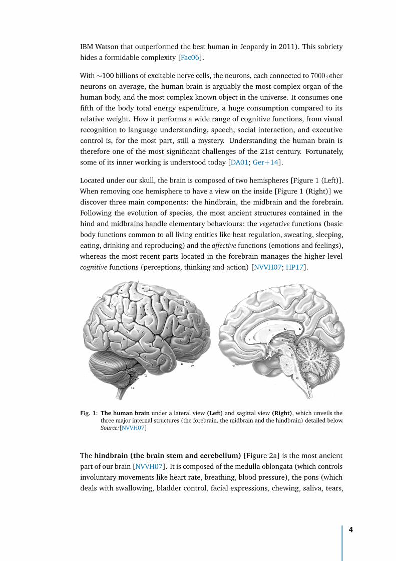
Located under our skull, the brain is composed of two hemispheres [Figure 1 (Left)].When removing one hemisphere to have a view on the inside [Figure 1 (Right)] wediscover three main components: the hindbrain, the midbrain and the forebrain.Following the evolution of species, the most ancient structures contained in thehind and midbrains handle elementary behaviours: the vegetative functions (basicbody functions common to all living entities like heat regulation, sweating, sleeping,eating, drinking and reproducing) and the affective functions (emotions and feelings),whereas the most recent parts located in the forebrain manages the higher-levelcognitive functions (perceptions, thinking and action) [NVVH07; HP17].

Fig. 1: The human brain under a lateral view (Left) and sagittal view (Right), which unveils thethree major internal structures (the forebrain, the midbrain and the hindbrain) detailed below.Source:[NVVH07]

The hindbrain (the brain stem and cerebellum) [Figure 2a] is the most ancientpart of our brain [NVVH07]. It is composed of the medulla oblongata (which controlsinvoluntary movements like heart rate, breathing, blood pressure), the pons (whichdeals with swallowing, bladder control, facial expressions, chewing, saliva, tears,

4

Page 10

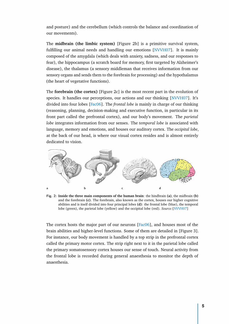
and posture) and the cerebellum (which controls the balance and coordination ofour movements).

The midbrain (the limbic system) [Figure 2b] is a primitive survival system,fulfilling our animal needs and handling our emotions [NVVH07]. It is mainlycomposed of the amygdala (which deals with anxiety, sadness, and our responses tofear), the hippocampus (a scratch board for memory, first targeted by Alzheimer’sdisease), the thalamus (a sensory middleman that receives information from oursensory organs and sends them to the forebrain for processing) and the hypothalamus(the heart of vegetative functions).

The forebrain (the cortex) [Figure 2c] is the most recent part in the evolution ofspecies. It handles our perceptions, our actions and our thinking [NVVH07]. It’sdivided into four lobes [Fac06]. The frontal lobe is mainly in charge of our thinking(reasoning, planning, decision-making and executive function, in particular in itsfront part called the prefrontal cortex), and our body’s movement. The parietallobe integrates information from our senses. The temporal lobe is associated withlanguage, memory and emotions, and houses our auditory cortex. The occipital lobe,at the back of our head, is where our visual cortex resides and is almost entirelydedicated to vision.

a b c d

Fig. 2: Inside the three main components of the human brain: the hindbrain (a), the midbrain (b)and the forebrain (c). The forebrain, also known as the cortex, houses our higher cognitiveabilities and is itself divided into four principal lobes (d): the frontal lobe (blue), the temporallobe (green), the parietal lobe (yellow) and the occipital lobe (red). Source:[NVVH07]

The cortex hosts the major part of our neurons [Fac06], and houses most of thebrain abilities and higher-level functions. Some of them are detailed in [Figure 3].For instance, our body movement is handled by a top strip in the prefrontal cortexcalled the primary motor cortex. The strip right next to it in the parietal lobe calledthe primary somatosensory cortex houses our sense of touch. Neural activity fromthe frontal lobe is recorded during general anaesthesia to monitor the depth ofanaesthesia.

5

Page 11

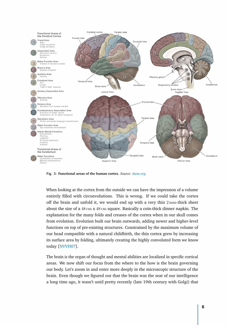
Fig. 3: Functional areas of the human cortex. Source: dana.org.

When looking at the cortex from the outside we can have the impression of a volumeentirely filled with circonvolutions. This is wrong. If we could take the cortexoff the brain and unfold it, we would end up with a very thin 2 mm-thick sheetabout the size of a 48 cm x 48 cm square. Basically a coin-thick dinner napkin. Theexplanation for the many folds and creases of the cortex when in our skull comesfrom evolution. Evolution built our brain outwards, adding newer and higher-levelfunctions on top of pre-existing structures. Constrained by the maximum volume ofour head compatible with a natural childbirth, the thin cortex grew by increasingits surface area by folding, ultimately creating the highly convoluted form we knowtoday [NVVH07].

The brain is the organ of thought and mental abilities are localized in specific corticalareas. We now shift our focus from the where to the how is the brain governingour body. Let’s zoom in and enter more deeply in the microscopic structure of thebrain. Even though we figured out that the brain was the seat of our intelligencea long time ago, it wasn’t until pretty recently (late 19th century with Golgi) that

6

Page 12

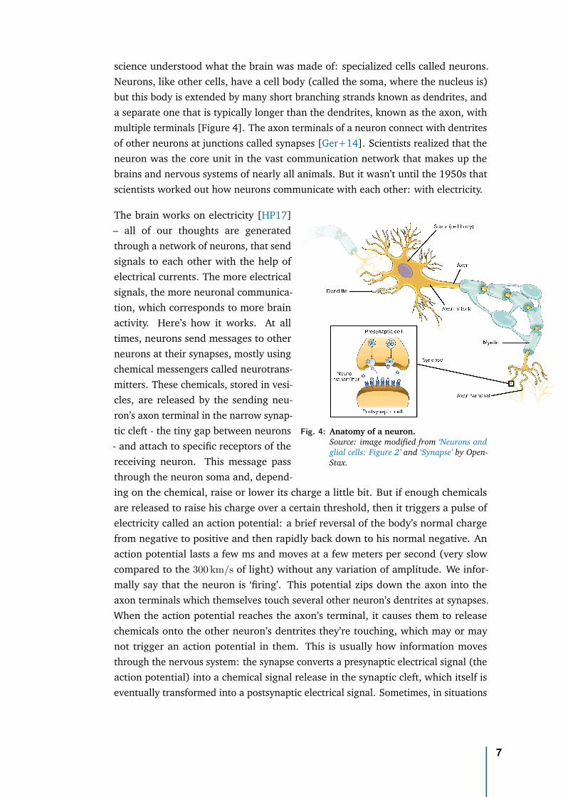
science understood what the brain was made of: specialized cells called neurons.Neurons, like other cells, have a cell body (called the soma, where the nucleus is)but this body is extended by many short branching strands known as dendrites, anda separate one that is typically longer than the dendrites, known as the axon, withmultiple terminals [Figure 4]. The axon terminals of a neuron connect with dentritesof other neurons at junctions called synapses [Ger+14]. Scientists realized that theneuron was the core unit in the vast communication network that makes up thebrains and nervous systems of nearly all animals. But it wasn’t until the 1950s thatscientists worked out how neurons communicate with each other: with electricity.

Fig. 4: Anatomy of a neuron.Source: image modified from ‘Neurons andglial cells: Figure 2’ and ‘Synapse’ by Open-Stax.

The brain works on electricity [HP17]– all of our thoughts are generatedthrough a network of neurons, that sendsignals to each other with the help ofelectrical currents. The more electricalsignals, the more neuronal communica-tion, which corresponds to more brainactivity. Here’s how it works. At alltimes, neurons send messages to otherneurons at their synapses, mostly usingchemical messengers called neurotrans-mitters. These chemicals, stored in vesi-cles, are released by the sending neu-ron’s axon terminal in the narrow synap-tic cleft - the tiny gap between neurons- and attach to specific receptors of thereceiving neuron. This message passthrough the neuron soma and, depend-ing on the chemical, raise or lower its charge a little bit. But if enough chemicalsare released to raise his charge over a certain threshold, then it triggers a pulse ofelectricity called an action potential: a brief reversal of the body’s normal chargefrom negative to positive and then rapidly back down to his normal negative. Anaction potential lasts a few ms and moves at a few meters per second (very slowcompared to the 300 km/s of light) without any variation of amplitude. We infor-mally say that the neuron is ‘firing’. This potential zips down the axon into theaxon terminals which themselves touch several other neuron’s dentrites at synapses.When the action potential reaches the axon’s terminal, it causes them to releasechemicals onto the other neuron’s dentrites they’re touching, which may or maynot trigger an action potential in them. This is usually how information movesthrough the nervous system: the synapse converts a presynaptic electrical signal (theaction potential) into a chemical signal release in the synaptic cleft, which itself iseventually transformed into a postsynaptic electrical signal. Sometimes, in situations

7

Page 13

when the body needs to move a signal more quickly, neuron-to-neuron connectionscan themselves be electric, passing not through chemical but electrical synapses inwhich ions flow directly between cells.

The density of this network in the cortex is almost unthinkable: each 1 mm3 of cortexgray matter contains 50 000 neurons, each of them giving rise to 6000 synapses sototaling roughly 300 M synapses [NVVH07]. The thin convoluted cortex, constitutingthe bark of the brain, is called the grey matter in contrast with the space underneath,mostly occupied by wiring, the axons of cortical neurons, sheathed with a fatty whitematter called myelin. We can think of the cortex as a command center that sendmany of its orders through the mass of axons making up the white matter beneath it.Now let’s zoom out again to see the biggest picture.

Fig. 5: Human central and peripheralnervous systems.Source: modified from Wikipedia‘Nervous system diagram’.

The cortical axons of neurons in the brain mightbe taking information to either another partwithin the cortex, to the lower parts of the brain(brain stem or limbic system), or through thespinal cord (a massive bundle of axons com-posing the nervous system’s superhighway) intothe rest of the body. Indeed, the whole nervoussystem is divided into two parts: the central ner-vous system (the brain and spinal cord) and theperipheral nervous system (different types ofneurons that radiate outwards from the spinalcord into the rest of the body). Bundles of ax-ons of these neurons are wrapped together in alittle cord called a nerve. Sensory nerves bringsignals into the central nervous system, motornerves carry signals out of it [Fac06].

Let’s take an example to illustrate how theseparts interact: when a fly touches our skin it

stimulates many sensory nerves The axon terminals of the sensory neurons inthe nerves start firing, send the signal into the spinal cord and up to the brain,more precisely in this case the somas in the somatosensory cortex. To trigger anaction (chasing away the fly), the somasensory cortex then send action potentials toparticular somas in the motor cortex that connect to the muscles in our arm that startfiring, sending the signals back into the spinal cord and then out to the muscles ofthe arm. The axon terminals at the end of those neurons stimulate the arm muscles.

The scientific study of the brain has lead to remarkable advances since the middleof the twentieth century, both at the macroscopic level [NVVH07] (the major brainanatomical functions and structures) and at the microscopic level [DA01] (how a

8

Page 14

MRI fMRI MEG EEG

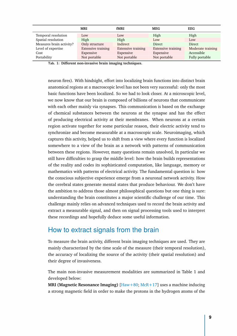
Temporal resolution Low Low High HighSpatial resolution High High Low LowMeasures brain activity? Only structure Indirect Direct DirectLevel of expertise Extensive training Extensive training Extensive training Moderate trainingCost Expensive Expensive Expensive AccessiblePortability Not portable Not portable Not portable Fully portable

Tab. 1: Different non-invasive brain imaging techniques.

neuron fires). With hindsight, effort into localizing brain functions into distinct brainanatomical regions at a macroscopic level has not been very successful: only the mostbasic functions have been localized. So we had to look closer. At a microscopic level,we now know that our brain is composed of billions of neurons that communicatewith each other mainly via synapses. This communication is based on the exchangeof chemical substances between the neurons at the synapse and has the effectof producing electrical activity at their membranes. When neurons at a certainregion activate together for some particular reason, their electric activity tend tosynchronize and become measurable at a macroscopic scale. Neuroimaging, whichcaptures this activity, helped us to shift from a view where every function is localizedsomewhere to a view of the brain as a network with patterns of communicationbetween these regions. However, many questions remain unsolved, In particular westill have difficulties to grasp the middle level: how the brain builds representationsof the reality and codes its sophisticated computation, like language, memory ormathematics with patterns of electrical activity. The fundamental question is: howthe conscious subjective experience emerge from a neuronal network activity. Howthe cerebral states generate mental states that produce behaviour. We don’t havethe ambition to address those almost philosophical questions but one thing is sure:understanding the brain constitutes a major scientific challenge of our time. Thischallenge mainly relies on advanced techniques used to record the brain activity andextract a measurable signal, and then on signal processing tools used to interpretthese recordings and hopefully deduce some useful information.

How to extract signals from the brainTo measure the brain activity, different brain imaging techniques are used. They aremainly characterized by the time scale of the measure (their temporal resolution),the accuracy of localizing the source of the activity (their spatial resolution) andtheir degree of invasiveness.

The main non-invasive measurement modalities are summarized in Table 1 anddeveloped below:MRI (Magnetic Resonance Imaging) [Haw+80; McR+17] uses a machine inducinga strong magnetic field in order to make the protons in the hydrogen atoms of the

9

Page 15

water in our body to point in the same direction. Then it measures the energyemitted from the relaxation of protons to this aligned state when briefly disruptedby a radio pulse. This allows the computer to determine what the tissue looked like,depending on this energy that is released, and show an image of the tissue. MRIthus excels at isolating anatomical details, revealing the brain’s structure and thedifferent types of tissue present, like white and grey matter. This is the modalitymostly used in literature to estimate the brain age. Yet, MRI only shows us a staticanatomical image of the brain, not the brain’s actual activity.fMRI (Functional MRI) [Kwo+92; Log+01] uses the same mechanism than MRIto also measure the energy emitted from the relaxation of protons but this timeaimed at determining the oxygenated blood flow changes in response to neuralactivity. The neuronal activation is therefore indirectly measured via local changesin the level of blood oxygenation, known as the BOLD (Blood-Oxygenation LevelDependent) response, with a limited temporal resolution (typically around 1 s) dueto slow changes of the blood flow. Nevertheless fMRI has a better spatial resolutionnow below 1 mm, allowing to finely measure activity across different brain regions,enabling precise functional brain mappings.EEG (electroencephalography) [Ber29; HP17] uses an array of electrodes on acap placed on the scalp on a subject to directly measure the electrical activity ofthe brain. To facilitate comparisons between experiments, it is common practice toput the electrodes on standard positions. See Figure 2.4 for an example. The EEGamplitude mainly depends on the size of the active area as the voltage under eachelectrode is not the result of the electrical activity of a single neuron but instead asummed potential of populations of thousands of neurons. It also depends on thedistance between the sources in the brain and the electrodes, taking into accountthe signal attenuation induced by the scalp. EEG signals typically are 50 to 100 µV inamplitude, about 1 M times lower than voltages used to power home equipments,thus need to be amplified. Recordings of sufficient quality can nevertheless beperformed in regular rooms and even in real-life settings using mobile EEG devices,with controlling head and body movements as they may cause artifacts. Thanks toits portability, EEG is operated in a wide array of peculiar situations, such as surgery[Bak+75], flying an aircraft [SS65] or sleeping [AJWW66]. For example EEG is usedto diagnose pathologies for which the cerebral bioelectrical activity is susceptible tobe perturbed, and especially to precise the location of cerebral tumors or differenttypes of epilepsy and epileptic sources.MEG (magnetoencephalography) [Häm+93; HP17] uses sensors to measure themagnetic field produced by the brain. Indeed, any electric current is associated withmagnetic fields as a consequence of Maxwell’s theory. Therefore, the brain generatestiny magnetic fields outside the head (~100 fT) 10−8 times the strength of the earth’ssteady magnetic field, requiring very sensitive sensors and heavy noise cancellation.Their extreme sensitivity is challenged by many electromagnetic nuisance sources(any moving metal objects like cars or elevators) or electrically powered instruments,

10

Page 16

generating magnetic induction that is orders of magnitude stronger than the brain’s.The measurement itself is therefore done inside a special magnetically shielded roomto dampen external ambient magnetic disturbances. Their influence can be furtherreduced by combining magnetometers coils (that directly measure the absolutemagnitude of the magnetic field) with gradiometers coils (that record the gradientof the magnetic field in certain directions). Those gradiometers, arranged either in aradial or tangential (planar) way, record the gradient of the magnetic field towards2 perpendicular directions hence inherently greatly emphasize brain signals withrespect to environmental noise. Unlike EEG, MEG is not portable but captures a moreselective set of brain sources with greater spectral and spatial definition [Ahl+10;HLR00], as the skull smears electrical but not magnetical signal.

More invasive techniques, using electrodes placed closer to the brain, are requiredto obtain both a good temporal and spatial resolution. Such techniques includeECoG (electrocorticography) [Pal06] which uses electrodes placed on the corticalsurface below the skull and LFP (local field potential) [DCS99] which uses micro-electrodes directly placed inside the brain to record the electric potential in theextracellular space of the brain tissue. Small intracerebral electrodes are typicallyused to measure these potentials as opposed to large surface electrodes used in EEG,enabling measurement of more localized populations of neurons. These techniquesprovides extremely valuable recordings with excellent resolution and Signal-to-NoiseRatio (SNR) but are really invasive and offer a limited coverage of the brain.

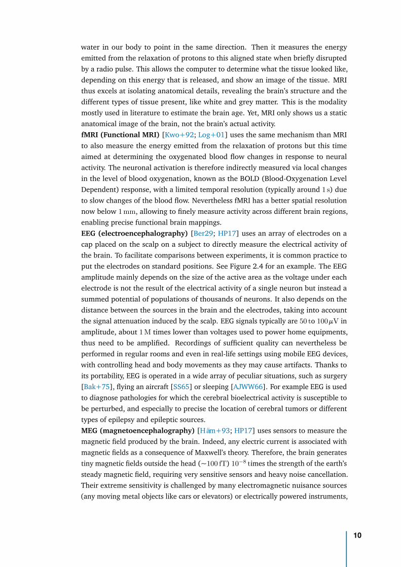
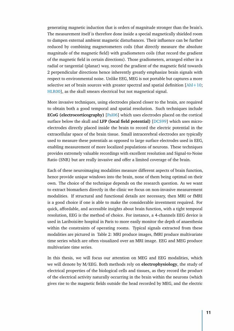
Each of these neuroimaging modalities measure different aspects of brain function,hence provide unique windows into the brain, none of them being optimal on theirown. The choice of the technique depends on the research question. As we wantto extract biomarkers directly in the clinic we focus on non-invasive measurementmodalities. If structural and functional details are necessary, then MRI or fMRIis a good choice if one is able to make the considerable investment required. Forquick, affordable, and accessible insights about brain function, with a tight temporalresolution, EEG is the method of choice. For instance, a 4-channels EEG device isused in Lariboisière hospital in Paris to more easily monitor the depth of anaesthesiawithin the constraints of operating rooms. Typical signals extracted from thesemodalities are pictured in Table 2: MRI produce images, fMRI produce multivariatetime series which are often visualized over an MRI image. EEG and MEG producemultivariate time series.

In this thesis, we will focus our attention on MEG and EEG modalities, whichwe will denote by M/EEG. Both methods rely on electrophysiology, the study ofelectrical properties of the biological cells and tissues, as they record the productof the electrical activity naturally occurring in the brain within the neurons (whichgives rise to the magnetic fields outside the head recorded by MEG, and the electric

11

Page 17

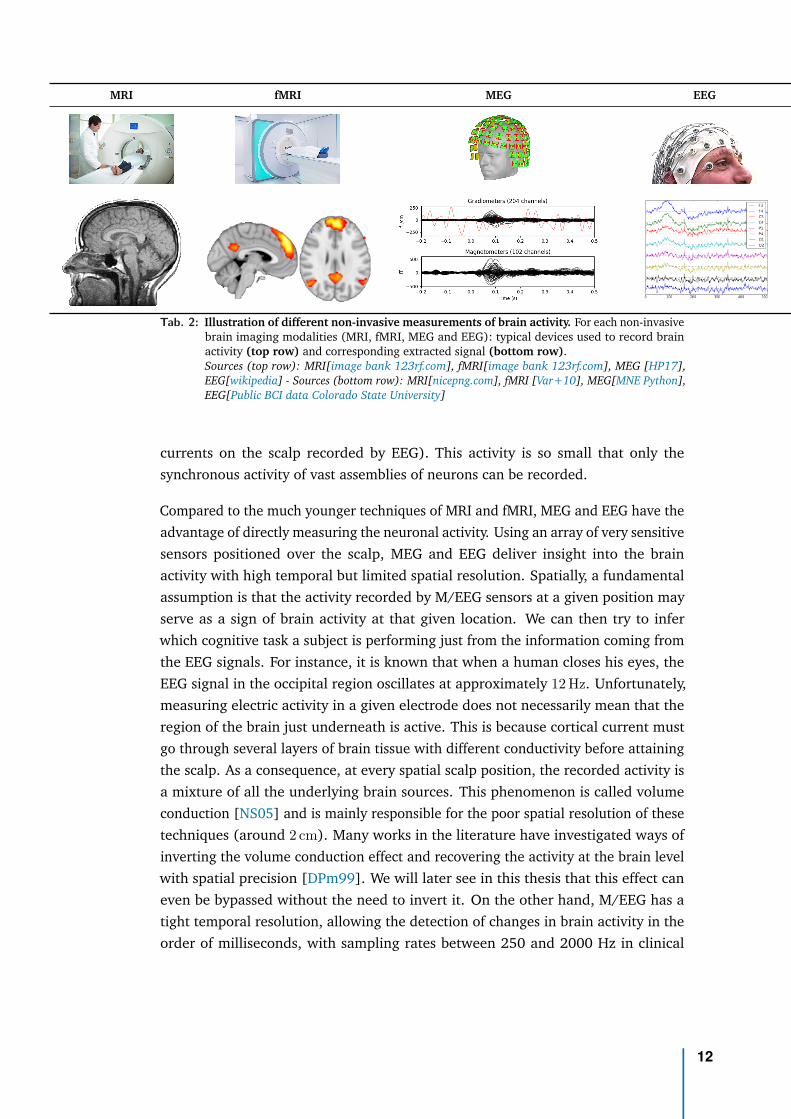
MRI fMRI MEG EEG

Tab. 2: Illustration of different non-invasive measurements of brain activity. For each non-invasivebrain imaging modalities (MRI, fMRI, MEG and EEG): typical devices used to record brainactivity (top row) and corresponding extracted signal (bottom row).Sources (top row): MRI[image bank 123rf.com], fMRI[image bank 123rf.com], MEG [HP17],EEG[wikipedia] - Sources (bottom row): MRI[nicepng.com], fMRI [Var+10], MEG[MNE Python],EEG[Public BCI data Colorado State University]

currents on the scalp recorded by EEG). This activity is so small that only thesynchronous activity of vast assemblies of neurons can be recorded.

Compared to the much younger techniques of MRI and fMRI, MEG and EEG have theadvantage of directly measuring the neuronal activity. Using an array of very sensitivesensors positioned over the scalp, MEG and EEG deliver insight into the brainactivity with high temporal but limited spatial resolution. Spatially, a fundamentalassumption is that the activity recorded by M/EEG sensors at a given position mayserve as a sign of brain activity at that given location. We can then try to inferwhich cognitive task a subject is performing just from the information coming fromthe EEG signals. For instance, it is known that when a human closes his eyes, theEEG signal in the occipital region oscillates at approximately 12 Hz. Unfortunately,measuring electric activity in a given electrode does not necessarily mean that theregion of the brain just underneath is active. This is because cortical current mustgo through several layers of brain tissue with different conductivity before attainingthe scalp. As a consequence, at every spatial scalp position, the recorded activity isa mixture of all the underlying brain sources. This phenomenon is called volumeconduction [NS05] and is mainly responsible for the poor spatial resolution of thesetechniques (around 2 cm). Many works in the literature have investigated ways ofinverting the volume conduction effect and recovering the activity at the brain levelwith spatial precision [DPm99]. We will later see in this thesis that this effect caneven be bypassed without the need to invert it. On the other hand, M/EEG has atight temporal resolution, allowing the detection of changes in brain activity in theorder of milliseconds, with sampling rates between 250 and 2000 Hz in clinical

12

Page 18

and research settings, making them extremely useful for extracting the temporaldynamics of brain activity.

To extract biomarkers from such heterogeneous multimodal brain data, the Ma-chine Learning approach has recently received significant interest in clinical neuro-science [Woo+17].

How to predict from brain signalsBrain activity, when recorded on P sensors, produce signals that can be mathemat-ically modelled as a multivariate time-series x(t) ∈ RP , t = 1 . . . T . This signalcontains both spatial information (at a particular time t0, one record P values aroundthe head, forming a random vector x(t0) ∈ RP ), and temporal information (at eachsensor located on a particular location k on the scalp, one record the variation of thesignal across time, forming the univariate time-series xk(t) ∈ R). Typical numberof time-samples is in the order of T =100 000 corresponding to a few minutes ofsignal sampled at 1000 Hz and typical number of sensors ranges from P =10 forclinical-grade EEG to 300 for research-grade MEG. This signal is therefore veryhigh-dimensional: we need a few million data points to represent one M/EEG signal.

Once the M/EEG recordings are stored, and before analyzing the data, some signalpreprocessing steps are carried out. A first important step is to filter artefacts, toavoid making conclusions about the brain activity based on elements that are notphysiologically relevant. Artefacts commonly removed include: the spectral peak at50 Hz due to the power line frequency, environmental artefacts and physiologicalartefacts (cardiac and ocular). A second common processing step is to bandpass filterthe signal to some frequency interval carrying physiological information relevant forthe analysis being done.

Let’s suppose we want to predict a variable of interest y e.g., a biomedical outcome,related to the brain activity x(t) through an unknown statistical relationship. Itcould be the health status (how sick one is), a physiological variable (the age)or a biomarker for any cognitive process. Due to the high dimensionality of theM/EEG signal, it is difficult for a human eye to quantify patterns in those brain data,especially for large quantity of data. One recent solution is to teach a computerto help automate the prediction, finding the most useful quantitative summariesin this wealth of data: this is the field of statistical learning, or Machine Learning(ML) [SSBD14]. ML algorithms when used for such a prediction task are designed toapproximate the general relationship between y and x(t) using a dataset of examples:a series of recorded brain data xi(t) and its corresponding target variable yi for a lotof subjects i = 1 . . . N . After incorporating those examples (in the so-called trainingphase) the algorithm is able to predict the variable y from the brain data x(t) ofany person (the generalization phase), not just the one it has seen during training.

13

Page 19

When the prediction task aims at predicting a continuous variable (y ∈ R) it is calleda regression task, when it aims at predicting a categorical variable (y ∈ finite set) itis called a classification task.

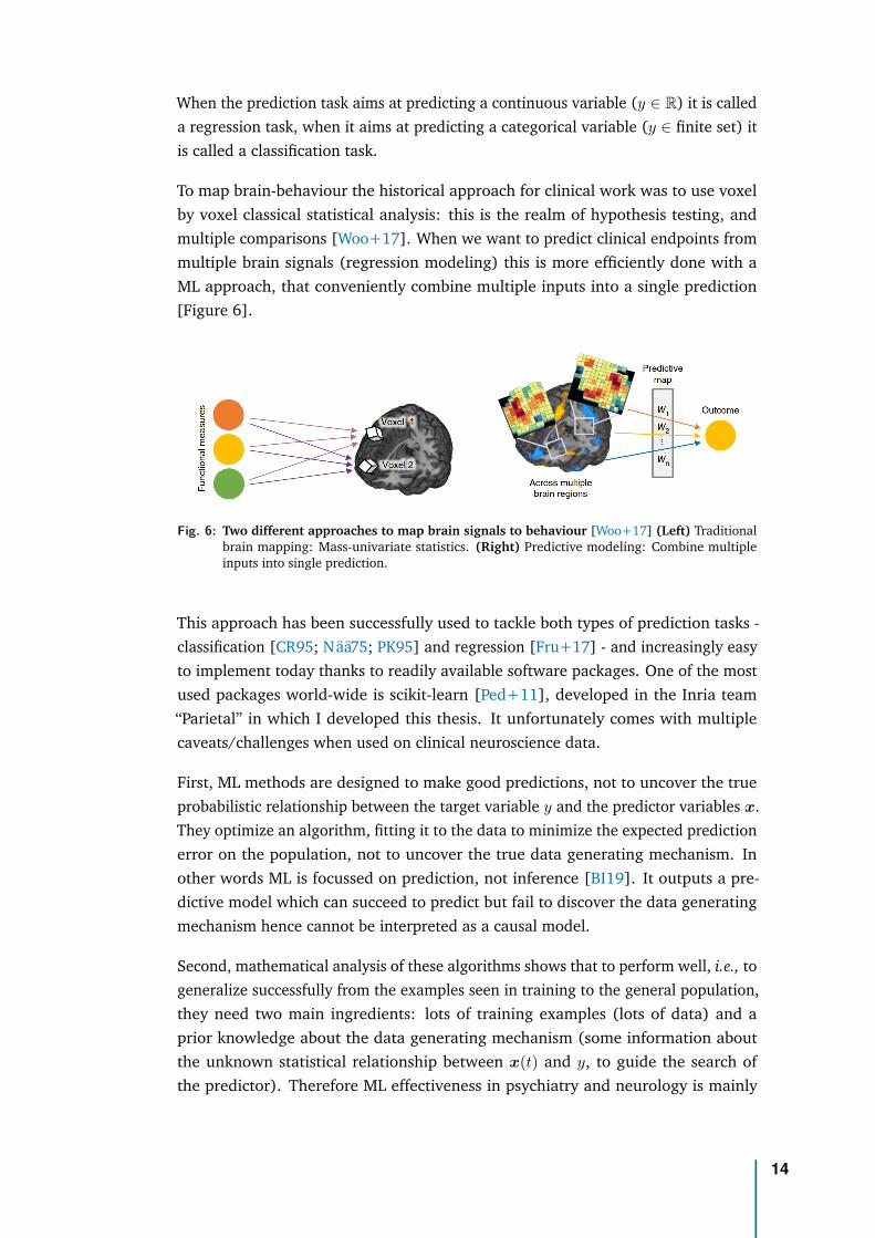
To map brain-behaviour the historical approach for clinical work was to use voxelby voxel classical statistical analysis: this is the realm of hypothesis testing, andmultiple comparisons [Woo+17]. When we want to predict clinical endpoints frommultiple brain signals (regression modeling) this is more efficiently done with aML approach, that conveniently combine multiple inputs into a single prediction[Figure 6].

Fig. 6: Two different approaches to map brain signals to behaviour [Woo+17] (Left) Traditionalbrain mapping: Mass-univariate statistics. (Right) Predictive modeling: Combine multipleinputs into single prediction.

This approach has been successfully used to tackle both types of prediction tasks -classification [CR95; Nää75; PK95] and regression [Fru+17] - and increasingly easyto implement today thanks to readily available software packages. One of the mostused packages world-wide is scikit-learn [Ped+11], developed in the Inria team“Parietal” in which I developed this thesis. It unfortunately comes with multiplecaveats/challenges when used on clinical neuroscience data.

First, ML methods are designed to make good predictions, not to uncover the trueprobabilistic relationship between the target variable y and the predictor variables x.They optimize an algorithm, fitting it to the data to minimize the expected predictionerror on the population, not to uncover the true data generating mechanism. Inother words ML is focussed on prediction, not inference [BI19]. It outputs a pre-dictive model which can succeed to predict but fail to discover the data generatingmechanism hence cannot be interpreted as a causal model.

Second, mathematical analysis of these algorithms shows that to perform well, i.e., togeneralize successfully from the examples seen in training to the general population,they need two main ingredients: lots of training examples (lots of data) and aprior knowledge about the data generating mechanism (some information aboutthe unknown statistical relationship between x(t) and y, to guide the search ofthe predictor). Therefore ML effectiveness in psychiatry and neurology is mainly

14

Page 20

constrained by the lack of large high-quality datasets [Var+17; Woo+17; Eng+18;Bzd17]. and comparably limited understanding about the data generating mecha-nisms [JK17]. This, potentially, limits the advantage of complex learning strategies.In clinical neuroscience, prediction can therefore be pragmatically approached withlow-complexity classical machine learning algorithms [Dad+19] implementing sim-ple learning strategies, expert-based feature engineering and increasing emphasison surrogate tasks, for which dataset of examples are more easily found.

Regarding the features, many studies have shown the importance and predictivecapabilities of the spectral content of M/EEG signal, i.e., how it oscillates. This signalcan indeed be decomposed in multiple simple waves or rhythms, characterized bytheir frequencies and amplitude [BD04; BL17].

In numerous experiments, where M/EEG activity of a subject was recorded whileperforming different cognitive tasks, it has been observed that the signal oscillatedifferently in different parts of the brain. M/EEG have an unparalleled capacity forcapturing these brain rhythms without penetrating the skull [HP17].

Among them we can distinguish five types of rhythms or frequency bands:

▷ delta rhythm (frequency between 1 Hz to 4 Hz; amplitude between 1 µV to200 µV): present in infants and in the deep state of sleep of adults, but that canconvey serious cerebral suffering when present in the awaken adult [AYH18].

▷ theta rhythm (frequency between 4 Hz to 8 Hz; amplitude between 150 µVto 200 µV): rhythm of temporal and parietal regions, for example arising inchildren and adults in emotional conditions [AG01].

▷ alpha rhythm (frequency between 8 Hz to 12 Hz; amplitude between 50 µV to100 µV): rhythm of the occipital region recorded on healthy awaken subjects,usually associated to a relaxed state of mind, e.g., eyes closed in restingstate. This rhythm mostly disappears when the subject opens his eyes orfocus his attention on a mental activity and make way for the faster betarhythm [Gol+02].

▷ beta rhythm (frequency between 12 Hz to 30 Hz; amplitude between 10 µVto 50 µV): rhythm originating in parietal and frontal regions associated to anormal state of consciousness [Pfu92].

▷ gamma rhythm (frequency between 30 Hz to 120 Hz; amplitude between 2 µVto 10 µV): associated with large scale brain network activity and cognitivephenomena such as working memory and attention. Altered gamma activ-ity has been observed in many cognitive disorders such as Alzheimer’s dis-ease [VD+08].

Regarding the learning strategy, the gold standard method when predicting fromM/EEG signals is source modeling, whereby a specific algorithm is used to find the

15

Page 21

most probable sources in the brain that account for the recorded signal. This method,however, requires precise anatomical information provided by MRI scans. In theclinic, MRI recordings are rarely routinely available to do source reconstruction.Even when present in the hospital the machine is overloaded by patients that need itthe most (not strictly necessary for knee surgery). An important question then is:when source localization is not available, and when we have some prior knowledgeabout the data generating mechanism, is there an optimal ML regression algorithmto predict from M/EEG signals, i.e., an algorithm with perfect prediction in thelimiting case of infinite number of samples? This important question is addressedby our first (methodological) contribution [Sab+19a] and will be investigated inChapter 1.

Armed with this theoretically optimal algorithm to predict from our input data (theM/EEG brain signal), simple enough to be usable in the clinic, we will then focus ondesigning our surrogate task, the target of prediction (the y), a target that should beboth easily available and a promising biomarker of neurocognitive disorders.

What to predict from brain signals: the brain ageNow that we have a clearer view on our input data (the M/EEG signal representingthe brain activity) and that we found an optimal algorithm to predict from it, wefocus our attention on the target of prediction.

In medicine, a biomarker is a measurable indicator of some disease state. For ex-ample, body temperature is a well-known biomarker for fever. Blood pressure isused to determine the risk of stroke. It is also widely known that cholesterol valuesare a biomarker and risk indicator for coronary and vascular disease. It can bediscovered using genomics, proteomics technologies or imaging technologies. Ourgoal is to develop a biomarker of neurocognitive disorders through brain electro-physiology. Biomarkers are useful in a number of ways: they can help in earlydiagnosis, measuring the progress of a disease, evaluate most effective therapeuticregimes, prevent diseases, or identify drug target or drug response. A biomarker of aparticular endpoint can be obtained by training a ML algorithm to accurately predictthe endpoint. This training phase uses a dataset of patients for which we have botha brain signal and the corresponding endpoint [Par+15].

The gold-standard method to uncover risk factors and biomarkers in particular islarge-scale population studies, generally based on meta-analyses or large biobanks[Cox+19]. When one can’t afford the effort and the cost associated with them,we have to resort to experimental studies in clinical subgroups where ML canhelp in clinical diagnosis [Gau+19; Eng+18]. These studies that focus on clinicalpopulation are inevitably based on a limited number of patients, leading to smallsamples. Besides, as clinical data is rarely made public, meta-analyses are not

16

Page 22

always possible. Those studies can therefore be statistically underpowered, and as aconsequence often show optimistic biases in accuracy [PHV20; Woo+17].

To counter the scarcity of data samples of the precious clinical outcome (e.g., inour case, cognitive decline), we adopted the alternative approach of designing asurrogate task: predict an endpoint that’s widely available and then exploit itscorrelation with the actual endpoint of interest. As a surrogate variable we focusedon age.

Our chronological age is determined by the number of years since our birth. Butour body, our organs, our brain also have a biological age. Biological age could forinstance be measured by looking at the integrity of the DNA in cells or by measuringthe levels of proteins in the blood. Both chronological or biological ages are simpleindicators of general health. Crucially, people with the same chronological age mayhave different biological ages. Individual-specific differences in their organs agereflect deviations from what is statistically expected and can be used to communicaterisks [Spi16]. For example the bones age allows to identify growth pathologiesbetween two children of the same age. Similarly, we can hope to be able to readout the age in the brain and that the age extracted from brain signals, the brain age,captures individual cerebral fragility.

Fig. 7: How old is this brain? Source: [CR+07].

As a 70y old liver in a 50y personcould provide hint of a chronic over-consumption of alcohol, an older braincould point to an undetected patho-logical brain aging. By definition, anhealthy person should have a biologicalbrain age similar to his chronologicalage. Our optimal ML model, previouslydesigned, should then be first trainedto accurately predict the chronologicalage of an healthy population. It wouldapproximate age as a function of brainimages. Given a new data point - a brainimage - the function tells the expectedage. This ”prediction“ expresses wherethe brain is positioned in the population,e.g., whether that brain ”looks“ older or younger. The resulting measure broughtby ML gives rise to brain predicted age as the solution to a regression problemfrom brain imaging, with more than 10 years of established literature [Dos+10]. Itmay seem irrelevant at first to predict the age as endpoint as there are very seldomsituations where age is unknown. But we can hope that this brain predicted agecontain information not present in chronological age. For instance, when computed

17

Page 23

from fMRI data, it could capture volume reduction that comes with normal agingbut could also reveal less volume than expected so captures pathological atrophy.

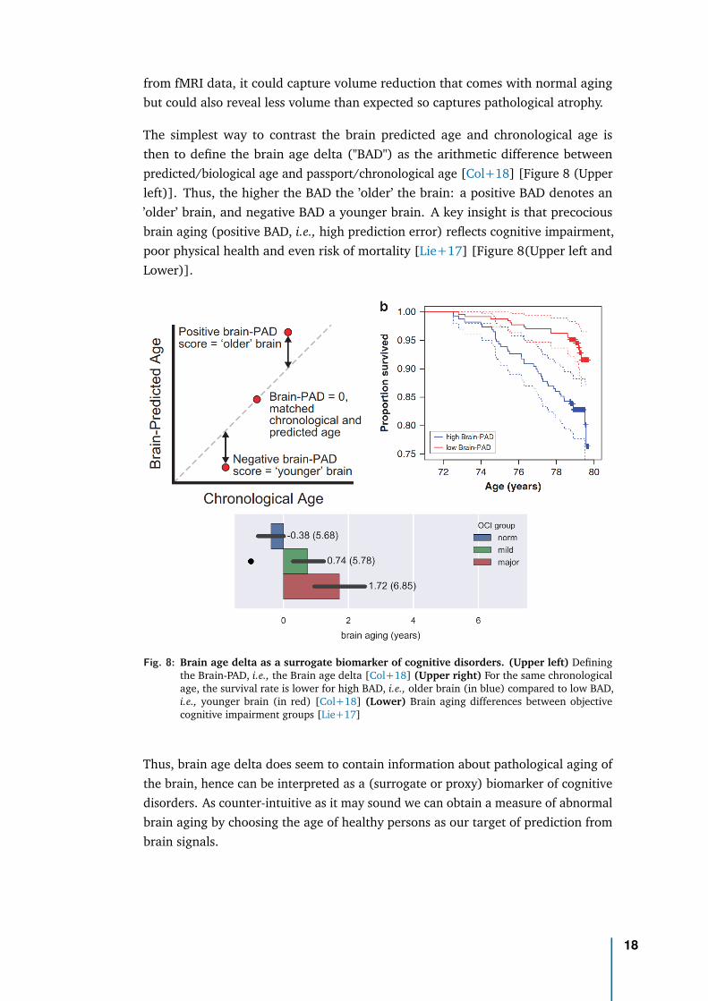
The simplest way to contrast the brain predicted age and chronological age isthen to define the brain age delta ("BAD") as the arithmetic difference betweenpredicted/biological age and passport/chronological age [Col+18] [Figure 8 (Upperleft)]. Thus, the higher the BAD the ’older’ the brain: a positive BAD denotes an’older’ brain, and negative BAD a younger brain. A key insight is that precociousbrain aging (positive BAD, i.e., high prediction error) reflects cognitive impairment,poor physical health and even risk of mortality [Lie+17] [Figure 8(Upper left andLower)].

Fig. 8: Brain age delta as a surrogate biomarker of cognitive disorders. (Upper left) Definingthe Brain-PAD, i.e., the Brain age delta [Col+18] (Upper right) For the same chronologicalage, the survival rate is lower for high BAD, i.e., older brain (in blue) compared to low BAD,i.e., younger brain (in red) [Col+18] (Lower) Brain aging differences between objectivecognitive impairment groups [Lie+17]

Thus, brain age delta does seem to contain information about pathological aging ofthe brain, hence can be interpreted as a (surrogate or proxy) biomarker of cognitivedisorders. As counter-intuitive as it may sound we can obtain a measure of abnormalbrain aging by choosing the age of healthy persons as our target of prediction frombrain signals.

18

Page 24

So we know what to predict (the brain age), how to predict (with our optimal MLmodel), but from which brain data? The BAD has been historically measured throughMRI. Yet, we saw that other brain imaging modalities provide unique informationabout the brain. This raises the question of which brain imaging modality should ourML model use to compute brain age and which features are most informative aboutage. Let’s imagine we are not in the clinic yet but in the comfortable conditions of aresearch laboratory where we have them all: MRI, fMRI and MEG.

How to estimate brain age in the labBrain biological age is typically estimated with MRI but can M/EEG be useful ? Untilrecently, most studies were dedicated to establish that M/EEG and MRI capture somesimilar information, for instance Brookes et al. [Bro+11] showed that fMRI restingstate networks can be reconstructed from MEG, and Hipp and Siegel [HS15] thatBOLD and MEG show similar spatial correlations across many frequency bands. Wenow have independent evidence that they also do carry independent information:Kumral et al. [Kum+19] showed that BOLD and EEG signal variability at restdifferently relate to aging, Nentwich et al. [Nen+20] demonstrated that fMRI andEEG connectivity is different, Gaubert et al. [Gau+19] showed EEG-signatures inpreclinical Alzheimer’s disease.

Distinct features measured by all three techniques – MRI, fMRI and electrophysiology– have been associated with aging. For example, differences between younger andolder people have been observed in the proportion of grey to white matter (throughMRI), the communication between certain brain regions (through fMRI), and theintensity of neural activity in alpha band (through M/EEG). Literature on brainaging has historically focus on MRIs which, with their anatomical details, remain thego-to for predicting the biological age of the brain. But patterns of neuronal activitycaptured by electrophysiology also provide information about how well the brainis working. However, it remains unclear how electrophysiology could be combinedwith other brain imaging methods, like MRI and fMRI. Can data from these threetechniques be combined to better predict brain age? We investigated this question inan article I co-authored [Eng+20].

We first trained our computer model with a subset of data from the Cam-CANdatabase, which holds MRI, fMRI, MEG and neuropsychological data for 650 healthypeople aged between 17 and 90 years old. To handle the different modalities weused a computer model based on stacking: we first summarize the data in eachmodality with linear models (for which sample error grows only linearly with samplesize) and then correct for bias of linear models with a non-linear Random Forestmodel [Eng+20].

19

Page 25

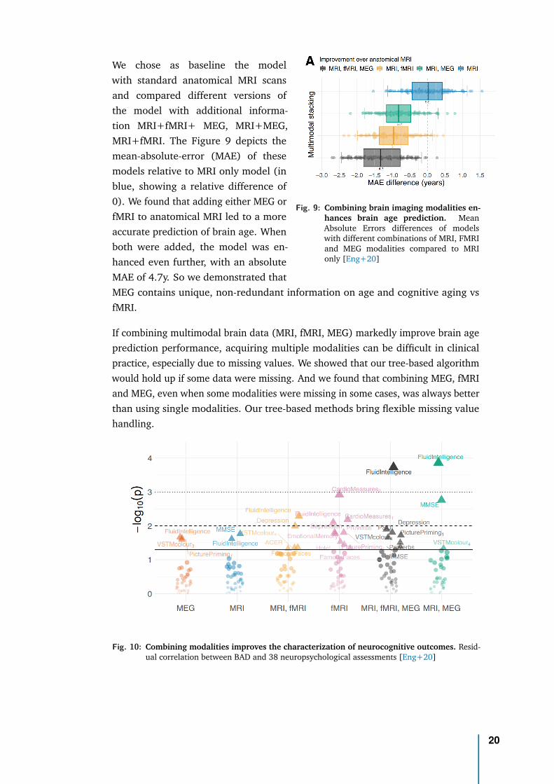
Fig. 9: Combining brain imaging modalities en-hances brain age prediction. MeanAbsolute Errors differences of modelswith different combinations of MRI, FMRIand MEG modalities compared to MRIonly [Eng+20]

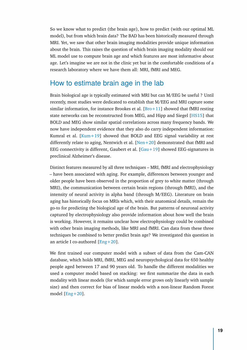
We chose as baseline the modelwith standard anatomical MRI scansand compared different versions ofthe model with additional informa-tion MRI+fMRI+ MEG, MRI+MEG,MRI+fMRI. The Figure 9 depicts themean-absolute-error (MAE) of thesemodels relative to MRI only model (inblue, showing a relative difference of0). We found that adding either MEG orfMRI to anatomical MRI led to a moreaccurate prediction of brain age. Whenboth were added, the model was en-hanced even further, with an absoluteMAE of 4.7y. So we demonstrated thatMEG contains unique, non-redundant information on age and cognitive aging vsfMRI.

If combining multimodal brain data (MRI, fMRI, MEG) markedly improve brain ageprediction performance, acquiring multiple modalities can be difficult in clinicalpractice, especially due to missing values. We showed that our tree-based algorithmwould hold up if some data were missing. And we found that combining MEG, fMRIand MEG, even when some modalities were missing in some cases, was always betterthan using single modalities. Our tree-based methods bring flexible missing valuehandling.

Fig. 10: Combining modalities improves the characterization of neurocognitive outcomes. Resid-ual correlation between BAD and 38 neuropsychological assessments [Eng+20]

20

Page 26

This flexible algorithm learnt better model of aging but is it relevant for neuropsy-chological score? We demonstrated that this combination also lead to enhancedcharacterization of neurocognitive phenotypes [Figure 10]: with unique discoveriesor increased effect sizes associating the out-of-sample BAD with neurocognitive out-comes. The predictions correlated with the cognitive fitness of individuals. Peoplewith older brains tended to complain about the quality of their sleep and scoredworse on memory and speed-thinking tasks. This suggests that BAD can be a goodsurrogate biomarker of cognitive aging and contains useful clinical information.Not only adding MEG boosts performance, but it also improves brain-behaviourcorrelation.

Fig. 11: Investigating most influential featuresto predict brain age from MEG. MEGperformance is predominantly driven bysource power [Eng+20]

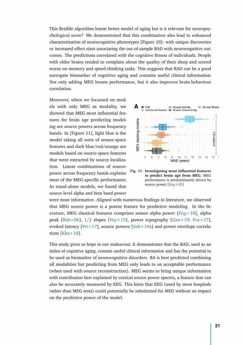
Moreover, when we focussed on mod-els with only MEG as modality, weshowed that MEG most influential fea-tures for brain age predicting model-ing are source powers across frequencybands: In [Figure 11], light blue is themodel taking all sorts of sensor-spacefeatures and dark blue/red/orange aremodels based on source-space featuresthat were extracted by source localiza-tion. Linear combinations of source-power across frequency bands explainsmost of the MEG-specific performance.As stand-alone models, we found thatsource-level alpha and beta band powerwere most informative. Aligned with numerous findings in literature, we observedthat MEG source power is a potent feature for predictive modeling. In the lit-erature, MEG classical features comprises sensor alpha power [Eng+18], alphapeak [Bab+06], 1/f slopes [Voy+15], power topography [Gau+19; Fru+17],evoked latency [Pri+17], source powers [Sab+19a] and power envelope correla-tions [Kha+18].

This study gives us hope in our endeavour. It demonstrates that the BAD, used as anindex of cognitive aging, contain useful clinical information and has the potential tobe used as biomarker of neurocognitive disorders. BA is best predicted combiningall modalities but predicting from MEG only leads to an acceptable performance(when used with source reconstruction). MEG seems to bring unique informationwith contribution best explained by cortical source power spectra, a feature that canalso be accurately measured by EEG. This hints that EEG (used by most hospitalsrather than MEG tests) could potentially be substituted for MEG without an impacton the predictive power of the model.

21

Page 27

Unfortunately, it also suppose conditions not easily available in clinical practice, andcertainly not compatible with a usage in the operating room. First, it requires to haveMRI data: even the MEG only experiment relied on MEG features that require MRIacquisitions and tedious data processing to do source reconstruction Second, it usesresearch-grade high-fidelity MEG devices. Finally it requires highly-preprocessedMEG data. We will show in our first contribution in Chapter 1 that our proposedmethod can accommodate the absence of MRI data under certain ideal conditionsbut does it hold on real M/EEG data when those conditions are challenged? Isour method performant and robust enough to accommodate low-fidelity and low-preprocessed EEG measures (clinical-grade EEG vs research-grade MEG)? This willbe investigated in our second (empirical) contribution [Sab+20] and described inChapter 2.

We will see that our regression model has indeed the potential to be used in theclinic: it operates in sensor-space (avoiding costly source localization), it is robust toenvironmental and physiological artefacts and it accommodates cheap EEG record-ings. This optimal, robust and light model is then a good candidate to develop ourBAD biomarker. Now that we have a method to robustly determine brain age in thelab, the critical question is: does it translate to the clinic, is it really usable in theoperating room?

How to translate brain age to the clinicIn the clinic, virtually all patients undergoing surgery go through a general anesthesia(GA). This procedure concerns millions of people every year: more than 300 millionworldwide in 2020 [Csj]. If we include rachianesthesia and loco-regional proceduresthis number is even far greater. In France, 9.5 M of general anesthesia procedureshave been performed in 2010 (excluding childbirth) with an average yearly increaserate of 1.89 % between 1991 and 2010 [Dad+15]. Since a precise physiologicalmonitoring is required during GA, often including brain monitoring, this means thatthere exists a population-wide dataset of neural signals, today largely untapped.

Besides, the period of GA is a particularly favorable period to extract signals frompatients with minimal artefact due to muscle-inhibitor drugs, hence a particularlyadapted moment to build biomarkers. Moreover, EEG is already routinely used inthe operating room during general anesthesia to monitor the depth of anesthesia asrecommended by scholar societies of anaesthesiologists. Yet, despite its ubiquity, thewealth of physiological signals recordings including EEG and potential good signalquality, GA has never been used to estimate brain age.

22

Page 28

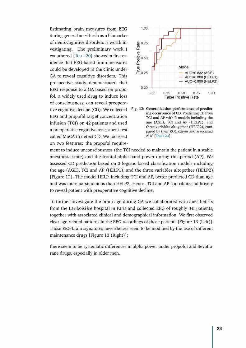
Fig. 12: Generalization performance of predict-ing occurrence of CD. Predicting CD fromTCI and AP with 3 models including theage (AGE), TCI and AP (HELP1), andthree variables altogether (HELP2), com-pared by their ROC curves and associatedAUC [Tou+20].

Estimating brain measures from EEGduring general anesthesia as a biomarkerof neurocognitive disorders is worth in-vestigating. The preliminary work Icoauthored [Tou+20] showed a first ev-idence that EEG-based brain measurescould be developed in the clinic underGA to reveal cognitive disorders. Thisprospective study demonstrated thatEEG response to a GA based on propo-fol, a widely used drug to induce lossof consciousness, can reveal preopera-tive cognitive decline (CD). We collectedEEG and propofol target concentrationinfusion (TCI) on 42 patients and useda preoperative cognitive assessment testcalled MoCA to detect CD. We focussedon two features: the propofol require-ment to induce unconsciousness (the TCI needed to maintain the patient in a stableanesthesia state) and the frontal alpha band power during this period (AP). Weassessed CD prediction based on 3 logistic based classification models includingthe age (AGE), TCI and AP (HELP1), and the three variables altogether (HELP2)[Figure 12]. The model HELP, including TCI and AP, better predicted CD than ageand was more parsimonious than HELP2. Hence, TCI and AP contributes additivelyto reveal patient with preoperative cognitive decline.

To further investigate the brain age during GA we collaborated with anesthetistsfrom the Lariboisière hospital in Paris and collected EEG of roughly 345 patients,together with associated clinical and demographical information. We first observedclear age-related patterns in the EEG recordings of those patients [Figure 13 (Left)].Those EEG brain signatures nevertheless seem to be modified by the use of differentmaintenance drugs [Figure 13 (Right)]:

there seem to be systematic differences in alpha power under propofol and Sevoflu-rane drugs, especially in older men.

23

Page 29

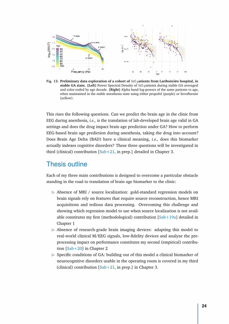
Fig. 13: Preliminary data exploration of a cohort of 345 patients from Lariboisière hospital, instable GA state. (Left) Power Spectral Density of 345 patients during stable GA averagedand color-coded by age decade. (Right) Alpha band log-powers of the same patients vs age,when maintained in the stable anesthesia state using either propofol (purple) or Sevoflurane(yellow).

This rises the following questions. Can we predict the brain age in the clinic fromEEG during anesthesia, i.e., is the translation of lab-developed brain age valid in GAsettings and does the drug impact brain age prediction under GA? How to performEEG-based brain age prediction during anesthesia, taking the drug into account?Does Brain Age Delta (BAD) have a clinical meaning, i.e., does this biomarkeractually indexes cognitive disorders? These three questions will be investigated inthird (clinical) contribution [Sab+21, in prep.] detailed in Chapter 3.

Thesis outlineEach of my three main contributions is designed to overcome a particular obstaclestanding in the road to translation of brain age biomarker to the clinic:

▷ Absence of MRI / source localization: gold-standard regression models onbrain signals rely on features that require source reconstruction, hence MRIacquisitions and tedious data processing. Overcoming this challenge andshowing which regression model to use when source localization is not avail-able constitutes my first (methodological) contribution [Sab+19a] detailed inChapter 1

▷ Absence of research-grade brain imaging devices: adapting this model toreal-world clinical M/EEG signals, low-fidelity devices and analyze the pre-processing impact on performance constitutes my second (empirical) contribu-tion [Sab+20] in Chapter 2

▷ Specific conditions of GA: building out of this model a clinical biomarker ofneurocognitive disorders usable in the operating room is covered in my third(clinical) contribution [Sab+21, in prep.] in Chapter 3.

24

Page 30

Proposition

My own mathematical contributions, in the form of propositions, are denotedin boxes of this kind.

These results were presented at various national and international conferences(JDSE 2019 for which I received the best paper award, NeurIPS 2019, OHBM 2020)and have been accepted at two symposiums (VPH 2020, CompAge 2020) and twosummer schools (AI4Health, DS3). I also co-authored three additional publications:the two papers detailed in this introduction [Tou+20; Eng+20] along with a recentbenchmark paper on brain age [Eng+21] for which I contributed data analysis tools.

All numerical illustrations have been carried out on publicly available datasets:Cam-CAN [Tay+17], TUH [Har+14] and FieldTrip [Oos+11] with the exception ofthe unique GA dataset collected in Lariboisière hospital in Paris, exclusively for thisthesis.

Finally, in order to foster reproducible research, Python and R code for all methodsdiscussed in this thesis are available online on public repositories:

▷ https://github.com/DavidSabbagh/NeurIPS19_manifold-regression-meeg/Python code for the NeurIPS 2019 article [Sab+19a]- tools to preprocess rawMEG data from Cam-CAN dataset, vectorize covariance matrices, launch simu-lations and real-data analysis.

▷ https://github.com/DavidSabbagh/meeg_power_regressionPython and R code for the NeuroImage 2020 article [Sab+20] - tools topreprocess raw MEG & EEG data from Cam-CAN, TUH and provided by theFieldTrip website, to analyze regression performance, inspect model by error-decomposition and assess pre-processing impact on performance.

▷ https://github.com/DavidSabbagh/larib-EEGPython and R code for the clinical article [Sab+21, in prep.] - tools to collectdata and metadata from Lariboisière hospital, extract the features, explore thedata, compare and inspect the regression models, perform data and statisticalanalysis.

We used the R-programming language and its ecosystem for visualizing the re-sults [R C19; AUT19; Wic16; CSM17] and run part of the statistical analysis. Dataanalysis has been performed with Python 3.7 and only relies on open-source li-braries: the Scikit-Learn software [Ped+11], the MNE software for processingM/EEG data [Gra+14], the PyRiemann package [CBA13] for manipulating Rie-mannian objects, and ‘Coffeine’ (https://github.com/coffeine-labs/coffeine)whom I developed the core features during my PhD and that provides a high-levelinterface to all predictive modeling techniques we present in this thesis.

25

Page 31

1Theory of power regression onsensor-space M/EEG withRiemannian Geometry

Contents1.1 Statistical Learning theory . . . . . . . . . . . . . . . . . . . . . 31

1.1.1 Learning a task . . . . . . . . . . . . . . . . . . . . . . . 31

1.1.2 Performance of a learning algorithm . . . . . . . . . . . 36

1.1.3 Lessons for regression on M/EEG signals . . . . . . . . . 38

1.2 Multivariate time series analysis . . . . . . . . . . . . . . . . . . 40

1.2.1 Statistical and temporal moments . . . . . . . . . . . . . 40

1.2.2 Statistical assumptions . . . . . . . . . . . . . . . . . . . 42

1.2.3 The covariance matrix . . . . . . . . . . . . . . . . . . . 45

1.2.4 M/EEG preprocessing induces rank-deficiency . . . . . . 46

1.3 Riemannian matrix manifolds . . . . . . . . . . . . . . . . . . . . 50

1.3.1 Riemannian manifolds . . . . . . . . . . . . . . . . . . . 50

1.3.2 The positive definite manifold S++P . . . . . . . . . . . . 51

1.3.3 The fixed rank SDP manifold S+P,R . . . . . . . . . . . . . 54

1.4 Generative models of M/EEG signals and outcome . . . . . . . . 56

1.4.1 Prior knowledge . . . . . . . . . . . . . . . . . . . . . . 56

1.4.2 The classical approaches to predict from M/EEG observa-tions . . . . . . . . . . . . . . . . . . . . . . . . . . . . . 61

1.5 A family of statistically consistent regression algorithms . . . . . 66

1.5.1 Four statistically consistent regression algorithms . . . . 67

1.5.2 Model violations . . . . . . . . . . . . . . . . . . . . . . 74

1.5.3 Validation with simulations . . . . . . . . . . . . . . . . 77

26

Page 32

Mathematical notations used in the chapter

Z set of integer numbersx ∈ R Scalar (lower case)x ∈ RP Vector of size P (bold lower case)

∥x∥2 ℓ2 norm of vector x:√∑

i x2i

M Matrix (bold uppercase)IN Identity matrix of size N[·]⊤ Transposition of a vector or a matrixtr(M) Trace of matrix M

diag(M) Diagonal of matrix M

||M ||F Frobenius norm of matrix M :√

Tr(MM⊤) =√∑

|Mij |2

rank(M) Rank of matrix M

Upper(M) upper triangular coefficients of M , with unit weights on the diagonaland

√2 weights on the off-diagonal

S cross-spectral density matrixC spatial covariance matrixMP Space of P × P square real-valued matricesSP Subspace of P × P symmetric matrices: {M ∈ MP ,M

⊤ = M}S++

P Subspace of P × P symmetric positive definite matrices:{M ∈ SP ,x

⊤Mx > 0,∀x ∈ RP ,x = 0}M is full rank, invertible (with M−1 ∈ S++

P )M is diagonalizable with real positive eigenvalues:M = UΛU⊤ with U orthogonal matrix of eigenvectors (UU⊤ = IP )and Λ = diag(λ) matrix of positive eigenvalues (λ1 ≥ · · · ≥ λP > 0)

S+P Subspace of P × P symmetric semi-definite positive (SPD) matrices:

{S ∈ SP ,x⊤Sx ≥ 0, ∀x ∈ RP }

S+P,R Subspace of SPD matrices of fixed rank R: {S ∈ S+

P , rank(S) = R}log(M) Logarithm of matrix M ∈ S++

P : U diag(log(λ1), . . . , log(λn)) U⊤ ∈ SP

exp(M) Exponential of matrix M ∈ SP : U diag(exp(λ1), . . . , exp(λn)) U⊤ ∈ S++P

N (µ, σ2) Normal (Gaussian) distribution of mean µ and variance σ2

Es[x] Expectation of any random variable x w.r.t. its subscript s when needed(Z,F , l) task components: set of task objects, set of potential solutions, objective functionS sample (z1, . . . , zn) ∈ Zn

Dn distribution of sample SH hypothesis classTM tangent space at point M

27

Page 33

Acronyms used in the chapter

BCI brain-computer interfaceDTFT discrete-time Fourier transformERM empirical risk minimizationERP event-related potentialEOG electro-oculogramECG electro-cardiogramfMRI functional magnetic resonance imagingM/EEG magneto- and electroencephalographyML machine learningMAE mean absolute errorMSE mean squared errorMNE mnimium norm estimateMRI magnetic resonance imagingPAC probably approximately correctPSD power spectral densityPCA principal component analysisSPD symmetric positive definiteSPoC source power comodulationSSS Signal Space SeparationSSP Signal Space ProjectionWSS wide-sense stationary

28

Page 34

In the Introduction, we investigated how the brain is structured, how it operates andhow to capture its activity by extracting a measurable signal x(t). In this chapter, wenow seek a regression algorithm to predict, from this brain signal as input data, anyoutcome y physiologically related to neural dynamics. This is a key step to developa predictive clinical biomarker. This algorithm should be both performant, henceadapted to the particular class of signals it works on, and simple enough to be usablein the clinic, which discard most of the classical algorithms. This chapter presentssuch an algorithm as my first contribution [Sab+19a], along with the theoreticalfoundations on which it rely.

Section 1.1 summarizes the Machine Learning (ML) theoretical framework to per-form prediction. We will investigate the different sources of errors of any predictionalgorithm and show that a performing predictive biomarker should be based on astatistically consistent algorithm. Such algorithm has to be adapted to the probabil-ity distribution of its input hence require some form of prior knowledge about thedata generating mechanism (No-Free-Lunch theorem). Our data signal is neverthe-less not well adapted to classical regression algorithms that require low dimensionalinputs (to fight curse of dimensionality) that live in a vector space. Armed withthese theoretical insights, the following sections investigate how to meet theserequirements.

Section 1.2 will allow us to find such a low dimensional compact representation ofthe M/EEG signal: its spatial covariance matrix. It introduces statistical tools for theanalysis of multivariate time series and discuss two fundamental assumptions thatare typically done regarding their statistics: wide-sense stationarity and ergodicity.These assumptions allow to estimate a set of parameters that describe the statisticalbehaviour of a real multivariate time series: its mean vector and its cross-spectraldensity matrices, a continuous set of positive definite matrices. This set can be furthersummarized by using one of such matrices: the band-specific covariance matrix.One may then approximately compare two time series by comparing the covariancematrices used to parametrize them. These matrices are most often rank-deficientdue to practical reasons investigated at the end of this section.

Armed with this compact matrix representation, we’ll still need to vectorize it. Theset of covariance matrices, either full rank or not, is known to have a particularintrinsic geometry - they live on a Riemmanian manifold - and in Section 1.3 wegive an overview of its properties. Understanding the intrinsic geometry of a setof data points very often lead to more efficient algorithms, e.g., deep learningmethods adapted to data defined in a manifold [Bro+17], or text classification usingRiemannian geometry [Leb05]. This is particularly true in the field of brain-computerinterfaces (BCI) where classification methods have been largely improved using suchgeometry-aware algorithms [Lot+18; CBB17; YBL17]. Here, using concepts fromdifferential geometry, we will present a distance between positive definite matrices

29

Page 35

that is invariant to affine-invariant transformations (e.g. the action of a matrix), avery useful property when parametrizing multivariate time series. This will lead toan appropriate vector representation of a covariance matrix.

Section 1.4 introduces a prior knowledge about our task in a form of a generativemodel of M/EEG signals and outcome and will detail state-of-the-art approachesto predict from such M/EEG signals. We will delve into three classical family ofmethods, well-suited in certain contexts but that are unsatisfying for the present task.Biophysical source modeling using anatomically constrained inverse methods needsanatomical prior knowledge so requires specialized workforce and equipment, whichmay reduce wider applicability in clinical practice. Statistical sources modelingusing unsupervised spatial filtering (e.g., ICA) are blind to the prediction targethence requires additional modeling efforts for subsequent regression tasks. Sensor-space linear modeling leverages the power of linear models but is not optimalwhen predicting from brain rhythms, hence not adapted to our generative modelsassumptions. We will show that none of them is suitable to our task, hence the needfor a new algorithm.

Finally, Section 1.5 introduces statistically consistent regression algorithms to predictfrom M/EEG signals, adapted to our generative model and usable in the clinic.We provide mathematical proof of consistency under certain conditions. We alsopresent simulations to illustrate these mathematical guarantees and investigate therobustness of our algorithms to model violations. One of these model relies onconcepts from Riemannian geometry and can easily be adapted to handle rank-deficient covariances.

Simulations in this chapter and real-world experiments in the next two were carriedout using Python libraries including: scikit-learn [Ped+11], MNE-python [Gra+14]and pyRiemann1. We also ported to Python some part of the Matlab code of Manopttoolbox [Bou+14] for computations involving Wasserstein distance. The scriptsgenerating associated figures are available in the GitHub repositories:

▷ https://github.com/DavidSabbagh/NeurIPS19_manifold-regression-meeg/▷ https://github.com/DavidSabbagh/meeg_power_regression

Every code runs on a standard laptop.

1http://pyriemann.readthedocs.io/

30

Page 36

1.1 Statistical Learning theoryIn this section, we will present the mathematical framework of Statistical Learning,or Machine Learning (ML). For this introduction we adapted concepts and partiallyborrowed notations from [SSBD14].

1.1.1 Learning a taskReal-world task. Let’s assume we face with a real-world task we’d like to solve. Thistask could be: compute the area of circle of radius r, add two big integer numbers,decide which animal portrays an image, predict breast cancer from mammography,predict cognitive function from M/EEG brain activity, or clustering active EEGelectrodes that record task-relevant neurophysiological activity. We will see thatthese tasks, very different in nature, can share a common formalism but are tackledusing different approaches. The very first step to solve the task is to model itmathematically.

Model the task. We represent the task by a triplet:

T = (Z,F , l) , (1.1)

where Z is the set of task’s objects, called the instance set, formally a measurablespace; F is the set of all potential solutions, formally a set of functions; l is theerror made by a solution on an object, called a loss or a cost, formally a functionF × Z 7→ R.

For example prediction is the task of predicting an outcome y from a statisticallyrelated input x ∈ RP . When y is a continuous (resp. discrete) variable, the predictiontask is called regression (resp. classification). Hence, a regression task operates onpairs of variables (x, y) ∈ (X ,Y) as objects, with x observed and y unobserved, andlooks for the function f : X 7→ Y that best predicts y given x, where ‘best’ may mean‘with minimal quadratic error’. Therefore, this task can be modeled by the tripletZ = X × Y a bounded subset of RP × R, F the set of all bounded functions from Xto Y and l(f, (x, y)) = (f(x) − y)2, the squared loss. Many tasks can be formalizedthis way. Some examples are detailed in table 1.1:

Task Z F l

Prediction:Regression X × Y bounded subset of RP × R {f : X 7→ Y bounded} l(f, (x, y)) = (f(x) − y)2 squared lossPrediction:Classification X × {0, 1} {f : X 7→ {0, 1}} l(f, (x, y)) = 1{f(x) =y} 0-1 lossLarge margin classification X × {0, 1} bounded subset of RKHS bounded subset of RKHS max(0, 1 − y < x, h >) hinge lossK-means clustering RP all subsets of RP of size K l(f, z) = minc∈f ∥c − z∥2 dist.to nearest centroidDensity estimation ⊂ RP {bounded pdf on Z} l(f, z) = − log(f(z)) negative log-likelihood

Tab. 1.1: Example of tasks

1.1 Statistical Learning theory 31

Page 37

The task we want to solve in this thesis is a particular regression task: predict acontinuous neuro-outcome y ∈ R from a multivariate M/EEG signal x(t) ∈ RP . Thecontent of this section is nevertheless very general and apply to any kind of task thatcan be formalized this way.

Solving the task. The first approach is to try to solve it exactly, i.e., find a solutionthat never make any mistake for all objects z ∈ Z. This exact solution can either beanalytical or algorithmic. For example the task of computing the area of a circle ofradius r can be solved exactly analytically using the mathematical tool of integrationand yield f∗(r) = πr2. The task of adding two big integer numbers cannot besolved analytically but has an algorithmic solution, actually the first algorithm mostkids learn in first grade. Yet, some tasks don’t have any analytic nor algorithmicsolutions. This is generally the case either because they must adapt to fluctuatingenvironments (changes over time or over users) or because they are too complex toprogram, being specific to human capabilities (no good known algorithmic solution)or beyond human capabilities (analysis of very large and complex dataset). Examplesof such tasks are: deciding which animal portrays an image [LNH09] (multi-classclassification task), predict breast cancer from mammography [Bar+06] (binaryclassification task), predict age from M/EEG brain activityi [Sab+20] (regressiontask), or clustering active EEG electrodes that record task-relevant neurophysiologicalactivity [Sab+19b] (clustering task).

When a task cannot be solved exactly, either with an analytic formula or a predefinedalgorithm, we have to look for approximate solutions, allowing ourselves to makeerrors from time to time while trying to be maximally right on average. In thisapproach, we represent the class of objects by a random variable Z ∈ Z followingan unknown probability distribution D that reflect the common properties of thoseobjects and then look for the solution with smallest error on average:

Z ∈ Z ∼ D (1.2)

f∗ = arg minf∈F

L(f) with L(f) = EZ≃D[l(f,Z)] (1.3)

For a regression problem, D is the joint probability distribution of z = (x, y) thatdescribes, in its most general form, how both variables are statistically related. Thedistribution D is unique to the particular task we want to solve. For instance thejoint probability distribution of (M/EEG signal, age) is of course very different fromthe one describing (mammography, breast cancer indicator).

Even if we know D, finding f∗ in general, for any task T , is NP-hard, hence a hopelessendeavour. Yet, in this case, certain tasks have an explicit solution. For instance,the regression task with squared loss l(f, (x, y)) = (f(x) − y)2 has the solutionf∗(x) = E[Y |X = x], the regression tasks with absolute loss l(f, (x, y)) = |f(x) − y|

1.1 Statistical Learning theory 32

Page 38

is solved by f∗(x) = Median[Y |X = x], the binary classification task with 0-1 lossl(f, (x, y)) = 1{f(x)=y} by f∗(x) = 1P[Y =1|X=x]>1/2. This optimal solution f∗, calledthe Bayes solution, achieves the minimal possible error that can be achieved on thistask: for this it needs to access the oracle, i.e., know D, to compute the expectation.Note that most often L(f∗) = 0 so even this optimal solution makes an error, calledthe irreducible error. In the literature, L(f) is called the true risk or the true error orthe generalization error of solution f and is a measure of its performance.

Since D is unknown, we can’t compute L, nor the optimal solution f∗ hence can’tsolve T . Yet, if we have a sample from D, we can still hope to learn it.

(PAC-)Learning a task. If we can perceive the world D through a random and finitesample

S = (z1, . . . , zn) ∼ Dn , (1.4)

i.e., access a realization of n i.i.d. random variables drawn from D, then we canhope to benefit from that limited experience of the unknown world D to learn thetask: improve our performance at task T (lower L) with more experience (larger n).Learning the task (T ,D) therefore amounts to find a function A : S 7→ F , called alearning rule, that uses the sample S to output an hypothesis hS ∈ F that is, withhigh probability, arbitrarily close to the optimal (Bayes) solution f∗ with enoughsamples:

hS = A(S) ∈ F s.t. L(hS) ≃ L(f∗) (1.5)

One example of learning rule is the so-called Empirical Risk Minimization (ERM)that finds the hypothesis that minimizes the (computable) empirical risk: hS =ERMF (S) = arg minh∈F LS(h) with LS(h) = EZ∼data[l(h,Z)] = 1

n

∑i l(h, zi).

Other learning rules are widely used: SRM (Structural Risk Minimization) thatspecifies weights over subsets of hypotheses of H reflecting preferences over somesubclass of hypotheses, RLM (Regularized Loss Minimization) that jointly minimizesthe empirical risk and a regularization function, MDL (Minimum Description Length)where hypotheses with shorter descriptions are preferred or SGD (Stochastic GradientDescent) that directly minimizes, under certain conditions, the risk function L(h)and not an intermediate objective function LS(h) without the need to know D.

Since we face a task T , with an unknown distribution D, we would like to learn Tfor any distribution D. Is it possible? More precisely, given a task T , can we find alearning rule A and a sample size n such that for every distribution D, if A receivesn i.i.d. examples from D, it outputs a solution hS that has close-to-minimal errorwith high probability. Unfortunately, the No-Free-Lunch theorem states that no suchuniversal learner exists [SSBD14].

No-Free-Lunch theorem. For every learning rule A there exists a distribution D onwhich it fails to learn T (it outputs an hypothesis hS likely to have a large error),

1.1 Statistical Learning theory 33

Page 39

whereas for the same distribution, there exists another learner that will succeed (itoutputs a hypothesis with close to minimal error). In other words, the theorem statesthat no learner can succeed on all learnable tasks (on all distribution D). Everylearner has tasks on which it fails while other learners succeed: the learner has tobe specified to the task at hand. Therefore, when approaching a particular learningtask (T ,D), the learner should have some prior knowledge on the distribution Din order to succeed. One type of such prior knowledge is that D comes fromsome specific parametric family of distributions. This is the realm of MaximumLikelihood parameter estimation, and is not the approach taken in this thesis. Indeed,our objective is to make distribution-agnostic predictions, not to uncover the truedata generating mechanism that requires to make an appropriate assumption on aparticular probabilistic model for the data.

Another approach is to adapt the learning rule to the task at hand to avoid thedistributions that will cause us to fail when learning that task. The fundamentalproblem of any learning rule presented above is that its search space, the class of allfunctions F , is ‘too big’: every possible function is considered a good candidate. Thisrepresents lack of prior knowledge. According to the No-Free-Lunch theorem it willfail on some learning task. For instance the ERM learning rule can find a functionthat has no error on the sample LS(hS) = 0 (because it can output arbitrary complexfunctions) but high error on the population L(hS) ≃ 1/2 (high generalization error).This phenomenon is called overfitting: the learning rule has been misled by thetraining data. The idea is then to restrict the search space F of our learner to apredefined hypothesis class H ⊂ F and introduce the best hypothesis within thisclass:

h∗ = arg minh∈H

L(h) . (1.6)

We say that we learn the hypothesis class H if we find a learning rule that outputsan hypothesis hS ∈ H that can be, with high probability, arbitrarily close to the besthypothesis in H, with enough samples, and for any distribution D:

hS = A(S) ∈ H s.t. L(hS) ≃ L(h∗) ∀D (1.7)

In this case, we have learnt the task, i.e., found hS s.t. L(hS) ≃ L(f∗), only ifL(h∗) ≃ L(f∗). In a sense, this approach is another type of prior knowledge: thebelief that one of the members of the hypothesis class H is a low-error model forour task, i.e., the best hypothesis h∗ in H is close to the best solution f∗ in F , theoptimal Bayes solution.

Note that we can never be sure to exactly find the best solution in H ((L(hS) = L(h∗))because we only access the world D through a sample S that is 1/ random (so theywill always be a chance that S is not representative of D e.g., if a domain point issampled over and over again) and 2/ finite (even if S is representative there may

1.1 Statistical Learning theory 34

Page 40

always be some details of D it will fail to reflect). We can therefore only hope thatthere exists a sample size above which we can find a Probably (with confidence1− δ) Approximately (up to an error of ϵ) Correct solution hS , a PAC solution, i.e., anhypothesis that probably approximately has the minimal possible error in H:

∀D ∀ϵ, δ P [|L(hS) − L(h∗)| < ϵ] ≥ 1 − δ (1.8)

with ϵ being the accuracy parameter that determines how far we are from optimum(we forgive the learner to make small mistakes) and 1 − δ being the confidenceparameter that determines how likely we meet the accuracy requirement. If thisholds, i.e., if we can, with enough samples, come arbitrarily close to the best solutionin H with high probability for any distribution D, we say that the learning ruleA learns H or that H is PAC-learnable with learner A. The amount of samplesnecessary to reach a given accuracy and confidence is called the sample complexity oflearning. The No-Free-Lunch theorem precisely states that the class of all functionsF is not PAC-learnable.

Learning algorithm. To successfully learn a task, we need a complete learningalgorithm, composed of: an hypothesis class H on which we restrict the searchspace of the learning rule, a learning rule A that uses the sample S to choose afunction in H (often the minimizer of some computable objective function LS), andan optimization algorithm to actually compute this chosen function.

For example, the linear regression algorithm consists in using the ERM learning ruleover the hypothesis class of linear functions, using no optimization algorithm sincewe have an analytic formula for the minimum. The LASSO (resp. Ridge) regressionalgorithm consists in using the RLM learning rule with a l1 (resp. l2)-regularizationfunction to learn linear functions. Support Vector Machine algorithm uses the RLMscheme to learn linear functions using an iterative optimization algorithm. DecisionTree algorithms use the MDL learning rule to learn the class of decision trees. NeuralNetworks uses the SGD learning rule to learn a class of function defined by multiplelayers of linear functions composed over non-linear activation functions. Note that,in general, this class of function H can be defined as the composition of functions thatpre-process the data, functions that transform the data and functions that actuallycompute the solution. Most of classical regression algorithms operates on objects inZ = (X ,Y) ⊂ Rn × R, i.e., on Euclidean objects.

We have seen that a learning rule is not enough to learn the task, we must alsorestrict its search space to an hypothesis class. But how should we choose a goodhypothesis class? On the one hand, we want to believe that the smallest errorachievable by a hypothesis from this class is close to the smallest error achievableon the task. On the other hand, we have just seen that we cannot simply choose

1.1 Statistical Learning theory 35

Page 41

the richest class – the class of all functions over the given domain. This trade-off isdiscussed in the following section.

1.1.2 Performance of a learning algorithmThe generalization error of a learning algorithm can be decomposed into three errorsof very different nature:

L(hS) = L(f∗)︸ ︷︷ ︸bayes error

+ L(h∗) − L(f∗)︸ ︷︷ ︸approximation error

+L(hS) − L(h∗)︸ ︷︷ ︸estimation error≥0

(1.9)

Bayes error. This component is the error made by the Bayes optimal solution. Fora prediction task, this error is zero only when y is a deterministic function of x.For instance, if the binary variable y is a deterministic function of x corrupted withadditive random noise, we can never hope to perfectly separate the two classes sowe’ll always have an error. The Bayes error is the minimal, yet inevitable, errordue to the possible non-determinism of the world in our model. Since it is the bestperformance we can hope for (reachable only if we know D), this error is also calledthe irreducible error.

Approximation error. This component reflects the quality of our prior knowledge,measured by the minimal risk achievable by a hypothesis in our hypothesis class,L(h∗) = minh∈H L(h). It measures how much error we have due to the restrictionto a specific class, i.e., how much inductive bias the algorithm has towards choosinga hypothesis from H. This error is small only if the best function in H is close to thebest function in F , ideally with the true function linking y and x belonging to H.We then say that H is adapted to D, or has a small bias. The approximation errordepends on the size, or complexity, of H (it can decrease with ‘larger’ H), on thedistribution D, but does not depend on the learning rule A, nor the sample size n.

Estimation error. This component arises because the learning rule looks for anhypothesis that is not a minimizer of the (unknown) generalization error L. Forexample, the ERM learning rule minimizes the empirical risk that is only an estimateof the true risk. By the definition of Eq. (1.8), this error can be made arbitrarilysmall with enough samples, for any D, if H is learnable by A. The quality of theestimation, hence this error, depends on the size of H (it decreases with ‘smaller’ H)and the sample size n (it decreases with larger n).

Statistical Learning theory gives us crisp characterization of hypothesis classes thatare learnable. For example if H has finite VC-dimension 2 then it is learnable, withthe ERM learning rule. If H is a countable union of finite VC-dimensional spaces

2The VC-dimension of a class of functions is a combinatorial property that denotes the maximalsample size that can be shattered by the class.

1.1 Statistical Learning theory 36

Page 42

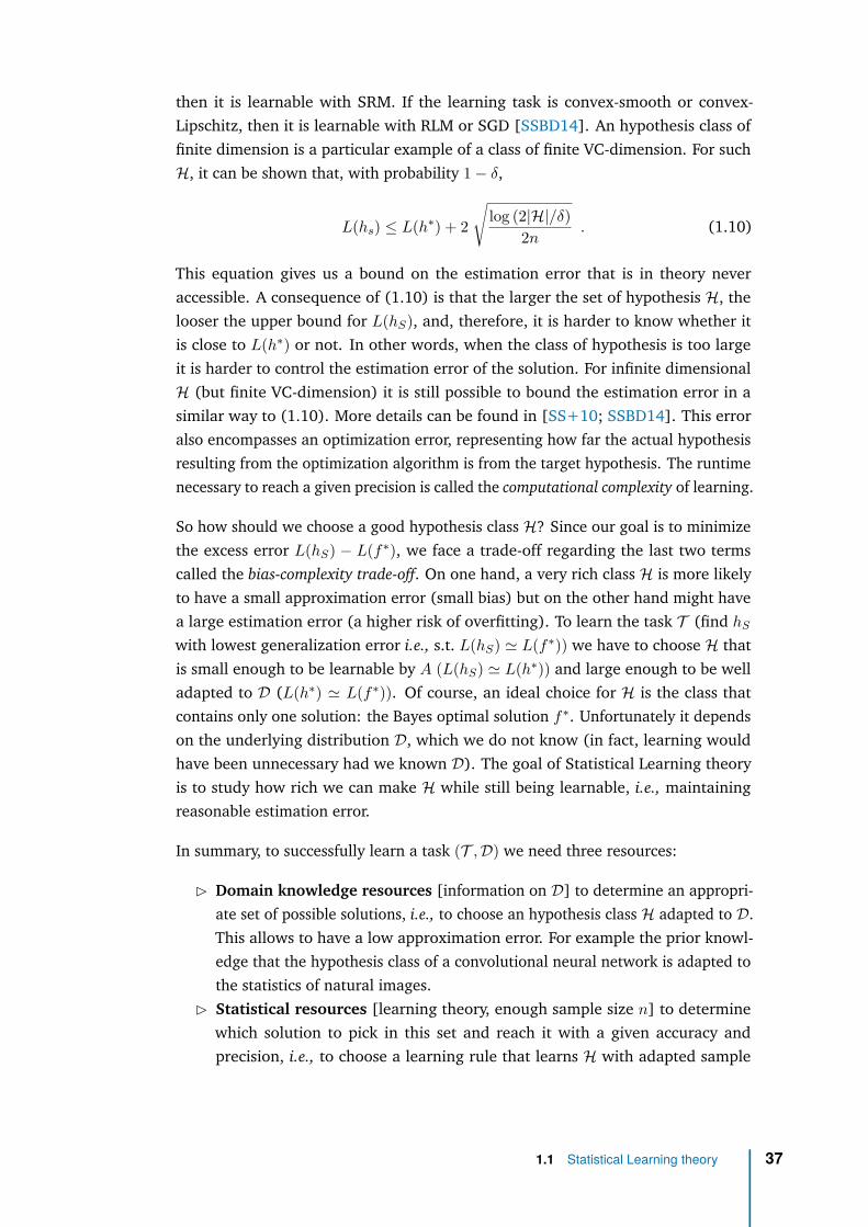
then it is learnable with SRM. If the learning task is convex-smooth or convex-Lipschitz, then it is learnable with RLM or SGD [SSBD14]. An hypothesis class offinite dimension is a particular example of a class of finite VC-dimension. For suchH, it can be shown that, with probability 1 − δ,

L(hs) ≤ L(h∗) + 2

√log (2|H|/δ)

2n . (1.10)

This equation gives us a bound on the estimation error that is in theory neveraccessible. A consequence of (1.10) is that the larger the set of hypothesis H, thelooser the upper bound for L(hS), and, therefore, it is harder to know whether itis close to L(h∗) or not. In other words, when the class of hypothesis is too largeit is harder to control the estimation error of the solution. For infinite dimensionalH (but finite VC-dimension) it is still possible to bound the estimation error in asimilar way to (1.10). More details can be found in [SS+10; SSBD14]. This erroralso encompasses an optimization error, representing how far the actual hypothesisresulting from the optimization algorithm is from the target hypothesis. The runtimenecessary to reach a given precision is called the computational complexity of learning.

So how should we choose a good hypothesis class H? Since our goal is to minimizethe excess error L(hS) − L(f∗), we face a trade-off regarding the last two termscalled the bias-complexity trade-off. On one hand, a very rich class H is more likelyto have a small approximation error (small bias) but on the other hand might havea large estimation error (a higher risk of overfitting). To learn the task T (find hS

with lowest generalization error i.e., s.t. L(hS) ≃ L(f∗)) we have to choose H thatis small enough to be learnable by A (L(hS) ≃ L(h∗)) and large enough to be welladapted to D (L(h∗) ≃ L(f∗)). Of course, an ideal choice for H is the class thatcontains only one solution: the Bayes optimal solution f∗. Unfortunately it dependson the underlying distribution D, which we do not know (in fact, learning wouldhave been unnecessary had we known D). The goal of Statistical Learning theoryis to study how rich we can make H while still being learnable, i.e., maintainingreasonable estimation error.

In summary, to successfully learn a task (T ,D) we need three resources:

▷ Domain knowledge resources [information on D] to determine an appropri-ate set of possible solutions, i.e., to choose an hypothesis class H adapted to D.This allows to have a low approximation error. For example the prior knowl-edge that the hypothesis class of a convolutional neural network is adapted tothe statistics of natural images.

▷ Statistical resources [learning theory, enough sample size n] to determinewhich solution to pick in this set and reach it with a given accuracy andprecision, i.e., to choose a learning rule that learns H with adapted sample

1.1 Statistical Learning theory 37

Page 43

complexity, This allows to have a low estimation error. For example we’llchoose the ERM learning rule if H has finite VC dimension and learning theorygives us the number of samples necessary the reach the best solution in H witha given accuracy and precision.

▷ Computational resources [powerful computer] to determine precisely howto pick this solution, i.e., to design an algorithm that implements the learningrule with reasonable computational complexity. This allows to have a lowoptimisation error.

Cross-validation. Once we have designed or chosen a learning algorithm, how canwe compute its true error. A practical way to get an estimate of the generalizationerror L(hS) is by evaluating its empirical error on a set of data points that were notconsidered during the minimization procedure leading to its estimation. Based onthis idea, one may assess how good the solution proposed by a learning algorithm isfor a certain dataset S using a cross-validation procedure [Bis07]:

▷ Partition S into K subsets containing (approximately) the same number ofelements: S = S1 ∪ · · · ∪ SK .

▷ For k = 1 . . .K, define the train and test folds: Straink = S \ Sk and Stest

k =Sk and compute the empirical error calculated on each test fold, Lk =LStest

k

(hStrain

k

).

▷ Define the average performance of the learning algorithm on dataset S byL = 1

K

∑Kk=1 Lk, which is the average empirical error of the solutions proposed

by the learning algorithm on each test fold; the expected value of L is thegeneralization error of hS [SSBD14].

Even if this method often works very well in practice, the exact behaviour of cross-validation is not yet fully understood theoretically [BHT21].

1.1.3 Lessons for regression on M/EEG signalsIn many cases, empirical research focuses on designing good hypothesis classesfor a certain domain, i.e., classes for which the approximation error would not beexcessively high, classes adapted to our task at hand. The idea is that although wecan’t access the oracle D and do not know how to construct the optimal classifierf∗, we still have some prior knowledge on our specific task, which enables us todesign hypothesis classes for which both the approximation error and the estimationerror are not too large. Indeed, our first contribution, derived in this chapter, hasbeen to design a class H perfectly adapted to M/EEG signals and source-poweroutcome, in the sense that it shows no approximation error. Such algorithms aresaid to be statistically consistent. When learning from a sufficiently large numberof samples (no estimation error) and without noise in y (no irreducible error), aregression algorithm with no approximation error will have no generalization error

1.1 Statistical Learning theory 38

Page 44

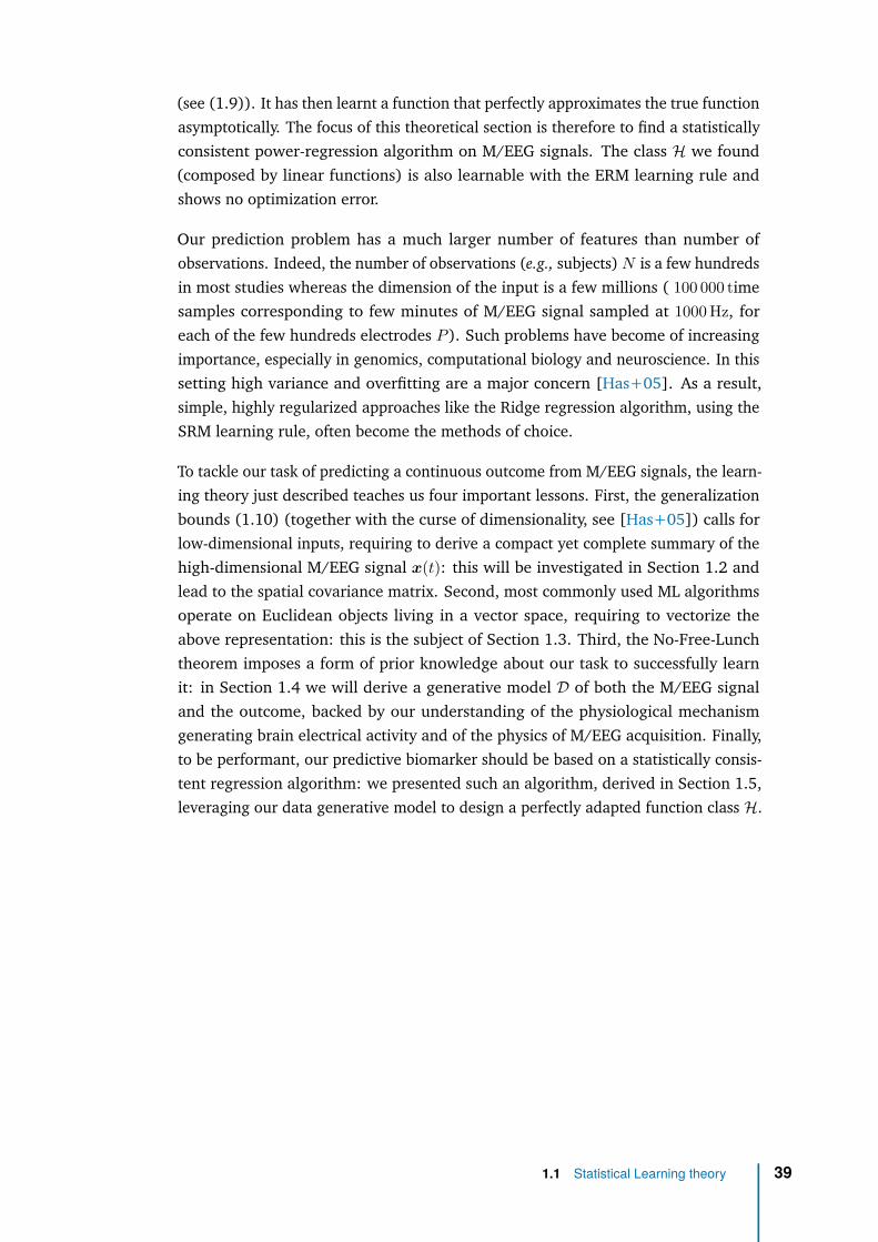
(see (1.9)). It has then learnt a function that perfectly approximates the true functionasymptotically. The focus of this theoretical section is therefore to find a statisticallyconsistent power-regression algorithm on M/EEG signals. The class H we found(composed by linear functions) is also learnable with the ERM learning rule andshows no optimization error.

Our prediction problem has a much larger number of features than number ofobservations. Indeed, the number of observations (e.g., subjects)N is a few hundredsin most studies whereas the dimension of the input is a few millions ( 100 000 timesamples corresponding to few minutes of M/EEG signal sampled at 1000 Hz, foreach of the few hundreds electrodes P ). Such problems have become of increasingimportance, especially in genomics, computational biology and neuroscience. In thissetting high variance and overfitting are a major concern [Has+05]. As a result,simple, highly regularized approaches like the Ridge regression algorithm, using theSRM learning rule, often become the methods of choice.

To tackle our task of predicting a continuous outcome from M/EEG signals, the learn-ing theory just described teaches us four important lessons. First, the generalizationbounds (1.10) (together with the curse of dimensionality, see [Has+05]) calls forlow-dimensional inputs, requiring to derive a compact yet complete summary of thehigh-dimensional M/EEG signal x(t): this will be investigated in Section 1.2 andlead to the spatial covariance matrix. Second, most commonly used ML algorithmsoperate on Euclidean objects living in a vector space, requiring to vectorize theabove representation: this is the subject of Section 1.3. Third, the No-Free-Lunchtheorem imposes a form of prior knowledge about our task to successfully learnit: in Section 1.4 we will derive a generative model D of both the M/EEG signaland the outcome, backed by our understanding of the physiological mechanismgenerating brain electrical activity and of the physics of M/EEG acquisition. Finally,to be performant, our predictive biomarker should be based on a statistically consis-tent regression algorithm: we presented such an algorithm, derived in Section 1.5,leveraging our data generative model to design a perfectly adapted function class H.

1.1 Statistical Learning theory 39

Page 45

1.2 Multivariate time series analysisMost phenomena are visible to us via signals - measurable temporal variations ofdifferent sources of activity. The scientific study of these phenomena thereforerelies on the analysis of these signals. For example the yearly land-ocean surfacetemperatures recorded at different locations on Earth may help to study globalwarming, the quarterly earnings per share of biggest companies in a particularindustry may reflect its global financial health, brain electrical activity recorded fromvarious locations on the scalp via M/EEG could allow testing how different brainareas are responding to a particular stimulus. To study these phenomena, scientistsneed mathematical tools to quantify, understand, model, and predict the timeevolution of such signals. Multivariate time series are the standard mathematicaltool for describing and analysing signals coming from measurements from multiplesensors during a physical or biological experiments. In this section, we definemultivariate time series and present probabilistic tools to analyze them. We willdiscuss some common assumptions regarding their statistics and then define acompact representation in the form of the covariance matrix. Finally we’ll explainwhy these matrices are often rank-deficient in the case of M/EEG signals.

1.2.1 Statistical and temporal momentsWhen an analog signal (valued at continuous time t ∈ R) is measured by anelectronic device, it is generally sampled with a uniform interval of length Ts, thesampling period, by recording its values at times {tTs}t∈Z. This gives rise to adigital signal (valued at discrete-time t ∈ Z). Discrete signal processing has replacedanalog signal processing in most applications with more sophisticated and precisealgorithms. Then, reconstructing the initial continuous-time signal from its samplesis, in some conditions, possible using interpolation algorithms.

Most real-world digital deterministic signals can be modeled by a multivariatetime series. A multivariate time series is a collection of P -dimensional vectors,indexed by t ∈ Z:

x(t) =

x1(t)

...xP (t)

(1.11)

Each dimension xk(t), k = 1 . . . P in x(t) represents a different quantity: it candescribe the time evolution of a certain stock composing a portfolio of P stocksin Finance [Lut07], the voice recorded at one of the P microphone in an acousticexperiment [OS94], or the neural activity registered by one electrode placed on asubject’s scalp [SC07] in a P -channel EEG recording.

1.2 Multivariate time series analysis 40

Page 46

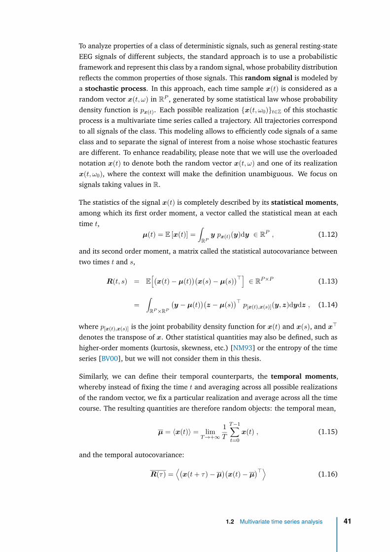
To analyze properties of a class of deterministic signals, such as general resting-stateEEG signals of different subjects, the standard approach is to use a probabilisticframework and represent this class by a random signal, whose probability distributionreflects the common properties of those signals. This random signal is modeled bya stochastic process. In this approach, each time sample x(t) is considered as arandom vector x(t, ω) in RP , generated by some statistical law whose probabilitydensity function is px(t). Each possible realization {x(t, ω0)}t∈Z of this stochasticprocess is a multivariate time series called a trajectory. All trajectories correspondto all signals of the class. This modeling allows to efficiently code signals of a sameclass and to separate the signal of interest from a noise whose stochastic featuresare different. To enhance readability, please note that we will use the overloadednotation x(t) to denote both the random vector x(t, ω) and one of its realizationx(t, ω0), where the context will make the definition unambiguous. We focus onsignals taking values in R.

The statistics of the signal x(t) is completely described by its statistical moments,among which its first order moment, a vector called the statistical mean at eachtime t,

µ(t) = E [x(t)] =∫RP

y px(t)(y)dy ∈ RP , (1.12)

and its second order moment, a matrix called the statistical autocovariance betweentwo times t and s,

R(t, s) = E[(

x(t) − µ(t))(

x(s) − µ(s))⊤] ∈ RP ×P (1.13)

=∫RP ×RP

(y − µ(t)

)(z − µ(s)

)⊤p[x(t),x(s)](y, z)dydz , (1.14)

where p[x(t),x(s)] is the joint probability density function for x(t) and x(s), and x⊤

denotes the transpose of x. Other statistical quantities may also be defined, such ashigher-order moments (kurtosis, skewness, etc.) [NM93] or the entropy of the timeseries [BV00], but we will not consider them in this thesis.

Similarly, we can define their temporal counterparts, the temporal moments,whereby instead of fixing the time t and averaging across all possible realizationsof the random vector, we fix a particular realization and average across all the timecourse. The resulting quantities are therefore random objects: the temporal mean,

µ = ⟨x(t)⟩ = limT →+∞

1T

T −1∑t=0

x(t) , (1.15)

and the temporal autocovariance:

R(τ) =⟨(

x(t+ τ) − µ)(

x(t) − µ)⊤⟩ (1.16)

1.2 Multivariate time series analysis 41

Page 47

1.2.2 Statistical assumptionsInferring statistically valid conclusions about populations from samples requiressome background assumptions, statements that one makes to make the building oftheoretical models easier. For instance we can use these assumptions to obtain betterestimators for describing the statistical law of the samples (less bias and smallervariance), as well as clearer interpretations about the underlying stochastic processthat generated them [Lut07]. However, they must be made carefully, since incorrectassumptions can yield to highly inaccurate conclusions.

Stationarity. One of the most common assumptions refers to how the statistics ofx(t) evolves in time. Strict-sense stationarity assumes that any joint probability lawis invariant by any temporal shift, which we can roughly think of as “the statisticalmoments do not depend on time”. Most of the time in signal processing we observeonly one realization, from which one want to estimate certain parameters of theunderlying stochastic process. The poorness of this numerical information generallylimits the investigation to the study to its mean and autocovariance. Since we onlystudy the second-order moments of the process, we generally adopt the milderhypothesis of wide-sense stationarity (WSS), that assumes stationarity up the secondorder. This implies that the statistical mean of the multivariate time series do notdepend on time,

µ(t) = µ , (1.17)

and that the autocovariance matrix between two times t and s depends only on theirdifference τ = s− t, and not on time t:

R(t, s) = R(t, t+ τ) = R(τ) = E[x(t+ τ) − µ)(x(t) − µ)⊤

]. (1.18)

Under the WSS hypothesis, the cross-power spectral density of a multivariate timeseries is defined as the discrete-time Fourier transform (DTFT) of the sequence ofauto-covariance matrices [Pri83; PW93]:

S(f) =∑k∈Z

R(k)e−j2πfk . (1.19)

The cross-power spectral density matrices are positive definite matrices whosediagonal values (also known as the power spectral density or PSD) describehow the power (or variance) of each time series in x(t) is distributed along thefrequency domain; the out-of-diagonal values portray the statistical correlationbetween the time series in each pair of dimensions in the frequency domain. Forexample the spectral power of a univariate white noise (a WSS process whosevalues at different times are uncorrelated) is constant. These matrices completely

1.2 Multivariate time series analysis 42

Page 48

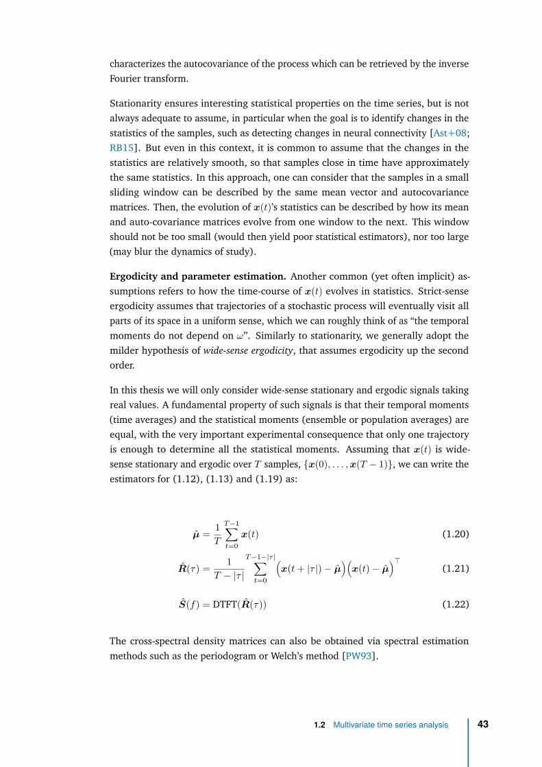
characterizes the autocovariance of the process which can be retrieved by the inverseFourier transform.

Stationarity ensures interesting statistical properties on the time series, but is notalways adequate to assume, in particular when the goal is to identify changes in thestatistics of the samples, such as detecting changes in neural connectivity [Ast+08;RB15]. But even in this context, it is common to assume that the changes in thestatistics are relatively smooth, so that samples close in time have approximatelythe same statistics. In this approach, one can consider that the samples in a smallsliding window can be described by the same mean vector and autocovariancematrices. Then, the evolution of x(t)’s statistics can be described by how its meanand auto-covariance matrices evolve from one window to the next. This windowshould not be too small (would then yield poor statistical estimators), nor too large(may blur the dynamics of study).

Ergodicity and parameter estimation. Another common (yet often implicit) as-sumptions refers to how the time-course of x(t) evolves in statistics. Strict-senseergodicity assumes that trajectories of a stochastic process will eventually visit allparts of its space in a uniform sense, which we can roughly think of as “the temporalmoments do not depend on ω”. Similarly to stationarity, we generally adopt themilder hypothesis of wide-sense ergodicity, that assumes ergodicity up the secondorder.

In this thesis we will only consider wide-sense stationary and ergodic signals takingreal values. A fundamental property of such signals is that their temporal moments(time averages) and the statistical moments (ensemble or population averages) areequal, with the very important experimental consequence that only one trajectoryis enough to determine all the statistical moments. Assuming that x(t) is wide-sense stationary and ergodic over T samples, {x(0), . . . ,x(T − 1)}, we can write theestimators for (1.12), (1.13) and (1.19) as:

µ = 1T

T −1∑t=0

x(t) (1.20)

R(τ) = 1T − |τ |

T −1−|τ |∑t=0

(x(t+ |τ |) − µ

)(x(t) − µ

)⊤(1.21)

S(f) = DTFT(R(τ)) (1.22)

The cross-spectral density matrices can also be obtained via spectral estimationmethods such as the periodogram or Welch’s method [PW93].

1.2 Multivariate time series analysis 43

Page 49

Without loss of generality, we will consider that all time series are zero-mean, so thattheir parametrization, up to the second order, may be done using their cross-spectraldensity matrices only. Furthermore, we will assume that the time series have beenbandpass filtered and so their spectral content is supported on a set of frequenciesdenoted by F .

A special note on the Gaussianity assumption. Another usual assumption concernsthe statistics of x(t) and assume that px(t) can be approximated by a multivariateGaussian distribution. Under this hypothesis, the second-order moments, the meanvector and sequence of autocovariance matrices R(τ) (or, equivalently, the cross-spectral density matrices S(f)) exhaustively describe the full statistical behavior ofx(t) [Pri83]. This hypothesis is appealing in numerous ways e.g., a WSS Gaussianprocess has also the much stronger property of being strict-sense stationary. Itcan also be used for defining a notion of distance between two time series. Sincethe second-order moments encapsulates information about the whole probabilitydistribution, we can use them to compare two time series, xi(t) and xj(t) by definingtheir cross-spectrum distance as

dS

(xi(t),xj(t)

)2 =∫

Fd2(Si(f),Sj(f)

)df , (1.23)

where Si(f) and Sj(f) are the cross-spectral density matrices of xi(t) and xj(t),respectively, and d is some distance between matrices. The choice of the distanced will be extensively discussed in Section 1.3. This approach of comparing twotime series based on their cross-spectral densities is more appropriate than directlycomparing their samples on a given realization because it is based on informationdefining the whole probability distribution. It also lead to stronger performance onclassification [CRJ19], regression [Sab+19a] and clustering tasks [Cha+13].

The Gaussianity assumption is often justified in the literature by different arguments.If several independent factors play a role in the generation of the data, one may usethe central limit theorem to argue that the sum of all their contributions yields astatistical behavior that can be well described by a Gaussian distribution [PP02]. Asa result, Gaussian processes appear in numerous physical phenomena. It also gives anumerical advantage: parameter estimation under the Gaussian model yields convexoptimization problems that have analytic solutions. Finally, without any knowledgeabout the statistics of the data, in particular with no information on the momentsof order strictly higher than two, the Gaussian distribution is the most conservativeassumption: among all probability distributions defined on an infinite domain andwith a given mean and variance, it is the one with maximal differential entropyi.e., the one that requires the maximum quantity of information to encode it.

However, the Gaussian assumption is very strong and is not always justified. Forinstance, the statistics of rare events are better described by Poisson distributions. In

1.2 Multivariate time series analysis 44

Page 50

general, the use of Gaussian distributions to model data is appropriate when onehas no knowledge about the physical phenomena that generates its samples. As wewill develop a generative model of M/EEG signals and related biomedical outcomes,we will not resort to this strong hypothesis. This will give a wider generality to ourcontribution, and will yield a more robust biomarker. Note that we can still considerthat, up to the second order, we have:

dS

(xi(t),xj(t)

)2 ≃∫

Fd2(Si(f),Sj(f)

)df . (1.24)

1.2.3 The covariance matrixA good estimate of the cross-spectral density matrix requires enough time samples.If not the case, it is wiser to condense the information contained in the spectruminto a single parameter. Comparing two time series then amounts to compare theircorresponding parameters. One can do this by noticing that the inverse DTFT appliedto the cross-spectral density matrices of a zero-mean F -bandpass filtered time seriesx(t) gives ∫

FS(f)df = R(0) = E[x(t)x(t)⊤] = C , (1.25)

which is the covariance matrix of x(t) and can be calculated without having toestimate its spectrum. Denoting the data matrix X ∈ RP ×T with T the number oftime samples, and using (1.21) with τ = 0, the covariance matrix reads:

C ≃ XX⊤

T∈ RP ×P with X ∈ RP ×T . (1.26)

For the sake of simplicity, we assume that T is the same for each time series, althoughit is not required by the following method. The diagonal of this matrix represents thevariance (power) of each sensor, while the off-diagonal terms contain the covariancebetween each pair of signals. Negative values in the off-diagonal express negativecorrelations.

We may then approximately compare two time series xi(t) and xj(t) using thedistance between their respective covariance matrices Ci and Cj as

dS

(xi(t),xj(t)

)2 ≃ d2(Ci,Cj) . (1.27)

Under our assumptions, comparing two time series boils down to estimating theircovariance matrices. A common problem arising from covariance estimation inM/EEG signals is rank-deficiency, mainly occurring for two different reasons. First,high-dimensional statistics show that one need enough available samples to expecta good estimate of the covariance matrix that describes the statistics of the data.This may not be the case for some applications. The covariance C is a P × P matrix

1.2 Multivariate time series analysis 45

Page 51

which is a sum of T rank-one matrices (as per (1.21) with τ = 0). Therefore, thereshould be at least P samples available for the estimate C to have a chance of notbeing rank-deficient. In fact, the number of parameters to estimate in a covariancegrows quadratically with dimension so many more samples are required than thereare sensors to accurately estimate such matrices [EG15; Rod+17]. A commonapproach for alleviating such problem, called ‘shrinkage’, use a regularization termthat adds a weighted Identity matrix to C, with the optimal weight being determinedfrom the data. Many methods have been proposed for determining the weight ofthe regularization term [Che+10; EG15]. Second, even in the case where wehave enough available samples to estimate the covariance matrix, the signal pre-processing used to enhance the SNR of noisy signals lead to inherently rank-deficientcovariance matrices. This is the case of M/EEG signals.

1.2.4 M/EEG preprocessing induces rank-deficiencyEven though the magnetic shielded room and gradiometer coils can help to reducethe effects of external interferences on MEG signal (as seen in the Introduction chap-ter), the problem mainly remains and further reduction is needed. Also, additionalartifact signals can be caused by movement of the subject during recording if thesubject has small magnetic particles on his body or head. The Signal Space Separa-tion (SSS) method can help mitigate those problems [TK05]. Besides, physiologicalartifacts (eye blinks and heart beats) can cause prominent artifacts in the recording.The Signal Space Projections (SSP) method is typically used to reduce them [UI97].Both of these methods are described below and enable to increase the SNR, at aprice of rendering covariance matrices rank-deficient.

Signal Space Separation (SSS)

The Signal Space Separation (SSS) method [TK05], also called Maxwell Filtering,is a biophysical spatial filtering method, purely MEG specific, that aim to produceMEG signals cleaned from external interferences and from movement distortionsand artifacts.

A MEG device records the neuro-magnetic field distribution by sampling the fieldsimultaneously at P distinct locations around the subject’s head. At each momentof time, the measurement is a vector x ∈ RP where P is the total number ofrecording channels. In theory, any direction of this vector in the signal spacerepresents a valid measurement of a magnetic field, however the knowledge of thelocation of possible sources of magnetic field, the geometry of the sensor array andelectromagnetic theory (Maxwell’s equations and the quasi static approximation)considerably constrain the relevant signal space and allow us to differentiate betweensignal space directions consistent with a brain’s field and those that are not.

1.2 Multivariate time series analysis 46

Page 52

To be more precise, it has been shown that the recorded magnetic field is a gradientof a harmonic scalar potential. A harmonic potential V (r) is a solution of theLaplacian differential equation ∇2V = 0, where r is represented by its sphericalcoordinates (r, θ, ψ). It is known that a harmonic function in a three-dimensionalspace can be represented as a series expansion of spherical harmonic functionsYlm(θ, ϕ):

V (r) =∞∑

l=1

l∑m=−l

αlmYlm(θ, ϕ)rl+1 +

∞∑l=1

l∑m=−l

βlmrlYlm(θ, ϕ) (1.28)

We can separate this expansion into two sets of functions: those proportional toinverse powers of r and those proportional to powers of r. From a given array ofsensors and a coordinate system with its origin somewhere inside of the helmet, wecan compute the signal vectors corresponding to each of the terms in 1.28.

Following notations of [TK05], let alm be the signal vector corresponding to termYlm(θ,ϕ)

rl+1 and blm the signal vector corresponding to rlYlm(θ, ϕ), our measurement isgiven by:

x =∞∑

l=1

l∑m=−l

αlmalm +∞∑

l=1

l∑m=−l

βlmblm (1.29)

A set of P such signal vectors forms a basis in the P dimensional signal space. Thisbasis is not orthogonal, but still linearly independent so any measured signal vectorhas a unique representation in this basis:

x = [Sin Sout][

xin

xout

], (1.30)

where the sub-bases Sin and Sout contain the basis vectors alm and blm respectively,and vectors xin and xout contain the corresponding αlm and βlm values.

It can be shown that the basis vectors corresponding to the terms in the secondsum in expansion (1.28) represent the perturbation sources external to the helmet.We can then separate the components of field arising from sources inside andoutside of the helmet. We can therefore decompose the signal vector x into thesum of 2 components: ϕin = Sinxin in the brain signal space with basis Sin andϕout = Soutxout in the interference space with basis Sout (not necessarily orthogonalto Sin). By discarding ϕout, we are left with the part of the signal coming from insideof the helmet only. Hence, ϕin reproduces in all the MEG channels the signals thatwould be seen if no interference from sources external to the helmet existed: wehave performed signal space separation. To further reduce the noise, we can discardthe high l,m end of the spectrum: indeed the spherical harmonic functions are

1.2 Multivariate time series analysis 47

Page 53

known to contain increasingly higher spatial frequencies when going to higher indexvalues (l,m) so that the signals from real magnetic sources are mostly contained inthe low l,m end of the spectrum.

After projection in the lower-dimensional SSS basis we project back the signal in itsoriginal space producing a signal Xclean = SinS⊤

inX ∈ RP ×T (Sin ∈ RP ×R) witha much better SNR (reduced noise variance) but with a rank R ≤ P . As a resulteach reconstructed sensor is then a linear combination of R synthetic source signals,which modifies the inter-channel correlation structure, rendering the covariancematrix rank-deficient.

Signal Space Projection (SSP)

If one knows, or can estimate, K linearly independent source patterns a1, . . . ,aK

that span the space S = span(a1, . . . ,aK) ⊂ RP , one can estimate an orthonormalbasis UK ∈ RP ×K of S by taking the first K left singular vectors in the singularvalue decomposition (SVD) of the matrix formed by the source patterns in columns.We can then separate the sensor-space signal x into a signal s∥ produced by thoseK sources (belonging to the subspace S) and a signal s⊥ that can’t be produced byany linear combination of those sources (belonging to the corresponding orthogonalsubspace):

x = x∥ + x⊥ = UKU⊤Kx + (I − UKU

⊤K)x (1.31)

If S is formed from specific artifacts then x⊥ is mostly free of those.

This is the idea behind the Signal Space Projections (SSP) method [UI97]. Inpractice SSP is used to reduce physiological artifacts (eye blinks and heart beats)that cause prominent artifacts in the recording. SSP projections are computedfrom time segments contaminated by the artifacts and the first component (perartifact and sensor type) are projected out. To take a more concrete example, in theCam-CAN MEG dataset [Sha+14], eye blinks are monitored by 2 electro-oculogram(EOG channels), and heart beats by an electro-cardiogram (ECG channel). TheEOG and ECG channels are used to identify the artifact events (after a first band-pass filter to remove DC offset and an additional [1-10]Hz filter applied only toEOG channels to remove saccades vs blinks). As an illustration of this process,in our MEG experiment described in Section 2.1.2, we filtered the raw signal in[1-35]Hz band and created data segments (called epochs) around those events,rejecting those whose peak-to-peak amplitude exceeds a certain global threshold.For each artifact and sensor type these epochs are then averaged and the firstcomponent of maximum variance is extracted via PCA. Signal is then projected inthe orthogonal space, again leading to rank-deficient covariance matrices. Thisfollows the guidelines of the MNE software [Gra+14]. It is interesting to compareSSP with SSS geometrically. Like SSP, SSS is a form of projection. Whereas SSP

1.2 Multivariate time series analysis 48

Page 54

empirically determines a noise subspace based on data (empty-room recordings, EOGor ECG activity, etc.) and projects the measurements onto a subspace orthogonalto the noise, SSS mathematically constructs the external and internal subspacesfrom spherical harmonics and reconstructs the sensor signals using only the internalsubspace (i.e., does an oblique projection).

To summarize this section, we saw that our assumptions of stationarity and ergodicityallowed to represent a M/EEG time series x(t) by its covariance matrix C in acertain frequency band, either full rank or rank-deficient. Covariance matrices arepositive matrices, so they have a particular structure. This structure implies thatthey don’t live in a flat space (a vector space), they live in a curved space, called amanifold. Hence, a covariance matrix can’t be readily vectorized. Even though somealgorithms can manipulate covariance matrices directly as input [Bar+12], mostcommonly used ML regression algorithms (and also the most performant ones forM/EEG classification tasks) assume an Euclidean structure of their input requiringto vectorize the covariance matrix. To do that properly, we must first introduce someimportant concepts regarding Riemannian manifold.

1.2 Multivariate time series analysis 49

Page 55

1.3 Riemannian matrix manifolds

1.3.1 Riemannian manifolds

ξ MT

M

M M

M'

LogM

ExpM

Fig. 1.1: Tangent Space, exponentialand logarithm on Riemannianmanifold illustration

In this work, we consider differentiable man-ifolds M in RP of dimension K. Intuitivelydifferentiable manifolds are "curved" spaces thatlocally at each point resemble a flat vector space(see [AMS09], chap. 3 and [PFA06]). Examplesof differentiable manifolds in R3 are curves (one-dimensional manifolds which locally look likea straight line) and surfaces (two-dimensionalmanifolds which locally look like a plane). Moreprecisely, each point of the manifold M ∈ M isassociated to a vector space called tangent space at M , denoted TM . For any matrixM ′ ∈ M, as M ′ → M , ξM = M ′ − M ∈ TM . It is the set of derivatives of curveson the manifold passing through M . The dimension of TM is K, the dimension ofM. The differentiable manifold becomes Riemannian when each tangent spaceTM is endowed with a metric, i.e. an inner product ⟨·, ·⟩M : TM × TM → R, thatdefines a local Euclidean structure. This metric is supposed smooth across pointson the manifold. An Euclidean space is a particular Riemannian manifold with aconstant metric. We can then define:

A norm on the tangent space TM : ∥ξM ∥2M = ⟨ξM , ξM ⟩M for ξM ∈ TM .

The length of a path between two points M ,M ′ ∈ M: for a path γ : [0, 1] → Msuch that γ(0) = M and γ(1) = M ′, the length of γ is L(γ) =

∫ 10 ∥γ(t)∥γ(t)dt. This

generalizes the usual notion of path length in Euclidean spaces.

A distance on the manifold M, defined as the minimum length of paths: d(M ,M ′) =minL(γ) such that γ(0) = M , and γ(1) = M ′. This distance is called the geodesicdistance. If M is an Euclidean space, this distance is simply the usual Euclideandistance: d(M ,M ′) = ∥M − M ′∥2, achieved when γ is a straight line between M

and M ′.

The Frechet mean M of a set of points Mi ∈ M is defined as

M = Meand(M1, . . . ,MN ) = arg minM∈M

N∑i=1

d(M ,Mi)2 . (1.32)

This is a generalization of averaging on manifolds. Indeed, in an Euclidean space, theaverage 1

N

∑Ni=1 Mi is the Frechet mean of M1, . . .MN with respect to the Euclidean

distance d(M ,M ′) = ∥M − M ′∥2. Another example in R∗+, the geometric mean

1.3 Riemannian matrix manifolds 50

Page 56

between positive numbers a1, . . . , aN > 0, given by a = (a1 × · · · × aN )1/N , is theFrechet mean of (a1, . . . , aN ) with respect to the distance d(a, a′) = | log( a

a′ )|.

The exponential mapping ExpM : TM → M is the operation that maps the tangentspace, which has a simple Euclidean structure, to the manifold which might havea much more complicated structure. It satisfies d(ExpM (ξM ),M) = ∥ξM ∥M forξM ∈ TM small enough.

The logarithm mapping LogM : M → TM is defined as the reciprocal of the ex-ponential mapping which hence verifies ∥LogM (M ′)∥M = d(M ,M ′) for M ′ ∈ Mclose enough from M . It maps the manifold to the tangent space, while preservingthe local properties of the manifold.

The vectorization operator. The logarithm mapping is of crucial importance inpractical applications, since it allows to manipulate and store vectors (belongingto the tangent space) instead of points on the manifold. To be more concrete,since each tangent space is a K-dimensional Euclidean space, there exists a linearand invertible mapping ϕM : TM → RK such that ∥ξM ∥M = ∥ϕM (ξM )∥2 for allξM ∈ TM . Combining ϕM and LogM gives the vectorization operator at ∈ M,PM = ϕM ◦ LogM which maps M to RK , and verifies:

∥PM (M ′)∥2 = d(M ,M ′) for M ′ ∈ M . (1.33)

This operator explicitly captures the local Euclidean properties of the Riemannianmanifold. Fig. 1.1 illustrates these concepts. Finally, if a set of matrices M1, . . . ,MN

is located in a small portion of the manifold, denoting M = Meand(M1, . . . ,MN ),it holds:

d(Mi,Mj) ≃ ∥PM (Mi) − PM (Mj)∥2 (1.34)

The vectorization operator is key for machine learning applications: it projects pointsin M on RK , and the distance d on M is approximated by the distance ℓ2 on RK .Therefore, those vectors can be used as input for any standard regression technique,which often assumes a Euclidean structure of the data.

As a final note, all the notions developed above are based on the metric ⟨·, ·⟩M .Different metrics lead to different geodesic distances, Frechet means, exponentialand logarithm mapping and vectorization operator. Choosing the right metric for aparticular problem may lead to substantial benefits. For additional details on matrixmanifolds, see [AMS09], chap. 3.

1.3.2 The positive definite manifold S++P

In this thesis, we are interested in one Riemannian manifold in particular: the mani-fold of positive definite matrices S++

P [FM03], to which most full rank covariance

1.3 Riemannian matrix manifolds 51

Page 57

matrices C belong. This is not a vector space, as for example the difference of twopositive definite matrices may not be positive definite. It is a differentiable manifoldof dimension P (P +1)

2 , with fixed tangent spaces TC = S+P for all C ∈ S++

P .

We endow the manifold with the geometric metric given by: ⟨P ,Q⟩C = Tr(P C−1QC−1).The associated geometric norm generalizes the Froebenius norm: ∥P ∥I (identity) =∥P ∥F (Frobenius) for P ∈ TI . This metric has two main advantages. First, it is affine-invariant as for any invertible matrix W it verifies ⟨W P W ⊤,W QW ⊤⟩W CW ⊤ =⟨P ,Q⟩C . Second, it leads to closed-form formulas for most Riemannian notionsseen above:

The geometric geodesic distance on the manifold S++P is:

d2G(C,C ′) = ∥ log(C−1/2C ′C−1/2)∥2

F =P∑

k=1log2(λk) , (1.35)

where λk, k = 1 . . . P are the real eigenvalues of C−1/2C ′C−1/2 , or equivalently ofC−1C ′. Please note that these 2 matrices have the same eigenvalues but not the samesingular values (hence not the same Frobenius norm) since C−1C ′ is not symmetrical.Compared to the more naive Frobenius distance d2

F (C,C′) = ∥C −C′∥2F =

∑Pk=1 λ

2k

where λk are the eigenvalues of C − C′, the geometric distance is a geodesicdistance, which takes into account the intrinsic geometry of the positive definitemanifold [Bha09]. We also see that the singular matrices act as a barrier for thisdistance: if C or C ′ is close from being singular, one eigenvalue λk goes either to 0or +∞, and dG(C,C ′) goes to infinity. Following the corresponding property of thegeometric metric, this distance is affine invariant, i.e.,

For W invertible, dG(W CW ⊤,W C ′W ⊤) = dG(C,C ′) . (1.36)

This is an important property for our purpose: assume that C and C ′ are covariancesof some signals x and x′ ∈ RP , the distance dS (1.24) between x and x′ is alsoinvariant to linear transforms of the signals W x and W x′: the distance is blind toglobal mixing effects. Indeed, when using the geometric distance in (1.24), we havefor any invertible matrix W ∈ RP ×P ,

dS

(W xi(t),W xj(t)

)2 ≃∫

Fd2(W Si(f)W ⊤,W Sj(f)W ⊤)df , (1.37)

=∫

F

d∑k=1

log2(µk(f))df , (1.38)

1.3 Riemannian matrix manifolds 52

Page 58

where µk(f) are the eigenvalues of matrix (W Si(f)W ⊤)−1(W Sj(f)W ⊤)= W −T S−1

i (f)Sj(f)W T which, by similarity, has the same eigenvalues of S−1i (f)Sj(f).

Therefore,

dS

(W xi(t),W xj(t)

)2 ≃∫

Fd2(Si(f),Sj(f)

)df ≃ dS

(xi(t),xj(t)

)2. (1.39)

This shows that distance (1.24) is invariant to affine transformations of time seriesthemselves, a property that is very useful in practice. Indeed, we often observemixing effects when working with time series related to physical phenomena. Theseeffects can be often be approximated by the action of a linear operator, as we will seein Section 1.4.2 for M/EEG signals. In such cases, the distance (1.24) is invariantto these effects. For instance, very conveniently, the geometric distance betweentwo time series recorded with different measurement scales (e.g., V or µV) is thesame. The effect of slightly moving the positions of electrodes on a subject’s scalp orthe effects caused by the mixture of different sources of activity in a person’s brainare also examples of such mixing effects approximated by a linear operator, hencethat leave the distance between time series unchanged. This distance has achievedstate-of-art performance in EEG-based Brain-Computer Interfaces (BCI) classificationtasks [Bar+12] using only covariance matrices as features of EEG signals.

The Frechet mean, for P = 1, is the geometric mean between positive scalars. Inhigher dimension, no closed-form formula for the Frechet mean has been discovered,but iterative algorithms to compute it are available [JVV12; CPB16]. The meanis also affine invariant, in the sense that W C W ⊤ = W CiW ⊤ (applying linearmixing on the mean of the covariances is the same as computing the mean over allindividually mixed covariances). As a consequence, if the matrices Ci were jointlydiagonalizable, i.e. Ci = AΛiA

⊤ with A invertible and Λi diagonal, we would have

C = A(∏N

i=1 Λi

)1/NA⊤. This property is used in the proof of consistency of the

Riemann regression algorithm in Section 1.5.1.

The logarithm mapping at C is given by LogC(C ′) = C1/2 log(C−1/2C ′C−1/2)C1/2 ∈TC , and the vectorization operator w.r.t. C is

PC(C ′) = Upper(C− 12 LogC(C ′)C− 1

2 ) = Upper(log(C−1/2C ′C−1/2)) , (1.40)

where Upper(M) is the vector of size P (P + 1)2 containing the upper triangularcoefficients of M , with unit weights on the diagonal and

√2 weights on the off-

diagonal. This weighting ensures that the vector and the matrix have same norms(∥Upper(M)∥2 = ∥M∥F ). Once again, if C and C ′ are covariances of x and x′, itamounts to whitening x′ with C, and then applying a "spectral" non-linear transformon the resulting covariance, where the transform only changes the eigenvalues andnot the eigenvectors.

1.3 Riemannian matrix manifolds 53

Page 59

1.3.3 The fixed rank SDP manifold S+P,R

When a covariance matrix is -rank-deficient, it does not belong to S++P but to S+

P,R,the subspace of SPD matrices of fixed rank R. Unlike S++

P , it is hard to endowthe S+

P,R manifold with a distance that yields tractable or cheap-to-compute loga-rithms [VAV09]. This manifold is classically viewed as S+

P,R = {YY⊤|Y ∈ RP ×R∗ },

where RP ×R∗ is the set P ×R matrices of rank R [Jou+10]. This view allows to write

S+P,R as a quotient manifold RP ×R

∗ /OR, where OR is the orthogonal group of size R.This means that each matrix YY⊤ ∈ S+

P,R is identified with the set {YQ|Q ∈ OR}.

It has recently been proposed [MA18] to use the standard Frobenius metric on thetotal space RP ×R

∗ . This metric in the total space is equivalent to the Wassersteindistance [BJL18] on S+

P,R:

dW (S,S′) =[Tr(S) + Tr(S′) − 2Tr((S

12 S′S

12 )

12 )] 1

2 (1.41)

This provides cheap-to-compute logarithm mapping:

LogY Y ⊤(Y ′Y ′⊤) = Y ′Q∗ − Y ∈ RP ×R∗ , (1.42)

where UΣV ⊤ = Y ⊤Y ′ is a singular value decomposition and Q∗ = V U⊤. Thevectorization operator is then given by PY Y ⊤(Y ′Y ′⊤) = vect(Y ′Q∗ − Y ) ∈ RP R,where the vect of a matrix is the vector containing all its coefficients.

This framework offers closed-form projections in the tangent space for the Wasser-stein distance, which can be used to perform regression. Importantly, since S++

P =S+

P,P , we can also use this distance on the positive definite matrices. This distancepossesses the orthogonal invariance property:

For W orthogonal, dW (W ⊤SW ,W ⊤S′W ) = dW (S,S′) . (1.43)

This property is weaker than the affine invariance of the geometric distance. Anatural question is whether such an affine invariant distance also exists on thismanifold. Unfortunately, it is shown in [BS09] that the answer is negative for R < P .The proof is sufficiently simple to be derived here.

Theorem. There is no continuous affine invariant distance on S+P,R if R < P

Proof. We show the result for P = 2 and R = 1; the demonstration can straight-forwardly be extended to the other cases. The proof, from [BS09], is by con-tradiction. Assume that d is a continuous invariant distance on S+

2,1. Consider

A =(

1 00 0

)and B =

(1 11 1

), both in S+

2,1. For ε > 0, consider the invert-

1.3 Riemannian matrix manifolds 54

Page 60

ible matrix Wε =(

1 00 ε

). We have: WεAW ⊤

ε = A, and WεBW ⊤ε =

(1 ε

ε ε2

).

Hence, as ε goes to 0, we have WεBW ⊤ε → A Using affine invariance, we have:

d(A,B) = d(WεAW ⊤ε ,WεBW ⊤

ε ) . Letting ε → 0 and using continuity of d yieldsd(A,B) = d(A,A) = 0, which is absurd since A = B.

To close this section, we have now compactly represented a M/EEG time series x(t)by its covariance matrix C in a certain frequency band. This matrix can either befull rank C ∈ S++

P or most often rank-deficient C ∈ S+P,R. In any case, the only way

to vectorize a covariance matrix while enjoying the affine invariance property is byprojecting it into a tangent space. Only once a matrix has been vectorized this way,can we use it as features to a standard regression algorithm. We will now presentour prior knowledge on the M/EEG data generating mechanism and detail classicalapproaches to predict from such signals.

1.3 Riemannian matrix manifolds 55

Page 61

1.4 Generative models of M/EEG signals andoutcome

In this thesis we are interested in predicting a continuous bio-medical neuro-outcomey ∈ R from brain activity, measured by MEG/EEG and represented by the multivariatesignal x(t) ∈ RP , where P corresponds to the number of sensors. As prior knowledgeabout this task we will derive a neurophysiological generative model of brain activity,and its approximation by a statistical generative model. Note that, in this thesis, weuse the term generative model in the statistical sense of a probabilistic model of theM/EEG observations and the biomedical outcomes.

1.4.1 Prior knowledgePhysiological generative model. We assume the existence of M ≫ P electricalphysiological sources in the brain that emerge from the synchronous activity of corticallayer IV pyramidal neurons [Häm+93]. The activity of these neural current genera-tors form the time series z(t) ∈ RM , where t represents time. These sources can bethought of as localized current sources, such as a patch of cortex with synchronouslyfiring neurons, or a large set of patches forming a network. The underlying assump-tion is that these unobservable physiological sources are at the origin of the M/EEGsignals x(t), and that they are statistically related to y. Often they are even theactual generators of y, e.g., , the neurons producing the finger movement of a person.Here, we embrace the statistical machine learning paradigm where one aims to learna predictive model from a set of N labeled training samples, (xi(t), yi), i = 1, . . . , N ,which we see, fundamentally, as a function approximation problem. We will considerpredicted outcomes that do not depend on time. The physics of the problem andthe linearity of the quasi-static approximation of Maxwell’s equations guarantee thatMEG/EEG acquisition is linear too: the signals measured are obtained by linearcombination of the underlying physiological sources. This leads to:

xi(t) = Gi zi(t) , (1.44)

where Gi ∈ RP ×M is the leadfield, also commonly referred to as gain matrix.Therefore, the observed M/EEG signal xi(t) ∈ RP recorded by the external sensorscontains information on unobserved brain internal sources zi(t) ∈ RM , distorted byindividual brain anatomy represented by Gi. Note that here the j-th column of Gi

is not necessarily constrained to be the forward model of a focal electrical currentdipole in the brain. It can also correspond to large distributed sources. Besides, theneuro-outcome is also related to the sources through an unknown function:

yi = ϕ(zi(t)) . (1.45)

1.4 Generative models of M/EEG signals and outcome 56

Page 62

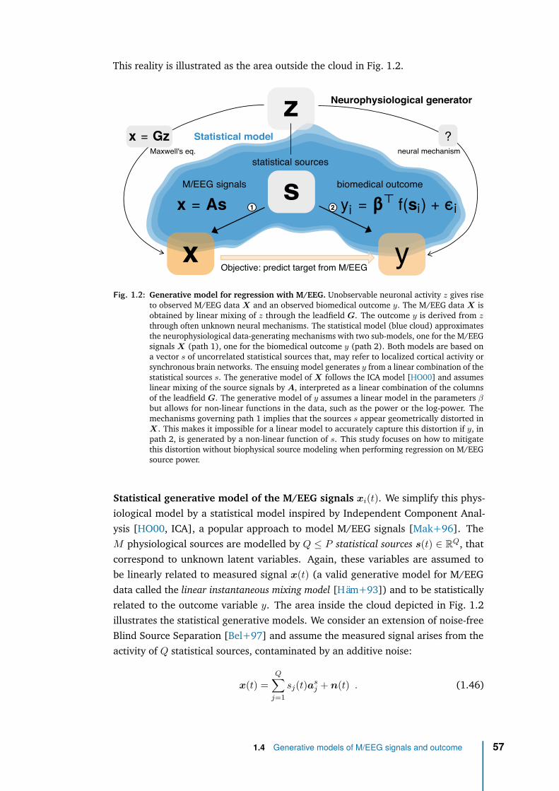
This reality is illustrated as the area outside the cloud in Fig. 1.2.

z

s

?

Objective: predict target from M/EEG

Neurophysiological generator

Statistical model

biomedical outcome

statistical sources

M/EEG signals

Maxwell's eq. neural mechanism

1 2

x yFig. 1.2: Generative model for regression with M/EEG. Unobservable neuronal activity z gives rise

to observed M/EEG data X and an observed biomedical outcome y. The M/EEG data X isobtained by linear mixing of z through the leadfield G. The outcome y is derived from zthrough often unknown neural mechanisms. The statistical model (blue cloud) approximatesthe neurophysiological data-generating mechanisms with two sub-models, one for the M/EEGsignals X (path 1), one for the biomedical outcome y (path 2). Both models are based ona vector s of uncorrelated statistical sources that, may refer to localized cortical activity orsynchronous brain networks. The ensuing model generates y from a linear combination of thestatistical sources s. The generative model of X follows the ICA model [HO00] and assumeslinear mixing of the source signals by A, interpreted as a linear combination of the columnsof the leadfield G. The generative model of y assumes a linear model in the parameters βbut allows for non-linear functions in the data, such as the power or the log-power. Themechanisms governing path 1 implies that the sources s appear geometrically distorted inX. This makes it impossible for a linear model to accurately capture this distortion if y, inpath 2, is generated by a non-linear function of s. This study focuses on how to mitigatethis distortion without biophysical source modeling when performing regression on M/EEGsource power.

Statistical generative model of the M/EEG signals xi(t). We simplify this phys-iological model by a statistical model inspired by Independent Component Anal-ysis [HO00, ICA], a popular approach to model M/EEG signals [Mak+96]. TheM physiological sources are modelled by Q ≤ P statistical sources s(t) ∈ RQ, thatcorrespond to unknown latent variables. Again, these variables are assumed tobe linearly related to measured signal x(t) (a valid generative model for M/EEGdata called the linear instantaneous mixing model [Häm+93]) and to be statisticallyrelated to the outcome variable y. The area inside the cloud depicted in Fig. 1.2illustrates the statistical generative models. We consider an extension of noise-freeBlind Source Separation [Bel+97] and assume the measured signal arises from theactivity of Q statistical sources, contaminated by an additive noise:

x(t) =Q∑

j=1sj(t)as

j + n(t) . (1.46)

1.4 Generative models of M/EEG signals and outcome 57

Page 63

The sensor signal x(t) ∈ RP is a linear combination of Q unit vectors in RP calledthe source patterns. Each of the Q source pattern as

j is the sensor measure of a unit-amplitude source and is weighted by the corresponding source amplitude sj(t) ∈ R.This model is conveniently written in matrix form, for each sample i = 1 . . . N :

xi(t) = Asi si(t) + ni(t) , (1.47)

where si(t) ∈ RQ is the source vector formed by the time series of the Q sourcesamplitude of sample i and ni(t) ∈ RP is the contamination due to noise. Thecolumns of the time-independent mixing matrix As ∈ RP ×Q are the Q linearlyindependent source patterns [Hau+14], which correspond to topographies on thesensor array: As = [as

1, . . . ,asQ] ∈ RP ×Q. Each quantity in the right-hand side

of Eq. (1.47), A, si(t) and ni(t), is unknown and should be inferred from xi(t).This setting encompasses both event-level regression, where the samples xi(t) aremultiple epochs of signal from a unique subject (i stands for a particular timewindow), and subject-level regression where the samples represent the full signal ofmultiple subjects (i then stands for a particular subject).

The following proposition shows that, under certain assumptions, our generativemodel (1.47) has a full-rank formulation.

Proposition : Full-rank formulation of M/EEG signal generative model

Under the following statistical model assumptions:▷ The signal x(t) ∈ RP arises from Q < P statistical sources contaminated

by additive noise▷ The source space is the same for all samples and of dimension Q,▷ The noise space is the same for all samples,▷ The source and noise spaces are not mixed (i.e., in direct sum in RP ),

the statistical model (1.47) can be compactly rewritten as :

xi(t) = Aηi(t) , (1.48)

where A ∈ RP ×P is an invertible matrix (which includes source and noisepatterns) and ηi(t) ∈ RP is the concatenation of source and noise signals.

1.4 Generative models of M/EEG signals and outcome 58

Page 64

Proof

We assume that the measured signal arises from the activity of sources, con-taminated by additive noise: xi(t) = xs

i (t) + xni (t) ∈ RP .

Since the sources span a space of dimension Q, shared across all samples,there exists Q linearly independent vectors of RP forming the columns of asample-independent matrix As = [as

1, . . . ,asQ] such that xs

i (t) = Assi(t) withsi(t) ∈ RQ.We say that two subspaces are in direct sum in RP (or that they are supple-mentary in RP , or that RP is the co-product of the two subspaces) if anyvector in RP can be uniquely decomposed as a sum of vectors from thesesubspaces. This is equivalent to saying that the juxtaposition of their basisforms as basis of RP , or, as RP has a finite dimension, that the sum of theirdimension is P and their intersection is reduced to the null vector. We theninformally say that the subspaces are not mixed.Since noise space is in direct sum with the source space in RP , and is sharedacross samples, there exists P −Q linearly independent vectors of RP form-ing the columns of a sample-independent matrix An = [an

1 , . . . ,anP −Q] ∈

RP ×(P −Q) such that xni (t) = Anni(t) with ni(t) ∈ RP −Q.

So we have xi(t) = Assi(t) + Anni(t). Denoting A =[As,An] = [as

1, . . . ,asQ,a

n1 , . . . ,a

nP −Q] ∈ RP ×P and ηi(t) =

[si,1(t), . . . si,Q(t), ni,1(t), . . . , ni,P −Q(t)] ∈ RP , the generative model can berewritten as:

xi(t) = Aηi(t) ,

The matrix A is invertible since the source and noise subspaces span all RP .

By making additional statistical assumptions, the following proposition shows thatthe covariance matrix of the M/EEG signal has a very particular structure:

Proposition : Structure of covariance matrix of M/EEG signal

If we further assume that:▷ the sources are zero-mean and uncorrelated,▷ the sources are uncorrelated from the noise,

the covariances are full rank and given by:

Ci = AEiA⊤ , (1.49)

where Ei is a block diagonal matrix, whose upper Q × Q block is diag(pi)with pi = E[s2

i (t)] ∈ RQ, the power of the sources of sample i.

1.4 Generative models of M/EEG signals and outcome 59

Page 65

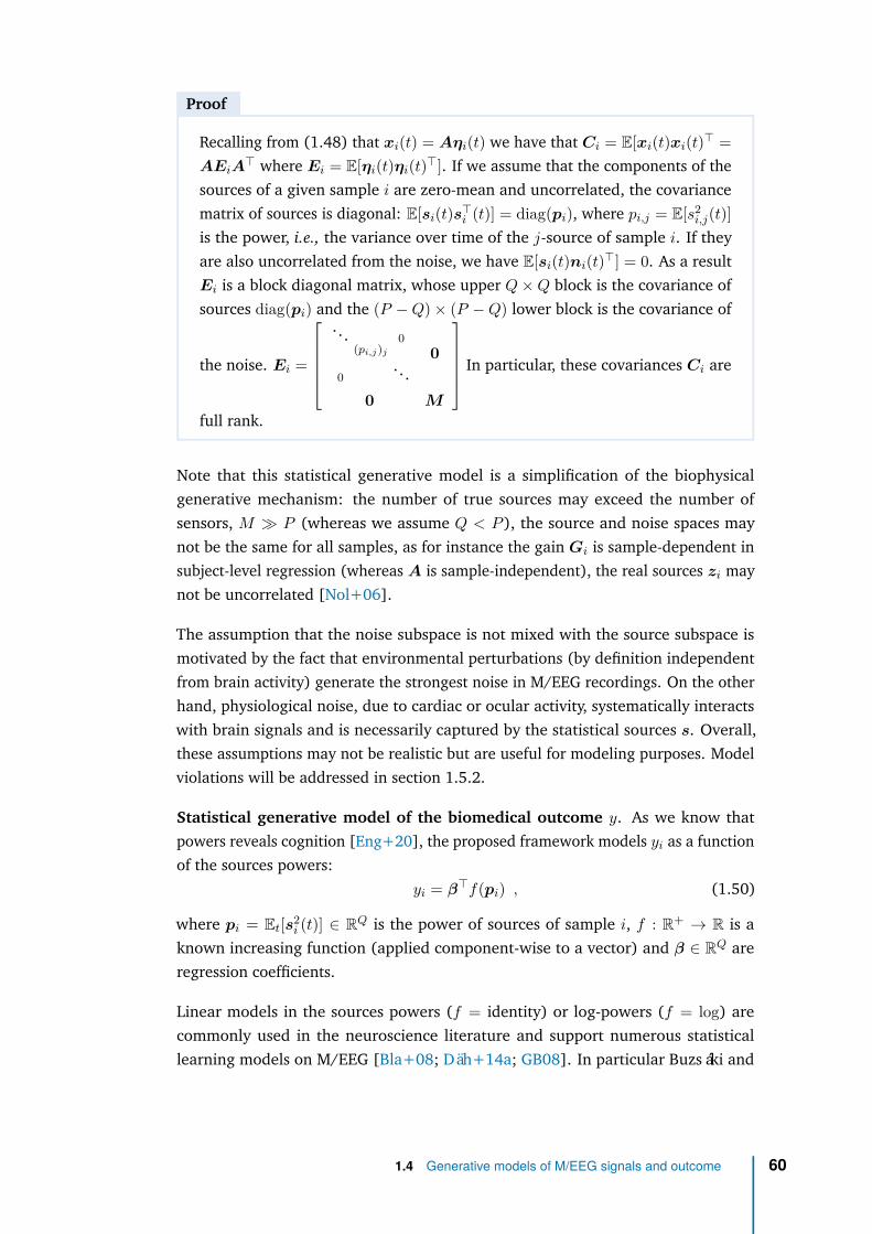
Proof

Recalling from (1.48) that xi(t) = Aηi(t) we have that Ci = E[xi(t)xi(t)⊤ =AEiA

⊤ where Ei = E[ηi(t)ηi(t)⊤]. If we assume that the components of thesources of a given sample i are zero-mean and uncorrelated, the covariancematrix of sources is diagonal: E[si(t)s⊤

i (t)] = diag(pi), where pi,j = E[s2i,j(t)]

is the power, i.e., the variance over time of the j-source of sample i. If theyare also uncorrelated from the noise, we have E[si(t)ni(t)⊤] = 0. As a resultEi is a block diagonal matrix, whose upper Q×Q block is the covariance ofsources diag(pi) and the (P −Q) × (P −Q) lower block is the covariance of

the noise. Ei =

. . . 0

(pi,j)j

0. . .

0

0 M

In particular, these covariances Ci are

full rank.

Note that this statistical generative model is a simplification of the biophysicalgenerative mechanism: the number of true sources may exceed the number ofsensors, M ≫ P (whereas we assume Q < P ), the source and noise spaces maynot be the same for all samples, as for instance the gain Gi is sample-dependent insubject-level regression (whereas A is sample-independent), the real sources zi maynot be uncorrelated [Nol+06].

The assumption that the noise subspace is not mixed with the source subspace ismotivated by the fact that environmental perturbations (by definition independentfrom brain activity) generate the strongest noise in M/EEG recordings. On the otherhand, physiological noise, due to cardiac or ocular activity, systematically interactswith brain signals and is necessarily captured by the statistical sources s. Overall,these assumptions may not be realistic but are useful for modeling purposes. Modelviolations will be addressed in section 1.5.2.

Statistical generative model of the biomedical outcome y. As we know thatpowers reveals cognition [Eng+20], the proposed framework models yi as a functionof the sources powers:

yi = β⊤f(pi) , (1.50)

where pi = Et[s2i (t)] ∈ RQ is the power of sources of sample i, f : R+ → R is a

known increasing function (applied component-wise to a vector) and β ∈ RQ areregression coefficients.

Linear models in the sources powers (f = identity) or log-powers (f = log) arecommonly used in the neuroscience literature and support numerous statisticallearning models on M/EEG [Bla+08; Däh+14a; GB08]. In particular Buzsáki and

1.4 Generative models of M/EEG signals and outcome 60

Page 66

Mizuseki [BM14] discusses a wide body of evidence arguing in favor of log-linearrelationships between brain dynamics and cognition. Both possibilities for f will beconsidered in below sections.

According to (1.50), yi is related to the power of the sources hence to diag(pi).According to (1.49) the sensor signal xi, through its covariance matrix Ci, alsocontain information about powers of the sources pi in Ei but this information isnoisy and distorted through unknown linear field spread A. As our task is to uncoverthe relationship between yi and xi, this unknown mixing makes it challenging tofind optimal regression algorithms with no approximation error.

The broadband covariance (computed on the raw signal without temporal filtering)largely reflects low-frequency power as consequence of the predominant 1/f powerspectrum, hence, is rarely of interest for predicting. In practice, one prefers frequencyspecific models, where the previous relationships are obtained after si(t) has beenbandpass filtered in a specific frequency range. In frequency-specific models, thepowers are replaced by band-powers: power of the source in the chosen frequencyband. Note that source power in a given frequency band is simply the variance ofthe signal in that frequency band.

1.4.2 The classical approaches to predict from M/EEGobservations

We will now present three family of approaches classically used to predict fromM/EEG observations. We will see that, as each of those methods are well-suited incertain contexts, they all fall short for our specific task of prediction in a clinicalsetting.

Biophysical sources modeling. Since both our input xi(t) and output yi are re-lated to physiological sources zi(t), the most natural approach is to get back toour physiological generative model and try to estimate the sources before fittinga regression model. One important family of approaches for predictive modelingwith M/EEG is therefore relying on explicit biophysical source modeling. It con-sists in estimating the locations, amplitudes and extents of the sources from theMEG/EEG data. This estimation is known as the inverse problem [Bai17]. Tosolve it, anatomically constrained inverse methods are used to infer the most likelyelectromagnetic source configuration given the observations [Häm+93]. Commontechniques rely on fitting electrical-current dipoles [MLL92] or involve penalizedlinear inverse models to estimate the current distribution over a pre-specified dipolegrid [HI94; Lin+06; VVB88; HS14]. Anatomical prior knowledge is injected throughthe well-defined forward model: Maxwell equations enable computing leadfieldsfrom the geometry and composition of the head, which predict propagation froma known source to the sensors [Häm+93; MLL99]. Let us denote G ∈ RP ×Q the

1.4 Generative models of M/EEG signals and outcome 61

Page 67

instantaneous mixing matrix that relates the sources in the brain to the MEG/EEGmeasurements. Here Q ≥ P corresponds to the number of candidate sources in thebrain. This forward operator matrix is obtained by solving numerically Maxwell’sequations after specifying a geometrical model of the head, typically obtained usingan anatomical MRI image [HP17]. Using G the Minimum Norm Estimate (MNE)source imaging technique [HI84] offers a way to solve the inverse problem. MNEcan be seen as standard Tikhonov regularized estimation, also similar to a ridgeregression in statistics, and is therefore linear. Using such problem formulation, thesources are obtained from the measurements with a linear operator which is givenby:

WMNE = G⊤(GG⊤ + λIP )−1 ∈ RQ×P . (1.51)

From a signal-processing standpoint, when these steps lead to a linear estimation ofthe sources, the rows of this linear operator WMNE can be seen also as spatial filtersthat are mapped to specific locations in the brain. MNE approach can then be thoughtof as biophysical spatial filtering, informed by the individual anatomy of each sub-ject. From the estimated sources, one can then learn to predict y as the distortionsinduced by individual head geometry are mitigated, see for example [Wes+18;Kie+19; Kha+18]. While approaching the problem from this perspective has impor-tant benefits, such as the ability to exploit the geometry and the physical propertiesof the head tissues of each subject, there are certain drawbacks. First, the inverseproblem is ill-posed and notoriously hard to solve. Second, computing Gi requirescostly T1-weighted MRI acquisitions and time-consuming manual labor by experi-enced MEG/EEG practitioners [Bai17]: precise measure of the head in the MEGdevice coordinate system, anatomical coregistration and tedious data-cleaning tomitigate electromagnetic artefacts caused by environmental or physiological sourcesof non-interest outside of the brain. Using a MRI template, e.g., MNI brain, wouldalleviate this issue but amounts to consider a common average brain, ignoring inter-individuals anatomical variability. Hence, this method is likely to yield suboptimalperformances, as hinted by a recent work [Eng+21] benchmarking different modelsfor brain age prediction. Besides, it is still costly in terms of computation and rest onthe relevance of the MNI brain model. This gold-standard approach of biophysicalsources modeling is therefore hard to automate and poses challenges to clinicalpractice. This justifies the statistical generative model approximation used in thisthesis enabling to learn a regression model without biophysical source modeling.

Statistical sources modeling. A second family is motivated by unsupervised decom-position techniques such as Independent Component Analysis [HO00; Mak+97],which yield estimates of maximally independent statistical sources that can be usedfor prediction and corresponding spatial filters [SNS14; WM09; SG10]. In gen-eral, spatial filtering consists in computing linear combinations of the original Psensors signals to produce so-called ‘spatially filtered’ signals, or ‘source’ signals,

1.4 Generative models of M/EEG signals and outcome 62

Page 68

W ⊤xi. The weights of the combination form a spatial filter. Considering R ≤ P

filters, it corresponds to the columns of the matrix W ∈ RP ×R of rank R whichis common to all samples (e.g., subjects). If R < P , then spatial filtering reducesthe dimension of the data. The covariance matrices of ‘spatially filtered’ signalsW ⊤xi ∈ RR is readily obtained as: Σi = W ⊤CiW ∈ RR×R. With probability one,rank(Σi) = min(rank(W ), rank(Ci)) = R, hence Σi ∈ S++

R . Since the Ci’s do notspan the same image, applying W destroys some information. Recently, geometry-aware dimensionality reduction techniques, both supervised and unsupervised, havebeen developed on covariance manifolds [HYS16; HSH17]. Many different spatialfilters have been designed to produce virtual signals that help the prediction task.Such methods model the data as an independent set of statistical sources that areentangled by a so-called mixing matrix, often interpreted as the leadfields. Here,the sources are purely statistical objects and no anatomical notion applies directly.In practice, unsupervised spatial filters are often combined with source modelingand capture a wide array of situations ranging from single dipole-sources to entirebrain-networks [HIN09; Bro+11; Del+12]. Being unsupervised, hence blind to thetarget y, these methods are not optimal for regression. Also, each ICA filters is fittedindependently for each sample (subject) making it difficult to compare the resultingfilters.

Linear models in sensor-space. Finally, a third family directly applies general-purpose machine learning directly on sensor space signals xi(t) without explicitlyconsidering the data generating mechanism. Following a common trend in otherareas of neuroimaging research [Dad+19; Sch+19; He+19], linear predictionmethods have turned out extraordinarily well-suited for this task, i.e., , logisticregression [And+15], linear discriminant analysis [War+16], linear support vec-tor machines [Kin+13]. The success of linear models deserves separate attentionas these methods enable remarkable predictive performance with simplified fastcomputation [Par+05]. While interpretation and incorporation of prior knowledgeremain challenging, significant advances have been made in the past years. Thishas led to novel methods for specifying and interpreting linear models [Hau+14;VS19]. Recent work has even suggested that for the case of learning from evoked re-sponses, linear methods are compatible with the statistical models implied by sourcelocalization and unsupervised spatial filtering [Kin+18; KD14; SWS15]. Indeed,if the outcome is linear in the source signal, i.e., , due to the linear superpositionprinciple, the mixing in the input amounts to a linear transform of the sources thatcan therefore be captured by a linear model with sufficient data. Additional sourcelocalization or spatial filtering should therefore be unnecessary in this case.

On the other hand, the situation is more complex when predicting outcomes frombrain rhythms, e.g., , induced responses [TBB99] or spontaneous oscillations. Asbrain-rhythms are not strictly time-locked to external events, they cannot be accessed

1.4 Generative models of M/EEG signals and outcome 63

Page 69

by averaging. Instead, they are commonly represented by the signal power in shorteror longer time windows and often give rise to log-linear models [BM14; RBB15]. Aconsequence of such non-linearities is that it cannot be readily captured by a linearmodel. Moreover, simple strategies such as log-transforming the power estimatesonly address the issue when applied at the source-level: the leadfields have alreadyspatially smeared the signal presented on the sensors.

Alternative approaches. This leads back to spatial filtering approaches. Beyondsource localization and unsupervised filtering, supervised spatial filtering methodshave recently become more popular beyond the context of BCIs. These methods solvegeneralized eigenvalue problems to estimate coordinate systems constructed withregard to criteria relevant for prediction. For example, spatio-spectral-decomposition(SSD) is an unsupervised technique that enhances SNR with regard to powerin surrounding frequencies [NNC11]. On the other hand, Common Spatial Pat-terns [Kol91], Joint Decorrelation [CP14] and Source Power Comodulation (SPoC)focus on correlation with the outcome [Bla+08; Däh+14a; Däh+13], MultiViewICA [Ric+20] extends the ICA model to group studies, whereas [Dmo+12] haveproposed variants of Canonical Correlation Analysis (CCA) [Hot92; Däh+14b] with-out orthogonality constraint to focus on shared directions of variation betweenrelated datasets or by proposing shared envelope correlations as optimization tar-get [Däh+14b]. This yields a two-step procedure: 1) spatial filters model thecorrelation induced by the leadfields and provide unmixed time series 2) somenon-linear transforms such as logarithms are applied to these time series as thevalidity of linear equations is now secured.

A more recent single-step approach consists in learning directly from spatiallycorrelated power-spectra with linear models and Riemannian geometry [Bar+11;Bar+13; YBL17; RJC19; Fru+17]. This mathematical framework, introducedin Section 1.3, provides principles to correct for the geometric distortions arisingfrom linear mixing of non-linear sources. These models are blind to the linear mixingAs and working with the signals x is similar to working directly with the sources s.Riemannian geometry is a natural setting where such affine invariance properties arefound [FM03]. It allows to represent the covariance matrices used for representingthe M/EEG signal as Euclidean objects for which linear models apply. This approachhas turned out to be promising for enhancing classification of event-level data andhas been the important ingredient of several winning solutions in recent data analysiscompetitions, e.g., , the seizure prediction challenge organized by the Universityof Melbourne in 2016. Classification based on tangent vectors has also been usedin [Bar+12] for BCI classification. Recently, this approach has been explored forprediction of subject-level brain volume from clinical EEG in Alzheimer’s disease inabout 100 patients [Fru+17].

1.4 Generative models of M/EEG signals and outcome 64

Page 70

We have presented classical methods for regressing an outcome from M/EEG sig-nals. Biophysical sources modeling using anatomically constrained inverse methodscorrects for distortions induced by individual head anatomy but is not scalable asit requires MRI scans and MEG manual expertise: it is therefore not well adaptedto clinical practice. Statistical sources modeling using unsupervised spatial filtering(e.g., ICA) are blind to the prediction target hence not optimal for regression. Sensor-space linear modeling leverages the power of linear models but are not optimalwhen predicting from brain rhythms, hence not adapted to our generative modelsassumptions. We will now present how to mitigate the distortion without biophysicalsource modeling when performing regression on M/EEG source power. We will seethat we can indeed overcome volume conduction with an appropriate regressionalgorithm, adapted to the generative process.

1.4 Generative models of M/EEG signals and outcome 65

Page 71

1.5 A family of statistically consistent regressionalgorithms

To recall our generative model setup: our input is a P -dimensional signal x(t) arisingfrom Q < P sources and additive noise. Assuming the source and noise spaces areunmixed, shared across samples and of respective dimension Q and P −Q then wecan write xi(t) = Aηi(t) where A ∈ RP ×P is an invertible matrix (which includessource and noise patterns) and ηi(t) ∈ RP is the concatenation of source si(t) andnoise signals. If the sources are zero-mean, uncorrelated and uncorrelated from thenoise, then the covariances are full-rank and writes Ci = AEiA

⊤ where Ei is ablock diagonal matrix, whose upper Q×Q block is diag(pi) with pi = E[s2

i (t)] ∈ RQ,the power of the sources of sample i. Our output is a continuous target yi modelledas a function of these source powers yi = β⊤f(pi) without additional noise. In thissection, we assume these ideal conditions hold (fixed volume conduction acrosssamples, full rank signals, no noise in target).

Given this generative model as our prior knowledge, our goal is to find a regressionalgorithm to predict the target yi from sensor-space M/EEG signal xi(t), that donot require to estimate the sources si(t) and that has no approximation error. Ourinput signal is assumed to depend linearly on the sources, whereas our target onthe power of sources (i.e., the squared amplitude of the source signal). This non-linear dependence hints at using non-linear models. Deep learning models haveshown strong performance in learning non-linear functions but require lots of data.Scarcity of high-dimensional medical data would therefore favor the use of linearmechanics, applied to non-linear features of the M/EEG signal (Generalized LinearModel strategy). Its covariance matrix Ci seems a good candidate as it containspowers & cross-powers of sensors. This representation is the adequate approximationof the neural signals at the second order and is low-dimensional. These covariances,computed at the sensor-level, also contain information about the powers of thesources (∈ Ei) but this information is noisy and distorted through field spread A.Can we get rid of it?

In this thesis, we introduce four different regression algorithms: Upper, Riemann,Wasserstein and SPoC. They are all based on a linear model, applied to carefully cho-sen vectorization vi of the covariance Ci. Showing that these models are statisticallyconsistent amounts to proving that the real relationship between yi and vi is linear.In particular, we show that different functions f yield a linear relationship betweenthe yi’s and the vi’s for different Riemannian metrics, hence show that these fourregression models successfully achieve statistical consistency for different generativeassumptions.

1.5 A family of statistically consistent regression algorithms 66

Page 72

More specifically, throughout this study, we consider the following regression pipeline.Given a training set of samples x1(t), . . . ,xN (t) ∈ RP and target continuous variablesy1, . . . , yN ∈ R, we first compute the covariances of each sample C1, . . . ,CN ∈RP ×P . After computing their vectorization v1, . . . ,vN ∈ RK (cf. below), a linearregression technique (e.g. ridge regression) with parameters β ∈ RK can beemployed assuming that yi ≃ v⊤

i β.

1.5.1 Four statistically consistent regression algorithms

Proposition : Consistency of Upper regression algorithm

The Upper regression algorithm consists in taking the Euclidean vectoriza-tion:

vi = Upper(Ci) ∈ RP (P +1)

2 , (1.52)

where Upper(M) is defined as the vector containing the upper triangu-lar coefficients of M , with off-diagonal terms weighted by a factor

√2.

This weighting ensures that the vector and the matrix have same norms(∥Upper(M)∥2 = ∥M∥F ).This model is statistically consistent in the particular case where f = identity:the relationship between yi and Upper(Ci) is linear.

Proof

We assume f(p) = p. Rewriting Eq. (1.49) as Ei = A−1CiA−⊤, and since the

pi,j are on the diagonal of the upper block of Ei, the relationship between thepi,j and the coefficients of Ci is also linear. Since the variable of interest yi islinear in the coefficients of pi, it is also linear in the coefficients of Ci, hencelinear in the coefficients of vi. In other words, yi is a linear combination of thevectorization of Ci w.r.t. the standard Euclidean distance, hence the ‘upper’regression algorithm is statistically consistent for f = identity.

Note that this method cannot be generalized to an arbitrary spectral function f

because f(Ci) = A f(Ei) A⊤.

1.5 A family of statistically consistent regression algorithms 67

Page 73

Proposition : Consistency of Riemann regression algorithm

The Riemann regression algorithm consists in taking the Geometric vector-ization:

vi = PC(Ci) = Upper(log

(C

−1/2CiC

−1/2)) ∈ RP (P +1)

2 , (1.53)

the vectorization of Ci w.r.t. the geometric distance using as reference C =MeanG(C1, . . . ,CN ) the geometric mean of the dataset.This model is statistically consistent in the particular case where f = log: therelationship between yi and PC(Ci) is linear.

Proof

The proof relies crucially on the affine invariance property: using Rie-mannian embeddings of the Ci’s, is equivalent to working directly withthe Ei’s. First, we note that by invariance, C = MeanG(C1, . . . ,CN ) =AMeanG(E1, . . . ,EN )A⊤ = AEA⊤, where E has the same block diag-onal structure as the Ei’s, and Ejj = (

∏Ni=1 pi,j)

1N for j ≤ Q. Denote

U = C12 A−⊤E

− 12 . By simple verification, we obtain U

⊤U = IP , i.e. U

is orthogonal.Furthermore, we have:

U⊤

C− 1

2 CiC− 1

2 U = E− 1

2 EiE− 1

2 . (1.54)

It follows that for all i,

U⊤ log(C− 1

2 CiC− 1

2 )U = log(E− 12 EiE

− 12 ) (1.55)

Note that log(E− 12 EiE

− 12 ) shares the same structure as the Ei’s, and that

log(E− 12 EiE

− 12 )jj = log(pi,j

pj) for j ≤ Q.

Therefore, the relationship between log(C− 12 CiC

− 12 ) and the log(pi,j)j is

linear.Finally, since vi = Upper(log(C− 1

2 CiC− 1

2 )), the relationship between the vi’sand the log(pi,j)j is linear, and the result holds.

1.5 A family of statistically consistent regression algorithms 68

Page 74

Proof : Alternative proof

First, we note that by invariance, C = AEA⊤, where E has the same blockdiagonal structure as the Ei’s, and Ejj = (

∏Ni=1 pi,j)

1N ≜ pj for j ≤ Q.

The vectorization is vi = Upper(log(C−1/2

CiC−1/2)

). We observe that

C−1/2

CiC−1/2 = C

−1/2 (CiC

−1)C

1/2 = BEiE−1

B−1 with B = C−1/2

A

invertible. Therefore, log(C−1/2CiC

−1/2) = B log(EiE

−1)B−1, since ma-

trix logarithm is equivariant by similarity. The Q values on the diagonal partof log(EiE

−1) are the log(pi,j/pj

). In particular, by denoting b−1

j the j-throw of B−1 and bj the j-th column of B, we find:

log(pi,j) = (b−1j )⊤ log(C−1/2

CiC−1/2)bj + log(pj) . (1.56)

This equation means that log(pi,j) is obtained as a linear combination of thecoefficients in log(C−1/2

CiC−1/2), i.e. the coefficients of the vectorization

vi. Since yi is itself a linear combination of the log(pi,j), the advertised resultholds.As a side note, we have that ∥vi∥2 =

∥∥∥log(C

−1/2CiC

−1/2)∥∥∥F

=∥∥∥log(C

−1Ci

)∥∥∥F

= d(Ci,C) = d(Ei,E) , by affine-invariance of the geo-metric distance d(·) (see Appendix 1.3.3): the norm of vi does not depend onA, but only on the log source powers and noise.

The Riemannian embedding yields a representation of sensor-level power and itscorrelation structure relative to a common reference. In the particular case wheref = log, the idea is to normalize each covariance Ci by a common reference C,the geometric mean of covariances Ci. We normalize using C

−1/2CiC

−1/2, whichhas the advantage over CiC

−1 to be symmetrical while having the same eigen-values. We showed that a linear model applied to feature vector vi = PC(Ci) =Upper

(log

(C

−1/2CiC

−1/2)) leads to a consistent regression algorithm. This, es-

sentially, means taking the log of Ci after it has been whitened by C−1/2, making the

quantity of interest relative to some reference C that hopefully will get rid of mixingmatrix A. In terms of Riemannian geometry this is the projection of covariance matrixCi to a common Euclidean space: the tangent space at C. In particular the normof vi can be interpreted as the (geometric) distance between Ci and C and doesnot depend on A. Essentially, the Riemannian approach projects out fixed linearspatial mixing through the whitening with the common reference. Finally, eventhough the geometric mean is the most natural reference on the positive definitemanifold, consistency of the Riemann regression algorithm still holds when usingthe Euclidean mean as the common reference point. Indeed, a recent study onfMRI-based predictive modeling has reported negligible differences between the twooptions [Dad+19, appendix A].

1.5 A family of statistically consistent regression algorithms 69

Page 75

Proposition : Consistency of Wasserstein regression algorithm

The Wasserstein regression algorithm consists in taking the Wassersteinvectorization:

vi = PC(Ci) ∈ RP (P +1)

2 , (1.57)

the vectorization of Ci w.r.t. the Wasserstein distance using as referenceC = MeanW (C1, . . . ,CN ) the Wasserstein mean of the dataset.This model is statistically consistent in the particular case where f =

√· and

A orthogonal: the relationship between yi and PC(Ci) is linear.

Proof

First, we note that Ci = AEiA⊤ ∈ S++

P = S+P,P so it can be decomposed as

Ci = YiY⊤

i with Yi = AE12i .

By orthogonal invariance, C = MeanW (C1, . . . ,CN ) =AMeanW (E1, . . . ,EN )A⊤ = AEA⊤, where E has the same block di-agonal structure as the Ei’s, and Ejj = (

∑i√pij)2 for j ≤ Q. C is also

decomposed as C = Y Y⊤ with Y = AE

12 .

Further, Q∗i = ViU

⊤i with Ui and Vi coming from the SVD of Y

⊤Yi = E

12 E

12i

which has the same structure as the Ei’s. Therefore Q∗i has also the same

structure with the identity matrix as its upper block.Finally we have vi = PC(Ci) = vect(YiQ

∗i − Y ) so it is linear in

√(pi,j) for

j ≤ Q.

The restriction to the case where A is orthogonal stems from the orthogonal in-variance of the Wasserstein distance. In the neuroscience literature square rootrectifications are however not commonly used for M/EEG modeling. Nevertheless, itis interesting to see that the Wasserstein metric that can naturally cope with rankreduced data is consistent with this particular generative model.

1.5 A family of statistically consistent regression algorithms 70

Page 76

Proposition : Consistency of SPoC regression algorithm

The SPoC regression algorithm consists in using all the P SPoC spatial filters:

vi = f(diag

(WSPoC Ci W ⊤

SPoC

))∈ RP , (1.58)

with WSPoC a matrix W ∈ RP ×P solution of the generalized eigenvalueproblem:

CyW = CW diag(λ1, . . . , λP ) subject to W ⊤CW = IP , (1.59)

with C = 1N

∑Ni=1 Ci the Euclidean average covariance matrix and Cy =

1N

∑Ni=1 yiCi the weighted average covariance matrix, and λ1, . . . , λP the

generalized eigenvalues. We assume that the eigenvalues are all distinct, andtherefore without loss of generality λ1 > · · · > λP .This model is statistically consistent for any function f : the relationshipbetween yi and vi is linear. It achieves consistency by taking a rather differentapproach than previous models: it recovers in WSPoC the inverse of the mixingmatrix A.

1.5 A family of statistically consistent regression algorithms 71

Page 77

Proof

If the eigenvalues are all distinct, the generalized eigenvalue problem hasa unique solution W . We recall the definition Ei = E[ηi(t)ηi(t)⊤], which isblock-diagonal with the sources powers pi,j as coefficient (j, j) when j ≤ Q.We have Ci = A Ei A⊤, and therefore C = A E A⊤ and Cy = A Ey A⊤,with E = 1

N

∑Ni=1 Ei and Ey = 1

N

∑Ni=1 yiEi sharing the same block-diagonal

structure than the Ei. Their lower (P − Q) × (P − Q) diagonal blocks,respectively Σ and Σy, are symmetric matrices. Further, Σ is definite positive,as a linear combination with positive coefficients of definite positive matrices.Hence, Σ and Σy are co-diagonalizable i.e., there exists an invertible matrix Z

such that Σy = ZDyZ⊤ and Σ = ZDZ⊤. By denoting A′ = A×[

IQ 00 Z

],

we have that C and Cy are co-diagonalized by A′. Let D the diagonal matrixsuch that C = A′DA′⊤. The matrix W = A′−⊤D−1/2 is solution of thegeneralized eigenvalue problem. By the unicity assumption, SPoC recoversW up to a permutation of its columns. The first Q rows of W ⊤ are the first Qcolumns of A′−⊤, hence the first Q rows of A−1, up to scale. In particular, thetransform W ⊤xi recovers the Q sources si, so that WSPoC Ci W ⊤

SPoC recoversthe pi. Finally, since yi is linearly related to the components of f(pi) thatthemselves are linearly related to the components of vi, it will also be linearlyrelated to the components of the feature vector vi, hence the consistency ofthe SPoC regression algorithm.

As an historical side note, the SPoC algorithm is a supervised spatial filtering al-gorithm simultaneously discovered by [CP14] and [Däh+14a]. The main idea ofthe SPoC algorithm is to use the information contained in the outcome variableto guide the decomposition, giving priority to source signals whose band powercorrelates with y. Note that it was originally developed for event-level regression,e.g., in BCI, and we adapt it here to a general problem that can also accommo-date subject-level regression, where one observation corresponds to one subjectinstead of one trial. More formally, the filters W are chosen to synthesize sig-nals whose powers maximally covariates with the outcome y. Which may be agood idea since we supposed that our target is linearly related to the power of thesources. Denoting by C = 1

N

∑Ni=1 Ci the Euclidean average covariance matrix and

Cy = 1N

∑Ni=1 yiCi the weighted average covariance matrix, the first filter wSPoC is

given by: wSPoC = arg maxww⊤Cyw

w⊤Cw. In practice, all the filters in WSPoC are obtained

by solving the generalized eigenvalue decomposition problem [Däh+14a]. Theproof is quite straightforward and given below. Note that here we use all the Pspatial filters (R = P ).

1.5 A family of statistically consistent regression algorithms 72

Page 78

Proof. We assume that the signal x(t) is band-pass filtered in one frequency band ofinterest, so that for each subject the band power of signal is approximated by thevariance over time of the signal. We denote the expectation E and the variance Varover time t or subject i by a corresponding subscript.

The source extracted by a spatial filter w for subject i is si = w⊤xi(t). Its powerreads: Φw

i = Vart[w⊤xi(t)] = Et[w⊤xi(t)x⊤i (t)w] = w⊤Ciw and its expectation

across subjects is given by: Ei[Φwi ] = w⊤Ei[Ci]w = w⊤Cw, where C = 1

N

∑i Ci

is the average covariance matrix across subjects. Note that here, Ci refers to thecovariance of the xi and not its estimate as in Sec. 1.2.3.

We aim to maximize the covariance between the target y and the power of the sources,Covi[Φw

i , yi]. This quantity is affected by the scaling of its arguments. To address this,the target variable y is normalized: Ei[yi] = 0 Vari[yi] = 1 . Following [Däh+14a],to also scale Φw

i we constrain its expectation to be 1: Ei[Φwi ] = w⊤Cw = 1 The

quantity one aims to maximize reads:

Covi[Φwi , yi] = Ei[ (Φw

i − Ei[Φwi ]) (yi − Ei[yi]) ]

= w⊤Ei[Ciyi]w − w⊤CwEi[yi]

= w⊤Cyw

where Cy = 1N

∑i yiCi.

Taking into account the normalization constraint we obtain: w = arg maxw⊤Cw=1 w⊤Cyw.Note that it can be also written as a generalized Rayleigh quotient:

w = arg maxw

w⊤Cyw

w⊤Cw.

Its Lagrangian reads F (w, λ) = w⊤Cyw+λ(1−w⊤Cw). Setting its gradient w.r.t. w

to 0 yields a generalized eigenvalue problem: ∇wF (w, λ) = 0 =⇒ Σyw = λΣxw

This equation has a unique closed-form solution called the generalized eigenvectorsof (Cy,C). The second derivative gives:

∇λF (w, λ) = 0 =⇒ λ = w⊤Σyw = Covi[Φwi , yi] (1.60)

This equation leads to an interpretation of λ as the covariance between Φw and y,which should be maximal. As a consequence, WSPoC is built from the generalizedeigenvectors of the generalized eigenvalue problem above, sorted by decreasingeigenvalues.

Link between the regression algorithms It is noteworthy that both SPoC andRiemann models have in common to whiten the covariances Ci with a commonreference covariance (the Euclidean mean for SPoC and the geometric mean for

1.5 A family of statistically consistent regression algorithms 73

Page 79

Riemann): Riemann explicitly with C−1/2

CiC−1/2, SPoC implicitly by solving gener-

alized eigenvalue problem of (Cy,C), or equivalently of (Ci,C) which is equivalentto solving the regular eigenvalue problem of Ci after whitening with C ([Fuk90;NNC11] eq. 13-16). SPoC retrieves the eigenvectors of (Ci,C). Riemann producesvectors whose size depend on the log eigenvalues of (Ci,C). They both producenon-linear features that measure powers relative to a common reference.

‘Upper’ and Riemann models both avoid inverting A by being insensitive to it.More precisely, they consist in building from Ci a P × P symmetric matrix Mi

mathematically congruent to a block-diagonal matrix Di whose Q×Q upper blockis diag(f(pi)) i.e., that writes Mi = B Di B⊤, for some invertible matrix B. Indeed,if this holds, the coefficients of f(pi) are a linear combination of coefficients of Mi

which implies that the outcome yi is linear in the coefficients of Mi. Therefore alinear model applied to the features vi = Upper(Mi) is statistically consistent. For‘Upper’ Mi = Ci and for Riemann Mi = log(C−1/2

CiC−1/2).

Finally, these two models amounts to estimating Q parameters (the powers of eachsources) from P (P + 1)/2 parameters (the upper part of a symmetric matrix). Again,it is important to emphasize that we are not aiming for explicitly estimating themost probable model parameters β but rather a function that has the smallestapproximation error possible, even if over-parametrized. These approaches achieveconsistency without inverting A at a price of over-parametrization: the number ofparameters will always be a lot higher than the number of samples N . Learningin this under determined high dimensional setting requires regularizing the linearmodel to stabilize learning. We will thus use a Ridge regression algorithm withlinear kernel, but in a data-driven fashion with nested generalized cross-validation,leading to effective degrees of freedom less than numerical rank of the input data.

In this thesis we will compare these four regression algorithms to the inconsistentdiag regression algorithm as baseline. This model is probably the historically mostfrequently used model in M/EEG research in countless publications. Here, powersare considered on the sensor array while the correlation structure is being ignored.This consists in taking only the diagonal elements of the covariance matrix Ci asfeatures, i.e., the powers (variances) of sensor-level signals:

vi = f(diag(Ci)) ∈ RP . (1.61)

1.5.2 Model violationsThe current theoretical analysis implies that the mixing matrix A must be commonto all subjects and the covariance matrices must be full rank. However, this is rarelythe case in practice. If these conditions are not satisfied, the consistency guaranteesare lost, rendering model performance an empirical question. This will be addressed

1.5 A family of statistically consistent regression algorithms 74

Page 80

with simulations (Section 1.5.3), in which we know the true brain-behaviour link,and real-world data analysis (Section 2.1) in which multiple uncertainties arise atthe same time.

Noise in the target variable. Most often the target variable is corrupted by a smalladditive random perturbation εi. The noise in the outcome variable depends onthe context: it can represent intrinsic measurement uncertainty of yi, for examplesampling rate and latency jitter in behavioral recordings, inter-rater variability fora psychometric score, or simply a model mismatch. The true model may not belinear for example. It can also regroup all the other dependencies we considernon-discriminative.

Individual mixing matrix. A model where the mixing matrix A is subject-dependentreads: xi(t) = Aisi(t) + ni(t) . Such situations typically arise when performingsubject-level regression due to individual head geometry, individual head positions inMEG and individual locations of EEG electrodes. In this setting, we loose consistencyguarantees, but since the Ai cannot be completely different from each other (they alloriginate from human brains), we can still hope that our models perform reasonablywell.

Rank-deficient signal. We have seen that M/EEG data is in practice often rank-reduced for mainly two reasons. First, popular techniques for cleaning the dataamounts to reduce the noise by projecting the data in a subspace, supposed topredominantly contain the signal. Second, a limited amount of data may lead topoor estimation of covariance matrices. This leads to rank-deficient covariancematrices.

Riemann regression algorithms must be adapted since singular matrices are atinfinite distance from any regular matrices. Assuming the rank R < P is the sameacross subjects, the corresponding covariance matrices do not belong to the S++

P

manifold anymore but to the S+P,R manifold of positive semi-definite matrices of fixed

rank R. To handle the rank-deficiency one can then project the covariance matriceson S++

R , the manifold of full-rank matrices of reduced size R to make them fullrank, and then use the geometric distance. To do so, a common strategy is to projectthe data into a subspace (here of size R) that captures most of its variance. This isachieved by Principal Component Analysis (PCA) applied to the average covariancematrix across subjects. We denote the filters in this case by WUNSUP = U ∈ RR×P ,where U contains the eigenvectors corresponding to the top R eigenvalues of theaverage covariance matrix C = 1

N

∑Ni=1 Ci. This step is blind to the values of y and

is therefore unsupervised. Note that under the assumption that the time series acrosssubjects are independent, the average covariance C is the covariance of the dataover the full population. The Riemann regression algorithm is then applied to the

1.5 A family of statistically consistent regression algorithms 75

Page 81

spatially-filtered covariance matrix WUNSUP Ci W ⊤UNSUP ∈ RR×R, of rank R hence

belonging to S++R .

If covariances are rank-deficient, we will use low-rank versions of both SPoC andRiemann models where only the first components of the spatial filters up to theirrank R are kept. In SPoC, components are ordered by covariance with the outcome(supervised algorithm). In Riemann, components are ordered by explained variancein the predictors, not the outcome (unsupervised algorithm). By construction, wecan then expect that SPoC achieves similar best performance than Riemann withfewer components: the variance related to the outcome can be represented withfewer dimensions.

Besides helping to cope with rank-reduced data, the effect of spatial filtering can bedifficult to predict: it helps the regression algorithm by reducing the dimensionalityof the problem making it statistically easier, but it can also destroy information ifthe individual covariance matrices are not aligned (if they span different spaces).We expect to observe this trade-off via low-rank optima, with a plateau after theeffective rank R of the data (see Section 2.1.2).

To summarize: we presented four regression algorithms, linear models applied tofour particular vectorization of the covariance matrix Ci: ‘Upper’ takes its upper-part (powers & cross-powers of sensors), Riemann takes its Riemannian embeddingw.r.t. the geometric distance i.e., its projection in a common tangent space takenat their geometric mean, Wasserstein takes its Riemannian embedding w.r.t. theWasserstein distance, and finally SPoC takes the diagonal of the covariance matrixof spatially-filtered signals where the filters are generalized eigenvectors of (Ci,C)with C the mean of the Ci’s. They will be compared to the ‘diag’ baseline modelthat takes its log-diagonal (log-powers of sensors).

We demonstrated mathematically that, if we have constant volume conduction acrosssamples and if the signal is full rank, these regression algorithms are statisticallyconsistent for some function f defined in our generative model. Each of themuses a different strategy to bypass the mixing effect of the matrix A and can thenreplace the need for source localization. When f = Identity (yi is linear in thecoefficient of source powers pi) Upper achieves consistency by taking the coefficientsof Ci as input vector. When f = Log (yi is log-linear in the coefficient of sourcepowers pi), Riemann achieves consistency by being simply insensitive to A, blind tolinear projections. Finally, SPoC learns to invert the mixing matrix A by incidentallyrecovering a co-block-diagonalization basis of all the Ci’s, hence recovering thestatistical sources: it is therefore consistent for any function f . In those idealizedconditions, we demonstrated that source localization can be replaced with eitherspatial filters or with Riemannian embeddings.

1.5 A family of statistically consistent regression algorithms 76

Page 82

1.5.3 Validation with simulationsWe now consider simulations to illustrate these mathematical guarantees and inves-tigate theoretical performance as model violations are gradually introduced (noisein target, individual mixing matrices). We focused on the ‘linear-in-powers’ and the‘log-linear-in-powers’ generative models (Eq. 1.50 with f = identity and f = log)and compared the performance of the proposed approaches by measuring their scoreas the average mean absolute error (MAE) obtained with 10-fold cross-validation.Independent identically distributed covariance matrices C1, . . . ,CN ∈ S++

P andvariables y1, . . . , yN were generated following each generative model. The mixingmatrix A was defined as exp(µB) with the random matrix B ∈ RP ×P and the scalarµ ∈ R to control the distance of A from identity (µ = 0 yields A = IP , increasedµ means more mixing). This is not a model violation but a way to validate thatthe affine invariance property of the geometric Riemmanian distance indeed makethe Riemann model blind to A. The outcome variable was linked to the sourcepowers (i.e., the variance): yi =

∑j αjf(pij) with f(x) = x or log(x). We chose

P = 5, N = 100 and Q = 2. In these idealized conditions (no noise in target, fixedA and full rank signals), our consistent regression algorithms should show perfectout-of-sample prediction (no generalization error). Then, to investigate more realis-tic scenarios, we corrupted the clean ground truth data in two ways. First we addGaussian noise in the outcome variable: yi =

∑j αjf(pij) + εi where εi ∼ N (0, σ2)

is a small additive random perturbation. Second, we consider individual mixingmatrices deviating from a reference: Ai = A + Ei, where entries of Ei sampledi.i.d. from N (0, σ2). The reference A can then be thought of as representing thehead of a mean-subject. With these more realistic assumptions our mathematicalguarantees break but our simulations will reveal the robustness of our regressionalgorithms to model violations.

Fig. 1.3 A displays the results for the linear generative model (f = identity inEq. (1.50)). The left panel shows the scores of each method as the parameters µcontrolling the distance from the mixing matrix A to the identity matrix IP increases(more mixing). We see that the Riemannian method is not affected by µ (orange),which is consistent with the affine invariance property of the geometric distance. Atthe same time, it is not the correct method for this generative model as is revealed byits considerable prediction error greater than 0.5. Unsurprisingly, the ‘diag’ method(green) is highly sensitive to changes in A with errors proportional to the mixingstrength. On the contrary, both ‘upper’ (blue) and SPoC (dark orange) methods leadto perfect out-of-sample prediction (MAE = 0) even as mixing strength increases.This demonstrates consistency of these methods for the linear generative model.They both transparently access the statistical sources, either by being blind to themixing matrix A (‘upper’) or by explicitly inverting it (SPoC). Hence, they mayenable regression on M/EEG brain signals without source localization. When we

1.5 A family of statistically consistent regression algorithms 77

Page 83

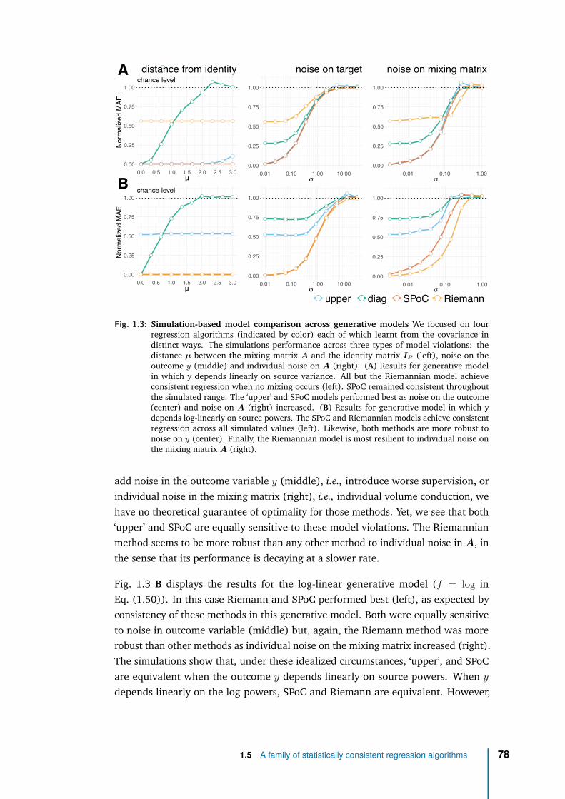
chance level

0.00

0.25

0.50

0.75

1.00

0.0 0.5 1.0 1.5 2.0 2.5 3.0µ

Normalize

dMAE

chance level

0.00

0.25

0.50

0.75

1.00

0.0 0.5 1.0 1.5 2.0 2.5 3.0µ

Normalize

dMAE

0.00

0.25

0.50

0.75

1.00

0.01 0.10 1.00 10.00σ

0.00

0.25

0.50

0.75

1.00

0.01 0.10 1.00σ

distance from identity noise on target noise on mixing matrix

0.00

0.25

0.50

0.75

1.00

0.01 0.10 1.00 10.00σ

0.00

0.25

0.50

0.75

1.00

0.01 0.10 1.00σ

A

B

upper diag SPoC Riemann

Fig. 1.3: Simulation-based model comparison across generative models We focused on fourregression algorithms (indicated by color) each of which learnt from the covariance indistinct ways. The simulations performance across three types of model violations: thedistance µ between the mixing matrix A and the identity matrix IP (left), noise on theoutcome y (middle) and individual noise on A (right). (A) Results for generative modelin which y depends linearly on source variance. All but the Riemannian model achieveconsistent regression when no mixing occurs (left). SPoC remained consistent throughoutthe simulated range. The ‘upper’ and SPoC models performed best as noise on the outcome(center) and noise on A (right) increased. (B) Results for generative model in which ydepends log-linearly on source powers. The SPoC and Riemannian models achieve consistentregression across all simulated values (left). Likewise, both methods are more robust tonoise on y (center). Finally, the Riemannian model is most resilient to individual noise onthe mixing matrix A (right).

add noise in the outcome variable y (middle), i.e., introduce worse supervision, orindividual noise in the mixing matrix (right), i.e., individual volume conduction, wehave no theoretical guarantee of optimality for those methods. Yet, we see that both‘upper’ and SPoC are equally sensitive to these model violations. The Riemannianmethod seems to be more robust than any other method to individual noise in A, inthe sense that its performance is decaying at a slower rate.

Fig. 1.3 B displays the results for the log-linear generative model (f = log inEq. (1.50)). In this case Riemann and SPoC performed best (left), as expected byconsistency of these methods in this generative model. Both were equally sensitiveto noise in outcome variable (middle) but, again, the Riemann method was morerobust than other methods as individual noise on the mixing matrix increased (right).The simulations show that, under these idealized circumstances, ‘upper’, and SPoCare equivalent when the outcome y depends linearly on source powers. When y

depends linearly on the log-powers, SPoC and Riemann are equivalent. However,

1.5 A family of statistically consistent regression algorithms 78

Page 84

when every data point comes with a different mixing matrix, Riemann may be thebest default choice, irrespective of the generative model of y. The Wassersteinregression algorithm has not been pictured here to avoid overloading but has asimilar behaviour to the ‘Upper’ model with the same MAE profile, yet a marginallybetter performance. The same experiment with f(p) = √

p yields comparable results,yet with Wasserstein distance performing best and achieving perfect out-of-sampleprediction when σ → 0 and A is orthogonal.

To summarize we have proposed four different regression algorithms and showed,both theoretically and with simulated data, that they can each perfectly approximatesthe true function asymptotically hence supports perfect prediction with enough data,under a particular generative model. For this consistency to hold, we need 2conditions: A must be fixed across samples and the signal hence the covariancematrix must be full rank. If they are satisfied, these models, as they stay in sensor-space, overcome volume conduction problem and avoid the need of costly sourcelocalization. These models can readily accommodate rank-deficient covariancematrices. Other models are working, for instance [Sch+17] uses deep learningmethod that does implicit filtering to handle the fieldspread. Our models havethe advantages to be simple, to work with smaller quantities of data and aboveall propose an explicit explanation of why they work by making explicit the datagenerative model to which they are adapted. Let’s now apply these regressionalgorithms to real-life empirical data: in ideal laboratory conditions first, then inclinical conditions.

1.5 A family of statistically consistent regression algorithms 79

Page 85

2Application with laboratory data

Contents2.1 Empirical validation with real M/EEG data . . . . . . . . . . . . 85

2.1.1 Predicting muscle contraction from MEG on FieldTrip data 85

2.1.2 Predicting age from MEG on Cam-CAN data . . . . . . . 87

2.1.3 Predicting age from EEG on TUH data . . . . . . . . . . 92

2.2 Model inspection . . . . . . . . . . . . . . . . . . . . . . . . . . . 95

2.2.1 Spatial patterns . . . . . . . . . . . . . . . . . . . . . . . 95

2.2.2 MEG and EEG as a cheap MRI? . . . . . . . . . . . . . . 96

2.3 Model robustness . . . . . . . . . . . . . . . . . . . . . . . . . . 99

2.4 Discussion . . . . . . . . . . . . . . . . . . . . . . . . . . . . . . 102

80

Page 86

List of acronyms and notations of the chapter

BCI brain-computer interfaceBAD Brain Age Delta

Cam-CAN Cambridge Center of AgingERM empirical risk minimizationEOG electro-oculogramECG electro-cardiogramEMG eletromyogram

M/EEG magneto- and electroencephalographyML machine learning

MAE mean absolute errorMNE mnimium norm estimateMRI magnetic resonance imagingOAS Oracle Approximation ShrinkagePCA principal component analysisSPoC source power comodulationSSS Signal Space SeparationSSP Signal Space ProjectionTUH Temple University Hospital

81

Page 87

In Chapter 1, we detailed our first (theoretical) contribution [Sab+19a]: whenfaced with the particular task of predicting, from M/EEG signals, an outcome thatis (log)-linear in sources powers, we have found three learning algorithms withno approximation error. They are all based on a linear function class, applied toparticular vectorization on the spatial covariance matrix:

H = {X ∈ RP ×T 7→ w⊤v(XX⊤

T),∀w} , (2.1)

where v has been previously defined as per our Upper, Riemann and SPoC regressionalgorithms. We leveraged our domain prior knowledge of M/EEG signals to designthese hypothesis classes and show that they are perfectly adapted to the data-generating mechanism, depending on how outcome could linearly depends onsource powers: Upper for linear-in-powers outcome, SPoC or Riemann for linear-in-logpowers outcome. Yet, this guarantee of no approximation error holds only iftwo model assumptions are verified: the mixing matrix A is fixed across samples,and the signal (hence the covariance matrix) is full-rank. Besides, these algorithmsshow no optimization error. Indeed, since the hypothesis classes are linear in theparameter w, they are all learnable with the ERM learning rule and no optimizationalgorithm is necessary to implement it since there is an analytic solution to theoptimization problem. Additionally, if the outcome is noiseless (no irreducible error)and the data sample is infinite (no estimation error), then our algorithms haveperfect generalization error.

In this Chapter 2, presenting our second (experimental) contribution [Sab+20], wenow confront our theoretical results to real-life regression tasks of predicting a con-tinuous neuro-outcome from real M/EEG data. In real-life experiments, we do nothave access to the actual sources and do not know a priori which generative model,hence, which regression algorithm performs best. The true outcome-generatingmechanism can be linear in sources powers, log-linear in sources powers or some-thing completely different. Likewise, even if our algorithms are adapted to the datadistribution, we cannot expect perfect out-of-sample prediction (no generalizationerror): the outcome variable may be noisy (leading to irreducible error), data sam-ples are finite (leading to estimation error) and, most importantly, the two mainmodeling assumptions that guarantee consistency may not hold (leading to approx-imation error). Indeed, the mixing matrix A is not fixed when predicting at thesubject-level as each individual has her own head and brain. Also the M/EEG data isoften rank-reduced in practice, for mainly two reasons. First, popular techniques forcleaning the data amounts to reduce the noise by projecting the data in a subspace,supposed to predominantly contain the signal. Second, a limited amount of datamay lead to poor estimation of covariance matrices. However, by performing modelcomparisons based on cross-validation errors, we can potentially infer which modelprovides the better approximation.

82

Page 88

This chapter is organized as follows. To validate our algorithms on real M/EEGdata, we first benchmarked them against a prediction task from M/EEG band-limited covariances (i.e., computed separately within different frequency bands)on three datasets, for which multiple model violations occur at once. Then wewill further inspect our regression models to gain physiological insights. Finally, inorder to further clear the road towards their clinical translation, we will probe theirrobustness, both to low-fidelity devices and to signal preprocessing.

Section 2.1 details the motivation, methods and results obtained by our regressionalgorithms on three experiments, chosen to cover a wide range of model violations.In the first experiment, we focussed on predicting muscle contraction of a singlesubject from MEG beta activity on the FieldTrip data, for which we can consider themixing matrices to be constant across samples. Compared to the ideal conditionsnecessary to obtain the mathematical guarantees of consistency, this experimentnevertheless presents one model violation: rank-deficient covariance matrices dueto limited amount of data. In the other two experiments, we apply our methods toinfer age from brain signals. Age is a dominant driver of cross-person variance inneuroscience data and a serious confounder [SN18]. As a consequence of the globallyincreased average lifespan, ageing has become a central topic in public health thathas stimulated neuropsychiatric research at large scales. The link between age andbrain function is therefore of utmost practical interest in neuroscientific research.The second experiment consists in predicting the age from MEG on Cam-CAN data,where we have the two model violations at once: variable mixing matrices andrank-reduced data, this time due to preprocessing. Finally, the third experimentalso focus on age prediction but using EEG signals from the TUH dataset, where thecovariances are full rank but the mixing matrices are individual.

Section 2.2 will dvelve into model inspection beyond performance. First, some of ouralgorithms use spatial filters, hence support inspection of the corresponding spatialpatterns. This will allow to check that the patterns they learnt are physiologicallyplausible but more importantly that they are informative on the brain regionspotentially involved in the task. Second, we will perform a sensitivity analysis of thealgorithms to assess the individual relative influence of the data generating factorsof head geometry, uniform global power and topographic information. We willshow that all methods learn from anatomy but the Riemannian embeddings bettercapture individual head geometry, suggesting a complementary use of M/EEG to MRI.One important strength of our algorithms is that they avoid source reconstruction,facilitating their translation to the clinic.

In Section 2.3 we further investigate the robustness of our algorithms in order toassess their potential usage in the clinic, where only low-density EEG devices arereally practical and a light preprocessing pipeline is conceivable. We will see that,again, the Riemannian model is particularly robust to preprocessing options and

83

Page 89

performs well even when no preprocessing is done. This will clear the way totranslating our algorithms to the clinic, which will be the focus of the next chapter.

Statistical modeling. Note that since our problem is high-dimensional (the numberof dimensions will always be much higher than the number of available samples) wewill have to stabilize the ERM learning rule using regularization, hence using a RLMlearning rule (for instance ridge or Lasso). Here, we used ridge regression [HK70]to predict from the vectorized covariance matrices and tuned its regularizationparameter by generalized cross-validation [GHW79] on a logarithmic grid of 100values in [10−5, 103] on each training fold of a 10-fold cross-validation loop. Foreach model described in previous sections (‘diag’, Upper, SPoC, Riemann), westandardized the features enforcing zero mean and unit variance. This preprocessingstep is standard for penalized linear models. To compare models against chance,we estimated the chance-level empirically through a dummy-regressor predictingthe mean outcome of the training data. Uncertainty estimation was obtained fromthe cross-validation distribution. Note that formal hypotheses testing for modelcomparison was not available for any of the datasets analyzed as this would haverequired several datasets, such that each average cross-validation score wouldhave made one observation. To improve conditioning of the covariance estimates,across all analyses, additional low-rank shrinkage for spatial filtering with SPoCand unsupervised spatial filtering with Riemann was fixed at the mean of the valueranges tested in [Sab+19a] i.e., 0.5 and 10−5, respectively.

Software. All numerical analyses were performed in Python 3.7 using the Scikit-Learn software [Ped+11], the MNE software for processing M/EEG data [Gra+14],the PyRiemann package [CBA13] for manipulating Riemannian objects, and the open-source Python library ‘Coffeine’ (https://github.com/coffeine-labs/coffeine)that provides a high-level interface to the predictive modeling techniques we de-velop in this chapter. We used the R-programming language and its ecosystem forvisualizing the results [R C19; AUT19; Wic16; CSM17].

84

Page 90

2.1 Empirical validation with real M/EEG dataIn Chapter 1 we have seen that Riemannian approaches has turned out to be promis-ing for enhancing classification of event-level data [Bar+12] for BCI classification.Yet, systematic comparisons against additional baselines and competing regressionalgorithms on larger datasets and other outcomes are missing. Importantly, themajority of approaches have focused on event-level prediction problems instead ofsubject-level prediction and have never been been systematically compared in termsof their statistical properties and empirical behavior. Here we will explicitly mainlyfocus on subject-level as contrasted to event-level prediction, both, theoreticallyand at the level of data analysis. Note that this thesis does not focus on event-levelprediction with generalization across subjects [HP18; Wes+18; OKA14], which is adistinct and more complex problem inheriting its structure from, both, event-leveland subject-level regression.

2.1.1 Predicting muscle contraction from MEG on FieldTripdata

In a first step, we considered a problem where the unit of observation was individualbehavior of one single subject with some unknown amount of noise affecting themeasurement of the outcome. The problem is an event-level regression task ofpredicting continuous electromyogram (EMG) from brain beta activity capturedconcomitantly with MEG. In this scenario, the mixing matrix is fixed to the extentthat the subject avoided head movements, which was enforced by the experimentaldesign. At the time of the analysis, individual anatomical data was not available,hence we constrained the analysis to the sensor-space.

Data acquisition. We analyzed one anonymous subject from the data presentedin [Sch+11] and provided by the FieldTrip website to study cortico-muscular co-herence [Oos+11]. The MEG recording was acquired with 151 axial gradiometersand the Omega 2000 CTF whole-head system. EMG of forceful contraction of thewrist muscles (bilateral musculus extensor carpi radialis longus) was concomitantlyrecorded with two silver chloride electrodes. MEG and EMG data was acquired at1200Hz sampling-rate and online-filtered at 300Hz. For additional details pleaseconsider the original study [Sch+11].

Data processing and feature engineering. The analysis closely followed thecontinuous outcome decoding example from the MNE-Python website [Gra+14].We considered 200 seconds of joint MEG-EMG data. First, we filtered the EMGabove 20 Hz using a time-domain firwin filter design, a Hamming window with 0.02passband ripple, 53 dB stop band attenuation and transition bandwidth of 5 Hz (-6 dB at 17.5 Hz) with a filter-length of 661 ms. Then we filtered the MEG between 15and 30 Hz using an identical filter design, however with 3.75 Hz transition bandwidth

2.1 Empirical validation with real M/EEG data 85

Page 91

for the high-pass filter (-6 dB at 13.1 Hz) and 7.5 Hz for the low-pass filter (-6 dB at33.75 Hz). The filter-length was about 880 ms. Note that the transition bandwidthand filter-length was adaptively chosen by the default procedure implemented inthe filter function of MNE-Python. We did not apply any artifact rejection as the rawdata was of high quality. The analysis then ignored the actual trial structure of theexperiment and instead considered a sliding window-approach with 1.5 s windowsspaced by 250 ms. Allowing for overlap between windows allowed to increase samplesize. We then computed the covariance matrix in each time window and appliedOracle Approximation Shrinkage (OAS) [Che+10] to improve conditioning of thecovariance estimate. The outcome was defined as the variance of the EMG in eachwindow.

Model evaluation. For event-level regression with overlapping windows, we applied10-fold cross-validation without shuffling such that folds correspond to blocks ofneighboring time windows preventing data-leakage between training and testingsplits. The initialization of the random number generator used for cross-validationwas fixed, ensuring identical train-test splits across models. Note that a Monte Carloapproach with a large number of splits would lead to significant leakage, hence,optimistic bias [Var+17]. This, unfortunately, limits the resolution of the uncertaintyestimates and precludes formalized inference. As we did not have any a prioriinterest in the units of the outcome, we used the R2 metric, a.k.a. coefficient ofdetermination, for evaluation. Compared to the ideal conditions necessary to obtainthe mathematical guarantees of consistency, this experiment presents one modelviolation: rank-deficient covariance matrices (along with noise in outcome).

Results: models performance. The results are depicted in Fig. 2.1. The analysisrevealed that only models including the cross-terms of the covariance predictedvisibly better than chance (Fig. 2.1A). For the methods with projection step (SPoCand Riemann) we reported the performance using the full 151 components, equalto the total number of gradiometer channels. Importantly, extensive search formodel order for SPoC and Riemann revealed important low-rank optima (Fig. 2.1B)with performance around 50% variance explained on unseen data. This is notsurprising when considering the difficulty of accurate covariance estimation fromlimited data. Indeed, low-rank projection is one important method in regularizedestimation of covariance [EG15]. Interestingly, SPoC showed stronger performancewith fewer components than Riemann (4 vs 42). This is not surprising: SPoC is asupervised algorithm, constructed such that its first components concentrate mostof the covariance between their power and the outcome variable. The variancerelated to y can hence be represented with fewer dimensions than Riemann thatuses unsupervised spatial filtering. However, it remains equivocal which statisticalmodel best matches this regression problem. The best performing models all impliedthe log-linear model. Yet, compared to the linear-in-power Upper model, the low-

2.1 Empirical validation with real M/EEG data 86

Page 92

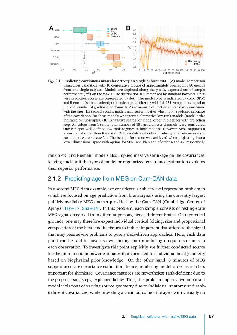
0.49

0.45

0.27

0.21

0.07

−0.07

predictingEM

G

Riemann42

SPoC4

Riemann

upper

SPoC

diag

−0.4 −0.2 0.0 0.2 0.4 0.6R2

upperdiagSPoCRiemann

−0.2

−0.1

0.0

0.1

0.2

0.3

0.4

0.5

0.6

0.7

0 10 20 30 40 50 60 70 80 90 100 110 120 130 140 150#components

R2

Riemann42SPoC4

A B

Fig. 2.1: Predicting continuous muscular activity on single-subject MEG. (A) model comparisonusing cross-validation with 10 consecutive groups of approximately overlapping 80 epochsfrom one single subject. Models are depicted along the y-axis, expected out-of-sampleperformance (R2) on the x-axis. The distribution is summarized by standard boxplots. Split-wise prediction scores are represented by dots. The model type is indicated by color. SPoCand Riemann (without subscript) includes spatial filtering with full 151 components, equal tothe total number of gradiometer channels. As covariance estimation is necessarily inaccuratewith the short 1.5 second epochs, models may perform better when fit on a reduced subspaceof the covariance. For these models we reported alternative low-rank models (model orderindicated by subscripts). (B) Exhaustive search for model order in pipelines with projectionstep. All values from 1 to the total number of 151 gradiometer channels were considered.One can spot well defined low-rank regimes in both models. However, SPoC supports alower model order than Riemann. Only models explicitly considering the between-sensorcorrelation were successful. The best performance was achieved when projecting into alower dimensional space with optima for SPoC and Riemann of order 4 and 42, respectively.

rank SPoC and Riemann models also implied massive shrinkage on the covariances,leaving unclear if the type of model or regularized covariance estimation explainstheir superior performance.

2.1.2 Predicting age from MEG on Cam-CAN dataIn a second MEG data example, we considered a subject-level regression problem inwhich we focused on age prediction from brain signals using the currently largestpublicly available MEG dataset provided by the Cam-CAN (Cambridge Center ofAging) [Tay+17; Sha+14]. In this problem, each sample consists of resting-stateMEG signals recorded from different persons, hence different brains. On theoreticalgrounds, one may therefore expect individual cortical folding, size and proportionalcomposition of the head and its tissues to induce important distortions to the signalthat may pose severe problems to purely data-driven approaches. Here, each datapoint can be said to have its own mixing matrix inducing unique distortions ineach observation. To investigate this point explicitly, we further conducted sourcelocalization to obtain power estimates that corrected for individual head geometrybased on biophysical prior knowledge. On the other hand, 8 minutes of MEGsupport accurate covariance estimation, hence, rendering model-order search lessimportant for shrinkage. Covariance matrices are nevertheless rank-deficient due tothe preprocessing steps, explained below. Thus, this problem imposes two importantmodel violations of varying source geometry due to individual anatomy and rank-deficient covariances, while providing a clean outcome - the age - with virtually no

2.1 Empirical validation with real M/EEG data 87

Page 93

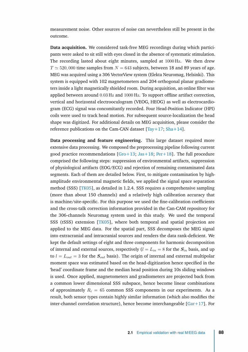
measurement noise. Other sources of noise can nevertheless still be present in theoutcome.

Data acquisition. We considered task-free MEG recordings during which partici-pants were asked to sit still with eyes closed in the absence of systematic stimulation.The recording lasted about eight minutes, sampled at 1000 Hz. We then drewT ≃ 520, 000 time samples from N = 643 subjects, between 18 and 89 years of age.MEG was acquired using a 306 VectorView system (Elekta Neuromag, Helsinki). Thissystem is equipped with 102 magnetometers and 204 orthogonal planar gradiome-ters inside a light magnetically shielded room. During acquisition, an online filter wasapplied between around 0.03 Hz and 1000 Hz. To support offline artifact correction,vertical and horizontal electrooculogram (VEOG, HEOG) as well as electrocardio-gram (ECG) signal was concomitantly recorded. Four Head-Position Indicator (HPI)coils were used to track head motion. For subsequent source-localization the headshape was digitized. For additional details on MEG acquisition, please consider thereference publications on the Cam-CAN dataset [Tay+17; Sha+14].

Data processing and feature engineering. This large dataset required moreextensive data processing. We composed the preprocessing pipeline following currentgood practice recommendations [Gro+13; Jas+18; Per+18]. The full procedurecomprised the following steps: suppression of environmental artifacts, suppressionof physiological artifacts (EOG/ECG) and rejection of remaining contaminated datasegments. Each of them are detailed below. First, to mitigate contamination by high-amplitude environmental magnetic fields, we applied the signal space separationmethod (SSS) [TK05], as detailed in 1.2.4. SSS requires a comprehensive sampling(more than about 150 channels) and a relatively high calibration accuracy thatis machine/site-specific. For this purpose we used the fine-calibration coefficientsand the cross-talk correction information provided in the Can-CAM repository forthe 306-channels Neuromag system used in this study. We used the temporalSSS (tSSS) extension [TK05], where both temporal and spatial projection areapplied to the MEG data. For the spatial part, SSS decomposes the MEG signalinto extracranial and intracranial sources and renders the data rank-deficient. Wekept the default settings of eight and three components for harmonic decompositionof internal and external sources, respectively (l = Lin = 8 for the Sin basis, and upto l = Lout = 3 for the Sout basis). The origin of internal and external multipolarmoment space was estimated based on the head-digitization hence specified in the‘head’ coordinate frame and the median head position during 10s sliding windowsis used. Once applied, magnetometers and gradiometers are projected back froma common lower dimensional SSS subspace, hence become linear combinationsof approximately Ri = 65 common SSS components in our experiments. As aresult, both sensor types contain highly similar information (which also modifies theinter-channel correlation structure), hence become interchangeable [Gar+17]. For

2.1 Empirical validation with real M/EEG data 88

Page 94

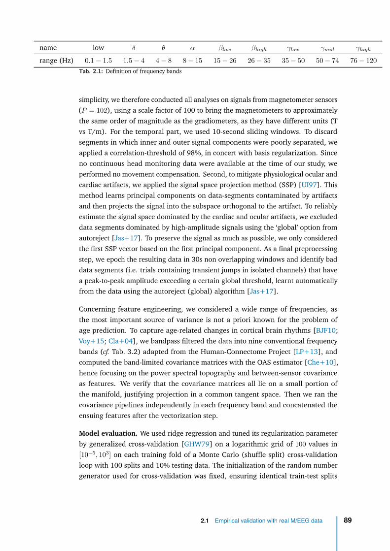
name low δ θ α βlow βhigh γlow γmid γhigh

range (Hz) 0.1 − 1.5 1.5 − 4 4 − 8 8 − 15 15 − 26 26 − 35 35 − 50 50 − 74 76 − 120Tab. 2.1: Definition of frequency bands

simplicity, we therefore conducted all analyses on signals from magnetometer sensors(P = 102), using a scale factor of 100 to bring the magnetometers to approximatelythe same order of magnitude as the gradiometers, as they have different units (Tvs T/m). For the temporal part, we used 10-second sliding windows. To discardsegments in which inner and outer signal components were poorly separated, weapplied a correlation-threshold of 98%, in concert with basis regularization. Sinceno continuous head monitoring data were available at the time of our study, weperformed no movement compensation. Second, to mitigate physiological ocular andcardiac artifacts, we applied the signal space projection method (SSP) [UI97]. Thismethod learns principal components on data-segments contaminated by artifactsand then projects the signal into the subspace orthogonal to the artifact. To reliablyestimate the signal space dominated by the cardiac and ocular artifacts, we excludeddata segments dominated by high-amplitude signals using the ‘global’ option fromautoreject [Jas+17]. To preserve the signal as much as possible, we only consideredthe first SSP vector based on the first principal component. As a final preprocessingstep, we epoch the resulting data in 30s non overlapping windows and identify baddata segments (i.e. trials containing transient jumps in isolated channels) that havea peak-to-peak amplitude exceeding a certain global threshold, learnt automaticallyfrom the data using the autoreject (global) algorithm [Jas+17].

Concerning feature engineering, we considered a wide range of frequencies, asthe most important source of variance is not a priori known for the problem ofage prediction. To capture age-related changes in cortical brain rhythms [BJF10;Voy+15; Cla+04], we bandpass filtered the data into nine conventional frequencybands (cf. Tab. 3.2) adapted from the Human-Connectome Project [LP+13], andcomputed the band-limited covariance matrices with the OAS estimator [Che+10],hence focusing on the power spectral topography and between-sensor covarianceas features. We verify that the covariance matrices all lie on a small portion ofthe manifold, justifying projection in a common tangent space. Then we ran thecovariance pipelines independently in each frequency band and concatenated theensuing features after the vectorization step.

Model evaluation. We used ridge regression and tuned its regularization parameterby generalized cross-validation [GHW79] on a logarithmic grid of 100 values in[10−5, 103] on each training fold of a Monte Carlo (shuffle split) cross-validationloop with 100 splits and 10% testing data. The initialization of the random numbergenerator used for cross-validation was fixed, ensuring identical train-test splits

2.1 Empirical validation with real M/EEG data 89

Page 95

across models. This choice also allowed us to obtain more fine-grained uncertaintyestimates than was possible with the time-series data used for subject-level regression.As absolute changes of the unit of the outcome is meaningful, we used the meanabsolute error (MAE) as evaluation metric. The proposed method, including all datapreprocessing, applied on the 500GB of raw MEG data from the Cam-CAN dataset,runs in approximately 12 hours on a regular desktop computer with at least 16GB ofRAM. The preprocessing for the computation of the covariances is embarrassinglyparallel and can therefore be significantly accelerated by using multiple CPUs. Theactual predictive modeling can be performed in less than a minute on standardlaptop.

Results: models performance in sensor space. Fig. 2.2 displays the results for ourdifferent regression models. The analysis revealed that all models performed clearly

8

10

12

14

16

0 10 20 30 40 50 60 70 80 90 100#components

MAE Riemann53

SPoC67

A B

7.98

8.11

8.76

8.76

9.17

10.89

predictingage

Riemann53

Riemann

SPoC67

SPoC

diag

upper

8 10 12 14 16MAE

upperdiagSPoCRiemann

Fig. 2.2: Predicting age from subject-level MEG in sensor space. (A) model comparison usingMonte Carlo cross-validation with 100 splits sampled from 596 subjects. Models are depictedalong the y-axis, expected out-of-sample performance (mean absolute error) on the x-axis. The distribution is summarized by standard boxplots. Split-wise prediction scores aredepicted by dots. The model type is indicated by color. Here, covariance estimation was basedon 8 minutes of MEG, hence, the impact of shrinkage should be small. For comparison withthe single-subject data (Fig. 2.1), we nevertheless reported the alternative low-rank models(model order indicated by subscripts, no subscript meaning an order of 65, the minimumrank of covariances). (B) Exhaustive search for model order in pipelines with projectionstep. All values from 1 to the total number of 102 magnetometer channels were considered.One can see that performance starts to saturate around 40 to 50. No striking advantage ofmodel-order search was evident compared to deriving the order from prior knowledge onrank deficiency at a value of about 65. We see no low-rank minima, best performance isobtained with the full signals. All models performed better than chance, however, modelsconsistent with log-linear model and using correlation terms performed better. On real data,when multiple model violations occur, the Riemannian models performed best.

better than chance. The Riemannian model (orange) yielded the best performance(8y MAE), followed by SPoC (dark orange, 8.8y MAE) (2.2A). The diagonal (green)and upper-triangle (blue) models performed worse. The chance level was ∼ 16yMAE. Model-order search did not reveal striking low-rank optima. Models aboverank 40 seem approximately equivalent, especially when considering the estimationuncertainty of standard deviation above 1 year of MAE. For both SPoC and Riemann,the best low-rank model was close to the model at the theoretically derived rankof 65 (due to preprocessing with SSS, see [TK05]). For subsequent analyses, we,nevertheless, retained the best models.

2.1 Empirical validation with real M/EEG data 90

Page 96

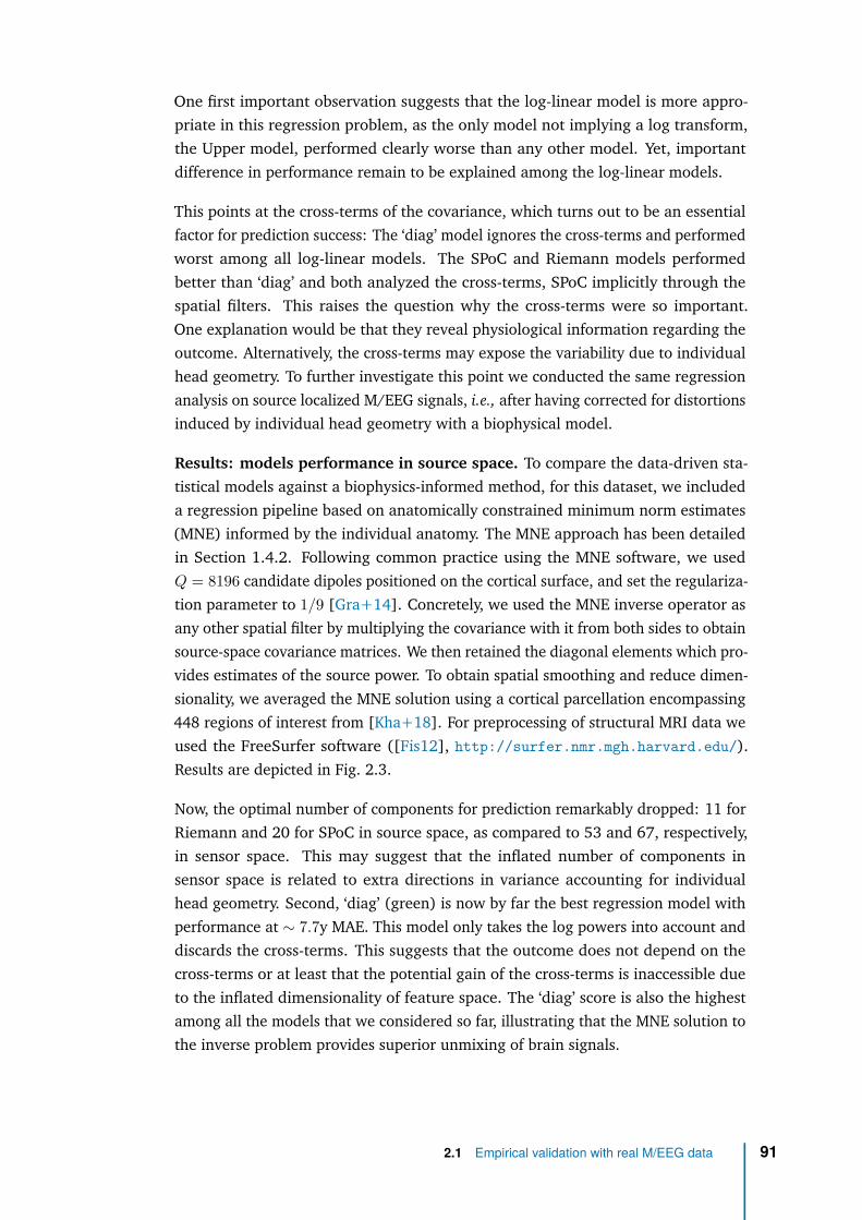
One first important observation suggests that the log-linear model is more appro-priate in this regression problem, as the only model not implying a log transform,the Upper model, performed clearly worse than any other model. Yet, importantdifference in performance remain to be explained among the log-linear models.

This points at the cross-terms of the covariance, which turns out to be an essentialfactor for prediction success: The ‘diag’ model ignores the cross-terms and performedworst among all log-linear models. The SPoC and Riemann models performedbetter than ‘diag’ and both analyzed the cross-terms, SPoC implicitly through thespatial filters. This raises the question why the cross-terms were so important.One explanation would be that they reveal physiological information regarding theoutcome. Alternatively, the cross-terms may expose the variability due to individualhead geometry. To further investigate this point we conducted the same regressionanalysis on source localized M/EEG signals, i.e., after having corrected for distortionsinduced by individual head geometry with a biophysical model.

Results: models performance in source space. To compare the data-driven sta-tistical models against a biophysics-informed method, for this dataset, we includeda regression pipeline based on anatomically constrained minimum norm estimates(MNE) informed by the individual anatomy. The MNE approach has been detailedin Section 1.4.2. Following common practice using the MNE software, we usedQ = 8196 candidate dipoles positioned on the cortical surface, and set the regulariza-tion parameter to 1/9 [Gra+14]. Concretely, we used the MNE inverse operator asany other spatial filter by multiplying the covariance with it from both sides to obtainsource-space covariance matrices. We then retained the diagonal elements which pro-vides estimates of the source power. To obtain spatial smoothing and reduce dimen-sionality, we averaged the MNE solution using a cortical parcellation encompassing448 regions of interest from [Kha+18]. For preprocessing of structural MRI data weused the FreeSurfer software ([Fis12], http://surfer.nmr.mgh.harvard.edu/).Results are depicted in Fig. 2.3.

Now, the optimal number of components for prediction remarkably dropped: 11 forRiemann and 20 for SPoC in source space, as compared to 53 and 67, respectively,in sensor space. This may suggest that the inflated number of components insensor space is related to extra directions in variance accounting for individualhead geometry. Second, ‘diag’ (green) is now by far the best regression model withperformance at ∼ 7.7y MAE. This model only takes the log powers into account anddiscards the cross-terms. This suggests that the outcome does not depend on thecross-terms or at least that the potential gain of the cross-terms is inaccessible dueto the inflated dimensionality of feature space. The ‘diag’ score is also the highestamong all the models that we considered so far, illustrating that the MNE solution tothe inverse problem provides superior unmixing of brain signals.

2.1 Empirical validation with real M/EEG data 91

Page 97

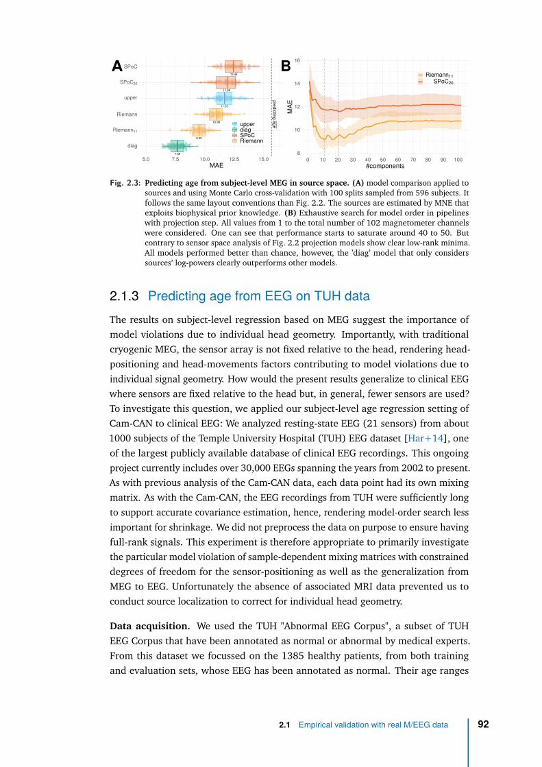
8

10

12

14

16

0 10 20 30 40 50 60 70 80 90 100#components

MAE

Riemann11SPoC20

7.69

9.50

10.98

11.67

11.86

12.46

predictingage

diag

Riemann11

Riemann

upper

SPoC20

SPoC

5.0 7.5 10.0 12.5 15.0 17.5MAE

upperdiagSPoCRiemann

A B

Fig. 2.3: Predicting age from subject-level MEG in source space. (A) model comparison applied tosources and using Monte Carlo cross-validation with 100 splits sampled from 596 subjects. Itfollows the same layout conventions than Fig. 2.2. The sources are estimated by MNE thatexploits biophysical prior knowledge. (B) Exhaustive search for model order in pipelineswith projection step. All values from 1 to the total number of 102 magnetometer channelswere considered. One can see that performance starts to saturate around 40 to 50. Butcontrary to sensor space analysis of Fig. 2.2 projection models show clear low-rank minima.All models performed better than chance, however, the ’diag’ model that only considerssources’ log-powers clearly outperforms other models.

2.1.3 Predicting age from EEG on TUH dataThe results on subject-level regression based on MEG suggest the importance ofmodel violations due to individual head geometry. Importantly, with traditionalcryogenic MEG, the sensor array is not fixed relative to the head, rendering head-positioning and head-movements factors contributing to model violations due toindividual signal geometry. How would the present results generalize to clinical EEGwhere sensors are fixed relative to the head but, in general, fewer sensors are used?To investigate this question, we applied our subject-level age regression setting ofCam-CAN to clinical EEG: We analyzed resting-state EEG (21 sensors) from about1000 subjects of the Temple University Hospital (TUH) EEG dataset [Har+14], oneof the largest publicly available database of clinical EEG recordings. This ongoingproject currently includes over 30,000 EEGs spanning the years from 2002 to present.As with previous analysis of the Cam-CAN data, each data point had its own mixingmatrix. As with the Cam-CAN, the EEG recordings from TUH were sufficiently longto support accurate covariance estimation, hence, rendering model-order search lessimportant for shrinkage. We did not preprocess the data on purpose to ensure havingfull-rank signals. This experiment is therefore appropriate to primarily investigatethe particular model violation of sample-dependent mixing matrices with constraineddegrees of freedom for the sensor-positioning as well as the generalization fromMEG to EEG. Unfortunately the absence of associated MRI data prevented us toconduct source localization to correct for individual head geometry.

Data acquisition. We used the TUH "Abnormal EEG Corpus", a subset of TUHEEG Corpus that have been annotated as normal or abnormal by medical experts.From this dataset we focussed on the 1385 healthy patients, from both trainingand evaluation sets, whose EEG has been annotated as normal. Their age ranges

2.1 Empirical validation with real M/EEG data 92

Page 98

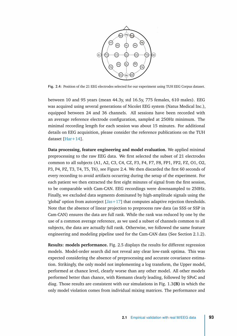
Fig. 2.4: Position of the 21 EEG electrodes selected for our experiment using TUH EEG Corpus dataset.

between 10 and 95 years (mean 44.3y, std 16.5y, 775 females, 610 males). EEGwas acquired using several generations of Nicolet EEG system (Natus Medical Inc.),equipped between 24 and 36 channels. All sessions have been recorded withan average reference electrode configuration, sampled at 250Hz minimum. Theminimal recording length for each session was about 15 minutes. For additionaldetails on EEG acquisition, please consider the reference publications on the TUHdataset [Har+14].

Data processing, feature engineering and model evaluation. We applied minimalpreprocessing to the raw EEG data. We first selected the subset of 21 electrodescommon to all subjects (A1, A2, C3, C4, CZ, F3, F4, F7, F8, FP1, FP2, FZ, O1, O2,P3, P4, PZ, T3, T4, T5, T6), see Figure 2.4. We then discarded the first 60 seconds ofevery recording to avoid artifacts occurring during the setup of the experiment. Foreach patient we then extracted the first eight minutes of signal from the first session,to be comparable with Cam-CAN. EEG recordings were downsampled to 250Hz.Finally, we excluded data segments dominated by high-amplitude signals using the‘global’ option from autoreject [Jas+17] that computes adaptive rejection thresholds.Note that the absence of linear projection to preprocess raw data (as SSS or SSP inCam-CAN) ensures the data are full rank. While the rank was reduced by one by theuse of a common average reference, as we used a subset of channels common to allsubjects, the data are actually full rank. Otherwise, we followed the same featureengineering and modeling pipeline used for the Cam-CAN data (See Section 2.1.2).

Results: models performance. Fig. 2.5 displays the results for different regressionmodels. Model-order search did not reveal any clear low-rank optima. This wasexpected considering the absence of preprocessing and accurate covariance estima-tion. Strikingly, the only model not implementing a log transform, the Upper model,performed at chance level, clearly worse than any other model. All other modelsperformed better than chance, with Riemann clearly leading, followed by SPoC anddiag. Those results are consistent with our simulations in Fig. 1.3(B) in which theonly model violation comes from individual mixing matrices. The performance and

2.1 Empirical validation with real M/EEG data 93

Page 99

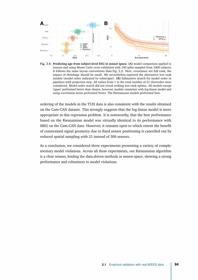
9

11

13

0 10 20#components

MAE Riemann19

SPoC21

8.21

8.27

9.63

10.72

predictingage

Riemann19

Riemann

SPoC21

diag

upper

5.0 7.5 10.0 12.5 15.0MAE

upperdiagSPoCRiemann

A B

Fig. 2.5: Predicting age from subject-level EEG in sensor space. (A) model comparison applied tosensors and using Monte Carlo cross-validation with 100 splits sampled from 1000 subjects.It follows the same layout conventions than Fig. 2.2. Here, covariance are full rank, theimpact of shrinkage should be small. We nevertheless reported the alternative low-rankmodels (model order indicated by subscripts). (B) Exhaustive search for model order inpipelines with projection step. All values from 1 to the total number of 21 electrodes wereconsidered. Model-order search did not reveal striking low-rank optima. All models except’upper’ performed better than chance, however, models consistent with log-linear model andusing correlation terms performed better. The Riemannian models performed best.

ordering of the models in the TUH data is also consistent with the results obtainedon the Cam-CAN dataset. This strongly suggests that the log-linear model is moreappropriate in this regression problem. It is noteworthy, that the best performancebased on the Riemannian model was virtually identical to its performance withMEG on the Cam-CAN data. However, it remains open to which extent the benefitof constrained signal geometry due to fixed sensor positioning is cancelled out byreduced spatial sampling with 21 instead of 306 sensors.

As a conclusion, we considered three experiments presenting a variety of comple-mentary model violations. Across all these experiments, our Riemannian algorithmis a clear winner, leading the data-driven methods in sensor-space, showing a strongperformance and robustness to model violations.

2.1 Empirical validation with real M/EEG data 94

Page 100

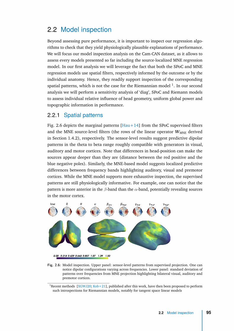
2.2 Model inspectionBeyond assessing pure performance, it is important to inspect our regression algo-rithms to check that they yield physiologically plausible explanations of performance.We will focus our model inspection analysis on the Cam-CAN dataset, as it allows toassess every models presented so far including the source-localized MNE regressionmodel. In our first analysis we will leverage the fact that both the SPoC and MNEregression models use spatial filters, respectively informed by the outcome or by theindividual anatomy. Hence, they readily support inspection of the correspondingspatial patterns, which is not the case for the Riemannian model 1. In our secondanalysis we will perform a sensitivity analysis of ‘diag’, SPoC and Riemann modelsto assess individual relative influence of head geometry, uniform global power andtopographic information in performance.

2.2.1 Spatial patternsFig. 2.6 depicts the marginal patterns [Hau+14] from the SPoC supervised filtersand the MNE source-level filters (the rows of the linear operator WMNE derivedin Section 1.4.2), respectively. The sensor-level results suggest predictive dipolarpatterns in the theta to beta range roughly compatible with generators in visual,auditory and motor cortices. Note that differences in head-position can make thesources appear deeper than they are (distance between the red positive and theblue negative poles). Similarly, the MNE-based model suggests localized predictivedifferences between frequency bands highlighting auditory, visual and premotorcortices. While the MNE model supports more exhaustive inspection, the supervisedpatterns are still physiologically informative. For example, one can notice that thepattern is more anterior in the β-band than the α-band, potentially revealing sourcesin the motor cortex.

Fig. 2.6: Model inspection. Upper panel: sensor-level patterns from supervised projection. One cannotice dipolar configurations varying across frequencies. Lower panel: standard deviation ofpatterns over frequencies from MNE projection highlighting bilateral visual, auditory andpremotor cortices.

1Recent methods [XGWJ20; Kob+21], published after this work, have then been proposed to performsuch introspections for Riemannian models, notably for tangent space linear models

2.2 Model inspection 95

Page 101

2.2.2 MEG and EEG as a cheap MRI?The Cam-CAN study revealed that the performance of Riemann in sensor space(Figure 2.2) is close to ‘diag’ in source space ( Figure 2.3), suggesting that the cross-term models, in sensor space, have learnt to some extent what ‘diag’, in source space,receives explicitly from source localization. Still, the good performance of ‘diag’ insource space may be due to two independent factors that are not mutually exclusive:It could be that source localization standardizes head geometry, hence, mitigatesthe variability of mixing. On the other hand, if the anatomy itself covaries with theoutcome, which is a safe assumption to make for the case of aging [Lie+17], theleadfields will also covary with the outcome. Source amplitudes may then change asa result of dampening-effects (See methods in Khan et al. [Kha+18]).

To disentangle the factors explaining model performance, and understand howRiemannian model partially handle individual volume conduction, we devised anovel error-decomposition method derived from the proposed statistical framework(Fig. 1.2). The link between the data-generating mechanism and the proposedregression models allows us to derive an informal analysis of variance [Gel+05]for estimating the importance of the data generating factors such as head geometry,uniform global power and topographic, i.e., spatial information. Given the knownphysics from Eq. (1.44), the data covariance can be written Ci = Gi Cz

i G⊤i , where

Czi is the covariance matrix of the physiological sources in a given frequency band.

The input to the regression model is therefore affected by both the head geometryexpressed in Gi, and the covariance of the sources. Using a simulation-basedapproach, we can therefore compute degraded observations, i.e., versions of the fullindividual covariance CD

i that were either exclusively influenced by the individualanatomy in terms of the leadfields, or also by additive uniform power. Subsequentmodel comparisons against the full models then allow isolating the relative meritof each of these specific components. Following common practice, we consideredelectrical dipolar sources zi(t) ∈ RM , with M ≈ 8000, and we computed theleadfield matrix Gi with a boundary element model (BEM) [Gra+14]. We thendefined two alternative models which are only based on the anatomical informationor, additionally, on the global signal power in a given frequency band withouttopographic structure. This simulation will therefore allow us to estimate to whichextent the log-linear models have learnt from anatomical information, global signalpower of the MEG and topographic details.

Model using anatomy only. Assuming the physiological sources are Gaussian,uncorrelated and of unit variance (power) zD

i (t) ∼ N (0, IM ), we can re-synthesizetheir covariance matrix from individual leadfields alone without taking into accountthe actual covariance structure:

CDi = GiG

⊤i . (2.2)

2.2 Model inspection 96

Page 102

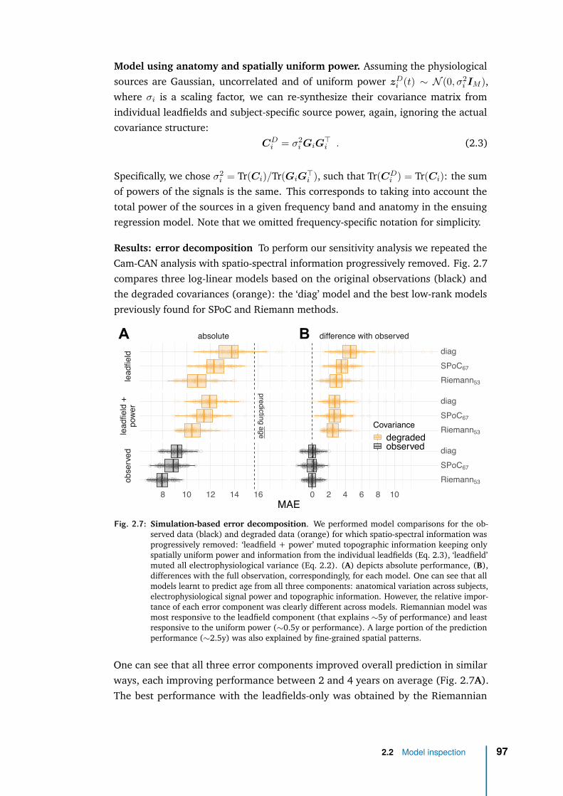
Model using anatomy and spatially uniform power. Assuming the physiologicalsources are Gaussian, uncorrelated and of uniform power zD

i (t) ∼ N (0, σ2i IM ),

where σi is a scaling factor, we can re-synthesize their covariance matrix fromindividual leadfields and subject-specific source power, again, ignoring the actualcovariance structure:

CDi = σ2

i GiG⊤i . (2.3)

Specifically, we chose σ2i = Tr(Ci)/Tr(GiG

⊤i ), such that Tr(CD

i ) = Tr(Ci): the sumof powers of the signals is the same. This corresponds to taking into account thetotal power of the sources in a given frequency band and anatomy in the ensuingregression model. Note that we omitted frequency-specific notation for simplicity.

Results: error decomposition To perform our sensitivity analysis we repeated theCam-CAN analysis with spatio-spectral information progressively removed. Fig. 2.7compares three log-linear models based on the original observations (black) andthe degraded covariances (orange): the ‘diag’ model and the best low-rank modelspreviously found for SPoC and Riemann methods.

predictingage

absolute difference with observed

leadfield

leadfield+

power

observed

8 10 12 14 16 0 2 4 6 8 10

Riemann53

SPoC67

diag

Riemann53

SPoC67

diag

Riemann53

SPoC67

diag

MAE

Covariancedegradedobserved

A B

Fig. 2.7: Simulation-based error decomposition. We performed model comparisons for the ob-served data (black) and degraded data (orange) for which spatio-spectral information wasprogressively removed: ‘leadfield + power’ muted topographic information keeping onlyspatially uniform power and information from the individual leadfields (Eq. 2.3), ‘leadfield’muted all electrophysiological variance (Eq. 2.2). (A) depicts absolute performance, (B),differences with the full observation, correspondingly, for each model. One can see that allmodels learnt to predict age from all three components: anatomical variation across subjects,electrophysiological signal power and topographic information. However, the relative impor-tance of each error component was clearly different across models. Riemannian model wasmost responsive to the leadfield component (that explains ∼5y of performance) and leastresponsive to the uniform power (∼0.5y or performance). A large portion of the predictionperformance (∼2.5y) was also explained by fine-grained spatial patterns.

One can see that all three error components improved overall prediction in similarways, each improving performance between 2 and 4 years on average (Fig. 2.7A).The best performance with the leadfields-only was obtained by the Riemannian

2.2 Model inspection 97

Page 103

model scoring an MAE of about 11y on average. Adding spatially uniform power, theRiemann model kept leading and improved by about 0.5y. Predictions based on theobserved data with full access to the covariance structure improved performanceby up to about 3y, suggesting that age prediction clearly benefits from informationbeyond the leadfields.

Generally, the choice of algorithm mattered across all levels of the data generat-ing scenario with Riemann always leading and the ‘diag’ model always trailing(Fig. 2.7A). Finally, the results suggest the presence of an interaction effect whereboth the leadfields and the uniform power components were not equally importantacross models (Fig. 2.7A,B). For the Riemannian model, when only learning fromleadfields, performance got as close as three years to the final performance of thefull model (Fig. 2.7B). The ‘diag’ model, instead, only arrived at 5 years of distancefrom the equivalent model with full observations (Fig. 2.7B). On the other hand, theRiemannian model extracted rather little additional information from the uniformpower and only made its next leap forward when accessing the full non-degradedcovariance structure. Please note that these analyses are based on cross-validation.The resulting resampling splits do not count as independent samples. This precludesformal analysis of variance with an ANOVA model.

Overall, error decomposition suggests that all methods learn from anatomy andthat indeed, the leadfield in isolation is predictive of age. Models consideringcross-terms of the covariance were however more sensitive. It turns out that theleadfield contained some information on aging and that Riemannian embeddingswere most sensitive to this information. Riemannian model was most responsive tothe leadfield component and least responsive to the uniform power. This informationwas not explained by head positioning, pointing at differences in brain anatomy.It’s conceivable that the Riemannian embedding better exposed this anatomicalinformation, facilitating deconfounding for the ridge model and/or contributingunique information. The fact that Riemannian embeddings seem to capture in-dividual head geometry justifies the use of EEG in the clinic beyond availability:brain age EEG and brain age MRI must be correlated because half the variance incovariances is anatomically explained. But also the fact that anatomical variationsdoes not fully explain the performance means that neuronal activity captured byM/EEG contributes to the prediction: something is unique about M/EEG. This is anadditional hint, beyond our article [Eng+20], and using a different method, thatM/EEG is complementary with MRI.

2.2 Model inspection 98

Page 104

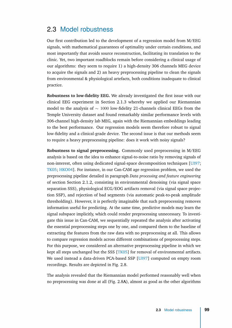
2.3 Model robustnessOur first contribution led to the development of a regression model from M/EEGsignals, with mathematical guarantees of optimality under certain conditions, andmost importantly that avoids source reconstruction, facilitating its translation to theclinic. Yet, two important roadblocks remain before considering a clinical usage ofour algorithms: they seem to require 1) a high-density 306 channels MEG deviceto acquire the signals and 2) an heavy preprocessing pipeline to clean the signalsfrom environmental & physiological artefacts, both conditions inadequate to clinicalpractice.

Robustness to low-fidelity EEG. We already investigated the first issue with ourclinical EEG experiment in Section 2.1.3 whereby we applied our Riemannianmodel to the analysis of ∼ 1000 low-fidelity 21-channels clinical EEGs from theTemple University dataset and found remarkably similar performance levels with306-channel high-density lab MEG, again with the Riemannian embeddings leadingto the best performance. Our regression models seem therefore robust to signallow-fidelity and a clinical-grade device. The second issue is that our methods seemto require a heavy preprocessing pipeline: does it work with noisy signals?

Robustness to signal preprocessing. Commonly used preprocessing in M/EEGanalysis is based on the idea to enhance signal-to-noise ratio by removing signals ofnon-interest, often using dedicated signal-space decomposition techniques [UI97;TK05; HKO04]. For instance, in our Can-CAM age regression problem, we used thepreprocessing pipeline detailed in paragraph Data processing and feature engineeringof section Section 2.1.2, consisting in environmental denoising (via signal spaceseparation SSS), physiological ECG/EOG artifacts removal (via signal space projec-tion SSP), and rejection of bad segments (via automatic peak-to-peak amplitudethresholding). However, it is perfectly imaginable that such preprocessing removesinformation useful for predicting. At the same time, predictive models may learn thesignal subspace implicitly, which could render preprocessing unnecessary. To investi-gate this issue in Can-CAM, we sequentially repeated the analysis after activatingthe essential preprocessing steps one by one, and compared them to the baseline ofextracting the features from the raw data with no preprocessing at all. This allowsto compare regression models across different combinations of preprocessing steps.For this purpose, we considered an alternative preprocessing pipeline in which wekept all steps unchanged but the SSS [TK05] for removal of environmental artifacts.We used instead a data-driven PCA-based SSP [UI97] computed on empty roomrecordings. Results are depicted in Fig. 2.8.

The analysis revealed that the Riemannian model performed reasonably well whenno preprocessing was done at all (Fig. 2.8A), almost as good as the other algorithms

2.3 Model robustness 99

Page 105

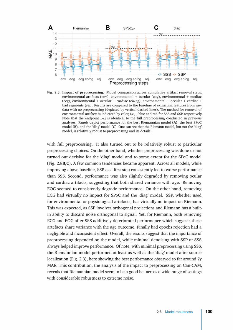
raw

raw

raw

Riemann53 SPoC67 diag

env eog ecg eo/cg rej env eog ecg eo/cg rej env eog ecg eo/cg rej67891011121314

Preprocessing steps

MAE

SSS SSP

A B C

Fig. 2.8: Impact of preprocessing. Model comparison across cumulative artifact removal steps:environmental artifacts (env), environmental + occular (eog), environmental + cardiac(ecg), environmental + occular + cardiac (eo/cg), environmental + occular + cardiac +bad segments (rej). Results are compared to the baseline of extracting features from rawdata with no preprocessing (depicted by vertical dashed lines). The method for removal ofenvironmental artifacts is indicated by color, i.e., , blue and red for SSS and SSP respectively.Note that the endpoint rej is identical to the full preprocessing conducted in previousanalyses. Panels depict performance for the best Riemannian model (A), the best SPoCmodel (B), and the ‘diag’ model (C). One can see that the Riemann model, but not the ‘diag’model, is relatively robust to preprocessing and its details.

with full preprocessing. It also turned out to be relatively robust to particularpreprocessing choices. On the other hand, whether preprocessing was done or notturned out decisive for the ‘diag’ model and to some extent for the SPoC model(Fig. 2.8B,C). A few common tendencies became apparent. Across all models, whileimproving above baseline, SSP as a first step consistently led to worse performancethan SSS. Second, performance was also slightly degraded by removing ocularand cardiac artifacts, suggesting that both shared variance with age. RemovingEOG seemed to consistently degrade performance. On the other hand, removingECG had virtually no impact for SPoC and the ‘diag’ model. SSP, whether usedfor environmental or physiological artefacts, has virtually no impact on Riemann.This was expected, as SSP involves orthogonal projections and Riemann has a built-in ability to discard noise orthogonal to signal. Yet, for Riemann, both removingECG and EOG after SSS additively deteriorated performance which suggests theseartefacts share variance with the age outcome. Finally bad epochs rejection had anegligible and inconsistent effect. Overall, the results suggest that the importance ofpreprocessing depended on the model, while minimal denoising with SSP or SSSalways helped improve performance. Of note, with minimal preprocessing using SSS,the Riemannian model performed at least as well as the ‘diag’ model after sourcelocalization (Fig. 2.3), here showing the best performance observed so far around 7yMAE. This contribution, the analysis of the impact to preprocessing on Can-CAM,reveals that Riemannian model seem to be a good bet across a wide range of settingswith considerable robustness to extreme noise.

2.3 Model robustness 100

Page 106

Finally, to summarize our two contributions so far, we found that when predictingfrom M/EEG power spectra is the priority, the capacity of linear models can beextended optimally by Riemannian embeddings despite model violations. Strikingly,applied to age prediction, this Riemannian regression algorithm has the potential tobe used in the clinic: it operates in sensor-space (avoiding costly source localization),it is robust to environmental and physiological artefacts and it accommodates cheapEEG recordings. This optimal, robust and light model is therefore a good candidateto develop our clinical Brain Age Delta (BAD) biomarker.

2.3 Model robustness 101

Page 107

2.4 DiscussionWhat distinguishes event-level from subject-level prediction in the light ofmodel violations?

Unsurprisingly, no model performed perfectly when applied to empirical data forwhich the data generating mechanism is by definition unobservable, multiple modelviolations may occur and information is only partially available. One importantsource of differences in model violation is related to whether outcomes are definedat the event-level or at the subject-level. When predicting outcomes from ongoingsegments of neural time-series within a subject, covariance estimation becomesnon-trivial as the event-level time windows are too short for accurate estimation.Even if regularized covariance estimates provide an effective remedy, there is not oneshrinkage recipe that works in every situation [EG15]. In this study, we have reliedon the oracle approximating shrinkage (OAS) [Che+10] as a default method in allanalyses. Yet, we found that additional low-rank shrinkage [EG15; Woo+11; TB99;RCJ18], as implied by the SPoC method [Däh+14a], or the unsupervised projectionfor the Riemannian model [Sab+19a], improved performance considerably forevent-level prediction. A spatial-filter method like SPoC [CP14; Däh+14a] can beparticularly convenient in this context. By design, it concentrates the variance mostimportant for prediction on a few dimensions, which can be easily searched for,ascending from the bottom of the rank spectrum. Riemannian methods can alsobe operated in low-rank settings [Sab+19a]. However, model-order search may bemore complicated as the best model may be anywhere in the spectrum. This canlead to increased computation times, which may be prohibitive in realtime settingssuch as BCI [Lot+07; Lot+18; Tan+08].

Issues with the numerical rank of the covariance matrix also appear when predictingat the subject-level. The reason for this is fundamentally different and rather unre-lated to the quality of covariance estimation. Many modern M/EEG preprocessingtechniques focus on estimating and projecting out the noise-subspace, which leads torank-deficient data. In our analysis of the Cam-CAN dataset [Sha+14; Tay+17], weapplied the SSS method [TK05] by default, which is the recommended way when nostrong magnetic shielding is available, as is the case for the Cambridge MEG-systemon which the data was acquired (see also discussion in [Jas+18]). However, SSSmassively reduces the rank down to about 64 out of 306 dimensions, which maydemand special attention when calibrating covariance estimation. Our results sug-gest that projection can indeed lead to slightly improved average prediction once acertain rank value is reached. Yet, thoughtful search of optimal model order maynot be worth the effort in practice when a reasonably good guess of model ordercan be derived from the understanding of the preprocessing steps applied. Ourfindings, moreover, suggest, that a Riemann-based model is, in general, a reasonably

2.4 Discussion 102

Page 108

good starting point, even when no model-order search is applied. What seems tobe a much more important issue in subject-level prediction from M/EEG are themodel violations incurred by individual anatomy. Our mathematical analysis andsimulations demonstrated that not even the Riemannian approach is immune tothose, for MEG and EEG.

What explains the performance in subject-level prediction?

Our results suggested that, for the current regression problems with MEG and EEG,the log-linear model was more appropriate than the linear-in-powers ones. Thisis well in line with practical experience and theoretical results highlighting theimportance of log-normal brain dynamics [BM14]. On the other hand, on the Cam-CAN data, we observed substantive differences in performance within the log-normalmodels highlighting a non-trivial link between the cross-terms of the covariance andsubject-level variation. Indeed, the ‘diag’ model, both in sensor and source space,ignored the cross-terms of the covariance, yet in source space, it performed about1.5 years better on average than in sensor space. This is rather unsurprising whenrecapitulating the fact that subject-level regression on M/EEG implies individualanatomy. Indeed, our mathematical analysis and simulations identified this factoras important model violation. MNE source localization, by design, uses the headand brain geometry to correct for such violations. On the other hand, if leadfieldsare correlated with the outcome, the source localization, which depends on theleadfields, will be predictive of the outcome too, even if no brain source is actuallyrelevant to the outcome. This suggests that the cross-term models that were moresuccessful than the ‘diag’ model may either convey biological information relevantto predict the outcome, or expose forward information on head geometry to theregression model, which then improved prediction by de-confounding for headgeometry. Our findings on source localization strongly suggested that correcting forgeometrical misalignment was the driving factor, evidenced by the fact that aftersource localization the simple ‘diag’ model performed best. Yet, these findings didnot rule out that leadfields themselves were not predictive of the outcome.

We, therefore, derived a novel error-decomposition technique from the statisticalframework presented in Fig. 1.2 to estimate the sensitivity of our M/EEG regressionmodels to anatomy, spatially uniform power and topographic details. We appliedthis technique on the Cam-CAN dataset to investigate the subject-level predictionproblem. While all models captured anatomical information and the Riemannianmodels were the most sensitive to it, anatomical information did not explain theperformance based on the full data. At the same time, this demonstrated thatMEG captures age-related anatomical information from the individual leadfields andraises the question of which aspects of anatomy were concerned. Neuroscience ofaging has suggested important alterations of the cortical tissues [Lie+17], relevantfor generating M/EEG signals, such as cortical surface area, cortical thickness or

2.4 Discussion 103

Page 109

cortical folding. Yet, more trivially, head size or posture are a common issue in MEGand could explain the present effect, which would be potentially less fascinatingfrom a neuroscientific standpoint. We investigated this issue post-hoc by predictingage from the device-to-head transform describing the position of the head relativeto the helmet and the coregistration transforms from head to MRI. Compared tothe Riemannian model applied to the leadfields-only surrogate data, this resultedin three years lower performance of around 14 years error, which is close to therandom guessing error and may at best explain the performance of the ‘diag’ model.Moreover, translating our approach to EEG for which sensor placement relative tothe head is less variable, we did not witness improvements over MEG. On the otherhand, this may be due to the smaller number of sensors available in EEG. Futurework will have to show, how these two factors interact in practice across predictionproblems and EEG-configurations.

Interestingly, also the SPoC model was more sensitive to anatomy than the ‘diag’model. This suggests that by learning adaptive spatial filters from the data to bestpredict age, SPoC may implicitly also tune the model to the anatomical informationconveyed by the leadfields. This seems even more plausible when considering thatfrom a statistical standpoint, SPoC learns how to invert the mixing matrix A toget the statistical sources implied by the predictive model. This must necessarilyyield a linear combination of the columns of G. As a consequence, SPoC does notlearn to invert the leadfields G but directly yields an imperfect approximation to G .Theoretically, unique SPoC solution can be found with arbitrary outcomes as long asthe data is full-rank and the target is noise-free. In practice, this is rarely the case.Therefore, the SPoC solution empirically depends on the choice of the outcome. Thisalso motivates the conjecture that differences between SPoC and Riemann shouldbecome smaller when the Gi are not correlated with the outcome (Riemann shouldstill enjoy an advantage due to increased robustness to model violations) or evenvanish when G is constant and no low-rank issues apply. The latter case is what weencountered in the event-level analysis where SPoC and Riemann where roughly onpar, suggesting that both handled the distortions induced by G.

Unfortunately, the current analysis did not elucidate the precise mechanism by whichdifferent models learnt from the individual anatomy and why the Riemannian modelwas so much more proficient. As a speculation, one can imagine that changes in theleadfields translate into simple topographic displacements that the ‘diag’ model caneasily capture. This would be in line with the performance of the ‘diag’ model on theleadfields-only surrogate data, which matched prediction performance based on thedevice-to-head transforms or the coregistration matrices previously mentioned. Withcross-terms included in the modeling, SPoC and, in particular, Riemann may betterunravel the directions of variation with regard to the outcome by considering theentire geometry presented in the leadfields. Instead, for the case of the leadfields-

2.4 Discussion 104

Page 110

only surrogates, SPoC attempts capturing sources which literally do not exist, hencemust yield a degraded view on G.

Overall, our results suggest that Riemannian models may also be the right choicewhen the anatomy is correlated with the outcome and the primary goal is prediction.The enhanced sensitivity of the Riemannian model to source and head geometry maybe precisely what brings them so close to performance based on source localization.Indeed, the TUH experiment shows that these properties render Riemannian modelsparticularly helpful in the case of EEG, where the leadfields should be less variableas the sensor cap is affixed to the head, which strongly limits variation due to headposture.

How important is preprocessing for subject-level prediction?

It is up to now equivocal how important preprocessing is when performing predictivemodeling at the subject-level. Some evidence suggests that preprocessing may benegligible when performing event-level decoding of evoked responses as a linearmodel may well learn to regress out the noise-subspace [Hau+14]. Our findingssuggest a more complex situation when performing subject-level regression fromM/EEG signal power. Strikingly, performing no preprocessing was clearly reducingperformance, for some models even dramatically, SPoC and in particular ‘diag’.The Riemann model, on the other hand, was remarkably robust and performedeven reasonably well without preprocessing. Among the preprocessing steps, theremoval of environmental artifacts seemed to be most important and most of thetime led to massive improvements in performance. Removing EOG and ECG artifactsmostly reduced performance suggesting that age-related information was presentin EOG and ECG. For example, one can easily imagine that older subjects producedless blinks or showed different eye-movement patterns [Tha+15] and also cardiacactivity may change across the lifespan [Att+19].

Interestingly, our results suggest that the method used for preprocessing was highlyimportant. In general, performance was clearly enhanced when SSS was usedinstead of SSP. Does this mean that SSP is a bad choice for removing environmentalartifacts? Our results have to be interpreted carefully, as the situation is morecomplicated when considering how fundamentally different SSP and SSS are interms of design. When performing SSS, one actually combines the information ofindependent gradiometer and magnetometer sensor arrays into one latent spaceof roughly 65 dimensions, less than the dimensionality of both sensor arrays (306sensors in total). Even when analyzing the magnetometers only after SSS, onewill also access the extra information from the gradiometers [Gar+17]. SSP onthe other hand is less invasive and is applied separately to magnetometers andgradiometers. It commonly removes only few dimensions from the data, yielding asubspace greater than 280 in practice. Our results therefore conflate two effects: 1)

2.4 Discussion 105

Page 111

learning from magnetometers and gradiometers versus learning from magnetometersonly and 2) differences in strength of dimensionality reduction. To disentangle thesefactors, careful experimentation with more targeted comparisons is indicated. Tobe conclusive, such an effort may necessitate computations at the scale of weeksand should be investigated in a dedicated study. For what concerns the currentresults, the findings simply suggest that SSS is a convenient tool as it allows one tocombine information from magnetometers and gradiometers into a subspace that issufficiently compact to enable efficient parameter estimation. It is not clear though,if careful processing with SSP and learning on both sensors types would not lead tobetter results.

Conclusion

Our study has investigated learning continuous outcomes from M/EEG signal powerfrom the perspective of generative models. Across datasets and electrophysiologicalmodalities, the log-linear model turned out to be more appropriate. In the lightof common empirical model violations and preprocessing options, models basedon Riemannian geometry stood out in terms of performance and robustness. Theoverall performance level is remarkable when considering the simplicity of the model.Our results demonstrate that a Riemannian model can actually be used to performend-to-end learning [Sch+17] involving nothing but signal filtering and covarianceestimation and, importantly, without deep-learning [Roy+19]. When using SSS,performance improves beyond the current benchmark set by the MNE model butprobably not because of denoising but rather due to the addition of gradiometer in-formation. Moreover, we observed comparable performance on minimally processedclinical-EEG with only 21 channels instead of 306 MEG-channels, suggesting that thecurrent approach may well generalize to certain clinical settings. This has at leasttwo important practical implications. First, this allows researchers and cliniciansto quickly assess the limits of what they can hope to learn in an economical andeco-friendly fashion [SGM19]. In this scenario, the Riemannian end-to-end modelrapidly delivers an estimate of the overall performance that could be reached byextensive and long processing, hence, support practical decision making on whethera deeper analysis is worth the investment of time and resources. Second, this resultsuggests that if prediction is the priority, availability of MRI and precious MEGexpertise for conducting source localization is not any longer the bottleneck. Thiscould potentially facilitate data collection and shift the strategy towards betting onthe law of large numbers: assembling an MEG dataset in the order of thousands iseasier when collecting MRI is not a prerequisite.

It is worthwhile to consider important limitations of this study. Unfortunately, wehave not had access to more datasets with other interesting continuous outcomes.In particular the conclusions drawn from the comparison between event-level andsubject-level regression may be expanded in the future when considering larger

2.4 Discussion 106

Page 112

event-level datasets and other outcomes for which the linear-in-powers model maybe more appropriate. Second, one has to critically acknowledge that the performancebenefit for the Riemannian model may be partially explained by increased sensitivityto anatomical information, which might imply reduced specificity with regard toneuronal activity. In this context it is noteworthy that recent regression pipelinesbased on a variant of SPoC [Däh+14b] made use of additional spatial filtering fordimensionality reduction, i.e., , SSD [NNC11] to isolate oscillatory componentsand discard arrhythmic (1/f) activity. This raises the question if the specificity ofa Riemannian model could be enhanced in a similar way. Ultimately, what modelto prefer, therefore, clearly depends on the strategic goal of the analysis [Bzd+18;BI19] and cannot be globally decided.

We hope that this study will provide the community with the theoretical frameworkand tools needed to deepen the study of regression on neural power spectra andsafely navigate between regression models and geometric distortions governingM/EEG observations.

2.4 Discussion 107

Page 113

3Application with clinical data:general anaesthesia

Contents3.1 Intraoperative brain age: from population modeling to anaesthesia110

3.2 Methods . . . . . . . . . . . . . . . . . . . . . . . . . . . . . . . 113

3.2.1 General anaesthesia setting . . . . . . . . . . . . . . . . 113

3.2.2 Data collection . . . . . . . . . . . . . . . . . . . . . . . 114

3.2.3 Data curation . . . . . . . . . . . . . . . . . . . . . . . . 115

3.2.4 Data processing and feature extraction . . . . . . . . . . 117

3.2.5 Machine learning and statistical modeling . . . . . . . . 121

3.3 Data exploration . . . . . . . . . . . . . . . . . . . . . . . . . . . 123

3.4 Results . . . . . . . . . . . . . . . . . . . . . . . . . . . . . . . . 126

3.4.1 Brain age during General Anesthesia . . . . . . . . . . . 126

3.4.2 Clinical impact of GA-based Brain age . . . . . . . . . . . 128

3.4.3 Drug impact on Brain age prediction during GA . . . . . 134

3.5 Discussion & future work . . . . . . . . . . . . . . . . . . . . . . 136

108

Page 114

List of acronyms and notations of the chapter

AI artificial intelligenceAPHP assistance publique - hôpitaux de parisASA american society of anesthesiologyBA brain age

BIDS brain imaging data structureBS burst suppressionBSI bispectral index

Cam-CAN Cambridge center of agingCV cross validationEDF european data formatEEG electroencephalographyGA general anaesthesia

GABA gamma-aminobutyric acidMAE mean absolute error

M/EEG magneto- and electroencephalographyMEG magnetoencephalography

MOCA Montreal cognitive assessmentML machine learningMRI magnetic resonance imagingOAS oracle approximating shrinkagePSD power spectral densityPSI patient state index

SEF95 spectral edge frequency(under which 95% of power is contained)

STD standard deviationTCI target controlled infusionTUH Temple University hospital

109

Page 115

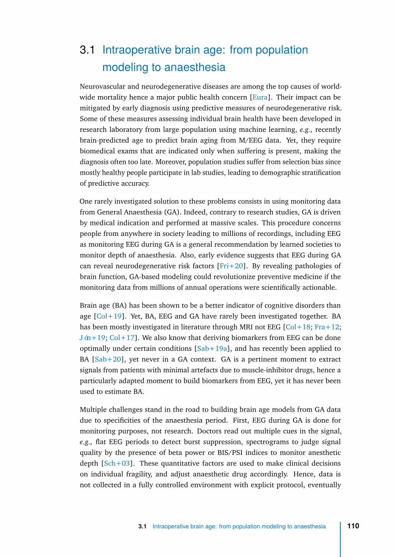
3.1 Intraoperative brain age: from populationmodeling to anaesthesia

Neurovascular and neurodegenerative diseases are among the top causes of world-wide mortality hence a major public health concern [Eura]. Their impact can bemitigated by early diagnosis using predictive measures of neurodegenerative risk.Some of these measures assessing individual brain health have been developed inresearch laboratory from large population using machine learning, e.g., recentlybrain-predicted age to predict brain aging from M/EEG data. Yet, they requirebiomedical exams that are indicated only when suffering is present, making thediagnosis often too late. Moreover, population studies suffer from selection bias sincemostly healthy people participate in lab studies, leading to demographic stratificationof predictive accuracy.

One rarely investigated solution to these problems consists in using monitoring datafrom General Anaesthesia (GA). Indeed, contrary to research studies, GA is drivenby medical indication and performed at massive scales. This procedure concernspeople from anywhere in society leading to millions of recordings, including EEGas monitoring EEG during GA is a general recommendation by learned societies tomonitor depth of anaesthesia. Also, early evidence suggests that EEG during GAcan reveal neurodegenerative risk factors [Fri+20]. By revealing pathologies ofbrain function, GA-based modeling could revolutionize preventive medicine if themonitoring data from millions of annual operations were scientifically actionable.

Brain age (BA) has been shown to be a better indicator of cognitive disorders thanage [Col+19]. Yet, BA, EEG and GA have rarely been investigated together. BAhas been mostly investigated in literature through MRI not EEG [Col+18; Fra+12;Jón+19; Col+17]. We also know that deriving biomarkers from EEG can be doneoptimally under certain conditions [Sab+19a], and has recently been applied toBA [Sab+20], yet never in a GA context. GA is a pertinent moment to extractsignals from patients with minimal artefacts due to muscle-inhibitor drugs, hence aparticularly adapted moment to build biomarkers from EEG, yet it has never beenused to estimate BA.

Multiple challenges stand in the road to building brain age models from GA datadue to specificities of the anaesthesia period. First, EEG during GA is done formonitoring purposes, not research. Doctors read out multiple cues in the signal,e.g., flat EEG periods to detect burst suppression, spectrograms to judge signalquality by the presence of beta power or BIS/PSI indices to monitor anestheticdepth [Sch+03]. These quantitative factors are used to make clinical decisionson individual fragility, and adjust anaesthetic drug accordingly. Hence, data isnot collected in a fully controlled environment with explicit protocol, eventually

3.1 Intraoperative brain age: from population modeling to anaesthesia 110

Page 116

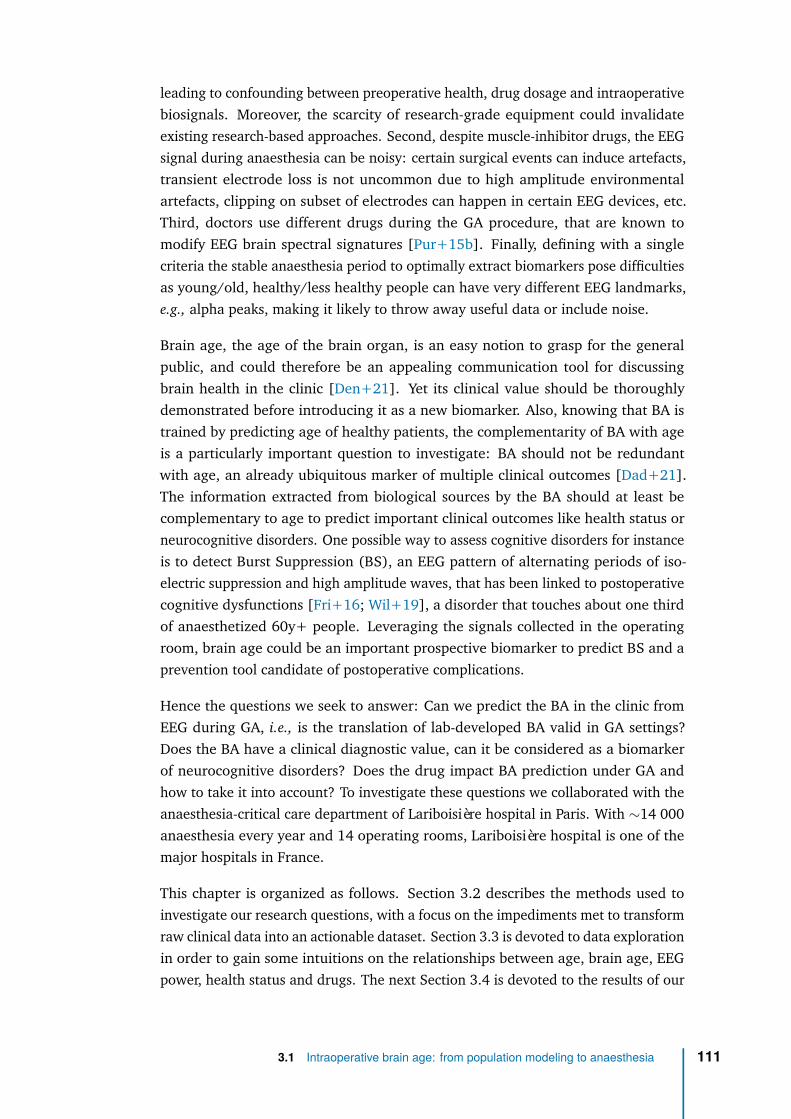
leading to confounding between preoperative health, drug dosage and intraoperativebiosignals. Moreover, the scarcity of research-grade equipment could invalidateexisting research-based approaches. Second, despite muscle-inhibitor drugs, the EEGsignal during anaesthesia can be noisy: certain surgical events can induce artefacts,transient electrode loss is not uncommon due to high amplitude environmentalartefacts, clipping on subset of electrodes can happen in certain EEG devices, etc.Third, doctors use different drugs during the GA procedure, that are known tomodify EEG brain spectral signatures [Pur+15b]. Finally, defining with a singlecriteria the stable anaesthesia period to optimally extract biomarkers pose difficultiesas young/old, healthy/less healthy people can have very different EEG landmarks,e.g., alpha peaks, making it likely to throw away useful data or include noise.

Brain age, the age of the brain organ, is an easy notion to grasp for the generalpublic, and could therefore be an appealing communication tool for discussingbrain health in the clinic [Den+21]. Yet its clinical value should be thoroughlydemonstrated before introducing it as a new biomarker. Also, knowing that BA istrained by predicting age of healthy patients, the complementarity of BA with ageis a particularly important question to investigate: BA should not be redundantwith age, an already ubiquitous marker of multiple clinical outcomes [Dad+21].The information extracted from biological sources by the BA should at least becomplementary to age to predict important clinical outcomes like health status orneurocognitive disorders. One possible way to assess cognitive disorders for instanceis to detect Burst Suppression (BS), an EEG pattern of alternating periods of iso-electric suppression and high amplitude waves, that has been linked to postoperativecognitive dysfunctions [Fri+16; Wil+19], a disorder that touches about one thirdof anaesthetized 60y+ people. Leveraging the signals collected in the operatingroom, brain age could be an important prospective biomarker to predict BS and aprevention tool candidate of postoperative complications.

Hence the questions we seek to answer: Can we predict the BA in the clinic fromEEG during GA, i.e., is the translation of lab-developed BA valid in GA settings?Does the BA have a clinical diagnostic value, can it be considered as a biomarkerof neurocognitive disorders? Does the drug impact BA prediction under GA andhow to take it into account? To investigate these questions we collaborated with theanaesthesia-critical care department of Lariboisière hospital in Paris. With ∼14 000anaesthesia every year and 14 operating rooms, Lariboisière hospital is one of themajor hospitals in France.

This chapter is organized as follows. Section 3.2 describes the methods used toinvestigate our research questions, with a focus on the impediments met to transformraw clinical data into an actionable dataset. Section 3.3 is devoted to data explorationin order to gain some intuitions on the relationships between age, brain age, EEGpower, health status and drugs. The next Section 3.4 is devoted to the results of our

3.1 Intraoperative brain age: from population modeling to anaesthesia 111

Page 117

study, answering each of our three scientific questions: Section 3.4.1 the feasibilityof clinical translation of BA to GA-settings, Section 3.4.2 the validation of modelpredictions against the occurrence of BS, and Section 3.4.3 the impact of GA drugson BA prediction. Section 3.5 proposes a discussion on the results and a perspectiveon future work.

3.1 Intraoperative brain age: from population modeling to anaesthesia 112

Page 118

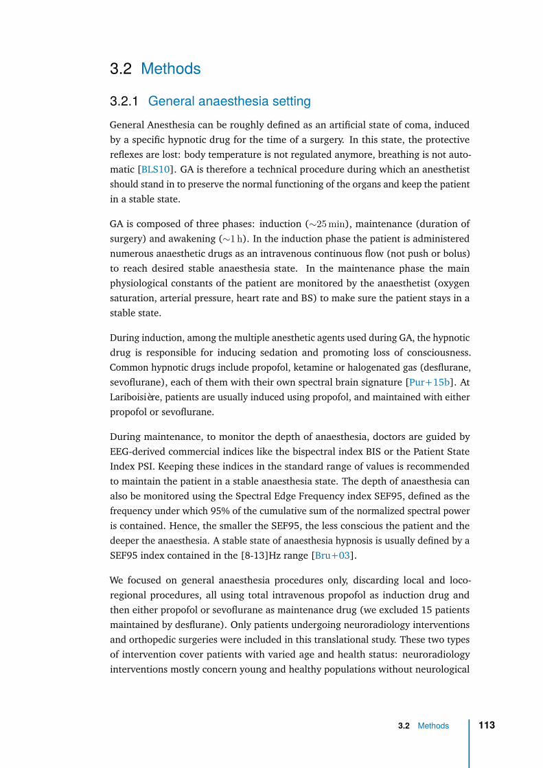
3.2 Methods

3.2.1 General anaesthesia settingGeneral Anesthesia can be roughly defined as an artificial state of coma, inducedby a specific hypnotic drug for the time of a surgery. In this state, the protectivereflexes are lost: body temperature is not regulated anymore, breathing is not auto-matic [BLS10]. GA is therefore a technical procedure during which an anesthetistshould stand in to preserve the normal functioning of the organs and keep the patientin a stable state.

GA is composed of three phases: induction (∼25 min), maintenance (duration ofsurgery) and awakening (∼1 h). In the induction phase the patient is administerednumerous anaesthetic drugs as an intravenous continuous flow (not push or bolus)to reach desired stable anaesthesia state. In the maintenance phase the mainphysiological constants of the patient are monitored by the anaesthetist (oxygensaturation, arterial pressure, heart rate and BS) to make sure the patient stays in astable state.

During induction, among the multiple anesthetic agents used during GA, the hypnoticdrug is responsible for inducing sedation and promoting loss of consciousness.Common hypnotic drugs include propofol, ketamine or halogenated gas (desflurane,sevoflurane), each of them with their own spectral brain signature [Pur+15b]. AtLariboisière, patients are usually induced using propofol, and maintained with eitherpropofol or sevoflurane.

During maintenance, to monitor the depth of anaesthesia, doctors are guided byEEG-derived commercial indices like the bispectral index BIS or the Patient StateIndex PSI. Keeping these indices in the standard range of values is recommendedto maintain the patient in a stable anaesthesia state. The depth of anaesthesia canalso be monitored using the Spectral Edge Frequency index SEF95, defined as thefrequency under which 95% of the cumulative sum of the normalized spectral poweris contained. Hence, the smaller the SEF95, the less conscious the patient and thedeeper the anaesthesia. A stable state of anaesthesia hypnosis is usually defined by aSEF95 index contained in the [8-13]Hz range [Bru+03].

We focused on general anaesthesia procedures only, discarding local and loco-regional procedures, all using total intravenous propofol as induction drug andthen either propofol or sevoflurane as maintenance drug (we excluded 15 patientsmaintained by desflurane). Only patients undergoing neuroradiology interventionsand orthopedic surgeries were included in this translational study. These two typesof intervention cover patients with varied age and health status: neuroradiologyinterventions mostly concern young and healthy populations without neurological

3.2 Methods 113

Page 119

antecedents, orthopedic surgeries are more often performed on aged patients knownfor cognitive disorders.

3.2.2 Data collectionCerebral activity during GA was monitored using Masimo device with a 4-frontalelectrodes EEG montage (Fp1, Fp2, F7 and F8), sampled at 63 Hz by default. EEGcap is placed on the patient’s scalp a few minutes before injection of the drugs andremoved at the end of anaesthesia. Peroperative EEG data are then extracted fromthe device, anonymized and stored on a file server in EDF format. APHP securitypolicy enforced a restricted access to this private and secured server, only accessiblefrom the Lariboisière local network to a small number of individuals. Each EDF file iscompletely anonymized and stored under a directory named after the correspondingoperating room. Because of this anonymization procedure we had to match eachpatient with its EDF files using only the date/time of surgery and the name of theoperating room, recorded in a separate file.

We also had access to non-EEG information collected during the mandatory anaesthesia-specific medical consultation, including demographic data (age, gender, weight,height, BMI), clinical information (type of surgery, type of anaesthesia, type ofdrug, ASA score, blood pressure) and medical information (neurological and cardio-vascular antecedents, neurological and cardiovascular treatments, cardiovascularrisk factors). These binary medical scores were either too scarcely collected or toounbalanced to be used in our statistical study. By contrast the ASA score ∈ {1, 2, 3},a standardized score indicating preoperative physical health status (the lower thehealthier), was more systematically collected. We also had access to informationmanually recorded by anesthetists during the intervention, among which the quan-tity and timing of administered drugs, timing of specific events and peroperativevariables. Nevertheless, lack of digitization prevented us from easily using thisinformation.

To detect iso-electrical suppressions (first part of the BS pattern) from intraoperativeEEG we adapted the method from [Car+19]. For each EEG, a trained clinicianidentified intraoperative periods based on the alpha-band. From this intraoperativeEEG signal S(t), we first discarded flat artifacts searching for segments below0.1 µV amplitude, lasting at least 1 s. Similarly, periods of high amplitude voltageabove 80 µV were also removed. To anticipate possible amplitude drift during theintervention, we rescaled the signal by first computing a rolling standard deviationover 30 s-long time windows Sstd(t), then building S(t) = S(t)

(1 + 2 ⟨Sstd(t)⟩

Sstd(t)

)/3 ,

where ⟨·⟩ indicates the temporal mean. A mask was constructed based on regionswhere |S(t)| < 2.5 µV, then we applied in series a 0.2 s erosion, a 1 s dilation and an0.8 s erosion. This output was used to estimate time and fraction of time spent in iso-electrical suppression during the entire intraoperative period including the induction

3.2 Methods 114

Page 120

(the first 25 min) and the maintenance phasess (after 25 min). We focused on themaintenance period for the better statistical properties of the signal (more samplesdue to a longer period, closer to stationarity and less artefacts) and potentially lowerfalse positive rate (drug-induced BS can arise at induction more often). However, thislengthy period is also more prone to confounding effects of drugs used to stabilizethe patient’s vital signs. Once detected, these episodes of iso-electrical suppressionswere automatically discarded from the signal via artefact rejection, hence never usedin subsequent steps including feature extraction and modeling.

3.2.3 Data curationNeuroscience data provided by research consortia are usually cleaned, processedand curated before made public, which facilitates further analysis. In this study, wedirectly worked with raw clinical data, originally collected for monitoring purposes.High quality monitoring is indeed the priority of anaesthetists to guarantee thequality of the GA procedure in a highly controlled clinical environment. To reusethe data for research purposes, an essential part of my thesis work was to develop adata curation strategy.

First, since the EEG data acquisition process has not been carried out to answera dedicated research question, the conditions of data collection were not ideallycontrolled, which is common in this situation. Doctors used different strategies toadminister propofol. Manual infusion consists in injecting a single dose of drug(bolus) and monitoring some physiological constants (heart rate, arterial pressure)for potential adjustments. Target Controlled Infusion (TCI) leverages modern syringedrivers that administer the drug continuously and automatically so that the cerebralconcentration saturates at a desired target value, using only age and weight as input.Stable Anaesthesia requirement let the doctor decide the dosage to meet a certaincriteria like SEF95 index in the [8-13]Hz range or to compensate for perceivedresistance to anaesthesia. Besides intervention in drug administration, we had todeal with other impediments in the data acquisition process. Some recordings failedfor practical reasons resulting in several small unusable EDF files. Some metadatawas lost as some students, helping with the process, used their own Excel templatefor their thesis with different formats, which ended up not being consolidated withthe main metadata file. Finally, the file server storing EEG data was not ideallyorganized, with inconsistent directory naming structure, duplicated patients underdifferent directories, nested patient directories, ghost directories containing patientsoperated in an unreported room number, etc. To mitigate this last obstacle, largelyunavoidable, the Lariboisière team developed a script running every day on the fileserver and providing an updated view on all EDF files in a searchable database. Adedicated script has also been developed to match each patient with its EDF filesfolder. Finally, we assigned a unique identifier to each patient for each visit at the

3.2 Methods 115

Page 121

hospital, as it is important to distinguish between two visits of the same patient,which can then present different characteristics (age, health status, etc.).

Regarding the EEG data quality, we also had to overcome multiple obstacles. Masimodevices impose a maximum file size to each recorded EDF file, leading to multipleEDF files per patient. The concatenation of these files was non-trivial because oftwo reasons. First, the data collection procedure led to excluding patients associatedwith only one EDF file of small size (considered as recording failure) and patientswith multiple files but whose first and second file are incomplete. For the remainingpatients we excluded the first file if it was incomplete and if the second file isat least 80% of its max size (a symptom that the device has been unplugged forsome reason, generally to facilitate the device transfer between the induction andoperating room). Second, the EEG device used in the operating room has not beendesigned for research but for monitoring usage. Hence the raw data it recordsstrictly follows data visualized on its screen. For instance, if the extreme traces onthe visualisation screen (which corresponded to the two electrodes Fp1 and F8)were clipped, the recorded raw data were also clipped. The raw data are thereforemodified whenever the device operator changes the visualization settings. Hence, thecalibration factor between two consecutive files could be different due to Masimo’soperator changing y-scale on the monitor, e.g., to avoid clipping of the extreme rawEEG traces during recording. For this reason we also excluded files that do not havethe same calibration factor than the first file in order to avoid error at concatenation.Finally the remaining files were downsampled to a common sampling frequency of63Hz before concatenation. The downsampling was necessary because samplingfrequency could change between two consecutive files due to Masimo’s operatorchanging x-scale on monitor during recording.

Regarding the metadata collection process, these data were recorded by hand byeach medical doctor on a paper sheet, before being further consolidated in an Excelfile. This process inevitably led to missing values: the anesthetists helped us to gothrough the archive department of the hospital and look at the paper record of a fewdozens of patients one by one to retrieve their drugs and their ASA score. We alsoencountered incorrect values (e.g., due to a change of convention between cohorts inthe encoding of the gender attribute), inconsistent values (e.g., some patients havingtwo different maintenance drugs, which could go unnoticed when filtering for thepresence of a particular drug), and finally unnormalized values (e.g., the letter O inplace of the number 0). These errors were corrected by hand, which is a commonreality in clinical settings. As a side note of interest, the growing number of researchprojects within the anaesthetists team has recently led to the hiring of a dedicateddata manager, leading the data curation effort.

Finally, from the 518 patients with demographic information, 473 underwent general(and not loco-regional) anaesthesia among which 435 had their maintenance drug

3.2 Methods 116

Page 122

informed. Among those patients, 348 had a successful EDF-files matching and 345with successful EDF files concatenation, leading to a dataset of 345 patients withboth a proper concatenated EEG recording (in FIF format) and metadata information.Finally we converted the resulting EEG dataset into the standard and anonymizedBIDS format [Per+19] with EDF files in Brainvision format using the MNE-BIDSPython library [App+19]. The statistics of the cohort is summarized in Table 3.1,along with a stratified view by the grouping variable ASA and drug.

3.2.4 Data processing and feature extractionThe data processing has been carried out using ‘mne-bids-pipeline’ (https://mne.tools/mne-bids-pipeline/). This tool is not a Python library but a suite of Pythonscripts that generate processed data in a FIF format from BIDS files. Processinginstructions are contained in a single configuration file that can be tailored toparticular needs. For our study, we minimally used it to generate epochs: for everypatient, the signal is epoched into 60 s sliding windows shifted by 10 s.

Intermediate power representations of the signal were computed using the open-source Python library ‘Coffeine’ (https://github.com/coffeine-labs/coffeine).In each window, the power spectral density, the covariance matrices and the cross-frequency covariance matrix are averaged across internal Hamming windows of8 s shifted by 4 s. The power spectral density was estimated in 244 frequency binsbetween 0 and 32 Hz and its averaging has been further robustified by trimmingdistribution from both tails at 25 % cutoff. The covariance matrices of the fourEEG channels are estimated using the ‘OAS’ shrinkage method[Che+10] in eachof five frequency bands as described in Table 3.2 leading to five 4 × 4 matrices.The cross-frequency covariance matrix is the covariance matrix of the 20 ‘virtual’channels constructed from each four real channels filtered in each five frequencybands, leading to a single 20 × 20 matrix. This matrix allows to investigate couplingbetween frequency bands, while still enjoying the same mathematical guaranteesobtained in Chapter 1 as it is a covariance matrix. Besides these covariance features,EEG-characteristics commonly used to judge the signal quality during monitoringare also computed: the SEF95 index and the maximum peak-to-peak amplitude, asthey are used to perform epochs-selection.

Epochs with peak-to-peak amplitude lower than 0.1 µV on any one electrode werediscarded on all electrodes, avoiding learning from BS periods or clipped segments.Epochs are then selected within the stable anaesthesia period, defined by the SEF95index belonging to the [8-13]Hz range. We focused on the longest period of consec-utive epochs of stable anaesthesia using the average SEF95 across the 4 channels,which gave better results than concatenating all epochs satisfying the SEF95 con-straint. The PSD, the covariance matrices and the cross-frequency covariance matrix

3.2 Methods 117

Page 123

Overall (N=330)Age

Mean (SD) 54.41 (19.43)Median (Q1, Q3) 56.00 (37.25, 69.00)Min - Max 16.00 - 99.00Missing 0

Genderfemale 213 (64.5%)male 117 (35.5%)Missing 0

HeightMean (SD) 167.58 (9.74)Median (Q1, Q3) 168.00 (160.00, 174.00)Min - Max 123.00 - 195.00Missing 4

WeightMean (SD) 74.39 (17.27)Median (Q1, Q3) 73.00 (60.00, 85.00)Min - Max 37.00 - 145.00Missing 6

BMIMean (SD) 26.35 (6.52)Median (Q1, Q3) 25.39 (22.32, 29.54)Min - Max 0.00 - 54.20Missing 8

ASAASA1 69 (21.3%)ASA2 185 (57.1%)ASA3 70 (21.6%)Missing 6

Neurological AntecedentsNo 162 (68.4%)Yes 75 (31.6%)Missing 93

Cardiovascular AntecedentsNo 194 (87.4%)Yes 28 (12.6%)Missing 108

Cardiovascular Risk FactorNo 109 (42.1%)Yes 150 (57.9%)Missing 71

Cardiovascular TreatmentNo 151 (64.3%)Yes 84 (35.7%)Missing 95

Neurological TreatmentNo 175 (80.6%)Yes 42 (19.4%)Missing 113

Drugpropofol 220 (66.7%)sevoflurane 110 (33.3%)Missing 0

Prop. time spent in BS during inductionMean (SD) 4.74 (9.55)Median (Q1, Q3) 0.96 (0.08, 4.14)Min - Max 0.00 - 72.09Missing 20

Prop. time spent in BS during maintenanceMean (SD) 3.65 (7.85)Median (Q1, Q3) 0.62 (0.05, 3.33)Min - Max 0.00 - 77.17Missing 20

Tab. 3.1: Descriptive summary statistics table of Lariboisière data.

3.2 Methods 118

Page 124

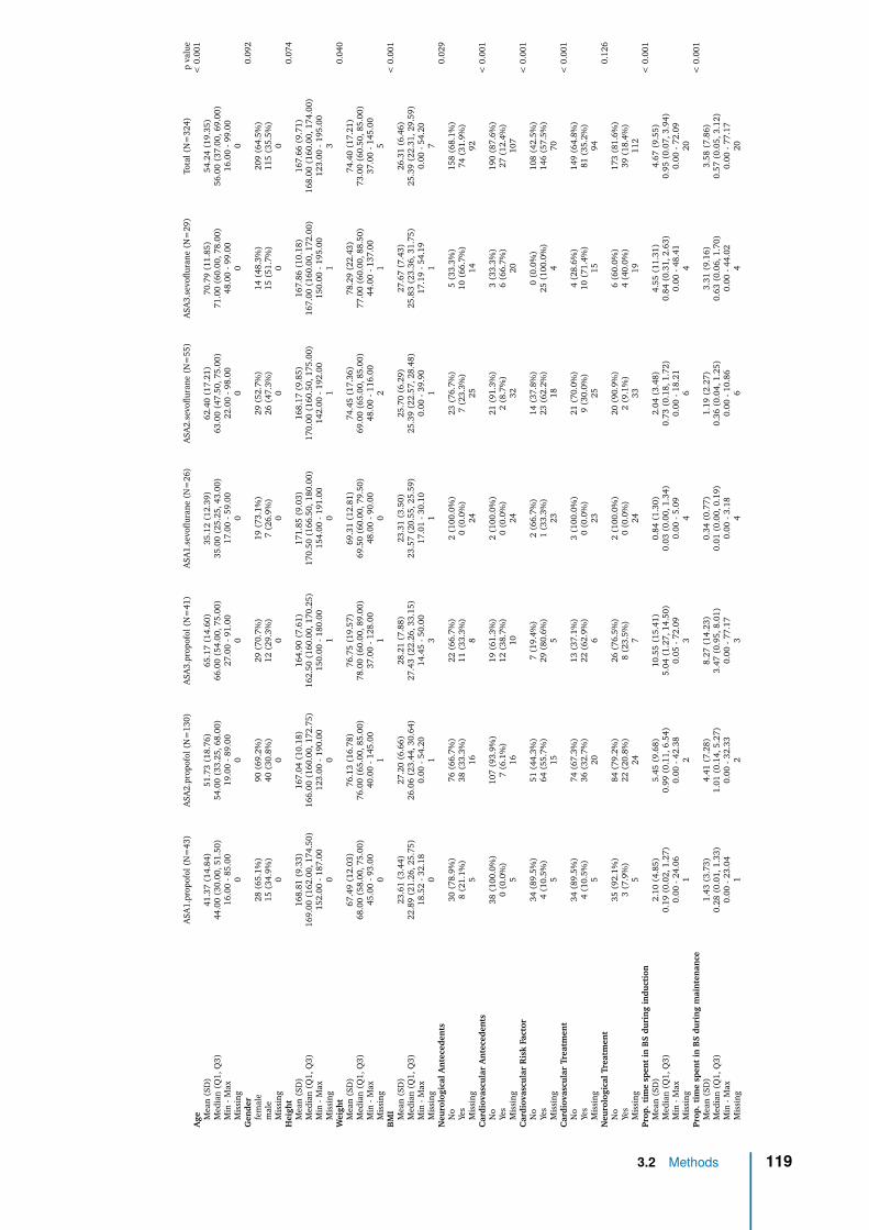
ASA

1.pr

opof

ol(N

=43

)A

SA2.

prop

ofol

(N=

130)

ASA

3.pr

opof

ol(N

=41

)A

SA1.

sevo

flura

ne(N

=26

)A

SA2.

sevo

flura

ne(N

=55

)A

SA3.

sevo

flura

ne(N

=29

)To

tal(

N=

324)

pva

lue

Age

<0.

001

Mea

n(S

D)

41.3

7(1

4.84

)51

.73

(18.

76)

65.1

7(1

4.60

)35

.12

(12.

39)

62.4

0(1

7.21

)70

.79

(11.

85)

54.2

4(1

9.35

)M

edia

n(Q

1,Q

3)44

.00

(30.

00,5

1.50

)54

.00

(33.

25,6

8.00

)66

.00

(54.

00,7

5.00

)35

.00

(25.

25,4

3.00

)63

.00

(47.

50,7

5.00

)71

.00

(60.

00,7

8.00

)56

.00

(37.

00,6

9.00

)M

in-M

ax16

.00

-85.

0019

.00

-89.

0027

.00

-91.

0017

.00

-59.

0022

.00

-98.

0048

.00

-99.

0016

.00

-99.

00M

issi

ng0

00

00

00

Gen

der

0.09

2fe

mal

e28

(65.

1%)

90(6

9.2%

)29

(70.

7%)

19(7

3.1%

)29

(52.

7%)

14(4

8.3%

)20

9(6

4.5%

)m

ale

15(3

4.9%

)40

(30.

8%)

12(2

9.3%

)7

(26.

9%)

26(4

7.3%

)15

(51.

7%)

115

(35.

5%)

Mis

sing

00

00

00

0H

eigh

t0.

074

Mea

n(S

D)

168.

81(9

.33)

167.

04(1

0.18

)16

4.90

(7.6

1)17

1.85

(9.0

3)16

8.17

(9.8

5)16

7.86

(10.

18)

167.

66(9

.71)

Med

ian

(Q1,

Q3)

169.

00(1

62.0

0,17

4.50

)16

6.00

(160

.00,

172.

75)

162.

50(1

60.0

0,17

0.25

)17

0.50

(166

.50,

180.

00)

170.

00(1

60.5

0,17

5.00

)16

7.00

(160

.00,

172.

00)

168.

00(1

60.0

0,17

4.00

)M

in-M

ax15

2.00

-187

.00

123.

00-1

90.0

015

0.00

-180

.00

154.

00-1

91.0

014

2.00

-192

.00

150.

00-1

95.0

012

3.00

-195

.00

Mis

sing

00

10

11

3W

eigh

t0.

040

Mea

n(S

D)

67.4

9(1

2.03

)76

.13

(16.

78)

76.7

5(1

9.57

)69

.31

(12.

81)

74.4

5(1

7.36

)78

.29

(22.

43)

74.4

0(1

7.21

)M

edia

n(Q

1,Q

3)68

.00

(58.

00,7

5.00

)76

.00

(65.

00,8

5.00

)78

.00

(60.

00,8

9.00

)69

.50

(60.

00,7

9.50

)69

.00

(65.

00,8

5.00

)77

.00

(60.

00,8

8.50

)73

.00

(60.

50,8

5.00

)M

in-M

ax45

.00

-93.

0040

.00

-145

.00

37.0

0-1

28.0

048

.00

-90.

0048

.00

-116

.00

44.0

0-1

37.0

037

.00

-145

.00

Mis

sing

01

10

21

5B

MI

<0.

001

Mea

n(S

D)

23.6

1(3

.44)

27.2

0(6

.66)

28.2

1(7

.88)

23.3

1(3

.50)

25.7

0(6

.29)

27.6

7(7

.43)

26.3

1(6

.46)

Med

ian

(Q1,

Q3)

22.8

9(2

1.26

,25.

75)

26.0

6(2

3.44

,30.

64)

27.4

3(2

2.26

,33.

15)

23.5

7(2

0.55

,25.

59)

25.3

9(2

2.57

,28.

48)

25.8

3(2

3.36

,31.

75)

25.3

9(2

2.31

,29.

59)

Min

-Max

18.5

2-3

2.18

0.00

-54.

2014

.45

-50.

0017

.01

-30.

100.

00-3

9.90

17.1

9-5

4.19

0.00

-54.

20M

issi

ng0

13

11

17

Neu

rolo

gica

lAn

tece

den

ts0.

029

No

30(7

8.9%

)76

(66.

7%)

22(6

6.7%

)2

(100

.0%

)23

(76.

7%)

5(3

3.3%

)15

8(6

8.1%

)Ye

s8

(21.

1%)

38(3

3.3%

)11

(33.

3%)

0(0

.0%

)7

(23.

3%)

10(6

6.7%

)74

(31.

9%)

Mis

sing

516

824

2514

92C

ardi

ovas

cula

rA

nte

cede

nts

<0.

001

No

38(1

00.0

%)

107

(93.

9%)

19(6

1.3%

)2

(100

.0%

)21

(91.

3%)

3(3

3.3%

)19

0(8

7.6%

)Ye

s0

(0.0

%)

7(6

.1%

)12

(38.

7%)

0(0

.0%

)2

(8.7

%)

6(6

6.7%

)27

(12.

4%)

Mis

sing

516

1024

3220

107

Car

diov

ascu

lar

Ris

kFa

ctor

<0.

001

No

34(8

9.5%

)51

(44.

3%)

7(1

9.4%

)2

(66.

7%)

14(3

7.8%

)0

(0.0

%)

108

(42.

5%)

Yes

4(1

0.5%

)64

(55.

7%)

29(8

0.6%

)1

(33.

3%)

23(6

2.2%

)25

(100

.0%

)14

6(5

7.5%

)M

issi

ng5

155

2318

470

Car

diov

ascu

lar

Trea

tmen

t<

0.00

1N

o34

(89.

5%)

74(6

7.3%

)13

(37.

1%)

3(1

00.0

%)

21(7

0.0%

)4

(28.

6%)

149

(64.

8%)

Yes

4(1

0.5%

)36

(32.

7%)

22(6

2.9%

)0

(0.0

%)

9(3

0.0%

)10

(71.

4%)

81(3

5.2%

)M

issi

ng5

206

2325

1594

Neu

rolo

gica

lTre

atm

ent

0.12

6N

o35

(92.

1%)

84(7

9.2%

)26

(76.

5%)

2(1

00.0

%)

20(9

0.9%

)6

(60.

0%)

173

(81.

6%)

Yes

3(7

.9%

)22

(20.

8%)

8(2

3.5%

)0

(0.0

%)

2(9

.1%

)4

(40.

0%)

39(1

8.4%

)M

issi

ng5

247

2433

1911

2Pr

op.

tim

esp

ent

inB

Sdu

rin

gin

duct

ion

<0.

001

Mea

n(S

D)

2.10

(4.8

5)5.

45(9

.68)

10.5

5(1

5.41

)0.

84(1

.30)

2.04

(3.4

8)4.

55(1

1.31

)4.

67(9

.55)

Med

ian

(Q1,

Q3)

0.19

(0.0

2,1.

27)

0.99

(0.1

1,6.

54)

5.04

(1.2

7,14

.50)

0.03

(0.0

0,1.

34)

0.73

(0.1

8,1.

72)

0.84

(0.3

1,2.

63)

0.95

(0.0

7,3.

94)

Min

-Max

0.00

-24.

060.

00-4

2.38

0.05

-72.

090.

00-5

.09

0.00

-18.

210.

00-4

8.41

0.00

-72.

09M

issi

ng1

23

46

420

Prop

.ti

me

spen

tin

BS

duri

ng

mai

nte

nan

ce<

0.00

1M

ean

(SD

)1.

43(3

.73)

4.41

(7.2

8)8.

27(1

4.23

)0.

34(0

.77)

1.19

(2.2

7)3.

31(9

.16)

3.58

(7.8

6)M

edia

n(Q

1,Q

3)0.

28(0

.01,

1.33

)1.

01(0

.14,

5.27

)3.

47(0

.95,

8.01

)0.

01(0

.00,

0.19

)0.

36(0

.04,

1.25

)0.

63(0

.06,

1.70

)0.

57(0

.05,

3.12

)M

in-M

ax0.

00-2

3.04

0.00

-32.

330.

00-7

7.17

0.00

-3.1

80.

00-1

0.86

0.00

-44.

020.

00-7

7.17

Mis

sing

12

34

64

20

3.2 Methods 119

Page 125

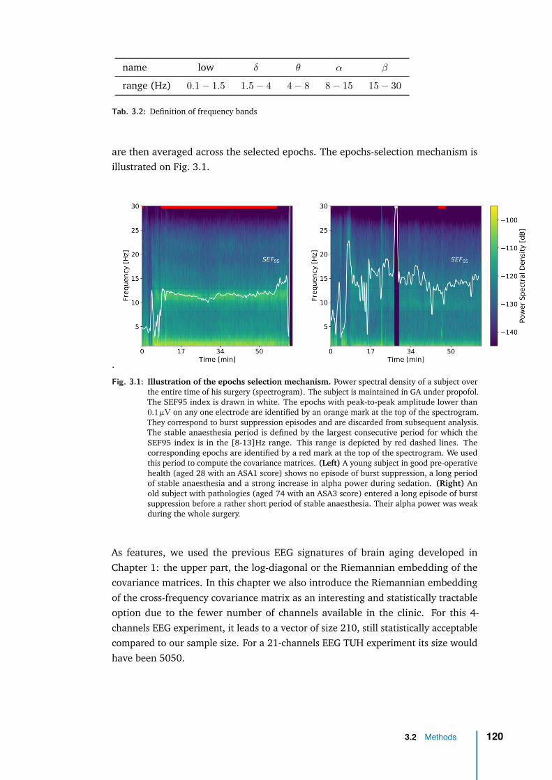
name low δ θ α β

range (Hz) 0.1 − 1.5 1.5 − 4 4 − 8 8 − 15 15 − 30

Tab. 3.2: Definition of frequency bands

are then averaged across the selected epochs. The epochs-selection mechanism isillustrated on Fig. 3.1.

.

Fig. 3.1: Illustration of the epochs selection mechanism. Power spectral density of a subject overthe entire time of his surgery (spectrogram). The subject is maintained in GA under propofol.The SEF95 index is drawn in white. The epochs with peak-to-peak amplitude lower than0.1 µV on any one electrode are identified by an orange mark at the top of the spectrogram.They correspond to burst suppression episodes and are discarded from subsequent analysis.The stable anaesthesia period is defined by the largest consecutive period for which theSEF95 index is in the [8-13]Hz range. This range is depicted by red dashed lines. Thecorresponding epochs are identified by a red mark at the top of the spectrogram. We usedthis period to compute the covariance matrices. (Left) A young subject in good pre-operativehealth (aged 28 with an ASA1 score) shows no episode of burst suppression, a long periodof stable anaesthesia and a strong increase in alpha power during sedation. (Right) Anold subject with pathologies (aged 74 with an ASA3 score) entered a long episode of burstsuppression before a rather short period of stable anaesthesia. Their alpha power was weakduring the whole surgery.

As features, we used the previous EEG signatures of brain aging developed inChapter 1: the upper part, the log-diagonal or the Riemannian embedding of thecovariance matrices. In this chapter we also introduce the Riemannian embeddingof the cross-frequency covariance matrix as an interesting and statistically tractableoption due to the fewer number of channels available in the clinic. For this 4-channels EEG experiment, it leads to a vector of size 210, still statistically acceptablecompared to our sample size. For a 21-channels EEG TUH experiment its size wouldhave been 5050.

3.2 Methods 120

Page 126

As a side note of interest, feature extraction was performed using the open-sourcePython library ‘Coffeine’ (https://github.com/coffeine-labs/coffeine) we de-veloped in the team as a result of this thesis. I contributed the core features of thislibrary implementing all the methods developed during my PhD and presented in ourarticles [Sab+19a; Sab+20; Eng+20]. In particular, this library provides a high-levelinterface to the predictive modeling techniques we developed and presented in 2using the M/EEG covariance matrix as representation of the signal.

3.2.5 Machine learning and statistical modelingFor the age prediction task of this Lariboisière experiment, we will benchmark theregression algorithms previously introduced in Chapter 1 i.e., simple regularizedlinear regression model (ridge regression) applied to particular vectorizations ofthe covariance matrices: its upper part (‘upper’ model), its log-diagonal (‘log-diag’model), its Riemannian embedding (‘Riemann’ model) and the Riemannian em-bedding of the cross-frequency covariance matrix, as defined in Section 3.2.4. TheRiemannian model was defined with no projection step since the covariance matricesare here full rank. Indeed, they are estimated from sufficiently large chunk of signalsand are not rank-reduced by preprocessing steps (see Chapter 1). Classical EEGaverage reference, that amounts to projecting the signal into the subspace orthogonalto the average signal, reduces the rank by one, but is not used in this study. Theregularization parameter of ridge is tuned by generalized cross-validation [GHW79]on a logarithmic grid of 100 values in [10−5, 103] on each training fold of a 10-foldcross-validation loop. For each model we standardized the features enforcing zeromean and unit variance, a standard preprocessing step for penalized linear mod-els. To compare models against chance, we estimated the chance-level empiricallythrough the performance of a dummy-regressor predicting the mean outcome ofthe training data without trying to find patterns, thus equivalent to random guess.Uncertainty estimation was obtained from the cross-validation distribution.

Note that formal hypothesis testing for model comparison was not available for anyof the datasets analyzed as this would have required several datasets, such thateach average cross-validation score would have made one observation. For dataexploration and statistical modeling, we used standard classical two-sample statisti-cal tests: Welch two sample t-test of difference means for continuous/categoricalvariables and Pearson’s chi2 of independence for categorical/categorical variables.

To assess the impact of drug on BA estimation we compared the performance of ourbrain age model when learning from two different drugs (propofol or sevoflurane).To investigate their cross-effects, we developed different classes of models. Drug-specific models learn from patients under one drug and predict on patients under thesame (propo/propo, sevo/sevo). The drug-agnostic model learns and predicts fromall patients without being informed on their drug (all/all). Drug-crossed models

3.2 Methods 121

Page 127

learn from patients under one drug and predict age of patients under the other(propo/sevo or sevo/propo). Drug-aware models learn jointly from all patients withdrug-interaction effects and predict on either drug (joint/propo, joint/sevo): theylearn a compromise between a global model that ignores drugs, and a specific modelhandling exceptions for the drugs, leveraging what the two drugs have in common.Drug-specific models and the drug-agnostic model are simple restrictions of ourmodel to different sub-populations. To compute CV-based uncertainty estimates ofthe performance of drug-crossed models, we splitted the training population into 10folds (with shuffling), trained the model on 9 folds and tested this fitted model onthe all testing population. This allows to probe the variance due to random trainingpopulation. To implement the drug-aware model (joint model with interaction effect)we expanded the original p-feature vector to a new (2p+ 1)-feature vector wherethe first p features are the original features, then the drug indicator variable (1 forpropofol, 0 for sevoflurane) then the product between the two, leading to eithera copy of the p features if propofol or a p-vector of zeros if sevoflurane. All thesemodels have been implemented in the ‘Coffeine’ library.

3.2 Methods 122

Page 128

3.3 Data explorationBefore diving into predictive modeling we visualized our sample to explore the linkbetween EEG during stable anaesthesia and age: is the age indeed visible in thebrain? The effect of age on EEG-brain signals could nevertheless be confounded byexternal factors.

We identified two major potential confounders: the health status and the mainte-nance drug. Intuitively, the health status is likely to be associated to both the age andthe EEG power, which has been confirmed by our anaesthetists collaborators andstatistical tests. The maintenance drug has a known effect on EEG power, e.g., propo-fol induces an anteriorization of the alpha rhythm during loss of consciousness[Vij+13]. Running basic statistical analysis we also discovered its association withage: the age distribution under propofol is significantly shifted towards youngerpeople compared to sevoflurane (t=4.73 p=8.065e-06). After investigation, wediscovered that this link was not causal (the doctors confirmed the choice of main-tenance drug is not driven by age) but more likely due to random circumstances:halogenated gas happened not to be available to neuroradiology interventions whichmostly concerns young and healthy subjects. Also, the data partially originates froma study focused on propofol effect, hence the biggest proportion of this drug in oursample. In general, the still most commonly used hypnotic drugs are halogenatedgas like sevoflurane for their ease of use, which amounts to opening a valve, andtheir lighter monitoring requirement. Yet propofol allows for a quicker and finercontrol of the anaesthetic state via TCI with a cleaner and more stable EEG spectralsignature [Pur+15b], hence was most commonly used in our study. We’ll thereforelook at how the EEG-age relationship is shifted by ASA and by drug, and run basicstatistical tests to assess whether these relationships are likely to generalize to thepopulation.

In Fig. 3.2 we explore how the link between EEG and age is modulated by healthstatus.

3.3 Data exploration 123

Page 129

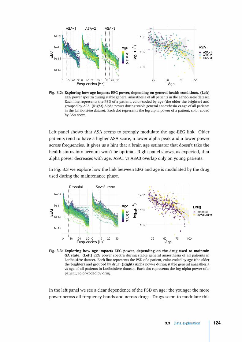
Fig. 3.2: Exploring how age impacts EEG power, depending on general health conditions. (Left)EEG power spectra during stable general anaesthesia of all patients in the Lariboisière dataset.Each line represents the PSD of a patient, color-coded by age (the older the brighter) andgrouped by ASA. (Right) Alpha power during stable general anaesthesia vs age of all patientsin the Lariboisière dataset. Each dot represents the log alpha power of a patient, color-codedby ASA score.

Left panel shows that ASA seems to strongly modulate the age-EEG link. Olderpatients tend to have a higher ASA score, a lower alpha peak and a lower poweracross frequencies. It gives us a hint that a brain age estimator that doesn’t take thehealth status into account won’t be optimal. Right panel shows, as expected, thatalpha power decreases with age. ASA1 vs ASA3 overlap only on young patients.

In Fig. 3.3 we explore how the link between EEG and age is modulated by the drugused during the maintenance phase.

Fig. 3.3: Exploring how age impacts EEG power, depending on the drug used to maintainGA state. (Left) EEG power spectra during stable general anaesthesia of all patients inLariboisière dataset. Each line represents the PSD of a patient, color-coded by age (the olderthe brighter) and grouped by drug. (Right) Alpha power during stable general anaesthesiavs age of all patients in Lariboisière dataset. Each dot represents the log alpha power of apatient, color-coded by drug.

In the left panel we see a clear dependence of the PSD on age: the younger the morepower across all frequency bands and across drugs. Drugs seem to modulate this

3.3 Data exploration 124

Page 130

link essentially in alpha band, with an apparent stronger power under sevoflurane.In the right panel we thus focus on the alpha log power where there seem to besystematic differences in alpha power under both drugs, confirmed by hypothesistesting (t=-2.1, p= 0.035). Also, a linear regression analysis of the alpha logpower on age gender and drug for healthy patients suggests that age and drug haveindependent (additive) effects in opposite direction but of similar magnitude: agereduces (and sevoflurane increases) power by 0.5 STD per STD (beta_age=-0.62,t=-13.8, p<2e-16 | beta_drug=0.44, t=4.7, p=4e-6). We therefore find systematicdifferences in EEG between propofol and sevoflurane, when taking age into account.It confirms that drugs may influence prediction and calls for a thorough drug impactstudy, which will be developed in the results Section 3.4.3.

3.3 Data exploration 125

Page 131

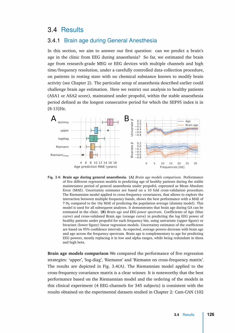
3.4 Results3.4.1 Brain age during General AnesthesiaIn this section, we aim to answer our first question: can we predict a brain’sage in the clinic from EEG during anaesthesia? So far, we estimated the brainage from research-grade MEG or EEG devices with multiple channels and hightime/frequency resolution, under a carefully controlled data collection procedure,on patients in resting state with no chemical substance known to modify brainactivity (see Chapter 2). The particular setup of anaesthesia described earlier couldchallenge brain age estimation. Here we restrict our analysis to healthy patients(ASA1 or ASA2 score), maintained under propofol, within the stable anaesthesiaperiod defined as the longest consecutive period for which the SEF95 index is in[8-13]Hz.

4 6 8 10 12 14 16 18Age prediction MAE (years)

dummy

upper

logdiag

Riemann

Riemannxfreq

0.80.60.40.20.00.2

Univ

ari

ate

Age

Brain age

0 5 10 15 20 25 30Frequencies [Hz]

0.80.60.40.20.00.2

Biv

ari

ate

A B

Fig. 3.4: Brain age during general anaesthesia. (A) Brain age models comparison. Performanceof five different regression models in predicting age of healthy patients during the stablemaintenance period of general anaesthesia under propofol, expressed as Mean AbsoluteError (MAE). Uncertainty estimates are based on a 10 fold cross-validation procedure.The Riemannian model applied to cross-frequency covariances, that allows to explore theinteraction between multiple frequency bands, shows the best performance with a MAE of7.9y, compared to the 16y MAE of predicting the population average (dummy model). Thismodel is used for all subsequent analyses. It demonstrates that brain age during GA can beestimated in the clinic. (B) Brain age and EEG power spectrum. Coefficients of Age (bluecurve) and cross-validated Brain age (orange curve) in predicting the log EEG power ofhealthy patients under propofol for each frequency bin, using univariate (upper figure) orbivariate (lower figure) linear regression models. Uncertainty estimates of the coefficientsare based on 95% confidence intervals. As expected, average powers decrease with brain ageand age across the frequency spectrum. Brain age is complementary to age for predictingEEG powers, mostly replacing it in low and alpha ranges, while being redundant in thetaand high beta.

Brain age models comparison We compared the performance of five regressionstrategies: ‘upper’, ‘log-diag’, ‘Riemann’ and ‘Riemann on cross-frequency matrix’.The results are depicted in Fig. 3.4(A). The Riemannian model applied to thecross-frequency covariance matrix is a clear winner. It is noteworthy that the bestperformance based on the Riemannian model and the ordering of the models inthis clinical experiment (4 EEG-channels for 345 subjects) is consistent with theresults obtained on the experimental datasets studied in Chapter 2: Cam-CAN (102

3.4 Results 126

Page 132

MEG magnetometers channels for 596 subjects) and for TUH (21 EEG channelsfor 1385 subjects). It is an additional and independent hint that the Riemannianmethods are the most efficient and robust models to perform M/EEG regression.This finding suggests that BA can be estimated during GA from routine monitoringEEG within the operative theater. All subsequent analyses are conducted using thebest regression model of Riemann on cross-frequency covariance.

Brain age and EEG power spectrum. Does this new measure of brain-predicted agecontain additional information on the EEG power spectrum than age? To investigatethe complementarity of age and brain age we ran a statistical linear regressionanalysis of the log EEG power in every frequency bin using the age and the brainage as predictors. Their coefficients, as a function of frequency, are reported inFig. 3.4(B).

Upper figure shows the coefficients of the two univariate linear regression models.As expected the marginal effect of age/brain age on the log powers (hence thecorrelations) are negative: the average brain power decreases with age and brainage across the frequency spectrum, the older the subject the less powerful his brainsignal. This effect is more pronounced around low and alpha frequencies. Also brainage alone is at least as correlated to EEG powers than age. Therefore, when lookingat EEG powers, anaesthetists can ‘trust’ this new biomarker as behaving similarly tothe usual marker of age. We should note that since BA itself is built from powersas features it is not surprising to see this correlation. However, the brain age asinput of this statistical model is cross-validated i.e., corresponds to the age predictedout-of-sample (see [Eng+20; HT08] for the methodology of using cross-validatedpredicted scores for statistical analysis). Also, it is predicted from only five frequencybands while we here investigate fine-grained frequency patterns in EEG powers tosee at which specific single frequency the model responds best.

These univariate models do not allow to disentangle both factors. The effect of brainage could be mainly due to the age itself. To regress out the effect of age on brainage we conducted the corresponding multiple regression analysis. Lower figureshows the coefficients of the multiple linear regression model using both age andbrain age as predictors. They are again all negative across the frequency spectrum.Importantly, when brain age is included in the model, there is no unique contributionof age to the variation of power: brain age captures all the information about brainpowers. This effect holds in the entire frequency spectrum with the exception ofthe high beta range. Therefore, brain age mostly replaces age for predicting EEGpowers.

3.4 Results 127

Page 133

3.4.2 Clinical impact of GA-based Brain ageIn this section, we aim to validate our brain age measure and answer our secondquestion: does the BA have a clinical diagnostic value of perioperative complications?

Perioperative complications are the third leading cause of mortality in the world [Nep+19],potentially affecting any person undergoing GA (today one of the most frequentprocedures in medicine, more than 300 million GA worldwide in 2020 [Csj], and 12million in France). Although anesthesia and surgery are safer than before, it remainsa risky procedure. They occur in about 25% of surgical operations involving generalanesthesia [GBD09; Khu+05] and they have a strong impact on the patients’ health:9 million per year will die within 30 days of the intervention, 66 additional millionwill die 9 years younger on average [Khu+05]. In fact, perioperative complicationshave an even greater impact on the survival rate than the preoperative conditionin major surgical operations [Khu+05]. Patients over the age of 60 are more likelyto suffer from complications, the severity of which is in general greater. This agegroup represents about one quarter of the global population – but more than 40%of all anesthetic procedures in France [Dad+15] – and will continue to grow at afast pace in the coming decades [Eurc; Eurb; Vol+20]: we expect twice more 65y+humans in 2050 than today globally [Un2].

Perioperative cognitive disorders don’t have precise definition in the US psychiatryreference manual DSM-5 classifying mental disorders, yet a possible classificationproposed by US anaesthetists and based on the DSM begins to emerge [ZLJZS+19].We can distinguish two main families. First, perioperative neurocognitive disor-ders (PND) are composed of three disorders of increasing duration of postoperativesymptoms: postoperative delirium (POD), delayed neurocognitive recovery (DNCR)previously called postoperative cognitive dysfunction POCD, and neurocognitivedisorders (NCD) that persist 30days after surgery. Second, cognitive decline (CD) isa loss of cognitive function (memory, language or thinking) not necessarily linkedto surgery, scored by a psychometric test vs an anterior baseline, e.g., by Montrealcognitive assessment (MOCA). It has recently been shown that patients experiencingCD have a higher incidence of PND [Fri+20]. Knowing patients’ cognitive statuswould therefore allow the doctors to adapt anesthesia and postoperative care. Un-fortunately, due to the large proportion of elderly patients going through GA, it isnot practical to perform the neurocognitive evaluations necessary to assess CD ona large scale in the clinic: in France, approximately one third of 50y+ patients arescheduled for surgery every year. We propose to take advantage of GA to addressthis issue and investigate if our EEG-based BA (that can be estimated in the clinicduring GA as seen in the previous section) can be used to provide an early diagnosis.

Some complications are directly related to surgery but the majority are related tothe anesthesia management. Although ML can help surgeons to better prepare for

3.4 Results 128

Page 134

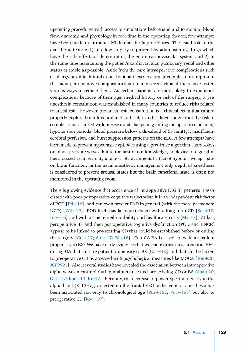
upcoming procedures with access to simulations beforehand and to monitor bloodflow, anatomy, and physiology in real-time in the operating theater, few attemptshave been made to introduce ML in anesthesia procedures. The usual role of theanesthesia team is 1) to allow surgery to proceed by administering drugs whichhave the side effects of deteriorating the entire cardiovascular system and 2) atthe same time maintaining the patient’s cardiovascular, pulmonary, renal and otherstatus as stable as possible. Aside from the rare intraoperative complications suchas allergy or difficult intubation, brain and cardiovascular complications representthe main perioperative complications and many recent clinical trials have testedvarious ways to reduce them. As certain patients are more likely to experiencecomplications because of their age, medical history or risk of the surgery, a pre-anesthesia consultation was established in many countries to reduce risks relatedto anesthesia. However, pre-anesthesia consultation is a clinical exam that cannotproperly explore brain function in detail. Pilot studies have shown that the risk ofcomplications is linked with precise events happening during the operation includinghypotension periods (blood pressure below a threshold of 65 mmHg), insufficientcerebral perfusion, and burst suppression patterns on the EEG. A few attempts havebeen made to prevent hypotensive episodes using a predictive algorithm based solelyon blood pressure waves, but to the best of our knowledge, no device or algorithmhas assessed brain viability and possible detrimental effect of hypotensive episodeson brain function. In the usual anesthetic management only depth of anesthesiais considered to prevent arousal states but the brain functional state is often notmonitored in the operating room.

There is growing evidence that occurrence of intraoperative EEG BS patterns is asso-ciated with poor postoperative cognitive trajectories: it is an independent risk factorof POD [Fri+16], and can even predict PND in general (with the more permanentNCD) [Wil+19]. POD itself has been associated with a long term CD [Sac+12;Ino+16] and with an increased morbidity and healthcare costs [Mar17]. At last,peroperative BS and then postoperative cognitive dysfunction (POD and DNCR)appear to be linked to pre-existing CD that could be established before or duringthe surgery [Cul+17; Spr+17; BI+16]. Can GA BA be used to evaluate patientpropensity to BS? We have early evidence that we can extract measures from EEGduring GA that capture patient propensity to BS [Car+19] and that can be linkedto preoperative CD as assessed with psychological measures like MOCA [Tou+20;JCPPV21]. Also, several studies have revealed the association between intraoperativealpha waves measured during maintenance and pre-existing CD or BS [Sha+20;Gia+17; Koc+19; Kre17]. Recently, the decrease of power spectral density in thealpha band (8–13Hz), collected on the frontal EEG under general anesthesia hasbeen associated not only to chronological age [Pur+15a; Pur+15b] but also topreoperative CD [Koc+19].

3.4 Results 129

Page 135

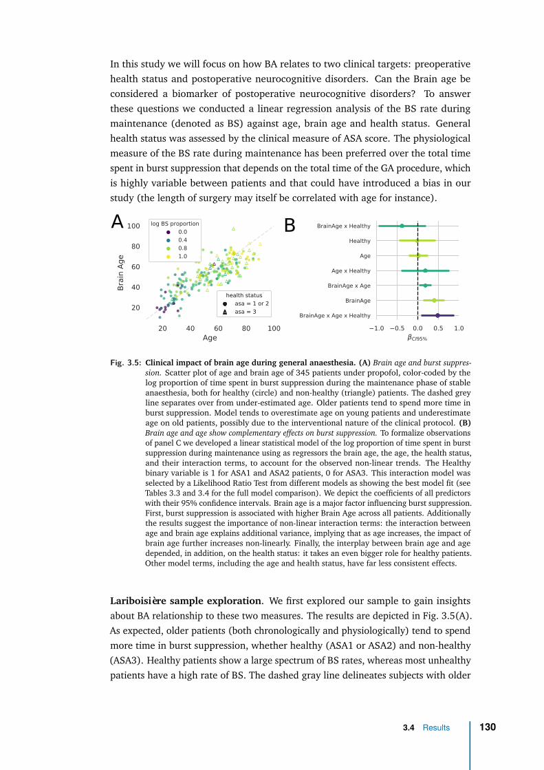
In this study we will focus on how BA relates to two clinical targets: preoperativehealth status and postoperative neurocognitive disorders. Can the Brain age beconsidered a biomarker of postoperative neurocognitive disorders? To answerthese questions we conducted a linear regression analysis of the BS rate duringmaintenance (denoted as BS) against age, brain age and health status. Generalhealth status was assessed by the clinical measure of ASA score. The physiologicalmeasure of the BS rate during maintenance has been preferred over the total timespent in burst suppression that depends on the total time of the GA procedure, whichis highly variable between patients and that could have introduced a bias in ourstudy (the length of surgery may itself be correlated with age for instance).

1.0 0.5 0.0 0.5 1.0

CI95%

BrainAge x Age x Healthy

BrainAge

BrainAge x Age

Age x Healthy

Age

Healthy

BrainAge x Healthy

20 40 60 80 100Age

20

40

60

80

100

Bra

in A

ge

log BS proportion

0.0

0.4

0.8

1.0

health status

asa = 1 or 2

asa = 3

health status

asa = 1 or 2

asa = 3

A B

Fig. 3.5: Clinical impact of brain age during general anaesthesia. (A) Brain age and burst suppres-sion. Scatter plot of age and brain age of 345 patients under propofol, color-coded by thelog proportion of time spent in burst suppression during the maintenance phase of stableanaesthesia, both for healthy (circle) and non-healthy (triangle) patients. The dashed greyline separates over from under-estimated age. Older patients tend to spend more time inburst suppression. Model tends to overestimate age on young patients and underestimateage on old patients, possibly due to the interventional nature of the clinical protocol. (B)Brain age and age show complementary effects on burst suppression. To formalize observationsof panel C we developed a linear statistical model of the log proportion of time spent in burstsuppression during maintenance using as regressors the brain age, the age, the health status,and their interaction terms, to account for the observed non-linear trends. The Healthybinary variable is 1 for ASA1 and ASA2 patients, 0 for ASA3. This interaction model wasselected by a Likelihood Ratio Test from different models as showing the best model fit (seeTables 3.3 and 3.4 for the full model comparison). We depict the coefficients of all predictorswith their 95% confidence intervals. Brain age is a major factor influencing burst suppression.First, burst suppression is associated with higher Brain Age across all patients. Additionallythe results suggest the importance of non-linear interaction terms: the interaction betweenage and brain age explains additional variance, implying that as age increases, the impact ofbrain age further increases non-linearly. Finally, the interplay between brain age and agedepended, in addition, on the health status: it takes an even bigger role for healthy patients.Other model terms, including the age and health status, have far less consistent effects.

Lariboisière sample exploration. We first explored our sample to gain insightsabout BA relationship to these two measures. The results are depicted in Fig. 3.5(A).As expected, older patients (both chronologically and physiologically) tend to spendmore time in burst suppression, whether healthy (ASA1 or ASA2) and non-healthy(ASA3). Healthy patients show a large spectrum of BS rates, whereas most unhealthypatients have a high rate of BS. The dashed gray line delineates subjects with older

3.4 Results 130

Page 136

brains (above the line) from subjects with younger brain (under the line). Restrictingour attention to healthy subjects, on which our brain age model has been fitted, wesee that the model tends to overestimate age on young patients and underestimateon old patients. Even if the mean absolute error of the model is 7.9y, it tends to bepositive for young people and negative for old people. This suggests a non-linearitythat is not captured by the brain age model. We then used this fitted model topredict the age of unhealthy subjects. Surprisingly, pathologies (ASA3) seem to beassociated with a younger brain. This is most probably due to a confounding effectof age. A common problem in establishing brain-behavior correlations for brain ageis spurious correlations due to shared age-related variance in the brain age delta andthe score of interest (here the ASA) [Smi+19]. By definition, the brain age delta isthe age residual. A perfect estimator of age should be orthogonal to age. If not thecase, then brain age delta would still depend on age. The relation between brain agedelta and ASA should therefore be interpreted with caution. This calls for a properdeconfounding analysis. Moreover, besides the confounding effect of age, we havetwo main hypotheses on the source of the problem: 1/ Lariboisière ASA1 and ASA2subjects, on which we fitted our model, should not be considered ‘healthy’ 2/ wedeal with an interventional dataset in which the drug dosage is changed by doctorsdepending on age, which bias the observations of the link between age and EEGwith a canceling effect: older subjects have less EEG-power but are administeredless drugs which increases their power. Both hypotheses are discussed in Section 3.5.But even if we can’t interpret the sign of Brain Age Delta, we can show that it is aclinically useful complement to age when predicting BS [Dad+21], for which wenow develop a statistical model.

Burst Suppression modeling. To account for the observed nonlinearity while stillenjoying the interpretability of linear models, we developed a linear statistical modelof the log proportion of time spent in burst suppression during maintenance using aspredictors the brain age, the age, and the health status. The Healthy binary variableis 1 for ASA1 and ASA2 patients (considered healthy), 0 for ASA3 (consideredunhealthy). We compared five different models: the two univariate models usingage and brain age, the two multivariate models (age, brain age) and (age, brain age,health status) and finally the model taking all the predictors and their interactionterms. The main statistics of the linear regression analysis for all five models aresummarized in Table 3.3.

3.4 Results 131

Page 137

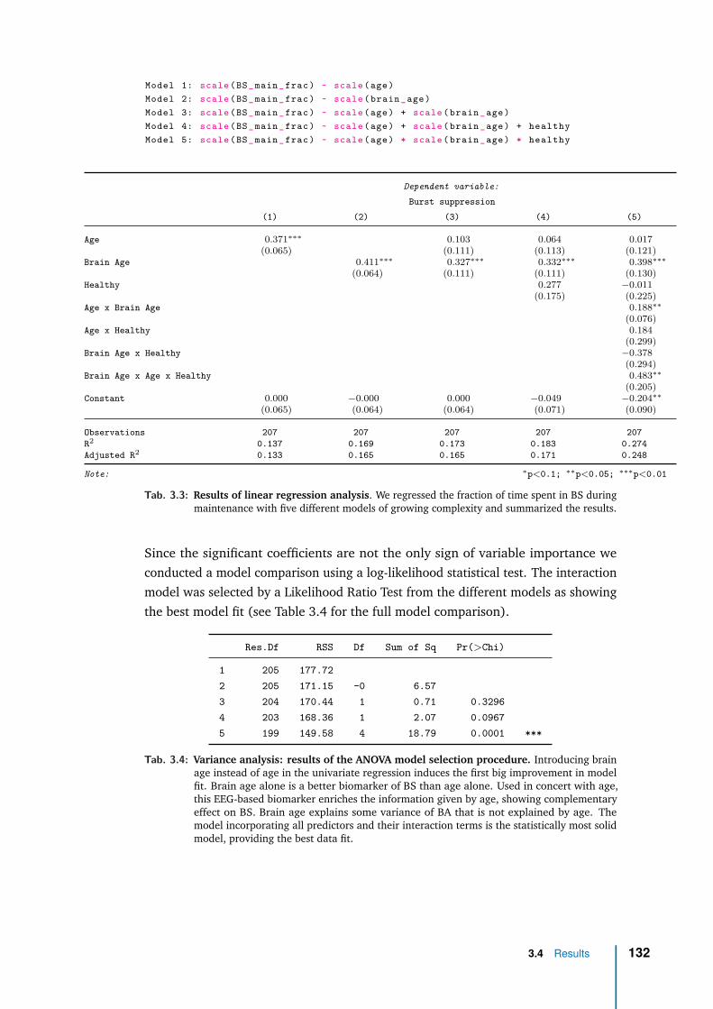
Model 1: scale (BS_main_frac) ~ scale (age)Model 2: scale (BS_main_frac) ~ scale ( brain _age)Model 3: scale (BS_main_frac) ~ scale (age) + scale ( brain _age)Model 4: scale (BS_main_frac) ~ scale (age) + scale ( brain _age) + healthyModel 5: scale (BS_main_frac) ~ scale (age) * scale ( brain _age) * healthy

Dependent variable:

Burst suppression

(1) (2) (3) (4) (5)

Age 0.371∗∗∗ 0.103 0.064 0.017(0.065) (0.111) (0.113) (0.121)

Brain Age 0.411∗∗∗ 0.327∗∗∗ 0.332∗∗∗ 0.398∗∗∗

(0.064) (0.111) (0.111) (0.130)Healthy 0.277 −0.011

(0.175) (0.225)Age x Brain Age 0.188∗∗

(0.076)Age x Healthy 0.184

(0.299)Brain Age x Healthy −0.378

(0.294)Brain Age x Age x Healthy 0.483∗∗

(0.205)Constant 0.000 −0.000 0.000 −0.049 −0.204∗∗

(0.065) (0.064) (0.064) (0.071) (0.090)

Observations 207 207 207 207 207R2 0.137 0.169 0.173 0.183 0.274Adjusted R2 0.133 0.165 0.165 0.171 0.248

Note: ∗p<0.1; ∗∗p<0.05; ∗∗∗p<0.01

Tab. 3.3: Results of linear regression analysis. We regressed the fraction of time spent in BS duringmaintenance with five different models of growing complexity and summarized the results.

Since the significant coefficients are not the only sign of variable importance weconducted a model comparison using a log-likelihood statistical test. The interactionmodel was selected by a Likelihood Ratio Test from the different models as showingthe best model fit (see Table 3.4 for the full model comparison).

Res.Df RSS Df Sum of Sq Pr(>Chi)

1 205 177.722 205 171.15 -0 6.573 204 170.44 1 0.71 0.32964 203 168.36 1 2.07 0.09675 199 149.58 4 18.79 0.0001 ***

Tab. 3.4: Variance analysis: results of the ANOVA model selection procedure. Introducing brainage instead of age in the univariate regression induces the first big improvement in modelfit. Brain age alone is a better biomarker of BS than age alone. Used in concert with age,this EEG-based biomarker enriches the information given by age, showing complementaryeffect on BS. Brain age explains some variance of BA that is not explained by age. Themodel incorporating all predictors and their interaction terms is the statistically most solidmodel, providing the best data fit.

3.4 Results 132

Page 138

The coefficients of the interaction model are depicted with their 95% confidenceintervals on Fig. 3.5(B). Brain Age is a major factor influencing BS as it is presenton all three significant predictors: Brain Age x Age x Healthy, Brain Age and BrainAge x Age. First, BS is associated with higher Brain Age across all patients atfixed age: elevated Brain Age increases fraction of time spent in BS by 0.4 STDper STD (equivalent to 3.4% additional time spent in BS per 15.8y of brain age).When taking age into account, brain age is associated with BS in a semanticallycorrect way. People with older brains tend to spend more time in burst suppression,possibly uncovering postoperative complications. Additionally the results suggestthe importance of non-linear interaction terms: the interaction between age andbrain age explains additional variance, implying that as age increases, the impactof brain age further increases non-linearly. Finally, the interplay between brain ageand age depended, in addition, on the health status: it takes an even bigger role forhealthy patients. All the other model terms, including the age and the health status,are not significant.

3.4 Results 133

Page 139

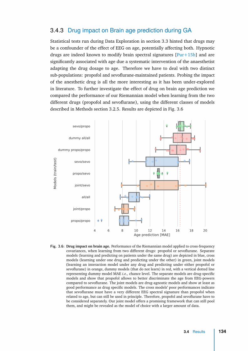
3.4.3 Drug impact on Brain age prediction during GAStatistical tests run during Data Exploration in section 3.3 hinted that drugs maybe a confounder of the effect of EEG on age, potentially affecting both. Hypnoticdrugs are indeed known to modify brain spectral signatures [Pur+15b] and aresignificantly associated with age due a systematic intervention of the anaesthetistadapting the drug dosage to age. Therefore we have to deal with two distinctsub-populations: propofol and sevoflurane-maintained patients. Probing the impactof the anesthetic drug is all the more interesting as it has been under-exploredin literature. To further investigate the effect of drug on brain age prediction wecompared the performance of our Riemannian model when learning from the twodifferent drugs (propofol and sevoflurane), using the different classes of modelsdescribed in Methods section 3.2.5. Results are depicted in Fig. 3.6

4 6 8 10 12 14 16 18 20Age prediction [MAE]

sevo/propo

dummy all/all

dummy propo/propo

sevo/sevo

propo/sevo

joint/sevo

all/all

joint/propo

propo/propo

Mod

els (

train

/test

)

Fig. 3.6: Drug impact on brain age. Performance of the Riemannian model applied to cross-frequencycovariances, when learning from two different drugs: propofol or sevoflurane. Separatemodels (learning and predicting on patients under the same drug) are depicted in blue, crossmodels (learning under one drug and predicting under the other) in green, joint models(learning an interaction model under any drug and predicting under either propofol orsevoflurane) in orange, dummy models (that do not learn) in red, with a vertical dotted linerepresenting dummy model MAE i.e., chance level. The separate models are drug-specificmodels and show that propofol allows to better discriminate the age from EEG-powerscompared to sevoflurane. The joint models are drug-agnostic models and show at least asgood performance as drug specific models. The cross models’ poor performances indicatethat sevoflurane must have a very different EEG spectral signature than propofol whenrelated to age, but can still be used in principle. Therefore, propofol and sevoflurane have tobe considered separately. Our joint model offers a promising framework that can still poolthem, and might be revealed as the model of choice with a larger amount of data.

3.4 Results 134

Page 140

Drugs indeed seem to greatly influence age prediction under GA: we can’t interpretEEG without drug information. The propofol-specific (propofol/propofol) model hasa better performance than the drug-agnostic model (all/all) that is not informed bythe drug. This drug-agnostic model as a single global linear model does not take intoaccount that the two drugs influence EEG signals based on distinct data generatingmechanisms in the two sub-populations hence does not perform optimally. Thisconfirms that propofol and sevoflurane have to be considered separately.

The propofol-specific model is also much better than the sevoflurane-specific model(sevo/sevo), hinting that propofol allows better discriminate of age from EEG-powerscompared to sevoflurane. This difference still holds when learning from a propofolpopulation resampled to match age distribution and sample size of sevoflurane,discarding the datashift hypothesis to account for the performance difference. Thisresult is also consistent with latest research that shows that intraoperative EEG alpha-band is a better proxy of preoperative cognitive function under propofol comparedto sevoflurane [recently submitted work]. One hypothesis for this difference comesfrom the different action mechanism of both drugs: propofol only acts on the GABAreceptors (it is a pure GABA agonist) whereas sevoflurane has several other actionmechanisms (mainly GABA agonist and NMDA antagonist) [Tra+00; CMF03], witha potentially netting effect, hence a loss of age-variability. Another hypothesis forthis reduced age-variability is that the dosage of sevoflurane is less variable thanpropofol across patients since it relies on standard abacus of MAC target values(minimum alveolar concentration), whereas propofol dosage is determined by apersonalized TCI target value.

Drug-crossed models’ poor performances indicate that sevoflurane must have amarkedly different EEG signature than propofol that somehow hinders age prediction:generalization across drugs does not work well. The performance of these crossmodels could also be driven by age instead of drug, knowing that patients maintainedunder sevoflurane are often older than under propofol, yet with a smaller STD.

The drug-aware model (joint/propofol) shows at least as good performance aspropofol-specific model when predicting on propofol subjects. Its observed reducedvariance could show a more refined prediction although we can’t rule out thestatistical effect of a larger training sample size. This joint model therefore offers apromising framework that can allow pooling of patients, and may reveal itself as themodel of choice when learning from larger amounts of data, leveraging what thetwo drugs have in common.

3.4 Results 135

Page 141

3.5 Discussion & future workOur work represents the most extensive validation of a ML approach to estimate BAduring GA. We presented a robust end-to-end biomarker learning strategy for EEGduring anaesthesia. We demonstrated how to achieve state-of-the-art performancefor EEG-based Brain age prediction during anaesthesia. We showed that the drugcritically impacts BA prediction under GA and analyzed its impact through interactionlearning.

We validated a potential EEG-based brain age measure against burst suppressionand ASA clinical score: higher brain age is correlated with more burst suppression,whereas age has a far less consistent effect. Hence we provided evidence that BAcaptures patient propensity to develop BS assuming a stable and adequate GA depth(SEF95 in the range of 8–13 Hz). We showed that EEG in the OR, today only usedfor monitoring depth of anaesthesia (via BIS and PSI indices), could be exploited toestimate a personalized physiological age of the brain of an anaesthetized subject thatcan help detect a propensity to the anomaly of BS, a recognized marker of the riskof developing cognitive dysfunction within the postoperative period. One possiblehypothesis consists in considering that the peroperative rate of suppression patternsand the cognitive trajectory of postoperative patients could be epiphenomena ofthe same symptom of an elevated brain age (and not chronological age), that canin principle be estimated before surgery. If this hypothesis is confirmed, this couldguide the therapeutic intervention in the operating room, but also would in principleallow to develop preventive procedures and help to improve postoperative medicalcare e.g., by early referring patient to a neurologist. A few open questions arenevertheless worth discussing.

One of the limitations of our study is methodological: the observation period ofthe features is defined using the SEF95 index, following a definition that is largelyagreed in the literature. But since the SEF95 is itself related to the EEG powerfeatures we could lose some variability that could be useful to predict. One possiblesolution would be to learn from the data itself the regions in the data that should betrusted and considered. Our algorithm could for instance select the best interval ofSEF95 in a nested cross-validation fashion and potentially discover that the [8-13]Hzinterval doctors are using may not be the optimal for building biomarkers. Also, thisstudy was restricted to one hospital. Results obtained should be replicated usingdata coming from other hospitals with different devices and clinical protocols.

Coming back to the unexpected experimental finding of Figure 3.5 where older andunhealthy patients seem to have a brain looking younger than their chronologicalage, we already discussed the potential confounding effect of age (age-relatedvariance in both the brain age delta and BS). Besides, we have two main hypotheses

3.5 Discussion & future work 136

Page 142

on the source of the problem. The first most obvious hypothesis is that Lariboisièresubjects should not be considered ‘healthy’: this is a suffering population as theycame to the hospital to undergo surgery. To test this hypothesis, one could usethe Riemann regression model trained on TUH healthy patients to predict age(restricted to four frontal electrodes), and test if indeed older brains are morefrequent in the non-healthy population, in effect sorting the ASA score in Lariboisièrepopulation in a coherent manner. Also the large number of subjects in the TUHdataset would address the sample bias we could have suffered from learning fromthe small sample size of Lariboisière data. The second hypothesis relates to thecausal structure of the data. According to this hypothesis, we don’t observe thenatural relation between resting state EEG and age because there’s an intervention,in the form of a treatment (the drug dosage) that biases it. Data have indeednot been collected in a controlled environment: most fragile patients have beentreated, here induced, differently precisely to avoid BS. We have been confirmedthat doctors changed the drug dosage according to their belief of age/health status,which then controls the EEG: most fragile patients have been administered lessdrugs, which increases the relative alpha power hence making them appear younger.If this is true, our age prediction may not be interpreted as brain age anymore andthe relation to BS is not easily interpretable. Other interventions occurred: somepatients received bolus of ketamine that is known to boost alpha and beta powerfor ∼ 20/30min, and some patients maintained with sevoflurane received bolus ofpropofol if necessary. Of course more data with the same data generating mechanism(the doctors) won’t help this causality problem. One possible solution would beto conduct deconfounding analysis by estimating the intervention effect with thepropofol target dosage (TCI). This way the treatment effect could be compensatedand treatment-independent conclusions reached. Such a study could be feasiblein the near future: Lariboisière hospital is currently testing a commercial solutionfor automated collection of hemodynamic and brain signals, synchronized with thetiming and volume of administered drugs. Finally, one alternative to this purelystatistical analysis, yet more demanding, would consist in doing causal inferencefrom carefully designed probabilistic graphical models.

Regarding the performance of our brain age model, it is noteworthy that we obtainedwith 4-channel clinical grade EEGs of 345 subjects the same performance in ageprediction (8y) than with 102-channels research-grade MEGs of 643 subjects (Cam-CAN) or 21-channels EEGs of 1000 subjects (TUH), for a comparable chance level.This result could come from several reasons but we can’t rule out a positive impact ofGA. According to this hypothesis, GA would be seen as a physiological stress test andthe hypnotic drug would enhance the brain response, forcing it to ‘speak’. With ∼10 m GA per year in France, the wealth of EEG recorded during GA has the potentialto allow medical discoveries if taking into account the specificities of GA. In thisthesis we established that Brain age under GA can be a serious candidate to be a

3.5 Discussion & future work 137

Page 143

drug-agnostic biomarker of BS, potentially integrated in a GA monitoring tool inthe future. Further studies could investigate its relation to medium and long-termoutcome of patients, e.g., the development of neurodegenerative disorders.

Finally, having the opportunity to work on a raw clinical dataset was a real chanceto glimpse over the real-world challenges of applying AI to medical data. I learnta few lessons along the way among which to discuss with the medical doctors andlook at the data the earlier possible to assess the data collection procedure. Thetime needed to clean and preprocess the data should also not be underestimated,which again is very common in real-world ML projects. Exploiting data in Healthcareis not an easy journey but can be very rewarding. We finally contributed to buildsomething unique since there’s no public or even private dataset of EEGs during GA,and hopefully something useful with potential medical application on health. Thisstudy could trigger a new line of research moving forward, developing clinically-relevant biomarkers from the GA period, with potential for medical applications as adiagnostic tool, paving the way for a finer understanding of brain diseases, and amore targeted approach to medical treatment.

3.5 Discussion & future work 138

Page 144

Conclusion

ContentsFuture directions . . . . . . . . . . . . . . . . . . . . . . . . . . . . . . 140

From scientific to societal impact . . . . . . . . . . . . . . . . . . . . . 141

Future directionsIn this thesis we established that Brain age under GA could be a candidate biomarkerof complications during general anesthesia. Yet, our brain age model would stillbenefit from a few technical refinements.

First it would need to be further robustified. To provide a robust end-to-endbiomarker learning strategy for EEG during anaesthesia, we should allow our al-gorithm to learn from the data itself the regions of the EEG recording that shouldbe trusted and considered, potentially challenging the mostly acceptable definitionof a SEF95 index in the [8-13]Hz range. To overcome limited spatial resolutionof clinical EEG it would also benefit from capturing temporal information of EEGand complement EEG with other signals monitored during GA. To demonstrateits generalization capacity we should also probe it using data coming from otherhospitals with difference devices and clinical protocols.

Then, we should disentangle the causal factors shaping GA observations, e.g., theeffect of drug dosage on the link between health and EEG. One possible solution isto conduct a deconfounding analysis by estimating the intervention effect with thePropofol target dosage and then compensate for it. This study will be feasible afterthe expected future technical upgrade of Lariboisière’s data collection system, whichwould allow the automated and time-synchronized collection of brain signals andvolume of administrated drugs. One more demanding alternative would consist indoing a proper causal inference from a carefully designed probabilistic graphicalmodels.

Moving forward, we are convinced that this study could trigger a new line of research,developing clinically-relevant biomarkers from the GA period, with potential for

140

Page 145

medical applications as a diagnostic tool. Nevertheless, we observe that mostmachine learning models trained to make medical decisions that perform at nearlythe same level as human experts are not in clinical use. Indeed collecting data fromone hospital, train and test the model on data from the same hospital, and showingthe algorithms are comparable to human doctors in spotting certain conditions isenough to publish a research paper. But it often turns out that the same modelused in a different hospital, applied to data collected with a different device, and aslightly different protocol used by the technician will show a significantly degradedperformance. In contrast, the performance of any human doctor would stay thesame. Indeed, there are challenges in translating a research paper into somethinguseful in a clinical setting: these models still need a lot of work to reach production.This proof-of-concept-to-production gap between research and practice is not uniqueto medicine but exists throughout the machine learning world. Modeling is just onestep towards production: finding the right data, deploying the model, monitoring itand showing safety are among other necessary steps.

If a proper randomized clinical study demonstrates that BA under GA is a validbiomarker for preoperative health it could be integrated into a GA monitoring tool toguide anesthetists in their perioperative decisions. If further studies show it is relatedto medium/long term outcome of patients, e.g., development of neurodegenerativedisorders, BA could even be part of a ‘medical consultation’ under GA: patients wouldreceive early feedback on brain age and risk of developing neurodegenerative dis-eases along with advices to improve brain health. These results would pave the wayfor a finer understanding of brain diseases, and a more targeted approach to medicaltreatment. This could set new standards in biomedical research, releasing GA-baseddata from the operating room into neurological and cardiological consulting, in thelong run of potential benefit to millions of patients

From scientific to societal impactThis thesis builds on the unique combination of expertise and associated preliminarydata obtained within the APHP and Inria teams, which have been engaged in aclose collaboration for over five years. Leveraging my 25y+ industry experience, mypost-thesis objective is to transfer these present and future scientific findings intothe socio-economic world by creating a medtech start-up company, which will leadthe transformation of this project results into a product on the market.

More precisely, this startup project would aim to reduce the risk of perioperativecomplications due to sub-optimal anesthesia management by providing an optimalknowledge of patient’s physiological state and by contributing to a more ‘intelligent’administration of anesthesia drugs (‘the right dose at the right time’). To thatpurpose, it will develop a combined alarm & decision support system – or virtual

141

Page 146

assistant – based on a predictive digital twin that integrates all information availableon a patient under anesthesia in a unified form, including the brain. The systemwill combine biophysical models and statistical models (our Brain Age) using thepatient’s physiological signals for optimized use of monitoring data. This augmentedcardiovascular and cerebral monitoring will provide a global vision of the patient’scondition and will help guide physicians’ therapeutic choices by recommendingpersonalized medical strategies. By doing so, we aim at significantly improve patientsconditions and quality of life after surgery. Additionally the startup will proposea post-surgery Personalized Anesthesia Report that describes patients’ reaction toanesthetic and surgical challenges and summarize cardiovascular and cerebral status(e.g., the Brain Age of the patient). This will help anesthesia management to passthe door of the operating room and propagate information to the following healthcare providers.

This project will benefit to all patients who will get surgery under general anesthe-sia. The greater benefits will be for patients labelled as high-risk surgical patientscontraindicated for surgery, namely patients older than 65 and/or with alteredcardiovascular function, and/or brain frailty since they are more prone to suffer fromcomplications. By using our virtual assistant, hospitals may offer novel opportunitiesto many patients previously excluded from surgery. Reducing peri-operative compli-cations immediately translates into reducing hospital length of stay and post-hospitaldischarge costs, in addition to improving patient’s quality of care. This approachgoes beyond the state of the art in anesthesia monitoring and opens new fields inthe patient pathway at the hospital.

To finance this entrepreneurial endeavour I participated to the creation of a con-sortium of academic (Inria), clinical (AP-HP Lariboisière) and industrial (PhilipsHealthcare) partners and answered two main Call for Proposals: European EITHealth 2022 and French RHU 2021 (Recherche Hospitalo Universitaire en santé).Our proposal and common aspiration is to leverage mathematical and AI new tech-niques to guide the medical doctors in their daily practice, with the hope to ultimatelygive scientific discoveries an additional social and economic impact on the world.

Synthèse en françaisLes maladies neurodégénératives figurent parmi les principales causes de mortalitédans le monde. Malheureusement, leur diagnostic précoce nécessite un examenmédical prescrit souvent trop tardivement et des équipements de laboratoire dédiés.Il repose aussi fréquemment sur des mesures prédictives souffrant d’un biais desélection. Cette thèse présente une solution prometteuse à ces problèmes : uneméthode robuste, directement utilisable en clinique, pour construire des biomar-

142

Page 147

queurs prédictifs à partir des signaux cérébraux M/EEG, validés contre les troublesneurocognitifs apparaissant après une anesthésie générale.

Dans une première contribution (théorique) [Sab+19], nous avons évalué desmodèles de régression capables d’apprendre des biomarqueurs à partir des matricesde covariance de signaux M/EEG. Notre analyse mathématique a identifié différentsmodèles garantissant une prédiction parfaite dans des circonstances idéales, lorsquela cible est une fonction (log-)linéaire en la puissance des sources cérébrales. Cesmodèles, basés sur les approches mathématiques de filtrage spatial supervisé etde géométrie riemannienne, permettent une prédiction optimale sans nécessiterune coûteuse localisation des sources. Nos simulations confirment cette analysemathématique et suggèrent que ces algorithmes de régression sont robustes à traversles mécanismes de génération de données et les violations de modèles. Cette étudesuggère que les méthodes riemanniennes sont des méthodes de choix pour l’analyseautomatisée à grande échelle des données M/EEG en l’absence d’IRM, conditionimportante pour pouvoir développer des biomarqueurs cliniques.

Dans une deuxième contribution (empirique) [Sab+20], nous avons validé nosmodèles prédictifs sur plusieurs ensembles de données de neuro-imagerie et avonsmontré qu’ils peuvent être utilisé pour apprendre l’âge du cerveau à partir de signauxcérébraux M/EEG, sans localisation de sources, et avec un prétraitement minimaldes données. De plus, la performance de notre méthode riemannienne est prochede celle des méthodes de référence nécessitant une localisation de sources et doncun traitement manuel des données, la disponibilité d’images IRM anatomiques etune expertise en modélisation de sources M/EEG. Une analyse empirique à grandeéchelle a ensuite permis de démontrer que l’âge du cerveau dérivé de la MEG capturedes informations uniques liées à l’activité neuronale et non expliquées par l’IRManatomique. Conformément aux simulations, ces résultats suggèrent également quel’approche riemannienne est une méthode pouvant s’appliquer dans un large éventailde situations, avec une robustesse considérable aux différents choix de prétraitement,y compris minimaliste. Les bonnes performances obtenues avec la MEG ont ensuiteété répliquées avec des EEGs de qualité recherche.

Dans une troisième contribution (clinique) [Sab+21, en préparation], nous avonsvalidé le concept d’âge cérébral directement au bloc opératoire de l’hôpital Lari-boisière à Paris, à partir d’EEG de qualité clinique recueillis pendant la période del’anesthésie générale. Nous avons évalué notre mesure de l’âge cérébral commeprédicteur de complications peropératoires liées aux dysfonctions cognitives postopération, validant ainsi l’âge du cerveau comme un biomarqueur clinique promet-teur des troubles neurocognitifs. Nous avons également montré que le sédatif utiliséa un impact important sur la prédiction de l’âge du cerveau et avons démontré larobustesse de notre approche à différents types de médicaments.

143

Page 148

Combinant des concepts précédemment étudiés séparément, notre contributiondémontre la pertinence clinique de la notion d’âge du cerveau prédit à partir de l’EEGpour révéler les pathologies des fonctions cérébrales dans des situations où l’IRMne peut pas être réalisée. Ces résultats fournissent également une première preuveque l’anesthésie générale est une période propice à la découverte de biomarqueurscérébraux, avec un impact potentiel profond sur la médecine préventive et uneinfluence sociale et économique durable.

144

Page 149

Bibliography

[Aa2] Alzheimer’s Disease Facts and Figures. Tech. rep. Alzheimer’s & Dementia,2021:17(3). Alzheimer’s Association 2021 (cit. on p. 2).

[AG01] LI Aftanas and SA Golocheikine. “Human anterior and frontal midline thetaand lower alpha reflect emotionally positive state and internalized attention:high-resolution EEG investigation of meditation”. In: Neuroscience letters 310.1(2001), pp. 57–60 (cit. on p. 15).

[Ahl+10] Seppo P Ahlfors, Jooman Han, John W Belliveau, and Matti S Hämäläinen.“Sensitivity of MEG and EEG to source orientation”. In: Brain topography 23.3(2010), pp. 227–232 (cit. on p. 11).

[AJWW66] HW Agnew Jr, Wilse B Webb, and Robert L Williams. “The first night effect:an EEG study of sleep”. In: Psychophysiology 2.3 (1966), pp. 263–266 (cit. onp. 10).

[AMS09] P-A Absil, Robert Mahony, and Rodolphe Sepulchre. Optimization algorithmson matrix manifolds. Princeton University Press, 2009 (cit. on pp. 50, 51).

[And+15] Lau M Andersen, Michael N Pedersen, Kristian Sandberg, and Morten Over-gaard. “Occipital MEG activity in the early time range (< 300 ms) predictsgraded changes in perceptual consciousness”. In: Cerebral Cortex 26.6 (2015),pp. 2677–2688 (cit. on p. 63).

[App+19] Stefan Appelhoff, Matthew Sanderson, Teon L Brooks, et al. “MNE-BIDS:Organizing electrophysiological data into the BIDS format and facilitating theiranalysis”. In: The Journal of Open Source Software 4.44 (2019) (cit. on p. 117).

[Ast+08] L. Astolfi, F. Cincotti, D. Mattia, et al. “Tracking the time-varying cortical con-nectivity patterns by adaptive multivariate estimators”. In: IEEE Transactionson Biomedical Engineering 55.3 (2008), pp. 902–913 (cit. on p. 43).

[Att+19] Zachi I. Attia, Paul A. Friedman, Peter A. Noseworthy, et al. “Age and SexEstimation Using Artificial Intelligence From Standard 12-Lead ECGs”. In:Circulation: Arrhythmia and Electrophysiology 12.9 (2019), e007284. eprint:https://www.ahajournals.org/doi/pdf/10.1161/CIRCEP.119.007284(cit. on p. 105).

[AUT19] JJ Allaire, Kevin Ushey, and Yuan Tang. reticulate: Interface to ’Python’. Rpackage version 1.11. 2019 (cit. on pp. 25, 84).

[AYH18] David B Arciniegas, Stuart C Yudofsky, and Robert E Hales. The AmericanPsychiatric Publishing Textbook of Neuropsychiatry and Behavioral Neuroscience.American Psychiatric Pub, 2018 (cit. on p. 15).

145

Page 150

[Bab+06] Claudio Babiloni, Giuliano Binetti, Andrea Cassarino, et al. “Sources of corticalrhythms in adults during physiological aging: a multicentric EEG study”. In:Human brain mapping 27.2 (2006), pp. 162–172 (cit. on p. 21).

[Bai17] Sylvain Baillet. “Magnetoencephalography for brain electrophysiology andimaging”. In: Nature Neuroscience 20 (Feb. 2017), 327 EP – (cit. on pp. 61,62).

[Bak+75] J Dennis Baker, Bernd Gluecklich, C Wesley Watson, et al. “An evaluationof electroencephalographic monitoring for carotid study”. In: Surgery 78.6(1975), pp. 787–794 (cit. on p. 10).

[Bar+06] William E Barlow, Emily White, Rachel Ballard-Barbash, et al. “Prospectivebreast cancer risk prediction model for women undergoing screening mam-mography”. In: Journal of the National Cancer Institute 98.17 (2006), pp. 1204–1214 (cit. on p. 32).

[Bar+11] Alexandre Barachant, Stéphane Bonnet, Marco Congedo, and Christian Jutten.“Multiclass brain–computer interface classification by Riemannian geometry”.In: IEEE Transactions on Biomedical Engineering 59.4 (2011), pp. 920–928(cit. on p. 64).

[Bar+12] A. Barachant, S. Bonnet, M. Congedo, and C. Jutten. “Multiclass Brain–ComputerInterface Classification by Riemannian Geometry”. In: IEEE Transactions onBiomedical Engineering 59.4 (2012), pp. 920–928 (cit. on pp. 49, 53, 64, 85).

[Bar+13] Alexandre Barachant, Stéphane Bonnet, Marco Congedo, and Christian Jutten.“Classification of covariance matrices using a Riemannian-based kernel for BCIapplications”. In: Neurocomputing 112 (2013), pp. 172–178 (cit. on p. 64).

[BD04] György Buzsáki and Andreas Draguhn. “Neuronal oscillations in cortical net-works”. In: science 304.5679 (2004), pp. 1926–1929 (cit. on p. 15).

[Bel+97] Adel Belouchrani, Karim Abed-Meraim, J-F Cardoso, and Eric Moulines. “Ablind source separation technique using second-order statistics”. In: IEEETransactions on signal processing 45.2 (1997), pp. 434–444 (cit. on p. 57).

[Ber29] Hans Berger. “Über das elektroenkephalogramm des menschen”. In: Archiv fürpsychiatrie und nervenkrankheiten 87.1 (1929), pp. 527–570 (cit. on p. 10).

[Bha09] Rajendra Bhatia. Positive definite matrices. Princeton university press, 2009(cit. on p. 52).

[BHT21] Stephen Bates, Trevor Hastie, and Robert Tibshirani. Cross-validation: whatdoes it estimate and how well does it do it? 2021. arXiv: 2104.00673 [stat.ME](cit. on p. 38).

[BI+16] Charles H Brown IV, Laura Max, Andrew LaFlam, et al. “The associationbetween preoperative frailty and postoperative delirium after cardiac surgery”.In: Anesthesia and analgesia 123.2 (2016), p. 430 (cit. on p. 129).

[BI19] Danilo Bzdok and John PA Ioannidis. “Exploration, inference, and predictionin neuroscience and biomedicine”. In: Trends in neurosciences (2019) (cit. onpp. 14, 107).

[Bis07] Christopher M. Bishop. Pattern Recognition and Machine Learning (InformationScience and Statistics). Springer, 2007 (cit. on p. 38).

Bibliography 146

Page 151

[BJF10] Luc Berthouze, Leon M James, and Simon F Farmer. “Human EEG shows long-range temporal correlations of oscillation amplitude in Theta, Alpha and Betabands across a wide age range”. In: Clinical Neurophysiology 121.8 (2010),pp. 1187–1197 (cit. on p. 89).

[BJL18] Rajendra Bhatia, Tanvi Jain, and Yongdo Lim. “On the Bures–Wassersteindistance between positive definite matrices”. In: Expositiones Mathematicae(2018) (cit. on p. 54).

[BL17] György Buzsáki and Rodolfo Llinás. “Space and time in the brain”. In: Science358.6362 (2017), pp. 482–485. eprint: https://science.sciencemag.org/content/358/6362/482.full.pdf (cit. on p. 15).

[Bla+08] B. Blankertz, R. Tomioka, S. Lemm, M. Kawanabe, and K. Muller. “OptimizingSpatial filters for Robust EEG Single-Trial Analysis”. In: IEEE Signal ProcessingMagazine 25.1 (2008), pp. 41–56 (cit. on pp. 60, 64).

[BLS10] Emery N Brown, Ralph Lydic, and Nicholas D Schiff. “General anesthesia, sleep,and coma”. In: New England Journal of Medicine 363.27 (2010), pp. 2638–2650(cit. on p. 113).

[BM14] György Buzsáki and Kenji Mizuseki. “The log-dynamic brain: how skeweddistributions affect network operations”. In: Nature Reviews Neuroscience 15.4(2014), p. 264 (cit. on pp. 60, 64, 103).

[Bou+14] N. Boumal, B. Mishra, P.-A. Absil, and R. Sepulchre. “Manopt, a Matlab Toolboxfor Optimization on Manifolds”. In: Journal of Machine Learning Research 15(2014), pp. 1455–1459 (cit. on p. 30).

[Bro+11] Matthew J Brookes, Mark Woolrich, Henry Luckhoo, et al. “Investigating theelectrophysiological basis of resting state networks using magnetoencephalog-raphy”. In: Proceedings of the National Academy of Sciences 108.40 (2011),pp. 16783–16788 (cit. on pp. 19, 63).

[Bro+17] M. M. Bronstein, J. Bruna, Y. LeCun, A. Szlam, and P. Vandergheynst. “Geomet-ric Deep Learning: Going beyond Euclidean data”. In: IEEE Signal ProcessingMagazine 34.4 (2017), pp. 18–42 (cit. on p. 29).

[Bru+03] Jörgen Bruhn, Thomas W Bouillon, Lucian Radulescu, et al. “Correlation ofapproximate entropy, bispectral index, and spectral edge frequency 95 (SEF95)with clinical signs of “anesthetic depth” during coadministration of propofoland remifentanil”. In: The Journal of the American Society of Anesthesiologists98.3 (2003), pp. 621–627 (cit. on p. 113).

[BS09] Silvere Bonnabel and Rodolphe Sepulchre. “Riemannian metric and geometricmean for positive semidefinite matrices of fixed rank”. In: SIAM Journal onMatrix Analysis and Applications 31.3 (2009), pp. 1055–1070 (cit. on p. 54).

[BV00] J. . Bercher and C. Vignat. “Estimating the entropy of a signal with applications”.In: IEEE Transactions on Signal Processing 48.6 (2000), pp. 1687–1694 (cit. onp. 41).

[Bzd17] Danilo Bzdok. “Classical Statistics and Statistical Learning in Imaging Neu-roscience”. In: Frontiers in Neuroscience 11.OCT (2017), pp. 1–23 (cit. onp. 15).

Bibliography 147

Page 152

[Bzd+18] Danilo Bzdok, Denis Engemann, Olivier Grisel, Gaël Varoquaux, and BertrandThirion. “Prediction and inference diverge in biomedicine: Simulations andreal-world data”. In: (2018) (cit. on p. 107).

[Car+19] Jérôme Cartailler, Pierre Parutto, Cyril Touchard, Fabrice Vallée, and DavidHolcman. “Alpha rhythm collapse predicts iso-electric suppressions duringanesthesia”. In: Communications biology 2.1 (2019), pp. 1–10 (cit. on pp. 114,129).

[CBA13] M. Congedo, A. Barachant, and A. Andreev. “A New Generation of Brain-Computer Interface Based on Riemannian Geometry”. In: arXiv e-prints (Oct.2013). arXiv: 1310.8115 [cs.HC] (cit. on pp. 25, 84).

[CBB17] Marco Congedo, Alexandre Barachant, and Rajendra Bhatia. “Riemanniangeometry for EEG-based brain-computer interfaces; a primer and a review”.In: Brain-Computer Interfaces 4.3 (2017), pp. 155–174 (cit. on p. 29).

[Cha+13] Frédéric Chazal, Leonidas J Guibas, Steve Y Oudot, and Primoz Skraba.“Persistence-based clustering in Riemannian manifolds”. In: Journal of theACM (JACM) 60.6 (2013), pp. 1–38 (cit. on p. 44).

[Che+10] Yilun Chen, Ami Wiesel, Yonina C Eldar, and Alfred O Hero. “Shrinkagealgorithms for MMSE covariance estimation”. In: IEEE Transactions on SignalProcessing 58.10 (2010), pp. 5016–5029 (cit. on pp. 46, 86, 89, 102, 117).

[Cla+04] C Richard Clark, Melinda D Veltmeyer, Rebecca J Hamilton, et al. “Spontaneousalpha peak frequency predicts working memory performance across the agespan”. In: International Journal of Psychophysiology 53.1 (2004), pp. 1–9 (cit.on p. 89).

[CMF03] Jason A Campagna, Keith W Miller, and Stuart A Forman. “Mechanisms ofactions of inhaled anesthetics”. In: New England Journal of Medicine 348.21(2003), pp. 2110–2124 (cit. on p. 135).

[Col+17] James H Cole, Rudra PK Poudel, Dimosthenis Tsagkrasoulis, et al. “Predictingbrain age with deep learning from raw imaging data results in a reliable andheritable biomarker”. In: NeuroImage 163 (2017), pp. 115–124 (cit. on p. 110).

[Col+18] James H Cole, Stuart J Ritchie, Mark E Bastin, et al. “Brain age predictsmortality”. In: Molecular psychiatry 23.5 (2018), p. 1385 (cit. on pp. 18, 110).

[Col+19] James H Cole, Riccardo E Marioni, Sarah E Harris, and Ian J Deary. “Brainage and other bodily ‘ages’: implications for neuropsychiatry”. In: Molecularpsychiatry 24.2 (2019), pp. 266–281 (cit. on p. 110).

[Cox+19] Simon R Cox, Donald M Lyall, Stuart J Ritchie, et al. “Associations betweenvascular risk factors and brain MRI indices in UK Biobank”. In: European heartjournal 40.28 (2019), pp. 2290–2300 (cit. on p. 16).

[CP14] Alain de Cheveigné and Lucas C. Parra. “Joint decorrelation, a versatile tool formultichannel data analysis”. In: NeuroImage 98 (2014), pp. 487 –505 (cit. onpp. 64, 72, 102).

[CPB16] M. Congedo, R. Phlypo, and A. Barachant. “A fixed-point algorithm for esti-mating power means of positive definite matrices”. In: 2016 24th EuropeanSignal Processing Conference (EUSIPCO). 2016, pp. 2106–2110 (cit. on p. 53).

Bibliography 148

Page 153

[CR+07] Delphine Cosandier-Rimélé, Jean-Michel Badier, Patrick Chauvel, and FabriceWendling. “A physiologically plausible spatio-temporal model for EEG signalsrecorded with intracerebral electrodes in human partial epilepsy”. In: IEEETransactions on Biomedical Engineering 54.3 (2007), pp. 380–388 (cit. onp. 17).

[CR95] Michael GH Coles and Michael D Rugg. Event-related brain potentials: Anintroduction. Oxford University Press, 1995 (cit. on p. 14).

[CRJ19] M. Congedo, P. L. C. Rodrigues, and C. Jutten. “The Riemannian MinimumDistance to Means Field Classifier”. In: Graz BCI Conference 2019. 2019 (cit. onp. 44).

[Csj] Blood flow, blood pressure or both? Tech. rep. vol. 9, no. 6, pp. 15–18, May2018. Clinical services journal (cit. on pp. 22, 128).

[CSM17] Erik Clarke and Scott Sherrill-Mix. ggbeeswarm: Categorical Scatter (ViolinPoint) Plots. R package version 0.6.0. 2017 (cit. on pp. 25, 84).

[Cul+17] Deborah J Culley, Devon Flaherty, Margaret C Fahey, et al. “Poor performanceon a preoperative cognitive screening test predicts postoperative complicationsin older orthopedic surgical patients”. In: Anesthesiology 127.5 (2017), pp. 765–774 (cit. on p. 129).

[DA01] Peter Dayan and Laurence F Abbott. Theoretical neuroscience: computationaland mathematical modeling of neural systems. Computational NeuroscienceSeries, 2001 (cit. on pp. 4, 8).

[Dad+15] Christophe Dadure, Anaïs Marie, Fabienne Seguret, and Xavier Capdevila.“One year of anaesthesia in France: A comprehensive survey based on thenational medical information (PMSI) database. Part 1: In-hospital patients”.In: Anaesthesia Critical Care & Pain Medicine 34.4 (2015), pp. 191–197 (cit. onpp. 22, 128).

[Dad+19] Kamalaker Dadi, Mehdi Rahim, Alexandre Abraham, et al. “Benchmarkingfunctional connectome-based predictive models for resting-state fMRI”. In:NeuroImage 192 (2019), pp. 115–134 (cit. on pp. 15, 63, 69).

[Dad+21] Kamalaker Dadi, Gaël Varoquaux, Josselin Houenou, et al. “Population mod-eling with machine learning can enhance measures of mental health”. In:GigaScience 10 (2021), pp. 1–16 (cit. on pp. 111, 131).

[Däh+13] Sven Dähne, Felix Bießmann, Frank C Meinecke, et al. “Integration of multivari-ate data streams with bandpower signals”. In: IEEE Transactions on Multimedia15.5 (2013), pp. 1001–1013 (cit. on p. 64).

[Däh+14a] Sven Dähne, Frank C Meinecke, Stefan Haufe, et al. “SPoC: a novel frameworkfor relating the amplitude of neuronal oscillations to behaviorally relevantparameters”. In: NeuroImage 86 (2014), pp. 111–122 (cit. on pp. 60, 64, 72,73, 102).

[Däh+14b] Sven Dähne, Vadim V Nikulin, David Ramírez, et al. “Finding brain oscillationswith power dependencies in neuroimaging data”. In: NeuroImage 96 (2014),pp. 334–348 (cit. on pp. 64, 107).

Bibliography 149

Page 154

[DCS99] Alain Destexhe, Diego Contreras, and Mircea Steriade. “Spatiotemporal analy-sis of local field potentials and unit discharges in cat cerebral cortex duringnatural wake and sleep states”. In: Journal of Neuroscience 19.11 (1999),pp. 4595–4608 (cit. on p. 11).

[Del+12] Arnaud Delorme, Jason Palmer, Julie Onton, Robert Oostenveld, and ScottMakeig. “Independent EEG sources are dipolar”. In: PloS one 7.2 (2012),e30135 (cit. on p. 63).

[Den+21] Stijn Denissen, Denis Alexander Engemann, Alexander De Cock, et al. “Brainage as a surrogate marker for information processing speed in multiple sclero-sis”. In: medRxiv (2021) (cit. on p. 111).

[Dmo+12] Jacek Dmochowski, Paul Sajda, Joao Dias, and Lucas Parra. “Correlated Com-ponents of Ongoing EEG Point to Emotionally Laden Attention – A PossibleMarker of Engagement?” In: Frontiers in Human Neuroscience 6 (2012), p. 112(cit. on p. 64).

[Dos+10] Nico UF Dosenbach, Binyam Nardos, Alexander L Cohen, et al. “Prediction ofindividual brain maturity using fMRI”. In: Science 329.5997 (2010), pp. 1358–1361 (cit. on p. 17).

[DPm99] Roberto Domingo Pascual-marqui. “Review of Methods for Solving the EEGInverse Problem”. In: Int. J. Biomagn. 1 (Oct. 1999) (cit. on p. 12).

[EG15] Denis A Engemann and Alexandre Gramfort. “Automated model selection incovariance estimation and spatial whitening of MEG and EEG signals”. In:NeuroImage 108 (2015), pp. 328–342 (cit. on pp. 46, 86, 102).

[Eng+18] Denis A Engemann, Federico Raimondo, Jean-Rémi King, et al. “Robust EEG-based cross-site and cross-protocol classification of states of consciousness”.In: Brain 141.11 (Oct. 2018), pp. 3179–3192. eprint: http://oup.prod.sis.lan/brain/article-pdf/141/11/3179/26172804/awy251.pdf (cit. onpp. 15, 16, 21).

[Eng+20] Denis Alexander Engemann, Oleh Kozynets, David Sabbagh, et al. “Combiningmagnetoencephalography with magnetic resonance imaging enhances learningof surrogate-biomarkers”. In: eLife 9 (2020), e54055 (cit. on pp. 19–21, 25,60, 98, 121, 127).

[Eng+21] Denis A Engemann, Apolline Mellot, Richard Hoechenberger, et al. “A reusablebenchmark of brain-age prediction from M/EEG resting-state signals”. In:bioRxiv (2021) (cit. on pp. 25, 62).

[Eura] Eurostat. [hlth_cd_acdr2] database (cit. on pp. 2, 110).

[Eurb] Eurostat. [proj_18ndbi] database (cit. on pp. 2, 128).

[Eurc] Eurostat. [proj_18np] database (cit. on pp. 2, 128).

[Fac06] Brain Facts. “a Primer on the Brain and Nervous System”. In: Washington, DC:Society for Neuroscience (2006) (cit. on pp. 4, 5, 8).

[Fis12] Bruce Fischl. “FreeSurfer”. In: NeuroImage 62.2 (2012), pp. 774–781 (cit. onp. 91).

Bibliography 150

Page 155

[FM03] Wolfgang Förstner and Boudewijn Moonen. “A metric for covariance matrices”.In: Geodesy-The Challenge of the 3rd Millennium. Springer, 2003, pp. 299–309(cit. on pp. 51, 64).

[Fra+12] Katja Franke, Eileen Luders, Arne May, Marko Wilke, and Christian Gaser.“Brain maturation: predicting individual BrainAGE in children and adolescentsusing structural MRI”. In: Neuroimage 63.3 (2012), pp. 1305–1312 (cit. onp. 110).

[Fri+16] Bradley A Fritz, Philip L Kalarickal, Hannah R Maybrier, et al. “Intraopera-tive electroencephalogram suppression predicts postoperative delirium”. In:Anesthesia and analgesia 122.1 (2016), p. 234 (cit. on pp. 111, 129).

[Fri+20] Bradley A Fritz, Christopher R King, Arbi Ben Abdallah, et al. “Preoperativecognitive abnormality, intraoperative electroencephalogram suppression, andpostoperative delirium: a mediation analysis”. In: Anesthesiology 132.6 (2020),pp. 1458–1468 (cit. on pp. 110, 128).

[Fru+17] Wolfgang Fruehwirt, Matthias Gerstgrasser, Pengfei Zhang, et al. “Rieman-nian tangent space mapping and elastic net regularization for cost-effectiveEEG markers of brain atrophy in Alzheimer’s disease”. In: arXiv preprintarXiv:1711.08359 (2017) (cit. on pp. 14, 21, 64).

[Fuk90] Keinosuke Fukunaga. “Chapter 2 - RANDOM VECTORS AND THEIR PROP-ERTIES”. In: Introduction to Statistical Pattern Recognition (Second Edition).Ed. by Keinosuke Fukunaga. Second Edition. Boston: Academic Press, 1990,pp. 11 –50 (cit. on p. 74).

[Gar+17] Pilar Garcés, David López-Sanz, Fernando Maestú, and Ernesto Pereda. “Choiceof magnetometers and gradiometers after signal space separation”. In: Sensors17.12 (2017), p. 2926 (cit. on pp. 88, 105).

[Gau+19] Sinead Gaubert, Federico Raimondo, Marion Houot, et al. “EEG evidence ofcompensatory mechanisms in preclinical Alzheimer?s disease”. In: Brain 142.7(2019), pp. 2096–2112 (cit. on pp. 16, 19, 21).

[GB08] M. Grosse-Wentrup* and M. Buss. “Multiclass Common Spatial Patterns andInformation Theoretic Feature Extraction”. In: IEEE Transactions on BiomedicalEngineering 55.8 (2008), pp. 1991–2000 (cit. on p. 60).

[GBD09] Amir A Ghaferi, John D Birkmeyer, and Justin B Dimick. “Variation in hospi-tal mortality associated with inpatient surgery”. In: New England Journal ofMedicine 361.14 (2009), pp. 1368–1375 (cit. on p. 128).

[Gel+05] Andrew Gelman et al. “Analysis of variance — why it is more important thanever”. In: The annals of statistics 33.1 (2005), pp. 1–53 (cit. on p. 96).

[Ger+14] Wulfram Gerstner, Werner M Kistler, Richard Naud, and Liam Paninski. Neu-ronal dynamics: From single neurons to networks and models of cognition. Cam-bridge University Press, 2014 (cit. on pp. 4, 7).

[GHW79] Gene H. Golub, Michael Heath, and Grace Wahba. “Generalized Cross-Validationas a Method for Choosing a Good Ridge Parameter”. In: Technometrics 21.2(1979), pp. 215–223 (cit. on pp. 84, 89, 121).

Bibliography 151

Page 156

[Gia+17] Charles M Giattino, Jacob E Gardner, Faris M Sbahi, et al. “Intraoperativefrontal alpha-band power correlates with preoperative neurocognitive functionin older adults”. In: Frontiers in systems neuroscience 11 (2017), p. 24 (cit. onp. 129).

[Gol+02] Robin I Goldman, John M Stern, Jerome Engel Jr, and Mark S Cohen. “Simul-taneous EEG and fMRI of the alpha rhythm”. In: Neuroreport 13.18 (2002),p. 2487 (cit. on p. 15).

[Gra+14] Alexandre Gramfort, Martin Luessi, Eric Larson, et al. “MNE software forprocessing MEG and EEG data”. In: NeuroImage 86 (2014), pp. 446–460 (cit.on pp. 25, 30, 48, 84, 85, 91, 96).

[Gro+13] Joachim Gross, Sylvain Baillet, Gareth R Barnes, et al. “Good practice forconducting and reporting MEG research”. In: Neuroimage 65 (2013), pp. 349–363 (cit. on p. 88).

[Häm+93] Matti Hämäläinen, Riitta Hari, Risto J Ilmoniemi, Jukka Knuutila, and Olli VLounasmaa. “Magnetoencephalography—theory, instrumentation, and appli-cations to noninvasive studies of the working human brain”. In: Reviews ofmodern Physics 65.2 (1993), p. 413 (cit. on pp. 10, 56, 57, 61).

[Har+14] A Harati, S Lopez, I Obeid, et al. “The TUH EEG CORPUS: A big data resourcefor automated EEG interpretation”. In: 2014 IEEE Signal Processing in Medicineand Biology Symposium (SPMB). IEEE. 2014, pp. 1–5 (cit. on pp. 25, 92, 93).

[Has+05] Trevor Hastie, Robert Tibshirani, Jerome Friedman, and James Franklin. “Theelements of statistical learning: data mining, inference and prediction”. In: TheMathematical Intelligencer 27.2 (2005), pp. 83–85 (cit. on p. 39).

[Hau+14] Stefan Haufe, Frank Meinecke, Kai Görgen, et al. “On the interpretation ofweight vectors of linear models in multivariate neuroimaging”. In: NeuroImage87 (2014), pp. 96 –110 (cit. on pp. 58, 63, 95, 105).

[Haw+80] RC Hawkes, GN Holland, WS Moore, and BS Worthington. “Nuclear magneticresonance (NMR) tomography of the brain: a preliminary clinical assessmentwith demonstration of pathology.” In: Journal of Computer Assisted Tomography4.5 (1980), pp. 577–586 (cit. on p. 9).

[He+19] Tong He, Ru Kong, Avram J. Holmes, et al. “Deep neural networks and kernelregression achieve comparable accuracies for functional connectivity predictionof behavior and demographics”. In: NeuroImage (2019), p. 116276 (cit. onp. 63).

[HI84] MS Hämäläinen and RJ Ilmoniemi. Interpreting magnetic fields of the brain:minimum norm estimates. Tech. rep. TKK-F-A559. Helsinki University of Tech-nology, 1984 (cit. on p. 62).

[HI94] Matti S Hämäläinen and Risto J Ilmoniemi. “Interpreting magnetic fields ofthe brain: minimum norm estimates”. In: Medical & biological engineering &computing 32.1 (1994), pp. 35–42 (cit. on p. 61).

[HIN09] Kenneth E Hild II and Srikantan S Nagarajan. “Source localization of EEG/MEGdata by correlating columns of ICA and lead field matrices”. In: IEEE Transac-tions on Biomedical Engineering 56.11 (2009), pp. 2619–2626 (cit. on p. 63).

Bibliography 152

Page 157

[HK70] Arthur E Hoerl and Robert W Kennard. “Ridge regression: Biased estimationfor nonorthogonal problems”. In: Technometrics 12.1 (1970), pp. 55–67 (cit. onp. 84).

[HKO04] Aapo Hyvärinen, Juha Karhunen, and Erkki Oja. Independent component analy-sis. Vol. 46. John Wiley & Sons, 2004 (cit. on p. 99).

[HLR00] Riitta Hari, Sari Levänen, and Tommi Raij. “Timing of human cortical functionsduring cognition: role of MEG”. In: Trends in cognitive sciences 4.12 (2000),pp. 455–462 (cit. on p. 11).

[HO00] Aapo Hyvärinen and Erkki Oja. “Independent component analysis: algorithmsand applications”. In: Neural networks 13.4-5 (2000), pp. 411–430 (cit. onpp. 57, 62).

[Hot92] Harold Hotelling. “Relations between two sets of variates”. In: Breakthroughsin statistics. Springer, 1992, pp. 162–190 (cit. on p. 64).

[HP17] Riitta Hari and Aina Puce. MEG-EEG Primer. Oxford University Press, 2017(cit. on pp. 4, 7, 10, 12, 15, 62).

[HP18] Hanna-Leena Halme and Lauri Parkkonen. “Across-subject offline decoding ofmotor imagery from MEG and EEG”. In: Scientific reports 8.1 (2018), pp. 1–12(cit. on p. 85).

[HS14] Olaf Hauk and Matti Stenroos. “A framework for the design of flexible cross-talk functions for spatial filtering of EEG/MEG data: DeFleCT”. In: Humanbrain mapping 35.4 (2014), pp. 1642–1653 (cit. on p. 61).

[HS15] Joerg F Hipp and Markus Siegel. “BOLD fMRI correlation reflects frequency-specific neuronal correlation”. In: Current Biology 25.10 (2015), pp. 1368–1374 (cit. on p. 19).

[HSH17] Mehrtash Harandi, Mathieu Salzmann, and Richard Hartley. “Dimensionalityreduction on SPD manifolds: The emergence of geometry-aware methods”.In: IEEE transactions on pattern analysis and machine intelligence 40.1 (2017),pp. 48–62 (cit. on p. 63).

[HT08] Holger Höfling and Robert Tibshirani. “A study of pre-validation”. In: TheAnnals of Applied Statistics 2.2 (2008), pp. 643–664 (cit. on p. 127).

[HYS16] Inbal Horev, Florian Yger, and Masashi Sugiyama. “Geometry-aware principalcomponent analysis for symmetric positive definite matrices”. In: MachineLearning 106 (Nov. 2016) (cit. on p. 63).

[Ino+16] Sharon K Inouye, Edward R Marcantonio, Cyrus M Kosar, et al. “The short-term and long-term relationship between delirium and cognitive trajectory inolder surgical patients”. In: Alzheimer’s & Dementia 12.7 (2016), pp. 766–775(cit. on p. 129).

[Jas+17] Mainak Jas, Denis A Engemann, Yousra Bekhti, Federico Raimondo, and Alexan-dre Gramfort. “Autoreject: Automated artifact rejection for MEG and EEG data”.In: NeuroImage 159 (2017), pp. 417–429 (cit. on pp. 89, 93).

Bibliography 153

Page 158

[Jas+18] Mainak Jas, Eric Larson, Denis A. Engemann, et al. “A reproducible MEG/EEGgroup study with the MNE software: Recommendations, quality assessments,and good practices”. In: Frontiers in Neuroscience 12.AUG (2018), pp. 1–18(cit. on pp. 88, 102).

[JCPPV21] C. Touchard J. Cartailler, C. Paquet P. Parutto E. Gayat, and F. Vallee. “Brainfragility among middle-aged and elderly patients from electroencephalogramduring induction of anaesthesia”. In: 38 (2021), pp. 1–3 (cit. on p. 129).

[JK17] Eric Jonas and Konrad Paul Kording. “Could a neuroscientist understand amicroprocessor?” In: PLoS computational biology 13.1 (2017), e1005268 (cit.on p. 15).

[Jón+19] Benedikt Atli Jónsson, Gyda Bjornsdottir, TE Thorgeirsson, et al. “Brain ageprediction using deep learning uncovers associated sequence variants”. In:Nature communications 10.1 (2019), pp. 1–10 (cit. on p. 110).

[Jou+10] Michel Journée, Francis Bach, P-A Absil, and Rodolphe Sepulchre. “Low-rankoptimization on the cone of positive semidefinite matrices”. In: SIAM Journalon Optimization 20.5 (2010), pp. 2327–2351 (cit. on p. 54).

[JVV12] Ben Jeuris, Raf Vandebril, and Bart Vandereycken. “A survey and comparisonof contemporary algorithms for computing the matrix geometric mean”. In:Electronic Transactions on Numerical Analysis 39.ARTICLE (2012), pp. 379–402(cit. on p. 53).

[KD14] Jean-Rémi King and Stanislas Dehaene. “Characterizing the dynamics of mentalrepresentations: the temporal generalization method”. In: Trends in cognitivesciences 18.4 (2014), pp. 203–210 (cit. on p. 63).

[Kha+18] Sheraz Khan, Javeria A Hashmi, Fahimeh Mamashli, et al. “Maturation trajec-tories of cortical resting-state networks depend on the mediating frequencyband”. In: NeuroImage 174 (2018), pp. 57–68 (cit. on pp. 21, 62, 91, 96).

[Khu+05] Shukri F Khuri, William G Henderson, Ralph G DePalma, et al. “Determinants oflong-term survival after major surgery and the adverse effect of postoperativecomplications”. In: Annals of surgery 242.3 (2005), p. 326 (cit. on p. 128).

[Kie+19] Tim C. Kietzmann, Courtney J. Spoerer, Lynn K. A. Sörensen, et al. “Recurrenceis required to capture the representational dynamics of the human visualsystem”. In: Proceedings of the National Academy of Sciences (2019). eprint:https://www.pnas.org/content/early/2019/10/04/1905544116.full.pdf (cit. on p. 62).

[Kin+13] Jean-Rémi King, Frédéric Faugeras, Alexandre Gramfort, et al. “Single-trialdecoding of auditory novelty responses facilitates the detection of residualconsciousness”. In: Neuroimage 83 (2013), pp. 726–738 (cit. on p. 63).

[Kin+18] Jean-Rémi King, Laura Gwilliams, Chris Holdgraf, et al. “Encoding and decod-ing neuronal dynamics: Methodological framework to uncover the algorithmsof cognition”. In: (2018) (cit. on p. 63).

[Kob+21] Reinmar J Kobler, Jun-Ichiro Hirayama, Lea Hehenberger, et al. “On the inter-pretation of linear Riemannian tangent space model parameters in M/EEG”. In:2021 43rd Annual International Conference of the IEEE Engineering in Medicine& Biology Society (EMBC). IEEE. 2021, pp. 5909–5913 (cit. on p. 95).

Bibliography 154

Page 159

[Koc+19] Susanne Koch, Insa Feinkohl, Sourish Chakravarty, et al. “Cognitive impairmentis associated with absolute intraoperative frontal α-band power but not withbaseline α-band power: a pilot study”. In: Dementia and geriatric cognitivedisorders 48.1-2 (2019), pp. 83–92 (cit. on p. 129).

[Kol91] Zoltan Joseph Koles. “The quantitative extraction and topographic mapping ofthe abnormal components in the clinical EEG”. In: Electroencephalography andclinical Neurophysiology 79.6 (1991), pp. 440–447 (cit. on p. 64).

[Kre17] Matthias Kreuzer. “EEG based monitoring of general anesthesia: taking thenext steps”. In: Frontiers in computational neuroscience 11 (2017), p. 56 (cit. onp. 129).

[Kum+19] D. Kumral, F. Sansal, E. Cesnaite, et al. “BOLD and EEG signal variability atrest differently relate to aging in the human brain”. In: NeuroImage (2019),p. 116373 (cit. on p. 19).

[Kwo+92] Kenneth K Kwong, John W Belliveau, David A Chesler, et al. “Dynamic mag-netic resonance imaging of human brain activity during primary sensorystimulation.” In: Proceedings of the National Academy of Sciences 89.12 (1992),pp. 5675–5679 (cit. on p. 10).

[Leb05] Guy Lebanon. “Riemannian Geometry and Statistical Machine Learning”.AAI3159986. PhD thesis. Pittsburgh, PA, USA, 2005 (cit. on p. 29).

[Lie+17] Franziskus Liem, Gaël Varoquaux, Jana Kynast, et al. “Predicting brain-agefrom multimodal imaging data captures cognitive impairment”. In: NeuroImage148 (2017), pp. 179 –188 (cit. on pp. 18, 96, 103).

[Lin+06] Fa-Hsuan Lin, John W Belliveau, Anders M Dale, and Matti S Hämäläinen. “Dis-tributed current estimates using cortical orientation constraints”. In: Humanbrain mapping 27.1 (2006), pp. 1–13 (cit. on p. 61).

[LNH09] Christoph H Lampert, Hannes Nickisch, and Stefan Harmeling. “Learning todetect unseen object classes by between-class attribute transfer”. In: 2009 IEEEConference on Computer Vision and Pattern Recognition. IEEE. 2009, pp. 951–958 (cit. on p. 32).

[Log+01] Nikos K Logothetis, Jon Pauls, Mark Augath, Torsten Trinath, and Axel Oelter-mann. “Neurophysiological investigation of the basis of the fMRI signal”. In:nature 412.6843 (2001), pp. 150–157 (cit. on p. 10).

[Lot+07] F Lotte, M Congedo, A Lécuyer, F Lamarche, and B Arnaldi. “A review ofclassification algorithms for EEG-based brain–computer interfaces”. In: Journalof Neural Engineering 4.2 (2007), R1–R13 (cit. on p. 102).

[Lot+18] F Lotte, L Bougrain, A Cichocki, et al. “A review of classification algorithms forEEG-based brain–computer interfaces: a 10 year update”. In: Journal of NeuralEngineering 15.3 (2018), p. 031005 (cit. on pp. 29, 102).

[LP+13] Linda J Larson-Prior, Robert Oostenveld, Stefania Della Penna, et al. “Addingdynamics to the Human Connectome Project with MEG”. In: Neuroimage 80(2013), pp. 190–201 (cit. on p. 89).

[Lut07] Helmut Lutkepohl. New introduction to multiple time series analysis. New YorkCity, US: Springer, 2007 (cit. on pp. 40, 42).

Bibliography 155

Page 160

[MA18] Estelle Massart and Pierre-Antoine Absil. Quotient geometry with simple geodesicsfor the manifold of fixed-rank positive-semidefinite matrices. Tech. rep. preprinton webpage at http://sites.uclouvain.be/absil/2018.06. UCLouvain,2018 (cit. on p. 54).

[Mak+96] Scott Makeig, Anthony J Bell, Tzyy-Ping Jung, and Terrence J Sejnowski. “In-dependent component analysis of electroencephalographic data”. In: Advancesin neural information processing systems. 1996, pp. 145–151 (cit. on p. 57).

[Mak+97] Scott Makeig, Tzyy-Ping Jung, Anthony J Bell, Dara Ghahremani, and TerrenceJ Sejnowski. “Blind separation of auditory event-related brain responses intoindependent components”. In: Proceedings of the National Academy of Sciences94.20 (1997), pp. 10979–10984 (cit. on p. 62).

[Mar17] Edward R Marcantonio. “Delirium in hospitalized older adults”. In: New Eng-land Journal of Medicine 377.15 (2017), pp. 1456–1466 (cit. on p. 129).

[McR+17] Donald W McRobbie, Elizabeth A Moore, Martin J Graves, and Martin R Prince.MRI from Picture to Proton. Cambridge university press, 2017 (cit. on p. 9).

[MLL92] John C Mosher, Paul S Lewis, and Richard M Leahy. “Multiple dipole modelingand localization from spatio-temporal MEG data”. In: IEEE Transactions onBiomedical Engineering 39.6 (1992), pp. 541–557 (cit. on p. 61).

[MLL99] John C Mosher, Richard M Leahy, and Paul S Lewis. “EEG and MEG: forwardsolutions for inverse methods”. In: IEEE Transactions on Biomedical Engineering46.3 (1999), pp. 245–259 (cit. on p. 61).

[Nää75] R Näätänen. “Selective attention and evoked potentials inhumans—A criticalreview”. In: Biological Psychology 2.4 (1975), pp. 237–307 (cit. on p. 14).

[Nen+20] Maximilian Nentwich, Lei Ai, Jens Madsen, et al. “Functional connectivity ofEEG is subject-specific, associated with phenotype, and different from fMRI”.In: NeuroImage 218 (2020), p. 117001 (cit. on p. 19).

[Nep+19] Dmitri Nepogodiev, Janet Martin, Bruce Biccard, et al. “Global burden ofpostoperative death”. In: The Lancet 393.10170 (2019), p. 401 (cit. on p. 128).

[NM93] C. L. Nikias and J. M. Mendel. “Signal processing with higher-order spectra”.In: IEEE Signal Processing Magazine 10.3 (1993), pp. 10–37 (cit. on p. 41).

[NNC11] Vadim V Nikulin, Guido Nolte, and Gabriel Curio. “A novel method for reliableand fast extraction of neuronal EEG/MEG oscillations on the basis of spatio-spectral decomposition”. In: NeuroImage 55.4 (2011), pp. 1528–1535 (cit. onpp. 64, 74, 107).

[Nol+06] Guido Nolte, Andreas Ziehe, Frank Meinecke, and Klaus-Robert Müller. “Ana-lyzing Coupled Brain Sources: Distinguishing True from Spurious Interaction”.In: Advances in Neural Information Processing Systems 18. Ed. by Y. Weiss, B.Schölkopf, and J. C. Platt. MIT Press, 2006, pp. 1027–1034 (cit. on p. 60).

[NS05] Paul L. Nunez and Ramesh Srinivasan. Electric Fields of the Brain - The Neuro-physics of EEG. Oxford University Press, 2005 (cit. on p. 12).

[NVVH07] Rudolf Nieuwenhuys, Jan Voogd, and Christiaan Van Huijzen. The humancentral nervous system: a synopsis and atlas. Springer Science & Business Media,2007 (cit. on pp. 4–6, 8).

Bibliography 156

Page 161

[OKA14] Emanuele Olivetti, Seved Mostafa Kia, and Paolo Avesani. “MEG decodingacross subjects”. In: 2014 International Workshop on Pattern Recognition inNeuroimaging. IEEE. 2014, pp. 1–4 (cit. on p. 85).

[Oos+11] Robert Oostenveld, Pascal Fries, Eric Maris, and Jan-Mathijs Schoffelen. “Field-Trip: open source software for advanced analysis of MEG, EEG, and invasiveelectrophysiological data”. In: Computational intelligence and neuroscience 2011(2011), p. 1 (cit. on pp. 25, 85).

[OS94] M. Omologo and P. Svaizer. “Acoustic event localization using a crosspower-spectrum phase based technique”. In: Proceedings of ICASSP ’94. IEEE Inter-national Conference on Acoustics, Speech and Signal Processing. Vol. ii. 1994,II/273–II/276 vol.2 (cit. on p. 40).

[Pal06] Andre Palmini. “The concept of the epileptogenic zone: a modern look at Pen-field and Jasper’s views on the role of interictal spikes”. In: Epileptic disorders8.2 (2006), pp. 10–15 (cit. on p. 11).

[Par+05] Lucas C Parra, Clay D Spence, Adam D Gerson, and Paul Sajda. “Recipes forthe linear analysis of EEG”. In: Neuroimage 28.2 (2005), pp. 326–341 (cit. onp. 63).

[Par+15] Chintan Parmar, Patrick Grossmann, Johan Bussink, Philippe Lambin, and HugoJWL Aerts. “Machine learning methods for quantitative radiomic biomarkers”.In: Scientific reports 5.1 (2015), pp. 1–11 (cit. on p. 16).

[Ped+11] F. Pedregosa, G. Varoquaux, A. Gramfort, et al. “Scikit-learn: Machine Learningin Python”. In: Journal of Machine Learning Research 12 (2011), pp. 2825–2830(cit. on pp. 14, 25, 30, 84).

[Per+18] Cyril R Pernet, Marta Garrido, Alexandre Gramfort, et al. Best Practices in DataAnalysis and Sharing in Neuroimaging using MEEG. 2018 (cit. on p. 88).

[Per+19] Cyril R Pernet, Stefan Appelhoff, Krzysztof J Gorgolewski, et al. “EEG-BIDS,an extension to the brain imaging data structure for electroencephalography”.In: Scientific data 6.1 (2019), pp. 1–5 (cit. on p. 117).

[PFA06] Xavier Pennec, Pierre Fillard, and Nicholas Ayache. “A Riemannian frameworkfor tensor computing”. In: International Journal of computer vision 66.1 (2006),pp. 41–66 (cit. on p. 50).

[Pfu92] Gert Pfurtscheller. “Event-related synchronization (ERS): an electrophysiologi-cal correlate of cortical areas at rest”. In: Electroencephalography and clinicalneurophysiology 83.1 (1992), pp. 62–69 (cit. on p. 15).

[PHV20] Russell A Poldrack, Grace Huckins, and Gael Varoquaux. “Establishment ofbest practices for evidence for prediction: a review”. In: JAMA psychiatry 77.5(2020), pp. 534–540 (cit. on p. 17).

[PK95] John Polich and Albert Kok. “Cognitive and biological determinants of P300:an integrative review”. In: Biological psychology 41.2 (1995), pp. 103–146(cit. on p. 14).

[PP02] Athanasios Papoulis and S. Unnikrishna Pillai. Probability, Random Variables,and Stochastic Processes. Fourth. Boston: McGraw Hill, 2002 (cit. on p. 44).

Bibliography 157

Page 162

[Pri+17] Darren Price, Lorraine Komisarjevsky Tyler, R Neto Henriques, et al. “Age-related delay in visual and auditory evoked responses is mediated by white-and grey-matter differences”. In: Nature communications 8 (2017), p. 15671(cit. on p. 21).

[Pri83] M. B. Priestley. Spectral Analysis and Time Series, Two-Volume Set, Volume 1-2:Volumes I and II. Academic Press, 1983 (cit. on pp. 42, 44).

[Pur+15a] Patrick L Purdon, KJ Pavone, O Akeju, et al. “The ageing brain: age-dependentchanges in the electroencephalogram during propofol and sevoflurane generalanaesthesia”. In: British journal of anaesthesia 115.suppl_1 (2015), pp. i46–i57(cit. on p. 129).

[Pur+15b] Patrick L Purdon, Aaron Sampson, Kara J Pavone, and Emery N Brown. “Clinicalelectroencephalography for anesthesiologists: part I: background and basicsignatures”. In: Anesthesiology 123.4 (2015), pp. 937–960 (cit. on pp. 111,113, 123, 129, 134).

[PW93] Donald B. Percival and Andrew T. Walden. Spectral analysis for physical ap-plications. Cambridge, US: Cambridge University Press, 1993 (cit. on pp. 42,43).

[R C19] R Core Team. R: A Language and Environment for Statistical Computing. RFoundation for Statistical Computing. Vienna, Austria, 2019 (cit. on pp. 25,84).

[RB15] Pedro L. C. Rodrigues and Luiz A. Baccala. “A new algorithm for neuralconnectivity estimation of EEG event related potentials”. In: 2015 37th AnnualInternational Conference of the IEEE Engineering in Medicine and Biology Society(EMBC). IEEE, Aug. 2015 (cit. on p. 43).

[RBB15] James A Roberts, Tjeerd W Boonstra, and Michael Breakspear. “The heavy tailof the human brain”. In: Current opinion in neurobiology 31 (2015), pp. 164–172 (cit. on p. 64).

[RCJ18] Pedro Luiz Coelho Rodrigues, Marco Congedo, and Christian Jutten. “Multi-variate Time-Series Analysis Via Manifold Learning”. In: 2018 IEEE StatisticalSignal Processing Workshop (SSP). IEEE. 2018, pp. 573–577 (cit. on p. 102).

[Ric+20] Hugo Richard, Luigi Gresele, Aapo Hyvärinen, et al. “Modeling shared re-sponses in neuroimaging studies through multiview ica”. In: arXiv preprintarXiv:2006.06635 (2020) (cit. on p. 64).

[RJC19] P. L. C. Rodrigues, C. Jutten, and M. Congedo. “Riemannian Procrustes Analysis:Transfer Learning for Brain–Computer Interfaces”. In: IEEE Transactions onBiomedical Engineering 66.8 (2019), pp. 2390–2401 (cit. on p. 64).

[Rod+17] Pedro Luiz Coelho Rodrigues, Florent Bouchard, Marco Congedo, and ChristianJutten. “Dimensionality Reduction for BCI classification using Riemannian ge-ometry”. In: 7th Graz Brain-Computer Interface Conference (BCI 2017). GernotR. Müller-Putz. Graz, Austria, 2017 (cit. on p. 46).

[Roy+19] Yannick Roy, Hubert Banville, Isabela Albuquerque, et al. “Deep learning-basedelectroencephalography analysis: a systematic review”. In: Journal of NeuralEngineering 16.5 (2019), p. 051001 (cit. on p. 106).

Bibliography 158

Page 163

[Sab+19a] David Sabbagh, Pierre Ablin, Gael Varoquaux, Alexandre Gramfort, and De-nis A. Engemann. “Manifold-regression to predict from MEG/EEG brain sig-nals without source modeling”. In: Advances in Neural Information ProcessingSystems 32. Ed. by H. Wallach, H. Larochelle, A. Beygelzimer, et al. CurranAssociates, Inc., 2019, pp. 7323–7334 (cit. on pp. 16, 21, 24, 25, 29, 44, 82,84, 102, 110, 121).

[Sab+19b] Krishnakant V Saboo, Yogatheesan Varatharajah, Brent M Berry, et al. “Unsuper-vised machine-learning classification of electrophysiologically active electrodesduring human cognitive task performance”. In: Scientific reports 9.1 (2019),pp. 1–14 (cit. on p. 32).

[Sab+20] David Sabbagh, Pierre Ablin, Gaël Varoquaux, Alexandre Gramfort, and DenisA. Engemann. “Predictive regression modeling with MEG/EEG: from sourcepower to signals and cognitive states”. In: NeuroImage (2020), p. 116893(cit. on pp. 22, 24, 25, 32, 82, 110, 121).

[Sac+12] Jane S Saczynski, Edward R Marcantonio, Lien Quach, et al. “Cognitive trajec-tories after postoperative delirium”. In: New England Journal of Medicine 367.1(2012), pp. 30–39 (cit. on p. 129).

[SC07] Saeid Sanei and J.A. Chambers. EEG Signal Processing. John Wiley and SonsLtd, 2007 (cit. on p. 40).

[Sch+03] G Schneider, AW Gelb, B Schmeller, R Tschakert, and E Kochs. “Detection ofawareness in surgical patients with EEG-based indices—bispectral index andpatient state index”. In: British journal of anaesthesia 91.3 (2003), pp. 329–335(cit. on p. 110).

[Sch+11] Jan-Mathijs Schoffelen, Jasper Poort, Robert Oostenveld, and Pascal Fries.“Selective movement preparation is subserved by selective increases in cortico-muscular gamma-band coherence”. In: Journal of Neuroscience 31.18 (2011),pp. 6750–6758 (cit. on p. 85).

[Sch+17] R Schirrmeister, Lukas Gemein, Katharina Eggensperger, Frank Hutter, andTonio Ball. “Deep learning with convolutional neural networks for decodingand visualization of EEG pathology”. In: 2017 IEEE Signal Processing in Medicineand Biology Symposium (SPMB). IEEE. 2017, pp. 1–7 (cit. on pp. 79, 106).

[Sch+19] Marc-Andre Schulz, Thomas Yeo, Joshua Vogelstein, et al. “Deep learning forbrains?: Different linear and nonlinear scaling in UK Biobank brain images vs.machine-learning datasets”. In: bioRxiv (2019), p. 757054 (cit. on p. 63).

[SG10] Abdulhamit Subasi and M Ismail Gursoy. “EEG signal classification using PCA,ICA, LDA and support vector machines”. In: Expert systems with applications37.12 (2010), pp. 8659–8666 (cit. on p. 62).

[SGM19] Emma Strubell, Ananya Ganesh, and Andrew McCallum. “Energy and PolicyConsiderations for Deep Learning in NLP”. In: arXiv preprint arXiv:1906.02243(2019) (cit. on p. 106).

[Sha+14] Meredith A Shafto, Lorraine K Tyler, Marie Dixon, et al. “The Cambridge Centrefor Ageing and Neuroscience (Cam-CAN) study protocol: a cross-sectional,lifespan, multidisciplinary examination of healthy cognitive ageing”. In: BMCneurology 14.1 (2014), p. 204 (cit. on pp. 48, 87, 88, 102).

Bibliography 159

Page 164

[Sha+20] Yu Raymond Shao, Pegah Kahali, Timothy T Houle, et al. “Low frontal alphapower is associated with the propensity for burst suppression: an electroen-cephalogram phenotype for a “Vulnerable Brain””. In: Anesthesia and analgesia131.5 (2020), p. 1529 (cit. on p. 129).

[Smi+19] Stephen M. Smith, Diego Vidaurre, Fidel Alfaro-Almagro, Thomas E. Nichols,and Karla L. Miller. “Estimation of brain age delta from brain imaging”. In:NeuroImage 200 (2019), pp. 528 –539 (cit. on p. 131).

[SN18] Stephen M Smith and Thomas E Nichols. “Statistical challenges in “big data”human neuroimaging”. In: Neuron 97.2 (2018), pp. 263–268 (cit. on p. 83).

[SNS14] Andrew X Stewart, Antje Nuthmann, and Guido Sanguinetti. “Single-trialclassification of EEG in a visual object task using ICA and machine learning”.In: Journal of neuroscience methods 228 (2014), pp. 1–14 (cit. on p. 62).

[Spi16] David Spiegelhalter. “How old are you, really? Communicating chronic riskthrough ‘effective age’of your body and organs”. In: BMC medical informaticsand decision making 16.1 (2016), pp. 1–6 (cit. on p. 17).

[Spr+17] J Sprung, RO Roberts, TN Weingarten, et al. “Postoperative delirium in elderlypatients is associated with subsequent cognitive impairment”. In: BJA: BritishJournal of Anaesthesia 119.2 (2017), pp. 316–323 (cit. on p. 129).

[SS+10] Shai Shalev-Shwartz, Ohad Shamir, Nathan Srebro, and Karthik Sridharan.“Learnability, stability and uniform convergence”. In: The Journal of MachineLearning Research 11 (2010), pp. 2635–2670 (cit. on p. 37).

[SS65] Eiuc R Skov and David G Simons. “EEG electrodes for in-flight monitoring”. In:Psychophysiology 2.2 (1965), pp. 161–167 (cit. on p. 10).

[SSBD14] Shai Shalev-Shwartz and Shai Ben-David. Understanding Machine Learning:From Theory to Algorithms. New York, NY, USA: Cambridge University Press,2014 (cit. on pp. 13, 31, 33, 37, 38).

[SWS15] Mark G Stokes, Michael J Wolff, and Eelke Spaak. “Decoding rich spatialinformation with high temporal resolution”. In: Trends in cognitive sciences19.11 (2015), pp. 636–638 (cit. on p. 63).

[Tan+08] Michael W Tangermann, Matthias Krauledat, Konrad Grzeska, et al. “Playingpinball with non-invasive BCI”. In: Proceedings of the 21st International Confer-ence on Neural Information Processing Systems. Citeseer. 2008, pp. 1641–1648(cit. on p. 102).

[Tay+17] Jason R Taylor, Nitin Williams, Rhodri Cusack, et al. “The Cambridge Centre forAgeing and Neuroscience (Cam-CAN) data repository: structural and functionalMRI, MEG, and cognitive data from a cross-sectional adult lifespan sample”.In: Neuroimage 144 (2017), pp. 262–269 (cit. on pp. 25, 87, 88, 102).

[TB99] Michael E Tipping and Christopher M Bishop. “Probabilistic principal compo-nent analysis”. In: Journal of the Royal Statistical Society: Series B (StatisticalMethodology) 61.3 (1999), pp. 611–622 (cit. on p. 102).

[TBB99] Catherine Tallon-Baudry and Olivier Bertrand. “Oscillatory gamma activity inhumans and its role in object representation”. In: Trends in cognitive sciences3.4 (1999), pp. 151–162 (cit. on p. 63).

Bibliography 160

Page 165

[Tha+15] Alisa T Thavikulwat, Patrick Lopez, Rafael C Caruso, and Brett G Jeffrey.“The effects of gender and age on the range of the normal human electro-oculogram”. In: Documenta Ophthalmologica 131.3 (2015), pp. 177–188 (cit.on p. 105).

[TK05] Samu Taulu and Matti Kajola. “Presentation of electromagnetic multichanneldata: the signal space separation method”. In: Journal of Applied Physics 97.12(2005), p. 124905 (cit. on pp. 46, 47, 88, 90, 99, 102).

[Tou+20] Cyril Touchard, Jérôme Cartailler, Charlotte Levé, et al. “Propofol Require-ment and EEG Alpha Band Power During General Anesthesia Provide Com-plementary Views on Preoperative Cognitive Decline”. In: Frontiers in agingneuroscience 12 (2020), p. 435 (cit. on pp. 23, 25, 129).

[Tra+00] GM Trapani, Cosimo Altomare, Enrico Sanna, Giovanni Biggio, and GaetanoLiso. “Propofol in anesthesia. Mechanism of action, structure-activity relation-ships, and drug delivery”. In: Current medicinal chemistry 7.2 (2000), pp. 249–271 (cit. on p. 135).

[UI97] Mikko A Uusitalo and Risto J Ilmoniemi. “Signal-space projection methodfor separating MEG or EEG into components”. In: Medical and BiologicalEngineering and Computing 35.2 (1997), pp. 135–140 (cit. on pp. 46, 48, 89,99).

[Un2] World Population Ageing 2019. Tech. rep. ST/ESA/SER.A/444. United Nations,Department of Economic and Social Affairs, Population Division (2020) (cit. onpp. 2, 128).

[Var+10] Gaël Varoquaux, Merlin Keller, Jean-Baptiste Poline, Philippe Ciuciu, andBertrand Thirion. “ICA-based sparse features recovery from fMRI datasets”.In: 2010 IEEE International Symposium on Biomedical Imaging: From Nano toMacro. IEEE. 2010, pp. 1177–1180 (cit. on p. 12).

[Var+17] Gaël Varoquaux, Pradeep Reddy Raamana, Denis A Engemann, et al. “Assess-ing and tuning brain decoders: cross-validation, caveats, and guidelines”. In:NeuroImage 145 (2017), pp. 166–179 (cit. on pp. 15, 86).

[VAV09] Bart Vandereycken, P-A Absil, and Stefan Vandewalle. “Embedded geometryof the set of symmetric positive semidefinite matrices of fixed rank”. In: 2009IEEE/SP 15th Workshop on Statistical Signal Processing. IEEE. 2009, pp. 389–392 (cit. on p. 54).

[VD+08] JA Van Deursen, EFPM Vuurman, FRJ Verhey, VHJM van Kranen-Mastenbroek,and WJ Riedel. “Increased EEG gamma band activity in Alzheimer’s disease andmild cognitive impairment”. In: Journal of neural transmission 115.9 (2008),pp. 1301–1311 (cit. on p. 15).

[Vij+13] Sujith Vijayan, ShiNung Ching, Patrick L Purdon, Emery N Brown, and Nancy JKopell. “Thalamocortical mechanisms for the anteriorization of alpha rhythmsduring propofol-induced unconsciousness”. In: Journal of Neuroscience 33.27(2013), pp. 11070–11075 (cit. on p. 123).

[Vol+20] Stein Emil Vollset, Emily Goren, Chun-Wei Yuan, et al. “Fertility, mortality,migration, and population scenarios for 195 countries and territories from2017 to 2100: a forecasting analysis for the Global Burden of Disease Study”.In: The Lancet 396.10258 (2020), pp. 1285–1306 (cit. on pp. 2, 128).

Bibliography 161

Page 166

[Voy+15] Bradley Voytek, Mark A Kramer, John Case, et al. “Age-related changes in 1/fneural electrophysiological noise”. In: Journal of Neuroscience 35.38 (2015),pp. 13257–13265 (cit. on pp. 21, 89).

[VS19] Marijn van Vliet and Riitta Salmelin. “Post-hoc modification of linear models:Combining machine learning with domain information to make solid inferencesfrom noisy data”. In: NeuroImage (2019), p. 116221 (cit. on p. 63).

[VVB88] Barry D Van Veen and Kevin M Buckley. “Beamforming: A versatile approachto spatial filtering”. In: IEEE assp magazine 5.2 (1988), pp. 4–24 (cit. on p. 61).

[War+16] Susan G Wardle, Nikolaus Kriegeskorte, Tijl Grootswagers, Seyed-Mahdi Khaligh-Razavi, and Thomas A Carlson. “Perceptual similarity of visual patterns predictsdynamic neural activation patterns measured with MEG”. In: Neuroimage 132(2016), pp. 59–70 (cit. on p. 63).

[Wes+18] Britta U Westner, Sarang S Dalal, Simon Hanslmayr, and Tobias Staudigl.“Across-subjects classification of stimulus modality from human MEG highfrequency activity”. In: PLoS computational biology 14.3 (2018), e1005938(cit. on pp. 62, 85).

[Wic16] Hadley Wickham. ggplot2: Elegant Graphics for Data Analysis. Springer-VerlagNew York, 2016 (cit. on pp. 25, 84).

[Wil+19] Troy S Wildes, Angela M Mickle, Arbi Ben Abdallah, et al. “Effect of electroencephalography-guided anesthetic administration on postoperative delirium among older adultsundergoing major surgery: the ENGAGES randomized clinical trial”. In: Jama321.5 (2019), pp. 473–483 (cit. on pp. 111, 129).

[WM09] Yijun Wang and Scott Makeig. “Predicting intended movement direction usingEEG from human posterior parietal cortex”. In: International Conference onFoundations of Augmented Cognition. Springer. 2009, pp. 437–446 (cit. onp. 62).

[Woo+11] Mark Woolrich, Laurence Hunt, Adrian Groves, and Gareth Barnes. “MEGbeamforming using Bayesian PCA for adaptive data covariance matrix regular-ization”. In: Neuroimage 57.4 (2011), pp. 1466–1479 (cit. on p. 102).

[Woo+17] Choong-Wan Woo, Luke J Chang, Martin A Lindquist, and Tor D Wager. “Build-ing better biomarkers: brain models in translational neuroimaging”. In: Natureneuroscience 20.3 (2017), p. 365 (cit. on pp. 13–15, 17).

[XGWJ20] Jiachen Xu, Moritz Grosse-Wentrup, and Vinay Jayaram. “Tangent space spatialfilters for interpretable and efficient Riemannian classification”. In: Journal ofneural engineering 17.2 (2020), p. 026043 (cit. on p. 95).

[YBL17] F. Yger, M. Berar, and F. Lotte. “Riemannian Approaches in Brain-Computer In-terfaces: A Review”. In: IEEE Transactions on Neural Systems and RehabilitationEngineering 25.10 (2017), pp. 1753–1762 (cit. on pp. 29, 64).

[ZLJZS+19] Yi Zou, Fu-Shan Liu-Jia-Zi Shao, et al. “New nomenclature of peri-operativecognitive impairments: possible impacts on further practice and research”. In:Chinese medical journal 132.15 (2019), p. 1859 (cit. on p. 128).

Bibliography 162