BPS spectra and non-perturbative gravitational couplings in N = 2, 4 supersymmetric string theories

arX

iv:h

ep-t

h/95

1212

9v3

9 F

eb 1

996

HUB-EP-95/33

CERN-TH/95-341

SNUTP-95/095

hep-th/9512129

BPS Spectra and Non-Perturbative Gravitational Couplings in N = 2, 4

Supersymmetric String Theories

Gabriel Lopes Cardosoa, Gottfried Curiob, Dieter Lustb, Thomas Mohauptb

and

Soo-Jong Reyc1

aTheory Division, CERN, CH-1211 Geneva 23, Switzerland

bHumboldt-Universitat zu Berlin, Institut fur Physik

D-10115 Berlin, Germany

cDepartment of Physics, Seoul National University, Seoul 151-742 Korea

ABSTRACT

We study the BPS spectrum in D = 4, N = 4 heterotic string compacti-

fications, with some emphasis on intermediate N = 4 BPS states. These

intermediate states, which can become short in N = 2 compactifications, are

crucial for establishing an S − T exchange symmetry in N = 2 compactifica-

tions. We discuss the implications of a possible S−T exchange symmetry for

the N = 2 BPS spectrum. Then we present the exact result for the 1-loop

corrections to gravitational couplings in one of the heterotic N = 2 models

recently discussed by Harvey and Moore. We conjecture this model to have

an S − T exchange symmetry. This exchange symmetry can then be used

to evaluate non-perturbative corrections to gravitational couplings in some of

the non-perturbative regions (chambers) in this particular model and also in

other heterotic models.

December 1995

1email: [email protected], [email protected], [email protected],

[email protected], [email protected]

1 Introduction

Recently, some major progress has been obtained in the understanding of non-

perturbative dynamics in field theories and string theories with extended supersymmetry

[1, 2, 3, 4, 5, 6, 7, 8, 9, 10, 11, 12]. One important feature of these theories is the existence

of BPS states. These BPS states play an important role in understanding duality sym-

metries and non-perturbative effects in string theory in various dimensions. They are,

for instance, essential to the resolution of the conifold singularity in type II string theory

[13]. BPS states also play a central role in 1-loop threshold corrections to gauge and

gravitational couplings in N = 2 heterotic string compactifications, as shown recently in

[14].

In the context of D = 4, N = 4 compactifications, BPS states also play a crucial role in

tests [15] of the conjectured strong/weak coupling SL(2,Z)S duality [16, 17, 18] in toroidal

compactifications of the heterotic string. Moreover, the conjectured string/string/string

triality [19] interchanges the BPS spectrum of the heterotic theory with the BPS spectrum

of the type II theory. In an N = 4 theory, BPS states can either fall into short or into

intermediate multiplets. In going from the heterotic to the type IIA side, for example,

the four dimensional axion/dilaton field S gets interchanged with the complex Kahler

modulus T of the 2-torus on which the type IIA theory has been compactified on [20, 21].

Thus, it is under the exchange of S and T that the BPS spectrum of the heterotic

and the type IIA string gets mapped into each other. The BPS mass spectrum of the

heterotic(type IIA) string is, however, not symmetric under this exchange of S and T .

This is due to the fact that BPS masses in D = 4, N = 4 compactifications are given

by the maximum of the 2 central charges |Z1|2 and |Z2|2 of the N = 4 supersymmetry

algebra [22].

On the other hand, states, which from the N = 4 point of view are intermediate, are

actually short from the N = 2 point of view. This then leads to the possibility that

the BPS spectrum of certain N = 2 heterotic compactifications is actually symmetric

under the exchange of S and T . If such symmetry exists a lot of information about

the BPS spectrum at strong coupling can be obtained, in particular about those BPS

states which can become massless at specific points in the moduli space. Assuming that

the contributions to the associated gravitational couplings are due to BPS states only

(as was shown to be the case at 1-loop for some classes of compactifications in [14]), it

follows that these gravitational couplings should also exhibit such an S ↔ T exchange

symmetry. The evaluation of non-perturbative corrections to gravitational couplings

is, however, very difficult. The existence of an exchange symmetry S ↔ T is extremly

1

helpful in that it allows for the evaluation of non-perturbative corrections to gravitational

couplings in some of the non-perturbative regions (chambers) in moduli space. This is

achieved by taking the known result for the 1-loop correction in some perturbative region

(chamber) of moduli space and applying the exchange symmetry to it. Three examples

will be discussed in this paper, namely the 2 parameter model P1,1,2,2,6(12) of [23], the

3 parameter model P1,1,2,8,12(24) [7, 12] (for these two models an exchange symmetry

S ↔ T has been observed in [9]) and the s = 0 model of [14] (for this example we

conjecture that there too is such an exchange symmetry).

The paper is organised as follows. In section 2 we introduce orbits for short and interme-

diate multiplets in D = 4, N = 4 heterotic string compactifications and we show how they

get mapped into each other under string/string/string triality. In section 3 we discuss

BPS states in the context of D = 4, N = 2 heterotic string compactifications and show

that states, which from the N = 4 point of view are intermediate, actually play an impor-

tant role in the correct evaluation of non-perturbative effects such as non-perturbative

monodromies. We also discuss exchange symmetries of the type S ↔ T in the 2 and 3

parameter models P1,1,2,2,6(12) and P1,1,2,8,12(24). In section 4 we introduce an N = 4

free energy as a sum over N = 4 BPS states and suggest that it should be identified with

the partition function of topologically twisted N = 4 string compactifications. In section

5 we introduce an N = 2 free energy as a sum over N = 2 BPS states and argue that

it should be identified with the heterotic holomorphic gravitational function Fgrav. We

discuss 1-loop corrections to the gravitational coupling and compute them exactly in the

s = 0 model of [14]. We then argue that this model possesses an S ↔ T exchange sym-

metry and use it to compute non-perturbative corrections to the gravitational coupling in

some non-perturbative regions of moduli space. We also discuss the 2 parameter model

P1,1,2,2,6(12) of [23] and compute the associated holomorphic gravitational coupling in the

decompactification limit T → ∞. Finally, appendices A and B contain a more detailed

discussion of some of the issues discussed in section 2.

2 The N = 4 BPS spectrum

2.1 The truncation of the mass formula

In this section we recall the BPS mass formulae for four-dimensional string theories with

N = 4 space-time supersymmetry [17, 19]. Specifically, we first consider the heterotic

string compactified on a six-dimensional torus. In N = 4 supersymmetry, there are in

general two central charges Z1 and Z2. There exist two kinds of massive BPS multiplets,

2

namely first the short multiplets which saturate two BPS bounds (the associated soliton

background solutions preserve 1/2 of the supersymmetries in N = 4), i.e.

m2S = |Z1|2 = |Z2|2; (2.1)

the short vector multiplets contain maximal spin one. Second there are the intermedi-

ate multiplets which saturate only one BPS bound and contain maximal spin 3/2 (the

associated solitonic backgrounds preserve only one supersymmetry in N = 4), i.e.

m2I = Max(|Z1|2, |Z2|2). (2.2)

The BPS masses are functions of the moduli parameter as well as functions of the dilaton-

axion field S = 4πg2 − i θ

2π= e−φ − ia. Specifically, the two central charges Z1,2 have the

following form [24, 19]

|Z1,2|2 = ~Q2 + ~P 2 ± 2√

~Q2 ~P 2 − ( ~Q · ~P )2, (2.3)

where ~Q and ~P are the (6-dimensional) electric and magnetic charge vectors which depend

on the moduli and on φ, a. One sees that for short vector multiplets, for with |Z1| = |Z2|,the square root term in (2.3) must be absent, which is satisfied for parallel electric and

magnetic charge vectors. In this case the BPS masses agree with the formula of Schwarz

and Sen [17].

In a general compactification on a six-dimensional torus T 6 the moduli fields locally

parametrize a homogeneous coset space SO(6, 22)/(SO(6)× SO(22)). In terms of these

moduli fields, the two central charges are then given2 by [19]

|Z1,2|2 =1

16

(

γTM(M + L)γ ±√

(γT ǫγ)ab(γT ǫγ)cd(M + L)ac(M + L)bd

)

(2.4)

where γT = (α, β). Let us from now on restrict the discussion by considering only an

SO(2, 2) subspace which corresponds to two complex moduli fields T and U . This means

that we will only consider the moduli degrees of freedom of a two-dimensional two-torus

T2. ( ~Q and ~P are now two-dimensional vectors.) Then, converting to a basis where L

has diagonal form, L = T−1LT, M = T−1MT, M + L = 2φφT = ϕϕ† + ϕϕT , the two

central charges can be written as

|Z1,2|2 =1

16

(

γTM(ϕϕ† + ϕϕT )γ ± 2√

(γT ǫγ)ab(γT ǫγ)cdRacRbd

)

(2.5)

where γT = (α, β) = (T−1α, T−1β) and where Rac = 12(ϕϕ† + ϕϕT )ac. Using that

(γT ǫγ)ab = αaβb − αbβa it follows that

|Z1,2|2 =1

16

(

γTM(ϕϕ† + ϕϕT )γ ± 4iαTIβ)

2We are using the notation of [18, 19].

3

=1

4(S + S)

(

αTRα + SSβTRβ + i(S − S)αTRβ

± i(S + S)αTIβ ) (2.6)

where I = 12(ϕϕ† − ϕϕT ). The central charges |Z1,2|2 can finally also be rewritten into

|Z1,2|2 =1

4(S + S)

(

αTRα + SSβTRβ ± i(S − S)αTRβ ± i(S + S)αTIβ)

=1

4(S + S)(T + T )(U + U)|M1,2|2

M1 =(

MI + iSNI

)

P I

M2 =(

MI − iSNI

)

P I (2.7)

where

P 0 = T + U , P 1 = i(1 + TU)

P 2 = T − U , P 3 = −i(1 − TU) (2.8)

and where M = α, N = β. Here, the MI (I = 0, . . . , 3) are the integer electric charge

quantum numbers of the Abelian gauge group U(1)4 and the NI are the corresponding

integer magnetic quantum numbers.

Note that |Z2|2 can be obtained from |Z1|2 by S ↔ S, NI → −NI . This amounts to

complex conjugating MI + iSNI .

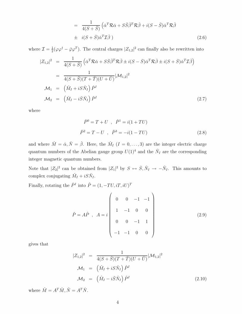
Finally, rotating the P I into P = (1,−TU, iT, iU)T

P = AP , A = i

0 0 −1 −1

1 −1 0 0

0 0 −1 1

−1 −1 0 0

(2.9)

gives that

|Z1,2|2 =1

4(S + S)(T + T )(U + U)|M1,2|2

M1 =(

MI + iSNI

)

P I

M2 =(

MI − iSNI

)

P I (2.10)

where M = AT M, N = AT N .

4

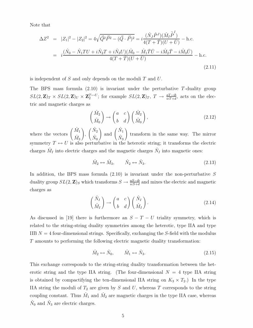
Note that

∆Z2 = |Z1|2 − |Z2|2 = 4√

~Q2 ~P 2 − ( ~Q · ~P )2 = i(NJ P J)(MI

¯P

I)

4(T + T )(U + U)− h.c.

= i(N0 − N1TU + iN2T + iN3U)(M0 − M1T U − iM2T − iM3U)

4(T + T )(U + U)− h.c.

(2.11)

is independent of S and only depends on the moduli T and U .

The BPS mass formula (2.10) is invariant under the perturbative T -duality group

SL(2,Z)T × SL(2,Z)U × ZT↔U2 ; for example SL(2,Z)T , T → aT−ib

icT+d, acts on the elec-

tric and magnetic charges as(

M2

M0

)

→(

a c

b d

)(

M2

M0

)

, (2.12)

where the vectors

(

M1

M3

)

,

(

N2

N0

)

and

(

N1

N3

)

transform in the same way. The mirror

symmetry T ↔ U is also perturbative in the heterotic string; it transforms the electric

charges MI into electric charges and the magnetic charges NI into magnetic ones:

M2 ↔ M3, N2 ↔ N3. (2.13)

In addition, the BPS mass formula (2.10) is invariant under the non-perturbative S

duality group SL(2,Z)S which transforms S → aS−ibicS+d

and mixes the electric and magnetic

charges as(

NI

MI

)

→(

a c

b d

)(

NI

MI

)

. (2.14)

As discussed in [19] there is furthermore an S − T − U triality symmetry, which is

related to the string-string duality symmetries among the heterotic, type IIA and type

IIB N = 4 four-dimensional strings. Specifically, exchanging the S-field with the modulus

T amounts to performing the following electric magnetic duality transformation:

M2 ↔ N0, M1 ↔ N3. (2.15)

This exchange corresponds to the string-string duality transformation between the het-

erotic string and the type IIA string. (The four-dimensional N = 4 type IIA string

is obtained by compactifying the ten-dimensional IIA string on K3 × T2.) In the type

IIA string the moduli of T2 are given by S and U , whereas T corresponds to the string

coupling constant. Thus M1 and M2 are magnetic charges in the type IIA case, whereas

N0 and N3 are electric charges.

5

The transformation S ↔ U , which corresponds to the string-string duality between the

heterotic and type IIB string, is obtained is an analogous way:

M1 ↔ N2, M3 ↔ N0. (2.16)

In the IIB string the moduli of T2 correspond to S and T , whereas the string coupling

constant is denoted by U . These two transformations S ↔ T and S ↔ U , are thus

of non-perturbative nature since electric charges and magnetic charges are exchanged.

However, as we will discuss in the following, the exchange S ↔ T is not a true symmetry

of the heterotic string. The BPS mass spectrum of the the heterotic (IIA, IIB) string is

not symmetric under the exchange S ↔ T (T ↔ U , S ↔ U), since the BPS masses are

given by the maximum of |Z1|2 and |Z2|2. These operations just exchange the spectrum

of the heterotic string with the spectrum of the type IIA, IIB strings.

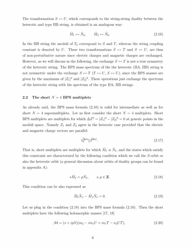
2.2 The short N = 4 BPS multiplets

As already said, the BPS mass formula (2.10) is valid for intermediate as well as for

short N = 4 supermultiplets. Let us first consider the short N = 4 multiplets. Short

BPS multiplets are multiplets for which ∆Z2 = |Z1|2 − |Z2|2 = 0 at generic points in the

moduli space. Namely Z1 and Z2 agree in the heterotic case provided that the electric

and magnetic charge vectors are parallel:

~Qhet||~P het. (2.17)

That is, short multiplets are multiplets for which MI ∝ NI , and the states which satisfy

this constraint are characterized by the following condition which we call the S-orbit or

also the heterotic orbit (a general discussion about orbits of duality groups can be found

in appendix A):

sMI = pNI , s, p ∈ Z. (2.18)

This condition can be also expressed as

MINJ − MJNI = 0. (2.19)

Let us plug in the condition (2.18) into the BPS mass formula (2.10). Then the short

multiplets have the following holomorphic masses [17, 18]

M = (s + ipS)(m2 − im1U + in1T − n2UT ), (2.20)

6

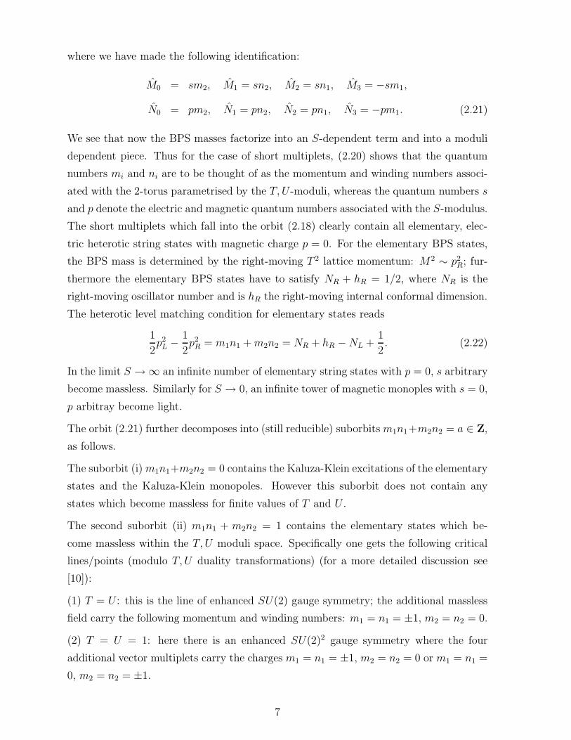
where we have made the following identification:

M0 = sm2, M1 = sn2, M2 = sn1, M3 = −sm1,

N0 = pm2, N1 = pn2, N2 = pn1, N3 = −pm1. (2.21)

We see that now the BPS masses factorize into an S-dependent term and into a moduli

dependent piece. Thus for the case of short multiplets, (2.20) shows that the quantum

numbers mi and ni are to be thought of as the momentum and winding numbers associ-

ated with the 2-torus parametrised by the T, U-moduli, whereas the quantum numbers s

and p denote the electric and magnetic quantum numbers associated with the S-modulus.

The short multiplets which fall into the orbit (2.18) clearly contain all elementary, elec-

tric heterotic string states with magnetic charge p = 0. For the elementary BPS states,

the BPS mass is determined by the right-moving T 2 lattice momentum: M2 ∼ p2R; fur-

thermore the elementary BPS states have to satisfy NR + hR = 1/2, where NR is the

right-moving oscillator number and is hR the right-moving internal conformal dimension.

The heterotic level matching condition for elementary states reads

1

2p2

L − 1

2p2

R = m1n1 + m2n2 = NR + hR − NL +1

2. (2.22)

In the limit S → ∞ an infinite number of elementary string states with p = 0, s arbitrary

become massless. Similarly for S → 0, an infinite tower of magnetic monoples with s = 0,

p arbitray become light.

The orbit (2.21) further decomposes into (still reducible) suborbits m1n1+m2n2 = a ∈ Z,

as follows.

The suborbit (i) m1n1+m2n2 = 0 contains the Kaluza-Klein excitations of the elementary

states and the Kaluza-Klein monopoles. However this suborbit does not contain any

states which become massless for finite values of T and U .

The second suborbit (ii) m1n1 + m2n2 = 1 contains the elementary states which be-

come massless within the T, U moduli space. Specifically one gets the following critical

lines/points (modulo T, U duality transformations) (for a more detailed discussion see

[10]):

(1) T = U : this is the line of enhanced SU(2) gauge symmetry; the additional massless

field carry the following momentum and winding numbers: m1 = n1 = ±1, m2 = n2 = 0.

(2) T = U = 1: here there is an enhanced SU(2)2 gauge symmetry where the four

additional vector multiplets carry the charges m1 = n1 = ±1, m2 = n2 = 0 or m1 = n1 =

0, m2 = n2 = ±1.

7

(3) T = U−1 = ρ = eiπ/6: this is the point of enhanced SU(3) gauge symmetry with

six additional massless vector multiplets of charges m1 = n1 = ±1, m2 = n2 = 0 or

m1 = n1 = m2 = ±1, n2 = 0 or m1 = n1 = −n2 = ±1, m2 = 0.

In addition, this suborbit (ii) contains also the socalled H monopoles.

2.3 The intermediate N = 4 BPS multiplets

Let us now investigate the structure of the intermediate N = 4 BPS multiplets. Interme-

diate BPS multiplets are multiplets for which ∆Z2 6= 0 at generic points in the moduli

space. Inspection of (2.11) shows that intermediate multiplets are dyonic and that the

vectors M and N are not proportional to each other. Heterotic intermediate orbits can

be characterized as follows

MINJ − MJNI 6= 0. (2.23)

In analogy to the constraint (2.21) for the short heterotic multiplets let us consider a

constraint which leads to a BPS mass formula which factorizes into a T -dependent and

into a S, U -dependent term. Specifically this constraint, the T -orbit or type IIA orbit,

has the form

M0 = sm2, M1 = −pm1, M2 = pm2, M3 = −sm1,

N0 = sn1, N1 = pn2, N2 = pn1, N3 = sn2, (2.24)

and the BPS mass formula (2.10) in the heterotic case can be written as

M1 = (s + ipT )(m2 − im1U + in1S − n2US),

M2 = (s + ipT )(m2 − im1U − in1S + n2US). (2.25)

This formula and the constraint (2.24) are invariant under SL(2,Z)S × SL(2,Z)T ×SL(2,Z)U . Clearly, the constraints (2.24) and (2.18) are just related by the S ↔ T

transformation given in eq.(2.15). The states satisfying the constraint (2.24) are short3

and also intermediate N = 4 multiplets in the heterotic string theory. However, using the

string-string duality between the heterotic string and the type IIA string, these states

are short N = 4 multiplets in the dual type IIA theory. This means that the orbit

condition (2.24) is satisfied for electric and magnetic charge vectors which are parallel

3As shown in appendix A, the short multiplets are precisely those which are simultanously in the T

and in the S orbit (and therefore in the STU orbit).

8

in the type IIA theory: ~QIIA||~P IIA ⇔ M(A) ∧ N(A) = 0.4 Then the transformations

SL(2,Z)S × SL(2,Z)U × ZU↔S2 are perturbative in the IIA theory, whereas SL(2,Z)T

is of non-perturbative origin. Thus, one can just repeat the analyis of the additional

massless states for the type IIA theory. Specifically, in the type IIA theory there is a

critical line S = U with two additional massless fields, a critical point S = U = 1 with

four additional massless points, and a critical point S = U−1 = ρ with six additional

massless fields. In the case of being electric (p = 0) these states lead to a gauge symmetry

enhancement in the type IIA theory. The corresponding charges immediately follow from

our previous discussion. Note, however, that the additional massless gauge bosons are

not elementary in the type II string but of solitonic nature [5].

Switching again back to the heterotic theory, there are no massless intermediate mul-

tiplets within this orbit at the line S = U or points S = U = 1, S = U−1 = ρ.

The reason is that we have to remind ourselves that the correct BPS masses are given

by the maximum of |Z1|2 and |Z2|2. To illustrate this, take S = U and consider as

an example the state with p = m2 = n2 = 0, m1 = n1 = 1 and s arbitrary, i.e.

M0 = M1 = M2 = N1 = N2 = N3 = 0, M3 = −s, N0 = s. The BPS mass of this

intermediate state is given by m2BPS = |Z2|2 = s2

4(T+T ). Thus we see that the heterotic

BPS mass formula is not symmetric under S ↔ T .

Of course, there exists another constraint, the U or type IIB orbit,

M0 = sm2, M1 = pn1, M2 = sn1, M3 = pm2,

N0 = −sm1, N1 = pn2, N2 = sn2, N3 = −pm1, (2.26)

for which the corresponding BPS mass formula factorises into

M1 = (s + ipU)(m2 − im1S + in1T − n2ST ),

M2 = (s + ipU)(m2 + im1S + in1T + n2ST ). (2.27)

The discussion of this case is completely analogous to the previous one; the states which

satisfy the constraint (2.26) correspond to the short N = 4 BPS multiplets in the dual

type IIB theory with ~QIIB||~P IIB ⇔ M(B) ∧ N(B) = 0.5

As discussed above, the orbits (2.24) and (2.26) do not contain additional massless in-

termediate states in the heterotic theory. There are, however, further lines in the moduli

space at which intermediate multiplets with spin 3/2 components appear to become

4 See the discussion given in appendix A.5 See the discussion in appendix A.

9

massless, as it was already observed in [24].6 Additional massless spin 3/2 multiplets

are clearly only physically acceptable if they lead to a consistent enhancement of the

local N = 4 supersymmetry to higher supergravity such as N = 5, 6, 8. However, we do

not find a non-perturbative enhancement of N = 4 supersymmetry at the lines of possi-

ble massless intermediate multiplets. Moreover it is absolutely not clear whether these

massless spin 3/2 fields really exist as physical soliton solutions. In fact there are some

additional good reasons to reject these states from the physical BPS spectrum. First

the explicitly known [24] heterotic soliton solutions for massless intermediate states are

singular. Second an argument against the existence of massless spin 3/2 multiplets could

be the fact that such states do not exist in any fundamental string at weak coupling.

Finally, in the next chapter will argue that these kind of massless states also do not ap-

pear in N = 2 heterotic strings. Nevertheless we think it is useful to further investigate

the interesting problem of non-perturbative supersymmetry enhancement in the future.

Therefore we list the possible massless spin 3/2 multiplets, i.e. the zeroes of the BPS

mass formula, in appendix B.

3 The N = 2 BPS Spectrum

3.1 General formulae

Let us now discuss the spectrum of BPS states in four-dimensional strings with N = 2

supersymmetry. These masses are dermined by the complex central charge Z of the

N = 2 supersymmetry algebra: m2BPS = |Z|2. In N = 2 supergravity the states that

saturate this BPS bound belong either to short N = 2 hyper multiplets or to short N = 2

vector multiplets. In general the mass formula as a function of n Abelian massless vector

multiplets φi (i = 1, . . . , nV ) is given by the following expression [26, 27, 28]

m2BPS = eK |MIP

I + iN IQI |2 = eK |M|2. (3.1)

Here K is the Kahler potential, the MI (I = 0, . . . , nV ) are the electric quantum numbers

of the Abelian U(1)nV +1 gauge group and the N I are the magnetic quantum numbers.

Ω = (P I , iQI)T denotes a symplectic section or period vector; the mass formula (3.1) is

6 A massive intermediate spin 3/2 multiplet saturating one central charge has the following component

structure: (1 × Spin 3/2, 6 × spin 1, 14 × spin 1/2, 14 × spin 0), where the components transform as

representations of USp(6). A massless spin 3/2 multiplet has the following structure (1 × spin 3/2, 4×spin 1, (6 + 1) × spin 1/2, (4 + 4) × spin 0). Then, if the intermediate multiplet becomes massless at

special points in the moduli space, the ’Higgs’ effect works such that 1 massive spin 3/2 multiplet splits

into a massless spin 3/2 plus 2 massless vector multiplets.

10

invariant under the following symplectic Sp(2nV + 2,Z) transformations, which act on

the period vector Ω as(

P I

iQI

)

→ Γ

(

P I

iQI

)

=

(

U Z

W V

)(

P I

iQI

)

, (3.2)

where the (nV + 1) × (nV + 1) sub-matrices U, V, W, Z have to satisfy the symplectic

constraints UT V − W T Z = V T U − ZT W = 1, UT W = W T U , ZT V = V T Z. Thus

the target space duality group Γ, perturbatively as well non-perturbatively, is a certain

subgroup of Sp(2nV + 2,Z).

The holomorphic section Ω is determined by the vacuum expectation values and cou-

plings of the nV + 1 massless vector multiplets XI belonging to the Abelian gauge group

U(1)nV +1. (The field X0, which belongs to the graviphoton U(1) gauge group, has no

physical scalar degree of freedom; in special coordinates it will simply be set to one:

X0 = 1; then one has φi = X i.) Specifically, in a certain coordinate system [25], one

can simply set P I = XI and the QI can be expressed in terms of the first derivative

of an holomorphic prepotential F (XI) which is an homogeneous function of degree two:

QI = FI = ∂F (XI)∂XI . The gauge couplings as well as the Kahler potential can be also

expressed in terms of F (XI); for example the Kahler potential is given by

K = − log(−iΩ†

0 1

−1 0

Ω) = − log(

XIFI + XIFI

)

(3.3)

which is, like M, again a symplectic invariant.

To be specific we will now consider an heterotic string which is obtained from six dimen-

sions as a compactification on a two-dimensional torus T2. The corresponding physical

vector fields are defined as S = iX1

X0 , T = −iX2

X0 , U = −iX3

X0 and the graviphoton corre-

sponds to X0. Thus there is an Abelian gauge group U(1)4.

3.2 The classical N = 2 BPS spectrum

Let us start by discussing the form of the classical BPS spectrum. The classical heterotic

prepotential is given by [27, 29, 30]

F = iX1X2X3

X0= −STU. (3.4)

This classical prepotential is obviously invariant under the full exchange of all vector

fields S ↔ T ↔ U . When considering the classical gauge Lagrangian [25], which follows

from this prepotential, one finds a complete ‘democracy’ among the three fields S, T

11

and U . Specifically, we will discuss three types of symplectic bases (the discussion about

these bases is quite analogous to the discussion about the three S, T, U orbits given in

the previous chapter).

First, consider a choice of symplectic basis (we call this the S-basis) in which the S-field

plays its conventional role as the loop counting parameter. The weak coupling limit,

i.e. the limit when all gauge couplings become simultaneously small, is given by the

limit S → ∞. As explained in [27, 29, 30], the period vector (XI , iFI) (FI = ∂FXI ), that

follows from the prepotential (3.4), does not lead to classical gauge couplings which all

become small in the limit of large S. Specifically, the gauge couplings which involve the

U(1)S gauge group are constant or even grow in the string weak coupling limit S → ∞like (S + S)−1, whereas the couplings for U(1)T × U(1)U behave in the standard way

as being proportional to S + S. In order to choose a period vector, with all gauge

couplings being proportional to S + S, one has to replace F Sµν by its dual which is weakly

coupled in the large S limit. This is achieved by the following symplectic transformation

(XI , iFI) → (P I , iQI) where7

P 1 = iF1, Q1 = iX1, and P i = X i, Qi = Fi for i = 0, 2, 3. (3.5)

In the S-basis the classical period vector takes the form

ΩT = (1, TU, iT, iU, iSTU, iS,−SU,−ST ), (3.6)

where X0 = 1. One sees that after the transformation (3.5) all electric period fields P I

depend only on T and U , whereas the magnetic period fields QI are all proportional to

S. In this basis Ω the holomorphic BPS masses (3.1) become8

M = M0 + M1TU + iM2T + iM3U + iS(N0TU + N1 + iN2U + iN3T ) (3.7)

Let us compare these N = 2 BPS masses with the N = 4 BPS masses discussed in

section 2. Specifically, comparing with eq.(2.10) we recognize that the classical N = 2

mass formula and the N = 4 mass formula M1 agree upon the trivial substitution

M1 = −M1, N0 = −N1, N1 = N0. (Substituting S by S and setting M0 = −M0,

M1 = M1, M2 = −M2, M3 = −M3, N0 = −N1, N1 = N0 the N = 2 BPS masses

agree with M2.) In contrast to N = 4, eq.(3.7) directly gives the correct BPS masses

7Note however that the new coordinates P I are not independent and hence there is no prepotential

Q(P I) with the property QI = ∂Q∂P I .

8We call this the classical BPS spectrum, since it is computed by using the tree level prepotential.

Nevertheless this BPS spectrum contains non-perturbative solitons, and this formula refers to their

‘classical’, i.e. weak coupling, masses.

12

without one having to take the maximum of two in general different central charges. The

reason for this is the fact that in N = 2 all BPS states belong to short (vector or hyper)

multiplets. In fact, when truncating the N = 4 heterotic string down to N = 2, the

short as well as the intermediate N = 4 multiplets become short in the N = 2 context.

This observation potentially leads to new N = 2 massless BPS multiplets which will be

a genuine N = 2 effect as we discuss in the following.

The classical U(1)4 gauge Lagrangian in the S-basis and the classical N = 2 BPS mass

formula are invariant under the perturbative duality symmetries SL(2,Z)T ×SL(2,Z)U ×ZT↔U

2 . As discussed above [27, 29, 30], these transformations can be written as spe-

cific Sp(8,Z) transformations Γclassical with the property that W classical = Zclassical = 0,

U classicalT V classical = 1. In addition, the field equations in the S-basis and the classical

BPS mass formula are also invariant under SL(2,Z)S and, in contrast to the N = 4

heterotic case, are also invariant under the transformations S ↔ T and S ↔ U . Of

course, whether the BPS spectrum is really invariant under the symmetries S ↔ T and

S ↔ U depends on the non-perturbative dynamics and cannot be read off from the BPS

mass formula. The point is that, unlike the N = 4 case, the N = 2 BPS mass formula

in principle allows for an S ↔ T ↔ U symmetric spectrum. Indeed there exist some

good indications that specific models are S ↔ T ↔ U symmetric even after taking into

account all non-perturbative corrections. The non-perturbative duality transformations

are given by specific Sp(8,Z) transformations with group elements, that have in general

non-zero submatrices W and Z. For example, the transformation S ↔ T corresponds to

the following non-perturbative symplectic Sp(8,Z) transformation:

P 1 ↔ −iQ3, P 2 ↔ iQ1. (3.8)

Analogously the transformation S ↔ U is induced by

P 1 ↔ −iQ2, P 3 ↔ iQ1. (3.9)

The symplectic transformations which correspond to SL(2,Z)S can be, for example,

found in [27, 29].

Let us now define a second symplectic basis, the T -basis, in which the T -field plays the

role of the loop counting parameter. In the T -basis all gauge couplings go to zero for

large T . As we will see, the T -basis is related to the standard S-basis essentially by

a non-perturbative S ↔ T transformation, i.e. by an exchange of certain electric and

magnetic fields [19]. In exact analogy to the S-field dependence of the classical gauge

couplings, the prepotential (3.4) leads to gauge couplings of U(1)T which are constant

or grow in the limit T → ∞. In order to obtain a uniform T -dependence of all gauge

13

couplings one has to perform an electric magnetic duality transformation for U(1)T , as

follows

P 2 = iF2, Q2 = iX2, and P i = X i, Qi = Fi for i = 0, 1, 3. (3.10)

Then the new classical period vector in the

T -basis reads ΩT = (1, iS,−SU, iU, iSTU, TU,−iT,−ST ). We recognize that all elec-

tric periods P I do not depend on T , whereas the magnetic periods QI are propotional

to T . Clearly the period vector Ω is just obtained by an S ↔ T transformation from the

period vector Ω together with some trivial relabeling of electric and magnetic charges.

In the T -basis the classical gauge Lagrangian as well as the BPS mass formula are invari-

ant under the transformations SL(2,Z)S × SL(2,Z)U × ZS↔U2 . These transformations

are of perturbative nature in the T -basis and correspond to sympletic matrices Γ with

W = Z = 0, UT V = 1. On the other hand the transformations SL(2,Z)T ×ZT↔U2 ×ZS↔T

2

are of non-perturbative nature with in general W , Z 6= 0.

It is obvious that one can finally choose another period vector, the U -basis, which leads

to classical gauge couplings which have a uniform dependence on U and vanish in the

limit of U → ∞. The corresponding formula look analogous to the one just discussed

and can be easily written down.

Next let us discuss the form of the classical N = 2 BPS spectrum with special focus on

the appearance of massless states. Specifically, the singular loci of additional massless

states in the classical moduli space fall into three different classes:

(i) First there are the elementary states which become massless at T = U , T = U = 1

and T = U = ρ, for all values of S. At these lines (points) the U(1)2L gauge symmetries

are classically enhanced to SU(2), SU(2)2 or SU(3) respectively. In the ‘standard’ S-

basis the corresponding BPS states carry only electric charges; however, when seen in

the T, U-basis, these states are dyonic.

(ii) Second, suppose that the S ↔ T ↔ U symmetry is present in the BPS spectrum.

Then there are massless BPS states at the lines (points) S = T 9, S = T = 1, S = T = ρ

for arbitray U and analogously at S = U , S = U = 1, S = U = ρ for arbitray T .

In case of a perfect dynamical realization of the triality symmetry S ↔ T ↔ U , the

BPS states are N = 2 vectormultiplets, and the Abelian gauge symmetries are again

enhanced to SU(2), SU(2)2 or SU(3) respectively. In the S-basis these BPS states are

non-perturbative dyons, whereas in the T respectively U -basis these states are purely

electric. Thus, in the S-basis, U(1) factors, which are magnetic, are enhanced at these

special points in the S, T, U moduli space. The possible appearance of these additional

9This line was already briefly noted in reference [21].

14

massless BPS fields for special values of the S-field is a genuine N = 2 effect not being

possible in N = 4.

(iii) Third, there are massless dyons for strong or weak coupling S = 0 or S = ∞ at the

lines eqs.(9.6) and (9.7) and, for all S, at T = U = 1, T = U = ρ. These states belong

to N = 2 BPS multiplets, which originate from N = 4 intermediate multiplets, and are

not related to an enhancement of the Abelian gauge symmetries. In case of a S ↔ T ,

S ↔ U symmetry there will be also analogous massless BPS states at the transformed

lines/points.

3.3 The quantum N = 2 BPS spectrum

Of course, in general there will be non-perturbative corrections which change the classical

BPS spectrum in a crucial way. In the following we will argue that for finite S, after

taking into account the non-perturbative corrections, the classical singular lines in (i)

split into lines of massless monopoles and dyons a la Seiberg and Witten. With respect

to the massless states in (ii), we will conjecture that in models, which are completely

S ↔ T ↔ U symmetric, there is a non-perturbative gauge symmetry enhancement for

large T or large U . Moreover we conjecture that for finite T , U respectively, these lines

of massless gauge bosons are again split into lines of massless monopoles and dyons.

However we will find no sign of massless states of type (iii) in the non-perturbative

spectrum.

In order to consider the form of the BPS spectrum after perturbative as well of non-

perturbative corrections, we make the following ansatz for the prepotential in the S-basis

F = iX1X2X3

X0+ (X0)2

(

f 1(T, U) + fNP(e−2πS, T, U))

(3.11)

Here f 1(T, U) denotes the one-loop prepotential [29, 30] which cannot, by simple power

counting arguments, depend on S. Clearly, for large S one gets back the tree level

prepotential. From the prepotential (3.11) we obtain the following non-perturbative

period vector ΩT = (P, iQ)

ΩT = (1, TU − fNPS , iT, iU, iSTU + 2i(f 1 + fNP) − iT (f 1

T + fNPT ) − iU(f 1

U + fNPU )

− iSfNPS , iS,−SU + f 1

T + fNPT ,−ST + f 1

U + fNPU ) (3.12)

This leads to the following non-perturbative mass formula for the BPS states

M = MIPI + iN IQI = M0 + M1(TU − fNP

S ) + iM2T + iM3U + iN0(STU

+ 2(f 1 + fNP) − T (f 1T + fNP

T ) − U(f 1U + fNP

U ) − SfNPS ) + iN1S

15

+ iN2(iSU − if 1T − ifNP

T ) + iN3(iST − if 1U − ifNP

U ) (3.13)

We see that all states with M1 6= 0 or N I 6= 0 undergo a non-perturbative mass shift. We

also recognize that electric states with N I = 0 do not get a mass shift at the perturbative

1- loop level. However the masses of states with magnetic charges N I 6= 0 are already

shifted at the 1-loop level.

The 1-loop prepotential f 1 exhibits logarithmic singularities exactly at the lines (points)

of the classically enhanced gauge symmetries and is therefore not a single valued function

when transporting the moduli fields around the singular lines (see [29, 30, 10] for all the

details). For example around the singular SU(2) line T = U 6= 1, ρ the function f 1 must

have the following form [29, 30, 10]

f 1(T, U) =1

π(T − U)2 log(T − U) + ∆(T, U), (3.14)

where ∆(T, U) is finite and single valued at T = U 6= 1, ρ. Around the point (T, U) =

(1, 1) the prepotential takes the form [29, 30, 10]

f 1(T, U = 1) =1

π(T − 1) log(T − 1)2 + ∆′(T ) (3.15)

and around (T, U) = (ρ, ρ) [29, 30, 10]

f 1(T, U = ρ) =1

π(T − ρ) log(T − ρ)3 + ∆′′(T ), (3.16)

where ∆′(T ), ∆′′(T ) are finite at T = 1, T = ρ respectively. It follows that, when

moving around these critical lines via duality transformations, one has non-trivial

monodromy properties. Hence at one-loop, the perturbative duality transformations

SL(2,Z)T × SL(2,Z)U × ZT↔U2 , called Γ∞, are given in terms of Sp(8,Z) matrices with

U∞ = U classical, W∞ 6= 0, but still Z∞ = 0. This results in non-trivial shifts of the θ-

angles at 1-loop. In contrast to Γclassical, the 1-loop duality matrices [30] do not preserve

the short orbit condition eq.(2.18). This means that, from the N = 4 point of view,

the N = 2 1-loop monodromies in general mix N = 2 BPS states which originate from

N = 4 vectormultiplets with hypermultiplets which are truncated N = 4 intermediate

multiplets.

Now, taking into account the non-perturbative effects with e−2πS 6= 0 , the non-Abelian

gauge symmetries are never restored, and each perturbative critical line splits into

two lines of massless monopoles and dyons respectively [1, 10, 11]. It follows that

each semiclassical, i.e. 1-loop, monodromy around the lines of enhanced gauge sym-

metries are given by the product of two monodromies around the singular monopole

and dyon lines, i.e. Γ∞ = Γmonopole × Γdyon with Γmonopole, Γdyon ∈ Sp(8) and

16

Wmonopole, Zmonopole, W dyon, Zdyon 6= 0. Thus, only in the limit S → ∞ is the theory

still symmetric under the perturbative duality group SL(2,Z)T × SL(2,Z)U × ZT↔U2 .

Making an reasonable ansatz for Γmonopole and Γdyon, one can show [10, 11] that this

splitting can be performed in such a way that in the rigid limit one precisely recovers the

results of Seiberg and Witten. In addition the correct rigid limit was confirmed [12, 11]

by directly computing the non-perturbative monodromies Γmonopole and Γdyon in type II

Calabi-Yau compactifications with h11 = 2, i.e. for models with two vector fields S and

T .

Consider for example the splitting of the critical line T = U with classically enhanced

gauge group SU(2); the associated magnetic monopole has non vanishing magnetic quan-

tum numbers N3 = −N2. Like the massless gauge bosons before, this magnetic monopole

corresponds to a short N = 4 vector multiplet, i.e. it belongs to the first orbit (2.21).

Using (3.13) its mass vanishes for Q2 = Q3, which leads to following singular monopole

locus

iS(T − U) − i(f 1T − f 1

U) − i(fNPT − fNP

U ) = 0 (3.17)

Similarly, the locus of massless dyons with charges M2 = −M3 = N3, N2 = −N3 has the

form T −U = Q2 −Q3. Like Γ∞, Γmonopole and Γdyon do not preserve the heterotic short

orbit condition eq.(2.18).

Let us now suppose that the full non-perturbative theory is symmetric under the exchange

symmetry S ↔ T . In fact the existence of this type of quantum symmetry was already

observed in models with only two fields S and T [9, 12, 11]. If this symmetry is exact

we expect that in the ‘weak coupling limit’ T → ∞ one finds an enhancement of the

Abelian gauge group at special points in the S, U moduli space. Specifically, at S = U

the enhanced gauge group should be SU(2), at S = U = 1 one has SU(2)2 and at S =

U−1 = ρ one should find SU(3). In the limit T → ∞ the non-perturbative prepotential,

written in the symplectic T -basis, then takes the form

f(S, U) =1

π(S − U)2 log(S − U) + . . . ; (3.18)

at the point (S, U) = (1, 1) the prepotential takes the form

f(S, U = 1) =1

π(S − 1) log(S − 1)2 + . . . (3.19)

and around (S, U) = (ρ, ρ)

f(S, U = ρ) =1

π(S − ρ) log(S − ρ)3 + . . . . (3.20)

17

It follows that, when moving around these critical lines via duality transformations, one

has non-trivial monodromy properties just like at one loop for large S. At large T the

theory is symmetric under the duality transformations SL(2,Z)S × SL(2,Z)U × ZS↔U2 ,

called Γ∞, which are then given in terms of Sp(8,Z) matrices with U∞V T = 1, W∞ 6= 0,

Z∞ = 0.

What will happen if we turn on the coupling e−2πT in a S ↔ T symmetric theory? In

the spirit of Seiberg and Witten we expect that the lines of enhanced gauge symmetries

at T = ∞ again split into two lines of massless monopoles and dyons for finite e−2πT .

The corresponding monopole and dyon monodromies Γmonopole and Γdyon are just given

by conjugating Γmonopole and Γdyon by the generator of the S ↔ T exchange symmetry.

An analogous discussion of course applies for the non-perturbative symmetry S ↔ U .

In order to make the existence of the S ↔ T , S ↔ U symmetries in certain type of models

more plausibel it is very useful to utilize the (conjectured, however already quite well

established) duality [7, 9, 11, 12, 8, 36, 37, 38] between heterotic N = 2 strings and type

II N = 2 strings on a suitably choosen Calabi-Yau backgrounds. Specifically consider

a Calabi-Yau background characterized by the two Hodge numbers h11 and h21. In the

type IIA models, h11 must agree with the number of massless vector multiplets nV in the

heterotic model. The number of hypermultiplets nH is given by h21 +1 where the extra 1

accounts for the type II dilaton. Since the type II dilaton sits in an N = 2 hypermultiplet

and does not couple to the vector multiplets, the classical type II prepotential is exact.

It follows that BPS spectrum of the form (3.1) is exact in the type II case as well. For

the type IIA models, the Calabi-Yau world-sheet instanton effects then correspond to the

target space instanton effects on the heterotic side [8].

After performing the mirror map from IIA to IIB, the number of massless fields in the

IIB Calabi-Yau compactification is determined as nH = h11 + 1, nV = h21. In the type

IIB case the holomorphic prepotential receives no world sheet instanton corrections; it

becomes singular at the socalled conifold points in the Calabi-Yau moduli space and at

some other isolated points. Then, within the string-string duality picture the type IIB

singular locus just corresponds to the locus of massless magnetic monopoles or dyons on

the heterotic side (see the discussion below).

Let us first consider as the most simple example the case with only two vector fields S

and T . Specifically we consider the Calabi-Yau space, constructed as a hypersurface of

degree 12 in WP1,1,2,2,6(12), with h11 = 2 and h21 = 128 [23]. It was observed in [9, 12]

that this model indeed possesses an exchange symmetry S ↔ T at the non-perturbative

level. This symmetry can be recognized by looking at the instanton expansions, as

18

done in [9]. Specifically, the transformation q1 → q1q2, q2 → 1/q2 (q1 = ei2πt1 = e−2πT ,

q2 = ei2πt2 = e−2π(S−T )) can be traced back to the monodromy considerations of [23].

Under this transformation nj,kqj1q

k2 → nj,kq

j1q

j−k2 , so that the non-perturbative symmetry

should come from nj,k = nj,j−k where the nj,k are world-sheet instanton numbers of

genus zero. Indeed, it was shown in [23] (there in the model P1,1,2,2,2(8), but this makes

no difference here) that the homology type of the holomorphic image of the worldsheet

Σ changes as Σj,k = jh + kl → j(h + l) + k(−l) = j′h + k′l with j′ = j, k′ = j − k under

the monodromy T∞ : (t1, t2) → (t1 + t2,−t2 + 1) on the periods (t1, t2).

The singular discriminant locus of this Calabi-Yau, on which certain BPS states become

massless, is given by the following equation [7]

∆ = (1 − y)((1 − x)2 − x2y). (3.21)

The conventional weak coupling limit is given by y = e−2πSinv = 0. In this limit one

recovers the perturbative duality symmetry SL(2,Z)T (Sinv is the 1-loop redefined S-field,

invariant under the perturbative duality group), and the parameter x can be expressed

[9, 12] in terms of modular functions as x = 1728/j(T ). In the limit y = 0, ∆ degenerates

into the quadratic factor (1− x)2, and at x = 1, i.e. T = 1, one finds the classical SU(2)

gauge symmetry enhancement. For y 6= 0 this line splits into the two lines of massless

monopoles and dyons [9, 12].

Using the S ↔ T symmetry, the discriminant locus has a second ‘weak coupling’ limit,

where ∆ quadratically degenerates. We suggest to identify this limit with T → ∞; in this

limit SL(2,Z)S should be a symmetry of the theory. In the limit T → ∞ the coupling

constant y should be given as y = e−2πTinv → 0, where Tinv is a redefined modulus,

invariant under SL(2,Z)S. Then ∆ takes again the form ∆ ∼ (1 − x)2 which signals

a SU(2) gauge symmetry enhancement at x = 1 now corresponding to S = 1. Thus

we conjecture to make the following identification for large T : x = 1728/j(S). Observe

that for large S, this x is exponential in S: x → e−2πS. Turning on the coupling y,

the quadratic degeneracy is again lifted, and we expect that the large T gauge group

enhancement is replaced by the existence of a massless monopole, dyon pair. Recall

that in the weak coupling limit S → ∞ the appearance of the modular function j(T )

originates from the fact that the underlying Calabi-Yau space can be constructed as a

K3-fibration [9], where S plays the role of the size of the base space [38]. In analogy,

the S ↔ T symmetric picture could then mean that there exist a dual ‘quantum K3

fibration’ with T being the modulus of the base space, implying the appearance of the

modular function j(S) in the limit T → ∞.

Now let us investigate the case of three moduli S, T, U . The singular loci of massless

19

BPS states for this type of N = 2 string models was recently derived [12] from a type

IIB compactification on a Calabi-Yau space WP1,1,2,8,12(24) with h21 = 3 and h11 = 243

leading to 244 hypermultiplets (including the type II dilaton multiplet). In ref.[9] some

arguments were given supporting the conjecture that this model is symmetric under the

exchange S ↔ T , S ↔ U . The discriminant locus of the P1,1,2,8,12(24) Calabi-Yau is [7, 9]

∆ = (y − 1) × (1 − z)2 − yz2

z2× ((1 − x)2 − z)2 − yz2

z2= ∆y × ∆z × ∆x. (3.22)

x, y, z are functions of the three vector fields S, T, U .

Let us now consider three differents limits where ∆ degenerates into quadratic factors

that signal an enhancement of the Abelian gauge symmetry at special (boundary) points

in the moduli space.

(i) First consider the conventional classical limit y = e−2πSinv = 0. In this limit one

recovers the perturbative duality symmetry SL(2,Z)T × SL(2,Z)U × ZT↔U2 (again, Sinv

is the 1-loop redefined S-field, invariant under the perturbative duality group), and the

parameters x, z can be expressed in terms of the fields T, U as follows [9, 31, 12]:

x =1

864

j(T )j(U) +√

j(T )j(U)(j(T ) − 1728)(j(U) − 1728)

j(T ) + j(U) − 1728,

z = 8642 x2

j(T )j(U). (3.23)

In this limit the two equations ∆x = 0 and ∆z = 0 are completely equivalent. They both

correspond to the classical enhancement of one Abelian U(1) gauge group to SU(2). Both

equations are solved only by the relation j(T ) = j(U), the line of enhanced SU(2) gauge

symmetry. More exactly, ∆x and ∆z are double valued functions in terms of j(T ), j(U).

For j(T ) = j(U) the branch points are at j(T ) = 0 and j(T ) = 1728, i.e. at T = ρ,

T = 1 respectively and at all the points obtained by duality transformations of these two

points. With j(T ) = j(U) one obtains in the first branch that z = 1, x = 1864

j(T ),√

∆x =4j(T )(j(T )−1728)

17282 ,√

∆z = (j(T )−j(U))2

4j(T )(j(T )−1728)= 0. The points x = 0, x = 2, where ∆ further

degenerates, correspond to the points of enhanced gauge symmetries SU(3) or SU(2)2

respectively. In the second branch j(T ) = j(U) belongs to z = 17282

(2j(T )−1728)2, x = 1 ±√

z,√∆x = (j(T )−j(U))2

4j(T )(j(T )−1728)= 0,

√∆z = 4j(T )(j(T )−1728)

17282 . However the product√

∆x∆z is single

valued, and one obtains as an identity in the limit y = 0 [40]:√

∆x

√∆z = (j(T )−j(U))2

17282 .

In summary, in the classical limit y = 0 one precisely finds the lines (points) of enhanced

gauge symmetries, namely first SU(2) with j(T ) = j(U) corresponding to T = U (plus

all dual equivalent lines), second SU(2)2 with j(T ) = j(U) = 1728 corresponding to

T = U = 1 and third SU(3) with j(T ) = j(U) = 0 corresponding to T = U = ρ.

20

(ii) There exists a second limit where ∆ degenerates into quadratic factors. We conjecture

that this limit corresponds to T → ∞ and make in this limit the identification y =

e−2πTinv . In this limit the theory is invariant under SL(2,Z)S × SL(2,Z)U × ZS↔U2 and

Tinv is a redefined modulus, invariant under this group. Thus for large T , ∆ = 0 at

the line z = 1 which should be the line of enhanced SU(2) gauge symmetry for S = U .

Analogous to the previous case one should get a further degeneration at the two points

S = U = 1 and S = U = ρ, with enhanced gauge groups SU(2)2, SU(3) respectively.

For T 6= ∞, the quadratic degeneracy is lifted, and we expect that the solutions of ∆ = 0

correspond to lines of massless monoples and dyons. Unfortunately we are at the moment

not ready to prove all these conjectures. It would require a complete reorganisation of

the instanton sums in the type II mirror map.

Finally there should exist also a third quadratic degeneration of ∆, namely in the limit

U → ∞ with SL(2,Z)S × SL(2,Z)T × ZS↔T2 duality symmetry. In this limit the gauge

symmetry enhancement then takes place at S = T , S = T = 1 and S = T = ρ.

At the end of this section let us also mention that in the quantum case we did not find any

trace of those massless states which we discussed under point (iii) at the classical level. If

they would exist they should have shown up for large S in ∆, since they were classically

present for any S and hence in particular for weak coupling. This observation may be one

more argument against the existence of the corresponding massless intermediate states

in the N = 4 heterotic string.

4 N = 4 BPS sums

4.1 The N = 4 free energy

In the next sections we will discuss the topological string partition function as a sum over

BPS states. A similar type of partition function was introduced in [26]. More recently

the sum over BPS states was also discussed by Vafa in [34]. Concretely, let us define the

following partition function Z10

log Z =∑

BPS states

log m2BPS (4.1)

In the following, we will discuss the non-perturbative partition function obtained by

summing over the heterotic N = 4 BPS spectrum. Specifically, we will consider the

10Here, Z is not to be confused with the central charge.

21

following holomorphic free energy

F =∑

MI ,NI

logM1,2, (4.2)

where the holomorphic BPS masses are given in (2.10). The holomorphic free energy and

the non-holomorphic partition function are related as

Z = eF+FeK , (4.3)

where K is the Kahler potential of the moduli fields S, T, U (we are restricting the

discussion to an SO(2, 2)-coset subspace of the toroidal moduli space). K is given by

K = − log[(S + S)(T + T )(U + U)], (4.4)

which transforms under SL(2,Z)S, S → aS−ibicS+d

, as K → K + log(icS + d)+ log(−icS + d)

and likewise for SL(2,Z)T and SL(2,Z)U . It follows that eF must be a modular function

of modular weight -1 under SL(2,Z)S, SL(2,Z)T and SL(2,Z)U in order for Z being

completely duality invariant. F and Z are clearly non-perturbative expressions since they

involve the summation over elementary string states as well as over soliton states like

magnetic monopoles etc. Thus Z, F will exhibit the non-perturbative dilaton dependence

of the string partition function. Note that by demanding Z to be completely duality

invariant we are requiring the absence of non-perturbative duality anomalies, in particular

the absence of S-duality anomalies.

The sum eq.(4.2) can be more conveniently computed by selecting some specific summa-

tion orbits. One criterion of selecting the relevant summation orbits is that at least all

singularities of the free energy have to be contained in the correct way; in other words,

this means that the sum has to contain all possible states which can become massless at

certain points in the moduli space. In addition, the duality invariance of the free energy

must not be destroyed by summing over specific orbits. Let us start by first summing

over the three orbits (2.21), (2.24) and (2.26), which are related by the triality exchange

S ↔ T ↔ U . (Each of these summation orbits will contain further suborbits.) FT↔U

sums over the BPS states in the first orbit (2.21) and is invariant under T ↔ U . There-

fore FT↔U is summing over the short heterotic N = 4 vector multiplets; using eq.(2.20)

FT↔U becomes

FT↔U =∑

MI ,NI |CKL=0

log(M0−M1TU+iM2T +iM3U+iN0S−iN1STU−N2ST−N3SU)

(4.5)

In order to perform the sum one must solve the six equations CKL = 0 in terms of

unconstrained summation variables. This can be done generalizing a method described

22

in [41]. Consider the three equations C0i = 0 first. Setting N1 = N2 = N3 = 0 they

are fulfilled if either (i) N0 = 0 or (ii) M1 = M2 = M3 = 0. In case (ii) the other three

equations are already solved. It only remains to sum over two unconstrained variables

s := M0 and p := N0. Thus the first contribution to the sum is∑

(s,p)6=(0,0) log(s + ipS).

In case (i) we are left with four unconstrained variables m2 := M0, n2 := M1, n1 := M2

and m1 := −M3 resulting in a second contribution∑

(m1,m2,n1,n2)6=(0,0,0,0) log(m2− im1U +

in1T −n2TU). Summarizing we have succeded in writing FT↔U as an unconstrained sum

FT↔U =∑

(s,p)6=(0,0)

log(s+ ipS)+∑

(m1,m2,n1,n2)6=(0,0,0,0)

log(m2− im1U + in1T −n2TU) (4.6)

which splits into a non–perturbative part, which only involves S, and into a perturbative

part only depending on the moduli T and U .

Consider the first term in (4.6). The regularized sum [41, 26] over the electric and

magnetic charges s, p leads to the following contribution:∑

s,p log(s + ipS) = log η(S)−2,

where η is the Dedekind function. This term describes the non-perturbative S dependence

of FT↔U . eFT↔U transforms as a modular function of modular weight -1 under SL(2,Z)S.

FT↔U diverges linearly for large S as well as for small S. These divergences reflect

the appearance of infinitely many massless electric or magnetic states for S → ∞, 0

respectively. Now, in order to evaluate the second term in expression (4.6) we split the

sum into the two further suborbits, namely (i): m1n1 +m2n2 = 0, (ii): m1n1 +m2n2 = 1.

This choice is dictated by the appearance of the massless fields (see [35] for a detailled

discussion). The suborbit (i) contains no states which become massless for finite T and

U but infinitely many states (Kaluza-Klein and winding modes) which become massless

in the degeration limits T, U → 0,∞. Summing over the suborbit (i) leads to a term

log η(T )−2η(U)−2 with linear divergences for T → ∞, 0 due to the massless Kaluza Klein

states or winding modes in this limit. The second suborbit (ii) contains the finite number

of states which are massless at the critical points in the moduli space T = U , T = U = 1

and T = U = ρ. Then the suborbit (ii) leads to [35] log(j(T ) − j(U),11 where j is the

absolute modular invariant function. This expression is logarithmically divergent at the

critical lines (points) where the residues of the poles correctly agree with the number of

massless fields at the symmetry enhancement points. Thus collecting the different terms

(the higher orbits m1n1 + n2m2 > 1 do not give new terms) we obtain the following

11Here we have assumed that the regularization procedure is modular invariant. This assumption

however may not hold, and the regularization procedure may possess a kind of modular anomaly which

destroys the duality covariance of the sum; thus non-modular invariant, but completely finite terms may

be added to the regularized sum. These finite terms can be absorbed by a redefinition of the dilaton

field [29].

23

holomorphic free energy

FT↔U = log(η(S)−2η(T )−2η(U)−2(j(T ) − j(U))r). (4.7)

The coefficient r is undetermined at this stage and corresponds to the overall number

of states becoming massless at the specific lines (points). Clearly eFT↔U transform as a

modular function of modular weight -1 under SL(2,Z)S ×SL(2,Z)T ×SL(2,Z)U , and it

is invariant under T ↔ U (up to a possible extra overall ± sign).

Next let us discuss the sum FS↔U over the orbit eq.(2.24). At the first glimpse one could

believe that this sum is just obtained by performing S ↔ T exchange in FT↔U . This

conclusion would be true, if there were intermediate massless states in the second orbit

for S = U , S = U = 1, S = U = ρ in the heterotic string theory. They however do

not exist. Thus we conclude that the suborbit (ii) does not lead to singularities for finite

S, T, U . The fact that FT↔U and FS↔U do not agree reflects the non-invariance of the

heterotic BPS spectrum under the exchange S ↔ T .

Finally, the discussion about the sum over the orbit eq.(2.26) is completely analogous to

the previous case.

In case that there exist massless intermediate states at specific points/lines in the moduli

space, these states would also contribute to the free energy. However, as we have discussed

in section 2.3 there are many good reasons to discard these massless spin 3/2 BPS

soliton states. Thus we take eq.(4.7) as the complete result for the N = 4 heterotic free

energy. The associated non-perturbative partition function is invariant under SL(2,Z)S×SL(2,Z)T ×SL(2,Z)U ×ZT↔U

2 . It is very similar to the ordinary bosonic string partition

function. The type IIA (IIB) partition function is finally obtained by the exchange S ↔ T

(S ↔ U) in eq.(4.7).

4.2 Absence of N = 4 thresholds and the role of the N = 4 free energy

In the N = 4 case the free energy does not correspond to threshold corrections in the

low energy effective action, since loop corrections are absent in N = 4, even at the non-

perturbative level. In the following we will, for example, first recall the absence of 1-loop

gravitational threshold corrections in N = 4 heterotic strings.

In N = 4 compactifications of the heterotic string the dilaton S = 1g2 − i θ

8π2 parametrises

a Kahlerian SU(1, 1)-coset, whereas the non-Kahlerian SO(6, 22)-coset is parametrised

by moduli ΦI .

In a string calculation, 1-loop corrections to gravitational couplings in N = 4 heterotic

24

compactifications should, if present, be of the form

1

g2grav

= 12(S + S) +bgrav

16π2log

M2string

p2+ ∆(ΦI) (4.8)

∆(Φ) denotes the moduli dependent 1-loop corrections due to both massless and massive

modes in the theory. bgrav, on the other hand, denotes the gravitational beta function

coefficient computed from the massless fields. Note that the scale appearing in the

logarithm in (4.8) is the string scale, as it should for a string calculation.

In a field theory calculation, on the other hand, it is the Planck scale which should appear

in a 1-loop calculation. Thus, consider rewriting (4.8) as

1

g21

= 12(S + S) +bgrav

16π2(log

M2P lanck

p2+ K) + ∆(ΦI) (4.9)

where K = − log(S+S). Here K denotes the Kahler potential for the Kahlerian SU(1, 1)-

coset parametrised by the dilaton field S. We have used that M2P lanck ∝ (S + S)M2

string.

Actually, a field theory calculation would a priori give that

1

g21

= 12(S + S) +bgrav

16π2log

M2P lanck

p2+

cgrav

16π2K + ∆(ΦI) (4.10)

with some coefficient cgrav. The term proportional to bgrav

16π2 logM2

Planck

p2 arises from a 1-loop

graph with 2 external gravitational legs sticking out and massless fields running in the

loop. The term proportional to cgravK arises from a triangle graph with 2 gravitational

legs and one am leg sticking out and with massless fields running in the loop. Indeed,

as shown in [43], every fermion in the N = 4 theory couples to the ”Kahler connection”

am ∝ ∂SK ∂mS − c.c associated to the SU(1, 1)-coset (note again that the SO(6, 22)-

coset is not Kahlerian and hence there is no ”Kahler connection” associated to it). If the

field theory calculation is to match the string calculation (4.8), then one has to find that

bgrav = cgrav in the field theory calculation.

Consider now calculating bgrav and cgrav in field theory. bgrav is nothing but the sum

over the trace anomalies of the massless multiplets in the theory. At generic points in

the SO(6, 22)-moduli space, the massless multiplets around are the N = 4 supergravity

multiplet and 22 abelian N = 4 vector multiplets. The trace anomaly for an N = 4

vector multiplet is zero, as it is wellknown. What about the trace anomaly of the N = 4

supergravity multiplet? For an N = 4 compactification of the heterotic string, the

axion is not really a scalar degree of freedom but rather an antisymmetric tensor degree

of freedom.12 Taking into account the following trace anomaly contributions (in units

12The associated N = 4 supergravity multiplet will thus contain 1 graviton, 4 gravitini, 6 graviphotons,

4 Weyl fermions, 1 antisymmetric tensor and one real scalar.

25

where a real scalar degree of freedom contributes an amount of 1) [44], namely 1 from

a real scalar field, 74

from a Weyl fermion, −13 from a vector field, 212 from a graviton,

−2334

from a gravitino and 91 from an antisymmetric tensor, then gives that bgrav = 0 for

an N = 4 heterotic compactification.

Since it must be that bgrav = cgrav, it follows that one should for consistency also find that

cgrav = 0 in a field theory calculation. cgrav is nothing but the Kahler anomaly coefficent.

Using the N = 1 assignments for the Kahler charges one has that the fermions in the

N = 4 gravitational multiplet carry charges +1, whereas the gauginos in the N = 4 vector

multiplets carry charges −1. Then it follows that indeed cgrav = 4(21 + 1 − 22) = 0.

The fact that bgrav = cgrav = 0 indicates that there are no 1-loop corrections to g2grav in

N = 4 heterotic compactifications at all, as indeed shown by string scattering amplitude

calculations in the context of orbifold compactifications [45].

Thus, the N = 4 holomorphic free energy cannot correspond to threshold corrections in

the low energy effective action. What role then does the N = 4 non-holomorphic free

energy discussed in the previous section play in the context of N = 4 heterotic strings?

We conjecture that it is the S-duality invariant partition function of topologically twisted

N = 4 heterotic string compactifications. A priori one might expect the partition function

of the topologically twisted theory to be holomorphic in the moduli fields. However, it

was pointed out in [46] that, at least in the context of topologically twisted N = 4

super Yang-Mills theory on four-manifolds, there are examples where this is not the case

due to the appearence of holomorphic anomalies. Hence, it is possible that the non-

holomorphicity of the N = 4 free energy is again a manifestation of the appearance of

holomorphic anomalies in the twisted version of N = 4 string compactifications.

If indeed the N = 4 free energy is to be identified with the partition function of topo-

logically twisted N = 4 string compactifications, then this implies that, whereas the

holomorphic gravitational coupling Fgrav = 24S of the untwisted model doesn’t receive

perturbative or non-perturbative corrections, the holomorphic coupling F1 of the twisted

model is more complicated and given by (4.7). Something similar happens in the case

of twisted N = 4 super Yang-Mills theory on four-manifolds. There, it was found [46]

that S-duality invariance of the twisted partition function only holds provided that there

are certain non-minimal couplings in the Lagrangian of the form log η(S)χ that involve

the background gravitational field, where χ denotes the Euler characteristic of the four-

manifold (χ ∝ ∫

GB, where GB denotes the Gauss-Bonnet combination). Namely, the

partition function Z[S] for the topologically twisted N = 4 super Yang-Mills theory

26

transforms like a modular form with modular weight w under S → 1S

Z[S] → SwχZ[S] (4.11)

(ignoring the issue of holomorphic anomalies). The following modified partition function

Z[S] = e−F1χZ[S] (4.12)

however, is invariant under S → 1S

provided that F1 ∝ log η(S).

5 N = 2 BPS sums

5.1 The N = 2 free energy

Let us again define the N = 2 holomorphic free energy F as the sum over the N = 2

BPS states (3.1), that is

F =∑

MI ,NI

log(MIPI + iN IQI). (5.1)

This formula was introduced in [26] in the context of string compactifications on Calabi-

Yau spaces. Like in the previous N = 4 case it is useful to split this sum into sums over

the different orbits of the relevant duality group Γ. Since the N = 2 Kahler potential

changes under duality transformations Γ =

(

U Z

W V

)

as

K → K + log |U0I P I/P 0|2 (5.2)

the holomorphic N = 2 free has to transform as

F → F − log U0I PI/P

0. (5.3)

The non-perturbative heterotic N = 2 free energy based on the non-perturbative BPS

mass formula (3.13) is in general very difficult to compute. It is clear that F will diverge

at those loci in the non-perturbative moduli space where BPS states become massless.

These are the loci of massless magnetic monopoles and massless dyons plus other singular

lines at strong coupling. Using the string-string duality between the N = 2 heterotic and

type IIA/B strings, the non-perturbative heterotic free energy is identical to the classical

free energy of the type II strings, where one sums over the classical BPS spectrum. Thus

F is singular precisely on the discriminant locus ∆ of the (mirror) Calabi-Yau which, for

the particular IIB model with h21 = 3 and h11 = 243 for example, is given in (3.22). In

the next chapter we will identify the N = 2 BPS sum F with the gravitational threshold

function on the heterotic side; on the type II side this is given by the known topological

function F II1 [32].

27

5.2 Perturbative and non-perturbative N = 2 gravitational threshold correc-

tions

In N = 2 supergravity a particular combination of higher derivative curvature terms

(namely of C2 and RR) resides in the square of the chiral Weyl superfield. Its coupling

to the abelian vector multiplets is governed by a holomorphic function Fgrav. Below,

Fgrav will be identified with the N = 2 holomorphic free energy F . We will, in the

following, focus on the dependence of Fgrav on S, T and U . The discussion given below

can, in principle, also be extended to the dependence of Fgrav on additional Wilson line

moduli.

In N = 2 heterotic string compactifications one has at tree-level that Fgrav = 24S, where

S = 1g2 − i θ

8π2 . The gravitational coupling g−2grav is then given by g−2

grav = ℜFgrav = 24ℜS.

At the 1-loop level, on the other hand, Fgrav reads [35, 36, 39, 40]

Fgrav = 24Sinv +bgrav

8π2log η−2(T )η−2(U) +

2

4π2log(j(T ) − j(U)) (5.4)

where bgrav = 46+2(nH−nV ) = 48−χ, χ = 2(nV −(nH−1)).13 nV denotes the number of

massless vector multiplets (not including the graviphoton) and nH the number of massless

hyper multiplets in the N = 2 heterotic string compactification. Here, Sinv = S+σ(T, U)

denotes the invariant dilaton field [29]. It was shown in [29] that σ = −12∂T ∂Uh(1) −

18π2 log(j(T )− j(U)). The term proportional to log(j(T )− j(U)) in (5.4) reflects the fact

that there are points of symmetry enhancement in the classical (T, U)-moduli space at

which additional BPS states become massless [35]. Fgrav has the correct modular weight

to render the perturbative gravitational coupling g2grav invariant under the perturbative

duality group SL(2,Z)T × SL(2,Z)U × ZT↔U2

1

g2grav

= ℜFgrav +bgrav

16π2(log

M2P lanck

p2+ K) +

12(3 − nV )

16π2log(S + S) (5.5)

where K denotes the tree-level Kahler potential K = − log(S + S)(T + T )(U + U). Note

that there is an additional dependence on log(S + S) in (5.5).14 The 1-loop corrected

gravitational coupling (5.5) can also be written as follows

1

g2grav

= 12(

S + S + VGS

)

+bgrav

16π2log

M2string

p2+

12(3 − nV )

16π2log(S + S)

+ ∆grav (5.6)

13χ is the Euler number of the associated CY manifold in the dual Type IIA formulation of the theory

(assuming that there exists such a dual formulation).14We thank Jan Louis for pointing this out to us.

28

where

∆grav = 12(−VGS + σ + σ) +bgrav

16π2K

+ ℜ(

bgrav

8π2log η−2(T )η−2(U) +

2

4π2log(j(T ) − j(U))

)

(5.7)

Here, M2P lanck ∝ (S + S)M2

string and K = − log(T + T )(U + U). VGS denotes the Green-

Schwarz term and S + S +VGS denotes the true loop counting parameter of the heterotic

string. Finally, note that (5.6) can also be written as

1

g2grav

=bgrav

16π2log

M2P lanck

p2+

1

16π2F1 (5.8)

where

F1 = logexp[(17

3+

5

3nV +

1

3nH)K] det K−2

ij e8π2(Fgrav+Fgrav) (5.9)

Here, Kij denotes the tree-level Kahler metric of the massless vector multiplets.

As explained in section (4.1), the term proportional to log η−2(T )η−2(U) arises from

BPS states laying on the orbit m1n1 + m2n2 = 0, whereas the term proportional to

log(j(T )− j(U)) arises from BPS states laying on the orbit m1n1 +m2n2 = 1. Thus, it is

natural to conjecture [26, 34, 14] that Fgrav is obtained by summing over suitable orbits

of BPS states, that is

Fgrav ∝ F = (vector∑

MI ,NI

−hyper∑

MI ,NI

) log(MIPI + iN IQI) (5.10)

Here, the period vector (P I , iQI) entering in (5.10) is given by the classical period vector

(3.6). Comparing (5.10) with (5.4) shows that the tree-level piece Fgrav = 24S should be

due to BPS states as well, that is it should arise from (5.10) when taking S → ∞. For

instance, it could arise from a term in Fgrav of the type15 log η−2(S) =∑

(s,p)6=(0,0) log(s+

ipS) in the limit S → ∞. Inspection of the mass formula (2.20) shows that such a term

could indeed arise.

Fgrav will, in general, receive non-perturbative corrections. It is natural to conjecture

that the non-perturbatively corrected Fgrav will be given as in (5.10), where this time the

period vector (P I , iQI) is the non-perturbative period vector (3.12). Finally note that,

whereas on the heterotic side F1 describes the gravitational threshold function, it is the

known topological function F II1 on the type II side [32].

15Here, S = 4πS = 4πg2 − i θ

2π. Then, under the axionic shift θ → θ + 2π, S → S − i.

29

Consider the 1-loop corrected gravitational coupling (5.6). In general, it is difficult to

compute ∆grav exactly at the 1-loop level. For the s=0 model (which has a gauge group

G = E8 × E7 × U(1)4 at generic points in the moduli space) discussed recently in [14],

however, this can be done using the technology introduced there, as follows.

It was shown in [14] that the Green-Schwarz term VGS is given by VGS = 216π2 ∆univ with

∆univ given in equation (4.4) of [14], that is16

VGS =2

−(ℜy)2ℜ(

h(1) − ya1∂yah(1)

)

=2(h(1) + h(1)) − (ya + ya)(∂yah(1) + ∂ya h(1))

(T + T )(U + U)(5.11)

where y = (y+, y−) = (T, U), y1 = ℜy. It is convenient to introduce a coupling S =

S− 12∂T ∂Uh(1). Then, it was shown in [14] that VGS and S satisfy the following differential

equation

1

2

(

−VGS + S − S + ˜S − S)

= − 1

12

1

16π2

(

I2,2 − I2,2

)

+1

8π2(log Ψ + log Ψ)

+b(E8)

16π2log(−y2

1) (5.12)

Inserting (5.12) into ∆grav in (5.7) gives that

∆grav = 24

(

− 1

12

1

16π2

(

I2,2 − I2,2

)

+1

8π2(log Ψ + log Ψ) +

b(E8)

16π2log(−y2

1)

)

− 12(

1

8π2log(j(T ) − j(U)) +

1

8π2log(j(T ) − j(U))

)

+bgrav

16π2K + ℜ

(

bgrav

8π2log η−2(T )η−2(U) +

2

4π2log(j(T ) − j(U))

)

(5.13)

Using that [14]

log Ψ =1

2log(j(T ) − j(U)) +

1

2b(E8) log η2(T )η2(U)

I2,2 = −c3(0) log(T + T )(U + U) − 2 log |j(T ) − j(U)|2

− c3(0) log |η2(T )η2(U)|2 + constant (5.14)

and inserting (5.14) into (5.13) gives that

∆grav = − 2

16π2I2,2 (5.15)

16Here, h(1) denotes the 1-loop correction to the prepotential F given in (3.11), that is h(1) = f1.

30

where we have used that bgrav = −2c1(0) = 528, c3(0) = −984, b(E8) = −60. I2,2 is given

by [14]

I2,2 =∫

F

d2τ

τ2

[Z2,2E4E6

η24(E2 −

3

πτ2

) − c1(0)] (5.16)

Using the results of [14], it is straightforward to show that I2,2 is related to the ”new

supersymmetric index” of [42] as follows

I2,2 = −1

2

∫

F

d2τ

τ2[− i

η2TrRJ0(−1)J0qL0−22/24qL0−9/24(E2 −

3

πτ2) − bgrav] (5.17)

Expression (5.17), on the other hand, was shown in [14] to be due to BPS states only.

That is, ∆grav is indeed due to BPS states, only. The integral I2,2 was explicitly evaluated

in [14] and is given by

I2,2 = 4ℜ(

∑

r>0

[c1(−r2

2)Li1(e

−2πr·y) +6

πy21

c1(−r2

2)P(r · y)]

)

+ c1(0)(

− log[−y21] − κ

)

+1

y21

[d2,2abcy

a1y

b1y

c1 + δ] (5.18)

Note that I2,2 possesses a T − U chamber dependence, i.e. I2,2(ℜT > ℜU) 6= I2,2(ℜU >

ℜT ). The exact expression for the 1-loop corrected gravitational coupling (5.6) then

follows from (5.18) and from the explicit evaluation of VGS given in [14] 17

VGS =1

y21

2

(2π)3ℜ(

∑

r>0

c1(−r2

2)P(r · y)

)

+1

96π2

1

y21

(

d2,2abcy

a1y

b1y

c1 + δ

)

(5.19)

Similarly, the exact expression for the 1-loop corrected holomorphic coupling Fgrav (5.4)

is given by

Fgrav = 24(

S − 1

768π2∂T ∂U

(

d2,2abcy

aybyc)

− 1

8π2log(j(T ) − j(U))

+1

8π2

∑

r>0

c1(kl)klLi1(e−2πr·y)

)

+bgrav

8π2log η−2(T )η−2(U)

+2

4π2log(j(T ) − j(U)) (5.20)

Now, consider taking the limit T → ∞ of (5.20) (keeping U finite). Then, using that

log η−2(T ) → π6T, log j(T ) → 2πT , it is straightforward to show that

Fgrav → 24S (5.21)

17Note that the polynomial term is missing in equation (4.28) of [14].

31

Note that a possible linear T -dependence drops out in this limit! (5.21) is nothing but

the holomorphic gravitational coupling of an N = 4 heterotic compactification. Thus, it

is suggestive to interprete the limit ℜS > ℜT → ∞ in this model as a limit in which one

obtains an N = 4 like situation.

N = 4 string/string/string triality, on the other hand, says that N = 4 compactifications

of the heterotic string and of the type II string are related through exchange symmetries

S ↔ T or S ↔ U [19]. Thus N = 4 string/string/string triality together with our

discussion in section (3.3) then suggests that there might be an S ↔ T, U exchange

symmetry at the non-perturbative level in the s = 0 model of [14]! As discussed in

section (3.3), such an exchange symmetry is made possible due to those short N =

2 BPS multiplets which from an N = 4 point of view are intermediate BPS states.

The direct evalution of non-perturbative corrections to Fgrav is very hard, because in

order to evaluate Fgrav ∝ (∑vector

MI ,NI −∑hyperMI ,NI ) log(MIP

I + iN IQI) knowledge of the non-

perturbative period vector Ω is needed. The existence of an exchange symmetry S ↔ T ,

on the other hand, would allow one to produce quantitative statements about Fgrav in a

certain strong coupling regime.

How would such an exchange symmetry act on Fgrav? Consider first the 2 parameter

model P1,1,2,2,6(12) of [23]. It was observed in [9] that this model indeed possesses an

exchange symmetry S ↔ T at the non-perturbative level. In this model, the holomorphic

gravitational coupling F top1 = 2π2

3Fgrav enjoys an instanton expansion of the following type

F top1 = −2πi

12c2 · (B + iJ) −

∑

j,k≥0

(

2djk log η(qj1q

k2) +

1

6njk log(1 − qj

1qk2))

(5.22)

where [23, 9] qi = e2πiti , t1 = iT , t2 = i(S − T ), qj1q

k2 = e−2πT (j−k)e−2πkS and where

c2 · (B + iJ) = 24t2 + 52t1 = i(24S + 28T ). Here, S = 4πS denotes the redefined

dilaton which enjoys modular properties (see footnote 15). In the weak coupling limit

ℜT < ℜS → ∞, qj1q

k2 → 0, and so

F top1 → −2πi

12c2 · (B + iJ) =

2π

12

(

24S + 28T)

(5.23)

This expression agrees with the large T limit of the known 1-loop expression [36]

Fgrav = 24Sinv +1

4π2log(j(T ) − j(1)) − 300

4π2log η2(T ) (5.24)

provided that Sinv = S + σ(T ) goes in the limit T → ∞ as Sinv → S − 14π

T .

In the strong coupling limit ℜT > ℜS → ∞, on the other hand, one has that qj1q

k2 is only

non-vanishing for k > j. For k > j one has that djk = 0, njk = 2δj0δk1. It follows that

∑

j,k≥0

njk log(1 − qj1q

k2) = 2 log(1 − q2) = 2 log q2 = 4iπt2 = −4π(S − T ) (5.25)

32

Then

F top1 → −2πi

12c2 · (B + iJ) +

4π

6(S − T ) =

2π

12

(

28S + 24T)

(5.26)

Combining (5.23) and (5.26) gives that as S → ∞, T → ∞

F top1 =

2π

12

(

(24S + 28T )θ(S − T ) + (28S + 24T )θ(T − S))

(5.27)

which exhibits the exchange symmetry S ↔ T . 18 Note that (5.27) exhibits an S − T

chamber dependence. Applying the S ↔ T exchange symmetry on the 1-loop expres-

sion eq.(5.24) we obtain for large T but arbitrary S the non-perturbative gravitational

coupling as

Fgrav = 24Tinv +1

4π2log(j(S) − j(1)) − 300

4π2log η2(S) (5.28)

Let us then assume that the s = 0 model of [14] also possesses an exchange symmetry

S ↔ T (and similarly for S ↔ U). Then, in view of (5.20), the non-perturbative Fgrav

should in the limit T → ∞ be given to all orders in S and U by

Fgrav = 24(

T

4π− 1

768π2∂S∂U

(

d2,2abcy

aybyc)

− 1

8π2log(j(S) − j(U))

+1

8π2

∑

r>0

c1(kl)klLi1(e−2πr·y)

)

+bgrav

8π2log η−2(S)η−2(U)

+2

4π2log(j(S) − j(U)) (5.29)

where y = (S, U). The logarithmic singularity at S = U corresponds to the SU(2) gauge

symmetry enhancement along this line, which is further enhanced to SU(2)2, SU(3) at

S = U = 1 and S = U−1 = ρ respectively. It follows that g2grav is invariant under

SL(2,Z)S ×SL(2,Z)U ×ZS↔U2 for large T . Taking the limit S → ∞ of (5.29) yields that

Fgrav → 6

πT (5.30)

(5.30) gives the holomorphic gravitational coupling for an N = 4 compactification of the

type IIA string. Combining both (5.21) and (5.30) yields that

Fgrav =6

π

(

Tθ(T − S) + Sθ(S − T ))

(5.31)

in analogy to (5.27).

18Taking T → ∞ corresponds to decompactification [33] to 5 dimensions. In 5 dimensions there is a

discontinuity at t = 1 (where t is the 5D modulus) corresponding to the non-perturbative singularity at

S = T in 4 dimensions [33].

33

Our results contain, as a subcase, the five dimensional results of [33] which discussed the

behavior of the model in the two limits ℜS > ℜT → ∞ and ℜT > ℜS → ∞. In five

dimensions the θ-function discontinuities in eq.(5.31) are again due to non-perturbative

states becoming massless at S = T and S = U [33]. However the S ↔ T exchange

symmetry provides also information in the entire strong coupling region T → ∞ for

arbitrary S (and U .) In particular this symmetry predicts the further gauge symmetry

enhancement at the strong coupling points S = U = 1 and S = U−1 = ρ.

6 Conclusions

In this paper, we studied the BPS spectrum in D = 4, N = 4 heterotic string compact-

ifications. These BPS states can either fall into short or into intermediate multiplets.

As pointed out in [19], the string/string/string triality conjecture between N = 4 com-

pactifications of the heterotic, the type IIA and the type IIB string implies, for instance,

that the BPS spectrum of the heterotic and of the type IIA string are mapped into each

other under the exchange S ↔ T . The BPS mass spectrum of the heterotic (type IIA)

string is, however, not symmetric under this exchange of S and T . This is due to the fact

that BPS masses in D = 4, N = 4 compactifications are given by the maximum of the 2

central charges |Z1|2 and |Z2|2. On the other hand, states, which from the N = 4 point of

view are intermediate, are actually short from the N = 2 point of view. This then leads

to the possibility that the BPS spectrum of certain N = 2 heterotic compactifications is

actually symmetric under the exchange of S and T . Since contributions to the holomor-

phic gravitational coupling Fgrav arise from BPS states only (as shown in [14] for 1-loop

contributions), it follows that Fgrav should exhibit a symmetry under the exchange of S

and T . As an example of an N = 2 compactification we took the s = 0 model of [14] and

computed the exact 1-loop contribution to the holomorphic gravitational coupling Fgrav

using the technology introduced in [14]. We then showed that in the decompactification

limit T → ∞ at weak coupling one recovers the tree level holomorphic gravitational

coupling. This N = 4 like situation then suggests that the N = 4 triality exchange

symmetries are actually realised as exchange symmetries S ↔ T and S ↔ U in the s = 0

N = 2 heterotic model. Assuming that there are indeed such exchange symmetries in

the s = 0 model allows one to evaluate non-perturbative corrections to the gravitational

couplings in some of the non-perturbative regions (chambers) in this particular heterotic

model.

34

7 Acknowledgement

We would like to thank L. Ibanez and F. Quevedo for their participation at the initial

stages of this work. We also would like to thank L. Alvarez-Gaume, J. Buchbinder, A.

Chamseddine, M. Cvetic, E. Derrick, S. Ferrara, R. Khuri, A. Klemm, W. Lerche, J.

Louis, P. Mayr and A. Sen for fruitful discussions. Two of us (D.L. & S.-J.R.) are grate-

ful to the Aspen Center of Physics, where part of this work was performed. The work

of T.M. is supported by DFG. The work of S.-J.R. is supported by U.S.NSF-KOSEF Bi-

lateral Grant, KRF Nondirected Research Grant 81500-1341, KOSEF Purpose-Oriented

Research Grant 94-1400-04-01-3, KRF International Collaboration Grant, Ministry of

Education BSRI-94-2418 and KOSEF-SRC Program.

8 Appendix A

We will, in this appendix, discuss orbits and invariants of duality groups. For many

purposes, like the computation of the BPS sums in the previous sections, it is very useful

to consider subsets of BPS states which fall into socalled orbits of the duality group. An

orbit of a group on a set is a subset that is invariant under the group action. To divide

a set into orbits one must therefore take group invariant constraints. We are interested

in finding orbits of the group

SL(2,Z)S ⊗ SL(2,Z)T ⊗ SL(2,Z)U ⊗ Z(Mirror)2 (8.1)

and some of its subgroups on the set of (short or intermediate) BPS states. Here Z(Mirror)2

denotes the perturbative Z2 group which permutes the two moduli of the theory under

consideration, i.e. T ↔ U for the heterotic theory. In the following we will for definiteness

always deal with the N = 4 heterotic string, if not specified otherwise.

As pointed out in eq.(2.12) and below, the quantities

M2

M0

,

M1

M3

,

N2

N0

,

N1

N3

(8.2)

transform as SL(2,Z)T vectors, i.e. by multiplication with

a c

b d

. Analogously, the

35

quantities

M3

M0

,

M1

M2

,

N3

N0

,

N1

N2

(8.3)

transform as SL(2,Z)U vectors. The non–perturbative SL(2,Z)S acts by

MS =

d · 14 b · 14

c · 14 a · 14

, (8.4)

where the representation space is now spanned by the vectors V = (M0, . . . , N3) consist-

ing of all electric and magnetic quantum numbers. In other words (MI , NI) transforms

as a SL(2,Z)S vector for fixed I.

Let us first discuss orbits and invariants of a single SL(2,Z), which for definiteness we

take to be SL(2,Z)S. The eight–dimensional representation on the quantum numbers

is of course reducible and decomposes into the four irreducible two–dimensional repre-

sentations specified above. We begin by looking at orbits and invariants associated to

an irreducible two–dimensional representation. In order to characterize orbits, we would

like to construct invariants out of vectors v, which could then lable the orbits. As is well

known the only invariant tensor of the corresponding continuous group SL(2,R) is the

ǫ tensor and the related invariant is nothing but the antisymmetric scalar product

(v,w) = ǫijviwj (8.5)

Due to antisymmetry we cannot construct a non–trivial invariant out of a single vector,

since (v,v) = 0. How then characterize orbits? First note that the vector (1, 0)T can

be mapped to any other vector v 6= 0 by an SL(2,R) transformation. Therefore the

continuous group has precisely two orbits, namely the zero vector v = 0 and the

punctured plane v 6= 0. The non–existence of a non–trivial invariant associated to a

single vector reflects the fact that all vectors v 6= 0 are related by group transformation.

Conversely groups like SO(2) where one has such invariants (the length) have orbits that

are labled by the invariant (circles of a given radius).

Clearly the orbit v 6= 0 becomes highly reducible, when switching to the discrete group

SL(2,Z). To see this just note that (p, 0)T and (q, 0)T , p, q ∈ Z cannot be related by

a SL(2,Z) for coprime p, q. However the discrete version of v 6= 0, namely (p, q) 6=(0, 0)|p, q ∈ Z is precisely the kind of orbit that one needs, since various modular forms

including all Eisenstein series and (using ζ regularization) the Dedeking η function can

be expressed as sums over a two dimensional lattice with the origin excluded.

36

Let us next discuss the reducible representation of SL(2,Z)S on the eight electric and

magnetic quantum numbers MI , NI . Since this decomposes into four irreducible repre-

sentations we can now construct six non–trivial (this means generically non–vanishing)

invariants by taking mutual scalar products between the various irreducible parts. These

invariants MINJ −NIMJ , I < J can be arranged into an antisymmetric invariant matrix:

MINJ − MJNI =: CIJ (8.6)

Note that this matrix is in fact the exterior product of the electric and magnetic part of

the vector of quantum numbers:

M ∧ N = C (8.7)

Further note that this product vanishes if and only if the electric and magnetic part are

parallel:

M ∧ N = 0 ⇐⇒ ~P het|| ~Qhet (8.8)

The groups SL(2,Z)T and SL(2,Z)U can be treated in a similar way. The simplest way

to obtain the corresponding invariants is to apply the duality transformations S ↔ T and

S ↔ U , respectively. Obviously the six non–trivial invariants of SL(2,Z)T (SL(2,Z)U)

vanish simultanously if and only if electric and magnetic vector of the IIA (IIB) theory

are parallel.

Let us now consider orbits and invariants for products of two SL(2,Z) groups. For

defineteness we will take the T duality group SL(2,Z)T ⊗ SL(2,Z)U of the heterotic

string. The eight–dimensional representation space splits under this group into two

irreducible four–dimensional representations spanned by the electric and magnetic parts.

The invariant tensor ǫ ⊗ ǫ is represented by a symmetric matrix on each irreducible

part which is easily found to be conjugated to the standard SO(2, 2) invariant metric, as

expected from the local isomorphism SL(2,R)⊗SL(2,R) ≃ SO(2, 2). The corresponding

invariant is the SO(2, 2) scalarproduct 〈, 〉, which reads in our parametrization:

〈V,W〉 = V0W1 + V1W0 − V3W2 − V2W3 (8.9)

Therefore one can construct three non–trivial invariants out of the quantum numbers

(M, N)T namely the scalar products 〈M, M〉, 〈N, N〉 and 〈M, N〉. SO(2, 2) orbits of the

form 〈M, M〉 = const play an important role in perturbative threshold corrections and

they are indeed related to SO(2, 2,Z) modular forms. Orbits of the form 〈M, N〉 = const

also play some role because they appear as suborbits of SL(2,Z)S⊗SL(2,Z)T⊗SL(2,Z)U

orbits. Finally note that the SO(2, 2) scalar product is also manifestly invariant under

the perturbative heterotic mirror symmetry Z(T↔U)2 and therefore it is invariant under

the full perturbative heterotic duality group SL(2,Z)T ⊗ SL(2,Z)U ⊗ Z(T↔U)2 .

37

Let us now discuss orbits and invariants of the full duality group SL(2,Z)S⊗SL(2,Z)T ⊗SL(2,Z)U×Z

(T↔U)2 . Under this group our eight–dimensional representation is irreducible

and since the invariant tensor ǫ ⊗ ǫ ⊗ ǫ is antisymmetric we cannot construct an in-

variant out of the vector (M, N)T . This situation is similar to that of the irreducible

two–dimensional representation of a single SL(2,Z). However the non–existence of an

invariant number that one can assign to an orbit does not mean that there are no invari-

ant equations that characterize orbits. A closer inspection shows that the six SL(2,Z)S

invariants CIJ are not invariant under SL(2,Z)T ⊗SL(2,Z)U ⊗Z(T↔U)2 for generic values,

but that they are invariant if and only if they vanish. Thus either CIJ = 0 or CIJ 6= 0 are

invariant equations which decompose the representation space into disjoint orbits. These

conditions are the analogue of v = 0, v 6= 0 in the case of a single SL(2,Z). In geomet-

rical terms one can say that although the ’angle’ between the electric and magnetic part

is not preserved, parallelity is respected.

Let us therefore summarize that the condition

M ∧ N = 0 (8.10)

defines an orbit of the full group SL(2,Z)S ⊗ SL(2,Z)T ⊗ SL(2,Z)U ⊗Z(T↔U)2 , which is

singled out by (i) the simultanous vanishing of all SL(2,Z)S invariants and (ii) by the

parallel alignement of the electric and magnetic quantum numbers. This orbit, which we

call the S orbit, is clearly a special, non–generic subset of vectors. Note that it contains

the short N = 4 BPS multiplets of the heterotic theory. Note also that M and N being

parallel implies that the quantum numbers are pairwise proportional, that is sMI = pNI ,

(∃p, s ∈ Z).

Obviously we can construct two further distinguished orbits of SL(2,Z)S ⊗ SL(2,Z)T ⊗SL(2,Z)U

19 by applying the transformations S ↔ T and S ↔ U to the S orbit. The

resulting orbits will be called the T and the U orbit. They are singled out by the simul-

tanous vanishing of the six SL(2,Z)T (SL(2,Z)U) invariants and by parallel alignement

of the electric and magnetic quantum numbers of the IIA (IIB) theory. Denoting these

electric and magnetic quantum numbers by

M(A) = (M0, N3, N0, M3)T , N(A) = (M2, N1, N2, M1)

T , (8.11)

M(B) = (M0, N2, M2, N0)T , N(B) = (M3, N1, M1, N3)

T , (8.12)

the T and the U orbit are characterized by

M(A) ∧ N(A) = 0, M(B) ∧ N(B) = 0, (8.13)

19 The Z(Mirror)2 symmetries will be discussed below.

38

respectively. The perturbative mirror symmetry Z(T↔U)2 of the heterotic string is mapped

to the corresponding perturbative mirror symmetries Z(S↔U)2 ( Z

(S↔T )2 ) of the IIA (IIB)

theory by the non–perturbative duality transformations S ↔ T and S ↔ U . Thus

the T orbit (U orbit) is invariant under the full duality group SL(2,Z)S ⊗ SL(2,Z)T ⊗SL(2,Z)U ⊗Z

(S↔U)2 (SL(2,Z)S⊗SL(2,Z)T ⊗SL(2,Z)U ⊗Z

(S↔T )2 ) of the IIA (IIB) string.

Another even more special orbit is given by the constraint that the non–trivial invariants

of all three SL(2,Z) groups vanish simultanously. This gives the intersection of the

S, T, U orbits and will therefore be called the STU orbit. The states in it fulfill

M0M1 = M2M3 (8.14)

on top of MI , NI being proportional.

One could also try to define orbits by setting the invariants of only two SL(2,Z) subgroups

simultanously to zero. But it turns out that then the invariants of the third SL(2,Z) are

automatically also zero and we are back at the STU orbit.

Finally note that the 0 vector is trivially an invariant suborbit of the STU orbit, and

that the STU orbit is itself an invariant suborbit of the S,T and U orbit. Therefore

disjoint invariant orbits are given bei 0, STU - 0, S - STU , T - STU , U - STU .

9 Appendix B

In this appendix we investigate at which points in the N = 4 heterotic moduli space one

can obtain, at least in principle, massless intermediate spin 3/2 BPS states. Clearly, at

the special points of massless intermediate states one has that |Z1|2 = 0 and ∆Z2 = 0.

In case that S + S 6= 0 this further implies that

M0 − M1TU + iM2T + iM3U = 0,

N0 − N1TU + iN2T + iN3U = 0. (9.1)

Thus intermediate multiplets may become massless at special lines/points in the T, U

moduli space for generic values of S. First consider the line T = U . It follows from (9.1)

that the only states becoming massless at this line are the states having M2 = −M3,

N2 = −N3 = 0, M0 = M1 = N0 = N1 = 0. However, for these states M ∝ N , so that

these states are actually short, and not intermediate.

Next consider intermediate states becoming massless at the point T = U = 1. These are

39

the states for which M1,2 = 0 at T = U = 1:

M0 − M1 + i(M2 + M3) = 0

N0 − N1 + i(N2 + N3) = 0 (9.2)

Then, the only intermediate states V = (M0, . . . , N3) satisfying (9.2) are as follows (we

rescrict the non-vanishing charges to be ±1):

a) M2 = −M3 = ±1, N0 = N1 = ±1

b) M2 = −M3 = ±1, N0 = N1 = ±1, N2 = −N3 = ±1

c) M0 = M1 = ±1, N2 = −N3 = ±1

d) M0 = M1 = ±1, M2 = −M3 = ±1, N2 = −N3 = ±1

e) M0 = M1 = ±1, M2 = −M3 = ±1, N0 = N1 = ±1

f) M0 = M1 = ±1, N0 = N1 = ±1, N2 = −N3 = ±1

g) M0 = M1 = ±1, M2 = −M3 = ±1, N0 = N1 = ∓1, N2 = −N3 = ±1 (9.3)

Next consider the point T = U = ρ. Here dyons become massless with the following

electric magnetic charge vectors

± (1, 1, 0, 0; 1, 0, 1,−1) , ±(1, 1, 0, 0;−1, 0,−1, 1), ±(1, 1, 0, 0; 0,−1, 1,−1),

±(1, 1, 0, 0; 0, 1,−1, 1) , ±(1, 0, 1,−1; 1, 1, 0, 0), ±(1, 0, 1,−1;−1,−1, 0, 0),

±(1, 0, 1,−1; 0,−1, 1,−1) , ±(1, 0, 1,−1; 0, 1,−1, 1), ±(0, 1,−1, 1; 1, 1, 0, 0),

±(0, 1,−1, 1;−1,−1, 0, 0) , ±(0, 1,−1, 1;−1, 0,−1, 1),

±(0, 1,−1, 1; 1, 0, 1,−1) . (9.4)

Next, let us discuss the possible appearance of massless intermediate multiplets for the

case of strong couplings, i.e. S1 = ReS = 0. (Of course, via S-duality one could

equivalently consider weak coupling.) Then one gets massless intermediate states if the

following condition is satisfied (S2 = ImS)

M0 − M1TU + iM2T + iM3U = S2(N0 − N1TU + iN2T + iN3U). (9.5)

Now consider one of the intermediate states given in (9.3), namely the state

(1, 1, 0, 0; 0, 0,−1, 1). In this strong coupling limit this state is not only massless at

T = U = 1 but also on the following critical line

U = −i1 + iS2T

S2 − iT. (9.6)

40

This line contains the point (T, U) = (1, 1) for all possible values of S2. For S2 = 0

this line becomes T = 1/U . For S2 = 1 one also obtains a special line in the T, U

moduli space: consider, for example, T2 = ImT = 0. Then U lies on the unit circle,

ReU2 + ImU2 = 1, which is the boundary of the U moduli space. A similar discussion

holds for all the other states in eq.(9.3). The associated critical line is obtained from

(9.6) by a corresponding T/U-duality transformation.

Next consider a state listed in (9.4), for example (1, 1, 0, 0; 1, 0, 1,−1). In the strong

coupling limit it is massless at the line

U =1 − S2 − iS2T

T − iS2

, (9.7)

which contains the point T = U = ρ. For S2 = 0 it becomes U = 1/T , and for S2 = 1

this relation is again satisfied for U lying on the unit circle if T lies on the boundary of

the moduli space, i.e. T2 = 1/2.

References

[1] N. Seiberg and E. Witten, Nucl. Phys. B 426 (1994) 19.

[2] N. Seiberg and E. Witten, Nucl. Phys. B 431 (1994) 484.

[3] A. Klemm, W. Lerche, S. Theisen and S. Yankielowicz Phys. Lett. B 344 (1995)

169; P. Argyres and A. Farraggi, Phys. Rev. Lett. 73 (1995) 3931.

[4] A. Klemm, W. Lerche and S. Theisen, hep-th/9505150.

[5] C. M. Hull and P. Townsend, Nucl. Phys. B 438 (1995) 109.

[6] E. Witten, Nucl. Phys. B 443 (1995) 85.

[7] S. Kachru and C. Vafa, Nucl. Phys. B 450 (1995) 69.

[8] S. Ferrara, J. Harvey, A. Strominger and C. Vafa, Phys. Lett. B 361 (1995) 59.

[9] A. Klemm, W. Lerche and P. Mayr, Phys. Lett. B 357 (1995) 313.

[10] G. Lopes Cardoso, D. Lust and T. Mohaupt, Nucl. Phys. B 455 (1995) 131.

[11] I. Antoniadis and H. Partouche, hep-th/9509009.

[12] S. Kachru, A. Klemm, W. Lerche, P. Mayr and C. Vafa, hep-th/9508155.

[13] A. Strominger, Nucl. Phys. B 451 (1995) 96.

41

[14] J. Harvey and G. Moore, hep-th/9510182.

[15] A. Sen, Nucl. Phys. B 329 (1994) 217.

[16] A. Font, L. Ibanez, D. Lust and F. Quevedo, Phys. Lett. B249 (1990) 35;

S. Rey, Phys. Rev. D43 (1991) 256;

A. Sen, Phys. Lett. B303 (1993) 22, Phys. Lett. B329 (1994) 217;

J. Schwarz and A. Sen, Nucl. Phys. B411 (1994) 35.

[17] J. Schwarz and A. Sen, Phys. Lett. B 312 (1993) 105.

[18] A. Sen, Int. Jour. Mod. Phys. A 9 (1994) 3707.

[19] M. Duff, J. T. Liu and J. Rahmfeld, hep-th/9508094.

[20] M. Duff, Nucl. Phys. B 442 (1995) 47.

[21] M. Duff, hep-th/9509106.

[22] S. Ferrara, C. A. Savoy and B. Zumino, Phys. Lett. B 100 (1981) 393.

[23] P. Candelas, X. de la Ossa, A. Font, S. Katz and D. R. Morrison, Nucl. Phys. B

416 (1994) 481.

[24] M. Cvetic and D. Youm, Phys. Lett. B 359 (1995) 87, hep-th/9507090, hep-

th/9508058 and hep-th/9510098.

[25] B. de Wit and A. Van Proeyen, Nucl. Phys. B245 (1984) 89; B. de Wit, P. Lauwers

and A. Van Proeyen, Nucl. Phys. B 255 (1985) 569; B. de Wit, C. Hull and

M. Rocek, Nucl. Phys. B 184 (1987) 233; E. Cremmer, C. Kounnas, A. Van

Proeyen, J.P. Derendinger, S. Ferrara, B. de Wit and L. Girardello, Nucl. Phys. B

250 (1985) 385; B. de Wit, P.G. Lauwers, R. Philippe, Su, S.-Q. and A. Van Proeyen,

Phys. Lett. B 134 (1984) 37; B. de Wit and A. Van Proeyen, Commun. Math. Phys.

149 (1992) 307, Phys. Lett. B 293 (1992) 94; B. de Wit, F. Vanderseypen and A.

Van Proeyen, Nucl. Phys. B 400 (1993) 463.

[26] S. Ferrara, C. Kounnas, D. Lust and F. Zwirner, Nucl. Phys. B 365 (1991) 431.

[27] A. Ceresole, R. D’Auria, S. Ferrara and A. Van Proyen, Nucl. Phys. B 444 (1995)

92.

[28] A. Ceresole, R. D’Auria and S. Ferrara, hep-th/9509160.

[29] B. de Wit, V. Kaplunovsky, J. Louis and D. Lust, Nucl. Phys. B 451 (1995) 53.

42

[30] I. Antoniadis, S. Ferrara, E. Gava, K. S. Narain and T. R. Taylor, Nucl. Phys. B

447 (1995) 35.

[31] B. Lian and S. T. Yau, hep-th/9507151 and hep-th/9507153.

[32] M. Bershadsky, S. Cecotti, H. Ooguri and C. Vafa, Nucl. Phys. B 405 (1993) 279.

[33] I. Antoniadis, S. Ferrara and T. R. Taylor, hep-th/9511108.

[34] C. Vafa, Nucl. Phys. B 447 (1995) 252.

[35] G. L. Cardoso, D. Lust and T. Mohaupt, Nucl. Phys. B 450 (1995) 115.

[36] V. Kaplunovsky, J. Louis and S. Theisen, Phys. Lett. B 357 (1995) 71.

[37] G. Aldazabal, A. Font, L. E. Ibanez and F. Quevedo, hep-th/9510093.

[38] P. S. Aspinwall and J. Louis, hep-th/9510234.

[39] I. Antoniadis, E. Gava, K.S. Narain and T.R. Taylor, hep-th/9507115.

[40] G. Curio, hep-th/9509042 and hep-th/9509146.

[41] H. Ooguri and C. Vafa, Nucl. Phys. B 367 (1991) 83.

[42] S. Cecotti, P. Fendley, K. Intrilligator and C. Vafa, Nucl. Phys. B 386 (1992) 405.

[43] M. de Roo, Nucl. Phys. B 255 (1985) 515.

[44] S. M. Christensen and M. J. Duff, Phys. Lett. B 76 (1978) 571; S. J. Gates, K. T.

Grisaru, M. Rocck and W. Siegel, Superspace (Benjamin Cummings, Reading, PA,

1983).

[45] I. Antoniadis, E. Gava and K. S. Narain, Nucl. Phys. B 383 (1992) 93, Phys. Lett.

B 283 (1992) 209.

[46] C. Vafa and E. Witten, Nucl. Phys. B 431 (1994) 3.

43