Bounds on the charged Higgs boson in the type III two Higgs doublet model from the Fermilab Tevatron

arX

iv:h

ep-p

h/02

1223

6v3

11

Apr

200

3

Bounds on charged higgs boson in the 2HDM type III from

Tevatron

R. Martinez, J-Alexis Rodriguez, and M. Rozo

Departamento de Fisica,

Universidad Nacional de Colombia

Bogota, Colombia

Abstract

We consider the Two Higgs Doublet Model (2HDM) of type III which leads to Flavour Changing

Neutral Currents (FCNC) at tree level. In the framework of this model we can use an appropriate

form of the Yukawa Lagrangian that makes the type II model limit of the general type III couplings

apparent. This way is useful in order to compare with the experimental data which is model

dependent. The analytical expressions of the partial width Γ (t → H+b) are derived and we compare

with the data available at this energy range. We examine the limits on the new parameters λij

from the validness of perturbation theory.

1

The Standard Model (SM) of particle physics based on the gauge group SU(3)c×SU(2)L×U(1)Y accommodates the symmetry breaking by including a fundamental weak doublet of

scalar Higgs bosons φ with a scalar potential V (φ) = λ(φ†φ − 12v2)2. However, the SM

does not explain the dynamics responsible for the generation of masses. Furthermore, the

scalar sector suffers from two serious problems, known as: the gauge hierarchy problem and

the triviality problem [1]. The scalars involved in electroweak symmetry breaking should

therefore be a party to new physics at some finite energy scale. Thus the SM would be

merely a low-energy effective field theory, and the dynamics responsible for generating mass

might lie in physics beyond the SM. There is the option of a model like the SM but including

a richer scalar sector, which includes one more Higgs doublet, it is called generically the Two

Higgs Doublet Model (2HDM).

There are several kinds of such 2HDM models. In the model called type I, one Higgs

Doublet provides masses to the up and down quarks, simultaneously. In the model type

II, one Higgs doublet gives masses to the up quarks and the other one to the down quarks.

These two models have a discrete symmetry to avoid FCNC at tree level [2]. However,

the discrete symmetry is not necessary in whose case both doublets generate the masses of

the quarks of up-type and down-type, simultaneously. In the literature, the latter model

is known as the model type III [3]. It has been used to look for physics beyond the SM

and specifically for FCNC at tree level [4, 5, 6]. In general, both doublets could acquire a

vacuum expectation value (VEV), but one of them can be absorbed redefining the Higgs

fields properly. Nevertheless, we have showed that from the case in which both doublets get

the VEV is possible to study the models type I and II in an specific limit [6]. Therefore we

consider the model type III in two basis. In the first base, the two Higgs doublets acquire

VEV (case (a) in ref.[6]). In the second one, only one Higgs doublet acquire VEV (case

(b) in ref[6])[4]. In the latter case the free parameter tanβ ≡ v2/v1 is removed from the

theory making its phenomenological analysis simpler. But in the former one is possible to

get bounds for the model type III using the experimental bounds which have been gotten

in the framework of the model type II.

In these kind of models (2HDM) additional degrees of freedom appear, providing a total of

five observable Higgs fields: two neutral CP-even scalars h0 and H0, a neutral CP-odd scalar

A0, and two charged scalars H±. Direct searches have carried out by LEP experiments, and

report a combined lower limit on MH± of 78.6 GeV [7]. The CDF collaboration has also

2

reported a direct search for charged Higgs boson, setting an upper limit on B(t → H+b)

around 0.6 at 95 % C.L. for masses in the range 60-160 GeV [8]. On the other hand, indirect

and direct searches have been carried out by D0 looking for a decrease in the tt̄ → W+W−bb̄

signal expected from the SM and the direct search for the decay mode H± → τ±ν. They

exclude most regions of the plane MH±−tan β where the B(t → bH+) > 0.36 [9]. We should

note that all the bounds have been gotten in the framework of the 2HDM type II. And, in

the framework of the 2HDM type II and MSSM a full one loop calculation of Γ(t → bH+)

including all sources for large Yukawa couplings were presented in references [10, 11]. In

what follows we concentrate on the charged sector, with the relevant parameters being its

mass MH± and the ratio of the VEV’s of the doublets, tanβ and the coupling intensities λtt

and λbb.

In the present work, we study the process t → bH+ in the 2HDM type III. If mH± <

mt − mb then the charged Higgs boson H± can be produced in the decay of the top quark

via t → bH+. This decay can be competitive with the dominant SM decay mode, t → bW+.

The Higgs boson production in top decays has been studied in the framework of the 2HDM

type II and under considerations that also apply to the MSSM [11]. We are going to work

in the Higgs mass range 60-160 GeV, assuming that B(t → bW+) + B(t → bH+) = 1 and

the masses of the neutral scalars are assumed to be large enough to be suppressed in H±

decays. In this way the only available decays of H± are fermionic.

The 2HDM type III is an extension of the SM plus a new Higgs doublet and three new

Yukawa couplings in the quark and leptonic sectors. The mass terms for the up-type or

down-type sector depends on two matrices or two Yukawa couplings. The rotation of the

quarks and lepton gauge eigenstates allow us to diagonalize one of the matrices but not both

simultaneously, so one of the Yukawa couplings remains non-diagonal, generating the FCNC

at tree level.

The Higgs couplings to fermions are model dependent. The most general structure for

the Higgs-fermion Yukawa couplings, 2HDM type-III [3], is as follow:

− £Y = ηU,0ij Q

0iLΦ̃1U

0jR + ηD,0

ij Q0iLΦ1D

0jR + ηE,0

ij l0

iLΦ1E0jR

+ ξU,0ij Q

0iLΦ̃2U

0jR + ξD,0

ij Q0iLΦ2D

0jR + ξE,0

ij l0

iLΦ2E0jR

+ h.c. (1)

where Φ1,2 are the Higgs doublets, Φ̃i ≡ iσ2Φ∗i , Q0

L is the weak isospin quark doublet, and

3

U0R, D0

R are weak isospin quark singlets, whereas η0ij and ξ0

ij are non-diagonal 3 × 3 non-

dimensional matrices and i, j are family indices. The superscript 0 indicates that the fields

are not mass eigenstates yet. In the so-called model type I, the discrete symmetry forbids the

terms proportional to η0ij , meanwhile in the model type II the same symmetry forbids terms

proportional to ξD,0ij , ηU,0

ij , ξE,0ij . We next shift the scalar fields according to their VEV’s, as

〈Φ1〉0 =

0

v1/√

2

, 〈Φ2〉0 =

0

v2/√

2

(2)

and we take the complex phase of v2 equal to zero since we are not interested in CP violation.

Then re-express the scalars in terms of the physical Higgs states and would-be Goldstone

bosons,

G±W

H±

=

cos β sin β

− sin β cos β

φ±1

φ±2

,

G0Z

A0

=

cos β sin β

− sin β cos β

√2Imφ0

1√2Imφ0

2

,

H0

h0

=

cos α sin α

− sin α cos α

√2Reφ0

1 − v1√

2Reφ02 − v2

(3)

where tan β ≡ tβ = v2/v1 and α is the mixing angle of the h0 , H0 CP-even neutral Higgs

sector. G0(±)Z(W ) are the would-be Goldstone bosons for Z0 (W±), respectively. And A0 is the

CP-odd neutral Higgs. H± are the charged physical Higgses.

In addition, we diagonalize the quark mass matrices and define the quark mass eigen-

states. The resulting Higgs-fermion Lagrangian can be written in several ways [6]. We choose

to display the form that makes the type-II model limit of the general type-III couplings

apparent. In the model type-II (where ηU,0ij = ξD,0

ij = 0) tree-level Higgs mediated flavor-

changing neutral currents are automatically absent, whereas these are generally present for

type-III couplings. The fermion mass eigenstates are related to the interaction eigenstates

by biunitary transformations:

UL = V UL U0

L , UR = V UR U0

R ,

DL = V DL D0

L , DR = V DR D0

R , (4)

and the Cabibbo-Kobayashi-Maskawa matrix is defined as K ≡ V UL V D †

L . It is also convenient

4

to define “rotated” coupling matrices:

ηU(ξU) ≡ V UL ηU,0(ξU,0)V U †

R ,

ηD(ξD) ≡ V DL ηD,0(ξD,0)V D †

R . (5)

The diagonal quark mass matrices are obtained by replacing the scalar fields with their

VEV’s:

MD =1√2(v1η

D + v2ξD) , MU =

1√2(v1η

U + v2ξU) . (6)

After eliminating ηD , ξU , the resulting Yukawa couplings are [6]:

LY =1

vDMDD

(sα

cβ

h0 − cα

cβ

H0

)+

i

vDMDγ5D(tβA0 − G0

Z)

− 1√2cβ

D(ξDPR + ξD†PL)D(cβ−αh0 − sβ−αH0) − i√

2cβ

D(ξDPR − ξD†PL)D A0

−1

vUMUU

(cα

sβ

h0 +sα

sβ

H0

)+

i

vUMUγ5U(t−1

β A0 + G0Z)

+1√2sβ

U(ηUPR + ηU †PL)U(cβ−αh0 − sβ−αH0) − i√

2sβ

U(ηUPR − ηU †PL)U A0

+

√2

v

[UKMDPRD(tβH+ − G+

W ) + UMUKPLD(t−1β H+ + G+

W ) + h.c.]

−[

1

sβ

UηU †KPLD H+ +

1

cβ

UKξDPRD H+ + h.c.

]. (7)

where we have used the notation s(c)α = sin(cos)α and sin(β − α) = sβ−α and so on.

In the 2HDM type III after using the parameterization proposed by Cheng and Sher [5]

for the couplings ξ(η)ii = λiigmi/(2mW ), we get the following expression for the decay width

t → bH+,

Γ(t → bH+) =GF K2

tb

4π√

2

[a2(m2

t + m2b − m2

H±) + 4abmtmb

+ b2(m2t + m2

b − m2H±)

]|~pH| (8)

where

|~pH | =[(m2

t − (mb + mH±)2)(m2t − (mH± − mb)

2)]1/2

/(2mt) , (9)

a = cot β − λtt√2

csc β ,

b =mb

mt

(tan β − λbb√

2 cos β

). (10)

5

Further we have taken the products (ηK)33 ∼ ηttKtb and (Kξ)33 ∼ ξbbKtb, neglecting the

off-diagonal terms because they are suppressed by the CKM entries. From the expression (8)

is possible to get the decay width in the framework of the 2HDM-II just replacing λii = 0.

In order to proceed with the numerical evaluations, we wonder about the perturbation

regime. First of all, we are calculating a decay width at tree level, therefore we should take

into account the possible values of λ which should be consistent with perturbation theory.

Looking at the coupling t̄bH+ from (7), we get

m2b

m2t

∣∣∣∣∣∣

√2

tβ√1 + t2β

− λbb

∣∣∣∣∣∣

2

+ t−2β

∣∣∣∣∣∣

√2

√1 + t2β

− λtt

∣∣∣∣∣∣

2

<8

1 + t2β. (11)

The allowed region in the plane λtt − λbb depends on tβ , but for a wide range of tβ , λbb is

inside the interval (-100 , 100) while λtt is in (-2.8 , 2.8).

On the other hand, we can consider the 2HDM-III in a basis where only one Higgs doublet

acquire VEV and then it does not have the parameter tanβ. It is the usual 2HDM type III

[5], where the Lagrangian of the charged sector is given by

− LIIIH±ud = H+U [KξDPR − ξUKPL]D + h.c. (12)

With the above Lagrangian the model is simpler due to the absence of the tanβ parameter,

and it can be obtained from a Lagrangian written in a basis where both doublets acquire

VEV different from zero [6]. For the decay width (8), it is reduced because now we have

a = λtt√2

and b = λbbmb√2mt

. And from the perturbation theory consideration we get

m2b

m2t

|λbb|2 + |λtt|2 < 8, (13)

which is an ellipse with |λbb| ≤ 100 and |λtt| ≤√

8; this constraint might be satisfied. In

this context, taking into account the bound from D0 experiment, B(t → H+b) ≤ 0.36 [9]

we present in figure 1 the plane mH± vs λbb. We are using the constraint from perturbation

in order to get the upper limit allowed in this plane. The allowed region is above the

curve shown. For small values of λbb the charged Higgs boson mass has a lower bound of

∼ 140GeV .

But notice that the bounds coming from the experiment (LEP and Tevatron) are really

gotten in a model dependent way, specifically they have been gotten in the framework

of the 2HDM-II. Then we should use the parameterization given by the Lagrangian (7)

6

which is the 2HDM-II plus new changing flavor interactions. This reason makes useful

the Lagrangian (7) in order to do comparisons of 2HDM-III with the experimental values

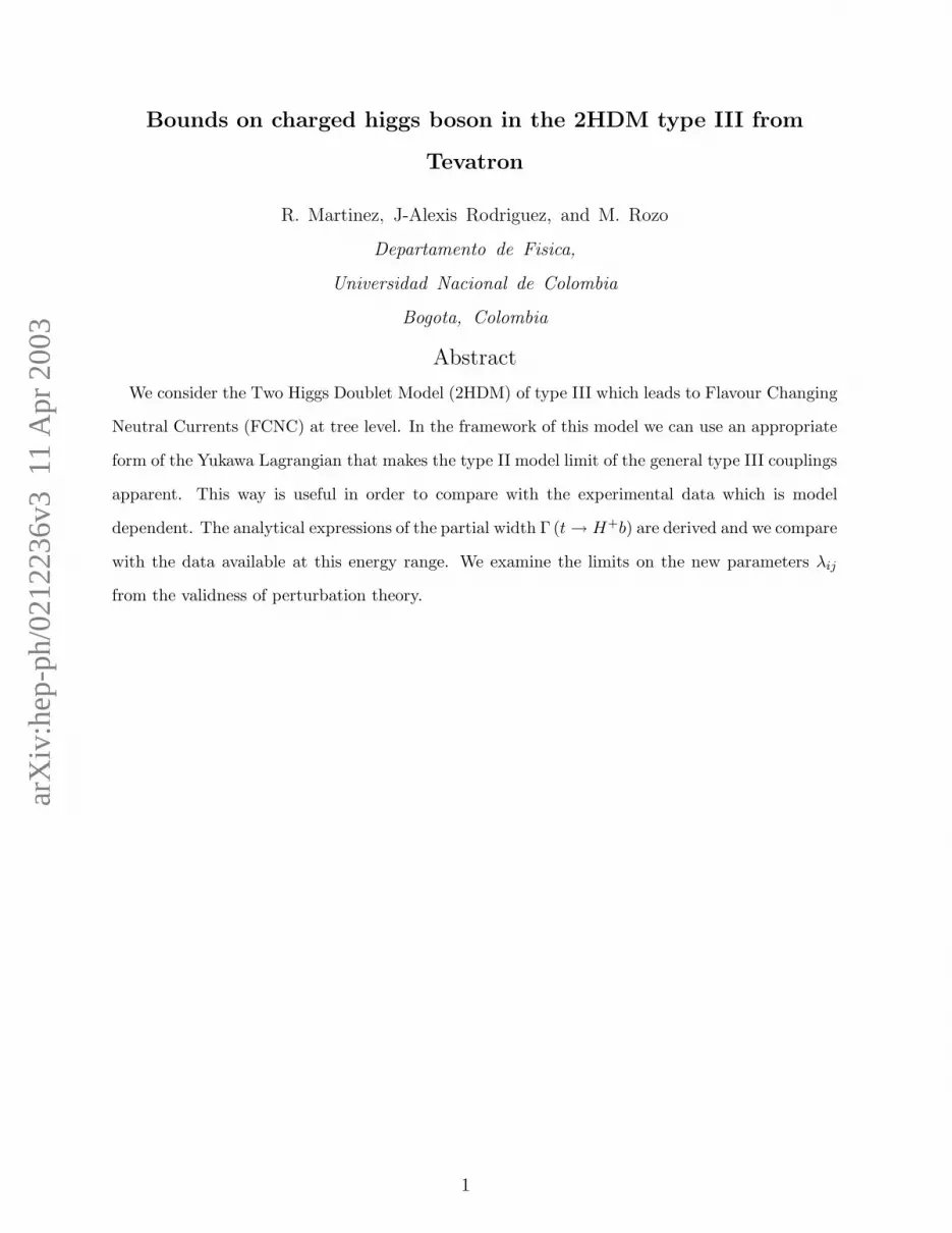
obtained using the 2HDM-II. In figures 2 and 3, we show the fraction B(t → bH+) vs tan β

for different values of λbb and λtt. The B(t → bH+) branching fraction for different values

of MH± is significant for very small or very large values of tanβ, while it is suppressed for

intermediate values of tanβ. This fact is because the fraction B(t → bH+) is proportional

to (m2b +m2

t −mH±)(m2t cot2 β + m2

b tan2 β)+ 4m2tm

2b which has a minimum around tanβ =

√mt/mb and is symmetric in log(tanβ) about this point. We note that for a charged Higgs

2HDM-II like, lighter than the top quark, it would be detected if tan β is substantially

different from√

mt/mb, it is because the branching fraction is very suppressed around this

point, by around 10−4. In what follows we are going to show that model type III can modify

this scenario. For λii = 0 we obtain the prediction of the 2HDM type II and it is symmetric

around tanβ = 6, but it is not the case for λii 6= 0 where the minimum is shifted. In this

analysis we are considering two different set of values for the λii parameters. In figure 2,

λtt is the order of λbb and in figure 3 λtt is one order of magnitude smaller than λbb, and in

both cases the charged Higss boson mass is fixed to 140 GeV. In figure 2 and 3, it is drawn

the most stringent bound coming from D0 collaboration on B(t → bH+) in the range of

0.3 ≤ tan β ≤ 150 which should be less than 0.36 (horizontal line).

Finally, in figure 4 we plot MH± vs tan β for different λii using the bound from Tevatron

B(t → bH+) ≤ 0.36. We show the excluded regions at 95 % C.L. by Tevatron from Run

I and the limits that will be reached on this plane in Run II using 2 and 10 fb−1 for the

integrated luminosity at√

s = 2 TeV. We should clarify that the exclusion regions taken

from D0 at Tevatron are a combination of two searches. An indirect search, looking for a

decrease in tt̄ → W+W−bb̄ signal expected from the SM, this search excludes simultaneously

both large and small tanβ. And a direct search, that look for the H± → τ±ν in the region

0.3 < tanβ < 150. This is because the fraction rate of the leptonic decay of H± is around

0.95 for large tanβ, and the other option H+ → cs̄ is important for tanβ < 0.4 and low

Higgs boson mass. In our case we could enhanced the influence of H+ → cs̄ channel due to

the appearance of new couplings, it does not matter the value of tan β, but that possibility

corresponds to a very unusual set of values of the new couplings λcc, λss and ξE, instead

of that we conserve the hierarchy of the decay channels according to the value of tan β in

order to consider a more general and conservative scenario where the experimental limits

7

can be used. The solid line inside the future explored region corresponds to λii = 0 which

is the region for the 2HDM-II with a fraction rate of 0.36. A charged Higgs 2HDM-III like

could have different scenarios, as we can see from figure 4 for λii different from zero. Again

we are considering two cases: λtt of the order of λbb and λtt one order of magnitude smaller

than λbb. The excluded region is below the curves, and we can see that there are values that

cover almost all the plane presented.

To summarize, in the present work we have examined a 2HDM type III which produces

FCNC at tree level, in general these new interactions are governed by parameters λij . The

experimental analysis has been carried out using the 2HDM type II as a framework, so

they are model dependent. We have already presented a form of the Yukawa Lagrangian

of the 2HDM-III (7) which can be reduced to the 2HDM-II as a limit [6], in this way it

can be used to compare the model type III with the experimental analysis based on 2HDM

type II. We have shown that 2HDM type III can modify the situation for the branching

fraction B(t → bH+) in the case of a charged Higgs boson in the allowed region from

kinematic considerations. For λii = 0, we obtain the prediction of the 2HDM type II and

it is symmetric around tanβ =√

mt/mb ∼ 6, but it is not the case for λii 6= 0. Finally,

we have presented the parameter plane tanβ − mH+ showing the experimental limits for

Run I and II and, in the same plot we show the solutions obtained in the cases of 2HDM-II

(λii = 0) and 2HDM-III (λtt 6= 0).

We acknowledge to R.A. Diaz for the careful reading of the manuscript, and J. P. Idarraga

for his collaboration with numerical calculations. This work was supported by COLCIEN-

CIAS.

8

[1] For a review see J. Gunion, H. Haber, G. Kane and S. Dawson, The Higgs Hunter’s Guide,

(Addison-Wesley, New York, 1990)

[2] S. Glashow and S. Weinberg, Phys. Rev. D 15, 1958 (1977).

[3] W.S. Hou, Phys. Lett B 296, 179 (1992); D. Cahng, W. S. Hou and W. Y. Keung, Phys.

Rev. D 48, 217 (1993); S. Nie and M. Sher, Phys. Rev. D 58, 097701 (1998); M. Sher and

Y. Yuan, Phys. Rev. D 44, 1461 (1991); D. Atwood, L. Reina and A. Soni, Phys. Rev. D 55,

3156 (1997); Phys. Rev. Lett. 75, 3800 (1995).

[4] D. Atwood, L. Reina and A. Soni, Phys. Rev. D 53, 1199 (1996); Phys. Rev. D 54, 3296

(1996); Phys. Rev. Lett. 75, 3800 (1993); D. Atwood, L. Reina and A. Soni, Phys. Rev. D 55,

3156 (1997); G. Cvetic, S. S. Hwang and C. S. Kim, Phys. Rev. D 58, 116003 (1998).

[5] Marc Sher and Yao Yuan, Phys. Rev. D 44, 1461 (1991); T.P. Cheng and M. Sher, Phys. Rev.

D 35, 3490 (1987)

[6] Rodolfo A. Diaz, R. Martinez and J.-Alexis Rodriguez, Phys. Rev. D 64, 033004 (2001); Phys.

Rev. D 63, 095500 (2001).

[7] LEP Collaborations, arXiv:hep-ex/0107031.

[8] CDF Collaboration, F. Abe, et. al, Phys. Rev. Lett. 79, 357 (1997); CDF Collaboration, T.

Affolder, et. al, Phys. Rev. D 62, 012004 (2000).

[9] D0 Collaboration, B. Abbot, et. al, Phys. Rev. Lett. 82, 4975 (1999); V. Abazov, et. al, Phys.

Rev. Lett. 88, 151803 (2002).

[10] A. Mendez and A. Pomarol, Phys. Lett. B 360, 47 (1995); C. Li and R. J. Oakes, Phys. Rev.

D 43, 855 (1991); A. Djouadi and P. Gambino, Phys. Rev. D 51, 218 (1995).

[11] M. Carena, D. Garcia, U. Nierste, C. Wagner, arXiv:hep-ph/9912516; M. Carena, J. Conway,

H. Haber and J. Hobbs, arXiv:hep-ph/0010338.

9

FIG. 1: Plot for the charged Higgs boson mass MH± versus the parameter λbb. In the 2HDM-III

when tan β is not present. The allowed region is above the curve.

10

FIG. 2: Plot for B(t → bH+) versus the tan β parameter for MH± = 140 GeV and different values

of the parameter λii. Each plane corresponds to a fixed λtt, downward = ±1,±2,±0.1 right side

positive values, left side negative values. And λbb = −2 dashed-line, = −1 dot-dashed line = 1

short-dashed line, and = 2 solid line. We also show the 2HDM-II case, dot-dot-dashed line, showing

the minimum around tan β ∼ 6. The excluded region by Tevatron (horizontal line) corresponds

to the right-up corner and the region for tan β < 0.3 (vertical line) is an unexplored region by

experiments.

11

FIG. 3: Like figure 2 but λbb = −20 dashed-line, = −10 dot-dashed line = 10 short-dashed line,

and = 20 solid line.

12

FIG. 4: Plot for MH± versus the tan β parameter when B(t → bH+) ≤ 0.36 for different set of

values of λii. Inside the figure are the labels for λtt and λbb = 1 except for the last one which

is λbb = 10. We overlap the expected limits from D0 for mt = 175 GeV and several values of

the integrated luminosity and√

s: (0.1 fb−1, 1.8TeV),(2 fb−1, 2 TeV),(10 fb−1, 2 TeV), assuming

σ(tt̄) = 7 pb. The limits were taken from reference [11].

13