Boundary Value Problems Numerical

ContentsContents 3333

Boundary Value Problems Numerical

33.1 Two-point Boundary Value Problems 2

33.2 Elliptic PDEs 18

Learning

In this Workbook, which follows on from Workbook 32, you will see some more numericalmethods for approximating solutions of differential equations. The methods to bepresented in this Workbook are most usually applied in engineering examples involvingso-called boundary data, that is, some of the available information arises "around the edges" of the problem area.

outcomes

Two-point BoundaryValue Problems

��

��33.1

IntroductionBoundary value problems arise in applications where some physical process involves knowledge ofinformation at the edges. For example, it may be possible to measure the electric potential aroundthe edge of a semi-conductor and then use this information to infer the potential distribution nearthe middle.

In this Section we discuss numerical methods that can be used for certain boundary value problemsinvolving processes that may be modelled by an ordinary differential equation.

�

�

�

�Prerequisites

Before starting this Section you should . . .

• revise central difference approximations( 31)

'

&

$

%Learning Outcomes

On completion you should be able to . . .

• approximate certain boundary value problemsusing central differences

• obtain simple numerical approximations tothe solutions to certain boundary valueproblems

2 HELM (2008):Workbook 33: Numerical Boundary Value Problems

®

1. Three point stencilLet us consider the boundary value problem defined by Equations (1):

p(x)y′′(x) + q(x)y′(x) + r(x)y(x) = s(x) (0 < x < `)a0y

′(0) + b0y(0) = c0

a1y′(`) + b1y(`) = c1

(1)

The first line is the differential equation, and the second and third lines are the boundary condi-tions which can involve derivatives.

It is our aim to approximate the solution of this problem numerically, and we adopt an approachsimilar to that seen in 32.

We divide the interval 0 < x < ` into a number, J say, of subintervals each of equal width h = `/J .Our numerical solution will provide an approximation to y = y(x) at each value of x where twosubintervals meet (see Figure 1).

xJ!1

l!hxJ

lxx2

2hx1

h

y0

y1

y2

yJ!1

yJ

x

yj

j

jh

Figure 1

Key Point 1

A numerical approximation to the boundary value problem

p(x)y′′(x) + q(x)y′(x) + r(x)y(x) = s(x) (0 < x < `)a0y

′(0) + b0y(0) = c0

a1y′(`) + b1y(`) = c1

is a sequence of numbers y0, y1, y2, y3, . . . , yJ .Here yj is an approximation to y(x) at x = jh, where h = `/J and j = 0, 1, 2, . . . , J .

It is useful to give a name to the x-values where we seek an approximation to y = y(x). Hence wewill sometimes write xj = jh j = 0, 1, 2, . . . , J.

The functions p, q, r and s will frequently occur evaluated at the values xj so it is convenient toset up the following abbreviations:

pj = p(xj), qj = q(xj), rj = r(xj), sj = s(xj).

HELM (2008):Section 33.1: Two-point Boundary Value Problems

3

A numerical approximation to Equations (1) can be found by approximating the derivatives by finitedifferences. Here we will approximate y′′(x) and y′(x) by central differences to obtain

p(xj)y(xj + h)− 2y(xj) + y(xj − h)

h2+ q(xj)

y(xj + h)− y(xj − h)

2h+ r(xj)y(xj) ≈ s(xj)

that is, on using the abbreviations established in Key Point 1,

pjy(xj + h)− 2y(xj) + y(xj − h)

h2+ qj

y(xj + h)− y(xj − h)

2h+ rjy(xj) ≈ sj

which we use as the motivation for the numerical method

pjyj+1 − 2yj + yj−1

h2+ qj

yj+1 − yj−1

2h+ rjyj = sj.

This last equation can be rearranged, gathering together all the like y-terms. It neatens things furtherto multiply through by h2 as well, and the result of these manipulations appears in the following KeyPoint.

Key Point 2

A central difference approximation to

p(x)y′′(x) + q(x)y′(x) + r(x)y(x) = s(x)

is

yj−1

(pj −

h

2qj

)+ yj

(h2rj − 2pj

)+ yj+1

(pj +

h

2qj

)= h2sj.

This approximation to the differential equation can be thought of as a three-point stencil linkingthree of the approximate y-values. The expression

yj−1

(pj −

h

2qj

)+ yj

(h2rj − 2pj

)+ yj+1

(pj +

h

2qj

)= h2sj.

is centred around x = xj and involves yj−1, yj and yj+1. The general rule when dealing with anumerical stencil like this is to centre the stencil at every point where y is unknown. (Thisgeneral rule will appear again, for example on page 13.)


®

Key Point 3

Centre the stencil at every x-point where y is unknown. This will give a set of equations for theunknown y-values, and we are guaranteed exactly as many equations as there are unknowns.

In the following Example, matters are simplified because the functions p, q, r and s are all constant.

Example 1Let y = y(x) be a solution to the boundary value problem

3y′′(x) + 4y′(x) + 5y(x) = 7 0 < x < 1.5

y(0) = 2, y(1.5) = 2.

Using a mesh width of h = 0.5, obtain a central difference approximation to thedifferential equation and hence find yj ≈ y(jh), j = 1, 2.

Solution

In general, the central difference approximation to

p(x)y′′(x) + q(x)y′(x) + r(x)y(x) = s(x)

is

yj−1

(pj −

h

2qj

)+ yj

(h2rj − 2pj

)+ yj+1

(pj +

h

2qj

)= h2sj.

In this case the coefficients are

pj −h

2qj = 2, h2rj − 2pj = −4.75, pj +

h

2qj = 4, h2sj = 1.75.

These values will be the same for all x because p, q, r and s are constants in this Example. Hencethe general stencil is

2yj−1 − 4.75yj + 4yj+1 = 1.75

In this case h = 0.5, and our numerical solution consists of the values

y0 = y(0) = 2 from the boundary condition

y1 ≈ y(0.5)

y2 ≈ y(1)

y3 = y(1.5) = 2 from the boundary condition


5

Solution (contd.)

So there are two unknowns, y1 and y2. We centre the stencil at each of the corresponding x values.Putting j = 1 in the numerical stencil gives

2y0 − 4.75y1 + 4y2 = 1.75

Moving the stencil one place to the right, we put j = 2 so that

2y1 − 4.75y2 + 4y3 = 1.75

In these two equations y0 and y3 are known from the boundary conditions and we move termsinvolving them to the right-hand side. This leads to the system of equations[

−4.75 42 −4.75

] [y1

y2

]=

[−2.25−6.25

]Solving this pair of simultaneous equations we find that

y1 = 2.45, y2 = 2.35

to 2 decimal places.

This approximation is shown in Figure 2 in which the numerical approximations to point values of yare shown as circles.

0 0.5 1 1.52

2.1

2.2

2.3

2.4

2.5

x

Figure 2

The question remains how close to the exact solution these approximations are. (Of course forExample 1 above it is possible to find the analytic solution fairly easily, but this will not usually bethe case.)

A pragmatic way to deal with this question is to recompute the results with a smaller value of h. Weknow from 31 that the central difference approximations get closer and closer to the derivativeswhich they approximate as h decreases. In Figure 3 the results for h = 0.5 are given again as circles,and a computer has been used to find more accurate approximations to y using h = 1.5

7(shown as

squares) and yet more accurate results (shown as dots) from using h = 1.510

. (This involves solvinglarger systems of equations than are manageable by hand. The methods seen in 30 can beused to deal with these larger systems.)


®

0 0.5 1 1.52

2.1

2.2

2.3

2.4

2.5

x

3 subintervals 7 subintervals10 subintervals

Figure 3

We can now have some confidence that the results we calculated using h = 0.5 tended to overestimatethe true values of y.


y′′(x) + 2y′(x)− 2y(x) = −3 0 < x < 2

y(0) = 1, y(2) = −2.

Using a mesh width of h = 0.5 obtain a central difference approximation tothe differential equation and hence find simultaneous equations satisfied by theunknowns y1, y2 and y3.

Solution


pj −h

2qj = 0.5, h2rj − 2pj = −2.5, pj +

h

2qj = 1.5, h2sj = −0.75.

These values will be the same for all x because p, q, r and s are constants in this Example.Hence the general stencil is

0.5yj−1 − 2.5yj + 1.5yj+1 = −3

Here we have h = 0.5 and our numerical solution consists of the values


y1 ≈ y(0.5)

y2 ≈ y(1)

y3 ≈ y(1.5)

y4 = y(2) = −2 from the boundary condition


7

Solution (contd.)

So there are three unknowns, y1, y2 and y3. We centre the stencil at each of the corresponding xvalues. Putting j = 1 in the numerical stencil gives

0.5y0 − 2.5y1 + 1.5y2 = −0.75.


0.5y1 − 2.5y2 + 1.5y3 = −0.75

and finally we let j = 3 so that

0.5y2 − 2.5y3 + 1.5y4 = −0.75

In these three equations y0 and y4 are known from the boundary conditions and we move termsinvolving them to the right-hand side. This leads to the system of equations −2.5 1.5 0

0.5 −2.5 1.50 0.5 −2.5

y1

y2

y3

=

−1.25−0.752.25

We can find (using methods from 30, for example) that the solution to the system of equationsin Example 2 is

y1 = 0.39 y2 = −0.18 y3 = −0.94 to 2 decimal places.

Task

Let y = y(x) be a solution to the boundary value problem

y′′(x) + 4y′(x) = 4 0 < x < 1

y(0) = −2, y(1) = 3.

Using a mesh width of h = 0.25 obtain a central difference approximation to thedifferential equation and hence find a system of equations satisfied by yj ≈ y(jh),j = 1, 2, 3.

Your solution

Work the solution on a separate piece of paper. Record the main results and your conclusions here.


®

AnswerIn general, the central difference approximation to

p(x)y′′(x) + q(x)y′(x) + r(x)y(x) = s(x)

is

yj−1

(pj −

h

2qj

)+ yj

(h2rj − 2pj

)+ yj+1

(pj +

h

2qj

)= h2sj.


pj −h

2qj = 0.5, h2rj − 2pj = −2, pj +

h

2qj = 1.5, h2sj = 0.25.

These values will be the same for all x because p, q, r and s are constants in this Example.In this case h = 0.25 and our numerical solution consists of the values


y1 ≈ y(0.25)

y2 ≈ y(0.5)

y3 ≈ y(0.75)



0.5y0 − 2y1 + 1.5 = 0.25


0.5y1 − 2y2 + 1.5 = 0.25


0.5y2 − 2y3 + 1.5 = 0.25

In these three equations y0 and y4 are known from the boundary conditions and we move termsinvolving them to the right-hand side. This leads to the system of equations −2 1.5 0

0.5 −2 1.50 0.5 −2

y1

y2

y3

=

1.250.25−4.25

(And you might like to check that the solution to this system of equations is y1 = 0.95, y2 = 2.1and y3 = 2.65.)


9

Example 3The temperature y of an electrically heated wire of length ` is affected by local aircurrents. This situation may be modelled by

d2y

dx2= −a− b(Y − y), (0 < x < `).

Consider the case where ` = 3, a = 50, b = 0.1 and Y = 20◦C and supposethat the ends of the wire are known (to 1 decimal place) to be at temperaturesy(0) = 15.0◦C and y(3) = 25.0◦C.Using a central difference to approximate the derivative and using 3 subintervalsobtain approximations to the temperature 1

3and 2

3of the length along the wire.

Solution

This Example falls into the general case given at the beginning of this Section if we choose p = 1,q = 0, r = −0.1 and s = −52. In this case h = 1 and our numerical solution consists of the values


y1 ≈ y(1)

y2 ≈ y(2)



y0 − 2.1y1 + y2 = −52


y1 − 2.1y2 + y3 = −52


−2.1 11 −2.1

] [y1

y2

]=

[−67−77


y1 = 63.8, y2 = 67.1

to 1 decimal place.

We conclude that the temperature 13

of the wire’s length from the cooler end is approximately 63.8◦Cand the temperature the same distance from the hotter end is approximately 67.1◦C, where we haverounded these numbers to the same number of places as the given boundary conditions.

The Examples and Task above were such that p, q, r and s were each equal to a constant for allvalues of x. More realistic engineering applications may involve coefficients that vary, and the nextExample is of this type.


®


ln(2 + x)y′′(x) + xy′(x) + (x + 1)2y(x) = cos(x) 0 < x < 1.2

y(0) = 0, y(1.2) = 2.

Using a mesh width of h = 0.4 obtain a central difference approximation to thedifferential equation and hence find yj ≈ y(jh), j = 1, 2.

Solution


p(x)y′′(x) + q(x)y′(x) + r(x)y(x) = s(x)

is

yj−1

(pj −

h

2qj

)+ yj

(h2rj − 2pj

)+ yj+1

(pj +

h

2qj

)= h2sj.

The coefficients will vary with j in this Example because the functions p, q, r and s are not allconstants. In this case h = 0.4 and our numerical solution consists of the values


y1 ≈ y(0.4)

y2 ≈ y(0.8)



0.795469y0 − 1.437337y1 + 0.955469y2 = 0.147370


0.869619y1 − 1.540839y2 + 1.189619y3 = 0.111473

In these two equations y0 and y3 are known from the boundary conditions and we move termsinvolving them to the right-hand side. This gives the pair of equations[

−1.437337 0.9554690.869619 −1.540839

] [y1

y2

]=

[0.147370−2.267766


y1 = 1.40, y2 = 2.26



11

Once again we can monitor the accuracy of the results obtained in the Example above by recomputingfor a smaller value of h. In Figure 4 the values calculated are shown as circles and a computer hasbeen used to obtain the more accurate results (shown as dots) obtained from choosing h = 1.2

20.

0.2 0.4 0.6 0.8 1 1.20

0.5

1

1.5

2

2.5

x

3 subintervals20 subintervals

Figure 4

In the next Example we see that the derivative y′ appears in the boundary condition at x = 0. Thismeans that y is not given at x = 0 and we use the general rule given earlier in Key Point 3:

centre the stencil at every xxx-value where yyy is unknown.

So this implies that we must centre the stencil at x = 0 and this will cause the value y−1 to appear.This is a fictitious value that plays no part in the solution we seek and we use the derivative boundarycondition to get y−1 in terms of y1. This is done with the central difference

y′(0) ≈ y1 − y−1

2h.

The following Example implements this idea.


ln(2 + x)y′′(x) + xy′(x) + 2y(x) = cos(x) 0 < x < 1.2

y′(0) = −1, y(1.2) = 2

(Note the derivative boundary condition at x = 0.)

Using a mesh width of h = 0.4 obtain a central difference approximation to thedifferential equation and hence find the system of equations satisfied by yj ≈ y(jh),j = 0, 1, 2.


®

Solution


p(x)y′′(x) + q(x)y′(x) + r(x)y(x) = s(x)

is

yj−1

(pj −

h

2qj

)+ yj

(h2rj − 2pj

)+ yj+1

(pj +

h

2qj

)= h2sj.

The coefficients vary with j in this Example because the functions p, q, r and s are not all constants.In this case h = 0.4 and our numerical solution consists of the values

y0 ≈ y(0) which is not given by the boundary condition

y1 ≈ y(0.4)

y2 ≈ y(0.8)



0.693147y−1 − 1.066294y0 + 0.6931472y1 = 0.16

which introduces the fictitious quantity y−1. We attach a meaning to y−1 on using the boundarycondition at x = 0. Approximating the derivative in the boundary condition by a central differencegives

y1 − y−1

2h= −1 ⇒ y−1 = y1 + 0.8

and we use this to remove y−1 from the equation where it first appeared. Hence

−1.066294y0 + 1.386294y1 = 0.7145177

The remaining steps are similar to previous Examples. Putting j = 1 in the stencil gives

0.795469y0 − 1.430937y1 + 0.955469y2 = 0.147370.


0.869619y1 − 1.739239y2 + 1.189619y3 = 0.111473

In the last equation y3 is known from the boundary conditions and we move the term involving itto the right-hand side. This leaves us with the system of equations −1.066294 1.386294 0

0.795469 −1.430937 0.9554690 0.869619 −1.739239

y0

y1

y2

=

0.7145180.147370−2.267766

where the components are given to 6 decimal places.


13

Exercises

1. Let y = y(x) be a solution to the boundary value problem

y′′(x)− 2y′(x) + 3y(x) = 6 0 < x < 0.75

y(0) = 2, y(0.75) = 1

Using a mesh width of h = 0.25 obtain a central difference approximation to the differentialequation and hence find y1 ≈ y(0.25) and y2 ≈ y(0.5).


2y′′(x) + 3y′(x) = 5 0 < x < 1.2

y(0) = −2, y(1.2) = 3

Using a mesh width of h = 0.3 obtain a central difference approximation to the differentialequation and hence find a system of equations satisfied by y1 ≈ y(0.3), y2 ≈ y(0.6) andy3 ≈ y(0.9).


y′′(x) + x2y′(x) + 3y(x) = x 0 < x < 1.5

y′(0) = 2, y(1.5) = 1. (Note the derivative boundary condition at x = 0.)

Using a mesh width of h = 0.5 obtain a central difference approximation to the differentialequation and hence find the system of equations satisfied by yj ≈ y(jh), j = 0, 1, 2.


®

Answers

1. In general, the central difference approximation to

p(x)y′′(x) + q(x)y′(x) + r(x)y(x) = s(x)

is

yj−1

(pj −

h

2qj

)+ yj

(h2rj − 2pj

)+ yj+1

(pj +

h

2qj

)= h2sj.


pj −h

2qj = 1.25, h2rj − 2pj = −1.8125, pj +

h

2qj = 0.75, h2sj = 0.375.



y1 ≈ y(0.25)

y2 ≈ y(0.5)


So there are two unknowns, y1 and y2. We centre the stencil at each of the corresponding xvalues. Putting j = 1 in the numerical stencil gives

1.25y0 − 1.8125y1 + 0.75y2 = 0.375


1.25y1 − 1.8125y2 + 0.75y3 = 0.375


−1.8125 0.751.25 −1.8125

] [y1

y2

]=

[−2.125−0.375

]with solution

y1 = 1.76, y2 = 1.42



15

Answers


p(x)y′′(x) + q(x)y′(x) + r(x)y(x) = s(x)

is

yj−1

(pj −

h

2qj

)+ yj

(h2rj − 2pj

)+ yj+1

(pj +

h

2qj

)= h2sj.


pj −h

2qj = 1.55, h2rj − 2pj = −4, pj +

h

2qj = 2.45, h2sj = 0.45.



y1 ≈ y(0.3)

y2 ≈ y(0.6)

y3 ≈ y(0.9)


So there are three unknowns, y1, y2 and y3. We centre the stencil at each of the correspondingx values. Putting j = 1 in the numerical stencil gives

1.55y0 − 4y1 + 2.45 = 0.45


1.55y1 − 4y2 + 2.45 = 0.45


1.55y2 − 4y3 + 2.45 = 0.45

In these three equations y0 and y4 are known from the boundary conditions and we moveterms involving them to the right-hand side. This leads to the system of equations −4 2.45 0

1.55 −4 2.450 1.55 −4

y1

y2

y3

=

3.550.45−6.9


®

Answers


p(x)y′′(x) + q(x)y′(x) + r(x)y(x) = s(x)

is

yj−1

(pj −

h

2qj

)+ yj

(h2rj − 2pj

)+ yj+1

(pj +

h

2qj

)= h2sj.

The coefficients vary with j in this exercise because the functions p, q, r and s are not allconstants. In this case h = 0.5 and our numerical solution consists of the values

y0 ≈ y(0) which is not given by the boundary condition

y1 ≈ y(0.5)

y2 ≈ y(1)


So there are three unknowns, y0, y1 and y2. We centre the stencil at each of the correspondingx values. Putting j = 0 in the numerical stencil gives

y−1 − 1.25y0 + y1 = 0

which introduces the fictitious quantity y−1. We attach a meaning to y−1 on using theboundary condition at x = 0. Approximating the derivative in the boundary condition by acentral difference gives

y1 − y−1

2h= 2 ⇒ y−1 = y1 − 2

and we use this to remove y−1 from the equation where it first appeared. Hence

−1.25y0 + 2y1 = −2

The remaining steps are similar to previous exercises. Putting j = 1 in the stencil gives

0.9375y0 − 1.25y1 + 1.0625y2 = 0.125


0.75y1 − 1.25y2 + 1.25y3 = 0.25

In the last equation y3 is known from the boundary conditions and we move the term involvingit to the right-hand side. This leads to the system of equations −1.25 2 0

0.9375 −1.25 1.06250 0.75 −1.25

y0

y1

y2

=

−20.125−1


17

Elliptic PDEs��

��33.2

IntroductionIn 32.4 and 32.5, we saw methods of obtaining numerical solutions to Parabolic and Hyperbolicpartial differential equations (PDEs). Another class of PDEs are the Elliptic type, and these usuallymodel time-independent situations. In this Section we will concentrate on two particularly importantElliptic type PDEs: Laplace’s equation and Poisson’s equation.

'

&

$

%Prerequisites

Before starting this Section you should . . .

• familiarise yourself with difference methodsfor approximating second derivatives (31.3 )

• revise the Jacobi and Gauss-Seidel methodsfrom ( 30.5)�

�

�

�Learning Outcomes

On completion you should be able to . . .

• obtain simple approximate solutions ofcertain elliptic equations


®

1. Elliptic equationsConsider a region R (for example, a rectangle) in the xy-plane. We might pose the following boundaryvalue problem

uxx + uyy = f(x, y) a given function, in R

u = g a given function, on the boundary of R

• if f = 0 everywhere, then the PDE is called Laplace’s equation

• if f is non-zero somewhere in R then the PDE is called Poisson’s equation

Laplace’s equation models a huge range of physical situations. It is used by coastal engineers toapproximate the motion of the sea; it is used to model electric potential; it can give an approximationto heat distribution in certain steady state problems. The list goes on and on. The generalisationto Poisson’s equation opens up further application areas, but for our purposes in this Section we willconcentrate on how to solve the equation, rather than on how it is applied.

2. A five point stencilThe approach we shall use is to approximate the two second derivatives using central differences.First we need some notation for our numerical solution, and we shall re-use some of the ideas seenin 32.4 and 32.5. We divide the x-axis up into subintervals of width δx and the y-axisinto subintervals of width δy.

There is a simplification available to us now that was not possible in 32. Here, the twoindependent variables (x and y) both measure distance (in 32 we had x measuring distanceand t measuring time) and there is no reason to suppose that one direction is more important thananother, so we may choose the subintervals δx and δy to be equal.

Key Point 4

In deriving numerical solutions to elliptic PDEs we use equal steps in the x and y directions. Thatis, we take

δx = δy = h (say)

So the idea is to approximate the second derivatives in the familiar way:

uxx ≈u(x + h, y)− 2u(x, y) + u(x− h, y)

h2, uyy ≈

u(x, y + h)− 2u(x, y) + u(x, y − h)

h2

We will write our numerical approximation as

ui,j ≈ u(i h , j h)︸︷︷︸↑ ↑

numerical exact (i.e. unknown) solutionapproximation evaluated at x = i× h, y = j × h

HELM (2008):Section 33.2: Elliptic PDEs

19

Key Point 5

We use subscripts on u to relate to space variables. For Elliptic PDEs both of the independentvariables measure distance and so we have two subscripts.

Key Point 6

If there is no danger of ambiguity we may omit the comma from the subscript. That is,

ui,j may be written uij and fi,j may be written fij

Given all of this preamble we can now write down a difference equation which approximates thepartial differential equation:

ui+1,j − 2ui,j + ui−1,j

h2︸︷︷︸ +ui,j+1 − 2ui,j + ui,j−1

h2︸︷︷︸ = fi,j

↑≈ uxx ≈ uyy notation for f(ih, jh)

Rearranging this gives

−4ui,j + ui+1,j + ui−1,j + ui,j+1 + ui,j−1 = h2fi,j

This equation defines a five-point stencil approximating the PDE. The following diagram showsthe stencil.

ui,j+1

ui!1,j ui,j ui+1,j

ui,j!1

j + 1

j

j ! 1

j ! 2i ! 1 i i + 1

The idea in an implementation of this stencil is to centre the cross-shape on each i, j node where wewant to find u. This guarantees that we will end up with the same number of equations as unknowns.An example of this approach will follow shortly, but first we note other ways of writing down thefive-point stencil.


®

As the diagram above shows, the stencil involves a centre point and four additional points eachcorresponding to one of the points of the compass. It is this observation which has led to a simplifiedversion of the mathematical expression and the diagram. The symbolic stencil can be written

−4u0 + uE + uW + uN + uS = h2f0,

where a subscript 0 corresponds to the centre of the stencil and other subscripts correspond tocompass points (North, South, East, West) in the obvious way. The diagram becomes

uN

uW u0 uE

uS

and we reinterpret the local “0, N, S, E,W” positions each time we move the stencil on the globalgrid.

Another way of writing the stencil is as follows:

1

1 −4 1

1

This latest version has the advantage of showing the values of the coefficients used in approximatinguxx + uyy.

We summarise in Key Point 7 the main idea using the notation established above.

Key Point 7

The five-point stencil used to approximate the partial differential equation

uxx + uyy = f(x, y)

gives rise to the difference equation

−4u0 + uE + uW + uN + uS = h2f0


21

Example 6Consider the boundary value problem

uxx + uyy = 0 in the square 0 < x < 1, 0 < y < 1

u = x2y on the boundary.

Use h = 13

and formulate a system of simultaneous equations for the 4 unknowns.

Solution

In the diagram on the right we see a schematicof the square in the xy plane. The numbers cor-respond to boundary data where the numericalgrid intersects that boundary. The (as yet un-known) numerical approximations are shown inthe positions where they approximate u(x, y).

y ↑0 1

949

1

0 u12 u2223

0 u11 u2113

0 0 0 0 → x

The numerical stencil in this case is −4u0 +uE +uW +uN +uS = 0 and we centre this at eachof the places where u is sought. There are four such places in this example:

bottom left: −4u11 + u21 + 0 + u12 + 0 = 0

bottom right: −4u21 + 13

+ u11 + u22 + 0 = 0

top left: −4u12 + u22 + 0 + 19

+ u11 = 0

top right: −4u22 + 23

+ u12 + 49

+ u21 = 0↑ ↑ ↑ ↑ ↑

Centre East West North South

This is a system of equations in the four unknowns which may be written

−4 1 1 0

1 −4 0 1

1 0 −4 1

0 1 1 −4

u11

u21

u12

u22

= −

0

13

19

109

It is now a (simple, in theory) matter of solving the system to obtain the numerical approximationto u.


®

It turns out that the solution to the system of equations is u11 = 112

, u21 = 736

, u12 = 536

andu22 = 13

36. These values are, to four decimal places, 0.0833, 0.1944, 0.1389 and 0.3611, respectively.

We will say more later about how to solve the system of equations, but first there is a Task to helpconsolidate what we have covered so far.

Task

Consider the boundary value problem

uxx + uyy = −2 in the square 0 < x < 1, 0 < y < 1

u = xy on the boundary.

Use h = 13

and hence formulate a system of simultaneous equations for the fourunknowns.

Your solution


23

Answer

In the diagram on the right we see a schematicof the square in the xy plane. The numbers cor-respond to boundary data where the numericalgrid intersects that boundary. The (as yet un-known) numerical approximations are shown inthe positions where they approximate u(x, y).

y ↑

0 13

23

1

0 u12 u2223

0 u11 u2113

0 0 0 0 → x

The numerical stencil in this case is

−4u0 + uE + uW + uN + uS = h2f0 = (1

3)2 × (−2) = −2

9

and we centre this at each of the places where u is sought. In this Example there are four suchplaces:

bottom left: −4u11 + u21 + 0 + u12 + 0 = −29

bottom right: −4u21 + 13

+ u11 + u22 + 0 = −29

top left: −4u12 + u22 + 0 + 13

+ u11 = −29

top right: −4u22 + 23

+ u12 + 23

+ u21 = −29

↑ ↑ ↑ ↑ ↑Centre East West North South

This is a system of equations in the four unknowns and it may be written

−4 1 1 0

1 −4 0 1

1 0 −4 1

0 1 1 −4

u11

u21

u12

u22

= −

29

59

59

149


®

3. Systems of equationsIn order to obtain accurate results over a large number of interior points, we need to decrease hcompared to the values used in the Examples above.The diagram below shows a case where 5 steps are used in each direction on a square domain. Itfollows that there will be 4×4 = 16 unknowns. Positioning the stencil over each xy position where uis unknown will give the right number of equations, and the order we take the 16 points is indicatedby the arrows on the diagram.

h

x

y

It follows that there will be a system of equations involving0BBBBBBBBBBBBBBBBBBBBBBBBBBBBBBBBBBBBBBBBBBBBBBBBBBBBBBB@

−4 1 0 0 1 0 0 0 0 0 0 0 0 0 0 0

1 −4 1 0 0 1 0 0 0 0 0 0 0 0 0 0

0 1 −4 1 0 0 1 0 0 0 0 0 0 0 0 0

0 0 1 −4 1 0 0 1 0 0 0 0 0 0 0 0

1 0 0 1 −4 1 0 0 1 0 0 0 0 0 0 0

0 1 0 0 1 −4 1 0 0 1 0 0 0 0 0 0

0 0 1 0 0 1 −4 1 0 0 1 0 0 0 0 0

0 0 0 1 0 0 1 −4 1 0 0 1 0 0 0 0

0 0 0 0 1 0 0 1 −4 1 0 0 1 0 0 0

0 0 0 0 0 1 0 0 1 −4 1 0 0 1 0 0

0 0 0 0 0 0 1 0 0 1 −4 1 0 0 1 0

0 0 0 0 0 0 0 1 0 0 1 −4 1 0 0 1

0 0 0 0 0 0 0 0 1 0 0 1 −4 1 0 0

0 0 0 0 0 0 0 0 0 1 0 0 1 −4 1 0

0 0 0 0 0 0 0 0 0 0 1 0 0 1 −4 1

0 0 0 0 0 0 0 0 0 0 0 1 0 0 1 −4

1CCCCCCCCCCCCCCCCCCCCCCCCCCCCCCCCCCCCCCCCCCCCCCCCCCCCCCCA

0BBBBBBBBBBBBBBBBBBBBBBBBBBBBBBBBBBBBBBBBBBBBBBBBBBBBBBB@

u11

u21

u31

u41

u12

u22

u32

u42

u13

u23

u33

u43

u14

u24

u34

u44

1CCCCCCCCCCCCCCCCCCCCCCCCCCCCCCCCCCCCCCCCCCCCCCCCCCCCCCCA

= ...

with a right-hand side that depends on the function f and the boundary conditions.

There is a great deal of structure in this matrix. Most of the elements are zero. Apart from that thereare five non-zero diagonal bands (from top-left to bottom-right), each corresponding to a componentof the five-point stencil. The main diagonal is made up of repetitions of −4, the coefficient from thecentre of the 5-point stencil. Immediately above and below the main diagonal are terms that comefrom the easterly and westerly extremes of the stencil, respectively. Separated from the tridiagonalband are two outlying lines of 1s. The uppermost sequence of 1s is due to the northerly point on thestencil and the lowermost is a consequence of the southerly point.


25

It is worth noting that much of this structure failed to emerge in the numerical examples consideredearlier. This was because the mesh was so coarse (that is, h was so large) that the stencil wasalways in touch with the boundary. It is more usual that most placings of the stencil will produce anequation involving five unknowns.

In general, then, an implementation of the five-point stencil will ultimately involve having to solve apotentially large number of simultaneous equations. We have seen in 30 methods for dealingwith systems of equations, for example we saw the Jacobi and Gauss-Seidel iterative methods. It ispossible, in the present application, to implement these methods directly via the numerical stencil.The next subsection describes how this may be achieved.

4. Iterative methodsAn implementation of the five-point stencil

−4u0 + uE + uW + uS + uN = h2f0

leads to a system of simultaneous equations in the unknowns. This system of equations can be dealtwith using methods seen in 30, but here we show ways in which systematic iterative methodscan be derived directly from the numerical stencil.The general approach is as follows:

1. Start with an initial guess for the unknowns. Call this initial guess u0i,j.

2. Use some means to improve the guess. Call the improvement u1i,j.

3. And so on. In general we derive a new set of approximations un+1i,j in terms of the previous

approximations uni,j.

Jacobi iterationThe approach we adopt here is to update the approximation at the centre of the stencil using thefour old values around the edge of the stencil. That is

−4un+10 + un

E + unW + un

S + unN = h2f0

rearranging this gives

un+10 =

1

4

(un

E + unW + un

S + unN − h2f0

)The following Example uses the same data (rounded to four decimal places here) as in Example 6.


®

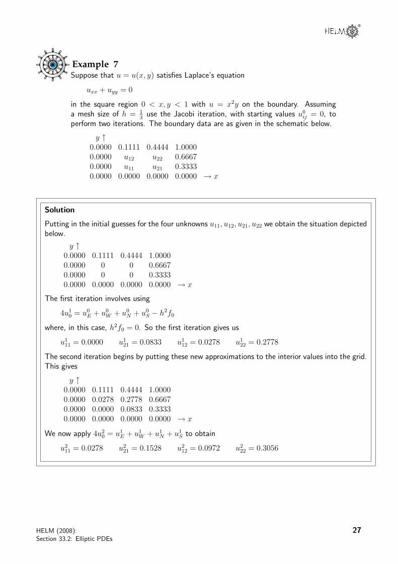
Example 7Suppose that u = u(x, y) satisfies Laplace’s equation

uxx + uyy = 0

in the square region 0 < x, y < 1 with u = x2y on the boundary. Assuminga mesh size of h = 1

3use the Jacobi iteration, with starting values u0

ij = 0, toperform two iterations. The boundary data are as given in the schematic below.

y ↑0.0000 0.1111 0.4444 1.00000.0000 u12 u22 0.66670.0000 u11 u21 0.33330.0000 0.0000 0.0000 0.0000 → x

Solution

Putting in the initial guesses for the four unknowns u11, u12, u21, u22 we obtain the situation depictedbelow.

y ↑0.0000 0.1111 0.4444 1.00000.0000 0 0 0.66670.0000 0 0 0.33330.0000 0.0000 0.0000 0.0000 → x

The first iteration involves using

4u10 = u0

E + u0W + u0

N + u0S − h2f0

where, in this case, h2f0 = 0. So the first iteration gives us

u111 = 0.0000 u1

21 = 0.0833 u112 = 0.0278 u1

22 = 0.2778

The second iteration begins by putting these new approximations to the interior values into the grid.This gives

y ↑0.0000 0.1111 0.4444 1.00000.0000 0.0278 0.2778 0.66670.0000 0.0000 0.0833 0.33330.0000 0.0000 0.0000 0.0000 → x

We now apply 4u20 = u1

E + u1W + u1

N + u1S to obtain

u211 = 0.0278 u2

21 = 0.1528 u212 = 0.0972 u2

22 = 0.3056


27

In practice, using a computer to carry out the arithmetic, we would continue iterating until the resultssettle down to a converged value. Using a computer spreadsheet, for example, we can see that atotal of 15 iterations is enough to achieve results converged to four decimal places. We noted earlierthat, to four decimal places, u11 = 0.0833, u21 = 0.1944, u12 = 0.1389 and u22 = 0.3611.

The following Task uses the same data as the preceding Task (pages 23-24), except that we haverounded the boundary data to four decimal places instead of using the exact fractions.

Task

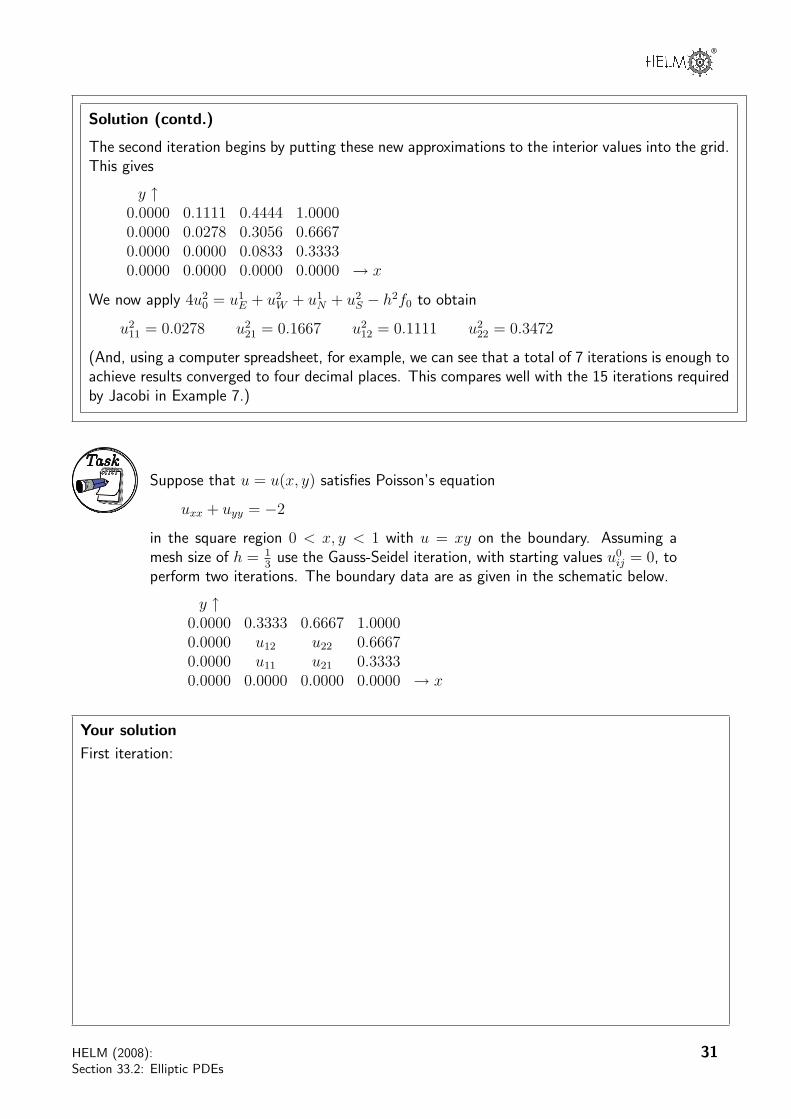
Suppose that u = u(x, y) satisfies Poisson’s equation

uxx + uyy = −2

in the square region 0 < x, y < 1 with u = xy on the boundary. Assuming a meshsize of h = 1

3use the Jacobi iteration, with starting values u0

ij = 0, to performtwo iterations. The boundary data are as given in the schematic below.

y ↑0.0000 0.3333 0.6667 1.00000.0000 u12 u22 0.66670.0000 u11 u21 0.33330.0000 0.0000 0.0000 0.0000 → x

Your solution

First iteration:

AnswerPutting in the initial guesses for the four unknowns we obtain the situation depicted below.

y ↑0.0000 0.3333 0.6667 1.00000.0000 0 0 0.66670.0000 0 0 0.33330.0000 0.0000 0.0000 0.0000 → x


4u10 = u0

E + u0W + u0

N + u0S − h2f0

where in this case h2f0 = −0.2222. So the first iteration gives us

u111 = 0.0556 u1

21 = 0.1389 u112 = 0.1389 u1

22 = 0.3889


®

Your solution

Second iteration:

AnswerThe second iteration begins by putting these new approximations to the interior values into the grid.This gives

y ↑0.0000 0.3333 0.6667 1.00000.0000 0.1389 0.3889 0.66670.0000 0.0556 0.1389 0.33330.0000 0.0000 0.0000 0.0000 → x

We now perform the second iteration 4u20 = u1

E + u1W + u1

N + u1S − h2f0 again, but with the new

values. We obtain

u211 = 0.1250

u221 = 0.2500

u212 = 0.2500

u222 = 0.4583

In the case above 17 iterations are required to achieve results that have converged to 4 decimalplaces. We find that u11 = 0.2222, u12 = 0.3333, u21 = 0.3333 and u22 = 0.5556.

Gauss-Seidel iterationIn the implementation of the Jacobi method we used old values for the southerly and westerly pointswhen new values had already been calculated.

new valuesalready found


29

The Gauss-Seidel method uses the new values as soon as they are available. Stating this formally wehave

new values here

↓ ↓un+1

0 = 14(un

E + un+1W + un+1

S + unN − h2f0

)Example 8 below uses the same data as Examples 6 and 7.

Example 8Suppose that u = u(x, y) satisfies Laplace’s equation

uxx + uyy = 0

in the square region 0 < x, y < 1 with u = x2y on the boundary. Assuming amesh size of h = 1

3, use the Gauss-Seidel iteration, with starting values u0


y ↑0.0000 0.1111 0.4444 1.00000.0000 u12 u22 0.66670.0000 u11 u21 0.33330.0000 0.0000 0.0000 0.0000 → x

Solution

Putting in the initial guesses for the four unknowns we obtain the situation depicted below.

y ↑0.0000 0.1111 0.4444 1.00000.0000 0 0 0.66670.0000 0 0 0.33330.0000 0.0000 0.0000 0.0000 → x


4u10 = u0

E + u1W + u0

N + u1S − h2f0

where in this case h2f0 = 0. So the first iteration gives us

u111 = 0.0000

u121 = 0.0833

u112 = 0.0278

u122 = 0.3056


®

Solution (contd.)

The second iteration begins by putting these new approximations to the interior values into the grid.This gives

y ↑0.0000 0.1111 0.4444 1.00000.0000 0.0278 0.3056 0.66670.0000 0.0000 0.0833 0.33330.0000 0.0000 0.0000 0.0000 → x


E + u2W + u1

N + u2S − h2f0 to obtain

u211 = 0.0278 u2

21 = 0.1667 u212 = 0.1111 u2

22 = 0.3472

(And, using a computer spreadsheet, for example, we can see that a total of 7 iterations is enough toachieve results converged to four decimal places. This compares well with the 15 iterations requiredby Jacobi in Example 7.)

Task

Suppose that u = u(x, y) satisfies Poisson’s equation

uxx + uyy = −2

in the square region 0 < x, y < 1 with u = xy on the boundary. Assuming amesh size of h = 1

3use the Gauss-Seidel iteration, with starting values u0


y ↑0.0000 0.3333 0.6667 1.00000.0000 u12 u22 0.66670.0000 u11 u21 0.33330.0000 0.0000 0.0000 0.0000 → x

Your solution

First iteration:


31

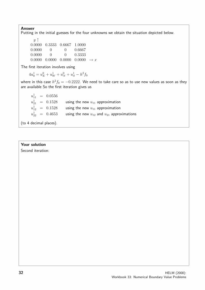
AnswerPutting in the initial guesses for the four unknowns we obtain the situation depicted below.

y ↑0.0000 0.3333 0.6667 1.00000.0000 0 0 0.66670.0000 0 0 0.33330.0000 0.0000 0.0000 0.0000 → x


4u10 = u0

E + u1W + u0

N + u1S − h2f0

where in this case h2f0 = −0.2222. We need to take care so as to use new values as soon as theyare available So the first iteration gives us

u111 = 0.0556

u121 = 0.1528 using the new u11 approximation


u122 = 0.4653 using the new u12 and u21 approximations

(to 4 decimal places).

Your solution

Second iteration:


®

AnswerThe second iteration begins by putting these new approximations to the interior values into the grid.This gives

y ↑0.0000 0.3333 0.6667 1.00000.0000 0.1528 0.4653 0.66670.0000 0.0556 0.1528 0.33330.0000 0.0000 0.0000 0.0000 → x


E + u2W + u1

N + u2S − h2f0 again, but with the new values. We obtain

u211 = 0.1319



u222 = 0.5330 using the new u12 and u21 approximations

and we can write this information in the form

y ↑0.0000 0.3333 0.6667 1.00000.0000 0.2882 0.5330 0.66670.0000 0.1319 0.2882 0.33330.0000 0.0000 0.0000 0.0000 → x

Again, a computer can be used to continue iterating until convergence. This method applied to thisTask needs 8 iterations to achieve 4 decimal place convergence, a fact which compares very well withthe 17 required by the Jacobi method.

ConvergenceWe now summarise some important points

1. For the problems discussed in these pages, the Jacobi and Gauss-Seidel methods will alwaysconverge for any initial guesses u0

ij. (Of course, very poor initial guesses will result in moreiterations being required.)

2. For a given problem and given starting guesses u0ij, the Gauss-Seidel method will, in general,

converge in fewer iterations than Jacobi. (That is, using the new, improved values assoon as they are available speeds up the process.)

3. One possible advantage with the Jacobi approach is that it can be parallelised, that is, it is intheory possible to do all the calculations for a given iteration simultaneously. In other words,everything we will need to know to carry out an iteration is known before the iteration begins.This is not the case with Gauss-Seidel in which during an iteration, most calculations use aresult from within the current iteration. This advantage with Jacobi only manifests itself whenusing computers with a parallelisation option and for large problems.


33

Exercises

1. Suppose that u = u(x, y) satisfies Laplace’s equation

uxx + uyy = 0

in the square region 0 < x, y < 1. Assuming a mesh size of h = 13

use the Jacobi iteration,with starting values u0

ij = 0, to perform two iterations. The boundary data are as given in theschematic below:

y ↑0.0000 0.2500 0.7500 1.00000.4000 u12 u22 0.80000.8000 u11 u21 0.40000.0000 0.7500 0.2500 0.0000 → x

2. Suppose that u = u(x, y) satisfies Laplace’s equation

uxx + uyy = 0

in the square region 0 < x, y < 1. Assuming a mesh size of h = 13

use the Gauss-Seideliteration, with starting values u0

ij = 0, to perform two iterations. The boundary data are asgiven in the schematic below.

y ↑0.0000 0.2500 0.7500 1.00000.4000 u12 u22 0.80000.8000 u11 u21 0.40000.0000 0.7500 0.2500 0.0000 → x


®

Answers

1. Putting in the initial guesses for the four unknowns we obtain the situation depicted below.

y ↑0.0000 0.2500 0.7500 1.00000.4000 0 0 0.80000.8000 0 0 0.40000.0000 0.7500 0.2500 0.0000 → x


4u10 = u0

E + u0W + u0

N + u0S − h2f0

where in this case h2f0 = 0.0000. So the first iteration gives us

u111 = 0.3875

u121 = 0.1625

u112 = 0.1625

u122 = 0.3875

The second iteration begins by putting these new approximations to the interior values intothe grid. This gives

y ↑0.0000 0.2500 0.7500 1.00000.4000 0.1625 0.3875 0.80000.8000 0.3875 0.1625 0.40000.0000 0.7500 0.2500 0.0000 → x


E + u1W + u1


u211 = 0.4688

u221 = 0.3563

u212 = 0.3563

u222 = 0.4688


35

Answers

2. Putting in the initial guesses for the four unknowns we obtain the situation depicted below.

y ↑0.0000 0.2500 0.7500 1.00000.4000 0 0 0.80000.8000 0 0 0.40000.0000 0.7500 0.2500 0.0000 → x


4u10 = u0

E + u1W + u0

N + u1S − h2f0

where in this case h2f0 = 0.0000. So the first iteration gives us

u111 = 0.3875

u121 = 0.2594

u112 = 0.2594

u122 = 0.5172

The second iteration begins by putting these new approximations to the interior values intothe grid. This gives

y ↑0.0000 0.2500 0.7500 1.00000.4000 0.2594 0.5172 0.80000.8000 0.3875 0.2594 0.40000.0000 0.7500 0.2500 0.0000 → x


E + u2W + u1


u211 = 0.5172

u221 = 0.4211

u212 = 0.4211

u222 = 0.5980


Boundary Value Problems Numerical

Documents