Boundary Growth in One-Dimensional Cellular Automata

Boundary Growth in One-Dimensional Cellular Automata

Charles D. Brummitt

Department of MathematicsandComplexity Sciences CenterUniversity of CaliforniaOne Shields AvenueDavis, CA 95616, USA

Eric Rowland

LaCIM, Université du Québec à MontréalMontréal, QC H2X 3Y7, Canada

The boundaries of one-dimensional, two-color cellular automata de-pending on four cells and begun from simple initial conditions are sys-tematically studied. The exact growth rates of the boundaries thatappear to be reducible are determined. The reducible boundaries arecharacterized by morphic words. For boundaries that appear to be irre-ducible, curve-fitting techniques are applied to compute an empiricalgrowth exponent and (in the case of linear growth) a growth rate. Therandom walk statistics of irreducible boundaries exhibit surprising regu-larities and suggest that a threshold separates two classes. Finally, a cel-lular automaton is constructed whose growth exponent does not exist,showing that a strict classification by exponent is not possible.

1. Introduction

Cellular automata are simple machines consisting of cells that updatein parallel at discrete time steps. In general, the state of a cell dependson the state of its local neighborhood at the previous time step. Theearliest known examples were engineered for specific purposes, suchas the two-dimensional cellular automaton constructed by von Neu-mann in 1951 to model biological self-replication [1]. Three decadeslater, researchers began to study entire classes of automata, such asthe 256 one-dimensional cellular automata that use k ! 2 colors andthat depend on d ! 3 cells [2, 3]. The behavior of these rules subse-quently garnered much attention. Most studies have focused on the in-teriors of patterns generated by cellular automata, likely because theboundaries are well known and simple for the k ! 2, d ! 3 rules,such as the three linear boundaries shown in Figure 1. However,boundaries of automata are diverse, often more predictable than inte-riors (and hence more amenable to mathematical study), and even use-ful for detecting interesting behavior.

Complex Systems, 21 © 2012 Complex Systems Publications, Inc.https://doi.org/10.25088/ComplexSystems.21.2.85

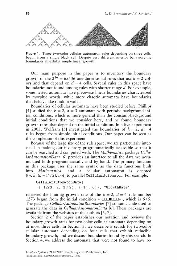
90 30 110Figure 1. Three two-color cellular automaton rules depending on three cells,begun from a single black cell. Despite very different interior behavior, theboundaries all exhibit simple linear growth.

Our main purpose in this paper is to inventory the boundarygrowth of the 216 ! 65536 one-dimensional rules that use k ! 2 col-ors and that depend on d ! 4 cells. Several rules in this space haveboundaries not found among rules with shorter range d. For example,some nested automata have piecewise linear boundaries characterizedby morphic words, while more chaotic automata have boundariesthat behave like random walks.

Boundaries of cellular automata have been studied before. Phillips[4] studied the k ! 2, d ! 3 automata with periodic-background ini-tial conditions, which is more general than the constant-backgroundinitial conditions that we consider here, and he found boundarygrowth rates that depend on the initial condition. In a live experimentin 2005, Wolfram [5] investigated the boundaries of k ! 2, d ! 4rules begun from simple initial conditions. Our paper can be seen asthe completion of this experiment.

Because of the large size of the rule space, we are particularly inter-ested in making our inventory programmatically accessible so that itcan be searched and computed with. The Mathematica package Cellu-larAutomatonData [6] provides an interface to all the data we accu-mulated both programmatically and by hand. The primary functionin this package uses the same syntax as the data functions builtinto Mathematica, and a cellular automaton is denoted88n, k, Hd - 1L ê 2<, init< to parallel CellularAutomaton. For example,

CellularAutomatonData@881273, 2, 3 ê 2<, 881<, 0<<, "GrowthRate"Dretrieves the limiting growth rate of the k ! 2, d ! 4 rule number1273 begun from the initial condition !···‡···!, which is 6 ê 5.The package CellularAutomatonBoundaries [7] contains code used togenerate the data in CellularAutomatonData [6]. These packages areavailable from the websites of the authors [6, 7].

Section 2 of the paper establishes our notation and reviews theboundary growth rates for two-color cellular automata depending onat most three cells. In Section 3, we describe a search for two-colorcellular automata depending on four cells that exhibit reducibleboundary growth, and we discuss boundaries found by this search. InSection 4, we address the automata that were not found to have re-

86 C. D. Brummitt and E. Rowland


ducible growth; we study their growth rates statistically using toolstypically applied to random walks. We also attempt to assign agrowth function tb to each automaton for some 0 § b § 1. However,in Section 5 we show that in general this is impossible by constructingan automaton for which no such b exists. In Section 6, we discuss pos-sible extensions and open questions.

Classifying automata by their boundaries identifies many automatawith interesting behavior. Many boundaries closely reflect the behav-ior of the interior. For example, nested boundaries arise from nestedautomata, while chaotic boundaries arise from complex automata.Some automata with complicated interiors (such as rules 30 and 110in Figure 1) nevertheless have simple boundaries. Thus the complexityof an automaton’s boundary provides a lower bound on the complex-ity of its interior. Throughout the paper, we describe many interestingautomata found in this way by using the boundary as a filter.

2. Background

2.1 One-Dimensional Cellular AutomataThe cellular automata that we study in this paper are one-dimen-sional. A one-dimensional cellular automaton consists of

† an alphabet S of size k,

† a positive integer d,

† a function i from the set of integers to S, and

† a function f from Sd (d-tuples of elements in S) to S.

The function i is called the initial condition, and the function f iscalled the rule. We think of the initial condition as an infinite row ofdiscrete cells, each assigned one of k colors. To evolve the cellular au-tomaton, we update all cells in parallel, where each cell updates ac-cording to f , a function of d cells in its vicinity on the previous step.

There are kkd rules on k colors depending on d cells. We adopt the

usual convention of naming a cellular automaton’s rule by the num-ber whose base-k digits consist of the outputs of the rule under the kd

possible inputs of d cells, ordered reverse-lexicographically. For exam-ple, the two-color rule depending on three cells that maps the eightpossible inputs according to the table

‡‡‡ ‡‡· ‡·‡ ‡·· ·‡‡ ·‡· ··‡ ···· · · ‡ ‡ ‡ ‡ ·

is rule 000111102 ! 30 in this numbering. Here we have identified0 ! · and 1 ! ‡.

Boundary Growth in One-Dimensional Cellular Automata 87


The evolution of a one-dimensional cellular automaton can be visu-alized in two dimensions by displaying each row below its predeces-sor. For example, Figure 1 shows 28 steps of three rules evaluatedfrom the initial condition !···‡···!. To create such pictures, wemust choose a horizontal offset. For instance, the offset of rule 30 inthe table above is center-aligned: every cell depends on the cells in thesame position, l ! 1 to the left, and r ! 1 to the right. For a differentoffset, the rows in the automaton will be the same; each row simplyshifts with respect to the row preceding it. In other words, shifting land r to l - D and r + D, respectively, only shears the two-dimensionalpicture. Therefore, for convenience we generally choose a horizontaloffset that minimizes the total width of the region of interest.

2.2 Row LengthsWe require that all but finitely many cells in the initial condition havethe same color. Then each row has finite length, which we define asfollows. If all cells in a row are the same color, the length of that rowis 0. Otherwise, the length of a row is the number of cells in the re-gion bordered by, and including, the first and last cells that differfrom the constant background. For a given cellular automaton, let "HtLbe the length of the row on step t for each t ¥ 0.

For example, the length "HtL for rule 90 begun from !···‡···!as in Figure 1 is "HtL ! 2 t + 1 for all t ¥ 0. For rule 30 the length isalso "HtL ! 2 t + 1, whereas for rule 110 it is "HtL ! t + 1. Note that"HtL does not depend on the horizontal offset chosen to display the au-tomaton.

At each step in a cellular automaton, information can propagate atmost l steps from the right boundary and at most r steps from the leftboundary, where l and r depend on the offset chosen but are subjectto l + 1 + r ! d. In other words, the maximum growth rate possible(called the “speed of light”) is d - 1 cells per step, and if the maxi-mum growth rate persists over time, then "HtL ! Hd - 1L t + c for somec. If the maximum growth is achieved at every step, then"HtL ! Hd - 1L t + "H0L for all t ¥ 0.

Because each row in a cellular automaton depends only on the pre-vious row, the difference sequence "Ht + 1L - "HtL is particularly rele-vant, since it gives the number of cells by which the automaton growsor shrinks at each step. It will be useful to think of the difference se-quence as an infinite word on the set of integers.

Definition 1. The boundary word of a cellular automaton is the se-quence 8"Ht + 1L - "HtL<t¥0.

We will see that the boundary word frequently reflects propertiesof an automaton.

If the boundary word is eventually periodic, then "HtL can be writ-ten as a piecewise expression in linear functions. Namely, there existintegers m, tmin and rational numbers a and c0, c1, …, cm-1 such that


Complex Systems, 21 © 2012 Complex Systems Publications, Inc. https://doi.org/10.25088/ComplexSystems.21.2.85

0 m for all t ¥ tmin we have

(1)"HtL !

a t + c0 if t ª 0 mod m

a t + c1 if t ª 1 mod m

ª ª

a t + cm-1 if t ª m - 1 mod m.

For example, the sequence "HtL for rule 45 begun from !···‡···!,shown in Figure 2, is 1, 3, 4, 6, 7, …. The boundary word 212121!

is periodic with period length 2, and the length of the row at step t is

"HtL !3 t ê 2 + 1 if t ª 0 mod 2

3 Ht + 1L ê 2 if t ª 1 mod 2

for t ¥ 0. Rule 107 begun from a single black cell is also shown in Fig-ure 2; its boundary word 121202020242024!, where 4 ! -4, iseventually periodic with period length 4, and for t ¥ 7

"HtL !

11 if t ª 0 mod 4

11 if t ª 1 mod 4

13 if t ª 2 mod 4

09 if t ª 3 mod 4.

All two-color cellular automata depending on d ! 2 cells have even-tually periodic boundary words, either with growth rate a ! 0 ora ! 1.

45 107 106Figure 2. Rules 45 and 107 have row lengths that can be expressed by equa-tion (1). Rule 106 exhibits square-root growth when begun from two adja-cent black cells.

The boundaries of two-color cellular automata depending ond ! 3 cells are largely similar. These automata generate a variety of in-ternal structures: rule 90, for example, produces nested structure,while rules 30 and 110 yield complex behavior. One new feature seenfor d ! 3 is square-root growth, exhibited for example by rule 106 be-gun from the initial condition !···‡‡···!, as shown in Figure 2.We discuss square-root growth further in Section 3.3. However, withthe exceptions of rules 106, 120, 169, and 225, each two-color cellu-lar automaton depending on d ! 3 cells has an eventually periodicboundary word. Moreover, for every automaton in this space (with a



constant-background initial condition), the limiting growth rate

(2)limtØ¶

"HtLt

exists and is an element of 80, 1, 3 ê 2, 2<. In particular, for rule 106this limit is 0. (Note that if we allow a general periodic backgroundfor the initial condition, then the boundary word is not necessarilyeventually periodic; for example, the left boundary of rule 30 begunfrom the initial condition

!·‡·‡·‡‡‡·‡·‡·! ! !0101011101010!

appears to be chaotic.)In general, the limiting growth rate limtØ¶ "HtL ê t of a cellular au-

tomaton may not exist, as we see in Section 3. Moreover, the limitinggrowth exponent limtØ¶ logt "HtL may not exist, as we show in Sec-tion!5. However, in most cases these values do appear to exist, so inSection 4 we use them as statistical information about boundaries.

We mention the observation of Phillips [4] that if the sequence ofrows in an automaton is not eventually periodic, then "HtL grows atleast logarithmically. This is because for " ¥ 2 there are k!-1Hk - 1L2possible rows of length ", so a cellular automaton that never returnsto the same state has at most exponentially many rows of length ".Logarithmic growth is not seen for k ! 2 and d § 3, and we did notfind logarithmic growth among d ! 4 rules, either. However, it is pos-sible to construct an automaton that implements counting in binaryby using additional colors (and additional steps) to propagate carries,and this automaton grows logarithmically [4].

3. Automata with Reducible Growth

In this section, we describe a combined automated–manual search forreducible boundaries among all two-color rules depending on d ! 4cells begun from single-cell initial conditions. Eventually periodicboundary words can be detected completely automatically, and we ex-amine by hand the automata that are not found to have an eventuallyperiodic boundary word.

As in every space of cellular automaton rules, some rules in thisspace are equivalent to others by simple transformations. For exam-ple, reversing each tuple in the definition of the rule and reversing theinitial condition results in an image that is simply the left–right reflec-tion of the original. Similarly, permuting the colors in a rule and inthe initial condition produces an image that is obtained from the origi-nal by the same permutation. Therefore, it suffices to consider onlyone rule among each equivalence class of rules obtained by reflectingand permuting. For this we choose the rule with minimal rule num-



ber. For k ! 2 and d ! 4, this reduces the number of rules from65536 to 16704.

As a simplifying assumption, we consider only the two initial condi-tions !···‡···! and !‡‡‡·‡‡‡!, each consisting of an infiniteconstant background with a single perturbed cell. This results in33408 automata (two initial conditions for each rule). In many casesthese initial conditions suffice to characterize the growth of the rule.However, for rules that grow dramatically differently depending onthe initial condition, the data we collect may not be representative oftypical growth.

We further restrict the initial condition by requiring the back-ground color to reoccur on some later step (but not necessarily thenext step). That is, we only consider the initial condition!···‡···! if a white background reoccurs on some later step. Sim-ilarly, we only consider !‡‡‡·‡‡‡! if a black background reoccurson a later step. We ignore these initial conditions otherwise becausewe are interested in long-term behavior, and a background that doesnot reoccur is a type of transience. Doing so reduces the number of au-tomata to 25088.

We run each of these automata for tmax steps and consider thedifference sequence "Ht + 1L - "HtL for tmin § t § tmax - 1, withsome tmin > 0 allowing for transience. Let m be the smallest positiveinteger such that "Ht + 1 + mL - "Ht + mL ! "Ht + 1L - "HtL for alltmin § t § tmax - 1 - m. If m < Htmax - tminL ê 4, then we deem theboundary word to be eventually periodic (and "HnL to satisfy equa-tion!(1)), and we record the period length m and the growth rate

(3)a !sum of the terms in the period

m!

"Ht + mL - "HtLm

.

Otherwise we consider the period length unreliable and this testinconclusive.

In choosing a time range tmin § t § tmax on which to test periodic-ity, we face opposing goals: to overcome possible transience, we wanttmin to be large, but for speed we want tmax to be small. Our solutionis to use the four short time ranges 20 § t § 100, 50 § t § 300,200 § t § 600, and 400 § t § 1000 as successive filters, followed by amore extensive range. If a reliable period length is found in any ofthese ranges, then we skip the remaining ranges and compute the pe-riod length in a final range 500 § t § 4000 to confirm that the periodlength persists. This final time range identifies only 32 corrections toperiod lengths found by one of the first four ranges, and all but one ofthose (correcting the slope from 7 ê 4 to 18 ê 11 for rule 23726 begunfrom !···‡···!) are cases where the boundary word does not ap-pear to be eventually periodic. Running all 25088 automata throughthe four filter ranges took approximately 20 minutes on a 2.5 GHzmachine. Running the final time range took approximately two and ahalf days.

!



While we believe that confirming each period length in the range500 § t § 4000 has allowed our data to be highly reliable, this algo-rithm clearly does not guarantee that if a period length was foundthen the boundary word is in fact eventually periodic (false positives),nor does it guarantee that if a period length was not found then theboundary word is not eventually periodic (false negatives). There areseveral automata whose boundaries do not stabilize until well after400 steps or whose eventual behavior is unclear. For example,rule!11109 begun from !···‡···! grows to "H1722L ! 918, andthereafter has average growth rate 0. Rule 4713 begun from!···‡···! jettisons a particle at step 915, leaving behind an other-wise chaotic left boundary. Rule 10633 (begun from either initial con-dition) appears to have an eventually periodic boundary word due toits internal froth generally moving away from the boundary, but it isnot clear that this will continue indefinitely. Worse, there are au-tomata whose growth is periodic for short time intervals but that aremost likely not periodic in general. For example, rule 457 begun fromeither initial condition has a boundary word that is periodic in therange 100 § t § 200, but for larger ranges we see that the periodicitydoes not continue.

These examples indicate that in general the long-term behavior ofthe boundary of a cellular automaton cannot be determined by exam-ining finitely many steps. Of course, this is not surprising, because theboundary can depend sensitively on the interior of the automaton,and it is known that some cellular automaton rules are computation-ally universal. Indeed, we determined the four time ranges only aftersome experimentation with a selection of rules.

Executing this automatic search yields 837 automata (with 620 dis-tinct rules) that were not found to have an eventually periodic bound-ary word. Among these 837, there are only 757 distinct pictures (atleast for 500 rows), because several pairs of inequivalent rules appearto nonetheless generate the same evolution due to certain configura-tions not appearing. We examined each of these classes manually andfound that 36 automata do in fact appear to have eventually periodicboundary words, while another 81 exhibit self-similarity. Therefore, aclassification of the 25088 automata is as follows.

1. 24287 automata have eventually periodic boundary words.

2. 81 automata have boundary words that are not eventually periodic butare reducible.

3. 720 automata have boundaries that are most likely not reducible.

Analyzing automata in the third class is the subject of Section 4. Au-tomata in the first two classes have boundary words with simple de-scriptions, and they are the subject of this section.

A note regarding the level of rigor is in order. We do not formallyprove the claims in this section, neither the explicit growth rates norother properties we describe. Therefore they can either be taken as



conjectures or as semi-rigorous results that are experimentally verifiedfor the first 4000 (and in some cases many more) steps of the cellularautomata involved. Proving each claim is beyond the scope of the cur-rent paper, although we touch on this in Section 6.

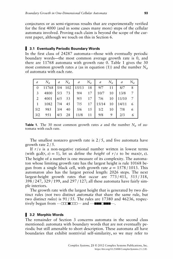
3.1 Eventually Periodic Boundary WordsIn the first class of 24287 automata—those with eventually periodicboundary words—the most common average growth rate is 0, andthere are 11768 automata with growth rate 0. Table 1 gives the 30most common growth rates a (as in equation (1)) and the number Naof automata with each rate.

a Na a Na a Na a Na a Na

0 11768 5/4 102 15/13 18 9/7 11 8/7 8

3 4800 5/3 73 9/4 17 10/7 10 13/8 7

2 4001 6/5 53 9/5 17 7/6 10 11/10 7

1 1082 7/4 45 7/5 17 15/14 10 14/11 6

5/2 985 3/4 40 5/6 15 1/2 10 7/8 6

3/2 951 4/3 28 11/8 11 9/8 9 2/3 6

Table 1. The 30 most common growth rates a and the number Na of au-tomata with each rate.

The smallest nonzero growth rate is 2 ê 5, and five automata havegrowth rate 2 ê 5.

If r ê s is a non-negative rational number written in lowest terms(with gcdHr, sL ! 1), let us define the height of r ê s to be maxHr, sL.The height of a number is one measure of its complexity. The automa-ton whose limiting growth rate has the largest height is rule 10168 be-gun from a single black cell, with growth rate a ! 1578 ê 1013. Thisautomaton also has the largest period length: 2026 steps. The nextlargest-height growth rates that occur are 773 ê 411, 515 ê 318,398 ê 247, 329 ê 199, and 297 ê 127; all these automata have fairly sim-ple interiors.

The growth rate with the largest height that is generated by two dis-tinct rules (not two distinct automata that share the same rule, buttwo distinct rules) is 91 ê 55. The rules are 17380 and 46236, respec-tively begun from !···‡···! and !‡‡‡·‡‡‡!.

3.2 Morphic WordsThe remainder of Section 3 concerns automata in the second classmentioned: automata with boundary words that are not eventually pe-riodic but still amenable to short description. These automata all haveboundaries that exhibit nontrivial self-similarity, so we may refer to



these as fractal boundaries. It turns out that the boundary words forall these automata are morphic words—words generated by iteratinga morphism (also known as a substitution system).

Let S and D be finite alphabets, and let S* denote the set of all fi-nite words with letters in S. The empty word is denoted by e. For afunction j : S Ø D* and a (finite or infinite) sequence w0, w1, … of let-ters in S, define jHw0 w1 …L ! jHw0L jHw1L…. We refer to j as a mor-phism, since jHx yL ! jHxL jHyL for all words x, y. If D ! S and there issome letter A œ S and some word x œ S* such that jHAL ! A x, thenby iteratively applying j to A we obtain prefixes of the word

jwHAL := A x jHxL j2HxL… ,

which is a fixed point of j. Moreover, this word is the unique fixedpoint of j beginning with A. An infinite word (or, equivalently, an in-finite sequence) w is morphic if there is a letter A œ S and morphismsj : S Ø S* and y : S Ø D* such that

w ! yHjwHALL.We see in the following subsections that, for each cellular automatonwith reducible boundary structure, the boundary word is morphic(and is a word on some finite set D of integers).

In the next three subsections we address fractal automata whoselimiting growth rates exist. We will see that these rates do not ap-proach the complexity of some of the growth rates observed for even-tually periodic boundary words in Section 3.1. In the final subsectionwe discuss automata whose limiting growth rates do not exist. (Manyof the rules discussed have nearly identical behavior when begun fromthe two initial conditions; in these cases we only discuss one initialcondition without mentioning this further.)

We refer the reader to the book of Allouche and Shallit [8, Chap-ters 6–8] for a comprehensive treatment of morphic words. For ourimmediate purposes, it suffices to mention that prepending a word toa morphic word produces another morphic word. In particular, everyeventually periodic word is morphic.

3.3 Square-Root GrowthBefore discussing square-root growth among two-color rules depend-ing on four cells, we first discuss d ! 3 rule 106, which also exhibitssquare-root growth. Figure 2 shows the evolution of rule 106 begunfrom two adjacent black cells. The boundary word of this automatonis the infinite word

w106 ! 11010011000000010000000011010011!

on the alphabet 80, 1<. Let us rewrite the boundary word as

w106 ! 12 01 11 02 12 07 11 08 12 01 11 02 12 031 11 032 ! ,



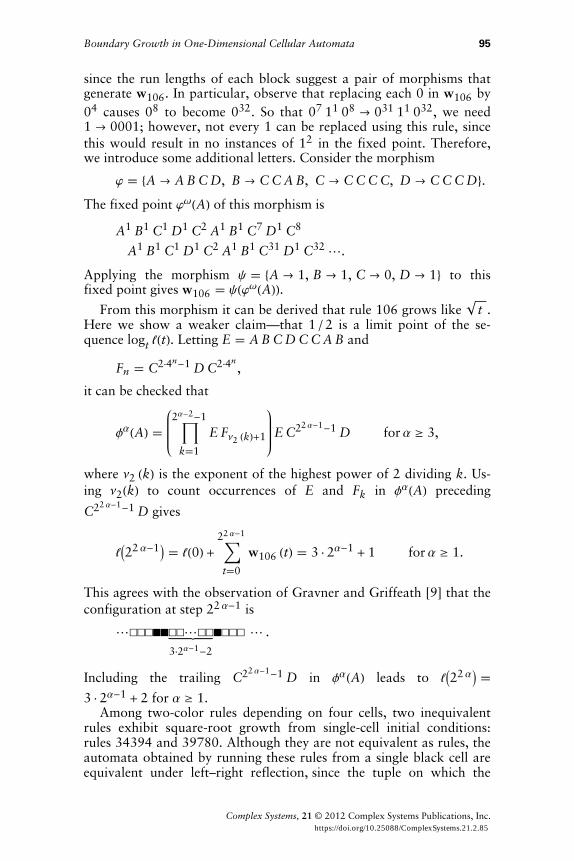
since the run lengths of each block suggest a pair of morphisms thatgenerate w106. In particular, observe that replacing each 0 in w106 by04 causes 08 to become 032. So that 07 11 08 Ø 031 11 032, we need1 Ø 0001; however, not every 1 can be replaced using this rule, sincethis would result in no instances of 12 in the fixed point. Therefore,we introduce some additional letters. Consider the morphism

j ! 8A Ø A B C D, B Ø C C A B, C Ø C C C C, D Ø C C C D<.The fixed point jwHAL of this morphism is

A1 B1 C1 D1 C2 A1 B1 C7 D1 C8

A1 B1 C1 D1 C2 A1 B1 C31 D1 C32 !.

Applying the morphism y ! 8A Ø 1, B Ø 1, C Ø 0, D Ø 1< to thisfixed point gives w106 ! yHjwHALL.

From this morphism it can be derived that rule 106 grows like t .Here we show a weaker claim—that 1 ê 2 is a limit point of the se-quence logt "HtL. Letting E ! A B C D C C A B and

Fn ! C2ÿ4n-1 D C2ÿ4n,

it can be checked that

faHAL ! ‰k"1

2a-2-1

E Fn2 HkL+1 E C22 a-1-1 D for a ¥ 3,

where n2 HkL is the exponent of the highest power of 2 dividing k. Us-ing n2HkL to count occurrences of E and Fk in faHAL preceding

C22 a-1-1 D gives

"I22 a-1M ! "H0L + ‚t"0

22 a-1

w106 HtL ! 3 ÿ 2a-1 + 1 for a ¥ 1.

This agrees with the observation of Gravner and Griffeath [9] that theconfiguration at step 22 a-1 is

!···‡‡··!··

3ÿ2a-1-2

‡··· ! .

Including the trailing C22 a-1-1 D in faHAL leads to "I22 aM !3 ÿ 2a-1 + 2 for a ¥ 1.

Among two-color rules depending on four cells, two inequivalentrules exhibit square-root growth from single-cell initial conditions:rules 34394 and 39780. Although they are not equivalent as rules, theautomata obtained by running these rules from a single black cell areequivalent under left–right reflection, since the tuple on which the



rules differ does not occur in the evolution begun from a single blackcell. In particular, rule 39780 is known to exhibit conditional re-versibility, due to the local rule being a bijective function in the left-most position [10], whereas rule 34394 does not have this property.Figure 3 shows rule 39780.

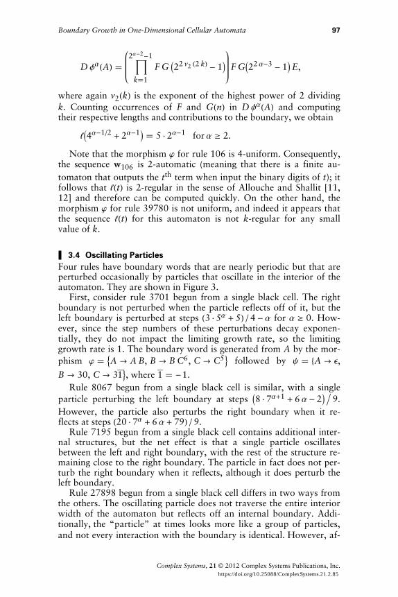
39780

3701 8067

7195 27898

Figure 3. Rule 39780 grows like t . The other four automata pictured herecontain oscillating particles.

For both of these automata, the boundary word is

w39780 ! 2210221111111022102211111111! ,

a word on the alphabet 8-1, 0, 1, 2<, where we have written 1 for -1.Because of the repeating 11 oscillations, the run lengths of the originalsequence do not reveal much. However, partitioning into blocks oflength 2 as

w39780 ! H22L1 H10L1 H22L1 I11M3 H10L1 H22L1 H10L1 H22L1 I11M15

H10L1 H22L1 H10L1 H22L1 I11M3 H10L1 H22L1 H10L1 H22L1 I11M63!

shows some structure. If j is the morphism

8A Ø A B C, B Ø D A B,C Ø C E C E, D Ø C E C D, E Ø C E C E<

and y ! 9A Ø 2, B Ø 2, C Ø 1, D Ø 0, E Ø 1=, then w39780 !yHjwHALL. To show again that 1 ê 2 is a limit point of logt "HtL, letF ! D A B C D A B C and GHnL ! HE CLn. Then for a ¥ 3



D faHAL ! ‰k"1

2a-2-1

F G I22 n2 H2 kL - 1M F GI22 a-3 - 1ME,

where again n2HkL is the exponent of the highest power of 2 dividingk. Counting occurrences of F and GHnL in D faHAL and computingtheir respective lengths and contributions to the boundary, we obtain

"I4a-1ê2 + 2a-1M ! 5 ÿ 2a-1 for a ¥ 2.

Note that the morphism j for rule 106 is 4-uniform. Consequently,the sequence w106 is 2-automatic (meaning that there is a finite au-tomaton that outputs the tth term when input the binary digits of t); itfollows that "HtL is 2-regular in the sense of Allouche and Shallit [11,12] and therefore can be computed quickly. On the other hand, themorphism j for rule 39780 is not uniform, and indeed it appears thatthe sequence "HtL for this automaton is not k-regular for any smallvalue of k.

3.4 Oscillating ParticlesFour rules have boundary words that are nearly periodic but that areperturbed occasionally by particles that oscillate in the interior of theautomaton. They are shown in Figure 3.

First, consider rule 3701 begun from a single black cell. The rightboundary is not perturbed when the particle reflects off of it, but theleft boundary is perturbed at steps H3 ÿ 5a + 5L ê 4 - a for a ¥ 0. How-ever, since the step numbers of these perturbations decay exponen-tially, they do not impact the limiting growth rate, so the limitinggrowth rate is 1. The boundary word is generated from A by the mor-phism j ! 9A Ø A B, B Ø B C6, C Ø C5= followed by y ! 8A Ø e,

B Ø 30, C Ø 31=, where 1 ! -1. Rule 8067 begun from a single black cell is similar, with a single

particle perturbing the left boundary at steps I8 ÿ 7a+1 + 6 a - 2M ë 9.However, the particle also perturbs the right boundary when it re-flects at steps H20 ÿ 7a + 6 a + 79L ê 9.

Rule 7195 begun from a single black cell contains additional inter-nal structures, but the net effect is that a single particle oscillatesbetween the left and right boundary, with the rest of the structure re-maining close to the right boundary. The particle in fact does not per-turb the right boundary when it reflects, although it does perturb theleft boundary.

Rule 27898 begun from a single black cell differs in two ways fromthe others. The oscillating particle does not traverse the entire interiorwidth of the automaton but reflects off an internal boundary. Addi-tionally, the “particle” at times looks more like a group of particles,and not every interaction with the boundary is identical. However, af-



ter four reflections the particle returns to its original state, so the oscil-latory behavior is in fact simple.

The respective limiting growth rates for rules 8067, 7195, and27898 are 6 ê 5, 5 ê 4, and 3 ê 2. Although we do not determine themorphisms here, the regularity of the oscillations in these automataimply that the boundary words are morphic.

3.5 Two Automata with Limiting Growth RatesFigure 4 shows rule 1273 begun from a single black cell andrule!36226 begun from a single white cell. The boundary words forthese automata are not eventually periodic, but they are morphic.Moreover, the limiting growth rate limtØ¶ "HtL ê t (equation (2)) existsfor each.

Figure 4. Rows 0 through 28 - 1 of rule 1273 and rule 36226, where the limit-ing growth rates have been used to shear the images such that the nonperiodicboundaries are vertical. The colors of rule 36226 have been reversed to placeit against a white background.

We begin with rule 36226 because its boundary is simpler. On aglobal scale, this automaton exhibits nested structure similar to thatproduced by d ! 3 rule 90 begun from a single black cell (see Fig-ure!1). However, the right boundary is fractal. The boundary word

w36226 ! 12211221221112212211221221111221!

can be obtained by dropping the first two letters in the fixed point2212211! of the morphism j ! 81 Ø 1, 2 Ø 221<. Recalling thatn2HnL denotes the exponent of the highest power of 2 dividing n, wecan also write

w36226 ! ‰n¥2

1n2HnL 2.

The limiting growth rate of the automaton is determined by the fre-quencies of 1 and 2 in w36226. The frequency of a letter x in an infi-



nite word w0 w1 … is

limtØ¶

†80 § i § t - 1 : wi ! x<§t

.

To compute the letter frequencies, we examine the incidence matrixof j, which records for each pair of letters x, y the number of occur-rences of x in jHyL. The incidence matrix for j is

1 1

0 2 .

If the frequency of each letter in a morphic word jwHAL exists, thenthe vector whose components are the letter frequencies is an eigenvec-tor of the incidence matrix corresponding to the largest positive eigen-value [8, Theorem 8.4.6]. In the case of w36226, the letter frequenciesexist, and that vector is H1 ê 2, 1 ê 2L. Therefore the letters 1 and 2 oc-cur with equal frequency, and on average the automaton grows 3 ê 2cells per step.

Now consider rule 1273 begun from a single black cell. The inte-rior is also nested, although the nestedness is not as obvious visually.For this automaton, the boundary word

w1273 ! 31303031313130303131313030313030!

(where again 1 ! -1) is given by I31M1 H30L2 yHjwHALL, where

j ! 8A Ø A C, B Ø A D, C Ø B A, D Ø B B<,and y maps

A Ø I31M3 H30L2 I31M3 H30L2 I31M1 H30L2B Ø I31M3 H30L2 I31M5 H30L2C Ø I31M5 H30L2 I31M3 H30L2 I31M1 H30L2D Ø I31M5 H30L2 I31M5 H30L2.

The incidence matrix for j is

1 1 1 0

0 0 1 2

1 0 0 0

0 1 0 0

,

so the vector with components equal to the frequencies of the four let-ters A, B, C, D is H4 ê 9, 2 ê 9, 2 ê 9, 1 ê 9L. The letters A, B, C, and Dcorrespond to respective net changes of 32, 28, 36, and 32 cells over



26, 24, 30, and 28 steps, and so it can be computed that the limitinggrowth rate is 6 ê 5 cells per step.

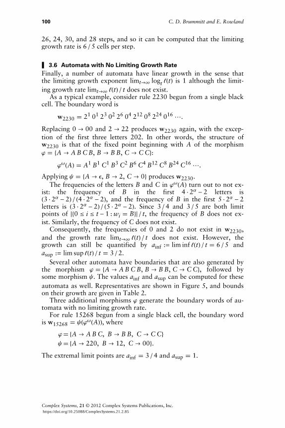
3.6 Automata with No Limiting Growth RateFinally, a number of automata have linear growth in the sense thatthe limiting growth exponent limtØ¶ logt "HtL is 1 although the limit-ing growth rate limtØ¶ "HtL ê t does not exist.

As a typical example, consider rule 2230 begun from a single blackcell. The boundary word is

w2230 ! 21 01 23 02 26 04 212 08 224 016 !.

Replacing 0 Ø 00 and 2 Ø 22 produces w2230 again, with the excep-tion of the first three letters 202. In other words, the structure ofw2230 is that of the fixed point beginning with A of the morphismj ! 8A Ø A B C B, B Ø B B, C Ø C C<:

jwHAL ! A1 B1 C1 B3 C2 B6 C4 B12 C8 B24 C16 !.

Applying y ! 8A Ø e, B Ø 2, C Ø 0< produces w2230.The frequencies of the letters B and C in jwHAL turn out to not ex-

ist: the frequency of B in the first 4 ÿ 2a - 2 letters isH3 ÿ 2a - 2L ê H4 ÿ 2a - 2L, and the frequency of B in the first 5 ÿ 2a - 2letters is H3 ÿ 2a - 2L ê H5 ÿ 2a - 2L. Since 3 ê 4 and 3 ê 5 are both limitpoints of †80 § i § t - 1 : wi ! B<§ ê t, the frequency of B does not ex-ist. Similarly, the frequency of C does not exist.

Consequently, the frequencies of 0 and 2 do not exist in w2230,and the growth rate limtØ¶ "HtL ê t does not exist. However, thegrowth can still be quantified by ainf := lim inf "HtL ê t ! 6 ê 5 andasup := lim sup "HtL ê t ! 3 ê 2.

Several other automata have boundaries that are also generated bythe morphism j ! 8A Ø A B C B, B Ø B B, C Ø C C<, followed bysome morphism y. The values ainf and asup can be computed for theseautomata as well. Representatives are shown in Figure 5, and boundson their growth are given in Table 2.

Three additional morphisms j generate the boundary words of au-tomata with no limiting growth rate.

For rule 15268 begun from a single black cell, the boundary wordis w15268 ! yHjwHALL, where

j ! 8A Ø A B C, B Ø B B, C Ø C C<y ! 8A Ø 220, B Ø 12, C Ø 00<.

The extremal limit points are ainf ! 3 ê 4 and asup ! 1.



2230 10644

3283 11032

6681 37018

10155 39066

10389 39394

10389 41114

Figure 5. Some nested automata with boundary words generated by the mor-phism 8A Ø A B C B, B Ø B B, C Ø C C<. They are variants on a common un-derlying structure, for which the limiting growth rate does not exist.



Rule Initial Condition yHAL yHBL yHCL ainf asup

2230 !···‡···! e 2 0 6 ê 5 3 ê 2

3283 !···‡···! 21 2121 22 3 ê 4 6 ê 7

6681 !···‡···! 31 3231 33 15 ê 16 15 ê 14

10155 !‡‡‡·‡‡‡! 2121 1121 11 15 ê 16 15 ê 14

10389 !···‡···! 32 3232 33 9 ê 8 9 ê 7

10389 !‡‡‡·‡‡‡! 230 3030 33 9 ê 8 9 ê 7

10644 !···‡···! 2 12 0 9 ê 8 9 ê 7

11032 !···‡···! 12 12 0 9 ê 8 9 ê 7

37018 !‡‡‡·‡‡‡! 2 02 0 3 ê 4 6 ê 7

39066 !‡‡‡·‡‡‡! 1 11 0 3 ê 4 6 ê 7

39394 !‡‡‡·‡‡‡! 12220 12220 00 21 ê 19 21 ê 17

41114 !‡‡‡·‡‡‡! 22 02 0 3 ê 4 6 ê 7

Table 2. Growth rate bounds for automata whose boundaries are generatedby the morphism j ! 8A Ø A B C B, B Ø B B, C Ø C C<.

For rule 4334 begun from a single black cell, the morphisms are

j ! 8A Ø A E D B B, B Ø B B, C Ø C C, D Ø D B, E Ø E C<y ! 8A Ø 122, B Ø 22, C Ø 00, D Ø 12, E Ø 10<,

and we have ainf ! 6 ê 5 and asup ! 3 ë 2.For rule 11172 begun from a single black cell, the morphisms are

j ! 8A Ø A E D B, B Ø B B, C Ø C C, D Ø D B, E Ø E C<y ! 9A Ø 2, B Ø 21, C Ø 00, D Ø 02, E Ø 21=,

and we have ainf ! 3 ê 4 and asup ! 1.

4. Automata with Irreducible Boundaries

Among the 25088 equivalence classes of k ! 2, d ! 4 cellular au-tomata, 720 automata evaded all attempts to reduce their boundaries.Among these 720, there are only 688 distinct pictures, since somepairs of inequivalent rules appear to generate the same evolution. Inthis section, we first comment on the variety of unpredictable behav-ior found among these boundaries, and then we use tools from Brown-ian motion to study them more quantitatively.



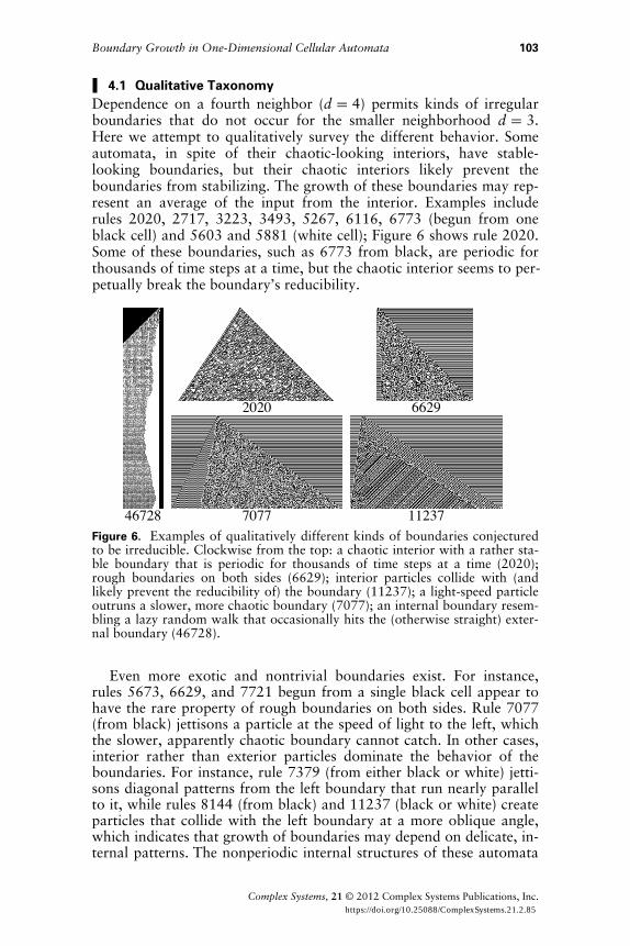
4.1 Qualitative TaxonomyDependence on a fourth neighbor (d ! 4) permits kinds of irregularboundaries that do not occur for the smaller neighborhood d ! 3.Here we attempt to qualitatively survey the different behavior. Someautomata, in spite of their chaotic-looking interiors, have stable-looking boundaries, but their chaotic interiors likely prevent theboundaries from stabilizing. The growth of these boundaries may rep-resent an average of the input from the interior. Examples includerules 2020, 2717, 3223, 3493, 5267, 6116, 6773 (begun from oneblack cell) and 5603 and 5881 (white cell); Figure 6 shows rule 2020.Some of these boundaries, such as 6773 from black, are periodic forthousands of time steps at a time, but the chaotic interior seems to per-petually break the boundary’s reducibility.

46728

2020 6629

7077 11237Figure 6. Examples of qualitatively different kinds of boundaries conjecturedto be irreducible. Clockwise from the top: a chaotic interior with a rather sta-ble boundary that is periodic for thousands of time steps at a time (2020);rough boundaries on both sides (6629); interior particles collide with (andlikely prevent the reducibility of) the boundary (11237); a light-speed particleoutruns a slower, more chaotic boundary (7077); an internal boundary resem-bling a lazy random walk that occasionally hits the (otherwise straight) exter-nal boundary (46728).

Even more exotic and nontrivial boundaries exist. For instance,rules 5673, 6629, and 7721 begun from a single black cell appear tohave the rare property of rough boundaries on both sides. Rule 7077(from black) jettisons a particle at the speed of light to the left, whichthe slower, apparently chaotic boundary cannot catch. In other cases,interior rather than exterior particles dominate the behavior of theboundaries. For instance, rule 7379 (from either black or white) jetti-sons diagonal patterns from the left boundary that run nearly parallelto it, while rules 8144 (from black) and 11237 (black or white) createparticles that collide with the left boundary at a more oblique angle,which indicates that growth of boundaries may depend on delicate, in-ternal patterns. The nonperiodic internal structures of these automata



come remarkably close to the left boundaries; the internal structuresseem to persist, causing the boundaries to be nonperiodic.

Most of these boundaries grow with significant average velocitynear the speed of light (d - 1 cells per time step). Others grow asslowly as 0.02 cells per time step (see Section 4.3). For instance, rule46728 from white (shown in Figure 6) has an internal boundary re-sembling a lazy random walk that occasionally collides with the(otherwise straight) external boundary. To quantify descriptions likethese, we next study the 688 unpredictable boundaries by treatingthem like Brownian motion.

4.2 Random Walk StatisticsTo draw an analogy between unpredictable boundaries and randomwalks, we note that the average growth "HtL ê t and variance of the dif-ference sequence "Ht + 1L - "HtL of boundaries of cellular automata areanalogs of the drift and diffusivity of the Brownian motion of molecu-lar motors [13]. In light of this parallel, we define the drift U to be theaverage growth rate

U ! limtØ¶

"HtLt

and the diffusivity D to be the variance of the difference sequence

D ! limtØ¶

VarH"H1L - "H0L, "H2L - "H1L, … , "Ht + 1L - "HtLL.Continuing the analogy with molecular motors, we define a Peclétnumber for boundaries of automata to be the ratio of the drift anddiffusivity,

Pe !†U§D

.

The Peclét number Pe measures the coherence of the boundary [13]: alarge Pe indicates nearly deterministic movement in a clear direction,whereas a small Pe indicates a meandering, noisy trajectory. Its in-verse r ! 1 ê Pe is the randomness of the boundary [13].

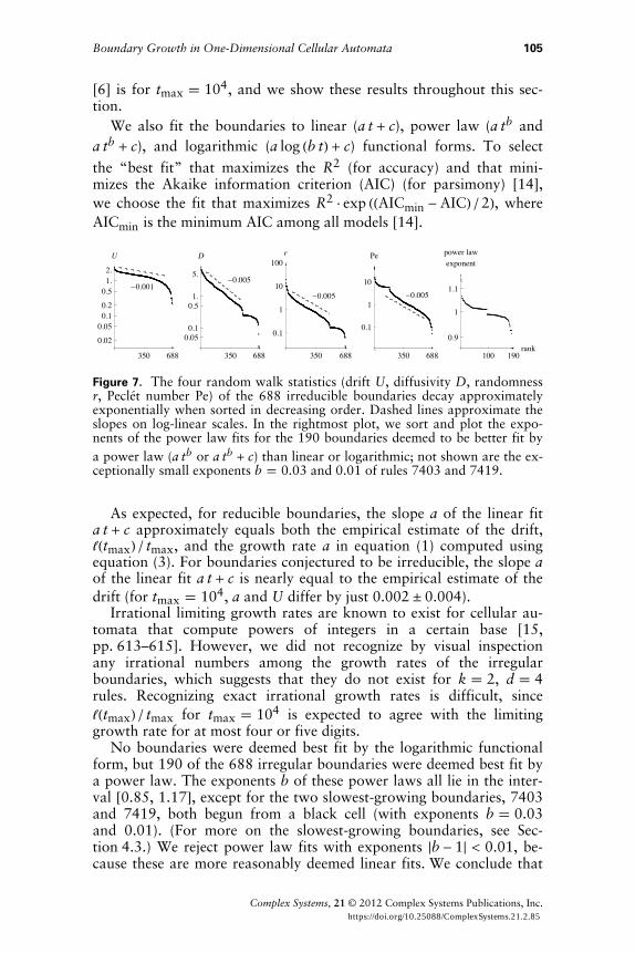
In Figure 7, we plot the distributions of the four random walkstatistics (U, D, r, Pe) of the 688 irreducible boundaries. Sorting andplotting these on log-linear scales shows that U, D, r, Pe decay ap-proximately exponentially over two orders of magnitude among the688 irregular boundaries. This observation, and others in this section,are robust to changes in the number of time stepstmax œ 8500, 1500, 5000, 10000< of evaluating the automata. (Thevalues of U, D for almost every automaton change little from calcula-tions up to time tmax ! 5000 to calculations up to timetmax ! 10000—e.g., 2 ê 3 of the diffusivities change by < 0.01, while90% change by < 0.05.) The data stored in CellularAutomatonData



[6] is for tmax ! 104, and we show these results throughout this sec-tion.

We also fit the boundaries to linear (a t + c), power law (a tb anda tb + c), and logarithmic (a log Hb tL + c) functional forms. To selectthe “best fit” that maximizes the R2 (for accuracy) and that mini-mizes the Akaike information criterion (AIC) (for parsimony) [14],we choose the fit that maximizes R2 ÿ exp HHAICmin - AICL ê 2L, whereAICmin is the minimum AIC among all models [14].

Figure 7. The four random walk statistics (drift U, diffusivity D, randomnessr, Peclét number Pe) of the 688 irreducible boundaries decay approximatelyexponentially when sorted in decreasing order. Dashed lines approximate theslopes on log-linear scales. In the rightmost plot, we sort and plot the expo-nents of the power law fits for the 190 boundaries deemed to be better fit bya power law (a tb or a tb + c) than linear or logarithmic; not shown are the ex-ceptionally small exponents b ! 0.03 and 0.01 of rules 7403 and 7419.

As expected, for reducible boundaries, the slope a of the linear fita t + c approximately equals both the empirical estimate of the drift,"HtmaxL ê tmax, and the growth rate a in equation (1) computed usingequation (3). For boundaries conjectured to be irreducible, the slope aof the linear fit a t + c is nearly equal to the empirical estimate of thedrift (for tmax ! 104, a and U differ by just 0.002 ! 0.004).

Irrational limiting growth rates are known to exist for cellular au-tomata that compute powers of integers in a certain base [15,pp.!613–615]. However, we did not recognize by visual inspectionany irrational numbers among the growth rates of the irregularboundaries, which suggests that they do not exist for k ! 2, d ! 4rules. Recognizing exact irrational growth rates is difficult, since"HtmaxL ê tmax for tmax ! 104 is expected to agree with the limitinggrowth rate for at most four or five digits.

No boundaries were deemed best fit by the logarithmic functionalform, but 190 of the 688 irregular boundaries were deemed best fit bya power law. The exponents b of these power laws all lie in the inter-val @0.85, 1.17D, except for the two slowest-growing boundaries, 7403and 7419, both begun from a black cell (with exponents b ! 0.03and 0.01). (For more on the slowest-growing boundaries, see Sec-tion!4.3.) We reject power law fits with exponents †b - 1§ < 0.01, be-cause these are more reasonably deemed linear fits. We conclude that



!

nearly all the boundaries that grow as power laws have exponentsnear 1. Exponents above 1 occur when the parameter a < 1, whichcannot be accurate for sufficiently large t because "HtL § 3 t + 1 for alld ! 4 automata begun from a single-cell initial condition. Neither ad-justing tmax nor dropping tens or hundreds of the first boundarylengths (to allow for a transient) eliminates the power law exponentslarger than 1. This illustrates the difficulties of fitting irregular bound-aries to functional forms using standard nonlinear fitting algorithms.

The drift U and diffusivity D characterize what kinds of randomwalks these irregular boundaries behave like. Notably, one quarter ofthe 688 automata have diffusivity 0.15 < D < 0.25, which creates a“knee” in Figure 7. For comparison, a simple random walk with steps1, -1 occurring with probability p, 1 - p has variance 0.25 for p !I2 - 3 M ë 4 º 0.067. Such a random walk moves rather coherentlyin a certain direction, reflected by its large Peclét number Pe !2 3 º 3.5 that is also common among the irregular boundaries.

Turning our attention to the drift U and diffusivity D of all 688 ir-regular boundaries, we find a gap in the scatter plot of D and U inFigure 8. This gap suggests the existence of a threshold: irreducibleboundaries of automata either grow quickly and erratically (largeU, D; upper-right region of Figure 8) or more slowly and deterministi-cally (small U, D; lower-left region of Figure 8). This scatter plot andits gap do not change qualitatively for different numbers of time stepstmax.

0.5 1.0 1.5 2.0U

2

4

6

8

D

Figure 8. An unexpected gap in the relationship between diffusivity D anddrift U (computed for 104 steps) suggests a threshold exists in the behavior ofirreducible boundaries of cellular automata: they either grow erratically andquickly or more deterministically and slowly.

4.3 Slow Growth Fast boundary growth is common: the mean growth rate among theboundaries conjectured to be irreducible is large, XU\ º 1.27. Slowgrowth, by contrast, is delicate and rare (see the sparse region



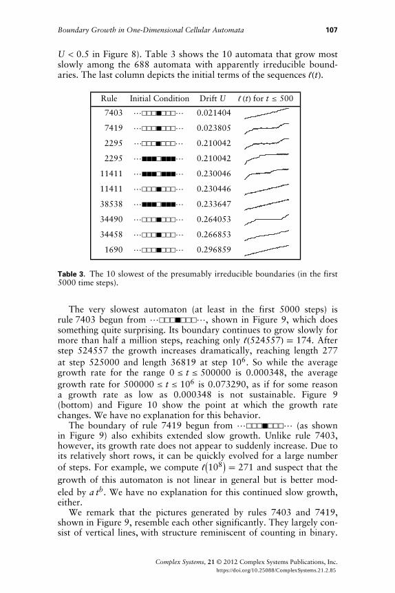
U < 0.5 in Figure 8). Table 3 shows the 10 automata that grow mostslowly among the 688 automata with apparently irreducible bound-aries. The last column depicts the initial terms of the sequences "HtL.

Rule Initial Condition Drift U " HtL for t § 500

7403 !···‡···! 0.021404

7419 !···‡···! 0.023805

2295 !···‡···! 0.210042

2295 !‡‡‡·‡‡‡! 0.210042

11411 !‡‡‡·‡‡‡! 0.230046

11411 !···‡···! 0.230446

38538 !‡‡‡·‡‡‡! 0.233647

34490 !···‡···! 0.264053

34458 !···‡···! 0.266853

1690 !···‡···! 0.296859

Table 3. The 10 slowest of the presumably irreducible boundaries (in the first5000 time steps).

The very slowest automaton (at least in the first 5000 steps) isrule!7403 begun from !···‡···!, shown in Figure 9, which doessomething quite surprising. Its boundary continues to grow slowly formore than half a million steps, reaching only "H524557L ! 174. Afterstep 524557 the growth increases dramatically, reaching length 277at step 525000 and length 36819 at step 106. So while the averagegrowth rate for the range 0 § t § 500000 is 0.000348, the averagegrowth rate for 500000 § t § 106 is 0.073290, as if for some reasona growth rate as low as 0.000348 is not sustainable. Figure 9(bottom) and Figure 10 show the point at which the growth ratechanges. We have no explanation for this behavior.

The boundary of rule 7419 begun from !···‡···! (as shownin Figure 9) also exhibits extended slow growth. Unlike rule 7403,however, its growth rate does not appear to suddenly increase. Due toits relatively short rows, it can be quickly evolved for a large numberof steps. For example, we compute "I108M ! 271 and suspect that thegrowth of this automaton is not linear in general but is better mod-eled by a tb. We have no explanation for this continued slow growth,either.

We remark that the pictures generated by rules 7403 and 7419,shown in Figure 9, resemble each other significantly. They largely con-sist of vertical lines, with structure reminiscent of counting in binary.



Further work should be undertaken to understand these rules and todetermine the extent to which they are reducible.

Figure 9. Top: rules 7403 and 7419 begun from !···‡···!, the slowest-growing k ! 2, d ! 4 automata with single-cell initial conditions. Bottom:the first 6ä105 steps of rule 7403, sampled every 128 steps, illustrate the ex-plosion of boundary growth at step 524557.



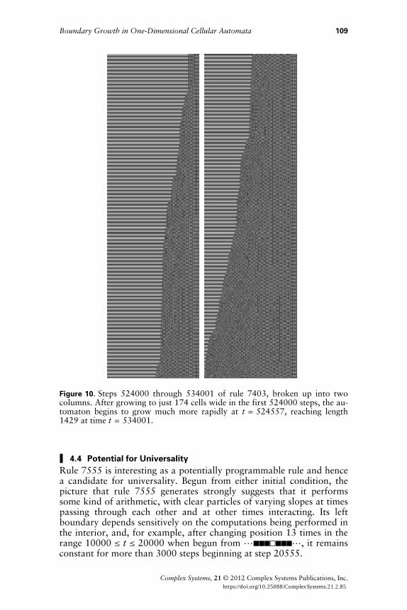
Figure 10. Steps 524000 through 534001 of rule 7403, broken up into twocolumns. After growing to just 174 cells wide in the first 524000 steps, the au-tomaton begins to grow much more rapidly at t = 524557, reaching length1429 at time t = 534001.

4.4 Potential for UniversalityRule 7555 is interesting as a potentially programmable rule and hencea candidate for universality. Begun from either initial condition, thepicture that rule 7555 generates strongly suggests that it performssome kind of arithmetic, with clear particles of varying slopes at timespassing through each other and at other times interacting. Its leftboundary depends sensitively on the computations being performed inthe interior, and, for example, after changing position 13 times in therange 10000 § t § 20000 when begun from !‡‡‡·‡‡‡!, it remainsconstant for more than 3000 steps beginning at step 20555.



5. An Automaton with No Growth Exponent

In this section, we show that it is not possible in general to assign agrowth function tb to a cellular automaton. In particular, we con-struct an automaton such that the limiting growth exponent

limtØ¶

logt "HtLdoes not exist.

The idea is to take rule 106 begun from !···‡‡···! (shown inFigure 2), which grows like t , and to graft onto it an automatonthat roughly squares the length of a row. We set up the squaring ruleto be activated at certain steps, causing the sequence "HtL to grow to beon the order of t, and then we allow it to fall back to the boundary ofrule 106 on the order of t before being activated again. As a result,the sequence "HtL oscillates between square-root growth and lineargrowth and satisfies

lim inftØ¶

logt "HtL !1

2, lim sup

tØ¶logt "HtL ! 1.

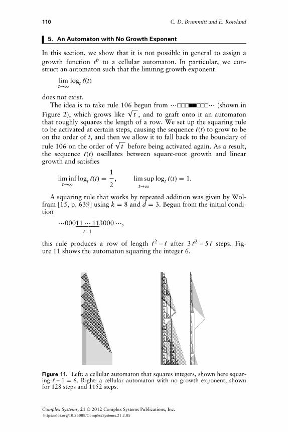
A squaring rule that works by repeated addition was given by Wol-fram [15, p. 639] using k ! 8 and d ! 3. Begun from the initial condi-tion

!00011! 11!-1

3000!,

this rule produces a row of length "2 - " after 3 "2 - 5 " steps. Fig-ure!11 shows the automaton squaring the integer 6.

Figure 11. Left: a cellular automaton that squares integers, shown here squar-ing " - 1 ! 6. Right: a cellular automaton with no growth exponent, shownfor 128 steps and 1152 steps.



A k1-color rule and a k2-color rule can be combined into a singleHk1 k2L-color rule that can be thought of as their direct product andthat can run the two rules in parallel. Since of course we do not wantthe two rules to run completely independently, we modify the compos-ite rule so that there is some interaction. In particular, modificationsto the squaring automaton, including the addition of one color, in-hibit future squarings until the current squaring is finished and the au-tomaton has shrunk to the width of rule 106. Hence our compositerule uses 2ä9 ! 18 colors. The broad outline is as follows.

Step 3 in rule 106 consists of four black cells. We choose the initialcondition so that the squaring automaton is first activated on step 4.Since the squaring needs to be activated locally, we modify the squar-ing automaton so that it squares a row using only information fromits two endpoints rather than from the entire interval of cells. The rele-vant interval for squaring on step 4 has length " ! 5, so the squaringautomaton takes 3 "2 - 5 " ! 50 steps to square. From the time thesquaring begins until it finishes, the squaring automaton runs indepen-dently of rule 106.

After the squaring completes at step 54, we must clear the cellsused by the squaring automaton. To do this, we add a new color tomark the leftmost nonempty column. When the last addition is com-plete, we send out a particle from this column that travels to the rightand clears the cells involved in squaring.

When the clearing particle reaches the rightmost remnant of thesquaring automaton, we trigger a particle traveling back to the left tosignify that the next squaring can begin. When this particle first en-counters a structure from rule 106, it stops propagating to the leftand remains in that column to trigger the next squaring when rule106 next has two adjacent black cells at the right endpoint, and theprocess begins again.

The result is a rule with k ! 18 and d ! 4, begun from the initialcondition !0002899003000!. Figure 11 shows two images of thisautomaton. The complete rule instructions are available in CellularAu-tomatonData [6]. Even though both rule 106 and the squaring au-tomaton are functions of three cells, it is necessary to shear one of therules relative to the other to bring their structures into alignment,hence d ! 4.

We now verify by induction that triggering the initial squaring onstep 3 enables easy determination of when all future squarings will oc-cur. (For other initial triggering steps, this is not the case.) We claimthat squarings are triggered precisely on steps 24 a+2 - 1 for a ¥ 0.

For a ! 0, the squaring at step 3 is guaranteed by our choice of ini-tial condition.

Inductively, assume that a squaring is triggered on step 24 a+2 - 1for a fixed a. On step 24 a+2 - 1, rule 106 has a solid black row oflength 3 ÿ 22 a + 1. The squaring rule begins squaring 3 ÿ 22 a + 2 on



the following step and reaches maximum length 9 ÿ 24 a + 9 ÿ 22 a + 5on step 31 ÿ 24 a + 21 ÿ 22 a + 2. The length is maximal for three steps,and then the length shrinks one cell per step until the particle reachesthe boundary of rule 106; this occurs at step 5 ÿ 24 a+3 + 9 ÿ 22 a+1 + 3,because the length of rule 106 is 3 ÿ 22 Ha+1L + 1 for all24 a+5 § t § 24 a+6 - 1, and it is checked that

24 a+5 < 5 ÿ 24 a+3 + 9 ÿ 22 a+1 + 3 < 24 a+6 - 2.

For 24 a+5 § t § 24 a+6 - 2, the right endpoint of rule 106 is a singleblack cell, and the next occurrence of two adjacent black cells is onstep 24 Ha+1L+2 - 1.

It follows that the subsequence of the steps where squarings beginhas limiting exponent

limaØ¶

log I3 ÿ 22 a + 1Mlog I24 a+2 - 1M !

1

2,

and the subsequence of the steps where squarings end has limitingexponent

limaØ¶

log I9 ÿ 24 a + 9 ÿ 22 a + 5Mlog I31 ÿ 24 a + 21 ÿ 22 a + 2M ! 1.

6. Conclusions and Open Questions

In this paper, we have inventoried the boundaries of all cellular au-tomaton rules using k ! 2 colors and depending on d ! 4 cells whenbegun from a single cell on a constant background. Within this rulespace we have encountered several kinds of behavior not seen insmaller spaces. In particular, we find fractal boundaries described bymorphic words. By studying the unpredictable boundaries as if theywere random walks, we find approximately exponential distributionsof the mean and variance of the boundaries’ growth and a possibleseparation into two classes of automata: those that grow quickly anderratically and others that grow slowly and more deterministically.

For simplicity, we have restricted our attention in many ways. Wehave only considered the two initial conditions !···‡···! and!‡‡‡·‡‡‡!. A more general study of k ! 2, d ! 4 rules will con-sider other initial conditions and attempt to determine to what extenteach rule has a representative growth rate. More generally still, initialconditions with backgrounds that are not constant but are periodiccan be considered because there still exists a natural notion of thelength of a row. Finally, the rule space we studied is big, but it is nothuge, and performing similar analyses on larger spaces of cellular au-



tomata can be imagined. We hope that researchers in fact do all ofthese things, and we have designed the function CellularAutomatonÖData to scale to these more general settings.

Another topic to be addressed is the issue of distinct automata thatnevertheless generate the same evolution (or an evolution equivalentunder reflection or permutation of colors) because certain local config-urations of cells do not appear. For example, rules 34394 and 39780can generate identical evolutions, as mentioned in Section 3.3. At thebeginning of Section 4, we encountered this phenomenon again.(Although we did not mention it earlier, among the 688 distinct evolu-tions generated by the 720 irreducible automata, there appear to beonly 658 distinct boundary words.) The prevalence of equivalent evo-lutions generated by inequivalent rules suggests that more complexinitial conditions should be used to distinguish such rules. One possi-ble criterion for a representative initial condition for a given rule isthat all kd local configurations that can (for some initial condition) oc-cur infinitely often in an evolution do occur infinitely often.

This paper concerns external boundaries, which are simply specialcases of general boundaries between distinct regions of a cellular au-tomaton’s evolution. The advantage of studying external boundariesis the ease of defining and therefore programmatically detecting them.However, internal boundaries (or particles) are common in automata,and several information-theoretic measures have been used to detectthem [16–19] and their collisions [20]. We expect that our automatedand manual methods could inform a study of general boundaries.Conversely, information-theoretic tools for internal boundaries maybe applied to external boundaries to systematically measure, for in-stance, how much they store and process information [21, 22].

In most cases, the cellular automaton data we computed is empiri-cal and has not been formally proved to be correct. (We welcome anycorrections.) Of course, ideally, we would like to have proofs. Theautomata with morphic boundary words that are not eventually peri-odic are few enough, at least in the space k ! 2, d ! 4, that it is rea-sonable to attempt to prove manually that each boundary word isdescribed by the morphism claimed. On the other hand, for the24287 automata with eventually periodic boundary words, obtainingproofs by hand is not reasonable, and automated techniques must bedeveloped for examining a rule and initial condition to determine(rigorously) the growth rate and the eventual period length. Ofcourse, the question of whether the boundary word is eventually peri-odic is likely undecidable in general. However, a symbolic approachcapable of proving a large number of growth rates would be of greatinterest.

From the results in this paper, several natural questions arise re-garding the growth of cellular automata.

† Which morphic words occur as the boundary word of a cellular automa-ton?



† For what real numbers 0 § b § 1 is there a cellular automaton with lim-iting growth exponent b ! limtØ¶ logt "HtL? Schaeffer [23] has recentlyconstructed cellular automata with row lengths that grow like t1êm for

any integer m ¥ 3, and tlog2 f where f ! J1 + 5 N í 2.

† Schaeffer [23] has also constructed an automaton with

"HtL ! OJ t log tN. What can be said in general about possible and im-

possible growth functions?

† How does the growth of an automaton depend on k and d? For exam-ple, what is the smallest nonzero rational growth rate that occurs forgiven k and d?

These and other questions indicate the breadth of mathematics and ex-perimentation to be done on the boundaries of cellular automata.

Acknowledgments

We thank Hector Zenil for contributions at the NKS Summer School2009 and Janko Gravner for useful discussion. The first author wassupported by the Defense Threat Reduction Agency, Basic ResearchAward HDTRA1-10-1-0088, and by the Department of Defense(DoD) through the National Defense Science and Engineering Gradu-ate Fellowship (NDSEG) program. The second author was supportedin part by National Science Foundation (NSF) grant DMS-0239996.

References

[1] J. von Neumann, “The General and Logical Theory of Automata,” inCerebral Mechanisms in Behavior: The Hixon Symposium (L. A. Jef-fress, ed.), New York: John Wiley & Sons, 1951.

[2] S. Wolfram, “Statistical Mechanics of Cellular Automata,” Reviews ofModern Physics, 55(3), 1983 pp. 601–644.doi:10.1103/RevModPhys.55.601.

[3] S. Wolfram, “Universality and Complexity in Cellular Automata,” Phys-ica D: Nonlinear Phenomena, 10(1–2), 1984 pp. 1–35.doi:10.1016/0167-2789(84)90245-8.

[4] R. Phillips, “Growth of the Boundaries of Simple Cellular Automata,”presentation given at NKS Summer School 2004, Boston.http://www.wolframscience.com/conference/2004/presentations/material/rphillips-growth.nb.

[5] S. Wolfram. “CA Growth Rates: A Live Experiment.” (Mar 29, 2005)http://www.stephenwolfram.com/publications/recent/cagrowthrates.

[6] C. D. Brummitt and E. Rowland. CellularAutomatonData, a Mathe-matica package. http://thales.math.uqam.ca/~rowland/packages.html#CellularAutomatonData.



http://www.wolframscience.com/conference/2004/presentations/material/rphillips-growth.nb

http://www.wolframscience.com/conference/2004/presentations/material/rphillips-growth.nb

http://thales.math.uqam.ca/~rowland/packages.html#CellularAutomatonData

http://thales.math.uqam.ca/~rowland/packages.html#CellularAutomatonData

http://www.stephenwolfram.com/publications/recent/cagrowthrates

[7] C. D. Brummitt and E. Rowland, CellularAutomatonBoundaries, aMathematica package. http://thales.math.uqam.ca/~rowland/packages.html#CellularAutomatonBoundaries.

[8] J.-P. Allouche and J. Shallit, Automatic Sequences: Theory, Applica-tions, Generalizations, Cambridge: Cambridge University Press, 2003.

[9] J. Gravner and D. Griffeath, “Robust Periodic Solutions and Evolutionfrom Seeds in One-Dimensional Edge Cellular Automata,” forthcoming.http://www.math.ucdavis.edu/~gravner/edge.

[10] E. Rowland, “Local Nested Structure in Rule 30,” Complex Systems,16(3), 2006 pp. 239–258.http://www.complex-systems.com/pdf/16-3-4.pdf.

[11] J.-P. Allouche and J. Shallit, “The Ring of k-Regular Sequences,” Theo-retical Computer Science, 98(2), 1992 pp. 163–197.doi:10.1016/0304-3975(92)90001-V.

[12] J.-P. Allouche and J. Shallit, “The Ring of k-Regular Sequences, II,” The-oretical Computer Science, 307(1), 2003 pp. 3–29.doi:10.1016/S0304-3975(03)00090-2.

[13] P. R. Kramer, J. C. Latorre, and A. A. Khan, “Two Coarse-GrainingStudies of Stochastic Models in Molecular Biology,” Communications inMathematical Sciences, 8(2), 2010 pp. 481–517.http://www.intlpress.com/CMS/p/2010/issue8-2/CMS-8-2-A9.pdf.

[14] K. P. Burnham and D. R. Anderson, Model Selection and Multimodel In-ference: A Practical Information-Theoretic Approach, 2nd ed., NewYork: Springer, 2002.

[15] S. Wolfram, A New Kind of Science, Champaign, IL: Wolfram Media,Inc., 2002.

[16] A. Wuensche, “Classifying Cellular Automata Automatically: FindingGliders, Filtering, and Relating Space-Time Patterns, Attractor Basins,and the Z Parameter,” Complexity, 4(3), 1999 pp. 47–66.doi:10.1002/(SICI)1099-0526(199901/02)4:3<47::AID-CPLX9>3.0.CO;2-V.

[17] J. T. Lizier, M. Prokopenko, and A. Y. Zomaya, “Local InformationTransfer as a Spatiotemporal Filter for Complex Systems,” Physical Re-view E, 77(2), 2008 p. 026110. doi:10.1103/PhysRevE.77.026110.

[18] T. Helvik, K. Lindgren, and M. G. Nordahl, “Local Information in One-Dimensional Cellular Automata,” in Cellular Automata: Proceedings ofthe 6th International Conference on Cellular Automata for Researchand Industry (ACRI04), Amsterdam, The Netherlands (P. M. A. Sloot,B. Chopard, and A. G. Hoekstra, eds.), Berlin: Springer, 2004pp. 121–130. doi:10.1007/978-3-540-30479-1_13.

[19] C. R. Shalizi, R. Haslinger, J.-B. Rouquier, K. L. Klinkner, andC. Moore, “Automatic Filters for the Detection of Coherent Structure inSpatiotemporal Systems,” Physical Review E, 73(3), 2006 p. 036104.doi:10.1103/PhysRevE.73.036104.

[20] J. T. Lizier, M. Prokopenko, and A. Y. Zomaya, “Information Modifica-tion and Particle Collisions in Distributed Computation,” Chaos, 20,2010 p. 037109. doi:10.1063/1.3486801.

[21] J. E. Hanson and J. P. Crutchfield, “Computational Mechanics of Cellu-lar Automata: An Example,” Physica D: Nonlinear Phenomena, 103(1–4), 1997 pp. 169–189. doi:10.1016/S0167-2789(96)00259-X.



http://thales.math.uqam.ca/~rowland/packages.html#CellularAutomatonBoundaries

http://thales.math.uqam.ca/~rowland/packages.html#CellularAutomatonBoundaries

http://www.math.ucdavis.edu/~gravner/edge

http://www.complex-systems.com/pdf/16-3-4.pdf

http://www.intlpress.com/CMS/p/2010/issue8-2/CMS-8-2-A9.pdf

[22] W. Hordijk, C. R. Shalizi, and J. P. Crutchfield, “Upper Bound on theProducts of Particle Interactions in Cellular Automata,” Physica D: Non-linear Phenomena, 154(3–4), 2001 pp. 240–258.doi:10.1016/S0167-2789(01)00252-4.

[23] L. Schaeffer. “Gallery of Cellular Automata.” (Jun 20, 2012)http://www.student.cs.uwaterloo.ca/~l3schaef/CA.



http://www.student.cs.uwaterloo.ca/~l3schaef/CA

Boundary Growth in One-Dimensional Cellular Automata

Documents