Boundary estimation and patrolling algorithmscarmenere.ucsd.edu/pdfs/CDC08workshop-DCRN-BulloCortesMartinez-lecture5.pdfLecture #5: Boundary estimation and patrolling algorithm Francesco

Lecture #5:Boundary estimation and patrolling algorithm

Francesco Bullo1 Jorge Cortes2 Sonia Martınez2

1Department of Mechanical EngineeringUniversity of California, Santa [email protected]

2Mechanical and Aerospace EngineeringUniversity of California, San Diego{cortes,soniamd}@ucsd.edu

Workshop on “Distributed Control of Robotic Networks”IEEE Conference on Decision and Control

Cancun, December 8, 2008

Acknowledgements: Sara Susca, Honeywell

Summary Introduction

Motion coordination objective: boundary estimation & sensing

Boundary approximation through polygonal approximations

Distributed approach based on linear iterations

Model for “event-driven” robotic networks

Proof of correctness

2 / 50

Boundary estimation and patrolling algorithms

Objective: Detection/estimation of an evolving 2D boundary

Motivation:

Demarcation of hazardous environmentsValidation of oceanographic/atmospheric models

Delimit areas with abrupt changes of temperatureEstablish the front of a highly-pollutant expanding substance

Challenges:

How to devise a decentralized scheme (no fusion center)Sudden events require event-driven coordination algorithms

3 / 50

Outline

1 Intro to boundary estimation

2 Event-driven control and communication laws

3 Interpolations of planar boundaries by inscribed polygons

4 Network model and boundary estimation taskSingle-robot estimate update lawCooperative estimate update lawCyclic balancing algorithm for agent equidistance law

5 Simulations

6 Proof of correctness

7 Summary

4 / 50

Event-driven robotic networks

An event-driven control and communication law ECCis defined for a robotic network S = (I,R, Ecmm)

Recall that S = (I,R, Ecmm) has physical componentsI = {1, . . . , n}, the set of UIDs for the robotsR = {R[i]} = {(X, U,X0, f)}, group of mobile robotsEcmm communication edge map

Here, x 7→ (I, Ecmm) topology of communication graph,that is, a proximity graph; e.g. a geometric graph

5 / 50

Event-driven control and communication law

1 communication alphabet A including the null message

2 processor state space W [i], with initial allowable W[i]0

3 message-trigger function msg-trig[i]: X [i]×W [i]→{true, false}4 message-gen function msg-gen[i] : X [i] ×W [i] × I → A5 message-recept function msg-rec[i]:X [i]×W [i]× A× I→W [i]

6 state-trans trigger functs stf-trig[i]k :X [i]×W [i]→{true, false}

7 state-trans functions stf[i]k : X [i] ×W [i] → W [i]

8 control function ctl : X [i] ×W [i] → U [i]

6 / 50


Note the differences betweenan event-driven and a synchronous CCL:

1 No common time schedulefor robots to send/receive msgs or update their states

2 The function msg-gen is replaced bythe tripplet (msg-trig,msg-rec,msg-gen)

3 The function stf is replaced by the pairs (stf-trigk, stfk)

4 The control function depends only upon current robot position

7 / 50


Executions: Only when an event happens,an agent sends/receives a message or updates its state.

The trigger functs check these constraints acting as guard maps

Move - Update physical state

Event

state-tran

triggerprocessor state updtmsg-trig msg-gen

8 / 50

Event-driven robotic networks – formal execution

Evolution of (S, ECC)

with dwell time δ ∈ R≥0 and x[i]0 ∈ X

[i]0 , w

[i]0 ∈ W

[i]0 , i ∈ I,

are x[i] : R≥0 → X [i], and w[i] : R≥0 → W [i], i ∈ I, such that

x[i](t) = f(x[i](t), ctl[i]

(x[i](t), w[i](t)

)),

w[i](t) = 0,

with x[i](0) = x[i]0 and w[i](0) = w

[i]0 , i ∈ I, and such that

I. for i ∈ I and t1 ∈ R>0, msg generated by i, received by j are

y[j]i (t1) = msg-gen[i]

(x[i](t1), w

[i](t1), j),

w[j](t1) = msg-rec[j](x[j](t1), lim

t→t−1

w[j](t), y[j]i (t1), i

),

if msg-trig[i](x[i](t1), w[i](t1)) = true and agent i has not

transmitted any message during the time interval ]t1 − δ, t1[∩R>0.

9 / 50

Event-driven robotic networks – formal execution

II. for every i ∈ I, k ∈ {1, . . . ,K[i]stf} and t2 ∈ R>0 the state-transition

function stf[i]k is executed, that is,

w[i](t2) = stf[i]k

(x[i](t2), lim

t→t−2

w[i](t)),

if stf-trig[i]k (x[i](t2), w

[i](t2)) = true and there has been noexecution of stf[i]k during the time interval ]t2 − δ, t2[∩R>0.

10 / 50

Outline





5 Simulations


7 Summary

11 / 50

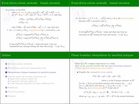
Planar boundary interpolation by inscribed polygons

Given Q ⊆ R2 a simply connected set or a body,How can we concisely describe ∂Q? use approximating polygonsCritical inscribed polygons for convex bodies

Consider the symmetric error metric

δS(C,B) = µ(C ∪B)− µ(C ∩B),

where µ is the Lebesgue measure on R2

Let Qm ⊆ Q be an inscribed polygon with vertices {q1, . . . , qm}Let sj ∈ [0, 2π] be such that qj = γ(sj), for j ∈ {1, . . . ,m}Then, Qm is a critical point of δS if and only if

ι(γ′(sj))× ι(qj+1 − qj−1) = 03, for all j ∈ {1, . . . ,m},

where q0 = qm, qm+1 = q1 and ι : R2 → R3 is the natural inclusion

12 / 50


An illustrative example

Consider the convex body

Then, critical inscribed polygons are:

But the last critical polygon is a saddle

13 / 50


Asymptotic formula of McClure and VitaleLet ρ be curvature radius and κabs curvature of the boundarySuppose that ∂Q is of class C2 with κabs > 0. Then

limm→+∞

m2δS(Q,Q∗m) =

1

12

(∫ 2π

0

ρ(θ)2/3dθ

)Method of empirical distributions

γarc(%) arc-length parametrization of ∂Qγpolar(θ), polar variable parameterization, of ∂Q

Let q1, . . . , qm such that qi = γarc(%i) and qi = γ(θi), fori ∈ {1, . . . ,m}. Then, take the qi so that

∫ θi+1

θi

ρ(θ)2/3dθ ≈∫ θi

θi−1

ρ(θ)2/3dθ

14 / 50


Adaptation to non-convex boundaries as follows:Let qi = γarc(%i) and qj = γarc(%j), with %i < %j , then

Dcurvature(qi, qj) =

∫ %j

%i

κabs(γarc(%))1/3d%,

L(qi, qj) = %j − %i.

are positive only when ∂Q is transversed counterclockwise from qi to qj

For λ ∈ [0, 1], define the pseudo-distance Dλ between qi and qj as

Dλ(qi, qi+1) = λDcurvature(qi, qj) + (1− λ)L(qi, qi+1).

Interpretation:λ ≈ 1 =⇒ method of empirical distributionsλ ≈ 0 =⇒ equal division of boundaryλ ∈ (0, 1) =⇒ midway approximation

15 / 50

Outline





5 Simulations


7 Summary

16 / 50

Network model

From now on, Q is a body with differentiable boundary ∂Q

Robotic Network:Sbndry = (I,R, Ecmm), with I = {1, . . . , n}, where

(∂Q, [−vmin, vmax], ∂Q, (0, e)),

e vector field tangent to ∂Q (counterclockwise motion)Ecmm is the ring graph or the Delaunay graph on ∂Q

Assume also thatunit speed is admissible; i.e. 1 ∈ [−vmin, vmax]

Each robot can sense its own location p[i] ∈ ∂Q, i ∈ I

17 / 50

Boundary estimation tasks

Overall nip interpolation points are used to approximate ∂QThus, a robot’s processor state component is q[i] ∈ (R2)nip , for i ∈ I

Boundary estimation taskTε-bndry : (∂Q)n × ((R2)nip)n → {true, false} for Sbndry is

Tε-bndry(p[1], . . . , p[n], q[1], . . . , q[n]) = true if and only if∣∣∣Dλ(q

[i]α−1, q

[i]α )−Dλ(q[i]

α , q[i]α+1))

∣∣∣ < ε, α ∈ {1, . . . , nip} and i ∈ I.

Agent equidistance task Tε-eqdstnc : (∂Q)n → {true, false} is true∣∣L(p[i−1], p[i])− L(p[i], p[i+1])∣∣ < ε, for all i ∈ I,

where L is the counterclockwise arc-length distance along ∂Q.

18 / 50

Outline





5 Simulations


7 Summary

19 / 50

Estimate update and cyclic balancing law

We will present this event-driven law incrementally

Single robot estimate update lawCooperative estimate update lawCyclic balancing algorithm for agent equidistance task

Single robot estimate update law

Describes the single-robot operation “projection-and-update”

20 / 50


Processor state of robot i ∈ I

1 a counter nxt ∈ {1, . . . , nip}index of interpolation point the agent projects next;

2 a boundary representation

{(qα, vα) ∈ (R2)2 | α ∈ {1, . . . , nip}},

here qα is the position of the α int. pointand vα is the tangent vector of ∂Q at qα

3 a curve path : [0, t] → R2

followed by the agent until present time t

21 / 50


Rules for processor update – Informal description

Rule #1 When and how to project qnxt onto ∂Q

Let qnxt be the point to be projected and vnxt its tangent

The projection takes place when the agent crosses the line, denoted by

linenxt, that passes through qnxt and is perpendicular to vnxt. At this

crossing time q+nxt ∈ path, is the point on path where the agent

trajectory crosses the line linenxt

We write

q+nxt := perp-proj(qnxt, vnxt, path).

22 / 50


Rule #2 When and how to optimize the interpolation point

After the projection of qnxt, qnxt−1 is re-placed to balance its

pseudodistance to neighboring interpolation points. Specifically, define

cyclic-balance : (R2)3 × C(R2) → R2 by

cyclic-balance(qnxt−2, qnxt−1, qnxt, path) = q∗ s.t.

Dλ(qnxt−2, q∗) =

3

4Dλ(qnxt−2, qnxt−1) +

1

4Dλ(qnxt−1, qnxt)

In this way,

q+nxt−1 := cyclic-balance(qnxt−2, qnxt−1, qnxt, path)

23 / 50


The optimal placement q+nxt−1 can be equivalently defined by

Dλ(q+nxt−1, qnxt) =

1

4Dλ(qnxt−2, qnxt−1) +

3

4Dλ(qnxt−1, qnxt),

so that it achieves the balancing property that[Dλ(qnxt−2, q

+nxt−1)

Dλ(q+nxt−1, qnxt)

]=

1

4

[3 11 3

] [Dλ(qnxt−2, qnxt−1)Dλ(qnxt−1, qnxt)

]

Finally, a last useful operation

v := tangentat(path, q).

24 / 50


Formal Single-Robot Estimate Update Law description

Robot: single robot moving at constant speed along ∂Q,continuously recording its trajectory

Event-driven Algorithm: Single-Robot Estimate Update LawProcessor State: w = (nxt, {(qα, vα)}nip

α=1, path), where

nxt ∈ {1, . . . , nip}, initially equal to index of the inter-polation point closest to robot mov-ing counterclockwise

{(qα, vα)}nipα=1 ⊂ R2 × R2, initially counterclockwise along boundary

path ∈ C(R2), continuously recording agent’s trajectory

25 / 50


% A state transition is triggered when the agent crosses a certain linefunction stf-trig(p, w)

1: linenxt := line through point qnxt perpendicular to direction vnxt2: if p ∈ linenxt then3: return true4: else5: return false

%The current interpolation point and tangent vector are projected andthe previous interpolation point is optimized along the new boundaryfunction stf(p, w)

1: {(q+α , v+

α )}nipα=1 := {(qα, vα)}nip

α=1

2: q+nxt := perp-proj(qnxt, vnxt, path)

3: q+nxt−1 := cyclic-balance(qnxt−2, qnxt−1, q

+nxt, path)

4: v+nxt := tangentat(path, q+

nxt)5: v+

nxt−1 := tangentat(path, q+nxt−1)

6: return (nxt + 1, {(q+α , v+

α )}nipα=1, path)

26 / 50

Outline





5 Simulations


7 Summary

27 / 50

Cooperative estimate update law

Informal description

Parallel version of the Single-Robot Estimate Update Law:

each agent updates its boundary representation separatelyevery time an agent updates two interpolation points, this agenttransmits these to its neighborsIn turn, the neighbors record the updates in their individualboundary representation

Agents must satisfy the two-hop separation rule

A group of n ≥ 2 agents istwo-hop separated along the interpolation points

if nxt[i−1] ≤ nxt[i] − 2 for all i ∈ I at all times

28 / 50


Formal description of the cooperative estimate update law

Robotic Network: Sbndry, assume agentswith absolute sensing of own position, communicatingwith clockwise and counterclockwise neighbors

Event-driven Algorithm: Cooperative Estimate Update LawAlphabet: A = {1, . . . , nip} × (R2)2 × (R2)2 ∪{null}Processor State, function stf-trig, and function stf

same as in Single-Robot Estimate Update Law

29 / 50


%A transmission is triggered right after the interpolation points areupdatedfunction msg-trig(p, w)

1: return stf-trig(p, w)

%The updated interpolation points (and reference label) are transmittedfunction msg-gen(p, w, i)

1: return(nxt, (qnxt−1, vnxt−1), (qnxt−2, vnxt−2)

)%The received updated interpolation points are storedfunction msg-rec(p, w, y, i)

1: {(q+α , v+

α )}nipα=1 := {(qα, vα)}nip

α=1

2: (nxtrec, y1, y2) := y3: (q+

nxtrec−1, v+nxtrec−1) := y1

4: (q+nxtrec−2, v

+nxtrec−2) := y2

5: return (nxt, {(q+α , v+

α )}nipα=1, path)

30 / 50

Outline





5 Simulations


7 Summary

31 / 50

Cyclic balancing algorithm for agent equidistance law

Motion control law for each agentSuppose agent i ∈ I is at position p[i] movingin continuous time with speed v[i] along ∂Q. Then,

v[i] = 1 + kprop

(L(p[i], p[i+1])− L(p[i−1], p[i])

),

where kprop ∈ R>0 is a fixed control gain.

To enforce the constraint v ∈ [−vmin, vmax], we introduce

v[i] = sat[vmin,vmax]

(1 + kprop

(L(p[i], p[i+1])− L(p[i−1], p[i])

)),

where

sat[a,b](x) =

a, if x < a,

x, if x ∈ [a, b],

b, if x > b.

32 / 50

Cyclic balancing algorithm for agent equidistance law

Approximation ofthe counterclockwise arc-length distance between robots

Given {q1, . . . , qnip} and r1, r2 ∈ ∂Q, let the indices [r1] and [r2] of thecounterclockwise-closest interpolation points from r1, r2, respectively.

L(r1, r2) = L(r1, q[r1]) +

[r2]−2∑α=[r1]

L(qα, qα+1) + L(q[r2]−1, r2) (1)

≈ dist2(r1, q[r1]) +

[r2]−2∑α=[r1]

dist2(qα, qα+1) + dist2(q[r2]−1, r2). (2)

Both (1) or (2) approximations may be possible,depending on info available

33 / 50

Outline





5 Simulations


7 Summary

34 / 50

Simulations

35 / 50

Outline





5 Simulations


7 Summary

36 / 50

Correctness of the estimate updt and cyclic blncg law

Theorem (Correctness of the exact and approximate laws)

On the network Sbndry, along evolutions with the two-hop property,1 the Estimate Update and Balancing Law achieves the

boundary estimation task Tε-bndry and the agent equidistance taskTε-eqdstnc for any ε ∈ R>0 if the boundary is time-independent, and

2 the Approximate Estimate and Balancing Law achieves theboundary estimation task Tε-bndry and the agent equidistance taskTε-eqdstnc for some ε ∈ R>0 if the boundary varies in acontinuously differentiable way and sufficiently slowly with time,and its length is upper bounded.

37 / 50

Proofs – Time-invariant boundary

Let us focus on Tε-bndry in two cases:Time-invariant boundaries and no approximationsTime-varying boundaries and approximations

That is, we need to show that∣∣∣Dλ(q[i]α−1, q

[i]α )−Dλ(q[i]

α , q[i]α+1))

∣∣∣ < ε,

For time-invariant boundaries,suppose that path is exact and there are no other approximations

Consider Dα = Dλ(qα, qα+1), α ∈ {1, . . . , nip}, andD = (D1, . . . ,Dnip) ∈ Rnip

>0 . A single robot changes D as[Dnxt−2

Dnxt−1

]+

=1

4

[3 11 3

] [Dnxt−2

Dnxt−1

]

38 / 50


Denote D+α = Dλ(q+

α , q+α+1), for α ∈ {1, . . . , nip}

For nxt ∈ {1, . . . , nip}, define Anxt ∈ Rnip×nip by

(Anxt)jk =

3/4, if (j, k) equals (nxt− 1, nxt− 1) or (nxt− 2, nxt− 2),

1/4, if (j, k) or (j, k) equals (nxt− 1, nxt− 2),

δjk, otherwise

Define a graph Gnxt

over {1, . . . , nip}, with the single edge (nxt− 1, nxt− 2)

In summary, the matrix Anxt determines the change of stateD+ = AnxtD when a projection-and-placement event takes place withcounter nxt and its associated graph is Gnxt.

39 / 50


Let ` be the time marking a projection-and-placement event. Then,

D(`) = Anxt(`)D(`− 1), ` ≥ 1

Observe that:Anxt(`) is non-degenerate, symmetric and doubly stochastic∪τ≥` Gnxt(τ) is connected

Thus,

lim`→∞

Dα(`) =1

nip

nip∑α=1

Dα(0) =1

niplength(∂Q)

Reasoning can be extended to multiple agents with two hop condition

40 / 50

Proofs – Time-varying boundary

Consider now time-varying boundaries, t 7→ ∂Q(t), such that:length(∂Q(t)) is uniformly bounded for all t

The boundary ∂Q(t) is smooth for all t

No other approximations take place; e.g. no distance approx

Observe that now:The state trajectory D : R≥0 → Rnip will be time-varyingWe redefine Dα to measure pseudodistance betweeninterpolation points along path

The bound on length(∂Q) guarantees finite time between two updates

41 / 50


Let ` mark the projection-and-update event timesWe model the time-varying boundary effect as

D(`) = Anxt(`)

(D(`− 1) + U(`)

),

here U is a disturbance such that:Its non-zero entries are the (nxt(`)− 1)th and (nxt(`)− 2)th

it vanishes at the rate of change of the boundary

Now define the disagreement vector ` → d(`) ∈ span{1nip}⊥ by

d(`) = D(`)−1T

nipD(`)

nip1nip

42 / 50


Since Anxt(`) is doubly stochastic, the update law for d is

d(`) = Anxt(`)d(`− 1) + u(`), ` ∈ N,

where u(`) = U(`)− 1nip

1TnipU(`)1nip

(correct for one or several robots with two-hop property)

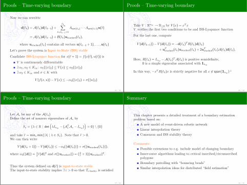
Our task is satisfied if equivalently d ≈ 0. In simulation,

0 20 40 60 80 100 120 140 160 180 2000.2

0.4

0.6

0.8

1

1.2

1.4

1.6

time (sec)

Maximum error in Dlambda

43 / 50


A subsequence of d(`) will help us conclude the result

Define `k ∈ N, for k ∈ N,

`1 = 1, and assume agent 1 executes the firstprojection-and-placement event with index nxt(1),`k ≥ 2 be the k-th time when agent 1 does theprojection-and-placement event with the same index nxt(1)

It can be seen that `k − `k−1 ≤ 2n · nip.

Define now A`k∈ Rnip×nip , for k ∈ N, by A(1) = Anxt(1). Then

A(`k) = Anxt(`k) · · ·Anxt(`k−1+2)Anxt(`k−1+1), for k ≥ 2,

where A(`k) is doubly stochastic and irreducible

44 / 50


Now we can rewritte

d(`k) = A(`k)d(`k−1) +

`k∑`=`k−1+1

Anxt(`k) · · ·Anxt(`+1)u(`)

= A(`k)d(`k−1) + B(`k)ustacked(`k),

where ustacked(`k) contains all vectors u(`k−1 + 1), . . . ,u(`k)

Let’s prove the system is Input-to-State (ISS) stable

Candidate ISS-Lyapunov function for x(` + 1) = f(x(`), u(`)) is

V is continuously differentiable∃α1, α2 ∈ K∞: α1(‖x‖2) ≤ V (x) ≤ α2(‖x‖2)

∃α3 ∈ K∞ and σ ∈ K with

V (f(x, u))− V (x) ≤ −α3(‖x‖2) + σ(‖u‖2)

45 / 50


Take V : Rnip → R≥0 by V (x) = xT xV verifies the first two conditions to be and ISS-Lyapunov function

For the last one, compute

V (d(`k+1))− V (d(`k)) = −d(`k)T R(`k)d(`k)

+ uTstacked(`k)ustacked(`k) + 2uT

stacked(`k)A(`k)d(`k),

Here, R(`k) = Inip −A(`k)TA(`k) is positive semidefinite,0 is a simple eigenvalue associated with 1nip

In this way, −xT R(`k)x is strictly negative for all x 6∈ span{1nip}⊥

46 / 50


Let As be any of the A(`k)Define the set of nonzero eigenvalues of As by

Ss = {λ ∈ R | det(λInip − (AT

s As − Inip))

= 0} \ {0}

and take r = mins min{|λ| | λ ∈ Ss}. Note that r > 0.We can then write

V (d(`k + 1))− V (d(`k)) ≤ −α3(‖d(`k)‖) + σ(‖ustacked(`k)‖),

where α3(‖d‖) = 12r‖d‖2 and σ(‖ustacked‖) = ( 2

r + 1)‖ustacked‖2.

Thus the system defined on d(`) is input-to-state stableThe input-to-state stability implies ∃ ε > 0 so that Tε-bndry is satisfied

47 / 50

Summary

This chapter presents a detailed treatment of a boundary estimationproblem based on:

A new model of event-driven robotic networkLinear interpolation theoryConsensus and ISS stability theory

Comments:Possible extensions to e.g. include model of changing boundaryInner-outer algorithms leading to critical inscribed/circumscribedpolygonsBoundary patrolling with “bouncing beads”Similar interpolation ideas for distributed “field estimation”

48 / 50

Bibliographical Notes

On hybrid systems:

A. J. van der Schaft and H. Schumacher. An Introduction to Hybrid

Dynamical Systems, volume 251 of Lecture Notes in Control and

Information Sciences. Springer, 2000

On interpolated curves by polygons:

P. M. Gruber. Approximation of convex bodies. In P. M. Gruber and

J. M. Willis, editors, Convexity and its Applications, pages

131--162. Birkhauser, 1983

49 / 50

Bibliographical Notes

Boundary estimation and tracking:

D. Marthaler and A. L. Bertozzi. Tracking environmental level sets

with autonomous vehicles. In S. Butenko, R. Murphey, and P. M.

Pardalos, editors, Recent Developments in Cooperative Control and

Optimization, pages 317--330. Kluwer Academic Publishers, 2003

D. W. Casbeer, S.-M. Li, R. W. Beard, R. K. Mehra, and T. W. McLain.

Forest fire monitoring with multiple small UAVs. In American Control

Conference, pages 3530--3535, Portland, OR, June 2005

D. W. Casbeer, D. B. Kingston, R. W. Beard, T. W. Mclain, S.-M. Li,

and R. Mehra. Cooperative forest fire surveillance using a team of

small unmanned air vehicles. International Journal of Systems

Sciences, 37(6):351--360, 2006

F. Zhang and N. E. Leonard. Generating contour plots using multiple

sensor platforms. In IEEE Swarm Intelligence Symposium, pages

309--316, Pasadena, CA, June 2005

50 / 50

Boundary estimation and patrolling algorithmscarmenere.ucsd.edu/pdfs/CDC08workshop-DCRN-BulloCortesMartinez-lecture5.pdfLecture #5: Boundary estimation and patrolling algorithm Francesco

Documents