BOUNDARY ELEMENT FORMULATION FOR FLOW IN ...

International Journal of Applied Mathematics & Engineering SciencesVol. 1, No. 1, January-June 2007

BOUNDARY ELEMENT FORMULATION FORFLOW IN UNSATURATED POROUS MEDIA

Bruno Natalini, Viktor Popov & Carlos A. Brebbia

ABSTRACT: Numerical model for two phase (air and water) unsaturated flow has been derived and solved usingthe boundary element method (BEM). The equations have been represented as non-homogeneous Laplaceequations, and the non-homogeneous part has been dealt with by using the dual reciprocity method (DRM). Thesoil-water characteristic curve according to the modified van Genuchten approach was employed. The developedscheme was applied to solution of upward and downward infiltration in clay showing good agreement withnumerical solutions previously reported in open literature.

1. INTRODUCTION

Modelling of unsaturated flow in porous media is applied in a number of different areas. Some areas of interestinclude hydrology, environmental protection and remediation and disposal of hazardous waste in undergroundrepositories. In this work a numerical model for unsaturated flow where both phases, water and air, are modelledis developed. Such model could be of importance for solution of the problem of wetting of clay in undergroundrepositories where the air cannot escape freely during the wetting of the clay, a process which may increase theair pressure slowing down the actual wetting process.

The model is solved by using the BEM DRM-MD approach which has shown good stability for solvingnon-linear problems in the past.

2. GOVERNING EQUATIONS FOR FLOW IN UNSATURATED POROUS MEDIA

In this section a quick derivation of the governing equations is presented. It is considered that each phaseoccupies part of the domain and follows its own set of tortuous paths. A detailed treatment of the theory of flowin unsaturated media is given by Bear & Verruijt [1] and Helmig [2].

2.1 Equation for the water phase

The mass balance equation is given as

� �0��

��

wwww q

t

Sn ��

�(1)

where:

n is the porosity

�w is the water density

Sw is the water saturation

Sw is defined as the relation of the volume of water in a representative elementary volume (REV) and thevolume of voids in the REV. Sw ranges from zero to one.

The specific discharge is defined using the Darcy law

� �zgpk

q www

ww ��

��

� (2)

International Journal of Applied Mathematics and Engineering SciencesVol. 2 No. 2 (December, 2017)

132 Bruno Natalini and Viktor Popov

where:

kw is the effective permeability for water (a function of Sw)

mw is the dynamic viscosity of water

pw is the water pressure

z is the elevation

By substituting (2) into (1) and considering that n and rw are constant, (1) can take the following form

zkk

gpk

kt

Sn

kp w

w

www

w

w

w

ww ��

��

�� 12

(3)

The water relative permeability is defined as

)1(

)()(

w

wwwrw k

SkSk � (4)

and

)1(wk = g

K

w

ww

��

(5)

where wK is the hydraulic conductivity for water, yielding

g

KSkSk

w

wwwrwww �

�)()( � (6)

By substituting (6) into (3), the equation for the water phase is obtained as

zkk

gpk

kt

S

Kk

gnp rw

rw

wwrw

rw

w

wrw

ww ��

��

�� 12

(7)

Note that it is possible to use equation (3) for the water phase, however (7) is a more suitable form since rwk

is non-dimensional and ranges from 0 to 1. Conversely, wk has dimensions, which makes its order of magnitude

dependant on the scale factors, which can produce higher errors when the term ww

kk

�1

is calculated rather

than rwrw

kk

�1

.

2.2 Equation for the Air Phase

The starting point for development of the equation for air phase is the mass balance equation:

� �0��

��

aaaa q

t

Sn ��

�(8)

combined with the Darcy law

Boundary Element Formulation for Flow in Unsaturated Porous Media 133

� �zgpk

q aaa

aa ��

��

� (9)

where the nomenclature analogous to the one in (1) and (2), the sub-index ‘a’ identifying air properties. Notethat

1 S S aw (10)

By substituting (9) into (8), considering n to be constant and neglecting the gravitational term zga ��

� , and

by using g

Kkk

a

ara

a

a

�� , the following equation is obtained

� � � � 0��

�ara

aaa pkg

K

t

Sn

��(11)

Further, developing both terms in (11), considering that ra is linked to pa through the equation of state andrearranging the equation yields

� ��

��

��

�

��

��

��

�� araaa

aa

aara

a pkg

K

t

Sp

t

pS

TR

n

Kk

gp

��

'2

(12)

The derivative in time of the saturation appearing in (7) and (12) can be handled in the following way:

w w c w c

c c

pS dS p dS p

t dp t dp p t�

�

��

� � � � (13)

where subscript � stands for “w” or “a” depending on the equation that is solved. Taking into account that thecapillary pressure can be expressed as pc = pa – pw, it is obvious that �pc/�pg = (1 or –1). If furthermore we use

(10) to eliminate aS , the final equations for water and air become

zkk

gpk

kt

p

p

S

Kk

gnp rw

rw

wwrw

rw

w

c

w

wrw

ww ��

��

��

�� 12

(14)

and

� � � ��

�

��

��

��

��

��

��

�� araaa

c

waw

araa pk

g

K

t

p

p

SpS

TR

n

Kk

gp

��1

'2

(15)

Equations (14) and (15) are the equations to be solved by the code, being wp and ap the unknown potential

fields. The constants needed in the model are g , w� , n , wK , aK , 'R andT while rwk , wS and rak are

functions of wp and ap . The functions linking the potential fields and rwk , wS and rak variables are given bythe soil water retention curve.

3. SOIL WATER RETENTION CURVE

The soil water retention curve describes the relation between the capillary pressure, pc, and Sw. There are severalfunctions that have been proposed; among the most popular for the air-water system are those given by Leverett


[3], Brooks and Corey [4] and van Genuchten [5]. Recently Vogel et al. [6, 7] suggested the use of the followingrelation:

� ��

��

�

�

��

��

�

sc

sc

c

awmw

w

ppwhen

ppwhenp

SSSS

S

1

a1mn

000

(16)

where Sm is a fictitious extrapolated parameter; Sm > 1, and ps is called the minimum capillary pressure. Themodified Van Genuchten’s relative water permeabilities as a function of saturations are

2

)1(1

)(1��

��

��

�F

SFSk e

erw and � �2

2

1

)1(1

)1()(1 ��

�

��

��

��

F

FSFSk e

era (17)

where

mm/1*1)( ��

�� ee SSF and e

awm

we S

SSS

SS

00

0* 1

��

� (18)

and

00

0

1 aw

wwe SS

SSS

��

� (19)

Equation (16) has been originally proposed in terms of water contents; here it is modified in order to match

with the definition (19), which takes into account 0aS , and the relative permeability of the air phase. Equations

(16) – (19) will be referred to as the modified Van Genuchten model (VGM). The modified VGM eliminatesnumerical instabilities appearing near saturation and this formulation is further used in the numerical examplesin section 6.

4. SOLVING THE SYSTEM OF EQUATIONS

When considering the simultaneous flow of both the water and the air in the unsaturated zone, the system ofequations is represented by (14) and (15) together with those coming from the soil water model. Though thenumerical model is developed for the case of variable air pressure, further in this work the air pressure isconsidered to be constant and equal to the atmospheric pressure. Therefore, in the examples presented here only(14) is solved; which is equivalent to solving the Richard´s equation.

The code developed obtains solutions at different timesteps by using a linear time finite differenceapproximation. As the equations are non-linear, in each timestep an iterative procedure is applied. The codestarts by calculating pc from the initial conditions of the problem, then Sw and krw are calculated and finally(14) is solved. In the next iteration, with the obtained value of pw, a new value for pc is calculated, then Sw andkrw are recalculated and (14) is solved again. The process is repeated until convergence is reached within eachtimestep.

The derivative of wS in respect to cp appearing in the equations will depend on the soil water retention

model used and for the modified VGM it can be obtained as


� ��

��

�

��

�

�

�

��

��

��

�

sc

sc

c

cawm

c

w

ppwhen

ppwhenp

pSSS

p

S

0

a1

anma1mn

1n00

(20)

5. BEM DRM-MD IMPLEMENTATION FOR THE WATER PHASE

The dual reciprocity method (DRM), which was introduced by Nardini & Brebbia [8], is acknowledged to beone of the most effective boundary element method (BEM) techniques for transforming domain integrals intoboundary integrals.

Popov and Power implemented a scheme using domain subdivision in conjunction with the DRM to avoiddomain integration and called it the Dual Reciprocity Method - Multi-Domain approach (DRM-MD). Theinitial problem solved using this formulation was the flow of a mixture of gases through a porous media [9, 10,11]. The DRM-MD has also been applied to linear and non-linear advection-diffusion problems [12], drivencavity flow of Navier-Stokes equations [13], non-Newtonian fluids [14], and flow of polymers inside mixerswith complex geometries [15]. Though the above applications are two-dimensional (2D), recently the techniquehas been applied to three-dimensional (3D) problems by Natalini and Popov [16, 17] and Peratta and Popov[18, 19].

DRM-MD does not suffer the two main problems related to standard DRM; the systems of equations producedby DRM-MD are sparse and well conditioned, and the number and position of DRM nodes is usually notcritical, since small sub-domains usually require no or few interior DRM nodes.

Starting from a Poisson-like governing equation

� � � �2u ,t b u, ,t� �x x (21)

where u(x,t) is a scalar field (potential field), b(u,x,t) is the non-homogeneous term and x is a position vector inthe domain with components xi, after applying the DRM approach (for more details see Partridge et al. [20]), thefollowing equation is obtained

��

�� yy dquduqu )(),()(),()()( ** yyxyyxxx�

� ��

� ��

��

��

��

��

�

��

�

��

IJ

ky

ky

kkk dquduqu

1

** ),(ˆ),(),(ˆ),(),(ˆ)( zyyxzyyxzxx�� (22)

where u*(x,y) is the fundamental solution of the Laplace equation, q(y) = �u(y)/�n, q*(x,y) = �u*(x,y)/�n and n isthe unit vector normal to the boundary of the domain. The constant l(x) has values between 1 and 0, being equalto 1/2 on smooth parts of boundaries and being equal to 1 for points inside the domain. Constants ak are unknowncoefficients and the DRM approximation is applied to J nodes on the boundary � of the domain and I nodesinside the domain W.

After application of collocation technique to all boundary nodes, (22) can be written in terms of four matrices,

H, G, U and Q which depend only on the geometry of the problem.

αqu )ˆˆ( QGUHGH �� (23)


Since the non-homogeneous term b in the DRM is expressed in the following form

� Fb α (24)

after expressing a in terms of b, the following equation is obtained

bqu 1)ˆˆ( �� FQGUHGH (25)

The DRM integral formulation for wp is obtained by replacing the non-homogeneous term in (14) into (25)

�

��

�

��

�

��

��

�

�

��

�

�

��

�

�

��

�

�

�

�

�

��

�

�

�

��

�

�

�

�

��

�

�

��

��

n

j

rw

rw

wij

n

j wrwwrwwrw

w

w

c

w

wrw

w

ij

n

jwij

n

jwij

z

k

k

gs

z

p

z

k

y

p

y

k

x

p

x

k

k

t

p

p

S

Kk

gn

sqgph

j

j

jjjjjj

j

jj

j

jj

1

111

~

~

~~~

~1

~

~

�

�

(26)

where sij is the matrix 1)ˆˆ( �� FQGUH and jrwk~

and jw cS / p� �� are calculated using values of ap = patm

(atmospheric pressure) and wp coming from the previous iteration, which will be denoted by wp~ from here on.

x

pjw

�

� and all the others partial derivatives are obtained by applying the DRM approximation (24) which in

index notation is given as

x

pjw

�

�=��

� �

�

�

�n

k

n

lwlk

jlk

pfx

f

1 1

1(27)

The time discretization is based on the implicit/explicit Euler method

� � 1mm θθ1 �� wpwpw pppww

(28)

� � 1mm θθ1 �� wqwqw qqqww

(29)

The time derivative is approximated using a finite-difference scheme

� �m1m1ww

w pptt

p�

��

��

(30)

By applying (27) – (30), (26) can be recast as

� ��

� � vSG

RTHGT

RH WW

~θ1

~~

1θθ~

θ~

θ

m

m1m1m

g

tt

wwq

ww

pwqwpw

p

w

wwww

��

��

��

��

��

��

��

��

q

pqp

(31)


where wR~

is a matrix of components

c

w

wrw

wijw p

S

Kk

gnsr j

jij �

��

~

~~ �(32)

and WT~ is defined as

1 1 1x y zx y z

� � ��

� �� W

F F FT D F D F D F� � � �

(33)

where xD~

has components

�ijd x

k

ks j

j

rw

rwij �

�~

~1

(34)

and similar for yD~

and zD~ matrices. The components of vector v~ is defined as

z

k

kv j

j

rw

rwj �

��

~

~1~

(35)

The interface conditions between two sub-domains for pressure and flux state that the pressure and the fluxmust preserve continuity. In the case of pressure the interface conditions result in the following equation

21 ww pp � (36)

In the case of flux the interface conditions are equivalent to applying the mass conservation principle andcan be derived starting from the flux of water trough the interface per unit surface and unit time for bothinterfaces as given below

11 n1

�� wqQ and 22 n

2

�� wqQ (37)

where 1n�

and 2n�

are the unit normal vectors to the interface calculated from 1� and 2� respectively. As 1wq�

=

2wq�

and 21 nn��

�� the following is valid

21 QQ �� (38)

Further considering that

1

1

1

1 n1 zww

ww

w

wg

kq

kQ �

�� and 2

2

2

2 n2 zww

ww

w

w gk

qk

Q ��

�� (39)

where 1nz is the z-component of 1n

� and

2nz is the z-component of

2n�

. Finally, the matching condition for flux

is obtained as

222

2211

122

11

2n zw

wrw

wrwwrww

wrw

wrww g

Kk

KkKkq

Kk

Kkq �

�� (40)


or

BAqq ww ��12 (41)

6. NUMERICAL EXAMPLES

All the examples presented here use discontinuous elements combined with the augmented thin plate splinefunction as approximation function in the DRM approximation with no internal DRM nodes.

6.1 CASE 1: Upward infiltration in clay

The first case simulates infiltration in a 1m long clay column that initially is assumed to be in equilibrium with

an imposed water pressure, wp , of zero Pa at the bottom of the column (z = 1). The boundary conditions were

98060 Pa of water pressure (atmospheric pressure) at the bottom of the column (z = 1) combined with zero fluxat the top (z = 0), leading to upward infiltration against gravity. A numerical solution of this case using a 1Dmodel has been presented by Vogel et al. [7]. The soil-water retention curve used was the modified Van Genuchtenmodel. The same parameters were used as in the Vogel’s example:

Porosity, n 0.38

Hydraulic conductivity of water, wK 5.56E-07 m/s or 4.8 cm/day

Irreducible water saturation, 0wS 0.17895

Van Genuchten’s a parameter 0.8 1/m or 0.008 1/cm

Van Genuchten’s n parameter 1.09

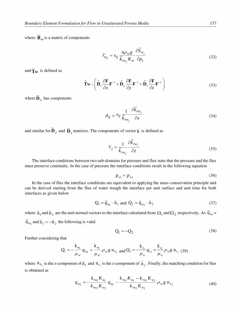
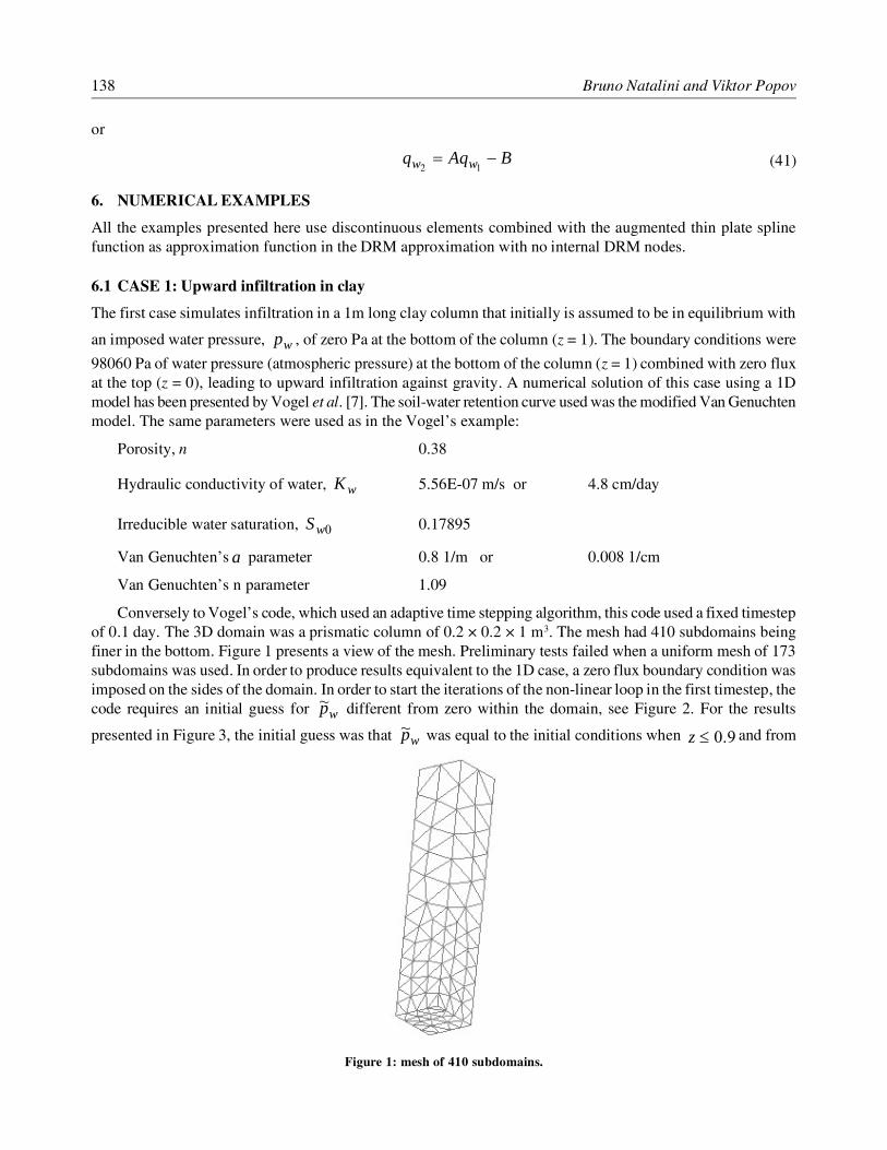
Conversely to Vogel’s code, which used an adaptive time stepping algorithm, this code used a fixed timestepof 0.1 day. The 3D domain was a prismatic column of 0.2 × 0.2 × 1 m3. The mesh had 410 subdomains beingfiner in the bottom. Figure 1 presents a view of the mesh. Preliminary tests failed when a uniform mesh of 173subdomains was used. In order to produce results equivalent to the 1D case, a zero flux boundary condition wasimposed on the sides of the domain. In order to start the iterations of the non-linear loop in the first timestep, thecode requires an initial guess for wp~ different from zero within the domain, see Figure 2. For the results

presented in Figure 3, the initial guess was that wp~ was equal to the initial conditions when 9.0�z and from

Figure 1: mesh of 410 subdomains.


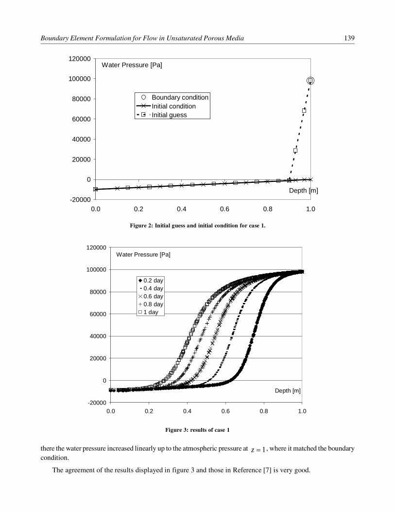
there the water pressure increased linearly up to the atmospheric pressure at 1�z , where it matched the boundarycondition.

The agreement of the results displayed in figure 3 and those in Reference [7] is very good.

Figure 2: Initial guess and initial condition for case 1.

-20000

0

20000

40000

60000

80000

100000

120000

0.0 0.2 0.4 0.6 0.8 1.0

Boundary conditionInitial conditionInitial guess

Water Pressure [Pa]

Depth [m]

Figure 3: results of case 1

-20000

0

20000

40000

60000

80000

100000

120000

0.0 0.2 0.4 0.6 0.8 1.0

0.2 day0.4 day0.6 day0.8 day1 day

Water Pressure [Pa]

Depth [m]


Table 1 presents the number of iterations needed in every timestep to converge. Note how the convergenceis easier as the pressure distribution becomes smoother.

Table 1Number of Iterations in Every Timestep for case 1.

Timestep 1 2 3 4 5 6 7 8 9 10

No. of iterations 19 18 15 12 11 9 8 8 6 6

6.2 CASE 2: Downward Infiltration in Clay

This example was used by Vogel et al. [7]. It is the simulation of infiltration in a 1m long clay column that,

again, initially was assumed to be in equilibrium with an imposed water pressure, wp , of zero Pa at the bottom

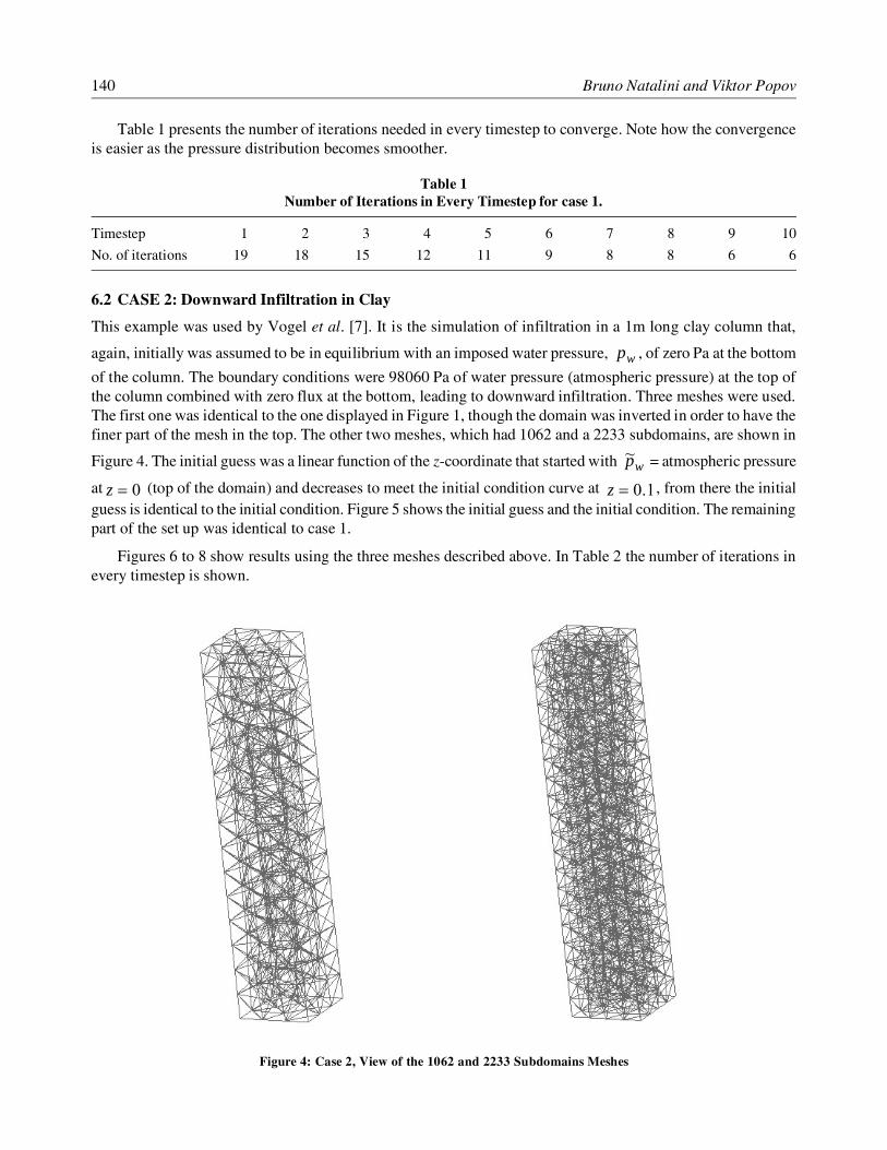
of the column. The boundary conditions were 98060 Pa of water pressure (atmospheric pressure) at the top ofthe column combined with zero flux at the bottom, leading to downward infiltration. Three meshes were used.The first one was identical to the one displayed in Figure 1, though the domain was inverted in order to have thefiner part of the mesh in the top. The other two meshes, which had 1062 and a 2233 subdomains, are shown in

Figure 4. The initial guess was a linear function of the z-coordinate that started with wp~ = atmospheric pressure

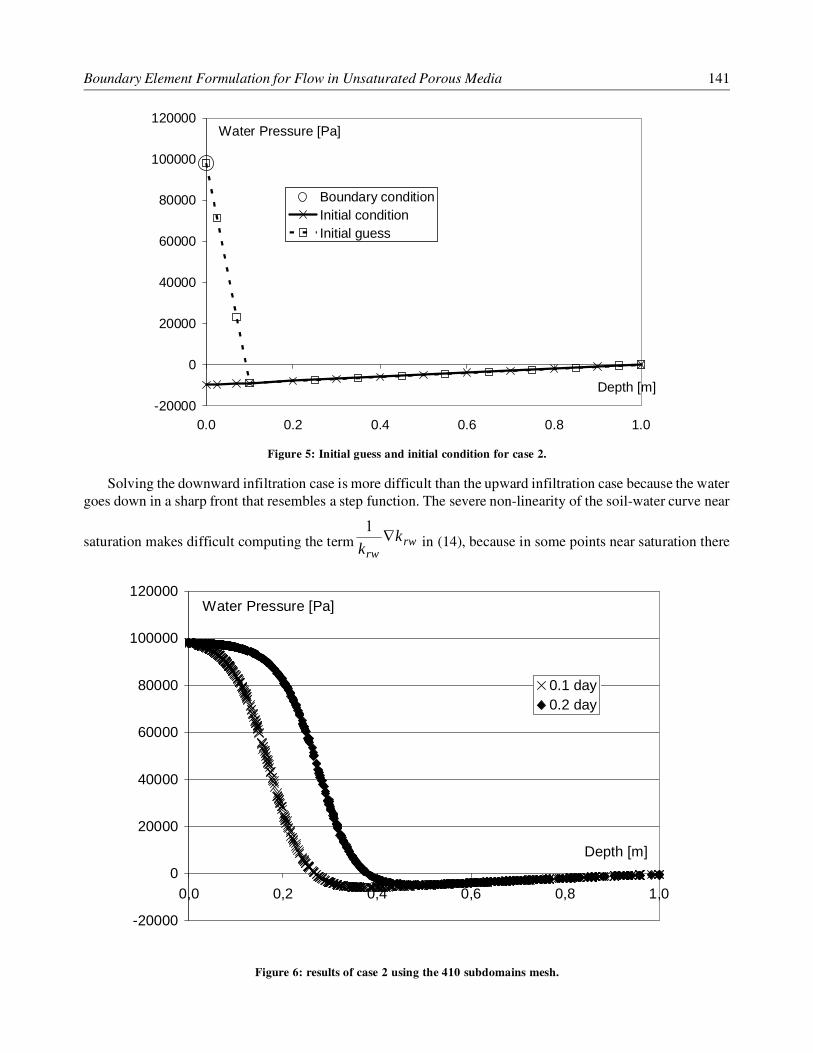
at 0�z (top of the domain) and decreases to meet the initial condition curve at 1.0�z , from there the initialguess is identical to the initial condition. Figure 5 shows the initial guess and the initial condition. The remainingpart of the set up was identical to case 1.

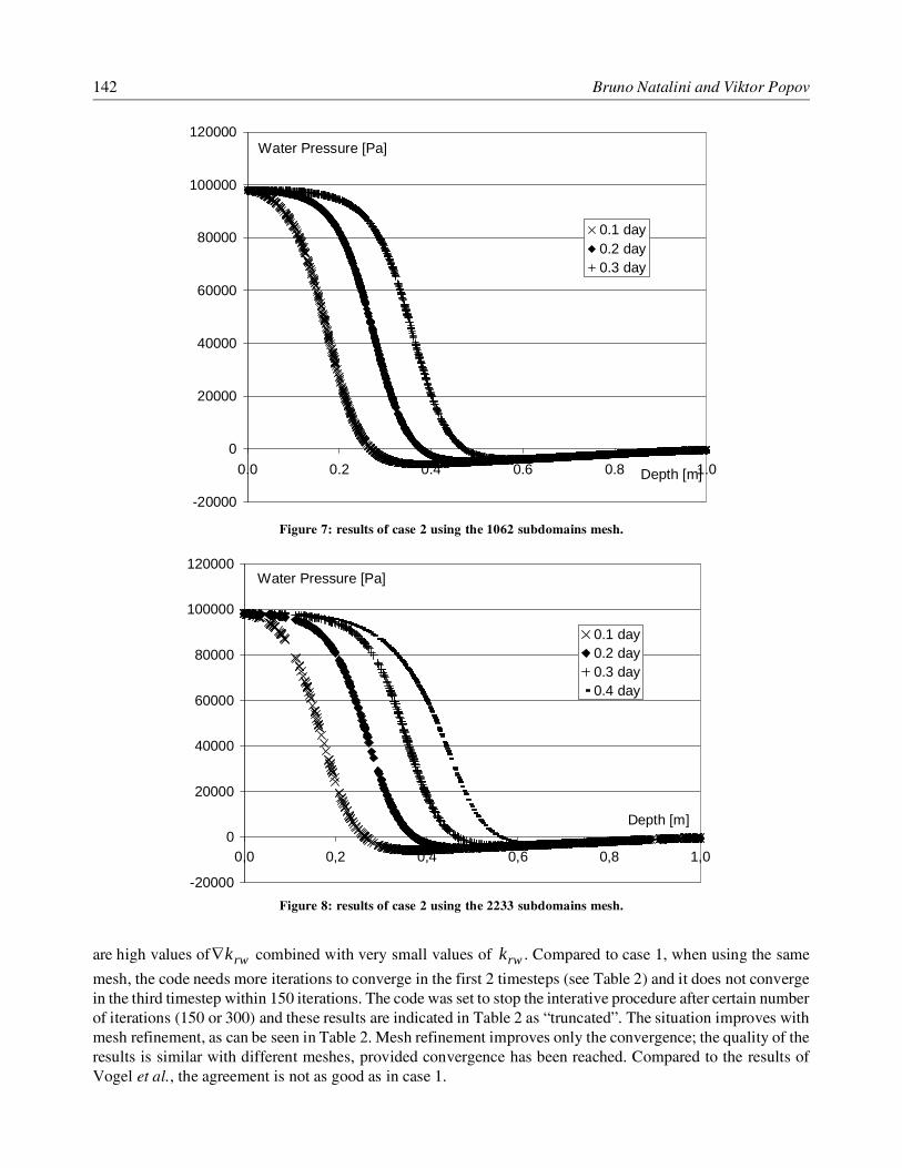
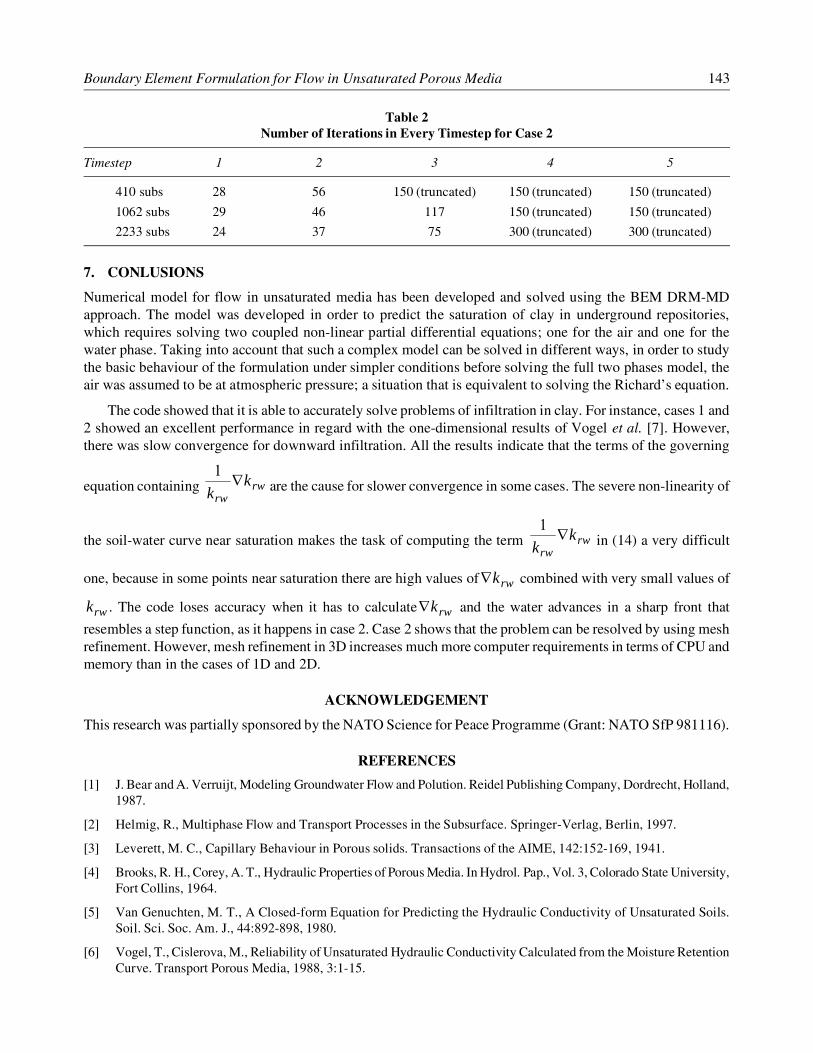
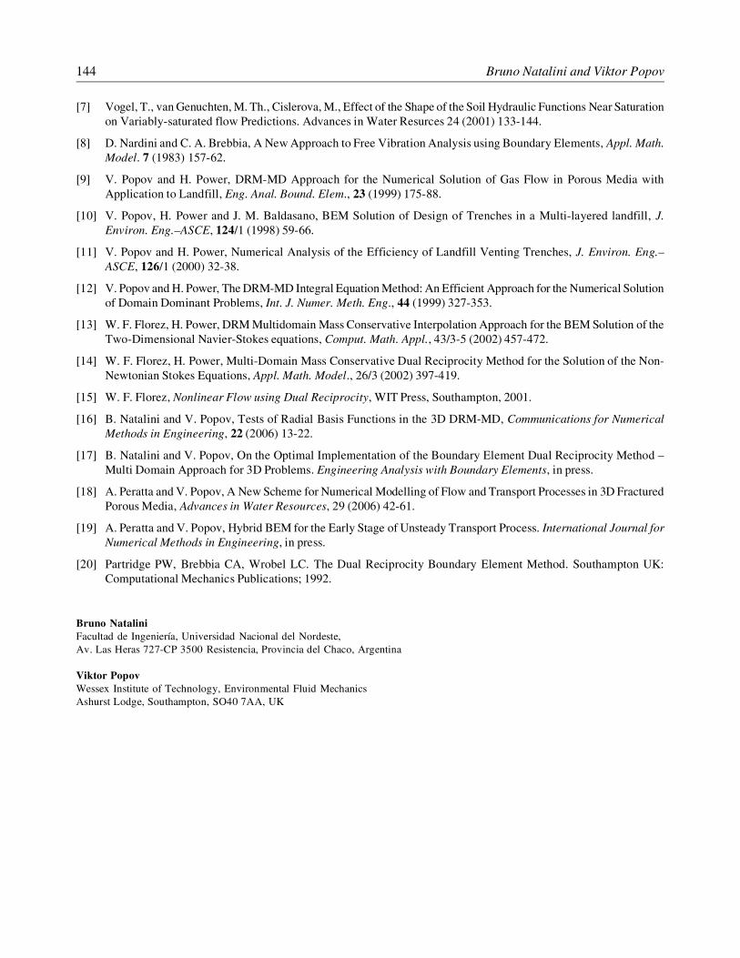
Figures 6 to 8 show results using the three meshes described above. In Table 2 the number of iterations inevery timestep is shown.

Figure 4: Case 2, View of the 1062 and 2233 Subdomains Meshes


Solving the downward infiltration case is more difficult than the upward infiltration case because the watergoes down in a sharp front that resembles a step function. The severe non-linearity of the soil-water curve near

saturation makes difficult computing the term rwrw

kk

�1

in (14), because in some points near saturation there

Figure 5: Initial guess and initial condition for case 2.

-20000

0

20000

40000

60000

80000

100000

120000

0.0 0.2 0.4 0.6 0.8 1.0

Boundary conditionInitial conditionInitial guess

Water Pressure [Pa]

Depth [m]

Figure 6: results of case 2 using the 410 subdomains mesh.

-20000

0

20000

40000

60000

80000

100000

120000

0,0 0,2 0,4 0,6 0,8 1,0

0.1 day0.2 day

Water Pressure [Pa]

Depth [m]


are high values of rwk� combined with very small values of rwk . Compared to case 1, when using the same

mesh, the code needs more iterations to converge in the first 2 timesteps (see Table 2) and it does not convergein the third timestep within 150 iterations. The code was set to stop the interative procedure after certain numberof iterations (150 or 300) and these results are indicated in Table 2 as “truncated”. The situation improves withmesh refinement, as can be seen in Table 2. Mesh refinement improves only the convergence; the quality of theresults is similar with different meshes, provided convergence has been reached. Compared to the results ofVogel et al., the agreement is not as good as in case 1.



-20000

0

20000

40000

60000

80000

100000

120000

0.0 0.2 0.4 0.6 0.8 1.0

0.1 day0.2 day0.3 day

Water Pressure [Pa]

Depth [m]

-20000

0

20000

40000

60000

80000

100000

120000

0,0 0,2 0,4 0,6 0,8 1,0

0.1 day0.2 day0.3 day0.4 day

Water Pressure [Pa]

Depth [m]


Table 2Number of Iterations in Every Timestep for Case 2

Timestep 1 2 3 4 5

410 subs 28 56 150 (truncated) 150 (truncated) 150 (truncated)

1062 subs 29 46 117 150 (truncated) 150 (truncated)

2233 subs 24 37 75 300 (truncated) 300 (truncated)

7. CONLUSIONS

Numerical model for flow in unsaturated media has been developed and solved using the BEM DRM-MDapproach. The model was developed in order to predict the saturation of clay in underground repositories,which requires solving two coupled non-linear partial differential equations; one for the air and one for thewater phase. Taking into account that such a complex model can be solved in different ways, in order to studythe basic behaviour of the formulation under simpler conditions before solving the full two phases model, theair was assumed to be at atmospheric pressure; a situation that is equivalent to solving the Richard’s equation.

The code showed that it is able to accurately solve problems of infiltration in clay. For instance, cases 1 and2 showed an excellent performance in regard with the one-dimensional results of Vogel et al. [7]. However,there was slow convergence for downward infiltration. All the results indicate that the terms of the governing

equation containing rwrw

kk

�1

are the cause for slower convergence in some cases. The severe non-linearity of

the soil-water curve near saturation makes the task of computing the term rwrw

kk

�1

in (14) a very difficult

one, because in some points near saturation there are high values of rwk� combined with very small values of

rwk . The code loses accuracy when it has to calculate rwk� and the water advances in a sharp front that

resembles a step function, as it happens in case 2. Case 2 shows that the problem can be resolved by using meshrefinement. However, mesh refinement in 3D increases much more computer requirements in terms of CPU andmemory than in the cases of 1D and 2D.

ACKNOWLEDGEMENT

This research was partially sponsored by the NATO Science for Peace Programme (Grant: NATO SfP 981116).

REFERENCES

[1] J. Bear and A. Verruijt, Modeling Groundwater Flow and Polution. Reidel Publishing Company, Dordrecht, Holland,1987.

[2] Helmig, R., Multiphase Flow and Transport Processes in the Subsurface. Springer-Verlag, Berlin, 1997.

[3] Leverett, M. C., Capillary Behaviour in Porous solids. Transactions of the AIME, 142:152-169, 1941.

[4] Brooks, R. H., Corey, A. T., Hydraulic Properties of Porous Media. In Hydrol. Pap., Vol. 3, Colorado State University,Fort Collins, 1964.

[5] Van Genuchten, M. T., A Closed-form Equation for Predicting the Hydraulic Conductivity of Unsaturated Soils.Soil. Sci. Soc. Am. J., 44:892-898, 1980.

[6] Vogel, T., Cislerova, M., Reliability of Unsaturated Hydraulic Conductivity Calculated from the Moisture RetentionCurve. Transport Porous Media, 1988, 3:1-15.


[7] Vogel, T., van Genuchten, M. Th., Cislerova, M., Effect of the Shape of the Soil Hydraulic Functions Near Saturationon Variably-saturated flow Predictions. Advances in Water Resurces 24 (2001) 133-144.

[8] D. Nardini and C. A. Brebbia, A New Approach to Free Vibration Analysis using Boundary Elements, Appl. Math.Model. 7 (1983) 157-62.

[9] V. Popov and H. Power, DRM-MD Approach for the Numerical Solution of Gas Flow in Porous Media withApplication to Landfill, Eng. Anal. Bound. Elem., 23 (1999) 175-88.

[10] V. Popov, H. Power and J. M. Baldasano, BEM Solution of Design of Trenches in a Multi-layered landfill, J.Environ. Eng.–ASCE, 124/1 (1998) 59-66.

[11] V. Popov and H. Power, Numerical Analysis of the Efficiency of Landfill Venting Trenches, J. Environ. Eng.–ASCE, 126/1 (2000) 32-38.

[12] V. Popov and H. Power, The DRM-MD Integral Equation Method: An Efficient Approach for the Numerical Solutionof Domain Dominant Problems, Int. J. Numer. Meth. Eng., 44 (1999) 327-353.

[13] W. F. Florez, H. Power, DRM Multidomain Mass Conservative Interpolation Approach for the BEM Solution of theTwo-Dimensional Navier-Stokes equations, Comput. Math. Appl., 43/3-5 (2002) 457-472.

[14] W. F. Florez, H. Power, Multi-Domain Mass Conservative Dual Reciprocity Method for the Solution of the Non-Newtonian Stokes Equations, Appl. Math. Model., 26/3 (2002) 397-419.

[15] W. F. Florez, Nonlinear Flow using Dual Reciprocity, WIT Press, Southampton, 2001.

[16] B. Natalini and V. Popov, Tests of Radial Basis Functions in the 3D DRM-MD, Communications for NumericalMethods in Engineering, 22 (2006) 13-22.

[17] B. Natalini and V. Popov, On the Optimal Implementation of the Boundary Element Dual Reciprocity Method –Multi Domain Approach for 3D Problems. Engineering Analysis with Boundary Elements, in press.

[18] A. Peratta and V. Popov, A New Scheme for Numerical Modelling of Flow and Transport Processes in 3D FracturedPorous Media, Advances in Water Resources, 29 (2006) 42-61.

[19] A. Peratta and V. Popov, Hybrid BEM for the Early Stage of Unsteady Transport Process. International Journal forNumerical Methods in Engineering, in press.

[20] Partridge PW, Brebbia CA, Wrobel LC. The Dual Reciprocity Boundary Element Method. Southampton UK:Computational Mechanics Publications; 1992.

Bruno NataliniFacultad de Ingeniería, Universidad Nacional del Nordeste,Av. Las Heras 727-CP 3500 Resistencia, Provincia del Chaco, Argentina

Viktor PopovWessex Institute of Technology, Environmental Fluid MechanicsAshurst Lodge, Southampton, SO40 7AA, UK

BOUNDARY ELEMENT FORMULATION FOR FLOW IN ...

Documents