Boundary conformal field theories, limit sets of Kleinian groups and holography

arX

iv:h

ep-t

h/99

0216

7v4

24

Jun

1999

The Date

Boundary Conformal Field Theories, Limit

Sets of Kleinian Groups and Holography

Arkady L.Kholodenko∗

Abstract

In this paper, based on the available mathematical works on geometry andtopology of hyperbolic manifolds and discrete groups, some results of Freed-man et al (hep-th/9804058) are reproduced and broadly generalized.Amongmany new results the possibility of extension of work of Belavin,Polyakovand Zamolodchikov to higher dimensions is investigated. Known in physicalliterature objections against such extension are removed and the possibilityof an extension is convinsingly demonstrated

∗375 H.L. Hunter Laboratories, Clemson University ,Clemson, SC 29634-1905 ,USA

.e-mail: [email protected]

1

2

1. Introduction

Recently, there had been attempts to extend the results of two dimen-sional conformal field theories(CFT) to higher dimensions [1.2]. Since publi-cation of papers by Witten[3, 4]it had become clear that there is a very closecorrespondence between 2d physics of critical phenomena and 3d physicsof knots and links. A very detailed study of this correspondence is devel-oped by Moore and Seiberg [5]. Additional contributions more recently weremade in Ref[6], etc. All these works heavily exploit the algebraic aspects ofthis correspondence through use of Yang-Baxter equations, quantum groups,etc. Much lesser efforts had been spent on development of the same corre-spondence from the topological point of view through study of 3-manifoldscomplementary to knots(links) in S3=R3 ∪ ∞. Such study is potentiallymore beneficial since it is known [7] that in four dimensions all knots are triv-ial (i.e.unknotted) so that the algebraic methods used so far are necessarilylimited to 3 dimensions and, accordingly, to study of two dimensional CFTonly. At the same time, topological study of manifolds is not limited to threedimensions. The reasons why such studies are useful could be understoodfrom the following simple arguments taken from the book by Maskit [8].

Define an inclusion of Rd into Rd+1 through Rd =(x,t)| t = 0 wherex∈ Rd,−∞ ≤ t ≤ ∞. The upper half space Poincare′ model of hyperbolicspace Hd+1is defined by

Hd+1 = (x, t) | t > 0 (1.1)

with x ∈ Rd so that ∂Hd+1 = Rd. Consider a special group G of motionsG=Md+1 of Rd+1 = x, t made of

a) translations: (x,t)→ (x + a, t) ,a ∈ Rd−1 ;

b) rotations : (x,t)→ (r(x),t) , r∈ O(d − 1);

c) dilatations : x→ λx ,λ > 0, λ 6= 1 and

d) inversions : x→ x|x|2

.

It can be proven[8] that the group G acts as a group of isometries ofHd+1and is called d dimensional Mobius group. In its action on Rd ”G actsas a group of conformal motions but not as a group of isometries in anymetric”.

At the same time, it is well established[9] that in any dimension thephysical system at criticality possesses the invariance which is described in

3

terms of the group G. Hence, the very existence of criticality is closelyassociated with the hyperbolicity of the adjacent space.

Let x∈ Hd+1 and γ ∈G. Consider a motion (an orbit) in Hd+1 by succes-sive applications of γ to x. It is of interest to study if such a motion willever hit ∂Hd+1 = Rd. This problem is highly nontrivial and was solved byBeardon and Maskit[10] (e.g.see section 5 below for more details) for d=2.The nontriviality of this problem could be better understood if, instead ofthe upper half space Hd+1model, we would consider the unit ball Bd+1 modelof the hyperbolic space with the unit sphere Sd

∞ (sphere at infinity) playingthe same role as in this model as ∂Hd+1 = Rd in the upper half space model.Since not all subgroups of G will allow hitting of the boundary, it is clear,that one should be interested only in those subgroups whose orbits end upat the boundary. These subgroups, in turn, could be further subdivided intothose whose limit points on Sd

∞ will cover the entire sphere and those whichwill cover only a part of Sd

∞. This part we shall denote as Λ. The limit setΛ is actually a fractal . The fractal dimension of Λ is directly related to thecritical indices of the two-point correlation functions of the correspondingconformal models at criticality. Different subgroups of Mobius group G willproduce different fractal dimensions. In turn, the corresponding hyperbolicmanifolds associated with these groups could be viewed as complements of therelated knots (links) in the case of 2+1 dimensions so that different confor-mal models, indeed, could be associated with different types of knots(links).This association becomes unnecessary when one is interested in conformalmodels in dimensions 3 and higher. One could still consider motions associ-ated with subgroups of Mobius group and the corresponding, say, hyperbolic4-manifolds without using knots, braids, Yang-Baxter equations, etc.

Although stated in different form, recent results of Maldacena[11] andtheir subsequent refinements in Refs[12-16] (and many additional referencestherein and elsewhere which we do not include) are actually directly con-nected with ideas just described. In physics literature the connection be-tween ”surface” and ”bulk” field theories is known as holographic principle(holographic hypothesis)[17,18]. In simple terms [19], it can be formulatedas statement that ”a macroscopic region of space and everything inside itcan be represented by a boundary theory living on the boundary region”.Mathematical support of this principle in physics literature is attributed toworks by Fefferman and Graham [20] and Graham and Lee[21]. These worksdiscuss boundary conditions at infinity for Einstein manifolds (spaces) and

4

initial value problem for Einstein’s equations. Although our previous discus-sion did not involve the Einstein manifolds, actually, the results of Ref.[21]are consistent with those which follow from the hyperbolic geometry. Thiscan be understood if one takes into account that Einstein spaces are charac-terized by the property that the Ricci tensor Rij is proportional to the metrictensor gij [22], that is

Rij = λgij. (1.1)

Since the scalar curvature R = gijRij , the above equation can be rewrittenas

Rij =R

dgij (1.2)

where d is the dimensionality of space (as before). The Einstein tensor

Gij = Ri

j −1

2δijR (1.3)

acquires a particularly simple form with help of Eq.(1.2):

Gij = (

1

d−

1

2)δi

jR (1.4)

and, because Gij,h =0, we obtain,

(1

d−

1

2)R ,j = 0. (1.5)

This implies ,that the scalar curvature R is constant . For isotropic ho-mogenous spaces Ed the Riemann curvature tensor is known to be[23] givenby

Rijkl = k(x)(gikgjl − gilgjk) (1.6)

so that the Ricci tensor is given by

Rij = (d − 1)k(x)gij , (1.7)

where k(x) is the sectional curvature at the point x∈Ed . The Schur’stheorem[23] guarantees, that k(x) = k = const for d ≥ 3 .Comparison be-tween Eqs.(1.1) and (1.7) produces then : λ = (d − 1)k and, accordingly,

5

R = d(d − 1)k . The spatial coordinates can always be rescaled so that, fork < 0 we obtain, the canonical value k = −1 characteristic of hyperbolicspace[24,25] . Since in the work by Graham and Lee [21] the condition givenby Eq.(1.7) is used (with k = −1), the connections with hyperbolic geometryis evedent. Since Eq.(1.4) can be equivalently rewritten with help of Eq.(1.7)as

Rij −1

2gijR + Λgij = 0, (1.8)

with the cosmological term Λ =-12(d− 1)(d− 2),thus obtained equation pro-

duces metric for Einstein space known in literature as anti-de Sitter (AdS)space[26]. Hence, in part, the purpose of this work is to investigate in somedetail connections between the results obtained in physics literature and re-lated to CFT-AdS correspondence, e.g.see Ref.[12], and those known in math-ematics those known in mathematics and related to hyperbolic geometry andhyperbolic spaces. Not only it is possible to reobtain results known in physicsusing these connections, but many more follow along the way of physicalreinterpretation of known results in mathematics. Establishing these con-nections touches many aspects of modern mathematics such as the geometryand topology of hyperbolic manifolds[25], multidimensional extension of thetheory of Teichmuller spaces[27], spectral analysis of hyperbolic manifolds[28](including those with cusps[29]), random walks on group manifolds[30], the-ory of deformations of Kleinian and Fuchsian groups[31](and Mobius groupsin general), ergodic theory of discrete groups[32], Kodaira-Spencer theoryof deformations of complex manifolds[33], loop groups[34],cohomology ofgroups, etc. In particular, the cohomological aspects of these connectionslead directly to the Virasoro algebra and its generalizations thus allow-ing us to dicuss the extension of fundamental results of Belavin-Polyakov-Zamolodchikov(BPZ) [35] to higher dimensions(e.g.see section 8). To makeour presentation self-contained, we had incorporated some the auxiliary re-sults from mathematics into text which are meant only to facilitate reader’sunderstanding without detracting of his/her attention from physical goalsand motivations of this work. A quick summary of some auxiliary math-ematical results related to hyperbolic 3-manifolds and Einstein spaces alsocould be found in our papers, Ref.s[36,37].

This paper is organized as follows. In section 2 we discuss an auxiliaryPlateau problem in d+1 dimensional Euclidean space. Already in two di-mensions the full analysis of the Plateau problem is quite nontrivial as it was

6

demonstrated in classical work of Douglas published in 1939 [38]. Multidi-mensional treatment of this problem is even more nontrivial and touchesmany subtle aspects of the harmonic analysis [39]. Nevertheless, the ex-tension of the Euclidean variant of the Plateau problem to the hyperbolicHd+1space is actually not difficult and was accomplished rather long timeago by Ahlfors[25]. Using the results of Ahlfors we were able to reobtain theresults of Freedman et al, Ref.[12], almost straightforwardly in section 3. Wedeliberately considering only the scalar field case in this work since the exten-sion of our treatment to vector and tensor fields (to be briefly considered inSection 8 ) does not cause much additional conceptual problems. To gener-alize the results of section 3 and to put them in an appropriate mathematicalcontext, we discuss (in section 4) diffusion in the hyperbolic space. This isdone with several purposes. First, using symmetries of the Laplace operatoracting in the hyperbolic space it is possible to subdivide Brownian motionson transient and recurrent. Only transient motions can reach the boundaryof the hyperbolic space. The transience and/or recurrence is associated withconvergence /or divergence of certain infinite sums known as Poincare′ se-ries.The convergence or divergence of such series is being controlled by thecritical exponent α. Patterson[40], Sullivan[41], Ahlfors[25], Thurston [42]and others [32] had shown that this exponent is associated with the fractaldimension of the limit set Λ. Stated in physical terms, it is shown in section5 that this exponent is associated with the exponent 2ν for the two-pointcorrelation function of the corresponding boundary CFT . The exponent αdepends upon the specific group of motions in Hd+1. This group is directlyassociated with the hyperbolic manifold so that different groups associ-ated with different manifolds will produce different α′s. Being armedwith these ideas it is possible to improve the existing physical results us-ing spectral theory of hyperbolic manifolds in section 6. In this section itis shown that the obtained eigenvalue spectrum of the hyperbolic Laplaciandiscussed in physics literature is incomplete and much more results could beobtained with help of the existing mathematical literature, e.g.see Ref.[28].For instance, 2d critical exponent 2ν for the Ising model is almost straight-forwardly obtained with help of the recently obtained results of Bishop andJones[43] .With this result obtained, it is only natural to look for connectionsbetween the boundary CFT results and those coming from the fundamentalwork of BPZ[35] .The connection can be established rather easily,e.g.see sec-tion 7 ,based on the theory of deformation of Kleinian groups[27, 31] which isclosely associated with the theory of Teichmuller spaces[44] as it was demon-

7

strated by Bers[45] some time ago. One of the sources which generates ”new”Kleinian groups from the ”old” ones is through the extension of the quasicon-formal deformations produced at the boundary Ω = S2

∞−Λ of the hyperbolicspace into the bulk(i.e.holography in physical terminology). The theory ofsuch deformations was under development in mathematics for quite sometime. However, the results which are essential for making connections withcurrent physics literature had been obtained by mathematicians only quiterecently. In particular, Canary and Taylor[46] had demonstrated that thelimit set of Kleinian groups which produce critical exponents α in physicallyinteresting range (e.g. for 0<α < 1 one obtains the correct Ising model criti-cal exponent 2ν = 1/4, etc.) is a circle S, perhaps, with some points(or, maybe, segments) being removed (e.g. see section 7 for more details). These factsnaturally explain the crucial role being played by the loop groups and theloop algebras[34] in the conformal field theories and other exactly integrablesystems [47]. At the same time, Nag and Verjovsky[48] had demonstratedhow the boundary deformations of such circle is connected with the centralextension term of the Virasoro algebra thus providing major physical rea-sons for existence of such term. Moreover, the analysis of the seminal workby Nag and Verjovsky indicates that, actually, their main results are basedentirely on much earlier work by Ahlfors[49] . The Virasoro algebra andall results of the CFT [35] could be obtained much earlier should work byAhlfors[49], written in 1961, be properly interpreted at that time. Ahlforsand many others (e.g.see Ref. [27] for a review) had developed extension oftheory of 2 dimensionalquasiconformal deformations to hyperbolic spaces ofhigher dimensions. When these results are being put in a proper physicalcontext they allow extension of the BPZ formalism to higher dimensions.The possibility of such extension(s) is discussed in section 8. Taking intoaccount that the conformal group in d dimensions is isomorphic to the Liegroup O(d+1,1) as noticed by Cartan in 1920’s [50], for d=2 we obtain theLie group O(3,1) known also as Lorentz group. The connected part of thisgroup is isomorphic to PSL(2, C) [51]. The Lie algebra of this group liesin the center (V ectS1) of the Virasoro algebra . The central extension ofthis algebra is just the Virasoro algebra. For d=3 we have the Lie groupO(4,1) known as de Sitter group. The representations of the Lie algebrafor this group ,fortunately, were studied both in mathematics [52,53] and inphysics[54,55] in connection with exact algebraic solution of the hydrogenatom.Since the hydrogen atom is exactly solvable quantum mechanical prob-lem, construction of representations of the Lie algebra for the de Sitter Lie

8

group is also known. It is facilitated by the major observation[52,53] that theLie algebra of the de Sitter group can be presented as direct tensor productof the Lie algebras for the group SO(3)≃ PSL(2, C). Hence, it is possible toconstruct the central extensions for each of the Lie algebras so(3) indepen-dently thus forming two copies of Virasoro algebras with different centralcharges in general. Construction of the tensor products of Virasoro algebrashad been discussed in the literature already (e.g. see Lecture 12 of Ref.[56]).This possibility is worth discussing only if the limit set Λ is union of twoindependent circles. Since this fact had not been proven, to our knowlege,other possibilities also exist, e.g. Λ is still a circle. These possibilities are dis-cussed briefly in the same section. Recently, Bakalov, Kac and Voronov[57]were able to extend the cohomological analysis of Gelfand and Fuks[58] thusobtaining the higher dimensional analogue of the Virasoro conformal algebra(e.g. see section 10 of Ref.[57]). It remains a challenging problem to recoverthese results by developing the Kodaira-Spencer-like cohomological theory ofmultidimensional quasiconformal deformations. Some efforts in this directionare mentioned in the same section.

2. The Plateau problem in d+1 dimensional Euclideanspace

The classical Plateau problem, when stated mathematically, essentiallycoincides with the Dirichlet problem. In two dimensions the Dirichlet prob-lem can be formulated as follows:among functions ϕ(z), z ∈ A (where A issome closed domain of the complex plane C) which take values ϕ0(z) at ∂Afind such that the Dirichlet integral D[ϕ] defined by

D[ϕ] =

∫∫

A

d2z(~∇ϕ · ~∇ϕ) (2.1)

has the lowest possible value. Evidently, the above problem can be reducedto the problem of finding the harmonic function ϕ(z), i.e. the function whichobeys the Laplace equation

∆ϕ = 0 if z ∈ A but z /∈ A (2.2)

and takes at the boundary ∂A the preassigned values

ϕ |∂A= ϕ0(z) . (2.3)

9

If G(z, z′) is the Green’s function of the Laplace operator ∆, then the har-monic function which possess the above properties is given by the followingboundary integral

ϕ(z) = −

∫

∂A

dσϕ0(σ)∂G

∂n(2.4)

with normal derivative taken with respect to the direction of the exteriornormal.Use of Green’s formulas allows one to rewrite the Dirichlet integralin the following equivalent form

D[ϕ] =

∫∫

A

d2z(~∇ϕ · ~∇ϕ) =

∫

∂A

dσϕ0(σ)∂ϕ

∂n|z=σ . (2.5)

By combining Eq.s (2.4) and (2.5) we obtain,

D[ϕ] = −

∫

∂A

dσϕ0(σ)

∫

∂A

dσ′

ϕ0(σ′)

∂2G

∂n∂n′. (2.6)

Taking into account that

∫

∂A

dσ∂G

∂n= 1 (2.7)

which implies

∂

∂n′

∫

∂A

dσ∂G

∂n= 0 (2.8)

we can rewrite Eq.(2.6) in the following equivalent form

D[ϕ] =1

2

∫

dσ

∫

dσ′[ϕ0(σ) − ϕ0(σ′)]2

∂2G

∂n∂n′. (2.9)

Eq.(2.9) was derived by Douglas[38] in 1939 in connection with his exten-sive study of the Plateau problem and serves as starting point of all furtherinvestigations related to two dimensional Plateau problem.

10

In the case if ∂A is extended (long enough) contour, following Douglas,we can use the Green’s function for the half space given by

G(z, z′) = −1

4πln

(x − x′)2 + (y − y′)2

(x − x′)2 + (y + y′)2(2.10)

with z=x+iy, y>0. To get ∂2G∂n∂n′

we have to keep only the infinitesimal valuesof y and y’ in Eq.(2.10).This then produces,

G(z, z′) ≈ −1

π

yy′

(x − x′)2, (2.11)

so that

∂2G

∂n∂n′=

1

π

1

(x − x′)2. (2.12)

Using this result in Eq.(2.9) we obtain,

D[ϕ] =1

2π

∫

dσ

∫

dσ′[ϕ0(σ) − ϕ0(σ′)]2

1

(σ − σ′)2. (2.13)

This result is manifestly nonsingular for the well behaved function ϕ0(σ). The requirements on ϕ0(σ) needed for D[ϕ] to be nondivergent could befound in the already cited paper by Douglas[38].In anticipation of physicalapplications, obtained results can be easily extended now to higher dimen-sions. To do so, the metric of the underlying space should be specified .Below we develop our results for the case of Euclidean spaces of dimensiond+1 while in the next section we shall extend these results to the case ofhyperbolic(Lobachevski) space Hd+1. In the case of d+1 Euclidean space itis sufficient[39] to consider the Dirichlet problem for the half-space :x,z |z>0so that dd+1x = ddxdz and ϕ(x) = ϕ(x,z) with ϕ0(x) ≡ ϕ(x, 0) or,equivalently, in the unit d+1 dimensional ball Bd+1. An analogue of thePoisson formula, Eq.(2.4), is known [39] to be

ϕ(x, z) =

∫

∂A

ddx PE(z,x − x′)ϕ0(x) (2.14)

with

PE(z,x − x′) = cd+1z

[(x − x′)2 + z2]d+1

2

(2.15)

11

where cd+1 = 2(d+1)V (B)

with

V (B) =

πd+12

[(d+1)/2]!if d+1 is even

2d+22 π

d2

1·3·3···(d+1)if d+1 is odd

(2.16)

For example, if d+1=2 we obtain c2 = 1π

. This result is in accord withEq.(2.11) since using this equation and prescription of Douglas [38] we obtain,

PE(z,x − x′) =∂

∂nG =

1

π

z

z2 + (x − x′)2. (2.17)

By repeating the same steps as in two dimensional case ,we obtain now thefollowing value for the Dirichlet integral

D[ϕ] =cd+1

2

∫

∂A

ddx

∫

∂A

ddx′[ϕ0(x) − ϕ0(x′)]2

1

|x − x′|d+1. (2.18)

This result coincides with earlier obtained, Eq.(2.13), for the case of two di-mensions as required. Evidently, it could be made nonsingular if the bound-ary function ϕ0(x) is appropriately chosen . Eq.(2.18) differs from that knownin physical literature, e.g. see Ref.[59] where, instead, the following value forthe Dirichlet integral was obtained

D[ϕ] = ad

∫

∂A

ddx

∫

∂A

ddx′ϕ0(x)ϕ0(x′)

|x − x′|d+1(2.19)

with constant ad left unspecified. Such integral could be potentially diver-gent, unlike that given by Eq.(2.18), and, therefore, provides no acceptablesolution to the Dirichlet (or Plateau) problem in any dimension. Obtainedresults can be easily generalized to the case of hyperbolic space. This gener-alization is being treated in the next section.

3. The Plateau problem in d+1 dimensional hyper-bolic space

Since the Euclidean variant of the AdS space is just a normal hyperbolicspace Hd+1 as was noticed in Ref.[13], we shall treat only the hyperbolic

12

Dirichlet (Plateau) problem in this paper. This is justified by the fact thatall results obtained in this work are in agreement with those obtained inphysics literature with help of less mathematically rigorous methods. Suchan agreement is not totally coincidental since it follows from deep resultsobtained by Scannell[60] which provide a unified description of hyperbolic,de Sitter and AdS spaces.

As it was shown by Ahlfors[25] the Green’s formulas of harmonic analysissurvive transfer to the hyperbolic space with minor modifications. For exam-ple, for arbitrary (but well behaved) functions u and v the Green’s formulaanalogue for the hyperbolic space is given by

∫

V

u∆hvdhx =

∫

∂V

u∂v

∂nh· dσh −

∫

V

(~∇hu · ~∇hv)dxh . (3.1)

In particular, if u = v and u is hyperharmonic, i.e.

∆hu = 0 in V (3.2)

then,

D[u] =

∫

V

dxh(~∇hu · ~∇hu) =

∫

∂V

u∂u

∂nh· dσh (3.3)

which is the hyperbolic analogue of Eq.(2.5). The subscript h in all aboveequations stands for ”hyperbolic”. In particular, in case of Bd+1(d+1 di-mensional ball of unit radius) model of hyperbolic space we have for thehyperbolic Laplacian the following result

∆hf(r) =1

4(1 − r2)2[∆f +

2(d − 1)

1 − r2r∂f

∂r] (3.4)

with r = |x| , ( |x| =

√

d+1∑

i=1

x2i ) and

∆f(r) =d2

dr2f +

d

r

df

dr(3.5)

while in the case of upper half space realization of the hyperbolic space wehave as well

∆hf(x,z) = z2[∆f − (d − 1)1

z

∂f

∂z] , z>0. (3.6)

13

It can be easily shown[32], that for the upper half space model the followingeigenfunction equation holds

∆hzα = α(α − d)zα (3.7)

so that the function zd is hyperharmonic since it obeys the hyperharmonicgeneralization of the Laplace Eq. (2.2):

∆hzd = 0. (3.8)

In the case of Bd+1 model we have as well [25]

dxh =2d+1dx1dx2...dxd+1

(1 − |x|2)d+1, (3.9)

dσh =2ddx1dx2...dxd

(1 − |x|2)d, (3.10)

∂u

∂nh=

1 − |x|2

2

∂u

∂n, (3.11)

~∇hu =1 − |x|2

2~∇u . (3.12)

The analogous formulas could be obtained for the Hd+1 model as well. Thehyperbolic Laplacian ∆h possesses very important property of Mobius invari-ance which can be formulated as follows. Let γx = x′ be Mobius transforma-tion of the hyperbolic space, i.e. let γ ∈ Γ where Γ is the group of isometrieswhich leave Hd+1(or Bd+1) invariant then, for any function f, such that

∆hf(x) = F (x) (3.13a)

we have as well

∆hf(γx) = F (γx). (3.13b)

In particular, if the function f(x) is hyperharmonic, then the function f(γx)is also hyperharmonic. We have already mentioned, e.g. Eq.(3.7) ,that the

14

function zd is hyperharmonic. Now we would like to use the property ofthe hyperharmonic Laplacian given by Eq.(3.13b) in order to obtain moregeneral form of the hyperharmonic function in Hd+1. Using known resultsfor Mobius transformations in Hd+1 one easily obtains (with accuracy up tounimportant constant)

f(x) =

[

z

|z2 + (x − x′)2|2

]d

. (3.14)

Let us check this result for the case of two dimensions first. In this cased=1 in Eq.(3.14) and we obtain (with accuracy up to constant) Eq.(2.17).This fact is not totally coincidental since, in view of Eq.(3.6), the hyperbolicLaplacian coincides with the usual one for d=1. Therefore, we can write aswell in d+1 dimensions:

PH(z,x − x′) = cd

[

z

|z2 + (x − x′)2|2

]d

, (3.15)

to be compared with Eq.(2.15). To calculate the constant cd we have touse known general properties of the Poisson kernels[39]. In particular, thenormalization requirement

cd

∫

ddx

[

z

|z2 + x2|2

]d

= 1 (3.16)

makes PH to act as probability density. This fact is going to be exploitedbelow.

Using spherical system of coordinates we easily obtain:

c−1d = ωd

∞∫

0

dxxd−1

(x2 + 1)d=

ωd

2

Γ(d2)Γ(d

2)

Γ(d), (3.17)

where ωd is the surface area of d-dimensional unit sphere ,

ωd =2π

d

2

Γ(d2)

. (3.18)

By combining this result with Eq.(3.17) we obtain,

cd =Γ(d)

πd

2 Γ(d2)

. (3.19)

15

Given the results above, to obtain the Dirichlet integral using Eq.(3.3) israther straightforward, especially, by working in Hd+1 space. In this case wehave to replace Eq.s (3.9)-(3.12) by the following equivalent expressions:

dσh =ddx

xd0

(3.20)

and

∂u

∂nh= x0

∂u

∂x0(3.21)

while keeping in mind Eq.(3.16). With these remarks we obtain at once

D[ϕ] = −dcd

∫

ddx

∫

ddx′ϕ0(x)ϕ0(x′)

|x − x′|2d. (3.22)

This result coincides with that obtained by Freedman et al in Ref[12]and,later, in Ref.[15]. In both cases the methods which were used are noticeablydifferent fro ours.

From the discussion presented in section 2 it is clear that this resultcan be rewritten in a manifestly nonsingular way thus removing need forrenormalization advocated in Ref.[14]. Actually, there is much more to it aswe shall demonstrate shortly below.

4. Diffusion in the hyperbolic space and boundaryCFT

The connection between the Klein-Gordon (K-G) and the Schrodingerpropagators had been discussed already by Feynman long time ago and hadbeen exploited recently in our work, Ref.[61]. For reader’s convenience,wewould like to repeat here these simple arguments. To this purpose,let usconsider the equation for K-G propagator in Euclidean space first. We have

(

∆ − m2)

G(x,x′) = δd(x − x′) . (4.1)

By introducing the fictitious (or real) time variable t the auxiliary equation

∂

∂tG(x,x′; t) =

(

∆ − m2)

G(x,x′; t) (4.2)

16

supplemented with the initial condition

G(x,x′; t = 0) = δd(x − x′) (4.3)

is useful to consider in connection with Eq.(4.1). The correctness of theinitial condition could be easily cheked. Indeed, since the solution of Eq.(4.2)is known to be

G(x,x′; t) =

∫

ddk

(2π)dexp−ik · (x − x′) − t(k2 + m2) (4.4)

one obtains immediately the result given by Eq.(4.3). At the same time, ifthe solution of Eq.(4.2) is known then, the solution of Eq.(4.1) is known aswell and is given simply by

G(x,x′) =

∞∫

0

dtG(x,x′; t) . (4.5)

One can do even better by noticing that the mass term in Eq.(4.2) can besimply eliminated by using the following substitution:

G(x,x′; t) = e−m2tG(x,x′; t) . (4.6)

Thus introduced function G obeys the standard diffusion equation:

∂

∂tG(x,x′; t) = ∆G(x,x′; t) . (4.7)

which is just the Euclidean version of The Schrodinger equation for the freeparticle propagator. From the theory of random walks it is well known[62]that in the case of m2 = 0 and x = x′ the quantity

G(0) =

∞∫

0

dtG(0; t) (4.8)

represents the average time < T > which Brownian particle spends at theorigin(initial point).The probability Π(0) of returning to the origin is knownto be related to G(0) as follows[62]

Π(0) = 1 −1

G(0). (4.9)

17

Accordingly,the random walk is recurrent or transient depending uponΠ(0) being equal to or lesser than one. The ”recurrent” means that the”particle” will come to the origin time and again while the ”transient” meansthat finite probability it will leave the origin and may never come back.

Thus, from the point of view of the theory of Brownian motion, theDirichlet problem discussed in sections 2 and 3 is associated with the questionabout the probability for the random walker to reach the boundary Sd

∞ (inthe case of Bd+1 model)or Rd (in the case of Hd+1model)of the hyperbolicspace or, alternatively, the random walk must be transient in order to beable to reach the boundary. This can be formulated also as the condition

G(0) < ∞ (4.10)

for the Dirichlet problem to be well posed. This condition may or may notbe fulfilled as we shall discuss shortly. In the meantime, we would like toreturn to the massive case in order to extend to this case the above describedconcepts. Using Eq.(3.7) we obtain now for the massive case the followingrequirement

α(α − d) − m2 = 0 (4.11)

for the function zα to remain hyperharmonic. Eq.(4.11) leads to the followingvalues of α :

α1,2 =d

2±

√

(

d

2

)2

+ m2 . (4.12)

To determine which of the values of α are acceptable, it is sufficient only tocheck the normalization condition analogous to that used in Eq.(3.16). Tothis purpose the Poisson-like formula (e.g. see Eq.(2.14)) is helpful. In thepresent case we have

ϕ(x, z) = cα

∫

Rd

ddx

[

z

(x − x′)2 + z2

]α

ϕ0(x′) . (4.13)

If α = d , then it is easy to see that for ϕ0(x)=const the r.h.s. of Eq.(4.13)is z-independent. If α 6= d , then after rescaling: x→ x

z≡ y ,we are left with

the factor zd−α under the integral.This factor can be eliminated if we require

zd−αϕ0(yz) = ϕ0(y). (4.14)

18

This provides the boundary field ϕ0 with the scaling dimension ∆0 = d − αin complete accord with Ref.[12] where this result was obtained by use ofslightly different set of arguments.

Now we are in the position to determine the actual value of the constantcα. By analogy with Eq.(3.17) we obtain,

c−1α = ωd

∞∫

0

dxxd−1

(x2 + 1)α =ωd

2

Γ(α − d2)Γ(d

2)

Γ(α)

or, alternatively,

cα =Γ(α)

πd

2 Γ(α − d2)

. (4.15)

For α = d2

the above equation becomes singular. This observation leaves uswith an option of choosing ”+” sign in Eq.(4.12). This option, is not theonly one as it will be demonstrated below. In addition, the mass m2 should

be larger than -(

d2

)2for the sake of the normalization requirement. These

conclusions coincide with the results of Sullivan [41] who reached them byusing a somewhat different set of arguments. Using Eq.(4.13) and repeatingthe same steps as in the massless case, e.g.see Eqs.(3.20)-(3.22), we obtainfor the Dirichlet integral the following final result:

D[ϕ] = −cα+

∫

ddx

∫

ddx′ϕ0(x)ϕ0(x′)

|x − x′|2α+. (4.16)

Eq.(4.16) is in formal agreement with results obtained in Refs[12],[15]. UnlikeRefs[12],[15], where no further analysis of these results was made, we wouldlike to examine obtained results in more detail. As we had mentioned alreadyin the Introduction, according to Maskit[8], the group of Mobius transforma-tions acts as a group of isometries in the hyperbolic space Hd+1( or Bd+1) butnot at its boundary. At the boundary of the hyperbolic space it acts onlyas a group of conformal ”motions”(transformations) which is ”not a groupof isometries in any metric”[8]. If we take into account that the isometricmotions in the hyperbolic space are described by a group Γ of Mobius trans-formations, then Eq.s(4.5),(4.6) should be modified. In particular, we shouldwrite, instead of Eq.(4.5), the following result:

G(x,x′) =∑

γ∈Γ

∞∫

0

dte−m2tG(x, γx′; t). (4.17)

19

The integral in Eq. (4.17) can be estimated ,e.g.see the discussion presentedin sections 5 and 6, and is roughly given by

∞∫

0

dte−m2tG(x, γx′; t). . c exp−α+ρ(x, γx′) (4.18)

where ρ(x,x′) is the hyperbolic distance between x and x′. It can be shown[32], [41], that the convergence or divergence of the Poincare′ series

gα+(x,x′) =

∑

γ∈Γ

exp−α+ρ(x, γx′) (4.19)

is actually independent of x and x′ . Hence, one can choose as well bothx and x′ at the center of the hyperbolic ball Bd+1. Then, if the Poincare′

series is divergent, we have the recurrence (or ergodicity[31], [41]) accordingto Eq.(4.9), and if it is convergent, we have the transience. In this case therandom walk which had originated somewhere inside of the hyperbolic spaceis going to end up its ”motion” at the boundary of this space. The exponentα+ responsible for this process of convergence or divergence is associatedwith particular Kleinian (Mobius) group Γ so that different groups may havedifferent exponents. To facilitate reader’s understanding, we would like toprovide an introduction into these very interesting topics in the next section.

5. The limit sets of Kleinian groups

By definition, Kleinian groups are groups of isometries of H3 (or B3),e.g.see Ref[8], while Mobius groups are groups of isometries of Hd+1(or Bd+1)for d≥ 1. Hence, Kleinian groups are just a special case of the Mobius groups.Recall also that Kleinian groups are just complex version of Fuchsian groupsacting on H2.

Let Γ be one of such groups and let γ ∈ Γ be some representative elementof such group. For an arbitrary x ∈Hd+1 the group Γ acts discontinuouslyif γx ∩ x is nonempty only for finitely many γ ∈ Γ . In particular, the finitesubgroup G0 is called stabilizer of the group Γ if gx∗ = x∗ for g ∈ G0 ∈ Γand x∗ ∈Hd+1. The fixed point(s) x∗ could be either inside of Hd+1 or atits boundary Rd . Every discontinuous group is also discrete [63]. A groupΓ is discrete if there is no sequence γn → I, n = 1, 2, ... with all γn being

20

distinct. Discretness implies that for any x ∈ Bd+1the orbit: γx, γ2x, γ3xaccumulates only at Sd

∞ ,e.g.see Refs[10],[63],[64].

An orbit which has precisely one fixed point on Sd∞ is being associated

with the parabolic subgroup elements of Γ while an orbit which has two fixedpoints on Sd

∞ is being associated with the hyperbolic subgroup elements ofΓ. Some important physical applications of these definitions associated withThurston’s theory of measured foliations and laminations had been recentlydiscussed in Refs[36],[37] in connection with description of dynamics of 2+1gravity and disclinations in liquid crystals.

There are also elliptic transformations but their fixed points always lieinside of Bd+1and, therefore, are not of immediate physical interest. Theparabolic transformations are conjugate to translations T:x → x + 1(in theHd+1 model these motions are motions in Rd which leave the ”time” axisz unchanged ).The hyperbolic transformations are conjugate to dilatationsD:x → kx with k > 0 and k 6= 1,while the elliptic transformations areconjugate to rotations R: x → eiθx about the origin .

The question arises: how to describe the limit set Λ of fixed points whichbelong to Sd

∞? First, it is clear that, by construction, Λ is closed set since forall x ∈ Bd+1the orbit γx ∈ Λ . Second, it can be shown [64] that Λ mayeither contain no more than two points (elementary set) or uncountablenumber of points (non- elementary set ). In the last case either Λ = Sd

∞

or Λ is nowhere dense in Sd∞. Mobius (or Kleinian) groups for which Λ = Sd

∞

are known as Mobius (or Kleinian) groups of the first kind while Mobius (orKleinian) groups for which Λ 6= Sd

∞ are known as groups of the second kind.The main goal of the subsequent discussion is to provide enough evidenceto the fact that the Green’s function for the hyperbolic Laplacian, Eq.(3.6),exist if and only if the Mobius group Γ is of convergence type (that isthe Poincare′ series, e.g. see Eq.(5.7) below, is convergent). In Ref.[25] it isdemonstrated that every Mobius group of the second kind is of convergencetype. This implies that the correlation function exponent, e.g. see Eq.(4.16),is associated with the Hausdorff dimension of the limit set Λ which thusforms a fractal.

Let us begin with the fundamental property of the hyperbolic Laplacianexpressed in Eq.s (3.13a) and (3.13b). This property implies that in thehyperbolic space Bd+1the Dirichlet (or Plateau) problem can be consideredonly in conjunction with the group of motions (isometries) in this space. Inparticular, let us consider an analogue of the Poisson formula, Eq.(2.14), for

21

the hyperbolic Bd+1 model. We have,

ϕ(x) =1

ωd

∫

Sd∞

dω(x′)

(

1 − |x|2

|x − x′|2

)d

ϕ0(x′) (5.2)

where dω is the areal measure of Sd∞. Consider now a special case of Eq.(5.2)

when ϕ0(x) = const. Then, evidently, ϕ(x) = const too since the r.h.s. isconstant by requirement of normalization as it was discussed in section 3.This means, in turn, that Eq.(4.16) does not exist for ϕ0(x) = const. Assumenow that ϕ0(x) is given by χ(x) with χ(x) being the characterristic functionof the set Λ ∈ Sd

∞. Let us assume furthermore, in accord with definitioinsprovided earlier, that χ(γx) = χ(x) (since the set Λ is closed) with γ ∈ Γ.Then, using Eq.(5.2), we obtain,

ϕ(γx) =1

ωd

∫

Sd∞

dω(x′)

(

1 − |γx|2

|γx − γx′|2

)d

|γ′(x′)|dχ(x′) . (5.3)

But, since it is known [25] that

1 − |γx|2 = |γ′(x)| (1 − |x|2)

and

|γx − γx′|2

= |γ′(x)| |γ′(x′)| |x − x′|2

where γ′(x) = dγdx

, we obtain,

ϕ(γx) =1

ωd

∫

Sd∞

dω(x′)

(

1 − |x|2

|x − x′|2

)d

χ(x′) . (5.4)

That is

ϕ(γx) = ϕ(x). (5.5)

This means, that the function ϕ(x) is authomorphic. Since the Poisson ker-nel, in Eq.(5.4) is related to the corresponding Poisson kernel, Eq.(3.14),in Hd+1 model, and, therefore, is related to the eigenfunction zd of the hy-perbolic Laplacian defined by Eq.s (3.7),(3.8), we conclude, that ϕ(x) is

22

hyperharmonic and is nonconstant. This however, cannot be the case forany nonzero areal measure, i.e. ∀χ(x)dω 6= 0 . To understand why this is soseveral facts from the theory of fractals are helpful at this point. FollowingMandelbot[65], let us recall the Olbers paradox. Consider an observer in flatEuclidean Universe (which is assumed to be 3 dimensional) located at somefixed point chosen as an origin. The amount of light reaching an observercoming from some star located at distance∼ R is known to scale as R−2. Atthe same time, if the density of stars is roughly uniform, then the total massof stars in the spherical volume of radius R is ∼ R3 so that the number ofstars located at the visual sphere of radius R is ∼ R2 and, therefore, theamount of light coming to observer is of order ∼ R2 · R−2 = const. That isthe sky in such Euclidean Universe is uniformly lit day and night. This is, ofcourse, not true. The resolution of this paradox can be reached if one assumesthat the distribution of stars is that characteristic for fractals with the totalmass of stars on the visual sphere being ∼ RD where the fractal dimensionD < 2. That this is indeed the case was demonstrated by Sullivan[66] (and,independently, by Tukia[67]) based on earlier work by Thurston[42] provided,that our Universe is not Euclidean but Hyperbolic. Both Thurston and Sul-livan were not concerned with Olbers paradox but rather with the fractaldimension of the limit set Λ which is located at the sphere at infinity S2

∞ inB2+1model of the hyperbolic space. Using intuitive terminology, their resultscould be stated as follows.

Let B0 be some small ball located inside the hyperbolic space B3 at somepoint a ∈ B3 . Let the noneuclidean radius ρ of B0be so small that theimages of B0 given by γB0, γ

2B0, ...., γ ∈ Γ, do not overlap. Instead of ballsconsider now their ”shadows” on S2

∞(as if inside of B0 there is a source oflight which illuminates B3 Universe). Denote γB0 = B1, ..., γ

nB0 = Bn, etc.,and, accordingly,for shadows, B

′

1, B′

2, ..., B′

n ,... Let now L=⋃

i

B′

i so that the

areal measure ω ≡ m(L).

The Thurston- Ahlfors Theorem [25] can now be informally stated asfollows.

If∞∑

i=0

m(B′

i) < ∞,

then, m(L) = 0 and vice versa.

The above is possible only if some of the shadows of the balls Bi liecompletely (or partially) inside the shadows of other balls (located closer toB0). The hard part of the proof of this theorem lies precisely in proving that

23

this is the case. We are not going to reproduce the details of the proof inthis paper(the reader is urged to consult Refs[25],[31]section 9.9, for elegantand detailed proofs). Rather, we would like to state the same results in moreprecise terms. This can be done by noticing that, if

∫

dω(x)χ(x) = 0, (5.6)

then the Poincare′ series (e.g.see Eq.(4.19)) converges, that is∑

γ∈Γ

exp−αρ(x, γx′) < ∞ (5.7)

and vice versa. Or, equivalently, if∫

dω(x)χ(x) = ωd (5.8)

with ωd being given by Eq.(3.18),then∑

γ∈Γ

exp−αρ(x, γx′) = ∞ . (5.9)

Let us explain the obtained results in more physically familiar terms. First,in view of the results of section 4, it is clear, that the results obtained abovecould be equivalently stated in terms of recurrence(transience) of randomwalks. Next, let us examine closer the Poisson kernel in Eq.(5.2), that is

P αH(x, x′) =

(

1 − |x|2

|x − x′|2

)α

(5.10)

where we had replaced d in Eq.(5.2) by α for reasons which will become clearshortly below. Notice, that x′ ∈ Sd

∞ while x ∈ Bd+1 in Eq.(5.10). Considerthe horoball centered at x′ ∈ Sd

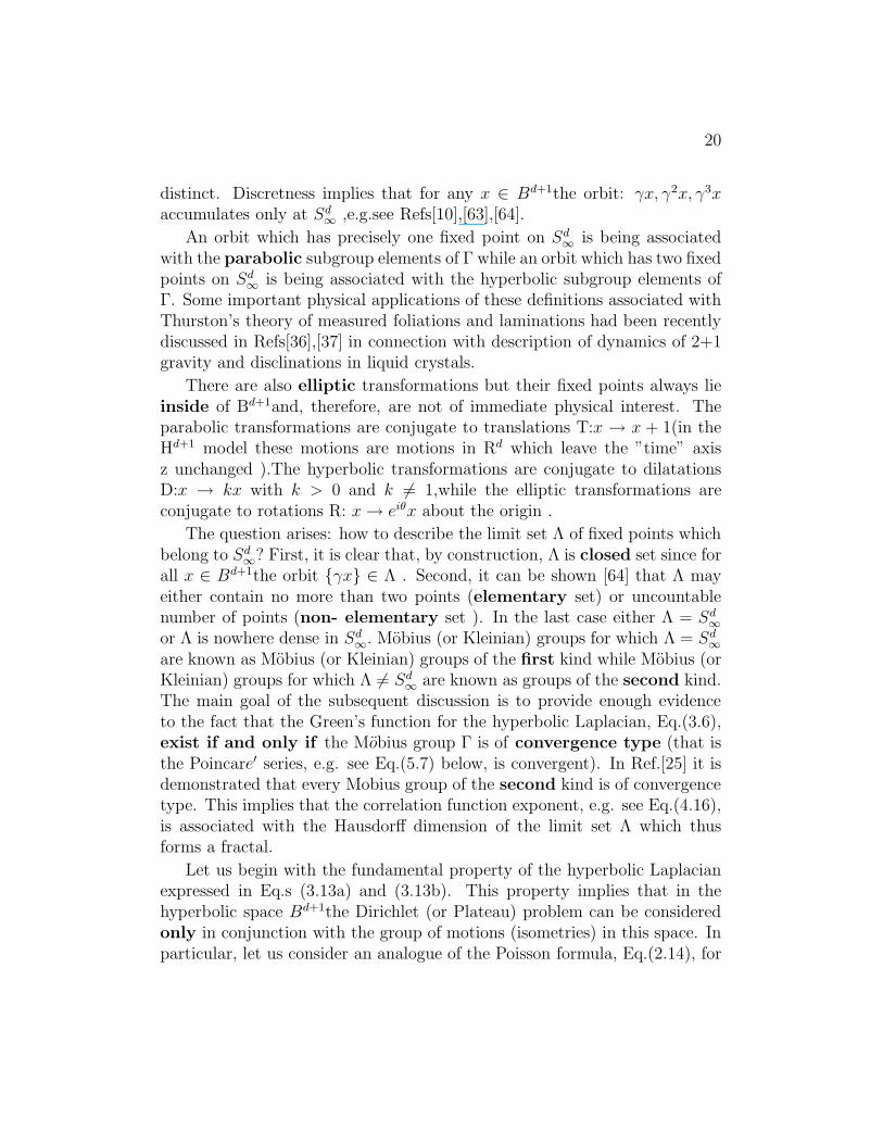
∞ and passing through point x ∈ Bd+1asdepicted in Fig.1

Using the cosine theorem for the angle xox′ in the triangle ∆xox′ we obtain,

|x|2 + 1 − 2 |x| cos(xox′) = |x − x′|2

. (5.11)

Alternatively, by using the triangle ∆xoc we get

|x|2 +

∣

∣

∣

∣

w +1

2(1 − w)

∣

∣

∣

∣

2

− 2 |x|

∣

∣

∣

∣

w +1

2(1 − w)

∣

∣

∣

∣

cos(xox′) =1

4(1 − |w|)2.

(5.12)

24

Figure 1: Some geometric relations in the hyperbolic ball model

By eliminating cos(xox′) from these two equations we obtain,

1 + |x|2 − |x − x′|2

2= 1 +

|x|2 − 1

1 + |w|. (5.13)

This result can be equivalently rewritten as

1 − |w|

1 + |w|=

|x − x′|2

|x|2 − 1. (5.14)

The hyperbolic distance ρ(0, w) is known to be [63]

ρ(0, w) = ln

(

1 + |w|

1 − |w|

)

. (5.15)

Accordingly, the Poisson kernel, Eq.(5.10), can be equivalently rewritten as

PH(x, x′) = expαρ(0, w). (5.16)

The hyperbolic Fourier transform can be defined now as [68]

ϕα(x) =1

ωd

∫

Sd∞

dω(x′) expα < x, x′ >ϕ(x′) (5.17)

25

with scalar product < x, x′ > being defined through the hyperbolic distanceρ(0, w) according to Eq.s (5.14),(5.15).

With help of the results just obtained it is possible to give better interpre-tation of the Ahlfors-Thurston Theorem. Indeed, in view of Eq.s(5.3)-(5.5)we obtain,

ϕ(0) =1

ωd

∑

γ∈Γ

∫

Sd∞

dω(x′)

(

1 − |γ(0)|2

|γ(0) − x′|2

)d

χ(x′), (5.18)

where ,without loss of generality, we had put x=0 (i.e.placed the initial pointx at the center of Bd+1) .Surely, |γ(0) − x|2 ≤ 4 since we are dealing withthe ball of unit radius. Therefore, we also have

ϕ(0) <1

ωd

∑

γ∈Γ

∫

Sd∞

dω(x′)(1 − |γ(0)|2)dχ(x′) . (5.19)

Consider now the convergence(or divergence) of the series

Sd =∑

γ∈Γ

(1 − |γ(0)|2)d (5.20)

or, more generally,

Sα =∑

γ∈Γ

(1 − |γ(0)|2)α . (5.21)

Clearly, the last expression is going to be divergent or convergent along with

gα(0, 0) =∑

γ∈Γ

(

1 − |γ(0)|

1 + |γ(0)|

)α

=∑

γ∈Γ

exp−αρ(0, γ(0)) (5.22)

in view of Eq.s (5.15) and (4.19). But the convergence(divergence) of thePoincare′ series , Eq.(5.22), leads us to the results given by Eq.s(5.6)-(5.9).and also earlier stated result, Eq.(4.19).

The results just obtained admit yet another interpretation. Convergence(or divergence) of the series, Eq.(5.22), is associated with existence or nonex-istence of the Green’s function acting in Bd+1as we had mentioned alreadybeforeEq.(5.2). Deep results of Ahlfors[25], Thurston[42], Patterson[40], Beardon[69]

26

and Sullivan [41] state that if the Poincare′ series converges, then the Green’sfunction in Bd+1 exist and the limit set Λ ⊂ Sd

∞ is fractal with areal measureequal to zero but Hausdorff dimension equal to α (in this case α lies at theborder between the convegence and divergence of the series,Eq.(5.22))and,for d=2, α ≤ 2 according to Sullivan[66] and Tukia[67] . Additional veryimportant results related to the limit set Λ were obtained by Beardon andMaskit[10] who had proved the following

Theorem 5.1.(Beardon Maskit) Let Γ be a discrete M obius group ofisometries of H 3, then, if Γ is geometrically finite, the limit set Λ com-prizes of parabolic limit points and conical limit points .

We would like now to explain the physical significance and the meaning ofthese statements. First, by looking at Eq.s(4.12)and (4.16) we conclude thatm2 ≤ 0 (because of the results of Sullivan and Tukia). Second, for the groupΓ to be geometrically finite (in B3) it is required that the fundamentaldomain for Γ is being made of finite sided polyhedron P in B3 (just like forthe Riemann surface of finite genus we should have a finite sided polygon inthe unit disk D whose boundary at infinity is S1

∞). Every hyperbolic manifoldM3 is defined through use of some fundamental polyhedron P so that, in fact[42],

M3 = (B3 ∪ Ω)/Γ (5.23)

where Ω = S2∞ −Λ is the open set of discontinuity of Γ. In general, Ω repre-

sents some collection of Riemann surfaces which belong to the boundary ofM3. This fact has some relevance to problems associated with 2+1 gravityas explained in Ref.[27],[28]. The boundary set Ω is not accessible dynam-ically however since it is a complement of the limit set Λ in S2

∞. Based inthe information provided, study of the hyperbolic 3-manifolds is equivalentto study of the action of discrete subroups Γ of the Mobius group G on H3(orB3). In particular, if the quotient, Eq.(5.23), is compact, then Γ is said to becocompact and if the quotient, Eq.(5.23), has finite invariant volume, thenΓ is said to be cofinite. Incidentally, if Γ contains parabolic subgroups, thenΓ is not cocompact. As it was shown by Thurston[42](for some illustrations,please, see also Ref.[70]), complements of most of knots embedded in S3areassociated with the hyperbolic 3-manifolds. Accordingly, if CFT are to beassociated with knots/links (e.g.see Refs[3],[5],[6]), then the correspondingcomplements of such knots/links, most likely, should be associated with thehyperbolic 3-manifolds. Moreover, the spectral characteristics of different

27

Figure 2: A typical Z-cusp in the upper half space model realization of H3

hyperbolic manifolds should be different as well [19]. This difference shouldbe also connected with difference in fractal dimensions of the correspond-ing limit sets which, in turn, will correspond to different type (universalityclasses)of the CFT. Conversely, given the fractal dimension of the limit setΛ , is it possible to determine the Kleinian (or Mobius )group (or groups)which is associated with this limit set ? Evidently, this problem is morecomplicated than the direct one. Nevertheless, the above discussion is notlimited to H3 ( or B3) and, therefore, it becomes potentially possible to studyand to classify boundary CFT in dimensions higher than two. More on thissubject is presented in sections 7 and 8.

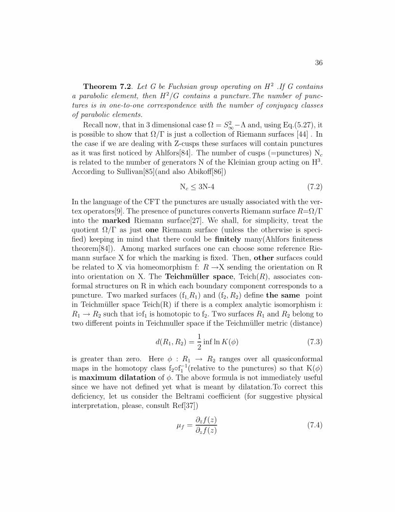
Let us now give the precise definitions of parabolic and conical limit pointswhich were mentioned in the theorem by Beardon and Maskit stated above.An extensive discussion of both parabolic and conical limit points (and sets)could be found in Ref.[71]. From this reference we find that ”for any discretegroup the set of bounded parabolic points and the set of conical limit pointsare disjoint”. Given this, and recalling that the parabolic transformationsare associated with translations we are left with the following two options(inthe case of H3) : a)either the parabolic subgroup has just one generator oftranslations so that the ”fundamental polyhedron” is the region between twoparallel planes as depicted in Fig.2.

28

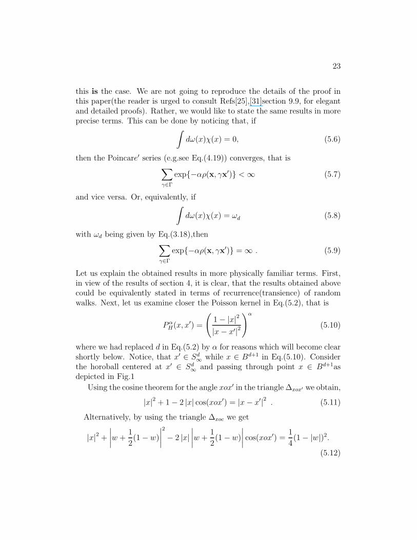
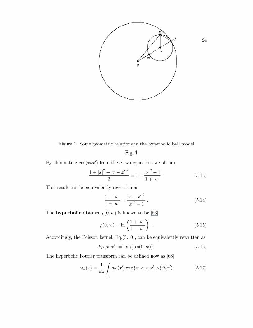
Figure 3: A typical Z⊕Z type cusp in the upper half space realization of H3

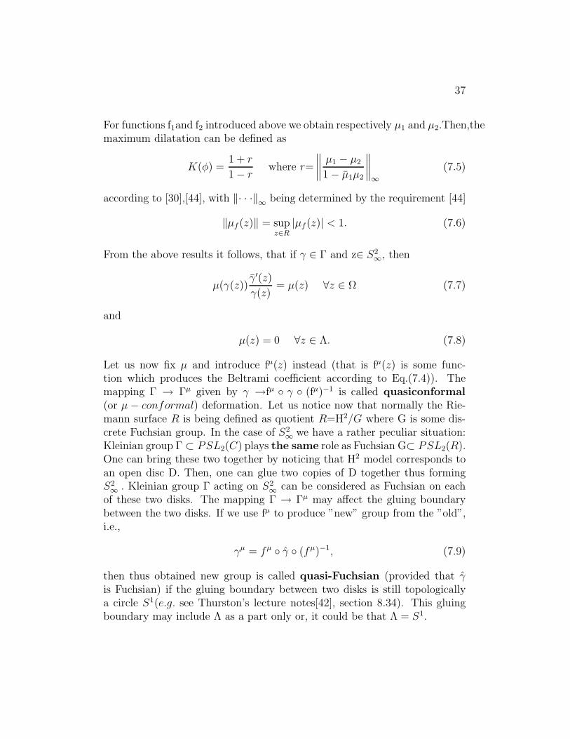
Such construction is called rank 1 ( or Z- cusp). Evidently,topologicallymotion ⊥ to these planes is the same as motion on the circle S1 as it wasrecently discussed at some length in Ref[70]in connection with some problemsin polymer physics. Accordingly, such parabolic subgroup is isomorphic to Zor,.b) the parabolic subgroup has two generators so that the ”fundamentalpolyhedron” is the region defined by the transverse pairs of parallel planes,as depicted in Fig.3

Such construction is called rank 2 ( or Z⊕Z ) cusp. Topologically, motion⊥ to such planes is being associated with the motion on the torus. Therestriction to have only Z and Z⊕Z cusps for hyperbolic 3-manifolds imposesvery important restrictions on the boundary CFT to be discussed in section7.

The conical limit set is not specific to the hyperbolic spaces. Accordingto Ref.[39], in the case of Euclidean half-space Hn for which the typical pointy=(x,z), z>0, x∈ Rn−1,the conical limit set Γα(a) is defined through

Γα(a) = (x, z) ∈ Hn : |x − a| < αz. (5.24)

Geometrically, Γα(a) is a cone as depicted in Fig.4 with vertex a and axis ofsymmetry parallel to z-axis.

A function u defined on Hn is said to have nontangential limit L ata ∈ Rn−1 if for every α > 0, u(y) → L as y → a within Γα(a). The term

29

Figure 4: The light cone associated with the conical limit set point locatedat the boundary of hyperbolic space

”nontangential” is being used because no curve in Γα(a) that approaches acan be tangent to ∂Hn = Rn−1. It is quite remarkable that such nontangentialbehavior is being observed already for harmonic functions on Euclidean half-space Hn[39] .Use of stereographic projection allows us to formulate the sameproblem in the Euclidean ball Bn. Respectively, exactly the same definitionsare extended to Hd+1 and Bd+1.Specifically, in the case of Bd+1 model onecan say that x ∈ Bd+1 belongs to the cone at ξ ∈ Sd

∞ of opening λ and,further, |x − ξ| < 2 cos λ . Analogously to Eq. (5.24), one can write

|x − ξ| < α(1 − |x|), α > 0. (5.25)

With such background,we would like discuss in some detail the spectral the-ory of hyperbolic 3-manifolds. This is accomplished in the next section.

6. Spectral theory of hyperbolic 3-manifolds

In section 3 we had discussed the eigenvalue equation, Eq.(3.7), so that,naively, one might think that this equation provides the complete answer to

30

the question about the spectrum of hyperbolic Laplacian . This is not true,however. Surprisingly, this problem still remains a very active area of researchin mathematics. For a comprehensive and very up to date introduction tothis field, please, consult Ref[28]. The fact that the spectral theory of hyper-bolic Laplacians is absolutely essential for understanding of the spectrum ofHausdorff dimensions of the limit set Λ was realized already by Patterson[72]long time ago. Since, even now, the spectrum issue is not completely settled,we would like only to give an outline of the current situation leaving most ofthe details for future work.

In his 1987 paper[70] Sullivan had stated the Theorem (2.17)(numerationtaken from his work)which he calls the Patterson-Elstrodt theorem( inciden-tally, the recent monograph, Ref[28], is written by Elstrodt ). Based on theresults of previous sections it can be formulated as follows:

Theorem 6.1.(Patterson-Elstrodt-Sullivan).

Let

−∆hϕ = λϕ (6.1)

be the eigenvalue problem for the hyperbolic Laplacian on Md+1 = Hd+1/Γthen, the lowest eigenvalue λ0(M

d) satisfies

λ0(Md+1) =

d2

4if α ≤ d

2

α(Γ)(α(Γ) − d) if α ≥ d2

(6.2)

where α(Γ) is the ”critical” exponent of the Poincare′ series, Eq.(4.19) orEq.(5.22).

By looking at Eqs.(4.11),(4.12), these results can be restated as

m2 =

λ0 if α ≥ d2

−d2

4if α ≤ d

2.

(6.3)

Additional work by Patterson[62] indicates that, at least for M3, 0 < α ≤ 2.In view of this , by looking at Eq. (4.12), it is reasonable to consider both”+” and ”-” branches of solution for α , provided that −d2

4< m2 ≤ 0. This

possibility, indeed, had been recognized in Ref.[75]. The results obtained byLax and Phillips[76] (and also by Epstein[77]) indicate that for 3-manifoldswithout parabolic cusps the spectrum of -∆h acting on L(M3) normedmetric Hilbert space is of the form:

λ0, ..., λk ∪ [d2

4,∞) (6.4)

31

where

0 < α(d − α) = λ0 < λ1 < ... < λk <d2

4(6.5)

are eigenvalues of finite multiplicity and λ0 has multiplicity one. Moreover,the part of spectrum [d2

4,∞) is absolutely continuous (i.e.for m2 ≤ −d2

4the

spectrum is continuous). The problem with Lax-Phillips[76] and Epstein[77]works lies, however, in the fact that the explicit form of the discrete spec-trum had not been obtained. Only the existence of such possibility had beenproven.

Remark 6.2. In view of Beardon-Maskit Theorem (section 5) one can-not by pass careful study of the spectrum of hyperbolic Laplacian for somediscrete subgroups Γ of Mobius group G if one is interested in finding thecorrect fractal dimension of the limit set Λ .

For the sake of applications to statistical mechanics (e.g.see section 7)one is also interested in spectral properties of 3-manifolds with paraboliccusps. This can be intuitively understood already now based on the followingarguments. If we would choose the sign ”-” in Eq. (4.12) (which,by the waywould produce ”+” sign in front of Eq. (4.16), then for m2 in the range−d2

4≤ m2 < 0 we would have α in the range 0 < α ≤ 1 for d=2. This

range is of interest since it covers all physically interesting CFT discussed inthe literature[9]. If α is to be associated with the Hausdorff dimension of thelimit set Λ, then according to Sullivan ,e.g.see Theorem 2 of Ref.[66], only 3manifolds with no cusps or rank 1 (Fig.2) cusps will yield α in the desiredrange. The spectral theory of hyperbolic manifolds with cusps is still underactive development in mathematics[29]. Therefore, we would like to restrictourself with some qualitative estimates of the spectrum based on topologicalarguments. Here and below we shall discuss only the case d=2 (i.e.H3 or B3).This restriction is by no means severe. It is motivated only by the fact thatmore explicit analytical results are available for this case in mathematicalliterature. This, however, does not imply that the case d=2 is more specialthan say d=3. For instance, Burger and Canary [78] had demonstrated thatfor any d>1 the Hausdorff dimension α is bounded by

α ≤ (d − 1) −Kd

(d − 1)vol(C(Md))2(6.6)

where Kd and C(Md) are some d-dependent constants which can be calcu-lated in principle .

32

In the case if hyperbolic manifold M3 is topologically tame (that is it ishomeomorphic to the interior of a compact 3 manifold), then Theorem 2.1.of Canary et all [79] states that

Theorem 6.3.(Canary, Minsky and Taylor) If M 3 is topologically tamehyperbolic 3-manifold, then the lowest eigenvalue λ0 of the hyperbolic Lapla-cian (-∆h) is given by λ0 = α(2−α) unless α < 1, in which case λ0(M

3) = 1.

Remark 6.4 As before, α is the Hausdorff dimension of the limit set Λ.

Remark 6.5 From the above Theorem 6.3. it appears that the resultsof section 4 become invalid when α < 1 since Eq.(4.12) cannot be used. Thesituation can be easily repaired as it is explained in the next section.

Remark 6.6. Theorem 6.3.allows us to obtain the following additionalestimates based on recent results by Bishop and Jones[43].

Theorem 6.7.(Bishop and Jones). Let Γ be any discrete M obius groupand let M3 = (B3∪Ω)/Γ . Suppose that the lowest eigenvalue λ0 is nonzero.Then,there are constants C < ∞ and c > 0 (depending upon λ0 only)so that forany x,y with ρ(x,y) ≥ 8 we have

G(x,y) =

∞∫

0

dtG(x,y; t) ≤C

λ0exp−cρ(x,y) (6.7)

where ρ(x,y) is the hyperbolic distance between x and y and c=min18λ0,

14.

Corollary.6.8.Using this result in combination with Eqs.(4.18),(4.19)and the Theorem 6.3. we obtain, α = λ0

8= 1

8. If this result is substituted

into Eq.(4.16) we obtain the exact result for two-point correlation functionof two dimensional Ising model.

Remark 6.9.The theorem of Bishop and Jones depends crucially on theexplicit form for the heat kernel G(x,y; t) in H3. Quite recently, Grigori’yanand Noguchi[80] had obtained explicit formulas for the heat kernel for anydimension of hyperbolic space. This opens a possibility to obtain an analogueof inequality (6.7) in any dimension following ideas of Bishop and Jones.

With all plausibility of the Corollary 6.8. it remains to demonstrate thatsuch substitution of α into Eq. (4.16) is indeed legitimate.To this purposewe would like to provide a somewhat different interpretation of Eq.(4.16) inorder to demonstrate that Eq.(4.17) makes sense even without arguments as-sociated with Plateau/Dirichlet problem. To begin, we would like, by analogywith the Liouville theorem in standard textbooks on statistical mechanics,to construct a measure associated with the geodesic flow in hyperbolic space.

33

Figure 5: Geometry of geodesics in the ball model of hyperbolic space

Following Ref.[25] ,we would like to associate with each point x ∈ Bd+1 ≡B a unit vector ξ ∈ Sdof directions. This vector plays the same role as veloc-ity v in conventional statistical mechanics. Indeed,∀v 6= 0 one can constructa vector ξ= v

|v|and then proceed with standard development. The Mobius

group Γ is acting on the phase space T(B)=B×S according to the rule

(x, ξ) →

(

γx,γ

′

(x)

|γ′(x)|ξ

)

, ∀γ ∈ Γ. (6.8)

The invariant phase space volume element dΩ is given therefore by

dΩ = dxhdω(ξ) (6.9)

with dω(ξ) being a spatial angle measure and dxh being an element of a hy-perbolic volume. The above chosen variables may not be the most convenientones. More convenient are variables associated with actual location of theends of geodesics u and v on Sd

∞.This situation is depicted in Fig.5

It is clear, that ∀x ∈ B one can select a geodesic which passes through x.To this purpose it is not sufficient to assign u and v on Sd

∞ but, in addition,one has to provide a location α(u, v) of the midpoint for such geodesics. Let

34

s be the directional hyperbolic distance between α and x, then, one should beable to find a correspondence between (x,ξ) and (u, v, s), that is one shouldbe able to find a diffeomorphism between B × S and S × S × R, i.e.oneexpects to find an explicit form of the function f(u, v) which enters into theexpression for the volume element given below:

dΩ = dxhdω(ξ) = f(u, v)dω(v)dω(u)ds (6.10)

A simple argument given in Ref[25] produces

f(u, v) =G

|u − v|2d(6.11)

with G being some normalization constant. Looking now at Eq. (3.22), it isclear, that one can now replace it with

D[ϕ] =

∫

dΩ

dsϕ0(u)ϕ0(v) . (6.12)

It is also clear, in view of the transformation properties of the functionϕ0given by Eq.(4.14), that, in general, one can replace Eq.(6.12) with

D[ϕ] = G

∫

ϕ0(u)ϕ0(v)

|u − v|2α dω(v)dω(u) (6.13)

where the exponent α is associated with the Hausdorff dimension of thelimit set Λ .This is indeed the case, e.g.see page 286 of Ref[64]. Thus, theexponent α in Eq. (6.13) is the same as the exponent α in Eq. (5.22). Thisobservation provides the necessary support to the claims made after Eq.(6.7).

Given all above, the obtained results show no apparent connections withthe existing conformal field theories. We would like to correct this deficiencyin the next two sections.

7. Connections with the existing formalism of CFT

In section 5 we had introduced Z and Z⊕Z cusps, e.g. see Figs 2,3.According to Sullivan[66],only 3-manifolds with no cusps or just Z-cusps willproduce limit sets Λ with Hausdorff dimension α in the range 0 < α ≤ 1.Naively, it means, that only consideration of the CFT on the strip with

35

periodic boundary conditions(thus making it a cylinder) will yield the criticalexponents for two point correlation functions in the above range. This caseis, indeed, frequently discussed in physics literature[9]. For the strip of widthL use of the conformal transformation

z′ = w(z) =L

2πln z (7.1)

converting strip of width L to the entire complex plane (rigorously speaking,we are dealing here with C\0 complex plane[81]). Although the abovediscussion appears to be plausible ,the description of Z-cusps (as well as Z⊕Zcusps ) is actually considerably more sophisticated. In this paper we onlyprovide a brief outline of what is actually involved reserving full treatmentfor future publications.

In section 5 we had noticed that Λ may contain no more than two limitingpoints (elementary set) or infinite number of points (non-elementary set).The Kleinian groups which are associated with the elementary limit sets areknown [8], [31] and, basically, are reducible to the following list:

1) a parabolic infinite cyclic Abelian group Γ : z → z + 1;

2) a parabolic rank 2 Abelian group Γ : z → z + 1, z → z + τ ; Im τ > 0;

3) a loxodromic cyclic group Γ : z→ λz with λ ∈ C\0, 1.

Let now M3 be some 3-manifold and let M(0,ε) be a subset of pointsp ∈ M3 such that there is a closed nontrivial curve passing through p whosehyperbolic length l is less than ε. Then, if ε < 2r0 where r0 is some known(Margulis)constant, the M(0,ε) part of M3 (the ”thin part”) is a quotientH3/Γ where Γ is just one of these three elementary groups. The complementof M(0,ε) in M3 is called ”thick” part. The above construction is not limitedto M3and is applicable to any Md+1(with Margulis constant being, of course,different for different d’s). The ”thin” part is associated with Z and Z⊕Zcusps.

Remark 7.1.Recently, we had briefly considered the ”thick ” -”thin” de-composition of hyperbolic 3-manifolds in connection with dynamics of 2+1gravity [36], [37]. For a comprehensive mathematical treatment of these is-sues, please, consult Ref[42],[71],[82].

To realize, that the ”thin” part is associated with Z cusps it is sufficientto look at H2 model of hyperbolic space first. In this case, the followingTheorem can be proven[83]

36

Theorem 7.2. Let G be Fuchsian group operating on H 2 .If G containsa parabolic element, then H 2/G contains a puncture.The number of punc-tures is in one-to-one correspondence with the number of conjugacy classesof parabolic elements.

Recall now, that in 3 dimensional case Ω = S2∞−Λ and, using Eq.(5.27), it

is possible to show that Ω/Γ is just a collection of Riemann surfaces [44] . Inthe case if we are dealing with Z-cusps these surfaces will contain puncturesas it was first noticed by Ahlfors[84]. The number of cusps (=punctures) Nc

is related to the number of generators N of the Kleinian group acting on H3.According to Sullivan[85](and also Abikoff[86])

Nc ≤ 3N-4 (7.2)

In the language of the CFT the punctures are usually associated with the ver-tex operators[9]. The presence of punctures converts Riemann surface R=Ω/Γinto the marked Riemann surface[27]. We shall, for simplicity, treat thequotient Ω/Γ as just one Riemann surface (unless the otherwise is speci-fied) keeping in mind that there could be finitely many(Ahlfors finitenesstheorem[84]). Among marked surfaces one can choose some reference Rie-mann surface X for which the marking is fixed. Then, other surfaces couldbe related to X via homeomorphism f: R →X sending the orientation on Rinto orientation on X. The Teichmuller space, Teich(R), associates con-formal structures on R in which each boundary component corresponds to apuncture. Two marked surfaces (f1,R1) and (f2, R2) define the same pointin Teichmuller space Teich(R) if there is a complex analytic isomorphism i:R1 → R2 such that if1 is homotopic to f2. Two surfaces R1 and R2 belong totwo different points in Teichmuller space if the Teichmuller metric (distance)

d(R1, R2) =1

2inf ln K(φ) (7.3)

is greater than zero. Here φ : R1 → R2 ranges over all quasiconformalmaps in the homotopy class f2f

−11 (relative to the punctures) so that K(φ)

is maximum dilatation of φ. The above formula is not immediately usefulsince we have not defined yet what is meant by dilatation.To correct thisdeficiency, let us consider the Beltrami coefficient (for suggestive physicalinterpretation, please, consult Ref[37])

µf =∂zf(z)

∂zf(z)(7.4)

37

For functions f1and f2 introduced above we obtain respectively µ1 and µ2.Then,themaximum dilatation can be defined as

K(φ) =1 + r

1 − rwhere r=

∥

∥

∥

∥

µ1 − µ2

1 − µ1µ2

∥

∥

∥

∥

∞

(7.5)

according to [30],[44], with ‖· · ·‖∞ being determined by the requirement [44]

‖µf (z)‖ = supz∈R

|µf(z)| < 1. (7.6)

From the above results it follows, that if γ ∈ Γ and z∈ S2∞, then

µ(γ(z))γ′(z)

γ(z)= µ(z) ∀z ∈ Ω (7.7)

and

µ(z) = 0 ∀z ∈ Λ. (7.8)

Let us now fix µ and introduce fµ(z) instead (that is fµ(z) is some func-tion which produces the Beltrami coefficient according to Eq.(7.4)). Themapping Γ → Γµ given by γ →fµ γ (fµ)−1 is called quasiconformal(or µ − conformal) deformation. Let us notice now that normally the Rie-mann surface R is being defined as quotient R=H2/G where G is some dis-crete Fuchsian group. In the case of S2

∞ we have a rather peculiar situation:Kleinian group Γ ⊂ PSL2(C) plays the same role as Fuchsian G⊂ PSL2(R).One can bring these two together by noticing that H2 model corresponds toan open disc D. Then, one can glue two copies of D together thus formingS2∞ . Kleinian group Γ acting on S2

∞ can be considered as Fuchsian on eachof these two disks. The mapping Γ → Γµ may affect the gluing boundarybetween the two disks. If we use fµ to produce ”new” group from the ”old”,i.e.,

γµ = fµ γ (fµ)−1, (7.9)

then thus obtained new group is called quasi-Fuchsian (provided that γis Fuchsian) if the gluing boundary between two disks is still topologicallya circle S1(e.g. see Thurston’s lecture notes[42], section 8.34). This gluingboundary may include Λ as a part only or, it could be that Λ = S1.

38

Recently, Canary and Taylor [46] had proved the following remarkabletheorem.

Theorem 7.3.(Canary and Taylor). Let Γ be a nonelementary finitelygenerated Kleinian group and let Λ denote its limit set. If the Hausdorffdimension α of Λ is less than one, then Γ is geometrically finite and hasa finite index subgroup which is quasiconformally conjugate to a Fuchsiangroup of the second kind .

Remark 7.4. Recall[87], that for the Fuchsian groups of the secondkind the limit points are nowhere dense on S1.Since, according to results ofsection 6, we are interested mainly in the α−domain given by 0 < α ≤ 1,we notice that we have to deal with the quasiconformal deformations of S1

associated with Fuchsian groups of the second kind.

For completeness, we would like also to provide the results related mainlyto the Fuchsian groups of the first kind for which the limit set Λ coincideswith S. These are summarized in the following

Theorem 7.5.(Canary and Taylor[46]) Let Γ be a nonelementary finitelygenerated Kleinian group and let Λ denote its limit set. If α = 1, then Γeither a function group with connected domain of discontinuity or containsa subgroup of index at most 2 which is the Fucsian group of the first kind.Alternatively, if α = 1 and Γ is geometrically finite, then either Γ has a finiteindex subgroup which is quasiconformally conjugate to a Fuchsian group ofthe second kind or Γ contains a subgroup of index at most 2 which is theFuchsian group of the first kind.

Remark 7.6.Much earlier Bowen[88] had proven an analogous theoremfor the Fuchsian groups of the first kind. According to Bowen, the Hausdorffdimension of Λ is greater than one. Since Bowen’s proof is nonconstructive,there is no way to estimate, based on his results, to what extent α is largerthan one. Thus, there is no contradiction between Theorem 7.5. and Bowen’sresults since α can be infinitesimally close to 1.

Remark 7.7.For the case of Fuchsian groups of the first kind it is known[88], that Ω/Γ consists of exactly two Riemann surfaces :one for each diskD. It is also known[45], that for the Fuchsian group of the second kind Ω/Γis made of just one Riemann surface so that S2

∞ is boundary at infinity forthis surface.

In mathematics literature[31] a finitely generated non elementary Kleiniangroup which has just one invariant component Ω is called function group.If, in addition, Ω is simply connected, then such group is called B-group.

39

More complicated Kleinian groups could be constructed from simpler onesand B-group is one of the main building blocks in such construction[90].

Remark 7.8.In string theory (and, therefore, in the CFT)the Schottky-type groups are being used[91]. Schottky group is a function group but nota B-group [31].

Remark 7.9. There is one-to one correspondence between the quasicon-formal deformations of Kleinian groups and quasisometric deformations ofhyperbolic 3-manifolds. The theory is not limited to 3-manifolds, however,and can be considered for any d≥ 2. More specifically, there is a

Theorem 7.10. For a quasiconformal automorphism f of S2∞ compatible

with a Kleinian group Γ, there exist a quasi-isometric automorphism F of H 3

which is an extension of f and which is compatible with Γ, namely, FγF∈Mob(B3) for any γ ∈ Γ.

Proof : Please, consult Ref.[31] (page 157).

Remark 7.11.The above theorem follows directly from the discussionrelated to Eq.s (7.7)–(7.9) and for additional details and motivations, please,consult the work by Bers, Ref.[45].

Remark 7.12.The above Theorem is applicable to the case when, insteadof S2

∞, we use S1∞(taking into account the results on Canary and Taylor,

Theorems 7.3 and 7.5)

The observations presented above allow us to make a direct connectionwith the existing results associated with 2 dimensional CFT. To begin, letus notice that if we would have S1

∞ as limit set Λ for the Fuchsian groups ofthe first kind, then, according to Eq. (7.8) we could not use the quasicon-formal mapping and, accordingly,we would be stuck with just one conformalstructure. This fact is known in mathematics as Mostow rigidity theorem.Usually, this theorem is applied to spaces of dimensionality ≥ 3 (for moredetails,please,see section 8).At the same time, if we consider Fuchsian groupsof the second kind, then, we need to deal with maps of S1

∞ acting on someopen intervals (since Λ is closed set) of S1

∞. This is not exactly the situationwhich is known in physics literature. Indeed, in physics literature on CFTone is dealing with the Virasoro algebra. Let us recall how one can arriveat this algebra. Following Ref.[56], let us consider the group G=DiffS1 oforientation preserving diffeomorphisms of S1

∞. Let α1(z) and α2(z) be twoelements of G, then the group composition law can be defined by

α1 α2(z) = α1(α2(z)) , z = expiθ. (7.10)

40

The representation of the group G is defined according to the following pre-scription:

U(α)f(z) = f(α−1(z)), (7.11)

where the operator U(α) acts on the vector space of smooth complex-valuedfunctions on S1

∞.The explicit form of the operator U(α) can be easily foundif one notices that

α(z) = z(1 + ε(z)) = z +∞∑

n=−∞

εnzn+1, εn → 0+. (7.12)

Using this expansion and keeping only terms up to 1st order in εn we obtain,

U(α)f(z) = f(z −∞∑

n=−∞

εnzn+1) = (1 +

∑

n

εndn)f(z) (7.13)

with operator dn given by

dn = −zn+1 d

dz= i expinθ

d

dθ. (7.14)

The operators dn form a closed Lie algebra V ectS1 described in terms of thefollowing commutator

[

dm, dn

]

= (m − n)dm−n (7.15)

The central extension of this algebra (to be discussed later in this section)produces the Virasoro algebra. V ectS1 contains a closed subalgebra formedby d0, d1 and d−1 corresponding to the infinitesimal conformal transforma-tions of the extended complex plane S2=C ∪ ∞ caused by the action ofPSL(2, C). Thus, even though we had started with diffeomorphisms of thecircle, we ended up with the automorphisms of the extended complex plane.The question arises: is such extension unique ? The answer is: ”no” ! Be-cause of this negative answer, there is a real possibility of extension of theoperator formalism of 2d CFT to higher dimensions. This issue is going tobe discussed in the next section. For the time being,we would like to explainthe reasons why the answer is ”no”.

Following Ahlfors[92], and, more recently, Gardiner and Sullivan[93],wewould like to consider a quasisymmetric mapping (to be defined below) of the

41

disk D to itself which induces a topological mapping of the circumference,i.e. S1

∞. To this purpose it is convenient to use a conformal transformationwhich converts the disk model to the upper halfplane Poincare′ model of thehyperbolic space H2. Next, it is convenient to select points x,x-t, and x+t onthe real line R (corresponding to S1

∞) so that the mapping h(x) satisfies theM-condition

M−1 ≤h(x + t) − h(t)

h(x) − h(x − t)≤ M (7.16)

Let h be a homeomorphism mapping of an open intrerval I of the real axisinto the real axis. Then, h is quasisymmetric on I if there exist a constantM such that the inequality (7.16) is satisfied for all x-t, x, x+t in I. Thusdefined quasisymmetric mapping forms a group(which we shall denote as QS)which obeys the same composition law as given by Eq.(7.10) (except now zis on the real line). The real line R is the universal covering of the circle. Theexponential mapping, exp (2πiθ), induces an isomorphism between R/Z andS1. The homeomorphism h(x) of S1which is characterized by the properties[93]

h(0) = 0, h(x) + 1 = h(x + 1)

can be lifted to a homeomorphism h(x) of R which obeys the following in-equalities:

1 − ε(t) ≤h(x + t) − h(x)

h(x) − h(x − t)≤ 1 + ε(t), (7.17)

where ε converges to zero with t.

It is easy to check that this result is consistent with Eq.(7.12) and, there-fore, the group G=DiffS1 is called the group of symmetric homeomor-phisms. G is proper subgroup of QS[93]. Looking at Eq.(7.5) and identi-fying r with ε(t) we conclude, that the subgroup G has boundary dilatationasymptotically equal to one. That is such transformation do not cause thedeformations of hyperbolic 3-manifolds. The above deficiency of the group Gwas recognized and corrected in the fundamental work by Nag and Verjovsky[48]. Below, we would like to provide the summary of their accomplishmentsin the light of results just described and with purpose of extension of these re-sults in section 8. In order to do so, we still need to make several observationsrelated to QS group. Let us begin with

42

Theorem 7.13.(Ahlfors-Beurling[94]) Assume h is homeomorphism ofR .Then, h is quasisymmetric if, and only if, there exists a quasiconformalextension h of h to the complex plane . If h is normalized to fix three points,say 0,1 and ∞, then h is quasisymmetric with constant M. The quasiconfor-mal extension h can be selected so that its dilatation K is less than or equalto c1(M) where c1(M) → 1 as M → 1.

Remark 7.14. The symmetric homeomorphism α(z) by contrast fixesonly one point: z=0. Some explicit examples of construction of h are givenin the papes by Carleson[95] and Agard and Kelingos [96].

Remark 7.15.Because c1(M) → 1 when M→ 1 any symmetric home-omorphism of S1 can be approximated by quasisymmetric one. This is themost important fact facilitating development of conformal field theories be-yond 2 dimensions.

Remark 7.16. Construction of h is closely related to study of maps ofthe circle as it is known in the theory of dynamical systems[97]. Evidently,oneis interested in maps which map points ∈ Λ to points in Λ and (or), alter-natively, in maps which map points in Ω to points in Ω. Notice, that undersuch conditions the Lie algebra V ectS1can always be constructed since itsconstruction requires only existence of some open interval around any pointz∈ Ω. But, by definition, the set Ω is open.

Let us discuss now the issue of central extension of V ectS1. The needto introduce the central extension of the Lie algebra V ectS1 is by no meansintrinsic just for this group. Already Schur developed general method of con-structing projective representations of finite groups about a hundred yearsago. The extension of his method to Lie groups is relatively straightforwardand is wonderfully presented in the book by Hamermesh[98]. The compre-hensive up to date summary of results in this direction could be found inthe encyclopedic work, Ref[99]. It is not our purpose to provide a review ofthese results. We would like here to explain the physical motivations leadingto the projective representations of Lie groups since the central extension isdirectly related to construction of these projective representations.

As is well known, there are actually two different ways to solve quantummechanical problems. The first one comes from mathematics of solving of2nd order ordinary differential equations while the second one comes fromthe algebraic (group-theoretic) approach to the same problem. The projec-tive representations are naturally associated with the second approach. Inparticular, let g1 and g2 be two elements of some Lie group G. One can think

43

of unitary representations associated with group G. That is one can try tofind a unitary operator U(g), g ∈ G, such that

U(g1)U(g2) = U(g1 g2) . (7.18)

Such representation of the group G is called vector representation(by anal-ogy with finite dimensional space where the role of U is being played by finitematrices acting on vectors). In quantum mechanics, as is well known, thewave function is determined with accuracy up to a phase factor. This meansthat, along with Eq.(7.18), one can think of alternative way of writing thecomposition law, e.g.

U(g1)U(g2) = ω(g1, g2)U(g1 g2) . (7.19)

Surely, one should require |ω(g1, g2)| = 1. This then allows us to write thefactor ω(g1, g2) as

ω(g1, g2) = expiξ(g1, g2) (7.20)

The phase factor ξ(g1, g2) is associated with the topology of the underlyinggroup space. Finally, in our case of DiffS1 the action of the operator U(g)on the vector f(z) is given by Eq.s(7.11)-(7.13) so that the composition law,Eq.(7.19), along with definition, Eq.(7.20), allows us to obtain in a ratherstandard way[100] the centrally extended Lie algebra V ectS1 which is knownas Virasoro algebra and it is given by

[

dm, dn

]

= (m − n)dm−n + ca(m, n) (7.21)

where c is some number (related to the central charge) and the two-cocyclea(m, n) is related to ξ(g1, g2) and can be easily obtained explicitly by usingthe Jacoby identity and the commutation relations given by Eq.(7.21). Thefinal result can be written in the form suggested by Kac[56]

[

dm, dn

]

= (m − n)dm−n + δm,n(m3 − n)

12c (7.22)

with c being the central charge. For the developments presented below inthis paper it is very important to recognize the physical reason for theemergence of the two-cocycle a(m,n). Nag and Verjovsky[48] had demon-strated that it is related to the quasisymmetric deformations of the projective

44

structures on S1by diffeomorphisms. These structures were fully classified inRef[101]. Basically, they are associated with group of Mobius transforma-toions PSL(2,R)

x =ax + b

cx + d(7.23)

on the real line. Study of the deformations of the projective structure onthe line which was initiated by Ahlfors and Beurling[94] was considerably de-veloped by Carleson[95] and Agard and Kelingos[96] and culminated in thework of Nag and Verjovsky[48] . To make our presentation self-contained,we would like now to summarize their results from the point of view of ideaspresented in this section. This summary is needed whenever one is contem-plating about the extension of the existing 2 dimensional results related toCFT to higher dimensions (to be discussed in some detail in the next section).

Consider a quotient T(1)=QS/PSL(2,R) that is the space of ”true” qua-sisymmetric deformations which fix 3 points, e.g.say, 1,-1 and -i on S1, thenT(1) is associated with universal Teichmuller space in a sense of Bers[102].The space M = DiffS1/PSL(2, R) is embeddable inside of T(1). The spaceM can be equipped with the complex structure so that it becomes infinite di-mensional Kahler manifold. For the vectors v =

∑

m

vmdm and w =∑

m

wmdm

tangent to M at some point chosen as the origin one can construct theKahler metric g(v, w). The most spectacular result of Ref [48] lies in theproof of the fact that the Kahler 2-form

ω(v, w) = g(v, Jw), (7.24)

where ω(v, w) =∑

n,m

vnwma(m, n), with a(m, n) being the same as in Eq.(7.21),

(7.22), and Jw being defined through equation

Jw =∑

m

(−i)sign(m)wmdm, (7.25)

coincides with the Weil-Petersson metric,

g(v, w) = W-P(v, w) (7.26)

where W-P(v, w) is the Weil-Petersson (W-P) metric on T(1).The Weil-Petersson metric on Teicmuller space is discussed in sufficient detail in Ref[45].If

45

µ(z)dzdz

is the Beltrami differential,e.g. see Eq.(7.4),and ϕ([ν])(z)dz2 is thequadratic differential (e.g. see Ref[37] for an elementary discussion of quadraticdifferentials) then, the W-P inner product is defined by the following formula

< µ, ϕ[ν] >= W-P(µ, ν) (7.27)

=

∫∫

∆/F

×

∫∫

∆

µ(z)ν(ζ)

(1 − zζ)4dξdηdxdy

with ν → ϕ([ν])(z) being given by

ϕ([ν])(z) =

∫∫

∆

ν(ζ)

(1 − zζ)4dξdη (7.28)

, herez = x+iy , ζ = ξ+iη and ∆ is the unit disk with F beingsome Fuchsiangroup thus making the quotient ∆/F a Riemann surface. In the present caseF≡ 1 as it will be explained shortly. In view of this, one should not worryabout F.

Remark 7.17.a) The Kalerity of W-P metric expressed by Eq.(7.24) hadactually been proven by Ahlfors[49] in 1961. b) In the same paper by Ahlfors,Eq.(7.28) has been derived which differs in sign and numerical prefactor fromEq.(7.28). This, fortunately, plays no role in the final results obtained inRef.[48].

Remark 7.18 Since Eq.(7.28) plays the central role in the rest of calcu-lations presented below,we would like to provide some additional informationrelated to this equation(not contained in Ref[48]) in order to help physicallyeducated reader to appreciate its significance . To this purpose let µf inEq.(7.4) be written as µ(t)(z) = tν(z). Then, it can be shown [44] that forsolution fµ of the Beltrami Eq.(7.4) the following limiting result holds

v[µ](z) = limt→0

fµ − z

t(7.29)

= −1

π

∫∫

H2

ν(z)z(z − 1)

ζ(ζ − 1)(ζ − z)dξdη .

With help of Eq.(7.29) we obtain,

fµ(z) = z + v[µ](z)t + o(t) , t → 0, (7.30)

46

to be compared with Eq.(7.12). From this comparison it follows, that thequasisymmetric vector field v on S1 can be defined as

v = v[µ](z)d

dz. (7.31)

In addition, using Eq.(7.30), we obtain,

d

dzfµ(z) = 1 + t

d

dzv[µ](z) ≡ 1 + tv[µ]′ (7.32)

and also,

d2

dz2fµ(z) = tv[µ]′′ (7.33)

and

d3

dz3fµ(z) = tv[µ]′′′ . (7.34)

The Schwarzian derivative of fµ, z defined by

ϕt[ν(z) = fµ, z =f ′′′(z)

f ′(z)−

3

2

(

f ′′(z)

f ′(z)

)2

(7.35)

can now be constructed so that in the limit t → 0 using Eqs(7.32)-(7.35) weobtain,

ϕt[ν](z) = tv[µ]′′′ + o(t) . (7.36)

Let now µ(t) = µ + tν[z], then we can construct

ϕ[z](z) =ϕt[ν](z) − ϕ0[ν](z)

t(7.37)

= −12

π

∫∫

H2

ν(z)

(ζ − z)4dξdη

where the use was made of Eq.(7.29) in order to perforn z-differentiation ineq.(7.36) explicitly. Obtained result is documented on p.138 of Ahlfors book,Ref[92], and should be compared against Eq.(7.28) upon conversion from H2

plane to the disc ∆. Since it is well known[44] that the Schwarzian derivative

47

acts like a quadratic differential under the transformations which belong tothe Fuchsian group F, we conclude that, indeed, up to unimportant constant(which may differ from −12

πwhen the transformation from H2 to ∆ is made

) Eqs.(7.28) and (7.37) are equivalent.

Next, by combining Eqs.(7.21),(7.24),(7.25) it can be shown, that

g(v, w) = −2ic Re∞∑

m=2

vmwm(m3 − m). (7.38)

In addition, it is possible to show that the Fourier coefficients of v[µ] (and,analogously, w[µ]) defined by Eq.(7.31),are given by

vk =i

π

∫∫

∆

µ(z)zk−2dxdy, (7.39a)

and

wk =i

π

∫∫

∆

ν(z)zk−2dxdy , k ≥ 2. (7.39b)

Using these results in Eq.(7.38), we obtain,

∞∑

m=2

vmwm(m3 − m) = −1

π2

∫∫

∆

×

∫∫

∆

µ(z)ν(ζ)(∞∑

m=2

zm−2ζm−2(m2 − m))dξdηdxdy

(7.40)

Using summation formula

∞∑

m=2

(m3 − m)xm−2 =−1

6(1 − x)4, |x| < 1 (7.41)

in Eq(7.40) we obtain,

g(v, w) = −ic

3π2W-P(µ, ν) (7.42)

with W-P(µ, ν) being defined by Eq.(7.27) were now we have to put F=1.Surely, c can be replaced by ib and we can adjust b in such a way that b

2π2 = c12

in accord with Eq.(7.22).

48

Thus, we have demonstrated, following Nag and Verjovsky[48], that thecentral charge of the Virasoro algebra is directly associated withthe quasisymmetric deformations of ∆ (or H2).In view of this fact, itbecomes possible to consider extensions of the existing formalism to higherdimensions. This is the subject of the next section.

Remark 7.18. Since the Virasoro algebra, Eq.(7.22), with fixed centralcharge provides solution of a particular CFT at criticality, to crossover fromone universality class (given by fixed central charge) to another (given by dif-ferent value of the central charge) Zamolodchikov [103] had developed theory(known in physics literature as c-theorem) which describes the dynamics ofcrossover between different values of central charge. It would be very inter-esting to explain his results by developing ideas of Nag and Verjovsky[48].

8. Beyond two dimensions

In 1968 Mostow[104] proved very important theorem which is known asMostow rigidity theorem. It can be formulated as follows.

Theorem 8.1.(Mostow)Let N=H d+1/Γ be a complete hyperbolic manifold, d≥ 2, and let N

′

=H d+1/Γ′ be some other hyperbolic manifold, then if thereis a quasi-isometric homeomorphism f: N→N

′

, then f is homotopic to anisometry N→N ′ if and only if both Mobius groups Γ and Γ′ are of the firstkind (i.e. Ω = Sd

∞ − Λ = 0,e.g. see section 5).

Remark 8.2.This result could be easily understood in view of Eq.s (7.7)and (7.8). For an additional illustration of the existing possibilities one is en-couraged to look at the paper by Donaldson and Sullivan[105] who establishedthat some closed four-manifolds have infinitely many distinct quasiconformalstructures while others do not admit the quasiconformal structure at all.

Remark 8.3.Mostow rigidity theorem can be viewed as an extensionand ramification of much earlier theorem by Liouville (originally proven in1850)[106] which can be stated as follows.

Theorem 8.4.(Liouville) Let U be some open subset of Rd ∪ ∞ ≡Rd

and let f :U →Rd be a conformal map, then f is just a Mobius transformationfor d≥ 3.

It is because of this theorem, known in physics literature[9], there is awidespread belief that results of two dimensional CFT cannot be extendedto higher dimensions.

49

Remark 8.5. In order to study d dimensional systems at criticality(d≥ 2) one should look for the Mobius groups of the second kind . Then, thequestion arises immediatly : is there an analogue of physically funadamen-tally important Canary-Taylor theorems (Theorems 7.3. and 7.5) in higherdimensions? We are unaware of a comprehensive answer to this question.However, we would like to mention the ”tour de force” papers by Gromov,Lawson and Thurston[107] and also by Kuiper[108] from which it followsthat, at least for groups of isometries of H4 considered in these references,the limit set is a circle S1(actually, nowhere differentiable Julia-like set).

In view of the above lack of Canary-Taylor theorems in higher dimen-sions, we would like to discuss now different methods of study of the limitsets (and their complements) of Mobius groups in dimensions higher than3. To this purpose, using Eqs (5.2)-(5.5) and following McMullen[27](andThurston[42],chapter 11), we define the map :

av : C∞(Sd∞, R) → C∞(Hd+1, R)

or

F(0) ≡ av(f)(0) =1

ωd

∫

Sd

dω(x)f(x) (8.1)

i.e. the map av(f) is the average of f over Sd∞. Using Eqs.(5.2),(5.5), we

obtain:

F(y) = F(γ0) =1

ωd

∫

Sd

dω(x)f(γx) (8.2)

=1

ωd

∫

Sd

dω(x)f(T−1y x)

=1

ωd

∫

Sd

dω(x)∣

∣T ′y(x)

∣

∣

df(x)

=1

ωd

∫

Sd

dω(x)

(

1 − |y|2

|x − y|2

)d

f(x)

= av(γf)(0)

here y∈Hd+1, T−10 = y.

50

Using Eq.s (2.14),(3.7),(3.8),(3.15) and (5.2) we conclude that

∆hav(γf)(0) = 0. (8.3)

That is the avarage av(f) is a harmonic function in hyperbolic metric. Itis clear, that to restore the harmonic function F(x) in Hd+1 it is sufficientto know the function f(x) at the boundary of hyperbolic space, i.e. on Sd

∞(recall the holography principle discussed in section 1)

Let now v(x) be some vector field, v(x) ∈ Sd∞.Then, as before, one can

extend it to the bulk of hyperbolic space by using the prescription:

av(v)(0) =1

ωd

∫

Sd

dω(x)v(x) (8.4)

In the case of functions, av(f) by design provides a continuous functionon Sd

∞∪Hd+1. This is not true for vectors (or tensors in general). In thecase of vectors, one defines the extension operator ex(f) via the followingprescription:

ex(f) = av(f) for scalar fields(functions), (8.5)

ex(v) =d + 1

2dav(v) for vector fields, etc. (8.6)

Being armed with these results we are ready to extend the results of previoussection to higher dimensions. To this purpose, we need to reanalyze Eq.(7.29)first. It is equation for the vector field which is created by deformation ν(ζ).It can be shown, e.g.see pages 196-197 of Ref[44], that

∂

∂zv[µ](z) = ν(z) (8.7)

that is when ν(z) = 0, v[µ](z) is just a holomorphic function which obeysthe Cauchy-Riemann equations. Ahlfors had demonstrated [25]that, thereis an analogue of Eq.(8.7) in higher dimensions. Let fi(x) = vi[µ](x), x ∈Sd∞∪Hd+1then, the higher dimensional analogue of Eq.(8.7) is given by

(Sf)ij =1

2

(

∂fi

∂xj+

∂fj

∂xi

)

−δij

d + 1

d+1∑

k=1

∂fk

∂xk= Ξij(x). (8.8)

51

It can be shown, that Eq.(8.8) is reduced to Eq.(8.7) in two dimensions. Ina special case Ξij(x) = 0 one obtains solution of Eq.(8.8) in the form

f 0i = ai +

∑

j

Aijxj + bix2 − 2(b · x)xi (8.9)

where a and b are some constant vectors and A is a constant matrix which isthe sum of skew-symmetric and diagonal (with the same elements along thediagonal)matrices. Apart from the matrix term in Eq.(8.9), the above resultis identical with that known in physics literature, (e.g.see Ref.[9], Eq.(4.14)).By analogy with Eq.(7.31) in two dimensions (taking into account the be-haviour at infinity[27]) one obtains for the vector field

v(z) = (a + bz + cz2)∂

∂z(8.10)

which clearly obeys V ectS1 Lie algebra, Eq.(7.15), as expected.The centralextension of this algebra given by Eq.s(7.21),(7.22) is not affected by thisfield since for indices 1,0,-1 one has a(m, n) = 0. This is also in completeaccord with Eq.(7.38). This observation has very important consequences.In particular, if one would like to obtain solution to Eq.(8.8) for Ξ 6= 0,then,obviously, the general solution fi is going to be given by

fi = f 0i + ϕi . (8.11)

Hence, physically interesting nontrivial solutions of Eq.(8.8) are given byϕi = fi − f 0

i . This obseravtion can be broadly generalized from the point ofview of cohomology theory to be discussed briefly below. In the meantime,one is faced with the problem of finding solutions to Eq.(8.8) for Ξ 6= 0 .Ahlfors[25] had found a very ingenious way of doing this. To this purpose,he had introduced the operator S∗ adjoint to S. Without going into details ofits explicit form which could be found in his work, the main point of havingsuch an operator lies in selecting such Ξ(s) for which

S∗Ξ = 0 . (8.12)

Then, by analogy with results of sections 2 and 3, one obtains the followingDirichlet-type problem of finding the solutions of the Laplace-like equationin Bd+1 :

ρ−d−3S∗ρd+1Sv = 0 , ρ =1

1 − x2, (8.13)

52

supplemented with the boundary condition

v |Sd∞

= f , x2 = 1 at Sd∞. (8.14)

To solve this equation, one has to assign the vector fields at the boundary.A complete solution which takes into account Eqs.(8.5),(8.6) was obtainedby Reiman[109]. An alternative derivation which uses the theory of pseudo-Anosov homeomorphisms (which we had discussed in connection with dy-namics of 2+1 gravity and textures in liquid crystals[36],[37]) was recentlyobtained by Kapovich[110]. He proved the following

Theorem 8.6.(Kapovich) Suppose that v is a smooth automorphic k-quasiconformal vector field on the open unit ball Bd+1 in Rd+1, d ≥ 2. Thenv admits a continuous tangential extension v∞ to Sd

∞. The vector field v∞

is again a k-quasiconformal vector field on the sphere Sd∞.

Remark 8.7.Recent attempts [1],[111] to extend CFT theories to higherdimensions for technical reasons are limited to even dimensionalities, e.g. 2,4 and 6. The results of Reiman and Kapovich can be used for any d≥ 2.Thisfact is consistent with latest results of Bakalov et al [57].

To have some appreciation of these more general results, our experiencewith two dimensional case discussed in section 7 is helpful. It is also use-ful for development of cohomological methods[112] of study of deformationsof Kleinian (and, in general, Mobius ) groups.We shall follow mainly theideas of Refs[44]and[113] since, in our opinion, they are the most helpfulfor undrstanding of more sophisticated treatments[112], [114] not limited todimension two.

The starting point is Eq.(8.7). If v[µ](z) ≡ F (z) is a vector field, then,naturally, we have to require

F (γ z) = γ′F (z), (8.15)

where γ′ was defined after Eq.(5.4). Following Ref[45], let us call F (z) a ”po-tential” for ν. It is clear, that Eq.(8.7) must be consistent with Eq.(8.15).This imposes some restrictions on the potential F that is we have to de-mand that the combination F (γ z) − γ′F (z) vanishes for any γ ∈ Γ.Define now the function χF (γ) = (F (γ z)/γ′) − F . Taking into accountEqs(7.29),(7.31),(8.7),(8.9) and (8.10), we conclude, that vector χF (γ) shouldbe proportional to that given in Eq.(8.10). At the same time, it should satisfythe one-cocycle condition

χF (γ1 γ2) = (γ2)∗ (χF (γ1)) + χF (γ2) , γ1, γ2 ∈ Γ (8.16)

53

with

γ∗(P ) =P γ

γ′. (8.17)

Indeed, since we have

χF (γ1) =F γ1

γ′1

− F

and

χF (γ2) =F γ2

γ′2

− F,

we expect that

χF (γ1 γ2) =F (γ1 γ2)

(γ1 γ2)′

− F.

Use of these results in Eq.(8.16) produces the result which is well known inthe theory of dynamical systems[97] :

(γ1 γ2)′ = γ

′

1 · γ′

2 . (8.18)

Let W be another potential for ν, then P = W − F is again proportional tothe vector field given by Eq.(8.10). Thus, χW − χF = δ(P ) where δ(P )(γ) =γ∗(P ) − P. Recall now that, according Eq.(7.29), we had defined µ(t)(z) =tν(z). Therefore Eq.(7.9) can be rewritten as γt = f t γ (f t)−1 so thatddt

γt |t=0= γ. By combining this result with Eq.(7.29) we obtain,

df t

dt|t=0= F (z) ≡ f [µ], (8.19)

and also,obviously,

f t γ = γt f t. (8.20)

Differentiating the last equation and, again, taking into account Eq.(7.29)we obtain,

f [µ] γ = γ + f [µ] · γ′. (8.21)

54

This leads us to

χf [µ] =f [µ] γ

γ′− f [µ] =

γ

γ. (8.22)

In view of Eq.(8.15) we observe that the obtained result is nontrivial. Ac-cordingly, if χf [µ] is the vector space Z1 of cocycles and δ(P ) is the vector

space B1 of coboundaries, then the quotient

H1 = Z1/B1 (8.23)

defines the first Eichler cohomology group of Γ, that is the group of non-trivial deformations. With some efforts[113] it is possible to construct thesecond and higher Eihler cohomology groups. Although the above analysisseems quite natural, the higher dimensional generalizations of such cohomo-logical arguments so far had been based on the cohomology theory developedby Eilenberg and MacLane [115],e.g.see Ref[112], which is conceptually sim-ilar but technically a bit different from the Eichler theory[113]. The reasonsfor such limitations of Eichler’s approach are clear : all arguments use twodimensional complex analysis. In our opinion, Eilenberg-MacLane approachis more formal and, hence, allows much lesser use of physical intuition. Thefamous Gelfand-Fuks two- cocycle obtained with help of Eilenberg-MacLanecohomology theory (also in a rather formal way) for the Lie algebra of thevector fields is known to produce the central extension of the V ectS1 Lie al-gebra [58],e.g. see eq.(7.15). Recently, the authors of Ref.[57] had sucseededin consistently extending the cohomological results of Gelfand and Fuks tohigher dimensions (although some work is still in progress).It remains a chal-lenging problem to connect these results with the cohomological results ofJohnson and Millson[112] and Kourouniotis [116] which take explicitly intoaccount deformations of hyperbolic groups. In anticipation of more rigor-ous mathematical results, we would like to present now some more intuitivephysical -type arguments which enable us to provide some answers to theseproblems.

First, we have to think about the higher dimensional analogue of the Liealgebra for the group PSL(2,C). In two dimensions it forms a closed sub-algebra within the Virasoro algebra. For concretness, let us think aboutdescription of 3 dimensional conformal models, i.e.d+1=4 . As it was shownby Cartan[50], the Lie algebra of conformal transformations of Rd+1 is iso-morphic to the Lie algebra of the group O(d+1,1). For our purposes we need

55

actually only the component connected to identity SO0(d+1,1) of O(d+1,1).As it was shown recently by Scannell[60], this group is simultaneously iso-morphic to the group Isom+(Hd+1) which is group of orientation -preservingisometries of Hd+1, the group Mob+(Sd)of orientation -preserving Mobiustransformations of Sd

∞ and the group Isom+(Sd+11 ) of isometries of the de

Sitter space (Sd+11 = v ∈ Rd+2

1 |< v,v >= 1 with Rd+21 being the space

Rd+2 equipped with the signature (d+1,1)). We shall use the last option forreasons which will become obvious momentarily. Incidentally, for d=2 wehave to deal with the group SO(3,1) which is just the Lorentz group isomor-phic to PSL(2,C) as discussed in great detail in Ref[[51]. It is very strikingthat the representations of the Lie group SO(4,1) and, in particular, its con-nected component, describe the spectrum of the hydrogen atom[55]. This factis helpful for treatment of 3d conformal models. From the detailed analysis ofthe de Sitter group performed in Refs[52],[53] it follows, that the Lie algebraof the group SO(4,1) is isomorphic to the direct product of two Lie algebrasof the group SO(3),i.e. so(4, 1)=so(3)⊗ so(3). But it is well known that Liealgebra so(3) can be mapped onto PSL(2,C) (it is intuitively clear since viastereographic projection the sphere S2, on which so(3) acts, is being mappedonto the extended complex plane(on which PSL(2,C) acts) and, indeed, thecommutation relations given by Eq.s (4.3) of Ref[52], up to a trivial rescal-ing, coinside exactly with those given by Eq.(7.15). Since V ectS1 Lie algebra,Eq.(7.15), admits central extension, we, thus, arrive at the direct product oftwo Virasoro algebras which may have different central charges in general.The task now is to find the highest weight representations for such tensorproduct of two Virasoro algebras. This task makes sence to discuss only ifthe limit set Λ is union of two independent circles. In the light of the resultsof Gromov, Lawson and Thurston [107] for some four-manifolds the limit setis, still, just a circle S1. Balinskii and Novikov[117] had proposed the multi-component extension of the Virasoro algebra (e.g. see Eq.(14) of Ref[117]).Their work considers the embedding of S1into n-dimensional smooth mani-fold M, i.e.f : S1 → M , f(x)=ui(x), 1 ≤ i ≤ n; x ∈ S1. Accordingly, thereis only one central charge. The cohomological analysis of this embeddingis discussed in a recent survey by Mokhov[47]. Apparently, the results ofBakalov et al [57] are different from that discussed by Mokhov. Full analysisof the emerging possibilities is left for future work.

Acknowelegements.During the course of this work we had contacted

56

many people.The author would like to apologize if unintentionally he hadforgotten some names.Dick Canary (U.of Michigan) had provided us withmany of his published and yet unpublished papers, Katsuhiko Matsutaki(Ochanomizu U.,Japan) had kindly informed us about his book (togetherwith M.Taniguchi) on hyperbolic manifolds just published by Oxford U.Press,Kenneth Stephenson (U.of Tennessee , Knoxville) had provided us withan unpublished lecture notes by Chris Bishop (Stony Brook) on Kleiniangroups,3-manifolds,etc, Mike Wolf (Rice University) had connected us withKevin Scannell (U.of St.Louis) whose recently finished PhD thesis and cur-rent work on de Sitter and anti de Sitter spaces had been helpful ,AlbertMarden (U.of Minnesota ) had provided us with (yet unpublished) funda-mental paper on the monodromy groups of Schwarzian equations on com-pact Riemann surfaces,Jay Jorgensen (U.of Oklahoma) had provided us withyet unpublished works on spectral properties of 3-manifolds, Lou Kauffman(U.of Illinois at Chicago) had been very attentive to the course of this workand had asked many hard questions which eventually helped to improvethe presentation , Dave Crockett (Clemson U.) had provided some assis-tance with graphics, finally, the author acknowledges an unlimited supportof his wife, Sophia, whose relentless trips into the math library of the Uni-versity of Chicago made this work actually possible. When this work wasalready completed Prof.W. Thurston had kindly informed us about usefulweb sourcehttp://www.maths.warwick.ac.uk where under the section ”Jour-nals and Monographs” one can find additional up to date useful informationrelated to the subject matters of this paper.

57

References

[1] A.Popov, ”Holomorphic Chern-Simons-Witten theory:

from 2d to 4d conformal field theories”, hep-th/9806239.

[2] E.Fradkin and M.Palchik, Phys. Reports 300 (1998) 1.

[3] E.Witten,Comm. Math.Physics 121 (1989) 351.

[4] E.Witten, ”The central charge in 3 dimensions”, in Physics and

Mathematics of Strings,World Scientific,Singapore ,1990.

[5] G.More and N.Seiberg, Comm.Math.Physics 123 (1989)177.

[6] L.Funar, Comm. Math. Physics 171 (1995) 405.

[7] R.Bing and V.Klee, J.London Math.Soc.39 (1964) 86.

[8] B.Maskit, Kleinian Groups, Springer-Verlag, Berlin,1987.

[9] P. Di Francesco,P.Mathieu and D.Senechal ,Conformal Field

Theory, Springer-Verlag, Berlin ,1997.

[10] A.Beardon and B.Maskit, Acta Math. 132 (1974) 1.

[11] J.Maldacena ,”The large N limit of superconformal field theories

and supergravity”, hep-th/9711200.

[12] D.Friedman,S Mathur, A.Matusis and L.Rastelli, ”Correlation

functions in the CFTd/AdSd+1 correspondence”, hep-th/9804058.

[13] E.Witten, ”Anti de Sitter space and holography”, hep-th/9802150.

[14] I.Aref’eva and I.Volovich, Phys.Lett. B 433 (1998)49..

[15] W.Muck and K.Viswanathan, Phys.Rev.D 58 (1998) 041901.

[16] W.Muck and K.Viswanathan, Phys.Rev.D 58 (1998) 106006.

[17] L.Suskind , J.Math.Phys.36 (1995) 6377.

[18] G.’t Hooft, ”Dimensional reduction in quantum gravity”

, qr-qc/9310026.

[19] L.Suskind and E.Witten, ”The holographic bound in anti de-Sitter

space”, hep-th/9805114.

[20] C.Fefferman and C.Graham, ”Conformal invariants”, pp.92-116

in Asterisque (hors serie),1985.

[21] C.Graham and J.Lee,Adv.Math.87 (1991) 186.

[22] A.Petrov, Einsein Spaces, Pergamon, London, 1969.

[23] T.Willmore, Riemannian Geometry, Clarendon Press, Oxford,1993.

[24] R.Kulkarni,”Conformal structures and Mobius structures”,

pp.1-39 in Conformal Geometry, F.Vieveg&Sohn, Wiesbaden,1988.

58

[25] L.Ahlfors, M obius Transformations in Several Dimensions ,

Lecture Notes ,U.of Minnesota ,1981.

[26] S.Hawking and G.Ellis, The Large Scale Structure of Space-Time,

Cambridge U.Press, Cambridge,1973.

[27] C.McMullen , Renormalization and 3-manifolds Which Fiber

Over the Circle, Princeton U.Press, Princeton, 1996.

[28] J.Elstrodt, F.Grunevald and J.Mennicke ,Groups Acting on

Hyperbolic Space, Springer-Verlag , Berlin, 1998.

[29] J.Dozdziuk and J.Jorgenson, Memoirs of AMS 643 (1998).

[30] D.Sullivan, J.Differential Geometry 18 (1983) 723,

and also T.Lyons and D.Sullivan, J.Diff.Geometry 19 (1984) 299.

[31] K.Matsutaki and M.Taniguchi, Hyperbolic Manifolds and Kleinian

Groups, Oxford U.Press, Oxford ,1998.

[32] P.Nicholls, The Ergodic Theory of Discrete Groups,

Cambridge U.Press , Cambridge ,1989 .

[33] J.Morrow and K.Kodaira, Complex Manifolds, Holt et all

Inc., New York ,1971.

[34] A.Presley and G.Segal, Loop Groups, Oxford U.Press,

Oxford ,1986 .

[35] A.Belavin,A.Polyakov and A.Zamolodchikov,

Nucl. Phys. B 241(1984) 333.

[36] A.Kholodenko, ”Use of meanders and train tracks for

description of defects and textures in liquid crystals and

2+1 gravity” , hep-th/9901040 (JGP, in press).

[37] A.Kholodenko,”Use of quadratic differentials for description

of defects and textures in liquid crystals and 2+1 gravity” ,

hep-th/9901047 (JGP,in press).

[38] J.Douglas ,Am.J.of Mathematics 61(1939) 545.

[39] S.Axler, P.Bourdon and W.Ramey , Harmonic Function Theory

,Springer- Verlag, Berlin,1992 .

[40] S.Patterson, Acta Math.136 (1976) 241.

[41] D.Sullivan, I.H.E.S .Publ. 50 (1979) 171.

[42] W.Thurston , Geometry and Topology of 3-Manifolds,

Princeton U.Lecture Notes, 1979. (http://www.msri.org/gt3m/)

59

[43] C.Bishop and P.Jones, Acta Math. 179 (1997)1.

[44] Y. Imayoshi and M.Taniguchi , An Introduction to Teichmuller

Spaces, Sringer-Verlag, Berlin ,1992 .

[45] L.Bers, Bull.London Math.Soc.4 (1972) 257.

[46] R.Canary and E.Taylor, Duke Math.Journal 73 (1994) 371.

[47] O.Mokhov, Russian Math. Surveys 53 (1998) 86 (in Russian).

[48] S.Nag and A. Verjovsky, Comm.in Math.Physics 130 (1990) 123.

[49] L.Ahlfors, Ann. of Math. 74 (1961)171 .

[50] E.Cartan, ”Les espaces a′ connexion conforme”,

Ouevres Complete Vol.1, part III, pp.747-797 ,

Gauthier-Villars, Paris,1955.

[51] I.Gelfand, P.Milnos and Z.Shapiro, Representations of the

Rotation and Lorenz Groups , Nauka, Moscov ,1958 ( in Russian).

[52] L.Thomas, Ann.Math. 42 (1941)113.

[53] T.Newton, Ann.Math.51 (1950)730 .

[54] E.Sudarshan, N.Mukuda and L.O’Raiifeartaigh,

Phys.Lett. 19 (1965) 322 .

[55] H.Bacry , Il Nuovo Cim. 16 (1966) 322 .

[56] V.Kac and A.Raina , Highest Weight Representations of Infinite

Dimensional Lie Algebras ,World Scientific, Singapore,1987.

[57] B.Bakalov,V.Kac and A.Voronov,Comm.

Math.Phys.200(1999)561.

[58] I. Gelfand and D.Fuks, Funct. Analysis and Appl.

2 (1968) 92 (in Russian).

[59] I.Aref’eva and I.Volovich ,”On large N conformal theories ,

field theories in anti de Sitter space and singletons” ,

hep-th/9803028.

[60] K.Scannell, Flat Conformal Structures and Causality in de

Sitter Manifolds, PhD Thesis, U.of California ,Los Angeles,1996.

[61] A.Kholodenko, J.Math.Physics 37(1996)1287.

[62] C. Itzykson and J-M Drouffe, Statistical Field Theory ,Vol.1,

Cambridge U.Press , Cambridge, 1989.

[63] A. Beardon, The Geometry of Discrete Groups, Springer-

Verlag, Berlin, 1983 .

60

[64] A.Beardon in Ergodic Theory,Symbolic Dynamics and

Hyperbolic Spaces, T.Bedford, M.Keane and C.Series

Editors,Oxford U.Press,Oxford (1992).

[65] B.Mandelbrot , The Fractal Geometry of Nature , W.Freeeman

Co., New York ,1982.

[66] D.Sullivan, Acta Math.153 (1984) 259.

[67] P.Tukia, Acta Math. 152 (1984)127.

[68] S.Helgason ,Groups and Geometric Analysis, Academic Press,

New York ,1984.

[69] A.Beardon, Proc.London.Math.Soc.18 (1968) 461.

[70] A.Kholodenko and T.Vilgis, Phys.Reports 298 (1998) 251.

[71] B.Bowditch, J.of Functional Analysis 113 (1993) 245 .

[72] S.Patterson,Compositio Math. 31(1975) 83;ibid 32(1976)71;

ibid 33(1976) 227.

[73] D.Sullivan, J.of Differential Geom. 25 (1987)327.

[74] S.Patterson, Tohoku Math.Journ.35 (1983) 357.

[75] E.Davies, B.Simon and M.Taylor, J.of Funct.

Analysis 78 (1988)116.

[76] P.Lax and R.Phillips,Comm.on Pure and Appl.Math.37(1984)303.

[77] C.Epstein, Memoirs of AMS 335 (1985).

[78] M.Burger and R.Canary , J.Reine Angew. Math. 454 (1994) 37.

[79] R.Canary, Y.Minsky and E.Taylor ,”Spectral theory ,

Hausdorff dimension and the topology of hyperbolic

3-manifolds” , J.of Geometric Analysis (1999) (to be published)

[80] A.Grigoryan and M.Noguchi, Bull.London Math.Soc.30(1998)643.

[81] W.Massey , Algebraic Topology: An Itroduction,

Springer-Verlag, Berlin ,1967 .

[82] R.Benedetti and C.Petronio, Lectures on Hyperbolic Geometry,

Springer-Verlag, Berlin,1992.

[83] H.Farkas and I.Kra, Riemann Surfaces, Springer-Verlag,

Berlin, 1992.

[84] L.Ahlfors, Am.J.of Math. 86 (1964) 413.

61

[85] D.Sullivan, Acta Math. 147 (1981) 289.

[86] W.Abikoff, Proceedings AMS 97 (1986) 593.

[87] S.Katok, Fuchsian Groups,U.of Chicago Press ,

Chicago,1992 .

[88] R.Bowen, I.H.E.S.Publ. 50 (1979)11.

[89] L.Bers, Proc.Symp.in Pure Math. 28 (1976) 559.

[90] W.Abikoff and B.Maskit, Am.J.Math. 99 (1977) 687.

[91] J.Polchinski, String Theory ,Vols I and II, Cambridge

U.Press,Cambridge ,1998.

[92] L.Ahlfors, Lectures on Quasiconformal Mappings,

D.van Nostrand Co, New York,1966 .

[93] F.Gardiner and D.Sullivan, Am.J.Math.114(1992) 683.

[94] A.Beurling and L.Ahlfors, Acta Math.96 (1956)124.

[95] L.Carleson, J. d’Analyse Math.19 (1967)1.

[96] S.Agard and J.Keling, Comm.Math.Helv.44 (1969) 446.

[97] W.de Melo and S. van Strien, One Dimensional Dynamics ,

Springer- Verlag , Berlin ,1993 .

[98] M.Hamermesh, Group Theory, Addison-Wesley ,

Reading , MA ,1964 .

[99] J.de Azcarraga and J.Izquierdo, Lie Groups, Lie Algebras,

Cohomology and Some Applications in Physics,

Cambridge U.Press,Cambridge,1998 .

[100] Y.Choquet-Bruhat and C.DeWitt-Morette, Analysis, Manifolds

and Physics, Part II, Nort-Holland, Amsterdam ,1989 .

[101] N.Kuiper,Michigan Math.Journ.2 (1952) 95.

[102] L.Bers,Bull.Am.Math.Soc. (New Series) 5 (1981)131.

[103] A.Zamolodchikov, JETP Lett.43 (1986) 730;

Sov.J.Nucl.Phys.46 (1987)1090.

[104] G.Mostow, I.H.E.S.Publ.34 (1968)53.

[105] S.Donaldson and D.Sullivan, Acta Math.163 (1989)181.

[106] S.Matsumoto, Adv.Stud. in Pure Math.20 (1992)167 .

[107] M.Gromov,H.Lawson Jr.and W.Thurston,

I.H.E.S. Publ.68 (1988) 27.

[108] N.Kuiper, I.H.E.S.Publ. 80 (1988) 47.

62

[109] H.Reimann, Ann.Acad.Sci.Fenn.10(1985) 477.

[110] M.Kapovich, Ann.Acad.Sci. Fenn. 23 (1998) 83.

[111] M.Hennington and K.Skanderis, ”The holographic Weil

anomaly”, hep-th/9806087.

[112] D.Johnson and J.Millson, ”Deformation spaces associated

to compact hyperbolic manifolds”, in Discrete Groups in

Geometry and Analysis, Birhauser, Boston,1987.

[113] I.Kra , Automorphic Forms and Kleinian Groups,

W.A.Benjamin, Reading , MA,1972 .

[114] A.Borel and N.Wallach , Continuous Cohomology,

Discrete Subgroups and Representations of Reductive

Groups, Ann.Math.Studies 94 , Princeton U.Press ,1980 .

[115] S.Eilenberg and S.McLane, Ann.Math.48 (1947) 51.

[116] C.Kourouniotis, Math.Proc. Cambr.Phil.Soc. 98 (1985) 247.

[117] A.Balinskii and S.Novikov, Sov.Math. Dokl. 32(1985) 228.