Bound lengths for type-I progressive hybrid burr type-XII ...

Submit Manuscript | http://medcraveonline.com

Abbreviations: SS-PALT, step-stress partially accelerated life test; T-IPH, Type-I progressive hybrid; BPBL, bayes prediction bound lengths; BCL, bootstrap confidence lengths; ACL, approximate confidence lengths; T-I, Type-I censoring; PT-II, Progressive Type-II

IntroductionA family of distributions, which includes twelve different

cumulative distribution functions, was suggested by Burr.1 The suggested distribution was named as Burr distribution, having a variety of density shapes. Burr Type-XII distribution have been considered in the present discussion due to its applicability on several applied fields. For example, business, chemical engineering, quality control, duration analysis, failure time modeling and reliability studies etc. The probability density function and cumulative density function along with Hazard rate function and Reliability function of Burr Type-XII distribution are given as

( ) ( ) 11; , 1 ; 0, 0, 0,f y y y y

αβ βα β β α α β− −−= + > > ≥ (1)

( ) ( ); , 1 1 ; 0, 0, 0,F y y yαβα β α β−

= − + > > ≥ (2)

1( ) ; 0, 0, 0

1yy y

y

β

βρ β α α β−

= > > ≥+

(3)

and

( ) ( ) 1 ; 0, 0, 0R y y y

αβ α β−

= + > > ≥ . (4)

Parameter α and β are denoted by the shape parameters of the Burr Type-XII distribution. The underlying distribution is selected for the present discussion because it covers a wide range of values of skewness and kurtosis and is fit for any general lifetime data model.

A massive amount of references available for concerned distribution, only few important and recent references is included here. Abd-Elfattah et al.2 presents some estimation problems under step-stress partially accelerated life tests for the Burr Type-XII distribution on Type-I censoring pattern. Khalaf et al.3 discussed about the finite mixture of Burr Type-XII distribution with its reciprocal and proposed

failure rate for the new model, covers several types of failure rates. Soliman et al.4 deals Bayesian inference and prediction problems by using a Gibbs sampling procedure in Burr Type-XII distribution on progressive first failure censoring criteria.

Jang et al.5 discussed properties of the estimation on a Bayesian setup by using progressive censoring on underlying distribution. A multi-component stress strength reliability model was proposed by Rao et al.6 for Burr Type-XII distribution. Panahi & Sayyareh7 presents the statistical inference and prediction on unified hybrid-censored Burr Type-XII data by using Lindley’s approximation.

Prakash8 discussed different confidence limits on constant stress partially accelerated life test for Burr Type-XII distribution under progressive Type-II censoring. Asl et al.9 studied the properties of maximum likelihood and Bayes estimators on progressive Type-II hybrid censored samples for underlying distribution by using expectation -maximization algorithm. Recently, Prakash9 studied the properties of Bayes estimators by using constant stress partially accelerated life test, assuming that the lifetimes of test items follow Burr Type-XII distribution on progressive Type-II censored data.

The usefulness of censoring and/or accelerated life test criteria is, minimizes the test expenditures and length of testing. In the present study, we considered both, the Type-I progressive hybrid censoring and step-stress partially accelerated life test. No such study has found for the combination of these two along with Bayes prediction in the literature. So, the main objective of the study is to combine these two for investigating the fruitfulness in terms of bounds lengths for the unknown parameters. One-Sample Bayes prediction bound lengths along with Approximate and Bootstrap confidence lengths are obtained for the study.

T-IPH censoring with their special cases viz., Type-I (T-I) and Progressive Type-II (PT-II) has also been investigated in terms of bound lengths under SS-PALT in the present discussion. Asymptotic variance of ML estimation was minimized for determining an optimal stress change time for refining the quality of the inference. Metropolis–Hastings (M-H) algorithm has been used in the simulation study along with real data examples.

Biom Biostat Int J. 2021;10(1):4‒22. 4©2021 Prakash. This is an open access article distributed under the terms of the Creative Commons Attribution License, which permits unrestricted use, distribution, and build upon your work non-commercially.

Bound lengths for type-I progressive hybrid burr type-XII censored data under SS-PALT

Volume 10 Issue 1 - 2021

Gyan Prakash Department of Community Medicine, Moti Lal Nehru Medical College, India

Correspondence: Gyan Prakash, Department of Community Medicine, Moti Lal Nehru Medical College, Allahabad, U. P., India, Email

Received: June 07, 2020 | Published: February 23, 2021

Abstract

Our main focus on combining two different approaches, Step-Stress Partially Accelerated Life Test and Type-I Progressive Hybrid censoring criteria in the present article. The fruitfulness of this combination has been investigated by bound lengths for unknown parameters of the Burr Type-XII distribution. Approximate confidence intervals, Bootstrap confidence intervals and One-Sample Bayes prediction bound lengths have been obtained under the above scenario. Particular cases of Type-I Progressive Hybrid censoring (Type-I and Progressive Type-II censoring) has also evaluated under SS-PALT. Optimal stress change time also measured by minimizing the asymptotic variance of ML Estimation. A simulation study based on Metropolis-Hastings algorithm have carried out along with a real data set example.

Keywords: Progressive Type-II, probability, Burr Type-XII distribution, chemical engineering, quality control

Biometrics & Biostatistics International Journal

Research Article Open Access

https://creativecommons.org/licenses/by-nc/4.0/

https://crossmark.crossref.org/dialog/?doi=10.15406/bbij.2021.10.00325&domain=pdf

Bound lengths for type-I progressive hybrid burr type-XII censored data under SS-PALT 5Copyright:

©2021 Prakash

Citation: Prakash G. Bound lengths for type-I progressive hybrid burr type-XII censored data under SS-PALT. Biom Biostat Int J. 2021;10(1):4‒22. DOI: 10.15406/bbij.2021.10.00325

Type-I Progressive hybrid (T-IPH) censoring

Following Prakash,11 let us suppose total n live test units are placed on a life test with 1 2, ,..., nT T T corresponding lifetimes respectively. Units under test are identical and independently distributed Eq. (1). It is noted further that, T-IPH censoring is the mixture of Type-I censoring and Progressive Type-II censoring pattern. Hence, in T-IPH censoring, the test stops either at pre-considered number of failure

( )m n≤ or at pre-considered time t , which one occurred earlier, and both are pre-fixed at the time of life test start.

Now, there arises two circumstances, first, if the trial stops at thm failure then the observed samples are

1 2 1, ,..., , ,..., ; m mX X X X X X tε ε + < with assumed censoring pattern

( )1 2, ,..., mR R R R≅ and must be satisfied 1 2n m R R− = + ... mR+ +, and is called progressive Type-II censoring. In the second state, if the experiment stops at time t with a number of failures jX , then they must satisfy the condition 1j jX t X +< < and remaining all the live test units are removed from the test. So, the observed samples

are 1 2 1, ,..., ,X X X Xε ε + 1,..., , j j jX if X t X +< < with 1n R− −

2 ... *jR R j R− − − = (say). Hence, in T-IPH censoring pattern the observed samples have drawn from following two ways

( )( )

1 2 1

1 2 1 1

: , ,..., , ,..., ,

: , ,..., , ,..., , m m

j j j

I X X X X X if X t

II X X X X X if X t Xε ε

ε ε

+

+ +

<

< <

Numerous literatures on progressive hybrid censoring has available, a little few important studies are discussed here, however, no any such study has found on above considered scenario. Some classical estimation of unknown parameters was discussed by Lin et al.12 for two-parameter Weibull distribution on Type-II progressive hybrid censored pattern. Lin & Huang13 discussed adaptive Type-I progressive hybrid censoring scheme and derived the exact distribution of the maximum likelihood estimator of the mean lifetime of an Exponential distribution. Singh et al.14 discussed about the properties of Bayes estimation for unknown parameters of the Lindley distribution under Type-II hybrid censored data.

For more informative literature on hybrid censoring one may go with Balakrishnan & Cramer.15 Elshahhat & Ashour16 discussed about the Bayesian and non-Bayesian estimation under the generalized Type-II progressive hybrid censoring scheme for Weibull parameters. Some inferences on Burr Type-XII distribution have recently discussed by Kayal et al.17 under Type-I progressive hybrid censoring.

Step - stress partially accelerated life test

Due to the reliability of the products, there occurred few failures at the end of several life tests. In such lifetime test, the test on normal stress condition more expensive and time intense. In such cases, accelerated life test is used for getting information about the lifetime distribution of item shortly and less expensive by test units kept at higher than usual stress conditions. In step stress accelerated life test, usually the test starts at a low stress (normal) condition, if the units do not fail at a pre-specified time, stress on its elevated and held at specified times. Stress is recurrently increased until the test unit fails or censoring time is reached.18 A great amount of literature available on SS-PALT, see Prakash19 for recent studies on SS-PALT.

All live units are verified first at normal stress condition in SS-PALT, if test units do not fail for a pre-assumed time å (say), then the

test is swapped at higher stress and continued until test units fail. A reformed random variable model was discussed by DeGroot & Goel20 for the management of such issue, and defined here by the help of stress change time parameter ε and acceleration factor parameter λ as

(5)

Here, the normal stress and higher stress conditions are denoted by “I” and “II” respectively for SS-PALT. If X is assumed as the total lifetime of a test item, then Eq. (5) is rewritten as

( )( )( )

111

112

I: 1 ; 0; ,

II: 1 ; , ( ) .

f x x xf x

f x x x x x

αβ β

αβ β

β α εα β

β α λ ε ε λ ε

− −−

− −−

= + < ≤= = + > = − +

(6)

Under T-IPH censoring, the joint probability density (likelihood) function is now written by using Eq. (6) as

( )( ) ( )( )( ) ( )( ) ( ) ( )( )

1 1 2 21 1

* *1 1 1 2 2 2

1 1

I: 1 1

II: 1 1 ( ) 1 1 ( )

k mR Ri i

i i kjl

R R R Ri i

i i l

L f F f F

L f F F t f F F t

= = +

= = +

∝ − × −

∝ − − × − −

∏ ∏

∏ ∏

(7)

Solving Eq. (7), we get

0 1 d d d dL e αωδβ α λ ω ω −−∝ ; (8)

where (i) ( )0

1

,

1i

i i

xR

δ ξω

=

=

+ ∏ ( ) ( )1 ( )

11 log 1 ,

k

i ii

W R xβ=

= + +∑

I : ,

II :m

dj

=

I :

,II :

kl

δ

=

(i) ( )1

1

,

1

di

i i

xRδ

ξω

= +

= + ∏

1 2

3 4

I : ,

II :dW WW W

ω+

= +

( ) ( ) ( )3 ( )

11 log 1 *log 1 ,

l

i ii

W R x R tβ β

=

= + + + +∑

( ) ( )2 ( )

11 log 1 ,

m

i ii k

W R xβ= +

= + +∑

( ) ( ) ( )4 ( )1

1 log 1 *log 1 ,j

i ii l

W R x R tβ β

= +

= + + + +∑

1(i) ( )ixβξ −=

( )

1 ,1

i

i

Rxβ

+ +

1(i) ( )

( )

11

ii

i

R xx

ββξ −

+ = +

and ( )t t ε λ ε= − + .

Optimization criterion in SS-PALT

The optimization criterion provided the optimum time duration for the lower stress level. This design is important for improving the precision in estimating the life distribution at design stress and for refining the quality of the inference. The proposed optimization criterion is based on the maximization of the determinant of Fisher’s

; 0

; .

Y YX Y Y

εεε ε

λ

< ≤= −

+ >

https://doi.org/10.15406/bbij.2021.10.00325


©2021 Prakash


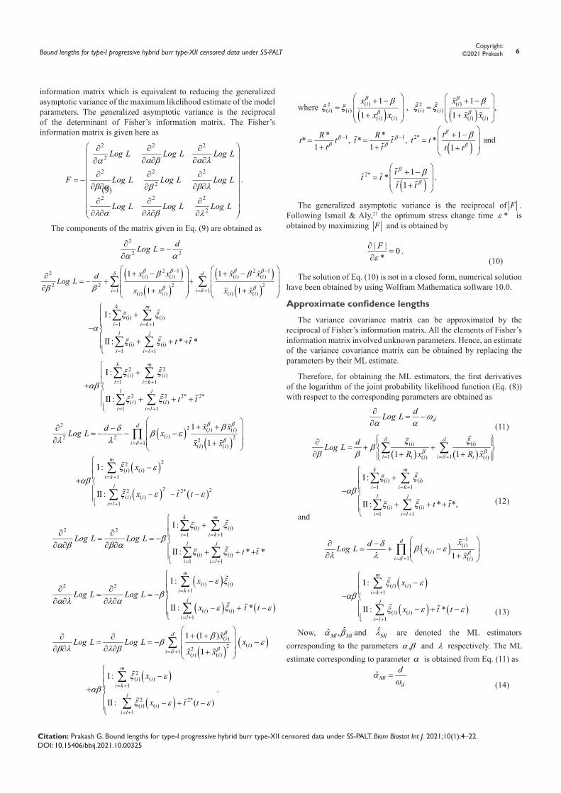
information matrix which is equivalent to reducing the generalized asymptotic variance of the maximum likelihood estimate of the model parameters. The generalized asymptotic variance is the reciprocal of the determinant of Fisher’s information matrix. The Fisher’s information matrix is given here as

2 2 2

2

2 2 2

2

2 2 2

2

Log L Log L Log L

F Log L Log L Log L

Log L Log L Log L

α β α λα

β α β λβ

λ α λ β λ

∂ ∂ ∂

∂ ∂ ∂ ∂∂ ∂ ∂ ∂ = −∂ ∂ ∂ ∂ ∂

∂ ∂ ∂

∂ ∂ ∂ ∂ ∂

. (9)

The components of the matrix given in Eq. (9) are obtained as

2

2 2 dLog Lα α∂

= −∂

( )( )

( )( )

2 1 2 12 ( ) ( ) ( ) ( )2 2 2 2

1 1( ) ( ) ( ) ( )

1 1

1 1

di i i i

i ii i i i

x x x xdLog Lx x x x

β β β βδ

β βδ

β β

β β

− −

= = +

+ − + −∂ = − + + ∂ + + ∑ ∑

(i) (i)1 1

(i) (i)1 1

I :

II : * *

k m

i i kjl

i i lt t

ξ ξα

ξ ξ

= = +

= = +

+

− + + +

∑ ∑

∑ ∑

2 2( ) ( )

1 1

2 2 2* 2*( ) ( )

1 1

I :

II :

k m

i ii i k

jl

i ii i l

t t

ξ ξαβ

ξ ξ

= = +

= = +

+

+ + + +

∑ ∑

∑ ∑

( )( )

2 2 ( ) ( )( )2 2 221 ( ) ( )

1

1

di i

ii i i

x xdLog L xx x

β β

βδ

βδ β ελ λ = +

+ +∂ − = − − − ∂ + ∏

( )

( ) ( )

22( ) ( )

1

2 22 2*( ) ( )

1

I :

II :

m

i ii k

j

i ii l

x

x t t

ξ εαβ

ξ ε ε

= +

= +

−

+ − − −

∑

∑

(i) (i)2 21 1

(i) (i)1 1

I :

II : * *

k m

i i kjl

i i l

Log L Log Lt t

ξ ξβ

α β β αξ ξ

= = +

= = +

+

∂ ∂ = = − ∂ ∂ ∂ ∂ + + +

∑ ∑

∑ ∑

( )

( ) ( )

( ) (i)2 21

( ) (i)1

I :

II : *

m

ii k

j

ii l

xLog L Log L

x t t

ε ξβ

α λ λ αε ξ ε

= +

= +

−

∂ ∂ = = − ∂ ∂ ∂ ∂ − + −

∑

∑

( )( )( )

( )221 ( ) ( )

1 (1 )

1

di

ii i i

xLog L Log L x

x x

β

βδ

ββ ε

β λ λ β = +

+ +∂ ∂ = = − − ∂ ∂ ∂ ∂ + ∑

( )

( )

2( ) ( )

1

2 2*( ) ( )

1

I :

II : ( )

m

i ii k

j

i ii l

x

x t t

ξ εαβ

ξ ε ε

= +

= +

−

+ − + −

∑

∑

.

where ( )

( )2( ) ( )

( ) ( )

1 ,

1i

i ii i

x

x x

β

β

βξ ξ

+ − = +

( )

( )2( ) ( )

( ) ( )

1,

1i

i ii i

x

x x

β

β

βξ ξ

+ − = +

1** ,1

Rt tt

ββ

−=+

1** ,1

Rt tt

ββ

−=+

( )2* 1*

1tt tt t

β

β

β + − = +

and

( )

2* 1*1

tt tt t

β

β

β + − = +

.

The generalized asymptotic variance is the reciprocal of F . Following Ismail & Aly,21 the optimum stress change time *ε is obtained by maximizing F and is obtained by

| | 0*

Fε

∂=

∂.

(10)

The solution of Eq. (10) is not in a closed form, numerical solution have been obtained by using Wolfram Mathematica software 10.0.

Approximate confidence lengths

The variance covariance matrix can be approximated by the reciprocal of Fisher’s information matrix. All the elements of Fisher’s information matrix involved unknown parameters. Hence, an estimate of the variance covariance matrix can be obtained by replacing the parameters by their ML estimate.

Therefore, for obtaining the ML estimators, the first derivatives of the logarithm of the joint probability likelihood function (Eq. (8)) with respect to the corresponding parameters are obtained as

d

dLog L ωα α∂

= −∂

(11)

( ) ( )

(i) (i)

1 1( ) ( )

1 1

d

i ii i i i

dLog LR x R x

δ

β βδ

ξ ξβ

β β = = +

∂ = + + ∂ + +

∑ ∑

(i) (i)1 1

(i) (i)1 1

I :

II : * *,

k m

i i kjl

i i lt t

ξ ξαβ

ξ ξ

= = +

= = +

+

− + + +

∑ ∑

∑ ∑

(12)

and

( )

1( )

( )1 ( )

1

di

ii i

xdLog L xxβδ

δ β ελ λ

−

= +

∂ − = + − ∂ +

∏

( )

( ) ( )

( ) ( )1

( ) ( )1

I :

II : *

m

i ii k

j

i ii l

x

x t t

ξ εαβ

ξ ε ε

= +

= +

−

− − + −

∑

∑

(13)

Now, ˆˆ ,Ml Mlα β and ˆMlλ are denoted the ML estimators

corresponding to the parameters ,α β and λ respectively. The ML estimate corresponding to parameter α is obtained from Eq. (11) as

ˆMld

dαω

= (14)



©2021 Prakash


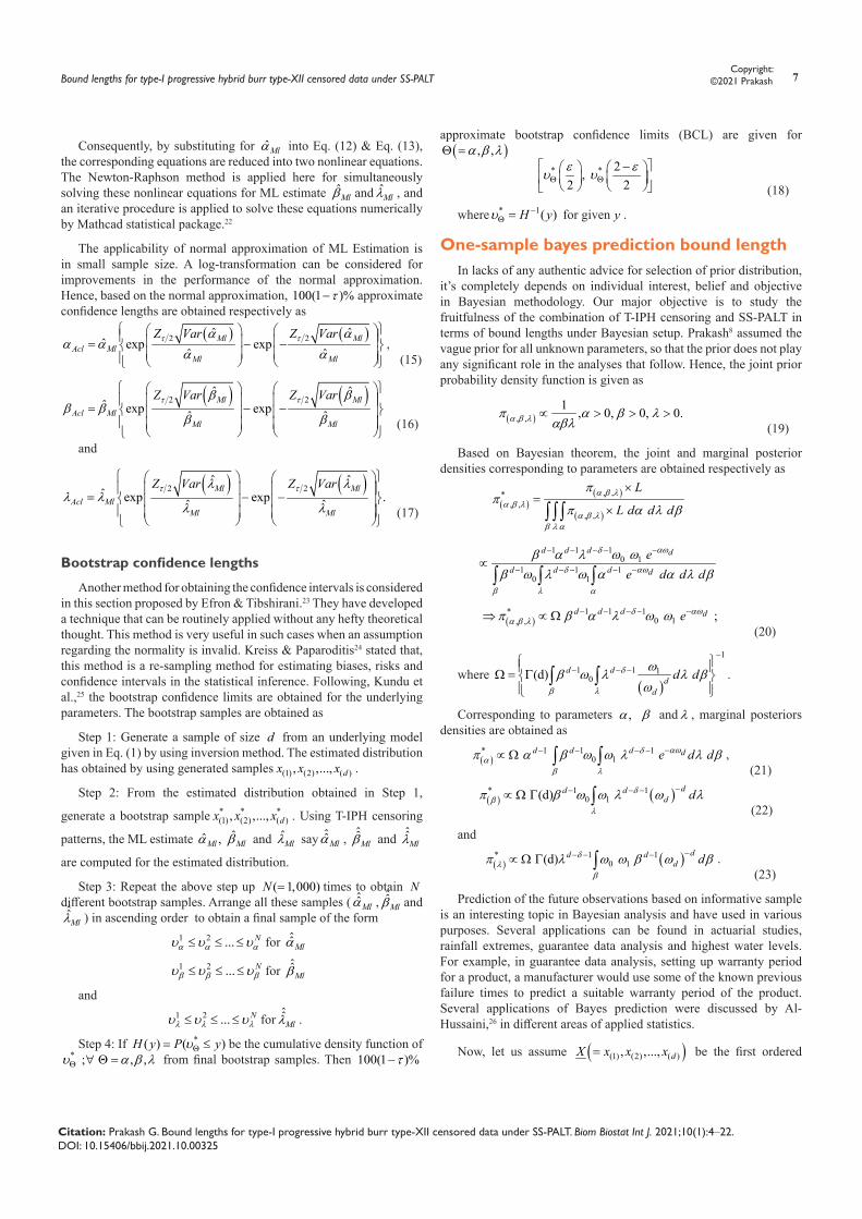
Consequently, by substituting for ˆMlα into Eq. (12) & Eq. (13), the corresponding equations are reduced into two nonlinear equations. The Newton-Raphson method is applied here for simultaneously solving these nonlinear equations for ML estimate ˆ

Mlβ and ˆMlλ , and

an iterative procedure is applied to solve these equations numerically by Mathcad statistical package.22

The applicability of normal approximation of ML Estimation is in small sample size. A log-transformation can be considered for improvements in the performance of the normal approximation. Hence, based on the normal approximation, 100(1 )%τ− approximate confidence lengths are obtained respectively as

( ) ( )2 2ˆ ˆˆ exp exp

ˆ ˆMl Ml

Acl MlMl Ml

Z Var Z Varτ τα αα α

α α

= − − ,

(15)

( ) ( )2 2ˆ ˆ

ˆ exp expˆ ˆMl Ml

Acl MlMl Ml

Z Var Z Varτ τβ ββ β

β β

= − −

(16)

and

( ) ( )2 2ˆ ˆ

ˆ exp exp .ˆ ˆMl Ml

Acl MlMl Ml

Z Var Z Varτ τλ λλ λ

λ λ

= − −

(17)

Bootstrap confidence lengths

Another method for obtaining the confidence intervals is considered in this section proposed by Efron & Tibshirani.23 They have developed a technique that can be routinely applied without any hefty theoretical thought. This method is very useful in such cases when an assumption regarding the normality is invalid. Kreiss & Paparoditis24 stated that, this method is a re-sampling method for estimating biases, risks and confidence intervals in the statistical inference. Following, Kundu et al.,25 the bootstrap confidence limits are obtained for the underlying parameters. The bootstrap samples are obtained as

Step 1: Generate a sample of size d from an underlying model given in Eq. (1) by using inversion method. The estimated distribution has obtained by using generated samples (1) (2) ( ), ,..., dx x x .

Step 2: From the estimated distribution obtained in Step 1,

generate a bootstrap sample * * *(1) (2) ( ), ,..., dx x x . Using T-IPH censoring

patterns, the ML estimate ˆ ,Mlα ˆMlβ and ˆ

Mlλ say ˆMlα , ˆ

Mlβ and ˆMlλ

are computed for the estimated distribution.

Step 3: Repeat the above step up ( 1,000)N = times to obtain Ndifferent bootstrap samples. Arrange all these samples ( ˆ

Mlα , ˆMlβ andˆ

Mlλ ) in ascending order to obtain a final sample of the form

1 2 ... Nα α αυ υ υ≤ ≤ ≤ for ˆ

Mlα

1 2 ... Nβ β βυ υ υ≤ ≤ ≤ for ˆ

Mlβ

and

1 2 ... Nλ λ λυ υ υ≤ ≤ ≤ for ˆ

Mlλ .

Step 4: If *( ) ( )H y P yυΘ= ≤ be the cumulative density function of *υΘ ; , ,α β λ∀ Θ = from final bootstrap samples. Then 100(1 )%τ−

approximate bootstrap confidence limits (BCL) are given for ( ), ,α β λΘ =

* * 2, 2 2ε ευ υΘ Θ

−

(18)

where * 1( )H yυ −Θ = for given y .

One-sample bayes prediction bound length In lacks of any authentic advice for selection of prior distribution,

it’s completely depends on individual interest, belief and objective in Bayesian methodology. Our major objective is to study the fruitfulness of the combination of T-IPH censoring and SS-PALT in terms of bound lengths under Bayesian setup. Prakash8 assumed the vague prior for all unknown parameters, so that the prior does not play any significant role in the analyses that follow. Hence, the joint prior probability density function is given as

( ), ,1 , 0, 0, 0.α β λπ α β λ

αβλ∝ > > >

(19)

Based on Bayesian theorem, the joint and marginal posterior densities corresponding to parameters are obtained respectively as

( )( )

( )

, ,*, ,

, ,

L

L d d dα β λ

α β λα β λ

β λ α

ππ

π α λ β

×=

×∫ ∫ ∫

1 1 10 1

1 1 10 1

d d d d

d d d d

ee d d d

αωδ

αωδ

β λ α

β α λ ω ωβ ω λ ω α α λ β

−− − − −

−− − − −∝∫ ∫ ∫

( )* 1 1 1

0 1, , ;d d d de αωδα β λπ β α λ ω ω −− − − −⇒ ∝Ω

(20)

where ( )

1

1 1 10(d) d d

dd

d dδ

β λ

ωβ ω λ λ βω

−

− − − Ω = Γ

∫ ∫ .

Corresponding to parameters ,α β and λ , marginal posteriors densities are obtained as

( )* 1 1 1

0 1 d d d de d dαωδα

β λ

π α β ω ω λ λ β−− − − −∝ Ω ∫ ∫ , (21)

( ) ( )* 1 10 1 (d) dd d

d dδβ

λ

π β ω ω λ ω λ−− − −∝ Ω Γ ∫ (22)

and

( ) ( )* 1 1

0 1 (d) dd dd dδ

λβ

π λ ω ω β ω β−− − −∝ Ω Γ ∫ . (23)

Prediction of the future observations based on informative sample is an interesting topic in Bayesian analysis and have used in various purposes. Several applications can be found in actuarial studies, rainfall extremes, guarantee data analysis and highest water levels. For example, in guarantee data analysis, setting up warranty period for a product, a manufacturer would use some of the known previous failure times to predict a suitable warranty period of the product. Several applications of Bayes prediction were discussed by Al-Hussaini,26 in different areas of applied statistics.

Now, let us assume ( )(1) (2) ( ), ,..., dX x x x= be the first ordered



©2021 Prakash


observed items from Burr Type-XII distribution under above considered scenario. If Z is assumed as future random variable following underlying model having independent ordered sample

( )(1) (2) ( ), ,..., dZ z z z= under similar scenario. Then the Bayes predictive density function corresponding to a variable ,Z is denoted and defined as

( ) ( ) ( )*| ; , ; , ,h z x f z dα β π α β λΘ

Θ

= × Θ Θ =∫ . (24)

The Eq. (24) is known as Bayes predictive density function, defined for the parameters ,α β and acceleration factor λ separately. No explicit solution of Eq. (24) exist for either parameter. We continue with Eq. (24) numerically for all parameters respectively. The lower and upper Bayes prediction bound limits are denoted by 1l and 2lrespectively. Thus, the 100 (1 )%τ− BPBL for Z corresponding to the parameterΘ , under the considered censoring scenario is obtained by solving following equation

( ) ( )2 1 .2 2

L P Z l P Z lτ τ = ≥ = − ≤ =

(25)

Simplifying Eq. (25), we get the non-simplified expressions for the lower and upper Bayes prediction bound limits as

( ) ( )*

11 1 ; , ,2

l dατ π α β λ−Θ

Θ

− = − × Θ Θ = ∫

(26)

and

( ) ( )

*21 ; , ,

2l dατ π α β λ−

ΘΘ

= − × Θ Θ = ∫ .

(27)

Eq. (26) and Eq. (27) has not simplified further for parameters ,α β and λ separately. Numerical technique is applied herewith for

obtaining the BPBL under the above scenario.

Numerical study based on simulated data

A simulation study by using Metropolis-Hastings algorithm has been carried out for analyzing fruitfulness of considered scenario in this section. Metropolis et al.27 and Hastings28 has deliberated this algorithm which was based on the posterior distribution by use of an arbitrary proposal distribution for simulating samples. Mahmoud et al.29 and Kayal et al., recently explored more about the M-H algorithm. The main objective of the present paper is to assess the effect of combining two different approaches SS-PALT and T-IPH censoring on bound lengths. The numerical findings are computed by using Monte Carlo simulations on 10,000 replications followed by Kayal et al.17

Thirty test units (n 30)= have been fixed for the numerical study in prior. Three different censoring stages 10, 15 and 20 along with four pre-assumed different progressive censoring patterns have been designated for the studying of the behavior of censored sample size and censoring patterns. The pre-assumed progressive censoring schemes are (2, 1, 3, 2, 3, 2, 2, 0, 2, 3) , (0, 1, 1 ,1, 0, 2, 1, 0, 3, 0, 2, 1, 2, 1, 0) (1, 0, 1, 0, 1, 1, 2, 3, 0, 2, 0, 1, 0, 1, 2) and (0, 1, 0, 1, 0, 1, 0,0, 2, 0, 1, 0, 1, 0, 1, 0, 1, 0, 1, 0) . For perceiving the effect of censoring pattern when other parametric values are fixed a different censoring pattern for m( 15)= has assumed also.

The stress change time å is optimized as discussed in the previous section by the method of minimization of the asymptotic variance of ML estimators for ,α β and λ . The values for the parameters under study

has assumed for numerical extents as 0.50 (0.10) 2.50α β λ= = = . In the present discussion, we also have to find out the optimum values of ,α β and λ for which the magnitude of bound lengths maximizes numerically when other parametric values considered to be fixed. Therefore, we assumed all possible combinations of values of these three parameters from 0.50 to 2.50 with an increment of 0.10 . The failure time was assumed here as t 05, 09= . In the present article, our focus is not only on combining the SS-PALT with T-IPH. We have also studied Type-I censoring & Type-II progressive censoring combined with SS-PALT under similar test situations.

The numerical findings in terms of bound lengths on simulated data are presented in Tables 1-3. The Bayes prediction bound length has been obtained for each parameter for all pre-assumed parametric values as discussed above. From all possible combinations of pre-assumed numerical values of ,α β and λ the widest BPBL have noticed for 1.40,α = 0.90β = and 1.60λ = . Hence, the numerical findings are presented here only for three combinations 0.50α β λ= = = ,

1.40,α = 0.90, 1.60β λ= = and 2.50α β λ= = = .

One-sample Bayes prediction bound lengths have been present in Table 03 for selected parametric values as discussed in the above paragraphs. It has been observed that, BPBL getting wider as the level of significance increases. Further, the bound lengths getting narrower when censored sample size m increases. For fixed 15m =, two different censoring patterns have been used and it has observed that, the different censoring patterns play a significant role in BPBL. The magnitude of BPBL has observed wider for first censoring pattern when they compared with second one for fixed 15m = . The BPBL also has seen wider for small t . It has been already discussed that, the BPBL increases first when values of parameter under consideration increases from 0.50α β λ= = = and touches maximum at

1.40, 0.90,α β= = 1.60λ = , then the bound lengths decreases for other values of parameter under consideration.

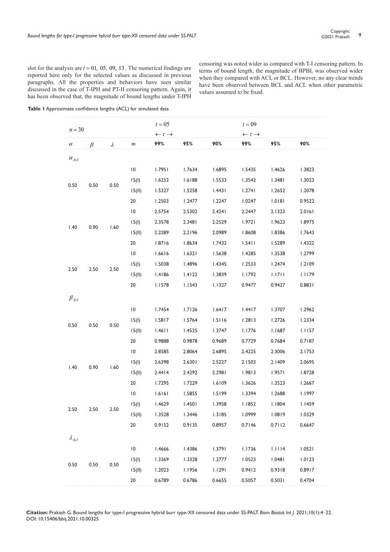
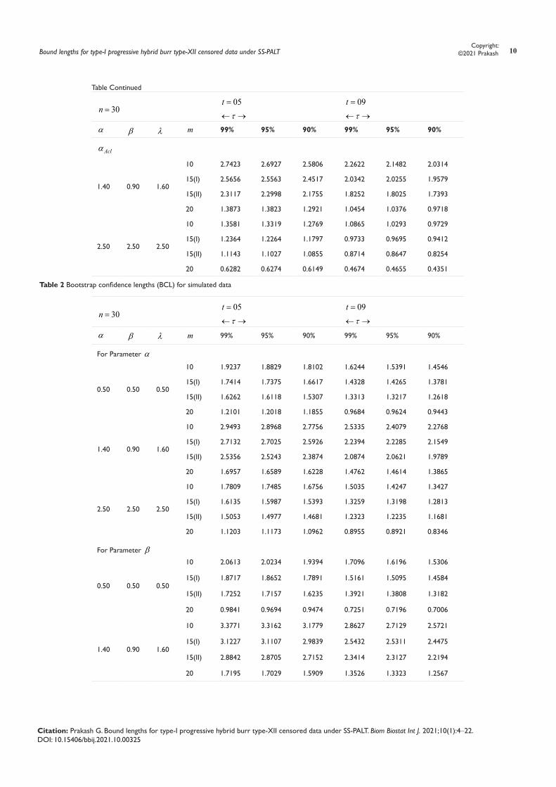
The Table 01 & Table 02 presents the approximate confidence lengths (ACL) and bootstrap confidence lengths (BCL) respectively for selected parametric values. All properties have been seen similar as discussed in above for BPBL. In terms of the bound lengths, the BPBL has seen wider when they compared with BCL and ACL. On the other hand, magnitudes of bootstrap confidence length have seen wider when they compared with ACL. However, for large sample ( 20)m = the inverse effect has been observed.

In the present discussion, we also appraise two different censoring patterns (Progressive Type-II (PT-II) and Type-I censoring (T-I)) separately under above supposed settings combined with SS-PAT. The numerical findings are obtained for all pre-assumed values; however, avoiding a number of tables, the numerical findings are presented here for selected values only.

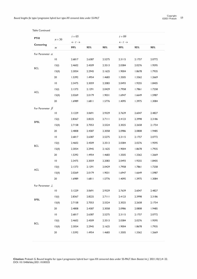
Table 04, shows the bound lengths under PT-II censoring on SS-PALT for all parameters under consideration. The numerical findings are reported similar behavior as discussed above in the case of T-IPH censoring pattern. The remarkable point is that, the magnitude of bound lengths was noted narrower for PT-II censoring when they compared with T-IPH censoring pattern (other parametric values assumed to be fixed).

Under T-I censoring scheme on SS-PALT, Table 05 presents the BPBL, BCL & ACL for a total of 30n = units and a fixed censored sample size 15m = with both censoring schemes. The selected time



©2021 Prakash


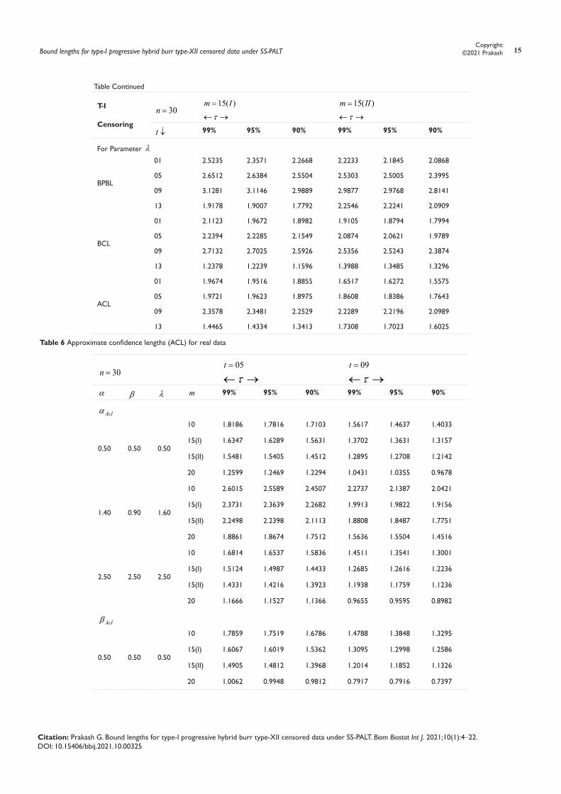
slot for the analysis are 01, 05, 09, 13t = . The numerical findings are reported here only for the selected values as discussed in previous paragraphs. All the properties and behaviors have seen similar discussed in the case of T-IPH and PT-II censoring pattern. Again, it has been observed that, the magnitude of bound lengths under T-IPH

censoring was noted wider as compared with T-I censoring pattern. In terms of bound length, the magnitude of BPBL was observed wider when they compared with ACL or BCL. However, no any clear trends have been observed between BCL and ACL when other parametric values assumed to be fixed.

Table 1 Approximate confidence lengths (ACL) for simulated data

30n =05t = 09t =τ← → τ← →

α β λ m 99% 95% 90% 99% 95% 90%

Aclα

0.50 0.50 0.50

10 1.7951 1.7634 1.6895 1.5435 1.4626 1.3823

15(I) 1.6252 1.6188 1.5533 1.3542 1.3481 1.3023

15(II) 1.5327 1.5258 1.4431 1.2741 1.2652 1.2078

20 1.2503 1.2477 1.2247 1.0247 1.0181 0.9522

1.40 0.90 1.60

10 2.5754 2.5302 2.4241 2.2447 2.1323 2.0161

15(I) 2.3578 2.3481 2.2529 1.9721 1.9623 1.8975

15(II) 2.2289 2.2196 2.0989 1.8608 1.8386 1.7643

20 1.8716 1.8634 1.7432 1.5411 1.5289 1.4322

2.50 2.50 2.50

10 1.6616 1.6321 1.5638 1.4285 1.3538 1.2799

15(I) 1.5038 1.4896 1.4345 1.2533 1.2474 1.2109

15(II) 1.4186 1.4122 1.3839 1.1792 1.1711 1.1179

20 1.1578 1.1543 1.1327 0.9477 0.9427 0.8831

Aclβ

0.50 0.50 0.50

10 1.7454 1.7126 1.6417 1.4417 1.3707 1.2962

15(I) 1.5817 1.5764 1.5116 1.2813 1.2726 1.2334

15(II) 1.4611 1.4525 1.3747 1.1776 1.1687 1.1157

20 0.9888 0.9878 0.9689 0.7729 0.7684 0.7187

1.40 0.90 1.60

10 2.8585 2.8064 2.6895 2.4225 2.3006 2.1753

15(I) 2.6398 2.6301 2.5227 2.1503 2.1409 2.0695

15(II) 2.4414 2.4292 2.2981 1.9813 1.9571 1.8728

20 1.7295 1.7229 1.6109 1.3626 1.3523 1.2667

2.50 2.50 2.50

10 1.6161 1.5855 1.5199 1.3394 1.2688 1.1997

15(I) 1.4629 1.4501 1.3958 1.1852 1.1804 1.1459

15(II) 1.3528 1.3446 1.3185 1.0999 1.0819 1.0329

20 0.9152 0.9135 0.8957 0.7146 0.7112 0.6647

Aclλ

0.50 0.50 0.50

10 1.4666 1.4386 1.3791 1.1736 1.1114 1.0521

15(I) 1.3369 1.3328 1.2777 1.0523 1.0481 1.0123

15(II) 1.2023 1.1956 1.1291 0.9412 0.9318 0.8917

20 0.6789 0.6786 0.6655 0.5057 0.5031 0.4704



©2021 Prakash


30n =05t = 09t =τ← → τ← →

α β λ m 99% 95% 90% 99% 95% 90%

Aclα

1.40 0.90 1.60

10 2.7423 2.6927 2.5806 2.2622 2.1482 2.0314

15(I) 2.5656 2.5563 2.4517 2.0342 2.0255 1.9579

15(II) 2.3117 2.2998 2.1755 1.8252 1.8025 1.7393

20 1.3873 1.3823 1.2921 1.0454 1.0376 0.9718

2.50 2.50 2.50

10 1.3581 1.3319 1.2769 1.0865 1.0293 0.9729

15(I) 1.2364 1.2264 1.1797 0.9733 0.9695 0.9412

15(II) 1.1143 1.1027 1.0855 0.8714 0.8647 0.8254

20 0.6282 0.6274 0.6149 0.4674 0.4655 0.4351

Table 2 Bootstrap confidence lengths (BCL) for simulated data

30n =05t = 09t =τ← → τ← →

α β λ m 99% 95% 90% 99% 95% 90%

For Parameter α

0.50 0.50 0.50

10 1.9237 1.8829 1.8102 1.6244 1.5391 1.4546

15(I) 1.7414 1.7375 1.6617 1.4328 1.4265 1.3781

15(II) 1.6262 1.6118 1.5307 1.3313 1.3217 1.2618

20 1.2101 1.2018 1.1855 0.9684 0.9624 0.9443

1.40 0.90 1.60

10 2.9493 2.8968 2.7756 2.5335 2.4079 2.2768

15(I) 2.7132 2.7025 2.5926 2.2394 2.2285 2.1549

15(II) 2.5356 2.5243 2.3874 2.0874 2.0621 1.9789

20 1.6957 1.6589 1.6228 1.4762 1.4614 1.3865

2.50 2.50 2.50

10 1.7809 1.7485 1.6756 1.5035 1.4247 1.3427

15(I) 1.6135 1.5987 1.5393 1.3259 1.3198 1.2813

15(II) 1.5053 1.4977 1.4681 1.2323 1.2235 1.1681

20 1.1203 1.1173 1.0962 0.8955 0.8921 0.8346

For Parameter β

0.50 0.50 0.50

10 2.0613 2.0234 1.9394 1.7096 1.6196 1.5306

15(I) 1.8717 1.8652 1.7891 1.5161 1.5095 1.4584

15(II) 1.7252 1.7157 1.6235 1.3921 1.3808 1.3182

20 0.9841 0.9694 0.9474 0.7251 0.7196 0.7006

1.40 0.90 1.60

10 3.3771 3.3162 3.1779 2.8627 2.7129 2.5721

15(I) 3.1227 3.1107 2.9839 2.5432 2.5311 2.4475

15(II) 2.8842 2.8705 2.7152 2.3414 2.3127 2.2194

20 1.7195 1.7029 1.5909 1.3526 1.3323 1.2567

Table Continued



©2021 Prakash


30n =05t = 09t =τ← → τ← →

α β λ m 99% 95% 90% 99% 95% 90%

For Parameter α

2.50 2.50 2.50

10 1.9086 1.8743 1.7952 1.5825 1.4992 1.4175

15(I) 1.7314 1.7146 1.6519 1.4028 1.3965 1.3558

15(II) 1.5972 1.5883 1.5572 1.2878 1.2783 1.2203

20 0.9112 0.9035 0.8907 0.7086 0.7012 0.6547

For Parameter λ

0.50 0.50 0.50

10 1.6272 1.5991 1.5335 1.3033 1.2351 1.1686

15(I) 1.4875 1.4812 1.4203 1.1704 1.1655 1.1257

15(II) 1.3342 1.3259 1.2557 1.0451 1.0422 0.9913

20 0.6598 0.6578 0.6565 0.4997 0.4887 0.4674

1.40 0.90 1.60

10 3.0458 2.9928 2.8691 2.5132 2.3873 2.2568

15(I) 2.8531 2.8412 2.7215 2.2619 2.2515 2.1758

15(II) 2.5664 2.5562 2.4187 2.0274 2.0032 1.9253

20 1.3453 1.3243 1.2791 1.0324 1.0306 0.9688

2.50 2.50 2.50

10 1.5066 1.4804 1.4201 1.2065 1.1437 1.0817

15(I) 1.3759 1.3631 1.3113 1.0827 1.0781 1.0457

15(II) 1.2357 1.2306 1.2074 0.9674 0.9607 0.9178

20 0.6122 0.6094 0.5914 0.4564 0.4555 0.4235

Table 3 Bayes prediction bound lengths for simulated data

30n =05t = 09t =τ← → τ← →

α β λ m 99% 95% 90% 99% 95% 90%

For Parameter α

0.50 0.50 0.50

10 2.5541 2.5107 2.4047 2.2368 2.1201 2.0045

15(I) 2.3126 2.3027 2.2097 1.9541 1.9449 1.8799

15(II) 2.2023 2.1942 2.0746 1.8597 1.8472 1.7633

20 1.9728 1.9677 1.9321 1.6553 1.6443 1.5379

1.40 0.90 1.60

10 3.4295 3.3709 3.2289 3.0319 2.8804 2.7234

15(I) 3.1281 3.1146 2.9889 2.6512 2.6384 2.5504

15(II) 2.9877 2.9768 2.8141 2.5303 2.5005 2.3995

20 2.7328 2.7199 2.5452 2.3002 2.2815 2.1372

2.50 2.50 2.50

10 2.3639 2.3235 2.2256 2.0701 1.9621 1.8549

15(I) 2.1402 2.1193 2.0415 1.8085 1.7999 1.7471

15(II) 2.0382 2.0307 1.9892 1.7209 1.7098 1.6319

20 1.8273 1.8209 1.7872 1.5312 1.5227 1.4233

For Parameter β

Table Continued



©2021 Prakash


30n =05t = 09t =τ← → τ← →

α β λ m 99% 95% 90% 99% 95% 90%

For Parameter α

0.50 0.50 0.50

10 3.2855 3.2279 3.0923 2.7762 2.6309 2.4875

15(I) 2.9889 2.9727 2.8561 2.4545 2.4435 2.3618

15(II) 2.7765 2.7644 2.6145 2.2749 2.2519 2.1565

20 2.0752 2.0707 2.0327 1.6599 1.6493 1.5426

1.40 0.90 1.60

10 5.0395 4.9515 4.7437 4.3337 4.1167 3.8924

15(I) 4.6469 4.6279 4.4403 3.8347 3.8167 3.6895

15(II) 4.3312 4.3143 4.0794 3.5679 3.5253 3.3831

20 3.3532 3.3382 3.1223 2.6999 2.6784 2.5089

2.50 2.50 2.50

10 3.0412 2.9875 2.8623 2.5695 2.4349 2.3021

15(I) 2.7655 2.7395 2.6382 2.2713 2.2611 2.1947

15(II) 2.5701 2.5587 2.5071 2.1053 2.0911 1.9959

20 1.9217 1.9159 1.8798 1.5353 1.5271 1.4274

For Parameter λ

0.50 0.50 0.50

10 3.1472 3.0912 2.9617 2.6123 2.4754 2.3405

15(I) 2.8703 2.8593 2.7429 2.3237 2.3135 2.2361

15(II) 2.6323 2.6207 2.4729 2.1251 2.1191 2.0143

20 1.7976 1.7941 1.7609 1.4039 1.3951 1.3048

1.40 0.90 1.60

10 5.1594 5.0685 4.8561 4.3761 4.1568 3.9303

15(I) 4.7846 4.7654 4.5719 3.8958 3.8777 3.7485

15(II) 4.4055 4.3867 4.1482 3.5784 3.5354 3.3928

20 3.1375 3.1239 2.9221 2.4708 2.4512 2.2961

2.50 2.50 2.50

10 2.9134 2.8611 2.7416 2.4179 2.2921 2.1661

15(I) 2.6556 2.6321 2.5334 2.1501 2.1406 2.0779

15(II) 2.4374 2.4258 2.3772 1.9668 1.9532 1.8643

20 1.6644 1.6598 1.6283 1.2983 1.2916 1.2072

Table 4 Bound lengths for simulated data under Type-II progressive censoring scheme

PT-II

Censoring

30n =05t = 09t =

τ← → τ← →

m 99% 95% 90% 99% 95% 90%

For Parameter α

BPBL

10 3.1229 3.0691 2.9329 2.7639 2.6047 2.4827

15(I) 2.8367 2.8225 2.7111 2.4123 2.3998 2.3186

15(II) 2.7158 2.7053 2.5524 2.3025 2.2658 2.1754

20 2.4808 2.4587 2.3058 2.0986 2.0808 1.9485

Table Continued



©2021 Prakash


PT-II

Censoring

30n =05t = 09t =

τ← → τ← →

m 99% 95% 90% 99% 95% 90%

For Parameter α

BCL

10 2.6817 2.6387 2.5275 2.3115 2.1757 2.0772

15(I) 2.4602 2.4509 2.3513 2.0384 2.0276 1.9595

15(II) 2.3054 2.2945 2.1625 1.9004 1.8678 1.7935

20 1.5392 1.4954 1.4683 1.3505 1.3362 1.2669

ACL

10 2.3475 2.3059 2.2083 2.0493 1.9255 1.8405

15(I) 2.1373 2.1291 2.0429 1.7958 1.7861 1.7258

15(II) 2.0269 2.0179 1.9031 1.6947 1.6649 1.5987

20 1.6989 1.6811 1.5776 1.4095 1.3975 1.3084

For Parameter β

BPBL

10 3.1229 3.0691 2.9329 2.7639 2.6047 2.4827

15(I) 2.8367 2.8225 2.7111 2.4123 2.3998 2.3186

15(II) 2.7158 2.7053 2.5524 2.3025 2.2658 2.1754

20 2.4808 2.4587 2.3058 2.0986 2.0808 1.9485

BCL

10 2.6817 2.6387 2.5275 2.3115 2.1757 2.0772

15(I) 2.4602 2.4509 2.3513 2.0384 2.0276 1.9595

15(II) 2.3054 2.2945 2.1625 1.9004 1.8678 1.7935

20 1.5392 1.4954 1.4683 1.3505 1.3362 1.2669

ACL

10 2.3475 2.3059 2.2083 2.0493 1.9255 1.8405

15(I) 2.1373 2.1291 2.0429 1.7958 1.7861 1.7258

15(II) 2.0269 2.0179 1.9031 1.6947 1.6649 1.5987

20 1.6989 1.6811 1.5776 1.4095 1.3975 1.3084

For Parameter λ

BPBL

10 3.1229 3.0691 2.9329 2.7639 2.6047 2.4827

15(I) 2.8367 2.8225 2.7111 2.4123 2.3998 2.3186

15(II) 2.7158 2.7053 2.5524 2.3025 2.2658 2.1754

20 2.4808 2.4587 2.3058 2.0986 2.0808 1.9485

BCL

10 2.6817 2.6387 2.5275 2.3115 2.1757 2.0772

15(I) 2.4602 2.4509 2.3513 2.0384 2.0276 1.9595

15(II) 2.3054 2.2945 2.1625 1.9004 1.8678 1.7935

20 1.5392 1.4954 1.4683 1.3505 1.3362 1.2669

Table Continued



©2021 Prakash


PT-II

Censoring

30n =05t = 09t =

τ← → τ← →

m 99% 95% 90% 99% 95% 90%

For Parameter α

ACL

10 2.3475 2.3059 2.2083 2.0493 1.9255 1.8405

15(I) 2.1373 2.1291 2.0429 1.7958 1.7861 1.7258

15(II) 2.0269 2.0179 1.9031 1.6947 1.6649 1.5987

20 1.6989 1.6811 1.5776 1.4095 1.3975 1.3084

Table 5 Bound lengths for simulated data under Type-I censoring scheme

T-I

Censoring

30n =15( )m I= 15( )m II=

τ← → τ← →

t ↓ 99% 95% 90% 99% 95% 90%

For Parameter α

BPBL

01 2.5235 2.3571 2.2668 2.2233 2.1845 2.0868

05 2.6512 2.6384 2.5504 2.5303 2.5005 2.3995

09 3.1281 3.1146 2.9889 2.9877 2.9768 2.8141

13 1.9178 1.9007 1.7792 2.2546 2.2241 2.0909

BCL

01 2.1123 1.9672 1.8982 1.9105 1.8794 1.7994

05 2.2394 2.2285 2.1549 2.0874 2.0621 1.9789

09 2.7132 2.7025 2.5926 2.5356 2.5243 2.3874

13 1.2378 1.2239 1.1596 1.3988 1.3485 1.3296

ACL

01 1.9674 1.9516 1.8855 1.6517 1.6272 1.5575

05 1.9721 1.9623 1.8975 1.8608 1.8386 1.7643

09 2.3578 2.3481 2.2529 2.2289 2.2196 2.0989

13 1.4465 1.4334 1.3413 1.7308 1.7023 1.6025

For Parameter β

BPBL

01 2.5235 2.3571 2.2668 2.2233 2.1845 2.0868

05 2.6512 2.6384 2.5504 2.5303 2.5005 2.3995

09 3.1281 3.1146 2.9889 2.9877 2.9768 2.8141

13 1.9178 1.9007 1.7792 2.2546 2.2241 2.0909

BCL

01 2.1123 1.9672 1.8982 1.9105 1.8794 1.7994

05 2.2394 2.2285 2.1549 2.0874 2.0621 1.9789

09 2.7132 2.7025 2.5926 2.5356 2.5243 2.3874

13 1.2378 1.2239 1.1596 1.3988 1.3485 1.3296

ACL

01 1.9674 1.9516 1.8855 1.6517 1.6272 1.5575

05 1.9721 1.9623 1.8975 1.8608 1.8386 1.7643

09 2.3578 2.3481 2.2529 2.2289 2.2196 2.0989

13 1.4465 1.4334 1.3413 1.7308 1.7023 1.6025

Table Continued



©2021 Prakash


T-I

Censoring

30n =15( )m I= 15( )m II=

τ← → τ← →

t ↓ 99% 95% 90% 99% 95% 90%

For Parameter λ

BPBL

01 2.5235 2.3571 2.2668 2.2233 2.1845 2.0868

05 2.6512 2.6384 2.5504 2.5303 2.5005 2.3995

09 3.1281 3.1146 2.9889 2.9877 2.9768 2.8141

13 1.9178 1.9007 1.7792 2.2546 2.2241 2.0909

BCL

01 2.1123 1.9672 1.8982 1.9105 1.8794 1.7994

05 2.2394 2.2285 2.1549 2.0874 2.0621 1.9789

09 2.7132 2.7025 2.5926 2.5356 2.5243 2.3874

13 1.2378 1.2239 1.1596 1.3988 1.3485 1.3296

ACL

01 1.9674 1.9516 1.8855 1.6517 1.6272 1.5575

05 1.9721 1.9623 1.8975 1.8608 1.8386 1.7643

09 2.3578 2.3481 2.2529 2.2289 2.2196 2.0989

13 1.4465 1.4334 1.3413 1.7308 1.7023 1.6025

Table 6 Approximate confidence lengths (ACL) for real data

30n =05t = 09t =

→←τ →←τα β λ m 99% 95% 90% 99% 95% 90%

Aclα

0.50 0.50 0.50

10 1.8186 1.7816 1.7103 1.5617 1.4637 1.4033

15(I) 1.6347 1.6289 1.5631 1.3702 1.3631 1.3157

15(II) 1.5481 1.5405 1.4512 1.2895 1.2708 1.2142

20 1.2599 1.2469 1.2294 1.0431 1.0355 0.9678

1.40 0.90 1.60

10 2.6015 2.5589 2.4507 2.2737 2.1387 2.0421

15(I) 2.3731 2.3639 2.2682 1.9913 1.9822 1.9156

15(II) 2.2498 2.2398 2.1113 1.8808 1.8487 1.7751

20 1.8861 1.8674 1.7512 1.5636 1.5504 1.4516

2.50 2.50 2.50

10 1.6814 1.6537 1.5836 1.4511 1.3541 1.3001

15(I) 1.5124 1.4987 1.4433 1.2685 1.2616 1.2236

15(II) 1.4331 1.4216 1.3923 1.1938 1.1759 1.1236

20 1.1666 1.1527 1.1366 0.9655 0.9595 0.8982

Aclβ

0.50 0.50 0.50

10 1.7859 1.7519 1.6786 1.4788 1.3848 1.3295

15(I) 1.6067 1.6019 1.5362 1.3095 1.2998 1.2586

15(II) 1.4905 1.4812 1.3968 1.2014 1.1852 1.1326

20 1.0062 0.9948 0.9812 0.7917 0.7916 0.7397

Table Continued



©2021 Prakash


30n =05t = 09t =

→←τ →←τα β λ m 99% 95% 90% 99% 95% 90%

1.40 0.90 1.60

10 2.9119 2.8653 2.7451 2.4772 2.3314 2.2243

15(I) 2.6837 2.6745 2.5653 2.1941 2.1836 2.1096

15(II) 2.4884 2.4754 2.3367 2.0221 1.9877 1.9032

20 1.7601 1.7413 1.6347 1.3973 1.3859 1.2975

2.50 2.50 2.50

10 1.6543 1.6226 1.5546 1.3747 1.2811 1.2313

15(I) 1.4858 1.4733 1.4183 1.2117 1.2059 1.1695

15(II) 1.3803 1.3714 1.3396 1.1249 1.0969 1.0483

20 0.9313 0.9191 0.9067 0.7377 0.7333 0.6847

Aclλ

0.50 0.50 0.50

10 1.5315 1.5018 1.4389 1.2294 1.1431 1.1021

15(I) 1.3843 1.3806 1.3236 1.0975 1.0922 1.0538

15(II) 1.2512 1.2436 1.1694 0.9822 0.9627 0.9224

20 0.7043 0.6936 0.6857 0.5352 0.5316 0.4963

1.40 0.90 1.60

10 2.8555 2.8034 2.6859 2.3592 2.2192 2.1185

15(I) 2.6595 2.6505 2.5421 2.1166 2.1067 2.0352

15(II) 2.4026 2.3897 2.2554 1.8997 1.8664 1.8021

20 1.4396 1.4242 1.3361 1.0953 1.0863 1.0167

2.50 2.50 2.50

10 1.4189 1.3911 1.3328 1.1319 1.0579 1.0199

15(I) 1.2801 1.2702 1.2219 1.0155 1.0106 0.9809

15(II) 1.1598 1.1472 1.1241 0.9097 0.8931 0.8536

20 0.6517 0.6405 0.6332 0.4954 0.4925 0.4597

Table 7 Bootstrap confidence lengths (BCL) for real data

30n =05t = 09t =τ← → τ← →

α β λ m 99% 95% 90% 99% 95% 90%

For Parameter α

0.50 0.50 0.50

10 1.9867 1.9441 1.8682 1.6811 1.5716 1.5053

15(I) 1.7867 1.7833 1.7056 1.4781 1.4707 1.4196

15(II) 1.6749 1.6595 1.5709 1.3737 1.3542 1.2939

20 1.2436 1.2246 1.2136 1.0057 0.9986 0.9787

1.40 0.90 1.60

10 3.0409 2.9863 2.8605 2.6155 2.4647 2.3504

15(I) 2.7856 2.7752 2.6624 2.3072 2.2951 2.2181

15(II) 2.6096 2.5974 2.4515 2.1509 2.1152 2.0311

20 1.7427 1.6945 1.6631 1.5277 1.5116 1.4333

2.50 2.50 2.50

10 1.8399 1.8016 1.7298 1.5567 1.4514 1.3903

15(I) 1.6552 1.6406 1.5797 1.3682 1.3611 1.3201

15(II) 1.5506 1.5422 1.5066 1.2712 1.2532 1.1976

20 1.1513 1.1378 1.1218 0.9308 0.9264 0.8616

Table Continued



©2021 Prakash


30n =05t = 09t =τ← → τ← →

α β λ m 99% 95% 90% 99% 95% 90%

For Parameter β

0.50 0.50 0.50

10 2.1378 2.0904 2.0027 1.7701 1.6558 1.5848

15(I) 1.9223 1.9162 1.8381 1.5651 1.5574 1.5035

15(II) 1.7782 1.7678 1.6677 1.4375 1.4162 1.3531

20 1.0121 0.9866 0.9697 0.7563 0.7497 0.7289

1.40 0.90 1.60

10 3.4836 3.4204 3.2769 2.9564 2.7806 2.6563

15(I) 3.2093 3.1976 3.0673 2.6217 2.6084 2.5211

15(II) 2.9706 2.9559 2.7909 2.4141 2.3749 2.2802

20 1.7687 1.7412 1.6317 1.4018 1.3801 1.3011

2.50 2.50 2.50

10 1.9729 1.9317 1.8544 1.6394 1.5312 1.4684

15(I) 1.7718 1.7613 1.6917 1.4485 1.4411 1.3979

15(II) 1.6465 1.6367 1.5995 1.3302 1.3107 1.2523

20 0.9371 0.9188 0.9113 0.7393 0.7308 0.6817

For Parameter λ

0.50 0.50 0.50

10 2.1378 2.0904 2.0027 1.7701 1.6558 1.5848

15(I) 1.9223 1.9162 1.8381 1.5651 1.5574 1.5035

15(II) 1.7782 1.7678 1.6677 1.4375 1.4162 1.3531

20 1.0121 0.9866 0.9697 0.7563 0.7497 0.7289

1.40 0.90 1.60

10 3.4836 3.4204 3.2769 2.9564 2.7806 2.6563

15(I) 3.2093 3.1976 3.0673 2.6217 2.6084 2.5211

15(II) 2.9706 2.9559 2.7909 2.4141 2.3749 2.2802

20 1.7687 1.7412 1.6317 1.4018 1.3801 1.3011

2.50 2.50 2.50

10 1.9729 1.9317 1.8544 1.6394 1.5312 1.4684

15(I) 1.7718 1.7613 1.6917 1.4485 1.4411 1.3979

15(II) 1.6465 1.6367 1.5995 1.3302 1.3107 1.2523

20 0.9371 0.9188 0.9113 0.7393 0.7308 0.6817

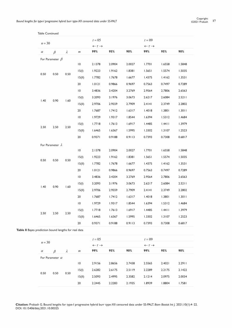
Table 8 Bayes prediction bound lengths for real data

30n =05t = 09t =τ← → τ← →

α β λ m 99% 95% 90% 99% 95% 90%

For Parameter α

0.50 0.50 0.50

10 2.9156 2.8656 2.7438 2.5565 2.4021 2.2911

15(I) 2.6282 2.6175 2.5119 2.2289 2.2175 2.1422

15(II) 2.5093 2.4995 2.3582 2.1214 2.0975 2.0034

20 2.2445 2.2283 2.1935 1.8939 1.8804 1.7581

Table Continued



©2021 Prakash


30n =05t = 09t =τ← → τ← →

α β λ m 99% 95% 90% 99% 95% 90%

1.40 0.90 1.60

10 3.9117 3.8444 3.6816 3.4613 3.2672 3.1019

15(I) 3.5561 3.5414 3.3986 3.0221 3.0066 2.9052

15(II) 3.4031 3.3921 3.1997 2.8845 2.8409 2.7273

20 3.1093 3.0843 2.8912 2.6277 2.6055 2.4401

2.50 2.50 2.50

10 2.6992 2.6526 2.5434 2.3669 2.2223 2.1208

15(I) 2.4322 2.4088 2.3205 2.0632 2.0525 1.9911

15(II) 2.3226 2.3134 2.2613 1.9635 1.9412 1.8538

20 2.0792 2.0613 2.0286 1.7526 1.7421 1.6277

For Parameter β

0.50 0.50 0.50

10 5.0621 4.9729 4.7631 4.2808 4.0356 3.8356

15(I) 4.5933 4.5619 4.3899 3.7801 3.7622 3.6353

15(II) 4.2733 4.2541 4.0183 3.5039 3.4588 3.3134

20 3.1911 3.1738 3.1211 2.5631 2.5459 2.3805

1.40 0.90 1.60

10 7.7595 7.6236 7.3028 6.6761 6.3207 5.9962

15(I) 7.1431 7.1145 6.8262 5.9027 5.8741 5.6772

15(II) 6.6642 6.6376 6.2712 5.4924 5.4171 5.1998

20 5.1566 5.1231 4.7968 4.1625 4.1285 3.8665

2.50 2.50 2.50

10 4.6863 4.6032 4.4094 3.9629 3.7342 3.5505

15(I) 4.2497 4.2104 4.0548 3.4983 3.4817 3.3783

15(II) 3.9558 3.9377 3.8532 3.2413 3.2115 3.0664

20 2.9551 2.9358 2.8859 2.3714 2.3579 2.2033

For Parameter λ

0.50 0.50 0.50

10 3.4994 3.4367 3.2919 2.9082 2.7347 2.6056

15(I) 3.1797 3.1681 3.0392 2.5822 2.5709 2.4828

15(II) 2.9224 2.9089 2.7398 2.3619 2.3456 2.2307

20 1.9931 1.9789 1.9478 1.5672 1.5565 1.4551

1.40 0.90 1.60

10 5.7308 5.6294 5.3927 4.8642 4.5993 4.3686

15(I) 5.3026 5.2819 5.0675 4.3255 4.3046 4.1601

15(II) 4.8888 4.8673 4.5976 3.9736 3.9162 3.7593

20 3.4791 3.4535 3.2355 2.7503 2.7277 2.5544

2.50 2.50 2.50

10 3.2401 3.1815 3.0478 2.6926 2.5314 2.4122

15(I) 2.9416 2.9162 2.8069 2.3897 2.3782 2.3074

15(II) 2.7063 2.6928 2.6337 2.1864 2.1616 2.0643

20 1.8454 1.8299 1.8007 1.4501 1.4417 1.3468

Table Continued



©2021 Prakash


Table 9 Bound lengths for real data under Type-II progressive censoring scheme

PT-II

Censoring

30n =05t = 09t =τ← → τ← →

m 99% 95% 90% 99% 95% 90%

For Parameter α

BPBL

10 3.5607 3.4939 3.3501 3.1538 2.9559 2.8263

15(I) 3.2253 3.2125 3.0831 2.7419 2.7341 2.6407

15(II) 3.0933 3.0824 2.9025 2.6241 2.5748 2.4723

20 2.8226 2.7895 2.6199 2.3926 2.3749 2.2235

BCL

10 2.7701 2.7199 2.6045 2.3859 2.2273 2.1424

15(I) 2.5257 2.5169 2.4147 2.1022 2.0881 2.0169

15(II) 2.3725 2.3609 2.2232 1.9581 1.9136 1.8409

20 1.5819 1.5277 1.5049 1.3973 1.3818 1.3094

ACL

10 2.3712 2.3319 2.2325 2.0756 1.9313 1.8641

15(I) 2.1512 2.1435 2.0568 1.8132 1.8034 1.7423

15(II) 2.0459 2.0362 1.9143 1.7129 1.6724 1.6085

20 1.7121 1.6847 1.5849 1.4299 1.4117 1.3226

For Parameter β

BPBL

10 3.5607 3.4939 3.3501 3.1538 2.9559 2.8263

15(I) 3.2253 3.2125 3.0831 2.7419 2.7341 2.6407

15(II) 3.0933 3.0824 2.9025 2.6241 2.5748 2.4723

20 2.8226 2.7895 2.6199 2.3926 2.3749 2.2235

BCL

10 2.7701 2.7199 2.6045 2.3859 2.2273 2.1424

15(I) 2.5257 2.5169 2.4147 2.1022 2.0881 2.0169

15(II) 2.3725 2.3609 2.2232 1.9581 1.9136 1.8409

20 1.5819 1.5277 1.5049 1.3973 1.3818 1.3094

ACL

10 2.3712 2.3319 2.2325 2.0756 1.9313 1.8641

15(I) 2.1512 2.1435 2.0568 1.8132 1.8034 1.7423

15(II) 2.0459 2.0362 1.9143 1.7129 1.6724 1.6085

20 1.7121 1.6847 1.5849 1.4299 1.4117 1.3226

For Parameter λ

BPBL

10 3.5607 3.4939 3.3501 3.1538 2.9559 2.8263

15(I) 3.2253 3.2125 3.0831 2.7419 2.7341 2.6407

15(II) 3.0933 3.0824 2.9025 2.6241 2.5748 2.4723

20 2.8226 2.7895 2.6199 2.3926 2.3749 2.2235

BCL

10 2.7701 2.7199 2.6045 2.3859 2.2273 2.1424

15(I) 2.5257 2.5169 2.4147 2.1022 2.0881 2.0169

15(II) 2.3725 2.3609 2.2232 1.9581 1.9136 1.8409

20 1.5819 1.5277 1.5049 1.3973 1.3818 1.3094

ACL

10 2.3712 2.3319 2.2325 2.0756 1.9313 1.8641

15(I) 2.1512 2.1435 2.0568 1.8132 1.8034 1.7423

15(II) 2.0459 2.0362 1.9143 1.7129 1.6724 1.6085

20 1.7121 1.6847 1.5849 1.4299 1.4117 1.3226



©2021 Prakash


Table 10 Bound lengths for real data under Type-I censoring scheme

T-I

Censoring

30n =05t = 09t =τ← → τ← →

m 99% 95% 90% 99% 95% 90%

For Parameter α

BPBL

10 2.8666 2.6868 2.5639 2.5244 2.4747 2.3751

15(I) 3.0221 3.0066 2.9052 2.8845 2.8409 2.7273

15(II) 3.5561 3.5414 3.3986 3.4031 3.3921 3.1997

20 2.1748 2.1587 2.0211 2.5656 2.5355 2.3814

BCL

10 2.1687 2.0245 1.9473 1.9639 1.9283 1.8465

15(I) 2.3072 2.2951 2.2181 2.1509 2.1152 2.0311

15(II) 2.7856 2.7752 2.6624 2.6096 2.5974 2.4515

20 1.2701 1.2546 1.1902 1.4379 1.3886 1.3679

ACL

10 1.9866 1.9679 1.8994 1.6643 1.6367 1.5667

15(I) 1.9913 1.9822 1.9156 1.8808 1.8487 1.7751

15(II) 2.3731 2.3639 2.2682 2.2498 2.2398 2.1113

20 1.4527 1.4385 1.3477 1.7445 1.7166 1.6149

For Parameter β

BPBL

10 2.8666 2.6868 2.5639 2.5244 2.4747 2.3751

15(I) 3.0221 3.0066 2.9052 2.8845 2.8409 2.7273

15(II) 3.5561 3.5414 3.3986 3.4031 3.3921 3.1997

20 2.1748 2.1587 2.0211 2.5656 2.5355 2.3814

BCL

10 2.1687 2.0245 1.9473 1.9639 1.9283 1.8465

15(I) 2.3072 2.2951 2.2181 2.1509 2.1152 2.0311

15(II) 2.7856 2.7752 2.6624 2.6096 2.5974 2.4515

20 1.2701 1.2546 1.1902 1.4379 1.3886 1.3679

ACL

10 1.9866 1.9679 1.8994 1.6643 1.6367 1.5667

15(I) 1.9913 1.9822 1.9156 1.8808 1.8487 1.7751

15(II) 2.3731 2.3639 2.2682 2.2498 2.2398 2.1113

20 1.4527 1.4385 1.3477 1.7445 1.7166 1.6149

For Parameter λ

BPBL

10 2.8666 2.6868 2.5639 2.5244 2.4747 2.3751

15(I) 3.0221 3.0066 2.9052 2.8845 2.8409 2.7273

15(II) 3.5561 3.5414 3.3986 3.4031 3.3921 3.1997

20 2.1748 2.1587 2.0211 2.5656 2.5355 2.3814

BCL

10 2.1687 2.0245 1.9473 1.9639 1.9283 1.8465

15(I) 2.3072 2.2951 2.2181 2.1509 2.1152 2.0311

15(II) 2.7856 2.7752 2.6624 2.6096 2.5974 2.4515

20 1.2701 1.2546 1.1902 1.4379 1.3886 1.3679

ACL

10 1.9866 1.9679 1.8994 1.6643 1.6367 1.5667

15(I) 1.9913 1.9822 1.9156 1.8808 1.8487 1.7751

15(II) 2.3731 2.3639 2.2682 2.2498 2.2398 2.1113

20 1.4527 1.4385 1.3477 1.7445 1.7166 1.6149



©2021 Prakash


Numerical illustration

In this section, the numerical illustration was based on the dataset provided by Box & Cox30 for survival time of animals observed due to different dosage of poison administered. The observations are listed as

0.18 0.21 0.22 0.22 0.23 0.23 0.23 0.24 0.25 0.29 0.29 0.30 0.30 0.31 0.31 0.31 0.33 0.35 0.36 0.36 0.37 0.38 0.38 0.40 0.40 0.43 0.43 0.44 0.45 0.45 0.45 0.46 0.49 0.56 0.61 0.62 0.63 0.66 0.71 0.71 0.72 0.76 0.82 0.88 0.92 1.02 1.10 1.24.

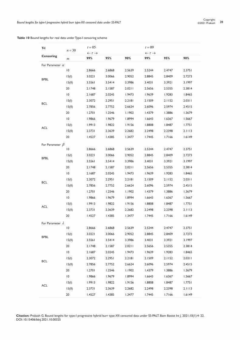
The Kolmogorov-Smirnov (KS) test (test statistic value = 0.1440 with p-value 0.2724) was afforded a satisfactory fit the underlying distribution of this data set. For the numerical illustration, a set of 30 ( n)= randomly selected data from given dataset was assumed. For simplicity in comparison, similar censoring patterns have used for considering censored sample size with all above pre-assumed parametric values. The bound lengths ACL, BCL and BPBL have been presented in Tables 6-10 respectively for the parameters under study. All the properties and trends have seen similar as discussed above in the case of simulated data. The remarkable point is that, the narrower bound lengths have noticed for simulated data set when they compared with the corresponding real dataset under all considered censoring criterion and censoring patterns for all parameters under study.

Summary

No any literature has noticed in studying the properties of the bound length by using SS-PALT and T-IPH censoring. The present article motivated for that. In the present article, we focused not only for combining the SS-PALT with T-IPH censoring. We are also trying to develop the scenario for combining SS-PALT with Type-I censoring and progressive Type-II censoring pattern, respectively and studying the fruitfulness in terms of different bound lengths. The Bayes predictive bound length (BPBL), bootstrap bound length (BCL) and approximate confidence lengths (ACL) has been observed on several combinations of the parametric values. Wider BPBL has been observed in T-IPH censoring over others on both real and simulated datasets. On real and simulated data set, the magnitude of BPBL was seen wider for real data set. The present discussion showed that, the T-IPH censoring maximizes the bound lengths over T-I or PT-II censoring.

Conflicts of interestThere are no conflicts of interest.

AcknowledgementNone.

References1. Burr WI. Cumulative frequency distribution. Annals of Mathematical

Statistics. 1942;13:215–232.

2. Abd–Elfattah AM, Hassan AS, Nassr SG. Estimation in step–stress partially accelerated life tests for the Burr Type–XII distribution using Type–I censoring. Statistical Methodology. 2008;5(6):502–514.

3. Khalaf EA, Zeinhum J, Heba SM. Finite mixture of Burr Type–XII distribution and its reciprocal: Properties and applications. Statistical Papers. 2011;52:835–845.

4. Soliman AA, Abd–Ellah AH, Abou–Elheggag NA. et al. Bayesian inference and prediction of Burr Type–XII distribution for progressive first failure censored sampling. Intelligent Information Management.

2011;3:175–185.

5. Jang DH, Jung M, Park JH, et al. Bayesian estimation of Burr Type–XII distribution based on general progressive Type–II censoring. Applied Mathematical Sciences. 2014;8:3435–3448.

6. Rao GS, Aslam M, Kundu D. Burr–XII distribution parametric estimation and estimation of reliability of multicomponent stress–strength. Communications in Statistics–Theory & Methods. 2015;4:4953–4961.

7. Panahi H, Sayyareh A. Estimation and prediction for a unified hybrid–censored Burr Type–XII distribution. Journal of Statistical Computation & Simulation. 2015;86(1):55–73.

8. Prakash G. Confidence limits for progressive censored Burr Type–XII data under CP–ALT. Journal of Statistics Applications & Probability. 2017;6(2):295–303.

9. Asl MN, Belaghi RA, Bevrani H. On Burr XII distribution analysis under progressive Type–II hybrid censored data. Methodology & Computing in Applied Probability. 2017;9(2):665–683.

10. Prakash G. Bayes estimation for C–PALT progressively censored Burr–XII data. International Journal of Intelligent Technologies & Applied Statistics. 2018a;11(1): 01–14.

11. Prakash G. Progressively censored Rayleigh data under Bayesian estimation. The International Journal of Intelligent Technologies & Applied Statistics. 2015;8(3):257–273.

12. Lin CT, Ng HKT, Chan PS. Statistical inference of Type–II progressively hybrid censored data with Weibull lifetimes. Communications in Statistics–Theory & Methods. 2009;38:1710–1729.

13. Lin CT, Huang YL. On progressive hybrid censored Exponential distribution. Journal of Statistical Computation & Simulation. 2012;82(5):689–709.

14. Singh B, Gupta PK, Sharma VK. On Type–II hybrid censored Lindley distribution. Statistics Research Letters. 2014;3:58–62.

15. Balakrishnan N, Cramer E. The art of progressive censoring: Applications to reliability and quality. Birkhäuser, Boston; 2014.

16. Elshahhat A, Ashour S. Bayesian and non–Bayesian estimation for Weibull parameters based on generalized Type–II progressive hybrid censoring scheme. Pakistan Journal of Statistics & Operation Research. 2016;12(2):213–226.

17. Kayal T, Tripathi YM, Rastogi MK, et al. Inference for Burr XII distribution under Type–I progressive hybrid censoring. Communication in Statistics–Simulation & Computation. 2017;46(9):7447–7465.

18. Nelson W. Accelerated Life Testing: Statistical Models, Test Plans and Data Analysis. John Wiley & Sons, New York; 1990.

19. Prakash G. Generalized inverted Exponential distribution on Optimum SS–PALT: Some Bayes estimation. Journal of Statistics Applications & Probability. 2018b;7(3):457–467.

20. DeGroot MH, Goel PK. Bayesian and optimal design in partially accelerated life testing. Naval Research Logistics. 1979;16 (2):223–235.

21. Ismail AA, Aly H M. Optimal planning of failure step–stress partially accelerated life tests under Type–II censoring. International Journal of Mathematical Analysis. 2009;3(31):1509–1523.

22. Mathcad. Statistical package. 2001.

23. Efron B, Tibshirani R. Bootstrap methods for standard errors, confidence intervals, and other measures of statistical accuracy. Statistical Science. 1986;1(1):54–77.

24. Kreiss JP, Paparoditis E. Bootstrap methods for dependent data: a review. Journal of Korean Statistical Society. 2011;40:357–378.

25. Kundu D, Kannan N, Balakrishnan N. Analysis of Progressively censored


https://www.sciencedirect.com/science/article/abs/pii/S1572312707000755



https://econpapers.repec.org/article/sprstpapr/v_3a52_3ay_3a2011_3ai_3a4_3ap_3a835-845.htm



http://www.m-hikari.com/ams/ams-2014/ams-69-72-2014/kimchansooAMS69-72-2014.pdf



https://www.tandfonline.com/doi/abs/10.1080/03610926.2013.821490






http://www.naturalspublishing.com/files/published/6zg969j19cky88.pdf



https://link.springer.com/article/10.1007/s11009-016-9514-7



https://web.b.ebscohost.com/abstract?direct=true&profile=ehost&scope=site&authtype=crawler&jrnl=19985010&AN=129435694&h=1X%2fTatdiUCM8jiPjHQ2MCMG5rNfh48dIOB%2fGjSuee3AJaafYqply8H0VarXFxq7gjotPgLy6Luxfz065s4PU0g%3d%3d&crl=c&resultNs=AdminWebAuth&resultLocal=ErrCrlNotAuth&crlhashurl=login.aspx%3fdirect%3dtrue%26profile%3dehost%26scope%3dsite%26authtype%3dcrawler%26jrnl%3d19985010%26AN%3d129435694



https://www.airitilibrary.com/Publication/alDetailedMesh?DocID=19985010-201509-201510020024-201510020024-257-273



https://www.tandfonline.com/doi/abs/10.1080/03610920902850069






https://www.springer.com/gp/book/9780817648060

https://www.springer.com/gp/book/9780817648060

https://pjsor.com/pjsor/article/view/1273







https://aip.scitation.org/doi/10.1063/1.1699114


http://www.naturalspublishing.com/files/published/15fit8r6jj0c64.pdf



https://onlinelibrary.wiley.com/doi/abs/10.1002/nav.3800260204

https://onlinelibrary.wiley.com/doi/abs/10.1002/nav.3800260204

http://www.m-hikari.com/ijma/ijma-password-2009/ijma-password29-32-2009/ismailIJMA29-32-2009.pdf



https://projecteuclid.org/journals/statistical-science/volume-1/issue-1/Bootstrap-Methods-for-Standard-Errors-Confidence-Intervals-and-Other-Measures/10.1214/ss/1177013815.full



https://link.springer.com/article/10.1016%2Fj.jkss.2011.08.009

https://link.springer.com/article/10.1016%2Fj.jkss.2011.08.009

http://citeseerx.ist.psu.edu/viewdoc/summary?doi=10.1.1.526.995


©2021 Prakash


competing risks data. In: Balakrishnan N, Rao CR, editors. Handbook of statistics. 2004;23:331–348.

26. Al–Hussaini EK. Predicting observables from a general class of distributions. Journal of Statistical Planning & Inference. 1999;79:79–91.

27. Metropolis N, Rosenbluth AW, Rosenbluth MN, et al. Equations of state calculations by fast computing machines. Journal of Chemical Physics. 1953;21:1087–1092.

28. Hastings WK. Monte Carlo sampling methods using Markov Chains and their applications. Biometrika. 1970;57:97–109.

29. Mahmoud MAW, EL–Sagheer RM, Nagaty H. Inference for constant–stress partially accelerated life test model with progressive Type–II censoring scheme. Journal of Statistics Applications Proc. 2017;6(2):373–383.

30. Box GEP, Cox DR. An analysis of transformations (with discussion). Journal of the Royal Statistical Society–B. 1964;26:211–252.









https://www.jstor.org/stable/2334940?seq=1


http://www.naturalspublishing.com/files/published/7p91m6u03t2al9.pdf






Bound lengths for type-I progressive hybrid burr type-XII ...

Documents