[email protected] Geometric structures underlying ... · So space geo-metry (in the strong sense of assigning metric properties—distances, areas, angles, etc.—to the space

Alain BossavitLaboratoire de Génie Electrique de Paris (CNRS)

[email protected]

´

Geometric structures underlying

mimetic approachesto the discretization of Maxwell's equations

A tour of the workshop

Vector: Covector:

vω

b

a

〈v ; ω〉 = b/a

〈v ; ω〉 = v · Ω – but "proxy vector" Ω dependson (most often, irrelevant) metric of ambient space

(virtual) displacement, velocity, ...are vectors

force,momentum, ...

are covectorsv → <virt. work>is linear map, i.e.,a covector, say f.

<virt. work> = 〈v ; f〉

Vector: Covector:

vω

b

a

〈v ; ω〉 = b/a

〈v ; ω〉 = v · Ω – but "proxy vector" Ω dependson (most often, irrelevant) metric of ambient space

Vector Covector

v

b

a

⟨v ; ⟩ = b/a

Come also in "twisted" variety

(also called "axial" vectors or covectors)

{v, w} ~ {v', w} ~ {v', w'}

v

w

v'

w

v'

w'

x x x

Case p = 2 (bivector) (denoted v ∧ w or v ∨ w) p-vectors: (Grassmann algebra)

〈v ∨ w ; ω ∧ η 〉 = 〈v ; ω〉〈w ; η〉 – 〈w ; ω〉〈v ; η〉

wedgeproduct

v ∨ w ω ∧ η

v

wω

η

Grassmann algebraof multi-covectors, too

p-covectors:

("join")("wedge")

ωη∧ =

Orientation, twisted objects

Or ∈ {direct, skew} Or = ⇔ – Or = ,

On the set of pairs {, Or}, equivalence relation:

~{, Or} {–, –Or}

Then = equivalence class ~ ^

∂1

∂3∂2 ∂1

∂3

∂2

Outer orientation:

Of vector subspace: an orientation of (one of its) complement(s)

Of submanifold: consistent orientations of all its tangent spaces

Of affine subspace: an outer orientation of the vector subspace parallel to it

Objects we’ll work with – straight

Affine 3D space, with associated vector space,but no orientation, no metric structure (for a while)

Points, vectors, multivectors (Grassmann algebra)

0 1 2 3

Smooth sub-manifolds, with own orientation:

+ c SD

+–D

Objects we’ll work with – twisted

Affine 3D space, with associated vector space,but no orientation, no metric structure (for a while)

Points, vectors, multivectors (Grassmann algebra)

0 1 2 3

Sub-manifolds, with own outer orientation:

c SD +

+

Computers

Mathematical physics

Calculus

Numerical modelsDiscrete calculus?

Reformulating theories:

not necessarily the right objects to deal with

B, H, E, ... are just elements of a mathematical representation of electromagnetic phenomena, and

Most physical fields are covector-fields rather than vector fields

Ground at potential 0

Charged body at potential V

Ambient electric field ... ... E = – grad v

a field of covectors...

... x → e(x),denoted e.

Most physical fields are covector-fields rather than vector fields

Ground at potential 0

Charged body at potential V

Ambient electric field ... ... E = – grad v

a field of covectors...

... x → e(x),denoted e.c

Most physical fields are covector-fields rather than vector fields

Ground at potential 0

Charged body at potential V

Ambient electric field ... ... E = – grad v

a field of covectors...

... x → e(x),denoted e.

V = lim ∑ 〈v ; e(x )〉 ≡ ∫ e ≡ 〈c ; e〉 ci i i

c

xi

vi

E(the vector field)

e(the 1-form)

as a proxy for

Change “ • ”, change E (and ), for same e

c

∫e = Ec

∫c

The observable is not E but e, the form

(later called cochain)

ORIENTED_LINE → REAL

map, denoted e here

So what counts is the

Same about magnetic induction b: A field of 2-covectors

S

xi

v ∨ wi i

b(x)

x

〈S ; b〉 = lim ∑ 〈v ∨ w ; b(x )〉 iii

≡ bS

∂S

i

∫

Same about magnetic induction b: A field of 2-covectors

S

xi

v ∨ wi i

b(x)

x

〈S ; b〉 = lim ∑ 〈v ∨ w ; b(x )〉 iii

≡ bS

∂S

Faraday:

∂ b + de = 0

∂ [∫ b] + ∫ e = 0S ∂St

∂ 〈S ; b〉 + 〈∂S ; e〉 = 0 ti.e., if one defines d by

〈S ; de〉 = 〈∂S ; e〉,

∀ S,

t

i

∫

B(the vector field)

b(the 2-form)

as a proxy for

Change “ • ”, change B (and n), for same b

∫ b = n BS

∫S

The observable is not B but b, the 2-form

S

n

∂S

Change to , change B to –B, for same b

Slightly different for h and j:

j is a field of "twisted" 2-covectors

Σ

xi

v ∨ wi i

j(x)

x

dh = j ∂Σ

h a field of twisted covectors

Covector:Vector:~ ~

v~ ω~

Ampère (in statics):

J(the vector field)

j(the 2-form)

as a proxy for

Change “ • ”, change J (and n), for same j

∫ j = n JS

∫S

Σ

n

Ambient space orientation, or , irrelevant

~

The observable is not J but j, the 2-form~

Two kinds of forms, depending on which kind of orientation is conferred to the manifold:

Fields of p-covectors are called p-forms (for "differential forms of degree p")

Quite often, physical fields are usefully modelled by p-forms

p-forms, meant to be integrated over p-submanifolds (of space, or spacetime)

Highly meaningful distinction in physics: straight [resp. twisted] forms represent intensive [resp. extensive] entities

straight twisted(inner orientation) (outer orientation)

T he concept of chain:

Embed set of curves in vector space of singular 1-chains

c cc1

2 3

c = r c + r c + r c11

22

33

S1S

2

c1

c2

c3S ∂S = c – c + c321Boundary operator ∂:

1-chains: 2-chains:

e.g., S = S – S 1 2

Same with surfaces

etc.:

p-chains

(Linear map: )

What about dual objects (linear functionals), called cochains?

∂(S – S ) = ∂S – ∂S1 2 1 2

Chains model probes. Cochains model fields.

Voltmeter:V

(p = 1)

e.m.f. V = ∫ ec

c

a 1-cochain.

Electric field seen as map c → <emf along c>, map here denoted e,

Magnetic induction as map b, the 2-cochain

S → <flux embraced by S>.

Small probe <––> p-vector Local field <––> p-covector

Fluxmeter:

(p = 2) S

Maxwell's Theory

Faraday's law, in terms of cochains:

webers

∫ bS

∂S

S

or ∂ b + de = 0, with d defined by ∫ de = ∫ et S ∂S

volts

∫ e∂S

2-cochain 1-cochain

ddt

Sb + e

∂S= 0∫∫

for all 2-chains S,

Ampère-Maxwell's law, in terms of cochains:

coulombs

∫ dΣ

∂Σ

Σ

or –∂ d + dh = j t

ampères

∫ h∂Σ

2-cochain 1-cochain

ddt

Σd + h

∂Σ= j∫∫

for all 2-chains Σ,~

~ ~∫Σ

– 2-cochain~given

∫

q = ∫∂

d ∫q∂t

+∫∂ j = 0

- ∂ ∫ d + ∫ h = ∫ j ∂ t

S ∂ ∫ b + ∫ e = 0S ∂St

d = eb = µh

- ∂ ∫ d + ∫ h = ∫ j ∂ t

S ∂ ∫ b + ∫ e = 0S ∂St

(– ∂ D + rot H = J, ∂ B + rot E = 0)tt

?

The real nature of µ (“Hodge operator”):

b : a map of type SURFACE → REAL ("2-cochain")

h : a map of type LINE → REAL

b = µ h("1-cochain")~

S

Sarea(S) =

length()

S = vectorial area of S = vector along

1area(S) ∫S

b = h1 ∫lgth()

S

Sarea(S) =

length()B • • H

=

S = vectorial area of S = vector along

µ

µ

which defines 2-form b knowing scalar factor µ and 1-form h

T he Hodge operator:

S

1area(S) ∫S

b= 1 ∫hlength() µ

b = µ h h = ν b⇔

Further structuration of space: the Hodge map

Determines a metric ("-adapted")

VECTOR (n – 1)-VECTOR twisted or straight straight or twisted

(Select reference 3-vector ∆ and real . Set v ∨ v = |v| ∆, hence a norm, scaling as . Adjust for -volume of ∆ to be .)

22

2

Equip space with such a map, . (Another one, denoted , will be needed.)

Only requirement, "non-degeneracy".

(Volume v ∨ v, built on v and its image,

must be ≠ 0.)

→

By duality, yields Hodge map on covectors:

=

~1-VECTOR 2-VECTOR →

~1-COVECTOR 2-COVECTOR ←

Hence relation h = b (and also d = e) between cochains, i.e., fields

1-vector

1-covector

⟨v ; b⟩2-vector

2-covector

⟨v ; b⟩

So space geo-metry (in the strong sense of assigning metric properties—distances, areas,

angles, etc.—to the space we inhabit) amounts to specifying constitutive laws in electrodynamics.

Should not sound strange: Don't we use light rays to measure the Earth?

Why two metrics (ν ≡ µ and ε)? Because 3D shadows of Minkowski's 4D (pseudo-)metric

–1

ε ≠ ε and µ ≠ µ when we wish to ignore details of microscopic interactions and geometrize them wholesale

0 0

Maxwell, in terms of cochains:

-∂ ∫ d + ∫ h =∫ j ∂

d = e h = bt

S ∂ ∫ b +∫ e = 0S ∂St

– ∂ d + dh = jt

∂ b + de = 0t

h = b

d = e

b12

straight twistede

d, jh

Maxwell, in terms of cochains:

-∂ ∫ d + ∫ h =∫ j ∂

d = e h = bt

S ∂ ∫ b +∫ e = 0S ∂St

– ∂ d + dh = jt

∂ b + de = 0t

h = b

d = e

Discretization strategy: Only enforce these laws for finite system of surfaces S or Σ: those made of faces of a mesh. DoF's are then face-integrals of b, d, and relate to edge-integrals of e, h.

Maxwell, in terms of cochains:

-∂ ∫ d + ∫ h =∫ j ∂

d = e h = bt

S ∂ ∫ b +∫ e = 0S ∂St

– ∂ d + dh = jt

∂ b + de = 0t

h = b

d = e

Problem: Should be same number of DoF's for b and h (resp. for d and e) for discrete versions ε and ν (matrices) of hodges ε and ν to be square (since they must be invertible).

Gen = – 1Rfe = – 1

vfD = 1v

enf +

DR = 0, RG = 0

+N E F V

Select centers inside primal simplexes. Join them to make dual.

, : primal cells: dual cells,

2D

3D

Orient all primal cells, independently. Take induced orientation on dual cells:

N → E → F → V G R Dgrad rot div

h = {h : f ∈ F}fb = {b : f ∈ F}f

e = {e : e ∈ E}e d = {d : e ∈ E}e

νε

here, R = – 1fe

at edges

h at dual edges(i.e., faces)

at dual faces

e

f

b at faces

Approximate representation of the field by degrees offreedom assigned to both kinds of cells

fluxes

e.m.f.'s

m.m.f.'s

(cumulated) intensities

e, a d, j

not for all surfaces S, but for all those made of primal faces. This requires (when S = f, a primal face),

∂ b + Re = 0t

∂ ∫ b + ∫ e = 0t S ∂SEnforce Faraday's law,

i.e.,f

2

3

1

Rf 2= – 1

∂ b + e – e – e = 0 t f 321

not for all surfaces Σ, but for all those made of dual faces such as e here. This gives

∂ ∫ d + ∫ h = 0t Σ ∂ΣEnforce Ampère's law, –

∂ d + R h = jt–t

ee~

~

f~f

because

Re f~~ = Rf e

+–

∂ b + Re = 0t

h = ν b–∂ d + R h = jt

t

d = ε e

The final product:

Leap-frog time discretization gives

"Yee scheme" (1966), aka FDTD

b – bk + 1/2 k – 1/2+ Re = 0k

t

ε– e – ek + 1 k

t + R b = jνt k + 1/2k + 1/2

–∂ d + R h = jtt∂ b + Re = 0t

h = bν d = eε

D of this: G of that:t

Recall that ∂ q – G j = 0,tt

(because ∂ q + div j = 0, and – G ~ div) tt

hence – G d = qt

–∂ d + R h = jt∂ b + Re = 0th = bν d = eε

Use DR = 0 and G R = 0 to gettt

t

d = ε e– G d = qt

Re = – ∂ bth = ν bDb = 0

tR h = j + ∂ dt

Kirchhoff's node law

(∂ q – G j = 0)tt

If ε and ν diagonal, ε and ν can be seen as branch impedances

ee ff

Two interlocked, cross-talking, networks

Kirchhoff's loop law"electric" network "magnetic" network

Discrete ("mimetic") structuresSpace (comput. domain) Cell complex→

Hodge map(s) → Hodge matrix(es)

cellular chains

cellular cochains

consistency required there, for convergence of numerical schemes

b b

h hν νfields DoF arrays

submanifolds (such as S, Σ) →fields (such as b, h, e, d) →

e

f

ef

~~

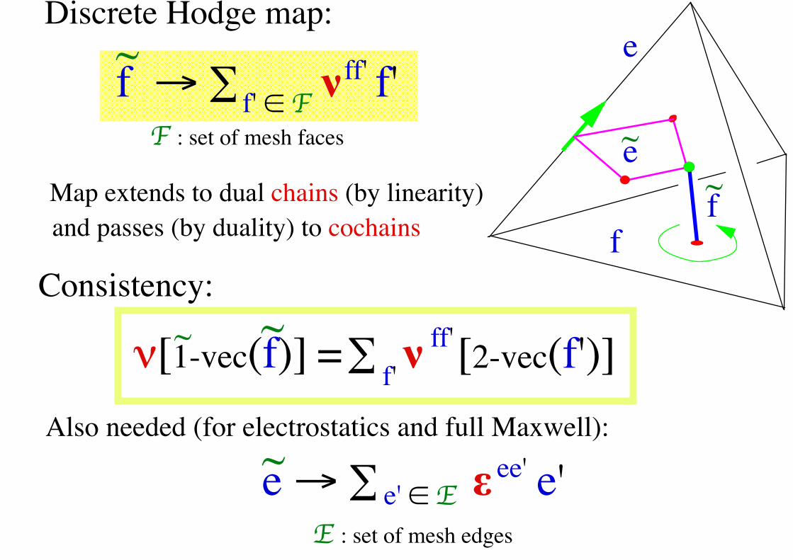
Discrete Hodge map:

f → ∑ ν f'f' ∈ Fff'~

Consistency:

ν[1-vec(f)] = ∑ ν [2-vec(f')]ff'f'

~ ~

Also needed (for electrostatics and full Maxwell):

Map extends to dual chains (by linearity)and passes (by duality) to cochains

F : set of mesh faces

e → ∑ ε e'e' ∈ E ee'~

E : set of mesh edges

e

f

ef

~~

Consistency condition: ν[1-vec(f)] = ∑ ν [2-vec(f')]ff'f'

~ ~

b b

h hν ν

makes commutative

when b and h are piecewise uniform:

ff'~ ~ = ∑ ν ⟨f'; b⟩f'hf ⟨f ; νb⟩= ⟨νf ; b⟩= =∑ν bff'

f' f'

the diagram = ∑ ν f'ff'

f'νf~→ →

abridged as

=⟨f ; νb⟩→~ → →! !

If dual mesh barycentric, criterion met by the "Galerkin Hodge", defined as

ν = ∫ ν w ∧ wff' f f'

where w is Whitney form of facet ff

f

Prop. 1: Select centers inside primal simplexes. Join them to make dual. Then unique ν conforming to criterion.

But this ν non-symmetric!! (Yet, pos. def.)

Prop. 2: If centers such that

Then ν symmetric. ∑ vec(f) × vec(f) = 0

~f

f f~Corollary: If at barycenters, then ν symmetric for all positions of inside.

Proof. True if at barycenter (Galerkin ν). Now,

∑ vec(f) × vec(f + v) = 0 + (∑ vec(f)) × v = 0. f f

~if ← + v, and because ∑ vec(f) = 0, f

☐

vec(f) = vectorial area of f here

vec(f) = vector along f (with usual orientation

of ambient space)

~ ~

An interesting solution (Weiland, Tonti et al., ...)

f f~

Centers at circumcenters:

ν f = ν fff ~Then, f // f, so ~

ffi.e., ν = ν length(f)/area(f)

, other terms 0, → →

~

(vectorialarea)

ff~

f~

f f~ f

Highly desirable mutual orthogonalityof primal and dual meshes

Here, f // f, and

f = fff ~

→~ →

→ →

→ →

?

?Alas ...

Only specially designed primal meshes will admit an orthogonal dual

and besides, Delaunay doesn't quite make it:

A sufficient condition:The "circumcenter inside" property

... satisfied by the Sommerville tetrahedron:

D.M.Y. Sommerville: "Space-filling Tetrahedra in Euclidean Space", Proc. Edinburgh Math. Soc., 41 (1923), pp. 49-57.

D.M.Y. Sommerville: "Division of Space by Congruent Triangles and Tetrahedra", Proc. Roy. Soc. Edinburgh, 43 (1923), pp. 85-116.

ab

ab

bb

a

a

a

a

a

b b

a

b bb

The Sommerville tetrahedron,a space-filler:

3 a = 4 b2 2We'll take

a = 2, b = √3

One may now stack the hexahedra thus obtained,which amounts to combine octahedra andtetrahedra in the familiar "octet truss" pattern:First lay the octahedra side by side, like this,

then add S-tetrahedra, two for each octahedron, like this:

so one is left with a horizontal egg-crate shaped slab,with pyramidal holes, ready to be filled by a similarslab, superposed, thus filling space.

No privileged direction:

Notorious “staircase” problem, alleviated:

The dual mesh:

(truncated octahedron, aka tetrakaidecahedron)

"More isotropic" than the Yee lattice:

√5/2

√3/2

√5/√3 < √3

2

All dual-edge lengths 1/√2

area 1/2

area 3√3/4

area(f)

length(f)~ = = 2

√2

1/√2

area(e)

length(e)

~= or1/2

2

3√3/4 √3

Convergence issues

(r h) = ∫ h(r b) = ∫ bm f f m f f~

Computed fluxes

Forms

D.o.F.pmrm

bpmb

b brm

hpmh

h hrmComputed mmf’s

b= {b : f ∈ F}f h= {h : f ∈ F}f

True ones

k

n

ly

mx

k

n

l

y

m

x

z

k

n

l

x

m

0 1 2 k

n

l

y

mx

z

3w

wn w{m, n} w{l, m, n} w{k, l, m, n}

n

d – dn m m n

d ∧ d + ... + ...]l m n2[

Whitney forms

6 d ∧ d ∧ d k l m

k

n

l

x

m

0

wn

n

k

n

ly

mx

1

w{m, n}

d – dn m m n

v = y – x = ∑ ⟨v ; w (x)⟩ e e ∈ E

e

(last e, by notational abuse, is vec(e), aka e) →

Mapping points to cellular 0-chains, weights given by Whitney 0-forms:

Mapping (bound) vectors to cellular 1-chains, weights given by Whitney 1-forms:

x = ∑ w (x) n n ∈ N

n

Sketch of convergence proof, in magnetostatics

(easy extension to full Maxwell, by using Laplace transform)

Notation: ||b|| = ∑ ν b bν2

f, f 'ff'

f 'f ("ν–norm"), (b, h) = ∑ b hf f f

Db h = jRth = b, = 0, νD b = 0rm h = jRt rmrm

(h – r h) – ν(b – r b) =m m m m (νr – r )b∈ ker(R )t ∈ ker(D)

(because Dr = r d)m m (because R r = r d)m mt

||b – r b|| + ||h – r h|| = ||(r – r )b||2 2 2

µm m m m ≡ ||(µr – r µ)h||ν2

m mν µ

p r b → bConsistency+

Stability :=

Convergence :

(νr – r )b → 0

p b ≤ b νm

p (b – r b) ≤ b – r b m m1m

≤ – (νr – r )b → 0 1

m m ⇒

m

µ

when "m → 0"

µ

ν

p b → bm

ν

m

m m

Why Galerkin method fulfills

consistency requirement:

k

n

ly

mx

k

n

l

y

m

x

z

k

n

l

x

m

0 1 2 k

n

l

y

mx

z

3w

wn w{m, n} w{l, m, n} w{k, l, m, n}

n

∇ – ∇n m m n

∇ × ∇ + ... + ...]l m n2[

Whitney form proxies

1/vol({k, l, m, n})

etc.

∑ w (x) ⊗ e = 1 x

Whitney forms as a partition of unity

∑ w (x) = 1 xnn

ee

i.e., ∑ (v · w (x)) e = v v ee

∑ w (x) ⊗ f = 1 xff

••

•

Consequence: T he “mass matrix” ε of edge elements ...

∑ ε e' = ∫ εw (x) = εe (!) e'ee' e ~

∑ (εw (x) · w (x)) e' = εw (x) e'e e' e

∑ ∫ (ε w (x) · w (x)) e' = ∫ εw (x) e'e e' e

D D

... satisfies the consistency requirement D

ln

mn

k

lmn

mkn

o

kl

lmn

k

lm

mn

mkml

omkn

e~T

∫ ∇w = {k, l, m}/3 T

n

∫ w ∇w – w ∇w = ({k, l, m}/3 + {k, l, n}/3)/4 = e

Tm n m n

~

e

So Galerkin is a mimetic method too!

But non-diagonal ε, making Yee scheme

implicit, thus expensive

A.B. and L. Kettunen, paper #128 at http://butler.cc.tut.fi/~bossavit/Papers.html

Diagonal lumping at the rescue

But note that requires acute dihedral angle at e! ε > 0 eediag

There is a unique diagonal matrix ε , indexed over edges, such that G (ε – ε )G = 0. Its entries aret

Galdiag

for each edge e going from node m to node n. If ε > 0

ε = ε and ε = ε have the same limit when "m → 0"

–(G ε G) Gal

mntε = eediag

diag

diag Gal

eediag

(plus mild stability assumptions), the Yee schemes with

which discrete Hodge?Galerkin works on all simplicial meshes

But non-diagonal ε and ν. Diagonal lumping?Yes, for ε (not for ν) if acute dihedral angles

but require mutual orthogonality of primal/dual cell pairs.

FIT/CM make diagonal hodges

Which primal mesh,

Definition. Acute n-simplex: Dihedral angles (i.e., angles between hyperplanes subtending (n – 1)-faces) all < 90°.

Converse not true:

Proposition. Faces of an acute n-simplex are acute.

with acute facets:

x y

zn

n

xy

z (Push n a bit to the left)

A non-acute tetrahedronProof:

h h

<

Couldn’t acute tetrahedra be preferable?A Venn diagram:

Acute tetra

cc of tetrainside

cc of facetsinside

T he A15 acute tiling of space*

To nodes ofSommervillemesh, add centers of one S. tetra out of two...

... build Voronoi cells of lattice thus obtained,

then take Delaunay

tetras of this.

* D. Eppstein, J.M. Sullivan, A. Üngör: "Tiling space and slabs with acute tetrahedra", arXiv:cs.CG/0302027 v1 (19 Feb. 2003).

Surfaces, curves, etc. Cell chains

Fields b, h, ... Cell cochains (DoF arrays) b, h, ...Constitutive laws "Discrete hodges", εεεε, νννν, σσσσ ...

grad, rot, div G, R, D (primal side), –D , R , –G (dual side)t t t

The tools in the box:

–∂ D + rot H = J, D = εE

∂ B + rot E = 0, H = νBdiv D = Q, div B = 0

t

t

E = – grad ϕ – ∂ At

t–∂ d + R h = j, d = εεεεe ∂ b + R e = 0, h = ννννb

–G d = q, Db = 0

t

t t

e = –G ϕϕϕϕ – ∂ atetc.

products, E × H, J · E "wedge" product, e ∧ h, j ∧ e

What about "force related" entities, like

Good, but not enough:

E × H (Poynting) ?

J × B (Laplace) ?

Q(E + v × B) (Lorentz) ?

B ⊗ H (Maxwell) ?

Heuristic hint: force is a covector, cf. v → ⟨v ; f⟩

Flux of Poynting "vector"Computing ∫ e ∧ h, for primal triangle t,t

knowing DoF-arrays e, h, would be simple:

abc

t

∫ e ∧ h = – [e h + e h + e h t a b cb ac16 a b b c c a– h e – h e – h e ]

(get e and h from e and h using 2D Whitney 1-forms and develop)

But ...

1

e1

e3

e4

e5

hh

Flux of Poynting "vector"... we want ∫ e ∧ h with a dual 2-chain,

i.e., a sum of integrals

e2

h ill-definedthere

like ∫ e ∧ h here:

and needed edge values of h not available. Reconstruct them from h , h shown here, thanks to the fact that h = νb = νda (only way to obtain h) is uniform in the tetrahedron

T

2

h1

1 2

Get h , h from1 2h = ν bT

1

e1

e3

e4

e5

hh

Flux of Poynting "vector" Final recipe for ∫ e ∧ h :

e2T

2

Get h , h from1 2

h = ν bT

h

h h + 32

h

h h+ 23

e + e + e + e 1 2 3 4

8

e + e + 2e 1 4 5

12

e + e 1 3

61

1

12

2

2

c a

b c c a

∫ e ∧ h = – [e h + e h + e h a bb c

a b– h e – h e – h e ] ...a

bct

16t

with these values and orientations:

1

e1

e3

e4

e5

hh

Flux of Poynting "vector" Final recipe for ∫ e ∧ h :

e2T

2

Get h , h from1 2

h = ν bT

h

h h + 32

h

h h+ 23

e + e + e + e 1 2 3 4

8

e + e + 2e 1 4 5

12

e + e 1 3

61

1

12

2

2

c a

b c c a

∫ e ∧ h = – [e h + e h + e h a bb c

a b– h e – h e – h e ] ...a

bct

16t

with these values and orientations:

The Lorentz forceF = E + v × B on unit chargeForce

B proxy for b: ⟨v ∨ w ; b⟩ = B · (v × w) ≡ – (v × B) · w

Define i b as the covector w → ⟨v ∨ w ; b⟩ v

called interior product of b and v

v × B proxy for – i bv

E proxy for e

is the covector e – i bLorentz force on unit charge passing

through point x with velocity v

at point xv

v

w v ∨ w

So how to "mimic" the inner product

i b?v

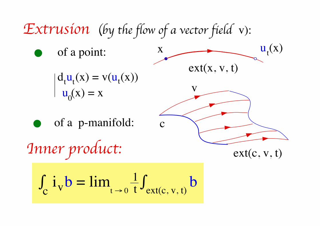
ext(c, v, t)

Extrusion (by the flow of a vector field v):

∫ i b = lim ∫ bvc1tt → 0 ext(c, v, t)

of a point:

c

v

of a p-manifold:

x

d u (x) = v(u (x))t

ext(x, v, t)

Inner product:

u (x)t

t t

u (x) = x0

The Lorentz force

v × B proxy for – i bv

(vector fields) (1-cochain)

∫ i b ~ ∫ be v ext(e, v)

Extrusion of an edge, as a chain of facets?

n (at point )

y = x + v(x )n n n

exn

yn

k

l

m

ext(e, v) ≈ (y ) nmk + (y ) nmln nk l

I(e, e', f) = weight of facet f in extrusion of edge e by the field λ e'n

e

n

f

e'

v ≈ ∑ λ (x) v = ∑ λ (x) v e'nn n

nne'

n, e'b = ∑ b w

ff

f(i b) = ∑ I(e, e', f) b vv e e', f f n

e'

Well and good. But is it true that

(i b) = – (i b) ?–v ve e

n

e

n

e

v

–v

Needed: a discrete notion of "tangent plane at n", or local affine structure

But there is a hitch: Missing the notion of tangent space at a node, we miss the linearity of inner product (andhence, of Lie derivative) w.r.t. flow vector field

But there is a hitch: Missing the notion of tangent space at a node, we miss the linearity of inner product (andhence, of Lie derivative) w.r.t. flow vector field

Now, one can assign a map from T to T to edge e: n mParallel transport from n to m, connection, etc.

∑ a e = 0nee

d(n) edgesaround n of the form

d(n) – D relations

n e m

dimension D (2 here)

,This structural element must be specified apart (just as discrete Hodge needed to be)

Local affine structure:

The Laplace force proxy for v → i b ∧ jv

(vector field) (covector-valued twisted 3-form)J × B

n

To be integrated over dual 3-cell n:~

Electric energy, ∫ e ∧ d, treated like ∫ i b ∧ jvn~ n~

Then, covector v → ∫ i b ∧ j is force exerted on n ~n~ v

Similar to ∫ e ∧ h, but now~ ~

1 ∧ 2 instead of 1 ∧ 1 n~

Energy

e

e~

ff~

∑ e de ∈ E e e

(electric)

∑ h bf ∈ F f f

(magnetic)

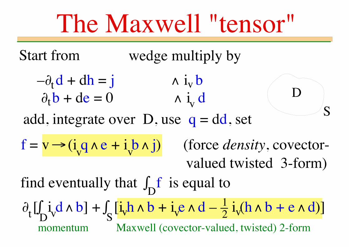
DS

Start from

–∂ d + dh = j ∧ i b

wedge multiply by

∂ b + de = 0 ∧ i dv

vt

t

add, integrate over D, use q = dd, set

valued twisted 3-form)find eventually that ∫ f is equal to

The Maxwell "tensor"

D

∂ [∫ i d ∧ b] + ∫ [i h ∧ b + i e ∧ d – – i (h ∧ b + e ∧ d)]v v vD S12

momentum Maxwell (covector-valued, twisted) 2-form

vt

f = v → (i q ∧ e + i b ∧ j) (force density, covector- vv

DS

∫ f =

The Maxwell "tensor"

D

∂ [∫ i d ∧ b] + ∫ [i h ∧ b + i e ∧ d – – i (h ∧ b + e ∧ d)]v v vD S12

momentum Maxwell (covector-valued, twisted) 2-form

vt

∫ [i h ∧ b – – i (h ∧ b)] =S v

12v ∫ [i b ∧ h + – i (h ∧ b)]

S v12v

treat like e ∧ h

extrude dual faces by v, use result about h ∧ b

Conclusion

and procedures that apply to them, described

Object-oriented programming agenda

Specific difficulty: infinite dimensional entities

Candidates to "object" status (mesh-related things) have been identified,

Discrete avatars of geometrical objects, for

(fields) vs finite data structures

which traditional vector fields are only proxies

Thanks