Bosonic fields in crystal manifold

Bosonic fields in crystal manifold

G. Alencar a, M.O. Tahim b, R.R. Landim a, R.N. Costa Filho a,∗a Departamento de Física, Universidade Federal do Ceará, Caixa Postal 6030, Campus do Pici, 60440-554 Fortaleza, Ceará, Brazilb Universidade Estadual do Ceará, Faculdade de Educação, Ciências e Letras do Sertão Central, Rua Epitácio Pessoa, 2554, 63.900-000 Quixadá, Ceará, Brazil

A crystal-like universe made of membranes in extra dimensions in a Randall–Sundrum scenario isstudied. A background gravitational metric satisfying the right boundary conditions is considered tostudy the localization of the scalar, gauge and Kalb–Ramond fields. It is found that the wave function forthe fields are Bloch waves. The mass modes equations are calculated allowing us to show the zero-gapmass behavior and the mass dispersion relation for each field. Finally we generalize all these results andconsider q-forms in the crystal membrane universe. We add the dilaton interaction in order to guaranteelocalization of forms. We show that, due to the dimension D , the form q and the dilaton coupling λ, themass spectrum can be the same for the different bosonic fields studied. Such a result is a different wayto see the duality between forms.

1. Introduction

The model regarding a universe with extra dimensions in sucha way that the membranes itself generate a kind of crystal [1–3]is interesting. In such a situation we can think about membranesin every direction in the bulk, with intersections, etc. These areconfigurations already discussed in the context of string theoryphenomenology, where we can generate the families of particlesof the Standard Model plus some corrections [4–8]. There are lotsof consequences to the phenomenology of the four-dimensionalworld we live [9]. The point we would like to address here isthat, in the case of membranes distributed along extra dimensionswhich are slices of AdS spaces, we can find Bloch like solutionsto the equations of motion. This means these models presents thesimilar behavior of electrons of conduction bands of materials weclassify as having metallic characteristics. In this sense, the investi-gations related to that scenario only discussed the behavior of thegravity field. In this work we extend that idea in order to studythe behavior of bosonic form fields in the crystal manifold uni-verse.

There are lots of important motivations to study higher ranktensor fields in several contexts related either to String Theory orto Mathematics [10–21]. Generally the q-forms of highest rank donot have physical relevance. This is due to the fact that the big-ger is its rank, the higher is the number of gauge freedom. Such

* Corresponding author.E-mail addresses: [email protected] (G. Alencar), [email protected]

(M.O. Tahim), [email protected] (R.R. Landim), [email protected] (R.N. Costa Filho).

fact can be used to cancel the dynamics of the field in the brane[22]. The mass spectrum of the two and three-form have beenstudied, for example, in Refs. [23] and [24] in a context of fivedimensions with codimension one. Posteriorly, the coupling be-tween the two and three-forms with the dilaton was studied, indifferent contexts, in [25–27]. In these scenarios, some facts aboutlocalization of fields are known: The scalar field (0-form) is lo-calizable, but the vector gauge fields (1-form), the Kalb–Ramondfield (2-form) and the three-form field are not. The reason whythis happens with the vector field is that, in four dimensions, itis conformal and all information coming from warp factors dropsout, necessarily rendering a non-normalizable four-dimensional ef-fective action. However, in the work of Kehagias and Tamvakis[28], it is shown that the coupling between the dilaton and thevector gauge field produces localization of the vector field. In anal-ogy with the work of Kehagias and Tamvakis [28], as cited above,the authors have also considered these coupling with a three-formfield [29], where a condition for localization is found. More re-cently the authors made a work generalizing the same aspects toq-forms [30,31].

In this work we are interested in check the Block like behaviorfor general bosonic fields in the crystal manifold universe. We goright to the point of analysis of the fields subject to the backgrounddescribed in [1]. The mass modes equations are calculated allowingus to show the zero-gap mass behavior and the mass dispersionrelation for each field. We generalize all these results and considerq-forms in the crystal membrane universe. We add the dilaton in-teraction in order to guarantee localization of q-form fields. Weshow that, due to the dimension D , the form q and the dilatoncoupling λ the mass spectrum can be the same for the different

bosonic field studied which is a different way to show duality be-tween forms.

To start the analysis of the fields subject to the backgrounddescribed in [1], we consider the simplest case with one extra di-mension, with the conformal metric defined as

ds25 = Ω2(z)

(ημν dxμ dxν + dz2), (1)

with Ω−1 = L−1S(z) + 1 where L is the AdS radius. The functionS(z) satisfy the equations

d2S(z)

d(z)2= 2

∑j

(−1) jδ(z − jl),

∣∣∣∣dS(z)

dz

∣∣∣∣ = 1,

and are given by (l being the spacing between the branes)

S(z) =

⎧⎪⎪⎨⎪⎪⎩

. . . ,

2pl − z, for (2p − 1)l < z < 2pl,

z − 2pl, for 2pl < z < (2p + 1)l,

. . . ,

(2)

where p = 1,2,3, . . . . In order to analyze the dilaton we will usethe same procedure as in Ref. [32] where the metric now reads

ds2 = e2A(y)ημν dxμ dxν + e2B(y) dy2, (3)

and after solving Einstein’s equation we get the relations [28].

B(y) = A(y)/4, π = −√

3M3 A(y). (4)

The parameter b is such that B(y) = (1 − b)A(y), where b = 3/4is the case with dilaton and b = 1 otherwise. To obtain the con-formal metric (1), we use the transformation dy/dz = e A(y)−B(y) =eb A(y) = Ω(z) in (3). We obtain A(z) = ln Ω(z)/b, where A(y) =A(z).

That will be the metric used in all the cases where the equationof motion has the following general form[− d2

dy2+ P ′(y)

d

dy+ V (y)

]ψ(y) = m2 Q (y)ψ(y), (5)

where P (y) = γ A(y), Q (y) = e−2b A(y) and V (y) = 0 for all fieldsexcept gravity, where V (y) = 2A′′(y)− 2(1 + b)A′(y)2. That can betransformed into the following Schrödinger-like equation[− d2

dz2+ U

]ψ(z) = m2ψ(z), (6)

where the potential U (z) = c A′′(z) + c2[ A′(z)]2 is given by

U (z) =(

c

b+ c2

b2

)(Ω−1)′ 2

(Ω−1)2− c

b

(Ω−1)′′

(Ω−1), (7)

where c is a parameter that depends on the form studied. Thepotential has been expressed in terms of Ω−1 due to the formof the conformal factor. It is interesting to note that the form ofthe potential coefficients simplifies the solution. Taking Ω given asdefined above we get the final Schrödinger-like equation

ψ ′′ +[

m2 −(

c

b+ c2

b2

)1

(S(z) + L)2+ 2

c

b

∑j(−1) jδ(z − jl)

(S(z) + L)

]ψ

= 0. (8)

This equation is very similar to the Schrödinger equation for aparticle propagating in a one-dimensional periodic potential (1D-crystal). In order to solve it we have to consider two adjacent

elementary cells in the region 0 � z � 4l. Focusing on the region0 � z � 2l we need to find the appropriate boundary conditions.First of all we must have ψ(l+) = ψ(l−) and ψ(2l+) = ψ(2l−).Where we use the definition l± = limε→0(l ± ε). To obtain the cor-rect boundary condition for the derivative we simply integrate theabove equation from l−(2l−) to l+(2l+) to obtain

ψ ′(l+) − ψ ′(l−) = 2c

b(l + L)ψ(l),

ψ ′(2l+) − ψ ′(2l−) = − 2c

bLψ(2l). (9)

The equation for the first elementary cell is

ψ ′′ + m2ψ =

⎧⎪⎪⎨⎪⎪⎩

( cb + c2

b2 )

(z+L)2 ψ for 0 < z < l,

( cb + c2

b2 )

(2l−z+L)2 ψ for l < z < 2l

(10)

and the above equations can be expressed in terms of a Besselequation. For this we just perform the transformations

ψ ={√

uΨ (u), u = m(z + L), for 0 < z < l,√vΨ (v), v = m(2l − z + L), for l < z < 2l,

(11)

to get

u2Ψ ′′ + uΨ ′ + (u2 − ν2)Ψ = 0, (12)

where ν2 = ( 12 + c

b )2. It is important to mention that the quantityν2 is related to the kind of field we consider. The solution of theabove equation is given by

ψ ={√

u(AH+ν (u) + B H−

ν (u)), 0 < z < l, u = m(z + L),√v(C H+

ν (v) + D H−ν (v)), l < z < 2l, v = m(2l − z + L),

(13)

where H+(−)ν are. Now using the transfer matrix technique we can

relate the constants C, D with A, B to obtain

(CD

)=

⎛⎜⎝

−h−ν h+

ν−1+h+ν h−

ν−1

h−ν h+

ν−1−h+ν h−

ν−1

−2h−ν h−

ν−1

h−ν h+

ν−1−h+ν h−

ν−1

2h+ν h+

ν−1

h−ν h+

ν−1−h+ν h−

ν−1

(h−ν h+

ν−1+h+ν h−

ν−1)

h−ν h+

ν−1−h+ν h−

ν−1

⎞⎟⎠

(AB

)

≡ K

(AB

). (14)

Similarly, we can solve for the next cell (2l < z < 4l) to find

(CD

)=

⎛⎜⎝

− h−ν h+

ν−1+h+ν h−

ν−1

h−ν h+

ν−1−h+ν h−

ν−1

−2h−ν h−

ν−1

h−ν h+

ν−1−h+ν h−

ν−1

2h+ν h+

ν−1

h−ν h+

ν−1−h+ν h−

ν−1

(h−ν h+

ν−1+h+ν h−

ν−1)

h−ν h+

ν−1−h+ν h−

ν−1

⎞⎟⎠

(AB

)

= K

(AB

)(15)

and therefore we have four constants A, B, A and B to be deter-mined. In order to get this we impose the following conditions

ψ(2l) = e2iqlψ(0), (16)

ψ(4l) = e2iqlψ(2l), (17)

ψ(2l+) = ψ(2l−), (18)

ψ ′(2l+) − ψ ′(2l−) = − 2c

bLψ(2l). (19)

The first of the above conditions can be written as

e2iql( h+ν h−

ν

)(AB

)= (

h+ν h−

ν

)(CD

)

= (h+ν h−

ν

)K

(AB

), (20)

where we have used H(u) = h and H(2l) = H(0) ≡ h, resulting in

cos(lq) = ( jνnν−1 + jν−1nν)( jνnν−1 + jν−1nν)

2( jνnν−1 − jν−1nν)( jνnν−1 − jν−1nν)

− jν−1 jν( jν−1 jν + 3nν−1nν)

2( jνnν−1 − jν−1nν)( jνnν−1 − jν−1nν)

− nν−1nν(3 jν−1 jν + nν−1nν)

2( jνnν−1 − jν−1nν)( jνnν−1 − jν−1nν). (21)

The above equation gives us the dispersion relation for the mass,where one can find, for example, the mass gap of the system con-sidered.

Next, we are going to consider several cases starting with thelocalization of the zero mode. The action for the scalar field with-out the dilaton coupling is given by

S =∫

d4x dz√−GG MN∂MΦ∂NΦ (22)

and the zero mode is obtained taking Φ = χ(x), which is equiv-alent to set m = 0. Using Eq. (1) as metric the effective actionbecomes

S =∫

dz Ω3(z)

∫d4xημν∂μχ∂νχ, (23)

and according to the solution∫

Ω3(z) < ∞ we have a well de-fined four-dimensional action. The scalar field is localized withoutthe dilaton coupling. This coupling does not change the localizabil-ity of the field, but it must be considered because of the gaugefield localization. Therefore, due to consistency it will be includein the analysis. With the dilation we have to use the metric de-fined in Eq. (3). As we have found before, the potential is writtenin a general form

U (z) = ci A′′(z) + c2i

[A′(z)

]2. (24)

The prime means a derivative with respect to z, and to obtain thatresult we have used dy/dz = e−bi A , where the label i = 1 and 2stands for the case with and without the dilaton, respectively, andare given by

b1 = 3

4, c1 =

(3

2+ λ

√3M3

2

),

b2 = 1, c2 = 3

2, (25)

and we get

ν21 =

(5

2+ 2λ

√3M3

3

)2

, ν2 = 2. (26)

Now for a gauge field living in the crystal manifold. The actionfor this field is given by

S X =∫

d5x√−G

[Y M1 M2 Y M1 M2

], (27)

where Y M1 M2 = ∂[M1 XM2] is the field strength for the 1-form X .The study of the zero mode is made using XM1 = XM1 (xμ) and, assaid in the second section, we must consider the metric given in

Eq. (1) for the case without the dilaton coupling. In this case weget the effective action

S X =∫

dz Ω

∫d4x

[Yμ1μ2 Y μ1μ2

]. (28)

Like in the case with just one brane∫

dz Ω → ∞, and we have aill defined action. However, we can consider the coupling of thisfield with the dilaton, with the action given by

S X =∫

d5x√−Ge−λπ

[Y M1 M2 Y M1 M2

], (29)

where λ is the dilaton coupling. With this and using the metricdefined in Eq. (3) the effective action becomes

S X =∫

dz Ω( 54 −λπ)

∫d4x

[Yμ1μ2 Y μ1μ2

]. (30)

The integration must be performed in the crystal manifold. How-ever, as mentioned previously, the finiteness of the z dependenceis reduced to the finiteness of integral in one cell. With the ex-pression for Ω we see that this is reached if λ > −1/

√3M3. This

is the same condition as the one obtained for the localization ofgauge field in the model with just one brane. In order to analyzethe massive modes, we must come back to the metric defined byEq. (3). The equations of motion are given by

∂M1

(√−GG M1 P G M2 Q Y P Q) = 0. (31)

We use a gauge freedom to fix X y = ∂μ Xμ = 0 and using thetransformations dz

dy = e−3A/4 and dzdy = e−A respectively, we get

the same potentials for the Schrödinger-like equation for the caseswith and without the dilaton Eq. (24), but now

b1 = 3

4, c1 =

(1

2+ λ

√3M3

2

),

b2 = 1, c2 = 1

2, (32)

with

ν21 =

(7

6+ 2λ

√3M3

3

)2

, ν2 = 1. (33)

The action for the Kalb–Ramond field is defined by

S X =∫

d5x√−GY M1 M2 M3 Y M1 M2 M3 , (34)

where Y M1 M2 M3 = ∂[M1 XM2 M3] is the field strength for the 2-formX . Again, we must consider the zero mode given by XM1 M2 =XM1 M2 (xμ), with an effective action in the conformal metric (1)given by

S X =∫

dz Ω−2∫

d4x[Yμ1μ2μ3 Y μ1μ2μ3

], (35)

and, as in the gauge field case, we have a ill defined effective ac-tion since

∫dz Ω−2 → ∞. Now we turn to the action with the

dilaton coupling defined by

S X =∫

d5x√−Ge−λπ Y M1 M2 M3 Y M1 M2 M3 , (36)

where again λ is the dilaton coupling. With this and using themetric in Eq. (3) the effective action becomes

S X =∫

dz Ω(− 34 −λπ)

∫d4x

[Yμ1μ2 Y μ1μ2

]. (37)

With the expression for Ω we see that the zero mode localiza-tion is reached if λ > 7/4

√3M3. Again, we find the same condition

as that obtained for the localization of Kalb–Ramond field in themodel with just one brane. Now we analyze the massive modescoming back to the metric defined by Eq. (3). The new equation ofmotion is:

∂M(√−GG M P G N Q G LR e−λπ H P Q R

) = 0. (38)

Here, we can use gauge freedom to fix Xμ1 y = ∂μ1 Xμ1μ2 = 0 andby using the transformations dz

dy = e−3A/4 and dzdy = e−A respec-

tively, we have the following expression for the constants bi and ci

b1 = 3

4, c1 =

(−1

2+ λ

√3M3

2

),

b2 = 1, c2 = −1

2, (39)

and we obtain the solutions

ν21 =

(−1

6+ 2λ

√3M3

3

)2

, ν2 = 0. (40)

Now we can readily generalize our previous results to a q-formin a p-brane, where p = D − 2. In a recent paper the authors haveconsidered this issue and we are going to use those results here[30]. Just as before we must consider the cases with and withoutthe dilaton coupling. The action is given by

S X =∫

dD x√−G

[Y M1...Mq+1 Y M1...Mq+1

](41)

and considering XM1 M2 M3 = XM1 M2 M3 (xμ) with the metric ofEq. (1) we arrive at the effective action

S X =∫

dz Ω D−2(q+1)

∫d4x

[Yμ1...μq+1 Y μ1...μq+1

]. (42)

It is evident why the gauge field is not localizable in five dimen-sions. From the above we get the condition q < (D − 3)/2, whichfor D = 5 give us q < 1. We also see that in higher dimensions wecan have localized form fields without the inclusion of the dilatoncoupling. However, if we want to localize all the form fields wemust consider the dilaton coupling with an action defined by

S X =∫

dD x√−Ge−λπ

[Y M1...Mq+1 Y M1...Mq+1

](43)

and considering again XM1 M2 M3 = XM1 M2 M3 (xμ) and Eq. (3) we getthe effective action

S X =∫

dz Ω(p−2q+ 14 −λπ)

∫d4x

[Yμ1...μq+1 Y μ1...μq+1

]. (44)

From the above expression we get the condition λ > (8q − 4p +3)/4

√3M3 for localization. We must note that all the previous

conditions are enclosed in this one. This expression is the sameobtained for the localization in the case of one brane. To considerthe massive modes we must consider the metric defined by Eq. (3),and the equations of motion for this case is given by

∂M(√−g gMN1 · · · gMq Nq+1 Y N1...Nq+1

) = 0. (45)

Using the gauge freedom to fix Xμ1...μq−1 y = ∂ν Xν...μq = 0 and the

transformations dzdy = e−3A/4 and dz

dy = e−A we arrive to the fol-lowing expressions for the parameters bi and ci :

b1 = 3

4, c1 = −

(α

2+ 3

8

),

b2 = 1, c2 =(

p − q

), (46)

2

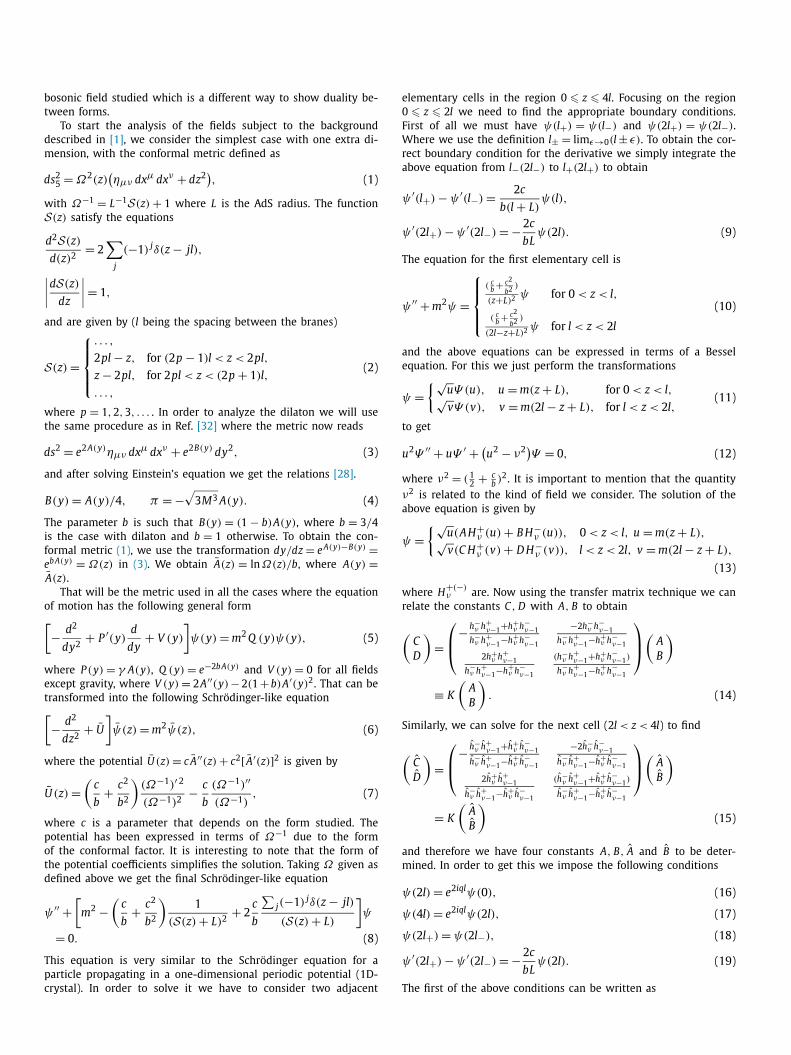
Fig. 1. The lowest mass modes for the case without dilaton and the scalar fieldν = 2.

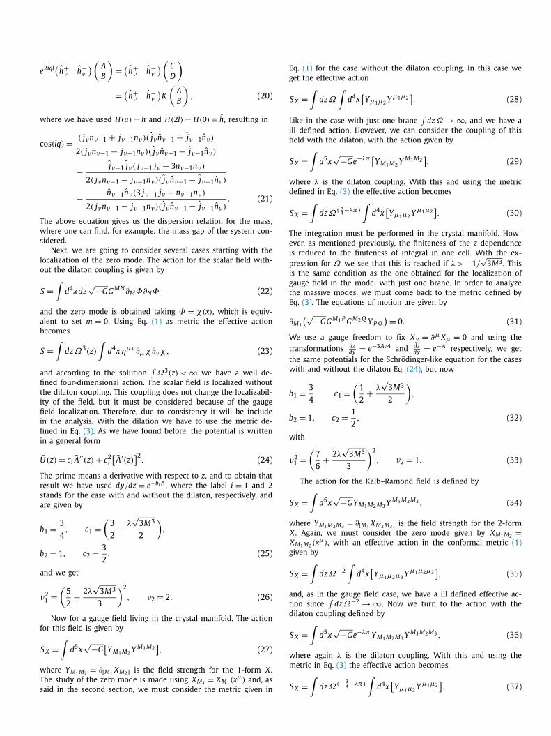
Fig. 2. The mass modes for both the gauge (ν = 1.0) and Kalb–Ramond (ν = 0.0)fields.

with α = (8q − 4p − 3)/4 − λ√

3M3. From these the solutions aregiven by

ν21 =

(2α

3

)2

, ν22 =

(1 + p

2− q

)2

. (47)

The important information one can get from the calculationsin previous sections is the allowed values of mass for each field.That can be obtained by solving numerically Eq. (21) for the caseswith and without dilaton. For the case without dilaton, we solveEq. (21) for the scalar field using ν = 2, for the gauge field ν = 1,and the Kalb–Ramond field ν = 0. The allowed masses for thescalar field are shown in Fig. 1 where the lowest mass modesare plotted. As one can see, the lowest mode or the gap of masshas its maximum value at q = 0, and for small values of |q| thereare only four allowed mass values. The interesting feature aboutthe dispersion relation equation is that due to the Bessel functionproperty j−1 = − j1 and n−1 = −n1, the gauge field and the Kalb–Ramond field have the same mass dispersion as shown in Fig. 2.The main characteristic of these fields is that around q = 0 no massis allowed. In fact for m > 0.5 the existence of mass particles is re-stricted to values of q ≈ 0.5π/l.

When considering the dilaton, depending on the coupling theorder of the Bessel functions in the dispersion relation can be non-integer. For λ = 1/

√(3M3) Fig. 3 shows the mass dispersion for

the q = 0, 1, and 2 forms in panels (a), (b), and (c) respectively.For the scalar field Fig. 3(a) shows a different behavior from Fig. 1

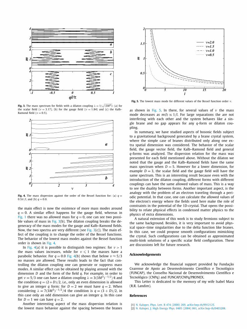
Fig. 3. The mass spectrum for fields with a dilaton coupling λ = 1/√

(3M3): (a) forthe scalar field (ν = 3.17), (b) for the gauge field (ν = 1.84) and (c) the Kalb–Ramond field (ν = 0.5).

Fig. 4. The mass dispersion against the order of the Bessel function for: (a) q =0.5π/l, and (b) q = 0.0.

the main effect is now the existence of more mass modes aroundq = 0. A similar effect happens for the gauge field, whereas inFig. 1 there was no allowed mass for q = 0, one can see two possi-ble values of mass in Fig. 3(b). The dilaton coupling breaks the de-generacy of the mass modes for the gauge and Kalb–Ramond fields.Now, the two spectra are very different (see Fig. 3(c)). The main ef-fect of the coupling is to change the order of the Bessel functions.The behavior of the lowest mass modes against the Bessel functionorder is shown in Fig. 4.

In Fig. 4(a) it is possible to distinguish two regimes: for ν > 1the mass values increases, while for ν � 1 the masses have aparabolic behavior. For q = 0.0 Fig. 4(b) shows that below ν ≈ 5/3no masses are allowed. These results leads to the fact that con-trolling the dilaton coupling one can generate or suppress massmodes. A similar effect can be obtained by playing around with thedimension D and the form of the field q. For example, in order toget ν = 5/3 one can have a dilaton coupling λ = 3(3M3)−1/2/4 andthe condition q = (2+ D)/2, i.e., only an even dimension is allowedto give an integer q form: for D = 2 we must have q = 2. Whenconsidering λ = 7(3M3)−1/2/4 the condition is q = (3 + D)/2, inthis case only an odd dimension can give an integer q. In this casefor D = 1 we can have q = 2.

Another interesting aspect of the mass dispersion relation isthe lowest mass behavior against the spacing between the branes

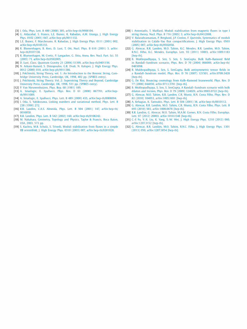
Fig. 5. The lowest mass mode for different values of the Bessel function order ν .

as shown in Fig. 5. In there, for several values of ν the massmode decreases as m(l) ∝ 1/l. For large separations the are notinterfering with each other and the system behaves like a sin-gle brane and no gap appears for any q-form or dilaton cou-pling.

In summary, we have studied aspects of bosonic fields subjectto a gravitational background generated by a brane crystal system,where the simple case of branes distributed only along one ex-tra spatial dimension was considered. The behavior of the scalarfield, the gauge vector field, the Kalb–Ramond field and generalq-forms was analyzed. The dispersion relation for the mass waspresented for each field mentioned above. Without the dilaton wenoted that the gauge and the Kalb–Ramond fields have the samemass spectrum when D = 5. However for a lower dimension, forexample D = 3, the scalar field and the gauge field will have thesame spectrum. This is an interesting result because even with theintroduction of the dilaton coupling, different forms with differentcouplings can have the same allowed values of mass. This is a wayto see the duality between forms. Another important aspect, is theanalogy with the problem of an electron traveling through a peri-odic potential. In that case, one can calculate the allowed values ofthe electron’s energy where the fields used here make the role ofconstraints in the potential of the 1D-crystal. That opens the possi-bility to relate physical effects in condensed matter physics to thephysics of extra dimensions.

A natural extension of this work is to study fermions subject tothe same background. Besides, it is very important to avoid phys-ical space–time singularities due to the delta function like branes.In this case, we could propose smooth configurations mimickingthe crystal. Such configurations can be obtained as approximatedmulti-kink solutions of a specific scalar field configuration. Theseare discussions left for future research.

Acknowledgements

We acknowledge the financial support provided by FundaçãoCearense de Apoio ao Desenvolvimento Científico e Tecnológico(FUNCAP), the Conselho Nacional de Desenvolvimento Científico eTecnológico (CNPq) and FUNCAP/CNPq/PRONEX.

This Letter is dedicated to the memory of my wife Isabel Mara(R.R. Landim).

References

[1] N. Kaloper, Phys. Lett. B 474 (2000) 269, arXiv:hep-th/9912125.[2] N. Kaloper, J. High Energy Phys. 0405 (2004) 061, arXiv:hep-th/0403208.

[3] I. Oda, Phys. Lett. B 480 (2000) 305, arXiv:hep-th/9908104.[4] G. Aldazabal, S. Franco, L.E. Ibanez, R. Rabadan, A.M. Uranga, J. High Energy

Phys. 0102 (2001) 047, arXiv:hep-ph/0011132.[5] L.E. Ibanez, F. Marchesano, R. Rabadan, J. High Energy Phys. 0111 (2001) 002,

arXiv:hep-th/0105155.[6] R. Blumenhagen, B. Kors, D. Lust, T. Ott, Nucl. Phys. B 616 (2001) 3, arXiv:

hep-th/0107138.[7] R. Blumenhagen, M. Cvetic, P. Langacker, G. Shiu, Annu. Rev. Nucl. Part. Sci. 55

(2005) 71, arXiv:hep-th/0502005.[8] D. Lust, Class. Quantum Gravity 21 (2004) S1399, arXiv:hep-th/0401156.[9] N. Arkani-Hamed, S. Dimopoulos, G.R. Dvali, N. Kaloper, J. High Energy Phys.

0012 (2000) 010, arXiv:hep-ph/9911386.[10] J. Polchinski, String Theory, vol. 1: An Introduction to the Bosonic String, Cam-

bridge University Press, Cambridge, UK, 1998, 402 pp. (SPIRES entry).[11] J. Polchinski, String Theory. Vol. 2: Superstring Theory and Beyond, Cambridge

University Press, Cambridge, UK, 1998, 531 pp. (SPIRES entry).[12] P. Van Nieuwenhuizen, Phys. Rep. 68 (1981) 189.[13] A. Smailagic, E. Spallucci, Phys. Rev. D 61 (2000) 067701, arXiv:hep-

th/9911089.[14] A. Smailagic, E. Spallucci, Phys. Lett. B 489 (2000) 435, arXiv:hep-th/0008094.[15] I. Oda, S. Yahikozawa, Linking numbers and variational method, Phys. Lett. B

238 (1990) 272.[16] R.R. Landim, C.A.S. Almeida, Phys. Lett. B 504 (2001) 147, arXiv:hep-th/

0010050.[17] R.R. Landim, Phys. Lett. B 542 (2002) 160, arXiv:hep-th/0108242.[18] M. Nakahara, Geometry, Topology and Physics, Taylor & Francis, Boca Raton,

USA, 2003, 573 pp.[19] S. Kachru, M.B. Schulz, S. Trivedi, Moduli stabilization from fluxes in a simple

IIB orientifold, J. High Energy Phys. 0310 (2003) 007, arXiv:hep-th/0201028.

[20] I. Antoniadis, T. Maillard, Moduli stabilization from magnetic fluxes in type Istring theory, Nucl. Phys. B 716 (2005) 3, arXiv:hep-th/0412008.

[21] V. Balasubramanian, P. Berglund, J.P. Conlon, F. Quevedo, Systematics of modulistabilisation in Calabi–Yau flux compactifications, J. High Energy Phys. 0503(2005) 007, arXiv:hep-th/0502058.

[22] G. Alencar, R.R. Landim, M.O. Tahim, K.C. Mendes, R.R. Landim, M.O. Tahim,R.N.C. Filho, K.C. Mendes, Europhys. Lett. 93 (2011) 10003, arXiv:1009.1183[hep-th].

[23] B. Mukhopadhyaya, S. Sen, S. Sen, S. SenGupta, Bulk Kalb–Ramond fieldin Randall–Sundrum scenario, Phys. Rev. D 70 (2004) 066009, arXiv:hep-th/0403098.

[24] B. Mukhopadhyaya, S. Sen, S. SenGupta, Bulk antisymmetric tensor fields ina Randall–Sundrum model, Phys. Rev. D 76 (2007) 121501, arXiv:0709.3428[hep-th].

[25] G. De Risi, Bouncing cosmology from Kalb–Ramond braneworld, Phys. Rev. D77 (2008) 044030, arXiv:0711.3781 [hep-th].

[26] B. Mukhopadhyaya, S. Sen, S. SenGupta, A Randall–Sundrum scenario with bulkdilaton and torsion, Phys. Rev. D 79 (2009) 124029, arXiv:0903.0722 [hep-th].

[27] G. Alencar, M.O. Tahim, R.R. Landim, C.R. Muniz, R.N. Costa Filho, Phys. Rev. D82 (2010) 104053, arXiv:1005.1691 [hep-th].

[28] A. Kehagias, K. Tamvakis, Phys. Lett. B 504 (2001) 38, arXiv:hep-th/0010112.[29] G. Alencar, R.R. Landim, M.O. Tahim, C.R. Muniz, R.N. Costa Filho, Phys. Lett. B

693 (2010) 503, arXiv:1008.0678 [hep-th].[30] R.R. Landim, G. Alencar, M.O. Tahim, M.A.M. Gomes, R.N. Costa Filho, Europhys.

Lett. 97 (2012) 20003, arXiv:1010.1548 [hep-th].[31] C.-E Fu, Y.-X. Liu, K. Yang, S.-W. Wei, J. High Energy Phys. 1210 (2012) 060,

arXiv:1207.3152 [hep-th].[32] G. Alencar, R.R. Landim, M.O. Tahim, R.N.C. Filho, J. High Energy Phys. 1301

(2013) 050, arXiv:1207.3054 [hep-th].