Bose–Einstein condensation in satisfiability problems

Bose-Einstein Condensation in Satisfiability Problems

Claudio Angione1, Annalisa Occhipinti2, Giovanni Stracquadanio 3 Giuseppe Nicosia4

1Computer Laboratory - University of Cambridge, UK2Dept. of Mathematics and Computer Science - University of Catania, Italy3Department of Biomedical Engineering - Johns Hopkins University, USA

4Dept. of Mathematics and Computer Science - University of Catania and Institute for Advanced Studies, [email protected]; [email protected]; [email protected]; [email protected]

Keywords: k–SAT, complex networks, Bose-Einstein condensation, phase transition, performance.

Abstract. This paper is concerned with the complex behavior arising in satisfiability problems.We present a new statistical physics-based characterization of the satisfiability problem. Specifically,we design an algorithm that is able to produce graphs starting from a k–SAT instance, in order toanalyze them and show whether a Bose-Einstein condensation occurs. We observe that, analogouslyto complex networks, the networks of k–SAT instances follow Bose statistics and can undergoBose-Einstein condensation. In particular, k–SAT instances move from a fit-get-rich network to awinner-takes-all network as the ratio of clauses to variables decreases, and the phase transition of k–SAT approximates the critical temperature for the Bose-Einstein condensation. Finally, we employthe fitness-based classification to enhance SAT solvers (e.g., ChainSAT) and obtain the consistentlyhighest performing SAT solver for CNF formulas, and therefore a new class of efficient hardwareand software verification tools.

1 Introduction

Satisfiability (SAT) is a famous logical reasoning problem defined in terms of Boolean variables andlogical constraints (clauses) describing the relation among these variables. Each such variable can benegated or not, that is, each variable (a literal) can be either True or False; the constraint is built asthe OR function of the k variables (k–SAT) [1]. In general, propositional formulas are represented inConjunctive Normal Form (CNF). A CNF formula consists of a conjunction of m clauses, each of whichconsists of a disjunction of k literals. SAT has received a great deal of theoretical and experimentalstudy as the paradigmatic NP-complete problem as decision problem [2,3] and NP-hard as solutionwhen there are more than two literals for each clause [4]. The SAT problem is also crucial for solvinglarge-scale computational problems, such as AI planning, scheduling [5], protein structure prediction,haplotype inference, circuit-level prediction of crosstalk noise, computer chip verification, terminationanalysis in term-rewrite systems, model checking, and hardware and software verification [6,7]. Indeed,most verification tools consist of decision procedures to check the satisfiability of a given formula generatedby the verification process. As a result, the subject of practical SAT solvers has received considerableresearch attention, and numerous solver algorithms have been proposed and implemented [8,9,10]. Inparticular, several SAT solvers rely on linear programming [4] or tabu search [11] and have been thoroughlyanalyzed in their worst cases [12]. When we consider randomly generated instances, SAT is called randomsatisfiability problem. The original aim for inspecting random instances of k–SAT has been the desire todecipher the hardness and complexity of typical (standard) instances. For this reason, research works onk–SAT have been focused on developing algorithms for counting the number of solutions [13,14,15], andanalyzing their computational complexity [16].

The cooperative dynamics of the interacting clauses can exhibit new rich behavior that is not evident inthe properties of the individual clauses and literals (the elementary units) that make up a SAT formula(the many-body system) of a very large numbers of these units. Standard experimental methods forstudying NP-complete problems use a random generator of the problem instances and an exact (possibly

arX

iv:1

304.

0810

v1 [

cs.D

S] 2

Apr

201

3

2

optimized by means of heuristics) algorithm to solve them. By analyzing the results with proper measures(e.g., the number of recursive calls), one can obtain important information about the problem, such asphase transitions, topological characterization of the search space, and clusters of solutions [17]. Duringthe last twenty years, studies in theoretical computer science have exploited new methodologies, basedon statistical physics and experimental computer science, for investigating the nature and properties ofNP-complete problems [18,19,20].

There is a deep connection between NP-complete problems and models studied in statistical physics.This connection leads to determining computational complexity from characteristic phase transitions inthe k–SAT problem [2]. In Sherrington’s work [21], k–SAT is thought of as an extension of the Sherringtonand Kirkpatrick’s spin glass model [22]. Moreover, its graph structure is an extension of the Erdos-Renyirandom graphs; in particular, k–SAT models on Erdos-Renyi graphs showed the existence of free energylimits [23]. Although computer programs based on local dynamical algorithms are unable to reach theHARD-SAT phase in the neighborhood of the k–SAT phase transition, spin glasses techniques [24] allow toquantify the HARD-SAT region between the SAT and UNSAT ones. Mezard et al. [3] showed the existenceof an intermediate phase in k–SAT problems below the phase transition threshold, and a powerful classof optimization algorithms was designed and tested successfully on the largest existing benchmark of k–SAT. Krzaka la et al. [25] discovered and analyzed four phase transitions in the solution space of randomk–SAT. As the constraint density increases, clusters of solutions appear in the solution space; then,solutions condense over a few large clusters. These results strengthen the link between computationalmodels and properties of physical systems, and offer the possibility of new developments and discoveriesin this research field.

The goal of our research is to characterize the condensation phenomenon for k–SAT problems bytranslating a formula into a graph G = (V,E), and then to employ this characterization to improvethe well-known ChainSAT algorithm [26]. Inspired by Bianconi and Barabasi’s research work on Bose-Einstein condensation (BEC) in complex networks [27], we design an algorithm that produces graphsstarting from a k–SAT instance and associates each clause to a fitness value. The phase diagram ofthe graph provided by the algorithm shows evidence of BEC for low values of the clauses-to-variablesratio. The BEC, from the very beginning, was associated to superfluidity: as London stated in 1938,“the peculiar phase transition (λ point) that liquid helium undergoes at 2.19 K, most probably has tobe regarded as the condensation phenomenon of the Bose-Einstein statistic” [28]. Hence, superfluidity ina k-SAT formula could be thought of as a consequence of the low constraint density that we find in theSAT phase. Our results give new hints in understanding the complexity and the structure of a k–SATinstance in phase transition. The graph of a given instance allows us to satisfy it by finding a truthassignment only for the fittest clauses. Our approach makes use of complex networks in order to operateon the instance, without requiring a priori investigation of its solutions.

The rest of the paper is organized as follows. First, we give an overview of the Bose-Einstein distri-bution and tailor it to the satisfiability problem by translating a SAT formula into a graph. Then, weinvestigate two variants of our algorithm. We present experimental evidence supporting the hypothesisthat the phase transition between solvable and unsatisfiable instances of 3-SAT approximates the locus ofthe Bose-Einstein condensation in the phase diagram of 3-SAT formulas. Finally, we show how to improvethe ChainSAT solver by using our algorithm to provide a clause ordering.

2 Bose-Einstein Distribution

The analysis of the state of matter, from a quantum point of view, states that all particles of the same typeare equal and indistinguishable. Let us consider an isolated system of N identical and indistinguishablebosons confined to a space of volume V and sharing a given energy E. These latter are particles that donot obey the Pauli exclusion principle, since two or more bosons may have exactly the same quantumnumbers. We assume that these bosons can be distributed into a set of energy levels, where each levelEi is characterized by an energy εi, i.e., the energy of each particle settled on that energy level, anda degeneration gi, representing the number of different physical states that can be found at that level.Accordingly, the N identical and indistinguishable particles are distributed among the energy levels, and

3

each level Ei contains ni particles, to be accommodated among its gi quantum states. For instance, ifni = 2 and gi = 3, the particles a and b can settle on Ei in one of these ways: ab‖−‖−, −‖ab‖−, −‖−‖ab, a‖ − ‖b, a‖b‖−, −‖a‖b. (Permutations of particles must not be included, since a and b areindistinguishable.)

It is straightforward to check that ni particles may be put on the level Ei (consisting of gi states) in[ni + (gi − 1)]! different ways. Since bosons are indistinguishable and the physical states are equivalent,the number of possible assignments of ni bosons on Ei is:

wi =(ni + gi − 1)!

ni!(gi − 1)!=

(ni + gi − 1

ni

). (1)

By iterating for all the energy levels Ei, one can observe that a distribution {ni} (i.e., a distribution withni particles on the level Ei, ∀i) can be obtained in

W =∏i

wi =∏i

(ni + gi − 1)!

ni!(gi − 1)!(2)

different ways. In other words, wi is the number of distinct microstates associated with the i-th level of thespectrum, while W is the number of distinct microstates associated with the whole distribution set {ni}.The particles distribution corresponding to the statistical equilibrium is the most probable one, thus it isthe one that may be reached in the largest number of possible ways. Hence, in order to find it, we computethe maximumW subject to the conservation of the number of particles

∑i ni = N , and to the preservation

of the system energy∑i εini = E. We adopt the method of Lagrange’s undetermined multipliers, but

rather than maximizing W directly, we maximize logW , since log is a monotone transformation. Thismethod results in the following condition:∑

i

[log

(ni + gini

)− α− βεi

]δni = 0, (3)

where α and β are the Lagrangian undetermined multipliers associated with the two restrictive conditionsof conservation. Since the variations δni are completely arbitrary, this condition can be satisfied if andonly if all their coefficients vanish identically, namely:

log

(ni + gini

)− α− βεi = 0, ∀i.

This equality leads to the following definition of Bose-Einstein distribution:

ni =gi

eα+βεi − 1, (4)

where α = − µCkBT

and β = 1kBT

are inversely proportional (by means of Boltzmann’s constant kB) to theabsolute temperature T of the system at the equilibrium, and µC represents the chemical potential.

Given an ideal Bose-Einstein gas in equilibrium below its transition temperature, the Bose-Einsteincondensation (BEC) is the property that a finite fraction of particles occupies the lowest energy level.According to Penrose and Onsager [29], we can provide a criterion of BEC for an ideal gas in equilibrium:

BEC ⇐⇒ 〈n0〉N = eO(1), No BEC ⇐⇒ 〈n0〉

N = o(1), where 〈n0〉 is the average number of particles that

occupy the lowest energy level E0. (The first equation is equivalent to 〈n0〉N = constant, but it is weaker

and easier to apply.) For low values of temperature, i.e., when T → 0 K, the BEC takes place [30]. Thisphenomenon consists of a very unusual state of aggregation of particles, called Bose-Einstein condensate.Its characteristic is different from those of the solid state, liquid state, gas and plasma, thus it is known as“the fifth state of matter”. In particular, below a critical temperature TBEC , all the particles settle on thesame quantum state and occupy the same energy level. Hence, they are absolutely identical, inasmuch asthere is no possible measurement that can tell them apart. In other words, they lose their individuality,and the single-particle perception is missing.

4

Inspired by Bianconi and Barabasi’s work [27], we provide an algorithm to investigate the BEC phe-nomenon in the k–SAT problem. By translating a SAT formula into a graph, we define the condensation ofthe formula over its fittest clause as the emergence of a star-like topology in the graph. This phenomenonis associated with the condensation of bosons on the lowest energy level (see examples in SupportingInformation).

3 The SAT to Graph Algorithm

An instance of the k–SAT problem consists of:

· a set X of variables, with |X| = n;· a set C of clauses over X, where |C| = m, such that each clause Ci ∈ C, ∀i = 1, ...,m, has k

literals and can be written as Ci = L1 ∨ L2 ∨ ... ∨ Lk. Each literal Lµ ∈ L, ∀µ = 1, ..., l, whereL = X ∪X ∪ {True, False} is the set of literals, |L| = l.

The problem is to find a satisfying truth assignment for the following formula:

F = C1 ∧ C2 ∧ ... ∧ Cm. (5)

The SAT to Graph Transformation Algorithm (S2G) translates a k–SAT instance into a graph G =(V,E), where V are the vertices and E are the edges. A vertex vi is a clause Ci of the formula F , i.e.,vi = v(Ci), whereas each edge ejh represents a relation between two clauses, i.e., ejh = (v(Cj), v(Ch)), aswe see later. Let us introduce two functions for literals and clauses. Firstly, we define the global frequencyof literals as:

ϕG(Lµ) = occurrences of Lµ in F , µ = 1, ..., l, (6)

which reports the frequency of a literal into a k–SAT formula. Secondly, we define the global fitness ofclauses as:

fG(Ci) =

k∑µ=1

ϕG(Lµ), Lµ ∈ Ci, i = 1, ...,m, (7)

which is a fitness function to evaluate clauses and grows with a monotonic behavior with respect to theϕG of its literals. The construction of the graph G = (V,E) is an iterative process in which each clauseCi is assigned to a vertex (node) vi, and edges ejh are links established according to an affinity function,as we see below. Since the construction is dynamical, we need to define the local frequency of literals andthe local fitness of clauses. While the global ones are determined on the complete formula F , the localones concern only the clauses that have been added as vertices in V using a subset F ′ of the clauses ofF . In particular, we define the local frequency of literals as follows:

ϕL(Lµ) = occurrences of Lµ in F ′, µ = 1, ..., l. (8)

Analogously, the local fitness of clauses is defined as:

fL(Ci) =

k∑µ=1

ϕL(Lµ), Lµ ∈ Ci, i = 1, ...,m. (9)

It is obvious that, at iteration i, a literal Lµ has ϕL(Lµ) = 0 in case it belongs to a clause that has notbeen added to V (G) yet; when the algorithm ends, ϕG(Lµ) = ϕL(Lµ), ∀µ = 1, .., l.

Hereinafter we need to suppose that the order of literals in a clause has no importance. However,since the OR operator is commutative, it is possible to define a distance metric that states how manyliterals are not in common between two clauses. Let Ci, Cj be two clauses made up of literals Liµ and Ljµrespectively; we define the following distance:

d(Ci, Cj) =∣∣ {µ ∈ {1, ..., k} : Liµ 6= Ljµ

} ∣∣ , (10)

5

which is a metric distance that can be related to the well-known Hamming distance [31]. In SupportingInformation A, we prove that d is a metric.

Let G = (V,E) be the graph obtained at the (i−1)-th iteration, and F ′ ⊂ F be the temporary k–SATsubformula F ′ = Ct1 ∧ Ct2 ∧ ... ∧ Cti−1 . In order to add a clause Cti to G as a node v(Cti), we estimatethe probability of being connected to a node that already belongs to the graph; this probability must becomputed for each node (clause) added to G, since it is the criterion to build edges between nodes. Wedefine the probability that a new node v(Cti) is connected to the node v(Ctj ) ∈ V (G) as:

Πtj =ktj · fL(Ctj )

|V |∑ν=1

ktν · fL(Ctν )

, (11)

where ktj = degree(v(Ctj )) is the connectivity of Ctj (i.e., the number of links shared by node v(Ctj )),and fL(Ctj ) is the fitness of the clause Ctj . This probability distribution ensures that a new vertex islikely linked to an existing one with high fitness value or/and high connectivity [27]. We deduce thatthis process brings to a model in which the attractiveness and evolution of a node are determined by itsfitness and by its number of links.

In order to assign the new node-clause Cti an appropriate number representing an energy level [27],it is necessary to normalize the local fitness values as fLr (Cti) = fL(Cti)/f

L(Ct), where Ct is the fittestclause in the temporary graph already built using F ′. As a result, as soon as the node v(Cti) enters thesystem, it has the following energy (see [27]):

εti = −T · log fLr (Cti), (12)

where T = 1β , and β is a parameter used to model the temperature of the system. (In this work, when

comparing two or more energy levels, we omit the multiplicative factor T .) If two different nodes areassigned the same energy value in our model, it means (from a physical point of view) that they representtwo different degeneration states of the same energy level, as shown in Table 1.

G = (V,E) k–SAT Statistical physics

node clause degeneration state of the energy level of the nodeedge link between two clauses one particle for each degeneration state involved

node weight fitness of a clause value of the energy leveledge weight probability of being established weight on particles

Table 1. Dictionary translating the graph (left) into the k–SAT problem (centre) and statistical physicslanguage (right).

The definition of probabilities and the linking criterion are the building blocks of the S2G algorithm,which consists of three main steps.

Step I. Let Λ = ∅, V = ∅, E = ∅, and F ′ = ∅. Let i be the index representing the number of theiteration. Here, we set i = 1. The first clause Ct1 to add to F ′ is chosen randomly among the m clauses ofthe given formula F . After computing the local fitness of the clause, we assign to it the normalized localfitness fLr (Ct1). Since Ct1 is the only clause added to the graph so far, its fLr is set to 1. After that, wecompute the energy level εt1 , which in this case is equal to 0. The variable t is used to store the index ofthe fittest clause. Obviously, at the first iteration, it must be set to t1. The pseudo-code of the first stepis presented in Algorithm S1.

6

Step II. Successively, we perform another step of the algorithm, in order to establish the first linkbetween two clauses, as shown in Algorithm S4. This step and the following ones include two procedures,shown in Algorithm S2 and Algorithm S3. The second clause is chosen such that it is the closest toCt1 , in terms of the distance defined in (10). If two or more clauses have the same minimum distancefrom Ct1 , then a random clause is chosen among them. Notice that at every iteration i all the localfrequencies of literals are updated, therefore the local fitness and the energy level of clauses are updatedas well. We perform the normalization of the fitness in order to obtain a non-negative energy level. Indeed,the logarithm function, when its base is greater than 1 and its argument belongs to the interval ]0; 1],returns a non-positive value; since the absolute temperature T is non-negative, the energy level becomesa non-negative value, as expected.

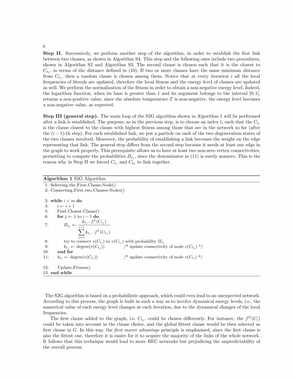
Step III (general step). The main loop of the S2G algorithm shown in Algorithm 1 will be performedafter a link is established. The purpose, as in the previous step, is to choose an index ti such that the Ctiis the clause closest to the clause with highest fitness among those that are in the network so far (afterthe (i− 1)-th step). For each established link, we put a particle on each of the two degeneration states ofthe two clauses involved. Moreover, the probability of establishing a link becomes the weight on the edgerepresenting that link. The general step differs from the second step because it needs at least one edge inthe graph to work properly. This prerequisite allows us to have at least two non-zero vertex connectivities,permitting to compute the probabilities Πtj , since the denominator in (11) is surely nonzero. This is thereason why in Step II we forced Ct1 and Ct2 to link together.

Algorithm 1 S2G Algorithm

1: Selecting the First Clause-Node()2: Connecting First two Clauses-Nodes()

3: while i < m do4: i← i+ 15: Find Closest Clause()6: for j ← 1 to i− 1 do

7: Πtj ←ktj · fL(Ctj )

i−1∑ν=1

ktν · fL(Ctν )

8: try to connect v(Cti) to v(Ctj ) with probability Πtj9: ktj ← degree(v(Ctj )) /* update connectivity of node v(Ctj ) */

10: end for11: kti ← degree(v(Cti)) /* update connectivity of node v(Cti) */

12: Update Fitness()13: end while

The S2G algorithm is based on a probabilistic approach, which could even lead to an unexpected network.According to this process, the graph is built in such a way as to involve dynamical energy levels, i.e., thenumerical value of each energy level changes at each iteration, due to the dynamical changes of the localfrequencies.

The first clause added to the graph, i.e. Ct1 , could be chosen differently. For instance, the fG(Ci)could be taken into account in the clause choice, and the global fittest clause would be then selected asfirst clause in G. In this way, the first mover advantage principle is emphasized, since the first clause isalso the fittest one, therefore it is easier for it to acquire the majority of the links of the whole network.It follows that this technique would lead to more BEC networks but prejudicing the unpredictability ofthe overall process.

7

When the graph is completed, we consider the connectivity of the richest node (the node that has themaximum number of links) in order to decide whether a Bose-Einstein condensation has occurred. If theconnectivity is large enough (the thresholds have been determined experimentally, see Working hypothesis2), we say that a BEC has taken place in the graph, i.e., one node has a huge fraction of edges and theremaining fraction is shared among all the other nodes. If the graph does not show any condensation, wecompute the degree distribution in order to understand what kind of network has developed. Moreover,we compute the mean and the standard deviation of all nodes except the winner (i.e., the richest), so asto obtain simple statistics involving the rest of the degree distribution.

The computational complexity of our algorithm is polynomial. The Step II procedure has a complexityof O(N3), where N = max{n,m, k}, due to the subprocedure that computes the distance d between theclauses eligible to join the graph and the fittest clause already added to it. The main loop of the S2Galgorithm has O(N4) time complexity, since it consists of the Step II procedure applied (with slightmodifications) to all of the remaining clauses of the k–SAT formula.

4 Fitness-Based Preferential Attachment

In this section we extend the S2G algorithm by including the concept of preferential attachment, thusobtaining a new algorithm called S2G-PA. Even this model starts with two nodes connected by an edge.Exactly as in the previous model, at each iteration a new node is added to the graph. The preferentialattachment implemented in the new algorithm is based on the same principle of the algorithm used so far:if we consider a single node of the network, the probability of acquiring new edges is positively correlatedwith its degree. According to the previous section, in the fitness-based model the connectivity is notthe only parameter taken into account, but also the fitness plays an important role in computing theprobability of acquiring new edges.

The main difference between this model and the model presented before consists of the preferentialout-degree (ρ), a technique applicable to directed graphs. At each iteration i, the node that joins the graphis forced to connect at most to ρ existing nodes and at least to one node. Recall that in the previous modelthere were no restrictions to the number of outgoing links (od(v)) that a node could have. It follows thata number of nodes, when they joined the existing network, did not link to any other node of the graph.This caused the probability Π (probability of linking a new node to them) to remain always 0, thereforetheir degree remained equal to 0 during the whole process, i.e., they never linked to the main connectedcomponent of the graph. On the contrary, the new algorithm ensures that all the nodes will be part ofthe network, i.e., all the nodes will have at least one link and G has only one connected component. Theoutput networks of S2G and S2G-PA can be compared in Supporting Information C and SupportingInformation D. When the most connected nodes have the highest number of particles, and the winnernode is identified with the lowest energy level, we obtain a clear “signature” of BEC in a preferentialattachment scheme with fitness, as proved by Borgs et al. [32]. These facts help us confirm that when theBEC occurs there is a clear mapping between the Bose gas and the graph derived by the S2G algorithm.

The preferential attachment ensures that the condition 1 ≤ od(v(Cti)) ≤ ρ, ∀i = 1, ...,m holds ateach iteration, where od is the node out-degree. In practice, our new algorithm sets the out-degree toρ, but two or more links may be directed to the same node, depending on the probabilities computed(nevertheless, multiple links are considered as simple ones). Hence, the resulting out-degree of the newnode may be less than ρ, but it is always ≥ 1. Conversely, the in-degree has no restrictions. Generally,the standard preferential attachment leads to random scale-free Barabasi and Albert networks [33], inwhich the distribution of degree decreases with a power law, that is reduced to a line in logarithmic scale.In our case, the preferential attachment is accompanied by a fitness function (that is why the algorithmhas been called fitness based preferential attachment), so the resulting network is not exactly a scale-freenetwork. Furthermore, the new model causes competition among nodes [34]. Indeed, a new node has afixed number ρ of links available, therefore the old nodes have to compete to acquire one link from thenew node. This competition gets more and more challenging as the graph increases, since the number ofnodes increases but the number of available links from a new node remains the same. It is evident thatthe resulting network obeys the widely known first mover advantage principle [27], according to which the

8

first nodes of the graph have more time to gain links than the last ones. Finally, our fitness-based modelensures a lot of unpredictability to the system, since the fitness of each node changes at each iteration, asexplained before. Thanks to this mechanism, a node with high fitness may get into the graph at a latertime and become richer and richer till it overcomes the richest nodes. On the other hand, once that anode has entered the graph, its fitness may remain the same in the iterations after, thus other nodes mayovercome it. These features lead to a dynamic and erratic evolution of the network.

5 Non-Integer Out-Degree

Let us consider the i-th iteration of the graph generation, when the node v(Cti) is added to the network.Suppose that, according to the probabilities Π, the new node v(Cti) must be linked to the existing nodev(Ctj ). In this section, we make the following hypothesis.

Working hypothesis 1. An outgoing link is less important than an incoming link, that is, the incominglinks are rewarded more than the outgoing links.

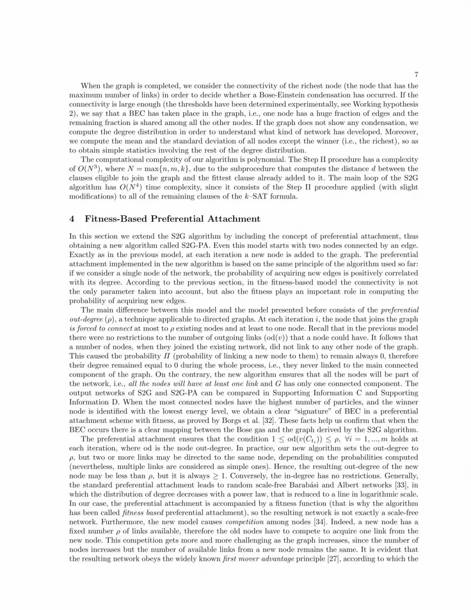
This hypothesis implies that our graph must be regarded as a directed graph in order to maintain thecorrespondence between a k–SAT instance and its graph, as well as to distinguish between outgoing andincoming links. According to the Google-like reference [35], the same edge between the new node v(Cti)and the existing node v(Ctj ) does not increase their connectivity kti and ktj (respectively) in the sameway (see Figure 1).

Cti

Ctj

θ

1

kti ← kti + θ, where 0 < θ < 1

ktj ← ktj + 1

Fig. 1. Link between Cti and Ctj . The dashed line represents the non-integer out-degree θ of Cti , whilethe continuous line represents the integer in-degree of Ctj .

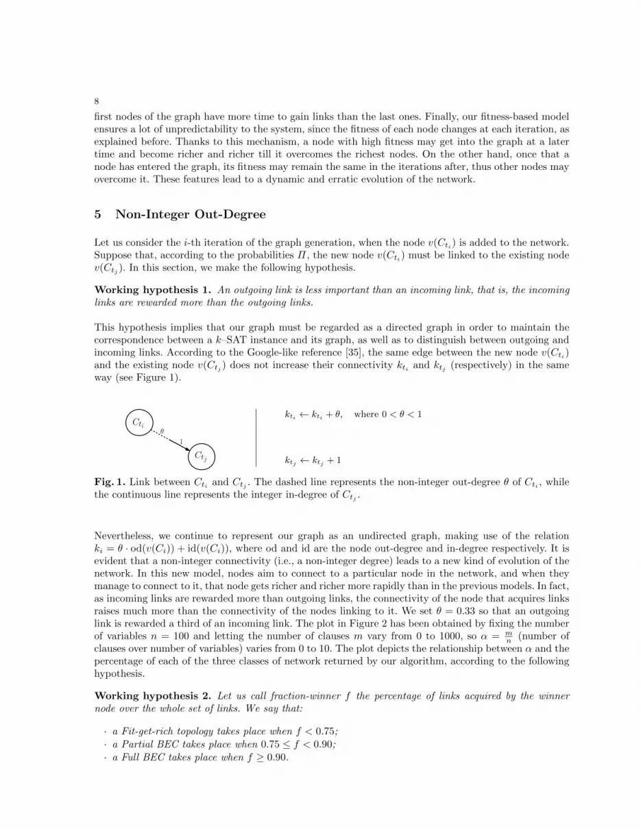
Nevertheless, we continue to represent our graph as an undirected graph, making use of the relationki = θ · od(v(Ci)) + id(v(Ci)), where od and id are the node out-degree and in-degree respectively. It isevident that a non-integer connectivity (i.e., a non-integer degree) leads to a new kind of evolution of thenetwork. In this new model, nodes aim to connect to a particular node in the network, and when theymanage to connect to it, that node gets richer and richer more rapidly than in the previous models. In fact,as incoming links are rewarded more than outgoing links, the connectivity of the node that acquires linksraises much more than the connectivity of the nodes linking to it. We set θ = 0.33 so that an outgoinglink is rewarded a third of an incoming link. The plot in Figure 2 has been obtained by fixing the numberof variables n = 100 and letting the number of clauses m vary from 0 to 1000, so α = m

n (number ofclauses over number of variables) varies from 0 to 10. The plot depicts the relationship between α and thepercentage of each of the three classes of network returned by our algorithm, according to the followinghypothesis.

Working hypothesis 2. Let us call fraction-winner f the percentage of links acquired by the winnernode over the whole set of links. We say that:

· a Fit-get-rich topology takes place when f < 0.75;· a Partial BEC takes place when 0.75 ≤ f < 0.90;· a Full BEC takes place when f ≥ 0.90.

9

0

0.1

0.2

0.3

0.4

0.5

0.6

0.7

0.8

0.9

1

0 1 2 3 4 5 6 7 8 9 10

Per

cent

age

of d

istr

ibut

ions

α

Fit Fit-get-richFit Partial BEC

Fit Full BEC

0

0.1

0.2

0.3

0.4

0.5

0.6

0.7

0.8

0.9

1

0 1 2 3 4 5 6 7 8 9 10

Per

cent

age

of d

istr

ibut

ions

α

Fit-get-richPartial BEC

Full BEC

0

0.1

0.2

0.3

0.4

0.5

0.6

0.7

0.8

0.9

1

0 1 2 3 4 5 6 7 8 9 10

Per

cent

age

of d

istr

ibut

ions

α

Fit-get-richPartial BEC

Full BEC

Fig. 2. Percentage of each kind of network against ratio of clauses to variables, with fixed number ofvariables n = 100 and non-integer out-degree θ = 0.33. The lines represent a sixth-order polynomialregression to fit the data. Full BEC occurs when the winner node gets greater or equal to 90% of links ofthe network. Partial BEC occurs when the winner node gets greater or equal to 75% and less than 90%of links of the network. If the percentage is less than 75%, the network has a Fit-get-rich topology.

As shown in Figure 2, we obtain a large number of networks that can undergo the full BEC (in whichone node is an evident “winner” node). Figure 2 also shows that the number of BEC networks producedby our algorithm increases as α decreases.

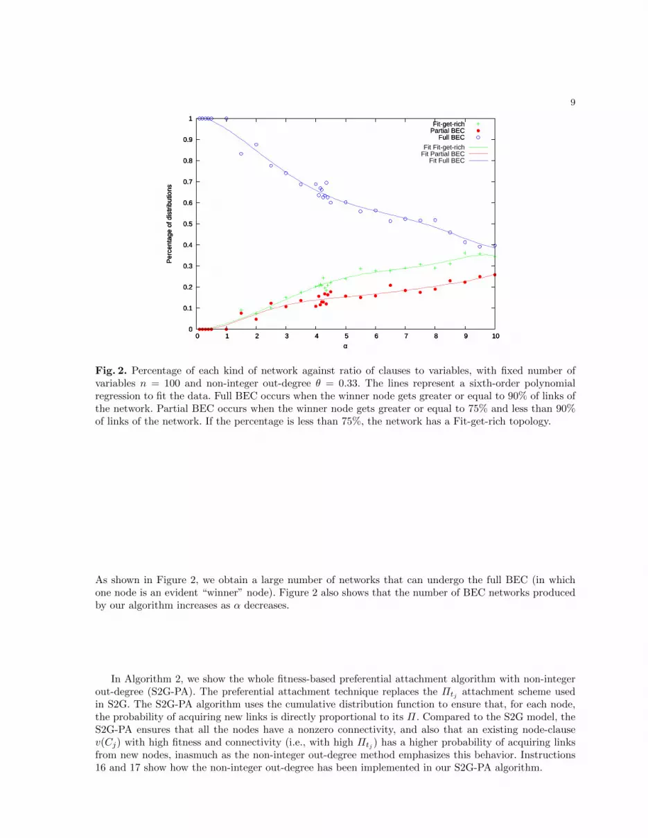
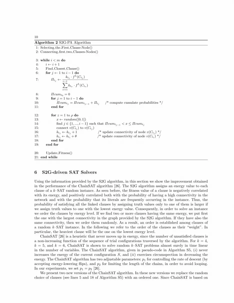
In Algorithm 2, we show the whole fitness-based preferential attachment algorithm with non-integerout-degree (S2G-PA). The preferential attachment technique replaces the Πtj attachment scheme usedin S2G. The S2G-PA algorithm uses the cumulative distribution function to ensure that, for each node,the probability of acquiring new links is directly proportional to its Π. Compared to the S2G model, theS2G-PA ensures that all the nodes have a nonzero connectivity, and also that an existing node-clausev(Cj) with high fitness and connectivity (i.e., with high Πtj ) has a higher probability of acquiring linksfrom new nodes, inasmuch as the non-integer out-degree method emphasizes this behavior. Instructions16 and 17 show how the non-integer out-degree has been implemented in our S2G-PA algorithm.

10

Algorithm 2 S2G-PA Algorithm

1: Selecting the First Clause-Node()2: Connecting first two Clauses-Nodes()

3: while i < m do4: i← i+ 15: Find Closest Clause()6: for j ← 1 to i− 1 do

7: Πtj ←ktj · fL(Ctj )

i−1∑ν=1

ktν · fL(Ctν )

8: Πcumt0 = 09: for j = 1 to i− 1 do

10: Πcumtj = Πcumtj−1 +Πtj /* compute cumulate probabilities */11: end for

12: for z = 1 to ρ do13: x← random(]0; 1])14: find j ∈ {1, ..., i− 1} such that Πcumtj−1 < x ≤ Πcumtj

15: connect v(Cti) to v(Ctj )16: ktj ← ktj + 1 /* update connectivity of node v(Ctj ) */17: kti ← kti + θ /* update connectivity of node v(Cti) */18: end for19: end for

20: Update Fitness()21: end while

6 S2G-driven SAT Solvers

Using the information provided by the S2G algorithm, in this section we show the improvement obtainedin the performance of the ChainSAT algorithm [26]. The S2G algorithm assigns an energy value to eachclause of a k–SAT random instance. As seen before, the fitness value of a clause is negatively correlatedwith its energy, and positively correlated both with the probability of having a high connectivity in thenetwork and with the probability that its literals are frequently occurring in the instance. Thus, theprobability of satisfying all the linked clauses by assigning truth values only to one of them is larger ifwe assign truth values to one with the lowest energy value. Consequently, in order to solve an instancewe order the clauses by energy level. If we find two or more clauses having the same energy, we put firstthe one with the largest connectivity in the graph provided by the S2G algorithm. If they have also thesame connectivity, then we order them randomly. As a result, an order is established among clauses ofa random k–SAT instance. In the following we refer to the order of the clauses as their “weight”. Inparticular, the heaviest clause will be the one on the lowest energy level.

ChainSAT [26] is a heuristic that never moves up in energy, since the number of unsatisfied clauses isa non-increasing function of the sequence of trial configurations traversed by the algorithm. For k = 4,k = 5, and k = 6, ChainSAT is shown to solve random k–SAT problems almost surely in time linearin the number of variables. The ChainSAT algorithm, given in pseudo-code in Algorithm S5, (i) neverincreases the energy of the current configuration S, and (ii) exercises circumspection in decreasing theenergy. The ChainSAT algorithm has two adjustable parameters: p1 for controlling the rate of descent (byaccepting energy-lowering flips), and p2 for limiting the length of the chains, in order to avoid looping.In our experiments, we set p1 = p2 [26].

We present two new versions of the ChainSAT algorithm. In these new versions we replace the randomchoice of clauses (see lines 5 and 18 of Algorithm S5) with an ordered one. Since ChainSAT is based on

11

a non-increasing energy principle [26], and given the energy levels provided by the S2G algorithm, ouridea is to select clauses with minimum energy even when ChainSAT performs a random selection.

Let us introduce a set A = {a1, a2, ..., am}, where m is the number of clauses of the k–SAT formula.The set A is used to record which clauses of the k–SAT instance have already been chosen, so that loops(consisting of choosing the same clause repeatedly) are avoided. Let H = {C1, C2, ..., Cr} be the set ofclauses among which the algorithm chooses (line 5 or 18 of Algorithm S5). We suppose that these clausesare arranged in a decreasing order of weight. In particular, C1 is one of the heaviest clauses in H, i.e.,C1 is one of the clauses of H with the lowest energy. The steps for selecting a clause in the line 5 or 18of Algorithm S5 are the following. Initially we set ai = 0, ∀ i = 1, ...,m. At each step we require that thealgorithm chooses the heaviest clause Ci among those in H such that ai = 0. Every time a clause Ci ischosen, we set ai = 1. Step by step, the number of elements in A equal to 1 increases. When ai = 1, ∀ Ci∈ H, then the clause is chosen randomly. This random choice is necessary to prevent that our algorithmalways analyzes the same chains clause-variable-clause.

Our modified version of ChainSAT presented so far, selects the new clause using the same set ofelements ai = 0, ∀ i = 1, ...,m, both for the satisfied and for the unsatisfied clauses. We call this versionLC-ChainSAT, where LC stands for “Linked Clauses”, since the choice of a clause in lines 5 and 18 ofAlgorithm S5 is based on the same set A.

We also present a second new version of the ChainSAT algorithm, called NLC-ChainSAT, where NLCstands for “Non Linked Clauses”. This new version differs from the first one because we replace A withtwo sets Asat and Aunsat, with the same structure of A. We use Aunsat to store the clauses chosen (asnot satisfied) by line 5 of Algorithm S5, and Asat to store the ones chosen (as satisfied) by line 18. Thenew algorithm runs exactly like the previous one but when it must select a new clause, it examines theset Aunsat or Asat depending on whether the new clause is chosen by line 5 or by line 18 respectively.

7 Experimental Results

In this section we investigate the outcomes of our algorithms. First, we give numerical evidence of thepresence of Bose-Einstein condensation in the k–SAT problem, focusing on the phase transition region.We evaluate the phase diagram of the S2G algorithm to show the transition between a fit-get-rich phaseand a winner-takes-all phase. Second, we analyze the SAT solvers proposed above by evaluating theirperformance on both random and real-life SAT instances.

7.1 S2G Results

For the 3–SAT problem there is strong evidence [2] that the phase transition between solvable andunsatisfiable instances is located at α = 4.256, where α = m

n is the ratio between the number of clauses mand the number of variables n. For our experiments we use the A. van Gelder’s k–SAT instance generatormkcnf.c1. We asked the program to generate uniformly satisfiable and unsatisfiable formulas to obtaina purely uniform random k–SAT distribution. For our experimental protocol, we consider α ∈]0, 10] andn ∈ {10, 25, 50, 75, 100}. For each value of α, we consider 100 formulas and perform 30 independent graphG constructions per formula. We make use of the S2G-PA algorithm by imposing θ = 0.33 and ρ = 1.

In Figure 3 we plot the percentage of BEC networks observed by varying α. In general, when α < 3the resulting graph most likely undergoes a clear Bose-Einstein condensation; in this phase, the fittestclause maintains a large number of links even if the graph expands. Moreover, if α increases and entersthe phase transition region, it is evident that the drop in the number of Bose-Einstein condensationsbecomes smoother. This different behavior seems to match with the increasing complexity of formulaswith α ≈ 4.256 (the locus of the phase transition for 3–SAT), and therefore we investigate it more

1 Available atftp://dimacs.rutgers.edu/pub/challenge/satisfiability/contributed/UCSC/instances.The program mkcnf.c takes four inputs: r, the random seed; k, the number of literals in each clause; n, thenumber of Boolean variables; m, the number of clauses.

12

0.3

0.4

0.5

0.6

0.7

0.8

0.9

1

0 1 2 3 4 5 6 7 8 9 10

Per

cent

age

of B

EC

α

α=4.256

Fit 10 VariablesFit 25 VariablesFit 50 VariablesFit 75 Variables

Fit 100 Variables

0.3

0.4

0.5

0.6

0.7

0.8

0.9

1

0 1 2 3 4 5 6 7 8 9 10

Per

cent

age

of B

EC

α

α=4.25610 Variables25 Variables50 Variables75 Variables

100 Variables

0.3

0.4

0.5

0.6

0.7

0.8

0.9

1

0 1 2 3 4 5 6 7 8 9 10

Per

cent

age

of B

EC

α

α=4.25610 Variables25 Variables50 Variables75 Variables

100 Variables

Fig. 3. Bose-Einstein condensation (BEC) in 3–SAT. We report on the x-axis the ratio α of clauses tovariables, and on the y-axis the percentage of BEC networks found. The points have been fitted through asixth-order polynomial regression. The gray stripe shows the region where the critical temperature TBECfor Bose-Einstein condensation could be located.

thoroughly later. For α > 5, the graph shows a fit-get-rich behavior, i.e., there is an increasing numberof fittest nodes (clauses), but there is no more a unique winner node. This behavior remarks that, forincreasing α values (close to the UNSAT phase of 3–SAT), we have to find a truth assignment formany clauses to obtain a satisfiable formula. These empirical evidences are consistent with the transitionbetween SAT and UNSAT instances [3].

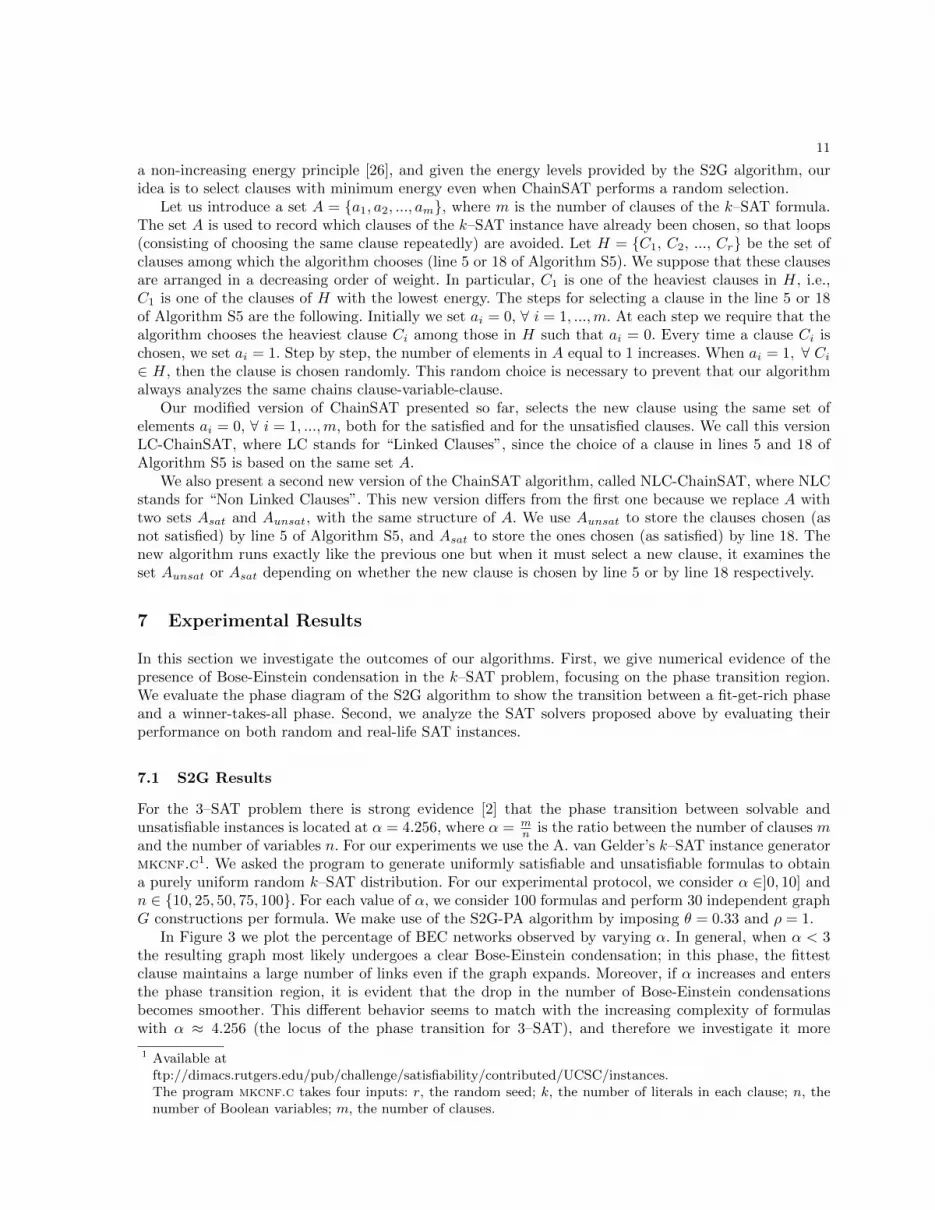
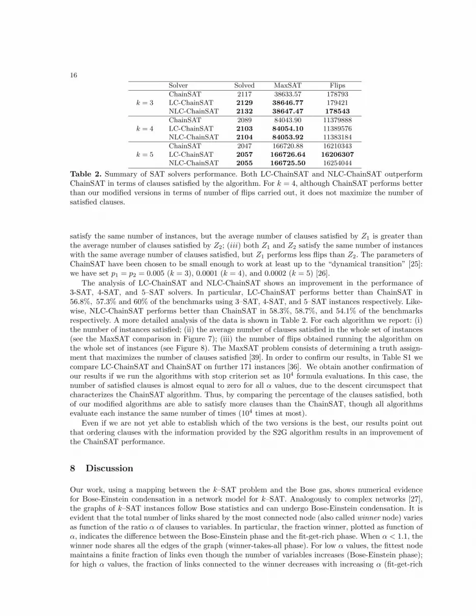
In order to evaluate the way in which α (i.e., the ratio clauses to variables) influences the evolution ofthe graph associated with k–SAT instances, we examine the fraction winner f defined as the ratio of thenumber of links shared by the winner (i.e., the highest degree node) to the number of links of the wholegraph. Figure 4 shows how the fraction winner varies as function of the ratio of clauses to variables. Welet the number of variables vary in the set {10, 25, 50, 75, 100}. Each point of the plot has been computedby averaging over 1000 different 3–SAT instances, with 30 graph generations per instance. The plot showsthat the fraction-winner f decreases with α. When a 3–SAT instance is satisfiable (with high probability),the S2G-PA algorithm produces a graph condensed over the fittest clause. Conversely, when a 3–SATinstance is unsatisfiable (with high probability), its graph exhibits a winner node incapable of maintainingthe whole connectivity of the network, and some hubs appear and grow following the fit-get-rich model.By looking at the plots in Figure 4 from right to left, one can observe that when α becomes smaller thanthe critical value 4.256, the winner node holds the vast majority of links. In this case, the Bose-Einsteincondensation takes place regardless of the number of variables. Moreover, the plot concerning the case of50 variables clearly shows a smooth drop for 4 < α < 5, indicating that the 50-variables graphs undergothe slowest Bose-Einstein condensation (provided that α decreases). It is possible to note that for α < 1.1the fraction winner is equal to 1, since the winner node holds all the links in the network, i.e., all the edgeshave the winner node as a vertex. Our results suggest that this phase, called winner-takes-all (WTA),starts at α = 1 for large values of n.

One can notice that below the phase transition region the slopes of the plots exhibit a different behaviorthan in the other regions. Specifically, below the phase transition of 3–SAT, located at α = 4.256, the

13

0.65

0.7

0.75

0.8

0.85

0.9

0.95

1

0 1 2 3 4 5 6 7 8 9 10

Fra

ctio

n W

inne

r

α

WTA FGRBE

TBEC

α=4.256α=1.1

Fit 10 VariablesFit 25 VariablesFit 50 VariablesFit 75 Variables

Fit 100 Variables

0.65

0.7

0.75

0.8

0.85

0.9

0.95

1

0 1 2 3 4 5 6 7 8 9 10

Fra

ctio

n W

inne

r

α

WTA FGRBE

TBEC

α=4.256α=1.1

10 Variables25 Variables50 Variables75 Variables

100 Variables

0.65

0.7

0.75

0.8

0.85

0.9

0.95

1

0 1 2 3 4 5 6 7 8 9 10

Fra

ctio

n W

inne

r

α

WTA FGRBE

TBEC

α=4.256α=1.1

10 Variables25 Variables50 Variables75 Variables

100 Variables

Fig. 4. Phase diagram of 3–SAT. We report the fraction of links shared by the winner against α (the ratioof clauses to variables). Each point is an average over 1000 3–SAT instances with 30 graphs per instance.We have performed a sixth-order polynomial regression to fit the data. Satisfiable instances (with highprobability) belong to the winner-takes-all phase. Unsatisfiable instances (with high probability) belongto the fit-get-rich phase. The critical temperature TBEC for Bose-Einstein condensation could be locatedin the grey area in the neighborhood of the SAT-UNSAT phase transition α = 4.256. Below the criticaltemperature, the fraction winner increases at a higher rate.

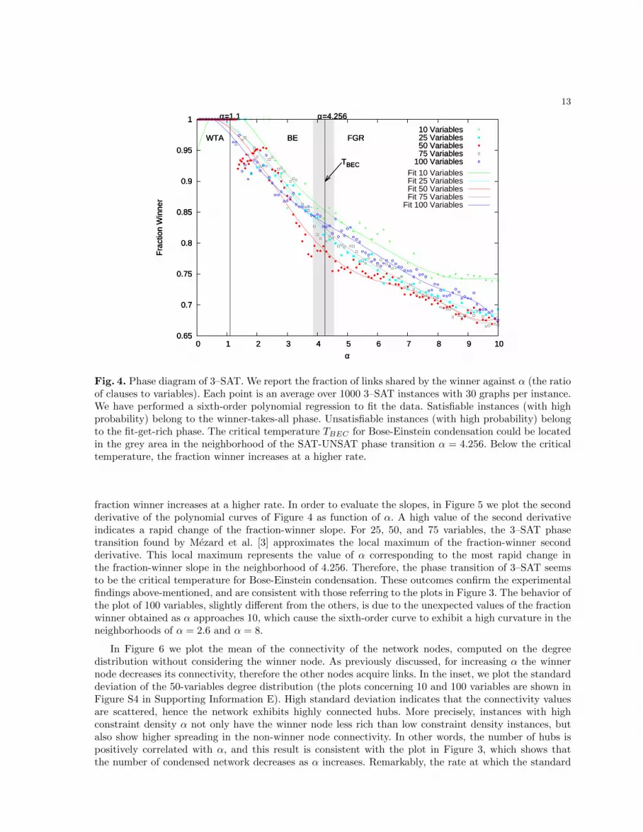
fraction winner increases at a higher rate. In order to evaluate the slopes, in Figure 5 we plot the secondderivative of the polynomial curves of Figure 4 as function of α. A high value of the second derivativeindicates a rapid change of the fraction-winner slope. For 25, 50, and 75 variables, the 3–SAT phasetransition found by Mezard et al. [3] approximates the local maximum of the fraction-winner secondderivative. This local maximum represents the value of α corresponding to the most rapid change inthe fraction-winner slope in the neighborhood of 4.256. Therefore, the phase transition of 3–SAT seemsto be the critical temperature for Bose-Einstein condensation. These outcomes confirm the experimentalfindings above-mentioned, and are consistent with those referring to the plots in Figure 3. The behavior ofthe plot of 100 variables, slightly different from the others, is due to the unexpected values of the fractionwinner obtained as α approaches 10, which cause the sixth-order curve to exhibit a high curvature in theneighborhoods of α = 2.6 and α = 8.

In Figure 6 we plot the mean of the connectivity of the network nodes, computed on the degreedistribution without considering the winner node. As previously discussed, for increasing α the winnernode decreases its connectivity, therefore the other nodes acquire links. In the inset, we plot the standarddeviation of the 50-variables degree distribution (the plots concerning 10 and 100 variables are shown inFigure S4 in Supporting Information E). High standard deviation indicates that the connectivity valuesare scattered, hence the network exhibits highly connected hubs. More precisely, instances with highconstraint density α not only have the winner node less rich than low constraint density instances, butalso show higher spreading in the non-winner node connectivity. In other words, the number of hubs ispositively correlated with α, and this result is consistent with the plot in Figure 3, which shows thatthe number of condensed network decreases as α increases. Remarkably, the rate at which the standard

14

-10

-8

-6

-4

-2

0

2

4

0 1 2 3 4 5 6 7 8 9 10

Sec

ond

Der

ivat

ive

of F

ract

ion

Win

ner

α

max=4.469

α=4.256

-10

-8

-6

-4

-2

0

2

4

0 1 2 3 4 5 6 7 8 9 10

Sec

ond

Der

ivat

ive

of F

ract

ion

Win

ner

α

max=4.469

α=4.256

-10

-8

-6

-4

-2

0

2

4

0 1 2 3 4 5 6 7 8 9 10

Sec

ond

Der

ivat

ive

of F

ract

ion

Win

ner

α

max=4.469

α=4.256

-8

-6

-4

-2

0

2

4

6

8

10

0 1 2 3 4 5 6 7 8 9 10

Sec

ond

Der

ivat

ive

of F

ract

ion

Win

ner

α

max=4.320

α=4.256

-8

-6

-4

-2

0

2

4

6

8

10

0 1 2 3 4 5 6 7 8 9 10

Sec

ond

Der

ivat

ive

of F

ract

ion

Win

ner

α

max=4.320

α=4.256

-8

-6

-4

-2

0

2

4

6

8

10

0 1 2 3 4 5 6 7 8 9 10

Sec

ond

Der

ivat

ive

of F

ract

ion

Win

ner

α

max=4.320

α=4.256

(n = 25) (n = 50)

-4

-2

0

2

4

6

8

0 1 2 3 4 5 6 7 8 9 10

Sec

ond

Der

ivat

ive

of F

ract

ion

Win

ner

α

max=4.582

α=4.256

-4

-2

0

2

4

6

8

0 1 2 3 4 5 6 7 8 9 10

Sec

ond

Der

ivat

ive

of F

ract

ion

Win

ner

α

max=4.582

α=4.256

-4

-2

0

2

4

6

8

0 1 2 3 4 5 6 7 8 9 10

Sec

ond

Der

ivat

ive

of F

ract

ion

Win

ner

α

max=4.582

α=4.256

-14

-12

-10

-8

-6

-4

-2

0

2

0 1 2 3 4 5 6 7 8 9 10

Sec

ond

Der

ivat

ive

of F

ract

ion

Win

ner

α

max=2.609

α=4.256

-14

-12

-10

-8

-6

-4

-2

0

2

0 1 2 3 4 5 6 7 8 9 10

Sec

ond

Der

ivat

ive

of F

ract

ion

Win

ner

α

max=2.609

α=4.256

-14

-12

-10

-8

-6

-4

-2

0

2

0 1 2 3 4 5 6 7 8 9 10

Sec

ond

Der

ivat

ive

of F

ract

ion

Win

ner

α

max=2.609

α=4.256

(n = 75) (n = 100)

Fig. 5. 3–SAT Bose-Einstein condensation locus. We plot the second derivative of the fraction winneras function of the ratio α of clauses to variables. The SAT-UNSAT phase transition α = 4.256 is nearthe local maximum of the second derivative, and therefore corresponds to a quick change of the fraction-winner slope. In other words, the 3–SAT phase transition acts as the BEC critical temperature.

15

deviation increases is higher to the left of the Bose-Einstein condensation region. The growing hubs oftypical S2G-PA output networks are shown in Figure S5 in Supporting Information F.

0.3

0.35

0.4

0.45

0.5

0.55

0.6

0.65

0.7

0 1 2 3 4 5 6 7 8 9 10

Non

-Win

ner

Mea

n

α

α=4.256

Fit 10 VariablesFit 50 Variables

Fit 100 Variables

0.3

0.35

0.4

0.45

0.5

0.55

0.6

0.65

0.7

0 1 2 3 4 5 6 7 8 9 10

Non

-Win

ner

Mea

n

α

10 Variables50 Variables

100 Variables

0.3

0.35

0.4

0.45

0.5

0.55

0.6

0.65

0.7

0 1 2 3 4 5 6 7 8 9 10

Non

-Win

ner

Mea

n

α

10 Variables50 Variables

100 Variables

0 0.5

1 1.5

2 2.5

3 3.5

4 4.5

0 1 2 3 4 5 6 7 8 9 10

Fig. 6. Average non-winner connectivity in 3–SAT networks. We report the mean of the connectivity ofall the nodes except the winner, as function of the clauses-to-variables ratio. Each point is an averageover 100 3–SAT instances with 30 graphs per instance. We have performed a sixth-order polynomialregression to fit the data. In the inset, we report the standard deviation of the mean connectivity for 50-variables instances. Satisfiable instances (with high probability) are translated into condensed graphs, asall the connectivities are equal to θ and the standard deviation is zero. Conversely, unsatisfiable instances(with high probability) are translated into fit-get-rich networks with high standard deviation, thus withemerging hubs. In agreement with the fraction winner, to the left of the condensation area of Figure 4both the mean and the standard deviation exhibit a higher slope.

7.2 LC-ChainSAT and NLC-ChainSAT Results

We evaluate each algorithm on a collection of 6885 k–SAT instances obtained from publicly availablesources. This benchmark consists of (i) 40 Intel sequential circuits and 95 l2s benchmarks used in the2007 and 2008 hardware model checking competition [36], (ii) 2250 random instances for each value ofk (k = 3, k = 4, and k = 5), generated uniformly at random using the A. van Gelder’s generator. Weuse aigtocnf [37] to convert instances from AIG format to CNF. Then, we convert them into 3-CNFinstances. We set n ∈ {25, 50, 75, 100, 125} and m such that α = m

n ∈ [αsat(k) − 4;αsat(k) + 2], whereαsat(k) has the estimated values αsat(3) = 4.256, αsat(4) = 9.931, αsat(5) = 21.117 (see [38]). For eachvalue of α, we generate 30 different k–SAT instances. We also introduce the following stop criterion [2]: westop the algorithm either when a solution is found or when 106 cycles of the main body of the algorithm(i.e., 106 formula evaluations) have been carried out.

The comparison between ChainSAT and our two modified versions is based on the following definition.Let Z1 and Z2 be two algorithms tested on the same set of instances. We say that Z1 performs better thanZ2 if one of the following conditions is met: (i) Z1 satisfies more instances than Z2; (ii) both Z1 and Z2

16

Solver Solved MaxSAT Flips

ChainSAT 2117 38633.57 178793k = 3 LC-ChainSAT 2129 38646.77 179421

NLC-ChainSAT 2132 38647.47 178543

ChainSAT 2089 84043.90 11379888k = 4 LC-ChainSAT 2103 84054.10 11389576

NLC-ChainSAT 2104 84053.92 11383184

ChainSAT 2047 166720.88 16210343k = 5 LC-ChainSAT 2057 166726.64 16206307

NLC-ChainSAT 2055 166725.50 16254044

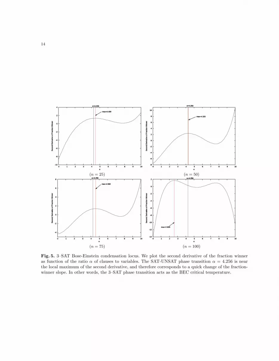
Table 2. Summary of SAT solvers performance. Both LC-ChainSAT and NLC-ChainSAT outperformChainSAT in terms of clauses satisfied by the algorithm. For k = 4, although ChainSAT performs betterthan our modified versions in terms of number of flips carried out, it does not maximize the number ofsatisfied clauses.

satisfy the same number of instances, but the average number of clauses satisfied by Z1 is greater thanthe average number of clauses satisfied by Z2; (iii) both Z1 and Z2 satisfy the same number of instanceswith the same average number of clauses satisfied, but Z1 performs less flips than Z2. The parameters ofChainSAT have been chosen to be small enough to work at least up to the “dynamical transition” [25]:we have set p1 = p2 = 0.005 (k = 3), 0.0001 (k = 4), and 0.0002 (k = 5) [26].

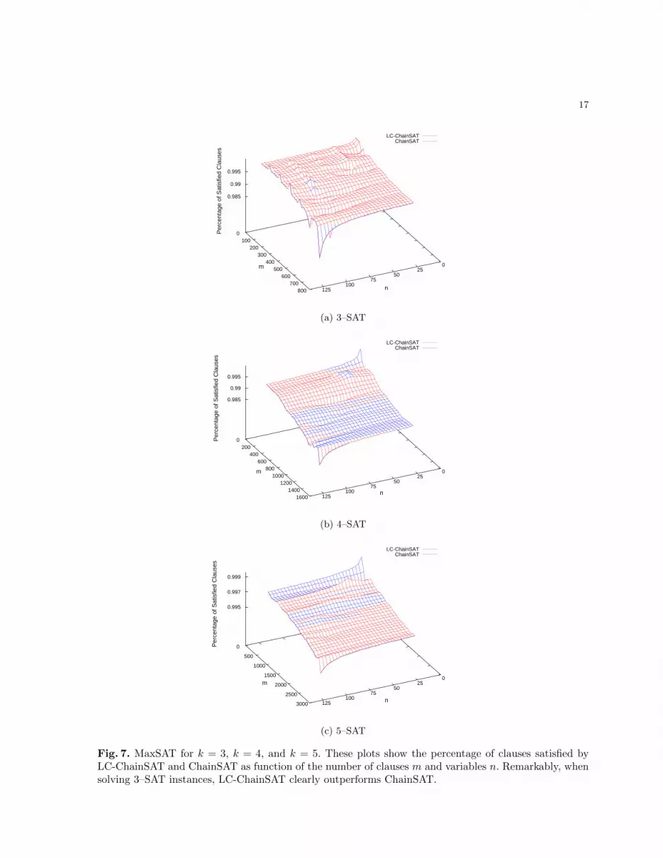
The analysis of LC-ChainSAT and NLC-ChainSAT shows an improvement in the performance of3-SAT, 4-SAT, and 5–SAT solvers. In particular, LC-ChainSAT performs better than ChainSAT in56.8%, 57.3% and 60% of the benchmarks using 3–SAT, 4-SAT, and 5–SAT instances respectively. Like-wise, NLC-ChainSAT performs better than ChainSAT in 58.3%, 58.7%, and 54.1% of the benchmarksrespectively. A more detailed analysis of the data is shown in Table 2. For each algorithm we report: (i)the number of instances satisfied; (ii) the average number of clauses satisfied in the whole set of instances(see the MaxSAT comparison in Figure 7); (iii) the number of flips obtained running the algorithm onthe whole set of instances (see Figure 8). The MaxSAT problem consists of determining a truth assign-ment that maximizes the number of clauses satisfied [39]. In order to confirm our results, in Table S1 wecompare LC-ChainSAT and ChainSAT on further 171 instances [36]. We obtain another confirmation ofour results if we run the algorithms with stop criterion set as 104 formula evaluations. In this case, thenumber of satisfied clauses is almost equal to zero for all α values, due to the descent circumspect thatcharacterizes the ChainSAT algorithm. Thus, by comparing the percentage of the clauses satisfied, bothof our modified algorithms are able to satisfy more clauses than the ChainSAT, though all algorithmsevaluate each instance the same number of times (104 times at most).

Even if we are not yet able to establish which of the two versions is the best, our results point outthat ordering clauses with the information provided by the S2G algorithm results in an improvement ofthe ChainSAT performance.

8 Discussion

Our work, using a mapping between the k–SAT problem and the Bose gas, shows numerical evidencefor Bose-Einstein condensation in a network model for k–SAT. Analogously to complex networks [27],the graphs of k–SAT instances follow Bose statistics and can undergo Bose-Einstein condensation. It isevident that the total number of links shared by the most connected node (also called winner node) variesas function of the ratio α of clauses to variables. In particular, the fraction winner, plotted as function ofα, indicates the difference between the Bose-Einstein phase and the fit-get-rich phase. When α < 1.1, thewinner node shares all the edges of the graph (winner-takes-all phase). For low α values, the fittest nodemaintains a finite fraction of links even though the number of variables increases (Bose-Einstein phase);for high α values, the fraction of links connected to the winner decreases with increasing α (fit-get-rich

17

m

n

Per

cent

age

of S

atis

fied

Cla

uses

LC-ChainSATChainSAT

0 25

50 75

100 125

0 100

200 300

400 500

600 700

800

0.985

0.99

0.995

(a) 3–SAT

m

n

Per

cent

age

of S

atis

fied

Cla

uses

LC-ChainSATChainSAT

0 25

50 75

100 125

0 200

400 600

800 1000

1200 1400

1600

0.985

0.99

0.995

(b) 4–SAT

m

n

Per

cent

age

of S

atis

fied

Cla

uses

LC-ChainSATChainSAT

0 25

50 75

100 125

0

500

1000

1500

2000

2500

3000

0.995

0.997

0.999

(c) 5–SAT

Fig. 7. MaxSAT for k = 3, k = 4, and k = 5. These plots show the percentage of clauses satisfied byLC-ChainSAT and ChainSAT as function of the number of clauses m and variables n. Remarkably, whensolving 3–SAT instances, LC-ChainSAT clearly outperforms ChainSAT.

18

m n

Num

ber

of F

lips

(nor

mal

ized

to 1

)

LC-ChainSATChainSAT

0

20

40

60

80

100

120

0

500

1000

1500

2000

2500

3000

0.4

0.5

0.6

0.7

0.8

0.9

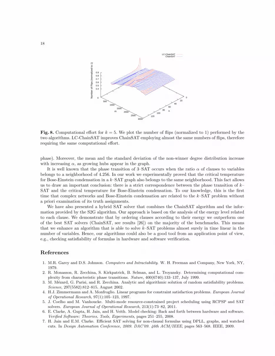
Fig. 8. Computational effort for k = 5. We plot the number of flips (normalized to 1) performed by thetwo algorithms. LC-ChainSAT improves ChainSAT employing almost the same numbers of flips, thereforerequiring the same computational effort.

phase). Moreover, the mean and the standard deviation of the non-winner degree distribution increasewith increasing α, as growing hubs appear in the graph.

It is well known that the phase transition of 3–SAT occurs when the ratio α of clauses to variablesbelongs to a neighborhood of 4.256. In our work we experimentally proved that the critical temperaturefor Bose-Einstein condensation in a k–SAT graph also belongs to the same neighborhood. This fact allowsus to draw an important conclusion: there is a strict correspondence between the phase transition of k–SAT and the critical temperature for Bose-Einstein condensation. To our knowledge, this is the firsttime that complex networks and Bose-Einstein condensation are related to the k–SAT problem withouta priori examination of its truth assignments.

We have also presented a hybrid SAT solver that combines the ChainSAT algorithm and the infor-mation provided by the S2G algorithm. Our approach is based on the analysis of the energy level relatedto each clause. We demonstrate that by ordering clauses according to their energy we outperform oneof the best SAT solvers (ChainSAT, see results [26]) on the majority of the benchmarks. This meansthat we enhance an algorithm that is able to solve k–SAT problems almost surely in time linear in thenumber of variables. Hence, our algorithms could also be a good tool from an application point of view,e.g., checking satisfiability of formulas in hardware and software verification.

References

1. M.R. Garey and D.S. Johnson. Computers and Intractability. W. H. Freeman and Company, New York, NY,1979.

2. R. Monasson, R. Zecchina, S. Kirkpatrick, B. Selman, and L. Troyansky. Determining computational com-plexity from characteristic phase transitions. Nature, 400(6740):133–137, July 1999.

3. M. Mezard, G. Parisi, and R. Zecchina. Analytic and algorithmic solution of random satisfiability problems.Science, 297(5582):812–815, August 2002.

4. H.J. Zimmermann and A. Monfroglio. Linear programs for constraint satisfaction problems. European Journalof Operational Research, 97(1):105–123, 1997.

5. J. Coelho and M. Vanhoucke. Multi-mode resource-constrained project scheduling using RCPSP and SATsolvers. European Journal of Operational Research, 213(1):73–82, 2011.

6. E. Clarke, A. Gupta, H. Jain, and H. Veith. Model checking: Back and forth between hardware and software.Verified Software: Theories, Tools, Experiments, pages 251–255, 2008.

7. H. Jain and E.M. Clarke. Efficient SAT solving for non-clausal formulas using DPLL, graphs, and watchedcuts. In Design Automation Conference, 2009. DAC’09. 46th ACM/IEEE, pages 563–568. IEEE, 2009.

19

8. Y. Hamadi, S. Jabbour, and L. Sais. ManySAT: a parallel SAT solver. Journal on Satisfiability, BooleanModeling and Computation, 6:245–262, 2009.

9. M.W. Moskewicz, C.F. Madigan, Y. Zhao, L. Zhang, and S. Malik. Chaff: Engineering an efficient SAT solver.In Proceedings of the 38th annual Design Automation Conference, pages 530–535. ACM, 2001.

10. M.K. Ganai, P. Ashar, A. Gupta, L. Zhang, and S. Malik. Combining strengths of circuit-based and CNF-based algorithms for a high-performance SAT solver. In Proceedings of the 39th annual Design AutomationConference, pages 747–750. ACM, 2002.

11. K. Nonobe and T. Ibaraki. A tabu search approach to the constraint satisfaction problem as a general problemsolver. European Journal of Operational Research, 106(2):599–623, 1998.

12. M. Mastrolilli and L.M. Gambardella. Maximum satisfiability: how good are tabu search and plateau movesin the worst-case? European Journal of Operational Research, 166(1):63–76, 2005.

13. E. Birnbaum and E.L. Lozinskii. The good old Davis-Putnam procedure helps counting models. Journal ofArtificial Intelligence Research, 10(1):457–477, 1999.

14. O. Dubois. Counting the number of solutions for instances of satisfiability. Theoretical Computer Science,81(1):49–64, 1991.

15. W. Zhang. Number of models and satisfiability of sets of clauses. Theoretical Computer Science, 155(1):277–288, 1996.

16. M.L. Littman, S.M. Majercik, and T. Pitassi. Stochastic Boolean satisfiability. Journal of Automated Rea-soning, 27(3):251–296, 2001.

17. A. Montanari, F. Ricci-Tersenghi, and G. Semerjian. Clusters of solutions and replica symmetry breaking inrandom k-satisfiability. Journal of Statistical Mechanics: Theory and Experiment, 4:004, 2008.

18. D. Mitchell, B. Selman, and H. Levesque. Hard and easy distributions of SAT problems. In Proceedings of theNational Conference on Artificial Intelligence, number July, pages 459–465. AAAI Press/MIT Press, 1992.

19. T. Hogg, B.A. Huberman, and C.P. Williams. Phase transitions and the search problem. Artificial intelligence,81(1-2):1–15, 1996.

20. O.C. Martin, R. Monasson, and R. Zecchina. Statistical mechanics methods and phase transitions in opti-mization problems. Theoretical computer science, 265(1-2):3–67, 2001.

21. D. Sherrington. Physics and complexity. Philosophical Transactions of the Royal Society A: Mathematical,Physical and Engineering Sciences, 368(1914):1175–1189, 2010.

22. D. Sherrington and S. Kirkpatrick. Solvable model of a spin-glass. Physical Review Letters, 35(26):1792, 1975.23. M. Bayati, D. Gamarnik, and P. Tetali. Combinatorial approach to the interpolation method and scaling

limits in sparse random graphs. In Proceedings of the 42nd ACM symposium on Theory of computing, pages105–114. ACM, 2010.

24. M. Mezard and A. Montanari. Information, physics, and computation. Oxford University Press, USA, 2009.25. F. Krzaka la, A. Montanari, F. Ricci-Tersenghi, G. Semerjian, and L. Zdeborova. Gibbs states and the set

of solutions of random constraint satisfaction problems. Proceedings of the National Academy of Sciences,104(25):10318, 2007.

26. M. Alava, J. Ardelius, E. Aurell, P. Kaski, S. Krishnamurthy, P. Orponen, and S. Seitz. Circumspect descentprevails in solving random constraint satisfaction problems. Proceedings of the National Academy of Sciences,105(40):15253, 2008.

27. G. Bianconi and A.L. Barabasi. Bose-Einstein condensation in complex networks. Physical Review Letters,86(24):5632–5635, 2001.

28. F. London. On the Bose-Einstein condensation. Physical Review, 54(11):947–954, 1938.29. O. Penrose and L. Onsager. Bose-Einstein condensation and liquid helium. Physical Review, 104(3):576–584,

1956.30. R.K. Pathria. Statistical mechanics. Butterworth-Heinemann, 1996.31. S. Roman. Coding and information theory. Springer Verlag, 1992.32. C. Borgs, J. Chayes, C. Daskalakis, and S. Roch. First to market is not everything: an analysis of preferential

attachment with fitness. In Proceedings of the thirty-ninth annual ACM symposium on Theory of computing,pages 135–144. ACM, 2007.

33. A.L. Barabasi and R. Albert. Emergence of scaling in random networks. Science, 286(5439):509–512, 1999.34. G. Bianconi and A.L. Barabasi. Competition and multiscaling in evolving networks. Europhysics Letters,

54:436–442, 2001.35. A.N. Langville and C.D. Meyer. Google’s PageRank and beyond: the science of search engine rankings.

Princeton University Press, 2006.36. Hardware model checking competition, http://fmv.jku.at/hwmcc07/, http://fmv.jku.at/hwmcc08/.37. AIGER, http://fmv.jku.at/aiger.

20

38. S. Mertens, M. Mezard, and R. Zecchina. Threshold values of random k-SAT from the cavity method. RandomStructures & Algorithms, 28(3):340–373, 2006.

39. B. Escoffier and V.T. Paschos. Differential approximation of MinSAT, MaxSAT and related problems. Euro-pean Journal of Operational Research, 181(2):620–633, 2007.

21

Supporting Information

A

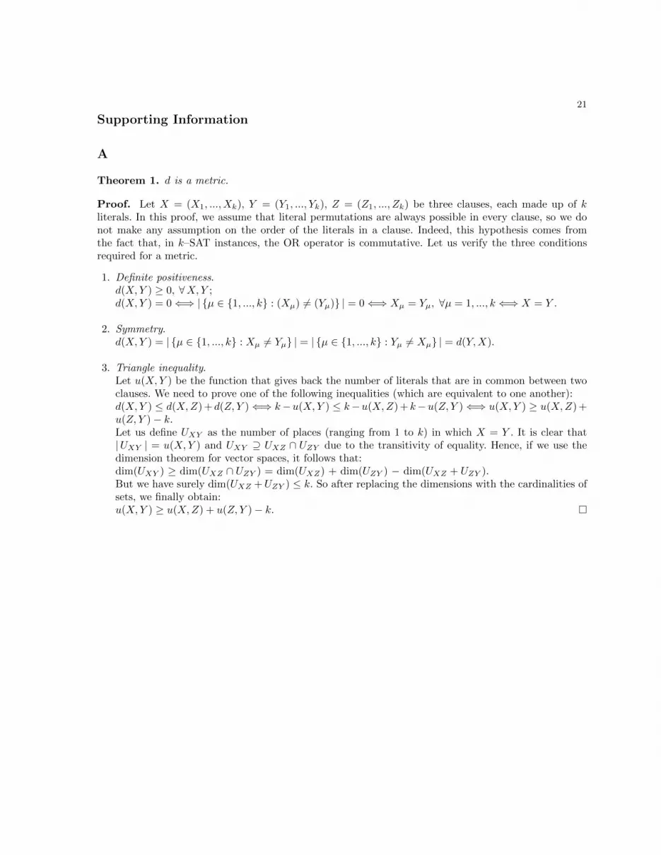
Theorem 1. d is a metric.

Proof. Let X = (X1, ..., Xk), Y = (Y1, ..., Yk), Z = (Z1, ..., Zk) be three clauses, each made up of kliterals. In this proof, we assume that literal permutations are always possible in every clause, so we donot make any assumption on the order of the literals in a clause. Indeed, this hypothesis comes fromthe fact that, in k–SAT instances, the OR operator is commutative. Let us verify the three conditionsrequired for a metric.

1. Definite positiveness.d(X,Y ) ≥ 0, ∀X,Y ;d(X,Y ) = 0⇐⇒ |{µ ∈ {1, ..., k} : (Xµ) 6= (Yµ)} | = 0⇐⇒ Xµ = Yµ, ∀µ = 1, ..., k ⇐⇒ X = Y .

2. Symmetry.d(X,Y ) = | {µ ∈ {1, ..., k} : Xµ 6= Yµ} | = | {µ ∈ {1, ..., k} : Yµ 6= Xµ} | = d(Y,X).

3. Triangle inequality.Let u(X,Y ) be the function that gives back the number of literals that are in common between twoclauses. We need to prove one of the following inequalities (which are equivalent to one another):d(X,Y ) ≤ d(X,Z) + d(Z, Y )⇐⇒ k−u(X,Y ) ≤ k−u(X,Z) + k−u(Z, Y )⇐⇒ u(X,Y ) ≥ u(X,Z) +u(Z, Y )− k.Let us define UXY as the number of places (ranging from 1 to k) in which X = Y . It is clear that|UXY | = u(X,Y ) and UXY ⊇ UXZ ∩ UZY due to the transitivity of equality. Hence, if we use thedimension theorem for vector spaces, it follows that:dim(UXY ) ≥ dim(UXZ ∩ UZY ) = dim(UXZ) + dim(UZY ) − dim(UXZ + UZY ).But we have surely dim(UXZ +UZY ) ≤ k. So after replacing the dimensions with the cardinalities ofsets, we finally obtain:u(X,Y ) ≥ u(X,Z) + u(Z, Y )− k. �

22

B Supporting Algorithms and Tables

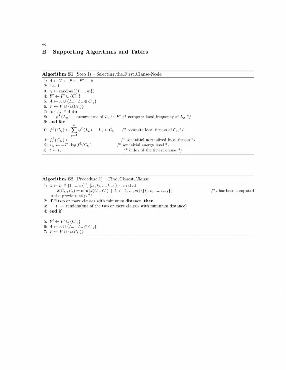
Algorithm S1 (Step I) – Selecting the First Clause-Node

1: Λ← V ← E ← F ′ ← ∅2: i← 13: ti ← random({1, ...,m})4: F ′ ← F ′ ∪ {Cti}5: Λ← Λ ∪ {Lµ : Lµ ∈ Cti}6: V ← V ∪ {v(Cti)}7: for Lµ ∈ Λ do8: ϕL(Lµ)← occurrences of Lµ in F ′ /* compute local frequency of Lµ */9: end for

10: fL(Cti)←k∑µ=1

ϕL(Lµ), Lµ ∈ Cti /* compute local fitness of Cti*/

11: fLr (Cti)← 1 /* set initial normalized local fitness */12: εti ← −T · log fLr (Cti) /* set initial energy level */13: t← ti /* index of the fittest clause */

Algorithm S2 (Procedure I) – Find Closest Clause

1: ti ← ti ∈ {1, ...,m} \ {t1, t2, ..., ti−1} such thatd(Cti , Ct) = min{d(Cti , Ct) | ti ∈ {1, ...,m}\{t1, t2, ..., ti−1}} /* t has been computed

in the previous step */2: if ∃ two or more clauses with minimum distance then3: ti ← random(one of the two or more clauses with minimum distance)4: end if

5: F ′ ← F ′ ∪ {Cti}6: Λ← Λ ∪ {Lµ : Lµ ∈ Cti}7: V ← V ∪ {v(Cti)}

23

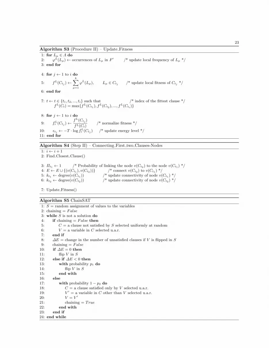
Algorithm S3 (Procedure II) – Update Fitness

1: for Lµ ∈ Λ do2: ϕL(Lµ)← occurrences of Lµ in F ′ /* update local frequency of Lµ */3: end for

4: for j ← 1 to i do

5: fL(Ctj )←k∑µ=1

ϕL(Lµ), Lµ ∈ Ctj /* update local fitness of Ctj */

6: end for

7: t← t ∈ {t1, t2, ..., ti} such that /* index of the fittest clause */fL(Ct) = max{fL(Ct1), fL(Ct2), ..., fL(Cti)}

8: for j ← 1 to i do

9: fLr (Ctj )←fL(Ctj )

fL(Ct)/* normalize fitness */

10: εtj ← −T · log fLr (Ctj ) /* update energy level */11: end for

Algorithm S4 (Step II) – Connecting First two Clauses-Nodes

1: i← i+ 12: Find Closest Clause()

3: Πt1 ← 1 /* Probability of linking the node v(Ct2) to the node v(Ct1) */4: E ← E ∪ {(v(Ct1), v(Ct2))} /* connect v(Ct2) to v(Ct1) */5: kt1 ← degree(v(Ct1)) /* update connectivity of node v(Ct1) */6: kt2 ← degree(v(Ct2)) /* update connectivity of node v(Ct2) */

7: Update Fitness()

Algorithm S5 ChainSAT

1: S = random assignment of values to the variables2: chaining = False3: while S is not a solution do4: if chaining = False then5: C = a clause not satisfied by S selected uniformly at random6: V = a variable in C selected u.a.r.7: end if8: ∆E = change in the number of unsatisfied clauses if V is flipped in S9: chaining = False

10: if ∆E = 0 then11: flip V in S12: else if ∆E < 0 then13: with probability p1 do14: flip V in S15: end with16: else17: with probability 1− p2 do18: C = a clause satisfied only by V selected u.a.r.19: V ′ = a variable in C other than V selected u.a.r.20: V = V ′

21: chaining = True22: end with23: end if24: end while

24

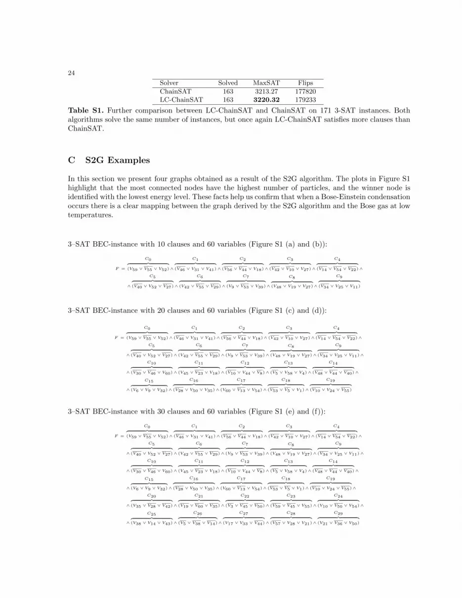
Solver Solved MaxSAT Flips

ChainSAT 163 3213.27 177820LC-ChainSAT 163 3220.32 179233

Table S1. Further comparison between LC-ChainSAT and ChainSAT on 171 3-SAT instances. Bothalgorithms solve the same number of instances, but once again LC-ChainSAT satisfies more clauses thanChainSAT.

C S2G Examples

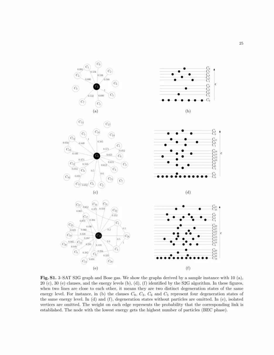
In this section we present four graphs obtained as a result of the S2G algorithm. The plots in Figure S1highlight that the most connected nodes have the highest number of particles, and the winner node isidentified with the lowest energy level. These facts help us confirm that when a Bose-Einstein condensationoccurs there is a clear mapping between the graph derived by the S2G algorithm and the Bose gas at lowtemperatures.

3–SAT BEC-instance with 10 clauses and 60 variables (Figure S1 (a) and (b)):

F =

C0︷ ︸︸ ︷(V59 ∨ V55 ∨ V52)∧

C1︷ ︸︸ ︷(V46 ∨ V31 ∨ V41)∧

C2︷ ︸︸ ︷(V56 ∨ V44 ∨ V18)∧

C3︷ ︸︸ ︷(V42 ∨ V10 ∨ V27)∧

C4︷ ︸︸ ︷(V14 ∨ V54 ∨ V22)∧

∧

C5︷ ︸︸ ︷(V40 ∨ V52 ∨ V27)∧

C6︷ ︸︸ ︷(V42 ∨ V55 ∨ V29)∧

C7︷ ︸︸ ︷(V9 ∨ V53 ∨ V39)∧

C8︷ ︸︸ ︷(V48 ∨ V19 ∨ V27)∧

C9︷ ︸︸ ︷(V34 ∨ V25 ∨ V11)

3–SAT BEC-instance with 20 clauses and 60 variables (Figure S1 (c) and (d)):

F =

C0︷ ︸︸ ︷(V59 ∨ V55 ∨ V52)∧

C1︷ ︸︸ ︷(V46 ∨ V31 ∨ V41)∧

C2︷ ︸︸ ︷(V56 ∨ V44 ∨ V18)∧

C3︷ ︸︸ ︷(V42 ∨ V10 ∨ V27)∧

C4︷ ︸︸ ︷(V14 ∨ V54 ∨ V22)∧

∧

C5︷ ︸︸ ︷(V40 ∨ V52 ∨ V27)∧

C6︷ ︸︸ ︷(V42 ∨ V55 ∨ V29)∧

C7︷ ︸︸ ︷(V9 ∨ V53 ∨ V39)∧

C8︷ ︸︸ ︷(V48 ∨ V19 ∨ V27)∧

C9︷ ︸︸ ︷(V34 ∨ V25 ∨ V11)∧

∧

C10︷ ︸︸ ︷(V30 ∨ V46 ∨ V60)∧

C11︷ ︸︸ ︷(V45 ∨ V23 ∨ V18)∧

C12︷ ︸︸ ︷(V10 ∨ V44 ∨ V8)∧

C13︷ ︸︸ ︷(V5 ∨ V58 ∨ V4)∧

C14︷ ︸︸ ︷(V48 ∨ V44 ∨ V40)∧

∧

C15︷ ︸︸ ︷(V6 ∨ V9 ∨ V32)∧

C16︷ ︸︸ ︷(V28 ∨ V50 ∨ V35)∧

C17︷ ︸︸ ︷(V60 ∨ V13 ∨ V54)∧

C18︷ ︸︸ ︷(V53 ∨ V5 ∨ V1)∧

C19︷ ︸︸ ︷(V10 ∨ V24 ∨ V55)

3–SAT BEC-instance with 30 clauses and 60 variables (Figure S1 (e) and (f)):

F =

C0︷ ︸︸ ︷(V59 ∨ V55 ∨ V52)∧

C1︷ ︸︸ ︷(V46 ∨ V31 ∨ V41)∧

C2︷ ︸︸ ︷(V56 ∨ V44 ∨ V18)∧

C3︷ ︸︸ ︷(V42 ∨ V10 ∨ V27)∧

C4︷ ︸︸ ︷(V14 ∨ V54 ∨ V22)∧

∧

C5︷ ︸︸ ︷(V40 ∨ V52 ∨ V27)∧

C6︷ ︸︸ ︷(V42 ∨ V55 ∨ V29)∧

C7︷ ︸︸ ︷(V9 ∨ V53 ∨ V39)∧

C8︷ ︸︸ ︷(V48 ∨ V19 ∨ V27)∧

C9︷ ︸︸ ︷(V34 ∨ V25 ∨ V11)∧

∧

C10︷ ︸︸ ︷(V30 ∨ V46 ∨ V60)∧

C11︷ ︸︸ ︷(V45 ∨ V23 ∨ V18)∧

C12︷ ︸︸ ︷(V10 ∨ V44 ∨ V8)∧

C13︷ ︸︸ ︷(V5 ∨ V58 ∨ V4)∧

C14︷ ︸︸ ︷(V48 ∨ V44 ∨ V40)∧

∧

C15︷ ︸︸ ︷(V6 ∨ V9 ∨ V32)∧

C16︷ ︸︸ ︷(V28 ∨ V50 ∨ V35)∧

C17︷ ︸︸ ︷(V60 ∨ V13 ∨ V54)∧

C18︷ ︸︸ ︷(V53 ∨ V5 ∨ V1)∧

C19︷ ︸︸ ︷(V10 ∨ V24 ∨ V55)∧

∧

C20︷ ︸︸ ︷(V35 ∨ V28 ∨ V42)∧

C21︷ ︸︸ ︷(V19 ∨ V60 ∨ V35)∧

C22︷ ︸︸ ︷(V3 ∨ V45 ∨ V50)∧

C23︷ ︸︸ ︷(V59 ∨ V45 ∨ V55)∧

C24︷ ︸︸ ︷(V10 ∨ V50 ∨ V54)∧

∧

C25︷ ︸︸ ︷(V38 ∨ V14 ∨ V43)∧

C26︷ ︸︸ ︷(V5 ∨ V38 ∨ V14)∧

C27︷ ︸︸ ︷(V17 ∨ V33 ∨ V44)∧

C28︷ ︸︸ ︷(V57 ∨ V28 ∨ V21)∧

C29︷ ︸︸ ︷(V21 ∨ V36 ∨ V50)

25

0.600

C0

C5

C6

C2

C3C7

C8

C4

C1

C9

0.536

0.588

1

0.532

0.606

0.5560.091 C9

C7C4C2C1

C8C3C6C5

C0

ε

(a) (b)

C0

C1

C8

C3

C4

C7C15

C2C6C11

C9

C12

C16

C18

C14

C5

C13

C10

C17

C19

0.4480.034

0.446

0.474

0.053

0.553

0.5

0.031

0.052

0.6

0.6120.615

0.621

0.5710.052

0.5651

C4C9

C11C8C1

C18C14C12C10C2C6C5

C3C0

ε

(c) (d)

C26C19

C22

C4

C1

C16

C12

C6

0.5

1

0.5

0.356

0.4

0.2

0.133

C8

0.2950.048

C10

C25

0.023

0.338

0.357

C130.091

0.382

0.371

C17

0.070 0.394

0.106

C200.085

C21

0.333

0.352

0.360

C270.052

0.065

C29

0.335C19

ε

C26

C16

C20

C6

C10

C12

C13

C17

C22

C27

C29

C4

C1

C8

C25

C21

(e) (f)

Fig. S1. 3–SAT S2G graph and Bose gas. We show the graphs derived by a sample instance with 10 (a),20 (c), 30 (e) clauses, and the energy levels (b), (d), (f) identified by the S2G algorithm. In these figures,when two lines are close to each other, it means they are two distinct degeneration states of the sameenergy level. For instance, in (b) the clauses C8, C3, C6 and C5 represent four degeneration states ofthe same energy level. In (d) and (f), degeneration states without particles are omitted. In (e), isolatedvertices are omitted. The weight on each edge represents the probability that the corresponding link isestablished. The node with the lowest energy gets the highest number of particles (BEC phase).

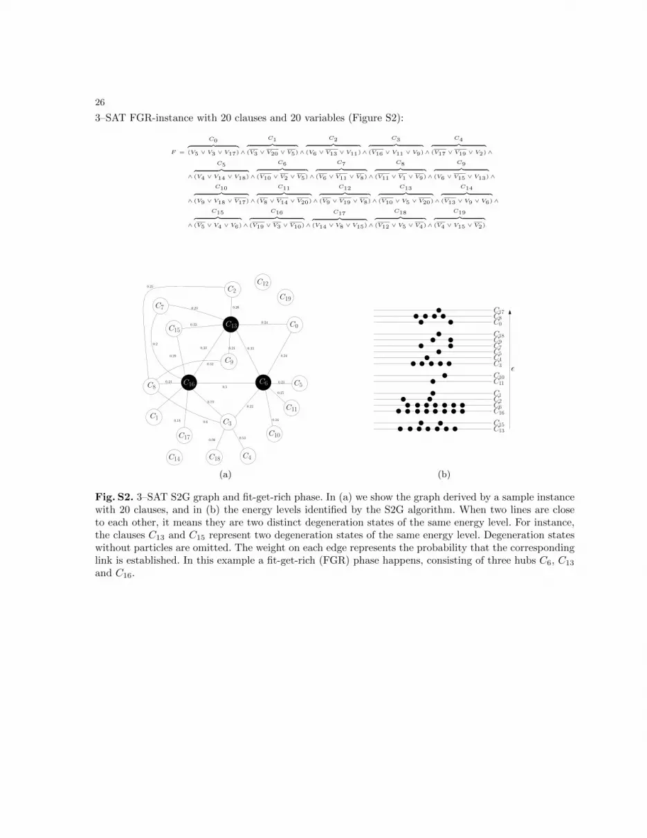
26

3–SAT FGR-instance with 20 clauses and 20 variables (Figure S2):

F =

C0︷ ︸︸ ︷(V5 ∨ V3 ∨ V17)∧

C1︷ ︸︸ ︷(V3 ∨ V20 ∨ V5)∧

C2︷ ︸︸ ︷(V6 ∨ V13 ∨ V11)∧

C3︷ ︸︸ ︷(V16 ∨ V11 ∨ V9)∧

C4︷ ︸︸ ︷(V17 ∨ V19 ∨ V2)∧

∧

C5︷ ︸︸ ︷(V4 ∨ V14 ∨ V18)∧

C6︷ ︸︸ ︷(V10 ∨ V2 ∨ V5)∧

C7︷ ︸︸ ︷(V6 ∨ V11 ∨ V8)∧

C8︷ ︸︸ ︷(V11 ∨ V1 ∨ V9)∧

C9︷ ︸︸ ︷(V6 ∨ V15 ∨ V13)∧

∧

C10︷ ︸︸ ︷(V9 ∨ V18 ∨ V17)∧

C11︷ ︸︸ ︷(V8 ∨ V14 ∨ V20)∧

C12︷ ︸︸ ︷(V9 ∨ V19 ∨ V8)∧

C13︷ ︸︸ ︷(V10 ∨ V5 ∨ V20)∧

C14︷ ︸︸ ︷(V13 ∨ V9 ∨ V6)∧

∧

C15︷ ︸︸ ︷(V5 ∨ V4 ∨ V6)∧

C16︷ ︸︸ ︷(V19 ∨ V3 ∨ V10)∧

C17︷ ︸︸ ︷(V14 ∨ V8 ∨ V15)∧

C18︷ ︸︸ ︷(V12 ∨ V5 ∨ V4)∧

C19︷ ︸︸ ︷(V4 ∨ V15 ∨ V2)

C13

C16 C6

C1

C11

0.5

0.25

0.33 0.33

C150.23

0.29

C00.24

0.24

C2

0.28

C3

0.19

0.22

C4

0.53

C50.21

C7

0.2

0.23

C80.21

0.6

0.25

C9

0.21

0.52

C10

0.16

C12

C14

C17

0.18

C18

0.08

C19

C5C4C3

C16

C2C6

C1

C15C13

εC10C11

C9C7

C18

C8C0

C17

(a) (b)

Fig. S2. 3–SAT S2G graph and fit-get-rich phase. In (a) we show the graph derived by a sample instancewith 20 clauses, and in (b) the energy levels identified by the S2G algorithm. When two lines are closeto each other, it means they are two distinct degeneration states of the same energy level. For instance,the clauses C13 and C15 represent two degeneration states of the same energy level. Degeneration stateswithout particles are omitted. The weight on each edge represents the probability that the correspondinglink is established. In this example a fit-get-rich (FGR) phase happens, consisting of three hubs C6, C13

and C16.

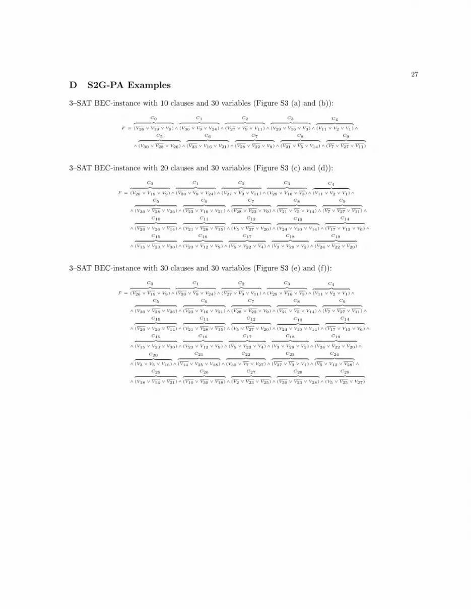
27

D S2G-PA Examples

3–SAT BEC-instance with 10 clauses and 30 variables (Figure S3 (a) and (b)):

F =

C0︷ ︸︸ ︷(V26 ∨ V19 ∨ V9)∧

C1︷ ︸︸ ︷(V30 ∨ V9 ∨ V24)∧

C2︷ ︸︸ ︷(V27 ∨ V9 ∨ V11)∧

C3︷ ︸︸ ︷(V29 ∨ V16 ∨ V3)∧

C4︷ ︸︸ ︷(V11 ∨ V2 ∨ V1)∧

∧

C5︷ ︸︸ ︷(V30 ∨ V28 ∨ V26)∧

C6︷ ︸︸ ︷(V23 ∨ V16 ∨ V21)∧

C7︷ ︸︸ ︷(V28 ∨ V22 ∨ V9)∧

C8︷ ︸︸ ︷(V21 ∨ V5 ∨ V14)∧

C9︷ ︸︸ ︷(V7 ∨ V27 ∨ V11)

3–SAT BEC-instance with 20 clauses and 30 variables (Figure S3 (c) and (d)):

F =

C0︷ ︸︸ ︷(V26 ∨ V19 ∨ V9)∧

C1︷ ︸︸ ︷(V30 ∨ V9 ∨ V24)∧

C2︷ ︸︸ ︷(V27 ∨ V9 ∨ V11)∧

C3︷ ︸︸ ︷(V29 ∨ V16 ∨ V3)∧

C4︷ ︸︸ ︷(V11 ∨ V2 ∨ V1)∧

∧

C5︷ ︸︸ ︷(V30 ∨ V28 ∨ V26)∧

C6︷ ︸︸ ︷(V23 ∨ V16 ∨ V21)∧

C7︷ ︸︸ ︷(V28 ∨ V22 ∨ V9)∧

C8︷ ︸︸ ︷(V21 ∨ V5 ∨ V14)∧

C9︷ ︸︸ ︷(V7 ∨ V27 ∨ V11)∧

∧

C10︷ ︸︸ ︷(V20 ∨ V26 ∨ V14)∧

C11︷ ︸︸ ︷(V21 ∨ V28 ∨ V15)∧

C12︷ ︸︸ ︷(V5 ∨ V27 ∨ V20)∧

C13︷ ︸︸ ︷(V24 ∨ V10 ∨ V14)∧

C14︷ ︸︸ ︷(V17 ∨ V13 ∨ V6)∧

∧

C15︷ ︸︸ ︷(V15 ∨ V23 ∨ V30)∧

C16︷ ︸︸ ︷(V23 ∨ V12 ∨ V9)∧

C17︷ ︸︸ ︷(V5 ∨ V22 ∨ V4)∧

C18︷ ︸︸ ︷(V3 ∨ V29 ∨ V2)∧

C19︷ ︸︸ ︷(V24 ∨ V22 ∨ V20)

3–SAT BEC-instance with 30 clauses and 30 variables (Figure S3 (e) and (f)):

F =

C0︷ ︸︸ ︷(V26 ∨ V19 ∨ V9)∧

C1︷ ︸︸ ︷(V30 ∨ V9 ∨ V24)∧

C2︷ ︸︸ ︷(V27 ∨ V9 ∨ V11)∧

C3︷ ︸︸ ︷(V29 ∨ V16 ∨ V3)∧

C4︷ ︸︸ ︷(V11 ∨ V2 ∨ V1)∧

∧

C5︷ ︸︸ ︷(V30 ∨ V28 ∨ V26)∧

C6︷ ︸︸ ︷(V23 ∨ V16 ∨ V21)∧

C7︷ ︸︸ ︷(V28 ∨ V22 ∨ V9)∧

C8︷ ︸︸ ︷(V21 ∨ V5 ∨ V14)∧

C9︷ ︸︸ ︷(V7 ∨ V27 ∨ V11)∧

∧

C10︷ ︸︸ ︷(V20 ∨ V26 ∨ V14)∧

C11︷ ︸︸ ︷(V21 ∨ V28 ∨ V15)∧

C12︷ ︸︸ ︷(V5 ∨ V27 ∨ V20)∧

C13︷ ︸︸ ︷(V24 ∨ V10 ∨ V14)∧

C14︷ ︸︸ ︷(V17 ∨ V13 ∨ V6)∧

∧

C15︷ ︸︸ ︷(V15 ∨ V23 ∨ V30)∧

C16︷ ︸︸ ︷(V23 ∨ V12 ∨ V9)∧

C17︷ ︸︸ ︷(V5 ∨ V22 ∨ V4)∧

C18︷ ︸︸ ︷(V3 ∨ V29 ∨ V2)∧

C19︷ ︸︸ ︷(V24 ∨ V22 ∨ V20)∧

∧

C20︷ ︸︸ ︷(V3 ∨ V5 ∨ V16)∧

C21︷ ︸︸ ︷(V14 ∨ V25 ∨ V18)∧

C22︷ ︸︸ ︷(V30 ∨ V7 ∨ V27)∧

C23︷ ︸︸ ︷(V27 ∨ V3 ∨ V1)∧

C24︷ ︸︸ ︷(V5 ∨ V12 ∨ V28)∧

∧

C25︷ ︸︸ ︷(V18 ∨ V14 ∨ V21)∧

C26︷ ︸︸ ︷(V10 ∨ V30 ∨ V18)∧

C27︷ ︸︸ ︷(V2 ∨ V23 ∨ V25)∧

C28︷ ︸︸ ︷(V30 ∨ V23 ∨ V28)∧

C29︷ ︸︸ ︷(V5 ∨ V25 ∨ V27)

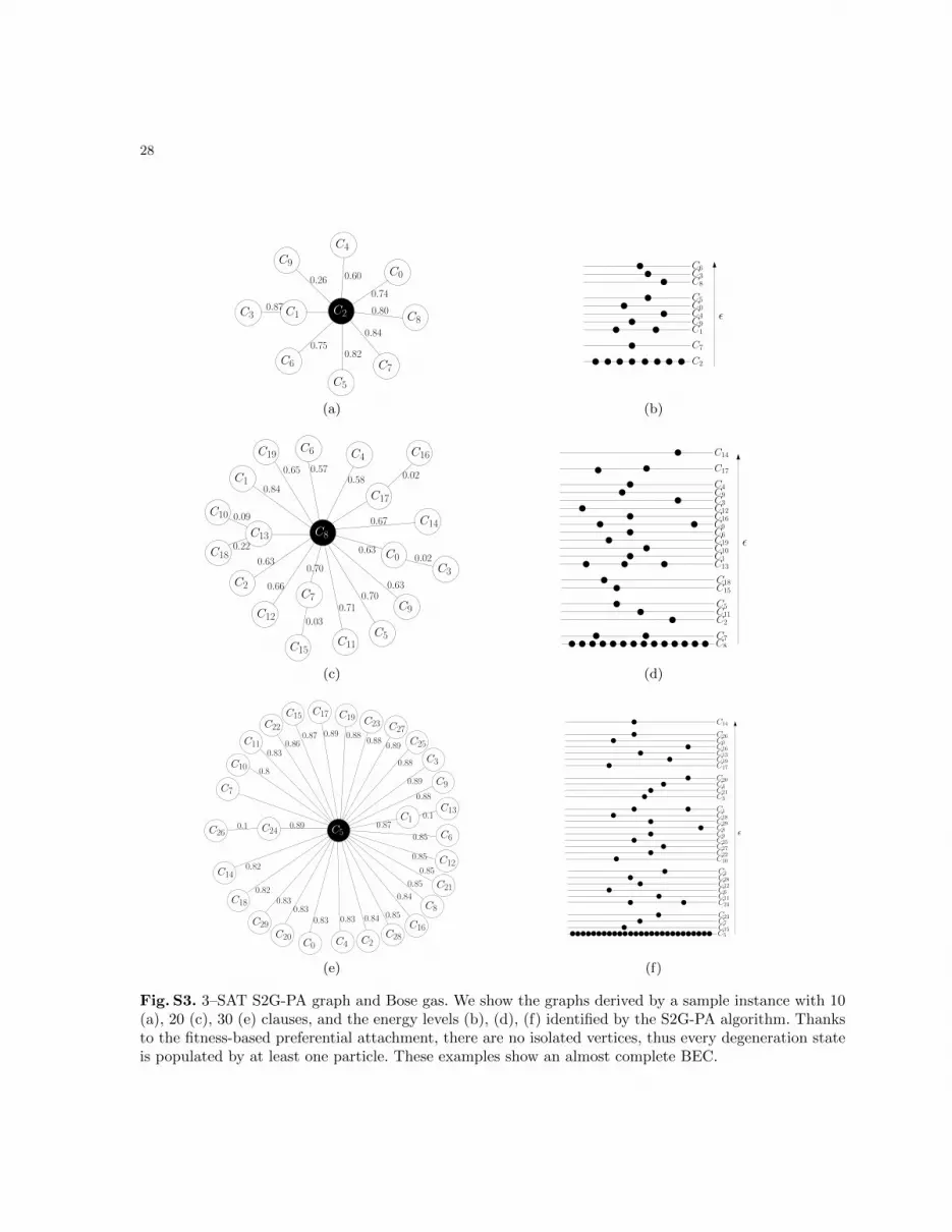
28

C2C1C30.87

C9

C4

C0

C7

C5

C6

C8

0.26 0.60

0.74

0.80

0.84

0.820.75

C2

C7

C1

C9

C4

C0

C5

C8

C3

C6

ε

(a) (b)

C5

C10

C18

C13 C8

C17

C7

C16

0.22

C6 C4

C1

C19

C14

C0

C9

C11

C12

C2

C3

C15

0.84

0.09

0.65 0.570.58

0.67

0.630.70

0.71

0.02

0.66

0.020.630.70

0.03

0.63

C8

C7

C2

C11

C5

C15

C18

ε

C13

C1

C10

C19

C6

C0

C16

C12

C3

C17

C9

C4

C14

(c) (d)

C9

C2

C5C24C26

C7

C10

C11

C15 C17 C19 C23 C27

C25

C4C0C20

C29

C18

C14

C28C16

C8

C21

C12

C6

C3

C13

C22

0.8

0.830.86

0.87 0.89 0.880.88

0.89

0.88

0.89

0.88

0.85

0.85

0.85

0.85

0.84

0.850.840.830.830.83

0.830.82

0.82

C10.1 0.89 0.87

0.1

C5

ε

C15

C7

C23

C24

C11

C6

C12

C28

C2

C10

C22

C27

C25

C9

C8

C29

C18

C1

C3

C21

C4

C20

C17

C19

C13

C16

C0

C26

C14

(e) (f)

Fig. S3. 3–SAT S2G-PA graph and Bose gas. We show the graphs derived by a sample instance with 10(a), 20 (c), 30 (e) clauses, and the energy levels (b), (d), (f) identified by the S2G-PA algorithm. Thanksto the fitness-based preferential attachment, there are no isolated vertices, thus every degeneration stateis populated by at least one particle. These examples show an almost complete BEC.

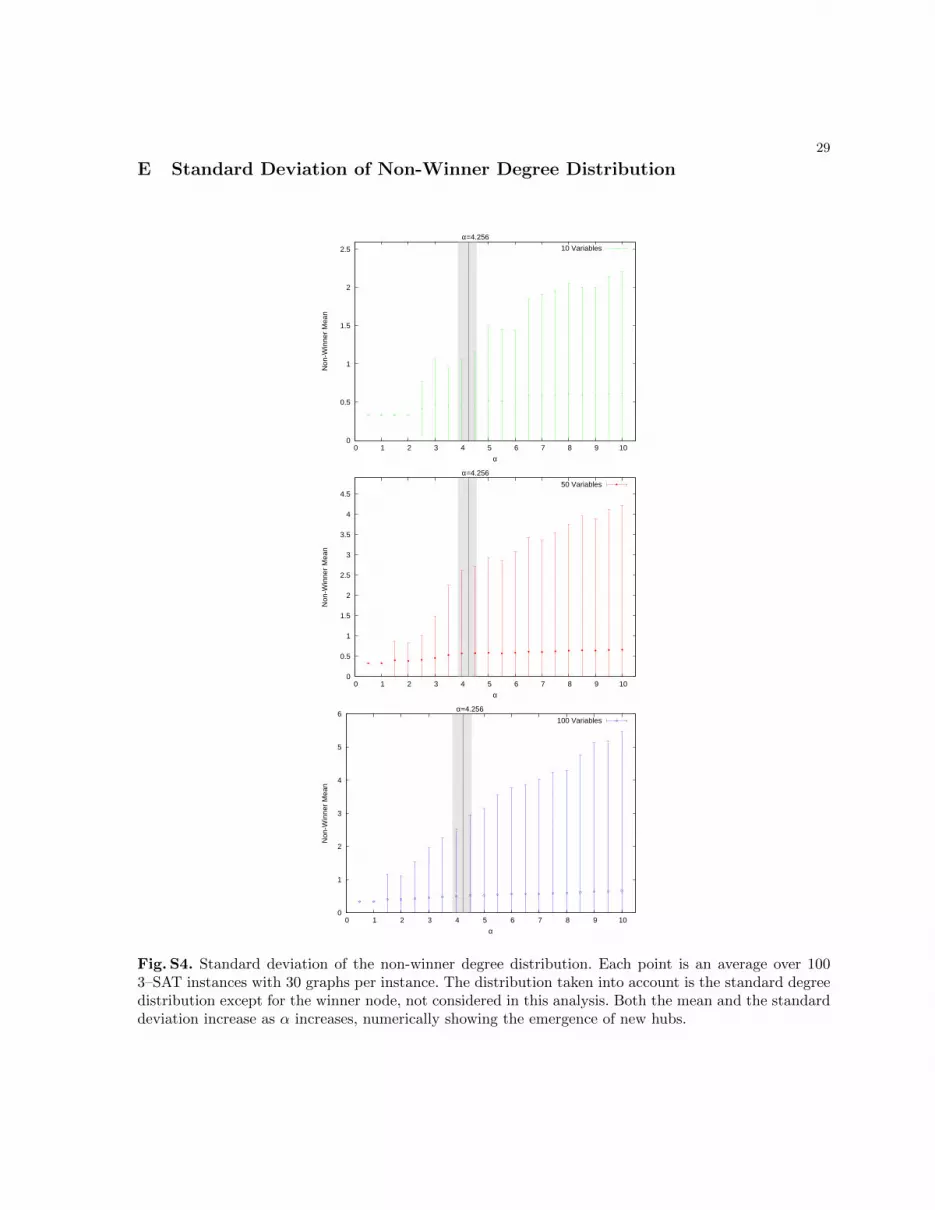
29

E Standard Deviation of Non-Winner Degree Distribution

0

0.5

1

1.5

2

2.5

0 1 2 3 4 5 6 7 8 9 10

Non

-Win

ner

Mea

n

α

α=4.256

10 Variables

0

0.5

1

1.5

2

2.5

3

3.5

4

4.5

0 1 2 3 4 5 6 7 8 9 10

Non

-Win

ner

Mea

n

α

α=4.256

50 Variables

0

1

2

3

4

5

6

0 1 2 3 4 5 6 7 8 9 10

Non

-Win

ner

Mea

n

α

α=4.256

100 Variables

Fig. S4. Standard deviation of the non-winner degree distribution. Each point is an average over 1003–SAT instances with 30 graphs per instance. The distribution taken into account is the standard degreedistribution except for the winner node, not considered in this analysis. Both the mean and the standarddeviation increase as α increases, numerically showing the emergence of new hubs.

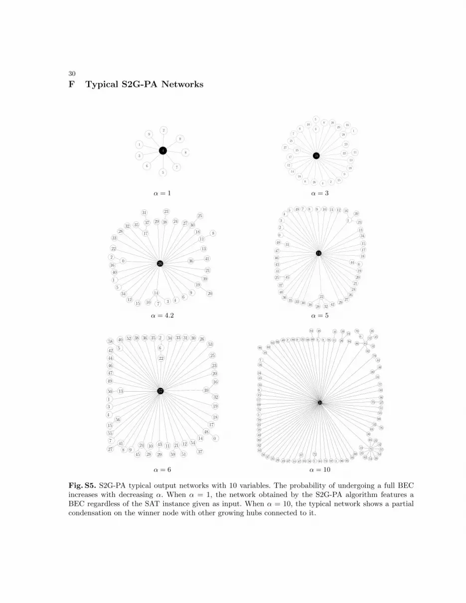
30

F Typical S2G-PA Networks

4

1

3

92

0

7

5

6

824

27

17

12

1125

4260

18

149

15

5

3

22

2

13

19

16

128

8

23

2910

6

7

21

20

α = 1 α = 3

0

14

10 73

19

20

1

5

34

1215

46

9

39

21

1322

2

16

40

4126

38

23

29

17

35 37

31

3228

33 11

8

25

30

18

2724

36

14

38 28 32 42

1

1639

23

4831

4525

37

44 6

22

0

2

3

45 8 9 10 11 12

13

34

15

17

18

19

20

21

24

2627

2930333536

40

41

43

46

47

49 7

α = 4.2 α = 5

57

29

43

6

2

22

39

16

32

4127

50 13

58

5

48

054

37

21

5159

24

2845

5615

42

44

46

47

49

1

3

4

55

7

8 910 11 12

14

17

18

20

23

25

343536385240 26303133

19

53

36

51

55

99

3276

197736456851467192935

3750

83

92

80

40

18

23

78

3

59

9

15

17

69

74

9395

60

96

30

47

87

5

72

71

22

42

57

54

65

285362

25

13

277524

61

43

34

498 89 8 91 1149 2 2188 0

84

26

41

94

3916

48

52

12 45

81

82

86

6

70 38

44

79

46

20

33

77

31

58

7

10

90 68

63 66

α = 6 α = 10

Fig. S5. S2G-PA typical output networks with 10 variables. The probability of undergoing a full BECincreases with decreasing α. When α = 1, the network obtained by the S2G-PA algorithm features aBEC regardless of the SAT instance given as input. When α = 10, the typical network shows a partialcondensation on the winner node with other growing hubs connected to it.