BORCHERS 2010

EURING PROCEEDINGS

A non-technical overview of spatially explicit capture–recapturemodels

David Borchers

Received: 13 December 2009 / Revised: 31 August 2010 / Accepted: 10 September 2010

� Dt. Ornithologen-Gesellschaft e.V. 2010

Abstract Most capture–recapture studies are inherently

spatial in nature, with capture probabilities depending on

the location of traps relative to animals. The spatial com-

ponent of the studies has until recently, however, not been

incorporated in statistical capture–recapture models. This

paper reviews capture–recapture models that do include an

explicit spatial component. This is done in a non-technical

way, omitting much of the algebraic detail and focussing

on the model formulation rather than on the estimation

methods (which include inverse prediction, maximum

likelihood and Bayesian methods). One can view spatially

explicit capture–recapture (SECR) models as an endpoint

of a series of spatial sampling models, starting with circular

plot survey models and moving through conventional dis-

tance sampling models, with and without measurement

errors, through mark–recapture distance sampling (MRDS)

models. This paper attempts a synthesis of these models in

what I hope is a style accessible to non-specialists, placing

SECR models in the context of other spatial sampling

models.

Keywords Spatially explicit capture–recapture �Spatial sampling � Measurement error � Capture function �Plot sampling � Distance sampling

Introduction

Trapping is a common means of obtaining capture–recap-

ture data, and one that has been used for decades, but

models that explicitly incorporate the spatial component of

such data are relatively new. The need for a spatial com-

ponent in models arises from the fact that animals located

closer to traps tend to be more likely to be captured and

animals sufficiently far from the traps will certainly not be

captured. Spatially explicit capture–recapture (SECR)

methods incorporate the spatial information in inference.

SECR methods have found applications in a wide and

growing number of areas. These include cage-trapping of

possums (Efford et al. 2005), mist-netting birds (Efford

et al. 2004; Borchers and Efford 2008), acoustic ‘‘trapping’’

of cetaceans from their vocalizations (Marques et al. 2010),

acoustic ‘‘trapping’’ of birds from their song (Efford et al.

2009b; Dawson and Efford 2009), use of hair snares for

stoats and bears together with individual identification via

DNA analysis (Efford et al. 2009a; Obbard et al. 2010),

visual capture–recapture of lizards (Royle and Young

2008), and camera-trapping of tigers with visual individual

identification (Royle et al. 2009a, b; Royle and Dorazio

2008).

These studies have used a range of detection devices,

some of which are traps while others detect without actu-

ally trapping. The devices include cage-traps (which are

single-catch traps), mist-nets (a kind of multi-catch trap),

acoustic detectors (both terrestrial and marine), sightings

by humans, and detection by cameras. The methods are

surprisingly versatile. Their basic requirements are that the

location of detectors is known and that there is some means

of identifying detected individuals at each detector (what-

ever it is) on each occasion. Actually, it turns out that, for

detectors that allow detection of the same individual by

Communicated by M. Schaub.

D. Borchers (&)

Centre for Research into Ecological and Environmental

Modelling, The Observatory, Buchanan Gardens,

University of St Andrews, Fife KY16 9LZ, UK

e-mail: [email protected]

123

J Ornithol

DOI 10.1007/s10336-010-0583-z

more than one detector on a single occasion (true, e.g., for

acoustic detectors, hair snares and camera traps), the

methods require only a single occasion—see below for

details.

These basic requirements are likely to have been met by

many capture–recapture studies conducted before the

advent of SECR methods, making it possible to apply

SECR methods retrospectively to data from such studies.

The key additional data that SECR analyses require,

over and above the data used in non-spatial capture–

recapture studies, are the locations of traps at which indi-

viduals were captured. So, to develop SECR models, we

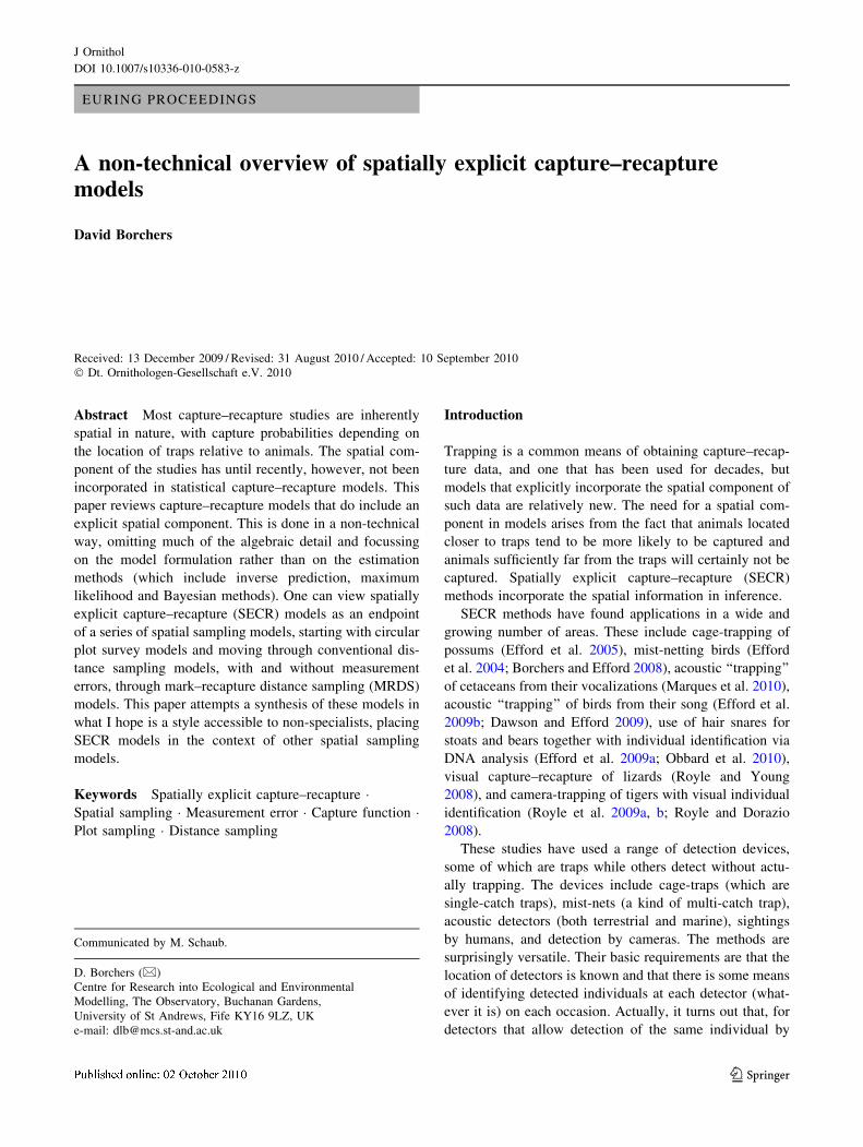
need some notation for trap location. Here, it is denoted x,

while the animal location ‘‘centroid’’ is denoted X. This

centroid is just a means of associating a single location

with an animal, it need not have biological significance.

Capture probability is modeled as a function of distance

from the centroid to traps. That is, capture probability

depends on the distance from x to X (||x - X||). The situ-

ation is illustrated in Fig. 1.

A key question for estimating animal density is ‘‘What

area do the traps effectively cover?’’. Because SECR

models incorporate the location of traps relative to animals,

they allow this question to be answered in a statistically

rigorous way from the capture–recapture data themselves.

Non-spatial methods rely on methods which are at least

partly ad hoc to convert abundance estimates to density

estimates.

Only models in which time is divided into discrete

intervals called occasions are considered here. New ani-

mals may be captured, marked and released on each

occasion and even captured more than once within an

occasion. Traps may be of various sorts, including single-

catch traps (that hold animals for the duration of the

occasion and are rendered inactive for the remainder of the

occasion once they contain an animal), multiple-catch traps

(that hold animals for the duration of the occasion but

which remain active whether or not they contain animals)

and ‘‘proximity detectors’’ (traps that register animals’

presence and identity, but do not hold the animal in any

way). Here are some examples. Cage-traps are single-catch

traps because once they hold one animal the trap can catch

no others, and once it has been caught, the animal cannot

be caught in any other trap before the end of the occasion.

Mist-nets are multi-catch traps because they can hold any

number of animals, but once an animal has been caught in a

mist-net it cannot be caught in any other mist-net before

the end of the occasion. Camera-traps are proximity

detectors because they can detect multiple animals within

an occasion, and they do not detain detected animals,

which remain free to be detected by other camera-traps

within each occasion.

SECR methods can be viewed as particular kinds of

spatial sampling methods. I think it is therefore useful to

place them in the context of other spatial sampling meth-

ods, and to this end, I very briefly review spatial sampling

methods, starting with circular plot sampling in ‘‘Plot

sampling’’. Conventional point transect sampling is sum-

marized in ‘‘Distance sampling: point transects’’, followed

by mark–recapture distance sampling for point transects in

‘‘Mark–recapture distance sampling’’ and point transect

sampling with measurement errors in ‘‘Point transects with

measurement error’’. This leads on to consideration of

SECR methods proper in ‘‘Spatially explicit capture–

recapture models’’.

For the purposes of this paper, I refer to target objects as

‘‘animals’’, although in reality they might be any kind of

fauna, flora or inanimate object. I use the terms ‘‘captured’’

and ‘‘detected’’ interchangeably; in some contexts, it is

more natural to use one rather than the other, but the

models themselves make no distinction between the two.

Spatial sampling models

Plot sampling

The simplest kind of spatial sampling method is a plot

sample, in which some plots comprising a subset of the

survey region are sampled in such a way that every animal

within the selected plot(s) is detected. The shape of the

plot(s) is immaterial, and for the purposes of reviewing

spatial sampling models, I consider only circular plots.

Generalizing the models to plots of other shapes is

straightforward but unnecessary for my purposes here.

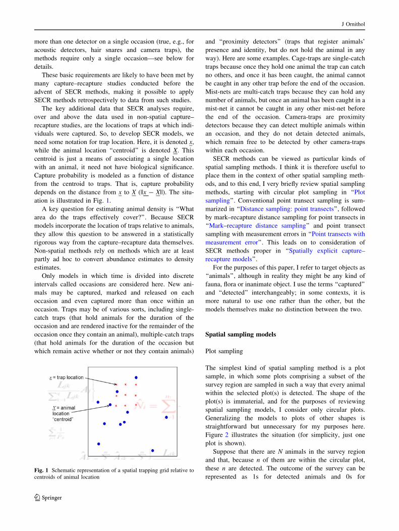
Figure 2 illustrates the situation (for simplicity, just one

plot is shown).

Suppose that there are N animals in the survey region

and that, because n of them are within the circular plot,

these n are detected. The outcome of the survey can be

represented as 1s for detected animals and 0s forFig. 1 Schematic representation of a spatial trapping grid relative to

centroids of animal location

J Ornithol

123

undetected animals. Following Borchers et al. (2002), a

useful way to model how these data arose is to use (1) a

‘‘state model’’ that describes probabilistically the distribu-

tion of animal locations and (2) an ‘‘observation model’’

that describes probabilistically how observations are

obtained, given animal locations.

If we denote the ith animal’s location using the vector Xi

(comprising its Cartesian coordinates in 2-dimensional

space), the state model specifies the joint distribution of X1

to XN: f(X1,…, XN). The simplest such model is one in

which animals are distributed independently in a region

with surface area A according to a 2-dimensional uniform

probability density function (pdf):

f X1; . . . XNð Þ ¼YN

i¼1

1

A: ð1Þ

If the reason for the 1/A term above is not obvious to

you, the following analogy may help. Suppose the survey

area was divided into A grid cells of equal size. And

suppose that, instead of being an exact location, Xi was an

integer between 1 and A, denoting the cell in which the

animal occurred. Then, if animals are equally likely to be

located anywhere in the survey region, the probability that

animal i is located in any particular grid cell is 1/A, i.e. the

probability of the animal having location Xi. is 1/A. This is

true for every one of the N animals. And if animals are

located independently, the probability of the cells they are

in being X1,…, XN is the product of the N individual

probabilities, as in Eq. 1 above.

Unless stated otherwise, I will assume this form for

f(X1,…, XN) throughout this paper. In addition to it being a

simple form, it has the advantage that with it the mean

capture probability has an intuitive interpretation in terms

of the fraction of the survey area covered by the traps (see

below). This interpretation is lost with more complicated

state models.

An alternative form of state model, used quite exten-

sively in the SECR literature, that also implies a uniform

pdf of animal locations, is a homogeneous Poisson process.

The essential difference between that and the pdf in Eq. 1

is that, with the Poisson process, animal density (D) rather

than animal abundance (N) is a state model parameter and

N is a random variable. For the purposes of this overview,

I treat N as fixed.

A key quantity in SECR analysis is the ‘‘effective

sample area’’. If all animals in an area of size A were

captured (and none outside this area were captured) in the

study, the effective sample area would fairly self-evidently

be A. Similarly, if half the animals in an area of size A were

captured (and none outside this area were captured), the

effective sample would be 0.5A. In general (when animals

are uniformly distributed in the survey area), the effective

sample area is E[p]A, where E[p] is the mean capture

probability in the area.

Now, if p(X) is the capture probability for an animal at

X, then the mean capture probability of a randomly chosen

animal in the population is E½p� ¼R

A p Xð Þf Xð ÞdX; where

integration is over the whole survey region (with area A).

If f Xð Þ ¼ 1A then E½p� ¼

RA p Xð ÞdX=A ¼ a

A where a ¼RA p Xð ÞdX; which is readily interpreted as the effective

sample area, since a/A is the fraction of the survey area

effectively sampled by the survey. In the case of a plot

survey, p(X) = 1 inside the plots and zero outside them (by

definition), so that with a single circular plot the effective

sample area is just the area of the plot.

Pursuing the grid analogy introduced above a little

further and recalling that in the gridded area case X is the

grid cell number, then for a plot survey, p(X) = 1 for all

grid cells inside the plots (assuming here that cells are

either completely inside of completely outside it). And the

effective sample area a is just the sum of the areas of all the

grid cells falling inside the plots.

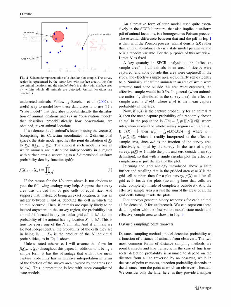
Plot surveys generate binary responses for each animal

(1 for detected, 0 for undetected). We can represent these

data, together with the observation model, state model and

effective sample area as shown in Fig. 3.

Distance sampling: point transects

Distance sampling methods model detection probability as

a function of distance of animals from observers. The two

most common forms of distance sampling methods are

point transects and line transects. In the case of line tran-

sects, detection probability is assumed to depend on the

distance from a line traversed by an observer, while in

the case of point transects, detection probability depends on

the distance from the point at which an observer is located.

We consider only the latter here, as they provide a simpler

Fig. 2 Schematic representation of a circular plot sample. The survey

region is represented by the outer box, with surface area A, the dotsare animal locations and the shaded circle is a plot (with surface area

a), within which all animals are detected. Animal locations are

denoted X

J Ornithol

123

extension of the circular plot survey considered above and

an easier analogy when we deal with SECR models later.

Given the location (x, say) of an observer in the survey

region, the probability of detecting an animal located at

X is modeled as a (usually decreasing) function of the

distance from x to X (i.e., of ||x - X||). Figure 4 illustrates

the situation.

For brevity (and since we take the observer position x as

known), we write the detection probability as p(X) rather

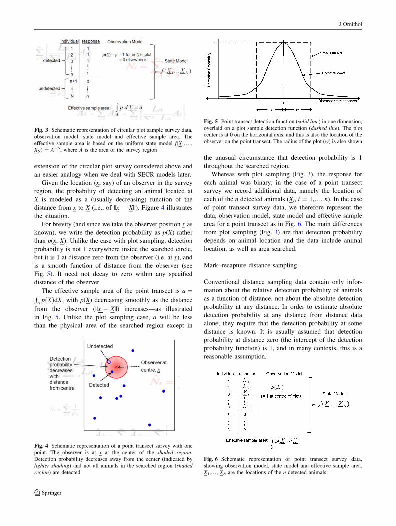
than p(x, X). Unlike the case with plot sampling, detection

probability is not 1 everywhere inside the searched circle,

but it is 1 at distance zero from the observer (i.e. at x), and

is a smooth function of distance from the observer (see

Fig. 5). It need not decay to zero within any specified

distance of the observer.

The effective sample area of the point transect is a ¼RA p Xð ÞdX; with p(X) decreasing smoothly as the distance

from the observer (||x - X||) increases—as illustrated

in Fig. 5. Unlike the plot sampling case, a will be less

than the physical area of the searched region except in

the unusual circumstance that detection probability is 1

throughout the searched region.

Whereas with plot sampling (Fig. 3), the response for

each animal was binary, in the case of a point transect

survey we record additional data, namely the location of

each of the n detected animals (Xi, i = 1,…, n). In the case

of point transect survey data, we therefore represent the

data, observation model, state model and effective sample

area for a point transect as in Fig. 6. The main differences

from plot sampling (Fig. 3) are that detection probability

depends on animal location and the data include animal

location, as well as area searched.

Mark–recapture distance sampling

Conventional distance sampling data contain only infor-

mation about the relative detection probability of animals

as a function of distance, not about the absolute detection

probability at any distance. In order to estimate absolute

detection probability at any distance from distance data

alone, they require that the detection probability at some

distance is known. It is usually assumed that detection

probability at distance zero (the intercept of the detection

probability function) is 1, and in many contexts, this is a

reasonable assumption.

Fig. 3 Schematic representation of circular plot sample survey data,

observation model, state model and effective sample area. The

effective sample area is based on the uniform state model f(X1,…,

XN) = A-N, where A is the area of the survey region

Fig. 4 Schematic representation of a point transect survey with one

point. The observer is at x at the center of the shaded region.

Detection probability decreases away from the center (indicated by

lighter shading) and not all animals in the searched region (shadedregion) are detected

Fig. 5 Point transect detection function (solid line) in one dimension,

overlaid on a plot sample detection function (dashed line). The plot

center is at 0 on the horizontal axis, and this is also the location of the

observer on the point transect. The radius of the plot (w) is also shown

Fig. 6 Schematic representation of point transect survey data,

showing observation model, state model and effective sample area.

X1,…, XN are the locations of the n detected animals

J Ornithol

123

However, in some situations, the assumption that all

animals at distance zero from the observer are detected is

unrealistic. This is the case for many marine surveys,

where animals can be underwater and hence undetectable

even though they are at distance zero. In this case, a

combination of mark–recapture and distance sampling

(MRDS) methods can be used (see Borchers 1996, 1998;

Manly et al. 1996). These methods have been developed

extensively for line transect surveys and also used on cue-

counting surveys (which are like moving point transects;

see Buckland et al. 2001). They have been used to a much

lesser extent for stationary point transects (see Kissling

et al. 2006, for an example). The underlying theory is as

applicable to point transects as to line transects and it is

MRDS point transect surveys that are considered here.

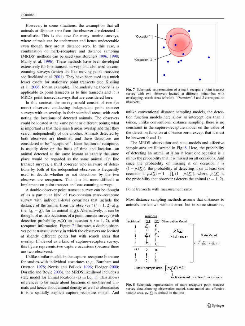
In this context, the survey would consist of two (or

more) observers conducting independent point transect

surveys with an overlap in their searched areas, with each

noting the locations of detected animals. The observers

could be located at the same point or different points; what

is important is that their search areas overlap and that they

search independently of one another. Animals detected by

both observers are identified and these detections are

considered to be ‘‘recaptures’’. Identification of recaptures

is usually done on the basis of time and location—an

animal detected at the same instant at exactly the same

place would be regarded as the same animal. On line

transect surveys, a third observer who is aware of detec-

tions by both of the independent observers is frequently

used to decide whether or not detections by the two

observes are recaptures. This is a bit more difficult to

implement on point transect and cue-counting surveys.

A double-observer point transect survey can be thought

of as a particular kind of two-occasion mark–recapture

survey with individual-level covariates that include the

distance of the animal from the observer t (t = 1, 2) at xt

(i.e. ||xt - X||, for an animal at X). Alternatively, it can be

thought of as two occasions of a point transect survey (with

detection probability pt(X) on occasion t; t = 1, 2), with

recapture information. Figure 7 illustrates a double-obser-

ver point transect survey in which the observers are located

at slightly different points but with search areas that

overlap. If viewed as a kind of capture–recapture survey,

this figure represents two capture occasions (because there

are two observers).

Unlike similar models in the capture–recapture literature

for studies with individual covariates (e.g., Burnham and

Overton 1978; Norris and Pollock 1996; Pledger 2000;

Dorazio and Royle 2003), the MRDS likelihood includes a

state model for animal locations (as in Eq. 1). This allows

inferences to be made about locations of unobserved ani-

mals and hence about animal density as well as abundance;

it is a spatially explicit capture–recapture model. And

unlike conventional distance sampling models, the detec-

tion function models here allow an intercept less than 1

(since, unlike conventional distance sampling, there is no

constraint in the capture–recapture model on the value of

the detection function at distance zero, except that it must

be between 0 and 1).

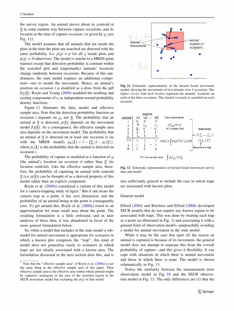
The MRDS observation and state models and effective

sample area are illustrated in Fig. 8. Here, the probability

of detecting an animal at X on at least one occasion is 1

minus the probability that it is missed on all occasions. And

since the probability of missing it on occasion t is

1� pt Xð Þð Þ; the probability of detecting it on at least one

occasion is p� Xð Þ ¼ 1�Q

t 1� pt Xð Þð Þ; where, pt Xð Þ is

the probability that observer t detects the animal (t = 1, 2).

Point transects with measurement error

Most distance sampling methods assume that distances to

animals are known without error, but in some situations,

Fig. 7 Schematic representation of a mark–recapture point transect

survey with two observers located at different points but with

overlapping search areas (circles). ‘‘Occasion’’ 1 and 2 correspond to

observers

Fig. 8 Schematic representation of mark–recapture point transect

survey data, showing observation model, state model and effective

sample area. p� Xð Þ is defined in the text

J Ornithol

123

there is substantial error in measuring distances. This

problem has been addressed for both line transect surveys

(Alpizar-Jara 1997; Chen 1998; Chen and Cowling 2001;

Marques 2004, Borchers et al. 2010) and various kinds of

point transect survey, including cue-counting surveys

(Hiby et al. 1989; Borchers et al. 2009, 2010). A point

transect survey (i.e. one with certain detection at distance

zero) in which there is measurement error is illustrated

schematically in Fig. 9.

Dealing with measurement error requires an additional

component for the distance sampling observation model,

namely a model for the measurement error process. This is

denoted f(x|X) where x is the recorded location (including

measurement error) and X is the true location of an animal.

(Note that here we use x for recorded location, whereas

before we used it for observer location.) Detection proba-

bility, and hence effective sample area, depends on X not

x. Because X is unobserved and we model the distribution

of X, it can be thought of as a random effect (with uniform

distribution in the simple case).

The data and models from this kind of survey are

illustrated in Fig. 10. Note that because we measure loca-

tions with error, our data comprise the recorded distances

x1,…, xn instead of the true animal locations X1,…, Xn. The

measurement error process is captured in the probability

density function f(x|X) (which may need to be estimated

from a subset of data for which true location is known).

Detection probability still depends on the true locations,

not the recorded locations. And because we are dealing

with conventional distance sampling again here, we assume

that detection probability at distance zero from the observer

is 1. (We are forced to assume this because conventional

distance data are not adequate to estimate absolute detec-

tion probability anywhere, as discussed above.) Finally,

because the detection probability depends on a variable that

is not observed (true animal location), true animal location

can be thought of as a random effect in the model.

Point transects with measurement error are of interest in

this paper because it turns out that observations of location

from SECR models can also be viewed as a kind of mea-

surement error model: the location of animals’ home range

centers (for example) cannot be observed, but one can

consider the locations of the traps at which an animal is

detected as observations of the center with measurement

error (more on this below).

Spatially explicit capture–recapture models

Efford (2004) proposed the first spatially explicit estima-

tion method, based on inverse prediction. Unlike the

maximum-likelihood and Bayesian estimation methods, it

is not based on an explicit likelihood function and does not

have the same inference foundation as these methods. It is,

however, a very general estimation method, able to deal not

only with all the cases that existing maximum likelihood

and Bayesian methods are able to but also the single-catch

trap case. In this paper, I focus on methods based on

explicit likelihood functions. These are summarized briefly

below.

Movement-based model

Royle and Young (2008) proposed a SECR model for

estimation of horned lizard density, based on animal

movement between capture occasions. Each capture occa-

sion consisted of searching one or more rectangular plots in

Fig. 9 Schematic representation of a point transect survey with

measurement error. Here, an animal at location X is recorded by the

observer as being at location x. (Note that here we use x for recorded

location, whereas before we used it for observer location.) The

measurement error is difference between the two locations (as only

radial distance is normally recorded, the measurement error would

usually be just the difference in radial distance to the true and

recorded locations)

Fig. 10 Schematic representation point transect survey data with

measurement error, showing observation model, state model and

effective sample area. Data comprise recorded locations and the

model includes a measurement error model governing how recorded

locations arise from true locations

J Ornithol

123

the survey region. An animal moves about its centroid at

X in some random way between capture occasions, and its

location at the time of capture occasion t is given by xt (see

Fig. 11).

The model assumes that all animals that are inside the

plots at the time the plots are searched are detected with the

same probability (i.e. p(x) = p for all x inside plots and

p(x) = 0 otherwise). The model is similar to a MRDS point

transect except that detection probability is constant within

the searched plot and (importantly) animals’ locations

change randomly between occasions. Because of this ran-

domness, the state model requires an additional compo-

nent—one to model the movement. Hence, an animal’s

position on occasion t is modeled as a draw from the pdf

f(xt|X). Royle and Young (2008) modeled the northing and

easting components of xt as independent normal probability

density functions.

Figure 12 illustrates the data, model and effective

sample area. Note that the detection probability function on

occasion t depends on xt, not X. The probability that an

animal at X is detected, p(X), depends on the movement

model f(x|X). As a consequence, the effective sample area

also depends on the movement model. The probability that

an animal at X is detected on at least one occasion is (as

with the MRDS model) p� Xð Þ ¼ 1�Q

t 1� pt Xð Þð Þ;where pt Xð Þ is the probability that the animal is detected on

occasion t.

The probability of capture is modeled as a function of xt

(the animal’s location on occasion t) rather than X (its

location centroid). Like the effective sample area, there-

fore, the probability of capturing an animal with centroid

X (i.e. p(X)) can be thought of as a derived property of this

model rather than an explicit component.

Royle et al. (2009a) considered a variant of this model

for a camera-trapping study of tigers.1 But if one treats the

camera trap as a point, it has zero dimension, and the

probability of an animal being at the point is consequently

zero. To get around this, Royle et al. (2009a) resort to an

approximation for some small area about the point. The

resulting formulation is a little awkward, and in later

analyses of these data, it was abandoned in favor of the

more general formulation below.

So, while a model that includes in the state model a sub-

model for animal movement is appropriate for scenarios in

which a known plot comprises the ‘‘trap’’, this kind of

model does not generalize easily to scenarios in which

traps are not clearly associated with a known area. The

formulation discussed in the next section does this, and is

also sufficiently general to include the case in which traps

are associated with known plots.

General model

Efford (2004) and Borchers and Efford (2008) developed

SECR models that do not require any known region to be

associated with traps. This was done by treating each trap

as a point (as illustrated in Fig. 1) and associating it with a

general form of observation model—purposefully avoiding

a model for animal movement in the state model.

While it may be the case that (part of) the reason an

animal is captured is because of its movement, the general

model does not attempt to separate this from the overall

probability of capture—and this gives it flexibility. It can

cope with situations in which there is animal movement

and those in which there is none. The model is shown

schematically in Fig. 13.

Notice the similarity between the measurement error

observation model in Fig. 10 and the SECR observa-

tion model in Fig. 13. The only differences are (1) that the

Fig. 11 Schematic representation of the horned lizard movement

model, showing the movements of two animals over 3 occasions. The

lighter circles with dark borders represent the animals’ locations on

each of the three occasions. The shaded rectangle is searched on each

occasion

Fig. 12 Schematic representation of horned lizard movement survey

data and model

1 Note that the ‘‘effective sample area’’ of Royle et al. (2009a) is not

the same thing as the effective sample area of this paper. Their

effective sample area is the effective area within which animals might

be captured—analogous to the area of the searched region in the

SECR movement model but excluding the p(x) of that model.

J Ornithol

123

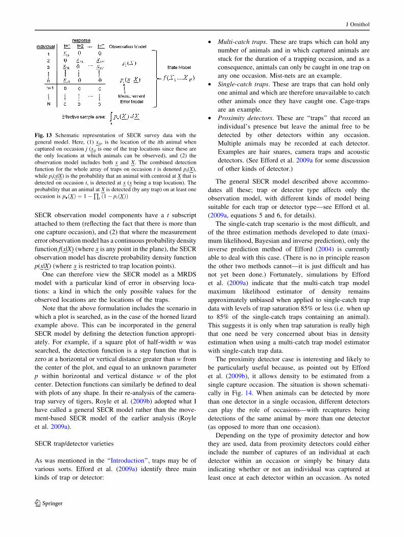
SECR observation model components have a t subscript

attached to them (reflecting the fact that there is more than

one capture occasion), and (2) that where the measurement

error observation model has a continuous probability density

function f(x|X) (where x is any point in the plane), the SECR

observation model has discrete probability density function

p(x|X) (where x is restricted to trap location points).

One can therefore view the SECR model as a MRDS

model with a particular kind of error in observing loca-

tions: a kind in which the only possible values for the

observed locations are the locations of the traps.

Note that the above formulation includes the scenario in

which a plot is searched, as in the case of the horned lizard

example above. This can be incorporated in the general

SECR model by defining the detection function appropri-

ately. For example, if a square plot of half-width w was

searched, the detection function is a step function that is

zero at a horizontal or vertical distance greater than w from

the center of the plot, and equal to an unknown parameter

p within horizontal and vertical distance w of the plot

center. Detection functions can similarly be defined to deal

with plots of any shape. In their re-analysis of the camera-

trap survey of tigers, Royle et al. (2009b) adopted what I

have called a general SECR model rather than the move-

ment-based SECR model of the earlier analysis (Royle

et al. 2009a).

SECR trap/detector varieties

As was mentioned in the ‘‘Introduction’’, traps may be of

various sorts. Efford et al. (2009a) identify three main

kinds of trap or detector:

• Multi-catch traps. These are traps which can hold any

number of animals and in which captured animals are

stuck for the duration of a trapping occasion, and as a

consequence, animals can only be caught in one trap on

any one occasion. Mist-nets are an example.

• Single-catch traps. These are traps that can hold only

one animal and which are therefore unavailable to catch

other animals once they have caught one. Cage-traps

are an example.

• Proximity detectors. These are ‘‘traps’’ that record an

individual’s presence but leave the animal free to be

detected by other detectors within any occasion.

Multiple animals may be recorded at each detector.

Examples are hair snares, camera traps and acoustic

detectors. (See Efford et al. 2009a for some discussion

of other kinds of detector.)

The general SECR model described above accommo-

dates all these; trap or detector type affects only the

observation model, with different kinds of model being

suitable for each trap or detector type—see Efford et al.

(2009a, equations 5 and 6, for details).

The single-catch trap scenario is the most difficult, and

of the three estimation methods developed to date (maxi-

mum likelihood, Bayesian and inverse prediction), only the

inverse prediction method of Efford (2004) is currently

able to deal with this case. (There is no in principle reason

the other two methods cannot—it is just difficult and has

not yet been done.) Fortunately, simulations by Efford

et al. (2009a) indicate that the multi-catch trap model

maximum likelihood estimator of density remains

approximately unbiased when applied to single-catch trap

data with levels of trap saturation 85% or less (i.e. when up

to 85% of the single-catch traps containing an animal).

This suggests it is only when trap saturation is really high

that one need be very concerned about bias in density

estimation when using a multi-catch trap model estimator

with single-catch trap data.

The proximity detector case is interesting and likely to

be particularly useful because, as pointed out by Efford

et al. (2009b), it allows density to be estimated from a

single capture occasion. The situation is shown schemati-

cally in Fig. 14. When animals can be detected by more

than one detector in a single occasion, different detectors

can play the role of occasions—with recaptures being

detections of the same animal by more than one detector

(as opposed to more than one occasion).

Depending on the type of proximity detector and how

they are used, data from proximity detectors could either

include the number of captures of an individual at each

detector within an occasion or simply be binary data

indicating whether or not an individual was captured at

least once at each detector within an occasion. As noted

Fig. 13 Schematic representation of SECR survey data with the

general model. Here, (1) xij, is the location of the ith animal when

captured on occasion j (xij is one of the trap locations since these are

the only locations at which animals can be observed), and (2) the

observation model includes both x and X. The combined detection

function for the whole array of traps on occasion t is denoted pt(X),

while pt(x|X) is the probability that an animal with centroid at X that is

detected on occasion t, is detected at x (x being a trap location). The

probability that an animal at X is detected (by any trap) on at least one

occasion is p� Xð Þ ¼ 1�Q

t 1� pt Xð Þð Þ

J Ornithol

123

by Efford et al. (2009b) and Royle et al. (2009b), the

binary data are a reduced-information summary of the

capture frequencies. One would therefore expect estima-

tors based on binary data to perform less well than those

based on frequency data. Efford et al. (2009b) found in a

simulation study that while it did so, the difference

between estimator performance in the two cases was

small except in those scenarios when there was less than

one recapture per individual in the population on

average.

Summary and discussion

A decade ago, apparently unrelated line transect models

and capture–recapture models were combined to create a

model for situations in which neither approach on its own

was adequate. Since then, there have been methodological

advances for distance sampling when there is distance

measurement error, and this has happened for the most part

quite separately from advances in the development of

spatially explicit capture–recapture models and methods

(Royle and Dorazio 2008 being the exception).

It turns out that SECR models can be viewed as MRDS

models with measurement error, and vice versa. As well as

being intellectually satisfying, the marriage of MRDS and

SECR models has benefits for both. For example, distance

sampling detection function models have provided a basis

for the development of suitable capture function models

for SECR analyses (see, e.g., Efford 2004; Borchers and

Efford 2008), and SECR models provide a framework for

analysis of MRDS surveys with measurement error (as

noted by Royle and Dorazio 2008). I expect that the

exchange of ideas and methods between the two will

continue, to their mutual benefit.

One area in particular which seems ripe for methodo-

logical development is the extension of SECR methods to

include additional distance-related information. You can

think of an MRDS point transect survey with no movement

and no measurement error as the best possible kind of

SECR survey—it is effectively SECR with observed ani-

mal locations. And you can think of the SECR models

outlined above as MRDS point transect surveys in which

none of the captured animals’ locations are observed. There

are a number of intermediate possibilities, including direct

observation of some, but not all, animal locations, partial

observation of locations (e.g., angles but not distances from

traps to animals, or distances but not angles) and obser-

vation of additional variables associated with location,

angle or distance (e.g., signal strength).

There has already been some development in this

direction. Efford et al. (2009b) used acoustic signal

strength of audially detected animals on a passive acoustic

array to supplement the SECR data described above

(Fig. 14), and found that using signal strength led to sub-

stantial improvements in the precision of density estimates

for small arrays even though the signal strength was not

calibrated against distance. I expect that, in the near future,

method development will extend further into the gray area

between MRDS point transects and the SECR models

described above.

Other areas of likely development include the develop-

ment of methods to deal with uncertain recapture identifi-

cation, incorporation of models for acoustic (and other

kinds of) availability, and extension to scenarios in which

animals’ location centroids are not stationary.

I have attempted to provide a synthesis that shows how

various SECR models in the literature are related to other

spatial sampling models for animal density and to each

other. In trying to keep the overview accessible, I have had to

restrict myself to the simpler versions of the models con-

sidered. Before leaving the subject, I should point out some

of the areas in which currently available models are not quite

as simple as they have appeared in my descriptions.

The first simplification I made was in considering only a

uniform probability density function (pdf) for animal

locations. This assumption allowed me to work with the

intuitively appealing concept of effective sample area, and

this helped link the various kinds of spatial sampling

model. But there is no reason in principle to restrict models

to have a uniform location pdf. The models of Borchers

and Efford (2008), for example, include the case in which

animals are distributed according to a heterogeneous

Poisson process (which corresponds to a non-uniform

location pdf). In this case E½p� ¼R

A p Xð Þf Xð ÞdX does not

Fig. 14 Schematic representation of single-occasion SECR survey

data and model. Note that data columns that corresponded to

occasions in Fig. 13 correspond to traps here. The t subscript has

been replaced with a dot in p� Xð Þ; which is the probability that an

animal is detected by at least one trap; p(xk|X) is the probability that

an animal with centroid at X which is detected, is detected by the

detector at xk

J Ornithol

123

have the interpretation of effective proportion of the survey

area covered by the traps, instead it has a non-spatial

interpretation: the expected proportion of the population

that is detected or captured.

I have not considered models in which detection or

capture functions depend on covariates, individual-level,

survey-level or otherwise. Nor have I considered models

that accommodate unobserved individual-level heteroge-

neity in capture/detection probability. All these kinds of

model appear in the literature, together with methods such

as Akaike’s Information Criterion (AIC) for selecting

between candidate models. I have not considered good-

ness-of-fit. This is an area that would benefit from further

research.

Finally, I have not discussed methods of drawing

inference using any of the models mentioned here. Inverse

prediction methods, maximum likelihood methods and

Bayesian methods have been developed and used suc-

cessfully; see Efford (2004) for the inverse prediction

method, Borchers and Efford (2008) and Efford et al.

(2009a, b) for maximum likelihood methods, and Royle

and Young (2008), Royle and Dorazio (2008) and Royle

et al. (2009a, b) for Bayesian methods.

Acknowledgments I would like to thank Andy Royle for inviting

me to present this work at the 2009 EURING Meeting, Tiago Mar-

ques and Len Thomas for useful feedback on an earlier draft, which

led to a much improved manuscript, and to the anonymous reviewers

for making suggestions that improved the accessibility and readability

of the manuscript.

References

Alpizar-Jara R (1997) Assessing assumption violation in line transect

sampling. PhD thesis, North Carolina State University, Raleigh

Borchers DL (1996) Line transect estimation with uncertain detection

on the trackline. PhD thesis, University of Cape Town

Borchers DL, Efford MG (2008) Spatially explicit maximum

likelihood methods for capture–recapture studies. Biometrics

64:377–385

Borchers DL, Zucchini W, Fewster RM (1998) Mark-recapture

models for line transect surveys. Biometrics 54:1207–1220

Borchers DL, Buckland ST, Zucchini W (2002) Estimating animal

abundance: closed populations. Springer, London

Borchers DL, Pike D, Gunnlaugsson T, Vikingsson GA (2009) Minke

whale abundance estimation from the NASS 1987 and 2001 cue

counting surveys taking account of distance estimation errors.

North Atlantic Marine Mammal Commission Special Issue 7:

North Atlantic Sightings Surveys (1987–2001), pp 95–110

Borchers DL, Marques TA, Gunlaugsson T, Jupp P (2010) Estimating

distance sampling detection functions when distances are

measured with errors. J Agric Biol Environ Stat. doi:10.1007/

s13253-010-0021-y

Buckland ST, Anderson DR, Burnham KP, Laake JL, Borchers DL,

Thomas L (2001) Introduction to distance sampling: estimating

abundance of biological populations. Oxford University Press,

Oxford

Burnham KP, Overton WS (1978) Estimation of the size of a closed

population when capture probabilities vary among animals.

Biometrika 65:625–633

Chen SX (1998) Measurement errors in line transect surveys.

Biometrics 54:899–908

Chen SX, Cowling A (2001) Measurement errors in line transect

sampling where detectability varies with distance and size.

Biometrics 57:732–742

Dawson DK, Efford MG (2009) Bird population density estimated

from acoustic signals. J Appl Ecol 46:1201–1209

Dorazio RM, Royle JA (2003) Mixture models for estimating the size

of a closed population when capture rates vary among individ-

uals. Biometrics 59:351–364

Efford MG (2004) Density estimation in live-trapping studies. Oikos

106:598–610

Efford MG, Dawson DK, Robbins CS (2004) DENSITY: software for

analysing capture–recapture data from passive detector arrays.

Anim Biodivers Conserv 27:217–228

Efford MG, Warburton B, Coleman MC, Barker RJ (2005) A field test

of two methods for density estimation. Wildl Soc Bull

33:731–738

Efford MG, Borchers DL, Byrom AE (2009a) Density estimation by

spatially explicit capture–recapture: likelihood-based methods.

In: Thompson DL, Cooch EG, Conroy MJ (eds) Modeling

demographic processes in marked populations. Springer, New

York, pp 255–269

Efford MG, Dawson DK, Borchers DL (2009b) Population density

estimated from locations of individuals on a passive detector

array. Ecology 90:2676–2682

Hiby L, Ward A, Lovell P (1989) Analysis of the North Atlantic

sightings survey 1987: aerial survey results. Rep Int Whaling

Comm 39:447–455

Kissling ML, Garton EO, Handel CM (2006) Estimating detection

probability and density from point-count surveys: a combination

of distance and double-observer sampling. Auk 123:735–752

Manly B, McDonald L, Garner G (1996) Maximum likelihood

estimation for the double-count method with independent

observers. J Agric Biol Environ Stat 1:170–189

Marques TA (2004) Predicting and correcting bias caused by

measurement error in line transect sampling using multiplicative

error models. Biometrics 60:757–763

Marques TA, Thomas L, Martin SW, Mellinger DK, Jarvis S,

Morrissey RP, Ciminello C, DiMarzio N (2010) Spatially

explicit capture recapture methods to estimate minke whale

abundance from data collected at bottom mounted hydrophones.

J Ornithol. doi:10.1007/s10336-010-0535-7

Norris JL, Pollock KH (1996) Nonparametric MLE under two closed

capture–recapture models with heterogeneity. Biometrics 52:

639–649

Obbard ME, Howe EJ, Kyle C (2010) Empirical comparison of

density estimates for large carnivores. J Appl Ecol 47:76–84

Pledger S (2000) Unified maximum likelihood estimates for closed

capture–recapture models using mixtures. Biometrics 56:434–

442

Royle JA, Dorazio RM (2008) Hierarchical modeling and inference in

ecology. Academic, London

Royle JA, Young KV (2008) A hierarchical model for spatial

capture–recapture data. Ecology 89:2281–2289

Royle JA, Nichols JD, Karanth KU, Gopalaswamy AM (2009a) A

hierarchical model for estimating density in camera-trap studies.

J Appl Ecol 46:118–127

Royle JA, Karanth KU, Gopalaswamy AM, Kumar NS (2009b)

Bayesian inference in camera-trapping studies for a class of

spatial capture–recapture models. Ecology 90:3233–3244

J Ornithol

123