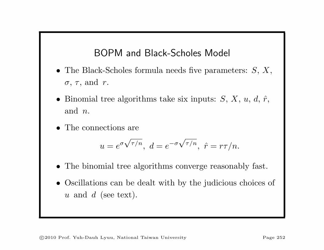
BOPM and Black-Scholes Model • The Black-Scholes formula needs five parameters: S , X , σ , τ , and r . • Binomial tree algorithms take six inputs: S , X , u, d,ˆ r , and n. • The connections are u = e σ √ τ/n ,d = e −σ √ τ/n , ˆ r = rτ/n. • The binomial tree algorithms converge reasonably fast. • Oscillations can be dealt with by the judicious choices of u and d (see text). c ⃝2010 Prof. Yuh-Dauh Lyuu, National Taiwan University Page 252

Welcome message from author
This document is posted to help you gain knowledge. Please leave a comment to let me know what you think about it! Share it to your friends and learn new things together.
Transcript
BOPM and Black-Scholes Model
• The Black-Scholes formula needs five parameters: S, X,
σ, τ , and r.
• Binomial tree algorithms take six inputs: S, X, u, d, r̂,
and n.
• The connections are
u = eσ√
τ/n, d = e−σ√
τ/n, r̂ = rτ/n.
• The binomial tree algorithms converge reasonably fast.
• Oscillations can be dealt with by the judicious choices of
u and d (see text).
c⃝2010 Prof. Yuh-Dauh Lyuu, National Taiwan University Page 252
5 10 15 20 25 30 35n
11.5
12
12.5
13
Call value
0 10 20 30 40 50 60n
15.1
15.2
15.3
15.4
15.5Call value
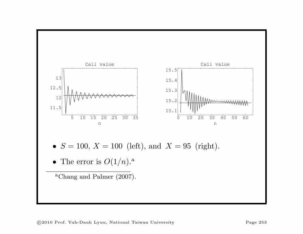
• S = 100, X = 100 (left), and X = 95 (right).
• The error is O(1/n).a
aChang and Palmer (2007).
c⃝2010 Prof. Yuh-Dauh Lyuu, National Taiwan University Page 253
Implied Volatility
• Volatility is the sole parameter not directly observable.
• The Black-Scholes formula can be used to compute the
market’s opinion of the volatility.
– Solve for σ given the option price, S, X, τ , and r
with numerical methods.
– How about American options?
• This volatility is called the implied volatility.
• Implied volatility is often preferred to historical
volatility in practice.a
aIt is like driving a car with your eyes on the rearview mirror?
c⃝2010 Prof. Yuh-Dauh Lyuu, National Taiwan University Page 254

Problems; the Smile
• Options written on the same underlying asset usually do
not produce the same implied volatility.
• A typical pattern is a “smile” in relation to the strike
price.
– The implied volatility is lowest for at-the-money
options.
– It becomes higher the further the option is in- or
out-of-the-money.
• Other patterns have also been observed.
c⃝2010 Prof. Yuh-Dauh Lyuu, National Taiwan University Page 255
Problems; the Smile (concluded)
• To address this issue, volatilities are often combined to
produce a composite implied volatility.
• This practice is not sound theoretically.
• The existence of different implied volatilities for options
on the same underlying asset shows the Black-Scholes
model cannot be literally true.
c⃝2010 Prof. Yuh-Dauh Lyuu, National Taiwan University Page 256

Trading Days and Calendar Days
• Interest accrues based on the calendar day.
• But σ is usually calculated based on trading days only.
– Stock price seems to have lower volatilities when the
exchange is closed.a
– σ measures the volatility of stock price one year from
now (regardless of what happens in between).
• How to incorporate these two different ways of day
count into the Black-Scholes formula and binomial tree
algorithms?
aFama (1965); French (1980); French and Roll (1986).
c⃝2010 Prof. Yuh-Dauh Lyuu, National Taiwan University Page 257
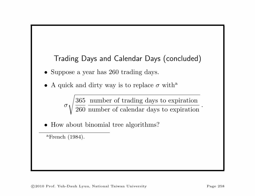
Trading Days and Calendar Days (concluded)
• Suppose a year has 260 trading days.
• A quick and dirty way is to replace σ witha
σ
√365
260
number of trading days to expiration
number of calendar days to expiration.
• How about binomial tree algorithms?
aFrench (1984).
c⃝2010 Prof. Yuh-Dauh Lyuu, National Taiwan University Page 258
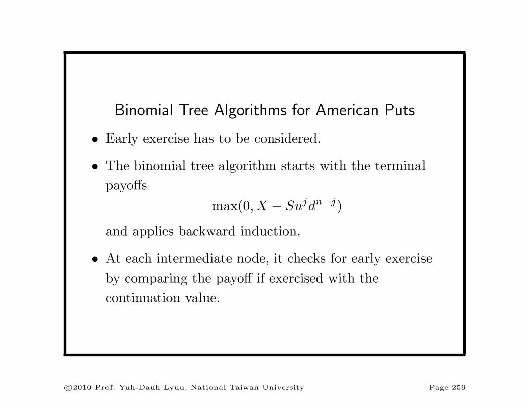
Binomial Tree Algorithms for American Puts
• Early exercise has to be considered.
• The binomial tree algorithm starts with the terminal
payoffs
max(0, X − Sujdn−j)
and applies backward induction.
• At each intermediate node, it checks for early exercise
by comparing the payoff if exercised with the
continuation value.
c⃝2010 Prof. Yuh-Dauh Lyuu, National Taiwan University Page 259
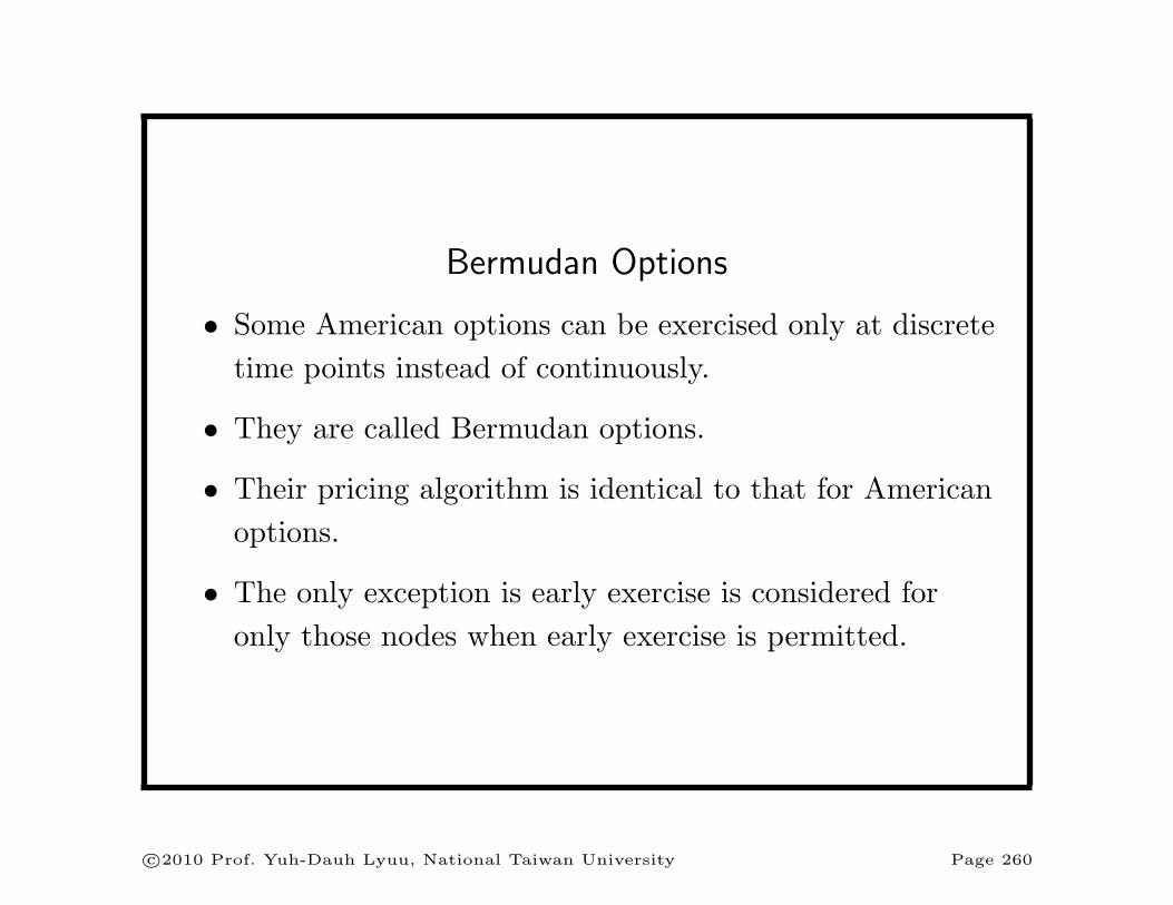
Bermudan Options
• Some American options can be exercised only at discrete
time points instead of continuously.
• They are called Bermudan options.
• Their pricing algorithm is identical to that for American
options.
• The only exception is early exercise is considered for
only those nodes when early exercise is permitted.
c⃝2010 Prof. Yuh-Dauh Lyuu, National Taiwan University Page 260
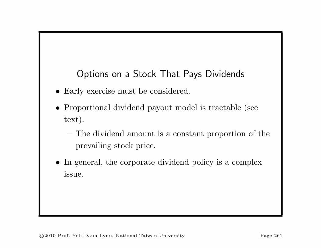
Options on a Stock That Pays Dividends
• Early exercise must be considered.
• Proportional dividend payout model is tractable (see
text).
– The dividend amount is a constant proportion of the
prevailing stock price.
• In general, the corporate dividend policy is a complex
issue.
c⃝2010 Prof. Yuh-Dauh Lyuu, National Taiwan University Page 261
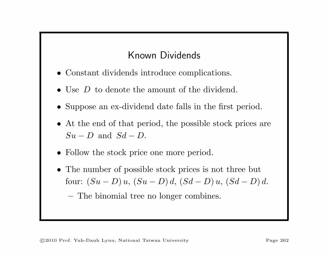
Known Dividends
• Constant dividends introduce complications.
• Use D to denote the amount of the dividend.
• Suppose an ex-dividend date falls in the first period.
• At the end of that period, the possible stock prices are
Su−D and Sd−D.
• Follow the stock price one more period.
• The number of possible stock prices is not three but
four: (Su−D)u, (Su−D) d, (Sd−D)u, (Sd−D) d.
– The binomial tree no longer combines.
c⃝2010 Prof. Yuh-Dauh Lyuu, National Taiwan University Page 262

(Su−D)u
↗Su−D
↗ ↘(Su−D) d
S
(Sd−D)u
↘ ↗Sd−D
↘(Sd−D) d
c⃝2010 Prof. Yuh-Dauh Lyuu, National Taiwan University Page 263
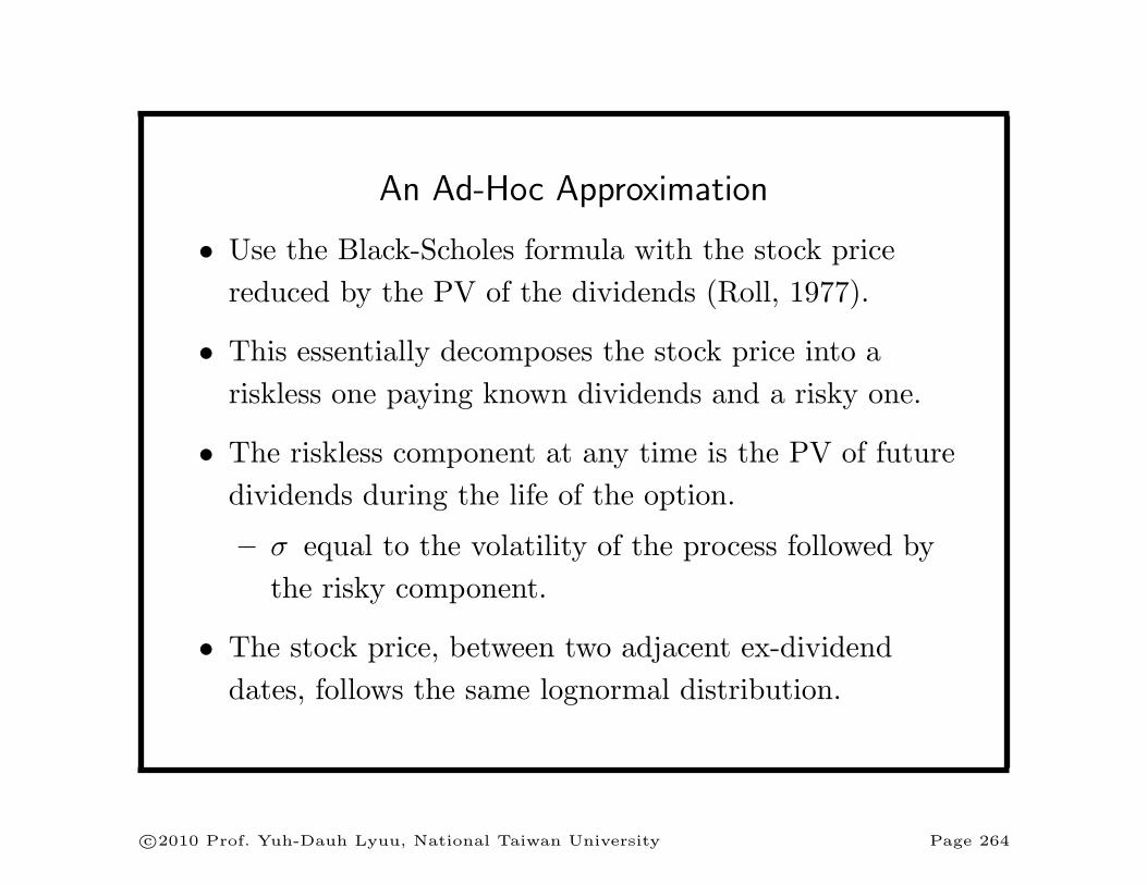
An Ad-Hoc Approximation
• Use the Black-Scholes formula with the stock price
reduced by the PV of the dividends (Roll, 1977).
• This essentially decomposes the stock price into a
riskless one paying known dividends and a risky one.
• The riskless component at any time is the PV of future
dividends during the life of the option.
– σ equal to the volatility of the process followed by
the risky component.
• The stock price, between two adjacent ex-dividend
dates, follows the same lognormal distribution.
c⃝2010 Prof. Yuh-Dauh Lyuu, National Taiwan University Page 264
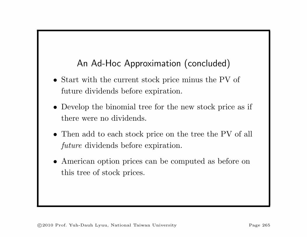
An Ad-Hoc Approximation (concluded)
• Start with the current stock price minus the PV of
future dividends before expiration.
• Develop the binomial tree for the new stock price as if
there were no dividends.
• Then add to each stock price on the tree the PV of all
future dividends before expiration.
• American option prices can be computed as before on
this tree of stock prices.
c⃝2010 Prof. Yuh-Dauh Lyuu, National Taiwan University Page 265
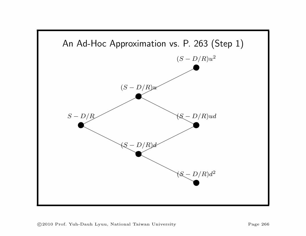
An Ad-Hoc Approximation vs. P. 263 (Step 1)
S −D/R
*
j
(S −D/R)u
*
j
(S −D/R)d
*
j
(S −D/R)u2
(S −D/R)ud
(S −D/R)d2
c⃝2010 Prof. Yuh-Dauh Lyuu, National Taiwan University Page 266
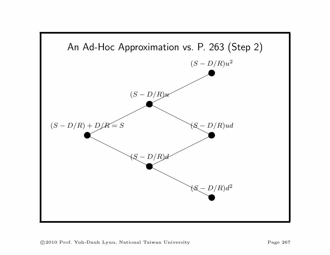
An Ad-Hoc Approximation vs. P. 263 (Step 2)
(S −D/R) +D/R = S
*
j
(S −D/R)u
*
j
(S −D/R)d
*
j
(S −D/R)u2
(S −D/R)ud
(S −D/R)d2
c⃝2010 Prof. Yuh-Dauh Lyuu, National Taiwan University Page 267
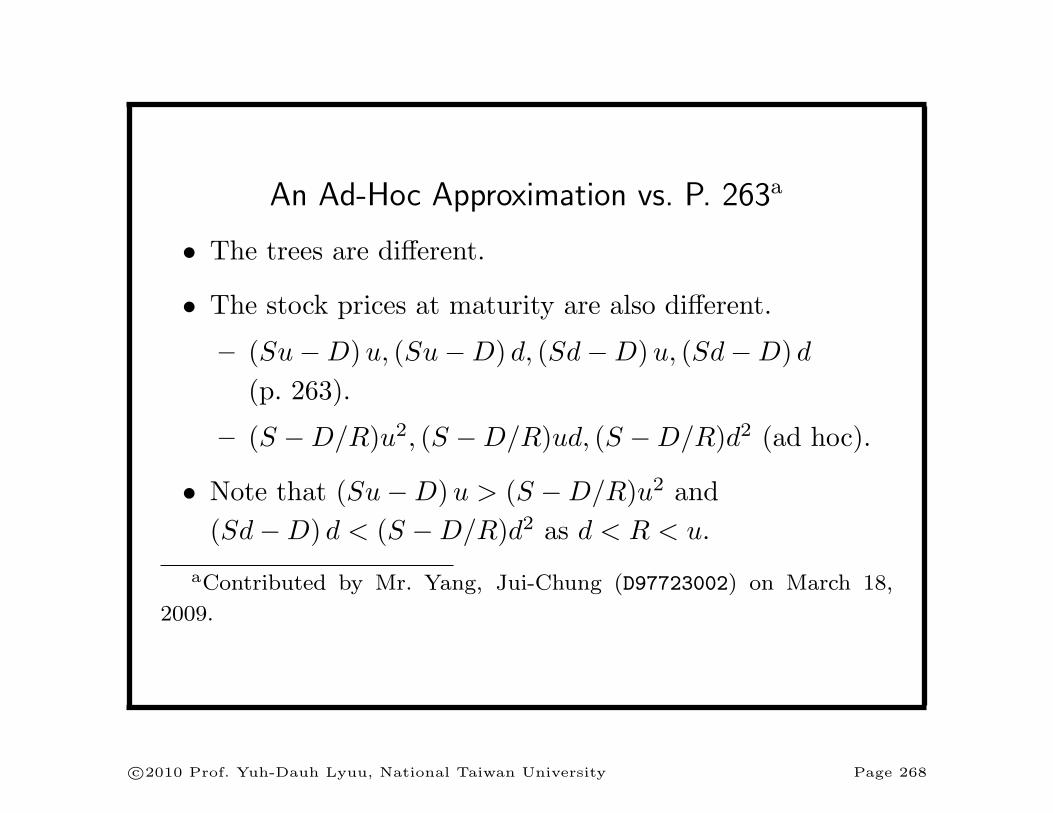
An Ad-Hoc Approximation vs. P. 263a
• The trees are different.
• The stock prices at maturity are also different.
– (Su−D)u, (Su−D) d, (Sd−D)u, (Sd−D) d
(p. 263).
– (S −D/R)u2, (S −D/R)ud, (S −D/R)d2 (ad hoc).
• Note that (Su−D)u > (S −D/R)u2 and
(Sd−D) d < (S −D/R)d2 as d < R < u.
aContributed by Mr. Yang, Jui-Chung (D97723002) on March 18,
2009.
c⃝2010 Prof. Yuh-Dauh Lyuu, National Taiwan University Page 268
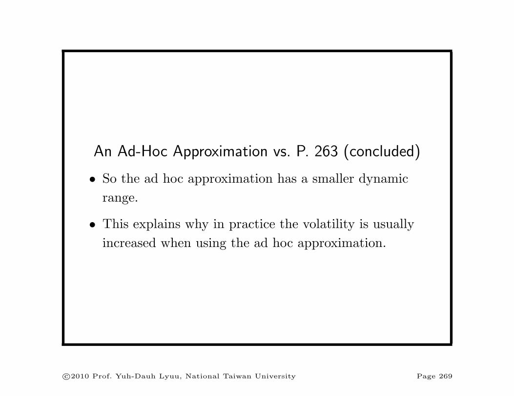
An Ad-Hoc Approximation vs. P. 263 (concluded)
• So the ad hoc approximation has a smaller dynamic
range.
• This explains why in practice the volatility is usually
increased when using the ad hoc approximation.
c⃝2010 Prof. Yuh-Dauh Lyuu, National Taiwan University Page 269
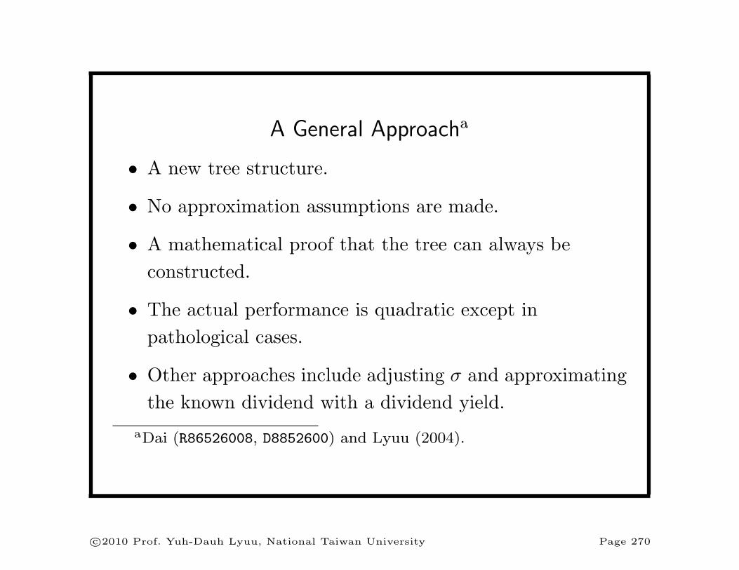
A General Approacha
• A new tree structure.
• No approximation assumptions are made.
• A mathematical proof that the tree can always be
constructed.
• The actual performance is quadratic except in
pathological cases.
• Other approaches include adjusting σ and approximating
the known dividend with a dividend yield.
aDai (R86526008, D8852600) and Lyuu (2004).
c⃝2010 Prof. Yuh-Dauh Lyuu, National Taiwan University Page 270

Continuous Dividend Yields
• Dividends are paid continuously.
– Approximates a broad-based stock market portfolio.
• The payment of a continuous dividend yield at rate q
reduces the growth rate of the stock price by q.
– A stock that grows from S to Sτ with a continuous
dividend yield of q would grow from S to Sτeqτ
without the dividends.
• A European option has the same value as one on a stock
with price Se−qτ that pays no dividends.
c⃝2010 Prof. Yuh-Dauh Lyuu, National Taiwan University Page 271

Continuous Dividend Yields (continued)
• The Black-Scholes formulas hold with S replaced by
Se−qτ :a
C = Se−qτN(x)−Xe−rτN(x− σ√τ), (25)
P = Xe−rτN(−x+ σ√τ)− Se−qτN(−x),
(25′)
where
x ≡ln(S/X) +
(r − q + σ2/2
)τ
σ√τ
.
• Formulas (25) and (25’) remain valid as long as the
dividend yield is predictable.
aMerton (1973).
c⃝2010 Prof. Yuh-Dauh Lyuu, National Taiwan University Page 272
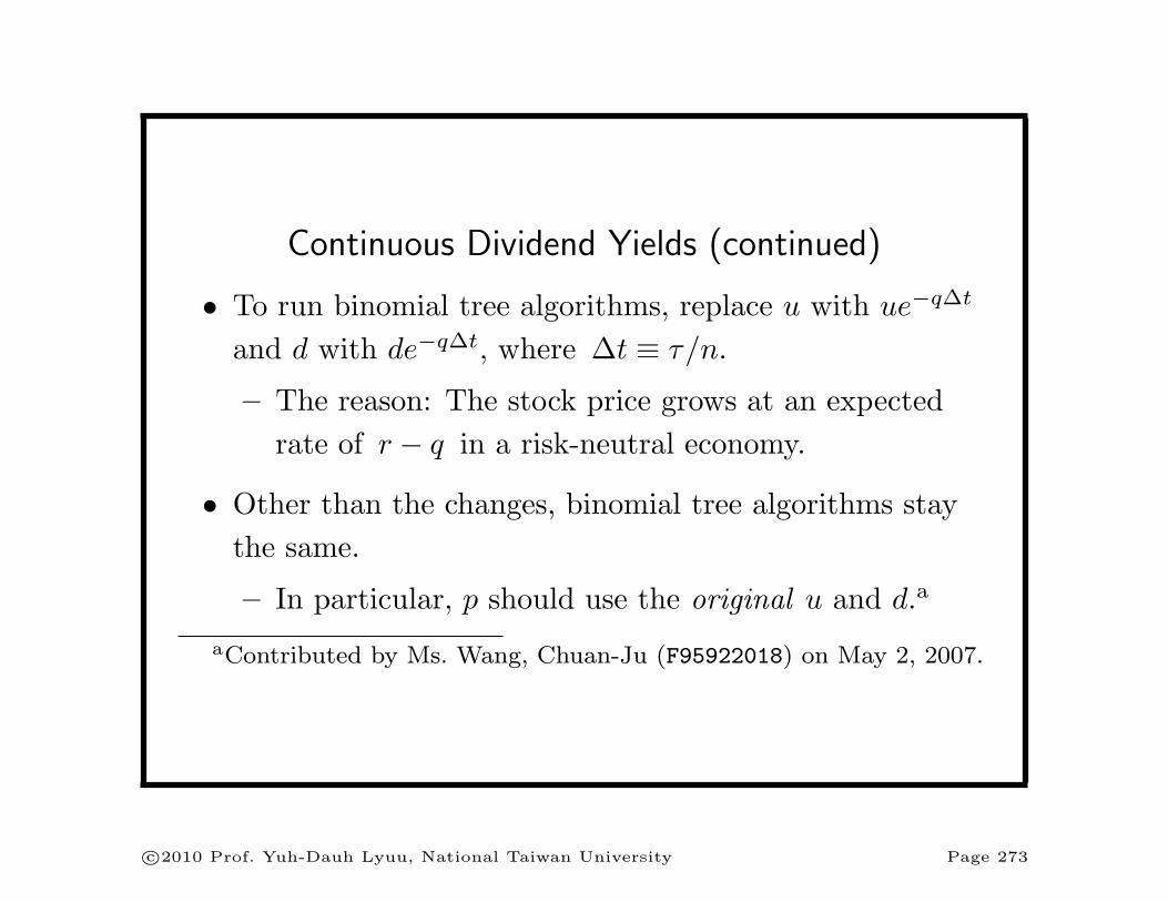
Continuous Dividend Yields (continued)
• To run binomial tree algorithms, replace u with ue−q∆t
and d with de−q∆t, where ∆t ≡ τ/n.
– The reason: The stock price grows at an expected
rate of r − q in a risk-neutral economy.
• Other than the changes, binomial tree algorithms stay
the same.
– In particular, p should use the original u and d.a
aContributed by Ms. Wang, Chuan-Ju (F95922018) on May 2, 2007.
c⃝2010 Prof. Yuh-Dauh Lyuu, National Taiwan University Page 273

Continuous Dividend Yields (concluded)
• Alternatively, pick the risk-neutral probability as
e(r−q)∆t − d
u− d, (26)
where ∆t ≡ τ/n.
– The reason: The stock price grows at an expected
rate of r − q in a risk-neutral economy.
• The u and d remain unchanged.
• Other than the change in Eq. (26), binomial tree
algorithms stay the same.
c⃝2010 Prof. Yuh-Dauh Lyuu, National Taiwan University Page 274
Sensitivity Analysis of Options
c⃝2010 Prof. Yuh-Dauh Lyuu, National Taiwan University Page 275
Cleopatra’s nose, had it been shorter,
the whole face of the world
would have been changed.
— Blaise Pascal (1623–1662)
c⃝2010 Prof. Yuh-Dauh Lyuu, National Taiwan University Page 276
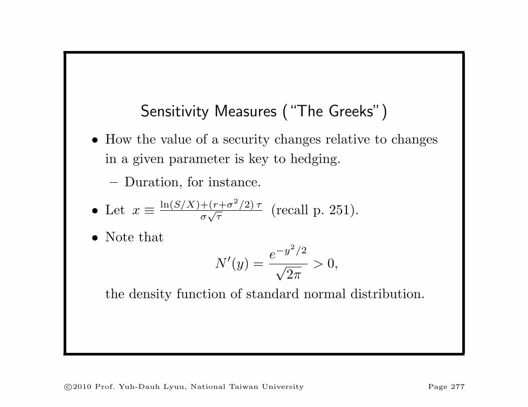
Sensitivity Measures (“The Greeks”)
• How the value of a security changes relative to changes
in a given parameter is key to hedging.
– Duration, for instance.
• Let x ≡ ln(S/X)+(r+σ2/2) τσ√τ
(recall p. 251).
• Note that
N ′(y) =e−y2/2
√2π
> 0,
the density function of standard normal distribution.
c⃝2010 Prof. Yuh-Dauh Lyuu, National Taiwan University Page 277

Delta
• Defined as ∆ ≡ ∂f/∂S.
– f is the price of the derivative.
– S is the price of the underlying asset.
• The delta of a portfolio of derivatives on the same
underlying asset is the sum of their individual deltas.
– Elementary calculus.
• The delta used in the BOPM is the discrete analog.
c⃝2010 Prof. Yuh-Dauh Lyuu, National Taiwan University Page 278

Delta (concluded)
• The delta of a European call on a non-dividend-paying
stock equals∂C
∂S= N(x) > 0.
• The delta of a European put equals
∂P
∂S= N(x)− 1 < 0.
• The delta of a long stock is 1.
c⃝2010 Prof. Yuh-Dauh Lyuu, National Taiwan University Page 279
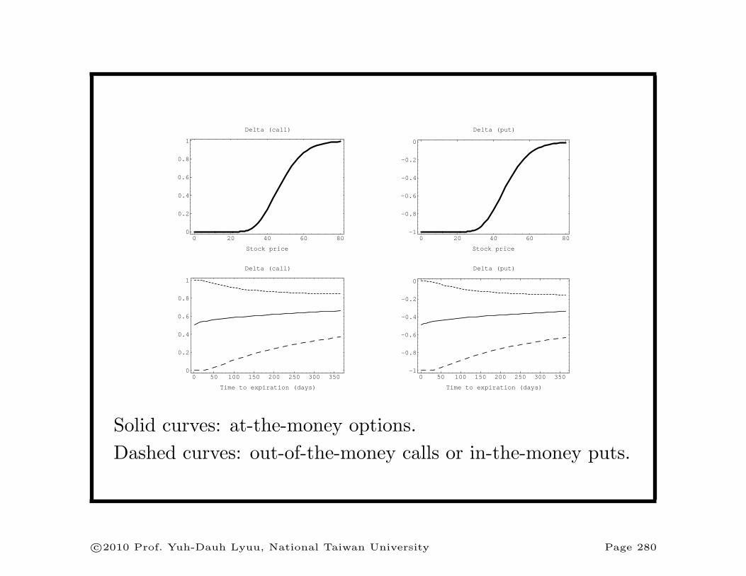
0 50 100 150 200 250 300 350
Time to expiration (days)
0
0.2
0.4
0.6
0.8
1
Delta (call)
0 50 100 150 200 250 300 350
Time to expiration (days)
-1
-0.8
-0.6
-0.4
-0.2
0
Delta (put)
0 20 40 60 80
Stock price
0
0.2
0.4
0.6
0.8
1
Delta (call)
0 20 40 60 80
Stock price
-1
-0.8
-0.6
-0.4
-0.2
0
Delta (put)
Solid curves: at-the-money options.
Dashed curves: out-of-the-money calls or in-the-money puts.
c⃝2010 Prof. Yuh-Dauh Lyuu, National Taiwan University Page 280
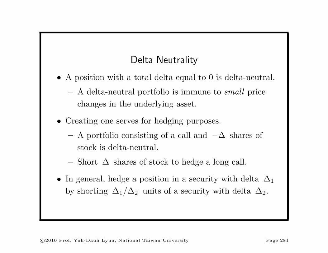
Delta Neutrality
• A position with a total delta equal to 0 is delta-neutral.
– A delta-neutral portfolio is immune to small price
changes in the underlying asset.
• Creating one serves for hedging purposes.
– A portfolio consisting of a call and −∆ shares of
stock is delta-neutral.
– Short ∆ shares of stock to hedge a long call.
• In general, hedge a position in a security with delta ∆1
by shorting ∆1/∆2 units of a security with delta ∆2.
c⃝2010 Prof. Yuh-Dauh Lyuu, National Taiwan University Page 281
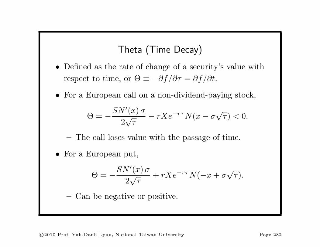
Theta (Time Decay)
• Defined as the rate of change of a security’s value with
respect to time, or Θ ≡ −∂f/∂τ = ∂f/∂t.
• For a European call on a non-dividend-paying stock,
Θ = −SN ′(x)σ
2√τ
− rXe−rτN(x− σ√τ) < 0.
– The call loses value with the passage of time.
• For a European put,
Θ = −SN ′(x)σ
2√τ
+ rXe−rτN(−x+ σ√τ).
– Can be negative or positive.
c⃝2010 Prof. Yuh-Dauh Lyuu, National Taiwan University Page 282
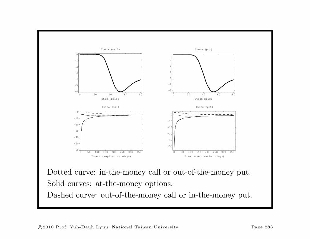
0 50 100 150 200 250 300 350
Time to expiration (days)
-60
-50
-40
-30
-20
-10
0
Theta (call)
0 50 100 150 200 250 300 350
Time to expiration (days)
-50
-40
-30
-20
-10
0
Theta (put)
0 20 40 60 80
Stock price
-6
-5
-4
-3
-2
-1
0
Theta (call)
0 20 40 60 80
Stock price
-2
-1
0
1
2
3
Theta (put)
Dotted curve: in-the-money call or out-of-the-money put.
Solid curves: at-the-money options.
Dashed curve: out-of-the-money call or in-the-money put.
c⃝2010 Prof. Yuh-Dauh Lyuu, National Taiwan University Page 283

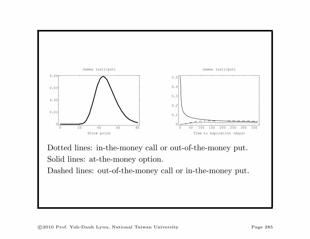
Gamma
• Defined as the rate of change of its delta with respect to
the price of the underlying asset, or Γ ≡ ∂2Π/∂S2.
• Measures how sensitive delta is to changes in the price of
the underlying asset.
• In practice, a portfolio with a high gamma needs be
rebalanced more often to maintain delta neutrality.
• Roughly, delta ∼ duration, and gamma ∼ convexity.
• The gamma of a European call or put on a
non-dividend-paying stock is
N ′(x)/(Sσ√τ) > 0.
c⃝2010 Prof. Yuh-Dauh Lyuu, National Taiwan University Page 284
0 20 40 60 80
Stock price
0
0.01
0.02
0.03
0.04
Gamma (call/put)
0 50 100 150 200 250 300 350
Time to expiration (days)
0
0.1
0.2
0.3
0.4
0.5
Gamma (call/put)
Dotted lines: in-the-money call or out-of-the-money put.
Solid lines: at-the-money option.
Dashed lines: out-of-the-money call or in-the-money put.
c⃝2010 Prof. Yuh-Dauh Lyuu, National Taiwan University Page 285
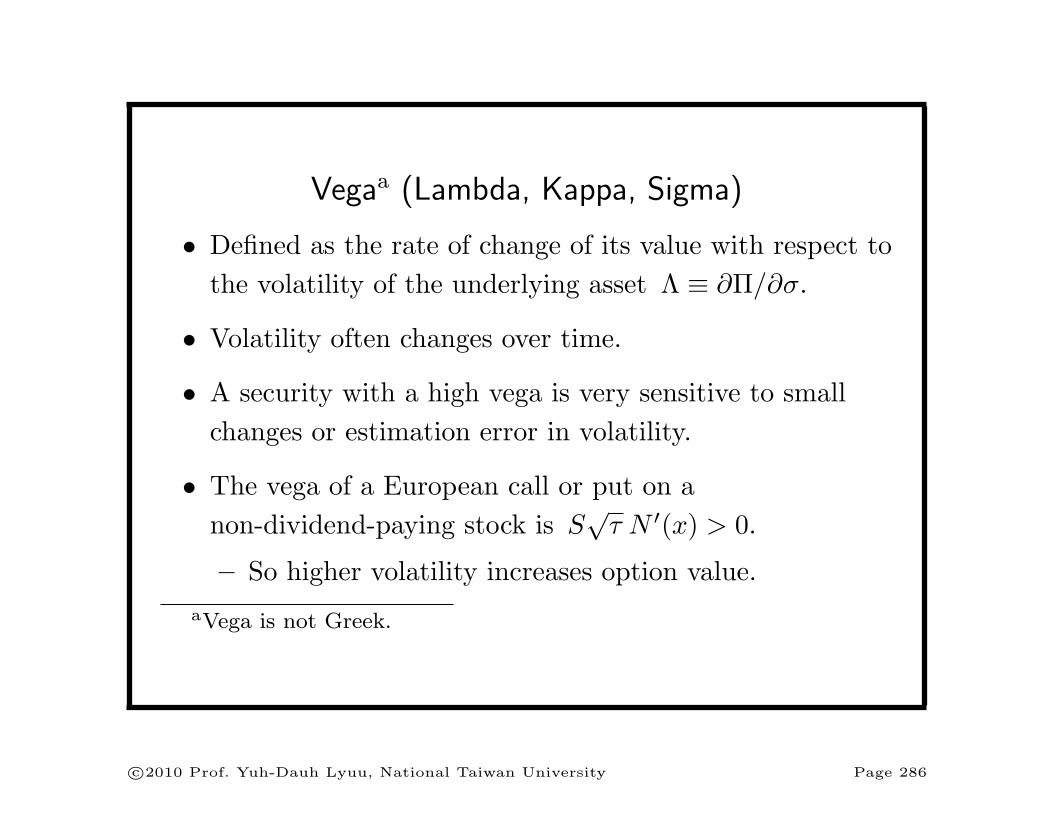
Vegaa (Lambda, Kappa, Sigma)
• Defined as the rate of change of its value with respect to
the volatility of the underlying asset Λ ≡ ∂Π/∂σ.
• Volatility often changes over time.
• A security with a high vega is very sensitive to small
changes or estimation error in volatility.
• The vega of a European call or put on a
non-dividend-paying stock is S√τ N ′(x) > 0.
– So higher volatility increases option value.
aVega is not Greek.
c⃝2010 Prof. Yuh-Dauh Lyuu, National Taiwan University Page 286

0 20 40 60 80
Stock price
0
2
4
6
8
10
12
14
Vega (call/put)
50 100 150 200 250 300 350
Time to expiration (days)
0
2.5
5
7.5
10
12.5
15
17.5
Vega (call/put)
Dotted curve: in-the-money call or out-of-the-money put.
Solid curves: at-the-money option.
Dashed curve: out-of-the-money call or in-the-money put.
c⃝2010 Prof. Yuh-Dauh Lyuu, National Taiwan University Page 287
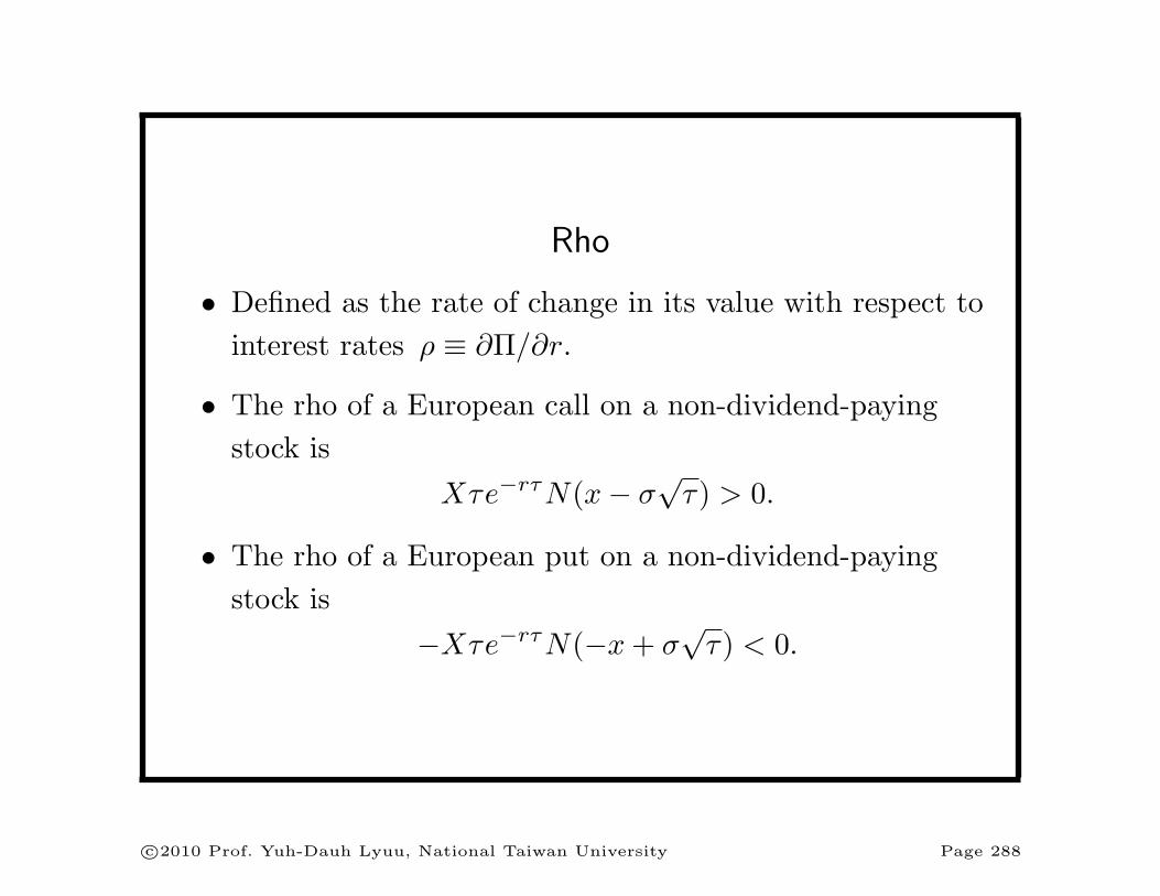
Rho
• Defined as the rate of change in its value with respect to
interest rates ρ ≡ ∂Π/∂r.
• The rho of a European call on a non-dividend-paying
stock is
Xτe−rτN(x− σ√τ) > 0.
• The rho of a European put on a non-dividend-paying
stock is
−Xτe−rτN(−x+ σ√τ) < 0.
c⃝2010 Prof. Yuh-Dauh Lyuu, National Taiwan University Page 288

50 100 150 200 250 300 350
Time to expiration (days)
0
5
10
15
20
25
30
35
Rho (call)
50 100 150 200 250 300 350
Time to expiration (days)
-30
-25
-20
-15
-10
-5
0
Rho (put)
0 20 40 60 80
Stock price
0
5
10
15
20
25
Rho (call)
0 20 40 60 80
Stock price
-25
-20
-15
-10
-5
0
Rho (put)
Dotted curves: in-the-money call or out-of-the-money put.
Solid curves: at-the-money option.
Dashed curves: out-of-the-money call or in-the-money put.
c⃝2010 Prof. Yuh-Dauh Lyuu, National Taiwan University Page 289
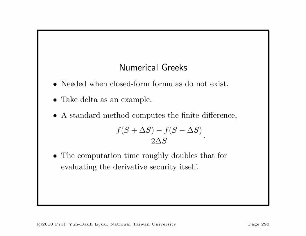
Numerical Greeks
• Needed when closed-form formulas do not exist.
• Take delta as an example.
• A standard method computes the finite difference,
f(S +∆S)− f(S −∆S)
2∆S.
• The computation time roughly doubles that for
evaluating the derivative security itself.
c⃝2010 Prof. Yuh-Dauh Lyuu, National Taiwan University Page 290
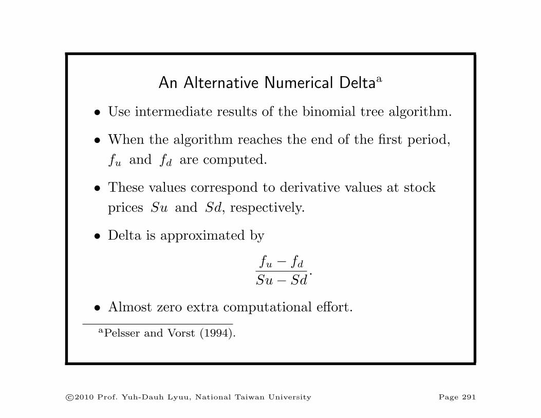
An Alternative Numerical Deltaa
• Use intermediate results of the binomial tree algorithm.
• When the algorithm reaches the end of the first period,
fu and fd are computed.
• These values correspond to derivative values at stock
prices Su and Sd, respectively.
• Delta is approximated by
fu − fdSu− Sd
.
• Almost zero extra computational effort.
aPelsser and Vorst (1994).
c⃝2010 Prof. Yuh-Dauh Lyuu, National Taiwan University Page 291
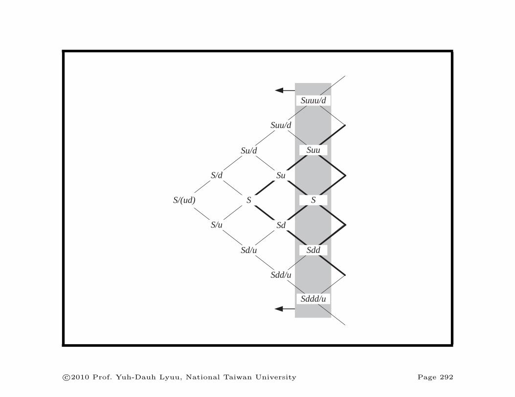
S/(ud)
S/d
S/u
Su/d
S
Sd/u
Su
Sd
Suu/d
Sdd/u
Suuu/d
Suu
S
Sdd
Sddd/u
c⃝2010 Prof. Yuh-Dauh Lyuu, National Taiwan University Page 292
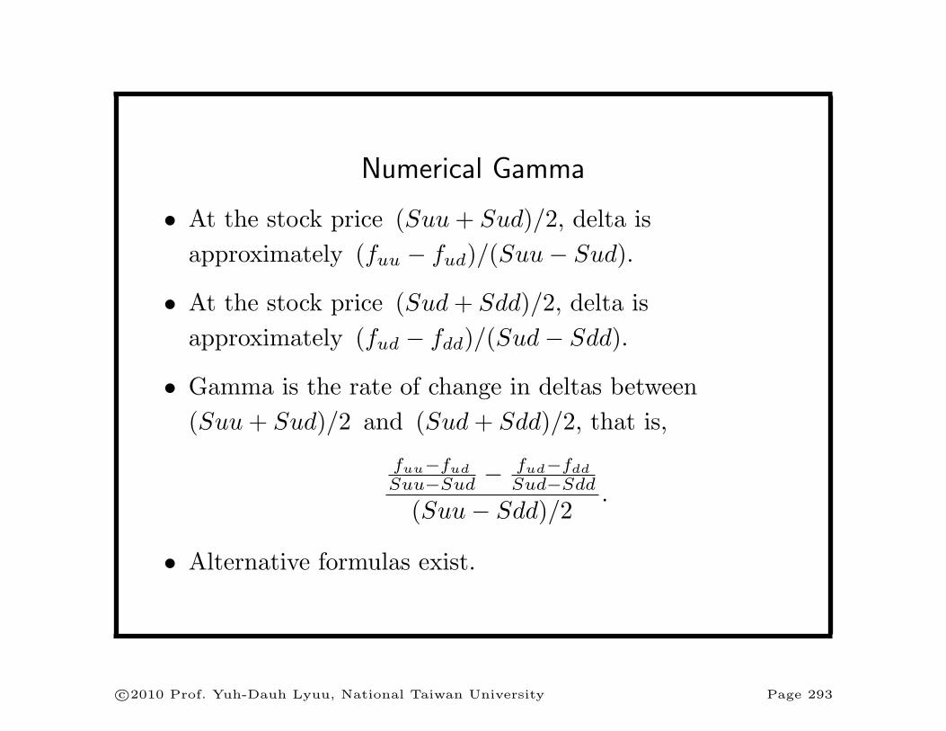
Numerical Gamma
• At the stock price (Suu+ Sud)/2, delta is
approximately (fuu − fud)/(Suu− Sud).
• At the stock price (Sud+ Sdd)/2, delta is
approximately (fud − fdd)/(Sud− Sdd).
• Gamma is the rate of change in deltas between
(Suu+ Sud)/2 and (Sud+ Sdd)/2, that is,
fuu−fud
Suu−Sud − fud−fddSud−Sdd
(Suu− Sdd)/2.
• Alternative formulas exist.
c⃝2010 Prof. Yuh-Dauh Lyuu, National Taiwan University Page 293
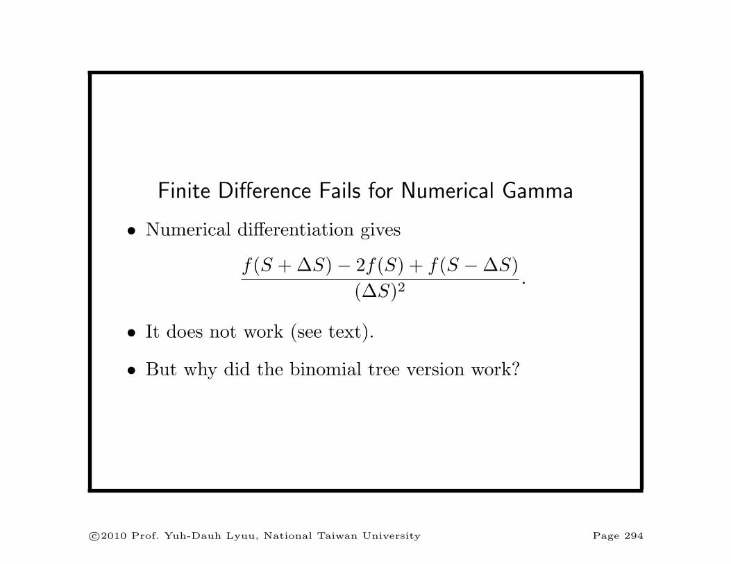
Finite Difference Fails for Numerical Gamma
• Numerical differentiation gives
f(S +∆S)− 2f(S) + f(S −∆S)
(∆S)2.
• It does not work (see text).
• But why did the binomial tree version work?
c⃝2010 Prof. Yuh-Dauh Lyuu, National Taiwan University Page 294
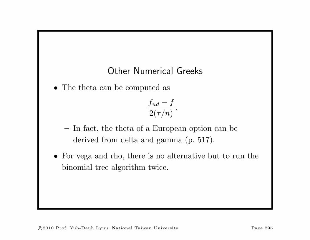
Other Numerical Greeks
• The theta can be computed as
fud − f
2(τ/n).
– In fact, the theta of a European option can be
derived from delta and gamma (p. 517).
• For vega and rho, there is no alternative but to run the
binomial tree algorithm twice.
c⃝2010 Prof. Yuh-Dauh Lyuu, National Taiwan University Page 295
Extensions of Options Theory
c⃝2010 Prof. Yuh-Dauh Lyuu, National Taiwan University Page 296

As I never learnt mathematics,
so I have had to think.
— Joan Robinson (1903–1983)
c⃝2010 Prof. Yuh-Dauh Lyuu, National Taiwan University Page 297
Pricing Corporate Securitiesa
• Interpret the underlying asset as the total value of the
firm.
• The option pricing methodology can be applied to
pricing corporate securities.
• Assume:
– A firm can finance payouts by the sale of assets.
– If a promised payment to an obligation other than
stock is missed, the claim holders take ownership of
the firm and the stockholders get nothing.
aBlack and Scholes (1973).
c⃝2010 Prof. Yuh-Dauh Lyuu, National Taiwan University Page 298
Risky Zero-Coupon Bonds and Stock
• Consider XYZ.com.
• Capital structure:
– n shares of its own common stock, S.
– Zero-coupon bonds with an aggregate par value of X.
• What is the value of the bonds, B?
• What is the value of the XYZ.com stock?
c⃝2010 Prof. Yuh-Dauh Lyuu, National Taiwan University Page 299
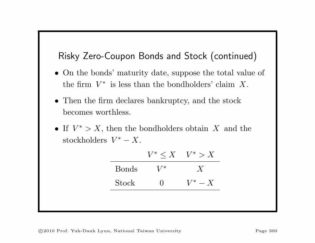
Risky Zero-Coupon Bonds and Stock (continued)
• On the bonds’ maturity date, suppose the total value of
the firm V ∗ is less than the bondholders’ claim X.
• Then the firm declares bankruptcy, and the stock
becomes worthless.
• If V ∗ > X, then the bondholders obtain X and the
stockholders V ∗ −X.
V ∗ ≤ X V ∗ > X
Bonds V ∗ X
Stock 0 V ∗ −X
c⃝2010 Prof. Yuh-Dauh Lyuu, National Taiwan University Page 300

Risky Zero-Coupon Bonds and Stock (continued)
• The stock is a call on the total value of the firm with a
strike price of X and an expiration date equal to the
bonds’.
– This call provides the limited liability for the
stockholders.
• The bonds are a covered call on the total value of the
firm.
• Let V stand for the total value of the firm.
• Let C stand for a call on V .
c⃝2010 Prof. Yuh-Dauh Lyuu, National Taiwan University Page 301
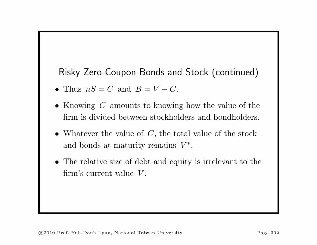
Risky Zero-Coupon Bonds and Stock (continued)
• Thus nS = C and B = V − C.
• Knowing C amounts to knowing how the value of the
firm is divided between stockholders and bondholders.
• Whatever the value of C, the total value of the stock
and bonds at maturity remains V ∗.
• The relative size of debt and equity is irrelevant to the
firm’s current value V .
c⃝2010 Prof. Yuh-Dauh Lyuu, National Taiwan University Page 302
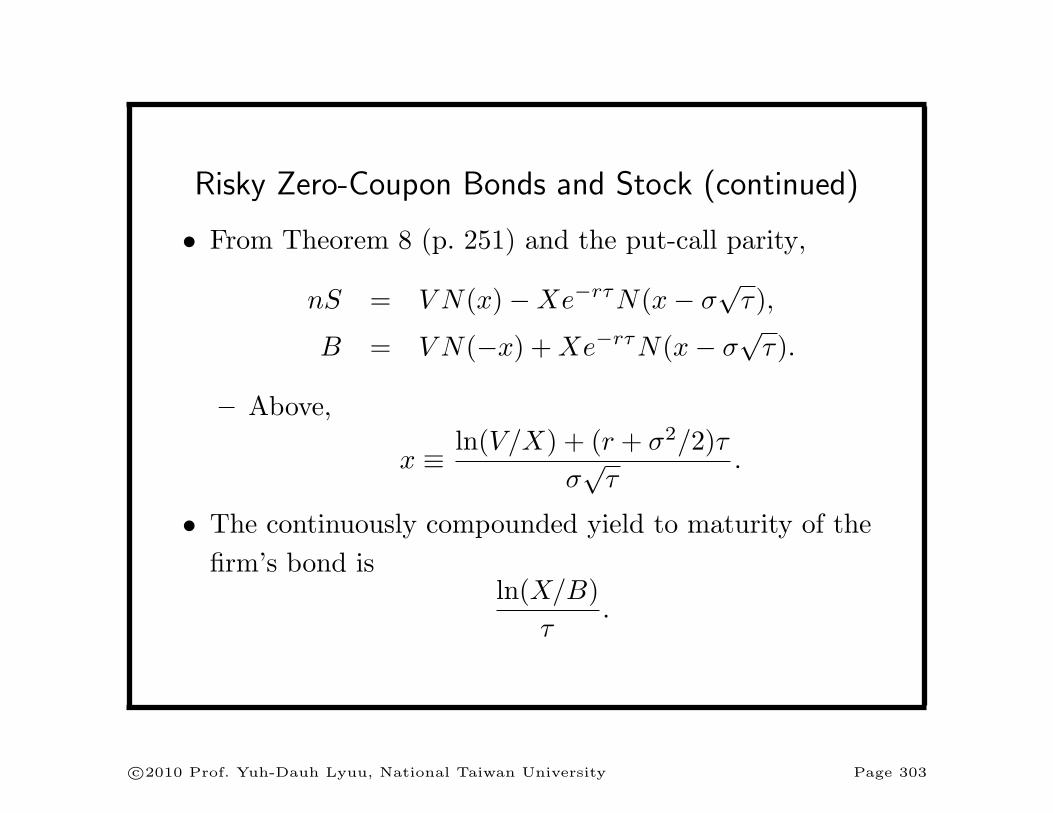
Risky Zero-Coupon Bonds and Stock (continued)
• From Theorem 8 (p. 251) and the put-call parity,
nS = V N(x)−Xe−rτN(x− σ√τ),
B = V N(−x) +Xe−rτN(x− σ√τ).
– Above,
x ≡ ln(V/X) + (r + σ2/2)τ
σ√τ
.
• The continuously compounded yield to maturity of the
firm’s bond isln(X/B)
τ.
c⃝2010 Prof. Yuh-Dauh Lyuu, National Taiwan University Page 303

Risky Zero-Coupon Bonds and Stock (concluded)
• Define the credit spread or default premium as the yield
difference between risky and riskless bonds,
ln(X/B)
τ− r
= −1
τln
(N(−z) +
1
ωN(z − σ
√τ)
).
– ω ≡ Xe−rτ/V .
– z ≡ (lnω)/(σ√τ) + (1/2)σ
√τ = −x+ σ
√τ .
– Note that ω is the debt-to-total-value ratio.
c⃝2010 Prof. Yuh-Dauh Lyuu, National Taiwan University Page 304
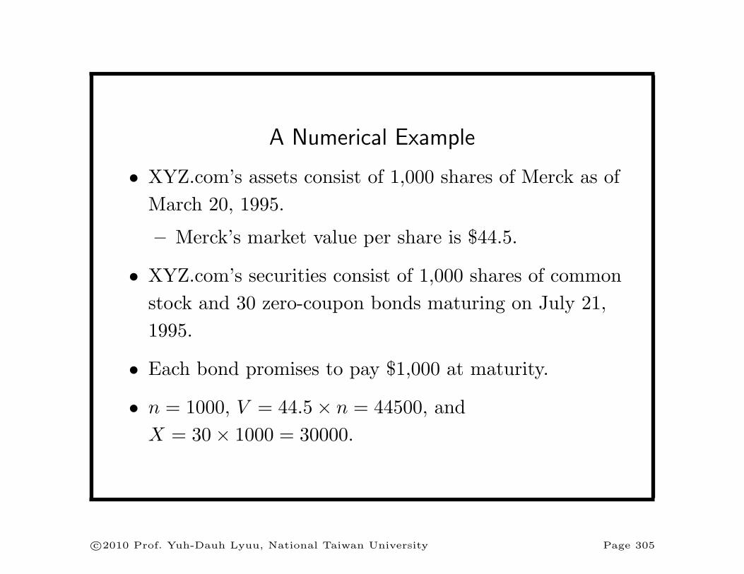
A Numerical Example
• XYZ.com’s assets consist of 1,000 shares of Merck as of
March 20, 1995.
– Merck’s market value per share is $44.5.
• XYZ.com’s securities consist of 1,000 shares of common
stock and 30 zero-coupon bonds maturing on July 21,
1995.
• Each bond promises to pay $1,000 at maturity.
• n = 1000, V = 44.5× n = 44500, and
X = 30× 1000 = 30000.
c⃝2010 Prof. Yuh-Dauh Lyuu, National Taiwan University Page 305

—Call— —Put—
Option Strike Exp. Vol. Last Vol. Last
Merck 30 Jul 328 151/4 . . . . . .
441/2 35 Jul 150 91/2 10 1/16
441/2 40 Apr 887 43/4 136 1/16
441/2 40 Jul 220 51/2 297 1/4
441/2 40 Oct 58 6 10 1/2
441/2 45 Apr 3050 7/8 100 11/8
441/2 45 May 462 13/8 50 13/8
441/2 45 Jul 883 115/16 147 13/4
441/2 45 Oct 367 23/4 188 21/16
c⃝2010 Prof. Yuh-Dauh Lyuu, National Taiwan University Page 306

A Numerical Example (continued)
• The Merck option relevant for pricing is the July call
with a strike price of X/n = 30 dollars.
• Such a call is selling for $15.25.
• So XYZ.com’s stock is worth 15.25× n = 15250 dollars.
• The entire bond issue is worth
B = 44500− 15250 = 29250 dollars.
– Or $975 per bond.
c⃝2010 Prof. Yuh-Dauh Lyuu, National Taiwan University Page 307
A Numerical Example (continued)
• The XYZ.com bonds are equivalent to a default-free
zero-coupon bond with $X par value plus n written
European puts on Merck at a strike price of $30.
– By the put-call parity.
• The difference between B and the price of the
default-free bond is the value of these puts.
• The next table shows the total market values of the
XYZ.com stock and bonds under various debt amounts
X.
c⃝2010 Prof. Yuh-Dauh Lyuu, National Taiwan University Page 308
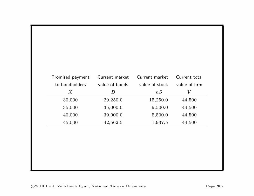
Promised payment Current market Current market Current total
to bondholders value of bonds value of stock value of firm
X B nS V
30,000 29,250.0 15,250.0 44,500
35,000 35,000.0 9,500.0 44,500
40,000 39,000.0 5,500.0 44,500
45,000 42,562.5 1,937.5 44,500
c⃝2010 Prof. Yuh-Dauh Lyuu, National Taiwan University Page 309
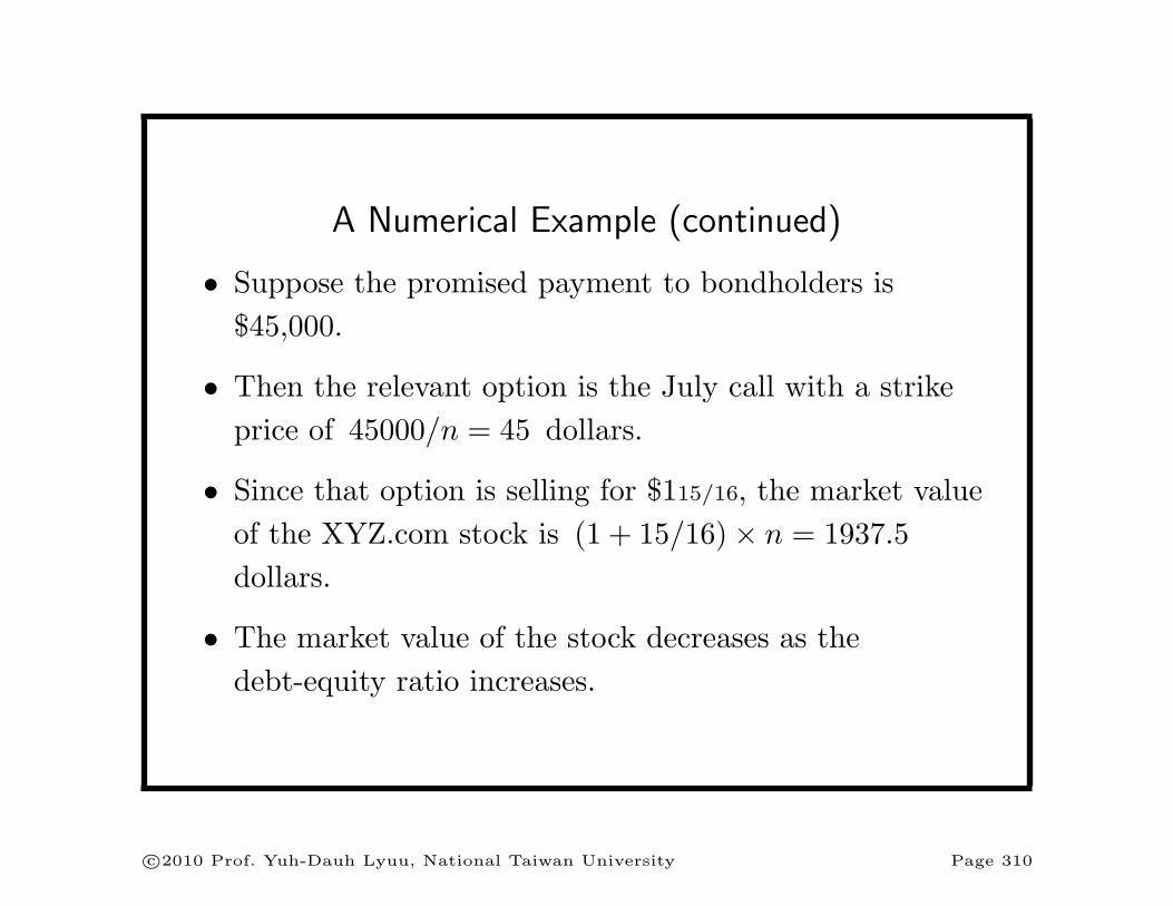
A Numerical Example (continued)
• Suppose the promised payment to bondholders is
$45,000.
• Then the relevant option is the July call with a strike
price of 45000/n = 45 dollars.
• Since that option is selling for $115/16, the market value
of the XYZ.com stock is (1 + 15/16)× n = 1937.5
dollars.
• The market value of the stock decreases as the
debt-equity ratio increases.
c⃝2010 Prof. Yuh-Dauh Lyuu, National Taiwan University Page 310
A Numerical Example (continued)
• There are conflicts between stockholders and
bondholders.
• An option’s terms cannot be changed after issuance.
• But a firm can change its capital structure.
• There lies one key difference between options and
corporate securities.
– Parameters such volatility, dividend, and strike price
are under partial control of the stockholders.
c⃝2010 Prof. Yuh-Dauh Lyuu, National Taiwan University Page 311
A Numerical Example (continued)
• Suppose XYZ.com issues 15 more bonds with the same
terms to buy back stock.
• The total debt is now X = 45,000 dollars.
• The table on p. 309 says the total market value of the
bonds should be $42,562.5.
• The new bondholders pay 42562.5× (15/45) = 14187.5
dollars.
• The remaining stock is worth $1,937.5.
c⃝2010 Prof. Yuh-Dauh Lyuu, National Taiwan University Page 312
A Numerical Example (continued)
• The stockholders therefore gain
14187.5 + 1937.5− 15250 = 875
dollars.
• The original bondholders lose an equal amount,
29250− 30
45× 42562.5 = 875. (27)
c⃝2010 Prof. Yuh-Dauh Lyuu, National Taiwan University Page 313

A Numerical Example (continued)
• Suppose the stockholders sell (1/3)× n Merck shares to
fund a $14,833.3 cash dividend.
• They now have $14,833.3 in cash plus a call on
(2/3)× n Merck shares.
• The strike price remains X = 30000.
• This is equivalent to owning 2/3 of a call on n Merck
shares with a total strike price of $45,000.
• n such calls are worth $1,937.5 (p. 309).
• So the total market value of the XYZ.com stock is
(2/3)× 1937.5 = 1291.67 dollars.
c⃝2010 Prof. Yuh-Dauh Lyuu, National Taiwan University Page 314

A Numerical Example (concluded)
• The market value of the XYZ.com bonds is hence
(2/3)× n× 44.5− 1291.67 = 28375 dollars.
• Hence the stockholders gain
14833.3 + 1291.67− 15250 ≈ 875
dollars.
• The bondholders watch their value drop from $29,250 to
$28,375, a loss of $875.
c⃝2010 Prof. Yuh-Dauh Lyuu, National Taiwan University Page 315
Related Documents


![Black scholes[1]](https://static.cupdf.com/doc/110x72/558c2b99d8b42a9f738b45b4/black-scholes1.jpg)


![A Skewness-Adjusted Binomial Model for Pricing …file.scirp.org/pdf/JMF20120100011_82298793.pdf · Black-Scholes (B-S) [2] model and the binomial option pricing model (BOPM) with](https://static.cupdf.com/doc/110x72/5b6b45f97f8b9a422e8d3f09/a-skewness-adjusted-binomial-model-for-pricing-filescirporgpdfjmf20120100011.jpg)
