Working Paper 08-11 Departamento de Estadística Statistic and Econometric Series 04 Universidad Carlos III de Madrid March 2008 Calle Madrid, 126 28903 Getafe (Spain) Fax (34-91) 6249849 BOOTSTRAP PREDICTION INTERVALS IN STATE SPACE MODELS ∗ Alejandro Rodriguez 1 and Esther Ruiz 2 Abstract Prediction intervals in State Space models can be obtained by assuming Gaussian innovations and using the prediction equations of the Kalman filter, where the true parameters are substituted by consistent estimates. This approach has two limitations. First, it does not incorporate the uncertainty due to parameter estimation. Second, the Gaussianity assumption of future innovations may be inaccurate. To overcome these drawbacks, Wall and Stoffer (2002) propose to obtain prediction intervals by using a bootstrap procedure that requires the backward representation of the model. Obtaining this representation increases the complexity of the procedure and limits its implementation to models for which it exists. The bootstrap procedure proposed by Wall and Stoffer (2002) is further complicated by fact that the intervals are obtained for the prediction errors instead of for the observations. In this paper, we propose a bootstrap procedure for constructing prediction intervals in State Space models that does not need the backward representation of the model and is based on obtaining the intervals directly for the observations. Therefore, its application is much simpler, without loosing the good behavior of bootstrap prediction intervals. We study its finite sample properties and compare them with those of the standard and the Wall and Stoffer (2002) procedures for the Local Level Model. Finally, we illustrate the results by implementing the new procedure to obtain prediction intervals for future values of a real time series. Keywords: Backward representation, Kalman filter, Local Level Model, Unobserved Components. ∗ Financial support from Project SEJ2006-03919 by the Spain government is gratefully acknowledged. The usual disclaims apply. 1 Department of Statistics, Universidad Carlos III de Madrid, e-mail: [email protected] . 2 Department of Statistics, Universidad Carlos III de Madrid, e-mail: [email protected] .

Welcome message from author
This document is posted to help you gain knowledge. Please leave a comment to let me know what you think about it! Share it to your friends and learn new things together.
Transcript
Working Paper 08-11 Departamento de Estadística Statistic and Econometric Series 04 Universidad Carlos III de Madrid March 2008 Calle Madrid, 126 28903 Getafe (Spain) Fax (34-91) 6249849
BOOTSTRAP PREDICTION INTERVALS IN STATE SPACE MODELS∗
Alejandro Rodriguez1 and Esther Ruiz 2
Abstract Prediction intervals in State Space models can be obtained by assuming Gaussian innovations and using the prediction equations of the Kalman filter, where the true parameters are substituted by consistent estimates. This approach has two limitations. First, it does not incorporate the uncertainty due to parameter estimation. Second, the Gaussianity assumption of future innovations may be inaccurate. To overcome these drawbacks, Wall and Stoffer (2002) propose to obtain prediction intervals by using a bootstrap procedure that requires the backward representation of the model. Obtaining this representation increases the complexity of the procedure and limits its implementation to models for which it exists. The bootstrap procedure proposed by Wall and Stoffer (2002) is further complicated by fact that the intervals are obtained for the prediction errors instead of for the observations. In this paper, we propose a bootstrap procedure for constructing prediction intervals in State Space models that does not need the backward representation of the model and is based on obtaining the intervals directly for the observations. Therefore, its application is much simpler, without loosing the good behavior of bootstrap prediction intervals. We study its finite sample properties and compare them with those of the standard and the Wall and Stoffer (2002) procedures for the Local Level Model. Finally, we illustrate the results by implementing the new procedure to obtain prediction intervals for future values of a real time series. Keywords: Backward representation, Kalman filter, Local Level Model, Unobserved Components.
∗ Financial support from Project SEJ2006-03919 by the Spain government is gratefully acknowledged. The usual disclaims apply.
1 Department of Statistics, Universidad Carlos III de Madrid, e-mail: [email protected]. 2 Department of Statistics, Universidad Carlos III de Madrid, e-mail: [email protected].
Bootstrap Prediction Intervals inState Space Models
Alejandro Rodriguez and Esther Ruiz∗†
March 2008
Abstract
Prediction intervals in State Space models can be obtained by assum-ing Gaussian innovations and using the prediction equations of the Kalmanfilter, where the true parameters are substituted by consistent estimates.This approach has two limitations. First, it does not incorporate the uncer-tainty due to parameter estimation. Second, the Gaussianity assumption offuture innovations may be inaccurate. To overcome these drawbacks, Walland Stoffer (2002) propose to obtain prediction intervals by using a boot-strap procedure that requires the backward representation of the model.Obtaining this representation increases the complexity of the procedureand limits its implementation to models for which it exists. The boot-strap procedure proposed by Wall and Stoffer (2002) is further complicatedby fact that the intervals are obtained for the prediction errors instead offor the observations. In this paper, we propose a bootstrap procedure forconstructing prediction intervals in State Space models that does not needthe backward representation of the model and is based on obtaining theintervals directly for the observations. Therefore, its application is muchsimpler, without loosing the good behavior of bootstrap prediction inter-vals. We study its finite sample properties and compare them with those ofthe standard and the Wall and Stoffer (2002) procedures for the Local LevelModel. Finally, we illustrate the results by implementing the new procedureto obtain prediction intervals for future values of a real time series.
Keywords: Backward representation, Kalman filter, Local Level Model, Unobserved Com-ponents.
∗Corresponding author, Department of Statistics, Universidad Carlos III de Madrid, e-mail:[email protected].†Financial support from Project SEJ2006-03919 by the Spain government is gratefully ac-
knowledged. The usual disclaims apply.
Rodriguez & Ruiz 2
1 Introduction
When analyzing economic and financial time series, sometimes it is useful to
decompose them into latent components such as, for example, trend, seasonal,
cyclic and irregular component which have a direct interpretation; see Harvey
(1989) and Durbin and Koopman (2001) for extensive descriptions of Unobserved
Component models. The empirical applications of these models are very wide; for
instance, the evolution of inflation could be represented by a model with long-run
level, seasonal and transitory components; see, for example, Ball et al. (1990),
Evans (1991), Kim (1993) and Broto and Ruiz (2006). Cavaglia (1992) analyzes
the dynamic behavior of ex-ante real interest differentials across countries by a
linear model in which the ex-post real interest differential is expressed as the ex-
ante real interest differential (underlying unobserved component) plus the cross
country differential inflation forecast error. When modelling financial returns, the
volatility can also be modelled as an unobserved component as in the Stochastic
Volatility (SV) models proposed by Taylor (1982) and popularized by Harvey et al.
(1994).
The parameters of models with unobserved components can be estimated by
Quasi-Maximum Likelihood (QML) by casting the model in the State Space (SS)
form and using the Kalman filter to obtain the one-step ahead prediction error
expression of the Gaussian likelihood. Once the parameters have been estimated,
the unknown parameters can be substituted by the corresponding QML estimates,
so that the filter provides estimations and predictions of the unobserved compo-
nents. It also delivers future predictions of the series of interest together with
their corresponding mean square errors (MSE). However, these MSEs are based
on assuming known parameters and Gaussian errors. Therefore, the correspond-
ing prediction intervals may be inaccurate, because they do not incorporate the
variability due to parameter estimation, and also, because the Normal distribution
could be different from the true one. In the context of ARIMA models several,
authors propose to use bootstrap procedures to construct prediction intervals that
overcome these limitations. The seminal paper in this area is Thombs and Schu-
Bootstrap Prediction Intervals in SS Models 3
cany (1990) who propose a bootstrap procedure to obtain prediction intervals for
AR(p) models based on estimating directly the distribution of the conditional
predictions. They propose to incorporate the uncertainty due to parameter esti-
mation by generating bootstrap replicates of the observed series and estimating
parameters in each of them. All bootstrap replicates have the same last p values
and, consequently, the procedure of Thombs and Schucany (1990) requires the
use of the backward representation of the model. The need of this representa-
tion complicates computationally the procedure and limits its implementation to
models with it. On the other hand, Pascual et al. (2004) show that when trying
to incorporate parameter uncertainty in prediction intervals, there is not need of
fixing the last p observations of each bootstrap replicate. They only fix the last
p observations to obtain bootstrap replicates of future values of the series but
the estimated parameters are bootstrapped without fixing any observation in the
sample. Consequently, the backward representation is unnecessary, which simpli-
fies the construction of bootstrap prediction intervals and allows to extend the
procedure to models without such representation.
Unlike ARIMA models, models with unobserved components may have sev-
eral disturbances. Therefore, the bootstrap procedures proposed by Thombs and
Schucany (1990) and Pascual et al. (2004) cannot be directly applied to them.
However, the innovation form of SS models has only one disturbance. Conse-
quently, Wall and Stoffer (2002) propose using it to obtain prediction intervals for
future observations. However, as in Thombs and Schucany (1990), the bootstrap
procedure proposed by Wall and Stoffer (2002) requires the use of the backward
representation. Furthermore, its implementation is complicated by the fact that
the bootstrap density of the prediction errors is obtained in two steps. First, the
density that takes into account the parameter estimation uncertainty is obtained
and then the density that takes into in account the variability of future inno-
vations. Finally, these two densities are combined in the overall density of the
prediction errors that is itself used to obtain the density of future observations.
They show that their procedure works well in the context of Gaussian SS models.
Moreover, Pfeffermann and Tiller (2005) show that the bootstrap estimator of the
Rodriguez & Ruiz 4
underlying unobserved component based on the innovation form is asymptotically
consistent. However, it is computationally complicated to implement in practice
and to extend to more general models the bootstrap procedure proposed by Wall
and Stoffer (2002). Alternatively, following Pascual et al. (2004), in this paper
we propose a bootstrap procedure to obtain directly prediction intervals of future
observations in SS models that does not require the backward representation. As
in Wall and Stoffer (2002), our proposed bootstrap procedure is based on the in-
novation form of SS models. We show that the new procedure has the advantage
of being much simpler without loosing the good behavior of bootstrap prediction
intervals. The finite sample behavior of the new intervals is compared with in-
tervals based on the standard Kalman filter and on the Wall and Stoffer (2002)
procedure in the context of Gaussian and non-Gaussian linear SS models.
The rest of the paper is organized as follows. Section 2 describes the Kalman
filter, the innovation representation and the construction of prediction intervals.
Section 3 deals with the construction of bootstrap prediction intervals in SS mod-
els. We first describe the procedure proposed by Wall and Stoffer (2002) (WS)
and then the new procedure proposed in this paper. Section 4 analyzes the finite
sample properties of the new procedure by means of Monte Carlo experiments.
They are then compared with those of the standard and WS prediction intervals.
Section 5 presents an application of the new bootstrap procedure to a real time
series. Section 6 concludes the paper with our conclusions and some suggestions
for future research.
2 State Space Models and the Kalman Filter
Consider the following SS model,
yt = Z tαt + d t + εt, (1a)
αt = T tαt−1 + ct + Rtηt, t = 1, . . . , T. (1b)
where yt is a univariate time series observed at time t, Z t is a 1×m vector, d t is
a scalar and εt is a serially uncorrelated disturbance with zero mean and variance
Bootstrap Prediction Intervals in SS Models 5
H t. On the other hand, αt is the m × 1 vector of unobservable state variables,
T t is an m×m matrix, ct is an m× 1 vector, Rt is an m× g matrix and ηt is a
g × 1 vector of serially uncorrelated disturbances with zero mean and covariance
matrix Q t. Finally, the disturbances εt and ηt are uncorrelated with each other
in all time periods. The system matrices {Z t,T t,Q t,H t,Rt, ct,d t} are assumed
to be time-invariant and the subindex t is dropped from them. The specification
of the SS system is completed with the initial state vector, α0, which has mean
a0 and covariance matrix P0.
The Kalman filter is a recursive algorithm for estimating the state vector, αt,
and its MSE based on the information available at time t. These estimates are
given by the following updating equations
at = at|t−1 + Pt|t−1Z′F−1t vt, (2a)
Pt = Pt|t−1 − Pt|t−1Z′F−1t ZPt|t−1, (2b)
where at|t−1 and Pt|t−1 are the one-step ahead prediction of the state and its MSE
which given by the following prediction equations
at|t−1 = Tat−1 + c (2c)
Pt|t−1 = TPt−1T′ + RQR′. (2d)
Finally, vt = yt − d − Zat|t−1 is the innovation and Ft is its variance given by
Ft = ZPt|t−1Z’ + H . When the model in (1) is time-invariant the Kalman filter
converges to a steady state with covariance matrices Pt|t−1 = P and Pt = aP ,
where a is a constant, and Ft = F ; see Anderson and Moore (1979) and Harvey
(1989).
If the model is conditionally Gaussian, then at = Et[αt], where the t under the
expectation means that it is conditional on the information available at time t,
and has minimum MSE. However, if the conditional Gaussianity assumption is
not fulfilled, the filter provides estimates with minimum MSE among the linear
estimators. Finally, if the initial conditions are not given as a part of the model
specification, then, it is possible to initialize the filter via one of the following
Rodriguez & Ruiz 6
approaches. First, when the state is generated by a stationary process, the filter
can be initialized by the marginal mean and variance of the state. When the state
is non stationary, we can assume that α0 has a diffuse distribution with zero mean
and covariance matrix P0 = kIm, where k −→∞, which is equivalent to using the
first observations of the series as initial values. Also, in the non stationary case, it
is also possible to assume that the initial state, α0, is fixed, i.e. its distribution is
degenerated with P0 = 0. In this case, its elements must be estimated by treating
them as unknown parameters in the model; see, for instance, Harvey (1989) for
more details.
Although, the SS model in (1) has several disturbances, it is possible to express
it in what is known as the Innovation Form (IF) which has a unique disturbance
yt = Zat|t−1 + d + vt. (3a)
Combining equations (2c) and (2a) it is straightforward to see that
at+1|t = Tat|t−1 + c + KF−1vt, (3b)
where K = TPZ ′. Equations (3a) and (3b) conform the IF.
As an illustration, consider the Local Level model given by
yt = µt + εt, εt ∼ IID(0, σ2ε), (4a)
µt = µt−1 + ηt, ηt ∼ IID(0, qσ2ε), (4b)
where the unobserved state, αt, is the level of the series, denoted by µt, that
evolves over time following a random walk. In this model Z = T = R = 1,
c = d = 0, H = σ2ε and Q = qσ2
ε , where q is known as the signal to noise ratio.
The corresponding IF is given by
yt = mt|t−1 + vt, (5a)
mt+1|t = mt|t−1 +
(P
F
)vt, (5b)
where F = P + σ2ε . Finally, if the initial conditions are assumed to be given by
Bootstrap Prediction Intervals in SS Models 7
a diffuse distribution, then the filter can be initialized using the first observation,
i.e. m1|0 = y1 and P1|0 = σ2ε .
After the last observation is available, the Kalman filter can still be run without
the updating equations, in (2a) and (2b). In this case, the k-step ahead predictions
of the underlying unobserved components are given by
aT+k|T = T kaT +k−1∑j=0
T jc, k = 1, 2, . . . , (6a)
while the associated MSE matrix is given by
PT+k|T =(T k)PT(T k)′
+k−1∑j=0
[(T j)RQR′
(T j)′]
, k = 1, 2, . . . , (6b)
where PT = P . The k-step ahead prediction of yT+k is given by
yT+k|T = ZaT+k|T + d , k = 1, 2, . . . , (7a)
with prediction MSE given by
MSE(yT+k|T ) ≡ FT+k|T = ZPT+k|TZ’ + H , k = 1, 2, . . . . (7b)
Consequently, assuming that future prediction errors are Normally distributed,
prediction intervals for yT+k are given by
[yT+k|T − z1−α/2
√FT+k|T , yT+k|T + z1−α/2
√FT+k|T
], (8)
where z1−α/2 is the(1− α
2
)-percentile of the Standard Normal distribution; see,
for example, Durbin and Koopman (2001).
The point prediction yT+k|T and its MSE in (7a) and (7b) respectively, are
obtained assuming known parameters. However, in practice, the unknown pa-
rameters are substituted by consistent estimates. In this paper, we consider the
QML estimator due to its well known asymptotic properties; see, for example,
Harvey (1989) and Durbin and Koopman (2001). Hence, denoting by Z , d and
H the system of matrices where the parameters have been substituted by their
Rodriguez & Ruiz 8
QML estimates, the k-step ahead prediction of yT+k is given by
yT+k|T = Z aT+k|T + d (9a)
with estimated MSE given by
ˆMSE(yT+k|T
)= FT+k|T = Z P Z
′+ H (9b)
where aT+k|T , P given by the filter run with QML estimates. Consequently, in
practice, the prediction intervals for future values of yt are given by[yT+k|T − z1−α/2
√FT+k|T , yT+k|T + z1−α/2
√FT+k|T
]. (10)
We call the interval in (10) as standard (ST).
Note that the MSE in (9b) does not take into in account the uncertainty due
to parameter estimation and therefore, the corresponding prediction intervals, in
(10), underestimate, in general, the variability of the forecasting error. Moreover,
these intervals could have inaccurate coverage when the prediction errors are not
Gaussian.
Consider again the local level model. In this case, the estimated predictions
of future observations, yT+k, are given by
yT+k|T = mT , k = 1, 2, . . . , (11a)
with MSE
FT+k|T = P + kqσ2ε + σ2
ε . (11b)
Finally, the ST prediction interval for yT+k is[mT − z1−α/2
√P + σ2
ε (1 + kq), mT + z1−α/2
√P + σ2
ε (1 + kq)
]. (12)
Bootstrap Prediction Intervals in SS Models 9
3 Bootstrap Prediction Intervals in State Space
Models
In this section we describe the bootstrap procedure proposed by Wall and Stoffer
(2002) for constructing prediction intervals in SS models. Then, we propose a new
simpler procedure which avoids using the backward representation and obtains
directly the intervals of future observations.
3.1 The Wall Stoffer Procedure
Wall and Stoffer (2002) propose to use bootstrap procedures to construct pre-
diction intervals for future values of series modeled by linear SS models. Their
procedure is based on the IF in (3) that only has one disturbance. Following
Thombs and Schucany (1990), they propose to use the backward SS represen-
tation to generate bootstrap replicates of the series with fixed last observations.
These replicates are used to incorporate in the density of the prediction errors, the
uncertainty due to parameter estimation. Then, they obtain the density of the
prediction errors constructed when considering that the parameters are fixed. Fi-
nally, combining both densities, they obtain the density of the conditional forecast
errors and use it for constructing the corresponding bootstrap prediction interval.
Next, we describe in detail the Wall and Stoffer (2002) procedure.
The backward representation of SS models is based on the IF in (3). To
simplify the procedure, we consider that d = c = 0. Let’s define vst = vt√F, t =
1, . . . , T, the standardized innovations. The following equations represent the
backward recursion of the SS model in (1)
yt = N tτt+1 − Ltat|t−1 + M tvst , t = T − 1, . . . , 1, (13a)
τt = T ′τt+1 + Atat|t−1 −B tvst , t = T − 1, . . . , 1, (13b)
where τt is the reverse time estimate of the state vector with τT = V −1T aT |T−1.
The matrices in the backward recursions are given by N t = ZV tT′+FK
′, Lt =
F1/2
B ′t − ZV tAt, M t = F1/2
C t − ZV tB t, At = V −1t − T ′V −1
t+1T , B t =
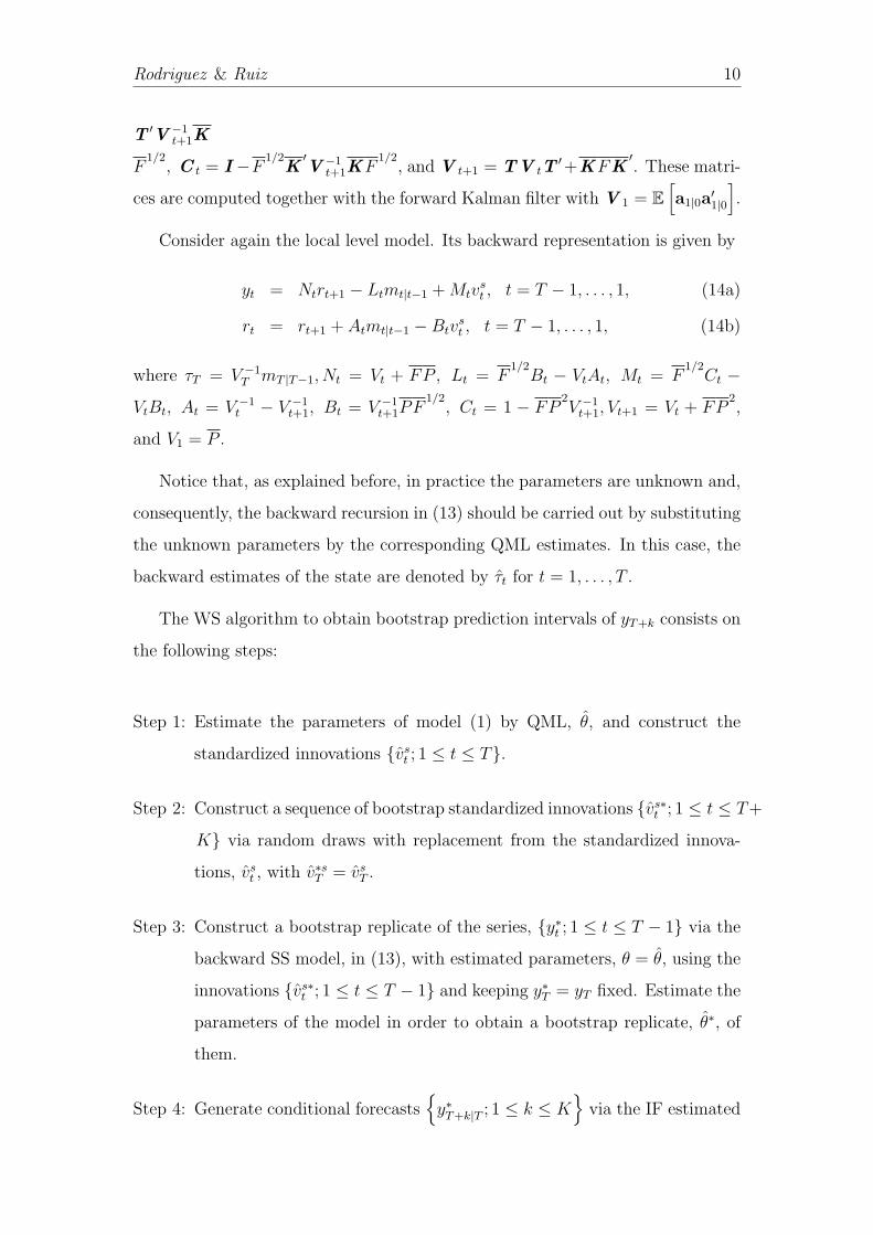
Rodriguez & Ruiz 10
T ′V −1t+1K
F1/2, C t = I −F 1/2
K′V −1
t+1KF1/2, and V t+1 = TV tT
′+KFK′. These matri-
ces are computed together with the forward Kalman filter with V 1 = E[a1|0a
′1|0
].
Consider again the local level model. Its backward representation is given by
yt = Ntrt+1 − Ltmt|t−1 +Mtvst , t = T − 1, . . . , 1, (14a)
rt = rt+1 + Atmt|t−1 −Btvst , t = T − 1, . . . , 1, (14b)
where τT = V −1T mT |T−1, Nt = Vt + FP , Lt = F
1/2Bt − VtAt, Mt = F
1/2Ct −
VtBt, At = V −1t − V −1
t+1, Bt = V −1t+1PF
1/2, Ct = 1 − FP 2
V −1t+1, Vt+1 = Vt + FP
2,
and V1 = P .
Notice that, as explained before, in practice the parameters are unknown and,
consequently, the backward recursion in (13) should be carried out by substituting
the unknown parameters by the corresponding QML estimates. In this case, the
backward estimates of the state are denoted by τt for t = 1, . . . , T .
The WS algorithm to obtain bootstrap prediction intervals of yT+k consists on
the following steps:
Step 1: Estimate the parameters of model (1) by QML, θ, and construct the
standardized innovations {vst ; 1 ≤ t ≤ T}.
Step 2: Construct a sequence of bootstrap standardized innovations {vs∗t ; 1 ≤ t ≤ T+
K} via random draws with replacement from the standardized innova-
tions, vst , with v∗sT = vsT .
Step 3: Construct a bootstrap replicate of the series, {y∗t ; 1 ≤ t ≤ T − 1} via the
backward SS model, in (13), with estimated parameters, θ = θ, using the
innovations {vs∗t ; 1 ≤ t ≤ T − 1} and keeping y∗T = yT fixed. Estimate the
parameters of the model in order to obtain a bootstrap replicate, θ∗, of
them.
Step 4: Generate conditional forecasts{y∗T+k|T ; 1 ≤ k ≤ K
}via the IF estimated
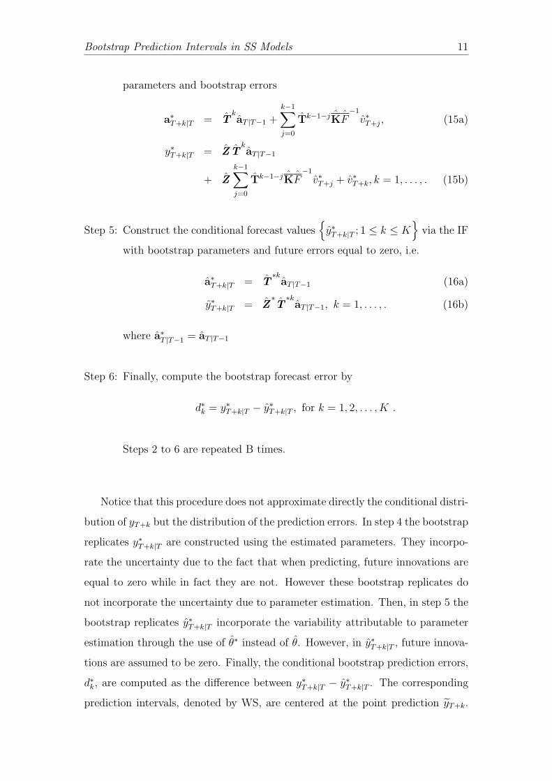
Bootstrap Prediction Intervals in SS Models 11
parameters and bootstrap errors
a∗T+k|T = TkaT |T−1 +
k−1∑j=0
Tk−1−jKF−1
v∗T+j, (15a)
y∗T+k|T = Z TkaT |T−1
+ Zk−1∑j=0
Tk−1−jKF−1
v∗T+j + v∗T+k, k = 1, . . . , . (15b)
Step 5: Construct the conditional forecast values{y∗T+k|T ; 1 ≤ k ≤ K
}via the IF
with bootstrap parameters and future errors equal to zero, i.e.
a∗T+k|T = T∗k
aT |T−1 (16a)
y∗T+k|T = Z∗T∗k
aT |T−1, k = 1, . . . , . (16b)
where a∗T |T−1 = aT |T−1
Step 6: Finally, compute the bootstrap forecast error by
d∗k = y∗T+k|T − y∗T+k|T , for k = 1, 2, . . . , K .
Steps 2 to 6 are repeated B times.
Notice that this procedure does not approximate directly the conditional distri-
bution of yT+k but the distribution of the prediction errors. In step 4 the bootstrap
replicates y∗T+k|T are constructed using the estimated parameters. They incorpo-
rate the uncertainty due to the fact that when predicting, future innovations are
equal to zero while in fact they are not. However these bootstrap replicates do
not incorporate the uncertainty due to parameter estimation. Then, in step 5 the
bootstrap replicates y∗T+k|T incorporate the variability attributable to parameter
estimation through the use of θ∗ instead of θ. However, in y∗T+k|T , future innova-
tions are assumed to be zero. Finally, the conditional bootstrap prediction errors,
d∗k, are computed as the difference between y∗T+k|T − y∗T+k|T . The corresponding
prediction intervals, denoted by WS, are centered at the point prediction yT+k.
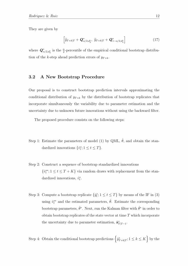
Rodriguez & Ruiz 12
They are given by [yT+k|T + Q∗α/2,d∗k , yT+k|T + Q∗1−α/2,d∗k
](17)
where Q∗α/2,d∗k is the α2-percentile of the empirical conditional bootstrap distribu-
tion of the k-step ahead prediction errors of yT+k.
3.2 A New Bootstrap Procedure
Our proposal is to construct bootstrap prediction intervals approximating the
conditional distribution of yT+k by the distribution of bootstrap replicates that
incorporate simultaneously the variability due to parameter estimation and the
uncertainty due to unknown future innovations without using the backward filter.
The proposed procedure consists on the following steps:
Step 1: Estimate the parameters of model (1) by QML, θ, and obtain the stan-
dardized innovations {vst ; 1 ≤ t ≤ T}.
Step 2: Construct a sequence of bootstrap standardized innovations
{vs∗t ; 1 ≤ t ≤ T +K} via random draws with replacement from the stan-
dardized innovations, vst .
Step 3: Compute a bootstrap replicate {y∗t ; 1 ≤ t ≤ T} by means of the IF in (3)
using vs∗t and the estimated parameters, θ. Estimate the corresponding
bootstrap parameters, θ∗. Next, run the Kalman filter with θ∗ in order to
obtain bootstrap replicates of the state vector at time T which incorporate
the uncertainty due to parameter estimation, a∗T |T−1.
Step 4: Obtain the conditional bootstrap predictions{y∗T+k|T ; 1 ≤ k ≤ K
}by the
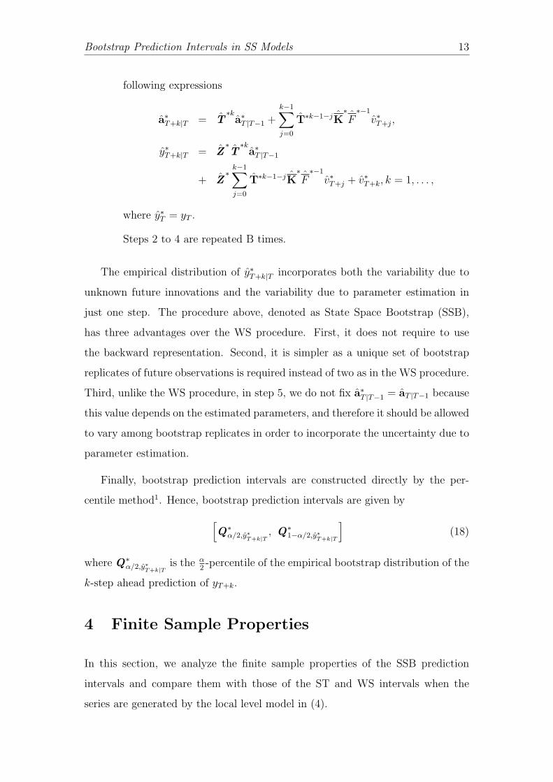
Bootstrap Prediction Intervals in SS Models 13
following expressions
a∗T+k|T = T∗k
a∗T |T−1 +k−1∑j=0
T∗k−1−jK∗F∗−1
v∗T+j,
y∗T+k|T = Z∗T∗k
a∗T |T−1
+ Z∗k−1∑j=0
T∗k−1−jK∗F∗−1
v∗T+j + v∗T+k, k = 1, . . . ,
where y∗T = yT .
Steps 2 to 4 are repeated B times.
The empirical distribution of y∗T+k|T incorporates both the variability due to
unknown future innovations and the variability due to parameter estimation in
just one step. The procedure above, denoted as State Space Bootstrap (SSB),
has three advantages over the WS procedure. First, it does not require to use
the backward representation. Second, it is simpler as a unique set of bootstrap
replicates of future observations is required instead of two as in the WS procedure.
Third, unlike the WS procedure, in step 5, we do not fix a∗T |T−1 = aT |T−1 because
this value depends on the estimated parameters, and therefore it should be allowed
to vary among bootstrap replicates in order to incorporate the uncertainty due to
parameter estimation.
Finally, bootstrap prediction intervals are constructed directly by the per-
centile method1. Hence, bootstrap prediction intervals are given by[Q∗α/2,y∗
T+k|T, Q∗1−α/2,y∗
T+k|T
](18)
where Q∗α/2,y∗T+k|T
is the α2-percentile of the empirical bootstrap distribution of the
k-step ahead prediction of yT+k.
4 Finite Sample Properties
In this section, we analyze the finite sample properties of the SSB prediction
intervals and compare them with those of the ST and WS intervals when the
series are generated by the local level model in (4).
Rodriguez & Ruiz 14
Simulation results are based on R = 1000 replicates of series of sizes T =
50, 100 and 500. The parameters of the model have been chosen to cover a wide
range of different situations from cases in which the noise is large relative to the
signal, i.e. q is small, to cases in which q is large. In particular, we consider
q = {0.1, 1, 2}. With respect to the disturbances, we consider two distributions,
Gaussian and a centered and re-scaled Chi-square with 1 degree of freedom2, χ2(1).
For each simulated series, {yr1, . . . , yrT}, r = 1, 2, . . . , R, we first generate B = 1000
observations of yrT+k for prediction horizons k = 1, 5 and 15, and then obtain, 95%
prediction intervals computed using, the ST intervals in (12), the WS intervals in
(17) and the SSB intervals in (18). Finally, we compute the coverage of each of
these intervals as well as the length and the percentage of observations left out on
the right size and on the left size of the limits of the prediction intervals3.
Bootstrap Prediction Intervals in SS Models 15
Tab
le1:
Mon
teC
arlo
Ave
rage
cove
rage
s,le
ngt
han
dp
erce
nta
geof
obse
rvat
ions
left
out
onth
eri
ght
and
onth
ele
ftof
the
pre
dic
tion
inte
rval
sco
nst
ruct
edusi
ng
ST
,W
San
dSSB
when
ε tisN
(0,1
),η t
isN
(0,q
)an
dth
enom
inal
cove
rage
is95
%
k
Mea
nco
ver
age
Mea
nco
ver
age
inta
ils
Mea
nle
ngth
ST
WS
SSB
ST
WS
SSB
ST
WS
SSB
Bel
ow
/A
bove
Bel
ow
/A
bove
Bel
ow
/A
bove
T=
50
q=
0.1
10.9
27
0.9
35
0.9
36
0.0
36
/0.0
37
0.0
30
/0.0
35
0.0
31
/0.0
33
4.5
30
4.5
97
4.7
74
50.9
27
0.9
40
0.9
43
0.0
36
/0.0
37
0.0
29
/0.0
31
0.0
28
/0.0
29
5.1
82
5.2
85
5.5
39
15
0.9
15
0.9
28
0.9
40
0.0
42
/0.0
42
0.0
35
/0.0
37
0.0
30
/0.0
31
6.4
60
6.6
33
7.0
52
q=
11
0.9
36
0.9
23
0.9
28
0.0
29
/0.0
35
0.0
36
/0.0
41
0.0
36
/0.0
35
6.1
57
6.2
50
6.2
80
50.9
27
0.9
21
0.9
38
0.0
35
/0.0
39
0.0
37
/0.0
42
0.0
32
/0.0
31
9.7
22
9.7
18
10.2
74
15
0.9
14
0.9
09
0.9
34
0.0
41
/0.0
45
0.0
43
/0.0
47
0.0
33
/0.0
33
15.2
58
15.1
94
16.4
69
q=
21
0.9
38
0.9
30
0.9
30
0.0
32
/0.0
29
0.0
36
/0.0
34
0.0
36
/0.0
34
7.4
24
7.5
67.4
33
50.9
26
0.9
24
0.9
31
0.0
37
/0.0
36
0.0
38
/0.0
38
0.0
34
/0.0
34
12.8
49
12.8
80
13.0
88
15
0.9
18
0.9
15
0.9
30
0.0
41
/0.0
41
0.0
42
/0.0
42
0.0
35
/0.0
35
20.8
89
20.8
30
21.6
32
T=
100
q=
0.1
10.9
45
0.9
41
0.9
43
0.0
25
/0.0
30
0.0
31
/0.0
28
0.0
26
/0.0
31
4.5
69
4.5
76
4.6
18
50.9
45
0.9
42
0.9
48
0.0
25
/0.0
30
0.0
30
/0.0
28
0.0
24
/0.0
29
5.2
06
5.2
38
5.3
34
15
0.9
38
0.9
38
0.9
45
0.0
29
/0.0
33
0.0
32
/0.0
30
0.0
26
/0.0
30
6.4
98
6.5
75
6.7
43
q=
11
0.9
44
0.9
40
0.9
39
0.0
28
/0.0
28
0.0
30
/0.0
29
0.0
30
/0.0
31
6.2
71
6.3
14
6.2
78
50.9
39
0.9
37
0.9
42
0.0
31
/0.0
30
0.0
32
/0.0
31
0.0
29
/0.0
29
9.8
74
9.8
73
10.1
20
15
0.9
34
0.9
32
0.9
40
0.0
33
/0.0
33
0.0
34
/0.0
34
0.0
30
/0.0
30
15.5
47
15.5
21
16.1
65
q=
21
0.9
45
0.9
37
0.9
39
0.0
28
/0.0
27
0.0
32
/0.0
30
0.0
31
/0.0
30
7.4
76
7.5
37
7.4
60
50.9
39
0.9
38
0.9
39
0.0
30
/0.0
30
0.0
31
/0.0
31
0.0
31
/0.0
31
13.1
37
13.1
55
13.2
10
15
0.9
35
0.9
35
0.9
37
0.0
32
/0.0
32
0.0
32
/0.0
33
0.0
31
/0.0
31
21.5
09
21.5
39
21.7
58
T=
500
q=
0.1
10.9
46
0.9
48
0.9
45
0.0
27
/0.0
27
0.0
25
/0.0
28
0.0
28
/0.0
27
4.5
92
4.5
77
4.5
82
50.9
46
0.9
47
0.9
46
0.0
26
/0.0
28
0.0
25
/0.0
28
0.0
27
/0.0
27
5.2
17
5.2
06
5.2
23
15
0.9
46
0.9
45
0.9
45
0.0
26
/0.0
29
0.0
26
/0.0
29
0.0
27
/0.0
28
6.5
15
6.4
77
6.5
11
q=
11
0.9
48
0.9
48
0.9
47
0.0
29
/0.0
23
0.0
27
/0.0
25
0.0
27
/0.0
25
6.3
39
6.3
35
6.3
14
50.9
48
0.9
47
0.9
47
0.0
27
/0.0
25
0.0
27
/0.0
26
0.0
28
/0.0
25
10.0
75
10.0
49
10.0
73
15
0.9
47
0.9
46
0.9
47
0.0
27
/0.0
26
0.0
27
/0.0
27
0.0
27
/0.0
26
15.9
56
15.9
19
15.9
44
q=
21
0.9
47
0.9
45
0.9
47
0.0
27
/0.0
26
0.0
29
/0.0
26
0.0
27
/0.0
26
7.5
63
7.5
46
7.5
40
50.9
48
0.9
48
0.9
48
0.0
27
/0.0
27
0.0
27
/0.0
25
0.0
27
/0.0
27
13.4
18
13.4
46
13.3
87
15
0.9
47
0.9
48
0.9
47
0.0
27
/0.0
26
0.0
26
/0.0
26
0.0
26
/0.0
27
22.0
66
22.1
12
22.0
51
Rodriguez & Ruiz 16
Tab
le2:
Mon
teC
arlo
Ave
rage
cove
rage
s,le
ngt
han
dp
erce
nta
geof
obse
rvat
ions
left
out
onth
eri
ght
and
onth
ele
ftof
the
pre
dic
tion
inte
rval
sco
nst
ruct
edusi
ng
ST
,W
San
dSSB
when
ε tisχ
2 (1),η t
isN
(0,q
)an
dth
enom
inal
cove
rage
is95
%
Case
k
Mea
nco
ver
age
Mea
nco
ver
age
inta
ils
Mea
nle
ngth
ST
WS
SSB
ST
WS
SSB
ST
WS
SSB
Bel
ow
/A
bove
Bel
ow
/A
bove
Bel
ow
/A
bove
T=
50
q=
0.1
10.9
41
0.9
40
0.9
42
0.0
10
/0.0
49
0.0
30
/0.0
30
0.0
27
/0.0
31
4.5
13
4.9
09
4.7
34
50.9
43
0.9
34
0.9
46
0.0
13
/0.0
44
0.0
39
/0.0
27
0.0
27
/0.0
26
5.2
21
5.5
07
5.5
96
15
0.9
30
0.9
19
0.9
50
0.0
25
/0.0
45
0.0
53
/0.0
29
0.0
27
/0.0
23
6.5
72
6.6
65
7.3
29
q=
11
0.9
35
0.9
32
0.9
34
0.0
26
/0.0
39
0.0
34
/0.0
34
0.0
34
/0.0
32
6.2
00
6.5
14
6.4
59
50.9
26
0.9
26
0.9
30
0.0
34
/0.0
40
0.0
40
/0.0
34
0.0
38
/0.0
32
9.6
82
9.8
03
9.9
19
15
0.9
13
0.9
14
0.9
23
0.0
42
/0.0
45
0.0
41
/0.0
36
0.0
45
/0.0
41
15.1
26
15.1
76
15.5
97
q=
21
0.9
37
0.9
33
0.9
32
0.0
28
/0.0
35
0.0
34
/0.0
34
0.0
35
/0.0
33
7.3
78
7.7
14
7.5
75
50.9
27
0.9
24
0.9
27
0.0
35
/0.0
38
0.0
40
/0.0
36
0.0
38
/0.0
35
12.8
05
12.8
97
12.9
57
15
0.9
19
0.9
17
0.9
23
0.0
40
/0.0
41
0.0
43
/0.0
40
0.0
40
/0.0
37
20.8
39
20.8
80
21.2
36
T=
100
q=
0.1
10.9
47
0.9
39
0.9
43
0.0
06
/0.0
48
0.0
33
/0.0
28
0.0
27
/0.0
29
4.5
52
4.7
73
4.7
10
50.9
46
0.9
37
0.9
42
0.0
10
/0.0
43
0.0
37
/0.0
26
0.0
31
/0.0
27
5.1
96
5.3
56
5.4
14
15
0.9
39
0.9
29
0.9
44
0.0
21
/0.0
40
0.0
45
/0.0
26
0.0
32
/0.0
24
6.4
91
6.5
97
6.9
12
q=
11
0.9
42
0.9
39
0.9
43
0.0
21
/0.0
37
0.0
30
/0.0
30
0.0
30
/0.0
27
6.2
44
6.4
83
6.5
01
50.9
37
0.9
36
0.9
39
0.0
28
/0.0
34
0.0
35
/0.0
29
0.0
22
/0.0
35
9.8
13
9.9
19
10.0
17
15
0.9
32
0.9
30
0.9
35
0.0
33
/0.0
35
0.0
37
/0.0
33
0.0
28
/0.0
32
15.4
38
15.4
45
15.7
42
q=
21
0.9
47
0.9
44
0.9
45
0.0
22
/0.0
31
0.0
28
/0.0
28
0.0
27
/0.0
28
7.5
07
7.6
85
7.6
86
50.9
42
0.9
41
0.9
43
0.0
28
/0.0
30
0.0
31
/0.0
28
0.0
30
/0.0
27
13.2
20
13.3
07
13.3
99
15
0.9
38
0.9
37
0.9
40
0.0
30
/0.0
31
0.0
33
/0.0
30
0.0
32
/0.0
28
21.6
59
21.7
52
21.9
41
T=
500
q=
0.1
10.9
48
0.9
40
0.9
50
0.0
06
/0.0
45
0.0
33
/0.0
26
0.0
23
/0.0
27
4.5
75
4.6
97
4.7
07
50.9
48
0.9
39
0.9
47
0.0
11
/0.0
41
0.0
36
/0.0
25
0.0
28
/0.0
25
5.1
84
5.2
72
5.3
14
15
0.9
46
0.9
37
0.9
46
0.0
19
/0.0
35
0.0
39
/0.0
24
0.0
31
/0.0
24
6.4
55
6.5
07
6.6
31
q=
11
0.9
47
0.9
47
0.9
48
0.0
20
/0.0
33
0.0
20
/0.0
33
0.0
27
/0.0
26
6.3
38
6.4
92
6.4
72
50.9
48
0.9
48
0.9
48
0.0
24
/0.0
28
0.0
29
/0.0
23
0.0
27
/0.0
25
10.0
73
10.1
81
10.1
37
15
0.9
47
0.9
46
0.9
47
0.0
25
/0.0
27
0.0
29
/0.0
24
0.0
28
/0.0
25
15.9
52
15.9
83
15.9
57
q=
21
0.9
44
0.9
45
0.9
44
0.0
26
/0.0
30
0.0
27
/0.0
28
0.0
29
/0.0
26
7.5
54
7.6
48
7.6
36
50.9
47
0.9
47
0.9
48
0.0
26
/0.0
27
0.0
28
/0.0
25
0.0
28
/0.0
24
13.3
69
13.4
47
13.4
66
15
0.9
47
0.9
47
0.9
48
0.0
26
/0.0
27
0.0
28
/0.0
25
0.0
27
/0.0
25
21.9
68
21.9
92
22.0
85
Bootstrap Prediction Intervals in SS Models 17
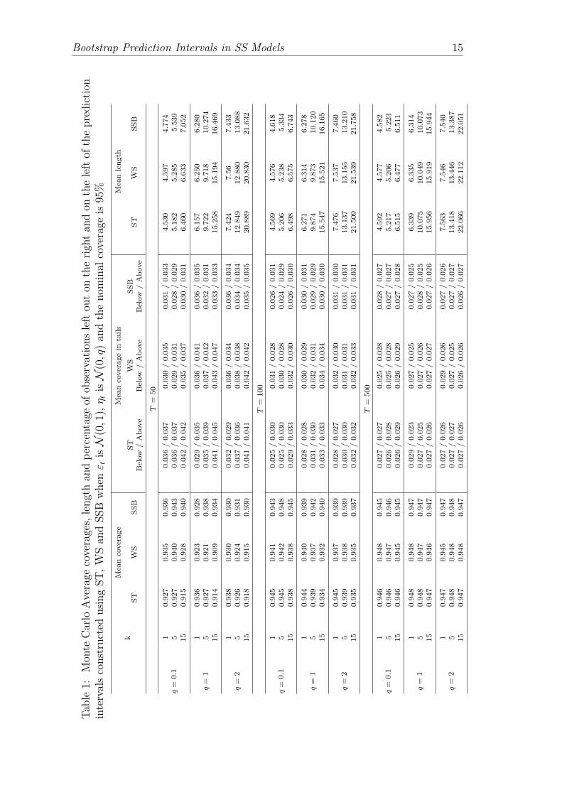
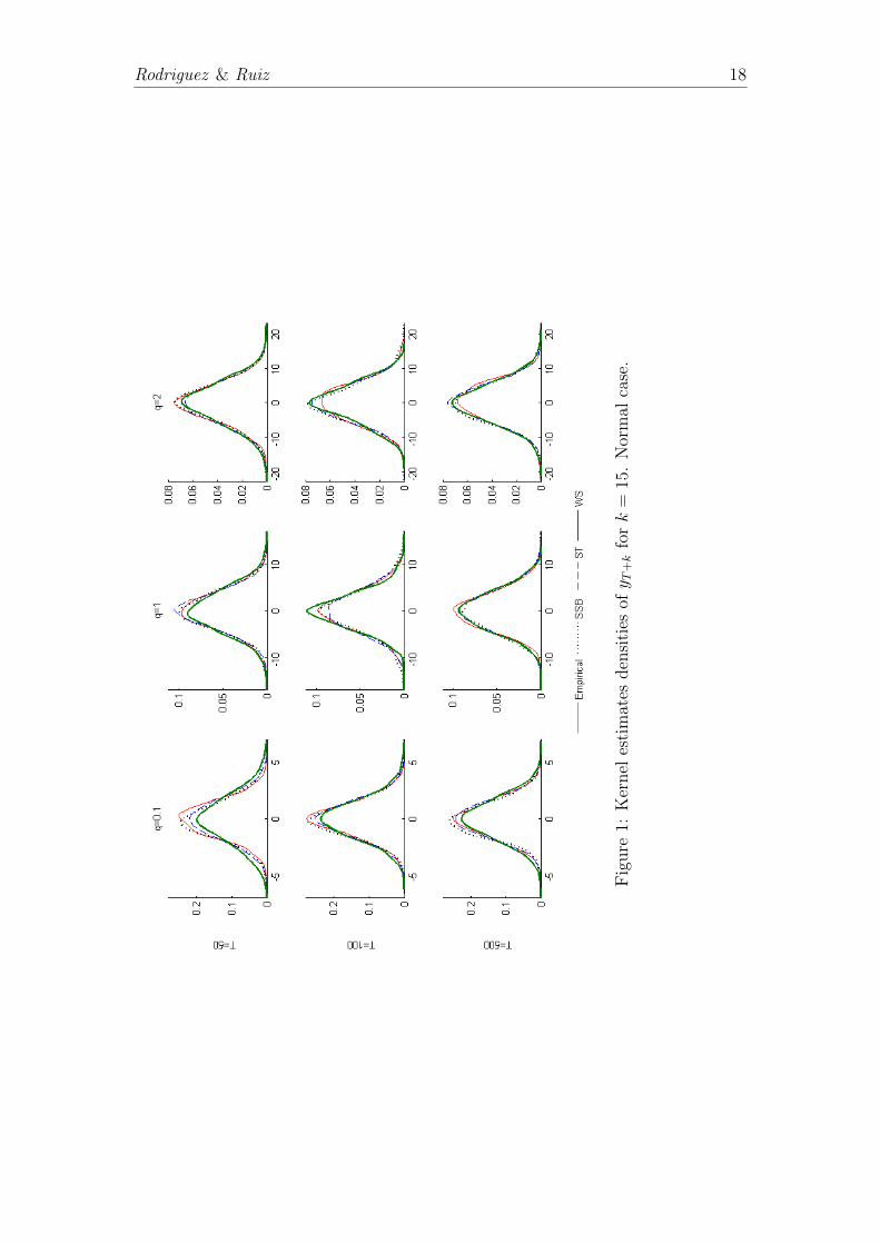
Table 1 reports the Monte Carlo averages of these quantities when both dis-
turbances are Gaussian, and the predictions are calculated for k = 1, 5 and 15
prediction horizons. The table shows that the three procedures are very similar.
The SSB procedure seems to be slightly better specially when the sample size is
small and the prediction horizon increases. This result is illustrated in Figure
1 that plots kernel estimates of the ST, WS and SSB densities for the 15-steps
ahead predictions for one particular series generated by each of the three models
considered with T = 50, 100 and 500 together with the empirical density. Note
that when the signal to noise ratio is small, i.e. q = 0.1, the SSB procedure seems
to be more similar to the empirical densities than the other procedures.
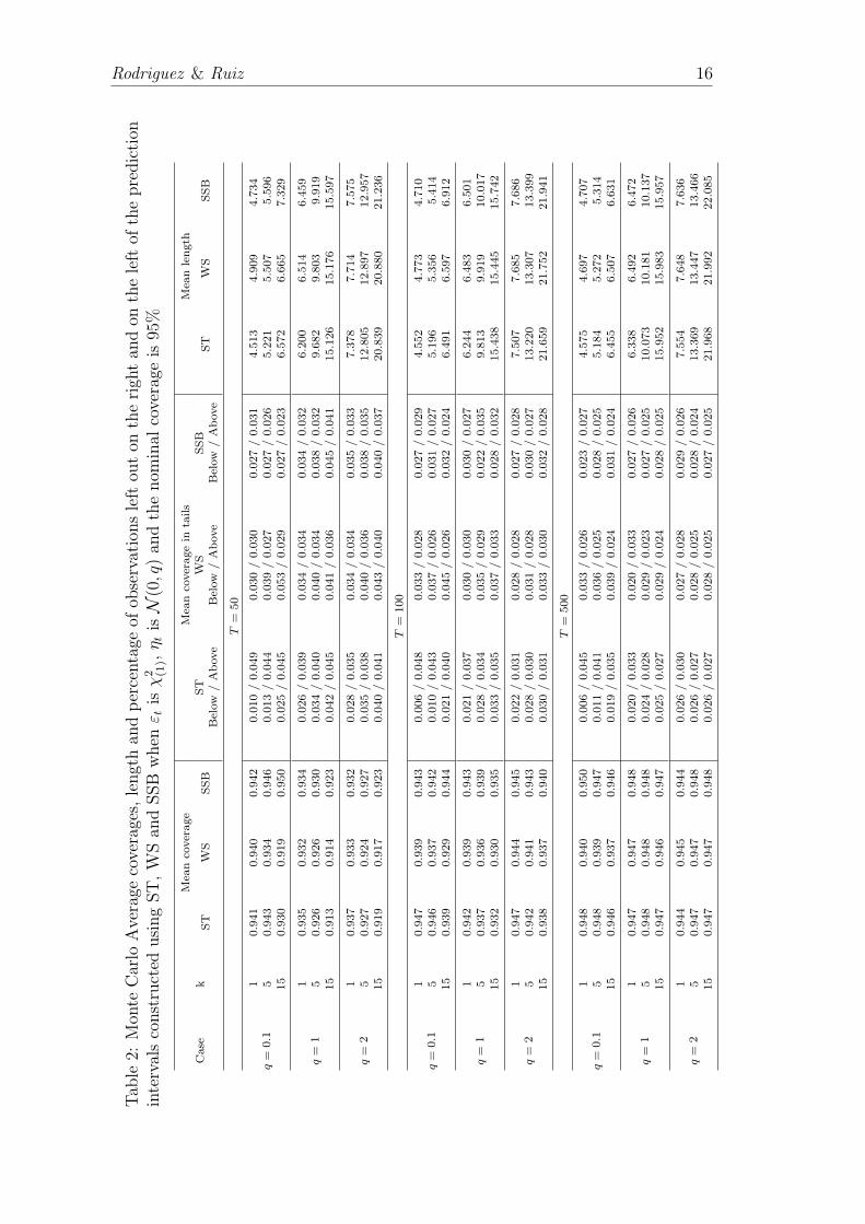
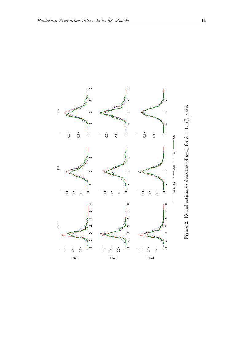
Table 2, that reports the results when εt is χ2(1) and ηt is Gaussian, shows
that the mean coverage of the ST intervals is close to the nominal. However,
they are not able of dealing with the asymmetry in the distribution of εt. The
average coverage in the left tail is smaller than in the right tail. The difference
between the coverage in both tails is larger in the model with q = 0.1 where
the signal is relatively small with respect to the noise which has a non-Gaussian
distribution. Note that the lack of capability of the ST intervals to deal with the
asymmetry in the distribution of εt is larger the larger the sample size. On the
other hand, the coverages of the WS and SSB intervals are rather similar with
SSB being slightly closer to the nominal, for almost all models and sample sizes
considered. Both bootstrap intervals are able to cope with the asymmetry of the
distribution of εt. Consequently, according to the results reported in Table 2,
using the much simpler SSB method does not imply a worse performance of the
prediction intervals. Figure 2 illustrates these results plotting the kernel density
of the simulated yT+1 together with the ST, WS and SSB densities obtained with
a particular series generated by each of the models and sample sizes considered.
This figure also illustrates the lack of fit of the ST density when q = 0.1 and 1.
On the other hand, the shapes of the WS and SSB densities are similar, with SSB
being always closer to the empirical.
Rodriguez & Ruiz 18
Fig
ure
1:K
ernel
esti
mat
esden
siti
esofy T
+k
fork
=15
.N
orm
alca
se.
Bootstrap Prediction Intervals in SS Models 19
Fig
ure
2:K
ernel
esti
mat
esden
siti
esofy T
+k
fork
=1.χ
2 (1)
case
.
Rodriguez & Ruiz 20
5 Application
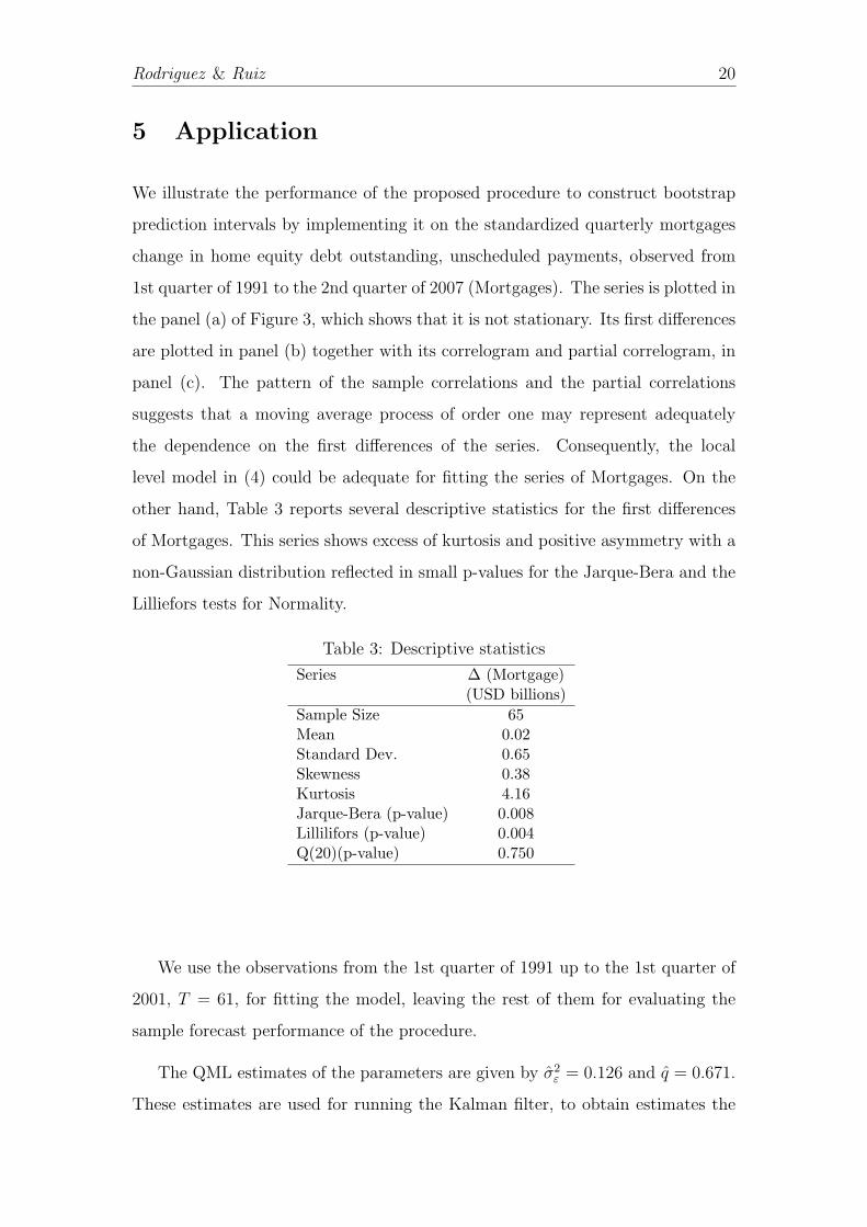
We illustrate the performance of the proposed procedure to construct bootstrap
prediction intervals by implementing it on the standardized quarterly mortgages
change in home equity debt outstanding, unscheduled payments, observed from
1st quarter of 1991 to the 2nd quarter of 2007 (Mortgages). The series is plotted in
the panel (a) of Figure 3, which shows that it is not stationary. Its first differences
are plotted in panel (b) together with its correlogram and partial correlogram, in
panel (c). The pattern of the sample correlations and the partial correlations
suggests that a moving average process of order one may represent adequately
the dependence on the first differences of the series. Consequently, the local
level model in (4) could be adequate for fitting the series of Mortgages. On the
other hand, Table 3 reports several descriptive statistics for the first differences
of Mortgages. This series shows excess of kurtosis and positive asymmetry with a
non-Gaussian distribution reflected in small p-values for the Jarque-Bera and the
Lilliefors tests for Normality.
Table 3: Descriptive statistics
Series ∆ (Mortgage)(USD billions)
Sample Size 65Mean 0.02Standard Dev. 0.65Skewness 0.38Kurtosis 4.16Jarque-Bera (p-value) 0.008Lillilifors (p-value) 0.004Q(20)(p-value) 0.750
We use the observations from the 1st quarter of 1991 up to the 1st quarter of
2001, T = 61, for fitting the model, leaving the rest of them for evaluating the
sample forecast performance of the procedure.
The QML estimates of the parameters are given by σ2ε = 0.126 and q = 0.671.
These estimates are used for running the Kalman filter, to obtain estimates the
Bootstrap Prediction Intervals in SS Models 21
(a)
(b) (c)
Figure 3: (a) The Mortgages series. (b) First difference of Mortgages. (c) SampleAutocorrelation and Partial-Autocorrelation of the first difference of the Mort-gages data.
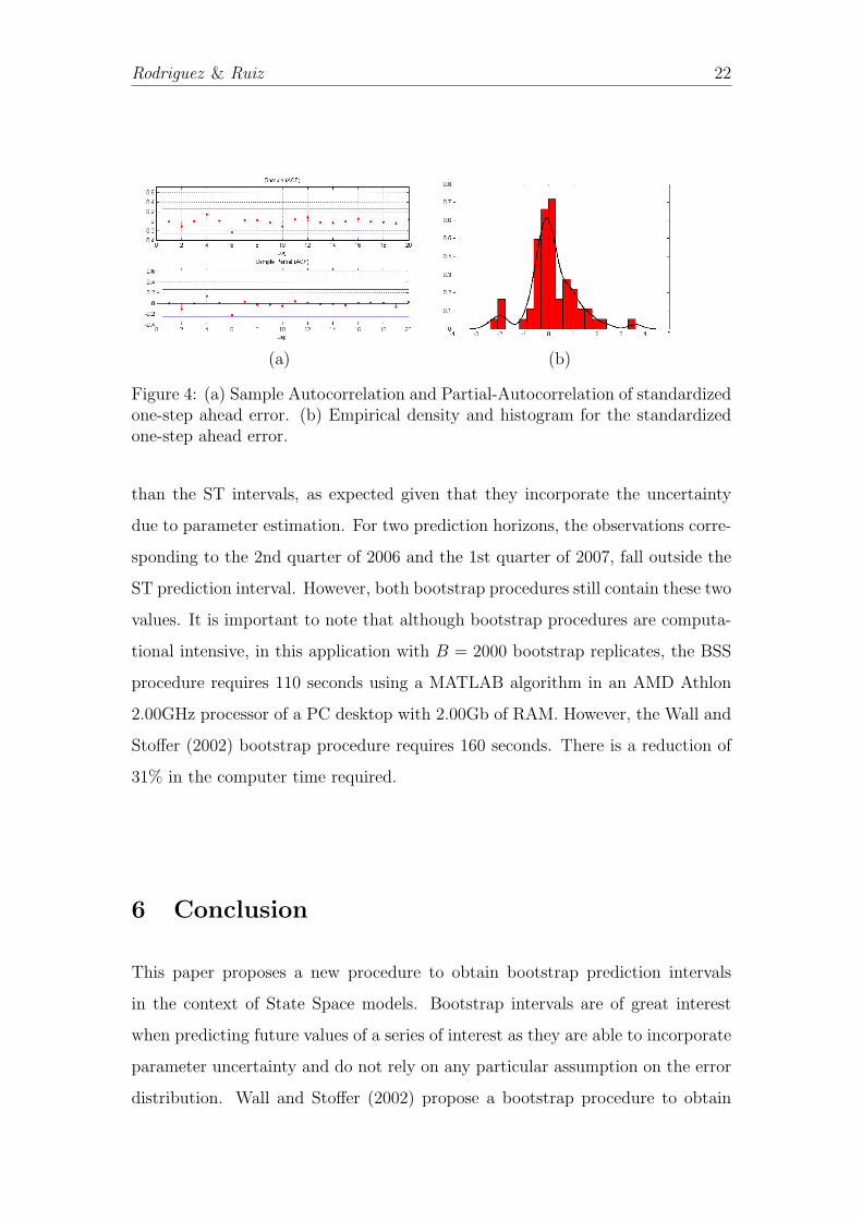
innovations and their variances. Figure 4 plots the correlogram and a kernel
estimates of the density of the within sample standardized one-step ahead errors.
The correlations and partial correlations are not any longer significant. However,
the density of the errors suggests that they are obviously far from Normality.
Therefore, the local level model seems appropriate to represent the dependencies
in the conditional mean of the Mortgages series although for predicting future
values it is convenient to implement a procedure that takes into in account the
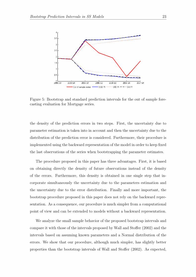
non-Normality of the errors. We construct prediction intervals up to 5 steps ahead
using the ST, WS and SSB procedures. The resulting intervals are plotted in Fig-
ure 5 together with the observed values of the Mortgages series. First, observe
that the two bootstrap procedures generate very similar intervals which are wider
Rodriguez & Ruiz 22
(a) (b)
Figure 4: (a) Sample Autocorrelation and Partial-Autocorrelation of standardizedone-step ahead error. (b) Empirical density and histogram for the standardizedone-step ahead error.
than the ST intervals, as expected given that they incorporate the uncertainty
due to parameter estimation. For two prediction horizons, the observations corre-
sponding to the 2nd quarter of 2006 and the 1st quarter of 2007, fall outside the
ST prediction interval. However, both bootstrap procedures still contain these two
values. It is important to note that although bootstrap procedures are computa-
tional intensive, in this application with B = 2000 bootstrap replicates, the BSS
procedure requires 110 seconds using a MATLAB algorithm in an AMD Athlon
2.00GHz processor of a PC desktop with 2.00Gb of RAM. However, the Wall and
Stoffer (2002) bootstrap procedure requires 160 seconds. There is a reduction of
31% in the computer time required.
6 Conclusion
This paper proposes a new procedure to obtain bootstrap prediction intervals
in the context of State Space models. Bootstrap intervals are of great interest
when predicting future values of a series of interest as they are able to incorporate
parameter uncertainty and do not rely on any particular assumption on the error
distribution. Wall and Stoffer (2002) propose a bootstrap procedure to obtain
Bootstrap Prediction Intervals in SS Models 23
Figure 5: Bootstrap and standard prediction intervals for the out of sample fore-casting evaluation for Mortgage series.
the density of the prediction errors in two steps. First, the uncertainty due to
parameter estimation is taken into in account and then the uncertainty due to the
distribution of the prediction error is considered. Furthermore, their procedure is
implemented using the backward representation of the model in order to keep fixed
the last observations of the series when bootstrapping the parameter estimates.
The procedure proposed in this paper has three advantages. First, it is based
on obtaining directly the density of future observations instead of the density
of the errors. Furthermore, this density is obtained in one single step that in-
corporate simultaneously the uncertainty due to the parameters estimation and
the uncertainty due to the error distribution. Finally and more important, the
bootstrap procedure proposed in this paper does not rely on the backward repre-
sentation. As a consequence, our procedure is much simpler from a computational
point of view and can be extended to models without a backward representation.
We analyze the small sample behavior of the proposed bootstrap intervals and
compare it with those of the intervals proposed by Wall and Stoffer (2002) and the
intervals based on assuming known parameters and a Normal distribution of the
errors. We show that our procedure, although much simpler, has slightly better
properties than the bootstrap intervals of Wall and Stoffer (2002). As expected,
Rodriguez & Ruiz 24
we also show that bootstrap intervals are more adequate than standard intervals
mainly in the presence of non-Normal errors. In general, the standard intervals
are thinner than expected to have the nominal coverage and cannot deal with
asymmetries.
Finally, our proposed bootstrap procedure to obtain prediction intervals in
State Space models is illustrated by implementing it to obtain intervals for future
values of a series of Mortgages modelled by the local level model. We show that
there is an important improvement in terms of computer time when implementing
our proposed procedure with respect to implementing the procedure proposed by
Wall and Stoffer (2002).
When fitting State Space models to represent the dynamic evolution of a time
series, it is often of interest to obtain prediction not only of future values of the
series but also of future values of the unobserved states. We are also working on
the adequacy of the proposed bootstrap prediction intervals when implemented
with this goal. A issue left for further research is the implementation of the
proposed procedure when the system of matrices are time-varying.
References
Anderson, B. D. O. and J. B. Moore (1979). Optimal Filtering. Prentice-Hall,
Inc., Englewood Cliffs.
Ball, L., S. G. Cecchetti, and R. J. Gordon (1990). Inflation and uncertainty at
short and long horizons. Broking Papers on Economic Activity 1990, 215–254.
Broto, C. and E. Ruiz (2006). Using auxiliary residuals to detect conditional
heteroscedasticity in inflaction. Manuscript, Universidad Carlos III de Madrid .
Cavaglia, S. (1992). The persistence of real interest differentials: A Kalman fil-
tering approach. Journal of Monetary Economics 29, 429–443.
Bootstrap Prediction Intervals in SS Models 25
Durbin, J. and S. J. Koopman (2001). Time Series Analysis by State Space
Methods. New York: Oxford University Press.
Efron, B. (1987). Better bootstrap confidence intervals. Journal of the American
Statistical Association 82, 171–185.
Evans, M. (1991). Discovering the link between inflation rates and inflation un-
certainty. Journal of Money, Credit and Banking 23, 169–184.
Harvey, A. C. (1989). Forecasting, Structural Time Series Models and the Kalman
Filter. Cambridge: Cambridge University Press.
Harvey, A. C., E. Ruiz, and N. G. Shephard (1994). Multivariate stochastic
variance models. The Review of Economic Studies 61, 247–264.
Kim, C. J. (1993). Unobserved-component time series models with markov-
switching heterskedasticity: Changes in regimen and the link between inflation
rates and inflation uncertainty. Journal of Business and Economic Statistics 11,
341–349.
Pascual, L., J. Romo, and E. Ruiz (2004). Bootstrap predictive inference for
ARIMA processes. Journal of Time Series Analysis 25, 449–465.
Pfeffermann, D. and R. Tiller (2005). Bootstrap approximation to prediction MSE
for State-Space models with estimated parameters. Journal of Time Series
Analysis 26, 893–916.
Taylor, S. J. (1982). Financial returns modelled by the product of two stochastic
processes, a study of daily sugar prices, 1961-78. In Anderson (Ed.), Time Series
Analysis : Theory and Practice 1, pp. 203–226. North Holland, Amsterdam.
Thombs, L. A. and W. R. Schucany (1990). Bootstrap prediction intervals for
autoregression. Journal of the American Statistical Association 85, 486–492.
Rodriguez & Ruiz 26
Wall, K. D. and D. S. Stoffer (2002). A State Space approach to bootstrapping
conditional forecasts in ARMA models. Journal of Time Series Analysis 23,
733–751.
Notes
1We try alternative methods as the bias-corrected and the acceleration bias-corrected withsimilar results; see Efron (1987) for a definition of these intervals.
2We are particularly interested in dealing with this distribution due to its relation withthe linear transformation of the Autoregressive Stochastic Volatility Model; see, for instance,Harvey et al. (1994). Results for other distributions are similar and are not reported to savespace. Available for the authors upon request.
3All, simulation, estimation and prediction has been done with programs developed by theauthors using the software MATLAB, version 7.2.
Related Documents