Boosting Contextual Information for Deep Neural Network ...

Technical Report OSU-CISRC-5/15-TR06Department of Computer Science and EngineeringThe Ohio State UniversityColumbus, OH 43210-1277

Ftpsite: ftp.cse.ohio-state.eduLogin: anonymousDirectory: pub/tech-report/2015File: TR06.pdfWebsite: http://www.cse.ohio-state.edu/research/techReport.shtml

Boosting Contextual Information for Deep Neural Network BasedVoice Activity Detection

Xiao-Lei ZhangDepartment of Computer Science and Engineering

The Ohio State University, Columbus, OH 43210, [email protected]

DeLiang WangDepartment of Computer Science and Engineering & Center for Cognitive and Brain Sciences

The Ohio State University, Columbus, OH 43210, [email protected]

Abstract – Voice activity detection (VAD) is an important topic in audio signal processing.Contextual information is important for improving the performance of VAD at low signal-to-noise ratios. Here we explore contextual information by machine learning methods at threelevels. At the top level, we employ an ensemble learning framework, named multi-resolutionstacking (MRS), which is a stack of ensemble classifiers. Each classifier in a building blockinputs the concatenation of the predictions of its lower building blocks and the expansionof the raw acoustic feature by a given window (called a resolution). At the middle level,we describe a base classifier in MRS, named boosted deep neural network (bDNN). bDNNfirst generates multiple base predictions from different contexts of a single frame by only oneDNN and then aggregates the base predictions for a better prediction of the frame, and it isdifferent from computationally-expensive boosting methods that train ensembles of classifiersfor multiple base predictions. At the bottom level, we employ the multi-resolution cochleagramfeature, which incorporates the contextual information by concatenating the cochleagramfeatures at multiple spectrotemporal resolutions. Experimental results show that the MRS-based VAD outperforms other VADs by a considerable margin. Moreover, when trained ona large amount of noise types and a wide range of signal-to-noise ratios, the MRS-based

OSU Dept. of Computer Science and Engineering Technical Report #08, 2014

VAD demonstrates surprisingly good generalization performance on unseen test scenarios,approaching the performance with noise-dependent training.

Index Terms – Boosting, cochleagram, deep neural network, multi-resolution stacking, voiceactivity detection.

2

1

Boosting Contextual Information for Deep NeuralNetwork Based Voice Activity Detection

Xiao-Lei Zhang, Member, IEEE and DeLiang Wang, Fellow, IEEE

Abstract—Voice activity detection (VAD) is an important topicin audio signal processing. Contextual information is importantfor improving the performance of VAD at low signal-to-noiseratios. Here we explore contextual information by machinelearning methods at three levels. At the top level, we employ anensemble learning framework, named multi-resolution stacking(MRS), which is a stack of ensemble classifiers. Each classifierin a building block inputs the concatenation of the predictions ofits lower building blocks and the expansion of the raw acousticfeature by a given window (called a resolution). At the middlelevel, we describe a base classifier in MRS, named boosted deepneural network (bDNN). bDNN first generates multiple basepredictions from different contexts of a single frame by onlyone DNN and then aggregates the base predictions for a betterprediction of the frame, and it is different from computationally-expensive boosting methods that train ensembles of classifiersfor multiple base predictions. At the bottom level, we employthe multi-resolution cochleagram feature, which incorporatesthe contextual information by concatenating the cochleagramfeatures at multiple spectrotemporal resolutions. Experimentalresults show that the MRS-based VAD outperforms other VADsby a considerable margin. Moreover, when trained on a largeamount of noise types and a wide range of signal-to-noiseratios, the MRS-based VAD demonstrates surprisingly goodgeneralization performance on unseen test scenarios, approachingthe performance with noise-dependent training.

Index Terms—Boosting, cochleagram, deep neural network,multi-resolution stacking, voice activity detection.

I. INTRODUCTION

VOICE activity detection (VAD) is an important prepro-cessor for many audio signal processing systems. For

example, it improves the efficiency of speech communicationsystems [2] by detecting and transmitting only speech sig-nals. It helps speech enhancement algorithms [3] and speechrecognition systems [9], [13] by filtering out silence and noisesegments. One of the major challenging problems of VAD isto make it perform in low signal-to-noise ratio (SNR) envi-ronments. Early research focused on signal processing basedacoustic features, including energy in the time domain, pitchdetection, zero-crossing rate, and several spectral energy basedfeatures such as energy-entropy, spectral correlation, spectraldivergence, higher-order statistics [25]. Recent developmentincludes low-frequency ultrasound [22] and single frequencyfiltering [1]. Exploring feature is important in improving VADresearch from the aspect of acoustic mechanism. However,each acoustic feature reflects only some characteristics of hu-man voice. Moreover, using the features independently is not

Xiao-Lei Zhang and DeLiang Wang are with the Department of ComputerScience & Engineering and Center for Cognitive & Brain Sciences, The OhioState University, Columbus, OH, USA (e-mail: [email protected],[email protected]).

very effective in extremely difficult scenarios. Hence, fusingthe features together as the input of some data-driven methodsmay be an effective usage of the features for improving theoverall performance of VAD.

Another important research branch of VAD is statisticalsignal processing. These techniques make model assumptionson the distributions of speech and background noise (usuallyin the spectral domain) respectively, and then design statisticalalgorithms to dynamically estimate the model parameters.Typical model assumptions include the Gaussian distribution[34], [43], Laplace distribution [16], Gamma distribution [6],or their combinations [6]. The most popular parameter esti-mation method is the minimum mean square error estimation[12]. In addition, long-term contextual information is shownto be useful in improving the performance [30]. Due to thesimplicity of the model assumptions and online updating ofthe parameters, this kind of methods may generate reasonableresults in various noise scenarios. In many cases, they workbetter than energy based methods. But statistical model basedmethods have limitations. First, model assumptions may notfully capture global data distributions, since the models usuallyhave too few parameters and they estimate parameters on-the-fly from limited local observations. Second, with relatively fewparameters, they may not be flexible enough in fusing multipleacoustic features. Moreover, most methods update parametersduring the pure noise phase which may cause them fail whenthe noise changes rapidly during the voice phase.

The third popular branch of VAD research is machine learn-ing methods, which train acoustic models from given noisycorpora and apply the models to real-world test environments.They have two main research objectives: one is to improve thediscriminative ability of models when the noise scenarios oftraining and test corpora are matching; the other is to improvethe generalization ability (i.e. detection accuracy) of models totest noise scenarios when the test noise scenarios are unseenfrom or mismatching with the training noise scenarios.

Most machine learning methods focus on how to im-prove the discriminative ability. We summarize them brieflyas follows. In terms of whether their training corpora aremanually labeled, they can be categorized to unsupervisedlearning which uses unlabeled training corpora, or super-vised learning which uses labeled training corpora. Manyunsupervised methods belong to dimensionality reduction,which first extract noise-robust low-dimensional features fromhighly-variant high-dimensional observations and then applythe features to classifiers. They include principle componentanalysis [31], non-negative matrix factorization [36], and spec-tral decomposition of graph Laplacian [23]. Some methods

2

use clustering algorithms directly, such as k-means clustering[17] and Gaussian mixture models [31]. Unsupervised methodsare able to explore multiple features and train robust modelsfrom vast amount of recorded data, however, when the tasksare too difficult that most speech signal is drowned in background noise, such as babble noise with an SNR below 0 dB,unsupervised methods are helpless. Note that, statistical signalprocessing based VADs can also be regarded as unsupervisedmethods, which train models from a few local observationsand accumulated historical information.

Supervised learning methods take VAD as a binary-classclassification problem—speech or non-speech. The techniquescan be roughly categorized to four classes: probabilistic mod-els, kernel methods, neural networks, and ensemble methods.Probabilistic models include Gaussian mixture models [26]and conditional random fields [36]. Kernel methods mainlyinclude various support vector machines (SVM), such as [11],[33]. These two kinds cannot handle large-scale corpora well,so that they are difficult to be used in practice since we needlarge-scale training corpora to cover rather complicated real-world noisy environments.

Recently, deep neural networks (DNN) and their extensions[14], [21], [32], [38], [45], [47], which have a strong scalabilityto large-scale corpora, showed good performance in extremelydifficult scenarios and are competitive in real-world applica-tions. Specifically, in [45], Zhang and Wu proposed to applystandard deep belief networks to VAD and reported betterperformance than SVM, where the networks were pretrainedas in [9]. In [47], Zhang and Wang further proposed to generatemultiple different predictions from a single DNN by boostingcontextual information and reported significant improvementover the standard DNN in difficult noise scenarios and lowSNR levels. In [14], [21], the authors applied deep recurrentneural networks to capture historical contextual informationand reported significant improvement over Gaussian mixturemodels and statistical signal processing methods. However,the performance improvements of the aforementioned DNNmethods were observed when the DNNs were trained noise-dependently, i.e. the noise scenarios of training and test arematching. When applying DNN-based VADs to unseen testscenarios, the performance dropped significantly as shown in[14], [46]. Recently, in [32], [38], the authors trained DNNand convolutional neural networks together from large-scalereal-world data [39] and demonstrated impressive two-phaseimprovements. However, because each model in [32], [38]were binded to a given channel, we still do not know exactlyhow the models will generalize to different noise scenarios.Due to the restriction of the task setting, the results do nothave a quantitative evaluation on how the models vary withSNR levels, which need a further investigation.

To summarize, DNN-based VADs with noise dependenttraining have demonstrated good performance and have shownstrong potential in practice. In this paper, we further developDNN-based VADs by exploring contextual information heavilyin three novel levels. Motivated by recent progress of speechseparation [41], [42], we also investigate quantitatively howDNN-based VADs can generalize to unseen test noise sce-narios with the variation of SNR through noise-independent

training. The main contributions of this paper are summarizedas follows:• Multi-resolution stacking (MRS). MRS is a stack of

ensemble classifiers. Each classifier in a building blocktakes the concatenation of the soft output predictionsof the lower building block and the expansion of theoriginal acoustic feature in a window (called a resolution).The classifiers in the same building block have differentresolutions, which is the novelty of this framework.

• Boosted deep neural network (bDNN). bDNN is pro-posed as the base classifier of MRS. It first generatesmultiple base predictions on a frame by boosting thecontextual information of the frame, and then aggregatesthe base predictions for a stronger one. bDNN generatesmultiple predictions from a single DNN, which is itsnovelty compared to ensemble DNNs. Preliminary results[47] showed that it can significantly outperform DNN-based VAD without increasing computational complexity.

• Multi-resolution cochleagram (MRCG) feature.MRCG [7], which was first proposed for speechseparation, is employed as a new acoustic feature forVAD. It concatenates multiple cochleagram featurescalculated at different spectral and temporal resolutions.

• Noise-independent training. We train the proposedmethod with a corpus that has a vast amount of noisescenarios with a wide variation of SNR levels, and test itin unseen and difficult noise scenarios. We find that themethod can generalize well.

Empirical results on the AURORA2 [28] and AURORA4 cor-pora [29] show that the MRS-based VAD outperforms a DNN-based VAD [45] and 4 other comparison methods. Moreover,when the proposed method is trained noise-independently,its performance on unseen test noise scenarios at variousSNR levels is surprisingly as good as the proposed methodwith noise-dependent training. This paper differs from ourpreliminary work [47] in several major aspects, which includethe use of MRS and noise-independent training in this paper(but not in [47]) and new parameter settings for bDNN andMRCG. Consequently, experimental results in this paper aredifferent from those reported in [47].

The paper is organized as follows. In Section II, we intro-duce the MRS framework. In Section III, we present the bDNNmodel. In Section IV, we introduce the MRCG feature. InSection V, we present results with noise-dependent training. InSection VI, we present results with noise-independent training.Finally, we conclude in Section VII.

II. MULTI-RESOLUTION STACKING

We formulate VAD as a supervised classification problem.Specifically, a long speech signal is divided to multiple short-term overlapped frames, each of which ranges usually from 10to 25 milliseconds. For a classification problem, each frameom in the time domain is transformed to an acoustic featurein the spectral domain, denoted as xm, where m = 1, . . . ,Mindexes the time of the frame. To construct a training set, theframe xm is manually labeled as ym = 1 or ym = 0, indicatingxm is a speech or noise frame respectively. A classifier f(·)

3

Buildingblock 1

Buildingblock 2

Building block 3

Hard decision

Classifier

Acoustic feature

Prediction

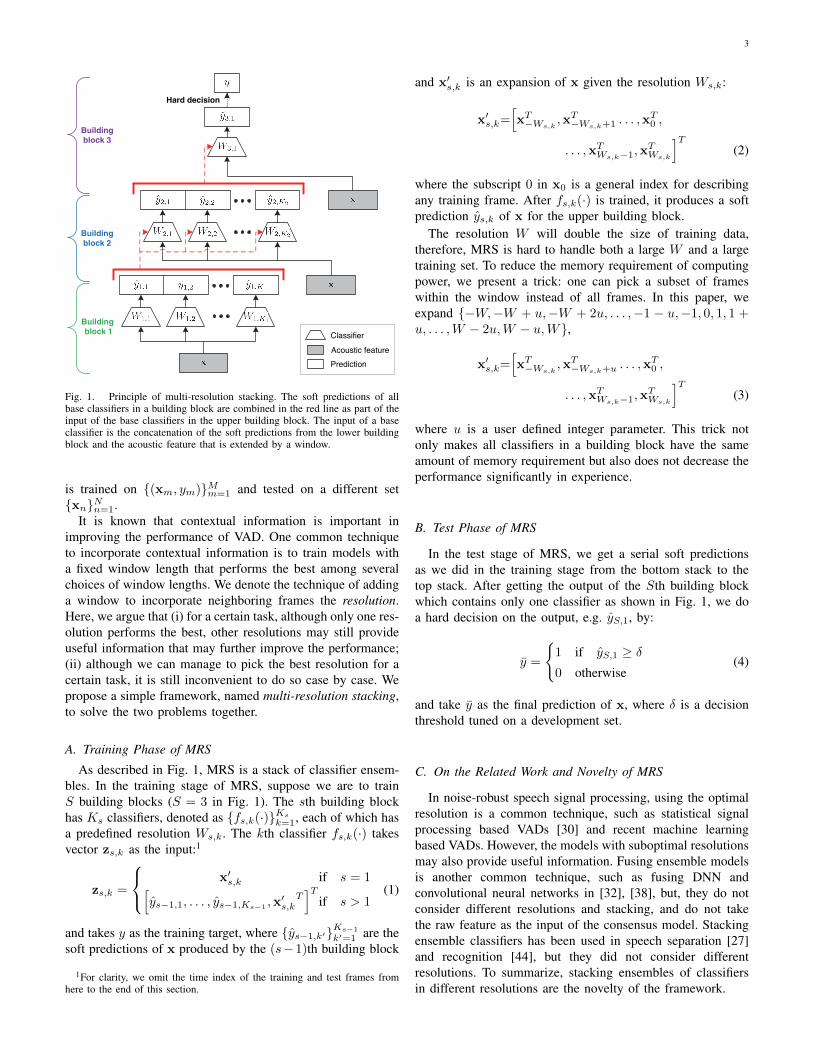
Fig. 1. Principle of multi-resolution stacking. The soft predictions of allbase classifiers in a building block are combined in the red line as part of theinput of the base classifiers in the upper building block. The input of a baseclassifier is the concatenation of the soft predictions from the lower buildingblock and the acoustic feature that is extended by a window.

is trained on {(xm, ym)}Mm=1 and tested on a different set{xn}Nn=1.

It is known that contextual information is important inimproving the performance of VAD. One common techniqueto incorporate contextual information is to train models witha fixed window length that performs the best among severalchoices of window lengths. We denote the technique of addinga window to incorporate neighboring frames the resolution.Here, we argue that (i) for a certain task, although only one res-olution performs the best, other resolutions may still provideuseful information that may further improve the performance;(ii) although we can manage to pick the best resolution for acertain task, it is still inconvenient to do so case by case. Wepropose a simple framework, named multi-resolution stacking,to solve the two problems together.

A. Training Phase of MRS

As described in Fig. 1, MRS is a stack of classifier ensem-bles. In the training stage of MRS, suppose we are to trainS building blocks (S = 3 in Fig. 1). The sth building blockhas Ks classifiers, denoted as {fs,k(·)}Ks

k=1, each of which hasa predefined resolution Ws,k. The kth classifier fs,k(·) takesvector zs,k as the input:1

zs,k =

x′s,k if s = 1[ys−1,1, . . . , ys−1,Ks−1 ,x

′s,k

T]T

if s > 1(1)

and takes y as the training target, where {ys−1,k′}Ks−1

k′=1 are thesoft predictions of x produced by the (s−1)th building block

1For clarity, we omit the time index of the training and test frames fromhere to the end of this section.

and x′s,k is an expansion of x given the resolution Ws,k:

x′s,k=[xT−Ws,k

,xT−Ws,k+1 . . . ,x

T0 ,

. . . ,xTWs,k−1,x

TWs,k

]T(2)

where the subscript 0 in x0 is a general index for describingany training frame. After fs,k(·) is trained, it produces a softprediction ys,k of x for the upper building block.

The resolution W will double the size of training data,therefore, MRS is hard to handle both a large W and a largetraining set. To reduce the memory requirement of computingpower, we present a trick: one can pick a subset of frameswithin the window instead of all frames. In this paper, weexpand {−W,−W + u,−W + 2u, . . . ,−1 − u,−1, 0, 1, 1 +u, . . . ,W − 2u,W − u,W},

x′s,k=[xT−Ws,k

,xT−Ws,k+u . . . ,x

T0 ,

. . . ,xTWs,k−1,x

TWs,k

]T(3)

where u is a user defined integer parameter. This trick notonly makes all classifiers in a building block have the sameamount of memory requirement but also does not decrease theperformance significantly in experience.

B. Test Phase of MRS

In the test stage of MRS, we get a serial soft predictionsas we did in the training stage from the bottom stack to thetop stack. After getting the output of the Sth building blockwhich contains only one classifier as shown in Fig. 1, we doa hard decision on the output, e.g. yS,1, by:

y =

{1 if yS,1 ≥ δ0 otherwise

(4)

and take y as the final prediction of x, where δ is a decisionthreshold tuned on a development set.

C. On the Related Work and Novelty of MRS

In noise-robust speech signal processing, using the optimalresolution is a common technique, such as statistical signalprocessing based VADs [30] and recent machine learningbased VADs. However, the models with suboptimal resolutionsmay also provide useful information. Fusing ensemble modelsis another common technique, such as fusing DNN andconvolutional neural networks in [32], [38], but, they do notconsider different resolutions and stacking, and do not takethe raw feature as the input of the consensus model. Stackingensemble classifiers has been used in speech separation [27]and recognition [44], but they did not consider differentresolutions. To summarize, stacking ensembles of classifiersin different resolutions are the novelty of the framework.

4

III. BOOSTED DNN

In this section, we fill MRS by a strong base classifier—boosted DNN. We first present the bDNN algorithm in Sec-tions III-A, then introduce the motivation of bDNN in SectionIII-C, and our DNN model in Section III-B. Finally, we presentthe novelty of the bDNN model in Section III-D.

Deep neural network is a strong classifier that can approachto the minimum expectation risk—the ideal minimum riskgiven the infinite amount of training data—when the input datais large scale. It has been adopted in recent VAD studies. Onecommon technique to further improve the prediction accuracyof DNN is ensemble learning, which trains multiple DNNsthat yield different base predictions, such that when the basepredictions are aggregated, the final prediction is boosted tobe better than any of the base predictions. However, it istoo expensive to train a set of DNNs if they do not receivesignificantly different knowledge from the input. To alleviatethe computational load but benefit from ensemble learning, weproposed bDNN, which can generate multiple different basepredictions on a single frame by training only one DNN.

A. Boosted DNN

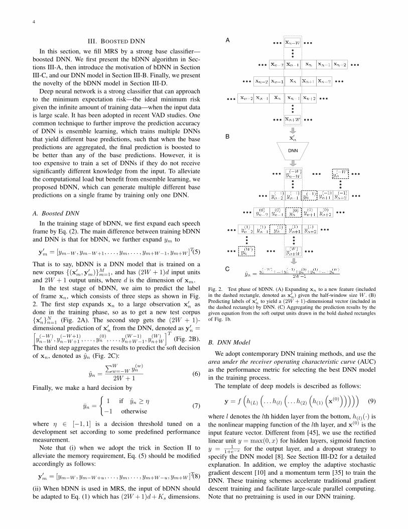
In the training stage of bDNN, we first expand each speechframe by Eq. (2). The main difference between training bDNNand DNN is that for bDNN, we further expand ym to

y′m = [ym−W , ym−W+1, . . . , ym, . . . , ym+W−1, ym+W ]T(5)

That is to say, bDNN is a DNN model that is trained on anew corpus {(x′m,y′m)}Mm=1, and has (2W + 1)d input unitsand 2W + 1 output units, where d is the dimension of xm.

In the test stage of bDNN, we aim to predict the labelof frame xn, which consists of three steps as shown in Fig.2. The first step expands xn to a large observation x′n asdone in the training phase, so as to get a new test corpus{x′n}Nn=1 (Fig. 2A). The second step gets the (2W + 1)-dimensional prediction of x′n from the DNN, denoted as y′n =[y(−W )n−W , y

(−W+1)n−W+1 , . . . , y

(0)n , . . . , y

(W−1)n+W−1, y

(W )n+W

]T(Fig. 2B).

The third step aggregates the results to predict the soft decisionof xn, denoted as yn (Fig. 2C):

yn =

∑Ww=−W y

(w)n

2W + 1(6)

Finally, we make a hard decision by

yn =

{1 if yn ≥ η−1 otherwise

(7)

where η ∈ [−1, 1] is a decision threshold tuned on adevelopment set according to some predefined performancemeasurement.

Note that (i) when we adopt the trick in Section II toalleviate the memory requirement, Eq. (5) should be modifiedaccordingly as follows:

y′m = [ym−W , ym−W+u, . . . , ym, . . . , ym+W−u, ym+W ]T(8)

(ii) When bDNN is used in MRS, the input of bDNN shouldbe adapted to Eq. (1) which has (2W + 1)d+Ks dimensions.

DNN

A

B

C

Fig. 2. Test phase of bDNN. (A) Expanding xn to a new feature (includedin the dashed rectangle, denoted as x′

n) given the half-window size W . (B)Predicting labels of x′

n to yield a (2W +1)-dimensional vector (included inthe dashed rectangle) by DNN. (C) Aggregating the prediction results by thegiven equation from the soft output units drawn in the bold dashed rectanglesof Fig. 1b.

B. DNN Model

We adopt contemporary DNN training methods, and use thearea under the receiver operating characteristic curve (AUC)as the performance metric for selecting the best DNN modelin the training process.

The template of deep models is described as follows:

y = f(h(L)

(. . . h(l)

(. . . h(2)

(h(1)

(x(0)

)))))(9)

where l denotes the lth hidden layer from the bottom, h(l)(·) isthe nonlinear mapping function of the lth layer, and x(0) is theinput feature vector. Different from [45], we use the rectifiedlinear unit y = max(0, x) for hidden layers, sigmoid functiony = 1

1+e−x for the output layer, and a dropout strategy tospecify the DNN model [8]. See Section III-D2 for a detailedexplanation. In addition, we employ the adaptive stochasticgradient descent [10] and a momentum term [35] to train theDNN. These training schemes accelerate traditional gradientdescent training and facilitate large-scale parallel computing.Note that no pretraining is used in our DNN training.

5

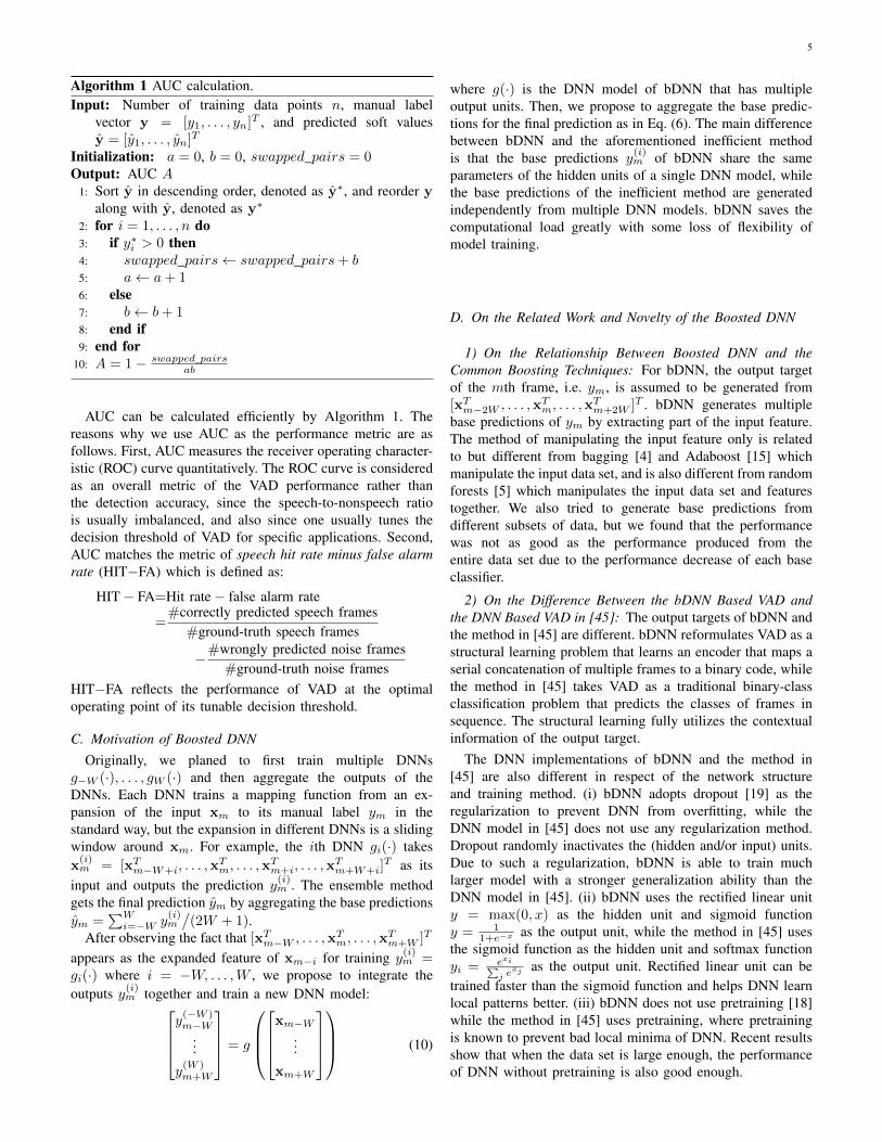
Algorithm 1 AUC calculation.Input: Number of training data points n, manual label

vector y = [y1, . . . , yn]T , and predicted soft valuesy = [y1, . . . , yn]T

Initialization: a = 0, b = 0, swapped_pairs = 0Output: AUC A

1: Sort y in descending order, denoted as y∗, and reorder yalong with y, denoted as y∗

2: for i = 1, . . . , n do3: if y∗i > 0 then4: swapped_pairs← swapped_pairs+ b5: a← a+ 16: else7: b← b+ 18: end if9: end for

10: A = 1− swapped_pairsab

AUC can be calculated efficiently by Algorithm 1. Thereasons why we use AUC as the performance metric are asfollows. First, AUC measures the receiver operating character-istic (ROC) curve quantitatively. The ROC curve is consideredas an overall metric of the VAD performance rather thanthe detection accuracy, since the speech-to-nonspeech ratiois usually imbalanced, and also since one usually tunes thedecision threshold of VAD for specific applications. Second,AUC matches the metric of speech hit rate minus false alarmrate (HIT−FA) which is defined as:

HIT− FA=Hit rate− false alarm rate

=#correctly predicted speech frames

#ground-truth speech frames

−#wrongly predicted noise frames#ground-truth noise frames

HIT−FA reflects the performance of VAD at the optimaloperating point of its tunable decision threshold.

C. Motivation of Boosted DNNOriginally, we planed to first train multiple DNNs

g−W (·), . . . , gW (·) and then aggregate the outputs of theDNNs. Each DNN trains a mapping function from an ex-pansion of the input xm to its manual label ym in thestandard way, but the expansion in different DNNs is a slidingwindow around xm. For example, the ith DNN gi(·) takesx(i)m = [xT

m−W+i, . . . ,xTm, . . . ,x

Tm+i, . . . ,x

Tm+W+i]

T as itsinput and outputs the prediction y

(i)m . The ensemble method

gets the final prediction ym by aggregating the base predictionsym =

∑Wi=−W y

(i)m

/(2W + 1).

After observing the fact that [xTm−W , . . . ,xT

m, . . . ,xTm+W ]T

appears as the expanded feature of xm−i for training y(i)m =

gi(·) where i = −W, . . . ,W , we propose to integrate theoutputs y(i)m together and train a new DNN model:

y(−W )m−W

...

y(W )m+W

= g

xm−W

...

xm+W

(10)

where g(·) is the DNN model of bDNN that has multipleoutput units. Then, we propose to aggregate the base predic-tions for the final prediction as in Eq. (6). The main differencebetween bDNN and the aforementioned inefficient methodis that the base predictions y

(i)m of bDNN share the same

parameters of the hidden units of a single DNN model, whilethe base predictions of the inefficient method are generatedindependently from multiple DNN models. bDNN saves thecomputational load greatly with some loss of flexibility ofmodel training.

D. On the Related Work and Novelty of the Boosted DNN

1) On the Relationship Between Boosted DNN and theCommon Boosting Techniques: For bDNN, the output targetof the mth frame, i.e. ym, is assumed to be generated from[xT

m−2W , . . . ,xTm, . . . ,x

Tm+2W ]T . bDNN generates multiple

base predictions of ym by extracting part of the input feature.The method of manipulating the input feature only is relatedto but different from bagging [4] and Adaboost [15] whichmanipulate the input data set, and is also different from randomforests [5] which manipulates the input data set and featurestogether. We also tried to generate base predictions fromdifferent subsets of data, but we found that the performancewas not as good as the performance produced from theentire data set due to the performance decrease of each baseclassifier.

2) On the Difference Between the bDNN Based VAD andthe DNN Based VAD in [45]: The output targets of bDNN andthe method in [45] are different. bDNN reformulates VAD as astructural learning problem that learns an encoder that maps aserial concatenation of multiple frames to a binary code, whilethe method in [45] takes VAD as a traditional binary-classclassification problem that predicts the classes of frames insequence. The structural learning fully utilizes the contextualinformation of the output target.

The DNN implementations of bDNN and the method in[45] are also different in respect of the network structureand training method. (i) bDNN adopts dropout [19] as theregularization to prevent DNN from overfitting, while theDNN model in [45] does not use any regularization method.Dropout randomly inactivates the (hidden and/or input) units.Due to such a regularization, bDNN is able to train muchlarger model with a stronger generalization ability than theDNN model in [45]. (ii) bDNN uses the rectified linear unity = max(0, x) as the hidden unit and sigmoid functiony = 1

1+e−x as the output unit, while the method in [45] usesthe sigmoid function as the hidden unit and softmax functionyi = exi∑

j exj as the output unit. Rectified linear unit can betrained faster than the sigmoid function and helps DNN learnlocal patterns better. (iii) bDNN does not use pretraining [18]while the method in [45] uses pretraining, where pretrainingis known to prevent bad local minima of DNN. Recent resultsshow that when the data set is large enough, the performanceof DNN without pretraining is also good enough.

6

Time domain noisy speech

8-D feature

8-channel cochleagram:

Frame length = 20 ms;Frame shift = 10 ms

8-channel cochleagram:

Frame length = 200 ms;Frame shift = 10 ms

Smoothing each unit in a 11x11 square window

Smoothing each unit in a 23x23 square window

A

B 32-D MRCG feature

32-D Delta feature

32-D Delta-Delta feature

CSpeech signal

8-channel gammatone filter

(Frequency range:[80, 5000] Hz)

Calculating the energy of each frame in each

channel

8-D feature

8-D feature 8-D feature 8-D feature

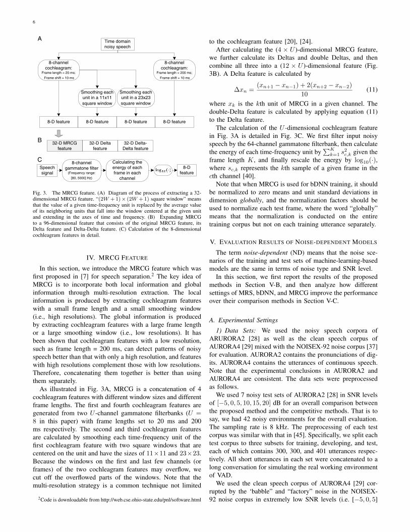
Fig. 3. The MRCG feature. (A) Diagram of the process of extracting a 32-dimensional MRCG feature. “(2W +1)× (2W +1) square window” meansthat the value of a given time-frequency unit is replaced by the average valueof its neighboring units that fall into the window centered at the given unitand extending in the axes of time and frequency. (B) Expanding MRCGto a 96-dimensional feature that consists of the original MRCG feature, itsDelta feature and Delta-Delta feature. (C) Calculation of the 8-dimensionalcochleagram features in detail.

IV. MRCG FEATURE

In this section, we introduce the MRCG feature which wasfirst proposed in [7] for speech separation.2 The key idea ofMRCG is to incorporate both local information and globalinformation through multi-resolution extraction. The localinformation is produced by extracting cochleagram featureswith a small frame length and a small smoothing window(i.e., high resolutions). The global information is producedby extracting cochleagram features with a large frame lengthor a large smoothing window (i.e., low resolutions). It hasbeen shown that cochleagram features with a low resolution,such as frame length = 200 ms, can detect patterns of noisyspeech better than that with only a high resolution, and featureswith high resolutions complement those with low resolutions.Therefore, concatenating them together is better than usingthem separately.

As illustrated in Fig. 3A, MRCG is a concatenation of 4cochleagram features with different window sizes and differentframe lengths. The first and fourth cochleagram features aregenerated from two U -channel gammatone filterbanks (U =8 in this paper) with frame lengths set to 20 ms and 200ms respectively. The second and third cochleagram featuresare calculated by smoothing each time-frequency unit of thefirst cochleagram feature with two square windows that arecentered on the unit and have the sizes of 11×11 and 23×23.Because the windows on the first and last few channels (orframes) of the two cochleagram features may overflow, wecut off the overflowed parts of the windows. Note that themulti-resolution strategy is a common technique not limited

2Code is downloadable from http://web.cse.ohio-state.edu/pnl/software.html

to the cochleagram feature [20], [24].After calculating the (4 × U )-dimensional MRCG feature,

we further calculate its Deltas and double Deltas, and thencombine all three into a (12 × U )-dimensional feature (Fig.3B). A Delta feature is calculated by

∆xn =(xn+1 − xn−1) + 2(xn+2 − xn−2)

10(11)

where xk is the kth unit of MRCG in a given channel. Thedouble-Delta feature is calculated by applying equation (11)to the Delta feature.

The calculation of the U -dimensional cochleagram featurein Fig. 3A is detailed in Fig. 3C. We first filter input noisyspeech by the 64-channel gammatone filterbank, then calculatethe energy of each time-frequency unit by

∑Kk=1 s

2c,k given the

frame length K, and finally rescale the energy by log10(·),where sc,k represents the kth sample of a given frame in thecth channel [40].

Note that when MRCG is used for bDNN training, it shouldbe normalized to zero means and unit standard deviations indimension globally, and the normalization factors should beused to normalize each test frame, where the word “globally”means that the normalization is conducted on the entiretraining corpus but not on each training utterance separately.

V. EVALUATION RESULTS OF NOISE-DEPENDENT MODELS

The term noise-dependent (ND) means that the noise sce-narios of the training and test sets of machine-learning-basedmodels are the same in terms of noise type and SNR level.

In this section, we first report the results of the proposedmethods in Section V-B, and then analyze how differentsettings of MRS, bDNN, and MRCG improve the performanceover their comparison methods in Section V-C.

A. Experimental Settings

1) Data Sets: We used the noisy speech corpora ofARURORA2 [28] as well as the clean speech corpus ofAURORA4 [29] mixed with the NOISEX-92 noise corpus [37]for evaluation. AURORA2 contains the pronunciations of dig-its. AURORA4 contains the utterances of continuous speech.Note that the experimental conclusions in AURORA2 andAURORA4 are consistent. The data sets were preprocessedas follows.

We used 7 noisy test sets of AURORA2 [28] in SNR levelsof [−5, 0, 5, 10, 15, 20] dB for an overall comparison betweenthe proposed method and the competitive methods. That is tosay, we had 42 noisy environments for the overall evaluation.The sampling rate is 8 kHz. The preprocessing of each testcorpus was similar with that in [45]. Specifically, we split eachtest corpus to three subsets for training, developing, and test,each of which contains 300, 300, and 401 utterances respec-tively. All short utterances in each set were concatenated to along conversation for simulating the real working environmentof VAD.

We used the clean speech corpus of AURORA4 [29] cor-rupted by the ‘babble” and “factory” noise in the NOISEX-92 noise corpus in extremely low SNR levels (i.e. [−5, 0, 5]

7

0 100 200 300 400 500-1

0

1Clean wave

0 100 200 300 400 500-1

0

1Noisy speech (babble, SNR = -5 dB)

0 100 200 300 400 5000

1

Zhang13 VAD

0 100 200 300 400 5000

1

-based VAD

0 100 200 300 400 5000

1

Sohn VAD

0 100 200 300 400 5000

1

Ramirez05 VAD

0 100 200 300 400 5000

1

Ying VAD

0 100 200 300 400 5000

1

SVM VAD

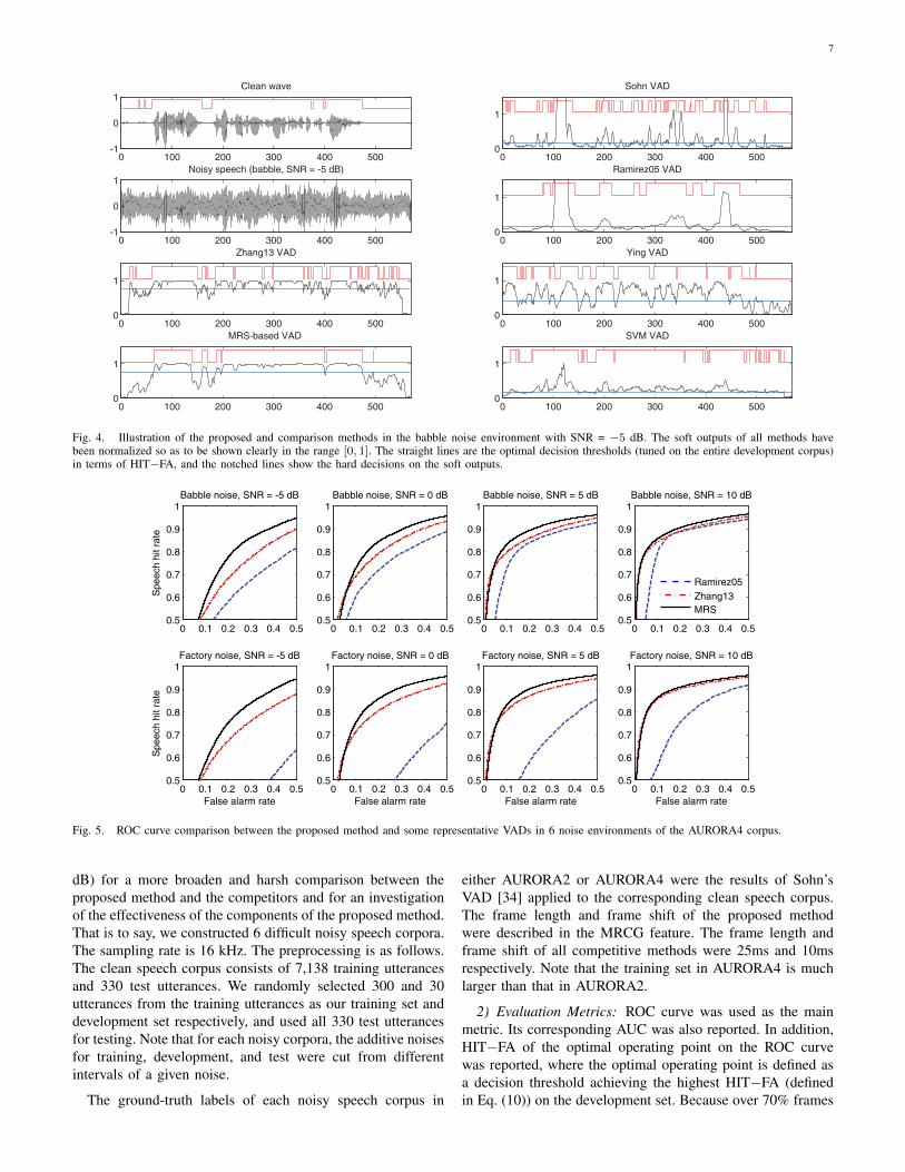
Fig. 4. Illustration of the proposed and comparison methods in the babble noise environment with SNR = −5 dB. The soft outputs of all methods havebeen normalized so as to be shown clearly in the range [0, 1]. The straight lines are the optimal decision thresholds (tuned on the entire development corpus)in terms of HIT−FA, and the notched lines show the hard decisions on the soft outputs.

0 0.1 0.2 0.3 0.4 0.50.5

0.6

0.7

0.8

0.9

1Babble noise, SNR = -5 dB

Spe

ech

hit r

ate

0 0.1 0.2 0.3 0.4 0.50.5

0.6

0.7

0.8

0.9

1Babble noise, SNR = 0 dB

0 0.1 0.2 0.3 0.4 0.50.5

0.6

0.7

0.8

0.9

1Babble noise, SNR = 5 dB

0 0.1 0.2 0.3 0.4 0.50.5

0.6

0.7

0.8

0.9

1Babble noise, SNR = 10 dB

0 0.1 0.2 0.3 0.4 0.50.5

0.6

0.7

0.8

0.9

1Factory noise, SNR = -5 dB

Spe

ech

hit r

ate

False alarm rate0 0.1 0.2 0.3 0.4 0.5

0.5

0.6

0.7

0.8

0.9

1Factory noise, SNR = 0 dB

False alarm rate0 0.1 0.2 0.3 0.4 0.5

0.5

0.6

0.7

0.8

0.9

1Factory noise, SNR = 5 dB

False alarm rate0 0.1 0.2 0.3 0.4 0.5

0.5

0.6

0.7

0.8

0.9

1Factory noise, SNR = 10 dB

False alarm rate

Ramirez05Zhang13MRS

Fig. 5. ROC curve comparison between the proposed method and some representative VADs in 6 noise environments of the AURORA4 corpus.

dB) for a more broaden and harsh comparison between theproposed method and the competitors and for an investigationof the effectiveness of the components of the proposed method.That is to say, we constructed 6 difficult noisy speech corpora.The sampling rate is 16 kHz. The preprocessing is as follows.The clean speech corpus consists of 7,138 training utterancesand 330 test utterances. We randomly selected 300 and 30utterances from the training utterances as our training set anddevelopment set respectively, and used all 330 test utterancesfor testing. Note that for each noisy corpora, the additive noisesfor training, development, and test were cut from differentintervals of a given noise.

The ground-truth labels of each noisy speech corpus in

either AURORA2 or AURORA4 were the results of Sohn’sVAD [34] applied to the corresponding clean speech corpus.The frame length and frame shift of the proposed methodwere described in the MRCG feature. The frame length andframe shift of all competitive methods were 25ms and 10msrespectively. Note that the training set in AURORA4 is muchlarger than that in AURORA2.

2) Evaluation Metrics: ROC curve was used as the mainmetric. Its corresponding AUC was also reported. In addition,HIT−FA of the optimal operating point on the ROC curvewas reported, where the optimal operating point is defined asa decision threshold achieving the highest HIT−FA (definedin Eq. (10)) on the development set. Because over 70% frames

8

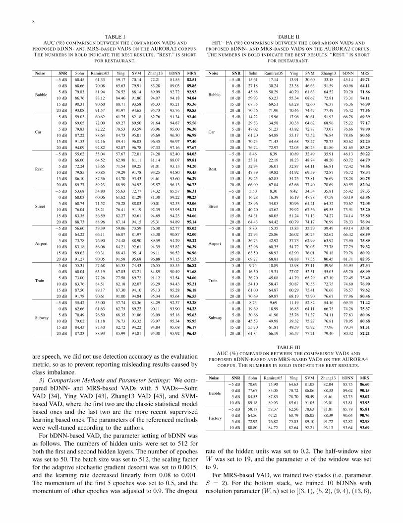
TABLE IAUC (%) COMPARISON BETWEEN THE COMPARISON VADS AND

PROPOSED BDNN- AND MRS-BASED VADS ON THE AURORA2 CORPUS.THE NUMBERS IN BOLD INDICATE THE BEST RESULTS. “REST.” IS SHORT

FOR RESTAURANT.

Noise SNR Sohn Ramirez05 Ying SVM Zhang13 bDNN MRS

Babble

−5 dB 60.45 61.33 59.17 70.14 72.21 81.55 82.510 dB 68.66 70.08 65.63 79.91 83.28 89.03 89.855 dB 79.83 81.94 76.52 88.14 89.99 92.72 92.93

10 dB 86.76 88.12 84.46 91.86 94.07 94.18 94.8415 dB 90.31 90.60 88.71 93.58 95.33 95.21 95.3620 dB 93.08 91.57 91.97 94.65 95.73 95.76 95.85

Car

−5 dB 59.03 60.62 61.75 82.18 82.76 91.34 92.400 dB 69.05 72.00 69.27 89.50 91.64 94.87 95.565 dB 79.83 82.22 78.53 93.59 93.96 95.60 96.30

10 dB 87.22 88.64 84.73 95.01 95.69 96.30 96.9815 dB 91.53 92.16 89.41 96.05 96.45 96.97 97.4020 dB 94.09 92.82 92.87 96.78 97.33 97.16 97.67

Rest.

−5 dB 55.62 55.04 57.67 72.01 74.20 82.40 84.030 dB 66.00 64.52 62.98 81.11 81.14 88.07 89.815 dB 72.24 73.65 71.54 89.25 91.01 93.13 94.20

10 dB 79.85 80.85 79.29 91.78 93.25 94.80 95.4515 dB 86.10 87.36 84.70 93.43 94.61 95.60 96.2920 dB 89.27 89.23 88.99 94.92 95.57 96.13 96.73

Street

−5 dB 53.68 54.80 55.63 72.77 74.32 85.57 86.310 dB 60.03 60.06 61.62 81.29 81.38 89.22 90.235 dB 68.74 71.52 70.28 88.03 90.01 92.53 93.06

10 dB 76.04 78.21 76.41 91.19 92.39 93.95 94.2115 dB 83.35 86.59 82.27 92.61 94.69 94.23 94.6620 dB 88.73 88.96 87.14 94.15 95.31 94.89 95.14

Airport

−5 dB 56.60 59.39 59.06 73.59 76.30 82.77 85.020 dB 64.22 66.11 66.07 81.97 83.38 90.87 92.005 dB 73.78 76.90 74.48 88.90 89.59 94.29 95.22

10 dB 83.18 86.06 84.21 92.61 94.35 95.82 96.3915 dB 89.62 90.31 88.43 95.14 96.11 96.52 96.9620 dB 91.27 90.05 91.58 95.68 96.88 97.15 97.53

Train

−5 dB 55.31 57.68 61.35 74.43 76.55 85.55 86.820 dB 60.04 63.19 67.85 83.21 84.89 90.49 91.685 dB 73.00 77.26 77.58 89.72 91.12 93.54 94.60

10 dB 83.76 84.51 82.18 92.07 93.29 94.43 95.2115 dB 87.50 89.17 87.30 94.10 95.13 95.28 96.1820 dB 91.78 90.61 91.00 94.84 95.34 95.64 96.55

Subway

−5 dB 55.42 55.00 57.74 83.36 84.29 92.37 93.280 dB 62.66 61.63 62.75 89.22 90.11 93.90 94.235 dB 70.49 76.50 68.35 91.86 93.09 95.18 95.63

10 dB 79.02 81.18 76.73 93.32 93.97 95.34 95.9515 dB 84.43 87.40 82.72 94.22 94.84 95.68 96.1720 dB 87.23 88.93 85.99 94.81 95.38 95.92 96.43

are speech, we did not use detection accuracy as the evaluationmetric, so as to prevent reporting misleading results caused byclass imbalance.

3) Comparison Methods and Parameter Settings: We com-pared bDNN- and MRS-based VADs with 5 VADs—SohnVAD [34], Ying VAD [43], Zhang13 VAD [45], and SVM-based VAD, where the first two are the classic statistical modelbased ones and the last two are the more recent supervisedlearning based ones. The parameters of the referenced methodswere well-tuned according to the authors.

For bDNN-based VAD, the parameter setting of bDNN wasas follows. The numbers of hidden units were set to 512 forboth the first and second hidden layers. The number of epocheswas set to 50. The batch size was set to 512, the scaling factorfor the adaptive stochastic gradient descent was set to 0.0015,and the learning rate decreased linearly from 0.08 to 0.001.The momentum of the first 5 epoches was set to 0.5, and themomentum of other epoches was adjusted to 0.9. The dropout

TABLE IIHIT−FA (%) COMPARISON BETWEEN THE COMPARISON VADS AND

PROPOSED BDNN- AND MRS-BASED VADS ON THE AURORA2 CORPUS.THE NUMBERS IN BOLD INDICATE THE BEST RESULTS. “REST.” IS SHORT

FOR RESTAURANT.

Noise SNR Sohn Ramirez05 Ying SVM Zhang13 bDNN MRS

Babble

−5 dB 15.61 17.14 13.91 30.60 33.18 45.14 49.710 dB 27.18 30.24 23.38 46.63 51.59 60.96 64.115 dB 45.88 50.29 40.79 61.63 64.52 70.20 71.86

10 dB 59.93 63.23 55.34 68.67 72.81 73.31 74.1115 dB 67.35 69.51 63.28 72.60 76.37 76.36 76.9920 dB 70.56 71.90 70.46 74.47 77.49 76.42 77.56

Car

−5 dB 14.22 15.96 17.96 50.61 51.93 66.78 69.390 dB 29.83 34.58 30.38 64.62 68.96 75.22 77.175 dB 47.02 51.23 43.82 72.87 73.07 76.66 78.90

10 dB 61.20 64.88 55.17 75.52 76.84 78.86 80.6515 dB 70.73 71.43 64.68 78.27 78.75 80.62 82.2320 dB 76.74 72.97 72.05 80.23 81.80 81.65 83.29

Rest.

−5 dB 8.46 8.39 10.89 32.49 35.91 46.13 50.220 dB 23.81 22.19 18.23 48.74 48.20 60.72 64.795 dB 32.94 36.01 32.87 64.11 66.81 72.42 74.86

10 dB 47.39 49.82 44.92 69.59 72.87 76.72 78.3415 dB 59.25 62.85 54.25 73.81 76.69 78.28 80.7520 dB 66.09 67.84 62.66 77.40 78.69 80.55 82.04

Street

−5 dB 5.50 8.30 9.42 34.34 35.81 55.42 57.350 dB 16.28 16.39 16.19 47.78 47.59 63.19 65.865 dB 28.96 34.05 30.96 61.21 64.52 70.67 72.05

10 dB 40.20 43.62 39.92 67.36 69.55 73.91 75.2015 dB 54.31 60.05 51.24 71.13 74.27 74.14 75.8020 dB 64.43 64.42 60.79 74.17 76.99 76.33 76.94

Airport

−5 dB 8.80 15.35 13.83 35.29 39.49 49.14 53.010 dB 22.93 25.86 26.02 50.25 52.62 66.42 68.595 dB 36.73 42.92 37.73 62.99 63.92 73.90 75.89

10 dB 52.96 60.35 54.72 70.05 73.78 77.79 79.3215 dB 63.50 68.93 62.99 76.01 78.18 79.78 80.9220 dB 69.27 68.81 68.88 77.35 80.45 81.71 82.95

Train

−5 dB 9.75 10.89 15.98 37.11 39.96 54.93 57.340 dB 16.50 19.31 27.07 52.51 55.05 65.20 68.995 dB 36.20 45.08 41.79 65.29 67.10 72.45 75.40

10 dB 54.10 58.47 50.87 70.55 72.75 74.60 76.9015 dB 61.00 64.87 60.29 75.41 76.66 76.57 79.6220 dB 70.69 69.87 68.19 75.90 76.67 77.96 80.46

Subway

−5 dB 8.23 9.69 11.19 52.82 54.16 69.35 71.420 dB 19.69 18.99 16.85 64.11 66.75 74.26 75.375 dB 30.66 41.90 25.76 71.37 74.11 77.63 80.06

10 dB 45.53 49.98 39.32 75.27 76.81 78.95 80.6815 dB 55.70 61.81 49.59 75.92 77.96 79.34 81.5120 dB 61.84 66.19 56.57 77.21 79.40 80.32 82.21

TABLE IIIAUC (%) COMPARISON BETWEEN THE COMPARISON VADS AND

PROPOSED BDNN-BASED AND MRS-BASED VADS ON THE AURORA4CORPUS. THE NUMBERS IN BOLD INDICATE THE BEST RESULTS.

Noise SNR Sohn Ramirez05 Ying SVM Zhang13 bDNN MRS

Babble

−5 dB 70.69 75.90 64.63 81.05 82.84 85.75 86.600 dB 77.67 83.05 70.72 86.06 88.33 89.62 90.155 dB 84.53 87.85 78.70 90.49 91.61 92.75 93.02

10 dB 89.18 89.93 85.61 91.05 93.01 93.81 93.93

Factory

−5 dB 58.17 58.37 62.56 78.63 81.81 85.78 85.810 dB 64.56 67.21 68.79 86.05 88.39 90.64 90.765 dB 72.92 76.82 75.83 89.10 91.72 92.82 92.98

10 dB 80.80 84.72 82.64 92.21 93.13 93.64 93.69

rate of the hidden units was set to 0.2. The half-window sizeW was set to 19, and the parameter u of the window was setto 9.

For MRS-based VAD, we trained two stacks (i.e. parameterS = 2). For the bottom stack, we trained 10 bDNNs withresolution parameter (W,u) set to [(3, 1), (5, 2), (9, 4), (13, 6),

9

TABLE IVHIT−FA (%) COMPARISON BETWEEN THE COMPARISON VADS AND

PROPOSED BDNN-BASED VAD ON THE AURORA4 CORPUS. THENUMBERS IN BOLD INDICATE THE BEST RESULTS.

Noise SNR Sohn Ramirez05 Ying SVM Zhang13 bDNN MRS

Babble

−5 dB 29.44 38.45 21.03 45.69 48.33 56.13 57.920 dB 40.64 52.09 29.76 56.31 60.01 63.94 65.155 dB 54.42 65.23 42.70 67.77 69.94 72.04 73.10

10 dB 67.50 70.89 56.12 69.75 74.75 75.74 76.03

Factory

−5 dB 12.00 13.43 19.50 42.11 47.42 54.60 55.510 dB 21.04 25.63 28.42 56.93 62.00 66.64 67.185 dB 33.40 40.11 38.83 64.19 70.72 72.25 73.18

10 dB 47.33 55.39 50.47 73.36 75.66 75.86 76.44

TABLE VAUC (%) ANALYSIS OF THE RELATIVE CONTRIBUTIONS OF BDNN, MRS,

AND MRCG. “COMB” DENOTES A SERIAL COMBINATION OF 11ACOUSTIC FEATURES IN [45].

Noise SNRDNN+ bDNN+ MRS+ DNN+ bDNN+ MRS+COMB COMB COMB MRCG MRCG MRCG

Babble

−5 dB 81.53 84.62 86.11 81.54 85.75 86.600 dB 85.48 88.84 89.76 86.48 89.62 90.155 dB 89.08 92.11 92.82 90.05 92.75 93.02

10 dB 90.56 93.10 93.65 91.64 93.81 93.93

Factory

−5 dB 80.16 83.51 85.75 79.70 85.78 85.810 dB 84.59 88.95 90.35 86.51 90.64 90.765 dB 87.79 91.91 92.70 89.76 92.82 92.98

10 dB 89.16 92.79 93.75 90.95 93.64 93.69

(15, 7), (17, 8), (19, 9), (21, 10), (23, 11), (25, 12)] respec-tively. The parameter setting of each bDNN was exactly thesame as that of the aforementioned bDNN-based VAD. For thetop stack, we trained 1 bDNN with (W,u) set to (19, 9). Theparameter setting of the bDNN was as follows. The numbersof hidden units were set to 128 for both the first and secondhidden layers. The number of epoches was set to 7.

B. Results

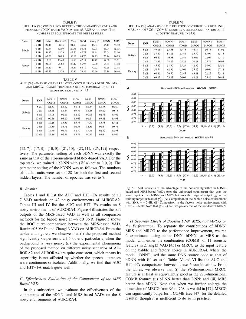
Tables I and II list the AUC and HIT−FA results of all7 VAD methods on 42 noisy environments of AURORA2.Tables III and IV list the AUC and HIT−FA results on 8noisy environments of AURORA4. Figure 4 illustrates the softoutputs of the MRS-based VAD as well as all comparisonmethods for the babble noise at −5 dB SNR. Figure 5 showsthe ROC curve comparison between the MRS-based VAD,Ramirez05 VAD, and Zhang13 VAD on AURORA4. From thetables and figures, we observe that (i) the proposed methodsignificantly outperforms all 5 others, particularly when thebackground is very noisy; (ii) the experimental phenomenaof the proposed method on different noisy scenarios of AU-RORA2 and AURORA4 are quite consistent, which means itssuperiority is not affected by whether the speech utteranceswere continuous or isolated. Additionally, we find that AUCand HIT−FA match quite well.

C. Effectiveness Evaluation of the Components of the MRSBased VAD

In this subsection, we evaluate the effectiveness of thecomponents of the bDNN- and MRS-based VADs on the 8noisy environments of AURORA4.

TABLE VIHIT−FA (%) ANALYSIS OF THE RELATIVE CONTRIBUTIONS OF BDNN,MRS, AND MRCG. “COMB” DENOTES A SERIAL COMBINATION OF 11

ACOUSTIC FEATURES IN [45].

Noise SNRDNN+ bDNN+ MRS+ DNN+ bDNN+ MRS+COMB COMB COMB MRCG MRCG MRCG

Babble

−5 dB 49.15 53.58 55.75 46.14 56.13 57.920 dB 57.60 61.81 63.44 55.79 63.94 65.155 dB 66.40 70.58 72.47 65.06 72.04 73.10

10 dB 71.83 74.22 75.21 70.28 75.74 76.03

Factory

−5 dB 45.82 51.30 55.29 42.32 54.60 55.510 dB 54.54 62.36 65.64 55.82 66.64 67.185 dB 64.46 70.50 72.45 63.88 72.25 73.18

10 dB 69.17 73.83 76.09 68.21 75.86 76.44

0.85

0.87

0.89

unboosted DNN with window bDNN MRS

0.75

0.77

0.79

0.81

0.83

(3,1) (5,2) (9,4) (13,6) (15,7) (17,8) (19,9) (21,10) (23,11) (25,12)

AU

C

(W, u)

0.85

0.87

0.89

unboosted DNN with window bDNN MRS

0.75

0.77

0.79

0.81

0.83

(3,1) (5,2) (9,4) (13,6) (15,7) (17,8) (19,9) (21,10) (23,11) (25,12)A

UC

(W, u)

A

B

Fig. 6. AUC analysis of the advantage of the boosted algorithm in bDNN-based and MRS-based VADs over the unboosted counterpart that uses thesame input x′

n as bDNN and MRS but uses the original output yn as thetraining target instead of y′

n. (A) Comparison in the babble noise environmentwith SNR = −5 dB. (B) Comparison in the factory noise environment withSNR = −5 dB. Note that (W,u) are two parameters of the window of bDNN.

1) Separate Effects of Boosted DNN, MRS, and MRCG onthe Performance: To separate the contributions of bDNN,MRS and MRCG to the performance improvement, we ran6 experiments using either DNN, bDNN, or MRS as themodel with either the combination (COMB) of 11 acousticfeatures in Zhang13 VAD [45] or MRCG as the input featureon the babble and factory noises in AURORA4, where themodel “DNN” used the same DNN source code as that ofbDNN with W set to 0. Tables V and VI list the AUC andHIT−FA comparisons between these 6 combinations. Fromthe tables, we observe that (i) the 96-dimensional MRCGfeature is at least as equivalently good as the 273-dimensionalCOMB feature; (ii) bDNN better than DNN; and (iii) MRSbetter than bDNN. Note that when we further enlarge thedimension of MRCG from 96 to 768 as we did in [47], MRCGcan significantly outperform COMB (see [47] for the detailedresults), though it is inefficient to do so in practice.

10

0 0.1 0.2 0.3 0.4 0.50.5

0.6

0.7

0.8

0.9

1

Spe

ech

hit r

ate

bDNN, W = 1 (Babble, SNR = -5 dB)

0 0.1 0.2 0.3 0.4 0.50.5

0.6

0.7

0.8

0.9

1bDNN, W = 19 (Babble, SNR = -5 dB)

0 0.1 0.2 0.3 0.4 0.50.5

0.6

0.7

0.8

0.9

1bDNN, W = 1 (Factory, SNR = -5 dB)

0 0.1 0.2 0.3 0.4 0.50.5

0.6

0.7

0.8

0.9

1bDNN, W = 19 (Factory, SNR = -5 dB)

0 0.1 0.2 0.3 0.4 0.50.5

0.6

0.7

0.8

0.9

1

False alarm rate

Spe

ech

hit r

ate

MRS, W = 1 (Babble, SNR = -5 dB)

0 0.1 0.2 0.3 0.4 0.50.5

0.6

0.7

0.8

0.9

1

False alarm rate

MRS, W = 19 (Babble, SNR = -5 dB)

0 0.1 0.2 0.3 0.4 0.50.5

0.6

0.7

0.8

0.9

1

False alarm rate

MRS, W = 1 (Factory, SNR = -5 dB)

0 0.1 0.2 0.3 0.4 0.50.5

0.6

0.7

0.8

0.9

1

False alarm rate

MRS, W = 19 (Factory, SNR = -5 dB)

CG1CG2CG3CG4MRCG

Fig. 8. ROC curve analysis of the MRCG feature versus its components at AURORA4.

0.6

0.65

0.7

unboosted DNN with window bDNN MRS

0.35

0.4

0.45

0.5

0.55

(3,1) (5,2) (9,4) (13,6) (15,7) (17,8) (19,9) (21,10) (23,11) (25,12)

HIT

-FA

(W, u)

A

0.6

0.65

0.7

A

unboosted DNN with window bDNN MRS

0.35

0.4

0.45

0.5

0.55

(3,1) (5,2) (9,4) (13,6) (15,7) (17,8) (19,9) (21,10) (23,11) (25,12)

HIT

-FA

(W, u)

B

Fig. 7. HIT−FA analysis of the advantage of the boosted algorithm inbDNN-based and MRS-based VADs over the unboosted counterpart that usesthe same input x′

n as bDNN and MRS but uses the original output yn as thetraining target instead of y′

n. (A) Comparison in the babble noise environmentwith SNR = −5 dB. (B) Comparison in the factory noise environment withSNR = −5 dB. Note that (W,u) are two parameters of the window of bDNN.

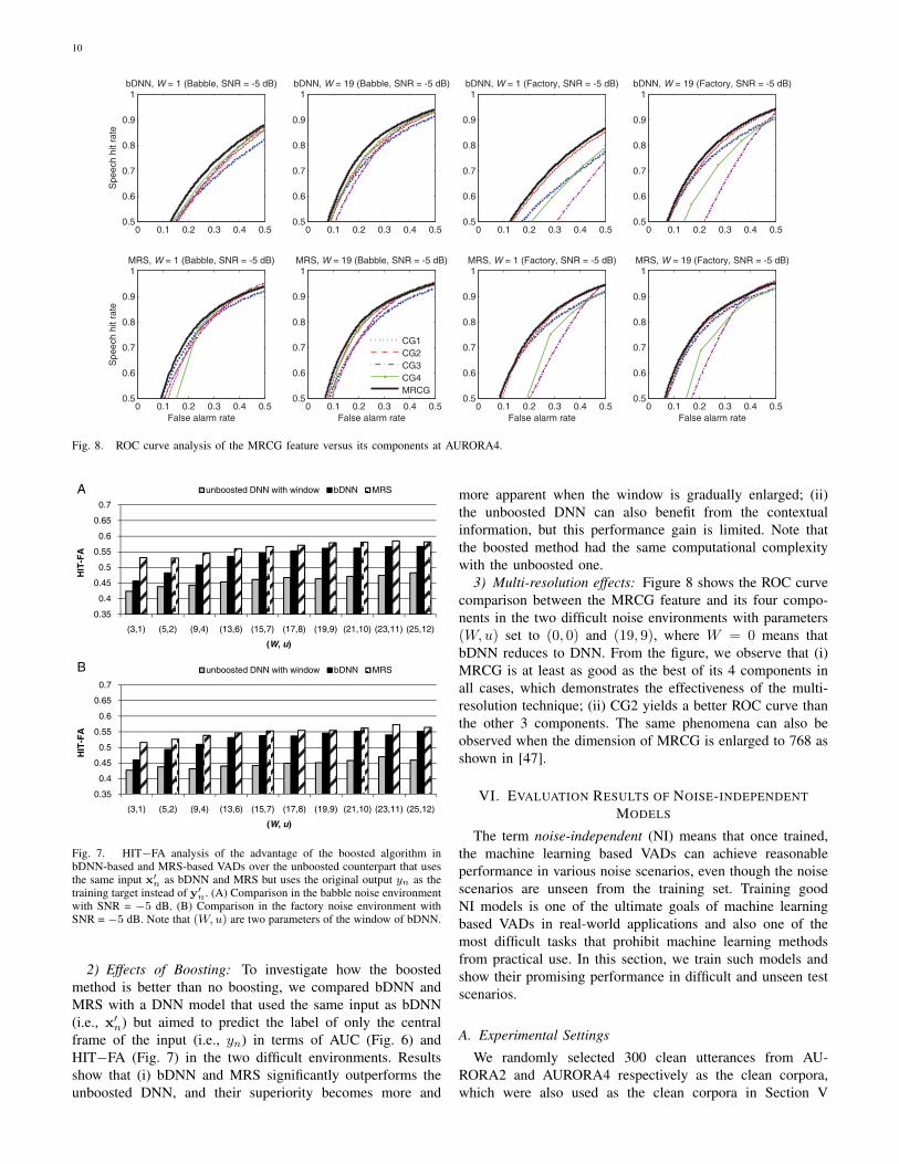
2) Effects of Boosting: To investigate how the boostedmethod is better than no boosting, we compared bDNN andMRS with a DNN model that used the same input as bDNN(i.e., x′n) but aimed to predict the label of only the centralframe of the input (i.e., yn) in terms of AUC (Fig. 6) andHIT−FA (Fig. 7) in the two difficult environments. Resultsshow that (i) bDNN and MRS significantly outperforms theunboosted DNN, and their superiority becomes more and

more apparent when the window is gradually enlarged; (ii)the unboosted DNN can also benefit from the contextualinformation, but this performance gain is limited. Note thatthe boosted method had the same computational complexitywith the unboosted one.

3) Multi-resolution effects: Figure 8 shows the ROC curvecomparison between the MRCG feature and its four compo-nents in the two difficult noise environments with parameters(W,u) set to (0, 0) and (19, 9), where W = 0 means thatbDNN reduces to DNN. From the figure, we observe that (i)MRCG is at least as good as the best of its 4 components inall cases, which demonstrates the effectiveness of the multi-resolution technique; (ii) CG2 yields a better ROC curve thanthe other 3 components. The same phenomena can also beobserved when the dimension of MRCG is enlarged to 768 asshown in [47].

VI. EVALUATION RESULTS OF NOISE-INDEPENDENTMODELS

The term noise-independent (NI) means that once trained,the machine learning based VADs can achieve reasonableperformance in various noise scenarios, even though the noisescenarios are unseen from the training set. Training goodNI models is one of the ultimate goals of machine learningbased VADs in real-world applications and also one of themost difficult tasks that prohibit machine learning methodsfrom practical use. In this section, we train such models andshow their promising performance in difficult and unseen testscenarios.

A. Experimental Settings

We randomly selected 300 clean utterances from AU-RORA2 and AURORA4 respectively as the clean corpora,which were also used as the clean corpora in Section V

11

0 100 200 300 400 500-0.2

0

0.2

Clean wave

0 100 200 300 400 500-2

0

2Noisy speech (babble, SNR = -5 dB)

0 100 200 300 400 500-2

0

2Noisy speech (babble, SNR = 0 dB)

0 100 200 300 400 500-2

0

2Noisy speech (babble, SNR = 5 dB)

0 100 200 300 400 500-2

0

2Noisy speech (babble, SNR = 10 dB)

0 100 200 300 400 5000

0.5

1

1.5ND model (babble, SNR = -5 dB)

0 100 200 300 400 5000

0.5

1

1.5ND model (babble, SNR = 0 dB)

0 100 200 300 400 5000

0.5

1

1.5ND model (babble, SNR = 5 dB)

0 100 200 300 400 5000

0.5

1

1.5ND model (babble, SNR = 10 dB)

0 100 200 300 400 5000

0.5

1

1.5NI model (babble, SNR = -5 dB)

0 100 200 300 400 5000

0.5

1

1.5NI model (babble, SNR = 0 dB)

0 100 200 300 400 5000

0.5

1

1.5NI model (babble, SNR = 5 dB)

0 100 200 300 400 5000

0.5

1

1.5NI model (babble, SNR = 10 dB)

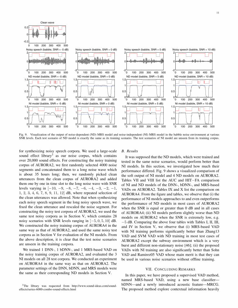
Fig. 9. Visualization of the output of noise-dependent (ND) MRS model and noise-independent (NI) MRS model in the babble noise environment at variousSNR levels. Each test scenario of ND model is exactly the same as its training scenario. The test scenarios of NI model are unseen from its training corpus.

for synthesizing noisy speech corpora. We used a large-scalesound effect library3 as our noise corpus, which containsover 20,000 sound effects. For constructing the noisy trainingcorpus of AURORA2, we first randomly selected 4000 noisesegments and concatenated them to a long noise wave whichis about 35 hours long; then, we randomly picked cleanutterances from the clean corpus of AURORA2 and addedthem one by one in time slot to the long noise wave with SNRlevels varying in [−10, −9, −8, −7, −6, −4, −3, −2, −1,1, 2, 3, 4, 6, 7, 8, 9, 11, 12] dB, where repeated selection ofthe clean utterances was allowed. Note that when synthesizingeach noisy speech segment in the long noisy speech wave, wefixed the clean utterance and rescaled the noise segment. Forconstructing the noisy test corpora of AURORA2, we used thesame test noisy corpora as in Section V, which contains 28noisy scenarios with SNR levels ranging in [−5, 0, 5, 10] dB.We constructed the noisy training corpus of AURORA4 in thesame way as that of AURORA2, and used the same noisy testcorpora as in Section V for evaluation of the NI models. Fromthe above description, it is clear that the test noise scenariosare unseen in the training corpora.

We trained 1 DNN-, 1 bDNN-, and 1 MRS-based VAD onthe noisy training corpus of AURORA2, and evaluated the 3NI models on all 28 test corpora. We conducted an experimenton AURORA4 in the same way as that on AURORA2. Theparameter settings of the DNN, bDNN, and MRS models werethe same as their corresponding ND models in Section V.

3The library was requested from http://www.sound-ideas.com/sound-effects/series-6000-combo-sound-effects.html

B. Results

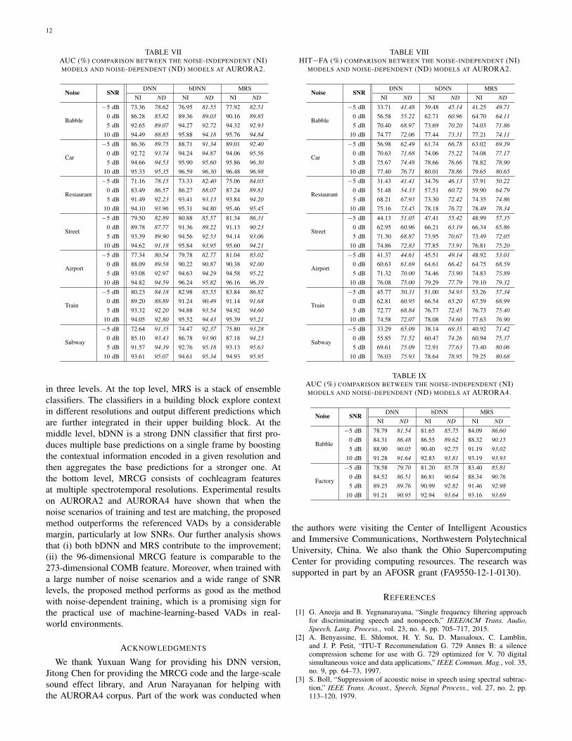
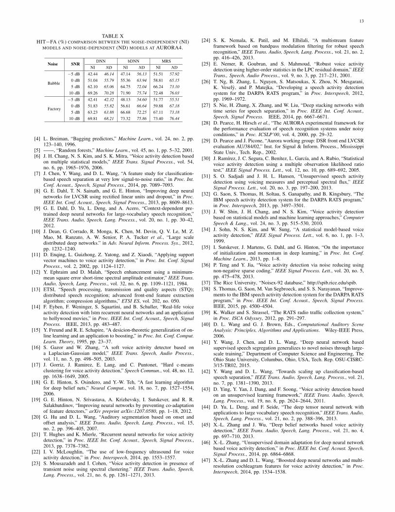
It was supposed that the ND models, which were trained andtested in the same noise scenarios, would perform better thanNI models. In this section, we investigated how much theirperformance differed. Fig. 9 shows a visualized comparison ofthe soft output of NI model and 4 ND models on AURORA2.Tables VII and VIII list the AUC and HIT−FA comparisonof NI and ND models of the DNN-, bDNN-, and MRS-basedVADs on AURORA2. Tables IX and X list the comparison onAURORA4. From the figure and tables, we observe that (i) theperformance of NI models approaches to and even outperformsthe performance of ND models in most cases of AURORA2when the SNR is equal or greater than 0 dB and in all casesof AURORA4; (ii) NI models perform slightly worse than NDmodels on AURORA2 when the SNR is extremely low, e.g.−5 dB. Comparing the above four tables with Tables I, II, III,and IV in Section V, we observe that (i) MRS-based VADwith NI training performs significantly better than Zhang13VAD and SVM VAD with ND training in most test cases ofAURORA2 except the subway environment which is a veryburst and different non-stationary noise [46]; (ii) the proposedVADs with NI training are also significantly better than SohnVAD and Ramirez05 VAD whose main merit is that they canbe used in various noise scenarios without offline training.

VII. CONCLUDING REMARKS

In this paper, we have proposed a supervised VAD method,named MRS-based VAD, using a new base classifier—bDNN—and a newly introduced acoustic feature—MRCG.The proposed method explore contextual information heavily

12

TABLE VIIAUC (%) COMPARISON BETWEEN THE NOISE-INDEPENDENT (NI)MODELS AND NOISE-DEPENDENT (ND) MODELS AT AURORA2.

Noise SNRDNN bDNN MRS

NI ND NI ND NI ND

Babble

−5 dB 73.36 78.62 76.95 81.55 77.92 82.510 dB 86.28 85.82 89.36 89.03 90.16 89.855 dB 92.65 89.07 94.27 92.72 94.32 92.93

10 dB 94.49 88.85 95.88 94.18 95.76 94.84

Car

−5 dB 86.36 89.75 88.71 91.34 89.01 92.400 dB 92.72 93.74 94.24 94.87 94.06 95.565 dB 94.66 94.53 95.90 95.60 95.86 96.30

10 dB 95.33 95.35 96.59 96.30 96.48 96.98

Restaurant

−5 dB 71.16 78.15 73.33 82.40 75.06 84.030 dB 83.49 86.57 86.27 88.07 87.24 89.815 dB 91.49 92.23 93.41 93.13 93.84 94.20

10 dB 94.10 93.96 95.31 94.80 95.46 95.45

Street

−5 dB 79.50 82.89 80.88 85.57 81.34 86.310 dB 89.78 87.77 91.36 89.22 91.13 90.235 dB 93.39 89.90 94.56 92.53 94.14 93.06

10 dB 94.62 91.18 95.84 93.95 95.60 94.21

Airport

−5 dB 77.34 80.54 79.78 82.77 81.04 85.020 dB 88.09 89.58 90.22 90.87 90.38 92.005 dB 93.08 92.97 94.63 94.29 94.58 95.22

10 dB 94.82 94.59 96.24 95.82 96.16 96.39

Train

−5 dB 80.23 84.18 82.98 85.55 83.84 86.820 dB 89.20 88.89 91.24 90.49 91.14 91.685 dB 93.32 92.20 94.88 93.54 94.92 94.60

10 dB 94.05 92.80 95.52 94.43 95.39 95.21

Subway

−5 dB 72.64 91.35 74.47 92.37 75.80 93.280 dB 85.10 93.43 86.78 93.90 87.18 94.235 dB 91.57 94.39 92.76 95.18 93.13 95.63

10 dB 93.61 95.07 94.61 95.34 94.93 95.95

in three levels. At the top level, MRS is a stack of ensembleclassifiers. The classifiers in a building block explore contextin different resolutions and output different predictions whichare further integrated in their upper building block. At themiddle level, bDNN is a strong DNN classifier that first pro-duces multiple base predictions on a single frame by boostingthe contextual information encoded in a given resolution andthen aggregates the base predictions for a stronger one. Atthe bottom level, MRCG consists of cochleagram featuresat multiple spectrotemporal resolutions. Experimental resultson AURORA2 and AURORA4 have shown that when thenoise scenarios of training and test are matching, the proposedmethod outperforms the referenced VADs by a considerablemargin, particularly at low SNRs. Our further analysis showsthat (i) both bDNN and MRS contribute to the improvement;(ii) the 96-dimensional MRCG feature is comparable to the273-dimensional COMB feature. Moreover, when trained witha large number of noise scenarios and a wide range of SNRlevels, the proposed method performs as good as the methodwith noise-dependent training, which is a promising sign forthe practical use of machine-learning-based VADs in real-world environments.

ACKNOWLEDGMENTS

We thank Yuxuan Wang for providing his DNN version,Jitong Chen for providing the MRCG code and the large-scalesound effect library, and Arun Narayanan for helping withthe AURORA4 corpus. Part of the work was conducted when

TABLE VIIIHIT−FA (%) COMPARISON BETWEEN THE NOISE-INDEPENDENT (NI)

MODELS AND NOISE-DEPENDENT (ND) MODELS AT AURORA2.

Noise SNRDNN bDNN MRS

NI ND NI ND NI ND

Babble

−5 dB 33.71 41.48 39.48 45.14 41.25 49.710 dB 56.58 55.22 62.71 60.96 64.70 64.115 dB 70.40 68.97 73.69 70.20 74.03 71.86

10 dB 74.77 72.06 77.44 73.31 77.21 74.11

Car

−5 dB 56.98 62.49 61.74 66.78 63.02 69.390 dB 70.63 71.68 74.06 75.22 74.08 77.175 dB 75.67 74.48 78.66 76.66 78.82 78.90

10 dB 77.40 76.71 80.01 78.86 79.65 80.65

Restaurant

−5 dB 31.43 41.41 34.76 46.13 37.91 50.220 dB 51.48 54.33 57.51 60.72 59.90 64.795 dB 68.21 67.93 73.30 72.42 74.35 74.86

10 dB 75.16 73.45 78.18 76.72 78.49 78.34

Street

−5 dB 44.13 51.05 47.41 55.42 48.99 57.350 dB 62.95 60.96 66.21 63.19 66.34 65.865 dB 71.30 68.87 73.95 70.67 73.49 72.05

10 dB 74.86 72.83 77.85 73.91 76.81 75.20

Airport

−5 dB 41.37 44.61 45.51 49.14 48.92 53.010 dB 60.63 61.69 64.61 66.42 64.75 68.595 dB 71.32 70.00 74.46 73.90 74.83 75.89

10 dB 76.08 75.00 79.29 77.79 79.10 79.32

Train

−5 dB 45.77 50.31 51.00 54.93 53.26 57.340 dB 62.81 60.95 66.54 65.20 67.59 68.995 dB 72.77 68.84 76.77 72.45 76.73 75.40

10 dB 74.58 72.07 78.08 74.60 77.63 76.90

Subway

−5 dB 33.29 65.09 38.14 69.35 40.92 71.420 dB 55.85 71.52 60.47 74.26 60.94 75.375 dB 69.61 75.09 72.91 77.63 73.40 80.06

10 dB 76.03 75.93 78.64 78.95 79.25 80.68

TABLE IXAUC (%) COMPARISON BETWEEN THE NOISE-INDEPENDENT (NI)MODELS AND NOISE-DEPENDENT (ND) MODELS AT AURORA4.

Noise SNRDNN bDNN MRS

NI ND NI ND NI ND

Babble

−5 dB 78.79 81.54 81.65 85.75 84.09 86.600 dB 84.31 86.48 86.55 89.62 88.32 90.155 dB 88.90 90.05 90.40 92.75 91.19 93.02

10 dB 91.28 91.64 92.83 93.81 93.19 93.93

Factory

−5 dB 78.58 79.70 81.20 85.78 83.40 85.810 dB 84.52 86.51 86.81 90.64 88.34 90.765 dB 89.25 89.76 90.99 92.82 91.46 92.98

10 dB 91.21 90.95 92.94 93.64 93.16 93.69

the authors were visiting the Center of Intelligent Acousticsand Immersive Communications, Northwestern PolytechnicalUniversity, China. We also thank the Ohio SupercomputingCenter for providing computing resources. The research wassupported in part by an AFOSR grant (FA9550-12-1-0130).

REFERENCES

[1] G. Aneeja and B. Yegnanarayana, “Single frequency filtering approachfor discriminating speech and nonspeech,” IEEE/ACM Trans. Audio,Speech, Lang. Process., vol. 23, no. 4, pp. 705–717, 2015.

[2] A. Benyassine, E. Shlomot, H. Y. Su, D. Massaloux, C. Lamblin,and J. P. Petit, “ITU-T Recommendation G. 729 Annex B: a silencecompression scheme for use with G. 729 optimized for V. 70 digitalsimultaneous voice and data applications,” IEEE Commun. Mag., vol. 35,no. 9, pp. 64–73, 1997.

[3] S. Boll, “Suppression of acoustic noise in speech using spectral subtrac-tion,” IEEE Trans. Acoust., Speech, Signal Process., vol. 27, no. 2, pp.113–120, 1979.

13

TABLE XHIT−FA (%) COMPARISON BETWEEN THE NOISE-INDEPENDENT (NI)

MODELS AND NOISE-DEPENDENT (ND) MODELS AT AURORA4.

Noise SNRDNN bDNN MRS

NI ND NI ND NI ND

Babble

−5 dB 42.44 46.14 47.14 56.13 51.51 57.920 dB 51.04 55.79 55.36 63.94 58.81 65.155 dB 62.10 65.06 64.75 72.04 66.24 73.10

10 dB 69.26 70.28 71.90 75.74 72.48 76.03

Factory

−5 dB 42.41 42.32 48.13 54.60 51.77 55.510 dB 51.83 55.82 56.61 66.64 59.88 67.185 dB 63.23 63.88 66.68 72.25 67.11 73.18

10 dB 69.81 68.21 73.32 75.86 73.40 76.44

[4] L. Breiman, “Bagging predictors,” Machine Learn., vol. 24, no. 2, pp.123–140, 1996.

[5] ——, “Random forests,” Machine Learn., vol. 45, no. 1, pp. 5–32, 2001.[6] J. H. Chang, N. S. Kim, and S. K. Mitra, “Voice activity detection based

on multiple statistical models,” IEEE Trans. Signal Process., vol. 54,no. 6, pp. 1965–1976, 2006.

[7] J. Chen, Y. Wang, and D. L. Wang, “A feature study for classification-based speech separation at very low signal-to-noise ratio,” in Proc. Int.Conf. Acoust., Speech, Signal Process., 2014, pp. 7089–7093.

[8] G. E. Dahl, T. N. Sainath, and G. E. Hinton, “Improving deep neuralnetworks for LVCSR using rectified linear units and dropout,” in Proc.IEEE Int. Conf. Acoust., Speech, Signal Process., 2013, pp. 8609–8613.

[9] G. E. Dahl, D. Yu, L. Deng, and A. Acero, “Context-dependent pre-trained deep neural networks for large-vocabulary speech recognition,”IEEE Trans. Audio, Speech, Lang. Process., vol. 20, no. 1, pp. 30–42,2012.

[10] J. Dean, G. Corrado, R. Monga, K. Chen, M. Devin, Q. V. Le, M. Z.Mao, M. Ranzato, A. W. Senior, P. A. Tucker et al., “Large scaledistributed deep networks.” in Adv. Neural Inform. Process. Sys., 2012,pp. 1232–1240.

[11] D. Enqing, L. Guizhong, Z. Yatong, and Z. Xiaodi, “Applying supportvector machines to voice activity detection,” in Proc. Int. Conf. SignalProcess., vol. 2, 2002, pp. 1124–1127.

[12] Y. Ephraim and D. Malah, “Speech enhancement using a minimum-mean square error short-time spectral amplitude estimator,” IEEE Trans.Audio, Speech, Lang. Process., vol. 32, no. 6, pp. 1109–1121, 1984.

[13] ETSI, “Speech processing, transmission and quality aspects (STQ);distributed speech recognition; advanced front-end feature extractionalgorithm; compression algorithms,” ETSI ES, vol. 202, no. 050.

[14] F. Eyben, F. Weninger, S. Squartini, and B. Schuller, “Real-life voiceactivity detection with lstm recurrent neural networks and an applicationto hollywood movies,” in Proc. IEEE Int. Conf. Acoust., Speech, SignalProcess. IEEE, 2013, pp. 483–487.

[15] Y. Freund and R. E. Schapire, “A desicion-theoretic generalization of on-line learning and an application to boosting,” in Proc. Int. Conf. Comput.Learn. Theory, 1995, pp. 23–37.

[16] S. Gazor and W. Zhang, “A soft voice activity detector based ona Laplacian-Gaussian model,” IEEE Trans. Speech, Audio Process.,vol. 11, no. 5, pp. 498–505, 2003.

[17] J. Gorriz, J. Ramirez, E. Lang, and C. Puntonet, “Hard c-meansclustering for voice activity detection,” Speech Commun., vol. 48, no. 12,pp. 1638–1649, 2005.

[18] G. E. Hinton, S. Osindero, and Y.-W. Teh, “A fast learning algorithmfor deep belief nets,” Neural Comput., vol. 18, no. 7, pp. 1527–1554,2006.

[19] G. E. Hinton, N. Srivastava, A. Krizhevsky, I. Sutskever, and R. R.Salakhutdinov, “Improving neural networks by preventing co-adaptationof feature detectors,” arXiv preprint arXiv:1207.0580, pp. 1–18, 2012.

[20] G. Hu and D. L. Wang, “Auditory segmentation based on onset andoffset analysis,” IEEE Trans. Audio, Speech, Lang. Process., vol. 15,no. 2, pp. 396–405, 2007.

[21] T. Hughes and K. Mierle, “Recurrent neural networks for voice activitydetection,” in Proc. IEEE Int. Conf. Acoust., Speech, Signal Process.,2013, pp. 7378–7382.

[22] I. V. McLoughlin, “The use of low-frequency ultrasound for voiceactivity detection,” in Proc. Interspeech, 2014, pp. 1553–1557.

[23] S. Mousazadeh and I. Cohen, “Voice activity detection in presence oftransient noise using spectral clustering.” IEEE Trans. Audio, Speech,Lang. Process., vol. 21, no. 6, pp. 1261–1271, 2013.

[24] S. K. Nemala, K. Patil, and M. Elhilali, “A multistream featureframework based on bandpass modulation filtering for robust speechrecognition,” IEEE Trans. Audio, Speech, Lang. Process., vol. 21, no. 2,pp. 416–426, 2013.

[25] E. Nemer, R. Goubran, and S. Mahmoud, “Robust voice activitydetection using higher-order statistics in the LPC residual domain,” IEEETrans., Speech, Audio Process., vol. 9, no. 3, pp. 217–231, 2001.

[26] T. Ng, B. Zhang, L. Nguyen, S. Matsoukas, X. Zhou, N. Mesgarani,K. Vesely, and P. Matejka, “Developing a speech activity detectionsystem for the DARPA RATS program,” in Proc. Interspeech, 2012,pp. 1969–1972.

[27] S. Nie, H. Zhang, X. Zhang, and W. Liu, “Deep stacking networks withtime series for speech separation,” in Proc. IEEE Int. Conf. Acoust.,Speech, Signal Process. IEEE, 2014, pp. 6667–6671.

[28] D. Pearce, H. Hirsch et al., “The AURORA experimental framework forthe performance evaluation of speech recognition systems under noisyconditions,” in Proc. ICSLP’00, vol. 4, 2000, pp. 29–32.

[29] D. Pearce and J. Picone, “Aurora working group: DSR front end LVCSRevaluation AU/384/02,” Inst. for Signal & Inform. Process., MississippiState Univ., Tech. Rep., 2002.

[30] J. Ramírez, J. C. Segura, C. Benítez, L. García, and A. Rubio, “Statisticalvoice activity detection using a multiple observation likelihood ratiotest,” IEEE Signal Process. Lett., vol. 12, no. 10, pp. 689–692, 2005.

[31] S. O. Sadjadi and J. H. L. Hansen, “Unsupervised speech activitydetection using voicing measures and perceptual spectral flux,” IEEESignal Process. Lett., vol. 20, no. 3, pp. 197–200, 2013.

[32] G. Saon, S. Thomas, H. Soltau, S. Ganapathy, and B. Kingsbury, “TheIBM speech activity detection system for the DARPA RATS program,”in Proc. Interspeech, 2013, pp. 3497–3501.

[33] J. W. Shin, J. H. Chang, and N. S. Kim, “Voice activity detectionbased on statistical models and machine learning approaches,” ComputerSpeech & Lang., vol. 24, no. 3, pp. 515–530, 2010.

[34] J. Sohn, N. S. Kim, and W. Sung, “A statistical model-based voiceactivity detection,” IEEE Signal Process. Lett., vol. 6, no. 1, pp. 1–3,1999.

[35] I. Sutskever, J. Martens, G. Dahl, and G. Hinton, “On the importanceof initialization and momentum in deep learning,” in Proc. Int. Conf.Machine Learn., 2013, pp. 1–8.

[36] P. Teng and Y. Jia, “Voice activity detection via noise reducing usingnon-negative sparse coding,” IEEE Signal Process. Lett., vol. 20, no. 5,pp. 475–478, 2013.

[37] The Rice University, “Noisex-92 database,” http://spib.rice.edu/spib.[38] S. Thomas, G. Saon, M. Van Segbroeck, and S. S. Narayanan, “Improve-

ments to the IBM speech activity detection system for the DARPA RATSprogram,” in Proc. IEEE Int. Conf. Acoust., Speech, Signal Process.IEEE, 2015, pp. 4500–4504.

[39] K. Walker and S. Strassel, “The RATS radio traffic collection system,”in Proc. ISCA Odyssey, 2012, pp. 291–297.

[40] D. L. Wang and G. J. Brown, Eds., Computational Auditory SceneAnalysis: Principles, Algorithms and Applications. Wiley-IEEE Press,2006.

[41] Y. Wang, J. Chen, and D. L. Wang, “Deep neural network basedsupervised speech segregation generalizes to novel noises through large-scale training,” Department of Computer Science and Engineering, TheOhio State University, Columbus, Ohio, USA, Tech. Rep. OSU-CISRC-3/15-TR02, 2015.

[42] Y. Wang and D. L. Wang, “Towards scaling up classification-basedspeech separation,” IEEE Trans. Audio, Speech, Lang. Process., vol. 21,no. 7, pp. 1381–1390, 2013.

[43] D. Ying, Y. Yan, J. Dang, and F. Soong, “Voice activity detection basedon an unsupervised learning framework,” IEEE Trans. Audio, Speech,Lang. Process., vol. 19, no. 8, pp. 2624–2644, 2011.

[44] D. Yu, L. Deng, and F. Seide, “The deep tensor neural network withapplications to large vocabulary speech recognition,” IEEE Trans. Audio,Speech, Lang. Process., vol. 21, no. 2, pp. 388–396, 2013.

[45] X.-L. Zhang and J. Wu, “Deep belief networks based voice activitydetection,” IEEE Trans. Audio, Speech, Lang. Process., vol. 21, no. 4,pp. 697–710, 2013.

[46] X.-L. Zhang, “Unsupervised domain adaptation for deep neural networkbased voice activity detection,” in Proc. IEEE Int. Conf. Acoust. Speech,Signal Process., 2014, pp. 6864–6868.

[47] X.-L. Zhang and D. L. Wang, “Boosted deep neural networks and multi-resolution cochleagram features for voice activity detection,” in Proc.Interspeech, 2014, pp. 1534–1538.