Boost Neural Networks by Checkpoints - NeurIPS Proceedings

Boost Neural Networks by Checkpoints

Feng Wang1, Guoyizhe Wei1, Qiao Liu2, Jinxiang Ou1, Xian Wei3, Hairong Lv1,4 ∗1Department of Automation, Tsinghua University

2Department of Statistics, Stanford University3Software Engineering Institute, East China Normal University

4Fuzhou Institute of Data Technologywangf19, wgyz19, [email protected]

[email protected], [email protected]@tsinghua.edu.cn

Abstract

Training multiple deep neural networks (DNNs) and averaging their outputs is asimple way to improve the predictive performance. Nevertheless, the multipliedtraining cost prevents this ensemble method to be practical and efficient. Severalrecent works attempt to save and ensemble the checkpoints of DNNs, which onlyrequires the same computational cost as training a single network. However,these methods suffer from either marginal accuracy improvements due to the lowdiversity of checkpoints or high risk of divergence due to the cyclical learningrates they adopted. In this paper, we propose a novel method to ensemble thecheckpoints, where a boosting scheme is utilized to accelerate model convergenceand maximize the checkpoint diversity. We theoretically prove that it converges byreducing exponential loss. The empirical evaluation also indicates our proposedensemble outperforms single model and existing ensembles in terms of accuracyand efficiency. With the same training budget, our method achieves 4.16% lowererror on Cifar-100 and 6.96% on Tiny-ImageNet with ResNet-110 architecture.Moreover, the adaptive sample weights in our method make it an effective solutionto address the imbalanced class distribution. In the experiments, it yields up to5.02% higher accuracy over single EfficientNet-B0 on the imbalanced datasets.

1 Introduction

DNN ensembles often outperform individual networks in either accuracy or robustness [Hansen andSalamon, 1990, Zhou et al., 2002]. Particularly, in the cases when memory is restricted, or complexmodels are difficult to deploy, ensembling light-weight networks is a good alternative to achievethe performance comparable with deep models. However, since training DNNs is computationallyexpensive, straightforwardly ensembling multiple networks is not acceptable in many real-worldscenarios.

A trick to avoid the exorbitant computational cost is to fully utilize the middle stages — or so-calledcheckpoints — in one training process, instead of training additional networks. Here we refer to thistechnique as Checkpoint Ensemble (CPE). Despite its merit of no additional training computation, anobvious problem of CPE is that the checkpoints sampled from one training process are often verysimilar, which violates the consensus that we desire the base models in an ensemble are accurate butsufficiently diverse. To enhance the diversity, conventional ensembles often differ the base modelsfrom initialization, objective function, or hyperparameters [Breiman, 1996, Freund and Schapire,1997, Zhou et al., 2002], whilst the recent CPE methods try to achieve this goal by cyclical learning∗Corresponding author

35th Conference on Neural Information Processing Systems (NeurIPS 2021).

rate scheduling, with the assumption that the high learning rates are able to force the model jumpingout of the current local optima and visiting others [Huang et al., 2017a, Garipov et al., 2018, Zhanget al., 2020]. However, this effect is not theoretically promised and the cyclically high learning ratesmay incur oscillation or even divergence when training budget is limited.

In this paper, we are motivated to efficiently exploit the middle stages of neural network trainingprocess, obtaining significant performance improvement only at the cost of additional storage,meanwhile the convergence is promised. We design a novel boosting strategy to ensemble thecheckpoints, named CBNN (Checkpoint-Boosted Neural Network). In contrast to cyclical learningrate scheduling, CBNN encourages checkpoints diversity by adaptively reweighting training samples.We analyze its advantages in Section 4 from two aspects. Firstly, CBNN is theoretically provedto be able to reduce the exponential loss, which aims to accelerate model convergence even if thenetwork does not have sufficiently low error rate. Secondly, reweighting training samples is equivalentto tuning the loss function. Therefore, each reweighting process affects the distribution of localminimum on the loss surface, and thereby changes the model’s optimization direction, which explainsthe high checkpoint diversity of CBNN.

Moreover, the adaptability of CBNN makes it effective in tackling with imbalanced datasets (datasetswith imbalanced class distribution). This is due to CBNN’s ability to automatically allocate highweights to the “minority-class” samples, while most commonly used imbalanced learning methodsrequire manually assigning sample weights [Buda et al., 2018, Johnson and Khoshgoftaar, 2019].

2 Related Work

In general, training a collection of neural networks with conventional ensemble strategies such asBagging [Breiman, 1996] and Boosting [Freund and Schapire, 1997] improves the predictors onaccuracy and generalization. For example, [Moghimi et al., 2016] proposed the BoostCNN algorithm,where a finite number of convolutional neural networks (CNNs) are trained based on a boostingstrategy, achieving a superior performance than a single model. Several other strategies such asassigning different samples to the base models [Zhou et al., 2018] or forming ensembles with sharedlow-level layers of neural networks [Zhu et al., 2018] also combine the merits of DNNs and ensemblelearning.

However, these methods are computationally expensive. Alternatively, the “implicit ensemble”techniques [Wan et al., 2013, Srivastava et al., 2014, Huang et al., 2016] or adding random noiselayers [Liu et al., 2018] avoid this problem. Such methods are sometimes seen as regularizationapproaches and can work in coordination with our proposed method. Recently, checkpoint ensemblehas become increasingly popular as it improves the predictors “for free” [Huang et al., 2017a, Zhanget al., 2020]. It was termed as “Horizontal Voting” in [Xie et al., 2013], where the outputs of thecheckpoints are straightforwardly ensembled as the final prediction. However, these checkpointsshare a big intersection of misclassified samples which only bring very marginal improvements.

Therefore, the necessary adjustments to the training process should be made to enhance this diversity.For instance, [Huang et al., 2017a] proposed the Snapshot Ensemble method, adopting the cycliccosine annealing learning rate to enforce the model jumping out of the current local optima. Similarly,another method FGE (Fast Geometric Ensembling) [Garipov et al., 2018] copies a trained modeland further fine-tunes it with a cyclical learning rate, saving checkpoints and ensembling them withthe trained model. More recently, [Zhang et al., 2020] proposed the Snapshot Boosting, where theymodified the learning rate restarting rules and set different sample weights during each training stageto further enhance the diversity of checkpoints. Although there are weights of training samples inSnapshot Boosting, these weights are updated only after the learning rate is restarted and each updatebegins from the initialization. Such updates are not able to significantly affect the loss function, henceit is essentially still a supplementary trick for learning rate scheduling to enhance the diversity.

In this paper, our proposed method aims to tune the loss surface during training by the adaptiveupdate of sample weights, which induces the network to visit multiple different local optima. Ourexperimental results further demonstrate that our method, CBNN significantly promotes the diversityof checkpoints and thereby achieves the highest test accuracy on a number of benchmark datasetswith different state-of-the-art DNNs.

2

Algorithm 1 Checkpoint-Boosted Neural NetworksInput: Number of training samples: n; number of classes: k; deviation rate: η;total training iterations: T ; training iterations per checkpoint: tRequire: Estimated weight of the trained model: λ0Output: An ensemble of networks G1(x), G2(x) . . . (Note thatGj(x) ∈ Rk, Gy

j (x) = 1 ifGj(x)

predicts x belonging to the y-th class, otherwise Gyj (x) = 0)

1: Initialize m← 1 // number of base models2: Uniformly initialize the sample weights:

ωmi ← 1/n, i← 1, ..., n

3: while T −mt > 0 &∑m−1

j=0 λj < 1/η do4: Train model for min(t, T −mt) iterations, get Gm(x)5: Calculate the weighted error rate on training set:

em ←∑n

i=1 ωmiI(Gyim(xi) = 0)

6: Calculate the weight of m-th checkpoint:λm ← log((1− em)/em) + log(k − 1)

7: Update the sample weights:ωm+1,i ← ωmiexp (−ηλmGyi

m(xi)) /∑n

i=1 ωmiexp (−ηλmGyim(xi))

8: Save the checkpoint model at current step.9: m← m+ 1

10: end while11: Train model for max(t, T − (m− 1)t) iterations, get Gm(x).12: Execute step 5 and 6 to calculate λm.13: return G(x) =

∑mj=1 λjGj(x)/

∑mj=1 λj

3 Methodology

3.1 Overview of Checkpoint-Boosted Neural Networks

CBNN aims to accelerate convergence and improve accuracy by saving and ensembling the middlestage models during neural networks training. Its ensemble scheme is inspired by boosting strategies[Freund and Schapire, 1997, Hastie et al., 2009, Mukherjee and Schapire, 2013, Saberian andVasconcelos, 2011], whose main idea is to sequentially train a set of base models with weights fortraining samples. After one base model is trained, it enlarges the weights of the misclassified samples(meanwhile, the weights of the correctly classified samples are reduced after re-normalization).Intuitively, this makes the next base model focus on the samples that were previously misclassified. Intesting phase, the output of boosting is the weighted average of the base models’ predictions, wherethe weights of the models depend on their error rates on the training set.

We put the sample weights on the loss function, which is also reported in many cost-sensitive learningand imbalanced learning methods [Buda et al., 2018, Johnson and Khoshgoftaar, 2019]. In general,given a DNN model p ∈ R|G| and training dataset D = (xi, yi)(|D| = n, xi ∈ Rd, yi ∈ R) where|G| is the number of model parameters and xi, yi denote the features and label of the i-th sample, theweighted loss is formulated as

L =

∑ni=1 ωil(yi, f(xi; p))∑n

i=1 ωi+ r(p), (1)

where l is a loss function (e.g. cross-entropy), f(xi; p) is the output of xi with the model parametersp, and r(p) is the regularization term.

The next section introduces the training procedure of CBNN, including the weight update rules andensemble approaches, which are also summarized in Algorithm 1.

3.2 Training Procedure

We start training a network with initializing the sample weight vector as a uniform distribution:

Ω1 = [ω1,1, ..., ω1,i, ..., ω1,n] , ω1,i =1

n, (2)

3

where n denotes the number of training samples. After every t iterations of training, we updatethe weights of training samples and save a checkpoint, where the weight of the m-th checkpoint iscalculated by

λm = log1− emem

+ log(k − 1), (3)

in which k is the number of classes, and

em =

n∑i=1

ωmiI(Gyim(xi) = 0) (4)

denotes the weighted error rate. Note that Gm(x) ∈ Rk yields a one-hot prediction, i.e., given thepredicted probabilities of x, [py(x)]

ky=1,

Gym(x) =

1, py(x) > py

′(x), ∀y′ 6= y, y′ ∈ [1, k]

0, else. (5)

Briefly, Gym(x) = 1 implies that the model Gm(·) correctly predict the sample x and Gy

m(x) = 0implies the misclassification. According to Equation 3, the weight of a checkpoint increases withthe decrease of its error rate. The term log(k − 1) may be confusing, which is also reported in themulti-class boosting algorithm SAMME [Hastie et al., 2009]. Intuitively, log(k − 1) makes theweight of the base models λm positive, since the error rate in a k-classification task is no less than(k − 1)/k (random choice is able to obtain 1/k accuracy). In fact, the positive λm is essential forconvergence, which will be further discussed in Section 4.1.

We then update the sample weights with the rule that the weight of the sample (xi, yi) increases ifGyi

m(xi) = 0 (i.e., it is misclassified) and decrease if Gyim(xi) = 1, which is in accordance with what

we introduced in Section 3.1. They are updated by

ωm+1,i =ωmi

Zmexp (−ηλmGyi

m(xi)) , (6)

where η is a positive hyperparameter named “deviation rate” and

Zm =

n∑i=1

ωmiexp (−ηλmGyim(xi)) (7)

is a normalization term to keep∑n

i=1 ωmi = 1. It is very important to consider the tradeoff of thedeviation rate η. Here we firstly present an intuitive explanation. In Equation 6, a high deviationrate speeds up the weight update, which seems to help enhance the checkpoint diversity. However,this will lead to very large weights until some specific samples dominate the training set. From gridsearch, we find that setting η = 0.01 achieves significant performance improvement.

In Section 4.1, we are going to prove that CBNN reduces the exponential loss with the conditionM∑

m=1

λm < 1/η, (8)

i.e., the sum of the weights of M − 1 checkpoints λm (m = 1, 2, . . . ,M − 1) and the finally trainedmodel λM should be limited. To meet this condition, therefore, sometimes we need to limit thenumber of checkpoints. However, we cannot acquire λM beforehand. A simple way to address thisissue is to estimate the error rate of the finally trained model and calculate its weight (denoted by λ0)according to Equation 3. For example, if regard that the error rate of the network in a 100-class taskis not less than 0.05, we can estimate λ0 as log(0.95/0.05) + log(99) = 7.54. Then, we stop savingcheckpoints and updating the sample weights until

∑mj=0 λj > 1/η.

The final classifier is an ensemble of the finally trained model GM (X) and M − 1 checkpointsGm(X), m = 1, 2, . . . ,M − 1:

G(x) =

M∑m=1

λmGm(x)/

M∑m=1

λm. (9)

For saving storage and test time, we can select part of the M − 1 checkpoints to ensemble, whileselecting with equal interval is expected to achieve high diversity.

4

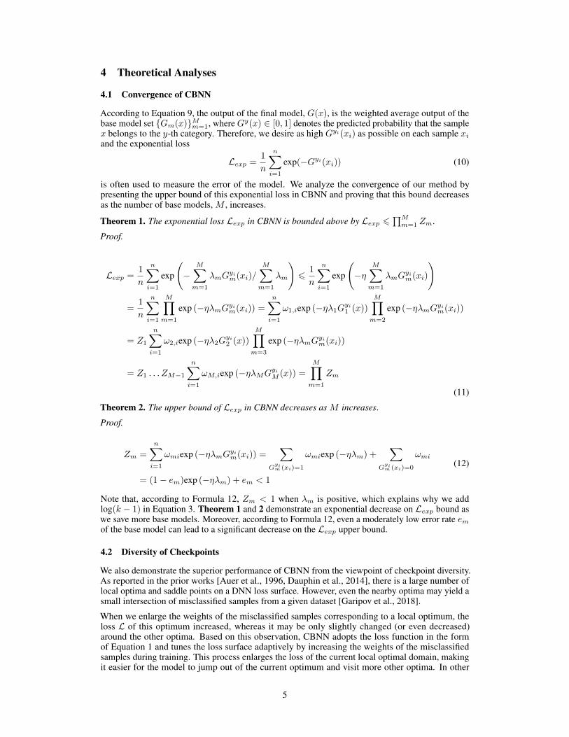
4 Theoretical Analyses

4.1 Convergence of CBNN

According to Equation 9, the output of the final model, G(x), is the weighted average output of thebase model set Gm(x)Mm=1, where Gy(x) ∈ [0, 1] denotes the predicted probability that the samplex belongs to the y-th category. Therefore, we desire as high Gyi(xi) as possible on each sample xiand the exponential loss

Lexp =1

n

n∑i=1

exp(−Gyi(xi)) (10)

is often used to measure the error of the model. We analyze the convergence of our method bypresenting the upper bound of this exponential loss in CBNN and proving that this bound decreasesas the number of base models, M , increases.

Theorem 1. The exponential loss Lexp in CBNN is bounded above by Lexp 6∏M

m=1 Zm.

Proof.

Lexp =1

n

n∑i=1

exp

(−

M∑m=1

λmGyim(xi)/

M∑m=1

λm

)6

1

n

n∑i=1

exp

(−η

M∑m=1

λmGyim(xi)

)

=1

n

n∑i=1

M∏m=1

exp (−ηλmGyim(xi)) =

n∑i=1

ω1,iexp (−ηλ1Gyi

1 (x))

M∏m=2

exp (−ηλmGyim(xi))

= Z1

n∑i=1

ω2,iexp (−ηλ2Gyi

2 (x))

M∏m=3

exp (−ηλmGyim(xi))

= Z1 . . . ZM−1

n∑i=1

ωM,iexp (−ηλMGyi

M (x)) =

M∏m=1

Zm

(11)

Theorem 2. The upper bound of Lexp in CBNN decreases as M increases.

Proof.

Zm =

n∑i=1

ωmiexp (−ηλmGyim(xi)) =

∑G

yim (xi)=1

ωmiexp (−ηλm) +∑

Gyim (xi)=0

ωmi

= (1− em)exp (−ηλm) + em < 1

(12)

Note that, according to Formula 12, Zm < 1 when λm is positive, which explains why we addlog(k − 1) in Equation 3. Theorem 1 and 2 demonstrate an exponential decrease on Lexp bound aswe save more base models. Moreover, according to Formula 12, even a moderately low error rate emof the base model can lead to a significant decrease on the Lexp upper bound.

4.2 Diversity of Checkpoints

We also demonstrate the superior performance of CBNN from the viewpoint of checkpoint diversity.As reported in the prior works [Auer et al., 1996, Dauphin et al., 2014], there is a large number oflocal optima and saddle points on a DNN loss surface. However, even the nearby optima may yield asmall intersection of misclassified samples from a given dataset [Garipov et al., 2018].

When we enlarge the weights of the misclassified samples corresponding to a local optimum, theloss L of this optimum increased, whereas it may be only slightly changed (or even decreased)around the other optima. Based on this observation, CBNN adopts the loss function in the formof Equation 1 and tunes the loss surface adaptively by increasing the weights of the misclassifiedsamples during training. This process enlarges the loss of the current local optimal domain, makingit easier for the model to jump out of the current optimum and visit more other optima. In other

5

40 20 0 20 40 60 80 100 120

10

0

10

20

30

40

50

p1

50-th epoch

<0.5

0.54

0.61

0.72

0.93

1.29

1.93

3.04

>5.0

40 20 0 20 40 60 80 100 120

10

0

10

20

30

40

50

p1

p2

100-th epoch

<0.5

0.54

0.61

0.72

0.93

1.29

1.93

3.04

>5.0

40 20 0 20 40 60 80 100 120

10

0

10

20

30

40

50

p1

p2 p3

150-th epoch

<0.5

0.54

0.61

0.72

0.93

1.29

1.93

3.04

>5.0

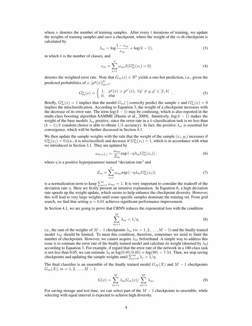
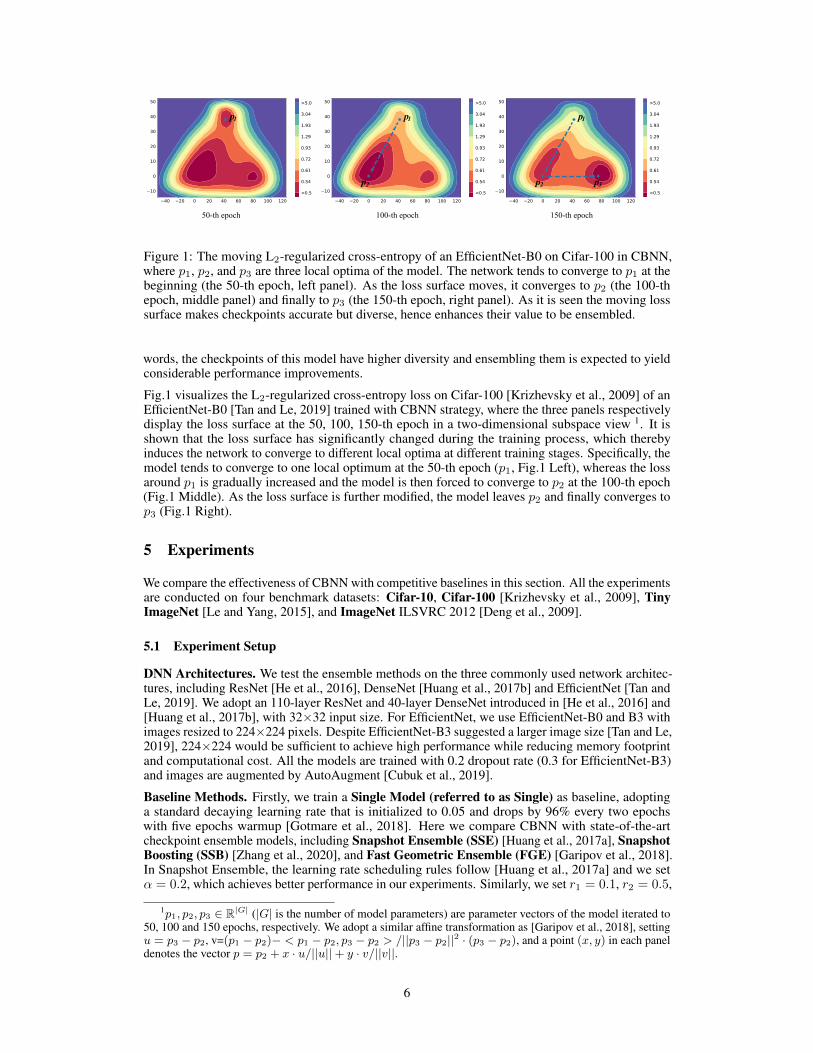
Figure 1: The moving L2-regularized cross-entropy of an EfficientNet-B0 on Cifar-100 in CBNN,where p1, p2, and p3 are three local optima of the model. The network tends to converge to p1 at thebeginning (the 50-th epoch, left panel). As the loss surface moves, it converges to p2 (the 100-thepoch, middle panel) and finally to p3 (the 150-th epoch, right panel). As it is seen the moving losssurface makes checkpoints accurate but diverse, hence enhances their value to be ensembled.

words, the checkpoints of this model have higher diversity and ensembling them is expected to yieldconsiderable performance improvements.

Fig.1 visualizes the L2-regularized cross-entropy loss on Cifar-100 [Krizhevsky et al., 2009] of anEfficientNet-B0 [Tan and Le, 2019] trained with CBNN strategy, where the three panels respectivelydisplay the loss surface at the 50, 100, 150-th epoch in a two-dimensional subspace view 1. It isshown that the loss surface has significantly changed during the training process, which therebyinduces the network to converge to different local optima at different training stages. Specifically, themodel tends to converge to one local optimum at the 50-th epoch (p1, Fig.1 Left), whereas the lossaround p1 is gradually increased and the model is then forced to converge to p2 at the 100-th epoch(Fig.1 Middle). As the loss surface is further modified, the model leaves p2 and finally converges top3 (Fig.1 Right).

5 Experiments

We compare the effectiveness of CBNN with competitive baselines in this section. All the experimentsare conducted on four benchmark datasets: Cifar-10, Cifar-100 [Krizhevsky et al., 2009], TinyImageNet [Le and Yang, 2015], and ImageNet ILSVRC 2012 [Deng et al., 2009].

5.1 Experiment Setup

DNN Architectures. We test the ensemble methods on the three commonly used network architec-tures, including ResNet [He et al., 2016], DenseNet [Huang et al., 2017b] and EfficientNet [Tan andLe, 2019]. We adopt an 110-layer ResNet and 40-layer DenseNet introduced in [He et al., 2016] and[Huang et al., 2017b], with 32×32 input size. For EfficientNet, we use EfficientNet-B0 and B3 withimages resized to 224×224 pixels. Despite EfficientNet-B3 suggested a larger image size [Tan and Le,2019], 224×224 would be sufficient to achieve high performance while reducing memory footprintand computational cost. All the models are trained with 0.2 dropout rate (0.3 for EfficientNet-B3)and images are augmented by AutoAugment [Cubuk et al., 2019].

Baseline Methods. Firstly, we train a Single Model (referred to as Single) as baseline, adoptinga standard decaying learning rate that is initialized to 0.05 and drops by 96% every two epochswith five epochs warmup [Gotmare et al., 2018]. Here we compare CBNN with state-of-the-artcheckpoint ensemble models, including Snapshot Ensemble (SSE) [Huang et al., 2017a], SnapshotBoosting (SSB) [Zhang et al., 2020], and Fast Geometric Ensemble (FGE) [Garipov et al., 2018].In Snapshot Ensemble, the learning rate scheduling rules follow [Huang et al., 2017a] and we setα = 0.2, which achieves better performance in our experiments. Similarly, we set r1 = 0.1, r2 = 0.5,

1p1, p2, p3 ∈ R|G| (|G| is the number of model parameters) are parameter vectors of the model iterated to50, 100 and 150 epochs, respectively. We adopt a similar affine transformation as [Garipov et al., 2018], settingu = p3 − p2, v=(p1 − p2)− < p1 − p2, p3 − p2 > /||p3 − p2||2 · (p3 − p2), and a point (x, y) in each paneldenotes the vector p = p2 + x · u/||u||+ y · v/||v||.

6

Table 1: Error rates (%) on the four datasets with different ensemble methods. We repeat theseexperiments five times to get the average test error and standard deviation. Note that we omit thedeviations of Cifar-10 since they are relatively low and similar. The best results of each model anddataset are bolded.

Model Method Cifar-10 Cifar-100 Tiny-ImageNet ImageNet

ResNet-110

Single 5.63 27.67 ± 0.25 45.10 ± 0.36 -SSE 5.41 24.27 ± 0.26 39.08 ± 0.34 -SSB 5.61 27.09 ± 0.35 43.68 ± 0.49 -FGE 5.50 26.21 ± 0.23 41.16 ± 0.31 -

CBNN 5.25 23.51 ± 0.20 38.14 ± 0.22 -

DenseNet-40

Single 5.13 23.15 ± 0.22 38.24 ± 0.34 -SSE 4.78 21.45 ± 0.29 36.35 ± 0.30 -SSB 5.13 22.59 ± 0.31 37.99 ± 0.44 -FGE 4.82 22.07 ± 0.28 37.72 ± 0.27 -

CBNN 4.78 20.66 ± 0.17 34.28 ± 0.20 -

EfficientNet-B0

Single 3.88 20.87 ± 0.25 34.50 ± 0.35 23.70 ± 0.21SSE 3.56 19.70 ± 0.25 33.02 ± 0.32 23.51 ± 0.24SSB 3.87 20.12 ± 0.41 34.02 ± 0.46 23.75 ± 0.35FGE 3.68 19.58 ± 0.24 32.76 ± 0.31 23.43 ± 0.22

CBNN 3.37 18.06 ± 0.20 31.16 ± 0.26 22.69 ± 0.19

EfficientNet-B3

Single 3.45 17.28 ± 0.22 31.86 ± 0.30 18.30 ± 0.15SSE 3.30 16.84 ± 0.29 31.01 ± 0.31 19.16 ± 0.22SSB 3.43 17.25 ± 0.32 31.49 ± 0.42 19.59 ± 0.34FGE 3.27 16.96 ± 0.24 30.97 ± 0.30 18.68 ± 0.20

CBNN 3.28 16.07 ± 0.13 29.85 ± 0.23 17.55 ± 0.14

p1 = 2 and p2 = 6 for Snapshot Boosting. In Fast Geometric Ensemble (FGE), we train the firstmodel with standard learning rate (the same as Single Model) and the other models with the settingsaccording to [Garipov et al., 2018], and set α1 = 5 · 10−2, α2 = 5 · 10−4 to all the datasets and DNNarchitectures. Our method, CBNN adopts the learning rate used in training Single Model as well, andsetting η = 0.01.

Training Budget. Checkpoint ensembles are designed to save training costs, therefore, to fullyevaluate their effects, the networks should be trained for relatively fewer epochs. In our experiments,we train the DNNs from scratch for 200 epochs on Cifar-10, Cifar-100, Tiny-ImageNet and 300epochs on ImageNet. We save six checkpoint models for SSE and FGE, however, considering thelarge scale and complexity of ImageNet, saving three base models is optimal for SSE and FGE sincemore learning rate cycles may incur divergence. This number of SSB is automatically set by itself.Although our method supports a greater number of base models which leads to higher accuracy, forclear comparison, we only select the same number of checkpoints as SSE and FGE.

5.2 Evaluation of CBNN

The evaluation results are summarized in Table 1, where all the methods listed are at the same trainingcost. It is seen that in most cases, CBNN achieves the lowest error rate on the four tested datasetswith different DNN architectures. Our method achieves a significant error reduction on Cifar-100and Tiny-ImageNet. For instance, with EfficientNet-B0 as the base model, using CBNN decreasesthe mean error rate by 2.81% and 3.34%, on Cifar-100 and Tiny-ImageNet, respectively. In theexperiments, networks tend to converge with a lower speed on ImageNet mainly due to the higherlevel of complexity and a larger number of training images in this dataset. Although we reduce thelearning rate cycles of SSE and FGE (SSB automatically restarts the learning rate), these ensemblemethods only slightly increase the accuracy on ImageNet with EfficientNet-B3.

We quantitatively evaluate the efficiency of ensemble methods by comparing the GPU hours theytake to achieve a certain test accuracy for a given DNN and dataset. For the checkpoint ensemblemethods, the test accuracy is calculated by the ensemble of current model and saved checkpoints. For

7

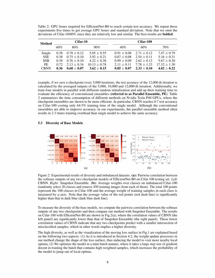
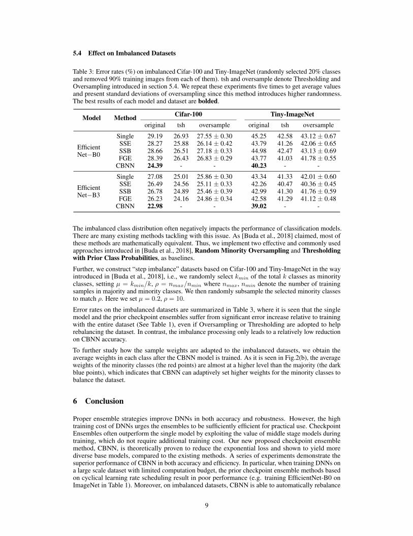
Table 2: GPU hours required for EfficientNet-B0 to reach certain test accuracy. We repeat theseexperiments five times to get average GPU hours and standard deviation. Note that we omit thedeviations of Cifar-10/60% since they are relatively low and similar. The best results are bolded.

Method Cifar-10 Cifar-10060% 80% 90% 40% 60% 70%

Single 0.38 0.78 ± 0.12 5.05 ± 0.55 0.91 ± 0.08 2.71 ± 0.12 7.47 ± 0.79SSE 0.38 0.75 ± 0.10 3.92 ± 0.21 0.87 ± 0.08 2.54 ± 0.11 5.16 ± 0.31SSB 0.39 0.76 ± 0.10 4.22 ± 0.38 0.99 ± 0.09 2.62 ± 0.12 5.67 ± 0.30PE 0.72 2.13 ± 0.34 10.13 ± 0.78 2.11 ± 0.11 7.78 ± 1.23 17.32 ± 1.30

CBNN 0.36 0.68 ± 0.07 3.62 ± 0.15 0.85 ± 0.07 2.33 ± 0.10 4.82 ± 0.22

example, if we save a checkpoint every 5,000 iterations, the test accuracy of the 12,000-th iteration iscalculated by the averaged outputs of the 5,000, 10,000 and 12,000-th iteration. Additionally, wetrain four models in parallel with different random initialization and add up their training time toevaluate the efficiency of conventional ensembles (referred to as Parallel Ensemble, PE). Table2 summarizes the time consumption of different methods on Nvidia Tesla P40 GPUs, where thecheckpoint ensembles are shown to be more efficient. In particular, CBNN reaches 0.7 test accuracyon Cifar-100 costing only 64.5% training time of the single model. Although the conventionalensembles are able to improve accuracy, in our experiments, the parallel ensemble method oftenresults in 2-3 times training overhead than single model to achieve the same accuracy.

5.3 Diversity of Base Models

1 2 3 4 5 6

12

34

56

1 0.68 0.68 0.68 0.68 0.68

0.68 1 0.75 0.75 0.75 0.75

0.68 0.75 1 0.8 0.78 0.79

0.68 0.75 0.8 1 0.82 0.83

0.68 0.75 0.78 0.82 1 0.85

0.68 0.75 0.79 0.83 0.85 10.72

0.78

0.84

0.90

0.96

1 2 3 4 5 6

12

34

56

1 0.86 0.86 0.86 0.86 0.86

0.86 1 0.88 0.87 0.87 0.87

0.86 0.88 1 0.89 0.88 0.87

0.86 0.87 0.89 1 0.9 0.89

0.86 0.87 0.88 0.9 1 0.9

0.86 0.87 0.87 0.89 0.9 10.87

0.90

0.93

0.96

0.99

(a)

0 20 40 60 80 100

0.8

1.0

1.2

1.4

1.6

1.8

2.0

2.2

Ave

rage

Wei

ght

Majority ClassesMinority Classes

(b)

Figure 2: Experimental results of diversity and imbalanced datasets. (a): Pairwise correlation betweenthe softmax outputs of any two checkpoint models of EfficientNet-B0 on Cifar-100 testing set. Left:CBNN. Right: Snapshot Ensemble. (b): Average weights over classes on imbalanced Cifar-100(randomly select 20 classes and remove 450 training images from each of them). The total 100 pointsrepresent the 100 classes in Cifar-100 and the average weight of training samples in each class ismeasured by y-axis. Note that the average value of the red points (red dash line) is significantlyhigher than that in dark blue (dark blue dash line).

To measure the diversity of the base models, we compute the pairwise correlation between the softmaxoutputs of any two checkpoints and then compare our method with Snapshot Ensemble. The resultson Cifar-100 with EfficientNet-B0 are shown in Fig.2(a), where the correlation values of CBNN (theleft panel) are significantly lower than that of Snapshot Ensemble (the right panel). These lowercorrelation values of CBNN indicate that any two checkpoints predict with a smaller intersection ofmisclassified samples, which in other words implies a higher diversity.

The high diversity, as well as the visualization of the moving loss surface in Fig.1 are explained basedon the following two aspects: (1) As it is introduced in Section 4.2, the weight update processes inour method change the shape of the loss surface, thus inducing the model to visit more nearby localoptima; (2) We optimize the model in a mini-batch manner, where it takes a large step size of gradientdecent in training the batch that contains high weighted samples, which increases the probability ofthe model to jump out of local optima.

8

5.4 Effect on Imbalanced Datasets

Table 3: Error rates (%) on imbalanced Cifar-100 and Tiny-ImageNet (randomly selected 20% classesand removed 90% training images from each of them). tsh and oversample denote Thresholding andOversampling introduced in section 5.4. We repeat these experiments five times to get average valuesand present standard deviations of oversampling since this method introduces higher randomness.The best results of each model and dataset are bolded.

Model Method Cifar-100 Tiny-ImageNetoriginal tsh oversample original tsh oversample

EfficientNet−B0

Single 29.19 26.93 27.55 ± 0.30 45.25 42.58 43.12 ± 0.67SSE 28.27 25.88 26.14 ± 0.42 43.79 41.26 42.06 ± 0.65SSB 28.66 26.51 27.18 ± 0.33 44.98 42.47 43.13 ± 0.69FGE 28.39 26.43 26.83 ± 0.29 43.77 41.03 41.78 ± 0.55

CBNN 24.39 - - 40.23 - -

EfficientNet−B3

Single 27.08 25.01 25.86 ± 0.30 43.34 41.33 42.01 ± 0.60SSE 26.49 24.56 25.11 ± 0.33 42.26 40.47 40.36 ± 0.45SSB 26.78 24.89 25.46 ± 0.39 42.99 41.30 41.76 ± 0.59FGE 26.23 24.16 24.86 ± 0.34 42.58 41.29 41.12 ± 0.48

CBNN 22.98 - - 39.02 - -

The imbalanced class distribution often negatively impacts the performance of classification models.There are many existing methods tackling with this issue. As [Buda et al., 2018] claimed, most ofthese methods are mathematically equivalent. Thus, we implement two effective and commonly usedapproaches introduced in [Buda et al., 2018], Random Minority Oversampling and Thresholdingwith Prior Class Probabilities, as baselines.

Further, we construct “step imbalance” datasets based on Cifar-100 and Tiny-ImageNet in the wayintroduced in [Buda et al., 2018], i.e., we randomly select kmin of the total k classes as minorityclasses, setting µ = kmin/k, ρ = nmax/nmin where nmax, nmin denote the number of trainingsamples in majority and minority classes. We then randomly subsample the selected minority classesto match ρ. Here we set µ = 0.2, ρ = 10.

Error rates on the imbalanced datasets are summarized in Table 3, where it is seen that the singlemodel and the prior checkpoint ensembles suffer from significant error increase relative to trainingwith the entire dataset (See Table 1), even if Oversampling or Thresholding are adopted to helprebalancing the dataset. In contrast, the imbalance processing only leads to a relatively low reductionon CBNN accuracy.

To further study how the sample weights are adapted to the imbalanced datasets, we obtain theaverage weights in each class after the CBNN model is trained. As it is seen in Fig.2(b), the averageweights of the minority classes (the red points) are almost at a higher level than the majority (the darkblue points), which indicates that CBNN can adaptively set higher weights for the minority classes tobalance the dataset.

6 Conclusion

Proper ensemble strategies improve DNNs in both accuracy and robustness. However, the hightraining cost of DNNs urges the ensembles to be sufficiently efficient for practical use. CheckpointEnsembles often outperform the single model by exploiting the value of middle stage models duringtraining, which do not require additional training cost. Our new proposed checkpoint ensemblemethod, CBNN, is theoretically proven to reduce the exponential loss and shown to yield morediverse base models, compared to the existing methods. A series of experiments demonstrate thesuperior performance of CBNN in both accuracy and efficiency. In particular, when training DNNs ona large scale dataset with limited computation budget, the prior checkpoint ensemble methods basedon cyclical learning rate scheduling result in poor performance (e.g. training EfficientNet-B0 onImageNet in Table 1). Moreover, on imbalanced datasets, CBNN is able to automatically rebalance

9

the class distribution by adaptive sample weights, which outperforms the commonly used methodswith manually rebalancing approaches.

Acknowledgement

This work was supported by the National Nature Science Foundation of China under Grant No.42050101 and U1736210.

ReferencesPeter Auer, Mark Herbster, and Manfred KK Warmuth. Exponentially many local minima for single

neurons. In Advances in neural information processing systems, pages 316–322, 1996.

Leo Breiman. Bagging predictors. Machine learning, 24(2):123–140, 1996.

Mateusz Buda, Atsuto Maki, and Maciej A Mazurowski. A systematic study of the class imbalanceproblem in convolutional neural networks. Neural Networks, 106:249–259, 2018.

Ekin D Cubuk, Barret Zoph, Dandelion Mane, Vijay Vasudevan, and Quoc V Le. Autoaugment:Learning augmentation strategies from data. In Proceedings of the IEEE conference on computervision and pattern recognition, pages 113–123, 2019.

Yann N Dauphin, Razvan Pascanu, Caglar Gulcehre, Kyunghyun Cho, Surya Ganguli, and YoshuaBengio. Identifying and attacking the saddle point problem in high-dimensional non-convexoptimization. Advances in neural information processing systems, 27:2933–2941, 2014.

Jia Deng, Wei Dong, Richard Socher, Li-Jia Li, Kai Li, and Li Fei-Fei. Imagenet: A large-scalehierarchical image database. In 2009 IEEE conference on computer vision and pattern recognition,pages 248–255. Ieee, 2009.

Yoav Freund and Robert E Schapire. A decision-theoretic generalization of on-line learning and anapplication to boosting. Journal of computer and system sciences, 55(1):119–139, 1997.

Timur Garipov, Pavel Izmailov, Dmitrii Podoprikhin, Dmitry P Vetrov, and Andrew G Wilson. Losssurfaces, mode connectivity, and fast ensembling of dnns. In Advances in Neural InformationProcessing Systems, pages 8789–8798, 2018.

Akhilesh Gotmare, Nitish Shirish Keskar, Caiming Xiong, and Richard Socher. A closer look at deeplearning heuristics: Learning rate restarts, warmup and distillation. In International Conference onLearning Representations, 2018.

Lars Kai Hansen and Peter Salamon. Neural network ensembles. IEEE transactions on patternanalysis and machine intelligence, 12(10):993–1001, 1990.

Trevor Hastie, Saharon Rosset, Ji Zhu, and Hui Zou. Multi-class adaboost. Statistics and its Interface,2(3):349–360, 2009.

Kaiming He, Xiangyu Zhang, Shaoqing Ren, and Jian Sun. Deep residual learning for imagerecognition. In Proceedings of the IEEE conference on computer vision and pattern recognition,pages 770–778, 2016.

Gao Huang, Yu Sun, Zhuang Liu, Daniel Sedra, and Kilian Q Weinberger. Deep networks withstochastic depth. In European conference on computer vision, pages 646–661. Springer, 2016.

Gao Huang, Yixuan Li, Geoff Pleiss, Zhuang Liu, John E Hopcroft, and Kilian Q Weinberger.Snapshot ensembles: Train 1, get m for free. International Conference on Learning Representations,2017a.

Gao Huang, Zhuang Liu, Laurens Van Der Maaten, and Kilian Q Weinberger. Densely connectedconvolutional networks. In Proceedings of the IEEE conference on computer vision and patternrecognition, pages 4700–4708, 2017b.

10

Justin M Johnson and Taghi M Khoshgoftaar. Survey on deep learning with class imbalance. Journalof Big Data, 6(1):1–54, 2019.

Alex Krizhevsky, Geoffrey Hinton, et al. Learning multiple layers of features from tiny images. 2009.

Ya Le and Xuan Yang. Tiny imagenet visual recognition challenge. CS 231N, 7, 2015.

Xuanqing Liu, Minhao Cheng, Huan Zhang, and Cho-Jui Hsieh. Towards robust neural networks viarandom self-ensemble. In Proceedings of the European Conference on Computer Vision (ECCV),pages 369–385, 2018.

Mohammad Moghimi, Serge J Belongie, Mohammad J Saberian, Jian Yang, Nuno Vasconcelos, andLi-Jia Li. Boosted convolutional neural networks. In BMVC, volume 5, page 6, 2016.

Indraneel Mukherjee and Robert E Schapire. A theory of multiclass boosting. Journal of MachineLearning Research, 14(Feb):437–497, 2013.

Mohammad J Saberian and Nuno Vasconcelos. Multiclass boosting: Theory and algorithms. In NIPS,pages 2124–2132, 2011.

Nitish Srivastava, Geoffrey Hinton, Alex Krizhevsky, Ilya Sutskever, and Ruslan Salakhutdinov.Dropout: a simple way to prevent neural networks from overfitting. The journal of machinelearning research, 15(1):1929–1958, 2014.

Mingxing Tan and Quoc Le. Efficientnet: Rethinking model scaling for convolutional neural networks.In International Conference on Machine Learning, pages 6105–6114, 2019.

Li Wan, Matthew Zeiler, Sixin Zhang, Yann Le Cun, and Rob Fergus. Regularization of neuralnetworks using dropconnect. In International conference on machine learning, pages 1058–1066,2013.

Jingjing Xie, Bing Xu, and Zhang Chuang. Horizontal and vertical ensemble with deep representationfor classification. arXiv preprint arXiv:1306.2759, 2013.

Wentao Zhang, Jiawei Jiang, Yingxia Shao, and Bin Cui. Snapshot boosting: a fast ensembleframework for deep neural networks. Science China Information Sciences, 63(1):112102, 2020.

Tianyi Zhou, Shengjie Wang, and Jeff A Bilmes. Diverse ensemble evolution: Curriculum data-modelmarriage. In Advances in Neural Information Processing Systems, pages 5905–5916, 2018.

Zhi-Hua Zhou, Jianxin Wu, and Wei Tang. Ensembling neural networks: many could be better thanall. Artificial intelligence, 137(1-2):239–263, 2002.

Xiatian Zhu, Shaogang Gong, et al. Knowledge distillation by on-the-fly native ensemble. InAdvances in neural information processing systems, pages 7517–7527, 2018.

11