Book

A brief introduction to Madagascar

Jeff Godwin

c© February 11, 2014

Contents

1 Introduction i

2 Users 1

2.1 Introduction to Madagascar . . . . . . . . . . . . . . . . . . . . . . . . . . . 1

2.1.1 Madagascar’s design . . . . . . . . . . . . . . . . . . . . . . . . . . . 1

2.1.2 RSF file format . . . . . . . . . . . . . . . . . . . . . . . . . . . . . . 3

2.1.3 Additional documentation . . . . . . . . . . . . . . . . . . . . . . . . 4

2.2 Command line interface . . . . . . . . . . . . . . . . . . . . . . . . . . . . . 5

2.2.1 Using programs . . . . . . . . . . . . . . . . . . . . . . . . . . . . . . 5

2.2.2 Self-documentation . . . . . . . . . . . . . . . . . . . . . . . . . . . . 6

2.2.3 Piping . . . . . . . . . . . . . . . . . . . . . . . . . . . . . . . . . . . 7

2.2.4 Interacting with files from the command line . . . . . . . . . . . . . 8

2.3 Plotting . . . . . . . . . . . . . . . . . . . . . . . . . . . . . . . . . . . . . . 9

2.3.1 VPLOT . . . . . . . . . . . . . . . . . . . . . . . . . . . . . . . . . . 9

2.3.2 Creating plots . . . . . . . . . . . . . . . . . . . . . . . . . . . . . . 9

2.3.3 Visualizing plots . . . . . . . . . . . . . . . . . . . . . . . . . . . . . 10

2.3.4 Converting VPLOT to other formats . . . . . . . . . . . . . . . . . . 10

2.4 Scripting Madagascar . . . . . . . . . . . . . . . . . . . . . . . . . . . . . . 11

2.4.1 Shell scripting . . . . . . . . . . . . . . . . . . . . . . . . . . . . . . 12

2.4.2 SCons . . . . . . . . . . . . . . . . . . . . . . . . . . . . . . . . . . . 12

2.4.3 SConstructs and commands . . . . . . . . . . . . . . . . . . . . . . . 12

2.4.4 Creating an SConstruct . . . . . . . . . . . . . . . . . . . . . . . . . 14

2.4.5 Executing SCons . . . . . . . . . . . . . . . . . . . . . . . . . . . . . 15

2.4.6 Common errors in SConstructs . . . . . . . . . . . . . . . . . . . . . 16

2.4.7 Additional SCons commands . . . . . . . . . . . . . . . . . . . . . . 17

CONTENTS

2.4.8 Final thoughts . . . . . . . . . . . . . . . . . . . . . . . . . . . . . . 19

2.5 Advanced SCons . . . . . . . . . . . . . . . . . . . . . . . . . . . . . . . . . 19

2.5.1 Multiple input files . . . . . . . . . . . . . . . . . . . . . . . . . . . . 19

2.5.2 Multiple outputs . . . . . . . . . . . . . . . . . . . . . . . . . . . . . 22

2.5.3 None inputs . . . . . . . . . . . . . . . . . . . . . . . . . . . . . . . . 22

2.5.4 Toggling standard input and standard output . . . . . . . . . . . . . 22

2.5.5 Plots with a different output name . . . . . . . . . . . . . . . . . . . 22

2.6 Integrating Python with SCons . . . . . . . . . . . . . . . . . . . . . . . . . 23

2.6.1 A forewarning . . . . . . . . . . . . . . . . . . . . . . . . . . . . . . . 23

2.6.2 Variables . . . . . . . . . . . . . . . . . . . . . . . . . . . . . . . . . 23

2.6.3 String substitution . . . . . . . . . . . . . . . . . . . . . . . . . . . . 24

2.6.4 Dictionaries . . . . . . . . . . . . . . . . . . . . . . . . . . . . . . . . 24

2.6.5 Loops . . . . . . . . . . . . . . . . . . . . . . . . . . . . . . . . . . . 25

2.6.6 Functions . . . . . . . . . . . . . . . . . . . . . . . . . . . . . . . . . 26

2.6.7 Modules . . . . . . . . . . . . . . . . . . . . . . . . . . . . . . . . . . 27

2.6.8 Classes . . . . . . . . . . . . . . . . . . . . . . . . . . . . . . . . . . 27

2.6.9 Final thoughts . . . . . . . . . . . . . . . . . . . . . . . . . . . . . . 27

3 Authors 29

3.1 Getting started . . . . . . . . . . . . . . . . . . . . . . . . . . . . . . . . . . 29

3.1.1 Downloading LATEX . . . . . . . . . . . . . . . . . . . . . . . . . . . 29

3.1.2 Downloading SEGTeX . . . . . . . . . . . . . . . . . . . . . . . . . . 30

3.1.3 Updating your LATEXinstall . . . . . . . . . . . . . . . . . . . . . . . 30

3.2 Papers . . . . . . . . . . . . . . . . . . . . . . . . . . . . . . . . . . . . . . . 31

3.2.1 Paper organization . . . . . . . . . . . . . . . . . . . . . . . . . . . . 31

3.2.2 Locking figures . . . . . . . . . . . . . . . . . . . . . . . . . . . . . . 31

3.2.3 Tex files . . . . . . . . . . . . . . . . . . . . . . . . . . . . . . . . . . 32

3.2.4 Paper SConstructs . . . . . . . . . . . . . . . . . . . . . . . . . . . . 33

3.2.5 Templates . . . . . . . . . . . . . . . . . . . . . . . . . . . . . . . . . 34

3.2.6 Handouts . . . . . . . . . . . . . . . . . . . . . . . . . . . . . . . . . 34

3.2.7 EAGE abstracts . . . . . . . . . . . . . . . . . . . . . . . . . . . . . 34

3.2.8 SEG abstracts . . . . . . . . . . . . . . . . . . . . . . . . . . . . . . 34

CONTENTS

3.2.9 Geophysics manuscripts . . . . . . . . . . . . . . . . . . . . . . . . . 34

3.2.10 CWP reports . . . . . . . . . . . . . . . . . . . . . . . . . . . . . . . 35

3.3 Slides . . . . . . . . . . . . . . . . . . . . . . . . . . . . . . . . . . . . . . . 35

3.4 Theses . . . . . . . . . . . . . . . . . . . . . . . . . . . . . . . . . . . . . . . 35

3.5 Books . . . . . . . . . . . . . . . . . . . . . . . . . . . . . . . . . . . . . . . 35

3.6 Adding/modifying LATEXclass files . . . . . . . . . . . . . . . . . . . . . . . 35

3.7 Using the default LATEXclass files . . . . . . . . . . . . . . . . . . . . . . . . 35

4 Developers 37

4.1 Core design . . . . . . . . . . . . . . . . . . . . . . . . . . . . . . . . . . . . 37

4.2 Core API . . . . . . . . . . . . . . . . . . . . . . . . . . . . . . . . . . . . . 38

4.3 Program design philosophy . . . . . . . . . . . . . . . . . . . . . . . . . . . 38

4.4 Final thoughts . . . . . . . . . . . . . . . . . . . . . . . . . . . . . . . . . . 38

4.5 Further information . . . . . . . . . . . . . . . . . . . . . . . . . . . . . . . 39

5 Quick reference 41

5.1 Environmental variables . . . . . . . . . . . . . . . . . . . . . . . . . . . . . 41

5.2 Command line usage . . . . . . . . . . . . . . . . . . . . . . . . . . . . . . . 41

5.3 Some useful programs . . . . . . . . . . . . . . . . . . . . . . . . . . . . . . 42

5.4 SCons commands . . . . . . . . . . . . . . . . . . . . . . . . . . . . . . . . . 42

CONTENTS

Chapter 1

Introduction

Welcome to a brief introduction to Madagascar. The purpose of this document is to teachnew users how to use the powerful tools in Madagascar to: process data, produce documentsand build your own Madagascar programs.

To gradually introduce you to Madagascar, we have created a series of tutorials that aretargeted to distinct audiences and designed to make you an experienced Madagascar userin a short-time period. The tutorials are divided by interest into three main categories:

Users learn about Madagascar, how to use the processing programs, and build scripts.

Authors learn how to build reproducible documents using Madagascar.

Developers build new Madagascar programs that add additional functionality to Mada-gascar.

Each tutorial is designed to be completed in a short period of time. Additionally, eachtutorial has hands-on examples that you should be able to reproduce on your computer asyou go along with the tutorials. Most tutorials will use scripts that you can edit, modify, orplay with to further gain experience and understanding. By the end of the tutorial series,you should be able to use all of the tools inside of Madagascar. Please note that this tutorialseries does not explicitly show you how to process certain types of data, or how to performcommon data processing operations (e.g. CMP semblance picking, time migration,etc.).Additional tutorials on those specific subjects will be added over time. The purpose of thisdocument is simply to familiarize you with the Madagascar framework in a general sense.

Before you go on, here are some notes on notation:

• important names, or program names are usually bold in the text. For example: sfwin-dow

• code snippets are always in the following formatting:

sfwindow

i

ii CHAPTER 1. INTRODUCTION

Chapter 2

Users

The Users tutorials demonstrate how to use the Madagascar framework to create, processand visualize data, and to create reproducible scripts for processing data. The main goalsof the Users tutorials are to learn about:

• the Madagascar framework,

• the RSF file format,

• the command line interface,

• how to interact with files on the command line,

• commonly used programs,

• how to make plots in Madagascar,

• how to make reproducible scripts,

• how to use SCons and Python,

• how to visualize your data.

By the end of this tutorial group you should be able to fully use all of Madagascar’s built-intools for data processing and scripting. By using these tools, you’ll be able to process dataranging from tens of megabytes to tens of terabytes in a reproducible fashion.

2.1 Introduction to Madagascar

To begin, let’s talk about the core principles of Madagascar, and the RSF file format.

2.1.1 Madagascar’s design

There are a few layers to Madagascar. At the bottom-most layer, is the RSF file format,which is a common exchange format that all Madagascar programs use. Non-Madagascar

1

2 CHAPTER 2. USERS

LaTeX

?

Python

?

SCons

�����

����

VPLOT

HHHHH

HHHj

HHHHH

HHHj

�����

����

Programs

RSF file format

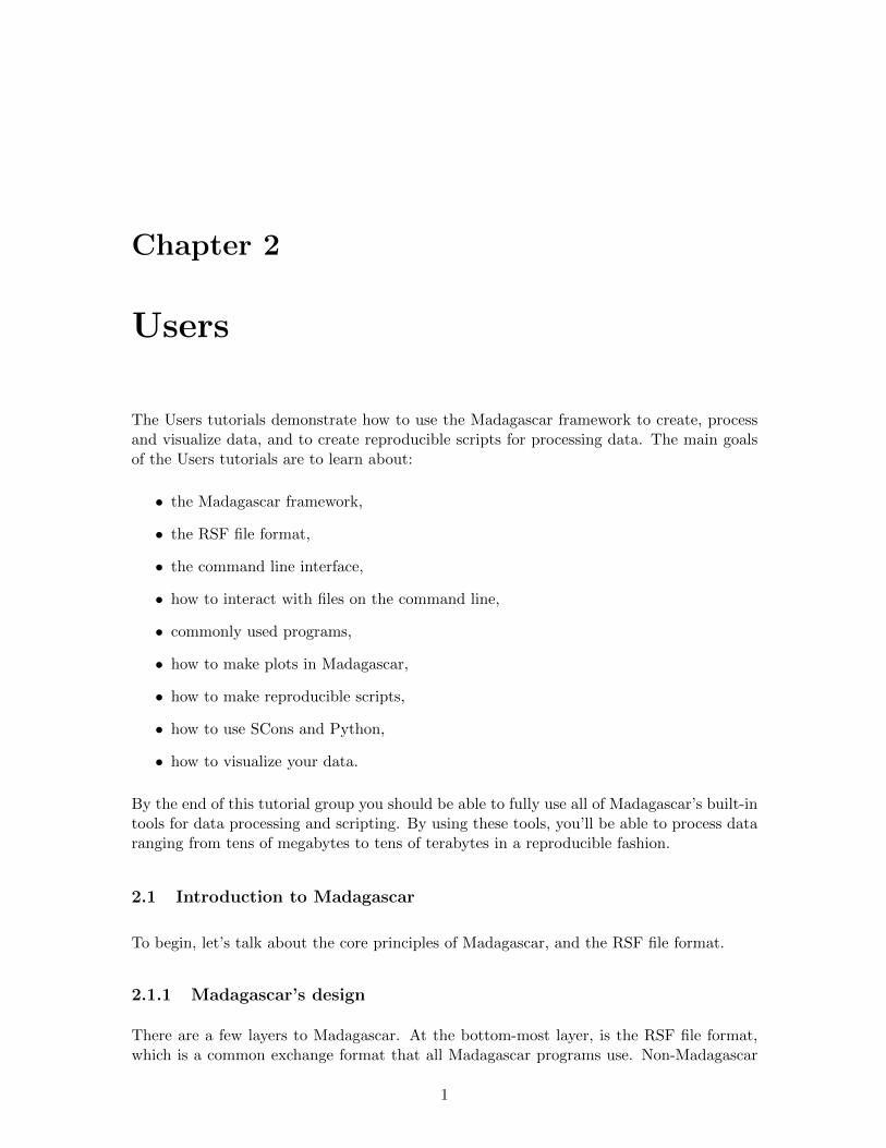
Figure 2.1: The hierarchy of Madagascar. Fundamentally, everything builds off of the RSFfile format. As you go up the chain the complexity level may increase, but the capabilitiesof the processing package increase as well.

2.1. INTRODUCTION TO MADAGASCAR 3

programs can also read/write to and from RSF because it is an open exchange format.The next level of Madagascar contains the actual Madagascar programs that manipulateRSF files to process data. Concurrent to this level is the VPLOT graphics library whichallows users to plot and visualize RSF files. The scripting utilities in Python and SConsare up another level from the core programs. These scripting utilities allow users to makepowerful scripts that can perform even the most advanced data processing tasks. Thelast level includes support for LaTeX which allows you to make documents combining thefeatures of Madagascar with the powerful typesetting of LaTeX. Throughout the course ofthese tutorials, we will examine all of these components, and demonstrate how they canbe used individually, as well as together. When combined, the individual components ofMadagascar allow us to: conduct experiments, process data, visualize our results, makereproducible scripts that can be shared with others, and write papers to document ourexperiments. Thus, Madagascar provides a fully integrated research environment.

2.1.2 RSF file format

As previously mentioned, the lowest level of Madagascar is the RSF file format, which isthe format used to exchange information between Madagascar programs. Conceptually,the RSF file format is one of the easiest to understand, as RSF files are simply regularlysampled hypercubes of information. For reference, a hypercube is a hyper dimensional cube(or array) that can best be visualized as an N -dimensional array, where N is between 1 and9 in Madagascar.

RSF hypercubes are defined by two files, the header file and the binary file. The headerfile contains information about the dimensionality of the hypercube as well as the datacontained within the hypercube. Information contained in the header file may include thefollowing:

• number of elements on all axes,

• the origin of the axes,

• the sampling interval of elements on the axes,

• the type of elements in the axes (i.e. float, integer),

• the size of the elements (e.g. single or double precision),

• and the location of the actual binary file.

Since we often want to view this information about files without deciphering it, we storethe header file as an ASCII text file in the local directory, usually with the suffix .rsf. Atany time, you can view or edit the contents of the header files using a text editor such asgedit, VIM, or Emacs.

The binary file is a file stored remotely (i.e. in a separate directory) that contains theactual hypercube data. Because the hypercube data can be very large (10s of GB or TB)we usually store the binary files in a remote directory with the suffix .rsf@. The remotedirectory is specified by the user using the DATAPATH environmental variable. The

4 CHAPTER 2. USERS

Header

?

Binary

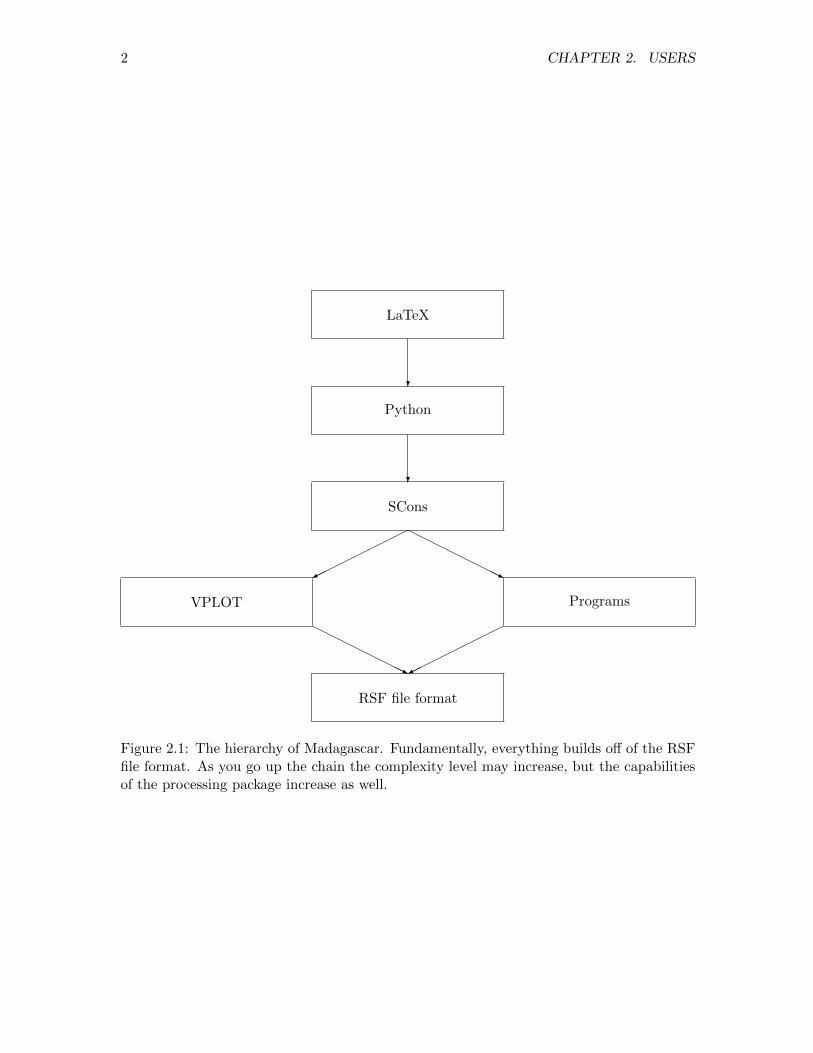
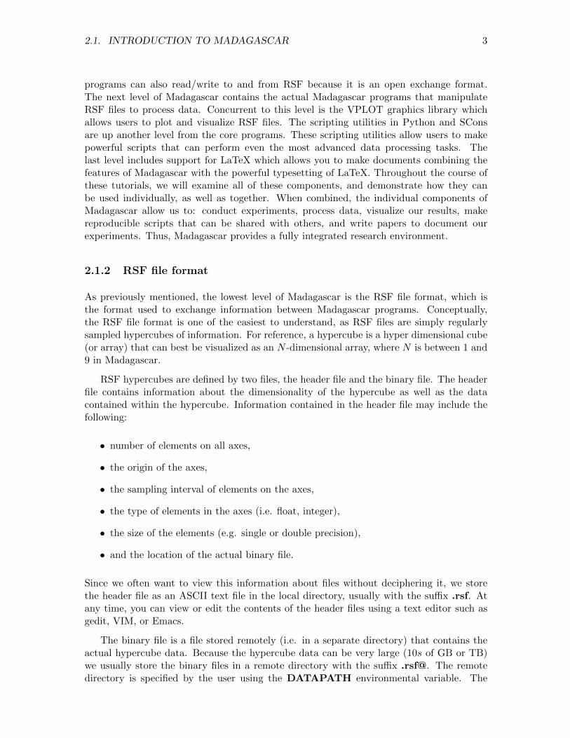
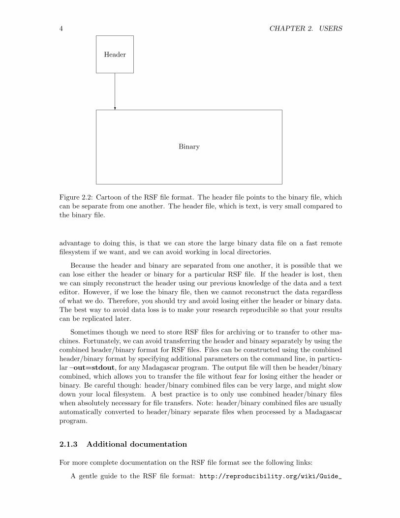
Figure 2.2: Cartoon of the RSF file format. The header file points to the binary file, whichcan be separate from one another. The header file, which is text, is very small compared tothe binary file.

advantage to doing this, is that we can store the large binary data file on a fast remotefilesystem if we want, and we can avoid working in local directories.

Because the header and binary are separated from one another, it is possible that wecan lose either the header or binary for a particular RSF file. If the header is lost, thenwe can simply reconstruct the header using our previous knowledge of the data and a texteditor. However, if we lose the binary file, then we cannot reconstruct the data regardlessof what we do. Therefore, you should try and avoid losing either the header or binary data.The best way to avoid data loss is to make your research reproducible so that your resultscan be replicated later.

Sometimes though we need to store RSF files for archiving or to transfer to other ma-chines. Fortunately, we can avoid transferring the header and binary separately by using thecombined header/binary format for RSF files. Files can be constructed using the combinedheader/binary format by specifying additional parameters on the command line, in particu-lar –out=stdout, for any Madagascar program. The output file will then be header/binarycombined, which allows you to transfer the file without fear for losing either the header orbinary. Be careful though: header/binary combined files can be very large, and might slowdown your local filesystem. A best practice is to only use combined header/binary fileswhen absolutely necessary for file transfers. Note: header/binary combined files are usuallyautomatically converted to header/binary separate files when processed by a Madagascarprogram.

2.1.3 Additional documentation

For more complete documentation on the RSF file format see the following links:

A gentle guide to the RSF file format: http://reproducibility.org/wiki/Guide_

2.2. COMMAND LINE INTERFACE 5

to_RSF_file_format

A detailed guide to the RSF file format: http://reproducibility.org/wiki/RSF_

Comprehensive_Description

2.2 Command line interface

Madagascar was designed initially to be used from the command line. Programmers createMadagascar programs (prefixed with the sf designation) that read and write Madagascarfiles. These programs are designed to be as general as possible, so that each one couldoperate on any dataset in RSF format, provided you also supply the correct parametersand have the right type of data for the program.

2.2.1 Using programs

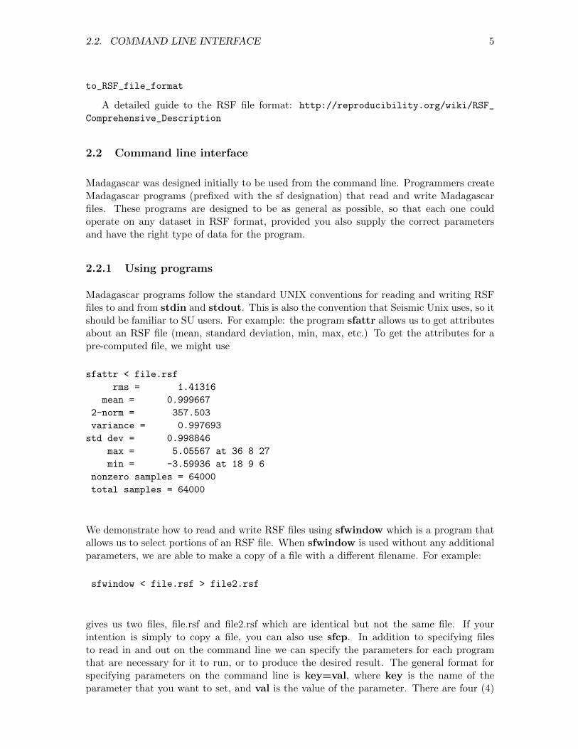
Madagascar programs follow the standard UNIX conventions for reading and writing RSFfiles to and from stdin and stdout. This is also the convention that Seismic Unix uses, so itshould be familiar to SU users. For example: the program sfattr allows us to get attributesabout an RSF file (mean, standard deviation, min, max, etc.) To get the attributes for apre-computed file, we might use

sfattr < file.rsf

rms = 1.41316

mean = 0.999667

2-norm = 357.503

variance = 0.997693

std dev = 0.998846

max = 5.05567 at 36 8 27

min = -3.59936 at 18 9 6

nonzero samples = 64000

total samples = 64000

We demonstrate how to read and write RSF files using sfwindow which is a program thatallows us to select portions of an RSF file. When sfwindow is used without any additionalparameters, we are able to make a copy of a file with a different filename. For example:

sfwindow < file.rsf > file2.rsf

gives us two files, file.rsf and file2.rsf which are identical but not the same file. If yourintention is simply to copy a file, you can also use sfcp. In addition to specifying filesto read in and out on the command line we can specify the parameters for each programthat are necessary for it to run, or to produce the desired result. The general format forspecifying parameters on the command line is key=val, where key is the name of theparameter that you want to set, and val is the value of the parameter. There are four (4)

6 CHAPTER 2. USERS

types of values that are acceptable: integers, floating point numbers, booleans, or strings.Going back to the window program, we can specify the number of traces or pieces of thefile that we want to keep like:

sfwindow < file.rsf n1=10 > file-win.rsf

2.2.2 Self-documentation

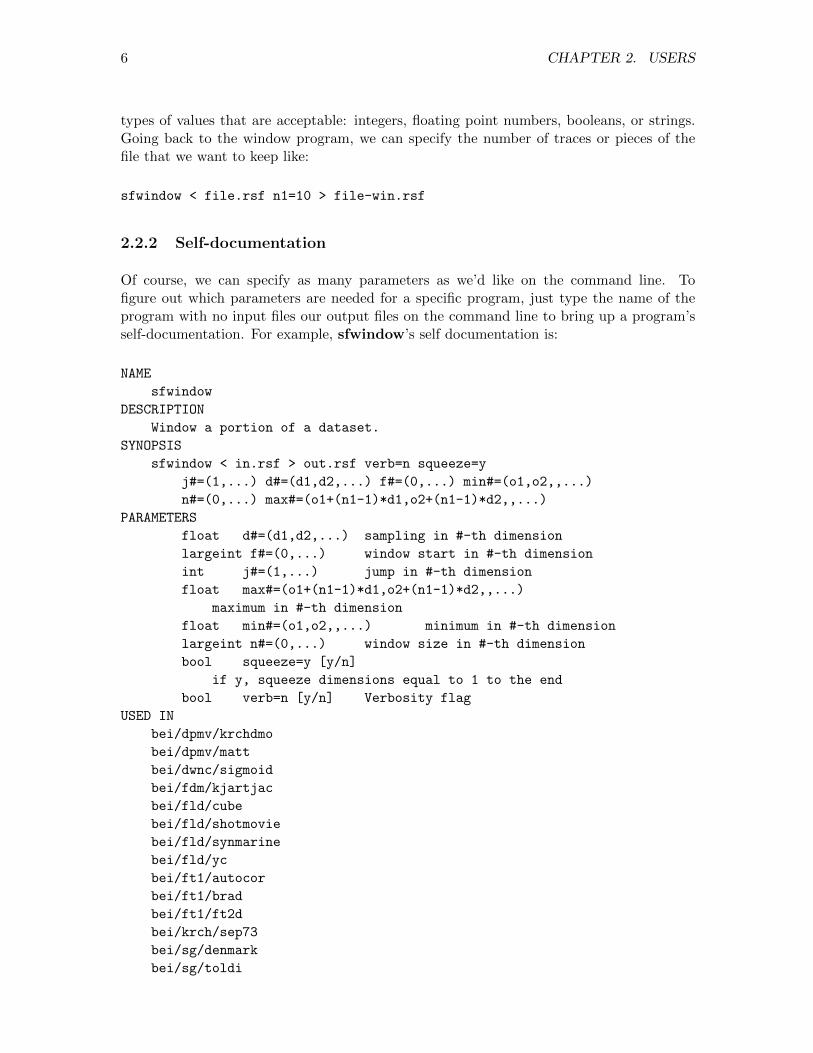
Of course, we can specify as many parameters as we’d like on the command line. Tofigure out which parameters are needed for a specific program, just type the name of theprogram with no input files our output files on the command line to bring up a program’sself-documentation. For example, sfwindow’s self documentation is:

NAME

sfwindow

DESCRIPTION

Window a portion of a dataset.

SYNOPSIS

sfwindow < in.rsf > out.rsf verb=n squeeze=y

j#=(1,...) d#=(d1,d2,...) f#=(0,...) min#=(o1,o2,,...)

n#=(0,...) max#=(o1+(n1-1)*d1,o2+(n1-1)*d2,,...)

PARAMETERS

float d#=(d1,d2,...) sampling in #-th dimension

largeint f#=(0,...) window start in #-th dimension

int j#=(1,...) jump in #-th dimension

float max#=(o1+(n1-1)*d1,o2+(n1-1)*d2,,...)

maximum in #-th dimension

float min#=(o1,o2,,...) minimum in #-th dimension

largeint n#=(0,...) window size in #-th dimension

bool squeeze=y [y/n]

if y, squeeze dimensions equal to 1 to the end

bool verb=n [y/n] Verbosity flag

USED IN

bei/dpmv/krchdmo

bei/dpmv/matt

bei/dwnc/sigmoid

bei/fdm/kjartjac

bei/fld/cube

bei/fld/shotmovie

bei/fld/synmarine

bei/fld/yc

bei/ft1/autocor

bei/ft1/brad

bei/ft1/ft2d

bei/krch/sep73

bei/sg/denmark

bei/sg/toldi

2.2. COMMAND LINE INTERFACE 7

bei/trimo/mod

bei/trimo/subsamp

bei/vela/stretch

bei/vela/vscan

bei/wvs/head

bei/wvs/vscan

cwp/geo2006TimeShiftImagingCondition/flat

cwp/geo2006TimeShiftImagingCondition/icomp

cwp/geo2006TimeShiftImagingCondition/zicig

cwp/geo2007StereographicImagingCondition/flat4

cwp/geo2007StereographicImagingCondition/gaus1

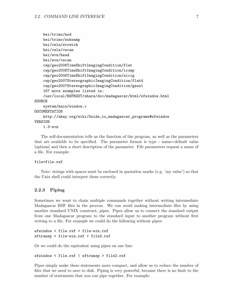
167 more examples listed in:

/usr/local/RSFROOT/share/doc/madagascar/html/sfwindow.html

SOURCE

system/main/window.c

DOCUMENTATION

http://ahay.org/wiki/Guide_to_madagascar_programs#sfwindow

VERSION

1.3-svn

The self-documentation tells us the function of the program, as well as the parametersthat are available to be specified. The parameter format is type - name=default value[options] and then a short description of the parameter. File parameters request a name ofa file. For example:

file=file.rsf

Note: strings with spaces must be enclosed in quotation marks (e.g. ’my value’) so thatthe Unix shell could interpret them correctly.

2.2.3 Piping

Sometimes we want to chain multiple commands together without writing intermediateMadagascar RSF files in the process. We can avoid making intermediate files by usinganother standard UNIX construct, pipes. Pipes allow us to connect the standard outputfrom one Madagascar program to the standard input to another program without firstwriting to a file. For example we could do the following without pipes:

sfwindow < file.rsf > file-win.rsf

sftransp < file-win.rsf > file2.rsf

Or we could do the equivalent using pipes on one line:

sfwindow < file.rsf | sftransp > file2.rsf

Pipes simply make these statements more compact, and allow us to reduce the number offiles that we need to save to disk. Piping is very powerful, because there is no limit to thenumber of statements that you can pipe together. For example:

8 CHAPTER 2. USERS

sfwindow < file.rsf | sftransp | sfnoise var=1 > file2.rsf

If you’re using multiple programs, and do not want to save the intermediate files, then pipeswill greatly reduce the number of files that you have to keep track of.

2.2.4 Interacting with files from the command line

Ultimately though, 95% of your time using Madagascar on the command line will be toinspect and view files that are output by your scripts. Some of the key commands that areused to interact with files on the command line are:

• sfin, used to get header information,

• sfattr, used to get file attributes,

• sfwindow, used to select portions of RSF files,

• and sftransp, used to reorder files.

Here are detailed usage examples and explanations of what the above programs do:

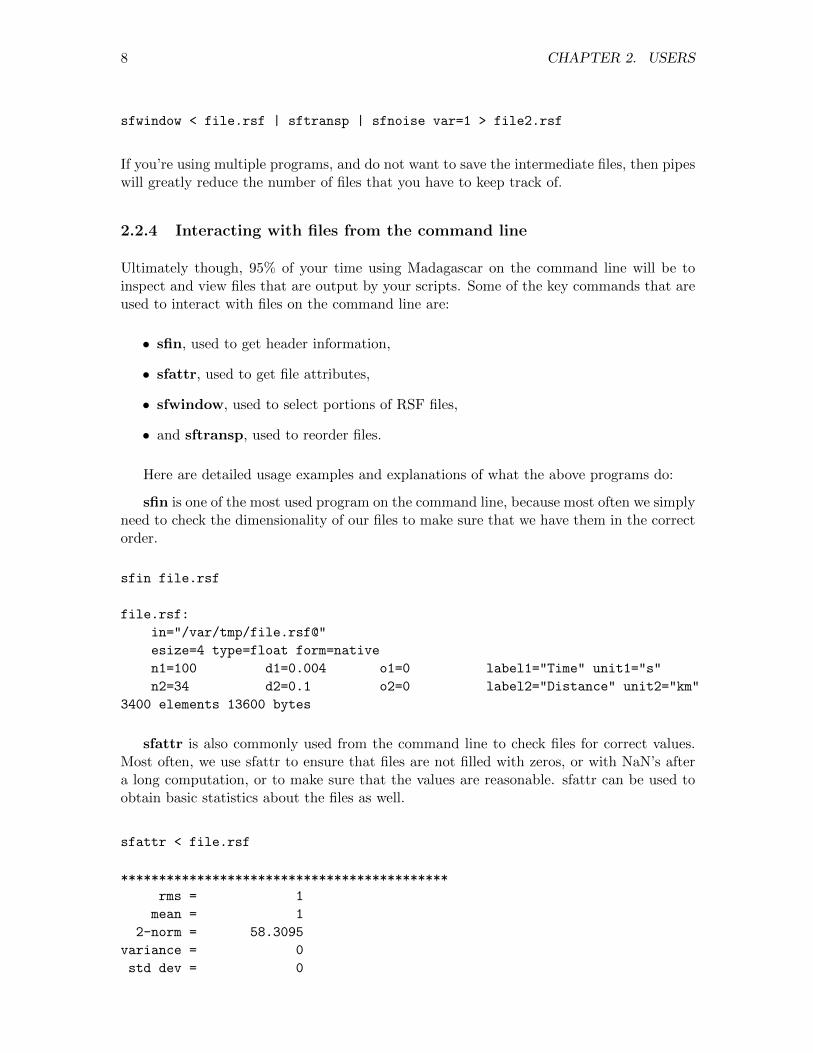
sfin is one of the most used program on the command line, because most often we simplyneed to check the dimensionality of our files to make sure that we have them in the correctorder.

sfin file.rsf

file.rsf:

in="/var/tmp/file.rsf@"

esize=4 type=float form=native

n1=100 d1=0.004 o1=0 label1="Time" unit1="s"

n2=34 d2=0.1 o2=0 label2="Distance" unit2="km"

3400 elements 13600 bytes

sfattr is also commonly used from the command line to check files for correct values.Most often, we use sfattr to ensure that files are not filled with zeros, or with NaN’s aftera long computation, or to make sure that the values are reasonable. sfattr can be used toobtain basic statistics about the files as well.

sfattr < file.rsf

*******************************************

rms = 1

mean = 1

2-norm = 58.3095

variance = 0

std dev = 0

2.3. PLOTTING 9

max = 1 at 1 1

min = 1 at 1 1

nonzero samples = 3400

total samples = 3400

*******************************************

sfwindow is used to select subsets of the data contained in an RSF file for computationelsewhere. Typically, you specify the data subset you want to keep using, the n, j, and fparameters which specify the number of indices in the arrays to keep, the jump in indices,and the first index to keep from the file in the respective dimension. For example if wewant to keep the 15th-30th time samples from the first axis in file.rsf, we might use thefollowing command:

sfwindow < file.rsf f1=15 n1=15 j1=1 > file-win.rsf

sftransp is used to reorder RSF files for other programs to be used. For example:

sftransp < file.rsf plane=12 > file-transposed.rsf

swaps the first and second axes, so that now the first axis is distance and the second axisis time.

For more information about commonly used Madagascar programs please see the guideto Madagascar programs: http://reproducibility.org/wiki/Guide_to_madagascar_

programs.

2.3 Plotting

VPLOT provides a method for making plots that are small in size, aesthetically pleasing, andeasily compatible with Latex for rapid creation of productio-quality images in Madagascar.

2.3.1 VPLOT

The VPLOT file format (.vpl suffix) is a self-contained binary data format that describesin vector format how to draw a plot on the screen or a page using an interpreter. SinceVPLOT is not a standard imaging format, VPLOT files must be viewed with interpreterprograms which, for historical reasons, are called pens. Each pen interfaces VPLOT with athird-party graphing library such as X11, plplot, opengl, and others. This flexibility makesVPLOT files almost as portable as standard image formats such as: EPS, GIF, JPEG,PDF, PNG, SVG, and TIFF. Unlike rasterized formats, VPLOT files can be scaled to anysize without losing image quality.

2.3.2 Creating plots

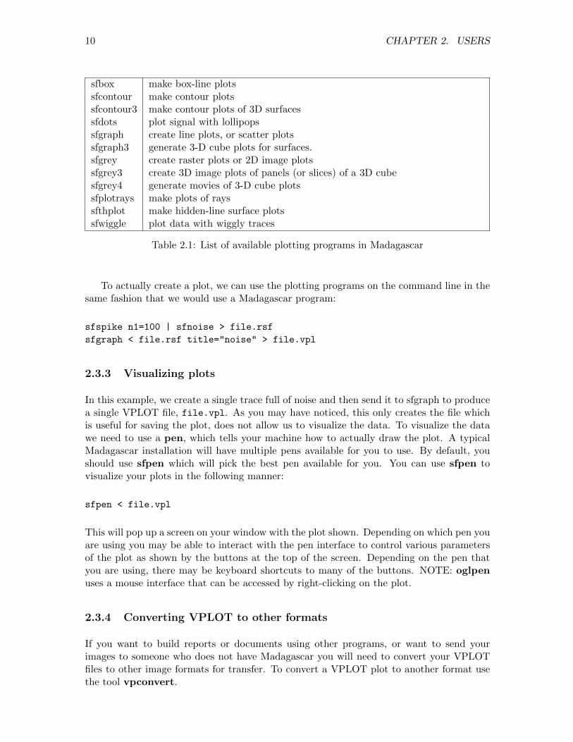
To generate VPLOT files, we need to pass our computed RSF files through VPLOT filters,that convert RSF data files to VPLOT files. The VPLOT filters are named by the type ofplot that they produce. Table 2.1 lists all of the available VPLOT filters.

10 CHAPTER 2. USERS

sfbox make box-line plotssfcontour make contour plotssfcontour3 make contour plots of 3D surfacessfdots plot signal with lollipopssfgraph create line plots, or scatter plotssfgraph3 generate 3-D cube plots for surfaces.sfgrey create raster plots or 2D image plotssfgrey3 create 3D image plots of panels (or slices) of a 3D cubesfgrey4 generate movies of 3-D cube plotssfplotrays make plots of rayssfthplot make hidden-line surface plotssfwiggle plot data with wiggly traces

Table 2.1: List of available plotting programs in Madagascar

To actually create a plot, we can use the plotting programs on the command line in thesame fashion that we would use a Madagascar program:

sfspike n1=100 | sfnoise > file.rsf

sfgraph < file.rsf title="noise" > file.vpl

2.3.3 Visualizing plots

In this example, we create a single trace full of noise and then send it to sfgraph to producea single VPLOT file, file.vpl. As you may have noticed, this only creates the file whichis useful for saving the plot, does not allow us to visualize the data. To visualize the datawe need to use a pen, which tells your machine how to actually draw the plot. A typicalMadagascar installation will have multiple pens available for you to use. By default, youshould use sfpen which will pick the best pen available for you. You can use sfpen tovisualize your plots in the following manner:

sfpen < file.vpl

This will pop up a screen on your window with the plot shown. Depending on which pen youare using you may be able to interact with the pen interface to control various parametersof the plot as shown by the buttons at the top of the screen. Depending on the pen thatyou are using, there may be keyboard shortcuts to many of the buttons. NOTE: oglpenuses a mouse interface that can be accessed by right-clicking on the plot.

2.3.4 Converting VPLOT to other formats

If you want to build reports or documents using other programs, or want to send yourimages to someone who does not have Madagascar you will need to convert your VPLOTfiles to other image formats for transfer. To convert a VPLOT plot to another format usethe tool vpconvert.

2.4. SCRIPTING MADAGASCAR 11

vpconvert allows you to convert VPLOT files to any of the following formats, providedthat you have the appropriate third-party libraries installed:

• avi,

• eps,

• gif,

• jpeg/jpg,

• mpeg/mpg (movie format),

• pdf,

• png,

• ppm,

• ps,

• svg,

• and tif.

Here’s an example of how to use vpconvert:

vpconvert file.vpl format=jpeg

NOTE: details on how to install these third-party libraries are not included with theMadagascar library, and we provide no support on installing them. Most users will be ableto install them using either package management software (on Linux, Windows, and Mac)or pre-compiled binaries. The PS and EPS support is provided by default.

2.4 Scripting Madagascar

Madagascar’s command line interface allows us to create, manipulate and plot data. Oftenthough, we want to create scripts that will perform these operations automatically for us.Scripting is especially important when processing large amounts of data, or performing acomplex chain of file manipulations in order to ensure that operations are completed in theright order or with proper parameters.

In Madagascar, there are two main ways of creating scripts: shell scripts, and Pythonscripts using SCons.

12 CHAPTER 2. USERS

2.4.1 Shell scripting

Shell scripting is the first option for creating scripts. In shell scripting we simply copy thecommand lines that we would use and paste them into a file that is recognized by eitherBASH, C-shell or another shell of your choosing. Shell scripting may be familiar to users ofother packages such as SU, because it is the primary method of scripting there. An exampleof a Madagascar shell script is shown below:

#!/bin/bash

sfspike n1=100 > file.rsf

< file.rsf sfgraph > file.vpl

For simple processing flows, shell scripting is a quick and easy approach to saving yourprocessing flow. However, shell scripts quickly become unmanageable when more compli-cated processing flows are used. Additionally, shell scripts have no way to avoid repeatingcommands that have already been successfully run, which causes shell scripts to spend asignificant amount of time duplicating already completed work. Because of these issues,Madagascar’s main scripting option is to use a build manager called SCons for scriptinginstead of shell scripts.

2.4.2 SCons

SCons is a program written in 100% Python. As a build manager, SCons keeps track of threeitems for each file built in the script: the name of the output file(s), the name of the inputfile(s), and the rule (Madagascar program(s) with options) used to build the output file(s)from the input file(s). The advantage to keeping track of these items is that SCons can thencheck to see if any of those items have changed and if so mark the output file to be rebuilt.If no changes are detected, and the output file already exists, then SCons skips the outputfile and goes onto building other files. This gives the user the ability to avoid re-runningportions of their scripts that previously completed without issue, which is very importantwhen working on processing flows with large datasets where individual commands may takehours to execute. SCons also tracks dependencies between various processing commands.For example, if command 2 depends on the ouptut of command 1, and the input to command1 changes, then SCons will automatically know that the input to command 2 has changedand will re-run command 2 as well. Furthermore, SCons allows us to run multiple processingcommands at the same time on computers with sufficient capabilities, further reducing theamount of time that it takes for us to process data in Madagascar. Now, we’ll discuss howto create SCons scripts and use SCons on the command line.

2.4.3 SConstructs and commands

SCons scripts are called SConstructs. In order to use SCons, you must create an SConstructin the local directory where you want to work. Since SCons is written in Python, anSConstruct is simply a text file written using Python syntax. If you don’t know Python,you can still use SCons, because the syntax is simple.

2.4. SCRIPTING MADAGASCAR 13

First, a primer on Python syntax. In SConstructs we are going to deal with Pythonfunctions and strings. Python functions are simple, and should be familiar to anyone whohas used a programming language. For example, calling a Python function, foo, looks like:

One argument - foo(1).

Many arguments - foo(1,2,3,4,5,123)

Python functions can take many arguments, and arguments of different types, but thesyntax is the same. Python strings are also very similar to other programming languages.In Python anything inside double quotes is automatically considered to be a string, and nota variable declaration. However, Python also supports a few notations to indicate strings(or long strings) as shown below:

"this is a string"

’this is a string’

"""this is a string"""

’’’this is a string’’’

Somtimes in Python you will need to nest a string within a string. To do use one of thestring representations for the outer string, and use a different one for the inner string. Forexample:

"""sfgraph title="my plot" """ OR

’’’ sfgraph title="my plot" ’’’ OR

’ sfgraph title="my plot" ’

Fundamentally, Madagascar’s data-processing SConstructs are composed of only fourcommands: Fetch, Flow, Plot and Result. The main command is Flow. A Flow createsa relationship between the input file, the output file, and the processing command used tocreate the output file from the input file. The syntax for a Flow is:

Flow(output file,input file,command)

where, target and source are file names (strings), and command is a string that containsthe Madagascar program to be used, along with the command line parameters needed forthat program to run. For example:

Flow("spike1","spike","scale dscale=4.0")

creates a dependency relationship between the output file ’spike1’ and the input file ’spike’.The dependency indicates that ’spike1’ cannot be created without ’spike’ and that if ’spike’changes then ’spike1’ also changes. The relationship in this case is that ’spike1’ should be’spike’ scaled by four times. The equivalent command on the command line would be:

< spike.rsf sfscale dscale=4.0 > spike1.rsf

14 CHAPTER 2. USERS

Note: the file names of the input and output files do not need to include ’.rsf ’on the end of the files as SCons automatically adds the suffix to all of our filenames.

Now that we can create relationships between files using Flows, we can create an SCon-struct to do all of our data processing using SCons. However, we often want to visualize theresults of our processing in order to quality control the results. In order to create Plots (orother visualizations) in Madagascar we have two additional SCons commands: Plot andResult. Plot and Result tell SCons how to use Madagascar’s plotting programs to createvisualizations of files on the fly after they have been computed. The syntax for both Plotand Result is as follows:

Plot(input file, command)

OR

Result(input file, command)

In both cases, the Plot or Result command tells SCons to build a VPLOT file with samefile name as the input file (with the .vpl suffix instead) from the input file using the commandprovided. For example, if we want to make a graph of a file we could use:

Plot("spike1","sfgraph pclip=100")

Behind the scenes, SCons establishes that we want to use ”spike1.rsf” to create a Plotcalled ”spike1.vpl” using sfgraph. The equivalent command line operation is:

< spike1.rsf sfgraph pclip=100 > spike1.vpl

Result can be used in the same way as Plot, illustrated above.

At this point, you might be asking yourself, what’s the difference between Plot andResult? The answer is that Plot creates all VPLOT files in the local directory, whereasResult creates its VPLOT files in a subdirectory called Fig. Fig is a location used to storePlots that we want to later use when creating papers using LATEX. By default, you shoulduse Plot when creating visualizations. Only use Result when you want to save somethingto be used in a paper. Note: since the VPLOTs from Plot and Result are placed indifferent locations you can use both Plot and Result for a single RSF file, but create twodifferent plots for the same file.

2.4.4 Creating an SConstruct

Now that we have the three SConstruct commands, we can write our first SConstruct. Todo so, open the SConstruct file in your favorite text editor. Before we can create any Flow,Plot or Result statements we have to add a first statement to the SConstruct. Enter thefollowing statement (verbatim) into your new SConstruct:

from rsf.proj import *

2.4. SCRIPTING MADAGASCAR 15

This statement tells SCons where to find the Flow, Plot and Result commands, and mustbe included in every SConstruct.

After that statement has been entered, you can enter as many Flow, Plot and Resultcommands as you wish making sure to use proper syntax. It’s helpful to use a text editorthat has Python syntax highlighting, as that will help you find and remedy strings thatare not closed. You can also create Python comments using the # mark to indicate thebeginning of a comment to help document your SConstructs.

Lastly, you must include the following statement at the end of your SConstruct:

End()

This statement tells SCons that the script is done and that it should not look for anythingelse in the script. Make sure to include this statement as the very last item in everySConstruct.

Here’s a sample SConstruct:

from r s f . p ro j import ∗ # Remember , t h i s s ta tement comes f i r s t . . . ALWAYS

Flow ( ” sp ike ” ,None , ” s f s p i k e n1=100 k1=50” )# None i s a t r i c k , see Advanced SCons f o r more in format ionFlow ( ” sp ike1 ” , ” sp ike ” , ” s fadd s c a l e =4.0” )Flow ( ” no i s e ” , ” sp ike1 ” , ” s f n o i s e ” )

Plot ( ” sp ike ” , ’ s f g raph t i t l e =”sp ike ” ’ ) # Note s t r i n g ne s t i n gPlot ( ” sp ike1 ” , ’ s fg raph t i t l e =”sp ike1 ” ’ )Plot ( ” no i s e ” , ’ s fg raph t i t l e =”no i sy ” ’ )

Result ( ” no i s e ” , ’ s fg raph t i t l e =”no i sy ” p c l i p =75 ’ )

End ( ) # Remember , t h i s a lways ends the s c r i p t .

Note: you do not have to order your Flow, Plot and Result commands as shown above.You can mix Flow, Plot and Result in any order. SCons automatically establishes therelationships between related files and commands.

2.4.5 Executing SCons

Now that you have an SConstruct, you can start processing data the Madagascar way. Todo so open a terminal and navigate to the local directory where your SConstruct is located.To execute your SConstruct simply run: scons . When you run SCons, it will check tomake sure that all necessary dependencies are found and that all of your commands insidethe SConstruct are valid. If not, SCons will return an error message showing you whereyou made a mistake. If everything is OK, then SCons will begin creating your files in thelocal directory and will output its progress as it executes the Madagascar programs onthe command line. For example, running the sample SConstruct from above should showsomething similar to the following output:

16 CHAPTER 2. USERS

scons: Reading SConscript files ...

scons: done reading SConscript files.

scons: Building targets ...

/opt/rsf/bin/sfspike n1=100 k1=50 > spike.rsf

< spike.rsf /opt/rsf/bin/sfadd scale=4.0 > spike1.rsf

< spike1.rsf /opt/rsf/bin/sfnoise > noise.rsf

< spike.rsf /opt/rsf/bin/sfgraph title="spike" > spike.vpl

< spike1.rsf /opt/rsf/bin/sfgraph title="spike1" > spike1.vpl

< noise.rsf /opt/rsf/bin/sfgraph title="noisy" > noise.vpl

< noise.rsf /opt/rsf/bin/sfgraph title="noisy" pclip=75 > Fig/noise.vpl

scons: done building targets.

If the execution of scons ends with, ”scons: done building targets” then the scriptcompleted successfully. Check your local directory for your output files.

2.4.6 Common errors in SConstructs

There are two common errors that most users will experience when executing SConstructs:missing dependency errors, and misconfiguration errors. We’ll demonstrate both of theseerrors to help new users troubleshoot them below.

The first error is caused by missing a dependency in the SConstruct. To introduce thiserror into your SConstruct modify the sample SConstruct from above to the following:

from r s f . p ro j import ∗ # Remember , t h i s s ta tement comes f i r s t . . . ALWAYS

Flow ( ” sp ike1 ” , ” sp ike ” , ” s fadd s c a l e =4.0” )Flow ( ” no i s e ” , ” sp ike1 ” , ” s f n o i s e ” )

Plot ( ” sp ike ” , ’ s f g raph t i t l e =”sp ike ” ’ ) # Note s t r i n g ne s t i n gPlot ( ” sp ike1 ” , ’ s fg raph t i t l e =”sp ike1 ” ’ )Plot ( ” no i s e ” , ’ s fg raph t i t l e =”no i sy ” ’ )

Result ( ” no i s e ” , ’ s fg raph t i t l e =”no i sy ” p c l i p =75 ’ )

End ( ) # Remember , t h i s a lways ends the s c r i p t .

Now when you run scons, you should get an error message:

scons: Reading SConscript files ...

scons: done reading SConscript files.

scons: Building targets ...

scons: *** [spike1.rsf] Source ‘spike.rsf’ not found, needed by target ‘spike1.rsf’.

scons: building terminated because of errors.

In this case, SCons tells you exactly which file is missing and which output file is missing oneof its dependencies. To solve this problem, add the Flow to create ’spike’ to the SConstruct.If your SConstruct uses a file that is not created inside the SConstruct, and is complaining

2.4. SCRIPTING MADAGASCAR 17

about a missing dependency, then make sure the file you are looking for is in a location thatthe SConstruct can access.

The second error, is caused by having a misconfigured command. To demonstrate thistype of error change your SConstruct to:

from r s f . p ro j import ∗ # Remember , t h i s s ta tement comes f i r s t . . . ALWAYS

\ t e x t b f {Flow }( ” sp ike ” ,None , ” s f s p i k e n1=100 k1=50” )# None i s a t r i c k , see Users 4 f o r more in format ion\ t e x t b f {Flow }( ” sp ike1 ” , ” sp ike ” , ” s f a s d s c a l e =4.0” )# HERE IS THE ERROR, NOTE s f a sd in s t ead o f s fadd\ t e x t b f {Flow }( ” no i s e ” , ” sp ike1 ” , ” s f n o i s e ” )

\ t e x t b f {Plot }( ” sp ike ” , ’ s fg raph t i t l e =”sp ike ” ’ ) # Note s t r i n g ne s t i n g\ t e x t b f {Plot }( ” sp ike1 ” , ’ s fg raph t i t l e =”sp ike1 ” ’ )\ t e x t b f {Plot }( ” no i s e ” , ’ s f g raph t i t l e =”no i sy ” ’ )

\ t e x t b f {Result }( ” no i s e ” , ’ s f g raph t i t l e =”no i sy ” p c l i p =75 ’ )

End ( ) # Remember , t h i s a lways ends the s c r i p t .

In this case, we’ve introduced a typo into one of our commands. When running scons, theresult is:

scons: Reading SConscript files ...

scons: done reading SConscript files.

scons: Building targets ...

/opt/rsf/bin/sfspike n1=100 k1=50 > spike.rsf

< spike.rsf sfasd scale=4.0 > spike1.rsf

sh: sfasd: command not found

scons: *** [spike1.rsf] Error 127

scons: building terminated because of errors.

Again, the error message is pretty descriptive and could help you track down the errorrelatively quickly. It’s important to note that in this case, the error was caught after SConstried to execute the command and failed to do so, whereas the dependency error was caughtbefore any commands were executed. This means that this typo error would kill a scriptthat’s been running a long time without any issues up till that point. Fortunately, SConswould restart the script at the point of failure thereby saving you all the additional time torecompute everything before this point in the script.

These are only two of the most common errors that novice users will see. For additionalinformation about debugging SConstructs, or for exceptionally strange errors please consultthe online documentation or the RSF users mailing list.

2.4.7 Additional SCons commands

Here are some additional SCons commands that are useful to know.

18 CHAPTER 2. USERS

Viewing Plots

If you’re running an SConstruct and want to view the plots that it generates as it createsthem, then you can use: scons view to force SCons to show the plots interactively. Doingso allows you to view your output at runtime and to stop the SConstruct as it’s running ifyou don’t like what you see.

Viewing only one plot

If you want to view the plot associated with only a single file you can tell SCons to viewthat plot by using the command: scons file.view where file is the filename of the itemthat you want to view. For example: scons spike.view would show the plot of the spike.rsffile. The advantage to using this command is that SCons will only build the dependenciesneeded to view that specific plot, which can save you a lot of time in longer processingscripts.

Building specific targets

If you want to build a specific RSF file, or a few specific RSF files you can simply specifythem on the command line when you execute SCons as follows: scons file.rsf file2.rsffile3.rsf .... The advantage to doing this, is that SCons will only build those files and theirdependencies instead of running through the entire script.

Cleaning up

After we’ve executed our SConstruct and viewed the results of the processings flow, we mightdecide that we want to clean up our project and go work on something else. Normally, onewould have to delete all of the files and then move on, but SCons automates this processusing the command: scons -c. Simply execute it in the local directory and SCons willremove all of the built RSF files, and VPLOT files. SCons will not remove files that it doesnot have rules for.

Dry-runs

Sometimes we want to test an SConstruct through the end of the script without waiting forit to run completely. To do so, we can use scons -n which tells SCons to simulate an actualexecution. During a dry-run SCons will check all of the commands, and dependencies toensure that they exist and are properly configured. If not, then SCons will tell you whichcommands are misconfigured. This command can save you hours of debugging! Use itliberally.

Parallel executions

For long scripts we can use parallel execution to run multiple processing commands at thesame time. Parallel execution requires that the commands can function independently of

2.5. ADVANCED SCONS 19

one another (i.e. there are commands that do not depend on each other’s output). To useparallel execution use: pscons which launches the maximum number of parallel jobs thatyour computer can handle at once. Parallel execution can greatly speed up your processingflows if SCons can parallelize it. In the worst case, SCons won’t be able to parallelize yourscript and it will run at the same speed as if you just used scons.

2.4.8 Final thoughts

At this point you should have a solid understanding of how to use SCons and create SCon-structs to script your Madagascar processing flows. Admittedly, SCons is somewhat com-plicated and difficult to understand at first, but don’t give up. By using SCons, you areable to create powerful Madagascar scripts that are completely reproducible and enjoy thebenefits of using a powerful build management system. However, we have not shown youthe most useful aspects of SCons, which are demonstrated in the next tutorial, where weshow how to integrate Python with SCons, thereby making processing flows that are evenmore powerful.

2.5 Advanced SCons

Now that you have a grasp of how to use SCons to put together simple processing flows, we’regoing to show you how to abuse SCons to make more advanced processing flows that canhandle multiple input and output files properly. Additionally, we’re going to demonstratesome SCons tricks that make your life easier, and allow you to work faster, and smarter.

2.5.1 Multiple input files

Many Madagascar programs require multiple input files and/or output multiple files. Inorder for SCons to properly recognize that these additional files are dependencies for aspecific output file we have to change the syntax that we use for Flow, Plot and Resultstatements. To do so, we’ll need to use Python lists to help us keep everything togetherwhen using our SCons commands. We first discuss the case where we need multiple inputfiles.

An example of a Madagascar program that requires multiple input files is sfcat. Forreference, sfcat is used to concatenate multiple files together, essentially a file manipulationprogram. For example, we might use sfcat on the command line in the following fashion:

< file.rsf sfcat axis=2

file1.rsf file2.rsf file3.rsf file4.rsf > catted.rsf

To replicate this behavior using SCons we need to tell our Flow statements about thepresence of multiple input files. Important: if we do not indicate to SCons that wehave multiple input files then the dependency chain will not be correct and wecannot guarantee our results are correct. We can easily tell SCons of the presence ofmultiple input files by using a Python list as our input file, instead of a string:

20 CHAPTER 2. USERS

Flow(’catted’,[’file’,’file1’,’file2’,’file3’,’file4’],

’sfcat axis=2 ${SOURCES[1:-1]}’)

or, equivalently,

Flow(’catted’,’file file1 file2 file3 file4’,

’sfcat axis=2 ${SOURCES[1:-1]}’)

As you may have noticed, there are two new items in this Flow statement, but let’s startby discussing only the list of file names: [’file’,’file1’,’file2’,’file3’,’file4’]. The list of filenames is simply a Python list of strings that contains each of the names of the files that wewant to use in this Flow command. As usual, we don’t have to append the ’.rsf’ suffix tothe end of these names because SCons adds it for us.

The second new part to the Flow command is: $SOURCES[1:-1], referred to as theSCons source list, which tells SCons about the presence of additional input files in thecommand, and to substitute the names into the command automatically. Without thiscommand, SCons would not include the files in the final command. As an example of whatthe SCons source list does, compare the two SConstructs below against one another. Thetop is correct, the bottom is incorrectly configured:

# Correctfrom r s f . p ro j import ∗Flow ( ’ f i l e ’ ,None , ’ sp ike n1=100 ’ )Flow ( ’ f i l e 1 ’ ,None , ’ sp ike n1=100 mag=2 ’ )Flow ( ’ f i l e 2 ’ ,None , ’ sp ike n1=100 mag=3 ’ )Flow ( ’ f i l e 3 ’ ,None , ’ sp ike n1=100 mag=4 ’ )Flow ( ’ f i l e 4 ’ ,None , ’ sp ike n1=100 mag=5 ’ )

Flow ( ’ cat ted ’ , [ ’ f i l e ’ , ’ f i l e 1 ’ , ’ f i l e 2 ’ , ’ f i l e 3 ’ , ’ f i l e 4 ’ ] ,’ s f c a t a x i s=2 ${SOURCES[1 : −1 ]} ’ )

End ( )

# Wrongfrom r s f . p ro j import ∗Flow ( ’ f i l e ’ ,None , ’ sp ike n1=100 ’ )Flow ( ’ f i l e 1 ’ ,None , ’ sp ike n1=100 ’ )Flow ( ’ f i l e 2 ’ ,None , ’ sp ike n1=100 ’ )Flow ( ’ f i l e 3 ’ ,None , ’ sp ike n1=100 ’ )Flow ( ’ f i l e 4 ’ ,None , ’ sp ike n1=100 ’ )

Flow ( ’ cat ted ’ , [ ’ f i l e ’ , ’ f i l e 1 ’ , ’ f i l e 2 ’ , ’ f i l e 3 ’ , ’ f i l e 4 ’ ] , ’ s f c a t a x i s=2 ’ )End ( )

If you noticed the command line output from SCons, you would find that for the incorrectSConstruct, SCons ran the following command:

< file.rsf sfcat axis=2 > catted.rsf

2.5. ADVANCED SCONS 21

which is not correct. This is because SCons was not informed that the additional sourcesactually are used inside the command and did not substitute them in.

The SCons source list contains a reference to all of the file names that we passed in ourPython list earlier. In order to access those names we have to use a specific notation, but itis essentially a Python list enclosed in curly brackets that begins with a $. Since the sourcelist is a Python list, we can get the file names in a few ways if we follow standard Pythonlist conventions. Standard Python list conventions are:

• List indexing starts with index 0,

• Lists may be negatively indexed, which returns the items from the end (e.g. LIST[-1]),

• Lists may be sliced using the LIST[start:end] notation, where start and end are indices,

• List slicing indices are inclusive for the starting index, and exclusive for the endingindex (e.g. LIST[0:4] returns LIST[0],LIST[1],LIST[2],LIST[3] but NOT LIST[4],

• Open slicing indices may be used (e.g. LIST[2:] gets everything from index 2 to theend, and LIST[:4] returns everything from 0 to but not including 4).

• Negative and positive indices may be used together (e.g. LIST[1:-1] returns all ele-ments but the first and last).

These are the most useful conventions to remember, and the ones you will most frequentlysee. Please see the Python documentation (freely available online) for more informationabout dealing with Lists.

Using the above conventions the following Flow statements are all equivalent for lettingsSCons know about the presence of multiple input files:

Flow(’catted’,[’file’,’file1’,’file2’,’file3’,’file4’],

’’’

sfcat axis=2 ${SOURCES[1]} ${SOURCES[2]}

${SOURCES[3]} ${SOURCES[4]}

’’’)

Flow(’catted’,[’file’,’file1’,’file2’,’file3’,’file4’],

’’’

sfcat axis=2 ${SOURCES[1:5]}

’’’)

Flow(’catted’,[’file’,’file1’,’file2’,’file3’,’file4’],

’’’

sfcat axis=2 ${SOURCES[1:-1]}

’’’)

Note: never use SOURCES[0] because SOURCES[0] corresponds to ’file’ which is alreadyused by SCons for standard input. Also, never use open slicing on the SOURCES list,because at the end of the SOURCES list are extra items added by SCons for safe keepingthat will break the command if accidentally used.

22 CHAPTER 2. USERS

2.5.2 Multiple outputs

For multiple outputs, we can use the same conventions as before, except we specify a listof output files instead of input files, and we use the TARGETS SCons list, instead ofSOURCES. For example:

Flow([’pef’,’lag’], ’dat’, ’sflpef lag=${TARGETS[1]}’).

2.5.3 None inputs

Sometimes, Flows are created that don’t have an input file. For example, files createdusing sfspike do not require input files. To get around the need for an input file, we canuse the Python keyword None, equivalent to NULL in C or Java, to indicate to SCons thatno input file is needed. For example:

Flow(’spike’,None,’sfspike n1=100’)

2.5.4 Toggling standard input and standard output

When None inputs are used, then standard input is no longer needed and can be disabled.To turn off standard input on a Flow, add another argument to the Flow statement:

Flow(’spike’,None,’sfspike n1=100’,stdin=0)

When SCons runs this Flow, the output command line will be:

sfspike n1=100 > spike.rsf

Likewise, we can toggle output to standard output as well. Standard output has two options,redirect to null or completely off. For some programs we need to redirect standard outputto null, and others will require standard output to be completely off. To toggle standardoutput off use the following syntax:

Flow(’spike’,None,’sfspike n1=100’,stdout=-1)

OR to redirect to /dev/null:

Flow(’spike’,None,’sfspike n1=100’,stdout=0)

2.5.5 Plots with a different output name

Occasionally, you might want to create a plot with a different name than the input file. Forexample, a file might have multiple axes, and you could window along one of the axes, tocreate multiple graphs from a single input file. To distinguish between the different plots,you can rename the output files from Plot and Result commands using a syntax similar toFlow:

2.6. INTEGRATING PYTHON WITH SCONS 23

Plot(’output’,’input’,’sfgraph’)

This Plot command will produce output.vpl instead of input.vpl. In this way, you can createmultiple visualizations of the same file. This applies to Result commands as well.

2.6 Integrating Python with SCons

Because SCons is written in Python, we can take advantage of all the features of thePython programming language. By doing so, we are able to make our life a lot easierby: compartmentalizing build commands, creating functions for commonly used scripts,organizing our scripts to make them easier to understand. Instead of giving an exhaustivetutorial of the combination of SCons and Python, we’re going to demonstrate a few of themore commonly features of Python inside of SConstructs. We leave it to the end user todevelop additional techniques that further exploit the power of Python.

2.6.1 A forewarning

While Python and SCons are compatible with one another they are not completely inter-changeable. To understand why that is the case, you need to understand the underlyingdesign of SCons. SCons is a declarative language, which means that you tell SCons whatto do through the: Flow, Plot, and Result commands, and then SCons decides how andwhen to execute those commands. Python on the other hand is imperative, which meansthat as Python reads a Python script, it executes the commands immediately. Python doesnot take time to decide how or when to execute your commands. This point causes a bit ofconfusion to users who start to combine Python and SCons together because they expectSCons commands to execute in the order that they place them, which is not the case. Be-cause of this, you may not be able to use certain Python features in their native Pythonway. For example, loops which require repeated computation, and whose results depend onthe result of the last iteration are not possible using SCons. It is also not usually possi-ble to use Python variables that change during execution with SCons because the variablevalue that SCons will use is always the last value of the variable. Typically, you cannot useconditional statements in SCons, where the choice depends on a file that SCons will build.

To be safe, you should always assume that whatever Python does happens before SConsstarts running commands.

2.6.2 Variables

The most effective way to combine SCons and Python is to use Python to manage importantvariables for your scripts. For example, if you want to test a variety of values for a certainprocessing Flow, then you might save the value to a variable and then let Python formatit correctly for you, instead of changing the string each time you want to run a new test.You can also save all your variables in a convenient location and then easily change themto test different parameters as well. For example:

nx = 100

24 CHAPTER 2. USERS

nz = 100

Flow(’model’,None,

’’’sfspike n1=’’’+str(nx)+’’’n2=’’’+str(nz))

Note: variables must be converted to strings in order to be combined into the commandstatements. Because these variables are converted using string concatenation, there is apossibility that a user could give a value of a wrong type.

2.6.3 String substitution

While using variables is convenient, formatting them in the fashion shown above is notconvenient. An easier way to format variables for strings is to use string substitution.String substitution works in the same way as the C - printf function works, i.e. we placemarkers that indicate where values should be substituted and what format they should bein. The above example using string substitution is:

nx = 100

nz = 100

Flow(’model’,None,

’’’

sfspike n1=%d n2=%d

’’’ % (nx,nz) )

In this statement, both nx, and nz are formatted as integers, and contained inside atuple. All variables to be used for string substitution must be contained within the tupleat the end of the string statement. For reference, all C-printf like formatting choices areavailable in Python as well. Note: treat booleans as integers in Python.

2.6.4 Dictionaries

When scripts have a large number of variables, it is often easier to contain them within aPython dictionary instead of letting them float around the script. Dictionaries are declaredin key=value format in Python using the dict keyword. For example:

parameters = dict(nx=100,nz=100,verb=True,final_file=’output123’)

To access variables from within the dictionary, we use list-like indexing where the indexgiven is the name of the variable that we want to access:

nx = parameters[’nx’] # Returns 100

We can also set variables within the dictionary, or modify their values after the initialdeclaration:

2.6. INTEGRATING PYTHON WITH SCONS 25

parameters[’nx’] = 200 # Sets nx to 200

parameters[’ny’] = 150 # Adds ny, and sets it to 150

To use the dictionary for string substitution, we only need to modify our formattersto include the key names of the variables that we wish to access from the dictionary. Forexample:

Flow(’model’,None,

’’’

sfspike n1=%(nx)d n2=%(nz)d

’’’ % parameters )

Notice that the formatters now have the name of the variable inside parentheses: %(nx)dbefore the formatting expression. Then, the entire dictionary is passed to the string forsubstitution. At runtime, Python places the values for the keys from the dictionary into thestring. If the values are the wrong type, or the key does not exist in the dictionary, thenPython will throw an error at runtime, and prevent you from running with a bad value.

By using dictionaries with string substitution, we can add flexibility to our scripts, andimprove their readability, which ultimately improves the ability of others to reproduce ourwork. Thus, you should strive to use dictionaries wherever possible in your SConstructs.

2.6.5 Loops

Perhaps the most useful construct from Python that can be added to SConstructs are loops.By using loops, we can automate many redundant processes. To use a Python loop we justuse the standard Python syntax in the following fashion:

from r s f . p ro j import ∗

for i in range ( 1 0 ) :count = s t r ( i ) # Convert i n t e g e r to s t r i n gFlow ( ’ sp ike− ’+count , None , ’ s f s p i k e n1=100 mag=%d ’ % i )Plot ( ’ sp ike− ’+count , ’ s fg raph ’ )

End ( )

In order for the loop to work, you need to make sure that all the files that are created havea unique file name. The easiest way to do so is to use the loop index in the filename, thecount variable in this case. The count variable must be a string, because only strings can beconcatenated together in Python. If you want to make more complicated file names (fromnested loops) then examine the printf like syntax for Python strings.

All the usual Python rules apply to these loops. Typically, for loops are easier tounderstand than while loops in Python, and so we recommend using for loops for mostpurposes.

26 CHAPTER 2. USERS

2.6.6 Functions

Python functions are incredibly useful because you can compartmentalize repeated uses ofcommonly used Flows, and then use them in multiple SConstructs. For the best use ofPython functions you should use the following conventions:

• always use keyword=value arguments to help document your code,

• list file names for input and output first, then other arguments,

• use default values for all arguments, even if they are None,

• use the locals() dictionary to get the values of the arguments,

• always perform an action inside the function (i.e. create a Flow, Plot or Result),

• do not return anything from the function,

• and always accept **kwargs as the last argument to allow for dictionary substitution.

Here’s an example of a well-defined function to create a Ricker wavelet with a peakfrequency specified by the user:

def ricker(out=’wave’,freq=20.0,kt=100,nt=1001,dt=0.01,ot=0.0,**kwargs):

Flow(out,None,

’’’

sfspike n1=%(nt)d o1=%(ot)f d1=%(d1)f

nsp=1 mag=1.0 k1=%(kt)d l1=%(kt)d |

sfricker1 frequency=%(freq)f

’’’ % locals())

Notice that we use the python function locals() for string substitution. This functionreturns a dictionary that contains only the names and values of the named arguments forthe function.

To call this function, you can use it as a normal Python function. Since there are defaultarguments, not all arguments need to be passed as long as you are OK with the defaultvalue.

ricker(’wave’,freq=30,kt=50)

If you are using a dictionary that has all of your variables in it, then you can call thefunction using explicit parameter fetching:

ricker(’wave’,parameters[’freq’],parameters[’kt’],...)

where you have to explicitly grab certain variables from the parameter dictionary. Con-versely, you can use automatic parameter fetching:

2.6. INTEGRATING PYTHON WITH SCONS 27

ricker(’wave’,**parameters)

which will look for all the named arguments to the ricker function in the parameterdictionary, and send their values to the function. When there are many parameters, andyou have already set them in the dictionary, then automatic parameter fetching is the bestway to go.

2.6.7 Modules

Of course, functions can be compiled into groups and then placed into Python modules forwidespread re-use throughout your SConstructs. Commonly used Python modules are cur-rently located in $RSFROOT/book/Recipes, which is where you should place your modulesas well. As usual, you must use correct Python syntax to access functions contained withinmodules. For example, if you create a module called myutil.py, then you can access yourfunctions in the following manner:

import myutil

myutil.ricker(...)

2.6.8 Classes

The least used, but most powerful part of Python that you can bring into your SConstructsare Python classes. For example, if you are writing a script to process multiple models inthe exact same way, but that have different parameters you would have to write separateFlow statements to process each of them, OR you could write a Python class that takes themodel parameters and uses those parameters to generate Flow statements automatically,similar to functions. However, a class can allow you to group functions together into asingle coherent body and allow you to drastically reduce the amount of code that must bereused.

We refer the reader to the Python documentation for more information on creating andusing classes.

2.6.9 Final thoughts

Congratulations on completing the Madagascar User tutorial series. Now, you should haveall the tools to: use Madagascar programs, write SConstructs to script your processingflows, and combine Python with SCons to make powerful scripts that can process data inways not previously possible. From here, you can continue learning about how to write yourown Madagascar programs, or learn about how to make reproducible documents using theMadagascar framework.

28 CHAPTER 2. USERS

Chapter 3

Authors

The Authors tutorials demonstrate how one can create reproducible documents using theMadagascar processing package and LATEXtogether. By the end of the Authors tutorials,you should be able to:

• build papers, including: SEG and EAGE abstracts, manuscripts for Geophysics, andhandouts,

• build a CSM thesis,

• build a CWP report,

• build slides,

• and add/modify Latex class files to add your custom document formats to Madagas-car.

After completing this tutorial series, you will be able to maximize your research productivityusing Madagascar.

3.1 Getting started

Before you can get started writing reproducible documents, you need to ensure that yoursystem is properly setup. This section of the tutorial will walk you through the setup pro-cess, which can be somewhat difficult and laborious depending on which operating systemyou are on, as you will need a full installation of LATEXand additional LATEXclass files thatMadagascar makes available to you. The good news is that this configuration only happensonce.

3.1.1 Downloading LATEX

To begin, you need to download a full installation of LATEXfor your operating system. To doso, you may need to contact your system administrator. If you have administrative rights,then you can download a full install for your platform from the following locations:

29

30 CHAPTER 3. AUTHORS

• Linux - use your package management software to install a full texlive (you may needadditional packages depending on your distribution).

• Mac - install MacTex http://www.tug.org/mactex/2011/.

• Windows - install MikTex http://miktex.org/.

The respective downloads typically are quite large and take a substantial amount oftime to complete, so start the download and come back later. Once your download is done,test your installation by executing pdflatex at the command line. If everything works finethen continue onwards.

3.1.2 Downloading SEGTeX

The next step is to download the SEGTEXclass files, which tells LATEXhow to build certaindocuments that we commonly use. To download SEGTEXfirst cd to a directory whereLATEXcan find additional class files. This directory is typically operating system depen-dent, and may be distribution dependent for Linux. Typically, you can place these files in$HOME/texmf. Otherwise, you will need to place them in the root installation for Latexwhich can be found by searching for the basic class files, such as article.cls. On a Mac thetypical place to put these files is $HOME/Library/texmf. In any case, once you arein the proper location, then use the following command to download the class files (usingsubversion):

svn co https://segtex.svn.sourceforge.net/svnroot/segtex/trunk texmf

or download a stable release from http://sourceforge.net/projects/segtex/files/

and unpack it into the texmf directory.

3.1.3 Updating your LATEXinstall

Once the class files are successfully downloaded, you will need to run texhash or texconfigrehash to update LATEXabout the new class files. For reference, a successful run of texhashproduces the following output:

jgodwin$ texhash

texhash: Updating /usr/local/texlive/2010/../texmf-local/ls-R...

texhash: Updating /usr/local/texlive/2010/texmf/ls-R...

texhash: Updating /usr/local/texlive/2010/texmf-config/ls-R...

texhash: Updating /usr/local/texlive/2010/texmf-dist/ls-R...

texhash: Updating /usr/local/texlive/2010/texmf-var/ls-R...

texhash: Done.

To determine if these files are found successfully, go into $RSFROOT/book/rsf/manualand run scons manual.read. If LATEXcomplains about being unable to find the class filesthen you should re-run texhash, or make sure that your class files are in the proper location.If you are still having difficulties, then contact the SEGTEXwebpage or the user mailing listfor further information.

3.2. PAPERS 31

3.2 Papers

With LATEXinstalled, we can now create reproducible documents using Madagascar. First,we will demonstrate how to build shorter, less complicated documents using Madagascar,such as SEG/EAGE abstracts, Geophysics articles, and handouts. All of these papershave similar build styles, so the rules for building each respective paper have only slightdifferences from one another. Instead of talking in detail about each of these documents, weillustrate the basic idea for each of the documents, and provide examples that demonstratethe particulars for each type of document.

3.2.1 Paper organization

All Madagascar papers expect a specific organization to your directories. In particular, youare expected to have a paper-level directory where your tex files and main SConstruct willexist. These files will tell Madagascar how to build your documents for a particular project.You can have multiple documents built from the same location, using the same SConstructas we will demonstrate later.

Below the paper directory, are the individual “chapters” that contain the processingflows used to generate the plots or process the data that you wish to use in your repro-ducible documents. Ideally, each “chapter” directory correlates to the processing flows orexamples in each chapter or section for your paper. Additionally, each “chapter” containsits own SConstruct that operates independently of the paper SConstruct one level aboveit. Furthermore, inside the “chapter” folder, Madagascar needs to have a Fig folder thatcontains all of the VPLOT files that were created using Result commands during process-ing. This folder is automatically created during processing using SCons, so you don’t needto manually create it. It is important to note that Madagascar can only locate VPLOTfiles that are in this file hierarchy for use in your papers. Figure 3.1 illustrates the folderhierarchy as well.

Note: “chapter” folders may be symbolic links that point to folders elsewhere on the filesystem. This trick can be useful to reuse figures without copying files and folders around tovarious folders. If you use symlinks, make sure to avoid editing files that are symbolicallylinked, as your changes may propagate in unintended ways to other projects and papers.

3.2.2 Locking figures

Once you have created the necessary folder hierarchy with your “chapters” and processingflows, then go ahead and run your processing SConstructs. After those are finished, youneed to lock your figures using scons lock. scons lock tells Madagascar that the figuresyou have generated are ready to go into a publication, and will store them in a subfolderof the $RSFFIGS directory for safe keeping. Locked figures are used for document figuresinstead of the figures in your local directory, because they are locked and not still changing.If you change your plots but do not lock your figures, you will not see your figures change.Always make sure to lock your figures before building a document.

32 CHAPTER 3. AUTHORS

Folder hierarchy Contents

Book Book SConstruct

?

-

Chapter Paper SConstruct, TeX files

?

-

Project Processing SConstruct, data, RSF files

?

-

Fig VPLOT files, Results ONLY-

Figure 3.1: The organizational hierarchy for Madagascar paper directories.

3.2.3 Tex files

Now that your figures are locked, you can create your first reproducible document in Mada-gascar. To do so, you will need to:

• make your tex files, and

• make a paper SConstruct,

Before making a document, you need to create your TeX files in the paper level direc-tory. For example, to create an EAGE abstract, you would create a main TeX file called:eageabs.tex which contains the content and TeX commands to build your abstract. YourTeX file can use all of the standard and expanded LATEXcommands provided by any avail-able packages on your system. It’s important to remember that you should try and breakapart your TeX files into manageable chunks, so that you can modify them independently,or reuse the content in other documents. For example, instead of having a single TeX filefor your EAGE abstract, you could have a separate TeX file that contains:input... statements that include additional TeX files for each section, such as the abstract,theory, discussion, conclusions, etc.

Additionally, Madagascar provides some convenience commands for often used LATEXfunctions.Here is a short description of some of those convenience commands that you may run across.Here’s a brief list of these convenience functions:

3.2. PAPERS 33

• \plot,

• \multiplot,

• \sideplot,

• and more.

These convenience functions are not available for every type of document, but are demon-strated in documents where they are available. The definition for the convenience functionsmay be found in the LATEXclass definitions listed at the end of this tutorial.

3.2.4 Paper SConstructs

One of Madagascar’s aims is to make TeX files as layout-agnostic as possible. To do so,Madagascar automatically adds the TeX document preamble (including the LATEXdocumentclass information), the LATEXpackage inclusions, and end of document information at run-time. This allows you to generate multiple documents from a single TeX file by simplychanging the SConstruct, instead of the TeX file.

Note: the paper SConstruct is only used to build papers. It contains no other informa-tion, and cannot be used to process data in the same SConstruct. This is why the paperSConstruct must exist in a separate directory from any processing SConstructs.

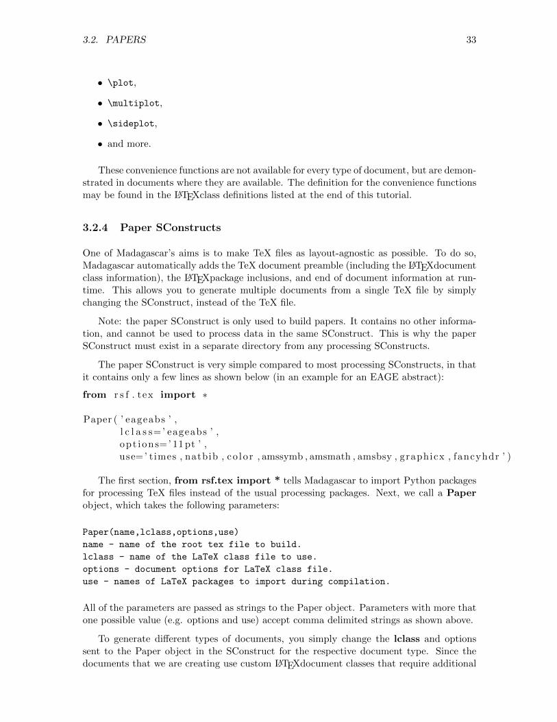
The paper SConstruct is very simple compared to most processing SConstructs, in thatit contains only a few lines as shown below (in an example for an EAGE abstract):

from r s f . tex import ∗

Paper ( ’ eageabs ’ ,l c l a s s=’ eageabs ’ ,opt i ons=’ 11 pt ’ ,use=’ times , natbib , co lo r , amssymb , amsmath , amsbsy , graphicx , fancyhdr ’ )

The first section, from rsf.tex import * tells Madagascar to import Python packagesfor processing TeX files instead of the usual processing packages. Next, we call a Paperobject, which takes the following parameters:

Paper(name,lclass,options,use)

name - name of the root tex file to build.

lclass - name of the LaTeX class file to use.

options - document options for LaTeX class file.

use - names of LaTeX packages to import during compilation.

All of the parameters are passed as strings to the Paper object. Parameters with more thatone possible value (e.g. options and use) accept comma delimited strings as shown above.

To generate different types of documents, you simply change the lclass and optionssent to the Paper object in the SConstruct for the respective document type. Since thedocuments that we are creating use custom LATEXdocument classes that require additional

34 CHAPTER 3. AUTHORS

TeX commands to function properly, it is easier for us to provide you with a templateinstead of discussing the details of each document class. The templates for the documentscan be found in the following directory: $RSFSRC/book/tutorial/authors.

3.2.5 Templates

To run the templates, you first need to generate the data used for them in the data directoryinside of the $RSFSRC/book/tutorial/authors. To do so, run scons lock which willproduce and lock the figures necessary. Then go into the template directory that you areinterested in, and make a symbolic link to the data directory: ln -s ../data and a symboliclink to the BibTeX file: ln -s ../demobib.bib in the template directory. After those stepsare made you can build and view the paper using scons or scons paper.read where paperis the name of the root tex file. Of course, if you want to remove all the generated files,then you can use scons -c to clean the directory.

3.2.6 Handouts

Handouts are informal documents that are loosely formatted, and very flexible. The handoutexample is located in: $RSFSRC/book/tutorial/authors/handout. Handouts do notrequire many additional arguments and are the most flexible of the documents discussedhere.

3.2.7 EAGE abstracts

EAGE abstracts are short documents, with a few particular formatting tricks. In particular,EAGE requires the logo of the current year’s convention to appear in the abstract. Atemplate is available in: $RSFSRC/book/tutorial/authors/eage.

3.2.8 SEG abstracts

SEG abstracts are different from EAGE abstracts in that they require two-column for-matting and are strictly limited to four pages not including references. To build an SEGabstract, we first build the abstract, and then build another document using the segcut.texfile that removes the references from the final pdf. An example is found in: $RSFSRC/-book/tutorial/authors/seg.

3.2.9 Geophysics manuscripts

Geophysics manuscripts come in two flavors: the first is the manuscript prepared for peerreview, and the second is the final document that would appear in a print version of Geo-physics. The example shows how to build both from the same TeX files, which makes itpainless to transition the formatting between the two documents. An example is located in:$RSFSRC/book/tutorial/authors/geophys. Make sure to use the template as thereare quite a few additional TeX commands that have to be used to get the correct formatting.

3.3. SLIDES 35

3.2.10 CWP reports

CWP reports are slightly more complicated then most documents in that they requiresubstantial modification to get the proper formatting. The CWP template is available in$RSFSRC/book/tutorial/authors/cwp.

3.3 Slides

Additionally, one can create presentation slides using LATEXand Madagascar together. Tocreate slides, we use the Beamer class files that have been customized for the CWP. Slideshave distinctly different commands then regular documents, so be sure to examine the tem-plate before diving in. The template is in: $RSFSRC/book/tutorial/authors/slides.

3.4 Theses

One can also create very complex documents using Madagascar in a reproducible way. Toiillustrate this point we provide a template for building a thesis for the Colorado School ofMines. This template is quite heavily modified, and requires substantial modification dueto all the formatting requirements. If you want to include a thesis template for anotherinstitution then you can do so by examining this template along with the CSM class files.The template is located in: $RSFSRC/book/tutorial/authors/thesis.

3.5 Books

You can make whole books using Madagascar. The advantage to doing so, is that youcan make individual chapters with examples of processing or workflows that can be runindependently of one another. Then Madagascar will stitch the chapters together into acohesive package seamlessly. The example for a book is this document itself, which islocated in: $RSFSRC/book/tutorial. Note: creating a book is significantly differentfrom creating a paper.

3.6 Adding/modifying LATEXclass files

The LATEXclass files made available from SEGtex are found in texmf/tex/latex. You canmodify these files locally by changing the files inside this location.

To add your own LATEXclass files, place them in this same directory, and then requestSEGTEXaccess to commit them to the main repository.

3.7 Using the default LATEXclass files

Lastly, you can use any of the default LATEXclass files just by changing the options to thePaper object to the appropriate lclass and options. For example:

36 CHAPTER 3. AUTHORS

Paper ( ’ a r t i c l e ’ ,l c l a s s=’ a r t i c l e ’ ,opt i ons=’ 11 pt ’ ,use=’ times , natbib , co lo r , amssymb , amsmath , amsbsy , graphicx , fancyhdr ’ )

Chapter 4

Developers

The goal of this brief tutorial is to demonstrate the key concepts behind writing programsfor Madagascar. Since the Madagascar API is well documented, we focus on a high levelview of the development process and the core design functionality. For technical details ofhow to interface with the Madagascar API for a specific programming language, we referthe reader to the current online documentation mentioned at the end of this tutorial.

By the end of this tutorial, you should understand the basic design of Madagascarprograms, and where to find more information about how to develop programs using yourprogramming language of choice.

4.1 Core design

As previously mentioned, the main way for programs to communicate in Madagascar isthrough RSF files. Thus, Madagascar programs are expected to read RSF files, processthem, and then write RSF files as outputs that can be then used in other RSF programs.At the highest level of abstraction, we can consider RSF programs as black boxes thatsimply input and output RSF files and do something to them in between. From a practicalstandpoint, your programs will first read RSF files from disk into memory (or progressivelydo so) as hypercubes. Once the file is read,the program processes the hypercubes using rou-tines that you design or external libraries. After processing, you then write the hypercubesto RSF files on disk.

In pseudocode this process looks something like:

data = make_array()

input = rsf_input()

rsf_read(input,data)

. . . process data . . .

output = rsf_output()

37

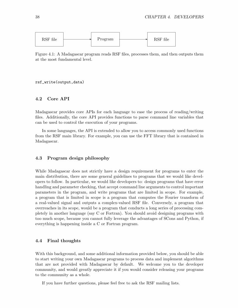
38 CHAPTER 4. DEVELOPERS

RSF file - Program - RSF file

Figure 4.1: A Madagascar program reads RSF files, processes them, and then outputs themat the most fundamental level.

rsf_write(output,data)

4.2 Core API

Madagascar provides core APIs for each language to ease the process of reading/writingfiles. Additionally, the core API provides functions to parse command line variables thatcan be used to control the execution of your programs.

In some languages, the API is extended to allow you to access commonly used functionsfrom the RSF main library. For example, you can use the FFT library that is contained inMadagascar.

4.3 Program design philosophy

While Madagascar does not strictly have a design requirement for programs to enter themain distribution, there are some general guidelines to programs that we would like devel-opers to follow. In particular, we would like developers to: design programs that have errorhandling and parameter checking, that accept command line arguments to control importantparameters in the program, and write programs that are limited in scope. For example,a program that is limited in scope is a program that computes the Fourier transform ofa real-valued signal and outputs a complex-valued RSF file. Conversely, a program thatoverreaches in its scope, would be a program that conducts a long series of processing com-pletely in another language (say C or Fortran). You should avoid designing programs withtoo much scope, because you cannot fully leverage the advantages of SCons and Python, ifeverything is happening inside a C or Fortran program.

4.4 Final thoughts

With this background, and some additional information provided below, you should be ableto start writing your own Madagascar programs to process data and implement algorithmsthat are not provided with Madagascar by default. We welcome you to the developercommunity, and would greatly appreciate it if you would consider releasing your programsto the community as a whole.

If you have further questions, please feel free to ask the RSF mailing lists.

4.5. FURTHER INFORMATION 39

4.5 Further information

For more information about using the API for a particular language, please see: http:

//ahay.org/wiki/Guide_to_madagascar_API.

For more information about developing Madagascar programs in general see: http:

//ahay.org/wiki/Adding_new_programs_to_Madagascar.

For more information about contributing your programs see: http://ahay.org/wiki/

Contributing_new_programs_to_Madagascar.

For a full reference of the C API see: http://www.ahay.org/RSF/book/rsf/manual/

manual_html/

40 CHAPTER 4. DEVELOPERS

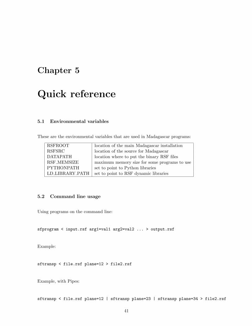
Chapter 5

Quick reference

5.1 Environmental variables

These are the environmental variables that are used in Madagascar programs:

RSFROOT location of the main Madagascar installationRSFSRC location of the source for MadagascarDATAPATH location where to put the binary RSF filesRSF MEMSIZE maximum memory size for some programs to usePYTHONPATH set to point to Python librariesLD LIBRARY PATH set to point to RSF dynamic libraries

5.2 Command line usage

Using programs on the command line:

sfprogram < input.rsf arg1=val1 arg2=val2 ... > output.rsf

Example:

sftransp < file.rsf plane=12 > file2.rsf

Example, with Pipes:

sftransp < file.rsf plane=12 | sftransp plane=23 | sftransp plane=34 > file2.rsf

41

42 CHAPTER 5. QUICK REFERENCE

5.3 Some useful programs

sfdoc -k . | less show program descriptionssfbrowser show program browsersfgui show tkMadagascar GUIsfspike create RSF filessfmath create and manipulate RSF filessfadd add, subtract, multiply datasets togethersftransp change the order of axes in RSF filessfwindow window out portions of RSF filessfricker1 create a Ricker waveletsffft1 FFT on the first axis (real to complex)sffft3 FFT on other axes (complex)sfnoise add noisesfdd convert datasetssfgrey make raster plotssfcat concatenate datasets togethersfput modify header valuessfsegyread read SEGY/SU filessfsegywrite write SEGY/SU files

5.4 SCons commands

scons run an SConstructscons view view the results from an SConstruct, run if necessaryscons lock lock the results from an SConstructscons -c clean the local directory, delete all filesscons -n dry-run of an SConstructscons –debug=explain explain why SCons is doing what it doespscons parallel execution of an SConstruct