The Book of Greeks Edition L1 0 Rahul Bhattacharya CFE School, Risk Latte Company Limited, Hong Kong 2011

Welcome message from author
This document is posted to help you gain knowledge. Please leave a comment to let me know what you think about it! Share it to your friends and learn new things together.
Transcript
8/12/2019 Book of Greeks
http://slidepdf.com/reader/full/book-of-greeks 1/135
The
Book
of GreeksEdition L1 0
Rahul Bhattacharya
CFE School, Risk Latte Company Limited, Hong Kong
2011

8/12/2019 Book of Greeks
http://slidepdf.com/reader/full/book-of-greeks 2/135
2
The Book of Greeks
Certificate in Financial Engineering (CFE) www.risklatte.com
Dedicated to my father, Chandranath Bhattacharya
8/12/2019 Book of Greeks
http://slidepdf.com/reader/full/book-of-greeks 3/135
3
The Book of Greeks
Certificate in Financial Engineering (CFE) www.risklatte.com
What Industry Practitioners have to say about this book?
Rahul Bhattacharya has composed an indispensable collection of notes on Quantitative
Finance with an astonishingly broad coverage. The book familiarizes the reader with awide array of models used in the industry with tips on implementation in Excel™. Excel™is an excellent pedagogical tool and the material in the book invites the reader to
implement the models. The book also contains an extensive coverage of structures traded
across asset classes and even the most seasoned professional will find something new in it.
This is more than a study aid; this is an excellent reference that should be kept within reachon any derivatives desk.
Boris MangalFX Options TraderRBC Capital Markets, Tokyo
The Book of Greeks is an amazingly useful compendium. Rahul Bhattacharya has produced
an easy-reference compilation of the main results in quantitative finance, with just enough
write-ups to be able to apply them in practice, and spanning the entire field from basic stochastic processes to equity, credit, and rates, as well as exotic payoffs and numerical
methods. It distils the key results from an entire library of books, periodicals, and academic
papers into a single short volume that will save practitioners a lot of time and effort .
James de Castro
Former Head of Trading, Asia-Pacific (ex-Japan)
Merrill Lynch, Hong Kong
The Book of Greeks is a perfect companion for any risk manager, quant or derivatives
trader. It manages to have a unique blend of practical application through it's reference to
excel whilst giving the reader all the technical and academic detail he could ever require.
It takes time to give background to the world of modern derivatives and describes the
origins of advanced techniques and models we all take for granted. Everything from
pricing today's exotic derivatives to simple black-scholes greeks are covered. No one
should ever be at their desk without it.
Richard Kendrick
Market Risk ManagementGoldman SachsLondon
8/12/2019 Book of Greeks
http://slidepdf.com/reader/full/book-of-greeks 4/135
4
The Book of Greeks
Certificate in Financial Engineering (CFE) www.risklatte.com
Foreward
The Book of Greeks is an excellent compendium of formulae, models and quantitative
techniques that should be in the repertoire of any derivatives trader, hedge fund manager,
derivatives structurer, academic or student of financial engineering.
Often when we work on trading desks or while structuring derivatives, we wish that we had
a book that had the answers and solutions to the myriad financial products that we have to
price or trade. Well, "The Book of Greeks" is the answer to our prayers. A wonderful, well
compiled book, it offers both the practitioner as well as the academic a one stop source of
mathematical techniques used in the world of financial engineering.
I have enjoyed going through this book and am delighted to be able to recommend it to
anyone who has an interest in quantitative finance and financial engineering.
Rajat BhatiaCEO, Neural CapitalFormer SVP, Citibank Global Asset Management, London& former VP, Lehman Brothers International, London.
8/12/2019 Book of Greeks
http://slidepdf.com/reader/full/book-of-greeks 5/135
5
The Book of Greeks
Certificate in Financial Engineering (CFE) www.risklatte.com
First Few Words
This book is a collection of lecture notes that I’ve used for my CFE classes over the past 2years. These notes are intended to help the reader navigate through various formulas,
equations and algorithms that are used in the four modules of our Certificate in FinancialEngineering (CFE) course. Also, these notes will help all those students taking our CFEExam to better understand the landscape of the entire subject. However, by no means dothese notes present a comprehensive or an exhaustive list of formulas and equations that areused in the study of financial engineering and quantitative finance. At best, it is a miniscule portion of the entire discipline. If anything, these notes aim to provide to the reader aglimpse of the giant canvas on which the subject of Quantitative Finance is written.
All formulas and equations that are used in these notes are meant to be implemented on anExcel™ spr eadsheet. In our CFE course, we implement all these formulas and equations inExcel/VBA and then build quantitative models of financial derivatives and asset portfolio
pricing and risk analysis.
Financial Engineering or Quantitative Finance (and we shall use both these termsinterchangeably) is neither just physics nor applied mathematics, and much more than thesum total of the two. Quantitative Finance is concerned with the application of all those physics-like theories and advanced mathematical concepts and methodologies for thedevelopment of mathematical models and algorithms with which financial derivatives andfinancial asset portfolios can be traded, valued and their risks can be analyzed. However,such is not possible unless all those complex and abstract formulas and equations aretransformed into simpler workable format and implemented on a platform. And that platform has to be something that is very simple to understand and work on.
For our CFE course that platform is the Microsoft Excel™ spreadsheet.
These notes are exclusively meant for supplementing the knowledge and skills imparted inthe CFE course and helping students take the CFE examination. Other than that, this bookhas no other objective or pretense. This book should not be seen as an alternative orsupplement to any textbook on the subject of quantitative finance, a partial list of which isgiven at the end in the reference section. There are no substitutes for the great bookswritten by Jamil Baz, George Chacko, John Hull, Jim Gatheral, Rebonato Riccardo, PaulWilmott, to name only a few.
Rahul Bhattacharya
8/12/2019 Book of Greeks
http://slidepdf.com/reader/full/book-of-greeks 6/135
6
The Book of Greeks
Certificate in Financial Engineering (CFE) www.risklatte.com
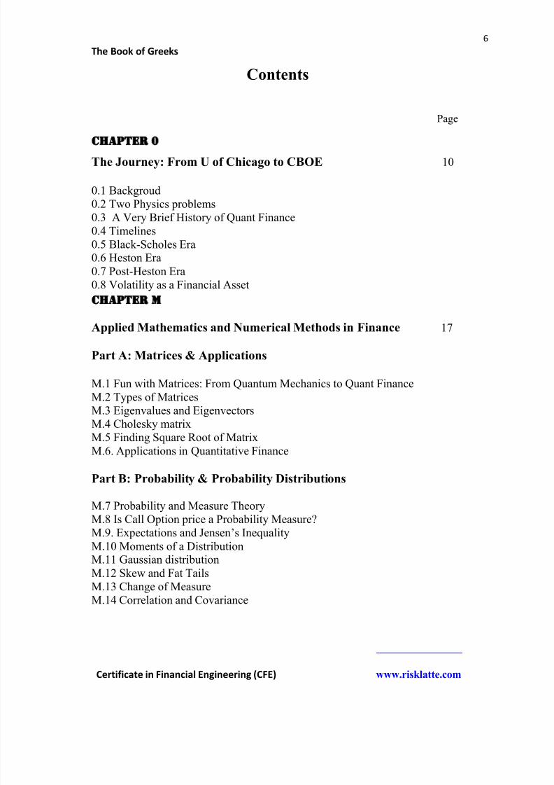
Contents
Page
Chapter
The Journey: From U of Chicago to CBOE 10
0.1 Backgroud0.2 Two Physics problems0.3 A Very Brief History of Quant Finance0.4 Timelines0.5 Black-Scholes Era0.6 Heston Era
0.7 Post-Heston Era0.8 Volatility as a Financial Asset
Chapter M
Applied Mathematics and Numerical Methods in Finance 17
Part A: Matrices & Applications
M.1 Fun with Matrices: From Quantum Mechanics to Quant FinanceM.2 Types of Matrices
M.3 Eigenvalues and EigenvectorsM.4 Cholesky matrixM.5 Finding Square Root of MatrixM.6. Applications in Quantitative Finance
Part B: Probability & Probability Distributions
M.7 Probability and Measure TheoryM.8 Is Call Option price a Probability Measure?M.9. Expectations and Jensen’s Inequality
M.10 Moments of a DistributionM.11 Gaussian distributionM.12 Skew and Fat Tails
M.13 Change of MeasureM.14 Correlation and Covariance
8/12/2019 Book of Greeks
http://slidepdf.com/reader/full/book-of-greeks 7/135
7
The Book of Greeks
Certificate in Financial Engineering (CFE) www.risklatte.com
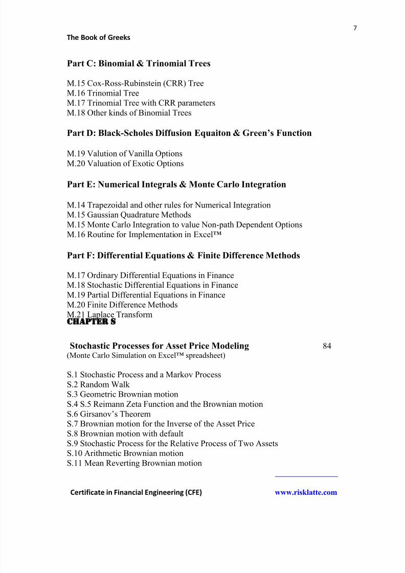
Part C: Binomial & Trinomial Trees
M.15 Cox-Ross-Rubinstein (CRR) TreeM.16 Trinomial Tree
M.17 Trinomial Tree with CRR parametersM.18 Other kinds of Binomial Trees
Part D: Black-Scholes Diffusion Equaiton & Green’s Function
M.19 Valution of Vanilla OptionsM.20 Valuation of Exotic Options
Part E: Numerical Integrals & Monte Carlo Integration
M.14 Trapezoidal and other rules for Numerical IntegrationM.15 Gaussian Quadrature MethodsM.15 Monte Carlo Integration to value Non-path Dependent OptionsM.16 Routine for Implementation in Excel™
Part F: Differential Equations & Finite Difference Methods
M.17 Ordinary Differential Equations in FinanceM.18 Stochastic Differential Equations in FinanceM.19 Partial Differential Equations in FinanceM.20 Finite Difference MethodsM.21 Laplace Transform
Chapter S
Stochastic Processes for Asset Price Modeling 84 (Monte Carlo Simulation on Excel™ spreadsheet)
S.1 Stochastic Process and a Markov ProcessS.2 Random WalkS.3 Geometric Brownian motion
S.4 S.5 Reimann Zeta Function and the Brownian motionS.6 Girsanov’s Theorem S.7 Brownian motion for the Inverse of the Asset PriceS.8 Brownian motion with defaultS.9 Stochastic Process for the Relative Process of Two AssetsS.10 Arithmetic Brownian motionS.11 Mean Reverting Brownian motion
8/12/2019 Book of Greeks
http://slidepdf.com/reader/full/book-of-greeks 8/135
8
The Book of Greeks
Certificate in Financial Engineering (CFE) www.risklatte.com
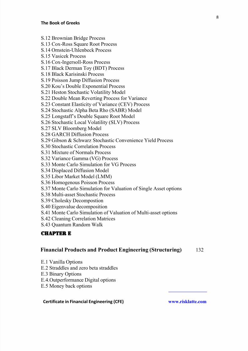
S.12 Brownian Bridge ProcessS.13 Cox-Ross Square Root ProcessS.14 Ornstein-Uhlenbeck ProcessS.15 Vasicek Process
S.16 Cox-Ingersoll-Ross ProcessS.17 Black Derman Toy (BDT) ProcessS.18 Black Karisinski ProcessS.19 Poisson Jump Diffusion ProcessS.20 Kou’s Double Exponential Process S.21 Heston Stochastic Volatility ModelS.22 Double Mean Reverting Process for VarianceS.23 Constant Elasticity of Variance (CEV) ProcessS.24 Stochastic Alpha Beta Rho (SABR) ModelS.25 Longstaff’s Double Square Root Model
S.26 Stochastic Local Volatility (SLV) ProcessS.27 SLV Bloomberg ModelS.28 GARCH Diffusion ProcessS.29 Gibson & Schwarz Stochastic Convenience Yield ProcessS.30 Stochastic Correlation ProcessS.31 Mixture of Normals ProcessS.32 Variance Gamma (VG) ProcessS.33 Monte Carlo Simulation for VG ProcessS.34 Displaced Diffusion ModelS.35 Libor Market Model (LMM)
S.36 Homogenous Poisson ProcessS.37 Monte Carlo Simulation for Valuation of Single Asset optionsS.38 Multi-asset Stochastic ProcessS.39 Cholesky DecompostionS.40 Eigenvalue decompositionS.41 Monte Carlo Simulation of Valuation of Multi-asset optionsS.42 Cleaning Correlation MatricesS.43 Quantum Random Walk
Chapter E
Financial Products and Product Engineering (Structuring) 132
E.1 Vanilla OptionsE.2 Straddles and zero beta straddlesE.3 Binary OptionsE.4.Outperformance Digital optionsE.5 Money back options
8/12/2019 Book of Greeks
http://slidepdf.com/reader/full/book-of-greeks 9/135
9
The Book of Greeks
Certificate in Financial Engineering (CFE) www.risklatte.com
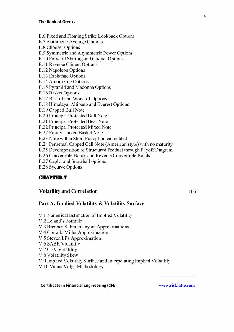
E.6 Fixed and Floating Strike Lookback OptionsE.7 Arithmetic Average OptionsE.8 Chooser OptionsE.9 Symmetric and Asymmetric Power Options
E.10 Forward Starting and Cliquet OptionsE.11 Reverse Cliquet OptionsE.12 Napoleon OptionsE.13 Exchange OptionsE.14 Amortizing OptionsE.15 Pyramid and Madonna OptionsE.16 Basket OptionsE.17 Best of and Worst of OptionsE.18 Himalaya, Altipano and Everest OptionsE.19 Capped Bull Note
E.20 Principal Protected Bull NoteE.21 Principal Protected Bear NoteE.22 Principal Protected Mixed NoteE.22 Equity Linked Basket NoteE.23 Note with a Short Put option embeddedE.24 Perpetual Capped Call Note (American style) with no maturityE.25 Decomposition of Structured Product through Payoff DiagramE.26 Convertible Bonds and Reverse Convertible BondsE.27 Caplet and Snowball optionsE.28 Sycurve Options
Chapter V
Volatility and Correlation 166
Part A: Implied Volatility & Volatility Surface
V.1 Numerical Estimation of Implied VolatilityV.2 Leland’s Formula V.3 Brenner-Subrahmanyam Approximations
V.4 Corrado Miller ApproximationV.5 Steven Li’s Approximation V.6 SABR VolatilityV.7 CEV VolatilityV.8 Volatility SkewV.9 Implied Volatility Surface and Interpolating Implied VolatilityV.10 Vanna Volga Methodology
8/12/2019 Book of Greeks
http://slidepdf.com/reader/full/book-of-greeks 10/135
10
The Book of Greeks
Certificate in Financial Engineering (CFE) www.risklatte.com
V.11 Local VolatilityV.12 Local Volatility in presence of Default
Part A: Historical Volatility
V.13 Historical Volatility using close to close priceV.14 Parkinson’s Number V.15 Garman-Klass EstimatorV.16 EWMA VolatilityV.17 GARCH Process
Part C: Model Free Volatility and Variance Swaps
V.18 Log Contract
V.19 Britten-Jones & Neuberger ModelV.20 Variance SwapV.21 VIX IndexV.22 Volatility SwapV.23 Correlation and Implied CorrelationV.24 Correlation SkewV.25 Dispersion
Chapter O
Options and Financial Derivatives Valuation 195
O.1 Vanilla Options using Black-Scholes ModelO.2 Put-Call Parity and Put-Call SymmetryO.3 Straddle OptionsO.4 Option pricing using Displaced Diffusion modelO.5 Power OptionO.6 Exchange OptionO.7 Binary OptionO.8 Barrier OptionO.9 One Touch Option
O.9 Double Barrier (Binary) OptionO.10 Fixed and Floating Strike Lookback optionsO.11 Arithmetic Average optionO.12 Forward Starting optionO.13 Caps and FloorsO.14 Swaption Valuation using Black’s formulaO.15 SYCURVE Options
8/12/2019 Book of Greeks
http://slidepdf.com/reader/full/book-of-greeks 11/135
11
The Book of Greeks
Certificate in Financial Engineering (CFE) www.risklatte.com
O.16 Bond Option pricing using Black’s formulaO.17 Options on Zero Coupon Bond using Vasicek’s Model O.18 Options on Variance
Chapter G
Greeks for Vanilla & Exotic Options 221
G.1 Call and Put DeltaG.2 Call and Put GammaG.3 Vega of OptionsG.4 Hedging Error due to Volatility SmileG.5 Theta and Rho of Vanilla optionsG.6 Binary Call and Put DeltaG.7 Dirac Delta Function and the Binary
G.8 Binary Gamma and VegaG.9 Variance Swap Greeks
Chapter P
Portfolio Analysis & Asset Allocation 230
P.1 Sharpe Ratio, Treynor Ration and Jensen’s Alpha P.2 Portfolio VolatilityP.3 Expected Return for Stocks and BondsP.4 Volatility of Spreads
P.5 Probability of Stocks Outperforming BondsP.6 Mean-Variance Optimization for a Total Return ObjectiveP.7 Mean-Variance Optimization by maximizing Sharpe RatioP.8 Sharpe’s Algorithm for Efficient Frontier P.9 Portfolio InsuranceP.10 Constant Proportion Portfolio Insurance (CPPI)P.11 Capital Asset Pricing Model (CAPM)P.12 Minimization of Risk and MCR AlgorithmP.13 Statistical ArbitrageP.14 Triangular Arbitrage
8/12/2019 Book of Greeks
http://slidepdf.com/reader/full/book-of-greeks 12/135
12
The Book of Greeks
Certificate in Financial Engineering (CFE) www.risklatte.com
Chapter 0
The Journey From the University of Chicago to Chicago Board Options Exchange……
Background
Before we talk about Quantitative Finance, talk about its brief history and then plungeourselves into the thick of this discipline with formulas, equations and theory, it isworthwhile to understand the background in which this discipline originated some 50 to 60years ago. That background is physics. The foundations of quant finance were laid based ontheories and models of physics. The twin concepts of “equilibrium” and “linearity” whichunderlie almost all of early theories and models of quant finance are both borrowed from physics, as is most of the math and the rationale.
Two Physics problems and the Birth of Quant Finance
I. Albert Einstein and the Random Walk (Diffusion) Problem
Diffusion is one of the fundamental physical processes by which material in nature moves. Itis found in biology, chemistry, geology, engineering, and above all in physics. The processfirst originated in physics in the form of Brownian motion and was studied by none other thefamous physicist Albert Einstein in 1905. Diffusion arises due to the constant thermal motionof atoms, molecules, and particles and causes material to move from areas of highconcentration to low concentration. Therefore, the final outcome of diffusion would be astate of constant concentration across space. Take a bottle of deodorant or perfume and sprayit heavily inside a small closed room. Eventually the smell spreads across the room and the
entire room starts to smell nice. This is an example of diffusion. Take an iron rod and heatone end of it. Eventually, the other end becomes hot as well, because heat was transferredfrom the hot end to the cold end.
Actually, Albert Einstein had solved the Black-Scholes problem long ago. While studyingBrownian motion of particles to complete his Ph.D. thesis, he realized that the randommotion of the molecules at the microscopic level is ultimately responsible for the process ofdiffusion that occurs at the macroscopic level. Physicists had long studied the macroscopic phenomenon of diffusion and established the governing partial differential equation, PDE,( see below for more details on what is a PDE ). However, it took Einstein’s genius to realizethat the constant coefficient of diffusion in the governing PDE of the diffusion process is
actually the same as the volatility parameter, , of the microscopic random process of themolecules.
Note: Fischer Black and Myron Scholes, while formulating the option pricing problem inearly 1970s, followed more or less the same rationale and thought process as Einstein. Themath and the physics was exactly the same. Only the context was different and certain broad
8/12/2019 Book of Greeks
http://slidepdf.com/reader/full/book-of-greeks 13/135
13
The Book of Greeks
Certificate in Financial Engineering (CFE) www.risklatte.com
(and sweeping) assumptions were made about the economy and the investors in relating the problem in physics to that in financial economics.
II. Richard Feynman’s “Path Integrals” and Feynman-Kac Approach
In 1948, Richard Feynman, another eminent physicist of the twentieth century made a simpleand stunning discovery. He found out that the Schrodinger’s partial differential equation(another example of a PDE) in quantum mechanics could be solved by some kind ofaveraging over the paths. This led to the reformulation of the entire quantum mechanicaltheory in physics in terms of what is known as “path integrals”. Mark Kac, a mathematicianand a colleague of Feynman at Cornell, immediately realized that the concept of “averagingof paths” could be applied to the solution of heat equation with boundary conditions andother kinds of diffusion equations in physics. In short, a diffusive partial differential equationcan be solved as an expectation, under a certain probability measure, of a function thatcontains a Brownian motion. This expectation approach has come to be known as the
Feynman-Kac solution.
Note: The expectations approach, developed by latter day quants and still used extensively by practicing quants in the banks and the academic theorists, to solve the pricing problem forvanilla and exotic options is exactly like Feynman and Kac’s approach. In f act, even quantscall it the Feynman-Kac approach. Everywhere, in finance textbooks, research papers and
other technical documents, you’ll see the expectation operator, E written as .Q E and inside
the brackets you’d see an option payoff. This is nothing but Feynman-Kac approach.
A Very Brief History of Quant Finance
The history of Quantitative Finance is essentially a history of the conquest of "Volatility".The story is about how a few exceptionally talented men across both sides of the Atlanticgrappled with the concept of volatility and ultimately tamed it. The story starts off in 1952with volatility being a statistical measure of financial risk and ends in the present day with it becoming a financial asset. That’s pretty much all there is to quantitative finance. Rest is justdetails and an awful lot of very advanced math and computer programming.
It all started in Chicago in 1952 with Harry Markowitz and ended in Chicago sometimearound 2003 when the new VIX was introduced. In that sense we may be living in the post-historical period.
Timeline
This timeline outlines how Volatility got transformed from being a measure of financial riskto financial asset. If we were to take a Jurassic Park style tour of Quant Finance then we’d betaken through the following periods:
Black-Scholes Era (1952 – 1987)
Heston Era (1988 – 2007)
8/12/2019 Book of Greeks
http://slidepdf.com/reader/full/book-of-greeks 14/135
14
The Book of Greeks
Certificate in Financial Engineering (CFE) www.risklatte.com
Post Heston (2007 – Present)
The History tour of Quant Finance
Black-Scholes Era (1952 – 1987)
Black Scholes era began when in 1952, Harry Markowtiz, during the course of completinghis Ph.D. dissertation realized that volatility is a statistical concept and in fact, is the same asthe concept of standard deviation. And mathematically speaking, this is the proxy forfinancial “risk”.
Constant Volatility
It was in 1973, when Fischer Black and Myron Scholes presented their seminal – perhaps,the most famous paper in all of quantitative finance – on option pricing. This could be
considered a formal beginning of the discipline of quant finance.
Here are the defining characteristics and landmarks of this era
In 1973 Black-Scholes option pricing model was introduced which modeled asset prices as following a geometric Brownian motion – a Gaussian diffusion process – with a fixed volatility parameter and option prices are determined as functions of theunderlying asset price. This fixed volatility parameter was important as this is thesame parameter that appears in the partial diffusion equation (PDE) for the option price as the “coefficient of diffusion”.
The physics of the problem was this: asset price is like the molecule following a
random walk suspended in a medium, where the “molecule” was the stock (asset) andthe “medium” was the volatility.
The fact that volatility is constant is extremely important in a Black-Scholes world, because it simplifies life enormously. Constant volatility implies and causes thefollowing:
(i) A market consisting of a stock and an interest-bearing bond is “complete”, inthe sense that all derivative payoffs can be replicated by a dynamic portfolioconsisting of the stock and the bond only.
(ii) Corollary to the above point is that the principle of no arbitrage leads to aunique equivalent martingale measure that can be used to price derivatives.
(iii) The Black-Scholes PDE (with boundary conditions) can be solved exactly as aheat equation and a neat formula for option price can be extracted (this is theBlack-Scholes option pricing formula).
In 1977 Oldrich Vasicek presented the mean reverting random walk model for asset price. This has now come to be known as the Vasicek model and over the years thismodel has found wide applications in interest rate derivatives valuation.
8/12/2019 Book of Greeks
http://slidepdf.com/reader/full/book-of-greeks 15/135
15
The Book of Greeks
Certificate in Financial Engineering (CFE) www.risklatte.com
In 1976 John Cox and Steven Ross presented their risk-neutral argument andintuitively one of the most curious facts of the Black-Scholes model, that is, as to whythe drift term in the asset price equation of random walk drops out of the option pricing equation and the Black-Scholes formula.
Cox and Ross also presented the square root diffusion model of asset price which onceagain opened up new ways at looking at the option pricing problem. Closely related tothe Cox-Ross model was the Cox-Ingersoll-Ross (CIR) model of asset prices, anothermean reverting, arithmetic Brownian motion model of asset price. This model alsofound wide applications in interest rate modeling. More importantly, CIR model wouldform the basis for the stochastic volatility model developed by Heston in the early1990s.
Black-Scholes era came to an end with the stock market crash of 1987 when investorsrealized that volatility is not constant. The notion of volatility smile (skew) – a varyingimplied volatility across strike prices – was born and Wall Street started becoming a very
comfortable place for the quants. Strangely, as the physics was getting out of the way ofquantitative finance and making way for something far more complex (at least in terms ofcomprehension and conceptualization), more and more physicists started getting hired onWall Street.
Heston Era (1988 – 2007)
In my opimion the Heston era began around the time when John Hull and Alan White published their one factor stochastic volatility model in 1987. But this was still not a gamechanger. The real paradigm shift happened when Steven Heston came up with his two factorstochastic volatility model. This was the first break with physics like models.
Stochastic Volatility Here are the defining characteristics and landmarks of this era
Heston postulated that not only the asset price but volatility associated with that asset price is stochastic. In other words, both the asset price and the volatility of that asset price evolve randomly over time. Even though the asset price in Heston’s modelfollows the same geometric Brownian motion, i.e. a Gaussian diffusion process, as theBlack-Scholes model, the volatility is assumed to follow a square root diffusion process, more popularly known as the Cox-Ingersoll-Ross (CIR) process. Thus, the
probability distribution of the asset price was Gaussian (Log-normal) but that of thevolatility was not.
Volatility, which varies stochastically, is also mean reverting;
And above all, the stochastic processes for the asset and the volatility are correlated.This is where there was a paradigm shift in the world view. For, there was no parallelof such a process in physics. Imagine, Einstein thinking about a diffusion process of amolecule which follows a random walk in a “medium” which is itself vibrating in arandom manner.

8/12/2019 Book of Greeks
http://slidepdf.com/reader/full/book-of-greeks 16/135
16
The Book of Greeks
Certificate in Financial Engineering (CFE) www.risklatte.com
Since volatility was not a tradable asset – by which we mean, an explicitly tangibletradable asset – a random volatility would give rise to a situation where a riskless portfolio cannot be constructed to replicate the option price; hence we would end up ina state where markets would no longer be complete.
And the PDE for the option got far more complex. Fortunately, Heston’s model generated a closed form solution – a formula, if you will
– with which option prices could be calculated.
And last but certainly not the least, Heston, during the course of his work on stochasticvolatility, introduced the use of Fourier transform into the quant finance domain (thistechnique would be later utilized to solve various option pricing problem extensively by many quants, most notably Peter Carr).
However, ironically, even though Heston introduced a revolutionary way of visualizingvolatility and the option pricing problem and, advertently or inadvertently, made a decisive break with physics-like models of quant finance, much of the Heston era was dominated by
the other type of volatility models, i.e. the volatility surface and local volatility. It was onlyfrom 2003 onwards that banks started using Heston’s model extensively and quants andtraders started recognizing the utility of this model.
In fact, to be precise, both concepts of “volatility surface” and “local volatility” do not meritthe addition of the word “model” after them. Vol surface and Local Vol are not reallymodels. They are just another way of looking at stochastic volatility.
Anyway, as things stand today Heston’s stochastic volatility model has become a veryimportant and essential tool in the repertoire of most quants and traders in the banks aroundthe world. This change has come about in the last 8 to 9 years.
Volatility Surface
As noted that with the demise of the Black-Scholes world view after the crash of 1987,investors and option traders discovered the volatility smile.
It was observed in the market that implied volatility of options varied across strike prices for a given maturity. From 1987 onwards, it was observed that at least forequity index options, almost always, implied volatilities increase with decreasingstrike – that is, out-of-the-money puts trade at higher implied volatilities than out-of-the-money calls. This feature is often referred to as a “negative” skew, where
skew is just another characterization of smile. It was observed that there is a term structure of volatility, i.e. implied volatility
varied across different maturities; another key observation was that long-termimplied volatilities exceed short-term implied volatilities
From this, the notion of volatility surface was born. This was a surface – a twodimensional matrix – where implied volatility was plotted against strike pricesand time to maturity. From this surface, implied volatility of any arbitrary optioncan be interpolated.
8/12/2019 Book of Greeks
http://slidepdf.com/reader/full/book-of-greeks 17/135
17
The Book of Greeks
Certificate in Financial Engineering (CFE) www.risklatte.com
Local Volatility in a Stochastic Volatility world
In 1994, Emanuel Derman, Iraz Kani and Bruno Dupire noted that under the condition of riskneutrality there is a unique diffusion process that is consistent with the distribution of market
prices of the European options. Derman and Kani, then at Goldman Sachs, presented thisargument using a discrete time binomial tree whereas, Dupire, working separately, presentedthe continuous time version of the same argument. Their work was based on the earlier workof Breeden and Litzenberger done in 1978.
The import of their arguments was a simple modification in the way we looked at volatility.Rather than thinking of volatility as a constant coefficient of a diffusion process, as given bythe Black-Scholes model, they assumed that volatility was now a state dependent function
expressed as: t S L , , where, the subscript L stood for the word local. The volatility
was now a function of S , the asset price and time, t . This shift in the way how volatility wasdefined by Dupire, Derman and Kani (DDK), based on what was observed in the market as
well as that of theoretical foundations of Breeden and Litzenberger’s work, presented acomplexity. How exactly can we define “local volatility”? This is a question that many seniorquants and traders in banks will have difficulty answering.
Jim Gatheral has presented a unique interpretation of this concept in his book Volatility andCorrelation. He doubts if the proponents of DDK local volatility model visualized this as amodel of evolution of volatility. In fact, he doesn’t believe that “local volatility” should forma separate class of models. Gatheral’s interpretation is that “local volatility” can be thoughtof as an average of all possible instantaneous volatilities in a stochastic volatility world .Gatheral has actually demonstrated this notion, using sophisticated mathematics, in his book.
As David de Rosa (64) points out it is important to note that even though local volatility is afunction of a stochastic variable, i.e. the asset price, in itself it is not stochastic. Thisdistinction is important to capture the essence of local volatility. Local volatility isn’t somemeasure of stochastic volatility, rather, given the existence of vanilla option prices in themarket it is a process through which quants make some simplifying assumptions to priceexotic options that are consistent with the prices of the vanilla options traded in the market.
Post Heston (2007 – Present)
One can say that the post-Heston era started with the financial crisis of 2007-2008. Duringthe ensuing market turmoil the stochastic volatility models more or less broke down. This is a
period that witnessed big spikes in volatility in many FX options market, such as the Dollar-Yen market, it caused serious problems for traders. What was really troubling, and perhaps bewildering at the same time, was the observation that somehow volatility has acquired a lifeof its own independent of that of the underlying asset. Is such a thing possible? Is it possiblefor volatility to have the freedom to rise or fall on its own accord without any change in theunderlying asset, say, the FX rate?
8/12/2019 Book of Greeks
http://slidepdf.com/reader/full/book-of-greeks 18/135
18
The Book of Greeks
Certificate in Financial Engineering (CFE) www.risklatte.com
Enter a new class of models known as the Stochastic Local Volatility (SLV) models. Themost important development came with the publication of a stochastic local volatility model by Ren, Madan, and Qian in 2007. As we shall see later on in these notes, this modelincorporated an independent stochastic component in the volatility process that would change
the dynamics of the process significantly. Grigore Tataru and Travis Fisher at Bloombergalso developed an SLV model in 2010 for pricing barrier options. Tataru and Fisher make akey observation in their paper, which perhaps explains the motivation for the development ofSLV models and what we have argued in the above paragraph. The authors note that pricesof barrier and path dependent options mostly depend on the dynamics of the market. Vanillaoption prices don’t matter that much for their pricing. What is important is how the market behaves and, in particular, how volatility rises and falls with the arrival of information and passage of time. SLV models try to matching this extra market dimension to obtain goodexotic option prices.
Volatility as a Financial Asset
Right from the onset in early 1970s when option trading began on the Chicago Board,investors bought or sold options for its value which was captured, mainly, by the volatility ofthe underlying asset. Therefore, implicitly at least, investors were buying and sellingvolatility via options. But this trade was an imperfect trade in volatility. Volatility in itselfwas not a tradable asset. Still, traders and sophisticated investors used various optionstrategies to create as perfect a trade as possible to trade only the volatility of the asset.
During the Heston era two fundamental developments happened that would transformvolatility into a “nearly tangible” asset. The first was the development of variance swaps (andvolatility swaps). In 1994, Anthony Neuberger introduced the Log contract. A keymathematical ingredient in the variance swap pricing mechanism was this Log contract.Variance swaps were developed mainly by Derman and his colleagues at Goldman Sachs,though many others, like Jim Gatheral, contributed to the understanding and development ofthe pricing of this product, and other related products such as volatility swaps. Varianceswap was first instrument in the history of quant finance which allowed investors to trade“pure” volatility, as if it were an asset.
The second development was the creation of the new VIX index by the Chicago BoardOptions Exchange (CBOE) in 2003. The construction of this volatility index would not have been possible without the introduction of the variance swaps. Through this new VIX indexvolatility became an exchange traded commodity and options on this VIX index have now been developed.
From being just the standard deviation of asset returns to becoming an exchanged tradedasset is the story of volatility; which, as I said before, is pretty much the story of quantitativefinance. From the University of Chicago in 1952, when Harry Markowitz had to defend hisnovel concept of risk to Milton Friedman, to the Chicago Board Options Exchange in 2003,when the new VIX was introduced, is a very short distance. But it’s been a long andfascinating journey in time.
8/12/2019 Book of Greeks
http://slidepdf.com/reader/full/book-of-greeks 19/135
19
The Book of Greeks
Certificate in Financial Engineering (CFE) www.risklatte.com
Chapter M Applied Mathematics and
Numerical Methods in Finance
Part A
Matrices & Applications
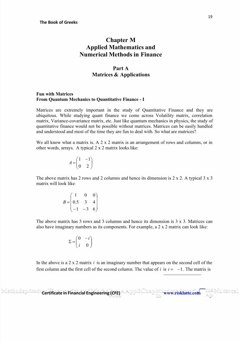
Fun with Matrices
From Quantum Mechanics to Quantitative Finance - I
Matrices are extremely important in the study of Quantitative Finance and they areubiquitous. While studying quant finance we come across Volatility matrix, correlation
matrix, Variance-covariance matrix, etc. Just like quantum mechanics in physics, the study ofquantitative finance would not be possible without matrices. Matrices can be easily handledand understood and most of the time they are fun to deal with. So what are matrices?
We all know what a matrix is. A 2 x 2 matrix is an arrangement of rows and columns, or inother words, arrays. A typical 2 x 2 matrix looks like:
20
11 A
The above matrix has 2 rows and 2 columns and hence its dimension is 2 x 2. A typical 3 x 3matrix will look like:
631
435.0
001
B
The above matrix has 3 rows and 3 columns and hence its dimension is 3 x 3. Matrices canalso have imaginary numbers as its components. For example, a 2 x 2 matrix can look like:
00i
i
In the above is a 2 x 2 matrix i is an imaginary number that appears on the second cell of the
first column and the first cell of the second column. The value of i is 1i . The matrix is
8/12/2019 Book of Greeks
http://slidepdf.com/reader/full/book-of-greeks 20/135
20
The Book of Greeks
Certificate in Financial Engineering (CFE) www.risklatte.com
designated as , which is called the “sigma” (in capital) in Greek. The above matrix forms part of something very important in quantum mechanics in physics and is known as one ofthe Pauli matrices. The above matrices are all square matrices. Why “square”? That is because the number of rows is equal to the number of columns. A 2 x 2, 3 x 3, 8 x 8 or an N
x N matrix are all examples of square matrices. In quantitative finance we only deal withsquare matrices.
Of course, non-square matrices do exist and they do have applications in other fields ofstudy, such as Cryptography. But we shall not talk about them here.
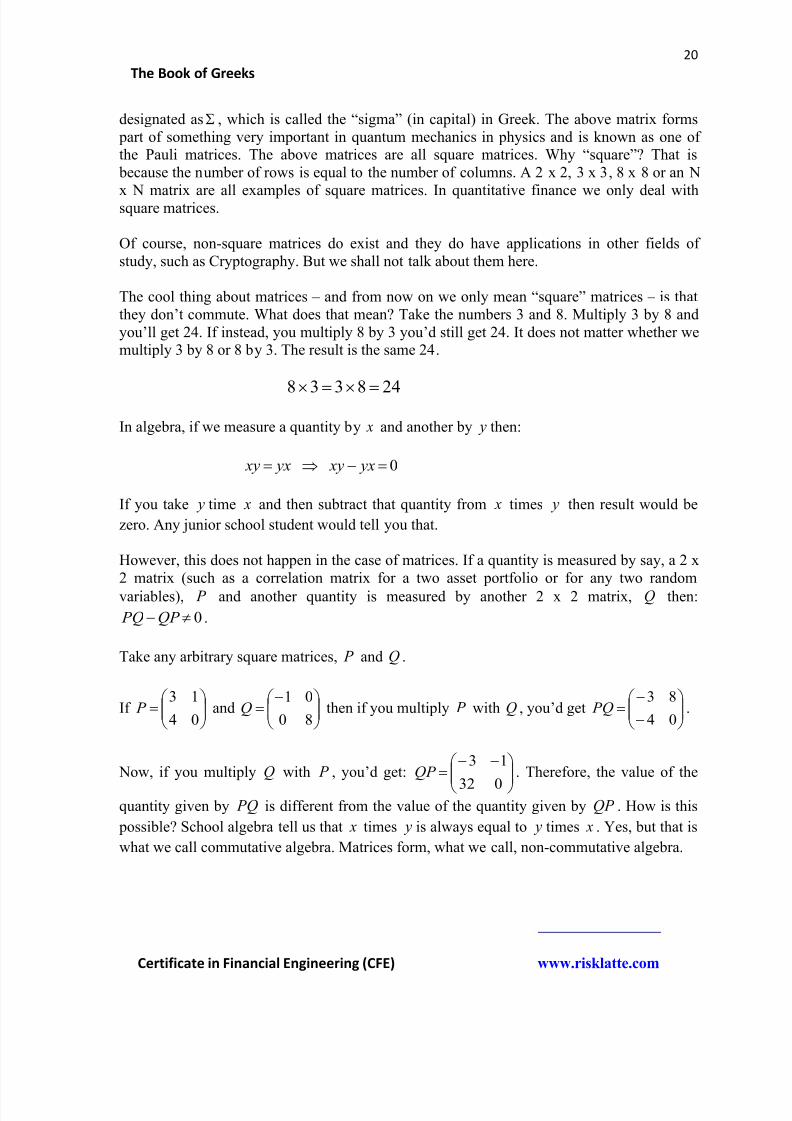
The cool thing about matrices – and from now on we only mean “square” matrices – is thatthey don’t commute. What does that mean? Take the numbers 3 and 8. Multiply 3 by 8 andyou’ll get 24. If instead, you multiply 8 by 3 you’d still get 24. It does not matter whether wemultiply 3 by 8 or 8 by 3. The result is the same 24.
248338
In algebra, if we measure a quantity by x and another by y then:
0 yx xy yx xy
If you take y time x and then subtract that quantity from x times y then result would be
zero. Any junior school student would tell you that.
However, this does not happen in the case of matrices. If a quantity is measured by say, a 2 x2 matrix (such as a correlation matrix for a two asset portfolio or for any two random
variables), P and another quantity is measured by another 2 x 2 matrix, Q then:
0 QP PQ .
Take any arbitrary square matrices, P and Q .
If
04
13 P and
80
01Q then if you multiply P with Q , you’d get
04
83 PQ .
Now, if you multiply Q with P , you’d get:
032
13QP . Therefore, the value of the
quantity given by PQ is different from the value of the quantity given by QP . How is this
possible? School algebra tell us that x times y is always equal to y times x . Yes, but that is
what we call commutative algebra. Matrices form, what we call, non-commutative algebra.
8/12/2019 Book of Greeks
http://slidepdf.com/reader/full/book-of-greeks 21/135
21
The Book of Greeks
Certificate in Financial Engineering (CFE) www.risklatte.com
It may seem trivial to many of you but this simple, non-commutative property of matrices,
i.e. the fact that 0 QP PQ gave physicists the first glimpse into the world of Quantum
Mechanics.
Fun with MatricesFrom Quantum Mechanics to Quantitative Finance - II
There is a beautiful book – perhaps, one of the best in its field – titled Quantum Mechanics in
Simple Matrix Form by Thomas F. Jordan. This article is inspired from that book.
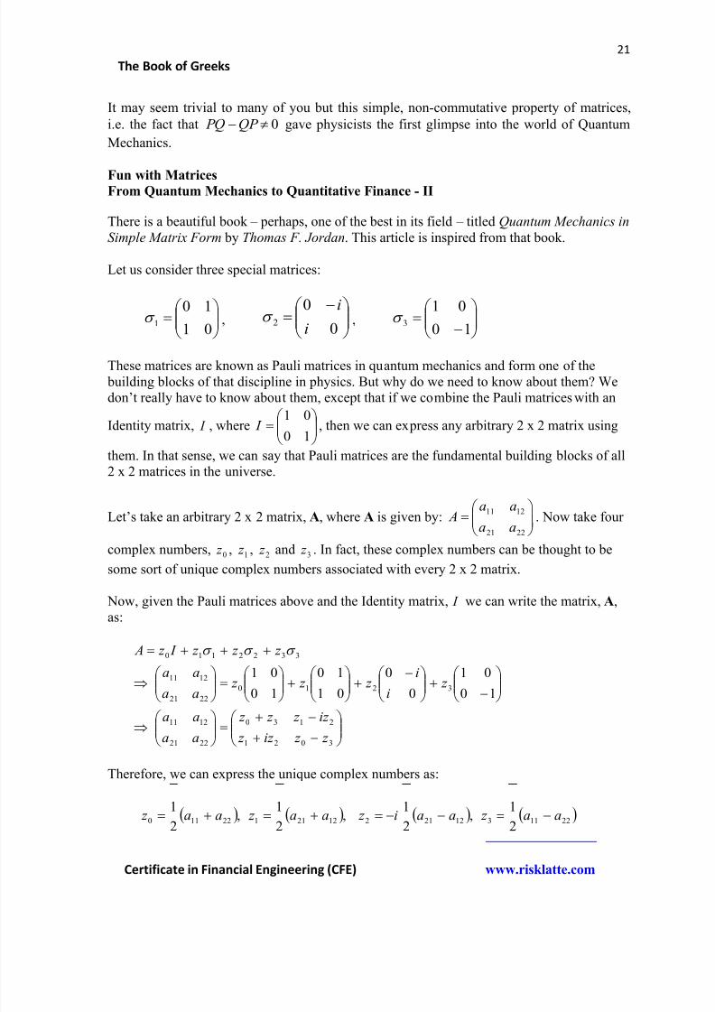
Let us consider three special matrices:
01
101
,
0
02
i
i ,
10
013
These matrices are known as Pauli matrices in quantum mechanics and form one of the building blocks of that discipline in physics. But why do we need to know about them? Wedon’t really have to know about them, except that if we combine the Pauli matrices with an
Identity matrix, I , where
10
01 I , then we can express any arbitrary 2 x 2 matrix using
them. In that sense, we can say that Pauli matrices are the fundamental building blocks of all2 x 2 matrices in the universe.
Let’s take an arbitrary 2 x 2 matrix, A, where A is given by:
2221
1211
aa
aa A . Now take four
complex numbers, 0 z , 1 z , 2 z and 3 z . In fact, these complex numbers can be thought to be
some sort of unique complex numbers associated with every 2 x 2 matrix.
Now, given the Pauli matrices above and the Identity matrix, I we can write the matrix, A,as:
3021
2130
2221
1211
3210
2221
1211
3322110
10
01
0
0
01
10
10
01
z z iz z
iz z z z
aa
aa
z i
i z z z
aa
aa
z z z I z A
Therefore, we can express the unique complex numbers as:
221131221212211221102
1,
2
1,
2
1,
2
1aa z aai z aa z aa z
8/12/2019 Book of Greeks
http://slidepdf.com/reader/full/book-of-greeks 22/135
22
The Book of Greeks
Certificate in Financial Engineering (CFE) www.risklatte.com
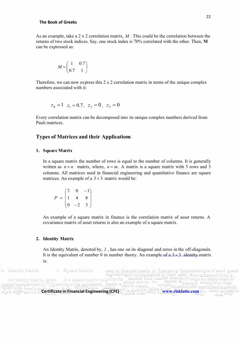
As an example, take a 2 x 2 correlation matrix, M . This could be the correlation between thereturns of two stock indices. Say, one stock index is 70% correlated with the other. Then, M can be expressed as:
17.0
7.01 M
Therefore, we can now express this 2 x 2 correlation matrix in terms of the unique complexnumbers associated with it:
10 z 7.01 z , 02 z , 03 z
Every correlation matrix can be decomposed into its unique complex numbers derived fromPauli matrices.
Types of Matrices and their Applications
1. Square Matrix
In a square matrix the number of rows is equal to the number of columns. It is generally
nn mn written as matrix, where, . A matrix is a square matrix with 3 rows and 3
columns. All matrices used in financial engineering and quantitative finance are square
33 matrices. An example of a matrix would be:
320
841
102
P
An example of a square matrix in finance is the correlation matrix of asset returns. Acovariance matrix of asset returns is also an example of a square matrix.
2. Identity Matrix
I An Identity Matrix, denoted by, , has one on its diagonal and zeros in the off-diagonals.
33 It is the equivalent of number 0 in number theory. An example of a identity matrix
is:
8/12/2019 Book of Greeks
http://slidepdf.com/reader/full/book-of-greeks 23/135
23
The Book of Greeks
Certificate in Financial Engineering (CFE) www.risklatte.com
100
010
001
I
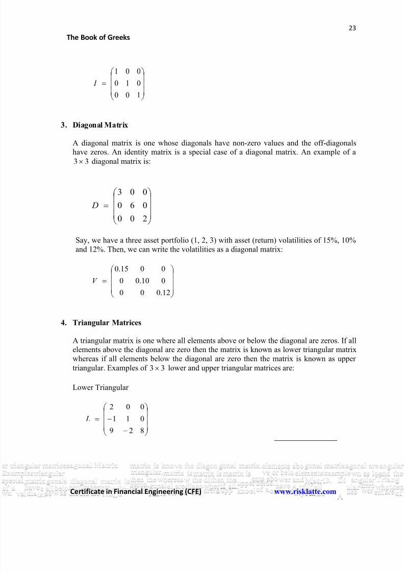
3. Diagonal Matrix
A diagonal matrix is one whose diagonals have non-zero values and the off-diagonalshave zeros. An identity matrix is a special case of a diagonal matrix. An example of a
33 diagonal matrix is:
200
060
003
D
Say, we have a three asset portfolio (1, 2, 3) with asset (return) volatilities of 15%, 10%and 12%. Then, we can write the volatilities as a diagonal matrix:
12.000
010.00
0015.0
V
4. Triangular Matrices
A triangular matrix is one where all elements above or below the diagonal are zeros. If allelements above the diagonal are zero then the matrix is known as lower triangular matrixwhereas if all elements below the diagonal are zero then the matrix is known as upper
33 triangular. Examples of lower and upper triangular matrices are:
Lower Triangular
829
011
002
L
8/12/2019 Book of Greeks
http://slidepdf.com/reader/full/book-of-greeks 24/135
24
The Book of Greeks
Certificate in Financial Engineering (CFE) www.risklatte.com
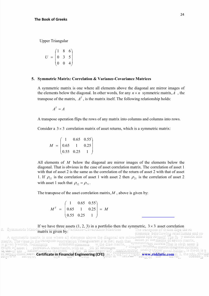
Upper Triangular
400
530681
U
5. Symmetric Matrix: Correlation & Variance-Covariance Matrices
A symmetric matrix is one where all elements above the diagonal are mirror images of
nn Athe elements below the diagonal. In other words, for any symmetric matrix, , theT Atranspose of the matrix, , is the matrix itself. The following relationship holds:
A AT
A transpose operation flips the rows of any matrix into columns and columns into rows.
33 Consider a correlation matrix of asset returns, which is a symmetric matrix:
125.055.0
25.0165.0
55.065.01
M
M All elements of below the diagonal are mirror images of the elements below thediagonal. That is obvious in the case of asset correlation matrix. The correlation of asset 1with that of asset 2 is the same as the correlation of the return of asset 2 with that of asset
12 21 1. If is the correlation of asset 1 with asset 2 then is the correlation of asset 2
2112 with asset 1 such that .
M The transpose of the asset correlation matrix, , above is given by:
M M T
125.055.0
25.0165.0
55.065.01
If we have three assets (1, 2, 3) in a portfolio then the symmetric, 33 asset correlation
matrix is given by:
8/12/2019 Book of Greeks
http://slidepdf.com/reader/full/book-of-greeks 25/135
25
The Book of Greeks
Certificate in Financial Engineering (CFE) www.risklatte.com
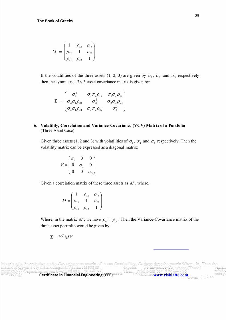
1
1
1
3231
2321
1312
M
If the volatilities of the three assets (1, 2, 3) are given by 1 , 2 and 3 respectively
then the symmetric, 33 asset covariance matrix is given by:
2
332233113
2332
2
22112
13311221
2
1
6. Volatility, Correlation and Variance-Covariance (VCV) Matrix of a Portfolio(Three Asset Case)
1 2 3 Given three assets (1, 2 and 3) with volatilities of , and respectively. Then the
volatility matrix can be expressed as a diagonal matrix:
3
2
1
00
00
00
V
M Given a correlation matrix of these three assets as , where,
1
1
1
3231
2321
1312
M
M jiij Where, in the matrix , we have . Then the Variance-Covariance matrix of the
three asset portfolio would be given by:
MV V T
8/12/2019 Book of Greeks
http://slidepdf.com/reader/full/book-of-greeks 26/135
26
The Book of Greeks
Certificate in Financial Engineering (CFE) www.risklatte.com
2
323321331
2332
2
21221
13311221
2
1
3
2
1
3231
2321
1312
3
2
1
00
00
00
1
1
1
00
00
00
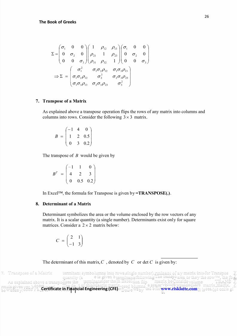
7. Transpose of a Matrix
As explained above a transpose operation flips the rows of any matrix into columns and
33 columns into rows. Consider the following matrix.
2.030
5.021
041
B
BThe transpose of would be given by
2.05.00
324
011T B
In Excel™, the formula for Transpose is given by =TRANSPOSE(.).
8. Determinant of a Matrix
Determinant symbolizes the area or the volume enclosed by the row vectors of anymatrix. It is a scalar quantity (a single number). Determinants exist only for square
22 matrices. Consider a matrix below:
31
12C
C C C detThe determinant of this matrix, , denoted by or is given by:
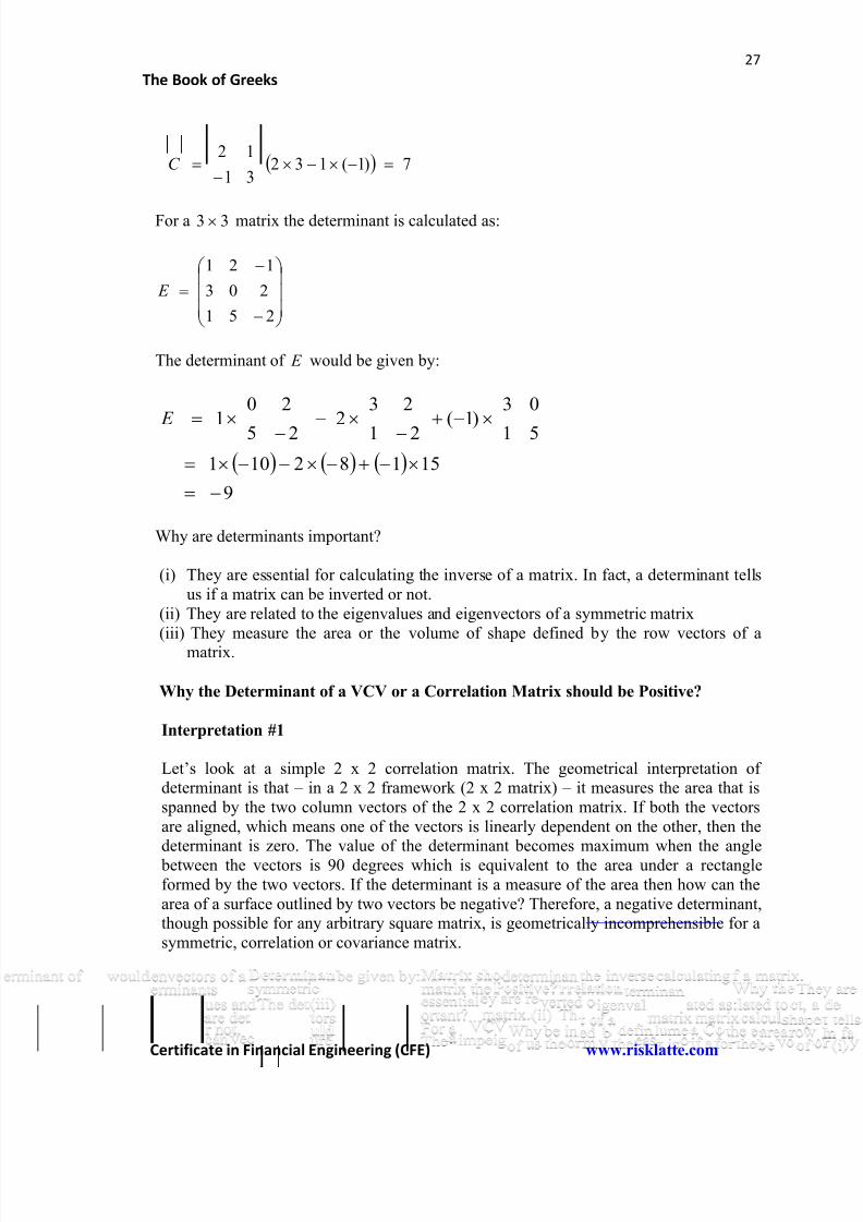
8/12/2019 Book of Greeks
http://slidepdf.com/reader/full/book-of-greeks 27/135
27
The Book of Greeks
Certificate in Financial Engineering (CFE) www.risklatte.com
7)1(13231
12
C
33 For a matrix the determinant is calculated as:
251
203
121
E
E The determinant of would be given by:
9
15182101
51
03
)1(21
23
225
20
1
E
Why are determinants important?
(i) They are essential for calculating the inverse of a matrix. In fact, a determinant tellsus if a matrix can be inverted or not.
(ii) They are related to the eigenvalues and eigenvectors of a symmetric matrix(iii) They measure the area or the volume of shape defined by the row vectors of a
matrix.
Why the Determinant of a VCV or a Correlation Matrix should be Positive?
Interpretation #1
Let’s look at a simple 2 x 2 correlation matrix. The geometrical interpretation ofdeterminant is that – in a 2 x 2 framework (2 x 2 matrix) – it measures the area that isspanned by the two column vectors of the 2 x 2 correlation matrix. If both the vectorsare aligned, which means one of the vectors is linearly dependent on the other, then thedeterminant is zero. The value of the determinant becomes maximum when the angle between the vectors is 90 degrees which is equivalent to the area under a rectangleformed by the two vectors. If the determinant is a measure of the area then how can thearea of a surface outlined by two vectors be negative? Therefore, a negative determinant,though possible for any arbitrary square matrix, is geometrically incomprehensible for asymmetric, correlation or covariance matrix.
8/12/2019 Book of Greeks
http://slidepdf.com/reader/full/book-of-greeks 28/135
28
The Book of Greeks
Certificate in Financial Engineering (CFE) www.risklatte.com
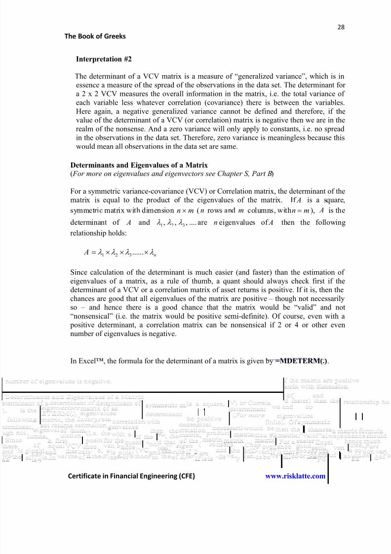
Interpretation #2
The determinant of a VCV matrix is a measure of “generalized variance”, which is inessence a measure of the spread of the observations in the data set. The determinant for
a 2 x 2 VCV measures the overall information in the matrix, i.e. the total variance ofeach variable less whatever correlation (covariance) there is between the variables.Here again, a negative generalized variance cannot be defined and therefore, if thevalue of the determinant of a VCV (or correlation) matrix is negative then we are in therealm of the nonsense. And a zero variance will only apply to constants, i.e. no spreadin the observations in the data set. Therefore, zero variance is meaningless because thiswould mean all observations in the data set are same.
Determinants and Eigenvalues of a Matrix( For more on eigenvalues and eigenvectors see Chapter S, Part B)
For a symmetric variance-covariance (VCV) or Correlation matrix, the determinant of the Amatrix is equal to the product of the eigenvalues of the matrix. If is a square,
mn n m mn Asymmetric matrix with dimension ( rows and columns, with ), is the
A ....,,, 321 n Adeterminant of and are eigenvalues of then the following
relationship holds:
n A ......321
Since calculation of the determinant is much easier (and faster) than the estimation ofeigenvalues of a matrix, as a rule of thumb, a quant should always check first if the
determinant of a VCV or a correlation matrix of asset returns is positive. If it is, then thechances are good that all eigenvalues of the matrix are positive – though not necessarilyso – and hence there is a good chance that the matrix would be “valid” and not“nonsensical” (i.e. the matrix would be positive semi-definite). Of course, even with a positive determinant, a correlation matrix can be nonsensical if 2 or 4 or other evennumber of eigenvalues is negative.
In Excel™, the formula for the determinant of a matrix is given by =MDETERM(.).
8/12/2019 Book of Greeks
http://slidepdf.com/reader/full/book-of-greeks 29/135
29
The Book of Greeks
Certificate in Financial Engineering (CFE) www.risklatte.com
9. Inverse of a Matrix
A 1 A A 1 AThe inverse of a matrix, , is defined as where, multiplied by is equal to the
I I AA 1identity matrix, . Mathematically, we can write, .The inverse of a matrix is
calculated as:
A
Aadj A 1
If the determinant of a matrix is zero then the inverse of the matrix will not exist. We saythat the matrix is non-invertible. Such matrices are known as Singular matrices.
In Excel™, the formula for the inverse of a matrix is given by =MINVERSE(.).
10. Matrix Multiplication
Two matrices can be multiplied to produce a third matrix. However, two matrices canonly be multiplied if the column of the first matrix is equal to the row of the secondmatrix. The dimension of the third matrix, which is the product of the first and the secondmatrix, would be the rows of the first matrix and the columns of the second matrix.
22 A BIf we have two matrices, and given as follows
2221
1211
2221
1211
bb
bb B
aa
aa A
B A Then the product of the two matrices, is given by
2222122121222121
2212121121121111
2221
1211
2221
1211
babababa
babababa
bb
bb
aa
aa B AC
Say, we have a three asset portfolio (1, 2, 3) with asset (return) volatilities of 10%, 15%
33 and 12% respectively and expressed as a diagonal matrix as:
12.000
015.00
0010.0
V
8/12/2019 Book of Greeks
http://slidepdf.com/reader/full/book-of-greeks 30/135

8/12/2019 Book of Greeks
http://slidepdf.com/reader/full/book-of-greeks 31/135
31
The Book of Greeks
Certificate in Financial Engineering (CFE) www.risklatte.com
Then, the Trading Covariance matrix in Dollars per share is given by the followingmatrix multiplication:
m
T
m
mn
m
m
mm
T
p
p
p
p
p
p
P M P
00
00
00
00
00
00
1
1
1
00
00
00
00
00
00
2
1
2
1
21
221
112
2
1
2
1
12. Power of a Matrix
One of the problems of matrices is that they cannot be raised to non-integer powers. Wecan raise a square matrix to a power of 2, 3, 4….. but we cannot raise a matrix to the power of 0.5 (half) or 0.75. Thus we cannot find the square root of a matrix. Consider the
33 following matrix:
651
113
012
X
If we want to find the square of the matrix we simply multiply the matrix with itself(same as raising the matrix to the power of 2).
313623
718
137
651
113
012
651
113
0122 S S S
S 3 2S S Similarly we can raise the matrix to the power of by multiplying with ; and so
S on for higher powers of
S However, if we want to raise the matrix, , to the power of half (0.5), i.e. if we want to
S S find the square root of the matrix , we cannot do it. Square roots of the matrix, exists but they are very different from the notion of a square root that we have from number
8/12/2019 Book of Greeks
http://slidepdf.com/reader/full/book-of-greeks 32/135
32
The Book of Greeks
Certificate in Financial Engineering (CFE) www.risklatte.com
theory. In fact, a square matrix can have numerous square roots, something that we don’t
3 3see in number theory. The number, has a unique square root given by, .
13. Eigenvalues and Eigenvectors of a Matrix
Let A be an nn square matrix. There exists a number that is said to be the
eigenvalue of A if there exists a non-zero solution vector, W to the linear system ofequations:
W AW
The solution vector, W , is said to the eigenvector of A corresponding to the particular
eigenvalue, .
To solve for we set up the characteristic equation as follows:
00
0
I AW I A
W AW
Where, I A represents the determinant of I A . This characteristic equation
yields a closed form real or complex solution for the eigenvalues, . The eigenvalues, will be the solution of the polynomial (quadratic, cubic, etc.) equation generated by the
characteristic equation above. If A is a 22 matrix then there would be 2 values of , (
1 and 2 ). If A is a 33 matrix then there would be 3 values of , ( 1 , 2 and 3 )
and so on. Eigenvalues are scalar quantities and are simply real or complex numbers.
Once the eigenvalues of the matrix, A are determined then the eigenvectors, W aredetermined. Except for very rare instances, closed form solutions do not exist for
eigenvectors and the eigenvectors, W , corresponding to each eigenvalue is estimatediteratively using numerical algorithms.
If A is an nn square matrix (i.e. n rows and n columns) then there would be n
eigenvectors and W would be expressed as an nn square matrix. If A is 22 then
even W would be 22 in dimension and if A is 33 then even W would be 33 in
dimension. The matrix A and W have the same dimensions.
8/12/2019 Book of Greeks
http://slidepdf.com/reader/full/book-of-greeks 33/135
33
The Book of Greeks
Certificate in Financial Engineering (CFE) www.risklatte.com
For any arbitrary square matrix, A given by:
nnnn
n
n
aaa
aaa
aaa
A
21
22221
11211
We have the corresponding eigenvalues are n ,....,, 21 and the matrix of
eigenvectors W is given as:
nnnn
n
n
www
www
www
W
21
22221
11211
Here,
nw
w
w
W
1
12
11
1
is the eigenvector corresponding to the eigenvalue 1 ,
2
22
12
2
nw
w
w
W
is
the eigenvector corresponding to the eigenvalue 2 and so on.
14. Square Root of a Matrix
K A square matrix can have many square roots. A matrix is said to be the square root of
M M M K 22 a matrix, , if the product equals to . For example, consider a matrix B
as given by
3721
2816 B
This matrix has many square roots. One of the square roots of this matrix is a matrix given
53
42 R B R R by because, .
8/12/2019 Book of Greeks
http://slidepdf.com/reader/full/book-of-greeks 34/135
34
The Book of Greeks
Certificate in Financial Engineering (CFE) www.risklatte.com
15. Methods of Finding the Square Root of a Matrix( Please see the Eigenvalues and Eigenvectors of a Matrix to understand this part fully)
th N There are many methods for finding the square root or the root of a square matrix.One of the most common and robust ways of finding the square root of a matrix is via thediagonalization method using the eigenvalues and the eigenvectors of the matrix.
X jk W If is a square matrix of dimension given by and is the matrix of the
X jk eigenvectors of with the same dimension of and is a diagonal matrix of the
X X eigenvalues of then can be decomposed as:
1 W W X
th N X Then, the root of the matrix is given by:
1
1
ˆ W W X N
th N Where, is a diagonal matrix with the diagonal elements being the root of the
k .......,,, 21 33 individual eigenvalues, . For a matrix we get the following.
33 X
333231
232221
131211
x x x
x x x
x x x
X If we have a matrix, , given by:
W And if the matrix of eigenvectors, , and the diagonal matrix of the eigenvalues, , aregiven by:
333231
232221
131211
www
www
www
W
3
2
1
00
00
00
and
8/12/2019 Book of Greeks
http://slidepdf.com/reader/full/book-of-greeks 35/135
35
The Book of Greeks
Certificate in Financial Engineering (CFE) www.risklatte.com
16. Cholesky Matrix
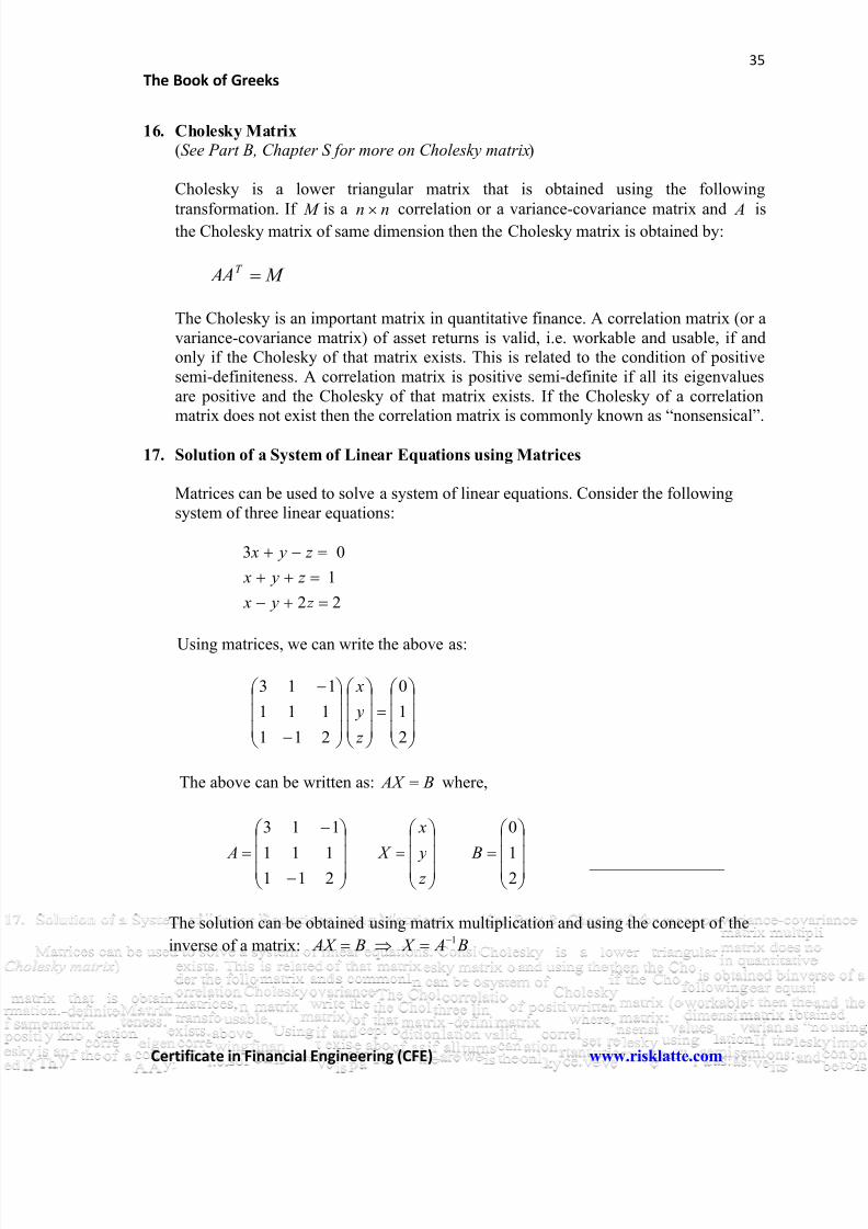
(See Part B, Chapter S for more on Cholesky matrix)
Cholesky is a lower triangular matrix that is obtained using the following
M nn Atransformation. If is a correlation or a variance-covariance matrix and isthe Cholesky matrix of same dimension then the Cholesky matrix is obtained by:
M AAT
The Cholesky is an important matrix in quantitative finance. A correlation matrix (or avariance-covariance matrix) of asset returns is valid, i.e. workable and usable, if andonly if the Cholesky of that matrix exists. This is related to the condition of positivesemi-definiteness. A correlation matrix is positive semi-definite if all its eigenvaluesare positive and the Cholesky of that matrix exists. If the Cholesky of a correlationmatrix does not exist then the correlation matrix is commonly known as “nonsensical”.
17. Solution of a System of Linear Equations using Matrices
Matrices can be used to solve a system of linear equations. Consider the followingsystem of three linear equations:
22
1
03
z y x
z y x
z y x
Using matrices, we can write the above as:
2
1
0
211
111
113
z
y
x
B AX The above can be written as: where,
21
0
211111
113
B z y
x
X A
The solution can be obtained using matrix multiplication and using the concept of the
B A X B AX 1inverse of a matrix:
8/12/2019 Book of Greeks
http://slidepdf.com/reader/full/book-of-greeks 36/135
36
The Book of Greeks
Certificate in Financial Engineering (CFE) www.risklatte.com
8.0
1.0
3.0
2
1
0
211
111
113 1
z
y
x
X
3.0 x 1.0 y 8.0 z Thus, , and
Applications of Matrices in Quantitative Finance
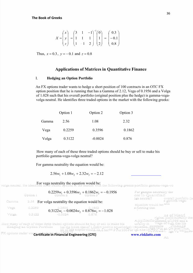
I. Hedging an Option Portfolio
An FX options trader wants to hedge a short position of 100 contracts in an OTC FXoption position that he is running that has a Gamma of 2.12, Vega of 0.1956 and a Volga
of 1.028 such that his overall portfolio (original position plus the hedge) is gamma-vega-volga neutral. He identifies three traded options in the market with the following greeks:
Option 1 Option 2 Option 3
Gamma 2.56 1.08 2.32
Vega 0.2259 0.3596 0.1862
Volga 0.3122 -0.0024 0.876
How many of each of these three traded options should he buy or sell to make his portfolio gamma-vega-volga neutral?
For gamma neutrality the equation would be:
12.232.208.156.2 321 www
For vega neutrality the equation would be:
1956.01862.03596.02259.0 321 www
For volga neutrality the equation would be:
028.1876.00024.03122.0 321 www
8/12/2019 Book of Greeks
http://slidepdf.com/reader/full/book-of-greeks 37/135
37
The Book of Greeks
Certificate in Financial Engineering (CFE) www.risklatte.com
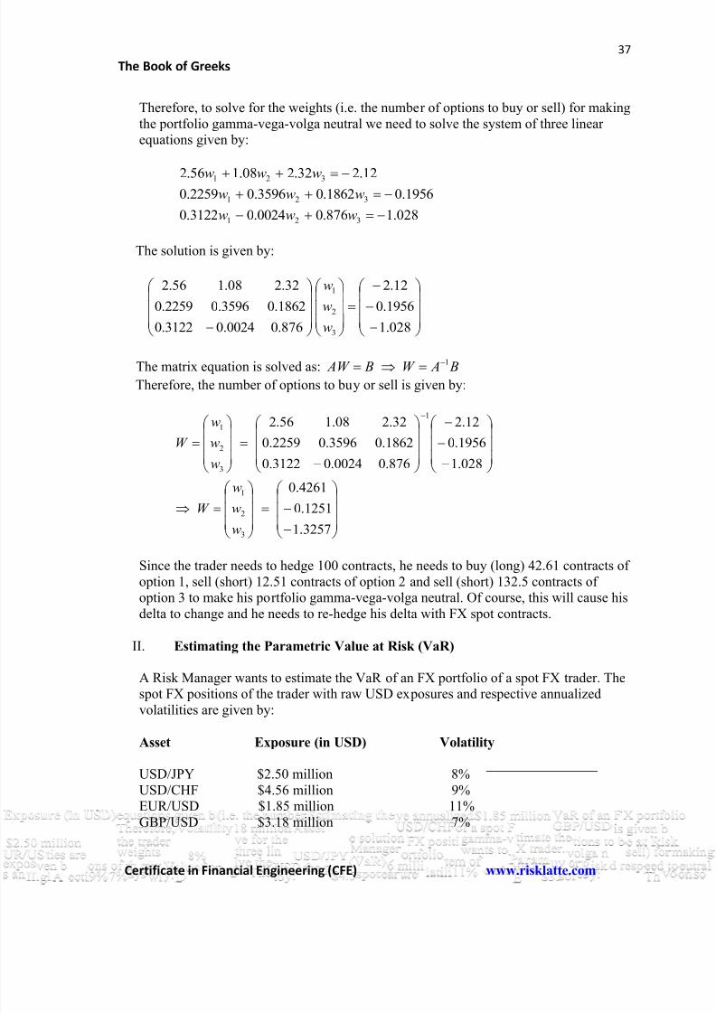
Therefore, to solve for the weights (i.e. the number of options to buy or sell) for makingthe portfolio gamma-vega-volga neutral we need to solve the system of three linearequations given by:
12.232.208.156.2 321 www 1956.01862.03596.02259.0 321 www
028.1876.00024.03122.0 321 www
The solution is given by:
028.1
1956.0
12.2
876.00024.03122.0
1862.03596.02259.0
32.208.156.2
3
2
1
w
w
w
The matrix equation is solved as: B AW B AW 1
Therefore, the number of options to buy or sell is given by:
3257.1
1251.0
4261.0
028.1
1956.0
12.2
876.00024.03122.0
1862.03596.02259.0
32.208.156.2
3
2
1
1
3
2
1
w
w
w
W
w
w
w
W
Since the trader needs to hedge 100 contracts, he needs to buy (long) 42.61 contracts ofoption 1, sell (short) 12.51 contracts of option 2 and sell (short) 132.5 contracts ofoption 3 to make his portfolio gamma-vega-volga neutral. Of course, this will cause hisdelta to change and he needs to re-hedge his delta with FX spot contracts.
II. Estimating the Parametric Value at Risk (VaR)
A Risk Manager wants to estimate the VaR of an FX portfolio of a spot FX trader. Thespot FX positions of the trader with raw USD exposures and respective annualized
volatilities are given by:
Asset Exposure (in USD) Volatility
USD/JPY $2.50 million 8%USD/CHF $4.56 million 9%EUR/USD $1.85 million 11%GBP/USD $3.18 million 7%
8/12/2019 Book of Greeks
http://slidepdf.com/reader/full/book-of-greeks 38/135
38
The Book of Greeks
Certificate in Financial Engineering (CFE) www.risklatte.com
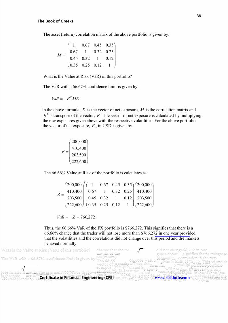
The asset (return) correlation matrix of the above portfolio is given by:
112.025.035.0
12.0132.045.0
25.032.0167.0
35.045.067.01
M
What is the Value at Risk (VaR) of this portfolio?
The VaR with a 66.67% confidence limit is given by:
ME E VaR T
E M In the above formula, is the vector of net exposure, is the correlation matrix andT E E is transpose of the vector, . The vector of net exposure is calculated by multiplying
the raw exposures given above with the respective volatilities. For the above portfolio E the vector of net exposure, , in USD is given by
600,222
500,203
400,410
000,200
E
The 66.66% Value at Risk of the portfolio is calculates as:
600,222
500,203
400,410
000,200
112.025.035.0
12.0132.045.0
25.032.0167.0
35.045.067.01
600,222
500,203
400,410
000,200 T
Z
272,766 Z VaR
Thus, the 66.66% VaR of the FX portfolio is $766,272. This signifies that there is a66.66% chance that the trader will not lose more than $766,272 in one year providedthat the volatilities and the correlations did not change over this period and the markets behaved normally.
8/12/2019 Book of Greeks
http://slidepdf.com/reader/full/book-of-greeks 39/135
39
The Book of Greeks
Certificate in Financial Engineering (CFE) www.risklatte.com
III. Portfolio Optimization: Strategic Asset Allocation Problems
Linear equations also appear in portfolio optimization problems (mean-variance
optimization) that appear in strategic asset allocation models used by fund managers toallocate funds between various asset classes and individual securities within assetclasses.
See Chapter P for more details on this.
IV. Applications in Algorithmic Trading (Minimization of MCR)
Matrices are also used to solve complex mathematical algorithms used by algorithmicand high frequency traders to buy and sell stocks and other assets. A particular exampleis the minimization of the Marginal Contribution of Risk (MCR) to determine the
number of stocks to buy and/or sell in a trade list.
See Chapter P for more details on this.
V. Estimating the Variance-Covariance (VCV) Matrix from Market Data
Quantitative equity analysts, fund managers and risk managers in bank need to have thevariance covariance (VCV) matrix of asset returns almost on a real time basis. How dowe estimate the VCV matrix from market data of stock (asset) prices?
The best, and the easiest way, to extract the VCV matrix from the market data is toestimate it via excess return. From a time series of stock price data we can calculate themean return of the stock and hence determine the excess return for a particular period,
i.e. the return of a particular period less the mean return. Let’s say that we have K riskyassets (stocks or stock indices, etc.) and for each of these assets we have price data
(which we can easily obtain in real time from Bloomberg) for N periods (say, 12months, 52 weeks or 5 years, etc.)
Then, here’s the algorithm for obtaining the VCV matrix of the portfolio of K assets:
1. Estimate the return on each of these assets over N periods; ideally, all percentage asset returns should be annualized
2. Calculate the mean return for each of the assets (stocks);
3. Estimate the excess return matrix; the matrix of excess returns, Rˆ is given by:
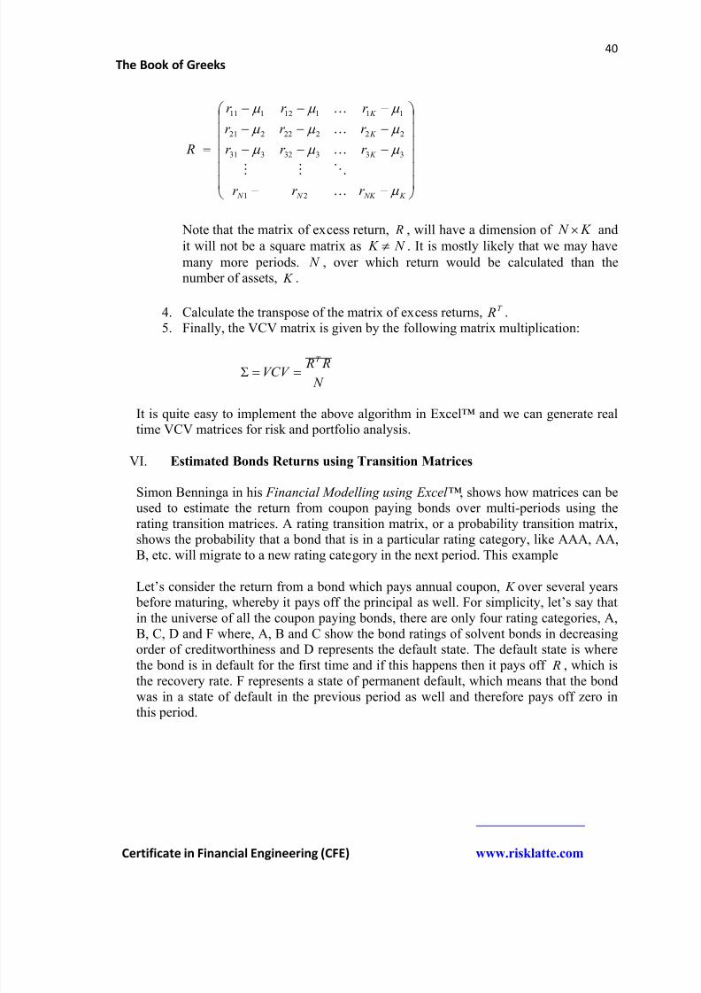
8/12/2019 Book of Greeks
http://slidepdf.com/reader/full/book-of-greeks 40/135
40
The Book of Greeks
Certificate in Financial Engineering (CFE) www.risklatte.com
K NK N N
K
K
K
r r r
r r r
r r r
r r r
R
21
33332331
22222221
11112111
ˆ
Note that the matrix of excess return, R , will have a dimension of K N and
it will not be a square matrix as N K . It is mostly likely that we may have
many more periods. N , over which return would be calculated than thenumber of assets, K .
4. Calculate the transpose of the matrix of excess returns, T Rˆ .5. Finally, the VCV matrix is given by the following matrix multiplication:
N
R RVCV
T ˆˆ
It is quite easy to implement the above algorithm in Excel™ and we can generate realtime VCV matrices for risk and portfolio analysis.
VI. Estimated Bonds Returns using Transition Matrices
Simon Benninga in his Financial Modelling using Excel™ , shows how matrices can beused to estimate the return from coupon paying bonds over multi-periods using the
rating transition matrices. A rating transition matrix, or a probability transition matrix,shows the probability that a bond that is in a particular rating category, like AAA, AA,B, etc. will migrate to a new rating category in the next period. This example
Let’s consider the return from a bond which pays annual coupon, K over several years before maturing, whereby it pays off the principal as well. For simplicity, let’s say thatin the universe of all the coupon paying bonds, there are only four rating categories, A,B, C, D and F where, A, B and C show the bond ratings of solvent bonds in decreasingorder of creditworthiness and D represents the default state. The default state is wherethe bond is in default for the first time and if this happens then it pays off R , which isthe recovery rate. F represents a state of permanent default, which means that the bond
was in a state of default in the previous period as well and therefore pays off zero inthis period.
8/12/2019 Book of Greeks
http://slidepdf.com/reader/full/book-of-greeks 41/135
41
The Book of Greeks
Certificate in Financial Engineering (CFE) www.risklatte.com
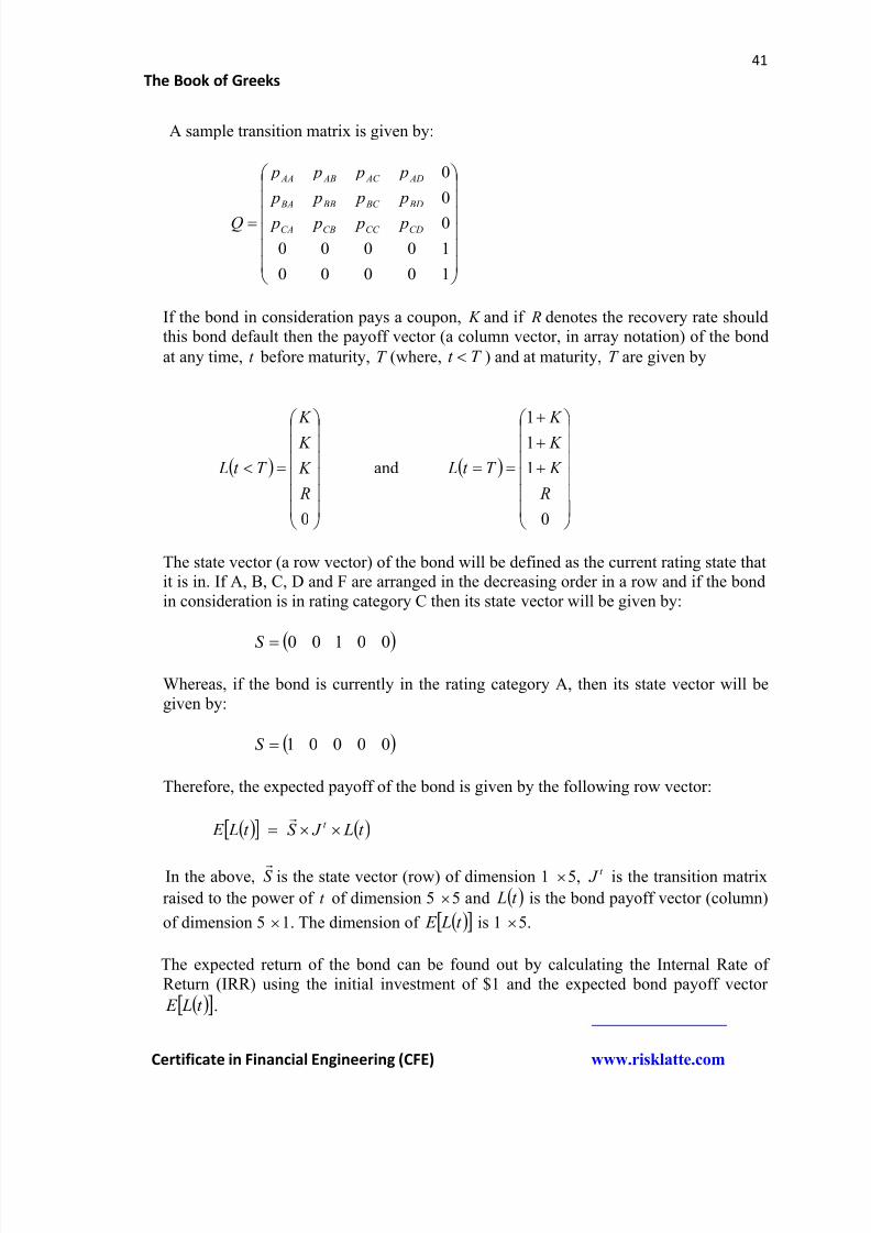
A sample transition matrix is given by:
10000
10000
0
0
0
CDCC CBCA
BD BC BB BA
AD AC AB AA
p p p p
p p p p
p p p p
Q
If the bond in consideration pays a coupon, K and if R denotes the recovery rate shouldthis bond default then the payoff vector (a column vector, in array notation) of the bond
at any time, t before maturity, T (where, T t ) and at maturity, T are given by
0
R
K
K
K
T t L and
0
1
1
1
R
K
K
K
T t L
The state vector (a row vector) of the bond will be defined as the current rating state thatit is in. If A, B, C, D and F are arranged in the decreasing order in a row and if the bondin consideration is in rating category C then its state vector will be given by:
00100S
Whereas, if the bond is currently in the rating category A, then its state vector will begiven by:
00001S
Therefore, the expected payoff of the bond is given by the following row vector:
t L J S t L E t
In the above, S is the state vector (row) of dimension 1 5, t J is the transition matrix
raised to the power of t of dimension 5 5 and t L is the bond payoff vector (column)
of dimension 5 1. The dimension of t L E is 1 5.
The expected return of the bond can be found out by calculating the Internal Rate ofReturn (IRR) using the initial investment of $1 and the expected bond payoff vector
t L E .
8/12/2019 Book of Greeks
http://slidepdf.com/reader/full/book-of-greeks 42/135
42
The Book of Greeks
Certificate in Financial Engineering (CFE) www.risklatte.com
VII. Fibonacci Numbers and the Golden Ratio – An Eigenvalue problem
Fibonacci Numbers and the Golden Ratio are used quite extensively by technical
analysts to predict stock and currency market moves. However, even though both theFibonacci numbers and the Golden Ratio are staple diet for technical analysts inanalyzing stock and currency charts, many would have trouble grasping the relationship between these two mathematical constructs.
What is the relationship between Fibonacci numbers and the Golden Ratio? As it turnsout Golden Ratio is one of the eigenvalues of a Fibonacci matrix.
A Fibonacci sequence of numbers is given by:
0, 1, 1, 2, 3, 5, 8, 13, 21, ………………
Where, each number, except for zero and one, is the sum of the previous two numbers.
In general they can be written as, with seed values, 00 f and 11 f :
21 k k k f f f
Golden Ratio is the irrational number 1.6180339……. It is generally denoted by the
Greek alphabet (psi) and is an extremely important ratio that is found in mathematics,
nature and the world of arts. Some mathematicians, represent it as:2
51 . And
interestingly, many Renaissance artists believed that the Golden Ratio was a “divine proportion”.
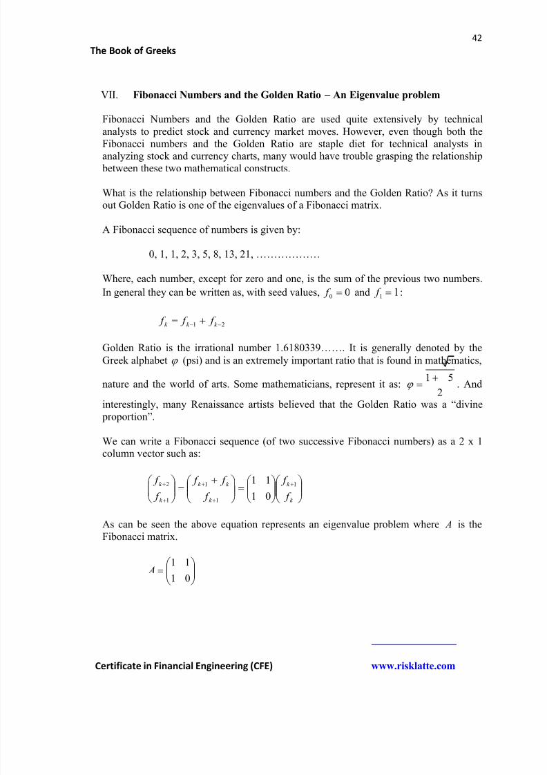
We can write a Fibonacci sequence (of two successive Fibonacci numbers) as a 2 x 1column vector such as:
k
k
k
k k
k
k
f
f
f
f f
f
f 1
1
1
1
2
01
11
As can be seen the above equation represents an eigenvalue problem where A is theFibonacci matrix.
01
11 A
8/12/2019 Book of Greeks
http://slidepdf.com/reader/full/book-of-greeks 43/135
43
The Book of Greeks
Certificate in Financial Engineering (CFE) www.risklatte.com
It can be easily shown that one of the eigenvalues, 1 , of A is equal to the Golden
Ratio, 1.6180339…..
Setting up the characteristic equation as 0 I A where, is the eigenvalue of A
we get the quadratic equation:
012
Solving the above, we get:2
51 where:
......6180339.12
511
and .....6180339.0
2
512
Hence, one of the eigenvalues of A, 1
is equal to the irrational number 1.6180339…which is the Golden Ratio.
A whole New Branch of Study
Random Matrices
From Nuclear Physics to Quantitative Finance - I
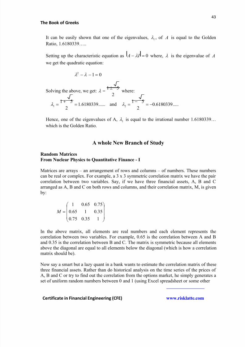
Matrices are arrays – an arrangement of rows and columns – of numbers. These numberscan be real or complex. For example, a 3 x 3 symmetric correlation matrix we have the pair
correlation between two variables. Say, if we have three financial assets, A, B and Carranged as A, B and C on both rows and columns, and their correlation matrix, M, is given by:
135.075.0
35.0165.0
75.065.01
M
In the above matrix, all elements are real numbers and each element represents thecorrelation between two variables. For example, 0.65 is the correlation between A and B
and 0.35 is the correlation between B and C. The matrix is symmetric because all elementsabove the diagonal are equal to all elements below the diagonal (which is how a correlationmatrix should be).
Now say a smart but a lazy quant in a bank wants to estimate the correlation matrix of thesethree financial assets. Rather than do historical analysis on the time series of the prices ofA, B and C or try to find out the correlation from the options market, he simply generates aset of uniform random numbers between 0 and 1 (using Excel spreadsheet or some other
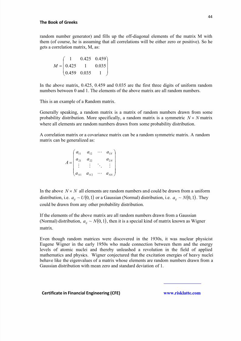
8/12/2019 Book of Greeks
http://slidepdf.com/reader/full/book-of-greeks 44/135
8/12/2019 Book of Greeks
http://slidepdf.com/reader/full/book-of-greeks 45/135
45
The Book of Greeks
Certificate in Financial Engineering (CFE) www.risklatte.com
Ever since then random matrices and Random Matrix Theory have been applied to variousdisciplines including electrical engineering, quantum mechanics, sociology, econometricsand even quantitative finance.
Random MatricesFrom Nuclear Physics to Quantitative Finance - II
Consider a large N N square matrix, A, whose elements are random numbers drawn from
a certain probability distribution, say the Gaussian distribution. Then, for such a matrix, A,what can be said about the probabilities of a few of the eigenvalues or the eigenvectors ofthis matrix? This is the central problem in Random Matrix Theory (RMT) and the answerto this question has far reaching ramifications, not only in nuclear physics but also in suchdiverse areas as quantitative finance, mathematics and mechanical engineering, etc.
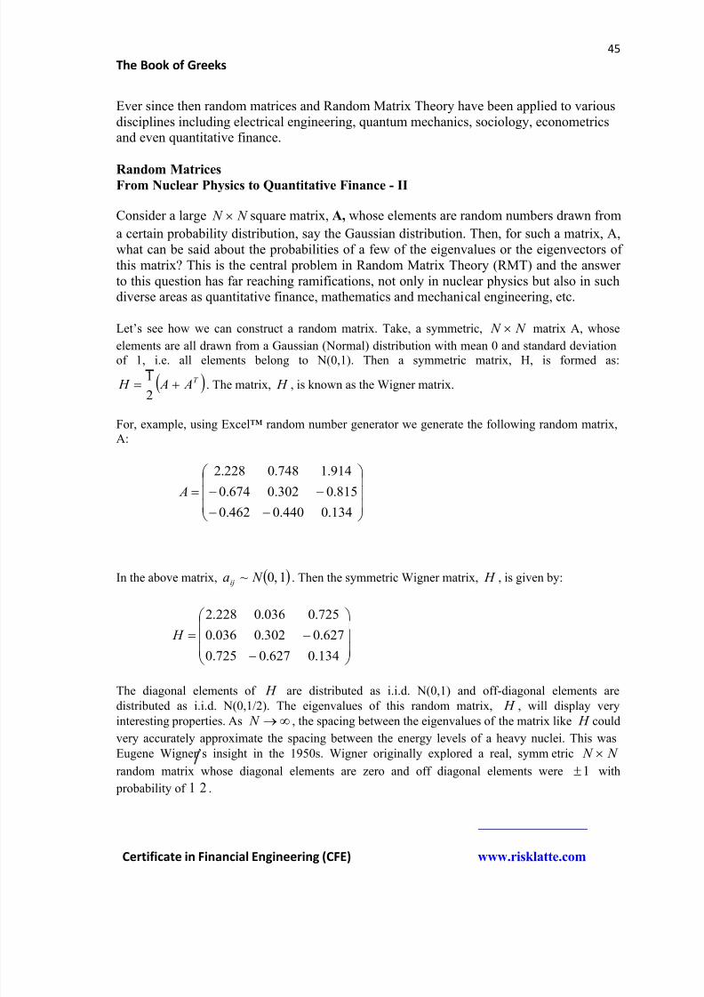
Let’s see how we can construct a random matrix. Take, a symmetric, N N matrix A, whose
elements are all drawn from a Gaussian (Normal) distribution with mean 0 and standard deviationof 1, i.e. all elements belong to N(0,1). Then a symmetric matrix, H, is formed as:
T A A H 2
1. The matrix, H , is known as the Wigner matrix.
For, example, using Excel™ random number generator we generate the following random matrix,A:
134.0440.0462.0
815.0302.0674.0
914.1748.0228.2
A
In the above matrix, 1,0~ N aij . Then the symmetric Wigner matrix, H , is given by:
134.0627.0725.0
627.0302.0036.0
725.0036.0228.2
H
The diagonal elements of H are distributed as i.i.d. N(0,1) and off-diagonal elements are
distributed as i.i.d. N(0,1/2). The eigenvalues of this random matrix, H , will display very
interesting properties. As N , the spacing between the eigenvalues of the matrix like H could
very accurately approximate the spacing between the energy levels of a heavy nuclei. This was
Eugene Wigner’s insight in the 1950s. Wigner originally explored a real, symmetric N N
random matrix whose diagonal elements are zero and off diagonal elements were 1 with
probability of 21 .
8/12/2019 Book of Greeks
http://slidepdf.com/reader/full/book-of-greeks 46/135
46
The Book of Greeks
Certificate in Financial Engineering (CFE) www.risklatte.com
How’s all this relevant to the study of quantitative finance?
Take an example from portfolio analysis and asset allocation. When an equity analyst in ahedge fund quantitatively analyzes a large portfolio of stocks (or any other asset) she first
and foremost estimates the correlation and/or the covariance matrix of the stock returns.Let’s say that the covariance matrix of stock returns is M and random (symmetric) matrixof the type described above (with suitable constraints) is H . If the eigenvalues of M aredistributed in a similar fashion as the eigenvalues of H then the analyst will conclude thatthe elements of M , the actual, observable covariance matrix, have considerable degree ofrandomness. This means that there is a lot of noise in the stock price data that she observesfor all the stocks in her portfolio. Random matrix theory can be used to filter out noise froma correlation or a covariance matrix in a portfolio of assets. There are many other importantapplications of random matrices in quantitative finance.
Part BProbability and Probability Distributions
Probability and Measure Theory
We consider a quantity that can take certain value, x . This quantity could be the price ofMicrosoft stock or the S&P500 index or the temperature of New York City. Let’s say that
this quantity given by, x , fluctuates randomly. In other words, x is a random number.
Now, for each possible value of x there exists a number, x p , between 0 and 1 which we
call the probability. In the simplest possible terms, we can think of x p as the likelihood
of occurrence of the variable x (though strictly speaking “likelihood” is not “probability”).The number x p can be best thought of as a “measure”. Just like the notion of “area” and
“volume” which are more general notion of measure, a probability number, x p , is also a
“measure” (of events occurring); a “ probability measure”, in fact, tells us the likelihood ofobserving any “conceivable event” in an experiment whose outcome is uncertain. However,
probability measure, x p , must assign a value 1 to the entire probability space. In fact,
probability satisfies the mathematical definition of a “measure” which is concerned withthe notion of (a) a space and (b) additivity.
Think of the area of a rectangle, which is equal to length multiplied by width, can beviewed as a product of two intervals to form a certain space and the area of the rectangle isthe measure of that space. Within this overall space, enclosed by the length and width, wecan think of many smaller rectangles enclosed and the sum of the areas of all thoserectangles will be equal to the area original space enclosed by the rectangle. Similarly, probability is also concerned with a space, known as the probability space, which can bethought of as a set of all events. Within that set lies the sub-sets of “conceivable events”that can occur and probability measures these conceivable events in such a way that thesum of the probabilities of all these conceivable events is equal to 1.
8/12/2019 Book of Greeks
http://slidepdf.com/reader/full/book-of-greeks 47/135
47
The Book of Greeks
Certificate in Financial Engineering (CFE) www.risklatte.com
The last line means that the sum of the probabilities of all possible values of x is equal toone. Therefore, the probability measure satisfies these two properties:
(i) 0 < x p < 1
(ii) 1 x
x p
The mean or the expected value of x is written as x and is denoted by the Greek letter,
mu, . This mean is given by:
x
x xp x
The uncertainty in the value of x , i.e. how much the value of x is going to differ from the
expected value (mean), x , is usually denoted by the Greek letter and is given by theexpression:
2 x x
This is called the standard deviation of x . The quantity 2 x x measures the
dispersion in the value of x and is known as the variance of x .
Is Call Option Price a Probability Measure?
There is a deep connection between the prices of financial derivatives and probability,though, within the context of derivatives we usually deal with “risk neutral” probabilities.The theory of probability and probability distributions forms the foundation for the study offinancial derivatives. It is well known that the price of a digital (binary) call or a put optionin a Black-Scholes framework is nothing but the discounted value of the probability of thestock (asset) finishing in the money. It has been shown by Peter Carr and Dilip Madan thata call or a put option price can symbolize a probability measure under a different measure.
If T S is the price of the asset at maturity and K is the strike price then the (undiscounted)
price of a call option is given by:
dS S K S K C T 0,max
In terms of the expectation operator we can write the above price as:
0,max K S E K C T
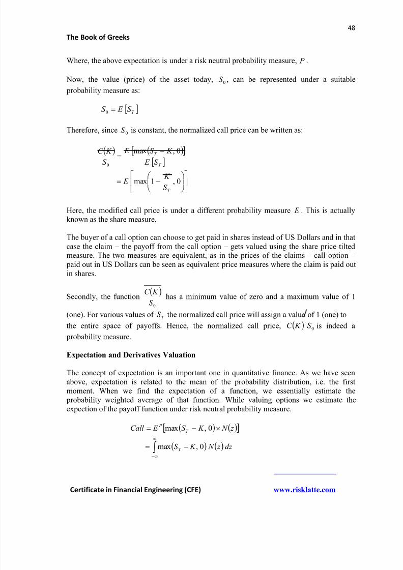
8/12/2019 Book of Greeks
http://slidepdf.com/reader/full/book-of-greeks 48/135
48
The Book of Greeks
Certificate in Financial Engineering (CFE) www.risklatte.com
Where, the above expectation is under a risk neutral probability measure, P .
Now, the value (price) of the asset today, 0S , can be represented under a suitable
probability measure as:
T S E S 0
Therefore, since 0S is constant, the normalized call price can be written as:
0,1maxˆ
0,max
0
T
T
T
S
K E
S E
K S E
S
K C
Here, the modified call price is under a different probability measure E ˆ . This is actuallyknown as the share measure.
The buyer of a call option can choose to get paid in shares instead of US Dollars and in thatcase the claim – the payoff from the call option – gets valued using the share price tiltedmeasure. The two measures are equivalent, as in the prices of the claims – call option – paid out in US Dollars can be seen as equivalent price measures where the claim is paid outin shares.
Secondly, the function
0S
K C
has a minimum value of zero and a maximum value of 1
(one). For various values of T S the normalized call price will assign a value of 1 (one) to
the entire space of payoffs. Hence, the normalized call price, 0S K C is indeed a
probability measure.
Expectation and Derivatives Valuation
The concept of expectation is an important one in quantitative finance. As we have seenabove, expectation is related to the mean of the probability distribution, i.e. the firstmoment. When we find the expectation of a function, we essentially estimate the
probability weighted average of that function. While valuing options we estimate theexpection of the payoff function under risk neutral probability measure.
dz z N K S
z N K S E Call
T
T
P
0,max
0,max
8/12/2019 Book of Greeks
http://slidepdf.com/reader/full/book-of-greeks 49/135
49
The Book of Greeks
Certificate in Financial Engineering (CFE) www.risklatte.com
Where, z is a random normal variable and 1,0~ N z . In the above z N is the measure of
the probability that the stock will finish in the money.
It can be better understood in discrete form, where the integral gets replaced by the
summation sign.
i
iT i z N K S Call 0,max ,
In a simple binomial model say, that the risk neutral probability of up move is 60% and thedown move is 40% and the current stock price is 100. In an up move the asset will finish at120 and in a down move the asset will finist at 80. Then what is the value of a 100 strikecall option.
Using the above formula for the call value as an expectation we get:
124.00,10080max6.00,100120max Call
A key point that has to be noted is that when we are estimating the option price using anexpectations approach, we always take the expectation of the option payoff and not theexpection of the asset price. This is because the option payoff is a convex function andJensen’s inequality holds.
Jensen’s Inequality
Jensen’s Inequality states that for a convex function, such as the payoff of a call option, theexpected value of the function is greater than or equal to the function of the expected value.
In other words, if x f is a convex function in x , then
x E f x f E
Paul Wilmott in his Frequently Asked Questions in Quantitative Finance and Spiegeleerand Schoutens in their The Handbook of Convertible Bonds have shown, how using aTaylor series expansion on the above expression we can explain the concepts of convexityand gamma of an option.
Jensen’s inequality is one of the most important theorems in quantitative finance and it isthe reason why financial derivatives have value embedded in their gammas. Concept ofconvexity, Jensen’s inequality, randomness and volatility of an asset price are intricatelylinked. In my opinion, study of financial derivatives should start with an understanding andthe explanation of convex functions and the Jensen’s inequality.
8/12/2019 Book of Greeks
http://slidepdf.com/reader/full/book-of-greeks 50/135
50
The Book of Greeks
Certificate in Financial Engineering (CFE) www.risklatte.com
More on Jensen’s Inequality: Explaining Convexity with Numbers
If k is a constant and x is a variable, then what is common between the functions 2 x x f
and 0,max k x x g ?
Most of us would immediately recognize the second function as the payoff from a calloption. But what about the first function? That doesn’t seem like the payoff of a financialderivative. Actually, both the above functions share the property of “convexity”. In other
words, both these functions are convex. And the function, 2 x x f is as much a payoff of
a financial derivative as the function 0,max k x x f . One of the chief reasons why
every financial derivative has inherent value (and which sometimes is also known as the“time value”) is because all financial derivatives have a convex payoff. Convexity is alsoknown as “gamma” in option parlance. It is the same as what mathematicians call“curvature” of function (or a graph).
Therefore, for financial derivatives to have value they must have a convex payoff. Everyoption, vanilla or exotic, every structured product has to have a convex payoff for it to haveinherent value based on which it can be traded. Without convexity in its payoff, thefinancial derivative would just become the underlying asset (equity, FX, interest rate, etc.)
How do we define a convex payoff or a convex function?
If, , is a small parameter (constant) between 0 and 1 (i.e. 10 ) then, for a given
interval 21, x x , a convex function has the following property:
2121 11 x f x f x x f
Let’s take some numbers to see if the two functions above share the above property.
Let’s take 75.0 and let’s take the interval [100, 110]. Applying the above inequality on
the first function, 2 x x f , we get:
525,10506,10
11025.010075.05.102
11025.010075.0110*25.0100*75.0
f f f
f f f
Therefore, the left hand side is less than (or equal to) the right hand side. So, the function isconvex.
8/12/2019 Book of Greeks
http://slidepdf.com/reader/full/book-of-greeks 51/135
51
The Book of Greeks
Certificate in Financial Engineering (CFE) www.risklatte.com
Now, let’s take the second function, 0,max k x x g which is in fact, the payoff
function for a call option. Let’s keep the interval the same, i.e. [100, 110] and 75.0 . We
choose the constant, k (strike) to be 102. In fact, the choice of k doesn’t matter at all and
we can choose any value for k . Now, applying the property of convexity to this function
we get:
25.0
102110max*25.00,102100max*75.00,1025.102max
11025.010075.05.102
11025.010075.0110*25.0100*75.0
g g g
g g g
Once again we see that the left hand side is less than (or equal to) the right hand side. Thisshows that the function for the call option payoff is indeed convex.
In fact, we can take any values for between 0 and 1 and choose any interval 21, x x , the
above property (inequality) for convexity will always hold. We leave it as an exercise for
the readers to choose different values of in 10 and any arbitrary interval 21, x x
to test whether the inequality for convexity holds for both the above functions.
Like the previous example, let’s take two functions, x f and x g which are given by
2 x x f and 0,max k x x g respectively representing the payoff functions of
financial derivatives on the same underlying asset, say, S&P500. Here, we should note that
x is a random variable (drawn from a certain probability distribution). For example, x can
be the price of S&P500 stock index. As again, x g is the payoff of a call option, say on
SP500, with a constant strike price k . The function x f would also give the payoff of a
financial financial derivative which is given by the square of x , or in this case, the squareof the final price of S&P500 stock index. Both functions are convex.
In the above context, we should write the Jensen’s inequality as:
T T x E f x f E
The subscript T denotes the final price of the variable (SP500); for example, T could beequal to one year if the maturity of the derivative is one year.
I will now take a very simple and highly stylized example, using numbers, to prove theJensen’s inequality. Say, S&P500 is currently trading at 100 (normalized value). Now, tokeep things extremely simple let’s say that SP500 index can only take 6 (final) values at the
end of one year. The final price of S&P500, T x can be any one of these values: 100, 110,
120, 130, 140 and 150.
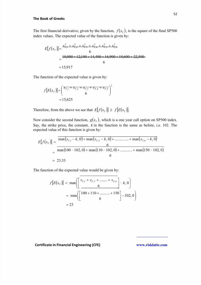
8/12/2019 Book of Greeks
http://slidepdf.com/reader/full/book-of-greeks 52/135
52
The Book of Greeks
Certificate in Financial Engineering (CFE) www.risklatte.com
The first financial derivative, given by the function, T x f , is the square of the final SP500
index values. The expected value of the function is given by:
917,15
6
500,22600,19900,16400,14100,12000,10
6
2
6,
2
5,
2
4,
2
3,
2
2,
2
1,
T T T T T T
T
x x x x x x
x f E
The function of the expected value is given by:
625,15
6
2
5,4,3,2,1,
T T T T T
T
x x x x x x E f
Therefore, from the above we see that T T x E f x f E .
Now consider the second function, T x g , which is a one year call option on SP500 index.
Say, the strike price, the constant, k in the function is the same as before, i.e. 102. Theexpected value of this function is given by:
33.23
60,102150max............0,102110max0,102100max
6
0,max..............0,max0,max 6,2,1,
k xk xk x x f E
T T T
T
The function of the expected value would be given by:
23
0,102
6
150..........110100max
0,6
........max
6,2,1,
k
x x x x E f
T T T
T
8/12/2019 Book of Greeks
http://slidepdf.com/reader/full/book-of-greeks 53/135
53
The Book of Greeks
Certificate in Financial Engineering (CFE) www.risklatte.com
Therefore, once again we see that T T x E f x f E . Hence we observe that given
these values of T x (all of which are assumed to be random) both the functions, x f and
x g satisfy the Jensen’s inequality.
One can take any values and a large enough set of numerical values for T x the Jensen’s
inequality for both the above functions will hold. We would urge our readers to experiment
with any random set (no matter how large is the set) of numerical values for T x to test the
Jensen’s inequality.
Since, the expected value of the function, x g , is always greater than the function of the
expected value, a call option on SP500 (or a call option on any other asset that is modeledas a random walk) will have an inherent, fundamental value at inception (time, t = 0). And
that fundamental value is given by the (discounted) expected value of the function T x g .
In our simple and stylized example above we assumed only six possible values for the
variable (SP500) T x . In reality, there will a large – infinite – number of values for T x all
drawn from a certain probability distribution (because T x is random). Thus, in real life, the
fair value of a call option on SP500 stock index at inception (t = 0) would be given by:
T
QrT x f E eCall
Where, Q is the probability measure under which the expectation, E (or, in layman’s
terms, the averaging) is being carried out. In fact, as Wilmott shows
termsorder higher x E f x f E T T
The “higher order terms” capture the gamma (convexity) of the option and the variance of
the randomness. All financial derivatives, whether they are given by functions, T x f ,
T x g or any other convex functions (of a random variable) share the above property.
Convexity terms (higher order terms) are added to the expected value (mean) of thefunction to give the financial derivative a fundamental fair value at inception (t = 0).
Probability Distribution and the Gaussian
If there is a random variable X which can take all possible values, each of which has acertain probability of occurrence, such that the sum of all probabilities is 1, then a probability distribution of X will show how the total value of 1 is distributed over all possible values. An example of a probability distribution is the famous Normal, or theGaussian, probability distribution.
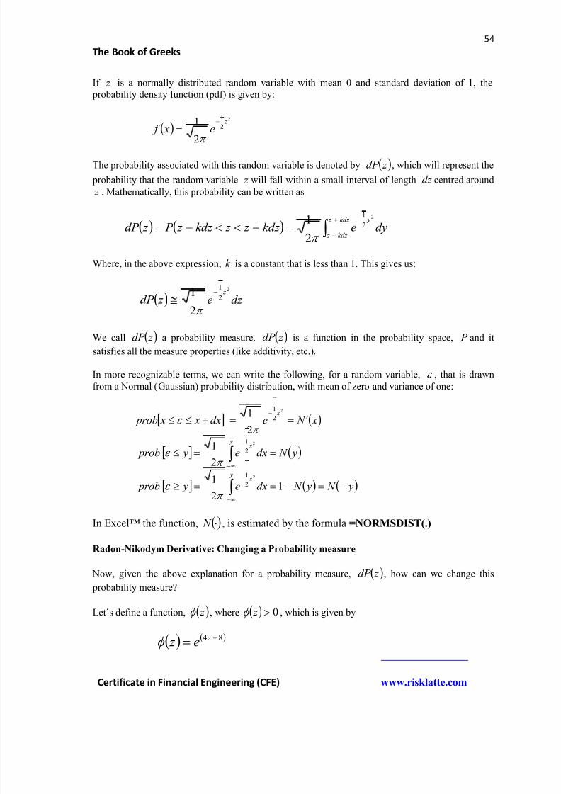
8/12/2019 Book of Greeks
http://slidepdf.com/reader/full/book-of-greeks 54/135
54
The Book of Greeks
Certificate in Financial Engineering (CFE) www.risklatte.com
If z is a normally distributed random variable with mean 0 and standard deviation of 1, the probability density function (pdf) is given by:
2
2
1
2
1 z
e x f
The probability associated with this random variable is denoted by z dP , which will represent the
probability that the random variable z will fall within a small interval of length dz centred around
z . Mathematically, this probability can be written as
dyekdz z z kdz z P z dP kdz z
kdz z
y
2
2
1
2
1
Where, in the above expression, k is a constant that is less than 1. This gives us:
dz e z dP z 2
2
1
2
1
We call z dP a probability measure. z dP is a function in the probability space, P and it
satisfies all the measure properties (like additivity, etc.).
In more recognizable terms, we can write the following, for a random variable, , that is drawn
from a Normal (Gaussian) probability distribution, with mean of zero and variance of one:
x N edx x x prob x
2
2
1
21
y N dxe y prob
y x
2
2
1
2
1
y N y N dxe y prob
y x
12
1 2
2
1
In Excel™ the function, N , is estimated by the formula =NORMSDIST(.)
Radon-Nikodym Derivative: Changing a Probability measure
Now, given the above explanation for a probability measure, z dP , how can we change this
probability measure?
Let’s define a function, z , where 0 z , which is given by
84 z e z
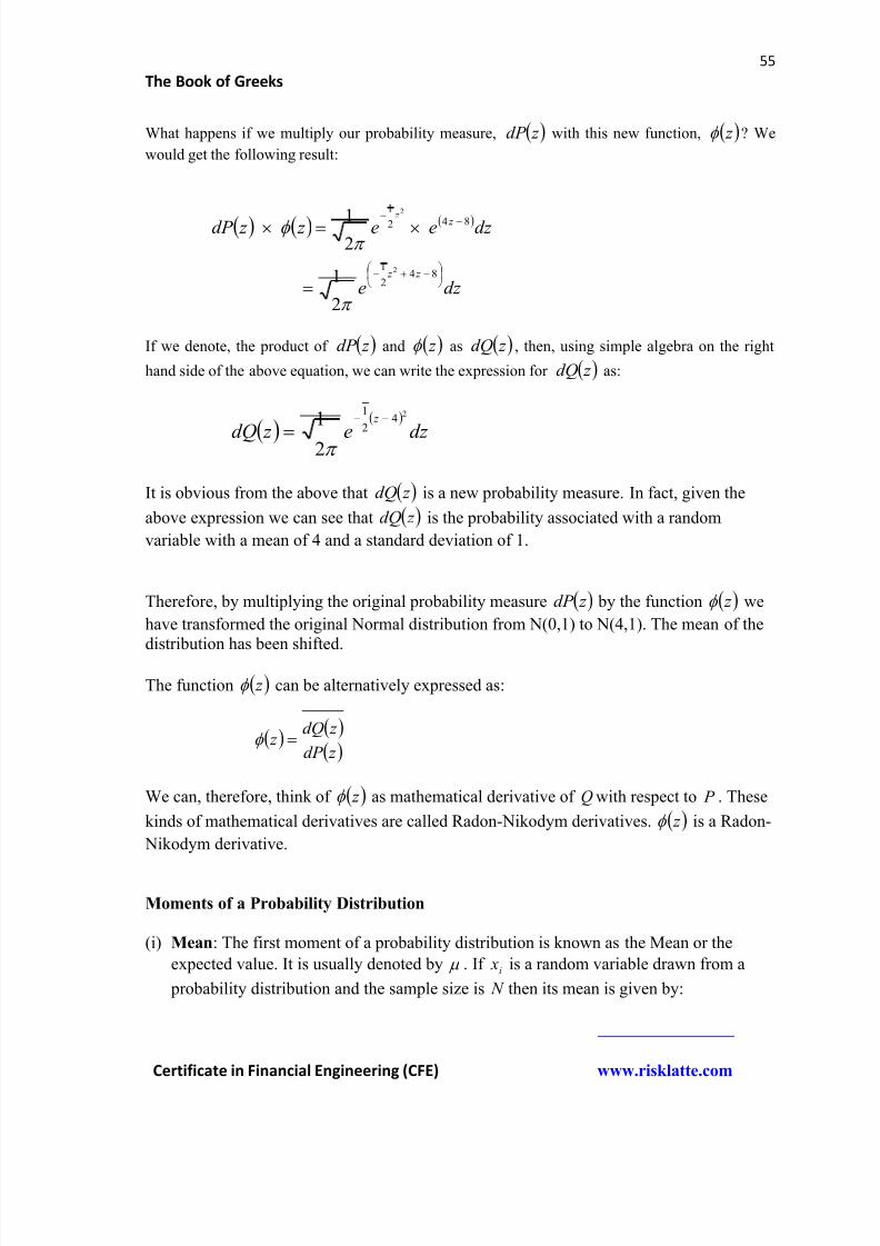
8/12/2019 Book of Greeks
http://slidepdf.com/reader/full/book-of-greeks 55/135
55
The Book of Greeks
Certificate in Financial Engineering (CFE) www.risklatte.com
What happens if we multiply our probability measure, z dP with this new function, z ? We
would get the following result:
dz e
dz ee z z dP
z z
z z
842
1
842
1
2
2
2
1
21
If we denote, the product of z dP and z as z dQ , then, using simple algebra on the right
hand side of the above equation, we can write the expression for z dQ as:
dz e z dQ
z 24
2
1
2
1
It is obvious from the above that z dQ is a new probability measure. In fact, given the
above expression we can see that z dQ is the probability associated with a random
variable with a mean of 4 and a standard deviation of 1.
Therefore, by multiplying the original probability measure z dP by the function z we
have transformed the original Normal distribution from N(0,1) to N(4,1). The mean of thedistribution has been shifted.
The function z can be alternatively expressed as:
z dP
z dQ z
We can, therefore, think of z as mathematical derivative of Q with respect to P . These
kinds of mathematical derivatives are called Radon-Nikodym derivatives. z is a Radon-
Nikodym derivative.
Moments of a Probability Distribution
(i) Mean: The first moment of a probability distribution is known as the Mean or the
expected value. It is usually denoted by . If i x is a random variable drawn from a
probability distribution and the sample size is N then its mean is given by:
8/12/2019 Book of Greeks
http://slidepdf.com/reader/full/book-of-greeks 56/135
56
The Book of Greeks
Certificate in Financial Engineering (CFE) www.risklatte.com
N
i
i x N 1
1
(ii) Variance: The second moment of a probability distribution is known as the Variance.If i x is a random variable drawn from a probability distribution and the sample size is
N then its Variance is given by:
N
i
i x N 1
22
1
1
The standard deviation, which also measures the historical volatility of assets and is oneof the common measures of financial risk, is given by the square root of the variance:
N
i
i x N 1
2
1
1
In Excel™ the standard deviation of a time series is calculated by the formula
=STDEV(.)
(iii) Skew: The third moment of a probability distribution is known as the skewness, or
sometimes just skew. If i x is a random variable drawn from a probability distribution
and the sample size is N and the first and the second moments are and 2 then its
Skew is given by:
N
i
i x
N N
N Skewness
1
2
21
Skew measures the symmetry in the distribution. A Normal (Gaussian) distribution issupposed to be symmetrical around the mean and hence should ideally display zeroskew. However, in practice that is never the case. In the financial markets, just as inlife, probability distributions are greatly skewed either to the left or the right of themean.
The Odd Moment: More on Skewness of Probability Distributions
The notion of skewness, or simply the skew, the measure of the third central moment ofa probability distribution, is fundamental to financial markets and understanding the behaviour of agents who operate in it. If the distribution is negatively skewed then thetrader will experience frequent small gains and infrequent large losses and thedistribution will exhibit a long tail on the left hand side (relative to the mean) of thedistribution. This happens when you are long options or follow a bleed strategy. A
8/12/2019 Book of Greeks
http://slidepdf.com/reader/full/book-of-greeks 57/135
57
The Book of Greeks
Certificate in Financial Engineering (CFE) www.risklatte.com
trader or a hedge fund manager continuously but steadily buys options, usually out ofthe money options, thereby paying a small premium or in other words, bleeding cash.
His book will show frequent small losses. However, once in a while, mostly due to rare
events or one single Black Swan event, there would big gains when the out of themoney options will be in the money. This strategy of trading, which exhibits negativeskew, is known as a “bleed strategy”. A prime (but an extreme) example is that ofQuantum Fund, the hedge fund run and managed by George Soros and his traderStanley Druckenmiller. In September, 1992, these two traders bought large quantities ofout of the money put options in Pound Sterling against the Deutsche Mark. The strike price of these put options were outside the Government bank (as specified by the thenexisting Exchange Rate Mechanism, or the ERM in Europe). During the entire monththey kept on buying these options steadily thereby paying premium. This showed asteady loss on their books. Since the strike price was outside the ERM government band most traders working in the banks in London and New York, who sold these
options to Soros and Drukenmiller, thought that their own chances of their makingmoney was 99% since even 1% chance of Pound Sterling breaking the ERM bandagainst the Deutsche Mark (thereby making the GBP put options in the money) wasquite remote. However, we all now know that the unthinkable happened. GBP brokethe ERM and Soros and Druckenmiller allegedly made a billion dollars on the trade.
A positive skew on the other hand will create a long tail on the right hand side (relativeto the mean) of the distribution. This is the case with short options strategy. Whentraders steadily sell out of the money options to customers they realize immediate profits. Their estimate is that 99% of the time the options will expire worthless andhence they stand to make profits on 99% of the short option trades. However, they aresubject to infrequent loss, and sometimes a huge loss due to Black Swan and other rareevents which can wipe out their entire profits and more. The hedge fund LTCM is acase in point. Another example of a negatively skewed bet is that of banks andfinancial institutions that lend money to customers, both corporates and retail. In fact, banks lend money to countries as well who are considered sovereign clients with verylow default risk. The lending can be in the form of loans or they can buy bonds. The banks lend money over and above the risk free rate (and their own borrowing costs)thereby making a nice spread and steadily earning profits. However, there is a defaultrisk of the customer and when the customer defaults your entire earnings are wiped out.The banks think that the client is a triple A rated client with very low default risk andhence makes the loan or gives line of credit (or guarantees). The chance of the customerdefaulting is 1% and 99% of the time the banks make good money. However, when that1% happens due to some rare event – the customer suddenly goes from triple A to bankruptcy due to severe cash flow problems or due to worsening financial markets – the banks lose all their gains (on the coupon spread) and has to even write off the principal. When a bank makes a loan to a customer with a credit risk, it is essentiallyshorting a spread option (a loan can be thought of as a portfolio of short spread optionand a credit default swap, CDS). As an example, look what’s happening in Greece now.
8/12/2019 Book of Greeks
http://slidepdf.com/reader/full/book-of-greeks 58/135
58
The Book of Greeks
Certificate in Financial Engineering (CFE) www.risklatte.com
9 out of 10 people in the financial markets live the life on the “positively skewed side”of the probability distribution. They think that this is desirable and safe, unless ofcourse, an LTCM, a Lehman Brothers collapse or Greece happens. Then they look with
envy to that one guy on the other side of the mean who has lived life on the “negativelyskewed side” of the distribution all along.
(iv) Kurtosis Kurtosis is the fourth moment of a probability distribution. If i x is a random:
variable drawn from a probability distribution with the sample size N and the first and
the second moments are and 2 then the kurtosis is given by the following
expression:
32
13
321
1 24
1
N N
N x
N N N
N N Kurtosis
N
i
i
This fourth moment measures the peakedness of the distribution and the heaviness ofthe tails of the distribution. In the financial markets and option trading parlance it isrelated to the notion of “fat tails”. Heavy tails occur when the distribution exhibits positive kurtosis. In this case, most of the observations lie towards the extreme end ofthe probability distributions and there are only a few observations near the mean. Thedistribution therefore has distinct, sharp peak but it falls off very fast around the meanand make the tails heavy. Negative kurtosis is the opposite of this where most of theobservations are clustered around the mean. Here, the mean is flatter.
Fat Tails in the Markets
One of the vexing issues in the derivatives market is the phenomenon of “volatility ofvolatility” or vvol. Every trader’s volatility estimate has volatility and he knows thatthis is what gives rise to “fat tails” and the “gamma of the gamma”, the fourth momentof a probability distribution. Many seasoned traders will tell you that “fat tails” – the probability of rare events, like stock markets falling by 10% in a day, happening farmore frequently than what is predicted by the Normal probability distribution – don’thave to be necessarily caused by blown out variances. A fat tail can occur even when anasset has a low volatility but a very high volatility of volatility.
Option traders believe that fat tails are caused due to a variable volatility. In a Black-
Scholes world, where volatility is constant, there would be no fat tails. However, thefact that volatility is variable (and stochastically so) gives rise to volatility of volatility.High volatility causes a market to move towards the tail of a probability distribution.According to many traders one of the main reasons for the higher price of in the moneyand out of the money options than the Black-Scholes value is because of the existenceof volatility of volatility which causes the tails of the distribution to become fat.
8/12/2019 Book of Greeks
http://slidepdf.com/reader/full/book-of-greeks 59/135
59
The Book of Greeks
Certificate in Financial Engineering (CFE) www.risklatte.com
Correlation and Covariance
If x and y are two random variables drawn from a probability distribution and i x and
i y are two historical time series of these two random variables then the correlation
between them is given by:
N
i
N
i
yi xi
N
i
yi xi
y x
y x
y x
1 1
22
1
,
Here, y x, is known as the “correlation coefficient”. Within the context of asset prices
this is called the historical or realized correlation.
Correlation coefficient measures the association between the movements of two
random variables, such as the return on securities. If the return on security A moves inthe same direction as the return on seucurity B then AB will be positive. The value of
the correlation coefficient lies between +1 and -1. A +1 correlation coefficient signifiesa perfect positive correlation between two random variables whereas a -1 correlationcoefficient signifies a perfect negative correlation between the two random variables.In Excel™ the correlation coefficient between two time series is calculated by the
formula =CORREL(.).
Drawbacks of the Correlation measure:
(i) It only measures the linear relationships between variables. For example, if x and
y vary quadratically, via, say an equation like 2 x y , then even though there is a
perfect co-movement between the two variables the correlation coefficient will failto capture that relationship.
(ii) It only measures the direction and the degree of association between themovements of two random variables but does not take into account the magnitudeof variation in the movements. For that reason Covariance is a better estimate ofco-movement.
Covariance between two random variables, x and y is the product of correlation
coefficient and the standard deviations of variable x and y
y DevStd x DevStd y xnCorrelatio y xCov ,,
Or, we can write the covariance of x and y as xy , using the familiar notations for
correlation and standard deviations as:
y x x xy
8/12/2019 Book of Greeks
http://slidepdf.com/reader/full/book-of-greeks 60/135
60
The Book of Greeks
Certificate in Financial Engineering (CFE) www.risklatte.com
Harry Markowitz Introduces Covariance
It is interesting to note that Harry Markowitz introduced the statistical concept of
“Covariance” in the early 1950s while working on the portfolio selection problem andthe Mean-Variance optimization technique.
Markowitz was the first to think of the statistical concept of variance of a financialasset’s returns as the measure of a financial security’s “risk”, or “financial risk”. If thereturn of the asset prices follows a Gaussian (Normal) distribution then the variance ofthese returns, or the standard deviation (volatility) which is the square of the variance,measured over a historical time period is the measure of that asset’s risk. However, ifthere are two assets, each of whose returns follow a Gaussian distribution, then how dowe measure the portfolio risk? The problem is compounded because besides the twovariances (or standard deviations), one for each asset, there is also the correlation
coefficient which measures the co-movement between them. However, the correlationcoefficient is an imperfect measure of co-movement as it only captures the direction ofco-movement, but not the quantum of variation. Markowtiz’s insight was that if we areto simply take the average of the variances of the two assets then we would not be ableto capture the co-movement between them, as the correlation would be left out. By itselfcorrelation is not sufficient to capture both the direction (co-movement) and thequantum of movement of each asset. Therefore, the best way to capture portfolio riskwould be to multiply the correlation with the product of each asset’s variance. This wasthe only way in which portfolio risk of two assets can reduce to the risk of a single assetif one of them were to disappear. The covariance of a financial asset with itself willsimply become the variance of that asset because the correlation coefficient of an assetwith itself is +1.
y x then 21, x x x xy y xCov If, then
Real (Actual) versus Risk Neutral Probability
Real probability measure is the actual probability that cash flows will be large or smallwhere estimation is done using historical data and other fundamental insights about the
company. It is generally represented as
In derivatives pricing however, we are concerned not with real or actual probabilities but
with risk neutral probabilities. In an arbitrage free, frictionless market there exists a riskneutral probability measure which makes the price of any derivative today equal to theexpected value of the payoff, discounted by a risk free rate. In a complete market thisrisk neutral probability measure is unique which renders the option price unique. Risk
neutral probability is generally represented as
8/12/2019 Book of Greeks
http://slidepdf.com/reader/full/book-of-greeks 61/135
61
The Book of Greeks
Certificate in Financial Engineering (CFE) www.risklatte.com
Other Probability distributions
Binomial distribution
Binomial distribution is used in the construction and analysis of a binomial tree to value
options and financial derivatives. A binomial distribution is a discrete probability
distribution (unlike the Normal distribution, which is a continuous distribution) where
the stochastic (random) variable can take on only two values. Within the context of a
binomial tree ( see below more details on binomial tree models of option valuation) these
two values can be denoted as “up-value” and “down-value” representing the stock going
up or down respectively. The random variable, t S (stock or the asset price) is called a
Bernoulli variable and has two states of existence in the next period.
If the probability of the “up state” is given by p and that of the “down state” is given by
)1( pq then the probability mass function of this distribution is given by:
mnmmnm
m
n p pmnm
n p pC m P
1
!!
!1
Where, m P , denote the probability of the stock (asset) price going up m times out of
n trials. The events in a binomial distribution are independent of each other. The above
formula is very useful in creating a binomial tree for the asset price movement and
option valuation using VBA code in Excel™.
Poisson distribution
A Poisson distribution is a discrete probability distribution and it gives the probability
that a certain number, m , of a particular event – say, the default on a bond – are going to
happen when the average occurrence, , of such an event in a given time interval is
already known. The probability of exactly m events occurring is given by:
!m
em P
m
The events in a Poisson distribution are independent of each other. Poisson distributionis quite helpful in modeling extreme events where the frequency of occurrence of the
events is less. This distribution is used in many stochastic models of asset prices which
have jumps in their paths and is associated with Poisson process and the Cox process
( see below).
8/12/2019 Book of Greeks
http://slidepdf.com/reader/full/book-of-greeks 62/135
62
The Book of Greeks
Certificate in Financial Engineering (CFE) www.risklatte.com
Entropy
The concept of entropy is related to that of probability. Entropy can be defined as the measure of
“disorder” in a system. A system with high order has low entropy whereas one with a low order
(disorder) has high entropy. Entropy is a fact of life and nature. It is found in all physical, natural
and financial systems. For example, when we get older the entropy increases; when a star like
our sun burns out and becomes a red giant or a white dwarf the entropy increases; when the
pollution in our environment increases, the entropy increases.
Ludwig Boltzman was the first to derive a mathematical expression for Entropy. However, to
understand entropy fully one needs to understand a “microstate” and a “macrostate”. A
macrostate denotes the gross, overall description of a system, say our body. And, a microstate
refers to the specific arrangement of the particles of that system, in this context it will be the cells
of our body. In physics, a gas inside a container is a macrostate and the particles – the molecules
– of the gas comprise the microstate. In the context of finance, or a financial system, such a
characterization of a microstate and a macrostate may not appear that intuitive, but it still holds
true. A stock price can be considered to be a microstate and the option price or the derivatives
based on that stock can be seen as the macrostate. Or, financial assets traded in a financial
markets may be considered to be the microstates and the given financial market (asset market)
the macrostate. A macrostate subsumes a microstate and there can be, and, in most systems, there
are many microstates in a single macrostate.
Thermodynamic entropy of a macrostate is simply defined as the natural logarithm of the number
of microstates consistent with this macrostate. If n is a “macrostate” and m as the “microstate”
then the number of microstates in a given macrostate can be found out using the following
formula for Combinations:
)!(!
!
k nm
nW
The sign “!” in the above formula denotes factorial where, 12!2 and 123456!6
and so on. The above formula simply states how many ways are there to make m choices from n
objects. For example, in how many ways can we form a 3 member team from 12 candidates? The
answer is 220. Or say, if there are 200 coins then in how many ways can we get one (1) head?
The answer is 200 (because all 200 coins can result in a head once)
Boltzman defined (in fact, he derived this expression) entropy as:
W k E ln
8/12/2019 Book of Greeks
http://slidepdf.com/reader/full/book-of-greeks 63/135
63
The Book of Greeks
Certificate in Financial Engineering (CFE) www.risklatte.com
Or, in other words, we can write the expression for thermodynamic entropy as:
)!(!
!ln
k nm
nk E
The constant, k , is known as the Boltzman’s constant and is an extremely small number.
Say, we have a system where there are 200 coins. This is the macrostate, whereas the
combination of number of heads and/or tails in all these 200 coins is a microstate. Now how
many ways can we get 1 “head” out of the 200 coins in a single toss? The answer is:
200!)1200(!1
!200
. If for the sake of simplicity, if we assume the value of the constant, k , to be
one (which is not true, as k is a very small number and is equal to 231038.1 k ), then the
entropy of this system – with the possibility of one head out of 200 coins – is given by:
2983.5!199!1
!200ln1
)!(!
!ln
k nm
nk E
Now, if we want to find the entropy of the system wher e we want to have say, the 25 “heads” out
of 200 coins in a single toss, it would be given by:
65.21!195!5
!200ln1
)!(!
!ln
k nm
nk E
The entropy increases when we increase the number of “heads” from 1 to 5 in a system of 200coins. If we continue the above exercise by finding out the entropy of the above system
consisting of 200 coins and we increase the number of heads from 5, 10, 20, 100, 150, 175, 195
and all the way up to 200, we will notice an interesting fact: the entropy increases and then
decreases when we increase the number of “heads” in a single toss in a 200 coins system.
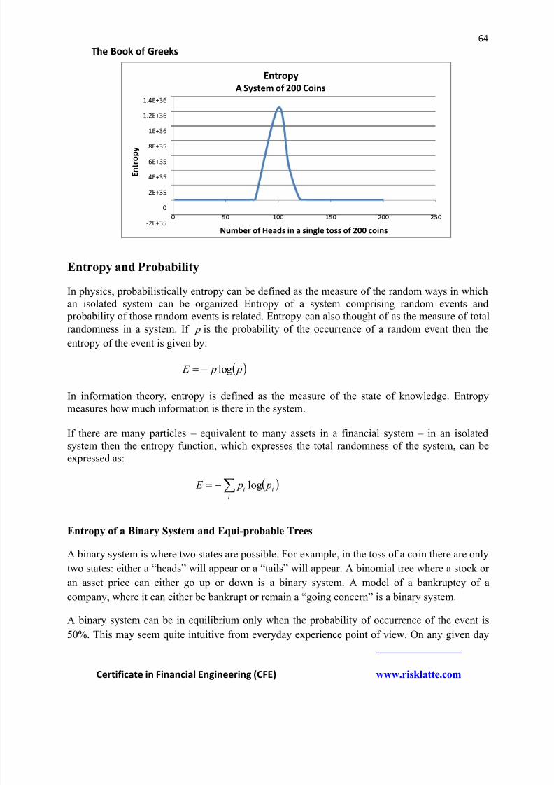
8/12/2019 Book of Greeks
http://slidepdf.com/reader/full/book-of-greeks 64/135
64
The Book of Greeks
Certificate in Financial Engineering (CFE) www.risklatte.com
Entropy and Probability
In physics, probabilistically entropy can be defined as the measure of the random ways in whichan isolated system can be organized Entropy of a system comprising random events and probability of those random events is related. Entropy can also thought of as the measure of total
randomness in a system. If p is the probability of the occurrence of a random event then the
entropy of the event is given by:
p p E log
In information theory, entropy is defined as the measure of the state of knowledge. Entropy
measures how much information is there in the system.
If there are many particles – equivalent to many assets in a financial system – in an isolatedsystem then the entropy function, which expresses the total randomness of the system, can beexpressed as:
i
ii p p E log
Entropy of a Binary System and Equi-probable Trees
A binary system is where two states are possible. For example, in the toss of a coin there are only
two states: either a “heads” will appear or a “tails” will appear. A binomial tree where a stock or
an asset price can either go up or down is a binary system. A model of a bankruptcy of a
company, where it can either be bankrupt or remain a “going concern” is a binary system.
A binary system can be in equilibrium only when the probability of occurrence of the event is
50%. This may seem quite intuitive from everyday experience point of view. On any given day
-2E+35
0
2E+35
4E+35
6E+35
8E+35
1E+36
1.2E+36
1.4E+36
0 50 100 150 200 250
E n t r o p y
Number of Heads in a single toss of 200 coins
Entropy
A System of 200 Coins
8/12/2019 Book of Greeks
http://slidepdf.com/reader/full/book-of-greeks 65/135
65
The Book of Greeks
Certificate in Financial Engineering (CFE) www.risklatte.com
ask a man on the street as to what is the probability of the stock market going up the next day
and he’d answer 50%. It’s always 50:50 chances in life. Toss a coin and there is a 50% chance
that “heads” will appear and 50% chance that “tails” will appear. Talking in these terms is almost
trivial. However, this 50:50 rule is the only way that markets attain maximum entropy. All
systems move towards maximum entropy. In other words, an equi-probable binomial tree (50%
chance of stock going up and 50% chance of stock going down) is in the state of maximum
entropy. Any other probabilities of up-move or a down-move will contravene the law of
maximum entropy.
Mathematically, the above can be shown as below.
Say, there is only one stock in the system and the stock’s movement is a binary function, i.e. the
stock can either go up or down in the next period. The probability of the up move is p and that
of the down move is p1 . Therefore, the entropy of the system will be:
p p p p
p p E i
ii
1log1log
log
To find the value of p , the probability of the occurrence of the random event (the up move of
the stock price), we need to take the first mathematical derivative of the above expression andequate it to zero.
01log1log
0
p p p pdpd
dp
dE
Differentiating the above expression by parts and equating it to zero gives:
2
1
01loglog
p
p p
Therefore, if a stock (asset) price is modelled as a binomial system (a binomial tree) whereby
there are two states of movement (up and down move) in the next period then for the system to be in equilibrium the probabilities of the up move and the down move have to be equal to 50%.
Part C
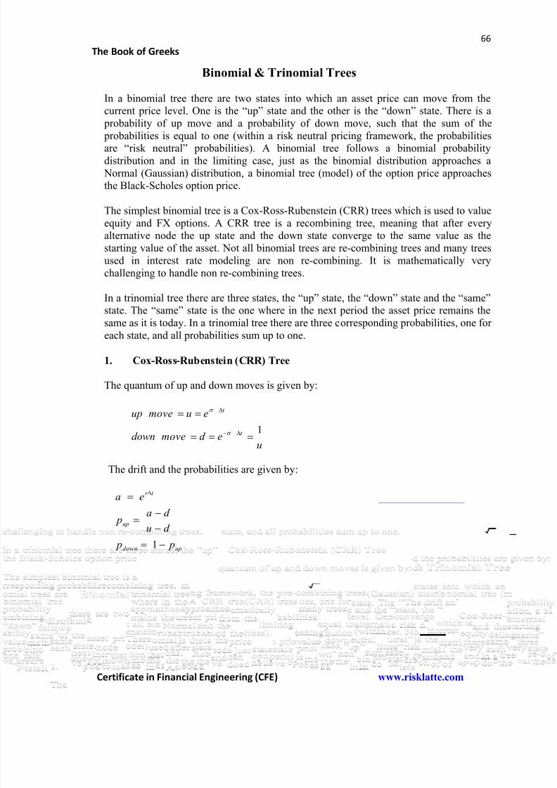
8/12/2019 Book of Greeks
http://slidepdf.com/reader/full/book-of-greeks 66/135
66
The Book of Greeks
Certificate in Financial Engineering (CFE) www.risklatte.com
Binomial & Trinomial Trees
In a binomial tree there are two states into which an asset price can move from thecurrent price level. One is the “up” state and the other is the “down” state. There is a probability of up move and a probability of down move, such that the sum of the
probabilities is equal to one (within a risk neutral pricing framework, the probabilitiesare “risk neutral” probabilities). A binomial tree follows a binomial probabilitydistribution and in the limiting case, just as the binomial distribution approaches a Normal (Gaussian) distribution, a binomial tree (model) of the option price approachesthe Black-Scholes option price.
The simplest binomial tree is a Cox-Ross-Rubenstein (CRR) trees which is used to valueequity and FX options. A CRR tree is a recombining tree, meaning that after everyalternative node the up state and the down state converge to the same value as thestarting value of the asset. Not all binomial trees are re-combining trees and many treesused in interest rate modeling are non re-combining. It is mathematically very
challenging to handle non re-combining trees.
In a trinomial tree there are three states, the “up” state, the “down” state and the “same”state. The “same” state is the one where in the next period the asset price remains thesame as it is today. In a trinomial tree there are three corresponding probabilities, one foreach state, and all probabilities sum up to one.
1. Cox-Ross-Rubenstein (CRR) Tree
The quantum of up and down moves is given by:
ued movedown
eumoveup
t
t
1
The drift and the probabilities are given by:
updown
up
t r
p p
d u
d a p
ea
1

8/12/2019 Book of Greeks
http://slidepdf.com/reader/full/book-of-greeks 67/135
67
The Book of Greeks
Certificate in Financial Engineering (CFE) www.risklatte.com
Implementing a CRR Tree in Excel™
2. Jarrow- Rudd (JR) Tree
8/12/2019 Book of Greeks
http://slidepdf.com/reader/full/book-of-greeks 68/135
68
The Book of Greeks
Certificate in Financial Engineering (CFE) www.risklatte.com
The quantum of up and down moves is given by:
11
11
2
2
t t r
t t r
eed
eeu
The most popular choice for the quantum of up and down moves for a JR tree is:
2
2
1
r
ed
eu
t t
t t
The probabilities are given by:
2
1 d u p p
3. Trinomial Tree
Trinomial Tree with CRR Parameters
If a trinomial tree can be constructed with CRR parameters, such that there are threestates: an up move, a down move and a move where the asset (stock) price remains thesame, then the quantum of respective moves will be given by:
t eu 2
t ed 2
and the respective risk neutral probabilities will be given by:
2
22
22
1
t t
t t qr
up
ee
ee p
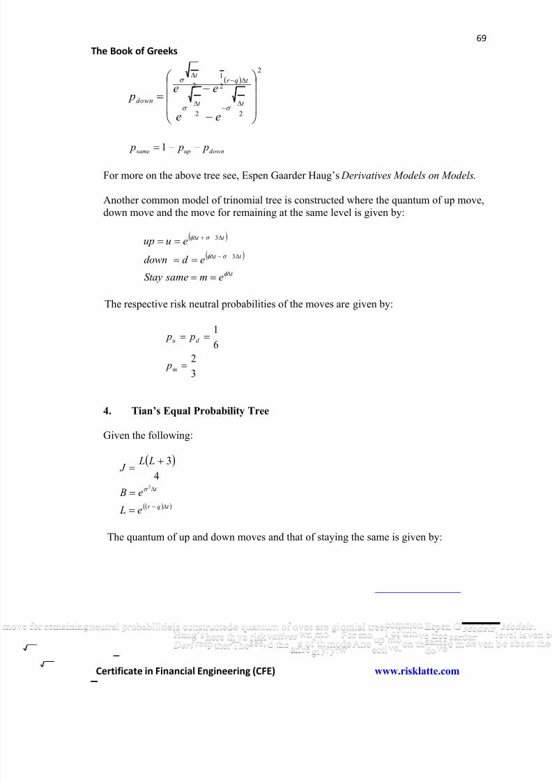
8/12/2019 Book of Greeks
http://slidepdf.com/reader/full/book-of-greeks 69/135
69
The Book of Greeks
Certificate in Financial Engineering (CFE) www.risklatte.com
2
22
2
1
2
t t
t qr t
down
ee
ee p
downup same p p p 1
For more on the above tree see, Espen Gaarder Haug’s Derivatives Models on Models.
Another common model of trinomial tree is constructed where the quantum of up move,down move and the move for remaining at the same level is given by:
t
t t
t t
em sameStay
ed down
euup
3
3
The respective risk neutral probabilities of the moves are given by:
3
2
6
1
m
d u
p
p p
4. Tian’s Equal Probability Tree
Given the following:
t qr
t
e L
e B
L L J
2
4
3
The quantum of up and down moves and that of staying the same is given by:
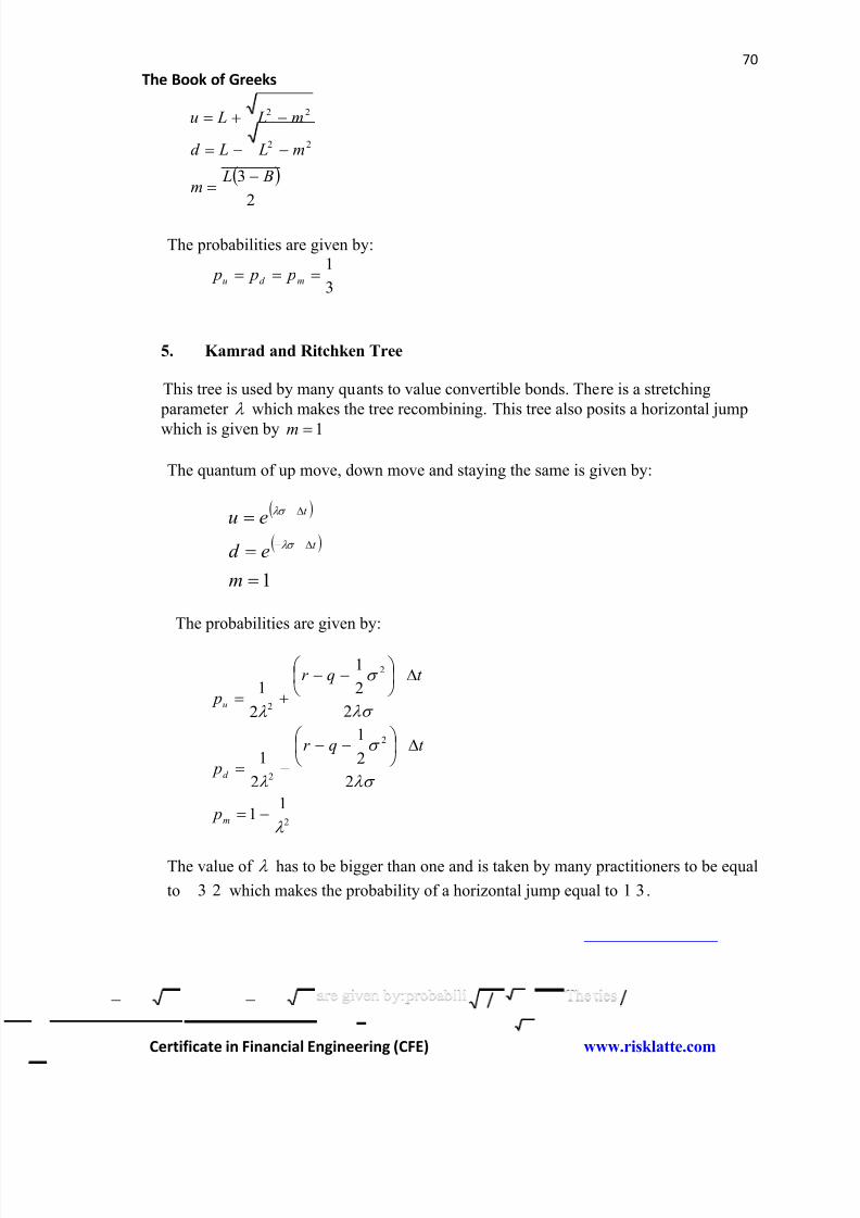
8/12/2019 Book of Greeks
http://slidepdf.com/reader/full/book-of-greeks 70/135
70
The Book of Greeks
Certificate in Financial Engineering (CFE) www.risklatte.com
2
3
22
22
B Lm
m L Ld
m L Lu
The probabilities are given by:
3
1 md u p p p
5. Kamrad and Ritchken Tree
This tree is used by many quants to value convertible bonds. There is a stretching
parameter which makes the tree recombining. This tree also posits a horizontal jump
which is given by 1m
The quantum of up move, down move and staying the same is given by:
1
m
ed
eu
t
t
The probabilities are given by:
2
2
2
2
2
11
2
2
1
2
1
2
2
1
2
1
m
d
u
p
t qr
p
t qr
p
The value of has to be bigger than one and is taken by many practitioners to be equal
to 23 which makes the probability of a horizontal jump equal to 31 .
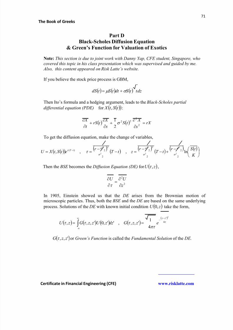
8/12/2019 Book of Greeks
http://slidepdf.com/reader/full/book-of-greeks 71/135
71
The Book of Greeks
Certificate in Financial Engineering (CFE) www.risklatte.com
Part D
Black-Scholes Diffusion Equation
& Green’s Function for Valuation of Exotics
Note: This section is due to joint work with Danny Yap, CFE student, Singapore, whocovered this topic in his class presentation which was supervised and guided by me.
Also, this content appeared on Risk Latte’s website.
If you believe the stock price process is GBM,
dz t t S dt t S t dS
Then Ito’s formula and a hedging argument, leads to the Black-Scholes partial
differential equation (PDE) for t S t X , :
rX s
X t S
s
X t rS
t
X
2
222
2
1
To get the diffusion equation, make the change of variables,
K
t S r t T
r z t T
r et S t X U t T r ln,,,
2
2
2
2
2
2
2
2)(
2
2
2
2
2
2
Then the BSE becomes the Diffusion Equation (DE) for z U , ,
2
2
z
U U
In 1905, Einstein showed us that the DE arises from the Brownian motion ofmicroscopic particles. Thus, both the BSE and the DE are based on the same underlying
process. Solutions of the DE with known initial condition z U ,0 take the form,
4
' 2
4
1',,,'',0',,,
z z
e z z Gdz z U z z G z U
',, z z G or Green’s Function is called the Fundamental Solution of the DE.
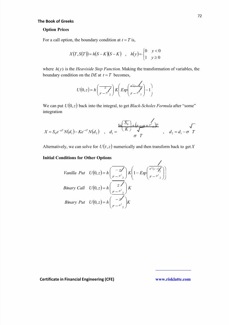
8/12/2019 Book of Greeks
http://slidepdf.com/reader/full/book-of-greeks 72/135
72
The Book of Greeks
Certificate in Financial Engineering (CFE) www.risklatte.com
Option Prices
For a call option, the boundary condition at T t is,
01
00,,
y
y yh K S K S hT S T X
where )( yh is the Heaviside Step Function. Making the transformation of variables, the
boundary condition on the DE at T t becomes,
1,02
2
2
2
2
2
r Exp K
r
z h z U
z
We can put z U ,0 back into the integral, to get Black-Scholes Formula after “some”
integration
T d d T
T qr K
S
d d N Ked N eS X rT qT
12
20
1210 ,
ln
,
2
Alternatively, we can solve for z U , numerically and then transform back to get X
Initial Conditions for Other Options
K r
z h z U Put Binary
K r
z h z U Call Binary
r Exp K
r z h z U Put Vanilla
z
2
2
2
2
2
2
2
2
2
2
,0
,0
1,0
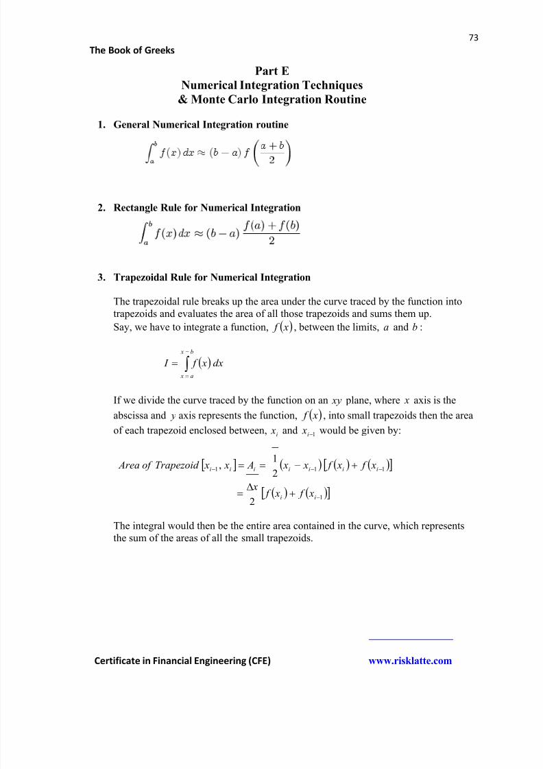
8/12/2019 Book of Greeks
http://slidepdf.com/reader/full/book-of-greeks 73/135
73
The Book of Greeks
Certificate in Financial Engineering (CFE) www.risklatte.com
Part E
Numerical Integration Techniques
& Monte Carlo Integration Routine
1. General Numerical Integration routine
2. Rectangle Rule for Numerical Integration
3. Trapezoidal Rule for Numerical Integration
The trapezoidal rule breaks up the area under the curve traced by the function intotrapezoids and evaluates the area of all those trapezoids and sums them up.
Say, we have to integrate a function, x f , between the limits, a and b :
b x
a x
dx x f I
If we divide the curve traced by the function on an xy plane, where x axis is theabscissa and y axis represents the function, x f , into small trapezoids then the area
of each trapezoid enclosed between, i x and 1i x would be given by:
1
111
2
2
1,
ii
iiiiiii
x f x f x
x f x f x x A x xTrapezoid of Area
The integral would then be the entire area contained in the curve, which represents
the sum of the areas of all the small trapezoids.
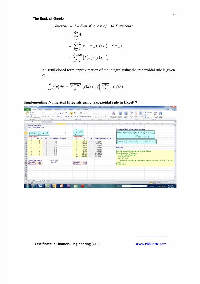
8/12/2019 Book of Greeks
http://slidepdf.com/reader/full/book-of-greeks 74/135
74
The Book of Greeks
Certificate in Financial Engineering (CFE) www.risklatte.com
b
ai
ii
b
ai
iiii
b
ai
i
x f x f x
x f x f x x
A
Trapezoids All of Areasof Sum I Integral
1
11
2
2
1
A useful closed form approximation of the integral using the trapezoidal rule is given by:
b f
ba f a f
abdx x f
b
a 24
6
Implementing Numerical Integrals using trapezoidal rule in Excel™
8/12/2019 Book of Greeks
http://slidepdf.com/reader/full/book-of-greeks 75/135
8/12/2019 Book of Greeks
http://slidepdf.com/reader/full/book-of-greeks 76/135
76
The Book of Greeks
Certificate in Financial Engineering (CFE) www.risklatte.com
One of the GQ methods is the Gauss-Legendre quadrature (GLQ) method. GLQmethods are based on the Legendre polynomials of the first kind. GLQ.
GLQ are constructed for integrals over the range [-1, 1]. However, we can generalize
the intervals by a suitable transformation. With a function, x f and weighting
coefficients iw , GLQ is a summation given by:
n
i
ii x f wdx x f 1
1
1
If we want to have a more general limit of integration, say, [a, b], then we use atransformation:
ab
ba x z
2
With the above transformation the integral becomes:
dz ab z ab
f ab
dx x f I
b
a
1
1 22
Using a set of weights, iw the above expression in discrete form becomes
22 1
ab z ab f w
abdx x f I
N
i i
b
a
In the GLQ method the values of the abscissas, i x , and the weights, iw , are
determined using Legendre polynomials. The Legendre polynomials, x P N , are a set
of polynomials of degree N and the roots of x P N are distinct in the interval (-1, 1)
and symmetric with respect to the origina. Legendre polynomials for N up to 100 are
already published and freely available. In the GLQ method, increasing N increasesthe accuracy of the evaluation process.
When 2 N (not at all desirable as the accuracy will be quite low) the integral can
be approximated, with a degree of precision 3, as:
3
3
3
31
1 f f dx x f
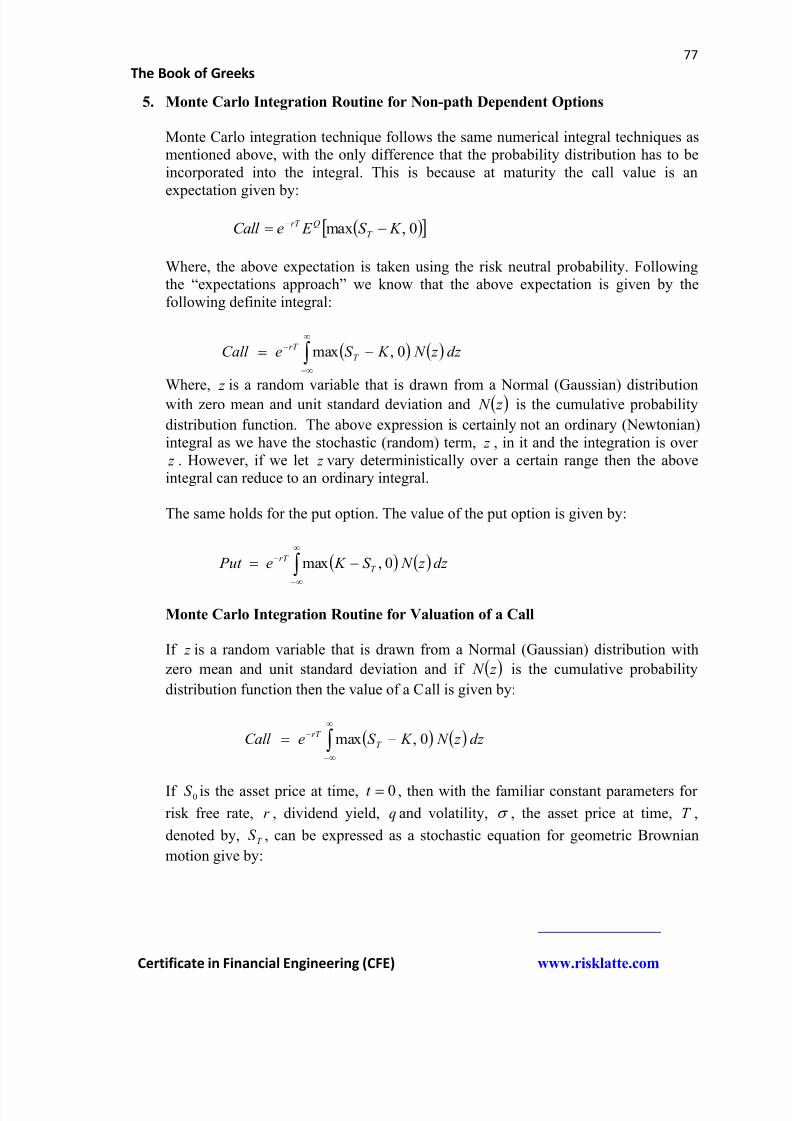
8/12/2019 Book of Greeks
http://slidepdf.com/reader/full/book-of-greeks 77/135
77
The Book of Greeks
Certificate in Financial Engineering (CFE) www.risklatte.com
5. Monte Carlo Integration Routine for Non-path Dependent Options
Monte Carlo integration technique follows the same numerical integral techniques asmentioned above, with the only difference that the probability distribution has to beincorporated into the integral. This is because at maturity the call value is an
expectation given by:
0,max K S E eCall T
QrT
Where, the above expectation is taken using the risk neutral probability. Followingthe “expectations approach” we know that the above expectation is given by thefollowing definite integral:
dz z N K S eCall T
rT 0,max
Where, z is a random variable that is drawn from a Normal (Gaussian) distributionwith zero mean and unit standard deviation and z N is the cumulative probability
distribution function. The above expression is certainly not an ordinary (Newtonian)integral as we have the stochastic (random) term, z , in it and the integration is over z . However, if we let z vary deterministically over a certain range then the aboveintegral can reduce to an ordinary integral.
The same holds for the put option. The value of the put option is given by:
dz z N S K e Put T
rT 0,max
Monte Carlo Integration Routine for Valuation of a Call
If z is a random variable that is drawn from a Normal (Gaussian) distribution with
zero mean and unit standard deviation and if z N is the cumulative probability
distribution function then the value of a Call is given by:
dz z N K S eCall T
rT 0,max
If 0S is the asset price at time, 0t , then with the familiar constant parameters for
risk free rate, r , dividend yield, q and volatility, , the asset price at time, T ,
denoted by, T S , can be expressed as a stochastic equation for geometric Brownian
motion give by:
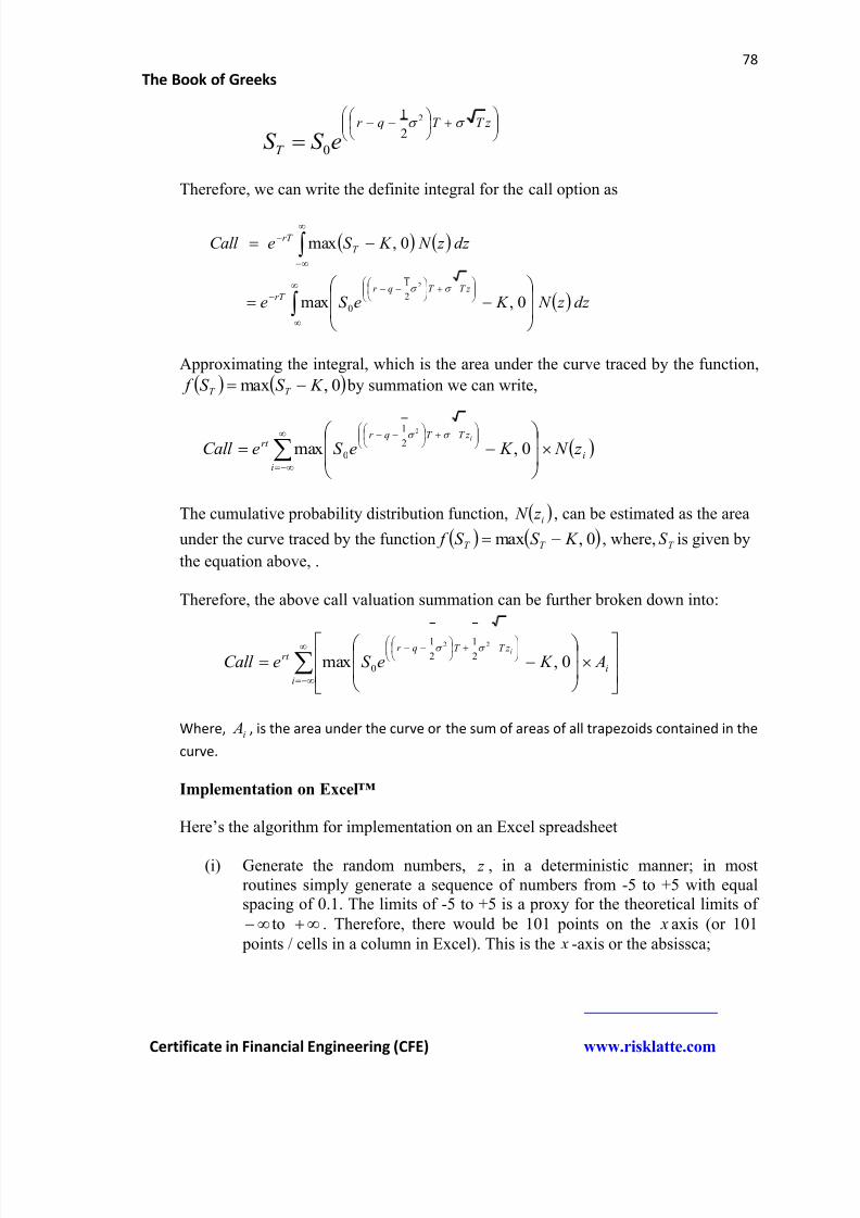
8/12/2019 Book of Greeks
http://slidepdf.com/reader/full/book-of-greeks 78/135
78
The Book of Greeks
Certificate in Financial Engineering (CFE) www.risklatte.com
z T T qr
T eS S 2
2
1
0
Therefore, we can write the definite integral for the call option as
dz z N K eS e
dz z N K S eCall
z T T qr rT
T
rT
0,max
0,max
2
2
1
0
Approximating the integral, which is the area under the curve traced by the function,
0,max K S S f T T by summation we can write,
i
i
z T T qr rt z N K eS eCall
i
0,max
2
2
1
0
The cumulative probability distribution function, i z N , can be estimated as the area
under the curve traced by the function 0,max K S S f T T , where, T S is given by
the equation above, .
Therefore, the above call valuation summation can be further broken down into:
i
i
z T T qr rt A K eS eCall
i
0,max
22
2
1
2
1
0
Where, i A , is the area under the curve or the sum of areas of all trapezoids contained in the
curve.
Implementation on Excel™
Here’s the algorithm for implementation on an Excel spreadsheet
(i) Generate the random numbers, z , in a deterministic manner; in mostroutines simply generate a sequence of numbers from -5 to +5 with equalspacing of 0.1. The limits of -5 to +5 is a proxy for the theoretical limits of
to . Therefore, there would be 101 points on the x axis (or 101
points / cells in a column in Excel). This is the x -axis or the absissca;
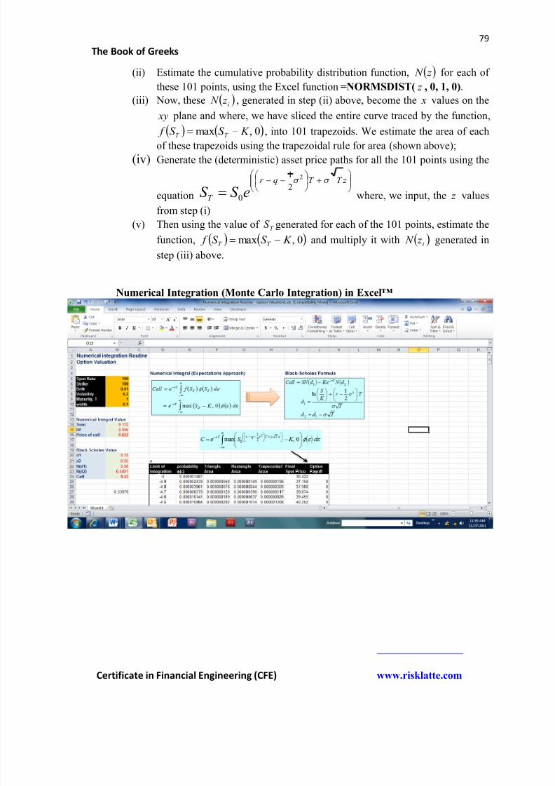
8/12/2019 Book of Greeks
http://slidepdf.com/reader/full/book-of-greeks 79/135
79
The Book of Greeks
Certificate in Financial Engineering (CFE) www.risklatte.com
(ii) Estimate the cumulative probability distribution function, z N for each of
these 101 points, using the Excel function =NORMSDIST( z , 0, 1, 0).
(iii) Now, these i z N , generated in step (ii) above, become the x values on the
xy plane and where, we have sliced the entire curve traced by the function,
0,max K S S f
T T
, into 101 trapezoids. We estimate the area of each
of these trapezoids using the trapezoidal rule for area (shown above);
(iv) Generate the (deterministic) asset price paths for all the 101 points using the
equation
z T T qr
T eS S 2
2
1
0 where, we input, the z values
from step (i) (v) Then using the value of T S generated for each of the 101 points, estimate the
function, 0,max K S S f T T and multiply it with i z N generated in
step (iii) above.
Numerical Integration (Monte Carlo Integration) in Excel™
8/12/2019 Book of Greeks
http://slidepdf.com/reader/full/book-of-greeks 80/135
80
The Book of Greeks
Certificate in Financial Engineering (CFE) www.risklatte.com
Part F
Differential Equations
&
Finite Difference Methods
A differential equations is an equation, describing the change and rate of change of
variables, that contains terms likedx
d ,
x
,
2
2
x
,
y x
2
, etc. which are terms used in the
study of calculus. However, there are two kinds Calculus, in mathematics:
Newtonian calculus
Stochastic calculus
Newtonian calculus describes the dynamics of variables that change deterministically,
whereas, Stochastic calculus describes the dynamics of variables that change randomly(via random numbers). Ordinary differential equations (ODE) and partial differentialequations (PDE) fall in the realm of Newtonian calculus whereas stochastic differentialequations inhabit the world of stochastic calculus.
In Finance, we come across three kinds of differential equations.
Ordinary differential equations (ODE)
Partial differential equations (PDE)
Stochastic differential equations (SDE)
Ordinary Differential Equations in Finance
An ordinary differential equation (ODE) describes the dynamics of a variable that varies
with another variable in a deterministic manner. For example, if there is a variable, y ,
the change of whose value, or the rate of change of whose value, is governed by the
change in the value of another variable, x , then we can describe such a relationship viaan ODE.
Savings Account
An example of ordinary differential equation is the everyday savings account in a bankthat we use. If we deposit M as the amount of money (in Dollars) in a savings accountwhere the interest paid on the deposit is r (which is constant), then over a period of time,t , the amount in the account will be given by:
8/12/2019 Book of Greeks
http://slidepdf.com/reader/full/book-of-greeks 81/135
81
The Book of Greeks
Certificate in Financial Engineering (CFE) www.risklatte.com
t r M t M
Here, the functional form of relationship is: t f t M , where the money deposited in
the savings account is only a function of time elapsed.
The way the money will grow in the account over a time period, t , and t t , where,t is a very small (infinitesimally small) time interval, will be given by:
t Mr t t t r M t M t t M
Writing, the expression, t M t t M , as t M , where, is the delta representing a
very small (infinitesimally small) change in the value of M , the amount of money in theaccount.
Therefore, we can write the above equation for the change in the amount of money in the
savings account as:
rM t
M
t r M
M
Taking the limit as 0t , we write the above equation in the familiar differentialcalculus form as
rM dt
dM
The above is an example of an ordinary differential equation (ODE). The above ordinarydifferential equation can be easily solved.
American Capped Call Option
Another example of an ordinary differential equation is the American style capped calloption. If we consider an American style call option which is capped at a certain level,then the underlying dynamics of the call option price is described by an ordinary
differential equation as shown below. If AC is an American style capped call option, suchthat when the cap is hit, the option expires, with no maturity, such that the functional
relationship is mathematically expressed as: S f S C A . Here, the call price is only a
function of the underlying asset price, S .
The ODE for a capped American style call option is given by:
8/12/2019 Book of Greeks
http://slidepdf.com/reader/full/book-of-greeks 82/135
82
The Book of Greeks
Certificate in Financial Engineering (CFE) www.risklatte.com
02
12
222 r C
dS
C d S
dS
dC S qr A
At
At
Important Note
Almost always, the underlying dynamics for the change of an option price, C with theunderlying asset price, S is a function of both, S and the time, t , i.e. t S f t S C ,, . In
such cases, the differential equation describing the change in the option price with bothasset price and time will be described by a partial differential equation (PDE), like theBlack-Scholes PDE, because, the option price is partially dependent on the asset priceand partially on the time. However, in some rare cases a partial differential equation canreduce to an ordinary differential equation, like when we use the Laplace transforms tosolve derivatives problems as well as like the case above, when the option price is afunction of only one variable, i.e. the asset price.
Stochastic Differential Equation in Finance
A stochastic differential equation (SDE) is a differential equation that describes the behavior of a dependent variable with respect to an independent variable that changesrandomly. For example, the price of a financial asset (other than cash), like a stock, astock index, an FX pair or an interest rate, is assumed to follow a random processwhereby it is a function of time but the evolution of the asset price over tine is random.
An example of a stochastic differential equation is the equation of the famous geometric
Brownian motion, where, the asset price, t S , varies in a random manner:
t
t
t dW dt S
dS
It is because of the second term in the above equation, t dW , that separates this equation
from an ordinary differential equation because t dW varies in a random manner that is
unpredictable. Here, t dW varies as: t dW t t , where, t is a random number drawn
from a standard Normal distribution.
The key characteristic that separates a stochastic differential equation from an ordinary
differential equation, is the fact that the asset price, t S , is not differential with respect to
time. With the risk of oversimplification, one can say that the asset price movement overa small period of time, say, a day, is indistinguishable from the asset price movementover a smaller period of time, say, an hour. In other words, the change of asset price with
respect to time,dt
dS t , does not converge.
8/12/2019 Book of Greeks
http://slidepdf.com/reader/full/book-of-greeks 83/135
83
The Book of Greeks
Certificate in Financial Engineering (CFE) www.risklatte.com
Here we follow the arguments of Jamil Baz and George Chacko. Consider an arithmetic
Brownian motion for the asset price, t S , given by:
t dt dS
dW dt dS
t
t t
Taking, the discrete version of the above equation
t t S t
Dividing the above equation by t we get
t t
S t
Taking the limits as 0t , i.e. time slice becomes infinitesimally small, we get
t t Lim
t
S t Lim t
00
Hence, the change of asset price with respect to the time goes to plus or minus infinity
(depending on the random variable, ) as the time interval is made smaller and smaller.This makes the Brownian motion unpredictable over short intervals of time. This alsoshows that the asset price is not differentiable.
Partial Differential Equations (PDEs) in Finance
A partial differential equation (PDE) is an equation which has partial (mathematical)
derivatives in it. If we have a function, y which is dependent on two variables, x , which
is say, a spatial variable and t , which denotes time, such that t x f y , then a partial
mathematical derivatives of y are given by: x
y
and
t
y
. The first partial derivative
shows the variation of y with respect to x and the second partial derivative shows the
variation of y with respect to t . We can combine these two partial derivatives and write
an equation as:
2
2
x
y
t
y
The above is known as a heat equation and is an example of a PDE. This equation hasapplications in the field of financial derivatives.
8/12/2019 Book of Greeks
http://slidepdf.com/reader/full/book-of-greeks 84/135
84
The Book of Greeks
Certificate in Financial Engineering (CFE) www.risklatte.com
In quantitative finance, a financial derivative, such as a call option on a stock, is afunction of two variables, the underlying asset, such as the stock, and the time. We can
write the call option on the stock as t S C t S f C ,, which shows that its value
changes with the change in S and t . Therefore, the partial derivatives of a call option can be written as:
t
C
= first partial derivative of the call option with respect to time
S
C
= first partial derivative of the call option with respect to the asset price
2
2
S
C
= second partial derivative of the call option price with respect to the asset price
All these three partial derivatives can be combined to give a partial differential equationfor the call option price:
rC S
C S
S
C rS
t
C
2
222
2
1
This is the famous Black-Scholes PDE, the solution of which yields the Black-Scholes
call option pricing formula.
It has to be noted that all PDEs that we study in finance are linear in nature.
Partial differential equations (PDE) are divided into three major categories:
Parabolic Elliptic
Hyperbolic
The parabolic equation, of which diffusion and convection-diffusion equation is a subclass, is the most used and popular one in the world of derivatives. Black-Scholes PDE,the solution of which gives the celebrated Black-Scholes option pricing formula, is aconvection-diffusion equation. However, elliptic and hyperbolic (a 2nd order hyperbolicequation is a wave equation) equations are also found in some financial derivativesapplications.
Parabolic PDE
Parabolic PDEs model heat flow (financial derivatives) and fluid flow phenomenon. TheBlack-Scholes (PDE) in quantitative finance is a parabolic PDE and is given by:
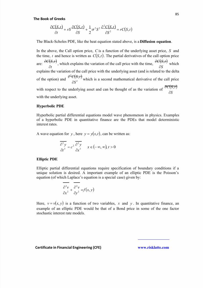
8/12/2019 Book of Greeks
http://slidepdf.com/reader/full/book-of-greeks 85/135
85
The Book of Greeks
Certificate in Financial Engineering (CFE) www.risklatte.com
t S rC
S
t S C S
S
t S C rS
t
t S C ,
,
2
1,,2
222
The Black-Scholes PDE, like the heat equation stated above, is a Diffusion equation.
In the above, the Call option price, C is a function of the underlying asset price, S andthe time, t and hence is written as t S C , . The partial derivatives of the call option price
are:
t
t S C
,, which explains the variation of the call price with the time,
S
t S C
,which
explains the variation of the call price with the underlying asset (and is related to the delta
of the option) and
2
2 ,
S
t S C
which is a second mathematical derivative of the call price
with respect to the underlying asset and can be thought of as the variation of S
t S C
,
with the underlying asset.
Hyperbolic PDE
Hyperbolic partial differential equations model wave phenomenon in physics. Examplesof a hyperbolic PDE in quantitative finance are the PDEs that model deterministicinterest rates.
A wave equation for y , here t x y y , , can be written as:
2
22
2
2
x
yc
t
y
0,, t x
Elliptic PDE
Elliptic partial differential equations require specification of boundary conditions if aunique solution is desired. A important example of an elliptic PDE is the Poisson’sequation (of which Laplace’s equation is a special case) given by:
y x f y
v
x
v,
2
2
2
2
Here, y xvv , is a function of two variables, x and y . In quantitative finance, an
example of an elliptic PDE would be that of a Bond price in some of the one factorstochastic interest rate models.
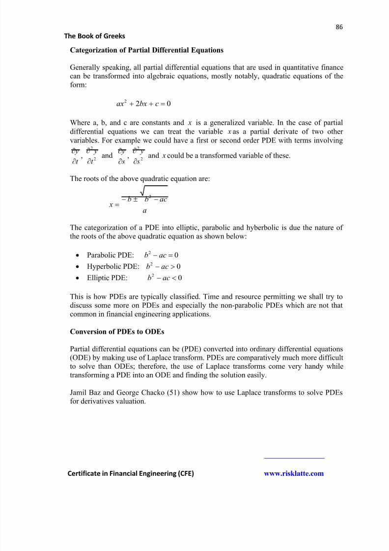
8/12/2019 Book of Greeks
http://slidepdf.com/reader/full/book-of-greeks 86/135
86
The Book of Greeks
Certificate in Financial Engineering (CFE) www.risklatte.com
Categorization of Partial Differential Equations
Generally speaking, all partial differential equations that are used in quantitative financecan be transformed into algebraic equations, mostly notably, quadratic equations of theform:
022 cbxax
Where a, b, and c are constants and x is a generalized variable. In the case of partial
differential equations we can treat the variable x as a partial derivate of two othervariables. For example we could have a first or second order PDE with terms involving
t
y
,
2
2
t
y
and
s
y
,
2
2
s
y
and x could be a transformed variable of these.
The roots of the above quadratic equation are:
a
acbb x
2
The categorization of a PDE into elliptic, parabolic and hyberbolic is due the nature ofthe roots of the above quadratic equation as shown below:
Parabolic PDE: 02 acb
Hyperbolic PDE: 02 acb
Elliptic PDE: 02 acb
This is how PDEs are typically classified. Time and resource permitting we shall try todiscuss some more on PDEs and especially the non-parabolic PDEs which are not thatcommon in financial engineering applications.
Conversion of PDEs to ODEs
Partial differential equations can be (PDE) converted into ordinary differential equations(ODE) by making use of Laplace transform. PDEs are comparatively much more difficultto solve than ODEs; therefore, the use of Laplace transforms come very handy whiletransforming a PDE into an ODE and finding the solution easily.
Jamil Baz and George Chacko (51) show how to use Laplace transforms to solve PDEsfor derivatives valuation.
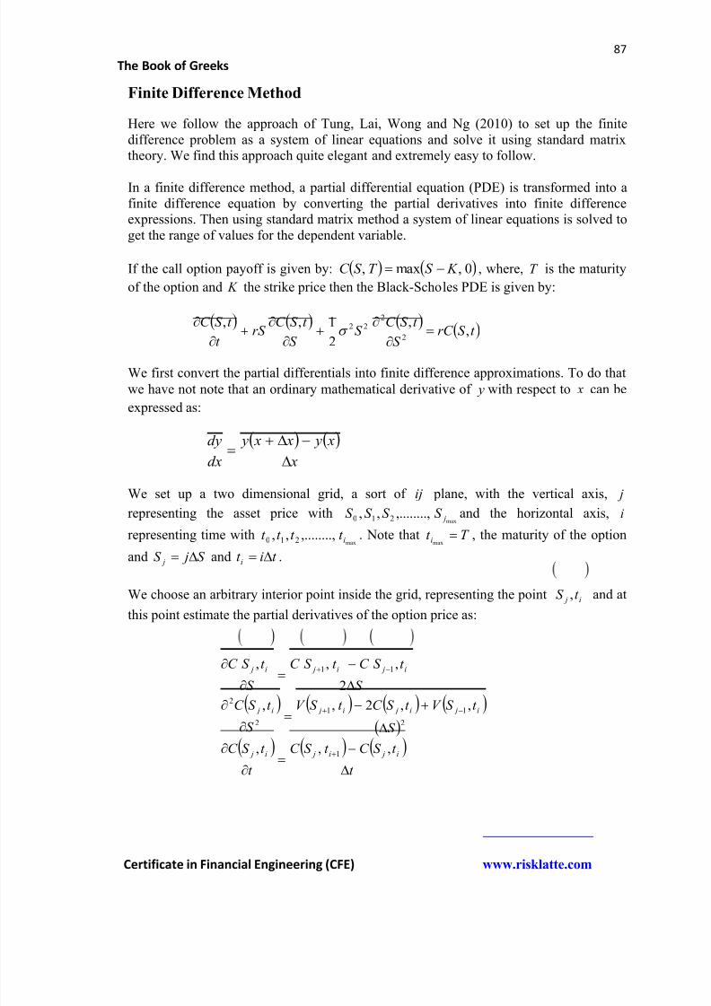
8/12/2019 Book of Greeks
http://slidepdf.com/reader/full/book-of-greeks 87/135
87
The Book of Greeks
Certificate in Financial Engineering (CFE) www.risklatte.com
Finite Difference Method
Here we follow the approach of Tung, Lai, Wong and Ng (2010) to set up the finitedifference problem as a system of linear equations and solve it using standard matrixtheory. We find this approach quite elegant and extremely easy to follow.
In a finite difference method, a partial differential equation (PDE) is transformed into afinite difference equation by converting the partial derivatives into finite differenceexpressions. Then using standard matrix method a system of linear equations is solved toget the range of values for the dependent variable.
If the call option payoff is given by: 0,max, K S T S C , where, T is the maturity
of the option and K the strike price then the Black-Scholes PDE is given by:
t S rC
S
t S C S
S
t S C rS
t
t S C ,
,
2
1,,2
222
We first convert the partial differentials into finite difference approximations. To do that
we have not note that an ordinary mathematical derivative of y with respect to x can be
expressed as:
x
x y x x y
dx
dy
We set up a two dimensional grid, a sort of ij plane, with the vertical axis, j
representing the asset price withmax
,........,,, 210 jS S S S and the horizontal axis, i
representing time withmax
,........,,, 210 it t t t . Note that T t i max
, the maturity of the option
and S jS j and t it i .
We choose an arbitrary interior point inside the grid, representing the point i j t S , and at
this point estimate the partial derivatives of the option price as:
t
t S C t S C
t
t S C
S
t S V t S C t S V
S
t S C
S
t S C t S C
S
t S C
i ji ji j
i ji ji ji j
i ji ji j
,,,
,,2,,
2
,,,
1
2
11
2
2
11
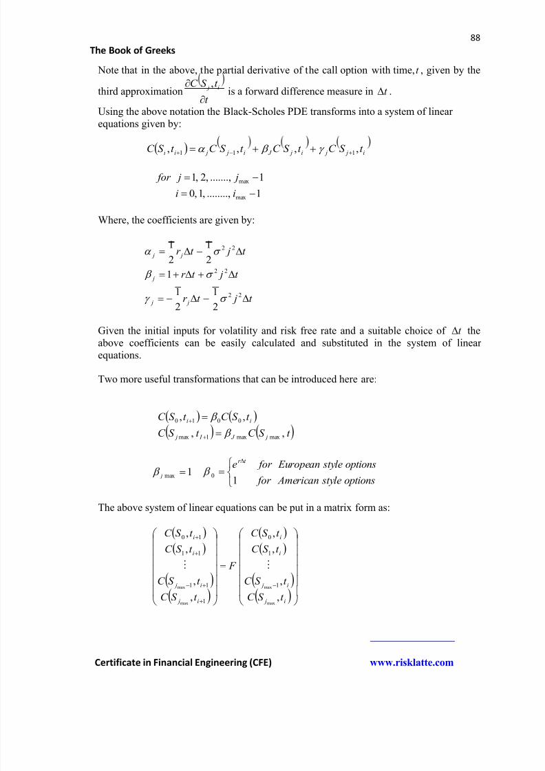
8/12/2019 Book of Greeks
http://slidepdf.com/reader/full/book-of-greeks 88/135
88
The Book of Greeks
Certificate in Financial Engineering (CFE) www.risklatte.com
Note that in the above, the partial derivative of the call option with time, t , given by the
third approximationt
t S C i j
, is a forward difference measure in t .
Using the above notation the Black-Scholes PDE transforms into a system of linearequations given by:
i j ji j J i j jii t S C t S C t S C t S C ,,,, 111
1........,,1,0
1.......,,2,1
max
max
ii
j j for
Where, the coefficients are given by:
t jt r
t jt r
t jt r
j j
j
j j
22
22
22
2
1
2
1
1
2
1
2
1
Given the initial inputs for volatility and risk free rate and a suitable choice of t theabove coefficients can be easily calculated and substituted in the system of linearequations.
Two more useful transformations that can be introduced here are:
t S C t S C
t S C t S C
j J I j
ii
,,
,,
maxmax1max
0010
1max j
options style American for
options style European for e t r
10
The above system of linear equations can be put in a matrix form as:
i j
i j
i
i
i j
i j
i
i
t S C
t S C
t S C
t S C
F
t S C
t S C
t S C
t S C
,
,
,
,
,
,
,
,
max
max
max
max 1
1
0
1
11
11
10
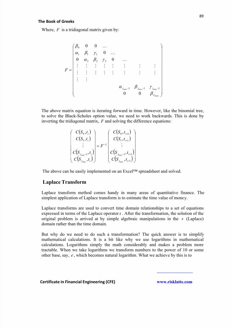
8/12/2019 Book of Greeks
http://slidepdf.com/reader/full/book-of-greeks 89/135
89
The Book of Greeks
Certificate in Financial Engineering (CFE) www.risklatte.com
Where, F is a tridiagonal matrix given by:
MAX J
j j j
F
00
00
0
00
111
222
111
0
maxmaxmax
The above matrix equation is iterating forward in time. However, like the binomial tree,
to solve the Black-Scholes option value, we need to work backwards. This is done byinverting the tridiagonal matrix, F and solving the difference equations:
1
11
11
10
1
1
1
0
,
,
,
,
,
,
,
,
max
max
max
max
i j
i j
i
i
i j
i j
i
i
t S C
t S C
t S C
t S C
F
t S C
t S C
t S C
t S C
The above can be easily implemented on an Excel™ spreadsheet and solved.
Laplace Transform
Laplace transform method comes handy in many areas of quantitative finance. Thesimplest application of Laplace transform is to estimate the time value of money.
Laplace transforms are used to convert time domain relationships to a set of equations
expressed in terms of the Laplace operator s . After the transformation, the solution of the
original problem is arrived at by simple algebraic manipulations in the s (Laplace)domain rather than the time domain.
But why do we need to do such a transformation? The quick answer is to simplifymathematical calculations. It is a bit like why we use logarithms in mathematicalcalculations. Logarithms simply the math considerably and makes a problem moretractable. When we take logarithms we transform numbers to the power of 10 or some
other base, say, e , which becomes natural logarithm. What we achieve by this is to
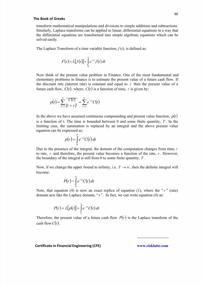
8/12/2019 Book of Greeks
http://slidepdf.com/reader/full/book-of-greeks 90/135
90
The Book of Greeks
Certificate in Financial Engineering (CFE) www.risklatte.com
transform mathematical manipulations and divisions to simple additions and subtractions.Similarly, Laplace transforms can be applied to linear, differential equations in a way thatthe differential equations are transformed into simple algebraic equations which can besolved easily.
The Laplace Transform of a time variable function, f (t ), is defined as:
0
dt t f et f L s F st
Now think of the present value problem in Finance. One of the most fundamental andelementary problems in finance is to estimate the present value of a future cash flow. Ifthe discount rate (interest rate) is constant and equal to r then the present value of a
future cash flow, t C , where, t C is a function of time, t is given by:
T
t
rt
T
t t
t C er t C t p
11 1
In the above we have assumed continuous compounding and present value function, t p
is a function of t. The time is bounded between 0 and some finite quantity, T . In thelimiting case, the summation is replaced by an integral and the above present valueequation can be expressed as:
T
rt dt t C er p0
Due to the presence of the integral, the domain of the computation changes from time, t to rate, r and therefore, the present value becomes a function of the rate, r . However,the boundary of the integral is still from 0 to some finite quantity, T .
Now, if we change the upper bound to infinity, i.e. T , then the definite integral will
become:
0
dt t C er P rt
Note, that equation (4) is now an exact replica of equation (1), where the “ r ” (rate)
domain acts like the Laplace domain, “ s ”. In fact, we can write equation (4) as:
0
dt t C et p Lr P rt
Therefore, the present value of a future cash flow r P is the Laplace transform of the
cash flow t C .
8/12/2019 Book of Greeks
http://slidepdf.com/reader/full/book-of-greeks 91/135
91
The Book of Greeks
Certificate in Financial Engineering (CFE) www.risklatte.com
Of course, one needs to be cognizant of the fact that the bounds of the integral above arefrom 0 to infinity. In other words, the Laplace transform equation, (3), exactly translatesinto the discrete time present value equation (2) only when we are considering a very
long period of time. If the cash flow is $1 then by equation (4), r
r P 1 and if the cash
flow is K (where, K is constant) then equation (4) will yield r
K r P . Actually, this can
be very easily verified using an Excel spreadsheet. Choose any interest rate, say, 5% andchoose a cash flow equal to $100. Then, over say, a 100 year period (100 years is longenough to be the real life equivalent of infinity) the present value of all the cash flows(summed up over 100 years) would be equal to $1,985. Using the Laplace transformresult, you’d get $2,000.
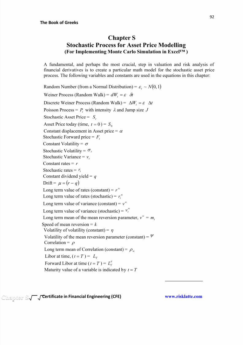
8/12/2019 Book of Greeks
http://slidepdf.com/reader/full/book-of-greeks 92/135
92
The Book of Greeks
Certificate in Financial Engineering (CFE) www.risklatte.com
Chapter S
Stochastic Process for Asset Price Modelling(For Implementing Monte Carlo Simulation in Excel™ )
A fundamental, and perhaps the most crucial, step in valuation and risk analysis offinancial derivatives is to create a particular math model for the stochastic asset price process. The following variables and constants are used in the equations in this chapter:
Random Number (from a Normal Distribution) = 1,0~ N t
Weiner Process (Random Walk) = t dW t
Discrete Weiner Process (Random Walk) = t W t
Poisson Process = t P with intensity and Jump size J
Stochastic Asset Price = t S
Asset Price today (time, 0t ) = 0S
Constant displacement in Asset price =
Stochastic Forward price = t F
Constant Volatility =
Stochastic Volatility = t
Stochastic Variance = t v
Constant rates = r
Stochastic rates = t r
Constant dividend yield = q
Drift = qr
Long term value of rates (constant) = r
Long term value of rates (stochastic) = t r
Long term value of variance (constant) = v
Long term value of variance (stochastic) =t v
Long term mean of the mean reversion parameter,
v = t m
Speed of mean reversion = k
Volatility of volatility (constant) = Volatility of the mean reversion parameter (constant) =
Correlation =
Long term mean of Correlation (constant) = Libor at time, ( T t ) = T L
Forward Libor at time ( T t ) = F
T L Maturity value of a variable is indicated by T t
8/12/2019 Book of Greeks
http://slidepdf.com/reader/full/book-of-greeks 93/135
93
The Book of Greeks
Certificate in Financial Engineering (CFE) www.risklatte.com
Stochastic Process
“Stochastic” means “Random”. A Stochastic process, t W , where T t t W W t , , is
defined as a sequence of random variables, t W , where the parameter, t denotes time
and flows over an index T . The state space of the stochastic process, is given by the setof all possible values for the random variables t W and each of these possible values is
called the state of the process. If T represents a countable set then W is a discrete
stochastic process and will represent discrete time measurements. The process t W is
a continuous stochastic process if the index T is a finite continuum.
Simply put, a stochastic process is variable who value over a period of time changes in arandom (stochastic) manner. A stock price is a stochastic process, as is the FX rate or theinterest rate. If we measure the random changes in the variable over discrete timeinterval, such as one month, one day, one hour, one minute, one second, etc. then it is
known as a discrete time stochastic process. Here we denote the change in the timeinterval – over which the value of the variable changes randomly – as t . If we measurethe random changes in the variable over infinitesimally small time intervals, such that
0t , then the process is known as a continuous time stochastic process. An example
of a stochastic process is a Weiner Process or what is popularly known as Random Walk.
Two World Views for Incorporating Stochasticity (Randomness)
In Finance, stochastic processes are generally of two kinds:
A process where the “asset price” is stochastic;
A process where the “time” is stochastic;
Stochastic Processes of “Asset Price” and the Levy Process
Most stochastic processes in Finance that are used to describe asset price behavior belong to the family of Levy processes. A Levy process is a generalized stochastic process that has three independent components:
(i) Weiner process (i.e. a random walk)(ii) A deterministic drift(iii) A pure jump process
Classification of Stochastic Processes for investigating key Risk Factors
Damanio Brigo Damiano Brigo, Antonio Dalessandro, Matthias Neugebauer and FaresTriki in their excellent tutorial have identified two of the key characteristic features ofasset prices that a stochastic process should incorporate, especially if an investigation is
8/12/2019 Book of Greeks
http://slidepdf.com/reader/full/book-of-greeks 94/135
94
The Book of Greeks
Certificate in Financial Engineering (CFE) www.risklatte.com
made from a risk management point of view. These two features of the asset price are:
Fat Tails
Mean Reversion
Consequently, he characterizes the stochastic process of asset prices into followingcategories:
Basic process: Arithmetic Brownian Motion (ABM) and Geometric BrownianMotion (GBM)
Fat tails processes: GBM with lognormal jumps, ABM with normal jumps,GARCH and Variance Gamma (VG)
Mean Reverting processes: Vasicek, Cox-Ingersoll-Ross (CIR), ExponentialVasicek
Mean Reverting processes with Fat Tails: Vasicek with jumps, ExponentialVasicek with jumps.
However, note that the above categorization is neither exhaustive nor complete. Thereare numerous other stochastic processes that describe asset prices, volatility andcorrelation that have not been included above. The above classification is only one ofthe ways to look at stochastic processes.
Stochastic Processes of “Time” and the Poisson Process
Stochastic processes where time is a random variable mostly belong to the class ofPoisson processes, which are point processes.
Poisson Process
A Poisson process is an important stochastic process used to model insurance risk andhas wide applications in both finance and insurance. There are three kinds of Poisson processes that are of interest in the field of financial engineering:
Homogenous Poisson process
Non-homogenous Poisson process
Cox process (Doubly stochastic Poisson process)
In insurance, Poisson processes are used to model claims arrival time. In finance,Poisson processes (and especially, Cox processes) are used extensively to model defaulttimes, while valuing risky bonds and credit derivatives.
8/12/2019 Book of Greeks
http://slidepdf.com/reader/full/book-of-greeks 95/135
95
The Book of Greeks
Certificate in Financial Engineering (CFE) www.risklatte.com
Stochastic Processes for Modelling Asset Price
1. Markov Process
The stochastic processes that mostly studies in quantitative finance are MarkovProcesses. For example, the random walk and the Brownian motion describing equity(stock) prices and currencies (FX rates) are Markovian processes. A Markov Process is astochastic process where on the present value of the variable is relevant in determiningthe future values of the variables. In other words, the future evolution of the random pathof a variable in a Markov process is solely dependent on the present state of the variable.
2. Martingale Property of a Stochastic Process
The martingale property of a stochastic process states that the conditional expectation ofthe process at any time in the future is just the current value. Suppose you are playing the
coin tossing game with an opponent and every time heads show up in a toss, you win $1and if tails show up you lose $1. The martingale property of this stochastic process statesthat the conditional expectation of your winnings at any future time is just the amount ofdollars you already hold. In terms of probability notation we can write:
i ji X i j X X E ,
3. Random Walk (Weiner Process) and Brownian Motion
All Financial Assets, like stocks, currencies, interest rates, etc. are assumed to follow a
random walk and a Brownian motion. A random walk is a simple, continuous timeMarkovian diffusion process, which is stochastic in nature, and is more formally knownas a Weiner Process.
If t W is a Weiner process, where t is time, then its behaviour can be understood by the
following two properties:
(i) Over an infinitesimally small time interval, t , the change in t W , given by t W
is given by:
t t W t t W t W t
Where, t , is a random number drawn from a Normal (Gaussian) distribution with
zero mean and unit standard deviation. In other words, 1,0~ N t . In the limiting
case, when, 0t the Weiner process is given by:
8/12/2019 Book of Greeks
http://slidepdf.com/reader/full/book-of-greeks 96/135
96
The Book of Greeks
Certificate in Financial Engineering (CFE) www.risklatte.com
t t dW t
(ii) For any two values of time, and s , where, s the processes W and sW
are independently distributed which makes t W a Markov process.
If we add a drift to the random walk then we get a Brownian motion. A Brownian motionis a random walk plus a drift:
Brownian motion = Random Walk + Drift.
Financial assets and securities that follow a Brownian motion have two components totheir price change. The first is the drift and the second is the random walk. The randomwalk is tied to the volatility of the asset or the security. An example of drift is the riskneutral forward rate, i.e. risk free interest rate minus the dividend yield for equities or the
domestic interest rate minus the foreign interest rate for currencies.
Random Walks have these two important properties:
(i) They are Markovian in nature
(ii) They have the Martingale property
4. Geometric Brownian Motion (GBM) with constant volatility
Geometric Brownian motion (GBM) is used to model equity, equity indices, FX rates and
Commodity prices in Finance. A geometric Brownian motion (GBM) models the returnof the stock (price), where the return is expressed as the logarithm of the price relative. Inother words, in a GBM we model the rate of change of the asset price, i.e. the percentagechange. If we assume a lognormal process for the asset price, i.e. if the natural logarithmof the asset price follows a Normal (Gaussian) probability distribution then the Stochastic
Differential Equation (SDE) for the asset price, t S is given by:
t
t
t dW dt S
dS
Here, is a constant and represents the drift of the Brownian motion and is also a
constant and represents the volatility of the asset. The volatility is the coefficient ofthe diffusion process. In a risk neutral setting, where, r is the risk free rate in the
economy and q is the dividend yield of the asset, the drift can be expressed as: qr .
Therefore, the GBM for the asset price can be written as:
t
t
t dW dt qr S
dS
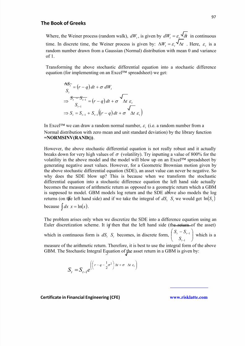
8/12/2019 Book of Greeks
http://slidepdf.com/reader/full/book-of-greeks 97/135
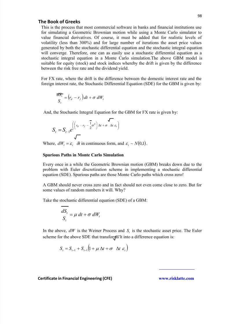
8/12/2019 Book of Greeks
http://slidepdf.com/reader/full/book-of-greeks 98/135
98
The Book of Greeks
Certificate in Financial Engineering (CFE) www.risklatte.com
This is the process that most commercial software in banks and financial institutions usefor simulating a Geometric Brownian motion while using a Monte Carlo simulator tovalue financial derivatives. Of course, it must be added that for realistic levels ofvolatility (less than 300%) and for large number of iterations the asset price valuesgenerated by both the stochastic differential equation and the stochastic integral equationwill converge. Therefore, one can as easily use a stochastic differential equation as a
stochastic integral equation in a Monte Carlo simulation.The above GBM model issuitable for equity (stock) and stock indices whereby the drift is given by the difference between the risk free rate and the dividend yield.
For FX rate, where the drift is the difference between the domestic interest rate and theforeign interest rate, the Stochastic Differential Equation (SDE) for the GBM is given by:
t f d
t
t dW dt r r S
dS
And, the Stochastic Integral Equation for the GBM for FX rate is given by:
t f d t t r r
t t eS S 2
2
1
1
Where, t dW t t in continuous form, and 1,0~ N t .
Spurious Paths in Monte Carlo Simulation
Every once in a while the Geometric Brownian motion (GBM) breaks down due to the
problem with Euler discretization scheme in implementing a stochastic differentialequation (SDE). Spurious paths are those Monte Carlo paths which cross zero!
A GBM should never cross zero and in fact should not even come close to zero. But forsome values of random numbers it will. Why?
Take the stochastic differential equation (SDE) of a GBM:
t
t
t dW dt S
dS
In the above, dW is the Weiner Process and t S is the stochastic asset price. The Euler
scheme for the above SDE that transforms it into a difference equation is:
t t t t t t S S S 111
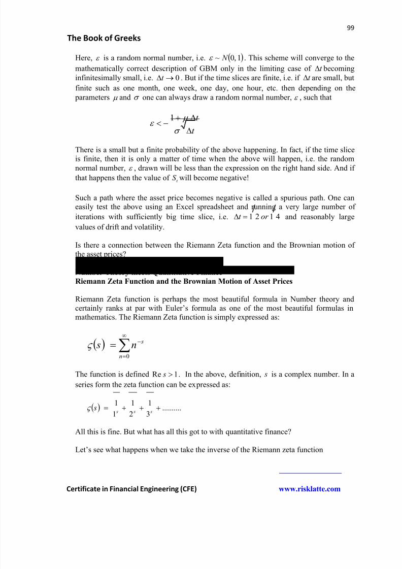
8/12/2019 Book of Greeks
http://slidepdf.com/reader/full/book-of-greeks 99/135
99
The Book of Greeks
Certificate in Financial Engineering (CFE) www.risklatte.com
Here, is a random normal number, i.e. 1,0~ N . This scheme will converge to the
mathematically correct description of GBM only in the limiting case of t becoming
infinitesimally small, i.e. 0t . But if the time slices are finite, i.e. if t are small, but
finite such as one month, one week, one day, one hour, etc. then depending on the
parameters and one can always draw a random normal number, , such that
t
t
1
There is a small but a finite probability of the above happening. In fact, if the time sliceis finite, then it is only a matter of time when the above will happen, i.e. the random
normal number, , drawn will be less than the expression on the right hand side. And if
that happens then the value of t S will become negative!
Such a path where the asset price becomes negative is called a spurious path. One caneasily test the above using an Excel spreadsheet and running a very large number of
iterations with sufficiently big time slice, i.e. 4121 or t and reasonably large
values of drift and volatility.
Is there a connection between the Riemann Zeta function and the Brownian motion ofthe asset prices?
Number Theory meets Quantitative Finance
Riemann Zeta Function and the Brownian Motion of Asset Prices
Riemann Zeta function is perhaps the most beautiful formula in Number theory andcertainly ranks at par with Euler’s formula as one of the most beautiful formulas inmathematics. The Riemann Zeta function is simply expressed as:
0n
sn s
The function is defined 1Re s . In the above, definition, s is a complex number. In a
series form the zeta function can be expressed as:
..........3
1
2
1
1
1
s s s s
All this is fine. But what has all this got to with quantitative finance?
Let’s see what happens when we take the inverse of the Riemann zeta function
8/12/2019 Book of Greeks
http://slidepdf.com/reader/full/book-of-greeks 100/135
100
The Book of Greeks
Certificate in Financial Engineering (CFE) www.risklatte.com
................
10
1
9
0
8
0
7
1
6
1
5
1
4
0
3
1
2
11
1 s s s s s s s s s s
The numerator of the above series are the values of the Mobius function, x , which iszero if x is square free, 1 if x has even number of prime factors and 1 if it has an oddnumber of prime factors. If we look at the values of the Mobius function the look like
.................,1,0,0,1,1,1,0,1,1,1
This can be thought of as a random walk in which a person – who is quite drunk – or afinancial asset such as a stock price of an FX pair stays where it is, i.e. 0, or takes onestep forward, i.e. +1 or takes one step backward, i.e. -1.
As David Wells writes in his excellent book, Prime Numbers, this observation was first
made by Von Sternbach in 1896, who also listed the first 150,000 values of the Mobiusfunction and estimated that the probability that x was non-zero was around 2
6
which is roughly equal to 0.608 with +1 and -1 having approximately equal probabilitiesof occurrence.
Therefore, the random walk, i.e. a Weiner process that models the asset price, is hiddendeep within the Riemann zeta function.
Let us look at some more evidence of this.
In 1997, in a seminal paper, Broadie, Glasserman and Kou, professors at ColumbiaUniversity and the University of Michigan respectively, proposed a beautiful formula forthe adjustment that needs to be made when we move from a continuous barrier to adiscrete barrier, while valuing a certain kind of financial derivative called the barrieroptions. Barrier options are extremely popular amongst sell side traders in the banks andinstitutional investors and are embedded in numerous structured products sold to retailinvestors as well.
All closed form solution for barrier options (knock-outs or knock-ins) are pricedassuming a continuous monitoring of the barrier, owing to the use of continuous timestochastic calculus in such mathematical modeling. However, in real life all optiontraders observe any barrier – a knock-out or a knock-in level of the asset, given a certain
asset price path – on a discrete basis, such as daily monitoring, weekly monitoring, etc.Therefore, adjustment needs to be made to compensate for this fact.
Broadie, Glasserman and Kou showed that if m is denotes monitoring points (number ofdays or number of months, etc.), H is the (theoretical) continuously monitored barrierlevel and H is the corresponding (practical) discrete barrier level then the two should beapproximately related by this formula (also, see Chapter O, #18 for this formula).
8/12/2019 Book of Greeks
http://slidepdf.com/reader/full/book-of-greeks 101/135
101
The Book of Greeks
Certificate in Financial Engineering (CFE) www.risklatte.com
m
T
He H
In the above formula, the authors showed that the constant is related to the Riemann
zeta function by
5826.0
2
21
In the above formula, s is the value of the Riemann zeta function around 21 s .
The plus and the minus sign in front of the constant represent an up barrier and a
down barrier option respectively. This beautiful formula is used today by traders tomake adjustments to the barrier level when valuing barrier options and the formula. The
function, s around 21
s has a special significance. The Riemann hypothesis statesthat the zeta function has non-real and non-trivial zeros only on the critical line for
which the real part of s is 21 .
The Riemann zeta function and the Riemann hypothesis are both related to the Primenumber theorem and the distribution of prime numbers. Prime numbers are used in many powerful mathematical algorithms to we generate random numbers. These randomnumbers are in turn used to simulate Brownian motion while modeling asset price pathsfor the valuation of financial derivatives.
5. GBM and the Log Returns in Continuous Time Finance
In continuous time finance, closely related to the notion of geometric Brownian motion(GBM) is the concept of log returns for assets. In a continuous time framework, when weslice time into smaller and smaller intervals, the return of an asset get expressed asnatural logarithm of this period’s price divided by the last period’s price . In other words,
if t S is this period’s price (say, today) and 1t S is last period’s price (say, yesterday) then
we express the return of the asset as
t
t t
S
S R ln .
It is a moot point and even though the above expression does not make intuitive sense to
the every day investors, traders and quants use this measure all the time in theircalculation. Actually, it comes from applying integral calculus to finance.
Asset return should be measured, as indeed it is by thousands of fund managers andinvestors around the world, as today’s price less yesterday’s price divided by yesterday’s
price. This is an arithmetic measure. In other words, if t S is this period’s asset price
(where the time period is discrete like one year, one month, one week, one day or even
8/12/2019 Book of Greeks
http://slidepdf.com/reader/full/book-of-greeks 102/135
102
The Book of Greeks
Certificate in Financial Engineering (CFE) www.risklatte.com
one minute) and 1t S is last period’s asset price then (assuming no dividend payments) the
asset return should be equal to:
1
1
t
t t t
S
S S R
The above formula gives the measure of an arithmetic return something that we are allfamiliar with. Now, if we have many periods, say, N, in one time interval (i.e. 12 monthsin an interval of one year) then the total return of the entire interval is simply the sum ofall the individual period’s returns, i.e.
N
t t
t t N
t
t T S
S S R R
1 1
1
1
However, what happens if we start to slice time into smaller and smaller intervals. Say,
we start slicing time (one year) into minutes, seconds, nanoseconds and so on until we getto the mathematical definition of an infinitesimally small interval of time. We are now
talking about the limit when delta t (the smallest measurable unit of time) goes to zero.
Mathematically speaking, we say that 0t . In the limit, the above expression for
return will reduce to:
N
t
N
t t
t
t t
t T
S
S Lt R Lt R
1 100
In the limiting case if 0t , then dS S and the summation sign will get replaced
by an integral. Therefore, the expression for the asset return (dropping the subscript fortime) becomes:
T S S
S S
T S
dS R
0
And the limits of the integral are chosen in line with the time limits, i.e. at start when
0t the asset price is 0S and at the end of the time interval (maturity), i.e. at T t , the
asset price is T S . From integral calculus, we know that x
x
dxln and therefore, we
have:
T S
S
T T T
S
S S S
S
dS R
0 0
0 lnlnln
8/12/2019 Book of Greeks
http://slidepdf.com/reader/full/book-of-greeks 103/135
103
The Book of Greeks
Certificate in Financial Engineering (CFE) www.risklatte.com
Therefore, in a time interval [0, T], if we assume a continuous time process, i.e. time issliced as infinitesimally small intervals, the asset return will be expressed as the naturallogarithm of the final price over the initial price.
6. Girsanov’s Theorem and Exotic Options Pricing
One of the fundamental concepts in asset price modeling for valuation of exotic optionsis the Girsanov’s theorem. It is closely related to the notion of Radon-Nikodymderivative that we learnt above. Barrier option traders come face to face with both theseconcepts quite regularly.
How can we explain Girsanov’s theorem?
According to one veteran exotic options trader Girsanov’s theorem makes the driftdisappear from an asset (diffusion process) making it a martingale. In other words, aBrownian motion with drift becomes a drift-less random walk changing the probability
of the asset hitting a barrier. In other words, we look at the problem of a barrier being hitnot under the real (physical) probability measure but a risk neutral one. The real(physical) probability of the barrier being hit may be too low or immeasurable but undera risk neutral probability measure the problem becomes tractable.
Another trader’s refrain was: options can be very easily priced using the difference between the two reflected processes. Reflection principle helps us in estimating the riskneutral probability of all random paths that reach a given point without going through a barrier. Under a real (physical) probability measure the Brownian motion of the asset price will have drift and hence the two Weiner processes will not be equivalent. Thedrift needs to get out of the way for the Weiner processes to be equivalent. Actually, the
probability takes care of the drift.
Say, you are a barrier options trader and you are investigating an asset price diffusion process given by:
t dW t dt t t dX
Here, t is the drift of the asset and t is the coefficient of diffusion (i.e. volatility).
You are interested in estimating the probability of t X , the asset price, entering a
certain space, say, B (the region around the barrier) in the time interval T ,0 . The only
way to do this is to run Monte Carlo simulations. So you set up an Excel™ spreadsheetsimulator and start to run simulations.
However, you are quite sure that the probability of this event happening is very small,
say, 510 . In other words, you’d have to run 100,000 iterations (realizations of asset price path) to measure this probability.
8/12/2019 Book of Greeks
http://slidepdf.com/reader/full/book-of-greeks 104/135
104
The Book of Greeks
Certificate in Financial Engineering (CFE) www.risklatte.com
Now say, you could somehow change the drift of the asset diffusion process, shown
above, in such a way that the probability of the above event, i.e. asset price, t X
entering the barrier space, B in the time interval T ,0 , becomes significantly larger
than 510 . Therefore, you’d need a lot less number of iterations (realizations of the asset
price paths) to measure this probability. This is music to a trader’s ears! Girsanov’stheorem does precisely that.
Two probability measures, Q and P are equivalent if Q is absolutely continuous with P
and P is absolutely continuous with Q . A probability measure Q is absolutely
continuous with P if the Radon-Nikodym derivative, shown below, exists.
dP
dQ
Say we have an Ito diffusion process (such as a Geometric Brownian motion) for anasset price given by
t dW t dt t t dX
Where, t W is a Weiner process (a random walk) under a probability measure, P . In
the above equation, t is the drift and t is the coefficient of diffusion (equivalent
to volatility).
Note that t X is a martingale if the above process is driftless, i.e. the drift, 0 . That
it, we would need the stochastic differential equation to be of the form t dW t dX .
How can we do so?
Rewrite the above diffusion equation as:
t W d t t dX
t dW t
t t t dX
The resultant equation also looks like a geometric Brownian motion. However, the new
Weiner process, t W is given by:
t
dst
t t W t W
dt t
t t dW t W d
0
8/12/2019 Book of Greeks
http://slidepdf.com/reader/full/book-of-greeks 105/135
8/12/2019 Book of Greeks
http://slidepdf.com/reader/full/book-of-greeks 106/135
106
The Book of Greeks
Certificate in Financial Engineering (CFE) www.risklatte.com
The Poisson process is related to the default intensity, where the probability that the
value of dQ will be 1 is equal to dt .
9. Geometric Brownian Motion for the Inverse of the Asset Price
This process comes handy in understanding the movements of FX rates (currency pairs).They can help us to investigate how the process of USD/JPY (Dollar-Yen) differs fromthe process for JPY/USD (Yen-Dollar).
Given the Jensen’s inequality
X E f x f E
The geometric Brownian motion for the inverse of the asset price, S Y 1 , is given by
t
t
t dW dt Y
dY 2
An example would be, if t S is the USD/JPY (Dollar-Yen) price then t t S Y 1 , would be
the JPY/USD (Yen-Dollar) price.
10. Stochastic Process for the Relative Performance of Two Assets
If there are two assets (two stocks or two stock indices), 1S and 2S such that their
respective stochastic processes (geometric Brownian motions) are given by:
dt dW dW where
dW dt S
dS
dW dt S
dS
t t
t
t
t
t
t
t
21
2
22
,2
,2
1
11
,1
,1
,
Where, the respective Weiner processes are correlated via the correlation coefficient, .
Now, consider a relative process (can be thought of as “relative performance”) given by:
2
1
21 ,S
S S S R
It can be shown that this relative process, R , also follows a geometric Brownian motion
given by:
8/12/2019 Book of Greeks
http://slidepdf.com/reader/full/book-of-greeks 107/135
107
The Book of Greeks
Certificate in Financial Engineering (CFE) www.risklatte.com
t R R
t
t dW dt R
dR
Where, 21
2
221 R and 21
2
2
2
1 2 R
11. Arithmetic Brownian motion with constant volatility
(See Vasicek and CIR process for Rates Modelling )
Arithmetic Brownian motion (ABM) are primarily used to model short rates (interestrates). Also, in stochastic volatility models, such as Heston (see below), the variance ofan asset price is assumed to follow a mean-reverting arithmetic Brownian motion.
In an arithmetic Brownian motion (ABM), we model the change in the value of the asset price and therefore, the value of the asset price can be negative in this model.
t t dW dt qr dS
12. Geometric Brownian Motion for the “Square of the Asset”
The GBM for the square of the asset is given by:
t t t t dW S dt S qr S d 2222 22
13. Geometric Brownian Motion for the thn Power of the Asset
The GBM for the n th power of the asset is given by:
t
N
t
N
t
N
t dW S N dt S N N qr N S d
212
1
14. Mean Reverting Geometric Brownian Motion
Geman (2005) describes a mean reverting geometric Brownian motion that is quite
popular in modeling commodities such as energy and agricultural commodities. If t S is
the asset price and S is the long term average of the asset price, k is the speed of mean
reversion, is the volatility of the asset and t W is a Weiner process such that
t dW t t and 1,0~ N t then the stochastic differential equation for the asset price
is given by:
t t
t
t dW dt S S k S
dS
ln
8/12/2019 Book of Greeks
http://slidepdf.com/reader/full/book-of-greeks 108/135
108
The Book of Greeks
Certificate in Financial Engineering (CFE) www.risklatte.com
Making the following transformations:
t t S G ln
t
rT
t GeY
and integrating between the limits T t , , we get the stochastic integral equation for the
asset price within the time limit T t , , where the value t Y at time t is observed and is the
starting value and T Y is a function of the Weiner process, t W .
t
kt kT kt kT
t T W k
eeee
k S Y Y
22
222
15. Brownian Bridge Process
A Brownian bridge is a “tied down” Brownian motion. It is used to model Treasury bonds where the asset redeems at par. In a Brownian bridge the final asset price reverts back to the par value or the starting price and is therefore known in advance. However,
between 0t and maturity, T t , the process is stochastic.
A Brownian bridge is described by the following process:
T t
T W T
t t W t B
,0
)(*)()( T W t t W t B
Where, t W is the corresponding Weiner process. The stochastic integral equation for
the asset (bond), with two known values, the starting price, 0S , the price at maturity, T S ,
T t
T W T
t W
T
t
s
S
t eS S
0
ln
0
16. Cox-Ross Square Root Process
A Cox-Ross, square root stochastic process is given by:
t t t t dW S dt S dS

8/12/2019 Book of Greeks
http://slidepdf.com/reader/full/book-of-greeks 109/135
109
The Book of Greeks
Certificate in Financial Engineering (CFE) www.risklatte.com
Where, t dW is a Weiner process given by t dW t . This is an extremely useful
process because of the additive property which also makes it a desirable process forvaluation of Asian options. But the most important property of a Cox-Ross process is thatit explains the volatility skew observed in the market. Let’s write the above square root
process differently and express the left hand side as a return process (as opposed to achange in price process).
dz S
dt S
dS
t t
t
It is obvious from the above return process that the instantaneous variance of the return2
t
t
S
dS is equal to
t S
2 . This is an inverse function of the equity (asset) price. Thus,
lower the equity (asset) price the higher the variance and vice-versa. This fact isempirically found to be true. Therefore, the Cox-Ross square root process is a better process than a geometric Brownian motion (GBM) when it comes to explaining thevolatility skew.
In fact, along with the square root process, Cox and Ross also introduced the ConstantElasticity of Variance (CEV) stochastic model of asset prices which till this day is popular amongst many FX option traders. CEV process can be viewed as a moregeneralized form of the Cox-Ross process.
17. Ornstein-Uhlenbeck Process
Ornstein-Uhlenbeck (OU) are a class of mean reverting, stochastic processes which findwide application in the modeling of interest rates and commodities. A generic OU process can be written as:
t t t dW dt S k dS
Where, t dW is a Weiner process given by t dW t t , where, 1,0~ N t is a random
number drawn from a Gaussian (Normal) distribution with mean zero and standarddeviation of one.
Discretization of OU process for Monte Carlo Simulation in Excel™
t t t t t t S k S S 11
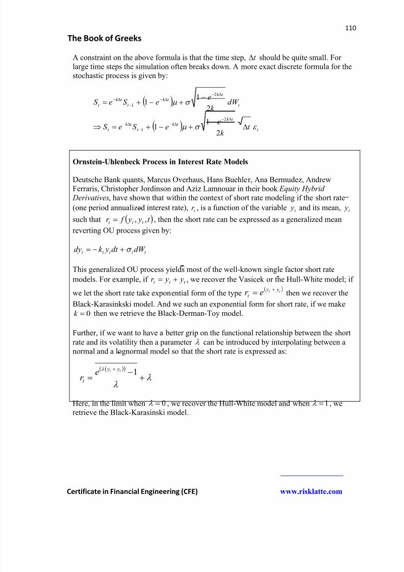
8/12/2019 Book of Greeks
http://slidepdf.com/reader/full/book-of-greeks 110/135
110
The Book of Greeks
Certificate in Financial Engineering (CFE) www.risklatte.com
A constraint on the above formula is that the time step, t should be quite small. Forlarge time steps the simulation often breaks down. A more exact discrete formula for thestochastic process is given by:
t
t k t k
t
t k
t
t
t k
t k t
t k t
t k
eeS eS
dW k
eeS eS
2
11
211
2
1
2
1
Ornstein-Uhlenbeck Process in Interest Rate Models
Deutsche Bank quants, Marcus Overhaus, Hans Buehler, Ana Bermudez, AndrewFerraris, Christopher Jordinson and Aziz Lamnouar in their book Equity Hybrid
Derivatives, have shown that within the context of short rate modeling if the short rate(one period annualized interest rate), t r , is a function of the variable t y and its mean, t y
such that t y y f r t t t ,, , then the short rate can be expressed as a generalized mean
reverting OU process given by:
t t t t t dW dt yk dy
This generalized OU process yields most of the well-known single factor short rate
models. For example, if t t t y yr , we recover the Vasicek or the Hull-White model; if
we let the short rate take exponential form of the type t t y y
t er then we recover the
Black-Karasinkski model. And we such an exponential form for short rate, if we make
0k then we retrieve the Black-Derman-Toy model.
Further, if we want to have a better grip on the functional relationship between the short
rate and its volatility then a parameter can be introduced by interpolating between anormal and a lognormal model so that the short rate is expressed as:
1t t y y
t
er
Here, in the limit when 0 , we recover the Hull-White model and when 1 , weretrieve the Black-Karasinski model.
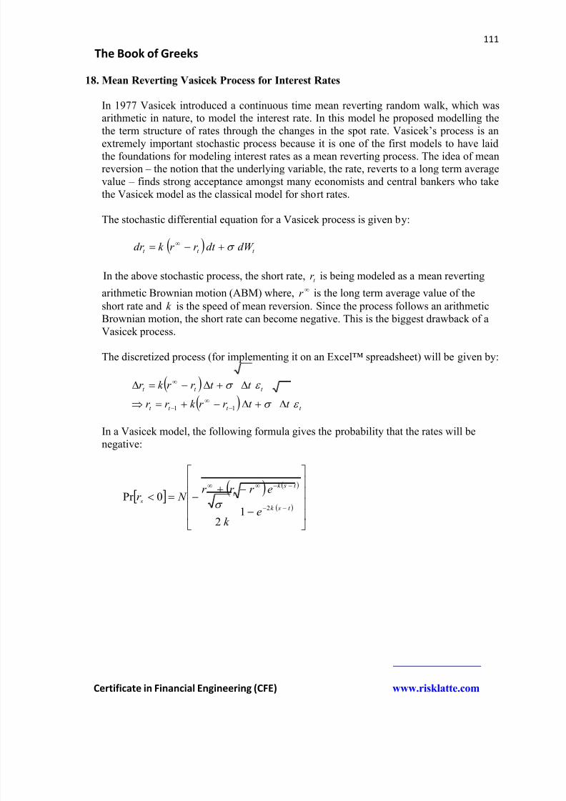
8/12/2019 Book of Greeks
http://slidepdf.com/reader/full/book-of-greeks 111/135
111
The Book of Greeks
Certificate in Financial Engineering (CFE) www.risklatte.com
18. Mean Reverting Vasicek Process for Interest Rates
In 1977 Vasicek introduced a continuous time mean reverting random walk, which wasarithmetic in nature, to model the interest rate. In this model he proposed modelling thethe term structure of rates through the changes in the spot rate. Vasicek’s process is an
extremely important stochastic process because it is one of the first models to have laidthe foundations for modeling interest rates as a mean reverting process. The idea of meanreversion – the notion that the underlying variable, the rate, reverts to a long term averagevalue – finds strong acceptance amongst many economists and central bankers who takethe Vasicek model as the classical model for short rates.
The stochastic differential equation for a Vasicek process is given by:
t t t dW dt r r k dr
In the above stochastic process, the short rate, t r is being modeled as a mean revertingarithmetic Brownian motion (ABM) where,
r is the long term average value of the
short rate and k is the speed of mean reversion. Since the process follows an arithmeticBrownian motion, the short rate can become negative. This is the biggest drawback of aVasicek process.
The discretized process (for implementing it on an Excel™ spreadsheet) will be given by:
t t t t
t t t
t t r r k r r
t t r r k r
11
In a Vasicek model, the following formula gives the probability that the rates will benegative:
t sk
t sk
t
s
ek
er r r N r
21
2
0Pr
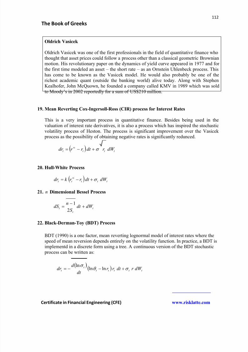
8/12/2019 Book of Greeks
http://slidepdf.com/reader/full/book-of-greeks 112/135
112
The Book of Greeks
Certificate in Financial Engineering (CFE) www.risklatte.com
Oldrich Vasicek
Oldrich Vasicek was one of the first professionals in the field of quantitative finance whothought that asset prices could follow a process other than a classical geometric Brownianmotion. His revolutionary paper on the dynamics of yield curve appeared in 1977 and forthe first time modeled an asset – the short rate – as an Ornstein Uhlenbeck process. Thishas come to be known as the Vasicek model. He would also probably be one of therichest academic quant (outside the banking world) alive today. Along with StephenKealhofer, John McQuown, he founded a company called KMV in 1989 which was soldto Moody’s in 2002 reportedly for a sum of US$210 million.
19. Mean Reverting Cox-Ingersoll-Ross (CIR) process for Interest Rates
This is a very important process in quantitative finance. Besides being used in thevaluation of interest rate derivatives, it is also a process which has inspired the stochasticvolatility process of Heston. The process is significant improvement over the Vasicek process as the possibility of obtaining negative rates is significantly redunced.
t t t t dW r dt r r dr
20. Hull-White Process
t t t t t dW dt r r k dr
21. n Dimensional Bessel Process
t
t
t dW dt S
ndS
2
1
22. Black-Derman-Toy (BDT) Process
BDT (1990) is a one factor, mean reverting lognormal model of interest rates where thespeed of mean reversion depends entirely on the volatility function. In practice, a BDT is
implementd in a discrete form using a tree. A continuous version of the BDT stochastic process can be written as:
t t t t t
t t dW r dt r r
dt
d dr
lnln
ln
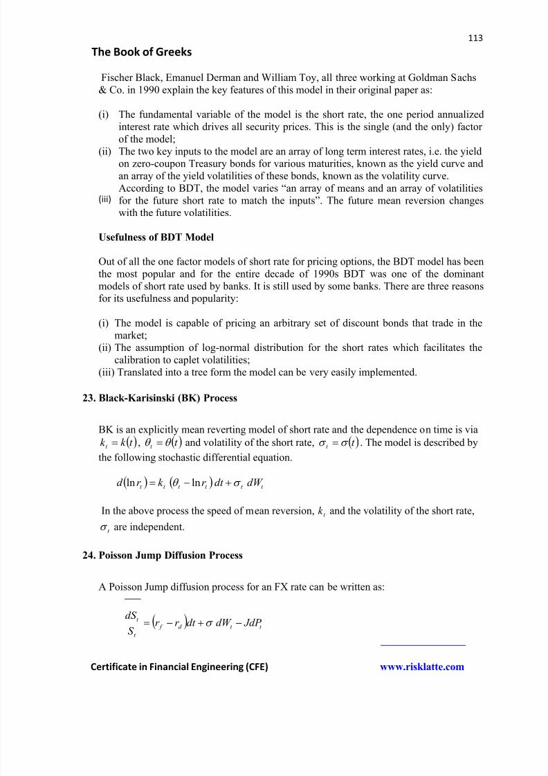
8/12/2019 Book of Greeks
http://slidepdf.com/reader/full/book-of-greeks 113/135
113
The Book of Greeks
Certificate in Financial Engineering (CFE) www.risklatte.com
Fischer Black, Emanuel Derman and William Toy, all three working at Goldman Sachs& Co. in 1990 explain the key features of this model in their original paper as:
(i) The fundamental variable of the model is the short rate, the one period annualizedinterest rate which drives all security prices. This is the single (and the only) factor
of the model;(ii) The two key inputs to the model are an array of long term interest rates, i.e. the yield
on zero-coupon Treasury bonds for various maturities, known as the yield curve andan array of the yield volatilities of these bonds, known as the volatility curve.
(iii) According to BDT, the model varies “an array of means and an array of volatilitiesfor the future short rate to match the inputs”. The future mean reversion changeswith the future volatilities.
Usefulness of BDT Model
Out of all the one factor models of short rate for pricing options, the BDT model has been
the most popular and for the entire decade of 1990s BDT was one of the dominantmodels of short rate used by banks. It is still used by some banks. There are three reasonsfor its usefulness and popularity:
(i) The model is capable of pricing an arbitrary set of discount bonds that trade in themarket;
(ii) The assumption of log-normal distribution for the short rates which facilitates thecalibration to caplet volatilities;
(iii) Translated into a tree form the model can be very easily implemented.
23. Black-Karisinski (BK) Process
BK is an explicitly mean reverting model of short rate and the dependence on time is via
t k k t , t t and volatility of the short rate, t t . The model is described by
the following stochastic differential equation.
t t t t t t dW dt r k r d lnln
In the above process the speed of mean reversion, t k and the volatility of the short rate,
t are independent.
24. Poisson Jump Diffusion Process
A Poisson Jump diffusion process for an FX rate can be written as:
t t d f
t
t JdP dW dt r r S
dS
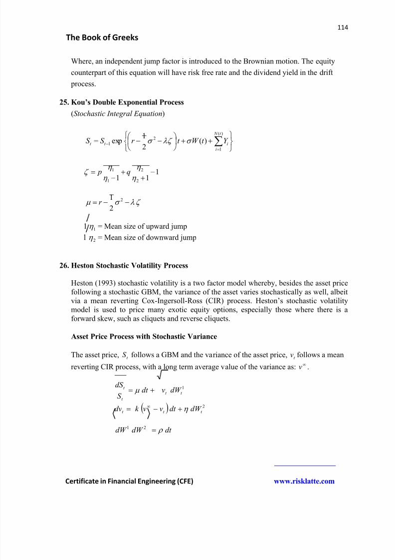
8/12/2019 Book of Greeks
http://slidepdf.com/reader/full/book-of-greeks 114/135
114
The Book of Greeks
Certificate in Financial Engineering (CFE) www.risklatte.com
Where, an independent jump factor is introduced to the Brownian motion. The equity
counterpart of this equation will have risk free rate and the dividend yield in the drift
process.
25. Kou’s Double Exponential Process
(Stochastic Integral Equation)
)(
1
2
1 )(2
1exp
t N
i
it t Y t W t r S S
111 2
2
1
1
q p
2
2
1r
11 = Mean size of upward jump
21 = Mean size of downward jump
26. Heston Stochastic Volatility Process
Heston (1993) stochastic volatility is a two factor model whereby, besides the asset price
following a stochastic GBM, the variance of the asset varies stochastically as well, albeitvia a mean reverting Cox-Ingersoll-Ross (CIR) process. Heston’s stochastic volatilitymodel is used to price many exotic equity options, especially those where there is aforward skew, such as cliquets and reverse cliquets.
Asset Price Process with Stochastic Variance
The asset price, t S follows a GBM and the variance of the asset price, t v follows a mean
reverting CIR process, with a long term average value of the variance as: v .
2
1
t t t
t t t
t
dW dt vvk dv
dW vdt S
dS
dt dW dW 21
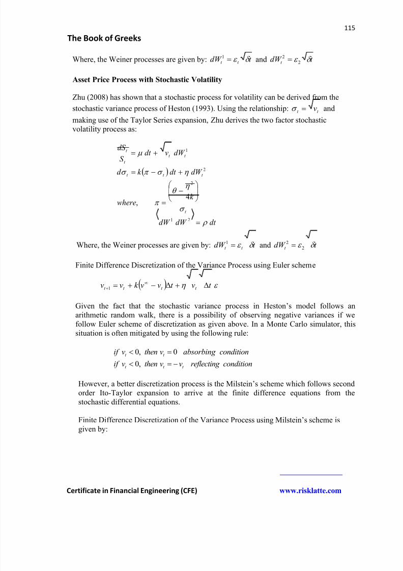
8/12/2019 Book of Greeks
http://slidepdf.com/reader/full/book-of-greeks 115/135
115
The Book of Greeks
Certificate in Financial Engineering (CFE) www.risklatte.com
Where, the Weiner processes are given by: t dW t t 1 and t dW t 22
Asset Price Process with Stochastic Volatility
Zhu (2008) has shown that a stochastic process for volatility can be derived from thestochastic variance process of Heston (1993). Using the relationship: t t v and
making use of the Taylor Series expansion, Zhu derives the two factor stochasticvolatility process as:
dt dW dW
k where
dW dt k d
dW vdt S
dS
t
t t t
t t
t
t
21
2
2
1
4,
Where, the Weiner processes are given by: t dW t t 1 and t dW t 22
Finite Difference Discretization of the Variance Process using Euler scheme
t vt vvk vv t t t t 1
Given the fact that the stochastic variance process in Heston’s model follows anarithmetic random walk, there is a possibility of observing negative variances if wefollow Euler scheme of discretization as given above. In a Monte Carlo simulator, thissituation is often mitigated by using the following rule:
conditionreflecting vvthenvif
conditionabsorbing vthenvif
t t t
t t
,0
0,0
However, a better discretization process is the Milstein’s scheme which follows secondorder Ito-Taylor expansion to arrive at the finite difference equations from the
stochastic differential equations.
Finite Difference Discretization of the Variance Pr ocess using Milstein’s scheme isgiven by:
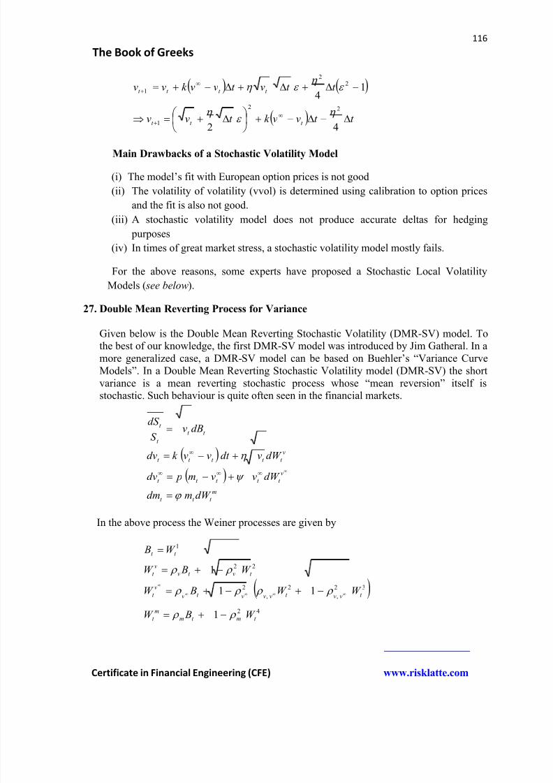
8/12/2019 Book of Greeks
http://slidepdf.com/reader/full/book-of-greeks 116/135
116
The Book of Greeks
Certificate in Financial Engineering (CFE) www.risklatte.com
t t vvk t vv
t t vt vvk vv
t t t
t t t t
42
14
22
1
22
1
Main Drawbacks of a Stochastic Volatility Model
(i) The model’s fit with European option prices is not good
(ii) The volatility of volatility (vvol) is determined using calibration to option prices
and the fit is also not good.
(iii) A stochastic volatility model does not produce accurate deltas for hedging
purposes
(iv) In times of great market stress, a stochastic volatility model mostly fails.
For the above reasons, some experts have proposed a Stochastic Local VolatilityModels ( see below).
27. Double Mean Reverting Process for Variance
Given below is the Double Mean Reverting Stochastic Volatility (DMR-SV) model. Tothe best of our knowledge, the first DMR-SV model was introduced by Jim Gatheral. In amore generalized case, a DMR-SV model can be based on Buehler’s “Variance CurveModels”. In a Double Mean Reverting Stochastic Volatility model (DMR-SV) the shortvariance is a mean reverting stochastic process whose “mean reversion” itself isstochastic. Such behaviour is quite often seen in the financial markets.
m
t t t
v
t t t t t
v
t t t t t
t t
t
t
dW mdm
dW vvm pdv
dW vdt vvk dv
dBvS
dS
In the above process the Weiner processes are given by
42
32
,
2
,
2
22
1
1
11
1
t mt m
m
t
t vvt vvvt v
v
t
t vt v
v
t
t t
W BW
W W BW
W BW
W B
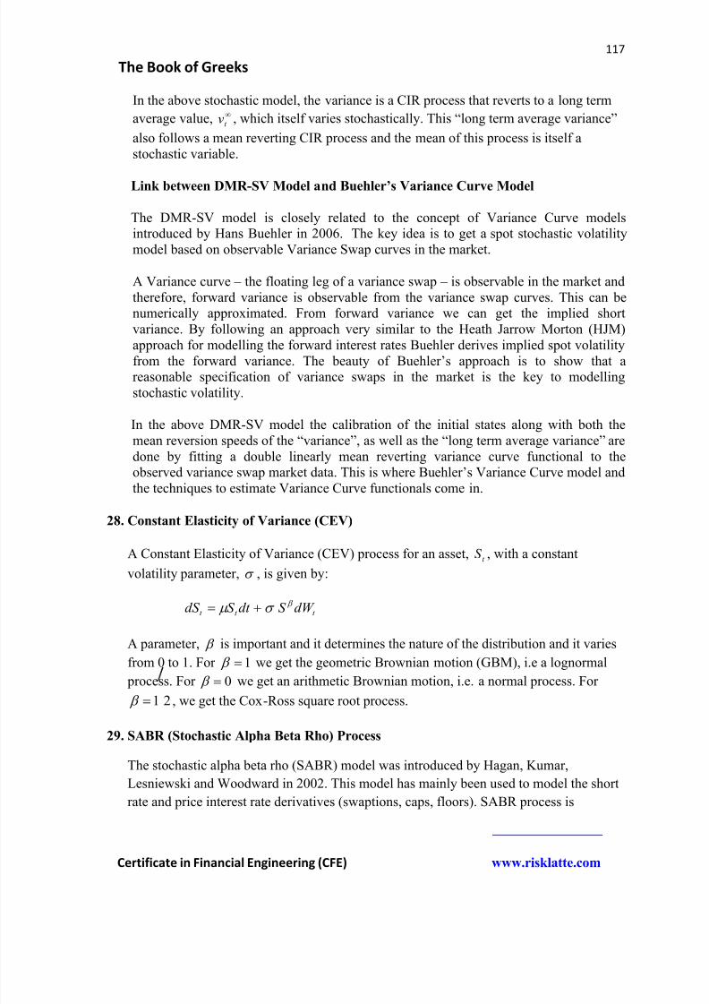
8/12/2019 Book of Greeks
http://slidepdf.com/reader/full/book-of-greeks 117/135
117
The Book of Greeks
Certificate in Financial Engineering (CFE) www.risklatte.com
In the above stochastic model, the variance is a CIR process that reverts to a long term
average value, t v , which itself varies stochastically. This “long term average variance”
also follows a mean reverting CIR process and the mean of this process is itself astochastic variable.
Link between DMR-SV Model and Buehler’s Variance Curve Model
The DMR-SV model is closely related to the concept of Variance Curve modelsintroduced by Hans Buehler in 2006. The key idea is to get a spot stochastic volatilitymodel based on observable Variance Swap curves in the market.
A Variance curve – the floating leg of a variance swap – is observable in the market andtherefore, forward variance is observable from the variance swap curves. This can benumerically approximated. From forward variance we can get the implied shortvariance. By following an approach very similar to the Heath Jarrow Morton (HJM)
approach for modelling the forward interest rates Buehler derives implied spot volatilityfrom the forward variance. The beauty of Buehler’s approach is to show that areasonable specification of variance swaps in the market is the key to modellingstochastic volatility.
In the above DMR-SV model the calibration of the initial states along with both themean reversion speeds of the “variance”, as well as the “long term average variance” aredone by fitting a double linearly mean reverting variance curve functional to theobserved variance swap market data. This is where Buehler’s Variance Curve model andthe techniques to estimate Variance Curve functionals come in.
28. Constant Elasticity of Variance (CEV)
A Constant Elasticity of Variance (CEV) process for an asset, t S , with a constant
volatility parameter, , is given by:
t t t dW S dt S dS
A parameter, is important and it determines the nature of the distribution and it varies
from 0 to 1. For 1 we get the geometric Brownian motion (GBM), i.e a lognormal
process. For 0 we get an arithmetic Brownian motion, i.e. a normal process. For
21 , we get the Cox-Ross square root process.
29. SABR (Stochastic Alpha Beta Rho) Process
The stochastic alpha beta rho (SABR) model was introduced by Hagan, Kumar,
Lesniewski and Woodward in 2002. This model has mainly been used to model the short
rate and price interest rate derivatives (swaptions, caps, floors). SABR process is
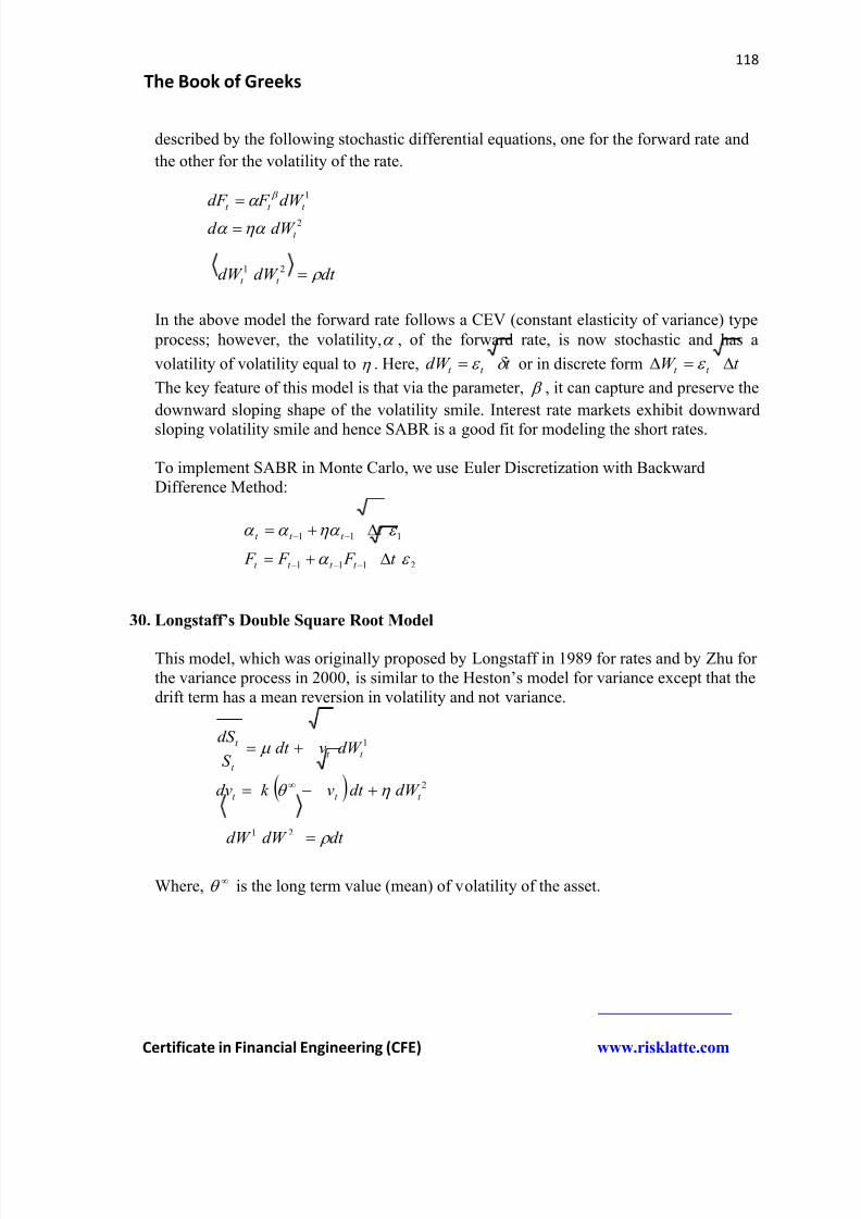
8/12/2019 Book of Greeks
http://slidepdf.com/reader/full/book-of-greeks 118/135
118
The Book of Greeks
Certificate in Financial Engineering (CFE) www.risklatte.com
described by the following stochastic differential equations, one for the forward rate and
the other for the volatility of the rate.
2
1
t
t t t
dW d
dW F dF
dt dW dW t t 21
In the above model the forward rate follows a CEV (constant elasticity of variance) type
process; however, the volatility, , of the forward rate, is now stochastic and has a
volatility of volatility equal to . Here, t dW t t or in discrete form t W t t
The key feature of this model is that via the parameter, , it can capture and preserve the
downward sloping shape of the volatility smile. Interest rate markets exhibit downward
sloping volatility smile and hence SABR is a good fit for modeling the short rates.
To implement SABR in Monte Carlo, we use Euler Discretization with BackwardDifference Method:
2111
111
t F F F
t
t t t t
t t t
30. Longstaff’s Double Square Root Model
This model, which was originally proposed by Longstaff in 1989 for rates and by Zhu forthe variance process in 2000, is similar to the Heston’s model for variance except that thedrift term has a mean reversion in volatility and not variance.
2
1
t t t
t t
t
t
dW dt vk dv
dW vdt S
dS
dt dW dW 21
Where, is the long term value (mean) of volatility of the asset.
8/12/2019 Book of Greeks
http://slidepdf.com/reader/full/book-of-greeks 119/135
119
The Book of Greeks
Certificate in Financial Engineering (CFE) www.risklatte.com
31. Stochastic Local Volatility (SLV) Process
In a Stochastic Local Volatility model we mix stochastic volatility with local volatilitymodels. In most “stochastic local volatility” model, volatility has the freedom to rise andfall independent of the underlying spot.
One form of a stochastic local volatility process is given by:
2
1,
t t t
t
v
t t L
t
t
dW dt kvdv
dW eS dt S
dS t
In this model, the second equation follows an Ornstein-Uhlenbeck log-variance process.
Ren, Madan and Qian (2007) have introduced a stochastic local volatility process given
by:
kt
t
t t t t
t t t L
t
t
ek
v
dW dt Z vk Z d
dW Z t S dt S
dS
22
2
1
12
lnln
,
dt dW dW t t 21
In the above model, k is the speed of mean reversion and is the volatility of volatility.
The long term drift, t v of t Z is deterministic and due to the last equation for t v , the
unconditional expectation of 2
t Z is unity. The two Brownian motions, 1
t dW and 2
t dW are
corrected via the correlation coefficient, . Also, it is assumed that 10 Z .
Ren, Madan and Qian’s model is important in one key aspect. In this model, there is an
independent stochastic component, t Z , t Z is not the variance process, though it does
depend on the long term average variance, t v , which is given by the third equation above.
In this basic form, however, the two Brownian motions are not correlated.
The asset price process, given by the first stochastic differential equation, almostmakes the asset price a local volatility process;
The process of t Z gives a lot of freedom for volatility to move regardless of the
underlying asset price’s move.
8/12/2019 Book of Greeks
http://slidepdf.com/reader/full/book-of-greeks 120/135
120
The Book of Greeks
Certificate in Financial Engineering (CFE) www.risklatte.com
32. Stochastic Local Volatility (SLV) / Bloomberg Model
Grigore Tataru and Travis Fisher at Bloomberg have proposed a model of asset priceswhich combines the features of a stochastic volatility process and a local volatilitysurface. Tataru and Fisher’s SLV process is given by:
dt dW dW
dW V dt V V k dV
dW V t S dt r r S
dS
t t
t t t t t
t t t L f d
t
t
21
2
1
.
,
The above model is specifically tailored towards modeling FX rates and valuation of
barrier options. In the above process, d r and f r are domestic and foreign interest rates.
In the above model the first equation describes the process for the asset price, t S and the
second equation describes the process for stochastic volatility, t V , where, t V is the long
term average of the volatility, k , is the speed of mean reversion, is the volatility of
volatility and t S t L , represents the local volatility, which Tataru and Fisher call the
“leverage surface”. The asset price and the stochastic volatility processes are correlated
via the correlation coefficient, .
Important Aspects of the SLV Model
In the above SLV model, if we make the volatility of volatility zero, i.e. 0
then SLV model degenerates into a pure local volatility model. On the other hand
making the local volatility (leverage surface) equal to one, i.e. 1, t S t L
recovers a purely stochastic volatility model.
Since both local volatility and stochastic volatility is present in the model, there is
a mixing fraction, which is controlled by the volatility of volatility parameter, .
33. GARCH Diffusion Process for Volatility
The GARCH diffusion model is the continuous-time limit of many GARCH-type
processes and in such a process volatility is modeled as a stochastic process given by:
t t t t dW dt bd
8/12/2019 Book of Greeks
http://slidepdf.com/reader/full/book-of-greeks 121/135
121
The Book of Greeks
Certificate in Financial Engineering (CFE) www.risklatte.com
Where, t dW is a Weiner process given by: t dW t and 1,0~ N . The mean
reversion in the volatility process is captured by the constant drift parameters, b and .
Since, , has dimensions of inverse time, the parameter 1 can be thought of as the
“half -life” of volatility.
Heston-Nandi(1997) has derived a degenerate case for the Heston(1993) stochasticvolatility process as a limiting case for a particular GARCH type process.
34. Mean Reverting Random Walk for Commodity Prices
Geman (2005) describes a mean reverting geometric Brownian motion that is quite popular in modeling commodities space such as energy and agricultural commodities.Here, mean reversion is introduced in a geometric Brownian motion (GBM), which isvery different from equity or FX processes. Due to the lognormal evolution the modeldoes not allow negative values for commodity prices
dW dt S S k S
dS t
t
t ln
Using the variables t t S G ln and t
rT
t GeY we get
t
kt kT kt kT
t T W k
eeee
k S Y Y
22
222
35. Gibson & Schwarz (1990) Stochastic Convenience Yield Process
The forward price of the commodity (Oil), at time, t for a contract maturing at t time, T
is related to the spot price by:
t T yr et S T t F ,
Where, r is the continuously compounded interest rate prevailing at t , for maturity, T
and y is convenience yield on the commodity. Gibson and Schwarz (1990) present the
following two factor model for pricing of contingent claims on Oil is given by:
2
2
1
1
t t t
t
t
t
dW dt yk dy
dW dt S
dS
dt dW dW t t 21.
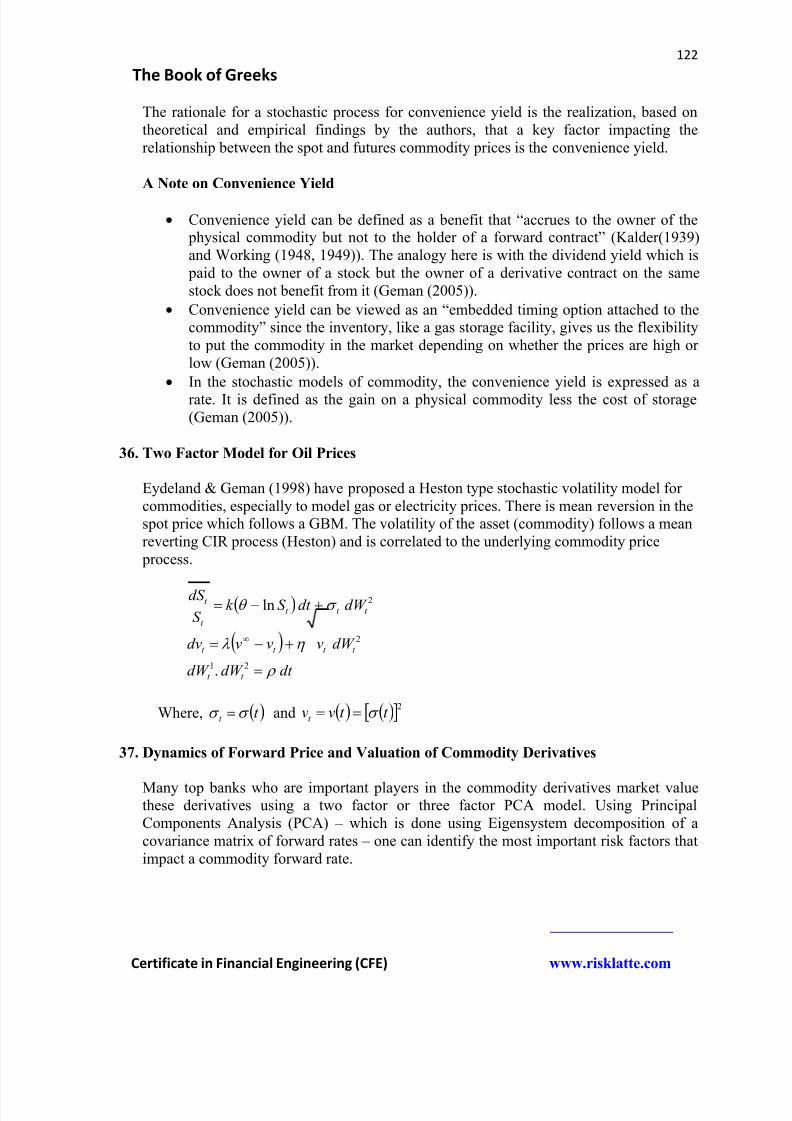
8/12/2019 Book of Greeks
http://slidepdf.com/reader/full/book-of-greeks 122/135
122
The Book of Greeks
Certificate in Financial Engineering (CFE) www.risklatte.com
The rationale for a stochastic process for convenience yield is the realization, based ontheoretical and empirical findings by the authors, that a key factor impacting therelationship between the spot and futures commodity prices is the convenience yield.
A Note on Convenience Yield
Convenience yield can be defined as a benefit that “accrues to the owner of the physical commodity but not to the holder of a forward contract” (Kalder(1939)and Working (1948, 1949)). The analogy here is with the dividend yield which is paid to the owner of a stock but the owner of a derivative contract on the samestock does not benefit from it (Geman (2005)).
Convenience yield can be viewed as an “embedded timing option attached to thecommodity” since the inventory, like a gas storage facility, gives us the flexibilityto put the commodity in the market depending on whether the prices are high orlow (Geman (2005)).
In the stochastic models of commodity, the convenience yield is expressed as arate. It is defined as the gain on a physical commodity less the cost of storage(Geman (2005)).
36. Two Factor Model for Oil Prices
Eydeland & Geman (1998) have proposed a Heston type stochastic volatility model forcommodities, especially to model gas or electricity prices. There is mean reversion in thespot price which follows a GBM. The volatility of the asset (commodity) follows a meanreverting CIR process (Heston) and is correlated to the underlying commodity price process.
dt dW dW
dW vvvdv
dW dt S k S
dS
t t
t t t t
t t t
t
t
21
2
2
.
ln
Where, t t and 2t t vvt
37. Dynamics of Forward Price and Valuation of Commodity Derivatives
Many top banks who are important players in the commodity derivatives market valuethese derivatives using a two factor or three factor PCA model. Using PrincipalComponents Analysis (PCA) – which is done using Eigensystem decomposition of acovariance matrix of forward rates – one can identify the most important risk factors thatimpact a commodity forward rate.
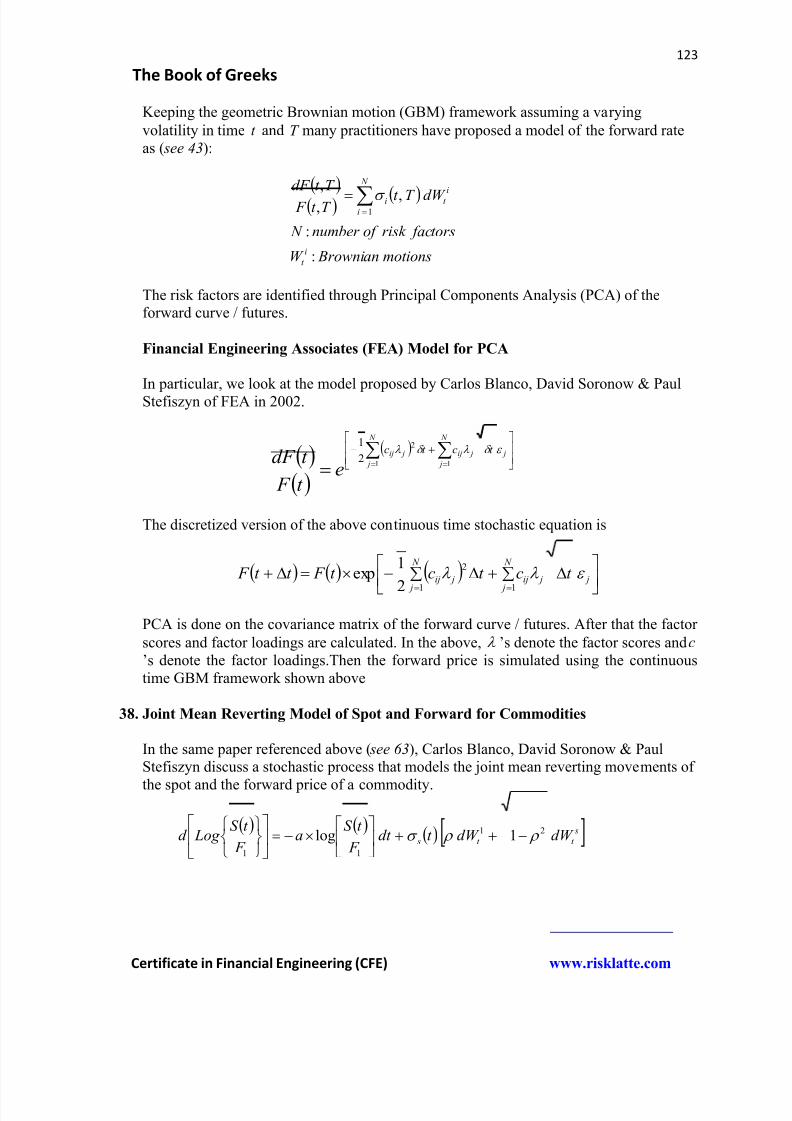
8/12/2019 Book of Greeks
http://slidepdf.com/reader/full/book-of-greeks 123/135
123
The Book of Greeks
Certificate in Financial Engineering (CFE) www.risklatte.com
Keeping the geometric Brownian motion (GBM) framework assuming a varying
volatility in time t and T many practitioners have proposed a model of the forward rateas ( see 43):
motions BrownianW
factorsrisk of number N
dW T t T t F
T t dF
i
t
N
i
i
t i
:
:
,,
,
1
The risk factors are identified through Principal Components Analysis (PCA) of theforward curve / futures.
Financial Engineering Associates (FEA) Model for PCA
In particular, we look at the model proposed by Carlos Blanco, David Soronow & PaulStefiszyn of FEA in 2002.
N
j
N
j
j jij jij t ct c
et F
t dF 1 1
2
2
1
The discretized version of the above continuous time stochastic equation is
N
j
N
j
j jij jij t ct ct F t t F 1 1
2
2
1exp
PCA is done on the covariance matrix of the forward curve / futures. After that the factor
scores and factor loadings are calculated. In the above, ’s denote the factor scores and c’s denote the factor loadings.Then the forward price is simulated using the continuoustime GBM framework shown above
38. Joint Mean Reverting Model of Spot and Forward for Commodities
In the same paper referenced above ( see 63), Carlos Blanco, David Soronow & PaulStefiszyn discuss a stochastic process that models the joint mean reverting movements of
the spot and the forward price of a commodity.
s
t t s dW dW t dt F
t S a
F
t S Log d 21
11
1log
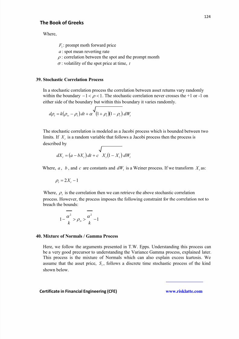
8/12/2019 Book of Greeks
http://slidepdf.com/reader/full/book-of-greeks 124/135
124
The Book of Greeks
Certificate in Financial Engineering (CFE) www.risklatte.com
Where,
1 F : prompt moth forward price
a : spot mean reverting rate
: correlation between the spot and the prompt month : volatility of the spot price at time, t
39. Stochastic Correlation Process
In a stochastic correlation process the correlation between asset returns vary randomly
within the boundary 11 . The stochastic correlation never crosses the +1 or -1 on
either side of the boundary but within this boundary it varies randomly.
t t t t t dW dt k d 11
The stochastic correlation is modeled as a Jacobi process which is bounded between two
limits. If t X is a random variable that follows a Jacobi process then the process is
described by
t t t t t dW X X cdt bX adX 1
Where, a , b , and c are constants and t dW is a Weiner process. If we transform t X as:
12 t t X
Where, t is the correlation then we can retrieve the above stochastic correlation
process. However, the process imposes the following constraint for the correlation not to breach the bounds:
1122
k k
40. Mixture of Normals / Gamma Process
Here, we follow the arguments presented in T.W. Epps. Understanding this process can be a very good precursor to understanding the Variance Gamma process, explained later.This process is the mixture of Normals which can also explain excess kurtosis. We
assume that the asset price, t S , follows a discrete time stochastic process of the kind
shown below.
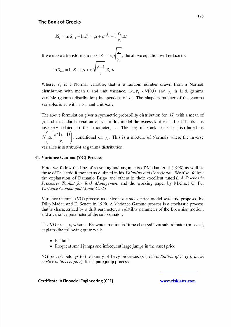
8/12/2019 Book of Greeks
http://slidepdf.com/reader/full/book-of-greeks 125/135
8/12/2019 Book of Greeks
http://slidepdf.com/reader/full/book-of-greeks 126/135
126
The Book of Greeks
Certificate in Financial Engineering (CFE) www.risklatte.com
The Need for a Variance Gamma (VG) Process
It is observed in real life that rather than following a purely diffusive process like ageometric Brownian motion, asset prices follow a diffusive process which has jumps init. It is observed that there are sizable jumps that occur over the path of the asset price.
These jumps are casued due to the arrival of news and information, including financialnews, in the market. Small pieces of news and information arrive quite frequently in the
market causing frequent jumps. Big news and large pieces of information are rare andtherefore they arrive infrequently in the market. This leads to small frequent jumps andlarge infrequent jumps in the asset prices over a particular time period. With theexception of interest rates, this fact is well borne out by almost all other asset marketssuch as equity, FX and commodities. Therefore, we need a mathematical model whichcan incorporate this fact of life in financial markets.
Another way of looking at the above is to note that perhaps “economic” time does not
have uniform speed due to the impact of “unpredictable news” and information whicharrives in market. As we move forward the flow of time accelerates or decelerates in arandom manner. “Time change” therefore should become a key feature of a stochasticasset price model.
What is so Unique about a Variance Gamma Process?
In most of the stochastic processes volatility is intricately linked to randomness. In aGBM or ABM, volatility, even though constant, is tied to the Weiner process, in GARCHstochastic process, even though conditional volatility is not random, the unconditionalvolatility is random; in stochastic volatility model volatility is itself a random process. In
other jump diffusion models, jumps add new source of randomness over and above theWeiner process. However, in all these processes the flow of time is not changed.
In a VG process, however, “financial time” is made random via a new process called the“subordinator”. Here, the “financial time” or the “market activity time” gets randomlytransformed from calendar time.
Concept of the Variance Gamma Process
We start with a standard Brownian motion that explains a pure diffusive process, withconstant or deterministic volatility:
t W t t B ,;
Note, that in the above, we have altered the flow of flow of time in a purely deterministic
manner via a constant volatility, . However, in a Variance Gamma setting we have tomove one step further and specify a “time change” process that is stochastic. This is
8/12/2019 Book of Greeks
http://slidepdf.com/reader/full/book-of-greeks 127/135
127
The Book of Greeks
Certificate in Financial Engineering (CFE) www.risklatte.com
because of the uncertain arrival of news and information that induces jumps and alters theflow of time in an uncertain manner. As Rebonato explains, this is accomplished byintroducing the condition that a Brownian motion should be evaluated at a particular time
by a gamma process, , with unit mean rate and a variance equal to v , i.e. vt t ,1, .
This gives us a process, t X , which is a kind of Levy process given by:
t W B X t t t
This new stochastic process, t X , is the Variance Gamma (VG) process. A key
observation to make here is that the “stochastic time” is present in both the drift term aswell as the stochastic term.
Distinguishing features of a VG Process
The following are the distinguishing features of a VG process
(i) The variance gamma process (VG) is a Lévy process and is characterized by arandom time change.
(ii) There diffusion component in the VG process is absent and it is instead a pure jump process.
(iii) The increments are independent and follow a Laplace distribution.
Difference between Brownian motion and the Variance Gamma (VG) Process
A Levy process is a kind of a generalized stochastic process which has independent andstationary increments. These increments are given by independent and identicallydistributed random numbers. Both the Brownian motion and the Variance Gamma (VG) process are Levy Process. In a standard Brownian motion (also known as a Weiner process), the mean of these stochastic increments is zero and the variance is proportional
to the size of the increment. If 2, N denotes a Normal (Gaussian) distribution with
mean, , and standard deviation, , then we can write a Weiner process as:
t N t W t t W t dW ,0~
In a Gamma process, the stochastic increments are gamma distributed and if , is a
gamma distribution with mean, and variance, 2 then the process is given by:
1,~ t t t t t d
8/12/2019 Book of Greeks
http://slidepdf.com/reader/full/book-of-greeks 128/135
128
The Book of Greeks
Certificate in Financial Engineering (CFE) www.risklatte.com
Given the above definition of a Gamma process a VG process can be characterized in twoalternative ways:
(i) It can be thought of as a time-changed, subordinated Brownian motion, wherethe subordinator is a gamma process.
(ii) A VG process can be thought of as a difference of two gamma processes.
Math Model for VG and Monte Carlo Simulation
Simulating VG as a Stochastic Differential Equation
Following the arguments used by Brigo, et al, if we consider a time changed Brownian
motion with mean, ˆ and volatility, and another constant then we can write the
stochastic differential equation for an asset price, t S , which follows a VG process as:
t g dW t dg dt S d t ˆˆlog
Where, .dW is a modified Weiner process. The only way that the above SDE differs
from a standard Brownian motion is that it contains the term t g , which, in probabilistic
term, is known as a subordinator. This term characterizes the market activity time. The
market activity time, t g , is a positive increasing random process where
st s g t g E . This reconciles the market activity time with the real time between
the time, t and s .
t s g t g s g W t g W ˆ~ˆ
Where, t , is a random normal number drawn from a Normal (Gaussian) distribution
with mean 0 and standard deviation of 1, i.e. 1,0~ N t .
Finally, VG model assumes, that the process t g is related to the Gamma process as
v
v
t t g ,~ , v being the variance of the gamma process. Here, the increments are
independent and stationary random variables drawn from a gamma distribution.
Simulating VG as a Stochastic Integral Equation
Take a Brownian motion, t B (which is a Weiner process, t W plus a deterministic drift,
) given by:
t t W t B
8/12/2019 Book of Greeks
http://slidepdf.com/reader/full/book-of-greeks 129/135
129
The Book of Greeks
Certificate in Financial Engineering (CFE) www.risklatte.com
In the above equation, qr , where, r is the risk free rate and q is the dividend yield
of the asset. Thereafter, we construct VG as Levy process, t X , that characterizes a time
changed Brownian motion with three parameters, the drift of the asset , the volatility of
the asset, and a constant given by:
t W B X t t t
Where, t , is a gamma process with unit mean and a variance parameter, v . Then the
equation for the asset price, t S , with risk free interest rate, r , and dividend yield q , will
be given by
t X t qr
t eS S
0
Where, , is a constant that makes the discounted asset price a martingle measure and isrelated to the characteristic function of the Levy process. This is the equation we woulduse to simulate the asset price.
In the above equation, is given by:
21ln1 2
42. Displaced Diffusion Model
Displaced diffusion model for asset prices was introduced by Rubinstein in 1983.
If t S is the asset price at time, t then in a displaced diffusion process, the quantity t S
follows a geometric Brownian motion, where, is a constant.
t
t
t dW S
S d
and are the drift and the volatility of the process, t S .
Advantages
It’s extremely simple to model
The process can be made to mimic a Constant Elasticity of Variance (CEV) process while retaining the analytical properties of a geometric Brownian motion.
8/12/2019 Book of Greeks
http://slidepdf.com/reader/full/book-of-greeks 130/135
130
The Book of Greeks
Certificate in Financial Engineering (CFE) www.risklatte.com
A closed form solution, similar to the Black-Scholes formula, can be found outeasily.
A displaced diffusion process may be quite suitable to model inflation andtherefore can find use in valuation of inflation derivatives;
Disadvantages
Whereas, the quantity t S , which follows a GBM in guaranteed to be positive,
there is no guarantee that the asset price, t S , will be positive. In this process, t S ,
is bounded in the range , .
43. Simplified Libor Market Model
(Single factor with Lognormal interest rates)
We assume that spot LIBOR, t L is stochastic and follows a lognormal distribution, i.e. a
geometric Brownian motion of the type:
t L L
t
t dW dt L
dL
However, instead of the above SDE, we use the stochastic integral equation for the GBMto model stochastic LIBOR. Also, we assume that LIBOR diffuses over the time interval
T t , . Therefore,
t l L L t T T T
t T e L L
2
2
1
Here, L is the LIBOR volatility which could be calibrated to caplet volatilities and L is
the drift of the LIBOR. Also, we assume that the forward LIBOR rates are not correlatedwith each other.
Given the fact that LIBOR has a well defined, observable forward curve at all points, thedrift of the LIBOR rate is given by:
F
t
F
T
L
L
L
Substituting the above in the equation for LIBOR above and doing some algebraicmanipulation we get the equation for LIBOR as:
8/12/2019 Book of Greeks
http://slidepdf.com/reader/full/book-of-greeks 131/135
131
The Book of Greeks
Certificate in Financial Engineering (CFE) www.risklatte.com
t L L t T
F
t
F
T t T e
L
L L L
2
2
1
In the above equation, t is a random number drawn from a Normal distribution with
zero mean and unit standard deviation.
44. Homogenous Poisson Process
This is a process for modeling stochastic time. A homogeneous Poisson process is a
continuous-time stochastic process 0: t P t with an intensity rate), , such that 0
with the following conditions:
(i) t P is a point process,
(ii) the times between events are i.i.d. (random variables) with an exponential
distribution, i.e. exponential with mean .
1.
A Poisson process with a parameter, ( 0 ) can be defined as an integer-valued,
continuous time stochastic process 0: t P t such that the following conditions hold:
(i) 000 P P ;
(ii) For all values of time, nt t t t ......210 , the increments, t dP given by
01 t P t P , 12 t P t P , ….., are independent random variables; (iii) For 0t , 0 and non-negative integers m , the increments have a Poisson
distribution given by:
!Pr
m
et m P t P
t m
8/12/2019 Book of Greeks
http://slidepdf.com/reader/full/book-of-greeks 132/135
132
The Book of Greeks
Certificate in Financial Engineering (CFE) www.risklatte.com
References:
1. Notes on Solving the Black-Scholes Equation, EOLA Investments, LLC, Oct 2009
2. Solution to the Black-Scholes Equation, S. Karim, MIT, May 20093. The Diffusion Equation – A Multidimensional Tutorial , T.S. Ursell, Caltech, 20074. Mathematical Methods in Earth Sciences, Lectures by Prof. Francis Nimmo, Department
of Earth and Planetary Sciences, University of California, Santa Cruz5. Equity Hybrid Derivatives, Marcus Overhaus, Ana Bermudez, Hans Buehler, Andrew
Ferraris, Christopher Jordinson and Aziz Lamnouar (John Wiley & Sons, Inc. 2007)6. The Volatility Surface, Jim Gatheral (John Wiley & Sons, Inc. 2006)7. Exotic Options and Hybrids, Mohamed Bouzoubaa, Adel Osseiran (John Wiley & Sons,
Ltd. 2010)8. Dynamic Hedging , Nassim Taleb (John Wiley & Sons, Inc. 1997)9. The Complete Guide to Option Pricing Formulas, Espen Gaarder Haug (McGraw-Hill,
2007)10. Volatility and Correlation, Riccardo Rebonato (John Wiley & Sons, Ltd. 2004)11. A New Formula for Computing Implied Volatility, Steven Li, School of Economics and
Finance, Queensland University of Technology, Brisbane, Australia12. A Primer for the Mathematics of Financial Engineering, Dan Stefanica (FE Press, NY)13. Frequently Asked Questions in Quantitative Finance, 2nd Edition, Paul Wilmott (John
Wiley & Sons, Limited)14. Asset Allocation for Institutional Portfolios, Mark P. Kritzman, Richard D.Irwin, 1990.15. Modern Portfolio Theory and Investment Analysis, 4
th Edition, Edwin J.Elton and Martin
J.Gruber, John Wiley & Sons, 1994.16. The Handbook of Exotic Options, Instruments, Analysis and Applications, Edited by
Israel Nelken, Irwin Professional Publishing, 1996.17. The Handbook of Convertible Bonds, Pricing, Strategies and Risk Management, Jan DeSpiegeleer and Wim Schoutens, John Wiley & Sons, Ltd. 2011.
18. FX Options and Structured Products, Uwe Wystup, John Wiley & Sons, Ltd. 2006.19. Demystifying Exotic Products, Interest Rates, Equities and Foreign Exchange, Chia
Chiang Tan, John Wiley & Sons, Ltd. 2010.20. Modeling Derivatives in C++, Justin London, John Wiley & Sons, Inc. 2005.21. Optimal Trading Strategies, Robert Kissell and Morton Glantz, AMACOM, 2003.22. Foreign Exchange Option Pricing, A Practitioner’s Guide, Iain J.Clark, John Wiley &
Sons Ltd., 201123. Structured Equity Derivatives, Harry M.Kat, John Wiley & Sons, Ltd. 2001.24. Paul Wilmott on Quantitative Finance, Volume 2, Second Edition, John Wiley & Sons,
Ltd., 2006.25. Modelling FX Skew, Dharminder Kainth and Nagulan Saravanamuttu, Royal Bank of
Scotland26. Quantum Mechanics in Simple Matrix Form by Thomas F. Jordan27. Derivatives Sensitive to Volatility Surface, Ser-Huang Poon, Manchester Business
School, April 26, 200828. High Frequency Trading, Irene Aldridge, John Wiley & Sons, 2010.
8/12/2019 Book of Greeks
http://slidepdf.com/reader/full/book-of-greeks 133/135
133
The Book of Greeks
Certificate in Financial Engineering (CFE) www.risklatte.com
29. Probability of Exercise in the Call Price, Fabrice Douglas Rouah, www.FRouah.com 30. Prime Numbers by David Wells (John Wiley & Sons, 2005)31. A Continuity Correction for Discrete Barrier Options, Mark Broadie, Paul Glasserman
(Columbia Univerity), Steven Kou (University of Michigan), Mathematical Finance, Vol
7, No. 4 (October 1997)32. On Pricing of Discrete Barrier Options, S.G.Kou, Columbia University, April 2001 /
2003.33. Pricing, Hedging and Trading Financial Instruments III, Carol Alexander, John Wiley &
Sons. (2008).
34. Fibonacci Numbers and Golden Ratio as an Eigenvalue Problem in Chapter M, #VII isreferenced from the work of Prof. Megumi Harada at the McMaster University, Ontario,
Canada. 35. Saddle Point Methods of Option Pricing , Peter Carr and Dilip Madan, The Journal of
Computational Finance, 2009 36. Bleed or Blowup? Why Do We Prefer Asymmetric Payoffs? Nassim Nicholas Taleb, Journal of
Behavioural Finance (2004, Vol 5, #1) .
37. Hedge Funds: Quantitative Insights, Francois-Serge Lhabitant, John Wiley & Sons(2004).
38. More than You Ever Wanted to Know about Volatility Swaps, Emanuel Derman, KresimirDemeterfi, Michael Kamal and Joseph Zou, Goldman Sachs (1999).
39. Hedging Volatility Risk , Menachem Brenner, Ernest Ou, Jin Zhang, Journal of Bankingand Finance (2006).
40. Consistent Variance Curves, Hans Buehler, Finance and Stochastics (2006);41. A Double Mean Reverting Stochastic Volatility Model with Concurrent Jumps by Chenxu
Li, Columbia University, October 200942. The Modigliani-Miller Theorem, The New Palgrave Dictionary of Economics, Anne P.
Villamil, University of Illinois.43. Commodities and Commodity Derivatives, Helyette Geman, John Wiley & Sons, 2005.44. http://quantlabs.net/labs/quant-books/cat_view/37-quant-simplified-math;
45. The Variance-Gamma (V.G.) model for share market returns, D.B. Madan and E. Seneta
Journal of Business, 63:511 – 524, 1990.
46. Derivatives Models on Models, Espen Gaarder Haug, John Wiley & Sons (2007).
47. Variance Gamma and Monte Carlo, Michael C. Fu, Robert H. Smith School of Business
Department of Decision & Information Technologies, University of Maryland
48. Path Dependent Options: Buy at the low, sell at the high, Barry Goldman, Howard Sosin
and Mary-Ann Gatto, The Journal of Finance (1979).
49. Stochastic Local Volatility, Grigore Tataru and Travis Fisher, Quantitative Development
Group, Bloomberg.
50. Pricing Derivatives Securities, 2nd Edition, T W Epps, World Scientific Publishing.
51. Financial Derivatives, Pricing, Applications and Mathematics, Jamil Baz and George
Chacko, Cambridge University Press (2004).
52. http://www.globalriskguard.com
8/12/2019 Book of Greeks
http://slidepdf.com/reader/full/book-of-greeks 134/135
134
The Book of Greeks
Certificate in Financial Engineering (CFE) www.risklatte.com
53. http://www.nas.ewi.tudelft.nl/people/Piet/CUPbookChapters/PACUP_Poisson.pdf
54. An Introduction to the Simulation of Risk Processes, Krzysztof Burnecki, Wolfgang
Härdle and Rafal Weron, Hugo Steinhaus Institute for Stochastic Methods, Institute of
Mathematics, Wroclaw University of Technology.55. Pricing Digital Outperformance Options with Uncertain Correlation, Jacinto Marabel
Romo, BBVA, Ph.D. Dissertation, University of Alcalá (UAH), Spain.
56. Stochastic Differential Equations, Diffusion Processes, and the Feynman-Kac Formula,
Lectures, Steven Lalley, Department of Statistics, University of Chicago
57. http://www.scienceisart.com/A_Diffus/DiffusMain_1.html
58. http://www.iasonltd.com/FileUpload/files/pdf_res_3.pdf
59. Process Dynamics: Laplace Transforms by M Tham, Department of Chemical and
Process Engineering, University of Newcastle upon Tyne
60. Laplace Transforms as Present Value Rules – A Note by Stephen A. Buser, The Ohio
State University.61. Option Valuation under Stochastic Volatility, Alan L. Lewis, Finance Press, Newport
Beach, California, USA (2000).
62. Option Pricing Models and Volatility, Fabrice Douglas Rouah and Gregory Vainberg,
John Wiley & Sons (2007).
63. Volatility Derivatives, Peter Carr and Roger Lee, Annual Review of Finance and
Economics (2009).
64. Options on Foreign Exchange, 3rd
Edition, David deRosa, John Wiley & Sons (2011)
65. Swaps and Other Derivatives, Richard Flavell, John Wiley & Sons (2002).
66. Optimal Trading Strategies, Robert Kissel and Morton Glantz, AMACOM (2003).
67. Financial Modelling, 3rd edition, Simon Benninga, MIT Press (2008)
68. Multi-Factor Models of the Forward Price, Curve Carlos Blanco, David Soronow &
Paul Stefiszyn , FEA, September 2002
8/12/2019 Book of Greeks
http://slidepdf.com/reader/full/book-of-greeks 135/135
135
The Book of Greeks
About the Author
Rahul Bhattacharya is the CEO of Risk Latte Company Limited. He has taught and conductedtraining sessions for traders, quants, structuring and sales professionals and risk managers in top
tier global banks and investments all over the world, such as Goldman Sachs, HSBC, Citigroup,Barclays Capital, Credit Suisse, RBS, to name only a few. He teaches the CFE course for theCFE School, which is the education and learning division of Risk Latte Company.
He has more than 15 years experience in options and FX trading, commodity structuring and riskadvisory and analytics and has worked all over the world. He holds an B.Sc. (Hons) in Physics,an M.Sc. in Nuclear Physics and an MBA in Finance.
He can be reached at [email protected]
CFE School
CFE School is the Education and Learning division of Risk Latte Company in Hong Kong andconducts the public course Certificate in Financial Engineering (CFE) and other specializedquantitative finance courses for banking and finance professionals all over the world.
For any queries on the CFE course or other programmes of the school, please send your requestto [email protected].
Related Documents