Bluefield State College Vehicle Design Report 2006 · 2006-09-21 · Bluefield State College Vehicle Design Report 2006 Lenny Lewis, ... As with any academic project, ... One is an

Bluefield State College

Vehicle Design Report

2006

Lenny Lewis, Joy Huntley, Jesse Farmer, Scott Baker, Joe Kessler,

Randall Farmer, Justin Stiltner, Joshua Eerenberg, James Cardwell

I, Dr. Robert Riggins, Professor of the Department of Electrical Engineering Technology

Department at Bluefield State College do hereby certify that the engineering design of the

vehicle, Anassa II, has been significant and each team member has earned two semester

hour credits for their work on this project.

Signed, Date

___________________________ _______

Bluefield State College

Center for Applied Research and Technology (CART)

Phone: (304) 327-4134

E-mail: [email protected]

1. Introduction

The Bluefield State College (BSC-CART) team is pleased to present a new and improved

Anassa II robot to the 14th annual IGVC. In IGVC 2005, BSC’s Anassa I completed the course

three times (BSC was one of the two schools that completed the autonomous challenge.) Due to

Anassa I’s previous performance, the team decided to re-use the rugged and durable platform that

was used in the 2005 IGVC. However, the robot has been outfitted with a completely new

software and sensor architecture. The in-depth knowledge from previous IGVC robots, along

with related autonomous ground robotic vehicle research, is joined together with the new talent

and ideas of upcoming students to produce another innovative design project. The team’s aim is

to create an autonomous ground robotic vehicle that is more intelligent than any of the previous

vehicles at BSC with ever-increasing human thought characteristics. Therefore, Anassa II will be

able to complete more difficult courses at top speeds close to 5 mph.

This paper will first describe the design process, followed by a description of the

computer-aided design tools used on this project. Next, there will be a discussion on the

mechanical and electrical designs. Then the software strategy will be discussed, followed by an

analysis of performance.

2. Design Process

2.1 Customer Identification

Typically, the team’s primary customers have been the judges of the IGVC and multiple

sponsors. However, the research conducted on this project has been incorporated into many other

robotic research projects. For instance, this robot is being used as a test platform for the upcoming

DARPA Urban Challenge event, and for CART, Inc. research involving industrial mining safety

and power utility maintenance. Other significant customers include Pemco, Inc. and ConnWeld

Industries for their sponsorship, as well as Bluefield State College and the community, whose

support is greatly appreciated.

2.2 Evaluation Process

The evaluation process for this project began during the 2005 IGVC event. While

competing in last year’s competition the team was able to see both performance successes and

areas that needed improvement. After the competition, the team held a series of meetings to

evaluate the design and formulate plans for improvement. Among the many successes of last

year’s design was the reliable control system and the rugged outdoor platform. Other aspects that

1

were noted by our customers were the sleek aesthetics of the robot and the spacious interior of the

body. Some of the failures associated with last year’s competition were problems with the

communications link between the robot’s onboard computers. This failure would momentarily

cause a disturbance in the navigation system, which led to inaccurate path planning. Another

problem with last year’s design was in the method used for computer vision. Previously, the

program examined the RGB values of a picture to detect objects such as white lines or orange

barrels. However, these values would vary depending on the intensity of the sun, which

necessitated constant recalibration of the system. Due to the failure during the navigation

challenge of last year’s competition, it was clear that a new navigation algorithm was needed,

along with sensors to accompany the GPS system. After careful consideration, the team devised

some alternative methods to correct the failures as well as new ideas to improve on the robot’s

autonomy.

The team made the observation during the past three IGVC events that there are two

different philosophies used among the IGVC robots. One uses a philosophy of “learning” the

course boundaries and other course attributes, and passing this knowledge to future runs and also

to other robots from the same school. The other philosophy treats each run as a completely new

experience (as Anassa I did.) The team met and decided that Anassa II would not keep the map

of the course for future runs. Instead, in the spirit of autonomy, she would complete each run

independently.

2.3 Development Process

To alleviate the data transfer problem between the two computers, the team studied

alternative methods of transferring data as well as ways to reduce the robot’s computing power

into a single computer. The team decided to use a single processor for all of the robot’s functions.

Consequently, faster navigation algorithms that use less processing power had to be created.

New software and methodologies were proposed for the computer vision used on Anassa

II. To aid in the localization and orientation of the robot, new sensors were implemented to

accompany the GPS system. Also, plans were made for an extended Kalman filter algorithm to

combine the data associated with the orientation and localization to give the best possible

estimate of the robot’s position and heading.

After the goals were set, the team was organized and responsibilities were assigned.

Appendix A lists each team member, responsibilities, and estimated time worked.

As with any academic project, safety was a major concern in the design, manufacturing,

and testing of Anassa II. Due to the team’s close acquaintances and dedication, no one was left

2

alone working on this project. Additionally, Anassa II’s hardware and software incorporated

many safety features. In hardware, multiple E-stops were used to provide varying levels of

control, along with a battery monitoring system to check the batteries’ status. In software,

programs continually monitor the system for errors in battery condition, control, and

communication. “Heartbeat” (fault monitoring) signals are measured wherever possible. In the

event that an error occurs, the program has the ability to stop the vehicle until the problems are

identified and corrected.

Cost was a major factor in the design of Anassa II. To keep the expenses low, the team

used many in-house components and sensors that were available. This, along with the many

donations of parts and labor, kept the cost of the robot extremely low. Appendix B lists the cost

of components included in the construction of Anassa II, including replacement costs and actual

costs.

3. Computer-Aided Design

3.1 Solid Edge Modeling

Two computer-aided design techniques were used in the design and testing of the vehicle.

First, the team utilized Solid Edge, a 3-D modeling software package to conceptualize and design

Anassa II’s body and various components. This design tool helped to speed up production and

eliminate any manufacturing errors before they were made. After the design was completed, the

model was given to local manufacturing companies to be manufactured.

3.2 Computer Simulation

Another computer aided design tool implemented this year was a computer simulation

that mimics sensor data for the robot (Appendix C). This simulation project has provided the team

with another testing tool to test algorithms associated with autonomous navigation. Certainly, a

computer simulation cannot replace real world testing. However, it does provide the team with a

controlled environment to debug and test algorithms, speeding up the programming process.

3

4. Mechanical Design

4.1 Vehicle Frame and Chassis

This vehicle uses a modified frame and chassis of a Jazzy

1170XL Electric Wheelchair. The frame is constructed of 14 gauge

milled steel square tubing that is built to sustain a payload of 400

lbs. Both the frame and chassis components are weatherized by

being coated with primer and multiple layers of enamel paint. The

chassis components include an active-track suspension system that

allows all wheels and the drive system to travel independently as the vehicle moves across

uneven ground. The vehicle is elevated by 16-inch pneumatic drive wheels, adjustable 9-inch rear

articulating caster wheels, and adjustable 8-inch anti-tip wheels for stability. The arrangement of

the wheels provides a 4.25 inch ground clearance which generates a low center of gravity. This,

coupled with the active-track suspension system, gives the robot a curb climbing height of 6

inches. The overall wheel base is 22.5 inches wide and 45 inches long, which provides a tight

turning radius of 23 inches.

4.2 Drive System

Anassa II uses two independent 24-volt DC motors for vehicle locomotion. The motors

are connected to a speed reducer that transfers the high-speed, low-torque output of the motors

into a low-speed, high-torque power that can adequately maneuver a 400 lb payload. The robot is

equipped with two methods of braking. One is an electronic regenerative braking system that

slows the vehicle down; the other is a mechanical disk parking brake that is used to hold the

vehicle still when it has come to a stop. The disk park brake was redesigned for the purpose of

incorporating encoders to the drive motors. With safety as the main focus, the single core

mechanical spring of the braking system was replaced with three smaller, stouter springs on the

outer surface of the brake shoe. This increased the surface area of the braking force by 3.8 in2

while increasing the total braking force by 138 %.

4.3 Body The body of Anassa II incorporated key concepts such as safety, rigidity, ease of access,

water resistance, spaciousness and aesthetics into its design. All of the body components were

made of aluminum to maintain strength, while reducing the weight. For the safety and rigidity

portion, the skeleton of the body was TIG- welded together to produce a single solid structure that

4

protects the delicate electronic equipment housed within it. For

easy access into the body of Anassa II, all of the panels were

designed to bolt on to allow quick removal. Also, a

combination of weather-stripping, rubber grommets, and sheet

metal skirts were used all around the body to make the shell

waterproof and the frame water resistant. To avoid clutter, all

components were arranged and placed in a way that provides

more space. Also, both the mast and body were designed to fasten to the chassis to allow easy

access into the internal parts and allow the robot to be disassembled for transportation. For

aesthetic reasons, the body panels were made of a combination of polished aluminum and tinted

lexan glass; the panels provide the body with strength, rigidity, and reduction in internal heat.

Appendix D shows additional views of Anassa II’s body.

5. Electrical Design

5.1 Power System

The Power System consists of four batteries. Two 12-volt batteries in series supply 24

volts to the two drive motors, motor controller, manual joy stick, and Sick LMS (Laser

Measurement System). Two other 12-volt batteries connected in parallel supply 12 volts to the

Differential Global Positioning System (DGPS) receiver, the wheel encoders, compass,

controller, and the power converter that supplies 5 and 12 volts to the electronics. A manual

switch is used to change from joy stick control to autonomous control. For safety, the controller

remains in an idle state upon power-up if this switch is in autonomous mode.

5.2 Power Monitor

A power monitor circuit alerts the robot to the battery status.

5.3 E-Stops

The Soft E-Stop and the Hard E-Stop are situated on the vehicle’s rear electrical panel

along with other system on and off switches. The Hard E-Stop shuts off all power except for the

battery in the computer. The manual Soft E-Stop and the wireless E-Stop turn off the controller

but keeps main power on. For safety, the two E-Stop systems are completely independent of each

other.

5

5.4 Sensors

The sensors include a variety of devices. These devices are listed below.

The CSI Wireless DGPS receiver and antennas give latitude, longitude, velocity, and

heading.

The Sick Laser Measurement System sweeps 180 degrees for object avoidance. Though

the LMS can reach as far as 80 meters, Anassa II uses only the first 8 meters for detection.

The Digital Camcorder is used to detect boundary lines. MATLAB’s image processing

toolbox is the primary tool.

The Digital Compass gives the actual heading of the vehicle along with the DGPS

heading. The digital compass is useful when the vehicle is stopped.

The Encoders are attached to the motor shafts and are used to determine distance

traveled and the direction of travel.

The Gyro is installed on the vehicle in order to provide another source for heading. It is

mainly used as a back up for the Navigation Challenge to stabilize the heading.

The Laptop Computer contains the Autonomous and Navigation Challenge programs

written in a combination of Visual Basic, MATLAB, and C++.

6. Software

6.1 Autonomous Challenge

6.1.1 Software Strategy

The team decided after IGVC 2005 that the main emphasis for IGVC 2006 in software

would be a new and improved vision capability, a mapping strategy for sensor integration, and a

new and improved path planner. These improvements will help Anassa II to achieve speeds of

five mph in the events. This section discusses these three tasks.

6.1.2 Image Processing

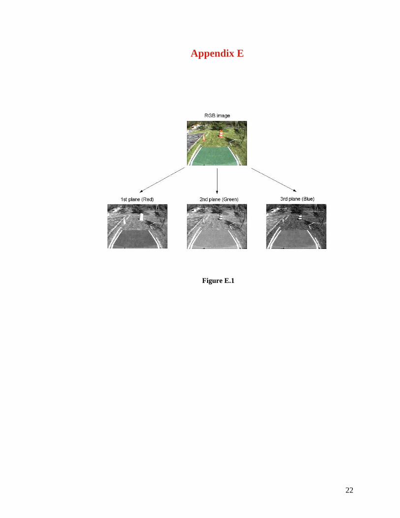
Digital images may be presented in RGB color space, so named because it uses three

separate 2-dimensional images – each a measure of the distribution of a single color (Red, Green,

or Blue) – and combines these into a single 3-D image. Each pixel is colored according to the

combination of three different values, each located in a 2-D “plane”. Think of these three planes

as being “stacked” on top of each other: imagine transparent sheets of plastic, on each of which is

printed a copy of the same picture in only one of the three colors – when all three sheets are

aligned together, the combination yields a “true color” picture.

6

Figure E.1 shows a sample image, taken during one of Anassa II’s outdoor test runs on a

mock course, with its three component RGB dimensions. Each component image is a grayscale

representation of the scene in terms of how much red, green, or blue is in each pixel. As an

intensity image, it shows low values of that color as darker (tending toward black), and high

values of the color as lighter (tending toward white). As one would expect, the dark shadow cast

by the tree to the right of the course remains nearly black in all three. But note also that the white

lines remain bright white – this is because what is perceived as “white” is equally high in all

colors.

The same image can be converted to the HSI (hue, saturation, intensity) color space.

Although the 3-D composite image is represented using a color scheme that, as can be seen in

Figure E.2, seems to make no sense, the three individual planes are much more readily

understood. The meanings of each component are best illustrated by the 3-D model in Figure E.3.

The triangle at left shows that the hue H is an angular measure, referenced from pure Red, of the

specific color – think of moving from the top to the bottom of a rainbow. The saturation S gives

the distance from the center point, where all colors combine equally to produce White – i.e., how

strong the hue is, relative to other colors in the spectrum. Now that these relationships have been

established, the third aspect of HSI, the intensity I, is basically the “brightness” of a pixel, which

ranges on a normalized scale from 0 (no reflected light, or “black”) to 1(maximum reflectance, or

“white”). The 2-D hue / saturation plane is largest at 0.5, in the middle of the vertical range; this

is because as zero (black) is approached, a greater amount of each color is being absorbed,

limiting the possible saturation – as all colors are increasingly reflected toward white, the same

effect occurs.

Referring back to Figure E.2, the image most “normal” in appearance is the intensity

plane, which is commonly referred to as a “black-and-white” picture. However, it is more

properly termed a gray-scale image, since there are clearly many intermediate shades displayed.

The hue plane may now be understood, as it can be seen that the orange portions of the barrels

stand out as practically black, since their color is very close to red, which is the zero-value

reference. Note that the asphalt (on the left), which is apparently mostly blue, is shown very

close to white here, as the blue / magenta section of the HSI triangle has the largest angular

distance (counter-clockwise) from the red axis. Also of note is that both white and black objects

in the real world are represented in the hue image as some medium shade of gray. This makes

sense considering that the vertical axis in the 3-D model passes directly through the center of the

hue / saturation 2-D space. For the same reason, both the asphalt and the white lines of the course

are almost totally black in the saturation image, since neither are any appreciable distance from

7

the vertical (black / white) axis. The barrels stand out because their orange color is smoothly

uniform and vibrant.

The location of barrels and cones is really not an essential function of the vision

processing software because these and other three-dimensional objects will be easily and

accurately detected by the robot’s on-board LMS. This approach involves finding the barrels and

cones only so that they can be removed from the image, for reasons explained in more detail later

in this section.

One surface Anassa II obviously needs to ignore is grass, and the first step to eliminate

grass is to employ a low-pass filter. High-frequency components characterize edges and other

sharp details of an image; this type of filter, then, will effect a blurring of the input image. An

example of the application of a simple averaging LPF is shown in Figure E.4.

Filtering makes all the difference when attempting to threshold a gray-scale image based

on intensity levels. "Thresholding" will output a binary image which is the ideal form for

computer processing because it is a simple matrix of 1’s and 0’s. Objects of interest are

represented by “1”-valued pixels (which will be white in the binary image) and everything else

(grass, for instance) is zero (black). Proper setting of the threshold value will accomplish this end

by forcing every pixel with a value lower than the threshold to zero, and making everything at or

above the threshold a “1”. However, direct application of this technique, due to its susceptibility

to changing incident light levels, often yields unacceptable results (Figure E.5).

Another image processing tool Anassa II uses is “edge detection”. Edge detection

generally is designed to operate on 2-D (gray-scale) images. It works by computing local

derivatives at transition points – areas where “lighter” regions meet “darker” ones. Such “edges”

in digital images are usually slightly blurred as a result of sampling, which yields a smooth linear

transition in the intensity plane. An edge is detected by the magnitude of the 1st derivative, and

the sign (positive or negative slope) of the 2nd derivative is used to ascertain whether a pixel lies

on the “dark” or “light” side of the edge. What is computed in practice is the gradient, which, for

an image f(x, y), points in the direction of maximum rate of change of f at (x, y). Figure E.6

shows a typical result of filtering an input RGB image, then taking the color gradient. Next, a

threshold is applied to the gradient, to produce a binary image (Figure E.7). Proper filtering and

threshold levels are still required, but the threshold value is less sensitive to lighting conditions

than in the previous approach.

As stated earlier, barrels and cones must be removed from the binary output; this is

advantageous because of the difficulty for a computer in distinguishing between lines painted on

the ground and barrels standing upright in such an image. The robot would interpret a barrel’s

8

binary representation as a thick line, extending from the real-world coordinates of the base,

forward to the point on the ground seen (by the human eye) just above the rearmost upper surface

of the barrel. The problem becomes very serious if, in the RGB image, a boundary line touches,

or is partly obscured by a barrel as shown in Figure E.8. Clearly, the robot would find only one

path to the right: it would have to turn before reaching the barrels. The alternative option –

passing the barrels on the left before turning right and traveling behind them – would not even be

recognized. In the situation shown above, this would be fine – but suppose the two barrels were

placed further to the right, prohibiting travel between them and the right boundary line: the robot

would find no navigable path whatsoever in that direction.

Trying various methods of barrel-and-cone extraction resulted in selecting the following

procedure. First, the incoming RGB image is converted to the NTSC color space, also known as

YIQ, whose three components are luminance (Y), hue (I), and saturation (Q). Figure E.9 shows

an image, along with the binary threshold of the 2nd plane image (hue) of the NTSC conversion.

This alone renders a rather incomplete description of such objects. To effectively remove

one of these obstacles entirely, as many pixels as possible are needed that are orange in the RGB

space, to hold a “1” value (white) in our binary image. The method used here is crude but

serviceable: all that is needed is to “fatten-up” the barrels and cones by simply dilating all regions

present in the binary version of the hue image.

Now that there are separate procedures for finding white lines and orange obstacles, the

results can be combined in order to obtain what is really wanted – a simple binary matrix showing

the locations of boundary lines, and omitting any barrels or cones that could be misinterpreted as

2-D lines on the ground. This is accomplished by merely subtracting the dilated [binary] hue

image from the [binary] gradient image (Figure E.10).

Previous applications of edge detection with BSC’s robots had encountered a thorny

dilemma, illustrated in Figure E.11, showing an image and the binary threshold of its color

gradient. On sunny days, shadows present a definite problem, especially when the sun is behind

the robot, as it is here. The shadow at the center of the foreground is cast by the top of the robot

itself, and the gradient image shows that it creates one of the strongest edges detected. Raising

our threshold high enough to eliminate it also gets rid of practically everything else. But the

shadow certainly must be eliminated because the robot will treat it as an obstacle directly in front

of it and will continually back away, confused.

Anassa II’s solution to this problem employs an intensity transformation function to

adjust the contrast of the image so as to minimize the difference in intensity between pixels in the

shadows and those of the grass. The function calls for user-defined input and output threshold

9

values: any pixel valued at or below the “Low In” value is changed to the output level set by

“Low Out”; anything above “High In” is mapped to the “High Out” level. The first step is to

compute the mean (average) intensity level of the entire grayscale image and use it as “Low Out”;

our “Low In” ensures that anything as dark as a shadow will be brought up to the mean intensity

level, which means that there is no longer a strong gradient between grass and shadows. Then, the

altered intensity plane is reinserted into the HSI image before converting back to RGB. Figure

E.12 shows an input image, the transformed intensity plane, and the reintegrated color output.

Now that the shadows are gone, the image can be processed in the same way that it has been

handling previous scenes. In fact, it can perform this intermediate step whether shadows are

present or not, with no detrimental effects.

The bridge on the IGVC course can pose problems for vision-processing software, due to

the highly reflective nature of its surface. The glare (seen in Figure E.13) is often

indistinguishable from white objects, such as the boundary lines on, or adjacent to, the bridge;

Figure E.14 reveals the difficulties presented by a typical result of a previous approach.

Before the robot can choose a method of safely crossing the bridge, it has to know when

the bridge is present, and if it is in a position to cross it. To do this, the program scans the hue

plane of each image’s HSI representation for the number of pixels that fall within the “green”

range. Whenever this number is large enough, the robot can assume that the bridge is in view and

very near. Figure E.15 shows the HSI plane of interest; the bridge stands out quite clearly.

Once the robot determines that it must prepare to cross the bridge, it can go into the

“Bridge Mode” algorithm, which first filters the gray-scale image, then employs edge detection

with a vertical bias. The resultant thin lines are dilated with a structuring element slightly larger

than the one used for this purpose in normal operation, giving a nice output in which the bridge’s

boundaries are by far the strongest regions shown (Figure E.16).

Often, depending on the strength of a boundary line in reality, or the length of the grass,

or the amount of glare and position of the sun and/or the robot’s camera, the robot will barely

pick up one of the two immediate boundary lines (sometimes none at all), or one or more lines

may break up into smaller pieces during processing. (A few examples are given in Figure E.17.)

What is to keep the robot from plotting a course that will lead it out of bounds?

Anassa II’s solution is to compute the “average slope” of an entire image and use such a

value to point the robot in the right general direction. First, the robot extracts that property of

individual regions in a binary image, as well as each region’s area (number of pixels). As many

output images contain small regions, especially in the background, whose slope may or may not

agree with the general trend of the image as a whole, each region’s proximity to the robot (the

10

foreground) can be used, together with its size, to weight the individual objects accordingly, in

order to emphasize the direction of detected boundary lines.

6.1.3 Sensor Integration

The sensor integration program places all the information available to Anassa II on a map

stored in its memory. Signal processing of the sensor information has transformed the sensor data

to a standard Cartesian coordinate frame surrounding the robot. The origin of the coordinate

frame is at the robot; the x-axis points out the back of the robot, and the y-axis points to the right.

Sensor information that is placed on this map is obtained from all sensors, including the camera,

the LMS, the DGPS, the compass, the encoders, and the gyro.

The attributes of the map were chosen to give Anassa II an adequate field of view with a

sufficiently small resolution, but not so good as to overburden the computer. The program stores

the map as an 80 by 80 matrix, for a total of 6400 matrix elements, called “nodes”. Each node

represents a 3.9 inch by 3.9 inch square on a flat plane surrounding Anassa II; thus, the horizontal

resolution of this map is 3.9 inches (0.1 meter) per node. The smallest feature of the autonomous

challenge is a 3-inch wide line that would encompass at least 75% of a node. The value of each

matrix element represents an attribute of that node, for example, the average height of the node.

In this sense, the map is 3-D. The map surrounds the robot such that the map’s horizontal field of

view is six meters to the front, two meters to the back, and four meters to each side. This field of

view is more than adequate for the autonomous challenge. Testing has shown that Anassa’s

autonomous challenge program minus the vision takes only 10 to 20 milliseconds per cycle,

definitely fast enough for a five-mile-per-hour robot!

One advantage of using such a map to integrate all sensor information is that real-time

mapping can be exploited. With heading and positional inputs available, the program can take

representations of objects and markings detected in a previous cycle and rotate and/or translate

them to the current cycle. In this way, Anassa II can “see” outside her sensors’ ranges using

memory as well as instantaneous sensing.

6.1.4 Path Following and Obstacle Avoidance

For the autonomous challenge, Anassa II must follow a path marked mostly in field grass

littered with obstacles such as construction barrels. She must also navigate through a section of

sand and over a bridge. The path markings may be absent in some spots and there can be obstacle

traps. Path markings could be absent on strategically bad places like at the beginning of a curve

or next to a trap. Glare on the bridge and glare on the grass pose additional challenges. Shadows

11

can appear and disappear depending on the sun and clouds. Anassa II’s Path Following and

Obstacle Avoidance algorithm, in addition to the other modules, meets all of these challenges! In

the remainder of this section, the Path Following and Obstacle Avoidance algorithm will be

referred to as the Path Planner.

The input to the Path Planner is a matrix of nodes as explained earlier, called the “map.”

The map contains all information from Anassa II’s sensors, covering an eight-meter by eight-

meter-sized area. Path markings, obstacles, and the robot are represented on the map as nodes or

groups of nodes. The sand, bridge, bridge glare, and bad spots in the grass are all extracted in the

vision module as described earlier.

The output of the Path Planner is a path from robot to a computed goal node. Two

outputs sent to the controller module are the initial speed and direction that the robot needs to do

to begin executing the path. The Path Planner recalculates the path on each cycle (total cycle

time is kept less than 200 milliseconds) and therefore outputs speed and direction after each

program cycle.

The Path Planner uses a four-step process:

Step 1 Calculate the “map slope” and “slope confidence”

Step 2 Set the goal node based on minimizing a cost equation

Step 3 Find the optimal path between robot and goal.

Step 4 Execute the planned path by outputting speed and direction

Each of these steps is a separate function and each step is executed in this order on every cycle.

The first step determines the best direction to search for a goal node. The autonomous

challenge has lanes that are roughly linear and parallel. The lanes are not perfectly linear or

parallel but may have missing segments and curves, and obstacles may obscure the linearity of

the lanes. Anassa II uses a new concept called “map slope” to head in the right direction despite

missing segments and curves. The map slope represents a rough estimate of the quantity of linear

components on the map and measures their average slope. This process involves correlating

computer-generated lines with real lanes detected by the vision module. Along with the map

slope, a “slope confidence” is also computed. The slope confidence is based on the total amount

of measurable linearity of these components. For example, if the vision module gives two line

segments representing path edges, and both segments are thin and long and relatively linear and

parallel, then map slope would give the combined average slope of these segments and a high

confidence level that this slope is correct. Knowing both the slope and confidence helps Anassa

II choose the best direction to search for a place to assign the goal node and keeps her from

12

exiting the path through a dashed line. To do this, these two values are used in a cost equation in

the next step to help set a goal node.

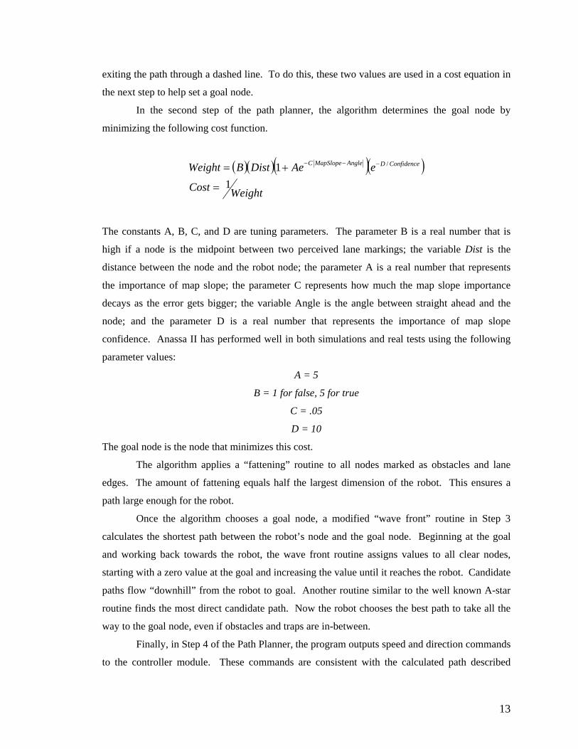
In the second step of the path planner, the algorithm determines the goal node by

minimizing the following cost function.

( )( )( )( )WeightCost

eAeDistBWeight ConfidenceDAngleMapSlopeC

11 /

=

+= −−−

The constants A, B, C, and D are tuning parameters. The parameter B is a real number that is

high if a node is the midpoint between two perceived lane markings; the variable Dist is the

distance between the node and the robot node; the parameter A is a real number that represents

the importance of map slope; the parameter C represents how much the map slope importance

decays as the error gets bigger; the variable Angle is the angle between straight ahead and the

node; and the parameter D is a real number that represents the importance of map slope

confidence. Anassa II has performed well in both simulations and real tests using the following

parameter values:

A = 5

B = 1 for false, 5 for true

C = .05

D = 10

The goal node is the node that minimizes this cost.

The algorithm applies a “fattening” routine to all nodes marked as obstacles and lane

edges. The amount of fattening equals half the largest dimension of the robot. This ensures a

path large enough for the robot.

Once the algorithm chooses a goal node, a modified “wave front” routine in Step 3

calculates the shortest path between the robot’s node and the goal node. Beginning at the goal

and working back towards the robot, the wave front routine assigns values to all clear nodes,

starting with a zero value at the goal and increasing the value until it reaches the robot. Candidate

paths flow “downhill” from the robot to goal. Another routine similar to the well known A-star

routine finds the most direct candidate path. Now the robot chooses the best path to take all the

way to the goal node, even if obstacles and traps are in-between.

Finally, in Step 4 of the Path Planner, the program outputs speed and direction commands

to the controller module. These commands are consistent with the calculated path described

13

above. However, this path is re-calculated on each controller cycle since new obstacles and

markings may be detected at any time. Thus, on each cycle, these two commands are the

commands needed to execute the initial phase of the planned path.

6.2 Navigation Challenge

The first step of the navigation design process was to correct the difficulties Anassa I

encountered in the navigation challenge event in 2005. The loss of the robot’s heading and some

program faults caused Anassa I to veer off course at about the third waypoint.

The restructuring possibilities were discussed by the team. The team decided to add a

digital compass, wheel encoders, and a gyro to correct or control the vehicle heading when the

loss of DGPS heading occurred at low speeds. The digital compass would provide the heading

when the speed dropped below 0.6mph. The wheel encoders and gyro would provide heading on

a sharp turn after switching from one waypoint to the next.

The systems used for the navigation challenge consists of the CSI Wireless receiver with

dual antennae, the digital compass, the wheel encoders, the gyro, the Sick 180 degree LMS and

the laptop computer. All the systems connect to the laptop via RS232 com ports or USB ports.

The program calculates a turn angle from knowing the robot’s heading and the bearing to

each waypoint. The actual turn command delivered to the controller depends on the distance to

the next waypoint. The following algorithm relates the angle and distance to the turn command.

( ) ( )DistBeAngleTurnACommandTurn −=

The constant A is a scale factor and the constant B affects the rate Anassa II turns as she

approaches a waypoint. The turn command is a set of digits (0 to 255) used for the digital-to-

analog converter in the controller. Path following is achieved by the algorithm described in the

section on the autonomous challenge.

The following list describes the challenges that had to be met, based on Anassa I’s

performance in IGVC 2005:

1. Heading stabilization was a major concern with Anassa I. When the vehicle was

slow or stopped, DGPS heading became inaccurate. To correct this, Anassa II uses

the digital compass, encoders, and/or gyro for the heading if the velocity is below 0.6

mph. This gives plenty of time for the DGPS to kick in and take over.

2. Most of the wobble of Anassa I was corrected in Anassa II by the algorithm used to

navigate to waypoints.

3. When Anassa I switched to the next target on some of the waypoints, it would make a

fast sharp angle. When testing with a compass, neither the compass heading or the

14

DGPS heading could keep up with the vehicle causing the vehicle to go out of

control. The actual heading was lagging behind the vehicle heading and would never

catch up. This challenge was solved by Anassa II’s team by compressing the amount

of angle the vehicle can turn, and by using encoders and the gyro during periods of

high dynamics.

The accuracy of arrival to the navigation waypoints was predicted to be within 1.5

meters. The DGPS has an accuracy of within two feet 95% of the time. Testing has verified this

kind of accuracy many times at BSC.

7. Analysis of Performance and Cost

7.1 Reliability and Durability

This team thinks that reliability and durability are components that work collectively. Of

course the determining factor for both of these components is time. Even though this is a

relatively new robot, the team is pleased with the seamless operation of two different versions

over the past two and a half years. The mechanical and electrical design was executed to make the

robot both durable and reliable. The frame and shell of the vehicle was built to sustain an impact,

and still protect the various components from damage. Electrical hardware was put under rigorous

testing, while backup components were acquired or built to facilitate quick repair. As with any

quality assurance process, the testing of this vehicle is continuous.

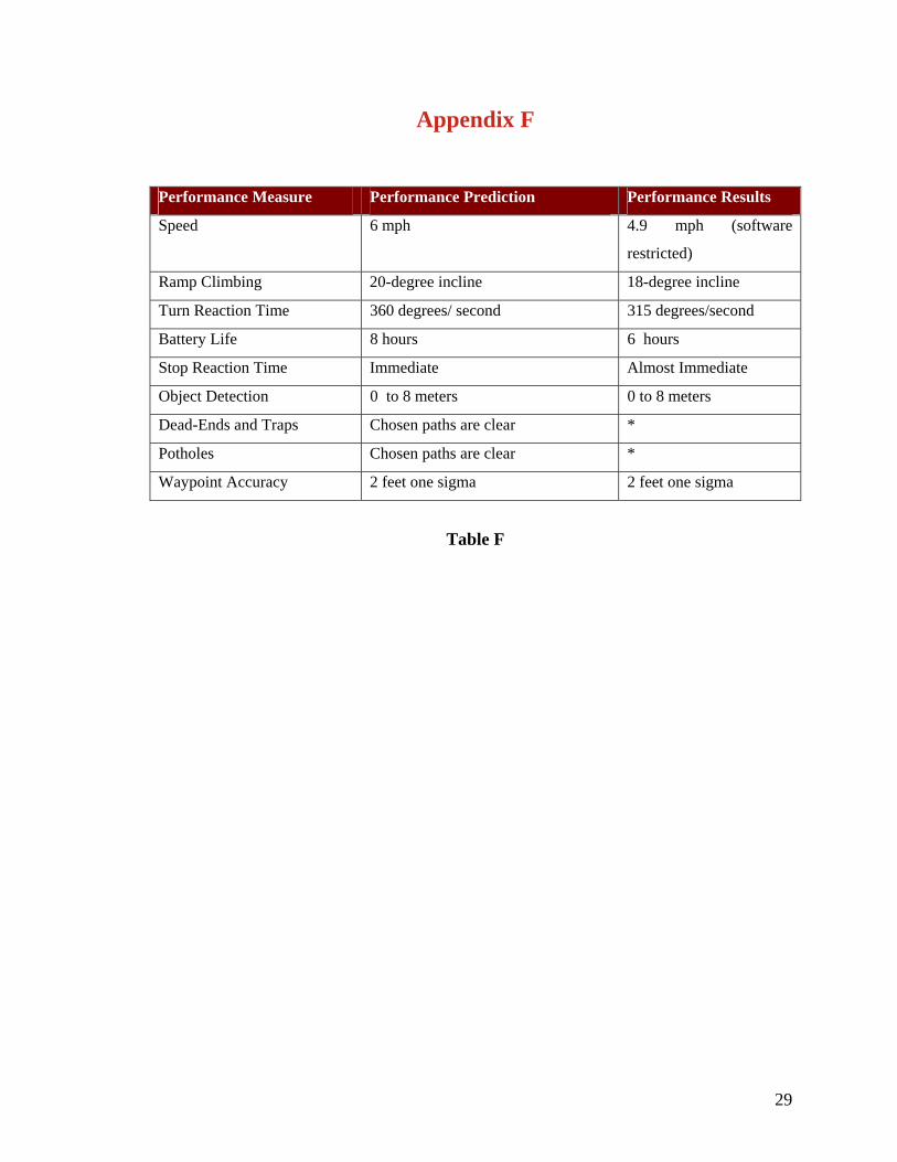
7.2 Analysis of Performance

Design and simulations indicate that Anassa II should perform as indicated in Appendix

F. The table also indicates results of actual testing. A “*” symbol means that Anassa II has not

been tested yet for that performance measure. Each prediction listed in the table comes from

analyses of components as well as overall performance.

8. Joint Architecture for Unmanned Systems (JAUS)

The Joint Architecture for Unmanned Systems (JAUS) is a relatively new initiative to

develop a set of standardized command structures for controlling different types of unmanned

systems, such as intelligent ground vehicles, in a cooperative environment. It will be deployed

both throughout the military services and become standard in the automotive industry as well.

While participation in this year’s JAUS implementation portion of the IGVC is considered

optional, Anassa II is designed and built to implement JAUS messages in accordance with the

IGVC official rules as well as more complex routines.

15

8.1 Implementation

Anassa II can read and execute JAUS message commands from an operator control unit

(OCU) via an RF (802.11g) data link. As in the IGVC demonstration portion, these messages can

start the vehicle moving forward in autonomous mode, stop the vehicle from moving in the

autonomous mode, and activate a warning device (horn/light).

8.1.1 Anassa II team’s process for learning about JAUS was based on literature review of the

current status of JAUS including a white paper entitled a Practical View and Future Look

at JAUS, May 2006, by Jorgen Pedersen, President and CEO, re², Inc. This review

helped answer such basic questions as: Why use JAUS? What is the terminology used in

the messages? How are these messages routed to the vehicle? How do these messages

support interoperability? What does it mean to be JAUS compliant?

8.1.2 Anassa II integrates JAUS messages based on two core elements (1) message

packing/unpacking and (2) message delivery. This was accomplished by modifying

codes from a software development kit to fit vehicle command programming discussed

earlier in the paper.

8.1.3 The Anassa II team addressed the challenges encountered in implementing JAUS by

making time to learn about a new requirement as described above. The primary

challenge was modifying the program codes required for JAUS to fit with existing

programs that control the vehicle.

16

Appendix A

Team Member Responsibilities Class Level- Major Hours worked

(est.) Lenny Lewis

(leader)

Software design,

Electrical design

Hardware

Construction

Senior – Electrical Eng. Tech. 1500

Joy Huntley Software Design Senior – Computer Science 1300

Joe Kessler Image Processing Junior – Electrical Eng. Tech. 400

Scott Baker Image Processing Senior – Electrical Eng. Tech. 400

Jesse Farmer Software design

Mechanical Design

Hardware

Construction

Senior – Mechanical Eng. Tech. 1400

Joshua Eerenberg Software Design Senior – Computer Science 500

Justin Stiltner Software Design

Hardware

Construction

Senior – Networking

200

James Cardwell Future Programmer Freshman – Computer Science 30

Randall Farmer Hardware

Construction

Senior – Electrical Eng. Tech. 500

Total Hours 6230

Table A

17

Appendix B

QUANTITY DESCRIPTION OUR COST Replacement

COST 1 1170 Wheelchair frame(Used) $1,037 $5,977 1 Dell computer $2,400 $2,400 1 Sony camera $700 $700 1 180 degree LMS(SICK) $3000 $5000 1 DGPS-w/antenna/cables $2100 $3000

1 Sea Level w/input/output

boards. $350 $350 1 Aluminum Platform $0 $500 1 Remote receiver kit $40 $40 1 LED Battery monitor kits $30 $30 1 Compass $700 $700

1 Computer Sense power

monitor for JAUS $12 $12

1 Heavy Duty 70 amp contact

relay $50 $50 1 Hard E-Stop $20 $20 1 Soft E-Stop $20 $20 2 12 volt Chargers $70 $70 2 12 volt Batteries $200 $200 1 Custom Controller Parts $25 $25 1 Cable connection box $15 $15 5 Toggle Switches $16 $16

1 Misc. Wire, Cables &

Connectors $50 $80

1 Misc. Mount Screws &

Hardware $20 $20 1 Gyro and controller $300 $500 1 USB Router 2.0 $20 $20 1 Two Encoders $0 $800 1 Temporary Platform $0 $15

Total $11,215 $20,065

Table B

18

Appendix C

Figure C. Still picture of simulation

19

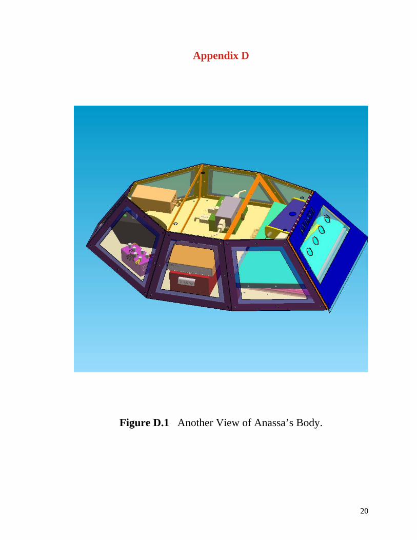
Appendix D

Figure D.1 Another View of Anassa’s Body.

20

Figure D.2 Another View of Anassa’s Frame/Chassis

21

Appendix E

Figure E.1

22

Figure E.2

Figure E.3

23

Figure E.4

Figure E.5

Figure E.6

24

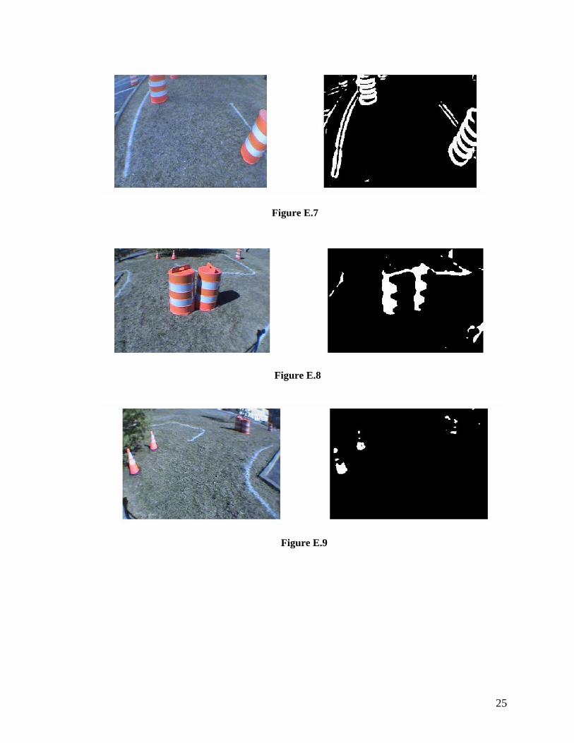
Figure E.7

Figure E.8

Figure E.9

25

Figure E.10

Figure E.11

Figure E.12

26

Figure E.13

Figure E.14

Figure E.15

Figure E.16

27

Figure E.17

28

Appendix F

Performance Measure Performance Prediction Performance Results

Speed 6 mph 4.9 mph (software

restricted)

Ramp Climbing 20-degree incline 18-degree incline

Turn Reaction Time 360 degrees/ second 315 degrees/second

Battery Life 8 hours 6 hours

Stop Reaction Time Immediate Almost Immediate

Object Detection 0 to 8 meters 0 to 8 meters

Dead-Ends and Traps Chosen paths are clear *

Potholes Chosen paths are clear *

Waypoint Accuracy 2 feet one sigma 2 feet one sigma

Table F

29