BLOODSTAIN PATTERN ANALYSIS: SCRATCHING THE SURFACE B A J LARKIN PhD 2015

Welcome message from author
This document is posted to help you gain knowledge. Please leave a comment to let me know what you think about it! Share it to your friends and learn new things together.
Transcript
BLOODSTAIN PATTERN ANALYSIS:
SCRATCHING THE SURFACE
B A J LARKIN
PhD 2015
1
BLOODSTAIN PATTERN ANALYSIS:
SCRATCHING THE SURFACE
BETHANY ALEXANDRIA JANE LARKIN
A thesis submitted in partial fulfilment of
the requirements of Manchester
Metropolitan University for the degree of
Doctor of Philosophy
School of Science and the Environment,
Manchester Metropolitan University
2015
2
ABSTRACT
Bloodstain Pattern Analysis (BPA) is a forensic application of the interpretation
of distinct patterns which blood exhibits during a bloodletting incident, providing key
evidence with its ability to potentially map the sequence of events. The nature of BPA
has given the illusion that its evidentiary significance is less than that of fingerprints or
DNA, relying solely on the interpretation of the analyst and focusing very little on any
scientific evaluation. Recent preliminary literature studies have involved a more
quantitative approach, developing directly crime scene applicable equations and
methodology, which have established new ways of predicting the angle of impact,
impact velocity, point of origin of blood and blood pattern type. Using these new
equations and further improving on them to include a variation of impact surfaces,
surface properties (i.e. porosity, roughness, manufacturing process etc.) and changes
in blood properties is the principal focus of this work.
The primary objective of this research is to expand the knowledge of blood and
surface interactions and generate general equation/s or quantitative approaches that
encompasses some of the possible conditions, in relation to Bloodstain Pattern
Analysis (BPA), which may be encountered at a crime scene. Overall validating BPA
and supporting a more reputable / respected scientific field giving credence to its
usage within criminal trials.
This thesis is presented in three parts:
The first part explores blood, its characteristics and how manipulating the
components of blood (i.e. packed cell volume, PCV), can alter the way a bloodstain
forms and dries. Since packed cell volume is instrumental in the overall viscosity of
blood, which ultimately determines the final bloodstain diameter via the natural
fluctuation exhibited throughout the body and by the individual human characteristics,
it was deemed necessary to investigate its effect on the interpretation of bloodstains.
Packed cell volume was found to alter the size of bloodstains significantly, where
increments in their diameter were experienced when PCV% was decreased; angled
impacts were unaffected.
The mechanism of drying blood was also analysed, the current understanding
being that blood dries primarily by the Marangoni Effect. However this is found to be
3
altered when PCV% is considered; low PCV% exhibits a strong Coffee Ring Effect
where higher PCV% levels dry by the Marangoni Effect.
Other drying characteristics considered were volume analysis, skeletonisation
and the halo effect where PCV% was manipulated. Volume analysis methods were
significantly affected by PCV%, where new drying constants were established and
several established scientific methods were shown to be unreliable at determining the
volume.
The second part of this thesis investigates surface interaction, exploring the
fundamentals of various common surface types, and how individual features (i.e.
surface roughness) affect the interpretation of bloodstains; four common surfaces
were considered (wood, metal, stone/tile and fabric). Blood drop tests were performed
at different heights and angles where recently formulated equations were applied to
the results to create new constants, which could be used to distinguish between
surface types. Wood and fabric were found to alter the spread of blood most
significantly, constants increased or decreased substantially, compared to the original
value.
The last part of this thesis expands the groundwork set forth in part two.
Surfaces were manipulated, either by heat or cleaning. Since it is possible that blood
may interact with a surface which may have been cleaned (to remove blood, or simply
to clean surface prior to any blood impaction) or heated (i.e. radiators), it is important
to fully explore surface alterations which commonly occur in an everyday environment
and therefore are highly probable to be encountered at a crime scene. Surface
manipulation is investigated in the form of a heated surface, where a blood boiling
curve reminiscent of the water boiling curve was created establishing four visibly
recognizable boiling regimes. Heat was found to decrease the resultant bloodstain
diameter, separate blood into its components and create reduction rings as the
temperature increased. An equation accounting for these changes was deduced,
further showing how simple alterations to the surface, which have previously been
overlooked, can interfere with the results. Further surface manipulation was
implemented in the form of cleaning, since cleaning can be performed before blood
impacts, therefore causing a surfactant layer, of after blood has impacted the surface,
indicating crime evasion.
Secondary analysis of blood on a heated surface in conjunction with cleaning
was implemented, establishing the effectiveness of presumptive testing and the ability

4
to extract valuable DNA. Initial presumptive testing and DNA extraction was found to
be successful for all temperatures, however when various cleaning methods were
applied (a common occurrence at crime scenes) DNA testing produced negative
results at temperatures of 50oC onwards.
Fabric washing, using various household detergents and methods of
washing/drying were also evaluated. Detergents significantly increased the resultant
diameters of bloodstains, secondary rings were experienced on all polyester and silk
fabrics, establishing constants relating to the secondary ring produced. Repeated
cycles of washing were found to produce a stable fabric after 6 cycles, for most fabric
types.

5
No other type of investigation of blood will yield so much useful information as an
analysis of the blood distribution patterns – Dr Paul Leland Kirk (BPA expert)

6
CONTENTS
Abstract .................................................................................................................... 2
Contents……………………………………………………………………………………..6
List of Tables………………………………………………………………………………14
List of Figures……………………………………………………………………………..16
1. Introduction ...................................................................................................... 23
1.1 Aims and Objectives ...................................................................................... 28
1.2 Background .................................................................................................... 29
1.2.1 What is Bloodstain Pattern Analysis? ...................................................... 29
1.2.2 History of BPA ........................................................................................ 29
1.2.2.1 BPA Historical Figures ................................................................. 30
1.2.2.1.1Dr. Eduard Piotrowski………………………………………….30
1.2.2.1.2 Dr. Victor Balthazard…………………………………………..30
1.2.2.1.3 Dr. Francis Camps……………………………………………..30
1.2.2.1.4 Hans Gross……………………………………………………..31
1.2.2.1.5 Dr. Josef Radziki……………………………………………….31
1.2.2.1.6 Dr. Paul Leland Kirk……………………………………………31
1.2.2.1.7 Dr. Herbert Leon MacDonell………………………………….31
1.3 Bloodstain Pattern Terminology………………………………………………...32
1.3.1 Blood Patterns……………………………………………………..32
1.3.2 Directionality………………………………………………………..33
1.3.3 Area of Convergence……………………………………………...34
1.3.4 Angle of Impact…………………………………………………….34
1.3.5 Area of Origin………………………………………………………35
1.3.6 Edge Characteristics………..……………………………………..37
1.4 Blood Properties and Characteristics........................................................... 37
1.4.1 Blood Drying……………………………………………………….38
1.5 Blood Drop Formation .................................................................................. 40
7
1.6 Surface Interactions .................................................................................... 42
1.7 Further Uses of Blood Evidence ................................................................. 45
1.8 Real Science? ............................................................................................ 47
2. Experimental Method and Materials ............................................................... 50
2.1 Blood…………………………………………………….....................................50
2.2 Blood Drop Tests…………………………………………………………………50
2.2.1 Pipettes…………………………………………………………….51
2.2.2 Rugometer…………………………………………………………51
2.2.3 Slow Motion Filming………………………………………………52
2.2.4 Bloodstain Measuring…………………………………………….52
2.3 Part I Experimentation Equipment……………………………………………...53
2.3.1 Rheometer…………………………………………………………54
2.3.2 Tensiometer……………………………………………………….54
2.3.3 Goniometer………………………………………………………..54
2.3.4 Microscope………………………………………………………...55
2.3.5 Specrophotometer………………………………………………...55
2.3.6 Hematocrit Centrifuge…………………………………………….55
2.4 Part II Experimentation Equipment……………………………………………...56
2.4.1 Smoothness & Air Permeance…………………………………...56
2.4.2 Scanning Electron Microscope…………………………………..56
2.5 Part III Experimentation Equipment…………………………………………….57
2.5.1 Furnace and Hot Plate……………………………………………57
2.5.2 Infra-Red Spectrophotometer……………………………………57
PART I: Blood ...................................................................................................... 58
3. Blood Characteristics ...................................................................................... 59
3.1 Blood ......................................................................................................... 59
3.1.1 Red Blood Cells…………………………………………………59
3.1.2 White Blood Cells……………………………………………….60
3.1.3 Platelets………………………………………………………….60
3.1.4 Plasma…………………………………………………………...60
3.1.5 Coagulation……………………………………………………...60
8
3.1.6 Viscosity………………………………………………………….61
3.1.7 Blood Grouping………………………………………………….62
3.1.8 Surface Tension…………………………………………………62
3.1.9 Adhesion and Cohesion………………………………………..62
3.1.10 Packed Cell Volume…………………………………………..63
3.2 Exploring the Applications of Equine Blood in BPA .......................... 64
3.2.1 Experimental ..................................................................... 65
3.2.2 Results and Discussion .................................................... 67
3.2.3 Summary .......................................................................... 79
3.3 Packed Cell Volume and Effects on BPA ............................................ 80
3.3.1 Experimental ..................................................................... 80
3.3.2 Results and Discussion .................................................... 81
3.3.3 Summary .......................................................................... 87
3.4 The Mechanism of Drying Blood and Volume Analysis .................... 89
3.4.1 Experimental ..................................................................... 89
3.4.2 Results and Discussion .................................................... 91
3.4.3 Summary ........................................................................ 111
3.5 Conclusions ......................................................................................... 113
PART II: Impact Surfaces ............................................................................... 115
4. Surfaces ......................................................................................................... 116
4.1 Surface Finish…………………………………………………………………116
4.1.1 Surface Roughness……………………………………………116
4.1.2 Lay……………………………………………………………...117
4.1.3 Waviness………………………………………………………117
4.2 Preliminary Investigation of Surface Finish ...................................... 118
4.2.1 Initial Observations……………………………………………118
4.3 Surface Finish Effects on Angled Surfaces ...................................... 119
4.3.1 Experimental.................................................................. 119
4.3.2 Results and Discussion ................................................. 119
4.3.3 Summary ....................................................................... 130
9
4.4 Single Surface Analysis ...................................................................... 131
4.5 Wood .................................................................................................... 131
4.5.1 Formation of Wood…………………………………………..131
4.5.2 Hardwood vs Softwood………………………………………132
4.5.3 Characteristics of Wood……………………………………..134
4.5.3.1 Grain…………………………………….134
4.5.3.2 Growth Rings…………………………...135
4.5.3.3 Knots…………………………………….136
4.5.3.4 Grade……………………………………136
4.5.4 Finishes…………………………………………………….....137
4.5.4.1 Green Wood Finishes…………………137
4.5.4.2 Varnish………………………………….137
4.5.4.3 Stain……………………………………..137
4.5.4.4 Dye………………………………………137
4.5.4.5 Wax……………………………………...137
4.5.4.6 Oil………………………………………..138
4.5.4.7 Wood Preserver………………………..138
4.6 Blood Impacting Wood ...................................................................... 138
4.6.1 Experimental .............................................................. 138
4.6.2 Results and Discussion ............................................. 139
4.6.3 Summary .................................................................... 148
4.7 Fabrics.................................................................................................. 149
4.7.1 Fabric Composition…………………………………………149
4.7.2 Fabric Finishes……………………………………………...152
4.7.3 Types of Fabric…………………………………….............153
4.7.3.1 Wool………………………………153
4.7.3.2 Silk………………………………..154
4.7.3.3 Cotton…………………………….155
4.7.3.4 Nylon……………………………..156
4.7.3.5 Polyester…………………………157
10
4.7.3.6 Linen……………………………...158
4.7.3.7 Denim…………………………….158
4.8 Blood Impacting Fabrics ..................................................................... 159
4.8.1 Experimental ............................................................... 159
4.8.2 Results and Discussion .............................................. 160
4.8.3 Summary .................................................................... 168
4.9 Metal ..................................................................................................... 170
4.9.1 Metal Composition………………………………………….170
4.9.2 Categories of Metals………………………………………..170
4.9.2.1 Base Metal………………………..170
4.9.2.2 Ferrous Metal…………………….170
4.9.2.3 Noble Metal……………………….170
4.9.2.4 Precious Metal……………………171
4.9.3 Metal Types………………………………………………….171
4.9.3.1 Aluminium………………………...171
4.9.3.2 Steel……………………………….171
4.9.3.3 Copper…………………………….172
4.9.3.4 Zinc………………………………..172
4.9.3.5 Brass………………………………173
4.9.4 Finishes……………………………………………………..173
4.10 Blood Impacting Metals .................................................................. 174
4.10.1 Experimental ............................................................ 174
4.10.2 Results and Discussion ........................................... 175
4.10.3 Summary ................................................................. 183
4.11 Stones and Tile .................................................................................. 184
4.11.1 Stone Types………………………………………………184
4.11.1.1 Sedimentary…………………...184
4.11.1.1.1 Sandstone………184
4.11.1.1.2 Limestone……….185
4.11.1.1.3 Travertine……….185

11
4.11.1.2 Metamorphic…………………..185
4.11.1.2.1 Marble…………...186
4.11.1.2.2 Slate……………..186
4.11.1.3 Igneous………………………...186
4.11.1.3.1 Granite…………..187
4.11.2 Finishes…………………………………………………..187
4.12 Blood Impacting Stones and Tile ................................................... 188
4.12.1 Experimental ........................................................... 188
4.12.2 Results and Discussion .......................................... 189
4.12.3 Summary ................................................................ 201
4.13 Conclusions ..................................................................................... 203
PART III: Surface Manipulation ..................................................................... 205
5. Manipulating Surfaces ................................................................................. 206
5.1 Heated Surfaces ................................................................................ 206
5.1.1 Underfloor Heating ................................................... 206
5.2 Effect of Underfloor Heating ............................................................ 207
5.2.1 Experimental ................................................................ 207
5.2.2 Results and Discussion ............................................... 208
5.2.3 Summary ..................................................................... 217
5.3 Common Heated Surfaces .............................................................. 218
5.4 Exploring Blood Impacting Heated Metal ...................................... 218
5.4.1 Experimental ................................................................ 218
5.4.2 Results and Discussion ............................................... 219
5.4.3 Summary ..................................................................... 229
5.5 Surface Cleaning ............................................................................. 230
5.5.1 Pre-treatment Cleaning……………………………………230
5.5.2 Post-treatment Cleaning…………………………………..230
5.6 Heated Surface Cleaning ............................................................... 230
5.6.1 Experimental ................................................................ 231
5.6.2 Results and Discussion ............................................... 234

12
5.6.3 Summary ..................................................................... 244
5.7 Fabric Laundering .......................................................................... 246
5.7.1 Experimental ................................................................ 246
5.7.2 Results and Discussion ............................................... 247
5.7.3 Summary ..................................................................... 263
5.8 Conclusions ..................................................................................... 264
6. Overall Conclusions ....................................................................................... 267
7. Future Research ............................................................................................. 272
8. Publications .................................................................................................... 273
9. References ...................................................................................................... 274
Appendix .............................................................................................................. 284
Appendix 1 Categorising Bloodstains…………………………………………………
Appendix 2 Ethics, COSHH and Risk Assessments………………………………...
Appendix 3 Three Blood Types Impacting Four Surfaces………………………..
3.1 Alsever’s Blood……………………………….
3.2 Human Blood………………………………….
3.3 Defibrinated Blood…………………………….
Appendix 4 Blood Impacting Angled Surfaces………………………………………
4.1 Plastic…………………………………………..
4.2 Steel…………………………………………….
4.3 Paper……………………………………………
Appendix 5 Bloodstains on Wood Surfaces…………………………………………
Appendix 6 Bloodstains on Fabric Surfaces………………………………………….
Appendix 7 Bloodstains on Metal Surfaces…………………………………………
Appendix 8 Bloodstains on Stones Surfaces…………………………………………
Appendix 9 Bloodstains on a Heated Surfaces………………………………………
Appendix 10 DNA Profiles for Cleaned Surfaces…………………………………….

13
LIST OF TABLES
Table 1: Average surface roughness of each experimental surface………………….51 Table 2: Release heights of blood drops calculated from the tip of pipette to the impacting surface and converted into impact velocity via the use of Equation (11)….66 Table 3: A comparison of published values obtained for the physical properties of equine, porcine and human blood (all unadulterated)…………………………………..67 Table 4: New constant values established for varying PCVs using equation (3) when different viscosity values were implemented…………………………………………….86 Table 5: Reference table depicting dry weight constants Wc
PCV derived for a range of PCVs……………………………………………………………………………………….107 Table 6: A comparison of surface type and dry weight constants (Wc
PCV) when PCV% has been incorporated, showing there to be no significant difference between surface type…………………………………………………………………………………………108 Table 7: Haemoglobin absorbance measured at 412 nm for different volumes, various PCVs and different surface types……………………………………………………….110 Table 8: Various parameters correlated against stain size found paper to establish the most significant R2 values and therefore the best coefficient…………………………120 Table 9: Number of spines correlated against various parameters to establish the best correlation coefficient, R2 value………………………………………………………….121 Table 10: The most significant R2 values when considering angled impacts on paper correlated against the number of spines……………………………………………….122 Table 11: R2 values established when considering the correlation of various parameters against stain size exhibited upon a steel surface……………………….124 Table 12: Resultant stain sizes on a plastic surface correlated against numerous parameters to determine the best coefficient R2 value……………………………….124 Table 13: The number of spines on a steel surface correlated against various theoretical parameters to determine significant R2 value…………………………….125 Table 14: R2 values established when correlating number of spines exhibited on a plastic surface with several theoretical parameters……………………………………126 Table 15: R2 values obtained when correlations using various theoretical parameters against the number of spines when considering an angled steel surface…………..126 Table 16: The most significant correlations of number of spines against parameters when varying angled impacts upon a plastic surface are performed………………..127 Table 17: Significant R2 value correlation coefficients were exhibited when plotting various parameters against the stain size presented on all surfaces (paper, steel and plastic)……………………………………………………………………………………..128 Table 18: Number of spines presented upon all surfaces (paper, plastic and steel) correlated against various parameters to determine significant R2 value…………..129 Table 19: Correlation coefficients (R2) established after plotting the number of spines against a series of parameters when angled impacts upon all surface types (steel, paper and plastic) are enforced…………………………………………………………129 Table 20: Physical characteristics of the 20 wood types used in this study…………140 Table 21: Various important knit types………………………………………………….150
14
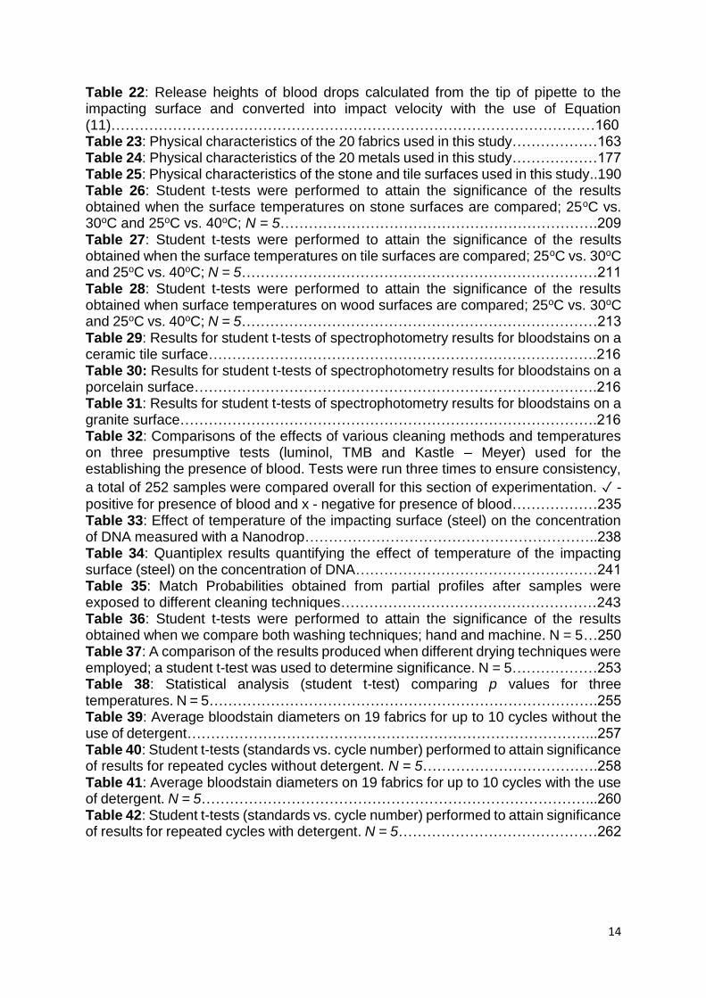
Table 22: Release heights of blood drops calculated from the tip of pipette to the impacting surface and converted into impact velocity with the use of Equation (11)…………………………………………………………………………………………160 Table 23: Physical characteristics of the 20 fabrics used in this study………………163 Table 24: Physical characteristics of the 20 metals used in this study………………177 Table 25: Physical characteristics of the stone and tile surfaces used in this study..190 Table 26: Student t-tests were performed to attain the significance of the results obtained when the surface temperatures on stone surfaces are compared; 25oC vs. 30oC and 25oC vs. 40oC; N = 5………………………………………………………….209 Table 27: Student t-tests were performed to attain the significance of the results obtained when the surface temperatures on tile surfaces are compared; 25oC vs. 30oC and 25oC vs. 40oC; N = 5…………………………………………………………………211 Table 28: Student t-tests were performed to attain the significance of the results obtained when surface temperatures on wood surfaces are compared; 25oC vs. 30oC and 25oC vs. 40oC; N = 5…………………………………………………………………213 Table 29: Results for student t-tests of spectrophotometry results for bloodstains on a ceramic tile surface……………………………………………………………………….216 Table 30: Results for student t-tests of spectrophotometry results for bloodstains on a porcelain surface………………………………………………………………………….216 Table 31: Results for student t-tests of spectrophotometry results for bloodstains on a granite surface…………………………………………………………………………….216 Table 32: Comparisons of the effects of various cleaning methods and temperatures on three presumptive tests (luminol, TMB and Kastle – Meyer) used for the establishing the presence of blood. Tests were run three times to ensure consistency,
a total of 252 samples were compared overall for this section of experimentation. ✓ -
positive for presence of blood and x - negative for presence of blood………………235 Table 33: Effect of temperature of the impacting surface (steel) on the concentration of DNA measured with a Nanodrop……………………………………………………..238 Table 34: Quantiplex results quantifying the effect of temperature of the impacting surface (steel) on the concentration of DNA……………………………………………241 Table 35: Match Probabilities obtained from partial profiles after samples were exposed to different cleaning techniques………………………………………………243 Table 36: Student t-tests were performed to attain the significance of the results obtained when we compare both washing techniques; hand and machine. N = 5…250 Table 37: A comparison of the results produced when different drying techniques were employed; a student t-test was used to determine significance. N = 5………………253 Table 38: Statistical analysis (student t-test) comparing p values for three temperatures. N = 5……………………………………………………………………….255 Table 39: Average bloodstain diameters on 19 fabrics for up to 10 cycles without the use of detergent…………………………………………………………………………...257 Table 40: Student t-tests (standards vs. cycle number) performed to attain significance of results for repeated cycles without detergent. N = 5……………………………….258 Table 41: Average bloodstain diameters on 19 fabrics for up to 10 cycles with the use of detergent. N = 5………………………………………………………………………...260 Table 42: Student t-tests (standards vs. cycle number) performed to attain significance of results for repeated cycles with detergent. N = 5……………………………………262

205
LIST OF FIGURES
Figure 1: A bloodstain expressing the final bloodstain diameter, Ds………………….25 Figure 2: A bloodstain displaying visible spines on the periphery…………………….26 Figure 3: An overview of different wooden surfaces and physical properties. Adapted from Ref [19]………………………………………………………………………………...27 Figure 4: Flow chart expressing blood stains into two categories; spatter and no-spatter……………………………………………………………………………………….33 Figure 5: Arrows indicate direction which bloodstain is travelling using tail and scallops of a bloodstain……………………………………………………………………………....33 Figure 6: Area of convergence, a common point where the majority of bloodstains intercept……………………………………………………………………………………..34 Figure 7: Diagram representing the theory of the occurrence of angled impacts……35 Figure 8: An angled bloodstain indicating where measurements should take place for angle of impact……………………………………………………………………………...35 Figure 9: Graphical representation of the area of origin determination……………….36 Figure 10: Bloodstain spines……………………………………………………………...37 Figure 11: Bloodstain scallops……………………………………………………………37 Figure 12: Bloodstain tail………………………………………………………………….37 Figure 13: Scaled stills of blood drops. Image A shows a still of defibrinated equine blood drop using a 1mL pipette (1 mm inner tip diameter); Image B is of defibrinated equine blood drop using a 1mL pipette (1.77 mm inner tip diameter)…………………52 Figure 14: Circular bloodstain depicting the actual diameter to be measured……….52 Figure 15: Angled impacts showing the diameter and ellipse length measured…….53 Figure 16: A red blood cell………………………………………………………………..59 Figure 17: A white blood cell………………………………………………………………60 Figure 18: Coagulation process, showing both intrinsic and extrinsic pathways…….61 Figure 19: Comparisons of blood stain diameters (Ds) for defibrinated equine blood (squares), human blood (triangles) and anti-coagulated equine blood (circles) dropped upon a paper surface, identifying that defibrinated equine blood gives the greatest comparability to human blood; N = 5……………………………………………………..68 Figure 20 : Blood stain diameters for defibrinated equine blood released upon different surfaces from a range of release heights; paper (crosses), plastic (triangles), tile (circles) and cold rolled steel (squares); A: using a 1 mL pipette (inner tip diameter 1 mm) and B: using a 1 mL pipette (inner tip diameter 1.77 mm); N = 5………………..70 Figure 21: Blood stain diameters (Ds) for Alsever’s blood released upon different surfaces from a range of release heights; paper (crosses), plastic (triangles), tile (circles) and cold rolled steel (squares); A: using a 1 mL pipette (inner tip diameter 1 mm) and B: using a 1 mL pipette (inner tip diameter 1.77 mm); N = 5………………..71 Figure 22: Blood stain diameters (Ds) for human blood released upon different surfaces from a range of release heights; paper (crosses), plastic (triangles), tile (circles) and cold rolled steel (squares); A: using a 1 mL pipette (inner tip diameter 1 mm) and B: using a 1 mL pipette (inner tip diameter 1.77 mm); N = 5……………….71 Figure 23: A new line of ‘best fit’ (solid line) was established when considering the spread factor versus the Reynolds on different surfaces; paper, plastic, tile and cold rolled steel. Comparing this to the original line of ‘best fit’ (dotted line) using equation
206
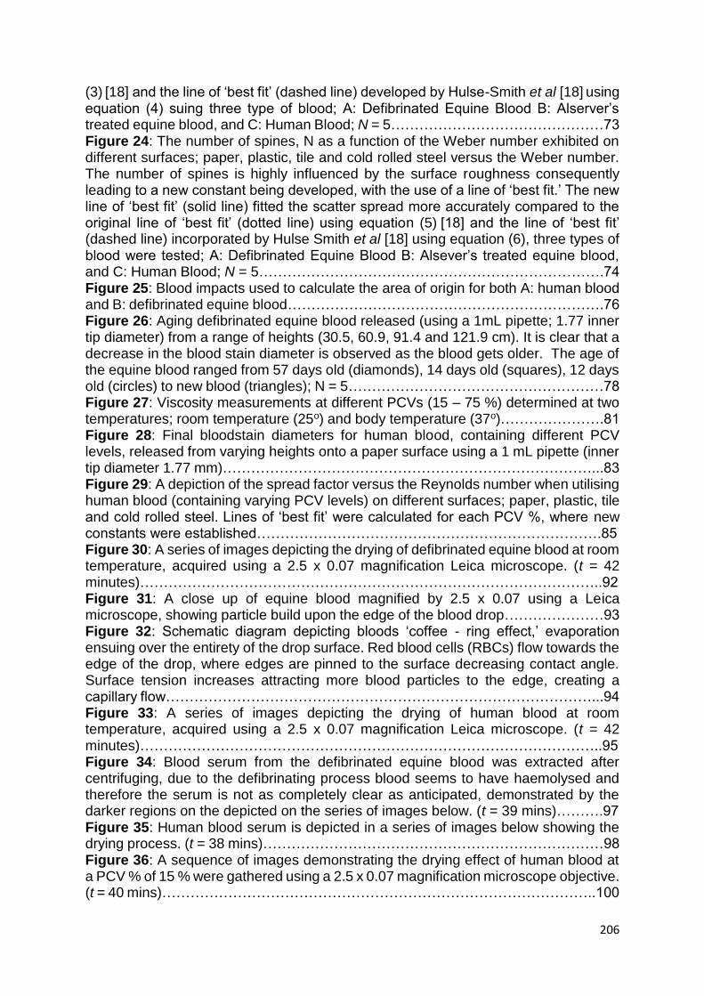
(3) [18] and the line of ‘best fit’ (dashed line) developed by Hulse-Smith et al [18] using equation (4) suing three type of blood; A: Defibrinated Equine Blood B: Alserver’s treated equine blood, and C: Human Blood; N = 5………………………………………73 Figure 24: The number of spines, N as a function of the Weber number exhibited on different surfaces; paper, plastic, tile and cold rolled steel versus the Weber number. The number of spines is highly influenced by the surface roughness consequently leading to a new constant being developed, with the use of a line of ‘best fit.’ The new line of ‘best fit’ (solid line) fitted the scatter spread more accurately compared to the original line of ‘best fit’ (dotted line) using equation (5) [18] and the line of ‘best fit’ (dashed line) incorporated by Hulse Smith et al [18] using equation (6), three types of blood were tested; A: Defibrinated Equine Blood B: Alsever’s treated equine blood, and C: Human Blood; N = 5……………………………………………………………….74 Figure 25: Blood impacts used to calculate the area of origin for both A: human blood and B: defibrinated equine blood………………………………………………………….76 Figure 26: Aging defibrinated equine blood released (using a 1mL pipette; 1.77 inner tip diameter) from a range of heights (30.5, 60.9, 91.4 and 121.9 cm). It is clear that a decrease in the blood stain diameter is observed as the blood gets older. The age of the equine blood ranged from 57 days old (diamonds), 14 days old (squares), 12 days old (circles) to new blood (triangles); N = 5………………………………………………78 Figure 27: Viscosity measurements at different PCVs (15 – 75 %) determined at two temperatures; room temperature (25o) and body temperature (37o)………………….81 Figure 28: Final bloodstain diameters for human blood, containing different PCV levels, released from varying heights onto a paper surface using a 1 mL pipette (inner tip diameter 1.77 mm)……………………………………………………………………...83 Figure 29: A depiction of the spread factor versus the Reynolds number when utilising human blood (containing varying PCV levels) on different surfaces; paper, plastic, tile and cold rolled steel. Lines of ‘best fit’ were calculated for each PCV %, where new constants were established……………………………………………………………….85 Figure 30: A series of images depicting the drying of defibrinated equine blood at room temperature, acquired using a 2.5 x 0.07 magnification Leica microscope. (t = 42 minutes)……………………………………………………………………………………..92 Figure 31: A close up of equine blood magnified by 2.5 x 0.07 using a Leica microscope, showing particle build upon the edge of the blood drop…………………93 Figure 32: Schematic diagram depicting bloods ‘coffee - ring effect,’ evaporation ensuing over the entirety of the drop surface. Red blood cells (RBCs) flow towards the edge of the drop, where edges are pinned to the surface decreasing contact angle. Surface tension increases attracting more blood particles to the edge, creating a capillary flow………………………………………………………………………………...94 Figure 33: A series of images depicting the drying of human blood at room temperature, acquired using a 2.5 x 0.07 magnification Leica microscope. (t = 42 minutes)……………………………………………………………………………………..95 Figure 34: Blood serum from the defibrinated equine blood was extracted after centrifuging, due to the defibrinating process blood seems to have haemolysed and therefore the serum is not as completely clear as anticipated, demonstrated by the darker regions on the depicted on the series of images below. (t = 39 mins)……….97 Figure 35: Human blood serum is depicted in a series of images below showing the drying process. (t = 38 mins)………………………………………………………………98 Figure 36: A sequence of images demonstrating the drying effect of human blood at a PCV % of 15 % were gathered using a 2.5 x 0.07 magnification microscope objective. (t = 40 mins)………………………………………………………………………………..100

207
Figure 37: Images collected with the use of a Leica microscope at magnification 2.5 x 0.07 demonstrating the drying effect of human blood at a PCV % of 40 %. (t = 42 mins)……………………………………………………………………………….101 Figure 38: A sequence of images collected using a microscope at magnification of 2.5 x 0.07, demonstrating the drying effect of human blood at a PCV % of 75 %. (t = 42 mins)……………………………………………………………………………………….102 Figure 39: A - The skeletonisation of blood, where a clear ring is left behind when the bloodstain has been wiped. B - The Halo Effect, a visible red outer ring/ ‘halo’ can be seen on the periphery of the bloodstain. A red ring is observed when a drop followed by a swipe action has occurred…………………………………………………………..103 Figure 40: A scaled bloodstain photograph, here, image software, Image J has been used to alter the threshold of the photograph allowing for the surface area to be measured………………………………………………………………………………….104 Figure 41: Calibration graphs expressing surface areas of bloodstains versus original volume on two different surface types: A- vinyl and B- laminate wood………………105 Figure 42: Representations of: A- PCV% and B- haemoglobin levels, against constants (m)……………………………………………………………………………...109 Figure 43: six main types of surface lay, created through the production process…117 Figure 44: Resultant stain size exhibited on paper at various impact angles plotted against REIMDoDo…………………………………………………………………………121 Figure 45: Cross-section of a tree trunk, showing the development of wood………132 Figure 46: Structure of hardwood, with observable vessels which transport water throughput the tree………………………………………………………………………..133 Figure 47: Structure of softwood, a vascular structure with medullary rays and tracheids which transports water and produce…………………………………………134 Figure 48: Four main longitudinal cell grain patterns found in wood…………………135 Figure 49: Bloodstain Diameters on all 20 wood types from various heights; 50cm, 100 cm, 150cm and 200cm, using the 1mm pipette……………………………………142 Figure 50: Bloodstain Diameters on all 20 wood types from various heights; 50cm, 100 cm, 150cm and 200cm, using the 1.77 mm pipette………………………………142 Figure 51: A new line of ‘best fit (solid line) was established when considering the spread factor versus the Reynolds number utilising human blood on various wood types. Comparing this to the original line of ‘best fit’ (dashed line) using equation (3) and the line of best fit (dotted line) developed by Hulse-Smith et al [18] using equation (4); N=5…………………………………………………………………………………….143 Figure 52: Bloodstain Diameters depicted the effect of wood type, where blood was deposited using A- 1mm pipette and B- 1.77mm pipette………………………………144 Figure 53: Bloodstain Diameters depicted the effect of wood grain, where blood was deposited using A- 1mm pipette and B- 1.77mm pipette………………………………145 Figure 54: Bloodstain Diameters depicted the effect of the manufacturing process of wood, where blood was deposited using A- 1mm pipette and B- 1.77mm pipette…146 Figure 55: Bloodstain Diameters depicted the effect of surface finish, where blood was deposited using A- 1mm pipette and B- 1.77mm pipette………………………………146 Figure 56: Bloodstain Diameters depicted the effect of surface characteristics, where blood was deposited using A- 1mm pipette and B- 1.77mm pipette………………….147 Figure 57: Plain weave…………………………………………………………………..149
Figure 58: Satin weave…………………………………………………………………..149 Figure 59: Twill weave…………………………………………………………………...150
Figure 60: STF……………………………………………………………………………151 Figure 61: A braid……………………………………………………………………...…151
208
Figure 62: Lace fabric……………………………………………………………………151
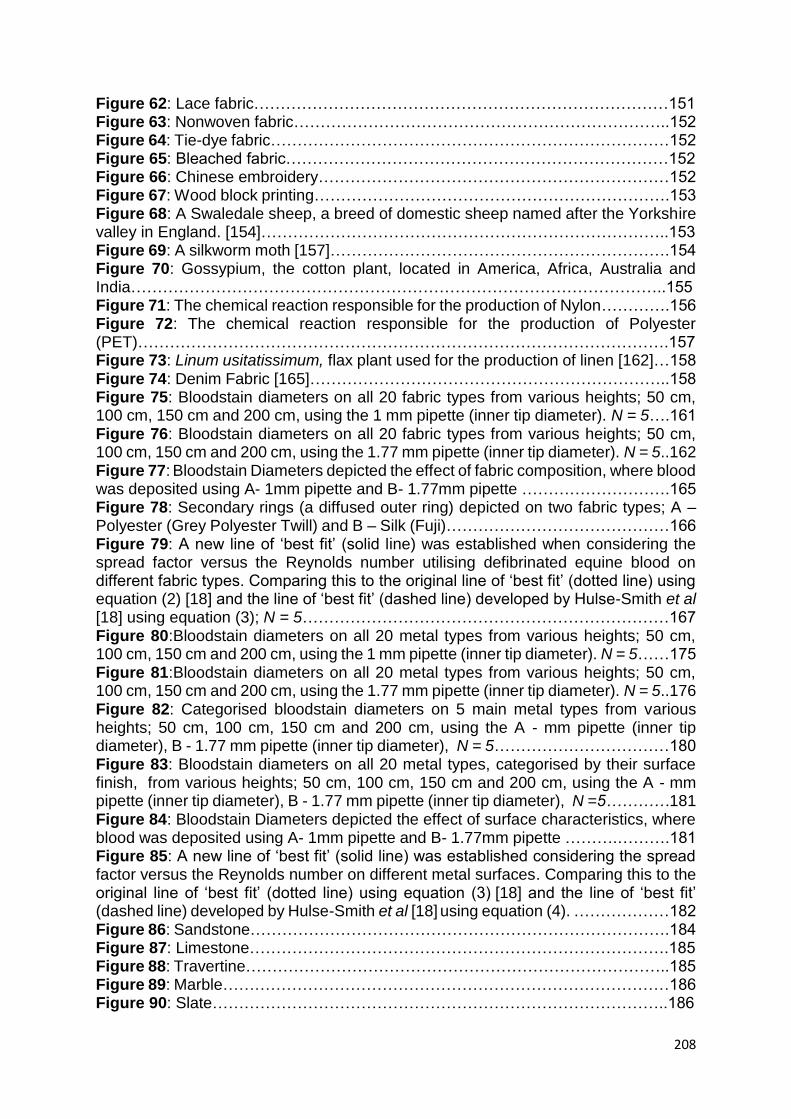
Figure 63: Nonwoven fabric……………………………………………………………..152 Figure 64: Tie-dye fabric…………………………………………………………………152 Figure 65: Bleached fabric………………………………………………………………152 Figure 66: Chinese embroidery…………………………………………………………152 Figure 67: Wood block printing………………………………………………………….153 Figure 68: A Swaledale sheep, a breed of domestic sheep named after the Yorkshire valley in England. [154]…………………………………………………………………..153 Figure 69: A silkworm moth [157]……………………………………………………….154 Figure 70: Gossypium, the cotton plant, located in America, Africa, Australia and India………………………………………………………………………………………..155Figure 71: The chemical reaction responsible for the production of Nylon………….156 Figure 72: The chemical reaction responsible for the production of Polyester (PET)……………………………………………………………………………………….157 Figure 73: Linum usitatissimum, flax plant used for the production of linen [162]…158 Figure 74: Denim Fabric [165]…………………………………………………………..158 Figure 75: Bloodstain diameters on all 20 fabric types from various heights; 50 cm, 100 cm, 150 cm and 200 cm, using the 1 mm pipette (inner tip diameter). N = 5….161 Figure 76: Bloodstain diameters on all 20 fabric types from various heights; 50 cm, 100 cm, 150 cm and 200 cm, using the 1.77 mm pipette (inner tip diameter). N = 5..162 Figure 77: Bloodstain Diameters depicted the effect of fabric composition, where blood was deposited using A- 1mm pipette and B- 1.77mm pipette ……………………….165 Figure 78: Secondary rings (a diffused outer ring) depicted on two fabric types; A – Polyester (Grey Polyester Twill) and B – Silk (Fuji)……………………………………166 Figure 79: A new line of ‘best fit’ (solid line) was established when considering the spread factor versus the Reynolds number utilising defibrinated equine blood on different fabric types. Comparing this to the original line of ‘best fit’ (dotted line) using equation (2) [18] and the line of ‘best fit’ (dashed line) developed by Hulse-Smith et al [18] using equation (3); N = 5……………………………………………………………167 Figure 80:Bloodstain diameters on all 20 metal types from various heights; 50 cm, 100 cm, 150 cm and 200 cm, using the 1 mm pipette (inner tip diameter). N = 5……175 Figure 81:Bloodstain diameters on all 20 metal types from various heights; 50 cm, 100 cm, 150 cm and 200 cm, using the 1.77 mm pipette (inner tip diameter). N = 5..176 Figure 82: Categorised bloodstain diameters on 5 main metal types from various heights; 50 cm, 100 cm, 150 cm and 200 cm, using the A - mm pipette (inner tip diameter), B - 1.77 mm pipette (inner tip diameter), N = 5……………………………180 Figure 83: Bloodstain diameters on all 20 metal types, categorised by their surface finish, from various heights; 50 cm, 100 cm, 150 cm and 200 cm, using the A - mm pipette (inner tip diameter), B - 1.77 mm pipette (inner tip diameter), N =5…………181 Figure 84: Bloodstain Diameters depicted the effect of surface characteristics, where blood was deposited using A- 1mm pipette and B- 1.77mm pipette ……….……….181 Figure 85: A new line of ‘best fit’ (solid line) was established considering the spread factor versus the Reynolds number on different metal surfaces. Comparing this to the original line of ‘best fit’ (dotted line) using equation (3) [18] and the line of ‘best fit’ (dashed line) developed by Hulse-Smith et al [18] using equation (4). ………………182 Figure 86: Sandstone…………………………………………………………………….184 Figure 87: Limestone…………………………………………………………………….185 Figure 88: Travertine……………………………………………………………………..185 Figure 89: Marble…………………………………………………………………………186 Figure 90: Slate…………………………………………………………………………..186

209
Figure 91: Granite………………………………………………………………………..187 Figure 92: Bloodstain diameters on all stone surfaces from various heights; 50 cm, 100 cm, 150 cm and 200 cm, using the 1 mm pipette (inner tip diameter). N = 5….189 Figure 93: Bloodstain diameters on all stone surfaces from various heights; 50 cm, 100 cm, 150 cm and 200 cm, using the 1 mm pipette (inner tip diameter). N = 5….190 Figure 94: Categorised bloodstain diameters on 5 main stone types from various heights; 50 cm, 100 cm, 150 cm and 200 cm, using the A - mm pipette (inner tip diameter), B - 1.77 mm pipette (inner tip diameter), N = 5……………………………194 Figure 95: Bloodstain diameters on all stone types, categorised by surface finish, from various heights; 50 cm, 100 cm, 150 cm and 200 cm, using the A - mm pipette (inner tip diameter), B - 1.77 mm pipette (inner tip diameter), N = 5…………………………195 Figure 96: Bloodstain diameters on all stone types, categorised by surface characteristics, from various heights; 50 cm, 100 cm, 150 cm and 200 cm, using the A - mm pipette (inner tip diameter), B - 1.77 mm pipette (inner tip diameter), N = 5..196 Figure 97: A new line of ‘best fit’ (solid line) was established considering the spread factor versus the Reynolds number on different stone surfaces. Comparing this to the original line of ‘best fit’ (dotted line) using equation (3) [18] and the line of ‘best fit’ (dashed line) developed by Hulse-Smith et al [18] using equation (4)………………197 Figure 98: Bloodstain diameters on all tile surfaces from various heights; 50 cm, 100 cm, 150 cm and 200 cm, using the 1 mm pipette (inner tip diameter). N = 5………198 Figure 99: Bloodstain diameters on all tile surfaces from various heights; 50 cm, 100 cm, 150 cm and 200 cm, using the 1 mm pipette (inner tip diameter). N = 5………199 Figure 100: Bloodstain diameters on all tile types, categorised by surface characteristics, from various heights; 50 cm, 100 cm, 150 cm and 200 cm, using the A - mm pipette (inner tip diameter), B - 1.77 mm pipette (inner tip diameter), N = 5..200 Figure 101: A new line of ‘best fit’ (solid line) was established considering the spread factor versus the Reynolds number on different tile surfaces. Comparing this to the original line of ‘best fit’ (dotted line) using equation (3) [18] and the line of ‘best fit’ (dashed line) developed by Hulse-Smith et al [18] using equation (4)………………201 Figure 102: Representation of the effect of heated stone surfaces on the size of bloodstains………………………………………………………………………………...209 Figure 103: Bloodstain diameters results when blood drops have impacted heated tile surfaces……………………………………………………………………………………210 Figure 104: A depiction of bloodstain diameter results which have impacted 20 different heated wood surfaces………………………………………………………….212 Figure 105: Bloodstains showing the effect of heated surfaces on the appearance of the bloodstain, where before depicts blood on a surface at room temperature and after shows bloodstains which have impacted a heated surface (40oC)………………….214 Figure 106: Spectrum depicting the increase in absorbance as the bloodstain is heated on a porcelain surface……………………………………………………………214 Figure 107: Spectrum depicting the increase in absorbance as the bloodstain is heated on a granite surface………………………………………………………………215 Figure 108: Spectrum depicting the increase in absorbance as the bloodstain is heated on a tile surface…………………………………………………………………..215 Figure 109: A typical boiling curve highlighting the boiling regimes for water; A: natural convection (around room temperature), B: nucleation boiling regime, C: transition boiling regime and D: film boiling regime………………………………………………..219 Figure 110: Effect of bloodstain diameters (Ds) for equine blood released onto cold rolled steel held at a range of temperatures and released from a range of heights; 30.5 cm (squares), 60.9 cm (circles), 91.4 cm (triangles), 121.9 cm (upside-down
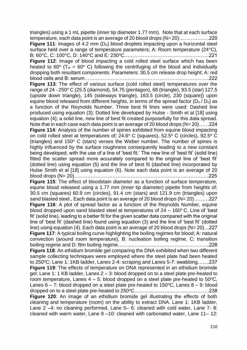
210
triangles) using a 1 mL pipette (inner tip diameter 1.77 mm). Note that at each surface temperature, each data point is an average of 20 blood drops (N= 20)………………220 Figure 111: Images of 4.2 mm (Do) blood droplets impacting upon a horizontal steel surface held over a range of temperature parameters; A: Room temperature (24°C), B: 60°C, C: 100°C, D: 140°C and E: 230oC……………………………………………221 Figure 112: Image of blood impacting a cold rolled steel surface which has been heated to 60o (Tw = 60o C) following the centrifuging of the blood and individually dropping both resultant components. Parameters: 30.5 cm release drop height; A: red blood cells and B: serum…………………………………………………………………222 Figure 113: The effect of various surface (cold rolled steel) temperatures over the range of 24 - 250o C (25.5 (diamond), 54.75 (pentagon), 68 (triangle), 93.5 (star) 127.5 (upside down triangle), 145 (sideways triangle), 163.5 (circle), 230 (square)) upon equine blood released from different heights, in terms of the spread factor (Ds / Do) as a function of the Reynolds Number. Three best fit lines were used: Dashed line produced using equation (3); Dotted line developed by Hulse - Smith et al [18] using equation (4); a solid line, new line of best fit created purposefully for this data spread. Note that in each case each data point is an average of 20 blood drops (N= 20)……224 Figure 114: Analysis of the number of spines exhibited from equine blood impacting on cold rolled steel at temperatures of; 24.6o C (squares), 52.5o C (circles), 92.5o C (triangles) and 150o C (stars) verses the Weber number. The number of spines is highly influenced by the surface roughness consequently leading to a new constant being developed, with the use of a line of ‘best fit.’ The new line of ‘best fit’ (solid line) fitted the scatter spread more accurately compared to the original line of ‘best fit’ (dotted line) using equation (5) and the line of best fit (dashed line) incorporated by Hulse Smith et al [18] using equation (6). Note each data point is an average of 20 blood drops (N= 20)………………………………………………………………………225 Figure 115: The effect of bloodstain diameter as a function of surface temperature, equine blood released using a 1.77 mm (inner tip diameter) pipette from heights of; 30.5 cm (squares) 60.9 cm (circles), 91.4 cm (stars) and 121.9 cm (triangles) upon sand blasted steel., Each data point is an average of 20 blood drops (N= 20)………227 Figure 116: A plot of spread factor as a function of the Reynolds Number, equine blood dropped upon sand blasted steel at temperatures of 24 – 160o C. Line of ‘best fit’ (solid line), leading to a better fit for the given scatter data compared with the original line of ‘best fit’ (dashed line) found using equation (3) and the line of ‘best fit’ (dotted line) using equation (4). Each data point is an average of 20 blood drops (N= 20)…227 Figure 117: A typical boiling curve highlighting the boiling regimes for blood; A: natural convection (around room temperature), B: nucleation boiling regime, C: transition boiling regime and D: film boiling regime……………………………………………….228 Figure 118: An ethidium bromide gel comparing the DNA exhibited when two different sample collecting techniques were employed where the steel plate had been heated to 250oC; Lane 1: 1KB ladder, Lanes 2-4: scraping and Lanes 5-7: swabbing…….237 Figure 119: The effects of temperature on DNA represented in an ethidium bromide gel; Lane 1: 1 KB ladder, Lanes 2 – 3: blood dropped on to a steel plate pre-heated to room temperature, Lanes 4 – 5: blood dropped on a steel plate pre-heated to 50oC, Lanes 6 – 7: blood dropped on a steel plate pre-heated to 150oC, Lanes 8 – 9: blood dropped on to a steel plate pre-heated to 250oC………………………………………238 Figure 120: An image of an ethidium bromide gel illustrating the effects of both cleaning and temperature (room) on the ability to extract DNA. Lane 1: 1KB ladder, Lane 2 –4: no cleaning performed, Lane 5– 6: cleaned with cold water, Lane 7- 8: cleaned with warm water, Lane 9 –10: cleaned with carbonated water, Lane 11– 12:
211
cleaned with soap and water, Lane 13–14: cleaned with 10% bleach, Lane 15 – 16: cleaned with 1M NaCl + 1M NaOH………………………………………………………239 Figure 121: A 1% agarose gel exposed to UV light showing the PCR amplification for locus D1S80;Lane 1: 100 bp ladder, Lane 2: swab control sample (blank), Lane 3: cleaned with cold water, Lane 4:cleaned with warm water, Lane 5: cleaned with carbonated water, Lane 6:cleaned with soap and water, Lane 7:cleaned with 10% household bleach, Lane 8: no cleaning performed, Lane 9: cleaned with 1M NaCl + 1M NaOH, Lane 10: negative control (distilled water)…………………………………240 Figure 122: A graphical representation of the average RFU value for peak height across the EPG when incorporating different surface temperatures alone without cleaning……………………………………………………………………………………242 Figure 123: Peak height ratios of profiles obtained when DNA was deposited on to a heated surface…………………………………………………………………………….242 Figure 124: Average bloodstain diameters when blood impacted fabric after it had been machine washed with 6 different detergent types. N = 5………………………248 Figure 125: Average bloodstain diameters when blood impacted fabric after it had been hand washed with 6 different detergent types. N = 5……………………………249 Figure 126: Comparison of diameter of bloodstains on non-laundered (standard) fabrics and fabrics after dry cleaning. N = 5……………………………………………251 Figure 127: A representation of the average bloodstain diameters created when blood impacted fabrics washed at 3 different temperatures; 30oC, 40oC and 60oC. N = 5...254
212
1. INTRODUCTION
In the philosophical words of Edmond Locard ‘every contact leaves a trace,’
[1 - 3] which is the basic principle behind forensic science, a science that utilises
evidence left at crime scenes to establish a connection between the crime and its
perpetrator. [1 - 3] Forensic science can be defined simply as the application of science
pertaining to the law. [1 - 3] It is through these words that the world of forensics has
expanded, creating a network of scientists which have made it extremely difficult for a
criminal not to be linked to their committed crime. Since every crime scene tells a story,
it takes only the correct interpretation of evidence to unveil the story, creating a true
representation of the preceding events. Forensic investigators are contingent on this
fact, depending on vital forms of evidence to help solve complex crimes and bring
justice to victims. [4 - 6] Bloodstain Pattern Analysis (BPA) epitomises this objective,
using the formation of blood as it impacts a surface to determine the sequence of
events and general movement of the perpetrator and / or victim throughout the scene.
[7, 8] BPA has become an increasingly employed forensic discipline due to bloods
presence at crime scenes and the weight it holds as a form of evidence within the legal
system. [4 - 6]
BPA has been a much overlooked field, although it is evident that people
generally acknowledged the presence of blood as being directly connected with death
/ a violent act, demonstrated even in early cave drawings and ancient paintings, [9]
investigators overlooked the potential of blood patterns until the 1960s. Although the
‘father’ of BPA is widely accredited to Dr Herbert L. MacDonell [9, 10, 11] it was in fact
the successful affidavit presented in 1966 by Dr Paul Kirk in the renowned case of
Samuel Sheppard (accused of murdering his wife) [7] which first catapulted BPA into
the realm of an acceptable / prominent form of evidence in legal proceedings. [4 - 6]
Presently BPA has been utilised in many high profile cases e.g. The Road
Rage killer.[12] Unfortunately due to the relatively late application of blood as an
evidence form, the field still remains somewhat subjective, where analysis can differ
depending on the analyst’s interpretation. A recent example of this discrepancy is
attested in the case of David Camm,[13] an Indiana State trooper sentenced to life
imprisonment in 2002 for the murder of his wife and two children, who were found,

213
shot to death in their car in the family’s garage.[13] The case was centred around the
interpretation of blood specks found on Camm’s t-shirt.[13] Experts stated that the blood
spatter was created by impact spatter as a result of Camm shooting his wife; however
other experts argue that the blood is simply caused by a transfer when Camm pulled
his child from the car.[13] It is now firmly believed that there was a miscarriage of justice,
on the 24th October 2013 after the third trial David Camm was acquitted. Unfortunately
this is not the only case in which problems with bloodstain analysis has arisen (i.e.
Billie–Joe Jenkins; expiration vs impact spatter). [14] It is through cases like these [13 -
16] and the prevalence of violent crime that has subsequently enhanced public scrutiny
upon the police and forensic scientists to produce more efficient, repeatable and
accurate methods of interpretation. The main aim of this research is to expand on the
limited research currently available regarding the interaction of bloodstains and impact
surfaces. Quantitative analysis (using the below equations) will be performed in the
hopes of generating an easily applicable method which can be utilised at crime scenes
and ultimately support the scientific validation of this ‘subjective’ discipline.
Steps towards a more scientific quantitative evaluation method have already
begun. Wonder introduced the SAADD system, which provided objective criteria in
which to identify blood patterns. Focusing on the size of the stains, distribution and the
appearance of the overall pattern. [9] Other methods have introduced the effects of
important physical properties of blood (viscosity, surface tension and density) on the
bloodstains final appearance. [17 - 19] Previous studies have overlooked the
accountability of these ever fluctuating parameters within the production of a
bloodstain, providing only constants for a typical blood drop (i.e. such as a fixed droplet
diameter of 4.6 mm). [20]
Hulse – Smith et al [18] led the way in this novel research utilising the Reynolds
and Weber numbers and applying them to the interpretation of bloodstain patterns.
The Reynolds and Weber numbers accumulate all of the aforementioned physical
parameters of blood, allowing for a full exploration of the physical variations a blood
drop may display. The Reynolds number (Re) is a dimensionless ratio relating the ratio
of fluid inertia to viscous forces, essentially quantifying these two forces for known flow
conditions. [18] The Reynolds number (Re) is expressed in equation (1) where Do is the
drop diameter, Vo is the impact velocity, µ is the (blood) viscosity and ρ is the (blood)
density. Equally the Weber number (We) detailed in equation (2) expresses the ratio
of inertia to surface tension forces, where σ is surface tension: [18]

214
We = ρDoVo2
σ
Further exploration revealed that the Reynolds number can be further applied
to find the maximum drop spread diameter to drop diameter ratio, where Dmax
corresponds to the maximum drop spread diameter (the greatest expansion when the
blood droplet initially impacts the surface). [18] The development of this equation (3)
suggests that when inertia from the drop impact is high enough surface tension can
be neglected, Weber and Reynolds numbers equating to We >> Re0.5 are required to
satisfy the above statement. [18]
Dmax
Do
= Re
0.25
2
Due to the difference between the final stain diameter, Ds (diameter of dried
bloodstain, see Figure 1), and Dmax as the drop rebounds being very subtle it can be
stated that Ds is equivalent to Dmax. [18]
Figure 1: A bloodstain expressing the final bloodstain diameter (mm), Ds.
A correction value (Cd) was added to the above equation (3) to rectify for experimental
inconsistencies encountered between measured and calculated values, [18] where Cd
equates to 1.11 producing equation (4):
0.25
0
Re
2
sd
DC
D
(3)
(4)
(1)
(2)
215
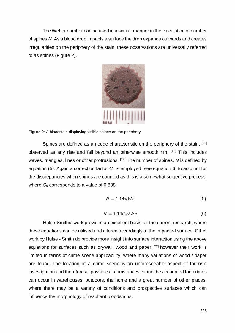
The Weber number can be used in a similar manner in the calculation of number
of spines N. As a blood drop impacts a surface the drop expands outwards and creates
irregularities on the periphery of the stain, these observations are universally referred
to as spines (Figure 2).
Figure 2: A bloodstain displaying visible spines on the periphery.
Spines are defined as an edge characteristic on the periphery of the stain, [21]
observed as any rise and fall beyond an otherwise smooth rim. [18] This includes
waves, triangles, lines or other protrusions. [18] The number of spines, N is defined by
equation (5). Again a correction factor Cn is employed (see equation 6) to account for
the discrepancies when spines are counted as this is a somewhat subjective process,
where Cn corresponds to a value of 0.838;
𝑁 = 1.14√𝑊𝑒 (5)
𝑁 = 1.14𝐶𝑛√𝑊𝑒 (6)
Hulse-Smiths’ work provides an excellent basis for the current research, where
these equations can be utilised and altered accordingly to the impacted surface. Other
work by Hulse - Smith do provide more insight into surface interaction using the above
equations for surfaces such as drywall, wood and paper [22] however their work is
limited in terms of crime scene applicability, where many variations of wood / paper
are found. The location of a crime scene is an unforeseeable aspect of forensic
investigation and therefore all possible circumstances cannot be accounted for; crimes
can occur in warehouses, outdoors, the home and a great number of other places,
where there may be a variety of conditions and prospective surfaces which can
influence the morphology of resultant bloodstains.
Ds final
bloodstain
diameter

216
Figure 3: An overview of different wooden surfaces and physical properties. Adapted from Ref [23].
It is these variations that will be investigated within this research; surfaces will be
stripped to its fundamentals and investigated. For example, if we consider the variants
of wood, [23] as expressed in Figure 3, each wood surface type will interact differently
with blood as a consequence of the physical properties and manufacturing process,
consequently producing a variety of different resultant bloodstains.
Due to the limited research into blood and surface interactions there are a
number of factors that must be explored not least the physical properties of both the
surface (i.e. roughness, topography) and the blood itself (i.e. PCV %) but also the
conditions of the surface, for instance if it is heated in the case of a radiator. During
this study many of these aforementioned bases will be approached culminating in a
final equation or several equations. To accomplish this a combination of blood drop
tests, DNA analysis and presumptive testing will be utilised in conjunction with the
above - mentioned pre-determined equations proposed by Hulse- Smith et al. [18] The
mission to find a purely quantitative reliable method of pattern analysis has been the
aim of many Bloodstain Pattern Analysts and therefore results obtained from this study
could be of significance for both use in the field and presentation in criminal trials.

217
1.1 AIMS AND OBJECTIVES
Academic Aim: To improve the scientific understanding of bloodstain pattern
analysis and generate directly applicable quantitative approaches which will in turn
establish a standard way of analysis within a Crime Scene.
Objectives:
2.1 - To examine aspects of blood that will heavily influence the blood patterns
produced such as, PCV % and its possible effect upon viscosity.
2.2 - To assess and evaluate how appropriate current quantitative methods of
analysis within BPA are when real life conditions such as the varying surfaces are
encountered.
2.3 - To develop new equations and easier methods of analysis when blood
patterns are encountered, pertaining to the aforementioned varying surfaces.
2.4 - To establish a valid and appropriate standard protocol pertaining to the
collection and preservation of BPA evidence, this can be used as a direct reference
at crime scenes.

218
1.2 BACKGROUND
1.2.1 What is Bloodstain Pattern Analysis?
Bloodstain Pattern Analysis (BPA) is the forensic study of blood formations
created at crime scenes during a bloodletting incident. [8, 9, 11 24] Analysts study the
shapes, sizes and locations of bloodstains in order to determine the physical events
which created them. These blood patterns are utilised to ascertain certain factors such
as: [20]
Sequence of events
Movement through the scene
Positions (i.e. sitting, standing etc.) of victim, assailant or objects.
Area of origin of bloodletting incident
Has the body been moved
Minimum number of blows executed
Possible weapon type
The analysis of bloodstains is achieved a number of ways. Direct scene evaluation is
preferable however when this option is not available, analysis of scene photographs
(scaled) is an alternative. [8, 24] In order to accomplish a thorough evaluation bloodstain
analysis is done in conjunction with clothing analysis, weapons analysis etc. and
require access to hospital records, post-mortem examination, post-mortem
photographs, lab reports, crime scene reports and statements. [8, 24]
1.2.2 History of BPA
The customary belief is that Bloodstain Pattern Analysis is a recent forensic
discipline, and it is true that up until the 1950s the field was neglected, however we
can date the recognition of BPA as a “crime solving” technique back to the 1890s when
the Polish scientist Dr Eduard Piotrowski recognised their importance. [8, 9, 11 24]
Prior to the development of BPA as a forensic speciality, artists and authors
recognised the importance of blood and its patterns. References to ‘gouts and
219
splashes which lay all around’ and ‘there were murderers, steeped in the colours of
their trade’ were made by Sir Arthur Conan Doyle (A Study in Scarlet; 1887) and
William Shakespeare (MacBeth; 1606) respectively, where they used the presence of
blood to indicate death, perpetrator identification and to highlight a violent criminal act
had taken place. [4, 9, 24] There are even earlier allusions to the significance of blood,
the 17,000 year old cave painting ‘How to Kill a Horse’ [9] is believed to depict arterial
breaching. [9]
1.2.2.1 BPA Historical Figures
BPA has made substantial advancements in recent times however it is the initial
groundwork put down by the following researchers which has made BPA a significant
discipline within the field of forensic science. [4, 8, 9, 11, 24]
1.2.2.1.1 Dr Eduard Piotrowski
Dr Eduard Piotrowski conducted the first major research (controversial for its
use of live rabbits) in 1895 regarding the analysis of bloodstains for the purpose of
criminal investigation. [4, 8, 9, 11, 24] Piotrowski wrote a paper entitled ‘Concerning the
Origin, Shape, and Direction of Bloodstains following Head Wounds caused by Blows’
where he highlighted the importance of a bloodstain tail in origin directionality. [4, 8, 9, 11,
24]
1.2.2.1.2 Dr Victor Balthazard
Dr Victor Balthazard was a French criminalist who performed original research
in 1939 concerning bloodstain pattern trajectories. [4, 8, 9, 11, 24] Balthazard later worked
alongside the now infamous Herbert MacDonell outlining the significances of elliptical
stains and the use of the width to length ratio; used to determine the angle of impact.
[4, 8, 9, 11, 24]
1.2.2.1.3 Dr Francis Camps
A French pathologist who worked on the Setty case in 1949. Stanley Setty had
been missing for 2 weeks, when his body was discovered in a marsh, it was then a
question of finding the primary crime scene. Dr Camps uncovered stab wounds to the
victim which would he said “have bled profusely”, he concluded that the original crime
220
scene would hold a significant bloodstain. [4, 8, 9, 11, 24] This proved to be the case,
highlighting the distinct link between blood and crime, even alluding to possible
sequencing capabilities. [4, 8, 9, 11, 24]
1.2.2.1.4 Hans Gross
Mr Gross wrote the book Criminal Investigations in 1892 where the German
discussed observations he made of bloodstain patterns while evaluating crime scenes.
Gross wrote about the directionality of stains, pointing to the shape as an indicator of
direction of travel. [4, 8, 9, 11, 24]
1.2.2.1.5 Dr Josef Radziki
Dr Josef Radziki introduced 3 categories of bloodstain patterns in his work
‘Bloodstain Prints in the Practice of Technology’; 1- bloodstains resulting from an
extravasation/fluid leakage, 2- bloodstains caused by some form of instrument and 3-
bloodstain which have been altered i.e. wiping. These 3 categories are now commonly
referred to as passive, projected and transfer. [4, 8, 9, 11, 24]
1.2.2.1.6 Dr Paul Leland Kirk
Dr Paul Kirk, a biochemist professor at UC Berkley, was one of the most
influential people in the field of forensic science, especially Bloodstain Pattern
Analysis. [4, 8, 9, 11, 24] He has been involved in very high profile cases; The Burton Abbott
case and his most famous case Dr Sam Sheppard. Dr Sam Sheppard was arrested
for the murder of his wife Marilyn in 1955, through numerous retrials Dr Sheppard
maintained his innocence. During the last retrial Dr Paul Kirk presented an affidavit on
the blood patterns present at the scene, his interpretation showed the relative position
of the attacker and the victim and he concluded that the perpetrator was left handed,
which Dr Sheppard was not. Dr Kirk’s evidence exonerated Dr Sheppard. Sheppard’s
story was immortalised in the film, ‘The Fugitive’ which is believed to be heavily based
on this case. [4, 8, 9, 11, 24]
1.2.2.1.7 Dr Herbert Leon MacDonell
MacDonell, considered to be the ‘Father of BPA’, together with the Law
Enforcement Assistance Administration (LEAA), conducted experimental research

221
into the recreation and duplication of bloodstains found at crime scenes for the
purpose of reconstruction. [4, 8, 9, 11, 24] From this research he published ‘Flight
Characteristics and Stain Patterns of Human Blood’ in 1971; later he revised this
(1982) under a new title ‘Bloodstain Pattern Interpretation’ and in 1993 he wrote ‘Blood
Patterns,’ all highly influential books. [4, 8, 9, 11, 24]
MacDonell, with many other experts, formed the International Association of
Bloodstain Pattern Analysts (IABPA) in 1983, the society now consists of over 800
members whose purpose is to publicise the discipline, create standards of training and
interpretation, and to promote BPA research. [4, 8, 9, 11, 24]
1.3 Bloodstain Pattern Terminology
Bloodstains can be created a number of ways, studying these patterns can
assist in ascertaining the mechanism behind the creation of the bloodstains.
Determining how the patterns were created is vital if an accurate reconstruction is to
be established. [24]
There are six basic reproducible pattern types, these include:
Blood ejected from a point source
Blood ejected over time from an object in motion
Blood ejected in a streaming ejection
Blood dispersed through air as a function of gravity
Blood that accumulates or flows on a surface
Blood deposited through transfer
1.3.1 Blood Patterns
Wonder, [9] and Gardner and Bevel [24] split bloodstain patterns into two groups (Figure
4), spatter and non-spatter. These categories where used to create a flow diagram in
which recognisable blood patterns were classified. More information regarding stain
description is provided within Appendix 1.

222
Figure 4: Flow chart expressing blood stains in to two categories; spatter and non-spatter.
The Terminology used by Gardner, Bevel and Wonder has been formalised by the
Scientific Working Group for Bloodstain Pattern Analysis and now forms the standard
of BPA terminology.
1.3.2 Directionality
The directionality of a blood drop can be determined using the shape of the resultant
bloodstain. When the drop hits the surface it will keep travelling in the same path that
it was travelling prior to hitting the surface. [4, 8, 9, 11, 24]
Figure 5: Arrows indicate direction which bloodstain was travelling using tail and scallops of a
bloodstain.
The tail/spines/scallops point to the direction of travel (Figure 5), therefore the
opposing direction points to where the drop originated. Directionality can be used to
- Spurt
- Cast-off
- Drip Trail
- Expiration
- Impact
- Mist
- Drip
- Smear
- Blood into Blood
- Gush/Splash
- Swipe
- Wipe
- Pattern Transfer
- Saturation
- Flow
- Pool
Irregular Linear Non-Linear
Spatter Non-Spatter
Blood
Regular

223
determine the movement within the crime scene at the time of the bloodletting event
(i.e. running, walking). [4, 8, 9, 11, 24]
1.3.3 Area of Convergence
The area of convergence is a shared area where individual bloodstains can be traced,
it represents a 2-D size and shape of the Area of Origin. [9] Strings or a pen and ruler
can been used to draw a line through the centre of well-formed bloodstains which are
extended back into the direction from which they came. [4, 8, 9, 11, 24] The strings or lines
will cross if they are the result of a single impact, an area of convergence will be formed
rather than a point, since no two drops will originate from the same point. [4, 8, 9, 11, 24]
Figure 6: Area of convergence, a common area where bloodstains intercept.
1.3.4 Angle of Impact
The angle of impact measures the acute angle created between the blood drop and
the surface it lands on. It is particularly useful as it is used to calculate the area of
origin. [4, 8, 9, 11, 24]
Area of Convergence

224
Figure 7: Diagram representing the theory of the occurrence of angled impacts
The angle of impact is currently measured using the width (w) and elliptical length (l)
of the bloodstain.
Figure 8: An elliptical directional bloodstain indicating where measurements should take place for angle
of impact calculation.
Note: measurements do not include the tail, spines, scallops or satellite spatter; only
the main body of the stain is measured. [4, 8, 9, 11, 24]
The angle of impact (θ) is calculated using the following equation 7;
Sinθ = (W/L) (7)
Results are an indication of angle of impact and generally give a 5 – 7o margin of error,
depending on the operator. [4, 8, 9, 11, 24]
1.3.5 Area of Origin
The determination of the area of origin is significant; it identifies where the blood
source was located at the time the distribution of blood was generated. It gives a 3D
indication of the area where the bloodletting incident occurred. [4, 8, 9, 11, 24] This can
prove or disprove a person’s statement pertaining to the sequence of events, i.e. a
person stating they were on the floor defending themselves however stains indicate
that the person was standing. [4, 8, 9, 11, 24]
Width (minor
axis) Length (major
axis)
a
c b
Droplet
Angle of
Impact
225
There are currently three methods for calculating the Area of Origin:
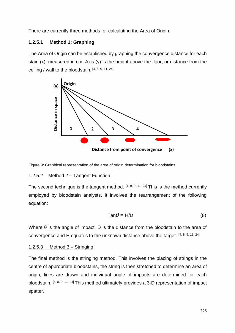
1.2.5.1 Method 1: Graphing
The Area of Origin can be established by graphing the convergence distance for each
stain (x), measured in cm. Axis (y) is the height above the floor, or distance from the
ceiling / wall to the bloodstain. [4, 8, 9, 11, 24]
Figure 9: Graphical representation of the area of origin determination for bloodstains
1.2.5.2 Method 2 – Tangent Function
The second technique is the tangent method. [4, 8, 9, 11, 24] This is the method currently
employed by bloodstain analysts. It involves the rearrangement of the following
equation:
Tanθ = H/D (8)
Where θ is the angle of impact, D is the distance from the bloodstain to the area of
convergence and H equates to the unknown distance above the target. [4, 8, 9, 11, 24]
1.2.5.3 Method 3 – Stringing
The final method is the stringing method. This involves the placing of strings in the
centre of appropriate bloodstains, the string is then stretched to determine an area of
origin, lines are drawn and individual angle of impacts are determined for each
bloodstain. [4, 8, 9, 11, 24] This method ultimately provides a 3-D representation of impact
spatter.
Distance from point of convergence (x)
1 2 3
Origin
4Dis
tan
ce in
sp
ace
(y)
226
There are other methods of analysis which are constantly developing, these involve of
computer programs (i.e. Backtrack, Hemospat) to generate a 3-dimensional
perspective. Currently the tangent method is still the analytical method of choice.
[4, 8, 9, 11, 24]
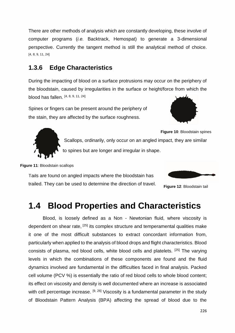
1.3.6 Edge Characteristics
During the impacting of blood on a surface protrusions may occur on the periphery of
the bloodstain, caused by irregularities in the surface or height/force from which the
blood has fallen. [4, 8, 9, 11, 24]
Spines or fingers can be present around the periphery of
the stain, they are affected by the surface roughness.
Scallops, ordinarily, only occur on an angled impact, they are similar
to spines but are longer and irregular in shape.
Tails are found on angled impacts where the bloodstain has
trailed. They can be used to determine the direction of travel.
1.4 Blood Properties and Characteristics
Blood, is loosely defined as a Non - Newtonian fluid, where viscosity is
dependent on shear rate, [25] its complex structure and temperamental qualities make
it one of the most difficult substances to extract concordant information from,
particularly when applied to the analysis of blood drops and flight characteristics. Blood
consists of plasma, red blood cells, white blood cells and platelets. [25] The varying
levels in which the combinations of these components are found and the fluid
dynamics involved are fundamental in the difficulties faced in final analysis. Packed
cell volume (PCV %) is essentially the ratio of red blood cells to whole blood content;
its effect on viscosity and density is well documented where an increase is associated
with cell percentage increase. [9, 26] Viscosity is a fundamental parameter in the study
of Bloodstain Pattern Analysis (BPA) affecting the spread of blood due to the
Figure 10: Bloodstain spines
Figure 11: Bloodstain scallops
Figure 12: Bloodstain tail
227
resistance to flow. [27] Resulting viscosity values are heavily reliant on; temperature,
time, shear rate and as previously stated, packed cell volume. A multitude of studies
have been executed exploring how the viscosity can ultimately determine the size of
the bloodstain diameter [4, 5, 9, 20], with the general consensus being that the higher the
viscosity the smaller the resultant bloodstain. Other studies involving the manipulation
of viscosity with drugs [27 - 28] and alcohol [20] have also been investigated, finding they
significantly decrease the dynamic viscosity, showing how easily manipulated
viscosity can be. There has yet to be however any exploration into the importance of
PCV % and its possible effect on the viscosity within the field of Bloodstain Pattern
Analysis; experts tend to focus on viscosity effects rather than the fundamental
parameters which give rise to the observed effect. [4, 5, 9, 20] The variance in the PCV %
levels is not only dependent upon location within the body [9] where values can deviate
from 30 – 52 % [9] but is influenced by the lifestyle of the person. Packed cell volume
levels as low as 15 % have been documented for persons who are drug abusers,
chronic alcoholics, malnourished and / or elderly. [9] Similarly new-borns, people
suffering from shock, extreme exercisers and heart attack victims have very high PCV
% reaching 75 %; [9] with values deviating from the normal to such an extent research
concerning PCV% could offer some interesting insights especially when considering
bloodstain size and appearance.
1.4.1 Blood Drying
Another highly influential biological parameter displayed within blood is drying.
[9, 29 - 32] This process is manipulated by surface type (e.g. wettability), environmental
conditions and climate, acting like a catalyst when conditions are particularly warm. [33]
The drying process of liquids in general is a fascinating topic, with recent
investigations unearthing some interesting conclusions. The ‘coffee-ring effect’ has
been identified where liquids display a ‘ring’ similar to that seen when a drop of coffee
dries, where suspended particles are pushed and collected on the periphery of the
drop. [34, 35] Yunker et al [36] have revealed that it is the shape of the suspended particle
that is the driving force behind the coffee-ring effect and by simply changing the shape
of the particles from spherical to elongated / ellipsoidal and uniformly dispersing these
within the colloidal substance causes an attraction between particles. [36] Due to the
nature of the ellipsoidal foreign particles being anisotropic (directionally dependent),
228
this prevents the particles from reaching the drop periphery and therefore dispersing
evenly throughout the drop. [36]
In recent studies by Brutin et al [37] it has been identified that the Marangoni
Effect is the mechanism by which blood dries, where surface tension forces drive the
drying effect. [38] A surface tension gradient is observed and is the driving force for
blood drying where the difference in surface tension, for instance, occurs between red
blood cells and plasma. [38] Brutin et al [37] performed these experiments using a digital
camera at a high optical zoom which does limit the overall visual analysis capable,
preventing true insights into particle travel, which may allow for further interpretation
in to drying. Although this research [37] offers insight into blood drying effects it does
not allow the effect of PCV % to be addressed, as previously specified packed cell
volume is a changeable parameter within blood and could alter drying significantly.
It is not merely the mechanism in which blood dries that is of importance but
what dried blood can reveal about the committed crime. Original volume estimation
can provide vital information as to the condition of the victim if the body is absent, it
can also be of medical significance giving an indication of expected survival time.
There are several methods of volume analysis [39 - 42], the oldest and currently the most
reliable is the dry weight method formulated by Lee et al. [39] Lee et al [39] conducted
several experiments where the dried blood is scraped off the surface and weighed.
This weight is then multiplied by the 3.25, a corrected constant derived again by Lee
et al, [39] to find the original volume. This method however is limited since it is only
suitable for non-absorbent surfaces and can be time consuming as the bloodstain
must be fully dried and scraped completely from the surface.
Lee et al developed many more methods of volume analysis, [39] indirect
approaches which can be used when direct methods are deemed unsuitable, where a
unit of the bloodstain is weighed, and an acetate overlay incorporated with a grid of
1cm squares can be placed over the top of the blood pool. [39] More recent direct
methods involve the utilisation of spectrophotometry, where the absorption of
haemoglobin is measured [40] and photography, where digital image software
calculates the surface area; this was found to closely correlate to the volume. [41] Other
observations that can be made pertaining to the drying of blood are; skeletonisation,
[4] where the outline of the blood is still present when the stain is wiped, and the halo
effect, [42] where a ring is apparent on the periphery of the stain; these techniques may
be used to sequence an event. For example the ring will appear red when a drop is
229
first deposited onto a surface and then is followed by a swipe after a small amount of
time. When this sequence is switched the ring will appear the same colour as the
surface in which it has impacted. [42]
However, as previously detailed (see section 1.3), blood can differ greatly
person to person; [9] it is unknown what the significances of such changes in the
components of blood will have on the drying bloodstains. Consequently the following
research explores the fundamental parameters of the drying effects of both human
and equine blood, the influence of PCV % when applied to drying time, volume
estimation, drying effects and resultant bloodstain size, and ultimately what
consequences this pertains to the field of BPA; as such this work is of both
fundamental and applied importance.
1.5 Blood Drop Formation
The study of drop formation has been researched for the last 100 years,
providing insight into key processes such as inkjet printing. Gaining knowledge of this
subject is of high importance if we are to understand the mechanics behind blood stain
patterns.
Water has similar properties to blood therefore much of the work exploring drop
formation is based on the previous studies of water droplets.
Rein [43] described the phenomena of water drops impacting solid and liquid
surfaces, which included bouncing, spreading and splashing. In this work Rein [43] used
and developed analytical models to predict maximum final stain diameter following
impact. Consideration was given to the liquid properties; surface tension and viscosity
which play a vital role in droplet spreading, proportionately increasing the resistance
to spreading. The Reynolds (equation 1) and Weber (equation 2) numbers describe
these liquid properties. Further exploration into droplet spreading was carried out by
Pasandideh-Fard et al [44] where water was photographed dropping onto a stainless
steel surface, these computer generated photographs were used to develop a model
to predict the maximum drop spread diameter (Dmax) following impact. Spines, the
protrusions exhibited around the edge of a drop / bloodstain, were investigated by
Mehdizadeh et al [45] continuing the innovative work of Balthazard et al, [46] who
originally introduced and correlated the number of spines found on the periphery of a

230
bloodstain with the release height of the drop, they however used water drops to create
an analytical solution for the calculation and prediction of number of spines. [45]
The evolutionary development of a bloodstain is a more complex process; the
forces acting upon a blood drop, the impacted surface and the composition of the
blood itself dictate the size, shape and overall appearance of the resultant bloodstain.
[7 - 9] Early works by the pioneers of BPA, Dr Paul Kirk [47] and Dr Herbert L. MacDonell,
[20] have involved the formation of circular bloodstains. This comprised dropping blood
onto surfaces at a 90o angle with results revealing an increase of bloodstain diameter
with increasing impact velocity up to terminal velocity (approximately above 200cm),
where forces reach an equilibrium and diameters cease to increase. [20, 47]
More recent developments within BPA have established equations that can be
readily applied at Crime Scenes; [17, 18] these equations can deduce the angle and
direction of the impacting blood drop with the use of the size and shape of the final
bloodstain; [17, 18] within these equations important physical properties of blood were
considered, namely the viscosity, surface tension and density. [7 - 9]
Collaborating all of the above data Hulse-Smith et al [18] generated equations
applicable to the formation and impacting of blood drops. These equations (4 and 6)
allowed the impact velocity of a blood droplet impacting a horizontal surface to be
determined from the number of spines around the bloodstain and the stains size.
Developing on this work Knock et al [17] investigated into the effect of the angle of
impact, offering a new way of predicting the origin of a bloodstain. [24] The conventional
way of determining the origin of impact is an archaic method known most commonly
as the stringing method. [24] The stringing method is a simple procedure to determine
the area of convergence, a shared area in which all stains in a distribution originate.
[24] An alternate more relevant method is that of the tangent method, where the
procedure is similar to that of the stringing method however lines instead of strings are
drawn and origins are established using the tangent of the angle of impact and
multiplying by the distance to the convergence. [24] However, again this is a very
laborious exercise and requires expertise/experience when choosing the convergence
site. Knock et al developed a new equation which considers all the physical properties,
impact velocity and angle of the impacting blood: [17]
ab = 111.74 ( Re0.5We0.25)0.75DoDo + 0.00084 (9)

231
where a and b are the width and elliptical length of the bloodstain respectively. [17]
Knock et al found that the impact angle could be neglected as it is independent of the
bloodstain size and therefore angles are excluded from the final equation to determine
bloodstain size. [17] It is noted however that there is a discrepancy within the research
where the first value changes from 111.74 to 11.74 and that this may alter the results
by a factor of 10. Investigations into the effects of angles upon the number of spines,
N, were also undertaken, again unveiling a new equation where an angle of impact
was included to the power of three: [17]
N = 0.76We0.5sin3θ (10)
This is an excellent step in the making BPA, a discipline noted for its subjective
nature, [17, 18, 24, 47] more quantitative and scientifically minded, this will be a point of
discussion later.
1.6 Surface Interactions
The impact surface is of great importance, it is what dictates the final overall
appearance and size of the bloodstain. [14, 20, 47] The substantial number of possible
surfaces that blood may contact during a bloodletting incident makes Bloodstain
Pattern Analysis particularly difficult. General observations regarding surface type
have been made; Kirk [47] observed the difference between absorbent and non-
absorbent surfaces, absorbent surfaces allow the blood drop to spread due to a
capillary action whereas non-absorbent surfaces will repel from the surface creating a
thinner initial stain. [47] MacDonell dispensed drops on various surface types (glass,
paper, wood, corrugated cardboard etc.) commenting on the surface roughness as
creating distorted asymmetrical stains and increased splash. [20]
Some single surface detailed analysis research has been performed on fabrics
and blood drops, due to the preponderance of blood found on the clothing of both the
victim and the assailant. [48 - 54] Similar findings to the general observations first
summarized by Kirk [47] were obtained; the bloodstain size depends on the
characteristics of the surface, decreasing the bloodstain size as the absorbance
increases. [48 - 54] These however are observations and again demonstrate the lack of
quantitative analysis within this field. However, some important insights are made in
these studies, for instance early works by White [51] focused on blood impacts, finding
that the angle of impact measured became unreliable due to the degree of distortion

232
a bloodstain experiences when it impacts upon a fabric. [51] Other investigations [48 – 50,
52 - 54] have primarily focused on the difference between projected stains and transfer
stains, these studies do not help with the current issue, verifying the science in the
interpretation of bloodstains.
Currently there are few statistically viable work conducted on the interaction of
blood on fabrics. [48, 49] De Castro et al [48] investigated individual passive, transferred
and absorbed blood drops on 2 types of cotton apparel. De Castro et al found that the
stain size was not dramatically different however the number of satellite spatter
changed significantly depending on height. [48] It is noted that the authors standardised
the fabrics using the protocol outlined in section 8A of BS EN ISO 6330/A1:2009, a
procedure procured for the domestic washing and drying of garments which produces
a standardised fabric. [55] Fabrics are laundered 6 times (washing cycles) and dried
flat following section 10C of the same method. [55] Although this standardisation
method is good practice as it should provide consistent, replicable results, it is not
indicative of real-life where fabrics/clothes are washed using various methods,
detergents and are dried using different techniques. The second quantitative study
involved the distinguishability of one fabric surface from another with the use of
satellite spatter. [49] Two fabrics of similar composition were evaluated. They
discovered there to be a statistical difference relating to the roughness of the surface
and the number of satellite spatter produced. [49] Concluding that as surface roughness
increases so does the number of satellite spatter and that this is directly related to the
composition of the fabric (synthetic vs. natural fibres). [49]
New recent works have focused on surface related quantitative analysis,
Hulse - Smith et al [18] introduced separate equations which were developed for three
different surface types, following on from his earlier work where a general equation
was established. [18] Although this is an excellent basis for future surface related
research it is an unrealistic approach, as previously discussed there are many varieties
of a particular surface (i.e. porosity, surface finish) and testing one version cannot
possibly be emblematic of the overall surface type. Studies need to address the
properties of a surface before any real equations can be formulated.
It is not purely the type of surface which effects the formation of a bloodstain;
the condition of the surface will also influence the final stain. For instance if the surface
is heated; blood could impinge common heated surfaces such as a radiator, heated
flooring, oven or stove potentially heating any impinging blood up to temperatures of

233
900° C. [56] Previous investigations into acts of arson and homicides that have involved
fire give an indication as to the potential effects of heat on blood. [57 – 58] These cases
however only show the effects of extreme heat, where the heat is applied after blood
spillage often leaving the bloodstain covered in soot; instead of a pre-heated surface
where the bloodstain may be cooked. There has yet to be any published research on
the effects of blood on a heated surface with respect to BPA, however there is an
extensive library of research exploring water droplets and various other liquids
impinging heated surfaces. [24, 40 – 43] Much of this research has been performed with
the use of high speed photography, analysing the rebound of the drop and the way in
which the drop behaves when heated. [59 – 63] Four major heating regimes of liquid
media have been identified by Nukijama: [62] 1) Natural Convection; 2) Nucleate
Boiling; 3) Transition Boiling; and 4) Film Boiling. These regimes where first
established for pool boiling, where the heated surface is submerged in a static liquid,
[63] with subsequent work revealing their applications within liquid sprays and in liquid
drops. [63] A boiling curve demonstrating the occurrence of these regimes was diligently
created by Farber and Scorah et al, [63] where heat flux is plotted against ΔT ( Tw –
Tsat, the difference in surface temperature (ΔT) and temperature of the liquid’s
saturation point respectively). Natural convection is the natural heat flow and occurs
when Tw (surface temperature) is equal to room temperature or slightly above;
increasing Tw towards the maximum boiling point (100oC) creates nucleation zones
where bubbles start to form in the centre of the liquid. [62] The third regime, transition,
occurs directly after the nucleation regime and ends at the Leidenfrost point. [59] The
Leidenfrost point takes place during the Leidenfrost effect where the temperature of
the surface is substantially hotter than the liquid’s boiling point usually at ΔT ≥ 120oC
and above. During the Leidenfrost effect initial rapid evaporation occurs
instantaneously creating a stable layer of vapour between the liquid and the surface,
exemplified in the dropping of cooking oil into a hot pan where this effect is put into
action, oil skids around the metal pan never making contact with the surface. In this
regime, the liquid does not fully contact the surface and therefore overall takes a longer
time to evaporate. The last regime is the film boiling regime where the Leidenfrost
effect is realised. [62] Since water constitutes 83% of whole blood it is thought that it
may behave it a similar way and therefore these regimes should fit the analysis of
heated blood.

234
Similarly there has been only one published investigation into the effect of a
cold surface and impacting blood, where Leak et al [64] described bloodstains found
during an outdoor crime scene search, where bloodstains were located on snow. The
freezing temperatures (2oF/16oC) caused a discolouration of the blood and created an
overall puffiness to the stain; this led to the initial mis–interpretation of the stains as
being brain matter. [64] Again some water droplet studies can offer more insights, where
drops formed ice pellets at the impact sight, [65] the solidified drops were noted for the
protrusions present on the top of the drop and the deformation of the final shape. [44]
However these protrusions were found to be surface dependent, and only appeared
on hydrophilic surfaces and not on hydrophobic surfaces. [57]
Despite all the above research there have been few developments (i.e.
objective criteria) [9] which can realistically be used during a crime scene situation.
Many factors are missing from the current equations meaning BPA is still being
analysed using the old subjective methods.
1.7 Further uses of Blood evidence
It is not only for the patterns it leaves to why blood is an important form of
evidence; blood is an excellent source of DNA (deoxyribonucleic acid) which is
essentially a genetic fingerprint of an individual. [66] DNA (deoxyribonucleic acid) is a
long molecule consisting of two polynucleotide strands wound around each other
connected via hydrogen bonds forming the distinct double – strand helix.
Each strand consists of a sugar-phosphate backbone and organic bases attached in
pairs. [66] There are four types of nucleotides within DNA, which are able to connect
pairs in any order and at various lengths; these four nucleotides differ in that they
contain a different base (adenine, thymine, guanine, and cytosine), it is the sequence
of these bases which is unique to the individual. [66] Although only 0.1% of a person’s
genetic code differs from any other there has yet to be two individuals (with the
exception of identical twins) with the same DNA profile. [66] The presence of DNA in
such samples as; blood, semen, human tissue, is the pretext behind their prevalence
as an extremely useful forensic technique, with DNA databases cataloguing the
profiles of individuals reaching 7.8 million profiles in the USA [67]and over 6 million in
the UK. [68]

235
Since 1984 when Alec Jeffreys first introduced the potential of DNA analysis
as a forensic technique, [66] its evidentiary significance has been apparent, providing
the basis for scientific testimony and evaluation which can be utilised within criminal
trials. This has led to perpetrators resorting to innovative ways of ‘covering up’ their
crime; i.e. cleaning away bloodstains. There have been significant reports upon the
possible effects of cleaning of crime scenes; [67 - 69] criminals are now attempting to
eliminate any trace of DNA via various methods of cleaning. Previous investigations
have been undertaken into commonly used methods of cleaning such as water, 10%
bleach and detergents. [66] A study conducted by Harris et al [66] on the cleaning of
different substrates and the ability to extract a DNA profile discovered that although
bleach had deleterious qualities, it did not eliminate the entire profile, in fact the
efficiency in which DNA was extracted was dependent upon the substrate from which
DNA was collected.[66] Bright et al [70] further supported these findings with research on
cleaning reagents using multiplex kits (Identifiler™ and PowerPlex® Y) where again
cleaning reagents proved ineffective at removing the DNA. This research however only
confirms conventional methods of cleaning, crime evasion / committing the ‘perfect’
crime is heavily publicised within the media and popular television shows and it
therefore seems inevitable that new more innovative ways of cleaning the scene will
be attempted, using stronger solvents that due to the world wide web may be easier
to access.
As stated by Harris et al [66] it is in fact the substrate which determines how
effective the DNA extraction will be. Extractions performed on certain dyed fabrics are
particularly problematic where dyes can inhibit the PCR (Polymerase Chain Reaction)
causing heterozygote imbalance, allelic dropout, stutter and non-specific artefacts (i.e.
primer dimer). [71] Generally DNA extraction has proven possible on most other
surfaces, Stein et al [72] investigated the typing of biological stains on typically
encountered crime scene surfaces; glass, metal, paper, adhesive tape and plastic,
finding that all samples could be profiled regardless of the surface type. [72] The robust
nature of DNA offers a stability that most other evidence forms lack, its survival through
difficult environment conditions such as humidity, [73] direct UV exposure [73] and fire
[58] has been well documented. Currently it is unknown if DNA will survive if applied to
a pre-treated surface, for instance the effect of DNA left on a heated surface, where
the DNA could be affectively “cooked,” which could subsequently destroy the DNA. As
explained above it is a realistic possibility that blood, could spatter onto a heated
236
surface i.e. a radiator. Like BPA, DNA is still a relatively new field in relation to other
forensic disciplines; incredible advances have been made in the last 40 years making
it one of the most (alongside fingerprints) important evidence forms. [2, 3]
1.8 Real Science?
Even with BPA being readily used as an evidence form in both UK and US
courts, there are still sceptics who do not believe it to have any scientific merit. [75 - 77]
BPA is considered to be a subjective discipline, with the basis of its analysis being on
the recognition of patterns identified by experienced analysts. The main issue this
presents is the variation in professional opinion when analysing blood patterns, this
issue has been raised multiple times over the years and is still a very present problem.
Discrepancies can occur in several levels of analysis with disputes ranging from
the correct way to measure a bloodstain to the taxonomy and categorisation of stains.
Taxonomy is important in any discipline but is crucial in forensic disciplines as it will
be referred to in court. Having a structured and easily explainable taxonomy makes
court presentations simpler, providing the ‘expert’ with strong support which they can
state their conclusions on. BPA does have a formalised standard international
taxonomy which is available from the SWGSTAIN website, however it appears that
other well established experts still follow their own taxonomy leading to confusion
when collaborating with other experts and presenting findings in court. MacDonell
referred to them as dynamics where size of stains distinguishes the action; Low
velocity Spatter (LVIS≥4mm), Medium Velocity Spatter (1mm≤MVIS≥4mm) and High
Velocity Spatter (HVIS≤1mm). [11] In 2002 another taxonomic system was developed
by Bevel and Gardner, [24] here patterns were classified into three categories: Passive,
Transfer and Dynamic, in 2005 James et al [4] altered this to Passive, Transfer and
Projected. Recently Wonder [9] documented the stains as spatter and non-spatter
(Appendix 1), creating a flow chart which categorised the patterns into each
classification. This method was modified by Bevel and Gardner [24] who developed a
flow chart with a comprehensive methodology and stain description, an excellent and
portable equipment piece which can be carried to the crime scene by analysts. A
complete description of each stain is essential as it provides support for the analyst
should they be questioned about their conclusions in a courtroom scenario.
237
The lack of a unified taxonomy amongst BPA professionals gives the
impression that the basis of BPA analysis is loose and subjective, less rigorous than
other forensic fields such as fingerprints which has a universal taxonomy used by all
fingerprint experts (e.g. whorl, loop etc.). It is up to the BPA community as a whole to
adopt the SWGSTAIN terminology, cementing the groundwork for which all
interpretations are based.
A further bone of contention within the field of BPA is the error associated with
the majority of the calculations performed. For example the angle of impact. It seems
simple to measure the elliptical length and width of a stain, however, every analyst
does it differently. Since stains are not always perfectly round or smooth, sometimes
protrusions are present on the periphery, it is difficult to gauge where the stain actually
begins and ends. Computer programs such as Backtrack which are supposed to
enhance the way interpretation can be performed carry this error, where analysts have
to stencil round the stain. Leading analysts to over or under estimate the angle of
impact. Steps towards solving this problem have been crafted, standard stencils have
been developed which can be placed on the stain, giving a guideline of the parts of
the stain to include. Other methods such as halving the stain then doubling the length
measurement has become the practiced method. Amendments to computer programs
have been established to improve the accuracy at which the angle of impact can be
calculated. Despite these amendments the manual method of measuring is still
considered the most accurate therefore it is a case of standardising training. The
IABPA offer many courses, basic and advanced which should be attended by all BPA
analysts. The courses are presented by experts who will be equipped to divulge a
standard way of measuring which would decrease analyst errors. It is important for all
those thinking of a career to attend these courses, therefore maintaining the integrity
of BPA as a forensic discipline.
Recent years have been a testing time for the field of Bloodstain Pattern
Analysis, doubts being raised publicly over its overall accuracy and applicability to
complex crime scenes. [76, 77] The case of David Camm is most likely the main cause
of people’s recent intense scrutiny of the field. [76, 77] In 2002 David Camm was
convicted of a triple murder (his wife; Kim, son; Brad, and daughter; Jill), his conviction
was largely based on the interpretation of bloodstain pattern evidence. [77] Since the
first trial, five renowned BPA experts [77] have assisted on the case, each interpreting
the stains differently, disagreeing on the nature of 8 bloodstains found on Camm’s T-
238
shirt. Were they impact stains (i.e. backspatter from shooting) or were the stains
caused by transfer (i.e. Camm moving his son and performing CPR)? [77] On the 24th
October 2013 after the third trial David Camm was acquitted. There are other
underlying issues this case has brought to light. One of the experts claimed a new
form of bloodstain, ‘the painted fibre’ supposedly only visible when blood is transferred
to a fabric and is not evident when blood impacts the surface by force. Since there is
no literature available on this discovery it was particularly damaging to the BPA field,
leading people to believe BPA experts will fabricate evidence to fit their theories.
Therefore it is important that experts publish their findings, avoiding this confusion in
the future.
The other weakness this case exposed was the lack of surface interaction
understanding. As demonstrated (see Section 1.6) surface analysis has been
neglected so far in the field, researchers giving broad interpretations (i.e. non-
absorbent vs absorbent) rather than focusing on surface properties (i.e. porosity,
composition).
Although experts try to mimic the surface as closely, to the crime scene surface
during a reconstruction, as possible, the exact surface is not always available.
Therefore it is important to understand how fundamental changes to surfaces such as
the porosity, surface finish etc. effect the formation and spreading of bloodstains.
It is clear from the above observations why BPA is sometimes considered
unscientific, however positive strives have been taken towards changing this
misconception.
The research presented in this thesis aims to expand the knowledge of blood
and surface interaction, by applying quantitative techniques, with the hope of
improving understanding and helping towards the verification of BPA as an essential
scientific forensic discipline.
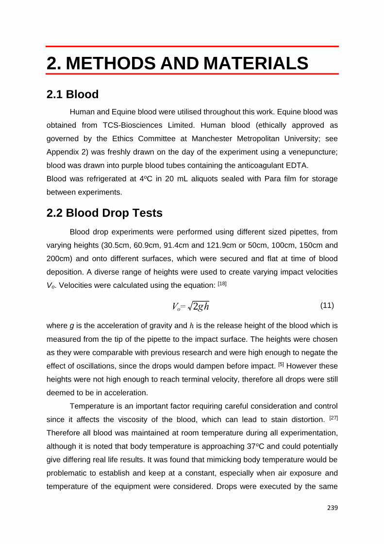
239
2. METHODS AND MATERIALS
2.1 Blood
Human and Equine blood were utilised throughout this work. Equine blood was
obtained from TCS-Biosciences Limited. Human blood (ethically approved as
governed by the Ethics Committee at Manchester Metropolitan University; see
Appendix 2) was freshly drawn on the day of the experiment using a venepuncture;
blood was drawn into purple blood tubes containing the anticoagulant EDTA.
Blood was refrigerated at 4oC in 20 mL aliquots sealed with Para film for storage
between experiments.
2.2 Blood Drop Tests
Blood drop experiments were performed using different sized pipettes, from
varying heights (30.5cm, 60.9cm, 91.4cm and 121.9cm or 50cm, 100cm, 150cm and
200cm) and onto different surfaces, which were secured and flat at time of blood
deposition. A diverse range of heights were used to create varying impact velocities
Vo. Velocities were calculated using the equation: [18]
where g is the acceleration of gravity and ℎ is the release height of the blood which is
measured from the tip of the pipette to the impact surface. The heights were chosen
as they were comparable with previous research and were high enough to negate the
effect of oscillations, since the drops would dampen before impact. [5] However these
heights were not high enough to reach terminal velocity, therefore all drops were still
deemed to be in acceleration.
Temperature is an important factor requiring careful consideration and control
since it affects the viscosity of the blood, which can lead to stain distortion. [27]
Therefore all blood was maintained at room temperature during all experimentation,
although it is noted that body temperature is approaching 37oC and could potentially
give differing real life results. It was found that mimicking body temperature would be
problematic to establish and keep at a constant, especially when air exposure and
temperature of the equipment were considered. Drops were executed by the same
(11)
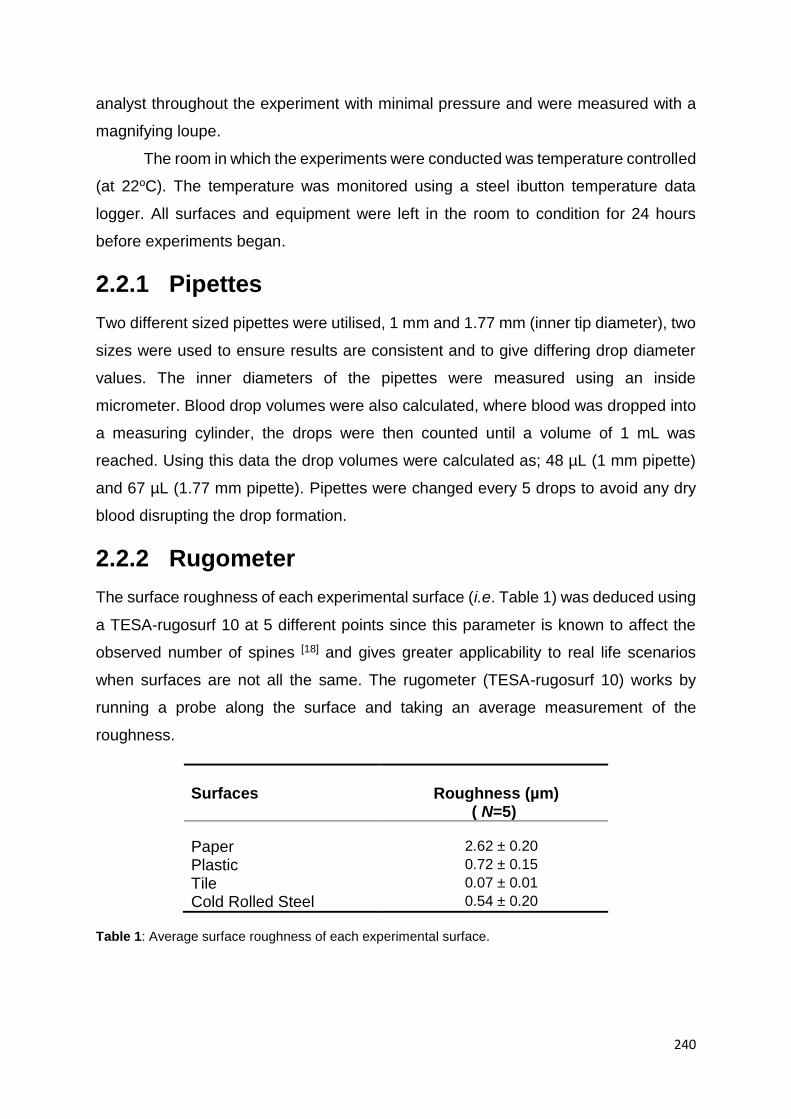
240
analyst throughout the experiment with minimal pressure and were measured with a
magnifying loupe.
The room in which the experiments were conducted was temperature controlled
(at 22oC). The temperature was monitored using a steel ibutton temperature data
logger. All surfaces and equipment were left in the room to condition for 24 hours
before experiments began.
2.2.1 Pipettes
Two different sized pipettes were utilised, 1 mm and 1.77 mm (inner tip diameter), two
sizes were used to ensure results are consistent and to give differing drop diameter
values. The inner diameters of the pipettes were measured using an inside
micrometer. Blood drop volumes were also calculated, where blood was dropped into
a measuring cylinder, the drops were then counted until a volume of 1 mL was
reached. Using this data the drop volumes were calculated as; 48 µL (1 mm pipette)
and 67 µL (1.77 mm pipette). Pipettes were changed every 5 drops to avoid any dry
blood disrupting the drop formation.
2.2.2 Rugometer
The surface roughness of each experimental surface (i.e. Table 1) was deduced using
a TESA-rugosurf 10 at 5 different points since this parameter is known to affect the
observed number of spines [18] and gives greater applicability to real life scenarios
when surfaces are not all the same. The rugometer (TESA-rugosurf 10) works by
running a probe along the surface and taking an average measurement of the
roughness.
Surfaces
Roughness (µm)
( N=5)
Paper 2.62 ± 0.20
Plastic 0.72 ± 0.15
Tile 0.07 ± 0.01
Cold Rolled Steel 0.54 ± 0.20
Table 1: Average surface roughness of each experimental surface.

241
All surfaces were cleaned with 1% ethanol and paper towel and rinsed with deionised
water, where surfaces were then left to dry and stabilise in temperature before any
blood drops were performed.
2.2.3 Slow Motion Filming
Blood drops were filmed in slow motion at 1200 fps (frames per second) using the
Casio Ex-F1 Digital Camera, enabling the capture of scaled still images of the blood
drops as they departed the pipette tip to allow the drop diameters, Do, to be deduced
as depicted in Figure 13.
A.) B.)
Figure 13: Scaled stills of blood drops. Image A shows a still of defibrinated equine blood drop using a
1mL pipette (1 mm inner tip diameter); Image B is of defibrinated equine blood drop using a 1mL pipette
(1.77 mm inner tip diameter).
Drops were discharged as close to the ruler as possible to avoid any size distortion.
2.2.4 Bloodstain Measuring
As aforementioned (section 1.7) it is important to establish a standard method of stain
measurement, therefore avoiding discrepancies in results attributed to analyst error.
The following method was adhered to for circular stain measuring:
Figure 14: Circular bloodstain depicting the actual diameter to be measured.
A circular stain is measured using the diameter/width,
this excludes any spines or fingers on the periphery of
the bloodstain (see Figure 14).
A magnifying loupe was utilised.

242
Similarly, angled impact stains were measured using the below approach.
Again the diameter/width of the stain was measured excluding any scallops/spines.
The ellipse length was consistently calculated, through all trials, by measuring half the
length of the stain up to the diameter (half length), this number was then doubled to
give the total ellipse length (Figure 15). This method is used as it excludes the tail and
scallops and gives a full ellipse length which is vital in order to calculate an accurate
angle of impact.
Half length
Elli
pse
le
ngth
width
Ellipse length
wid
th
Figure 15: Angled impacts showing the diameter and ellipse length measured

243
2.3 Part I Experimentation Equipment
2.3.1 Rheometer
A cone and plate rheometer (Kinexus Pro Rheometer) was utilised throughout this
study to measure the viscosity of blood. It is used to determine the viscosity in fluids
whose value does not remain constant, due to the shear forces present within the
liquid. [78, 79]
A cone and plate type rheometer consists of a horizontal plate and a shallow cone.
Liquid is placed onto the plate and the cone is lowered into the liquid. [78, 79] The plate
is then rotated and the force of the cone is measured. The viscosity is expressed as
the ratio of shear stress to shear rate, where the stress equates to the torque and the
shear rate relates to the angular velocity. [78, 79]
Blood viscosity was measured at shear rates of 100s-1 as this is when the viscosity
becomes constant and a single value can be determined. [18] Shear rates do not go
above 100s-1 within this research; therefore this is a valid approach. [18]
2.3.2 Tensiometer
A tensiometer is used to measure the surface tension of a liquid or a surface.
The type of tensiometer utilised in this research was the Du Noüy Ring Tensiometer
(CSC Du Nouy Precision Tensiometer), where a platinum ring is submerged in a liquid,
the ring is then slowly extracted. [80, 81] Once the ring is resting on top of the liquid a
measurement can be taken. The ring must be clean and free of scratches to attain an
accurate reading. [80, 81]
2.3.3 Goniometer
A goniometer is used to measure the contact angle of liquids on a surface. [81, 82]
A drop of liquid is deposited onto the surface whilst being filmed using a CCD
(charged-coupled device) camera. The drop profile of the captured image is then
extracted and computer software is used to fit the Young-Laplace equation: [81, 82]
∆𝑃 = 𝛾 (1
𝑅1|
1
𝑅2) (12)
where 𝛾 is the interfacial tension, P equates to the pressure and radius is defined as

244
R. [81, 82] The contact angle is important as it describes the degree of wetting which
ultimately determines the spreading of the liquid.
2.3.4 Microscope
An optical microscope (bright-field microscopy) uses reflection and absorption to
investigate the properties of substances. [83, 84]
The sample is placed on the stage of the microscope where an incandescent light,
situated beneath the sample, is shone through the sample where it is collected by an
objective lens, positioned above the stage. [83, 84] An aperture, contained within the
lens condenser, controls the amount of light and focus on the sample. [83, 84] The
objective lens magnifies the light and transmits an image to the eyepiece.
The microscope utilised in this study is attached to digital imaging equipment
(Leica DFC365FX), this allows the image to capture both still and filmed images.
2.3.5 Spectrophotometer
A spectrophotometer is an analytical instrument which quantitatively measures the
reflectance/ transmittance of a material. [85, 86]
It uses a photometer which measures a light beam’s intensity as a function of its colour.
The spectrophotometer used in this research was a UV spectrophotometer
(Spectrophotometer Model 6305 UV-VIS and Spectruino Arduino Spectrometer) this
focuses on the UV and visible regions of the spectrum. [85, 86] Samples are usually
prepared in cuvettes (plastic, glass and quartz) and light is shone through the sample.
An absorbance spectrum is formed which plots the absorbance vs wavelength. The
wavelength λmax is the most important wavelength, where the absorbance is at its
greatest. [85] It is characteristic of each compound and provides details on structure
which can be used to obtain high sensitivity when further testing is performed.
2.3.6 Hematocrit Centrifuge
Similar to a normal centrifuge, it spins a solution at a high frequency for a selected
time frame. [87, 88] The PCV% of blood was determined using a hematocrit centrifuge.
Blood is placed in a capillary tube (microhematocrit tube), the tube is positioned in a
hematocrit centrifuge which spins the blood at 10,000 RPM for 5 minutes. The blood
is separated into plasma, red blood cells and a buffy coat (white blood cells and

245
platelets). The lengths of the blood and red cells are measured to obtain a percentage.
[82, 83]
2.4 Part II Experimentation Equipment
2.4.1 Smoothness & Air Permeance (Bendtsen Type)
The roughness or smoothness of the sample is measured by establishing the volume
or air that passes through the material at a given pressure.
The test is performed accordingly. [89, 90]
The sample is placed on the glass plate, a measuring head is placed on the sample.
Air is then passed through the flat metal ring and sample at a given pressure. The
pressure difference is read. [89, 90]
2.4.2 Scanning electron microscope (SEM)
A Scanning Electron Microscope (SEM) is utilised throughout this study to capture
images of the surfaces. [91, 92]
An SEM is a type of electron microscope which produces highly magnified images of
a sample by scanning it with a focused beam of electrons. [91, 92]
The electrons interact with the atoms in the sample, producing signals which can
detect and hold information regarding the surface’s topography and composition.
[86, 87]

246
2.5 Part III Experimentation Equipment
2.5.1 Furnace and Hot Plate
A furnace was used to heat surfaces to temperatures of up to 250oC, the temperature
was maintained with the use of a hot plate, which was placed underneath the surfaces
as testing proceeded. The temperatures were tested with an infra-red temperature
gun.
2.5.2 Infra-Red Spectrometer
The infra-red (IR) spectrometer focuses on the infrared region of the electromagnetic
spectrum, where light has longer wavelengths and occur at a lower frequency than
those in the visible light. [93, 94] Molecules absorb at specific frequencies which are
characteristic of their structure, IR uses this fact as an identifier. Spectroscopy is
performed by passing a beam of infrared light through the sample, when the IR
frequency matches that of the vibrational frequency an IR spectrum is formed. [93, 94]
The IR spectrum created plots the wavelength/frequency against the
absorbance/transmittance. A Fourier Transform Infrared Spectroscopy (FTIR) is the
type of IR utilised within this work, [94] which works in a similar way to IR however the
FTIR runs several scans, uses an interferometer and uses Fourier Transforms to
convert the interferogram into an IR spectrum. [94]

247
PART I:
BLOOD

248
3. BLOOD CHARACTERISTICS
The following chapter discusses blood and its components, where three studies
were undertaken to gain a better understanding of how blood components/blood
substitutes may alter the current analysis of bloodstains.
3.1 Blood
Blood, is a Non – Newtonian pseudoplastic fluid, where viscosity is dependent
on shear rate. [95 - 99] It has a complex structure which is temperamental in nature,
where changes in behaviour can occur in accordance with the composition, health and
environmental conditions of the blood. It is a suspension of solid materials in an
aqueous solution consisting of plasma, red blood cells (RBCs), white blood cells
(WBCs) and platelets. [95 - 99] Blood is a life-sustaining fluid circulated around the body
through blood vessels by the pumping action of the heart, it contributes to around 7%
of a human’s body weight (approx. 5 litres), accounting for its regular occurrence at
violent scenes of crime.
3.1.1 Red Blood Cells
.
Figure 16: A red blood cell
Red blood cells (erythrocytes) make up the majority
of the suspended material (4 – 6 million per mm3), they are
formed in the bone marrow and are responsible for the
transportation of oxygen to the cells and carbon dioxide
away from them. [95 - 99] RBCs are normally biconcave
shaped and measure 7 to 8 µm in diameter with a
thickness of 2 µm. [95 - 99] Haemoglobin is present within the
erythrocytes, it is a metalloprotein in which the oxygen is
transported. [95 - 99]
Since oxygen has low solubility in water, which is a major constituent of blood, there
needs to be an oxygen transport protein which permits oxygen to become soluble, this
is provided by haemoglobin. Two αβ dimers combine to form the complete haemoglobin
molecule. [95 - 99] The haemoglobin structure consists of four heme groups, a ring-shaped
molecule. In the centre of each heme is an iron atom (giving blood its red colour), which
is available to bind to an oxygen molecule, allowing for transportation. [95 - 99]
249
3.1.2 White Blood Cells
3.1.3 Platelets
Platelets (thrombocytes) are instrumental in the clotting process, forming the
initial plug on a wound and sending out chemicals which trigger other parts of the
clotting process. [95 - 99] A normal platelet count is between 150,000 and 450,000
platelets per microliter of blood. They are 2 – 4 µm in size and are released from the
megakaryocyte (a bone marrow precursor). [95 - 99] The megakaryocyte is a large cell
which breaks into fragments, these fragments are known as platelets. [95 - 99]
3.1.4 Plasma
Plasma is the aqueous portion of blood, in this, proteins, carbohydrates, fats,
minerals, antibodies and clotting materials are dissolved in water (up to 95% of the
total volume). [95 - 99] It is pale yellow in colour and contributes to around 55% of the
total volume of whole blood. Plasma is vital for the preservation of the human body,
keeping electrolytes balanced and protecting the body from infection. [95 - 99]
Blood serum is blood plasma minus the clotting factors, this is often the case
when performing blood pattern experiments where coagulation would cause
difficulties.
3.15 Coagulation
Coagulation is the complex process of blood clotting initiating when a wound is formed;
there are several stages: [98]
Primary hemostasis - This is the first stage where blood vessel constriction
(vasoconstriction) and platelet aggregation at the site of vessel injury takes place. [93]
Figure 17: A white blood cell
White blood cells (leukocytes) are found in
the lymph nodes and unlike the RBCs have a
nucleus and therefore harbour DNA. [95 - 99] There
are fewer WBCs in blood (5000-11000 per mm3)
than RBCs and their primary function is to fight
infection. Leukocytes come in several subtypes
e.g. lymphocytes, monocytes etc., based on the
morphological and tinctorial (colouring/staining)
characteristics when stained. [95 - 99]
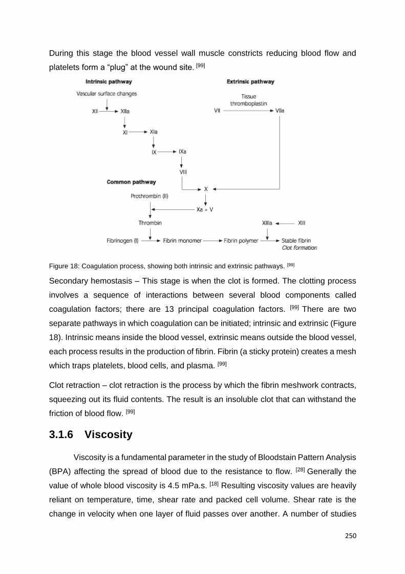
250
During this stage the blood vessel wall muscle constricts reducing blood flow and
platelets form a “plug” at the wound site. [99]
Figure 18: Coagulation process, showing both intrinsic and extrinsic pathways. [99]
Secondary hemostasis – This stage is when the clot is formed. The clotting process
involves a sequence of interactions between several blood components called
coagulation factors; there are 13 principal coagulation factors. [99] There are two
separate pathways in which coagulation can be initiated; intrinsic and extrinsic (Figure
18). Intrinsic means inside the blood vessel, extrinsic means outside the blood vessel,
each process results in the production of fibrin. Fibrin (a sticky protein) creates a mesh
which traps platelets, blood cells, and plasma. [99]
Clot retraction – clot retraction is the process by which the fibrin meshwork contracts,
squeezing out its fluid contents. The result is an insoluble clot that can withstand the
friction of blood flow. [99]
3.1.6 Viscosity
Viscosity is a fundamental parameter in the study of Bloodstain Pattern Analysis
(BPA) affecting the spread of blood due to the resistance to flow. [28] Generally the
value of whole blood viscosity is 4.5 mPa.s. [18] Resulting viscosity values are heavily
reliant on temperature, time, shear rate and packed cell volume. Shear rate is the
change in velocity when one layer of fluid passes over another. A number of studies

251
have been executed exploring how the viscosity can ultimately determine the size of
the bloodstain diameter [4, 5, 9, 20], with the general consensus being that the higher the
viscosity the smaller the bloodstain. Other studies involving the manipulation of
viscosity with drugs [27 - 28] and alcohol [20] have also been investigated, finding they
significantly decrease the dynamic viscosity, showing how readily viscosity can be
manipulated.
3.1.7 Blood Grouping
A blood group or blood type is the classification of blood based on the presence
or absence of inherited antigenic substances on the surface of red blood cells (RBCs).
[95 - 99] The blood type is inherited and represents a contribution from both parents.
There are 33 recognised human blood type systems, two of the most medically
significant being the ABO and RH systems. The ABO system is mostly associated with
blood transfusion, persons may have type A, type B, type O, or type AB blood. O is
the most common type of blood throughout the world, however this can deviate
depending on the country/continent; i.e. Type B is predominant in Asia. [95 - 99] The
Rhesus system (Rh) is used in conjunction with the ABO system. This system was
developed on the basis of the presence or absence of the D antigen on the red blood
cell surface. [95 - 99] This information is combined with the ABO blood type where a
person with A type blood could be classified as A negative or positive. The majority of
the population are positive for the D antigen, again this is dependent on other factors,
such as ethnicity. [95 - 99]
3.1.8 Surface Tension Surface tension is the force (resistance), caused by the molecular friction within the
fluid, which prevents the penetration or break up of blood. Blood surface tension
measures 5.1 – 5.7 x 10 -2 N/m. [18]
3.1.9 Adhesion and Cohesion
Adhesion is the attraction between unlike molecules, for instance blood on a
weapon. Cohesion is the attraction between like molecules, this attraction is what
maintains the spherical shape exhibited when blood falls. [9, 10, 11]

252
3.1.10 Packed Cell Volume
Packed cell volume (PCV %) is the ratio of red blood cells to plasma content in
total whole blood volume; its effect on viscosity is well documented where an increase
is associated with cell percentage increase. [9, 26, 27]
The variance in the PCV % levels is not only dependent upon location within
the body [9] where values can deviate from 30 – 52 % [9] but is influenced by the lifestyle
of the person. Packed cell volume levels as low as 15 % have been documented for
persons who are drug abusers, chronic alcoholics, pregnant, malnourished and / or
elderly. [9] Similarly new-borns, people suffering from shock, extreme exercisers and
heart attack victims have very high PCV % reaching 75 %. [9]
253
3.2 EXPLORING THE APPLICATIONS OF
EQUINE BLOOD IN BPA
Initial investigation of surface interactions with blood were conducted with a
human blood substitute, which was thought to have been the most resourceful and
economical way of conducting preliminary experiments. Animal blood has been
concluded as the closest and therefore the most suitable alternate, however it seems
that currently only porcine blood is most prominently utilised. [5, 17 - 18] This poses
difficulties as porcine blood is extremely difficult to obtain, often requiring the use of a
slaughter house which again raises several issues; ethical, moral and safety (blood is
unscreened). Safety aspects are paramount when dealing with any biological fluid; the
use of animal blood has been acknowledged as a safe substitute to human blood,
decreasing but not eliminating the risks of coming into contact with pathogens and
diseases, i.e. HIV, Hepatitis etc. [5] Despite the dependable reputation of porcine blood,
other animal bloods are still employed. A study by Christman et al [74] compared
various animal bloods (swine, bovine, equine and porcine) to determine suitability as
a human blood substitute, where impacts and general appearance of the blood were
compared. [100] Although their study gives an insight into the functionality of animal
blood as a human blood substitute it uses now out-dated terminology (low impact
velocity etc.) and suffers from any real statistical analysis which is considered
obligatory within the forensic field. Due to the foundations of this project being primarily
blood related it is thought essential to fully establish the suitability of equine blood as
a more commercially available, animal friendly [101, 102], human blood substitute in the
interpretation of bloodstain patterns. In order to accomplish this aim, visual
observations the point of origin and equations developed by Hulse-Smith et al [18] (see
introduction) which allowed direct comparisons with previous results where porcine
blood was utilised, were used.
Using the general experimental method, stipulated in section 3, two samples of
equine blood were tested, each with different anti-clotting methods employed; the first
was defibrinated, where the fibrin (an essential component in clotting) is removed.
Second an anticoagulant was utilised, Alsever’s, which is considered to be the most
stable and commonly used anticoagulant. [102] Last, attention was turned to the
254
consideration of the age of blood and its potential effect upon BPA experimentation. It
is well documented that age of porcine blood alters bloodstains; decreasing the
diameter of the resultant bloodstain as the blood ages [5] and therefore considerations
pertaining to shelf life (time viable after opening the container or first exposing the
blood to air) have to be made when conducting experiments or crime scene
reconstruction to account for these changes. Presently it is unknown if this is the case
for equine blood as there is no definitive published shelf-life, this was duly explored
since any such changes would need to be accounted for in future BPA activities to
avoid possible misinterpretations of patterns.
3.2.1 Experimental
3.2.1.1 Resources
All equine blood (defibrinated and Alsever’s) was obtained from TCS-
Biosciences Limited at a PCV % (Packed Cell Volume) of 45%. Human blood was
freshly drawn on the day of the experiment using a venepuncture; blood was drawn
into purple blood tubes containing the anticoagulant EDTA.
3.2.1.2 Method
Blood drop tests for all bloods were dispensed according to the instructions
stipulated in the Materials and Methods section. Four different surfaces were utilised:
paper, plastic, tile and steel. Surfaces were new; paper (80mgs; standard A4,) plastic
sheet (Medium Density Polyethylene), tile (ceramic gloss) and cold rolled steel. The
surface roughness of each experimental surface (Table 1) was deduced using a
TESA-rugosurf 10 at 5 different points.
Blood drops Do were established using the slow motion filming described in the Method
and Materials section. [4]

255
Table 2: Release heights
of blood drops calculated from the tip of pipette to the impacting surface and converted into impact
velocity via the use of Equation (11).
A diverse range of heights were used to create varying impact velocities Vo as
expressed in Table 2, velocities were calculated using the equation described in the
experimental section. Here it was assumed that the path of the blood drop can be
defined by the equations for the movement of a rigid object, therefore disregarding
parameters such as drag. [17] These particular heights were chosen as they can be
directly compared to the results obtained by Hulse-Smith et al [18] who also used animal
blood (porcine) as a human blood substitute. It is noted that there is a possibility of
oscillation during the initial phase of the falling drop, however studies have shown that
this oscillation is less dramatic than that produced in a raindrop and is therefore likely
not to have a marked effect. [24] It has also been demonstrated that the drop oscillation
will not be a significant factor as oscillation does not occur after 40cm release height,
which is below most of the heights used in this experiment. [5]
3.2.1.3 Age Experiment
The same experimental procedure was adhered to for the aged equine blood,
though Do was not deemed necessary to calculate as diameter and number of spines
were the focal interests of the aged blood. Drops were again manually dispensed from
heights of 30.5, 60.9, 91.4 and 121.9 cm onto a paper surface (80mgs, A4 standard).
Drops were repeated 5 times and stain diameters were measured using a magnifying
loupe. Viscosity measurements were performed using a Kinexus Pro Rheometer.
Release Heights (cm)
Impact Velocity (m/s)
30.5
2.45
60.9
3.46
91.4
4.24
121.9
4.89

256
3.2.2. Results and Discussion
3.2.2.1 Blood Type properties
Equine Blood [24, 102]
Porcine Blood [18]
Human Blood [104]
Density (kg/m3)
1050
1062
1052 - 1063
Viscosity (mPa.s) 3.3 – 5.6 3.4 – 6.1 3.8 – 5.1 Surface Tension (x 10 -2
N/m) 5.1 5.3 – 5.8 5.1 – 5.7
PCV (%) 32 - 46 38.9 – 46.3 40.0 – 45.0
Table 3: A comparison of published values obtained for the physical properties of equine, porcine and human blood (all unadulterated).
The physical properties of blood are of high importance since they determine
the resultant pattern of blood and are utilised in many of the aforementioned equations
(see introduction). Taking this into consideration, the physical properties of equine, [24,
102] porcine [18] and human blood [104] are compared in Table 3 which show there to be
no difference between physical properties of equine blood [103, 104] with that of porcine
and human blood, [4] suggesting its potential use in BPA.
3.2.2.2 Drop Diameters
Slow motion filming, as detailed in the experimental section was performed
enabling the capture of scaled still images of the blood drops as they are dispensed
from the pipette tip to allow the drop diameters, Do to be determined.
Drops were discharged as close to the scale as possible (1cm) to avoid any
size distortion. Such drop diameters result in an average drop diameter value of 4 mm
and 5 mm when defibrinated blood was utilised, 3.5 mm and 4 mm when Alsever’s
blood was dropped and lastly 4 mm and 4.5 mm when human blood was (utilising the
1 mm and 1.77 mm inner tip diameter pipettes respectively). These results are in
agreement with previous blood drop diameters reported by Hulse-Smith et al [18] and
Willis et al [104] where human [104] and porcine blood were utilised [18], showing no
difference in size (between 3.0 mm and 4.3 mm) or general shape of the droplet
exhibited.
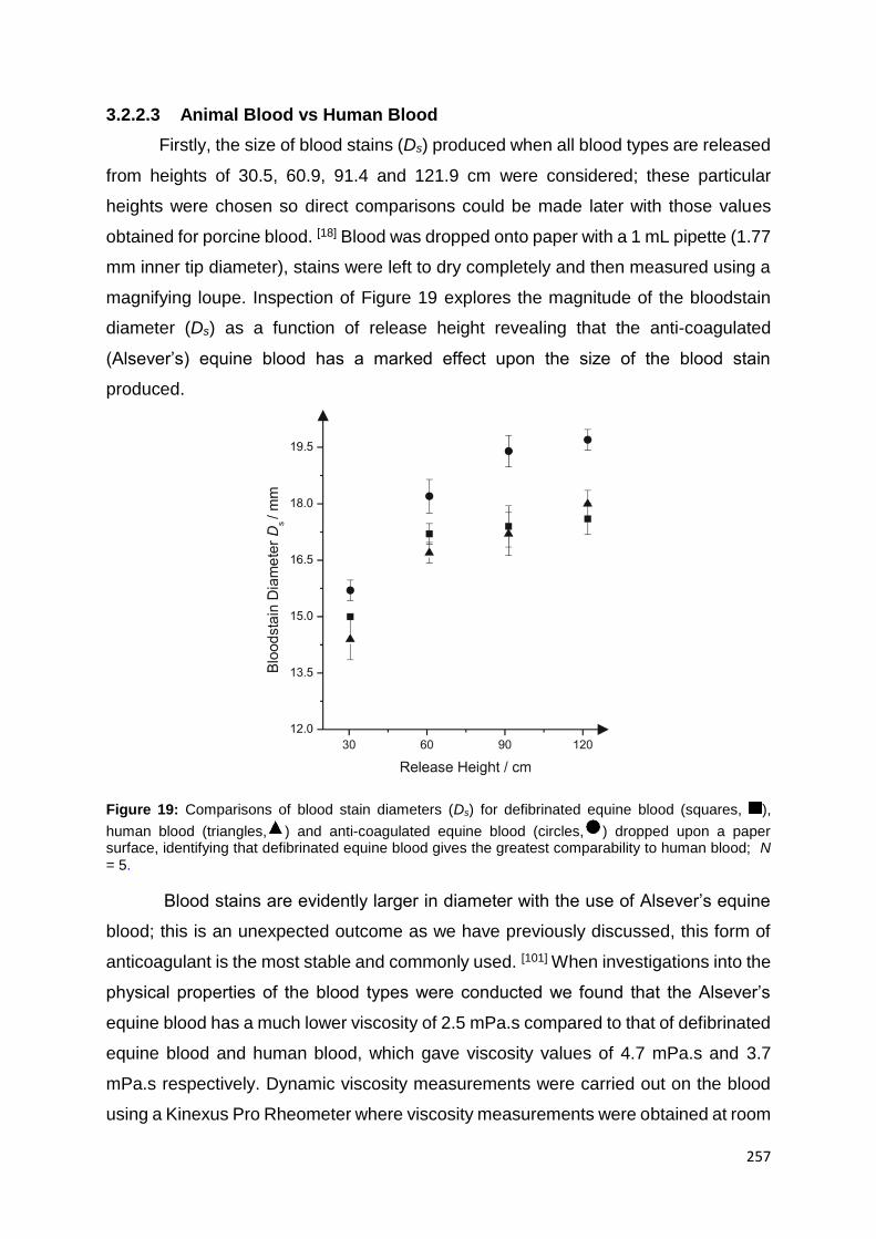
257
3.2.2.3 Animal Blood vs Human Blood
Firstly, the size of blood stains (Ds) produced when all blood types are released
from heights of 30.5, 60.9, 91.4 and 121.9 cm were considered; these particular
heights were chosen so direct comparisons could be made later with those values
obtained for porcine blood. [18] Blood was dropped onto paper with a 1 mL pipette (1.77
mm inner tip diameter), stains were left to dry completely and then measured using a
magnifying loupe. Inspection of Figure 19 explores the magnitude of the bloodstain
diameter (Ds) as a function of release height revealing that the anti-coagulated
(Alsever’s) equine blood has a marked effect upon the size of the blood stain
produced.
Figure 19: Comparisons of blood stain diameters (Ds) for defibrinated equine blood (squares, ),
human blood (triangles, ) and anti-coagulated equine blood (circles, ) dropped upon a paper surface, identifying that defibrinated equine blood gives the greatest comparability to human blood; N = 5.
Blood stains are evidently larger in diameter with the use of Alsever’s equine
blood; this is an unexpected outcome as we have previously discussed, this form of
anticoagulant is the most stable and commonly used. [101] When investigations into the
physical properties of the blood types were conducted we found that the Alsever’s
equine blood has a much lower viscosity of 2.5 mPa.s compared to that of defibrinated
equine blood and human blood, which gave viscosity values of 4.7 mPa.s and 3.7
mPa.s respectively. Dynamic viscosity measurements were carried out on the blood
using a Kinexus Pro Rheometer where viscosity measurements were obtained at room
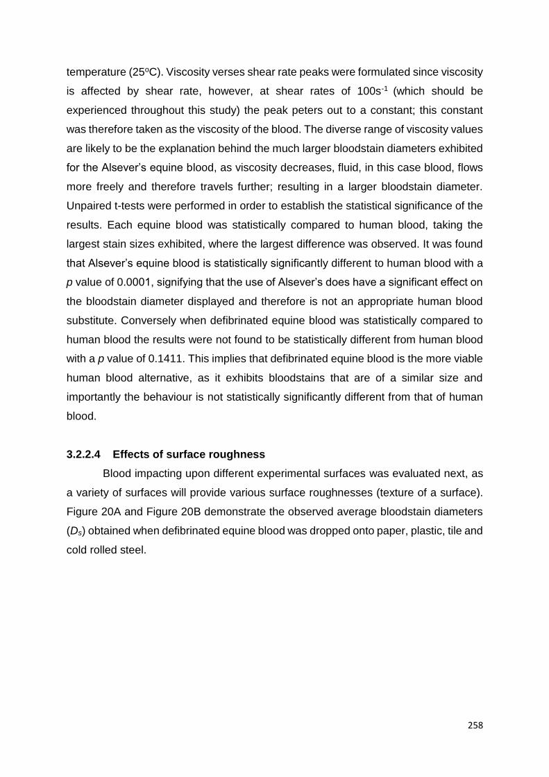
258
temperature (25oC). Viscosity verses shear rate peaks were formulated since viscosity
is affected by shear rate, however, at shear rates of 100s-1 (which should be
experienced throughout this study) the peak peters out to a constant; this constant
was therefore taken as the viscosity of the blood. The diverse range of viscosity values
are likely to be the explanation behind the much larger bloodstain diameters exhibited
for the Alsever’s equine blood, as viscosity decreases, fluid, in this case blood, flows
more freely and therefore travels further; resulting in a larger bloodstain diameter.
Unpaired t-tests were performed in order to establish the statistical significance of the
results. Each equine blood was statistically compared to human blood, taking the
largest stain sizes exhibited, where the largest difference was observed. It was found
that Alsever’s equine blood is statistically significantly different to human blood with a
p value of 0.0001, signifying that the use of Alsever’s does have a significant effect on
the bloodstain diameter displayed and therefore is not an appropriate human blood
substitute. Conversely when defibrinated equine blood was statistically compared to
human blood the results were not found to be statistically different from human blood
with a p value of 0.1411. This implies that defibrinated equine blood is the more viable
human blood alternative, as it exhibits bloodstains that are of a similar size and
importantly the behaviour is not statistically significantly different from that of human
blood.
3.2.2.4 Effects of surface roughness
Blood impacting upon different experimental surfaces was evaluated next, as
a variety of surfaces will provide various surface roughnesses (texture of a surface).
Figure 20A and Figure 20B demonstrate the observed average bloodstain diameters
(Ds) obtained when defibrinated equine blood was dropped onto paper, plastic, tile and
cold rolled steel.
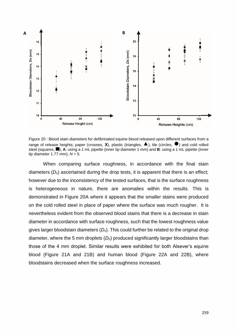
259
Figure 20 : Blood stain diameters for defibrinated equine blood released upon different surfaces from a
range of release heights; paper (crosses, X), plastic (triangles, ), tile (circles, ) and cold rolled
steel (squares, ); A: using a 1 mL pipette (inner tip diameter 1 mm) and B: using a 1 mL pipette (inner tip diameter 1.77 mm); N = 5.
When comparing surface roughness, in accordance with the final stain
diameters (Ds) ascertained during the drop tests, it is apparent that there is an effect;
however due to the inconsistency of the tested surfaces, that is the surface roughness
is heterogeneous in nature, there are anomalies within the results. This is
demonstrated in Figure 20A where it appears that the smaller stains were produced
on the cold rolled steel in place of paper where the surface was much rougher. It is
nevertheless evident from the observed blood stains that there is a decrease in stain
diameter in accordance with surface roughness, such that the lowest roughness value
gives larger bloodstain diameters (Ds). This could further be related to the original drop
diameter, where the 5 mm droplets (Do) produced significantly larger bloodstains than
those of the 4 mm droplet. Similar results were exhibited for both Alsever’s equine
blood (Figure 21A and 21B) and human blood (Figure 22A and 22B), where
bloodstains decreased when the surface roughness increased.
A B

260
Figure 21: Blood stain diameters (Ds) for Alsever’s blood released upon different surfaces from a range
of release heights; paper (crosses, X), plastic (triangles, ), tile (circles, ) and cold rolled steel (squares, ); A: using a 1 mL pipette (inner tip diameter 1 mm) and B: using a 1 mL pipette (inner tip diameter 1.77 mm); N = 5.
Figure 22: Blood stain diameters (Ds) for human blood released upon different surfaces from a range
of release heights; paper (crosses, X), plastic (triangles, ), tile (circles, ) and cold rolled steel (squares, ); A: using a 1 mL pipette (inner tip diameter 1 mm) and B: using a 1 mL pipette (inner tip diameter 1.77 mm); N = 5.
B
A B
A B

261
This is further demonstrated by performing t-tests where all p values for the
three bloods were found to be statistically significant, p < 0.0015. When we compare
all three bloods it is evident that Alsever’s equine blood on the whole generates much
larger stains than that of human and defibrinated equine blood, this is consistent with
the results reported earlier (see blood type section).
Further investigations were performed with the use of equations (3) - (6). Figure
23 A-C depicts the ratio of drop spread (Ds / Do) in relation to the Reynolds number
where lines of ‘best fit’ where undertaken.
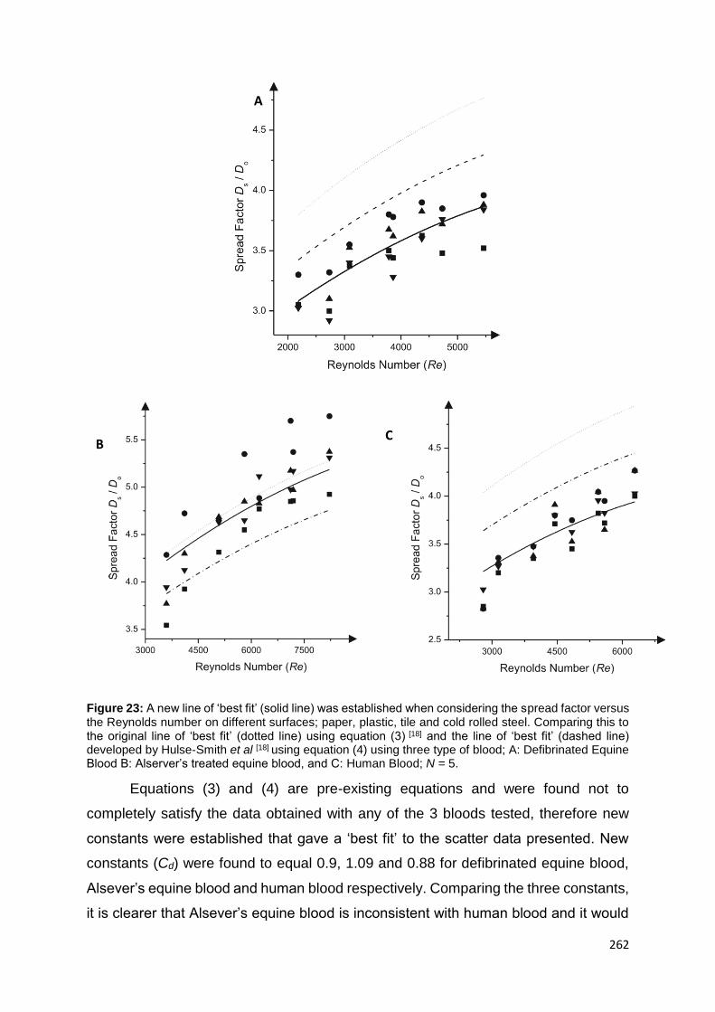
262
Figure 23: A new line of ‘best fit’ (solid line) was established when considering the spread factor versus the Reynolds number on different surfaces; paper, plastic, tile and cold rolled steel. Comparing this to the original line of ‘best fit’ (dotted line) using equation (3) [18] and the line of ‘best fit’ (dashed line) developed by Hulse-Smith et al [18] using equation (4) using three type of blood; A: Defibrinated Equine Blood B: Alserver’s treated equine blood, and C: Human Blood; N = 5.
Equations (3) and (4) are pre-existing equations and were found not to
completely satisfy the data obtained with any of the 3 bloods tested, therefore new
constants were established that gave a ‘best fit’ to the scatter data presented. New
constants (Cd) were found to equal 0.9, 1.09 and 0.88 for defibrinated equine blood,
Alsever’s equine blood and human blood respectively. Comparing the three constants,
it is clearer that Alsever’s equine blood is inconsistent with human blood and it would
A
B C
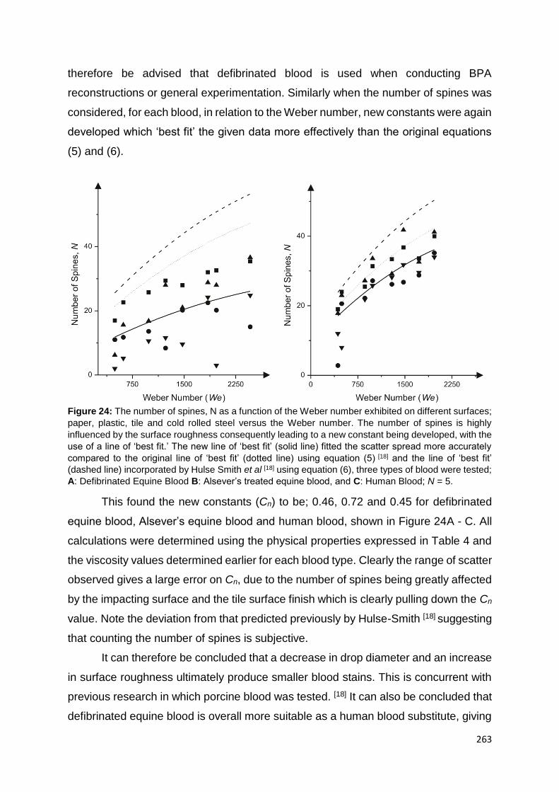
263
therefore be advised that defibrinated blood is used when conducting BPA
reconstructions or general experimentation. Similarly when the number of spines was
considered, for each blood, in relation to the Weber number, new constants were again
developed which ‘best fit’ the given data more effectively than the original equations
(5) and (6).
Figure 24: The number of spines, N as a function of the Weber number exhibited on different surfaces;
paper, plastic, tile and cold rolled steel versus the Weber number. The number of spines is highly
influenced by the surface roughness consequently leading to a new constant being developed, with the
use of a line of ‘best fit.’ The new line of ‘best fit’ (solid line) fitted the scatter spread more accurately
compared to the original line of ‘best fit’ (dotted line) using equation (5) [18] and the line of ‘best fit’
(dashed line) incorporated by Hulse Smith et al [18] using equation (6), three types of blood were tested;
A: Defibrinated Equine Blood B: Alsever’s treated equine blood, and C: Human Blood; N = 5.
This found the new constants (Cn) to be; 0.46, 0.72 and 0.45 for defibrinated
equine blood, Alsever’s equine blood and human blood, shown in Figure 24A - C. All
calculations were determined using the physical properties expressed in Table 4 and
the viscosity values determined earlier for each blood type. Clearly the range of scatter
observed gives a large error on Cn, due to the number of spines being greatly affected
by the impacting surface and the tile surface finish which is clearly pulling down the Cn
value. Note the deviation from that predicted previously by Hulse-Smith [18] suggesting
that counting the number of spines is subjective.
It can therefore be concluded that a decrease in drop diameter and an increase
in surface roughness ultimately produce smaller blood stains. This is concurrent with
previous research in which porcine blood was tested. [18] It can also be concluded that
defibrinated equine blood is overall more suitable as a human blood substitute, giving

264
consistently comparable results throughout experimentation and on any surface type.
Results obtained for number of spines observed when using all bloods are also in
excellent agreement with previous research, [18] showing that the rougher the surface,
the greater preponderance of spines. It is noted that there is a lower overall number
of spines acquired within this study compared to that of Hulse-Smith [18] however, this
may be attributed to the physical property deviations of the tested bloods or the
subjective technique of counting spines. All data is provided in Appendix 3.
3.2.2.5 Area of Origin
The area of origin provides the analyst with a 3D perspective, helping them to
‘picture’ the incident and therefore giving greater insight into the series of events. [4]
The application of the area of origin is a vital piece of information, which highlights the
area in which a blood spatter was generated.

265
A
B
Figure 25: Blood impacts used to calculate the area of origin for both A: human blood and B:
defibrinated equine blood.
Here the tangent method was utilised to calculate the Area of Origin, where
bloodstains and the area of convergence were measured manually. Only human blood
and defibrinated equine blood were compared for this section of analysis as the
Alsever’s equine blood proved to be providing less comparable results to that of
human blood throughout the previous experiments and further experimentation was
deemed frivolous. To create the area of origin, a series of impacts were generated
266
using a Proctor Little Nipper Rat Trap ®, where 1 – 1.5 mLs of blood was loaded onto
the edge of the trap. The rat trap catch was covered in tape to prevent blood soaking
into the wood. The trap was set onto a large sheet of paper at ground level and at 12
cm height to create differing area of origins. When the rat trap device snapped the
impact spatter collected onto the paper (lining) where it could be measured and
visually compared. Traps were cleaned thoroughly between snaps and different traps
(same make) were used for each height. Figures 25A and 25B show the impacts of
human and defibrinated equine blood, respectively. Although visually both blood
impacts may look very similar and are hard to distinguish from one another, when the
criteria set forth by Wonder [9] is adhered to it is apparent that they are very different.
The left side of the spatter depicts the origin of the spatter, when these are compared
it is clear than human blood has visibly smaller stains than those produced when horse
blood was used, this is due to the viscosity of horse blood being higher than human
blood. However, when the area of origin were calculated for all impacts it was found
that both could accurately calculate the area of origin and that only a small variance
between the two existed of around ± 2 cm, which is relatively insignificant in terms of
determining an area of origin.
3.2.2.6 New vs Aged Blood
Finally the effects of age on equine blood was evaluated. New equine blood
and aged equine blood (over the time period 12 days, 14 days and 57 days) were all
compared, defining the differences by alteration in diameter size and number of
spines.

267
Figure 26: Aging defibrinated equine blood released (using a 1mL pipette; 1.77 inner tip diameter)
from a range of heights (30.5, 60.9, 91.4 and 121.9 cm). It is clear that a decrease in the blood stain
diameter is observed as the blood gets older. The age of the equine blood ranged from 57 days old
(diamonds), 14 days old (squares), 12 days old (circles) to new blood (triangles); N = 5.
Figure 26 illustrates the differences experienced; diameters were found to significantly
decrease after 14 days by up to 6.38 % and decrease further after 57 days up to 12.78
%. A student t-test was performed to determine the significance of these results, a p
value of 0.0003 was calculated using the values for 57 days and fresh blood at a height
of 120 cm and a p value of 0.0020 when 14 days was compared to fresh blood at the
same height. These results are considered to be statistically significant and therefore
it can be stated that age of blood has a significant effect on the bloodstain diameter.
The aging process of blood increased the viscosity to 5mPA.s and 5.3 mPa.s for 14
and 57 days respectively, ultimately resulting in smaller stains. [5] However it was found
that the PCV% was unaffected. [105] It is unknown why this affect occurred but is
thought to be accounted for by the effects of aging in RBCs (Red Blood Cells). [105]
Plasma viscosity can be a discounted factor since previous studies [105] have found
that plasma viscosity increases due to fibrinogen production and this has been
removed in our blood. Age was not found to have any effect on the number of spines
observed, where spines were counted for bloodstains at various ages. Results concur
with previous reports, where aged porcine blood was investigated and resulted in a
decrease in diameter size. [5] Consideration should be made when undertaking future

268
experiments to the time period in which equine blood can be utilised as it is clear that
age has a significant effect on the bloodstains produced.
3.2.3 Summary
It has been established that defibrinated equine blood can be used as a BPA
human blood substitute. Equine blood follows the same trend as both the human and
porcine blood [5] in that when drop height increases so does the resultant stain
diameter. When utilising the pre-existing equations it was recognised the need for new
constants to ‘best fit’ the given data. New values for the Reynolds numbers are smaller
than one obtained previously for porcine blood but do not deviate that greatly from the
original equation as to be questionable. When the human blood constant and
defibrinated equine blood constant were compared they deviated little with one
another, conversely Alsever’s equine blood was found to be inconsistent to human
blood and therefore not a viable substitute. Constant values for the Weber number
suggest a much lower progression of number of spines than values found for porcine
blood; this is accounted for by the subjective nature of spine counting.
Aged defibrinated equine blood presented large changes in diameter size as
the blood got older, deviations amounting to 12.78 % when blood was 57 days old,
this is thought to be related to the change in the viscosity of the blood over time and
the effect of the aging process upon the RBCs. Similar deviations are experienced
when porcine blood is utilised [5].
Overall it can be concluded that defibrinated equine blood is a reliable substitute
for human blood, any deviations experienced from the previously reported results
obtained from the utilisation of porcine blood are due to inconsistent physical
properties used for the comparisons. Further analysis using a greater variation in
physical properties and impacted surfaces needs to be undertaken; this will provide a
greater understanding of the true usefulness of these more quantitative approaches.

269
3.3 PACKED CELL VOLUME AND ITS
EFFECTS ON BPA
As demonstrated in the work by Hulse-Smith et al [18] viscosity is a fundamental
parameter in the study of Bloodstain Pattern Analysis, affecting the spread of blood
due to the resistance to flow. [7] Resulting viscosity values are heavily reliant on
temperature (higher temperatures equating to lower viscosity readings and vice versa
for lower temperatures), shear rate (rate of change of velocity when one layer of fluid
passes over an adjacent layer) and packed cell volume. [80, 106, 107] The importance of
PCV % and its clear effect on viscosity have been overlooked within the field of BPA.
[7, 108 - 109]
The variance of these PCV levels has been documented, where levels can
fluctuate from 15- 75% depending on lifestyle, gender and position in the human body.
Taking these facts into account and the known effects PCV % has on viscosity [7] PCV
% is applied as a parameter of blood, observing its effect on the size of bloodstain
diameters and its overall impact on BPA.
3.3.1 Experimental
Human blood was utilised throughout this research, ethical approval was
obtained prior to any experiments and granted by Manchester Metropolitan University.
Only one donor was utilised throughout this study to maintain consistency and control
over parameters. In order to study the effect of PCV, blood was centrifuged twice at
3000 rpm for 10 minutes. Different volumes of red blood cells to plasma were added
to create varying packed cell volumes, generating percentages between 15 and 75 %.
Packed cell volumes were then checked, filling three - quarters of a capillary tube with
the sample and centrifuging at 12, 000 rpm for 5 minutes; the blood separates into its
components and the percentage of blood cells can be determined using a micro-
hematocrit chart.
Blood was dropped (according to the methods and materials section) using
different sized pipettes, from varying heights (50, 100, 150 and 200 cm), angles (20 o,
40 o, 60 o, 80 o and 90 o) created utilising a spatter board and on different surfaces
(paper, tile, plastic and steel), each of the different packed cell volume percentages
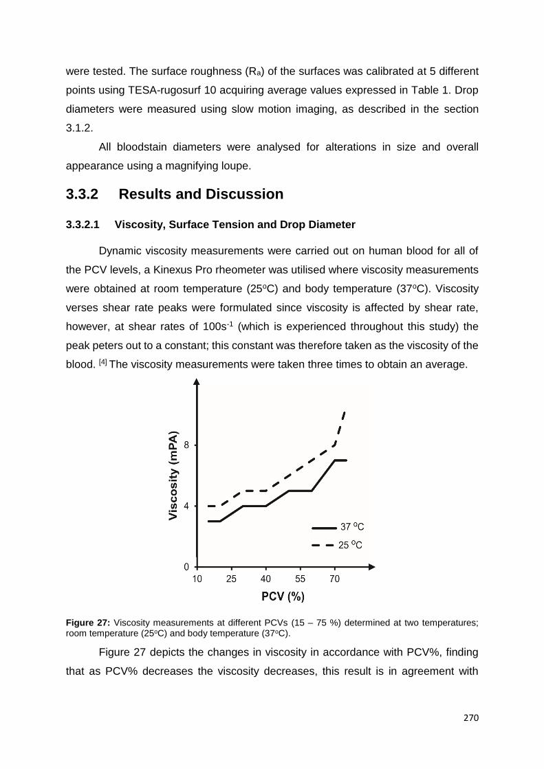
270
were tested. The surface roughness (Ra) of the surfaces was calibrated at 5 different
points using TESA-rugosurf 10 acquiring average values expressed in Table 1. Drop
diameters were measured using slow motion imaging, as described in the section
3.1.2.
All bloodstain diameters were analysed for alterations in size and overall
appearance using a magnifying loupe.
3.3.2 Results and Discussion
3.3.2.1 Viscosity, Surface Tension and Drop Diameter
Dynamic viscosity measurements were carried out on human blood for all of
the PCV levels, a Kinexus Pro rheometer was utilised where viscosity measurements
were obtained at room temperature (25oC) and body temperature (37oC). Viscosity
verses shear rate peaks were formulated since viscosity is affected by shear rate,
however, at shear rates of 100s-1 (which is experienced throughout this study) the
peak peters out to a constant; this constant was therefore taken as the viscosity of the
blood. [4] The viscosity measurements were taken three times to obtain an average.
Figure 27: Viscosity measurements at different PCVs (15 – 75 %) determined at two temperatures; room temperature (25oC) and body temperature (37oC).
Figure 27 depicts the changes in viscosity in accordance with PCV%, finding
that as PCV% decreases the viscosity decreases, this result is in agreement with
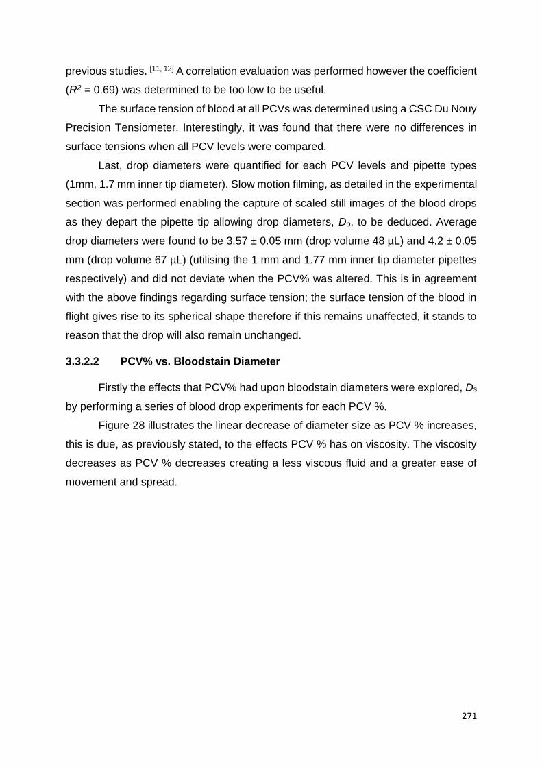
271
previous studies. [11, 12] A correlation evaluation was performed however the coefficient
(R2 = 0.69) was determined to be too low to be useful.
The surface tension of blood at all PCVs was determined using a CSC Du Nouy
Precision Tensiometer. Interestingly, it was found that there were no differences in
surface tensions when all PCV levels were compared.
Last, drop diameters were quantified for each PCV levels and pipette types
(1mm, 1.7 mm inner tip diameter). Slow motion filming, as detailed in the experimental
section was performed enabling the capture of scaled still images of the blood drops
as they depart the pipette tip allowing drop diameters, Do, to be deduced. Average
drop diameters were found to be 3.57 ± 0.05 mm (drop volume 48 µL) and 4.2 ± 0.05
mm (drop volume 67 µL) (utilising the 1 mm and 1.77 mm inner tip diameter pipettes
respectively) and did not deviate when the PCV% was altered. This is in agreement
with the above findings regarding surface tension; the surface tension of the blood in
flight gives rise to its spherical shape therefore if this remains unaffected, it stands to
reason that the drop will also remain unchanged.
3.3.2.2 PCV% vs. Bloodstain Diameter
Firstly the effects that PCV% had upon bloodstain diameters were explored, Ds
by performing a series of blood drop experiments for each PCV %.
Figure 28 illustrates the linear decrease of diameter size as PCV % increases,
this is due, as previously stated, to the effects PCV % has on viscosity. The viscosity
decreases as PCV % decreases creating a less viscous fluid and a greater ease of
movement and spread.
272
Figure 28: Final bloodstain diameters for human blood, containing different PCV levels, released from
varying heights onto a paper surface using a 1 mL pipette (inner tip diameter 1.77 mm).
There was a maximum decrease of bloodstain diameter equating to 3.93, 4.10,
4.83 and 6.00 mm, when considering the different surfaces; paper, plastic, steel and
tile respectively and the use of the larger pipette (1.7 mm inner diameter) from all
heights. These values are equivalent to between a 26.50 - 35.07 % maximum
decrease when the highest and lowest PCV % values (15 % and 75 %) were
considered. However, when the difference of normal human levels of PCV % (around
40 %), to the higher (75 %) and then the lower (15 %) PCV % levels are considered,
this change is less prominent, becoming 16.15 - 23.91 % and 6.00 – 12.07 %
respectively. By performing t - tests the true significance of these bloodstain alterations
can be established, if the highest (75%) and lowest PCV (15%) levels are compared
a p value of less than 0.0001 is obtained, for all surface types, which acknowledges
that this data is extremely significant. However, aforementioned there is unlikely to be
such extremes (15 – 75%), therefore it is proposed to adopt a middle (normal) PCV
level of 40 % and compare this with the highest and lowest PCV% levels. When
considering the lowest level (15%) with a normal level (40%) for all surfaces, p values
of 0.0001 - 0.0322 are deduced, which are still considered to be very statistically
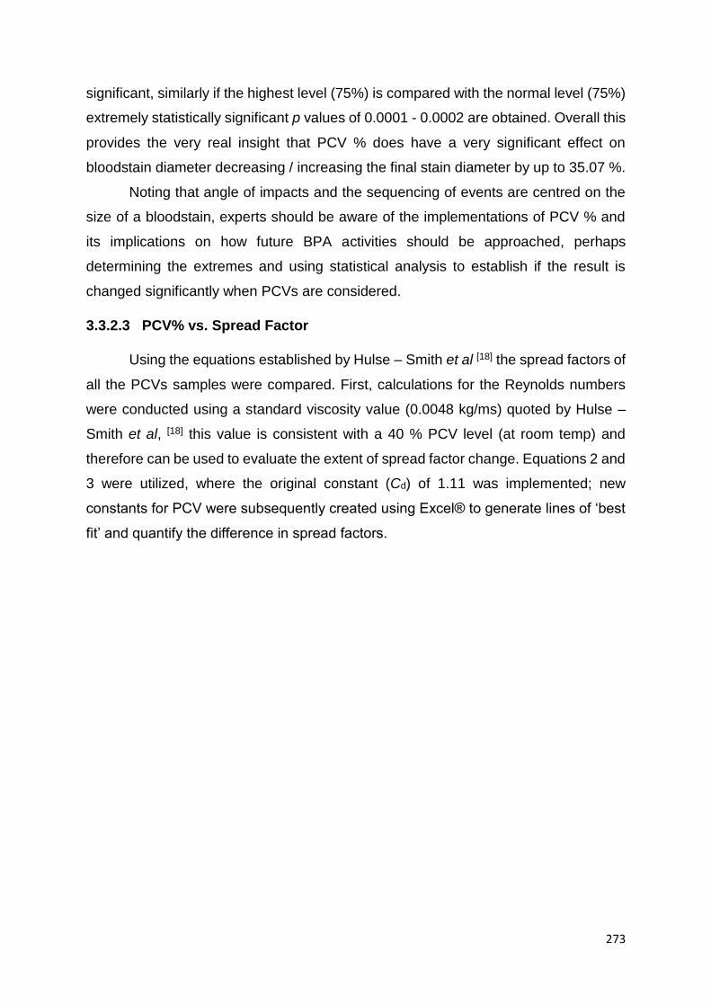
273
significant, similarly if the highest level (75%) is compared with the normal level (75%)
extremely statistically significant p values of 0.0001 - 0.0002 are obtained. Overall this
provides the very real insight that PCV % does have a very significant effect on
bloodstain diameter decreasing / increasing the final stain diameter by up to 35.07 %.
Noting that angle of impacts and the sequencing of events are centred on the
size of a bloodstain, experts should be aware of the implementations of PCV % and
its implications on how future BPA activities should be approached, perhaps
determining the extremes and using statistical analysis to establish if the result is
changed significantly when PCVs are considered.
3.3.2.3 PCV% vs. Spread Factor
Using the equations established by Hulse – Smith et al [18] the spread factors of
all the PCVs samples were compared. First, calculations for the Reynolds numbers
were conducted using a standard viscosity value (0.0048 kg/ms) quoted by Hulse –
Smith et al, [18] this value is consistent with a 40 % PCV level (at room temp) and
therefore can be used to evaluate the extent of spread factor change. Equations 2 and
3 were utilized, where the original constant (Cd) of 1.11 was implemented; new
constants for PCV were subsequently created using Excel® to generate lines of ‘best
fit’ and quantify the difference in spread factors.
274
Figure 29: A depiction of the spread factor versus the Reynolds number when utilising human blood
(containing varying PCV levels) on different surfaces; paper, plastic, tile and cold rolled steel. Lines of
‘best fit’ were calculated for each PCV %, where new constants were established (see Table 4 for a
clearer view of the constants).
Figure 29 illustrates the new constants established for each PCV %. It is evident
that the PCV % has a marked effect on the spread of the blood drop, altering the
constant by (+) 6.96 % and (–) 15.35 % when comparing the average PCV (40 %) with
the lowest PCV (15 %) and highest PCV (75 %), respectively. Statistics assessing the
average PCV against the lowest and the highest PCV were carried out to verify the
significance of these results, a p value of less than 0.0001 was obtained, clearly
showing that PCV % significantly affects the spread factor of the blood drop. Since
only the standard value for viscosity [15] was used further calculations were necessary
where all viscosity values (at room temp) were incorporated for each corresponding
PCV %.

275
PCV
Cd
(µ = 0.0048 kg/ms)
Cd
(µ measured at PCV %)
15 1.19
1.14
20 1.15 1.10
30 1.12
1.14
40 1.11
1.12
50 1.05
1.11
60 1.02
1.12
70 0.99
1.12
75 0.96
1.17
Table 4: New constant values established for varying PCVs using equation (3) when different viscosity values were implemented.
Table 4 expresses the new constant values, where the results appear much
closer to the original constant (Cd = 1.11) proposed by Hulse – Smith et al. [18] However
in exploring the statistical significance between the values, using 40% as the standard,
p values of a very high significance are still achieved, and therefore it may not merely
be the viscosity that is effecting the spread factor. It is unclear at present what the
underlying cause for the differing constants is. It is conceivable that as shear rate
affects viscosity it is not effectively possible to determine a constant value and
therefore the measured viscosity values may not be 100% accurate if the correct shear
rate (100s-1) was not reached. Other possible causes could be the way in which the
blood interacts with the surface (wetting), drying effects and measuring discrepancies
(analyst error).
After exploring the effects of PCV % on bloods spreading capabilities it can
asserted that there is a significant effect when comparing the highest PCV % values
with the lowest PCV % values (15 % and 75 %). In terms of the real life applications,
PCV % can vary within people due to lifestyle or psychological state. [2] For example if
a person is in a panicked state packed cell volume would be expected to increase [2]
and therefore would decrease the size of the resultant bloodstain diameter (Ds) in the
276
case of bloodshed, and is therefore extremely relevant in terms of its application within
BPA. Future investigation where blood is a source of evidence need to consider the
factor of PCV % and time should be taken to ascertain if the lifestyle or psychological
state especially as bloodstain size is used in other areas of BPA pertaining to impact
and pattern type and maybe misleading.
3.3.2.4 PCV% vs. Angle of Impact
The Angles of Impact (AOI) are a vital piece of information, providing the
preliminary step to attaining the Area of Origin. [1, 2, 14, 18] To find the angle of impact
of a bloodstain, we used equation (7).
Five angles were tested on three surface types (paper, plastic and steel), where
AOIs were subsequently determined. It was found that calculated AOIs did not alter
despite the varying PCV level. It was noted that stains in general were larger when
lower PCVs were utilised and vice versa when higher PCVs were considered, however
the elliptical length and width adjusted accordingly and therefore did not affect the final
angle.
These results to can be applied to the current knowledge of the creation of an
impact spatter, where the applied force has to overcome the surface tension. Since
the surface tension remained unchanged throughout experimentation and the new
knowledge that viscosity doesn’t affect the angle of impact (see above) it is expected
that there would be no effect on the impact spatter created and therefore equally the
calculation of area of origin would remain unaffected. However the overall stain is
either larger or smaller than it would be at an average PCV%, this could lead to
misinterpretation of pattern types which are reliant on size (i.e. spurt vs gush), in
accordance with the criteria set forth by Wonder. [9]
3.3.3 Summary
For the first time the effect of varying PCVs on the evaluation of resultant
bloodstains has been explored. Using PCV % of 15 - 75 % it was determined that
diameters (Ds) significantly decreased as packed cell volume increased; this is
explained by the viscosity increase which would have ensued. New constants for each
PCV% were found when spread factor was investigated, where equations
implemented by Hulse – Smith et al [18] were applied. Although generally
acknowledged as passive stains (due to them usually being produced as a result of

277
gravity), though they can also be a result of a projection, [13, 14, 18 - 19] circular bloodstains
can used to establish impact velocity and sequence of events, i.e. if a person is stood
still and blood is dripping from a weapon this can indicate positioning. [13, 14, 18 - 19] With
the knowledge that PCV% can alter the size of a bloodstain this should be integrated
into any calculations regarding bloodstain size where differences from the average
value (45%) with regards to the lowest and highest extremes of PCV% should be
calculated, therefore establishing an error range. Investigators should try to establish
potential PCV% altering conditions such as pregnancy, anaemia and drug use (i.e.
doctor’s patient history). There may also be opportunities at crime scenes where fresh
blood pooling is present (thus easier to obtain an adequate amount of sample) and
therefore every opportunity should be seized to obtain a sample for haematological
testing. [13, 14, 18 – 19]
Last it was discovered that PCV% does not alter the calculated angle of impact,
this is an important result since angles of impact are used to find the area of origin,
the area of origin is vital when establishing an impact site. Further investigations could
be carried out using more surface types, drying and blood warmed to body
temperature. Also further exploration into different blood patterns should be
investigated (i.e. spatters, spurts, pools) to establish the overall effect of PCV% and
potential blood collecting methods should also be explored so an accurate PCV%
measurement can be obtained from the scene.

278
3.4 THE MECHANISM OF DRYING
BLOOD AND VOLUME ANALYSIS
As previously detailed (see section 4.1.10), blood can differ greatly from person
to person; [4] it is unknown what the significances of such changes in the components
of blood will have on the drying of bloodstains. Consequently this study explores the
fundamental parameters of the drying effects of both human and equine blood, the
influence of PCV % when applied to drying time, volume estimation and drying effects,
and ultimately what consequences this pertains to the field of BPA; as such this work
is of both fundamental and applied importance.
3.4.1 Experimental
3.4.1.1 Blood and PCV% Preparation
Two types of blood were utilised throughout this study; defibrinated equine
blood provided by TCS-Biosciences Limited (PCV 50 %) and screened EDTA
(Ethylenediaminetetraacetic acid) treated human blood type O+ supplied by a local
blood bank. Fresh blood could not be utilised due to the size of the equipment used,
as the blood would have clotted before analysis could proceed.
Blood samples were heated to 37o C before dropping in order to align to real
life applications where blood would evacuate the body at body temperature in a violent
assault. Blood samples were stored at 4o C when not required for experimentation.
In order to study the effect of PCV, human blood was centrifuged twice using
the same parameters as previously stipulated. Different volumes of red blood cells to
serum were added to create varying packed cell volumes, generating percentages
between 15 and 75 %. Packed cell volumes were then checked using the procedure
described in section 3.2.6. Equine blood was used for volume estimation, due to its
availability in abundance; the same method above for the preparation of PCV
concentrations was followed.
3.4.1.2 Microscope analysis
Defibrinated equine blood and human blood were individually dropped onto a
microscope slide using a syringe and subsequently filmed using a Leica AF6000
279
microscope and Leica DFC340FX camera until completely dry at room temperature
(24o C). Temperature was controlled in an incubator in which the microscope was
encased, this avoided any turbulent air that may have disrupted or altered drying and
prevented heat from the lamp disrupting drying. Blood serum for both human and
equine blood were analysed by centrifuging the blood at 2988 rpm for 15 minutes at
4o C, separating it into serum and red blood cells and carefully extracting the serum
using a pipette, the aforementioned method was then used to examine the drying
effect.
Blood drops were performed for each of the different packed cell volume
percentages and the drying process was recorded again using the Leica microscope.
3.4.1.3 Volume and Drying analysis
Three types of volume analysis were conducted;
Scaled Photograph – Three PCVs (15, 40 and 75%) were analysed on two different
surface types (vinyl and laminate wood). Blood (5 – 50mL) was poured onto the
surface where it was left to naturally flow to a stop. Scaled photographs were taken of
each of the bloodstains using a Casio Ex-F1 Digital Camera and surface areas were
determined using the image software Image J. [41]
Dry Weight – This method is only suitable for non-absorbent surfaces therefore only
vinyl and laminate wood were included for experimentation. [42] Three PCVs were
tested (15, 40 and 75%), blood volumes (5mL, 10mL and 20mL) were deposited onto
the surfaces as stipulated above and left to dry overnight. Stains were scraped off the
surface using a sterilised razor blade, scrapings were placed into closed containers
and weighed. Wet and dry weights for 1mL of blood were determined for each of the
PCVs to obtain a constant. [42]
Spectrophotometry – Again three PCVs were evaluated (15, 40 and 75%); calibration
graphs were generated, volumes of 10 µL - 100 µL diluted with distilled water up to
100mL were made for each PCV, a series of sonification and vortex-mixing were
incorporated in order to fully mix the blood. [40] Absorbance measurements were
performed at 412 nm, which has been found to be λmax when an absorption spectra
measurement was performed between wavelengths of 300 – 700 nm. [40]
Blood volumes of 5mL, 10mL and 20mL were tested on different surfaces
(carpet, vinyl and laminate wood), where blood was decanted onto the different

280
surfaces and left to dry for two days. [40] Dependent on the surface type, the stains
were either scraped or the stain was cut away from the surface and deposited into
500mL beakers filled to the mark with distilled water. [40] These were then left overnight
to soak and dissolve. When all blood had been fully mixed (no floating particles) a 1:50
dilution was made, again with distilled water. Absorbance measures were carried out.
[40]
Drying times were established by skeletonisation rate, where blood drops for
each PCV% were deposited on a plastic surface, drops were wiped at various time
increments; 1 minute, 5 minutes, 10 minutes, 20 minutes, 40 minutes, an hour and
final dried spot (5 drops for each time interval).
The Halo effect was also investigated; drops (at heights of 10 cm and 40 cm)
and swipe patterns were performed for each PCV% and left to air dry. [115] Once dry,
drops were deposited on top of the swipes and similarly swipes were positioned on
top of the dried drops. [115]
3.4.2 Results and Discussion
3.4.2.1 Defibrinated Equine v Human Blood
During forensic investigation it is not always suitable to utilise human blood,
given that the potential risks of biological infection are often too severe. [20] Equine
blood has been identified as a viable human blood substitute when reconstructing
violent crimes, offering a safer alternative. [21] In comparing the physical properties of
human and equine blood (see Table 2) it is readily observed that both have similar
characteristics and should potentially therefore yield similar results.

281
A B
C D
E F
Figure 30: A series of images depicting the drying of defibrinated equine blood at room temperature,
acquired using a 2.5 x 0.07 magnification Leica microscope. (t = 42 minutes)

282
Figure 30 depicts a series of images of defibrinated equine blood captured
under a Leica microscope at 2.5 x 0.07 magnification, where the images show the
drying of a blood drop.
Figure 31: A close up of equine blood magnified by 2.5 x 0.07 using a Leica microscope, showing
particle build upon the edge of the blood drop.
If this is magnified further, as shown in Figure 31, we can perceive the build-up
of suspended particles on the periphery of the blood drop similar to that observed
during the ‘coffee-ring effect’ (Figure 32).

283
Figure 32: Schematic diagram depicting bloods ‘coffee - ring effect,’ evaporation ensuing over the
entirety of the drop surface. Red blood cells (RBCs) flow towards the edge of the drop, where edges
are pinned to the surface. Surface tension increases attracting more blood particles to the edge,
creating a capillary flow.
In comparison of images acquired for equine blood to that of human blood (see
Figure 33) it is apparent that there are no distinct differences in appearance except
clearer images, which can be attributed to the defibrination process undertaken on the
equine blood by the manufacturer. Both blood samples display the same general
drying mechanism where the red blood cells builds on the periphery of the drop;
however this is only clear under high magnification and is not overtly obvious through
a 2.5 x 0.07 magnification. There is also evidence that the overall driving force behind
the blood drop drying is a weak Marangoni flow, where blood clearly dries inwards
towards the centre of the drop where surface tension is greatest and where the
majority of red blood cells lie. This observation is verified by previous studies
performed by Brutin et al. [37]

284
A B
C D
E F
Figure 33: A series of images depicting the drying of human blood at room temperature, acquired using
a 2.5 x 0.07 magnification Leica microscope. (t = 42 minutes)
Blood, however, does not dry uniformly and there is still a ring clearly present
on the periphery, therefore Marangoni flow cannot be the only driving force operating
for the drying of the blood drop as previously stipulated in the work by Brutin et al. [37]

285
Although Brutin et al [37] could identify the Marangoni flow the use of a digital camera
to record the drying of the blood drops displayed less detail than that of a microscope
used in this study, therefore some details such as the build-up of red blood cells on
the stain periphery were overlooked. Similar remarks can be made for human and
equine blood serum which was extracted after centrifuging for 15 minutes.
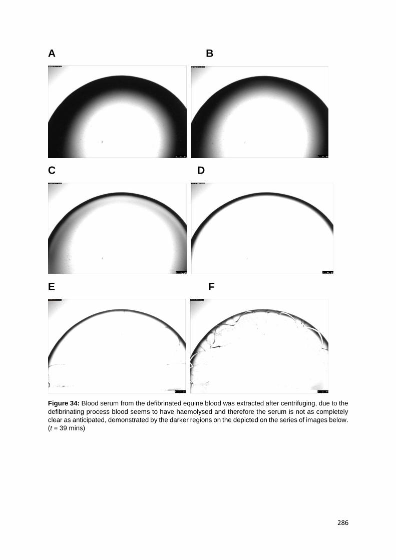
286
A B
C D
E F
Figure 34: Blood serum from the defibrinated equine blood was extracted after centrifuging, due to the
defibrinating process blood seems to have haemolysed and therefore the serum is not as completely
clear as anticipated, demonstrated by the darker regions on the depicted on the series of images below.
(t = 39 mins)

287
A B
C D
E F
Figure 35: Human blood serum is depicted in a series of images below showing the drying process. (t
= 38 mins)
Both blood serums (Figure 34 and 35) exhibit similar drying mechanisms, viz.
the coffee ring effect, where there is clear flow towards the periphery of the drop where
particles start to accumulate. The mechanism is best represented in Figure 34, the
equine serum, the blood had clearly haemolysed which is most likely a result of the

288
defibrination process, leaving deposits of haemoglobin within the serum and therefore
provides a visible contrast against the clear serum. Drying times of human and equine
blood drops were also compared and it was found that there were no significant
differences in times.
3.4.2.2 Effects of PCV % upon the drying mechanism
A range of PCV % were tested from 15 to 75 % as this relates to the lowest and
highest values experienced in potential victims / injured parties. [4] Figures 36 through
to 38 depict the drying processes exhibited by changing the PCV %.

289
A B
C D
E F
Figure 39: A sequence of images demonstrating the drying effect of human blood at a PCV % of 15 %
were gathered using a 2.5 x 0.07 magnification microscope objective. (t = 40 mins)

290
A B
C D
E F
Figure 37: Images collected with the use of a Leica microscope at magnification 2.5 x 0.07
demonstrating the drying effect of human blood at a PCV % of 40 %. (t = 42 mins)
The lower percentages (Figure 36) show the drop to be more transparent in
appearance when microscopically viewed; this is due to the overwhelming proportions
of plasma present in the lower packed cell volumes.

291
A B
C D
E F
Figure 38: A sequence of images collected using a microscope at magnification of 2.5 x 0.07,
demonstrating the drying effect of human blood at a PCV % of 75 %. (t = 42 mins)
Comparing the lower values of PCVs with the higher values (Figure 38) an
apparent absence of a ring in lower concentrations is observed, where all red blood
cells are observed in the centre of the drop, this is strange considering the previous
results for serum, where the coffee ring effect (see section 1.3.1) seemed to be the
driving drying force. Since individual RBCs in a bloodstain are difficult to visualise
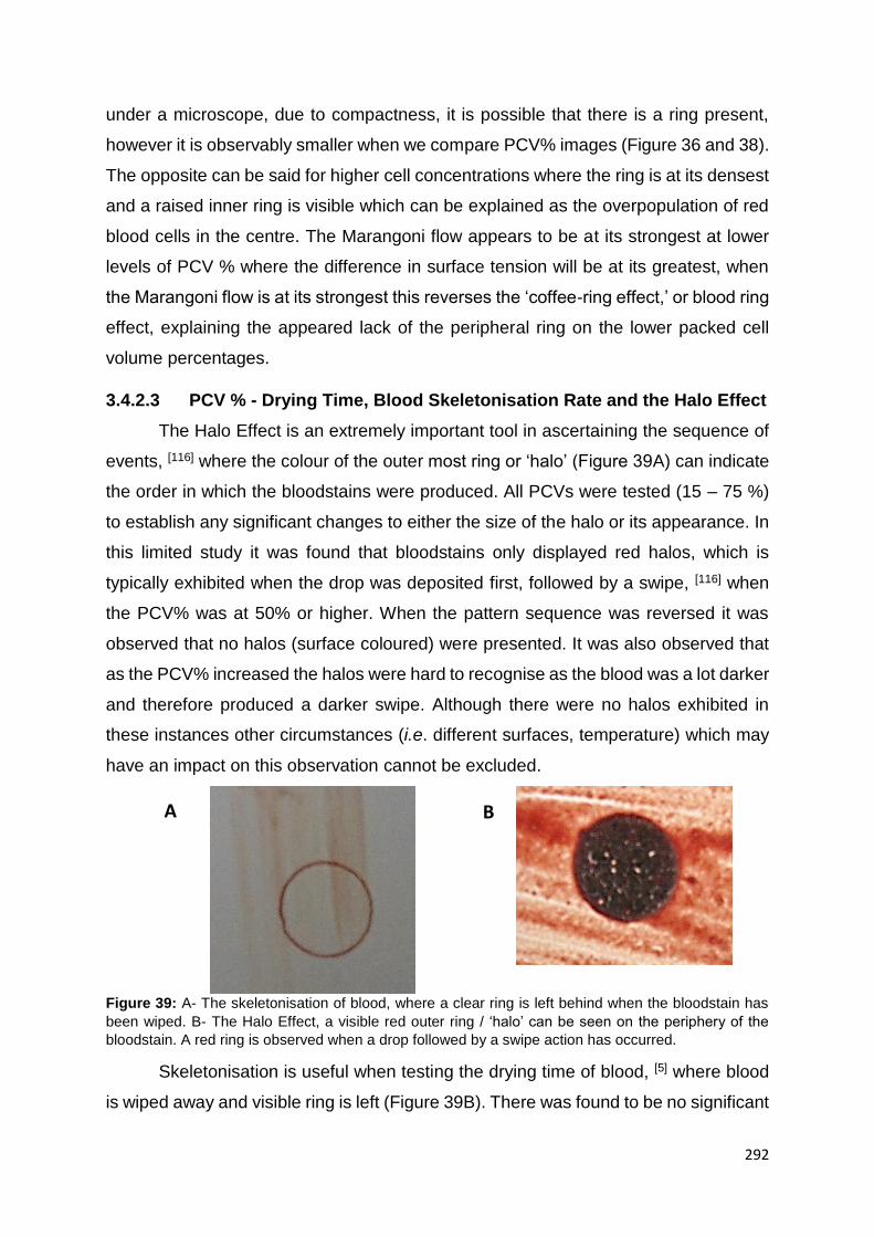
292
under a microscope, due to compactness, it is possible that there is a ring present,
however it is observably smaller when we compare PCV% images (Figure 36 and 38).
The opposite can be said for higher cell concentrations where the ring is at its densest
and a raised inner ring is visible which can be explained as the overpopulation of red
blood cells in the centre. The Marangoni flow appears to be at its strongest at lower
levels of PCV % where the difference in surface tension will be at its greatest, when
the Marangoni flow is at its strongest this reverses the ‘coffee-ring effect,’ or blood ring
effect, explaining the appeared lack of the peripheral ring on the lower packed cell
volume percentages.
3.4.2.3 PCV % - Drying Time, Blood Skeletonisation Rate and the Halo Effect
The Halo Effect is an extremely important tool in ascertaining the sequence of
events, [116] where the colour of the outer most ring or ‘halo’ (Figure 39A) can indicate
the order in which the bloodstains were produced. All PCVs were tested (15 – 75 %)
to establish any significant changes to either the size of the halo or its appearance. In
this limited study it was found that bloodstains only displayed red halos, which is
typically exhibited when the drop was deposited first, followed by a swipe, [116] when
the PCV% was at 50% or higher. When the pattern sequence was reversed it was
observed that no halos (surface coloured) were presented. It was also observed that
as the PCV% increased the halos were hard to recognise as the blood was a lot darker
and therefore produced a darker swipe. Although there were no halos exhibited in
these instances other circumstances (i.e. different surfaces, temperature) which may
have an impact on this observation cannot be excluded.
Figure 39: A- The skeletonisation of blood, where a clear ring is left behind when the bloodstain has
been wiped. B- The Halo Effect, a visible red outer ring / ‘halo’ can be seen on the periphery of the
bloodstain. A red ring is observed when a drop followed by a swipe action has occurred.
Skeletonisation is useful when testing the drying time of blood, [5] where blood
is wiped away and visible ring is left (Figure 39B). There was found to be no significant
A B
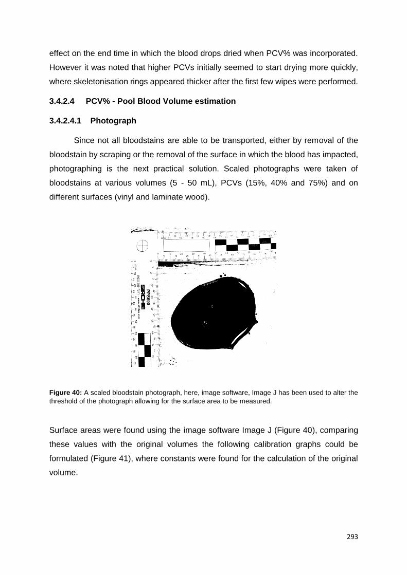
293
effect on the end time in which the blood drops dried when PCV% was incorporated.
However it was noted that higher PCVs initially seemed to start drying more quickly,
where skeletonisation rings appeared thicker after the first few wipes were performed.
3.4.2.4 PCV% - Pool Blood Volume estimation
3.4.2.4.1 Photograph
Since not all bloodstains are able to be transported, either by removal of the
bloodstain by scraping or the removal of the surface in which the blood has impacted,
photographing is the next practical solution. Scaled photographs were taken of
bloodstains at various volumes (5 - 50 mL), PCVs (15%, 40% and 75%) and on
different surfaces (vinyl and laminate wood).
Figure 40: A scaled bloodstain photograph, here, image software, Image J has been used to alter the
threshold of the photograph allowing for the surface area to be measured.
Surface areas were found using the image software Image J (Figure 40), comparing
these values with the original volumes the following calibration graphs could be
formulated (Figure 41), where constants were found for the calculation of the original
volume.

294
Figure 41: Calibration graphs expressing surface areas of bloodstains versus original volume on two
different surface types: A- vinyl and B- laminate wood.
Figure 41A displays the lines of ‘best fit’ (y = mx) for volumes on a vinyl surface, it is
observed that the constant (m) changes with PCV%, the corresponding constants (i.e.
15% PCV, 0.0013) are multiplied by the surface area (found using Image J) to give the
original volume. A constant (0.0015) was obtained for all PCVs collectively (average),
again using a line of ‘best fit’, the constant, however, was found not to be suitable
leading to errors of ±6.78 - 49.47% in final volume estimation. Similarly this was found
to be true for laminate wood (Figure 41B) where the constant (m) for all PCVs equated
to (0.0013) and gave errors of ±1.87 - 43.95%. It is clear from the high error
A.)
B.)

295
percentages that are present when trying to collate all PCV data that PCVs need to be
analysed individually, indicating the importance of this information at a crime scene
when investigating volume analysis. Unfortunately PCV% cannot be identified in dried
blood and therefore cannot be ascertained at a crime scene, since this method without
the knowledge of PCV% has excessive error rates it is not advised to use this
technique. It is noted that the type of surface had no substantial effect, however both
surfaces are non-porous and therefore this may differ when a porous surface is used.
It was also observed that as the PCV% decreased the surface area increased due to
the viscous forces being reduced, allowing the liquid to spread further. This is an
important observation as other volume estimations which have not been included in
this study also require the measurement of the area of the bloodstain, or the
reconstruction of the bloodstain and this may prove difficult when considering PCV%
and potential spread.
3.4.2.4.2 Dry Weight
The dry weight method is currently considered to be the most accurate method
of volume estimation at a crime scene for non-porous media. Lee et al [39] developed
this method by generating a constant, which could be used to determine the original
volume (V). This involves taking the dry weight of liquid blood from the wet weight of
blood, where the wet weight of 1 mL of blood was found to correspond to 10.2 mg and
the dry weight of 1mL of blood was found to be 2.4 mg. However it seems that the
calculation is incorrect, Lee et al [39] uses the weight loss (10.2 – 2.4 = 7.8) and divides
by the dry weight (2.4) to find the drying constant, which is calculated to give the
(corrected) value of 3.25, as described by equation (13).1 Unfortunately this does not
give the original volume unless the dry weight is again added; see equation 14.
V = Dry Weight x 3.25 (13)
V = (Dry Weight x 3.25) + Dry Weight (14)
1 Following the publication of Lee's approach, an erratum was published in which the original error in the
calculation of the drying constant was corrected from the (incorrect) published value of 4.167 to 3.25. In fact, the
drying constant was shown in the erratum to derive from a plot of dry weight of blood against the original volume
which resulted in the mathematical relationship: original volume = weight x 4.167 mL/0.1 mg. In fact, 4.167
should be replaced with the more accurate 4.1364 which is found from plotting the same data as Lee but using the
line of best fit produced via Microsoft TM Excel.

296
If however we divide the wet weight (10.2) by the dry weight (2.4) this will then give
the correct constant and subsequently the final and correct equation (15):
V = Dry Weight x 4.25 (15)
All PCVs were tested for the drying rate of 1 mL; Table 5 expresses the results, where
drying constants were generated.
PCV
%
Wet Weight
(mg)
(Ww)
Dry Weight (mg)
(Wd)
Ww / Wd
(WcPCV)
15 1027.00 126.10 8.14
20 1028.00 131.60 7.81
30 1026.30 157.70 6.51
40 1026.50 190.03 5.40
50 1010.80 230.87 4.38
60 1005.30 265.70 3.78
70 993.40 297.33 3.34
75 980.90 298.00 3.29
Table 5: Reference table depicting dry weight constants WcPCV derived for a range of PCVs.
There is a significant decrease in the drying constant as the PCV increases;
this can be attributed to the drying process. Normal blood is generally composed of
around 45% PCV, red blood cells have a typical water content of 72% - 73%, [102, 104]
plasma has an average water content value of 93% - 94% and whole blood has a
water content of 83%. Taking this into consideration, when PCVs are fluctuated, water
content can deviate from 77.5% – 90.5% for 15 % - 75% PCV, respectively. Since
water will be evaporated as the blood dries, it is understandable that dried blood of a
PCV% of 15 will weigh less than that of 75% PCV. Unpaired student t-tests were
conducted to verify the significance of the data, constants for 15% vs. 75%, 15% vs.
40% and 40% vs. 75% were all compared. Every comparison undertaken resulted in
a p-value of less than 0.0001; this is considered to be extremely statistically significant.
It can therefore be concluded that PCV% has a significant effect on the dry weight of
blood. Consequently the constant originally devised by Lee et al [39] is quantitatively
altered:
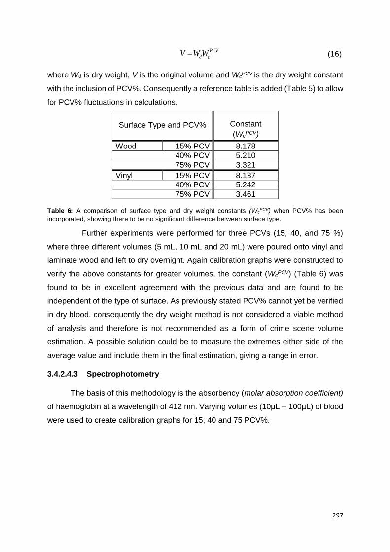
297
PCV
d cV W W (16)
where Wd is dry weight, V is the original volume and WcPCV
is the dry weight constant
with the inclusion of PCV%. Consequently a reference table is added (Table 5) to allow
for PCV% fluctuations in calculations.
Surface Type and PCV% Constant
(WcPCV)
Wood 15% PCV 8.178
40% PCV 5.210
75% PCV 3.321
Vinyl 15% PCV 8.137
40% PCV 5.242
75% PCV 3.461
Table 6: A comparison of surface type and dry weight constants (WcPCV) when PCV% has been
incorporated, showing there to be no significant difference between surface type.
Further experiments were performed for three PCVs (15, 40, and 75 %)
where three different volumes (5 mL, 10 mL and 20 mL) were poured onto vinyl and
laminate wood and left to dry overnight. Again calibration graphs were constructed to
verify the above constants for greater volumes, the constant (WcPCV) (Table 6) was
found to be in excellent agreement with the previous data and are found to be
independent of the type of surface. As previously stated PCV% cannot yet be verified
in dry blood, consequently the dry weight method is not considered a viable method
of analysis and therefore is not recommended as a form of crime scene volume
estimation. A possible solution could be to measure the extremes either side of the
average value and include them in the final estimation, giving a range in error.
3.4.2.4.3 Spectrophotometry
The basis of this methodology is the absorbency (molar absorption coefficient)
of haemoglobin at a wavelength of 412 nm. Varying volumes (10µL – 100µL) of blood
were used to create calibration graphs for 15, 40 and 75 PCV%.

298
Figure 42: Representations of: A- PCV% and B- haemoglobin levels, against constants (m).
The corresponding calibration plots were found to be linear in nature, where the
lines of ‘best fit’ were determined to correspond to: y = 0.0158x, R² = 0.8622 (75%
PCV), y = 0.0078x, R² = 0.9522 (40% PCV) and y = 0.0037x, R² = 0.9665 (15% PCV),
where x is PCV% and y is absorbance. Using these lines of ‘best fit’ (slope) a further
calibration graph for PCV% was constructed, again a line of ‘best fit’ was formulated;
y = 0.0002x, R² = 0.9915 (Figure 42 A), where x is PCV% and y is the absorbance
slope. As the basis of this research is PCV% and previous research was focused
around haemoglobin levels the calibration results are slightly different, giving a lower
value for the absorbance. However through the introduction of equation (17) we can
convert PCV% to haemoglobin values:
A.)
B.)

299
% 0.0485( ) 0.0083 100PCV ctHb x (17)
where ctHb (blood concentration of haemoglobin) has the units mmolL-1. Therefore
the calibration now becomes: y = 0.0006x; R² = 0.9902 (see Figure 42 B). The obtained
results are now in a much better agreement with the previously reported value for the
line of best fit, although they are still slightly lower, which could be attributed to the
expansion of the haemoglobin range under investigation, i.e. 4.71 - 24.6 gr/dl (R2 =
0.99) as opposed to 13.3 – 14.5 gr/dl (R2 = 0.87). [40]
Three types of surfaces were utilised (carpet, vinyl and laminate wood), where
three different volumes were analysed (5mL, 10mL and 20mL). Table 7 expresses the
absorbance results.
PCV% Material 5mL (Average Absorption)
10mL (Average
Absorption)
20mL (Average
Absorption)
15% Wood 0.060 0.128 0.161
Vinyl 0.065 0.093 0.277
Carpet 0.047 0.124 0.322
40% Wood 0.016 0.364 0.576
Vinyl 0.081 0.233 0.425
Carpet 0.174 0.399 0.825
75% Wood 0.243 0.551 1.252
Vinyl 0.433 0.669 1.295
Carpet 0.359 0.780 1.341
Table 7: Haemoglobin absorbance measured at 412 nm for different volumes, various PCVs and
different surface types.
It is apparent that PCV% affects the absorbance levels, generally increasing
the absorption peak as the PCV% increases; this is to be expected, since red blood
cells increase as PCV increase, and corroborates previous investigations using
haemoglobin levels. Ordinarily the calibration graph (Figure 42A) for PCV% versus
constants could be used to rectify these differences, providing new constants for each
PCV, however it is clear that the surface in which the blood has impacted/ dried on
has a considerable effect on the absorbance level. Percentage error rates for each
surface were calculated to be: carpet ± 6.08 - 36.59, vinyl ± 2.42 - 47.83 and laminate
wood ± 0.92 - 45.77. It is therefore evident that calibrations need to be undertaken for
each surface type, this is still possible if a sample of the surface is taken from the crime
scene. Ultimately this method, although it accounts for haemoglobin and PCV%
300
fluctuation, is still not functional as a volume estimation method, again due to there
being no way of measuring the haemoglobin level or PCV% from dried blood, however
this method is much more promising that the previous two since it at least
acknowledges the significance of PCV%.
3.4.3 Summary
It has been determined that blood does in fact dry in a similar way to the ‘coffee-
ring effect,’ it’s mechanism depicted in Figure 30, where the edges of the drop are
pinned to the impact surface creating a contact angle which when decreased produces
a capillary flow and in turn increases surface tension. This causes the collection of
particles (i.e. red blood cells) on the drop periphery; such an effect is now termed the
blood ring effect. [38, 39] Further research exploring the deformation of red blood cells
(in diseases such as Thrombotic Microangiopathy) and how this effects drying should
be examined. Particle shape (i.e. sphere to elongate) has been previously
demonstrated to play a vital role in the drying mechanism when considering the coffee-
ring effect [38] and could therefore potentially change the drying process. It is important
to recognise the processes which drive the drying effects and how physical differences
between individuals alter these processes as this may ultimately effect drying times.
Finally the application of PCV % has been investigated. It has been widely
reported that packed cell volume physically alters viscosity values and would therefore
be expected to modify blood drops. Observations under magnification revealed that
the drying mechanism changes as PCV decreases, seemingly displaying a much
lower coffee-ring effect but maintaining a strong Marangoni flow; this is due to the red
blood cells being mainly located within the centre of the drop where surface tension is
at its strongest pulling particles inwards. Drying observations which can be used to
determine sequencing and volume of blood patterns were also investigated. It was
discovered that the halo effect does not appear on bloodstains with less than 50%
PCV, limiting its value as an events sequencer. However this study is limited and
warrants further investigation using varying conditions. The overall drying time was not
affected by PCV%, this was tested using skeletonisation where a ring remains when
the stain is wiped. Three volume estimations were carried out; dry weight, scaled
photographs and spectrophotometry. Although all three in theory work after some
alterations to account for PCV% and surface type, none are viable options as PCV%
cannot yet be identified in dried blood. This research was conducted merely to

301
highlight the importance of considering PCV% in blood experiments and calculations.
It is important in future investigations to consider PCV %, with the causes behind such
high and low PCV % being centred on health and lifestyle it would be detrimental to
an investigation to ignore it. Investigators should try to establish potential PCV%
altering conditions wherever possible, such as; pregnancy, anaemia and drug use (i.e.
doctor’s patient history). There may also be opportunities at crime scenes where blood
pooling is present and therefore every opportunity should be seized to obtain a sample
for haematological testing.

302
3.5 CONCLUSIONS
This section has investigated the influence components and substitute blood
types have on bloodstains.
Firstly a substitute blood for human blood was explored. Since human blood
may contain diseases such as HIV, which is potentially deathly, blood substitutes are
often employed as a safe alternative. Current alternatives include porcine and sugar
based substitutes, however they are difficult to obtain or are unrealistic and therefore
lack the reliability to produce a viable substitute.
Equine blood is a more readily available animal blood and is ethically gathered
from the horses, however only limited research had previously been performed on
equine bloods applicability to real human blood. In the first study this was investigated.
Horse blood was found to be a viable substitute, mimicking the stain size and spread
of human blood (similar Cd values). This result is only valid, however, with certain
anticoagulants. Alsever’s anticoagulant created a less viscous blood, increasing the
stain size significantly. Defibrinated equine blood exhibited bloodstains which closely
resembled human blood and therefore is concluded to be a reliant human blood
substitute.
Secondly, packed cell volume was explored, since PCV% directly effects the
viscosity and subsequently the spread of liquid. Varying PCV% levels were tested,
ranging from 15%-75% which relate to certain physiological occurrences within a
human (i.e. anaemia). Results found that PCV% significantly affected the size of
bloodstain diameters, where diameters decreased as PCV% increased. This result
was anticipated since PCV% directly relates to the viscosity of blood, thus effectively
altering the spread of blood due to the change in resistance to flow. Angled impacts
remained unchanged, suggesting that spread was evenly distorted throughout the
stain; length and width are the same, therefore cancelling changes out. However since
the bloodstain increases in size it still possible that misinterpretations of patterns may
arise (i.e. a mist pattern vs. impact pattern, or a spurt vs. a gush).
Finally the drying mechanism of blood has been evaluated. Marangoni flow/
effect was recently attributed to be the sole driving force of blood drying. [33] Studies
within this research found similar conclusions, however also discovered that

303
Marangoni was not the lone drying force; the coffee ring effect was also present,
creating small, thick ring around the periphery of the stain. This was further altered
when PCV% was considered, where lower PCV% exhibited a predominantly coffee
ring driven drying compared to higher PCV% where a Marangoni flow acted alone.
Further drying studies evaluated volume analysis, skeletonisation and the halo
effect. The PCV% was found not to change the skeletonisation or halo effect, however
volume analysis was altered substantially. There are several methods of establishing
the volume of bloodstains; each of these was evaluated to determine the effect PCV%
had on the reliability/validity of the methods. All volume estimation methods were
found to be unreliable once PCV% is considered. As blood is predominantly water
(83%), when drying occurs most of this water evaporates leaving a smaller, less heavy
stain. When PCV% is changed this can increase / decrease the water content
significantly, due to water content in plasma and red blood cells. Most methods of
volume determination do not account for either the change in the weight nor the
decrease in flow due to viscosity changes, since most volume estimation is reliant on
size/ spread/ weight of the blood it is unsurprising that these methods are unreliable
when blood components are changed. Therefore extremes should be calculated,
therefore establishing an error which can be applied to the final estimation.
In conclusion, this section has highlighted how the simple manipulation of RBC
ratio, which occurs naturally, can alter the way bloodstains spread, mechanism of
blood drying and ultimately result in unreliable methods of volume estimation.
It is important to establish how PCV% affected bloodstains not only for the
benefits it holds when evaluating stains at crime scenes but for accuracy when
conducting experiments, where PCV% can and should be controlled, setting
provisions where this is not possible.
304
PART II:
IMPACT SURFACES

305
4. SURFACES
Look around the room you are in, no doubt it will have a floor, a ceiling and
walls, what are they made from? How are they decorated? Typically a room will house
a variety of different surfaces, for example floors can be made from wood, be carpeted
or tiled. One of the main factors that must be considered when interpreting bloodstain
patterns is the impact surface. The topography and composition of the surface is
important as it can affect the size, shape and spreading of blood.
It is an impossible feat to test every single surface possible, not only are there
too many but the conditions which they can be found in are variable (finishes,
weathering, temperature and wear and tear). Therefore the following analysis only
scratches the surfaces of this topic, however it should offer valuable insights into
surface interaction which has, so far, not been researched in this depth before.
4.1 Surface Finish
Surface Finish (surface topography) is the deliberate manufacturing
/modification of a surface to create a certain product, e.g. a polished finish. [119 – 122]
Finishing processes can be exercised to: improve appearance, change wettability,
weathering resistance, wear resistance, modify electrical conductivity, remove flaws
or wettability, and control the surface friction.
There are a multitude of manufacturing processes e.g. polishing, abrasive
blasting, honing, chemical milling etc. Each manufacturing process produces a
different surface texture. [119 – 122]
Surface finish is defined using three characteristics:
4.1.1 Surface Roughness - Surface roughness is effectively the small
irregularities found on the surface, which are inherent in the material or production
process. Roughness plays a vital role in determining how the surface will react with a
given environment, where rougher surfaces tend to wear more quickly. [119 – 122]
The surface roughness will also affect the way liquids impinge and spread on a
surface, a factor which is significant when topic at hand is considered. [119 – 122]

306
4.1.2 Lay - Lay or directionality is the direction of the surface pattern (Figure 43),
which is determined by the production process. [119 – 122]
Radial Vertical Horizontal
Circular Isotropic Cross-Hatched
Figure 43: Six main types of surface lay, created through the production process. [119 – 122]
4.1.3 Waviness - Waviness is a broader measure than surface roughness which
measures surface irregularities caused by instabilities (warping, vibrations, or
deflection) experienced during the machining process. [119 – 122]

307
4.2 PRELIMINARY SURFACE ANALYSIS
Since there has been little quantitative research performed presently with regards to
blood drops and the known direct correlation there is between roughness and fluid
flow, [14, 20, 47] surface roughness was the first surface property to be investigated.
4.2.1 Initial Observations
As some previous experimentation (section 3.2) on different surfaces had
already been carried out during the validation of defibrinated equine blood as a viable
human blood substitute, initial observations and calculations were undertaken using
the data collected.
When comparing surface roughness, in accordance with the final stain
diameters (Ds) ascertained during the drop tests, it was apparent that there is an effect;
however due to the inconsistency of the tested surfaces, that is the surface roughness
is heterogeneous in nature, there are anomalies within the results. This is
demonstrated in Figure 20 where it appears that the smaller stains were produced on
the cold rolled steel when compared to the paper, where the surface was much
rougher. It is nevertheless evident from the observed blood stains that there is a
decrease in stain diameter in accordance with surface roughness, such that the lowest
roughness value gives larger bloodstain diameters (Ds). Similar results were exhibited
for both Alsever’s equine blood (Figure 21) and human blood (Figure 22), where
bloodstains decreased when the surface roughness increased. Further verified by
performing t-tests where all p values for the three bloods were found to be extremely
statistically significant, p < 0.0015.
Initial conclusions could therefore be formed stating that a decrease in drop
diameter and an increase in surface roughness ultimately produce smaller blood
stains. This is concurrent with previous research in which porcine blood was tested.
[18] Spines were also evaluated, counting them on the periphery of the bloodstain.
Results obtained for the number of spines observed when using all bloods were also
in excellent agreement with previous research, [18] showing that the rougher the
surface, the greater preponderance of spines.

308
4.3 ANGLED SURFACE STUDY
4.3.1 Experimental
Impact angles (22.7°, 43.5°, 56.3°, 61.6°, 78.8° and 90°) were created by moving
surfaces vertically to create a multitude of angles ranging from 22.7o to 90o. Heights
of 50 – 200 cm were chosen as blood drop release heights as these could be easily
correlated with previous values when angled impacts were considered. [17]
4.3.2 Results and Discussion
4.3.2.1 Considering the surface type - Paper
The first surface to be considered was paper which has been previously utilised
in research by both Knock et al [17] and Hulse-Smith et al [18] and is therefore an
appropriate approach to allow a direct method comparison to be made and ensure the
validity of the equine blood which is utilised throughout the investigation. When
considering angled impacts both the width (a) and elliptical length (b) of the stain are
noted, as a bloodstain elongates as the angle increases. In order to use the
correlations of the Reynolds and Weber numbers it is necessary to use dimensionless
constant, α for angled impacts:
α = ab
Do2
Measurements of the width and length of the bloodstain were undertaken. Equation
(19) was utilised to identify the stain size S, which is a generic equation used to find
the area of an ellipse:
Knock et al [17] created further theoretical parameters ReI and ReIM which were found
to be proportional to the Weber and Reynolds numbers, where ReI is the original
equation [17] (equation 20) and ReIM is the (mis)printed equation (equation 21)
developed after countless experiments undertaken on a variety of liquids: [17]
ReI ∞ Re1/2We1/4 (20)
(18)
(19)

309
ReI ∞ (Re1/2We1/4) 0.75 (21)
Table 8 shows the relationships of various parameters (Equations 18 – 21) to
determine the best correlation; these parameters have previously been demonstrated
to give excellent correlations. [17]
Vertical 90o Vertical 90o All data All data
Equation y = mx + c y = mx y = mx + c y = mx
S vs. Re
R² = 0.61
R² = 0.54
R² ² = 0.53
R² = 0.45
S vs. We R² = 0.47
R² = -0.71
R² = 0.40
R² = -0.69
S vs. ReDoDo y = 0.002x +
59.751 R² = 0.93
y = 0.003x R² = 0.74
y = 0.002x + 68.891
R² = 0.82
y = 0.003x R² = 0.64
S vs. ReIDoDo R² = 0.92
R² = 0.76
R² = 0.8
R² = 0.66
S vs. ReIMDoDo R² = 0.83
R² = 0.65
y = 0.1247x + 32.937
R² = 0.84
y = 0.1463x R² = 0.81
α vs. Re R² = 0.93
R² = 0.28
R² = 0.67
R² = 0.16
α vs. Re0.5 R² = 0.93
R² = 0.92
R² = 0.67
R² = 0.67
α vs. We R² = 0.92
R² = -3.18
R² = 0.65
R² = -2.53
α vs. ReI R² = 0.93
R² = 0.35
R² = 0.67
R² = 0.21
α vs. ReIM R² = 0.93
R² = 0.80
R² = 0.67
R² = 0.56
Table 8: Various parameters correlated against stain size found paper to establish the most significant R2 values and therefore the best coefficient.
It was found that stain size exhibits poor correlations when plotted against the original
Weber and Reynolds number expressing a coefficient of just R2 = 0.4 and R2 = 0.53
respectively. However when the theoretical parameters were used, (ReI, ReIM, Re0.5,
We0.5) as introduced by Knock et al [17] much more effective coefficients were observed
ranging from R2 = 0.67 to R2 = 0.84 (see Figure 44) when all data points were
considered (angled and vertical impacts).

310
Figure 44: Resultant stain size exhibited on paper at various impact angles plotted against REIMDoDo
Using the most significant correlation these parameters can be applied to the
mathematical equation introduced by Knock et al: [17]
ab = m1MD2o + c1 (22)
where m1 and c1 are constants and M is an non-dimensional number i.e. ReDoDo.
Similarly to previous work [17] the number of spines exhibits significant
correlations, which is shown in Table 9, were found when the square root of the Weber
number and ReIM were employed.
Vertical 90o Vertical 90o All data All data
Equation y = mx+ c y = mx y = mx+ c y = mx
N vs. Re
R² = 0.96
R² = 0.66
R² = 0.20
R² = 0.20
N vs. We R² = 0.93
R² = -1.64
R² = 0.19
R² = 0.03
N vs. We0.5 R² = 0.96
R² = 0.91
R² = 0.20
R² = 0.16
N vs. ReI R² = 0.96
R² = 0.71
R² = 0.20
R² = 0.20
N vs. ReIM R² = 0.97
R² = 0.94
R² = 0.20
R² = 0.19
Table 9: Number of spines correlated against various parameters to establish the best correlation
coefficient, R2 value.
Next to be considered was the effect of the angle of impact upon the
correlations which have shown to be significant when considering the vertical impact.
When stain size is analysed the most significant correlation occurs when θ is zero, this
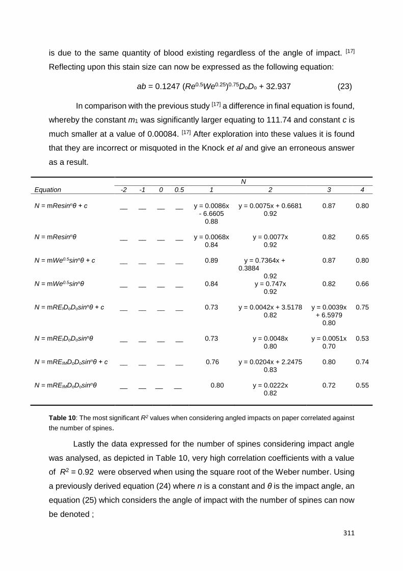
311
is due to the same quantity of blood existing regardless of the angle of impact. [17]
Reflecting upon this stain size can now be expressed as the following equation:
ab = 0.1247 (Re0.5We0.25)0.75DoDo + 32.937 (23)
In comparison with the previous study [17] a difference in final equation is found,
whereby the constant m1 was significantly larger equating to 111.74 and constant c is
much smaller at a value of 0.00084. [17] After exploration into these values it is found
that they are incorrect or misquoted in the Knock et al and give an erroneous answer
as a result.
N
Equation -2 -1 0 0.5 1 2 3 4
N = mResinnθ + c __ __ __ __ y = 0.0086x
- 6.6605 0.88
y = 0.0075x + 0.6681 0.92
0.87 0.80
N = mResinnθ __ __ __ __ y = 0.0068x
0.84 y = 0.0077x
0.92 0.82 0.65
N = mWe0.5sinnθ + c __ __ __ __ 0.89 y = 0.7364x + 0.3884
0.92
0.87 0.80
N = mWe0.5sinnθ __ __ __ __ 0.84 y = 0.747x 0.92
0.82 0.66
N = mREIDoDosinnθ + c __ __ __ __ 0.73 y = 0.0042x + 3.5178 0.82
y = 0.0039x + 6.5979
0.80
0.75
N = mREIDoDosinnθ __ __ __ __ 0.73 y = 0.0048x 0.80
y = 0.0051x 0.70
0.53
N = mREIMDoDosinnθ + c __ __ __ __ 0.76 y = 0.0204x + 2.2475 0.83
0.80 0.74
N = mREIMDoDosinnθ __ __ __ __ 0.80
y = 0.0222x 0.82
0.72
0.55
Table 10: The most significant R2 values when considering angled impacts on paper correlated against
the number of spines.
Lastly the data expressed for the number of spines considering impact angle
was analysed, as depicted in Table 10, very high correlation coefficients with a value
of R2 = 0.92 were observed when using the square root of the Weber number. Using
a previously derived equation (24) where n is a constant and θ is the impact angle, an
equation (25) which considers the angle of impact with the number of spines can now
be denoted ;

312
y = m x sinn θ + c (24)
N = 0.75We0.5sin2θ (25)
The constant n has now changed from the previous value [17] of 3 to 2; however
constant m has remained unchanged. Due to the uncertain nature of spines and their
calculation, it is difficult to establish the correct equation constants as both produce
realistic spine values. It would therefore be advised not to use spines in analysis at all;
they offer no concrete results and add an unnecessary and time consuming aspect to
an already complex analytical field.
4.3.2.2 Considering the surface type - Steel and Plastic
The effects of angles on different surfaces, namely plastic and steel were
investigated. It has already been widely recognised that surface roughness is highly
influential in the final appearance of the bloodstain and is therefore an anticipated
exploration which was not previously undertaken by Knock et al whose work centred
around paper. [17] Similarly to that of the paper surface, blood was dropped from a
range of heights at varying impact angles onto both surface types (steel and plastic)
where widths and elliptical lengths were subsequently measured.

313
Vertical 90o Vertical 90o All data All data
Equation y = mx+ c y = mx y = mx+ c y = mx
S vs. Re R² = 0.60
R² = 0.56
R² = 0.49
R² = 0.45
S vs. We R² = 0.44
R² = -0.46
R² = 0.36
R² = -0.51
S vs. ReDoDo y = 0.002x + 54.995
R² = 0.93
y = 0.003x R² = 0.83
y = 0.003x + 61.693
R² = 0.80
y = 0.003x
R² = 0.70
S vs. ReIDoDo R² = 0.91
R² = 0.38
R² = 0.78
R² = 0.7
S vs. ReIMDoDo y = 0.1407x + 14.095
R² = 0.96
y = 0.1499x R² = 0.95
y = 0.1448x + 19.574
R² = 0.83
y = 0.1576x
R² = 0.82
α vs. Re R² = 0.95
R² = 0.60
R² = 0.67
R² = 0.31
α vs. Re0.5 R² = 0.97
R² = 0.94
R² = 0.67
R² = 0.67
α vs. We R² = 0.88
R² = -2.07
R² = 0.61
R² = -2.00
α vs. ReI R² = 0.94
R² = 0.61
R² = 0.65
R² = 0.32
α vs. ReIM R² = 0.94 R² = 0.90 R² = 0.65 R² = 0.59
Table 11: R2 values established when considering the correlation of various parameters against stain
size exhibited upon a steel surface.
Vertical 90o Vertical 90o All data All data
Equation y = mx+ c y = mx y = mx+ c y = mx
S vs. Re R² = 0.69
R² = 0.60
R² = 0.58
R² = 0.55
S vs. We R² = 0.54
R² = -0.90
R² = 0.44
R² = -0.44
S vs. ReDoDo y = 0.002x + 76.053
R² = 0.95
y = 0.003x R² = 0.65
y = 0.002x + 58.239
R² = 0.88
y = 0.003x
R² = 0.77
S vs. ReIDoDo R² = 0.94
R² = 0.69
R² = 0.87
R² = 0.78
S vs. ReIMDoDo y = 0.1119x + 44.648
R² = 0.96
y = 0.1411x R² = 0.89
y = 0.1405x + 17.771
R² = 0.91
y = 0.1521x
R² = 0.8985
α vs. Re R² = 0.85
R² = 0.12
R² = 0.82
R² = 0.49
α vs. Re0.5 R² = 0.87
R² = 0.87
R² = 0.84
R² = 0.82
α vs. We R² = 0.86
R² = -3.44
R² = 0.77
R² = -1.89
α vs. ReI R² = 0.89
R² = 0.25
R² = 0.82 R² = 0.52
α vs. ReIM R² = 0.90 R² = 0.75 R² = 0.82 R² = 0.78
Table 12: Resultant stain sizes on a plastic surface correlated against numerous parameters to
determine the best coefficient R2 value.

314
Stain sizes were correlated against numerous parameters, as shown in Tables 11 and
12 and exhibited profound correlations when ReDoDo, REIMDoDo and REIDoDo were
used. When the most significant parameters were applied and a further consideration
of impact angle (θ) is added it was again observed that the best correlation was
exhibited when θ is zero, cementing the evaluation that stain size is not directly
influenced by angle of impact. [17] Final stain size equations for both steel (equation
26) and plastic (equation 27) were therefore generated using equation (22) and the
parameter REIMDoDo which exhibited coefficient values of 0.83 and 0.91:
ab = 0.1448 (Re0.5We0.25)0.75DoDo + 19.574 (26)
ab = 0.1405 (Re0.5We0.25)0.75DoDo + 17.771 (27)
Tables 13 and 14 evaluate the correlation of the number of spines for steel and plastic
respectively, where low correlations were realised in both the vertical impact and in
considering all the data (angles 22.7o to 90o). The number of spines (N) is affected by
the surface (steel) it impacts and could explain the low correlations due to the lack of
surface roughness to produce a significant amount of stain disruption and
subsequently the production of spines.
Vertical 90o Vertical 90o All data All data
Equation y = mx+ c y = mx y = mx+ c y = mx
N vs. Re R² = 0.75
R² = 0.53 R² = 0.35
R² = 0.24
N vs. We R² = 0.73
R² = 0.70
R² = 0.32
R² = 0.31
N vs. We0.5 R² = 0.71
R² = 0.50
R² = 0.32
R² = 0.22
N vs. ReI R² = 0.74
R² = 0.52
R² = 0.34
R² = 0.23
N vs. ReIM R² = 0.73
R² = 0.42
R² = 0.34
R² = 0.19
Table 13: The number of spines on a steel surface correlated against various theoretical parameters to
determine significant R2 value.

315
Vertical 90o Vertical 90o All data All data
Equation y = mx+ c y = mx y = mx+ c y = mx
N vs. Re R² = 0.31
R² = 0.25
R² = 0.29
R² = 0.25
N vs. We R² = 0.19
R² = 0.18
R² = 0.26
R² = 0.26
N vs. We0.5 R² = 0.18
R² = 0.16
R² = 0.25
R² = 0.22
N vs. ReI R² = 0.24
R² = 0.21
R² = 0.27
R² = 0.24
N vs. ReIM R² = 0.24
R² = 0.17 R² = 0.27
R² = 0.20
Table 14: R2 values established when correlating number of spines exhibited on a plastic surface with
several theoretical parameters.
Although there were no distinctive correlations, spines were still investigated at
different impacting angles (viz. Table 15 and 16) to verify their usefulness, however
again no significant correlations were realised. The use of different surfaces has
exposed the variability of spines as a BPA concept and their ultimate unsuitability
within this scientific discipline.
N
Equation -2 -1 0 0.5 1 2 3 4
N = mResinnθ + c __ __ __ __ y = 0.0066x - 8.5947 0.65
y = 0.0054x - 1.8795
0.59
0.52 0.46
N = mResinnθ __ __ __ __ y = 0.0043x 0.56
y = 0.0048x
0.58
0.51 0.41
N = mWe0.5sinnθ + c __ __ __
__
y = 0.6263x -
8.1468 0.59
y = 0.507x - 1.4733 0.55
0.50 0.42
N = mWe0.5sinnθ __
__ __ __ y = 0.416x 0.52
y = 0.4667x
0.54
0.49 0.37
N = mREIDoDosinnθ + c __ __ __ __ y = 0.0038x - 6.414 0.70
y = 0.0034x - 1.5335
0.67
0.61 0.54
N = mREIDoDosinnθ __ __ __ __ y = 0.0028x 0.64
y = 0.0031x
0.67
0.60
0.50
N = mREIMDoDosinnθ + c __ __ __ __ 0.59 0.54 0.49 0.43
N = mREIMDoDosinnθ __ __ __ __ 0.46 0.50 0.48 0.43
Table 15: R2 values obtained when correlations using various theoretical parameters against the
number of spines when considering an angled steel surface.
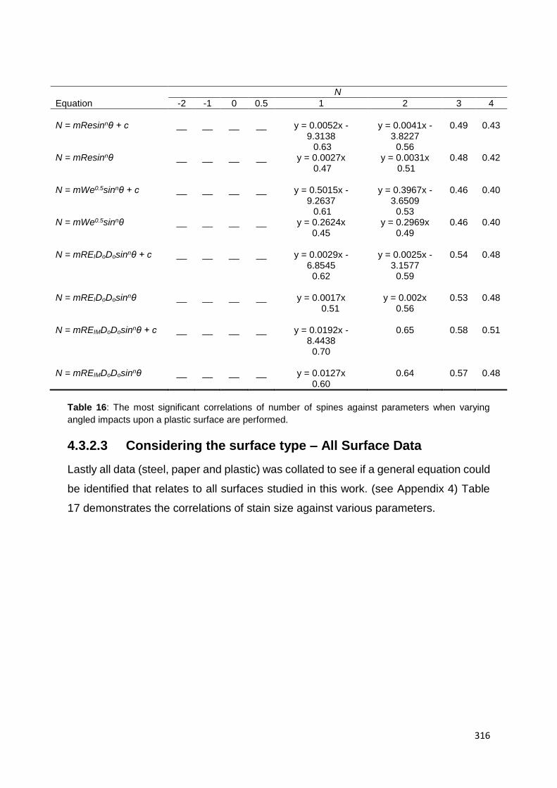
316
N
Equation -2 -1 0 0.5 1 2 3 4
N = mResinnθ + c __ __ __ __ y = 0.0052x -
9.3138 0.63
y = 0.0041x - 3.8227
0.56
0.49 0.43
N = mResinnθ __ __ __ __ y = 0.0027x 0.47
y = 0.0031x 0.51
0.48 0.42
N = mWe0.5sinnθ + c __ __ __ __ y = 0.5015x - 9.2637 0.61
y = 0.3967x - 3.6509
0.53
0.46 0.40
N = mWe0.5sinnθ __ __ __ __ y = 0.2624x 0.45
y = 0.2969x 0.49
0.46 0.40
N = mREIDoDosinnθ + c __ __ __ __ y = 0.0029x - 6.8545
0.62
y = 0.0025x - 3.1577
0.59
0.54
0.48
N = mREIDoDosinnθ __ __ __ __ y = 0.0017x 0.51
y = 0.002x 0.56
0.53 0.48
N = mREIMDoDosinnθ + c __ __ __ __ y = 0.0192x - 8.4438
0.70
0.65 0.58 0.51
N = mREIMDoDosinnθ __ __ __ __ y = 0.0127x
0.60 0.64 0.57 0.48
Table 16: The most significant correlations of number of spines against parameters when varying
angled impacts upon a plastic surface are performed.
4.3.2.3 Considering the surface type – All Surface Data
Lastly all data (steel, paper and plastic) was collated to see if a general equation could
be identified that relates to all surfaces studied in this work. (see Appendix 4) Table
17 demonstrates the correlations of stain size against various parameters.
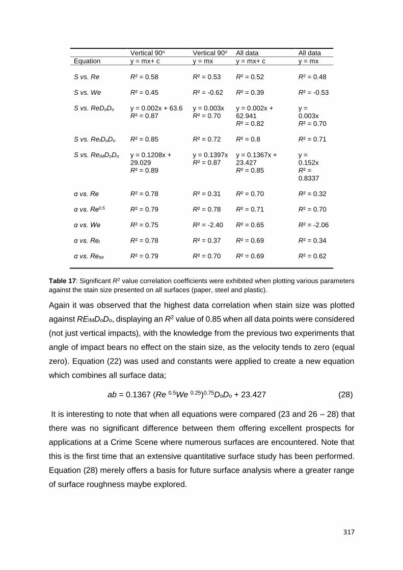
317
Vertical 90o Vertical 90o All data All data
Equation y = mx+ c y = mx y = mx+ c y = mx
S vs. Re R² = 0.58
R² = 0.53
R² = 0.52
R² = 0.48
S vs. We R² = 0.45
R² = -0.62
R² = 0.39
R² = -0.53
S vs. ReDoDo y = 0.002x + 63.6 R² = 0.87
y = 0.003x R² = 0.70
y = 0.002x + 62.941 R² = 0.82
y = 0.003x R² = 0.70
S vs. ReIDoDo R² = 0.85
R² = 0.72
R² = 0.8
R² = 0.71
S vs. ReIMDoDo y = 0.1208x + 29.029 R² = 0.89
y = 0.1397x R² = 0.87
y = 0.1367x + 23.427 R² = 0.85
y = 0.152x R² = 0.8337
α vs. Re R² = 0.78
R² = 0.31
R² = 0.70
R² = 0.32
α vs. Re0.5 R² = 0.79
R² = 0.78
R² = 0.71
R² = 0.70
α vs. We R² = 0.75
R² = -2.40
R² = 0.65
R² = -2.06
α vs. ReI R² = 0.78
R² = 0.37
R² = 0.69
R² = 0.34
α vs. ReIM R² = 0.79
R² = 0.70
R² = 0.69
R² = 0.62
Table 17: Significant R2 value correlation coefficients were exhibited when plotting various parameters
against the stain size presented on all surfaces (paper, steel and plastic).
Again it was observed that the highest data correlation when stain size was plotted
against REIMDoDo, displaying an R2 value of 0.85 when all data points were considered
(not just vertical impacts), with the knowledge from the previous two experiments that
angle of impact bears no effect on the stain size, as the velocity tends to zero (equal
zero). Equation (22) was used and constants were applied to create a new equation
which combines all surface data;
ab = 0.1367 (Re 0.5We 0.25)0.75DoDo + 23.427 (28)
It is interesting to note that when all equations were compared (23 and 26 – 28) that
there was no significant difference between them offering excellent prospects for
applications at a Crime Scene where numerous surfaces are encountered. Note that
this is the first time that an extensive quantitative surface study has been performed.
Equation (28) merely offers a basis for future surface analysis where a greater range
of surface roughness maybe explored.
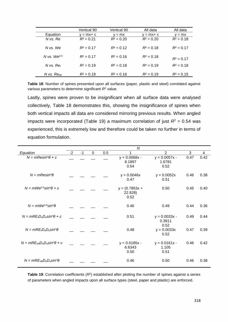
318
Vertical 90 Vertical 90 All data All data
Equation y = mx+ c y = mx y = mx+ c y = mx
N vs. Re R² = 0.21
R² = 0.20
R² = 0.20
R² = 0.18
N vs. We R² = 0.17
R² = 0.12
R² = 0.18
R² = 0.17
N vs. We0.5 R² = 0.17
R² = 0.16
R² = 0.18
R² = 0.17
N vs. ReI R² = 0.19
R² = 0.18
R² = 0.19
R² = 0.18
N vs. ReIM R² = 0.19 R² = 0.16 R² = 0.19 R² = 0.15
Table 18: Number of spines presented upon all surfaces (paper, plastic and steel) correlated against
various parameters to determine significant R2 value.
Lastly, spines were proven to be insignificant when all surface data were analysed
collectively, Table 18 demonstrates this, showing the insignificance of spines when
both vertical impacts all data are considered mirroring previous results. When angled
impacts were incorporated (Table 19) a maximum correlation of just R2 = 0.54 was
experienced, this is extremely low and therefore could be taken no further in terms of
equation formulation.
N
Equation -2 -1 0 0.5 1 2 3 4
N = mResinnθ + c __ __ __ __ y = 0.0068x - 8.1897 0.54
y = 0.0057x - 1.6781
0.52
0.47 0.42
N = mResinnθ __ __ __ __ y = 0.0046x 0.47
y = 0.0052x 0.51
0.46 0.38
N = mWe0.5sinnθ + c __ __ __ __ y = (0.7853x + 22.928)
0.52
0.50 0.45 0.40
N = mWe0.5sinnθ __ __ __ __ 0.46 0.49 0.44 0.36
N = mREIDoDosinnθ + c __ __ __ __ 0.51 y = 0.0033x - 0.3911
0.52
0.49 0.44
N = mREIDoDosinnθ __ __ __ __ 0.48 y = 0.0033x 0.52
0.47 0.39
N = mREIMDoDosinnθ + c __ __ __ __
y = 0.0185x - 6.6343 0.50
y = 0.0161x - 1.105 0.51
0.46 0.42
N = mREIMDoDosinnθ __ __ __ __ 0.46 0.50 0.46 0.38
Table 19: Correlation coefficients (R2) established after plotting the number of spines against a series
of parameters when angled impacts upon all surface types (steel, paper and plastic) are enforced.
319
4.3.3 Summary
After investigation into the effects of various surfaces on the angle of impact, a
useful equation has been formulated for the first time which includes all surfaces to
enable a stain size to be established where ab = 0.1367 (Re0.5We0.25)0.75DoDo +
23.427. However this formula has a correlation coefficient of just 0.85 so merely forms
a basis to provide insights and start to allow the subject to become semi-quantitative.
Note though, this would not be sufficient enough to use in a crime scene scenario,
since it is only 85% reliable and due to BPAs use in legal proceedings where ‘proof
beyond reasonable doubt’ is vital to sustaining a conviction or an acquittal.
It is recognised throughout this investigation that there was a need for a more
proficient and structured procedure of analysis as there appears to be substantial
differences when experimental research is compared, for instance the significance of
spines within BPA analysis has been brought into question within this paper and yet
seems to be noteworthy in other studies. [17 - 18]
It is found that although spines did follow the general pattern of increasing with
release height, spines are insignificant and hold no real purpose this context. Spines
do not tell us anything unique about a bloodstain that we do not already know from
interpreting the size of the bloodstain. However spines can be utilised to determine
directionality and evaluate surface finish, so are useful in real crime scene scenarios
when interpreting bloodstain patterns. Size and diameter interpretation of a bloodstain
seems to be the more viable option in this study, giving more consistent and applicable
results.

320
4.4 SINGLE SURFACE ANALYSIS
It is not only the surface type alone which can alter bloodstains (i.e. stone,
metal, wood etc.), [14, 18, 20, 47] the individual properties which are divided into sub-types
within one surface can also potentially alter the way a liquid (blood) impinges on the
target surface.
This chapter is divided into individual surfaces where characteristics such as
the finish, grade, roughness and density etc. are taken into consideration. Detailed
analysis of individual surface types has not currently been investigated prior to this
work and therefore should provide some novel insights into surface impacts.
4.5 WOOD
Wood is over 400 billion years old and is one of the most important renewable
resources in the world providing fuel, construction material, furniture, paper etc. [123 –
126] The use of wood to this extent makes it one of the most common surfaces expected
to be encountered at a crime scene, and subsequently its likely interaction with blood
should a blood shedding incident occur. The complex nature of wood however means
that blood interactions may vary significantly. The way wood naturally develops
creates variations in wood grain, porosity, colour, surface finish and imperfections (i.e.
knots), this does not include how we ourselves manufacture (i.e. engineered, solid)
and treat wood (i.e.varnish). [123 – 126]
The following study investigates some of these variations, considering surface
finish, wood type, wood grade and engineered vs. solid wood.
4.5.1 Formation of Wood
Wood is a hard fibrous material manufactured from trees and woody plants, it
is found in the roots and stems, growing in concentric layers (Figure 45). [123 – 126] These
layers are visible when they are sliced through the trunk or any other part of the woody
plant (revealing cross-section). [123 – 126]
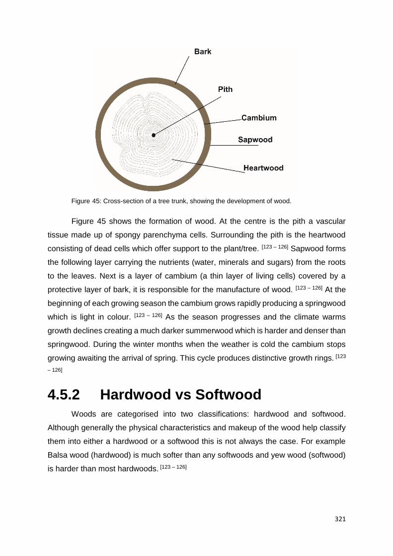
321
Figure 45: Cross-section of a tree trunk, showing the development of wood.
Figure 45 shows the formation of wood. At the centre is the pith a vascular
tissue made up of spongy parenchyma cells. Surrounding the pith is the heartwood
consisting of dead cells which offer support to the plant/tree. [123 – 126] Sapwood forms
the following layer carrying the nutrients (water, minerals and sugars) from the roots
to the leaves. Next is a layer of cambium (a thin layer of living cells) covered by a
protective layer of bark, it is responsible for the manufacture of wood. [123 – 126] At the
beginning of each growing season the cambium grows rapidly producing a springwood
which is light in colour. [123 – 126] As the season progresses and the climate warms
growth declines creating a much darker summerwood which is harder and denser than
springwood. During the winter months when the weather is cold the cambium stops
growing awaiting the arrival of spring. This cycle produces distinctive growth rings. [123
– 126]
4.5.2 Hardwood vs Softwood
Woods are categorised into two classifications: hardwood and softwood.
Although generally the physical characteristics and makeup of the wood help classify
them into either a hardwood or a softwood this is not always the case. For example
Balsa wood (hardwood) is much softer than any softwoods and yew wood (softwood)
is harder than most hardwoods. [123 – 126]

322
Hardwood - Hardwood grows from deciduous and broad-leaf evergreen trees. All
hardwoods are angiosperms (flowering plants) which are the most assorted and
largest group of land plants. [123 – 126] Flowering plants are categorised as those who
shed their leaves in autumn and winter (i.e. maple, oak etc.). The structure of a
hardwood is more complex than that of softwood, where xylem vessels (hollow tubes)
transport water to and throughout the tree (Figure 46). [123 – 126] The structure is denser
as the cell walls are lined with lignin a hard material which supports the plant above
the surface. The quantity of lignin is the main factor creating the namesake hardness
associated with hardwood. [123 – 126]
Figure 46: Structure of hardwood, with observable vessels which transport water throughput the tree.
[127]
Types: There are around 100 times more species of hardwood than softwood.
Examples of the most common hardwoods are: balsa, beech, mahogany, maple, oak,
teak, and walnut. [123 – 126]
Uses: Due to the hardness/density of hardwoods they are used to make
numerous items such as: furniture, flooring, construction materials, utensils,
instruments and paper/tissue. [123 – 126]
Softwood – Softwoods come from coniferous (gymnosperm) trees which have
needles instead of leaves, these needles last all year round (Evergreen). [123 – 126]
Unlike hardwood softwoods rely on medullary rays and tracheids to transport water
and produce sap (Figure 47). [123 – 126] The structure is vascular accounting for the
lower density and ‘softness’. Softwoods also contain lignin though in lower quantities
than in hardwoods and of a slightly different composition. [123 – 126]

323
Figure 47: Structure of softwood, a vascular structure with medullary rays and tracheids which
transports water and produce. [127]
Types: Some examples of softwood: cedar, fir, pine, redwood, spruce, and
yew. [123 – 126]
Uses: As softwoods grow faster than hardwoods they are cheaper and can
therefore provide a less expensive option. Some uses of softwoods are: building
components (i.e. doors), timber, furniture, medium-density fibreboard (MDF),
Christmas trees and paper (softwoods have longer fibres and are more suited for
paper products such as paper bags, cardboard and shipping containers). [123 – 126]
4.5.3 Characteristics of Wood
4.5.3.1 Grain
Two types of wood cells are created during the cambium growth. [128 – 130] Long and
narrow longitudinal cells that align themselves with the axis of the trunk, limb, or root.
The longitudinal cells are responsible for the wood’s grain. The second type of cells
are ray cells which extend out from the pith, perpendicular to the axis. [128 – 130] There
are two classifications of grain; open and closed. When vessels are sliced open they
create pores, these are visible to the naked eye and are defined as open grain. [128 –
130] For those which cannot be detected these are characterised as closed grain.
Softwoods do not contain vessels and therefore have neither. [128 – 130]
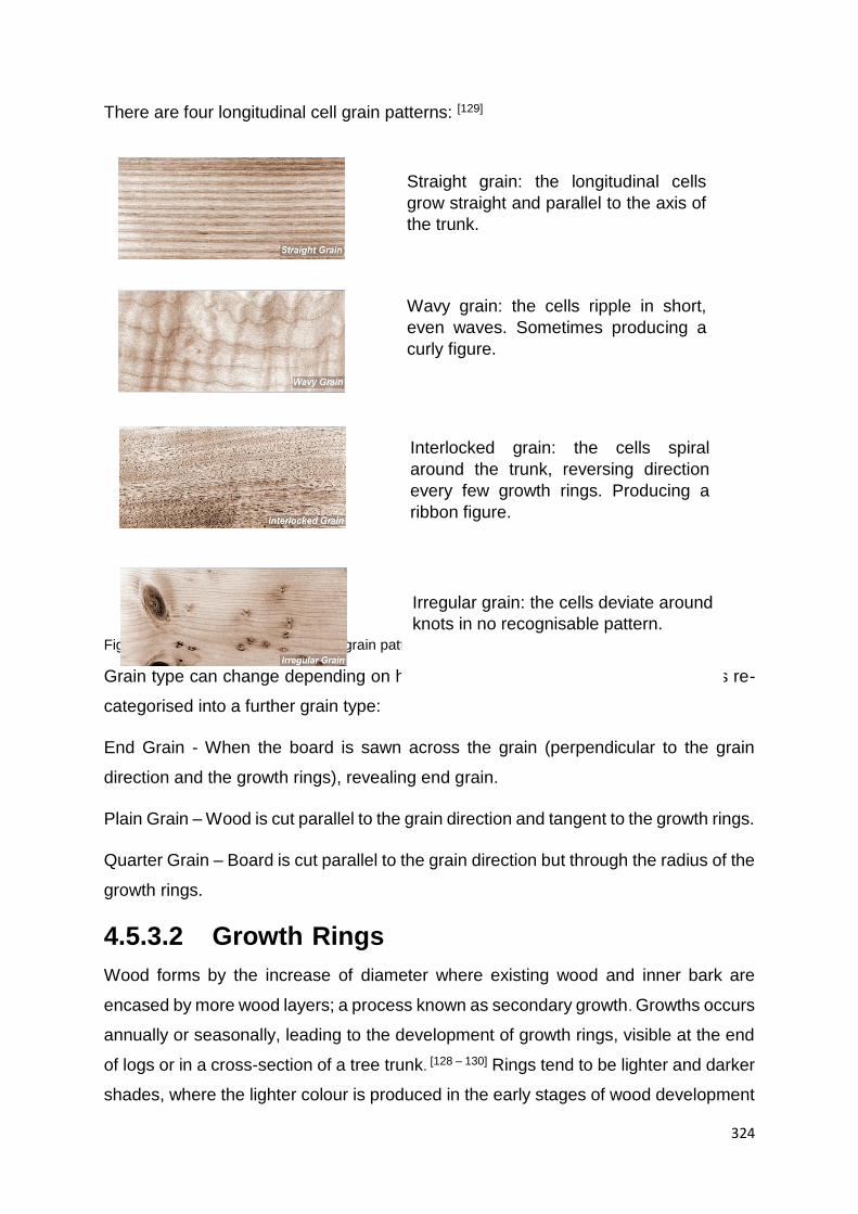
324
There are four longitudinal cell grain patterns: [129]
Figure 48: Four main longitudinal cell grain patterns found in wood [129]
Grain type can change depending on how the wood is cut (sawn), where wood is re-
categorised into a further grain type:
End Grain - When the board is sawn across the grain (perpendicular to the grain
direction and the growth rings), revealing end grain.
Plain Grain – Wood is cut parallel to the grain direction and tangent to the growth rings.
Quarter Grain – Board is cut parallel to the grain direction but through the radius of the
growth rings.
4.5.3.2 Growth Rings Wood forms by the increase of diameter where existing wood and inner bark are
encased by more wood layers; a process known as secondary growth. Growths occurs
annually or seasonally, leading to the development of growth rings, visible at the end
of logs or in a cross-section of a tree trunk. [128 – 130] Rings tend to be lighter and darker
shades, where the lighter colour is produced in the early stages of wood development
Straight grain: the longitudinal cells
grow straight and parallel to the axis of
the trunk.
Wavy grain: the cells ripple in short,
even waves. Sometimes producing a
curly figure.
Interlocked grain: the cells spiral
around the trunk, reversing direction
every few growth rings. Producing a
ribbon figure.
Irregular grain: the cells deviate around
knots in no recognisable pattern.
325
(springwood) and darker wood is produced in the latter stages (summerwood). The
size and colour of the rings can vary dramatically depending on the type of wood. [128
– 130]
4.5.3.3 Knots
A knot is a type of imperfection in a piece of wood which will affect the properties of
the wood, for instance render it weaker more easily broken. [128 – 130] A knot is created
when lower branches die but remain attached, layers continue to grow around it
therefore producing a knot. Knots can also provide a visual effect providing decorative
aspects and visual interest. [128 – 130]
4.5.3.4 Grade
Wood is available in many grade types, categorised for the defects, colour variation,
stiffness, strength and sap presence they contain. [130]
The four main grades for wood flooring are: [130]
Prime – The highest grade, where boards will have a minimal amount of knots and
imperfections (sapwood and filler defects). [130]
Select – A mixture of prime boards and other planks, wood boards display an
infrequent number of knots, heartwood and colour variation and mineral streaking.
Classic / Character – More knots are apparent and checks are visible (cracks
across the growth ring). Colour variation between boards is high. It is sometimes
referred to as natural.
Rustic – The most popular grade for its character and low price. There are a large
amount of knots present, checks and end shake (cracks between the rings). Also
contains heavy grain markings and high colour variation. [130]
This grading system is similar through all wooden surfaces (i.e. worktops), however
the names of the categories change. For instance A, B and C teak grades, where A is
the highest and C is the lowest. [130]
4.5.4 Finishes

326
Wood finishes provide protection and refinement to the wood surface. [131, 132] The first
step of wood finishing is sanding, scraping or planning the surface. Corrections are
made to the wood such as nail holes filled with putty. The wood is finally stained,
coloured and/ or protected etc. using numerous techniques. [131, 132]
4.5.4.1 Green Wood Finishes
There are a variety of eco-friendly finishes: beeswax, linseed oil, safflower oil and
carnauba wax. These are all naturally occurring and therefore are more eco-friendly
than the chemically based finishes, though synthetic versions are available. [131, 132]
4.5.4.2 Varnish
Varnish is used as both a preservative and for decorative purposes, providing a high
end finish for furniture. [131, 132] There are many types of varnish which will fit the
specifications and use that is desired, they can be bought as water or oil based, matte
or high-gloss and either transparent or coloured. For interior or exterior use as
specified on the label. [131, 132]
4.5.4.3 Stain
Provides both a decorative and preservative finish. Stain soaks into the wood,
darkening or colouring it. It is available in matte, gloss, water-based and oil-based. [131,
132] Can be used both on the interior and the exterior; using a varnish to protect the
stained surface.
4.5.4.4 Dye
Like the stain dyes can be used to change or enhance the colour of the wood. Provide
a matt finish and are available as a water-based and oil-based finish. [131, 132] Similar
to the stain finish, dye can be used both on the interior and exterior (if protected by
varnish).
4.5.4.5 Wax
Provides a transparent or translucent decorative finish and can be buffed to a high
gloss. [131, 132] Similar to the oil finish wax nourishes and protects the wood, however
wax is a high maintenance finish needing several coats and constant upkeep. Both
327
water-based and oil-based types are available and is only suitable for interior use. [131,
132]
4.5.4.6 Oil
Oil provides a transparent finish which both nourishes and protects the wood. Can be
used both internally and externally but must be applied to unsealed wood as it will not
penetrate a sealed surface. [131, 132]
4.5.4.7 Wood Preserver
This is supplied as a transparent or coloured with a matter or semi-gloss finish and are
available as water or oil-based. Wood preserver is for exterior use only preventing rot
and insect damage. [131, 132]
4.6 BLOOD IMPACTING WOOD
Since wood is one of the most versatile natural resources in the world it is used
readily in the households, at places of work and other public places. This increases
the chances of blood interacting with a wooden surface such as a flooring, furniture or
buildings constructed of wood.
The difficulty BPA experts face is the wide varieties of wood types, wood
grades, finishes and manufacturing processes (solid or engineered) that are available.
The following research looks at three popular wood types (maple, oak and walnut),
altering the finish, grade and manufacturing process to evaluate how the individual
properties effect the interpretation of bloodstains.
4.6.1 Experimental
Human blood (PCV: 37 %) was utilised, collected from the Manchester Royal Infirmary
blood bank. Blood drop experiments were performed using the method described in
section 2.2. Three types of wood were utilized:
Oak: is the most popular hardwood, with over 60 species split into either white or red
types. It is a strong, heavy wood with large pores which give oak a noticeable grain
and rough texture.

328
species of maple only 5 of these are imported commercially into the UK. Maple is very
hard and resistant to wear, the pores are small creating a fine, smooth texture.
Walnut: known for its versatility it is a popular high end wood (used for making
cabinets, flooring etc.). Walnut is a strong, durable wood with a variety of grains
making it particularly desirable as a design wood.
The woods were of different grades (rustic, natural and prime), finishes (matt
lacquer, stain lacquer, oil and untreated) and manufacturing processes (engineered
and solid).
The following woods were used:
European Maple Oak, Clear Oil Oak, Oak Natural Siera Matt Lacquered, Maple Silk
Matt Lacquered, Natura American Black Walnut Rosshill, Natura Walnut Ironbank
Mississippi, Quickstep Villa Walnut Satin Lacquer, Kahrs Maple Toronto Satin
Lacquer, Kahrs Walnut Rustic Nature Oil, Maple Ultra Matt Lacquered, Oak Silk Matt,
Kahrs Maple Bevelled Edge Rustic, Kahrs Maple Natural Satin Lacquer, Kahrs Linnea
Walnut Bloom Prime Satin Lacquer, Kahrs Linnea Walnut Microbevelled Edge Prime
Matt Lacquer, Natura Walnut Lacquered Satin Lacquer, Kahrs Oak Sienna Natural,
Natura Oak Prime Parquet, Kahrs Oak Siena Engineered Natural, Oak Solid Plank
Untreated.
Blood was released from heights of 50, 100, 150 and 200 cm and at various
angles (20o, 40o, 60o, 80o, 90o). Bloodstains were measured and analysed using
equations (1, 3 and 4).
4.6.2 Results and Discussion
4.6.2.1 Blood Drops on Wood Surfaces
Twenty common wood surfaces were tested to establish the effect each had on
bloodstains. SEMs of the surfaces were performed and roughnesses were evaluated
for each surface (Table 20). Blood was released from 4 different heights, using two
pipette types and bloodstains were measured and compared (see Appendix 5).

329
Wood and Characterisation
SEM Finish Manufacturing Process
Grade Roughness
European Maple Oak
(Pitted)
Satin Lacquer Solid Prime 2.01
Clear Oil Oak (Pitted)
Oil Solid Rustic 1.07
Oak Natural Siera Matt
Lacquered (Bumped)
Matt Lacquer
Engineered Natural 1.55
Maple Silk Matt Lacquered (Smooth)
Satin Lacquer
Engineered Prime 0.64
Natura American Black
Walnut Rosshill (Smooth)
Satin Lacquer
Engineered Rustic 1.14
Natura Walnut Ironbank
Mississippi (Bumped)
Matt Lacquer
Engineered Rustic 1.26
Quickstep Villa Walnut
Satin Lacquer (Bumped)
Satin Lacquer
Engineered Natural 1.02
Kahrs Walnut Rustic Nature
Oil (Striated)
Oil Engineered Rustic 1.19
Maple Ultra Matt Lacquered (Pitted)
Matt Lacquer
Solid Rustic 1.99
Oak Silk Matt (Smooth)
Matt Lacquer
Solid Rustic 0.64
Kahrs Maple Bevelled Edge
Rustic (Smooth)
Satin Lacquer
Engineered Rustic 1.03
Kahrs Maple Natural Satin
Lacquer (Bumped)
Satin Lacquer
Engineered Natural 0.90
Kahrs Linnea Walnut Bloom
Prime Satin Lacquer (Pitted)
Satin Lacquer
Engineered Prime 1.70

330
Kahrs Linnea Walnut
Microbevelled Edge Prime
Matt Lacquer (Bumped)
Matt Lacquer
Engineered Prime 3.77
Natura Walnut Lacquered
Satin Lacquer (Smooth)
Satin Lacquer
Solid Natural 1.45
Kahrs Oak Sienna Natural (Bumped)
Matt Lacquer
Engineered Natural 2.61
Natura Oak Prime Parquet (Striated)
Untreated Solid Prime 5.55
Kahrs Oak Siena Engineered
Natural (Bumped)
Satin Lacquer
Engineered Natural 1.97
Oak Solid Plank Untreated (Striated)
Untreated Solid Rustic 5.89
Kahrs Maple Toronto Satin
Lacquer (Bumped)
Satin Lacquer
Engineered Prime 1.60
Table 20: Physical characteristics of the 20 wood types used in this study.
Figures (49 and 50) illustrate the size of bloodstain diameters when blood impacted
on each wood surface for both pipette sizes.
Bloodstains on all wood surfaces were found to follow the same trends, as height
increased so did the diameter of the bloodstains. Where sharp increases were
observed for the drop at lower heights then reaching 200cm most bloodstains reached
terminal velocity, therefore bloodstains desisted increasing or the increase was less
pronounced.

331
Figure 49: Bloodstain Diameters on all 20 wood types from various heights; 50cm, 100 cm, 150cm and
200cm, using the 1mm pipette.
Figure 50: Bloodstain Diameters on all 20 wood types from various heights; 50cm, 100 cm, 150cm
and 200cm, using the 1.77 mm pipette.
This effect is well documented and was an expected result. Comparing these results
to the roughness’s we find that the rougher surfaces give the smaller bloodstains. This

332
is due to the resistance the rougher surfaces forces on the spreading of the drop. It
can also be attributed to the increased splash experienced on rougher surfaces, where
satellite spatter are formed around the periphery of the stain, therefore decreasing the
volume of the bloodstain and subsequently the eventual diameter.
Next, Reynolds (equation 1) numbers using the physical properties of blood (viscosity
is 5mPa.s) were calculated.
Figure 51: A new line of ‘best fit (solid line) was established when considering the spread factor versus
the Reynolds number utilising human blood on various wood types. Comparing this to the original line
of ‘best fit’ (dashed line) using equation (3) and the line of best fit (dotted line) developed by Hulse-
Smith et al [18] using equation (4); N=5
These were graphed against the spread factor of bloodstains to determine a constant
(Figure 51). A new constant equalling 1.20 was developed for Cd, deviating from the
original value (1.11) devised by Hulse-Smith et al. Viscosity measurements are similar
in both studies, 5 mPa.s in the current study compared to 4.8 mPa.s, therefore
thechange can be attributed to the surface. Wood surfaces produce larger bloodstains
in general when analysed separately to other surface types.
4.6.2.2 Wood Characteristics

333
Since each wood was finished, manufactured and graded differently, woods were split
onto categories to determine if changes in bloodstain size could be pinpointed to a
particular factor/s. Firstly, wood type was evaluated. Three types of wood were utilised
in this study; maple, oak and walnut. Figures 52 A and B show that maple and walnut
are similar in the size of stains they produce, almost mapping each other exactly. Oak,
however, seemed to consistently produce smaller bloodstains.
Figure 50:
Figure 52: Bloodstain Diameters depicted the effect of wood type, where blood was deposited using A-
1mm pipette and B- 1.77mm pipette.
Since oak has large pores, porosity is high, therefore leading to smaller bloodstains.
The wood characteristics table (Table 20) show that on average oak has a rougher
surface, again accounting for the smaller bloodstains produced.
Constant values were calculated for each wood type to fully evaluate the changes
between them. Again Reynolds and Spread Factors were graphed and lines of ‘best
fit’ were drawn, constants (Cd) 1.16, 1.23 and 1.22 were found for oak, maple and
walnut, respectively. These constant support the previous evaluation that maple and
walnut produce similar results and oak yield significantly smaller results.
The grade of the wood and manufacturing process were analysed next (Figures 53
and 54).
A B
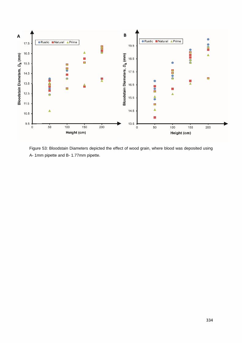
334
Figure 53: Bloodstain Diameters depicted the effect of wood grain, where blood was deposited using
A- 1mm pipette and B- 1.77mm pipette.
B A
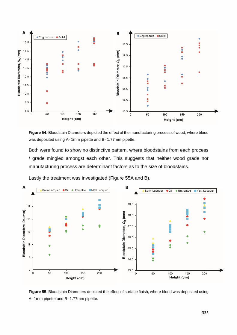
335
Figure 54: Bloodstain Diameters depicted the effect of the manufacturing process of wood, where blood
was deposited using A- 1mm pipette and B- 1.77mm pipette.
Both were found to show no distinctive pattern, where bloodstains from each process
/ grade mingled amongst each other. This suggests that neither wood grade nor
manufacturing process are determinant factors as to the size of bloodstains.
Lastly the treatment was investigated (Figure 55A and B).
Figure 55: Bloodstain Diameters depicted the effect of surface finish, where blood was deposited using
A- 1mm pipette and B- 1.77mm pipette.
B A
A B

336
A distinct pattern was discovered; the smallest bloodstains were created when the
wood was unfinished (not treated), most likely the result of the porous properties of
the wood when left untreated. Larger stains were generated when lacquer finishes
were utilised. Lacquers produce a smoother surface and inhibit the natural porosity of
the wood.
The Reynolds and Spread Factors of each treatment type were plotted, where new
constants Cd were determined; 1.22, 1.23, 1.07, 1.13 for satin lacquer, matt lacquer,
untreated and oil finishes, respectively. Again this further supports the conclusion that
the lowest blood spreading occurs when the wood is unfinished and that lacquers
either satin or matt produce very similar results to one another.
Figure 56: Bloodstain Diameters depicted the effect of surface characteristics, where blood was
deposited using A- 1mm pipette and B- 1.77mm pipette.
All woods were characterised into four groups (pitted, smooth, striated and
bumped) according to their physical appearance (see Table 20 for characterisation).
Figures 56 A and B show that smooth surfaces produced bigger resultant bloodstains,
however all bloodstains did not differ substantially from one another regardless of the
surface characteristics. A reason for this could be attributed to the surface finish, since
this dictates the overall texture of surface, thus covering any defects or distinct
features of the surface to a typical surface finish.
337
Angled impacts were also investigated, errors up to 29.02% were observed
when acute impacts were tested (20oC). Angles were found to consistently decrease
for every wood type tested. Surface finish did not affect the degree of error exhibited
with angled impacts.
4.6.3 Summary
Three wood types were evaluated during this study. The woods were finished,
graded and manufactured differently to fully understand the effects certain
characteristics had on a bloodstain.
Walnut and maple were discovered to behave very similarly, producing nearly
carbon copy diameter results and very close spread factor constants. Oak was found
to produce much smaller bloodstains, since oak is generally rougher and bears bigger
grains and therefore a larger porosity.
Manufacturing processes and grades of wood where found to have no
discernible effect on blood stain size.
Lacquered finishes, both satin and matt, gave much larger stains than oil and
untreated wood finishes. Again this can be attributed to the natural porosity of wood
and roughness, which ultimately effect the spread of liquids.
New constants were found for several factors, the largest deviations were
calculated for the finishes, where lacquers produced constant of 1.23 or 1.22, and
untreated wood had a constant of 1.07. This indicates that although wood type does
heavily influence the size of a bloodstain, the finish is the overriding factor.

338
4.7 FABRICS
Textiles or fabrics are woven materials composed of a network of fibres (thread
/ yarn). The thread is created by spinning raw fibres (i.e. wool, cotton etc.), the thread
is then woven, knitted, crocheted, knotted or pressed together to form the fabric.
Fabrics have a variety of uses: clothing, carpets, upholstered furnishings, beds,
art, quilts, backpacks etc. The presence of fabrics in everyday life make the probability
of interaction with blood during a blood-letting incident high.
4.7.1 Fabric Composition
There are several methods of fabric composition: [133 - 134]
Weaving – this involves the interlacing of long threads (warp) with a set of crossing
thread (weft). Although some weaving can be done by hand it is generally completed
using a frame or a loom. [133]
There are three main types of weaves (see below), most other types are deviations
on the main three.
Plain Weave
Figure 57: Plain weave [135]
Satin
Plain weaves are the most common type of weave, they are
simplistic but are the most stable. The pattern created in the plain
weave is symmetrical, where the warp fibre passes under and over
each weft alternatively. [133] Due to its high stability it is one of the
most difficult weaves to drape, it has high levels of fibre crimp
(waviness) which gives low mechanical properties, therefore this
type of weave is not often used for larger fibres (heavy fabrics).
The satin weave appears differently on each side of the fabric. The
front of the fabric consists of mainly warps running over three or
more weft threads, the reverse has fibres predominately running in
the weft direction. [133] The number of warp or weft fibres crossed
and passed under, before the pattern repeats is known as the
harness number, typically this is 4, 5 and 8 in a satin weave. Unlike
plain weaves satin weaves have a high level of drape and low crimp
and therefore impart good mechanical properties. Although the satin
weave allow fibres to be tightly woven the weave has very low
stability. [133]
Figure 58: Satin weave [135]
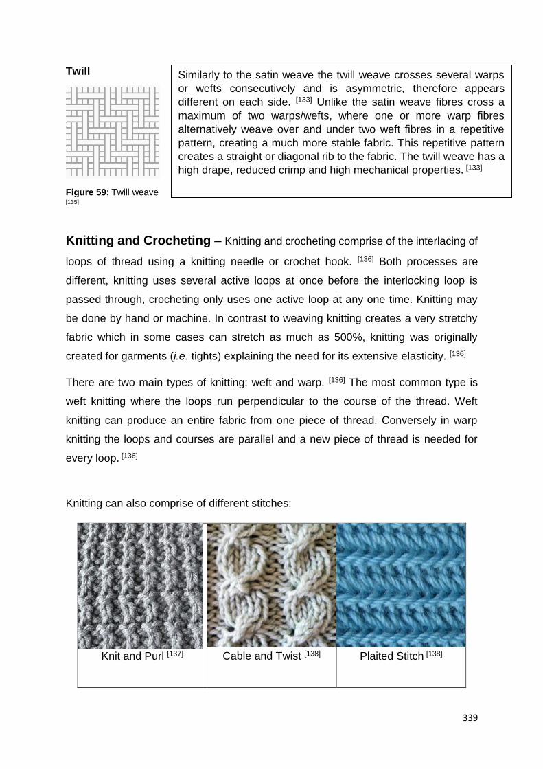
339
Twill
Figure 59: Twill weave [135]
Knitting and Crocheting – Knitting and crocheting comprise of the interlacing of
loops of thread using a knitting needle or crochet hook. [136] Both processes are
different, knitting uses several active loops at once before the interlocking loop is
passed through, crocheting only uses one active loop at any one time. Knitting may
be done by hand or machine. In contrast to weaving knitting creates a very stretchy
fabric which in some cases can stretch as much as 500%, knitting was originally
created for garments (i.e. tights) explaining the need for its extensive elasticity. [136]
There are two main types of knitting: weft and warp. [136] The most common type is
weft knitting where the loops run perpendicular to the course of the thread. Weft
knitting can produce an entire fabric from one piece of thread. Conversely in warp
knitting the loops and courses are parallel and a new piece of thread is needed for
every loop. [136]
Knitting can also comprise of different stitches:
Knit and Purl [137] Cable and Twist [138] Plaited Stitch [138]
Similarly to the satin weave the twill weave crosses several warps
or wefts consecutively and is asymmetric, therefore appears
different on each side. [133] Unlike the satin weave fibres cross a
maximum of two warps/wefts, where one or more warp fibres
alternatively weave over and under two weft fibres in a repetitive
pattern, creating a much more stable fabric. This repetitive pattern
creates a straight or diagonal rib to the fabric. The twill weave has a
high drape, reduced crimp and high mechanical properties. [133]

340
Eyelet and Lace [139] Slipped Stitch Patterns
[140]
Rib Stitch [141]
Table 21: Various important knit types
Spread Tow Fabric (STF) – Spread Tow Fabric is an ultra-
lightweight fabric produced by the spreading of carbon fibre threads
(tow) into thin tapes, this tapes are then woven as a warp and weft.
[142] This method of fabrication has many advantages, avoids
crimps in the fabric, reduces the weight by
stopping the accumulation of matrix at interlacing points and
increases mechanical properties (thinness, drape etc). [142]
Lace – uses a backing and the interlocking, looping, twisting or
braiding of yarns together independently to create a fine
openwork fabric which comprises of patterned holes. [146] The
holes are generated by the removal of threads or can be
achieved during the construction process. Lace can be made
by either hand or machine and cotton is usually the fabric of
choice, though linen, silk, copper, synthetic, silver and gold
threads have be known to be utilised. [146] There are numerous
types of lace, categorised by how they are made. These include: Needle lace,
Figure 60: STF [143]
Braiding / Plaiting – Braids / Plaits are usually created with three
strands of fabric (hair or wires) interlaced and crossed over one another
(zigzagging). [144] Other plait types add-in odd strands to create a wider
structure. This technique is used to fashion dog leads, belts, whips and
rope. [144] Figure 61: A braid [143]
Figure 62: lace fabric. [145]

341
Cutwork, Bobbin lace, Tape lace, Knotted lace, Crocheted lace, Knitted lace, Machine-
made and Chemical lace.
Nonwoven – non-woven fabric is manufactured by the bonding
of 100% polypropylene fibres (i.e. felt), this may be achieved using
thermal, mechanical or adhesive bonding. [148] Non-woven fabrics
are generally manufactured for single use and are made for specific
functions such as cushioning, absorbency, insulation, liquid
repellence etc. [148] Combined with other materials non-woven
fabrics can be used for a multitude of purposes i.e. clothing,
engineering, home furnishings, health care and many more.
4.7.2 Fabric Finishes
Dye – changing the colour of a fabric can be achieved by
dyeing, this requires the use of water (a gallon of water for
every pound of clothing) and the dye. [149] Patterns in the
fabric can be created using resist dyeing processes such as
tie-dyeing, where areas of the fabric at tied off (see Figure
63). Fabrics may also be drawn on using wax, another form
of resist dyeing where the dye will not adhere to the areas covered in wax (known as
batik). [149]
Bleaching – used to turn a fabric white or make the fabric paler,
chemicals in bleach inhibit the chromophores present in most dyes
and pigments. [151]
Embroidery – the technique of weaving textiles or coloured
stitches into the fabric to create patterns or colour contrasts. [152]
Figure 63: nonwoven
fabric. [147]
Figure 64: tie-dye fabric [150]
Figure 65: bleached
fabric [151]
Figure 66: Chinese
embroidery [153]
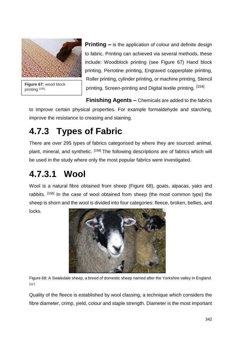
342
Printing – is the application of colour and definite design
to fabric. Printing can achieved via several methods, these
include: Woodblock printing (see Figure 67) Hand block
printing, Perrotine printing, Engraved copperplate printing,
Roller printing, cylinder printing, or machine printing, Stencil
printing, Screen-printing and Digital textile printing. [154]
Finishing Agents – Chemicals are added to the fabrics
to improve certain physical properties. For example formaldehyde and starching,
improve the resistance to creasing and staining.
4.7.3 Types of Fabric
There are over 295 types of fabrics categorised by where they are sourced: animal,
plant, mineral, and synthetic. [156] The following descriptions are of fabrics which will
be used in the study where only the most popular fabrics were investigated.
4.7.3.1 Wool
Wool is a natural fibre obtained from sheep (Figure 68), goats, alpacas, yaks and
rabbits. [156] In the case of wool obtained from sheep (the most common type) the
sheep is shorn and the wool is divided into four categories: fleece, broken, bellies, and
locks.
Figure 68: A Swaledale sheep, a breed of domestic sheep named after the Yorkshire valley in England.
[157]
Quality of the fleece is established by wool classing, a technique which considers the
fibre diameter, crimp, yield, colour and staple strength. Diameter is the most important
Figure 67: wood block
printing [155]

343
parameter, where the wool is measured in microns, the smaller the diameter the finer
the fabric and subsequently the better the quality (used for garments < 25 microns).
Wool is both hydrophobic and hygrophobic where the exterior of the wool fibres repel
liquid and the interior attracts the liquid, respectively. [156]
Global wool production is about 1.3 million tonnes per year, of which 60% goes into
clothing. Other products produced using wool are, rugs, blankets, insulation,
upholstery, nappies, body armour etc.
4.7.3.2 Silk
Silk is a natural protein fibre (fibroin)
produced by insect larvae to create
cocoons, which can then be woven into a
fabric. [158] Silks are produced by many
insects (i.e. spiders) the most recognised
is that produced by the silkworm
caterpillar (Bombyx mori) (Figure 69).
The silkworm is now bred in captivity,
regulating the amount of silk produced.
The eggs of the silkworm take around 14
days to hatch into larvae, it is during the pupal stage (third instar) when the larvae spin
their cocoon, made of raw silk produced by their salivary gland. [158] In captivity this
stage is when the silk cocoon would be boiled, killing the silkworm and making the silk
easier to unravel. This occurs as the moth releases proteolytic enzymes to make a
hole in the cocoon in which the moth can exit. The enzymes are destructive to the silk,
causing breakages and reducing the silk’s value. The process of killing the silkworm
larvae has been heavily criticised, specifically by Mahatma Gandhi going against the
Ahimsa philosophy of “not to hurt any living thing,” he promoted the use of cotton
spinning machine, wild silk and Ahimsa silk (aka peace silk). [159] Silk is one of the
strongest natural fibres, it has a smooth, soft, non-slip finish. However it has low
elasticity, loses nearly a quarter of its strength when wet and in most cases (as a
garment) requires special cleaning (i.e. dry cleaning) as the fabric may shrink when
washed. [158]
Figure 69: A silkworm moth [159]

344
Silk has many uses, these include: garments (shirts, ties, blouses etc.),
furnishings, upholstery, parachutes and artillery gunpowder bags etc.
4.7.3.3 Cotton
Cotton fibres are grown from the cotton plant Gossypium indigenous to the Americas,
Africa, Australia and India, the cotton grows in a boll and is mainly made of pure
cellulose. [160]
Cotton is picked from the bolls and is spun into thread which in turn is woven to create
cotton fabric. [160] Currently the world production of cotton reaches around 25 million
tonnes.
Figure 70: Gossypium, the cotton plant, located in America, Africa, Australia and India [161]
Its uses are vast, providing textile for garments (socks, t-shirts etc.), towels, bed
sheets, tents, explosive manufacture (nitrocellulose), cotton paper, bookbinding,
coffee filters etc. [160]
There are several other varieties of cotton;
- Shiny cotton: here the fibre is processed creating a shiny appearance (mimicking the
appearance of satin) and hydrophobic reaction to liquids.
- Egyptian cotton: regarded as the best cotton fibre worldwide, the Egyptian rich soil
and humid conditions allow the growth of long cotton fibres which are spun into fine
threads. [160]
- Pima cotton: comparable to Egyptian cotton due to the fine cotton threads which
are spun. It is grown in Peru, Australia and Southwest United States, and produces
long fibres which are longer than ordinary cotton but shorter than that produced in
Egyptian cotton. [160]

345
4.7.3.4 Nylon
Nylon is one of the most commonly used polymers. [165] It is synthesised by reacting
two large molecules (Adipic acid and Hexamethylenediamine) together using high heat
(around 285°C) and pressure in an autoclave. [165] The combination of these two
chemical causes a reaction known as condensation polymerisation, where a large
molecule commonly known as nylon-6,6 is produced. Other nylons can be
manufactured by varying the starting molecule (Adipic acid). [165]
Figure 71: The chemical reaction responsible for the production of Nylon [166]
Nylon is one of the most versatile synthetic fibres, responsible for garments
such as stocking/tights, fishing nets, ropes, parachutes and machine components.
[160]
Like polyester, nylon, can be combined with other materials to create a
composite. In conjunction with materials such as glass or carbon fibre (thermoplastic
composites) higher density materials are formulated which can be employed in car
component making (i.e. engines). [165]
Since nylon is essentially a synthetic plastic it has certain physical property
advantages which most natural fabric do not possess without modification. Nylon is
highly resistant to water, tough, resilient and impenetrable to insects, mold and fungi.
[165]
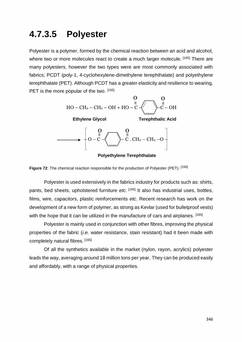
346
4.7.3.5 Polyester
Polyester is a polymer, formed by the chemical reaction between an acid and alcohol,
where two or more molecules react to create a much larger molecule. [165] There are
many polyesters, however the two types were are most commonly associated with
fabrics; PCDT (poly-1, 4-cyclohexylene-dimethylene terephthalate) and polyethylene
terephthalate (PET). Although PCDT has a greater elasticity and resilience to wearing,
PET is the more popular of the two. [165]
Figure 72: The chemical reaction responsible for the production of Polyester (PET). [166]
Polyester is used extensively in the fabrics industry for products such as: shirts,
pants, bed sheets, upholstered furniture etc. [165] It also has industrial uses, bottles,
films, wire, capacitors, plastic reinforcements etc. Recent research has work on the
development of a new form of polymer, as strong as Kevlar (used for bulletproof vests)
with the hope that it can be utilized in the manufacture of cars and airplanes. [165]
Polyester is mainly used in conjunction with other fibres, improving the physical
properties of the fabric (i.e. water resistance, stain resistant) had it been made with
completely natural fibres. [165]
Of all the synthetics available in the market (nylon, rayon, acrylics) polyester
leads the way, averaging around 18 million tons per year. They can be produced easily
and affordably, with a range of physical properties.
o
HO – CH2 – CH2 – OH + HO – C – –C – OH
=
= o
Ethylene Glycol Terephthalic Acid
– O – C – – C . CH2 – CH2 –O –
=
= o o
Polyethylene Terephthalate
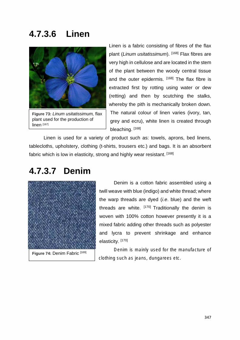
347
4.7.3.6 Linen
Linen is a fabric consisting of fibres of the flax
plant (Linum usitatissimum). [168] Flax fibres are
very high in cellulose and are located in the stem
of the plant between the woody central tissue
and the outer epidermis. [168] The flax fibre is
extracted first by rotting using water or dew
(retting) and then by scutching the stalks,
whereby the pith is mechanically broken down.
The natural colour of linen varies (ivory, tan,
grey and ecru), white linen is created through
bleaching. [168]
Linen is used for a variety of product such as: towels, aprons, bed linens,
tablecloths, upholstery, clothing (t-shirts, trousers etc.) and bags. It is an absorbent
fabric which is low in elasticity, strong and highly wear resistant. [168]
4.7.3.7 Denim
Denim is a cotton fabric assembled using a
twill weave with blue (indigo) and white thread; where
the warp threads are dyed (i.e. blue) and the weft
threads are white. [170] Traditionally the denim is
woven with 100% cotton however presently it is a
mixed fabric adding other threads such as polyester
and lycra to prevent shrinkage and enhance
elasticity. [170]
Denim is mainly used for the manufacture of
clothing such as jeans, dungarees etc.
Figure 73: Linum usitatissimum, flax
plant used for the production of
linen [167]
Figure 74: Denim Fabric [169]

348
4.8 BLOOD IMPACTING FABRIC
Fabrics are a particularly difficult surface for the interpretation of bloodstain
patterns, evident in the case of David Camm (see introduction) where the
misinterpretation led to a miscarriage of justice and doubts cast of the reality of BPA
as a forensic discipline.
This study investigates fabric types and the effect these have on the impact of
blood from various heights and angles.
4.8.1 Experimental
4.8.1.1 Resources
All equine blood (defibrinated) was obtained from TCS-Biosciences Limited at
a PCV % (Packed Cell Volume) of 43%.
In order to be representative of real-life the most common types of fabrics, [160]
for clothing, were tested: Cotton Duck, Cotton Jersey Ecru, Cotton Poplin, Denim, Fuji
Silk, Heavyweight Cotton, Jupiter Linen, Light Grey Polyester Twill, M&S T-shirt
Jersey, Medium Habotai Silk, Peasant Cotton, Poly Satin Heavy, Poly/linen/rayon
Pandora Devore, Raised Natural Cotton, Resida Bump Cotton, Silk Chiffon, Silk
Dupion, Wool Delaine (bleached) and Wool mix suiting. These fabrics were purchased
new and used without alteration.
4.8.1.2 Methods
Fabrics were characterised using several tests (see Table 24 for results). The
surface roughness of each fabric was determined using the Smoothness & Porosity
Tester (Bendtsen Type). Porosity was established by following the fluid re-saturation
method according to Ref 171. Fourier Transform Infra-red spectrometry (FTIR) was
also utilized to verify the composition of the fabrics and lastly Scanning Electron
Microscope images (SEMs) were taken of each fabric to ascertain the structure of the
fabric (i.e. weave).
Blood drops were dispensed manually using two different sized pipettes, 1 mm
and 1.77 mm (inner tip diameter), from varying heights (50 cm, 100 cm, 150 cm and
349
200 cm) (Table 22), at various impact angles (20o, 40 o, 60 o, 80 o, 90 o) and onto
different fabric types.
Table 22: Release heights of blood drops calculated from the tip of pipette to the impacting surface and
converted into impact velocity with the use of Equation (11).
A minimum amount of pressure was applied to the pipette each time and the
drops were performed by the same analyst to maintain continuity. Drops were
repeated 5 times and stain diameters were measured using a magnifying loupe.
4.8.2 Results and Discussion
4.8.2.1 Blood Drops on Fabrics
Twenty common fabric types were tested to establish the effect each had on
bloodstains. Blood was released from 4 different heights and bloodstains were
measured and compared. (see Appendix 6)
Release Heights (cm)
Impact Velocity (m/s)
50
3.13
100
4.43
150
5.42
200
6.26
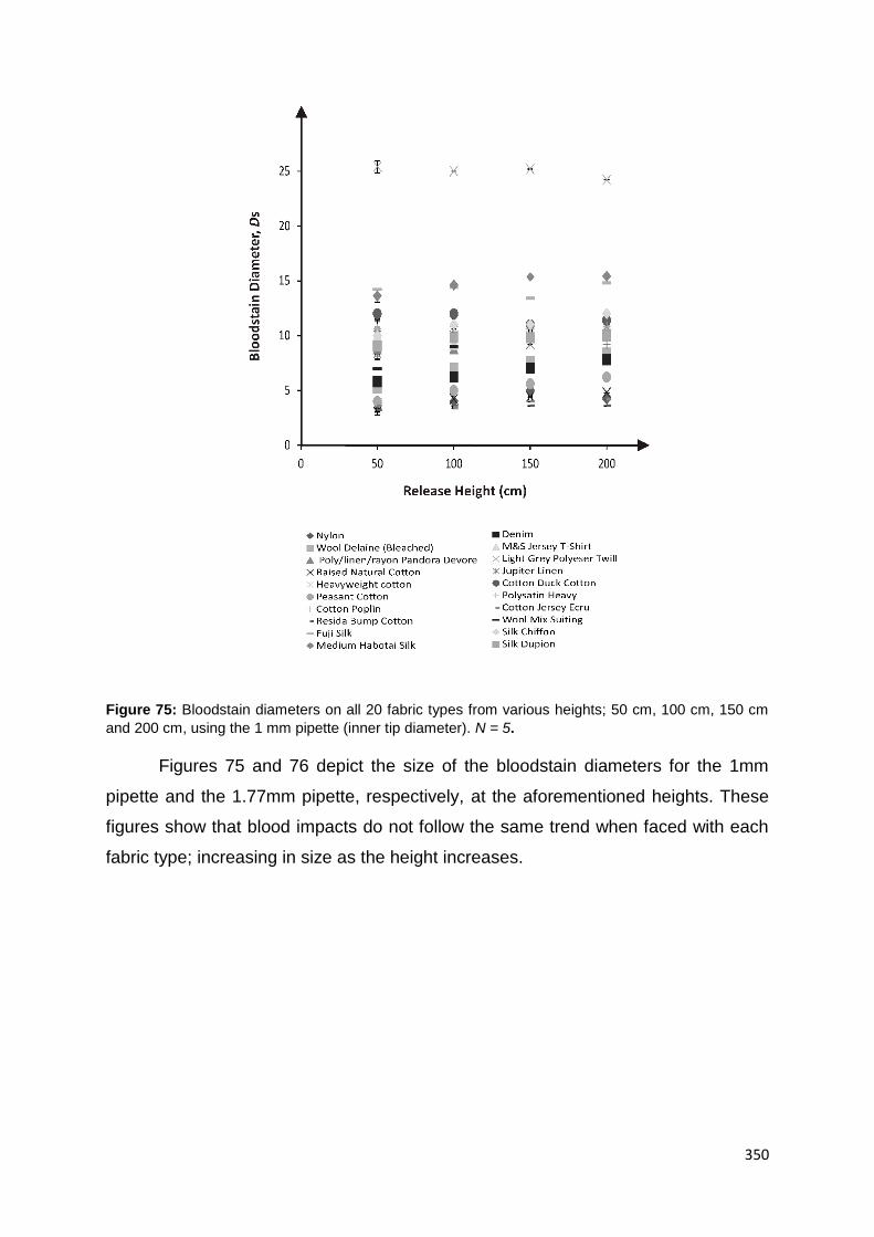
350
Figure 75: Bloodstain diameters on all 20 fabric types from various heights; 50 cm, 100 cm, 150 cm
and 200 cm, using the 1 mm pipette (inner tip diameter). N = 5.
Figures 75 and 76 depict the size of the bloodstain diameters for the 1mm
pipette and the 1.77mm pipette, respectively, at the aforementioned heights. These
figures show that blood impacts do not follow the same trend when faced with each
fabric type; increasing in size as the height increases.

351
Figure 76: Bloodstain diameters on all 20 fabric types from various heights; 50 cm, 100 cm, 150 cm
and 200 cm, using the 1.77 mm pipette (inner tip diameter). N = 5
In some cases (M&S T-shirt Jersey, Light Polyester Grey Twill, Cotton Duck,
Polysatin Heavy, Cotton Poplin, Resida Bump Cotton, Fuji Silk, Nylon and Jupiter
Linen) the bloodstain actually increases, then decreases, or stays relatively similar in
size in spite of the height increase. When we compare this data with the characteristics
of the fabrics (Table 23) it seems that the surface roughness and porosity does not
affect the size of the bloodstain, however the thickness of the fabric appears to have
a profound effect on bloodstain size i.e. Jupiter Linen and Polysatin/ Silk Dupion.

352
Type of Fabric SEM Composition And
Characterisation
Roughness (mL/min)
Thickness (mm)
Weight (g)
Porosity (%)
Jupiter Linen
Light weight even plain weave
4600 0.23 3.05
91.62
Raised Natural Cotton
Plain weave Cotton with soft
raised finish 4200 0.62 6.4
86.98
Fuji Silk
plain even weave Silk, Medium-weight fabric,
woven from spun silk fibres
2300 0.16 1.82
90.49
Heavyweight Cotton
Twill weave heavy Cotton
4200 0.39 5.05
96.84
Cotton Jersey Ecru
Knit Interlock pattern; knit one,
purl one 4500 0.47 4.3
83.04
Wool Mix Suiting
Plain Weave 3200 0.34 4.42
83.87
Wool Delaine (bleached)
Plain Weave 5000 0.26 2.52
85.60
Poly/linen/rayon Pandora Devore
Plain weave 4600 0.39 5.74
94.86
Peasant Cotton
Plain weave 4800 0.63 7.63
93.91
Resida Bump Cotton
Thick coarse loose Plain weave
4500 1.38 9.04
95.05

353
Table 23: Physical characteristics of the 20 fabrics used in this study.
Silk Dupion
Tight plain weave 4200 0.21 2.09
87.50
Silk Chiffon
loose, plain weave and tightly twisted single crêpe yarns in both warp and
weft
4000 0.09 0.34
88.02
Denim
Tight twill weave
5000 0.72 7.19
93.52
M&S T-Shirt Jersey
tight knit pattern (moss stitch), 1
knit, 1 purl 5600 0.35 2.85
95.22
Cotton Duck
Plain weave 4200 0.60 8.48
97.03
Medium Habotai Silk
Plain close weave 1400 0.07 0.67
82.05
Light Grey Polyester Twill
Twill weave 4000 0.23 2.18 98.21
Polysatin Heavy
Twill weave 2500 0.22 3.06
89.52
Cotton Poplin
Plain tight weave 3600 0.36 4.37
86.65
Nylon
Plain tight weave 4400 0.30 7.18 N/A
Water-proof

354
Figure 77: Bloodstain Diameters depicted the effect of fabric composition, where blood was deposited
using A- 1mm pipette and B- 1.77mm pipette.
The composition of the fabrics were explored next. Fabrics were categorised
into 5 groups; plain weave, loose plain weave, coarse plain weave, twill weave and
knit. Figures 77 A and B display the effects the fabric composition has on the spreading
of blood and final bloodstain. There was found to be no distinct difference between the
diameter of bloodstains and the fabric composition, there was a range of sizes
experienced independent of how the fabric was made (i.e. plain weave vs. twill weave).
There was an unusual phenomenon observed when polyester and silk fabrics
were tested, a secondary ring was produced. This is similar to the ones observed by
Slemko [50] who documented this occurrence on silk alone. A further 3 polyester fabrics
were examined, where a secondary ring was observed on every polyester fabric
(Figure 78A) at some stage.

355
Figure 78: Secondary rings (a diffused outer ring) depicted on two fabric types; A – Polyester (Grey
Polyester Twill) and B – Silk (Fuji)
This secondary ring on polyester was found not to be constant, as the degree
of diffusion depended on the height from which the blood drop was released and the
type of polyester. Four types of silk were examined, again this phenomenon was
apparent on all of the silks (Figure 78B). However only two of the silk fabrics produced
symmetrical rings at which were calculated to be at reduction constants of 1.24 and
1.25 for Fuji and Habotai silk, respectively.
B A
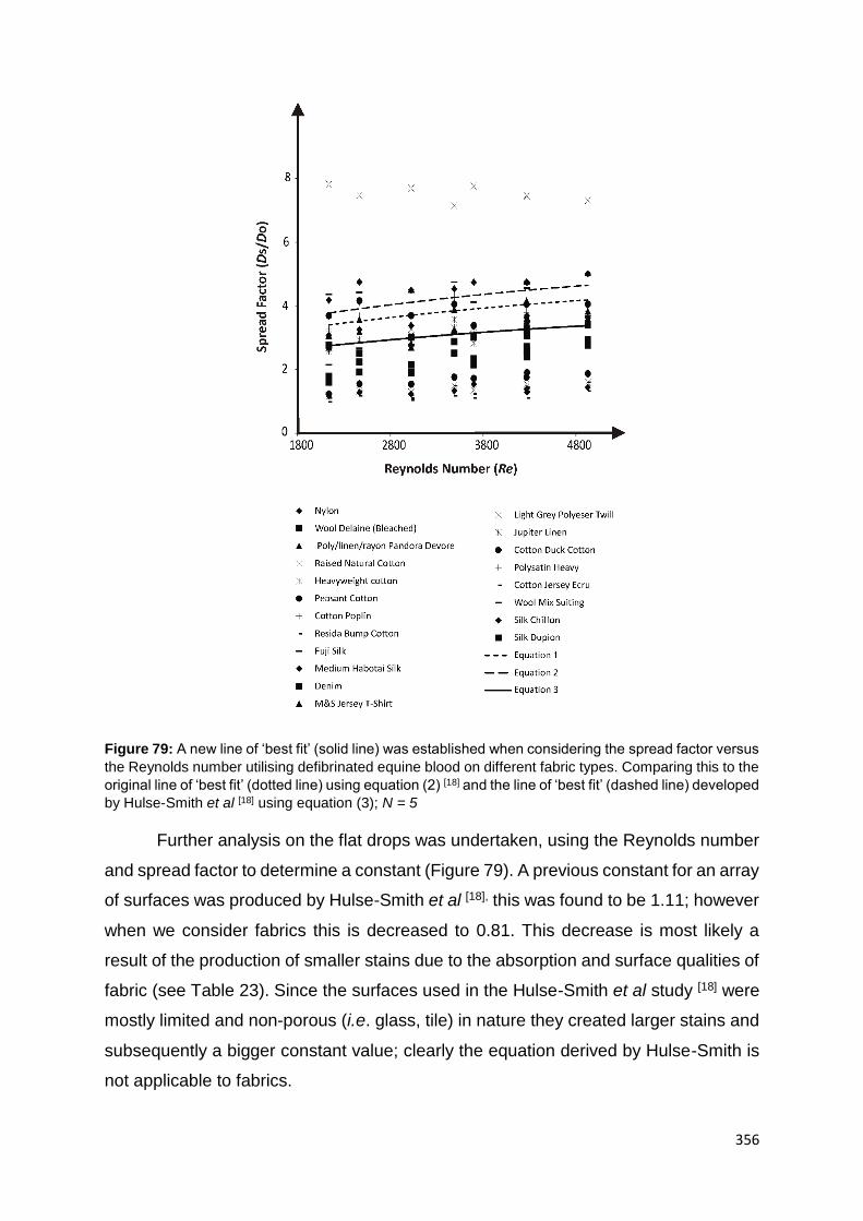
356
Figure 79: A new line of ‘best fit’ (solid line) was established when considering the spread factor versus
the Reynolds number utilising defibrinated equine blood on different fabric types. Comparing this to the
original line of ‘best fit’ (dotted line) using equation (2) [18] and the line of ‘best fit’ (dashed line) developed
by Hulse-Smith et al [18] using equation (3); N = 5
Further analysis on the flat drops was undertaken, using the Reynolds number
and spread factor to determine a constant (Figure 79). A previous constant for an array
of surfaces was produced by Hulse-Smith et al [18], this was found to be 1.11; however
when we consider fabrics this is decreased to 0.81. This decrease is most likely a
result of the production of smaller stains due to the absorption and surface qualities of
fabric (see Table 23). Since the surfaces used in the Hulse-Smith et al study [18] were
mostly limited and non-porous (i.e. glass, tile) in nature they created larger stains and
subsequently a bigger constant value; clearly the equation derived by Hulse-Smith is
not applicable to fabrics.
357
Angled impacts were also considered (data not included), where angles of 20o,
40 o, 60o and 80 o (experimental) were investigated. It was found that all angled stains
differed from the experimental angle, in most cases they were smaller (with only a few
exceptions which were larger) than the experimental impact angle. It is thought that
the blood absorbs more quickly on this surface type and therefore the stain produced
is significantly smaller (up to 75.18 %), this conclusion is concurrent with the results
obtained in White’s study. [51] Therefore it is deemed not appropriate to use angled
impacts when discussing bloodstains on clothing unless further detailed research is
conducted into individual fabrics and reduction constants can be determined, or
extensive testing is performed on the questioned fabric in the case of a reconstruction.
4.8.3 Summary
Fabric bloodstain interpretation is a fundamental element within the practice of
BPA. Blood often interacting clothing and upholsteries in a blood shedding incident.
Recent cases (Camm case) have highlighted the problematic nature of fabrics, where
stains can alter dramatically due to the surface.
This study has investigated blood interactions with 20 common fabric types,
applying equation and statistical analysis to fully comprehend the nature of the
alteration, Current research has only explored observational approaches, without any
quantitative analysis.
Results showed that fabrics do not follow the usual trend of increasing in stain
diameter as height increases. Analysis of this trend revealed that a possible reason
for this was the thickness of the fabric and not a result of the porosity or roughness of
the fabric.
A new constant for the spread factor was developed, where Cd equalled 0.81,
compared to the original constant devised by Hulse-Smith et al [18] of 1.11. The
decrease in constant is attributed to the consistent production of smaller stains, due
to the absorption qualities of the fabric. Since most of the surfaces analysed by Hulse-
Smith et al [18] where non-porous and therefore produced larger stains.
Secondary rings were found to be exhibited on all silk and polyester fabrics,
where reduction constants were calculated for two silk types (1.24; Fuji silk and 1.25;
Habotai silk).

358
Angled impacts were found to be immeasurable due to the distortion created
when blood impacted the fabric, developing large errors (75.1%) in the calculated
angle where stains where significantly smaller.
Overall fabrics were found to significantly alter final bloodstains in a multitude
of ways. The changes do not act in a predictable way and therefore it is advised that
direct fabric matches be used when evaluating bloodstains for a reconstruction.

359
4.9 METAL
Metals are naturally occurring elements, which are extracted from the Earth,
ores containing the metals are mined and metals are recovered by chemical or
electrolytic reduction. [172]
Metals are available in abundance and variety of forms offering a wide range of
properties that are invaluable in applications such as construction, thermal conduction,
electrical conduction etc. [172] Their use in these countless applications has secured
their place in homes, offices and public domains. This makes the likelihood of blood
interacting with a metal surface during a crime scene scenario all the more probable.
4.9.1 Metal composition
Metals are closely packed atoms which are formed in one of the following three
crystalline structures: [172-173]
1) body-centred cubic (BCC)
2) face-centred cubic (FCC)
3) hexagonal close-packed (HCP)
Atoms of metals readily lose their outer shell of electrons, resulting in free flowing
electrons. This provides metal with its ability to transmit heat and electricity. [172 - 173]
4.9.2 Categories of Metals
4.9.2.1 Base metal
A base metal is defined as a metal that oxidizes and/or corrodes easily and reacts with
dilute Hydrochloric Acid to form hydrogen, i.e. iron, nickel. [172 - 173]
4.9.2.2 Ferrous metal
Ferrous metals refer to metals containing iron, i.e. steel. [172 - 173]
4.9.2.3 Noble metal

360
Are often rare metals such as gold, platinum etc. They are resistant to corrosion and
oxidation. [172 - 173]
4.9.2.4 Precious metal
A rare metal of high economic value. They are generally highly conductive, and do not
react with chemicals. [172 - 173]
4.9.3 Metal types
4.9.3.1 Aluminium
Aluminium is the second most widely used metal in the world, due to its affinity to
oxygen it is almost never found in its elemental state. [174 -175] Aluminium is most
commonly extracted from the bauxite ore, found near the Earths’ crust. There are two
steps in the production of aluminium; 1- extraction of alumina (aluminium oxide) from
bauxite using the Bayer Process, 2- smelting of aluminium metal from alumina. [174 -
175]
Aluminium is lightweight, highly conductive, reflective and easily manufactured,
therefore it has many applications, including the construction of aircrafts, trains, cars,
packaging, furniture, street lights and baseball bats etc. [174 -175]
4.9.3.2 Steel
There are over 3,500 grades of steel, each displaying different physical, chemical and
environmental properties. [176] Steel is composed of iron and carbon, it is the level of
carbon which determines steel’s properties (0.1-1.5%). Other elements are present,
such as manganese, sulphur etc. [176]
The production of steel is a laborious process which can be divided into six: [176]
1- Ironmaking: raw materials (iron ore, coke, lime) are melted in a blast furnace.
2- Primary Steelmaking: Basic Oxygen Steelmaking (BOS) or Electric Arc
Furnace (EAF) methods are utilised. [176]
BOS- oxygen is blown through the metal, reducing the carbon.
EAF- recycled steel scrap is fed through a high power electric arc (1650oC),
where steel is melted and can be shaped. [176]

361
3- Secondary Steelmaking: molten steel is treated, elements are added or
removed in order to alter the composition. [176]
4- Continuous Casting: casted into a cool mould to solidify.
5- Primary Forming: steel is formed into various shapes, i.e. hot rolling. During this
stage defects are eliminated. [176]
6- Manufacturing, fabrication, finishing: final shaping is completed i.e. shaping
(cold rolling), coating, heat treatment, surface treatment etc. [176]
There are four main types of steel; [176]
Carbon steels – split into low (mild steel), medium and high
Alloy steels – alloys are added i.e. manganese, silicon etc.
Stainless steels – noted for its corrosion resistance, this steel type has a minimum of
10.5 % chromium present, which forms the protective film across the surface.
Tool steels – steel combined with high temperature alloys i.e. tungsten.
Application
Steel, due to its numerous grades, has many applications, these include: [176]
Packaging, transport, construction (i.e. stadiums, high-rise buildings), washing
machines, microwaves, radiators etc.
4.9.3.3 Copper
Copper can be found in its native state though it is most commonly located in
sulphide ores, oxide ores and carbonate ores. [177] The copper is extracted by smelting,
leaching and electrolysis. Copper is also present in minerals; malachite, cuprite and
chalcopyrite (most common). [177]
Second to only silver, copper is an extremely effective conductor of both heat and
electricity. [177] It is also malleable and ductile, explaining its application in plumbing
pipes. Other applications include cookware and coins etc. [177]
4.9.3.4 Zinc
Zinc (HCP structure) is extracted from ore containing zinc sulphide, zinc blende
or sphalente. It is inherent in the environment, present in rocks, minerals, water, air,
animals, humans and plants. [178]
Zinc is extracted from the earth’s crust, present in four deposit types: [178]
362
1. Volcanic hosted massive sulphides (VMS)
2. Carbonate hosted
3. Sediment hosted
4. Intrusion related
Zinc is the fourth most popular metal in the world, with its strong noncorrosive
properties it namely for its uses as a coating/ galvanizing other metals (i.e. steel). [178]
It is also used for: construction, transport, electrical appliances and general
engineering. [178]
4.9.3.5 Brass
Brass is an alloy metal composed of copper and zinc, varying the rate of these
components yields different properties, ordinarily brass consists of 67% copper and
33% zinc. [179] Lead is sometimes added to the brass to improve machinability. [179]
Brass is malleable, has acoustic properties, soft and has a shiny smooth texture.
These properties make brass perfect for producing musical instruments, fireplace trim,
bells and padlocks. [179]
4.9.4 Finishes
There are several types of finish, which are applied to the surface of the metal to
protect, change the colour, strength, wettability and texture of the surface. [180]
Below are the finishes investigated in the study: [180]
Galvanizing – applies a protective zinc coating using the submersion of steel or iron in
a bath of molten zinc, to prevent rusting. [180]
Anodising – electrolytic passivation process to increase the thickness of natural oxide
on the surface of the metal. [180]
Sandblasting – applying a stream of abrasive material under high pressure to a smooth
surface.
Polishing – abrasives are glued to a work wheel or leather strap and the surface is
worked to a high-end finish. [180]
Brushed – polishing metal with a grit belt.
363
4.10 BLOOD IMPACTING METAL
The application of metal into household items, and its structural benefits means
it is readily available for the incidental collision of blood on a metal surface during a
bloodletting incident.
The following research investigates the interaction of blood and metal.
Twenty common metals, consisting of several types and finishing, were tested.
Blood drops were performed from different heights and angles, where equations and
quantitative analysis could be completed on the result obtained.
4.10.1 Experimental
All human blood (PCV% 43%) used in this study was obtained from Manchester Royal
Infirmary and stored at 4oC whilst awaiting experimentation.
Several different metals were analysed, where 5 common metal types were analysed;
aluminium, brass, steel, zinc and copper. Multiple versions of each surface were used,
each with a different surface finish (polished, brushed, anodised, galvanized,
unfinished and sand-blasted).
The following lists the metals tested:
Aluminium Satin Anodised, Brushed Satin Aluminium, Stucco Aluminium, Natural
Semi Bright Aluminium, Bright Polished Aluminium, Copper Mirror Polish, Mild Steel,
Galvanized Mild Steel, Zintec Sheet, Stainless Steel Brushed, 316 Stainless Steel,
430 Bright Steel, 430 Brush Stainless Steel, 430 Circles Stainless Steel, Stainless
Sheet Super Mirror, Zinc Sheet Metal, Quartz Zinc Sheet Metal, Brass Mirror Polish,
Copper Sheet Metal, Natural Semi Bright Aluminium-Sandblasted, Mild Steel-
Sandblasted, 316 Stainless Sheet- Sandblasted and 430 Bright Stainless Steel-
Sandblasted.
Numbers such as 430 refer to the grade of the steel, the most common being 430, 316
and 330.
Roughness measures, using the rugometer (section 2.2.2) and SEM images (section
2.4.2) were performed for each surface type.

364
Blood drop test were conducted according to the description in section 2.2.Two types
of pipettes were utilised, and drops were deposited from heights (50, 100, 150 and
200 cm) and at angles of (20o, 40 o, 60 o, 80 o and 90 o).
Bloodstains were measured using a magnifying loupe and results were analysed using
equations set forth by Hulse-Smith et al. [15]
4.10.2 Results and Discussion
4.10.2.1 Bloodstain Diameter vs. Metals
Blood drop experiments were performed for each surface type, where drops were
repeated 5 times to obtain concordant results.
Figures 80 and 81 depict the results observed when both the 1mm and 1.77mm (inner
tip diameter) pipettes were utilised for drops deposited at various heights. (see
Appendix 7)
Figure 80: Bloodstain diameters on all 20 metal types from various heights; 50 cm, 100 cm, 150 cm
and 200 cm, using the 1 mm pipette (inner tip diameter). N = 5.
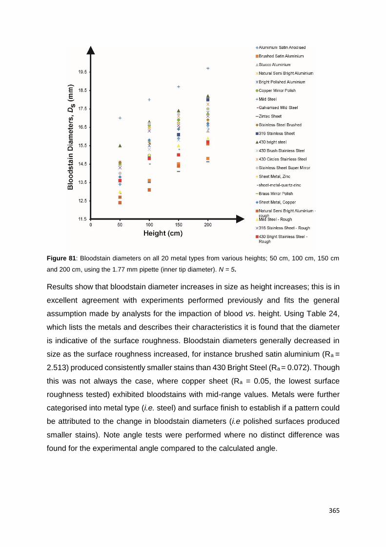
365
Figure 81: Bloodstain diameters on all 20 metal types from various heights; 50 cm, 100 cm, 150 cm
and 200 cm, using the 1.77 mm pipette (inner tip diameter). N = 5.
Results show that bloodstain diameter increases in size as height increases; this is in
excellent agreement with experiments performed previously and fits the general
assumption made by analysts for the impaction of blood vs. height. Using Table 24,
which lists the metals and describes their characteristics it is found that the diameter
is indicative of the surface roughness. Bloodstain diameters generally decreased in
size as the surface roughness increased, for instance brushed satin aluminium (Ra =
2.513) produced consistently smaller stains than 430 Bright Steel (Ra = 0.072). Though
this was not always the case, where copper sheet (Ra = 0.05, the lowest surface
roughness tested) exhibited bloodstains with mid-range values. Metals were further
categorised into metal type (i.e. steel) and surface finish to establish if a pattern could
be attributed to the change in bloodstain diameters (i.e polished surfaces produced
smaller stains). Note angle tests were performed where no distinct difference was
found for the experimental angle compared to the calculated angle.

366
Metal Names and Characterisation
SEM Types Finish Roughness
Aluminium Satin Anodised (Pitted)
Aluminium Anodised 0.328
Brushed Satin Aluminium (Striated)
Aluminium Brushed 2.513
Stucco Aluminium (Pitted)
Aluminium Unfinished 1.373
Natural Semi Bright
Aluminium (Striated)
Aluminium Polished 0.518
Bright Polished Aluminium (Striated)
Aluminium Polished 0.075
Copper Mirror Polish (Striated)
Copper Polished 0.05
Mild Steel (Textured)
Steel Unfinished 0.952
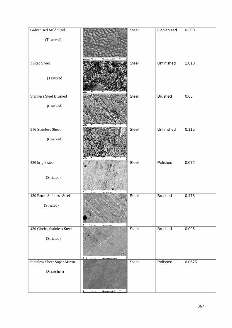
367
Galvanised Mild Steel (Textured)
Steel Galvanised 0.308
Zintec Sheet (Textured)
Steel Unfinished 1.018
Stainless Steel Brushed (Cracked)
Steel Brushed 0.65
316 Stainless Sheet (Cracked)
Steel Unfinished 0.115
430 bright steel (Striated)
Steel Polished 0.072
430 Brush Stainless Steel (Striated)
Steel Brushed 0.478
430 Circles Stainless Steel (Striated)
Steel Brushed 0.095
Stainless Sheet Super Mirror (Scratched)
Steel Polished 0.0675

368
Sheet Metal, Zinc (Striated)
Zinc Unfinished 0.168
sheet-metal-quartz-zinc (Striated)
Zinc Unfinished 0.457
Brass Mirror Polish (Scratched)
Brass Polished 0.065
Sheet Metal, Copper (Striated)
Copper Unfinished 0.07
Natural Semi Bright
Aluminium - rough (Textured)
Aluminium Sand-Blasted
2.13
Mild Steel - Rough (Textured)
Steel Sand-Blasted
2.26
316 Stainless Sheet - Rough (Textured)
Steel Sand-Blasted
2.17
430 Bright Stainless Steel -
Rough (Striated)
Steel Sand-Blasted
1.59
Table 24: Physical characteristics of the 20 metals used in this study.

369
Firstly, metal types were analysed. Figures 82 A and B show the size of bloodstains
when compared to the type of metal surface used, where both pipette types were used.
Zinc and aluminium produced smaller stains than other metal types; however, the
results did not deviate enough from other metal values for the type of metal to be
considered as a causative factor in the final bloodstain size.
Figure 82: Categorised bloodstain diameters on 5 main metal types from various heights; 50 cm, 100
cm, 150 cm and 200 cm, using the A - mm pipette (inner tip diameter), B - 1.77 mm pipette (inner tip
diameter), N = 5.
Next the surface finish was investigated (Figures 83A and B). No discernible pattern
was exhibited when surface finish was considered, however sand-blasted surface did
generally produce smaller bloodstains. Again, these were not found to be small
enough to be distinguishable between other surface finishes. Therefore surface finish
is not a deciding factor on the size of the resultant bloodstain produced.
B A

370
Figure 83: Bloodstain diameters on all 20 metal types, categorised by their surface finish, from various
heights; 50 cm, 100 cm, 150 cm and 200 cm, using the A - mm pipette (inner tip diameter), B - 1.77 mm
pipette (inner tip diameter), N = 5.
Figure 84: Bloodstain Diameters depicted the effect of surface characteristics, where blood was
deposited using A- 1mm pipette and B- 1.77mm pipette.
A B

371
Referring to Table 24, metals were further categorised depending on their
physical appearance, characterising the metals into 5 groups; pitted, striated, cracked,
scratched and textured. Surfaces were expected to alter the size of the bloodstains
due to certain surface characteristics, i.e. pitted surfaces may cause smaller
bloodstains due to blood falling into the pits rather than spreading as it would on a
completely flat, smooth surface. However this does not appear to be the case, a variety
of bloodstain sizes were apparent independent of the surface characteristic (Figures
84 A and B). A possible reason for this may be attributed to the surface finish, since
the finish is on the top layer of the surface this could render some surface
characteristics redundant, as the blood would not actually interact with them.
Figure 85: A new line of ‘best fit’ (solid line) was established considering the spread factor versus the
Reynolds number on different metal surfaces. Comparing this to the original line of ‘best fit’ (dotted line)
using equation (3) [18] and the line of ‘best fit’ (dashed line) developed by Hulse-Smith et al [18] using
equation (4).
Lastly Reynolds numbers and spread factors were calculated using equations (1, 3
and 4) where lines of ‘best fit’ were graphed (Figure 85) and a new constant was
established. The new constant equated to 1.09, which slightly deviates from the
original value determined by Hulse-Smith et al, where Cd equals 1.11. Since these

372
constant are not significantly different it can be concluded that metal surfaces do not
significantly alter the way a bloodstain forms, in spite of the type of metal and surface
finish utilised.
4.10.3 Summary
Since metal is a readily used resource in most environments, it is very
accessible to interaction with blood which may be expelled during a crime scene
scenario. This study has evaluated the impinging of blood on metal surfaces, where 5
common metal types and 5 surface finishes were analysed. Blood drop tests were
performed from different heights and using two pipette tip types.
Results found that the higher the release height the larger the bloodstain, this
was consistent for each metal type. This result is expected and is one of the
fundamental principals in BPA, first established in the 1950s. Roughness of the
surface was a determinant factor in the size of the final bloodstain diameter produced,
where bloodstains were smaller when the surface was rougher. However, this was not
always the case. Further analysis splitting the metals into types and finishes was
completed. Aluminium, zinc and sand-blasting the surface were found to produce
smaller bloodstains, however these stains were not significantly smaller than those
produced by other metal types and finishing techniques. It is therefore concluded that
neither metal type nor finishing technique dictates the end bloodstain diameter,
however the general roughness does.
Spread factors were also considered, where a new constant (Cd = 1.09) was
developed using the equations (3 and 4) set forth by Hulse-Smith et al [18] the new
constant is close to the original close; 1.11. Therefore, it was concluded that metal
surfaces do not deviate significantly from any other surface type, hence it does not
warrant any special consideration when analysing blood impacting metal surfaces in
a crime scene scenario.

373
4.11 STONE AND TILE
Rocks have been used for tools since the Stone Age, they are made up of
naturally occurring mineraloids or minerals. [181 - 183]
Presently rocks have multiple applications such as stairs, driveways, stepping
stones, paving, walls, columns, sculptures, floors, sinks and many more. [181 - 183]
Similarly to wood, stone would be expected to be present in a number of crime
scene scenarios and therefore in this section will investigated as a potential blood
impact surface. [181 - 183]
4.11.1 Stone Types
Stone can be categorised into three types of rocks:
4.11.1.1 Sedimentary
Sedimentary rocks are produced by the erosion of rocks. Eroded fragments
accumulate on the sea/river bed or on land where they are then buried (by more layers
of rock fragments) and compressed to form sedimentary rocks. [181 - 183]
There are two classifications of sedimentary rocks: clastic and non-clastic.
Clastic sedimentary rocks comprise of clasts, defined as fragments of pre-existing
rocks or minerals. Further categorisation is possible according to the size of clasts:
Boulder>200µm, Gravel 2 - 200 µm, Sand 0.06 - 2 µm and Mud < 0.002 – 0.06. [181 -
183]
Non-clastic sedimentary rocks are defined as rocks in which fragments have
not been transported but precipitated directly from water, therefore no clasts are
present.
The sedimentary rocks using in this study are:
4.11.1.1.1 Sandstone
Sandstone is composed of small grains of minerals, rocks or
organic matter and a cement like material (e.g. calcite clays and
silica) to bind the grains together. [184] The name sandstone does
not refer to the material from which the stone is composed but
rather the size of the grains. [184] Figure 86: Sandstone
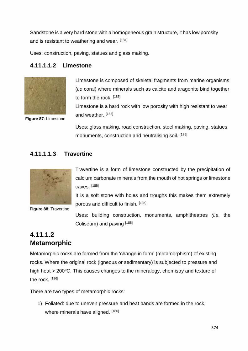
374
Sandstone is a very hard stone with a homogeneous grain structure, it has low porosity
and is resistant to weathering and wear. [184]
Uses: construction, paving, statues and glass making.
4.11.1.1.2 Limestone
4.11.1.1.3 Travertine
4.11.1.2
Metamorphic
Metamorphic rocks are formed from the ‘change in form’ (metamorphism) of existing
rocks. Where the original rock (igneous or sedimentary) is subjected to pressure and
high heat > 200oC. This causes changes to the mineralogy, chemistry and texture of
the rock. [186]
There are two types of metamorphic rocks:
1) Foliated: due to uneven pressure and heat bands are formed in the rock,
where minerals have aligned. [186]
Figure 87: Limestone
Figure 88: Travertine
Limestone is composed of skeletal fragments from marine organisms
(i.e coral) where minerals such as calcite and aragonite bind together
to form the rock. [185]
Limestone is a hard rock with low porosity with high resistant to wear
and weather. [185]
Uses: glass making, road construction, steel making, paving, statues,
monuments, construction and neutralising soil. [185]
Travertine is a form of limestone constructed by the precipitation of
calcium carbonate minerals from the mouth of hot springs or limestone
caves. [185]
It is a soft stone with holes and troughs this makes them extremely
porous and difficult to finish. [185]
Uses: building construction, monuments, amphitheatres (i.e. the
Coliseum) and paving [185]
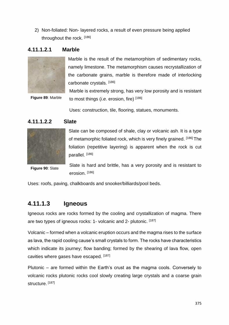
375
2) Non-foliated: Non- layered rocks, a result of even pressure being applied
throughout the rock. [186]
4.11.1.2.1 Marble Marble is the result of the metamorphism of sedimentary rocks,
namely limestone. The metamorphism causes recrystallization of
the carbonate grains, marble is therefore made of interlocking
carbonate crystals. [186]
Marble is extremely strong, has very low porosity and is resistant
to most things (i.e. erosion, fire) [186]
Uses: construction, tile, flooring, statues, monuments.
4.11.1.2.2 Slate
Slate can be composed of shale, clay or volcanic ash. It is a type
of metamorphic foliated rock, which is very finely grained. [186] The
foliation (repetitive layering) is apparent when the rock is cut
parallel. [186]
Slate is hard and brittle, has a very porosity and is resistant to
erosion. [186]
Uses: roofs, paving, chalkboards and snooker/billiards/pool beds.
4.11.1.3 Igneous
Igneous rocks are rocks formed by the cooling and crystallization of magma. There
are two types of igneous rocks: 1- volcanic and 2- plutonic. [187]
Volcanic – formed when a volcanic eruption occurs and the magma rises to the surface
as lava, the rapid cooling cause’s small crystals to form. The rocks have characteristics
which indicate its journey; flow banding; formed by the shearing of lava flow, open
cavities where gases have escaped. [187]
Plutonic – are formed within the Earth’s crust as the magma cools. Conversely to
volcanic rocks plutonic rocks cool slowly creating large crystals and a coarse grain
structure. [187]
Figure 90: Slate
Figure 89: Marble

376
4.11.1.3.1 Granite
Granite is a plutonic igneous rock it consists of quartz and
feldspar, which has formed in the earth’s crust. [187]
It is an extremely hard rock (only diamond is harder) with a low
porosity and high resistance to wear and erosion. [187]
Uses: building, statues, kitchens, flooring, roofing etc.
4.11.2 Finishes
A variety of finishes are available for stones, offering protection, colour change,
practicalities (non-slip floors) and high end finish. [188 - 191]
The following finishes are those to be explored in the research: [188 - 191]
Polished: uses fine abrasives which rubbed against the surface to give a high gloss
finish.
Honed: gives a smooth matt finish, recommended as a floor finish. This is produced
when the polishing process is stopped before it reaches the high gloss finish is
achieved. Abrasives are used which are less fine than those use for a polished finish.
[188 - 191]
Tumbled: produces a worn look, where stones are placed in a barrel along with grit
(i.e. silicon carbide) and liquid (water). [188 - 191]The barrel is rotated so the rocks collide
with the grit and are slowly polished. [188 - 191]
Flamed: stone is exposed to high temperature flames whilst wet, this triggering
thermal shock which causes grains to rise to the surface, creating a rough textured
surface.
Riven: where stone is split along the natural cleavage plane. Seen mostly in slate. [188
- 191]
Sand-blasted: creates a textured surface by applying high pressured jet of small
grains across the surface. [188 - 191]
Figure 91: Granite

377
5.11 BLOOD IMPACTING STONE AND TILE
Since the use of stone for important applications such as building, flooring etc
has been around for thousands of years the high probability of stone occurring in some
form at a crime scene is highly likely. [191]
The following research investigates the interaction of blood and stone.
Twenty-one common stone and tile types, consisting of several types and
finishing, were tested. Blood drops were performed from different heights and angles,
where equations and quantitative analysis could be completed on the results obtained.
5.11.1 Experimental
All human blood (PCV% 43%) used in this study was obtained from Manchester Royal
Infirmary and stored at 4oC whilst awaiting experimentation.
Several different stone and tile types were analysed, where 8 common stone types
were analysed; granite, marble, ceramic, porcelain, sandstone, limestone, travertine
and slate. Multiple versions of each surface were used, each with a different surface
finish (polished, unfinished, flamed, honed, riven and tumbled).
The following lists the stones and tiles tested:
Travertine (Classic Tumbled Unfilled Travertine, Classic Honed Travertine Paving,
Silver Latte Tumbled Travertine Paving Opus Pattern, Classic Travertine Filled and
Honed, Classic Chipped Edge Filled and Honed Travertine Opus Pattern), Limestone
(Yellow Limestone Paving), Sandstone (Indian Sandstone Paving Raj Blend Tumbled,
Indian Sandstone Paving Raj Blend Economy, Indian Sandstone Paving Sahara
Yellow Calibrated, Indian Sandstone Paving Rippon Buff, Indian Sandstone Paving
Modak Calibrated), Slate (Brazilian Black Slate Paving and Rusty Slate Paving),
Porcelain (Sandstone Rivon Porcelain and Super White Matt Porcelain), Ceramic
(Ceramic Matt and Ceramic Polished) and Beige Marble Polished.
Roughness measures, using the rugometer (section 2.2.2) and SEM images (section
2.4.2) were performed for each surface type.

378
Blood drop test were conducted according to the description in section .Two types of
pipettes were utilised, and drops were deposited from heights (50, 100, 150 and 200
cm) and at angles of (20o, 40 o, 60 o, 80 o and 90 o).
Bloodstains were measured using a magnifying loupe and results were analysed using
equations set forth by Hulse-Smith et al [18]
5.11.2 Results and Discussion
5.11.2.1 Bloodstain vs. Stone Surfaces
Blood drop tests were performed on all stone surfaces where the blood was
deposited from 4 different height (see Appendix 8) and at a range of angles. Figures
92 and 93 depict the effect stone surfaces had on the bloodstain diameter produced
when blood is released using both the 1mm pipette (inner tip diameter) and the 1.7mm
pipette (inner tip diameter). Diameters were found to increase as height increased until
terminal velocity (ordinarily around 200 cm) was reached, where diameter increases
become less pronounced.
Figure 92: Bloodstain diameters on all stone surfaces from various heights; 50 cm, 100 cm, 150 cm
and 200 cm, using the 1 mm pipette (inner tip diameter). N = 5.
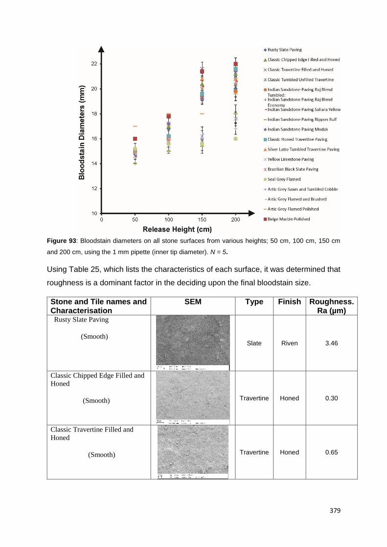
379
Figure 93: Bloodstain diameters on all stone surfaces from various heights; 50 cm, 100 cm, 150 cm
and 200 cm, using the 1 mm pipette (inner tip diameter). N = 5.
Using Table 25, which lists the characteristics of each surface, it was determined that
roughness is a dominant factor in the deciding upon the final bloodstain size.
Stone and Tile names and
Characterisation SEM Type Finish Roughness.
Ra (µm) Rusty Slate Paving (Smooth)
Slate Riven 3.46
Classic Chipped Edge Filled and
Honed (Smooth)
Travertine Honed 0.30
Classic Travertine Filled and
Honed (Smooth)
Travertine Honed 0.65
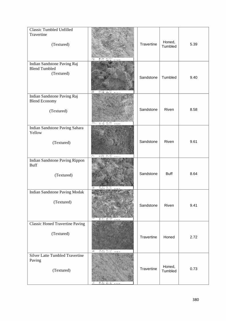
380
Classic Tumbled Unfilled
Travertine (Textured)
Travertine Honed,
Tumbled 5.39
Indian Sandstone Paving Raj
Blend Tumbled (Textured)
Sandstone Tumbled 9.40
Indian Sandstone Paving Raj
Blend Economy (Textured)
Sandstone Riven 8.58
Indian Sandstone Paving Sahara
Yellow (Textured)
Sandstone Riven 9.61
Indian Sandstone Paving Rippon
Buff (Textured)
Sandstone Buff 8.64
Indian Sandstone Paving Modak (Textured)
Sandstone Riven 9.41
Classic Honed Travertine Paving (Textured)
Travertine Honed 2.72
Silver Latte Tumbled Travertine
Paving (Textured)
Travertine Honed,
Tumbled 0.73

381
Yellow Limestone Paving (Cracked)
Limestone Riven 10.91
Brazilian Black Slate Paving (Textured)
Slate Riven 3.31
Seal Grey Flamed (Pitted)
Granite Flamed 6.10
Artic Grey Sawn and Tumbled
Cobble (Pitted)
Granite Tumbled 5.67
Artic Grey Flamed and Brushed (Pitted)
Granite Flamed 7.20
Artic Grey Flamed Polished (Smooth)
Granite Polished 0.03
Beige Marble Polished (Smooth)
Marble Polished 1.36
Ceramic Matt (Pitted)
Ceramic Matt 1.15
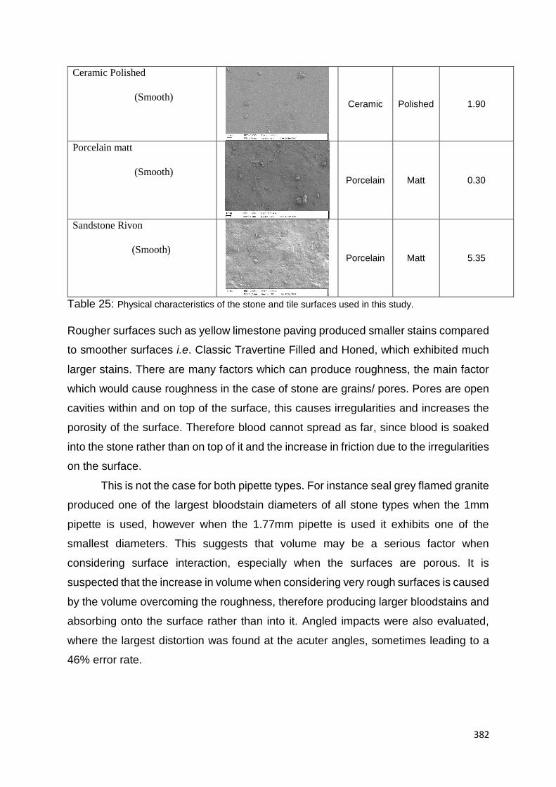
382
Ceramic Polished (Smooth)
Ceramic Polished 1.90
Porcelain matt (Smooth)
Porcelain Matt 0.30
Sandstone Rivon (Smooth)
Porcelain Matt 5.35
Table 25: Physical characteristics of the stone and tile surfaces used in this study.
Rougher surfaces such as yellow limestone paving produced smaller stains compared
to smoother surfaces i.e. Classic Travertine Filled and Honed, which exhibited much
larger stains. There are many factors which can produce roughness, the main factor
which would cause roughness in the case of stone are grains/ pores. Pores are open
cavities within and on top of the surface, this causes irregularities and increases the
porosity of the surface. Therefore blood cannot spread as far, since blood is soaked
into the stone rather than on top of it and the increase in friction due to the irregularities
on the surface.
This is not the case for both pipette types. For instance seal grey flamed granite
produced one of the largest bloodstain diameters of all stone types when the 1mm
pipette is used, however when the 1.77mm pipette is used it exhibits one of the
smallest diameters. This suggests that volume may be a serious factor when
considering surface interaction, especially when the surfaces are porous. It is
suspected that the increase in volume when considering very rough surfaces is caused
by the volume overcoming the roughness, therefore producing larger bloodstains and
absorbing onto the surface rather than into it. Angled impacts were also evaluated,
where the largest distortion was found at the acuter angles, sometimes leading to a
46% error rate.

383
Further observations were employed, where stones were categorised into type of
stone (travertine, limestone etc.) and finishing process (honed, polishes etc.), to
establish a direct link between stain size and a dominant characteristic.
Figures 94A and B express the type of stone used and the bloodstain produced for
pipette types 1mm and 1.77mm, respectively. Figure 94A shows that overall granite
produces the larger stains and limestone/ sandstone generate smaller stains, though
the differences are not pronounced enough to be able to distinguish between stone
types since some of the sandstone bloodstains (i.e. Indian Sandstone Paving Rippon
Buff) generate similar bloodstain diameters to granite, likely due to the type of finish
employed. Figure 94B does not follow the same trend as the first figure (94A), all stone
types appear to be mingled regardless of their stone type. Again this indicates that
volume is a considerable factor when evaluating blood impacting stones.
Figure 94: Categorised bloodstain diameters on 5 main stone types from various heights; 50 cm, 100
cm, 150 cm and 200 cm, using the A - mm pipette (inner tip diameter), B - 1.77 mm pipette (inner tip
diameter), N = 5
B A
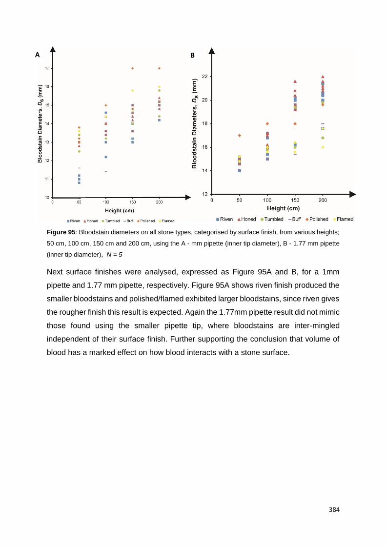
384
Figure 95: Bloodstain diameters on all stone types, categorised by surface finish, from various heights;
50 cm, 100 cm, 150 cm and 200 cm, using the A - mm pipette (inner tip diameter), B - 1.77 mm pipette
(inner tip diameter), N = 5
Next surface finishes were analysed, expressed as Figure 95A and B, for a 1mm
pipette and 1.77 mm pipette, respectively. Figure 95A shows riven finish produced the
smaller bloodstains and polished/flamed exhibited larger bloodstains, since riven gives
the rougher finish this result is expected. Again the 1.77mm pipette result did not mimic
those found using the smaller pipette tip, where bloodstains are inter-mingled
independent of their surface finish. Further supporting the conclusion that volume of
blood has a marked effect on how blood interacts with a stone surface.
B A

385
Figure 96: Bloodstain diameters on all stone types, categorised by surface characteristics, from various
heights; 50 cm, 100 cm, 150 cm and 200 cm, using the A - mm pipette (inner tip diameter), B - 1.77 mm
pipette (inner tip diameter), N = 5
Further analysis was performed, this time, comparing the surface characteristics of the
stones against the bloodstain size. Surface were categorised into 4 characteristic
types; smooth, pitted, textured and cracked (see Table 25), based on their physical
appearance using SEM images. Results showed (Figures 96 A and B) that smooth
surfaces produced larger bloodstains; this can be linked to the surface roughness. The
other surface characteristics (pitted, cracked and textured) did not differ substantially
from one another in the sizes of bloodstains they created.

386
Lastly, spread factors were considered (Figure 97). Reynolds numbers and spread
factors were calculated using equations 1, 3 and 4 and plotted against one another. A
line of ‘best fit’ was drawn onto the plot, were a new constant was derived for equation
4, where Cd equates to 1.16 which is substantially higher than that proposed by Hulse-
Smith et al, where Cd equals 1.11.
Figure 97: A new line of ‘best fit’ (solid line) was established considering the spread factor versus the
Reynolds number on different stone surfaces. Comparing this to the original line of ‘best fit’ (dotted
line) using equation (3) [18] and the line of ‘best fit’ (dashed line) developed by Hulse-Smith et al [18]
using equation (4).
This new constant suggests that blood spreads further when stone surfaces are
impacted, this can be attributed to the surface finish. Some surface finishes will cause
the blood to spread due to the absorption qualities, where liquid is effectively carried
along the surface rapidly spreading, similar to that exhibited on a fabric surface.
Polished surfaces, where friction is minimal, will also have assisted in the spreading
of the blood, since there is nothing present to stop it reaching until the first dry ring
(coffee ring) is formed.
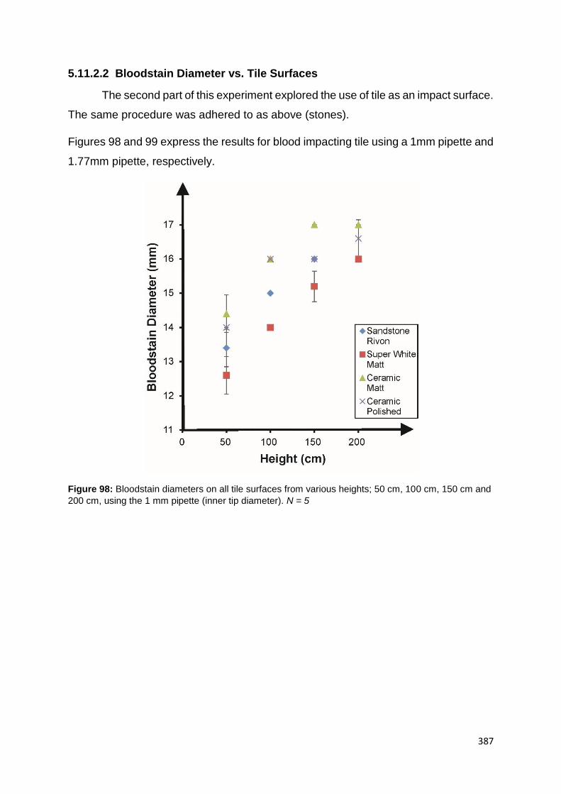
387
5.11.2.2 Bloodstain Diameter vs. Tile Surfaces
The second part of this experiment explored the use of tile as an impact surface.
The same procedure was adhered to as above (stones).
Figures 98 and 99 express the results for blood impacting tile using a 1mm pipette and
1.77mm pipette, respectively.
Figure 98: Bloodstain diameters on all tile surfaces from various heights; 50 cm, 100 cm, 150 cm and
200 cm, using the 1 mm pipette (inner tip diameter). N = 5
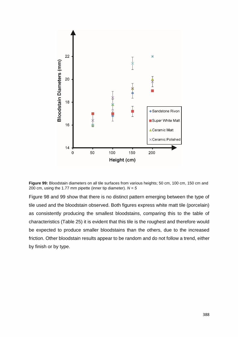
388
Figure 99: Bloodstain diameters on all tile surfaces from various heights; 50 cm, 100 cm, 150 cm and
200 cm, using the 1.77 mm pipette (inner tip diameter). N = 5
Figure 98 and 99 show that there is no distinct pattern emerging between the type of
tile used and the bloodstain observed. Both figures express white matt tile (porcelain)
as consistently producing the smallest bloodstains, comparing this to the table of
characteristics (Table 25) it is evident that this tile is the roughest and therefore would
be expected to produce smaller bloodstains than the others, due to the increased
friction. Other bloodstain results appear to be random and do not follow a trend, either
by finish or by type.

389
Figure 100: Bloodstain diameters on all tile types, categorised by surface characteristics, from various
heights; 50 cm, 100 cm, 150 cm and 200 cm, using the A - mm pipette (inner tip diameter), B - 1.77 mm
pipette (inner tip diameter), N = 5.
Again, surfaces were categorised into surface characteristics, pitted and smooth,
depending on the SEM images produced. Figure 100 A depicts bloodstains produced
on tile surfaces using a 1mL (1mm inner tip diameter), where pitted surfaces produced
larger bloodstains. This is unexpected, since smoother surfaces would typically
produce larger bloodstains, ordinarily attributed to the surface roughness. When this
figure is compared to Figure 100 B it is clear that the volume of blood impacting the
surface affects the size of the bloodstain and the way it interacts with the surface.

390
Figure 101: A new line of ‘best fit’ (solid line) was established considering the spread factor versus
the Reynolds number on different tile surfaces. Comparing this to the original line of ‘best fit’ (dotted
line) using equation (3) [18] and the line of ‘best fit’ (dashed line) developed by Hulse-Smith et al [18]
using equation (4).
Lastly the spread factor constant (Figure 101) was calculated using the above method.
A new constant equating to 1.24 was derived; again, this is considerably higher than
that calculated by Hulse-Smith et al. [18] If this is compared to the Table 26, which lists
the characteristics it is clear that roughness is the causative factor. Since the majority
of the tile surfaces are much lower in roughness than the stones or surfaces used in
the work by Hulse-Smith et al [18] the liquid is allowed to spread much further without
any real resistance, therefore creating larger bloodstains.
5.11.3 Summary
Stone is an ancient material used for thousands of years to build and create art
masterpieces, during this study, stone and tile have been investigated for their effects
on the impact and spread of blood.
391
Blood was released onto various types of tile and stone surfaces from different
heights and using two types of pipette. Results showed that roughness is a dominant
factor in the determination of bloodstain size. This result can be altered however when
volume of a blood drop is considered, where surface roughness in some instances
was overcome allowing the bloodstain to spread farther. This observation is unique to
this surface type, previous surfaces have followed the same trend regarding
roughness dictating the stain size regardless of volume utilised.
Spread factors were considered, where the Reynolds number and spread factor
were calculated using equations 3 and 4. A graph was plotted, where a new line of
best fit was created, leading to the formulation of a new constant value for both stone
and tile surfaces separately. Constant values of 1.16 and 1.24 were found for the stone
and tile surfaces, respectively. Compared to the original value noted by Hulse - Smith
et al [18] both of these values are substantially higher. This is again attributed to the
surface roughness where absorptive and finish properties (i.e. polished – low friction)
allowed blood to spread further than those surfaces used in the Hulse-Smith et al [18]
study.
Since volume and surface porosity appear to be related further studies should be
conducted to establish maximum levels of absorption in certain surfaces, like stone,
so corrections can be made if deemed necessary.
392
5.12 CONCLUSION
The objective of this section was to explore the importance of surface
interaction, focusing on surface characteristics and common surface types which are
likely to be encountered at a crime scene.
Firstly general surfaces were investigated together, where blood drops were
dispensed at different heights and angles on three surface types; paper, steel and
plastic.
New equations were established, developing on the work conducted by Knock
et al [17], where one surface type is used. Several equations had to be formulated since
each surface was significantly different from the other; therefore, further work
researching each surface alone was then conducted.
Four surface types were analysed (wood, stone and tile, metal and fabric), each with
a diverse range of attributes and very different surface composition.
All surfaces were subject to analysis using SEMs and roughness measures to
determine the topography of the surface. Blood drops tests were performed on each
surface from 4 different heights and a range of angles, using two volume types of
pipette to thoroughly investigate the effect on bloodstain patterns.
Equations were utilised to determine the degree of disruption caused when
these surface types were employed. Reynolds numbers and spread factors were
calculated to ascertain a constant, which could be compared to the constant derived
by Hulse-Smith et al, equating to Cd 1.11.
Wood, stone, tile and fabric were found to deviate significantly from the original
value (1.11), where constants were calculated to be 1.20, 1.16, 1.24 and 0.81
respectively, These results are largely attributed to the roughness and absorptive
properties of the surfaces. Wood, stone and tile surfaces were finished using a range
of methods, altering the natural porosity associated with these types of surfaces.
Volume, in some circumstances, altered the way blood spread across rough
surfaces. Stone surfaces exhibited different results when different pipettes were used,
where the volume seemed to overcome the surface roughness producing a larger
bloodstain.

393
Overall all surfaces reacted differently to the impaction of blood, the overwhelming
factor which dictated the size of stains in most surfaces was the surface roughness,
though a standard surface roughness constant could not be found which
encompassed all surfaces.

394
PART III:
SURFACE
MANIPULATION
395
5 MANIPULATING SURFACES
As aforementioned in section 1.6, surfaces can come in various conditions,
either by natural forces (i.e. rust) or manipulation by people (i.e. polished). This chapter
will investigate how we ourselves change the surface, since this has had little research
conducted on it compared to environmental changes, which we cannot control.
5.1 HEATED SURFACES
Heated surfaces in the context of BPA have never been studied before (Section 1.6),
since heated surfaces such as oven stoves, radiators or underfloor heating are present
in crime scenes it seems any significant results could have a substantial effect on the
way blood patterns are analysed. The following studies will investigate how various
heated surfaces alter the spreading of impacting blood drops.
5.1.1 UNDERFLOOR HEATING
Although underfloor heating is thought to be a fairly recent home luxury the technique
of heating the floor dates back thousands of years (5,000 BC), where people would
draft smoke from fires through the stone covered trenches which were excavated in
the floors of underground dwellings. [192 - 193] The smoke would heat the floor and
subsequently the heat would radiate the room, warming the entire dwelling. Nowadays
modern underfloor heating is provided by either fluid filled pipes or electrical cables.
[192 - 193]
Electric underfloor heating - made up of a network of wires under the floor which
can cover large areas. [194 - 196] The wires lie on top of a layer of insulation and are
connected to the thermostat and mains power supply. Heating mats are also available,
again comprising of a network of wires, this is often the cheaper option. [192 - 193]
Water underfloor heating – are comprised of a network of pipes which are connected
to the boiler and pump hot water around the room. Since this system needs water to
396
be at a lower temperature than a radiator it is much more efficient and cost effective
in the long term. [194 - 196]
Generally underfloor heating reaches temperatures of around 32oC and has become
a firm favourite in households due to its efficiency and the benefit of it being hidden so
as to frees up wall space (unlike radiators) and leave clean lines of a room unspoiled
therefore being the more aesthetically pleasing option. [194 - 196]
Underfloor heating can be used on a variety of surface types including: carpet,
ceramic, vinyl, timber, laminate and marble.
5.2 UNDERFLOOR HEATING STUDY
The following study explores the effects of underfloor heating on the size and
appearance of bloodstains. For this, a number of surfaces (stone paving, tiles and
wood flooring) were investigated at various temperatures and bloodstain size and
appearance were analysed.
5.2.1 Experimental
The blood utilised was human blood obtained from Manchester Royal Infirmary blood
bank. Blood was measured at a PCV% of 37%, where viscosity equalled 5
mPa.s.
Blood drop tests were performed according to the method described in section (2.2).
Drops were deposited on three different surface types: stone paving, tile and wood
flooring, however a multitude of each surface type was utilised to provide a thorough
representation of flooring.
Stone Paving – Travertine (Classic Tumbled Unfilled Travertine, Classic Honed
Travertine Paving, Silver Latte Tumbled Travertine Paving Opus Pattern, Classic
Travertine Filled and Honed, Classic Chipped Edge Filled and Honed Travertine Opus
Pattern), Limestone (Yellow Limestone Paving), Sandstone (Indian Sandstone Paving
Raj Blend Tumbled, Indian Sandstone Paving Raj Blend Economy, Indian Sandstone
Paving Sahara Yellow Calibrated, Indian Sandstone Paving Rippon Buff, Indian
Sandstone Paving Modak Calibrated), Slate (Brazilian Black Slate Paving and Rusty
Slate Paving).
397
Tile - Porcelain (Sandstone Rivon Porcelain and Super White Matt Porcelain), Ceramic
(Ceramic Matt and Ceramic Polished) and Beige Marble Polished
Wood Flooring – Oak (European Maple Oak, Clear Oil Oak, Oak Natural Siera Matt
Lacquered, Oak Silk Matt, Kahrs Oak Sienna Natural, Natura Oak Prime Parquet,
Kahrs Oak Siena Engineered Natural and Oak Solid Plank Untreated), Maple (Maple
Silk Matt Lacquered, Kahrs Maple Toronto Satin Lacquer, Maple Ultra Matt Lacquered,
Kahrs Maple Bevelled Edge Rustic and Kahrs Maple Natural Satin Lacquer) and
Walnut (Natura American Black Walnut Rosshill, Natura Walnut Ironbank Mississippi,
Quickstep Villa Walnut Satin Lacquer, Kahrs Walnut Rustic Nature Oil, Kahrs Linnea
Walnut Bloom Prime Satin Lacquer, Kahrs Linnea Walnut Microbevelled Edge Prime
Matt Lacquer and Natura Walnut Lacquered Satin Lacquer).
Drops were released from 30cm using the 1mm (inner tip) pipette. Surfaces were
heated, to 25oC, 30oC and 40oC; just above the maximum temperature of underfloor
heating, using a hot plate and the temperature was monitored using an infra-red
temperature gun. Surfaces were also monitored for the time taken to cool from
maximum temperature to evaluate how long surfaces retain heat.
5.2.2 Results and Discussion
5.2.2.1 Heated Stone Surface
Figure 102 depicts the results when blood was dropped on heated stone surfaces,
showing that for most surfaces the bloodstains decreased or increased in size but did
not deviate much from the original value, when the surface was at room temperature.
(see Appendix 9 for full data)

398
Figure 102: Representation of the effect of heated stone surfaces on the size of bloodstains
Table 26: Student t-tests were performed to attain the significance of the results obtained when the
surface temperatures on stone surfaces are compared; 25oC vs. 30oC and 25oC vs. 40oC; N = 5.
Stone Type p value (25 vs 30)
Sign. Yes or no
p value (25 vs 40)
Sign. Yes or no
Rusty Slate Paving 1.000 x 1 x
Classic Chipped Edge Filled and Honed 0.141 x 0.1411 x
Classic Travertine Filled and Honed 0.347 x 0.0001 ✓
Indian Sandstone Paving Raj Blend Tumbled 1.000 x 0.0598 x
Indian Sandstone Paving Raj Blend Economy 0.050 x 0.1411 x
Indian Sandstone Paving Sahara Yellow 1.000 x 0.172 x
Indian Sandstone Paving Rippon Buff 0.000 ✓ 0.005 ✓
Indian Sandstone Paving Modak 1.000 x 0.1411 x
Classic Honed Travertine Paving 0.347 x 0.3466 x
Silver Latte Tumbled Travertine Paving 0.141 x 0.1411 x
Yellow Limestone Paving 1.000 x 1 x
Brazilian Black Slate Paving 0.141 x 0.1411 x
Seal Grey Flamed Granite 1.000 x 0.0431 ✓
Artic Grey Sawn and Tumbled Cobble Granite 0.056 x 0.1411 x
Artic Grey Flamed and Brushed Granite 0.094 x 0.195 x
Artic Grey Flamed Polished Granite 0.040 ✓ 0.0001 ✓
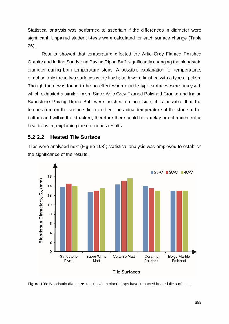
399
Statistical analysis was performed to ascertain if the differences in diameter were
significant. Unpaired student t-tests were calculated for each surface change (Table
26).
Results showed that temperature effected the Artic Grey Flamed Polished
Granite and Indian Sandstone Paving Ripon Buff, significantly changing the bloodstain
diameter during both temperature steps. A possible explanation for temperatures
effect on only these two surfaces is the finish; both were finished with a type of polish.
Though there was found to be no effect when marble type surfaces were analysed,
which exhibited a similar finish. Since Artic Grey Flamed Polished Granite and Indian
Sandstone Paving Ripon Buff were finished on one side, it is possible that the
temperature on the surface did not reflect the actual temperature of the stone at the
bottom and within the structure, therefore there could be a delay or enhancement of
heat transfer, explaining the erroneous results.
5.2.2.2 Heated Tile Surface
Tiles were analysed next (Figure 103); statistical analysis was employed to establish
the significance of the results.
Figure 103: Bloodstain diameters results when blood drops have impacted heated tile surfaces.

400
Ceramics (matt and polished) were found to change significantly at both temperature
intervals (25 vs 30 and 25 vs 40) (Table 27), though both reacted differently. Ceramic
polish tile bloodstain diameters decreased as temperature increased, this could be a
result of the difference in roughness at the top and bottom of the tile, the bottom being
rougher, thus creating a lesser heat transfer leading to smaller stains. Larger stains
would be expected as heat decreases the viscosity and therefore liquid would flow
more freely, resulting in the production of large stains.
Table 27: Student t-tests were performed to attain the significance of the results obtained when the
surface temperatures on tile surfaces are compared; 25oC vs. 30oC and 25oC vs. 40oC; N = 5.
Conversely ceramic matt tile bloodstain diameters increased as temperature
increased, due in part to the increase in viscosity but could also be attributed to the
surface finish. The super white matt tile behaved in a similar way to the ceramic matt
tile (increasing), surface finish is the most probable cause of the bloodstain diameter
change, since the SEMS characterised (Table 25) the two tile as different (smooth vs.
divots). Rougher surfaces hold and transfer heat more efficiently than smoother
polished surfaces which reflect heat. The surface finish and decrease in viscosity of
blood would then work in tandem to produce larger stains.
5.2.2.3 Heated Wood Surface
Lastly heated wood surfaces were investigated.
Tile Type p value (25 vs 30)
Sign. Yes or no
p value (25 vs 40)
Sign. Yes or no
Sandstone Rivon 0.000 ✓ 0.347 X
Super White Matt 0.172 X 0.004 ✓
Ceramic Matt 0.007 ✓ 0.002 ✓
Ceramic Polished 0.000 ✓ 0.000 ✓
Beige Marble Polished 1.000 X 1.000 X
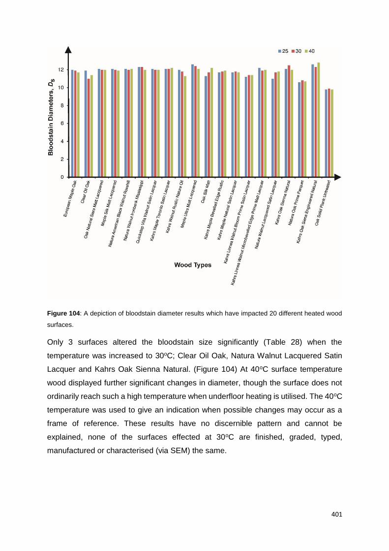
401
Figure 104: A depiction of bloodstain diameter results which have impacted 20 different heated wood
surfaces.
Only 3 surfaces altered the bloodstain size significantly (Table 28) when the
temperature was increased to 30oC; Clear Oil Oak, Natura Walnut Lacquered Satin
Lacquer and Kahrs Oak Sienna Natural. (Figure 104) At 40oC surface temperature
wood displayed further significant changes in diameter, though the surface does not
ordinarily reach such a high temperature when underfloor heating is utilised. The 40oC
temperature was used to give an indication when possible changes may occur as a
frame of reference. These results have no discernible pattern and cannot be
explained, none of the surfaces effected at 30oC are finished, graded, typed,
manufactured or characterised (via SEM) the same.
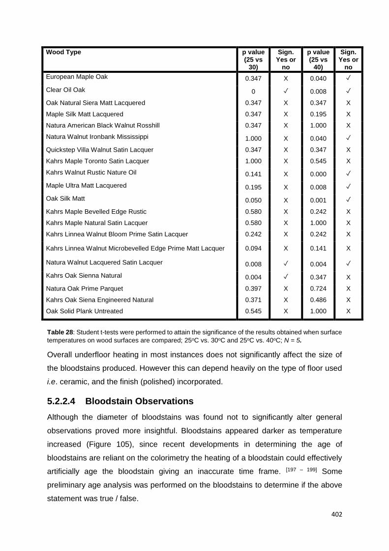
402
Wood Type p value (25 vs
30)
Sign. Yes or
no
p value (25 vs
40)
Sign. Yes or
no
European Maple Oak 0.347 X 0.040 ✓
Clear Oil Oak 0 ✓ 0.008 ✓
Oak Natural Siera Matt Lacquered 0.347 X 0.347 X
Maple Silk Matt Lacquered 0.347 X 0.195 X
Natura American Black Walnut Rosshill 0.347 X 1.000 X
Natura Walnut Ironbank Mississippi 1.000 X 0.040 ✓
Quickstep Villa Walnut Satin Lacquer 0.347 X 0.347 X
Kahrs Maple Toronto Satin Lacquer 1.000 X 0.545 X
Kahrs Walnut Rustic Nature Oil 0.141 X 0.000 ✓
Maple Ultra Matt Lacquered 0.195 X 0.008 ✓
Oak Silk Matt 0.050 X 0.001 ✓
Kahrs Maple Bevelled Edge Rustic 0.580 X 0.242 X
Kahrs Maple Natural Satin Lacquer 0.580 X 1.000 X
Kahrs Linnea Walnut Bloom Prime Satin Lacquer 0.242 X 0.242 X
Kahrs Linnea Walnut Microbevelled Edge Prime Matt Lacquer 0.094 X 0.141 X
Natura Walnut Lacquered Satin Lacquer 0.008 ✓ 0.004 ✓
Kahrs Oak Sienna Natural 0.004 ✓ 0.347 X
Natura Oak Prime Parquet 0.397 X 0.724 X
Kahrs Oak Siena Engineered Natural 0.371 X 0.486 X
Oak Solid Plank Untreated 0.545 X 1.000 X
Table 28: Student t-tests were performed to attain the significance of the results obtained when surface
temperatures on wood surfaces are compared; 25oC vs. 30oC and 25oC vs. 40oC; N = 5.
Overall underfloor heating in most instances does not significantly affect the size of
the bloodstains produced. However this can depend heavily on the type of floor used
i.e. ceramic, and the finish (polished) incorporated.
5.2.2.4 Bloodstain Observations
Although the diameter of bloodstains was found not to significantly alter general
observations proved more insightful. Bloodstains appeared darker as temperature
increased (Figure 105), since recent developments in determining the age of
bloodstains are reliant on the colorimetry the heating of a bloodstain could effectively
artificially age the bloodstain giving an inaccurate time frame. [197 – 199] Some
preliminary age analysis was performed on the bloodstains to determine if the above
statement was true / false.

403
Figure 105: Bloodstains showing the effect of heated surfaces on the appearance of the bloodstain,
where before depicts blood on a surface at room temperature and after shows bloodstains which have
impacted a heated surface (40oC).
Three surfaces were examined: granite, porcelain tile and ceramic tile. Blood was
deposited onto each surface heated to various temperatures (room, 30oC and 40oC)
and change in light intensity was monitored using a portable spectrophotometer
Spectruino.
Figures 106 - 108 show that there is an increase in light intensity when bloodstains,
formed on higher surface temperatures, were analysed. This is identical to what is
believed to happen as blood ages, the blood changes colour, darkening as the blood
is deoxygenated when exposed to air; the addition of heat mimics this behaviour.
Figure
106: Spectrum depicting the increase in absorbance as the bloodstain is heated on a porcelain surface
BEFORE AFTER BEFORE AFTER

404
Figure 107:
Spectrum depicting the increase in absorbance as the bloodstain is heated on a granite surface
Figure 108: Spectrum depicting the increase in absorbance as the bloodstain is heated on a tile surface
Unpaired student t-tests were performed, where entire data sets were compared
against one another to determine significance. Tables (29 - 31) express the results
obtained from the statistical analysis. Fresh refers to blood when it was deposited onto

405
the surface (not heated), fresh drying is blood after initial drying has begun (monitored
by drying on the edge of the stain), around 10 minutes and dried is when blood has
fully dried, this is the most important comparison as it is the one analysts will be
expected to encounter at scenes of crime.
State of Blood (surface not heated)
30oC 40oC
Fresh Drying 0.622 0.161
Fresh 0.002 0.000
Dried 0.002 0.000
Table 29: Results for student t-tests of spectrophotometry results for bloodstains on a ceramic tile
surface.
Table 30: Results for
student t-tests of spectrophotometry results for bloodstains on a porcelain surface.
Table 31: Results
for student t-tests of
spectrophotometry results for bloodstains on a granite surface.
Statistical analysis reveals that the changes in light intensity are significant when
comparing the most important factor, fully dried blood, for two of the three surfaces.
As the porcelain is a darker and less reflective surface (matt finish) than the ceramic
and granite surface, which exhibit polished finishes and are white and light grey in
colour, respectively. This outcome is not unexpected as currently research into the
aging of blood using shifts in light intensity has only successfully tested bright highly
reflective surfaces. [197 – 199]
The preliminary analysis performed here indicates that temperature does have
a significant effect on bloodstains, aging them prematurely. This insight is important
and should be analysed further to determine the extent to which heated bloodstains
mimic aged blood.
State of Blood (surface not heated)
30oC 40oC
Fresh Drying 0.109 0.000
Fresh 0.086 0.459
Dried 0.109 0.541
State of Blood (surface not heated)
30oC 40oC
Fresh Drying 0.627 0.008
Fresh 0.000 0.00
Dried 0.001 0.00

406
5.2.3 Summary
The effect of underfloor heating on three floor types has been examined; tile,
wood and stone. Bloodstain diameters were demonstrated to increase in size as
surface temperature increased. This is due to the known effect temperature has on
viscosity, where viscosity increases as temperature increases, therefore allowing the
blood to spread and flow further on the surface. Though the results did not show a
conclusive pattern, it is believed that surface finish is the overriding factor, since
rougher surfaces retain heat.
Observations revealed that the bloodstain darkens as temperature increases.
Further analysis was performed using a spectrophotometer to evaluate light intensity
and results were compared to recent research used to determine age of bloodstains.
The data was found to correlate, leading to the conclusion that temperature
prematurely ages the blood, therefore mimicking an old bloodstain. [197 – 199] This
conclusion is important as the technique for evaluating the age of a bloodstain is in its
early stages and therefore needs to consider such circumstances whilst developing
the method.

407
5.3 COMMON HEATED SURFACES
There are a multitude of hot surfaces which could be present at crime scenes, i.e.
stoves, radiators etc. [200 - 203] These surfaces can reach temperatures much higher
than that of underfloor heating and would therefore be expected to exhibit different
results. Presently it is unknown how higher temperatures will effect impacting blood
(section 1.6), as currently only the data is available referring to the effects of fire.
Common heated surfaces found in the home: [200 - 203]
Radiators – are a modern appliance used to radiate heat throughout a room. There
are six types of radiators: steam, cast iron, hot water, heat convectors, electric
convectors, and baseboard heaters. Heat is produced either by steam or heated water
connected to the boiler. [200]
Oven Stove – oven stoves (hobs), used for cooking, are often made from metal,
ceramic etc. The hobs themselves can reach temperatures above 200oC. [201]
Kitchen Splashbacks – installed around the oven stove, it protects the underlying wall
from oil, grease and heat. [202]
Fireplace – the fireplace trim and mantel can be constructed from brass, copper etc.
[203]
5.4 HEATED METAL STUDY
This study investigates the effects of heated surfaces on Bloodstain Pattern Analysis,
where temperatures reaching 250oC were employed. The boiling curve for water was
investigated and modified accordingly to fit impacting blood.
5.4.1 Experimental
Only steel (0.54 µm Ra) was used for this investigation. The steel was heated
to temperatures of 40 - 250° C using a furnace; temperatures were maintained during
the drop process by the use of a hot plate placed underneath the metal plate and
monitored using a infra-red temperature gun. The steel was also sand blasted to
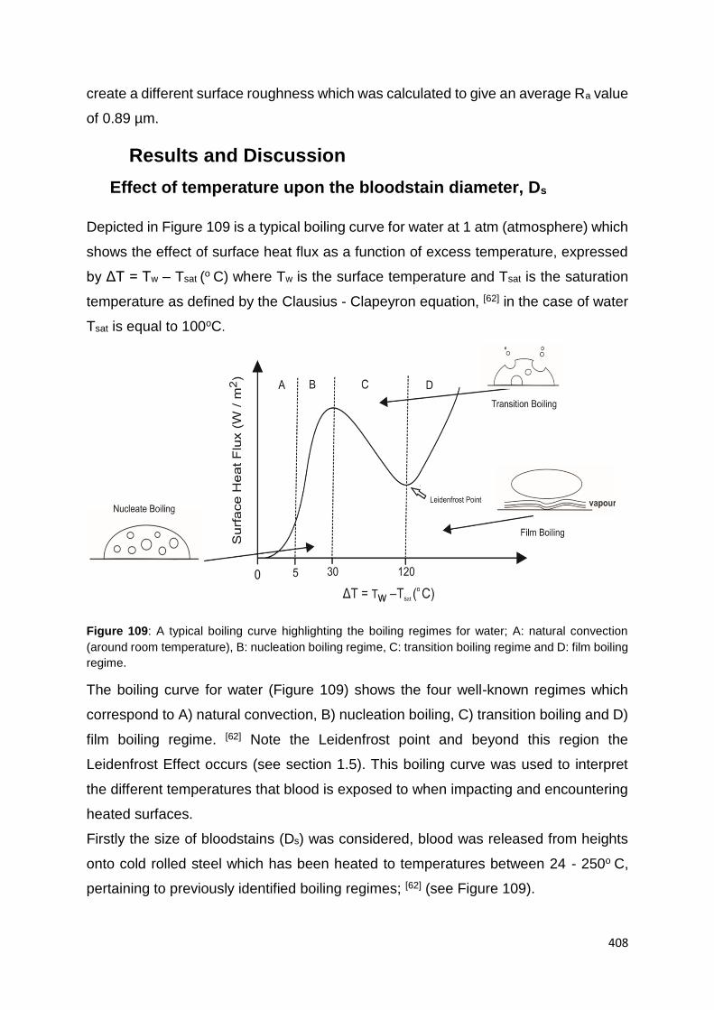
408
create a different surface roughness which was calculated to give an average Ra value
of 0.89 µm.
Results and Discussion
Effect of temperature upon the bloodstain diameter, Ds
Depicted in Figure 109 is a typical boiling curve for water at 1 atm (atmosphere) which
shows the effect of surface heat flux as a function of excess temperature, expressed
by ΔT = Tw – Tsat (o C) where Tw is the surface temperature and Tsat is the saturation
temperature as defined by the Clausius - Clapeyron equation, [62] in the case of water
Tsat is equal to 100oC.
Figure 109: A typical boiling curve highlighting the boiling regimes for water; A: natural convection
(around room temperature), B: nucleation boiling regime, C: transition boiling regime and D: film boiling
regime.
The boiling curve for water (Figure 109) shows the four well-known regimes which
correspond to A) natural convection, B) nucleation boiling, C) transition boiling and D)
film boiling regime. [62] Note the Leidenfrost point and beyond this region the
Leidenfrost Effect occurs (see section 1.5). This boiling curve was used to interpret
the different temperatures that blood is exposed to when impacting and encountering
heated surfaces.
Firstly the size of bloodstains (Ds) was considered, blood was released from heights
onto cold rolled steel which has been heated to temperatures between 24 - 250o C,
pertaining to previously identified boiling regimes; [62] (see Figure 109).

409
Figure 110: Effect of bloodstain diameters (Ds) for equine blood released onto cold rolled steel held at
a range of temperatures and released from a range of heights; 30.5 cm (squares ), 60.9 cm
(circles ), 91.4 cm (triangles ), 121.9 cm (upside-down triangles ) using a 1 mL pipette (inner tip
diameter 1.77 mm). Note that at each surface temperature, each data point is an average of 20 blood
drops (N= 20).
Figure 110 depicts the analysis of the observed bloodstain diameter (Ds) upon
impacting surface temperatures released from a range of heights where a noticeable
pattern is evident, where the bloodstain diameter (Ds) was observed to initially
increase, which then starts to decrease when the boiling point of blood is approached,
assumed to occur at 100oC. Beyond this point the bloodstain diameter was observed
to reduce as the surface temperature was increased up to 230oC. The observations in
Figure 110 were interpreted in terms of the blood drop expanding due to the addition
of heat, which likely arises due to the dependence of viscosity versus temperature,
such that up to the boiling point of blood, an increase in Ds is observed (Figure 110).
Beyond this point, Ds decreases with temperature, likely due to evaporation being the
overriding parameter evaporating the water component of blood. Since blood is
comprised of approximately 83% water, [204] the maximum boiling point should
theoretically be similar to that of water or very close.

410
Blood Impacts in the Natural Convection Regime
Figure 111: Images of 4.2 mm (Do) blood droplets impacting upon a horizontal steel surface held over
a range of temperature parameters; A: Room temperature (24°C), B: 60°C, C: 100°C, D: 140°C and E:
230oC.
This regime, shown as section (A) on Figure 111, involves natural heat flow and
temperatures of around 24oC (room temperature) and just below the boiling point of
blood. [59] As shown in Figure 110, the effect of the overall diameters were at their most
substantial when in the natural convection regime (see section 1.6) before any form of
significant evaporation transpires. It was acknowledged that there appears to be a
clear reduction in bloodstain diameter Ds from the initial impact of the droplet to when
it is dry, leaving a “doughnut” type shape bloodstain, as depicted in Figure 111B, this
effect occurs when temperatures are of 50oC ≤ Tw and at room temperature (see
Figure 110A). Further investigation into this reduction was performed, by centrifuging
the blood separating it into serum and red blood cells, and individually dropping them
onto the cold rolled steel (Figure 112A and B). As shown in Figure 112, it is evident
that a separation of the blood into serum and red blood cells creates this perceived
reduction; the red blood cells collect in the centre of the bloodstain thus creating a
hardened bubble when completely dry, with the serum generating the visible outer
ring.
A.) B.)
E.)
C.) D.)
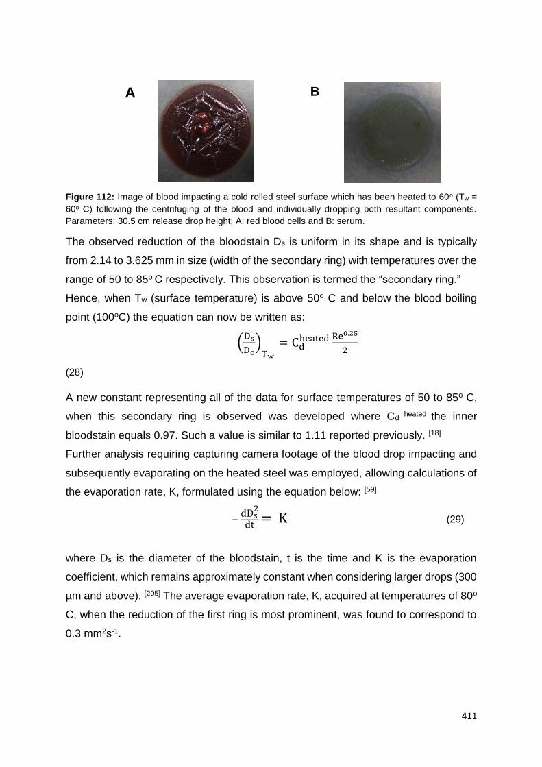
411
Figure 112: Image of blood impacting a cold rolled steel surface which has been heated to 60o (Tw =
60o C) following the centrifuging of the blood and individually dropping both resultant components.
Parameters: 30.5 cm release drop height; A: red blood cells and B: serum.
The observed reduction of the bloodstain Ds is uniform in its shape and is typically
from 2.14 to 3.625 mm in size (width of the secondary ring) with temperatures over the
range of 50 to 85o C respectively. This observation is termed the “secondary ring.”
Hence, when Tw (surface temperature) is above 50o C and below the blood boiling
point (100oC) the equation can now be written as:
(Ds
Do)
Tw
= Cdheated Re0.25
2
(28)
A new constant representing all of the data for surface temperatures of 50 to 85o C,
when this secondary ring is observed was developed where Cd heated the inner
bloodstain equals 0.97. Such a value is similar to 1.11 reported previously. [18]
Further analysis requiring capturing camera footage of the blood drop impacting and
subsequently evaporating on the heated steel was employed, allowing calculations of
the evaporation rate, K, formulated using the equation below: [59]
−dDs
2
dt= K (29)
where Ds is the diameter of the bloodstain, t is the time and K is the evaporation
coefficient, which remains approximately constant when considering larger drops (300
µm and above). [205] The average evaporation rate, K, acquired at temperatures of 80o
C, when the reduction of the first ring is most prominent, was found to correspond to
0.3 mm2s-1.
A B

412
Blood Impacts in the Nucleation Boiling Regime
Figure 111C depicts a typical bloodstain diameter (Ds) that is in the nucleation boiling
regime (see Fig 109), occurring at temperatures of 90 – 120o C. In this regime the
overall diameters were decreased as evaporation ensued due to the realisation of the
maximum boiling point at 100oC. Similarly to the natural convection regime, there was
a clear reduction followed by a series of uniform rings. Initial velocity, Vo predetermines
the number of rings the bloodstain encompasses, the greater the initial velocity, Vo
and therefore the higher the release height is, the greater number of rings are
observed this is due to the increase in bloodstain diameter size; heights of 121.9 cm
and 91.4 cm produce 5 distinct rings compared to only 4 and 3 rings observed at
heights of 60.9 cm and 30.5 cm respectively. The production of the rings can be
explained when the falling and successive splashing of the blood drop is observed as
it contacts the solid horizontal surface, there is a development of uniform capillary
waves / rings as the drop strikes and settles on the surface. It is evident that the inner
and outer ring impact the surface first and the middle ring follows later; the inner and
outer ring vaporize instantaneously as they touch the surface pushing the majority of
the red blood cells to the middle layer, explaining the darker appearance of the central
ring and increased vaporisation time. When drops at lower temperatures were
compared the drop impacts the surface similarly, however due to the lower
temperature instant vaporisation does not ensue and therefore the drop dries and
evaporates uniformly. This regime is one of the most important when considering
blood pattern recognition. During the nucleation regime bubbles form in the liquid, this
is reminiscent of the vacuoles present when blood is expirated. This is an important
insight since heated blood could be mistaken as expirated blood, which is vital when
determining useful patterns at a crime scene.
Blood Impacts in the Transition Boiling Regime
Further decline in bloodstain diameter (Ds) was observed due to the rapid evaporation
experienced at the higher temperatures (120oC - 230oC). A significant alteration in the
appearance of the final bloodstain (Ds) was observed, depicted in Figure 111D where
sporadically hardened red blood cells within the serum stain are all that remain. The
blood drop vaporizes the instant it contacts the surface, driving the red blood cells to
the centre of the bloodstain; evaporation starts on the periphery of the bloodstain and
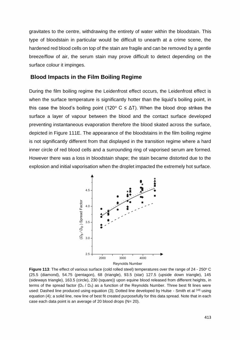
413
gravitates to the centre, withdrawing the entirety of water within the bloodstain. This
type of bloodstain in particular would be difficult to unearth at a crime scene, the
hardened red blood cells on top of the stain are fragile and can be removed by a gentle
breeze/flow of air, the serum stain may prove difficult to detect depending on the
surface colour it impinges.
Blood Impacts in the Film Boiling Regime
During the film boiling regime the Leidenfrost effect occurs, the Leidenfrost effect is
when the surface temperature is significantly hotter than the liquid’s boiling point, in
this case the blood’s boiling point (120o C ≤ ΔT). When the blood drop strikes the
surface a layer of vapour between the blood and the contact surface developed
preventing instantaneous evaporation therefore the blood skated across the surface,
depicted in Figure 111E. The appearance of the bloodstains in the film boiling regime
is not significantly different from that displayed in the transition regime where a hard
inner circle of red blood cells and a surrounding ring of vaporised serum are formed.
However there was a loss in bloodstain shape; the stain became distorted due to the
explosion and initial vaporisation when the droplet impacted the extremely hot surface.
Figure 113: The effect of various surface (cold rolled steel) temperatures over the range of 24 - 250o C
(25.5 (diamond), 54.75 (pentagon), 68 (triangle), 93.5 (star) 127.5 (upside down triangle), 145
(sideways triangle), 163.5 (circle), 230 (square)) upon equine blood released from different heights, in
terms of the spread factor (Ds / Do) as a function of the Reynolds Number. Three best fit lines were
used: Dashed line produced using equation (3); Dotted line developed by Hulse - Smith et al [18] using
equation (4); a solid line, new line of best fit created purposefully for this data spread. Note that in each
case each data point is an average of 20 blood drops (N= 20).

414
Although there was a significant difference between bloodstains Ds, when all the data
(i.e. all initial bloodstain diameters for each temperature) is transfigured into the spread
factor (Ds / Do), it was evident that there is actually little difference and the temperature
has no significant effect on the general scatter spread. Figure 113 highlights this using
lines of ‘best fit’ created by utilising previously defined equations and therefore
establishing a new constant of for Cd heated corresponding to 1.12, which is not
dissimilar to the original value of 1.11 observed by Hulse- Smith et al .[18]
Effect of temperature upon Number of Spines, N.
Figure 114: Analysis of the number of spines exhibited from equine blood impacting on cold rolled steel
at temperatures of; 24.6o C (squares), 52.5o C (circles), 92.5o C (triangles) and 150o C (stars) verses
the Weber number. The number of spines is highly influenced by the surface roughness consequently
leading to a new constant being developed, with the use of a line of ‘best fit.’ The new line of ‘best fit’
(solid line) fitted the scatter spread more accurately compared to the original line of ‘best fit’ (dotted line)
using equation (5) and the line of best fit (dashed line) incorporated by Hulse Smith et al [18] using
equation (6). Note each data point is an average of 20 blood drops (N= 20).
Figure 114 depicts the general scatter of data relating the number of spines to the
Weber number, there is a considerable deviation from the expected data when
applying equation (5) requiring the development of a new constant, Cn= 0.315
considerably different to the original value of 0.838, obtained by Hulse - Smith et al.
[18] The increase in temperature had a clear effect on the number of spines exhibited
however the effect did not follow a noticeable pattern, the subsequent expansion in
diameter, Ds, would have anticipated an increase in the amount of spines exhibited,
and this was not the case. As previously stated the bloodstain diameter, Ds, expands
in the natural convection regime, around 50°C yet when a temperature of 52.5°C was
415
applied the number of spines decreases. Spines could not be calculated at the highest
temperatures due to the distorted shape of the bloodstain. These results imply that the
use of spines as an evaluation tool is not viable when heat is applied. However it is
noted that there is a significant increase in satellite spatter when temperatures reach
the film boiling regime which could warrant future further investigation to establish a
pattern.
Effect of surface roughness
Only the 1.77 mm pipette was utilised in this experiment for the comparison of
surfaces due to unforeseen difficulties when heating the rougher steel.
The cold rolled steel was sand blasted to create a rougher surface; a rougher surface
affects the bloodstain diameter, Ds, expecting a smaller bloodstain to be the resultant.
Problems arose when heating the rougher surface; the coarser surface made it difficult
to heat the steel to the correct surface temperature, for example the new maximum
boiling point was equated to be at 60°C; 60°C was the highest temperature the rougher
surface was able to reach when 100°C was attempted in the furnace, this problem
continued through all of the boiling regimes. Only one side of the steel was sand
blasted, meaning the heat from the untouched surface which would have been at the
correct temperature could have been radiating through the steel affecting the blood
stains in the normal boiling regimes but not altering the surface temperature. Due to
this factor it was not thought necessary to develop a new boiling curve as the resulting
curve may not be an accurate representation of the actual temperatures achieved and
the highest temperature was not achievable resulting in the absence of the film boiling
regime from the final results of the sand blasted steel.
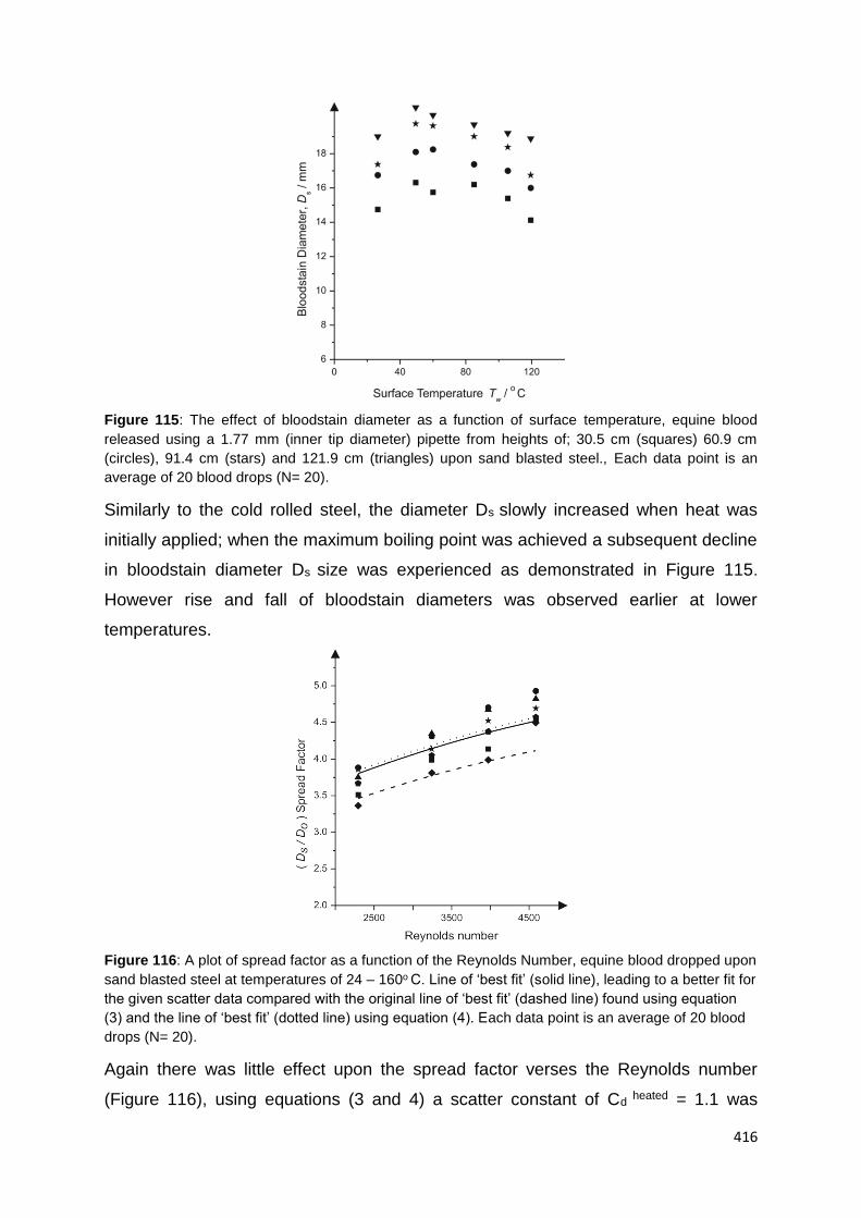
416
Figure 115: The effect of bloodstain diameter as a function of surface temperature, equine blood
released using a 1.77 mm (inner tip diameter) pipette from heights of; 30.5 cm (squares) 60.9 cm
(circles), 91.4 cm (stars) and 121.9 cm (triangles) upon sand blasted steel., Each data point is an
average of 20 blood drops (N= 20).
Similarly to the cold rolled steel, the diameter Ds slowly increased when heat was
initially applied; when the maximum boiling point was achieved a subsequent decline
in bloodstain diameter Ds size was experienced as demonstrated in Figure 115.
However rise and fall of bloodstain diameters was observed earlier at lower
temperatures.
Figure 116: A plot of spread factor as a function of the Reynolds Number, equine blood dropped upon
sand blasted steel at temperatures of 24 – 160o C. Line of ‘best fit’ (solid line), leading to a better fit for
the given scatter data compared with the original line of ‘best fit’ (dashed line) found using equation
(3) and the line of ‘best fit’ (dotted line) using equation (4). Each data point is an average of 20 blood
drops (N= 20).
Again there was little effect upon the spread factor verses the Reynolds number
(Figure 116), using equations (3 and 4) a scatter constant of Cd heated = 1.1 was

417
established which is similar to the original constant Cd = 1.11 and the constant acquired
for cold rolled steel, 1.12. Despite the difficulty in accomplishing the necessary
temperatures no significant changes in bloodstain diameter size were observable
between surfaces, however this can only be loosely surmised since a direct
comparison cannot be made due to the aforementioned difficulties.
Lastly the boiling curve for water (Figure 109) was revisited and adapted to illustrate
impacting blood.
Figure 117: A typical boiling curve highlighting the boiling regimes for blood; A: natural convection
(around room temperature), B: nucleation boiling regime, C: transition boiling regime and D: film boiling
regime.
Figure 117 depicts a typical boiling curve for blood at 1 atm which clearly shows the
typical blood impacts one will observe when blood impacts upon a heated surface.
Note that there are slightly differing values when comparing the blood boiling curve to
that of water, primarily it is recognised that regimes tend to occur approximately 10 -
20o C earlier for that of blood. An explanation for this could be the impurity of blood,
unlike water it contains, salts, proteins and other impurities that will ultimately alter its
boiling value. Regimes were recognised by the distinct change in bloodstain
appearance (Figure 111A - E) as temperature increased, the Leidenfrost point was
used as a reference marker.

418
5.4.3 Summary
It has been demonstrated for the first time that there is a distinct pattern in bloodstain
diameters when they impinge a heated surface, where bloodstain diameters
experienced an increase up to temperatures of 90o C and then subsequently decrease
at a parallel rate as temperature increases. This suggests a steady evaporation once
the boiling point is achieved. Four boiling regimes previously identified for water
pooling and droplets [62] can be equally applied to blood at slightly higher temperatures,
an anticipated outcome due to blood composing of 83 % water. [204] During these
regimes changes to the appearance of the final bloodstains Ds were observed; rings
were formed where separation of blood into its components takes place. A new
constant when considering this separation was developed, Cd heated. Further rings
developed when the temperature was increased; 5 rings were found on bloodstains
released onto a 90oC surface at heights of 121.9 and 91.4 cm. A correlation between
height, thus the initial velocity Vo of the blood drop and the number of rings was
ascertained, where lower heights produced fewer rings due to the size of the
bloodstain.
Lastly, the appearance of spines was counted and deemed to be insignificant when
blood is dropped on to a heated surface; their appearance becomes sporadic and
does not follow any general pattern. There was however an increase in the amount of
satellite spatter experienced especially in the higher temperatures, this could perhaps
substitute spines in cases of heat exposure and should be analysed further to attain
their true significance.
Overall it can be concluded that heated surfaces do have a significant effect on
bloodstains (Ds) changing their appearance and size dramatically. Ultimately possibly
leading to a misinterpretation of patterns (expirated stain vs heated stain).

419
5.5 SURFACE CLEANING
Another method of surface manipulation is cleaning. There are two ways cleaning may
affect bloodstains: 1- pre-treatment and 2- post-treatment.
5.5.1 Pre-treatment Cleaning
Pre-treatment cleaning is cleaning carried out before blood has impacted the surface.
Potentially altering the surface texture creating a surfactant layer of the cleaning
solution and possibly changing the absorbance properties of the surface, effecting the
spread of the liquid.
5.5.2 Post-treatment Cleaning
Post–treatment is where cleaning was performed to remove the blood from the
surface, in essence “covering up” the blood spill. This method destroys the bloodstain
patterns and could affect presumptive testing and DNA analysis (see section 1.7).
The following research looks at both these methods, using appropriate cleaning
methods and household detergents/cleaning solutions.
5.6 HEATED SURFACE CLEANING
Following the research of blood on a heated surface it was deemed appropriate to
evaluate other possible effects that the heat may have upon blood and its detection.
With the knowledge that blood evidence is a valuable source of DNA and the ever
increasing ways criminals are attempting to cover-up their crimes (see section 1.7),
several cleaning methods in conjunction with heat were tested. The results reflect the
effectiveness of three established presumptive tests and the ability of successfully
extracting DNA from blood that has been both cleaned and dropped onto a heated
surface.
In this study, two different routes of analysis was employed; the first was a high salt
extraction, conventional PCR and gel electrophoresis, utilising REDTaq® ReadyMixTM
PCR Reaction Mix and Variable Number Tandem Repeats (VNTRs). The second
method involved a silica based extraction, real-time PCR based DNA quantitation, end
420
point PCR and capillary electrophoresis, using the AmpFlSTR®NGM SElect™ PCR
Amplification Kit. This comparison was made to evaluate the effectiveness of the
newer technique over the older technique when considering an extreme case of DNA
degradation. The advances in DNA analysis mean that new methods are continually
replacing older methods; however these newer methods are very high in price and
may not be economically feasible for poorer countries. Therefore if it is found that the
cheaper method is a viable option, especially under the most extreme circumstances
that can be faced at a crime scene (cleaning and heat exposure) it can offer a cheaper
yet still accurate alternative method of analysis.
5.6.1 Experimental
All blood utilised was collected fresh on the day of analysis, where a venepuncture
was performed on the donor and extracted blood was collected in a BD Vacutainer®
whole blood tube, containing the anticoagulant EDTA. Blood was refrigerated at 4oC
for storage until required for experimentation. All chemicals were supplied by Sigma-
Aldrich and were of the highest analytical grade available.
5.6.1.1 Sample Preparation
A series of 50 µL blood drops were deposited onto a steel surface, using a Gilson®
pipette, which had previously been cleaned to remove any possible contaminants,
firstly using acetone and finally with triple deionised water where it was left to naturally
dry/evaporate at room temperature. After a minimum of 1 hour drying time to enable
the complete drying of the blood drops, a total of six cleaning procedures (plus a
control sample) were performed. These are as follows: 10 % bleach solution (sodium
hypochlorite solution), soap and water (1:1 dilution), cold water (20oC), warm water
(45oC), 1M NaCl + 1M NaOH solution (reported as a DNA degrading agent) [206 - 207]
and soda water. Bloodstains were cleaned off the surface until no visible trace (to the
naked eye) of them remained. This procedure was performed at various temperatures,
where the steel surface was heated, using an oven furnace, to temperatures of 50oC,
150oC and 250oC prior to blood being dropped. An infrared temperature gun was
utilized to ensure correct temperatures were reached and maintained throughout the
experiment.
421
5.6.1.2 Presumptive Test Preparation
Three presumptive tests for blood were performed on all bloodstains after temperature
and cleaning treatments. Each presumptive test solutions were made in accordance
with Refs [204 - 206]. For clarity the exact composition of each is as follows:
Luminol: consisted of a luminol stock solution (1g luminol and 7.5g potassium in 125
mL of distilled water) and a 3% hydrogen peroxide solution. [204] When performing the
test a mixture of 10 mL luminol stock solution and 10 mL of the hydrogen peroxide
solution was used. [204] The analysis was performed in a darkened room where the
mixture was simply sprayed (with a spray bottle) over the area under investigation.
When the surface luminesced; this was recorded as a positive result for the presence
of blood as suggested by a previous report. [204]
TMB (Tetramethylbenzidine): 0.2g TMB dissolved in 10 mL, which was refrigerated for
storage until required, and a 3% hydrogen peroxide solution. [206] The test was
performed by swabbing the area of interest, where a series of 2 drops of TMB (stock
solution) were applied followed by 2 drops of the hydrogen peroxide solution. [206] A
positive indication for blood was expressed when the swab turned a blue/green colour;
no colour change denoted a negative result as described in a previous study. [206]
Kastle Meyer (KM): 0.1g phenolphthalein, 25% w/v sodium hydroxide solution, 0.1g
zinc powder, 70% ethanol and distilled water, 3% hydrogen peroxide solution, distilled
water and 70% ethanol. [205] Similarly to the TMB test, the area under examination was
swabbed, where again a series of drops are added; 2 drops of the 70 % ethanol
solution, followed by 2 drops of the KM stock solution and lastly 2 drops of the 3%
hydrogen peroxide solution. [205] Again, a positive result for the presence of blood is
indicated by a colour change, in this case an intense pink colour is observed.
All presumptive tests were made fresh on the day of experimentation and were
performed three times to ensure consistency. Negative and positive controls were
employed to ensure that the presumptive tests were functioning properly. A bloodstain
was used as the positive control and a blank surface was used as the negative control.
5.6.1.3 Sample Collection
Two sampling techniques were employed, swabbing and scraping. [4] Swabbing
was performed with a class IIA Eurotubo wooden and cotton sterile swab; the swab
was slightly moistened with triple distilled water and the swab was rubbed over the
area under investigation. Scraping was performed using single edge razor blades, the
422
blades were sterilised before use. Each bloodstain was scraped using a new razor
blade to avoid any cross contamination. All temperature ranges were tested for both
techniques 3 times to attain uniform results, a total of 24 samples were prepared and
compared. It is noted that other collection techniques such as mini- tapes could have
been utilised; however these tend to be used for fabric materials whereas scraping
and swabbing are recognised collection techniques for blood / dried blood on a number
of surfaces. [4]
5.6.1.4 First Analytical Technique
A high salt extraction was performed as follows; [212] the bloodstain / cleaned area was
swabbed using a sterile swab moistened in triple deionised water, the swab was then
cut into a 1.5 mL eppendorf tube where a 150 µL of triple deionised water was added.
After 1 hour 150 µL of TNES (10mM Tris, 400mM NaCl, 100mM EDTA, 0.6% SDS)
buffer (warmed to 56oC) and 10 µL of Proteinase K were added, the solutions were
left to incubate overnight at 56oC in a water bath. [212] The following day 41.5 µL of 6M
NaCl (pre-warmed to 37oC) was included into the sample mixture, which was
subsequently vortexed for 15 seconds and then microfuged (13000 x g) for 10 mins.
The next step involved the careful removal of 300 µL of supernatant to a new tube
where an equal volume of 100% EtOH (300 µL) was added. [212] Again the solution
was microfuged (13000 x g) for 10 mins, however this time the supernatant was
disposed of and the pellet remained in the tube where 200 µL of 70% EtOH was added
and the solution was microfuged again, this time for 5 mins. Removal of supernatant
followed, where care was taken not to lose the pellet. This last step was repeated once
more as some blood samples can be very unclean. The pellet was then left to air dry
for 10 mins. Lastly 25 µL of TE (10 mM Tris-Cl, 1 mM EDTA) buffer was added to the
dry pellet which was then vortexed and left for 1 hour at room temperature ready for
ethidium bromide gel preparation. [212] Samples were run at 120 V on a 0.8 % Agarose
gel for 45 minutes, where the gel was subsequently exposed to UV light to visualize
any DNA bands.Samples were run at 120 V on a 0.8 % Agarose gel for 45 minutes,
where the gel was subsequently exposed to UV light to visualize any DNA bands.
Subsequent measurements were conducted using the Nanodrop, a device used to
quantify the amount of DNA present in a sample.
Further analysis utilising a conventional PCR amplification [213 - 214] was carried out,
where a REDTaq® ReadyMixTM PCR Reaction Mix was utilized. The primers used

423
(below) amplified the locus D1S80, [215 - 216] a common VNTR used in forensic
identification. [215 - 216] The locus is found on chromosome 1, the largest human
chromosome, 29 different alleles of the locus are presently known ranging in sizes of
200 bp to 700 bp. [215 - 216] The amplified DNA was successively run on an ethidium
bromide gel.
5.6.1.5 Second Analytical Technique
A silica based extraction was performed as per Ref. [217] Real-time PCR using a
Human Quantiplex Kit (Qiagen, UK) upon a RotorGene real-time PCR machine
(Qiagen, UK) was carried out on the extracts, quantifying the amount of DNA present
in each sample. These results were used to determine which samples were the most
suitable candidates to be analysed by capillary electrophoresis (CE) where full profiles
may be ascertained as well as providing data to optimal the template amount for
subsequent PCR analysis. These samples were amplified using AmpFLSTR® NGM
SElect™ PCR Amplification Kit (STR loci; D3S1358, vWA, D16S539, D2S1338,
D8S1179, D21S11, D18S51, D19S433, TH01, FGA, Amelogenin, D10S1248,
D22S1045, D2S441, D1S1656, D12S391) using the Veriti Thermal Cycler (Life
Technologies, UK) as per manufacturer’s instructions. The amplicons then fragment
analysis using an ABI3130 Genetic Analyser equipped with Genemapper V3.2
Software.
5.6.2 Results and Discussion
5.6.2.1 Presumptive Testing
First, three types of presumptive testing (luminol, TMB and Kastle–Meyer) were
performed on all bloodstains at varying temperatures after the cleaning methods (10
% bleach solution (sodium hypochlorite solution), soap and water (1:1 dilution), cold
water (20oC), warm water (45oC), 1M NaCl + 1M NaOH solution) had been completed.
Observations made prior to cleaning revealed flaking of the bloodstains at surface
temperatures of 50 – 150oC, making the overall cleaning much easier due to the easy
removal of the brittle flakes without much physical exertion. Higher temperatures
however were found to burn the blood into the steel surface and therefore were much
harder to remove without leaving a trace outline of where the blood had been
deposited. Presumptive testing was performed an hour after cleaning, giving the
surface enough time to dry and cool; all tests were performed three times. Initial

424
analysis revealed that temperature alone, contrary to previous reports, has no effect
upon the ability to detect the blood using any of the presumptive techniques. However
when we explored the use of these techniques when various cleaning methods had
been employed it was found that heat has an effect.
Temperatures of Impacted Surface (oC)
Cleaning Methods Room Temp
50oC 150oC 250oC
Luminol None ✓ ✓ ✓ ✓
Cold water ✓ ✓ ✓ x
Soap and water ✓ ✓ ✓ ✓
10% Bleach ✓ x x x
1M NaCl + NaOH ✓ ✓ x x
Club soda ✓ ✓ ✓ ✓
Warm water
✓ ✓ ✓ x
TMB None ✓ ✓ ✓ ✓
Cold water ✓ ✓ ✓ ✓
Soap and water ✓ ✓ ✓ ✓
10% Bleach ✓ ✓ ✓ ✓
1M NaCl + NaOH ✓ ✓ ✓ ✓
Club soda ✓ ✓ ✓ ✓
Warm water
✓ ✓ ✓ ✓
Kastle-Meyer None ✓ ✓ ✓ ✓
Cold water ✓ ✓ ✓ ✓
Soap and water ✓ ✓ x x
10% Bleach ✓ x x x
1M NaCl + NaOH ✓ x x x
Club soda ✓ ✓ x x
Warm water ✓ ✓ ✓ x
Table 32: Comparisons of the effects of various cleaning methods and temperatures on three
presumptive tests (luminol, TMB and Kastle – Meyer) used for the establishing the presence of blood.
Tests were run three times to ensure consistency, a total of 252 samples were compared overall for
this section of experimentation. ✓ - positive for presence of blood and x - negative for presence of blood.
Table 32 demonstrates the effect of both cleaning, and the effect of a heated surface
upon the efficiency of the blood visualising techniques; a tick signifies a positive result
for the presence of blood, which was indicated via a colour change/luminescence (20
seconds). Similarly a cross indicates a negative result for the presence of blood where

425
no colour change or luminescence was experienced after a period of 20 seconds.
Tests were performed three times where the rule of 2 out of 3 results (i.e. 2 positives
and 1 negative) were considered a majority and therefore taken as the final result.
There was however no deviations between the three runs performed; all results were
either positive or negative for all three attempts. All cleaning presented no effects when
applied at room temperature, as the heat is increased, negative results start to
emerge, for example at 50oC when the stain was cleaned with the bleach solution both
luminol and KM tests returned a negative result. At 250oC this pattern persists,
returning more negative results for 4 out of 7 of the cleaning methods when luminol is
used and 5 out of 7 when KM was utilized. It is unclear why these negative results
start to emerge as temperature increases, as temperature alone appears to have no
effect. A possible explanation could be that the heat weakens the haemoglobin
structure and therefore when cleaning is performed it is easier to remove any trace of
blood, using the more aggressive cleaning methods (i.e. bleach). TMB appeared to be
the most robust method of presumptive testing, yielding positive results for all cleaning
methods tested. It is suggested that future presumptive testing where crime scene
cleaning is suspected is performed using the TMB test, as although it is a time
consuming test, gives rise to more consistent results when the bloodstain has been
removed by cleaning.
There are countless other blood presumptive tests (leuchomalachite green,
fluorescein etc.), [24] however many of these are out-dated since they are thought to
use highly carcinogenic substances (an obvious Health and Safety issue) or are less
reliable than the aforementioned three.
5.6.2.2 First Analytical Technique
5.6.2.2.1 Ethidium Bromide Gels
The first ethidium bromide gel implemented was to compare the sample collecting
method of swabbing versus scraping both of which are readily employed collection
techniques at crime scenes. [24] Initial analysis of Figure 118 illustrates that both
swabbing and scraping produce viable DNA samples and are therefore equally as
suitable as collection techniques. This is further supported by the Nanodrop results
that show concentrations for swabbing and scraping to be very similar, except in the

426
case of the highest temperature (250oC) where scraping did not yield any results due
to the difficulty in removing the sample.
Figure 118: An ethidium
bromide gel comparing the DNA exhibited when two different sample collecting techniques were
employed where the steel plate had been heated to 250oC; Lane 1: 1KB ladder, Lanes 2-4: scraping
and Lanes 5-7: swabbing.
The Nanodrop, a device used to quantify the amount of DNA present in a sample, it is
a type of spectrophotometer basing its analysis on wavelengths; therefore if the
sample is unclean erroneous results are to be expected. Unpaired t-tests to establish
the statistical significance of the difference in DNA concentrations when employing the
two collection methods were performed. Results found p values of between 0.1917 -
0.4246 when comparing each temperature step with the collection method, these
values are not considered to be statistically significant and therefore confirm the claim
that either method of DNA collection is viable.
Lane Number

427
Figure 119: The effects of temperature on DNA represented in an ethidium bromide gel; Lane 1: 1 KB
ladder, Lanes 2 – 3: blood dropped on to a steel plate pre-heated to room temperature, Lanes 4 – 5:
blood dropped on a steel plate pre-heated to 50oC, Lanes 6 – 7: blood dropped on a steel plate pre-
heated to 150oC, Lanes 8 – 9: blood dropped on to a steel plate pre-heated to 250oC.
Further analysis utilising the Nanodrop reveals that the concentration of DNA
significantly decreases with temperature, this is not apparent when Figure 119 is
observed, which depicts the effect of temperature on DNA analysis using an ethidium
bromide gel. Table 33 demonstrates the Nanodrop results showing that the
concentration of DNA nearly halves with every temperature step.
Temperature (oC) Scrape DNA concentration(ng/µL)
Swab DNA concentration
(ng/µL)
Room 46.40 38.08 50 19.75 14.58
150 4.50 5.90 250 - 2.75
Table 33: Effect of temperature of the impacting surface (steel) on the concentration of DNA measured
with a Nanodrop.
Again unpaired t-tests were performed to ascertain the statistical significance of the
results; DNA concentration results for the highest and lowest temperatures were
compared for both collection techniques. Results found p values of 0.0042 and 0.0182
when scraping and swabbing were employed, respectively, both values are
considered to be extremely statistically significant. This suggests that temperature
influences the concentration of DNA significantly, decreasing the concentration as
Lane Number
1 2 3 4 5 6 7 8 9
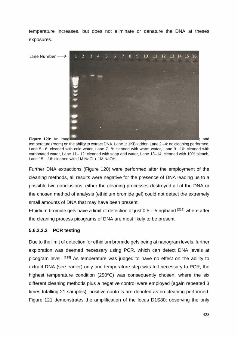
428
temperature increases, but does not eliminate or denature the DNA at theses
exposures.
Figure 120: An image of an ethidium bromide gel illustrating the effects of both cleaning and
temperature (room) on the ability to extract DNA. Lane 1: 1KB ladder, Lane 2 –4: no cleaning performed,
Lane 5– 6: cleaned with cold water, Lane 7- 8: cleaned with warm water, Lane 9 –10: cleaned with
carbonated water, Lane 11– 12: cleaned with soap and water, Lane 13–14: cleaned with 10% bleach,
Lane 15 – 16: cleaned with 1M NaCl + 1M NaOH.
Further DNA extractions (Figure 120) were performed after the employment of the
cleaning methods, all results were negative for the presence of DNA leading us to a
possible two conclusions; either the cleaning processes destroyed all of the DNA or
the chosen method of analysis (ethidium bromide gel) could not detect the extremely
small amounts of DNA that may have been present.
Ethidium bromide gels have a limit of detection of just 0.5 – 5 ng/band [217] where after
the cleaning process picograms of DNA are most likely to be present.
5.6.2.2.2 PCR testing
Due to the limit of detection for ethidium bromide gels being at nanogram levels, further
exploration was deemed necessary using PCR, which can detect DNA levels at
picogram level. [218] As temperature was judged to have no effect on the ability to
extract DNA (see earlier) only one temperature step was felt necessary to PCR, the
highest temperature condition (250oC) was consequently chosen, where the six
different cleaning methods plus a negative control were employed (again repeated 3
times totalling 21 samples), positive controls are denoted as no cleaning performed.
Figure 121 demonstrates the amplification of the locus D1S80; observing the only
Lane Number 1 2 3 4 5 6 7 8 9 10 11 12 13 14 15 16

429
presence of DNA in lane 8, where the bloodstain was not treated with a cleaning
process.
Figure 121: A 1% agarose gel exposed to UV light showing the PCR amplification for locus D1S80;Lane
1: 100 bp ladder, Lane 2: swab control sample (blank), Lane 3: cleaned with cold water, Lane 4:cleaned
with warm water, Lane 5: cleaned with carbonated water, Lane 6:cleaned with soap and water, Lane
7:cleaned with 10% household bleach, Lane 8: no cleaning performed, Lane 9: cleaned with 1M NaCl
+ 1M NaOH, Lane 10: negative control (distilled water).
With the previous knowledge that the treatment of heat causes a decrease in DNA
concentration but does not eliminate it, it can be concluded that the absence of any
DNA is a result of cleaning; this is further supported by the appearance of a DNA band
(Figure 121, lane 8) where heat but no cleaning was employed. Water acts as a lysing
agent; [219] therefore it is a plausible result that even the use of plain water can eliminate
DNA. It is noted however that these results are highly dependent on the ‘cleaner,’
where effectiveness of DNA elimination depends on how hard and for how long you
scrub, in this study bloodstains were scrubbed until they could no longer be visualised
via the naked eye.
5.6.2.3 Second Analytical Technique
Real-time PCR (using the AmpFLSTR® NGM SElect™ PCR Amplification Kit) was
use to quantify the amount of DNA present within each sample, 28 samples were
tested (4 different temperatures with 6 cleaning methods and blanks). It was found
that only four samples, those which were exposed only to different surface
temperatures where no form of cleaning had been attempted, showed presence of
DNA. Table 34 expresses the DNA concentrations, it is noted that as temperature
Lane Number 1 2 3 4 5 6 7 8 9 10

430
increases the amount of DNA decreases. Student t-tests were performed to explore
the significance of the results, a value for p was found to be 0.0001, and is therefore
considered to be extremely significant. Hence, it can now be stated that heated
surfaces do have a significant effect on DNA analysis, decreasing but not eliminating
it as the surface temperature rises.
Temperature (oC)
DNA concentration (ng/µL)
Room (25) 1.302
50 1.221
150 0.719
250 0.145
Table 34 - Quantiplex results quantifying the effect of temperature of the impacting surface (steel) on
the concentration of DNA.
Based on the results using the Quantiplex kit it was determined that only the four
surface temperature affected samples were worthwhile advancing to the next stage of
analysis, being the most viable samples in which to obtain a full profile. However, as
a precaution, the room temperature samples for each cleaning method were also
analysed (7 samples). Samples were amplified (see experimental section) and
analysed using Capillary Electrophoresis. It was found that full DNA profiles could be
obtained from all samples which were exposed solely to different surface temperatures
without any subsequent cleaning. Figures 122 and 123 demonstrate the apparent
effects of degradation by surface temperature, where both the Relative Fluorescence
Units (RFU) and ratios (between the low molecular weight markers and the high
molecular weight markers) decrease as temperature rises, this is characteristic of a
degraded DNA profile.

431
Figure 122: A graphical representation of the average RFU value for peak height across the EPG
when incorporating different surface temperatures alone without cleaning.
Figure 123: Peak height ratios of profiles obtained when DNA
was deposited on to a heated surface.
Again statistical analysis was performed to evaluate the significance of the results,
when the RFU values (for room temp and 250oC) were considered the data was found
to be extremely statistically significant giving a p value of 0.0002, however when the
ratios (for room temp and 250oC) were analysed a p value of 0.4178 was found which
is deemed as not statistically significant. Given that the full profile could be recovered
successfully for all temperatures it is reasonable to assume that temperature does not
have a significant effect on the quality of DNA recovered.

432
Next the capillary electrophoresis results were analysed for the 7 samples where
cleaning had been performed (room temp; 25oC); it was discovered that only partial
profiles could be recovered. Match probabilities were calculated from these partial
profiles, expressed in Table 35, to evaluate the strength of the profiles as potential
evidence in a forensic case.
Table 35 - Match
Probabilities obtained from
partial profiles after samples
were exposed to different cleaning techniques.
Given that the match probability of the full profile was measured to be 4.262E+26 and
the low probabilities displayed in Table 35, the profiles obtained after cleaning were
deemed unusable and would not be used as forensic evidence. (Appendix 10)
Therefore it can be stated that cleaning completely removes any viable trace of DNA
in this study, again this may dependent on the ‘cleaner’ and surface type. It was also
noticed that the effect of cleaning appeared to contribute additional DNA to the result.
The STR analysis was carried out in DNA clean condition and the negative controls
showed no amplification at all; however, extraneous DNA was detected in the results
following cleaning (Appendix 10). Further investigation shows there to be several
alleles present, expressing multiple contamination. This may be attributed to people
involved in the manufacturing process (i.e. soap manufacturing, paper towel
manufacturing), where several people could have come into contact with the materials
utilised in this study, before they are packaged.
5.6.2.4 Old v New Techniques
Cleaning Method (At Room Temp)
Match Probability
Odds (1 in)
1M NaCl + NaOH 3
Bleach 3
Cold Water 1150
Soda Water -
Warm Water 12
Soap and Water 260

433
The two methods (salt extraction with PCR vs silica extraction with real-time PCR) of
analysis used in this paper are compared. The first method, by DNA standards, is an
old outdated technique and the second method uses up-to-date technology and is
standard in most forensic laboratories. Both methods differ significantly in price here
it is investigated why this might be.
Findings indicate that both methods work and draw the same conclusions,
temperature decreases the amount of available DNA and, in this study, cleaning
eliminates any trace of viable DNA. There are limitations to the former method
however; the agarose gel analysis can be highly inaccurate when trying to quantify the
DNA, often errors occurring due to band distortion. The gels in this study were used
purely to show that DNA was present, instead the Nanodrop was used for
quantification. Gel electrophoresis also lacks any real qualitative capabilities, merely
showing the presence of DNA, although some bands appeared to fade, indicating less
DNA, as temperature increased.
Surprisingly the VNTR worked well despite its reputation as being unsuitable for
degraded samples, due to the fragment sizes. Both extraction techniques were
successful in spite of there being no purification step in the high salt extraction method.
Overall it can be concluded that although the first method is old and out-dated the
technique remains robust, where even in the most extreme circumstances (i.e.
heat/cleaning or both) viable DNA can be extracted using the cheapest methods
available. This leaves economical options open to poorer countries which may not be
able to afford the more expensive methods of analysis, where at least preliminary
analysis of the DNA, i.e. is a profile feasible, can be carried out.
5.6.3 Summary
In this study a combination of surface heat and cleaning on the ability to extract DNA
was explored. Both a high salt extraction and silica based extraction procedure were
utilised, attempting to extract DNA after treatment of 4 varying temperatures and six
different cleaning methods. After exposure to three presumptive tests for blood
(luminol, TMB and Kastle – Meyer) it was discovered that the 10% bleach is the most
effective cleaning agent and temperature alone does not have an effect on the ability
to detect blood. TMB was found to be the most effective method of testing for the

434
presence of blood after cleaning; it is therefore advised that this be the presumptive
method of choice when cleaning has been employed at crime scenes.
After exploring the effects of surface temperature on the ability to extract viable DNA
it was found that the surface’s temperature decreases but does not eliminate the
amount of DNA available for extraction and that even at 250oC (for a small exposure
period) a full profile can be obtained. Cleaning (using cleaning solutions) conversely
was found to eliminate DNA completely in all cases, with all cleaning techniques. This
outcome is unexpected due to the known recovery of DNA from washed clothing which
was exposed to higher temperatures of around 50oC, [220] therefore results can be
attributed to two factors; firstly, the vigorous cleaning routine employed by the analyst
and it is impossible to cover all possible cleaning techniques of the cleaner due to the
individuality of the person and their situation at the time of the crime (i.e. are they in a
hurry), in this experiment surfaces were only cleaned until blood appeared to have
gone, therefore different results could be obtained if the time for cleaning increased/
reduced or of the person used less/more exertion. Secondly results can be assigned
to the type of surface utilised, the steel used in this experiment was non-porous and
therefore will not retain the blood / DNA as well as the clothing used in ref [220], further
exploration into different types of surfaces which can be heated (i.e. different types of
metal) should be investigated to fully understand the implications of surface type and
DNA recovery.
Finally two different routes of analysis (salt extraction with PCR vs silica extraction
with real-time PCR) were compared in order to explore whether greater expenditure
actually gives the better results which could otherwise not be reached with a cheaper
method. It was found that both methods reach the same end conclusion; this is
surprising as VNTRs are especially prone to degradation due to their size and yet,
sufficient amounts of DNA could still be extracted and analysed. There are limitations
to the older method ((salt extraction with PCR) that quality of DNA cannot be assessed
accurately, however the method is robust enough to still be used comfortably for
preliminary analysis of DNA, offering a cheaper alternative.

435
5.7 FABRIC LAUNDERING
The wear and tear of fabrics is a key concern when bloodstains are analysed on
clothing. The difference between a new piece of fabric and one which has been
repeatedly washed, dried, ironed etc. could have major implications on how the blood
impacts and absorbs into fabric, i.e. build-up of detergent creating a surfactant layer.
It is noted that fabrics can be standardised following the protocol outlined in 8A BS
ENISO 6330/A1:2009. This will be explored to establish if this concept is applicable to
all fabric types and to the impaction of blood.
The following study will investigate bloodstains on various fabrics and the effects
laundering, drying and repeated cycles have upon fabrics and subsequently the blood
that impacts them.
5.7.1 Experiment
Six commercially available washing detergents were investigated: Ariel (Actilift), Daz
(Regular), Persil (Colour Powder), Surf (with Essential Oils), Fairy (Non-Bio) and Bold
2 in 1 (Lavender and Camomile), these were chosen as they were found to be the
most popular brands used amongst the general population. [221]
The washing machine used throughout this investigation was the Hoover DYN 8144
D and the tumble dryer was a Hotpoint Aquarius Ultima Reversomatic Dryer Super De
Luxe TL31. A rinse cycle was performed on the washing machine before beginning
any testing.
Hand washing was performed where water was heated to 30oC, monitored using a
thermometer. The recommended amount of washing detergent (guided by
manufacturer of the packaging) was dissolved in the warm water. The fabrics were
allowed to soak for 10 minutes, scrubbed clean, soaked for a further 10 minutes, then
rinsed using cold water.
Blood drop experiments were performed as described in section 2.2. Stains were
measured once they were fully dried, therefore there was a degree of wicking present.
5.7.2 Results and Discussion
436
5.7.2.1 Detergent Form and Type
There are many varieties of washing detergent, for this study 6 were considered (Ariel,
Daz, Persil, Surf, Fairy and Bold 2 in 1). These detergents were chosen as they were
found to be the most popular and widely used in the home. [221 - 222] Fourier Transform
Infra-Red was performed on each detergent, the spectrums produced were
fundamentally similar as Fairy, Bold and Daz are produced by the same company
(Procter and Gamble). Before any analysis was conducted on the effect of different
detergents it was important to establish the influence the form in which the detergent
was in had when applied to the fabric. Detergent comes in many forms, [217] the forms
tested in this paper were: capsule, liquid and powder. Only 8 of the 20 fabrics (Cotton
Poplin, Medium Habotai Silk, Denim, M&S T- Shirt Jersey, Light Grey Polyester Twill,
Jupiter Linen, Wool Delaine and Nylon) were tested during this preliminary experiment,
each chosen for their characteristic differences and fabric type. Fabrics were both
hand-washed and machine washed and dried 3 different ways (air dry, radiator dry
and tumble dry). The manufacturer’s recommendations were followed regarding the
amount of detergent used and a rinse cycle was run between washes (30oC) to ensure
all detergent had gone from the washing machine. Blood drop tests were performed
using the larger pipette (1.77mm inner diameter) from a height of 50 cm. Results
showed that in general the form of detergent did not have a significant effect on the
size of the bloodstain produced. In fact the results highlighted the possibility of an
effect when different methods of drying and washing are considered (this will be
discussed later). Since there was deemed to be no significant difference when the
form of detergent was considered, powder was used for the remaining experiments.

437
Powder is used in most homes and is more cost effective than any other forms of
detergent.
Figure 124: Average bloodstain diameters when blood impacted fabric after it had been machine
washed with 6 different detergent types. N = 5
Next the six common brands of detergent were assessed. Two washing techniques
were employed (machine and hand) and fabrics were radiator dried (dial number 3;
20o C) Figure 124 shows the results amassed after the use of these 6 detergents;
finding bloodstain diameters significantly increased in size independent of the
detergent type. Results varied when a different washing technique (Figure 125) was
0
5
10
15
20
25
30
35
Jup
ite
r Li
nen
Rai
sed
Nat
ura
l Co
tto
n
Fuji
Silk
Hea
vyw
eig
ht
Co
tto
n
Co
tto
n P
op
lin
Co
tto
n J
ers
ey
Ecru
Wo
ol M
ix S
uit
ing
Wo
ol D
ela
ine
(ble
ach
ed)
Po
ly/l
ine
n/r
ayo
n P
and
ora
De
vore
Pe
asan
t C
ott
on
Re
sid
a B
um
p C
ott
on
Silk
Du
pio
n
Silk
Ch
iffo
n
Me
diu
m H
abo
tai S
ilk
De
nim
M&
S T-
Shir
t Je
rsey
Ligh
t G
rey
Po
lye
ste
r Tw
ill
Po
lysa
tin
Hea
vy
Co
tto
n D
uck
Blo
od
stai
n D
iam
eter
/ m
m
Fabric Types
Ariel Bold Daz Fairy Persil Surf

438
incorporated, where fabrics which were hand washed displayed little significant
difference (Table 36) when detergents were considered.
Figure 125: Average bloodstain diameters when blood impacted fabric after it had been hand washed
with 6 different detergent types. N = 5
Fabrics which were machine washed offered more significant changes to the diameter
size, this is perhaps the cause of the degree of agitation the fabric goes through when
it is being mechanically cleaned. Table 36 compares the two washing techniques using
the p values obtained after employing the unpaired student t-test. It is clear that
washing technique is a determinant factor in the size of the final bloodstain, showing
significant differences for almost all of the fabric independent of the detergent used.
0
5
10
15
20
25
30
Jup
ite
r Li
nen
Rai
sed
Nat
ura
l Co
tto
n
Fuji
Silk
Hea
vyw
eig
ht
Co
tto
n
Co
tto
n P
op
lin
Co
tto
n J
ers
ey
Ecru
Wo
ol M
ix S
uit
ing
Wo
ol D
ela
ine
(ble
ach
ed)
Po
ly/l
ine
n/r
ayo
n P
and
ora
De
vore
Pe
asan
t C
ott
on
Re
sid
a B
um
p C
ott
on
Silk
Du
pio
n
Silk
Ch
iffo
n
Me
diu
m H
abo
tai S
ilk
De
nim
M&
S T-
Shir
t Je
rsey
Ligh
t G
rey
Po
lye
ste
r Tw
ill
Po
lysa
tin
Hea
vy
Co
tto
n D
uck
Blo
od
stai
n D
iam
eter
/ m
m
Fabric Types
Ariel Bold Daz Fairy Persil Surf

439
Type of Fabric
p value Aerial
Sig. Yes
(✓)
or No (x)
p value Bold
Sig. Yes
(✓)
or No (x)
p value Daz
Sig. Yes
(✓)
or No (x)
p value Fairy
Sig. Yes
(✓)
or No (x)
p value Persil
Sig. Yes
(✓
or No (x)
p value Surf
Sig. Yes
(✓)
or No (x)
Jupiter Linen 0.31 X 0.63 X 0.38 X 0.68 X 0.06 X 0.25 X
Raised Natural Cotton 0.09 X 0.16 X 0.00 ✓ 0.21 X 0.00 ✓ 0.71 X
Fuji Silk 0.00 ✓ 0.00 ✓ 0.02 ✓ 0.00 ✓ 0.00 ✓ 0.00 ✓
Heavyweight Cotton 0.74 X 0.07 X 0.00 ✓ 0.00 ✓ 0.00 ✓ 0.06 X
Cotton Poplin 0.00 ✓ 0.00 ✓ 0.02 ✓ 0.10 X 0.23 X 0.00 ✓
Cotton Jersey Ecru 0.00 ✓ 0.36 X 1.00 X 0.00 ✓ 0.43 X 0.48 X
Wool Mix Suiting 0.00 ✓ 0.00 ✓ 0.00 ✓ 0.00 ✓ 0.00 ✓ 0.20 X
Wool Delaine (bleached) 0.00 ✓ 0.38 X 0.00 ✓ 0.00 ✓ 0.10 X 0.17 X
P/L/R Pandora Devore
0.00 ✓ 0.00 ✓ 0.00 ✓ 0.08 X 0.07 X 0.00 ✓
Peasant Cotton 0.00 ✓ 0.00 ✓ 0.00 ✓ 0.00 ✓ 0.00 ✓ 0.00 ✓
Resida Bump Cotton 0.00 ✓ 0.00 ✓ 0.00 ✓ 0.00 ✓ 0.00 ✓ 0.00 ✓
Silk Dupion 0.00 ✓ 0.20 X 0.00 ✓ 0.04 ✓ 0.00 ✓ 0.02 ✓
Silk Chiffon 0.00 ✓ 1.00 X 0.81 X 0.00 ✓ 0.00 ✓ 0.00 ✓
Medium Habotai Silk 0.00 ✓ 0.82 X 0.00 ✓ 0.00 ✓ 0.00 ✓ 0.00 ✓
Denim 0.46 X 0.39 X 0.00 ✓ 0.42 X 0.75 X 0.27 X
M&S T-Shirt Jersey 0.62 X 0.15 X 0.00 ✓ 1.00 X 0.00 ✓ 0.00 ✓
Light Grey Polyester Twill 0.05 ✓ 0.00 ✓ 0.56 X 0.00 ✓ 0.84 X 0.83 X
Polysatin Heavy 0.00 ✓ 0.00 ✓ 0.00 ✓ 0.00 ✓ 0.00 ✓ 0.00 ✓
Cotton Duck 0.00 ✓ 0.00 ✓ 0.00 ✓ 0.00 ✓ 0.01 ✓ 0.44 X
Table 36: Student t-tests were performed to attain the significance of the results obtained when we
compare both washing techniques; hand and machine. N = 5.
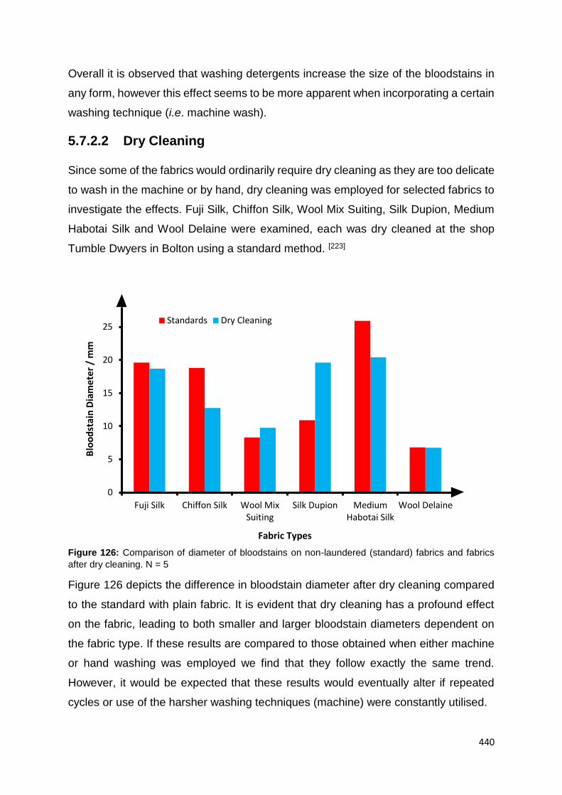
440
Overall it is observed that washing detergents increase the size of the bloodstains in
any form, however this effect seems to be more apparent when incorporating a certain
washing technique (i.e. machine wash).
5.7.2.2 Dry Cleaning
Since some of the fabrics would ordinarily require dry cleaning as they are too delicate
to wash in the machine or by hand, dry cleaning was employed for selected fabrics to
investigate the effects. Fuji Silk, Chiffon Silk, Wool Mix Suiting, Silk Dupion, Medium
Habotai Silk and Wool Delaine were examined, each was dry cleaned at the shop
Tumble Dwyers in Bolton using a standard method. [223]
Figure 126: Comparison of diameter of bloodstains on non-laundered (standard) fabrics and fabrics
after dry cleaning. N = 5
Figure 126 depicts the difference in bloodstain diameter after dry cleaning compared
to the standard with plain fabric. It is evident that dry cleaning has a profound effect
on the fabric, leading to both smaller and larger bloodstain diameters dependent on
the fabric type. If these results are compared to those obtained when either machine
or hand washing was employed we find that they follow exactly the same trend.
However, it would be expected that these results would eventually alter if repeated
cycles or use of the harsher washing techniques (machine) were constantly utilised.
0
5
10
15
20
25
Fuji Silk Chiffon Silk Wool MixSuiting
Silk Dupion MediumHabotai Silk
Wool Delaine
Blo
od
stai
n D
iam
ete
r /
mm
Fabric Types
Standards Dry Cleaning
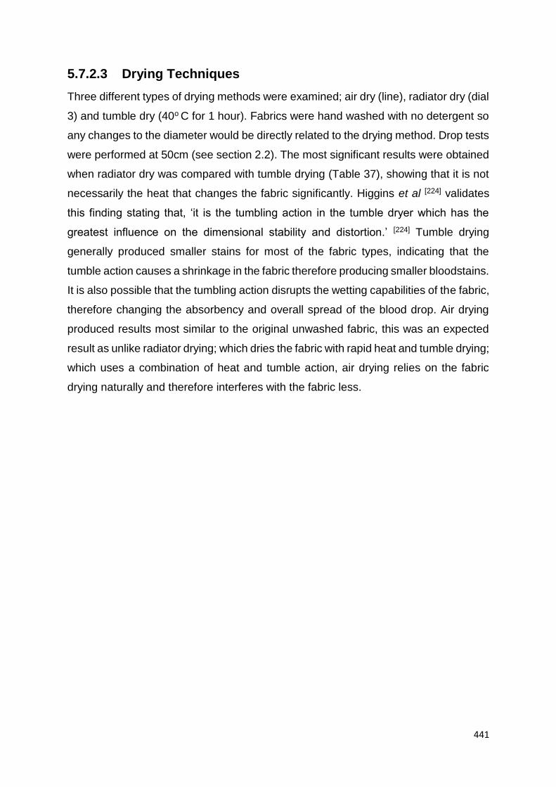
441
5.7.2.3 Drying Techniques
Three different types of drying methods were examined; air dry (line), radiator dry (dial
3) and tumble dry (40o C for 1 hour). Fabrics were hand washed with no detergent so
any changes to the diameter would be directly related to the drying method. Drop tests
were performed at 50cm (see section 2.2). The most significant results were obtained
when radiator dry was compared with tumble drying (Table 37), showing that it is not
necessarily the heat that changes the fabric significantly. Higgins et al [224] validates
this finding stating that, ‘it is the tumbling action in the tumble dryer which has the
greatest influence on the dimensional stability and distortion.’ [224] Tumble drying
generally produced smaller stains for most of the fabric types, indicating that the
tumble action causes a shrinkage in the fabric therefore producing smaller bloodstains.
It is also possible that the tumbling action disrupts the wetting capabilities of the fabric,
therefore changing the absorbency and overall spread of the blood drop. Air drying
produced results most similar to the original unwashed fabric, this was an expected
result as unlike radiator drying; which dries the fabric with rapid heat and tumble drying;
which uses a combination of heat and tumble action, air drying relies on the fabric
drying naturally and therefore interferes with the fabric less.
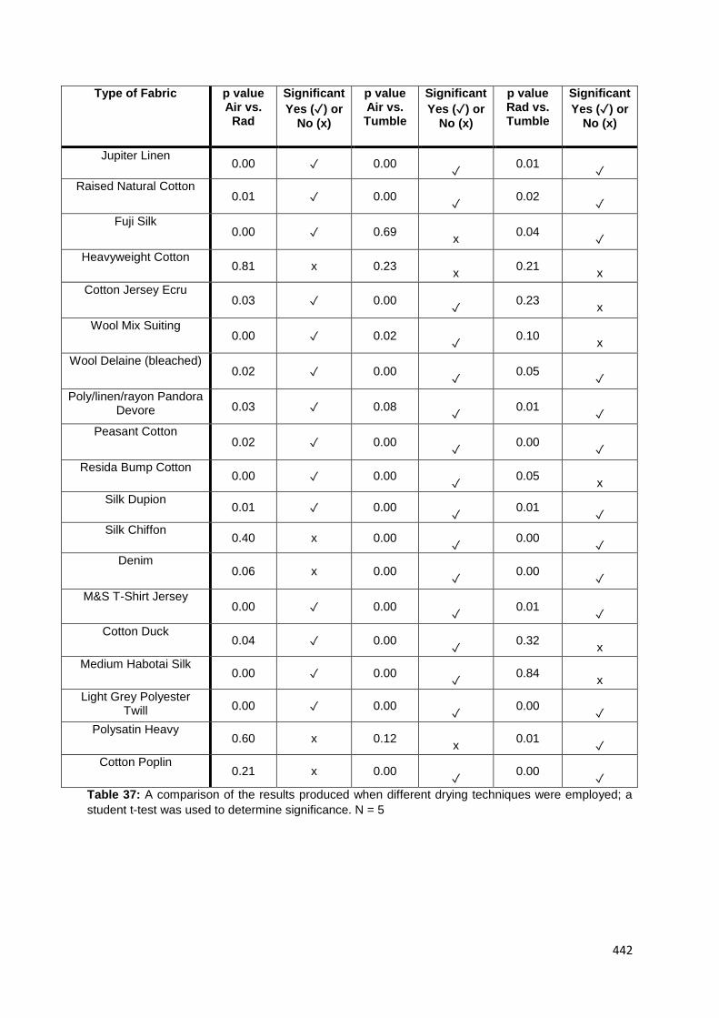
442
Type of Fabric p value Air vs.
Rad
Significant
Yes (✓) or
No (x)
p value Air vs. Tumble
Significant
Yes (✓) or
No (x)
p value Rad vs. Tumble
Significant
Yes (✓) or
No (x)
Jupiter Linen 0.00 ✓ 0.00
✓ 0.01
✓
Raised Natural Cotton 0.01 ✓ 0.00
✓ 0.02
✓
Fuji Silk 0.00 ✓ 0.69
x
0.04
✓
Heavyweight Cotton 0.81 x 0.23
x
0.21 x
Cotton Jersey Ecru 0.03 ✓ 0.00
✓ 0.23
x
Wool Mix Suiting 0.00 ✓ 0.02
✓ 0.10
x
Wool Delaine (bleached) 0.02 ✓ 0.00
✓ 0.05
✓
Poly/linen/rayon Pandora Devore 0.03 ✓ 0.08
✓ 0.01
✓
Peasant Cotton 0.02 ✓ 0.00
✓ 0.00
✓
Resida Bump Cotton 0.00 ✓ 0.00
✓ 0.05
x
Silk Dupion
0.01 ✓ 0.00
✓ 0.01
✓
Silk Chiffon
0.40 x 0.00
✓ 0.00
✓
Denim 0.06 x 0.00
✓ 0.00
✓
M&S T-Shirt Jersey 0.00 ✓ 0.00
✓ 0.01
✓
Cotton Duck 0.04 ✓ 0.00
✓ 0.32
x
Medium Habotai Silk 0.00 ✓ 0.00
✓ 0.84
x
Light Grey Polyester Twill 0.00 ✓ 0.00
✓ 0.00
✓
Polysatin Heavy 0.60 x 0.12
x
0.01
✓
Cotton Poplin 0.21 x 0.00
✓ 0.00
✓
Table 37: A comparison of the results produced when different drying techniques were employed; a
student t-test was used to determine significance. N = 5

443
This result is supported by the method (section 8A of BS EN ISO 6330/A1:2009) [55]
used by many researchers to stabilise fabrics, where the drying process stipulates ‘air
dried flat.’[55]
It is noted that heavyweight cotton exhibits no change regardless of the drying
procedure, this is most likely due to the composition. A twill weave (heavyweight cotton
structure) is a looser weave than a plain weave, therefore ay manipulation of the fabric
my result in a significant change in the way the fabric behaves (i.e. absorbency).
5.7.2.4 Machine Washing Temperatures
The temperature at which we wash our clothes will depend very much on the type of
fabric being washed and the degree of soiling. Most clothing is washed between 30oC
and 40oC and for the most soiled clothes the temperature is increased up to 60oC as
recommended by the fabric manufacturers. All fabrics (excluding nylon) were washed
at 30oC, 40oC and 60oC without detergent so the effects of temperature could be solely
explored.
Figure 127: A representation of the average bloodstain diameters created when blood impacted fabrics
washed at 3 different temperatures; 30oC, 40oC and 60oC. N = 5.
0
5
10
15
20
25
Jup
ite
r Li
nen
Hea
vyw
eig
ht
Co
tto
n
Co
tto
n J
ers
ey
Ecru
M&
S T-
Shir
t Je
rsey
Pan
do
ra D
evo
re
Wo
ol D
ela
ine
Wo
ol M
ix S
uit
ing
Pe
asan
t C
ott
on
Silk
Du
pio
n
Fuji
Silk
Ch
iffo
n S
ilk
Co
tto
n D
uck
Re
sid
a B
um
p C
ott
on
Nat
ura
l Rai
sed
Co
tto
n
Co
tto
n P
op
lin
Me
diu
m H
abo
tai S
ilk
De
nim
Ligh
t G
rey
Po
lye
ste
r Tw
ill
Po
lysa
tin
Hea
vy
Blo
od
stai
n D
iam
eter
/ m
m
Fabric Types
30 40 60
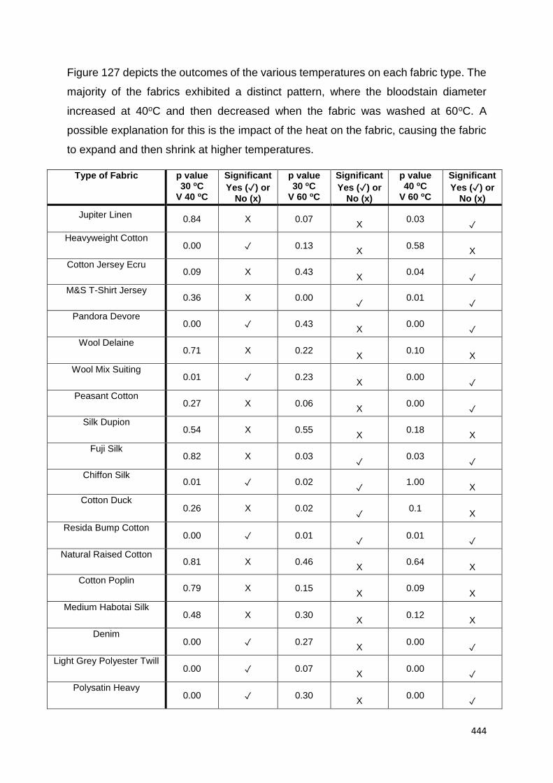
444
Figure 127 depicts the outcomes of the various temperatures on each fabric type. The
majority of the fabrics exhibited a distinct pattern, where the bloodstain diameter
increased at 40oC and then decreased when the fabric was washed at 60oC. A
possible explanation for this is the impact of the heat on the fabric, causing the fabric
to expand and then shrink at higher temperatures.
Type of Fabric p value 30 oC
V 40 oC
Significant
Yes (✓) or
No (x)
p value 30 oC
V 60 oC
Significant
Yes (✓) or
No (x)
p value 40 oC
V 60 oC
Significant
Yes (✓) or
No (x)
Jupiter Linen 0.84 X 0.07
X
0.03
✓
Heavyweight Cotton 0.00 ✓ 0.13
X
0.58
X
Cotton Jersey Ecru 0.09 X 0.43
X
0.04
✓
M&S T-Shirt Jersey 0.36 X 0.00
✓ 0.01
✓
Pandora Devore 0.00 ✓ 0.43
X
0.00
✓
Wool Delaine 0.71 X 0.22
X
0.10
X
Wool Mix Suiting 0.01 ✓ 0.23
X
0.00
✓
Peasant Cotton 0.27 X 0.06
X
0.00
✓
Silk Dupion 0.54 X 0.55
X
0.18
X
Fuji Silk 0.82 X 0.03
✓ 0.03
✓
Chiffon Silk 0.01 ✓ 0.02
✓ 1.00
X
Cotton Duck 0.26 X 0.02
✓ 0.1
X
Resida Bump Cotton 0.00 ✓ 0.01
✓ 0.01
✓
Natural Raised Cotton 0.81 X 0.46
X
0.64
X
Cotton Poplin 0.79 X 0.15
X
0.09
X
Medium Habotai Silk 0.48 X 0.30
X
0.12
X
Denim 0.00 ✓ 0.27
X
0.00
✓
Light Grey Polyester Twill 0.00 ✓ 0.07
X
0.00
✓
Polysatin Heavy 0.00 ✓ 0.30
X
0.00
✓

445
Table 38: Statistical analysis (student t-test) comparing p values for three temperatures. N = 5
Statistical analysis was performed (see Table 38) using an unpaired student t-test, it
is evident that most fabrics experienced a significant change around 40o C and
stabilised at 60oC.
Since temperature clearly has an effect on the fabric it is important to consider this in
reconstructions, especially as the effect is not predictable; sometimes increasing the
crime scene bloodstain diameters and other times decreasing depending on fabric
type.
5.7.2.5 Repeated Cycles
The International Organisation for Standardisation [55] states that the fabric becomes
standardised after 6 continuous cycle washes, therefore this has been incorporated
as the “norm” when other analysts have conducted work on fabrics. [44-48] Here this
theory is tested, extending the number of cycles to 10 and testing with and without
detergent.
Table 39 shows the progression of cycles without detergent, Table 40 expresses these
changes as p values after unpaired student tests were performed.
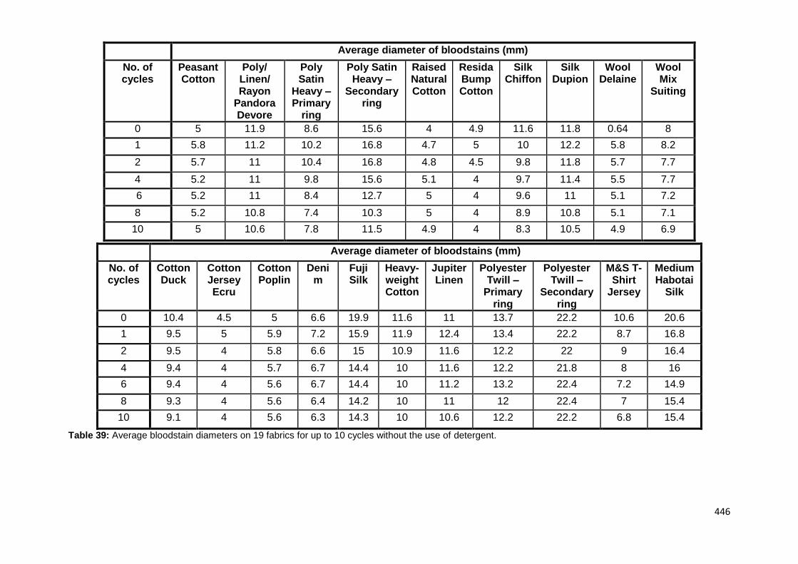
446
Table 39: Average bloodstain diameters on 19 fabrics for up to 10 cycles without the use of detergent.
Average diameter of bloodstains (mm)
No. of cycles
Peasant Cotton
Poly/ Linen/ Rayon
Pandora Devore
Poly Satin
Heavy – Primary
ring
Poly Satin Heavy –
Secondary ring
Raised Natural Cotton
Resida Bump Cotton
Silk Chiffon
Silk Dupion
Wool Delaine
Wool Mix
Suiting
0 5 11.9 8.6 15.6 4 4.9 11.6 11.8 0.64 8
1 5.8 11.2 10.2 16.8 4.7 5 10 12.2 5.8 8.2
2 5.7 11 10.4 16.8 4.8 4.5 9.8 11.8 5.7 7.7
4 5.2 11 9.8 15.6 5.1 4 9.7 11.4 5.5 7.7
6 5.2 11 8.4 12.7 5 4 9.6 11 5.1 7.2
8 5.2 10.8 7.4 10.3 5 4 8.9 10.8 5.1 7.1
10 5 10.6 7.8 11.5 4.9 4 8.3 10.5 4.9 6.9
Average diameter of bloodstains (mm)
No. of cycles
Cotton Duck
Cotton Jersey Ecru
Cotton Poplin
Denim
Fuji Silk
Heavy-weight Cotton
Jupiter Linen
Polyester Twill –
Primary ring
Polyester Twill –
Secondary ring
M&S T-Shirt
Jersey
Medium Habotai
Silk
0 10.4 4.5 5 6.6 19.9 11.6 11 13.7 22.2 10.6 20.6
1 9.5 5 5.9 7.2 15.9 11.9 12.4 13.4 22.2 8.7 16.8
2 9.5 4 5.8 6.6 15 10.9 11.6 12.2 22 9 16.4
4 9.4 4 5.7 6.7 14.4 10 11.6 12.2 21.8 8 16
6 9.4 4 5.6 6.7 14.4 10 11.2 13.2 22.4 7.2 14.9
8 9.3 4 5.6 6.4 14.2 10 11 12 22.4 7 15.4
10 9.1 4 5.6 6.3 14.3 10 10.6 12.2 22.2 6.8 15.4
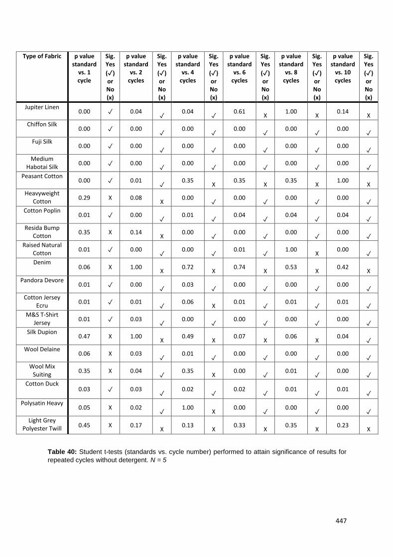
447
Table 40: Student t-tests (standards vs. cycle number) performed to attain significance of results for
repeated cycles without detergent. N = 5
Type of Fabric p value standard
vs. 1 cycle
Sig. Yes
(✓) or No (x)
p value standard
vs. 2 cycles
Sig. Yes
(✓) or No (x)
p value standard
vs. 4 cycles
Sig. Yes
(✓) or No (x)
p value standard
vs. 6 cycles
Sig. Yes
(✓) or No (x)
p value standard
vs. 8 cycles
Sig. Yes
(✓) or No (x)
p value standard
vs. 10 cycles
Sig. Yes
(✓) or No (x)
Jupiter Linen
0.00 ✓ 0.04
✓ 0.04
✓ 0.61
X
1.00
X 0.14
X
Chiffon Silk
0.00 ✓ 0.00
✓ 0.00
✓ 0.00
✓ 0.00
✓ 0.00
✓
Fuji Silk
0.00 ✓ 0.00
✓ 0.00
✓ 0.00
✓ 0.00
✓ 0.00
✓
Medium Habotai Silk
0.00 ✓ 0.00
✓ 0.00
✓ 0.00
✓ 0.00
✓ 0.00
✓
Peasant Cotton 0.00 ✓ 0.01
✓ 0.35
X
0.35
X 0.35
X
1.00
X
Heavyweight Cotton
0.29 X 0.08
X 0.00
✓ 0.00
✓ 0.00
✓ 0.00
✓
Cotton Poplin 0.01 ✓ 0.00
✓ 0.01
✓ 0.04
✓ 0.04
✓ 0.04
✓
Resida Bump Cotton
0.35 X 0.14
X 0.00
✓ 0.00
✓ 0.00
✓ 0.00
✓
Raised Natural Cotton
0.01 ✓ 0.00
✓ 0.00
✓ 0.01
✓ 1.00
X
0.00
✓
Denim 0.06 X 1.00
X
0.72
X 0.74
X
0.53
X 0.42
X
Pandora Devore 0.01 ✓ 0.00
✓ 0.03
✓ 0.00
✓ 0.00
✓ 0.00
✓
Cotton Jersey Ecru
0.01 ✓ 0.01
✓ 0.06
X
0.01
✓ 0.01
✓ 0.01
✓
M&S T-Shirt Jersey
0.01 ✓ 0.03
✓ 0.00
✓ 0.00
✓ 0.00
✓ 0.00
✓
Silk Dupion
0.47 X 1.00
X 0.49
X
0.07
X 0.06
X
0.04
✓
Wool Delaine 0.06 X 0.03
✓ 0.01
✓ 0.00
✓ 0.00
✓ 0.00
✓
Wool Mix Suiting
0.35 X 0.04
✓ 0.35
X
0.00
✓ 0.01
✓ 0.00
✓
Cotton Duck 0.03 ✓ 0.03
✓ 0.02
✓ 0.02
✓ 0.01
✓ 0.01
✓
Polysatin Heavy 0.05 X 0.02
✓ 1.00
X
0.00
✓ 0.00
✓ 0.00
✓
Light Grey Polyester Twill 0.45 X 0.17
X
0.13
X 0.33
X
0.35
X 0.23
X
448
Using both (detergent and repeated cycles) a change is observed in all the fabrics but
the Light Grey Polyester and the Denim, where persistent washing had no effect on
the size of the bloodstain. A pattern was apparent when the bloodstain sizes were
analysed, as the cycle number increases the bloodstain diameter decreases. It is
noted that most but not all fabrics stabilise after 6 continuous cycles, where polysatin
and chiffon silk exhibit significant changes between the sixth and tenth cycle when
statistical analysis was performed. However we acknowledge that chiffon silk would
be dry cleaned ordinarily so would not be expected to stabilise at all when machine
washed. Using the characteristics table (Table 23) these changes in bloodstain
diameter can be affiliated with the composition of the fabric. For example the fabrics
with tight plain weaves (i.e. Peasant Cotton etc.) or tight twill weaves (i.e. Light Grey
Polyester Twill, Denim etc.) tended to either not change at all or stabilise much quicker
after continuous cycles. This is important when scene reconstructions are attempted
since history of the fabric (wash history) will most likely be unknown. Finding the stable
point for a fabric provides a maximum change which the fabric will experience, thus
providing limits and a standard error in which to base final conclusions on.

449
Table 41:
Average bloodstain diameters on 19 fabrics for up to 10 cycles with the use of detergent. N = 5
Average diameter of bloodstains (mm)
No. of cycles
Cotton Duck
Cotton Jersey Ecru
Cotton Poplin
Denim Fuji Silk
Heavy-weight Cotton
Jupiter Linen
Polyester Twill -
Primary
Polyester Twill –
Secondary
M&S T-Shirt
Jersey
Medium Habotai
Silk
0 10.4 4.5 5 6.6 19.9 11.6 11 13.7 22.2 10.6 20.6
1 9.5 4 6.4 7.4 15.8 10.9 12.3 13.5 23.6 10.8 17.2
2 10.2 4.2 6.6 8.2 15.8 11 12.4 13.6 22.4 10.8 18.3
4 10.4 4.5 7.1 8.4 15.8 11 12.8 13.4 22 10.8 18.8
6 10.4 5.3 8.4 8.4 16.2 11 12.6 14.4 23 10.8 19
8 10.4 5.5 8.9 8.6 16.5 11.2 12.8 14.6 23.4 10.8 18.8
10 10.5 6.1 9.6 8.8 16.6 11.3 13.4 15 23.6 11 19
No. of cycles
Peasant Cotton
Poly/ Linen/ Rayon
Pandora Devore
Poly Satin
Heavy - Primary
Poly Satin Heavy -
Secondary
Raised Natural Cotton
Resida Bump Cotton
Silk Chiffon
Silk Dupion
Wool Delaine
Wool Mix
Suiting
0 5 11.9 8.6 15.6 4 4.9 11.6 11.8 6.4 8
1 7.1 11.2 10.4 16.5 4.4 4.7 10 14.8 6.1 10
2 7.9 12 12.2 18 5 4.9 10.6 8.2 6.2 10.2
4 8.6 12.2 12.2 18.8 6.1 5 11 8.4 6.3 10.4
6 8.6 12.4 11.2 19 6.2 5 11 12.8 6.4 10.6
8 10.2 12.5 12 18.2 6.3 5.1 11.2 14.6 6.3 10.7
10 10.2 12.4 12.4 17.8 7 5.2 11.2 15.8 6.2 11

319
Next the effect continuous cycles had when detergent was added was investigated;
surf powder detergent was added after every cycle as it would be in real life. Table 41
shows the changing in bloodstain diameters as the number of cycles with detergent
increases. Conversely to the results found without detergent when detergent is added,
in most cases, bloodstains appear to increase in size. It is not known why this occurs,
a possible explanation is the build-up of an enzymatic or surfactant layer on the surface
from the detergent which maybe altering the degree of wetting and wicking. This
steady increase in bloodstain diameter is expected, considering the results exhibited
for the initial tests in the detergent form and type section. Again statistical analysis was
performed in the form of unpaired student t-tests expressed in Table 42, showing that
the increasing of cycles (with detergent) significantly increases the bloodstain
diameter. It is noted that in some instances (i.e. Fuji Silk, Wool Mix Suiting etc.) the
diameters decreased then steadily increased and four fabrics (Light Grey Polyester
Twill, M&S T-shirt Jersey, Resida Bump Cotton and Wool Delaine) were found not to
change significantly at all (although diameters did increase). Further statistical analysis
was implemented to establish fabric stability after 6 cycles, where the sixth cycle
results were compared to the tenth cycle. It was determined that most fabrics were
stable after 6 cycles, where no significant diameter changes were experienced,
however 6 fabrics continued to significantly increase in diameter.

320
Table 42: Student t-tests (standards vs. cycle number) performed to attain significance of results for
repeated cycles with detergent. N = 5.
Fabric characteristics were investigated as possible cause for these changes, there
was found to be no relation between fabric characteristics (weave/knit, porosity,
thickness and roughness) and stability of continuously washed fabric.
Type of Fabric
p value standard vs. 1 cycle
Sig. Yes
(✓)
or No (x)
p value
standard vs.
2 cycles
Sig. Yes
(✓)
or No (x)
p value standard vs. 4 cycles
Sig. Yes
(✓)
or No (x)
p value
standard vs.
6 cycles
Sig. Yes
(✓)
or No (x)
p value
standard vs.
8 cycles
Sig. Yes
(✓)
or No (x)
p value
standard vs.
10 cycles
Sig. Yes
(✓)
or No (x)
Jupiter Silk
0.00 ✓ 0.00
✓ 0.00
✓ 0.00
✓ 0.00
✓ 0.00
✓
Chiffon Silk
0.00 ✓ 0.07
X 0.27
X
0.27
X 0.24
X
0.24
X
Fuji Silk
0.00 ✓ 0.00
✓ 0.00
✓ 0.00
✓ 0.00
✓ 0.00
✓
Medium Habotai Silk
0.00 ✓ 0.00
✓ 0.05
✓ 0.01
✓ 0.00
✓ 0.01
✓
Peasant Cotton
0.00 ✓ 0.00
✓ 0.00
✓ 0.00
✓ 0.00
✓ 0.00
✓
Heavyweight Cotton
0.03 ✓ 0.04
✓ 0.04
✓ 0.04
✓ 0.18
X
0.37
X
Cotton Poplin 0.00 ✓ 0.00
✓ 0.00
✓ 0.00
✓ 0.00
✓ 0.00
✓
Resida Bump Cotton
0.40 X 1.00
X 0.61
X
0.35
X 0.37
X
0.09
X
Raised Natural Cotton
0.07 X 1.00
X 0.00
✓ 0.00
✓ 0.00
✓ 1.00
X
Denim
0.03 ✓ 0.00
✓ 0.00
✓ 0.00
✓ 0.00
✓ 0.00
✓
Pandora Devore
0.01 ✓ 0.35
X 0.46
X
0.10
X 0.01
✓ 0.10
X
Cotton Jersey Ecru
0.01 ✓ 0.27
X 1.00
X
0.01
✓ 0.02
✓ 0.00
✓
M&S T-Shirt Jersey
0.72 X 0.72
X 0.76
X
0.72
X 0.72
X
0.52
X
Silk Dupion 0.00 ✓ 0.00
✓ 0.00
✓ 0.05
✓ 0.00
✓ 0.00
✓
Wool Delaine 0.20 X 0.49
X
0.72
X 1.00
X
0.67
X 0.49
X
Wool Mix Suiting
0.00 ✓ 0.00
✓ 0.00
✓ 0.00
✓ 0.00
✓ 0.00
✓
Cotton Duck
0.03 ✓ 0.54
X 1.00
X
1.00
X 1.00
X
0.77
X
Polysatin Heavy
0.09 X 0.00
✓ 0.00
✓ 0.00
✓ 0.00
✓ 0.00
✓
Light Grey Polyester
Twill 0.67 X 0.33
X
0.14
X 0.82
X
0.80
X 0.62
X

321
5.7.3 Summary
During this study the effects various fabrics types, washing and drying techniques,
detergent type, temperature and number of cycles has on bloodstains, namely their
size.
This study has revealed some important findings, which are pertinent to the
interpretation of bloodstain on fabrics. It was found that although neither the detergent
type nor form has a significant effect on the bloodstains produced the techniques used
to wash and dry the fabrics are highly influential in the stains final appearance. Both
machine washing and tumble drying offered the most significant differences to the
original (untouched fabric) values, this may be attributed to the degree of agitation
experienced in both these techniques which lead to fabric distortion, i.e. shrinking.
Other factors which were found to have a determinant effect on the final bloodstain
was the number of cycles. For both with and without detergent were tested and found
converse results. When detergent was not used the size of the bloodstain decreased
and when detergent was added for each cycle the size increased accordingly. These
changes can be attributed to the degree of wettability which is likely effected by the
surfactants/enzymes found in washing detergents.
Temperature was also discovered to have a marked effect on the size of the
bloodstains produced. As higher temperatures tend to cause a shrinkage in the fabric
smaller stains resulted, though this was not apparent in all fabrics, where exhibited
larger stains.
The overwhelming factor which attributed to most of the bloodstain changes was the
fabric type. Since all fabrics are different; in composition, thickness, porosity,
wettability etc. it is impossible to predict or obtain a recognisable pattern of change
which encompasses all fabrics. This is why it is important for analysts to try to match
the evidence fabric as close as possible when running tests. The problem that this
work now highlights is the fabric history, which will usually be unknown. For instance
if the fabric has a history of being machine washed at high temperatures then tumble
dried, how will this affect the ability to interpret the patterns exhibited effectively?
Clearly such important issues need to be considered in the field of bloodstain pattern
fabric analysis where misinterpretation can lead to errors that can be costly, and bring
the field of BPA into disrepute.
322
5.8 CONCLUSIONS
The final section has investigated the effects of surface manipulation on the final
bloodstain.
Much research has focused on environmental effects such as rain, UV etc. [73] on the
final bloodstain, where researchers have neglected the more apparent bloodstain
manipulation potential, which is present in our homes. Blood can impinge on many
surfaces, which are not only different in type of material but can possess changes
imparted by humans such as the heating or cleaning of a surface.
The first part of this section focuses on the effects of heat, both high and low
temperatures.
Firstly, underfloor heating was evaluated. Three surface types were
investigated; stone, tile and wood. Since all three can become very cold, especially in
the winter, the practice of underfloor heating has become ever more present in the
household, providing a cost-effective and efficient way of heating room. Surfaces were
heated to a maximum temperature of 40oC as underfloor does not reach more than
32oC ordinarily. All surface types showed no significant changes when surfaces were
heated, though some of the rougher surfaces (i.e. matt ceramic tile) presented an
affinity to blood, producing larger stains. This is thought to be associated with the ability
of rougher surfaces to absorb heat more efficiently compared to polished surfaces. In
turn, this is thought to decrease the viscosity and ultimately alter the size of the
bloodstain produced.
Secondary analysis was performed on the underfloor heating studies as
observations found stains to appear much darker after impacting a heated surface.
Since previous aging studies have focused on the colorimetry of bloodstains it was
important to investigate the potential for heat to prematurely age bloodstains. A
spectruino (portable UV spectrophotometer) was utilised for this preliminary analysis.
Results showed that there was an increase in absorbance as surface temperature
increased and the stains got darker. This result mimicked that which occurs when a
bloodstains age. Although this is only preliminary analysis it was thought important to
perform these secondary experiments to ensure that factors such as heat are
accounted for as the application of bloodstain age analysis develops.

323
The next heated study focused on high surface temperatures that would be
experienced if blood impinged on a radiator or hot stove. The temperatures used were
associated with the boiling curve and its regimes (nucleation, natural convection,
transition and film boiling). The boiling curve was found to fit the heating of blood with
a slight temperature change, where regimes appear earlier. Bloodstains increased in
diameter, due to heats effect on viscosity, then decreased after 90o C where
evaporation commenced. There were several observable influences heat had on the
final bloodstain, the main being the production of a secondary ring, where blood
separated into its components and yielded a reduction constant (Cd heated). Heat was
concluded to affect the size and appearance of bloodstains, where bloodstains had a
distinct appearance dependent on surface temperature, this could be used in crime
scene scenarios to predict surface temperature at the time of impact.
A further study investigated the effect surface temperature had on the efficiency
of DNA extraction, this was further expanded to include surface cleaning. Due to
popular TV shows and the public’s growing knowledge of evidence forms, cleaning
has become a popular crime evasion technique, where evidence is simply wiped away.
Results showed that temperature had some effect on the ability to amplify and extract
DNA, decreasing the amount of viable DNA available for extraction as temperature
increased. Bleach was the most efficient method of DNA removal when presumptive
testing was examined, where TMB was evaluated to be the best presumptive test
method when cleaning is suspected. All types of cleaning, even plain water, removed
DNA when evaluated using salt extraction with PCR and silica extraction with real-
time PCR. Evaluating the effectiveness of cleaning is difficult since in a real crime
scene environment it is expected that people will clean a surface differently, i.e. more
thorough, in a rush etc. therefore less controlled than the experiment.
Last a final study demonstrating the different technique of fabric cleaning and
drying was performed. Here detergent type and form, washing technique (machine,
hand), drying technique (air, radiator, tumble dryer), repeated cycles and temperature
were all investigated for their effects on blood impaction. Blood drop tests were
performed on 20 fabric types. Detergents significantly increased the size of the
bloodstain produced, possibly a result of the build-up of surfactant effecting the surface
tension of the surface. Secondary rings occurred on polyester and silk fabrics resulting
in constants for the diffused secondary ring. Tumble drying and machine washing
yielded significant changes to the bloodstain size, though these changes did not follow
324
a discernible pattern. Repeated cycles were evaluated both with and without
detergent; fabric stability was found for most fabrics at 6 cycles. Higher temperatures
(washing machine) were found to result in a reduction in the bloodstain diameter. The
results found during these experiments show that many factors should be considered
when evaluating bloodstains on a fabric. Pre-treatment is an important factor, although
it is unlikely this information will be available to the analyst, it is imperative that analysts
consider certain possibilities and make adjustments accordingly (i.e. determine limits
of change/ test fabric stability).
Overall this section has proven that we ourselves can manipulate surfaces,
whether intending to or not. Although it is not possible to account for and test all viable
scenarios, the observations made in this work highlight how everyday tasks such as
cleaning or cooking could inadvertently alter the way blood behaves when it impacts
a surface. These factors have not previously been considered and should draw
analyst’s attention to surface importance, not only what it is made from but its condition
and history of use.

325
6. OVERALL CONCLUSIONS
This thesis was presented in three main parts; blood (composition), impact surfaces
and surface manipulation. The purpose of this research was to broaden the field of
study concerning the interaction of blood with surface and introduce quantitative
techniques of analysing bloodstains.
To accomplish this, blood alone was considered first. One of the main issues with
blood is its complexity. This is especially important when trying to reconstruct events
using experimentation. Blood generally follows the laws of physics in flight, the way it
spreads and interacts with a surface can depend on its components.
During this thesis, research was conducted on packed cell volume which represents
the ratio of red blood cells to plasma content in whole blood. The importance of this
characteristic is its significant effect on viscosity, effectively increasing viscosity as
PCV% increases and vice versa when decreased. Since PCV% is altered in the body,
during physical activity, pregnancy, illnesses and drug use it would stand to reason
that there is ample probability a range of PCV% may be encountered during a blood
shedding incident. Two studies considering the effects of PCV% were performed,
firstly PCV% was investigated relating to angle of impact and single stain analysis;
secondly, drying mechanisms were studied where PCV% was manipulated to observe
drying behaviour and estimation of drying volume. Overall PCV% was found to
significantly affect bloodstain interpretation in both studies. The increasing of PCV (to
around 75%) produced smaller bloodstains, due to the increase in viscosity and
subsequent resistance to flow and spread. This effect did not carry through to the
angled impacts, since the spread would be even in both dimensions, length and width,
therefore any alteration is cancelled out. Drying studies showed a change in drying
mechanism depending on PCV%, where smaller PCVs exhibited a purely coffee ring
driven drying process compared to higher PCV% which dried by a Marangoni effect.
Volume analysis was also performed where the introduction of PCV% to the current
methods of analysis resulted in unreliability. Most volume analysis relies on weight or
spread, since PCV% causes an increase/decrease in viscosity this effects spread and
therefore this becomes an unreliable method of volume analysis. The alteration in
PCV% will also increase/decrease the water content, according to the amount of
326
plasma present, this in turn effects evaporation, which subsequently alters the weight
of the remaining bloodstain.
In conclusion it has been shown that PCV% is a vital component in BPA, not only
altering patterns and stain size but disrupting the drying mechanism and refuting
current volume analysis methodology.
The second part of this thesis focused on surface interactions, since blood can interact
with a number of surfaces during a crime scene scenario it is important to evaluate
these surfaces to a greater extent. The first study evaluated angled impacts on a
multitude of surfaces where recently derived equations were adjusted for three surface
types. This study highlighted the need for further exploration into surface properties,
since three separate equations were needed for each surface type. For the preceding
studies, surfaces were explored for their individual properties, namely surface
roughness, porosity and composition. Four surface types were assessed; fabric, wood,
metal and stone/tile. Surfaces were characterised using SEMs, roughness testers and
absorption testers. All surfaces reacted differently to the impacting of blood. Wood,
stone/tile and fabric significantly altered the spread factor of blood, in most cases
(apart from some fabric) increasing the spread. Surface roughness was the leading
cause of this alteration, the friction disrupted the blood flow in cases of high surface
roughness which produced smaller bloodstains. Volume of blood was a major factor
when stone surfaces were considered, due to the absorptive properties of stones.
When larger volumes of blood were deposited onto the surface, surface roughness
was, in some instances, overcome, therefore producing larger stains.
Thickness of the surface in fabric analysis was found to be the overriding factor on the
final stain size produced. This is likely attributed to the porosity of fabrics, where fabrics
act like filter paper. This leads blood to seep through thinner surfaces and spread when
porosity is high; compared to thicker fabrics, which produce a smaller more stable
stain which does not spread.
Though surface roughness in most instances was found to be the main factor effecting
stain size, standard equations could not be created. Roughness was not comparable
between surfaces i.e. a stone surface with the same roughness as a metal surface did
not produce the same size resultant bloodstain. Therefore pointing to multiple factors
contributing to the final stain size.
327
The evaluation of surfaces has taught that it is surface roughness which is the
important characteristic of a surface and that it is important when considering crime
scene reconstruction, to specifically use the surface encountered at the scene of
crime. If this option is not available the first provision should be to test the same surface
type (i.e wood) with the exact or near as possible surface roughness exhibited on the
scene sample.
The last part of this thesis evaluated the effect of surface manipulation on BPA. Two
types of surface manipulation were analysed; heat and cleaning. Heated surfaces are
available in abundance around our houses, work places and public domains (i.e.
radiators, underfloor heating). Heated surfaces had not been approached in terms of
effects on BPA, where research focused on effects on DNA or fire damage. Two heat
focused studies were conducted, firstly underfloor heating was evaluated on common
surface types where surfaces were heated to a maximum of 40oC. The second study
analysed much higher temperatures (up to 250oC) where results were fitted to boiling
curve, established for the analysis of water pool boiling.
The first study found no significant changes in bloodstain diameter when surface
temperature was increased, however there was an apparent change in bloodstain
appearance. Bloodstains became darker as surface temperature increased, further
analysis was undertaken using a spectrophotometer to evaluate the changes. Current
developing methods of age analysis use spectrophotometry to estimate the age of a
bloodstain, relying on the colour of the bloodstain. It was put forward that increasing
surface temperature gives the impression of prematurely aging the bloodstain, this
was supported by the preliminary analysis conducted in this study. There was an
increase in absorbance as the stain darkened (surface temperature increased), this
was similar to the effect exhibited when stains age. This observation is significant since
aging techniques are in the early stages of development it is important to highlight
potential flaws which may affect the overall reliability of the method.
The second study focused on the boiling regimes of liquid. Surfaces were heated up
to temperatures of 250oC and blood drop tests were performed to establish any effects
on stain size and appearance. Stains were found to increase in size when temperature
increased up to 60oC, this is due to the increase in viscosity when heated. Stains then
decreased after 60oC where evaporation would ensue, effectively decreasing water
content significantly and subsequently decreasing stain size. Bloodstains fit into the
boiling curve but at slightly lower temperatures, since 83% of blood is water this result
328
was expected. The appearance of the bloodstain for each boiling regime was
recognisable, where reduction rings appeared at natural convection boiling regime and
an evaporation constant could be established. Further rings were tangible in the
nucleate boiling regime and blood appeared cooked and flaky in the transition boiling
regime. The ability to distinguish between regimes by sight alone means it would be
possible to estimate a surface temperature from the appearance of the bloodstain.
The second part of this section was cleaning. Two studies were conducted, firstly,
following the heated surface study the effectiveness of DNA extraction was analysed
when both heat and cleaning were applied in conjunction with one another. Secondly,
fabric cleaning was evaluated, where detergent types, washing techniques, drying
techniques, repeated cycles and temperature were analysed.
The first study employed several methods of cleaning alongside the surface
temperatures discussed in the boiling curve experiments. The effectiveness of
cleaning in conjunction with heat was evaluated using presumptive testing, DNA
extraction and DNA quantifying. TMB was found to be the best form of presumptive
testing compared to luminol and Kastle-Meyer. Bleach was the most effective way of
cleaning a surface when presumptive testing was used, giving the most negative
results, indicating no trace of blood. Temperature did not affect the ability to extract
DNA from bloodstains, however it did significantly decrease the amount of viable DNA
available for extraction. All types of cleaning removed DNA, even water. It is important
to note that cleaning is a difficult area to fully evaluate the effectiveness of since not
everybody cleans the same, further studies using a range of different types of cleaners
could be used to establish if it is the solvents themselves which dictate the absence of
DNA or way it was cleaned i.e. rigorous.
The last study of this research was conducted on fabric cleaning. Fabric in itself is a
difficult surface to analyse, where distortion of stains is often associated. A current
method of stabilising fabrics was used [50] where fabrics no longer change significantly
in structure after six repeated cycle washes, this was evaluated in terms of BPA.
Detergents were found to significantly increase the size of bloodstains, this is
associated with the surfactant layer, which is likely to be present on the surface of the
fabric, therefore changing the surface tension of the fabric. Secondary rings were
discovered on silk and polyester fabrics, further testing showed this to be the case for
all polyester and silk fabrics, therefore a constant accounting for the reduction
(secondary) ring was formulated. Fabrics stabilised after 6 repeated cycles, though
329
this was not the case for all fabrics. Using the washing machine and tumble dryer led
to the most stain distortion, where fabric fibres shrunk. This comprehensive study
highlighted the issues with fabric pre-treatment, since most literature focuses on the
removal of stains and concealing of evidence this work has offered some novel
insights, emphasizing the importance of surface condition and history.
Overall this work did give an insight into some important aspects previously
unexplored within BPA, particularly PCV% and the effects of surface manipulation.
Although standard equations which encompassed all variables could not be
formulated, this work has highlighted where provisions need to be made when
conducting analysis and that it is not as simple as measuring a bloodstain. This
research offers a groundwork for further work to be conducted, introducing more
surface types, which may offer greater insights and will hopefully lead to a more
scientifically based discipline which can no longer be considered as subjective.
330
7. FUTURE WORK
The complex nature of blood and the insurmountable number of environments in which
blood can be imparted, means there is still much research to be conducted before a
full understanding is established.
This research has focused on some fundamental parameters of blood; changing the
ratio of its components to manipulate the flow resistance. Future works could focus on
red blood cells, where deformation due to disease (i.e. sickle cell anaemia) could be
a factor. The drying study (section 3.4) showed that shape of the red blood cells (i.e.
sphere to elongate) is important when considering the mechanism of drying liquids
and thus changes could alter the way blood dries.
Further studies could also include the coagulation mechanism present in blood. The
blood used throughout this work contained anticoagulant or had the fibrin removed to
prevent coagulation.
The surface analysis conducted in this work only scraped the surface of the types and
conditions of available surfaces. Other important surface interaction, which would be
useful to explore, are carpet, leather, plastic, paper and hydrophobic or hydrophilic
surfaces. It would also be beneficial to carry out further analysis regarding heat and
other conditions which may alter the apparent age of a bloodstain.
331
8. PUBLICATIONS
Larkin, Bethany AJ, and Craig E. Banks. "Preliminary Study on the Effect of Heated
Surfaces upon Bloodstain Pattern Analysis." Journal of forensic sciences 58, no. 5
(2013): 1289-1296.
Larkin, Bethany AJ, Meerna El-Sayed, Dale AC Brownson, and Craig E. Banks. "Crime
scene investigation III: Exploring the effects of drugs of abuse and neurotransmitters
on Bloodstain Pattern Analysis." Analytical Methods 4, no. 3 (2012): 721-729.
Larkin, Bethany AJ, and Craig E. Banks. "Bloodstain pattern analysis: looking at
impacting blood from a different angle." Australian Journal of Forensic Sciences 45,
no. 1 (2013): 85-102.
Larkin, Bethany AJ, and Craig E. Banks. “Exploring the implications of Packed Cell
Volume upon Bloodstain Pattern Analysis.” CSEye e-magazine. http://stage.cseye.fss.stage.ap16.com/content/2014/february/research/pc%20volume
Larkin, Bethany AJ, and Craig E. Banks, “Exploring the applicability of equine blood to
bloodstain pattern analysis.” Med Sci Law, doi: 10.1177/0025802414542456, In Press
332
9. REFERENCES
E. Locard, La police et les méthodes scientifiques, Editions Rieder, Paris, 1934.
Z. Erzinclioglu, Every Contact Leaves a Trace: Scientific Detection in the Twentieth
Century, 1st ed., Carlton Books; London UK, 2001.
W. J. Tilstone, Forensic Science: An Encyclopedia of History, Methods, and
Techniques, 1st ed. ABC-CLIO; USA, 2004.
S. H. James, P. E. Kish, and T. P. Sutton, Principles of Bloodstain Pattern Analysis:
Theory and Practice, CRC Press, Taylor and Francis Group, USA, 2005.
M. A. Raymond, Australian J. Forensic Sci. 2000, 32, 41.
T. Raymond, Australian J. Forensic Sci. 1997, 29, 69
A. Y. Wonder, Bloodstain Pattern Evidence: Objective Approaches and Case
Applications, 1st ed. Academic Press, 2007.
W. G. Eckert and S. H. James, Interpretation of Bloodstain Evidence at Crime Scenes,
2nd ed. CRC Press, 1998.
A. Y. Wonder, Blood Dynamics, 1st ed. Academic Press, USA, 2001
A. A. Lewis and H. L.MacDonell, The evidence never lies: the casebook of a modern
Sherlock Holmes, 1st ed. Holt, Rinehart and Winston, New York, 1984.
H. L. MacDonell, Bloodstain pattern interpretation, 1st ed. Laboratory of Forensic
Science Corning, N.Y. 1970.
M. Harvey, Pure Evil, 1st ed. John Blake Publishing Ltd, UK, 2008.
J. Glatt, One Deadly Night : A State Trooper, Triple Homicide, and a Search for Justice,
1st ed. St Martin's Press, USA, 2005.
J. Fraser and R. Williams, (Eds.) Handbook of forensic science. Routledge, 2013.
http://www.theguardian.com/uk/2008/dec/18/rachel-nickell-colin-stagg accessed
January 2015
http://www.telegraph.co.uk/comment/5012733/Sean-Hodgson-victim-of-a-double-
miscarriage-of-justice.html accessed January 2015.
C. Knock and M. Davison, J. Forensic Sci., 2007, 52, 1044.
L. Hulse-Smith, N. Z. Mehdizadeh and S. Chandra, J. Forensic Sci., 2005, 50, 54.
K. G. de Bruin, R. D. Stoel and J. C. M. Limborgh, J. Forensic Sci., 2011, 56, 1476.
H. L. MacDonell, Flight characteristics and stain patterns of human blood, National
Institute of Law Enforcement and Criminal Justice, 1971.
Scientific Working Group on Bloodstain Pattern Analysis (SWGSTAIN),
Recommended Terminology Forensic Science Communications, v.11(No.2) accessed
at www.swgstain.org (January 2015).
L. Hulse-Smith, and M. Illes, J. Forensic Sci., 2007, 52, 65.
http://www.hoovedesigns.com/woods.html accessed January 2013
T. Bevel and R. M. Gardner, Bloodstain Pattern Analysis with an Introduction to Crime
Scene Reconstruction, 3rd ed. CRC Press, 2008.

333
K. Rogers, Blood: Physiology and Circulation, 1st Ed. Britannica Educational Pub,
2011
R. E. Wells, and E. W. Merrill, J Clin Invest. 1962, 41, 1591.
D. A. C. Brownson and C. E. Banks, Anal. Methods, 2010, 2, 1885.
B. A. J. Larkin, M. El-Sayed, D. A. C. Brownson and C. E. Banks, Anal. Methods, 2012,
4, 721.
D. M. Eckmann, S. Bowers, M. Stecker & A. T. Cheung, Anesthesia & Analgesia, 2000,
91, 539.
W. Wu, T. L. Schifftner, W. G. Henderson, JAMA, 2007, 297, 2481.
W. Schmidt, B. Biermann,, P. Winchenbach, S. Lison & D. Boning, International
journal of sports medicine, 2000, 21, 133.
P. Thirup, Haematocrit. Sports Medicine, 2003, 33, 231.
L. McNally, R. C. Shaler, M. Baird, I. Balazs, P. De Forest and L. Kobilinsky, J. of
Forensic Sci, 1989, 34 1059.
http://www.npr.org/2011/08/17/139681851/scientists-crack-the-physics-of-coffee-
rings accessed March 2012
R. D. Deegan, O. Bakajin, T. F. Dupont, G. Huber, S. R. Nagel and T. A. Witten, Nature
1997, 389, 827.
P. J. Yunker, T. Still, M. A. Lohr and A. G. Yodh, Nature, 2011, 476, 308.
D. Brutin, B. Sobac, B, Loquet and J. Sampol, J. Fluid Mech. 2011, 667, 85.
M. B. Amar, A. Goriely, M. M. Muller, New Trends in Physics and Mechanics in
Biological Systems, Oxford Uni Press, UK, 2011.
H. C. Lee, R. E. Gaensslen and E. M. Pagliaro, IABPA News, 1986, 3, 47.
A. Grafit, A. Cohen and Y. Cohen, Journal of Forensic Identification, 2012, 62, 305.
H. F. Bartz, Estimating original bloodstain volume: the development of a new
technique relating volume and surface area, 4th Year thesis, Laurentian University,
USA, 2003.
https://www.bevelgardner.com/assets/files/Measuring%20Small%20Droplets%20Ma
cDonnel%20Lige%201990.pdf
M. Rein, Fluid Dyn Res, 1993, 12, 61
M. Pasandideh-Fard, R. Bhola, S. Chandra, J. Mostaghimi, Phys Fluids, 1996, 8, 650.
N. Z. Mehdizadeh, S. Chandra, J. Mostaghimi, J Fluid Mechanics, 2004, 510, 353.
V. Balthazard, R. Piedelievre, H. Desoille, L. DeRobert, Ann Med Leg Criminol Police
Sci Toxicol 1939, 19, 265.
P. L. Kirk and J. I. Thornton, Crime Investigation, 2nd ed. John Wiley & Sons Inc, 1974.
T. de Castro, T. Nickson, D. Carr and C. Knock, Int J Legal Med, 2013, 127, 251.
H. F. Miles, R. M. Morgan and J. E. Millington. Science & Justice, 2014, 4, 262.
J. A. Slemko, IABPA Newsletter, 2003, 19, 3.
B. White, Can Soc of Forensic Sci. J, 1986, 19, 3.
M. Holbrook, "Evaluation of blood deposition on fabric: distinguishing spatter and
transfer stains." International Association of Bloodstain Pattern Analysts News 26, no.
1, 2010.
B. Karger B, S. P. Rand, B. Brinkmann Experimental bloodstain on fabric from contact
and from droplets. Int J Legal Med, 1998, 111, 17.

334
E. Williams, E. Neumann, and M. Taylor. "2012 IABPA Officers 1 President’s Message
2 Arterial Bloodstain Patterns on Clothing-An Interesting Case Linking the Accused to
the Scene L. Allyn DiMeo and Jane Taupin, 3."
International Organization for Standardization, ISO 6330/A1:2009 textiles—domestic
washing and drying procedures for textile testing. International Organization for
Standardization, Switzerland, Geneva. 2009
http://www.thiscaringhome.org/products/low-temp-safety-burners.php accessed
January 2012.
K. L. Tontarski, K. A. Hoskins, T. G. Watkins, L. Brun-Conti, and A. L. Michaud, J
Forensic Sci., 2009, 54, 37.
C. Luche, R. Jordan and T. Larkin, Canadian Society of Forensic Sci J. 2011, 44, 47
N. Zhang and W. J. Yang, Experiments in Fluids 1, 1980, 1, 101.
L. H. J. Watchers and N. A. J. Westerling, Chem. Eng. Sci. 1966, 21, 1047.
E. F. Crafton and W. Z. Black, International J Heat Mass Transfer, 2004, 47, 1187.
M. Thirumaleshwar, Fundamentals of Heat and Mass Transfer, 1st ed. Dorling
Kindersley Pvt Ltd, 2006.
F. A. Farber and R. L. Scorah, Trans ASME, 1948, 79, 369.
G. Leak, IABPA Newsletter, 2006, 26 , 20
M. E. R. Walford, D. M. Hargreaves, S. Stuart-Smith, and M. V. Lowson, J. of
Glaciology, 1991, 37, 47.
K. A. Harris, C.R. Thacker, D. Ballard and D. S. Court, International Congress Series,
2006, 1288, 589.
R. K. Farmen, P. Cortez and E. S. Frøyland, Forensic Sci. Int. Genetics Supplement
Series, 2008, 1,418.
http://www.genewatch.org/sub-539478 accessed January 2015
J. M. Butler, Forensic DNA Typing: Biology, Technology, and Genetics of STR
Markers, 2nd Revised ed., Academic Press Inc; London UK, 2005.
J. A. Bright, S. Cockerton, S. Harbison, A. Russell, O. Samson and K. Stevenson.
(2011). The effect of cleaning agents on the ability to obtain DNA profiles using the
Identifiler™ and PowerPlex® Y multiplex kits. Journal of forensic sciences, 2011, 56,
181.
J. A. Soares-Viera, D. R. Muñoz, E. S. Iwamura, L. de Almeida Cardoso and A. E.
Billerbeck, A J FM P, 2001, 3, 308
C. Stein, S. H. Kyeck, C. J. Henssge, Forensic Sci. 1996, 6, 1012.
L. McNally, R. C. Shaler, M. Baird, I. Balazs, P. De Forest and L.Kobilinsky, J Forensic
Sci., 1989, 34, 1059.
D. V. Christman, Virginia Dep. Forensic Sci., Bloodstain Pattern Analysts Training
manual, Section 4.2.3.1, Oct.
B. E. Turvey, Forensic fraud: evaluating law enforcement and forensic science cultures
in the context of examiner misconduct. Academic Press, 2013
W. Abbott, Searching for Justice: The Trials of David Camm, Tate Publishing, 2013.
http://wrongfulconvictionsblog.org/2012/04/30/blood-spatter-evidence/

335
E. W. Merrill, Rheology of blood. Physiol. Rev, 49, 4, 1969 E. O Ott, H. Lechner, and A. Aranibar, High blood viscosity syndrome in cerebral
infarction. Stroke, 5, 3, 1974. K. Lunkenheimer, and K. D. Wantke, Determination of the surface tension of surfactant
solutions applying the method of Lecomte du Noüy (ring tensiometer). Colloid and
Polymer Science, 259, 3, 1981.
D. Y. Kwok, and A. W. Neumann, Contact angle measurement and contact angle
interpretation. Advances in colloid and interface science, 81, 3, 1999
L. M. Lander, L. M. Siewierski, W. J. Brittain, and E. A. Vogler, A systematic
comparison of contact angle methods. Langmuir, 9, 8, 1993.
W. O. Randy, Light and Video Microscopy, Academic Press; 1 edition, 2008
B. H. Estridge and A. P. Reynolds, Basic Clinical Laboratory Techniques, Cengage
Learning; 6 edition, 2011.
A. M. Gillespie Jr. Manual of Spectrofluorometric and Spectrophotometric Derivative
Experiments, CRC Press, 1994.
R. A. Jukka, UV-Visible Reflection Spectroscopy of Liquids, Springer, 2010.
R. I. Handin, S. E. Lux, and T. P. Stossel, Blood: principles and practice of hematology,
Lippincott Williams & Wilkins., Vol.1, 2003
E. Uthman, Understanding anemia. Univ. Press of Mississippi.2009
D. Twede, and S. E. Selke, Cartons, crates and corrugated board: handbook of paper
and wood packaging technology. DEStech Publications, Inc. 2005
V. M. Huynh, and F. M. Luk, U.S. Patent No. 4,878,114. Washington, DC: U.S. Patent
and Trademark Office. 1989.
M. Ezumi, and H. Todokoro, U.S. Patent No. 5,872,358. Washington, DC: U.S. Patent
and Trademark Office. 1999
P. Echlin, Handbook of sample preparation for scanning electron microscopy and x-
ray microanalysis. New York: Springer. 2009
B. Stuart, B, Infrared spectroscopy. John Wiley & Sons, Inc, 2005.
B. C. Smith, Fundamentals of Fourier transform infrared spectroscopy. CRC press,
2011
D. D. Chiras, Human biology. Jones & Bartlett Publishers, 2013.
G. Daniels, Human blood groups. John Wiley & Sons, 2013
C. D. Hillyer, Blood banking and transfusion medicine: basic principles & practice.
Elsevier Health Sciences, 2007.
R. Biggs, and G. Macfarlane, Human blood coagulation and its disorders. Blackwell
Scientific Publications, 1962.
http://www.aafp.org/afp/2001/0801/p419.html accessed June 2013
http://www.tcsbiosciences.co.uk/animal_blood_products.php accessed June 2012
http://www.pmlmicro.com/assets/TDS/133.pdf accessed June 1012
N. M. Palenske and D. K. Saunders, J. Thermal Bio, 2002, 27, 479.
T. Hamazaki, H. Shishido, Thromb. Res., 1983, 30, 587.
C. Willis, A. K. Piranian, J. R. Donaggio, R. J. Barnett & W. F. Rowe, ‘Errors in the
estimation of the distance of fall and angles of impact blood drops,’ Forensic Sci Int.
2001, 123, 1.

336
C. Carallo, C. Irace, M. S. De Franceschi, F. Coppoletta, R. Tiriolo, C. Scicchitano, F.
Scavelli, and A. Gnasso. ‘The effect of aging on blood and plasma viscosity. An 11.6
years follow-up study.’ Clinical hemorheology and microcirculation, 2011, 47, 67.
S. Chien, et al. J Applied Phys, 1966, 21.1, 81
O. K. Baskurt and H. J. Meiselman, New York: Stratton Intercontinental Medical Book
Corporation, 29, 5, c1974-, 2003
R. Cheeseman, J. Forensic Ident. 1999, 49, 261
A. R. Shen, G. J. Brostow, and R. Cipolla. Crime and Security, 2006. The Institution
of Engineering and Technology Conference on. IET, 2006.
H. O. Stone, H. K. Thompson, and K. Schmidt-Nielsen, Am J. of Physiol, 1968, 214,
913.
G. Demir, and M. Paç, Am J of Hypertension, 1999, 12, 739.
Z. Erzinclioglu, Every Contact Leaves a Trace: Scientific Detection in the Twentieth
Century, 1st ed., Carlton Books; London UK, 2001.
A. R.W. Jackson and J. M. Jackson, Forensic Science, 3 ed., Prentice Hall; London UK, 2011. Kabaliuk, N., et al. "Blood drop size in passive dripping from weapons." Forensic science international 228.1 (2013): 75-82. C. Corby, C. Hauke, B. Gestring and L. Quarino, Investigative Sci. J., 2012, 4, 18.
R. N. Walmsley, L. R. Watkinson and H. J. Cain, Cases in Chemical Pathology: A
Diagnostic Approach, 4th ed., WSPC, USA, 1999.
J. M. Burkitt Creedon and H. Davis, (2012) Advanced Monitoring and Procedures for
Small Animal Emergency and Critical Care, 1st ed., Wiley-Blackwell, USA,
J. D. Kirschmann, Nutrition Almanac, 6th ed. McGraw-Hill Contemporary, 2007.
Martin, C. (2005). The surface texture book: more than 800 colour and texture samples
for every surface, furnishing and finish. Thames & Hudson.
H. Dagnall, (1980). Exploring surface texture, Leicester; England: Rank Taylor
Hobson.
M. P. Groover, (2007). Fundamentals of modern manufacturing: materials processes,
and systems. John Wiley & Sons.
American National Standards Institute, Surface texture: surface roughness, waviness
and lay, American Society of Mechanical Engineers, 1986
J. Radkau, (2011). Wood: a history. Polity.
J. Fromm, (2013). Xylem development in trees: from cambial divisions to mature wood
cells. In Cellular Aspects of Wood Formation, Springer Berlin Heidelberg.
Wilson, B. F. (1984). The growing tree. Univ of Massachusetts Press.
R. Shmulsky, and P. D. Jones, Forest products and wood science. John Wiley & Sons,
2011
M. Andersson, L. Persson, L and S. Svanberg, Spectroscopic studies of wood-drying
processes. Optics express, 14, 8, 2006
A. Aghayere, and J. Vigil, Structural Wood Design: A Practice-Oriented Approach.
John Wiley & Sons, 2007.
http://workshopcompanion.com/KnowHow/Wood/Hardwoods_&_Softwoods/3_Physi
cal_Properties/3_Physical_Properties.htm#openclosedgrain accessed January 2013

337
A. J. Panshin, and C. D. Zeeuw, Textbook of wood technology. Volume I. Structure,
identification, uses, and properties of the commercial woods of the United States and
Canada. Textbook of wood technology. Volume I. Structure, identification, uses, and
properties of the commercial woods of the United States and Canada. (3rd ed.), 1970.
M. Dresdner, The new wood finishing book. Taunton Press, 1999.
D. Bollinger, Hardwood Floors: Laying, Sanding and Finishing. Taunton Press, 1990.
S. Adanur, Handbook of weaving. CRC press. 2000
N. Gokarneshan, Fabric structure and design. New Age International, 2004
http://denisebrain.blogspot.co.uk/2012/11/fabric-term-of-week-basic-weaves.html
accessed January 2013
C. Compton, and S. Whiting, The Knitting and Crochet Bible. David & Charles. 2008.
https://creatingruth.wordpress.com/category/tutorial/ accessed January 2013
http://www.en.neulakintaat.fi/12 accessed January 2013
http://freeknitstitches.com/knitlaceeyelets.php accessed January 2013
http://www.pinterest.com/alpacaknitster/knit-stitches/ accessed January 2013
http://www.craftelf.com/knitting-stitch-patterns/beaded-rib-knitting-stitch.html
accessed January 2013
M. Schwartz, M, Innovations in materials manufacturing, fabrication, and
environmental safety. CRC press. 2010 http://www.reinforcedplastics.com/view/31414/sigmatex-introduces-sigmast-spread-
tow-fabric/ accessed January 2013
http://candostreet.com/blog-parents/2010/12/making-braid-cloth-wreaths-fun-for-ma-
n-me/ accessed January 2013
C. Dahl, Transforming Fabric: Creative Ways to Paint, Dye and Pattern Cloth. Krause
Publications Craft. 2004 S. Sekhri, Textbook of Fabric Science: Fundamentals to Finishing. PHI Learning Pvt.
Ltd, 2012. http://www.laceforless.com/cgi-
bin/fabricshop/gallery.cgi?Allover%20Lace%20Fabric#.VGYWpfmsVic accessed
January 2013
W. Albrecht, H. Fuchs, and W. Kittelmann, (Eds.). Nonwoven fabrics: raw materials,
manufacture, applications, characteristics, testing processes. John Wiley & Sons.
2006 http://www.supplierlist.com/product_view/kkingwang/150408/100919/non_woven_fab
ric.htm accessed January 2013
N. Belfer, Batik and tie dye techniques. Courier Dover Publications.1992.
http://dianebecka.com/ice-dyeing/ accessed January 2013
K. Lacasse, and W. Baumann, Textile Chemicals: Environmental data and facts.
Springer, 2004.
http://electricstorm.blogspot.co.uk/2010/04/spiral-pattern.html accessed January
2013
I. Denamur, I and P. Ferbos, Moroccan: Textile Embroidery. Flammarion-Pere Castor.
2003
http://mbroider.net/indian-embroidered-fabric/ accessed January 2013
338
W. Endrei, The first hundred years of European textile-printing. Akadémiai Kiadó,
1998.
http://www.pinterest.com/katewhitehead/printing-block-woodblock-printing-is-a-
technique-f/ accessed January 2013
W. S. Simpson, and G. Crawshaw, Wool: science and technology. Elsevier, 2002.
http://www.adopt-a-sheep.com/sheep/041.htm accessed January 2013
S. Eichhorn, J. W. S Hearle, M. Jaffe, and T. Kikutani, Handbook of textile fibre
structure: Fundamentals and manufactured polymer fibres (Vol. 1). Elsevier, 2009. S. Radhakrishnan, H. G. Alexander and M. K. Gandhi, Mahatma Gandhi-100 Years.
Gandhi Peace Foundation, 1968.
http://www.rsc.org/chemistryworld/2012/07/silky-solution-storing-vaccines-and-drugs
accessed January 2013
S. Yafa, Cotton: the biography of a revolutionary fiber. Penguin, 2006
http://blog.massagetoday.com/wibb/2011/04/21/raw-material-costs-on-the-
rise/cotton-plant/ accessed January 2013
J. E. McIntyre, Synthetic fibres: nylon, polyester, acrylic, polyolefin. Elsevier, 2004
http://www.pslc.ws/macrog/nylon.htm accessed January 2013
http://phys.org/news177936316.html accessed January 2013
P. Baines, Flax and linen (No. 133). Osprey Publishing, 1985
http://fabrics.fibre2fashion.com/denim-fabric_buyers_p2065.html
I. Finlayson, Denim: an American legend. Parke Sutton, 1990
http://infohost.nmt.edu/~petro/faculty/Engler524/PET524-1b-porosity.pdf accessed
January 2013.
P. T. Craddock, Mining and metal production through the ages. British Museum Pubns
Ltd, 2003.
N. Wiberg, Holleman-Wiberg's inorganic chemistry. Academic Press, New York, 2001.
R. Lumley, Fundamentals of aluminium metallurgy: Production, processing and
applications. Elsevier, 2010.
R. V. Singh, Aluminium Rolling: Processes, Principles & Applications, Tata McGraw-
Hill Education Private Limited, 2011
A. Ghosh, and A. Chatterjee, Iron Making and Steelmaking: Theory and Practice. PHI
Learning Pvt. Ltd..M, 2008.
M. J. King, K. C. Sole, and W. G. Davenport, Extractive metallurgy of copper. Elsevier,
2011.
L. Pugazhenthy, Zinc handbook: properties, processing, and use in design. CRC
Press, 1991.
M. H. G. Kuijpers, Bronze Age metalworking in the Netherlands (c. 2000-800 BC): a
research into the preservation of metallurgy related artefacts and the social position of
the smith. Sidestone Press, 2008.
N. Hall, and J. Mazia, Metal Finishing Guidebook. Metals & Plastics, 1970.
M. Hryniuk, and F. Korvemaker. Legacy of Stone: Saskatchewan's Stone Buildings.
Coteau Books, 2008. M. R. Smith, Stone: Building stone, rock fill and armourstone in construction.
Geological Society of London, 1999
339
P. Brinkman, Rock Types. Benchmark Education Company. 2006.
F. J. Pettijohn, Sand and sandstone. Springer. 1987.
G. V. Chilingar, H. J. Bissell, and R. W. Fairbridge, Carbonate rocks (Vol. 9). Elsevier,
2011.
D. R. Stille, Metamorphic Rocks: Recycled Rock. Capstone, 2008
J. Mattern, J. Igneous Rocks and the Rock Cycle. The Rosen Publishing Group, 2006.
C. B. Carter, and M. G. Norton, Ceramic materials. Springer Science+ Business
Media, LLC, 2007.
D. J. Hall, and N. M. Giglio, Architectural Graphic Standards for Residential
Construction (Vol. 13). John Wiley & Sons, 2010.
C. Binggeli, Interior Graphic Standards: Student Edition (Vol. 21). John Wiley & Sons,
2011.
M. F. Knott, Kitchen and Bath Design: A Guide to Planning Basics. John Wiley & Sons,
2010. R. Bean, B. W. Olesen, and K. W. Kim, History of Radiant Heating 3 Cooling
Systems. Ashrae Journal, 52, 1, 2010
D. E. Watkins, Heating services in buildings. John Wiley & Sons, 2011.
K. Moss, and K. J. Moss, Heating and water services design in buildings. Routledge,
2013.
P. Mitchell, Central Heating, Installation, Maintenance and Repair. WritersPrintShop,
2008.
R. Matthews, All about Selfbuild: A Comprehensive Guide to Building Your Own
Unique Home. Blackberry Books, 2004.
E. Botonjic-Sehic, C. W. Brown, M. Lamontagne, and M. Tsaparikos, Forensic
application of near-infrared spectroscopy: aging of bloodstains.Spectroscopy, 24, 2,
2009
R. H. Bremmer, G. Edelman, T. D. Vegter, T. Bijvoets, and M. C. Aalders, Remote
Spectroscopic Identification of Bloodstains*. Journal of forensic sciences, 56, 6, , 2011.
G. Edelman, T. G. van Leeuwen, and M. C. Aalders, Hyperspectral imaging for the
age estimation of blood stains at the crime scene. Forensic science international, 223,
1, 2012.
B. Atkinson, R. Lovegrove, and G. Gundry, Electrical installation designs. John Wiley
& Sons. 2012.
M. Anson, J. M. Ko, and E. S. S. Lam, Advances in Building Technology. Elsevier,
2002.
P. Bright, Insider's Guide to Renovating for Profit. Brolga Publishing, 2011
N. Barton, Fireplace Decorating Ideas. Clinton Gilkie. 2012
W. E. Ranz and W. R. Marshall, Chemical Engineering Progress, 1952, 48, 173.
H. J. Holterman, Kinetics and evaporation of water drops in air, Wageningen: IMAG,
2003.
http://www.proteinguru.com/protocols/NaOH%20and%20column%20cleaning.pdf
accessed September 2012.
G. E Healthcare, Use of sodium hydroxide for cleaning and sanitising chromatography
media and systems. Application note 18-1124-57 AE, 2006.

340
K. Sutthapodjanarux, N. Panvisavas, and N. Chaikum, The Effect of Temperature and
pH on Forensic Examination of biological Evidence, Bangkok: Mahidol University;
2010.
http://chemistry.about.com/od/glowinthedarkprojects/a/luminolblood.htm Accessed
May 2013
https://static.dna.gov/labmanual/Linked%20Documents/Protocols/pdi_lab_pro_2.19.
pdf Accessed May 2013
https://static.dna.gov/labmanual/Linked%20Documents/Protocols/pdi_lab_pro_2.15.
pdf Accessed May 2013
T. V. Aravindakshan, A. M. Nainar, K. Nachimuthu, Indian J Exp. Biol.,1997, 35, 903.
P. Bastien, G. W. Procop and U. Reischl, J Clin Microbiol, 2008, 46, 1897.
K. Biedermann, N. Dandachi, M. Trattner, G. Vogl, H. Doppelmayr, E. Moré, A.
Staudach, O. Dietze, and C. Hauser-Kronberger. J of clinical microbiology, 2004, 42,
3758.
A. D. Kloosterman, B. Budowle, and P. Daselaar. Intl J of Legal Med. 1993, 105.5,
257.
M. V. Bloom, Human DNA fingerprinting by polymerase chain reaction, 1st ed.,C. A.
Goldman; USA, 1994.
http://dna.uga.edu/docs/QIAamp_DNA_Mini_and_Blood_Mini_Handbook%20(Qiage
n).pdf Accessed May 2013
H. H. Lee and O.Olsvik, Nucleic Acid Amplification Technologies: Application to
Disease Diagnosis, 1st ed., BirkhauserVerlag AG; USA, 1997.
M. A. Innis, D. H. Gelfand and J. J. Sninsky, Pcr Strategies, 1st ed., Academic Press;
London UK , 1995.
M. Roederer, Cytometry: New Developments, 4th ed., Academic Press; London UK,
2004.
http://www.marketingmagazine.co.uk/article/1142455/sector-insight-laundry-
detergents-fabric-conditioners accessed January 2013
U. Zoller, Handbook of Detergents, Part E: Applications, CRC Press, 2008.
D. R. Berndt, and J. M. Griffiss. "Dry cleaning method and solvent/detergent
mixture." U.S. Patent 6,063,135, issued May 16, 2000.
L. Higgins, S. C. Anand, M. E. Hall, and D. A. Holmes. "Factors during tumble drying
that influence dimensional stability and distortion of cotton knitted fabrics."
International Journal of Clothing Science and Technology 15, no. 2 (2003): 126-139.
http://chemistry.about.com/od/glowinthedarkprojects/a/luminolblood.htm%20Accessed%20September%202012

341
Appendix 1- Categorising Bloodstains
Spatter Stains
Spatter stains are defined as bloodstains which are formed and dispersed through the
air as a result of an application of an external force.
Morphological features of non-spatter stains can be: regular margins, spines,
secondary spatter.
Impact
An impact pattern is a radiating pattern created by an external force exhibited on blood.
Small individual stains are generated which can be used to define an area of impact,
or, in some cases, where the attack originated.
Cast-offs
Blood projected onto a surface via a centripetal force, for example blood being flung
off a weapon during an attack. The first blow of a weapon will cause bleeding,
subsequent blows the blood adheres to the weapon creating a cast off pattern in line
with the movement of the weapon.
Spurt
A spurt pattern is created when an artery or the heart is breached causing large
streams of blood under extreme pressure to be ejected. This pattern consists of large
elliptical stains, often in the pattern of a wave with possible flows in individual stains
(indicating a large volume).
Drip Trail
Individual spatter stains which demonstrate movement from one point to another,
these stains tend to large and circular in shape.
Drip
Again these stain types are individual spatter stains however in this case the stains
offer no directional orientation. Drips can be exhibited from a stationary bloody
weapon/or individual, for example a bloodied hand.

342
Expiration Pattern
Expiration or expectorate bloodstains are generated when blood is forced from the
mouth, nose or respiratory system under pressure. Sometimes mistaken for an impact
pattern expectorate bloodstains contain characteristics such as colour dilution or air
vacuoles etc. which distinguishes them from other patterns.
Mist Pattern
A mist pattern consists of very small spatter, where a large number of the spatter will
be sized just 0.1mm. Mist pattern is generated by a high impact event such as a
gunshot.
Non-Spatter Stains
Non-spatter stains are defined as other stain orientation where the primary stain is
neither elliptical nor circular in shape.
Morphological features of non-spatter stains can be: regular/ irregular margins, spines,
secondary spatter and feathering.
Gush/Splash
This pattern is created when a large volume of blood is ejected onto a surface.
Blood into Blood
Blood into blood like its name suggests involves the dripping of blood into a liquid
blood stain causing an accumulation of satellite spatter on the periphery of the stain.
Smear
A stain created by the transfer of blood from one source to another through contact
with a lateral movement.
Wipe
A wipe pattern alters the appearance of the already existing pattern. It is created by
the movement of an object or item through the wet bloodstain.
Swipe

343
Conversely a swipe pattern is created when a bloodied moving object comes into
contact with a non-bloodied surface, transferring the stain.
Pattern Transfer
Transfer patterns are defined as the patterns created due to contact between two
surfaces, where a minimum of one of them is bloodied. To be defined as a pattern
transfer there needs to be a recognisable pattern or image within the bloodstain i.e.
shape of a blade edge from a knife.
Pool Pattern
A pool pattern is an accumulation of blood in one place due to the blood source
remaining stationary. Pool patterns can be used to determine blood loss and can hold
clues to timing and sequence of events according to coagulation.
Saturation
This stain is generated when an accumulation of blood absorbs into a permeable
surface.
Flow
A flow pattern is the movement of liquid blood as a mass under the effect of gravity.
Flow patterns can indicate movement, direction change and large volume stains.

344
Appendix 2 - Ethics, COSHH and Risk
Assessments
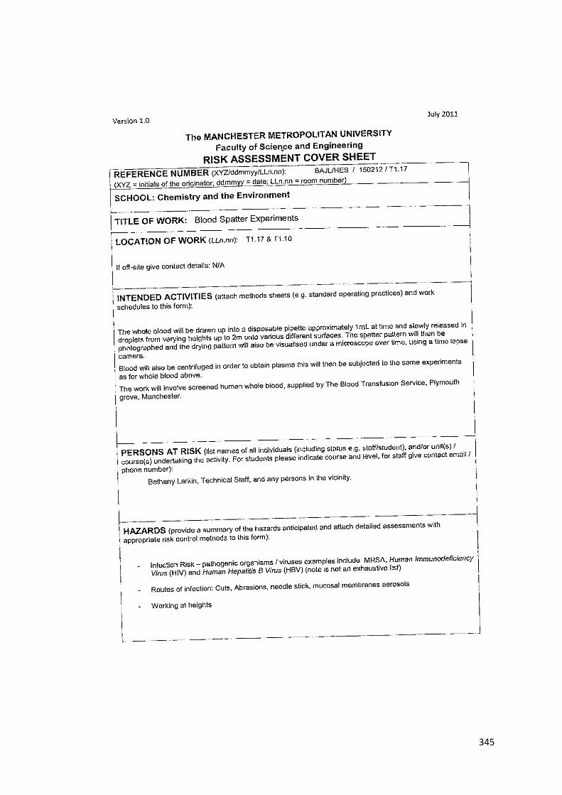
345

346
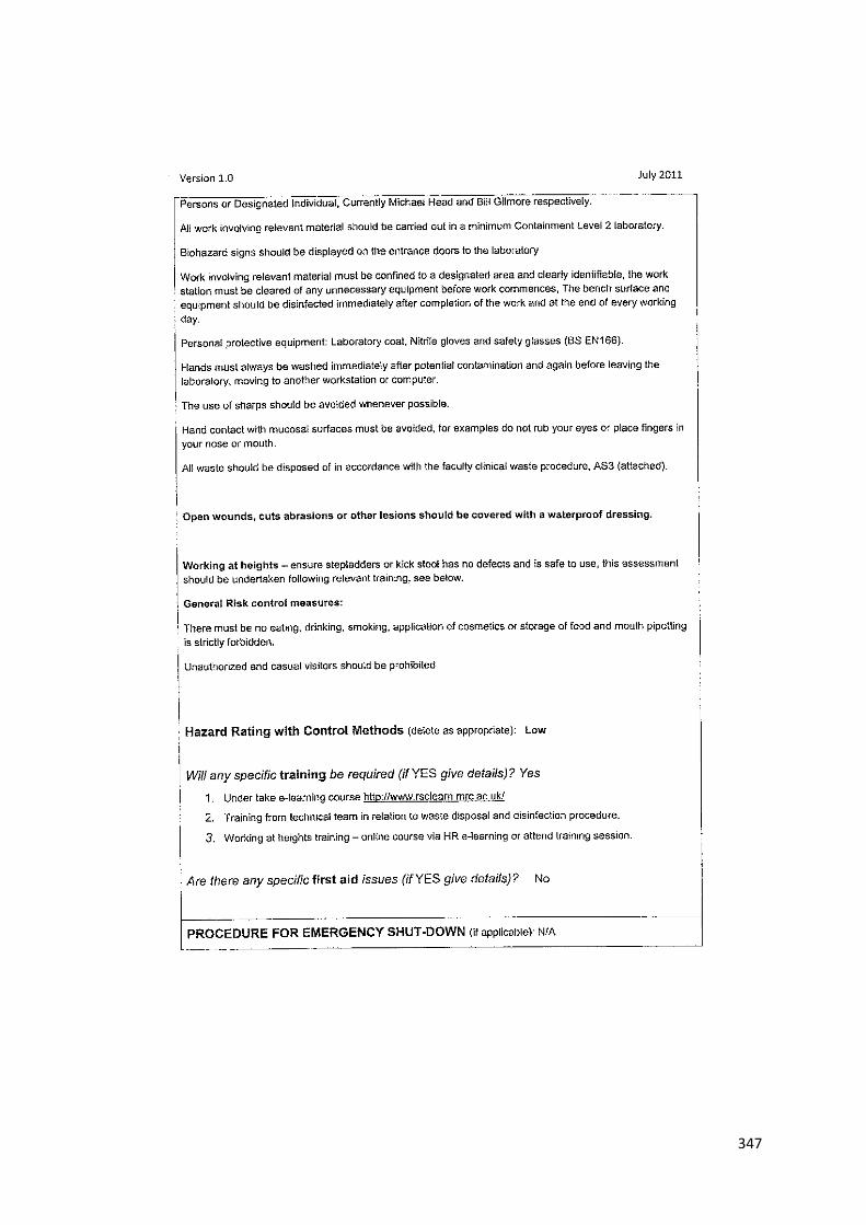
347

348
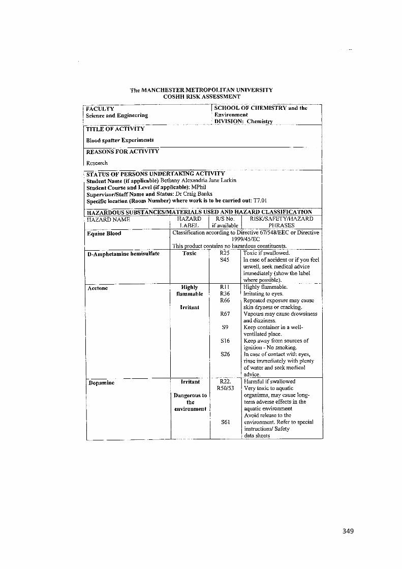
349

350

351

352
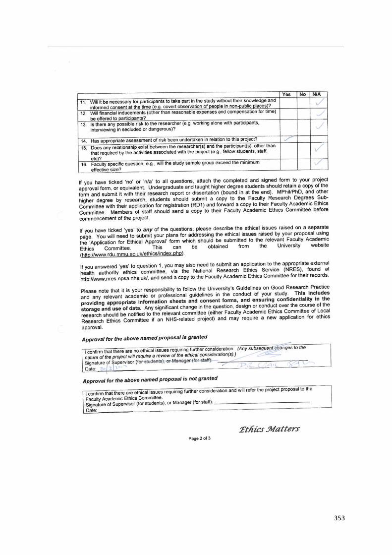
353

354
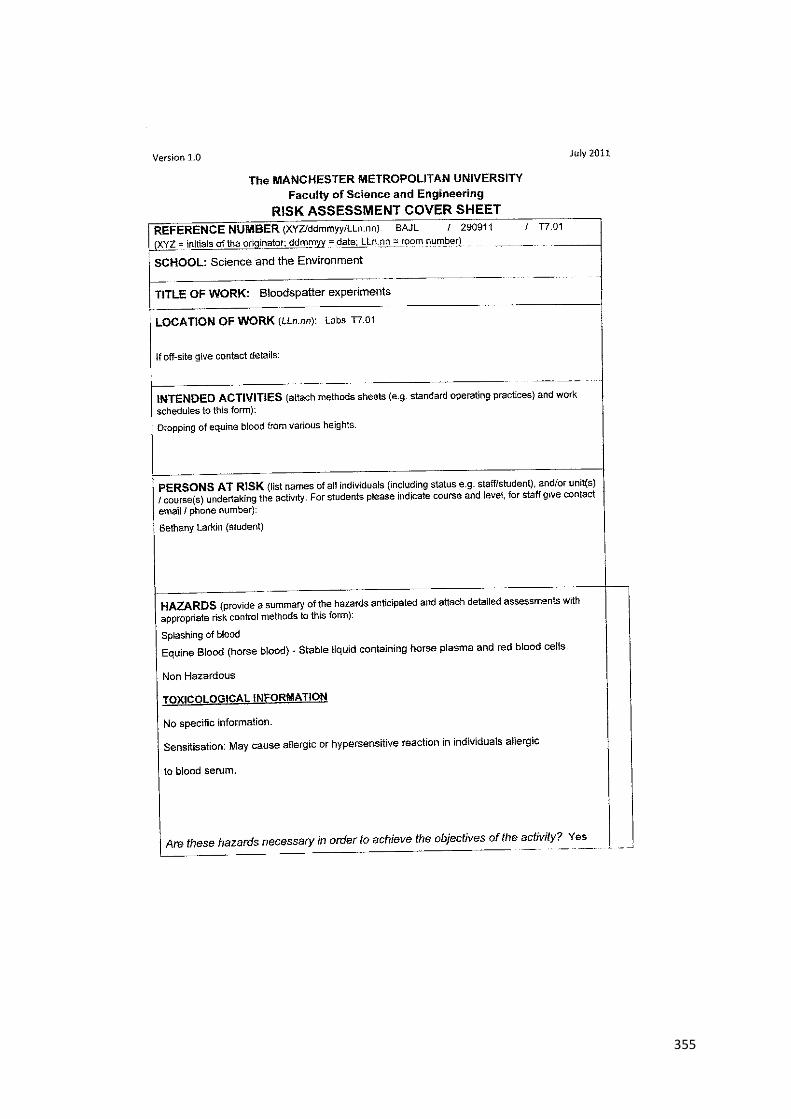
355

356
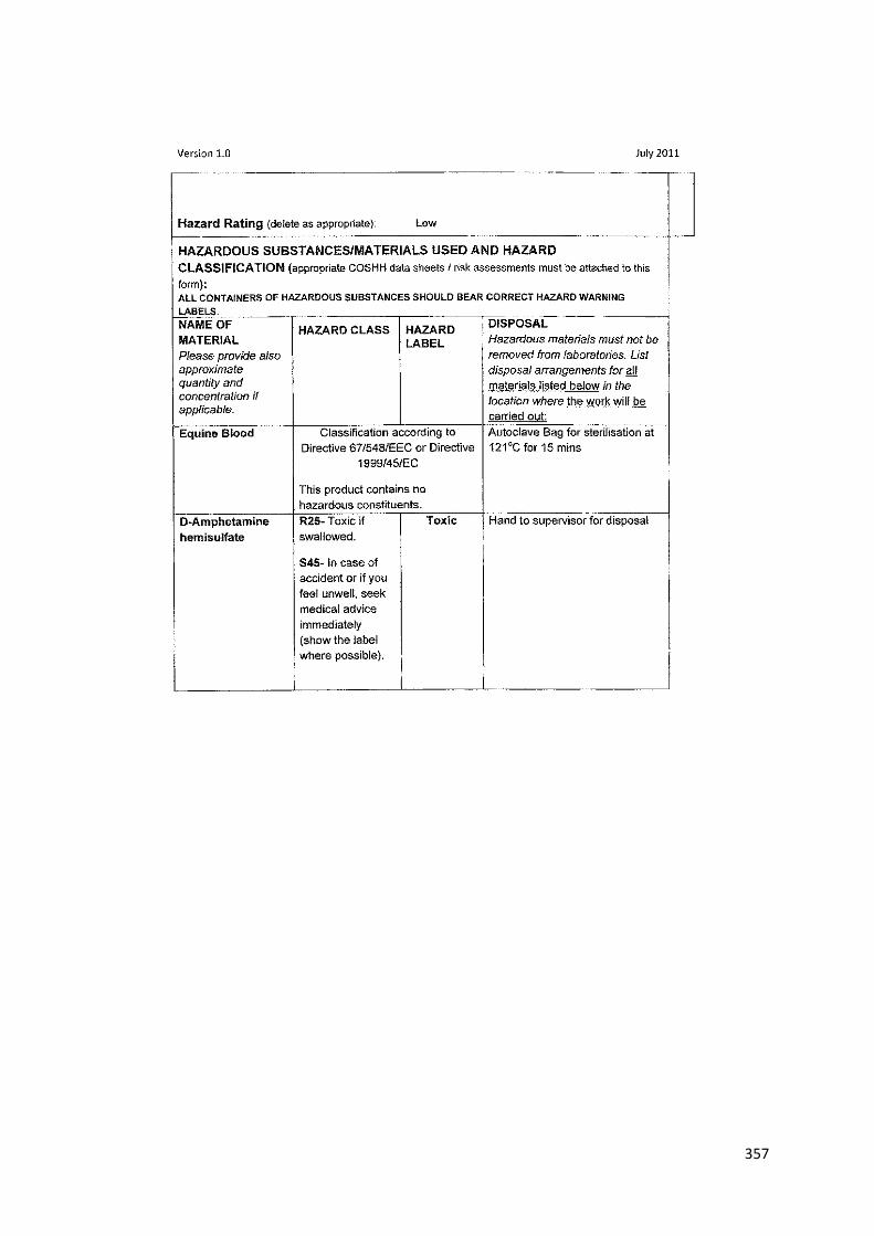
357

358

359

360

361
362

363

364

365

366

367

368
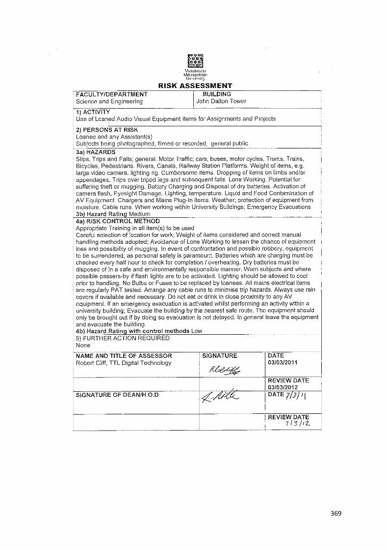
369
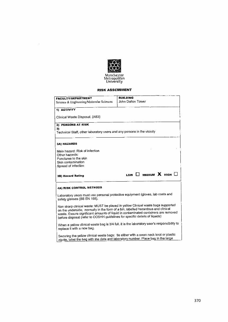
370
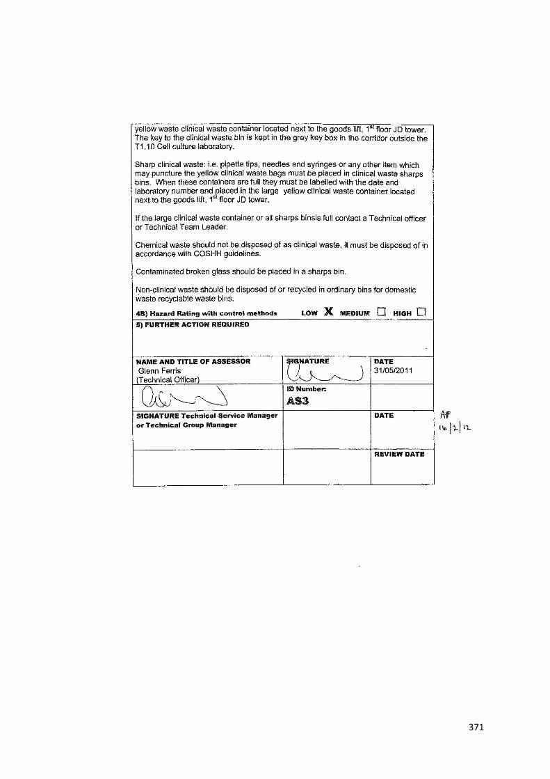
371
372
373
374
375

376
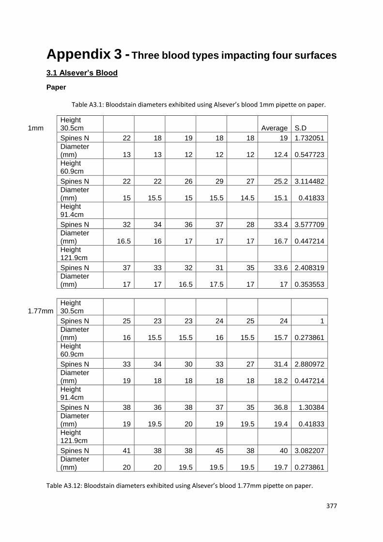
377
Appendix 3 - Three blood types impacting four surfaces
3.1 Alsever’s Blood
Paper
Table A3.12: Bloodstain diameters exhibited using Alsever’s blood 1.77mm pipette on paper.
1mm Height 30.5cm Average S.D
Spines N 22 18 19 18 18 19 1.732051
Diameter (mm) 13 13 12 12 12 12.4 0.547723
Height 60.9cm
Spines N 22 22 26 29 27 25.2 3.114482
Diameter (mm) 15 15.5 15 15.5 14.5 15.1 0.41833
Height 91.4cm
Spines N 32 34 36 37 28 33.4 3.577709
Diameter (mm) 16.5 16 17 17 17 16.7 0.447214
Height 121.9cm
Spines N 37 33 32 31 35 33.6 2.408319
Diameter (mm) 17 17 16.5 17.5 17 17 0.353553
1.77mm Height 30.5cm
Spines N 25 23 23 24 25 24 1
Diameter (mm) 16 15.5 15.5 16 15.5 15.7 0.273861
Height 60.9cm
Spines N 33 34 30 33 27 31.4 2.880972
Diameter (mm) 19 18 18 18 18 18.2 0.447214
Height 91.4cm
Spines N 38 36 38 37 35 36.8 1.30384
Diameter (mm) 19 19.5 20 19 19.5 19.4 0.41833
Height 121.9cm
Spines N 41 38 38 45 38 40 3.082207
Diameter (mm) 20 20 19.5 19.5 19.5 19.7 0.273861
Table A3.1: Bloodstain diameters exhibited using Alsever’s blood 1mm pipette on paper.

378
Steel
1mm Height 30.5cm Average S.D
Spines N 13 7 15 15 10 12 3.464102
Diameter (mm) 13.5 13.5 14 14 14 13.8 0.273861
Height 60.9cm
Spines N 21 22 25 19 22 21.8 2.167948
Diameter (mm) 16 16 15.5 16.5 17 16.2 0.570088
Height 91.4cm
Spines N 27 29 29 28 28 28.2 0.83666
Diameter (mm) 18 18 17.5 18 18 17.9 0.223607
Height 121.9cm
Spines N 29 25 33 29 32 29.6 3.130495
Diameter (mm) 18.5 18.5 17.5 18 18 18.1 0.41833
1.77mm Height 30.5cm Average S.D
Spines N 7 9 15 4 5 8 4.358899
Diameter (mm) 16.5 17 16.5 16 16.5 16.5 0.353553
Height 60.9cm
Spines N 27 30 26 23 23 25.8 2.949576
Diameter (mm) 19 18 18.5 19 18.5 18.6 0.41833
Height 91.4cm
Spines N 30 31 31 34 33 31.8 1.643168
Diameter (mm) 20 20 20 20 19.5 19.9 0.223607
Height 121.9cm
Spines N 30 35 39 32 34 3.91578
Diameter (mm) 20 23 21.5 20.5 21.25 1.322876
Table A3.14: Bloodstain diameters exhibited using Alsever’s blood 1.77mm pipette on steel.
Table A3.13: Bloodstain diameters exhibited using Alsever’s blood 1mm pipette on steel.

379
Plastic
1mm Height 30.5cm Average S.D
Spines N 17 19 18 15 20 17.8 1.923538
Diameter (mm) 13.5 13 13 13.5 13 13.2 0.273861
Height 60.9cm
Spines N 24 29 24 27 32 27.2 3.420526
Diameter (mm) 16 16 17 17 16 16.4 0.547723
Height 91.4cm
Spines N 37 28 25 30 26 29.2 4.764452
Diameter (mm) 17 17 17 17 16.5 16.9 0.223607
Height 121.9cm
Spines N 32 32 34 32 33 32.6 0.894427
Diameter (mm) 18 17 16.5 18 17.5 17.4 0.65192
1.77mm Height 30.5cm Average S.D
Spines N 21 21 23 23 27 23 2.44949
Diameter (mm) 18 16.5 17.5 17 17 17.2 0.570088
Height 60.9cm
Spines N 33 30 36 36 33 33.6 2.50998
Diameter (mm) 20 19.5 19 19 19.5 19.4 0.41833
Height 91.4cm
Spines N 41 43 40 41 44 41.8 1.643168
Diameter (mm) 21 20.5 21 21 20 20.7 0.447214
Height 121.9cm
Spines N 41 40 41 40 44 41.2 1.643168
Diameter (mm) 22.5 21 21.5 21 21.5 21.5 0.612372
Table A3.16: Bloodstain diameters exhibited using Alsever’s blood 1.77mm pipette on plastic.
Table A3.15: Bloodstain diameters exhibited using Alsever’s blood 1mm pipette on plastic.

380
Tile
1mm Height 30.5cm Average S.D
Spines N 23 22 20 22 17 20.8 2.387467
Diameter (mm) 15 15 15 15 15 15 0
Height 60.9cm
Spines N 24 24 20 21 22 22.2 1.788854
Diameter (mm) 16.5 16.5 16.5 16 16 16.3 0.273861
Height 91.4cm
Spines N 27 24 25 28 27 26.2 1.643168
Diameter (mm) 17 17 17 17 17.5 17.1 0.223607
Height 121.9cm
Spines N 32 23 32 29 28 28.8 3.701351
Diameter (mm) 20 19 18 19 18 18.8 0.83666
1.77mm Height 30.5cm Average S.D
Spines N 21 19 23 20 20 20.6 1.516575
Diameter (mm) 19 19 19 18.5 19 18.9 0.223607
Height 60.9cm
Spines N 27 28 23 27 31 27.2 2.863564
Diameter (mm) 22 21 22 21 21 21.4 0.547723
Height 91.4cm
Spines N 27 24 27 32 24 26.8 3.271085
Diameter (mm) 23.5 22.5 23 22.5 22.5 22.8 0.447214
Height 121.9cm
Spines N 32 38 34 36 36 35.2 2.280351
Diameter (mm) 23.5 23.5 23.5 22.5 22 23 0.707107
Table A3.18: Bloodstain diameters exhibited using Alsever’s blood 1.77mm pipette on tile.
Table A3.17: Bloodstain diameters exhibited using Alsever’s blood 1mm pipette on tile.
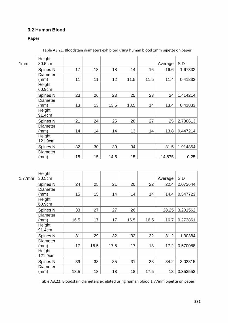
381
3.2 Human Blood
Paper
1mm Height 30.5cm Average S.D
Spines N 17 18 18 14 16 16.6 1.67332
Diameter (mm) 11 11 12 11.5 11.5 11.4 0.41833
Height 60.9cm
Spines N 23 26 23 25 23 24 1.414214
Diameter (mm) 13 13 13.5 13.5 14 13.4 0.41833
Height 91.4cm
Spines N 21 24 25 28 27 25 2.738613
Diameter (mm) 14 14 14 13 14 13.8 0.447214
Height 121.9cm
Spines N 32 30 30 34 31.5 1.914854
Diameter (mm) 15 15 14.5 15 14.875 0.25
1.77mm Height 30.5cm Average S.D
Spines N 24 25 21 20 22 22.4 2.073644
Diameter (mm) 15 15 14 14 14 14.4 0.547723
Height 60.9cm
Spines N 33 27 27 26 28.25 3.201562
Diameter (mm) 16.5 17 17 16.5 16.5 16.7 0.273861
Height 91.4cm
Spines N 31 29 32 32 32 31.2 1.30384
Diameter (mm) 17 16.5 17.5 17 18 17.2 0.570088
Height 121.9cm
Spines N 39 33 35 31 33 34.2 3.03315
Diameter (mm) 18.5 18 18 18 17.5 18 0.353553
Table A3.22: Bloodstain diameters exhibited using human blood 1.77mm pipette on paper.
Table A3.21: Bloodstain diameters exhibited using human blood 1mm pipette on paper.

382
Steel
1mm Height 30.5cm Average S.D
Spines N 2 7 3 0 0 2.4 2.880972
Diameter (mm) 12 12 12 12.5 12 12.1 0.223607
Height 60.9cm
Spines N 9 7 10 5 7 7.6 1.949359
Diameter (mm) 14 14 14 13.5 14 13.9 0.223607
Height 91.4cm
Spines N 17 19 16 19 16 17.4 1.516575
Diameter (mm) 14.5 14.5 14.5 14.5 14.5 14.5 0
Height 121.9cm
Spines N 17 20 17 20 20 18.8 1.643168
Diameter (mm) 15.5 14.5 15.5 15.5 15.5 15.3 0.447214
1.77mm Height 30.5cm Average S.D
Spines N 3 3 2 3 3 2.8 0.447214
Diameter (mm) 15 14.5 15 14.5 14.5 14.7 0.273861
Height 60.9cm
Spines N 12 11 13 13 11 12 1
Diameter (mm) 17 17 17.5 17.5 16.5 17.1 0.41833
Height 91.4cm
Spines N 22 24 22 22 19 21.8 1.788854
Diameter (mm) 18 18 17.5 18 17.5 17.8 0.273861
Height 121.9cm
Spines N 25 21 22 25 23.25 2.061553
Diameter (mm) 18.5 17.5 18 18.5 18.125 0.478714
Table A3.23: Bloodstain diameters exhibited using human blood 1mm pipette on steel.
Table A3.24: Bloodstain diameters exhibited using human blood 1.77mm pipette on steel.
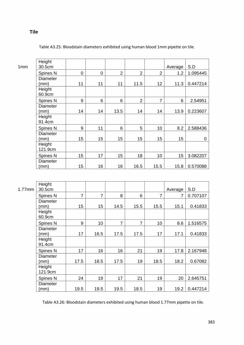
383
Tile
1mm Height 30.5cm Average S.D
Spines N 0 0 2 2 2 1.2 1.095445
Diameter (mm) 11 11 11 11.5 12 11.3 0.447214
Height 60.9cm
Spines N 9 6 6 2 7 6 2.54951
Diameter (mm) 14 14 13.5 14 14 13.9 0.223607
Height 91.4cm
Spines N 9 11 6 5 10 8.2 2.588436
Diameter (mm) 15 15 15 15 15 15 0
Height 121.9cm
Spines N 15 17 15 18 10 15 3.082207
Diameter (mm) 15 16 16 16.5 15.5 15.8 0.570088
1.77mm Height 30.5cm Average S.D
Spines N 7 7 8 6 7 7 0.707107
Diameter (mm) 15 15 14.5 15.5 15.5 15.1 0.41833
Height 60.9cm
Spines N 9 10 7 7 10 8.6 1.516575
Diameter (mm) 17 16.5 17.5 17.5 17 17.1 0.41833
Height 91.4cm
Spines N 17 16 16 21 19 17.8 2.167948
Diameter (mm) 17.5 18.5 17.5 19 18.5 18.2 0.67082
Height 121.9cm
Spines N 24 19 17 21 19 20 2.645751
Diameter (mm) 19.5 19.5 19.5 18.5 19 19.2 0.447214
Table A3.25: Bloodstain diameters exhibited using human blood 1mm pipette on tile.
Table A3.26: Bloodstain diameters exhibited using human blood 1.77mm pipette on tile.

384
Plastic
1mm Height 30.5cm Average S.D
Spines N 12 12 17 16 5 12.4 4.722288
Diameter (mm) 11.5 11 11 11.5 11.5 11.3 0.273861
Height 60.9cm
Spines N 18 17 21 18 15 17.8 2.167948
Diameter (mm) 13.5 13.5 14 13.5 13 13.5 0.353553
Height 91.4cm
Spines N 26 22 19 20 27 22.8 3.563706
Diameter (mm) 14 14.5 14 14 14 14.1 0.223607
Height 121.9cm
Spines N 24 24 19 23 26 23.2 2.588436
Diameter (mm) 14.5 14.5 14.5 14.5 15 14.6 0.223607
1.77mm Height 30.5cm Average S.D
Spines N 19 15 19 18 14 17 2.345208
Diameter (mm) 15 15 14 15 15.5 14.9 0.547723
Height 60.9cm
Spines N 22 25 23 24 21 23 1.581139
Diameter (mm) 18 17 17 18 18 17.6 0.547723
Height 91.4cm
Spines N 28 27 23 30 31 27.8 3.114482
Diameter (mm) 18.5 18 18.5 18 18 18.2 0.273861
Height 121.9cm
Spines N 20 33 26 24 20 24.6 5.366563
Diameter (mm) 19.5 18.5 19 19.5 19.5 19.2 0.447214
Table A3.27: Bloodstain diameters exhibited using human blood 1mm pipette on plastic.
Table A3.28: Bloodstain diameters exhibited using human blood 1.77mm pipette on plastic.

385
3.3 Defibrinated Blood
Paper
1mm Height 30.5cm Average S.D
Spines N 14 19 20 14 18 17 2.828427
Diameter (mm) 12 12 12 12.5 12.5 12.2 0.273861
Height 60.9cm
Spines N 24 29 26 25 25 25.8 1.923538
Diameter (mm) 14 13.5 14 13 13 13.5 0.5
Height 91.4cm
Spines N 30 29 25 27 29 28 2
Diameter (mm) 14 14 14 14 14 14 0
Height 121.9cm
Spines N 35 30 34 35 29 32.6 2.880972
Diameter (mm) 15 15 14 14.5 14 14.5 0.5
1.77mm Height 30.5cm Average S.D
Spines N 23 22 24 22 22 22.6 0.894427
Diameter (mm) 15 15 15 15 15 15 0
Height 60.9cm
Spines N 29 31 32 27 28 29.4 2.073644
Diameter (mm) 17 17 17.5 17 17.5 17.2 0.273861
Height 91.4cm
Spines N 27 33 32 36 32 32 3.24037
Diameter (mm) 17 17 17 18 18 17.4 0.547723
Height 121.9cm
Spines N 37 33 35 34 38 35.4 2.073644
Diameter (mm) 18 18 17.5 17.5 17 17.6 0.41833
Table A3.31: Bloodstain diameters exhibited using defibrinated horse blood 1mm pipette on paper.
Table A3.32: Bloodstain diameters exhibited using defibrinated horse blood 1.77mm pipette on paper.

386
Steel
1mm Height 30.5cm Average S.D
Spines N 4 2 3 1 0 2 1.581139
Diameter (mm) 12.5 12 12 12 12 12.1 0.223607
Height 60.9cm
Spines N 8 9 12 12 12 10.6 1.949359
Diameter (mm) 13.5 14 13.5 13.5 13.5 13.6 0.223607
Height 91.4cm
Spines N 8 11 11 9 9 9.6 1.341641
Diameter (mm) 13.5 14 14 13.5 14 13.8 0.273861
Height 121.9cm
Spines N 2 4 5 2 2 3 1.414214
Diameter (mm) 14 14.5 14.5 14.5 14.5 14.4 0.223607
1.77mm Height 30.5cm Average S.D
Spines N 5 9 3 3 6 5.2 2.48998
Diameter (mm) 15 14.5 14.5 14.5 14.5 14.6 0.223607
Height 60.9cm
Spines N 12 9 16 8 13 11.6 3.209361
Diameter (mm) 16.5 16.5 16.5 16 16.5 16.4 0.223607
Height 91.4cm
Spines N 21 28 23 26 23 24.2 2.774887
Diameter (mm) 19.5 18 18 19 19.5 18.8 0.758288
Height 121.9cm
Spines N 25 26 23 30 20 24.8 3.701351
Diameter (mm) 19 19 20 19.5 18.5 19.2 0.570088
Table A3.34: Bloodstain diameters exhibited using defibrinated horse blood 1.77mm pipette on steel.

387
Plastic
1mm Height 30.5cm Average S.D
Spines N 5 6 8 7 5 6.2 1.30384
Diameter (mm) 12 12 12 12.5 12.5 12.2 0.273861
Height 60.9cm
Spines N 17 15 16 18 18 16.8 1.30384
Diameter (mm) 14 14 14 14 14.5 14.1 0.223607
Height 91.4cm
Spines N 26 21 23 17 18 21 3.674235
Diameter (mm) 14.5 14.5 15 14.5 15 14.7 0.273861
Height 121.9cm
Spines N 31 23 28 27 31 28 3.316625
Diameter (mm) 15 15.5 16 15 15 15.3 0.447214
1.77mm Height 30.5cm Average S.D
Spines N 21 12 12 17 16 15.6 3.781534
Diameter (mm) 15 15.5 15.5 16 15.5 15.5 0.353553
Height 60.9cm
Spines N 28 29 29 27 27 28 1
Diameter (mm) 18 18 18 18 18.5 18.1 0.223607
Height 91.4cm
Spines N 31 30 27 25 31 28.8 2.683282
Diameter (mm) 18.5 18.5 18 19 19 18.6 0.41833
Height 121.9cm
Spines N 35 37 37 39 35 36.6 1.67332
Diameter (mm) 19 19 20 20 19 19.4 0.547723
Table A3.36: Bloodstain diameters exhibited using defibrinated horse blood 1.77mm pipette on plastic.

388
Tile
1mm Height 30.5cm Average SD
Spines N 10 12 10 11 12 11 1
Diameter (mm) 13 13.5 13.5 13.5 12.5 13.2 0.447214
Height 60.9cm
Spines N 13 12 15 11 17 13.6 2.408319
Diameter (mm) 14.5 14.5 14 14 14 14.2 0.273861
Height 91.4cm
Spines N 21 20 19 25 16 20.2 3.271085
Diameter (mm) 15 15 15.5 15.5 15 15.2 0.273861
Height 121.9cm
Spines N 19 22 16 20 24 20.2 3.03315
Diameter (mm) 16 16 15.5 15 15.5 15.6 0.41833
1.77mm Height 30.5cm Average SD
Spines N 12 9 16 10 11.75 3.095696
Diameter (mm) 16 16 17 17 17 16.6 0.547723
Height 60.9cm
Spines N 9 11 1 9 12 8.4 4.335897
Diameter (mm) 19 19 19 19 18.5 18.9 0.223607
Height 91.4cm
Spines N 23 20 27 20 22.5 3.316625
Diameter (mm) 19.5 19.5 19 19 19.25 0.288675
Height 121.9cm
Spines N 14 14 14 18 15 15 1.732051
Diameter (mm) 19 20 20.5 20 19.5 19.8 0.570088
Table A3.38: Bloodstain diameters exhibited using defibrinated horse blood 1.77mm pipette on tile.
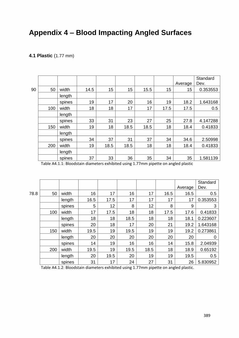
389
Appendix 4 – Blood Impacting Angled Surfaces
4.1 Plastic (1.77 mm)
Table A4.1.1: Bloodstain diameters exhibited using 1.77mm pipette on angled plastic
Table A4.1.2: Bloodstain diameters exhibited using 1.77mm pipette on angled plastic.
Average Standard Dev.
90 50 width 14.5 15 15 15.5 15 15 0.353553
length
spines 19 17 20 16 19 18.2 1.643168
100 width 18 18 17 17 17.5 17.5 0.5
length
spines 33 31 23 27 25 27.8 4.147288
150 width 19 18 18.5 18.5 18 18.4 0.41833
length
spines 34 37 31 37 34 34.6 2.50998
200 width 19 18.5 18.5 18 18 18.4 0.41833
length
spines 37 33 36 35 34 35 1.581139
Average Standard Dev.
78.8 50 width 16 17 16 17 16.5 16.5 0.5
length 16.5 17.5 17 17 17 17 0.353553
spines 5 12 8 12 8 9 3
100 width 17 17.5 18 18 17.5 17.6 0.41833
length 18 18 18.5 18 18 18.1 0.223607
spines 20 18 17 20 21 19.2 1.643168
150 width 19.5 19 19.5 19 19 19.2 0.273861
length 20 20 20 20 20 20 0
spines 14 19 16 16 14 15.8 2.04939
200 width 19.5 19 19.5 18.5 18 18.9 0.65192
length 20 19.5 20 19 19 19.5 0.5
spines 31 17 24 27 31 26 5.830952

390
Table A4.1.3: Bloodstain diameters exhibited using 1.77mm pipette on angled plastic.
Table A4.1.4: Bloodstain diameters exhibited using 1.77mm pipette on angled plastic
Average Standard Dev.
56.3 50 width 16 15.5 15.5 15.5 15.5 15.6 0.223607
length 18 17.5 17.5 17.5 17.5 17.6 0.223607
spines 12 9 9 12 12 10.8 1.643168
100 width 17 17.5 18.5 17 17.5 17.5 0.612372
length 19.5 20 20.5 19.5 19.5 19.8 0.447214
spines 19 20 13 17 17 17.2 2.683282
150 width 19 18.5 18.5 18.5 18 18.5 0.353553
length 21.5 21 21 21 21 21.1 0.223607
spines 23 24 18 30 24 23.8 4.266146
200 width 19 19 19 18.5 19 18.9 0.223607
length 22 21.5 22 21.5 21 21.6 0.41833
spines 29 29 38 31 34 32.2 3.834058
Average Standard Dev.
61.6 50 width 15 15 15 15 15 15 0
length 17 17 16.5 16.5 16.5 16.7 0.273861
spines 12 10 11 7 13 10.6 2.302173
100 width 17 16 17.5 16 17 16.7 0.67082
length 19 18 18.5 17.5 18.5 18.3 0.570088
spines 15 19 14 16 17 16.2 1.923538
150 width 17.5 17 17 17.5 18 17.4 0.41833
length 19 19 19.5 19.5 19.5 19.3 0.273861
spines 24 22 28 30 28 26.4 3.286335
200 width 18.5 19 17.5 18 18 18.2 0.570088
length 20 20 19 19.5 19.5 19.6 0.41833
spines 32 28 28 29 30 29.4 1.67332

391
Average Standard Dev.
43.3 50 width 13.5 14 13 13.5 13 13.4 0.41833
length 20 20 19 19 19 19.4 0.547723
spines 4 3 2 3 5 3.4 1.140175
100 width 16.5 16.5 16.5 16.5 16.5 16.5 0
length 22.5 22.5 21 22 21.5 21.9 0.65192
spines 3 8 5 6 9 6.2 2.387467
150 width 17 16.5 16.5 16.5 16.5 16.6 0.223607
length 23.5 24.5 23 23.5 24 23.7 0.570088
spines 25 27 19 19 17 21.4 4.335897
200 width 17.5 17 17.5 17.5 17 17.3 0.273861
length 25 23.5 23.5 23 22.5 23.5 0.935414
spines 16 15 20 15 16 16.4 2.073644
Table A4.1.5: Bloodstain diameters exhibited using 1.77mm pipette on angled plastic
Average Standard
Dev.
22.7 50 width 10 10.5 10 10 10.5 10.2 0.273861
length 27 28 28 26.5 28.5 27.6 0.821584
spines 0 0 0 0 0 0 0
100 width 11.5 12 12.5 12 12.5 12.1 0.41833
length 29 29 31 28 30 29.4 1.140175
spines 2 0 0 1 0 0.6 0.894427
150 width 12 11 11.5 12.5 12 11.8 0.570088
length 31 31 31 30.5 30.5 30.8 0.273861
spines 3 1 2 1 0 1.4 1.140175
200 width 12.5 12.5 12.5 12.5 12.5 12.5 0
length 33.5 33.5 33.5 33.5 30.5 32.9 1.341641
spines 1 2 4 1 2 2 1.224745
Table A4.1.6: Bloodstain diameters exhibited using 1.77mm pipette on angled plastic

392
Plastic (1 mm)
Average Standard Dev.
90 50 width 13 13.5 13.5 13 13 13.2 0.273861
length
spines 5 2 5 4 4 1.414214
100 width 14 14.5 15 14.5 14.5 14.5 0.353553
length
spines 2 4 2 2 3 2.6 0.894427
150 width 15 15.5 15.5 15 15 15.2 0.273861
length
spines 2 3 5 4 0 2.8 1.923538
200 width 15.5 16 16 16 15.5 15.8 0.273861
length
spines 5 6 6 5 5.5 0.57735
Table A4.1.7: Bloodstain diameters exhibited using 1mm pipette on angled plastic
Average Standard Dev.
78.8 50 width 13 13 13 13 12 12.8 0.447214
length 13.5 13.5 13.5 13.5 12.5 13.3 0.447214
spines 10 10 14 15 17 13.2 3.114482
100 width 14 13.5 13 13 13 13.3 0.447214
length 14.5 14 13.5 13.5 13.5 13.8 0.447214
spines 9 6 3 10 7 7 2.738613
150 width 14.5 15 15 15 14.5 14.8 0.273861
length 15 15.5 15.5 15.5 15 15.3 0.273861
spines 18 16 21 27 19 20.2 4.207137
200 width 15 15 15 15 15 15 0
length 16 16 16 16 15.5 15.9 0.223607
spines 26 30 25 23 34 27.6 4.393177
Table A4.1.8: Bloodstain diameters exhibited using 1mm pipette on angled plastic

393
Table A4.1.9: Bloodstain diameters exhibited using 1mm pipette on angled plastic
Average Standard Dev.
56.3 50 width 11.5 11 11 12 11 11.3 0.447214
length 13 13 13.5 14 13 13.3 0.447214
spines 2 2 4 5 6 3.8 1.788854
100 width 13 13.5 13 13.5 13.5 13.3 0.273861
length 15.5 16 15 15.5 16 15.6 0.41833
spines 8 9 7 10 10 8.8 1.30384
150 width 14.5 14.5 15 14.5 15 14.7 0.273861
length 18.5 18.5 18.5 18 18.5 18.4 0.223607
spines 8 10 10 7 13 9.6 2.302173
200 width 14.5 15 14.5 14.5 14.5 14.6 0.223607
length 18 19 19 18.5 18.5 18.6 0.41833
spines 15 14 14 14 13 14 0.707107
Table A4.1.10: Bloodstain diameters exhibited using 1mm pipette on angled plastic
Average Standard Dev.
61.6 50 width 12 12 11 12 12 11.8 0.447214
length 13 13 12 13 13 12.8 0.447214
spines 13 10 11 9 10 10.6 1.516575
100 width 13.5 13.5 13 13.5 14 13.5 0.353553
length 15 15 14.5 14.5 15 14.8 0.273861
spines 14 13 14 14 14 13.8 0.447214
150 width 14.5 14.5 15 15 14 14.6 0.41833
length 16 16 16 16 15 15.8 0.447214
spines 24 21 26 17 21 21.8 3.420526
200 width 15 15 15.5 15.5 15 15.2 0.273861
length 17 17 17.5 17 17 17.1 0.223607
spines 24 29 33 30 32 29.6 3.507136

394
Average Standard Dev.
43.3 50 width 10.5 11 11 10 10.5 10.6 0.41833
length 16 16.5 16.5 16 16 16.2 0.273861
spines 4 5 5 3 7 4.8 1.48324
100 width 12 12.5 12.5 12.5 12.5 12.4 0.223607
length 17 18 18 18 18 17.8 0.447214
spines 6 6 2 11 8 6.6 3.286335
150 width 13.5 12.5 13 13.5 13.5 13.2 0.447214
length 18 18 18.5 17.5 18 18 0.353553
spines 8 6 9 8 12 8.6 2.19089
200 width 13.5 13.5 13.5 13 13.5 13.4 0.223607
length 19 19 18.5 18 19 18.7 0.447214
spines 6 5 13 16 4 8.8 5.357238
Table A4.1.11: Bloodstain diameters exhibited using 1mm pipette on angled plastic.
Table A4.1.12: Bloodstain diameters exhibited using 1mm pipette on angled plastic
Average Standard Dev.
22.7 50 width 7.5 7.5 7.5 7 7.5 7.4 0.223607
length 25.5 25 24.5 23.5 24 24.5 0.790569
spines 0 0 0 0 0 0 0
100 width 7.5 8.5 7.5 9 9 8.3 0.758288
length 26.5 24 25.5 27 26.5 25.9 1.193734
spines 0 0 0 0 0 0 0
150 width 9.5 10 10 10 10 9.9 0.223607
length 24 25 26 24.5 25 24.9 0.74162
spines 6 5 3 5 3 4.4 1.341641
200 width 9.5 10 10.5 10 10 10 0.353553
length 25.5 25.5 27 27.5 27.5 26.6 1.024695
spines 5 5 1 4 4 3.8 1.643168

395
4.2 Steel (1.77mm)
Table A4.2.1: Bloodstain diameters exhibited using 1.77mm pipette on angled steel.
Table A4.2.2: Bloodstain diameters exhibited using 1.77mm pipette on angled steel.
Average Standard Dev.
90 50 width 16.5 16.5 16.5 16.5 16 16.4 0.223607
length
spines 0 0 0 0 0 0 0
100 width 17.5 18.5 18.5 18.5 18 18.2 0.447214
length
spines 5 5 8 10 11 7.8 2.774887
150 width 19 19 18.5 18 19 18.7 0.447214
length
spines 18 10 12 10 12 12.4 3.286335
200 width 19.5 19 20 20 19.5 19.6 0.41833
length
spines 5 19 30 24 24 20.4 9.449868
Average Standard Dev.
78.8 50 width 16 16 15.5 15.5 16 15.8 0.273861
length 16.5 16.5 16.5 16 16.5 16.4 0.223607
spines 3 4 3 5 5 4 1
100 width 17.5 18.5 18 19 18.25 0.645497
length 18 19 18.5 19 18.625 0.478714
spines 9 12 10 14 11.25 2.217356
150 width 17 18 18 18 18 17.8 0.447214
length 17.5 18 18.5 19 19 18.4 0.65192
spines 29 31 36 35 30 32.2 3.114482
200 width 18 18 18.5 18.5 18.25 0.288675
length 19 19 19 19 19 0
spines 31 36 35 32 28 32.4 3.209361
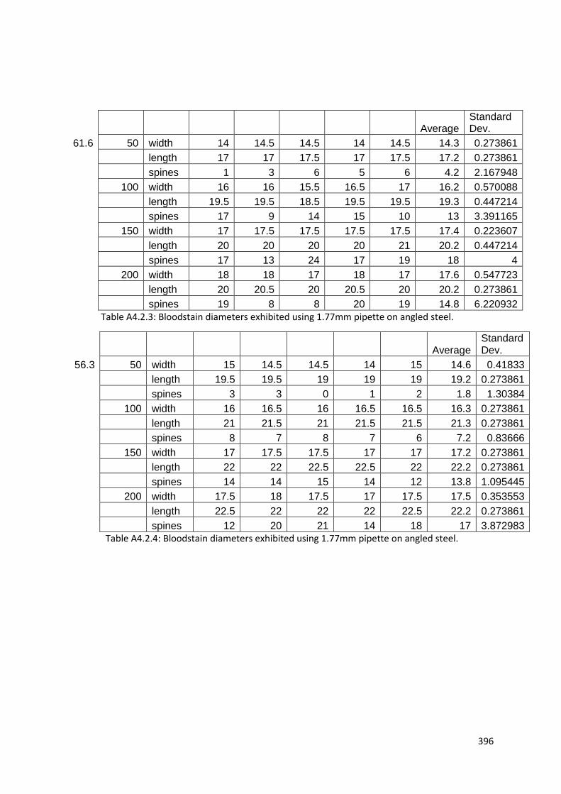
396
Average Standard Dev.
61.6 50 width 14 14.5 14.5 14 14.5 14.3 0.273861
length 17 17 17.5 17 17.5 17.2 0.273861
spines 1 3 6 5 6 4.2 2.167948
100 width 16 16 15.5 16.5 17 16.2 0.570088
length 19.5 19.5 18.5 19.5 19.5 19.3 0.447214
spines 17 9 14 15 10 13 3.391165
150 width 17 17.5 17.5 17.5 17.5 17.4 0.223607
length 20 20 20 20 21 20.2 0.447214
spines 17 13 24 17 19 18 4
200 width 18 18 17 18 17 17.6 0.547723
length 20 20.5 20 20.5 20 20.2 0.273861
spines 19 8 8 20 19 14.8 6.220932
Table A4.2.3: Bloodstain diameters exhibited using 1.77mm pipette on angled steel.
Average Standard Dev.
56.3 50 width 15 14.5 14.5 14 15 14.6 0.41833
length 19.5 19.5 19 19 19 19.2 0.273861
spines 3 3 0 1 2 1.8 1.30384
100 width 16 16.5 16 16.5 16.5 16.3 0.273861
length 21 21.5 21 21.5 21.5 21.3 0.273861
spines 8 7 8 7 6 7.2 0.83666
150 width 17 17.5 17.5 17 17 17.2 0.273861
length 22 22 22.5 22.5 22 22.2 0.273861
spines 14 14 15 14 12 13.8 1.095445
200 width 17.5 18 17.5 17 17.5 17.5 0.353553
length 22.5 22 22 22 22.5 22.2 0.273861
spines 12 20 21 14 18 17 3.872983
Table A4.2.4: Bloodstain diameters exhibited using 1.77mm pipette on angled steel.

397
Table A4.2.5: Bloodstain diameters exhibited using 1.77mm pipette on angled steel.
Table A4.2.6: Bloodstain diameters exhibited using 1.77mm pipette on angled steel.
Average Standard Dev.
43.3 50 width 14 13.5 13 12.5 13 13.2 0.570088
length 23.5 23.5 22 22.5 22.5 22.8 0.67082
spines 2 2 0 0 0 0.8 1.095445
100 width 15 15.5 15.5 14.5 14.5 15 0.5
length 24 25 25 24 24 24.4 0.547723
spines 7 7 9 4 6 6.6 1.81659
150 width 16 15 15 16.5 15.5 15.6 0.65192
length 29 27.5 26 28 28.5 27.8 1.151086
spines 8 6 8 6 9 7.4 1.341641
200 width 16.5 15.5 16 16 15.5 15.9 0.41833
length 29 27 27.5 27.5 27 27.6 0.821584
spines 6 6 9 10 7.75 2.061553
Average Standard Dev.
22.7 50 width 10.5 11 10.5 10.5 10 10.5 0.353553
length 29.5 30.5 30.5 31 30.5 30.4 0.547723
spines 0 0 0 0 0 0 0
100 width 12 12.5 12 12 12 12.1 0.223607
length 32 30.5 32 32 32 31.7 0.67082
spines 0 0 0 0 0 0 0
150 width 12 12.5 12.5 12.5 12 12.3 0.273861
length 35 33.5 34 34 34 34.1 0.547723
spines 0 0 0 0 0 0 0
200 width 13.5 13.5 13.5 13.5 13.5 13.5 0
length 36.5 34.5 36 36 36 35.8 0.758288
spines 0 0 0 0 0 0 0
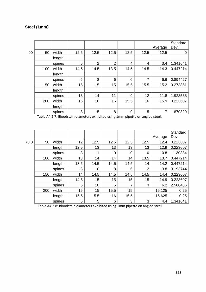
398
Steel (1mm)
Average Standard Dev.
90 50 width 12.5 12.5 12.5 12.5 12.5 12.5 0
length
spines 5 2 2 4 4 3.4 1.341641
100 width 14.5 14.5 13.5 14.5 14.5 14.3 0.447214
length
spines 6 8 6 6 7 6.6 0.894427
150 width 15 15 15 15.5 15.5 15.2 0.273861
length
spines 13 14 11 9 12 11.8 1.923538
200 width 16 16 16 15.5 16 15.9 0.223607
length
spines 8 5 8 9 5 7 1.870829
Table A4.2.7: Bloodstain diameters exhibited using 1mm pipette on angled steel.
Average Standard Dev.
78.8 50 width 12 12.5 12.5 12.5 12.5 12.4 0.223607
length 12.5 13 13 13 13 12.9 0.223607
spines 3 1 0 0 0 0.8 1.30384
100 width 13 14 14 14 13.5 13.7 0.447214
length 13.5 14.5 14.5 14.5 14 14.2 0.447214
spines 3 0 8 6 2 3.8 3.193744
150 width 14 14.5 14.5 14.5 14.5 14.4 0.223607
length 14.5 15 15 15 15 14.9 0.223607
spines 6 10 5 7 3 6.2 2.588436
200 width 15 15 15.5 15 15.125 0.25
length 15.5 15.5 16 15.5 15.625 0.25
spines 5 5 6 3 3 4.4 1.341641
Table A4.2.8: Bloodstain diameters exhibited using 1mm pipette on angled steel.

399
Average Standard Dev.
61.6 50 width 12 12 12.5 12 12 12.1 0.223607
length 14.5 14.5 14.5 14.5 13.5 14.3 0.447214
spines 0 5 2 0 5 2.4 2.50998
100 width 13 13 13.5 13 13 13.1 0.223607
length 15 15 15.5 15 15 15.1 0.223607
spines 7 6 7 7 8 7 0.707107
150 width 14 14 13.5 14.5 14 14 0.353553
length 16.5 16 16 16.5 16 16.2 0.273861
spines 10 12 14 11 11 11.6 1.516575
200 width 15 14.5 14.5 14.5 14 14.5 0.353553
length 17.5 17 17 17 16.5 17 0.353553
spines 15 15 17 19 16 16.4 1.67332
Table A4.2.9: Bloodstain diameters exhibited using 1mm pipette on angled steel
Average Standard Dev.
56.3 50 width 11.5 11.5 12 11.5 10.5 11.4 0.547723
length 15 15.5 16 15.5 14.5 15.3 0.570088
spines 0 0 0 0 2 0.4 0.894427
100 width 14.5 14 13.5 13.5 14 13.9 0.41833
length 18 17.5 17.5 17.5 17.5 17.6 0.223607
spines 3 3 7 3 6 4.4 1.949359
150 width 13.5 13.5 14 14 14 13.8 0.273861
length 15.5 16 16 16 16 15.9 0.223607
spines 18 18 18 24 20 19.6 2.607681
200 width 14 14.5 14.5 15 14 14.4 0.41833
length 16 16 17 18 17 16.8 0.83666
spines 20 24 21 22 32 23.8 4.816638
Table A4.2.10: Bloodstain diameters exhibited using 1mm pipette on angled steel
Average Standard Dev.
43.3 50 width 11 11 11 10.5 10.5 10.8 0.273861
length 18.5 18.5 18 18 18 18.2 0.273861
spines 2 0 1 3 1 1.4 1.140175
100 width 12 12.5 12 12 11.5 12 0.353553
length 19 19.5 18.5 19 18 18.8 0.570088
spines 2 2 4 5 5 3.6 1.516575
150 width 12.5 12.5 12.5 13.5 12.5 12.7 0.447214
length 19 19 19.5 20.5 18.5 19.3 0.758288
spines 3 6 2 4 5 4 1.581139
200 width 13.5 13.5 13.5 13.5 13 13.4 0.223607
length 21 20 20.5 21 20.5 20.6 0.41833
spines 3 8 5 7 7 6 2
Table A4.2.11: Bloodstain diameters exhibited using 1mm pipette on angled steel
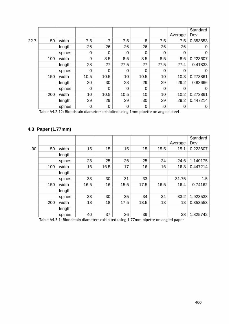
400
Average Standard Dev.
22.7 50 width 7.5 7 7.5 8 7.5 7.5 0.353553
length 26 26 26 26 26 26 0
spines 0 0 0 0 0 0 0
100 width 9 8.5 8.5 8.5 8.5 8.6 0.223607
length 28 27 27.5 27 27.5 27.4 0.41833
spines 0 0 0 0 0 0 0
150 width 10.5 10.5 10 10.5 10 10.3 0.273861
length 30 30 28 29 29 29.2 0.83666
spines 0 0 0 0 0 0 0
200 width 10 10.5 10.5 10 10 10.2 0.273861
length 29 29 29 30 29 29.2 0.447214
spines 0 0 0 0 0 0 0
Table A4.2.12: Bloodstain diameters exhibited using 1mm pipette on angled steel
4.3 Paper (1.77mm)
Average Standard Dev
90 50 width 15 15 15 15 15.5 15.1 0.223607
length
spines 23 25 26 25 24 24.6 1.140175
100 width 16 16.5 17 16 16 16.3 0.447214
length
spines 33 30 31 33 31.75 1.5
150 width 16.5 16 15.5 17.5 16.5 16.4 0.74162
length
spines 33 30 35 34 34 33.2 1.923538
200 width 18 18 17.5 18.5 18 18 0.353553
length
spines 40 37 36 39 38 1.825742
Table A4.3.1: Bloodstain diameters exhibited using 1.77mm pipette on angled paper

401
Table A4.3.2: Bloodstain diameters exhibited using 1.77mm pipette on angled paper.
Table A4.3.3: Bloodstain diameters exhibited using 1.77mm pipette on angled paper
Average Standard Dev
78.8 50 width 16 16 16 16 16 16 0
length 17.5 17 17 17 17 17.1 0.223607
spines 13 14 14 15 14 14 0.707107
100 width 17.5 17.5 17.5 17 17.375 0.25
length 18.5 18.5 18.5 18 18.375 0.25
spines 30 30 29 27 28 28.8 1.30384
150 width 17.5 17.5 18 18 18 17.8 0.273861
length 19 19 19 19 19 19 0
spines 38 38 36 37 36 37 1
200 width 18.5 19 19 19 18.875 0.25
length 20 20 20.5 20 20.125 0.25
spines 39 37 37 35 37 37 1.414214
Average Standard Dev
61.6 50 width 14.5 14 15 14.5 14.5 14.5 0.353553
length 17 16.5 16.5 16.5 16.5 16.6 0.223607
spines 14 20 19 22 19 18.8 2.949576
100 width 16.5 16.5 16.5 16.5 16.5 16.5 0
length 19 19.5 19.5 19 19 19.2 0.273861
spines 27 30 23 28 29 27.4 2.701851
150 width 17 16 16.5 16.5 16.5 16.5 0.353553
length 19.5 19.5 19.5 19 20 19.5 0.353553
spines 34 31 31 33 29 31.6 1.949359
200 width 17 17 16.5 17.5 18 17.2 0.570088
length 19.5 20 20 21 20.5 20.2 0.570088
spines 33 35 33 34 38 34.6 2.073644
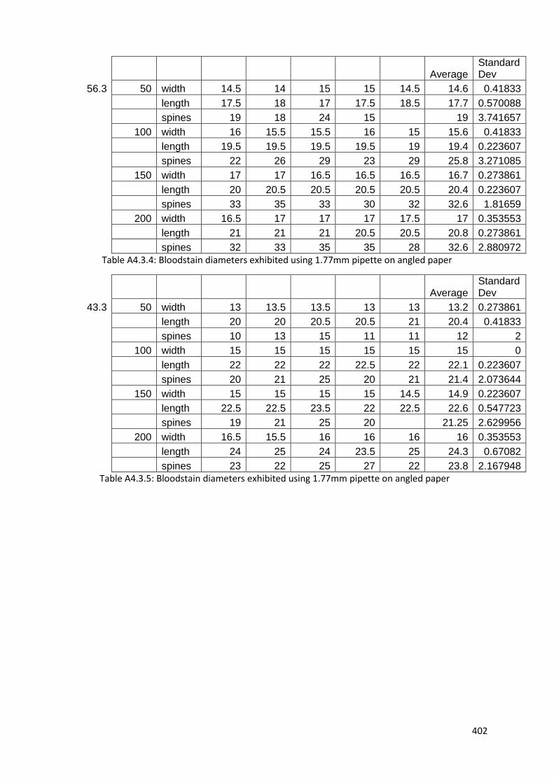
402
Table A4.3.4: Bloodstain diameters exhibited using 1.77mm pipette on angled paper
Average Standard Dev
43.3 50 width 13 13.5 13.5 13 13 13.2 0.273861
length 20 20 20.5 20.5 21 20.4 0.41833
spines 10 13 15 11 11 12 2
100 width 15 15 15 15 15 15 0
length 22 22 22 22.5 22 22.1 0.223607
spines 20 21 25 20 21 21.4 2.073644
150 width 15 15 15 15 14.5 14.9 0.223607
length 22.5 22.5 23.5 22 22.5 22.6 0.547723
spines 19 21 25 20 21.25 2.629956
200 width 16.5 15.5 16 16 16 16 0.353553
length 24 25 24 23.5 25 24.3 0.67082
spines 23 22 25 27 22 23.8 2.167948
Table A4.3.5: Bloodstain diameters exhibited using 1.77mm pipette on angled paper
Average Standard Dev
56.3 50 width 14.5 14 15 15 14.5 14.6 0.41833
length 17.5 18 17 17.5 18.5 17.7 0.570088
spines 19 18 24 15 19 3.741657
100 width 16 15.5 15.5 16 15 15.6 0.41833
length 19.5 19.5 19.5 19.5 19 19.4 0.223607
spines 22 26 29 23 29 25.8 3.271085
150 width 17 17 16.5 16.5 16.5 16.7 0.273861
length 20 20.5 20.5 20.5 20.5 20.4 0.223607
spines 33 35 33 30 32 32.6 1.81659
200 width 16.5 17 17 17 17.5 17 0.353553
length 21 21 21 20.5 20.5 20.8 0.273861
spines 32 33 35 35 28 32.6 2.880972
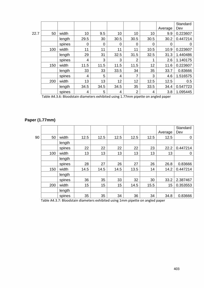
403
Table A4.3.6: Bloodstain diameters exhibited using 1.77mm pipette on angled paper
Paper (1.77mm)
Average Standard Dev
90 50 width 12.5 12.5 12.5 12.5 12.5 12.5 0
length
spines 22 22 22 22 23 22.2 0.447214
100 width 13 13 13 13 13 13 0
length
spines 28 27 26 27 26 26.8 0.83666
150 width 14.5 14.5 14.5 13.5 14 14.2 0.447214
length
spines 36 35 33 32 30 33.2 2.387467
200 width 15 15 15 14.5 15.5 15 0.353553
length
spines 35 35 34 36 34 34.8 0.83666
Table A4.3.7: Bloodstain diameters exhibited using 1mm pipette on angled paper
Average Standard Dev
22.7 50 width 10 9.5 10 10 10 9.9 0.223607
length 29.5 30 30.5 30.5 30.5 30.2 0.447214
spines 0 0 0 0 0 0 0
100 width 11 11 11 11 10.5 10.9 0.223607
length 29 31 32.5 31.5 32.5 31.3 1.440486
spines 4 3 3 2 1 2.6 1.140175
150 width 11.5 11.5 11.5 11.5 12 11.6 0.223607
length 33 33 33.5 34 35 33.7 0.83666
spines 4 5 4 7 3 4.6 1.516575
200 width 13 13 12 12 12.5 12.5 0.5
length 34.5 34.5 34.5 35 33.5 34.4 0.547723
spines 4 5 4 2 4 3.8 1.095445

404
Table A4.3.8: Bloodstain diameters exhibited using 1mm pipette on angled paper
Average Standard
Dev
61.6 50 width 12 12..5 12.5 12 11.5 12 0.408248
length 13.5 14.5 14 14.5 14 14.1 0.41833
spines 16 19 17 15 15 16.4 1.67332
100 width 13 13.5 13 12.5 13 13 0.353553
length 15.5 15.5 15.5 15 15 15.3 0.273861
spines 21 22 23 19 27 22.4 2.966479
150 width 14 14.5 14.5 14 14 14.2 0.273861
length 16 16 17 16 16.5 16.3 0.447214
spines 29 30 29 28 26 28.4 1.516575
200 width 15 15 14.5 14.5 14 14.6 0.41833
length 17 16.5 16.5 17 17 16.8 0.273861
spines 27 36 35 35 34 33.4 3.646917
Table A4.3.9: Bloodstain diameters exhibited using 1mm pipette on angled paper
Average Standard Dev
78.8 50 width 12.5 13 13 13 12 12.7 0.447214
length 13 13.5 13.5 13.5 12.5 13.2 0.447214
spines 23 24 21 22 22 22.4 1.140175
100 width 13.5 13.5 12.5 13 13.5 13.2 0.447214
length 14 14 13 13.5 14 13.7 0.447214
spines 25 26 26 25 28 26 1.224745
150 width 14.5 14 14 14 14.5 14.2 0.273861
length 15 14.5 14.5 14.5 15 14.7 0.273861
spines 31 31 32 36 32 32.4 2.073644
200 width 14.5 15 14.5 14.5 15 14.7 0.273861
length 15 15.5 15 15 15.5 15.2 0.273861
spines 36 37 38 30 36 35.4 3.130495

405
Table A4.3.10: Bloodstain diameters exhibited using 1mm pipette on angled paper
Table A4.3.11: Bloodstain diameters exhibited using 1mm pipette on angled paper
Average Standard Dev
56.3 50 width 12.5 11.5 11.5 11.5 12 11.8 0.447214
length 14.5 14 14 13.5 14 14 0.353553
spines 10 15 15 18 16 14.8 2.949576
100 width 12.5 13 13.5 13 13 13 0.353553
length 16 15.5 15.5 15 15.5 15.5 0.353553
spines 23 26 22 24 22 23.4 1.67332
150 width 13 13 14 13 13.5 13.3 0.447214
length 15.5 16 16 16 15.5 15.8 0.273861
spines 25 23 25 26 28 25.4 1.81659
200 width 14 14.5 14 14.5 14 14.2 0.273861
length 17.5 17 17 17 17.5 17.2 0.273861
spines 34 32 31 24 32 30.6 3.847077
Average Standard Dev
43.3 50 width 10.5 10 10.5 10.5 10.5 10.4 0.223607
length 16.5 16.5 16.5 16.5 15.5 16.3 0.447214
spines 6 7 10 7 10 8 1.870829
100 width 11 12 12 12 12.5 11.9 0.547723
length 19 18.5 17 18.5 18.5 18.3 0.758288
spines 10 11 10 12 14 11.4 1.67332
150 width 12 12.5 12 12.5 12.5 12.3 0.273861
length 20 19.5 19 20 18 19.3 0.83666
spines 16 15 16 14 17 15.6 1.140175
200 width 13 13 13 13.5 13.5 13.2 0.273861
length 20.5 20 20 20 20 20.1 0.223607
spines 22 23 21 12 18 19.2 4.438468

406
Average Standard Dev
22.7 50 width 8 8 8 7.5 7.5 7.8 0.273861
length 26.5 26 26 27 25 26.1 0.74162
spines 0 0 0 0 0 0 0
100 width 8.5 8.5 8.5 8.5 8.5 8.5 0
length 28.5 28.5 28.5 27.5 28 28.2 0.447214
spines 0 0 0 0 0 0 0
150 width 9.5 10 9 9.5 9.5 9.5 0.353553
length 29 31.5 28.5 31 29 29.8 1.350926
spines 4 4 3 3 3 3.4 0.547723
200 width 9.5 9.5 9.5 9.5 9.5 9.5 0
length 29.5 30 28.5 29 29.5 29.3 0.570088
spines 1 3 3 3 3 2.6 0.894427
Table A4.3.12: Bloodstain diameters exhibited using 1mm pipette on angled paper
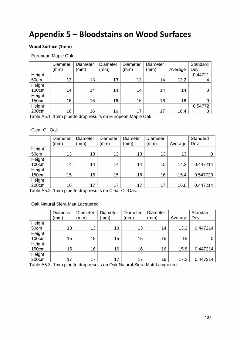
407
Appendix 5 – Bloodstains on Wood Surfaces Wood Surface (1mm)
European Maple Oak
Diameter (mm)
Diameter (mm)
Diameter (mm)
Diameter (mm)
Diameter (mm) Average
Standard Dev.
Height 50cm 13 13 13 13 14 13.2
0.447214
Height 100cm 14 14 14 14 14 14 0
Height 150cm 16 16 16 16 16 16 0
Height 200cm 16 16 16 17 17 16.4
0.547723
Table A5.1: 1mm pipette drop results on European Maple Oak
Clear Oil Oak
Diameter (mm)
Diameter (mm)
Diameter (mm)
Diameter (mm)
Diameter (mm) Average
Standard Dev.
Height 50cm 13 13 13 13 13 13 0
Height 100cm 14 14 14 14 15 14.2 0.447214
Height 150cm 15 15 15 16 16 15.4 0.547723
Height 200cm 16 17 17 17 17 16.8 0.447214
Table A5.2: 1mm pipette drop results on Clear Oil Oak.
Oak Natural Siera Matt Lacquered
Diameter (mm)
Diameter (mm)
Diameter (mm)
Diameter (mm)
Diameter (mm) Average
Standard Dev.
Height 50cm 13 13 13 13 14 13.2 0.447214
Height 100cm 15 15 15 15 15 15 0
Height 150cm 15 16 16 16 16 15.8 0.447214
Height 200cm 17 17 17 17 18 17.2 0.447214
Table A5.3: 1mm pipette drop results on Oak Natural Siera Matt Lacquered.
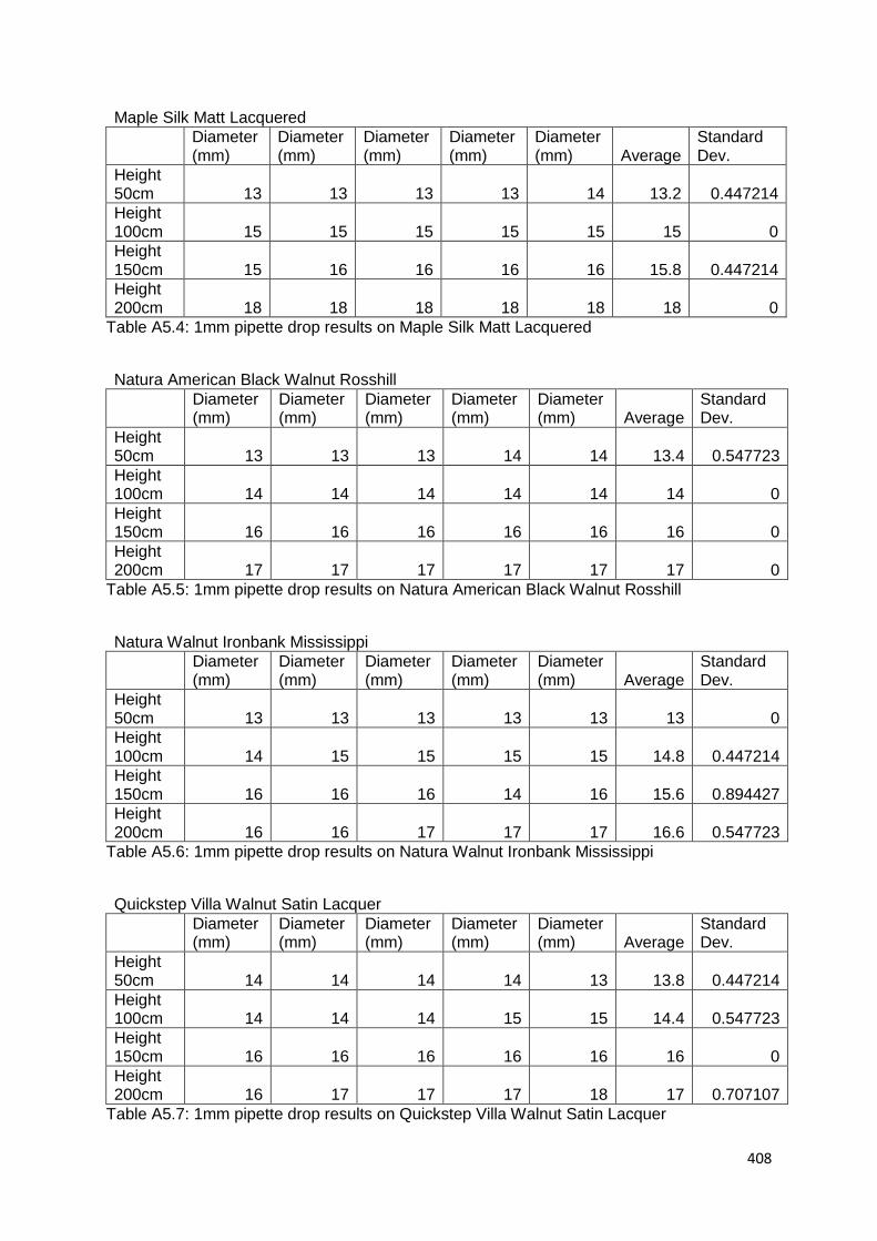
408
Maple Silk Matt Lacquered
Diameter (mm)
Diameter (mm)
Diameter (mm)
Diameter (mm)
Diameter (mm) Average
Standard Dev.
Height 50cm 13 13 13 13 14 13.2 0.447214
Height 100cm 15 15 15 15 15 15 0
Height 150cm 15 16 16 16 16 15.8 0.447214
Height 200cm 18 18 18 18 18 18 0
Table A5.4: 1mm pipette drop results on Maple Silk Matt Lacquered
Natura American Black Walnut Rosshill
Diameter (mm)
Diameter (mm)
Diameter (mm)
Diameter (mm)
Diameter (mm) Average
Standard Dev.
Height 50cm 13 13 13 14 14 13.4 0.547723
Height 100cm 14 14 14 14 14 14 0
Height 150cm 16 16 16 16 16 16 0
Height 200cm 17 17 17 17 17 17 0
Table A5.5: 1mm pipette drop results on Natura American Black Walnut Rosshill
Natura Walnut Ironbank Mississippi
Diameter (mm)
Diameter (mm)
Diameter (mm)
Diameter (mm)
Diameter (mm) Average
Standard Dev.
Height 50cm 13 13 13 13 13 13 0
Height 100cm 14 15 15 15 15 14.8 0.447214
Height 150cm 16 16 16 14 16 15.6 0.894427
Height 200cm 16 16 17 17 17 16.6 0.547723
Table A5.6: 1mm pipette drop results on Natura Walnut Ironbank Mississippi
Quickstep Villa Walnut Satin Lacquer
Diameter (mm)
Diameter (mm)
Diameter (mm)
Diameter (mm)
Diameter (mm) Average
Standard Dev.
Height 50cm 14 14 14 14 13 13.8 0.447214
Height 100cm 14 14 14 15 15 14.4 0.547723
Height 150cm 16 16 16 16 16 16 0
Height 200cm 16 17 17 17 18 17 0.707107
Table A5.7: 1mm pipette drop results on Quickstep Villa Walnut Satin Lacquer

409
Kahrs Maple Toronto Satin Lacquer
Diameter (mm)
Diameter (mm)
Diameter (mm)
Diameter (mm)
Diameter (mm) Average
Standard Dev.
Height 50cm 13 13 12 12 12 12.4 0.547723
Height 100cm 14 14 14 14 14 14 0
Height 150cm 15 15 16 16 16 15.6 0.547723
Height 200cm 16 16 17 17 17 16.6 0.547723
Table A5.8: 1mm pipette drop results on Kahrs Maple Toronto Satin Lacquer
Kahrs Walnut Rustic Nature Oil
Diameter (mm)
Diameter (mm)
Diameter (mm)
Diameter (mm)
Diameter (mm) Average
Standard Dev.
Height 50cm 13 13 12 12 12 12.4 0.547723
Height 100cm 14 14 14 14 14 14 0
Height 150cm 16 16 16 15 15 15.6 0.547723
Height 200cm 16 16 17 17 17 16.6 0.547723
Table A5.9: 1mm pipette drop results on Kahrs Walnut Rustic Nature Oil
Maple Ultra Matt Lacquered
Diameter (mm)
Diameter (mm)
Diameter (mm)
Diameter (mm)
Diameter (mm) Average
Standard Dev.
Height 50cm 13 13 13 14 14 13.4 0.547723
Height 100cm 15 15 15 15 15 15 0
Height 150cm 16 16 16 16 16 16 0
Height 200cm 16 17 17 17 17 16.8 0.447214
Table A5.10: 1mm pipette drop results on Maple Ultra Matt Lacquered
Oak Silk Matt
Diameter (mm)
Diameter (mm)
Diameter (mm)
Diameter (mm)
Diameter (mm) Average
Standard Dev.
Height 50cm 14 14 14 14 14 14 0
Height 100cm 15 15 15 15 15 15 0
Height 150cm 16 16 15 17 16 16 0.707107
Height 200cm 17 17 17 17 17 17 0
Table A5.11: 1mm pipette drop results on Oak Silk Matt
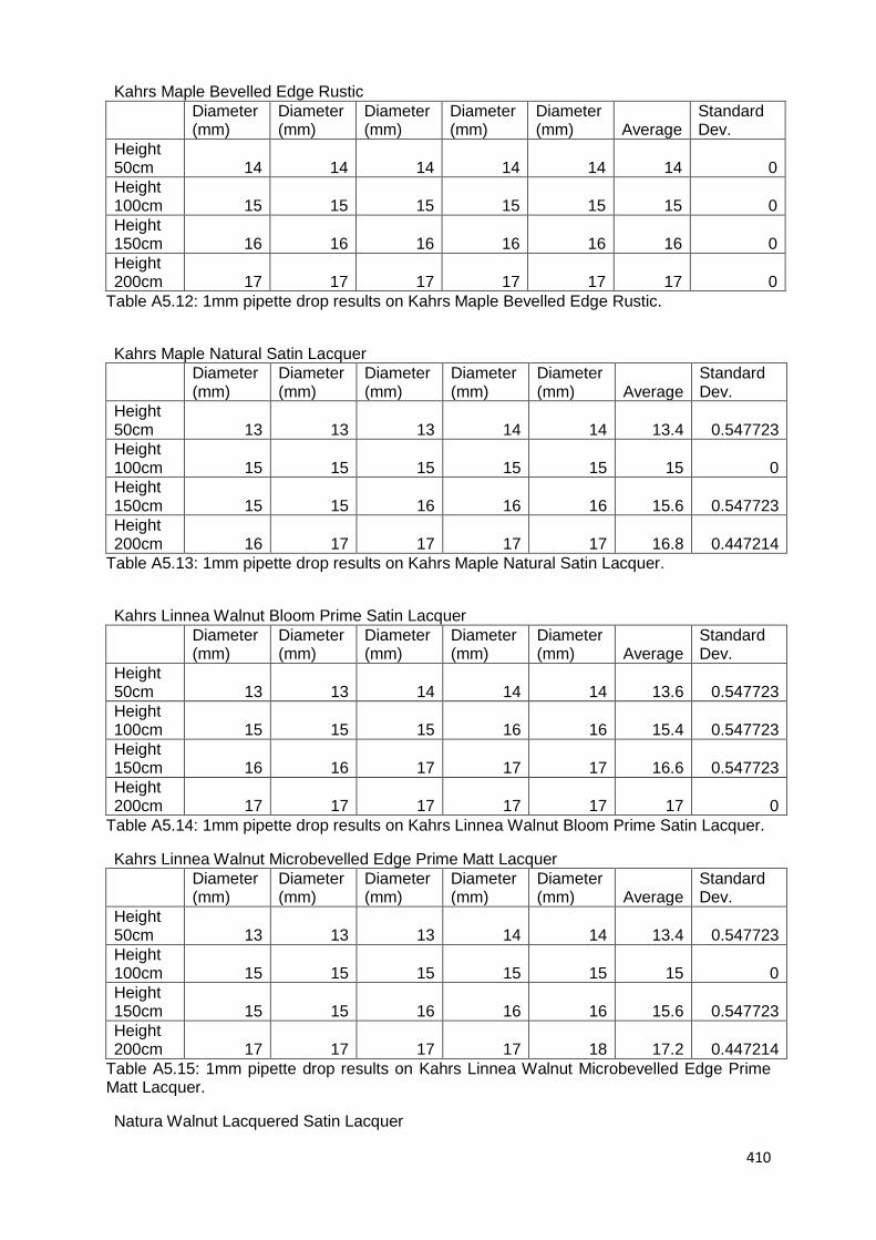
410
Table A5.12: 1mm pipette drop results on Kahrs Maple Bevelled Edge Rustic.
Kahrs Maple Natural Satin Lacquer
Diameter (mm)
Diameter (mm)
Diameter (mm)
Diameter (mm)
Diameter (mm) Average
Standard Dev.
Height 50cm 13 13 13 14 14 13.4 0.547723
Height 100cm 15 15 15 15 15 15 0
Height 150cm 15 15 16 16 16 15.6 0.547723
Height 200cm 16 17 17 17 17 16.8 0.447214
Table A5.13: 1mm pipette drop results on Kahrs Maple Natural Satin Lacquer.
Kahrs Linnea Walnut Bloom Prime Satin Lacquer
Diameter (mm)
Diameter (mm)
Diameter (mm)
Diameter (mm)
Diameter (mm) Average
Standard Dev.
Height 50cm 13 13 14 14 14 13.6 0.547723
Height 100cm 15 15 15 16 16 15.4 0.547723
Height 150cm 16 16 17 17 17 16.6 0.547723
Height 200cm 17 17 17 17 17 17 0
Table A5.14: 1mm pipette drop results on Kahrs Linnea Walnut Bloom Prime Satin Lacquer.
Kahrs Linnea Walnut Microbevelled Edge Prime Matt Lacquer
Diameter (mm)
Diameter (mm)
Diameter (mm)
Diameter (mm)
Diameter (mm) Average
Standard Dev.
Height 50cm 13 13 13 14 14 13.4 0.547723
Height 100cm 15 15 15 15 15 15 0
Height 150cm 15 15 16 16 16 15.6 0.547723
Height 200cm 17 17 17 17 18 17.2 0.447214
Table A5.15: 1mm pipette drop results on Kahrs Linnea Walnut Microbevelled Edge Prime Matt Lacquer.
Natura Walnut Lacquered Satin Lacquer
Kahrs Maple Bevelled Edge Rustic
Diameter (mm)
Diameter (mm)
Diameter (mm)
Diameter (mm)
Diameter (mm) Average
Standard Dev.
Height 50cm 14 14 14 14 14 14 0
Height 100cm 15 15 15 15 15 15 0
Height 150cm 16 16 16 16 16 16 0
Height 200cm 17 17 17 17 17 17 0

411
Diameter (mm)
Diameter (mm)
Diameter (mm)
Diameter (mm)
Diameter (mm) Average
Standard Dev.
Height 50cm 13 13 13 13 13 13 0
Height 100cm 15 15 15 15 15 15 0
Height 150cm 15 16 16 16 16 15.8 0.447214
Height 200cm 17 17 17 17 17 17 0
Table A5.16: 1mm pipette drop results on Natura Walnut Lacquered Satin Lacquer
Kahrs Oak Sienna Natural
Diameter (mm)
Diameter (mm)
Diameter (mm)
Diameter (mm)
Diameter (mm) Average
Standard Dev.
Height 50cm 13 13 13 13 14 13.2 0.447214
Height 100cm 15 15 15 16 16 15.4 0.547723
Height 150cm 16 16 16 16 16 16 0
Height 200cm 17 17 17 17 18 17.2 0.447214
Table A5.17: 1mm pipette drop results on Kahrs Oak Sienna Natural.
Natura Oak Prime Parquet
Diameter (mm)
Diameter (mm)
Diameter (mm)
Diameter (mm)
Diameter (mm) Average
Standard Dev.
Height 50cm 10 10 11 11 12 10.8 0.83666
Height 100cm 12 13 13 13 14 13 0.707107
Height 150cm 13 13 14 13 14 13.4 0.547723
Height 200cm 13 14 14 14 14 13.8 0.447214
Table A5.18: 1mm pipette drop results on Natura Oak Prime Parquet.
Kahrs Oak Siena Engineered Natural
Diameter (mm)
Diameter (mm)
Diameter (mm)
Diameter (mm)
Diameter (mm) Average
Standard Dev.
Height 50cm 12 13 13 13 13 12.8 0.447214
Height 100cm 13 13 13 13 13 13 0
Height 150cm 13 13 13 13 14 13.2 0.447214
Height 200cm 14 14 14 14 14 14 0
Table A5.19: 1mm pipette drop results on Kahrs Oak Siena Engineered Natural.

412
Oak Solid Plank Untreated
Diameter (mm)
Diameter (mm)
Diameter (mm)
Diameter (mm)
Diameter (mm) Average
Standard Dev.
Height 50cm 9 9 9 10 10 9.4 0.547723
Height 100cm 13 13 13 13 14 13.2 0.447214
Height 150cm 14 14 14 14 14 14 0
Height 200cm 14 14 14 14 14 14 0
Table A5.20: 1mm pipette drop results on Oak Solid Plank Untreated.
Wood (1.77mm)
European Maple Oak
Diameter (mm)
Diameter (mm)
Diameter (mm)
Diameter (mm)
Diameter (mm) Average
Standard Dev.
Height 50cm 16 16 16 16 16 16 0
Height 100cm 17 17 17 17 18 17.2 0.447214
Height 150cm 18 18 19 19 20 18.8 0.83666
Height 200cm 19 19 19 19 20 19.2 0.447214
Table A5.21: 1.77mm pipette drop results on European Maple Oak.
Clear Oil Oak
Diameter (mm)
Diameter (mm)
Diameter (mm)
Diameter (mm)
Diameter (mm) Average
Standard Dev.
Height 50cm 15 15 15 15 16 15.2 0.447214
Height 100cm 16 16 16 16 17 16.2 0.447214
Height 150cm 17 17 18 18 18 17.6 0.547723
Height 200cm 18 18 18 18 19 18.2 0.447214
Table A5.22: 1.77mm pipette drop results on Clear Oil Oak.
Oak Natural Siera Matt Lacquered
Diameter (mm)
Diameter (mm)
Diameter (mm)
Diameter (mm)
Diameter (mm) Average
Standard Dev.
Height 50cm 16 16 16 15 15 15.6 0.547723
Height 100cm 18 18 17 17 17 17.4 0.547723
Height 150cm 19 19 19 18 18 18.6 0.547723

413
Height 200cm 20 19 19 19 19 19.2 0.447214
Table A5.23: 1.77mm pipette drop results on Oak Natural Siera Matt Lacquered.
Maple Silk Matt Lacquered
Diameter (mm)
Diameter (mm)
Diameter (mm)
Diameter (mm)
Diameter (mm) Average
Standard Dev.
Height 50cm 16 16 16 16 15 15.8 0.447214
Height 100cm 17 17 17 17 18 17.2 0.447214
Height 150cm 19 19 19 19 19 19 0
Height 200cm 19 20 19 19 19 19.2 0.447214
Table A5.24: 1.77mm pipette drop results on Maple Silk Matt Lacquered.
Natura American Black Walnut Rosshill
Diameter (mm)
Diameter (mm)
Diameter (mm)
Diameter (mm)
Diameter (mm) Average
Standard Dev.
Height 50cm 17 17 17 17 16 16.8 0.447214
Height 100cm 17 17 17 18 18 17.4 0.547723
Height 150cm 18 18 18 18 19 18.2 0.447214
Height 200cm 19 19 19 19 20 19.2 0.447214
Table A5.25: 1.77mm pipette drop results on Natura American Black Walnut Rosshill.
Natura Walnut Ironbank Mississippi
Diameter (mm)
Diameter (mm)
Diameter (mm)
Diameter (mm)
Diameter (mm) Average
Standard Dev.
Height 50cm 15 15 15 16 16 15.4 0.547723
Height 100cm 17 17 17 17 18 17.2 0.447214
Height 150cm 19 19 19 19 18 18.8 0.447214
Height 200cm 19 19 19 20 20 19.4 0.547723
Table A5.26: 1.77mm pipette drop results on Natura Walnut Ironbank Mississippi.
Quickstep Villa Walnut Satin Lacquer
Diameter (mm)
Diameter (mm)
Diameter (mm)
Diameter (mm)
Diameter (mm) Average
Standard Dev.
Height 50cm 17 17 16 16 16 16.4 0.547723
Height 100cm 18 18 18 17 17 17.6 0.547723

414
Height 150cm 18 19 19 19 19 18.8 0.447214
Height 200cm 19 19 19 19 20 19.2 0.447214
Table A5.27: 1.77mm pipette drop results on Quickstep Villa Walnut Satin Lacquer.
Kahrs Maple Toronto Satin Lacquer
Diameter (mm)
Diameter (mm)
Diameter (mm)
Diameter (mm)
Diameter (mm) Average
Standard Dev.
Height 50cm 16 16 16 16 16 16 0
Height 100cm 17 17 17 18 18 17.4 0.547723
Height 150cm 18 18 18 19 19 18.4 0.547723
Height 200cm 19 19 19 20 20 19.4 0.547723
Table A5.28: 1.77mm pipette drop results on Kahrs Maple Toronto Satin Lacquer.
Kahrs Walnut Rustic Nature Oil
Diameter (mm)
Diameter (mm)
Diameter (mm)
Diameter (mm)
Diameter (mm) Average
Standard Dev.
Height 50cm 15 15 15 16 16 15.4 0.547723
Height 100cm 17 17 17 18 18 17.4 0.547723
Height 150cm 19 19 18 18 18 18.4 0.547723
Height 200cm 19 20 20 20 21 20 0.707107
Table A5.29: 1.77mm pipette drop results on Kahrs Walnut Rustic Nature Oil.
Maple Ultra Matt Lacquered
Diameter (mm)
Diameter (mm)
Diameter (mm)
Diameter (mm)
Diameter (mm) Average
Standard Dev.
Height 50cm 15 15 15 15 15 15 0
Height 100cm 17 17 17 17 17 17 0
Height 150cm 18 19 19 19 19 18.8 0.447214
Height 200cm 19 19 20 20 20 19.6 0.547723
Table A5.30: 1.77mm pipette drop results on Maple Ultra Matt Lacquered.
Oak Silk Matt
Diameter (mm)
Diameter (mm)
Diameter (mm)
Diameter (mm)
Diameter (mm) Average
Standard Dev.
Height 50cm 16 16 16 16 17 16.2 0.447214

415
Height 100cm 18 18 18 17 17 17.6 0.547723
Height 150cm 19 19 19 19 20 19.2 0.447214
Height 200cm 19 19 19 20 20 19.4 0.547723
Table A5.31: 1.77mm pipette drop results on Oak Silk Matt.
Kahrs Maple Bevelled Edge Rustic
Diameter (mm)
Diameter (mm)
Diameter (mm)
Diameter (mm)
Diameter (mm) Average
Standard Dev.
Height 50cm 16 16 16 16 17 16.2 0.447214
Height 100cm 19 19 18 18 17 18.2 0.83666
Height 150cm 19 19 19 19 19 19 0
Height 200cm 20 20 20 19 19 19.6 0.547723
Table A5.32: 1.77mm pipette drop results on Kahrs Maple Bevelled Edge Rustic.
Kahrs Maple Natural Satin Lacquer
Diameter (mm)
Diameter (mm)
Diameter (mm)
Diameter (mm)
Diameter (mm) Average
Standard Dev.
Height 50cm 16 16 16 16 16 16 0
Height 100cm 17 17 18 18 18 17.6 0.547723
Height 150cm 18 19 19 19 20 19 0.707107
Height 200cm 18 19 19 20 20 19.2 0.83666
Table A5.33: 1.77mm pipette drop results on Kahrs Maple Natural Satin Lacquer.
Kahrs Linnea Walnut Bloom Prime Satin Lacquer
Diameter (mm)
Diameter (mm)
Diameter (mm)
Diameter (mm)
Diameter (mm) Average
Standard Dev.
Height 50cm 15 15 16 16 16 15.6 0.547723
Height 100cm 17 17 17 17 17 17 0
Height 150cm 18 19 19 19 20 19 0.707107
Height 200cm 19 19 19 20 20 19.4 0.547723
Table A5.34: 1.77mm pipette drop results on Kahrs Linnea Walnut Bloom Prime Satin Lacquer.
Kahrs Linnea Walnut Microbevelled Edge Prime Matt Lacquer
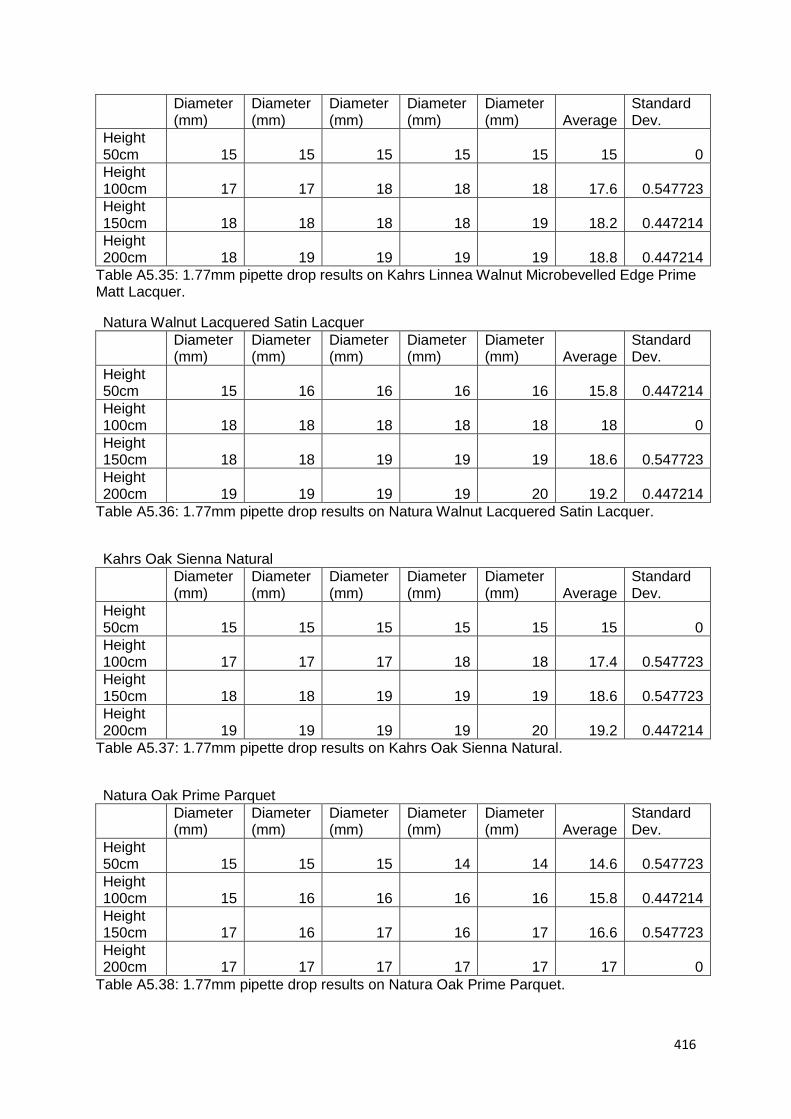
416
Diameter (mm)
Diameter (mm)
Diameter (mm)
Diameter (mm)
Diameter (mm) Average
Standard Dev.
Height 50cm 15 15 15 15 15 15 0
Height 100cm 17 17 18 18 18 17.6 0.547723
Height 150cm 18 18 18 18 19 18.2 0.447214
Height 200cm 18 19 19 19 19 18.8 0.447214
Table A5.35: 1.77mm pipette drop results on Kahrs Linnea Walnut Microbevelled Edge Prime Matt Lacquer.
Natura Walnut Lacquered Satin Lacquer
Diameter (mm)
Diameter (mm)
Diameter (mm)
Diameter (mm)
Diameter (mm) Average
Standard Dev.
Height 50cm 15 16 16 16 16 15.8 0.447214
Height 100cm 18 18 18 18 18 18 0
Height 150cm 18 18 19 19 19 18.6 0.547723
Height 200cm 19 19 19 19 20 19.2 0.447214
Table A5.36: 1.77mm pipette drop results on Natura Walnut Lacquered Satin Lacquer.
Kahrs Oak Sienna Natural
Diameter (mm)
Diameter (mm)
Diameter (mm)
Diameter (mm)
Diameter (mm) Average
Standard Dev.
Height 50cm 15 15 15 15 15 15 0
Height 100cm 17 17 17 18 18 17.4 0.547723
Height 150cm 18 18 19 19 19 18.6 0.547723
Height 200cm 19 19 19 19 20 19.2 0.447214
Table A5.37: 1.77mm pipette drop results on Kahrs Oak Sienna Natural.
Natura Oak Prime Parquet
Diameter (mm)
Diameter (mm)
Diameter (mm)
Diameter (mm)
Diameter (mm) Average
Standard Dev.
Height 50cm 15 15 15 14 14 14.6 0.547723
Height 100cm 15 16 16 16 16 15.8 0.447214
Height 150cm 17 16 17 16 17 16.6 0.547723
Height 200cm 17 17 17 17 17 17 0
Table A5.38: 1.77mm pipette drop results on Natura Oak Prime Parquet.
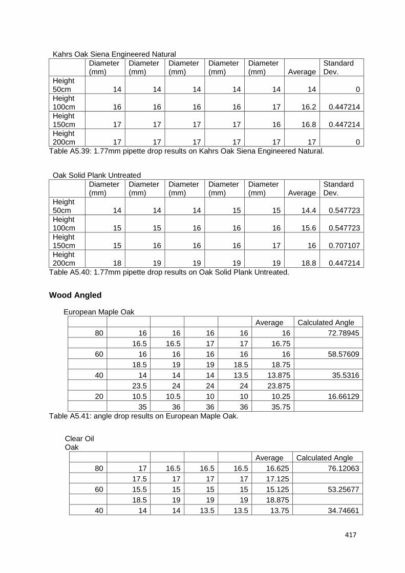
417
Kahrs Oak Siena Engineered Natural
Diameter (mm)
Diameter (mm)
Diameter (mm)
Diameter (mm)
Diameter (mm) Average
Standard Dev.
Height 50cm 14 14 14 14 14 14 0
Height 100cm 16 16 16 16 17 16.2 0.447214
Height 150cm 17 17 17 17 16 16.8 0.447214
Height 200cm 17 17 17 17 17 17 0
Table A5.39: 1.77mm pipette drop results on Kahrs Oak Siena Engineered Natural.
Oak Solid Plank Untreated
Diameter (mm)
Diameter (mm)
Diameter (mm)
Diameter (mm)
Diameter (mm) Average
Standard Dev.
Height 50cm 14 14 14 15 15 14.4 0.547723
Height 100cm 15 15 16 16 16 15.6 0.547723
Height 150cm 15 16 16 16 17 16 0.707107
Height 200cm 18 19 19 19 19 18.8 0.447214
Table A5.40: 1.77mm pipette drop results on Oak Solid Plank Untreated.
Wood Angled
European Maple Oak
Average Calculated Angle
80 16 16 16 16 16 72.78945
16.5 16.5 17 17 16.75
60 16 16 16 16 16 58.57609
18.5 19 19 18.5 18.75
40 14 14 14 13.5 13.875 35.5316
23.5 24 24 24 23.875
20 10.5 10.5 10 10 10.25 16.66129
35 36 36 36 35.75
Table A5.41: angle drop results on European Maple Oak.
Clear Oil Oak
Average Calculated Angle
80 17 16.5 16.5 16.5 16.625 76.12063
17.5 17 17 17 17.125
60 15.5 15 15 15 15.125 53.25677
18.5 19 19 19 18.875
40 14 14 13.5 13.5 13.75 34.74661

418
25 24 24 23.5 24.125
20 10 10 10 9.5 9.875 16.5094
34 35 35 35 34.75
Table A5.42: angle drop results on Clear Oil Oak.
Oak Natural Siera Matt Lacquered
Average Calculated Angle
80 17 17 17.5 17.5 17.25 78.15973
17.5 17.5 17.5 18 17.625
60 16 16 16.5 16.5 16.25 60.07357
19 19 18.5 18.5 18.75
40 14.5 14.5 14.5 14 14.375 38.19061
24 23.5 23 22.5 23.25
20 9 9.5 9.5 9.5 9.375 15.25752
35 35 36.5 36 35.625
Table A5.43: angle drop results on Oak Natural Siera Matt Lacquered.
Maple Silk Matt Lacquered
Average Calculated Angle
80 17 17 16.5 16.5 16.75 73.16502
17.5 17.5 17.5 17.5 17.5
60 16 16 16 16 16 57.3631
19 19 19 19 19
40 14 14 14.5 14.5 14.25 36.8699
24 24 23.5 23.5 23.75
20 10 10 10 10.5 10.125 15.50525
38 38 38 37.5 37.875
Table A5.44: angle drop results on Maple Silk Matt Lacquered.
Natura American Black Walnut Rosshill
Average Calculated Angle
80 17 17 17 17.5 17.125 76.31987
18 17.5 17.5 17.5 17.625
60 16.5 15.5 16 16 16 53.61329
20 20.5 19.5 19.5 19.875
40 14 14 14 13.5 13.875 35.5316
24 24 24 23.5 23.875
20 9 9 9.5 10 9.375 14.18763
39 38 38 38 38.25
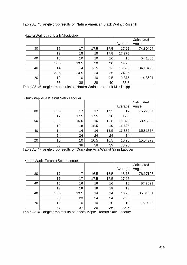
419
Table A5.45: angle drop results on Natura American Black Walnut Rosshill.
Natura Walnut Ironbank Mississippi
Average Calculated Angle
80 17 17 17.5 17.5 17.25 74.80404
18 18 18 17.5 17.875
60 16 16 16 16 16 54.1083
19.5 19.5 20 20 19.75
40 14 14 13.5 13 13.625 34.18423
23.5 24.5 24 25 24.25
20 10 10 10 9.5 9.875 14.8621
38 38 38 40 38.5
Table A5.46: angle drop results on Natura Walnut Ironbank Mississippi.
Quickstep Villa Walnut Satin Lacquer
Average Calculated Angle
80 16.5 17 17 17.5 17 76.27087
17 17.5 17.5 18 17.5
60 15.5 15.5 16 16.5 15.875 58.46809
19 18 18.5 19 18.625
40 14 14 14 13.5 13.875 35.31877
24 24 24 24 24
20 10 10 10.5 10.5 10.25 15.54373
38 38 38 39 38.25
Table A5.47: angle drop results on Quickstep Villa Walnut Satin Lacquer
Kahrs Maple Toronto Satin Lacquer
Average Calculated Angle
80 17 17 16.5 16.5 16.75 76.17126
17 17 17.5 17.5 17.25
60 16 16 16 16 16 57.3631
19 19 19 19 19
40 13.5 13.5 14 14 13.75 35.81051
23 23 24 24 23.5
20 10 10 10 10 10 15.9008
37 37 36 36 36.5
Table A5.48: angle drop results on Kahrs Maple Toronto Satin Lacquer.

420
Kahrs Walnut Rustic Nature Oil
Average Calculated Angle
80 16 16 16.5 17 16.375 74.4155
17 17 17.5 16.5 17
60 16.5 16.5 16.5 15.5 16.25 58.78882
19 19 19 19 19
40 14 14 14 14 14 34.25063
25 25 25 24.5 24.875
20 10 10 9.5 9.5 9.75 16.05713
35 35 35 36 35.25
Table A5.49: angle drop results on Kahrs Walnut Rustic Nature Oil.
Maple Ultra Matt Lacquered
Average Calculated Angle
80 17 17 17 17 17 76.27087
17.5 17.5 17.5 17.5 17.5
60 16 15.5 15.5 15.5 15.625 55.87489
18.5 19 19 19 18.875
40 14 14 14 14 14 36.3412
24 24 23.5 23 23.625
20 9 9 9.5 9.5 9.25 14.7838
35 35 37.5 37.5 36.25
Table A5.50: angle drop results on Maple Ultra Matt Lacquered.
Oak Silk Matt
Average Calculated Angle
80 17 17 17.5 18 17.375 76.41633
17.5 17.5 18 18.5 17.875
60 16 16 16 16 16 57.3631
19 19 19 19 19
40 14 14 14 14 14 35.90107
24 24 24 23.5 23.875
20 10.5 10.5 10.5 10.5 10.5 15.98644
38 38 38 38.5 38.125
Table A5.51: 1mm pipette angle drop results on Oak Silk Matt.
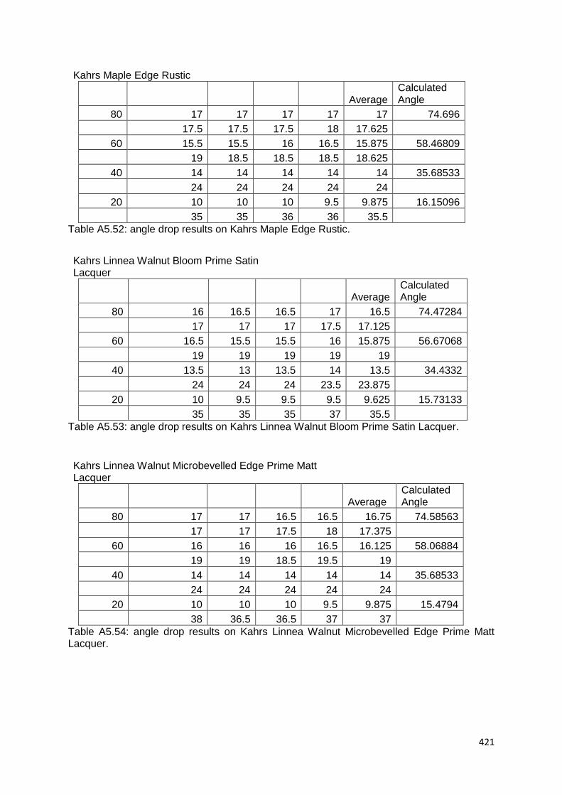
421
Kahrs Maple Edge Rustic
Average Calculated Angle
80 17 17 17 17 17 74.696
17.5 17.5 17.5 18 17.625
60 15.5 15.5 16 16.5 15.875 58.46809
19 18.5 18.5 18.5 18.625
40 14 14 14 14 14 35.68533
24 24 24 24 24
20 10 10 10 9.5 9.875 16.15096
35 35 36 36 35.5
Table A5.52: angle drop results on Kahrs Maple Edge Rustic.
Kahrs Linnea Walnut Bloom Prime Satin Lacquer
Average Calculated Angle
80 16 16.5 16.5 17 16.5 74.47284
17 17 17 17.5 17.125
60 16.5 15.5 15.5 16 15.875 56.67068
19 19 19 19 19
40 13.5 13 13.5 14 13.5 34.4332
24 24 24 23.5 23.875
20 10 9.5 9.5 9.5 9.625 15.73133
35 35 35 37 35.5
Table A5.53: angle drop results on Kahrs Linnea Walnut Bloom Prime Satin Lacquer.
Kahrs Linnea Walnut Microbevelled Edge Prime Matt Lacquer
Average Calculated Angle
80 17 17 16.5 16.5 16.75 74.58563
17 17 17.5 18 17.375
60 16 16 16 16.5 16.125 58.06884
19 19 18.5 19.5 19
40 14 14 14 14 14 35.68533
24 24 24 24 24
20 10 10 10 9.5 9.875 15.4794
38 36.5 36.5 37 37
Table A5.54: angle drop results on Kahrs Linnea Walnut Microbevelled Edge Prime Matt Lacquer.

422
Natura Walnut Lacquered Satin Lacquer
Average Calculated Angle
80 17 17.5 17 17 17.125 76.31987
17.5 17.5 17.5 18 17.625
60 16.5 17 16 15 16.125 61.34834
18 18 19 18.5 18.375
40 14.5 14.5 14.5 14 14.375 37.71268
24 23 23.5 23.5 23.5
20 10 10 9.5 9.5 9.75 15.22595
37.5 37.5 37 36.5 37.125
Table A5.55: angle drop results on Natura Walnut Lacquered Satin Lacquer.
Kahrs Oak Sienna Natural
Average Calculated Angle
80 16.5 16.5 17 17 16.75 76.17126
17 17 17.5 17.5 17.25
60 16 16 16.5 16.5 16.25 56.44269
19.5 19.5 19 20 19.5
40 13.5 13.5 13.5 13 13.375 34.07028
24 24.5 23.5 23.5 23.875
20 10 10 10 10 10 15.8451
36.5 36 37 37 36.625
Table A5.56: angle drop results on Kahrs Oak Sienna Natural.
Natural Oak Prime Parquet
Average Calculated Angle
80 14 14 13.5 13.5 13.75 74.77724
14.5 14.5 14 14 14.25
60 15 15 14.5 14.5 14.75 58.76774
17.5 17.5 17 17 17.25
40 13 13 13.5 13.5 13.25 40.86818
21 20 20 20 20.25
20 9 9 8.5 8.5 8.75 14.74665
35 33.5 35 34 34.375
Table A5.57: angle drop results on Natural Oak Prime Parquet.

423
Kahrs Oak Siena Engineered Natural
Average Calculated Angle
80 16.5 16.5 16.5 16 16.375 76.01769
17 17 17 16.5 16.875
60 16 16 16 15.5 15.875 57.85095
18 19 19 19 18.75
40 13.5 13.5 13.5 14 13.625 36.79124
23 23 22.5 22.5 22.75
20 9.5 10 10 10 9.875 16.6325
33 35 35 35 34.5
Table A5.58: angle drop results on Kahrs Oak Siena Engineered Natural.
Oak Solid Plank Untreated
Average Calculated Angle
80 15 15 15 15 15 75.40745
15.5 15.5 15.5 15.5 15.5
60 14 13.5 13.5 14.5 13.875 57.23624
16.5 16.5 17 16 16.5
40 13.5 13.5 13.5 14 13.625 39.8796
22 22 21 20 21.25
20 9 9 9 8.5 8.875 14.9622
35 35 33.5 34 34.375
Table A5.59: angle drop results on Oak Solid Plank Untreated.
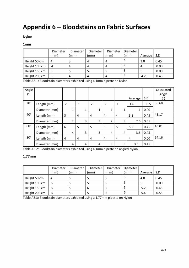
424
Appendix 6 – Bloodstains on Fabric Surfaces Nylon
1mm
Table A6.1: Bloodstain diameters exhibited using a 1mm pipette on Nylon.
Table A6.2: Bloodstain diameters exhibited using a 1mm pipette on angled Nylon.
1.77mm
Table A6.3: Bloodstain diameters exhibited using a 1.77mm pipette on Nylon
Diameter (mm)
Diameter (mm)
Diameter (mm)
Diameter (mm)
Diameter (mm) Average S.D
Height 50 cm 4 3 4 4 4 3.8 0.45
Height 100 cm 4 4 4 4 4 4 0.00
Height 150 cm 5 5 5 5 5 5 0.00
Height 200 cm 5 4 4 4 4 4.2 0.45
Angle (o)
Average S.D
Calculated Angle
(o)
20o Length (mm) 2 1 2 2 1 1.6 0.55 38.68
Diameter (mm) 1 1 1 1 1 1 0.00
40o Length (mm) 3 4 4 4 4 3.8 0.45 43.17
Diameter (mm) 2 3 3 2 3 2.6 0.55
60o Length (mm) 6 5 5 5 5 5.2 0.45 43.81
Diameter (mm) 4 3 3 4 4 3.6 0.45
80o Length (mm) 4 4 4 4 4 4 0.00 64.16
Diameter (mm) 4 4 4 3 3 3.6 0.45
Diameter (mm)
Diameter (mm)
Diameter (mm)
Diameter (mm)
Diameter (mm) Average S.D
Height 50 cm 4 5 5 5 5 4.8 0.45
Height 100 cm 5 5 5 5 5 5 0.00
Height 150 cm 5 5 6 5 5 5.2 0.45
Height 200 cm 5 5 5 6 6 5.4 0.55
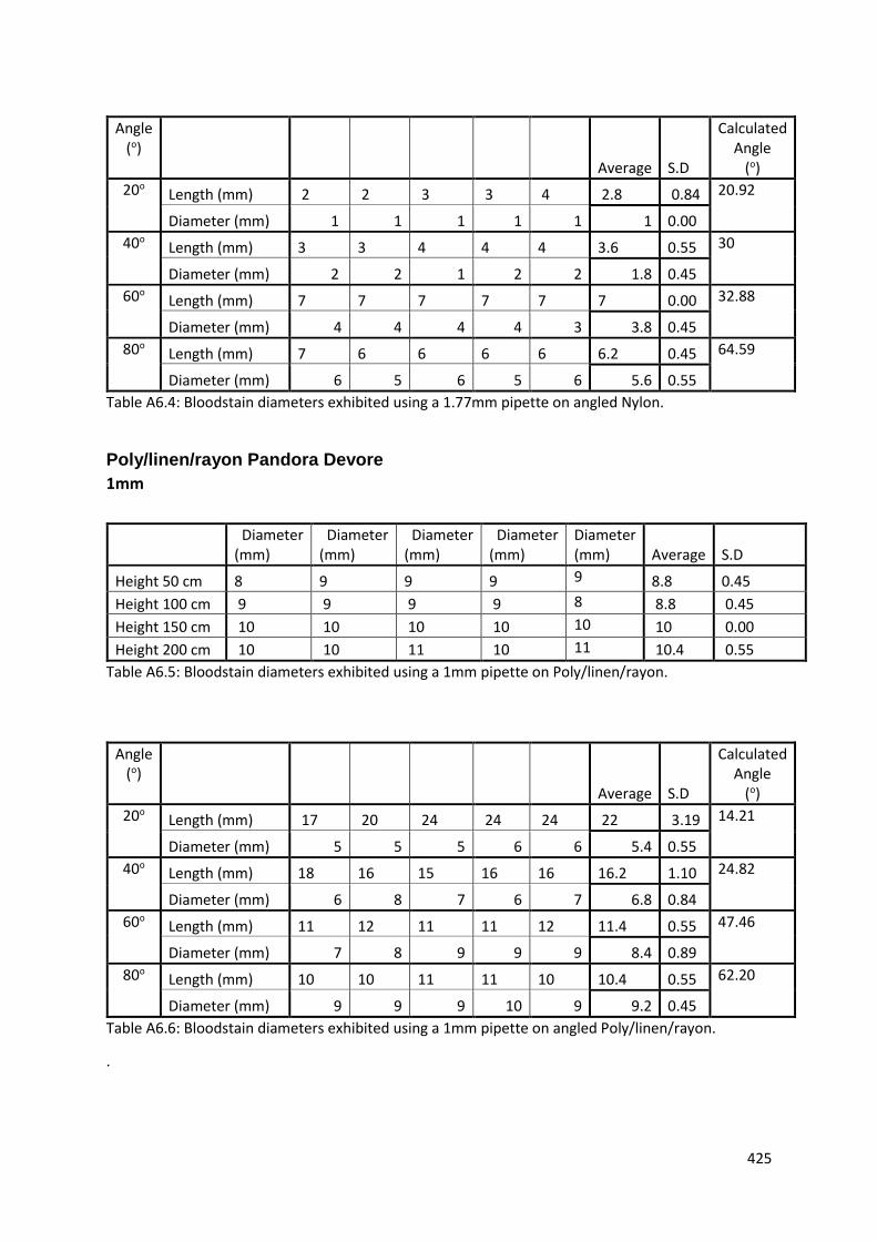
425
Table A6.4: Bloodstain diameters exhibited using a 1.77mm pipette on angled Nylon.
Poly/linen/rayon Pandora Devore
1mm
Table A6.5: Bloodstain diameters exhibited using a 1mm pipette on Poly/linen/rayon.
Table A6.6: Bloodstain diameters exhibited using a 1mm pipette on angled Poly/linen/rayon.
.
Angle (o)
Average S.D
Calculated Angle
(o)
20o Length (mm) 2 2 3 3 4 2.8 0.84 20.92
Diameter (mm) 1 1 1 1 1 1 0.00
40o Length (mm) 3 3 4 4 4 3.6 0.55 30
Diameter (mm) 2 2 1 2 2 1.8 0.45
60o Length (mm) 7 7 7 7 7 7 0.00 32.88
Diameter (mm) 4 4 4 4 3 3.8 0.45
80o Length (mm) 7 6 6 6 6 6.2 0.45 64.59
Diameter (mm) 6 5 6 5 6 5.6 0.55
Diameter (mm)
Diameter (mm)
Diameter (mm)
Diameter (mm)
Diameter (mm) Average S.D
Height 50 cm 8 9 9 9 9 8.8 0.45
Height 100 cm 9 9 9 9 8 8.8 0.45
Height 150 cm 10 10 10 10 10 10 0.00
Height 200 cm 10 10 11 10 11 10.4 0.55
Angle (o)
Average S.D
Calculated Angle
(o)
20o Length (mm) 17 20 24 24 24 22 3.19 14.21
Diameter (mm) 5 5 5 6 6 5.4 0.55
40o Length (mm) 18 16 15 16 16 16.2 1.10 24.82
Diameter (mm) 6 8 7 6 7 6.8 0.84
60o Length (mm) 11 12 11 11 12 11.4 0.55 47.46
Diameter (mm) 7 8 9 9 9 8.4 0.89
80o Length (mm) 10 10 11 11 10 10.4 0.55 62.20
Diameter (mm) 9 9 9 10 9 9.2 0.45

426
1.77mm
Table A6.7: Bloodstain diameters exhibited using a 1.77mm pipette on Poly/linen/rayon.
Table A6.8: Bloodstain diameters exhibited using a 1.77mm pipette on angled Poly/linen/rayon.
Wool Delaine
1mm
Table A6.9: Bloodstain diameters exhibited using a 1mm pipette on Wood Delaine
Diameter (mm)
Diameter (mm)
Diameter (mm)
Diameter (mm)
Diameter (mm) Average S.D
Height 50 cm 12 12 11 13 12 12 0.71
Height 100 cm 11 12 12 13 13 12.2 0.84
Height 150 cm 13 14 13 14 12 13.2 0.84
Height 200 cm 13 14 14 14 13 13.6 0.55
Angle (o)
Average S.D
Calculated Angle
(o)
20o Length (mm) 16 27 21 21 23 21.6 3.97 19.47
Diameter (mm) 7 7 7 8 7 7.2 0.45
40o Length (mm) 14 14 15 15 16 14.8 0.84 40.44
Diameter (mm) 9 9 10 10 10 9.6 0.55
60o Length (mm) 11 13 12 13 12 12.2 0.84 64.37
Diameter (mm) 10 11 12 11 11 11 0.71
80o Length (mm) 11 11 11 11 12 11.6 0.00 71.49
Diameter (mm) 11 12 11 12 11 11 0.55
Diameter (mm)
Diameter (mm)
Diameter (mm)
Diameter (mm)
Diameter (mm) Average S.D
Height 50 cm 5 5 6 5 5 5.2 0.45
Height 100 cm 7 7 7 7 7 7 0.00
Height 150 cm 8 7 8 8 7 7.6 0.55
Height 200 cm 8 8 9 8 9 8.4 0.55
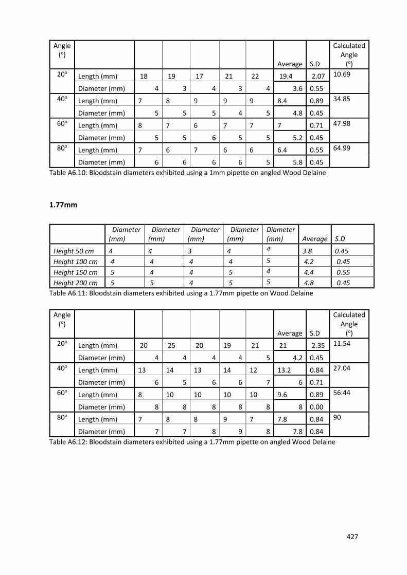
427
Table A6.10: Bloodstain diameters exhibited using a 1mm pipette on angled Wood Delaine
1.77mm
Table A6.11: Bloodstain diameters exhibited using a 1.77mm pipette on Wood Delaine
Table A6.12: Bloodstain diameters exhibited using a 1.77mm pipette on angled Wood Delaine
Angle (o)
Average S.D
Calculated Angle
(o)
20o Length (mm) 18 19 17 21 22 19.4 2.07 10.69
Diameter (mm) 4 3 4 3 4 3.6 0.55
40o Length (mm) 7 8 9 9 9 8.4 0.89 34.85
Diameter (mm) 5 5 5 4 5 4.8 0.45
60o Length (mm) 8 7 6 7 7 7 0.71 47.98
Diameter (mm) 5 5 6 5 5 5.2 0.45
80o Length (mm) 7 6 7 6 6 6.4 0.55 64.99
Diameter (mm) 6 6 6 6 5 5.8 0.45
Diameter (mm)
Diameter (mm)
Diameter (mm)
Diameter (mm)
Diameter (mm) Average S.D
Height 50 cm 4 4 3 4 4 3.8 0.45
Height 100 cm 4 4 4 4 5 4.2 0.45
Height 150 cm 5 4 4 5 4 4.4 0.55
Height 200 cm 5 5 4 5 5 4.8 0.45
Angle (o)
Average S.D
Calculated Angle
(o)
20o Length (mm) 20 25 20 19 21 21 2.35 11.54
Diameter (mm) 4 4 4 4 5 4.2 0.45
40o Length (mm) 13 14 13 14 12 13.2 0.84 27.04
Diameter (mm) 6 5 6 6 7 6 0.71
60o Length (mm) 8 10 10 10 10 9.6 0.89 56.44
Diameter (mm) 8 8 8 8 8 8 0.00
80o Length (mm) 7 8 8 9 7 7.8 0.84 90
Diameter (mm) 7 7 8 9 8 7.8 0.84
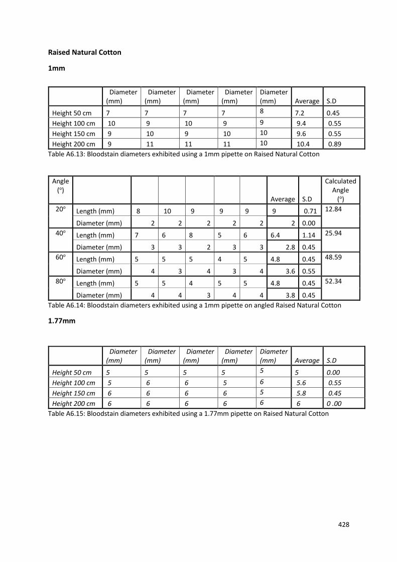
428
Raised Natural Cotton
1mm
Table A6.13: Bloodstain diameters exhibited using a 1mm pipette on Raised Natural Cotton
Table A6.14: Bloodstain diameters exhibited using a 1mm pipette on angled Raised Natural Cotton
1.77mm
Table A6.15: Bloodstain diameters exhibited using a 1.77mm pipette on Raised Natural Cotton
Diameter (mm)
Diameter (mm)
Diameter (mm)
Diameter (mm)
Diameter (mm) Average S.D
Height 50 cm 7 7 7 7 8 7.2 0.45
Height 100 cm 10 9 10 9 9 9.4 0.55
Height 150 cm 9 10 9 10 10 9.6 0.55
Height 200 cm 9 11 11 11 10 10.4 0.89
Angle (o)
Average S.D
Calculated Angle
(o)
20o Length (mm) 8 10 9 9 9 9 0.71 12.84
Diameter (mm) 2 2 2 2 2 2 0.00
40o Length (mm) 7 6 8 5 6 6.4 1.14 25.94
Diameter (mm) 3 3 2 3 3 2.8 0.45
60o Length (mm) 5 5 5 4 5 4.8 0.45 48.59
Diameter (mm) 4 3 4 3 4 3.6 0.55
80o Length (mm) 5 5 4 5 5 4.8 0.45 52.34
Diameter (mm) 4 4 3 4 4 3.8 0.45
Diameter (mm)
Diameter (mm)
Diameter (mm)
Diameter (mm)
Diameter (mm) Average S.D
Height 50 cm 5 5 5 5 5 5 0.00
Height 100 cm 5 6 6 5 6 5.6 0.55
Height 150 cm 6 6 6 6 5 5.8 0.45
Height 200 cm 6 6 6 6 6 6 0 .00

429
Table A6.16: Bloodstain diameters exhibited using a 1mm pipette on angled Raised Natural Cotton
Heavyweight Cotton
1mm
Table A6.17: Bloodstain diameters exhibited using a 1mm pipette on Heavyweight Cotton
Table A6.18: Bloodstain diameters exhibited using a 1mm pipette on angled Heavyweight Cotton
Angle (o)
Average S.D
Calculated Angle
(o)
20o Length (mm) 14 12 14 11 13 12.8 1.30 11.72
Diameter (mm) 2 3 3 2 3 2.6 0.55
40o Length (mm) 9 10 8 8 9 8.8 0.84 22.73
Diameter (mm) 4 4 3 3 3 3.4 0.55
60o Length (mm) 6 5 5 6 6 5.6 0.55 45.58
Diameter (mm) 4 4 4 4 4 4 0.00
80o Length (mm) 5 5 5 5 5 5 0.00 53.13
Diameter (mm) 4 4 4 4 4 4 0.00
Diameter (mm)
Diameter (mm)
Diameter (mm)
Diameter (mm)
Diameter (mm) Average S.D
Height 50 cm 10 10 10 10 10 10 0.00
Height 100 cm 10 11 11 11 10 10.6 0.55
Height 150 cm 10 10 11 12 11 10.8 0.84
Height 200 cm 11 11 11 11 11 11 0.00
Angle (o)
Average S.D
Calculated Angle
(o)
20o Length (mm) 35 31 29 30 32 31.4 2.30 9.16
Diameter (mm) 5 5 5 5 5 5 0.00
40o Length (mm) 18 19 19 24 19 19.8 2.39 21.95
Diameter (mm) 7 8 8 7 7 7.4 0.55
60o Length (mm) 12 11 11 10 11 11 0.71 46.66
Diameter (mm) 8 8 8 8 8 8 0.00
80o Length (mm) 9 10 10 10 10 9.8 0.45 66.69
Diameter (mm) 9 9 9 9 9 9 0.00

430
1.77mm
Table A6.19: Bloodstain diameters exhibited using a 1.77mm pipette on Heavyweight Cotton
Table A6.20: Bloodstain diameters exhibited using a 1.77mm pipette on angled Heavyweight Cotton.
Peasant Cotton
1mm
Table A6.21: Bloodstain diameters exhibited using a 1mm pipette on Peasant Cotton.
Diameter (mm)
Diameter (mm)
Diameter (mm)
Diameter (mm)
Diameter (mm) Average S.D
Height 50 cm 12 12 12 12 12 12 0.00
Height 100 cm 12 12 12 13 13 12.4 0.55
Height 150 cm 12 12 13 13 13 12.6 0.55
Height 200 cm 13 12 13 13 13 12.8 0.45
Diameter (mm)
Diameter (mm)
Diameter (mm)
Diameter (mm)
Diameter (mm) Average S.D
Height 50 cm 4 4 4 4 4 4 0.00
Height 100 cm 5 5 5 5 5 5 0.00
Height 150 cm 6 5 6 5 6 5.6 0.55
Height 200 cm 7 6 6 6 6 6.2 0.45
Angle (o)
Average S.D
Calculated Angle
(o)
20o Length (mm) 35 34 37 33 36 35 1.58 8.54
Diameter (mm) 5 5 5 6 5 5.2 0.45
40o Length (mm) 21 20 20 21 20 20.4 0.55 23.70
Diameter (mm) 7 8 9 9 8 8.2 0.84
60o Length (mm) 13 12 14 14 14 13.4 0.89 47
Diameter (mm) 10 9 10 10 10 9.8 0.45
80o Length (mm) 12 12 12 12 11 11.8 0.45 68.78
Diameter (mm) 11 11 11 11 11 11 0.00
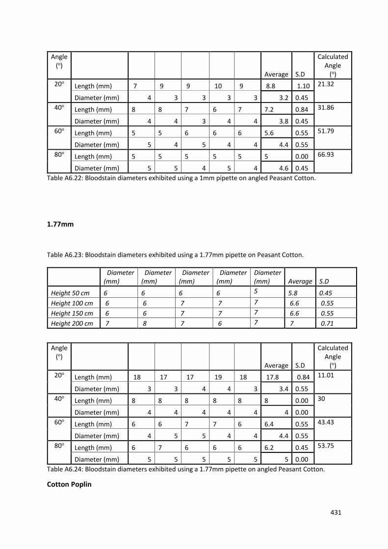
431
Table A6.22: Bloodstain diameters exhibited using a 1mm pipette on angled Peasant Cotton.
1.77mm
Table A6.23: Bloodstain diameters exhibited using a 1.77mm pipette on Peasant Cotton.
Table A6.24: Bloodstain diameters exhibited using a 1.77mm pipette on angled Peasant Cotton.
Cotton Poplin
Angle (o)
Average S.D
Calculated Angle
(o)
20o Length (mm) 7 9 9 10 9 8.8 1.10 21.32
Diameter (mm) 4 3 3 3 3 3.2 0.45
40o Length (mm) 8 8 7 6 7 7.2 0.84 31.86
Diameter (mm) 4 4 3 4 4 3.8 0.45
60o Length (mm) 5 5 6 6 6 5.6 0.55 51.79
Diameter (mm) 5 4 5 4 4 4.4 0.55
80o Length (mm) 5 5 5 5 5 5 0.00 66.93
Diameter (mm) 5 5 4 5 4 4.6 0.45
Diameter (mm)
Diameter (mm)
Diameter (mm)
Diameter (mm)
Diameter (mm) Average S.D
Height 50 cm 6 6 6 6 5 5.8 0.45
Height 100 cm 6 6 7 7 7 6.6 0.55
Height 150 cm 6 6 7 7 7 6.6 0.55
Height 200 cm 7 8 7 6 7 7 0.71
Angle (o)
Average S.D
Calculated Angle
(o)
20o Length (mm) 18 17 17 19 18 17.8 0.84 11.01
Diameter (mm) 3 3 4 4 3 3.4 0.55
40o Length (mm) 8 8 8 8 8 8 0.00 30
Diameter (mm) 4 4 4 4 4 4 0.00
60o Length (mm) 6 6 7 7 6 6.4 0.55 43.43
Diameter (mm) 4 5 5 4 4 4.4 0.55
80o Length (mm) 6 7 6 6 6 6.2 0.45 53.75
Diameter (mm) 5 5 5 5 5 5 0.00
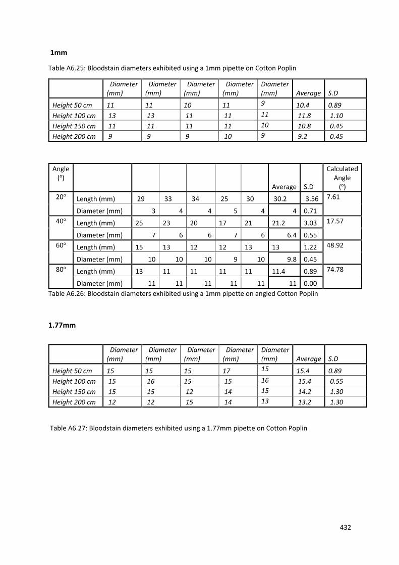
432
1mm
Table A6.25: Bloodstain diameters exhibited using a 1mm pipette on Cotton Poplin
Table A6.26: Bloodstain diameters exhibited using a 1mm pipette on angled Cotton Poplin
1.77mm
Table A6.27: Bloodstain diameters exhibited using a 1.77mm pipette on Cotton Poplin
Diameter (mm)
Diameter (mm)
Diameter (mm)
Diameter (mm)
Diameter (mm) Average S.D
Height 50 cm 11 11 10 11 9 10.4 0.89
Height 100 cm 13 13 11 11 11 11.8 1.10
Height 150 cm 11 11 11 11 10 10.8 0.45
Height 200 cm 9 9 9 10 9 9.2 0.45
Angle (o)
Average S.D
Calculated Angle
(o)
20o Length (mm) 29 33 34 25 30 30.2 3.56 7.61
Diameter (mm) 3 4 4 5 4 4 0.71
40o Length (mm) 25 23 20 17 21 21.2 3.03 17.57
Diameter (mm) 7 6 6 7 6 6.4 0.55
60o Length (mm) 15 13 12 12 13 13 1.22 48.92
Diameter (mm) 10 10 10 9 10 9.8 0.45
80o Length (mm) 13 11 11 11 11 11.4 0.89 74.78
Diameter (mm) 11 11 11 11 11 11 0.00
Diameter (mm)
Diameter (mm)
Diameter (mm)
Diameter (mm)
Diameter (mm) Average S.D
Height 50 cm 15 15 15 17 15 15.4 0.89
Height 100 cm 15 16 15 15 16 15.4 0.55
Height 150 cm 15 15 12 14 15 14.2 1.30
Height 200 cm 12 12 15 14 13 13.2 1.30
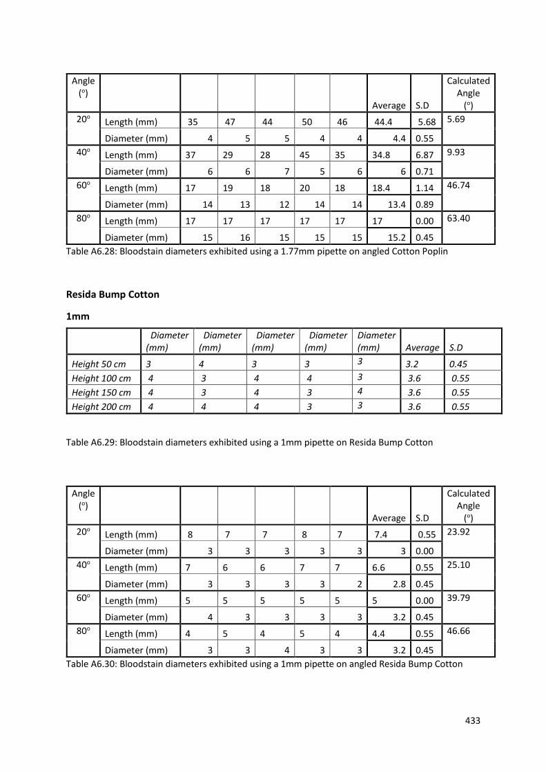
433
Table A6.28: Bloodstain diameters exhibited using a 1.77mm pipette on angled Cotton Poplin
Resida Bump Cotton
1mm
Table A6.29: Bloodstain diameters exhibited using a 1mm pipette on Resida Bump Cotton
Table A6.30: Bloodstain diameters exhibited using a 1mm pipette on angled Resida Bump Cotton
Angle (o)
Average S.D
Calculated Angle
(o)
20o Length (mm) 35 47 44 50 46 44.4 5.68 5.69
Diameter (mm) 4 5 5 4 4 4.4 0.55
40o Length (mm) 37 29 28 45 35 34.8 6.87 9.93
Diameter (mm) 6 6 7 5 6 6 0.71
60o Length (mm) 17 19 18 20 18 18.4 1.14 46.74
Diameter (mm) 14 13 12 14 14 13.4 0.89
80o Length (mm) 17 17 17 17 17 17 0.00 63.40
Diameter (mm) 15 16 15 15 15 15.2 0.45
Diameter (mm)
Diameter (mm)
Diameter (mm)
Diameter (mm)
Diameter (mm) Average S.D
Height 50 cm 3 4 3 3 3 3.2 0.45
Height 100 cm 4 3 4 4 3 3.6 0.55
Height 150 cm 4 3 4 3 4 3.6 0.55
Height 200 cm 4 4 4 3 3 3.6 0.55
Angle (o)
Average S.D
Calculated Angle
(o)
20o Length (mm) 8 7 7 8 7 7.4 0.55 23.92
Diameter (mm) 3 3 3 3 3 3 0.00
40o Length (mm) 7 6 6 7 7 6.6 0.55 25.10
Diameter (mm) 3 3 3 3 2 2.8 0.45
60o Length (mm) 5 5 5 5 5 5 0.00 39.79
Diameter (mm) 4 3 3 3 3 3.2 0.45
80o Length (mm) 4 5 4 5 4 4.4 0.55 46.66
Diameter (mm) 3 3 4 3 3 3.2 0.45

434
1.77mm
Table A6.31: Bloodstain diameters exhibited using a 1.77mm pipette on Resida Bump Cotton
Table A6.32: Bloodstain diameters exhibited using a 1.77mm pipette on angled Resida Bump Cotton
Fuji Silk
1mm
Table A6.33: Bloodstain diameters exhibited using a 1mm pipette on Fuji Silk
Diameter (mm)
Diameter (mm)
Diameter (mm)
Diameter (mm)
Diameter (mm) Average S.D
Height 50 cm 5 4 4 4 5 4.4 0.55
Height 100 cm 4 4 5 4 5 4.4 0.55
Height 150 cm 4 5 5 5 5 4.8 0.45
Height 200 cm 5 5 5 5 5 5 0.00
Angle (o)
Average S.D
Calculated Angle
(o)
20o Length (mm) 12 15 15 14 14 14 1.22 14.06
Diameter (mm) 4 4 3 3 3 3.4 0.55
40o Length (mm) 9 9 9 9 9 9 0.00 26.39
Diameter (mm) 4 4 5 3 4 4 0.71
60o Length (mm) 7 7 7 7 7 7 0.00 34.85
Diameter (mm) 4 4 4 4 4 4 0.00
80o Length (mm) 5 5 5 5 5 5 0.00 53.13
Diameter (mm) 4 4 4 4 4 4 0.00
Diameter (mm)
Diameter (mm)
Diameter (mm)
Diameter (mm)
Diameter (mm) Average S.D
Height 50 cm 13 14 14 14 16 14.2 1.09
Height 100 cm 15 15 14 14 14 14.4 0.55
Height 150 cm 12 14 14 14 13 13.4 0.89
Height 200 cm 14 15 15 15 15 14.8 0.45

435
Table A6.34: Bloodstain diameters exhibited using a 1mm pipette on angld Fuji Silk
1.77mm
Table A6.35: Bloodstain diameters exhibited using a 1.77mm pipette on angled Fuji Silk
Table A6.36: Bloodstain diameters exhibited using a 1.77mm pipette on Fuji Silk
Angle (o)
Average S.D
Calculated Angle
(o)
20o Length (mm) 31 23 33 32 32 30.2 4.09 20.55
Diameter (mm) 10 11 11 11 10 10.6 0.55
40o Length (mm) 25 25 24 24 25 24.6 0.55 31.90
Diameter (mm) 12 12 14 14 13 13 1
60o Length (mm) 20 20 21 20 20 20.2 0.45 53.32
Diameter (mm) 17 16 16 16 16 16.2 0.45
80o Length (mm) 16 18 18 18 16 17.2 1.10 66.72
Diameter (mm) 14 16 17 17 15 15.8 1.30
Diameter (mm)
Diameter (mm)
Diameter (mm)
Diameter (mm)
Diameter (mm) Average S.D
Height 50 cm 17 17 17 16 16 16.6 0.55
Height 100 cm 19 18 17 17 18 17.8 0.84
Height 150 cm 17 18 17 18 18 17.6 0.55
Height 200 cm 18 20 19 17 19 18.6 1.14
Angle (o)
Average S.D
Calculated Angle
(o)
20o Length (mm) 54 42 40 46 52 46.8 6.10 13.85
Diameter (mm) 11 12 12 11 10 11.2 0.84
40o Length (mm) 26 29 32 34 31 30.4 3.05 31.76
Diameter (mm) 16 16 16 16 16 16 0.00
60o Length (mm) 21 25 26 22 24 23.6 2.07 53.62
Diameter (mm) 19 19 19 19 19 19 0.00
80o Length (mm) 20 22 22 22 22 21.6 0.89 66.44
Diameter (mm) 19 21 19 20 20 19.8 0.84

436
Medium Habotai Silk
1mm
Table A6.37: Bloodstain diameters exhibited using a 1mm pipette on Medium Habotai Silk
Table A6.38: Bloodstain diameters exhibited using a 1mm pipette on angled Medium Habotai Silk
1.77mm
Table A6.39: Bloodstain diameters exhibited using a 1.77mm pipette on Medium Habotai Silk
Diameter (mm)
Diameter (mm)
Diameter (mm)
Diameter (mm)
Diameter (mm) Average S.D
Height 50 cm 10 10 10 10 10 10 0.00
Height 100 cm 9 9 9 9 10 9.2 0.45
Height 150 cm 10 10 10 10 10 10 0.00
Height 200 cm 10 11 11 11 11 10.8 0.45
Angle (o)
Average S.D
Calculated Angle
(o)
20o Length (mm) 44 49 45 50 46 46.8 2.59 17.15
Diameter (mm) 10 9 16 19 15 13.8 4.21
40o Length (mm) 38 32 36 32 31 84.5 3.03 14.81
Diameter (mm) 19 21 21 24 23 21.6 1.95
60o Length (mm) 27 28 27 27 29 27.6 0.89 58.77
Diameter (mm) 22 25 23 25 23 23.6 1.34
80o Length (mm) 28 25 25 29 25 26.4 1.95 61.50
Diameter (mm) 21 24 25 24 25 23.2 1.64
Diameter (mm)
Diameter (mm)
Diameter (mm)
Diameter (mm)
Diameter (mm) Average S.D
Height 50 cm 18 18 18 17 18 17.8 0.45
Height 100 cm 17 17 16 17 18 17 0.71
Height 150 cm 17 18 18 18 18 17.8 0.45
Height 200 cm 19 19 19 19 18 18.8 0.45
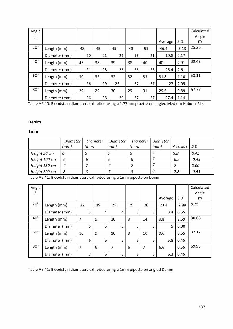
437
Table A6.40: Bloodstain diameters exhibited using a 1.77mm pipette on angled Medium Habotai Silk.
Denim
1mm
Table A6.41: Bloodstain diameters exhibited using a 1mm pipette on Denim
Table A6.41: Bloodstain diameters exhibited using a 1mm pipette on angled Denim
Angle (o)
Average S.D
Calculated Angle
(o)
20o Length (mm) 48 45 45 43 51 46.4 3.13 25.26
Diameter (mm) 20 21 21 16 21 19.8 2.17
40o Length (mm) 45 38 39 38 40 40 2.91 39.42
Diameter (mm) 21 28 26 26 26 25.4 2.61
60o Length (mm) 30 32 32 32 33 31.8 1.10 58.11
Diameter (mm) 26 29 26 27 27 27 2.05
80o Length (mm) 29 29 30 29 31 29.6 0.89 67.77
Diameter (mm) 26 28 29 27 27 27.4 1.14
Diameter (mm)
Diameter (mm)
Diameter (mm)
Diameter (mm)
Diameter (mm) Average S.D
Height 50 cm 6 6 6 6 5 5.8 0.45
Height 100 cm 6 6 6 6 7 6.2 0.45
Height 150 cm 7 7 7 7 7 7 0.00
Height 200 cm 8 8 7 8 8 7.8 0.45
Angle (o)
Average S.D
Calculated Angle
(o)
20o Length (mm) 22 19 25 25 26 23.4 2.88 8.35
Diameter (mm) 3 4 4 3 3 3.4 0.55
40o Length (mm) 7 9 10 9 14 9.8 2.59 30.68
Diameter (mm) 5 5 5 5 5 5 0.00
60o Length (mm) 10 9 10 9 10 9.6 0.55 37.17
Diameter (mm) 6 6 5 6 6 5.8 0.45
80o Length (mm) 7 6 7 6 7 6.6 0.55 69.95
Diameter (mm) 7 6 6 6 6 6.2 0.45

438
1.77mm
Table A6.42: Bloodstain diameters exhibited using a 1.77mm pipette on Denim
Table A6.43: Bloodstain diameters exhibited using a 1.77mm pipette on angled Denim
M&S T-Shirt Jersey
1mm
Table A6.44: Bloodstain diameters exhibited using a 1mm pipette on M & S Jersey
Diameter (mm)
Diameter (mm)
Diameter (mm)
Diameter (mm)
Diameter (mm) Average S.D
Height 50 cm 13 13 14 14 14 13.6 0.55
Height 100 cm 14 15 15 14 15 14.6 0.55
Height 150 cm 15 16 15 16 15 15.4 0.55
Height 200 cm 15 15 16 16 15 15.4 0.55
Angle (o)
Average S.D
Calculated Angle
(o)
20o Length (mm) 25 31 31 32 29 29.6 2.79 8.16
Diameter (mm) 4 5 4 4 4 4.2 0.45
40o Length (mm) 12 14 15 15 15 14.2 1.30 27.70
Diameter (mm) 6 6 7 7 7 6.6 0.55
60o Length (mm) 9 11 12 11 11 10.8 1.10 39.02
Diameter (mm) 6 7 6 8 7 6.8 0.84
80o Length (mm) 9 9 10 10 10 9.6 0.55 54.34
Diameter (mm) 8 8 8 8 7 7.8 0.45
Diameter (mm)
Diameter (mm)
Diameter (mm)
Diameter (mm)
Diameter (mm) Average S.D
Height 50 cm 8 8 9 9 8 8.4 0.55
Height 100 cm 9 9 10 10 9 9.4 0.55
Height 150 cm 10 9 10 11 11 10.2 0.84
Height 200 cm 11 12 11 11 10 11 0.71

439
Table A6.45: Bloodstain diameters exhibited using a 1mm pipette on angled M & S Jersey
1.77mm
Table A6.46: Bloodstain diameters exhibited using a 1.77mm pipette on M & S Jersey
Table A6.47: Bloodstain diameters exhibited using a 1.77mm pipette on angled M & S Jersey.
Angle (o)
Average S.D
Calculated Angle
(o)
20o Length (mm) 25 30 30 31 24 28 3.25 14.06
Diameter (mm) 7 7 6 7 7 6.8 0.45
40o Length (mm) 15 14 14 15 16 14.8 0.84 37.45
Diameter (mm) 9 9 9 9 9 9 0.00
60o Length (mm) 12 12 12 13 13 12.4 0.55 52.22
Diameter (mm) 10 9 10 10 10 9.8 0.45
80o Length (mm) 11 12 12 12 12 11.8 0.45 66.24
Diameter (mm) 10 10 12 11 11 10.8 0.84
Diameter (mm)
Diameter (mm)
Diameter (mm)
Diameter (mm)
Diameter (mm) Average S.D
Height 50 cm 13 13 14 14 13 13.4 0.55
Height 100 cm 14 16 14 14 15 14.6 0.89
Height 150 cm 15 15 16 16 16 15.6 0.55
Height 200 cm 14 14 14 15 15 14.4 0.55
Angle (o)
Average S.D
Calculated Angle
(o)
20o Length (mm) 27 27 30 24 32 28 3.08 15.75
Diameter (mm) 8 8 7 8 7 7.6 0.55
40o Length (mm) 21 23 18 20 17 19.8 2.39 31.01
Diameter (mm) 10 10 10 10 11 10.2 0.45
60o Length (mm) 15 17 17 15 17 16.2 1.10 48.86
Diameter (mm) 12 13 12 12 12 12.2 0.45
80o Length (mm) 13 14 14 15 16 14.4 1.14 66.44
Diameter (mm) 12 13 13 13 15 13.2 1.10
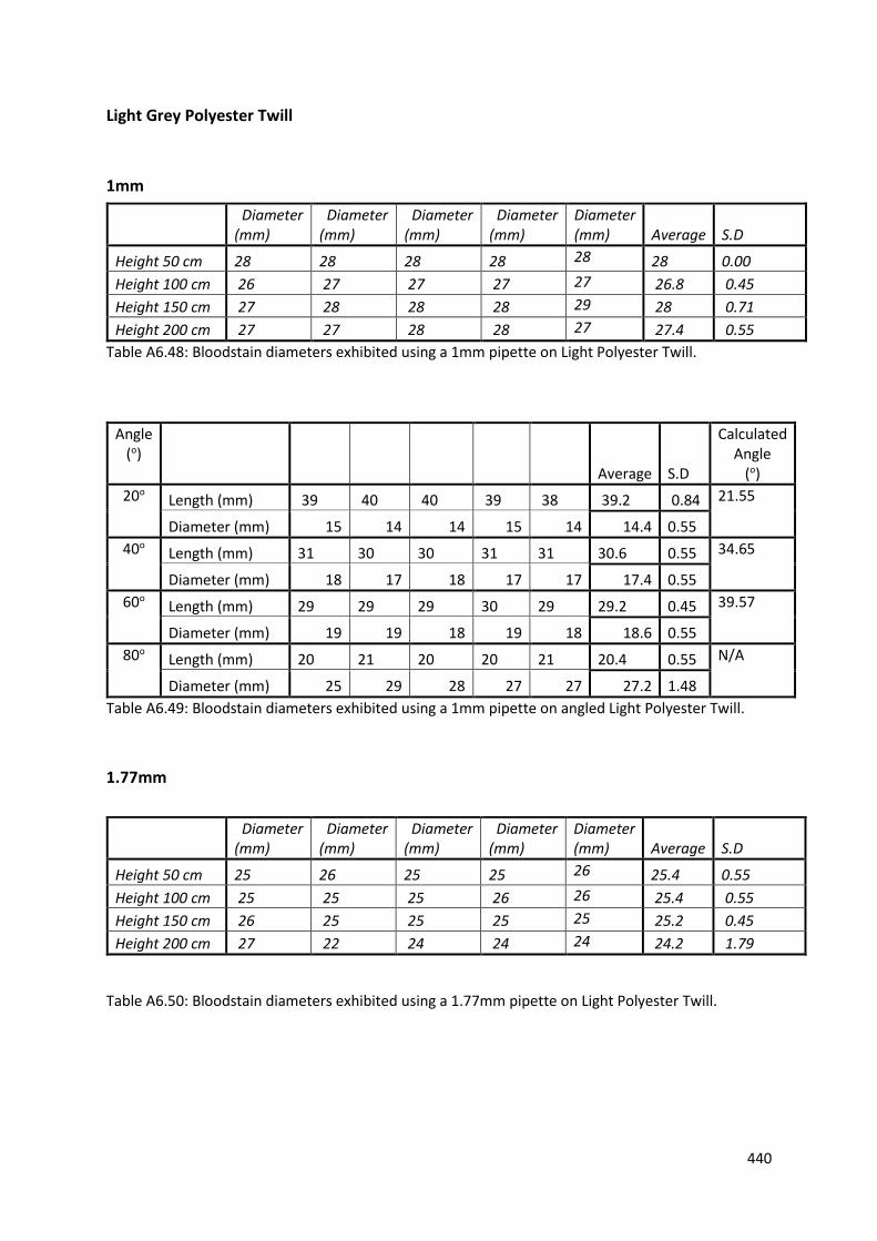
440
Light Grey Polyester Twill
1mm
Table A6.48: Bloodstain diameters exhibited using a 1mm pipette on Light Polyester Twill.
Table A6.49: Bloodstain diameters exhibited using a 1mm pipette on angled Light Polyester Twill.
1.77mm
Table A6.50: Bloodstain diameters exhibited using a 1.77mm pipette on Light Polyester Twill.
Diameter (mm)
Diameter (mm)
Diameter (mm)
Diameter (mm)
Diameter (mm) Average S.D
Height 50 cm 28 28 28 28 28 28 0.00
Height 100 cm 26 27 27 27 27 26.8 0.45
Height 150 cm 27 28 28 28 29 28 0.71
Height 200 cm 27 27 28 28 27 27.4 0.55
Angle (o)
Average S.D
Calculated Angle
(o)
20o Length (mm) 39 40 40 39 38 39.2 0.84 21.55
Diameter (mm) 15 14 14 15 14 14.4 0.55
40o Length (mm) 31 30 30 31 31 30.6 0.55 34.65
Diameter (mm) 18 17 18 17 17 17.4 0.55
60o Length (mm) 29 29 29 30 29 29.2 0.45 39.57
Diameter (mm) 19 19 18 19 18 18.6 0.55
80o Length (mm) 20 21 20 20 21 20.4 0.55 N/A
Diameter (mm) 25 29 28 27 27 27.2 1.48
Diameter (mm)
Diameter (mm)
Diameter (mm)
Diameter (mm)
Diameter (mm) Average S.D
Height 50 cm 25 26 25 25 26 25.4 0.55
Height 100 cm 25 25 25 26 26 25.4 0.55
Height 150 cm 26 25 25 25 25 25.2 0.45
Height 200 cm 27 22 24 24 24 24.2 1.79
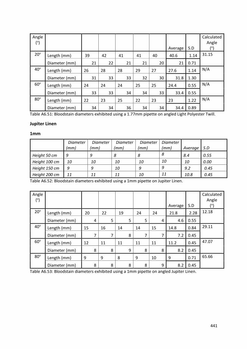
441
Table A6.51: Bloodstain diameters exhibited using a 1.77mm pipette on angled Light Polyester Twill.
Jupiter Linen
1mm
Table A6.52: Bloodstain diameters exhibited using a 1mm pipette on Jupiter Linen.
Table A6.53: Bloodstain diameters exhibited using a 1mm pipette on angled Jupiter Linen.
Angle (o)
Average S.D
Calculated Angle
(o)
20o Length (mm) 39 42 41 41 40 40.6 1.14 31.15
Diameter (mm) 21 22 21 21 20 21 0.71
40o Length (mm) 26 28 28 29 27 27.6 1.14 N/A
Diameter (mm) 31 33 33 32 30 31.8 1.30
60o Length (mm) 24 24 24 25 25 24.4 0.55 N/A
Diameter (mm) 33 33 34 34 33 33.4 0.55
80o Length (mm) 22 23 25 22 23 23 1.22 N/A
Diameter (mm) 34 34 36 34 34 34.4 0.89
Diameter (mm)
Diameter (mm)
Diameter (mm)
Diameter (mm)
Diameter (mm) Average S.D
Height 50 cm 9 9 8 8 8 8.4 0.55
Height 100 cm 10 10 10 10 10 10 0.00
Height 150 cm 9 9 10 9 9 9.2 0.45
Height 200 cm 11 11 11 10 11 10.8 0.45
Angle (o)
Average S.D
Calculated Angle
(o)
20o Length (mm) 20 22 19 24 24 21.8 2.28 12.18
Diameter (mm) 4 5 5 5 4 4.6 0.55
40o Length (mm) 15 16 14 14 15 14.8 0.84 29.11
Diameter (mm) 7 7 8 7 7 7.2 0.45
60o Length (mm) 12 11 11 11 11 11.2 0.45 47.07
Diameter (mm) 8 8 9 8 8 8.2 0.45
80o Length (mm) 9 9 8 9 10 9 0.71 65.66
Diameter (mm) 8 8 8 8 9 8.2 0.45
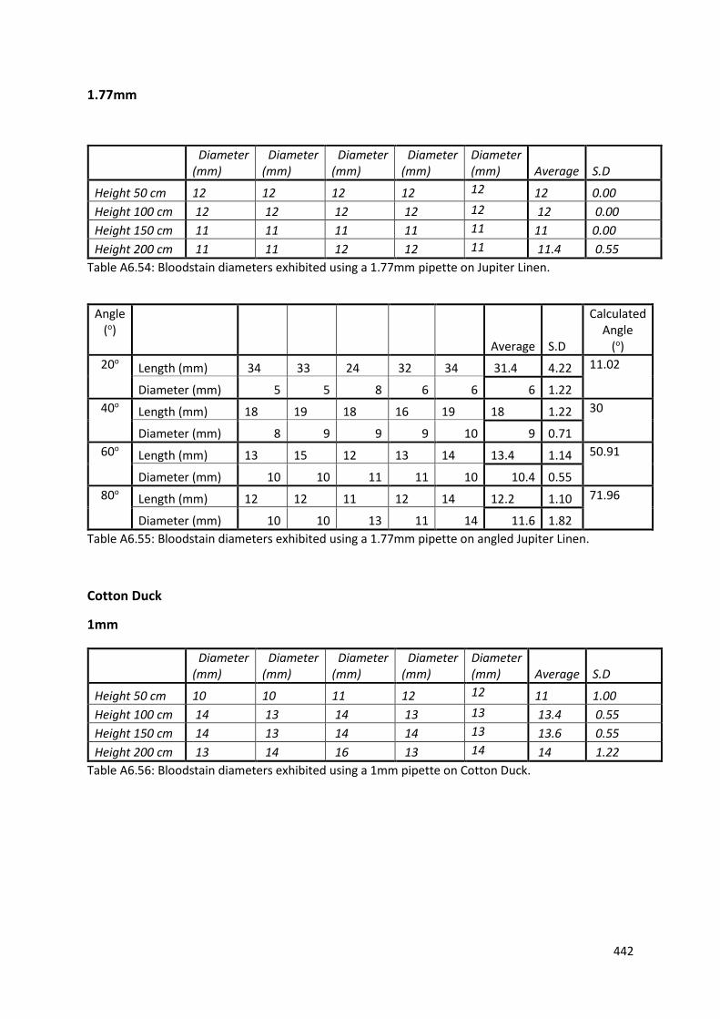
442
1.77mm
Table A6.54: Bloodstain diameters exhibited using a 1.77mm pipette on Jupiter Linen.
Table A6.55: Bloodstain diameters exhibited using a 1.77mm pipette on angled Jupiter Linen.
Cotton Duck
1mm
Table A6.56: Bloodstain diameters exhibited using a 1mm pipette on Cotton Duck.
Angle (o)
Average S.D
Calculated Angle
(o)
20o Length (mm) 34 33 24 32 34 31.4 4.22 11.02
Diameter (mm) 5 5 8 6 6 6 1.22
40o Length (mm) 18 19 18 16 19 18 1.22 30
Diameter (mm) 8 9 9 9 10 9 0.71
60o Length (mm) 13 15 12 13 14 13.4 1.14 50.91
Diameter (mm) 10 10 11 11 10 10.4 0.55
80o Length (mm) 12 12 11 12 14 12.2 1.10 71.96
Diameter (mm) 10 10 13 11 14 11.6 1.82
Diameter (mm)
Diameter (mm)
Diameter (mm)
Diameter (mm)
Diameter (mm) Average S.D
Height 50 cm 12 12 12 12 12 12 0.00
Height 100 cm 12 12 12 12 12 12 0.00
Height 150 cm 11 11 11 11 11 11 0.00
Height 200 cm 11 11 12 12 11 11.4 0.55
Diameter (mm)
Diameter (mm)
Diameter (mm)
Diameter (mm)
Diameter (mm) Average S.D
Height 50 cm 10 10 11 12 12 11 1.00
Height 100 cm 14 13 14 13 13 13.4 0.55
Height 150 cm 14 13 14 14 13 13.6 0.55
Height 200 cm 13 14 16 13 14 14 1.22
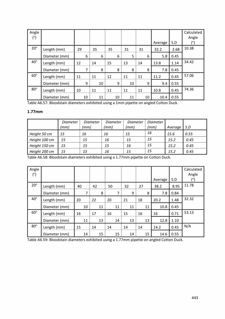
443
Table A6.57: Bloodstain diameters exhibited using a 1mm pipette on angled Cotton Duck.
1.77mm
Table A6.58: Bloodstain diameters exhibited using a 1.77mm pipette on Cotton Duck.
Table A6.59: Bloodstain diameters exhibited using a 1.77mm pipette on angled Cotton Duck.
Angle (o)
Average S.D
Calculated Angle
(o)
20o Length (mm) 29 35 35 31 31 32.2 2.68 10.38
Diameter (mm) 6 6 6 5 6 5.8 0.45
40o Length (mm) 12 14 15 13 14 13.8 1.14 34.42
Diameter (mm) 7 8 8 8 8 7.8 0.45
60o Length (mm) 11 11 12 11 11 11.2 0.45 57.06
Diameter (mm) 9 10 9 10 9 9.4 0.55
80o Length (mm) 10 11 11 11 11 10.8 0.45 74.36
Diameter (mm) 10 11 10 11 10 10.4 0.55
Diameter (mm)
Diameter (mm)
Diameter (mm)
Diameter (mm)
Diameter (mm) Average S.D
Height 50 cm 15 16 16 15 16 15.6 0.55
Height 100 cm 15 15 16 15 15 15.2 0.45
Height 150 cm 15 15 15 16 15 15.2 0.45
Height 200 cm 15 15 16 15 15 15.2 0.45
Angle (o)
Average S.D
Calculated Angle
(o)
20o Length (mm) 40 42 50 32 27 38.2 8.95 11.78
Diameter (mm) 7 8 7 9 8 7.8 0.84
40o Length (mm) 20 22 20 21 18 20.2 1.48 32.32
Diameter (mm) 10 11 11 11 11 10.8 0.45
60o Length (mm) 16 17 16 15 16 16 0.71 53.13
Diameter (mm) 11 13 14 13 13 12.8 1.10
80o Length (mm) 15 14 14 14 14 14.2 0.45 N/A
Diameter (mm) 14 15 15 14 15 14.6 0.55
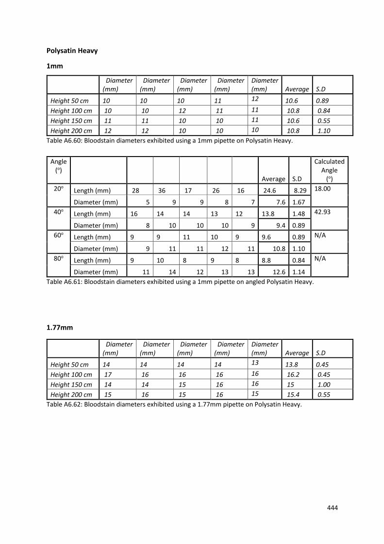
444
Polysatin Heavy
1mm
Table A6.60: Bloodstain diameters exhibited using a 1mm pipette on Polysatin Heavy.
Table A6.61: Bloodstain diameters exhibited using a 1mm pipette on angled Polysatin Heavy.
1.77mm
Table A6.62: Bloodstain diameters exhibited using a 1.77mm pipette on Polysatin Heavy.
Diameter (mm)
Diameter (mm)
Diameter (mm)
Diameter (mm)
Diameter (mm) Average S.D
Height 50 cm 10 10 10 11 12 10.6 0.89
Height 100 cm 10 10 12 11 11 10.8 0.84
Height 150 cm 11 11 10 10 11 10.6 0.55
Height 200 cm 12 12 10 10 10 10.8 1.10
Angle (o)
Average S.D
Calculated Angle
(o)
20o Length (mm) 28 36 17 26 16 24.6 8.29 18.00
Diameter (mm) 5 9 9 8 7 7.6 1.67
40o Length (mm) 16 14 14 13 12 13.8 1.48 42.93
Diameter (mm) 8 10 10 10 9 9.4 0.89
60o Length (mm) 9 9 11 10 9 9.6 0.89 N/A
Diameter (mm) 9 11 11 12 11 10.8 1.10
80o Length (mm) 9 10 8 9 8 8.8 0.84 N/A
Diameter (mm) 11 14 12 13 13 12.6 1.14
Diameter (mm)
Diameter (mm)
Diameter (mm)
Diameter (mm)
Diameter (mm) Average S.D
Height 50 cm 14 14 14 14 13 13.8 0.45
Height 100 cm 17 16 16 16 16 16.2 0.45
Height 150 cm 14 14 15 16 16 15 1.00
Height 200 cm 15 16 15 16 15 15.4 0.55
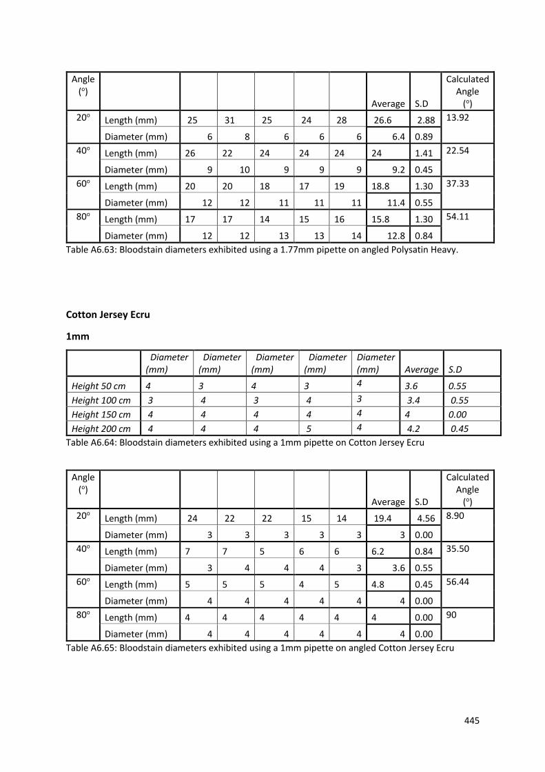
445
Table A6.63: Bloodstain diameters exhibited using a 1.77mm pipette on angled Polysatin Heavy.
Cotton Jersey Ecru
1mm
Table A6.64: Bloodstain diameters exhibited using a 1mm pipette on Cotton Jersey Ecru
Table A6.65: Bloodstain diameters exhibited using a 1mm pipette on angled Cotton Jersey Ecru
Angle (o)
Average S.D
Calculated Angle
(o)
20o Length (mm) 25 31 25 24 28 26.6 2.88 13.92
Diameter (mm) 6 8 6 6 6 6.4 0.89
40o Length (mm) 26 22 24 24 24 24 1.41 22.54
Diameter (mm) 9 10 9 9 9 9.2 0.45
60o Length (mm) 20 20 18 17 19 18.8 1.30 37.33
Diameter (mm) 12 12 11 11 11 11.4 0.55
80o Length (mm) 17 17 14 15 16 15.8 1.30 54.11
Diameter (mm) 12 12 13 13 14 12.8 0.84
Diameter (mm)
Diameter (mm)
Diameter (mm)
Diameter (mm)
Diameter (mm) Average S.D
Height 50 cm 4 3 4 3 4 3.6 0.55
Height 100 cm 3 4 3 4 3 3.4 0.55
Height 150 cm 4 4 4 4 4 4 0.00
Height 200 cm 4 4 4 5 4 4.2 0.45
Angle (o)
Average S.D
Calculated Angle
(o)
20o Length (mm) 24 22 22 15 14 19.4 4.56 8.90
Diameter (mm) 3 3 3 3 3 3 0.00
40o Length (mm) 7 7 5 6 6 6.2 0.84 35.50
Diameter (mm) 3 4 4 4 3 3.6 0.55
60o Length (mm) 5 5 5 4 5 4.8 0.45 56.44
Diameter (mm) 4 4 4 4 4 4 0.00
80o Length (mm) 4 4 4 4 4 4 0.00 90
Diameter (mm) 4 4 4 4 4 4 0.00

446
1.77mm
Table A6.66: Bloodstain diameters exhibited using a 1.77mm pipette on Cotton Jersey Ecru.
Table A6.67: Bloodstain diameters exhibited using a 1.77mm pipette on angled Cotton Jersey Ecru
Wool Mix Suiting
1mm
Table A6.68: Bloodstain diameters exhibited using a 1mm pipette on Wool Mix Suiting
Diameter (mm)
Diameter (mm)
Diameter (mm)
Diameter (mm)
Diameter (mm) Average S.D
Height 50 cm 5 5 5 5 5 5 0.00
Height 100 cm 5 5 6 6 6 5.6 0.55
Height 150 cm 5 6 5 6 5 5.4 0.55
Height 200 cm 6 6 6 6 6 6 0.00
Angle (o)
Average S.D
Calculated Angle
(o)
20o Length (mm) 15 16 22 23 18 18.8 3.56 10.42
Diameter (mm) 3 3 3 3 5 3.4 0.89
40o Length (mm) 6 7 7 7 7 6.8 0.45 36.03
Diameter (mm) 4 4 4 4 4 4 0.00
60o Length (mm) 5 6 5 6 6 5.6 0.55 51.79
Diameter (mm) 4 4 5 5 4 4.4 0.55
80o Length (mm) 5 5 5 5 5 5 0.00 N/A
Diameter (mm) 6 5 5 6 5 5.4 0.55
Diameter (mm)
Diameter (mm)
Diameter (mm)
Diameter (mm)
Diameter (mm) Average S.D
Height 50 cm 7 7 7 7 7 7 0.00
Height 100 cm 9 9 9 9 9 9 0.00
Height 150 cm 10 10 10 10 10 10 0.00
Height 200 cm 10 10 10 11 11 10.4 0.55
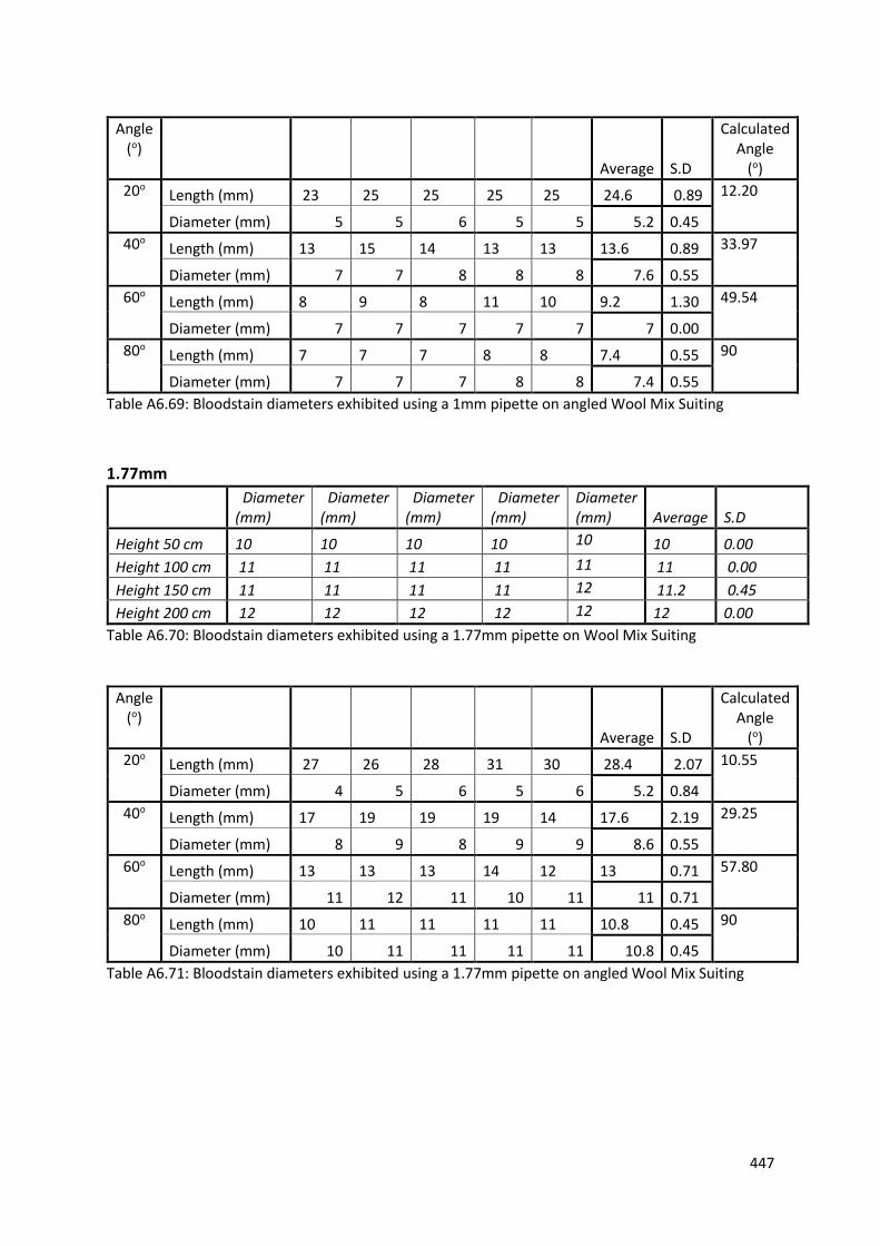
447
Table A6.69: Bloodstain diameters exhibited using a 1mm pipette on angled Wool Mix Suiting
1.77mm
Table A6.70: Bloodstain diameters exhibited using a 1.77mm pipette on Wool Mix Suiting
Table A6.71: Bloodstain diameters exhibited using a 1.77mm pipette on angled Wool Mix Suiting
Angle (o)
Average S.D
Calculated Angle
(o)
20o Length (mm) 23 25 25 25 25 24.6 0.89 12.20
Diameter (mm) 5 5 6 5 5 5.2 0.45
40o Length (mm) 13 15 14 13 13 13.6 0.89 33.97
Diameter (mm) 7 7 8 8 8 7.6 0.55
60o Length (mm) 8 9 8 11 10 9.2 1.30 49.54
Diameter (mm) 7 7 7 7 7 7 0.00
80o Length (mm) 7 7 7 8 8 7.4 0.55 90
Diameter (mm) 7 7 7 8 8 7.4 0.55
Diameter (mm)
Diameter (mm)
Diameter (mm)
Diameter (mm)
Diameter (mm) Average S.D
Height 50 cm 10 10 10 10 10 10 0.00
Height 100 cm 11 11 11 11 11 11 0.00
Height 150 cm 11 11 11 11 12 11.2 0.45
Height 200 cm 12 12 12 12 12 12 0.00
Angle (o)
Average S.D
Calculated Angle
(o)
20o Length (mm) 27 26 28 31 30 28.4 2.07 10.55
Diameter (mm) 4 5 6 5 6 5.2 0.84
40o Length (mm) 17 19 19 19 14 17.6 2.19 29.25
Diameter (mm) 8 9 8 9 9 8.6 0.55
60o Length (mm) 13 13 13 14 12 13 0.71 57.80
Diameter (mm) 11 12 11 10 11 11 0.71
80o Length (mm) 10 11 11 11 11 10.8 0.45 90
Diameter (mm) 10 11 11 11 11 10.8 0.45
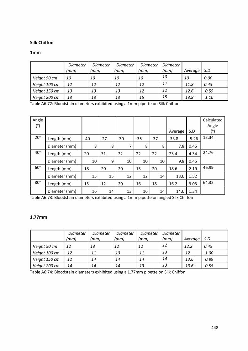
448
Silk Chiffon
1mm
Table A6.72: Bloodstain diameters exhibited using a 1mm pipette on Silk Chiffon
Table A6.73: Bloodstain diameters exhibited using a 1mm pipette on angled Silk Chiffon
1.77mm
Table A6.74: Bloodstain diameters exhibited using a 1.77mm pipette on Silk Chiffon
Diameter (mm)
Diameter (mm)
Diameter (mm)
Diameter (mm)
Diameter (mm) Average S.D
Height 50 cm 10 10 10 10 10 10 0.00
Height 100 cm 12 12 12 12 11 11.8 0.45
Height 150 cm 13 13 13 12 12 12.6 0.55
Height 200 cm 13 13 13 15 15 13.8 1.10
Angle (o)
Average S.D
Calculated Angle
(o)
20o Length (mm) 40 27 30 35 37 33.8 5.26 13.34
Diameter (mm) 8 8 7 8 8 7.8 0.45
40o Length (mm) 20 31 22 22 22 23.4 4.34 24.76
Diameter (mm) 10 9 10 10 10 9.8 0.45
60o Length (mm) 18 20 20 15 20 18.6 2.19 46.99
Diameter (mm) 15 15 12 12 14 13.6 1.52
80o Length (mm) 15 12 20 16 18 16.2 3.03 64.32
Diameter (mm) 16 14 13 16 14 14.6 1.34
Diameter (mm)
Diameter (mm)
Diameter (mm)
Diameter (mm)
Diameter (mm) Average S.D
Height 50 cm 12 13 12 12 12 12.2 0.45
Height 100 cm 12 11 13 11 13 12 1.00
Height 150 cm 12 14 14 14 14 13.6 0.89
Height 200 cm 14 14 14 13 13 13.6 0.55

449
Table A6.75: Bloodstain diameters exhibited using a 1.77mm pipette on angled Silk Chiffon
Silk Dupion
1mm
Table A6.76: Bloodstain diameters exhibited using a 1mm pipette on Silk Dupion.
Table A6.77: Bloodstain diameters exhibited using a 1mm pipette on angled Silk Dupion.
Angle (o)
Average S.D
Calculated Angle
(o)
20o Length (mm) 53 38 50 46 37 44.8 7.12 15.27
Diameter (mm) 11 11 10 13 14 11.8 1.64
40o Length (mm) 29 31 30 31 39 32 4 40.07
Diameter (mm) 20 24 24 19 16 20.6 3.44
60o Length (mm) 19 19 29 20 23 22 4.24 51.43
Diameter (mm) 17 18 18 17 16 17.2 0.84
80o Length (mm) 17 17 21 19 21 19 2 N/A
Diameter (mm) 17 19 20 21 19 19.2 1.48
Diameter (mm)
Diameter (mm)
Diameter (mm)
Diameter (mm)
Diameter (mm) Average S.D
Height 50 cm 9 10 9 8 9 9 0.71
Height 100 cm 9 9 11 11 9 9.8 1.10
Height 150 cm 10 10 10 9 10 9.8 0.45
Height 200 cm 11 10 9 10 10 10 0.71
Angle (o)
Average S.D
Calculated Angle
(o)
20o Length (mm) 12 27 24 17 29 21.8 7.12 11.64
Diameter (mm) 5 5 4 4 4 4.4 0.55
40o Length (mm) 11 10 11 10 13 11 1.22 33.06
Diameter (mm) 5 6 7 6 6 6 0.71
60o Length (mm) 11 12 10 11 12 11.2 0.84 38.68
Diameter (mm) 7 7 8 7 6 7 0.71
80o Length (mm) 9 10 9 9 8 9 0.71 43.55
Diameter (mm) 6 6 7 6 6 6.2 0.45
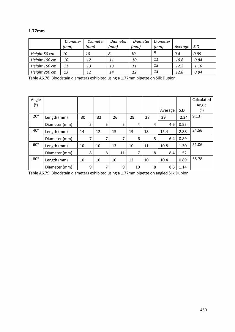
450
1.77mm
Table A6.78: Bloodstain diameters exhibited using a 1.77mm pipette on Silk Dupion.
Table A6.79: Bloodstain diameters exhibited using a 1.77mm pipette on angled Silk Dupion.
Diameter (mm)
Diameter (mm)
Diameter (mm)
Diameter (mm)
Diameter (mm) Average S.D
Height 50 cm 10 10 8 10 9 9.4 0.89
Height 100 cm 10 12 11 10 11 10.8 0.84
Height 150 cm 11 13 13 11 13 12.2 1.10
Height 200 cm 13 12 14 12 13 12.8 0.84
Angle (o)
Average S.D
Calculated Angle
(o)
20o Length (mm) 30 32 26 29 28 29 2.24 9.13
Diameter (mm) 5 5 5 4 4 4.6 0.55
40o Length (mm) 14 12 15 19 18 15.4 2.88 24.56
Diameter (mm) 7 7 7 6 5 6.4 0.89
60o Length (mm) 10 10 13 10 11 10.8 1.30 51.06
Diameter (mm) 8 8 11 7 8 8.4 1.52
80o Length (mm) 10 10 10 12 10 10.4 0.89 55.78
Diameter (mm) 9 7 9 10 8 8.6 1.14

319
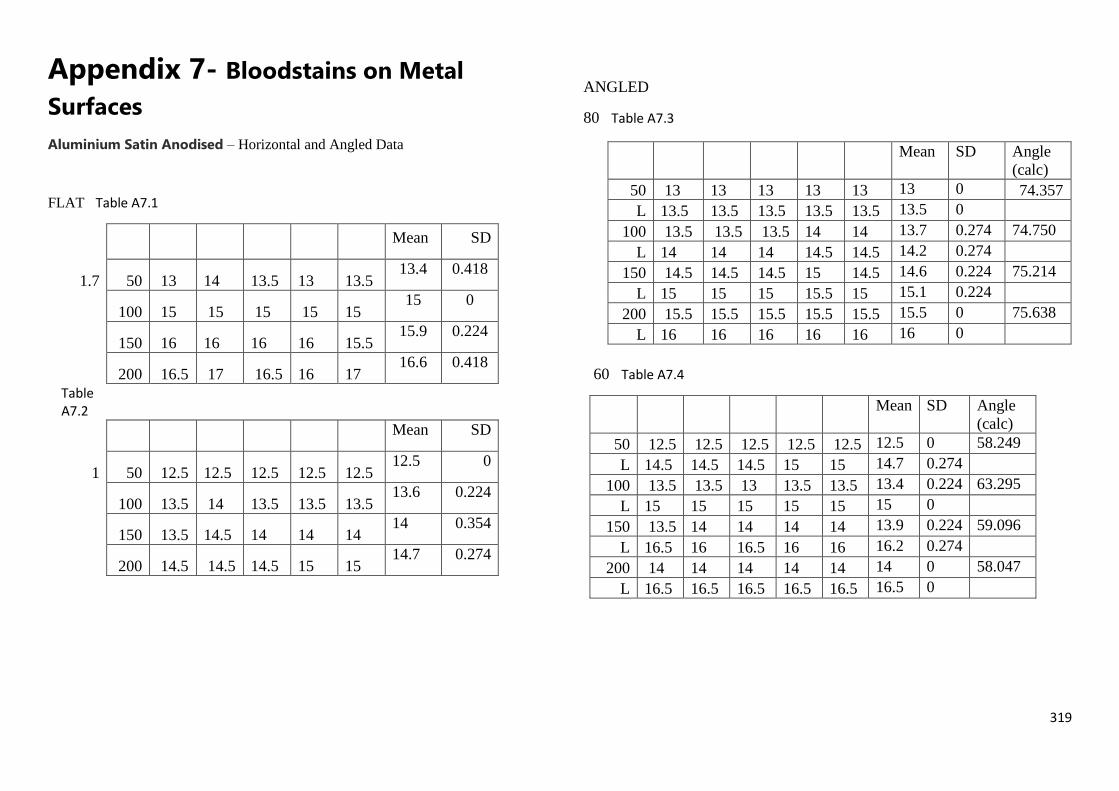
319
Appendix 7- Bloodstains on Metal
Surfaces
Aluminium Satin Anodised – Horizontal and Angled Data
FLAT Table A7.1
Mean SD
1.7 50 13 14 13.5 13 13.5 13.4 0.418
100 15 15 15 15 15 15 0
150 16 16 16 16 15.5 15.9 0.224
200 16.5 17 16.5 16 17 16.6 0.418
Table A7.2
Mean SD
1 50 12.5 12.5 12.5 12.5 12.5 12.5 0
100 13.5 14 13.5 13.5 13.5 13.6 0.224
150 13.5 14.5 14 14 14 14 0.354
200 14.5 14.5 14.5 15 15 14.7 0.274
ANGLED
80 Table A7.3
60 Table A7.4
Mean SD Angle
(calc)
50 12.5 12.5 12.5 12.5 12.5 12.5 0 58.249
L 14.5 14.5 14.5 15 15 14.7 0.274
100 13.5 13.5 13 13.5 13.5 13.4 0.224 63.295
L 15 15 15 15 15 15 0
150 13.5 14 14 14 14 13.9 0.224 59.096
L 16.5 16 16.5 16 16 16.2 0.274
200 14 14 14 14 14 14 0 58.047
L 16.5 16.5 16.5 16.5 16.5 16.5 0
Mean SD Angle
(calc)
50 13 13 13 13 13 13 0 74.357
L 13.5 13.5 13.5 13.5 13.5 13.5 0
100 13.5 13.5 13.5 14 14 13.7 0.274 74.750
L 14 14 14 14.5 14.5 14.2 0.274
150 14.5 14.5 14.5 15 14.5 14.6 0.224 75.214
L 15 15 15 15.5 15 15.1 0.224
200 15.5 15.5 15.5 15.5 15.5 15.5 0 75.638
L 16 16 16 16 16 16 0
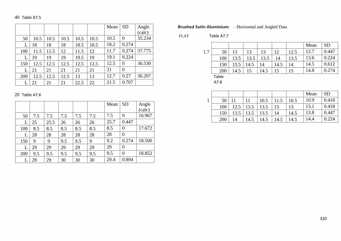
320
40 Table A7.5
Mean SD Angle
(calc)
50 10.5 10.5 10.5 10.5 10.5 10.5 0 35.234
L 18 18 18 18.5 18.5 18.2 0.274
100 11.5 11.5 12 11.5 12 11.7 0.274 37.775
L 19 19 19 19.5 19 19.1 0.224
150 12.5 12.5 12.5 12.5 12.5 12.5 0 36.530
L 21 21 21 21 21 21 0
200 12.5 12.5 12.5 13 13 12.7 0.27 36.207
L 21 21 21 22.5 22 21.5 0.707
20 Table A7.6
Mean SD Angle
(calc)
50 7.5 7.5 7.5 7.5 7.5 7.5 0 16.967
L 25 25.5 26 26 26 25.7 0.447
100 8.5 8.5 8.5 8.5 8.5 8.5 0 17.672
L 28 28 28 28 28 28 0
150 9 9 9.5 9.5 9 9.2 0.274 18.500
L 29 29 29 29 29 29 0
200 9.5 9.5 9.5 9.5 9.5 9.5 0 18.852
L 28 29 30 30 30 29.4 0.894
Brushed Satin Aluminium – Horizontal and Angled Data
FLAT Table A7.7
Mean SD
1.7 50 13 13 13 12 12.5 12.7 0.447
100 13.5 13.5 13.5 14 13.5 13.6 0.224
150 15.5 14.5 14 14.5 14 14.5 0.612
200 14.5 15 14.5 15 15 14.8 0.274
Table A7.8
Mean SD
1 50 11 11 10.5 11.5 10.5 10.9 0.418
100 12.5 13.5 13.5 13 13 13.1 0.418
150 13.5 13.5 13.5 14 14.5 13.8 0.447
200 14 14.5 14.5 14.5 14.5 14.4 0.224
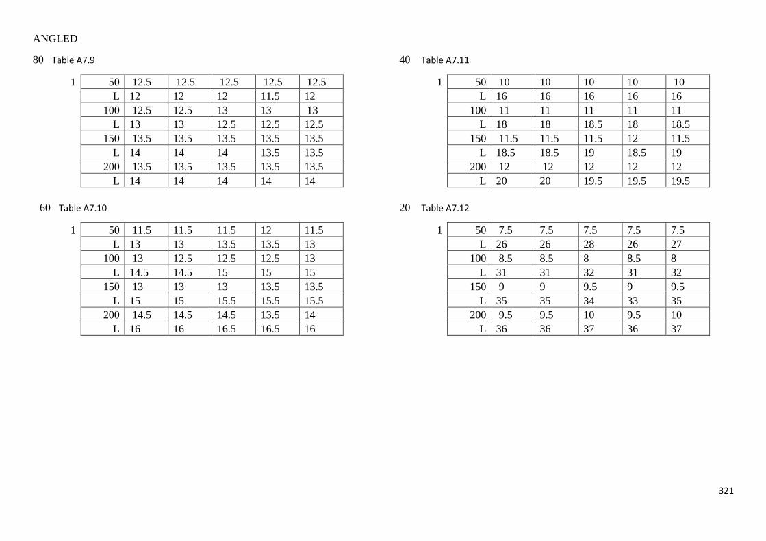
321
ANGLED
80 Table A7.9
1 50 12.5 12.5 12.5 12.5 12.5
L 12 12 12 11.5 12
100 12.5 12.5 13 13 13
L 13 13 12.5 12.5 12.5
150 13.5 13.5 13.5 13.5 13.5
L 14 14 14 13.5 13.5
200 13.5 13.5 13.5 13.5 13.5
L 14 14 14 14 14
60 Table A7.10
1 50 11.5 11.5 11.5 12 11.5
L 13 13 13.5 13.5 13
100 13 12.5 12.5 12.5 13
L 14.5 14.5 15 15 15
150 13 13 13 13.5 13.5
L 15 15 15.5 15.5 15.5
200 14.5 14.5 14.5 13.5 14
L 16 16 16.5 16.5 16
40 Table A7.11
1 50 10 10 10 10 10
L 16 16 16 16 16
100 11 11 11 11 11
L 18 18 18.5 18 18.5
150 11.5 11.5 11.5 12 11.5
L 18.5 18.5 19 18.5 19
200 12 12 12 12 12
L 20 20 19.5 19.5 19.5
20 Table A7.12
1 50 7.5 7.5 7.5 7.5 7.5
L 26 26 28 26 27
100 8.5 8.5 8 8.5 8
L 31 31 32 31 32
150 9 9 9.5 9 9.5
L 35 35 34 33 35
200 9.5 9.5 10 9.5 10
L 36 36 37 36 37

322
Stucco Aluminium – Horizontal and Angled Data
FLAT
Table A7.13
Mean SD
1.7 50 13.5 13.5 12.5 13.5 12 13 0.707
100 15 15 14 15 15 14.8 0.447
150 14.5 15.5 15 15 15 15 0.354
200 16.5 16.5 16.5 16 16 16.3 0.274
Table A7.14
Mean SD
1 50 12 12 11.5 12 12 11.9 0.224
100 13 12.5 12.5 12.5 13 12.7 0.274
150 13 13.5 13.5 13 13 13.2 0.274
200 14.5 14 14.5 14.5 14 14.3 0.274
ANGLED
80 Table A7.15
1 50 12 12.5 12 13 12.5
L 13 13 13 13.5 13.5
100 14 14 14 14 14
L 14.5 14.5 14.5 14.5 14.5
150 14.5 14.5 15 15 15
L 15 15 15.5 15.5 15.5
200 15 15.5 15 15.5 14.5
L 15.5 16 15.5 16 15
60 Table A7.16
1 50 11 11.5 11 11 11
L 13 13.5 13 14 13.5
100 13.5 13 13.5 13 13
L 15.5 15.5 15.5 15.5 15
150 14 13 13.5 13.5 13
L 16.5 16 15.5 15.5 15
200 14 14 13.5 14 14
L 16 16.5 16 16.5 16

323
40 Table A7.17
1 50 10 10.5 10.5 10 10.5
L 18 18 18 18 18
100 11.5 12 11.5 12 12
L 24 24 24 24 23
150 12 12 12 12 12
L 25 25 24 24.5 25.5
200 13 12.5 12.5 12.5 13
L 26 26 25 25.5 24
20 Table A7.18
1 50 7.5 7.5 7.5 7.5 7.5
L 27 27 27 27 27
100 8.5 8.5 8.5 8.5 8
L 28 30 29 30 29
150 9 9 9 9 9
L 33 31 31 31 33
200 8.5 9 9 9.5 9.5
L 28 30 29 30 33
Natural Semi Bright Aluminium – Horizontal and Angled Data
FLAT Table A7.19
Mean SD
1.7 50 14.5 14.5 14.5 14.5 15 14.6 0.224
100 16.5 17 16.5 16.5 16 16.5 0.354
150 16.5 16.5 17 17 17 16.8 0.274
200 17.5 17.5 17.5 17 17 17.3 0.274
Table A7.20
Mean SD
1 50 12.5 12.5 13 13 13 12.8 0.274
100 14.5 14.5 14.5 14.5 14.5 14.5 0
150 14.5 15 15 15 15 14.9 0.224
200 15.5 15.5 15.5 16 16 15.7 0.274
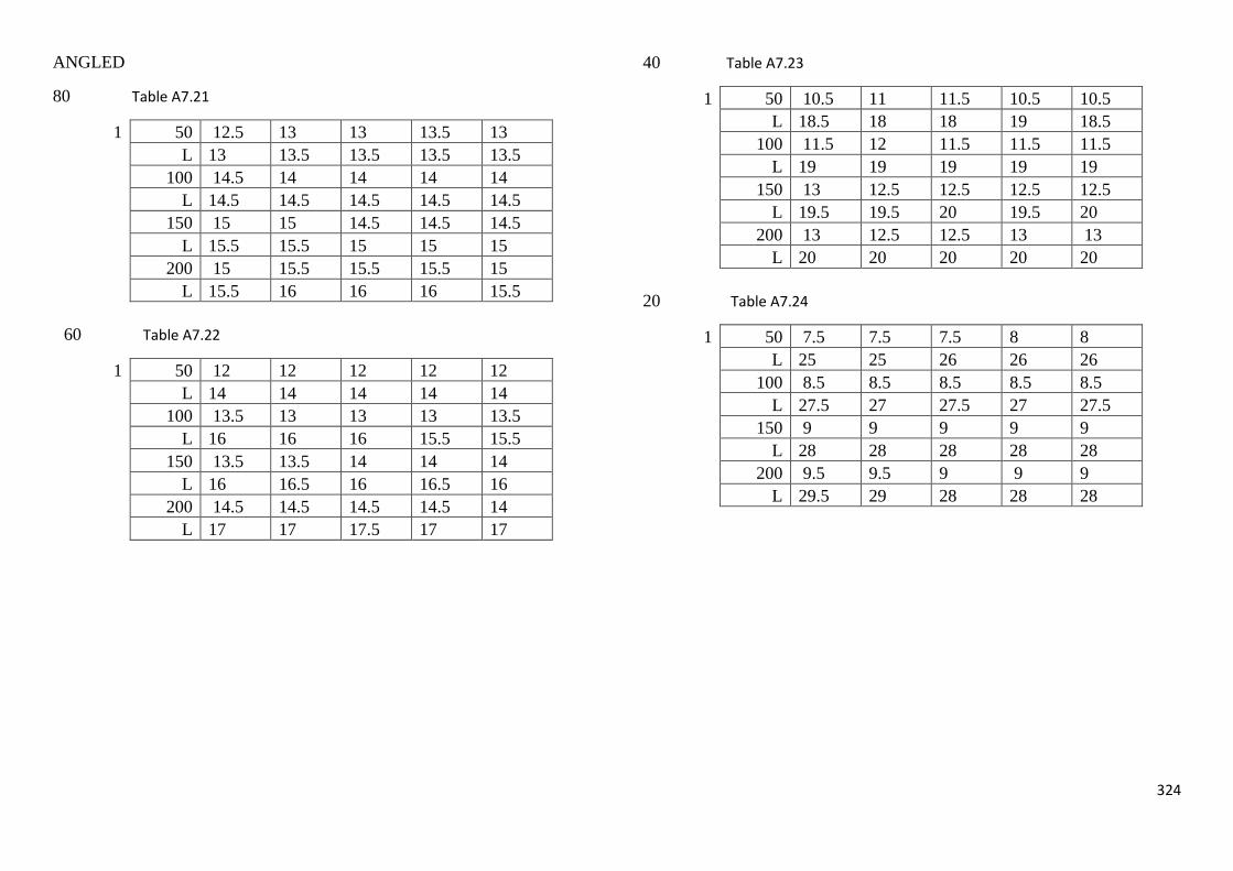
324
ANGLED
80 Table A7.21
1 50 12.5 13 13 13.5 13
L 13 13.5 13.5 13.5 13.5
100 14.5 14 14 14 14
L 14.5 14.5 14.5 14.5 14.5
150 15 15 14.5 14.5 14.5
L 15.5 15.5 15 15 15
200 15 15.5 15.5 15.5 15
L 15.5 16 16 16 15.5
60 Table A7.22
1 50 12 12 12 12 12
L 14 14 14 14 14
100 13.5 13 13 13 13.5
L 16 16 16 15.5 15.5
150 13.5 13.5 14 14 14
L 16 16.5 16 16.5 16
200 14.5 14.5 14.5 14.5 14
L 17 17 17.5 17 17
40 Table A7.23
1 50 10.5 11 11.5 10.5 10.5
L 18.5 18 18 19 18.5
100 11.5 12 11.5 11.5 11.5
L 19 19 19 19 19
150 13 12.5 12.5 12.5 12.5
L 19.5 19.5 20 19.5 20
200 13 12.5 12.5 13 13
L 20 20 20 20 20
20 Table A7.24
1 50 7.5 7.5 7.5 8 8
L 25 25 26 26 26
100 8.5 8.5 8.5 8.5 8.5
L 27.5 27 27.5 27 27.5
150 9 9 9 9 9
L 28 28 28 28 28
200 9.5 9.5 9 9 9
L 29.5 29 28 28 28
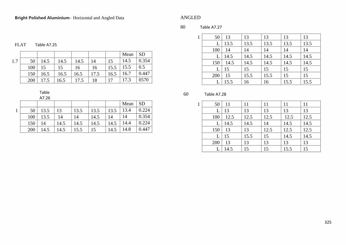
325
Bright Polished Aluminium– Horizontal and Angled Data
FLAT Table A7.25
Mean SD
1.7 50 14.5 14.5 14.5 14 15 14.5 0.354
100 15 15 16 16 15.5 15.5 0.5
150 16.5 16.5 16.5 17.5 16.5 16.7 0.447
200 17.5 16.5 17.5 18 17 17.3 0570
Table A7.26
Mean SD
1 50 13.5 13 13.5 13.5 13.5 13.4 0.224
100 13.5 14 14 14.5 14 14 0.354
150 14 14.5 14.5 14.5 14.5 14.4 0.224
200 14.5 14.5 15.5 15 14.5 14.8 0.447
ANGLED
80 Table A7.27
1 50 13 13 13 13 13
L 13.5 13.5 13.5 13.5 13.5
100 14 14 14 14 14
L 14.5 14.5 14.5 14.5 14.5
150 14.5 14.5 14.5 14.5 14.5
L 15 15 15 15 15
200 15 15.5 15.5 15 15
L 15.5 16 16 15.5 15.5
60 Table A7.28
1 50 11 11 11 11 11
L 13 13 13 13 13
100 12.5 12.5 12.5 12.5 12.5
L 14.5 14.5 14 14.5 14.5
150 13 13 12.5 12.5 12.5
L 15 15.5 15 14.5 14.5
200 13 13 13 13 13
L 14.5 15 15 15.5 15
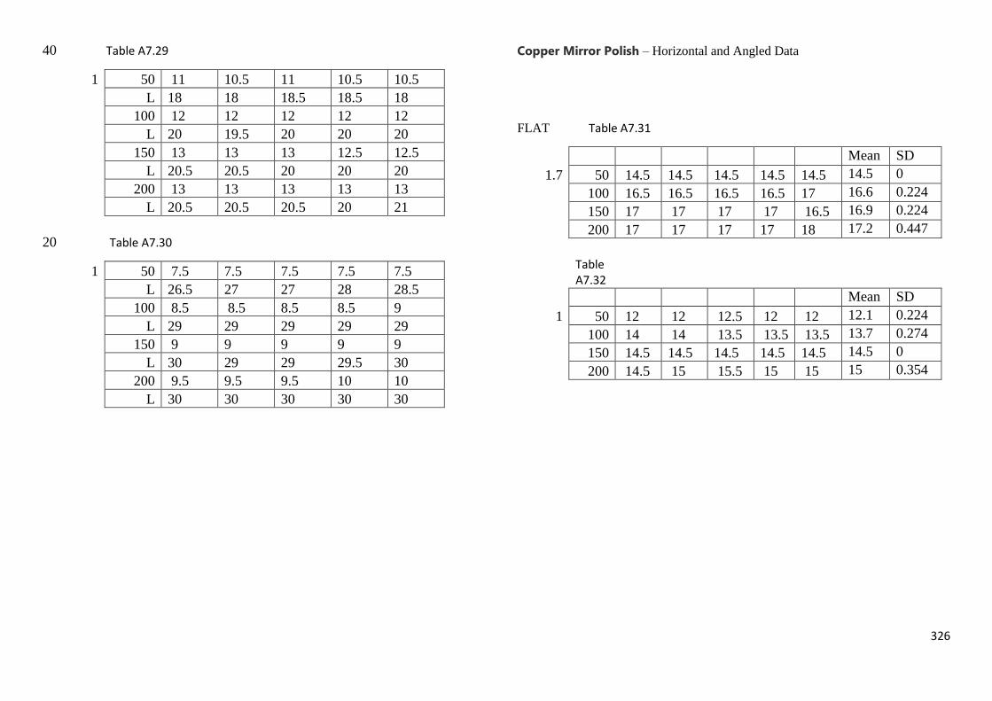
326
40 Table A7.29
1 50 11 10.5 11 10.5 10.5
L 18 18 18.5 18.5 18
100 12 12 12 12 12
L 20 19.5 20 20 20
150 13 13 13 12.5 12.5
L 20.5 20.5 20 20 20
200 13 13 13 13 13
L 20.5 20.5 20.5 20 21
20 Table A7.30
1 50 7.5 7.5 7.5 7.5 7.5
L 26.5 27 27 28 28.5
100 8.5 8.5 8.5 8.5 9
L 29 29 29 29 29
150 9 9 9 9 9
L 30 29 29 29.5 30
200 9.5 9.5 9.5 10 10
L 30 30 30 30 30
Copper Mirror Polish – Horizontal and Angled Data
FLAT Table A7.31
Mean SD
1.7 50 14.5 14.5 14.5 14.5 14.5 14.5 0
100 16.5 16.5 16.5 16.5 17 16.6 0.224
150 17 17 17 17 16.5 16.9 0.224
200 17 17 17 17 18 17.2 0.447
Table A7.32
Mean SD
1 50 12 12 12.5 12 12 12.1 0.224
100 14 14 13.5 13.5 13.5 13.7 0.274
150 14.5 14.5 14.5 14.5 14.5 14.5 0
200 14.5 15 15.5 15 15 15 0.354

327
ANGLED
80 Table A7.33
1 50 13 13 13 13 13.5
L 13.5 13.5 13.5 13.5 13.5
100 14 14 14 14 14
L 14.5 14.5 14.5 14.5 14.5
150 14.5 14.5 14.5 15 14.5
L 15 15.5 15 15.5 15
200 15.5 15.5 15.5 15.5 15.5
L 16 16 16 16 16
60 Table A7.34
1 50 11.5 11.5 12 12 12
L 14.5 14.5 14 14.5 14
100 13.5 13.5 14 13.5 13.5
L 16 16 16 15.5 15.5
150 14 14 14 14 14
L 16 16 15.5 16.5 16
200 14.5 14.5 15 15 14.5
L 17.5 17.5 17 17.5 17
40 Table A7.35
1 50 11 11 11 10.5 11
L 19.5 19.5 19 19.5 20
100 11.5 11.5 12 12 11.5
L 19.5 20.5 20 20 20
150 12 12 12.5 12.5 12
L 20.5 20.5 20.5 20 20
200 13 13 13 12.5 12.5
L 21 21 21.5 21.5 21
20 Table A7.36
1 50 7.5 7.5 7.5 7.5 7.5
L 28 27.5 28 28 27.5
100 8.5 8.5 8.5 9 9
L 30 30 30 30 30
150 9.5 9.5 9.5 9.5 9.5
L 34 34 34 34 34
200 9.5 9.5 9.5 10 10
L 35 35 35 36 36
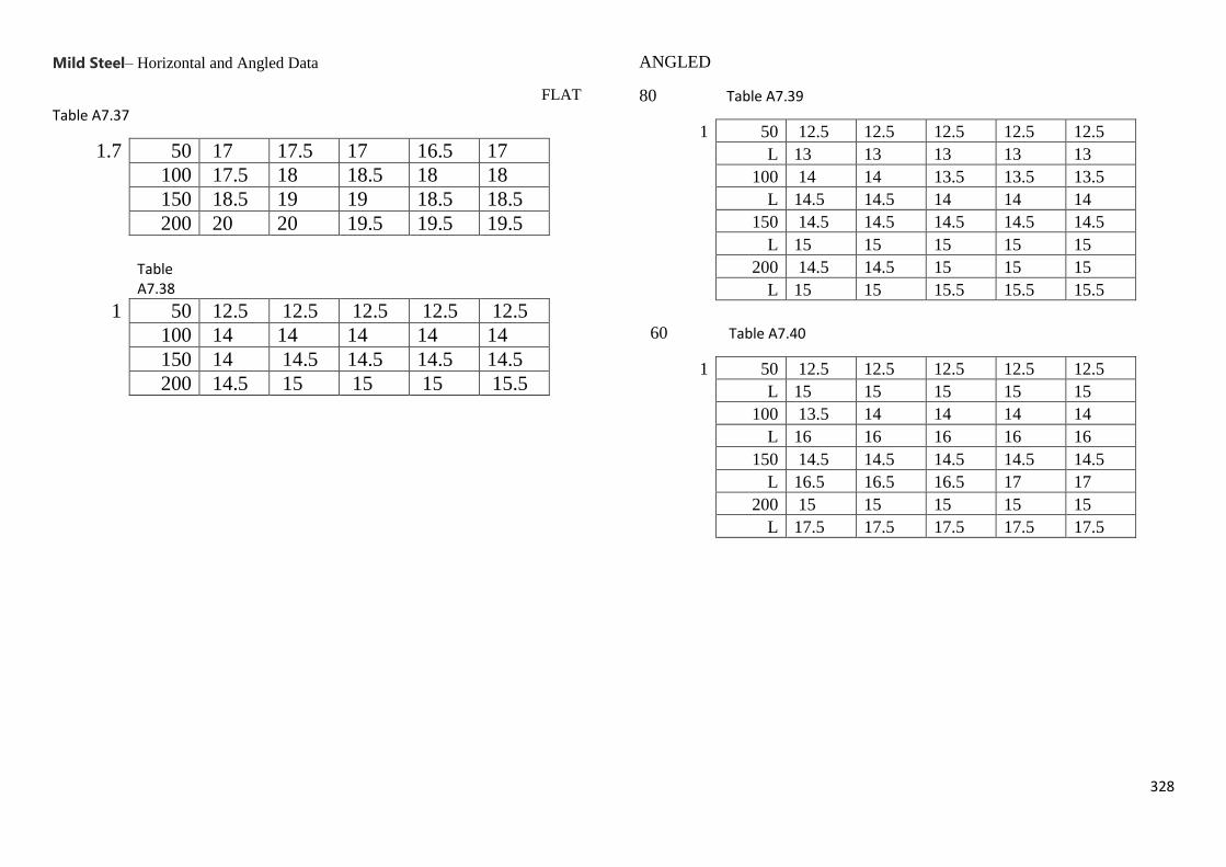
328
Mild Steel– Horizontal and Angled Data
FLAT
Table A7.37
1.7 50 17 17.5 17 16.5 17
100 17.5 18 18.5 18 18
150 18.5 19 19 18.5 18.5
200 20 20 19.5 19.5 19.5
Table A7.38
1 50 12.5 12.5 12.5 12.5 12.5
100 14 14 14 14 14
150 14 14.5 14.5 14.5 14.5
200 14.5 15 15 15 15.5
ANGLED
80 Table A7.39
1 50 12.5 12.5 12.5 12.5 12.5
L 13 13 13 13 13
100 14 14 13.5 13.5 13.5
L 14.5 14.5 14 14 14
150 14.5 14.5 14.5 14.5 14.5
L 15 15 15 15 15
200 14.5 14.5 15 15 15
L 15 15 15.5 15.5 15.5
60 Table A7.40
1 50 12.5 12.5 12.5 12.5 12.5
L 15 15 15 15 15
100 13.5 14 14 14 14
L 16 16 16 16 16
150 14.5 14.5 14.5 14.5 14.5
L 16.5 16.5 16.5 17 17
200 15 15 15 15 15
L 17.5 17.5 17.5 17.5 17.5

329
40 Table A7.41
1 50 11 10.5 10.5 10.5 10.5
L 18.5 18.5 18.5 18.5 18.5
100 12 12 12 12 12
L 19.5 19 20 19.5 19
150 13 13 12.5 12.5 12.5
L 20.5 20.5 20.5 20 20
200 13 13.5 13.5 13.5 13
L 21 21 21 21.5 20.5
20 Table A7.42
1 50 7.5 7.5 7.5 7.5 7.5
L 27 27 27 27 27
100 8.5 8.5 8.5 8.5 8.5
L 28 28 29 28.5 28
150 9.5 9.5 9 9 9
L 36 36 36 34 32
200 9.5 9.5 9.5 9.5 9.5
L 38 38 38 40 40
Galvanised Mild Steel – Horizontal and Angled Data
FLAT Table A7.43
1.7 50 13.5 14 14 14 14.5
100 15 16 15.5 15.5 16
150 16.5 16.5 16.5 16.5 16.5
200 16.5 16.5 16.5 17 17
Table A7.44
1 50 12.5 12.5 12.5 12.5 12.5
100 14 14 14.5 14.5 14
150 15 14.5 14.5 14.5 14.5
200 15 15.5 15.5 15.5 15.5
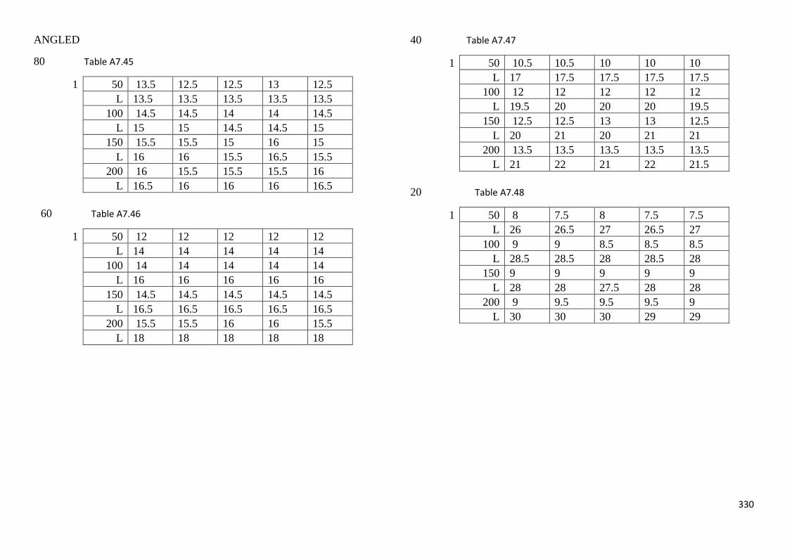
330
ANGLED
80 Table A7.45
1 50 13.5 12.5 12.5 13 12.5
L 13.5 13.5 13.5 13.5 13.5
100 14.5 14.5 14 14 14.5
L 15 15 14.5 14.5 15
150 15.5 15.5 15 16 15
L 16 16 15.5 16.5 15.5
200 16 15.5 15.5 15.5 16
L 16.5 16 16 16 16.5
60 Table A7.46
1 50 12 12 12 12 12
L 14 14 14 14 14
100 14 14 14 14 14
L 16 16 16 16 16
150 14.5 14.5 14.5 14.5 14.5
L 16.5 16.5 16.5 16.5 16.5
200 15.5 15.5 16 16 15.5
L 18 18 18 18 18
40 Table A7.47
1 50 10.5 10.5 10 10 10
L 17 17.5 17.5 17.5 17.5
100 12 12 12 12 12
L 19.5 20 20 20 19.5
150 12.5 12.5 13 13 12.5
L 20 21 20 21 21
200 13.5 13.5 13.5 13.5 13.5
L 21 22 21 22 21.5
20 Table A7.48
1 50 8 7.5 8 7.5 7.5
L 26 26.5 27 26.5 27
100 9 9 8.5 8.5 8.5
L 28.5 28.5 28 28.5 28
150 9 9 9 9 9
L 28 28 27.5 28 28
200 9 9.5 9.5 9.5 9
L 30 30 30 29 29
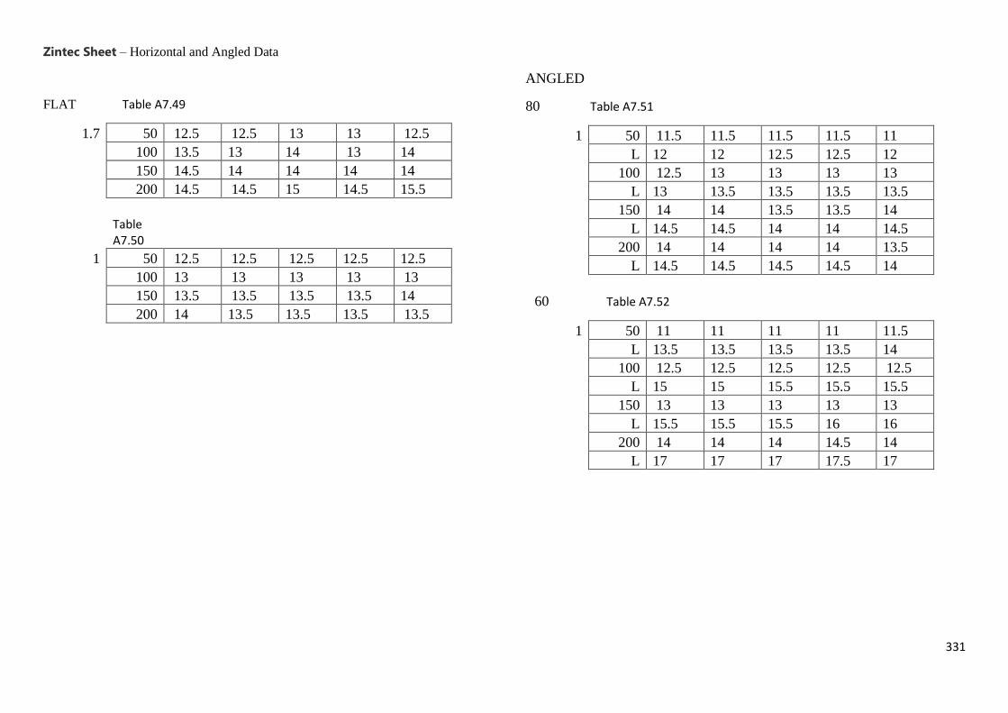
331
Zintec Sheet – Horizontal and Angled Data
FLAT Table A7.49
1.7 50 12.5 12.5 13 13 12.5
100 13.5 13 14 13 14
150 14.5 14 14 14 14
200 14.5 14.5 15 14.5 15.5
Table A7.50
1 50 12.5 12.5 12.5 12.5 12.5
100 13 13 13 13 13
150 13.5 13.5 13.5 13.5 14
200 14 13.5 13.5 13.5 13.5
ANGLED
80 Table A7.51
1 50 11.5 11.5 11.5 11.5 11
L 12 12 12.5 12.5 12
100 12.5 13 13 13 13
L 13 13.5 13.5 13.5 13.5
150 14 14 13.5 13.5 14
L 14.5 14.5 14 14 14.5
200 14 14 14 14 13.5
L 14.5 14.5 14.5 14.5 14
60 Table A7.52
1 50 11 11 11 11 11.5
L 13.5 13.5 13.5 13.5 14
100 12.5 12.5 12.5 12.5 12.5
L 15 15 15.5 15.5 15.5
150 13 13 13 13 13
L 15.5 15.5 15.5 16 16
200 14 14 14 14.5 14
L 17 17 17 17.5 17
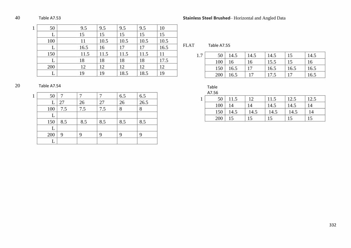
332
40 Table A7.53
1 50 9.5 9.5 9.5 9.5 10
L 15 15 15 15 15
100 11 10.5 10.5 10.5 10.5
L 16.5 16 17 17 16.5
150 11.5 11.5 11.5 11.5 11
L 18 18 18 18 17.5
200 12 12 12 12 12
L 19 19 18.5 18.5 19
20 Table A7.54
1 50 7 7 7 6.5 6.5
L 27 26 27 26 26.5
100 7.5 7.5 7.5 8 8
L
150 8.5 8.5 8.5 8.5 8.5
L
200 9 9 9 9 9
L
Stainless Steel Brushed– Horizontal and Angled Data
FLAT Table A7.55
1.7 50 14.5 14.5 14.5 15 14.5
100 16 16 15.5 15 16
150 16.5 17 16.5 16.5 16.5
200 16.5 17 17.5 17 16.5
Table A7.56
1 50 11.5 12 11.5 12.5 12.5
100 14 14 14.5 14.5 14
150 14.5 14.5 14.5 14.5 14
200 15 15 15 15 15

333
ANGLED
80 Table A7.57
1 50 12.5 12.5 12.5 13 13
L 12 12 12.5 12.5 12.5
100 13.5 13.5 13.5 13.5 13
L 13 13 13 13 12.5
150 14.5 14 14.5 14 14.5
L 14 13.5 14 13.5 14
200 14 14 14 14 14.5
L 14 14 14.5 14 14.5
60 Table A7.58
1 50 13 13 13 13 13
L 14 14 14 14 14
100 13.5 13.5 13.5 14 14
L 15 15 15 14.5 14.5
150 14.5 14.5 14.5 14.5 14.5
L 15.5 16 15.5 16 16
200 15 15 14.5 14.5 15
L 16 16 16 16 15.5
40 Table A7.59
1 50 10.5 10.5 10.5 10.5 10.5
L 16 16 16.5 16.5 16.5
100 11.5 12 12 11.5 11.5
L 17.5 17.5 17.5 17.5 17
150 12 12 12 12 12
L 18.5 18.5 18.5 18 18
200 12 12 12.5 12.5 12.5
L 19 19 18.5 18.5 18.5
20 Table A7.60
1 50 7.5 7.5 7.5 7.5 7.5
L 24 23.5 26 24.5 24.5
100 9 8.5 8.5 8.5 8.5
L 28 28 28 28 28
150 9 9 9 9 9
L 30 30 30 30 30
200 9.5 9.5 9 9 9.5
L 34 34 33 34 33
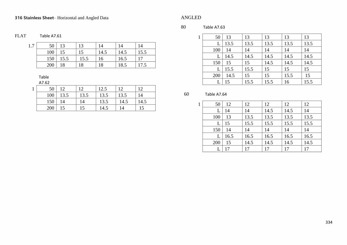
334
316 Stainless Sheet– Horizontal and Angled Data
FLAT Table A7.61
1.7 50 13 13 14 14 14
100 15 15 14.5 14.5 15.5
150 15.5 15.5 16 16.5 17
200 18 18 18 18.5 17.5
Table A7.62
1 50 12 12 12.5 12 12
100 13.5 13.5 13.5 13.5 14
150 14 14 13.5 14.5 14.5
200 15 15 14.5 14 15
ANGLED
80 Table A7.63
1 50 13 13 13 13 13
L 13.5 13.5 13.5 13.5 13.5
100 14 14 14 14 14
L 14.5 14.5 14.5 14.5 14.5
150 15 15 14.5 14.5 14.5
L 15.5 15.5 15 15 15
200 14.5 15 15 15.5 15
L 15 15.5 15.5 16 15.5
60 Table A7.64
1 50 12 12 12 12 12
L 14 14 14.5 14.5 14
100 13 13.5 13.5 13.5 13.5
L 15 15.5 15.5 15.5 15.5
150 14 14 14 14 14
L 16.5 16.5 16.5 16.5 16.5
200 15 14.5 14.5 14.5 14.5
L 17 17 17 17 17
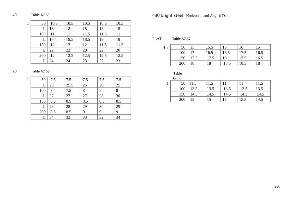
335
40 Table A7.65
1 50 10.5 10.5 10.5 10.5 10.5
L 18 18 18 18 18
100 11 11 11.5 11.5 11
L 18.5 18.5 18.5 19 19
150 12 12 12 11.5 11.5
L 22 22 20 22 20
200 12 12.5 12.5 12.5 12.5
L 24 24 23 22 23
20 Table A7.66
1 50 7.5 7.5 7.5 7.5 7.5
L 25 25.5 26 26 25
100 7.5 7.5 8 8 8
L 27 27 27 28 30
150 8.5 8.5 8.5 8.5 8.5
L 28 28 29 30 29
200 8.5 8.5 9 9 9
L 34 32 33 32 34
430 bright steel– Horizontal and Angled Data
FLAT Table A7.67
1.7 50 15 15.5 16 16 15
100 17 16.5 16.5 17.5 16.5
150 17.5 17.5 18 17.5 16.5
200 18 18 18.5 18.5 18
Table A7.68
1 50 11.5 11.5 11 11 11.5
100 13.5 13.5 13.5 13.5 13.5
150 14.5 14.5 14.5 14.5 14.5
200 15 15 15 15.5 14.5

336
ANGLED
80 Table A7.69
1 50 13.5 13.5 13 14 13
L 14 14 13.5 14.5 13.5
100 14.5 14.5 14.5 14.5 14.5
L 15 15 15 15 15
150 15 15.5 15.5 15.5 15.5
L 15.5 16 16 16 16
200 17 16.5 16.5 16.5 16
L 17.5 17 17 17 16.5
60 Table A7.70
1 50 12.5 13 13 12.5 13
L 15.5 15 15 15.5 15
100 14.5 14 14 14.5 14
L 16.5 17 17 16.5 17
150 14.5 14.5 14.5 14.5 14.5
L 17.5 17 17 17 17
200 15 15 15 15 15.5
L 18 18 18 18 18.5
40 Table A7.71
1 50 10 10 10 10 10
L 18 18 17.5 18 17.5
100 12 12 12 12 12
L 21 21 21 21 21
150 12.5 12.5 12.5 12.5 12.5
L 21.5 21.5 21.5 21.5 21.5
200 12.5 13 13 13 12.5
L 22 22 21.5 21.5 22
20 Table A7.72
1 50 8 8 7.5 7.5 7.5
L 28 28 28 28 28
100 8.5 8.5 9 9 8.5
L 30.5 30.5 31 31 30.5
150 9.5 9.5 9.5 9.5 9
L 31 31 31 31 32
200 10 10 10 10 9.5
L 31.5 32 32 32 32
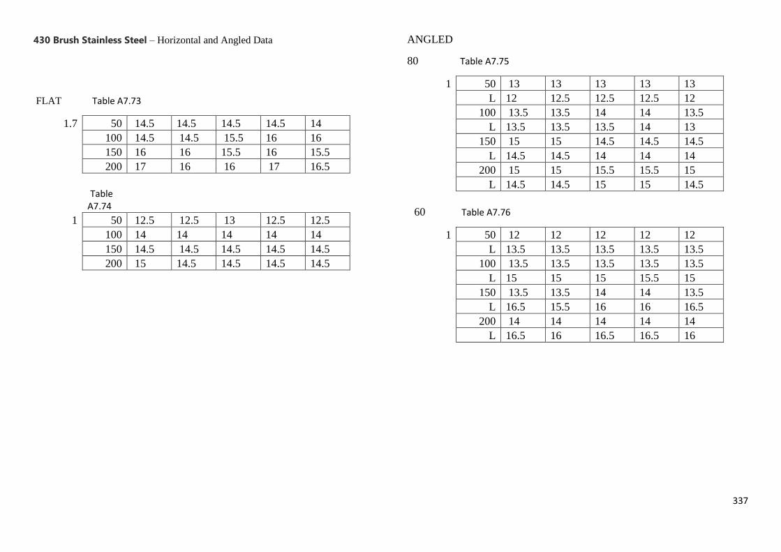
337
430 Brush Stainless Steel – Horizontal and Angled Data
FLAT Table A7.73
1.7 50 14.5 14.5 14.5 14.5 14
100 14.5 14.5 15.5 16 16
150 16 16 15.5 16 15.5
200 17 16 16 17 16.5
Table A7.74
1 50 12.5 12.5 13 12.5 12.5
100 14 14 14 14 14
150 14.5 14.5 14.5 14.5 14.5
200 15 14.5 14.5 14.5 14.5
ANGLED
80 Table A7.75
1 50 13 13 13 13 13
L 12 12.5 12.5 12.5 12
100 13.5 13.5 14 14 13.5
L 13.5 13.5 13.5 14 13
150 15 15 14.5 14.5 14.5
L 14.5 14.5 14 14 14
200 15 15 15.5 15.5 15
L 14.5 14.5 15 15 14.5
60 Table A7.76
1 50 12 12 12 12 12
L 13.5 13.5 13.5 13.5 13.5
100 13.5 13.5 13.5 13.5 13.5
L 15 15 15 15.5 15
150 13.5 13.5 14 14 13.5
L 16.5 15.5 16 16 16.5
200 14 14 14 14 14
L 16.5 16 16.5 16.5 16
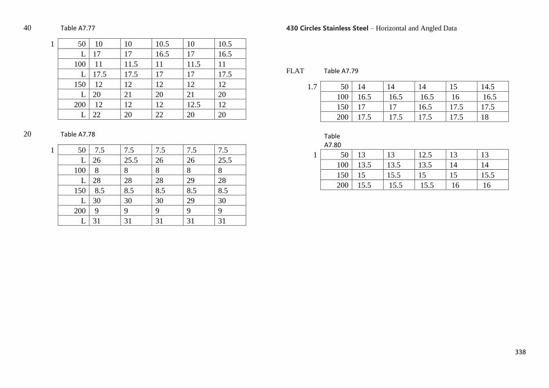
338
40 Table A7.77
1 50 10 10 10.5 10 10.5
L 17 17 16.5 17 16.5
100 11 11.5 11 11.5 11
L 17.5 17.5 17 17 17.5
150 12 12 12 12 12
L 20 21 20 21 20
200 12 12 12 12.5 12
L 22 20 22 20 20
20 Table A7.78
1 50 7.5 7.5 7.5 7.5 7.5
L 26 25.5 26 26 25.5
100 8 8 8 8 8
L 28 28 28 29 28
150 8.5 8.5 8.5 8.5 8.5
L 30 30 30 29 30
200 9 9 9 9 9
L 31 31 31 31 31
430 Circles Stainless Steel – Horizontal and Angled Data
FLAT Table A7.79
1.7 50 14 14 14 15 14.5
100 16.5 16.5 16.5 16 16.5
150 17 17 16.5 17.5 17.5
200 17.5 17.5 17.5 17.5 18
Table A7.80
1 50 13 13 12.5 13 13
100 13.5 13.5 13.5 14 14
150 15 15.5 15 15 15.5
200 15.5 15.5 15.5 16 16
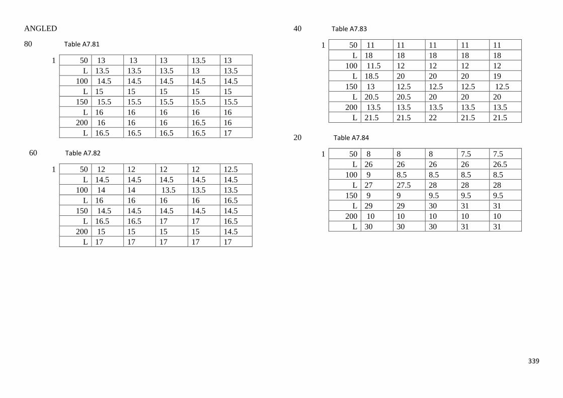
339
ANGLED
80 Table A7.81
1 50 13 13 13 13.5 13
L 13.5 13.5 13.5 13 13.5
100 14.5 14.5 14.5 14.5 14.5
L 15 15 15 15 15
150 15.5 15.5 15.5 15.5 15.5
L 16 16 16 16 16
200 16 16 16 16.5 16
L 16.5 16.5 16.5 16.5 17
60 Table A7.82
1 50 12 12 12 12 12.5
L 14.5 14.5 14.5 14.5 14.5
100 14 14 13.5 13.5 13.5
L 16 16 16 16 16.5
150 14.5 14.5 14.5 14.5 14.5
L 16.5 16.5 17 17 16.5
200 15 15 15 15 14.5
L 17 17 17 17 17
40 Table A7.83
1 50 11 11 11 11 11
L 18 18 18 18 18
100 11.5 12 12 12 12
L 18.5 20 20 20 19
150 13 12.5 12.5 12.5 12.5
L 20.5 20.5 20 20 20
200 13.5 13.5 13.5 13.5 13.5
L 21.5 21.5 22 21.5 21.5
20 Table A7.84
1 50 8 8 8 7.5 7.5
L 26 26 26 26 26.5
100 9 8.5 8.5 8.5 8.5
L 27 27.5 28 28 28
150 9 9 9.5 9.5 9.5
L 29 29 30 31 31
200 10 10 10 10 10
L 30 30 30 31 31
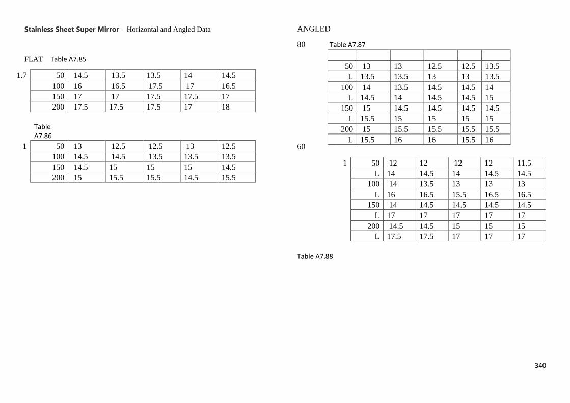
340
Stainless Sheet Super Mirror – Horizontal and Angled Data
FLAT Table A7.85
1.7 50 14.5 13.5 13.5 14 14.5
100 16 16.5 17.5 17 16.5
150 17 17 17.5 17.5 17
200 17.5 17.5 17.5 17 18
Table A7.86
1 50 13 12.5 12.5 13 12.5
100 14.5 14.5 13.5 13.5 13.5
150 14.5 15 15 15 14.5
200 15 15.5 15.5 14.5 15.5
ANGLED
80 Table A7.87
60
Table A7.88
1 50 12 12 12 12 11.5
L 14 14.5 14 14.5 14.5
100 14 13.5 13 13 13
L 16 16.5 15.5 16.5 16.5
150 14 14.5 14.5 14.5 14.5
L 17 17 17 17 17
200 14.5 14.5 15 15 15
L 17.5 17.5 17 17 17
50 13 13 12.5 12.5 13.5
L 13.5 13.5 13 13 13.5
100 14 13.5 14.5 14.5 14
L 14.5 14 14.5 14.5 15
150 15 14.5 14.5 14.5 14.5
L 15.5 15 15 15 15
200 15 15.5 15.5 15.5 15.5
L 15.5 16 16 15.5 16

341
40 Table A7.89
1 50 10 10 10.5 10.5 10
L 19 19 18 18 18
100 11.5 11.5 12 12 12
L 20 20 19.5 21 20
150 12 12 12 12 12
L 20 20.5 20.5 20 20
200 13 12.5 12.5 12 13
L 21 21 21 21 21
20 Table A7.90
1 50 7.5 7.5 7.5 7.5 7.5
L 28 28 28 28 28
100 8.5 8.5 8.5 8.5 8.5
L 30 30 30 29.5 30
150 9 9 9 9 9
L 30 30.5 31.5 31.5 31
200 9.5 9.5 9.5 9.5 9.5
L 32 32 32 32 32
Sheet Metal, Zinc– Horizontal and Angled Data
FLAT Table A7.91
1.7 50 14 14.5 14.5 14.5 14.5
100 16.5 16.5 16.5 16.5 16.5
150 16.5 16.5 17 16.5 17
200 17 17 16.5 16.5 17
Table A7.92
1 50 12.5 12.5 12.5 12.5 12.5
100 13.5 13 14.5 14 14
150 14.5 14 14 14 14
200 15.5 15 15 15 15

342
ANGLED
80 Table A7.93
1 50 13.5 13.5 14 13 13
L 14 14 14.5 14.5 13.5
100 14 14 14 14 14
L 14.5 14.5 14.5 14.5 14.5
150 14 14 14.5 14.5 14.5
L 14.5 14.5 15 15 15
200 15 15.5 15.5 15.5 15
L 16 16 16 16 15.5
60 Table A7.94
1 50 12 12 12.5 12.5 12.5
L 14.5 14.5 14.5 14 14
100 14 14 14 14 14
L 16 16 16 16 16.5
150 14.5 14.5 14.5 14.5 14.5
L 16.5 17.5 17.5 16.5 16.5
200 16.5 16.5 16 16 16
L 17.5 17.5 18.5 17.5 18.5
40 Table A7.95
1 50 10.5 10.5 10.5 10.5 10.5
L 17.5 17.5 17.5 17 17
100 12 12 12 11 11
L 19.5 19.5 19 19 19
150 12.5 12.5 12.5 13 13.5
L 20.5 20.5 20 19.5 20
200 13 13 13 13 13.5
L 21 21 20.5 19.5 20.5
20 Table A7.96
1 50 7.5 7.5 7.5 7.5 7.5
L 27 27 27 27 27
100 8.5 8.5 8.5 8.5 8.5
L 30 30 30 29 29
150 9 9 9 9 9
L 36 36 36 36 36
200 9 9.5 9.5 9.5 9
L 36 37 38 37 37

343
sheet-metal-quartz-zinc – Horizontal and Angled Data
FLAT
Table A7.97
1.7 50 13 13 13 12.5 13
100 14.5 14.5 14.5 14.5 14.5
150 15.5 15.5 15.5 15 15
200 16.5 16.5 16.5 16.5 16
Table A7.98
1 50 11 11.5 11.5 11.5 11.5
100 13 13 13.5 13 13
150 13.5 14 14 14 14
200 14.5 14.5 14 14 14.5
ANGLED
80 Table A7.99
1 50 11.5 11.5 11.5 11.5 11.5
L 12 12 12 12 12
100 12 12 12 11.5 11.5
L 12.5 12.5 12.5 12 12.5
150 14 13.5 13.5 13.5 13.5
L 14 14 14 14 14
200 14 14 14 13.5 13.5
L 14 14.5 14.5 14 14
60 Table A7.100
1 50 12 12 12 12 12
L 13.5 13.5 13.5 13.5 13.5
100 13 12.5 12.5 13 12.5
L 14.5 14.5 14.5 14.5 14.5
150 13.5 13.5 13.5 13.5 13.5
L 15.5 15.5 15.5 15.5 15.5
200 14.5 14.5 14.5 14.5 14.5
L 16 16 16.5 16.5 16.5

344
40 Table A7.101
1 50 10 10 10 10 10
L 16 16 16.5 16.5 16
100 10 10.5 10.5 10.5 10.5
L 16 16 17 17 17
150 11 11 11 11 11
L 16 17 17 17 17
200 11 11.5 11.5 11.5 11.5
L 18 18 18.5 18 18.5
20 Table A7.102
1 50 6.5 7 7 7 7
L 26 25 26 26 25
100 7.5 7.5 7.5 7.5 7
L 30 30 30 30 30
150 8 8 8 8 8
L 32 32 31 32 32
200 8.5 8.5 8.5 8.5 8
L 34 34 35 34 34
Brass Mirror Polish – Horizontal and Angled Data
FLAT Table A7.103
1.7 50 13.5 13.5 14 14 14
100 15.5 16 16 15.5 15.5
150 17 16 16 16.5 16.5
200 17.5 17.5 17.5 17.5 17.5
Table A7.104
1 50 12.5 12.5 12.5 13 12.5
100 14 14 14 13.5 13.5
150 14.5 14.5 14.5 14.5 14.5
200 14.5 15 15 15 15

345
ANGLED
80 Table A7.105
1 50 12.5 12.5 12.5 12.5 12.5
L 13 13 13 13 13
100 13 13 14 14 14
L 13.5 13.5 14.5 14.5 14
150 14 14 14.5 14.5 14
L 14.5 14.5 14.5 15 15
200 15 15 14.5 14.5 15
L 15.5 15.5 15 15 15.5
60 Table A7.106
1 50 12.5 12 12 12 12.5
L 14.5 14.5 14 14 14
100 13.5 13.5 13.5 13.5 13
L 15.5 15.5 15 15.5 16
150 14 14 14.5 14 14.5
L 15.5 16 16 16.5 16
200 15 15 15 15 14.5
L 17.5 17.5 17.5 17.5 17
40 Table A7.107
1 50 11 11 11 11 10.5
L 19 19 19 19 19
100 11.5 11.5 11.5 11.5 11.5
L 19.5 19.5 19.5 20 20
150 12 12 12 12.5 12
L 20 20.5 20.5 20.5 20
200 12.5 12.5 12.5 12 12.5
L 21 21 20.5 20.5 20.5
20 Table A7.108
1 50 8 7.5 7.5 8 7.5
L 25 27 27 28 27
100 8.5 8.5 8.5 8.5 8.5
L 29 29 29 29 30
150 9 9 9.5 9.5 9
L 32 32 32 31 32
200 9 9.5 9.5 9.4 9.5
L 34 34 34 34 34
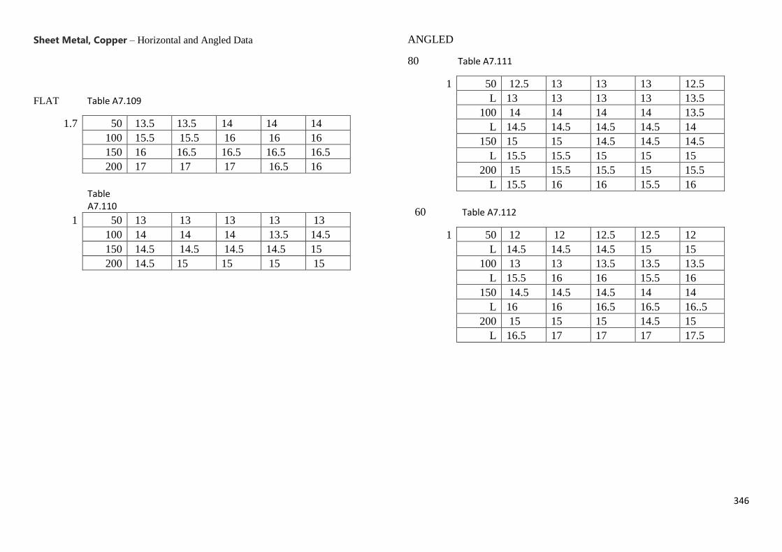
346
Sheet Metal, Copper – Horizontal and Angled Data
FLAT Table A7.109
1.7 50 13.5 13.5 14 14 14
100 15.5 15.5 16 16 16
150 16 16.5 16.5 16.5 16.5
200 17 17 17 16.5 16
Table A7.110
1 50 13 13 13 13 13
100 14 14 14 13.5 14.5
150 14.5 14.5 14.5 14.5 15
200 14.5 15 15 15 15
ANGLED
80 Table A7.111
1 50 12.5 13 13 13 12.5
L 13 13 13 13 13.5
100 14 14 14 14 13.5
L 14.5 14.5 14.5 14.5 14
150 15 15 14.5 14.5 14.5
L 15.5 15.5 15 15 15
200 15 15.5 15.5 15 15.5
L 15.5 16 16 15.5 16
60 Table A7.112
1 50 12 12 12.5 12.5 12
L 14.5 14.5 14.5 15 15
100 13 13 13.5 13.5 13.5
L 15.5 16 16 15.5 16
150 14.5 14.5 14.5 14 14
L 16 16 16.5 16.5 16..5
200 15 15 15 14.5 15
L 16.5 17 17 17 17.5

347
40 Table A7.113
1 50 10.5 10.5 11 11 11
L 18 18 18 18.5 18.5
100 12 12 12 12 12
L 19.5 19.5 19.5 19.5 19.5
150 12.5 12.5 12.5 12.5 12.5
L 20 20 20 20 20.5
200 13 13 13.5 13.5 13.5
L 21 21 21 21.5 21.5
20 Table A7.114
1 50 8 8 8 8 8
L 27 29 27 27 27
100 9 9 9 9 9
L 29 29 29 30 29
150 10 10 10 10 10
L 32 32 32 31 31
200 10 10.5 10 10.5 10.5
L 36 36 36 35 35
Natural Semi Bright Aluminium - rough
– Horizontal and Angled Data
FLAT Table A7.115
1.7 50 12.5 12.5 12.5 12.5 12
100 13 13 13.5 13 13
150 14.5 15 14.5 14 14
200 16 15.5 15.5 15 16
Table A7.116
1 50 11.5 12 12 11.5 11.5
100 13.5 13 12 13 13
150 13.5 13.5 13.5 13.5 13.5
200 13.5 14 14 14 14

348
ANGLED
80 Table A7.117
1 50 12 12.5 12.5 12 12
L 12.5 12.5 12.5 12.5 12.5
100 12.5 12.5 12.5 12.5 13
L 13 13 13 13 13.5
150 14 14 14 14 13.5
L 14.5 14.5 14 14.5 14
200 14.5 14.5 14 14.5 14
L 15 15 15 14.5 14.5
60 Table A7.118
1 50 11 11 11 11 11
L 13 13 13 13 13
100 12.5 12.5 13 13 13
L 14.5 14.5 14.5 15 15
150 12.5 12.5 13.5 13 13.5
L 15 15 16 16 15
200 13 13 13 13 13
L 16 15.5 16 15.5 16
40 Table A7.119
1 50 10 10 10 10 10
L 18 18 19 19 19
100 11 11 11 11 11
L 21 21 20 20 21
150 12 12 12 11.5 11.5
L 22 21 22 21 21
200 12 12.5 12 12 12
L 22 22 23 23 23
20 Table A7.120
1 50 7 7 7 7 7
L 26 26 26 26 26
100 8.5 8.5 8 8 8
L 32 32 28 28 28
150 8.5 8.5 9 9 9
L 30 30 32 32 32
200 9 9 9.5 9.5 9.5
L 34 34 34 33 32

349
Mild Steel – Rough
– Horizontal and Angled Data
FLAT Table A7.121
1.7 50 13 12.5 13 13 13.5
100 15 15 14.5 15.5 15
150 15.5 15.5 15.5 15.5 15.5
200 16 15 16 16.5 16
Table A7.122
1 50 11.5 11.5 11 12 11.5
100 13 13 13.5 13 13
150 13 13.5 14.5 13.5 13.5
200 14.5 14.5 14 14.5 14.5
ANGLED
80 Table A7.123
1 50 12 12 12 12 12
L 12.5 12.5 12.5 12.5 12.5
100 13 13 13 13 13
L 13.5 13.5 13.5 13.5 13.5
150 13.5 13.5 13.5 14 14
L 14 14 14 14.5 14.5
200 15 14.5 14.5 14.5 15
L 15.5 15 15 15 15.5
60 Table A7.124
1 50 12 12 12 11.5 11.5
L 14 14 14 15 15
100 12 12 12 12.5 12.5
L 14.5 14.5 14.5 14 14.5
150 14 13.5 13.5 13.5 14
L 15 15.5 15.5 15 15
200 14 14 14.5 14.5 14
L 16 16 16.5 16 16
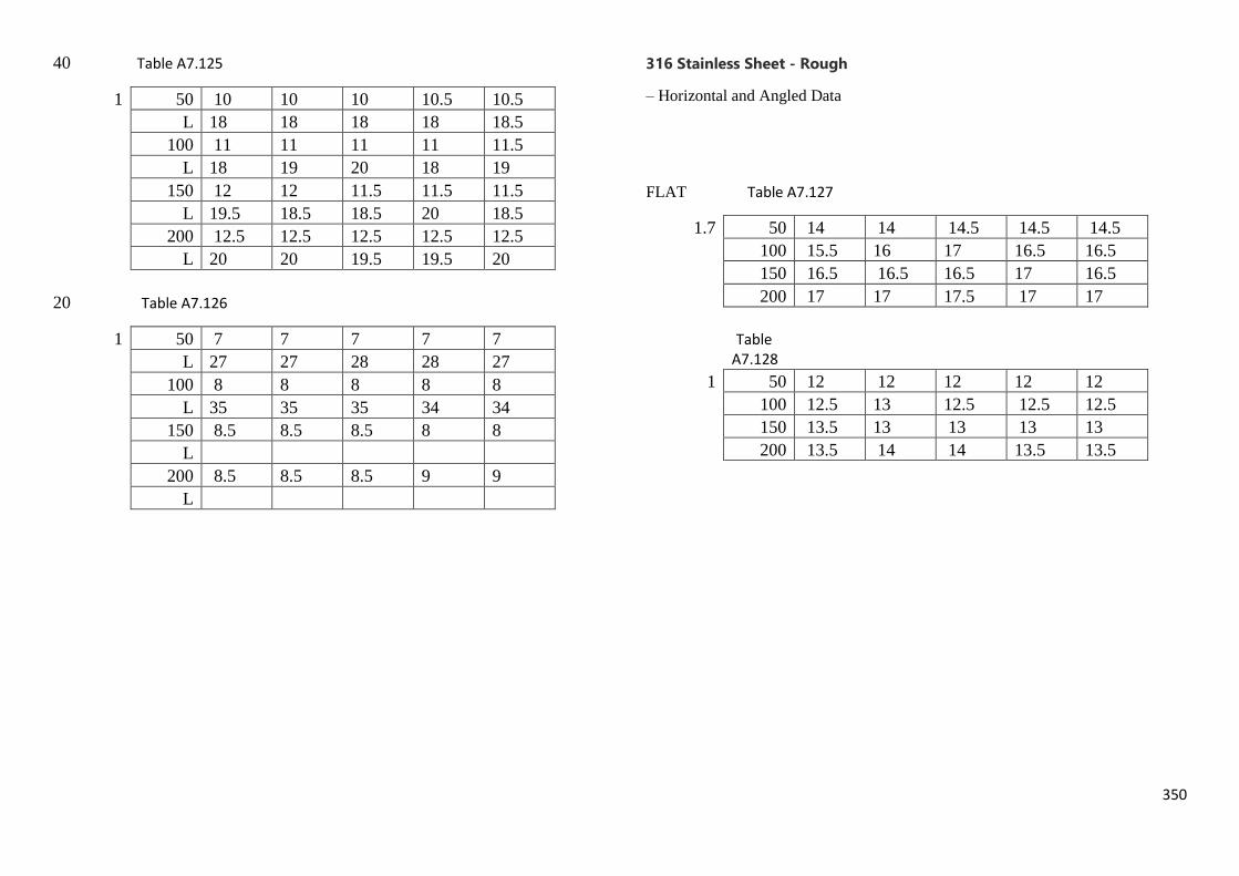
350
40 Table A7.125
1 50 10 10 10 10.5 10.5
L 18 18 18 18 18.5
100 11 11 11 11 11.5
L 18 19 20 18 19
150 12 12 11.5 11.5 11.5
L 19.5 18.5 18.5 20 18.5
200 12.5 12.5 12.5 12.5 12.5
L 20 20 19.5 19.5 20
20 Table A7.126
1 50 7 7 7 7 7
L 27 27 28 28 27
100 8 8 8 8 8
L 35 35 35 34 34
150 8.5 8.5 8.5 8 8
L
200 8.5 8.5 8.5 9 9
L
316 Stainless Sheet - Rough
– Horizontal and Angled Data
FLAT Table A7.127
1.7 50 14 14 14.5 14.5 14.5
100 15.5 16 17 16.5 16.5
150 16.5 16.5 16.5 17 16.5
200 17 17 17.5 17 17
Table A7.128
1 50 12 12 12 12 12
100 12.5 13 12.5 12.5 12.5
150 13.5 13 13 13 13
200 13.5 14 14 13.5 13.5

351
ANGLED
80 Table A7.129
1 50 11 11 11 11.5 11.5
L 11.5 11.5 11.5 12 12
100 13 12.5 13 12.5 12.5
L 13.5 13 13.5 13 13
150 13 13.5 13 13 13.5
L 13.5 14 13.5 13.5 14
200 13.5 13.5 13.5 13.5 13.5
L 14 14 13.5 13.5 14
60 Table A7.130
1 50 12 12 12 12 12
L 14 14 14 14 14
100 12.5 12.5 13 13.5 13
L 14.5 15 15 15.5 15
150 13.5 13.5 13.5 13.5 13.5
L 15.5 15.5 15.5 15.5 15.5
200 13.5 14 14 14 14
L 15 15 16 15.5 15.5
40 Table A7.131
1 50 10 10 10 10 10
L 17 17.5 17 17.5 18
100 11.5 11.5 11.5 11.5 11
L 19 19 19 18.5 19
150 11.5 11.5 12 12 11.5
L 19 19.5 19.5 19 19.5
200 12 12 12 12.5 12.5
L 20 20 20 21 21
20 Table A7.132
1 50 11.5 11.5 11.5 11.5 11.5
L 28 28 28 27 27
100 8.5 8.5 8 8 8.5
L 28 30 30 30 28
150 8.5 9 9 9 8.5
L 35 35 35 34 34
200 9 9 9.5 9.5 9
L 36 36 37 37 37
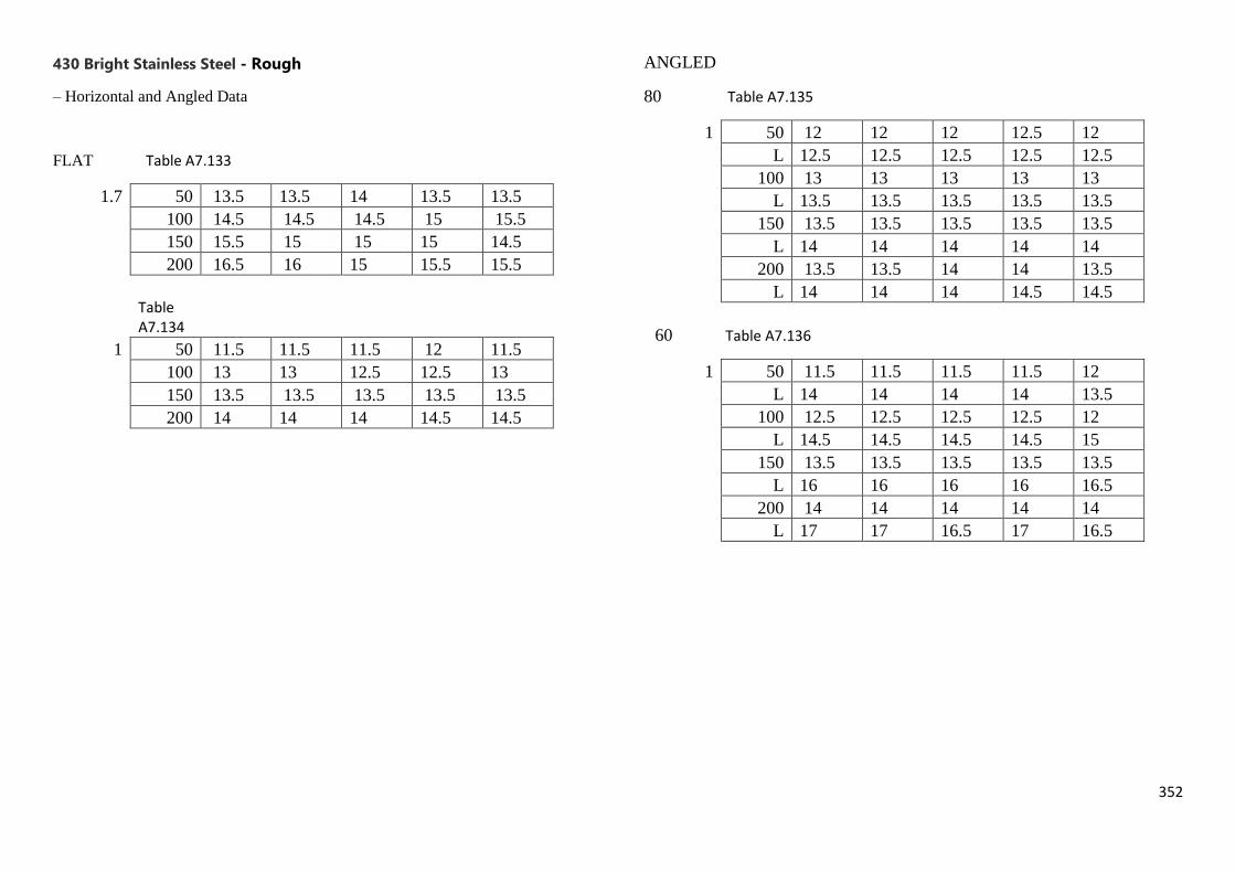
352
430 Bright Stainless Steel - Rough
– Horizontal and Angled Data
FLAT Table A7.133
1.7 50 13.5 13.5 14 13.5 13.5
100 14.5 14.5 14.5 15 15.5
150 15.5 15 15 15 14.5
200 16.5 16 15 15.5 15.5
Table A7.134
1 50 11.5 11.5 11.5 12 11.5
100 13 13 12.5 12.5 13
150 13.5 13.5 13.5 13.5 13.5
200 14 14 14 14.5 14.5
ANGLED
80 Table A7.135
1 50 12 12 12 12.5 12
L 12.5 12.5 12.5 12.5 12.5
100 13 13 13 13 13
L 13.5 13.5 13.5 13.5 13.5
150 13.5 13.5 13.5 13.5 13.5
L 14 14 14 14 14
200 13.5 13.5 14 14 13.5
L 14 14 14 14.5 14.5
60 Table A7.136
1 50 11.5 11.5 11.5 11.5 12
L 14 14 14 14 13.5
100 12.5 12.5 12.5 12.5 12
L 14.5 14.5 14.5 14.5 15
150 13.5 13.5 13.5 13.5 13.5
L 16 16 16 16 16.5
200 14 14 14 14 14
L 17 17 16.5 17 16.5

353
40 Table A7.137
1 50 10 10 10 10 9.5
L 17 17 17 16.5 17
100 11 11 11 10.5 11
L 17 17 17 17.5 17
150 12 12 12 11.5 11.5
L 19 19 19 18.5 19
200 12.5 12.5 12.5 12.5 12.5
L 19.5 19.5 19 19.5 20
20 Table A7.138
1 50 11.5 11.5 11 11.5 11
L 28 28 26.5 27 27
100 8.5 8.5 8 8 8.5
L 28 31 30 30 29
150 8.5 9 9 9 8.5
L 36 35 36 34 34
200 9 9 9.5 9.5 9
L 36 36 37 37 37

Appendix 8- Bloodstains on Stones Surfaces
Stones (1mm)
Rusty Slate Paving
Diameter (mm)
Diameter (mm)
Diameter (mm)
Diameter (mm)
Diameter (mm) Average SD
Height 50cm 13 13 13 13 13 13 0
Height 100cm 14 14 14 14 14 14 0
Height 150cm 15 15 15 15 15 15 0
Height 200cm 15 15 15 15 16 15.2 0.447214
Table A8.1: 1mm pipette drop results on Rusty Slate Paving.
Beige Marble Polished
Diameter (mm)
Diameter (mm)
Diameter (mm)
Diameter (mm)
Diameter (mm) Average SD
Height 50cm 14 14 13 14 14 13.8 0.447214
Height 100cm 14 14 14 14 14 14 0
Height 150cm 15 15 15 15 14 14.8 0.447214
Height 200cm 16 16 16 16 16 16 0
Table A8.2: 1mm pipette drop results on Beige Marble Polished.
Classic Chipped Edge Filled and Honed
Diameter (mm)
Diameter (mm)
Diameter (mm)
Diameter (mm)
Diameter (mm) Average SD
Height 50cm 12 13 13 13 13 12.8 0.447214
Height 100cm 14 14 15 14 15 14.4 0.547723
Height 150cm 15 14 14 14 15 14.4 0.547723
Height 200cm 15 15 15 15 15 15 0
Table A8.3: 1mm pipette drop results on Classic Chipped Edge Filled and Honed
Classic Travertine Filled and Honed

Diameter (mm)
Diameter (mm)
Diameter (mm)
Diameter (mm)
Diameter (mm) Average SD
Height 50cm 13 13 13 13 13 13 0
Height 100cm 14 14 14 14 14 14 0
Height 150cm 15 15 15 15 15 15 0
Height 200cm 15 15 15 16 16 15.4 0.547723
Table A8.4: 1mm pipette drop results on Classic Travertine Filled and Honed.
Classic Tumbled Unfilled Travertine
Diameter (mm)
Diameter (mm)
Diameter (mm)
Diameter (mm)
Diameter (mm) Average SD
Height 50cm 13 13 13 13 13 13 0
Height 100cm 14 13 13 14 13 13.4 0.547723
Height 150cm 13 13 14 14 14 13.6 0.547723
Height 200cm 15 15 15 15 14 14.8 0.447214
Table A8.5: 1mm pipette drop results on Classic Tumbled Unfilled Travertine
Indian Sandstone Paving Raj Blend Tumbled
Diameter (mm)
Diameter (mm)
Diameter (mm)
Diameter (mm)
Diameter (mm) Average SD
Height 50cm 12 12 13 13 12.5 0.57735
Height 100cm 13 14 13 13 13 13.2 0.447214
Height 150cm 14 14 14 14 14 14 0
Height 200cm 15 15 14 14 14 14.4 0.547723
Table A8.6: 1mm pipette drop results on Indian Sandstone Paving Raj Blend Tumbled.
Indian Sandstone Paving Raj Blend Economy
Diameter (mm)
Diameter (mm)
Diameter (mm)
Diameter (mm)
Diameter (mm) Average SD
Height 50cm 11 11 11 11 11 11 0
Height 100cm 13 13 13 13 13 13 0
Height 150cm 14 13 13 13 13 13.2 0.447214
Height 200cm 14 14 14 15 14 14.2 0.447214
Table A8.7: 1mm pipette drop results on Indian Sandstone Paving Raj Blend Economy
Indian Sandstone Paving Sahara Yellow

Diameter (mm)
Diameter (mm)
Diameter (mm)
Diameter (mm)
Diameter (mm) Average SD
Height 50cm 11 11 11 11 12 11.2 0.447214
Height 100cm 14 13 14 13 14 13.6 0.547723
Height 150cm 13 14 14 13 14 13.6 0.547723
Height 200cm 14 14 14 15 14 14.2 0.447214
Table A8.8: 1mm pipette drop results on Indian Sandstone Paving Sahara Yellow.
Indian Sandstone Paving Rippon Buff
Diameter (mm)
Diameter (mm)
Diameter (mm)
Diameter (mm)
Diameter (mm) Average SD
Height 50cm 11 12 12 11 12 11.6 0.547723
Height 100cm 11 11 12 12 11 11.4 0.547723
Height 150cm 13 14 14 14 13 13.6 0.547723
Height 200cm 14 15 15 15 15 14.8 0.447214
Table A8.9: 1mm pipette drop results on Indian Sandstone Paving Rippon Buff
Indian Sandstone Paving Modak
Diameter (mm)
Diameter (mm)
Diameter (mm)
Diameter (mm)
Diameter (mm) Average SD
Height 50cm 13 13 13 13 13 13 0
Height 100cm 14 14 15 15 15 14.6 0.547723
Height 150cm 14 15 14 15 15 14.6 0.547723
Height 200cm 15 15 15 15 15 15 0
Table A8.10: 1mm pipette drop results on Indian Sandstone Paving Modak.
Classic Honed Travertine Paving
Diameter (mm)
Diameter (mm)
Diameter (mm)
Diameter (mm)
Diameter (mm) Average SD
Height 50cm 13 13 13 13 13 0
Height 100cm 14 14 14 13 13 13.6 0.547723
Height 150cm 14 14 15 14 14 14.2 0.447214
Height 200cm 15 15 15 15 15 15 0
Table A8.11: 1mm pipette drop results on Classic Honed Travertine Paving.
Silver Latte Tumbled Travertine Paving

Diameter (mm)
Diameter (mm)
Diameter (mm)
Diameter (mm)
Diameter (mm) Average SD
Height 50cm 13 13 13 13 13 13 0
Height 100cm 14 13 13 13 14 13.4 0.547723
Height 150cm 14 15 14 14 14 14.2 0.447214
Height 200cm 15 15 15 15 15 15 0
Table A8.12: 1mm pipette drop results on Silver Latte Tumbled Travertine Paving.
Yellow Limestone Paving
Diameter (mm)
Diameter (mm)
Diameter (mm)
Diameter (mm)
Diameter (mm) Average SD
Height 50cm 10 11 11 11 11 10.8 0.447214
Height 100cm 12 12 12 12 13 12.2 0.447214
Height 150cm 13 13 13 13 13 13 0
Height 200cm 14 14 14 14 15 14.2 0.447214
Table A8.13: 1mm pipette drop results on Yellow Limestone Paving.
Brazilian Black Slate Paving
Diameter (mm)
Diameter (mm)
Diameter (mm)
Diameter (mm)
Diameter (mm) Average SD
Height 50cm 13 13 13 13 13 13 0
Height 100cm 13 13 13 14 14 13.4 0.547723
Height 150cm 14 14 14 14 14 14 0
Height 200cm 15 15 15 15 15 15 0
Table A8.14: 1mm pipette drop results on Brazilian Black Slate Paving.
Seal Grey Flamed
Diameter (mm)
Diameter (mm)
Diameter (mm)
Diameter (mm)
Diameter (mm) Average SD
Height 50cm 13 13 14 14 14 13.6 0.547723
Height 100cm 15 14 14 15 14 14.4 0.547723
Height 150cm 15 16 16 16 16 15.8 0.447214
Height 200cm 16 16 16 16 16 16 0
Table A8.15: 1mm pipette drop results on Seal Grey Flamed.
Artic Grey Sawn and Tumbled Cobble
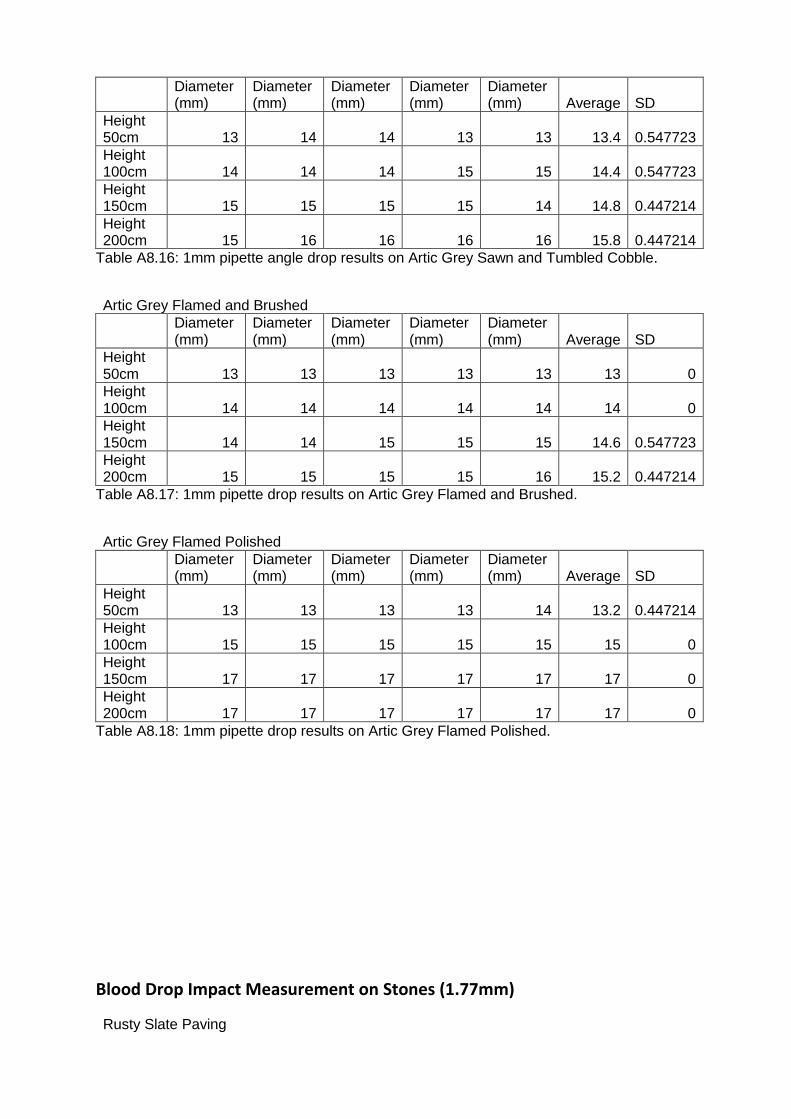
Diameter (mm)
Diameter (mm)
Diameter (mm)
Diameter (mm)
Diameter (mm) Average SD
Height 50cm 13 14 14 13 13 13.4 0.547723
Height 100cm 14 14 14 15 15 14.4 0.547723
Height 150cm 15 15 15 15 14 14.8 0.447214
Height 200cm 15 16 16 16 16 15.8 0.447214
Table A8.16: 1mm pipette angle drop results on Artic Grey Sawn and Tumbled Cobble.
Artic Grey Flamed and Brushed
Diameter (mm)
Diameter (mm)
Diameter (mm)
Diameter (mm)
Diameter (mm) Average SD
Height 50cm 13 13 13 13 13 13 0
Height 100cm 14 14 14 14 14 14 0
Height 150cm 14 14 15 15 15 14.6 0.547723
Height 200cm 15 15 15 15 16 15.2 0.447214
Table A8.17: 1mm pipette drop results on Artic Grey Flamed and Brushed.
Artic Grey Flamed Polished
Diameter (mm)
Diameter (mm)
Diameter (mm)
Diameter (mm)
Diameter (mm) Average SD
Height 50cm 13 13 13 13 14 13.2 0.447214
Height 100cm 15 15 15 15 15 15 0
Height 150cm 17 17 17 17 17 17 0
Height 200cm 17 17 17 17 17 17 0
Table A8.18: 1mm pipette drop results on Artic Grey Flamed Polished.
Blood Drop Impact Measurement on Stones (1.77mm)
Rusty Slate Paving
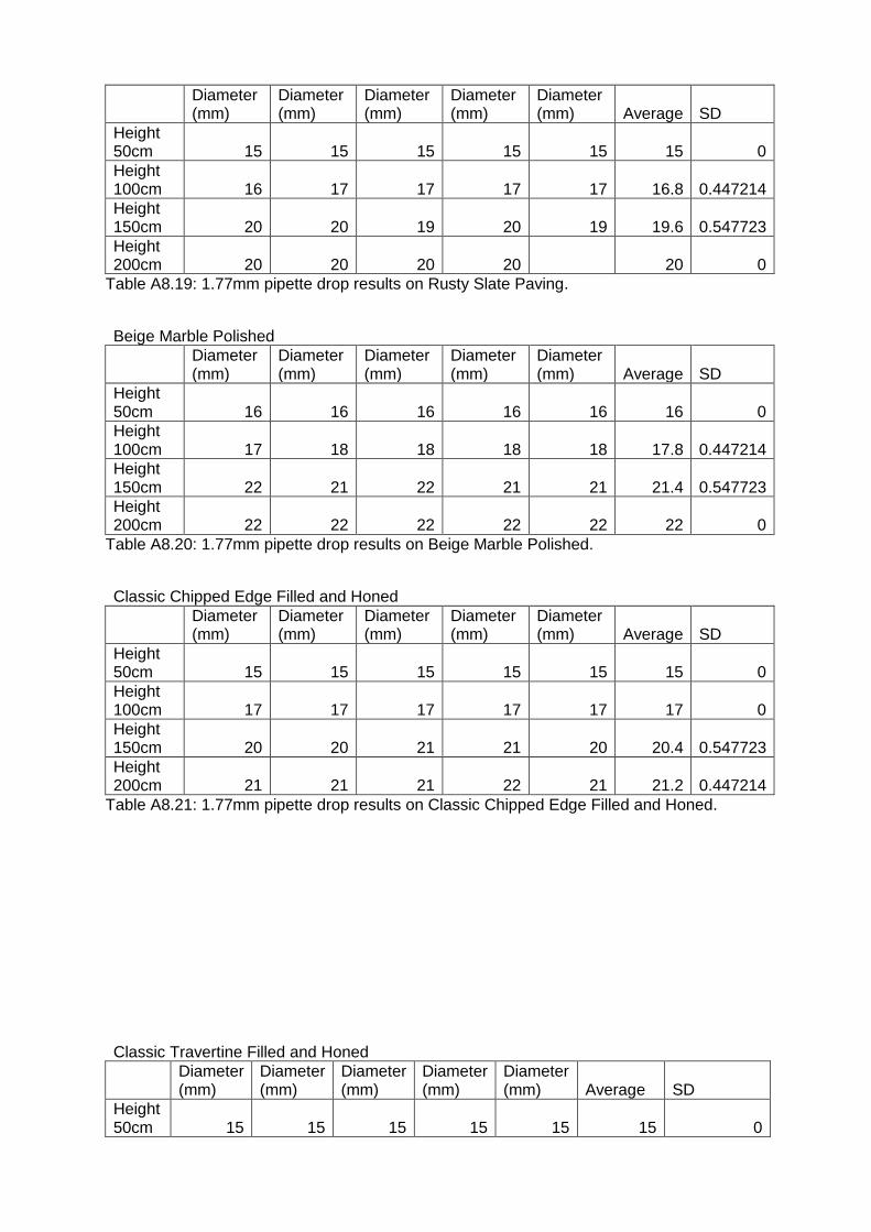
Diameter (mm)
Diameter (mm)
Diameter (mm)
Diameter (mm)
Diameter (mm) Average SD
Height 50cm 15 15 15 15 15 15 0
Height 100cm 16 17 17 17 17 16.8 0.447214
Height 150cm 20 20 19 20 19 19.6 0.547723
Height 200cm 20 20 20 20 20 0
Table A8.19: 1.77mm pipette drop results on Rusty Slate Paving.
Beige Marble Polished
Diameter (mm)
Diameter (mm)
Diameter (mm)
Diameter (mm)
Diameter (mm) Average SD
Height 50cm 16 16 16 16 16 16 0
Height 100cm 17 18 18 18 18 17.8 0.447214
Height 150cm 22 21 22 21 21 21.4 0.547723
Height 200cm 22 22 22 22 22 22 0
Table A8.20: 1.77mm pipette drop results on Beige Marble Polished.
Classic Chipped Edge Filled and Honed
Diameter (mm)
Diameter (mm)
Diameter (mm)
Diameter (mm)
Diameter (mm) Average SD
Height 50cm 15 15 15 15 15 15 0
Height 100cm 17 17 17 17 17 17 0
Height 150cm 20 20 21 21 20 20.4 0.547723
Height 200cm 21 21 21 22 21 21.2 0.447214
Table A8.21: 1.77mm pipette drop results on Classic Chipped Edge Filled and Honed.
Classic Travertine Filled and Honed
Diameter (mm)
Diameter (mm)
Diameter (mm)
Diameter (mm)
Diameter (mm) Average SD
Height 50cm 15 15 15 15 15 15 0

Height 100cm 17 17 17 18 17 17.2 0.447214
Height 150cm 22 22 22 21 21 21.6 0.547723
Height 200cm 22 22 22 22 22 22 0
Table A8.22: 1.77mm pipette drop results on Classic Travertine Filled and Honed. Classic Tumbled Unfilled Travertine
Diameter (mm)
Diameter (mm)
Diameter (mm)
Diameter (mm)
Diameter (mm) Average SD
Height 50cm 15 14 15 15 14 14.6 0.547723
Height 100cm 16 16 16 16 16 16 0
Height 150cm 19 19 19 20 19 19.2 0.447214
Height 200cm 21 21 21 21 21 21 0
Table A8.23: 1.77mm pipette drop results on Classic Tumbled Unfilled Travertine.
Indian Sandstone Paving Raj Blend Tumbled
Diameter (mm)
Diameter (mm)
Diameter (mm)
Diameter (mm)
Diameter (mm) Average SD
Height 50cm 15 15 15 16 15 15.2 0.447214
Height 100cm 16 16 16 16 16 16 0
Height 150cm 20 20 19 19 19 19.4 0.547723
Height 200cm 19 20 20 20 20 19.8 0.447214
Table A8.24: 1.77mm pipette drop results on Indian Sandstone Paving Raj Blend Tumbled.
Indian Sandstone Paving Raj Blend Economy
Diameter (mm)
Diameter (mm)
Diameter (mm)
Diameter (mm)
Diameter (mm) Average SD
Height 50cm 14 14 14 14 14 14 0
Height 100cm 15 15 15 15 15 15 0
Height 150cm 19 20 19 20 19 19.4 0.547723
Height 200cm 21 20 20 21 20 20.4 0.547723
Table A8.25: 1.77mm pipette drop results on Indian Sandstone Paving Raj Blend Economy.
Indian Sandstone Paving Sahara Yellow
Diameter (mm)
Diameter (mm)
Diameter (mm)
Diameter (mm)
Diameter (mm) Average SD
Height 50cm 14 14 15 15 15 14.6 0.547723
Height 100cm 16 16 16 16 16 16 0
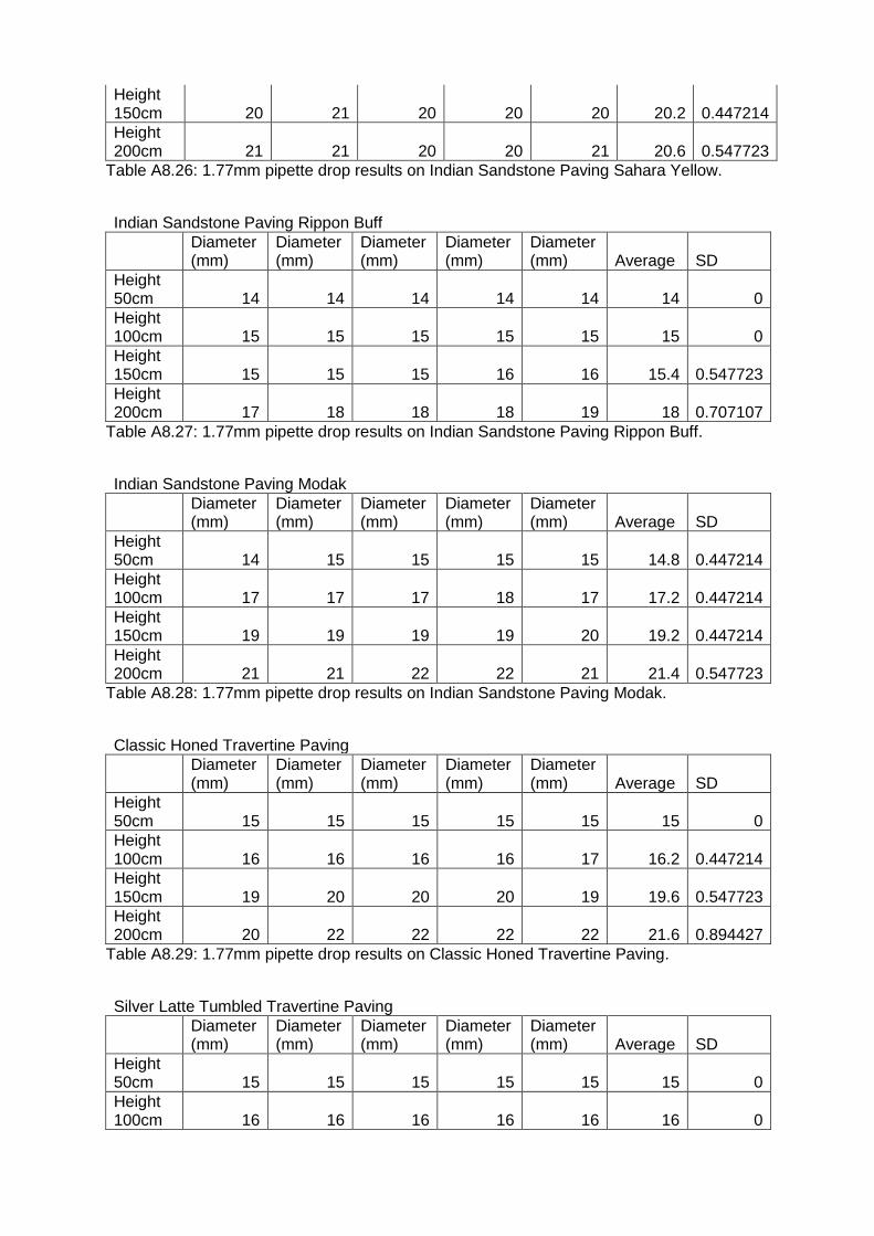
Height 150cm 20 21 20 20 20 20.2 0.447214
Height 200cm 21 21 20 20 21 20.6 0.547723
Table A8.26: 1.77mm pipette drop results on Indian Sandstone Paving Sahara Yellow.
Indian Sandstone Paving Rippon Buff
Diameter (mm)
Diameter (mm)
Diameter (mm)
Diameter (mm)
Diameter (mm) Average SD
Height 50cm 14 14 14 14 14 14 0
Height 100cm 15 15 15 15 15 15 0
Height 150cm 15 15 15 16 16 15.4 0.547723
Height 200cm 17 18 18 18 19 18 0.707107
Table A8.27: 1.77mm pipette drop results on Indian Sandstone Paving Rippon Buff.
Indian Sandstone Paving Modak
Diameter (mm)
Diameter (mm)
Diameter (mm)
Diameter (mm)
Diameter (mm) Average SD
Height 50cm 14 15 15 15 15 14.8 0.447214
Height 100cm 17 17 17 18 17 17.2 0.447214
Height 150cm 19 19 19 19 20 19.2 0.447214
Height 200cm 21 21 22 22 21 21.4 0.547723
Table A8.28: 1.77mm pipette drop results on Indian Sandstone Paving Modak.
Classic Honed Travertine Paving
Diameter (mm)
Diameter (mm)
Diameter (mm)
Diameter (mm)
Diameter (mm) Average SD
Height 50cm 15 15 15 15 15 15 0
Height 100cm 16 16 16 16 17 16.2 0.447214
Height 150cm 19 20 20 20 19 19.6 0.547723
Height 200cm 20 22 22 22 22 21.6 0.894427
Table A8.29: 1.77mm pipette drop results on Classic Honed Travertine Paving.
Silver Latte Tumbled Travertine Paving
Diameter (mm)
Diameter (mm)
Diameter (mm)
Diameter (mm)
Diameter (mm) Average SD
Height 50cm 15 15 15 15 15 15 0
Height 100cm 16 16 16 16 16 16 0
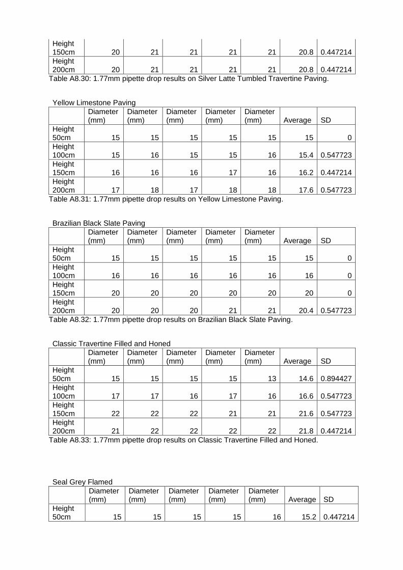
Height 150cm 20 21 21 21 21 20.8 0.447214
Height 200cm 20 21 21 21 21 20.8 0.447214
Table A8.30: 1.77mm pipette drop results on Silver Latte Tumbled Travertine Paving.
Yellow Limestone Paving
Diameter (mm)
Diameter (mm)
Diameter (mm)
Diameter (mm)
Diameter (mm) Average SD
Height 50cm 15 15 15 15 15 15 0
Height 100cm 15 16 15 15 16 15.4 0.547723
Height 150cm 16 16 16 17 16 16.2 0.447214
Height 200cm 17 18 17 18 18 17.6 0.547723
Table A8.31: 1.77mm pipette drop results on Yellow Limestone Paving.
Brazilian Black Slate Paving
Diameter (mm)
Diameter (mm)
Diameter (mm)
Diameter (mm)
Diameter (mm) Average SD
Height 50cm 15 15 15 15 15 15 0
Height 100cm 16 16 16 16 16 16 0
Height 150cm 20 20 20 20 20 20 0
Height 200cm 20 20 20 21 21 20.4 0.547723
Table A8.32: 1.77mm pipette drop results on Brazilian Black Slate Paving.
Classic Travertine Filled and Honed
Diameter (mm)
Diameter (mm)
Diameter (mm)
Diameter (mm)
Diameter (mm) Average SD
Height 50cm 15 15 15 15 13 14.6 0.894427
Height 100cm 17 17 16 17 16 16.6 0.547723
Height 150cm 22 22 22 21 21 21.6 0.547723
Height 200cm 21 22 22 22 22 21.8 0.447214
Table A8.33: 1.77mm pipette drop results on Classic Travertine Filled and Honed.
Seal Grey Flamed
Diameter (mm)
Diameter (mm)
Diameter (mm)
Diameter (mm)
Diameter (mm) Average SD
Height 50cm 15 15 15 15 16 15.2 0.447214
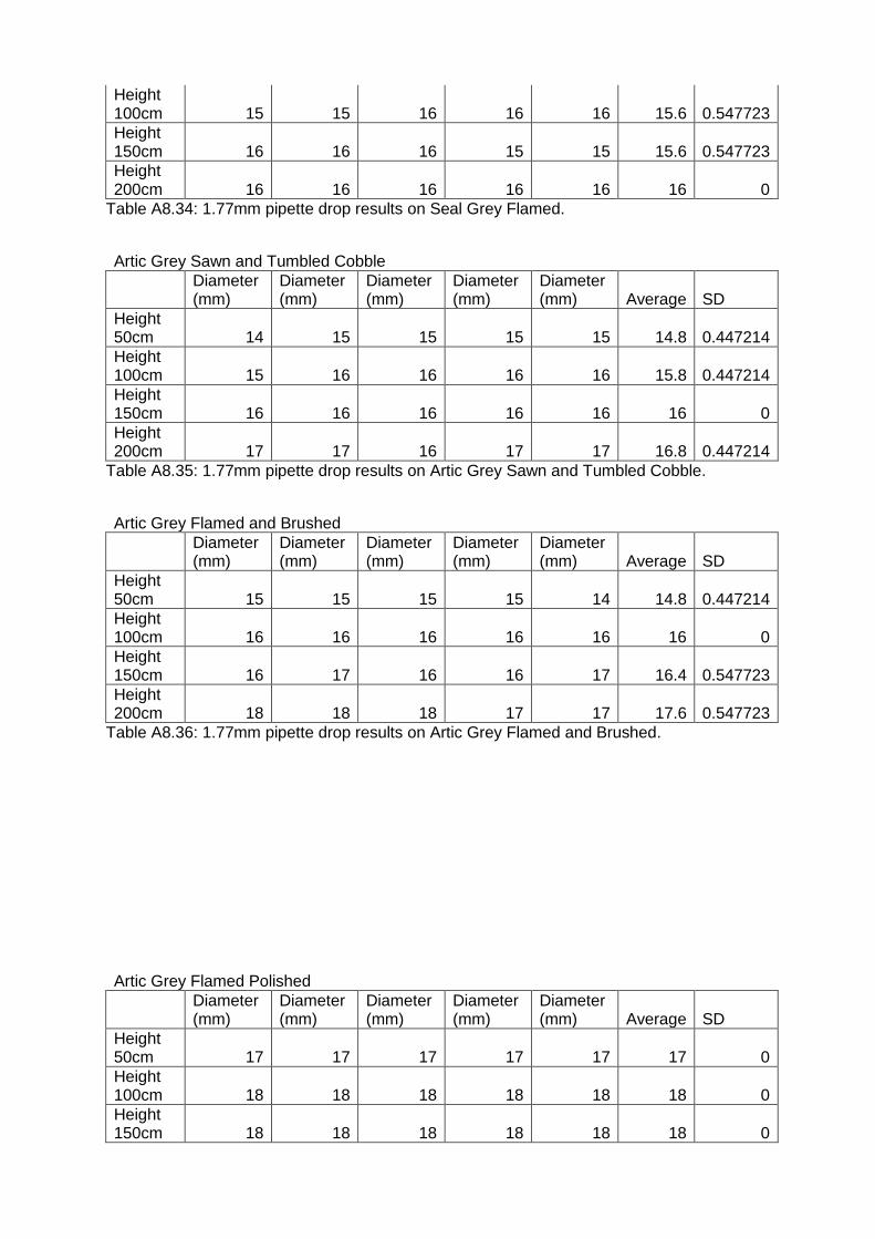
Height 100cm 15 15 16 16 16 15.6 0.547723
Height 150cm 16 16 16 15 15 15.6 0.547723
Height 200cm 16 16 16 16 16 16 0
Table A8.34: 1.77mm pipette drop results on Seal Grey Flamed.
Artic Grey Sawn and Tumbled Cobble
Diameter (mm)
Diameter (mm)
Diameter (mm)
Diameter (mm)
Diameter (mm) Average SD
Height 50cm 14 15 15 15 15 14.8 0.447214
Height 100cm 15 16 16 16 16 15.8 0.447214
Height 150cm 16 16 16 16 16 16 0
Height 200cm 17 17 16 17 17 16.8 0.447214
Table A8.35: 1.77mm pipette drop results on Artic Grey Sawn and Tumbled Cobble.
Artic Grey Flamed and Brushed
Diameter (mm)
Diameter (mm)
Diameter (mm)
Diameter (mm)
Diameter (mm) Average SD
Height 50cm 15 15 15 15 14 14.8 0.447214
Height 100cm 16 16 16 16 16 16 0
Height 150cm 16 17 16 16 17 16.4 0.547723
Height 200cm 18 18 18 17 17 17.6 0.547723
Table A8.36: 1.77mm pipette drop results on Artic Grey Flamed and Brushed.
Artic Grey Flamed Polished
Diameter (mm)
Diameter (mm)
Diameter (mm)
Diameter (mm)
Diameter (mm) Average SD
Height 50cm 17 17 17 17 17 17 0
Height 100cm 18 18 18 18 18 18 0
Height 150cm 18 18 18 18 18 18 0

Height 200cm 20 20 20 19 19 19.6 0.547723
Table A8.37: 1.77mm pipette drop results on Artic Grey Flamed Polished.
Appendix 9 - Bloodstains on a Heated Surfaces Stone Surfaces
Rusty Slate Paving
Diameter (mm)
Diameter (mm)
Diameter (mm)
Diameter (mm)
Diameter (mm) Average SD
25 12 12 12 12 12 12 0
30 12 12 12 12 12 12 0
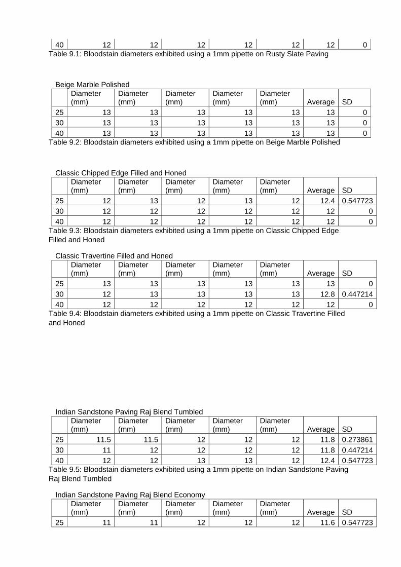
40 12 12 12 12 12 12 0
Table 9.1: Bloodstain diameters exhibited using a 1mm pipette on Rusty Slate Paving
Beige Marble Polished
Diameter (mm)
Diameter (mm)
Diameter (mm)
Diameter (mm)
Diameter (mm) Average SD
25 13 13 13 13 13 13 0
30 13 13 13 13 13 13 0
40 13 13 13 13 13 13 0
Table 9.2: Bloodstain diameters exhibited using a 1mm pipette on Beige Marble Polished
Classic Chipped Edge Filled and Honed
Diameter (mm)
Diameter (mm)
Diameter (mm)
Diameter (mm)
Diameter (mm) Average SD
25 12 13 12 13 12 12.4 0.547723
30 12 12 12 12 12 12 0
40 12 12 12 12 12 12 0
Table 9.3: Bloodstain diameters exhibited using a 1mm pipette on Classic Chipped Edge
Filled and Honed
Classic Travertine Filled and Honed
Diameter (mm)
Diameter (mm)
Diameter (mm)
Diameter (mm)
Diameter (mm) Average SD
25 13 13 13 13 13 13 0
30 12 13 13 13 13 12.8 0.447214
40 12 12 12 12 12 12 0
Table 9.4: Bloodstain diameters exhibited using a 1mm pipette on Classic Travertine Filled
and Honed
Indian Sandstone Paving Raj Blend Tumbled
Diameter (mm)
Diameter (mm)
Diameter (mm)
Diameter (mm)
Diameter (mm) Average SD
25 11.5 11.5 12 12 12 11.8 0.273861
30 11 12 12 12 12 11.8 0.447214
40 12 12 13 13 12 12.4 0.547723
Table 9.5: Bloodstain diameters exhibited using a 1mm pipette on Indian Sandstone Paving
Raj Blend Tumbled
Indian Sandstone Paving Raj Blend Economy
Diameter (mm)
Diameter (mm)
Diameter (mm)
Diameter (mm)
Diameter (mm) Average SD
25 11 11 12 12 12 11.6 0.547723

30 13 13 12 12 12 12.4 0.547723
40 12 12 12 12 12 12 0
Table 9.6: Bloodstain diameters exhibited using a 1mm pipette on Indian Sandstone Paving
Raj Blend Economy
Indian Sandstone Paving Sahara Yellow
Diameter (mm)
Diameter (mm)
Diameter (mm)
Diameter (mm)
Diameter (mm) Average SD
25 12 12 12 12 12 12 0
30 12 12 12 12 12 12 0
40 12 11 11.5 12 12 11.7 0.447214
Table 9.7: Bloodstain diameters exhibited using a 1mm pipette on Indian Sandstone Paving
Sahara Yellow
Indian Sandstone Paving Rippon Buff
Diameter (mm)
Diameter (mm)
Diameter (mm)
Diameter (mm)
Diameter (mm) Average SD
25 11.5 11 11 11.5 11.5 11.3 0.273861
30 12 12 12 12 12 12 0
40 13 12 12 12 12 12.2 0.447214
Table 9.8: Bloodstain diameters exhibited using a 1mm pipette on Indian Sandstone Paving
Rippon Buff
Indian Sandstone Paving Modak
Diameter (mm)
Diameter (mm)
Diameter (mm)
Diameter (mm)
Diameter (mm) Average SD
25 12 12 12 12 12 12 0
30 12 12 12 12 12 12 0
40 13 13 12 12 12 12.4 0.547723
Table 9.9: Bloodstain diameters exhibited using a 1mm pipette on Indian Sandstone Paving
Modak
Classic Honed Travertine Paving
Diameter (mm)
Diameter (mm)
Diameter (mm)
Diameter (mm)
Diameter (mm) Average SD
25 12 12 12 12 12 12 0
30 13 12 12 12 12 12.2 0.447214
40 13 12 12 12 12 12.2 0.447214
Table 9.10: Bloodstain diameters exhibited using a 1mm pipette on Classic Honed
Travertine Paving
Silver Latte Tumbled Travertine Paving
Diameter (mm)
Diameter (mm)
Diameter (mm)
Diameter (mm)
Diameter (mm) Average SD
25 12 12 12 12 12 12 0
30 12.5 12.5 12 12 12 12.2 0.273861
40 12 11 11 12 12 11.6 0.547723

Table 9.11: Bloodstain diameters exhibited using a 1mm pipette on Silver Latte Tumbled
Travertine Paving
Yellow Limestone Paving
Diameter (mm)
Diameter (mm)
Diameter (mm)
Diameter (mm)
Diameter (mm) Average SD
25 12 11 11 11 11 11.2 0.447214
30 11 12 11 11 11 11.2 0.447214
40 11 12 11 11 11 11.2 0.447214
Table 9.12: Bloodstain diameters exhibited using a 1mm pipette on Yellow Limestone
Paving
Brazilian Black Slate Paving
Diameter (mm)
Diameter (mm)
Diameter (mm)
Diameter (mm)
Diameter (mm) Average SD
25 12 12 13 13 12 12.4 0.547723
30 12 12 12 12 12 12 0
40 12 12 12 12 12 12 0
Table 9.13: Bloodstain diameters exhibited using a 1mm pipette on Brazilian Black Slate
Paving
Beige Marble Polished
Diameter (mm)
Diameter (mm)
Diameter (mm)
Diameter (mm)
Diameter (mm) Average SD
25 13 13 13 13 13 13 0
30 13 13 13 13 13 13 0
40 13 13 13 13 13 13 0
Table 9.14: Bloodstain diameters exhibited using a 1mm pipette on Beige Marble Polished
Blood on a Heated Tile Surface (1 mm pipette)
Sandstone Rivon
Diameter (mm)
Diameter (mm)
Diameter (mm)
Diameter (mm)
Diameter (mm) Average SD
25 14 14 14 13.5 13.5 13.8 0.273861
30 14.5 14.5 14.5 14.5 14.5 14.5 0
40 14 14 14.5 13.5 14 14 0.353553
Table 9.15: Bloodstain diameters exhibited using a 1mm pipette on Sandstone Rivon
Super White Matt
Diameter (mm)
Diameter (mm)
Diameter (mm)
Diameter (mm)
Diameter (mm) Average SD
25 12 13 12.5 13 13 12.7 0.447214
30 13 13 13 13 13 13 0
40 13.5 13.5 13.5 13.5 13.5 13.5 0

Table 9.16: Bloodstain diameters exhibited using a 1mm pipette on Super White Matt
Table 9.17: Bloodstain diameters exhibited using a 1mm pipette on Ceramic Matt
Ceramic Polished
Diameter (mm)
Diameter (mm)
Diameter (mm)
Diameter (mm)
Diameter (mm) Average SD
25 14 14 14 14 14 14 0
30 13.5 13.5 13.5 13.5 13.5 13.5 0
40 13 13 13 13 13 13 0
Table 9.18: Bloodstain diameters exhibited using a 1mm pipette on Ceramic Polished
Blood on a Wood Surface (1mm pipette)
Oak
European Maple Oak
1mm Mean 1mm SD 1.7mm Mean 1.7mm SD
50 cm 13.2 0.447214 16 0
100 cm 14 0 17.2 0.447214
150 cm 16 0 18.8 0.83666
200 cm 16.4 0.547723 19.2 0.447214
Table 9.19: Bloodstain diameters exhibited using a 1mm pipette on European Maple Oak
Clear Oil Oak
1mm Mean 1mm SD 1.7mm Mean 1.7mm SD
50 cm 13 0 15.2 0.447214
100 cm 14.2 0.447214 16.2 0.447214
150 cm 15.4 0.547723 17.6 0.547723
200 cm 16.8 0.447214 18.2 0.447214
Table 9.20: Bloodstain diameters exhibited using a 1mm pipette on Clear Oil Oak
Oak Natural Siera Matt Lacquered
1mm Mean 1mm SD 1.7mm Mean 1.7mm SD
50 cm 13 0.447214 15.6 0.489898
Ceramic Matt
Diameter (mm)
Diameter (mm)
Diameter (mm)
Diameter (mm)
Diameter (mm) Average SD
25 14 14.5 14 14 15 14.3 0.447214
30 15 15 15.5 15 15 15.1 0.223607
40 15.5 15 16 16 15.5 15.6 0.41833

100 cm 14.2 0 17.4 0.489898
150 cm 15.4 0.447214 18.6 0.489898
200 cm 16.8 0.447214 19.2 0.4
Table 9.21: Bloodstain diameters exhibited using a 1mm pipette on Oak Natural Siera Matt
Lacquered
Oak Silk Matt
1mm Mean 1mm SD 1.7mm Mean 1.7mm SD
50 cm 14 0 16.2 0.447214
100 cm 15 0 17.6 0.547723
150 cm 16 0.707107 19.2 0.447214
200 cm 17 0 19.4 0.547723
Table 9.22: Bloodstain diameters exhibited using a 1mm pipette on Oak Silk Matt
Kahrs Oak Sienna Natural
1mm Mean 1mm SD 1.7mm Mean 1.7mm SD
50 cm 13.2 0.447214 15 0
100 cm 15.4 0.547723 17.4 0.547723
150 cm 16 0 18.6 0.547723
200 cm 17.2 0.447214 19.2 0.447214
Table 9.23: Bloodstain diameters exhibited using a 1mm pipette on Kahrs Oak Sienna
Natural
Natura Oak Prime Parquet
1mm Mean 1mm SD 1.7mm Mean 1.7mm SD
50 cm 10.8 0.447214 14.6 0.547723
100 cm 13 0.547723 15.8 0.447214
150 cm 13.4 0 16.6 0.547723
200 cm 13.8 0.447214 17 0
Table 9.24: Bloodstain diameters exhibited using a 1mm pipette on Natura Oak Prime
Parquet
Kahrs Oak Siena Engineered Natural
1mm Mean 1mm SD 1.7mm Mean 1.7mm SD
50 cm 12.8 0.447214 14 0
100 cm 13 0 16.2 0.447214
150 cm 13.2 0.447214 16.8 0.447214
200 cm 14 0 17 0
Table 9.25: Bloodstain diameters exhibited using a 1mm pipette on Kahrs Oak Siena
Engineered Natural
Oak Solid Plank Untreated
1mm Mean 1mm SD 1.7mm Mean 1.7mm SD
50 cm 9.4 0.547723 14.4 0.547723
100 cm 13.2 0.447214 15.6 0.547723

150 cm 14 0 16 0.707107
200 cm 14 0 18.8 0.447214
Table 9.26: Bloodstain diameters exhibited using a 1mm pipette on Oak Solid Plank
Untreated
Maple
Maple Silk Matt Lacquered
1mm Mean 1mm SD 1.7mm Mean 1.7mm SD
50 cm 13.2 0.447214 15.8 0.447214
100 cm 15 0 17.2 0.447214
150 cm 15.8 0.447214 19 0
200 cm 18 0 19.2 0.447214
Table 9.27: Bloodstain diameters exhibited using a 1mm pipette on Maple Silk Matt
Lacquered
Kahrs Maple Toronto Satin Lacquer
1mm Mean 1mm SD 1.7mm Mean 1.7mm SD
50 cm 12.4 0.547723 16 0
100 cm 14 53.66563 17.4 0.547723
150 cm 15.6 0.547723 18.4 0.547723
200 cm 16.6 0.547723 19.4 0.547723
Table 9.28: Bloodstain diameters exhibited using a 1mm pipette on Kahrs Maple Toronto
Satin Lacquer
Maple Ultra Matt Lacquered
1mm Mean 1mm SD 1.7mm Mean 1.7mm SD
50 cm 13.4 0.547723 15 0
100 cm 15 0 17 0
150 cm 16 0 18.8 0.447214
200 cm 16.8 0.447214 0.547723
Table 9.29: Bloodstain diameters exhibited using a 1mm pipette on Maple Ultra Matt
Lacquered
Kahrs Maple Bevelled Edge Rustic
1mm Mean 1mm SD 1.7mm Mean 1.7mm SD
50 cm 14 0 16.2 0.447214
100 cm 15 0 18.2 0.83666
150 cm 16 0 19 0
200 cm 17 0 19.6 0.547723
Table 9.30: Bloodstain diameters exhibited using a 1mm pipette on Kahrs Maple Bevelled
Edge Rustic
Kahrs Maple Natural Satin Lacquer
1mm Mean 1mm SD 1.7mm Mean 1.7mm SD
50 cm 13.4 0.547723 16 0
100 cm 15 0 17.6 0.547723
150 cm 15.6 0.547723 19 0.707107
200 cm 16.8 0.447214 19.2 0.83666
Table 9.31: Bloodstain diameters exhibited using a 1mm pipette on Kahrs Maple Natural
Satin Lacquer
Walnut

Natura American Black Walnut Rosshill
1mm Mean 1mm SD 1.7mm Mean 1.7mm SD
50 cm 13.4 0.547723 16.8 0.447214
100 cm 14 0 17.4 0.547723
150 cm 16 0 18.2 0.447214
200 cm 17 0 19.2 0.447214
Table 9.32: Bloodstain diameters exhibited using a 1mm pipette on Natura American Black
Walnut Rosshill
Natura Walnut Ironbank Mississippi
1mm Mean 1mm SD 1.7mm Mean 1.7mm SD
50 cm 13 0 15.4 0.547723
100 cm 14.8 0.447214 17.2 0.447214
150 cm 15.6 0.894427 18.8 0.447214
200 cm 16.6 0.547723 19.4 0.547723
Table 9.33: Bloodstain diameters exhibited using a 1mm pipette on Natura Walnut Ironbank
Mississippi
Quickstep Villa Walnut Satin Lacquer
1mm Mean 1mm SD 1.7mm Mean 1.7mm SD
50 cm 13.8 0.447214 16.4 0.547723
100 cm 14.4 0.547723 17.6 0.547723
150 cm 16 0 18.8 0.447214
200 cm 17 0.707107 19.2 0.447214
Table 9.34: Bloodstain diameters exhibited using a 1mm pipette on Quickstep Villa Walnut
Satin Lacquer
Kahrs Walnut Rustic Nature Oil
1mm Mean 1mm SD 1.7mm Mean 1.7mm SD
50 cm 12.4 0.547723 15.4 0.547723
100 cm 14 0 17.4 0.547723
150 cm 15.6 0.547723 18.4 0.547723
200 cm 16.6 0.547723 20 0.707107
Table 9.35: Bloodstain diameters exhibited using a 1mm pipette on Kahrs Walnut Rustic
Nature Oil
Kahrs Linnea Walnut Bloom Prime Satin Lacquer
1mm Mean 1mm SD 1.7mm Mean 1.7mm SD
50 cm 13.6 0.547723 15.6 0.547723
100 cm 15.4 0.547723 17 0
150 cm 16.6 0.547723 19 0.707107
200 cm 17 0 19.4 0.547723
Table 9.36: Bloodstain diameters exhibited using a 1mm pipette on Kahrs Linnea Walnut
Bloom Prime Satin Lacquer
Kahrs Linnea Walnut Microbevelled Edge Prime Matt Lacquer

1mm Mean 1mm SD 1.7mm Mean 1.7mm SD
50 cm 13.4 0.547723 15 0
100 cm 15 0 17.6 0.547723
150 cm 15.6 0.547723 18.2 0.447214
200 cm 17.2 0.447214 18.8 0.447214
Table 9.37: Bloodstain diameters exhibited using a 1mm pipette on Kahrs Linnea Walnut
Microbevelled Edge Prime Matt Lacquer
Natura Walnut Lacquered Satin Lacquer
1mm Mean 1mm SD 1.7mm Mean 1.7mm SD
50 cm 13 0 15.8 0.447214
100 cm 15 0 18 0
150 cm 15.8 0.447214 18.6 0.547723
200 cm 17 0 19.2 0.447214
Table 9.38: Bloodstain diameters exhibited using a 1mm pipette on Natura Walnut
Lacquered Satin Lacquer
Appendix 10 – DNA Profiles for Cleaned
Surfaces


Dye/Sample Peak Sample File Name Marker Allele Size Height Area Data Point
1 B,1 A11_N.fsa 98 1255 1107
2 B,2 A11_N.fsa 88 1129 1143
3 B,3 A11_N.fsa 71 686 1174
4 B,4 A11_N.fsa 82 856 1211
5 B,5 A11_N.fsa 104 875 1295
6 B,6 A11_N.fsa 258 3408 1319
7 B,7 A11_N.fsa 160 2258 1350
8 B,8 A11_N.fsa 71 588 1366
9 B,9 A11_N.fsa 291 3567 1418
10 B,10 A11_N.fsa 197 1961 1434
11 B,11 A11_N.fsa 153 1249 1453
12 B,12 A11_N.fsa 253 2989 1464
13 B,13 A11_N.fsa 189 1662 1482
14 B,14 A11_N.fsa 111 747 1513
15 B,15 A11_N.fsa 4547 54399 1550
16 B,16 A11_N.fsa 2.48 4053 52633 1586
17 B,17 A11_N.fsa 5.97 2529 36334 1631
18 B,18 A11_N.fsa 10.47 443 4662 1689
19 B,19 A11_N.fsa 14.96 7905 101489 1747
20 B,20 A11_N.fsa 15.89 7935 100051 1759
21 B,21 A11_N.fsa 17.05 5957 58181 1774
22 B,22 A11_N.fsa 29.3 213 807 1932
23 B,23 A11_N.fsa 30.7 227 840 1950
24 B,24 A11_N.fsa 32.4 55 1482 1972
25 B,25 A11_N.fsa 37.75 148 539 2041
26 B,26 A11_N.fsa 44.88 111 452 2133
27 B,27 A11_N.fsa 47.75 2670 34250 2170
28 B,28 A11_N.fsa 52.64 231 1350 2233
29 B,29 A11_N.fsa 53.33 237 1212 2242
30 G,1 A11_N.fsa 63 954 1113
31 G,2 A11_N.fsa 50 1465 1163
32 G,3 A11_N.fsa 202 2238 1212
33 G,4 A11_N.fsa 167 1675 1307
34 G,5 A11_N.fsa 159 1928 1323
35 G,6 A11_N.fsa 555 6097 1380
36 G,7 A11_N.fsa 167 3987 1421
37 G,8 A11_N.fsa 55 607 1458
38 G,9 A11_N.fsa 2174 23489 1492
39 G,10 A11_N.fsa 5083 41370 1546
40 G,11 A11_N.fsa 0.08 6442 55046 1555

41 G,12 A11_N.fsa 1.16 356 3647 1569
42 G,13 A11_N.fsa 2.02 148 830 1580
43 G,14 A11_N.fsa 2.71 354 2445 1589
44 G,15 A11_N.fsa 5.19 3559 41940 1621
45 G,16 A11_N.fsa 6.67 5521 49817 1640
46 G,17 A11_N.fsa 8.45 380 3540 1663
47 G,18 A11_N.fsa 9.92 6652 53266 1682

Dye/Sample Peak Sample File Name Marker Allele Size Height Area Data Point
48 G,19 A11_N.fsa 13.33 790 11611 1726
49 G,20 A11_N.fsa 14.65 728 4086 1743
50 G,21 A11_N.fsa 15.27 373 3960 1751
51 G,22 A11_N.fsa 16.59 5749 40718 1768
52 G,23 A11_N.fsa 17.52 6451 49552 1780
53 G,24 A11_N.fsa 26.36 260 3361 1894
54 G,25 A11_N.fsa 30.0 3502 32569 1941
55 G,26 A11_N.fsa 31.01 58 465 1954
56 G,27 A11_N.fsa 37.67 10853 129119 2040
57 G,28 A11_N.fsa 46.05 10960 160811 2148
58 G,29 A11_N.fsa 47.44 84 1046 2166
59 G,30 A11_N.fsa 48.91 10965 115684 2185
60 G,31 A11_N.fsa 50.16 141 1553 2201
61 G,32 A11_N.fsa 52.95 268 1125 2237
62 Y,1 A11_N.fsa 88 973 1493
63 Y,2 A11_N.fsa 1048 3362 1544
64 Y,3 A11_N.fsa 0.16 1692 11548 1556
65 Y,4 A11_N.fsa 2.02 2452 18856 1580
66 Y,5 A11_N.fsa 2.79 2647 20353 1590
67 Y,6 A11_N.fsa 4.42 2269 12528 1611
68 Y,7 A11_N.fsa 5.04 1845 9311 1619
69 Y,8 A11_N.fsa 6.74 1441 10493 1641
70 Y,9 A11_N.fsa 8.14 1954 11765 1659
71 Y,10 A11_N.fsa 9.46 5116 36483 1676
72 Y,11 A11_N.fsa 10.31 6549 45428 1687
73 Y,12 A11_N.fsa 14.26 5001 32043 1738
74 Y,13 A11_N.fsa 16.05 2020 21480 1761
75 Y,14 A11_N.fsa 17.6 655 3336 1781
76 Y,15 A11_N.fsa 18.45 209 3551 1792
77 Y,16 A11_N.fsa 22.4 166 1790 1843
78 Y,17 A11_N.fsa 26.67 55 679 1898
79 Y,18 A11_N.fsa 27.75 102 845 1912
80 Y,19 A11_N.fsa 28.6 171 1515 1923
81 Y,20 A11_N.fsa 29.69 8291 89317 1937
82 Y,21 A11_N.fsa 30.31 8318 83579 1945
83 Y,22 A11_N.fsa 37.13 7133 45431 2033
84 Y,23 A11_N.fsa 38.29 6947 45053 2048
85 Y,24 A11_N.fsa 42.87 692 6609 2107
86 Y,25 A11_N.fsa 45.27 7582 95821 2138
87 Y,26 A11_N.fsa 46.82 6589 51036 2158

88 Y,27 A11_N.fsa 48.37 6857 45836 2178
89 Y,28 A11_N.fsa 49.46 6690 41717 2192
90 Y,29 A11_N.fsa 52.95 7452 86360 2237
91 Y,30 A11_N.fsa 54.26 91 1261 2254
92 R,1 A11_N.fsa 5553 45775 1550
93 R,2 A11_N.fsa 2.33 3429 21618 1584
94 R,3 A11_N.fsa 3.33 6756 62829 1597
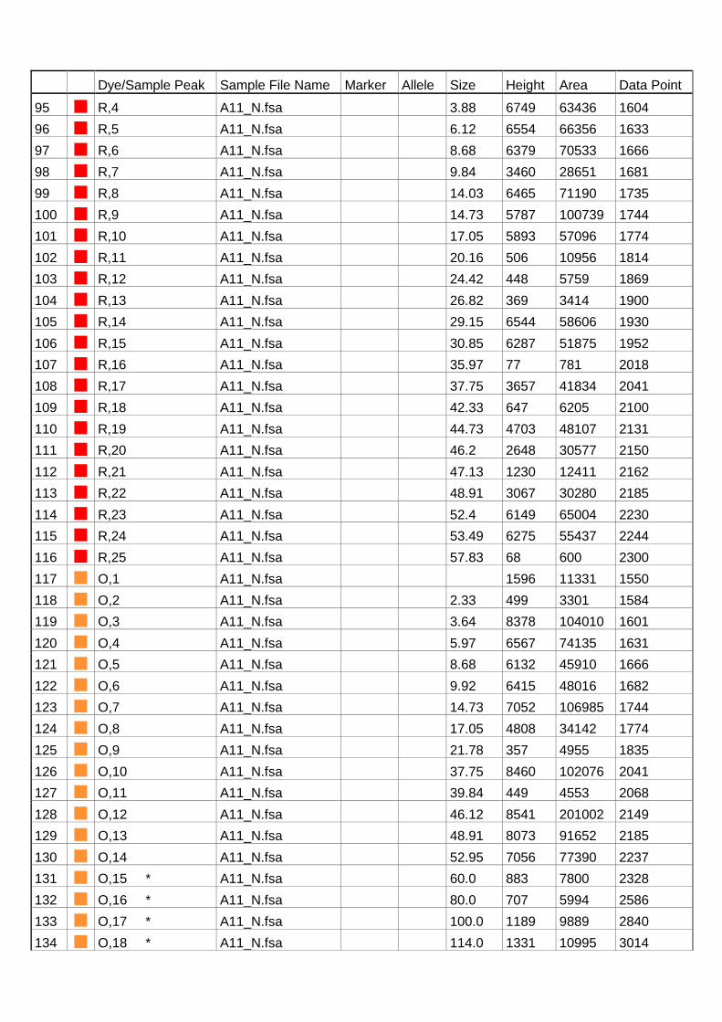
Dye/Sample Peak Sample File Name Marker Allele Size Height Area Data Point
95 R,4 A11_N.fsa 3.88 6749 63436 1604
96 R,5 A11_N.fsa 6.12 6554 66356 1633
97 R,6 A11_N.fsa 8.68 6379 70533 1666
98 R,7 A11_N.fsa 9.84 3460 28651 1681
99 R,8 A11_N.fsa 14.03 6465 71190 1735
100 R,9 A11_N.fsa 14.73 5787 100739 1744
101 R,10 A11_N.fsa 17.05 5893 57096 1774
102 R,11 A11_N.fsa 20.16 506 10956 1814
103 R,12 A11_N.fsa 24.42 448 5759 1869
104 R,13 A11_N.fsa 26.82 369 3414 1900
105 R,14 A11_N.fsa 29.15 6544 58606 1930
106 R,15 A11_N.fsa 30.85 6287 51875 1952
107 R,16 A11_N.fsa 35.97 77 781 2018
108 R,17 A11_N.fsa 37.75 3657 41834 2041
109 R,18 A11_N.fsa 42.33 647 6205 2100
110 R,19 A11_N.fsa 44.73 4703 48107 2131
111 R,20 A11_N.fsa 46.2 2648 30577 2150
112 R,21 A11_N.fsa 47.13 1230 12411 2162
113 R,22 A11_N.fsa 48.91 3067 30280 2185
114 R,23 A11_N.fsa 52.4 6149 65004 2230
115 R,24 A11_N.fsa 53.49 6275 55437 2244
116 R,25 A11_N.fsa 57.83 68 600 2300
117 O,1 A11_N.fsa 1596 11331 1550
118 O,2 A11_N.fsa 2.33 499 3301 1584
119 O,3 A11_N.fsa 3.64 8378 104010 1601
120 O,4 A11_N.fsa 5.97 6567 74135 1631
121 O,5 A11_N.fsa 8.68 6132 45910 1666
122 O,6 A11_N.fsa 9.92 6415 48016 1682
123 O,7 A11_N.fsa 14.73 7052 106985 1744
124 O,8 A11_N.fsa 17.05 4808 34142 1774
125 O,9 A11_N.fsa 21.78 357 4955 1835
126 O,10 A11_N.fsa 37.75 8460 102076 2041
127 O,11 A11_N.fsa 39.84 449 4553 2068
128 O,12 A11_N.fsa 46.12 8541 201002 2149
129 O,13 A11_N.fsa 48.91 8073 91652 2185
130 O,14 A11_N.fsa 52.95 7056 77390 2237
131 O,15 * A11_N.fsa 60.0 883 7800 2328
132 O,16 * A11_N.fsa 80.0 707 5994 2586
133 O,17 * A11_N.fsa 100.0 1189 9889 2840
134 O,18 * A11_N.fsa 114.0 1331 10995 3014

135 O,19 * A11_N.fsa 120.0 1104 9158 3091
136 O,20 * A11_N.fsa 140.0 869 7149 3342
137 O,21 * A11_N.fsa 160.0 939 7878 3583
138 O,22 * A11_N.fsa 180.0 1184 9958 3825
139 O,23 * A11_N.fsa 200.0 992 8513 4063
140 O,24 * A11_N.fsa 214.0 998 8605 4232
141 O,25 * A11_N.fsa 220.0 834 7379 4303

Dye/Sample Peak Sample File Name Marker Allele Size Height Area Data Point
142 O,26 * A11_N.fsa 240.0 1287 11600 4541
143 O,27 * A11_N.fsa 250.0 608 5651 4657
144 O,28 * A11_N.fsa 260.0 1031 9523 4778
145 O,29 * A11_N.fsa 280.0 1155 10958 5015
146 O,30 * A11_N.fsa 300.0 1233 11898 5254
147 O,31 * A11_N.fsa 314.0 852 8416 5421
148 O,32 * A11_N.fsa 320.0 943 9489 5488
149 O,33 * A11_N.fsa 340.0 1175 12231 5722
150 O,34 * A11_N.fsa 360.0 1025 10870 5954
151 O,35 * A11_N.fsa 380.0 709 7729 6187
152 O,36 * A11_N.fsa 400.0 1063 11915 6416
153 O,37 * A11_N.fsa 414.0 907 10322 6578
154 O,38 * A11_N.fsa 420.0 900 10451 6645
155 O,39 * A11_N.fsa 440.0 989 11879 6873
156 O,40 * A11_N.fsa 460.0 814 9873 7094
157 O,41 * A11_N.fsa 480.0 744 9293 7317
158 O,42 * A11_N.fsa 500.0 330 4184 7532
159 O,43 * A11_N.fsa 514.0 370 4757 7682
160 O,44 * A11_N.fsa 520.0 766 9955 7746
161 O,45 A11_N.fsa 540.25 599 8044 7962
162 O,46 A11_N.fsa 559.84 411 5696 8171
163 O,47 A11_N.fsa 578.97 596 8344 8375
164 O,48 A11_N.fsa 597.81 445 6353 8576

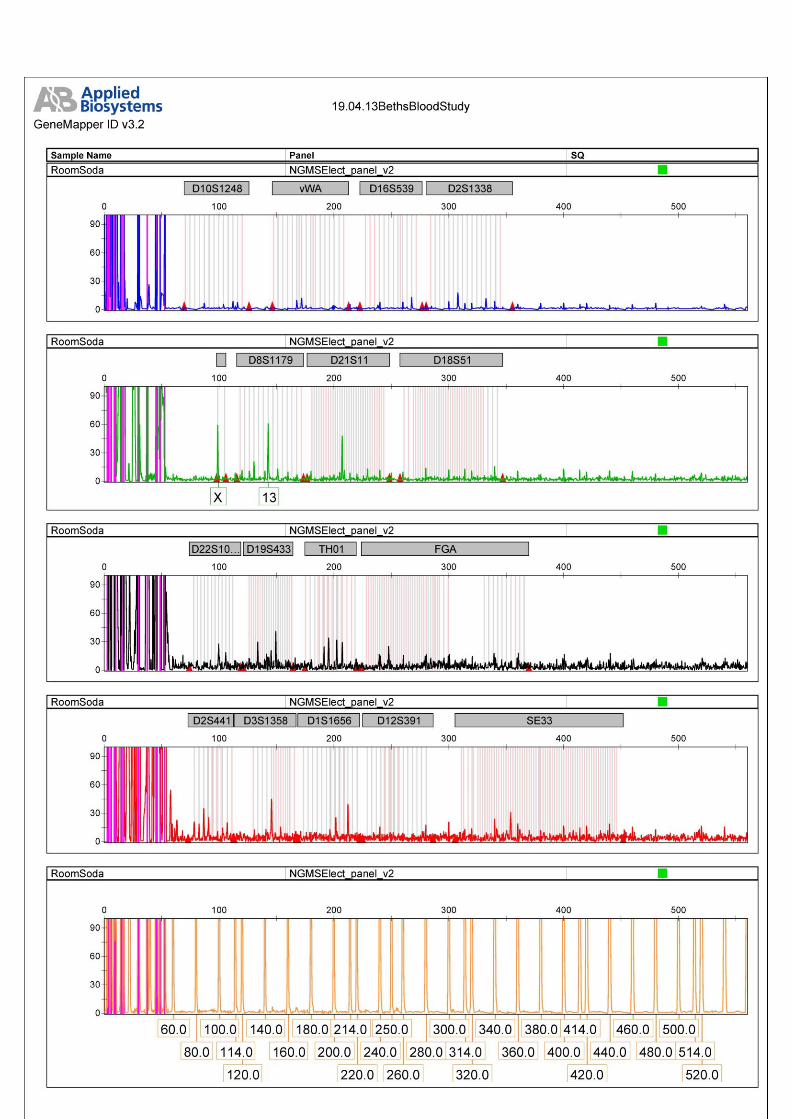
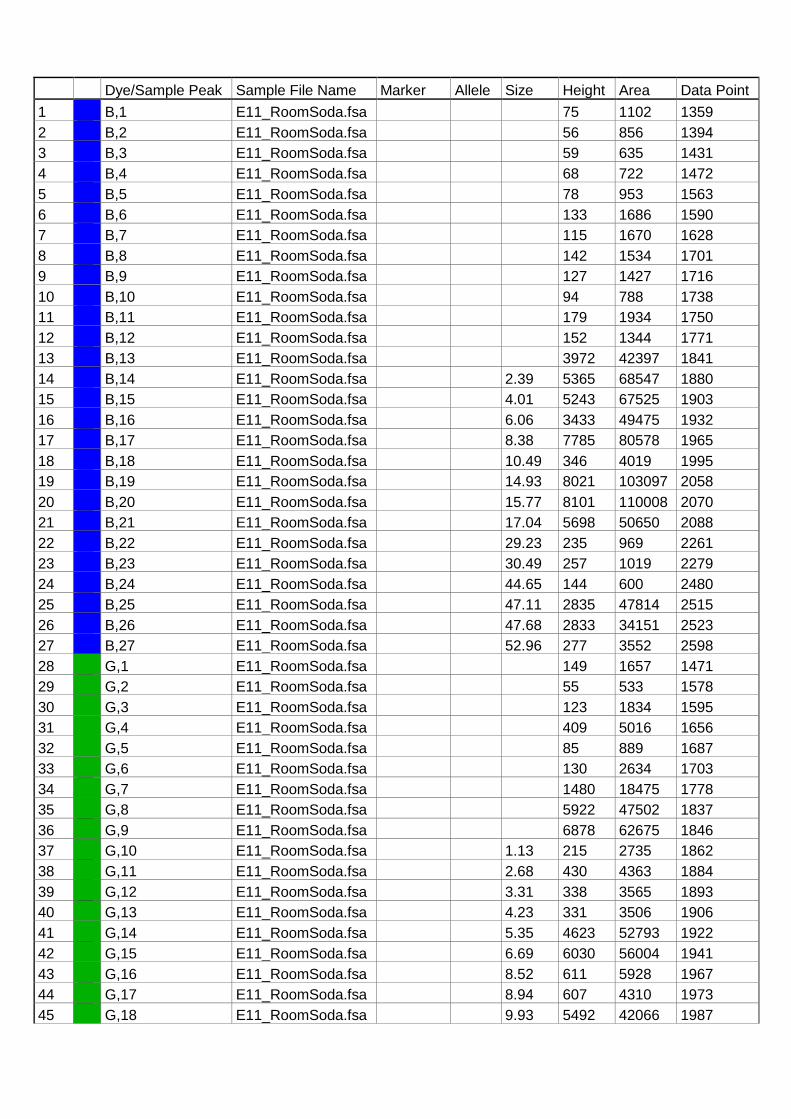
Dye/Sample Peak Sample File Name Marker Allele Size Height Area Data Point
1 B,1 E11_RoomSoda.fsa 75 1102 1359
2 B,2 E11_RoomSoda.fsa 56 856 1394
3 B,3 E11_RoomSoda.fsa 59 635 1431
4 B,4 E11_RoomSoda.fsa 68 722 1472
5 B,5 E11_RoomSoda.fsa 78 953 1563
6 B,6 E11_RoomSoda.fsa 133 1686 1590
7 B,7 E11_RoomSoda.fsa 115 1670 1628
8 B,8 E11_RoomSoda.fsa 142 1534 1701
9 B,9 E11_RoomSoda.fsa 127 1427 1716
10 B,10 E11_RoomSoda.fsa 94 788 1738
11 B,11 E11_RoomSoda.fsa 179 1934 1750
12 B,12 E11_RoomSoda.fsa 152 1344 1771
13 B,13 E11_RoomSoda.fsa 3972 42397 1841
14 B,14 E11_RoomSoda.fsa 2.39 5365 68547 1880
15 B,15 E11_RoomSoda.fsa 4.01 5243 67525 1903
16 B,16 E11_RoomSoda.fsa 6.06 3433 49475 1932
17 B,17 E11_RoomSoda.fsa 8.38 7785 80578 1965
18 B,18 E11_RoomSoda.fsa 10.49 346 4019 1995
19 B,19 E11_RoomSoda.fsa 14.93 8021 103097 2058
20 B,20 E11_RoomSoda.fsa 15.77 8101 110008 2070
21 B,21 E11_RoomSoda.fsa 17.04 5698 50650 2088
22 B,22 E11_RoomSoda.fsa 29.23 235 969 2261
23 B,23 E11_RoomSoda.fsa 30.49 257 1019 2279
24 B,24 E11_RoomSoda.fsa 44.65 144 600 2480
25 B,25 E11_RoomSoda.fsa 47.11 2835 47814 2515
26 B,26 E11_RoomSoda.fsa 47.68 2833 34151 2523
27 B,27 E11_RoomSoda.fsa 52.96 277 3552 2598
28 G,1 E11_RoomSoda.fsa 149 1657 1471
29 G,2 E11_RoomSoda.fsa 55 533 1578
30 G,3 E11_RoomSoda.fsa 123 1834 1595
31 G,4 E11_RoomSoda.fsa 409 5016 1656
32 G,5 E11_RoomSoda.fsa 85 889 1687
33 G,6 E11_RoomSoda.fsa 130 2634 1703
34 G,7 E11_RoomSoda.fsa 1480 18475 1778
35 G,8 E11_RoomSoda.fsa 5922 47502 1837
36 G,9 E11_RoomSoda.fsa 6878 62675 1846
37 G,10 E11_RoomSoda.fsa 1.13 215 2735 1862
38 G,11 E11_RoomSoda.fsa 2.68 430 4363 1884
39 G,12 E11_RoomSoda.fsa 3.31 338 3565 1893
40 G,13 E11_RoomSoda.fsa 4.23 331 3506 1906
41 G,14 E11_RoomSoda.fsa 5.35 4623 52793 1922
42 G,15 E11_RoomSoda.fsa 6.69 6030 56004 1941
43 G,16 E11_RoomSoda.fsa 8.52 611 5928 1967
44 G,17 E11_RoomSoda.fsa 8.94 607 4310 1973
45 G,18 E11_RoomSoda.fsa 9.93 5492 42066 1987

46 G,19 E11_RoomSoda.fsa 13.31 509 8132 2035
47 G,20 E11_RoomSoda.fsa 14.72 614 3573 2055

Dye/Sample Peak Sample File Name Marker Allele Size Height Area Data Point
48 G,21 E11_RoomSoda.fsa 15.21 343 3884 2062
49 G,22 E11_RoomSoda.fsa 16.62 6128 47062 2082
50 G,23 E11_RoomSoda.fsa 17.46 6881 61590 2094
51 G,24 E11_RoomSoda.fsa 25.0 176 2005 2201
52 G,25 E11_RoomSoda.fsa 26.27 457 5018 2219
53 G,26 E11_RoomSoda.fsa 29.86 2598 23436 2270
54 G,27 E11_RoomSoda.fsa 30.85 60 530 2284
55 G,28 E11_RoomSoda.fsa 37.46 11048 126866 2378
56 G,29 E11_RoomSoda.fsa 45.92 11059 151852 2498
57 G,30 E11_RoomSoda.fsa 46.97 58 544 2513
58 G,31 E11_RoomSoda.fsa 47.54 57 488 2521
59 G,32 E11_RoomSoda.fsa 48.66 10169 105928 2537
60 G,33 E11_RoomSoda.fsa 49.93 163 2602 2555
61 G,34 E11_RoomSoda.fsa 51.34 89 928 2575
62 G,35 E11_RoomSoda.fsa AMEL X 98.85 59 568 3246
63 G,36 E11_RoomSoda.fsa D8S1179 13 142.73 61 650 3860
64 Y,1 E11_RoomSoda.fsa 1036 3414 1836
65 Y,2 E11_RoomSoda.fsa 0.07 1752 11391 1847
66 Y,3 E11_RoomSoda.fsa 1.55 762 6030 1868
67 Y,4 E11_RoomSoda.fsa 2.18 2597 22259 1877
68 Y,5 E11_RoomSoda.fsa 2.96 2746 26474 1888
69 Y,6 E11_RoomSoda.fsa 4.51 2280 13537 1910
70 Y,7 E11_RoomSoda.fsa 5.28 1832 10041 1921
71 Y,8 E11_RoomSoda.fsa 6.76 1550 17342 1942
72 Y,9 E11_RoomSoda.fsa 8.24 2103 12411 1963
73 Y,10 E11_RoomSoda.fsa 9.58 6332 50487 1982
74 Y,11 E11_RoomSoda.fsa 10.28 7235 61589 1992
75 Y,12 E11_RoomSoda.fsa 14.37 3553 19358 2050
76 Y,13 E11_RoomSoda.fsa 15.99 2255 25811 2073
77 Y,14 E11_RoomSoda.fsa 17.46 797 6939 2094
78 Y,15 E11_RoomSoda.fsa 22.11 136 1711 2160
79 Y,16 E11_RoomSoda.fsa 28.31 125 1876 2248
80 Y,17 E11_RoomSoda.fsa 29.86 8698 166248 2270
81 Y,18 E11_RoomSoda.fsa 36.9 7653 55535 2370
82 Y,19 E11_RoomSoda.fsa 38.03 7534 55614 2386
83 Y,20 E11_RoomSoda.fsa 42.54 325 2686 2450
84 Y,21 E11_RoomSoda.fsa 45.07 7345 93205 2486
85 Y,22 E11_RoomSoda.fsa 46.48 6398 44891 2506
86 Y,23 E11_RoomSoda.fsa 48.17 6769 47117 2530
87 Y,24 E11_RoomSoda.fsa 49.23 6640 44181 2545
88 Y,25 E11_RoomSoda.fsa 52.68 7382 79057 2594
89 Y,26 E11_RoomSoda.fsa 54.01 83 1359 2613
90 R,1 E11_RoomSoda.fsa 4797 35115 1841
91 R,2 E11_RoomSoda.fsa 1.2 477 8304 1863
92 R,3 E11_RoomSoda.fsa 1.83 497 4394 1872

93 R,4 E11_RoomSoda.fsa 2.39 1465 8232 1880
94 R,5 E11_RoomSoda.fsa 3.45 6779 67570 1895

Dye/Sample Peak Sample File Name Marker Allele Size Height Area Data Point
95 R,6 E11_RoomSoda.fsa 4.01 6778 62767 1903
96 R,7 E11_RoomSoda.fsa 6.06 6533 104444 1932
97 R,8 E11_RoomSoda.fsa 8.73 6542 71326 1970
98 R,9 E11_RoomSoda.fsa 9.93 2994 25122 1987
99 R,10 E11_RoomSoda.fsa 14.15 6830 88110 2047
100 R,11 E11_RoomSoda.fsa 17.04 5831 54155 2088
101 R,12 E11_RoomSoda.fsa 20.28 327 8211 2134
102 R,13 E11_RoomSoda.fsa 24.23 323 4514 2190
103 R,14 E11_RoomSoda.fsa 26.62 203 1979 2224
104 R,15 E11_RoomSoda.fsa 29.08 6989 68745 2259
105 R,16 E11_RoomSoda.fsa 30.63 6717 62432 2281
106 R,17 E11_RoomSoda.fsa 37.46 3632 40932 2378
107 R,18 E11_RoomSoda.fsa 42.04 434 4456 2443
108 R,19 E11_RoomSoda.fsa 44.51 5462 58990 2478
109 R,20 E11_RoomSoda.fsa 45.92 2646 30189 2498
110 R,21 E11_RoomSoda.fsa 46.76 1162 11732 2510
111 R,22 E11_RoomSoda.fsa 48.66 2796 28724 2537
112 R,23 E11_RoomSoda.fsa 52.25 6858 78935 2588
113 R,24 E11_RoomSoda.fsa 53.17 6856 69937 2601
114 R,25 E11_RoomSoda.fsa 57.82 55 753 2667
115 O,1 E11_RoomSoda.fsa 1007 7289 1841
116 O,2 E11_RoomSoda.fsa 2.39 256 1581 1880
117 O,3 E11_RoomSoda.fsa 3.73 8091 102991 1899
118 O,4 E11_RoomSoda.fsa 6.06 4892 53987 1932
119 O,5 E11_RoomSoda.fsa 8.73 4285 32921 1970
120 O,6 E11_RoomSoda.fsa 9.93 4575 34790 1987
121 O,7 E11_RoomSoda.fsa 14.79 6557 88808 2056
122 O,8 E11_RoomSoda.fsa 17.04 3023 22527 2088
123 O,9 E11_RoomSoda.fsa 22.18 463 6906 2161
124 O,10 E11_RoomSoda.fsa 29.86 8240 149913 2270
125 O,11 E11_RoomSoda.fsa 37.46 8009 98739 2378
126 O,12 E11_RoomSoda.fsa 39.86 586 6576 2412
127 O,13 E11_RoomSoda.fsa 45.77 8535 202251 2496
128 O,14 E11_RoomSoda.fsa 48.66 7664 86578 2537
129 O,15 E11_RoomSoda.fsa 52.68 6434 66165 2594
130 O,16 * E11_RoomSoda.fsa 60.0 1139 11147 2698
131 O,17 * E11_RoomSoda.fsa 80.0 913 8674 2982
132 O,18 * E11_RoomSoda.fsa 100.0 1511 14119 3262
133 O,19 * E11_RoomSoda.fsa 114.0 1687 15519 3456
134 O,20 * E11_RoomSoda.fsa 120.0 1394 13034 3542
135 O,21 * E11_RoomSoda.fsa 140.0 1092 10121 3823
136 O,22 * E11_RoomSoda.fsa 160.0 1168 11121 4092
137 O,23 * E11_RoomSoda.fsa 180.0 1432 13911 4364
138 O,24 * E11_RoomSoda.fsa 200.0 1196 11847 4633
139 O,25 * E11_RoomSoda.fsa 214.0 1204 12053 4825

140 O,26 * E11_RoomSoda.fsa 220.0 1016 10342 4905
141 O,27 * E11_RoomSoda.fsa 240.0 1570 16287 5176
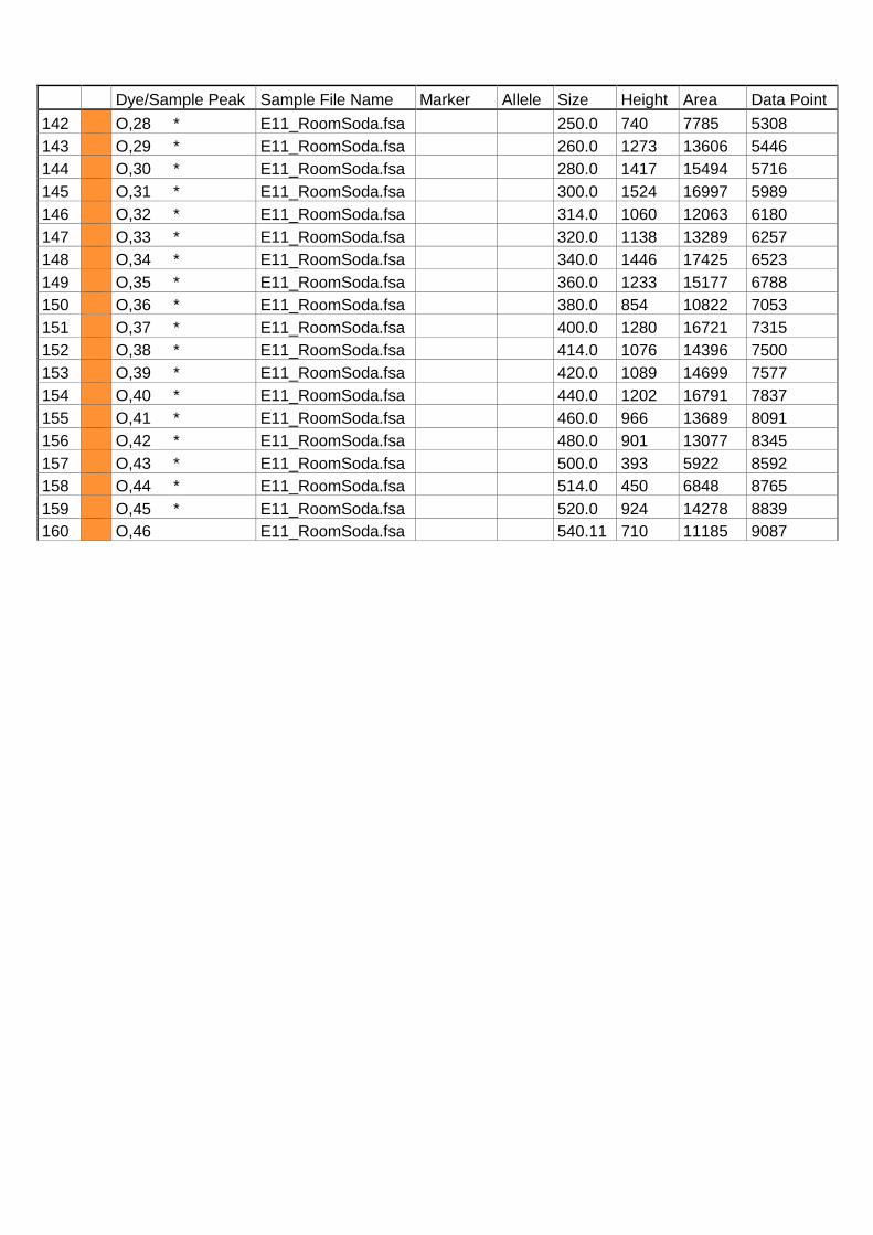
Dye/Sample Peak Sample File Name Marker Allele Size Height Area Data Point
142 O,28 * E11_RoomSoda.fsa 250.0 740 7785 5308
143 O,29 * E11_RoomSoda.fsa 260.0 1273 13606 5446
144 O,30 * E11_RoomSoda.fsa 280.0 1417 15494 5716
145 O,31 * E11_RoomSoda.fsa 300.0 1524 16997 5989
146 O,32 * E11_RoomSoda.fsa 314.0 1060 12063 6180
147 O,33 * E11_RoomSoda.fsa 320.0 1138 13289 6257
148 O,34 * E11_RoomSoda.fsa 340.0 1446 17425 6523
149 O,35 * E11_RoomSoda.fsa 360.0 1233 15177 6788
150 O,36 * E11_RoomSoda.fsa 380.0 854 10822 7053
151 O,37 * E11_RoomSoda.fsa 400.0 1280 16721 7315
152 O,38 * E11_RoomSoda.fsa 414.0 1076 14396 7500
153 O,39 * E11_RoomSoda.fsa 420.0 1089 14699 7577
154 O,40 * E11_RoomSoda.fsa 440.0 1202 16791 7837
155 O,41 * E11_RoomSoda.fsa 460.0 966 13689 8091
156 O,42 * E11_RoomSoda.fsa 480.0 901 13077 8345
157 O,43 * E11_RoomSoda.fsa 500.0 393 5922 8592
158 O,44 * E11_RoomSoda.fsa 514.0 450 6848 8765
159 O,45 * E11_RoomSoda.fsa 520.0 924 14278 8839
160 O,46 E11_RoomSoda.fsa 540.11 710 11185 9087


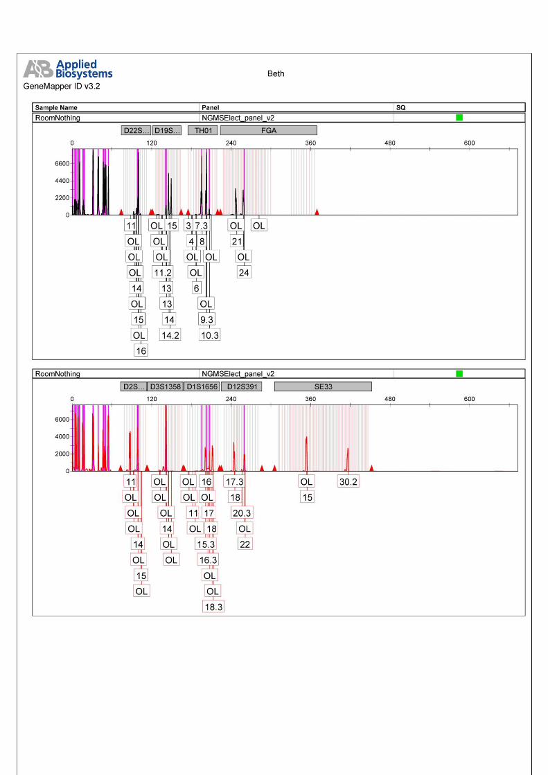


Beth Dye/Sample Peak Sample File Name Marker Allele Size Height Area Data Point
78 G,11 E10_RoomNothing.fsa 4.44 321 3142 1588
79 G,12 E10_RoomNothing.fsa 5.61 324 3138 1603
80 G,13 E10_RoomNothing.fsa 6.62 5003 49648 1616
81 G,14 E10_RoomNothing.fsa 7.87 6075 64158 1632
82 G,15 E10_RoomNothing.fsa 9.74 430 5797 1656
83 G,16 E10_RoomNothing.fsa 11.14 1895 9549 1674
84 G,17 E10_RoomNothing.fsa 12.47 111 804 1691
85 G,18 E10_RoomNothing.fsa 14.49 498 5894 1717
86 G,19 E10_RoomNothing.fsa 15.97 950 6126 1736
87 G,20 E10_RoomNothing.fsa 16.6 961 9218 1744
88 G,21 E10_RoomNothing.fsa 17.92 6711 54588 1761
89 G,22 E10_RoomNothing.fsa 18.62 7174 56164 1770
90 G,23 E10_RoomNothing.fsa 25.25 60 478 1855
91 G,24 E10_RoomNothing.fsa 26.42 191 2312 1870
92 G,25 E10_RoomNothing.fsa 27.51 221 2536 1884
93 G,26 E10_RoomNothing.fsa 31.56 2167 16927 1936
94 G,27 E10_RoomNothing.fsa 39.27 10548 106154 2035
95 G,28 E10_RoomNothing.fsa 47.69 11112 132144 2143
96 G,29 E10_RoomNothing.fsa 50.49 9655 91360 2179
97 G,30 E10_RoomNothing.fsa 51.74 146 1799 2195
98 G,31 E10_RoomNothing.fsa 52.83 104 1526 2209
99 G,32 E10_RoomNothing.fsa 53.77 84 627 2221
100 G,33 E10_RoomNothing.fsa 84.94 71 592 2621
101 G,34 E10_RoomNothing.fsa 90.62 65 494 2694
102 G,35 E10_RoomNothing.fsa 91.48 134 1285 2705
103 G,36 E10_RoomNothing.fsa AMEL X 98.49 2921 23063 2795
104 G,37 E10_RoomNothing.fsa AMEL OL 99.43 8996 92131 2807
105 G,38 E10_RoomNothing.fsa AMEL OL 103.25 175 1601 2856
106 G,39 E10_RoomNothing.fsa AMEL OL 104.1 183 1853 2867
107 G,40 E10_RoomNothing.fsa D8S1179 OL 119.84 58 378 3069
108 G,41 E10_RoomNothing.fsa D8S1179 OL 120.63 117 1317 3079
109 G,42 E10_RoomNothing.fsa 125.53 194 1570 3141
110 G,43 E10_RoomNothing.fsa 126.41 334 3997 3152
111 G,44 E10_RoomNothing.fsa D8S1179 OL 129.61 3431 26943 3192
112 G,45 E10_RoomNothing.fsa D8S1179 10 130.49 5973 56260 3203
113 G,46 E10_RoomNothing.fsa D8S1179 11 134.69 84 752 3255
114 G,47 E10_RoomNothing.fsa D8S1179 OL 135.51 104 1220 3265
115 G,48 E10_RoomNothing.fsa 141.66 351 2075 3340
116 G,49 E10_RoomNothing.fsa 142.74 539 4420 3353
117 G,50 E10_RoomNothing.fsa D8S1179 OL 144.74 62 392 3377
118 G,51 E10_RoomNothing.fsa D8S1179 OL 145.91 3610 28822 3391
119 G,52 E10_RoomNothing.fsa D8S1179 14 146.83 6087 56828 3402
120 G,53 E10_RoomNothing.fsa D8S1179 OL 149.08 85 453 3429
121 G,54 E10_RoomNothing.fsa D8S1179 OL 150.09 93 664 3441

122 G,55 E10_RoomNothing.fsa D8S1179 15 151.01 85 671 3452
123 G,56 E10_RoomNothing.fsa D8S1179 OL 154.36 83 612 3492
124 G,57 E10_RoomNothing.fsa 174.68 246 2204 3736

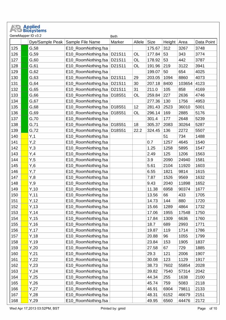
Beth Dye/Sample Peak Sample File Name Marker Allele Size Height Area Data Point
125 G,58 E10_RoomNothing.fsa 175.67 312 3267 3748
126 G,59 E10_RoomNothing.fsa D21S11 OL 177.84 53 343 3774
127 G,60 E10_RoomNothing.fsa D21S11 OL 178.92 53 442 3787
128 G,61 E10_RoomNothing.fsa D21S11 OL 191.96 219 3122 3941
129 G,62 E10_RoomNothing.fsa 199.07 50 654 4025
130 G,63 E10_RoomNothing.fsa D21S11 29 203.05 1094 8860 4073
131 G,64 E10_RoomNothing.fsa D21S11 30 207.18 8400 103654 4123
132 G,65 E10_RoomNothing.fsa D21S11 31 211.0 105 858 4169
133 G,66 E10_RoomNothing.fsa D18S51 OL 259.84 227 2636 4746
134 G,67 E10_RoomNothing.fsa 277.36 130 1756 4953
135 G,68 E10_RoomNothing.fsa D18S51 12 281.43 2523 36010 5001
136 G,69 E10_RoomNothing.fsa D18S51 OL 296.14 169 2885 5176
137 G,70 E10_RoomNothing.fsa 301.4 177 2648 5239
138 G,71 E10_RoomNothing.fsa D18S51 18 305.37 2083 30264 5287
139 G,72 E10_RoomNothing.fsa D18S51 22.2 324.45 136 2272 5507
140 Y,1 E10_RoomNothing.fsa 51 734 1488
141 Y,2 E10_RoomNothing.fsa 0.7 1257 4645 1540
142 Y,3 E10_RoomNothing.fsa 1.25 1258 5895 1547
143 Y,4 E10_RoomNothing.fsa 2.49 125 1206 1563
144 Y,5 E10_RoomNothing.fsa 3.9 2090 24940 1581
145 Y,6 E10_RoomNothing.fsa 5.61 2104 11920 1603
146 Y,7 E10_RoomNothing.fsa 6.55 1821 9814 1615
147 Y,8 E10_RoomNothing.fsa 7.87 1526 9569 1632
148 Y,9 E10_RoomNothing.fsa 9.43 2040 11898 1652
149 Y,10 E10_RoomNothing.fsa 11.38 6958 90374 1677
150 Y,11 E10_RoomNothing.fsa 13.56 66 433 1705
151 Y,12 E10_RoomNothing.fsa 14.73 144 880 1720
152 Y,13 E10_RoomNothing.fsa 15.66 1289 4864 1732
153 Y,14 E10_RoomNothing.fsa 17.06 1955 17548 1750
154 Y,15 E10_RoomNothing.fsa 17.84 1309 6636 1760
155 Y,16 E10_RoomNothing.fsa 18.7 689 2993 1771
156 Y,17 E10_RoomNothing.fsa 19.87 119 1714 1786
157 Y,18 E10_RoomNothing.fsa 20.88 96 1055 1799
158 Y,19 E10_RoomNothing.fsa 23.84 153 1905 1837
159 Y,20 E10_RoomNothing.fsa 27.58 67 729 1885
160 Y,21 E10_RoomNothing.fsa 29.3 121 2006 1907
161 Y,22 E10_RoomNothing.fsa 30.08 123 1129 1917
162 Y,23 E10_RoomNothing.fsa 38.73 7602 55854 2028
163 Y,24 E10_RoomNothing.fsa 39.82 7540 57314 2042
164 Y,25 E10_RoomNothing.fsa 44.34 255 1638 2100
165 Y,26 E10_RoomNothing.fsa 45.74 759 5083 2118
166 Y,27 E10_RoomNothing.fsa 46.91 6904 79811 2133
167 Y,28 E10_RoomNothing.fsa 48.31 6152 46679 2151
168 Y,29 E10_RoomNothing.fsa 49.95 6560 44476 2172

169 Y,30 E10_RoomNothing.fsa 50.96 6483 46851 2185
170 Y,31 E10_RoomNothing.fsa 54.62 6292 60580 2232
171 Y,32 E10_RoomNothing.fsa D22S1045 11 87.04 71 434 2648

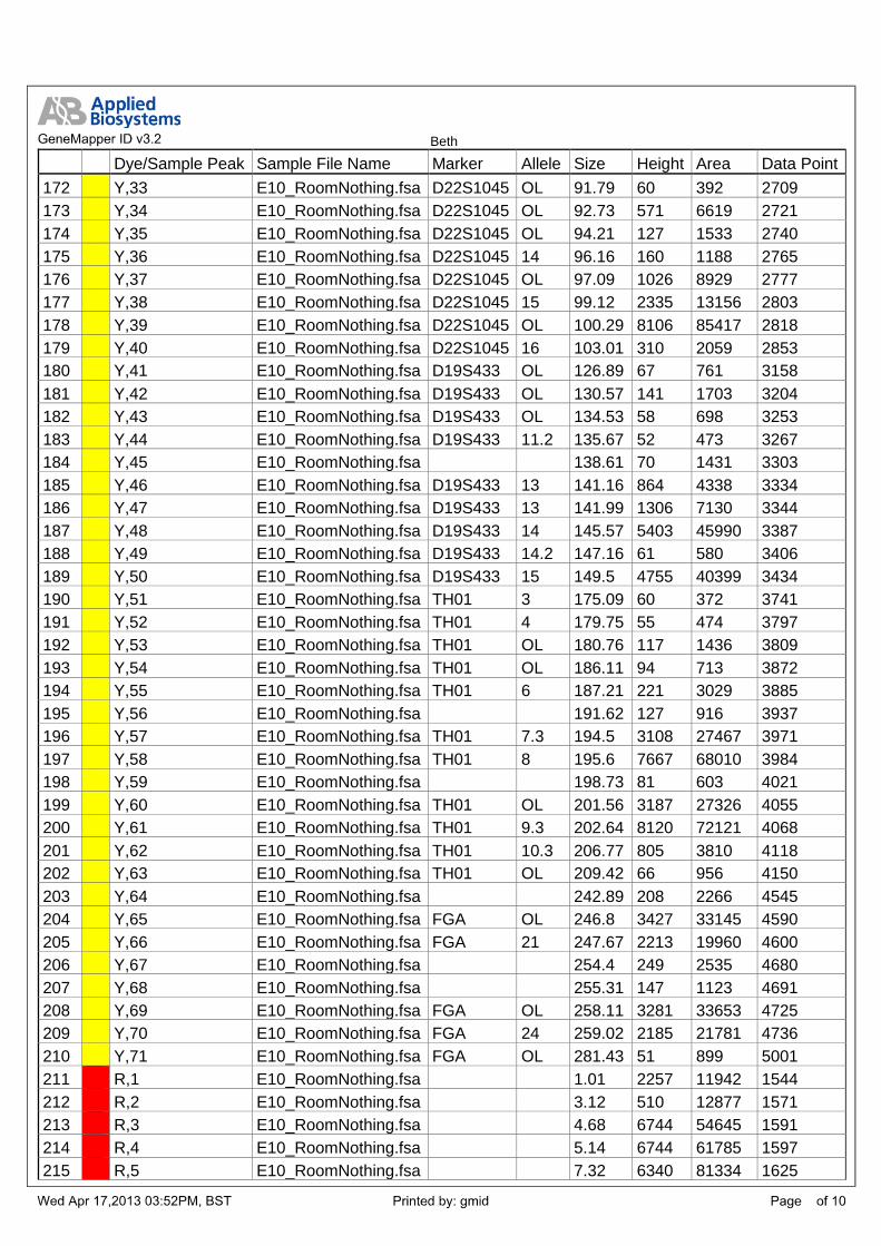
Beth Dye/Sample Peak Sample File Name Marker Allele Size Height Area Data Point
172 Y,33 E10_RoomNothing.fsa D22S1045 OL 91.79 60 392 2709
173 Y,34 E10_RoomNothing.fsa D22S1045 OL 92.73 571 6619 2721
174 Y,35 E10_RoomNothing.fsa D22S1045 OL 94.21 127 1533 2740
175 Y,36 E10_RoomNothing.fsa D22S1045 14 96.16 160 1188 2765
176 Y,37 E10_RoomNothing.fsa D22S1045 OL 97.09 1026 8929 2777
177 Y,38 E10_RoomNothing.fsa D22S1045 15 99.12 2335 13156 2803
178 Y,39 E10_RoomNothing.fsa D22S1045 OL 100.29 8106 85417 2818
179 Y,40 E10_RoomNothing.fsa D22S1045 16 103.01 310 2059 2853
180 Y,41 E10_RoomNothing.fsa D19S433 OL 126.89 67 761 3158
181 Y,42 E10_RoomNothing.fsa D19S433 OL 130.57 141 1703 3204
182 Y,43 E10_RoomNothing.fsa D19S433 OL 134.53 58 698 3253
183 Y,44 E10_RoomNothing.fsa D19S433 11.2 135.67 52 473 3267
184 Y,45 E10_RoomNothing.fsa 138.61 70 1431 3303
185 Y,46 E10_RoomNothing.fsa D19S433 13 141.16 864 4338 3334
186 Y,47 E10_RoomNothing.fsa D19S433 13 141.99 1306 7130 3344
187 Y,48 E10_RoomNothing.fsa D19S433 14 145.57 5403 45990 3387
188 Y,49 E10_RoomNothing.fsa D19S433 14.2 147.16 61 580 3406
189 Y,50 E10_RoomNothing.fsa D19S433 15 149.5 4755 40399 3434
190 Y,51 E10_RoomNothing.fsa TH01 3 175.09 60 372 3741
191 Y,52 E10_RoomNothing.fsa TH01 4 179.75 55 474 3797
192 Y,53 E10_RoomNothing.fsa TH01 OL 180.76 117 1436 3809
193 Y,54 E10_RoomNothing.fsa TH01 OL 186.11 94 713 3872
194 Y,55 E10_RoomNothing.fsa TH01 6 187.21 221 3029 3885
195 Y,56 E10_RoomNothing.fsa 191.62 127 916 3937
196 Y,57 E10_RoomNothing.fsa TH01 7.3 194.5 3108 27467 3971
197 Y,58 E10_RoomNothing.fsa TH01 8 195.6 7667 68010 3984
198 Y,59 E10_RoomNothing.fsa 198.73 81 603 4021
199 Y,60 E10_RoomNothing.fsa TH01 OL 201.56 3187 27326 4055
200 Y,61 E10_RoomNothing.fsa TH01 9.3 202.64 8120 72121 4068
201 Y,62 E10_RoomNothing.fsa TH01 10.3 206.77 805 3810 4118
202 Y,63 E10_RoomNothing.fsa TH01 OL 209.42 66 956 4150
203 Y,64 E10_RoomNothing.fsa 242.89 208 2266 4545
204 Y,65 E10_RoomNothing.fsa FGA OL 246.8 3427 33145 4590
205 Y,66 E10_RoomNothing.fsa FGA 21 247.67 2213 19960 4600
206 Y,67 E10_RoomNothing.fsa 254.4 249 2535 4680
207 Y,68 E10_RoomNothing.fsa 255.31 147 1123 4691
208 Y,69 E10_RoomNothing.fsa FGA OL 258.11 3281 33653 4725
209 Y,70 E10_RoomNothing.fsa FGA 24 259.02 2185 21781 4736
210 Y,71 E10_RoomNothing.fsa FGA OL 281.43 51 899 5001
211 R,1 E10_RoomNothing.fsa 1.01 2257 11942 1544
212 R,2 E10_RoomNothing.fsa 3.12 510 12877 1571
213 R,3 E10_RoomNothing.fsa 4.68 6744 54645 1591
214 R,4 E10_RoomNothing.fsa 5.14 6744 61785 1597
215 R,5 E10_RoomNothing.fsa 7.32 6340 81334 1625

216 R,6 E10_RoomNothing.fsa 8.26 350 2720 1637
217 R,7 E10_RoomNothing.fsa 9.9 6457 62681 1658
218 R,8 E10_RoomNothing.fsa 11.14 1277 6012 1674

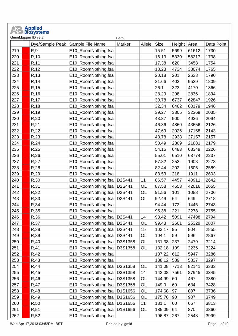
Beth Dye/Sample Peak Sample File Name Marker Allele Size Height Area Data Point
219 R,9 E10_RoomNothing.fsa 15.51 5699 61612 1730
220 R,10 E10_RoomNothing.fsa 16.13 5330 58217 1738
221 R,11 E10_RoomNothing.fsa 17.38 620 3458 1754
222 R,12 E10_RoomNothing.fsa 18.23 4734 33074 1765
223 R,13 E10_RoomNothing.fsa 20.18 201 2623 1790
224 R,14 E10_RoomNothing.fsa 21.66 403 9529 1809
225 R,15 E10_RoomNothing.fsa 26.1 323 4170 1866
226 R,16 E10_RoomNothing.fsa 28.29 298 2836 1894
227 R,17 E10_RoomNothing.fsa 30.78 6737 62847 1926
228 R,18 E10_RoomNothing.fsa 32.34 6462 60179 1946
229 R,19 E10_RoomNothing.fsa 39.27 3305 32369 2035
230 R,20 E10_RoomNothing.fsa 43.87 500 4936 2094
231 R,21 E10_RoomNothing.fsa 46.36 4860 43656 2126
232 R,22 E10_RoomNothing.fsa 47.69 2026 17158 2143
233 R,23 E10_RoomNothing.fsa 48.78 2938 27157 2157
234 R,24 E10_RoomNothing.fsa 50.49 2309 21881 2179
235 R,25 E10_RoomNothing.fsa 54.16 6483 68349 2226
236 R,26 E10_RoomNothing.fsa 55.01 6510 63774 2237
237 R,27 E10_RoomNothing.fsa 57.82 253 1903 2273
238 R,28 E10_RoomNothing.fsa 82.44 202 1605 2589
239 R,29 E10_RoomNothing.fsa 83.53 218 1911 2603
240 R,30 E10_RoomNothing.fsa D2S441 11 86.57 4457 40911 2642
241 R,31 E10_RoomNothing.fsa D2S441 OL 87.58 4653 42016 2655
242 R,32 E10_RoomNothing.fsa D2S441 OL 91.56 101 1088 2706
243 R,33 E10_RoomNothing.fsa D2S441 OL 92.49 64 649 2718
244 R,34 E10_RoomNothing.fsa 94.44 172 1445 2743
245 R,35 E10_RoomNothing.fsa 95.38 221 2278 2755
246 R,36 E10_RoomNothing.fsa D2S441 14 98.42 5091 47498 2794
247 R,37 E10_RoomNothing.fsa D2S441 OL 99.43 2601 25329 2807
248 R,38 E10_RoomNothing.fsa D2S441 15 103.17 95 804 2855
249 R,39 E10_RoomNothing.fsa D2S441 OL 104.1 59 596 2867
250 R,40 E10_RoomNothing.fsa D3S1358 OL 131.38 237 2479 3214
251 R,41 E10_RoomNothing.fsa D3S1358 OL 132.18 199 2235 3224
252 R,42 E10_RoomNothing.fsa 137.22 612 5947 3286
253 R,43 E10_RoomNothing.fsa 138.12 589 5837 3297
254 R,44 E10_RoomNothing.fsa D3S1358 OL 141.08 7713 82141 3333
255 R,45 E10_RoomNothing.fsa D3S1358 14 142.08 7561 87945 3345
256 R,46 E10_RoomNothing.fsa D3S1358 OL 144.99 60 467 3380
257 R,47 E10_RoomNothing.fsa D3S1358 OL 149.0 69 634 3428
258 R,48 E10_RoomNothing.fsa D1S1656 OL 174.68 97 807 3736
259 R,49 E10_RoomNothing.fsa D1S1656 OL 175.76 90 907 3749
260 R,50 E10_RoomNothing.fsa D1S1656 11 181.1 60 667 3813
261 R,51 E10_RoomNothing.fsa D1S1656 OL 185.09 64 870 3860
262 R,52 E10_RoomNothing.fsa 196.87 267 2548 3999

263 R,53 E10_RoomNothing.fsa 197.71 214 1809 4009
264 R,54 E10_RoomNothing.fsa D1S1656 15.3 200.82 2802 26675 4046
265 R,55 E10_RoomNothing.fsa D1S1656 16 201.65 2505 23894 4056


Beth Dye/Sample Peak Sample File Name Marker Allele Size Height Area Data Point
266 R,56 E10_RoomNothing.fsa D1S1656 OL 203.21 406 4625 4075
267 R,57 E10_RoomNothing.fsa D1S1656 16.3 204.2 403 7140 4087
268 R,58 E10_RoomNothing.fsa D1S1656 17 205.44 422 7728 4102
269 R,59 E10_RoomNothing.fsa D1S1656 OL 207.02 2434 12197 4121
270 R,60 E10_RoomNothing.fsa 208.43 189 1726 4138
271 R,61 E10_RoomNothing.fsa D1S1656 18 209.42 59 434 4150
272 R,62 E10_RoomNothing.fsa D1S1656 OL 211.5 3010 28156 4175
273 R,63 E10_RoomNothing.fsa D1S1656 18.3 212.42 2717 27193 4186
274 R,64 E10_RoomNothing.fsa 239.92 201 1805 4511
275 R,65 E10_RoomNothing.fsa 240.96 117 1080 4523
276 R,66 E10_RoomNothing.fsa D12S391 17.3 244.02 3347 32946 4558
277 R,67 E10_RoomNothing.fsa D12S391 18 244.98 2298 22465 4569
278 R,68 E10_RoomNothing.fsa D12S391 20.3 255.72 300 3048 4696
279 R,69 E10_RoomNothing.fsa 256.71 187 1841 4708
280 R,70 E10_RoomNothing.fsa D12S391 OL 259.75 2027 24085 4745
281 R,71 E10_RoomNothing.fsa D12S391 22 260.59 1982 19920 4755
282 R,72 E10_RoomNothing.fsa 349.05 159 1247 5793
283 R,73 E10_RoomNothing.fsa 350.0 159 1376 5804
284 R,74 E10_RoomNothing.fsa SE33 OL 353.19 3867 41577 5841
285 R,75 E10_RoomNothing.fsa SE33 15 354.05 4100 46363 5851
286 R,76 E10_RoomNothing.fsa 412.35 251 4029 6522
287 R,77 E10_RoomNothing.fsa SE33 30.2 416.41 2724 50614 6568
288 O,1 E10_RoomNothing.fsa 1.01 445 3042 1544
289 O,2 E10_RoomNothing.fsa 3.66 100 414 1578
290 O,3 E10_RoomNothing.fsa 4.91 7974 89439 1594
291 O,4 E10_RoomNothing.fsa 7.32 2955 27705 1625
292 O,5 E10_RoomNothing.fsa 9.9 3601 25020 1658
293 O,6 E10_RoomNothing.fsa 11.14 1333 8185 1674
294 O,7 E10_RoomNothing.fsa 16.13 3518 39594 1738
295 O,8 E10_RoomNothing.fsa 18.23 1617 10921 1765
296 O,9 E10_RoomNothing.fsa 23.22 250 3512 1829
297 O,10 E10_RoomNothing.fsa 31.56 8189 130984 1936
298 O,11 E10_RoomNothing.fsa 39.27 7766 84322 2035
299 O,12 E10_RoomNothing.fsa 40.99 313 3218 2057
300 O,13 E10_RoomNothing.fsa 47.61 8526 180608 2142
301 O,14 E10_RoomNothing.fsa 50.49 7490 76382 2179
302 O,15 E10_RoomNothing.fsa 54.55 5683 49446 2231
303 O,16 E10_RoomNothing.fsa 61.01 627 5606 2314
304 O,17 E10_RoomNothing.fsa 80.88 498 4326 2569
305 O,18 E10_RoomNothing.fsa 98.49 61 325 2795
306 O,19 E10_RoomNothing.fsa 99.43 1464 10343 2807
307 O,20 E10_RoomNothing.fsa 100.13 1645 18240 2816
308 O,21 * E10_RoomNothing.fsa 114.0 942 7970 2994
309 O,22 * E10_RoomNothing.fsa 120.0 780 6731 3071

310 O,23 * E10_RoomNothing.fsa 140.0 629 5155 3320
311 O,24 E10_RoomNothing.fsa 141.08 540 2792 3333
312 O,25 E10_RoomNothing.fsa 141.99 701 3831 3344


Beth Dye/Sample Peak Sample File Name Marker Allele Size Height Area Data Point
313 O,26 * E10_RoomNothing.fsa 160.0 677 5810 3559
314 O,27 * E10_RoomNothing.fsa 180.0 842 7336 3800
315 O,28 E10_RoomNothing.fsa 195.6 81 359 3984
316 O,29 * E10_RoomNothing.fsa 200.0 712 6266 4036
317 O,30 E10_RoomNothing.fsa 202.64 201 804 4068
318 O,31 E10_RoomNothing.fsa 207.02 512 3163 4121
319 O,32 * E10_RoomNothing.fsa 214.0 702 6272 4205
320 O,33 * E10_RoomNothing.fsa 220.0 598 5522 4275
321 O,34 * E10_RoomNothing.fsa 240.0 926 8618 4512
322 O,35 * E10_RoomNothing.fsa 250.0 435 4185 4627
323 O,36 * E10_RoomNothing.fsa 260.0 736 8069 4748
324 O,37 * E10_RoomNothing.fsa 280.0 833 8329 4984
325 O,38 * E10_RoomNothing.fsa 300.0 881 8804 5222
326 O,39 * E10_RoomNothing.fsa 314.0 615 6293 5389
327 O,40 * E10_RoomNothing.fsa 320.0 659 7010 5456
328 O,41 * E10_RoomNothing.fsa 340.0 853 9044 5688
329 O,42 * E10_RoomNothing.fsa 360.0 723 7961 5920
330 O,43 * E10_RoomNothing.fsa 380.0 513 5708 6152
331 O,44 * E10_RoomNothing.fsa 400.0 770 8857 6379
332 O,45 * E10_RoomNothing.fsa 414.0 662 7617 6541
333 O,46 * E10_RoomNothing.fsa 420.0 643 7661 6608
334 O,47 * E10_RoomNothing.fsa 440.0 730 8890 6833
335 O,48 * E10_RoomNothing.fsa 460.0 578 7317 7054
336 O,49 * E10_RoomNothing.fsa 480.0 542 7003 7275
337 O,50 * E10_RoomNothing.fsa 500.0 236 3096 7489
338 O,51 * E10_RoomNothing.fsa 514.0 262 3531 7638
339 O,52 * E10_RoomNothing.fsa 520.0 557 7534 7702
340 O,53 E10_RoomNothing.fsa 540.16 433 5945 7917
341 O,54 E10_RoomNothing.fsa 559.66 302 4251 8125
342 O,55 E10_RoomNothing.fsa 578.69 427 6153 8328
343 O,56 E10_RoomNothing.fsa 597.53 318 4663 8529


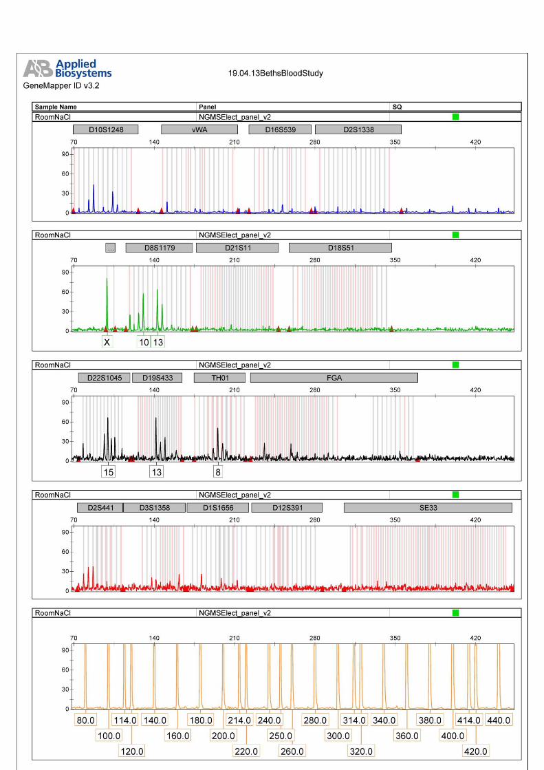

Dye/Sample Peak Sample File Name Marker Allele Size Height Area Data Point
1 B,1 H11_RoomNaCl.fsa 82 1168 1369
2 B,2 H11_RoomNaCl.fsa 59 878 1400
3 B,3 H11_RoomNaCl.fsa 61 623 1442
4 B,4 H11_RoomNaCl.fsa 69 800 1483
5 B,5 H11_RoomNaCl.fsa 72 917 1575
6 B,6 H11_RoomNaCl.fsa 130 1686 1602
7 B,7 H11_RoomNaCl.fsa 117 1686 1640
8 B,8 H11_RoomNaCl.fsa 140 1523 1713
9 B,9 H11_RoomNaCl.fsa 119 1322 1728
10 B,10 H11_RoomNaCl.fsa 95 825 1749
11 B,11 H11_RoomNaCl.fsa 170 1745 1762
12 B,12 H11_RoomNaCl.fsa 156 1417 1783
13 B,13 H11_RoomNaCl.fsa 3978 43746 1854
14 B,14 H11_RoomNaCl.fsa 2.39 5111 65544 1893
15 B,15 H11_RoomNaCl.fsa 4.0 5006 63361 1916
16 B,16 H11_RoomNaCl.fsa 6.04 3312 48451 1945
17 B,17 H11_RoomNaCl.fsa 10.46 388 4509 2008
18 B,18 H11_RoomNaCl.fsa 14.95 7835 99432 2072
19 B,19 H11_RoomNaCl.fsa 15.72 7884 109969 2083
20 B,20 H11_RoomNaCl.fsa 16.98 5681 50292 2101
21 B,21 H11_RoomNaCl.fsa 29.26 252 1069 2276
22 B,22 H11_RoomNaCl.fsa 30.53 276 1098 2294
23 B,23 H11_RoomNaCl.fsa 44.7 142 618 2496
24 B,24 H11_RoomNaCl.fsa 47.09 2881 36610 2530
25 B,25 H11_RoomNaCl.fsa 47.65 2883 46795 2538
26 B,26 H11_RoomNaCl.fsa 52.49 277 1951 2607
27 B,27 H11_RoomNaCl.fsa 53.05 292 2258 2615
28 G,1 H11_RoomNaCl.fsa 152 1608 1482
29 G,2 H11_RoomNaCl.fsa 58 606 1592
30 G,3 H11_RoomNaCl.fsa 123 1787 1607
31 G,4 H11_RoomNaCl.fsa 407 4963 1669
32 G,5 H11_RoomNaCl.fsa 91 972 1700
33 G,6 H11_RoomNaCl.fsa 125 2603 1714
34 G,7 H11_RoomNaCl.fsa 1476 18269 1791
35 G,8 H11_RoomNaCl.fsa 5940 48329 1850
36 G,9 H11_RoomNaCl.fsa 6857 62270 1859
37 G,10 H11_RoomNaCl.fsa 1.12 219 2707 1875
38 G,11 H11_RoomNaCl.fsa 2.18 419 2423 1890
39 G,12 H11_RoomNaCl.fsa 2.67 450 2707 1897
40 G,13 H11_RoomNaCl.fsa 3.23 326 3104 1905
41 G,14 H11_RoomNaCl.fsa 4.21 331 4150 1919
42 G,15 H11_RoomNaCl.fsa 5.33 4403 49122 1935
43 G,16 H11_RoomNaCl.fsa 6.67 5766 55913 1954
44 G,17 H11_RoomNaCl.fsa 8.49 448 4008 1980
45 G,18 H11_RoomNaCl.fsa 8.91 464 3816 1986

46 G,19 H11_RoomNaCl.fsa 9.89 5539 43064 2000
47 G,20 H11_RoomNaCl.fsa 13.26 514 7851 2048
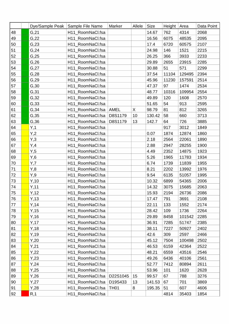
Dye/Sample Peak Sample File Name Marker Allele Size Height Area Data Point
48 G,21 H11_RoomNaCl.fsa 14.67 762 4314 2068
49 G,22 H11_RoomNaCl.fsa 16.56 6075 48535 2095
50 G,23 H11_RoomNaCl.fsa 17.4 6720 60575 2107
51 G,24 H11_RoomNaCl.fsa 24.98 146 1521 2215
52 G,25 H11_RoomNaCl.fsa 26.25 366 3933 2233
53 G,26 H11_RoomNaCl.fsa 29.89 2655 23915 2285
54 G,27 H11_RoomNaCl.fsa 30.88 51 571 2299
55 G,28 H11_RoomNaCl.fsa 37.54 11104 129495 2394
56 G,29 H11_RoomNaCl.fsa 45.96 11230 157591 2514
57 G,30 H11_RoomNaCl.fsa 47.37 97 1474 2534
58 G,31 H11_RoomNaCl.fsa 48.77 10316 109954 2554
59 G,32 H11_RoomNaCl.fsa 49.89 120 1608 2570
60 G,33 H11_RoomNaCl.fsa 51.65 54 913 2595
61 G,34 H11_RoomNaCl.fsa AMEL X 98.79 81 812 3265
62 G,35 H11_RoomNaCl.fsa D8S1179 10 130.42 58 660 3713
63 G,36 H11_RoomNaCl.fsa D8S1179 13 142.7 64 726 3885
64 Y,1 H11_RoomNaCl.fsa 917 3012 1849
65 Y,2 H11_RoomNaCl.fsa 0.07 1874 12874 1860
66 Y,3 H11_RoomNaCl.fsa 2.18 2564 22061 1890
67 Y,4 H11_RoomNaCl.fsa 2.88 2947 28255 1900
68 Y,5 H11_RoomNaCl.fsa 4.49 2352 14875 1923
69 Y,6 H11_RoomNaCl.fsa 5.26 1965 11783 1934
70 Y,7 H11_RoomNaCl.fsa 6.74 1739 11839 1955
71 Y,8 H11_RoomNaCl.fsa 8.21 2202 13992 1976
72 Y,9 H11_RoomNaCl.fsa 9.54 6135 51057 1995
73 Y,10 H11_RoomNaCl.fsa 10.32 6899 54365 2006
74 Y,11 H11_RoomNaCl.fsa 14.32 3075 15685 2063
75 Y,12 H11_RoomNaCl.fsa 15.93 2194 26736 2086
76 Y,13 H11_RoomNaCl.fsa 17.47 791 3691 2108
77 Y,14 H11_RoomNaCl.fsa 22.11 133 1552 2174
78 Y,15 H11_RoomNaCl.fsa 28.42 109 1736 2264
79 Y,16 H11_RoomNaCl.fsa 29.89 8458 101542 2285
80 Y,17 H11_RoomNaCl.fsa 36.91 7285 51747 2385
81 Y,18 H11_RoomNaCl.fsa 38.11 7227 50927 2402
82 Y,19 H11_RoomNaCl.fsa 42.6 309 2597 2466
83 Y,20 H11_RoomNaCl.fsa 45.12 7504 100498 2502
84 Y,21 H11_RoomNaCl.fsa 46.53 6159 42364 2522
85 Y,22 H11_RoomNaCl.fsa 48.21 6559 43516 2546
86 Y,23 H11_RoomNaCl.fsa 49.26 6436 40106 2561
87 Y,24 H11_RoomNaCl.fsa 52.77 7412 80894 2611
88 Y,25 H11_RoomNaCl.fsa 53.96 101 1620 2628
89 Y,26 H11_RoomNaCl.fsa D22S1045 15 99.57 67 788 3276
90 Y,27 H11_RoomNaCl.fsa D19S433 13 141.53 67 701 3869
91 Y,28 H11_RoomNaCl.fsa TH01 8 195.35 51 607 4606
92 R,1 H11_RoomNaCl.fsa 4814 35403 1854

93 R,2 H11_RoomNaCl.fsa 1.05 461 7465 1874
94 R,3 H11_RoomNaCl.fsa 2.39 1729 10382 1893
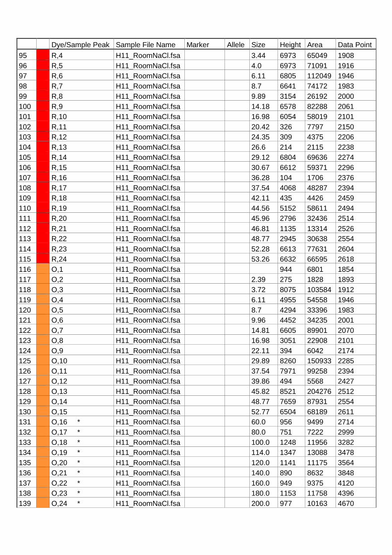
Dye/Sample Peak Sample File Name Marker Allele Size Height Area Data Point
95 R,4 H11_RoomNaCl.fsa 3.44 6973 65049 1908
96 R,5 H11_RoomNaCl.fsa 4.0 6973 71091 1916
97 R,6 H11_RoomNaCl.fsa 6.11 6805 112049 1946
98 R,7 H11_RoomNaCl.fsa 8.7 6641 74172 1983
99 R,8 H11_RoomNaCl.fsa 9.89 3154 26192 2000
100 R,9 H11_RoomNaCl.fsa 14.18 6578 82288 2061
101 R,10 H11_RoomNaCl.fsa 16.98 6054 58019 2101
102 R,11 H11_RoomNaCl.fsa 20.42 326 7797 2150
103 R,12 H11_RoomNaCl.fsa 24.35 309 4375 2206
104 R,13 H11_RoomNaCl.fsa 26.6 214 2115 2238
105 R,14 H11_RoomNaCl.fsa 29.12 6804 69636 2274
106 R,15 H11_RoomNaCl.fsa 30.67 6612 59371 2296
107 R,16 H11_RoomNaCl.fsa 36.28 104 1706 2376
108 R,17 H11_RoomNaCl.fsa 37.54 4068 48287 2394
109 R,18 H11_RoomNaCl.fsa 42.11 435 4426 2459
110 R,19 H11_RoomNaCl.fsa 44.56 5152 58611 2494
111 R,20 H11_RoomNaCl.fsa 45.96 2796 32436 2514
112 R,21 H11_RoomNaCl.fsa 46.81 1135 13314 2526
113 R,22 H11_RoomNaCl.fsa 48.77 2945 30638 2554
114 R,23 H11_RoomNaCl.fsa 52.28 6613 77631 2604
115 R,24 H11_RoomNaCl.fsa 53.26 6632 66595 2618
116 O,1 H11_RoomNaCl.fsa 944 6801 1854
117 O,2 H11_RoomNaCl.fsa 2.39 275 1828 1893
118 O,3 H11_RoomNaCl.fsa 3.72 8075 103584 1912
119 O,4 H11_RoomNaCl.fsa 6.11 4955 54558 1946
120 O,5 H11_RoomNaCl.fsa 8.7 4294 33396 1983
121 O,6 H11_RoomNaCl.fsa 9.96 4452 34235 2001
122 O,7 H11_RoomNaCl.fsa 14.81 6605 89901 2070
123 O,8 H11_RoomNaCl.fsa 16.98 3051 22908 2101
124 O,9 H11_RoomNaCl.fsa 22.11 394 6042 2174
125 O,10 H11_RoomNaCl.fsa 29.89 8260 150933 2285
126 O,11 H11_RoomNaCl.fsa 37.54 7971 99258 2394
127 O,12 H11_RoomNaCl.fsa 39.86 494 5568 2427
128 O,13 H11_RoomNaCl.fsa 45.82 8521 204276 2512
129 O,14 H11_RoomNaCl.fsa 48.77 7659 87931 2554
130 O,15 H11_RoomNaCl.fsa 52.77 6504 68189 2611
131 O,16 * H11_RoomNaCl.fsa 60.0 956 9499 2714
132 O,17 * H11_RoomNaCl.fsa 80.0 751 7222 2999
133 O,18 * H11_RoomNaCl.fsa 100.0 1248 11956 3282
134 O,19 * H11_RoomNaCl.fsa 114.0 1347 13088 3478
135 O,20 * H11_RoomNaCl.fsa 120.0 1141 11175 3564
136 O,21 * H11_RoomNaCl.fsa 140.0 890 8632 3848
137 O,22 * H11_RoomNaCl.fsa 160.0 949 9375 4120
138 O,23 * H11_RoomNaCl.fsa 180.0 1153 11758 4396
139 O,24 * H11_RoomNaCl.fsa 200.0 977 10163 4670

140 O,25 * H11_RoomNaCl.fsa 214.0 969 10340 4867
141 O,26 * H11_RoomNaCl.fsa 220.0 823 8957 4950

Dye/Sample Peak Sample File Name Marker Allele Size Height Area Data Point
142 O,27 * H11_RoomNaCl.fsa 240.0 1252 13972 5231
143 O,28 * H11_RoomNaCl.fsa 250.0 596 6780 5368
144 O,29 * H11_RoomNaCl.fsa 260.0 1016 11628 5512
145 O,30 * H11_RoomNaCl.fsa 280.0 1117 13166 5791
146 O,31 * H11_RoomNaCl.fsa 300.0 1191 14234 6073
147 O,32 * H11_RoomNaCl.fsa 314.0 825 10124 6270
148 O,33 * H11_RoomNaCl.fsa 320.0 902 11217 6348
149 O,34 * H11_RoomNaCl.fsa 340.0 1135 14538 6621
150 O,35 * H11_RoomNaCl.fsa 360.0 977 12598 6894
151 O,36 * H11_RoomNaCl.fsa 380.0 664 8873 7165
152 O,37 * H11_RoomNaCl.fsa 400.0 1024 13891 7431
153 O,38 * H11_RoomNaCl.fsa 414.0 854 11891 7619
154 O,39 * H11_RoomNaCl.fsa 420.0 860 12037 7697
155 O,40 * H11_RoomNaCl.fsa 440.0 957 13797 7960
156 O,41 * H11_RoomNaCl.fsa 460.0 756 11186 8216
157 O,42 * H11_RoomNaCl.fsa 480.0 718 10749 8474
158 O,43 * H11_RoomNaCl.fsa 500.0 305 4704 8723
159 O,44 * H11_RoomNaCl.fsa 514.0 354 5548 8896
160 O,45 * H11_RoomNaCl.fsa 520.0 722 11493 8971
161 O,46 H11_RoomNaCl.fsa 539.92 558 8928 9220

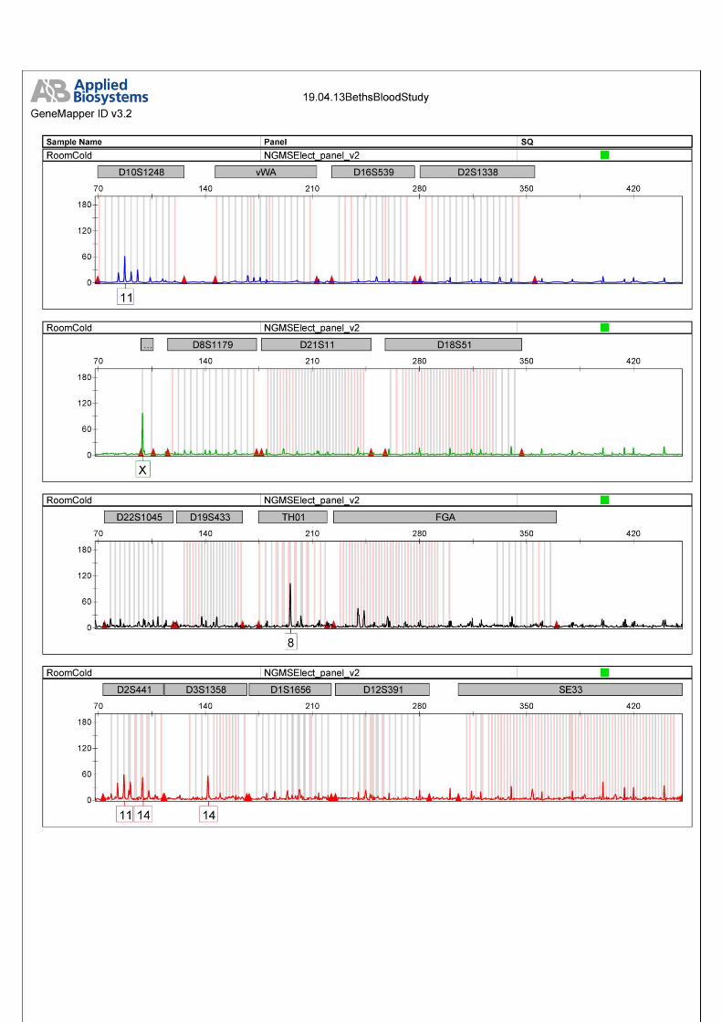
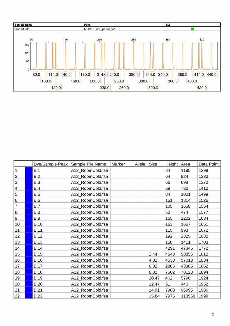
Dye/Sample Peak Sample File Name Marker Allele Size Height Area Data Point
1 B,1 A12_RoomCold.fsa 84 1185 1299
2 B,2 A12_RoomCold.fsa 64 924 1333
3 B,3 A12_RoomCold.fsa 66 698 1370
4 B,4 A12_RoomCold.fsa 69 730 1410
5 B,5 A12_RoomCold.fsa 84 1001 1499
6 B,6 A12_RoomCold.fsa 151 1814 1526
7 B,7 A12_RoomCold.fsa 105 1658 1564
8 B,8 A12_RoomCold.fsa 50 474 1577
9 B,9 A12_RoomCold.fsa 165 2202 1634
10 B,10 A12_RoomCold.fsa 163 1667 1651
11 B,11 A12_RoomCold.fsa 115 993 1672
12 B,12 A12_RoomCold.fsa 192 2325 1682
13 B,13 A12_RoomCold.fsa 158 1411 1703
14 B,14 A12_RoomCold.fsa 4291 47346 1772
15 B,15 A12_RoomCold.fsa 2.44 4640 58856 1812
16 B,16 A12_RoomCold.fsa 4.01 4530 57013 1834
17 B,17 A12_RoomCold.fsa 6.02 2886 43305 1862
18 B,18 A12_RoomCold.fsa 8.32 7502 78123 1894
19 B,19 A12_RoomCold.fsa 10.47 462 5790 1924
20 B,20 A12_RoomCold.fsa 12.47 51 440 1952
21 B,21 A12_RoomCold.fsa 14.91 7908 96995 1986
22 B,22 A12_RoomCold.fsa 15.84 7976 113569 1999
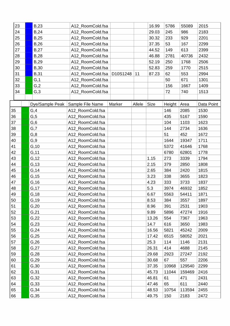
23 B,23 A12_RoomCold.fsa 16.99 5786 55089 2015
24 B,24 A12_RoomCold.fsa 29.03 245 986 2183
25 B,25 A12_RoomCold.fsa 30.32 233 929 2201
26 B,26 A12_RoomCold.fsa 37.35 53 167 2299
27 B,27 A12_RoomCold.fsa 44.52 149 613 2399
28 B,28 A12_RoomCold.fsa 46.88 2781 40736 2432
29 B,29 A12_RoomCold.fsa 52.19 250 1768 2506
30 B,30 A12_RoomCold.fsa 52.83 259 1770 2515
31 B,31 A12_RoomCold.fsa D10S1248 11 87.23 62 553 2994
32 G,1 A12_RoomCold.fsa 50 671 1301
33 G,2 A12_RoomCold.fsa 156 1667 1409
34 G,3 A12_RoomCold.fsa 72 740 1513
Dye/Sample Peak Sample File Name Marker Allele Size Height Area Data Point
35 G,4 A12_RoomCold.fsa 146 2085 1530
36 G,5 A12_RoomCold.fsa 435 5167 1590
37 G,6 A12_RoomCold.fsa 104 1103 1623
38 G,7 A12_RoomCold.fsa 144 2734 1636
39 G,8 A12_RoomCold.fsa 51 452 1672
40 G,9 A12_RoomCold.fsa 1644 19347 1711
41 G,10 A12_RoomCold.fsa 5372 41646 1768
42 G,11 A12_RoomCold.fsa 6780 62801 1778
43 G,12 A12_RoomCold.fsa 1.15 273 3339 1794
44 G,13 A12_RoomCold.fsa 2.15 379 2850 1808
45 G,14 A12_RoomCold.fsa 2.65 384 2420 1815
46 G,15 A12_RoomCold.fsa 3.23 338 3655 1823
47 G,16 A12_RoomCold.fsa 4.23 333 3733 1837
48 G,17 A12_RoomCold.fsa 5.3 3974 46932 1852
49 G,18 A12_RoomCold.fsa 6.67 5563 54411 1871
50 G,19 A12_RoomCold.fsa 8.53 384 3557 1897
51 G,20 A12_RoomCold.fsa 8.96 391 2531 1903
52 G,21 A12_RoomCold.fsa 9.89 5896 47274 1916
53 G,22 A12_RoomCold.fsa 13.26 554 7367 1963
54 G,23 A12_RoomCold.fsa 14.7 616 3650 1983
55 G,24 A12_RoomCold.fsa 16.56 5821 45242 2009
56 G,25 A12_RoomCold.fsa 17.42 6515 58052 2021
57 G,26 A12_RoomCold.fsa 25.3 114 1146 2131
58 G,27 A12_RoomCold.fsa 26.31 414 4688 2145
59 G,28 A12_RoomCold.fsa 29.68 2923 27247 2192
60 G,29 A12_RoomCold.fsa 30.68 67 557 2206
61 G,30 A12_RoomCold.fsa 37.35 10968 129540 2299
62 G,31 A12_RoomCold.fsa 45.73 11044 159469 2416
63 G,32 A12_RoomCold.fsa 46.81 61 471 2431
64 G,33 A12_RoomCold.fsa 47.46 65 611 2440
65 G,34 A12_RoomCold.fsa 48.53 10754 113594 2455
66 G,35 A12_RoomCold.fsa 49.75 150 2183 2472
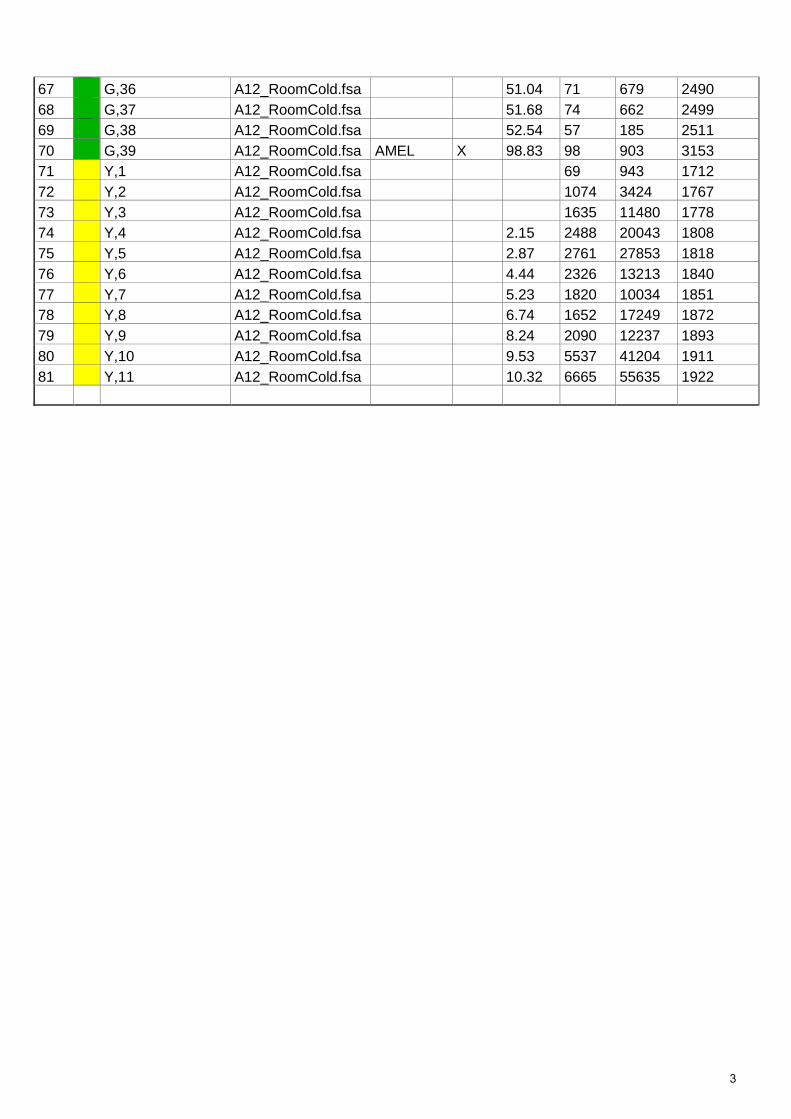
67 G,36 A12_RoomCold.fsa 51.04 71 679 2490
68 G,37 A12_RoomCold.fsa 51.68 74 662 2499
69 G,38 A12_RoomCold.fsa 52.54 57 185 2511
70 G,39 A12_RoomCold.fsa AMEL X 98.83 98 903 3153
71 Y,1 A12_RoomCold.fsa 69 943 1712
72 Y,2 A12_RoomCold.fsa 1074 3424 1767
73 Y,3 A12_RoomCold.fsa 1635 11480 1778
74 Y,4 A12_RoomCold.fsa 2.15 2488 20043 1808
75 Y,5 A12_RoomCold.fsa 2.87 2761 27853 1818
76 Y,6 A12_RoomCold.fsa 4.44 2326 13213 1840
77 Y,7 A12_RoomCold.fsa 5.23 1820 10034 1851
78 Y,8 A12_RoomCold.fsa 6.74 1652 17249 1872
79 Y,9 A12_RoomCold.fsa 8.24 2090 12237 1893
80 Y,10 A12_RoomCold.fsa 9.53 5537 41204 1911
81 Y,11 A12_RoomCold.fsa 10.32 6665 55635 1922

Dye/Sample Peak Sample File Name Marker Allele Size Height Area Data Point
82 Y,12 A12_RoomCold.fsa 14.34 4393 27670 1978
83 Y,13 A12_RoomCold.fsa 16.06 2217 25911 2002
84 Y,14 A12_RoomCold.fsa 17.49 984 7480 2022
85 Y,15 A12_RoomCold.fsa 22.01 147 1736 2085
86 Y,16 A12_RoomCold.fsa 26.24 73 684 2144
87 Y,17 A12_RoomCold.fsa 28.17 173 2587 2171
88 Y,18 A12_RoomCold.fsa 29.53 8580 93105 2190
89 Y,19 A12_RoomCold.fsa 29.89 8592 89910 2195
90 Y,20 A12_RoomCold.fsa 36.77 7345 49629 2291
91 Y,21 A12_RoomCold.fsa 37.92 7229 51490 2307
92 Y,22 A12_RoomCold.fsa 42.37 484 4793 2369
93 Y,23 A12_RoomCold.fsa 44.95 7479 97398 2405
94 Y,24 A12_RoomCold.fsa 46.38 6487 49631 2425
95 Y,25 A12_RoomCold.fsa 48.03 6681 46121 2448
96 Y,26 A12_RoomCold.fsa 49.1 6623 42902 2463
97 Y,27 A12_RoomCold.fsa 52.54 7550 85023 2511
98 Y,28 A12_RoomCold.fsa 53.84 80 1605 2529
99 Y,29 A12_RoomCold.fsa TH01 8 195.47 103 987 4444
100 R,1 A12_RoomCold.fsa 5212 39964 1773
101 R,2 A12_RoomCold.fsa 2.37 1965 11793 1811
102 R,3 A12_RoomCold.fsa 3.44 6784 61533 1826
103 R,4 A12_RoomCold.fsa 4.01 6779 68541 1834
104 R,5 A12_RoomCold.fsa 6.09 6659 112879 1863
105 R,6 A12_RoomCold.fsa 8.75 6516 73558 1900
106 R,7 A12_RoomCold.fsa 9.89 3333 28769 1916
107 R,8 A12_RoomCold.fsa 14.12 6724 84393 1975
108 R,9 A12_RoomCold.fsa 14.7 5827 92330 1983
109 R,10 A12_RoomCold.fsa 16.99 6011 58104 2015
110 R,11 A12_RoomCold.fsa 20.22 352 8177 2060
111 R,12 A12_RoomCold.fsa 24.01 353 4888 2113
112 R,13 A12_RoomCold.fsa 26.45 268 2544 2147
113 R,14 A12_RoomCold.fsa 28.89 6667 61029 2181
114 R,15 A12_RoomCold.fsa 30.47 6581 56825 2203
115 R,16 A12_RoomCold.fsa 37.35 3716 43388 2299
116 R,17 A12_RoomCold.fsa 41.86 508 5022 2362
117 R,18 A12_RoomCold.fsa 44.37 5202 54625 2397
118 R,19 A12_RoomCold.fsa 45.81 2585 30122 2417
119 R,20 A12_RoomCold.fsa 46.67 1289 13600 2429
120 R,21 A12_RoomCold.fsa 48.53 3027 31212 2455
121 R,22 A12_RoomCold.fsa 52.04 6457 70170 2504
122 R,23 A12_RoomCold.fsa 52.97 6418 63966 2517
123 R,24 A12_RoomCold.fsa D2S441 11 86.72 60 613 2987
124 R,25 A12_RoomCold.fsa D2S441 14 98.9 53 542 3154
125 R,26 A12_RoomCold.fsa D3S1358 14 141.67 57 648 3738
126 O,1 A12_RoomCold.fsa 1249 8911 1773

127 O,2 A12_RoomCold.fsa 2.37 314 1966 1811
128 O,3 A12_RoomCold.fsa 3.73 8268 105050 1830

Dye/Sample Peak Sample File Name Marker Allele Size Height Area Data Point
129 O,4 A12_RoomCold.fsa 6.09 5448 62269 1863
130 O,5 A12_RoomCold.fsa 8.75 4940 38216 1900
131 O,6 A12_RoomCold.fsa 9.89 5339 41370 1916
132 O,7 A12_RoomCold.fsa 14.77 6670 96406 1984
133 O,8 A12_RoomCold.fsa 16.99 3685 27366 2015
134 O,9 A12_RoomCold.fsa 22.15 615 9078 2087
135 O,10 A12_RoomCold.fsa 29.68 8256 151376 2192
136 O,11 A12_RoomCold.fsa 37.35 8203 102069 2299
137 O,12 A12_RoomCold.fsa 39.86 761 8314 2334
138 O,13 A12_RoomCold.fsa 45.66 8536 207216 2415
139 O,14 A12_RoomCold.fsa 48.53 7862 91250 2455
140 O,15 A12_RoomCold.fsa 52.47 6812 73816 2510
141 O,16 * A12_RoomCold.fsa 60.0 1504 14253 2615
142 O,17 * A12_RoomCold.fsa 80.0 1189 11017 2894
143 O,18 * A12_RoomCold.fsa 100.0 1993 18086 3169
144 O,19 * A12_RoomCold.fsa 114.0 2231 19931 3358
145 O,20 * A12_RoomCold.fsa 120.0 1831 16525 3442
146 O,21 * A12_RoomCold.fsa 140.0 1437 12982 3716
147 O,22 * A12_RoomCold.fsa 160.0 1541 14160 3978
148 O,23 * A12_RoomCold.fsa 180.0 1925 17706 4243
149 O,24 * A12_RoomCold.fsa 200.0 1617 15171 4503
150 O,25 * A12_RoomCold.fsa 214.0 1608 15480 4689
151 O,26 * A12_RoomCold.fsa 220.0 1398 13515 4767
152 O,27 * A12_RoomCold.fsa 240.0 2104 20939 5029
153 O,28 * A12_RoomCold.fsa 250.0 993 9938 5157
154 O,29 * A12_RoomCold.fsa 260.0 1692 17361 5291
155 O,30 * A12_RoomCold.fsa 280.0 1878 19766 5552
156 O,31 * A12_RoomCold.fsa 300.0 2023 21923 5817
157 O,32 * A12_RoomCold.fsa 314.0 1422 15395 6003
158 O,33 * A12_RoomCold.fsa 320.0 1545 17243 6077
159 O,34 * A12_RoomCold.fsa 340.0 1979 22536 6337
160 O,35 * A12_RoomCold.fsa 360.0 1707 19960 6596
161 O,36 * A12_RoomCold.fsa 380.0 1181 14130 6856
162 O,37 * A12_RoomCold.fsa 400.0 1803 22140 7115
163 O,38 * A12_RoomCold.fsa 414.0 1529 19301 7299
164 O,39 * A12_RoomCold.fsa 420.0 1531 19455 7376
165 O,40 * A12_RoomCold.fsa 440.0 1706 22230 7635
166 O,41 * A12_RoomCold.fsa 460.0 1359 18029 7887
167 O,42 * A12_RoomCold.fsa 480.0 1281 17486 8142
168 O,43 * A12_RoomCold.fsa 500.0 560 7885 8387
169 O,44 * A12_RoomCold.fsa 514.0 631 8922 8558
170 O,45 * A12_RoomCold.fsa 520.0 1307 18638 8632
171 O,46 A12_RoomCold.fsa 539.95 1008 14645 8878
172 O,47 A12_RoomCold.fsa 559.24 702 10540 9116


Applied Biosystems 19.04.13BethsB100dStudy
GeneMapper ID v3.2 Sam le Name Panel SQ RoomBleach NGMSElect anel v2
90
60
30 RoomBleach NGMSElect anel v2
90
60
30 RoomBleach NGMSElect anel
90
60
30 RoomBleach NGMSElect anel

90
60
30
11 15
RoomBleach NGMSElect anel v2
Fri Apr 19,2013 02:20PM, BST Printed by: gmid Page 1 of 1
70 140 210 280 350 420 90
60
30


Related Documents