7 Blood Electrolytes Changes after Burn Injury Ikpe Vitalis Department Biochemistry Caritas University, Enugu, Nigeria Email:[email protected] & Alumonah Emmanuel Biochemistry Department University of Nigeria, Nsukka, Nigeria Abstract Sixty five patients (35 males and 30 females, aged 16 - 45 years, average 30 years) admitted to the Burn unit of a regional burn centre, National Orthopeadic Hospital, Enugu, Nigeria, were investigated for serum levels of sodium, potassium, chloride, bicarbonate, urea and creatinine. The patients were divided into four groups according to percent total body surface area (%TBSA) affected by the burn. Healthy individuals (16 -45 years) who had no burn were used as control. Blood collection started on the first day of admission at 2-day intervals for 3weeks and weekly for the next 9 weeks. The results showed biochemical anomalies following burn Injury. The patients demonstrated significant (P< 0.05) decreases in the serum concentration of sodium, chloride and bicarbonate. Patients with 15-34% TBSA showed slight decreases while patients with 75% TBSA burn and above had marked decreases. In this group, potassium level was elevated form a control range of 4.0±0.5 mmol/l to 5.50±0.45 mmol/l and the mean urea concentration was 44±20mg/100ml compared with mean control value of 27.5±12.5 mg/100ml. Serum creatinine was increased to 1.7±0.7mg/100ml from a control value of 1.05±0.35mg/100ml. Serum sodium decreased to 131.5±2.5mmol/l from 141±4.0mmol/l, chloride decreased to 92±5.0mmol/l Pg 10-16

Welcome message from author
This document is posted to help you gain knowledge. Please leave a comment to let me know what you think about it! Share it to your friends and learn new things together.
Transcript
7
Blood Electrolytes Changes after Burn Injury
Ikpe Vitalis
Department Biochemistry
Caritas University, Enugu, Nigeria
Email:[email protected]
&
Alumonah Emmanuel
Biochemistry Department
University of Nigeria, Nsukka, Nigeria
Abstract
Sixty five patients (35 males and 30 females, aged 16 - 45 years, average
30 years) admitted to the Burn unit of a regional burn centre, National
Orthopeadic Hospital, Enugu, Nigeria, were investigated for serum
levels of sodium, potassium, chloride, bicarbonate, urea and creatinine.
The patients were divided into four groups according to percent total
body surface area (%TBSA) affected by the burn. Healthy individuals
(16 -45 years) who had no burn were used as control. Blood collection
started on the first day of admission at 2-day intervals for 3weeks and
weekly for the next 9 weeks. The results showed biochemical anomalies
following burn Injury. The patients demonstrated significant (P< 0.05)
decreases in the serum concentration of sodium, chloride and
bicarbonate. Patients with 15-34% TBSA showed slight decreases while
patients with 75% TBSA burn and above had marked decreases. In this
group, potassium level was elevated form a control range of 4.0±0.5
mmol/l to 5.50±0.45 mmol/l and the mean urea concentration was
44±20mg/100ml compared with mean control value of 27.5±12.5
mg/100ml. Serum creatinine was increased to 1.7±0.7mg/100ml from a
control value of 1.05±0.35mg/100ml. Serum sodium decreased to
131.5±2.5mmol/l from 141±4.0mmol/l, chloride decreased to 92±5.0mmol/l
Pg 10-16
8
from 102.5±7.5mmol/l and bicarbonate decreased to 20.5+ 2.5mmol/l from
a control value of 25.0±3.0mmol/l. Aggressive monitoring of electrolytes
is necessary for proper assessment of the extent of the initial
disturbances and the response to therapy.
Keywords: Burn, Electrolytes, Anomalies
INTRODUCTION
Burn Injury initiates the greatest dysregulation of homeostasis of any
injury and is an example of a general pathological condition that although
primarily located in one site produces a response in apparently unrelated
metabolic systems [1]. The determination of the serum level of a single
electrolyte is insufficient for an overall evaluation of a patient’s metabolic
state. When one wishes to determine the serum level of any electrolyte the
whole series should be ordered [3,4]. Electrolytes of clinical importance
include sodium, potassium, chloride and co2 content as bicarbonate. In
addition to electrolytes determination, it is extremely necessary that the
blood urea nitrogen (BUN) and creatinine which are products of
metabolism be determined as well [5,6]. This serves two purposes, first,
serum electrolytes values have one implication in the presence of an
elevated BUN level whereas when the BUN level is normal the
implication changes. Also the BUN is a relatively good indication of the
patients overall water metabolism and hydration status which has a
pronounced effect on the different electrolytes. Secondly, if replacement
therapy must be instituted it is essential to know kidney function [7,8,9].
METHOD
Sixty five patients admitted to the Burn unit of National Orthopaedic
Hospital, Enugu, Nigeria, were investigated for the serum levels of
sodium, potassium, chloride, bicarbonate, urea and creatinine. The patients
were divided into four groups using the Lund and Browder chart for
estimating severity of burn wound. Group A had 15-34 percent total body
surface area (% TBSA) affected; Group B, 35-54%TBSA; Group C,55 -
74%TBSA and Group D,75%TBSA and above . Blood collection started
on the day of admission at 2-day intervals for 3weeks and weekly for the
next 9weeks. Serum was separated from blood cells immediately after
clotting by centrifugation at 3000 revolution per minute for 5 minutes using
9
a temperature-regulated centrifuge (CRU 5000, Damon IIEC Division,
London).Healthy individuals without burn matched for age and sex were
used as control. Samples were analyzed on the day of collection. Serum
sodium and potassium were determined by Flame emission photometer and
serum chloride, bicarbonate, urea and creatinine by autoanalyser methods
(Chemwell, USA).
Statistical Analysis
Two way analysis of variance analysis (ANOVA) and correlation
coefficient were carried out for each group of patients. Results were
expressed as percentage or as mean± standard deviation. Statistical
significance was set at a p-value <0.05.
RESULTS
Burns cause excessive loss of body fluids and so of plasma volume. In the
acute phase of the burn Injury, the results were statistically significant
(p<0.05). We observed decreases in the serum concentration of sodium,
chloride and bicarbonate according to percent total body surface area
affected by burn especially in patients with 75%TBSA burn and above.
(Table 1). In this group sodium decreased from a control value of 141±4.0
mmol/l to 131.0±2.0 mmol/l, chloride decreased from 102.5±7.5 mmol/l to
89.0±2.0 mmol/l while serum bicarbonate decreased to 19.0±1.0 mmol/l
from 25.0±3.0 mmol/l. We noted a 21% elevation in potassium and 37.5%
increase in serum urea in patients with severe burn. The elevated creatinine
correlated with urea values. Five patients with 55%TBSA burn and above
had remarkable urea values in the range of 170mg/100ml, sodium in the
range of 127mmol/l and potassium of 7.5mmol/l.
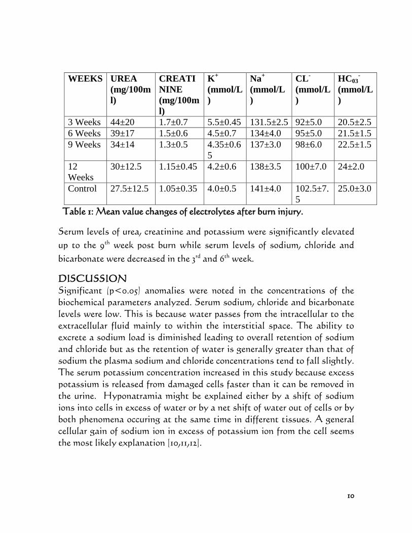
10
WEEKS UREA
(mg/100m
l)
CREATI
NINE
(mg/100m
l)
K+
(mmol/L
)
Na+
(mmol/L
)
CL-
(mmol/L
)
HC03-
(mmol/L
)
3 Weeks 44±20 1.7±0.7 5.5±0.45 131.5±2.5 92±5.0 20.5±2.5
6 Weeks 39±17 1.5±0.6 4.5±0.7 134±4.0 95±5.0 21.5±1.5
9 Weeks 34±14 1.3±0.5 4.35±0.6
5
137±3.0 98±6.0 22.5±1.5
12
Weeks
30±12.5 1.15±0.45 4.2±0.6 138±3.5 100±7.0 24±2.0
Control 27.5±12.5 1.05±0.35 4.0±0.5 141±4.0 102.5±7.
5
25.0±3.0
Table 1: Mean value changes of electrolytes after burn injury.
Serum levels of urea, creatinine and potassium were significantly elevated
up to the 9th
week post burn while serum levels of sodium, chloride and
bicarbonate were decreased in the 3rd
and 6th
week.
DISCUSSION
Significant (p<0.05) anomalies were noted in the concentrations of the
biochemical parameters analyzed. Serum sodium, chloride and bicarbonate
levels were low. This is because water passes from the intracellular to the
extracellular fluid mainly to within the interstitial space. The ability to
excrete a sodium load is diminished leading to overall retention of sodium
and chloride but as the retention of water is generally greater than that of
sodium the plasma sodium and chloride concentrations tend to fall slightly.
The serum potassium concentration increased in this study because excess
potassium is released from damaged cells faster than it can be removed in
the urine. Hyponatramia might be explained either by a shift of sodium
ions into cells in excess of water or by a net shift of water out of cells or by
both phenomena occuring at the same time in different tissues. A general
cellular gain of sodium ion in excess of potassium ion from the cell seems
the most likely explanation [10,11,12].
11
Mean urea concentration during the period of study was 44±20mg/dl
against a control value of 27.5±12.5mg/dl while mean serum creatinine level
was 1.7+0.7mg/dl compared with mean control value of 1.05±0.35 mg/dl.
Serum urea and creatinine levels were higher in males that in females. The
accelerated breakdown of muscle towards mobilization of amino acids
combined with any fall in the glomerular filtration rate results in a rise in
serum urea and creatinine. [13]. It was generally observed that severity of
the burn injury tallied with percentage increase or decrease in the serum
concentration of the biochemical parameters analyzed. In addition anion
gap difference and urea/creatinine ratio showed good correlation with
percent total body surface area affected. Serum levels of urea, creatinine
and potassium remained significantly altered till the 9th
week postburn,
though the initial changes observed abated gradually. The remarkable
results obtained from some patients included elevations in serum
potassium concentration to 7.5mmol/l, urea of 170mg/dl while serum
sodium decreased to 127 mmol/l. This may be due to decreased effective
blood circulation with the reduced plasma in this condition leading to low
blood pressure which ultimately reduced the effective filtration rate of the
glomeruli [14,15].
The clinician may need to seek the help of the biochemistry department to
monitor the severity of the initial disturbances and the effectiveness of the
response especially if there are complications and whether or not these are
modified by therapy. Such information and advice are often essential for
the care of the patient. This is because once the Injury is larger than 10-15%
total body surface area in size, the physiological impact is no longer local
but affects distant and systemic mechanism [16].
REFERENCES
[1] Sparkes, B.G.(1997). In Warfare, Disaster or Terrorist Strikes. Burn 23:
(3) 238 247
12
[2] Staley ,M., Richard, R., and Loader, G.D. (2004). Functional
Outcomes for the Patients with Burn Injuries. Journal of Burn Care
Rehabilitation 17: (4) 362-370
[3] Tietz, N.W.(2007).Determination of Serum Creatinine: In:
Fundamentals of Clinical Chemistry. 8th
Ed W.B.
Saunders Co. Philadelphia. 824-847
[4] Trader, D.L., and Herndon, Dal. (2009). Pathophysiology of Smoke
Inhalation: in: Smoke Inhalation and Burns. Mc Graw Hill Incorporated.
New York.61
[5] Walmsley, R.N. and Guerin, G.H. (2004) .Electrolyte Disorders. A
Guide to Diagnostic Clinical Chemistry: 4th
ed. Black Well
Company, London. 87-70
[6] Robbins, J., Bondy, P.k., and Rosenberg, L.T. (1995). Metabolic control
and diseases 8th
ed W.B. saunders Co. philadelphia .1325
[7] Salisbery, R.E. (2002). Thermal burns in plastic Surgery: Vol.1.W.B.
Saunders Co. Philadelphia. 787-813
[8] Phillips, A.W., and Copre,O. (2003) .Burn Therapy. Annals of Surgery
152: 762
[9] Renz, M.R., and Sherman, R.(1994). Hot tar burns: Twenty seven
hospitalized cases. Journal of Burn Care Rehabilitation .15:341-345
[10] Arnold, E. (1993) .Injury by Burning. In: The Pathology of Trauma 2nd
Ed. Hodder and Stoughton Ltd. Great Britain. 178-191
[11] Britton, K.E. (2004). Renal Failure: Clinical PHYSIOLOGY 10th
Ed
Blackwell Oxford London 166-170
13
[12] Roscoe, M.H. (1993). Clinical Significance of Creatinine. Journal of
Clinical Pathology 6:20729
[13] Green, H.N., Stoner, H.B., and Whiteby, H.J. (2001). The Effect of
Trauma on the Chemical Composition of Blood and Tissue of
Man. Clinical science 8:65-87
[14] Baron, D.N.(2008). The Kidneys: in: A Short Textbook of Chemical
Pathology 10th
Ed English Language Society London, 171-189
[15] Gyanog, W.F. (2006). Urea formation: Review of Medical Physiology
12th
Ed Lange Medical Publication, London 222-224
[16] Ryan, C.A., Shankowasky, H.R., and Tredget, E.E. (1992). Profile of
the Pediatric Burn Patient in a Canadian Burn Centre. Burns 18: No.4-
262-272
14
Study on the Implication of Land Use Expansion and
Land Cover Change around Yankari Game Reserve in
Relation to Wildlife Habitat Degradation
Mohammed, I1., Akosim, C
2., Suleiman, I. M
3 &Adamu Mato
4
1Department of Environmental Management Technology,
2
Department of Forestry and Wildlife Management, Moddibo Adama University of Technology, Yola
3
Department of Survey and Geo-informatics, Abubakar Tafawa Balewa University Bauchi
4Forestry Department, Bauchi College of Agriculture, Bauchi State
Email: [email protected]
Abstract
The research investigated the various types of land use practices around
5km outside the Yankari Game Reserve boundary and the extent of land
cover changes and degradation of biological resources inside there serve
for the period of 30years. Landsat imageries of the reserve from 1984 to
2014 were used for change detection using Maximum Likelihood
Algorism Method. The socio economic characteristics of the inhabitant
surrounding the reserve were investigated using questionnaire. The
results indicated that the major land use practice around the reserve
boundary include among others farming, livestock husbandry,
settlement, mining, fishing and hunting. While percentage changes in
land cover classes inside the reserve between 1984 and 2014 were: bare
ground (+36.67%), gallery forest (-3.02%), open savanna (+2.58%), rock
outcrop (+9.39%), build-up area (+4.39%), woodland savanna (-43.49%).
Changes within 5km outside the reserve between 1984 and 2014 were:
bare ground (+3.01%), gallery forest (-48.99%), open savanna (+8.45%),
rock outcrop (-30.88%), built-up area (-1.19%) and woodland Savanna (-
7.56.). Significant difference (p< 0.05) occurred in both inside and within
5km outside the reserve in changes of land cover classes between 1984
and 2014. The incidences of decimation of resources over the years in the
study area were driven by anthropogenic factors, engineered principally
by poverty and low literacy level. The study recommended that, the
support zone communities should be empowered economically, socially
and politically by adding value to their culture and tradition and selling
them to tourists, conservation education, illiteracy classes and visit to
successful conservation areas as well as seminars and workshops
relating conservation and policies issues among others.
Keywords: Land Use, Degradation, Habitat, Vegetation and Poverty
Pg 17-46
15
INTRODUCTION
Protected Area (PA) refers to any area of land and/or sea specially
dedicated for the protection and maintenance of biological diversity, and of
natural and associated cultural resources, and managed through legal and
other effective means. The basic role of a PA is to separate elements of
biodiversity from processes that threaten their existence in the wild.
Globally there are some 30,000 Protected Areas (PAs) covering about 12.8
million km2 which amount to 9.5% of the planet land area (World
Commission on Protected Area WCPA 2000). In Nigeria today there are
over 504 PAs covering about 12.8% of the country’s total land area,
harboring more than 5,000 species of plants and over 22,094 species of
animals including insects, 889 species of birds and 1,489 species of
microorganisms (Federal Environmental Protection Agency FEPA Annual
Report, 1999). These records placed Nigeria 8th
and 11th
highest African
country in terms of flora and fauna diversity respectively (Comesky, 2000).
Due to increase in population growth and growing demands for improved
livelihood condition, there is a corresponding pressure on PAs and their
surrounding environment which threatens the validity of most PAs
globally as well as endangering the health and wellbeing of the biological
resources in them. Damschen et al. (2006), Fischer (2007) and Fahrig (2003)
described this as an act where natural cover has been converted into
pasture, crop land, or urban use, which in turn affects biodiversity through
both habitat loss and fragmentation and in some cases alteration of
community composition (Pidgeon et al., 2007). Other effects include
limiting species ranges (Schulte et al., 2005), restricting animal dispersal
and migration (Damschen et al., 2006; Eigenbrod et al., 2008; Fahrig, 2003)
and facilitating invasion by non-native species (Gavier et al., 2010; Predick,
2008).
Studies have revealed that land use intensities around PAs soon after their
establishment has the effect of altering ecological stability, through
reduction in their effective size and fragmentation of the system (IUCN,
2010). In a study conducted by Sanderson et al. (2002), entitled “measuring
16
human footprint on biological resources”, it was observed that humans
have modified over 83% of the Earth’s land surface due to land-use. Thus,
changes in land-use practices, and more specifically, conversion of land
from more natural conditions to less natural conditions is one of the main
threats to biological diversity (Fischer, 2007; Vitousek, 1997). Intensifying
land uses around PAs often threaten their ecological integrity and
effectiveness of PAs as a conservation tool (Joppa et al., 2008).
In densely populated Mesoamerica for example, the expansion of
agriculture, mining and logging, infrastructural projects, land speculation,
urban, residential and tourism development threaten many protected areas
(Gude et al., 2007). Land is becoming a scarce resource due to immense
agricultural and demographic pressures. Haruna et al. (2010) have noted
that rapidly increasing human populations and expanding agricultural
activities have brought about extensive landuse changes throughout the
world. According to the projection by the United Nations, the world
population is expected to increase to 9 billion people by 2050. Most of the
additional 2.3 billion people will add to the population of developing
countries, which are projected to rise from 5.6 billion in 2009 to 7.9 billion in
2050.
The projection on global population however, the developing countries are
expected to have more pressure on demand for arable land, pastoral, and/or
settlement use. The remaining fringes of lands around most protected areas
(buffer zones) would be liable for such demand. Therefore, understanding
the level of landuse and landuse changes around protected areas at
different spatial levels is important to have a better understanding of the
effect of human pressures on protected areas. It is equally important
because species relate to landscape in different ways. Therefore, it is
important to understand land-use change at different scales that
correspond to the range of scales at which species relate to environment. In
developing countries like Nigeria, land use types include farming, grazing,
mining, hunting, use of forest as sacred groves and settlement emanating
from migration due to political, social and religious conflicts as well as
17
ecological degradations. The advent of protected area system meant that
some land area used for the above purposes became converted to
conservation areas. Unfortunately, there were no commensurate benefits
coming from the conservation projects as expected by people. The problem
became compounded with increasing population over the years. The
growing population meant increase in demand for more land to produce
more food, to build more houses and for other contingent needs.
Hence, the emergence of pressure on protected areas. The pressure in the
recent years has transformed into illegal grazing, hunting, mining, fishing
and encroachment of agricultural land into conservation areas. Marguba
(2002) observed that in spite of the enormous benefits derivable from
conservation areas the negative attitudes of local residents toward the
protected areas have persisted. These phenomena therefore forced many of
the Nigerian Game Reserves and Forest Reserves to exist only on paper
due to increasing pressure of land uses while many were degazatted and
converted to farmlands, settlements and or grazing reserves. The few that
can be seen, Yankari Game Reserve inclusive are becoming islands of
forest between human settlements and farmlands and have continued to
receive such pressure.
METHOD OF DATA COLLECTION
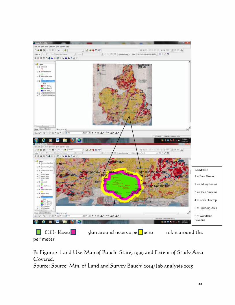
The Study Area
The research was conducted at Yankari Game Reserve (YGR) and 5km
around the reserve boundary in Alkaleri Local Government Area, 105km
from the state capital (Bauchi). The reserve is located at Latitude 090 45.131
’
N and Longitude 0100 30.746
’ E. It was established as Game Reserve in
1955 and upgraded to a National Park status in 1991 under the management
of the National Parks Service. In 2006, the Bauchi State Government
reclaimed it from the Federal Government, thus, reverting its status from
Yankari National Park to Yankari Game Reserve. The reserve falls
entirely within Bauchi State and occupies a total land area of 2,244.10 km2.
It covers Duguri, Pali and Gwana Districts of Alkaleri LGA (Green,
1987).
18
Data Source
The data used for this study was Landsat TM imagery of Bauchi and
environ for 1984, 1994, 2004 and 2014, obtained from center for Remote
Sensing, Jos. The imageries were taken during the rainy seasons of
precisely the month of May of the following years 1984, 1994, 2004 and
2014. In addition a geo-referenced land use Map of Bauchi was used to
carve out and code the extent of the study area using the upper and lower
limit coordinates of the Yankari Game Reserve with the aid of ArcMap
version 9.2 and AutoCAT- 2002 software. The areas include the core area
of the reserve and 5km around the perimeter of the reserve.
Equipment and Software Used
During the field survey and laboratory analysis, the equipment used
included a four wheel drive vehicle, motor cycle and Etrex Germin high
sensitivity Global Positioning System (GPS) for geo-referencing all the
communities located around 5km of the Game Reserve perimeter as well as
other land forms. In addition, Panasonic camcorder camera 32 pixil at
37mm optical zoom strength was used. The soft wares used included
Microsoft excel for importation of coordinates of various communities and
land features into ArcGIS software. Microsoft Word, IDIRISI 32, and
Integrated Land and Water Information System (ILWIS) were used for
laboratory analysis.
Steps Used in Image Processing
The images used for this study were processed in the laboratory using the
following steps;-
Step 1: Creation of Map List
The map list of 1984, 1994, 2004 and 2014 of Yankari Game Reserve and
5km imageries were created with the aid of ILWIS software. In order to
have sets of roster maps with the same geo-referenced parameters, imagery
of 1984 were paired with 1994 and 1994 was paired with 2004, similarly 2004
was paired with 2014. The idea of doing this was to ensure correlations
19
between possible changes of succeeding and preceding years when paired.
The same process was repeated for 5km in 1984, 1994, 2004 and 2014 Map
list.
Step 2: Image Importation
Selected bands of the imageries acquired ( Landsat MT) of 1984,1994, 2004
and 2014 bands 2, 3, and 4 were imported from the computer folder where
they were stored on ILWIS software for the classification of the land cover
of the study area. Accordingly band 2, 3, and 4 were selected for this
classification because land features such as vegetation, bare ground, rock
outcrop and water bodies are best displayed in blue, green, and red
wavelengths of the visible spectrum.
Step 3: Sub Mapping
This was achieved using Arc Map version 9.2 and Auto CAD, 2002
software. Top left and bottom right coordinates of the geo-referenced map
of the study area 634370.135mN, 694699.124mN and 633574.238mE,
691356.356mE were used to map out the area of interest in the images
(Bands 2, 3, and 4). This technique was used in order to reduce the data
quantity and to analyse the desirable areas of interest.
Step 4: Color Composite
The color composite of 1984, 1994, 2004 and 2014 images were formed by
combining the three sub mapped raster bands (Band 4-Red, Band 3-Green
and Band 2- Blue for Landsat cover changes that occurred in the reserve
and 5km outside the reserve, the total area covered by the YGR boundary
was extended to 5km beyond the perimeter of the reserve using the same
Arc Map version 9.2 Software TM) into single maps. This is done in order
to give the image a clear visual impression of the true picture on ground
instead of displaying one band at a time which its interpretation would
require highly specialize technology.
20
Step 5: Definition of Domain
In order to classify the image produced by the various land cover features
the Domain class has to be determined, coded and used as variables for the
image classification. These include Bare Ground (BG), Galary Forest
(GF), Open Savanna (OS), Rock Outcrop (RO), Build up area (Wikki
Camp) (WC) and Woodland Savanna (WL).
Step 6: Pixel Training/Creation of Sample Set
Sample set for 1984, 1994, 2004, and 2014 images were created using the
land cover class code from the domain. Each of the respective images was
classified by selecting and assigning names (Code) to group of training
pixels that are supposed to represent a known feature on the ground and
have similar spectral value in the map. This is so achieved with the aid of
the coordinates of a particular feature obtained from the field using GPS.
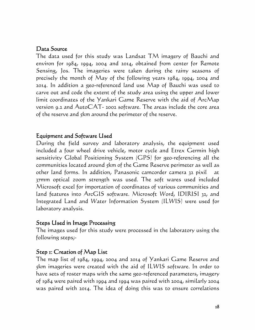
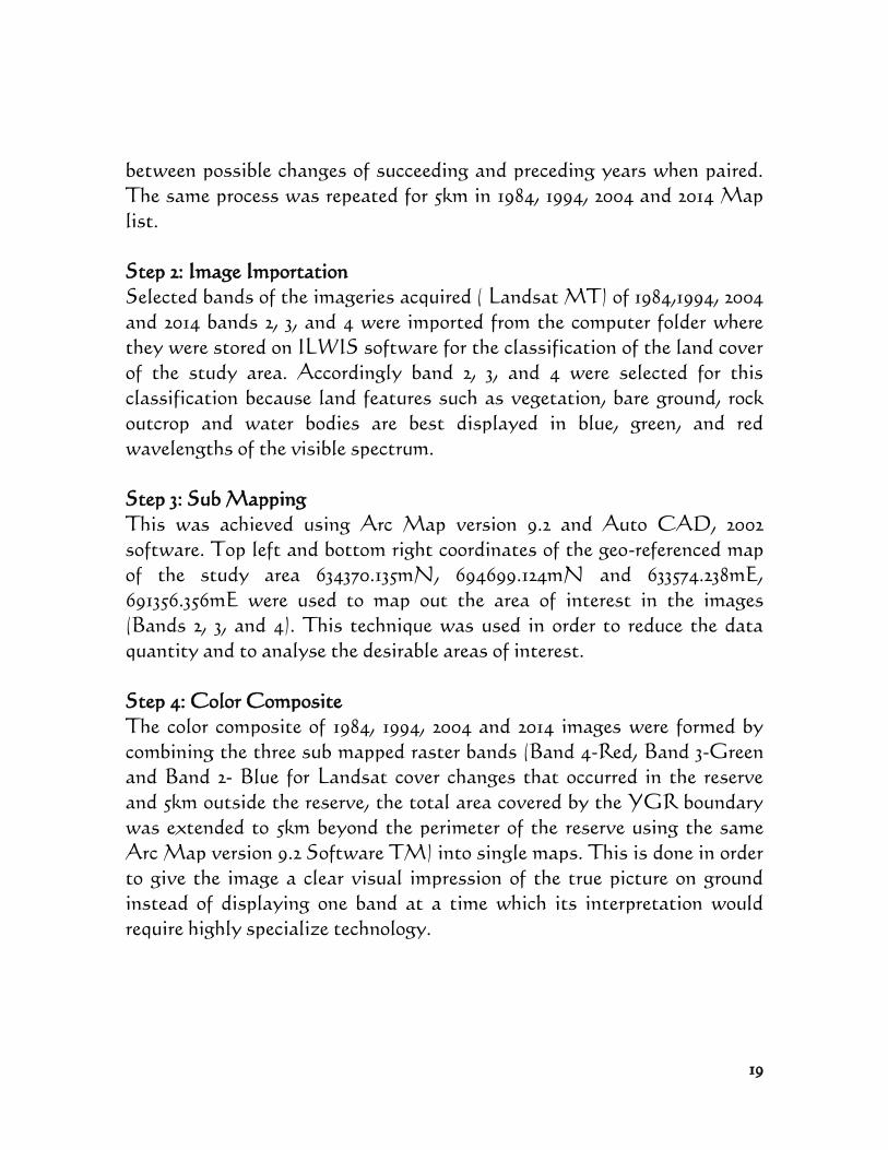
Step 7: Image Classification
At this stage the study area was classified into bare ground, gallery forest,
open savanna, rock outcrop, and build up area (Wikki Camp) as well as
woodland savanna for both images, except the 5km study area outside the
reserve. Wikki Camp was not considered as sample set, because bare
ground outside the reserve tends to dominate the buildup area (villages).
This is so, because of the fact that the buildup areas could not be captured
by the satellite due to its low resolution (Landsat TM). Hence, they
became overshadowed by the bare ground because Landsat TM satellite
captured only land features that are larger than 30m. After the completion
of the classification of the four (4) images (1984, 1994, 2004 and 2014), the
classified images were exported via windows Bitmap (BMP) to IDRISI 32
software for post classification comparisons and statistical analysis
21
LEGEND
1 = Bare Ground
2 = Gallery Forest
3 = Open Savanna
4 = Rock Outcrop
5 = Buildup Area
6 = Woodland
Savanna
LEGEND
1 = Bare Ground
2 = Gallery Forest
3 = Open Savanna
4 = Rock Outcrop
5 = Buildup Area
6 = Woodland
Savanna
Figure 2: May 2014 Classified Land Cover
Image of Yankari Game Reserve
Figure 1: May 1984 Classified Land Cover
Image of Yankari Game Reserve
22
CO- Reserve 5km around reserve perimeter 10km around the
perimeter
B: Figure 2: Land Use Map of Bauchi State, 1999 and Extent of Study Area
Covered.
Source: Source: Min. of Land and Survey Bauchi 2014; lab analysis 2015
LEGEND
1 = Bare Ground
2 = Gallery Forest
3 = Open Savanna
4 = Rock Outcrop
5 = Build-up Area
6 = Woodland
Savanna
23
RESULT AND DISCUSSION
Six land cover classes were identified in YGR for the purpose of this
study. They include, bare ground, gallery forest (riverine vegetation), open
savanna, rock outcrop, build-up areas and woodland savanna. The finding
of the supervised classification techniques of 1984 and 1994 imageries
indicated land cover classes changes within the reserve with the exception
of the bare ground. Build-up areas were not captured, either due to
situation that prevailed at the time of capture or because their ‘areas’ were
below 30m in radius. Gallery forest, open savanna and rock outcrop
increased in size while woodland savanna decreased in size. These findings
are in line with those of Gajere (2001) and Shuaibu (2012)
The cross tabulation analysis (CTA) result indicated that although an
increase occurred in gallery forest, the increase was not significant. The
open savanna which traversed the entire reserve adjoining all other land
cover classes indicated both gains and losses. Parts of the open savanna
were converted to gallery forest, woodland savanna and rock outcrop
between 1984 and 1994. Some patches of the open savanna remained
unchanged over the period under review. The woodland savanna which also
adjoins other land cover classes lost parts of its cover to gallery forest, open
savanna and the rock outcrop. The variation in changes in land cover
classes may not be unconnected with the location of the land cover class in
the reserve and its accessibility and vulnerability to human activities.
These observations agreed with those of Shuaibu (2012) who indicated that
land cover change in Mubi North was attributed to increased human
activities.
The resilience of the bare ground may not be unconnected with improper
use of fire for the ecosystem combined with inadequate protection against
overgrazing by the reserve management during the period under review.
The conversion of patches of the open savanna and woodland savanna to
the gallery forest can be explained by the fact that the management of the
YGR (during the period under review) ensured that the gallery forest and
the adjoining land were protected against both early and late fire regimes in
24
the reserve. Besides, protection was also ensured by the management
against lopping, grazing and fuel wood/ timber exploitation. The high
water table in the area could also have aided the growth of the vegetation
into a gallery forest ecosystem. Similarly, the effects of protection as
observed with the open savanna changing to gallery forest is in agreement
with the report of Geerling, (1973a) and Ola-Adam (1996) for the
vegetation utilization of YGR and Olokomeji forest reserve.
The loss of patches of the Open Savanna to Woodland Savanna may also
be attributed to the practice of controlled burning (early fire regime) and
protection against lopping and grazing. The loss of patches of Woodland
Savanna to Open Savanna may be connected with its attractiveness to the
pastoralists due to heavy presence of leguminous trees such as Afzelia
africana, Anogeisus leocarpuand, Prosopis africana which are highly
palatable to livestock (cattle sheep and goat). The pastoralists tend to defy
all management measures (as observed during the study) to access the
Woodlands, where they engage in both lopping and indiscriminate burning.
The results are loss of vigor by trees and susceptibility to infection by
diseases, and consequently death. Besides fire, fuel wood collection and
timber exploitation thrive in the Woodlands. These observations agree
with those of Gajere (2001) Ibrahim (2005) and Mohammed (2009).
The result of the study also revealed that patches of the open savanna and
that of the woodland savanna were lost to rock outcrop during the 1984-
1994 period. Rainfall data over the same period suggest that long period or
spells of drought may be contributing factor, coupled with wildfire, over
grazing and erosion. The observation agrees with that of Mohammed
(2014) and Ibrahim (2005).
Results of the supervised classification techniques of 1994 to 2004 as well
as the Cross Tabulation Analysis (CTA) also revealed that there was no
consistent change in Land Cover Class (LCC) during the period under
review. The results suggest that the threat factors and their pattern of
operations and influences on the land cover classes during the period 1984
to 1994 remained the same over the period 1984-2004. However, there were
25
exceptional cases. These are in respect of emergence of bare ground in
gallery forest and build-up areas in some land cover classes. In respect of
emergence of bare ground in the gallery forest, interaction with the
surrounding communities revealed that increase in agricultural activities
aided by agricultural mechanization, which took place within 5km outside
the reserve led to loss of woody vegetation from a large area. The result
was an unprecedented run-off following heavy rain falls into the tributaries
that feed the Gaji, Yashi and Yuli Rivers that are situated within the
basin of the reserve. This led to the over flow of the river banks and
consequently the flooding of the basin (Gaji river) at the center of the
reserve which contains the gallery forest. The repeat of this incidence over
the years may probably be caused of the death of the trees leaving the area
affected as bare ground. Similar close observations were reported by Gajere
(2001) Ibrahim (2005).
Gallery forest lost to woodland savanna, open savanna, rock outcrop and
build-up areas. Woodland savanna lost to gallery forest, open savanna, and
bare ground. Build-up areas, rock outcrop and open savanna lost to gallery
forest, woodland savanna, bare ground, rock outcrop and buildup area.
Rock outcrop lost to open savanna, and to build-up area.
Furthermore, observations during the study, indicated management failure
to repair the jeep tracks which serves as fire breaks that prevent annual fire
(control fire) from crossing into the gallery forest. This situation may also
have contributed to loss of vegetation along the riverine forest. Besides,
restriction of elephants to the riverine forest during the dry season for their
food which are mostly browsers, have been observed to account for a great
loss of woody plant species in the gallery forest. The Gaji river valley is
the only source of dry season water. Hence, enormous pressure is received
from the elephants and many other large mammals in the riverine forest
during the dry season. Trees are eaten up, trampled and killed by the
elephants, thus exposing some portions of the gallery forest to bare ground.
These observations agree with Green (1986). Geerling (1973a) and
26
Marshall (1985a) reported that elephant population in the reserve
constituted a threat to the reserve ecosystem.
Another serious ecological upset that developed during the period under
review was the build-up area. Gallery forest, woodland savanna, open
savanna and rock outcrop, all lost portions of their land to build-up area.
Investigation through ground truthing during the study revealed that
expansion of the Wikki Spring for sun bathing area as well as development
of spring beech for recreation activities resulted in the expansion of build-
up area. The excavations along the riverine forest for building
constructions, and development of wikki Camp also contributed to
increase build-up area in the reserve during 1994-2004 periods. The
implication is the reduction in wildlife habitat in the reserve.
Findings from the supervised classification techniques of 2004 to 2014 and
the cross tabulation analysis (CTA) of the data further revealed variation
in changes in land cover classes. The results indicated losses from gallery
forest, woodland savanna, and open savanna to bare ground; build-up area
and rock outcrop suggest the prevalence of such factors like flood,
uncontrolled fire, over grazing, lopping, logging, and fuel wood collection
and elephant activities. Conversely, the change from; open savanna to
woodland savanna and gallery forest; bare ground and rock outcrop to open
savanna suggest adequate management practices in terms of burning
practices and protection against over grazing, lopping, logging and fuel
wood collection as well as prevalence of good weather during 1984-2004
period. The observations agree with the report of Environ-Consult (2000;
2006) on Kaiji Lake National Park and Ola-Adams (1996) and on
Olokomeji forest reserve that control burning is responsible for the
maintenance of the ecological integrity of wildlife habitat.
Findings from the Supervised Classification Techniques (SCT) and Cross
Tabulation Analysis (CTA) of land cover class’s data obtained within
5km outside the reserve indicated similar pattern and trend as those
obtained within the reserve. This is because; like those obtained within the
27
reserve, there were no consistent changes in the land cover classes from
1984-1994; 1994-2004; 2004-2014. However, when the area (size) of bare
ground, build-up area, and rock outcrop within and outside of the reserve
were proportionately compared, it was found that those outside the reserve
were significantly (p<0.05) higher. Similarly, comparison of gallery forest,
woodland savanna and open savanna between those within the reserve and
those outside the reserve indicated significantly (p<0.05) higher values for
those within the reserve. The results therefore suggest that the
anthropogenic factors are the major factors impacting negatively on the
biological resources of the reserve. This observation agrees with those of
Akosim et al., (2004) and Yaduma (2012) for Kaiji Lake National Park and
Gashaka Gumti’s National Park respectively.
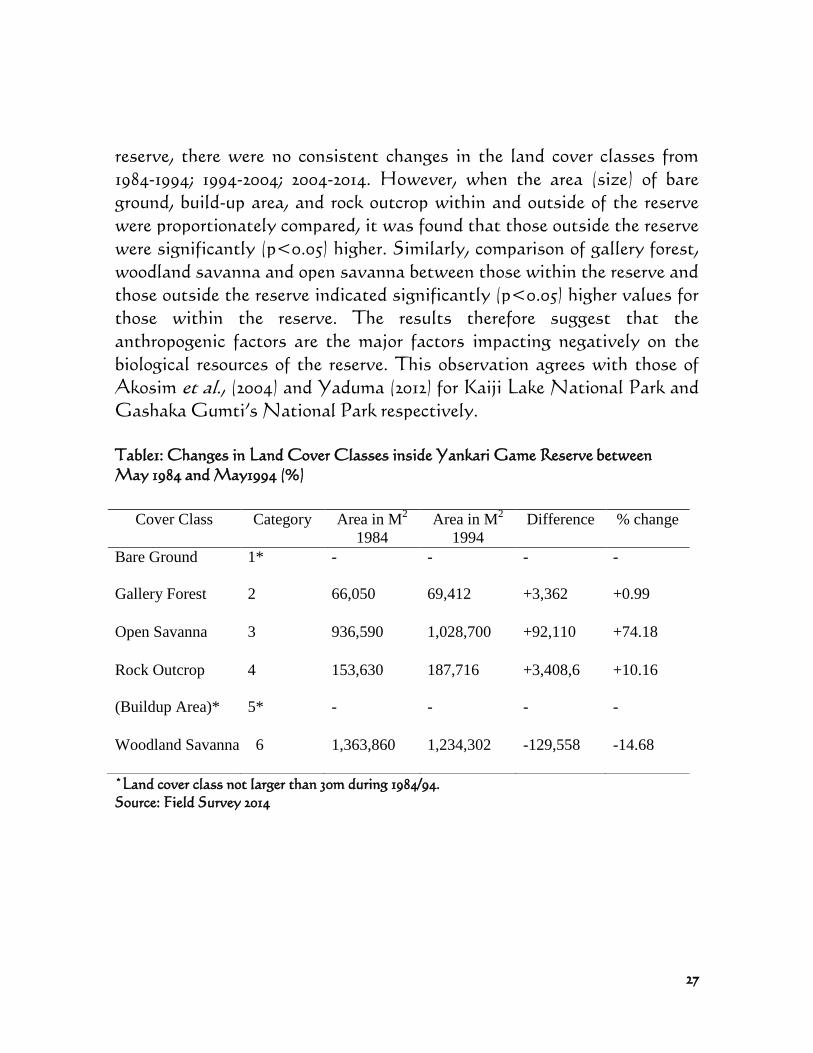
Table1: Changes in Land Cover Classes inside Yankari Game Reserve between
May 1984 and May1994 (%)
*Land cover class not larger than 30m during 1984/94.
Source: Field Survey 2014
Cover Class Category Area in M2
1984
Area in M2
1994
Difference % change
Bare Ground 1* - - - -
Gallery Forest 2 66,050 69,412 +3,362 +0.99
Open Savanna 3 936,590 1,028,700 +92,110 +74.18
Rock Outcrop 4 153,630 187,716 +3,408,6 +10.16
(Buildup Area)* 5* - - - -
Woodland Savanna 6 1,363,860 1,234,302 -129,558 -14.68
28
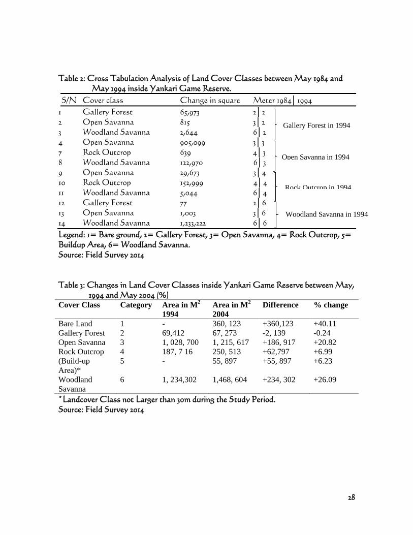
Table 2: Cross Tabulation Analysis of Land Cover Classes between May 1984 and
May 1994 inside Yankari Game Reserve.
S/N Cover class Change in square Meter 1984│1994
1 Gallery Forest 65,973 2│2
2 Open Savanna 815 3│2
3 Woodland Savanna 2,644 6│2
4 Open Savanna 905,099 3│3
7 Rock Outcrop 639 4│3
8 Woodland Savanna 122,970 6│3
9 Open Savanna 29,673 3│4
10 Rock Outcrop 152,999 4│4
11 Woodland Savanna 5,044 6│4
12 Gallery Forest 77 2│6
13 Open Savanna 1,003 3│6
14 Woodland Savanna 1,233,222 6│6
Legend: 1= Bare ground, 2= Gallery Forest, 3= Open Savanna, 4= Rock Outcrop, 5=
Buildup Area, 6= Woodland Savanna.
Source: Field Survey 2014
Table 3: Changes in Land Cover Classes inside Yankari Game Reserve between May,
1994 and May 2004 (%)
Cover Class Category Area in M2
1994
Area in M2
2004
Difference % change
Bare Land 1 - 360, 123 +360,123 +40.11
Gallery Forest 2 69,412 67, 273 -2, 139 -0.24
Open Savanna 3 1, 028, 700 1, 215, 617 +186, 917 +20.82
Rock Outcrop 4 187, 7 16 250, 513 +62,797 +6.99
(Build-up
Area)*
5 - 55, 897 +55, 897 +6.23
Woodland
Savanna
6 1, 234,302 1,468, 604 +234, 302 +26.09
*Landcover Class not Larger than 30m during the Study Period.
Source: Field Survey 2014
Gallery Forest in 1994
Open Savanna in 1994
Woodland Savanna in 1994
Rock Outcrop in 1994
29
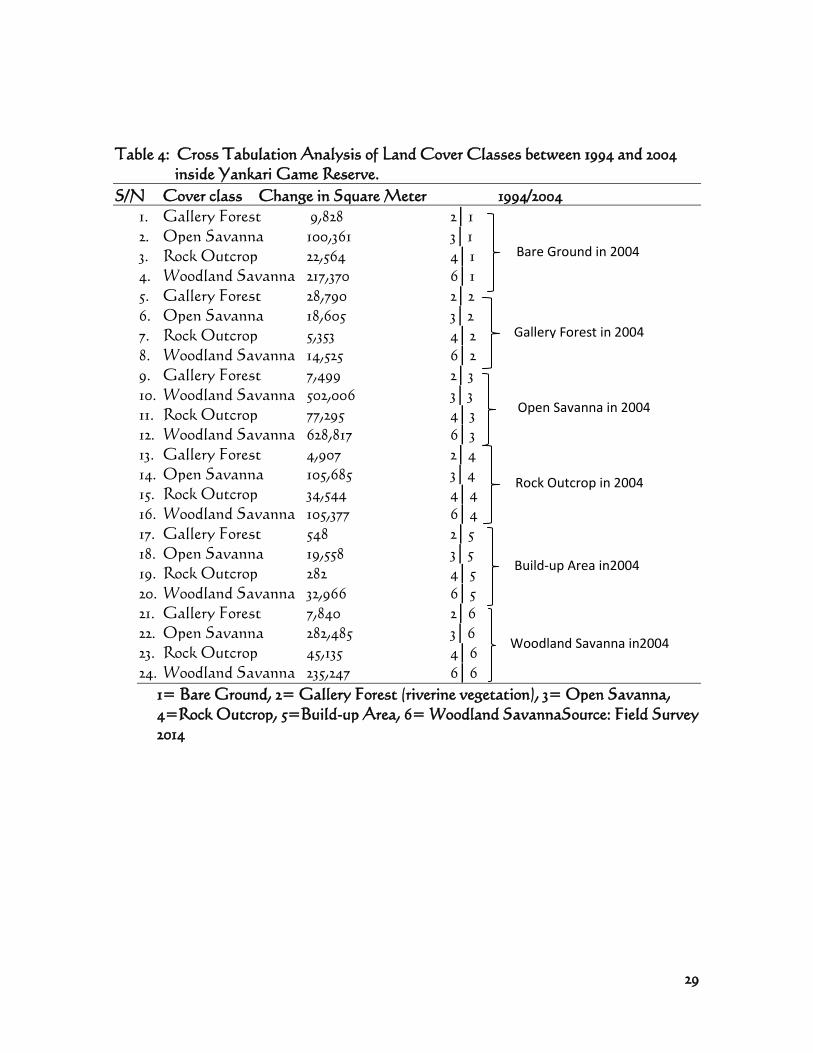
Table 4: Cross Tabulation Analysis of Land Cover Classes between 1994 and 2004
inside Yankari Game Reserve.
S/N Cover class Change in Square Meter 1994/2004
1. Gallery Forest 9,828 2│1
2. Open Savanna 100,361 3│1
3. Rock Outcrop 22,564 4│1
4. Woodland Savanna 217,370 6│1
5. Gallery Forest 28,790 2│2
6. Open Savanna 18,605 3│2
7. Rock Outcrop 5,353 4│2
8. Woodland Savanna 14,525 6│2
9. Gallery Forest 7,499 2│3
10. Woodland Savanna 502,006 3│3
11. Rock Outcrop 77,295 4│3
12. Woodland Savanna 628,817 6│3
13. Gallery Forest 4,907 2│4
14. Open Savanna 105,685 3│4
15. Rock Outcrop 34,544 4│4
16. Woodland Savanna 105,377 6│4
17. Gallery Forest 548 2│5
18. Open Savanna 19,558 3│5
19. Rock Outcrop 282 4│5
20. Woodland Savanna 32,966 6│5
21. Gallery Forest 7,840 2│6
22. Open Savanna 282,485 3│6
23. Rock Outcrop 45,135 4│6
24. Woodland Savanna 235,247 6│6
1= Bare Ground, 2= Gallery Forest (riverine vegetation), 3= Open Savanna,
4=Rock Outcrop, 5=Build-up Area, 6= Woodland SavannaSource: Field Survey
2014
Bare Ground in 2004
Gallery Forest in 2004
Open Savanna in 2004
Rock Outcrop in 2004
Build-up Area in2004
Woodland Savanna in2004
30
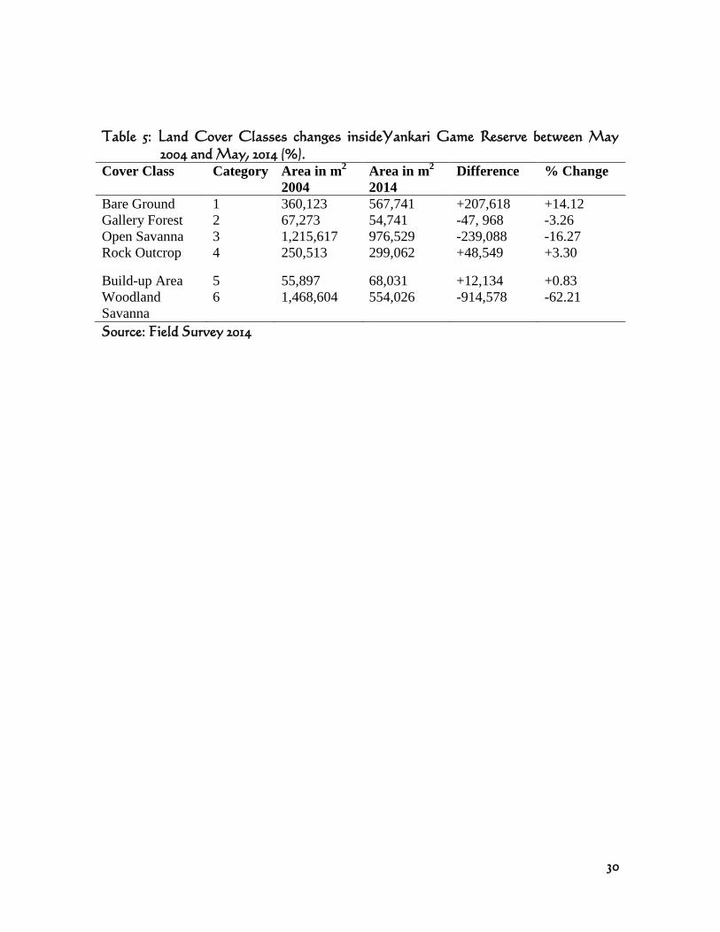
Table 5: Land Cover Classes changes insideYankari Game Reserve between May
2004 and May, 2014 (%).
Cover Class Category Area in m2
2004
Area in m2
2014
Difference % Change
Bare Ground 1 360,123 567,741 +207,618 +14.12
Gallery Forest 2 67,273 54,741 -47, 968 -3.26
Open Savanna 3 1,215,617 976,529 -239,088 -16.27
Rock Outcrop 4 250,513 299,062 +48,549 +3.30
Build-up Area 5 55,897 68,031 +12,134 +0.83
Woodland
Savanna
6 1,468,604 554,026 -914,578 -62.21
Source: Field Survey 2014
31
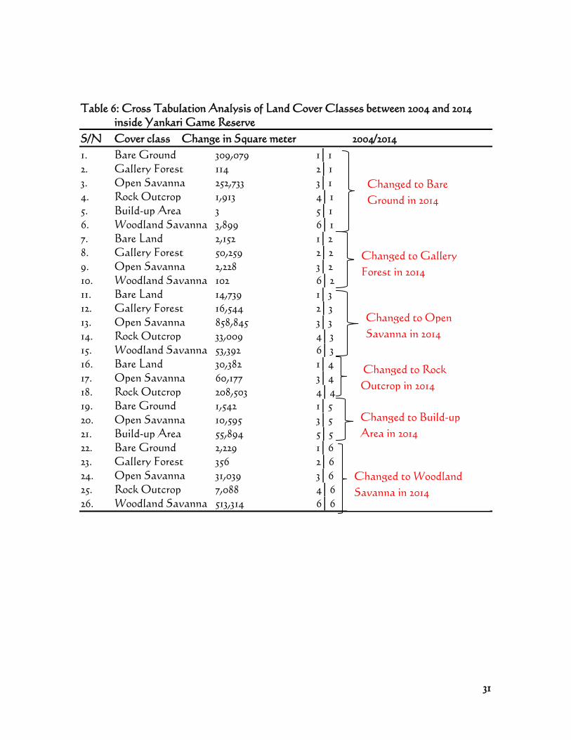
Table 6: Cross Tabulation Analysis of Land Cover Classes between 2004 and 2014
inside Yankari Game Reserve
S/N Cover class Change in Square meter 2004/2014
1. Bare Ground 309,079 1│1
2. Gallery Forest 114 2│1
3. Open Savanna 252,733 3│1
4. Rock Outcrop 1,913 4│1
5. Build-up Area 3 5│1
6. Woodland Savanna 3,899 6│1
7. Bare Land 2,152 1│2
8. Gallery Forest 50,259 2│2
9. Open Savanna 2,228 3│2
10. Woodland Savanna 102 6│2
11. Bare Land 14,739 1│3
12. Gallery Forest 16,544 2│3
13. Open Savanna 858,845 3│3
14. Rock Outcrop 33,009 4│3
15. Woodland Savanna 53,392 6│3
16. Bare Land 30,382 1│4
17. Open Savanna 60,177 3│4
18. Rock Outcrop 208,503 4│4
19. Bare Ground 1,542 1│5
20. Open Savanna 10,595 3│5
21. Build-up Area 55,894 5│5
22. Bare Ground 2,229 1│6
23. Gallery Forest 356 2│6
24. Open Savanna 31,039 3│6
25. Rock Outcrop 7,088 4│6
26. Woodland Savanna 513,314 6│6
Changed to Gallery
Forest in 2014
rest in 2014
Changed to Rock
Outcrop in 2014
ged to Rock Outcrop in
2014
Changed to Woodland
Savanna in 2014
Changed to Woodland
Savanna in 2014
Changed to Build-up
Area in 2014
Changed to Build-up
Area in 2014
Changed to Open
Savanna in 2014
in 2014
Changed to Bare
Ground in 2014
rest in 2014
32
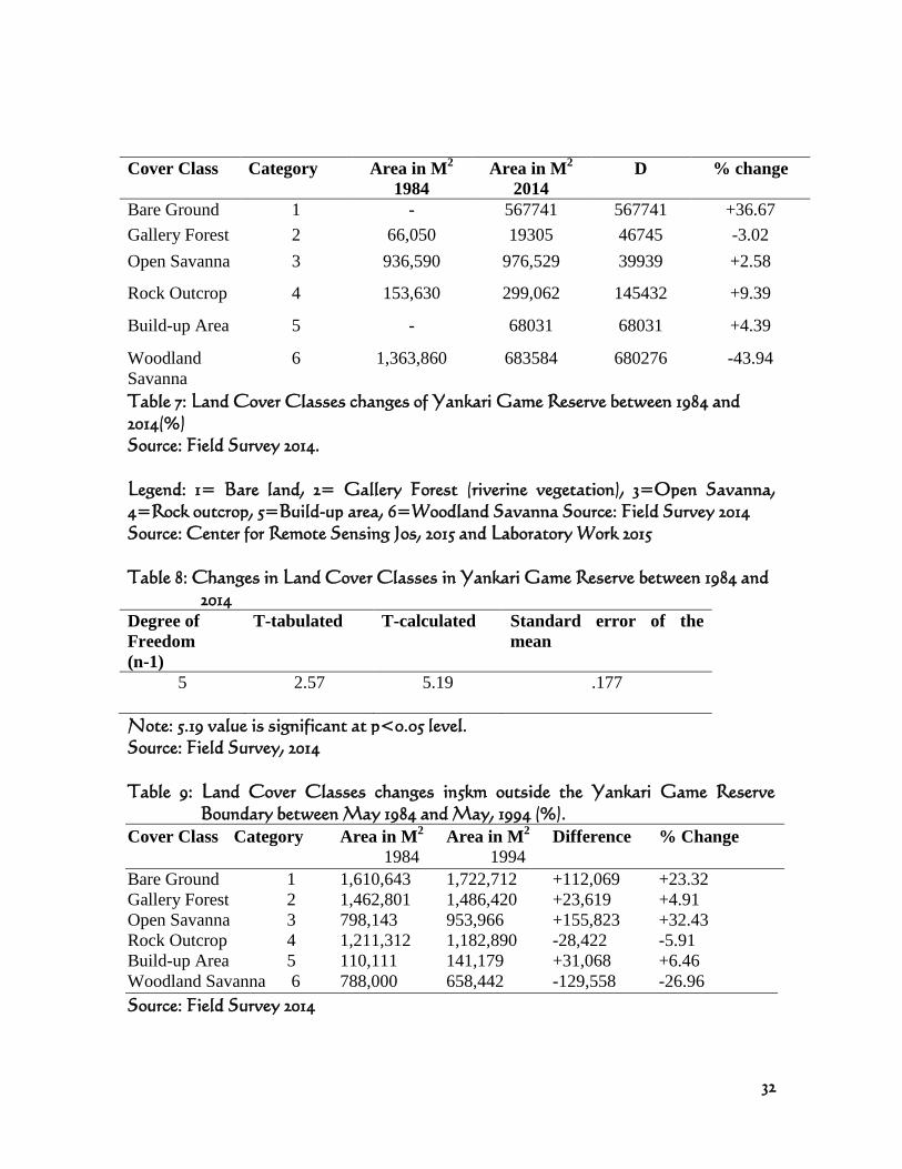
Table 7: Land Cover Classes changes of Yankari Game Reserve between 1984 and
2014(%)
Source: Field Survey 2014.
Legend: 1= Bare land, 2= Gallery Forest (riverine vegetation), 3=Open Savanna,
4=Rock outcrop, 5=Build-up area, 6=Woodland Savanna Source: Field Survey 2014
Source: Center for Remote Sensing Jos, 2015 and Laboratory Work 2015
Table 8: Changes in Land Cover Classes in Yankari Game Reserve between 1984 and
2014
Degree of
Freedom
(n-1)
T-tabulated T-calculated Standard error of the
mean
5 2.57 5.19 .177
Note: 5.19 value is significant at p<0.05 level.
Source: Field Survey, 2014
Table 9: Land Cover Classes changes in5km outside the Yankari Game Reserve
Boundary between May 1984 and May, 1994 (%).
Cover Class Category Area in M2 Area in M
2 Difference % Change
1984 1994
Bare Ground 1 1,610,643 1,722,712 +112,069 +23.32
Gallery Forest 2 1,462,801 1,486,420 +23,619 +4.91
Open Savanna 3 798,143 953,966 +155,823 +32.43
Rock Outcrop 4 1,211,312 1,182,890 -28,422 -5.91
Build-up Area 5 110,111 141,179 +31,068 +6.46
Woodland Savanna 6 788,000 658,442 -129,558 -26.96
Source: Field Survey 2014
Cover Class Category Area in M2
1984
Area in M2
2014
D % change
Bare Ground 1 - 567741 567741 +36.67
Gallery Forest 2 66,050 19305 46745 -3.02
Open Savanna 3 936,590 976,529 39939 +2.58
Rock Outcrop 4 153,630 299,062 145432 +9.39
Build-up Area 5 - 68031 68031 +4.39
Woodland
Savanna
6 1,363,860 683584 680276 -43.94
33
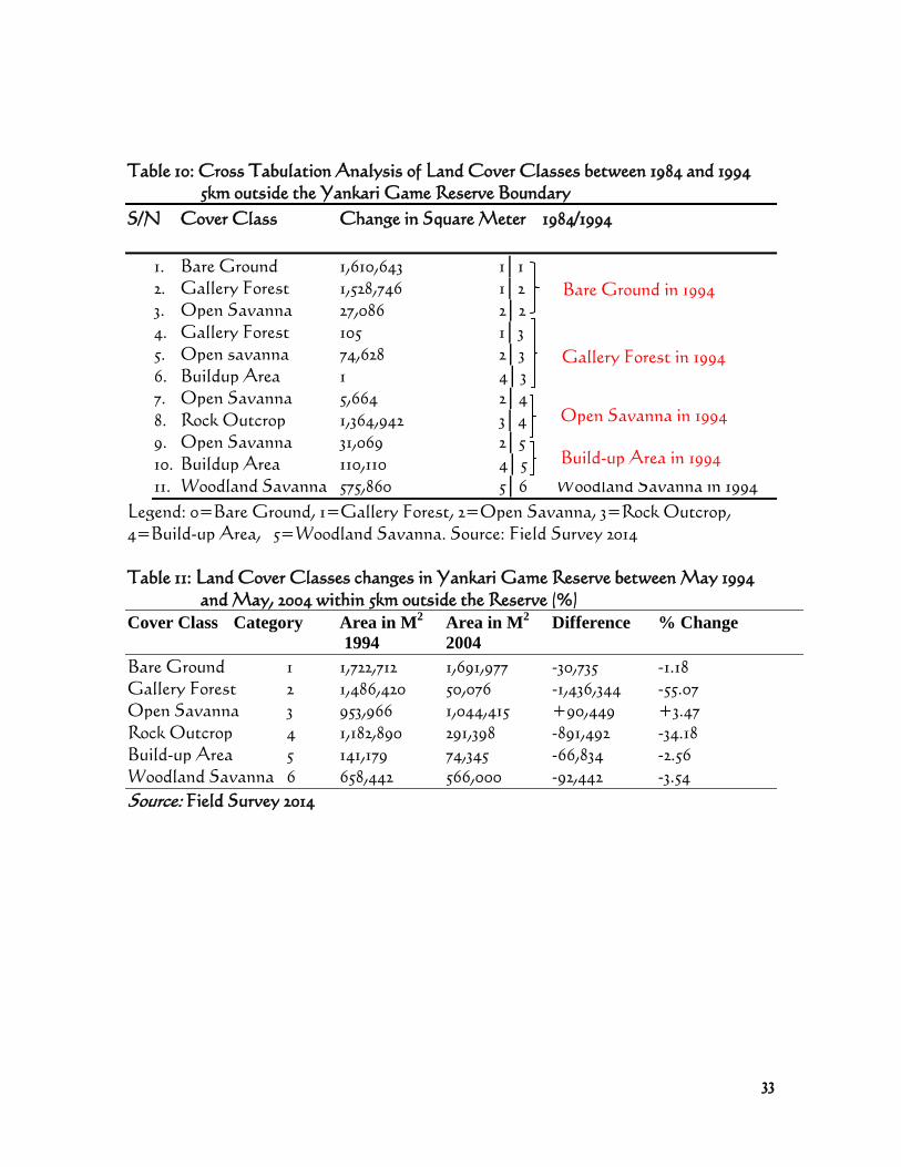
Table 10: Cross Tabulation Analysis of Land Cover Classes between 1984 and 1994
5km outside the Yankari Game Reserve Boundary
S/N Cover Class Change in Square Meter 1984/1994
1. Bare Ground 1,610,643 1│1
2. Gallery Forest 1,528,746 1│2
3. Open Savanna 27,086 2│2
4. Gallery Forest 105 1│3
5. Open savanna 74,628 2│3
6. Buildup Area 1 4│3
7. Open Savanna 5,664 2│4
8. Rock Outcrop 1,364,942 3│4
9. Open Savanna 31,069 2│5
10. Buildup Area 110,110 4│5
11. Woodland Savanna 575,860 5│6 Woodland Savanna in 1994
Legend: 0=Bare Ground, 1=Gallery Forest, 2=Open Savanna, 3=Rock Outcrop,
4=Build-up Area, 5=Woodland Savanna. Source: Field Survey 2014
Table 11: Land Cover Classes changes in Yankari Game Reserve between May 1994
and May, 2004 within 5km outside the Reserve (%)
Cover Class Category Area in M2 Area in M
2 Difference % Change
1994 2004
Bare Ground 1 1,722,712 1,691,977 -30,735 -1.18
Gallery Forest 2 1,486,420 50,076 -1,436,344 -55.07
Open Savanna 3 953,966 1,044,415 +90,449 +3.47
Rock Outcrop 4 1,182,890 291,398 -891,492 -34.18
Build-up Area 5 141,179 74,345 -66,834 -2.56
Woodland Savanna 6 658,442 566,000 -92,442 -3.54
Source: Field Survey 2014
Bare Ground in 1994G
Bare Ground in
1994allery Forest in 1994 Gallery Forest in 1994
pen Savanna in 1994
Open Savanna in 1994
Rock Outcrop in 1994 Build-up Area in 1994
uild-up Area in 1994
34
Table 12: Land Cover Classes changes in Yankari Game Reserve between May 2004
and May, 2014 5km outside the Reserve (%)
Cover Class Category Area in M2
2004
Area in M2
2014
Difference % Change
Bare Ground 1 1,691,977 1,700,361 +8, 384 +30.33
Gallery Forest 2 50,076 36,237 -13, 839 -50.06
Open Savanna 3 1,044,415 1,049,819 +5404 +19.54
Rock Outcrop 4 291,398 291,398 +0.00 0.00
Build-up Area 5 74,345 74,396 +15 +0.07
Woodland Area 6 566,000 566,000 +0.00 +0.00
Source: Field Survey 2014
35
Table 13: Cross Tabulation Analysis of Land Cover Classes between 1994 and 2004
5km outside the Boundary of Yankari Game Reserve (YGR)
S/N Cover Class Change in Square Meter 1994/2004
12. Bare Ground 826,604 1│1
13. Gallery Forest 26,143 2│1
14. Open Savanna 480,157 3│1
15. Rock Outcrop 59,298 4│1
16. Woodland Savanna 299,775 6│1
17. Bare Ground 13,521 1│2
18. Gallery Forest 26,551 2│2
19. Open Savanna 7,061 3│2
20. Rock Outcrop 1,689 4│2
21. Woodland Savanna 1,254 6│2
22. Bare Ground 413,028 1│3
23. Gallery Forest 9,408 2│3
24. Open Savanna 437,464 3│3
25. Rock Outcrop 31,835 4│3
26. Woodland Savanna 152,679 6│3
27. Bare Ground 103,992 1│4
28. Gallery Forest 6,901 2│4
29. Open Savanna 124,859 3│4
30. Rock Outcrop 24,375 4│4
31. Woodland Savanna 31,271 6│4
32. Bare Ground 32,900 1│5
33. Gallery Forest 316 2│5
34. Open Savanna 22,268 3│5
35. Rock Outcrop 1,959 4│5
36. Woodland Savanna 16,902 6│5
37. Open Savanna 165,786 1│6
38. Gallery Forest 5,415 2│6
39. Open Savanna 298,797 3│6
40. Rock Outcrop 22,023 4│6
41. Build-up Area 73,979 6│6
1= Bare Ground, 2=Gallery Forest, 3=Open Savanna, 4= Rock Outcrop, 5=Build-up
Area, 6=Woodland Savanna.
Source: Field Survey 2014
Turn to Bare
Ground in 2004
Turn to Bare
Ground in 2004
in 2004 Turn to
Gallery Forest
in 2004
Turn to Gallery
Forest in 2004
in 2004 Turn to Open
Savanna in 2004
Turn to Open
Savanna in 2004
in 2004 Turn to Rock
Outcrop in 2004
Turn to Rock
Outcrop in 2004
Turn to Build-up
Area in 2004
Turn to Build-up
Area in 2004
Turn to Woodland
Savanna in 2004
Turn to Woodland
Savanna in 2004
36
Table 14: Cross Tabulation Analysis of Land Cover Classes between 2004 and 2014
5km outside the Boundary of Yankari Game Reserve (YGR)
S/N Cover Class Change in Square Meter 2004/2014
1. Bare Ground 1,691,243 1│1
2. Gallery Forest 9,113 2│1
3. Bare Ground 729 1│2
4. Gallery Forest 35,492 2│2
5. Open Savanna 16 3│2
6. Gallery Forest 5,420 2│3
7. Open Savanna 1,044,399 3│3
8. Rock Outcrop 291,398 4│4
9. Gallery Forest 51 2│5
10. Build-up Area 74,345 5│5
11. Woodland Savanna 56,600 6│6
1=Bare Ground, 2=Gallery Forest, 3=Open Savanna, 4=Rock Outcrop, 5=Build-up
Area, 6=Woodland Savannah.
Source: Field Survey 2014
Table 15: Land Cover Classes Changes in 5km Outside Yankari Game Reserve
Boundary between 1984 and 2014 (%)
Cover Class Category Area in M2
1984
Area in M2
2014
D % change
Bare Ground 1 1, 610, 643 1, 700, 361 89718 3.01
Gallery Forest 2 1,462, 801 36, 237 -1459164 -48.99
Open Savanna 3 798, 143 1, 049, 819 251676 +8.45
Rock Outcrop 4 1, 211,312 291, 398 -919914 -30.88
Build-up Area 5 110, 111 74, 396 -35715 -1.19
Woodland
Savanna
6 788, 000 566,000 -222000 -7.56
Source: Field Survey 2014
Turned to Gallery Forest in 2014
Turned to Gallery Forest
in 2014 Turned to Open Savanna in 2014
Turned to Open Savanna
in 2014 Turned to Rock Outcrop in 2014
ned to Rock Outcrop in 2014 Turned to Build-up Area in 2014
urned to Build-up Area
in 2014 Turned to Woodland Savanna in 2014
urned to Woodland Savanna in 2014
in 2014
Turned to Bare Ground in 2014
37
Table 16: Changes in Land Cover Classes in 5km Outside the Boundary of Yankari
Game Reserve between 1984 and 2014.
DF
(n-1)
T-tabulated T-calculated Standard error
of the mean
5 2.57 7.74 .238
Note: 7.74 value is significant at p<0.05 level.
Source: Field Survey 2014
Figure 1: Proportional Area Comparison of Land Cover Classes (LCC) between
Inside and 5km outside YGR Boundary in 2014.
Source: Field Survey, 2014
0
200,000
400,000
600,000
800,000
1,000,000
1,200,000
1,400,000
1,600,000
1,800,000
Area in m2 inside reserve 2014
Area in m2 outside reserve 2014
38
CONCLUSION
The finding of this study have indicated that the biological resources and
their supporting systems in Yankari Game Reserve have been in a state of
dynamics, maintaining predominantly negative trends over the period of
thirty (30). The negative trends changes are linked to anthropogenic
activities and natural environmental hazards. Poor management of the
reserve also compounded the problems for over the period of about thirty
years. Similarly, the result indicated an abysmal net negative change in
land cover classes, with a significant reduction in Gallery forest and
woodland Savanna which once provided the much needed cover and food
for diverse and populous wildlife species of the reserve which have also
been decimated. There is also emerging expansion of portions of bare land,
Rock outcrop, buildup area and Open Savanna in places once covered by
luxuriant Woodlands and Gallery forest.
The study revealed a total depletion of wildlife habitat including land and
other supporting systems in the support zone communities. The
investigation also revealed that over the years, there has been a net influx
of migrants into the Support Zone Communities located within 5km
around the reserve boundary as a result of political, social and religious
conflicts as well as ecological degradation in the neighbouring states. The
combined effects of these factors results in an unprecedented pressure on
the resources of the reserve through livestock grazing and lopping of trees
for fodder, illegal hunting, fuel wood collection, lopping and collection of
stakes for fencing and roofing, collection of minor forest products, illegal
fishing with dangerous chemicals, mining and aiding of wildfire in the
reserve. It is the effects of these human activities combined with spells of
drought and other natural hazards such as floods, pests and diseases that
have decimated and degraded biological resources and their supporting
systems, thus bringing them to the current status in Yankari Game
reserve.
39
RECOMMENDATIONS
In view of the findings of this study, the following recommendations are
suggested:
(I) the support zone community should be empowered economically
through:
a. The establishment of community woodlot, game ranching and
captive breeding, mushroom production using simple
biotechnology techniques, adding values to agricultural waste
for local consumption and export, and integrated agriculture
involving fish farming, poultry, livestock farming and a little of
arable farming.
b. Encouraging the formation of cooperative association and
social groups that can access credit facilities and soft loan for
making a souvenir for tourist, setting of shops and restaurant
and building locally designed traditional chalets.
c. Adding value to culture and tradition of the Support Zone
Communities and selling them to tourists.
d. Eliminating ignorance by empowering the support zone
residents socially and politically through conservation
education, organizing illiteracy classes, organizing tours to
successful conservation areas as well as seminars and
workshops relating conservation to policies.
REFERENCES
Akosim, C., Mbaya, P. and Nyako, H.D. (2004). Evaluation of
Rangeland Condition and Stocking Rate of Jibiro Grazing Reserve,
Adamawa State. Journal of Arid Agriculture, 14; 35-39
Comesky, A.J. (2000). Biodiversity Monitoring and Assessment in the
Tropic Base on the Workshop on Monitoring of 1 ha Whittakker Plot
in Urban Division of Cross River National Park 2000. Smithsonian
Institute Monitoring and Assessment of Biodiversity Programme
Washington D.C 22/10/2001
40
Damschen, E.I., Haddad, N.M., Orrock, J.L., Tewksbury, J.J. and Levey,
D.J. (2006).Corridors Increase Plant Species Richness at Large
Scales. Science 313: 1284–1286. Retrieved November 6, 2013. doi:
10.1126/science.1130098.
Eigenbrod, F., Hecnar, S.J. and Fahrig, L. (2008). The Relative Effects of
Road Traffic and Forest Cover on Anuran Populations. Biological
Conservation 141: 35–46. Retrieved December 10, 2013.doi:
10.1016/j.biocon.2007.08.025.
Environ-Consult (2000).A Strict Nature Reserve of Kaiji Lake National
Park. Consultancy Report Submitted by Environ-Consult Ltd to
Kaiji Lake National Park Management, New Bussa, Niger State,
Nigeria.
Environ-Consult (2006).Development of Protected Areas Management
Plan; Interim Report on Socio-Economic and Natural Resources
Findings. Interim Report Submitted to the National Coordinator,
GEEF-LEEMP Coordinating Unit, NPS, Abuja, FCT.
Fahrig, L. (2003). Effects of Habitat Fragmentation on Biodiversity.
Annual Review of Ecology Evolution and Systematics 34: 487–515.
doi: 10.1146/annurev.ecolsys.34.011802.132419.
Federal Environmental Protection Agency Annual Report (1999).
Fischer, J., Lindenmayer, D.B. (2007) Landscape Modification and
Habitat Fragmentation: A Synthesis. Global Ecology and
Biogeography 16: 265–280. Retrieved June 15, 20013. URL:
www.http/; 10.1111/j.1466-8238.2007.00287.x.
Gajere, E.N. (2001). Assessment of Land Cover Change in Yankari
National Park – using Remote Sensing and GIS. Thesis Submitted
to Post Graduate School Abubakar Tafawa Balewa University
Bauchi. In Partial Fulfillment of the Requirement for the Award of
Degree of Master of Science in Apply Ecology. Biological Science
Programme, School of Science ATBU, Bauchi.
41
Gavier-Pizarro, G.I., Radeloff, V.C., Stewart, S.I., Huebner, C.D.,
Keuler, N.S. (2010). Rural Housing is Related to Plant Invasions in
Forests of Southern Wisconsin, USA. Landscape Cology 25: 1505–
1518.Retrieved June 15, 2013. doi: 10.1007/s10980-010-9516-8.
Geerling, L. (1973a). The Vegetation of Yankari Game Reserve: Its
Utilization and Condition. Department of Forestry Bull. No 3,
University of Ibadan.
Green, A and Amance, S. A. (1987). Management Plan for Yankari Game
Reserve Bauchi, Nigeria. WWF Tech Report 2.
Green, A. (1986). The Baseline Studies of Vegetation of Yankari Game
Reserve Nigeria. Report Submitted to NCF and WWF 1986.
Gude, P.H., Hensen, A.J., and Jones, D.A. (2007). Biodiversity
Consequences of Alternative Future Land Use Scenarios in Greater
Yellowstone. Ecological Application 17: 1000-1004
Haruna, A.U., Mohammed, I., Babanyara, Y.Y. (2010). The Threat of
Urban Poverty on the Environment: The Need for Sustainability.
Internal Journal of Environmental Issues Vol. 7.No. 2.Pp 28-37
Ibrahim, D.C. and Mohammed, I. (2005). Controlling Human-elephant
Conflict in Alkaleri Local Government Area Bauchi, Nigeria.
International journal of Environmental issues Vol.3 Nov.1 Pp 203-210
International Union of Conservation of Nature (IUCN) (2010). “Red List
of Threatened Species: Nigeria”.
Joppa, L.N., Loarie, S. R., and Pimm, S. L. (2008).On the Protection of
“Protected Areas”.In Proceedings of the National Academy of
Sciences of the United States of America 105: 6673–6678.Retrieved
November 15, 2013.doi: 10.1073/pnas.0802471105.
Marguba, L.B. (2002) National Parks and Their Benefits to Local
Communities in Nigeria. Nigeria National Park Service. Abuja.
Pp4-8
42
Marshall, P.J. (1985a). A New Method of Censuring Elephant and Hippo
in Yankari Game Reserve. Nigerian Field Journal Vol.29; 54-82.
Mohammed, I and Ibrahim, Z. U. (2014). Comparative Study on the
Implication of Charcoal Production Process on Soil Physico –
Chemical Properties: A Case Study of Barnawa Community of
Bauchi Local Government Area, Bauchi State. Paper Presented at
the Seventh Regional Conference on Sustainable Development.
June 10-11, 2014, Abuja Nigeria.
Mohammed, I. (2009). Trend of Vegetation Decline in the Adjoining
Forest of Yankari Game Reserve, Bauchi State, Nigeria.
International Journal of Environmental Issues Vol. 6. ISSN: 1597-
2417. 120-128
Ola-Adams, B.A. (1996). Conservation and Management of Biodiversity.
In the Iinception Meeting and Training Workshop on BRAAF-
Assessment and Monitoring Techniques in Nigeria. Eds. B.A. Ola-
Adams and L.O. Ojo. National committee on man and biosphere
PP. 118-125
Pidgeon. A.M., Radeloff, V.C., Flather, C.H., Lepczyk, C.A., Clayton,
M.K. (2007). Associations of Forest Bird Species Richness with
Housing and Landscape Patterns. Across the USA. Ecological
Applications 17: 1989–2010.Retrieved June 5, 2003. doi: 10.1890/06-
1489.1.
Predick, K.I., and Turner, M.G, (2008) Landscape Configuration and
Flood Frequency Influence Invasive Shrubs in Floodplain Forests of
the Wisconsin River (USA). Journal of Ecology 96: 91–102. doi:
10.1111/j.1365-2745.2007.01329.x.
Sanderson, E.W., Jaiteh, M., Levy, M.A., Redford, K.H., Wannebo, A.V.
(2002).The Human Footprint and the Last of the Wild. Bioscience 52:
891–904. Retrieved June 5, 2014.doi: 10.1641/0006- 3568.
43
Schulte, L.A., Pidgeon, A.M., Mladenoff, D.J. (2005). One Hundred
Fifty Years of Change in Forest Bird Breeding Habitat: Estimates
of Species Distributions. Conservation Biology. Retrieved
November 15, 2014. 19: 1944–1956. doi: 10.1111/j.1523-1739.2005.00254.x.
Shuaibu, M.A. and Suleiman, I.M. (2012).Application of Remote Sensing
and GIS in Land Cover Change Detection in Mubi, Adamawa
State Nigeria.Journal of Technology and Educational Research. 5 (1):
43-55. 2012.
Vitousek, P.M. and Mooney, H.A. (1997) Human Domination of Earth's
Ecosystems. Science 277: 494. doi: 10.1126/science.277.5325.494.
World Commission on Protected Area (WCPA), (2000).Protected Area in
Action. Beyond Boundaries , World Commission on protected area
in action.
Yaduma, B.Z. (2012). Analysis of Socio-Economic Benefit of North-East
Nigeria National Parks to Sport Zone Communities. A Thesis
Submitted to the Department of Forestry and Wildlife
Management, School of Agriculture and Agricultural Technology.
Modibbo Adama University of Technology in Partial Fulfillment for
the Award of Ph.D in Wildlife Management.
44
R Sarima Reanalysis of Dengue Cases in Campinas, Sao
Paulo, Brazil
Ette Harrison Etuk
Department of Mathematics
Rivers State University of Science and Technology, Port Harcourt,
Nigeria
Abstract
A well analyzed monthly time series of the number of dengue cases is
hereby re-analyzed. A controversy regarding the most adequate
SARIMA model is once again herein addressed. Monthly incidence
of dengue was initially believed to follow a SARIMA (2,1,2)x(1,1,1)12
model. Herein, analyzing the same realization of the time series by
the same software R, a SARIMA (2,1,1)x(1,1,1)12 model is found more
adequate than the former model. The likelihood therefore is that the
SARIMA (2,1,2)x(1,1,1)12 model was fitted in error using R.
Keywords: Dengue numbers, SARIMA, R, Eviews
INTRODUCTION
Martinez et al. (2011) analyzed a realization of the monthly number of
dengue cases from 1998 to 2008 in Campinas, State of Sao Paulo in Brazil.
They chose the SARIMA(2,1,2)x(1,1,1)12 model from a list of such models of
orders: (a,1,b)x(1,1,1)12 where (a,b) = (2,2), (2,1), (1,2), (1,1), (2,3) and (1,3). The
basis of their comparison was minimum Akaike Information Criterion,
AIC (Akaike, 1974). They used 2009 out-of-sample forecasts/observations
comparison to buttress their argument of model adequacy.
Etuk and Ojekudo(2014) reanalyzed the same data which was published by
Martinez et al.(2011) using Eviews software. They concluded that the
model selected by the latter was not the most adequate on the same AIC
grounds. They rather found the SARIMA(2,1,1)x(1,1,1)12 model to be best.
They suggested that this discrepancy could result from the software
difference.
Pg 47-52
45
This work is a further replication of the research work. The R software
which was originally used shall still be used for data analysis. The motive
of this write-up is to document the observed discrepancies in the analysis
of the same series by the same methods and to suggest that Martinez et al.
(2011) may have chosen the model using R in error.
MATERIALS AND METHODS
Since this is a replication of their research, the same materials used by
Martinez et al. (2011) were used. These include:
Data
As mentioned above, the same data as analyzed and published by
Martinez et al. (2011) shall be analyzed. They are monthly dengue cases
from 1998 to 2008 in Campinas, Sao Paulo, Brazil.
Sarima Model
Box and Jenkins (1976) defined a SARIMA(p,d,q)x(P,D,Q)s model as
A(L)(Ls)
X
t = B(L)(L
s)
t
(1)
where {Xt} is a time series; A(L) and (L) are the non-seasonal and the
seasonal autoregressive operators which are polynomials in L of orders p
and P, respectively; B(L) and (L) are the non-seasonal and the seasonal
moving average operators which are polynomials in L of orders q and Q
respectively; and s are the non-seasonal differencing operators defined
by =1-L and s=1-L
s where L is a backshift operator defined by L
kX
t =
Xt-k
and s is the period of seasonality of the series; {t} is a white noise
process.
Sarima modelling involves first of all the determination of the dimension of
the model. The autoregressive orders p and P are suggestive by the
respective non-seasonal and the seasonal cut-off lags of the partial
autocorrelation function. Similarly q and Q are suggestive by the
respective non-seasonal and seasonal cut-off lags of the autocorrelation
functions. The seasonal period s may be naturally suggestive by a
knowledge of the seasonal nature of the series. An inspection of the series
46
could also reveal a not-too-obvious seasonal tendency. The correlogram
could also reveal a seasonal tendency. The differencing orders d and D
should be used if the original series is non-stationary. Often at most two
differencings (seasonal and/or non-seasonal) are enough to get rid of the
non-stationary behaviour.
For model selection, the information criterion, AIC (Akaike, 1974) shall be
used.
Computer Software
The 3.3.1 version of the R software shall be used (Ihaka and Gentleman,
1996).
RESULTS AND DISCUSSION
The logarithm of Xt+1 is modelled where X
t is the number of dengues at
time t is modelled. The time plot is shown in Figure 1. Etuk and
Ojekudo(2014) have shown that this time series is not stationary and
neither are its seasonal (i.e, 12-monthly) differences. However they showed
that the non-seasonal differences of its seasonal differences are stationary.
This work is restricted to the chosen models of Martinez et al. (2011).
Table 1 shows that the SARIMA (2,1,1)x(1,1,1)12 model is the most
adequate with the least of AIC and error variance estimate. This is the
second best model in the analysis of Martinez et al.(2011). Table 2 shows
summaries of the relative orders of preferences of the models. It may be
observed that the optimum model of this work was also adjudged the most
adequate by Etuk and Ojekudo(2014). Therefore the model is
Yt = 1.4436Y
t-1 – 0.7070Y
t-2 - 0.3660Y
t-12 +
t - 0.8939
t-1 - 0.8939
t-12
(2)
where Yt =
12 log(X
t+1).
Adequacy of the model (2) is not in doubt given the residual plots of Figure
2. The residuals are all non-significant and are uncorrelated. Besides, the
Ljung-Box statistics are not statistically significant.
47
CONCLUSION
It is observed from our table 2 summaries that analysis of the same data by
different software or different versions of the same software could yield
different and at times contradictory results.
This raises some theoretical and computational issues. To reduce
controversies over model selection it is often advised that model selection
should not be based on a single criterion but on many criteria. For instance
Eviews 5.1 uses AIC and Schwarz criterion (Schwarz, 1978) while Eviews 7
adds an extra Hannan-Quinn criterion (Hannan and Quinn, 1979) for such
purpose. Apart from these information criteria, statistics such as R2, log
likelihood, Durbin-Watson statistic, standard error of regression, etc.
should be examined too. The R software used here uses AIC and residual
variance estimate only.
Programming error cannot be ruled out too. Further research needs be done
to unravel the reason why differences of computational results exist
between software and proffer a solution for this undesirable situation.
Figure 1: Time Plot of the Differences of the Seasonal Differences of the
Log-Transformed Data
48
Table 1: Relevant Model Statistics
Sarima Model AIC Residual variance
estimate
(2,1,2)x(1,1,1)12
340.64 0.6998
(2,1,1)x(1,1,1)12* 322.10* 0.6158*
(1,1,2)x(1,1,1)12 340.47 0.7100
(1,1,1)x(1,1,1)12 327.38 0.6166
(2,1,3)x(1,1,1)12 Not applicable Not applicable
(1,1,3)x(1,1,1)12
340.27 0.6963
*Optimum
Figure 2: Analysis of the Residuals of Model (2)
Table 2: Comparison of the Model Selection Summaries
Sarima model Martinez et al. Etuk and
Ojekudo
Current work
(2,1,2)x(1,1,1)12
1st
2nd
4th
(2,1,1)x(1,1,1)12 3
rd 1
st 1
st
(1,1,2)x(1,1,1)12 4
th 4
th 5
th
(1,1,1)x(1,1,1)12 6
th 3
rd 2
nd
(2,1,3)x(1,1,1)12 2
nd 5
th Non-invertible
(1,1,3)x(1,1,1)12
5th
6th
3rd
49
REFERENCES
Akaike, H. (1974). A New Look at the Statistical Model Identification.
IEEE Transaction on Automatic Control, 19(6): 716 – 723.
Box, G. E. P. and Jenkins, G. M. (1976). Time Series Analysis,
Forecasting and Control. San Francisco: Holden Day.
Etuk, E.H. and Ojekudo, N. (2014). Another Look at the Sarima Modeling
of the Number of Dengue Cases in Campinas, State of Sao Paulo,
Brazil. International Journal of Natural Sciences Research, 2(9): 156
– 164.
Hannan, E.J. and Quinn, B.G. (1979). The Determination of the Order of
an Autoregression. Journal of the Royal Statistical Society, Series B,
41: 190 – 195.
Ihaka, R. and Gentleman, R. (1996). R: A Language for Data Analysis
and Graphics Compute Graph Statist. 5: 299 – 314.
Martinez, E.Z., Soares da Silva, E.A. and Fabbro, A.L.D. (2011). A
SARIMA Forecasting Model to Predict the Number of Cases of
Dengue in Campinas, State of Sao Paulo, Brazil. Rev. Soc. Bras.
Med. Trop. , 44(4): 436 – 440.
Schwarz, G. E. (1978). Estimating the Dimension of a Model. Annals of
Statistics, 6(2): 461 – 464.
50
Knowledge and Perception of Undergraduate Nursing
Students in Tertiary Institution in Northern Nigeria
towards the Introduction of Internship for Graduates of
Nursing in Nigeria
Mfuh Anita Yafeh & Lukong C.S.
Department of Nursing Sciences, Ahmadu Bello University, Zaria
Department of Surgery, Usman Danfodiyo University Teaching Hospital, Sokoto
Email: [email protected]
Abstract
Internship refers to a period during which a fresh graduate in certain
profession is receiving practical training in a work environment. The
study determines the knowledge and perception of BNSc students in
Ahmadu Bello University, Zaria. This was a cross sectional descriptive
study in which 184 students were selected through stratified random
sampling technique and used for the study. Method of data collection
was by the use of structured administered questionnaire. Analysis was
by the use of Statistical Package for Social Sciences version 21.
Correlation coefficient was used to show the relationship between
variables. The findings of the study revealed that, majority of the
respondents (78%) were females, age range 18-45 years
(median=31years). Most (65%) were of Islamic religion. Some (48.4%) of
the students entered the department through University Matriculation
Examination (UME). All the students were aware of internship.
Majority (92.2%) were of the view that, internship will help plan and
provide quality nursing care to patients and also help gain work
experience. Majority (95.7%) were of the opinion that internship should
be for a period of 1 year. Most (91.5%) demonstrated the need for more
practical skill to enable them be recruited for jobs. More than half
(63.3%) of the nurses strongly agreed that there is need to include the
internship programme into the BNSc curriculum. The result on the
relationship between the need for more practical skills and the
introduction of internship showed a correlation coefficient of r=+1.00
signifying a positive correlation. Determining the relationship between
the need for recruitment of graduate nurses and the introduction of
internship, the result showed a correlation coefficient of r=+1.00 also
signifying a positive correlation.
Keywords: Knowledge, Perception, Students, Internship, Graduates.
Pp 53-66
51
INTRODUCTION
The period of post qualification work experience and training is called
internship. The term internship therefore refers to a period during which a
fresh graduates from certain profession receive practical training in a work
environment. Nursing Internship program is an "earn while you learn"
program designed to facilitate the role transition from novice/novice
beginner to competent1. An internship is a work-related learning experience
for individuals who wish to develop hands on work experience in a certain
occupational field. Most internships are temporary assignments that last
approximately three months up to a year2. Internship for Nurses in Nigeria
becomes necessary following the introduction of the generic baccalaureate
university education for preparing professional Nurses. The programme
started in Obafemi Awolowo University, (OAU) in 19733.
The ppurpose of internship is to expose fresh generic graduates who have
been criticized deficient in practical skills to acquire more practical skills
for practice as well as to qualify them for full registration and licensure
from professional statutory body. This provide the new nurse graduate
with opportunities for professional growth and autonomy leading to active
participation as members of clinical team. At the Cleveland clinic Health
system in United State, the graduate nurse internship program is a
transition from a student to a professional Nurse4. Entry requirement is
evidence of official graduation from an accredited school of Nursing
(Faculty or department) among other things peculiar to their setting.
Duration of the program is 1—12 weeks consisting of 40hrs work weeks.
New graduates who complete a nursing internship program have more
professional self-confidence and job satisfaction and are less stressed
because they are in a supportive environment5, 6
. It has been estimated that
it takes new graduates at least one year to master a job with successful
organization socialization 7
. They also do not feel skilled, comfortable or
confident for as long as one year after hire, 5
. Internship is practiced in
some African countries. In Nairobi, Kenyatta, Baraton, Moi and Great
Lakes universities, 214 graduate nurses protested the delay in the issuance
52
of their internship letters by the Ministry of Medical Services. They
stormed the Ministry of Health headquarters at Afya House demanding
the release of their internship letters, 8
.
The concept of internship is new to nursing education in Nigeria. Scholars
in Nursing had highlighted the need for the introduction of Internship for
graduants of nursing profession in Nigeria 9. The Nursing and Midwifery
Council of Nigeria has a structure for the programme yet to be
implemented, 10.
The products or graduates of generic Nursing program
have been criticized world wide of being deficient in practical skills which
is the core of patient care. Many countries have adopted internship into
their Nursing training program as a remedy or solution to tackle any
deficiency in practical skills and clinical competence among the products of
the generic program. Nigeria is yet to adopt internship into her generic
Nursing educational program.
The objectives of this study were;
To determine the knowledge of the students about internship in Nursing;
to determine the undergraduate nursing students perception towards the
introduction of internship for nurses,
To determine the relationship between the need for more practical skills
and the introduction of internship and to determine the relationship
between recruitment and retention of graduate nurses and the introduction
of internship.
MATERIALS AND METHOD
The study area was Department of Nursing Sciences, ABU-Zaria
Kaduna State, Nigeria. The Department is located on the 3rd
floor of the
three story building of the faculty of medicine. It started in 1997 with a
total number of five students under the leadership of late Dr. (Mrs.) Z.Y.
Yusuf as the Head of Department (HOD). The Department has
graduated nine sets numbering about seven hundred students and has
grown tremendously both in the number of students and staff strength. It
53
runs a five years undergraduate programme and had commenced her post
graduate programme in 2013/2014 academic session.
RESEARCH DESIGN
A descriptive cross sectional survey design was adopted for this study.
This is because it deals with accurate and factual description and summary
of the actual situation under study11.
POPULATION OF STUDY
This consists of Bachelor of Nursing Sciences students of the department
of Nursing Sciences, A.B.U. The total number of students was 460
SAMPLE SIZE DETERMINATION
This was by using the formular by Nwana (2007) 12
, which stated that, for a
population of hundreds, 40% of the population could serve as a sample size
for the population. Thus, sample size of 184 students were used for the
study.
SAMPLING TECHNIQUE
Stratified random sampling technique was used in which the classes were
grouped into stratum. Students were selected by simple random sampling
method from the different strata based on the number of students in each
class.
INSTRUMENT FOR DATA COLLECTION
This was by the use of structured questionnaire which consisted of both
closed and open ended questions. The questionnaire was made up of four
sections and the questions captured the objectives of the study. All
questionnaires administered were retrieved and used for the study within
five days.
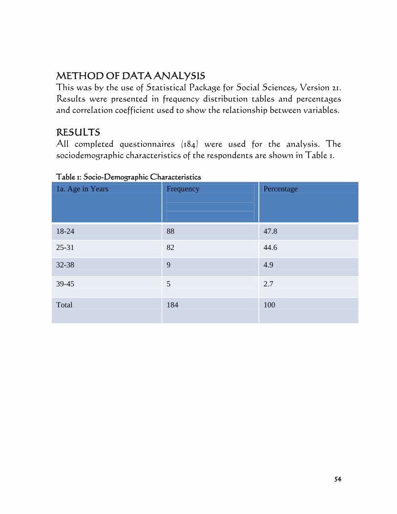
54
METHOD OF DATA ANALYSIS
This was by the use of Statistical Package for Social Sciences, Version 21.
Results were presented in frequency distribution tables and percentages
and correlation coefficient used to show the relationship between variables.
RESULTS
All completed questionnaires (184) were used for the analysis. The
sociodemographic characteristics of the respondents are shown in Table 1.
Table 1: Socio-Demographic Characteristics
1a. Age in Years Frequency
Percentage
18-24 88 47.8
25-31 82 44.6
32-38 9 4.9
39-45 5 2.7
Total 184 100
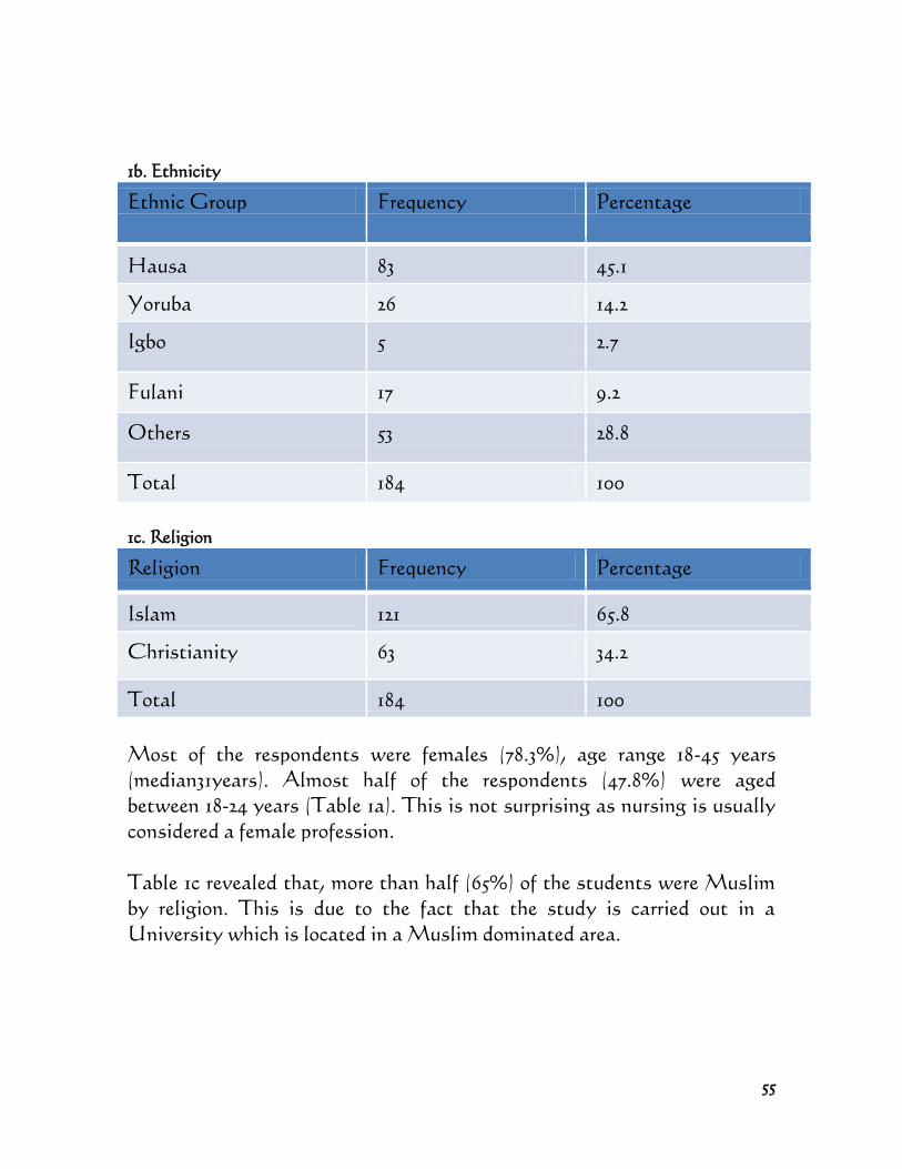
55
1b. Ethnicity
Ethnic Group Frequency Percentage
Hausa 83 45.1
Yoruba 26 14.2
Igbo 5 2.7
Fulani 17 9.2
Others 53 28.8
Total 184 100
1c. Religion
Religion Frequency Percentage
Islam 121 65.8
Christianity 63 34.2
Total 184 100
Most of the respondents were females (78.3%), age range 18-45 years
(median31years). Almost half of the respondents (47.8%) were aged
between 18-24 years (Table 1a). This is not surprising as nursing is usually
considered a female profession.
Table 1c revealed that, more than half (65%) of the students were Muslim
by religion. This is due to the fact that the study is carried out in a
University which is located in a Muslim dominated area.
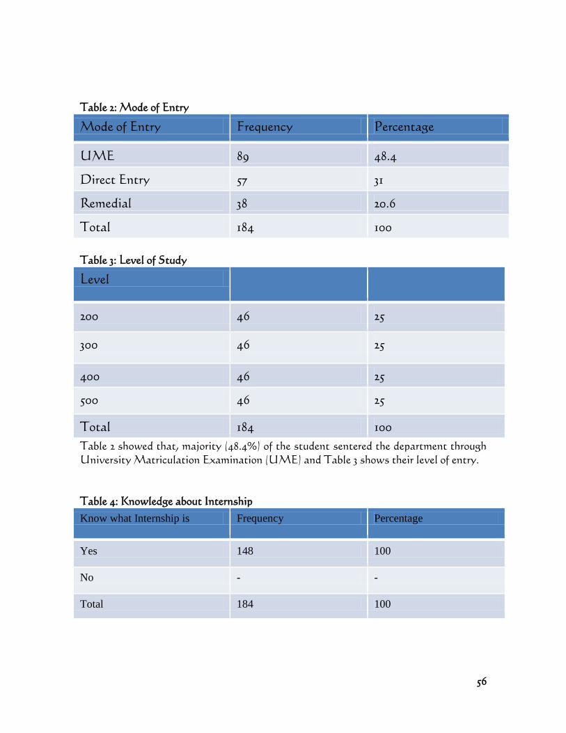
56
Table 2: Mode of Entry
Mode of Entry Frequency Percentage
UME 89 48.4
Direct Entry 57 31
Remedial 38 20.6
Total 184 100
Table 3: Level of Study
Level
200 46 25
300 46 25
400 46 25
500 46 25
Total 184 100
Table 2 showed that, majority (48.4%) of the student sentered the department through
University Matriculation Examination (UME) and Table 3 shows their level of entry.
Table 4: Knowledge about Internship
Know what Internship is Frequency Percentage
Yes 148 100
No - -
Total 184 100
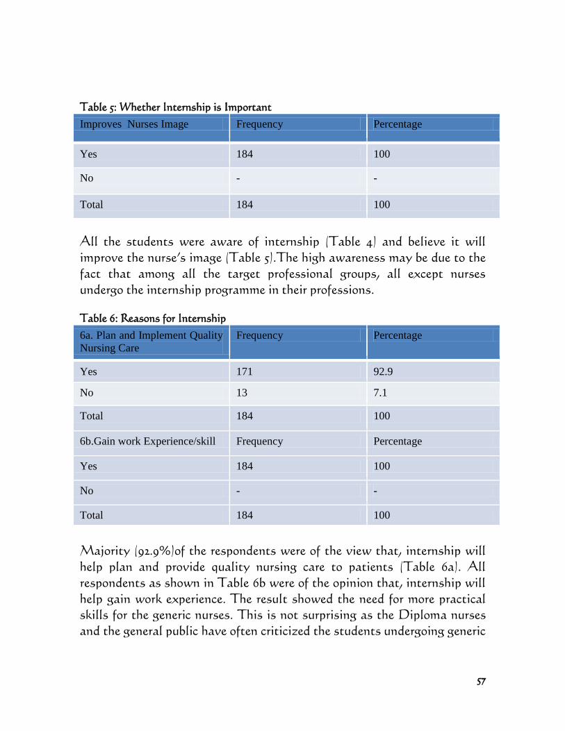
57
Table 5: Whether Internship is Important
Improves Nurses Image Frequency Percentage
Yes 184 100
No - -
Total 184 100
All the students were aware of internship (Table 4) and believe it will
improve the nurse’s image (Table 5).The high awareness may be due to the
fact that among all the target professional groups, all except nurses
undergo the internship programme in their professions.
Table 6: Reasons for Internship
6a. Plan and Implement Quality
Nursing Care
Frequency Percentage
Yes 171 92.9
No 13 7.1
Total 184 100
6b.Gain work Experience/skill Frequency Percentage
Yes 184 100
No - -
Total 184 100
Majority (92.9%)of the respondents were of the view that, internship will
help plan and provide quality nursing care to patients (Table 6a). All
respondents as shown in Table 6b were of the opinion that, internship will
help gain work experience. The result showed the need for more practical
skills for the generic nurses. This is not surprising as the Diploma nurses
and the general public have often criticized the students undergoing generic
58
programme in nursing for not having adequate clinical exposure or
experience, because according to them, more time is devoted to theoretical
instruction at the expense of clinical exposure.
Table 7: Duration of Internship
Duration Frequency Percentage
<1Year 8 4.3
1 Year 176 95.7
>1 Year - -
Total 184 100
Table 7 indicated that, majority (95.7%) of the respondents are of the
opinion that internship should be for a period of 1 year. The recommended
1year is in cognizance with the reviewed structure of 12 months for the
nursing programme in Nigerian Universities and duration of internship
programme in medicine, pharmacist, medical laboratory scientist and
radiologists in Nigeria14
. This is similar with what occur at King
Abdulaziz University15 and a at Kenya
16 where after passing the Nursing
Council Examination, the students undergo 12 months internship program
before fully registered to practice.
Table 8: Need for more Practical Skills
Recruitment Frequency Percentage
Yes 169 91.5
No 15 8.2
Total 184 100
59
Almost all the respondents (91.5%) demonstrated the need for more
practical skill to enable them be recruited for jobs (Table 8).The result of
this study is in line with a study conducted among health care workers at
Ahmadu Bello University Teaching Hospital, Zaria where 72.9% of
respondents said it is necessary to adopt internship for graduants of
nursing education as this will improve the practical and technical skills of
the nurse interns.
Figure 1: Areas of Rotation
Most (91.3%) were of the view that all the students should be rotated to all
the wards in the hospital (Figure 1).
Figure 2: Perception towards Internship
8.7
91.3
0 0 Areas of Rotation
Medical/Surgical Unit
All hospital wards
60
Figure 2 further showed that, 44% of the respondents strongly agreed that,
it is essential to complete the internship programme.
Figure 3: Include Internship into BNSc Programme
44
39.2
1.6 15.2
0 0
Essential to Complete the Programme
Strongly Agree
Agree
Strongly Disagree
Disagree
63.6 16.8
3.8 15.8
Inclusion in BNSc Programme
Strongly Agree
Agree
Strongly Disagree
Disagree
61
Figure 3 showed that, 63.3% of the nurses strongly agreed that there is need
to include the internship programme into the BNSc curriculum. Most
respondents (97.1%) also suggested training enough preceptors and clinical
instructors for supervision and clinical training of interns. This finding is
also in line with the observation made by Yusuf9
that generic graduate
nurses “may have theory but lack adequate practical exposure and
competence” paramount to nursing practice. It is not surprising that all the
students recommend internship and majority are of the view that it will
improve both their image and practical skill. No doubt, internship has been
described as a kind of work experiences program employed for graduate
professionals such as Law, Medicine, and Pharmacy among others. Its
purpose is to expose fresh graduates of those professions that are
practically intensive to the practice or clinical area to acquire and
consolidate more practical skills and technical knowledge necessary to
practice their profession as well as to qualify them for full registration and
licensure from professional statutory body. Internship for nurses in Nigeria
becomes necessary following the introduction of the generic baccalaureate
university education for preparing professional nurses13
.
The result on the relationship between the need for more practical skills
and the introduction of internship showed a correlation coefficient of
r=+1.00 signifying a positive correlation. On determining the relationship
between the need for recruitment of graduate nurses and the introduction of
internship, the result showed a correlation coefficient of r=+1.00 signifying
also signifying a positive correlation.
CONCLUSION
The study revealed great awareness about internship programme among
the students. The findings also showed that implementation of internship
into BNSC programme is necessary because it will improve the skills of
the generic nurses and also improve their image. It further revealed the
preparedness and acceptance of internship among the students. The
findings from this study will serve as a consideration to adopt internship
into the generic Nursing Education in Nigeria as other health care
62
practitioners. It will also serve as a useful guide that will help to forestall
obvious or anticipated problems in Nursing in Nigeria and further provide
the basis for making appropriate recommendations for the proposed
internship program. There is therefore the need for Nursing and Midwifery
Council of Nigeria to set up a committee to work out a thoughtful plan of
action for the implementation of internship into generic nursing education
in Nigeria.
REFERENCES
1. Benner P., Novice to Expert: Excellence and Power in Clinical Nursing
Practice. Menlo Park, CA: Addison-Wesley, 1984.
2.What is an Internship? Available at http://www.intstudy.com/study-in-
america/student-life/what-is-an-internship
3. Onyi N.A., Survey of Factors Militating Against University Education
of Nursing. A Project, University of Nigeria, Enugu Campus, 1998.
4. Cleveland Clinic Health System Graduate Nurse Internship Program.
www.southpiontshospital.org
5. Casey K.R., Fink M, Krugman J., "The Graduate Nurse Experience."
JONA 34(6): 303-11, 2006.
6. Owens D.L., Turjanica M.A., Scanion M.W., Sandhusen A.E.,
Williamson M.C.,Facteau, L(2001). "New Graduate R.N.
Internship Program: A Collaborative Approach for System Wide
Integration." Journal for Nurses in Staff Development 17(3): 144-50.
7. Tradewell G., "Rites of Passage: Adaptation of Nursing Graduates to
a Hospital Setting." Journal of Nursing Staff Development 12(4):
183-9, 1996.
8. Brian H., Delay of internship. Available at www.google.com, 2012
63
9. Yusuf ZY, Bachelor of Nursing Science Graduate and the Issuing of
Internship in Nigeria. A Paper Presented at Conference of
Committee of Heads of Nursing Departments (COHEDNUR) in
Nigerian Universities, Enugu, Nigeria, 2005.
10. Structure of the Internship Programme for Graduates of Bachelor of
Nursing Science Degree programme (Nursing and Midwifery
Council of Nigeria, 2012. Accessed on 1st
May 2012
11. Salau T.I., Introduction to Research Methodology, London: Limbs
Press, 1998, Pp22-23.
12. Nwanna, Textbook of Research Methodology. Published in Kenya,
2007.
13. Mfuh A.Y., Lukong C.S., Suleima D.,Health Workers Perception
towards the Introduction of Internship Programme for the BNSC
Student’s in Nigeria. A Case of ABUTH Zaria. A Paper
Presented at the 9TH
National Scientific Conference and Annual
General Meeting at School Of Nursing, Babcock University,
Ilishan-Remo , Ogun State, Nigeria. Date 20th
-25th
November 2011.
Published in Journal of Educational Research and Development,
Volume 7, Number 2, August, 2012
14. Ngozi P.O., Stakeholders Perception of Internship in Generic Nursing
Education in Nigeria – West African Journal of Nursing 20(2), 2009
15. King Abdulaziz University, Faculty of Applied Medical Sciences,
Department Of Nursing. Accessed on 1st
May 2012. Available at
www.google.com
16. Internship Programme in Kenya. Accessed on 1st
May 2012. Available
at www.google.com
64
India’s Food Crisis viz. Risk Inducing Factors-
Entitlement Failure: Empirical Evidence of Crop
Production in Rajasthan State, India
*Sadiq, M S1&2
., Singh, I.P3
.,
Umar, S.M4
., Grema, I.J5
., Usman, B.I6
. and Isah, M.A7
.
1
Resarch Scholar, Department of Agricultural Economics, SKRAU, Bikaner, India*
2
Department of Agricultural Economics and Extension Technology, FUT, Minna, Nigeria
3
Professor Emeritus, Department of Agricultural Economics, SKRAU, Bikaner, India
4
Research Scholar, Department of Agricultural Economics, PJSTSAU, Hyderabad, India
5
Department of Agricultural Technology, Yobe State College of Agriculture, Gujba, Nigeria
6Department of Agricultural and Bio-Environmental Engineering, Federal Polytechnic Bida, Nigeria
7
Research Scholar, Department of Agricultural Economics, UAS, Dharwad, India
Email: [email protected] (Tel: 07037690124)
Abstract
The study empirically investigated the sources of production instability in
Rajasthan State, India. Time series data spanning from 1994-2015 (post-
green revolution) viz. area, yield and production of 17 crops produced in 27
potential districts and the state were used and meticulously analyzed using
Coefficient of Variation and Hazell technique. Results indicated high
variability/fluctuation in yield to be the major cause of production
instability in all the kharif crops and some rabi crops like wheat and
mustard. On the contrary, high instability in area was the major source of
production instability for crops like taramira, gram, barley, cumin and
coriander. Performance of kharif crops were poor in general, as the
production and productivity of crops were observed to be declining.
Therefore, location specific technology development is needed in order to
give higher yield even in adverse weather condition, along with price
support, which would eventually expand the production. Rabi crops
performed better; as well their production increase was contributed by
increased area and yields. However, this performance was subjected to high
instability in both area and yields. Technological inputs like seeds,
fertilizers, pesticides and location-specific production technologies, timely
and assured electricity supply were important factors that will minimize
instability, thus, further increase in production. Furthermore, creation of
other infrastructural facilities like irrigation is imperative to increase
acreage and production stability.
Keywords: Instability; Area; Yield; Production; Kharif & Rabi crops;
Rajathan; India.
Pp 67-91
65
INTRODUCTION
The fundamental postulate of the modern welfare state is to help the
people in fulfillment of their needs for a decent and comfortable livelihood.
In this context, it is widely recognized that in the hierarchy of human
needs, food ranks first since the survival of Homo-sapiens hinges on it. As
such, it is a matter of paramount importance for the state to accord
overriding priority to the concerns for food security, more so, in a world
where aid and trade in food have to be tools of international diplomacy.
There is a growing concern in different quarters on the issues, “will there be
enough food for our children”? This question does cause alarm, particularly
in developing countries, because developed countries have successfully
tackled this problem through sustained growth over time.
In India, the expanding population which is at present estimated to be 110
crores is likely to cross 145 crores by the year 2030. This will necessitate on
an average above 4 percent growth in food production in order to achieve
self-sufficiency. To be fed, the population needs at least 270 million tonnes
of food grains and more in the near future; which will necessitate an overall
increase in food production. The country has put food security high on the
national agenda; from being a substantial net food importer in the 1970s, it
became self-sufficient in grain production from the early 1980s and more
than self-sufficient in the 1990s till date. The darker side of Indian
development during the last half century has been that the economic
growth did not percolate to the rural poor as “trickle down” has failed to
work. The critical appraisals of Indian planning strategy have clearly
shown that land reforms neither could be carried out to the extent of
eliminating unequal land holdings nor the economic growth could bring
prosperity to the rural small and marginal farmers to the extent as would
have been expected. Therefore, the future crisis in the food front emanates
not entirely in meeting the expected rise in the demand in the production
front but more importantly in the distribution front-equitable distribution
of not only resources but also equitable distribution of gains from economic
growth. However, the country often proclaimed self-sufficiency in food
production, yet things do not seem to be very bright particularly in near
66
future. If another green revolution is not experienced by India in near
future, it is expected to import annually 40 million tonnes of foodgrains by
the year 2030.
Agricultural production in Rajasthan State has undergone substantial
changes; production in the state has increased due to adoption of high
yielding varieties, use of chemical fertilizer and development of irrigation
structures. Studies viz. Sadiq and Grema (2016); Vanpal et al. (2015);
Swain (2013); Swain et al.(2012); Dutta and Kapadia (2011); Kumawat and
Meena (2005), all found out that growth in Rajasthan State agricultural
production was associated with instability, which adversely affected
production, employment and income distribution, thus, hampering
economic growth. To promote economic development, it becomes
imperative to identify risk inducing factors in crop production in the state
and potential district levels. Therefore, the essence of this research is to
describe empirically sources of production instability of various selected
crops of Rajasthan State in the last two decades. These sources of
instability were quantified by decomposing variance of production into
various sources viz. area variance, yield variance, area-yield covariance and
higher order interaction between area and yield.
RESEARCH METHODOLOGY
Rajasthan State is characterized by varied agro-climatic conditions which
favours cultivation of large number of crops. The present study made use of
time series data on area, production and productivity, covering post-green
revolution period, spanning from 1994-2015, obtained from secondary
sources viz. Statistical Abstract of Rajasthan State; Directorate of
Economics and Statistics (manual), Rajasthan State; Vital Agriculture
Statistics, Directorate of Agriculture, Jaipur, Rajasthan State. Criterion
for crop selection was that, a crop must have a minimum of 2.5 lakh hectare
of area under cultivation during the last 4-5 years (2010/11-2015), and since
aggregate analysis may not depict a true picture, only potential districts
67
which account for 50 percent share in the total area under cultivation of a
particular crop were selected. Thus, selected crops with respective
potential producing districts are presented in Table 1. The spanning period
was divided into two phases; Period I (1994-2004) and Period II (2005-2015),
in order to have decade wise comparisons. Coefficient of Variation (CV);
Instability Index model and Hazell technique, were used to analyze the
data.
Table 1: Selected crops with respective potential producing districts
Crops Districts
Bajra (Pennisetum typhoides) Barmer, Jodhpur, Churu and Nagaur
Barley (Hordeum vulgare) Jaipur, Sikar, Ajmer and Bhilwara
Coriander (Coriandrum
sativum )
Kota
Cotton (Gossypium
hirsutum)
Sri Ganganagar
Cumin (Cuminum eynum) Barmer and Jalore
Gram (Cicer arietinum) Sri Ganganagar, Churu, Jaipur and Jhunjhunu
Groundnut (Arachis hypogea) Jaipur, Chittorgarh, Sawai Modhopur and Bikaner
Guar (Cyamopsis
tetragonoloba)
Churu, Barmer, Sri Ganganagar and Nagaur
Jowar (Sorghum bicolor) Ajmer, Pali Tonk and Nagaur
Maize (Zea mays) Udaipur, Bhilwara and Chittorgarh
Moong (Vigna radiata) Nagaur, Jodhpur, Jalore and Ajmer
Moth (Phaseolus
aconitifolius)
Bikaner, Churu and Barmer
Rapseed and Mustard
(Brassica juncea)
Sri Ganganagar, Bharatpur, Alwar,
Sawai Madhopur and Tonk
Sesamum (Sesamum indicum) Pali, Jodhpur and Nagaur
Soyabeans (Glycine max) Kota and Jhalawar
Taramira (Eruca sativa) Nagaur, Bikaner and Pali
Wheat (Triticum aestivum) Sri Ganganagar, Jaipur, Bharatpur, Alwar, Kota
and Bundi
68
EMPIRICAL MODEL
Measurement of Instability
The measurement of instability requires that an implicit or explicit
judgment be made as to what constitutes the acceptable variability and
unacceptable variability. In time series analysis, the trend is removed from
the data before instability is measured on the ground that, those trends are
predictable and do not constitute instability. Deviation from the trend
constitutes the variability in question, hence used for measurement of
instability. Therefore area and productivity for each crop with respect to
each selected districts and the state as a whole were de-trended for each
time period separately using linear functional form.
Yt = a + bt + e
t …………………………………………….. (1)
Where,
Yt = dependent variable (area or productivity);
t = time trend
et = random residual
After de-trending the data, the residuals (et) were centered on the mean
area or productivity for each period, Y, resulting in de-trended time series
data of the following form:
Y = et + Y ………………………………………………………….. (2)
69
De-trended production data for each crop with respect to each district and
the state as a whole were obtained by multiplying the de-trended area with
de-trended productivity.
Instability was measured for all the time period by estimating the
coefficient of variation of production, area and productivity. Following
Sadiq (2015), CV is specified below:
CV = σij ……………………………………………………………. (3)
Xij
Where:
CV = coefficient of variation;
σij = standard deviating of the i
th variable in the j
th crop; and,
Xij = mean of the i
th variable in the j
th crop.
Sadiq and Grema (2016) stated that, one important point should be noted
in connection with the use of C.V., which is the most commonly used
index for measuring instability. CV has an easy interpretation in the
context of measuring an overall variation in the data not showing any
trend. But usually, when we have time series for variables showing some
kind of trend, which may be linear or non-linear, CV does not take into
account any such time trends of the data while measuring instability in the
variate values. Therefore, it may be desirable for general applicability that
an index of instability should be so derived as to give information about the
trend exhibited in the data on the variable under study. Sadiq and Grema
(2016) applied the following index as a measure of instability in time series
data:
70
I = CV2 (1-R
2) ………………………………………………………….. (4)
I= Instability;
CV = coefficient of variation; and,
R2 = coefficient of determination.
Sources of Instability
To examine instability sources, production instability was decomposed
into its sources, viz., area variance, yield variance, area-yield covariance
and higher order interaction between area and yield by using the following
Hazell technique:
V (Q) = A 2
V(Y) + Y2 V (A) + 2AY (A,Y) – COV (A,Y)
2 + R
………………. (5)
Where,
V (Q) = Production Instability/Production variance;
A = Mean area;
Y = Mean yield;
V(Y) = Yield variance;
V (A) = Area variance;
COV (A,Y) =Area-yield covariance;
COV (A,Y)2 = Higher order covariance between area and yield; and,
R = Residual term.
RESULTS AND DISCUSSION
Sources of Production Instability of Kharif Cereal Crops
Jowar Crop
Results in Table 2 revealed production instability of jowar crop in Ajmer
and Pali districts to be 83.41 percent and 81.28 percent respectively, during
Period I, and remained almost the same in Pali district in Period II; slightly
declined in Ajmer district during Period II. However, Nagaur district
witnessed a decline from 83.20 percent to 54.93 percent in Period II. Tonk
district experienced increase in production instability from 47.20 percent in
Period I to 57.30 percent in Period II. Also, the state observed increase in
production instability of jowar crop. Yield variance was observed to be the
71
major production instability source of jowar crop in all the selected districts
and the state during the period under consideration. The yield variance
declined from 105.13 percent; 130.62 percent and 94.02 percent during Period
I to 93.59 percent; 92.76 percent and 87.66 percent during Period II in Ajmer,
Nagaur districts and Rajasthan State, respectively. The yield variance
increased from 73.54 percent and 82.85 percent in Period I to 100.33 percent
and 87.93 percent during Period II in Pali and Tonk districts respectively.
In Nagaur district, the area-yield covariance was observed to be the
nullifying factor of production instability. The high yield variance needs to
be tackled to reduce the production instability of jowar crop in Rajasthan
State.
Maize Crop
Production instability of maize was low when compared to other kharif
cereals of Rajasthan State (Table 2). Results showed a decline from 42.74
percent; 42.57 percent; 30.01 percent and 36.04 percent during Period I to
25.30 percent; 25.62 percent; 17.97 percent and 14.43 percent in Period II in
Udaipur, Bhilwara, Chittore districts and Rajasthan State, respectively.
Findings revealed that maize production variance was mainly due to yield
variance; estimated yield variance were 92.04 percent; 93.27 percent; 113.01
percent and 86.17 percent in Udaipur, Bhilwara, Chittore districts and
Rajasthan State, respectively during Period II. However, area variance
was found to be less than 3 percent in all the districts as well as the state in
both periods. Therefore, it can be inferred that maize is the stable food crop
of the studied area of Rajasthan State.
Bajra Crop
Production instability of bajra increase in Churu and Barmer districts,
from 68.61 percent and 82.36 percent in Period I to 77.71 percent and 88.09
percent, respectively, during Period II. However, it declined in Jodhpur and
Nagaur districts and Rajasthan State, from 85.14 percent; 66.22 percent
and 47.59 percent in Period I to 80.58 percent; 30.93 percent and 36.40
percent in Period II, respectively. Decomposition analysis of production
variance indicates yield variance to be the major contributor of production
72
instability in all the districts and Rajasthan State during both periods.
However, the yield variance declined over time from 103.36 percent; 96.05
percent; 83.86 percent and 82.99 percent during Period I to 77.32 percent;
83.12 percent; 63.14 percent and 70.38 percent during Period II in Jodhpur,
Barmer, Nagaur districts and Rajasthan State, respectively. In Churu
district, yield variance increased from 75.47 percent in Period I to 82.55
percent during Period II. In Nagaur district, area-yield covariance was
found to be the next important source of production instability in both
periods (Table 2).
Table 2: Sources of production instability of kharif crops
Particulars Production
Instability
Area
variance
Yield variance Area-yield
covariance
Higher
order
covariance
Jower crop
Period I
Ajmer 83.41 0.77 105.13 -1.48 -4.41
Nagaur 83.2 17.02 130.62 -64.29 16.65
Pali 81.28 4.74 73.54 -3.09 24.81
Tonk 47.2 2.94 82.85 8.37 5.84
Rajasthan 31.09 5.47 94.02 -5.48 5.99
Period II
Ajmer 81.1 0.72 93.59 5.66 0.03
Nagaur 54.93 17.05 92.76 -10.81 1.01
Pali 81.89 0.87 100.33 -0.43 -0.77
Tonk 57.3 3.11 87.93 3.24 5.71
Rajasthan 37.82 5.53 87.66 2.83 3.97
Maize crop
Period I
Udaipur 42.74 1.62 93.86 13.26 -8.75
Bhilwara 42.57 3.13 102.39 10.36 -15.89
Chittore 30.01 0.8 93.64 6.92 -1.37
Rajasthan 36.04 2.57 100.37 6.8 -9.73
Period II
Udaipur 25.3 0.19 92.04 5.81 1.97
Bhilwara 25.62 1.01 93.27 5.82 -0.1
Chittore 17.97 2.39 113.01 -11.08 -4.33
Rajasthan 14.43 1.99 86.17 9.79 2.05
73
Bajra crop
Period I
Churu 68.61 3.38 75.47 15.28 5.87
Jodhpur 85.14 1.7 103.36 2.08 -7.13
Barmer 82.36 3.88 96.05 2.73 -2.66
Nagaur 66.22 3.28 83.86 12.24 0.63
Rajasthan 47.59 5.71 82.99 17.32 -6.03
Period II
Churu 77.71 0.68 82.55 9.68 7.1
Jodhpur 80.58 1.23 77.32 15.8 5.64
Barmer 88.09 1.04 83.12 13.11 2.72
Nagaur 30.93 6.71 63.14 28.35 1.8
Rajasthan 36.4 3.31 70.38 23.26 3.05
Sources of Production Instability of Rabi Cereal Crops
Wheat crop
Instability in the production of wheat declined over time in Jaipur, Alwar,
Bharatpur and Sri-Ganganagar districts (Table 3). Major sources of
production instability in these districts were area variance and yield
variance. Furthermore, it was observed that area-yield covariance
contributed in reducing the production instability in these districts. In
Kota, Bundi districts and Rajasthan State, the instability in wheat
production was found to increase due to increase in area-yield covariance.
Barley crop
Production instability of barley crop in Jaipur district was observed to be
lowest and it further declined to 12.81 percent in Period II from 16.53 percent
in Period I. Ajmer district exhibited maximum production instability and
increased to 34.60 percent in Period II from 29.03 percent in Period I.
However, Sikar district witnessed a decline in production instability, while
Bhilwara district and the state observed increased production instability.
In Ajmer district, yield variance emerged as the major source of production
variance. Furthermore, in Jaipur, Sikar, Bhilwara districts and Rajasthan
State, area variance was found to be the major determinant of production
variance. Decomposition analysis of production variance indicated area
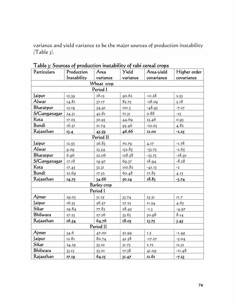
74
variance and yield variance to be the major sources of production instability
(Table 3).
Table 3: Sources of production instability of rabi cereal crops
Particulars Production
Instability
Area
variance
Yield
variance
Area-yield
covariance
Higher order
covariance
Wheat crop
Period I
Jaipur 15.39 18.13 90.62 -11.28 2.53
Alwar 14.81 37.17 85.75 -28.09 5.18
Bharatpur 15.19 54.91 101.3 -48.93 -7.27
S/Ganganagar 24.31 42.81 71.31 0.88 -15
Kota 17.03 30.93 44.69 23.46 0.93
Bundi 16.51 21.74 95.46 -22.03 4.82
Rajasthan 13.4 43.59 46.66 12.00 -2.25
Period II
Jaipur 12.55 26.83 70.79 4.17 -1.78
Alwar 9.09 23.54 132.85 -53.75 -2.65
Bharatpur 6.96 22.06 128.58 -23.73 -18.91
S/Ganganagar 17.18 19.97 69.37 18.94 -8.28
Kota 17.45 32.31 110.82 -41.13 -2
Bundi 22.69 17.52 60.48 17.85 4.15
Rajasthan 14.75 34.66 50.24 18.83 -3.74
Barley crop
Period I
Ajmer 29.03 31.25 33.74 23.31 11.7
Jaipur 16.53 56.57 27.25 11.54 4.65
Sikar 29.84 77.83 28.45 -1.3 -4.97
Bhilwara 27.23 27.26 33.63 30.98 8.14
Rajasthan 16.54 64.76 18.03 13.75 3.45
Period II
Ajmer 34.6 47.00 52.99 1.5 -1.49
Jaipur 12.81 80.74 41.58 -17.27 -5.04
Sikar 24.19 53.22 31.75 2.72 12.31
Bhilwara 33.15 53.01 17.38 41.09 -11.48
Rajasthan 17.19 64.15 31.47 11.61 -7.23
75
Sources of Production Instability of Kharif Pulse Crops
Moth crops
Production instability of moth crop declined over the period in all the
districts as well as the state (Table 4). In Bikaner district, yield variance
declined from 85.73 in Period I to 71.52 percent in Period II, and the area-
yield covariance increased from 13.36 in Period I to 25.27 percent during
Period II. Estimated yield variance of moth were 96.93 percent and 42.59
percent in Churu and Barmer districts, respectively in Period I, which
increased to 99.86 and 69.64 percent, respectively during Period II.
Findings observed yield variance to be the major determinant of production
instability in all the districts and the state as a whole. However, area
variance was observed to be low in all the districts as well as the state
which indicates possible sustainability of moth crop in the studied area.
Therefore, production of moth can be expanded by adoption of agricultural
technology such as development of drought tolerant variety, thus,
minimizing yield fluctuations.
Moong crop
Moong crop production was observed to be very high in Jalore district
(124.35 percent), followed by Jodhpur district (106.81 percent) and Nagaur
district (74.61 percent) in Period I. However, it slightly declined in Period II
viz. 99.10, 93.11 and 67.02 percent, respectively. Production instability
remained almost the same i.e 75 and 64 percent in Ajmer district and
Rajasthan State in both periods. It was observed that the production
variance of moong in Ajmer district was explained by yield variance (86.09
percent) and area variance (11.63 percent) during Period I, while yield
variance (78.51 percent) and higher order area-yield covariance (13.72
percent) were the major factors during Period II. Jodhpur district
experienced increase in yield variance over time; in Jalore district, yield
variance remained constant (81 percent) in both periods; in Nagaur district,
major source of moong production variance was yield variance (61.91
percent) and area-yield covariance (39.01 percent) during Period I. In Period
II, major sources of production instability were yield variance (68.85
percent) and area variance (24.47 percent). In Rajasthan State, yield
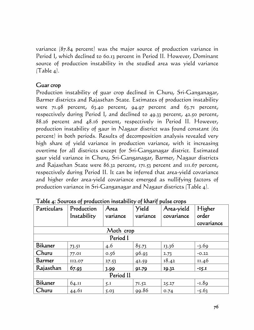
76
variance (87.84 percent) was the major source of production variance in
Period I, which declined to 60.13 percent in Period II. However, Dominant
source of production instability in the studied area was yield variance
(Table 4).
Guar crop
Production instability of guar crop declined in Churu, Sri-Ganganagar,
Barmer districts and Rajasthan State. Estimates of production instability
were 71.98 percent, 63.40 percent, 94.97 percent and 63.71 percent,
respectively during Period I, and declined to 49.33 percent, 42.50 percent,
88.26 percent and 48.16 percent, respectively in Period II. However,
production instability of gaur in Nagaur district was found constant (62
percent) in both periods. Results of decomposition analysis revealed very
high share of yield variance in production variance, with it increasing
overtime for all districts except for Sri-Ganganagar district. Estimated
gaur yield variance in Churu, Sri-Ganganagar, Barmer, Nagaur districts
and Rajasthan State were 86.32 percent, 171.53 percent and 111.67 percent,
respectively during Period II. It can be inferred that area-yield covariance
and higher order area-yield covariance emerged as nullifying factors of
production variance in Sri-Ganganagar and Nagaur districts (Table 4).
Table 4: Sources of production instability of kharif pulse crops
Particulars Production
Instability
Area
variance
Yield
variance
Area-yield
covariance
Higher
order
covariance
Moth crop
Period I
Bikaner 73.51 4.6 85.73 13.36 -3.69
Churu 77.01 0.56 96.93 2.73 -0.22
Barmer 112.07 27.53 42.59 18.42 11.46
Rajasthan 67.93 3.99 91.79 19.32 -15.1
Period II
Bikaner 64.11 5.1 71.52 25.27 -1.89
Churu 44.61 5.03 99.86 0.74 -5.63
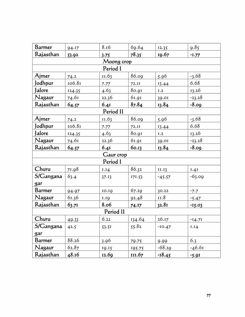
77
Barmer 94.17 8.16 69.64 12.35 9.85
Rajasthan 53.92 3.75 78.35 19.67 -1.77
Moong crop
Period I
Ajmer 74.2 11.63 86.09 5.96 -3.68
Jodhpur 106.81 7.77 72.11 13.44 6.68
Jalore 124.35 4.63 80.91 1.2 13.26
Nagaur 74.61 22.36 61.91 39.01 -23.28
Rajasthan 64.57 6.41 87.84 13.84 -8.09
Period II
Ajmer 74.2 11.63 86.09 5.96 -3.68
Jodhpur 106.81 7.77 72.11 13.44 6.68
Jalore 124.35 4.63 80.91 1.2 13.26
Nagaur 74.61 22.36 61.91 39.01 -23.28
Rajasthan 64.57 6.41 60.13 13.84 -8.09
Gaur crop
Period I
Churu 71.98 1.14 86.32 11.13 1.41
S/Gangana
gar
63.4 37.13 171.53 -45.57 -63.09
Barmer 94.97 10.19 67.29 30.22 -7.7
Nagaur 61.36 1.19 92.48 11.8 -5.47
Rajasthan 63.71 8.06 74.17 32.81 -15.03
Period II
Churu 49.33 6.22 134.64 26.17 -14.71
S/Gangana
gar
42.5 53.51 55.82 -10.47 1.14
Barmer 88.26 3.96 79.75 9.99 6.3
Nagaur 62.87 19.15 195.75 -68.29 -46.61
Rajasthan 48.16 12.69 111.67 -18.45 -5.91
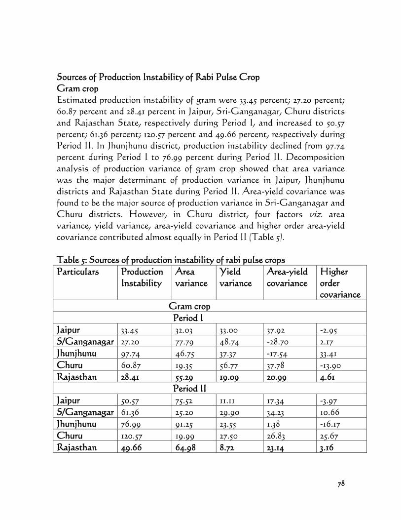
78
Sources of Production Instability of Rabi Pulse Crop
Gram crop
Estimated production instability of gram were 33.45 percent; 27.20 percent;
60.87 percent and 28.41 percent in Jaipur, Sri-Ganganagar, Churu districts
and Rajasthan State, respectively during Period I, and increased to 50.57
percent; 61.36 percent; 120.57 percent and 49.66 percent, respectively during
Period II. In Jhunjhunu district, production instability declined from 97.74
percent during Period I to 76.99 percent during Period II. Decomposition
analysis of production variance of gram crop showed that area variance
was the major determinant of production variance in Jaipur, Jhunjhunu
districts and Rajasthan State during Period II. Area-yield covariance was
found to be the major source of production variance in Sri-Ganganagar and
Churu districts. However, in Churu district, four factors viz. area
variance, yield variance, area-yield covariance and higher order area-yield
covariance contributed almost equally in Period II (Table 5).
Table 5: Sources of production instability of rabi pulse crops
Particulars Production
Instability
Area
variance
Yield
variance
Area-yield
covariance
Higher
order
covariance
Gram crop
Period I
Jaipur 33.45 32.03 33.00 37.92 -2.95
S/Ganganagar 27.20 77.79 48.74 -28.70 2.17
Jhunjhunu 97.74 46.75 37.37 -17.54 33.41
Churu 60.87 19.35 56.77 37.78 -13.90
Rajasthan 28.41 55.29 19.09 20.99 4.61
Period II
Jaipur 50.57 75.52 11.11 17.34 -3.97
S/Ganganagar 61.36 25.20 29.90 34.23 10.66
Jhunjhunu 76.99 91.25 23.55 1.38 -16.17
Churu 120.57 19.99 27.50 26.83 25.67
Rajasthan 49.66 64.98 8.72 23.14 3.16
79
Sources of Production Instability of Kharif Oilseed Crops
Groundnut Crop
Estimated production instability of groundnut was 51.96 percent, 50.22
percent and 23.63 percent in Sawai-Madhopur, Bikaner and Chittore,
respectively during Period I, and declined to 41.30 percent; 25.02 percent and
18.70 percent, respectively during Period II. The major contributing factor
in production variance was yield variance, followed by area variance and
area-yield covariance. The yield variance in Rajasthan State was 115.62
percent in Period I, and declined to 60.11 percent during Period II. For
Bikaner district, the production variance was due to area variance (67.63
percent), followed by yield variance (55.05 percent). It was also observed
that area-yield covariance and higher order covariance of area and yield
were the nullifying factors of production variance in Bikaner district (Table
6).
Soyabean Crop
The Jhalawar district showed decline in production instability of soyabean
from 65.55 percent in Period I to 30.38 percent in Period II. Kota district and
Rajasthan State had increase in production instability, from 19.94 percent
and 20.08 percent in Period I to 39.72 percent and 27.60 percent in Period II.
Area variance emerged as major factor in production variance, followed by
yield variance during both periods in Kota district. However, both area
variance and yield variance declined from 189.31 percent and 52.55 percent in
Period I to 41.45 percent and 37.24 percent, respectively during Period II.
Jhalawar district experienced production instability due to high yield
variance in both periods. The share of yield variance in production
instability increased over time in Jhalawar district (Table 6).
Sesamum Crop
Estimated production instability of sesamum in Jodhpur, Nagaur, Pali
districts and Rajasthan State were 108 percent; 80.78 percent; 72.46 percent
and 66.97 percent, respectively during Period I. It declined to 94.98 percent;
51.66 percent; 70.21 percent and 38.76 percent, respectively, during Period II.
The major sources of production instability were found to be yield variance,
80
followed by area-yield covariance in both periods. However, yield variance
of sesamum crop declined from 78.86 percent; 66.61 percent and 82.97
percent during Period I to 74.82 percent; 53.69 percent and 63.92 percent
during Period II in Jodhpur, Nagaur and Pali districts, respectively. At
state level, yield variance exhibited increase magnitude, from 68.02 percent
during Period I to 88.33 percent in Period II; yield variance constituted large
share in production instability (Table 6). Therefore, yield risk minimizing
policy may be devised in order to boost production of sesamum crop in the
state.
Table 6: Sources of production instability of kharif oilseed crops
Particulars Production
Instability
Area
variance
Yield
variance
Area-yield
covariance
Higher
order
covariance
Groundnut crop
Period I
Jaipur 37.92 25.39 52.76 21.95 -0.11
S/Madhopur 51.96 15.76 52.75 16.91 14.58
Bikaner 50.22 20.32 51.19 14.79 13.7
Chittore 23.63 26.48 81.11 -5.95 -1.64
Rajasthan 20.1 31.88 115.92 -34.84 -12.96
Period II
Jaipur 42.08 19.7 49.48 17.53 13.29
S/Madhopur 41.3 31.75 62.71 20.25 -14.71
Bikaner 25.02 67.63 55.05 -10.78 -11.89
Chittore 18.7 31.57 78.97 -10.23 -0.31
Rajasthan 27.03 8.53 60.11 26.98 4.38
Soyabean crop
Period I
Kota 19.94 189.31 52.55 -114.57 -27.29
Jhalawar 65.55 32.54 75.76 31.52 -39.83
Rajasthan 20.08 113.38 66.1 -49.91 -29.57
Period II
81
Kota 39.72 41.45 37.24 6.44 14.87
Jhalawar 30.38 6.63 95.12 -1.14 -0.6
Rajasthan 27.6 24.32 54.37 12.38 8.93
Sesamum crop
Period I
Jodhpur 108 7.05 78.86 17.42 -3.33
Nagaur 880.78 17.61 66.61 28.79 -13.01
Pali 72.46 7.77 82.97 15.77 -6.51
Rajasthan 66.97 12.49 68.02 28.12 -8.63
Period II
Jodhpur 94.98 3.86 74.82 6.6 14.7
Nagaur 51.66 18 53.69 17.37 10.94
Pali 70.21 8.41 63.92 17.56 10.1
Rajasthan 38.76 19.05 88.33 -6.12 -1.26
Sources of Production Instability of Rabi Oilseed Crops
Rapseed and mustard
Sources of production variance of rapseed and mustard crop in the districts
and Rajasthan State are presented in Table 7. Results revealed that Alwar
and Sri-Ganganagar districts experienced increase in production
instability over time, while Bharatpur, Sawai-Mahopur and Tonk districts
showed declined production instability. Production instability of rapeseed
and mustard in Rajasthan State was approximately 19 percent for both
periods. During Period I, area variance was observed to be the dominant
factor in production variance in all the districts, as well as in the state.
However, in Period II, production variance was caused by both area
variance and yield variance. In Alwar, Bharatpur and Sawai-Madhopur
districts, yield variance emerged as major component of production
variance, while in Sri-Ganganagar and Tonk districts and in the state, area
variance was observed to be the major source of production variance. Area-
yield covariance emerged as nullifying factor in Sawai-Madhopur and
contributing factor to production variance in Sri-Ganganagar district
during Period II.
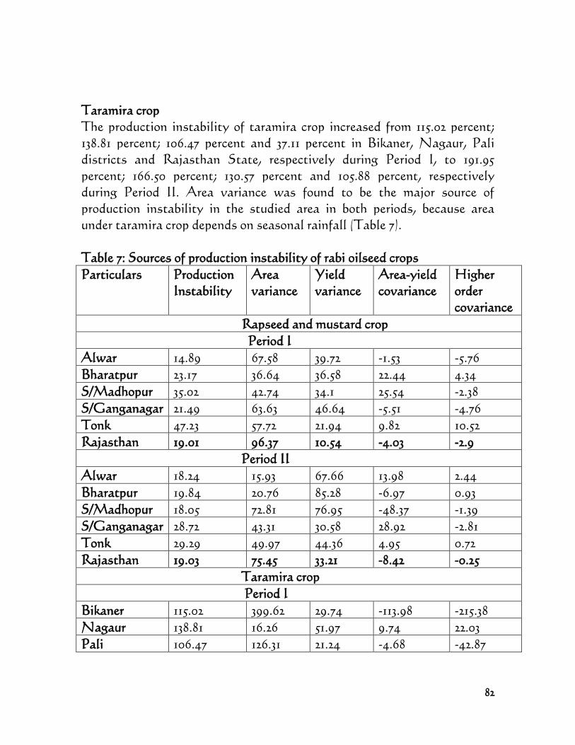
82
Taramira crop
The production instability of taramira crop increased from 115.02 percent;
138.81 percent; 106.47 percent and 37.11 percent in Bikaner, Nagaur, Pali
districts and Rajasthan State, respectively during Period I, to 191.95
percent; 166.50 percent; 130.57 percent and 105.88 percent, respectively
during Period II. Area variance was found to be the major source of
production instability in the studied area in both periods, because area
under taramira crop depends on seasonal rainfall (Table 7).
Table 7: Sources of production instability of rabi oilseed crops
Particulars Production
Instability
Area
variance
Yield
variance
Area-yield
covariance
Higher
order
covariance
Rapseed and mustard crop
Period I
Alwar 14.89 67.58 39.72 -1.53 -5.76
Bharatpur 23.17 36.64 36.58 22.44 4.34
S/Madhopur 35.02 42.74 34.1 25.54 -2.38
S/Ganganagar 21.49 63.63 46.64 -5.51 -4.76
Tonk 47.23 57.72 21.94 9.82 10.52
Rajasthan 19.01 96.37 10.54 -4.03 -2.9
Period II
Alwar 18.24 15.93 67.66 13.98 2.44
Bharatpur 19.84 20.76 85.28 -6.97 0.93
S/Madhopur 18.05 72.81 76.95 -48.37 -1.39
S/Ganganagar 28.72 43.31 30.58 28.92 -2.81
Tonk 29.29 49.97 44.36 4.95 0.72
Rajasthan 19.03 75.45 33.21 -8.42 -0.25
Taramira crop
Period I
Bikaner 115.02 399.62 29.74 -113.98 -215.38
Nagaur 138.81 16.26 51.97 9.74 22.03
Pali 106.47 126.31 21.24 -4.68 -42.87
83
Rajasthan 37.11 113.95 78.54 -46.34 -46.15
Period II
Bikaner 191.95 74.6 3.35 4.65 17.4
Nagaur 166.5 149.05 8.8 -27.92 -29.93
Pali 130.57 152.39 13.53 -20.04 -45.87
Rajasthan 105.88 104.76 1.47 -6.16 -0.07
Sources of Production Instability of Other Crops
Cotton crop
The production instability of cotton declined over the period, from 32.38
percent and 31.58 percent in Sri-Ganganagar district and Rajasthan State
in Period I, to 28.94 percent and 20.78 percent, respectively during Period II.
Decomposition analysis of production instability indicated yield variance
increased from 67.73 percent in Period I to 73.18 percent during Period II in
Sri-Ganganagar district. In Rajasthan State, it declined from 68.99
percent to 54.50 percent during period II. It was observed that the next
important contributor to the production instability was area variance
(Table 8).
Cumin crop
Decline in production instability of cumin crop was observed in Rajasthan
State. In Jalore district, area variance was the major source of production
instability in both periods. In Barmer district, area variance was the major
determinant of production instability in Period I, while during Period II,
yield variance was the major determinant factor of production instability.
However, in Rajasthan State, area variance was the major source of
production instability in both periods, but declined over time (Table 8).
Coriander crop
Production instability of coriander in Kota district and Rajasthan State
declined over time from 47.94 percent in Period I, to 21.79 percent and 28.52
percent, respectively in Period II. The production variance of coriander crop
due to yield variance was 67.84 percent, followed by area variance (38.03
percent) during Period I in Kota district. However, during Period II,
84
production variance was due to area variance (127.92 percent), followed by
yield variance (31.67 percent). Area-yield covariance was observed to be the
nullifying factor of production variance in Kota district during Period II
(Table 8).
Table 8: Sources of production instability of other crops
Particulars Production
Instability
Area
variance
Yield
variance
Area-yield
covariance
Higher
order
covariance
Cotton crop
Period I
S/Ganganagar 32.38 20.03 67.83 9.4 2.73
Rajasthan 31.58 16.79 68.99 19.05 -4.84
Period II
S/Ganganagar 28.94 8.32 73.18 4.75 13.75
Rajasthan 20.78 28.6 54.5 5.27 11.62
Cumin crop
Period I
Jalore 52.58 66.14 33.09 -14.15 14.92
Barmer 56.5 45.65 39.39 11.7 3.27
Rajasthan 50.00 81.17 16.36 -8.08 10.55
Period II
Jalore 39.72 69.11 37.63 8.51 -15.25
Barmer 44.32 9.71 105.6 -1.86 -13.45
Rajasthan 36.177 67.2 13.54 18.45 0,82
Coriander crop
Period I
Kota 47.94 38.03 67.84 2.00 -7.87
Rajasthan 40.7 44.92 49.23 12.87 -7.02
Period II
Kota 21.79 127.92 31.67 -45.31 -14.28
Rajasthan 28.52 69.86 113.67 -125.69 42.16
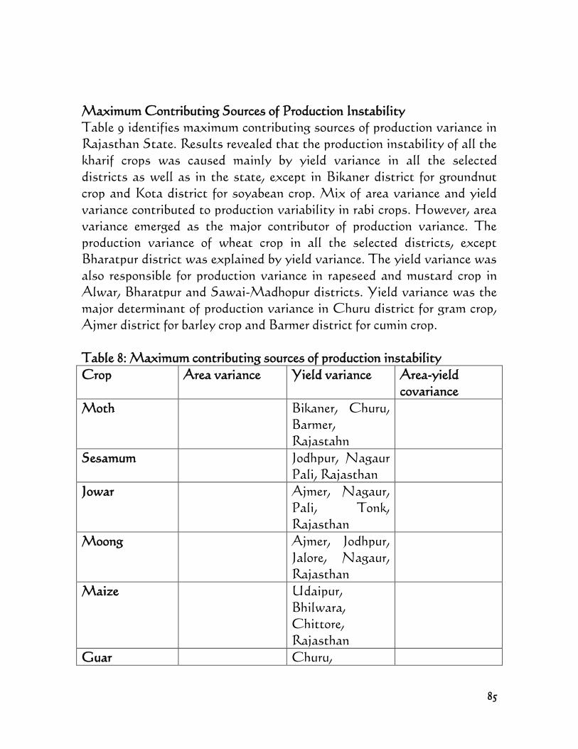
85
Maximum Contributing Sources of Production Instability
Table 9 identifies maximum contributing sources of production variance in
Rajasthan State. Results revealed that the production instability of all the
kharif crops was caused mainly by yield variance in all the selected
districts as well as in the state, except in Bikaner district for groundnut
crop and Kota district for soyabean crop. Mix of area variance and yield
variance contributed to production variability in rabi crops. However, area
variance emerged as the major contributor of production variance. The
production variance of wheat crop in all the selected districts, except
Bharatpur district was explained by yield variance. The yield variance was
also responsible for production variance in rapeseed and mustard crop in
Alwar, Bharatpur and Sawai-Madhopur districts. Yield variance was the
major determinant of production variance in Churu district for gram crop,
Ajmer district for barley crop and Barmer district for cumin crop.
Table 8: Maximum contributing sources of production instability
Crop Area variance Yield variance Area-yield
covariance
Moth Bikaner, Churu,
Barmer,
Rajastahn
Sesamum Jodhpur, Nagaur
Pali, Rajasthan
Jowar Ajmer, Nagaur,
Pali, Tonk,
Rajasthan
Moong Ajmer, Jodhpur,
Jalore, Nagaur,
Rajasthan
Maize Udaipur,
Bhilwara,
Chittore,
Rajasthan
Guar Churu,
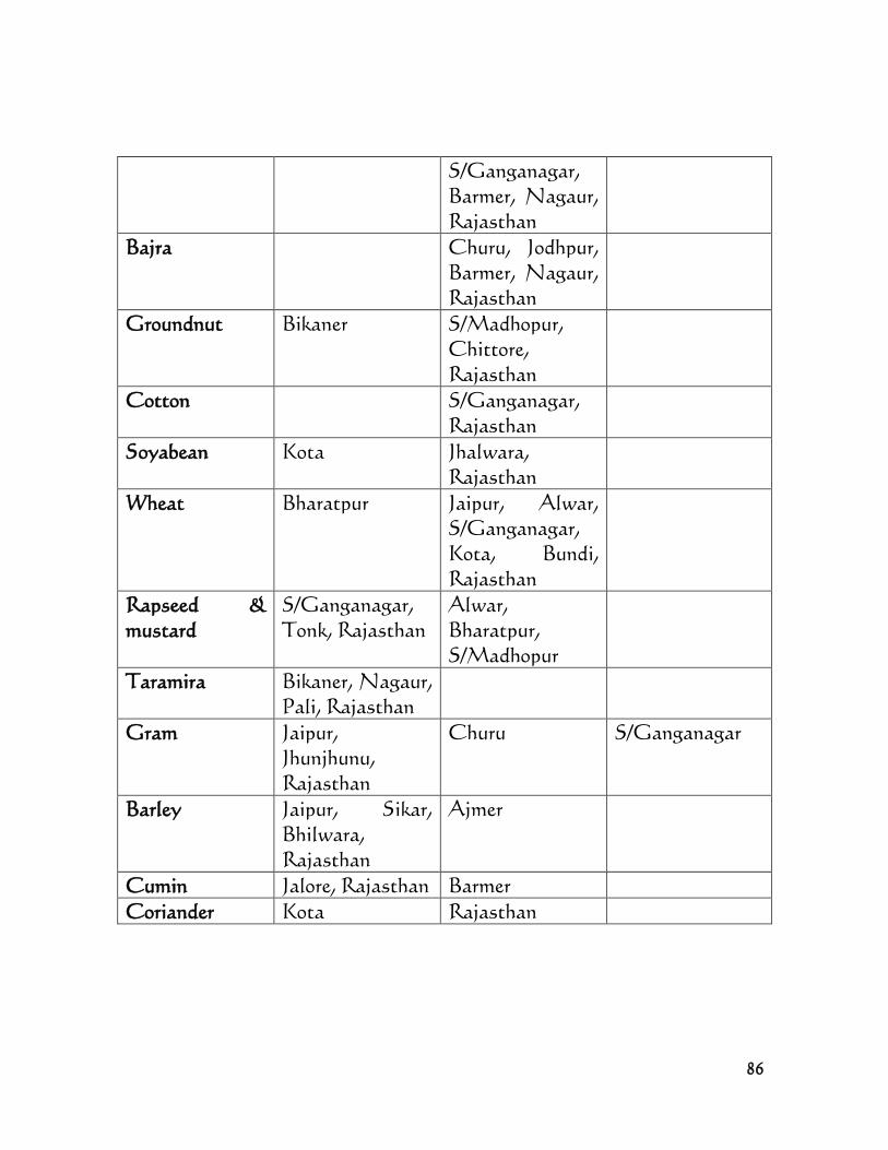
86
S/Ganganagar,
Barmer, Nagaur,
Rajasthan
Bajra Churu, Jodhpur,
Barmer, Nagaur,
Rajasthan
Groundnut Bikaner S/Madhopur,
Chittore,
Rajasthan
Cotton S/Ganganagar,
Rajasthan
Soyabean Kota Jhalwara,
Rajasthan
Wheat Bharatpur Jaipur, Alwar,
S/Ganganagar,
Kota, Bundi,
Rajasthan
Rapseed &
mustard
S/Ganganagar,
Tonk, Rajasthan
Alwar,
Bharatpur,
S/Madhopur
Taramira Bikaner, Nagaur,
Pali, Rajasthan
Gram Jaipur,
Jhunjhunu,
Rajasthan
Churu S/Ganganagar
Barley Jaipur, Sikar,
Bhilwara,
Rajasthan
Ajmer
Cumin Jalore, Rajasthan Barmer
Coriander Kota Rajasthan
87
CONCLUSION AND RECOMMENDATIONS
It is essential to identify the risk inducing factors i.e sources of production
instability. These sources were quantified by decomposing production
variance into various sources viz. area variance, yield variance, area-yield
covariance and higher order interaction between area and yield. High
fluctuating area and yield level were the main cause of crop production
instability in all kharif crops, mainly because of high dependence on
rainfall, thus, a cause of concern for policy makers to ensure sustained
growth of agriculture and farmers livelihood, given that virtually all of
them depend on agriculture for income. Rabi crops like wheat and mustard
also showed fluctuating yield levels inspite of overall growth over the
years. However, high area instability was the major contributing source of
production instability of crops like taramira, gram, barley, cumin and
coriander. Therefore, since it was observed that in most of the crops, yield
variability was more, farmers are advised to avail benefits of crop insurance
scheme launched by government to commensurate their returns. Also,
government should endeavour to enact insurance scheme for those crops
which are yet to be covered by insurance.
REFERENCES
Dutta, R.A. and Kapadia, K.(2011).Possibilities and Constraints in
Increasing Pulses Production in Rajasthan and Impacts of
National Food Security Mission on Pulses. Research Report No.
140, Agro-Economic Research Centre, Sardar Patel
University,Vallabh Vidyanagar, District Nagar, Anand,
Gujarat.
Kumawat, R.C. and Meena, P.C.(2005).Growth and Instability in Area,
Production and Yield of Major Spice Crops in Rajasthan vis-à-vis
India. Journal of Spices and Aromatic Crops, Vol. 14(2):102-111
Sadiq, M.S. and Grema, I.J.(2016).Instability in Indian Agriculture in the
Light of New Technology: Evidence of Crop Sub-Sector in
88
Rajasthan State, India. Global Journal of Agricultural Research
and Review, Vol. 4(1):158-389
Sadiq, M.S.(2015).Impact of India Economic Policies on Cotton Production
vis-a-vis Comparison between Pre-Economic Liberalization
Policy Period and Economic Liberalization Policy Period. An
International Journal of Agro Economist, Vol. 2(1):51- 58.
Swain, M.(2013).Problems and Prospects of Oilseeds Production in
Rajasthan-Special Reference to Rapeseed and Mustard. Research
Report No. 147, Agro-Economic Research Centre, Sardar Patel
University,Vallabh Vidyanagar, District Nagar, Anand, Gujarat.
Pp. 01-111
Swain, M., Kalamkar, S.S and Ojha, M.(2012).state of Rajasthan
agriculture 2011-2012. Research Report No. 145, Agro-Economic
Research Centre, Sardar Patel University, Vallabh
Vidyanagar, District Nagar, Anand, Gujarat. Pp. 01-33
Vanpal, K.B., Pant, D.C and Jaya, M.(2015).Growth, Instability and
Acreage Response Function in Production of Cumin in Rajasthan.
The Bioscan, Vol. 10(1):359-362.
89
The Frequency of ABO and Rhesus D Blood Group
Antigens amongst Blood Donors
Clement .K. Okpora Ph.D
Department of Medical Laboratory Sciences
Rivers State University of Science and Technology, Port Harcourt, Nigeria
E-mail: [email protected]
Abstract
The frequency distribution of ABO and Rh.D blood group antigens
amongst blood donors in Port Harcourt metropolis was investigated
in this study. A total of 150 blood donors recruited in a hospital in
Port Harcourt, Rivers State of Nigeria were collected by venepucture
from each of the male blood donors and transferred into bottles
containing Ethylenediaminetetra-acetic acid (EDTA). Fresh red cell
suspension and 20% suspension of known A,B and Rh.D antigens
were prepared. Tile agglutination technique was used in the
determination of ABO and Rh.D grouping system. The results
showed that for the distribution of percentage frequency of ABO
blood groups in the study population, 33 donors were blood group A
with percentage frequency of 22.0%, 31 donors were group B with
frequency of 20.7%, 12 donors were group AB with frequency of 8.0%
and 74 donors were group O with highest frequency of 49.3%. For the
distribution of percentage frequency of Rh.D blood group among the
blood donors, 138 donors with frequency of 92.0% were Rh.D positive
while 12 donors with percent frequency of 8.0% were Rh.D negative.
When the frequency distribution of Rh.D positive and Rh.D negative
subjects in ABO blood groups was assessed, it was shown that blood
group O had the highest number of donors with Rh.D positive, of 71
with frequency of 47.3%, then followed by group A with 31 donors
with frequency of 20.7%, group B with 27 donors with frequency of
18.0% and lastly group AB with 9 donors with frequency of 6.0%.
The Rh.D negative values were 3(2.0%) for group O, 1(0.7%) for group
A, 5 (3.3%) for group B and 9(6.0%) for group AB. The study therefore
concludes that blood group O with Rh.D positive antigens are the
Pp 92-107
90
most common blood groups among the blood donors in Port Harcourt
metropolis.
Keywords: Frequency, Blood, Donors, ABO, Agglutination and
Rh.D
INTRODUCTION
In 1900 an English scientist Karl Landsteiner when carrying out some
experiments with red cells of some individuals and then sera of others
observed some interesting results. He found that there were agglutinations
in some categories while in other there were no agglutination of the red
cells. Continuing his experiment he discovered it was possible to group his
findings. Three groups were possible which he classified as A, B, and O
groups. It was known that the red cell in group ‘A’ posses the antigen
designated as ‘A’. Those with antigen ‘B’ as group B and those with no
antigen on their red cell was designated O (Cheesbrough 2000).
Continuing his experiment it was revealed that blood that has group A
antigen has naturally occurring antibodies to the group B antigen (anti-B)
and those with group B antigen has naturally occurring antibodies to group
A antigen (anti-A). This soon became apparent as the major cause of
incompatibility leading to severe transfusion reaction. (Shaw et al;2010,
Bener et al;2012).
Two years after the death of Landsteiner one of his students opened further
investigation and discovered a fourth group of red cells which posses both
A and B antigen and is designated as group AB. They naturally do not
possess any of the A or B antibodies. Thus this blood grouping technique
became known as the Landsteiner’s ABO blood group system. For this
discovery, he was awarded the Nobel price in Medicine at that time.
(Schroedar and Jenson 2000, Waseem et al; 2012, Jassim 2012).
The adverse reactions in blood transfusion were not totally eliminated
following the discovery of A & B antigens hence prompting the need for
further investigations. In 1939 Landsteiner and Wiener discovered the
91
Rhesus antigen. They injected red cells of the monkey macacus rhesus into
rabbits thereby stimulating the production of an antibody. This antibody
then agglutinates the Rhesus monkey red cells. These antibodies also
agglutinate a large percentage of individual meaning they posses the
Rhesus antigen and a small percentage of individuals could not be
agglutinated. Those whose red cells are agglutinated are known as Rhesus
positive while other groups are known as Rhesus negative. (Lawler and
Lawier 1971).
Blood transfusion is a very important therapeutic process in modern
medicine (Mollison 1993). However, a lot of care is taken in carrying out
this all important process. The first aspect of this work which determines
to a large extent the success of the therapy is the correct grouping of the
donor and the recipient (Adam et al; 1996).
When blood is wrongly grouped it leads to an adverse transfusion reaction
in the recipient (Baker and Sylverton 1998). In the ABO system,
individuals naturally have antibody to the antigen it does not possess.
Antigen-antibody reaction can occur in vivo if proper care is not taken.
Antigen antibody reaction leads to agglutination and possible lysing of the
red cells. If this occurs, then the purpose of blood transfusion is defeated.
For instance, it is not compatible for a group A recipient to be transfused
with group B blood. This is because group A individuals has antibody B
(Anti-B) and will cause lysing of the transfused B red cells. To avoid
adverse transfusion reaction arising from ABO antigen, group compatible
blood is always used. (Antee 2010,Kamil et al;2010).
Group O individual can donate to any of the four groups individual as
universal donor while group AB individuals can receive blood from any of
the four blood group individuals as universal recipient (Jaggi and Yadav
2014).
92
The Rh.D blood group system is similar. Its difference is that wrong
transfusion does not result to all immediate adverse transfusion reaction
except in a subsequent transfusion. A Rhesus negative donor can donate to
a Rhesus positive individuals without any adverse reaction. However, if
Rh.D positive blood is given to Rh.D negative individual he or she
becomes sensitized and develops antibodies to the Rh.D antigen in the
next transfusion (Gravenhorst 1982, Dawti et al; 2011).
The frequency of ABO and Rh.D phenotypes varies in different
populations throughout the World (Aird 1953). In the study carried out by
Mollison et al; (1993), the commonest group in the Australian abonigines
are groups O and A. France (2002) gave the percentage distribution of
whites in the united states as blood group 0,46%, A ,41%, B, 9% and AB
4%. That of the Negroes New Yorkers were given as blood group 0, 25%,
group A, 18% group B and AB 5%. The African country of Kenya had a
percentage distribution of blood group 0 as 47.4%, A, 26.2%, B, 22.0% and
AB as 4.4% (Lyko et al; 1992). European population is 95% Rh.D positive
while 5% were Rh.D negative. For the United States 85% of the
population were found to be Rh.D positive while 15% were Rh.D negative
(France 2002). Marzban et al; (1988) gave 90% Rh.D positive and 10%
Rh.D negative in Ahwaz region population. Monica (2000) gave the
summary of Rh.D positive distribution as Asians 90-98%, Africans 94-
95%, Nepalese 99-100% and the Caucasians as 56%.
This study is therefore aimed at investigating the frequency distribution of
ABO and Rh.D blood group antigens amongst blood donors in Port
Harcourt Metropolis.
93
MATERIALS AND METHOD
Recruitment of Patients
A total of two hundred and four (204) students in a coeducational
institution in Nembe were used in this study. They were made up of one
hundred and twenty four (124) males and eighty (80) females.
Collection of Samples
5.0ml. of blood was collected from each of the recruited patients using
venepuncture technique and transferred into a bottle containing
ethylenediamine tetra acetic acid (EDTA). This was gently rocked to
ensure thorough mixing of the blood sample with the anticoagulant.
Preparation of Fresh Red Cell Suspension
This was done using each of the samples to be grouped. Two ml of the
samples were transferred from the EDTA bottle to a test tube. 3.0ml of
normal saline solution was added to the tube and the contents were mixed
and centrifuged for 5 minutes. The supernatant was decanted and this was
repeated three times.
20% suspension of known red cells containing the A, B, and Rhesus D
antigen were prepared in the same way and used for the serum (reverse)
grouping.
Procedures for ABO Grouping
Tile agglutination technique was used in this determination. Microtitre
wells were numbered 1-6 and one volume each of anti-A, Anti-B and Anti
AB were added to wells 1, 2 and 3 respectively, while one volume each of A
Cells, B cells and control 1 (patient cells and serum) were added to wells
no. 4,5 and 6 respectively.
To wells numbers 1-3 one volume of patients cells were added whereas in
wells number 4 and 5 one volume of patients serum were added. One
volume of low ionic strength solution (LISS) freshly prepared was added to
each well.
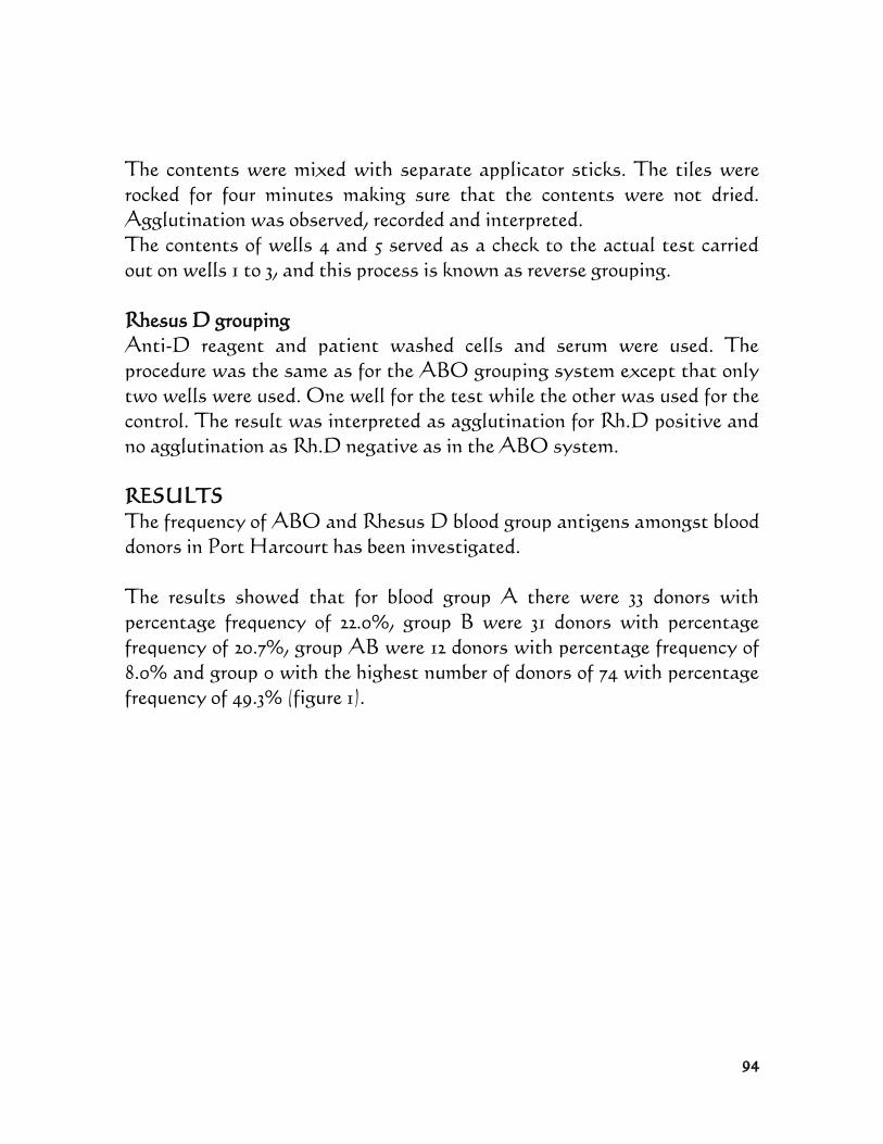
94
The contents were mixed with separate applicator sticks. The tiles were
rocked for four minutes making sure that the contents were not dried.
Agglutination was observed, recorded and interpreted.
The contents of wells 4 and 5 served as a check to the actual test carried
out on wells 1 to 3, and this process is known as reverse grouping.
Rhesus D grouping
Anti-D reagent and patient washed cells and serum were used. The
procedure was the same as for the ABO grouping system except that only
two wells were used. One well for the test while the other was used for the
control. The result was interpreted as agglutination for Rh.D positive and
no agglutination as Rh.D negative as in the ABO system.
RESULTS
The frequency of ABO and Rhesus D blood group antigens amongst blood
donors in Port Harcourt has been investigated.
The results showed that for blood group A there were 33 donors with
percentage frequency of 22.0%, group B were 31 donors with percentage
frequency of 20.7%, group AB were 12 donors with percentage frequency of
8.0% and group 0 with the highest number of donors of 74 with percentage
frequency of 49.3% (figure 1).
95
96
For the distribution of percentage frequency of Rh.D blood group in the
studied population, 138 donors with percentage frequency of 92.0% were of
Rh.D positive while 12 donors with the frequency of 8.0% were of Rh.D
negative (figure 2).
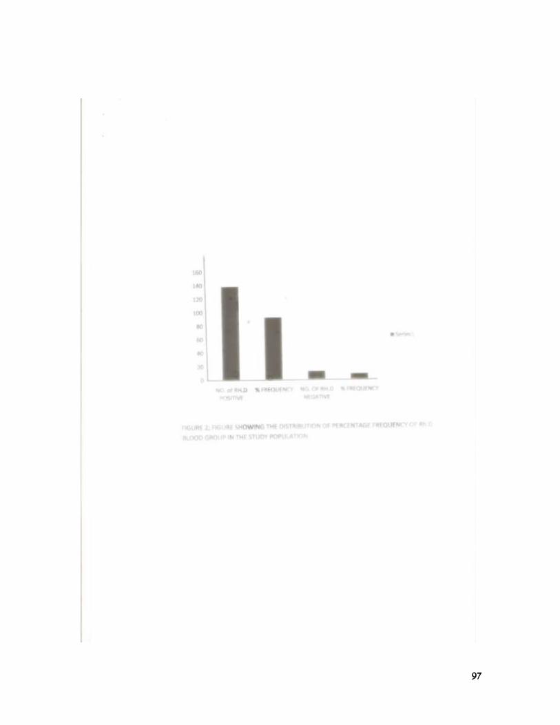
97
98
For the frequency distribution of Rh.D positive and Rh.D negative
subjects in the studied population, blood group A had 31 Rh.D positive
donors with frequency distribution of 20.7% and 1 Rh.D negative donor
with frequency of 0.7%. Blood group B had 27 Rh.D positive donors with
frequency of 18.0%. Blood group AB had 9 Rh.D positive donors with
frequency of 6.0% and 3 Rh.D negative donors with frequency of 2.0%.
Blood group “O” had the highest number of Rh.D positive donors of 71
with the percentage frequency of 47.3% and 3 Rh.D negative with
frequency of 2.0%.(Table 1).
Table 1: Table showing the frequency distribution of Rh.D positive and
Rh.D negative subjects in ABO blood groups
Blood groups Rh.D
Positive
%frequency Rh.D
Negative
%
Frequency
A 31 20.7 1 0.7
B 27 18.0 5 3.3
AB 9 6.0 3 2.0
0 71 47.3 3 2.0
Total 138 92 12 8.0
DISCUSSION
This study investigated the frequency distribution of ABO and Rh.D
antigens amongst blood donors in Port Harcourt. The ABO and Rhesus D
blood group systems are the most commonly used blood group system in
blood transfusion medicine (Frances et al; 2002).
The results showed the distribution of percentage frequency of ABO blood
group in the study population as blood group A 33 donors with percentage
frequency of 22.0%, group B, 31(20.7%), group AB, 12(8.0%) and group 0
with 74 donors and percentage frequency of 49.3%.
This finding agrees with the results of other investigators who showed
that blood group O is most common amongst the population of their
99
studies just as in this study. (France 2000,Mollison et al;1993 and Lykes et
al;1992).
For the frequency distribution of Rhesus D antigens the study showed that
138 donors with percentage frequency of 92% were Rh.D positive while 12
donors with percentage frequency of 8.0% were Rh.D negative. These
results also agrees with that of other investigators which showed that
Rh.D positive individuals were higher than the Rh.D negative ones in the
population studied. (France 2002, Marzban et al;1988 and Monica 2000).
For the frequency distribution of Rh.D positive and Rh.D negative
subjects in ABO blood groups. Blood group O was found to have the
highest frequency of 71 Rh.D positive individuals with percentage
frequency of 47.3%, followed by group A with 31 Rh.D positive with
frequency of 20.7%, then group B with 27 Rh.D positive with frequency of
18.0% and group AB with 9 Rh.D positive donors with frequency of 6.0%.
The frequency of Rh.D negative donors were 3(2.0%) for group 0, 1(0.7%)
for group A, then 5(3.3%) for group B and 3(2.0%) for group AB. These
findings also agreed with the findings of other studies cited above since
blood group O is shown to have the highest frequency of Rh.D positive
donors.
This study therefore concludes that blood group O with Rh.D positive
antigens are the most common amongst the blood donors in Port Harcourt
metropholis.
REFERENCES
Adams M.M, Gustafson J and Oakle G.P.(1996). Rhesus hemolytic
disease of the newborn using incidence observation to evaluate the
use of rhesus immune globulin. The American Journal of Public
Health. 71(982) 1031-1035.
100
Aird I, and Bentall,H.H (1953). A relationship between cancer of the
stomach and the ABO blood groups.British medical Journal 71(982):
1031-1035.
Aristee D.J. (2010). The relationship between blood groups and disease.
Blood 115:4635-4643.
Baker F.J. Silverton R.E and Pallister C.J. (1998).Introduction to Medical
laboratory 7th
edition Pp. 397-407 Butterworth Heinemann Oxford.
Bener A. Yousafzai M.T. Al-Hamaq O.A. (2012) Familiar aggregation
of T2 DM among arab diabetic population. International
Journal Diabetic Developing countries.32:90-92
Cheesbrough M. (2000). District laboratory practice in tropical countries
part 2 Pp 362-369 Cambridge University press U.K.
Dali Sahi M., Aour Metri A and Boza F. (2011). The relationship
between ABO/Rhesus blood groups and type 2 Diabetes in
Magnia/Western Algenia. South African Family Practice 53:568-
572.
Frances T.F. (2002). Blood Groups (ABO groups). In common
laboratory and diagnostic tests 3rd
edition Pp.194-195 philidelphis
Lippincott.
Gravenhorst J.B. (1982). Prevention of rhesus D iso-immunization after
abortion in Keirse M.J. second trimester pregnancy
termination. Boorhave series for post graduate medical education,
Netherland 22:168-173.
Jaggi S., and Yadav A.S. (2014). Distribution of ABO and Rh.D allele
frequency among the type 2 diabetes mellitus patients. American
101
international Journal Research for formal Applied Natural Sciences
1: 24-26.
Jassim W.E. (2012). Association of ABO blood group in Iragis with
hypercholesterolaemia, hypertension and diabetes mellitus. East
Mediteranean Health Journal. 18:88-891
Kamil M.AL-Jamal H.A and Yusoff N.M. (2010) Association of ABO
blood groups with diabetes mellitus. Libyan Journal of medicine
5:4847
Lyko J., Graestuer H., and Kaiti J.N. (1992).Blood group antigens ABO
and Rhesus in Kenyans. Hametard Medicus 3(3): 59-67.
Lawler S.D and Lawler L.J. (1971).Human blood groups and inheritance
Pp. 10-14.
Mollison P.L. Engelfret C.P, and Conteras M. (1993), Immunology of red
cells in blood transfusion in clinical medicine 9th
edition pp. 87-89
blackwell scientific publication oxford.
Marzban M. Kamah M.S and Hosseinbasi T. (1988). Blood groups of the
people of Ahwaz. Iran anthropol ANZ 46(1):83-89
Schroeder M.and Jensen (2000) Life’s Blood Pp 173-197 Butterworth
Heinemann Oxford.
Shaw J.E., Sicree R.A and Zimmet P.Z. (2010). Global estimates of the
prevalence of diabetes for 2010 and 2030. Diabetes Research clinical
practice 8:4-14.
Waseem A.G, Igbal M. Khan O A and Tahir M. (2012). Association of
diabetes mellitus with ABO and Rh.D blood groups. Annals of
Pakistan Institute of Medical Science 8:134-136
Related Documents