Welcome message from author
This document is posted to help you gain knowledge. Please leave a comment to let me know what you think about it! Share it to your friends and learn new things together.
Transcript

Eötvös Loránd University
Faculty of Science
Bálint Márk Vásárhelyi
Mathematical methods in DNA
sequence analysis
BsC Diploma Thesis
Supervisor:
Kristóf Bérczi
Department of Operations Research
Budapest, 2011

Contents
Introduction 3
1 Physical and genetic mappings 5
1.1 Physical mapping . . . . . . . . . . . . . . . . . . . . . . . . . . . . . . . . . . . . . 6
1.1.1 Clone libraries . . . . . . . . . . . . . . . . . . . . . . . . . . . . . . . . . . 6
1.1.2 Errors of STS-mapping . . . . . . . . . . . . . . . . . . . . . . . . . . . . . 7
1.2 Genetic mapping . . . . . . . . . . . . . . . . . . . . . . . . . . . . . . . . . . . . . 8
2 The tightest layout 9
2.1 Tightest layout of clones . . . . . . . . . . . . . . . . . . . . . . . . . . . . . . . . . 9
3 Betweenness problem 12
3.1 Parameterized problems . . . . . . . . . . . . . . . . . . . . . . . . . . . . . . . . . 12
3.2 Parameterization of Betweenness problem . . . . . . . . . . . . . . . . . . . . . . . 13
3.3 The Strictly Above/Below Expectation Method . . . . . . . . . . . . . . . . . . . . 13
3.4 FPT of BATLB . . . . . . . . . . . . . . . . . . . . . . . . . . . . . . . . . . . . . . 14
4 Comparison between di�erent sequences 16
4.1 Exact matching . . . . . . . . . . . . . . . . . . . . . . . . . . . . . . . . . . . . . . 16
4.1.1 The Naive Algorithm . . . . . . . . . . . . . . . . . . . . . . . . . . . . . . 16
4.1.2 The Boyer�Moore Algorithm . . . . . . . . . . . . . . . . . . . . . . . . . . 17
4.1.3 The Knuth�Morris�Pratt Algorithm . . . . . . . . . . . . . . . . . . . . . . 18
4.2 Inexact matching . . . . . . . . . . . . . . . . . . . . . . . . . . . . . . . . . . . . . 19
4.2.1 Edit distances of two strings . . . . . . . . . . . . . . . . . . . . . . . . . . 19
4.2.2 Representing DNA sequences with matrices . . . . . . . . . . . . . . . . . . 22
Summary 25
Bibliography 26
2

Introduction
Nowadays, one of the most promising �elds of mathematics is biomathematics.
There are several biological problems that can be treated with mathematical meth-
ods, and it seems to be very useful for both mathematics and biologics to combine
the results of the two disciplines. One of the most important problems is genetic
mapping and sequence analysis of DNA. There are several databases, the most well-
known is GenBank, which was created by the Los Alamos National Labs, but now it
is maintained by the National Center for Biotechnology Information. According to
[14], the size of stored DNA sequences was increased by about 75 % each year in the
1990s. Today, this number is even more large, as di�erent methods were published
since that time. In this thesis, several methods are shown used for mapping and
sequence analysis.
In Chapter 1, several ways of mapping are introduced. The main topic of this
part is STS-content mapping, which is a wide-spread method of sequence analysis.
We also consider genetic mappings.
Another approach of STS-content mapping is shown in Chapter 2. The aim of
this method is to �nd a layout of the clones, requiring the least space possible.
A special mapping problem is acquainted in Chapter 3. Sometimes, not all the
relations of mapping points are known, just a few of them. Here, only some triplets
are given with their central elements, and we present a method for �nding an order
of the elements that satis�es as more constraints as possible.
Comparison of two or more sequences is also of interest. A number of methods
for comparison is shown in Chapter 4. One may be curious about knowing if a short
sample is contained by a longer sequence, or we can compute the edit distance of
two strings.
3

INTRODUCTION 4
I say thanks to my supervisor, Kristóf Bérczi for his devoted professional help.
I thank to András Frank for making me available the book Algorithms on Strings,
Trees and Sequences of Dan Gus�eld.
SDG

Chapter 1
Physical and genetic mappings
In general, we distinguish genetic maps and physical maps [6]. Physical maps
are easier to be handled by mathematical methods, as here a DNA sequence can be
handled as a string.
Physical mappings establish on the true physical location of markers or known
patterns, such as microsatellites (microsatellites are repeating short substrings, usu-
ally two bases, for example ACACACACAC is a microsatellite). Usually the dis-
tance of two markers is the number of nucleotides between them. With this map
one can roughly place a gene on the map, we can notice a deletion or an insertion.
For example, the tumor suppressor gene of retinoblastoma was �rstly localized by
observing a deletion on the chromosome 13 [13]. The aim of physical mapping is to
locate the interesting genes on their base-pair location on a chromosome.
On the other side, genetic mappings are based on observing the degree of recom-
bination. This notion represent the relative frequency of cross-overs in a speci�ed
section of meiosis, and it is in connection with linked inheritance of genes at two
loci on the DNA. (See Figure 1.1.) It is supposed that the higher the frequency of
Figure 1.1: Cross-over between two double-chained DNA
5

1.1. Physical mapping 6
coinheritance, the closer the two loci are. Genetic mappings are more bene�cial in
genetics, because they reveal more information about the alleles on the DNA than
physical mapping. The unit of genetic mapping is called centimorgan, which is
usually referred to the distance of two alleles where the degree of recombination is
0.01. More precisely, the distance is d = 12
ln(1 − R), where R is the degree of re-
combination. The problem of genetic mappings is that the collection of data is more
di�cult, and centimorgan is not an absolute unit, but it is characteristic of species.
Now, we will study physical mappings.
1.1 Physical mapping
1.1.1 Clone libraries
A very important mapping strategy is the STS-content mapping. STS stands
for sequence-tagged-site, and it is a 200-300 nucleotides long DNA substring, whose
left and right 20-30 bases occur only once in the entire genome. One of the �rst
goals of the Human Genome Project was to �nd a set of STSs such that any 100,000
nucleotides long DNA substring contains at least one of them. [5]
We say that a clone library is a set of short DNA fragments or clones that
can overlap and that cover the whole DNA. The order of the clones are unknown.
One aim is to build a ordered clone library.
The goal of STS-content mapping is determining the order of STSs and building
the ordered clone library. First, the method determines which clone contains which
STSs. It can be implemented by hybridization or by PCR technology. The second
step is reconstructing the order of the STSs and placing the clones on a physical
map. Two basic ideas are used. The �rst is that the distance between STSi and
STSj is inversely related to the number of clones containing both STSi and STSj.
The second is that if STSi occurs in both clones clonek and clonel, then clonek and
clonel must overlap at STSi (see Figure 1.2).

1.1. Physical mapping 7
Figure 1.2: Input data of STS mapping
1 2 3 4
1 1 1 0 0
2 0 1 0 0
3 0 1 1 1
Table 1.1: The input matrix constructed from data in Figure 1.2
From the data of the PCR, an input matrix can be constructed (see Table 1.1).
The intersection of row i and column j would be 1 if clonei contains STSj, otherwise
0. The aim is to permute this matrix so that in each row, the ones are not separated
by zeros. Booth and Lueker [2] shows an algorithm for �nding such a permutation
or proving that there is no such a permutation.
1.1.2 Errors of STS-mapping
There are three important systematic errors of STS-content mapping, namely,
the false negative report, the false positive report and the chimeric clones.
False negative report is when it is reported that the clone does not contain the STS,
but actually it does. Respectively, false positive report is when it is reported that
an STS occurs in a clone, despite the fact that it does not.
Chimeric clones are a more complicated type of error. Sometimes, two di�erent
fragments of the original DNA join to each other, and a new DNA clone is created.
However, the location of the two fragments can be widely di�ering, which means
a great problem in STS-mapping. Existence of chimeric clones clearly makes the
mapping more di�cult, and unfortunately the more fragments we have the more
chimeric clones will be formed.

1.2. Genetic mapping 8
1.2 Genetic mapping
Genetic maps are based on genetic recombination. Genetic recombination is a
new allele combination which is di�erent from the parental one and it occurs when
there is an odd number of crossing overs between the two homologous chromosomes
in the section between two interested alelles. The ideal crossing over is pointwise,
autonomous and it occurs with a certain probability at each point [11].
One of the mapping functions is the Haldane function, which points at a relation
between the genetic linkage R (which is the relative frequency of odd number of
crossing overs) and the serial distance d between two alleles.
R =(1− e−2d
)The distance is given in centimorgans. From the Taylor series of ex the distance
of two alleles is one centimorgan if the relative frequency of crossing over between the
two alleles is approximately 1%. Of course, the Haldane function can be generalized
for more than two mapping points.

Chapter 2
The tightest layout
2.1 Tightest layout of clones
As we have seen in Chapter 1, in physical mappings we are given some clones
(substrings) from a DNA and some probes. It is known that which probes contain
which clones, and we have to show an arrangement of the probes. Karp et al. [1]
developed a method for this problem.
Let P be a set of probes and C be a set of clones. |C| is denoted by n. For
each clone c ∈ C let Pc be the set of the probes containing c. It is possible that a
probe occurs at more than one location. The number of times a probe appears is
not known.
We say that a mapping of clones in C and the probe occurrences is a feasible
layout, if each clone c ∈ C is contained at least one copy of each probe in Pc,
but no copies of probes in P \ Pc. Because a probe may occur at more than one
location, a feasible layout can be always shown: place each clone c separated from
the others, and place one copy of each required probe on the clone. We say that this
is a primitive feasible layout. Our aim is to �nd a tightest layout, which occupies
the least space on the real line and in which the fewest probe copies occurs.
Karp et al. [1] made two restriction to solve this problem. Assume that each
clone has equal length, and predetermine a permutation of the clones, so choose an
input permutation, in which the names of the clones are 1, .., n.
9

2.1. Tightest layout of clones 10
Lemma 2.1.1. Let i < j < k be three clones. If there is a p ∈ P occurring in clone
j, but neither in clone i nor k, then clones i and k are disjoint.
Proof. Suppose that i and k overlap. As the right end of i is more left than the
right end of j, the left end of k must be more left than the right end of j, so clearly
each probe in Pj is in Pi ∪ Pk, which means Pj ⊆ Pi ∪ Pk. �
In the proof we used that the clones are of equal length. From Lemma 2.1.1
follows that if i′ ≤ i < j < k ≤ k′ and i does not overlap k, then i′ does not overlap
k′.
If i′ and k′ are such that there exist i, j, k ∈ C with Pj \ (Pi ∪ Pk) 6= ∅ and
i′ ≤ i < j < k ≤ k′, then we say that the pair (i′, k′) is an excluded pair. In all
other cases we say that the pair is permitted.
Lemma 2.1.2. Let i < j < k be 3 clones. If (j, k) is an excluded pair, then (i, k) is
also excluded. If (i, k) is a permitted pair, then (j, k) is also permitted.
We will show how to construct a feasible layout, where every permitted pair
overlaps and no excluded pair does, further, it occupies a minimal span of the real
line. This is the greedy clone layout.
The algorithm of greedy clone layout
First, choose a starting point, and place clone 1 here with its left end. Then for
each k ≤ n �nd the smallest i < k for which (i, k) is permitted. It is clear that such
an i always exists, because (k− 1, k) is permitted. Now, place clone k in such a way
that it overlaps with clone i, but it does not with clone i− 1, and of course, its left
end is at the right of the left end of clone k − 1.
Gus�eld [6] proved the following theorems:
Theorem 2.1.1. At the end of the above algorithm, two clones overlap if and only
if they form a permitted pair.
To show that the greedy clone layout can be made feasible, we have to place the
probes on the real line. The method of the placement of the probes is the following:
Let i be the smallest index for which p ∈ Pi, and let j be the smallest index for

2.1. Tightest layout of clones 11
which i < j and (i, j) is excluded or p /∈ Pj. Then place a copy of p inside the clone
i in such a way that all clones in {i, . . . , j − 1} contain p, but j does not. If there is
a k ≥ j for which p is in Pk, then restart the method with i = k.
Theorem 2.1.2. It is possible to correct the above algorithm so that the result
occupies less span than all other feasible layouts, and the above method makes this
layout feasible.

Chapter 3
Betweenness problem
In genome projects, it is important to order the mapping points if some between-
ness constraints are given, such as one point is between two others. This problem
is discussed by Gutin et al. [7]. The problem is the following: we have a set V of
variables and a set C which contains the betweenness constraints. A betweenness
constraint looks like vi is between vj and vk (but is it not �xed if vj < vk or vk < vj),
and we sign it as (vi, {vj, vk}). The aim is to show an ordering of V which satis�es as
much betweenness constraints as much is possible. We will donate this ordering as an
α bijection from V to the set {1, . . . , |V |}, where α is called a linear arrangement.
Deciding whether all constraints can be satis�ed is NP-hard, so this problem is
NP-hard ([10]), and it is easy to see that the maximization problem is also NP-hard.
3.1 Parameterized problems
We call an L subset of Σ∗×N a parameterized problem where Σ∗ are the words
formed from the �nite alphabet Σ. We call the second component of an element of
L a parameter.
If the question (α, k) ∈ L can be decided in f(k) · |x|c time (where c is a real
number), then we call L �xed parameter tractable.
The kernelization of an L betweenness problem is a polynomial algorithm which
makes from an element (x, k) ∈ L another element (χ, κ) ∈ L, where the set of image
of the algorithm is the kernel. This algorithm has to have the following properties:
12

3.2. Parameterization of Betweenness problem 13
�rst, it is an L→ L injective function, it is contractive, so κ ≤ f(k), and |χ| ≤ g(k)
for some f and g functions. We say that g(k) is the size of the kernel.
3.2 Parameterization of Betweenness problem
In the so-called Betweenness problem we ask if we could arrange linearly the
elements by satisfying the most possible constraints. If we rather ask if there exists
any arrangement that satis�es at least k constraints, we have parameterized the
Betweenness problem with parameter k. Now we show that the Betweenness problem
is �xed parameter tractable with this parameter. If the linear arrangement is a totally
random permutation (with a probability of 1n!), then it is easy to see that it satis�es
|C|3constraints in expectation, hence if k is less than |C|
3, the answer for parameterized
betweenness problem is �yes�. However, if C contains all the possible constraints, then
no linear arrangement can satisfy more than |C|3constraints.
We have seen that we can satisfy at least |C|3constraints, so we can reparameterize
the problem: we ask if we can satisfy at least |C|3
+ k constraints. The name of this
problem is Betweenness Above Tight Lower Bound (henceforth referred to as
BATLB), and the question was opened by Benny Chor [4]. Gutin et al. [7] shows
that BATLB is �xed parameter tractable, and actually it has a kernel of size O(k2),
by using the Strictly Above/Below Expectation Method (henceforth referred
to as SABEM).
3.3 The Strictly Above/Below Expectation Method
With SABEM we can prove whether a parameterized problem Π is above a
tight lower bound. Firstly, SABEM reduces the problem, then it gives an X random
variable which takes higher value than the parameter k with nonzero probability if
and only if the answer for the reduced problem is �yes�.
SABEM needs the following lemmas:
Lemma 3.3.1. If the X random variable satis�es: E(X) = 0, E(X2) = σ2 6= 0,
E(X4) ≤ cσ4, where c is a constant, then the probability P (X > σ2√c) > 0.

3.4. FPT of BATLB 14
Lemma 3.3.2. If f is a polynomial of the random variable (X1, . . . , Xn) ∈ {−1, 1}n
with degree r and X = f(X1, . . . , Xn), then E(X4) ≤ 9rE(X2)2.
3.4 FPT of BATLB
Gutin et al. [7] shows that BATLB has a quadratic kernel size. We denote the
variables of the constraint C with vars(C), and we say that a triplet of constraints
A,B,C are complete if they have the same variables. If a complete triplet appears
in C, then we can remove this triplet with the variables which �gures only in the
triplet, because any linear arrangement satis�es exactly one constraint of the triplet.
This is the reduction rule. Moreover, we can delete all the complete triplets from
C one by one, and we call the �nal result (in which there are no complete triplets)
irreducible.
Lemma 3.4.1. If (V, C, k) is a BATLB-problem, and (V ′, C ′, k) is an irreducible
BATLB-problem reduced from the original one, then the answer for (V, C, k) is �yes�
if and only if it is �yes� for (V ′, C ′, k).
Now let φ : V → {0, 1, 2, 3} be a random function, and Λi(φ) is the set of the
variables which are mapped into i by φ (for i = 0, 1, 2, 3). We will use the following
notation: `i(φ) = |Λi(φ)|. Let α be a bijection between V and 1, . . . , |V |, which ran-
domly assigns the variables in Λ0(φ) to 1, . . . , `i(φ). Further, α assigns the variables
of Λi(φ) toi−1∑j=0
`j(φ) + 1, . . . ,i∑
j=0
`j(φ). We call this special linear arrangement of the
variables in V a φ-compatible linear arrangement.
Supposing that φ : V → {0, 1, 2, 3} is a �xed function, α is a φ-compatible linear
arrangement, we can de�ne the following function for each C ∈ C: vC(α) = 1 if
the constraint is satis�ed and 0 otherwise. Now, let w(C, φ) = E(v(α)) − 13and
w(C, φ) =∑C∈C
w(C, φ).
Lemma 3.4.2. [7] If w(C, φ) ≥ k, then the answer for the BATLB-problem (V, C, k)
is �yes�.

3.4. FPT of BATLB 15
Proof. k ≤ w(C, φ) =∑C∈C
w(C, φ) =∑C∈C
E(vC(α))− 13
= − |C|3
+∑C∈C
E(vC(α)).
After reordering, we get k + |C|3≤∑C∈C
E(vC(α)). Using the linearity of expectation,
it is equivalent to k+ |C|3≤ E
(∑C∈C
vC(α)
), which means that in expectation at least
k + |C|3constraints are satis�ed, so the answer is �yes�.
Gutin et al. [7] also proofs the following three lemmas:
Lemma 3.4.3. The expectation of w(C, φ) is zero.
Lemma 3.4.4. w(C, φ) is a polynomial with degree 6 and it satis�es the terms of
Lemma 3.3.2.
Lemma 3.4.5. If the BATLB problem (V, C, k) is irreducible, then E(w2(C, φ)) ≥11768|C|.
Finally, we get the following result:
Theorem 3.4.1. The size of the BATLB's kernel is O(k2).
Proof. Let (V, C) be a BATLB problem. First, we reduce it to an irreducible
problem (V ′, C ′) in O(m3) steps (Lemma 3.4.1), where the answer for the original
problem is �yes� if and only if it is �yes� for the reduced problem. The random
variable w(C ′, φ), which we de�ned above, is a polynomial with degree 6 (Lemma
3.4.4), so using Lemma 3.3.2 we get that E (w4(C ′, φ)) ≤ 96E (w2(C ′, φ))2. Further,
using Lemma 3.3.1 and Lemma 3.4.5, we receive P(w(C ′, φ) > 1
2·93
√11768|C ′|)> 0.
Lemma 3.4.2 shows that if 12·93
√11768|C ′| ≥ k, then the answer for the reduced problem
is �yes�. Moreover, it is also shown that |C ′| = O(k2). �

Chapter 4
Comparison between di�erent
sequences
4.1 Exact matching
Let P be a string called pattern and let W also be a string called text. The
Exact matching problem is to �nd all occurrences of P in T . For example, let
P be a nucleotide sequence ACA and let W be a part of human mitochondrial
tRNS: ATACCTACACA. P occurs twice in T , at positions 7 and 9. Of course, the
occurrences of P might overlap.
Let P (i, j) be a substring of P . If i = 1, then it is a pre�x of P , and if j = n,
where n is the length of P , then it is a su�x of P .
Gus�eld [6] cites certain methods for solve the Exact matching problem.
4.1.1 The Naive Algorithm
The naive method aligns the left end of P to the left end of W , and it compares
each pair of characters at the same position. One turn runs until the method �nds
a di�erence or it reaches the end of P , in which case an occurrence of P is found. In
each case, P is shifted one place to the right and a new turn is started. The process
comes to an end if P is longer than the remaining substring of W .
In the worst case, the number of comparisons is n(m − n + 1), where |P | = n
16

4.1. Exact matching 17
and |W | = m. This running time is tight, for example if W = AAAAAAA and
P = AAA, then the method makes 12 comparisons.
4.1.2 The Boyer�Moore Algorithm
The basic principles of the Boyer�Moore algorithm are the same as in the naive
algorithm, but it is updated by three new ideas, namely, the right-to-left scan, the
bad character shift rule and the good su�x shift rule. This method runs in O(m+n)
steps, it is linear in the worst case.
The right-to-left scan
The Boyer�Moore algorithm starts the comparison at the right end of P , and the
same happens as in the case of the naive method: we move leftwards until either a
mismatch is found or the left end of P is reached, then P is shifted one place right.
If the naive method is extended with this new rule, it is clear that the worst-case
time remains n(m− n+ 1).
The bad character rule
Let R(x) be the position of the right-most occurrence of x in P . Let R(x) be
zero if x does not appear in P . The R(x) values could be collected in O(n) time.
When the right-to-left scan �nds a mismatch in the i. position of P and the k.
position of W , the bad character rule comes into use. It shifts P right by max[1, i−
R(W (k))] places. The advantage of this rule is that P is shifted more than one
character if it is possible. After shifting, the method returns to the right end of P
and restarts the comparison.
Clearly, the bad character rule is not too e�ective for small alphabets, e.g. nu-
cleotides, but Boyer and Moore introduce a new rule for this purpose.
The good su�x rule
Assume that a substring w of W matches to a su�x P (i, n) of P and at the next
comparison (using the right-to-left scan) a mismatch is found. Let this substring be

4.1. Exact matching 18
w′. Now, search the right-most occurrence of w′ in the pre�x P (1, n − i), and if it
exists, shift P right so that w′ in P is below substring w′ in W . If w′ does not exist,
shift P so that the left end of P is placed at the start of w. In each case, restart the
right-to-left scan. It is easy to see that using the good su�x rule no occurrence of
P in W is missed.
Gus�eld [6] shows that the worst-case runtime of the Boyer�Moore algorithm is
O(m).
The original Boyer�Moore algorithm can be found in [3], and uses another version
of good su�x rule. The rule that we introduced is taken from [6].
4.1.3 The Knuth�Morris�Pratt Algorithm
The Knuth�Morris�Pratt algorithm is another improvement of the naive exact
matching. We keep the left-to-right scan method.
The basic idea of this algorithm is the following: if only the location of the
�rst mismatch is known, then P can be shifted by several places without knowing
anything about W . For example, if P = GACTAGCAGT and the �rst mismatch
is at the position 7 (so at C), then P can be shifted at least 5 places right, because
the distance between the �rst and the second G is 5.
To formalize the algorithm, we have to de�ne spi (i = 1, . . . , n) to be the length
of the longest proper su�x of P [1..i] which matches a pre�x of P but P (i + 1) 6=
P (spi + 1).
If the �rst mismatch appears at the i + 1. position of P and at the k. position
of W , then shift P to the right with i − spi positions. After the shift, the pre�x
P (1, spi) aligns with the substring W (k− spi, k− 1). If an occurrence of P is found,
then shift P to the right with n− spn places. This rule provides a matching of the
pre�x P (1, spi) with a substring of W . In the next step, W (k) and P (spi + 1) are
compared.
Using the KMP shift rule is bene�cial, because P is often shifted by more than
one character, and after a shift, the left spi characters match with the aligned char-
acters of W .

4.2. Inexact matching 19
Gus�eld [6] proved the following:
Theorem 4.1.1. If the �rst i characters of P match the opposing characters of
W but the (i + 1). character mismatches W (k), then P can be shifted with i − spipositions right, and no occurrence of P is passed.
Theorem 4.1.1 states that using the KMP shift rule no occurrences of P inW can
be missed, so it proves that the Knuth�Morris�Pratt-algorithm is correct. Gus�eld
also proves that the worst-case runtime is 2m.
4.2 Inexact matching
4.2.1 Edit distances of two strings
Comparing two strings, often we are curious about the distance between them.
There are a lot of ways to de�ne the distance between strings. Now, we will review
the edit distance, which concentrates on the transformation of one string into the
other [6]. The transformation uses four edit operations: I as insertion, D as deletion,
R as replacement and M as matching. There are given two input strings S1 and S2,
the task is two show a transformation of S1 into S2 using these four operations.
Let next1 and next2 be two pointers to some characters in S1 and S2, respectively,
and let their value be 1. Now we de�ne what the above operations do. I inserts
S2(next2) after S1(next1), then sets next1 to next1 + 1 and next2 to next2 + 1. D
deletes S1(next1) and raises next1 with 1. R replaces S1(next1) with S2(next2), if
S1(next1) 6= S2(next2), elseM matches them. The last two operations increase both
pointers with 1.
We say that the edit distance of S1 and S2 is the minimum number of edit
operations except M needed to transform S1 into S2. It is referred also as Leven-
shtein distance, since Levenshtein [9] discussed it �rst. An optimal transcript
is an edit transcript constructed from the operations I,D,R and M using minimum
numbers of operation.
4.2. Inexact matching 20
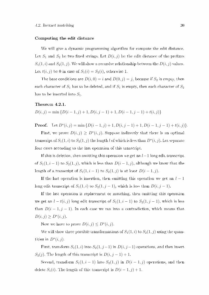
Computing the edit distance
We will give a dynamic programming algorithm for compute the edit distance.
Let S1 and S2 be two �xed strings. Let D(i, j) be the edit distance of the pre�xes
S1(1, i) and S2(1, j). We will show a recursive relationship between theD(i, j) values.
Let t(i, j) be 0 in case of S1(i) = S2(i), otherwise 1.
The base conditions are D(i, 0) = i and D(0, j) = j, because if S2 is empty, then
each character of S1 has to be deleted, and if S1 is empty, then each character of S2
has to be inserted into S1.
Theorem 4.2.1.
D(i, j) = min {D(i− 1, j) + 1, D(i, j − 1) + 1, D(i− 1, j − 1) + t(i, j)}
Proof. LetD∗(i, j) = min {D(i− 1, j) + 1, D(i, j − 1) + 1, D(i− 1, j − 1) + t(i, j)}.
First, we prove D(i, j) ≥ D∗(i, j). Suppose indirectly that there is an optimal
transcript of S1(1, i) to S2(1, j) the length l of which is less thanD∗(i, j). Let separate
four cases according to the last operation of this transcript.
If this is deletion, then omitting this operation we get an l−1 long edit transcript
of S1(1, i− 1) to S2(1, j), which is less than D(i− 1, j), although we know that the
length of a transcript of S1(1, i− 1) to S2(1, j) is at least D(i− 1, j).
If the last operation is insertion, then omitting this operation we get an l − 1
long edit transcript of S1(1, i) to S2(1, j − 1), which is less than D(i, j − 1).
If the last operation is replacement or matching, then omitting this operation
we get an l − t(i, j) long edit transcript of S1(1, i− 1) to S2(1, j − 1), which is less
than D(i − 1, j − 1). In each case we ran into a contradiction, which means that
D(i, j) ≥ D∗(i, j).
Now we have to prove D(i, j) ≤ D∗(i, j).
We will show three possible transformations of S1(1, i) to S2(1, j) using the quan-
tities in D∗(i, j).
First, transform S1(1, i) into S2(1, j−1) in D(i, j−1) operations, and then insert
S2(j). The length of this transcript is D(i, j − 1) + 1.
Second, transform S1(1, i − 1) into S2(1, j) in D(i − 1, j) operations, and then
delete S1(i). The length of this transcript is D(i− 1, j) + 1.

4.2. Inexact matching 21
- A A C C T G
- 0 ← 1 ← 2 ← 3 ← 4 ← 5 ← 6
A ↑ 1 ↖ 0 ←↖ 1 ← 2 ← 3 ← 4 ← 5
C ↑ 2 ↑ 1 ↖ 1 ↖ 1 ←↖ 2 ← 3 ← 4
A ↑ 3 ↖↑ 2 ↖ 1 ←↖↑ 2 ↖ 2 ←↖ 3 ←↖ 4
T ↑ 4 ↑ 3 ↑ 2 ↖ 2 ←↖↑ 3 ↖ 2 ←3
T ↑ 5 ↑ 4 ↑ 3 ↖↑ 3 ↖ 3 ↖↑ 3 ↖ 3
G ↑ 6 ↑ 5 ↑ 4 ↖↑ 4 ↖↑ 4 ↖↑ 4 ↖ 3
Table 4.1: Edit distances
Third, transform S1(1, i− 1) into S2(1, j − 1) in D(i− 1, j − 1) operations, and
then if S1(i) = S2(j) then match, else replace S1(i) to S2(j). The length of this
transcript is D(i− 1, j − 1) + t(i, j).
As we have this transformations, there exists an edit transcript with D∗(i, j)
operations, hence we got that D(i, j) ≤ D∗(i, j), and using our �rst result D(i, j) =
D∗(i, j). �
Using Theorem 4.2.1 we can compute the edit distance of S1 and S2. We will
construct a tabular of edit distances. In the intersection of row i and column j we
write D(i, j). An illustration for the edit distance tabular for the strings AACCTG
and ACATTG from [6] can be seen in Table 4.1. We place a pointer into each cell
by the following rule. Set a pointer from cell (i, j) to cell (i − 1, j) if D(i, j) =
D(i−1, j)+1, set a pointer from cell (i, j) to cell (i, j−1) if D(i, j) = D(i, j−1)+1
and respectively, set a pointer from cell (i, j) to cell (i − 1, j − 1) if D(i, j) =
D(i − 1, j − 1) + t(i, j). In each cell we �nd the value D(i, j), the edit distance of
S1(1, i) and S2(1, j).
Having the tabular, all optimal transcripts can be found by following the pointers
from cell (n,m) backwards to cell (0, 0).
Weighted edit distances
A generalization of edit distance is associating a weight or cost to each edit
operation. Let the insertion and the deletion step have weight d, a replacement has

4.2. Inexact matching 22
weight r and a matching has weight m. Usually m is much smaller than the other
weights. The task is to �nd an edit transcript that transforms S1 into S2 with the
minimum total operation weight.
The original edit distance is a special case of the weighted one with d = r = 1
and m = 0.
Clearly, if r > 2d then an optimal edit transcript does not contain any replace-
ments, because a replacement can be substituted for a deletion and an insertion.
We have a recursive formula for computing the operation-weighted edit dis-
tance. Let D(i, j) denote the weighted edit distance of S1(1, i) and S2(1, j)
and let t(i, j) be m if S1(i) = S2(j) else let it be r. It is easy to
see that D(i, 0) = id and D(0, j) = jd. The recursion is D(i, j) =
min {D(i, j − 1) + d,D(i− 1, j) + d,D(i− 1, j − 1) + t(i, j)}. This statement can
be proved similarly than 4.2.1.
In genetics, it often occurs that the weight depends on exactly which character is
removed and which is added. For example, transforming A into T is more costly than
into G. This distance is alphabet-weighted edit distance. Of course, operation-
weighted edit distance is a special alphabet-weighted edit distance.
4.2.2 Representing DNA sequences with matrices
Randi¢ [12] makes a representation of DNA sequences using 4× 4 matrices con-
structed in a special way, and he states that we can compare two sequences by
comparing several invariants of the matrices.
First, we make an n × n matrix (SD) from the serial distances of the sequence
(see Table 4.2 for the sequence Shine�Dalgarno [8]). That is, the i. row refers to the
i. position of the sequence and the j. column refers to the j. element (A, G, C or
T) of the sequence. aij = k if after the i. position the j. element of the sequence is
the k. of its type (so the same nucleotide base), when j > i. When j < i, let aij be
aji. In case of j = i, aij = 0. In the table only the part above the main diagonal is
represented.
Then we rearrange the n×nmatrix using the next method: the rows are classi�ed
by the appropriate base (so the �rst few columns are A, the next few are C, then T

4.2. Inexact matching 23
G1 A1 T1 T2 C1 C2 T3 A2 G2 G3 A4 G4 G5 T7 T8 T9
1 2 3 4 5 6 7 8 9 10 11 12 13 14 15 16
1 0 1 1 2 1 2 3 2 1 2 3 3 4 4 5 6
2 0 1 2 1 2 3 1 1 2 2 3 4 4 5 6
3 0 1 1 2 2 1 1 2 2 3 4 3 4 5
4 0 1 2 1 1 1 2 2 3 4 2 3 4
5 0 1 1 1 1 2 2 3 4 2 3 4
6 0 1 1 1 2 2 3 4 2 3 4
7 0 1 1 2 2 3 4 1 2 3
8 0 1 2 1 3 4 1 2 3
9 0 1 1 2 3 1 2 3
10 0 1 1 2 1 2 3
11 0 1 2 1 2 3
12 0 1 1 2 3
13 0 1 2 3
14 0 1 2
15 0 1
16 0
Table 4.2: The 16× 16 matrix created from the serial distances (SD)
A1 A2 A3 G1 G2 G3 G4 G5 C1 C2 T1 T2 T3 T4 T5 T6
2 8 11 1 9 10 12 13 5 6 3 4 7 14 15 16
2 0 1 2 1 1 2 3 4 1 2 1 2 3 4 5 6
8 0 1 2 1 2 3 4 1 1 1 1 1 1 2 3
11 0 3 1 1 1 2 2 2 2 2 2 1 2 3
1 0 1 2 3 4 1 2 1 2 3 4 5 6
9 0 1 2 3 1 1 1 1 1 1 2 3
10 0 1 2 2 2 2 2 2 1 2 3
12 0 1 3 3 3 3 3 1 2 3
13 0 4 4 4 4 4 1 2 3
5 0 1 1 1 1 2 3 4
6 0 2 2 1 2 3 4
3 0 1 2 3 4 5
4 0 1 2 3 4
7 0 1 2 3
14 0 1 2
15 0 1
16 0
Table 4.3: The reordered serial distance matrix, RSD
and G respectively). Let i∗ be min(i, j) and j∗ be max(i, j). The ij. element of the
reordered matrix (RSD) is the i∗j∗. element of the matrix SD (See Table 4.3).
In the next step we create the S/S matrix. The ij. element of the S/S matrix is
RSDij/s, where RSDij is the ij. element of the reordered serial distance matrix and
s = |i− j| (See Table 4.4). From this matrix, we create the MN submatrices (where
M,N ∈ A,C, T,G) (see Table . The ij. element of the AA submatrix is s/(j − i),
where s is the serial distance of the i. and the j. A. Respectively, we can create all
the 16 submatrices. The size of the MN submatrix is m×n if in the sequence there
are m M and n N bases. It is clear that MN = NMT .

4.2. Inexact matching 24
A1 A2 A3 G1 G2 G3 G4 G5 C1 C2 T1 T2 T3 T4 T5 T6
2 8 11 1 9 10 12 13 5 6 3 4 7 14 15 16
2 0/0 1/6 2/9 1/1 1/7 2/8 3/10 4/11 1/3 2/4 1/1 2/2 3/5 4/12 5/13 6/14
8 0/0 1/3 2/7 1/1 2/2 3/4 4/5 1/3 1/2 1/5 1/4 1/1 1/6 2/7 3/8
11 0/0 3/10 1/2 1/1 1/1 2/2 2/6 2/5 2/8 2/7 2/4 1/3 2/4 3/5
1 0/0 1/8 2/9 3/11 4/12 1/4 2/5 1/2 2/3 3/6 4/13 5/14 6/15
9 0/0 1/1 2/3 3/4 1/4 1/3 1/6 1/5 1/2 1/5 2/6 3/7
10 0/0 1/2 2/3 2/5 2/4 2/7 2/6 2/3 1/4 2/5 3/6
12 0/0 1/1 3/7 3/6 3/9 3/8 3/5 1/2 2/3 3/4
13 0/0 4/8 4/7 4/10 4/9 4/6 1/1 2/2 3/3
5 0/0 1/1 1/2 1/1 1/2 2/9 3/10 4/11
6 0/0 2/3 2/2 1/1 2/8 3/9 4/10
3 0/0 1/1 2/4 3/11 4/12 5/13
4 0/0 1/3 2/10 3/11 4/12
7 0/0 1/7 2/8 3/9
14 0/0 1/1 2/2
15 0/0 1/1
16 0/0
Table 4.4: The S/S matrix
Now we de�ne a matrix invariant: let W be the average of all elements in the
matrix. Compute W for all submatrices, and create the condensed matrix from this
16 data (See Table 4.5). The condensed matrix is symmetric, so it is enough to store
only the part above the main diagonal.
A G C T
A 0.1604 0.6461 0.4 0.4579
G 0.4429 0.0401 0.0163
C 0.5 0.0454
T 0.4087
Table 4.5: The condensed matrix
Randi¢ expected that di�erent sequences lead to di�erent condensed matrices,
but this is not proved. The other problem of this reduced data storing is that it
is not clear if any biological information can be restored of the condensed matrix,
however, this may be possible.

Summary
As a conclusion, it is clear that the communication between mathematicians and
biologists should be enhanced. Of course, this requires patience and compromises
from both parts. Nowadays, however, the tendencies are prospering.
The interpretation of results of di�erent mathematical methods is very interest-
ing. It is also possible that a result cannot be biologically interpreted. We should
make an e�ort to give a clear and true biological interpretation of mathematical
methods.
On the other hand, we can get di�erent answers for di�erent questions. For
example, the distance of two sequences is not a well-de�ned function.
All things considered, the interdisciplinary �eld biomathematics is very interest-
ing and full of promise.
25

Bibliography
[1] Alizadeh, F., Karp, R., Weisser, D., Zweig, G., Physical mapping of chromo-
somes using unique probes, Journal of Computational Biology, 51, 1990, pp.
431-453
[2] Booth, K., Lueker, G., Testing for the consecutive ones property, interval
graphs and graph planarity testing using pq-tree algorithms, Journal of Com-
puter and System Sciences, 13, 1976, pp. 333-379
[3] Boyer, R.S., Moore, J.S., A fast string searching algorithm, Communications
of the ACM, 1977, pp. 762-772
[4] Chor, B., Sudan, M., A geometric approach to betweenness, SIAM Journal
of Discrete Mathematics, 11, 1998, pp. 511-523
[5] Green, E., Green, P., Sequence-tagged site (STS) content mapping of human
chromosomes: theoretical considerations and early experiences, PCRMethods
and Applications, 1991, pp. 77-90
[6] Gus�eld, D., Algorithms on strings, trees and sequences, Cambridge Univer-
sity Press, 1999, pp. 5-29, 215-225, 395-412
[7] Gutin, G., et al., Betweenness parameterized above tight lower bound, Journal
of Computer and System Sciences, 2010
[8] Láng, F., et al., Növényélettan, A növényi anyagcsere II., in Hungarian,
2007, p. 695
[9] Levenshtein, V. I., Binary codes capable of correcting insertions and reversals,
Soviet Physics � Doklady, 10, 1996, pp. 707-710
26

BIBLIOGRAPHY 27
[10] Opatrny, J., Total ordering problem, SIAM Journal of Computation, 8, 1979,
pp. 111-114
[11] Orosz, L., Klasszikus és molekuláris genetika, in Hungarian, Akadémiai Ki-
adó, 1980
[12] Randi¢, M., On characterization of DNA primary sequences by a condensed
matrix, Chemical Physics Letters, 317, 2000, pp. 29-34
[13] Weinberg, R., Finding the anti-oncogene, Scienti�c American, 1998, pp. 44-51
[14] Williams, N., Europe opens institute to deal with gene data deluge, Science,
269, 1995, p. 630
Related Documents