HAL Id: tel-00486872 https://tel.archives-ouvertes.fr/tel-00486872 Submitted on 27 May 2010 HAL is a multi-disciplinary open access archive for the deposit and dissemination of sci- entific research documents, whether they are pub- lished or not. The documents may come from teaching and research institutions in France or abroad, or from public or private research centers. L’archive ouverte pluridisciplinaire HAL, est destinée au dépôt et à la diffusion de documents scientifiques de niveau recherche, publiés ou non, émanant des établissements d’enseignement et de recherche français ou étrangers, des laboratoires publics ou privés. Blind and semi-blind signal processing for telecommunications and biomedical engineering Vicente Zarzoso To cite this version: Vicente Zarzoso. Blind and semi-blind signal processing for telecommunications and biomedical engi- neering. Signal and Image processing. Université Nice Sophia Antipolis, 2009. tel-00486872

Welcome message from author
This document is posted to help you gain knowledge. Please leave a comment to let me know what you think about it! Share it to your friends and learn new things together.
Transcript
HAL Id: tel-00486872https://tel.archives-ouvertes.fr/tel-00486872
Submitted on 27 May 2010
HAL is a multi-disciplinary open accessarchive for the deposit and dissemination of sci-entific research documents, whether they are pub-lished or not. The documents may come fromteaching and research institutions in France orabroad, or from public or private research centers.
L’archive ouverte pluridisciplinaire HAL, estdestinée au dépôt et à la diffusion de documentsscientifiques de niveau recherche, publiés ou non,émanant des établissements d’enseignement et derecherche français ou étrangers, des laboratoirespublics ou privés.
Blind and semi-blind signal processing fortelecommunications and biomedical engineering
Vicente Zarzoso
To cite this version:Vicente Zarzoso. Blind and semi-blind signal processing for telecommunications and biomedical engi-neering. Signal and Image processing. Université Nice Sophia Antipolis, 2009. �tel-00486872�
Memoire en vue de l’obtention de
l’HABILITATION A DIRIGER DES RECHERCHES
Universite de Nice - Sophia Antipolis
U.F.R. Sciences
TRAITEMENT AVEUGLE ET SEMI-AVEUGLE DU
SIGNAL POUR LES TELECOMMUNICATIONS ET
LE GENIE BIOMEDICAL
Vicente ZARZOSO
Presente le
9 novembre 2009
devant le jury :
M. Pierre Comon President
M. Sergio Cerutti Rapporteur
M. Christian Jutten Rapporteur
M. John McWhirter Rapporteur
M. Eric Moreau Examinateur
M. Jean-Marc Vesin Examinateur

Resume
Ce rapport resume mes activites de recherche depuis l’obtention de mon doctorat.Je me suis penche sur le probleme fondamental de l’estimation de signaux sources apartir de l’observation de mesures corrompues de ces signaux, dans des scenarios oules donnees mesurees peuvent etre considerees comme une transformation lineaireinconnue des sources. Deux problemes classiques de ce type sont la deconvolutionou egalisation de canaux introduisant des distortions lineaires, et la separation desources dans des melanges lineaires. L’approche dite aveugle essaie d’exploiter unmoindre nombre d’hypotheses sur le probleme a resoudre : celles-ci se reduisenttypiquement a l’independance statistique des sources et l’inversibilite du canal oude la matrice de melange caracterisant le milieu de propagation. Malgre les avantagesqui ont suscite l’interet pour ces techniques depuis les annees soixante-dix, les criteresaveugles presentent aussi quelques inconvenients importants, tels que l’existenced’ambiguıtes dans l’estimation, la presence d’extrema locaux associes a des solutionsparasites, et un cout de calcul eleve souvent lie a une convergence lente.
Ma recherche s’est consacree a la conception de nouvelles techniques d’estimationde signal visant a pallier aux inconvenients de l’approche aveugle et donc a ameliorerses performances. Une attention particuliere a ete portee sur deux applications dansles telecommunications et le genie biomedical : l’egalisation et la separation desources dans des canaux de communications numeriques, et l’extraction de l’activiteauriculaire a partir des enregistrements de surface chez les patients souffrant de fib-rillation auriculaire. La plupart des techniques proposees peuvent etre considereescomme etant semi-aveugles, dans le sens ou elles visent a exploiter des informationsa priori sur le probleme etudie autres que l’independance des sources ; par exem-ple, l’existence de symboles pilotes dans les systemes de communications ou desproprietes specifiques de la source atriale dans la fibrillation auriculaire. Dans lestelecommunications, les approches que j’ai explorees incluent des solutions algebri-ques aux fonctions de contraste basees sur la modulation numerique, la combinaisonde contrastes aveugles et supervises dans des criteres semi-aveugles, et une techniqued’optimisation iterative basee sur un pas d’adaptation calcule algebriquement. Nosefforts visant a extraire le signal atrial dans des enregistrements de fibrillation auric-ulaire nous ont permis non seulement de degager de nouvelles fonctions de contrastebasees sur les statistiques de second ordre et d’ordre eleve incorporant l’informationa priori sur les statistiques des sources, mais aussi d’aboutir a de nouveaux resultatsd’impact clinique et physiologique sur ce trouble cardiaque encore mal compris. Cerapport se conclut en proposant quelques perspectives pour la continuation de cestravaux.

Ces recherches ont ete menees en collaboration avec un nombre de colleguesen France et a l’etranger, et ont egalement compris le co-encadrement de plusieursdoctorants. Les contributions qui en ont decoule ont donne lieu a plus de soixantepublications dans des journaux, des conferences et des ouvrages collectifs a caractereinternational. Quelques-unes de ces publications sont jointes a ce document.
Mots-cles : algebre tensorielle, analyse en composantes independantes, analyseen composantes principales, criteres bases sur l’alphabet fini, critere a module con-stant, deconvolution, egalisation du canal, electrocardiogramme, fibrillation auricu-laire, filtrage spatio-temporel, fonctions de contraste, information a priori, kurtosis,modulations numeriques, optimisation iterative, optimisation du pas d’adaptation,problemes inverses, separation de sources, statistiques de second ordre, statistiquesd’ordre eleve, techniques aveugles, techniques semi-aveugles, traitement d’antenne,traitement statistique du signal.

BLIND AND SEMI-BLIND SIGNAL PROCESSING
FOR TELECOMMUNICATIONS AND
BIOMEDICAL ENGINEERING
Report submitted in accordance with the requirements of the
University of Nice - Sophia Antipolis
Faculty of Science
to obtain the
AUTHORIZATION TO SUPERVISE RESEARCH
Vicente Zarzoso
Defended on
November 9, 2009
in front of the jury:
Pierre Comon Chairman
Sergio Cerutti Reviewer
Christian Jutten Reviewer
John McWhirter Reviewer
Eric Moreau Examiner
Jean-Marc Vesin Examiner

Abstract
The present report summarizes the research activities that I have carried out sincecompletion of my PhD. My attention has focused on the fundamental signal pro-cessing problem of source signal estimation from the observation of corrupted mea-surements, in scenarios where the measured data can be considered as unknownlinear transformations of the sources. Two typical problems of this kind are thedeconvolution or equalization of channels introducing linear distortions and sourceseparation in linear mixtures. The blind approach makes as few assumptions aspossible about the problem in hand: these typically reduce to the statistical in-dependence of the sources and the invertibility of the channel or mixing matrixcharacterizing the propagation medium. Despite the advantages that have driventhe interest in these techniques since the 70’s, blind criteria also present some im-portant drawbacks such as the existence of estimation ambiguities, the presence oflocal extrema leading to spurious solutions, and a high computational complexityoften linked to slow convergence.
My research has been devoted to the design of novel signal estimation techniquesalleviating the drawbacks and thus improving the performance of the blind approach.Special emphasis has been laid on two specific applications in telecommunicationsand biomedical engineering: equalization and source separation in digital communi-cation channels and atrial activity extraction in surface electrocardiogram recordingsof atrial fibrillation patients. Most of the proposed techniques can be consideredas semi-blind in that they aim at exploiting available prior information about theproblems under study other than source independence; e.g., the existence of train-ing data in communication systems or specific properties about the atrial source inatrial fibrillation. In communications, the approaches that I have explored includealgebraic solutions to contrast functions based on digital modulations, the combina-tion of blind and training-based contrasts into semi-blind criteria, and an iterativeoptimization technique with an optimal step-size coefficient computed algebraically.Our efforts to extract the atrial signal in multi-lead atrial fibrillation recordings hasled not only to new contrast functions based on second- and higher-order statisticsincorporating priors about the source statistics, but also to novel results of clinicaland physiological significance about this challenging cardiac condition. The reportconcludes by proposing some possible avenues for the continuation of this work.
This investigation has been carried out in collaboration with a number of col-leagues in France and abroad, and has also comprised the joint supervision of severalPhD students. The resulting contributions have given rise to over sixty publicationsin international journals, conferences and book chapters. A compilation of selected
i

ii
publications is attached to this document.
Keywords: alphabet-based criteria, array signal processing, atrial fibrillation,blind techniques, channel equalization, constant modulus, contrast functions, decon-volution, digital modulations, electrocardiogram, higher-order statistics, indepen-dent component analysis, inverse problems, iterative optimization, kurtosis, princi-pal component analysis, prior information, second-order statistics, semi-blind tech-niques, source separation, space-time filtering, statistical signal processing, step-sizeoptimization, tensor algebra.
Acknowledgments
A large part of the work summarized in this report has been made possible by theparticipation of many individuals, and citing them all would probably fill manypages.
First of all, I feel indebted to Pierre Comon, Olivier Meste and Tarek Hamel, fortheir constant support and encouragement, for believing in me, since I arrived at theI3S Laboratory. Many other people have greatly contributed to making my workat I3S very pleasant. I will just mention here Viviane Rosello, Micheline Hagnereand Sabine Barrere. I am also very grateful to my teaching colleagues at the GEIIDepartment, IUT Nice - Cote d’Azur, for the friendly work atmosphere.
Doing research is all about learning and discovering new things, and I have learntso many from all the collaborators I have worked with over the years, including thestudents I have helped supervise. Their knowledge, skills and enthusiasm have beena continuous source of stimulation. My collaborations with Pietro Bonizzi, NarcısCardona, Francisco Castells, Pierre Comon, Adriana Dapena, Yumang Feng, JorgeIgual, Kostas Kokkinakis, Olivier Meste, Jose Millet, Juan Jose Murillo, Asoke K.Nandi, Hector J. Perez-Iglesias, Ronald Phlypo, Jose J. Rieta, Ludwig Rota, Addis-son Salazar, Luis Vergara and Wenhuan Xu have been as enjoyable as rewarding,and often excitingly challenging.
I would like to express my most sincere gratitude to Sergio Cerutti, PierreComon, Christian Jutten, John McWhirter, Eric Moreau and Jean-Marc Vesin forwillingly accepting to be part of the jury. I feel honored that such renowned re-searchers have spent some of their precious time and energy to evaluate my work.
Olivier Meste, Herve Rix and Gerard Favier, colleagues at I3S, sacrificed valuabletime from their busy timetables to carefully read a preliminary version of this reportand give me some interesting suggestions. Together with Luc Deneire, they alsooffered me useful advice for my defense preparation. I thank them for their feedback.
Last but not least, I am infinitely grateful to my family. Without their love,everything else would have been impossible, if not just meaningless. My wife, Car-oline, has been particularly loving, patient and supportive over the preparation ofmy HDR.
iii


Contents
Abstract i
Acknowledgments iii
Acronyms ix
1 Extended CV 1
1.1 Personal Details . . . . . . . . . . . . . . . . . . . . . . . . . . . . . 1
1.2 Career Evolution . . . . . . . . . . . . . . . . . . . . . . . . . . . . . 1
1.3 Research Activities . . . . . . . . . . . . . . . . . . . . . . . . . . . . 2
1.3.1 Research Areas . . . . . . . . . . . . . . . . . . . . . . . . . . 2
1.3.2 Thematic Mobility . . . . . . . . . . . . . . . . . . . . . . . . 4
1.3.3 Geographic Mobility . . . . . . . . . . . . . . . . . . . . . . . 4
1.3.4 International Collaborations and Invitations by Foreign Uni-versities . . . . . . . . . . . . . . . . . . . . . . . . . . . . . . 5
1.3.5 Students’ Supervision . . . . . . . . . . . . . . . . . . . . . . 6
1.3.6 Publications . . . . . . . . . . . . . . . . . . . . . . . . . . . . 8
1.3.7 Presentations and Seminars . . . . . . . . . . . . . . . . . . . 8
1.3.8 Reviewing and Chairing . . . . . . . . . . . . . . . . . . . . . 9
1.3.9 PhD Thesis Jury Participation . . . . . . . . . . . . . . . . . 10
1.3.10 Research Funding Proposals . . . . . . . . . . . . . . . . . . . 11
1.4 Teaching Activities . . . . . . . . . . . . . . . . . . . . . . . . . . . . 11
1.5 Other Activities . . . . . . . . . . . . . . . . . . . . . . . . . . . . . . 12
1.5.1 Research-Related Responsibilities . . . . . . . . . . . . . . . . 12
1.5.2 Consultancy . . . . . . . . . . . . . . . . . . . . . . . . . . . . 12
1.6 Awards and Other Distinctions . . . . . . . . . . . . . . . . . . . . . 12
2 Introduction to Research Activities 15
2.1 Motivation . . . . . . . . . . . . . . . . . . . . . . . . . . . . . . . . 15
2.2 Mathematical Formulation and Problem Taxonomy . . . . . . . . . . 16
2.3 Brief Historical Survey . . . . . . . . . . . . . . . . . . . . . . . . . . 19
2.4 PhD Research . . . . . . . . . . . . . . . . . . . . . . . . . . . . . . . 22
2.4.1 Other PhD-Related Research . . . . . . . . . . . . . . . . . . 24
2.5 Research Goals After my PhD . . . . . . . . . . . . . . . . . . . . . . 25
v
vi CONTENTS
3 Robust Equalization and Source Separation 27
3.1 Motivation . . . . . . . . . . . . . . . . . . . . . . . . . . . . . . . . 27
3.2 ICA-Based MIMO Channel Equalization . . . . . . . . . . . . . . . . 28
3.3 Algebraic Equalizers . . . . . . . . . . . . . . . . . . . . . . . . . . . 30
3.3.1 Algebraic Solutions to the MMSE Criterion . . . . . . . . . . 31
3.3.2 Algebraic Solutions to the CM Criterion . . . . . . . . . . . . 32
3.3.3 Algebraic Solutions to the CP Criterion . . . . . . . . . . . . 33
3.3.3.1 Some definitions . . . . . . . . . . . . . . . . . . . . 34
3.3.3.2 Problem formulation . . . . . . . . . . . . . . . . . . 34
3.3.3.3 Determining a basis of the solution space . . . . . . 34
3.3.3.4 Matrix and tensor algebra problems . . . . . . . . . 35
3.3.3.5 Solution structuring methods . . . . . . . . . . . . . 36
3.3.3.6 A subspace approach to solution structuring . . . . 37
3.3.3.7 Recovering the equalizer vector from its symmetrictensor vectorization . . . . . . . . . . . . . . . . . . 37
3.3.3.8 Approximate solution in the presence of noise . . . 38
3.3.3.9 Experimental analysis . . . . . . . . . . . . . . . . . 39
3.4 Semi-Blind Criteria . . . . . . . . . . . . . . . . . . . . . . . . . . . . 39
3.4.1 Algebraic Semi-Blind Equalizers . . . . . . . . . . . . . . . . 40
3.4.2 Iterative Semi-Blind Equalizers . . . . . . . . . . . . . . . . . 41
3.5 Optimal Step-Size Iterative Search . . . . . . . . . . . . . . . . . . . 42
3.5.1 Approaches to Step-Size Selection . . . . . . . . . . . . . . . 42
3.5.2 An Algebraically Computed Optimal Step Size . . . . . . . . 43
3.5.3 The RobustICA Algorithm . . . . . . . . . . . . . . . . . . . 45
3.6 Additional results . . . . . . . . . . . . . . . . . . . . . . . . . . . . . 46
3.6.1 Source Extraction Using Alphabet-Based Criteria . . . . . . . 46
3.6.2 Blind Channel Estimation in Space-Time Coded Systems . . 48
3.6.3 Optical Transmission Monitoring . . . . . . . . . . . . . . . . 49
3.7 Summary . . . . . . . . . . . . . . . . . . . . . . . . . . . . . . . . . 50
4 Atrial Activity Extraction in AF episodes 53
4.1 Motivation . . . . . . . . . . . . . . . . . . . . . . . . . . . . . . . . 53
4.2 Approaches to Atrial Signal Extraction in AF . . . . . . . . . . . . . 54
4.3 Blind and Semi-Blind Biomedical Signal Processing . . . . . . . . . . 57
4.4 BSS/ICA Approach to Atrial Signal Extraction . . . . . . . . . . . . 58
4.5 Combining non-Gaussianity and Spectral Features . . . . . . . . . . 59
4.6 Exploiting Prior Information on Source Kurtoses . . . . . . . . . . . 60
4.6.1 Novel HOS-Based Contrasts Using Prior Information . . . . . 60
4.6.2 Atrial Signal Extraction by Kurtosis Maximization with Ro-bustICA . . . . . . . . . . . . . . . . . . . . . . . . . . . . . . 62
4.7 Exploiting Spectral Concentration with SOS Only . . . . . . . . . . 63
4.7.1 Atrial Signal Extraction by Spectral Concentration Maximiza-tion . . . . . . . . . . . . . . . . . . . . . . . . . . . . . . . . 63
4.7.2 A Novel Contrast for Source Extraction Based on ConditionalSecond-Order Moments . . . . . . . . . . . . . . . . . . . . . 64
4.7.3 Blind Source Extraction Based on Second-Order Statistics . . 68
CONTENTS vii
4.8 Exploiting the Spatial Topographies . . . . . . . . . . . . . . . . . . 694.9 Clinical and Physiological Information . . . . . . . . . . . . . . . . . 70
4.9.1 Atrio-ventricular junction behavior during AF . . . . . . . . 704.9.2 AF classification . . . . . . . . . . . . . . . . . . . . . . . . . 70
4.10 Summary . . . . . . . . . . . . . . . . . . . . . . . . . . . . . . . . . 72
5 Research Perspectives 735.1 Algorithms for Robust Equalization and Source Separation . . . . . 735.2 Atrial Fibrillation Analysis . . . . . . . . . . . . . . . . . . . . . . . 75
Bibliography 79Equalization and Source Separation . . . . . . . . . . . . . . . . . . . . . 79Atrial Fibrillation Analysis and Biomedical . . . . . . . . . . . . . . . . . 88Other Topics . . . . . . . . . . . . . . . . . . . . . . . . . . . . . . . . . . 91
List of Publications 93Submissions in Preparation or Under Review . . . . . . . . . . . . . . . . 93Published or in Press . . . . . . . . . . . . . . . . . . . . . . . . . . . . . . 94Publications Related to PhD Research . . . . . . . . . . . . . . . . . . . . 100
Selected Publications 103Journal Papers . . . . . . . . . . . . . . . . . . . . . . . . . . . . . . . . . 105Conference Papers . . . . . . . . . . . . . . . . . . . . . . . . . . . . . . . 231

Acronyms
AA atrial activityABS average beat subtractionACMA analytic constant modulus algorithmACPA analytic constant power algorithmAEML alternative extended maximum likelihoodAF atrial fibrillationAFL atrial flutterAML approximate maximum likelihoodANC adaptive noise cancellationAPF alphabet polynomial fittingASTRE former Signal Processing for Communications Research Group, now part
of the SIGNAL team at the I3S LabAV atrio-ventricular
BIOMED former Biomedical Signal Processing Research Group, now part of the SIG-NAL team at the I3S Lab
BPSK binary phase shift keyingBSPM body surface potential mappingBSS blind source separation
CCI co-channel interferenceCF Comon’s formulaCFAE complex fractionated atrial electrogramCHU university hospitalCM constant modulusCMA constant modulus algorithmCoM contrast maximizationCP constant powerCPA constant power algorithm
DERA Defence Evaluation and Research Agency, UKDFT discrete Fourier transform
ECG electrocardiogramEML extended maximum likelihoodETSIT Higher Telecommunications Engineering School at UPVEVD eigenvalue decomposition
FIR finite impulse response
GEII Electrical Engineering and Industrial Data Processing Department
HOS higher-order statistics
I3S Computer Science, Signals and Systems Laboratory of Sophia Antipolis,France
ICA independent component analysis
ix
x ACRONYMS
i.i.d. independent and identically distributedISI intersymbol interferenceISM industrial, scientific and medical frequency bandIUT University Institute of Technology
JADE joint approximate diagonalization of eigenmatrices
KM kurtosis maximizationKSP kurtosis sign priorsKVP kurtosis value priors
LMS least mean squaresLS least squares
MAP maximum a posterioriMaxViT maximum variance in tailsMIMO multiple input multiple outputMISO multiple input single outputML maximum likelihoodMMSE minimum mean square errorMSK minimum shift keying
NSR normal sinus rhythm
OS-CMA optimal step-size constant modulus algorithmOS-CPA optimal step-size constant power algorithmOSTBC orthogonal space-time block coding
PCA principal component analysispdf probability density functionPEDR bonus for research and doctoral supervisionPSK phase shift keying
QPSK quadrature phase shift keying
RACMA real analytic constant modulus algorithmRF radiofrequency
SC spectral concentrationSIMO single input multiple outputSISO single input single outputSNR signal-to-noise ratioSOBI second-order blind identificationSOS second-order statisticsSPC Signal Processing for Communications Research Group at the University
of Liverpool, UKSTC spatiotemporal QRST cancellationSVD singular value decomposition
UPV Polytechnic University of Valencia, Spain
VA ventricular activityV-BLAST vertical Bell Labs layered space-time architecture
WDA wavelength dependent attenuatorWDM wavelength division multiplexing
ZF zero forcing

Chapter 1
Extended CV
1.1 Personal Details
Name: Vicente ZARZOSO
Birth date and place: Sep. 12, 1973, Valencia (Spain)
Nationality: Spanish
Family status: married since July 15, 2005one child since Sep. 28, 2007
Personal address: 96 Corniche Fleurie, Sirius-B, 06200 Nice, France
Professional address: Laboratoire I3S, Les Algorithmes - Euclide-B2000 route des Lucioles, BP 12106903 Sophia Antipolis Cedex, FranceTel: +33 (0)4 92 94 27 95Fax: +33 (0)4 92 94 28 [email protected]
http://www.i3s.unice.fr/~zarzoso
1.2 Career Evolution
Since2005
Lecturer/researcher (maıtre de conferences)Teaching: Departement de Genie Electrique et Informatique Industrielle(GEII), IUT Nice - Cote d’Azur, Univ. Nice - Sophia Antipolis.Research: Laboratoire d’Informatique, Signaux et Systemes de Sophia An-tipolis (I3S).
In Jan. 2007, I was promoted to grade 3 (3eme echelon) of the maıtres deconferences salary scale.
Since Sep. 2007, I have been in receipt of a Bonus for Research and Doc-toral Supervision (Prime d’encadrement doctoral et de recherche, PEDR)from the French Ministry of Education.
1
2 CHAPTER 1. EXTENDED CV
2000–2005
Research Fellow, Royal Academy of Engineering, UKDepartment of Electrical Engineering & Electronics, University of Liver-pool, UK.Topic: blind signal separation for communications and biomedical engi-neering.
1999 PhD, University of Liverpool, UKThesis: “Closed-Form Higher-Order Estimators for Blind Separation ofIndependent Source Signals in Instantaneous Linear Mixtures” (PhD viva:Oct. 14, 1999).Supervisor: Prof. Asoke K. Nandi.Funding: University Scholarships; my first year was also partially fundedby the Defence Evaluation and Research Agency (DERA) of the UK.I was awarded the Robert Legget Prize (2000) for an especially distinguishedthesis submitted to the Faculty of Engineering.
1996 MEng Telecommunications, Universidad Politecnica de Valencia(UPV), SpainI graduated with the highest distinction (rank: 1st) at the Escuela TecnicaSuperior de Ingenieros de Telecomunicacion (ETSIT).
1.3 Research Activities
1.3.1 Research Areas
My research has focused on the fundamental signal processing problem of signalestimation in linear mixtures, including blind channel equalization, blind sourceseparation (BSS) and independent component analysis (ICA). I am interested inthe theoretical aspects at the heart of these techniques as well as their practicalapplication to telecommunications and biomedical engineering. Details about theseactivities can be found in Chapters 3 and 4.
Since 2005: my activities have lain at the interface between two groups of theI3S Lab: the Signal Processing for Communications (ASTRE) group, leaded byPierre Comon, and the Biomedical Signal Processing (BIOMED) group, leaded byHerve Rix.1
• In the area of signal processing for communications, I have worked on thefollowing topics:
– blind and semi-blind channel equalization based on the finite alphabetproperty of digital communication signals;
– efficient iterative optimization with optimal step-size selection for channelequalization and source separation;
– contrasts for BSS/ICA incorporating prior information about the signalsof interest.
1In 2008, both groups merged into the SIGNAL research team.
1.3. RESEARCH ACTIVITIES 3
Publications: [P4,P5,P8,P9,P14,P15,P37,P40,P41].2
• In biomedical signal processing, I have contributed to the topic of:
– atrial activity analysis in atrial fibrillation episodes using BSS/ICA-basedtechniques exploiting prior information.
Publications: [P1, P2, P3, P6, P10, P11, P13, P25, P26, P28, P29, P30, P31,P32,P33,P34,P35,P36,P38].
Publications involving a close collaboration between the ASTRE and BIOMEDgroups: [P5,P11,P14,P26,P30,P32,P38],
Publications issued from students’ supervision: [P1, P2, P3, P5, P6, P13, P14,P25,P28,P29,P31,P32,P33,P34,P35,P36,P38].
2000–2005: my postdoctoral research was carried out at the Signal Processing andCommunications (SPC) research group, leaded by Asoke K. Nandi, University ofLiverpool, UK. The final two years comprised a stay at the I3S Lab (Sec. 1.3.4).
• The topics covered during this period include the application of BSS/ICAtechniques to:
– space-time equalization in wireless digital communication systems;
– optical transmission monitoring;
– atrial activity extraction in atrial fibrillation episodes.
Publications: [P12, P17, P18, P19, P20, P21, P22, P23, P24, P42, P43, P44, P45,P46, P47, P48, P49, P50, P51, P52, P53, P54, P55, P56, P57, P58, P59, P60, P61,P62,P63,P64,P65,P66,P67]
Publications issued from students’ supervision: [P22, P42, P45, P51, P52, P58,P59,P61].
1995–1999: my MEng final year project and the first two years of my PhD stud-ies took place at the Department of Electrical & Electronic Eng., University ofStrathclyde, Glasgow, UK, under the supervision of Asoke K. Nandi. My PhD thenconcluded at the University of Liverpool.
• Topics:
– closed-form estimators for BSS/ICA in the two-signal case;
– application to non-invasive fetal activity extraction from maternal skinelectrode recordings.
Publications: [P69]– [P90].
2Underlined publications are attached to this report.
4 CHAPTER 1. EXTENDED CV
1.3.2 Thematic Mobility
Before2003
My research focused on generic theoretical aspects of blind signal processingand, in particular, the problems of BSS/ICA. The performance of theBSS/ICA techniques that I developed were illustrated on signals issuedfrom biomedical applications such as non-invasive fetal electrocardiogramextraction during pregnancy and, since 2000, non-invasive atrial activityextraction in atrial fibrillation episodes.
2003–2005
My postdoctoral stay at the I3S Lab (ASTRE group) allowed me to deepenmy understanding of the theoretical aspects of blind and semi-blind signalprocessing, with particular emphasis on applications related to telecommu-nications and biomedical engineering. Semi-blind techniques incorporateprior information into purely blind techniques, generating algorithms moreadapted to the particular problem under study and thus yielding improvedperformance.
Since2005
My research has been shared between the ASTRE and BIOMED groups(now SIGNAL team) of the I3S Lab, where
— I have been gaining further understanding of theoretical aspects ofblind and semi-blind signal processing;
— I have been searching for more specific semi-blind techniques foratrial fibrillation analysis.
1.3.3 Geographic Mobility
My studies and professional activities have taken place in four universities of threedifferent countries:
1991–1995
Universidad Politecnica de Valencia, SpainFirst four years of MEng in Telecommunications.
1995–1999
University of Strathclyde, Glasgow, UKErasmus year followed by my first two years of PhD studies.
1999–2003
University of Liverpool, UKEnd of my PhD studies and first three years of my postdoctoral research,funded by the Royal Academy of Engineering.
2003– Universite de Nice - Sophia Antipolis, FranceTwo-year postdoctoral stay at I3S Lab.Permanent lecturer/researcher position since Sep. 2005.
1.3. RESEARCH ACTIVITIES 5
1.3.4 International Collaborations and Invitations by Foreign Uni-versities
2006– Institute Biomedical Technology (IbiTech), Universiteit Gent,BelgiumCollaborators: Ronald Phlypo (PhD student) and Ignace Lemahieu.Topic: atrial activity extraction from surface recordings of atrial fibrillationby exploiting prior information about the signal of interest (Secs. 4.6–4.7,pp. 60–68.)Publications: [P1,P3,P5,P6,P11,P13,P14,P32,P33,P34,P36,P38].
2006– Departamento de Electronica y Sistemas, Universidad de laCoruna, SpainCollaborators: Hector J. Perez-Iglesias and Adriana Dapena.Topic: application of BSS/ICA techniques based on the eigenvalue de-composition of second- and fourth-order cumulant matrices to blind chan-nel estimation in space-time coded communications systems (Sec. 3.6.2,pp. 48–49).Publications: [P7,P16,P27,P39].
2004– Departamento de Senal y Comunicaciones, Universidad deSevilla, SpainCollaborator: Juan J. Murillo-Fuentes.Topic: algebraic solutions to ICA based on fourth-order statistics(Sec. 2.4.1, p. 24).Publications: [P18,P44,P49].
2003–2005
Groupe ASTRE, Laboratoire I3SCollaborator: Pierre Comon.Topic: during my postdoctoral stay, we worked on algebraic and iterativesolutions for blind and semi-blind channel equalization based on digitalsignal alphabets (Secs. 3.3–3.5, pp. 30–46, and Sec. 3.6.1, pp. 46–48).Stay funded by a “Research Fellowship” awarded by the Royal Academyof Engineering, UK.Publications: [P12,P17,P19,P42,P43,P45,P46].
12/03–01/04
Departamento de Comunicaciones, UPVCollaborators: Oscar Lazaro, Gema Pinero and Narcıs Cardona.Topic: blind channel estimation in 3rd-generation (UMTS) mobile tele-phony systems with distributed antennas.Stay funded by “Programa de Incentivo a la Investigacion de la UPV 2003— Estancias en la UPV de Investigadores de Prestigio.”The stay included a talk to the members of the department on the funda-mentals of blind channel identification (Sec. 1.3.7).
6 CHAPTER 1. EXTENDED CV
12/01–01/02
Departamento de Comunicaciones, UPVCollaborators: Jorge Igual and Luis Vergara.Topic: space-time MIMO channel equalization using BSS/ICA techniques(Sec. 3.2, pp. 28–30).Stay funded by “Programa de Incentivo a la Investigacion de la UPV 2001— Estancias en la UPV de Investigadores de Prestigio.”Publications: [P53,P60].
2000– Grupo de Bioingenierıa, UPVCollaborators: Jose J. Rieta, Francisco Castells and Jose Millet.Topic: biomedical signal processing applications, with focus on atrial fib-rillation analysis (Secs. 4.4–4.5, pp. 58–60, and Sec. 4.9.2, pp. 70–71).Stay partly funded by the Consejo Superior de Investigaciones Cientıficas(CSIC) [Spanish National Research Council].Publications: [P2,P20,P21,P25,P48,P56,P57,P63,P67,P73,P79].
1.3.5 Students’ Supervision
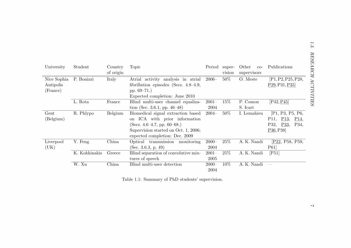
My implication in the supervision of PhD students is summarized in Table 1.1.I have helped supervise six students of five different nationalities from three differentuniversities. Four of these students have successfully completed their PhD, whereasthe two others are still pursuing their degree. This supervisory work has resultedin the publication of a book chapter [P11], three journal articles [P13, P14, P22]and sixteen conference papers [P25,P28,P29,P31,P32,P33,P34,P35,P36,P38,P42,P45, P51, P58, P59, P61] (Sec. 1.3.6). In addition, another book chapter [P1] isbeing prepared, while four journal articles [P2,P3,P5,P6] have been submitted forpublication.
I have also contributed to the supervision of several MSc students’ projects inthe UK:
Student Topic Year PublicationsK. Kokkinakis Blind audio source separation 2001 —S. Punnoose Blind multicarrier equalization 2002 —L. Sarperi Blind deconvolution of digital communica-
tion channels2002 [P52]
In addition, I have supervised the following final year project students:
Students School Topic Year
J. ThaonC. Beaussieux
IUT GEII Digital filtering of biomedical signals:a Java demonstrator
2007
J. NeveuxJ. Aumard
IUT GEII Digital filtering of biomedical signals:a Java demonstrator
2008
M. ZahriS. Canavese
IUT GEII Atrial fibrillation signal database 2009
J. NeveuxN. Bessou
ENSEA Cergy-Pontoise
Atrial fibrillation signal database 2009
1.3.R
ESE
AR
CH
AC
TIV
ITIE
S7
University Student Countryof origin
Topic Period super-vision
Other co-supervisors
Publications
Nice SophiaAntipolis(France)
P. Bonizzi Italy Atrial activity analysis in atrialfibrillation episodes (Secs. 4.8–4.9,pp. 69–71.)Expected completion: June 2010
2006– 50% O. Meste [P1,P2,P25,P28,P29,P31,P35]
L. Rota France Blind multi-user channel equaliza-tion (Sec. 3.6.1, pp. 46–48)
2001–2004
15% P. ComonS. Icart
[P42,P45]
Gent(Belgium)
R. Phlypo Belgium Biomedical signal extraction basedon ICA with prior information(Secs. 4.6–4.7, pp. 60–68.)Supervision started on Oct. 1, 2006;expected completion: Dec. 2009
2004– 50% I. Lemahieu [P1, P3, P5, P6,P11, P13, P14,P32, P33, P34,P36,P38]
Liverpool(UK)
Y. Feng China Optical transmission monitoring(Sec. 3.6.3, p. 49)
2000–2004
25% A. K. Nandi [P22, P58, P59,P61]
K. Kokkinakis Greece Blind separation of convolutive mix-tures of speech
2001–2005
25% A. K. Nandi [P51]
W. Xu China Blind multi-user detection 2000–2004
10% A. K. Nandi —
Table 1.1: Summary of PhD students’ supervision.

8 CHAPTER 1. EXTENDED CV
1.3.6 Publications
My list of publications appears at the end of the present document (pp. 93–102).The number of articles published or in press can be summarized as follows:
Chapters Journals Conferences
Total 6 21 54
First author 6 16 26Supervision 1 3 16Collaborations — 5 17
Implication in article composition, including works under review and in preparation:
• Main author of research work and paper writing (56):[P4,P5,P8,P9,P10,P11,P12,P14,P15,P17,P18,P19,P23,P24,P26,P30,P37,P40, P41, P42, P43, P44, P45, P46, P47, P50, P53, P54, P55, P60, P62, P64, P65,P66, P69, P70, P71, P72, P73, P74, P75, P76, P77, P78, P79, P80, P81, P82, P83,P84,P85,P86,P87,P88,P89,P90].
• Collaborator in research work and paper writing (30):[P1, P2, P3, P6, P7, P13, P16, P20, P21, P22, P25, P27, P28, P29, P31, P32, P33,P34,P35,P36,P38,P39,P48,P49,P51,P52,P58,P59,P61,P67].
• Collaborator in research work, without direct implication in paper writing (3):[P56,P57,P63].
Invited conference contributions (3): [P26,P30,P39].
1.3.7 Presentations and Seminars
I was an invited lecturer at the 6th International Summer School on BiomedicalSignal Processing, Siena, Italy, July 10–17, 2007, organized by the IEEE Engineeringin Medicine and Biology Society (EMBS). I delivered two lectures on “Blind sourceseparation: theory and methods” (1.5h) and “Application of BSS to cardiac signalextraction” (1.5h). The content of these lectures was later expanded into bookchapter [P10].
Talks at international conferences (16): [P26,P30,P37,P40,P41,P47,P53,P59,P60,P64,P82,P83,P85,P86,P87,P88]; invited: [P26,P30].
Poster presentations at international conferences (11): [P43,P44,P46,P50,P52,P61,P62,P65,P66,P84,P89].
I obtained an Award for meritorious final-year project poster presentation at the De-partment of Electrical & Electronic Engineering, University of Strathclyde, Glasgow(1996).
1.3. RESEARCH ACTIVITIES 9
Seminars:
July 72009
“Quelques resultats et perspectives sur l’analyse de la fibrillation auricu-laire”Dept. Cardiologie, Centre Hospitalier Princesse Grace, Monaco.
May 222008
“Egalisation robuste du canal de communication numerique”Laboratoire I3S, Signals, Images and Systems Research Pole seminar.
Sep. 42007
“Egalisation robuste du canal de communication numerique”Ecole Nationale d’Ingenieurs de Monastir, Tunisia, Departement de GenieElectrique, visiting researcher seminar invited by Hassani Messaoud.
Mar. 152006
“Extraction de l’activite auriculaire par des techniques de separation aveu-gle de sources”Laboratoire I3S, Doctoral Student Association (ADSTIC) seminar.
Mar. 312005
“Analyse de la fibrillation auriculaire par des techniques de separationaveugle de sources”Laboratoire des Images et des Signaux (LIS, now GIPSA-Lab), Grenoble.
Dec. 72004
“Cardiac signal extraction by blind source separation techniques”Laboratoire I3S, seminar invited by Luc Pronzato (then SIROCCO projectleader, now I3S Lab Director).
Nov. 32004
“Optimal step-size constant modulus algorithm for blind equalization”University of Liverpool, Dept. Electrical Eng. & Electronics, SPC Groupseminar.
Jan. 192004
“Blind processing of digital communication signals”UPV, Departamento de Comunicaciones, visiting researcher’s seminar in-vited by Narcıs Cardona.
Nov. 182003
“Application of independent component analysis to blind MIMO equaliza-tion”Laboratoire I3S, ASTRE team seminar.
Nov. 282002
“Blind space-time equalization for future wireless digital communicationsystems”University of Liverpool, Dept. Electrical Eng. & Electronics, departmentalseminar.
1.3.8 Reviewing and Chairing
Area Chair of the ”Signal Processing Theory, Detection and Estimation” Trackat EUSIPCO-2009, 17th European Signal Processing Conference, Glasgow, UK,Aug. 24-28, 2009. I managed the review of 15 submissions on this area.
Technical program committee member of the International Conference on Indepen-dent Component Analysis and Signal Separation 2004 (I reviewed 5 papers), 2006(6 papers), 2007 (5 papers) and 2009 (4 papers).
10 CHAPTER 1. EXTENDED CV
Reviewer of international conferences: IEEE International Conference on Acoustics,Speech and Signal Processing 2008 (2) and 2009 (2), IEEE Engineering in Medicineand Biology Conference 2007 (2) and 2008 (5), IEEE Workshop on Statistical SignalProcessing 2009 (1), IEEE International Symposium on Information Theory 2007(1), IEEE International Conference on Communications 2006 (1), IEEE Interna-tional Symposium on Circuits and Systems 2005 (4), European Signal ProcessingConference 2006 (1).
Reviewer of international journals: IEEE Transactions on Signal Processing (11),IEEE Transactions on Biomedical Engineering (11), IEEE Signal Processing Let-ters (8), IEEE Transactions on Neural Networks (2), IEEE Transactions on Circuitsand Systems I (2), IEEE Transactions on Speech and Audio Processing (1), IEEETransactions on Wireless Communications (1), IEEE Communications Letters (1),Elsevier’s Signal Processing (8), IEE Proceedings - Communications (1), IEE Pro-ceedings - Vision, Image and Signal Processing (2), Electronics Letters (8), Interna-tional Journal of Adaptive Control and Signal Processing (4), EURASIP Journal ofApplied Signal Processing (2), EURASIP Journal on Advances in Signal Process-ing (1), Neurocomputing (4), Medical & Biomedical Engineering & Computing (1).
Since 2000, I have reviewed 68 journal manuscripts and 39 conference submis-sions.
My reviewing activities were awarded an IEEE Reviewer Appreciation for sig-nificant commitment to the IEEE Transactions on Signal Processing reviewprocess in 2008 (by Prof. Alle-Jan van der Veen, IEEE TSP Editor-in-Chiefin 2006–2008).
I have chaired talk sessions at the following conferences:
DSP-2002, 14th International Conference on Digital Signal Processing, San-torini, Greece, July 1–3, 2002
ICA Research Network International Workshop, Liverpool, UK, Sept. 18–19,2006
Medical Physics and Biomedical Engineering World Congress, Sept. 7–12, 2009(Focus Session: PCA/ICA in Biomedical Signal Processing, co-chaired withLuca Mainardi, Politecnico di Milano, Italy).
1.3.9 PhD Thesis Jury Participation
Raul Llinares-Llopis, “Applications of semi-blind source separation in astrophysicsand biomedical engineering”, supervised by Jorge Igual, Universidad Politecnica deValencia, Spain (examination: Jan. 19, 2009).
Reza Sameni, “Extraction of fetal cardiac signals from an array of maternal abdom-inal recordings”, supervised by Christian Jutten and Mohammad B. Shamsollahi,Institut Polytechnique de Grenoble, GIPSA-Lab (July 7, 2008).
Ahmed R. Borsali, “Compression parametrique du signal electrocardiographique :application aux arythmies cardiaques”, supervised by Jacques Lemoine and Amine
1.4. TEACHING ACTIVITIES 11
Naıt-Ali, Laboratoire Images, Signaux et Systemes Intelligents (LISSI), UniversiteParis XII - Val de Marne (May 31, 2007).
Jose J. Rieta-Ibanez, “Estimacion de la actividad auricular en episodios de fibrilacionauricular mediante separacion ciega de fuentes”, supervised by Jose Millet-Roig,Universidad Politecnica de Valencia, Spain (July 21, 2003).
1.3.10 Research Funding Proposals
I have coordinated the following proposals submitted to the French National Re-search Agency (Agence nationale de la recherche, ANR) Young Investigators’ Pro-gram:
“Signal Extraction for the Analysis of Supraventricular Arrhythmias in theSurface Electrocardiogram” (Feb. 2008).
“Characterization of Complex Fractionated Electrograms for Improving theSuccess of Radiofrequency Catheter Ablation in Atrial Fibrillation Patients”(Nov. 2008).
These proposals were defined in the framework of a close collaboration betweenI3S’ BIOMED group and the Cardiology Department, Pasteur University Hospi-tal (CHU), Nice; the second proposal (briefly outlined in Sec. 5.2, pp. 76–77) alsoinvolved the Cardiology Department, Princess Grace Hospital, Monaco. After be-ing approved by the Emerging Pathologies and Orphan Diseases (ORPHEME, nowEuroBioMed) research pole, both proposals were finally rejected by the ANR.
During my postdoc at the University of Liverpool, I also submitted a standardresearch grant proposal to the Engineering and Physical Sciences Research Council(EPSRC) of the UK:
“Blind equalization of multiuser wireless communication channels”.
Unfortunately, the proposal was rejected too.
1.4 Teaching Activities
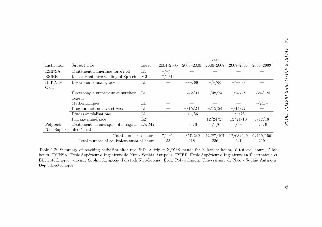
As summed up in Table 1.2, p. 13, my teaching activities after my PhD amountto over 1200 hours of lectures, tutorials and lab sessions, or nearly 1000 equiva-lent tutorial hours. Most of these have been carried out as a lecturer at the GEIIDepartment, IUT Nice - Cote d’Azur (since 2005).
In particular, I have created and been responsible for the “Digital filtering”(Filtrage numerique) optional subject at the GEII Department. This module givesan overview of the basic concepts of digital signal processing and digital filtering.Apart from lecture and tutorial preparation, the module has also involved the designof lab sessions with Matlab/Simulink and Spectrum Digital’s C6713 DSP Starter Kitboard based on Texas Instruments’ TMS320C6713 DSP. These lab sessions introducethe students to elementary computer-aided digital filter analysis and design as wellas DSP implementations for real-time filtering of audio signals. Since the creation
12 CHAPTER 1. EXTENDED CV
of the subject, several demos running on this DSP platform have attracted theattention of numerous visitors on the IUT’s annual open day.
During my PhD, I was a teaching assistant at the Department of Electrical &Electronic Engineering, University of Strathclyde, Glasgow (1996–1998). I taughtMicroprocessor Applications; DSP Lab of the MSc in Communications, Control andDigital Signal Processing; Analog Circuits; Circuit Analysis; and Signal Processing.
1.5 Other Activities
1.5.1 Research-Related Responsibilities
2008– Elected deputy member of I3S Lab Council (Conseil du laboratoire).
2007–2008
External member of Commission de specialistes, section 61, Universite duSud Toulon-Var.
2006–2008
Deputy member of Commission de specialistes, section 61, Universite deNice - Sophia Antipolis.
1.5.2 Consultancy
In March 2008, I worked as a consultant for “Sensor Products Inc.”, NJ, USA (CEO:Jeffrey Stark) on a project involving sensor-array data analysis.
1.6 Awards and Other Distinctions
Erasmus grant (1995)
I received one of the few Erasmus grants available at the ETSIT to spend the finalyear of my MEng at the University of Strathclyde, Glasgow, UK.
Award for meritorious final-year project poster presentation (1996)
Department of Electrical & Electronic Engineering, University of Strathclyde, Glas-gow.
MEng graduation with the highest distinction (1996)
I ranked first at the MEng in Telecommunications Engineering from ETSIT (class1991-1996).
Robert Legget Prize (2000)
For an especially distinguished PhD thesis submitted to the Faculty of Engineering,University of Liverpool, UK.
Royal Academy of Engineering Research Fellowship (2000–2005)
Open to young researchers from all branches of engineering, the Fellowships aim tohelp them develop their research careers at British universities. I was awarded oneof the first four Research Fellowships on offer in the UK. This allowed me to enjoya 5-year postdoctoral position at the University of Liverpool.
1.6.AW
AR
DS
AN
DO
TH
ER
DIS
TIN
CT
ION
S13
YearInstitution Subject title Level 2004–2005 2005–2006 2006–2007 2007–2008 2008–2009
ESINSA Traitement numerique du signal L4 –/–/50 — — — —
ESIEE Linear Predictive Coding of Speech M2 7/–/14 — — — —
IUT NiceGEII
Electronique analogique L1 — –/–/66 –/–/66 –/–/66 —
Electronique numerique et syntheselogique
L1 — –/42/90 –/48/74 –/24/98 –/24/126
Mathematiques L1 — — — — –/74/–Programmation Java et web L1 — –/15/24 –/15/24 –/15/27 —
Etudes et realisations L1 — –/–/56 — –/–/25 —Filtrage numerique L2 — — 12/24/27 12/24/18 6/12/18
Polytech’Nice-Sophia
Traitement numerique du signalbiomedical
L5, M2 — –/–/6 –/–/6 –/–/6 –/–/6
Total number of hours 7/–/64 –/57/242 12/87/197 12/63/240 6/110/150Total number of equivalent tutorial hours 53 218 236 241 219
Table 1.2: Summary of teaching activities after my PhD. A triplet X/Y/Z stands for X lecture hours, Y tutorial hours, Z labhours. ESINSA: Ecole Superieur d’Ingenieurs de Nice - Sophia Antipolis; ESIEE: Ecole Superieur d’Ingenieurs en Electronique etElectrotechnique, antenne Sophia Antipolis; Polytech’Nice-Sophia: Ecole Polytechnique Universitaire de Nice - Sophia Antipolis,Dept. Electronique.

14 CHAPTER 1. EXTENDED CV
Bonus for Research and Doctoral Supervision (2007–2011)This 4-year bonus (known as PEDR) is granted by the French Ministry of Educationto university lecturers with a good track record in research, so that they can continueto commit themselves to their research activities.
IEEE Reviewer Appreciation (2008)For significant commitment to the IEEE Transactions on Signal Processing reviewprocess.
Chapter 2
Introduction to ResearchActivities
2.1 Motivation
The estimation of signals from observations corrupted by noise and interference isa fundamental signal processing problem arising in a wide variety of real-life ap-plications. In telecommunications, limited bandwidth and multipath propagationmake the transmitted signal arrive at the receiving end with different delays. Thisphenomenon, known as intersymbol interference (ISI), can be modeled as a mix-ture of the desired signal and time-delayed replicas of itself, and worsens as thedata rate increases. The problem of recovering the original data from ISI-corruptedmeasurements is referred to as time equalization or channel deconvolution. Evenin time non-dispersive channels, signals from other users transmitting at the sametime/frequency/code slot can corrupt the signal of interest, generating co-channelinterference (CCI) at the receive sensor. Since these interfering signals typicallyoriginate from sources transmitting at different positions in space, such mixturesare called spatial, and the problem of resolving them is known as source separation,spatial filtering or beamforming. Signal processing techniques for the mitigationof transmission impairments such as ISI and CCI are crucial in meeting the re-quirements for higher data rates and improved quality of service of future wirelesscommunication systems [79,104].
Source separation problems are also common in biomedical engineering. Timedispersion effects are often negligible due to the bandwidth of physiological signalsand their propagation characteristics across the body tissues. During pregnancy, thefetal heartbeat signal is masked by the stronger maternal heartbeat at the outputof surface electrodes placed on the mother’s skin. In patients suffering from atrialfibrillation, the most common cardiac arrhythmia encountered in clinical practice,the bioelectrical activity from the atria appears mixed to that from the ventricleson surface recordings. An accurate estimation of the signal of interest (fetal heart-beat, atrial activity) from the observed mixtures is capital for its subsequent clinicalanalysis and may also provide further insights into the pathophysiological mecha-nisms of the medical condition under study. Other applications of signal estimation
15
16 CHAPTER 2. INTRODUCTION TO RESEARCH ACTIVITIES
from observed linear mixtures include seismic exploration, radar and sonar, imageprocessing, and circuit testing and diagnosis, to name but a few.
In the remaining of this introductory chapter, Sec. 2.2 provides a common math-ematical model and recalls some standard nomenclature for the different signal sce-narios studied in this work. A brief historical survey of techniques for signal estima-tion in linear mixtures is given in Sec. 2.3. My research activities during my PhDare summarized in Sec. 2.4, while the main research objectives after my PhD areoutlined in Sec. 2.5.
2.2 Mathematical Formulation and Problem Taxonomy
The channel equalization and source separation problems can jointly be cast inmathematical form as follows. In a generic setting, let us assume that K zero-mean source signals s(t) = [s1(t), s2(t), . . . , sK(t)]T propagate through a linear butpossibly time-dispersive medium. Symbol t denotes the continuous-time index and(·)T the transpose operator. Mixtures of the sources are observed at the outputof an array of L sensors, x(t) = [x1(t), x2(t), . . . , xL(t)]T. If hℓk(t) represents theimpulse response of the propagation channel between the kth source and the ℓthsensor, the ℓth sensor output is given by xℓ(t) =
∑Kk=1 hℓk(t) ∗ sk(t) + vℓ(t), where
symbol ∗ stands for the convolution operator and vℓ(t) is the additive noise thatmay further corrupt the measured signal. Denoting v(t) = [v1(t), v2(t), . . . , vL(t)]T,the discrete-time vector observation can be expressed in matrix form as:
xn =∑
m
Hmsn−m + vn (2.1)
where xn = x(nTs), sn = s(nTs), vn = v(nTs), [Hm]ℓk = hℓk(mTs), 1 ≤ k ≤ K,1 ≤ ℓ ≤ L, and Ts is the sampling period. Notation [A]ij represents the (i, j)-entry of matrix A. The objective of channel equalization and source separation isto recover the source signals sn from the observed corrupted measurements xn.
In communications, each source signal may be generated by a different user, orthe same user may generate different sources by transmitting through multiple an-tennas. Equation (2.1) also models a communication channel with a single sensoroutput x(t) sampled at L times the baud rate (fractional sampling or oversampling)excited by K inputs transmitting baud-spaced symbols sn = [s1,n, s2,n, . . . , sK,n]T.The channel impulse response between the kth source and the sensor may be denoted
as hk(t). In the resulting multi-channel scenario, the ℓth sensor output xℓ,ndef= [xn]ℓ
and its associated channels are virtual, and are given by the polyphase representa-tions xℓ,n = x
(nTs + (ℓ− 1)Ts/L
)and [Hm]ℓk = hk
(mTs + (ℓ− 1)Ts/L
), 1 ≤ ℓ ≤ L,
respectively [77, 96]. This signal model is easily generalized to the combined use ofspatially separated sensors and temporal oversampling.
To recover the source signals, a set of scalar equalizers can be employed. Letwkℓ(t) denote the impulse response of the filter linking the ℓth sensor signal and thekth equalizer output yk(t), so that yk(t) =
∑Lℓ=1 w∗
kℓ(t) ∗ xℓ(t), where (·)∗ denotescomplex conjugation. In discrete-time matrix notation, we can write:
yn =∑
m
WHmxn−m (2.2)
2.2. MATHEMATICAL FORMULATION AND PROBLEM TAXONOMY 17
where yn = [y1(nTs), y2(nTs), . . . , yK(nTs)]T and [Wm]ℓk = wkℓ(mTs), 1 ≤ k ≤ K,
1 ≤ ℓ ≤ L. Symbol (·)H stands for the conjugate-transpose (Hermitian) operator.If the equalizers are causal length-N finite impulse response (FIR) filters, eqn. (2.2)accepts the compact matrix formulation:
yn = WHxn (2.3)
where W = [WT0 ,WT
1 , . . . ,WTN−1]
T and
xn = [xTn ,xT
n−1, . . . ,xTn−N+1]
T (2.4)
is the stacked observation vector. Keeping this notation in mind, the kth component
of the output yn in (2.3), denoted yk,ndef= [yn]k, is given by
yk,n = wHk xn (2.5)
where wk represents the kth column of W. Depending on the values of L and N ,and whether time oversampling is performed or not, vector wk in eqn. (2.5) can actas a spatial, temporal or spatio-temporal filter for the linear extraction of a sourcecomponent; in general, it can simply be called linear extractor. The goal of channelequalization and source separation is then equivalent to the estimation of suitableextraction filters, represented by the columns of matrix W in eqn. (2.3), from theobserved data. For simplicity, we will sometimes refer to a generic component of yn
and the corresponding column of W with the shorthand notation
yn = wHxn. (2.6)
Similarly, time index n will be omitted when convenient.A case of particular interest occurs when the channel effects can be approximated
by FIR filters with maximum order M . Under this assumption, and according toeqn. (2.1), we can further express the stacked observation vector (2.4) as
xn = Hsn + vn (2.7)
wheresn = [sT
n , sTn−1, . . . , s
Tn−M−N+1]
T (2.8)
denotes the stacked source vector and H is the block Toeplitz matrix
H =
H0 H1 . . . HM 0L×K . . . 0L×K
0L×K H0 H1 . . . HM . . . 0L×K...
. . .. . .
. . .. . .
. . ....
0L×K . . . 0L×K H0 H1 . . . HM
with dimensions LN ×K(M + N); symbol 0L×K represents the matrix of (L×K)zeros. Depending on L, N and the oversampling factor, a column hk of the channel(or mixing) matrix H can be considered as the spatial, temporal or spatio-temporalsignature whereby the corresponding source component contributes to the observedvector xn. The mixing matrix columns are also known as source directions or transfer
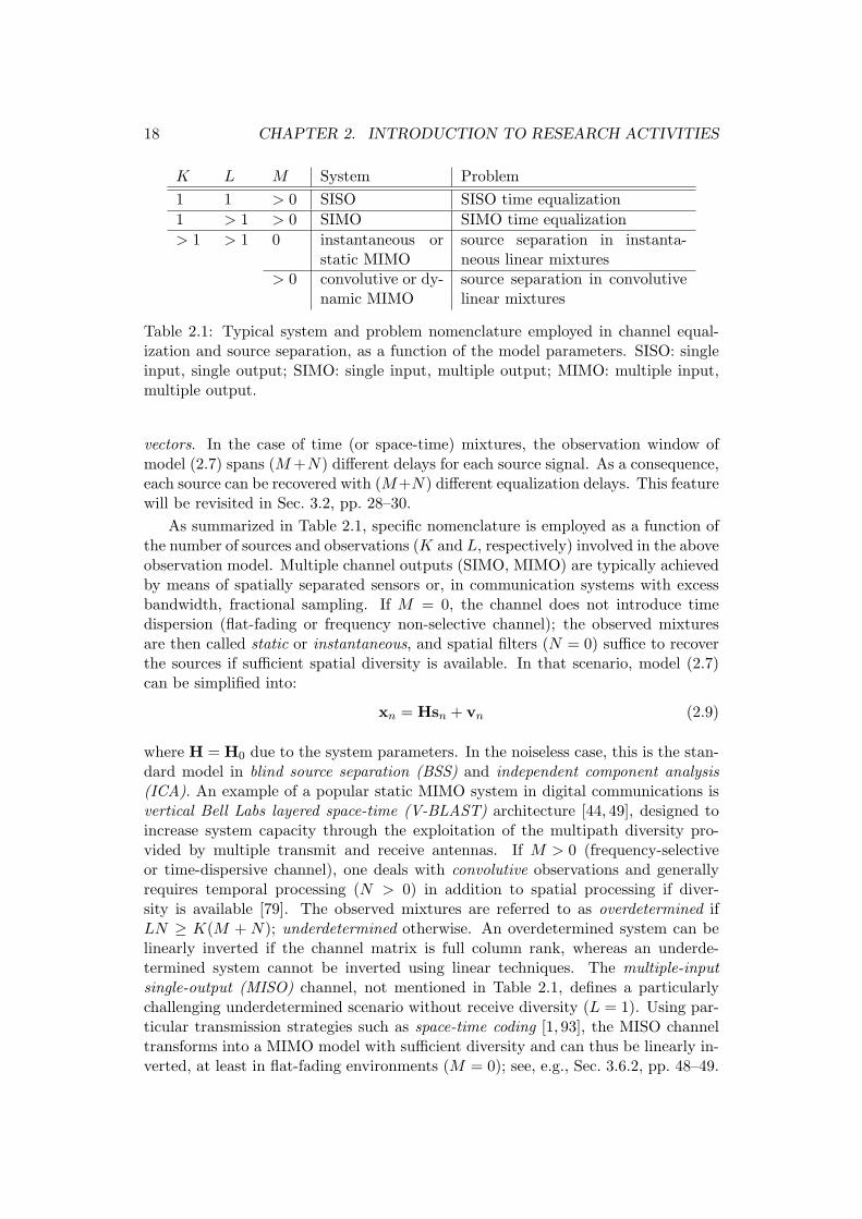
18 CHAPTER 2. INTRODUCTION TO RESEARCH ACTIVITIES
K L M System Problem
1 1 > 0 SISO SISO time equalization
1 > 1 > 0 SIMO SIMO time equalization
> 1 > 1 0 instantaneous orstatic MIMO
source separation in instanta-neous linear mixtures
> 0 convolutive or dy-namic MIMO
source separation in convolutivelinear mixtures
Table 2.1: Typical system and problem nomenclature employed in channel equal-ization and source separation, as a function of the model parameters. SISO: singleinput, single output; SIMO: single input, multiple output; MIMO: multiple input,multiple output.
vectors. In the case of time (or space-time) mixtures, the observation window ofmodel (2.7) spans (M +N) different delays for each source signal. As a consequence,each source can be recovered with (M+N) different equalization delays. This featurewill be revisited in Sec. 3.2, pp. 28–30.
As summarized in Table 2.1, specific nomenclature is employed as a function ofthe number of sources and observations (K and L, respectively) involved in the aboveobservation model. Multiple channel outputs (SIMO, MIMO) are typically achievedby means of spatially separated sensors or, in communication systems with excessbandwidth, fractional sampling. If M = 0, the channel does not introduce timedispersion (flat-fading or frequency non-selective channel); the observed mixturesare then called static or instantaneous, and spatial filters (N = 0) suffice to recoverthe sources if sufficient spatial diversity is available. In that scenario, model (2.7)can be simplified into:
xn = Hsn + vn (2.9)
where H = H0 due to the system parameters. In the noiseless case, this is the stan-dard model in blind source separation (BSS) and independent component analysis(ICA). An example of a popular static MIMO system in digital communications isvertical Bell Labs layered space-time (V-BLAST) architecture [44, 49], designed toincrease system capacity through the exploitation of the multipath diversity pro-vided by multiple transmit and receive antennas. If M > 0 (frequency-selectiveor time-dispersive channel), one deals with convolutive observations and generallyrequires temporal processing (N > 0) in addition to spatial processing if diver-sity is available [79]. The observed mixtures are referred to as overdetermined ifLN ≥ K(M + N); underdetermined otherwise. An overdetermined system can belinearly inverted if the channel matrix is full column rank, whereas an underde-termined system cannot be inverted using linear techniques. The multiple-inputsingle-output (MISO) channel, not mentioned in Table 2.1, defines a particularlychallenging underdetermined scenario without receive diversity (L = 1). Using par-ticular transmission strategies such as space-time coding [1, 93], the MISO channeltransforms into a MIMO model with sufficient diversity and can thus be linearly in-verted, at least in flat-fading environments (M = 0); see, e.g., Sec. 3.6.2, pp. 48–49.
2.3. BRIEF HISTORICAL SURVEY 19
2.3 Brief Historical Survey
In communications, classical channel equalization and source separation techniquesrely on the transmission of training or pilot sequences known to the receiver. Pilotdata enable the application of optimal Wiener filtering techniques based on second-order statistics (SOS), such as the minimum mean square error (MMSE) equalizer.The MMSE equalizer for the extraction of source k at equalization delay δk minimizesthe cost function:
ΥMMSE(y) = E{|yn − sk,n−δk|2} (2.10)
where sk,n denotes the kth-source training sequence and yn is the equalizer outputgiven by eqn. (2.6). Function (2.10) is minimized in closed-form by the well-knownWiener-Hopf solution, which simply reads:
w(δk)MMSE = R−1
x pδkwith pδk
= E{xns∗k,n−δk} (2.11)
and Rx = E{xnxHn } is the stacked observation covariance matrix. For uncorrelated
unit-variance source components, we have pδk= hδk
, where hδkis the column of
the channel matrix H associated with sk,n−δkin (2.7). In practice, expectations are
replaced by sample averaging over indices associated with the training data, as in theleast squares (LS) implementation (which will be recalled in Sec. 3.3.1, p. 31) Theprice to pay for conceptual simplicity and computational convenience in supervisedequalization is a poor utilization of the available bandwidth and power: up to 20%of the data rate is used for training in the GSM mobile telephony system [90].Also, the pilot sequence must be of sufficient length to compensate a channel of agiven order. In addition, training-based operation requires synchronization, whichis not always available or feasible in multiuser or non-cooperative (e.g., military)scenarios [100,104].
In the late 70’s, these limitations spurred the first researches into the so-calledblind equalization techniques [48,85,97], sparing the need for training sequences andeasing the synchronization requirements. Originally developed in the SISO case,blind techniques essentially rely on the idea of property restoration: the unknownwaveform is estimated by recovering at the equalizer output a known property ofthe transmitted signal. A cost, objective or contrast function quantifies the devia-tion from the desired property, and its optimization thus leads to equalizer filtersrecovering the source signal. Among the properties originally exploited are spe-cific features of digital modulations like their constant modulus (CM) [63, 97]. Thispopular criterion — which can be considered as a particular member of the moregeneral family of Godard’s methods [48] — is arguably the most widespread blindequalization principle. It aims at the minimization of the cost function:
ΥCM(y) = E{(|y|2 − γ)2} (2.12)
where γ is a constellation-dependent parameter. Although specifically designed forCM-type modulations like phase-shift keying (PSK), the CM criterion is also ableto recover non-CM modulations at the expense of an increased misadjustment dueto constellation mismatch. In parallel, measures based on higher-order statistics(HOS) such as the kurtosis began to draw the attention of the seismic exploration
20 CHAPTER 2. INTRODUCTION TO RESEARCH ACTIVITIES
community [43, 106], and were later taken up for the blind equalization of digitalcommunication channels as well [87]. The rationale behind the use of HOS lies inthe Central Limit Theorem: since mixing increases Gausssianity, one should proceedin the opposite direction, i.e., increasing non-Gaussianity by maximizing HOS, toachieve the separation. The kurtosis maximization criterion maximizes the contrast:
ΥKM(y) =|κy
4|(σ2
y)2
(2.13)
where κy4 = cum(y, y∗, y, y∗) is the marginal fourth-order cumulant of the equalizer
output and σ2y represents its variance. Cumulant definitions can be found in classical
references such as [157,159].
In the mid 90’s, the multi-channel (SIMO) scenario enabled by the use of timeoversampling or multiple sensors aroused great interest in the blind equalization com-munity. Indeed, while only non-minimum phase channels can be blindly identifiedby means of circular SOS in the SISO case, SIMO channels can be blindly identifiedregardless of their phase (minimal or otherwise) using such statistics. Moreover,FIR SIMO channels can be perfectly equalized by FIR filters in the absence ofnoise [77, 88, 96]. However, the channel must verify strict diversity conditions, anda good number of these methods do not work when the channel length is overesti-mated [16].
Concerning the MIMO case, traditional array processing or beamforming wasbuilt upon the array manifold concept, whereby the mixing matrix is parameterizedaccording to the sensor array geometry and the signal propagation model (e.g., far-field hypothesis) [86]. As a consequence, deviations from the model assumptions, theso-called calibration errors, can have a dramatic impact on the performance of theseearly techniques. A classical approach sparing the knowledge of the array manifoldis Widrow’s multi-reference adaptive noise cancellation (ANC) framework based onWiener’s optimal filtering [154] and closely connected to the MMSE receiver (2.10).The ANC approach, however, requires reference sensors sufficiently isolated fromthe physical phenomenon of interest, so as to capture components correlated withthe interference but uncorrelated with the desired signal.
The mid 80’s witnessed a rapidly increasing interest in the problem of BSS [56],in which spatial mixtures of the source signals are resolved without training dataor mixing-matrix parameterization. The assumed signal model can also be con-sidered as a generalization of Widrow’s ANC model whereby, under mild spatialdiversity conditions, all sources are allowed to contribute to all sensors simultane-ously. A first step towards rendering the classical Widrow’s ANC scheme suitablein this more general setup was taken in [2]; the blind approach was also formu-lated independently in [5, 39]. As in the closely related blind equalization problem,the main idea allowing the separation is the exploitation of an assumed propertyof the sources, such as their probability density function (pdf), statistical indepen-dence or, in digital communications, discrete alphabet. The first algorithms for BSSwere mainly based on heuristic ideas borrowed from neuro-mimetic information pro-cessing [21, 22, 26, 38, 56, 64, 65, 73, 89]. Other early methods solved the two-sourcetwo-mixture case in closed form by relating the higher-order cumulants of the sources
2.3. BRIEF HISTORICAL SURVEY 21
and the observations after a prewhitening step involving principal component anal-ysis (PCA) [24, 29]. The (2 × 2)-solution was then applied to all signal pairs untilconvergence, as in the Jacobi algorithm for matrix diagonalization [155].
Prompted by these encouraging early efforts, the mathematical cornerstone waslaid down by Comon in his pioneering contribution [25, 27]. He coined the notionof contrast function in the context of instantaneous BSS and developed the conceptof ICA, already suggested by Jutten and Herault in [65] as a generalization of thewell-known PCA technique. Contrasts can be defined as follows.
Definition 1 (contrast function for BSS). A function Υ(·) of the separatoroutput distribution is a contrast for BSS if it verifies:
Invariance: Υ(Gs) = Υ(s) for any (K ×K) matrix G = PD, where P is apermutation and D an invertible diagonal matrix.
Domination: Υ(Gs) ≤ Υ(s) for any (K ×K) matrix G.
Discrimination: Υ(Gs) = Υ(s) if and only if G = PD.
By virtue of the above characteristic properties, the global maximization of a con-trast function guarantees source separation. Contrasts requiring minimization canbe defined likewise. By assuming the sources to be statistically independent, infor-mation theoretical measures such as mutual information and negentropy were shownto perform the ICA of the observations and to constitute valid contrasts for the blindseparation of independent sources. Mathematical tractability could be improved byapproximating the source pdf’s via Gram-Charlier or Edgeworth expansions, leadingto operational algorithms based on HOS (higher-order cumulants) and the Jacobiiteration [24, 25, 27, 55]. One such algorithm is the so-called contrast maximization(CoM2) method of [25, 27], relying on the sum of square kurtoses of the separatoroutputs:
ΥCoM2(y) =K∑
k=1
(κyk
4
)2. (2.14)
Likewise, the CoM1 function
ΥCoM1(y) =K∑
k=1
∣∣κyk
4
∣∣ (2.15)
was later shown to be another valid contrast for the separation of independentsources [74]. When all the sources have the same sign of kurtosis, say ε, con-trast (2.15) becomes [13,74]:
Υε(y) = ε
K∑
k=1
κyk4 . (2.16)
This expression can be optimized using a closed-form solution at each pairwise iter-ation of the Jacobi algorithm [29].
Building on these fundamental ideas, iterative ICA algorithms based on gradientor Newton updates were also developed [54, 74]. Methods derived from the relative
22 CHAPTER 2. INTRODUCTION TO RESEARCH ACTIVITIES
or natural gradient were shown to provide uniform performance, whereby the sep-aration quality is independent of the mixing matrix structure [4, 13]. Extractingone source after another, i.e., performing deflation, emerged as another widespreadapproach to BSS. In this approach, the contribution of the latest source estimatecan be computed via linear regression and subtracted from the observations beforeperforming a new extraction, as in [98]; the process is then repeated until all sourceshave been obtained. The main advantage of deflation lies in the fact that extrac-tion contrasts such as the KM principle (2.13) are free of spurious solutions in theabsence of noise and estimation errors (infinite sample size) if the data model isperfectly fulfilled [37, 58, 87, 98]. Due to its simplicity and satisfactory performancein numerous applications, the deflationary FastICA algorithm [58, 60, 61] quicklygained popularity among ICA practitioners. Deflation (or symbol cancellation) hasalso been employed in the popular V-BLAST detection algorithm [44,49] (Sec. 2.2,p. 18). V-BLAST, however, requires an accurate channel matrix estimate based ontraining data.
In parallel, another important line of research began to explore the eigenstruc-ture of matrices and tensors made up of second- and higher-order cumulants of theobserved data [10]. This approach led to the widespread joint approximate diagonal-ization of eigenmatrices (JADE) method of [11] for blind separation of independentsources. The use of HOS precludes the treatment of Gaussian sources, which isnot a limiting constraint in most applications. The source second-order temporalstructure, if available, can likewise be exploited by the diagonalization approach, al-lowing the separation of Gaussian signals as well [7, 95]. The algorithm for multiplesignal extraction (AMUSE) of [95] is strongly reminiscent of the technique proposedin [96] for blind equalization of fractionally-spaced digital communication channels.This algorithm, in turn, was later generalized by the second-order blind identifica-tion (SOBI) method of [7]. Through the joint approximate diagonalization of theinput correlation matrices at several time lags, SOBI is more robust to the lag choiceand is particularly well suited to the separation of narrowband sources, with longcorrelation functions.
2.4 PhD Research
My PhD research focused on the problem of blind separation of independent sourcesin instantaneous linear mixtures (ICA), whose signal model is given by eqn. (2.9),p. 18. The so-called prewhitening process restores the source second-order covari-ance structure, yielding whitened observations zn linked to the sources through anunknown (K ×K) unitary matrix Q. In the noiseless case, this relationship reads:
zn = Qsn. (2.17)
If the time coherence of the sources is ignored or just cannot be exploited (as in thei.i.d. case), the estimation of matrix Q requires the use of HOS. In the real-valuedtwo-signal case (K = 2), matrix Q is a Givens rotation characterized by a singleparameter θ:
Q =
[cos θ − sin θsin θ cos θ
]
.
2.4. PHD RESEARCH 23
Different analytic methods for the estimation of θ had been proposed in the literature[24,29,55]. My doctoral investigation provided the first unified comprehensive visionof closed-form estimators for BSS based on higher-order cumulants, as summarizednext.
An approximate maximum likelihood (AML) estimator was proposed by Harroyand Lacoume in [55]. Its derivation assumed that both sources have symmetricdistributions and their kurtoses lie in a limited interval. In my PhD, a new estimator— named extended ML (EML) — was built as a complex-valued linear combinationof the whitened-data fourth-order statistics:
θEML =1
4∠(γξγ) (2.18)
with ξγ = (κz40 − 6κz
22 + κz04) + j4(κz
31 − κz13) and γ = κz
40 + 2κz22 + κz
04. Function∠(·) yields the phase of its complex variable relative to the positive real axis, andj =√−1 is the imaginary unit. The real-valued parameter γ is an estimate of the
source kurtosis sum (κs40 + κs
04). In these equations, the pairwise (p + q)th-ordercumulants are defined as in [159]:
κzpq = cum(z1, . . . , z1
︸ ︷︷ ︸
p
, z2, . . . , z2︸ ︷︷ ︸
q
).
The idea behind the EML estimator is that, under model (2.17) and no estima-tion errors (infinite sample length), we have that ξγ = (κs
40 + κs04)e
j4θ, from whicheqn. (2.18) readily follows. This estimator can also be expressed in term of a scatter-plot centroid, ξγ = E{(z1 + jz2)
4}, and accepts an intuitive geometric interpretationinspired by the work of Bogner and Clarke [23]. More importantly, the EML wasshown to generalize the AML to virtually any source probability distribution aslong as the source kurtosis sum is different from zero [P75,P86,P90]. The asymp-totic performance analysis of the estimator revealed closed-form expressions for itslarge-sample pdf and variance [P75,P81]. These expressions are able to predict theestimator’s behavior given the source statistics. The same analysis tools evidencedthe limitations of an earlier closed-form formula by Comon (CF) [P81,24].
The EML estimator was also shown to be the closed-form solution to the opti-mization of a contrast function [P81,P90]. Such a function resembles contrast (2.16),proposed by Moreau and Macchi in [74], which required all sources to have the sameknown sign of kurtosis. Yet the EML contrast shows that only the sign of source kur-tosis sum is pertinent for K = 2. In turn, this connection allowed the simplificationof the associated analytic solution derived by Comon and Moreau in [29].
These fourth-order estimators (AML, EML and CF) were shown to suffer asevere performance degradation when the source kurtosis sum approaches zero. Toovercome this drawback, a hybrid estimation strategy was adopted, based on anotherfourth-order estimator, the so-called alternative EML (AEML):
θAEML =1
2∠ξη (2.19)
with ξη = (κz40 − κz
04) + j2(κz31 + κz
13). The hybrid estimator consisted of a simpledecision rule to select the EML or the AEML depending on the whitened-observation
24 CHAPTER 2. INTRODUCTION TO RESEARCH ACTIVITIES
statistics [P73]. This way of combining the two estimators avoids their respectiveshortcomings.
Extensions to scenarios of more than two signals were implemented by meansof the Jacobi-like iteration strategy originally proposed by Comon [24, 25, 27]. Toillustrate their performance on real data, the resulting methods were successfullyapplied in the biomedical problem of non-invasive fetal electrocardiogram extractionfrom maternal cutaneous potential recordings [P72,P77,P79,P82,P85,P88,P89].
The compact centroid-based formulation of the EML and AEML estimators al-lowed the derivation of simple adaptive (on-line, stochastic, recursive) versions, oper-ating on a sample-by-sample basis. As shown by eqn. (2.18), the pertinent parameteris the orientation rather than the exact position of centroid ξγ , which is usually es-timated in a few iterations if the centroid is initialized at the origin. As a result, inthe two-signal case these adaptive methods present a remarkable convergence speedand global convergence under mild conditions [P74,P84].
The thesis concluded by generalizing some of the above results to other cumulantorders and the complex case. A closed-form estimation family based on the datarth-order statistics was derived, of which the EML turned out to be a particular casefor r = 4. For r = 3, a novel third-order estimator was also obtained and analyzed[P70,P81]. Through the so-called bicomplex numbers, some of the previous resultswere extended to complex-valued mixtures, evidencing an interesting connectionbetween the real and the complex case [P71,P80].
Numerical experiments supported the theoretical results, compared the tech-niques considered and contrasted them with other non-analytic procedures. Thecomputational complexity of the different methods was also discussed.
2.4.1 Other PhD-Related Research
The direct continuation of my PhD research addressed the direct combination of theEML and AEML estimators [eqns. (2.18)–(2.19)] by using the centroid:
ξλ = λγξγ + (1− λ)ξ2η .
An asymptotic performance analysis yielded the closed-form expression for the op-timal weight coefficient λ as a function of the source statistics. Depending on thesource combination to be separated, this generalized weighted fourth-order estimatoris able to provide significant performance gains relative to the two estimators fromwhich it is derived, and mitigates their performance degradation when the sourcekurtosis sum and difference, respectively, are close to zero [P18,P44,P49,P65,P66].1(p. 137)
(p. 281) When λ = 0.5 the above estimator is equivalent to JADE [11] in the case of K = 2sources. In the complex case, Cramer-Rao bounds for the estimation of the relevantparameters were derived in [P65].(p. 281)
Another line of work was an attempt to solve in closed-form the BSS problemin the three-signal case, where the unknown unitary mixing matrix after prewhiten-ing can be considered as a three-dimensional rotation. Quaternions, discovered by
1Marginal notes show the pages where the attached publications can be found at the end of thisdocument.
2.5. RESEARCH GOALS AFTER MY PHD 25
the Irish mathematician Sir William R. Hamilton in the 19th century, can be con-sidered as a natural extension of complex numbers and are characterized by theirability to perform rotations in the three-dimensional space. Exploiting this ability, aquaternion-based closed-form solution for the three-source BSS scenario was foundfor the first time in [P64]. This solution relies on the previous knowledge of certain (p. 277)source cumulants and remains to be extended to the fully blind case.
Publications [P69,P76,P78,P87] are also related to my PhD work.
2.5 Research Goals After my PhD
The research I have carried out after my PhD has aimed at the design of novel signalestimation techniques with improved performance. The guiding principle has beento capitalize on the available prior information in order to derive techniques moreadapted to the problems under study. Contributions of this kind have been madein two specific applications of telecommunications and biomedical engineering: theequalization of digital communication channels and the extraction of atrial activityin atrial fibrillation episodes. These contributions are summarized in Chapter 3,pp. 27–51, and Chapter 4, pp. 53–72, respectively. Some possible avenues for thecontinuation of this work are enumerated in Chapter 5, pp. 73–77.
For the sake of conciseness, in what follows we only elaborate on a few contri-butions to highlight certain aspects of theoretical interest, whereas the remainingcontributions are only briefly sketched. For further details, including experimentalresults, the reader is referred to the relevant publications, some of which are attachedto this report.

Chapter 3
Robust Equalization and SourceSeparation
3.1 Motivation
As introduced in Sec. 2.3, pp. 19–22, blind techniques have aroused an enormousresearch interest on account of their improved bandwidth utilization, robustness tocalibration errors and reduced synchronization requirements. However, these bene-fits come at the expense of some practical drawbacks, which are briefly summarizedbelow:
D1) Blind methods cannot resolve the indeterminacy of the amplitude and/or thephase of the estimated signal [see eqns. (2.12)–(2.13)], in addition to orderingindeterminacy in the case of multiple sources (multiple-input case). In caseswhere only a few of the source components are of interest (as in time-dispersivechannels, where recovering a single delay per source typically suffices), the per-mutation ambiguity causes particular problems: the whole mixture needs to beseparated before the desired component can be selected, with the subsequentincrease in computational complexity. Performing a full separation also wors-ens estimation errors in algorithms based on sequential extraction (deflation).This shortcoming is inherent to the blind approach and cannot be relievedwithout resorting to further information about the signal(s) of interest.
D2) Blind cost functions involve HOS, explicitly or implicitly. Their mathematicalcomplexity means that they are often notoriously multi-modal, presenting spu-rious local extrema [40,41,63]. These are are stable equilibria associated withfilter tap settings that cannot sufficiently open the eye pattern of the equalizeroutput signal, so that the detecting device is then unable to extract the trans-mitted symbols with a reasonably low probability of error. When the modelassumptions are violated or short sample blocks are processed, local extremacan also appear in contrasts that otherwise offer theoretical global convergence,like the KM (2.13) [94]. Clearly, spurious extrema hinder the convergence ofiterative search techniques used to optimize blind contrasts. In particular,their existence can render the performance of gradient- and Newton-based im-
27
28 CHAPTER 3. ROBUST EQUALIZATION AND SOURCE SEPARATION
plementations, such as the widespread CMA [97] or the popular kurtosis-basedFastICA [58,60,61], very dependent on the initial value of the extracting filter.These undesired effects have also been evidenced in [P9,P12,P17,P19,P41].(p. 133)
(p. 153)(p. 253) D3) An increased sample size is necessary to estimate HOS with an accuracy com-
parable to SOS. Larger data volumes (block sizes) than supervised methodsare thus required for the same signal estimation quality. In turn, this draw-back leads to increased computational demands and slow convergence, com-promising the tracking ability of blind techniques when system parametersvary rapidly.
As discussed in [40, 41, 94], among other works, the misconvergence problems ofiterative blind techniques calls for the design of suitable initialization schemes andadditional strategies to keep the filter tap trajectories away from undesired localequilibria.
An important part of my research has been devoted to proposing and analyz-ing a number of strategies to surmount the above limitations and lead to morerobust equalization and source separation techniques. My focus has been on digital-modulation based contrasts like the constant modulus and constant power principles,as well as constellation-independent criteria such as kurtosis. Three main strategieshave been developed, that can all be combined together: equalizer initialization bymeans of algebraic solutions, semi-blind operation, and iterative search based onan optimal step size. First, equalizers can be judiciously initialized with algebraicsolutions enabled by the use of training symbols known by the receiver (Sec. 3.2,pp. 28–30) or the finite-alphabet property of digital modulations (Sec. 3.3, pp. 30–39). Pilot information and blind contrasts can be used together, giving rise to semi-blind criteria (Sec. 3.4, pp. 39–42) whose optimization can outperform traditionaltraining-based techniques at a fraction of the bandwidth utilization and with just amoderate increase in computational cost. The cost-effectiveness and robustness toinitialization of semi-blind techniques can be further improved by an iterative searchtechnique based on an algebraic optimal step size (Sec. 3.5, pp. 42–46), which is alsoeffective in fully blind mode. The combination of these three strategies (algebraicinitialization, semi-blind criteria and optimal step-size iterative search) is able tomitigate the impact of local extrema and slow convergence typical of blind methods,leading to signal extractors with increased robustness, high convergence speed andmodest complexity. The chapter concludes by reporting other results related to theprocessing of telecommunication signals (Sec. 3.6, pp. 46–50).
3.2 ICA-Based MIMO Channel Equalization
My first efforts towards alleviating drawbacks D1–D3 above concern the convolutiveMIMO channel. If sufficiently spatio-temporal diversity is available at the receive endso that matrix H in eqn. (2.7), p. 17, is full column rank, the channel can be linearlyinverted; a necessary condition is that LN ≥ K(M+N), which imposes lower boundsfor the receive diversity L and equalizer length N as a function of the source numberK and channel order M . If the sources are i.i.d. (or, more generally, temporally
3.2. ICA-BASED MIMO CHANNEL EQUALIZATION 29
white), the components of vector s(t) in eqn. (2.8) are statistically independent. Theconvolutive MIMO model (2.7) can then be resolved by ICA techniques, as pointedout in [20,108,110]. An ICA method can be applied directly on the observed signalin (2.7), followed by a simple algorithm (e.g., based on cross-correlations) to identifyand group each source’s delays. Despite the conceptual simplicity of this approach,the computational complexity of separating K(M + N) independent componentscan become prohibitive in systems with long delay spreads as a result of high datarates, even for a moderate number of sources.
To overcome this difficulty, the classical blind channel identification methods of[77,96], originally designed for the single-input case, are generalized to the multiple-input case in [P53, P60]. After the application of these extensions, the spatio-temporal equalization is shown to reduce to a problem of source separation in instan-taneous linear mixtures characterized by model (2.9), p. 18. ICA can then be used toseparate the remaining spatial mixture, involving only K independent components.Computational complexity is thus considerably reduced [P24,P54,P55]. (p. 223)
To further improve performance, the ICA stage can be initialized by the Wienerreceiver, which is feasible in systems where channel state information or trainingdata are available [see eqns.(2.10)–(2.11), p. 19]. Conversely, this approach can beseen as the ICA-based refinement of the Wiener receiver. Indeed, the performance ofconventional linear equalizers, such as the MMSE (2.11) based on previous channelidentification, is shown to deteriorate in MIMO systems with many source compo-nents due to large delay spreads and/or number of inputs, even if the channel matrixis perfectly estimated. A typical effect is the severe performance flooring observedwhen the finite-sample noise level (estimation error due to finite data length) sur-passes the additive noise present at the sensor output. As noted in [83], the ICAstage has the potential to palliate this performance degradation by exploiting HOS.
Inspired by this idea, an ICA-based detection scheme originally put forward ina rather restrictive DS-CDMA signal model [83] is adapted in [P23] to the more (p. 203)general time-dispersive MIMO signal scenario (2.7), p. 17, with M > 0. Insteadof performing the full separation of all time delays associated with each source,computational complexity can be reduced while improving estimation quality byaiming at the simultaneous extraction of the optimum MMSE equalization delayof each source. The optimum delay for the extraction of the kth source, δopt
k , isfound by minimizing the equalizer output MSE over all possible extraction delays,1 ≤ δk ≤ (M + N), for which closed-form solutions exist as a function of theobservation covariance matrix and the channel matrix. Assuming that the sourcesignal is normalized (i.e., it has zero mean and unit variance), the MSE of the MMSEsolution with delay δk is given by:
MSEδk= 1− pH
δkR−1
x pδk. (3.1)
where pδkis defined as in eqn. (2.11), p. 19. Hence:
δoptk = arg min
δk
MSEδk= arg max
δk
pHδk
R−1x pδk
. (3.2)
The resulting ICA-based detection scheme with optimum-delay MMSE initializationis able to yield significant performance gains relative to conventional linear detec-tors [P23,P50,P55], tolerating higher co-channel interference and additive Gaussian (p. 203)
30 CHAPTER 3. ROBUST EQUALIZATION AND SOURCE SEPARATION
noise levels, and thus improving system capacity [P47], at only a moderate increasein computational cost. The ICA approach presents the benefit of constellation-independent symbol recovery, which makes it very attractive in next-generation ad-hoc networks as well as in non-cooperative military scenarios.
3.3 Algebraic Equalizers
As explained in the previous section, generic methods for BSS based on statisticalindependence (ICA) used in other applications can also be employed to perform dig-ital channel equalization if the sources present no time coherence. However, digitalcommmunication channels present particular features that can be capitalized on toimprove source recovery. Among them, digital modulations have finite support or,in other words, they contain only a small number of possible complex amplitudes.Criteria such as the constant modulus (CM) or the constant power (CP) are specifi-cally adapted to the blind estimation of signals with such modulations and, as shownin [35], constitute valid contrasts for the separation and extraction of these signalsin linear mixtures, either instantaneous or convolutive. The CM has long been usedin blind equalization [48, 85, 97], whereas the CP criterion has more recently beenproposed for inputs with q-ary phase shift keying (q-PSK) modulation, for an arbi-trary integer q ≥ 2. An interesting benefit of these criteria is that they spare theinput statistical independence assumption [34].
Furthermore, these constellation-adapted principles can be considered as quasi-deterministic rather than statistical criteria, in the sense that signals with adaptedmodulations cancel exactly (in the absence of noise and if the data model holdsperfectly) the sample version of the contrasts for any data length. As a result, thesecontrasts offer the potential of achieving good performance even for short samplesize. More interestingly, the optimization of these criteria accepts algebraic solutions,another approach to improving the shortcomings of blind techniques. Algebraicmethods (sometimes called analytic) provide an equalization or separation solution ina finite number of operations, and are associated with challenging matrix and tensordecomposition problems. Despite their fundamental theoretical interest, algebraicsolutions are only approximate in the presence of noise, too short sample size orwhen linear recovery solutions do not exist for lack of sufficient diversity. Hence,they generally require a refinement based on iterative optimization, and can indeedbe always employed as judicious initializations to iterative equalizers (Secs. 3.4–3.5).
Perfect zero-forcing (ZF) equalization of a SISO channel is possible when bothof the following conditions are verified:
C1) The channel admits a noiseless Mth-order auto-regressive (AR) model.
C2) The FIR equalizer length is sufficient, N ≥ N0, with N0 = (M + 1).
Indeed, a channel satisfying C1 can be equalized by an FIR filter w0 with minimumlength N0. If the equalizer filter is over-parameterized, N > N0, there exist P =(N −N0 + 1) exact ZF solutions, each one corresponding to a different equalizationdelay:
wp = [0Tp−1, wT
0 , 0TP−p]
T, 1 ≤ p ≤ P. (3.3)
3.3. ALGEBRAIC EQUALIZERS 31
As will be seen in the following, under these conditions the MMSE, CM and CP cri-teria can be perfectly minimized (even canceled if the sources verify the conditions ofeach criterion), and the global minimum can be computed algebraically, that is, with-out iterative optimization. A variety of algorithms aiming to estimate algebraicallythe best SISO equalizer, or to identify the SISO channel, when the input belongs toa known alphabet have been proposed in [6, 42, 45, 51, 53, 70, 91, 102, 103, 105, 109],among other works.
For their theoretical interest and potential use in practical systems, I have focusedon the algebraic solutions to the CM contrast [42,103,105] and the variants derivedfrom the CP criterion. The algebraic solution that we detail in Sec. 3.3.3 can beconsidered as a extension of the analytic constant modulus algorithm (ACMA) [103]to the CP principle. Algebraic solutions to supervised and blind criteria can also becombined together (Sec. 3.4.1), giving rise to algebraic semi-blind equalizers. Thesecontributions are developed at length in [P9,P12,P19]. We start our exposition in (p. 153)Secs. 3.3.1–3.3.2 by recalling the algebraic solutions to the supervised MMSE andblind CM criteria, respectively.
3.3.1 Algebraic Solutions to the MMSE Criterion
As recalled in Sec. 2.3, the MMSE criterion (2.10), p. 19, is minimized by the Wiener-Hopf solution (2.11); its reconstruction error is given by eqn. (3.1), p. 29. Let theTt pilot symbols be stored in vector
s = [s0, s1, . . . , sTt−1]H.
Canceling the criterion (2.10) is tantamount to solving the linear system:
XHδ w = s (3.4)
whereXδ = [xδ, xδ+1, . . . xδ+Tt−1] ∈ C
N×Tt (3.5)
and δ represents the equalization delay. If Tt ≥ N , the above system does notgenerally have an exact solution, as it consists of more equations than unknowns. Itcan still be solved in the LS sense, yielding:
w(δ)LS = (XδX
Hδ )−1Xδ s
that we consider here as the algebraic solution to the MMSE criterion (2.10). Thissolution exists and is unique as long as matrix Xδ is full rank, which is the case in thepresence of noise. In the noiseless case and under conditions C1–C2, matrix Xδ ineqn. (3.5) has rank N0, so that it exists an infinite number of solutions to system (3.4)
as soon as N > N0. The minimum-norm solution is given by w(δ)LS = X†
δ s, where(·)† denotes the Moore-Penrose pseudo-inverse [155]. This solution corresponds toone of the exact ZF equalizers (3.3), which are identical up to a delay. When noiseis present, the impact of delay on equalization performance may become important.The term 1
TtXδ s can be regarded as a sample estimate of pδ whereas 1
TtXδX
Hδ
approximates the covariance matrix Rx in eqn. (2.11), p. 19. The optimal delayin the MMSE sense, δopt, can be determined according to (3.2), p. 29, using theseapproximations.
32 CHAPTER 3. ROBUST EQUALIZATION AND SOURCE SEPARATION
3.3.2 Algebraic Solutions to the CM Criterion
Algebraic solutions to the CM contrast (2.12), p. 19, were originally developedin [103] and [42] in the context of blind separation and channel equalization, re-spectively. These methods concern the case where multiple exact solutions exist, asthe static MIMO case with L ≥ K or a SISO channel accepting FIR equalizers withperfect recovery (ZF) solutions (e.g., under conditions C1–C2 above). To describethese methods mathematically, we disregard the equalizer index k in eqn. (2.5), p. 17,and consider a single equalizer output, denoted by yn, as in eqn. (2.6). Let symbol Td
represent the number of observed baud periods, from which T = (Td−N +1) full ob-served vectors xn can be constructed in model (2.7), p. 17. The exact solutions to theCM criterion verify |yn|2 = 1, up to an irrelevant scale factor [constant γ in (2.12),p. 19], for all 0 ≤ n ≤ (T − 1). Denote as x⊛2
n the Kronecker product x∗n ⊗ xn,
which can also be expressed as vec{xnxHn }, where vec{A} is the vector obtained
by stacking the columns of matrix A; accordingly, unvec{·} performs the inverseoperation. Using this notation, we can write |yn|2 = wHxnx
Hnw = (x⊛2
n )Hw⊛2, andthe problem is equivalent to the solution of the linearized system:
[x⊛2N−1, x
⊛2N , . . . , x⊛2
Td−1]Hf = [1, 1, . . . , 1]T (3.6)
under the structural constraint f = w⊛2. When P equalizers {wp}Pp=1 exist, sys-
tem (3.6) without constraint accepts P solutions {fk}Pk=1 such that
fk =
P∑
p=1
αkpw⊛2p (3.7)
for certain unknown but linearly independent coefficients {αkp}Pk,p=1. In terms ofthe associated matrices, Fk = unvec{fk}, this relationship can be expressed in theform:
Fk =
P∑
p=1
αkpwpwHp = WAkW
H (3.8)
with W = [w1, . . . , wP ] and Ak = diag([αk1, . . . , αkP ]). It follows that the recoveryof the extracting filters {wp}Pp=1 from a basis of the solution space is tantamount tothe problem below [103]:
Problem 1 (joint diagonalization). Given the set of matrices {Fk}Pk=1 associ-ated with the non-structured solutions to the linearized problem (3.6), find matricesW and {Ak}Pk=1 verifying eqn. (3.8).
As opposed to other joint diagonalization algorithms such as SOBI [7] or JADE[11] (see also Sec. 2.3), the diagonalizing transformation in Problem 1, i.e., matrixW, is in general not unitary. This matrix is composed of the valid equalizer vectors.
From another perspective, the above equality can be considered as the search forcoefficients {βpk}Pp,k=1 such that the linear combination
∑Pk=1 βpkFk approximates
the rank-1 matrix wpwHp . This naturally leads to the following problem [33]:
3.3. ALGEBRAIC EQUALIZERS 33
Problem 2 (rank-1 matrix linear combination). Given matrices {Fk}Pk=1, findall solutions to
min{β1,...,βP },w
∥∥∥∥∥
P∑
k=1
βkFk −wwH
∥∥∥∥∥
.
In the general case, the ACMA of [103] tries to solve the joint diagonalizationproblem (3.8) by using the generalized Schur decomposition [155] of several (morethan two) matrices, a costly iterative method for which a convergence proof has notyet been found. Simplifications are possible [42] when the valid extracting filters aredelayed versions of each other, as under conditions C1–C2, where the P differentsolutions are given by eqn. (3.3), p. 30.
Once a non-structured solution has been obtained via, e.g., pseudo-inversionof the coefficient matrix in (3.6), the minimum-length equalizer can be extractedby a subspace-based approach or other simple procedures for structure restorationexploiting the presence of zero elements in w⊛2
p [see eqns. (3.3) and (3.7)]. In thereal case, nearly half the elements of x⊛2
n are redundant, so that ACMA requiresspecial modifications to process signals with one-dimensional alphabets (e.g., BPSK)[42,103]; such modifications give rise to the real ACMA (RACMA) method of [105].
3.3.3 Algebraic Solutions to the CP Criterion
In close collaboration with Pierre Comon, I have explored in [P19] the algebraic (p. 153)solutions to a novel property restoral principle for the blind equalization of q-PSKsignals, the so-called constant power (CP) criterion. This is a particular case ofthe alphabet polynomial fitting (APF) principle of [32, 34, 50] that aims to matchthe equalizer output constellation to that of the source, characterized by the com-plex roots of a specific polynomial Q(z) [34, 84]. Thus, APF criteria rely on theminimization of function
ΥAPF(y) = E{|Q(y)|2}As opposed to independence-based criteria, APF contrasts have the ability to sepa-rate spatially correlated and spectrally colored sources. As opposed to the CM cri-terion, APF can target sources with matching modulation (cf. drawback D1, p. 27).
In particular, the q-PSK modulation can be represented by the roots of the qthdegree polynomial Q(z) = zq − d, or by the solutions to zq = d, hence the nameconstant power. The values of q and d depend on the particular constellation; forinstance, (q, d) = (2, 1) for BPSK, (q, d) = (4, 1) for QPSK, etc. By allowing atime-varying d, the above definitions are directly extended to modulations otherthan PSK, such as minimum shift keying (MSK) [51], which can be described by(q, dn) =
(2, (−1)n
). Accordingly, the CP criterion reads:
ΥCP(y) = E{|yqn − dn|2}. (3.9)
The CP principle can be considered as an extension of the Godard family of criteria[48] that takes into account the particular properties of the q-PSK modulation. Thisprinciple is asymptotically insensitive to a large class of circularly distributed (atorder q) interference and noise. In the context of BSS, minimizing (3.9) is equivalent,for a sufficiently low noise level, to maximum a posteriori (MAP) estimation [30,50].
34 CHAPTER 3. ROBUST EQUALIZATION AND SOURCE SEPARATION
The development of analytic solutions to criterion (3.9) follows closely the CMcase. Hence, by analogy with the ACMA of [104], we refer to these solutions as an-alytic constant power algorithm (ACPA). From a linear algebra perspective, findingthe analytic solutions to the CP contrast optimization leads to tensorial generaliza-tions of the matrix problems set out in the previous section. To cast these tensorproblems mathematically, a few extra definitions are first required.
3.3.3.1 Some definitions
Let [A]i1i2...iq denote the (i1, i2, . . . , iq)-element of qth-order tensor A ∈ CM1×···×Mq ,
1 ≤ ip ≤Mp, p = 1, . . . , q. The Frobenius product of two tensors A and B with thesame order and dimensions is defined as 〈A,B〉 =
∑
i1...iq[A]i1...iq [B]i1...iq ; hence the
Frobenius norm ‖A‖2 = 〈A, A〉. The outer product of two tensors of orders p andq, C = A ◦ B is given by the (p + q)th-order tensor [C]i1...ipj1...jq = [A]i1...ip [B]j1...jq .Given a vector a ∈ C
L, we denote a◦q = a ◦ · · · ◦ a︸ ︷︷ ︸
q
(for instance, a◦2 = a◦a = aaT).
A symmetric tensor of order q and dimension N can be stored in a vector vecs{A},which contains the Nq =
(N+q−1
q
)different entries of A. These entries are normalized
so as to preserve the Frobenius norm, and we write a⊘q = vecs{a◦q}. Similarly,from a vector b of dimension Nq, unvecsq{b} represents the associated qth-ordersymmetric tensor.
3.3.3.2 Problem formulation
Recall that a total of T = (Td −N + 1) full observed vectors xn can be constructedfrom the Td observed baud periods in model (2.7), p. 17. Given such vectors, welook for the exact minimizers of the CP criterion, verifying
yqn = dn n = 0, 1, . . . , T − 1. (3.10)
Proofs of the claims that follow can be found in [P19], and can be considered as(p. 153)extensions to the tensor case of those developed for ACMA in [103]. With the abovedefinitions, we have that yq
n = (x⊘qn )Hw⊘q. As a result, the cancellation of the CP
criterion is equivalent to the solution of the linearized system
XqHf = d (3.11)
where Xq = [x⊘qN−1, x⊘q
N , . . . , x⊘qTd−1] and d = [d0, d1, . . . , dT−1]
H. Equation (3.11)
must be solved under the following structural constraint: f ∈ CNq must be of the
form form f = w⊘q, for certain vector w ∈ CN .
3.3.3.3 Determining a basis of the solution space
When P extracting filters exist (as occurs under conditions C1–C2, p. 30), sys-tem (3.11) without constraint accepts P linearly independent solutions {fk}Pk=1.Consequently, the dimension of the null space of XqH, denoted ker(XqH), is (P −1),and the solutions of (3.11) can be expressed as an affine space of the form f =
3.3. ALGEBRAIC EQUALIZERS 35
f0 +∑P−1
p=1 αpfp, where f0 is a particular solution to the non-homogeneous sys-
tem (3.11) and fp ∈ ker(XqH), for 1 ≤ p ≤ (P − 1).As in [103], we find it more convenient to work in a vector space, obtained through
a unitary transformation Q with dimensions (T ×T ), such that Qd = [√
T , 0TT−1]
T,where symbol 0T−1 stands for the vector of (T − 1) zeros. For instance, Q can bea Householder transformation [155] or, if d is composed of T equal values (as is thecase for q-PSK modulations), a T -point DFT matrix. Then, denoting:
QXqH =
[rH
R
]
system (3.11) reduces to:{
rHf =√
TRf = 0T−1.
under the constraint f = w⊘q. Similarly to [103, Lemma 4], it is possible to provethat this problem is equivalent to the solution of:
{Rf = 0T−1
f = w⊘q
followed by a scaling factor to enforce:
cHf = 1, with c =1
‖d‖2T−1∑
n=0
dnx⊘qn (3.12)
or, equivalently:
1
‖d‖2T−1∑
n=0
dn(wHxn)q = 1. (3.13)
If dim ker(XqH) = (P − 1) and
Td ≥ Nq + N0 − 1 (3.14)
(or T > Nq − P ), then dim ker(R) = P . Hence, all the solutions of Rf = 0 arelinearly spanned by a basis {fk}Pk=1 of ker(R). Such a basis can be computed fromthe singular value decomposition (SVD) of matrix R by taking its P least significantright singular vectors.
3.3.3.4 Matrix and tensor algebra problems
The structured solutions {w⊘qp }Pp=1 are also a basis of the solution space so that:
fk =P∑
p=1
αkpw⊘qp 1 ≤ k ≤ P (3.15)
for certain unknown coefficients {αkp}Pk,p=1 forming a full-rank matrix [A]kp = αpk.The problem of finding structured solutions to the linearized system (3.11) is hencea particular subspace fitting problem with structural constraints.
36 CHAPTER 3. ROBUST EQUALIZATION AND SOURCE SEPARATION
Problem 3 (subspace fitting with structural constraints). Given a set ofvector {fk}Pk=1, find coefficients {αkp}Pk,p=1 and vectors {wp}Pp=1 verifying relation-ship (3.15). Equivalently, given the qth-order tensors Fk = unvecs{fk}, find thesolutions to
Fk =
P∑
p=1
αkpWp
where Wp = w◦qp = unvecsq{w⊘q
p }.
As a result, the equalizer filter recovery can be considered as the following ten-sorial generalization of the rank-1 linear combination problem [33]:
Problem 4 (rank-1 tensor linear combination). Given the set of tensors{Fk}Pk=1, find all solutions of
min{β1,...,βP },w
∥∥∥∥∥
P∑
k=1
βkFk −w◦q∥∥∥∥∥
.
This tensor decomposition is generally a non-trivial task [28,33].
3.3.3.5 Solution structuring methods
According to Problem 4, finding a structured solution to the linearized system (3.11)consists in enforcing the rank-1 symmetric Kronecker structure to the basis {fk}Pk=1.In the context of the CM criterion (Problem 2, p. 33), a subspace method wasproposed in [42, section III.C], operating on a single non-structured (LS) solution.According to Problem 1, p. 32, this structure forcing procedure can be interpretedas the diagonalization of the matrix associated with the non-structured solution.
The method of [52] and [42, section III.B] is based on the observation that,according to eqns. (3.3), p. 30, and (3.15), the first N components of a solution fkare equal to
αk1wq−11 [w1,
√q w2, . . . ,
√q wN0−1,
√q wN0 , 0T
P−1]T
from which the minimum-length equalizer w0 = [w1, w2, . . . , wN0 ]T can easily be
deduced. This method is simple and ingenious, but inaccurate when coefficient αk1
or the first term w1 of the equalizer are small relative to the noise level.To surmount this limitation, one can also note from eqns. (3.3) and (3.15) that
the last components of fk are equal to [42, section III.B]:
αkP wq−1N0
[0TP−1, . . . ,
√q w1,
√q w2, . . . ,
√q wN0−1, wN0 ]
T
Appropriately combined with the estimation carried out from the first N compo-nents, this second option can provide an improved estimation of w0. To this end,we may employ the following heuristic (suboptimal) linear combination. Let ussuppose that the filters estimated from the first and the last non-overlapping com-ponents of a non-structure solution are, respectively, w1 = β1w0 and w2 = β2w0,with w0 = w0/‖w0‖. Then, the unit-norm minimum-length equalizer LS estimate
3.3. ALGEBRAIC EQUALIZERS 37
is given by ˆw0 = [w1, w2]γγγ, with γγγ = βββ∗/‖βββ‖2, βββ = [β1, β2]T. The coefficients of βββ
can simply be estimated from the equation βi = ‖wi‖, i = 1, 2. This type of linearmaximal ratio combining is reminiscent of the RAKE receiver and the matching fil-ter [80]. Robustness can still be improved by exploiting a whole basis of the solutionspace {fk}Pk=1 instead of a single solution.
3.3.3.6 A subspace approach to solution structuring
When the valid solutions are of the form (3.3), we have proposed a subspace methodreminiscent of [77] to recover the minimum-length equalizer w0 from a basis of (gen-erally) unstructured solutions {fk}Pk=1, thus solving the rank-1 linear combinationproblem (Problem 4) in that particular case. The method can be described as fol-lows [P19]. (p. 153)
The subspace fitting problem (3.15) can be written in compact form as F =WA, with F = [f1, . . . , fP ] and W = [w⊘q
1 , . . . , w⊘qP ]; the entries of matrix A are
defined after eqn. (3.15). Since A is full rank, matrices F and W span the samecolumn space. In particular, any vector ui in the orthogonal complement of F alsoverifies uH
i W = 0TP . There are dim ker(FH) = (Nq − P ) such linearly independent
vectors, where Nq =(N+q−1
q
). Since equalization solutions have the form (3.3),
p. 30, the corresponding columns of W have a particular structure whereby theelements not associated with the minimum-length equalizer w0 are all zero. Theremaining N0q =
(N0+q−1
q
)elements form w⊘q
0 . Let σp describe the set of N0q
positions of w⊘q0 in w⊘q
p , that is, σp ={j1 + N(j2 − 1) + · · · + N q−1(jq − 1)
},
with jk ∈ [p, p + N0 − 1], k = 1, . . . , q, and j1 ≥ j2 ≥ · · · ≥ jq. Similarly,(ui)σp ∈ C
N0q is the sub-vector composed of the elements of ui in positions σp. LetUi = [(ui)σ1 , . . . , (ui)σP ] ∈ C
N0q×P . Hence:
uHi W = 0T
P ⇔ UHi w⊘q
0 = 0P .
The above equalities define a set of P (Nq − P ) linear equations, characterized bymatrix U = [U1, . . . , UNq−P ] ∈ C
N0q×P (Nq−P ), where the unknowns are the compo-
nents of w⊘q0 . As long as N > N0, this linear system determines, up to scale, the well-
structured vector w⊘q0 . In practice, we minimize the quadratic form ‖UHw⊘q
0 ‖2 =
w⊘q0
HUUHw⊘q
0 , which leads to the estimation of w⊘q0 as the least significant left
singular vector of matrix U. Once matrix W has been reconstructed, an LS estimateof coefficients {αkp}Pk,p=1 can be obtained as ALS = (WHW)−1WHF = W†F. The
elements of ALS provide a solution to the rank-1 tensor linear combination problem(Problem 4, p. 36).
Unlike the ACMA methods of [42, 103], the proposed blind algebraic solutiondeals naturally with binary inputs (BPSK, MSK) without any modifications.
3.3.3.7 Recovering the equalizer vector from its symmetric tensor vec-torization
Another important issue concerning algebraic equalizers is the recovery of the equal-izer impulse response w0 from its symmetric vectorization w⊘q
0 estimated by the
38 CHAPTER 3. ROBUST EQUALIZATION AND SOURCE SEPARATION
above method. Denoting W0 = unvecsq{w⊘q0 }, one is actually facing another chal-
lenging tensor algebra problem:
Problem 5 (rank-1 symmetric tensor approximation). Given a symmetrictensor W0, find the solution to
minw
∥∥W0 −w◦q∥∥.
Contrary to the matrix case, this rank-1 tensor approximation is a notoriouslynon-trivial task. A simple solution is based on a matrix unfolding of W0 [32, 52].
Let us denote by W0 ∈ CN0×Nq−1
0 the matrix with elements
[W0]i1,i2+N0(i3−1)+...Nq−20 (iq−1)
= [W0]i1i2i3...iq .
In the ideal case, W0 = w◦q0 , and then W0 = w0w
T0 , with
[w0]i2+N0(i3−1)+...Nq−20 (iq−1)
= [w0]i2 [w0]i3 . . . [w0]iq .
Hence, matrix W0 has rank one and w0 can be estimated (up to a scale factor) asits dominant left singular vector.
In the presence of noise or estimation errors, however, it is generally no longerpossible to express the estimated vector w⊘q
0 as the symmetric vectorization of arank-1 tensor; in other words, no vector w0 exists such that w⊘q
0 = vecsq{w◦q0 } is
verified exactly. Consequently, the matrix unfolding will not be of rank one, andthe SVD-based solution will only be approximate. To date, only iterative solutions,e.g., inspired on the iterative power method [66, 69], have been proposed to solveProblem 5. Still, our experiments [P9,P12,P19] indicate that the solution previously(p. 153)described for the noiseless case, though suboptimal, yields encouraging performance.
3.3.3.8 Approximate solution in the presence of noise
In the presence of additive noise at the sensor output, conditions C1–C2 are nolonger satisfied, and an exact solution of (3.10), p. 34, may no longer exist. Anapproximate solution in the LS sense can be obtained by minimizing ‖XqHf − d‖2,under the structural constraint f = w⊘q. This minimization generally requires aniterative method (Secs. 3.4–3.5). Nevertheless, the guidelines for determining anexact solution in the noiseless case can still provide a sensible initialization to aniterative equalizer in the noisy case.
After applying the transformation Q (as in Sec. 3.3.3.3, p. 35), the LS problemproves equivalent to the minimization of the quadratic form:
|cHf − 1|2 + ‖Rf‖2. (3.16)
To find a basis of the solution space, we seek a set of vectors minimizing ‖Rf‖2 (forinstance, the least significant P right singular vectors of R), then structure themas in Sec. 3.3.3.6, pp. 37–37, and finally normalize the solution to satisfy cHf = 1[eqns. (3.12)–(3.13)].
3.4. SEMI-BLIND CRITERIA 39
A more accurate solution can be determined by realizing that expression (3.16)represents a non-negative quadratic form in vector [fT, 1]T. Formulating the prob-lem in the projective space, we can look for the least significant eigenvector vm ofmatrix: [
RRH + ccH −c−cH 1
]
and take as an approximate estimation of f the first dim(f) components of vm
normalized by the last one.
3.3.3.9 Experimental analysis
The numerical study of [P9,P12,P19] reveals the following results: (p. 153)
• Satisfactory algebraic CP equalization can be obtained with data length be-low the bound (3.14), p. 35, particularly for the subspace based solution(Sec. 3.3.3.6). Concerning the methods based on a single LS solution (seeSec. 3.3.3.5), performance improvement is observed once the bound is re-spected.
• As opposed to the ACMA method of [42], the proposed subspace methodtakes into account a complete basis of the solution space. As a result, it showsan improved robustness to noise and to the structure of the minimum-lengthequalizer, e.g., the presence of leading or trailing coefficients with small values.
• In the presence of noise, an algebraic solution can always benefit from aniterative optimization procedure such as those described in Secs. 3.4–3.5. Al-gebraic solutions can thus be considered as sensible initializations to iterativeequalizers.
3.4 Semi-Blind Criteria
The hybrid detection method described at the end of Sec. 3.2, pp. 28–30, can beconsidered as a semi-blind approach whereby the iterative ICA extractor is initializedby the Wiener receiver but otherwise operates freely. This notion can be extended bycombining a blind and a supervised contrast into a semi-blind criterion in which bothparts are to be optimized jointly. The combination of the blind CM and supervisedMMSE contrasts leads to the following semi-blind CM-MMSE criterion:
ΥSBCM(y) = λΥMMSE(y) + (1− λ)ΥCM(y). (3.17)
Parameter λ is a real-valued constant in the interval [0, 1] that can be consideredas the relative degree of confidence in the blind and pilot-based parts of the cri-terion. The MMSE part of the cost function aims at the extraction of a suitableequalization delay. Totally analogous semi-blind criteria can be defined if anotherblind criterion, e.g., the CP, is used instead of the CM in (3.17). The combina-tion of a training-based and a blind criterion has the potential of preventing theirrespective drawbacks while preserving their advantages. In the context of channel
40 CHAPTER 3. ROBUST EQUALIZATION AND SOURCE SEPARATION
identification, it was shown that any channel (SISO or SIMO) is identifiable from asmall number of known symbols. Thanks to the use of a blind criterion, the pilotsequence necessary to estimate a channel of given length can become shorter rel-ative to the training-only solution; spectral efficiency can thus be increased for afixed estimation quality. Hence, the semi-blind approach can be interpreted as theregularization of the conventional supervised approach, avoiding the performancedegradation for insufficient pilot length. As a result, semi-blind techniques oftenoutperform supervised and blind techniques; when these fail, their semi-blind asso-ciation can succeed [16].
Works [P9,P12,P19,P46] evaluate the performance of semi-blind criteria of the(p. 153)(p. 269) form (3.17) for direct equalization, i.e., without previous channel identification, in
the SISO and SIMO cases. As sketched next, both algebraic and iterative solutionscan be derived for the optimization of these criteria.
3.4.1 Algebraic Semi-Blind Equalizers
By extending the ideas of Sec. 3.3, we can also develop algebraic solutions to thesemi-blind criterion CP-MMSE based on eqn. (2.10), p. 19, and eqn. (3.9), p. 33. Thesolutions to criterion CM-MMSE (3.17) can be obtained in an analogous manner. Tominimize algebraically the CP-MMSE criterion, we seek the simultaneous solutionof systems (3.4), p. 31, and (3.11), p. 34:
XHδ w = s (3.18)
XqHf = d (3.19)
under the structural constraint f = w⊘q.
The case where conditions C1–C2 are verified is trivial, since both solutions ofthe composite system are exact and identical. Hence, let us first consider the caseof a noisy AR channel with a sufficiently long equalizer. A suboptimal solutioncan be obtained by combining the solutions computed separately for the two sub-systems [32, 52]. Let wMMSE denote the solution of (3.18) and w⊘q
CP that of (3.19)associated with the same equalization delay; these solutions can be computed asexplained in Sec. 3.3.1, pp. 31–31, and Sec. 3.3.3, pp. 33–39, respectively. Let usunfold unvecsq{w⊘q
CP} into a matrix WCP with dimensions(N×N q−1), as describedin Sec. 3.3.3.7. Then, the joint solution to (3.18)–(3.19) can be approximated by thedominant left singular vector of matrix
WSB = [λwMMSE, (1− λ)WCP].
In the noiseless case, it is obvious that solutions wMMSE and wCP coincide with thedominant left singular vector of the rank-1 matrix WSB.
In the case of an FIR channel, no exact solution to system (3.18)–(3.19) exists,even in the absence of noise. However, the two sub-systems can be solved separatelyin the LS sense and the respective solutions can then be combined according to theabove SVD-based procedure.
3.4. SEMI-BLIND CRITERIA 41
3.4.2 Iterative Semi-Blind Equalizers
The derivation of iterative gradient-based equalizers is straightforward, since thegradient of a semi-blind criterion is obtained from the same linear combination ofthe gradients of its blind and supervised parts. This leads to classical gradient-descent update rules with constant step size:
w+ = w − µ[λ∇ΥMMSE(w) + (1− λ)∇ΥCM(w)
](3.20)
where, with some abuse notation, the contrasts are expressed in terms of the equal-izer vector instead of the equalizer output.
Let us define the complex gradient of a generic real-valued function Υ(w) withrespect to complex variable w as:
∇Υ(w) = ∇wrΥ(w) + j∇wiΥ(w)
where wr = Re(w) and wi = Im(w) represent the real and imaginary parts,respectively, of vector w. Up to an inconsequential scale factor, this definitioncorresponds to Brandwood’s conjugate gradient [9]. Accordingly, the gradients ofthe MMSE (2.10), CM (2.12), KM (2.13) and CP (3.9) criteria can be expressedas [P9,P12,P4,P17,P19]: (p. 133)
(p. 153)∇ΥMMSE(w) = 2E
{[(wHx)− s
]∗x}
(3.21)
∇ΥCM(w) = 4E{(wHx)∗
[|wHx|2 − γ
]x}
(3.22)
∇ΥKM(w) =4
E2{|y|2}
{
E{|y|2y∗x} − E{yx}E{y∗2}
−(E{|y|4} − |E{y2}|2
)E{y∗x}
E{|y|2}
}
(3.23)
∇ΥCP(w) = 2qE{(wHx)q−1
[(wHx)q − d
]∗x}. (3.24)
In expression (3.23), the dependence on w is made explicit by relationship (2.6),p. 17, which has been directly incorporated into eqns. (3.21), (3.22) and (3.24). Themultiplicative factor sign(κy
4) is missing in the KM gradient, but becomes irrelevantwith the optimal step-size iterative search technique described later in this chapter.
As shown by the experimental analysis of [P9,P12,P19,P46], the benefits of these (p. 153)(p. 269)semi-blind iterative equalizers include:
• The incorporation of a few pilot symbols ‘smoothens’ the cost function, sup-pressing local minima and eliminating the indeterminacies of fully blind criteria(drawback D1, p. 27).
• Equalization performance is more robust to initialization than in the fully-blind case (drawback D2, p. 27).
• Thanks to the incorporation of the blind part of the criterion, source estimationquality is improved relative to the conventional MMSE equalizer with the samepilot-sequence length. Conversely, the same estimation quality can be achievedwith reduced pilot length relative to the conventional receiver, thus improvingspectral efficiency.
42 CHAPTER 3. ROBUST EQUALIZATION AND SOURCE SEPARATION
• Equalization performance is robust to confidence parameter λ.
The flattening of the cost function when incorporating training data can slightlyslow down convergence relative to the blind case, so that drawback D3, p. 28, is notmitigated by the semi-blind approach if used in conjunction with conventional fixedstep-size iterative search methods. However, this adverse effect is prevented by theuse of the optimal step-size technique described in Sec. 3.5.2, pp. 43–45.
The performance and robustness of the semi-blind approach justify by themselvesthe interest in this kind of techniques. The fact that many of the current as well asfuture communication systems include pilot sequences in their definition standards(in particular to assist in synchronization) provides a strong additional motivationfor semi-blind equalization techniques. Nevertheless, their use in currently availablecommercial products is rather limited.
3.5 Optimal Step-Size Iterative Search
3.5.1 Approaches to Step-Size Selection
The convergence properties of iterative equalization and source separation techniquesof the form (3.20) are to a large extent determined by the step size or learning rate,i.e., parameter µ, employed in their update rules. Classical asymptotic results forstochastic algorithms assume a sufficiently small adaption coefficient. Yet small step-size values may slow down convergence and thus restrain the tracking capabilities ofthe algorithm. Speed can be improved by increasing the step size, at the expense oflarger oscillations around the optimal solution after convergence (misadjustment) oreven the risk of not converging at all. Although convergence is often faster, similarproblems are still encountered in block or batch implementations. This difficult trade-off between convergence speed and accuracy has urged the development of iterativetechniques based on some form of step-size optimization. Such research efforts arenot exclusive to blind methods, but include a variety of iterative techniques such asthe ubiquitous LMS algorithm [46,57,67,68].
Amari [3,4] puts forward adaptive rules for learning the step size in the contextof neural algorithms. The idea is to make the step size depend on the gradient norm,in order to obtain a fast evolution at the beginning of the iterations and then a de-creasing misadjustment as a stationary point is reached. These step-size learningrules, in turn, include other learning coefficients which must be set appropriately.Although the resulting algorithms are said to be robust to the choice of these co-efficients, their optimal selection remains application dependent. Other guidelinesfor choosing the step size in natural gradient algorithms are given in [36], but aremerely based on local stability conditions.
In the context of batch algorithms, Regalia [81] finds bounds for the step sizeguaranteeing monotonic convergence of the normalized fourth-order moment of theextractor output, a contrast function related to the CM and KM criteria. Theseresults are later extended in [82] to a more general class of functions valid for real-valued sources under prewhitening. Determining these step-size bounds for mono-tonic convergence involves the eigenspectrum of a Hessian matrix on a convex subsetcontaining the unit sphere and is thus a computationally expensive task.
3.5. OPTIMAL STEP-SIZE ITERATIVE SEARCH 43
While still ensuring monotonic convergence, another optimal step-size approachis feasible when the contrast can be expressed as a rational function of the learn-ing rate at each iteration, as suggested in [32, 34, 50]. This approach consists ofcomputing at each iteration the step size leading to the absolute optimum of thecriterion along the search direction (typically the gradient). In close collaborationwith P. Comon, I have developed this optimal step-size technique in the contextof the CM, CP and KM contrasts, in both blind and semi-blind operation modes,and evaluated its performance in a variety of experimental scenarios, as summarizednext.
3.5.2 An Algebraically Computed Optimal Step Size
Given a point w, exact line search aims at the optimal step size leading to the globalmaximum of the objective function along the search direction g:
µopt = arg maxµ
Υ(w + µg).
Note that if the contrast is to be minimized, as is the case for the CM and CPcriteria in eqns. (2.12), p. 19, and (3.9), p. 33, one just needs to use −Υ(·) in theabove equation. In this one-dimensional optimization problem, vectors w and g arefixed, so that Υ(w+µg) becomes a function of the step size µ only and can thus bedenoted (with some abuse of notation) as Υ(µ). The exact line search technique isin general computationally intensive and presents other disadvantages [158], whichexplains why, despite being a well-known optimization method, it is very rarely usedin practice. However, for a variety of blind criteria such as the CM, KM and CPcontrasts, Υ(µ) is a rational function in µ [P4,P17,P41,P43,P46]. As a result, the (p. 133)
(p. 253)(p. 259)(p. 269)
numerator of ∂Υ(µ)/∂µ is a low-degree polynomial in µ, and its roots can easily becomputed by algebraic techniques.
Iterative algorithms based on this optimal step-size technique repeat the follow-ing steps until convergence:
S1) Compute the search direction g at current point w.
This direction is typically, but not necessarily, the gradient, g = ∇Υ(w).Gradient expressions for the MMSE, CM, KM and CP criteria are given ineqns. (3.21)–(3.24), p. 41. Newton directions can also be used at the expense ofincreased computational cost. To improve numerical conditioning, the searchdirection should be normalized to unit norm before passing to the next step.
S2) Compute the optimal step-size polynomial coefficients.
The optimal step size is found among the roots of the polynomial in the nu-merator of ∂Υ(µ)/∂µ. This polynomial presents the general form:
p(µ) =D∑
k=1
pkµk.
Coefficients {pk}Dk=1 depend on the observed data statistics as well as theextracting vector w and the search direction g at the current iteration. For the
44 CHAPTER 3. ROBUST EQUALIZATION AND SOURCE SEPARATION
MMSE, CM, KM and CP criteria, one obtains optimal step-size polynomials ofdegrees D = 1, D = 3, D = 4 and D = (2q−1), respectively. Exact expressionsof their optimal step-size polynomial coefficients are derived in [P4,P19,P41,P43], and are reproduced below for easy reference. In the following equations,we define g = gHx.
– Optimal step-size polynomial for the MMSE criterion [P19]:(p. 153)
p1 = E{|g|2} p0 = E{Re
(g∗(y − s)
)}.
– Optimal step-size polynomial for the CM criterion [P43]:(p. 259)
p3 = 2E{a2} p2 = 3E{ab}p1 = E{2ac + b2} p0 = E{bc}
where a = |g|2, b = 2Re(yg∗), and c = (|y|2 − γ).
– Optimal step-size polynomial for the KM criterion [P4,P41]:(p. 253)
p0 = −2h0i1 + h1i0 p1 = −4h0i2 − h1i1 + 2h2i0
p2 = −3h1i2 + 3h3i0 p3 = −2h2i2 + h3i1 + 4h4i0
p4 = −h3i2 + 2h4i1 (3.25)
with
h0 = E{|a|2} − |E{a}|2 h1 = 4E{|a|d} − 4Re(E{a}E{c∗})h2 = 4E{d2}+ 2E{|a||b|} − 4|E{c}|2 − 2Re(E{a}E{b∗})h3 = 4E{|b|d} − 4Re(E{b}E{c∗}) h4 = E{|b|2} − |E{b}|2i0 = E{|a|} i1 = 2E{d} i2 = E{|b|}a = y2 b = g2 c = yg d = Re(yg∗).
– Optimal step-size polynomial for the qth-order CP criterion [P19]:(p. 153)
pk =
∑kp=0(k + 1− p)E{Re(a∗k+1−pap)}
−(k + 1)E{Re(a∗k+1d)}, 0 ≤ k ≤ q − 1∑q
p=k+1−q(k + 1− p)E{Re(a∗k+1−pap)}, q ≤ k ≤ 2q − 1
with ap =(qp
)gpyq−p, 0 ≤ p ≤ q. Recall that d denotes here the
constellation-dependent parameter used in the CP criterion (3.9), p. 33.
S3) Extract the optimal step-size polynomial roots {µk}dk=1.
The step-size candidates are the real parts of the roots of the polynomial whosecoefficients have been calculated in step S2. The roots of polynomials of de-gree three (cubic) and four (quartic) can be found at practically no cost usingstandard algebraic procedures such as Cardano’s and Ferrari’s formula, respec-tively, known since the 16th century [158]. The computational complexity ofthis step is negligible compared with the calculation of the statistics requiredin the previous step.
3.5. OPTIMAL STEP-SIZE ITERATIVE SEARCH 45
S4) Select the root leading to the global maximum of the contrast along the searchdirection:
µopt = arg maxk
Υ(w + µkg).
To do so, we only need to plug back the step-size candidates into the con-trast expression. Again, this step is performed at a marginal cost from thecoefficients computed in step S2.
S5) Update w+ = w + µoptg.
In the context of blind equalization based on the CM and CP criteria, thisapproach gives rise to the so-called optimal step-size constant modulus algorithm(OS-CMA) and optimal step-size constant power algorithm (OS-CPA), respectively;semi-blind optimal step-size algorithms are easily derived by combining supervised(MMSE) and blind criteria, as explained in Sec. 3.4, pp. 39–42. A thorough ex-perimental study evidences the following benefits of the optimal step-size approach[P9,P12,P17,P19,P43,P46]: (p. 133)
(p. 153)(p. 259)(p. 253)
• In fully-blind mode, the optimal step size effectively increases the probabilityof finding the global optimum of the contrast function (e.g., optimum-delayMMSE equalizer), thus improving signal estimation quality and, in turn, pro-viding certain robustness to initialization (cf. drawback D2, p. 27).
• The blind OS-CMA offers a performance-complexity trade-off comparable tomore elaborate techniques like the RLS-CMA of [19].
• In semi-blind operation, the optimal step-size iterative search proves practi-cally independent of initialization from just a few pilot symbols (cf. draw-back D2), and yields a performance very close to the MMSE bound (where allsymbols in the transmitted burst are used for training) at only a fraction ofthe bandwidth utilization of the conventional MMSE receiver.
• Convergence is remarkably accelerated relative to the classical fixed step-size,in both blind and semi-blind modes (cf. drawback D3, p. 28).
3.5.3 The RobustICA Algorithm
Although it can also be applied to blind equalization, we have mainly developedand evaluated the optimal step-size technique operating on the KM contrast inthe context of BSS. The resulting method, based on gradient (3.23), p. 41, andoptimal step-size polynomial (3.25), p. 44, is called RobustICA [P4, P37, P41]; a (p. 253)Matlab implementation is freely available in [P68]. Compared with related classicaltechniques, such as the popular kurtosis-based FastICA algorithm [58, 60, 61], theadvantages of RobustICA are many-fold:
• The generality of the KM contrast guarantees that real- and complex-valuedsignals can be treated by exactly the same algorithm without any modification.Both type of source signals can be present simultaneously in a given mixture,and complex sources need not be circular.
46 CHAPTER 3. ROBUST EQUALIZATION AND SOURCE SEPARATION
• Prewhitening is not required, so that the performance limitations it imposes[12] can be avoided. Indeed, the absence of prewhitening improves asymptoticperformance. This feature may prove especially beneficial in ill-conditionedscenarios, the convolutive case and underdetermined mixtures. Sequential ex-traction (deflation) can be carried out via linear regression.
• The algorithm can target sub-Gaussian or super-Gaussian sources in the or-der defined by the user (cf. drawback D1, p. 27). This property enables theextraction of sources of interest when their Gaussianity character is known inadvance, thus sparing a full separation of the observed mixture as well as theconsequent unnecessary complexity and increased estimation error.
• The optimal step-size technique provides some robustness to the presence ofsaddle points and spurious local extrema in the contrast function, which tendto appear when short data blocks are processed [94] (drawback D2, p. 27).
• The method shows a very high convergence speed, that we objectively measurein terms of source extraction quality versus number of operations. In thereal-valued two-signal case, the algorithm converges in a single iteration, evenwithout prewhitening (cf. drawback D3, p. 28).
RobustICA’s cost-efficiency and robustness are particularly remarkable for shortsample length in the absence of prewhitening, where the method offers a superiorquality-cost performance compared to other kurtosis-based algorithms such as Fas-tICA [58,60,61] in the real case and some of its variants like [72,78] in the complexnon-circular case [P4, P37, P41]. In [P4, P26] (see also Sec. 4.6.2, p. 62), the algo-(p. 253)rithm is successfully applied to the extraction of atrial activity in atrial fibrillationepisodes.
In summary, this contribution to optimal step-size iterative search, though basedon simple theoretical tools, has remarkable operational implications which are notlimited to signal estimation in linear mixtures but extend to the general field ofnumerical optimization.
3.6 Additional results
Some additional lines of research related to telecommunications are sketched next.They include novel source extraction algorithms based on the finite alphabet ofdigital modulations (Sec. 3.6.1), blind channel identification in Alamouti’s space-time coded systems (Sec. 3.6.2) and the application of BSS/ICA techniques to opticaltransmission monitoring (Sec. 3.6.3).
3.6.1 Source Extraction Using Alphabet-Based Criteria
Despite its appealing simplicity, the deflation approach to BSS presents two maindrawbacks. Firstly, estimation errors caused in each extraction-deflation stage accu-mulate through successive stages. As a result, the source estimation quality deteri-orates progressively as more sources are obtained. Secondly, since a linear extractor
3.6. ADDITIONAL RESULTS 47
is usually employed, the maximum number of sources that can be separated is lim-ited by the available spatial diversity, i.e., it is generally impossible to extract moresources than sensors (Sec. 2.2). This limits the applicability of deflation in theinteresting scenario of underdetermined mixtures.
As part of Ludwig Rota’s PhD thesis, a novel approach to blind source extrac-tion in MIMO digital communication channels has been put forward in [P42,P45]. (p. 263)This approach exploits the discrete character (finite alphabet property) of digitalmodulations in the case where sources with different alphabet are present in themixture, as specified by the following hypothesis.
The source vector can be divided into R groups:
sn = [(s(1)n )T, (s(2)
n )T, . . . , (s(R)n )T]T.
The rth group is composed of Kr sources s(r)n = [s
(r)1,n, s
(r)2,n . . . , s
(r)Kr,n]T that be-
long to a finite alphabet characterized by dr complex distinct roots of polyno-mial Qr(z), where dr is the total number of possible symbols in the modulation(constellation size), 1 ≤ r ≤ R. The total number of emitted signals is thusK =
∑Rr=1 Kr.
Accordingly, the appropriate APF criterion can be employed to extract, throughdeflation, the sources with the same matching modulation in each group. Combin-ing appropriate APF criteria, sources with different modulations can be extractedin parallel from the same sensor data. This novel concept, referred to as paral-lel deflation, presents the potential of reducing both the signal estimation errorsthat typically accumulate in the conventional deflationary approach and the spatio-temporal diversity required for an adequate source extraction. In addition, APFcriteria can be optimized through a cost-effective optimal step-size technique (seeSec. 3.5.2, pp. 43–45) with the ability to escape local extrema.
In [P40], we analyze the use of APF criteria in the challenging scenario of under- (p. 249)determined mixtures, where the available spatio-temporal diversity is insufficient toguarantee a successful source estimation by linear extractors. An alphabet-matchedlinear extraction criterion (APF) followed by projection on the signal alphabet isshown to considerably improve the performance of classical regression-based defla-tion in extracting all sources from an underdetermined mixture with a reasonablylow probability of error. It is also demonstrated that APF criteria outperform theCM principle, even for CM-type sources. More interestingly, classical deflation canimprove on parallel deflation, but requires a refinement to render its performancerobust to the extraction ordering. Such a refinement can be briefly justified on thefollowing grounds. The amount of interference reduction at each stage of classicaldeflation depends on the quality of the source estimate. To minimize error accu-mulation, the ‘strongest’ or best estimated sources should be extracted and deflatedfirst. In supervised scenarios, the prior knowledge of the channel matrix simplifiesthe optimal ordering in terms of the output SNR, as in the V-BLAST detectionalgorithm [44, 49]. For the blind scenario, we propose an ordering method basedon a preliminary estimation of the channel matrix, the linear extractors and theadditive noise power, which are combined to provide an estimate of the probabil-ity of erroneous detection for the given modulation. Deflation is then repeated in
48 CHAPTER 3. ROBUST EQUALIZATION AND SOURCE SEPARATION
ascending order of detection probability, until the ordering converges, or just for afixed number of deflation iterations. As opposed to the popular V-BLAST tech-nique of [44, 49], the proposed method for optimizing the extraction order requiresno training data and can handle scenarios of less sensors that sources with possiblydifferent modulations.
3.6.2 Blind Channel Estimation in Space-Time Coded Systems
During the last decade, a large number of space-time coding techniques have beenproposed to exploit the spatial diversity in MIMO wireless communication systemsemploying multiple antennas at both transmission and reception [47,62]. A remark-able example is orthogonal space time block coding (OSTBC) because it is able toprovide full transmit diversity without any channel state information at transmissionand with very simple encoding and decoding procedures [1,93]. The basic premise ofOSTBC is the encoding of the transmitted symbols into an orthogonal matrix whichreduces the optimum maximum likelihood (ML) decoder to a matrix-matched filterfollowed by a symbol-by-symbol detector. The OSTBC scheme for MIMO systemswith two transmit antennas is known as the Alamouti code [1] and is the only OS-TBC capable of achieving full spatial rate for complex constellations. The Alamouticode can be used in systems with one or multiple antennas at the receiver. The(2 × 1) Alamouti coded system is the simplest of its kind and provides maximumdiversity gain while achieving the full available channel capacity. Because of theseadvantages, the Alamouti code has been incorporated in the IEEE 802.11 and IEEE802.16 standards.
Alamouti’s (2 × 1) OSTBC is based on two transmit antennas and only onereceive antenna, yet it accepts a MIMO model as described next. At the transmitend, a complex-modulation data stream sn is separated in two substreams, s2n
and s2n+1, for n = 0, 1, . . . . Each symbol pair {s2n, s2n+1} is transmitted in twoadjacent periods using a simple strategy: s2n and s2n+1 are transmitted from thefirst and the second antenna, respectively, during period 2n; then −s∗2n+1 and s∗2n
are transmitted from the first and the second antenna, respectively, during period2n + 1. The symbols transmitted through the ith antenna arrive at the receiveantenna through fading paths hi, i = 1, 2. Hence, the signal received during the firstsymbol period has the form:
x2n = h1s2n + h2s2n+1 + v2n (3.26)
where v2n represents the additive white Gaussian noise that may be corrupt thechannel output at instant 2n. Similarly, if the channel remains constant during twoconsecutive symbol periods, the signal received in the second period is given by:
x2n+1 = −h1s∗2n+1 + h2s
∗2n + v2n+1. (3.27)
Now, let us define the source and observation vectors as sn = [s2n, s2n+1]T and
xn = [x2n, x∗2n+1]
T, respectively. Expressions (3.26)–(3.27) show that these vectorsare related through the static MIMO model (2.9), p. 18, with
H =
[h1 h2
h∗2 −h∗
1
]
3.6. ADDITIONAL RESULTS 49
and additive noise vn = [v2n, v∗2n+1]T. Channel matrix H is unitary up to a scalar
factor, that is,
HHH = HHH = λI2 (3.28)
where λ = |h1|2 + |h2|2 and I2 is the (2 × 2) identity matrix. It follows that thetransmitted symbols can be recovered, up to scale, as s = HHx, where H is asuitable estimate of the channel matrix. As a result, this scheme supports MLdetection based only on linear processing at the receiver. However, the standardapproach to estimating the (2 × 2) channel matrix is through the transmission ofpilot symbols, with the subsequent reduction in spectral and power efficiency.
In collaboration with Hector J. Perez-Iglesias and Adriana Dapena, from theUniversidad de la Coruna, Spain, I have investigated the blind estimation of Alam-outi’s channel matrix through the eigendecomposition of matrices made up of theSOS or HOS of the received signal [P7, P16, P27, P39]. If the symbol substreams (p. 123)transmitted through each antenna are uncorrelated and have the same power, thechannel matrix cannot be uniquely identified from the channel output covariancematrix, due to property (3.28). To overcome this limitation, we propose in [P39]to unbalance the power of the substreams, so that the received signal covariancematrix is guaranteed to have different eigenvalues. As a result, the channel matrixis uniquely identifiable from the eigenvalue decomposition (EVD) of the receivedsignal covariance matrix. A second method is based on HOS and thus assumesthat the symbol substreams have non-Gaussian distributions and are statisticallyindependent, although their exact pdf’s may otherwise be unknown. This alterna-tive approach constructs a matrix from the fourth-order cumulants of the receivedsignal. The EVD of this matrix is shown to be more robust than similar previoustechniques, e.g., [8], to the relative values of the channel coefficients.
In [P16], we evaluate the performance of these blind channel estimation tech- (p. 123)niques over both computer simulated flat fading channels and realistic indoor sce-narios. For the latter, we have used a MIMO hardware demonstrator developedat the Universidad de la Coruna operating at the 2.4 GHz Industrial, Scientificand Medical (ISM) band. Results show the superior performance of the SOS-basedmethod and its ability to approach the MMSE bound while saving spectral efficiency.Moreover, the SOS-based method is also the least computationally demanding of allcompared techniques.
The eigenvalue spread of these HOS matrices is shown to be linked to Alam-outi’s channel estimation and symbol detection performance. Inspired by this idea,we explore in [P7,P27] the optimal selection of fourth-order cumulant matrices in theeigendecomposition approach. The resulting algorithms provide a performance com-parable other methods using exhaustively the fourth-order information contained inthe sensor output (e.g., JADE [11]) at a fraction of the computational cost.
3.6.3 Optical Transmission Monitoring
Wavelength division multiplexing (WDM) is arising as the preferred transmissiontechnology for future ultra-high bandwidth multichannel systems. Indeed, it is antic-ipated that high data-rate WDM-based optical networks will become the backboneof the next generation Internet. In WDM, several baseband-modulated channels
50 CHAPTER 3. ROBUST EQUALIZATION AND SOURCE SEPARATION
are transmitted along a single fibre, with each channel located at a different wave-length. To guarantee an adequate quality of service, WDM optical network man-agement requires monitoring a variety of transmission performance parameters suchas wavelength, power, SNR, etc., without compromising transparency. Traditionalmonitoring techniques are based on expensive optical components such as tunableoptical filters, phased-array demultiplexers or photo-diode arrays with diffractiongratings. In a bid to reduce complexity, alternative monitoring solutions aim toperform most of the processing electronically, with the subsequent benefits in cost.
As part of Yumang Feng’s PhD, the statistical independence between the WDMchannels has been exploited in [P22,P58,P59,P61] to simultaneously extract their(p. 189)respective waveforms, from which appropriate performance parameters can then beeasily measured. Direct photodetection of the WDM signal mixes the individualconstituent baseband channels. A wavelength dependent attenuator (WDA) can beemployed to alter the relative weights of each channel in the detected photocurrent.Following this procedure with different WDA attenuation patterns, an equivalentstatic MIMO signal model can be obtained with sufficient diversity for a suitableBSS method to recover the original WDM channel waveforms [P59,P61]. Contraryto the SOS-based technique used in [92], HOS-based BSS allows the extraction ofspectrally white sources, thus allowing potential beneficial reductions in the pho-tocurrent sampling rates. A more optimized optical-loop structure composed of asingle WDA-photodetector pair has been introduced in [P22,P58], providing equiv-(p. 189)alent separation performance with reduced hardware requirements. It is interestingto observe that the BSS approach is not only useful in monitoring, but is effec-tively demultiplexing the WDM composite signal. This features anticipates a vastpotential for blind techniques in optical transmission systems.
3.7 Summary
The limitations of classical HOS-based channel equalization and source separationtechniques, namely, estimation ambiguities, existence of spurious extrema and com-putational complexity (Sec. 3.1) can be overcome by exploiting the particularitiesof digital communication systems. The investigation summarized in this chapterhas laid particular emphasis on two kinds of prior information: the pilot symbolsknown by the receiver and the discrete character of digital sources. Pilot sequencescan be used to initialize blind iterative equalizers with the MMSE receiver (as inSec. 3.2). Alternatively, purely blind contrasts can be combined with the supervisedMMSE receiver, naturally giving rise to semi-blind criteria (Sec. 3.4). The finitealphabet property of digital modulations allows the derivation of algebraic equaliz-ers (Sec. 3.3) that, by construction, are insensitive to spurious extrema. Algebraicsolutions are linked to challenging tensor algebra problems, such as the rank-1 linearcombination. Partial solutions to such problems have been proposed under simpli-fying assumptions related to a particular SISO setup.
Despite their undeniable theoretical interest, algebraic solutions are only approx-imate in generic equalization scenarios, and iterative techniques are necessary to findthe global minimum of the criterion. Blind criteria such as the CM, KM and CP
3.7. SUMMARY 51
contrasts admit an iterative exact line search technique whereby the step size lead-ing to the global optimum of the criterion along the search direction can be adaptedalgebraically at each iteration (Sec. 3.5). This adaptation only involves the roots ofa polynomial that can often be solved by radicals. The optimal step-size iterativealgorithm offers a very fast convergence and, in semi-blind mode, yields equaliza-tion results very close to the MMSE bound while increasing the useful transmissionrate and the robustness to the equalizer vector initialization. In the static MIMOcase, the RobustICA technique derived from this idea shows a remarkable trade-offbetween extraction quality and computational cost compared to alternative ICAalgorithms.
Other contributions relying on the finite alphabet property include the possibilityof extracting in parallel sources with different modulations (Sec. 3.6.1). We havealso shown that the channel can be blindly identified in Alamouti’s space-time codedwireless systems using BSS/ICA-based techniques (Sec. 3.6.2). These prove useful aswell in cost-effectively demodulating WDM signals in optical transmission networks(Sec. 3.6.3).

Chapter 4
Atrial Activity Extraction inAtrial Fibrillation Episodes
4.1 Motivation
Atrial fibrillation (AF) is the most common sustained cardiac arrhythmia encoun-tered in clinical practice, as it affects approximately 4.5 million people in the Euro-pean Union and 2.3 million people in North America [121]. Its prevalence increaseswith age, and up to 10% of the population older than 75 years has been diag-nosed with the condition. Over the last two decades, hospital admissions due toAF have more than doubled owing to the aging of the population, a rising preva-lence of chronic heart disease and improved diagnostic methods. As a result, thedisease accounts for nearly one third of hospitalizations related to cardiac-rhythmdisturbances. Although most of its symptoms are not life-threatening, AF is alsoassociated with an increased long-term risk of thromboembolic events, as nearly 20%of strokes are thought to be caused by the condition. The mortality rate of AF suffer-ers almost doubles that of patients with normal sinus rhythm (NSR). Consequently,this cardiac trouble is an expensive public health problem, with a cost per patientper year of around 3000 =C and an overall annual cost rising to 13.5 billion =C in theEU alone [121]. Given its potential complications and self-perpetuating characteras well as the expected growth of the elderly population, AF is becoming a majorhealth concern for Western society. While practically all other cardiac arrhythmiasare well understood and effectively managed, the understanding of the generationand self-perpetuation mechanisms of this disease is still unsatisfactory, despite itsincidence, prevalence and risks of serious complications. Indeed, AF is often referredto as the “last great frontier” in cardiac electrophysiology [153].
In physiological conditions, i.e., NSR, the sinoatrial node is the natural pace-maker of the heart, generating 60 to 100 depolarization (activation) impulses perminute that are conducted towards the rest of the myocardium in a well-organizedmanner [145]. AF is caused by disorders in impulse generation (automaticity) andpropagation (reentry), two mechanisms that are likely to coexist [111, 121, 153].Rapidly-firing ectopic foci, often located near the pulmonary veins or vena cavajunctions [125, 131], can supersede the sinoatrial node and are held responsible for
53
54 CHAPTER 4. ATRIAL ACTIVITY EXTRACTION IN AF EPISODES
triggering the arrhythmia. A substrate composed of anatomic boundaries and/ortissues with different electrophysiologic properties (functional obstacles) may giverise to reentrant wavelets sustaining the arrhythmia. The result is an uncoordi-nated atrial activation and a consequent deterioration of atrial mechanical function.In turn, impaired hemodynamic ability increases the risk of thrombus formationand subsequent stroke. An electrophysiologic remodeling phenomenon progressivelyshortens the atrial myocytes’ effective refractory period, i.e., the shortest time in-terval between two consecutive stimuli capable of exciting the cell, increasing thenumber of simultaneous wavelets and the episode duration; thus the adage “AFbegets AF”: the disease self-perpetuates and shows a natural tendency to becomechronic, so that spontaneous cardioversion is less likely as AF evolves. On the sur-face electrocardiogram (ECG), the atrial activity (AA) signal associated with thewell-organized atrial activation in NSR is represented by the P-wave. During AF,however, the P-wave is replaced by rapid oscillations known as f-waves. By way of il-lustration, Fig. 4.1(a)(top) shows a 5-second segment of precordial lead V1 from thefirst patient of an AF ECG database, kindly made available by the HemodynamicsService, Valencia University Hospital, Spain. Lead V1 contains an important partof the AA observed externally, as this electrode lies close to the atria. As a result,the AA can clearly be perceived as rapid low-amplitude fluctuations between strongnegative-amplitude peaks representing consecutive ventricular activations.
Over recent years, signal processing has helped cardiologists in shedding somelight over AF. In particular, certain features of the AA signal recorded on the surfaceECG provide information about the arrhythmia while avoiding the cost and risksof endocardial electrogram recordings. The externally recorded AA signal has thepotential of aiding the physician to diagnose the condition, predict its evolution andselect the best treatment option. The dominant frequency of the AA signal, typi-cally located between 5 and 9 Hz, is closely related to the atrial cycle length and therefractory period of atrial myocardium cells. In turn, these parameters are linked tothe stage of evolution of the disease, its degree of organization and the probabilityof cardioversion (return to NSR) [114–116]. More specifically, a decreasing trend inthe main frequency is associated with a higher probability of spontaneous cardiover-sion of the fibrillatory episode. As observed in Fig. 4.1(a)(top), the AA is easilymeasured during the TQ intervals (time segments between two consecutive heart-beats). But, unfortunately, this signal is masked by the ventricular activity (VA),or QRST complex, precisely when the AA could provide crucial information aboutphysiological phenomena such as the ectopic activation of the atrio-ventricular (AV)node increasing the heart rate (tachycardia) during AF. As a result, the analysis andcharacterization of AA from the ECG requires (explicitly or otherwise) the previoussuppression of interference such as VA, artifacts and noise.
4.2 Approaches to Atrial Signal Extraction in AF
Isolating the ECG segments outside the QRST intervals, i.e., the TQ segments, isprobably the simplest possible option for AF analysis [146], but is not suitable whena continuous monitoring is required or in patients with high ventricular rates. Fig-
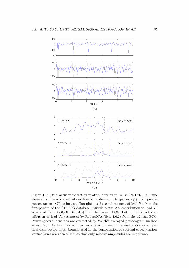
4.2. APPROACHES TO ATRIAL SIGNAL EXTRACTION IN AF 55
−1
−0.5
0
0.5
−0.2
0
0.2
0 1 2 3 4 5
−0.2
0
0.2
time (s)
(a)
0
2
4
fp = 5.37 Hz SC = 27.58%
0
2
4
fp = 5.98 Hz SC = 61.22%
0 1 2 3 4 5 6 7 8 9 100
2
4
frequency (Hz)
fp = 5.86 Hz SC = 71.63%
(b)
Figure 4.1: Atrial activity extraction in atrial fibrillation ECGs [P4,P26]. (a) Timecourses. (b) Power spectral densities with dominant frequency (fp) and spectralconcentration (SC) estimates. Top plots: a 5-second segment of lead V1 from thefirst patient of the AF ECG database. Middle plots: AA contribution to lead V1estimated by ICA-SOBI (Sec. 4.5) from the 12-lead ECG. Bottom plots: AA con-tribution to lead V1 estimated by RobustICA (Sec. 4.6.2) from the 12-lead ECG.Power spectral densities are estimated by Welch’s averaged periodogram methodas in [P20]. Vertical dashed lines: estimated dominant frequency locations. Ver-tical dash-dotted lines: bounds used in the computation of spectral concentration.Vertical axes are normalized, so that only relative amplitudes are important.
56 CHAPTER 4. ATRIAL ACTIVITY EXTRACTION IN AF EPISODES
ure 4.1(b)(top) shows the power spectral density of the V1-lead waveform displayedin Fig. 4.1(a)(top): the AA frequency components are buried under the VA strongerwider spectrum. This can be appreciated by looking at the middle and bottomplots in Fig. 4.1(b), corresponding to the spectra of two AA estimates (described inSecs. 4.5 and 4.6.2, respectively). Hence, classical frequency filters are also ineffec-tive in this context. More successful techniques focus on the explicit cancellationof the most significant features of the interfering cardiac waveform, that is, the pa-tient’s QRST complex. The average beat subtraction (ABS) method [114, 129, 149]computes a template of the interfering complex by synchronized averaging and thensubtracts it, after appropriate scaling, from the lead output. The technique relieson the assumptions that the interference and the signal of interest are uncoupled,and that the former presents a repetitive regular waveform. The ABS approachrequires beat detection and classification before averaging, is thus sensitive to themorphology of the ventricular beats, and cannot suppress noise and artifacts uncou-pled with the interfering signal (e.g., noise from electronic equipment). To mitigatethe sensitivity to local QRST morphological variations caused by minor changes inthe electrical axis of the heart (due, e.g., to respiration), the spatiotemporal QRSTcancellation (STC) technique [150] and related methods [140] take into account theaverage beats from adjacent leads via weighted LS fitting before subtraction. LikeABS, STC requires a sufficient number of beats with similar morphology in orderto obtain a significant QRST average and ensure the proper cancellation of AA inthe averaged beat. Alternative methods extract the VA using artificial neural net-works [152], or are based on the decomposition of the ECG using discrete packetwavelet transforms [147].
All the above techniques are unable to fully take advantage of the diversity pro-vided by the spatially-separated electrodes. Indeed, the standard ECG employedin clinical practice is composed of 12 leads, of which at least 8 provide linearly in-dependent measurements, while more sophisticated recording equipment used forbody surface potential mapping (BSPM) may include up to hundreds of leads. Eachlead captures a different mixture of bioelectrical phenomena of interest, artifacts,interference and noise. This spatial diversity can be efficiently exploited by process-ing, in a suitable manner, all leads simultaneously [P11]. The spatial informationthat can be derived by exploiting this kind of diversity may provide new insightsinto how the physiological mechanisms of interest (e.g., the atrial activation) andclinically relevant aspects (e.g., the degree of evolution of the disease) reflect on thesurface ECG, and may help assess the prognostic features of external recordings, cur-rently not fully understood. A classical approach attempting to exploit this diversityis Widrow’s multi-reference ANC method (see Sec. 2.3, p. 20), based on Wiener’soptimal spatial filtering theory [154]. However, the availability of reference leadslinked to the interference but free from the desired signal is a crucial assumptionfor the success of this method, and introduces strong constraints on the electrodelocation, as we have evidenced in the context of non-invasive fetal ECG extractionfrom maternal surface electrodes [P10,P11,P72].
To overcome the limitations of classical methods, a significant part of my re-search has been devoted to the design of novel spatial filtering techniques for AAextraction in AF. The first such techniques are fully blind in that they mainly exploit
4.3. BLIND AND SEMI-BLIND BIOMEDICAL SIGNAL PROCESSING 57
the statistical independence between the different cardiac signals during AF. Othermethods have also been put forward by taking into account additional propertiesof the biomedical problem under study. Due to the incorporation of extra priorinformation, the resulting techniques can be considered as semi-blind. Here, theterm is used in a wider sense than in communications, where it implies the existenceof a known time segment of the source signal(s), i.e., the availability of trainingdata. After developing in more detail the concept of semi-blind signal processingin biomedical applications (Sec. 4.3), the remaining of this chapter summarizes theresults obtained in the context of AA extraction in AF episodes.
4.3 Blind and Semi-Blind Biomedical Signal Processing
As briefly recalled in Sec. 2.3, pp. 19–22, BSS is more robust to calibration errorsthan more parametric techniques, thanks to the reduced number of model assump-tions. As a result, this methodology proves particularly interesting in biomedicalproblems, where parametric approaches may be cumbersome. Indeed, the use ofparameters would require time-consuming calibration protocols and may easily besubjected to a large patient-to-patient variability; parameters for the same patientmay also be expected to evolve with time. In addition, it is important that sig-nal processing methods be capable of providing adequate performance in a numberof potential pathophysiological conditions. Hence, the blind approach arises as ajudicious option in this uncertain environment [135, 136]. In the context of ECGprocessing, another valuable advantage of the fully-blind approach is that it doesnot require a preliminary heartbeat detection and classification stage and, as a re-sult, is essentially unaffected by wave morphology variations. Examples illustratingthis robustness to ectopic beats in pregnancy and AF ECG episodes are reportedin [136] and [118], respectively.
Despite the success achieved by fully-blind techniques over the last years, theirperformance may be inadequate in certain applications. Indeed, blindness is an at-tractive feature in the uncertainty of clinical environments, yet a single property likestatistical independence alone is sometimes unable to produce physiologically mean-ingful results in biomedical signal processing applications, as noted in [127, 128];another example is the direct application of ICA to AA extraction, as will be de-tailed in the next section. In these conditions, source extraction performance can beimproved by taking into account additional assumptions about the signals of inter-est or the mixing structure other than independence. Furthermore, the exploitationof prior knowledge may enable the resulting algorithms to focus on the extractionof the signal(s) of interest only, thus avoiding the unnecessary complexity of a fullseparation and the permutation ambiguity of blind methods (drawback D1, p. 27).
In a semi-blind setup, a Bayesian formulation is theoretically optimal but usuallyimpractical, as it involves the specification of probability distributions for the pa-rameters associated with the prior information. Determining such distributions maybe difficult or simply not feasible in certain scenarios. Moreover, the convergence ofBayesian model estimation methods (e.g., the expectation-maximization algorithm)is often very slow. These shortcomings have motivated the search for suboptimal
58 CHAPTER 4. ATRIAL ACTIVITY EXTRACTION IN AF EPISODES
but more practical alternatives for exploiting prior knowledge in BSS. These includethe use of signals correlated with the source of interest [113, 133, 138, 139, 148] andspatial patterns (mixing-matrix columns) related to the physiological activity underexamination [127,128]. This information can be incorporated into separation criteriato improve source separation performance.
In cooperation with Jose J. Rieta, Francisco Castells and Jose Millet, from UPV,Spain, my colleagues Olivier Meste and Pierre Comon, and my PhD students RonaldPhlypo and Pietro Bonizzi, I have investigated some of these practical alternatives tothe exploitation of prior information in AA signal extraction from the surface ECG.In particular, our researches have focused on the use of partial information about theatrial source statistics and spectral features [P20,P30,P33,P34,P36,P38] (Secs. 4.5–(p. 167)
(p. 237)(p. 245)
4.7, pp. 59–68) as well as constraints on the structure of the spatial topographies[P1, P29, P31] (Sec. 4.8, pp. 69–70). Working on the spatial dimension of multi-
(p. 231)lead ECG recordings has yielded results with potential clinical and physiologicalimpact related to AF classification [P2,P25] and the AV junction behavior duringAF [P35] (Sec. 4.9, pp. 70–71). Although originally aimed at solving a specific real-(p. 241)life problem, this research has also produced a number of theoretical results of muchwider scope, such as novel contrast functions for signal separation and extractionincorporating prior information about the sources. Some of these contrasts are basedon HOS [P5, P14] (Sec. 4.6.1, pp. 60–62), while others rely on SOS only [P6, P13](p. 117)
(p. 105) (Sec. 4.7.2, pp. 64–68). These contributions are explained next, after introducingthe BSS/ICA approach to AA extraction.
4.4 BSS/ICA Approach to Atrial Signal Extraction
In collaboration with J. J. Rieta and J. Millet, from UPV, Spain, I was part of theresearch team who first approached the AA signal extraction in ECG recordings asa BSS problem in instantaneous linear mixtures [P21, P67]. The adequacy of the(p. 177)static MIMO model (2.9), p. 18, finds strong theoretical support in electrophysio-logical considerations regarding the generation of cardiac electrical signals and theirpropagation across the human body. In the AA extraction context, vector sn iscomposed of atrial and ventricular activity sources, as well as other sources of in-terference and artifacts. Vector xn contains the signal mixtures observed at theelectrode array output. The mixing matrix coefficient hℓk = [H]ℓk represents thecontribution or projection of source k onto observation ℓ. The entries of the mixingmatrix columns {hk} reflect the spatial pattern or topography of the relative powercontribution described by the associated sources {sk,n} onto the spatially-separatedsensors, and correspond to potential field spatial distributions in the case of bioelec-trical signals. The mixing matrix coefficients associated with the cardiac sourcesare defined by the propagation of physiological signals from the heart to the elec-trodes through the body tissues. Due to the distance between heart and electrodes,the speed of propagation of electrical signals across the body and the bandwidth ofthe phenomena of interest, the transfer between sources and sensors can reasonablybe considered as linear and instantaneous. These facts support the suitability ofeqn. (2.9) to describe the signal generation model in this biomedical problem. By
4.5. COMBINING NON-GAUSSIANITY AND SPECTRAL FEATURES 59
estimating the sources of AA and the corresponding columns of the mixing matrix,and then isolating them from the remaining components, the AA signal can easilybe reconstructed in all leads free from VA and other interference.
Cardiac electrophysiology during AF leads to the assumption that AA and VAcan approximately be considered as statistically independent phenomena. This hy-pothesis enables the application of separation techniques exploiting the indepen-dence property like PCA and ICA. Compared to alternative methods such as multi-reference Wiener filtering, ABS or STC, the BSS approach does not assume anyparticular pattern for the contribution of the sources onto the electrodes (i.e., ex-istence of reference signals), nor a specific morphology or repetitive pattern for theinterfering waveforms. The results by PCA are unreliable since, by construction, thisapproach assumes a particular structure for the mixing matrix whereby its columnsare mutually orthogonal. Such a structure is difficult to enforce in the problem inhand, due to the spatial proximity between the atria and the ventricles. By contrast,ICA methods are generally more successful, as they allow a large degree of freedomin electrode placement relative to the source positions. A first validation of theseresults has been obtained in [P56,P63] by regarding the spectral signatures of the (p. 273)estimated sources. These signatures allow an automatic identification of the atrialsource among the separated components and are able to discriminate between NSR,AF and atrial flutter (AFL) [P57]. Despite the interest of these encouraging initialresults, AA can often present a near-Gaussian probability distribution, particularlyin more disorganized states of AF occurring as the disease evolves. This propertycompromises the separation of the atrial source from Gaussian noise and interferencewhen relying on HOS only.
4.5 Combining non-Gaussianity and Spectral Features
To improve the performance of conventional ICA in AA extraction, we have proposeda hybrid approach in [P20,P48]. The idea is to exploit a well-known feature of the (p. 167)AA signal: its time coherence, reflected on a quasi-periodic autocorrelation functionand a narrowband spectrum typically concentrated around a dominant frequency inthe 3–9 Hz band. HOS-based ICA, e.g., the FastICA algorithm, is first applied on thefull ECG recording in order to estimate the strongly non-Gaussian VA components.The remaining sources contain mixtures of AA and Gaussian noise, with low kurtosisvalues. A kurtosis threshold experimentally set at 1.5 allows the detection of theseremaining sources, which are then passed on as inputs to the SOBI method of [7].As explained at the end of Sec. 2.3, p. 22, SOBI is particularly well suited to theseparation of narrowband sources. In this application, the time lags of the correlationmatrices to be diagonalized are selected in accordance with typical AF cycle lengthvalues: the lag set spans a whole atrial period for the lowest expected dominantatrial frequency.
On the other hand, we have defined the spectral concentration (SC) as thepercentage of the estimated atrial signal power around its dominant frequencyfp [P20,P48]: (p. 167)
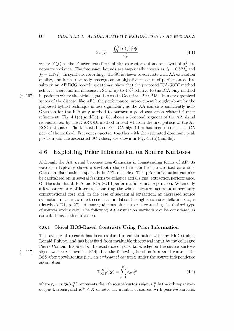
60 CHAPTER 4. ATRIAL ACTIVITY EXTRACTION IN AF EPISODES
SC(y) =
∫ f2
f1|Y (f)|2df
σ2y
(4.1)
where Y (f) is the Fourier transform of the extractor output and symbol σ2y de-
notes its variance. The frequency bounds are empirically chosen as f1 = 0.82fp andf2 = 1.17fp. In synthetic recordings, the SC is shown to correlate with AA extractionquality, and hence naturally emerges as an objective measure of performance. Re-sults on an AF ECG recording database show that the proposed ICA-SOBI methodachieves a substantial increase in SC of up to 40% relative to the ICA-only methodin patients where the atrial signal is close to Gaussian [P20,P48]. In more organized(p. 167)states of the disease, like AFL, the performance improvement brought about by theproposed hybrid technique is less significant, as the AA source is sufficiently non-Gaussian for the ICA-only method to perform a good extraction without furtherrefinement. Fig. 4.1(a)(middle), p. 55, shows a 5-second segment of the AA signalreconstructed by the ICA-SOBI method in lead V1 from the first patient of the AFECG database. The kurtosis-based FastICA algorithm has been used in the ICApart of the method. Frequency spectra, together with the estimated dominant peakposition and the associated SC values, are shown in Fig. 4.1(b)(middle).
4.6 Exploiting Prior Information on Source Kurtoses
Although the AA signal becomes near-Gaussian in longstanding forms of AF, itswaveform typically shows a sawtooth shape that can be characterized as a sub-Gaussian distribution, especially in AFL episodes. This prior information can alsobe capitalized on in several fashions to enhance atrial signal extraction performance.On the other hand, ICA and ICA-SOBI perform a full source separation. When onlya few sources are of interest, separating the whole mixture incurs an unnecessarycomputational cost and, in the case of sequential extraction, an increased sourceestimation inaccuracy due to error accumulation through successive deflation stages(drawback D1, p. 27). A more judicious alternative is extracting the desired typeof sources exclusively. The following AA estimation methods can be considered ascontributions in this direction.
4.6.1 Novel HOS-Based Contrasts Using Prior Information
This avenue of research has been explored in collaboration with my PhD studentRonald Phlypo, and has benefited from invaluable theoretical input by my colleaguePierre Comon. Inspired by the existence of prior knowledge on the source kurtosissigns, we have shown in [P14] that the following function is a valid contrast for(p. 117)BSS after prewhitening (i.e., an orthogonal contrast) under the source independenceassumption:
Υ(K+)KSP (y) =
K∑
k=1
εkκyk4 (4.2)
where εk = sign(κsk4 ) represents the kth source kurtosis sign, κyk
4 is the kth separator-output kurtosis, and K+ ≤ K denotes the number of sources with positive kurtosis.
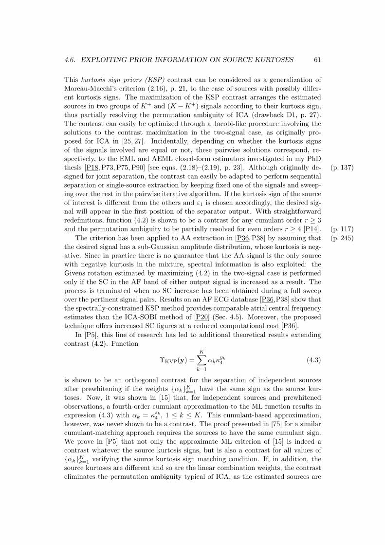
4.6. EXPLOITING PRIOR INFORMATION ON SOURCE KURTOSES 61
This kurtosis sign priors (KSP) contrast can be considered as a generalization ofMoreau-Macchi’s criterion (2.16), p. 21, to the case of sources with possibly differ-ent kurtosis signs. The maximization of the KSP contrast arranges the estimatedsources in two groups of K+ and (K −K+) signals according to their kurtosis sign,thus partially resolving the permutation ambiguity of ICA (drawback D1, p. 27).The contrast can easily be optimized through a Jacobi-like procedure involving thesolutions to the contrast maximization in the two-signal case, as originally pro-posed for ICA in [25, 27]. Incidentally, depending on whether the kurtosis signsof the signals involved are equal or not, these pairwise solutions correspond, re-spectively, to the EML and AEML closed-form estimators investigated in my PhDthesis [P18, P73, P75, P90] [see eqns. (2.18)–(2.19), p. 23]. Although originally de- (p. 137)signed for joint separation, the contrast can easily be adapted to perform sequentialseparation or single-source extraction by keeping fixed one of the signals and sweep-ing over the rest in the pairwise iterative algorithm. If the kurtosis sign of the sourceof interest is different from the others and ε1 is chosen accordingly, the desired sig-nal will appear in the first position of the separator output. With straightforwardredefinitions, function (4.2) is shown to be a contrast for any cumulant order r ≥ 3and the permutation ambiguity to be partially resolved for even orders r ≥ 4 [P14]. (p. 117)
The criterion has been applied to AA extraction in [P36,P38] by assuming that (p. 245)the desired signal has a sub-Gaussian amplitude distribution, whose kurtosis is neg-ative. Since in practice there is no guarantee that the AA signal is the only sourcewith negative kurtosis in the mixture, spectral information is also exploited: theGivens rotation estimated by maximizing (4.2) in the two-signal case is performedonly if the SC in the AF band of either output signal is increased as a result. Theprocess is terminated when no SC increase has been obtained during a full sweepover the pertinent signal pairs. Results on an AF ECG database [P36,P38] show thatthe spectrally-constrained KSP method provides comparable atrial central frequencyestimates than the ICA-SOBI method of [P20] (Sec. 4.5). Moreover, the proposedtechnique offers increased SC figures at a reduced computational cost [P36].
In [P5], this line of research has led to additional theoretical results extendingcontrast (4.2). Function
ΥKVP(y) =K∑
k=1
αkκyk4 (4.3)
is shown to be an orthogonal contrast for the separation of independent sourcesafter prewhitening if the weights {αk}Kk=1 have the same sign as the source kur-toses. Now, it was shown in [15] that, for independent sources and prewhitenedobservations, a fourth-order cumulant approximation to the ML function results inexpression (4.3) with αk = κsk
4 , 1 ≤ k ≤ K. This cumulant-based approximation,however, was never shown to be a contrast. The proof presented in [75] for a similarcumulant-matching approach requires the sources to have the same cumulant sign.We prove in [P5] that not only the approximate ML criterion of [15] is indeed acontrast whatever the source kurtosis signs, but is also a contrast for all values of{αk}Kk=1 verifying the source kurtosis sign matching condition. If, in addition, thesource kurtoses are different and so are the linear combination weights, the contrasteliminates the permutation ambiguity typical of ICA, as the estimated sources are
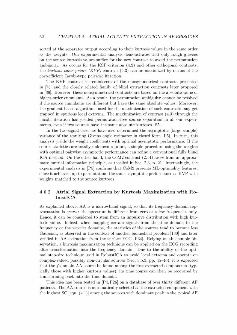
62 CHAPTER 4. ATRIAL ACTIVITY EXTRACTION IN AF EPISODES
sorted at the separator output according to their kurtosis values in the same orderas the weights. Our experimental analysis demonstrates that only rough guesseson the source kurtosis values suffice for the new contrast to avoid the permutationambiguity. As occurs for the KSP criterion (4.2) and other orthogonal contrasts,the kurtosis value priors (KVP) contrast (4.3) can be maximized by means of thecost-efficient Jacobi-type pairwise iteration.
The KVP contrast is reminiscent of the nonsymmetrical contrasts presentedin [75] and the closely related family of blind extraction contrasts later proposedin [36]. However, these nonsymmetrical contrasts are based on the absolute value ofhigher-order cumulants. As a result, the permutation ambiguity cannot be resolvedif the source cumulants are different but have the same absolute values. Moreover,the gradient-based algorithms used for the maximization of such contrasts may gettrapped in spurious local extrema. The maximization of contrast (4.3) through theJacobi iteration has yielded permutation-free source separation in all our experi-ments, even if two sources have the same absolute kurtoses [P5].
In the two-signal case, we have also determined the asymptotic (large sample)variance of the resulting Givens angle estimator in closed form [P5]. In turn, thisanalysis yields the weight coefficients with optimal asymptotic performance. If thesource statistics are totally unknown a priori, a simple procedure using the weightswith optimal pairwise asymptotic performance can refine a conventional fully blindICA method. On the other hand, the CoM2 contrast (2.14) arose from an approxi-mate mutual information principle, as recalled in Sec. 2.3, p. 21. Interestingly, theexperimental analysis in [P5] confirms that CoM2 presents ML-optimality features,since it achieves, up to permutation, the same asymptotic performance as KVP withweights matched to the source kurtoses.
4.6.2 Atrial Signal Extraction by Kurtosis Maximization with Ro-bustICA
As explained above, AA is a narrowband signal, so that its frequency-domain rep-resentation is sparse: the spectrum is different from zero at a few frequencies only.Hence, it can be considered to stem from an impulsive distribution with high kur-tosis value. Indeed, when mapping certain signals from the time domain to thefrequency or the wavelet domains, the statistics of the sources tend to become lessGaussian, as observed in the context of another biomedical problem [130] and laterverified in AA extraction from the surface ECG [P34]. Relying on this simple ob-servation, a kurtosis maximization technique can be applied on the ECG recordingafter transformation into the frequency domain. Due to the ability of the opti-mal step-size technique used in RobustICA to avoid local extrema and operate oncomplex-valued possibly non-circular sources (Sec. 3.5.3, pp. 45–46), it is expectedthat the f -domain AA source be found among the first extracted components (typ-ically those with higher kurtosis values); its time course can then be recovered bytransforming back into the time domain.
This idea has been tested in [P4,P26] on a database of over thirty different AFpatients. The AA source is automatically selected as the extracted component withthe highest SC [eqn. (4.1)] among the sources with dominant peak in the typical AF
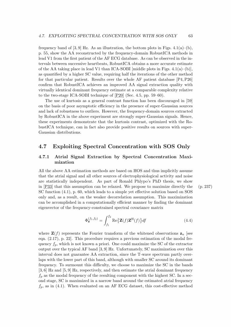
4.7. EXPLOITING SPECTRAL CONCENTRATION WITH SOS ONLY 63
frequency band of [3, 9] Hz. As an illustration, the bottom plots in Figs. 4.1(a)–(b),p. 55, show the AA reconstructed by the frequency-domain RobustICA methods inlead V1 from the first patient of the AF ECG database. As can be observed in the in-tervals between successive heartbeats, RobustICA obtains a more accurate estimateof the AA taking place in lead V1 than ICA-SOBI [middle plots in Figs. 4.1(a)–(b)],as quantified by a higher SC value, requiring half the iterations of the other methodfor that particular patient. Results over the whole AF patient database [P4, P26]confirm that RobustICA achieves an improved AA signal extraction quality withvirtually identical dominant frequency estimate at a comparable complexity relativeto the two-stage ICA-SOBI technique of [P20] (Sec. 4.5, pp. 59–60).
The use of kurtosis as a general contrast function has been discouraged in [59]on the basis of poor asymptotic efficiency in the presence of super-Gaussian sourcesand lack of robustness to outliers. However, the frequency-domain sources extractedby RobustICA in the above experiment are strongly super-Gaussian signals. Hence,these experiments demonstrate that the kurtosis contrast, optimized with the Ro-bustICA technique, can in fact also provide positive results on sources with super-Gaussian distributions.
4.7 Exploiting Spectral Concentration with SOS Only
4.7.1 Atrial Signal Extraction by Spectral Concentration Maxi-mization
All the above AA estimation methods are based on HOS and thus implicitly assumethat the atrial signal and all other sources of electrophysiological activity and noiseare statistically independent. As part of Ronald Phlypo’s PhD thesis, we showin [P33] that this assumption can be relaxed. We propose to maximize directly the (p. 237)SC function (4.1), p. 60, which leads to a simple yet effective solution based on SOSonly and, as a result, on the weaker decorrelation assumption. This maximizationcan be accomplished in a computationally efficient manner by finding the dominanteigenvector of the frequency-constrained spectral covariance matrix
Φ(f1,f2)z =
∫ f2
f1
Re{Z(f)ZH(f)
}df (4.4)
where Z(f) represents the Fourier transform of the whitened observations zn [seeeqn. (2.17), p. 22]. This procedure requires a previous estimation of the modal fre-quency fp, which is not known a priori. One could maximize the SC of the extractoroutput over the typical AF band [3, 9] Hz. Unfortunately, SC maximization over thisinterval does not guarantee AA extraction, since the T-wave spectrum partly over-laps with the lower part of this band, although with smaller SC around its dominantfrequency. To surmount this difficulty, we choose to maximize the SC in the bands[3, 6] Hz and [5, 9] Hz, respectively, and then estimate the atrial dominant frequencyfp as the modal frequency of the resulting component with the highest SC. In a sec-ond stage, SC is maximized in a narrow band around the estimated atrial frequencyfp, as in (4.1). When evaluated on an AF ECG dataset, this cost-effective method
64 CHAPTER 4. ATRIAL ACTIVITY EXTRACTION IN AF EPISODES
outperforms the original spatio-temporal ICA-SOBI algorithm of [P20] (Sec. 4.5,pp. 59–60) in terms of SC while providing comparable atrial frequency estimates.
The search for the atrial modal frequency is further refined in [P6] by partitioningthe typical AF band into more than two different subbands. Each subband is usedas a initial guess of the actual AF band present in the recording, from which an AAestimate can be obtained by the above SC maximization procedure. The actual AFband is recomputed as the set of frequencies associated with a fixed high percentileof the AA estimate’s amplitude spectrum. Using the new AF band estimate, a newAA signal is estimated and so on, until convergence. One atrial estimate per initialsubband is thus obtained and, among them, we retain that with the highest SC.This iterative method for the simultaneous estimation of the AA extraction filterand the significant AF band usually converges in a few iterations and, as quantifiedby SC, improves on the ICA-SOBI method of [P20] (Sec. 4.5).
4.7.2 A Novel Contrast for Source Extraction Based on ConditionalSecond-Order Moments
Generalizing these results, a novel criterion for source extraction is developed in [P13],(p. 105)based on the prior knowledge of the significant support of the source of interest si, i.e.,the set of time indices n over which |si,n| > C, for a given positive real constant C.Hence, the required prior information amounts to a presence indicator of the desiredsource. This presence indicator can also be specified in the frequency domain. Forsimplicity, in what follows we will assume real-valued sources and mixtures. Thecriterion relies on the following additional assumptions on the sources:
H1) The source of interest, si, is independent of the other sources, {sj}j 6=i. Theselatter are stored in vector s. Up to some irrelevant permutation of indices, wecan write s = [si, s
T]T.
H2) The sources {sk}Kk=1 have unit-variance continuous distributions with non-nullpdf in a finite interval of B = [−C,C].
It will be seen later that hypothesis H1 is too restrictive and can actually be reducedto second-order decorrelation. First of all, we need the following definition of con-trast function for blind source extraction [76], which can be considered as a directextension of Definition 1, p. 21.
Definition 2 (contrast function for blind extraction). A function Υ(·) of theextractor output distribution is a contrast for the blind extraction of the source ofinterest si if it verifies:
Invariance: Υ(λsi) = Υ(si) for any scalar λ 6= 0.
Domination: Υ(gTs) ≤ Υ(si) for any length-K vector g.
Discrimination: Υ(gTs) = Υ(s) if and only if g = λei, where λ 6= 0 and ei denotesthe canonical basis vector in R
K such that eTi s = si.
The starting point of the new extraction criterion is the expected log-likelihoodof the observed vector x under the ICA model (2.9), p. 18, which in the noiseless
4.7. EXPLOITING SPECTRAL CONCENTRATION WITH SOS ONLY 65
case reads [14,15]:
L(H∣∣x) = E{log px(x
∣∣H)} = E{log ps(H
−1x)} − log |detH|.
This function can also be expressed in terms of the separating matrix W as:
L(W∣∣x) = E{log ps(W
Tx)}+ log |detW| (4.5)
since y = WTx [eqn. (2.3), p. 17] so that WT is an estimate of H−1. Accordingto hypothesis H1, the source joint pdf can be decomposed as ps(s) = psi(si)ps(s).Likewise, the determinant in (4.5) can be written as the scalar product: detW =wTw, where [w]i contains the cofactor of element [w]i in matrix W. Hence, thelog-likelihood becomes:
L(W∣∣x) = E{log psi(w
Tx)}+ E{log ps(WTx)}+ log(wTw)
where matrix W contains all columns of matrix W except w. Since we are onlyinterested in extracting si, the estimation of s, and thus W, is irrelevant. Also, anyvariations in detW due to w can be absorbed by W. It follows that function
L(w∣∣x) = E{log psi(w
Tx)}
can be considered as the expected log-likelihood for the extraction of the desiredsource. Expressing the expectation in terms of the extractor output pdf, we arriveat:
L(w∣∣x) =
∫
R
py(u) log psi(u)du.
Recall that the dependence of the likelihood on the extraction filter w is madeexplicit in the extractor output pdf, py(·), by relationship (2.6), p. 17.
Now, according to the above result, we can consider the following function asthe expected conditional log-likelihood of the extractor output for the estimation ofthe desired source [P13]: (p. 105)
ΥC(y)def= L(w
∣∣x, I) =
∫
R
py|I(u) log psi|I(u)du
=
∫
B
py|I(u) log psi|I(u)du +
∫
B
py|I(u) log psi|I(u)du (4.6)
where I denotes the event |si| > C, and py|I(·) and psi|I(·) represent the pdf’s ofthe extractor output and the source of interest, respectively, conditioned on I. SetB is defined as B = R\B, where B is given in hypothesis H2. If we define P (I) =∫
Bpsi(u)du, the conditional pdf of the source of interest reads:
psi|I(u) =
{psi(u)/P (I), u ∈ B
0, u ∈ B.
Hence, the conditional likelihood (4.6) is heavily penalized by its last term as soonas py|I(u) 6= 0 for any u ∈ B, that is, if the extractor output does not verify thecondition |y| > C when the desired source does. Indeed, function (4.6) turns out tobe an extraction contrast.
66 CHAPTER 4. ATRIAL ACTIVITY EXTRACTION IN AF EPISODES
Proposition 1. Under hypotheses H1–H2, ΥC(y) is a contrast function for theextraction of source si in the noiseless model (2.9), p. 18, for any C > 0.
Proof. Under the conventional unit-variance source assumption, the invariance property isreadily verified. Domination and discrimination are deduced from the fact that function (4.6)is ruled by its penalizing term
∫
Bpy|I(u) log psi|I(u)du. If y = si, function ΥC(y) becomes
the entropy of si conditioned on I, which is a finite number. If a contribution from anothersource is present at the extractor output, we will have y = gisi + s, with s =
∑
j 6=i gjsj .Since si is independent of s (hypothesis H1), the distribution py|I(u) can be written as theconvolution of the distributions psi|I(u) and ps|I(u):
py|I(u) =
∫
R
psi|I(τ − u)ps|I(τ)dτ.
From hypotheses H1–H2, ps|I(u) 6= 0 over an interval of B with non-zero Lebesgue measure
and, from the above convolution product, ∃u ∈ B such that py|I(u) 6= 0. As a result,ΥC(y) ≤ ΥC(si), and the equality can hold only if s = 0, that is, gj = 0 for j 6= i.
Due to the penalty term in eqn. (4.6), the maximization of ΥC(y) is not tractable,as it requires an exhaustive search over all possible extraction filters w. This require-ment can be relaxed by considering the following weighted integral of the conditionalprobability of the extractor output:
Υ′C(y) =
∫
B
py|I(u)γ(u)du
where function γ(u) is positive except possibly at the origin. The following resultshows that
Lemma 2. Minimizing Υ′C(y) cancels the penalty term of ΥC(y) in (4.6).
Proof. Clearly, Υ′C(y) ≥ 0. The function is thus minimized at Υ′
C(y) = 0. Since γ(u) ispositive and can only be null at u = 0, at the minimum we can have at most py|I(u) =αδu, where α is an arbitrary scalar and δu represents Dirac’s delta function. In particular,py|I(u) = 0 elsewhere in B\{0}. Under hypothesis H2, we must have α = 0, and thus
py|I(u) = 0 over B.
Still, the minimization of Υ′C(y) with respect to w remains generally intractable.
However, with the choice γ(u) = u2, minimizing Υ′C(y) is intuitively equivalent to
maximizing ∫
Rpy|I(u)u2du
σ2y
(4.7)
where σ2y =
∫
Rpy(u)u2du appears in the denominator to guarantee the invariance
property. To see this, let us consider the equality:∫
Rpy|I(u)u2du
σ2y
=
∫
Bpy|I(u)u2du +
∫
Bpy|I(u)u2du
σ2y
.
Due to the chosen weighting function, the term∫
Bpy|I(u)u2du dominates the nom-
inator on the right-hand side. As a result, maximizing the left-hand side of theequality would tend to shift the probability mass of py|I(u) towards large values of
4.7. EXPLOITING SPECTRAL CONCENTRATION WITH SOS ONLY 67
y (|y| > C, but bounded by the variance normalization). In turn, this is equivalentto the minimization of Υ′
C(u), and thus (by virtue of Lemma 2) of∫
Bpy|I(u)du, as
required.
Criterion (4.7) seeks for the extractor output with maximum variance in thetails (MaxViT) of its distribution, and can be expressed as the maximization of theRayleigh quotient:
ΥMaxViT(y) =Φsi
y
Φy=
wTΦsix w
wTΦxw(4.8)
where Φy = E{y2} and Φsiy = E{y2
∣∣ I}; the observation covariance and constrained
covariance matrices are defined as Φx = E{xxT} and Φsix = E{xxT
∣∣ I}, respectively.
Proposition 3. Function ΥMaxViT(y) is a contrast function for the extraction ofsource si in the noiseless model (2.9), p. 18, under the following sufficient conditions:
C1) E{sjsk} = 0, ∀j 6= k
C2) E{sjsk
∣∣ I} = 0, ∀j 6= k
C3) E{s2i
∣∣ I} > E{s2
j
∣∣ I}, ∀j 6= i.
Proof. The denominator in eqn. (4.8) ensures the scale invariance property in Definition 2,p. 64. Now, under conditions C1–C2, we can write
ΥMaxViT(y) =wTΦsi
x w
wTΦxw=
gTΦsis g
gTΦsg=
∑
j g2j Φsi
sj∑
j g2j
(4.9)
where g = HHw and gi = [g]i. Accordingly, maximizing ΥMaxViT(y) is equivalent tomaximizing its numerator subject to ‖g‖ = 1. Splitting the numerator in the differentcontributions yields
g2i Φsi
si+
∑
j 6=i
g2j Φsi
sj+ Φsi
si
(∑
j 6=i
g2j −
∑
j 6=i
g2j
)
which can be rewritten as
Φsisi
+∑
j 6=i
g2j (Φsi
sj− Φsi
si) ≤ Φsi
si
where the inequality follows from (Φsisj−Φsi
si) < 0, ∀j 6= i, due to condition C3. This proofs
the domination. Moreover, we have
Φsiy = Φsi
si⇔
∑
j 6=i
g2j (Φsi
sj− Φsi
si) = 0.
Now, since (Φsisj− Φsi
si) < 0, ∀j 6= i, the above equality holds if and only if g2
j = 0, ∀j 6= i.This proves the discrimination.
Equation (4.9) has taken into account that the conditioned source covariance matrix Φsis
is diagonal, as expressed by condition C2 above. This can actually be relaxed to conditionaldecorrelation with the source of interest only:
C2’) E{sisj
∣∣ I} = 0, ∀j 6= i.
In such a case, condition C3 becomes Φsisi
> λmax, where λmax represents the dominanteigenvalue of Φsi
s [P13]. (p. 105)
68 CHAPTER 4. ATRIAL ACTIVITY EXTRACTION IN AF EPISODES
Condition C1 is a classical second-order decorrelation constraint, and is indeedweaker than the starting assumption H1, p. 64, employed to derive the conditionalML criterion (4.6), p. 65. Condition C2 (or C2’) imposes decorrelation over thesignificant support of si. Although full decorrelation can rarely hold in practice, atheoretical analysis and experimental results on simulated data show that MaxViT’ssource extraction quality is quite robust to violations of this hypothesis [P13]. Con-(p. 105)dition C3 ensures the domination property of the contrast when the desired sourceis recovered at the extractor output.
The maximization of contrast (4.8) reduces to the computation of the domi-nant eigenvalue of matrix Φsi
x after prewhitening [P13]. The contrast can thus beoptimized in a computationally efficient manner.
The method of conditional moments, proposed for BSS in [107] without a directlink with the theory of contrast functions, bears close resemblance to MaxViT.However, as opposed to [107], our method is linked to ML estimation, is designedto target a specific source, is not limited to symmetric distributions, can handle theextraction of Gaussian sources and does not require post-processing manipulationssuch as correcting rotations for super-Gaussian sources. Connections with otherreference-based BSS techniques, including [18,148], are discussed at length in [P13].(p. 105)
When computed in the frequency domain, the conditional covariance matrix Φsix
after prewhitening becomes the spectral covariance matrix shown in eqn. (4.4), p. 63,if the assumed significant spectral support lies in the interval [f1, f2] Hz. Indeed,the AA extraction methods proposed in [P6, P33] (see also Sec. 4.7.1, p. 63) are(p. 237)essentially the MaxViT algorithm in the frequency domain, where intervals of thetypical AF band serve as initial estimates of the significant support of the desiredsource.
4.7.3 Blind Source Extraction Based on Second-Order Statistics
A novel technique for blind source extraction relying on SOS has recently been pre-sented in [71]. The technique is based on the instantaneous linear mixing model (2.9),p. 18. The sources are assumed to be uncorrelated and colored with distinct spectra.Let Rx,τ = E{xnx
Tn−τ} denote the sensor-output autocorrelation matrix at time lag
τ . It is claimed in [71] that a valid extracting vector w can be obtained from theminimization of function
ΥLZ(w, t,d) =
D∑
k=0
‖Rx,τkw − dτk
t‖2 (4.10)
with respect to vectors w, t ∈ RK and d = [dτ0 , dτ1 , . . . , dτD ]T ∈ R
D+1. In [71], thisclaim is given a geometrical interpretation in terms of oblique projection operatorsand demonstrated through numerical experiments.
Work [P15] provides alternative justifications for this approach and proves that,(p. 121)under the given assumptions and with an appropriate choice of time lags {τk}Pk=0, theminimization of (4.10) is achieved if and only if w is indeed a valid extracting vector.Asymptotically, as the number of lags tends to infinity, the necessary condition forsource identifiability using this method becomes that of the popular SOBI algorithm
4.8. EXPLOITING THE SPATIAL TOPOGRAPHIES 69
[7] (Sec. 2.3, p. 22), i.e., that no pair of source spectra be equal up to scale. Thisalgorithm can thus be seen as an extension of SOBI to blind extraction. Nevertheless,the global convergence of the alternating LS algorithm proposed in [71] to minimizecriterion (4.10) is not guaranteed and remains to be proven theoretically.
4.8 Exploiting the Spatial Topographies
As explained earlier, the AA signal can often present a near-Gaussian statisticalbehavior, which renders HOS-based estimates suboptimal and points out the needfor further or alternative information to enhance AA estimation performance. Theuse of spectral features, through the application of time-coherence based separationmethods (e.g., SOBI) or the maximization of spectral concentration, allows the useof SOS only. Another approach of this kind explored in Pietro Bonizzi’s PhD thesisis the exploitation of the spatial signatures or topographies (i.e., the mixing-matrixcolumns or source directions) associated with the different cardiac complexes in themulti-lead recording. The key idea underlying this approach is the decompositionof the observed ECG signal into non-overlapping time segments associated with themost significant features of the cardiac period, namely, the QRS complex, the T waveand the TQ interval:
x = xQRS + xT + xTQ.
In each of these segments, one or both of the most important component interferingwith the AA, i.e., the QRS complex and the T wave, are missing. This leads to amore accurate description of the remaining activity, which can later be capitalizedon to enhance AA estimation. An obvious disadvantage of this approach is that, justlike STC methods [140,150], it requires a previous wave detection and segmentationstage.
The first algorithm of this type, developed in [P31], can be divided in three steps.First, a rough estimate of the AA source topography is obtained by the ICA of thewhole observation x. The VA source directions, including the QRS complex andthe T wave, are then computed from the PCA of xQRS and xT (via, e.g., the SVDof the respective data matrices). Finally, a refined spatial filter for AA extractionis obtained by projecting the initial AA topography estimate onto the orthogonalcomplement of the VA subspace using Gram-Schmidt orthogonalization. This spatialfilter is applied on x to obtain the atrial signal estimate over the whole recording. Onan AF ECG database, this simple procedure provides a performance up to the markof more elaborate techniques such as the STC method of [140] and the ICA-SOBIalgorithm of [P20] (Sec. 4.5, pp. 59–60).
The method put forward in [P29] builds upon the absence of QRST contribution (p. 231)in the TQ segment xTQ to refine the AA estimate obtained from the ICA of the wholeobservation x. Let h1 denote the atrial topography estimated by ICA applied on x.An additional atrial topography estimate, say h2, is obtained from the PCA of xTQ.A refined atrial extractor is sought in the plane spanned by the linear extractorsassociated with h1 and h2. Its optimal orientation is determined by maximizingthe SC of the resulting AA signal estimate, a process that, very much along thelines of Sec. 4.7, pp. 63–68, can be carried out algebraically. This method offers a
70 CHAPTER 4. ATRIAL ACTIVITY EXTRACTION IN AF EPISODES
similar performance to that of [P31] summarized in the above paragraph. Using ICAinstead of PCA when computing the reference topography h2 can slightly enhanceAA extraction quality.
4.9 Clinical and Physiological Information from Surface
Recordings
As introduced in Sec. 4.1, p. 54, the surface ECG has already reported to be usefulin the analysis of AF [114–116], and has the advantage over atrial electrograms ofbeing a non-invasive technique. An important part of Pietro Bonizzi’s PhD has beendevoted to analyzing whether useful additional clinical and physiological informationcan be gathered from surface recordings alone, with particular focus on two partic-ular aspects: the ventricular response during AF (Sec. 4.9.1) and AF classification(Sec. 4.9.2).
4.9.1 Atrio-ventricular junction behavior during AF
Although it is generally acknowledged that heart rate variability is enhanced duringAF [119], several studies reveal that the prevailing ventricular rate during highatrial rate seems to obey complex dynamics and no unifying mechanism has yetbeen found. To help shed light on this issue, several quantitative models of theventricular response during AF have been developed [119,137]. The activation modelby Cohen [119] introduced the hypothesis that the AV node can be treated as alumped structure with well-defined electrical properties, including the refractoryperiod, the automaticity and a certain depolarization threshold. According to thismodel, the AV conduction would be triggered, thus inducing a heartbeat, when theenergy of AA impulses impinging on the node exceeds the depolarization threshold.
In [P35], we attempt to confirm this hypothesis by analyzing the existence of a(p. 241)possible correlation between the occurrence of a heartbeat and the power of the AAobservable in the ECG during the preceding TQ interval. A weighted average ofthe power contained in all leads over the TQ segment is plotted against the dura-tion of the corresponding RR segment. Interestingly, the shape of the scatter plotso obtained from a healthy subject differs considerably from that of a pathologicalsubject. In the latter, an inverse relationship can be clearly perceived that seems tosupport the hypotheses of [119,137]. The scatter plot, however, shows an importantvariance for short RR periods, obscuring the relationship between RR interval dura-tion and the observed AA power. Such variance could be explained by the fact thatthe ECG is unable to capture all the AA actually contributing to the activation ofthe AV node, but could also be due to an increased noise variance when averagingover shorter TQ segments as the heart rate increases.
4.9.2 AF classification
Motivated by their potential relevance in clinical decision making, a number of previ-ous studies have attempted to distinguish between organized and disorganized states
4.9. CLINICAL AND PHYSIOLOGICAL INFORMATION 71
of AF by analyzing atrial electrograms [120, 134]. Using PCA, single-lead electro-grams of more organized AF were shown to be represented by a reduced number ofprincipal components [120]. More recent works have demonstrated the possibilityof visually evaluating different activation patterns in AF patients by exploiting thehigh spatial resolution of BSPM recordings [123].
In collaboration with Francisco Castells, Maria Guillem, Andreu Climent andJose Millet, from UPV, Spain, we continue to explore the spatial information pro-vided by surface recordings. In [P2, P25], we aim at an automated non-invasiveclassification of AF in 56-lead BSPM signals recorded from two groups of patients.These patients have been classified beforehand as AF type I (single wavefront prop-agating across the body surface) and type II/III (no observable clear wavefront ormultiple wavefronts that do not propagate across the body surface observed simul-taneously), according to Koning’s criteria [134].
To quantify the degree of spatio-temporal organization of the AA in AF, weanalyze the structure of the mixing matrix derived by the PCA of the TQ segmentsin the BSPM recording. For a given patient, the PCA of the cth segment yields anestimate of the noiseless BSS model (2.9), p. 18:
x(c) = H(c)s(c)
Our first study reveals that the average number of dominant components required toexplain 95% of the variance of type-I segments (4 components) is half that of type-II/III segments (9 components), with a p-value of p < 0.05. Hence, the number ofsignificant principal components give a first indication of AF organization in exter-nal recordings. These findings are consistent with those obtained from endocardialrecordings in [120].
To increase the discriminative power of our analysis, the data in the cth TQ seg-ment are projected on the spatial topographies associated with the most significantprincipal components of the initial segment. Let k denote the number of dominant
topographies, and let these k topographies be stored in matrix H(1)k . The projection
can then be expressed as:
x(c) = H(1)k
[(H
(1)k )TH
(1)k
]−1(H
(1)k )Tx(c).
From this relationship, the normalized reconstruction error between the data presentin the cth segment and their projection on the dominant principal topographies ofthe initial segment is easily computed. This error is a measure of the spatio-temporalstationarity or repetitiveness of the AA observed in the BSPM recording. By se-lecting the k = 3 most significant topographies of the initial segment, the averagereconstruction error across the remaining segments is shown to be significantly lowerin type-I patients than in type-II/III patients, with p < 10−4. This result revealsthat more organized states of AF are reflected on an increased repetitiveness of theprincipal spatial topographies across the surface recording.
This investigation shows that the automated classification of AF in surfacerecordings is indeed possible and strongly supports the appropriateness of signalprocessing approaches exploiting spatial diversity, such as BSS/ICA, in AF analy-sis.
72 CHAPTER 4. ATRIAL ACTIVITY EXTRACTION IN AF EPISODES
4.10 Summary
Atrial signal extraction in surface ECG recordings of AF can be modeled as a BSSproblem of instantaneous linear mixtures (Sec. 4.4). The pertinence of this approachis supported by considerations regarding the generation and propagation of electro-physiological signals across the body. Compared to alternative approaches such asANC, ABS or STC, BSS does not assume any particular structure for the contri-bution of the sources onto the electrodes, nor a specific morphology or repetitivepattern for the interfering waveforms. The independence between the sources ofinterest and the artifacts is a realistic assumption during AF.
Prior knowledge about the spectral content of the AA signal, its statistical behav-ior or its spatial topographies can also be incorporated into the separation criteriato improve source extraction performance and reduce computational complexity. Avariety of such semi-blind methods have been presented throughout this chapter(Secs. 4.5–4.8). As a valuable by-product, our attempt to design AA extractionmethods with improved performance has yielded new theoretical results in the areaof BSS/ICA, such as novel contrasts based on HOS (Sec. 4.6.1) and conditional SOS(Sec. 4.7.2). In addition, the exploitation of the spatial diversity of multi-lead surfacerecordings has been shown to reveal useful information of clinical and physiologicalrelevance (Sec. 4.9). These positive results encourage further research efforts intoAF analysis approaches exploiting spatial diversity.
Chapter 5
Research Perspectives
Numerous possible avenues remain open for the continuation of the research sum-marized in the previous chapters of this report. Some of the most promising arebriefly pointed out in the following paragraphs.
5.1 Algorithms for Robust Equalization and Source Sep-
aration
• The performance of algebraic equalizers (Sec. 3.3, pp. 30–39) depends on anaccurate estimation of the number of valid solutions, as well as their optimalequalization delays. Algorithms for the robust automatic detection of theseparameters need to be developed and assessed.
• The matrix and tensor problems associated with algebraic solutions (Sec. 3.3,pp. 30–39) would be considerably more involved in more elaborate scenariossuch as the convolutive MIMO case. Fresh researches would thus be necessaryto tackle them.
• Algebraically, the subspace method proposed to find the ACPA equalizer pro-vides a particular solution to the challenging rank-1 tensor linear combinationproblem (Sec. 3.3.3, pp. 33–39). In our numerical study, the proposed subspaceapproach proves more robust than other structuring methods, but the blind al-gebraic solutions offer a low tolerance to noise, particularly for long equalizers.The key point limiting performance is probably the SVD-based rank-1 tensorapproximation employed to extract the equalizer vector from the estimatedsymmetric tensor (Sec. 3.3.3.7, p. 37). A refinement of the SVD-based rank-1tensor approximation, such as that obtained by the power method [66,69] andother algorithms to be developed, could alleviate this limitation.
• Similarly, the semi-blind algebraic solution of Sec. 3.4.1, pp. 40–40, is onlyapproximate, and new more effective ways to combine analytic supervised andblind equalizers need to be explored.
• Iterative semi-blind criteria have proven rather robust to the confidence param-eter λ (Sec. 3.4.2, pp. 41–42), yet its appropriate choice could bring important
73
74 CHAPTER 5. RESEARCH PERSPECTIVES
performance gains in specific scenarios. Determining its optimal value wouldrequire the asymptotic variance analysis of semi-blind contrasts.
• The convergence of the optimal step-size iterative technique (Sec. 3.5, pp. 42–46) has always proven satisfactory in our experiments. However, analyzing thetheoretical convergence properties of this technique is a challenging open issue,especially in scenarios where spurious local extrema exist (finite data length,additive noise, violation of model assumptions). In general, the convergenceof source extraction algorithms based on HOS remains to be investigated inthis context.
• The use of cumulant-based criteria such as kurtosis has been objected in [59]on the grounds of its suboptimal asymptotic performance for super-Gaussiansources and lack of robustness to outliers. Robust cumulant estimators (see,e.g., [156] and references therein) could alleviate these potential difficulties.Whether the iterative optimization of criteria based on robust estimators couldstill benefit from the numerical convenience of the optimal step-size approach(Sec. 3.5.2–3.5.3, pp. 43–46) should also be ascertained.
• In conjunction with the optimal step-size technique, we have developed se-quential source separation algorithms based on linear regression; an exampleis RobustICA (Sec. 3.5.3, pp. 45–46). The performance of the regression ap-proach is shown to degrade as more components are extracted. More robustregression strategies, inspired by those in [17, 99], need to be developed andthoroughly assessed.
• Although alphabet-based criteria such as the APF and CP principles are shownto be valid contrasts for source separation and extraction [34], the presenceof local extrema should be clarified and their detrimental impact on sourceestimation performance evaluated. This study would be particularly relevantin scenarios where the lack of training data precludes the use of semi-blindmethods.
• The main drawback of APF criteria relative to alternative properties like CMor kurtosis is their sensitiveness to carrier residual [31, 32]. Carrier-residualeffects on APF-based equalizers need to be evaluated in detail and reducedthrough suitable compensation techniques. The inclusion of pilot informationin semi-blind criteria may already play a substantial role as a compensationmechanism.
• As most orthogonal contrasts for source separation, the KSP and KVP criteria(Sec. 4.6.1, pp. 60–62) can be maximized by the Jacobi pairwise iterationoriginally put forward for ICA in [24,25,27]. To date, this iterative techniquehas always yielded positive results, but its convergence has yet to be proventheoretically. Extending the Jacobi technique to single-source extraction andsequential source separation is another interesting open problem.
5.2. ATRIAL FIBRILLATION ANALYSIS 75
• The analysis of the alternating LS algorithm to optimize the blind source ex-traction contrast (4.10), p. 68, should be addressed in future investigations, aswell as the incorporation of prior information into the contrast.
• A more exhaustive comparison, both theoretical and experimental, of otherequalization and source separation principles with those studied in the presentwork remains to be made.
• Further research should also analyze the integration of the proposed techniquesin forthcoming commercial communications standards.
5.2 Atrial Fibrillation Analysis
Although the BSS/ICA approach has proven its potential in a variety of biomedi-cal signal processing problems beyond ECG analysis, further research is necessaryto answer some important open questions regarding its application in biomedicalcontexts and, particularly, AF analysis:
• A fundamental issue is the relationship between the signals estimated by sourceseparation techniques and the actual internal sources of electrophysiologicalactivity. The simultaneous recording of intracardiac and surface recordingsduring electrophysiological studies could play a crucial role in answering thisquestion.
• Another important point concerns the measure of atrial signal estimation qual-ity, which, as typically occurs in inverse problems, is hampered by the lack ofaccess to the actual physiological activity sources. Experiments on syntheticdata support the adequacy of SC as an objective performance index (Sec. 4.5,pp. 59–60). However, its suitability should be further validated by correlationwith endocardial signals. Alternative measures such as those based on thecompressed spectrum could prove more appropriate in more organized forms ofatrial arrhythmia like AFL [P28].
• The application of the blind source extraction contrast (4.10), p. 68, to AAextraction should be explored, and compared to the other techniques describedin Chapter 4.
• The AA is known in TQ segments, which can help obtain initial estimates of theatrial topography (Sec. 4.8, pp. 69–70). This information could be exploited toderive optimal spatial beamformers along the lines of [101] for the estimationof the AA in the whole recording, thus refining the topography-based atrialsignal extraction algorithms.
• In fetal ECG extraction during pregnancy, the fetal source typically contributesmore strongly to abdominal electrodes. Likewise, the atrial source is expectedto appear predominantly in the V1 lead in AA extraction during AF. Themathematical formulation of these fuzzy constraints and their incorporationinto signal estimation criteria are other interesting problems to be tackled.
76 CHAPTER 5. RESEARCH PERSPECTIVES
• A related issue is how to best exploit and combine various kinds of availableprior information (second- and higher-order statistics, time coherence, spatialtopographies, etc.) to improve separation performance while maintaining therobustness to modeling errors of the BSS/ICA approach.
• The optimal use of the variety of information provided by simultaneous record-ings in different modalities (e.g., ECG in combination with Doppler ultrasound)constitutes a major research challenge in the field of biomedical signal ex-traction. For instance, topography-based source extraction techniques couldbenefit from the improved spatial resolution of recording modalities such asmagnetic resonance imaging.
• Encouraging initial results on the ventricular response during AF and AFclassification have been obtained from the analysis of surface recordings alone(Sec. 4.9, pp. 70–71). Shedding light on the links between estimated sourcesand actual sources of cardiac electrical activity (see the first point above)should in turn help discern the additional clinical and physiological knowledgeto be gained from the analysis of the estimated signals.
To keep this work in the track of clinically relevant results, the continuation ofthis line of research is taking place in close collaboration with cardiologists fromProf. Jean-Pierre Camous’ Cardiology Department, Nice Pasteur University Hos-pital (CHU), and Prof. Nadir Saoudi’s Cardiology Department, Monaco PrincessGrace Hospital. Funding has been requested in the form of two joint project pro-posals submitted to the French National Research Agency (ANR) over the last twoyears (Sec. 1.3.10, p. 11). Both Cardiology Departments feature state-of-the-artelectrophysiological exploration laboratories, and specialize in the treatment of AFby radiofrequency (RF) catheter ablation. The proposed project aims at the anal-ysis and classification of atrial sites for successful catheter ablation, and is brieflysummarized below.
Although initially advocated as a second-line choice to pharmacological therapy,ablation of suitably chosen endocardial atrial areas with RF energy applied by meansof catheters is becoming an increasing popular treatment, due to its proven arrhyth-mia termination efficacy and low recurrence rate compared with antiarrhythmic drugtherapy. Since Haısaguerre and co-workers’ seminal work [124,125,131,132], conven-tional ablation procedures have mainly targeted sites of ectopic activity such as thepulmonary veins, which are held responsible for paroxysmal, usually more organized,forms of the disease [144]. Advances in RF-power delivery, catheter and endocardialmapping technology [122] as well as improved medical understanding of the potentialpathophysiological mechanisms of the disease and their relationship with the signalsobserved in electrophysiological studies [112, 117, 126, 141, 142, 144, 151] are all con-tributing to the development of RF catheter ablation as a first-line clinical optionfor the treatment of AF. Recent studies have shown that the so-called complex frac-tionated atrial electrograms (CFAEs), a special type of signals that can sometimesbe observed at different points of the atrial endocardium during electrophysiologicalstudies, play a prominent role in the identification of candidate points for success-ful ablation in chronic, often more disorganized forms of AF [142, 151]. CFAEs are
5.2. ATRIAL FIBRILLATION ANALYSIS 77
defined as atrial electrograms displaying waveforms with many deflections, often in-cluding baseline perturbation and a prolonged activation complex, or atrial electro-grams with very short cycle length. However, electrogram-based ablation requiresthe visual inspection of electrical activity recorded in numerous manually chosenatrial locations, and is therefore a tedious and time consuming procedure, usuallytaking several hours [142]. Due to its subjective character, incoherent success rateshave been reported by different experts applying the therapy [143].
To bridge this gap, the present joint project intends to develop novel signalprocessing techniques for a more detailed characterization of CFAEs allowing anautomated localization of candidate sites for successful ablation. In particular, weaim to answer the following open questions with potential clinical impact:
• Can the ablation outcome be predicted from certain features of external record-ings during AF? Appropriate non-invasive prediction methods would enablethe cardiologist to cost-effectively select patients for whom the ablation ther-apy is more likely to succeed.
• Can CFAEs be characterized externally? In particular, can active foci bedetected, classified and localized by relying only on the ECG or alternativesurface recordings with improved spatial resolution such as BSPM?
• If the information gathered externally proves insufficient, what features ofendocardial electrograms characterize active CFAE foci?
The proposed research aims to take advantage of the spatial diversity provided bythe simultaneous recording of bioelectrical activity from multiple surface and intrac-ardiac electrodes. The developed signal processing methods will give rise to novelspace-time-frequency characterizations of CFAEs both in external and intracardiacrecordings. Such quantitative characterizations are expected to lead not only toimproved success rates, but also to significant reductions of the duration, cost andrisks associated with the RF catheter ablation therapy for AF. To this end, spatialprocessing methods such as BSS/ICA could play an important role, but feature ex-traction, feature selection and data classification techniques will certainly also provenecessary. In turn, this clinically-oriented project could help shed some light on theother open topics enumerated earlier in this section.

Bibliography
Equalization and Source Separation
[1] S. M. Alamouti, “A simple transmit diversity technique for wireless communi-cations,” IEEE Journal on Selected Areas in Communications, vol. 16, no. 8,pp. 1451–1458, Oct. 1998.
[2] M. J. Al-Kindi and J. Dunlop, “Improved adaptive noise cancellation in thepresence of signal leakage on the noise reference channel,” Signal Processing,vol. 17, no. 3, pp. 241–250, July 1989.
[3] S. Amari, “Natural gradient works efficiently in learning,” Neural Computa-tion, vol. 10, no. 2, pp. 251–276, Feb. 1998.
[4] S. Amari and A. Cichocki, “Adaptive blind signal processing — neural networkapproaches,” Proceedings of the IEEE, vol. 86, no. 10, pp. 2026–2048, Oct.1998.
[5] Y. Bar-Ness, J. W. Carlin, and M. L. Steinberger, “Bootstrapping adaptivecross pol cancelers for satellite communications,” in Proc. IEEE InternationalConference on Communications, vol. 2, Philadelphia, PA, June 13–17, 1982,pp. 4F.5.1–4F.5.5.
[6] A. Belouchrani and J. F. Cardoso, “Maximum likelihood source separationfor discrete sources,” in Proc. EUSIPCO-94, VII European Signal ProcessingConference, Edinburgh, UK, Sept. 13–16, 1994, pp. 768–771.
[7] A. Belouchrani, K. Abed-Meraim, J.-F. Cardoso, and E. Moulines, “A blindsource separation technique using second-order statistics,” IEEE Transactionson Signal Processing, vol. 45, no. 2, pp. 434–444, Feb. 1997.
[8] E. Beres and R. B. Adve, “Blind channel estimation for orthogonal STBC inMISO systems,” in Proc. Global Telecommunications Conference, vol. 4, Nov.2004, pp. 2323–2328.
[9] D. H. Brandwood, “A complex gradient operator and its application in adap-tive array theory,” IEE Proceedings F: Communications Radar and SignalProcessing, vol. 130, no. 1, pp. 11–16, Feb. 1983.
79
80 BIBLIOGRAPHY
[10] J.-F. Cardoso, “Source separation using higher-order moments,” inProc. ICASSP-89, 14th IEEE International Conference on Acoustics, Speechand Signal Processing, Glasgow, Scotland, May 22–25, 1989, pp. 2109–2112.
[11] J.-F. Cardoso and A. Souloumiac, “Blind beamforming for non-Gaussian sig-nals,” IEE Proceedings-F, vol. 140, no. 6, pp. 362–370, Dec. 1993.
[12] J.-F. Cardoso, “On the performance of orthogonal source separation algo-rithms,” in Proc. EUSIPCO-94, VII European Signal Processing Conference,Edinburgh, UK, Sept. 13–16, 1994, pp. 776–779.
[13] J.-F. Cardoso and B. H. Laheld, “Equivariant adaptive source separation,”IEEE Transactions on Signal Processing, vol. 44, no. 12, pp. 3017–3030, Dec.1996.
[14] J.-F. Cardoso, “Blind signal separation: statistical principles,” Proceedings ofthe IEEE, vol. 86, no. 10, pp. 2009–2025, Oct. 1998.
[15] J.-F. Cardoso, “Higher-order contrasts for independent component analysis,”Neural Computation, vol. 11, pp. 157–192, 1999.
[16] E. De Carvalho and D. Slock, “Semi-blind methods for FIR multichannel es-timation,” in Signal Processing Advances in Wireless and Mobile Communi-cations. Vol. 1: Trends in Channel Estimation and Equalization, G. B. Gian-nakis, Y. Hua, P. Stoica, and L. Tong, Eds. Upper Saddle River, NJ: PrenticeHall, 2001, ch. 7, pp. 211–254.
[17] M. Castella, P. Bianchi, A. Chevreuil, and J.-C. Pesquet, “A blind source sep-aration framework for detecting CPM sources mixed by a convolutive MIMOfilter,” Signal Processing, vol. 86, no. 8, pp. 1950–1967, Aug. 2006.
[18] M. Castella, S. Rhioui, E. Moreau, and J.-C. Pesquet, “Quadratic higher or-der criteria for iterative blind separation of a MIMO convolutive mixture ofsources,” IEEE Transactions on Signal Processing, vol. 55, no. 1, pp. 218–232,Jan. 2007.
[19] Y. Chen, T. Le-Ngoc, B. Champagne, and C. Xu, “Recursive least squaresconstant modulus algorithm for blind adaptive array,” IEEE Transactions onSignal Processing, vol. 52, no. 5, pp. 1452–1456, May 2004.
[20] S. Choi and A. Cichocki, “Blind equalisation using approximate maximumlikelihood source separation,” Electronics Letters, vol. 37, no. 1, pp. 61–62,Jan. 2001.
[21] A. Cichocki, R. Ubehauen, L. Moszczynski, and E. Rummert, “A new on-line adaptive learning algorithm for blind separation of source signals,” inProc. International Symposium on Artificial Neural Networks, Taiwan, Dec.1994, pp. 406–411.
EQUALIZATION AND SOURCE SEPARATION 81
[22] A. Cichocki, W. Kasprzak, and S. Amari, “Multi-layer neural networks witha local adaptive learning rule for blind separation of source signals,” inProc. NOLTA-95, International Symposium on Nonlinear Theory and its Ap-plications, Tokyo, Japan, 1995, pp. 61–65.
[23] I. J. Clarke, “Direct exploitation of non-Gaussianity as a discriminant,”in Proc. EUSIPCO-98, IX European Signal Processing Conference, vol. IV,Rhodes, Greece, Sept. 8–11, 1998, pp. 2057–2060.
[24] P. Comon, “Separation of stochastic processes,” in Proc. Workshop on Higher-Order Spectral Analysis, Vail, CO, June 28–30, 1989, pp. 174–179.
[25] P. Comon, “Analyse en composantes independantes et identification aveugle,”Traitement du signal, vol. 7, no. 3, pp. 435–450, dec. 1990, numero special nonlineaire et non gaussien.
[26] P. Comon, C. Jutten, and J. Herault, “Blind separation of sources, part II:problems statement,” Signal Processing, vol. 24, no. 1, pp. 11–20, July 1991.
[27] P .Comon, “Independent component analysis, a new concept?” Signal Pro-cessing, vol. 36, no. 3, pp. 287–314, Apr. 1994, Special Issue on Higher-OrderStatistics.
[28] P. Comon and B. Mourrain, “Decomposition of quantics in sums of powersof linear forms,” Signal Processing (Special Issue on Higher-Order Statistics),vol. 53, no. 2, pp. 93–107, Sept. 1996.
[29] P. Comon and E. Moreau, “Improved contrast dedicated to blind separation incommunications,” in Proc. ICASSP-97, 22nd IEEE International Conferenceon Acoustics, Speech and Signal Processing, Munich, Germany, Apr. 21–24,1997, pp. 3453–3456.
[30] P. Comon, “Block methods for channel identification and source separation,”in Proc. IEEE Symposium on Adaptive Systems for Signal Processing, Com-munications and Control, Alberta, Canada, Oct. 1–4, 2000, pp. 87–92.
[31] P. Comon, “Independent component analysis, contrasts, and convolutive mix-tures,” in Proc. 2nd IMA International Conference on Mathematics in Com-munications, Lancaster, UK, Dec. 16–18, 2002, pp. 10–17.
[32] P. Comon, “Blind equalization with discrete inputs in the presence of carrierresidual,” in Proc. ISSPIT-2002, 2nd IEEE International Symposium on Sig-nal Processing and Information Technology, Marrakech, Morocco, Dec. 18–21,2002.
[33] P. Comon, “Tensor decompositions: state of the art and applications,” inMathematics in Signal Processing V, J. G. McWhirter and I. K. Proudler,Eds. Oxford, UK: Clarendon Press, 2002, pp. 1–24.
82 BIBLIOGRAPHY
[34] P. Comon, “Contrasts, independent component analysis, and blind decon-volution,” International Journal of Adaptive Control and Signal Processing(Special Issue on Blind Signal Separation), vol. 18, no. 3, pp. 225–243, Apr.2004.
[35] P. Comon and C. Jutten, Eds., Handbook of Blind Source Separation, Inde-pendent Component Analysis and Applications. Academic Press, in press.
[36] S. Cruces-Alvarez, A. Cichocki, and S. Amari, “From blind signal extractionto blind instantaneous signal separation: criteria, algorithms, and stability,”IEEE Transactions on Neural Networks, vol. 15, no. 4, pp. 859–873, July 2004.
[37] N. Delfosse and P. Loubaton, “Adaptive blind separation of independentsources: a deflation approach,” Signal Processing, vol. 45, no. 1, pp. 59–83,July 1995.
[38] Y. Deville, “A unified stability analysis of the herault-jutten source separationneural network,” Signal Processing, vol. 51, no. 3, pp. 229–233, June 1996.
[39] A. Dinc and Y. Bar-Ness, “Bootstrap: a fast blind adaptive signal separa-tor,” in Proc. ICASSP-92, 17th IEEE International Conference on Acoustics,Speech and Signal Processing, vol. II, San Francisco, CA, Mar. 23–26, 1992,pp. 325–328.
[40] Z. Ding, R. A. Kennedy, B. D. O. Anderson, and C. R. Johnson, “Ill-convergence of Godard blind equalizers in data communication systems,” IEEETransactions on Communications, vol. 39, no. 9, pp. 1313–1327, Sept. 1991.
[41] Z. Ding, C. R. Johnson, and R. A. Kennedy, “On the (non)existence of un-desirable equilibria of Godard blind equalizers,” IEEE Transactions on SignalProcessing, vol. 40, no. 10, pp. 2425–2432, Oct. 1992.
[42] K. Dogancay and R. A. Kennedy, “Least squares approach to blind channelequalization,” IEEE Transactions on Signal Processing, vol. 47, no. 11, pp.1678–1687, Nov. 1999.
[43] D. Donoho, “On minimum entropy deconvolution,” in Proc. 2nd Applied TimeSeries Analysis Symposium, Tulsa, OK, 1980, pp. 565–608.
[44] G. J. Foschini, “Layered space-time architecture for wireless communicationin a fading environment when using multiple antennas,” Bell LaboratoriesTechnical Journal, vol. 1, no. 2, pp. 41–59, 1996.
[45] E. Gassiat and F. Gamboa, “Source separation when the input sources arediscrete or have constant modulus,” IEEE Transactions on Signal Processing,vol. 45, no. 12, pp. 3062–3072, Dec. 1997.
[46] N. D. Gaubitch, M. Kamrul Hasan, and P. A. Naylor, “Generalized optimalstep-size for blind multichannel LMS system identification,” IEEE Signal Pro-cessing Letters, vol. 13, no. 10, pp. 624–627, Oct. 2006.
EQUALIZATION AND SOURCE SEPARATION 83
[47] D. Gesbert, M. Shafi, D. Shan-Shiu, P. J. Smith, and A. Naguib, “From theoryto practice: an overview of MIMO space-time coded wireless systems,” IEEEJournal on Selected Areas in Communications, vol. 21, no. 3, pp. 281–302,Apr. 2003.
[48] D. N. Godard, “Self-recovering equalization and carrier tracking in two-dimensional data communication systems,” IEEE Transactions on Commu-nications, vol. 28, no. 11, pp. 1867–1875, Nov. 1980.
[49] G. D. Golden, G. J. Foschini, R. A. Valenzuela, and P. Wolniansky, “Detectionalgorithm and initial laboratory results using V-BLAST space-time communi-cation architecture,” Electronics Letters, vol. 35, no. 1, pp. 14–15, Jan. 1999.
[50] O. Grellier and P. Comon, “Blind separation of discrete sources,” IEEE SignalProcessing Letters, vol. 5, no. 8, pp. 212–214, Aug. 1998.
[51] O. Grellier and P. Comon, “Blind equalization and source separation withMSK inputs,” in Proc. SPIE Conference on Advances in Signal Processing.,San Diego, CA, July 19–24, 1998, pp. 26–34.
[52] O. Grellier and P. Comon, “Closed-form equalization,” in Proc. SPAWC-99,2nd IEEE Workshop on Signal Processing Advances in Wireless Communica-tions, Annapolis, MD, May 9–12, 1999, pp. 219–222.
[53] O. Grellier, P. Comon, B. Mourrain, and P. Trebuchet, “Analytical blind chan-nel identification,” IEEE Transactions on Signal Processing, vol. 50, no. 9, pp.2196–2207, Sept. 2002.
[54] F. Harroy, J.-L. Lacoume, and M. A. Lagunas, “A general adaptive al-gorithm for nonGaussian source separation without any constraint,” inProc. EUSIPCO-94, VII European Signal Processing Conference, Edinburgh,UK, Sept. 13–16, 1994, pp. 1161–1164.
[55] F. Harroy and J.-L. Lacoume, “Maximum likelihood estimators and Cramer-Rao bounds in source separation,” Signal Processing, vol. 55, no. 2, pp. 167–177, Dec. 1996.
[56] J. Herault, C. Jutten, et B. Ans, “Detection de grandeurs primitives dans unmessage composite par une architecture neuromimetique en apprentissage nonsupervise,” in Actes 10eme Colloque GRETSI, Nice, France, 20–24 mai 1985,pp. 1017–1022.
[57] Y. Huang, J. Benesty, and J. Chen, “Optimal step size of the adaptive multi-channel LMS algorithm for blind SIMO identification,” IEEE Signal ProcessingLetters, vol. 12, no. 3, pp. 173–176, Mar. 2005.
[58] A. Hyvarinen and E. Oja, “A fast fixed-point algorithm for independent com-ponent analysis,” Neural Computation, vol. 9, no. 7, pp. 1483–1492, Oct. 1997.
84 BIBLIOGRAPHY
[59] A. Hyvarinen, “One-unit contrast functions for independent component anal-ysis: a statistical analysis,” in Proc. IEEE Neural Networks for Signal Pro-cessing Workshop, Amelia Island, FL, 1997, pp. 388–397.
[60] A. Hyvarinen, “Fast and robust fixed-point algorithms for independent com-ponent analysis,” IEEE Transactions on Neural Networks, vol. 10, no. 3, pp.626–634, May 1999.
[61] A. Hyvarinen, J. Karhunen, and E. Oja, Independent Component Analysis.New York: John Wiley & Sons, 2001.
[62] H. Jafarkhani, Space-Time Coding. Cambridge, UK: Cambridge UniversityPress, 2005.
[63] C. R. Johnson, P. Schniter, I. Fijalkow, L. Tong, J. D. Behm, et al., “The coreof FSE-CMA behavior theory,” in Unsupervised Adaptive Filtering, Vol. II:Blind Deconvolution, S. S. Haykin, Ed. New York: John Wiley & Sons, 2000,ch. 2, pp. 13–112.
[64] C. Jutten et J. Herault, “Une solution neuromimetique au probleme deseparation de sources,” Traitement du signal, vol. 5, no. 6, pp. 389–403, juin1988.
[65] C. Jutten and J. Herault, “Blind separation of sources, part I: an adaptivealgorithm based on neuromimetic architecture,” Signal Processing, vol. 24,no. 1, pp. 1–10, July 1991.
[66] E. Kofidis and P. Regalia, “On the best rank-1 approximation of higher-ordersupersymmetric tensors,” SIAM Journal on Matrix Analysis, vol. 23, no. 3,pp. 863–884, July 2002.
[67] A. M. Kuzminskiy, “Automatic choice of the adaption coefficient under nonsta-tionary conditions,” Radioelectronics and Communications Systems, vol. 25,no. 4, pp. 72–74, Apr. 1982.
[68] A. M. Kuzminskiy, “A robust step size adaptation scheme for LMS adap-tive filters,” in Proc. DSP’97, 13th International Conference on Digital SignalProcessing, vol. 1, Santorini, Greece, July 2–4, 1997.
[69] L. De Lathauwer, P. Comon, B. De Moor, and J. Vandewalle, “Higher-order power method - application in independent component analysis,” inProc. NOLTA-95, International Symposium on Nonlinear Theory and its Ap-plications, vol. 1, Las Vegas, NV, Dec. 10–14, 1995, pp. 91–96.
[70] T. H. Li and K. Mbarek, “A blind equalizer for nonstationary discrete-valuedsignals,” IEEE Transactions on Signal Processing, vol. 45, no. 1, pp. 247–254,Jan. 1997, Special Issue on Communications.
[71] X.-L. Li and X.-D. Zhang, “Sequential blind extraction adopting second-orderstatistics,” IEEE Signal Processing Letters, vol. 14, no. 1, pp. 58–61, Jan.2007.
EQUALIZATION AND SOURCE SEPARATION 85
[72] H. Li and T. Adali, “A class of complex ICA algorithms based on the kurtosiscost function,” IEEE Transactions on Neural Networks, vol. 19, no. 3, pp.408–420, Mar. 2008.
[73] O. Macchi and E. Moreau, “Self-adaptive source separation, part I: conver-gence analysis of a direct linear network controled by the Herault-Jutten algo-rithm,” IEEE Transactions on Signal Processing, vol. 45, no. 4, pp. 918–926,Apr. 1997.
[74] E. Moreau and O. Macchi, “High-order contrasts for self-adaptive source sep-aration,” International Journal of Adaptive Control and Signal Processing,vol. 10, no. 1, pp. 19–46, Jan. 1996.
[75] E. Moreau and N. Thirion-Moreau, “Nonsymmetrical contrasts for sourcesseparation,” IEEE Transactions on Signal Processing, vol. 47, no. 8, pp. 2241–2252, Aug. 1999.
[76] E. Moreau et P. Comon, “Contrastes,” in Separation de sources 1 : conceptsde base et analyse en composantes independantes, P. Comon et C. Jutten, Eds.Paris: Hermes, 2007, ch. 3.
[77] E. Moulines, P. Duhamel, J.-F. Cardoso, and S. Mayrargue, “Subspace meth-ods for the blind identification of multichannel FIR filters,” IEEE Transactionson Signal Processing, vol. 43, no. 2, pp. 516–525, Feb. 1995.
[78] M. Novey and T. Adali, “On extending the complex FastICA algorithm tononcircular sources,” IEEE Transactions on Signal Processing, vol. 56, no. 5,pp. 2148–2154, May 2008.
[79] H. V. Poor and G. W. Wornell, Eds., Wireless Communications: Signal Pro-cessing Perspectives. Upper Saddle River, NJ: Prentice Hall, 1998.
[80] J. G. Proakis, Digital Communications, 4th ed. New York: McGraw-Hill,2000.
[81] P. A. Regalia, “A finite-interval constant modulus algorithm,” inProc. ICASSP-2002, 27th International Conference on Acoustics, Speech andSignal Processing, vol. III, Orlando, FL, May 13–17, 2002, pp. 2285–2288.
[82] P. A. Regalia and E. Kofidis, “Monotonic convergence of fixed-point algorithmsfor ICA,” IEEE Transactions on Neural Networks, vol. 14, no. 4, pp. 943–949,July 2003.
[83] T. Ristaniemi and J. Joutsensalo, “Advanced ICA-based receivers for blockfading DS-CDMA channels,” Signal Processing, vol. 82, no. 3, pp. 417–431,Mar. 2002.
[84] L. Rota and P. Comon, “Blind equalizers based on polynomial criteria,” inProc. ICASSP-2004, 29th International Conference on Acoustics, Speech andSignal Processing, vol. IV, Montreal, Canada, May 17–21, 2004, pp. 441–444.
86 BIBLIOGRAPHY
[85] Y. Sato, “A method of self-recovering equalization for multi-level amplitudemodulation,” IEEE Transactions on Communications, vol. 23, pp. 679–682,June 1975.
[86] R. O. Schmidt, “Multiple emitter location and signal parameter estimation,”IEEE Transactions on Antennas and Propagation, vol. AP-34, no. 3, pp. 276–280, Mar. 1986.
[87] O. Shalvi and E. Weinstein, “New criteria for blind deconvolution of nonmin-imum phase systems (channels),” IEEE Transactions on Information Theory,vol. 36, no. 2, pp. 312–321, Mar. 1990.
[88] D. T. M. Slock, “Blind fractionally-spaced equalization, perfect-reconstructionfilter banks and multichannel linear prediction,” in Proc. ICASSP-94, 19thInternational Conference on Acoustics, Speech and Signal Processing, vol. IV,Adelaide, Australia, Apr. 19–22, 1994, pp. 585–588.
[89] E. Sorouchyari, “Blind separation of sources, part III: stability analysis,” Sig-nal Processing, vol. 24, no. 1, pp. 21–29, July 1991.
[90] R. Steele and L. Hanzo, Eds., Mobile Radio Communications, 2nd ed. NewYork: John Wiley & Sons, 1999.
[91] S. Talwar, M. Viberg, and A. Paulraj, “Blind separation of synchronous co-channel digital signals using an antenna array. Part I: Algorithms,” IEEETransactions on Signal Processing, vol. 44, no. 5, pp. 1184–1197, May 1996.
[92] E. Tangdiongga, N. Calabretta, P. C. W. Sommen, and H. J. S. Dorren, “WDMmonitoring technique using adaptive blind signal separation,” IEEE PhotonicsTechnology Letters, vol. 13, no. 3, pp. 248–250, Mar. 2001.
[93] V. Tarokh, H. Jafarkhani, and A. R. Calderbank, “Space-time block codesfrom orthogonal designs,” IEEE Transactions on Information Theory, vol. 45,no. 5, pp. 1456–1467, July 1999.
[94] P. Tichavsky, Z. Koldovsky, and E. Oja, “Performance analysis of the FastICAalgorithm and Cramer-Rao bounds for linear independent component analy-sis,” IEEE Transactions on Signal Processing, vol. 54, no. 4, pp. 1189–1203,Apr. 2006.
[95] L. Tong, R. Liu, V. C. Soon, and Y.-F. Huang, “Indeterminacy and identifi-ability of blind identification,” IEEE Transactions on Circuits and Systems,vol. 38, no. 5, pp. 499–509, May 1991.
[96] L. Tong, G. Xu, and T. Kailath, “Blind identification and equalization basedon second-order statistics: a time domain approach,” IEEE Transactions onInformation Theory, vol. 40, no. 2, pp. 340–349, Mar. 1994.
[97] J. R. Treichler and B. G. Agee, “A new approach to multipath correctionof constant modulus signals,” IEEE Transactions on Acoustics, Speech andSignal Processing, vol. 31, no. 2, pp. 459–472, Apr. 1983.
EQUALIZATION AND SOURCE SEPARATION 87
[98] J. K. Tugnait, “Identification and deconvolution of multichannel linear non-Gaussian processes using higher order statistics and inverse filter criteria,”IEEE Transactions on Signal Processing, vol. 45, no. 3, pp. 658–672, Mar.1997.
[99] J. K. Tugnait, “Adaptive blind separation of convolutive mixtures of inde-pendent linear signals,” Signal Processing, vol. 73, no. 1-2, pp. 139–152, Jan.1999.
[100] J. K. Tugnait, L. Tong, and Z. Ding, “Single-user channel estimation andequalization,” IEEE Signal Processing Magazine, vol. 17, no. 3, pp. 16–28,May 2000.
[101] H. L. Van Trees, Detection, Estimation, and Modulation Theory, Part IV:Optimum Array Processing. New York: John Wiley & Sons, 2002.
[102] A.-J. van der Veen, S. Talwar, and A. Paulraj, “Blind estimation of multi-ple digital signals transmitted over FIR channels,” IEEE Signal ProcessingLetters, vol. 2, no. 5, pp. 99–102, May 1995.
[103] A.-J. van der Veen and A. Paulraj, “An analytical constant modulus algo-rithm,” IEEE Transactions on Signal Processing, vol. 44, no. 5, pp. 1136–1155,May 1996.
[104] A.-J. van der Veen, S. Talwar, and A. Paulraj, “A subspace approach toblind space-time signal processing for wireless communication systems,” IEEETransactions on Signal Processing, vol. 45, no. 1, pp. 173–190, Jan. 1997.
[105] A.-J. van der Veen, “Analytical method for blind binary signal separation,”IEEE Transactions on Signal Processing, vol. 45, no. 4, pp. 1078–1082, Apr.1997.
[106] R. A. Wiggins, “Minimum entropy deconvolution,” Geoexploration, vol. 16,pp. 21–35, 1978.
[107] B. Xerri and B. Borloz, “An iterative method using conditional second-orderstatistics applied to the blind source separation problem,” IEEE Transactionson Signal Processing, vol. 52, no. 2, pp. 313–328, Feb. 2004.
[108] H. Yang, “On-line blind equalization via on-line blind separation,” Signal Pro-cessing, vol. 68, no. 3, pp. 271–281, Aug. 1998.
[109] D. Yellin and B. Porat, “Blind identification of FIR systems excited bydiscrete-alphabet inputs,” IEEE Transactions on Signal Processing, vol. 41,no. 3, pp. 1331–1339, Mar. 1993.
[110] Y. Zhang and S. A. Kassam, “Blind separation and equalization using frac-tional sampling of digital communications signals,” Signal Processing, vol. 81,no. 12, pp. 2591–2608, Dec. 2001.
88 BIBLIOGRAPHY
Atrial Fibrillation Analysis and Biomedical
[111] M. A. Allesie, P. A. Boyden, A. J. Camm, A. G. Kleber, M. J. Lab, et al.,“Pathophysiology and prevention of atrial fibrillation,” Circulation, vol. 103,no. 5, pp. 769–777, 2001.
[112] V. Barbaro, P. Bartolini, G. Calcagnini, F. Censi, S. Morelli, andA. Michelucci, “Mapping the organization of atrial fibrillation with basketcatheters Part I: validation of a real-time algorithm,” PACE, vol. 24, pp.1082–1088, 2001.
[113] A. K. Barros, R. Vigario, V. Jousmaki, and N. Ohnishi, “Extraction of event-related signals from multichannel bioelectrical measurements,” IEEE Trans-actions on Biomedical Engineering, vol. 47, no. 5, pp. 583–588, May 2000.
[114] A. Bollmann, N. K. Kanuru, K. K. McTeague, P. F. Walter, D. B. DeLurgio,and J. J. Langberg, “Frequency analysis of human atrial fibrillation using thesurface electrocardiogram and its response to Ibutilide,” American Journal ofCardiology, vol. 81, no. 12, pp. 1439–1445, June 1998.
[115] A. Bollmann and F. Lombardi, “Electrocardiology of atrial fibrillation,” IEEEEngineering in Medicine and Biology Magazine, vol. 25, no. 6, pp. 15–23,Nov./Dec. 2006.
[116] A. Bollmann, D. Husser, L. Mainardi, F. Lombardi, P. Langley, et al., “Anal-ysis of surface electrocardiograms in atrial fibrillation: techniques, research,and clinical applications,” Europace, vol. 8, no. 11, pp. 911–926, 2006.
[117] G. Calcagnini, F. Censi, A. Michelucci, and P. Bartolini, “Descriptors of wave-front propagation,” IEEE Engineering in Medicine and Biology Magazine,vol. 25, no. 6, pp. 71–78, Nov./Dec. 2006.
[118] F. Castells, J. Igual, J. J. Millet, and J. J. Rieta, “Atrial activity extractionfrom atrial fibrillation episodes based on maximum likelihood source separa-tion,” Signal Processing, vol. 85, no. 3, pp. 523–535, Mar. 2005.
[119] R. J. Cohen, R. D. Berger, and T. E. Dushane, “A quantitative model for theventricular response during atrial fibrillation,” IEEE Transactions on Biomed-ical Engineering, vol. 30, no. 12, pp. 781–796, Dec. 1983.
[120] L. Faes, G. Nollo, M. Kirchner, E. Olivetti, F. Gaita, R. Riccardi, and R. An-tolini, “Principal component analysis and cluster analysis for measuring thelocal organisation of human atrial fibrillation,” Medical and Biological Engi-neering and Computing, vol. 39, no. 6, pp. 656–636, Nov. 2006.
[121] V. Fuster, L. E. Ryden, D. S. Cannom, H. J. Crijns, A. B. Curtis, et al.,“ACC/AHA/ESC guidelines for the management of patients with atrial fibril-lation – executive summary,” Circulation, vol. 114, no. 7, pp. 700–752, 2006.
ATRIAL FIBRILLATION ANALYSIS AND BIOMEDICAL 89
[122] A. J. Greenspon, “Advances in catheter ablation for the treatment of car-diac arrhythmias,” IEEE Transactions on Microwave Theory and Techniques,vol. 48, no. 12, pp. 2670–2675, Dec. 2000.
[123] M. Guillem, A. Climent, F. Castells, D. Husser, J. Millet, A. Arya, C. Pi-orkowski, and A. Bollmann, “Noninvasive mapping of human atrial fibrilla-tion,” Journal of Cardiovascular Electrophysiology, vol. 20, no. 5, pp. 507–513,May 2009.
[124] M. Haıssaguerre, L. Gencel, B. Fischer, et al., “Successful catheter ablation ofatrial fibrillation,” Journal of Cardiovascular Electrophysiology, vol. 5, no. 12,pp. 1045–1052, 1994.
[125] M. Haıssaguerre, P. Jaıs, D. C. Shah, A. Takahashi, M. Hocini, et al., “Spon-taneous initiation of atrial fibrillation by ectopic beats originating in the pul-monary veins,” New England Journal of Medicine, vol. 339, no. 10, pp. 659–666, 1998.
[126] M. Haıssaguerre, P. Sanders, M. Hocini, L.-F. Hsu, D. C. Shah, et al.,“Changes in atrial fibrillation cycle length and inducibility during catheterablation and their relation to outcome,” Circulation, vol. 109, no. 24, pp.3007–3013, 2004.
[127] C. W. Hesse and C. J. James, “The FastICA algorithm with spatial con-straints,” IEEE Signal Processing Letters, vol. 12, no. 11, pp. 792–795, Nov.2005.
[128] C. W. Hesse and C. J. James, “On semi-blind source separation using spa-tial constraints with applications in EEG analysis,” IEEE Transactions onBiomedical Engineering, vol. 53, no. 12, pp. 2525–2534, Dec. 2006.
[129] M. Holm, S. Pehrson, M. Ingemansson, L. Sornmo, R. Johansson, et al., “Non-invasive assessment of the atrial cycle length during atrial fibrillation in man:introducing, validating and illustrating a new ECG method,” CardiovascularResearch, vol. 38, no. 1, pp. 69–81, Apr. 1998.
[130] M. G. Jafari and J. A. Chambers, “Fetal electrocardiogram extraction bysequential source separation in the wavelet domain,” IEEE Transactions onBiomedical Engineering, vol. 52, no. 3, pp. 390–400, Mar. 2005.
[131] P. Jaıs, M. Haıssaguerre, D. C. Shah, S. Chouairi, L. Gencel, et al., “A fo-cal source of atrial fibrillation treated by discrete radiofrequency ablation,”Circulation, vol. 95, pp. 572–576, 1997.
[132] P. Jaıs, D. C. Shah, M. Hocini, L. Macle, K.-J. Choi, et al., “Radiofrequencyablation for atrial fibrillation,” European Heart Journal Supplements, vol. 5,no. Supplement H, pp. H34–H39, 2003.
[133] C. J. James and O. J. Gibson, “Temporally constrained ICA: an application toartifact rejection in electromagnetic brain signal analysis,” IEEE Transactionson Biomedical Engineering, vol. 50, no. 9, pp. 1108–1116, Sept. 2003.
90 BIBLIOGRAPHY
[134] K. T. Konings, C. J. Kirchhof, J. R. Smeets, H. J. Wellens, O. C. Penn, andM. A. Allessie, “High-density mapping of electrically induced atrial fibrillationin humans,” Circulation, vol. 89, no. 4, pp. 1665–1680, Apr. 1994.
[135] L. De Lathauwer, D. Callaerts, B. De Moor, and J. Vandewalle, “Fetal electro-cardiogram extraction by source subspace separation,” in Proc. IEEE/ATHOSSignal Processing Conference on Higher-Order Statistics, Girona, Spain, June12–14, 1995, pp. 134–138.
[136] L. De Lathauwer, B. De Moor, and J. Vandewalle, “Fetal electrocardiogram ex-traction by blind source subspace separation,” IEEE Transactions on Biomed-ical Engineering, vol. 47, no. 5, pp. 567–572, May 2000, special Topic Sectionon Advances in Statistical Signal Processing for Biomedicine.
[137] J. Lian, D. Mussig, and V. Lang, “Computer modelling of ventricular rhythmduring atrial fibrillation and ventricular pacing,” IEEE Transactions onBiomedical Engineering, vol. 53, no. 8, pp. 1512–1520, Aug. 2006.
[138] W. Lu and J. C. Rajapakse, “Approach and applications of constrained ICA,”IEEE Transactions on Neural Networks, vol. 16, no. 1, pp. 203–212, Jan. 2005.
[139] W. Lu and J. C. Rajapakse, “ICA with reference,” Neurocomputing, vol. 69,pp. 2244–2257, Oct. 2006.
[140] O. Meste and N. Serfaty, “QRST cancellation using bayesian estimation for theauricular fibrillation analysis,” in Proc. 27th Annual International Conferenceof the IEEE Engineering in Medicine and Biology Society, Shanghai, China,Sept. 1–4, 2005, pp. 7083–7086.
[141] A. Michelucci, P. Bartolini, G. Calcagnini, F. Censi, A. Colella, et al., “Map-ping the organization of atrial fibrillation with basket catheters Part II: re-gional patterns in chronic patients,” PACE, vol. 24, pp. 1089–1096, 2001.
[142] K. Nademanee, J. McKenzie, E. Kosar, M. Schwab, B. Sunsaneewitayakul,et al., “A new approach for catheter ablation of atrial fibrillation: mapping ofthe electrophysiologic substrate,” Journal of the American College of Cardi-ology, vol. 43, no. 11, pp. 2044–2053, 2004.
[143] H. Oral, A. Chug, G. E., A. Wimmer, S. Dey, N. Gadeela, et al., “Radiofre-quency catheter ablation of chronic atrial fibrillation guided by complex elec-trograms,” Circulation, vol. 115, no. 20, pp. 2606–2612, 2007.
[144] C. Pappone, G. Oreto, F. Lamberti, G. Vicedomini, M. L. Loricchio, et al.,“Catheter ablation of paroxysmal atrial fibrillation using a 3D mapping sys-tem,” Circulation, vol. 100, no. 11, pp. 1203–1208, 1999.
[145] R. M. Rangayyan, Biomedical Signal Analysis. A Case-Study Approach. JohnWiley & Sons, Inc., 2002.
OTHER TOPICS 91
[146] D. S. Rosenbaum and R. J. Cohen, “Frequency based measures of atrial fib-rillation in man,” in Proc. 12th Annual International Conference of the IEEEEngineering in Medicine and Biology Society, 1990.
[147] C. Sanchez, J. Millet, and J. J. Rieta, “Packet wavelet decomposition: anapproach for atrial activity extraction,” in Computers in Cardiology, vol. 29,Rotterdam, The Netherlands, Sept. 2001, pp. 33–36.
[148] M. Sato, Y. Kimura, S. Chida, T. Ito, N. Katayama, K. Okamura, andM. Nakao, “A novel extraction method of fetal electrocadiogram from thecomposite abdominal signal,” IEEE Transactions on Biomedical Engineering,vol. 54, no. 1, pp. 49–58, Jan. 2007.
[149] J. Slocum, E. Byrom, L. McCarthy, A. Sahakian, and S. Swiryn, “Computerdetection of atrioventricular dissociation from surface electrocardiogram dur-ing wide QRS complex tachycardia,” Circulation, vol. 72, pp. 1028–1036, Nov.1985.
[150] M. Stridh and L. Sornmo, “Spatiotemporal QRST cancellation techniques foranalysis of atrial fibrillation,” IEEE Transactions on Biomedical Engineering,vol. 48, no. 1, pp. 105–111, Jan. 2001.
[151] Y. Takahashi, M. D. O’Neill, M. Hocini, R. Dubois, S. Matsuo, et al., “Char-acterization of electrograms associated with termination of chronic atrial fib-rillation by catheter ablation,” Journal of the American College of Cardiology,vol. 51, no. 10, pp. 1003–1010, 2008.
[152] C. Vasquez, A. Hernandez, F. Mora, G. Carrault, and G. Passariello, “Atrialactivity enhancement by Wiener filtering using an artificial neural network,”IEEE Transactions on Biomedical Engineering, vol. 48, no. 8, pp. 940–944,Aug. 2001.
[153] G. D. Veenhuyzen, C. S. Simpson, and H. Abdollah, “Atrial fibrillation,”Canadian Medical Association Journal, vol. 171, no. 7, pp. 755–760, 2004.
[154] B. Widrow, J. R. Glover, J. M. McCool, and et al., “Adaptive noise cancelling:principles and applications,” Proceedings of the IEEE, vol. 63, no. 12, pp.1692–1716, Dec. 1975.
Other Topics
[155] G. H. Golub and C. F. Van Loan, Matrix Computations, 3rd ed. Baltimore,MD: The John Hopkins University Press, 1996.
[156] D. Mampel and A. K. Nandi, “Robust cumulant estimation,” in Blind Esti-mation Using Higher-Order Statistics, A. K. Nandi, Ed. Boston, MA: KluwerAcademic Publishers, 1999, ch. 5.

92 BIBLIOGRAPHY
[157] P. McCullagh, Tensor Methods in Statistics, Monographs on Statistics andApplied Probability. London: Chapman and Hall, 1987.
[158] W. H. Press, S. A. Teukolsky, W. T. Vetterling, and B. P. Flannery, NumericalRecipes in C. The Art of Scientific Computing, 2nd ed. Cambridge, UK:Cambridge University Press, 1992.
[159] A. Stuart and K. Ord, Kendall’s Advanced Theory of Statistics, 6th ed. Hod-der Arnold, 1994, vol. 1.
List of Publications
Most of these publications, as well as additional documents not listed here (e.g.,internal reports), are available on-line at the address:
http://www.i3s.unice.fr/~zarzoso/research.html.
Underlined references are attached to this report on the pages shown in themargins.
Submissions in Preparation or Under Review
Book chapter in preparation:
[P1] R. Phlypo, P. Bonizzi, O. Meste, and V. Zarzoso, “Estimation of atrial fibril-latory activity in the electrocardiogram,” in Recent Advances in BiomedicalSignal Processing, J. M. Gorriz and E. Lang, Eds. Bentham Publishers, inpreparation.
Refereed journal submissions under review:
[P2] P. Bonizzi, M. S. Guillem, A. M. Climent, J. Millet, V. Zarzoso,F. Castells, and O. Meste, “Noninvasive assessment of the complex-ity and stationarity of the atrial wavefront patterns during atrial fib-rillation,” IEEE Transactions on Biomedical Engineering, submitted(http://www.i3s.unice.fr/~mh/RR/2009/RR-09.15-P.BONIZZI.pdf).
[P3] R. Phlypo, V. Zarzoso, and I. Lemahieu, “Spatial filtering and least squaresspline approximation for ECG baseline wander removal,” Electronics Letters,submitted.
[P4] V. Zarzoso and P. Comon, “Robust independent componentanalysis,” IEEE Transactions on Neural Networks, submitted(http://www.i3s.unice.fr/~mh/RR/2009/RR-09.02-V.ZARZOSO.pdf).
[P5] V. Zarzoso, P. Comon, and R. Phlypo, “A contrast functionfor independent component analysis without permutation am-biguity,” IEEE Transactions on Neural Networks, submitted(http://www.i3s.unice.fr/~mh/RR/2009/RR-09.04-V.ZARZOSO.pdf).
93
94 LIST OF PUBLICATIONS
[P6] R. Phlypo, V. Zarzoso, and I. Lemahieu, “Blind source extraction based onconditional maximum likelihood approach and its application to atrial activityestimation in atrial fibrillation ECGs,” Signal Processing, submitted.
[P7] A. Dapena, H. J. Perez-Iglesias, and V. Zarzoso, “Blind channel estimationbased on maximizing the eigenvalue spread of cumulant matrices in (2×1)Alamouti’s coding schemes,” Wireless Communications and Mobile Comput-ing, submitted.
Published or in Press
Book chapters:
[P8] V. Zarzoso and A. Hyvarinen, “Iterative algorithms,” in Handbook ofBlind Source Separation, Independent Component Analysis and Applications,P. Comon and C. Jutten, Eds. Academic Press, ch. 6, in press.
[P9] V. Zarzoso, P. Comon, and D. Slock, “Semi-blind methods for communi-cations,” in Handbook of Blind Source Separation, Independent ComponentAnalysis and Applications, P. Comon and C. Jutten, Eds. Academic Press,ch. 15, in press.
[P10] V. Zarzoso, “Extraction of ECG characteristics using source separation tech-niques: exploiting statistical independence and beyond,” in Advanced Biosig-nal Processing, A. Naıt-Ali, Ed. Berlin: Springer, 2009, ch. 2, pp. 15–48.
[P11] V. Zarzoso, R. Phlypo, O. Meste, and P. Comon, “Signal extraction in multi-sensor biomedical recordings,” in Advances in Biomedical Engineering, P. Ver-donck, Ed. Amsterdam: Elsevier, 2008, ch. 3, pp. 95–143.
[P12] V. Zarzoso and P. Comon, “Methodes semi-aveugles pour lestelecommunications,” in Separation de sources 2 : au dela de l’aveugleet applications, C. Jutten and P. Comon, Eds. Paris: Hermes, 2007, ch. 8,pp. 303–353.
Refereed journal papers:
[P13] R. Phlypo, V. Zarzoso, and I. Lemahieu, “Source extraction by maximizing the (p. 105)variance in the conditional distribution tails,” IEEE Transactions on SignalProcessing, accepted for publication.
[P14] V. Zarzoso, R. Phlypo, and P. Comon, “A contrast for independent component (p. 117)analysis with priors on the source kurtosis signs,” IEEE Signal ProcessingLetters, vol. 15, pp. 501–504, 2008.
[P15] V. Zarzoso, “Second-order criterion for blind source extraction,” Electronics (p. 121)Letters, vol. 44, no. 22, pp. 1327–1328, Oct. 2008.
PUBLISHED OR IN PRESS 95
[P16] H. J. Perez-Iglesias, J. A. Garcıa-Naya, A. Dapena, L. Castedo, and (p. 123)V. Zarzoso, “Blind channel identification in Alamouti coded systems: a com-parative study of eigendecomposition methods in indoor transmissions at 2.4GHz,” European Transactions on Telecommunications, vol. 19, no. 7, pp. 751–759, Sept. 2008.
[P17] V. Zarzoso and P. Comon, “Optimal step-size constant modulus algorithm,” (p. 133)IEEE Transactions on Communications, vol. 56, no. 1, pp. 10–13, Jan. 2008.
[P18] V. Zarzoso, J. J. Murillo-Fuentes, R. Boloix-Tortosa, and A. K. Nandi, “Op- (p. 137)timal pairwise fourth-order independent component analysis,” IEEE Trans-actions on Signal Processing, vol. 54, no. 8, pp. 3049–3063, Nov. 2006.
[P19] V. Zarzoso and P. Comon, “Blind and semi-blind equalization based on the (p. 153)constant power criterion,” IEEE Transactions on Signal Processing, vol. 53,no. 11, pp. 4363–4375, Nov. 2005.
[P20] F. Castells, J. J. Rieta, J. Millet, and V. Zarzoso, “Spatiotemporal blind source (p. 167)separation approach to atrial activity estimation in atrial tachyarrhythmias,”IEEE Transactions on Biomedical Engineering, vol. 52, no. 2, pp. 258–267,Feb. 2005.
[P21] J. J. Rieta, F. Castells, C. Sanchez, V. Zarzoso, and J. Millet, “Atrial activity (p. 177)extraction for atrial fibrillation analysis using blind source separation,” IEEETransactions on Biomedical Engineering, vol. 51, no. 7, pp. 1176–1186, July2004.
[P22] Y. Feng, V. Zarzoso, and A. K. Nandi, “Quality monitoring of WDM channels (p. 189)with blind signal separation methods,” Journal of Optical Networking (FeatureIssue on Optical Performance Monitoring), vol. 3, no. 7, pp. 477–489, July2004.
[P23] V. Zarzoso and A. K. Nandi, “Blind MIMO equalization with optimum de- (p. 203)lay using independent component analysis,” International Journal of Adap-tive Control and Signal Processing (Special Issue on Blind Signal Separation),vol. 18, no. 3, pp. 245–263, Apr. 2004.
[P24] V. Zarzoso and A. K. Nandi,“Exploiting non-Gaussianity in blind identifica- (p. 223)tion and equalization of MIMO FIR channels,” IEE Proceedings — Vision,Image and Signal Processing (Special Issue on non-Linear and non-GaussianSignal Processing), vol. 151, no. 1, pp. 69–75, Feb. 2004.
Conference papers:
[P25] P. Bonizzi, M. S. Guillem, F. Castells, A. M. Climent, V. Zarzoso, andO. Meste, “Significance of mixing matrix structure on principal component-based analysis of atrial fibrillation body surface potential maps,” inProc. Computers in Cardiology, Park City, UT, Sept. 13–16, 2009.
96 LIST OF PUBLICATIONS
[P26] V. Zarzoso and P. Comon, “Automated extraction of atrial fibrillation activ-ity from the surface ECG using independent component analysis in the fre-quency domain,” in Proc. Medical Physics and Biomedical Engineering WorldCongress, Sept. 7–12, 2009, invited.
[P27] H. Perez-Iglesias, D. Iglesia, A. Dapena, and V. Zarzoso, “Blind channelidentification in (2×1) Alamouti coded systems based on maximinizing theeigenvalue spread of cumulant matrices,” in Proc. ICA-2009, 8th Interna-tional Conference on Independent Component Analysis and Signal Separation,Paraty, Brazil, Mar. 15–18, 2009.
[P28] P. Bonizzi, O. Meste, and V. Zarzoso, “Spectral analysis of atrial signalsdirectly from surface ECG exploiting compressed spectrum,” in Proc. Com-puters in Cardiology, vol. 35, Bologna, Italy, Sep. 14–17, 2008, pp. 221–224.
[P29] P. Bonizzi, R. Phlypo, V. Zarzoso, O. Meste, and A. Fred, “Atrial sig- (p. 231)nal extraction in atrial fibrillation ECGs exploiting spatial constraints,” inProc. EUSIPCO-2008, 16th European Signal Processing Conference, Lau-sanne, Switzerland, Aug. 25–29, 2008.
[P30] V. Zarzoso and P. Comon, “Robust independent component analysis for blindsource separation and extraction with application in electrocardiography,” inProc. EMBC-2008, 30th Annual International Conference of the IEEE Engi-neering in Medicine and Biology Society, Vancouver, BC, Canada, Aug. 20–24,2008, pp. 3344–3347, invited.
[P31] P. Bonizzi, R. Phlypo, V. Zarzoso, and O. Meste, “The exploitation of spa-tial topographies for atrial signal extraction in atrial fibrillation ECGs,” inProc. EMBC-2008, 30th Annual International Conference of the IEEE Engi-neering in Medicine and Biology Society, Vancouver, BC, Canada, Aug. 20–24,2008, pp. 1867–1870.
[P32] R. Phlypo, V. Zarzoso, P. Comon, and I. Lemahieu, “Cumulant matching forindependent source extraction,” in Proc. EMBC-2008, 30th Annual Interna-tional Conference of the IEEE Engineering in Medicine and Biology Society,Vancouver, BC, Canada, Aug. 20–24, 2008, pp. 3340–3343.
[P33] R. Phlypo, V. Zarzoso, and I. Lemahieu, “Eigenvector analysis for separation (p. 237)of a spectrally concentrated source from a mixture,” in Proc. EMBC-2008,30th Annual International Conference of the IEEE Engineering in Medicineand Biology Society, Vancouver, BC, Canada, Aug. 20–24, 2008, pp. 1863–1866.
[P34] R. Phlypo, V. Zarzoso, and I. Lemahieu, “Exploiting independence measuresin dual spaces with application to atrial f-wave extraction in the ECG,” inProc. MEDSIP-2008, 4th International Conference on Advances in Medical,Signal and Information Processing, Santa Margherita Ligure, Italy, July 14–16, 2008.
PUBLISHED OR IN PRESS 97
[P35] P. Bonizzi, O. Meste, and V. Zarzoso, “Atrio-ventricular junction behaviour (p. 241)during atrial fibrillation,” in Proc. Computers in Cardiology, vol. 34, Durham,North Carolina, USA, Sep. 30–Oct. 3, 2007, pp. 561–564.
[P36] R. Phlypo, Y. D’Asseler, I. Lemahieu, and V. Zarzoso, “Extraction of the (p. 245)atrial activity from the ECG based on independent component analysis withprior knowledge of the source kurtosis signs,” in Proc. EMBC-2007, 29thAnnual International Conference of the IEEE Engineering in Medicine andBiology Society, Lyon, France, Aug. 23–26, 2007, pp. 6499–6502.
[P37] V. Zarzoso and P. Comon, “Comparative speed analysis of FastICA,” inProc. ICA-2007, 7th International Conference on Independent ComponentAnalysis and Signal Separation, London, UK, Sept. 9–12, 2007, pp. 293–300.
[P38] R. Phlypo, V. Zarzoso, P. Comon, Y. D’Asseler, and I. Lemahieu, “Extrac-tion of atrial activity from the ECG by spectrally constrained kurtosis signbased ICA,” in Proc. ICA-2007, 7th International Conference on IndependentComponent Analysis and Signal Separation, London, UK, Sept. 9–12, 2007,pp. 641–648.
[P39] H. J. Perez-Iglesias, A. Dapena, L. Castedo, and V. Zarzoso, “Blind channelidentification for Alamouti’s coding systems based on eigenvector decompo-sition,” in Proc. 13th European Wireless Conference, Paris, France, Apr. 1–42007, invited.
[P40] V. Zarzoso and P. Comon, “Alphabet-based deflation for blind source extrac- (p. 249)tion in underdetermined mixtures,” in Proc. ICA Research Network Interna-tional Workshop, Liverpool, UK, Sept. 18–19, 2006, pp. 21–24.
[P41] V. Zarzoso, P. Comon, and M. Kallel, “How fast is FastICA?” in (p. 253)Proc. EUSIPCO-2006, XIV European Signal Processing Conference, Florence,Italy, Sept. 4–8, 2006.
[P42] V. Zarzoso, L. Rota, and P. Comon, “Deflation parallele avec des contrastesAPF pour l’extraction aveugle de sources,” in Actes du 20eme ColloqueGRETSI : Traitement du signal et des images, vol. 2, Louvain-la-Neuve, Bel-gique, 6–9 sept. 2005, pp. 1069–1072.
[P43] V. Zarzoso and P. Comon, “Blind channel equalization with algebraic op- (p. 259)timal step size,” in Proc. EUSIPCO-2005, XIII European Signal ProcessingConference, Antalya, Turkey, Sept. 4–8, 2005.
[P44] V. Zarzoso, J. J. Murillo-Fuentes, R. Boloix-Tortosa, and A. K. Nandi,“Independent component analysis with optimized pairwise processing,” inProc. EUSIPCO-2005, XIII European Signal Processing Conference, Antalya,Turkey, Sept. 4–8, 2005.
[P45] L. Rota, V. Zarzoso, and P. Comon, “Parallel deflation with alphabet-based (p. 263)criteria for blind source extraction,” in Proc. SSP-2005, IEEE Workshop onStatistical Signal Processing, Bordeaux, France, July 17–20, 2005.
98 LIST OF PUBLICATIONS
[P46] V. Zarzoso and P. Comon, “Semi-blind constant modulus equalization with (p. 269)optimal step size,” in Proc. ICASSP-2005, 30th International Conference onAcoustics, Speech and Signal Processing, vol. III, Philadelphia, PA, Mar. 18–23, 2005, pp. 577–580.
[P47] V. Zarzoso and A. K. Nandi, “Improving MIMO channel equalization withindependent component analysis,” in Proc. 6th IMA International Conferenceon Mathematics in Signal Processing, Cirencester, UK, Dec. 14–16, 2004, pp.223–226.
[P48] F. Castells, J. Igual, V. Zarzoso, J. J. Rieta, and J. Millet, “Exploiting spa-tiotemporal information for blind atrial activity extraction in atrial arrhyth-mias,” in Proc. ICA-2004, 5th International Conference on Independent Com-ponent Analysis and Blind Signal Separation, Granada, Spain, Sept. 22–24,2004, pp. 18–25.
[P49] J. J. Murillo-Fuentes, R. Boloix-Tortosa, S. Hornillo-Mellado, and V. Zarzoso,“Independent component analysis based on marginal entropy approxima-tions,” in Proc. ISIAC-2004, 5th International Symposium on Intelligent Au-tomation and Control, Seville, Spain, June 28–July 1, 2004.
[P50] V. Zarzoso, “Exploiting independence for co-channel interference cancellationand symbol detection in multiuser digital communications,” in Proc. ISSPA-2003, 7th International Symposium on Signal Processing and its Applications,Paris, France, July 1–4, 2003.
[P51] K. Kokkinakis, V. Zarzoso, and A. K. Nandi, “Blind separation of acousticmixtures based on linear prediction analysis,” in Proc. ICA-2003, 4th Inter-national Symposium on Independent Component Analysis and Blind SignalSeparation, Nara, Japan, Apr. 1–4, 2003, pp. 343–348.
[P52] L. P. G. Sarperi, V. Zarzoso, and A. K. Nandi, “Blind equalization offractionally-spaced channels,” in Proc. ICA-2003, 4th International Sympo-sium on Independent Component Analysis and Blind Signal Separation, Nara,Japan, Apr. 1–4, 2003, pp. 1035–1040.
[P53] V. Zarzoso, A. K. Nandi, J. Igual-Garcıa, and L. Vergara-Domınguez, “Blindidentification and equalization of MIMO FIR channels based on subspace de-composition and independent component analysis,” in Proc. 2nd IMA In-ternational Conference on Mathematics in Communications, Lancaster, UK,Dec. 16–18, 2002.
[P54] A. K. Nandi and V. Zarzoso, “Novel air interface solutions based on alternativesystem properties,” in Proc. Wireless World Research Forum, 7th Meeting,vol. II, Eindhoven, The Netherlands, Dec. 3–4, 2002.
[P55] A. K. Nandi and V. Zarzoso, “On the use of statistical independence for blindequalization of wireless digital communication channels,” in Proc. WirelessWorld Research Forum, 7th Meeting, vol. II, Eindhoven, The Netherlands,Dec. 3–4, 2002.
PUBLISHED OR IN PRESS 99
[P56] J. Millet-Roig, J. J. Rieta, V. Zarzoso, A. Cebrian, F. Castells, C. Sanchez, (p. 273)and R. Garcıa-Civera, “Surface-ECG atrial activity extraction via blind sourceseparation: spectral validation,” in Proc. Computers in Cardiology, vol. 29,Memphis, TN, Sept. 23–25, 2002, pp. 605–608.
[P57] J. J. Rieta, J. Millet-Roig, V. Zarzoso, F. Castells, C. Sanchez, R. Garcıa-Civera, and S. Morell, “Atrial fibrillation, atrial flutter and normal sinusrhythm discrimination by means of blind source separation and spectral pa-rameters extraction,” in Proc. Computers in Cardiology, vol. 29, Memphis,TN, Sept. 23–25, 2002, pp. 25–28.
[P58] Y. Feng, V. Zarzoso, and A. K. Nandi, “Application of blind signal separa-tion to WDM optical transmission monitoring,” in Proc. EUSIPCO-2002, XIEuropean Signal Processing Conference, vol. III, Toulouse, France, Sept. 3–6,2002, pp. 383–386.
[P59] Y. Feng, V. Zarzoso, and A. K. Nandi, “WDM monitoring using blind signalseparation based on higher-order statistics,” in Proc. DSP-2002, 14th Inter-national Conference on Digital Signal Processing, vol. I, Santorini, Greece,July 1–3, 2002, pp. 155–158.
[P60] V. Zarzoso, A. K. Nandi, J. I. Garcıa, and L. V. Domınguez, “Blind identifica-tion and equalization of MIMO FIR channels based on second-order statisticsand blind source separation,” in Proc. DSP-2002, 14th International Confer-ence on Digital Signal Processing, vol. I, Santorini, Greece, July 1–3, 2002,pp. 135–138.
[P61] Y. Feng, V. Zarzoso, and A. K. Nandi, “WDM monitoring through blind signalseparation,” in Proc. OFC-2002, Optical Fiber Communication Conference,Anaheim, CA, Mar. 17–22, 2002, pp. 746–748.
[P62] V. Zarzoso and A. K. Nandi, “A general theory of closed-form estimators forblind source separation,” in Proc. ICA-2001, 3rd International Conferenceon Independent Component Analysis and Blind Signal Separation, San Diego,CA, Dec. 9–12, 2001, pp. 25–30.
[P63] J. J. Rieta, J. Millet, V. Zarzoso, P. Misa, C. Sanchez, R. Ruiz, S. Morell,and R. Garcıa-Civera, “Extraccion e identificacion de la actividad auricularen episodios de fibrilacion auricular mediante separacion ciega de fuentes yanalisis espectral,” in Actas CASEIB-2001, XIX Congreso Anual de la So-ciedad Espanola de Ingenierıa Biomedica, Madrid, Spain, Nov. 29–30, 2001,pp. 185–188.
[P64] V. Zarzoso and A. K. Nandi, “Closed-form semi-blind separation of three (p. 277)sources from three real-valued instantaneous linear mixtures via quaternions,”in Proc. ISSPA-2001, 6th International Symposium on Signal Processing andits Applications, vol. I, Kuala Lumpur, Malaysia, Aug. 13–16, 2001, pp. 1–4.
[P65] V. Zarzoso, F. Herrmann, and A. K. Nandi, “Weighted closed-form estimators (p. 281)
100 LIST OF PUBLICATIONS
for blind source separation,” in Proc. SSP-2001, 11th IEEE Workshop onStatistical Signal Processing, Singapore, Aug. 6–8, 2001, pp. 456–459.
[P66] V. Zarzoso and A. K. Nandi, “Blind source separation using closed-form esti-mators with optimal finite-sample performance,” in Proc. DERA/IEE Work-shop on Intelligent Sensor Processing, ser. no. 01/050, Birmingham, UK,Feb. 14, 2001, pp. 15/1–15/6.
[P67] J. J. Rieta, V. Zarzoso, J. Millet-Roig, R. Garcıa-Civera, and R. Ruiz-Granell,“Atrial activity extraction based on blind source separation as an alternativeto QRST cancellation for atrial fibrillation analysis,” in Proc. Computers inCardiology, vol. 27, Boston, MA, Sept. 24–27, 2000, pp. 69–72.
Software package:
[P68] “RobustICA package,” [Online].Available: http://www.i3s.unice.fr/~zarzoso/robustica.html
Publications Related to PhD Research
Book chapter:
[P69] V. Zarzoso and A. K. Nandi, “Blind source separation,” in Blind Estima-tion Using Higher-Order Statistics, A. K. Nandi, Ed. Boston, MA: KluwerAcademic Publishers, 1999, ch. 4, pp. 167–252.
Refereed journal papers:
[P70] V. Zarzoso and A. K. Nandi, “Closed-form estimators for blind separation ofsources — part I: real mixtures,” Wireless Personal Communications, vol. 21,no. 1, pp. 5–28, Apr. 2002.
[P71] V. Zarzoso and A. K. Nandi, “Closed-form estimators for blind separation ofsources — part II: complex mixtures,” Wireless Personal Communications,vol. 21, no. 1, pp. 29–48, Apr. 2002.
[P72] V. Zarzoso and A. K. Nandi, “Noninvasive fetal electrocardiogram extraction:blind separation versus adaptive noise cancellation,” IEEE Transactions onBiomedical Engineering, vol. 48, no. 1, pp. 12–18, Jan. 2001.
[P73] V. Zarzoso, A. K. Nandi, F. Herrmann, and J. Millet-Roig, “Combined es-timation scheme for blind source separation with arbitrary source PDFs,”Electronics Letters, vol. 37, no. 2, pp. 132–133, Jan. 2001.
[P74] V. Zarzoso and A. K. Nandi, “Adaptive blind source separation for virtu-ally any source probability density function,” IEEE Transactions on SignalProcessing, vol. 48, no. 2, pp. 477–488, Feb. 2000.
RELATED TO PHD RESEARCH 101
[P75] V. Zarzoso and A. K. Nandi, “Blind separation of independent sources for vir-tually any source probability density function,” IEEE Transactions on SignalProcessing, vol. 47, no. 9, pp. 2419–2432, Sept. 1999.
[P76] V. Zarzoso and A. K. Nandi, “Modelling signals of arbitrary kurtosis for test-ing BSS methods,” Electronics Letters, vol. 34, no. 1, pp. 29–30, Jan. 1998,(Errata: vol. 34, no. 7, Apr. 1998, p. 703).
[P77] V. Zarzoso, A. K. Nandi, and E. Bacharakis, “Maternal and foetal ECG sepa-ration using blind source separation methods,” IMA Journal of MathematicsApplied in Medicine & Biology, vol. 14, no. 3, pp. 207–225, 1997.
[P78] A. K. Nandi and V. Zarzoso, “Fourth-order cumulant based blind source sep-aration,” IEEE Signal Processing Letters, vol. 3, no. 12, pp. 312–314, Dec.1996.
Conference papers:
[P79] V. Zarzoso, J. Millet-Roig, and A. K. Nandi, “Fetal ECG extraction frommaternal skin electrodes using blind source separation and adaptive noisecancellation techniques,” in Proc. Computers in Cardiology, vol. 27, Boston,MA, Sept. 24–27, 2000, pp. 431–434.
[P80] V. Zarzoso and A. K. Nandi, “Unified formulation of closed-form estima-tors for blind source separation in complex instantaneous linear mixtures,”in Proc. EUSIPCO-2000, X European Signal Processing Conference, vol. I,Tampere, Finland, Sept. 5–8, 2000, pp. 597–600.
[P81] V. Zarzoso and A. K. Nandi, “Unified formulation of closed-form estima-tors for blind source separation in real instantaneous linear mixtures,” inProc. ICASSP-2000, 25th International Conference on Acoustics, Speech andSignal Processing, vol. V, Istanbul, Turkey, June 5–9, 2000, pp. 3160–3163.
[P82] V. Zarzoso and A. K. Nandi, “Comparison between blind separation andadaptive noise cancellation techniques for fetal electrocardiogram extraction,”in Proc. IEE Colloquium on Medical Applications of Signal Processing, ser.no. 107, Savoy Place, London, UK, Oct. 6, 1999, pp. 1/1–1/6.
[P83] V. Zarzoso and A. K. Nandi, “Blind source separation without optimizationcriteria?” in Proc. ICASSP-99, 24th International Conference on Acoustics,Speech and Signal Processing, vol. III, Phoenix, AZ, Mar. 15–19, 1999, pp.1453–1456.
[P84] V. Zarzoso and A. K. Nandi, “Source distribution independent adaptive blindsignal separation,” in Proc. ICA-99, 1st International Workshop on Indepen-dent Component Analysis and Signal Separation, Aussois, France, Jan. 11-15,1999, pp. 65–70.
102 LIST OF PUBLICATIONS
[P85] V. Zarzoso and A. K. Nandi, “Extraccion del ECG fetal mediante tecnicas deseparacion ciega de fuentes,” in Actas CASEIB-98, XVI Congreso Anual dela Sociedad Espanola de Ingenierıa Biomedica, Valencia, Spain, Sept. 21–23,1998, pp. 89–92.
[P86] V. Zarzoso and A. K. Nandi, “Generalization of a maximum-likelihood ap-proach to blind source separation,” in Proc. EUSIPCO-98, IX European Sig-nal Processing Conference, vol. IV, Rhodes, Greece, Sept. 8–11, 1998, pp.2069–2072.
[P87] V. Zarzoso and A. K. Nandi, “The potential of decorrelation in blind separa-tion of sources based on cumulants,” in Proc. ECSAP-97, 1st European Con-ference on Signal Analysis and Prediction, Prague, Czech Republic, June 24–27, 1997, pp. 293–296.
[P88] A. K. Nandi and V. Zarzoso, “Foetal ECG separation,” in Proc. IEE Collo-quium on the Use of Model Based Digital Signal Processing Techniques in theAnalysis of Biomedical Signals, Savoy Place, London, UK, Apr. 16, 1997, pp.8/1–8/6.
[P89] E. Bacharakis, A. K. Nandi, and V. Zarzoso, “Foetal ECG extraction us-ing blind source separation methods,” in Proc. EUSIPCO-96, VIII EuropeanSignal Processing Conference, Trieste, Italy, Sept. 10–13, 1996, pp. 395–398.
PhD Thesis:
[P90] V. Zarzoso, “Closed-form higher-order estimators for blind separation of inde-pendent source signals in instantaneous linear mixtures,” Ph.D. dissertation,The University of Liverpool, UK, Oct. 1999.
Selected Publications
Journal Papers
[P13] R. Phlypo, V. Zarzoso, and I. Lemahieu, “Source extraction by maximizing the vari-ance in the conditional distribution tails,” IEEE Transactions on Signal Processing(accepted for publication) . . . . . . . . . . . . . . . . . . . . . . . . . . . . . . . . . 105
[P14] V. Zarzoso, R. Phlypo, and P. Comon, “A contrast for independent componentanalysis with priors on the source kurtosis signs,” IEEE Signal Processing Letters,vol. 15, pp. 501–504, 2008 . . . . . . . . . . . . . . . . . . . . . . . . . . . . . . . . . 117
[P15] V. Zarzoso, “Second-order criterion for blind source extraction,” Electronics Letters,vol. 44, no. 22, pp. 1327–1328, Oct. 2008 . . . . . . . . . . . . . . . . . . . . . . . . 121
[P16] H. J. Perez-Iglesias, J. A. Garcıa-Naya, A. Dapena, L. Castedo, and V. Zarzoso,“Blind channel identification in Alamouti coded systems: a comparative study ofeigendecomposition methods in indoor transmissions at 2.4 GHz,” European Trans-actions on Telecommunications, vol. 19, no. 7, pp. 751–759, Sept. 2008 . . . . . . . . 123
[P17] V. Zarzoso and P. Comon, “Optimal step-size constant modulus algorithm,” IEEETransactions on Communications, vol. 56, no. 1, pp. 10–13, Jan. 2008 . . . . . . . . 133
[P18] V. Zarzoso, J. J. Murillo-Fuentes, R. Boloix-Tortosa, and A. K. Nandi, “Optimalpairwise fourth-order independent component analysis,” IEEE Transactions on Sig-nal Processing, vol. 54, no. 8, pp. 3049–3063, Nov. 2006 . . . . . . . . . . . . . . . . 137
[P19] V. Zarzoso and P. Comon, “Blind and semi-blind equalization based on the constantpower criterion,” IEEE Transactions on Signal Processing, vol. 53, no. 11, pp. 4363–4375, Nov. 2005 . . . . . . . . . . . . . . . . . . . . . . . . . . . . . . . . . . . . . . . 153
[P20] F. Castells, J. J. Rieta, J. Millet, and V. Zarzoso, “Spatiotemporal blind sourceseparation approach to atrial activity estimation in atrial tachyarrhythmias,” IEEETransactions on Biomedical Engineering, vol. 52, no. 2, pp. 258–267, Feb. 2005 . . . 167
[P21] J. J. Rieta, F. Castells, C. Sanchez, V. Zarzoso, and J. Millet, “Atrial activity extrac-tion for atrial fibrillation analysis using blind source separation,” IEEE Transactionson Biomedical Engineering, vol. 51, no. 7, pp. 1176–1186, July 2004 . . . . . . . . . 177
[P22] Y. Feng, V. Zarzoso, and A. K. Nandi, “Quality monitoring of WDM channels withblind signal separation methods,” Journal of Optical Networking (Feature Issue onOptical Performance Monitoring), vol. 3, no. 7, pp. 477–489, July 2004 . . . . . . . . 189
[P23] V. Zarzoso and A. K. Nandi, “Blind MIMO equalization with optimum delay usingindependent component analysis,” International Journal of Adaptive Control andSignal Processing (Special Issue on Blind Signal Separation), vol. 18, no. 3, pp. 245–263, Apr. 2004 . . . . . . . . . . . . . . . . . . . . . . . . . . . . . . . . . . . . . . . 203
[P24] V. Zarzoso and A. K. Nandi, “Exploiting non-Gaussianity in blind identification andequalization of MIMO FIR channels,” IEE Proceedings — Vision, Image and SignalProcessing (Special Issue on non-Linear and non-Gaussian Signal Processing), vol.151, no. 1, pp. 69–75, Feb. 2004 . . . . . . . . . . . . . . . . . . . . . . . . . . . . . 223
103
104 SELECTED PUBLICATIONS
Conference Papers
[P29] P. Bonizzi, R. Phlypo, V. Zarzoso, O. Meste, and A. Fred, “Atrial signal extractionin atrial fibrillation ECGs exploiting spatial constraints,” in Proc. EUSIPCO-2008,16th European Signal Process. Conf., Lausanne, Switzerland, Aug. 25–29, 2008 . . . 231
[P33] R. Phlypo, V. Zarzoso, and I. Lemahieu, “Eigenvector analysis for separation of aspectrally concentrated source from a mixture,” in Proc. EMBC-2008, 30th AnnualInternational Conference of the IEEE Engineering in Medicine and Biology Society,Vancouver, BC, Canada, Aug. 20–24, 2008, pp. 1863–1866 . . . . . . . . . . . . . . . 237
[P35] P. Bonizzi, O. Meste, and V. Zarzoso, “Atrio-ventricular junction behaviour dur-ing atrial fibrillation,” in Proc. Computers in Cardiology, vol. 34, Durham, NorthCarolina, USA, Sep. 30–Oct. 3, 2007, pp. 561–564 . . . . . . . . . . . . . . . . . . . 241
[P36] R. Phlypo, Y. D’Asseler, I. Lemahieu, and V. Zarzoso, “Extraction of the atrialactivity from the ECG based on independent component analysis with prior knowl-edge of the source kurtosis signs,” in Proc. EMBC-2007, 29th Annual InternationalConference of the IEEE Engineering in Medicine and Biology Society, Lyon, France,Aug. 23–26, 2007, pp. 6499–6502 . . . . . . . . . . . . . . . . . . . . . . . . . . . . . 245
[P40] V. Zarzoso and P. Comon, “Alphabet-based deflation for blind source extraction inunderdetermined mixtures,” in Proc. ICA Research Network International Workshop,Liverpool, UK, Sept. 18–19, 2006, pp. 21–24 . . . . . . . . . . . . . . . . . . . . . . . 249
[P41] V. Zarzoso, P. Comon, and M. Kallel, “How fast is FastICA?” in Proc. EUSIPCO-2006, XIV European Signal Processing Conference, Florence, Italy, Sept. 4–8, 2006 . 253
[P43] V. Zarzoso and P. Comon, “Blind channel equalization with algebraic optimal stepsize,” in Proc. EUSIPCO-2005, XIII European Signal Processing Conference, An-talya, Turkey, Sept. 4–8, 2005 . . . . . . . . . . . . . . . . . . . . . . . . . . . . . . . 259
[P45] L. Rota, V. Zarzoso, and P. Comon, “Parallel deflation with alphabet-based criteriafor blind source extraction,” in Proc. SSP-2005, IEEE Workshop on Statistical SignalProcessing, Bordeaux, France, July 17–20, 2005 . . . . . . . . . . . . . . . . . . . . . 263
[P46] V. Zarzoso and P. Comon, “Semi-blind constant modulus equalization with optimalstep size,” in Proc. ICASSP-2005, 30th Intl. Conf. on Acoustics, Speech and SignalProcessing, vol. III, Philadelphia, PA, Mar. 18–23, 2005, pp. 577–580 . . . . . . . . . 269
[P56] J. Millet-Roig, J. J. Rieta, V. Zarzoso, A. Cebrian, F. Castells, C. Sanchez, andR. Garcıa-Civera, “Surface-ECG atrial activity extraction via blind source separa-tion: spectral validation,” in Proc. Computers in Cardiology, vol. 29, Memphis, TN,Sept. 23–25, 2002, pp. 605–608 . . . . . . . . . . . . . . . . . . . . . . . . . . . . . . 273
[P64] V. Zarzoso and A. K. Nandi, “Closed-form semi-blind separation of three sourcesfrom three real-valued instantaneous linear mixtures via quaternions,” in Proc. ISSPA-2001, 6th International Symposium on Signal Processing and its Applications, vol. I,Kuala Lumpur, Malaysia, Aug. 13–16, 2001, pp. 1–4 . . . . . . . . . . . . . . . . . . 277
[P65] V. Zarzoso, F. Herrmann, and A. K. Nandi, “Weighted closed-form estimators forblind source separation,” in Proc. SSP-2001, 11th IEEE Workshop on StatisticalSignal Processing, Singapore, Aug. 6–8, 2001, pp. 456–459 . . . . . . . . . . . . . . . 281
IEEE Transactions on Signal Processing (to appear) [P13]
IEEE TRANSACTIONS ON SIGNAL PROCESSING (ACCEPTED FOR PUBLICATION) 1
Source Extraction by Maximizing the Variance inthe Conditional Distribution Tails
Ronald Phlypo*,Student Member, IEEE,Vicente Zarzoso,Member, IEEEand Ignace Lemahieu,Senior Member,IEEE
Abstract—This work presents a method for signal extractionbased on conditional second-order moments of the output ofthe extraction filter. The estimator of the filter is derived froman approximate maximum likelihood criterion conditioned ona presence indicator of the source of interest. The conditionalmoment is shown to be a contrast function under the conditionsthat (1) all cross-moments of the same order between the sourcesignal of interest and the other source signals are null and (2) thatthe source of interest has the largest conditional moment amongall sources. For the two-source two-observation case, this allowsus to derive the theoretical recovery bounds of the contrast whenthe conditional cross-moment does not vanish. A comparison withempirical results confirms these bounds. Simulations show thatthe estimator is quite robust to additive Gaussian distributednoise. Also through simulations, we show that the error levelinduced by a rough approximation of the presence indicatorshows a strong similarity with that of additive noise. Therobustness, both with respect to noise and to inaccuracies inthe prior information about the source presence, guarantees awide applicability of the proposed method.
Index Terms—Source Extraction, Estimation, Contrast Func-tions, Conditional Likelihood.
I. I NTRODUCTION
SIgnal extraction methods focus on the estimation of aspecific source when only a linear combination of source
signals is available on a sensor array. A classical approachtothe estimation of a specific source from the observations isbased on a complete separation of the observations into itssources, followed by a posterior selection of the source ofinterest. The first step is solved for with the class of Blindsource separation (BSS) algorithms. Their aim is to recoversource signals when only a mixture of them is observed on asensor array. This implicitly involves the inversion of an esti-mate of the linear mixture. This inverse of the estimate appliedto the observations then yields outputs that are estimates of thesource signals.
In the past two decades, the topic of blind separationhas received growing interest, specially since the introductionof the quite natural model of independent sources, whichseems to be an appropriate model for communications andbiomedical signal analysis, to give a few examples. BSS under
Copyright (c) 2008 IEEE. Personal use of this material is permitted. How-ever, permission to use this material for any other purposes must be obtainedfrom the IEEE by sending a request [email protected] .
R. Phlypo and I. Lemahieu are with MEDISIP/IBBT, UGent - Hey-mans Institute Block B, 185 De Pintelaan, 9000 Ghent, Belgium.E-mail:{ronald.phlypo ,ignace.lemahieu }@ugent.be
V. Zarzoso is with UNSA/CNRS, Les Algorithmes - Euclide B, B.P. 121,2000 Route des Lucioles, 06903 Sophia Antipolis Cedex, France. E-mail:[email protected]
the aforementioned model can be achieved by the tool of In-dependent Component Analysis (ICA) [1], [2]. The algorithmsfor ICA are based on the optimisation of a contrast function,imposing a measure for independence on the separator outputs.It has been shown that the optimisation of any a such measurebased on the independence of the outputs is sufficient to solvethe separation of the observations into the independent sources,up to the inherent ambiguities of scaling, source permutation(order) and phase [3]. Since these ambiguities are waveformpreserving, they are generally admissible. However, the abovedivide-and-conquer strategy presents a significant computa-tional overload for the estimation of a single component,especially when large datasets are considered.
Recently, specific contrast functions for source extractionhave been proposed in literature, e.g., in [4], [5], and valuableobjective functions are known to depend (implicitly) on themarginal negentropy of the extractor output. Theoretically, theextraction order of the sources can be fixed, based upon theirstochastic properties [6], allowing for the more informativesources (higher negentropy) to be extracted first. However,when the source of interest is not the source with highestnegentropy, the extraction has to be pursuit, estimating sourceby source until the source of interest has been found. Toprevent having twice an estimate of the same source, the ob-servation space is deflated by the current source space beforea next source has to be estimated [7], [8]. Unfortunately, thisiterative estimation-deflation scheme engenders a propagatingerror which accumulates over the iterations [7], [9]. Sincethesource of interest is not always the source with highest entropy,and since the extraction order of the sources can not always befixed in practice, the source of interest accumulates an error inits estimate whenever it does not appear in the first extraction.
It is clear from the above that we can not resolve for thepermutation ambiguity without adding some discriminatingin-formation about the source of interest - other than negentropy- into the source extraction objective function. However, theprior information used to discriminate our source of interestfrom the other sources, should be kept to a minimum if wewant to keep the source extraction maximally blind. This isthe aim of the class of constrained ICA (cICA) algorithmsproposed in [10], [11]. cICA introduces a constraint on thesolution space of the (approximated) negentropy objectivefunction, by means of a penalising term, generally based ona maximally admissible distance measure between the outputand a reference signal. In contrast to the solution obtainedby minimising the squared error between the filter output andthe reference signal (the basis to the Wiener filter [12]), thesolution to cICA is the output that has maximal negentropy
105
[P13] IEEE Transactions on Signal Processing (to appear)
2 IEEE TRANSACTIONS ON SIGNAL PROCESSING (ACCEPTED FOR PUBLICATION)
among the solutions meeting the constraint on the distancemeasure. A closely related algorithm is BSS with a reference(BSSR) [13], based on the higher order dependencies betweenthe output signal and a reference. The BSSR algorithm differsfrom the Wiener filter mainly in the distance measure used.Because higher order moments are considered, BSSR offersa better performance when the reference signal has relativelyfew non-zero values [13]. The Quadratic Higher Order Criteria(QHOC) [14], [15] can be considered as a generalisation ofthe BSSR approach. QHOC have been proven to be contrastsfor source separation, but they have not been derived in amaximum likelihood sense, so that they do not inherit theestimation optimality of maximum likelihood estimators inthe sense of Fisher’s information. Since the reference signalis chosen arbitrary, there is no explicit control over theextractor output. The best one could do if a specific sourceof interest has to be estimated, is the use of the QHOC withan estimation-deflation scheme until the source of interesthasbeen found. But this estimation-deflation scheme suffers fromerror propagation and accumulation as mentioned above.
The Method of Conditional Moments (MCM) has alsobeen used for source separation [16], where a possible linkwith the theory of contrast functions has been evoked. Inthis paper we will show that the use of well-chosen con-ditional moments indeed results in a contrast function forsource extraction. But contrary to the method of Xerrietal., our method is not limited to symmetrical distributions,does handle the extraction of Gaussian sources and does notrequire a posteriori manipulations, such as correcting rotationsfor super Gaussian distributed sources. Remark also that themethod in [16] does not envisage the estimation of a specificsource, but focusses solely on the full separation problem.Onthe other hand, although the approach of conditional momentsdiffers from that of reference based filtering, we will show thatfor certain well defined cases, the above algorithms, namely,BSSR, QHOC and Wiener filtering, can be related to thetheory presented in this paper.
The paper begins with an introduction on the signal modeland the notational conventions in Section II. We then providethe theoretical aspects of the framework and present ourmethod in Section III. Section IV places the presented methodin perspective with respect to some competing models andalgorithms found in literature and we show that under certainconditions, some explicit or implicit relations exist betweenthese methods and the proposed method. Because of theirsimilarities, these algorithms and models will be used incomparison studies in Section V after the performance boundsand some properties/characteristics of our model have beenexamined. This will be followed by a discussion in Section VIto conclude with a summary in Section VII.
II. SIGNAL MODEL AND NOTATION
A. Notational Conventions
Scalar variables, column vectors and matrices are respec-tively given by lowercase lightface (u), lowercase boldface(u) and uppercase boldface (U) characters. Consistency of thenotations then requires thej-th entry of u to be denoted by
uj and the j-th column ofU by uj . The probability densityfunction (pdf) associated to the random variablea will bedenoted bypa for continuous sample domains andPa fordiscrete sample domains. The association is denoted asa ∼ pa
and pa(u) ≡ p(a = u). Realizations of random variables orvectors are respectively given as scalars or vectors with an(arbitrary) indexing to identify the samples, e.g.,u[k] standsfor a sample ofu, referenced to by the indexk. Also, letconstants be given as uppercase lightface characters (U ), theset of real numbers asR and sets by calligraphic uppercasecharacters, such asU , whose cardinal number is#(U). A setof K realisations from the random vectoru (a population) isthen defined asU = {u[k]
∣∣ u ∼ pu, k = 1, 2 . . . K} and will
be referred to by the short-hand notation{u}K , although withsome abuse of notation we will commonly dropK as well asthe accolades.
Furthermore, the mathematical expectation of a functionfwith respect tou defined as
∫pu(x)f(x) dx will be denoted
by E{f(u)}. Finally, the transpose of a column vectoru iswritten asuT .
B. Signal Model and Contrast Functions
In this work, we assume the generative linear model whereanM -dimensional random observation vectory can be linkedto the underlyingN -dimensional random source vectors,through the instantaneous linear relation
y = As (1)
with M ≥ N . Contrary to classical algorithms, we assumethat sj is independently distributed with respect tos =[s1, s2, . . . , sj−1, sj+1, . . . , sN ]T , while mutual dependenciesmay exist between the entries ofs. We further assume that allrandom variables are zero-mean, without loss of generality.We denote byx = hT y an output of the filterh acting ony.
Our goal is to estimatesj from the observationsy. Anappropriate strategy is to use the notion of a contrast functionfor the extraction ofsj .
Definition 1: A function Ψ(x) is a contrast function for theextraction of the sourcesj from the observations under themodel (1) if it fulfils the following three properties:(P1) Scaling Invariance
Ψ(x) = Ψ(λx),∀λ ∈ R\{0}(P2) Domination
Ψ(sj) ≥ Ψ(gT s),∀g ∈ RN
(P3) DiscriminationΨ(sj) = Ψ(gT s) ⇔ g = λj
whereλj is thej-th column of a non-singular diagonal scalingmatrix Λ ∈ R
N×N .It follows that, if Ψ(x) is a contrast function for the
extraction of sj from the observations, we have thath =arg maxh Ψ(hT y) is an extraction filter andx = hT y = sj .We also observe that, by fixing the indexj, no permutationambiguity exists with the above definition of contrast functionsfor source extraction, contrary to the definition of contrastfunctions for source separation [2] and the previous definitionsof contrasts functions for source extraction [4], [5], [15]. Thisfollows from the fact that previous definitions of contrast
106
IEEE Transactions on Signal Processing (to appear) [P13]
PHLYPO et al.: SOURCE EXTRACTION BY TAIL VARIANCE MAXIMIZATION 3
functions for source extraction are based on a source by sourceextraction scheme to solve the full separation problem and donot consecrate more importance tosj than to any other source.
III. M ETHODS
A. A Likelihood Based Contrast
If we start from the distribution ofs and we supposeM =N we obtain the expected likelihood of the observationsy as
LBSS(A∣∣ y) =
∫
RN
pA−1y(u) log ps(u) du− log[det(A)]
whereϑs is a possible parametrisation of the source densitiesandA has been supposed non-singular. This is the maximumlikelihood approach to BSS proposed in [17], [18]. By fac-torising ps|ϑs
as psj |ϑsjps|ϑs
and retaining only the termsdepending on thej-th column of H = (A−1)T , which wedenote byh, we obtain
LE(h∣∣ y) ∝
∫
R
phT y(u) log psj(u) du (2)
where we have discarded the last term ofLBSS, sincelog[det(H)] = − log[det(A)] can be considered constant ifwe absorb any changes indet(H) due toh in the remainingcolumns ofH. If we want to consider the above likelihoodfunction as a contrast function for the extraction of the sourcesj , it should satisfy properties (P1)-(P3) of Def. 1, which isnot straightforward. It is obvious from Eq. (2) that two sourcessi and sj for which psi
= psjcannot be distinguished with
the above likelihood function.Our goal is to find some adaptation of the likelihood
LE(h∣∣y) such that it can be used as a contrast function for the
extraction ofsj , but without havingpsj(neither a parametri-
sation) at its disposition. In what follows, we illustrate first thebasis of the conditional expected log-likelihood as a contrastfunction for source extraction under the general model (1).Since the maximisation of the proposed estimator will beshown to be combinatorial in nature, we next derive a practicalalgorithm based on conditional second-order statistics.
B. The Conditional Likelihood
We assume that we have a presence indicatorIsjfor sj
with respect to a thresholdC, which is defined as{
Isjif |sj/σsj
| ≥ CIsj
otherwise. (3)
If we define furthermoreB = R\(−C,C) andB = (−C,C),then we may rewrite the log-likelihood of Eq. (2) conditionedon Isj
as
LE(h∣∣ y, Isj
) ∝
∫
B
px|Isj(u) log psj |Isj
(u) du
+
∫
B
px|Isj(u) log psj |Isj
(u) du (4)
With the definitionP (Isj) =
∫
Bpsj
(u) du, we have
psj |Isj(u) =
{psj
(u)/P (Isj), ∀u ∈ B
0, ∀u ∈ B
Let us admit the commonly accepted definition0 log 0∆= 0.
The conditional log-likelihood of Eq. (4) is heavily penalisedby the term
∫
Bpx|Isj
(u) log psj |Isj(u) du, which is 0 if and
only if h is such thatpx|Isj(u) = 0,∀u ∈ B.
Proposition 1: L(x) = LE(h∣∣ y, Isj
) is a contrast for thesource model (1) and this for anyC > 0.
For a proof, we refer the reader to the appendix.
We can follow an analogous reasoning for the conditionallog-likelihoodLC(h
∣∣y, Isj
), from which we see that our goalis to obtainpx|Isj
(u) = 0,∀u ∈ B.
SinceL(x) is a contrast under the above condition,h (andthus sj) can be found through its maximisation. However, theheavy penalisation term makes the solution not tractable andthe maximisation ofL(x) is equivalent to an exhaustive searchover all possible filtersh. This is an NP hard problem.
C. Relaxation of the Conditional Likelihood Function
We have seen that a numerical optimisation of the condi-tional log-likelihood in Eq. (4) is NP hard. In this paragraphwe try to relax the conditionpx|Isj
(u) = 0,∀u ∈ B such thata numerically tractable solution exists. Consider the followingrelaxation:
minh
∫
B
px|Isj(u)γ(u) du (5)
whereγ(u) is any positive function. It is straightforward thatpx|Isj
(u) = 0,∀u ∈ B ⇒∫
Bpx|Isj
(u)γ(u) = 0. The inverseholds equally true for all (general) distributions (proof inappendix). We thus have thatminh
∫
Bpx|Isj
(u)γ(u) du = 0,which is equivalent to the minimisation ofpx|Isj
. However,the above minimisation remains NP hard due to the integrationover the posteriorB.
To make the minimisation in Eq. (5) numerically tractable,we takeγ(u) = u2 as a possible weighting function. Theminimisation reads
minh
∫
B
px|Isj(u)u2 du
and would then intuitively be equivalent to a maximisationproblem
maxh
∫
Rpx|Isj
(u)u2 du
σ2x
(6)
where we usedσ2x =
∫
Rpx(u)u2 du in the denominator to
satisfy the scale invariance (P1). The equivalence can be seenfrom the equality∫
Rpx|Isj
(u)u2 du
σ2x
=
∫
Bpx|Isj
(u)u2 du+∫
Bpx|Isj
(u)u2 du
σ2x
where∫
Bpx|Isj
(u)u2 du dominates the nominator due to thechosen weighting function. Maximising the former means thatthe probability mass ofpx|Isj
(u) would shift towards largevalues ofx (|x| ≫ C, bounded by the variance normalisation),which can be regarded as a minimisation ofpx|Isj
(u),∀u ∈ B,as required.
107
[P13] IEEE Transactions on Signal Processing (to appear)
4 IEEE TRANSACTIONS ON SIGNAL PROCESSING (ACCEPTED FOR PUBLICATION)
D. A Contrast with an Algebraic Optimum
The maximisation in Eq. (6) is thus equivalent to themaximisation ofΨ(x) = Esj
{x2}/E{x2}, with Esj{x2} =
∫
Rpx|Isj
(u)u2 du. Introducing the shorthand notationsΦsju =
Esj{uuT } andΦu = E{uuT }, we write
Ψ(x) =Φ
sjx
Φx=
hT Φsjy h
hT Φyh. (7)
This is a generalised Rayleigh quotient, and its maximisationhas as an algebraic solution; see e.g., [19, Sec. 8.7.1].
The maximisation of Eq. (7) can be done through the eigen-value decomposition ofΦ−1
y Φsjy (wheneverΦy is invertible)
and choosing the major eigenvector/eigenvalue pairq, λ forwhich
Φ−1y Φ
sjy q = qλ . (8)
Taking h = q, we obtainx = sj = hT y andΨ(x) = λ.We have already seen that the log-likelihood as defined
in Eq. (4) is a contrast function for the extraction of asourcesj independently distributed with respect tos. However,sinceΨ(x) in Eq. (7) is an approximation thereof, we needto investigate under what conditions the above approximatelikelihood is indeed a contrast function.
Proposition 2:
Ψ(x) =Φ
sjx
Φxsubject tox = hT y (9)
is a contrast for the extraction ofsj under the followingsufficient conditions∀i 6= j:
(C1) E{sjsi} = 0 ;(C2) Esj
{sjsi} = 0 ;(C3) Esj
{s2j}/E{s2j} > Esj{s2i }/E{s2i } .
For the proof, we refer the reader to the appendix.Remark that the statistical independence ofsj with respect
to s is no longer a necessary condition, and that this conditionhas been relaxed to second-order independence (decorrelation)only. Since the conditioning on|sj | ≥ C is used for thecalculation of the conditional variance, we refer to our methodas the method ofMaximum Variance in the Tailsof theconditional distribution (MaxViT).
Remark that we can formulate a slightly adapted version forthe MaxViT contrast function as
Ψ′(x) =Esj{x2} − E{x2}E{x2} = Ψ(x)− 1 .
This equation has the same maximiserh, but we now havethat all eigenvalues - other than the major eigenvalue - equal0 under model (1).
IV. CONNECTION TOOTHER METHODS
While the starting point of our method is quite differentthan that of most of the methods that will be discussed below,certain connections exist with these methods. We insist onclarifying possible connections before the presentation of theresults as to motivate our choice of algorithms used in latersection V.
A. ICA
In most practical cases, the mutual independence of thesources is an acceptable prior, which makes ICA one of themost popular source separation algorithms nowadays [20],[21], [22], [2]. We prove next that the independence of thesourcesj with respect tos is a sufficient condition to be re-covered by the approximate maximum likelihood estimator ofMaxViT, under the assumption that the conditional covariancecan be calculated, i.e., the setCsj
should be available. As suchwe show also that our assumptions are more general than theassumptions made to derive Eq. (4).
Since the independence of the entries already assures that(C1) and (C2) are met, we are only left to show the plausibilityof (C3) under the independence assumption. Independencemeans thatpz|sj
(u) = pz(u),∀z 6= f(sj) and wheref(·)can be any function. We thus haveEsj
{s2i } = E{s2i },∀i 6= jand Esj
{s2j} > E{s2i }, where the last inequality is provenin the appendix. In addition, the results obtained in theappendix, allow us to alter the condition in Eq. (5) to∫
(−C,C)psj
(u)g(u)du → 0, which is a condition on thefunction g(u) = log psj |Isj
(u), but now directly in relationto psj
(u).
B. Reference-based Filtering
When a reference signal is available for the extraction ofa source, one can use extraction filters such as obtained,amongst others, via the optimal Wiener filter estimate [12] orvia Blind Source Separation with a Reference (BSSR) [13].In this section we show that by choosing the right referencefor the Wiener filter or the BSSR method, we obtain the sameresult as with the approximate maximum likelihood estimatorof MaxViT under certain conditions.
Consider first the Wiener filterhW = E{yyT }−1E{yr},
wherer is the reference signal. Taking as a referencer = sj ,we havehW = Φ−1
y E{ysj} and the variance of the outputxW = hT
W y is
ΦxW= E{sjy
T }Φ−1y E{ysj}
= E{sjsT }AT (AΦsA
T )−1AE{ssj}= E{s2j}2[Φ−1
s ]jj , (10)
where the last equality follows from (C1), fromwhich follows that [Φ−1
s ]jj = (det Φs)−1(det Φs) =
(det Φs)−1[Φs]
−1jj (det Φs) = [Φs]
−1jj = E{s2j}−1. The
conditional variance is analogously given by
ΦsjxW
= E{s2j}2[(Φsjs )−1]jj , (11)
where [(Φsjs )−1]jj = [(Φ
sjs )]−1
jj = Esj{s2j}−1 if (C2) is
fulfilled.The value of the solution to the Wiener filter in the contrast
function can be given by combining Eqs (10) and (11) andputting them into Eq. (7), yielding
Ψ(xW ) =Φ
sjxW
ΦxW
=Φsj
Φsjsj
≤ 1 ≤ Φsjsj
Φsj
, (12)
with equalities if and only ifΦsj= Φ
sjsj , or Psj
(B) = 0.Unfortunately, we then no longer have the dominance of the
108
IEEE Transactions on Signal Processing (to appear) [P13]
PHLYPO et al.: SOURCE EXTRACTION BY TAIL VARIANCE MAXIMIZATION 5
sourcesj in the contrast function since all sources now satisfyΦ
sjsi /Φsi
= 1.For the BSSR method we have the more general objective
function (defined for real variables):
φ(p)BSSR(x) =
1
2nE{(xr)2p} − λ
2(hT h− 1) , (13)
wherer is ana priori defined reference signal and2p the order.An iterative fixed-point algorithm has been proposed in [13]tomaximise this function, but, algebraic solutions exist at ordersp = 1/2 and p = 1. At p = 1/2 the BSSR cost functionaccepts the closed-form solutionh = E{yr} and is equivalentto the optimal Wiener filter associated with reference signal rif the observationsy are spatially white (Φy = Im). At orderp = 1, the cost function can also be solved algebraically;indeed,h is then given by the dominant eigenvector of thereference-weighted covariance matrixE{yyT r2}.
A similar approach can be found in the QHOC as developedin [14], [15], where we have in the real, instantaneous case
Ψ(R)QHOC(x, r) = κR,r{x}, subject toΦx = 1 , (14)
with κR,r{x} = Cum{x, x, r1, r2 . . . rR−2}. In practice, mostoften a single reference signalr is used, which is arbi-trarily chosen (e.g., as an arbitrary linear combination ofthe observations). By the multilinearity of cumulants, onemay then writeκR,r{x} = hT Φy,rh, where (Φy,r)i,j =Cum{yi, yj , r, r . . . r
︸ ︷︷ ︸
×(R−2)
}. Alternating between updates ofh =
arg maxh hT Φy,rh (subjected tohT Φyh = 1) and recalcu-lating the reference asr = hT y, one then obtains a sourceestimatesi. Contrary to the BSSR method, QHOC aim atestimating the full separation and thus no source order hasbeen fixed for the successive extractions (with possible defla-tion). Evidently, the reference could be chosen with respectto a specific source, similarly to the BSSR method. If theobservations are prewhitened, the BSSR objective [Eq. (13)]for p = 1 and the QHOC objective [Eq. (14)] forR = 2 arethen essentially the same.
The BSSR and QHOC methods are closely related in thesense that their objective differs mainly in their choice ofreference. Moreover, the BSSR at order2p = 2 and QHOCmethod for any pair orderR are similar to the MaxViT methodwhen using the following specific reference
r[k] =
{sign(sj [k]) if |sj [k]| ≥ C0 otherwise
, (15)
and for a spatially white observation vectory. The latter isnot explicitly required by MaxViT, which renders MaxViTless susceptible to the performance bounds imposed by aprewhitening stage [23], [9]. In addition, the choice of aconditional probability (resulting in the reference signal ofEq. (15) for QHOC or BSSR) guarantees an algebraic solutionfor MaxViT and no cumulating errors due to successiveestimation-deflation procedures as with a random referencein [15].
It should also be noted that the BSSR method in [13] hasbeen proposed with a specific application in mind, and littleresearch has been done on its convergence and robustness. In
this paper, we make use of the connection between BSSR andour method to show the robustness with respect to arbitrarybinary references, which we prefer to address as a conditionalindicator function. Remark that, whenever we will refer toBSSR in what follows, we refer explicitly to the originaliterative implementation as can be found in [13].
C. ICA with a reference
As we have shown above (Section IV-A), the independentsource model, which is the basis for ICA, is also a suitableMaxViT model under a not too restrictive condition (i.e.,the conditions (C1)-(C3) are generally satisfied under theICA model). Within this perspective, MaxViT may be seenas a direct competitor to cICA [11]. While the methods ofcICA are generally based on an augmented Lagrangian inthe framework of constrained programming using iterativeupdating methods, the contrast function in MaxViT offers aclosed-form estimator for the extraction filter. Contrary to thefamily of cICA algorithms, we can now guarantee a globaloptimiser in low-noise conditions. Moreover, in the noiselesscase and for independent sources, MaxViT will provide a filterestimate from which we can obtain the independent source,under the condition that we can approximate the conditionalsetCsj
sufficiently well. A simple indicator functionIsj, can
be used to construct a simple binary reference signal as in (15)(see also [24], [11]), where we have now shown its relationto a maximum likelihood approach. It should be investigatedwhether another choice for the conditional probability functionpsj |Isj
with an appropriate updating rule would yield betterresults.
D. Sparse Decompositions
Also interesting is the similarity between our method andthe sparsity pursuit methods (e.g. [25]), where the objective isto have a low approximation error of the observations (with re-spect to some measure, generallyℓ2) with as few representativebasis functions as possible. This is similar to the objective inour MaxViT model, aiming at minimising the approximationerror (through a maximisation of the explained variance ofthe observations) on a limited amount of samples (the basisfunctions being Dirac functions). While MaxViT needs a priorknowledge about the presence ofsj , which is reflected inthe conditionIsj
, sparsity pursuit for multidimensional signalsaims at searching a combination of a minimum number of dic-tionary elements to approximate the observations [26], whenthe mixing matrixA is supposed known. Combining thesetwo strategies would give a weighted conditional covarianceEsj{yyT } = E{yD(Isj
)D(Isj)T yT }, whereD can be any
linear basis andIsjacts as an indicator function for those
elements in that dictionary on whichsj has a significantpresence. Maximising the MaxViT contrast under a maximumsparsity constraint could then be done jointly overh andIsj
,but this problem will be tackled in future research.
Within the framework of sparse component analysis,MaxViT - calculating the variance dominance on a subsetof the observations - can also be seen in the category ofalgorithms based on piecewise linear source separation [26],
109
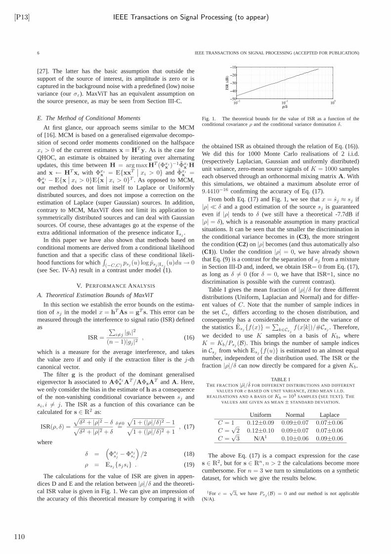
[P13] IEEE Transactions on Signal Processing (to appear)
6 IEEE TRANSACTIONS ON SIGNAL PROCESSING (ACCEPTED FOR PUBLICATION)
[27]. The latter has the basic assumption that outside thesupport of the source of interest, its amplitude is zero or iscaptured in the background noise with a predefined (low) noisevariance (ourσε). MaxViT has an equivalent assumption onthe source presence, as may be seen from Section III-C.
E. The Method of Conditional Moments
At first glance, our approach seems similar to the MCMof [16]. MCM is based on a generalised eigenvalue decompo-sition of second order moments conditioned on the halfspacexi > 0 of the current estimatesx = HT y. As is the case forQHOC, an estimate is obtained by iterating over alternatingupdates, this time betweenH = arg maxHT (Φxi
x )−1Φxix H
and x ← HT x, with Φxix = E{xxT
∣∣ xi > 0} and Φxi
x =Φxi
x − E{x∣∣ xi > 0}E{x
∣∣ xi > 0}T . As opposed to MCM,
our method does not limit itself to Laplace or Uniformlydistributed sources, and does not impose a correction on theestimation of Laplace (super Gaussian) sources. In addition,contrary to MCM, MaxViT does not limit its application tosymmetrically distributed sources and can deal with Gaussiansources. Of course, these advantages go at the expense of theextra additional information of the presence indicatorIsj
.In this paper we have also shown that methods based on
conditional moments are derived from a conditional likelihoodfunction and that a specific class of these conditional likeli-hood functions for which
∫
(−C,C)psj
(u) log psj |Isj(u)du→ 0
(see Sec. IV-A) result in a contrast under model (1).
V. PERFORMANCEANALYSIS
A. Theoretical Estimation Bounds of MaxViT
In this section we establish the error bounds on the estima-tion of sj in the modelx = hT As = gT s. This error can bemeasured through the interference to signal ratio (ISR) definedas
ISR =
∑
i6=j |gi|2(n− 1)|gj |2
, (16)
which is a measure for the average interference, and takesthe value zero if and only if the extraction filter is thej-thcanonical vector.
The filter g is the product of the dominant generalisedeigenvectorh associated toAΦ
sjs AT /AΦsA
T andA. Here,we only consider the bias in the estimate ofh as a consequenceof the non-vanishing conditional covariance betweensj andsi, i 6= j. The ISR as a function of this covariance can becalculated fors ∈ R
2 as:
ISR(ρ, δ) =
√
δ2 + |ρ|2 − δ√
δ2 + |ρ|2 + δ
δ 6=0=
√
1 + (|ρ|/δ)2 − 1√
1 + (|ρ|/δ)2 + 1, (17)
where
δ =(
Φsjsj− Φsj
si
)
/2 (18)
ρ = Esj{sjsi} . (19)
The calculations for the value of ISR are given in appen-dices D and E and the relation between|ρ|/δ and the theoreti-cal ISR value is given in Fig. 1. We can give an impression ofthe accuracy of this theoretical measure by comparing it with
Fig. 1. The theoretical bounds for the value of ISR as a function of theconditional covarianceρ and the conditional variance dominationδ.
the obtained ISR as obtained through the relation of Eq. (16)).We did this for 1000 Monte Carlo realisations of 2 i.i.d.(respectively Laplacian, Gaussian and uniformly distributed)unit variance, zero-mean source signals ofK = 1000 sampleseach observed through an orthonormal mixing matrixA. Withthis simulations, we obtained a maximum absolute error of9.4410−16 confirming the accuracy of Eq. (17).
From both Eq. (17) and Fig. 1, we see thatx = sj ≈ sj if|ρ| ≪ δ and a good estimation of the sourcesj is guaranteedeven if |ρ| tends toδ (we still have a theoretical -7.7dB if|ρ| = δ), which is a reasonable assumption in many practicalsituations. It can be seen that the smaller the discrimination inthe conditional variance becomes in (C3), the more stringentthe condition (C2) on |ρ| becomes (and thus automatically also(C1)). Under the condition|ρ| = 0, we have already shownthat Eq. (9) is a contrast for the separation ofsj from a mixturein Section III-D and, indeed, we obtain ISR= 0 from Eq. (17),as long asδ 6= 0 (for δ = 0, we have that ISR=1, since nodiscrimination is possible with the current contrast).
Table I gives the mean fraction of|ρ|/δ for three differentdistributions (Uniform, Laplacian and Normal) and for differ-ent values ofC. Note that the number of sample indices inthe setCsj
differs according to the chosen distribution, andconsequently has a considerable influence on the variance ofthe statisticsEsj
{f(x)} =∑
k∈Csjf(x[k])/#Csj
. Therefore,we decided to useK samples on a basis ofKb, whereK = Kb/Psj
(B). This brings the number of sample indicesin Csj
from whichEsj{f(u)} is estimated to an almost equal
number, independent of the distribution used. The ISR or thefraction |ρ|/δ can now directly be compared for a givenKb.
TABLE ITHE FRACTION |ρ|/δ FOR DIFFERENT DISTRIBUTIONS AND DIFFERENT
VALUES FOR c BASED ON UNIT VARIANCE, ZERO MEAN I.I .D.REALISATIONS AND A BASIS OFKb = 103 SAMPLES (SEE TEXT). THE
VALUES ARE GIVEN AS MEAN ± STANDARD DEVIATION .
Uniform Normal LaplaceC = 1 0.12±0.09 0.09±0.07 0.07±0.06
C =√
2 0.12±0.10 0.09±0.07 0.07±0.06
C =√
3 N/A1 0.10±0.06 0.09±0.06
The above Eq. (17) is a compact expression for the cases ∈ R
2, but for s ∈ Rn, n > 2 the calculations become more
cumbersome. Forn = 3 we turn to simulations on a syntheticdataset, for which we give the results below.
1For c =√
3, we havePsj (B) = 0 and our method is not applicable(N/A).
110
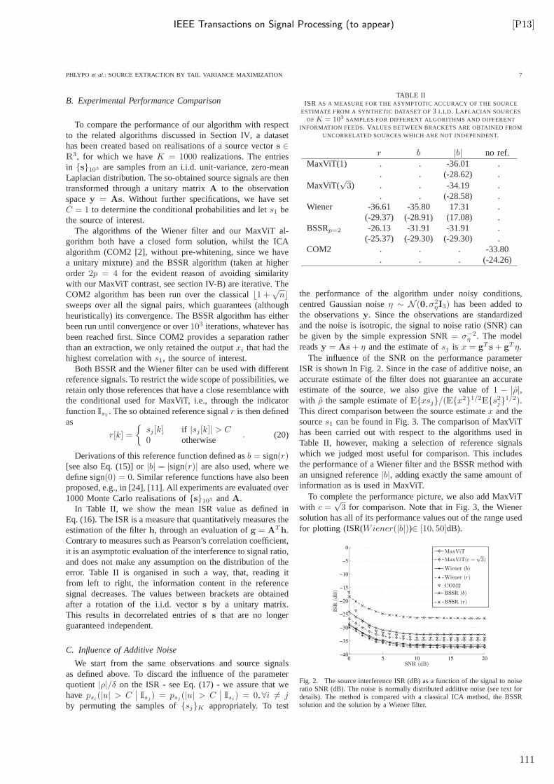
IEEE Transactions on Signal Processing (to appear) [P13]
PHLYPO et al.: SOURCE EXTRACTION BY TAIL VARIANCE MAXIMIZATION 7
B. Experimental Performance Comparison
To compare the performance of our algorithm with respectto the related algorithms discussed in Section IV, a datasethas been created based on realisations of a source vectors ∈R
3, for which we haveK = 1000 realizations. The entriesin {s}103 are samples from an i.i.d. unit-variance, zero-meanLaplacian distribution. The so-obtained source signals are thentransformed through a unitary matrixA to the observationspacey = As. Without further specifications, we have setC = 1 to determine the conditional probabilities and lets1 bethe source of interest.
The algorithms of the Wiener filter and our MaxViT al-gorithm both have a closed form solution, whilst the ICAalgorithm (COM2 [2], without pre-whitening, since we havea unitary mixture) and the BSSR algorithm (taken at higherorder 2p = 4 for the evident reason of avoiding similaritywith our MaxViT contrast, see section IV-B) are iterative. TheCOM2 algorithm has been run over the classical⌊1 +
√n⌋
sweeps over all the signal pairs, which guarantees (althoughheuristically) its convergence. The BSSR algorithm has eitherbeen run until convergence or over103 iterations, whatever hasbeen reached first. Since COM2 provides a separation ratherthan an extraction, we only retained the outputxi that had thehighest correlation withs1, the source of interest.
Both BSSR and the Wiener filter can be used with differentreference signals. To restrict the wide scope of possibilities, weretain only those references that have a close resemblance withthe conditional used for MaxViT, i.e., through the indicatorfunctionIs1
. The so obtained reference signalr is then definedas
r[k] =
{sj [k] if |sj [k]| > C0 otherwise
. (20)
Derivations of this reference function defined asb = sign(r)[see also Eq. (15)] or|b| = |sign(r)| are also used, where wedefine sign(0) = 0. Similar reference functions have also beenproposed, e.g., in [24], [11]. All experiments are evaluated over1000 Monte Carlo realisations of{s}103 andA.
In Table II, we show the mean ISR value as defined inEq. (16). The ISR is a measure that quantitatively measures theestimation of the filterh, through an evaluation ofg = AT h.Contrary to measures such as Pearson’s correlation coefficient,it is an asymptotic evaluation of the interference to signalratio,and does not make any assumption on the distribution of theerror. Table II is organised in such a way, that, reading itfrom left to right, the information content in the referencesignal decreases. The values between brackets are obtainedafter a rotation of the i.i.d. vectors by a unitary matrix.This results in decorrelated entries ofs that are no longerguaranteed independent.
C. Influence of Additive Noise
We start from the same observations and source signalsas defined above. To discard the influence of the parameterquotient |ρ|/δ on the ISR - see Eq. (17) - we assure that wehave psi
(|u| > C∣∣ Isj
) = psj(|u| > C
∣∣ Isi
) = 0,∀i 6= jby permuting the samples of{sj}K appropriately. To test
TABLE IIISR AS A MEASURE FOR THE ASYMPTOTIC ACCURACY OF THE SOURCE
ESTIMATE FROM A SYNTHETIC DATASET OF3 I .I .D. LAPLACIAN SOURCES
OF K = 103 SAMPLES FOR DIFFERENT ALGORITHMS AND DIFFERENT
INFORMATION FEEDS. VALUES BETWEEN BRACKETS ARE OBTAINED FROM
UNCORRELATED SOURCES WHICH ARE NOT INDEPENDENT.
r b |b| no ref.MaxViT(1) . . -36.01 .
. . (-28.62) .MaxViT(
√3) . . -34.19 .
. . (-28.58) .Wiener -36.61 -35.80 17.31 .
(-29.37) (-28.91) (17.08) .BSSRp=2 -26.13 -31.91 -31.91 .
(-25.37) (-29.30) (-29.30) .COM2 . . . -33.80
. . . (-24.26)
the performance of the algorithm under noisy conditions,centred Gaussian noiseη ∼ N (0, σ2
ηI3) has been added tothe observationsy. Since the observations are standardizedand the noise is isotropic, the signal to noise ratio (SNR) canbe given by the simple expression SNR= σ−2
η . The modelreadsy = As + η and the estimate ofsj is x = gT s + gT η.
The influence of the SNR on the performance parameterISR is shown In Fig. 2. Since in the case of additive noise, anaccurate estimate of the filter does not guarantee an accurateestimate of the source, we also give the value of1 − |ρ|,with ρ the sample estimate ofE{xsj}/(E{x2}1/2
E{s2j}1/2).This direct comparison between the source estimatex and thesources1 can be found in Fig. 3. The comparison of MaxViThas been carried out with respect to the algorithms used inTable II, however, making a selection of reference signalswhich we judged most useful for comparison. This includesthe performance of a Wiener filter and the BSSR method withan unsigned reference|b|, adding exactly the same amount ofinformation as is used in MaxViT.
To complete the performance picture, we also add MaxViTwith c =
√3 for comparison. Note that in Fig. 3, the Wiener
solution has all of its performance values out of the range usedfor plotting (ISR(Wiener(|b|))∈ [10, 50]dB).
Fig. 2. The source interference ISR (dB) as a function of the signal to noiseratio SNR (dB). The noise is normally distributed additive noise (see text fordetails). The method is compared with a classical ICA method, the BSSRsolution and the solution by a Wiener filter.
111
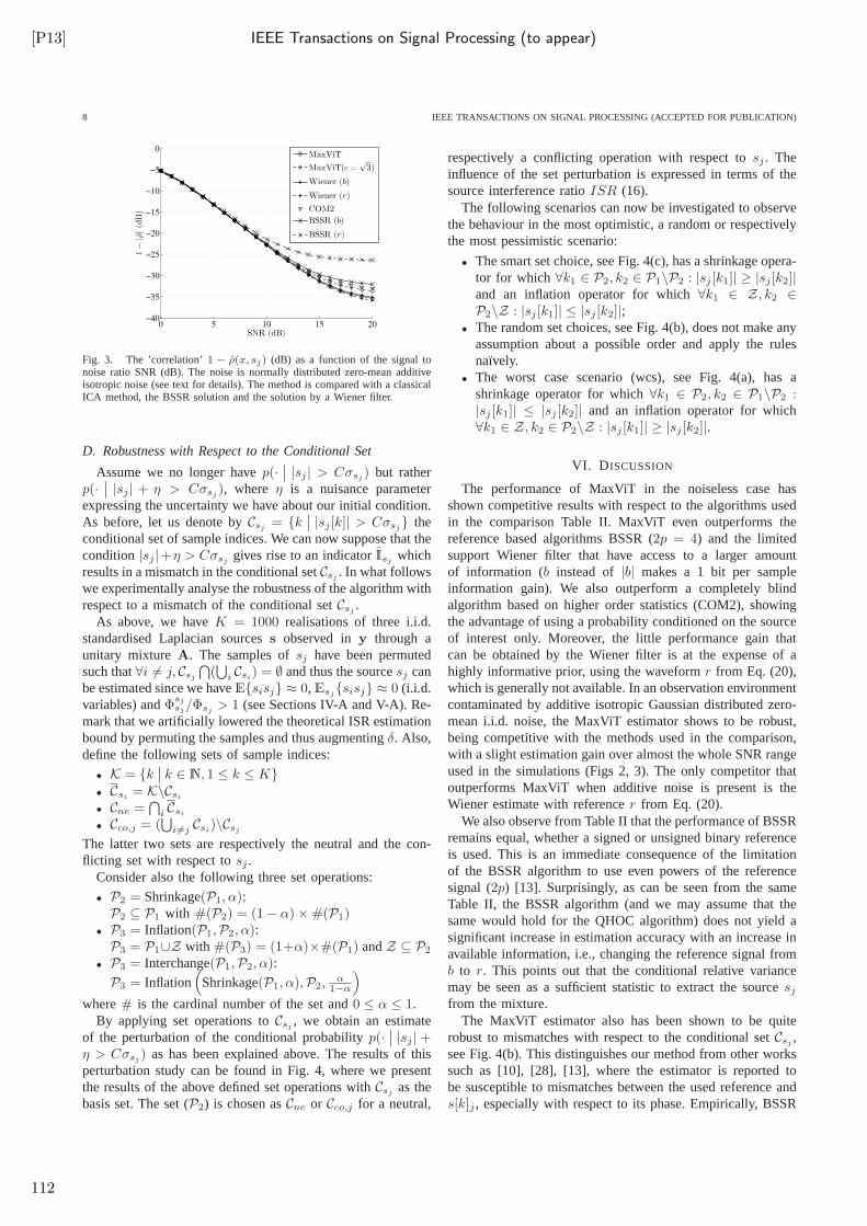
[P13] IEEE Transactions on Signal Processing (to appear)
8 IEEE TRANSACTIONS ON SIGNAL PROCESSING (ACCEPTED FOR PUBLICATION)
Fig. 3. The ’correlation’1 − ρ(x, sj) (dB) as a function of the signal tonoise ratio SNR (dB). The noise is normally distributed zero-mean additiveisotropic noise (see text for details). The method is comparedwith a classicalICA method, the BSSR solution and the solution by a Wiener filter.
D. Robustness with Respect to the Conditional Set
Assume we no longer havep(·∣∣ |sj | > Cσsj
) but ratherp(·
∣∣ |sj | + η > Cσsj
), where η is a nuisance parameterexpressing the uncertainty we have about our initial condition.As before, let us denote byCsj
= {k∣∣ |sj [k]| > Cσsj
} theconditional set of sample indices. We can now suppose that thecondition|sj |+η > Cσsj
gives rise to an indicatorIsjwhich
results in a mismatch in the conditional setCsj. In what follows
we experimentally analyse the robustness of the algorithm withrespect to a mismatch of the conditional setCsj
.As above, we haveK = 1000 realisations of three i.i.d.
standardised Laplacian sourcess observed iny through aunitary mixtureA. The samples ofsj have been permutedsuch that∀i 6= j, Csj
⋂(⋃
i Csi) = ∅ and thus the sourcesj can
be estimated since we haveE{sisj} ≈ 0, Esj{sisj} ≈ 0 (i.i.d.
variables) andΦsjsj/Φsj
> 1 (see Sections IV-A and V-A). Re-mark that we artificially lowered the theoretical ISR estimationbound by permuting the samples and thus augmentingδ. Also,define the following sets of sample indices:
• K = {k∣∣ k ∈ N, 1 ≤ k ≤ K}
• Csi= K\Csi
• Cne =⋂
i Csi
• Cco,j = (⋃
i6=j Csi)\Csj
The latter two sets are respectively the neutral and the con-flicting set with respect tosj .
Consider also the following three set operations:
• P2 = Shrinkage(P1, α):P2 ⊆ P1 with #(P2) = (1 − α) × #(P1)
• P3 = Inflation(P1,P2, α):P3 = P1∪Z with #(P3) = (1+α)×#(P1) andZ ⊆ P2
• P3 = Interchange(P1,P2, α):
P3 = Inflation(
Shrinkage(P1, α),P2,α
1−α
)
where# is the cardinal number of the set and0 ≤ α ≤ 1.By applying set operations toCsj
, we obtain an estimateof the perturbation of the conditional probabilityp(·
∣∣ |sj | +
η > Cσsj) as has been explained above. The results of this
perturbation study can be found in Fig. 4, where we presentthe results of the above defined set operations withCsj
as thebasis set. The set (P2) is chosen asCne or Cco,j for a neutral,
respectively a conflicting operation with respect tosj . Theinfluence of the set perturbation is expressed in terms of thesource interference ratioISR (16).
The following scenarios can now be investigated to observethe behaviour in the most optimistic, a random or respectivelythe most pessimistic scenario:
• The smart set choice, see Fig. 4(c), has a shrinkage opera-tor for which ∀k1 ∈ P2, k2 ∈ P1\P2 : |sj [k1]| ≥ |sj [k2]|and an inflation operator for which∀k1 ∈ Z, k2 ∈P2\Z : |sj [k1]| ≤ |sj [k2]|;
• The random set choices, see Fig. 4(b), does not make anyassumption about a possible order and apply the rulesnaıvely.
• The worst case scenario (wcs), see Fig. 4(a), has ashrinkage operator for which∀k1 ∈ P2, k2 ∈ P1\P2 :|sj [k1]| ≤ |sj [k2]| and an inflation operator for which∀k1 ∈ Z, k2 ∈ P2\Z : |sj [k1]| ≥ |sj [k2]|.
VI. D ISCUSSION
The performance of MaxViT in the noiseless case hasshown competitive results with respect to the algorithms usedin the comparison Table II. MaxViT even outperforms thereference based algorithms BSSR (2p = 4) and the limitedsupport Wiener filter that have access to a larger amountof information (b instead of |b| makes a 1 bit per sampleinformation gain). We also outperform a completely blindalgorithm based on higher order statistics (COM2), showingthe advantage of using a probability conditioned on the sourceof interest only. Moreover, the little performance gain thatcan be obtained by the Wiener filter is at the expense of ahighly informative prior, using the waveformr from Eq. (20),which is generally not available. In an observation environmentcontaminated by additive isotropic Gaussian distributed zero-mean i.i.d. noise, the MaxViT estimator shows to be robust,being competitive with the methods used in the comparison,with a slight estimation gain over almost the whole SNR rangeused in the simulations (Figs 2, 3). The only competitor thatoutperforms MaxViT when additive noise is present is theWiener estimate with referencer from Eq. (20).
We also observe from Table II that the performance of BSSRremains equal, whether a signed or unsigned binary referenceis used. This is an immediate consequence of the limitationof the BSSR algorithm to use even powers of the referencesignal (2p) [13]. Surprisingly, as can be seen from the sameTable II, the BSSR algorithm (and we may assume that thesame would hold for the QHOC algorithm) does not yield asignificant increase in estimation accuracy with an increase inavailable information, i.e., changing the reference signal fromb to r. This points out that the conditional relative variancemay be seen as a sufficient statistic to extract the sourcesj
from the mixture.The MaxViT estimator also has been shown to be quite
robust to mismatches with respect to the conditional setCsj,
see Fig. 4(b). This distinguishes our method from other workssuch as [10], [28], [13], where the estimator is reported tobe susceptible to mismatches between the used reference ands[k]j , especially with respect to its phase. Empirically, BSSR
112
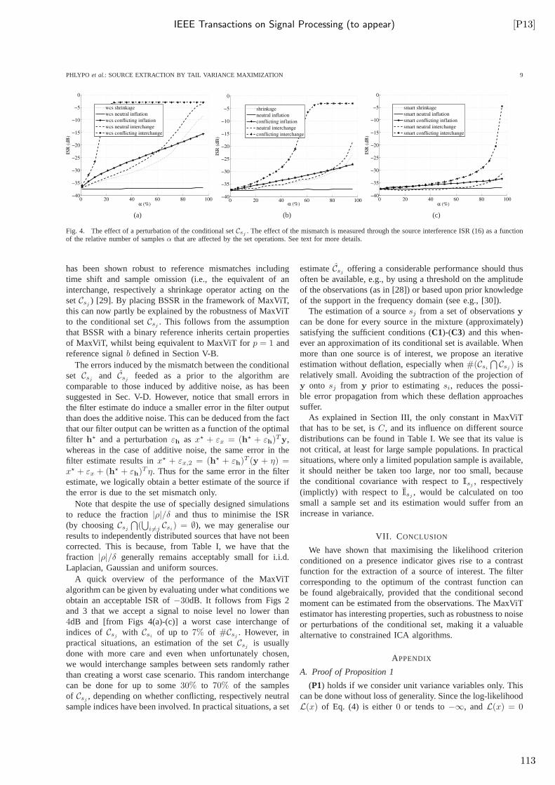
IEEE Transactions on Signal Processing (to appear) [P13]
PHLYPO et al.: SOURCE EXTRACTION BY TAIL VARIANCE MAXIMIZATION 9
(a) (b) (c)
Fig. 4. The effect of a perturbation of the conditional setCsj . The effect of the mismatch is measured through the source interference ISR (16) as a functionof the relative number of samplesα that are affected by the set operations. See text for more details.
has been shown robust to reference mismatches includingtime shift and sample omission (i.e., the equivalent of aninterchange, respectively a shrinkage operator acting on thesetCsj
) [29]. By placing BSSR in the framework of MaxViT,this can now partly be explained by the robustness of MaxViTto the conditional setCsj
. This follows from the assumptionthat BSSR with a binary reference inherits certain propertiesof MaxViT, whilst being equivalent to MaxViT forp = 1 andreference signalb defined in Section V-B.
The errors induced by the mismatch between the conditionalset Csj
and Csjfeeded as a prior to the algorithm are
comparable to those induced by additive noise, as has beensuggested in Sec. V-D. However, notice that small errors inthe filter estimate do induce a smaller error in the filter outputthan does the additive noise. This can be deduced from the factthat our filter output can be written as a function of the optimalfilter h⋆ and a perturbationεh as x⋆ + εx = (h⋆ + εh)T y,whereas in the case of additive noise, the same error in thefilter estimate results inx⋆ + εx,2 = (h⋆ + εh)T (y + η) =x⋆ + εx + (h⋆ + εh)T η. Thus for the same error in the filterestimate, we logically obtain a better estimate of the source ifthe error is due to the set mismatch only.
Note that despite the use of specially designed simulationsto reduce the fraction|ρ|/δ and thus to minimise the ISR(by choosingCsj
⋂(⋃
i6=j Csi) = ∅), we may generalise our
results to independently distributed sources that have notbeencorrected. This is because, from Table I, we have that thefraction |ρ|/δ generally remains acceptably small for i.i.d.Laplacian, Gaussian and uniform sources.
A quick overview of the performance of the MaxViTalgorithm can be given by evaluating under what conditions weobtain an acceptable ISR of−30dB. It follows from Figs 2and 3 that we accept a signal to noise level no lower than4dB and [from Figs 4(a)-(c)] a worst case interchange ofindices of Csj
with Csiof up to 7% of #Csj
. However, inpractical situations, an estimation of the setCsj
is usuallydone with more care and even when unfortunately chosen,we would interchange samples between sets randomly ratherthan creating a worst case scenario. This random interchangecan be done for up to some30% to 70% of the samplesof Csj
, depending on whether conflicting, respectively neutralsample indices have been involved. In practical situations, a set
estimateCsjoffering a considerable performance should thus
often be available, e.g., by using a threshold on the amplitudeof the observations (as in [28]) or based upon prior knowledgeof the support in the frequency domain (see e.g., [30]).
The estimation of a sourcesj from a set of observationsycan be done for every source in the mixture (approximately)satisfying the sufficient conditions (C1)-(C3) and this when-ever an approximation of its conditional set is available. Whenmore than one source is of interest, we propose an iterativeestimation without deflation, especially when#(Csi
⋂ Csj) is
relatively small. Avoiding the subtraction of the projection ofy onto sj from y prior to estimatingsi, reduces the possi-ble error propagation from which these deflation approachessuffer.
As explained in Section III, the only constant in MaxViTthat has to be set, isC, and its influence on different sourcedistributions can be found in Table I. We see that its value isnot critical, at least for large sample populations. In practicalsituations, where only a limited population sample is available,it should neither be taken too large, nor too small, becausethe conditional covariance with respect toIsj
, respectively(implictly) with respect toIsj
, would be calculated on toosmall a sample set and its estimation would suffer from anincrease in variance.
VII. C ONCLUSION
We have shown that maximising the likelihood criterionconditioned on a presence indicator gives rise to a contrastfunction for the extraction of a source of interest. The filtercorresponding to the optimum of the contrast function canbe found algebraically, provided that the conditional secondmoment can be estimated from the observations. The MaxViTestimator has interesting properties, such as robustness to noiseor perturbations of the conditional set, making it a valuablealternative to constrained ICA algorithms.
APPENDIX
A. Proof of Proposition 1
(P1) holds if we consider unit variance variables only. Thiscan be done without loss of generality. Since the log-likelihoodL(x) of Eq. (4) is either0 or tends to−∞, andL(x) = 0
113
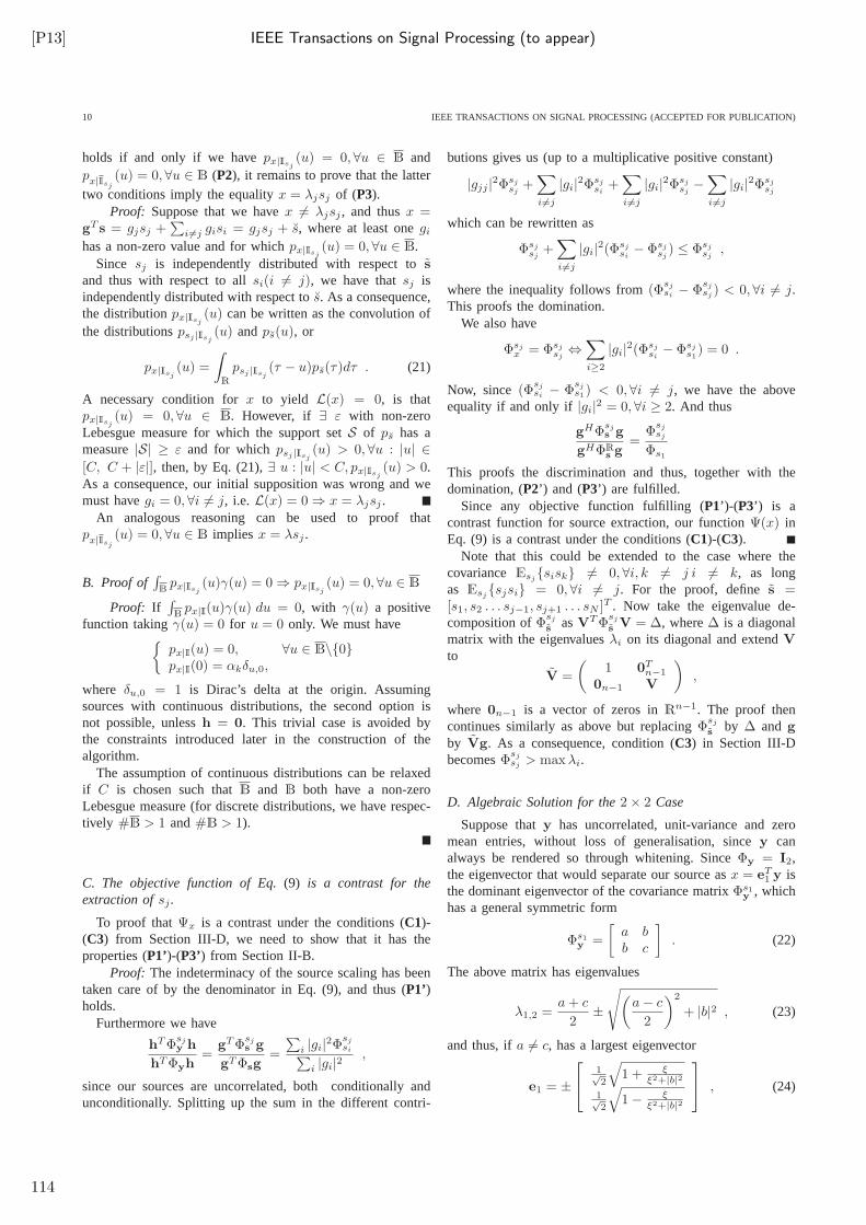
[P13] IEEE Transactions on Signal Processing (to appear)
10 IEEE TRANSACTIONS ON SIGNAL PROCESSING (ACCEPTED FOR PUBLICATION)
holds if and only if we havepx|Isj(u) = 0,∀u ∈ B and
px|Isj
(u) = 0,∀u ∈ B (P2), it remains to prove that the lattertwo conditions imply the equalityx = λjsj of (P3).
Proof: Suppose that we havex 6= λjsj , and thusx =gT s = gjsj +
∑
i6=j gisi = gjsj + s, where at least onegi
has a non-zero value and for whichpx|Isj(u) = 0,∀u ∈ B.
Since sj is independently distributed with respect tosand thus with respect to allsi(i 6= j), we have thatsj isindependently distributed with respect tos. As a consequence,the distributionpx|Isj
(u) can be written as the convolution ofthe distributionspsj |Isj
(u) andps(u), or
px|Isj(u) =
∫
R
psj |Isj(τ − u)ps(τ)dτ . (21)
A necessary condition forx to yield L(x) = 0, is thatpx|Isj
(u) = 0,∀u ∈ B. However, if ∃ ε with non-zeroLebesgue measure for which the support setS of ps has ameasure|S| ≥ ε and for whichpsj |Isj
(u) > 0,∀u : |u| ∈[C, C + |ε|], then, by Eq. (21),∃ u : |u| < C, px|Isj
(u) > 0.As a consequence, our initial supposition was wrong and wemust havegi = 0,∀i 6= j, i.e. L(x) = 0⇒ x = λjsj .
An analogous reasoning can be used to proof thatpx|Isj
(u) = 0,∀u ∈ B implies x = λsj .
B. Proof of∫
Bpx|Isj
(u)γ(u) = 0⇒ px|Isj(u) = 0,∀u ∈ B
Proof: If∫
Bpx|I(u)γ(u) du = 0, with γ(u) a positive
function takingγ(u) = 0 for u = 0 only. We must have{px|I(u) = 0, ∀u ∈ B\{0}px|I(0) = αkδu,0,
where δu,0 = 1 is Dirac’s delta at the origin. Assumingsources with continuous distributions, the second option isnot possible, unlessh = 0. This trivial case is avoided bythe constraints introduced later in the construction of thealgorithm.
The assumption of continuous distributions can be relaxedif C is chosen such thatB and B both have a non-zeroLebesgue measure (for discrete distributions, we have respec-tively #B > 1 and#B > 1).
C. The objective function of Eq.(9) is a contrast for theextraction ofsj .
To proof thatΨx is a contrast under the conditions (C1)-(C3) from Section III-D, we need to show that it has theproperties (P1’)-(P3’) from Section II-B.
Proof: The indeterminacy of the source scaling has beentaken care of by the denominator in Eq. (9), and thus (P1’)holds.
Furthermore we have
hT Φsjy h
hT Φyh=
gT Φsjs g
gT Φsg=
∑
i |gi|2Φ
sjsi
∑
i |gi|2,
since our sources are uncorrelated, both conditionally andunconditionally. Splitting up the sum in the different contri-
butions gives us (up to a multiplicative positive constant)
|gjj |2Φsj
sj+
∑
i6=j
|gi|2Φsj
si+
∑
i6=j
|gi|2Φsj
sj−
∑
i6=j
|gi|2Φsj
sj
which can be rewritten as
Φsjsj
+∑
i6=j
|gi|2(Φsj
si− Φsj
sj) ≤ Φsj
sj,
where the inequality follows from(Φsjsi − Φ
sjsj ) < 0,∀i 6= j.
This proofs the domination.We also have
Φsjx = Φsj
sj⇔
∑
i≥2
|gi|2(Φsj
si− Φsj
s1) = 0 .
Now, since (Φsjsi − Φ
sjs1) < 0,∀i 6= j, we have the above
equality if and only if|gi|2 = 0,∀i ≥ 2. And thus
gHΦsjs g
gHΦRs g
=Φ
sjsj
Φs1
This proofs the discrimination and thus, together with thedomination, (P2’) and (P3’) are fulfilled.
Since any objective function fulfilling (P1’)-(P3’) is acontrast function for source extraction, our functionΨ(x) inEq. (9) is a contrast under the conditions (C1)-(C3).
Note that this could be extended to the case where thecovarianceEsj
{sisk} 6= 0,∀i, k 6= j i 6= k, as longas Esj
{sjsi} = 0,∀i 6= j. For the proof, defines =[s1, s2 . . . sj−1, sj+1 . . . sN ]T . Now take the eigenvalue de-composition ofΦsj
s asVT Φsj
s V = ∆, where∆ is a diagonalmatrix with the eigenvaluesλi on its diagonal and extendVto
V =
(1 0T
n−1
0n−1 V
)
,
where 0n−1 is a vector of zeros inRn−1. The proof thencontinues similarly as above but replacingΦ
sj
s by ∆ and gby Vg. As a consequence, condition (C3) in Section III-DbecomesΦsj
sj > maxλi.
D. Algebraic Solution for the2 × 2 Case
Suppose thaty has uncorrelated, unit-variance and zeromean entries, without loss of generalisation, sincey canalways be rendered so through whitening. SinceΦy = I2,the eigenvector that would separate our source asx = eT
1 y isthe dominant eigenvector of the covariance matrixΦs1
y , whichhas a general symmetric form
Φs1y =
[a bb c
]
. (22)
The above matrix has eigenvalues
λ1,2 =a+ c
2±
√(a− c
2
)2
+ |b|2 , (23)
and thus, ifa 6= c, has a largest eigenvector
e1 = ±
1√2
√
1 + ξξ2+|b|2
1√2
√
1 − ξξ2+|b|2
, (24)
114
IEEE Transactions on Signal Processing (to appear) [P13]
PHLYPO et al.: SOURCE EXTRACTION BY TAIL VARIANCE MAXIMIZATION 11
with ξ = a−c2 .
E. Calculation of ISR
We induce the estimation bound in case the sources are notperfectly conditionally uncorrelated. Since we only considerunitary transformationsA = Q (for our y is or has beenrendered spatiallywhite), we know that the eigenvalues ofΦ
sjs and Φ
sjy are equal. Moreover, thei-th eigenvectorqi of
Φsjy equalsQei, whereei is the i-th eigenvector ofΦsj
s (seealso the equivariance property [9]). As a consequence, we onlyneed to consider the simpler case whereQ = Im, without lossof generality.
Limiting s to belong toR2, the matrixΦs1s takes the form
Φs1s =
[Φs1
s1Es1{s1s2}
Es1{s1s2} Φs1
s2
]
. (25)
From Eq. (24), one can explicitly calculate the separationfilter h associated toΦs1
s by the above Eq. (24). As such weobtain for the ISR (|g2|2/|g1|2 = |h2|2/|h1|2):
ISR =
√
δ2 + |ρ|2 − δ2√
δ2 + |ρ|2 + δ2, (26)
with δ =Φ
s1s1
−Φs1s2
2 andρ = Es1{s1s2}.
F. Proof of the inequalityEsj{s2j} ≥ E{s2j}
Proof: To proof the inequality, we proof the more generalformEsj
{γ(sj)} ≥ E{γ(sj)} for any positive valued functionγ. We have
Esj{γ(sj)} =
∫
psj |Isj(u)γ(u)du
=
∫
Bpsj
(u)γ(u)du∫
Bpsj
(u) du
=
∫psj
(u)γ(u)du−∫
Bpsj
(u)γ(u)du∫
Bpsj
(u) du
>
∫
psj(u)γ(u)du = E{γ(sj)} ,
These results hold if we impose the condition ofEq. (5), since we have from Holders inequality that∫
Bpsj
(u)du∫
Bγ(u)du ≥
∫
B psj(u)γ(u)du and thus
∫
Bpsj
(u)du → 0 ⇒∫
B psj(u)γ(u)du → 0 for all positive
valued functionsγ. As a consequence, we haveEsj{γ(sj)} ≥
E{γ(sj)} with equality if and only if∫
Bpsj
(u) du = 1, i.e.,C < min |sj |. Sinceu2 is a non-negative valued function,C > 0 and we generally havemin |sj [k]| = 0 (continu-ous distributions defined on the whole real line), we haveEsj{s2j} > E{s2j}.
REFERENCES
[1] C. Jutten and J. Herault, “Blind separation of sources, part i: An adap-tive algorithm based on neuromimetic architecture,”Signal Processing,vol. 24, no. 1, pp. 1–10, 1991.
[2] P. Comon, “Independent component analysis, a new concept?” SignalProcessing, vol. 36, pp. 287–314, 1994.
[3] L. Tong, R.-W. Liu, V. C. Soon, and Y.-F. Huang, “Indeterminacyand identifiability of blind identification,”IEEE Trans on Circuits andSystems, vol. 38, no. 5, pp. 499–509, 1991.
[4] S. A. Cruces-Alvarez, A. Cichocki, and S.-i. Amari, “Fromblind signalextraction to blind instantaneous signal separation: Criteria, algorithmsand stability,” IEEE Transactions on Neural Networks, vol. 15, no. 4,pp. 859–873, 2004.
[5] E. Moreau and P. Comon,Separation de sources. Hermes-Lavoisier,2007, vol. 1, ch. Fonctions de Contraste, pp. 75–115, in french.
[6] A. Cichocki, R. Thawonmas, and S. ichi Amari, “Sequential blindsignal extraction in order specified by stochastic properties,” ElectronicsLetters, vol. 33, no. 1, pp. 64–65, 1997.
[7] N. Delfosse and P. Loubaton, “Adaptive blind separationof independentsources: A deflation approach,”Signal Processing, vol. 45, pp. 59–83,1995.
[8] A. Hyvarinen and E. Oja, “Independent Component Analysis: Algo-rithms and Applications,”Neural Networks, vol. 13, no. 4-5, pp. 411–430, 2000.
[9] J.-F. Cardoso and B. H. Laheld, “Equivariant adaptive source separa-tion,” IEEE Trans. on Signal Processing, vol. 44, no. 12, pp. 3017–3030,1996.
[10] W. Lu and J. C. Rajapakse, “ICA with reference,” inProc. Int. Conf.on ICA and BSS, 2001, pp. 120 – 125.
[11] ——, “Approach and applications of constrained ica,”IEEE Trans onNeural Networks, vol. 16, no. 1, pp. 203–212, 2005.
[12] B. Widrow, J. R. Glover, J. M. McCool, J. Kaunitz, C. S. Williams,R. H. Hearn, J. R. Zeidler, E. Dong, and R. C. Goodlin, “Adaptivenoise cancelling: Principles and applications,”Proceedings of the IEEE,vol. 63, no. 12, pp. 1692–1716, 1975.
[13] M. Sato, Y. Kimura, S. Chida, T. Ito, N. Katayama, K. Okamura, andM. Nakao, “A novel extraction method of fetal electrocardiogram fromthe composite abdominal signal,”IEEE Trans on Biom Eng, vol. 54,no. 1, pp. 49–58, 2007.
[14] A. Adib, E. Moreau, and D. Aboutajdine, “Source separation contrastsusing a reference signal,”IEEE Signal Processing Letters, vol. 11, no. 3,pp. 312–315, 2004.
[15] M. Castella, S. Rhioui, E. Moreau, and J. C. Pesquet, “Quadratic higherorder criteria for iterative blind separation of a mimo convolutive mixtureof sources,”IEEE Trans. Signal Process., vol. 55, no. 1, pp. 218–232,Jan. 2007.
[16] B. Xerri and B. Borloz, “An iterative method using conditional second-order statistics applied to the blind source separation problem,” IEEETrans. Signal Process., vol. 52, no. 2, pp. 313–328, Feb. 2004.
[17] D.-T. Pham and P. Garat, “Blind separation of mixture of independentsources through a quasi-maximum likelihood approach,”IEEE Transac-tions on Signal Processing, vol. 45, no. 7, pp. 1712–1725, 1997.
[18] J.-F. Cardoso, “Infomax and maximum likelihood for blind sourceseparation,”IEEE Signal Processing Letters, vol. 4, no. 4, pp. 112–114,1997.
[19] G. H. Golub and C. F. Van Loan,Matrix Computations, 3rd ed. TheJohns Hopkins University Press, 1996.
[20] A. Hyvarinen, J. Karhunen, and E. Oja,Independent Component Anal-ysis. Wiley Interscience, 2001.
[21] A. Cichocki and S.-I. Amari,Adaptive Blind Signal and Image Process-ing: Learning Algorithms and Applications, 2005th ed. Wiley, 2002.
[22] S. Roberts and R. Everson, Eds.,Independent Component Analysis:Principles and Practice. Cambridge University Press, 2001.
[23] J.-F. Cardoso, “On the performance of orthogonal sourceseparationalgorithms,” inProc. EUSIPCO, Edinburgh, 1994, pp. 776–779.
[24] C. J. James and O. Gibson, “ICA with a reference: extracting desiredelectromagnetic brain signals,”Medical Applications of Signal Process-ing, 2002.
[25] S. Mallat and Z. Zhang, “Matching pursuits with time-frequency dictio-naries,” IEEE Trans on Signal Processing, vol. 41, no. 12, pp. 3397–3415, Dec. 1993.
[26] R. Gribonval, “Piecewise linear source separation,” in Proc. SPIE’03,ser. Wavelets: Applications in Signal and Image Processing,vol. 5207,San Diego, California, USA, 2003.
[27] M. Aharon, M. Elad, and A. Bruckstein, “K-SVD: An algorithm fordesigning overcomplete dictionaries for sparse representation,” IEEETrans. Signal Process., vol. 54, no. 11, pp. 4311–4322, Nov. 2006.
[28] C. J. James and O. J. Gibson, “Temporally constrained ICA:an applica-tion to artifact rejection in electromagnetic brain signal analysis,” IEEETrans on Biomed Eng, vol. 30, no. 9, pp. 1108–1115, 2003.
[29] T. Netabayashi, Y. Kimura, S. Chida, T. Ito, K. Ohwada, N.Katayama,K. Okamura, and M. Nakao, “Robustness of the blind source separationwith reference against uncertainties of the reference signals,” in 30thAnnual International IEEE EMBS Conference, vol. 30, Vancouver,British Columbia, Canada, 2008, pp. 1875–1878.
115
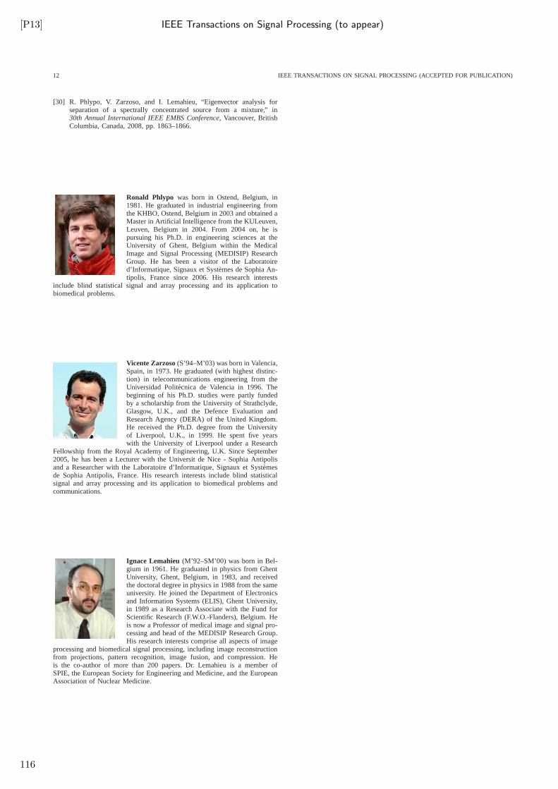
[P13] IEEE Transactions on Signal Processing (to appear)
12 IEEE TRANSACTIONS ON SIGNAL PROCESSING (ACCEPTED FOR PUBLICATION)
[30] R. Phlypo, V. Zarzoso, and I. Lemahieu, “Eigenvector analysis forseparation of a spectrally concentrated source from a mixture,” in30th Annual International IEEE EMBS Conference, Vancouver, BritishColumbia, Canada, 2008, pp. 1863–1866.
Ronald Phlypo was born in Ostend, Belgium, in1981. He graduated in industrial engineering fromthe KHBO, Ostend, Belgium in 2003 and obtained aMaster in Artificial Intelligence from the KULeuven,Leuven, Belgium in 2004. From 2004 on, he ispursuing his Ph.D. in engineering sciences at theUniversity of Ghent, Belgium within the MedicalImage and Signal Processing (MEDISIP) ResearchGroup. He has been a visitor of the Laboratoired’Informatique, Signaux et Systemes de Sophia An-tipolis, France since 2006. His research interests
include blind statistical signal and array processing and its application tobiomedical problems.
Vicente Zarzoso(S’94–M’03) was born in Valencia,Spain, in 1973. He graduated (with highest distinc-tion) in telecommunications engineering from theUniversidad Politecnica de Valencia in 1996. Thebeginning of his Ph.D. studies were partly fundedby a scholarship from the University of Strathclyde,Glasgow, U.K., and the Defence Evaluation andResearch Agency (DERA) of the United Kingdom.He received the Ph.D. degree from the Universityof Liverpool, U.K., in 1999. He spent five yearswith the University of Liverpool under a Research
Fellowship from the Royal Academy of Engineering, U.K. SinceSeptember2005, he has been a Lecturer with the Universit de Nice - Sophia Antipolisand a Researcher with the Laboratoire d’Informatique, Signaux et Systemesde Sophia Antipolis, France. His research interests include blind statisticalsignal and array processing and its application to biomedical problems andcommunications.
Ignace Lemahieu(M’92–SM’00) was born in Bel-gium in 1961. He graduated in physics from GhentUniversity, Ghent, Belgium, in 1983, and receivedthe doctoral degree in physics in 1988 from the sameuniversity. He joined the Department of Electronicsand Information Systems (ELIS), Ghent University,in 1989 as a Research Associate with the Fund forScientific Research (F.W.O.-Flanders), Belgium. Heis now a Professor of medical image and signal pro-cessing and head of the MEDISIP Research Group.His research interests comprise all aspects of image
processing and biomedical signal processing, including image reconstructionfrom projections, pattern recognition, image fusion, and compression. Heis the co-author of more than 200 papers. Dr. Lemahieu is a member ofSPIE, the European Society for Engineering and Medicine, and the EuropeanAssociation of Nuclear Medicine.
116
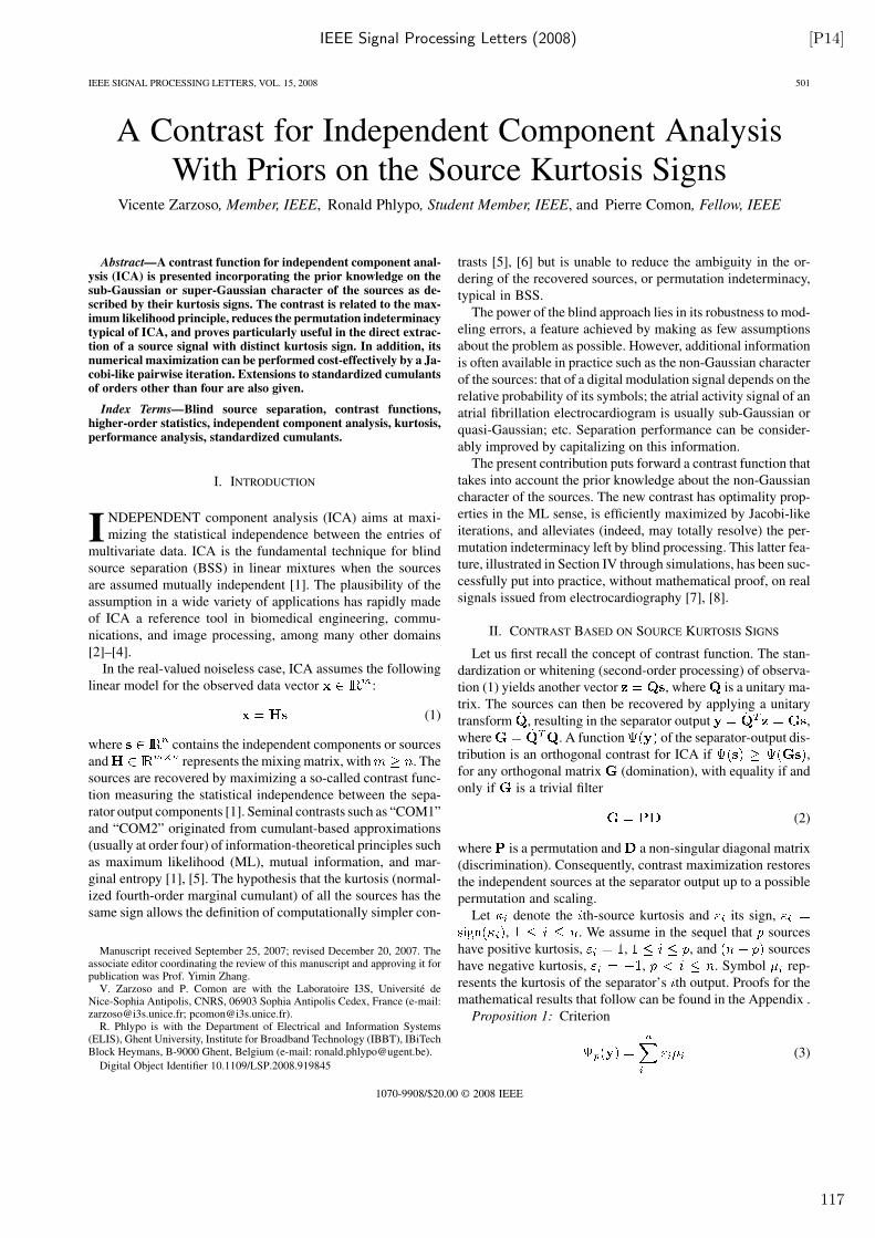
IEEE Signal Processing Letters (2008) [P14]
IEEE SIGNAL PROCESSING LETTERS, VOL. 15, 2008 501
A Contrast for Independent Component AnalysisWith Priors on the Source Kurtosis Signs
Vicente Zarzoso, Member, IEEE, Ronald Phlypo, Student Member, IEEE, and Pierre Comon, Fellow, IEEE
Abstract—A contrast function for independent component anal-ysis (ICA) is presented incorporating the prior knowledge on thesub-Gaussian or super-Gaussian character of the sources as de-scribed by their kurtosis signs. The contrast is related to the max-imum likelihood principle, reduces the permutation indeterminacytypical of ICA, and proves particularly useful in the direct extrac-tion of a source signal with distinct kurtosis sign. In addition, itsnumerical maximization can be performed cost-effectively by a Ja-cobi-like pairwise iteration. Extensions to standardized cumulantsof orders other than four are also given.
Index Terms—Blind source separation, contrast functions,higher-order statistics, independent component analysis, kurtosis,performance analysis, standardized cumulants.
I. INTRODUCTION
INDEPENDENT component analysis (ICA) aims at maxi-
mizing the statistical independence between the entries of
multivariate data. ICA is the fundamental technique for blind
source separation (BSS) in linear mixtures when the sources
are assumed mutually independent [1]. The plausibility of the
assumption in a wide variety of applications has rapidly made
of ICA a reference tool in biomedical engineering, commu-
nications, and image processing, among many other domains
[2]–[4].
In the real-valued noiseless case, ICA assumes the following
linear model for the observed data vector :
(1)
where contains the independent components or sources
and represents the mixing matrix, with . The
sources are recovered by maximizing a so-called contrast func-
tion measuring the statistical independence between the sepa-
rator output components [1]. Seminal contrasts such as “COM1”
and “COM2” originated from cumulant-based approximations
(usually at order four) of information-theoretical principles such
as maximum likelihood (ML), mutual information, and mar-
ginal entropy [1], [5]. The hypothesis that the kurtosis (normal-
ized fourth-order marginal cumulant) of all the sources has the
same sign allows the definition of computationally simpler con-
Manuscript received September 25, 2007; revised December 20, 2007. Theassociate editor coordinating the review of this manuscript and approving it forpublication was Prof. Yimin Zhang.
V. Zarzoso and P. Comon are with the Laboratoire I3S, Université deNice-Sophia Antipolis, CNRS, 06903 Sophia Antipolis Cedex, France (e-mail:[email protected]; [email protected]).
R. Phlypo is with the Department of Electrical and Information Systems(ELIS), Ghent University, Institute for Broadband Technology (IBBT), IBiTechBlock Heymans, B-9000 Ghent, Belgium (e-mail: [email protected]).
Digital Object Identifier 10.1109/LSP.2008.919845
trasts [5], [6] but is unable to reduce the ambiguity in the or-
dering of the recovered sources, or permutation indeterminacy,
typical in BSS.
The power of the blind approach lies in its robustness to mod-
eling errors, a feature achieved by making as few assumptions
about the problem as possible. However, additional information
is often available in practice such as the non-Gaussian character
of the sources: that of a digital modulation signal depends on the
relative probability of its symbols; the atrial activity signal of an
atrial fibrillation electrocardiogram is usually sub-Gaussian or
quasi-Gaussian; etc. Separation performance can be consider-
ably improved by capitalizing on this information.
The present contribution puts forward a contrast function that
takes into account the prior knowledge about the non-Gaussian
character of the sources. The new contrast has optimality prop-
erties in the ML sense, is efficiently maximized by Jacobi-like
iterations, and alleviates (indeed, may totally resolve) the per-
mutation indeterminacy left by blind processing. This latter fea-
ture, illustrated in Section IV through simulations, has been suc-
cessfully put into practice, without mathematical proof, on real
signals issued from electrocardiography [7], [8].
II. CONTRAST BASED ON SOURCE KURTOSIS SIGNS
Let us first recall the concept of contrast function. The stan-
dardization or whitening (second-order processing) of observa-
tion (1) yields another vector , where is a unitary ma-
trix. The sources can then be recovered by applying a unitary
transform , resulting in the separator output ,
where . A function of the separator-output dis-
tribution is an orthogonal contrast for ICA if ,
for any orthogonal matrix (domination), with equality if and
only if is a trivial filter
(2)
where is a permutation and a non-singular diagonal matrix
(discrimination). Consequently, contrast maximization restores
the independent sources at the separator output up to a possible
permutation and scaling.
Let denote the th-source kurtosis and its sign,
, . We assume in the sequel that sources
have positive kurtosis, , , and sources
have negative kurtosis, , . Symbol rep-
resents the kurtosis of the separator’s th output. Proofs for the
mathematical results that follow can be found in the Appendix .
Proposition 1: Criterion
(3)
1070-9908/$20.00 © 2008 IEEE
117
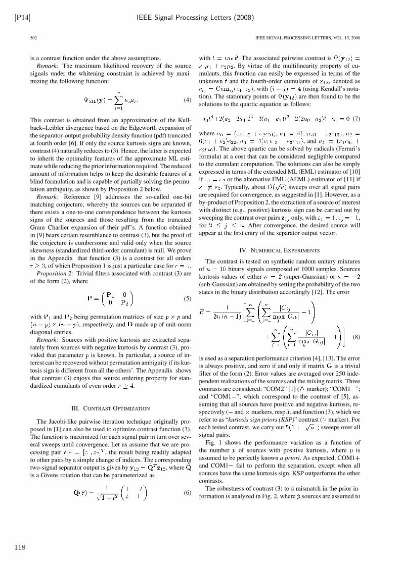
[P14] IEEE Signal Processing Letters (2008)
502 IEEE SIGNAL PROCESSING LETTERS, VOL. 15, 2008
is a contrast function under the above assumptions.
Remark: The maximum likelihood recovery of the source
signals under the whitening constraint is achieved by maxi-
mizing the following function:
(4)
This contrast is obtained from an approximation of the Kull-
back–Leibler divergence based on the Edgeworth expansion of
the separator-output probability density function (pdf) truncated
at fourth order [6]. If only the source kurtosis signs are known,
contrast (4) naturally reduces to (3). Hence, the latter is expected
to inherit the optimality features of the approximate ML esti-
mate while reducing the prior information required. The reduced
amount of information helps to keep the desirable features of a
blind formulation and is capable of partially solving the permu-
tation ambiguity, as shown by Proposition 2 below.
Remark: Reference [9] addresses the so-called one-bit
matching conjecture, whereby the sources can be separated if
there exists a one-to-one correspondence between the kurtosis
signs of the sources and those resulting from the truncated
Gram–Charlier expansion of their pdf’s. A function obtained
in [9] bears certain resemblance to contrast (3), but the proof of
the conjecture is cumbersome and valid only when the source
skewness (standardized third-order cumulant) is null. We prove
in the Appendix that function (3) is a contrast for all orders
, of which Proposition 1 is just a particular case for .
Proposition 2: Trivial filters associated with contrast (3) are
of the form (2), where
(5)
with and being permutation matrices of size and
, respectively, and made up of unit-norm
diagonal entries.
Remark: Sources with positive kurtosis are extracted sepa-
rately from sources with negative kurtosis by contrast (3), pro-
vided that parameter is known. In particular, a source of in-
terest can be recovered without permutation ambiguity if its kur-
tosis sign is different from all the others’. The Appendix shows
that contrast (3) enjoys this source ordering property for stan-
dardized cumulants of even order .
III. CONTRAST OPTIMIZATION
The Jacobi-like pairwise iteration technique originally pro-
posed in [1] can also be used to optimize contrast function (3).
The function is maximized for each signal pair in turn over sev-
eral sweeps until convergence. Let us assume that we are pro-
cessing pair , the result being readily adapted
to other pairs by a simple change of indices. The corresponding
two-signal separator output is given by , where
is a Givens rotation that can be parameterized as
(6)
with . The associated pairwise contrast is
. By virtue of the multilinearity property of cu-
mulants, this function can easily be expressed in terms of the
unknown and the fourth-order cumulants of , denoted as
, with (using Kendall’s nota-
tion). The stationary points of are then found to be the
solutions to the quartic equation as follows:
(7)
where , ,
, , and
. The above quartic can be solved by radicals (Ferrari’s
formula) at a cost that can be considered negligible compared
to the cumulant computation. The solutions can also be simply
expressed in terms of the extended ML (EML) estimator of [10]
if or the alternative EML (AEML) estimator of [11] if
. Typically, about sweeps over all signal pairs
are required for convergence, as suggested in [1]. However, as a
by-product of Proposition 2, the extraction of a source of interest
with distinct (e.g., positive) kurtosis sign can be carried out by
sweeping the contrast over pairs only, with , ,
for . After convergence, the desired source will
appear at the first entry of the separator output vector.
IV. NUMERICAL EXPERIMENTS
The contrast is tested on synthetic random unitary mixtures
of binary signals composed of 1000 samples. Sources
kurtosis values of either (super-Gaussian) or
(sub-Gaussian) are obtained by setting the probability of the two
states in the binary distribution accordingly [12]. The error
(8)
is used as a separation performance criterion [4], [13]. The error
is always positive, and zero if and only if matrix is a trivial
filter of the form (2). Error values are averaged over 250 inde-
pendent realizations of the sources and the mixing matrix. Three
contrasts are considered: “COM2” [1] ( marker); “COM1 ”;
and “COM1 ”; which correspond to the contrast of [5], as-
suming that all sources have positive and negative kurtosis, re-
spectively ( and markers, resp.); and function (3), which we
refer to as “kurtosis sign priors (KSP)” contrast ( marker). For
each tested contrast, we carry out sweeps over all
signal pairs.
Fig. 1 shows the performance variation as a function of
the number of sources with positive kurtosis, where is
assumed to be perfectly known a priori. As expected, COM1
and COM1 fail to perform the separation, except when all
sources have the same kurtosis sign. KSP outperforms the other
contrasts.
The robustness of contrast (3) to a mismatch in the prior in-
formation is analyzed in Fig. 2, where sources are assumed to
118
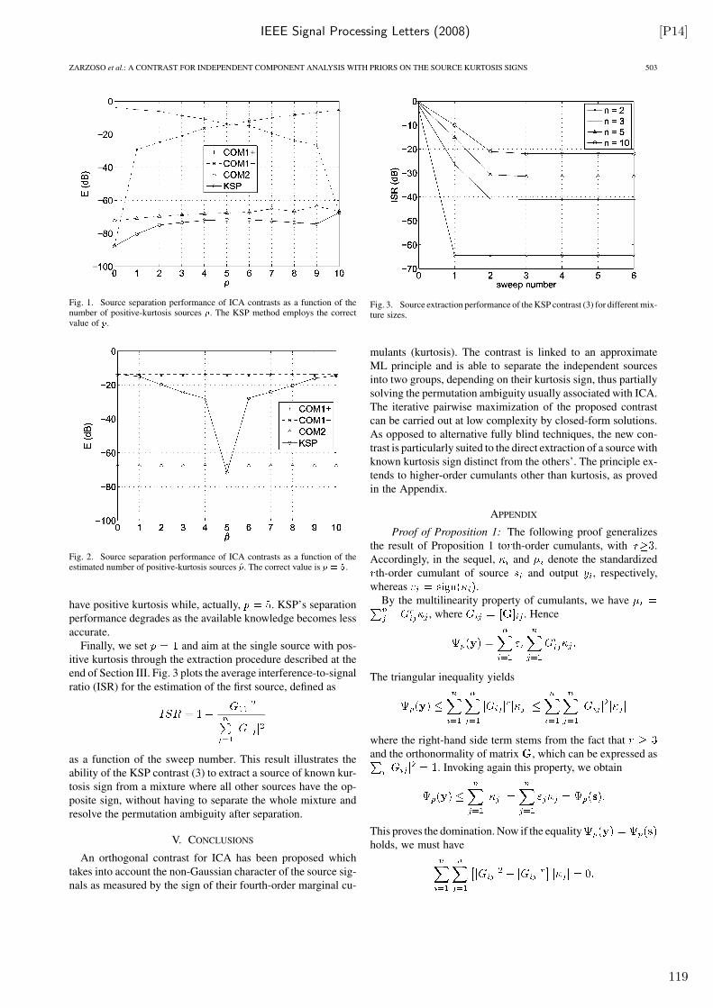
IEEE Signal Processing Letters (2008) [P14]
ZARZOSO et al.: A CONTRAST FOR INDEPENDENT COMPONENT ANALYSIS WITH PRIORS ON THE SOURCE KURTOSIS SIGNS 503
Fig. 1. Source separation performance of ICA contrasts as a function of thenumber of positive-kurtosis sources �. The KSP method employs the correctvalue of �.
Fig. 2. Source separation performance of ICA contrasts as a function of theestimated number of positive-kurtosis sources ��. The correct value is � � �.
have positive kurtosis while, actually, . KSP’s separation
performance degrades as the available knowledge becomes less
accurate.
Finally, we set and aim at the single source with pos-
itive kurtosis through the extraction procedure described at the
end of Section III. Fig. 3 plots the average interference-to-signal
ratio (ISR) for the estimation of the first source, defined as
as a function of the sweep number. This result illustrates the
ability of the KSP contrast (3) to extract a source of known kur-
tosis sign from a mixture where all other sources have the op-
posite sign, without having to separate the whole mixture and
resolve the permutation ambiguity after separation.
V. CONCLUSIONS
An orthogonal contrast for ICA has been proposed which
takes into account the non-Gaussian character of the source sig-
nals as measured by the sign of their fourth-order marginal cu-
Fig. 3. Source extraction performance of the KSP contrast (3) for different mix-ture sizes.
mulants (kurtosis). The contrast is linked to an approximate
ML principle and is able to separate the independent sources
into two groups, depending on their kurtosis sign, thus partially
solving the permutation ambiguity usually associated with ICA.
The iterative pairwise maximization of the proposed contrast
can be carried out at low complexity by closed-form solutions.
As opposed to alternative fully blind techniques, the new con-
trast is particularly suited to the direct extraction of a source with
known kurtosis sign distinct from the others’. The principle ex-
tends to higher-order cumulants other than kurtosis, as proved
in the Appendix.
APPENDIX
Proof of Proposition 1: The following proof generalizes
the result of Proposition 1 to th-order cumulants, with .
Accordingly, in the sequel, and denote the standardized
th-order cumulant of source and output , respectively,
whereas .
By the multilinearity property of cumulants, we have
, where . Hence
The triangular inequality yields
where the right-hand side term stems from the fact that
and the orthonormality of matrix , which can be expressed as
. Invoking again this property, we obtain
This proves the domination. Now if the equality
holds, we must have
119
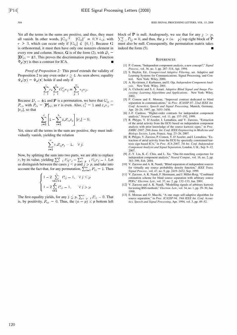
[P14] IEEE Signal Processing Letters (2008)
504 IEEE SIGNAL PROCESSING LETTERS, VOL. 15, 2008
Yet all the terms in the sums are positive, and thus, they must
all vanish. In other words, , with
, which can occur only if . Because
is orthonormal, it must then have only one nonzero element in
every row and column. Hence, is of the form (2), with
. This proves the discrimination property. Function
is thus a contrast for ICA.
Proof of Proposition 2: This proof extends the validity of
Proposition 2 to any even order . As seen above, equality
holds if and only if
Because and is a permutation, we have that
, with , as is even. Also, and
, so that
Yet, since all the terms in the sum are positive, they must indi-
vidually vanish, yielding the relation
Now, by splitting the sum into two parts, we are able to replace
by its value, yielding . Let
us distinguish between the cases and , and take into
account the fact that, for any permutation, . Then
The first equality yields, for any , . That
is, by positivity, . Thus, the bottom left
block of is null. Analogously, we see that for any ,
, and thus, the top right block of
must also be null. Consequently, the permutation matrix takes
indeed the form (5).
REFERENCES
[1] P. Comon, “Independent component analysis, a new concept?,” Signal
Process., vol. 36, no. 3, pp. 287–314, Apr. 1994.[2] S. Haykin, Ed., Unsupervised Adaptive Filtering, ser. Adaptive and
Learning Systems for Communications, Signal Processing, and Con-trol. New York: Wiley, 2000.
[3] A. Hyvärinen, J. Karhunen, and E. Oja, Independent Component Anal-
ysis. New York: Wiley, 2001.[4] A. Cichocki and S.-I. Amari, Adaptive Blind Signal and Image Pro-
cessing: Learning Algorithms and Applications. New York: Wiley,2002.
[5] P. Comon and E. Moreau, “Improved contrast dedicated to blindseparation in communications,” in Proc. ICASSP-97, 22nd IEEE Int.
Conf. Acoustics, Speech and Signal Processing, Munich, Germany,Apr. 20–24, 1997, pp. 3453–3456.
[6] J.-F. Cardoso, “Higher-order contrasts for independent componentanalysis,” Neural Comput., vol. 11, pp. 157–192, 1999.
[7] R. Phlypo, Y. D’Asseler, I. Lemahieu, and V. Zarzoso, “Extractionof the atrial activity from the ECG based on independent componentanalysis with prior knowledge of the source kurtosis signs,” in Proc.
EMBC-2007, 29th Annu. Int. Conf. IEEE Engineering in Medicine and
Biology Society, Lyon, France, Aug. 23–26, 2007.[8] R. Phlypo, V. Zarzoso, P. Comon, Y. D’Asseler, and I. Lemahieu, “Ex-
traction of atrial activity from the ECG by spectrally constrained kur-tosis sign based ICA,” in Proc. ICA-2007, 7th Int. Conf. Independent
Component Analysis and Signal Separation, London, U.K., Sep. 9–12,2007.
[9] Z.-Y. Liu, K.-C. Chiu, and L. Xu, “One-bit-matching conjecture forindependent component analysis,” Neural Comput., vol. 16, no. 2, pp.383–399, Feb. 2004.
[10] V. Zarzoso and A. K. Nandi, “Blind separation of independent sourcesfor virtually any source probability density function,” IEEE Trans.
Signal Process., vol. 47, no. 9, pp. 2419–2432, Sep. 1999.[11] V. Zarzoso, A. K. Nandi, F. Herrmann, and J. Millet-Roig, “Combined
estimation scheme for blind source separation with arbitrary sourcePDFs,” Electron. Lett., vol. 37, no. 2, pp. 132–133, Jan. 2001.
[12] V. Zarzoso and A. K. Nandi, “Modelling signals of arbitrary kurtosisfor testing BSS methods,” Electron. Lett., vol. 34, no. 1, pp. 29–30, Jan.1998.
[13] E. Moreau and O. Macchi, “A one stage self-adaptive algorithm forsource separation,” in Proc. ICASSP-94, 19th IEEE Int. Conf. Acous-
tics, Speech and Signal Processing, Apr. 1994, vol. 3, pp. 49–52.
120
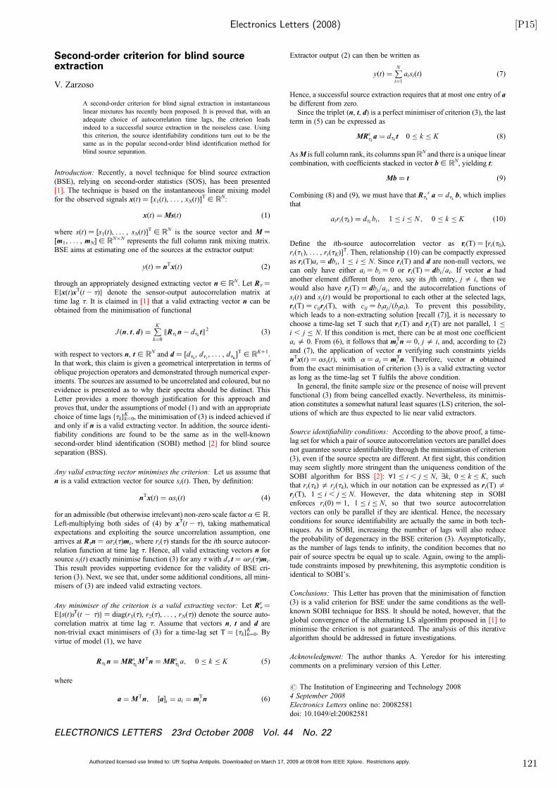
Electronics Letters (2008) [P15]
Second-order criterion for blind source
extraction
V. Zarzoso
A second-order criterion for blind signal extraction in instantaneous
linear mixtures has recently been proposed. It is proved that, with an
adequate choice of autocorrelation time lags, the criterion leads
indeed to a successful source extraction in the noiseless case. Using
this criterion, the source identifiability conditions turn out to be the
same as in the popular second-order blind identification method for
blind source separation.
Introduction: Recently, a novel technique for blind source extraction
(BSE), relying on second-order statistics (SOS), has been presented
[1]. The technique is based on the instantaneous linear mixing model
for the observed signals x(t) ¼ [x1(t), . . . , xN(t)]T[ R
N:
xðtÞ ¼ MsðtÞ ð1Þ
where s(t) ¼ [s1(t), . . . , sN(t)]T[ R
N is the source vector and M ¼[m1, . . . , mN] [ R
N�N represents the full column rank mixing matrix.
BSE aims at estimating one of the sources at the extractor output:
yðtÞ ¼ nTxðtÞ ð2Þ
through an appropriately designed extracting vector n [ RN. Let R
t¼
Efx(t)xT(t2 t)g denote the sensor-output autocorrelation matrix at
time lag t. It is claimed in [1] that a valid extracting vector n can be
obtained from the minimisation of functional
J ðn; t; dÞ ¼PK
k¼0
kRtkn� dtk tk
2 ð3Þ
with respect to vectors n, t [ RN and d ¼ [d
t0, d
t1, . . . , d
tK]T [ R
Kþ1.
In that work, this claim is given a geometrical interpretation in terms of
oblique projection operators and demonstrated through numerical exper-
iments. The sources are assumed to be uncorrelated and coloured, but no
evidence is presented as to why their spectra should be distinct. This
Letter provides a more thorough justification for this approach and
proves that, under the assumptions of model (1) and with an appropriate
choice of time lags ftkgk¼0K , the minimisation of (3) is indeed achieved if
and only if n is a valid extracting vector. In addition, the source identi-
fiability conditions are found to be the same as in the well-known
second-order blind identification (SOBI) method [2] for blind source
separation (BSS).
Any valid extracting vector minimises the criterion: Let us assume that
n is a valid extraction vector for source si(t). Then, by definition:
nTxðtÞ ¼ asiðtÞ ð4Þ
for an admissible (but otherwise irrelevant) non-zero scale factor a [ R.
Left-multiplying both sides of (4) by xT(t2 t), taking mathematical
expectations and exploiting the source uncorrelation assumption, one
arrives at Rtn ¼ ari(t)mi, where ri(t) stands for the ith source autocor-
relation function at time lag t. Hence, all valid extracting vectors n for
source si(t) exactly minimise function (3) for any t with dtt ¼ ari(t)mi.
This result provides supporting evidence for the validity of BSE cri-
terion (3). Next, we see that, under some additional conditions, all mini-
misers of (3) are indeed valid extracting vectors.
Any minimiser of the criterion is a valid extracting vector: Let Rt
s ¼Efs(t)sT(t 2 t)g ¼ diag(r1(t), r2(t), . . . , rN(t)) denote the source auto-
correlation matrix at time lag t. Assume that vectors n, t and d are
non-trivial exact minimisers of (3) for a time-lag set T ¼ ftkgk¼0K . By
virtue of model (1), we have
Rtkn ¼ MR
stkM
Tn ¼ MR
stka; 0 � k � K ð5Þ
where
a ¼ MTn; ½a�i ¼ ai ¼ m
Ti n ð6Þ
Extractor output (2) can then be written as
yðtÞ ¼PN
i¼1
aisiðtÞ ð7Þ
Hence, a successful source extraction requires that at most one entry of a
be different from zero.
Since the triplet (n, t, d) is a perfect minimiser of criterion (3), the last
term in (5) can be expressed as
MRstka ¼ dtk t 0 � k � K ð8Þ
AsM is full column rank, its columns spanRN and there is a unique linear
combination, with coefficients stacked in vector b[ RN, yielding t:
Mb ¼ t ð9Þ
Combining (8) and (9), we must have that Rtk
sa ¼ d
tkb, which implies
that
airiðtk Þ ¼ dtkbi; 1 � i � N ; 0 � k � K ð10Þ
Define the ith-source autocorrelation vector as ri(T) ¼ [ri(t0),
ri(t1), . . . , ri(tK)]T. Then, relationship (10) can be compactly expressed
as ri(T)ai ¼ dbi, 1 � i � N. Since ri(T) and d are non-null vectors, we
can only have either ai ¼ bi ¼ 0 or ri(T) ¼ dbi/ai. If vector a had
another element different from zero, say its jth entry, j= i, then we
would also have rj(T) ¼ dbj/aj, and the autocorrelation functions of
si(t) and sj(t) would be proportional to each other at the selected lags,
ri(T) ¼ cijrj(T), with cij ¼ biaj/(bjai). To prevent this possibility,
which leads to a non-extracting solution [recall (7)], it is necessary to
choose a time-lag set T such that ri(T) and rj(T) are not parallel, 1 �
i , j � N. If this condition is met, there can be at most one coefficient
ai= 0. From (6), it follows that mjTn ¼ 0, j= i, and, according to (2)
and (7), the application of vector n verifying such constraints yields
nTx(t) ¼ asi(t), with a ¼ ai ¼ mi
Tn. Therefore, vector n obtained
from the exact minimisation of criterion (3) is a valid extracting vector
as long as the time-lag set T fulfils the above condition.
In general, the finite sample size or the presence of noise will prevent
functional (3) from being cancelled exactly. Nevertheless, its minimis-
ation constitutes a somewhat natural least squares (LS) criterion, the sol-
utions of which are thus expected to lie near valid extractors.
Source identifiability conditions: According to the above proof, a time-
lag set for which a pair of source autocorrelation vectors are parallel does
not guarantee source identifiability through the minimisation of criterion
(3), even if the source spectra are different. At first sight, this condition
may seem slightly more stringent than the uniqueness condition of the
SOBI algorithm for BSS [2]: 81 � i , j � N, 9k, 0 � k � K, such
that ri(tk)= rj(tk), which in our notation can be expressed as ri(T)=
rj(T), 1 � i , j � N. However, the data whitening step in SOBI
enforces ri(0) ¼ 1, 1 � i � N, so that two source autocorrelation
vectors can only be parallel if they are identical. Hence, the necessary
conditions for source identifiability are actually the same in both tech-
niques. As in SOBI, increasing the number of lags will also reduce
the probability of degeneracy in the BSE criterion (3). Asymptotically,
as the number of lags tends to infinity, the condition becomes that no
pair of source spectra be equal up to scale. Again, owing to the ampli-
tude constraints imposed by prewhitening, this asymptotic condition is
identical to SOBI’s.
Conclusions: This Letter has proven that the minimisation of function
(3) is a valid criterion for BSE under the same conditions as the well-
known SOBI technique for BSS. It should be noted, however, that the
global convergence of the alternating LS algorithm proposed in [1] to
minimise the criterion is not guaranteed. The analysis of this iterative
algorithm should be addressed in future investigations.
Acknowledgment: The author thanks A. Yeredor for his interesting
comments on a preliminary version of this Letter.
# The Institution of Engineering and Technology 2008
4 September 2008
Electronics Letters online no: 20082581
doi: 10.1049/el:20082581
ELECTRONICS LETTERS 23rd October 2008 Vol. 44 No. 22
Authorized licensed use limited to: UR Sophia Antipolis. Downloaded on March 17, 2009 at 09:08 from IEEE Xplore. Restrictions apply. 121

[P15] Electronics Letters (2008)
V. Zarzoso (I3S Laboratory, University of Nice - Sophia Antipolis,
CNRS, Les Algorithmes, Euclide-B, BP 121, 2000 route des Lucioles,
Sophia Antipolis Cedex 06903, France)
E-mail: [email protected]
References
1 Li, X.-L., and Zhang, X.-D.: ‘Sequential blind extraction adoptingsecond-order statistics’, IEEE Signal Process. Lett., 2007, 14, (1),pp. 58–61
2 Belouchrani, A., Abed-Meraim, K., Cardoso, J.-F., and Moulines, E.: ‘Ablind source separation technique using second-order statistics’, IEEETrans. Signal Process., 1997, 45, (2), pp. 434–444
ELECTRONICS LETTERS 23rd October 2008 Vol. 44 No. 22
Authorized licensed use limited to: UR Sophia Antipolis. Downloaded on March 17, 2009 at 09:08 from IEEE Xplore. Restrictions apply. 122
European Transactions on Telecommunications (2008) [P16]
EUROPEAN TRANSACTIONS ON TELECOMMUNICATIONSEur. Trans. Telecomms. 2008; 19:751–759Published online 29 September 2008 in Wiley InterScience(www.interscience.wiley.com) DOI: 10.1002/ett.1321
Blind channel identification in Alamouti coded systems: a comparative study of
eigendecomposition methods in indoor transmissions at 2.4 GHz†
Hector J. Perez-Iglesias1, Jose A. Garcıa-Naya1, Adriana Dapena1∗, Luis Castedo1 and Vicente Zarzoso2
1Departamento de Electronica y Sistemas, Universidade da Coruna, Facultad de Informatica, Campus de Elvina, no. 5, 15071 A Coruna, Spain2Laboratoire I3S, Universite de Nice-Sophia Antipolis, Les Algorithmes, Euclide-B, BP 121 06903 Sophia Antipolis, France
SUMMARY
This paper focuses on blind channel estimation in Alamouti coded systems with one receiving antennaworking in indoor scenarios where the flat fading assumption is reasonable. A comparative study ofseveral channel estimation techniques in both simulated and realistic scenarios is presented. The testedmethods exploit the orthogonality property of the Alamouti coded channel matrix, and are based on theeigendecomposition of a square matrix made up of second-order statistics (SOS) or higher order statistics(HOS) of the observed signals. An experimental evaluation is carried out on a testbed developed at theUniversity of A Coruna (UDC) and operating at 2.4 GHz. The results show the superior performance of theSOS-based blind channel estimation technique in both line of sight (LOS) and non-LOS (NLOS) channels.Copyright © 2008 John Wiley & Sons, Ltd.
1. INTRODUCTION
During the last decade, a large number of space-time
coding (STC) techniques have been proposed to exploit
the spatial diversity in multiple input multiple output
(MIMO) wireless communication systems that employ
multiple antennas at both transmission and reception (see,
for instance, References [1, 2] and references therein). A
remarkable example is orthogonal space time block coding
(OSTBC) because it is able to provide full transmit diversity
without any channel state information (CSI) at transmission
and with very simple encoding and decoding procedures
[3, 4]. The basic premise of OSTBC is the encoding of
the transmitted symbols into an orthogonal matrix which
reduces the optimum maximum likelihood (ML) decoder
to a matrix-matched filter followed by a symbol-by-symbol
detector.
The OSTBC scheme for MIMO systems with two
transmit antennas is known as the Alamouti code [3] and it
is the only OSTBC capable of achieving full spatial rate for
* Correspondence to: Adriana Dapena, Departamento de Electronica y Sistemas, Universidade da Coruna, Facultad de Informatica, Campus de Elvina,no. 5, 15071 A Coruna, Spain. E-mail: [email protected]†A previous version of this paper was presented in the 13th European Wireless Conference (EW 2007), Paris, France.
complex constellations. Other OSTBCs have been proposed
for more than two transmit antennas but they suffer from
severe spatial rate loss [4, 5]. The Alamouti code can be
used in systems with one or multiple antennas at the receiver.
Here, (2 × 1) Alamouti coded systems are used due to their
simplicity and their ability to provide maximum diversity
gain while achieving the full available channel capacity. It
should be noted that Alamouti schemes do not achieve the
full potential capacity with more than one receive antenna
[6], although the difference is small and of course both
diversity and capacity are significantly increased with more
than one receive antenna. Because of these advantages, the
Alamouti code has been incorporated in the IEEE 802.11
and IEEE 802.16 standards [7].
Coherent detection in (2 × 1) Alamouti coded systems
requires the identification of a (2 × 2) unitary channel
matrix. The standard way to estimate this channel matrix is
through the transmission of pilot symbols, also referred to as
training sequences. However, the inclusion of pilot symbols
reduces the system throughput (equivalently, it reduces the
Copyright © 2008 John Wiley & Sons, Ltd. Accepted 16 June 2008
123
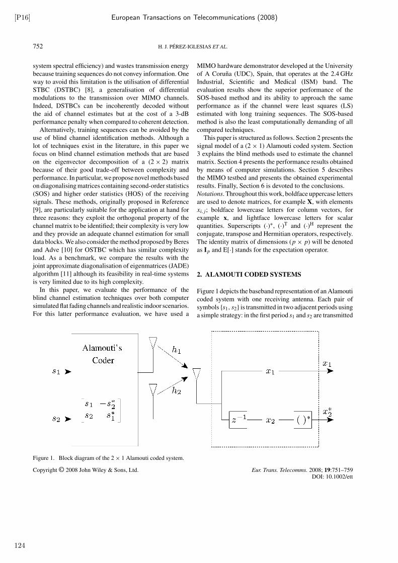
[P16] European Transactions on Telecommunications (2008)
752 H. J. PEREZ-IGLESIAS ET AL.
system spectral efficiency) and wastes transmission energy
because training sequences do not convey information. One
way to avoid this limitation is the utilisation of differential
STBC (DSTBC) [8], a generalisation of differential
modulations to the transmission over MIMO channels.
Indeed, DSTBCs can be incoherently decoded without
the aid of channel estimates but at the cost of a 3-dB
performance penalty when compared to coherent detection.
Alternatively, training sequences can be avoided by the
use of blind channel identification methods. Although a
lot of techniques exist in the literature, in this paper we
focus on blind channel estimation methods that are based
on the eigenvector decomposition of a (2 × 2) matrix
because of their good trade-off between complexity and
performance. In particular, we propose novel methods based
on diagonalising matrices containing second-order statistics
(SOS) and higher order statistics (HOS) of the receiving
signals. These methods, originally proposed in Reference
[9], are particularly suitable for the application at hand for
three reasons: they exploit the orthogonal property of the
channel matrix to be identified; their complexity is very low
and they provide an adequate channel estimation for small
data blocks. We also consider the method proposed by Beres
and Adve [10] for OSTBC which has similar complexity
load. As a benchmark, we compare the results with the
joint approximate diagonalisation of eigenmatrices (JADE)
algorithm [11] although its feasibility in real-time systems
is very limited due to its high complexity.
In this paper, we evaluate the performance of the
blind channel estimation techniques over both computer
simulated flat fading channels and realistic indoor scenarios.
For this latter performance evaluation, we have used a
MIMO hardware demonstrator developed at the University
of A Coruna (UDC), Spain, that operates at the 2.4 GHz
Industrial, Scientific and Medical (ISM) band. The
evaluation results show the superior performance of the
SOS-based method and its ability to approach the same
performance as if the channel were least squares (LS)
estimated with long training sequences. The SOS-based
method is also the least computationally demanding of all
compared techniques.
This paper is structured as follows. Section 2 presents the
signal model of a (2 × 1) Alamouti coded system. Section
3 explains the blind methods used to estimate the channel
matrix. Section 4 presents the performance results obtained
by means of computer simulations. Section 5 describes
the MIMO testbed and presents the obtained experimental
results. Finally, Section 6 is devoted to the conclusions.
Notations. Throughout this work, boldface uppercase letters
are used to denote matrices, for example X, with elements
xi,j; boldface lowercase letters for column vectors, for
example x, and lightface lowercase letters for scalar
quantities. Superscripts (·)∗, (·)T and (·)H represent the
conjugate, transpose and Hermitian operators, respectively.
The identity matrix of dimensions (p × p) will be denoted
as Ip and E[·] stands for the expectation operator.
2. ALAMOUTI CODED SYSTEMS
Figure 1 depicts the baseband representation of an Alamouti
coded system with one receiving antenna. Each pair of
symbols {s1, s2} is transmitted in two adjacent periods using
a simple strategy: in the first period s1 and s2 are transmitted
Figure 1. Block diagram of the 2 × 1 Alamouti coded system.
Copyright © 2008 John Wiley & Sons, Ltd. Eur. Trans. Telecomms. 2008; 19:751–759DOI: 10.1002/ett
124
European Transactions on Telecommunications (2008) [P16]
BLIND CHANNEL IDENTIFICATION IN ALAMOUTI CODED SYSTEMS 753
through the first and second antennas, respectively, and
in the second period −s∗2 is transmitted through the first
antenna and s∗1 from the second one. We assume that the
exact probability density function of si is unknown although
they take values from the alphabet of a typical complex
modulation such as QAM or PSK. The data sequence is
assumed to be composed of independent and identically
distributed symbols, so that s1 and s2 are statistically
independent.
In indoor scenarios, the delay spread of the different
multipaths is rather small so it is natural to model the
wireless channel as flat fading: the transmitted symbols
arrive at the receiving antenna through the fading paths h1
and h2. Thus, the signal received during the first period is
x1 = s1h1 + s2h2 + n1. Assuming that the channel remains
unchanged, the observation in the second period is given by
x2 = s∗1h2 − s∗2h1 + n2. Defining the observation vector as
x = [x1 x∗2]T, we obtain that the relationship between the
observation vector x and the source vector s = [s1 s2]T is
given by
x = Hs + n (1)
where H is the (2 × 2) effective channel matrix,
H =
[h1 h2
h∗2 −h∗
1
](2)
and where n = [n1 n∗2]T is the AWGN modelled as a vector
of two uncorrelated zero-mean, complex-valued, circularly
symmetric, Gaussian distributed random processes. It is
interesting to note that H is an orthogonal matrix, that is
HHH = HHH = ‖h‖2I2 where ‖h‖2 = |h1|2 + |h2|
2 is the
squared Euclidean norm of h.
Filtering x with the matrix-matched filter yields the
following decision statistics
y = HHx = ‖h‖2s + n (3)
where n = HHn is the output noise vector, with the same
statistical properties as the input noise. It is apparent
from Equation (3) that ML detection of s1 and s2 can
be calculated by applying y to a pair of independent
scalar slicers. Consequently, the correct detection of the
transmitted symbols s requires the accurate estimation of
the channel matrix H from the received data x.
3. MIMO CHANNEL ESTIMATION
This section describes the channel estimation techniques
that will be tested in Sections 4 and 5. The methods are
based on computing a (2 × 2) squared matrix, C, containing
SOS or HOS of the received signals. The basic premise of
the considered methods is that C has an algebraic structure
of the form H�HH where � is a diagonal matrix. Due
to the orthogonal structure of H, if the diagonal entries of
� are different, the channel matrix can be identified from
the eigenvectors of C with a possible change of scale and
permutation.
3.1. SOS-based approach
We will start by describing a method that estimates
the channel from the eigenvectors of the observations
autocorrelation matrix. Unlike other SOS-based algorithms
[12, 13], this method does not require the use of an
additional outer encoder.
According to the signal model in Equation (1), the
observations autocorrelation matrix can be written as
CSOS = E[xxH] = HRsHH + σ2
nI2 (4)
where σ2n is the noise power and Rs = E[ssH] is the
correlation matrix of the transmitted signals. Since H is
orthogonal, Equation (4) can be rewritten as the following
eigenvalue decomposition:
CSOS = H
(Rs +
σ2n
‖h‖2I2
)HH (5)
Notice that if the two transmitted sources have the same
power CSOS is diagonal and, as a consequence, H is not
identifiable from an eigenvalue decomposition.
For the system to be identifiable, we propose to unbalance
the power of the transmitted sources as follows:
E[|s′1|2] =
2σ2s
1 + γ2, E[|s′2|
2] =2γ2σ2
s
1 + γ2(6)
where 0 < γ2 < 1 and s′1, s′2 are the new unbalanced
sources. In spite of the power unbalancing, notice that the
total mean power remains unchanged (i.e. σ2s ). Now, the
eigenvalue decomposition of CSOS is
CSOS = σ2s H�SOSHH (7)
Copyright © 2008 John Wiley & Sons, Ltd. Eur. Trans. Telecomms. 2008; 19:751–759DOI: 10.1002/ett
125
[P16] European Transactions on Telecommunications (2008)
754 H. J. PEREZ-IGLESIAS ET AL.
where
�SOS =
[1 + σ2
h 0
0 γ2 + σ2h
](8)
contains the eigenvalues of CSOS and σ2h =
σ2n
σ2s ‖h‖2
. Thanks
to the source power imbalance, now matrix H is identifiable
from CSOS, as �SOS contains different eigenvalues.
Obviously, if the power of the two sources is unbalanced,
the total channel capacity is lower than that of equally
balanced sources. This is the price to be paid for making
the SOS-based method applicable and taking advantage of
its extremely low computational requirements. However,
in Sections 4 and 5, we will show that the best choice is
γ2 ≈ 0.6 and that in this case the total channel capacity is
quite close to the balanced case.
3.2. HOS-based approaches
The orthogonal MIMO channel matrix H can also be
estimated from the eigendecomposition of matrices made
up of HOS of the received signals without the need
of unbalancing the source powers. Indeed, for a (2 × 1)
observation vector, x, the fourth-order cumulant matrix
CHOS(M) is a (2 × 2) matrix with components
[CHOS(M)]ij =
2∑
k,ℓ=1
cum(xi, x∗j , xk, x
∗ℓ)mlk (9)
where mlk k, l = 1, 2, denote the entries of a (2 × 2) matrix
M and the fourth-order cumulant is defined by
cum(x1, x2, x3, x4) = E[x1x2x3x4] − E[x1x2]E[x3x4]
− E[x1x3]E[x2x4] − E[x1x4]E[x2x3]
(10)
It has been proved in Reference [11] that, for the particular
case of zero-mean signals, the cumulant matrix admits the
following decomposition
CHOS(M) = H�HOS(M)HH (11)
where ρ4i = cum(si, s∗i , si, s
∗i ) is the kurtosis of the ith
source and �(M) is a diagonal matrix given by
�HOS(M) = diag(ρ41hH1 Mh1, ρ42hH
2 Mh2) (12)
Here, hi is the ith column of H, that is h1 = [h1 h∗2]T
and h2 = [h2 − h∗1]T. Since for the Alamouti coded
scheme the channel matrix is orthogonal, HH diagonalises
CHOS(M) for any M provided that �(M) contains different
entries, that is
L =∣∣ρ41hH
1 Mh1 − ρ42hH2 Mh2
∣∣ �= 0 (13)
In particular, the approach proposed by Beres and Adve
in Reference [10] considers the cases m11 = 1, m12 =
m21 = m22 = 0; and m11 = m12 = m21 = 0 and m22 =
1. Assuming that the transmitted signals have the same
kurtosis, we obtain from Equation (13) that the channel
matrix is identifiable as long as |h1|2 �= |h2|
2.
As an extension of this approach, we propose to identify
H by computing the eigenvectors of a linear combination of
fourth-order cross-cumulant matrices. This can be obtained
by using a matrix M with entries m11 = 1, m12 = m21 =
0 and m22 = λ, being λ a real valued parameter. From
Equation (13), we conclude that this method allows to
estimate H as long as
L = (1 − λ)(|h1|2 − |h2|
2) �= 0 (14)
Thus, the channel is identifiable if λ �= 1 and |h1|2 �=
|h2|2. In particular, we propose the utilisation of λ =
−1 since this choice provides a significant performance
improvement with respect to the Beres and Adve approach
in Reference [10], as will be shown in the following
sections.
Another way to estimate the mixing matrix consists
in performing a simultaneous diagonalisation of several
fourth-order cumulant matrices, as the JADE algorithm
[11]. This algorithm provides an excellent performance
but, unfortunately, its computational load is very high. In
Sections 4 and 5, the JADE algorithm will be used only as
a benchmark.
4. COMPUTER SIMULATIONS
This section presents the results of several computer
simulations carried out to evaluate the performance of
the estimation algorithms proposed in Section 3. The
experiments have been carried out by simulating the
transmission of QPSK signals in Rayleigh-distributed
randomly generated flat fading channels affected by additive
white Gaussian noise (AWGN). We assume block fading
where the channel remains constant during the transmission
of a block of K symbols. The statistics in Equations (4) and
(9) have been calculated by sample averaging over each
Copyright © 2008 John Wiley & Sons, Ltd. Eur. Trans. Telecomms. 2008; 19:751–759DOI: 10.1002/ett
126
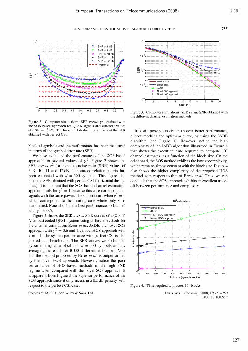
European Transactions on Telecommunications (2008) [P16]
BLIND CHANNEL IDENTIFICATION IN ALAMOUTI CODED SYSTEMS 755
0 0.1 0.2 0.3 0.4 0.5 0.6 0.7 0.8 0.9 110
−2
10−1
100
γ2
SE
R
SNR of 8 dB
SNR of 9 dB
SNR of 10 dB
SNR of 11 dB
SNR of 12 dB
Perfect CSI
Figure 2. Computer simulations: SER versus γ2 obtained withthe SOS-based approach for QPSK signals and different valuesof SNR = σ2
s /N0. The horizontal dashed lines represent the SERobtained with perfect CSI.
block of symbols and the performance has been measured
in terms of the symbol error rate (SER).
We have evaluated the performance of the SOS-based
approach for several values of γ2. Figure 2 shows the
SER versus γ2 for signal to noise ratio (SNR) values of
8, 9, 10, 11 and 12 dB. The autocorrelation matrix has
been estimated with K = 500 symbols. This figure also
plots the SER obtained with perfect CSI (horizontal dashed
lines). It is apparent that the SOS-based channel estimation
approach fails for γ2 = 1 because this case corresponds to
signals with the same power. The same occurs when γ2 = 0
which corresponds to the limiting case where only s1 is
transmitted. Note also that the best performance is obtained
with γ2 ≈ 0.6.
Figure 3 shows the SER versus SNR curves of a (2 × 1)
Alamouti coded QPSK system using different methods for
the channel estimation: Beres et al., JADE, the novel SOS
approach with γ2 = 0.6 and the novel HOS approach with
λ = −1. The system performance with perfect CSI is also
plotted as a benchmark. The SER curves were obtained
by simulating data blocks of K = 500 symbols and by
averaging the results for 10 000 different realisations. Note
that the method proposed by Beres et al. is outperformed
by the novel HOS approach. However, notice the poor
performance of HOS-based methods in the high SNR
regime when compared with the novel SOS approach. It
is apparent from Figure 3 the superior performance of the
SOS approach since it only incurs in a 0.5 dB penalty with
respect to the perfect CSI case.
0 2 4 6 8 10 12 14 16 18 2010
−4
10−3
10−2
10−1
100
SNR (dB)
SE
R
Perfect CSI
Beres et al.
JADE
Novel SOS approach
Novel HOS approach
Figure 3. Computer simulations: SER versus SNR obtained withthe different channel estimation methods.
It is still possible to obtain an even better performance,
almost reaching the optimum curve, by using the JADE
algorithm (see Figure 3). However, notice the high
complexity of the JADE algorithm illustrated in Figure 4
that shows the execution time required to compute 104
channel estimates, as a function of the block size. On the
other hand, the SOS method exhibits the lowest complexity,
which remains almost constant with the block size. Figure 4
also shows the higher complexity of the proposed HOS
method with respect to that of Beres et al. Thus, we can
conclude that the SOS approach exhibits an excellent trade-
off between performance and complexity.
0 50 100 150 200 250 300 350 400 450 5000
1
2
3
4
5
6
7
8
block size (symbols vectors)
tim
e (
seconds)
104 estimations
Beres et al.
JADE
Novel SOS approach
Novel HOS approach
Figure 4. Time required to process 104 blocks.
Copyright © 2008 John Wiley & Sons, Ltd. Eur. Trans. Telecomms. 2008; 19:751–759DOI: 10.1002/ett
127
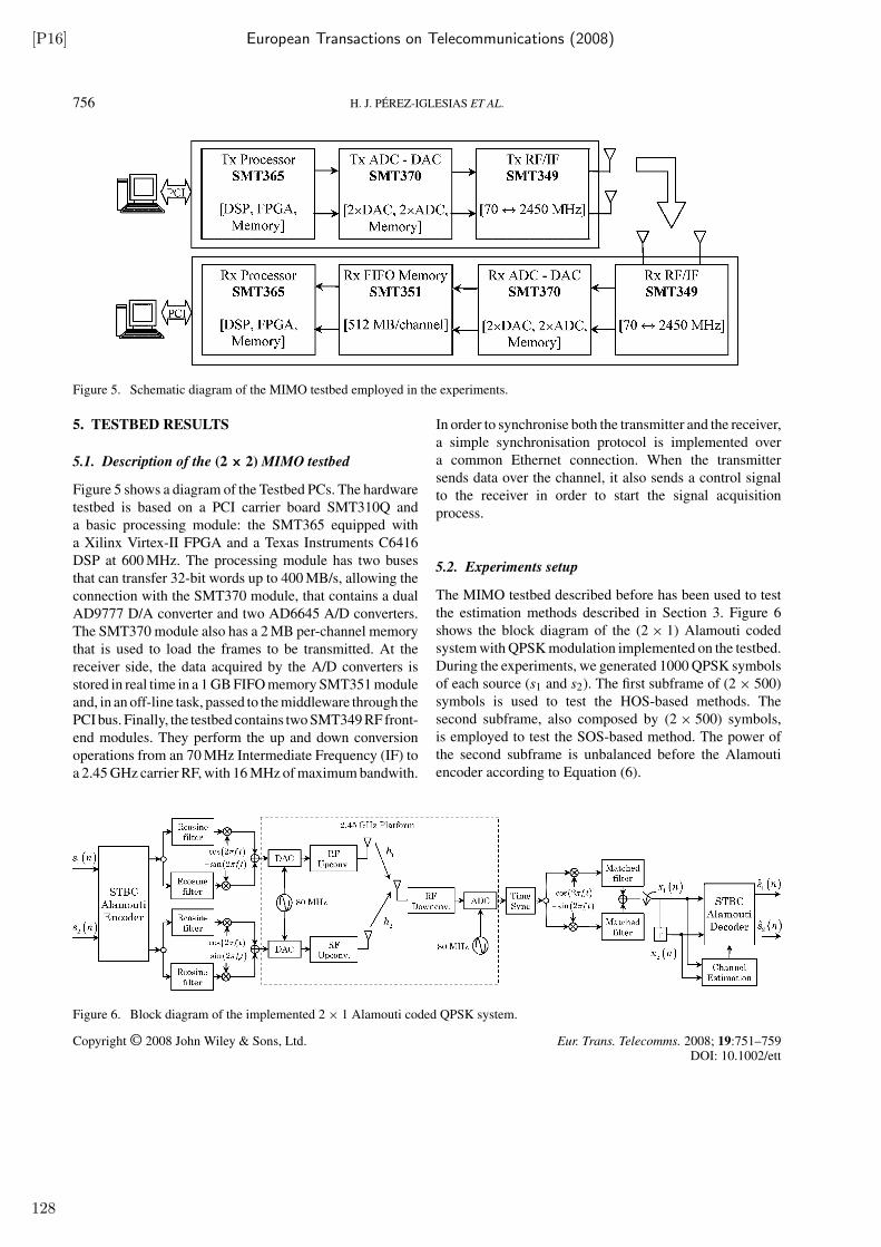
[P16] European Transactions on Telecommunications (2008)
756 H. J. PEREZ-IGLESIAS ET AL.
Figure 5. Schematic diagram of the MIMO testbed employed in the experiments.
5. TESTBED RESULTS
5.1. Description of the (2 × 2) MIMO testbed
Figure 5 shows a diagram of the Testbed PCs. The hardware
testbed is based on a PCI carrier board SMT310Q and
a basic processing module: the SMT365 equipped with
a Xilinx Virtex-II FPGA and a Texas Instruments C6416
DSP at 600 MHz. The processing module has two buses
that can transfer 32-bit words up to 400 MB/s, allowing the
connection with the SMT370 module, that contains a dual
AD9777 D/A converter and two AD6645 A/D converters.
The SMT370 module also has a 2 MB per-channel memory
that is used to load the frames to be transmitted. At the
receiver side, the data acquired by the A/D converters is
stored in real time in a 1 GB FIFO memory SMT351 module
and, in an off-line task, passed to the middleware through the
PCI bus. Finally, the testbed contains two SMT349 RF front-
end modules. They perform the up and down conversion
operations from an 70 MHz Intermediate Frequency (IF) to
a 2.45 GHz carrier RF, with 16 MHz of maximum bandwith.
In order to synchronise both the transmitter and the receiver,
a simple synchronisation protocol is implemented over
a common Ethernet connection. When the transmitter
sends data over the channel, it also sends a control signal
to the receiver in order to start the signal acquisition
process.
5.2. Experiments setup
The MIMO testbed described before has been used to test
the estimation methods described in Section 3. Figure 6
shows the block diagram of the (2 × 1) Alamouti coded
system with QPSK modulation implemented on the testbed.
During the experiments, we generated 1000 QPSK symbols
of each source (s1 and s2). The first subframe of (2 × 500)
symbols is used to test the HOS-based methods. The
second subframe, also composed by (2 × 500) symbols,
is employed to test the SOS-based method. The power of
the second subframe is unbalanced before the Alamouti
encoder according to Equation (6).
Figure 6. Block diagram of the implemented 2 × 1 Alamouti coded QPSK system.
Copyright © 2008 John Wiley & Sons, Ltd. Eur. Trans. Telecomms. 2008; 19:751–759DOI: 10.1002/ett
128
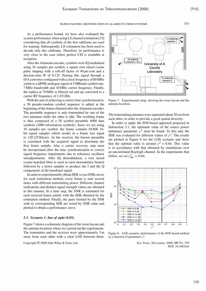
European Transactions on Telecommunications (2008) [P16]
BLIND CHANNEL IDENTIFICATION IN ALAMOUTI CODED SYSTEMS 757
As a performance bound, we have also evaluated the
system performance when using LS channel estimation [15]
considering that all symbols of the first subframe are used
for training. Subsequently, LS estimation has been used to
decode only this subframe. Therefore, its performance is
very close to the case where perfect CSI is available at
reception.
After the Alamouti encoder, symbols were IQ modulated
using 16 samples per symbol, a square root raised cosine
pulse shaping with a roll-off factor of 40 per cent and a
discrete-time IF of 0.125. Passing this signal through a
D/A converter configured with a clock frequency of 80 MHz
yields to a QPSK analogue signal of 5 MBauds symbol rate,
7 MHz bandwidth and 10 MHz carrier frequency. Finally,
the replica at 70 MHz is filtered out and up converted to a
carrier RF frequency of 2.45 GHz.
With the aim of achieving a correct time synchronisation,
a 50 pseudo-random symbol sequence is added at the
beginning of the frame obtained after the Alamouti encoder.
The preamble sequence is only transmitted by one of the
two antennas while the other is idle. The resulting frame
is thus composed of a 50 symbol preamble 4000 data
symbols (2000 information symbols). Since we are using
16 samples per symbol, the frame contains 65 600 16-
bit signal samples which results in a frame size equal
to 128 125 Kbytes. At the receiver, the known preamble
is correlated with the acquired signal to determine the
first frame sample. Also a carrier recovery step must
be incorporated after the time synchronisation to correct
signal frequency impairments due to reference oscillator
misadjustments. After IQ demodulation, a root raised
cosine-matched filter is used in each demodulator branch
followed by a down sampler to produce the I and the Q
components of the baseband signal.
In order to experimentally obtain SER versus SNR curves
for each estimation method, every frame is sent several
times with different transmitting power. Different channel
realisations and distinct signal strength values are obtained
in this manner. In a later step, the SNR is estimated for
each received frame jointly with the SER obtained by the
estimation method. Finally, the pairs formed by the SNR
with its corresponding SER are sorted by SNR value and
plotted to obtain a performance curve.
5.3. Scenario 1: line of sight (LOS)
Figure 7 shows a schematic diagram of the room layout and
the antenna locations where we carried out the experiments.
The transmitter and the receiver were approximately 5 m
away from each other with a clear LOS between them.
Figure 7. Experimental setup, showing the room layout and theantenna locations.
The transmitting antennas were separated about 30 cm from
each other, in order to provide a good spatial diversity.
In order to apply the SOS-based approach proposed in
Subsection 3.1, the optimum value of the source power
unbalance parameter γ2 must be found. To this end, the
SER was evaluated for different values of γ2. The results
are plotted in Figure 8 for the LOS scenario and show
that the optimal value is around γ2 = 0.64. This value
is in accordance with that obtained by simulations over
an uncorrelated Rayleigh channel. In the experiments that
follow, we set γ2opt = 0.64.
0 0.1 0.2 0.3 0.4 0.5 0.6 0.7 0.8 0.9 110
−3
10−2
10−1
100
γ 2
SE
R
SNR of 8 dB
SNR of 9 dB
SNR of 10 dB
SNR of 11 dB
SNR of 12 dB
Figure 8. LOS scenario: performance of the SOS-based methodas a function of parameter γ2.
Copyright © 2008 John Wiley & Sons, Ltd. Eur. Trans. Telecomms. 2008; 19:751–759DOI: 10.1002/ett
129
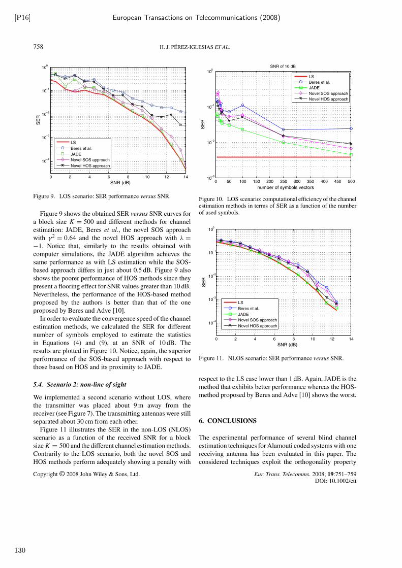
[P16] European Transactions on Telecommunications (2008)
758 H. J. PEREZ-IGLESIAS ET AL.
0 2 4 6 8 10 12 14
10−4
10−3
10−2
10−1
100
SNR (dB)
SE
R
LS
Beres et al.
JADE
Novel SOS approach
Novel HOS approach
Figure 9. LOS scenario: SER performance versus SNR.
Figure 9 shows the obtained SER versus SNR curves for
a block size K = 500 and different methods for channel
estimation: JADE, Beres et al., the novel SOS approach
with γ2 = 0.64 and the novel HOS approach with λ =
−1. Notice that, similarly to the results obtained with
computer simulations, the JADE algorithm achieves the
same performance as with LS estimation while the SOS-
based approach differs in just about 0.5 dB. Figure 9 also
shows the poorer performance of HOS methods since they
present a flooring effect for SNR values greater than 10 dB.
Nevertheless, the performance of the HOS-based method
proposed by the authors is better than that of the one
proposed by Beres and Adve [10].
In order to evaluate the convergence speed of the channel
estimation methods, we calculated the SER for different
number of symbols employed to estimate the statistics
in Equations (4) and (9), at an SNR of 10 dB. The
results are plotted in Figure 10. Notice, again, the superior
performance of the SOS-based approach with respect to
those based on HOS and its proximity to JADE.
5.4. Scenario 2: non-line of sight
We implemented a second scenario without LOS, where
the transmitter was placed about 9 m away from the
receiver (see Figure 7). The transmitting antennas were still
separated about 30 cm from each other.
Figure 11 illustrates the SER in the non-LOS (NLOS)
scenario as a function of the received SNR for a block
size K = 500 and the different channel estimation methods.
Contrarily to the LOS scenario, both the novel SOS and
HOS methods perform adequately showing a penalty with
0 50 100 150 200 250 300 350 400 450 50010
−3
10−2
10−1
100
SNR of 10 dB
number of symbols vectors
SE
R
LS
Beres et al.
JADE
Novel SOS approach
Novel HOS approach
Figure 10. LOS scenario: computational efficiency of the channelestimation methods in terms of SER as a function of the numberof used symbols.
0 2 4 6 8 10 12 14
10−4
10−3
10−2
10−1
100
SNR (dB)
SE
R
LS
Beres et al.
JADE
Novel SOS approach
Novel HOS approach
Figure 11. NLOS scenario: SER performance versus SNR.
respect to the LS case lower than 1 dB. Again, JADE is the
method that exhibits better performance whereas the HOS-
method proposed by Beres and Adve [10] shows the worst.
6. CONCLUSIONS
The experimental performance of several blind channel
estimation techniques for Alamouti coded systems with one
receiving antenna has been evaluated in this paper. The
considered techniques exploit the orthogonality property
Copyright © 2008 John Wiley & Sons, Ltd. Eur. Trans. Telecomms. 2008; 19:751–759DOI: 10.1002/ett
130
European Transactions on Telecommunications (2008) [P16]
BLIND CHANNEL IDENTIFICATION IN ALAMOUTI CODED SYSTEMS 759
of the effective MIMO channel matrix through the
eigendecomposition of matrices made up of SOS or HOS
of the received signals. The algorithms were tested via
computer simulations and on real data obtained from
indoor scenarios using a MIMO hardware platform working
at 2.4 GHz. Both simulations and realistic experiments
in LOS and NLOS scenarios show that the proposed
SOS-based method exhibit a performance penalty of less
than 1 dB when compared with the case of perfect CSI.
Thus, we can conclude that the SOS approach exhibits an
excellent compromise quality between channel estimation
and computational complexity.
ACKNOWLEDGEMENTS
This work has been partially supported by Xunta de Galicia,Ministerio de Educacion y Ciencia of Spain and FEDER funds ofthe European Union under grants number PGIDT06TIC10501PRand TEC2007-68020-C04-01.
REFERENCES
1. Gesbert D, Shafi M, Shan-Shiu D, Smith PJ, Naguib A. From theoryto practice: an overview of MIMO space-time coded wireless systems.IEEE Journal on Selected Areas in Communications 2003; 21:281–302.
2. Jafarkhani H. Space Time Coding. Cambridge University Press:Cambridge, UK, 2005.
3. Alamouti SM. A simple transmit diversity technique for wirelesscommunications. IEEE Journal on Selected Areas in Communications
1998; 16:1451–1458.
4. Tarokh V, Jafarkhani H, Calderbank AR. Space-time block codes fromorthogonal designs. IEEE Transactions on Information Theory 1999;45(5):1456–1467.
5. Larsson EG, Stoica P. Space-Time Block Coding for Wireless
Communications. Cambridge University Press: Cambridge, UK, 2003.6. Sandhu S, Paulraj A. Space-time block codes: a capacity perspective.
IEEE Communications Letter 2000; 4(12):384–386.7. Andrews JG, Ghosh A, Muhamed R. Fundamentals of WiMAX:
Understanding Broadband Wireless Networking. Prentice HallCommunications Engineering and Emerging Technologies Series,2007.
8. Hughes BL. Differential space-time modulation. IEEE Transactions
on Information Theory 2000; 46(7):2567–2578.9. Perez-Iglesias HJ, Dapena A, Castedo L, Zarzoso V. Blind channel
identification for Alamouti’s coding systems based on eigenvectordecomposition. In Proceedings of 13th European Wireless Conference,Paris, France. April 2007.
10. Beres E, Adve R. Blind channel estimation for orthogonal STBCin MISO systems. In Proceedings of Global Telecommunications
Conference, 2004, Vol. 4, November 2004; pp. 2323–2328.11. Cardoso J-F, Souloumiac A. Blind beamforming for non-Gaussian
signals. In IEE Proceedings-F, Vol. 140, no. 6, December 1993;pp. 362–370.
12. Shahbazpanah S, Gershman AB, Manton J. Closed-form blindMIMO channel estimation for orthogonal space-time blockcodes. IEEE Transactions on Signal Processing 2005; 53(12):4506–4516.
13. Vıa J, Santamarıa I, Perez J, Ramırez D. Blind decoding ofMISO-OSTBC systems based on principal component analysis. InProceedings of International Conference on Acoustic, Speech and
Signal Processing, Vol. IV, 2006; pp. 545–549.14. Garcıa-Naya JA, Fernandez-Carames T, Perez-Iglesias H, et al.
Performance of STBC transmissions with real data. In Proceedings
of 16th IST Mobile and Wireless Communications Summit, Budapest,Hungary, July 2007.
15. Naguib AF, Tarokh V, Seshadri N, Calderbank AR. A space-timecoding modem for high-data-rate wireless communications. IEEE
Journal on Selected Areas in Communications 1998; 16(8):1459–1478.
Copyright © 2008 John Wiley & Sons, Ltd. Eur. Trans. Telecomms. 2008; 19:751–759DOI: 10.1002/ett
131

IEEE Transactions on Communications (2008) [P17]
10 IEEE TRANSACTIONS ON COMMUNICATIONS, VOL. 56, NO. 1, JANUARY 2008
Optimal Step-Size Constant Modulus Algorithm
Vicente Zarzoso, Member, IEEE, and Pierre Comon, Fellow, IEEE
Abstract— The step size leading to the absolute minimum ofthe constant modulus (CM) criterion along the search directioncan be obtained algebraically at each iteration among the rootsof a third-degree polynomial. The resulting optimal step-sizeCMA (OS-CMA) is compared with other CM-based iterativetechniques in terms of performance-versus-complexity trade-off.
Index Terms— Adaption coefficient, blind equalization, CMA,exact line search, SIMO and SISO channels.
I. INTRODUCTION
AN important problem in digital communications is the
recovery of the data symbols transmitted through a
distorting medium. The constant modulus (CM) criterion
is arguably the most widespread blind channel equalization
principle [1], [2]. The CM criterion generally presents local
extrema — often associated with different equalization delays
— in the equalizer parameter space [3]. This shortcoming
renders the performance of gradient-based implementations,
such as the well-known constant modulus algorithm (CMA),
very dependent on the equalizer impulse response initializa-
tion. Even when the absolute minimum is found, convergence
can be severely slowed down for initial equalizer settings with
trajectories in the vicinity of saddle points [4], [5]. The con-
stant value of the step-size parameter (or adaption coefficient)
must be carefully selected to ensure a stable operation while
balancing convergence rate and final accuracy (misadjustment
or excess mean square error). The stochastic gradient CMA
drops the expectation operator and approximates the gradient
of the criterion by a one-sample estimate, as in LMS-based
algorithms. This rough approximation generally leads to slow
convergence and poor misadjustment, even if the step size is
carefully chosen.
As opposed to recursive (or sample-by-sample) algorithms,
block (or fixed-window) methods obtain a more precise gra-
dient estimate from a batch of channel output samples, im-
proving convergence speed and accuracy [6]. Tracking capa-
bilities are preserved as long as the channel remains stationary
over the observation window. Moreover, sample-by-sample
versions are easily obtained from block implementations by
considering signal blocks of one data vector and iterating
over consecutive received vectors. The block-gradient CMA
Paper approved by V. A. Aalo, the Editor for Diversity and Fading ChannelTheory of the IEEE Communications Society. Manuscript received November2, 2005; revised November 3, 2006. Supported through a Research Fellowshipawarded to V. Zarzoso by the Royal Academy of Engineering of the UK.
V. Zarzoso was with the Department of Electrical Engineering and Elec-tronics, The University of Liverpool, Liverpool L69 3GJ, UK. He is now withthe Laboratoire I3S, Université de Nice – Sophia Antipolis, France (e-mail:[email protected]).
P. Comon is with the Laboratoire I3S, CNRS/UNSA, 2000 routedes Lucioles, BP 121, 06903 Sophia Antipolis Cedex, France (e-mail:[email protected]).
Digital Object Identifier 10.1109/TCOMM.2008.050484.
(simply denoted as CMA hereafter) is particularly suited to
burst-mode transmission systems. Unfortunately, the multi-
modal nature of the CM criterion sustains the negative impact
of local extrema on block implementations. Asymptotically
(for sufficient block size), the least-squares CMA (LSCMA)
[7] guarantees global convergence to a cost function stationary
point, for any initial weight setting, with a cost per iteration
similar to CMA’s. This is achieved at the expense of an
increased computational overhead due to the calculation of the
data matrix pseudoinverse or its QR factorization, needed to
solve the LS step at each iteration. In the QR-CMA method of
[6], data prewhitening through the QR decomposition of the
sensor-output matrix simplifies the block-CMA iteration, so
that bounds on its step size can be found to ensure monotonic
convergence. The recently proposed recursive least squares
CMA (RLS-CMA) [8], which operates on a sample-by-sample
basis, also proves notably faster and more robust than the
classical CMA. The derivation of the RLS-CMA relies on
an approximation to the CM cost function in stationary or
slowly varying environments, where block implementations
may actually prove more efficient in exploiting the avail-
able information (the received signal burst). Interestingly, the
RLS-CMA turns out to be equivalent to the recursive CMA
(RCMA), put forward over a decade earlier in [9]; it also bears
close resemblance to the orthogonalized CMA (O-CMA) of
[10].
Analytical solutions to the minimization of the CM criterion
are developed in [11], [12]. After solving a linearized LS
problem, these methods require to recover the right structure
of the solution space when multiple equalization solutions
exist. In the general case, this can be achieved through a
costly QZ matrix iteration. In addition, special modifications
are required for input signals with a one-dimensional (i.e.,
binary) alphabet [11]–[13]. More importantly, these analytic
methods aim at exact solutions to the CM criterion, which
may yield suboptimal equalizers in the presence of noise.
A judicious alternative to existing techniques consists of
performing consecutive one-dimensional absolute minimiza-
tions of the CM cost function. This technique, known as exact
line search, is generally considered computationally inefficient
[14]. However, it was first observed in [15] that the value of
the adaption coefficient that leads to the absolute minimum
of most blind cost functions along a given search direction
can be computed algebraically. It was conjectured that the use
of this algebraic optimal step size could not only accelerate
convergence but also avoid local extrema in some cases.
The present Letter carries out a more detailed (yet concise)
theoretical development and experimental evaluation of the
optimal step-size CMA (OS-CMA) derived from this idea,
which was briefly presented in [16] under a different name.
0090-6778/08$25.00 c© 2008 IEEE
133
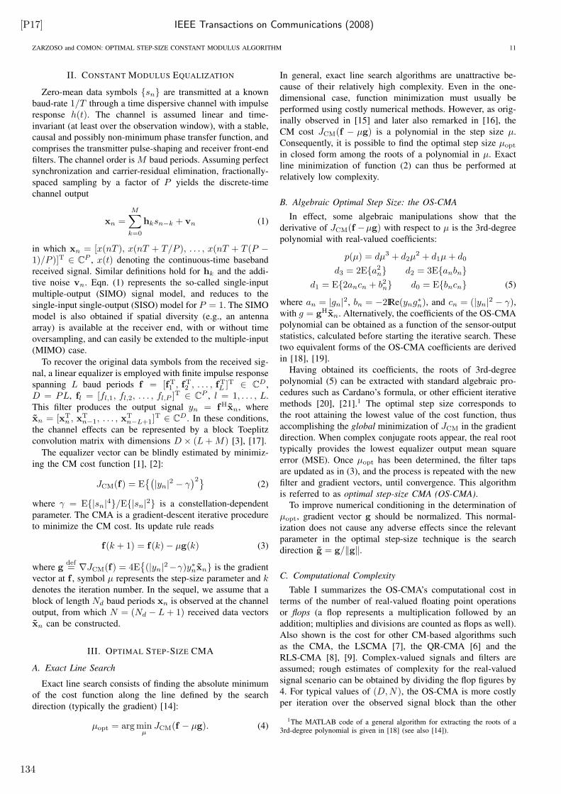
[P17] IEEE Transactions on Communications (2008)
ZARZOSO and COMON: OPTIMAL STEP-SIZE CONSTANT MODULUS ALGORITHM 11
II. CONSTANT MODULUS EQUALIZATION
Zero-mean data symbols {sn} are transmitted at a known
baud-rate 1/T through a time dispersive channel with impulse
response h(t). The channel is assumed linear and time-
invariant (at least over the observation window), with a stable,
causal and possibly non-minimum phase transfer function, and
comprises the transmitter pulse-shaping and receiver front-end
filters. The channel order is M baud periods. Assuming perfect
synchronization and carrier-residual elimination, fractionally-
spaced sampling by a factor of P yields the discrete-time
channel output
xn =M∑
k=0
hksn−k + vn (1)
in which xn = [x(nT ), x(nT + T/P ), . . . , x(nT + T (P −1)/P )]T ∈ C
P , x(t) denoting the continuous-time baseband
received signal. Similar definitions hold for hk and the addi-
tive noise vn. Eqn. (1) represents the so-called single-input
multiple-output (SIMO) signal model, and reduces to the
single-input single-output (SISO) model for P = 1. The SIMO
model is also obtained if spatial diversity (e.g., an antenna
array) is available at the receiver end, with or without time
oversampling, and can easily be extended to the multiple-input
(MIMO) case.
To recover the original data symbols from the received sig-
nal, a linear equalizer is employed with finite impulse response
spanning L baud periods f = [fT1 , f
T2 , . . . , f
TL ]T ∈ C
D,
D = PL, fl = [fl,1, fl,2, . . . , fl,P ]T ∈ CP , l = 1, . . . , L.
This filter produces the output signal yn = fHxn, where
xn = [xTn , x
Tn−1, . . . , x
Tn−L+1]
T ∈ CD. In these conditions,
the channel effects can be represented by a block Toeplitz
convolution matrix with dimensions D × (L+M) [3], [17].
The equalizer vector can be blindly estimated by minimiz-
ing the CM cost function [1], [2]:
JCM(f) = E{(
|yn|2 − γ
)2}(2)
where γ = E{|sn|4}/E{|sn|
2} is a constellation-dependent
parameter. The CMA is a gradient-descent iterative procedure
to minimize the CM cost. Its update rule reads
f(k + 1) = f(k) − µg(k) (3)
where gdef= ∇JCM(f) = 4E
{
(|yn|2−γ)y∗nxn} is the gradient
vector at f , symbol µ represents the step-size parameter and kdenotes the iteration number. In the sequel, we assume that a
block of length Nd baud periods xn is observed at the channel
output, from which N = (Nd − L+ 1) received data vectors
xn can be constructed.
III. OPTIMAL STEP-SIZE CMA
A. Exact Line Search
Exact line search consists of finding the absolute minimum
of the cost function along the line defined by the search
direction (typically the gradient) [14]:
µopt = arg minµJCM(f − µg). (4)
In general, exact line search algorithms are unattractive be-
cause of their relatively high complexity. Even in the one-
dimensional case, function minimization must usually be
performed using costly numerical methods. However, as orig-
inally observed in [15] and later also remarked in [16], the
CM cost JCM(f − µg) is a polynomial in the step size µ.
Consequently, it is possible to find the optimal step size µopt
in closed form among the roots of a polynomial in µ. Exact
line minimization of function (2) can thus be performed at
relatively low complexity.
B. Algebraic Optimal Step Size: the OS-CMA
In effect, some algebraic manipulations show that the
derivative of JCM(f −µg) with respect to µ is the 3rd-degree
polynomial with real-valued coefficients:
p(µ) = dµ3 + d2µ2 + d1µ+ d0
d3 = 2E{a2n} d2 = 3E{anbn}
d1 = E{2ancn + b2n} d0 = E{bncn} (5)
where an = |gn|2, bn = −2IRe(yng
∗n), and cn = (|yn|
2 − γ),with g = gHxn. Alternatively, the coefficients of the OS-CMA
polynomial can be obtained as a function of the sensor-output
statistics, calculated before starting the iterative search. These
two equivalent forms of the OS-CMA coefficients are derived
in [18], [19].
Having obtained its coefficients, the roots of 3rd-degree
polynomial (5) can be extracted with standard algebraic pro-
cedures such as Cardano’s formula, or other efficient iterative
methods [20], [21].1 The optimal step size corresponds to
the root attaining the lowest value of the cost function, thus
accomplishing the global minimization of JCM in the gradient
direction. When complex conjugate roots appear, the real root
typically provides the lowest equalizer output mean square
error (MSE). Once µopt has been determined, the filter taps
are updated as in (3), and the process is repeated with the new
filter and gradient vectors, until convergence. This algorithm
is referred to as optimal step-size CMA (OS-CMA).
To improve numerical conditioning in the determination of
µopt, gradient vector g should be normalized. This normal-
ization does not cause any adverse effects since the relevant
parameter in the optimal step-size technique is the search
direction g = g/‖g‖.
C. Computational Complexity
Table I summarizes the OS-CMA’s computational cost in
terms of the number of real-valued floating point operations
or flops (a flop represents a multiplication followed by an
addition; multiplies and divisions are counted as flops as well).
Also shown is the cost for other CM-based algorithms such
as the CMA, the LSCMA [7], the QR-CMA [6] and the
RLS-CMA [8], [9]. Complex-valued signals and filters are
assumed; rough estimates of complexity for the real-valued
signal scenario can be obtained by dividing the flop figures by
4. For typical values of (D,N), the OS-CMA is more costly
per iteration over the observed signal block than the other
1The MATLAB code of a general algorithm for extracting the roots of a3rd-degree polynomial is given in [18] (see also [14]).
134
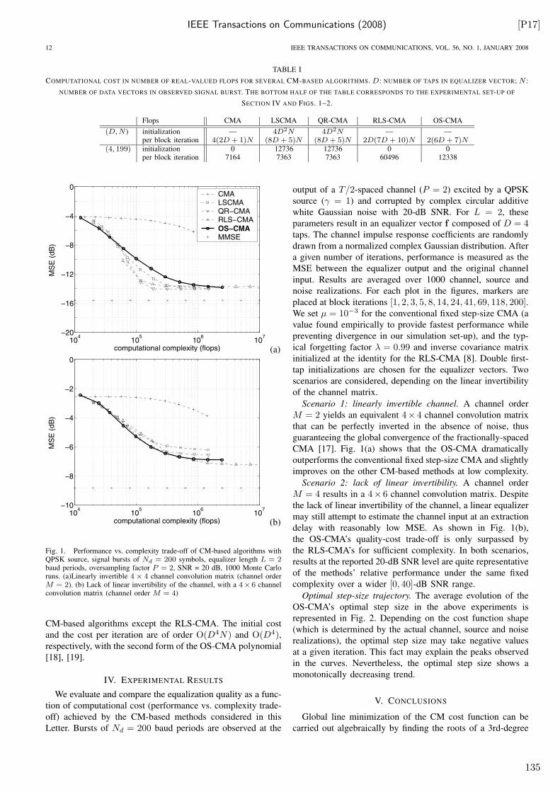
IEEE Transactions on Communications (2008) [P17]
12 IEEE TRANSACTIONS ON COMMUNICATIONS, VOL. 56, NO. 1, JANUARY 2008
TABLE I
COMPUTATIONAL COST IN NUMBER OF REAL-VALUED FLOPS FOR SEVERAL CM-BASED ALGORITHMS. D: NUMBER OF TAPS IN EQUALIZER VECTOR; N :
NUMBER OF DATA VECTORS IN OBSERVED SIGNAL BURST. THE BOTTOM HALF OF THE TABLE CORRESPONDS TO THE EXPERIMENTAL SET-UP OF
SECTION IV AND FIGS. 1–2.
Flops CMA LSCMA QR-CMA RLS-CMA OS-CMA
(D, N ) initialization — 4D2N 4D2N — —per block iteration 4(2D + 1)N (8D + 5)N (8D + 5)N 2D(7D + 10)N 2(6D + 7)N
(4, 199) initialization 0 12736 12736 0 0per block iteration 7164 7363 7363 60496 12338
104
105
106
107
−20
−16
−12
−8
−4
0
computational complexity (flops)
MS
E (
dB
)
CMALSCMAQR−CMARLS−CMAOS−CMA
MMSE
(a)
104
105
106
107
−10
−8
−6
−4
−2
0
computational complexity (flops)
MS
E (
dB
)
(b)
Fig. 1. Performance vs. complexity trade-off of CM-based algorithms withQPSK source, signal bursts of Nd = 200 symbols, equalizer length L = 2baud periods, oversampling factor P = 2, SNR = 20 dB, 1000 Monte Carloruns. (a)Linearly invertible 4 × 4 channel convolution matrix (channel orderM = 2). (b) Lack of linear invertibility of the channel, with a 4× 6 channelconvolution matrix (channel order M = 4)
CM-based algorithms except the RLS-CMA. The initial cost
and the cost per iteration are of order O(D4N) and O(D4),respectively, with the second form of the OS-CMA polynomial
[18], [19].
IV. EXPERIMENTAL RESULTS
We evaluate and compare the equalization quality as a func-
tion of computational cost (performance vs. complexity trade-
off) achieved by the CM-based methods considered in this
Letter. Bursts of Nd = 200 baud periods are observed at the
output of a T/2-spaced channel (P = 2) excited by a QPSK
source (γ = 1) and corrupted by complex circular additive
white Gaussian noise with 20-dB SNR. For L = 2, these
parameters result in an equalizer vector f composed of D = 4taps. The channel impulse response coefficients are randomly
drawn from a normalized complex Gaussian distribution. After
a given number of iterations, performance is measured as the
MSE between the equalizer output and the original channel
input. Results are averaged over 1000 channel, source and
noise realizations. For each plot in the figures, markers are
placed at block iterations [1, 2, 3, 5, 8, 14, 24, 41, 69, 118, 200].We set µ = 10−3 for the conventional fixed step-size CMA (a
value found empirically to provide fastest performance while
preventing divergence in our simulation set-up), and the typ-
ical forgetting factor λ = 0.99 and inverse covariance matrix
initialized at the identity for the RLS-CMA [8]. Double first-
tap initializations are chosen for the equalizer vectors. Two
scenarios are considered, depending on the linear invertibility
of the channel matrix.
Scenario 1: linearly invertible channel. A channel order
M = 2 yields an equivalent 4× 4 channel convolution matrix
that can be perfectly inverted in the absence of noise, thus
guaranteeing the global convergence of the fractionally-spaced
CMA [17]. Fig. 1(a) shows that the OS-CMA dramatically
outperforms the conventional fixed step-size CMA and slightly
improves on the other CM-based methods at low complexity.
Scenario 2: lack of linear invertibility. A channel order
M = 4 results in a 4× 6 channel convolution matrix. Despite
the lack of linear invertibility of the channel, a linear equalizer
may still attempt to estimate the channel input at an extraction
delay with reasonably low MSE. As shown in Fig. 1(b),
the OS-CMA’s quality-cost trade-off is only surpassed by
the RLS-CMA’s for sufficient complexity. In both scenarios,
results at the reported 20-dB SNR level are quite representative
of the methods’ relative performance under the same fixed
complexity over a wider [0, 40]-dB SNR range.
Optimal step-size trajectory. The average evolution of the
OS-CMA’s optimal step size in the above experiments is
represented in Fig. 2. Depending on the cost function shape
(which is determined by the actual channel, source and noise
realizations), the optimal step size may take negative values
at a given iteration. This fact may explain the peaks observed
in the curves. Nevertheless, the optimal step size shows a
monotonically decreasing trend.
V. CONCLUSIONS
Global line minimization of the CM cost function can be
carried out algebraically by finding the roots of a 3rd-degree
135
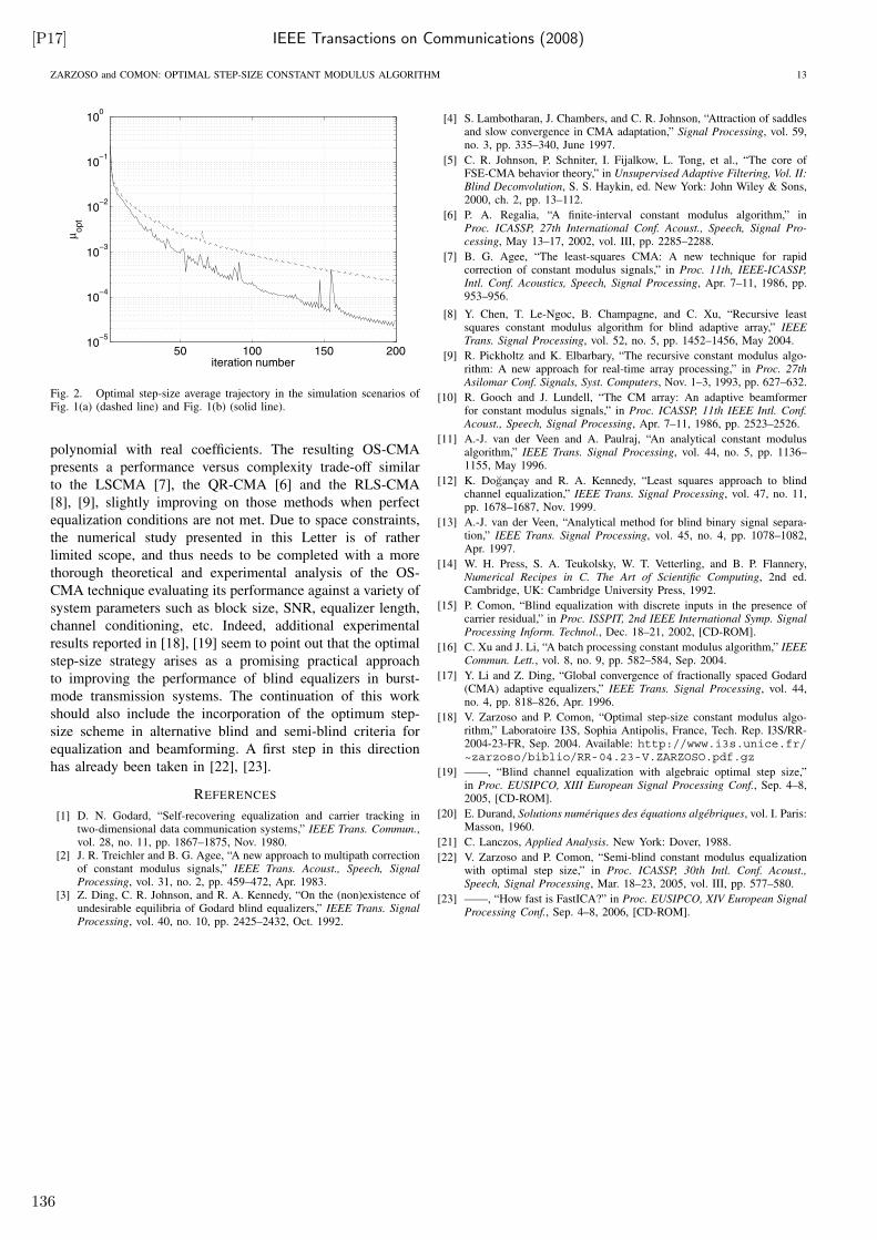
[P17] IEEE Transactions on Communications (2008)
ZARZOSO and COMON: OPTIMAL STEP-SIZE CONSTANT MODULUS ALGORITHM 13
50 100 150 20010
−5
10−4
10−3
10−2
10−1
100
iteration number
µopt
Fig. 2. Optimal step-size average trajectory in the simulation scenarios ofFig. 1(a) (dashed line) and Fig. 1(b) (solid line).
polynomial with real coefficients. The resulting OS-CMA
presents a performance versus complexity trade-off similar
to the LSCMA [7], the QR-CMA [6] and the RLS-CMA
[8], [9], slightly improving on those methods when perfect
equalization conditions are not met. Due to space constraints,
the numerical study presented in this Letter is of rather
limited scope, and thus needs to be completed with a more
thorough theoretical and experimental analysis of the OS-
CMA technique evaluating its performance against a variety of
system parameters such as block size, SNR, equalizer length,
channel conditioning, etc. Indeed, additional experimental
results reported in [18], [19] seem to point out that the optimal
step-size strategy arises as a promising practical approach
to improving the performance of blind equalizers in burst-
mode transmission systems. The continuation of this work
should also include the incorporation of the optimum step-
size scheme in alternative blind and semi-blind criteria for
equalization and beamforming. A first step in this direction
has already been taken in [22], [23].
REFERENCES
[1] D. N. Godard, “Self-recovering equalization and carrier tracking intwo-dimensional data communication systems,” IEEE Trans. Commun.,vol. 28, no. 11, pp. 1867–1875, Nov. 1980.
[2] J. R. Treichler and B. G. Agee, “A new approach to multipath correctionof constant modulus signals,” IEEE Trans. Acoust., Speech, Signal
Processing, vol. 31, no. 2, pp. 459–472, Apr. 1983.[3] Z. Ding, C. R. Johnson, and R. A. Kennedy, “On the (non)existence of
undesirable equilibria of Godard blind equalizers,” IEEE Trans. Signal
Processing, vol. 40, no. 10, pp. 2425–2432, Oct. 1992.
[4] S. Lambotharan, J. Chambers, and C. R. Johnson, “Attraction of saddlesand slow convergence in CMA adaptation,” Signal Processing, vol. 59,no. 3, pp. 335–340, June 1997.
[5] C. R. Johnson, P. Schniter, I. Fijalkow, L. Tong, et al., “The core ofFSE-CMA behavior theory,” in Unsupervised Adaptive Filtering, Vol. II:
Blind Deconvolution, S. S. Haykin, ed. New York: John Wiley & Sons,2000, ch. 2, pp. 13–112.
[6] P. A. Regalia, “A finite-interval constant modulus algorithm,” inProc. ICASSP, 27th International Conf. Acoust., Speech, Signal Pro-
cessing, May 13–17, 2002, vol. III, pp. 2285–2288.
[7] B. G. Agee, “The least-squares CMA: A new technique for rapidcorrection of constant modulus signals,” in Proc. 11th, IEEE-ICASSP,
Intl. Conf. Acoustics, Speech, Signal Processing, Apr. 7–11, 1986, pp.953–956.
[8] Y. Chen, T. Le-Ngoc, B. Champagne, and C. Xu, “Recursive leastsquares constant modulus algorithm for blind adaptive array,” IEEE
Trans. Signal Processing, vol. 52, no. 5, pp. 1452–1456, May 2004.
[9] R. Pickholtz and K. Elbarbary, “The recursive constant modulus algo-rithm: A new approach for real-time array processing,” in Proc. 27th
Asilomar Conf. Signals, Syst. Computers, Nov. 1–3, 1993, pp. 627–632.
[10] R. Gooch and J. Lundell, “The CM array: An adaptive beamformerfor constant modulus signals,” in Proc. ICASSP, 11th IEEE Intl. Conf.
Acoust., Speech, Signal Processing, Apr. 7–11, 1986, pp. 2523–2526.
[11] A.-J. van der Veen and A. Paulraj, “An analytical constant modulusalgorithm,” IEEE Trans. Signal Processing, vol. 44, no. 5, pp. 1136–1155, May 1996.
[12] K. Dogançay and R. A. Kennedy, “Least squares approach to blindchannel equalization,” IEEE Trans. Signal Processing, vol. 47, no. 11,pp. 1678–1687, Nov. 1999.
[13] A.-J. van der Veen, “Analytical method for blind binary signal separa-tion,” IEEE Trans. Signal Processing, vol. 45, no. 4, pp. 1078–1082,Apr. 1997.
[14] W. H. Press, S. A. Teukolsky, W. T. Vetterling, and B. P. Flannery,Numerical Recipes in C. The Art of Scientific Computing, 2nd ed.Cambridge, UK: Cambridge University Press, 1992.
[15] P. Comon, “Blind equalization with discrete inputs in the presence ofcarrier residual,” in Proc. ISSPIT, 2nd IEEE International Symp. Signal
Processing Inform. Technol., Dec. 18–21, 2002, [CD-ROM].
[16] C. Xu and J. Li, “A batch processing constant modulus algorithm,” IEEE
Commun. Lett., vol. 8, no. 9, pp. 582–584, Sep. 2004.
[17] Y. Li and Z. Ding, “Global convergence of fractionally spaced Godard(CMA) adaptive equalizers,” IEEE Trans. Signal Processing, vol. 44,no. 4, pp. 818–826, Apr. 1996.
[18] V. Zarzoso and P. Comon, “Optimal step-size constant modulus algo-rithm,” Laboratoire I3S, Sophia Antipolis, France, Tech. Rep. I3S/RR-2004-23-FR, Sep. 2004. Available: http://www.i3s.unice.fr/~zarzoso/biblio/RR-04.23-V.ZARZOSO.pdf.gz
[19] ——, “Blind channel equalization with algebraic optimal step size,”in Proc. EUSIPCO, XIII European Signal Processing Conf., Sep. 4–8,2005, [CD-ROM].
[20] E. Durand, Solutions numériques des équations algébriques, vol. I. Paris:Masson, 1960.
[21] C. Lanczos, Applied Analysis. New York: Dover, 1988.
[22] V. Zarzoso and P. Comon, “Semi-blind constant modulus equalizationwith optimal step size,” in Proc. ICASSP, 30th Intl. Conf. Acoust.,
Speech, Signal Processing, Mar. 18–23, 2005, vol. III, pp. 577–580.
[23] ——, “How fast is FastICA?” in Proc. EUSIPCO, XIV European Signal
Processing Conf., Sep. 4–8, 2006, [CD-ROM].
136
IEEE Transactions on Signal Processing (2006) [P18]
IEEE TRANSACTIONS ON SIGNAL PROCESSING, VOL. 54, NO. 8, AUGUST 2006 3049
Optimal Pairwise Fourth-Order IndependentComponent Analysis
Vicente Zarzoso, Member, IEEE, Juan José Murillo-Fuentes, Member, IEEE, Rafael Boloix-Tortosa, andAsoke K. Nandi, Senior Member, IEEE
Abstract—Blind source separation (BSS) aims at the reconstruc-tion of unknown mutually independent signals, so-called sources,from their mixtures observed at the output of a sensor array. TheBSS of instantaneous linear mixtures, which finds application innumerous fields, can be solved through the statistical tool of inde-pendent component analysis (ICA). This paper concentrates on theanalytic solutions for the fundamental two-signal ICA scenario. Anovel estimation class, so-called general weighted fourth-order es-timator (GWFOE), is put forward, which is based on the fourth-order statistics of the whitened sensor output. By means of a weightparameter, the GWFOE is able to unify a variety of apparentlydisparate estimation expressions previously scattered throughoutthe literature, including the well-known JADE method in the two-signal case. A theoretical asymptotic performance analysis is car-ried out, resulting in the GWFOE large-sample mean square errorand the source-dependent weight value of the most efficient esti-mator in the class. To extend the pairwise estimators to the gen-eral scenario of more than two sources, an improved Jacobi-likeoptimization technique is proposed. The approach consists of cal-culating the necessary sensor-output fourth-order statistics at theinitialization stage of the algorithm, which can lead to significantcomputational savings when large sample blocks are processed.Based on this idea, adaptive algorithms are also devised, showingvery satisfactory convergence characteristics. Experiments illus-trate the good performance of these optimal pairwise ICA strate-gies, in both off- and on-line processing modes.
Index Terms—Array signal processing, blind source separation,higher order statistics, independent component analysis, perfor-mance analysis, unsupervised learning.
I. INTRODUCTION
A. Problem and Motivation
The problem of blind source separation (BSS) consists of re-
covering a set of unobserved signals, so-called sources, from an-
other set of observed signals which are mixtures of the sources
[1]–[3]. The term “blind” signifies that (typically) very few as-
sumptions are made about the sources and the mixing process.
Manuscript received November 30, 2004; revised September 4, 2005. Theassociate editor coordinating the review of this manuscript and approving it forpublication was Dr. Peter Handel. The work of V. Zarzoso was supported by theRoyal Academy of Engineering, U.K., under a Research Fellowship. The workof J. J. Murillo-Fuentes and R. Boloix-Tortosa was supported by the SpanishGovernment under Grant MCYT TIC2003-03781.
V. Zarzoso was with the Department of Electrical Engineering and Elec-tronics, The University of Liverpool, U.K. He is now with Laboratoire I3S,Université de Nice - Sophia Antipolis, 06903 Sophia Antipolis Cedex, France(e-mail: [email protected]).
J. J. Murillo-Fuentes and R. Boloix-Tortosa are with the Departamento deTeoría de la Señal y Comunicaciones, Escuela Superior de Ingenieros, Univer-sidad de Sevilla, 41092 Sevilla, Spain (e-mail: [email protected]; [email protected]).
A. K. Nandi is with the Department of Electrical Engineering and Electronics,University of Liverpool, Liverpool L69 3GJ, U.K. (e-mail: [email protected]).
Digital Object Identifier 10.1109/TSP.2006.875391
By contrast, conventional array processing techniques (e.g., for
direction-of-arrival estimation) assume a certain structure for
the mixing matrix in terms of the array manifold, or the array
response as a function of the arrival angle. Deviations of the as-
sumed structure from reality (calibration errors) can have a sig-
nificant negative impact on the algorithms’ performance. The
relative freedom given by BSS methods to the mixing structure
makes them very robust to calibration errors [4]. This flexibility
and robustness have spurred the interest in the BSS problem over
the last decade. Another important motivation has been the vast
number of application areas where BSS proves useful [2], [3],
[5], ranging from communications [6] to biomedical signal pro-
cessing (electrocardiogram and electroencephalogram analysis,
fMRI, brain imaging) [7]–[9], condition monitoring, image pro-
cessing [10], financial data analysis, seismic exploration, clas-
sification, or data compression and coding [11], among others.
Instantaneous linear mixtures, where no time delays occur in the
propagation from sources to sensors, is a very accurate signal
model in many of those applications. The solution of the more
elaborate convolutive-mixture model can often be decoupled
into a stage resolving the effects caused by the multipath channel
(time equalization) followed by the separation of the remaining
instantaneous mixture. The separation of nonlinear mixtures is
more involved, and is also receiving attention by some authors
(see, e.g., [2], [3], and references therein).
When the time structure cannot be exploited or is simply
ignored, the basic approach to instantaneous linear source
separation consists of projecting the observation vectors into
some basis where the resulting components are statistically
independent. This is the independent component analysis (ICA)
of the observed data [12], and in its more general form it relies
(explictly or not) on higher order statistics. A previous spatial
whitening process (entailing second-order decorrelation and
power normalization) helps to reduce the number of unknowns,
resulting in a set of normalized uncorrelated components
(whitened signals) related with the sources through a unitary
transformation. ICA is then tantamount to the identification of
this unitary matrix.
B. Closed-Form Solutions in the Two-Signal Case
In the fundamental real-valued two-signal case, the problem
reduces to the identification of a single parameter, the un-
known angle characterizing the Givens-rotation mixing matrix.
A variety of closed-form methods for the estimation of this
angle have been proposed in the literature. These methods
arise from approximations of certain optimality criteria (con-
trast functions) and provide direct solutions with no iterative
search involved. Most of these share the common feature
1053-587X/$20.00 © 2006 IEEE
137
[P18] IEEE Transactions on Signal Processing (2006)
3050 IEEE TRANSACTIONS ON SIGNAL PROCESSING, VOL. 54, NO. 8, AUGUST 2006
of being based on the fourth-order statistics of the sensor
output. The first expression was obtained in [13] by relating the
fourth-order statistics of sources and sensors. Its performance
was later shown to depend on the actual value of the unknown
parameter [14], [15], thus losing the desirable uniform perfor-
mance property [16]. A good number of early methods were
derived from the maximum likelihood (ML) approach. The
truncated Gram–Charlier expansion of the source probability
density function (pdf) yielded the solution of [17], restricted to
symmetric sources with normalized kurtosis in certain positive
range. These validity conditions were broadened through the
extended ML (EML) and the alternative EML (AEML) estima-
tors [14], [18], [19]. The EML also generalized the maximum
kurtosis (MK) cost function of [20], [21], initially thought to be
valid only for sources with same kurtosis sign [14], to source
pairs with nonzero source kurtosis sum (sks). The EML and the
AEML remain consistent providing the sks and source kurtosis
difference (skd) are not null, respectively. This deficiency was
overcome in [14], [19], and [22]. In [14] and [19], the choice
between the EML or the AEML was made with a simple
decision rule as a function of the sensor-output fourth-order
statistics. In [22], adopting the ML framework of [17], the two
estimators were unified into a single analytic expression, the
approximate ML (AML).
The contrast function of [12], which had earlier been reached
from the ML principle [23], is itself an approximation of a
negentropy maximization principle measuring the deviation of
the separator output from Gaussianity. Negentropy can also be
readily connected to alternative information-theoretical criteria
such as the mutual information (MI) between the separator
outputs or the sum of their marginal entropies (ME) [4], [5].
Another major group of two-dimensional closed-form solu-
tions arises from the trigonometric expansion and approximate
minimization of the ME contrast criteria developed in [12]. The
MaSSFOC (maximum of sum squared fourth-order cumulant)
estimator [24] and the recently proposed sinusoidal ICA (SICA)
[25], which resemble the AML, are approximate minimizers
of the fourth-order contrast function. Further simplifications
of this contrast function when the source kurtoses have the
same modulus lead to the so-called source kurtosis sum and
source kurtosis difference estimators (SKSE, SKDE) [24], very
similar to the EML and AEML estimators [14], [18], [19],
respectively. The simultaneous exploitation of orders three and
four is shown to improve the separation performance when
some of the sources present nonsymmetric distributions [26].
The original solution to Comon’s fourth-order contrast in-
volved finding the roots of a fourth-degree polynomial (a bi-
quadratic or quartic equation). An analytic procedure for rooting
quartics is well known since the sixteenth century (Ferrari’s
formula), but its calculation can be cumbersome; approximate
numerical methods are usually preferred instead. The closed-
form estimators that we are concerned with are considerably less
elaborate: they consist of simple formulas involving straight-
forward operations on certain statistics of the whitened sensor
output.
The notion of linearly combining estimators was originally
put forward in [22]. Through a weight parameter, the EML
and AEML are combined together into a single expression, the
so-called weighted AML (WAML) estimator. It was suggested
that the weight parameter could be adjusted by taking advantage
of a priori information on the source pdfs, although no specific
guidelines were given on how the actual choice should be made.
C. Scenario of More Than Two Signals
In the -dimensional case, , ICA can be carried
out by applying the two-signal estimators to each whitened
signal pair over several sweeps until convergence [12]. This
iterative approach is reminiscent of the Jacobi optimization
(JO) technique for matrix diagonalization [27], [28], and can
indeed be seen as its extension to higher dimensional tensors
[12]. Although no theoretical proof of global convergence has
yet been obtained for the pairwise iterations in the tensor case
[12], [29], the method remains valid in practice since no exper-
imental or theoretical counterexample of misconvergence has
been encountered to date, provided that the validity conditions
of the two-dimensional criteria are fulfilled for every signal
pair. In the standard JO iteration, the fourth-order statistics
used by the closed-form estimators need to be computed for
each signal pair at every sweep until convergence. Typically,
the statistics are estimated from the signal samples, which may
involve extensive computations especially when processing
long signal blocks. Adaptive algorithms, such as the so-called
adaptive rotation (AROT) [13] and the adaptive EML (adEML)
[30], are easily derived from this strategy. However, they some-
times show poor convergence, especially for a large number of
sources.
D. Contributions and Outline
Many successful methods are available to perform ICA in the
general scenario of more than two sources (see, e.g., [2], [3],
and references therein). Nevertheless, the two-signal case re-
mains a scenario of fundamental importance, since it is the most
basic and can be considered as the elementary unit for the so-
lution of the general in the JO approach. Despite this
relevance, the relationships between the different analytic solu-
tions have only been explored to a limited extent. The purpose
of this paper is to fill the gap in these connections. By means of
the complex-centroid notation used in the EML and the AEML
[14], [18], [19], [31], we arrive at a compact formulation for the
WAML estimator of [22]. It is seen that through different values
of the weight parameter, many of the existing fourth-order es-
timators are obtained, including the well-known JADE method
[4] for ; hence the more suitable name of general weighted
fourth-order estimator (GWFOE). The centroid formalism al-
lows a simple derivation of the estimator’s large-sample mean
square error (MSE), from which the weight parameter of the op-
timal estimator is determined as a function of the source statis-
tics. Here, “optimal” refers to the asymptotically most efficient
estimator in the GWFOE class.
In the general case of more than two signals, we aim to op-
timize the computational cost of the JO technique. An alterna-
tive moment-calculation procedure is proposed, which is less
costly in scenarios where the sample size is large relative to the
number of sources. The relevant statistics are computed from the
sensor-output samples before starting the JO iterations and then
modified according to the pairwise rotations. We refer to this
138
IEEE Transactions on Signal Processing (2006) [P18]
ZARZOSO et al.: OPTIMAL PAIRWISE FOURTH-ORDER INDEPENDENT COMPONENT ANALYSIS 3051
method as initialized JO (IJO). By comparing the complexity
of the proposed and the conventional moment-estimation pro-
cedure, a decision rule is derived to select the most computa-
tionally efficient option. This results in the optimal JO (OJO).
Adaptive algorithms based on IJO can also be designed to im-
prove the convergence properties of previous online approaches.
In short, the results presented in this paper unify, generalize, and
enhance ICA techniques based on two-dimensional fourth-order
contrasts.
This paper encompasses substantially extended as well
as thoroughly revised versions of conference publications
[32]–[36]. The material is organized as follows. After re-
viewing the BSS signal model and ICA contrast functions in
Section II, Section III derives the GWFOE, highlights its con-
nections with other analytic solutions, performs its asymptotic
analysis, and obtains the best estimator of the class. Section IV
is devoted to the scenarios of more than two signals, featuring
the computationally efficient IJO and OJO procedures. Adap-
tive implementations are the focus of Section V. Experimental
results are reported in Section VI. Section VII concludes herein.
The Appendices contain some proofs and other mathematical
derivations.
E. Notations
Throughout this paper, vectors and matrices are represented
as lowercase and uppercase boldface letters, respectively.
Symbols and indicate the transpose and inverse
matrix operators, respectively. and are the sets of real
and complex numbers, respectively; symbol is the
imaginary unit; and denote the real and imaginary
part of its complex argument, respectively, whereas function
supplies its principal value (i.e., its argument in the in-
terval ). represents the mathematical expectation.
Given a set of signals , and
, , ,
denote their th-order moments and cumulants, respec-
tively, whose mathematical definitions can be found in
[37] and [38]. For the pairwise case, we prefer Kendall’s
notation [37]: and
stand for the th-order moment and
cumulant of the signal pair .
II. BSS AND ICA
A. Matrix Model
In its simplest form, the BSS problem accepts the
following matrix model. The entries of sensor-output
vector are instantaneous
linear combinations of a set of unobserved source signals
(1)
where represents the mixing matrix, with dimensions ,
. In this paper all signals and mixtures are assumed to be
real valued. If the mixing matrix is full column rank, the sources
are mutually independent, and at most one of them is Gaussian,
it is possible to obtain a separation matrix and estimate the
sources [12], [39] as
(2)
Since the scale and order of the components of do not af-
fect their statistical independence, a satisfactory separation is
characterized by a global matrix with a nonmixing structure,
that is, with a single nonnull element per row and per column
(the product of a invertible diagonal matrix and a permutation
matrix). As the source amplitudes are not important, it can be
assumed, without loss of generality, that the source variance is
unity .
Source separation is typically carried out in two steps. First,
whitening or standardization [principal component analysis
(PCA)] projects the observed vector on the signal subspace and
yields a set of second-order decorrelated, normalized signals
such that . As a result,
the source and whitened vectors must be related through a
unitary transformation
(3)
The separation problem thus reduces to the computation of uni-
tary matrix , which is accomplished in a second step. The ICA
approach to BSS consists of computing such that the entries
of the separator output are as independent as
possible.1 Since we consider methods that do not exploit the
temporal structure of the source process , in the sequel, the
time index will be dropped when convenient.
B. Contrast Functions
A contrast function [12] is a mapping from the set of
densities to satisfying the following require-
ments. If has independent components, then ,
nonsingular (domination), with equality if and only if
is nonmixing (discrimination); also, is unaltered by
permutations or scaling of the components of (invariance).
Thus, the maximization of a contrast function yields the ICA
solution. Contrasts are attractive because they allow an optimal
processing in the presence of unknown noise and interference,
adding robustness to the separation performance.
The ML principle provides the contrast [23]
(4)
1This two-step process corresponds to the “hard whitening” approach. Re-cently, the “soft whitening” concept has been introduced [40], in which thesecond- and higher order processing is carried out simultaneously.
139
[P18] IEEE Transactions on Signal Processing (2006)
3052 IEEE TRANSACTIONS ON SIGNAL PROCESSING, VOL. 54, NO. 8, AUGUST 2006
If this function is maximized for all possible distributions under
the whitening constraint, we arrive at the ME contrast [41]
(5)
where represents the differential entropy. Using the Edge-
worth expansion of the source pdf [37], after second-order
whitening, the ME contrast can be approximated as a function
of the fourth-order cumulants [12], [41]
(6)
where is the fourth-order marginal cumulant (kurtosis)
of , which, in the zero-mean unit-variance case, reduces
to . This contrast is discriminating over the set
of random vectors having at most one non-kurtic compo-
nent [12]. Alternatively, instead of maximizing the ML for
all possible distributions, we can also exploit some available
information on the source pdf to maximize the ML contrast.
In the fourth-order case, if all sources have the same sign of
kurtosis, (6) simplifies to [20]
(7)
Finally, the JADE method [4] is based on the criterion
(8)
whose maximization can be efficiently carried out as the joint
approximate diagonalization of a set of matrix slices of the
whitened cumulant tensor. In the two-signal scenario, approx-
imations to these optimality criteria can be solved in closed
form as explained in the next section. In the case of JADE, the
associated closed-form estimator that we develop is an exact
minimizer of criterion (8).
III. OPTIMAL ANALYTIC SOLUTION IN THE TWO-SIGNAL CASE
A. Complex Centroids
In the two-signal case, is a Givens rotation matrix, charac-
terized by an unknown angle
(9)
ICA then reduces to the estimation of from the whitened
sensor outputs. Relation (3) accepts a compact complex-valued
formulation
(10)
or , where and .
Geometrically, (10) signifies that the whitened-signal pdf is a
rotated version of the source pdf.
Centroids are defined as particular nonlinear averages of the
complex points (10) [14], [18], [31]. The following centroids are
useful in deriving closed-form expressions for the estimation of
(11)
(12)
(13)
When written as a function of the source statistics, the above
centroids yield
(14)
where symbols and represent
the sks and the skd, respectively.2
B. General Weighted Fourth-Order Estimator (GWFOE)
The EML estimator [18] can be expressed as
(15)
Similarly, the AEML [19] reads
(16)
Under mild conditions, the sample versions of centroids , ,
and are consistent estimators of , , and , respec-
tively, so that and consistently estimate as long
as and , respectively [14], [18]. The lack of consis-
tency for certain values of source kurtosis is precisely the main
drawback of these two estimators.
In order to circumvent this deficiency, let us form the com-
pound centroid
(17)
Then, parameter can also be estimated through
(18)
which we call the GWFOE. The relevance of the GWFOE lies
in the fact that it is a consistent estimator of for any source
distribution, since the GWFOE centroid consistently estimates
the complex number . More importantly,
the GWFOE unifies many of the analytic solutions already pro-
posed in the literature, which are simply obtained for different
values of the weight parameter :
i) : AEML estimator of [14], [19];
ii) : AML estimator of [22];
iii) : SICA estimator of [25], [33];
2Note that � is an estimate of from the whitened sensor output. Hence, theequality expressed in (14) only holds for the ensemble averages.
140
IEEE Transactions on Signal Processing (2006) [P18]
ZARZOSO et al.: OPTIMAL PAIRWISE FOURTH-ORDER INDEPENDENT COMPONENT ANALYSIS 3053
iv) : MaSSFOC estimator of [24];
v) : EML estimator of [14], [18].
In addition, Appendix I proves that the solution provided by
JADE [4] for sources is equivalent to the GWFOE with
. Similarly, the fourth-order part of the recently pro-
posed CuBICA method [26] corresponds to the GWFOE with
. On the other hand, by substituting with 1 in
(17)–(18), we also obtain the ML, MK, and SKSE/SKDE es-
timators of [17], [20], [21], [24], and [41]. These latter methods
require advance knowledge of the source kurtosis sign.
Some of the above estimators arise from the ML criterion
when the source pdf is approximated by its Gram–Charlier ex-
pansion truncated at fourth-order, and the sources are symmet-
rically distributed. Different solutions are then obtained under
additional conditions:
EML estimator: , ;
AEML estimator: , ;
AML estimator: , .
The GWFOE does not directly arise from the ML criterion, but
it can be considered as the combination of two solutions (EML
and AEML) which are approximate ML estimators under spe-
cific assumptions. Even if the validity conditions of an approx-
imate ML solution hold, the use of a different weight will di-
vert the GWFOE from such a solution. However, the GWFOE
variance can be fine-tuned by appropriately selecting . In this
manner the GWFOE can be made more efficient than any of the
pairwise ML methods, especially in scenarios where their va-
lidity conditions do not hold. This improved efficiency is pos-
sible because the other estimators are only approximate ML so-
lutions. This interesting feature will be developed in the next
section and illustrated by the experiments of Section VI.
The use of the complex-centroid formalism allows us to bring
out the connections with other existing closed-form solutions
and facilitates the theoretical performance analysis of the esti-
mator (as carried out next). Since some of these solutions (such
as MaSSFOC or SICA) were originally obtained as approxima-
tions to optimality criteria other than ML, we prefer to adhere
to the more generic denomination of GWFOE.
C. Performance Analysis: Optimal GWFOE
In this section, we intend to provide specific guidelines for
the choice of GWFOE’s weight parameter. We search for the
value of that minimizes the asymptotic (large-sample) MSE
of the GWFOE class.
The asymptotic MSE of the GWFOE (18) is determined in
Appendix II and is given by
MSE
(19)
where is the number of samples per signal. It is interesting to
note the following.
i) MSE reduces to the asymptotic MSE of the
AEML and EML estimators [14], [15] for and
, respectively. This is not surprising, since the
GWFOE becomes such estimators at those weight values
(see the previous section).
ii) When (respectively, ), GWFOE performance
reduces to that of the AEML (respectively, EML) esti-
mator, for any .
If , the global minimum of MSE (19) is
obtained at (see Appendix II)
(20)
If , the derivative of MSE with respect to
does not change sign and thus MSE is monotonic in
such an interval. In that case, we choose between
(AEML) and (EML) the value that provides the lowest
MSE in (19). If , case ii) holds. Hence,
given the source statistics, one can select the estimator of the
GWFOE family with minimum asymptotic MSE. The experi-
ments of Section VI will illustrate the validity of the asymptotic
approximation (19) and the performance improvements that can
be derived from the use of the optimal weight coefficient.
In the event that nothing is known in advance about the source
statistics, a possible simple strategy is to perform an initial sep-
aration with any . The optimal value of can then
be estimated from the obtained sources, and the separation can
be repeated until converges. This iterative estimation of
converges very fast (typically within one to two iterations),
as will be demonstrated in the experiments of Section VI. De-
pending on the actual source statistics and the application in
hand, the performance gain may compensate the increased cost
of performing several separations.
IV. MORE THAN TWO SIGNALS CASE
A. Standard Jacobi Optimization
Jacobi optimization (JO) techniques have favorable
rounding-error properties and high computational parallelism,
allowing for numerically stable efficient implementations [28].
In the ICA context, Comon applied a JO-like procedure to
extend a two-dimensional contrast to the -dimensional
scenario, with . Thanks to its flexibility, the JO approach
can easily integrate any valid two-signal solution, such as the
GWFOE.
Algorithm (JO-GWFOE)
-dimensional GWFOE using conventional Jacobi
optimization.
1) Whitening. Compute the whitened signals as
from a whitening matrix . Set and sweep number
.
2) Sweep . For all , , do
a) Set and compute the Givens
angle from (18).
b) If , rotate the pair by .
3) End? If the number of sweeps reaches a maximum value
or no angle has been updated, terminate.
Otherwise go to Step 2) for another sweep, with .
141
[P18] IEEE Transactions on Signal Processing (2006)
3054 IEEE TRANSACTIONS ON SIGNAL PROCESSING, VOL. 54, NO. 8, AUGUST 2006
In [41], the algorithm only stops when the whole set of
Givens rotations have been updated by a value under a threshold
, but no limit is set on the number of sweeps . The value
is chosen in such a way that rotations by a smaller angle
are not statistically significant; typically, ,
where is the sample size. In [12], the algorithm stops after
sweeps. This limit is also appropriate in our im-
plementation, due to the existing connection between the con-
trast of [12] in the basic two-dimensional case and the GWFOE
solutions. In a bid to avoid useless computations, we also set a
fixed threshold rad (0.5 ).
B. Initialized Jacobi Optimization
Step 2a) of the JO-GWFOE computes the Givens angle by
using (18). The centroids (11)–(13) are calculated by averaging
over the whole set of samples of signal pair . Since the
sample averaging is repeated over several sweeps, this proce-
dure may be computationally very costly for large sample sizes.
A more efficient alternative may be obtained as follows. Cen-
troids (11)–(13) may be written as a function of the moments
of the current output pair . The idea is to compute
the whole set of whitened-signal moments just once at an ini-
tial stage and later “rotate” them at each step of the algorithm
without reusing the observed signal samples. The relationship
between the moments of the whitened sensor output and their
rotated counterparts is established below (Appendix III).
Proposition 1: Let , where is an arbitrary
matrix. Then, there exists a symmetric matrix ,
with , such that
(21)
where
(22)
Moreover, there exist vectors , , and of length , such
that the fourth-order moments of the outputs are given
by
(23)
The formulation introduced above allows an easy computa-
tion of the output statistics for a given rotation matrix, as the
entries of are easily arranged into the three “rotation vec-
tors” , , and used in (23). Since only the subset
is needed in matrix , the number of
computed moments reduces to .
The resulting ICA algorithm based on this algebraic structure is
outlined below.
Algorithm (IJO-GWFOE)
-dimensional GWFOE using initialized Jacobi optimization.
1) Whitening. Compute a whitening matrix and set
.
2) Moments Initialization. Compute matrix in (21) from
the sample estimates of , . Initialize
the accumulated rotation matrix as .
3) Sweep . For all , , do
a) Compute the moments of current signal pair
from (23) and . Compute the Givens angle
from (18).
b) if , update the rotation matrix by
rotating an angle the proper coordinates.
4) End? If the number of sweeps satisfies or no
angle has been updated, terminate. Otherwise return
to Step 3) for another sweep, with .
At convergence, matrix is an estimate of in (3). The
main advantage of the alternative formulation presented in this
section is that the whitened sensor samples are directly used
only once, for computing matrix before starting the itera-
tions. The moments of each signal pair at each step of Algorithm
IJO-GWFOE are computed as quadratic forms involving simple
vector-matrix products. The main drawback of this alternative
procedure is that at a large number of components, the number
of entries of the moment matrix is of order . However, we
will show later in this section that the complexity of the stan-
dard JO can be improved if the number of sources is low. Hence,
memory problems will not appear. By “initialization” we mean
a previous computation of the whitened-signal statistics to sim-
plify subsequent calculations.
The IJO algorithm described above is reminiscent of JADE
[4]. Indeed, the GWFOE with is equivalent to JADE
in the scenario of sources, as seen in Section III-B
and Appendix I. Moreover, JADE also calculates the cumulant
matrix in advance and performs planar rotations in a JO-like
fashion. Nevertheless, the equivalence between JADE and
GWFOE-based algorithms vanishes in the presence of more
than two sources, for JADE’s cost function involves cumulants
from more than two signals at each Jacobi iteration. On the
other hand, JADE updates the cumulant matrix with the Givens
angles after each iteration, whereas the IJO algorithm calculates
the pertinent signal-pair cumulants from the moment matrix as
in Proposition 1, without updating the moment matrix.
C. Computational Complexity: Optimal Jacobi Optimization
This section compares the computational complexity of the
initialized and standard JO methods. As in [30], and for the sake
of comparison, a floating-point operation (flop) will be consid-
ered as a real multiplication followed by an addition. The fol-
lowing values are used: is the number of signal
pairs, denotes the maximum number of sweeps
in the JO, and represents the dimension of the
moment matrix in (21).
The computational burden of a fourth-order moment sample
estimate is flops. The number of flops for the JO-GWFOE
algorithm is
(24)
The first term is the computational cost related to the calcula-
tion of the moments, whereas the second accounts for the data
142
IEEE Transactions on Signal Processing (2006) [P18]
ZARZOSO et al.: OPTIMAL PAIRWISE FOURTH-ORDER INDEPENDENT COMPONENT ANALYSIS 3055
Fig. 1. Computational burden ratio between the JO and the IJO approaches.The vertical lines represent the range of (n; T ) with � between 0.9 and 1.1.
rotation performed at Step 2b) of Algorithm JO-GWFOE. The
number of operations of the IJO-GWFOE algorithm is given by
(25)
where the first term is the number of operations needed to com-
pute the entries of the moment matrix (21). Since some multi-
plications are repeated in the calculation of the moments (e.g.,
the product appears in any term of the form ),
this number could be further reduced to . The
second term in (25) is the number of operations in computing
(23) at each Givens angle. Hence, the relation between and
is
(26)
Fig. 1 plots the loci of . We can draw the fol-
lowing conclusions. Since usually , IJO is to be used for
a low number of sources, . As , the number of mo-
ments becomes of the order , making
for any sample size. This outcome takes place at . Since
the IJO is not to be used for large numbers of components, po-
tential memory problems associated with the storage of matrix
are avoided. As a result of the above decision rule, the fol-
lowing computationally optimal JO algorithm can be devised.
Algorithm (OJO-GWFOE)
-dimensional GWFOE using computationally optimal Jacobi
optimization.
1) Compute the condition in (26), and decide:
a) If then use JO-GWFOE.
b) Else, use IJO-GWFOE.
V. ADAPTIVE ALGORITHMS
A. Adaptive Jacobi Optimization
The JO procedure is easily extended to operate online, re-
sulting in the adaptive Jacobi optimization (AJO). The AROT
[13] and the adEML [30] are methods of this type. This section
derives the AJO implementation of the GWFOE pairwise solu-
tion. This implementation is referred to as AJO-GWFOE.
The JO computes the two-dimensional estimate for
each signal pair over several sweeps. Accordingly, centroids
(11)–(13) must be calculated for every sweep and signal pair
. In the design of an adaptive version, such statistics can
be updated with a new sample arriving at instant as
(27)
(28)
(29)
where is the learning or adaption coefficient. Since we esti-
mate the rotation matrix under the whitening constraint, we
must first update the whitening matrix . In the following,
we will use the relative gradient based whitening algorithm [16]
(30)
where is the associated learning rate, which may be different
from . The adaptive algorithm is then:
Algorithm (AJO-GWFOE)
Adaptive -dimensional GWFOE using standard Jacobi
optimization.
Initial setting. Set .
At each sample instant: run Algorithm JO-GWFOE replacing
the following steps:
Step 1) Use (30) to update the whitening matrix .
Compute . Set and
.
Step 2)
a) Set to update
centroid estimates , and
in (27)–(29). Compute the Givens
angle in (18) from those estimates.
Algorithm AJO-GWFOE is the adaptive version of Al-
gorithm JO-GWFOE. From the connections established in
Section III-B, it turns out that adEML of [30] is equivalent to
the AJO-GWFOE with .
B. Adaptive Initialized Jacobi Optimization
In this section, we develop the adaptive version of the IJO-
GWFOE—consequently called AIJO-GWFOE—aiming to al-
leviate the computational burden and covergence problems of
143
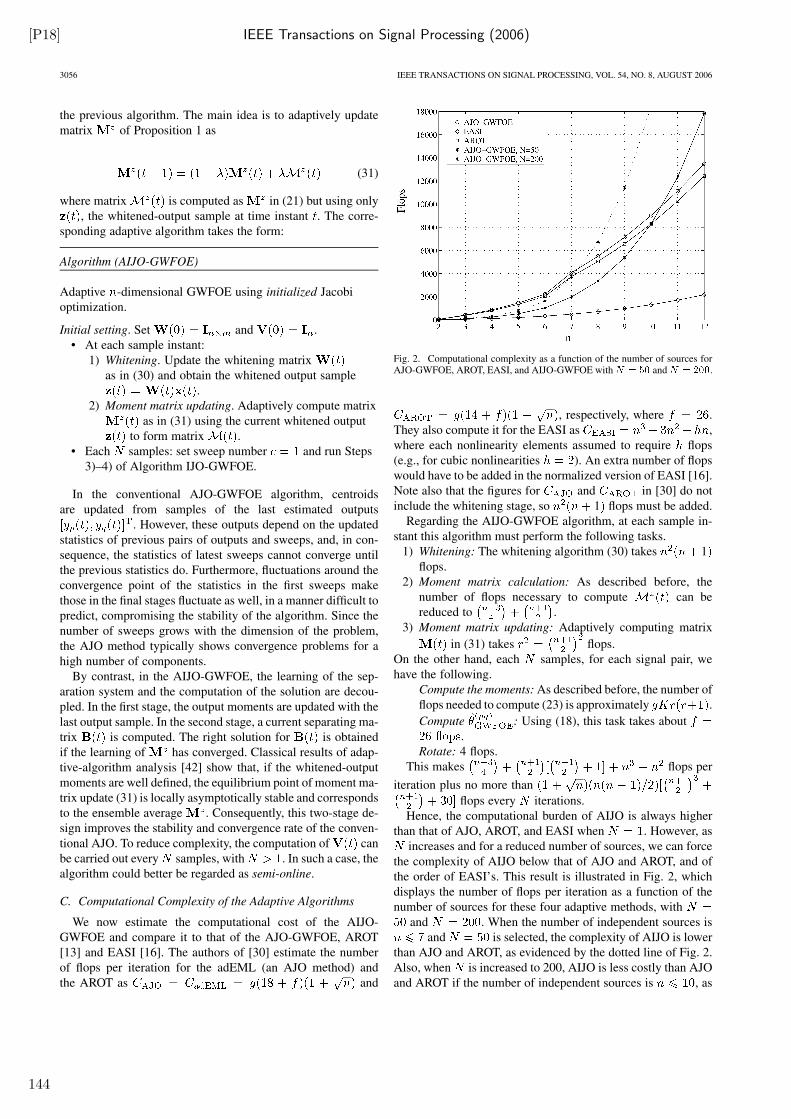
[P18] IEEE Transactions on Signal Processing (2006)
3056 IEEE TRANSACTIONS ON SIGNAL PROCESSING, VOL. 54, NO. 8, AUGUST 2006
the previous algorithm. The main idea is to adaptively update
matrix of Proposition 1 as
(31)
where matrix is computed as in (21) but using only
, the whitened-output sample at time instant . The corre-
sponding adaptive algorithm takes the form:
Algorithm (AIJO-GWFOE)
Adaptive -dimensional GWFOE using initialized Jacobi
optimization.
Initial setting. Set and .
• At each sample instant:
1) Whitening. Update the whitening matrix
as in (30) and obtain the whitened output sample
.
2) Moment matrix updating. Adaptively compute matrix
as in (31) using the current whitened output
to form matrix .
• Each samples: set sweep number and run Steps
3)–4) of Algorithm IJO-GWFOE.
In the conventional AJO-GWFOE algorithm, centroids
are updated from samples of the last estimated outputs
. However, these outputs depend on the updated
statistics of previous pairs of outputs and sweeps, and, in con-
sequence, the statistics of latest sweeps cannot converge until
the previous statistics do. Furthermore, fluctuations around the
convergence point of the statistics in the first sweeps make
those in the final stages fluctuate as well, in a manner difficult to
predict, compromising the stability of the algorithm. Since the
number of sweeps grows with the dimension of the problem,
the AJO method typically shows convergence problems for a
high number of components.
By contrast, in the AIJO-GWFOE, the learning of the sep-
aration system and the computation of the solution are decou-
pled. In the first stage, the output moments are updated with the
last output sample. In the second stage, a current separating ma-
trix is computed. The right solution for is obtained
if the learning of has converged. Classical results of adap-
tive-algorithm analysis [42] show that, if the whitened-output
moments are well defined, the equilibrium point of moment ma-
trix update (31) is locally asymptotically stable and corresponds
to the ensemble average . Consequently, this two-stage de-
sign improves the stability and convergence rate of the conven-
tional AJO. To reduce complexity, the computation of can
be carried out every samples, with . In such a case, the
algorithm could better be regarded as semi-online.
C. Computational Complexity of the Adaptive Algorithms
We now estimate the computational cost of the AIJO-
GWFOE and compare it to that of the AJO-GWFOE, AROT
[13] and EASI [16]. The authors of [30] estimate the number
of flops per iteration for the adEML (an AJO method) and
the AROT as and
Fig. 2. Computational complexity as a function of the number of sources forAJO-GWFOE, AROT, EASI, and AIJO-GWFOE withN = 50 andN = 200.
, respectively, where .
They also compute it for the EASI as ,
where each nonlinearity elements assumed to require flops
(e.g., for cubic nonlinearities ). An extra number of flops
would have to be added in the normalized version of EASI [16].
Note also that the figures for and in [30] do not
include the whitening stage, so 1 flops must be added.
Regarding the AIJO-GWFOE algorithm, at each sample in-
stant this algorithm must perform the following tasks.
1) Whitening: The whitening algorithm (30) takes 1
flops.
2) Moment matrix calculation: As described before, the
number of flops necessary to compute can be
reduced to .
3) Moment matrix updating: Adaptively computing matrix
in (31) takes flops.
On the other hand, each samples, for each signal pair, we
have the following.
Compute the moments: As described before, the number of
flops needed to compute (23) is approximately .
Compute : Using (18), this task takes about
.
Rotate: 4 flops.
This makes flops per
iteration plus no more than
flops every iterations.
Hence, the computational burden of AIJO is always higher
than that of AJO, AROT, and EASI when . However, as
increases and for a reduced number of sources, we can force
the complexity of AIJO below that of AJO and AROT, and of
the order of EASI’s. This result is illustrated in Fig. 2, which
displays the number of flops per iteration as a function of the
number of sources for these four adaptive methods, with
and . When the number of independent sources is
and is selected, the complexity of AIJO is lower
than AJO and AROT, as evidenced by the dotted line of Fig. 2.
Also, when is increased to 200, AIJO is less costly than AJO
and AROT if the number of independent sources is , as
144
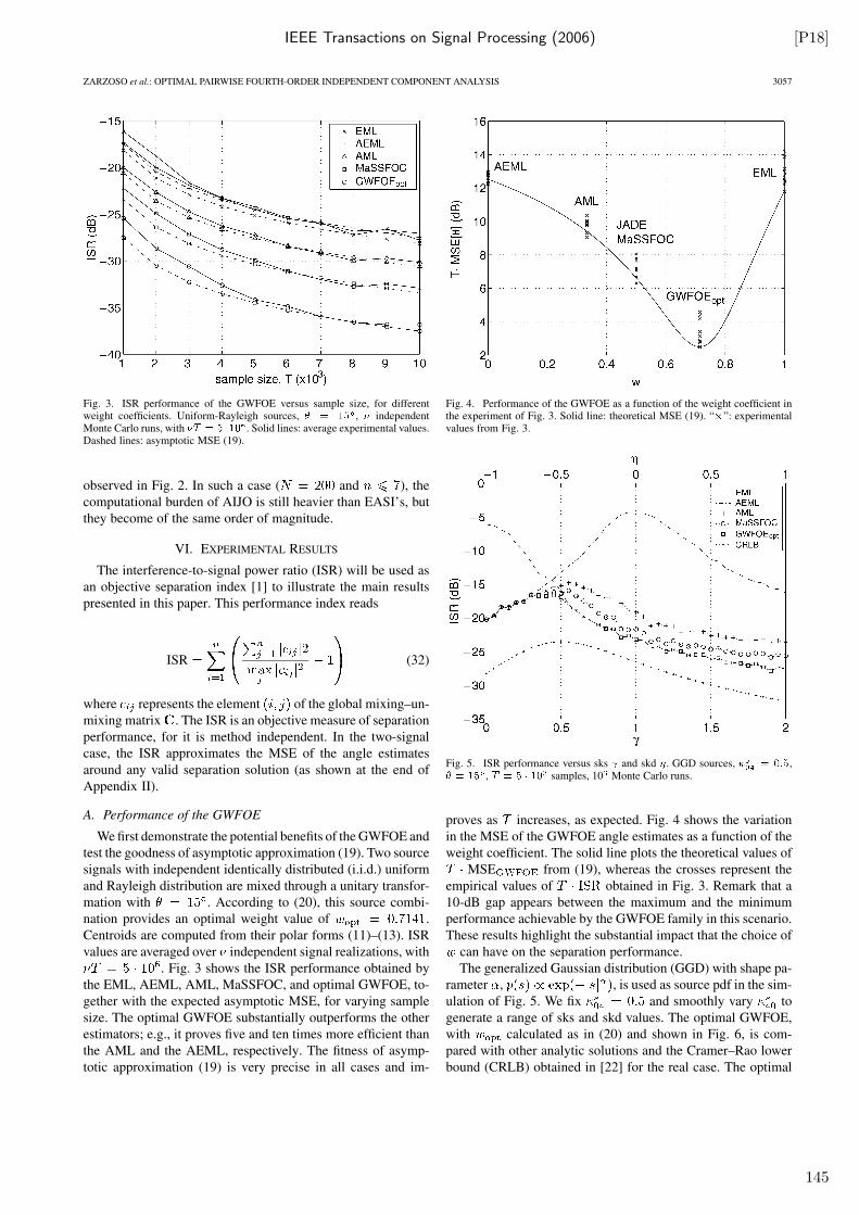
IEEE Transactions on Signal Processing (2006) [P18]
ZARZOSO et al.: OPTIMAL PAIRWISE FOURTH-ORDER INDEPENDENT COMPONENT ANALYSIS 3057
Fig. 3. ISR performance of the GWFOE versus sample size, for differentweight coefficients. Uniform-Rayleigh sources, � = 15 , � independentMonte Carlo runs, with �T = 5 �10 . Solid lines: average experimental values.Dashed lines: asymptotic MSE (19).
observed in Fig. 2. In such a case ( and ), the
computational burden of AIJO is still heavier than EASI’s, but
they become of the same order of magnitude.
VI. EXPERIMENTAL RESULTS
The interference-to-signal power ratio (ISR) will be used as
an objective separation index [1] to illustrate the main results
presented in this paper. This performance index reads
ISR (32)
where represents the element of the global mixing–un-
mixing matrix . The ISR is an objective measure of separation
performance, for it is method independent. In the two-signal
case, the ISR approximates the MSE of the angle estimates
around any valid separation solution (as shown at the end of
Appendix II).
A. Performance of the GWFOE
We first demonstrate the potential benefits of the GWFOE and
test the goodness of asymptotic approximation (19). Two source
signals with independent identically distributed (i.i.d.) uniform
and Rayleigh distribution are mixed through a unitary transfor-
mation with . According to (20), this source combi-
nation provides an optimal weight value of .
Centroids are computed from their polar forms (11)–(13). ISR
values are averaged over independent signal realizations, with
. Fig. 3 shows the ISR performance obtained by
the EML, AEML, AML, MaSSFOC, and optimal GWFOE, to-
gether with the expected asymptotic MSE, for varying sample
size. The optimal GWFOE substantially outperforms the other
estimators; e.g., it proves five and ten times more efficient than
the AML and the AEML, respectively. The fitness of asymp-
totic approximation (19) is very precise in all cases and im-
Fig. 4. Performance of the GWFOE as a function of the weight coefficient inthe experiment of Fig. 3. Solid line: theoretical MSE (19). “�”: experimentalvalues from Fig. 3.
Fig. 5. ISR performance versus sks and skd �. GGD sources, � = 0:5,� = 15 , T = 5 � 10 samples, 10 Monte Carlo runs.
proves as increases, as expected. Fig. 4 shows the variation
in the MSE of the GWFOE angle estimates as a function of the
weight coefficient. The solid line plots the theoretical values of
MSE from (19), whereas the crosses represent the
empirical values of obtained in Fig. 3. Remark that a
10-dB gap appears between the maximum and the minimum
performance achievable by the GWFOE family in this scenario.
These results highlight the substantial impact that the choice of
can have on the separation performance.
The generalized Gaussian distribution (GGD) with shape pa-
rameter , , is used as source pdf in the sim-
ulation of Fig. 5. We fix and smoothly vary to
generate a range of sks and skd values. The optimal GWFOE,
with calculated as in (20) and shown in Fig. 6, is com-
pared with other analytic solutions and the Cramer–Rao lower
bound (CRLB) obtained in [22] for the real case. The optimal
145
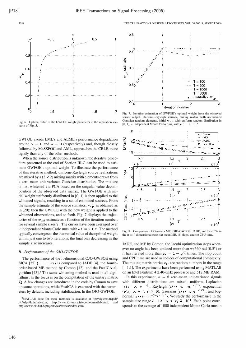
[P18] IEEE Transactions on Signal Processing (2006)
3058 IEEE TRANSACTIONS ON SIGNAL PROCESSING, VOL. 54, NO. 8, AUGUST 2006
Fig. 6. Optimal value of the GWFOE weight parameter in the separation sce-nario of Fig. 5.
GWFOE avoids EML’s and AEML’s performance degradation
around and (respectively) and, though closely
followed by MaSSFOC and AML, approaches the CRLB more
tightly than any of the other methods.
When the source distribution is unknown, the iterative proce-
dure presented at the end of Section III-C can be used to esti-
mate GWFOE’s optimal weight. To illustrate the performance
of this iterative method, uniform-Rayleigh source realizations
are mixed by a (2 2) mixing matrix with elements drawn from
a zero-mean unit-variance Gaussian distribution. The mixture
is first whitened via PCA based on the singular value decom-
position of the observed data matrix. The GWFOE with ini-
tial weight uniformly distributed in [0, 1] is then applied to the
whitened signals, resulting in a set of estimated sources. From
the sample estimate of the source statistics, is obtained as
in (20); then the GWFOE with the new weight is applied to the
whitened observations, and so forth. Fig. 7 displays the trajec-
tories of the estimate as a function of the iteration number,
for several sample sizes . The curves have been averaged over
independent Monte Carlo runs, with . The method
typically converges to the theoretical value of the optimal weight
within just one to two iterations, the final bias decreasing as the
sample size increases.
B. Performance of the OJO-GWFOE
The performance of the -dimensional OJO-GWFOE using
SICA [25] is compared to JADE [4], the fourth-
order-based ME method by Comon [12], and the FastICA al-
gorithm [43].3 The same whitening method is used in all algo-
rithms, as the focus is on the computation of the unitary matrix
. A few changes are introduced in the code by Comon to save
up some operations, while FastICA is executed with the param-
eters by default, including stabilization. In the OJO-GWFOE,
3MATLAB code for these methods is available at ftp://sig.enst.fr/pub/jfc/Algo/Jade/jadeR.m, http://www.i3s.unice.fr/~comon/matlab.html, andhttp://www.cis.hut.fi/projects/ica/fastica/index.shtml.
Fig. 7. Iterative estimation of GWFOE’s optimal weight from the observedsensor output. Uniform-Rayleigh sources, mixing matrix with normalizedGaussian random elements, initial w with uniform random distribution in[0, 1], � independent Monte Carlo runs, with �T = 5 � 10 .
Fig. 8. Comparison of Comon’s ME, OJO-GWFOE, JADE, and FastICA inthe n = 6 dimensional case: (a) mean ISR, (b) flops, and (c) CPU time.
JADE, and ME by Comon, the Jacobi optimization stops when-
ever no angle has been updated more than 360 rad (0.5 ) or
it has iterated more than times. The flop count
and CPU time are used as indices of computational complexity.
The mixing matrix entries are random numbers in the range
[ 1,1]. The experiments have been performed using MATLAB
on an Intel Pentium 4 2.40-GHz processor and 512 MB RAM.
In this experiment, zero-mean unit-variance signals
with different distributions are mixed: uniform, Laplacian
, Rayleigh , exponential
( , ), Gaussian , and log-
normal . We study the performance in the
sample-size range . Each point corre-
sponds to the average of 1000 independent Monte Carlo runs in
146
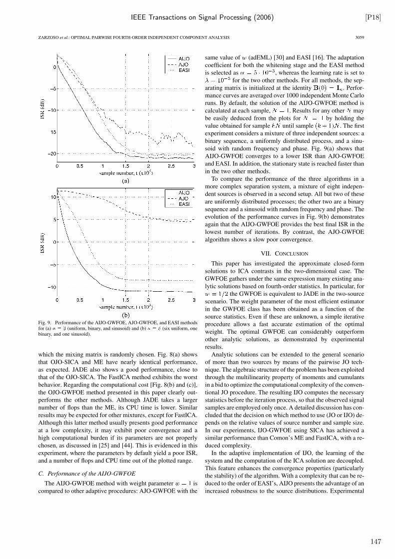
IEEE Transactions on Signal Processing (2006) [P18]
ZARZOSO et al.: OPTIMAL PAIRWISE FOURTH-ORDER INDEPENDENT COMPONENT ANALYSIS 3059
Fig. 9. Performance of the AIJO-GWFOE, AJO-GWFOE, and EASI methodsfor (a) n = 3 (uniform, binary, and sinusoid) and (b) n = 8 (six uniform, onebinary, and one sinusoid).
which the mixing matrix is randomly chosen. Fig. 8(a) shows
that OJO-SICA and ME have nearly identical performance,
as expected. JADE also shows a good performance, close to
that of the OJO-SICA. The FastICA method exhibits the worst
behavior. Regarding the computational cost [Fig. 8(b) and (c)],
the OJO-GWFOE method presented in this paper clearly out-
performs the other methods. Although JADE takes a larger
number of flops than the ME, its CPU time is lower. Similar
results may be expected for other mixtures, except for FastICA.
Although this latter method usually presents good performance
at a low complexity, it may exhibit poor convergence and a
high computational burden if its parameters are not properly
chosen, as discussed in [25] and [44]. This is evidenced in this
experiment, where the parameters by default yield a poor ISR,
and a number of flops and CPU time out of the plotted range.
C. Performance of the AIJO-GWFOE
The AIJO-GWFOE method with weight parameter is
compared to other adaptive procedures: AJO-GWFOE with the
same value of (adEML) [30] and EASI [16]. The adaptation
coefficient for both the whitening stage and the EASI method
is selected as , whereas the learning rate is set to
for the two other methods. For all methods, the sep-
arating matrix is initialized at the identity . Perfor-
mance curves are averaged over 1000 independent Monte Carlo
runs. By default, the solution of the AIJO-GWFOE method is
calculated at each sample, . Results for any other may
be easily deduced from the plots for by holding the
value obtained for sample until sample 1 . The first
experiment considers a mixture of three independent sources: a
binary sequence, a uniformly distributed process, and a sinu-
soid with random frequency and phase. Fig. 9(a) shows that
AIJO-GWFOE converges to a lower ISR than AJO-GWFOE
and EASI. In addition, the stationary state is reached faster than
in the two other methods.
To compare the performance of the three algorithms in a
more complex separation system, a mixture of eight indepen-
dent sources is observed in a second setup. All but two of these
are uniformly distributed processes; the other two are a binary
sequence and a sinusoid with random frequency and phase. The
evolution of the performance curves in Fig. 9(b) demonstrates
again that the AIJO-GWFOE provides the best final ISR in the
lowest number of iterations. By contrast, the AJO-GWFOE
algorithm shows a slow poor convergence.
VII. CONCLUSION
This paper has investigated the approximate closed-form
solutions to ICA contrasts in the two-dimensional case. The
GWFOE gathers under the same expression many existing ana-
lytic solutions based on fourth-order statistics. In particular, for
the GWFOE is equivalent to JADE in the two-source
scenario. The weight parameter of the most efficient estimator
in the GWFOE class has been obtained as a function of the
source statistics. Even if these are unknown, a simple iterative
procedure allows a fast accurate estimation of the optimal
weight. The optimal GWFOE can considerably outperform
other analytic solutions, as demonstrated by experimental
results.
Analytic solutions can be extended to the general scenario
of more than two sources by means of the pairwise JO tech-
nique. The algebraic structure of the problem has been exploited
through the multilinearity property of moments and cumulants
in a bid to optimize the computational complexity of the conven-
tional JO procedure. The resulting IJO computes the necessary
statistics before the iteration process, so that the observed signal
samples are employed only once. A detailed discussion has con-
cluded that the decision on which method to use (JO or IJO) de-
pends on the relative values of source number and sample size.
In our experiments, IJO-GWFOE using SICA has achieved a
similar performance than Comon’s ME and FastICA, with a re-
duced complexity.
In the adaptive implementation of IJO, the learning of the
system and the computation of the ICA solution are decoupled.
This feature enhances the convergence properties (particularly
the stability) of the algorithm. With a complexity that can be re-
duced to the order of EASI’s, AIJO presents the advantage of an
increased robustness to the source distributions. Experimental
147
[P18] IEEE Transactions on Signal Processing (2006)
3060 IEEE TRANSACTIONS ON SIGNAL PROCESSING, VOL. 54, NO. 8, AUGUST 2006
results have shown that the convergence of AIJO is faster than
EASI’s and adEML’s (indeed, its ISR evolution is always below
that of the other methods), reaching the best final performance
for any number of sources and different source distributions.
Further work includes the development of GWFOE’s optimal
weight coefficient as a function of the array-output statistics in
order to enable a fully blind operation and the incorporation of
the optimal GWFOE in the multidimensional JO-based algo-
rithms. The separation performance and convergence character-
istics in the presence of additive noise and interference needs to
be explored, for both offline and online implementations. Ex-
tensions to statistics of orders other than four also deserves to
be investigated. The use of characteristic functions [45] might
prove helpful in that line of inquiry.
APPENDIX I
EQUIVALENCE BETWEEN GWFOE
WITH AND JADE FOR
The maximization of contrast function (8) is associated with
the joint approximate diagonalization of the so-called parallel
set of cumulant matrices , whose entries are defined as
[4]. In this Appendix we prove that, in the
two-source scenario, the solution provided by the conventional
version of JADE based on the parallel set provides the GWFOE
solution (18) with .
For , the cumulant matrices of the parallel have the
form
(33)
As shown in [4, Sec. 8.1], the joint diagonalization criterion is
equivalent to maximizing , where
are the diagonal elements of , matrix denoting the
sought Givens rotation of angle in (9). Following [4, Sec.
8.1], the criterion can be expressed as , with
and , ,
, where and represent the
diagonal and off-diagonal entries, respectively, of . Hence,
is the dominant eigenvector of the symmetric matrix
, whose elements are given by
(34)
(35)
(36)
Now, to find the dominant eigenvector of , we take into ac-
count that its eigenvector matrix must be of the form
, with . Also, matrix must
diagonalize . Thus, we force a diagonal structure for matrix
, which leads to two constraints on the resulting off-di-
agonal elements reducing to
. We thus obtain .
By means of some straightforward algebraic manipulations on
(34)-(36), this solution is readily shown to coincide with the
GWFOE solution (18) for .
APPENDIX II
ASYMPTOTIC ANALYSIS OF THE GWFOE
In this Appendix, we analyze the asymptotic performance of
the GWFOE estimator (18) for i.i.d. sources. Our main objec-
tive is an analytic expression for its large-sample MSE. The es-
timator reads
(37)
where
(38)
are the sample estimates of centroids (11)-(13). Note that
(39)
with
(40)
Hence, , where
. By virtue of the law of large numbers, the combined
source centroid is a consistent estimator of a positive real
number
(41)
It follows that the GWFOE is also consistent and, in particular
(42)
Now, MSE MSE . At large , and
since the estimator is consistent, will be close to zero; thus
. Also, since is small and, according to
(41), typically , the variations of will
148
IEEE Transactions on Signal Processing (2006) [P18]
ZARZOSO et al.: OPTIMAL PAIRWISE FOURTH-ORDER INDEPENDENT COMPONENT ANALYSIS 3061
be mainly due to fluctuations in the imaginary part of . As a
result, we can approximate
(43)
Being real valued, does not alter the argument of . More-
over, on the grounds of consistency, it can be further assumed
that . Then
(44)
(45)
with
(46)
(47)
where, to ease the notation, we have written ,
. The denominator of (43) can be easily obtained by in-
voking the consistency of the real part of in (41). The calcula-
tion of the numerator is slightly more involved. From (45)–(47),
we have (48) as shown at the bottom of the page. Taking into ac-
count the i.i.d. assumption, the most significant parts of terms
A–C turn out to be
(49)
Gathering and rearranging terms, we arrive at
(50)
Finally, the combination of (41), (43), and (50) yields the
asymptotic MSE of the GWFOE shown in (19).
The derivation of is simplified with the substitutions
and , in which case
MSE can be written as
MSE (51)
This function of becomes constant if , i.e.,
. Performance then reduces to that of the EML (when
) or AEML (when ) estimators for any . Otherwise, in
the interval of interest, , we have that
. The derivative of (51) then cancels at
(52)
Some tedious but straightforward algebraic simplifications then
show that the above expression reduces to (20). In addition, it
is simple to check that MSE , so that
defines a minimum.
To conclude this asymptotic study, it is interesting to realize
the connection between and the ISR performance pa-
rameter (32). Assuming a unitary mixture in the two-signal case,
the global transformation is a rotation
of angle . Any angle estimate of the form
, with small and integer , provides a valid sep-
aration solution up to the inherent separation indeterminacies
mentioned in Section II. This angle estimate produces ISR
. As a result, in the vicinity of a valid separation
solution, the average ISR approximates MSE without the po-
tential bias introduced by the admissible -rad rotations.
(48)
149
[P18] IEEE Transactions on Signal Processing (2006)
3062 IEEE TRANSACTIONS ON SIGNAL PROCESSING, VOL. 54, NO. 8, AUGUST 2006
APPENDIX III
PROOF OF PROPOSITION 1
Expression (23) is a particular case of
(53)
Let us denote the , , symmetric matrix
containing the fourth-order moments . Moment
is stored in the entry , where is given
by (22). In order to exploit the symmetry of the whitened-output
moment tensor, only the moments with and are
kept. The computation of (53) can be expressed as a quadratic
form involving matrix and a pair of column vectors related
to matrix
(54)
To guarantee the equivalence between this quadratic form and
(53), vectors and must be constructed by arranging the
entries of in accordance with the structure of
(55)
where indexes and are related through (22).
ACKNOWLEDGMENT
V. Zarzoso wishes to thank P. Comon for his kind hospitality.
REFERENCES
[1] V. Zarzoso and A. K. Nandi, “Blind source separation,” in Blind Esti-mation Using Higher-Order Statistics, A. K. Nandi, Ed. Boston, MA:Kluwer Academic, 1999, ch. 4, pp. 167–252.
[2] A. Hyvärinen, J. Karhunen, and E. Oja, Independent Component Anal-ysis. New York: Wiley, 2001.
[3] A. Cichocki and S. Amari, Adaptive Blind Signal and Image Pro-cessing. Chichester, U.K.: Wiley, 2002.
[4] J. F. Cardoso and A. Souloumiac, “Blind beamforming fornon-Gaussian signals,” Proc. Inst. Elect. Eng. F, vol. 140, no. 6,pp. 362–370, Dec. 1993.
[5] J. F. Cardoso, “Blind signal separation: Statistical principles,” Proc.IEEE, vol. 86, pp. 2009–2025, Oct. 1998.
[6] A. Caamaño-Fernandez, R. Boloix-Tortosa, J. Ramos, and J. J. Murillo-Fuentes, “Hybrid higher-order statistics learning in multiuser detec-tion,” IEEE Trans. Syst., Man, Cybern. C, Appl. Rev., vol. 34, no. 4,pp. 417–424, Nov. 2004.
[7] S. Makeig, T.-P. Jung, D. Ghahremani, A. Bell, and T. Sejnowski,“Blind separation of auditory event-related brain responses intoindependent components,” in Proc. Nat. Acad. Sci., 1997, pp.10979–10984.
[8] L. De Lathauwer, B. De Moor, and J. Vandewalle, “Fetal electrocar-diogram extraction by blind source subspace separation,” IEEE Trans.Biomed. Eng. (Special Topic Section Advances in Statistical SignalProcessing for Medicine), vol. 47, pp. 567–572, May 2000.
[9] V. Zarzoso and A. K. Nandi, “Noninvasive fetal electrocardiogram ex-traction: Blind separation versus adaptive noise cancellation,” IEEETrans. Biomed. Eng., vol. 48, pp. 12–18, Jan. 2001.
[10] J. Murillo-Fuentes, H. Molina-Bulla, and F. González-Serrano, “Inde-pendent component analysis applied to digital image watermarking,”in Proc. ICASSP’01, Salt Lake City, UT, May 2001, vol. III, pp.1997–2000.
[11] T. Lee, M. Lewicki, and T. Sejnowski, “Unsupervised classificationwith non-Gaussian mixture models using ICA,” in Advances in NeuralInformation Processing Systems. Cambridge, MA: MIT Press, 1999,vol. 11, pp. 58–64.
[12] P. Comon, “Independent component analysis, a new concept?,” SignalProcess., vol. 36, no. 3, pp. 287–314, Apr. 1994.
[13] ——, “Separation of stochastic processes,” in Proc. Workshop Higher-Order Spectral Anal., Vail, CO, Jun. 28–30, 1989, pp. 174–179.
[14] V. Zarzoso, “Closed-form higher-order estimators for blind separationof independent source signals in instantaneous linear mixtures,” Ph.D.dissertation, Univ. of Liverpool, Liverpool, U.K., Oct. 1999.
[15] V. Zarzoso and A. K. Nandi, “Unified formulation of closed-form es-timators for blind source separation in real instantaneous linear mix-tures,” in Proc. ICASSP’00, Istanbul, Turkey, Jun. 5–9, 2000, vol. V,pp. 3160–3163.
[16] J. F. Cardoso and B. H. Laheld, “Equivariant adaptive source separa-tion,” IEEE Trans. Signal Process., vol. 44, no. 12, pp. 3017–3030,Dec. 1996.
[17] F. Harroy and J.-L. Lacoume, “Maximum likelihood estimators andCramer-Rao bounds in source separation,” Signal Process., vol. 55, no.2, pp. 167–177, 1996.
[18] V. Zarzoso and A. K. Nandi, “Blind separation of independent sourcesfor virtually any source probability density function,” IEEE Trans.Signal Process., vol. 47, no. 9, pp. 2419–2432, Sep. 1999.
[19] V. Zarzoso, A. K. Nandi, F. Herrmann, and J. Millet-Roig, “Combinedestimation scheme for blind source separation with arbitrary sourcePDFs,” Electron. Lett., vol. 37, no. 2, pp. 132–133, Jan. 2001.
[20] E. Moreau and O. Macchi, “Higher order contrast for self-adaptivesource separation,” Int. J. Adapt. Contr. Signal Process., vol. 10, no.1, pp. 19–46, Jan 1996.
[21] P. Comon and E. Moreau, “Improved contrast dedicated to blind sep-aration in communications,” in Proc. ICASSP’97, Munich, Germany,1997, vol. V, pp. 3453–3456.
[22] M. Ghogho, A. Swami, and T. Durrani, “Approximate maximum like-lihood blind source separation with arbitrary source pdfs,” in Proc.SSAP’00, Pocono Manor, PA, Aug. 14–16, 2000, pp. 368–372.
[23] M. Gaeta and J.-L. Lacoume, “Source separation without a prioriknowledge: the maximum likelihood solution,” in Proc. EUSIPCO’90,Barcelona, Spain, 1990, vol. V, pp. 621–624.
[24] F. Herrmann and A. Nandi, “Blind separation of linear instantaneousmixture using close forms estimators,” Signal Process., vol. 81, no. 7,pp. 1537–1556, Jul. 2001.
[25] J. J. Murillo-Fuentes and F. J. González-Serrano, “A sinusoidalcontrast function for the blind separation of statistically independentsources,” IEEE Trans. Signal Process., vol. 52, pp. 3459–3463, Dec.2004.
[26] T. Blaschke and L. Wiskott, “CuBICA: Independent componentanalysis by simultaneous third- and fourth-order cumulant diagonal-ization,” IEEE Trans. Signal Process., vol. 52, pp. 1250–1256, May2004.
[27] G. H. Golub and C. F. Van Loan, Matrix Computations, 3rd ed. Bal-timore, MD: Johns Hopkins Univ. Press, 1996.
[28] A. Bunse-Gerstner, R. Byers, and V. Mehrmann, “Numerical methodsfor simultaneous diagonalization,” SIAM J. Matrix Anal. Applicat., vol.14, no. 4, pp. 927–949, 1993.
[29] P. Comon, “Remarques sur la diagonalisation tensorielle par laméthode de Jacobi,” in Proc. XIVème Colloque GRETSI, Juan-les-Pins,France, Sep. 13–16, 1993, pp. 125–128.
[30] V. Zarzoso and A. K. Nandi, “Adaptive blind source separation forvirtually any source probability density function,” IEEE Trans. SignalProcess., vol. 48, pp. 477–488, Feb. 2000.
[31] I. J. Clarke, “Direct exploitation of non-Gaussianity as a discriminant,”in Proc. EUSIPCO’98, Rhodes, Greece, Sept. 8–11, 1998, vol. IV, pp.2057–2060.
[32] V. Zarzoso, F. Herrmann, and A. K. Nandi, “Weighted closed-formestimators for blind source separation,” in Proc. SSP-2001, 11th IEEEWorkshop Statist. Signal Process., Singapore, Aug. 6–8, 2001, pp.456–459.
[33] J. Murillo-Fuentes and F. González-Serrano, “Independent componentanalysis with sinusoidal fourth-order contrast,” in Proc. ICASSP’01,Salt Lake City, UT, May 2001, vol. V, pp. 2785–2788.
[34] J. J. Murillo-Fuentes, R. Boloix-Tortosa, and F. J. González-Serrano,“Initialized Jacobi optimization in independent component analysis,”in Proc. ICA-2003 4th Int. Symp. Indep. Comp. Anal. Blind Signal Sep-arat., Nara, Japan, Apr. 1–4, 2003.
[35] ——, “Adaptive initialized Jacobi optimization in independent com-ponent analysis,” in Proc. ICA-2003 4th Int. Symp. Indep. Comp. Anal.Blind Signal Separat., Nara, Japan, Apr. 1–4, 2003.
[36] J. J. Murillo-Fuentes, R. Boloix-Tortosa, S. Hornillo-Mellado, and V.Zarzoso, “Independent component analysis based on marginal entropyapproximations,” in Proc. ISIAC’04 5th Int. Symp. Intell. Autom.Contr., Seville, Spain, Jun. 28–Jul. 1, 2004.
150
IEEE Transactions on Signal Processing (2006) [P18]
ZARZOSO et al.: OPTIMAL PAIRWISE FOURTH-ORDER INDEPENDENT COMPONENT ANALYSIS 3063
[37] A. Stuart and J. K. Ord, Kendall’s Advanced Theory of Statistics, 6thed. London, U.K.: Edward Arnold, 1994, vol. I.
[38] P. McCullagh, Tensor Methods in Statistics, ser. Monographs on Statis-tics and Applied Probability. London, U.K.: Chapman & Hall, 1987.
[39] F. J. Theis, “A new concept for separability problems in blind sourceseparation,” Neural Comput., vol. 16, pp. 1827–1850, 2004.
[40] A. Yeredor, “Non-orthogonal joint diagonalization in the least-squaressense with application in blind source separation,” IEEE Trans. SignalProcess., vol. 50, pp. 1545–1553, Jul. 2002.
[41] J. F. Cardoso, “High-order contrasts for independent component anal-ysis,” Neural Comput., vol. 11, no. 1, pp. 157–192, Jan 1999.
[42] A. Benveniste, M. Métivier, and P. Priouret, Adaptive Algorithms andStochastic Approximations. Berlin, Germany: Springer-Verlag, 1990.
[43] A. Hyvärinen, “Fast and robust fixed-point algorithms for independentcomponent analysis,” IEEE Trans. Neural Netw., vol. 10, no. 3, pp.626–634, 1999.
[44] X. Giannakopoulos, J. Karhunen, and E. Oja, “An experimentalcomparison of neural ICA algorithms,” in Proc. ICANN’98, Skovde,Sweden, Sep 1998, pp. 651–656.
[45] J. Eriksson and V. Koivunen, “Characteristics-function based indepen-dent component analysis,” Signal Process., vol. 83, pp. 2195–2208,2003.
Vicente Zarzoso (S’94–M’03) was born in Valencia,Spain, in 1973. He graduated (with highest distinc-tion) in telecommunications engineering from theUniversidad Politécnica de Valencia in 1996. Thebeginning of his Ph.D. studies were partly fundedby a scholarship from the University of Strathclyde,Glasgow, U.K., and the Defence Evaluation andResearch Agency (DERA) of the United Kingdom.He received the Ph.D. degree from the University ofLiverpool, U.K., in 1999.
He spent five years with the University of Liver-pool under a Research Fellowship from the Royal Academy of Engineering,U.K. Since September 2005, he has been a Lecturer with the Université de Nice- Sophia Antipolis and a Researcher with the Laboratoire d’Informatique, Sig-naux et Systèmes de Sophia Antipolis, France. His research interests includeblind statistical signal and array processing and its application to biomedicalproblems and communications.
Juan José Murillo-Fuentes (M’99) was born inSevilla, Spain, in 1973. He received the telecommu-nications engineering degree from the Universidad deSevilla in 1996 and the Ph.D. degree in telecommu-nication engineering in 2001 from the UniversidadCarlos III de Madrid, Spain.
He is currently an Associate Professor in the De-partment of Signal Theory and Communication, Uni-versidad de Sevilla. His research interests lie in al-gorithm development for blind source separation andother signal-processing tools and their application to
digital communications and image processing.
Rafael Boloix-Tortosa received the M.Eng. degreein telecommunications engineering and the Ph.D. de-gree from the Universidad de Sevilla, Spain, in 2000and 2005, respectively.
He joined the School of Engineering there in1999 as Research Assistant with the Department ofElectronic Engineering. Currently, he is an AssistantProfessor with the Department of Signal Theoryand Communications. His research interests includeblind source separation and higher order statisticsand their application to digital communications.
Asoke K. Nandi (SM’96) received the Ph.D. degreefrom Trinity College, University of Cambridge, Cam-bridge, U.K., in 1979.
He held research positions with Rutherford Ap-pleton Laboratory, U.K.; the European Organisationfor Nuclear Research, Switzerland; the Departmentof Physics, Queen Mary College, London, U.K.; andthe Department of Nuclear Physics, Oxford, U.K.In 1987, he joined Imperial College London as theSolartron Lecturer in the Signal Processing Sectionof the Electrical Engineering Department. In 1991,
he jointed the Signal Processing Division of the Electronic and ElectricalEngineering Department, University of Strathclyde, Glasgow, U.K., as a SeniorLecturer; subsequently, he became a Reader in 1995 and a Professor in 1998.In 1999, he joined the University of Liverpool, Liverpool, U.K., as the DavidJardine Chair of Signal Processing in the Department of Electrical Engineeringand Electronics. In 1983, he was a member of the UA1 team at CERN that dis-covered the three fundamental particles known asW ,W and Z , providingthe evidence for the unification of the electromagnetic and weak forces, whichwas recognized by the Nobel Committee for Physics in 1984. Currently, heis Head of the Signal Processing and Communications Research Group, withinterests in the areas of nonlinear systems, non-Gaussian signal processing, andcommunications research. With his group he has been carrying out research inblind source separation, blind deconvolution, machine condition monitoring,signal modelling, system identification, communication signal processing,time-delay estimation, biomedical signals, underwater sonar, and applicationsand development of machine learning. He has authored or coauthored morethan 130 journal papers and more than 300 technical publications, includingAutomatic Modulation Recognition of Communications Signals (Boston, MA:Kluwer Academic, 1996) and Blind Estimation Using Higher-Order Statistics
(Boston, MA: Kluwer Academic, 1999).Prof. Nandi is a Fellow of the Cambridge Philosophical Society, the Institu-
tion of Engineering and Technology, U.K., the Institute of Mathematics and itsApplications, the Institute of Physics, and the Royal Society of Arts. He receivedthe Mounbatten Premium Division Award from the Electronics and Communi-cations Division, the Institution of Electrical Engineers, in 1998 and the WaterArbitration Prize from the Institution of Mechanical Engineers, U.K., in 1999.
151

IEEE Transactions on Signal Processing (2005) [P19]
IEEE TRANSACTIONS ON SIGNAL PROCESSING, VOL. 53, NO. 11, NOVEMBER 2005 4363
Blind and Semi-Blind Equalization Based on theConstant Power Criterion
Vicente Zarzoso, Member, IEEE, and Pierre Comon, Senior Member, IEEE
Abstract—This paper focuses on the constant power (CP) crite-rion for blind linear equalization of digital communication chan-nels. This recently proposed criterion is specially designed for theextraction of -ary phase shift keying ( -PSK) signals using finiteimpulse response equalizers. When zero-forcing equalizers exist,the CP cost function accepts exact analytic solutions that are un-affected by undesired local extrema and spare costly iterative op-timization. A subspace-based method exploiting the Toeplitz-likestructure of the solution space is put forward to recover the min-imum-length equalizer impulse response from the overestimated-length solutions. The proposed method is more robust to the rel-ative weights of the minimum-length equalizer taps than existingtechniques. In less ideal scenarios where the analytic solutions areonly approximate minimizers of the criterion, a gradient-descentalgorithm is proposed to minimize the cost function. To reduce thedetrimental effects of suboptimal equilibria and accelerate conver-gence, the iterative algorithm is initialized with the approximateclosed-form solution, and an optimal step size is incorporated intoits updating rule. This optimal step size, which globally minimizesthe cost function along the search direction, can be computed al-gebraically. A semi-blind implementation, which is useful whentraining data are available, further reduces the impact of unde-sired local extrema and enhances the convergence characteristics(particularly the robustness to the equalizer initialization) of theiterative algorithm from just a few pilot symbols. All these benefi-cial features are demonstrated with an experimental study of theproposed CP-based methods in a variety of channels and simula-tion conditions.
Index Terms—Analytical constant power algorithm, blind equal-ization, closed-form solutions, iterative algorithms, optimal stepsize, semi-blind equalization, subspace methods, tensor algebra.
I. INTRODUCTION
A. Background
In digital communications, transmission effects such as mul-
tipath propagation and limited bandwidth produce linear dis-
tortion in the emitted signal, causing intersymbol interference
(ISI) at the receive sensor output. To enable the recovery of the
input symbols, channel equalization aims to compensate these
distorting effects [1]. Since the late 1970s, the drawbacks of
training-based methods [1], [2] have aroused considerable re-
search interest in the so-called blind equalization techniques,
Manuscript submitted July 23, 2004; revised January 10, 2005. This workwas supported by a Research Fellowship awarded to V. Zarzoso by the RoyalAcademy of Engineering of the U.K. The associate editor coordinating the re-view of this manuscript and approving it for publication was Dr. Markus Rupp.
V. Zarzoso was with the Department of Electrical Engineering and Elec-tronics, The University of Liverpool, Liverpool L69 3GJ U.K. He is now withthe Laboratoire I3S, Les Algorithmes, 06903 Sophia Antipolis, France (e-mail:[email protected]).
P. Comon is with the Laboratoire I3S, Les Algorithmes, 06903 Sophia An-tipolis, France (e-mail: [email protected]).
Digital Object Identifier 10.1109/TSP.2005.857051
which spare the use of bandwidth-consuming pilot sequences
and prove especially attractive in broadcast and noncooperative
scenarios. In the fundamental single-input single-output (SISO)
scenario, nonminimum phase (NMP) channels cannot be blindly
identified using only second-order statistics (SOS); hence, the
need for blind SISO equalizers to rely (explicitly or not) on
higher-order statistics (HOS) [3]–[5]. Most blind methods are
essentially property restoral techniques: The equalizer filter is
updated to produce an output signal that recovers an a priori
known property of the input signal, such as the finite alphabet
or constant modulus of its data symbols.
The constant modulus (CM) criterion [4], [5]—which
can be considered as a particular member of the more gen-
eral family of Godard’s methods [4]—is arguably the most
widespread blind equalization principle. Although Godard’s
methods were proven to be globally convergent in the combined
channel-equalizer parameter space, they were later shown to
generally present suboptimal equilibria in the equalizer pa-
rameter space [6], [7]. Suboptimal equilibria are stable local
extrema associated with filter tap settings that cannot suffi-
ciently open the equalizer output signal eye pattern so that
the detecting device is then unable to extract the transmitted
symbols with a reasonably low probability of error.1 This
shortcoming renders the performance of gradient-based imple-
mentations of Godard’s criterion very dependent on the initial
value of the equalizer impulse response. As discussed in [6]
and [7], the misconvergence problems of iterative blind SISO
equalization methods calls for the design of suitable initial-
ization schemes and, perhaps, additional strategies to keep the
equalizer tap trajectories away from undesired local equilibria.
Analytic methods can be used as judicious initializations for
iterative equalizers. A closed-form CM solution is obtained in
[8], where the CM criterion is posed as a nonlinear least squares
(LS) problem. Through an appropriate mapping of the equal-
izer parameter space, the nonlinear setting is transformed into a
linear LS problem subject to a constraint on the solution struc-
ture. Recovering the right structure of the solution space is par-
ticularly important when multiple zero-forcing (ZF) solutions
exist; for instance, in all-pole channels with overparameterized
finite impulse response (FIR) equalizers, different ZF equal-
ization delays are possible. From a matrix algebra perspective,
imposing this structure can be considered as a matrix diago-
nalization problem, in which the matrix performing the diag-
onalization of the unstructured solution matrix is composed of
1Suboptimal equilibria are sometimes referred to as spurious equilibria inthe literature. However, as will be illustrated in Section VII, such solutionsoften lie near Wiener equalizers, which questions the appropriateness of theterm “spurious.”
1053-587X/$20.00 © 2005 IEEE
153
[P19] IEEE Transactions on Signal Processing (2005)
4364 IEEE TRANSACTIONS ON SIGNAL PROCESSING, VOL. 53, NO. 11, NOVEMBER 2005
the equalizers’ tap vectors. After obtaining a nonstructured LS
solution via pseudoinversion, the minimum-length equalizer is
extracted by a subspace-based approach or two other simpler
structuring procedures. Least mean squares (LMS) and recur-
sive least squares (RLS) algorithms are also designed to solve
the linear LS problem; hence, they still require structuring after
convergence. Alternatively, the linearized LMS algorithm can
be modified to partially impose the appropriate structure. How-
ever, the introduction of nonlinear constraints precludes the for-
mulation of a closed-form solution.
The blind equalization method of [8] is strongly related to
the analytical CM algorithm (ACMA) of [9] for blind source
separation, which is a related but somewhat different problem.
ACMA provides, in the noiseless case, exact closed-form solu-
tions for the spatial filters that extract the source signals from
their observed instantaneous linear mixtures. Interestingly, re-
covering the separating spatial filters from a basis of the solu-
tion space turns out to be tantamount to the joint diagonalization
of the corresponding matrices. This joint diagonalization can be
achieved through the generalized Schur decomposition [10] of
several (more than two) matrices, for which convergence proof
has yet to be found. Whether for source separation or for equal-
ization, ACMA requires special modifications to handle input
signals with a one-dimensional (i.e., binary) alphabet [8], [9],
[11]. These modifications give rise to the so-called real ACMA
(RACMA) method [11].
Multichannel (fractionally spaced) implementations are also
able to avoid some of the deficiencies of SISO equalizers. In the
first place, single-input multiple-output (SIMO) channels can
be blindly identified using only SOS, regardless of their phase
characteristics. In addition, FIR SIMO channels can be per-
fectly equalized, in the absence of noise, by FIR filters. Seminal
methods are presented in [12]–[14]. Godard SIMO equalizers do
not present suboptimal minima for noiseless channels satisfying
length and zero conditions [15]. All minima are global and co-
incide with the minimum mean square error (MMSE) solutions
associated with the attainable equalization delays. In the pres-
ence of noise, however, some of the minima become local, their
respective equalizers providing different levels of MSE perfor-
mance [16]. Depending on its performance, a local minimum
may also become suboptimal. Hence, the need for techniques
to avoid local extrema remains pertinent in the multichannel
context. In certain practical scenarios, it may not be possible
to achieve the degree of spatio-temporal diversity required by a
SIMO formulation, due to lack of excess bandwidth or to hard-
ware constraints limiting the number of receiving sensors (e.g.,
antennas in a mobile handset). This paper is mainly concerned
with, but not restricted to, the basic SISO model.
B. Contribution and Outline
The present contribution studies a novel criterion for the blind
equalization of digital channels excited by input signals with
-ary phase shift keying ( -PSK) modulations for arbitrary
. The criterion can be considered as a modification on the orig-
inal Godard’s family of blind equalizers, with a power value
matched to the signal constellation, hence, the suitable name of
constant power (CP) criterion. It is shown that if multiple ZF
solutions exist—e.g., when the noiseless SISO channel follows
a pure autoregressive (AR) model and the FIR equalizer filter
is of sufficient length—the criterion accepts, much in ACMA’s
fashion, an exact solution that can be computed analytically,
i.e., without iterative optimization. The minimum-length equal-
izer impulse response can then be obtained from a joint decom-
position of th-order tensors: the so-called rank-1 combination
problem [17]. Since no effective tool has yet been developed
for this task, an approximate solution is proposed in the form of
a subspace-based method, which exploits the particular struc-
ture of the tensors associated with satisfactory equalization so-
lutions. As opposed to [8], the subspace method proposed herein
takes into account a whole basis of the solution space. This use
of extra information is expected to increase the algorithm’s ro-
bustness to the minimum-length equalizer structure. In addition,
our closed-form blind equalization method naturally deals with
binary inputs (e.g., BPSK, MSK) without further modification.
In additive noise or less ideal channel-equalizer conditions,
the CP cost function can be minimized through a gradient-de-
scent algorithm. The impact of undesired extrema are consid-
erably reduced by initializing the algorithm with the approxi-
mate closed-form solution. In computationally limited systems,
however, simple initializations may be preferred to more so-
phisticated, and thus more complex, alternatives. Whatever the
option, the value of the step size (adaptation coefficient) that
globally minimizes the cost function along the search direction
can be computed analytically at each iteration. This optimal
step size provides remarkable benefits in convergence speed
and avoidance of local extrema, even with conventional (e.g.,
center-tap) initializations. The CP criterion is easily modified to
operate in semi-blind mode, which is relevant in communica-
tion scenarios where training sequences are available. The op-
timal step size can also be algebraically computed in pilot-as-
sisted operation. Using just a few pilot symbols, this semi-blind
optimal step-size algorithm shows an outstanding robustness to
the equalizer filter initialization.
The material is organized as follows. A brief explanation of
the problem and the signal model is given in Section II. After
presenting the CP criterion in Section III, its closed-form solu-
tions are found in Section IV with the aid of a subspace-based
algorithm for recovering the minimum-length equalizer. Iter-
ative implementations are the focus of Section V, featuring
the optimal step-size gradient-descent algorithm. Semi-blind
solutions, in block and iterative operation, are put forward in
Section VI. An experimental study is reported in Section VII.
Finally, the summary and concluding remarks of Section VIII
bring the paper to an end. For the sake of clarity, proofs and
other mathematical derivations are postponed to the Appendix.
C. Notations
In the following, scalars, vectors, and tensors (of which
matrices are assumed a particular case) will usually be denoted
by plain lowercase , boldface lowercase , and boldface
uppercase symbols, respectively, the only exceptions being
the structures derived from Kronecker tensorial products, as ex-
plained below. refers to the identity matrix, whereas
is the length- zero vector; , , and indicate
the transpose, Hermitian (conjugate-transpose), and inverse
matrix operators, respectively; is the conventional 2-norm.
154
IEEE Transactions on Signal Processing (2005) [P19]
ZARZOSO AND COMON: BLIND AND SEMI-BLIND EQUALIZATION BASED ON THE CONSTANT POWER CRITERION 4365
denotes the entry located in position
of the th-order tensor . is the set of complex numbers;
and denote the real and imaginary part, respec-
tively, of their complex argument; is the imaginary
unit. represents the mathematical expectation. Symbol
denotes the convolution operator, whereas and stand
for the outer and elementwise products, respectively. Given a
vector , we define its th-order rank-1 Kronecker tensor
product as (e.g., ). A
symmetric tensor of order and dimension can be stored
in a vector , which contains only the
distinct entries of , scaled by the square root of the number of
times they appear so that the Frobenius norm is preserved [17].
In particular, we denote . Similarly, given a
vector of dimension , denotes the symmetric
th-order tensor constructed from its entries.
II. PROBLEM STATEMENT AND SIGNAL MODEL
The problem of channel equalization can simply be posed as
follows. A digital signal is transmitted
at a known baud-rate through a time dispersive channel
with impulse response . The channel is assumed linear and
time-invariant (at least over the observation window) with a
stable, causal, and possibly nonminimum phase transfer func-
tion. The continuous-time baseband signal at the receive sensor
output is given by , where
denotes the noiseless observation and the additive noise.
Assuming perfect synchronization and carrier-residual elimina-
tion, baud-rate sampling produces the discrete-time output
(1)
in which , and analogous definitions hold for
, , and . Each observed sample consists of a noisy
linear mixture of the original data symbols, which is an
undesired phenomenon known as intersymbol interference
(ISI). Our goal is to recover the original data symbols from
the received signal corrupted by ISI and noise. To this end,
a baud-spaced linear equalizer with impulse response taps
is sought so that the equalizer output
is a close estimate of the source symbols , where
.
In this paper, the data symbols are assumed to belong to a
-ary phase shift keying ( -PSK) constellation ,
with , in which depends on the actual con-
stellation; for instance, for BPSK, and
for QPSK.2 By allowing a time-varying , the above def-
initions are readily extended to encompass other non-PSK mod-
ulations such as MSK [18], modeled with .
III. BLIND EQUALIZATION CRITERION FOR PSK MODULATIONS
A. Constant Power Criterion
Since , it follows that . In particular, the
th power of input symbols drawn from a -PSK constellation
2Defining the QPSK alphabet as A = f1;�1; j;�jg, we would have(q; d) = (4; 1).
is constant. Thus, a somewhat natural cost function to measure
the closeness of the equalizer output to the original data symbols
is given by the constant power (CP) criterion
(2)
Cost function (2) is a particular case of the more general class of
alphabet polynomial fitting (APF) criteria, where the equalizer
output constellation is matched to the source alphabet, charac-
terized by the complex roots of a specific polynomial [19], [20].
In the context of blind source separation, criterion (2) is shown
to be equivalent, for sufficiently low noise levels, to the max-
imum a posteriori (MAP) principle [21], [22]. In addition, it is
proved in [19] that, when the total channel-equalizer impulse
response is of finite length and the input signal sufficiently ex-
citing, the global minima in the combined noiseless channel and
equalizer parameter space of the sample estimate of criterion (2)
correspond to ZF equalization solutions. However, this result
does not assure that the desired solutions can always be reached
or that undesired equilibria do not exist when the cost function
is observed from the actual equalizer parameter space, as noted
in [6] and [7] for Godard’s criterion. The existence of subop-
timal extrema in the CP criterion will be illustrated with a few
simple experiments in Section VII.
B. Connections With Existing Criteria
CP functional (2) bears close resemblance to Godard’s class
of cost functions [4], which in the PSK case shows the general
form
(3)
For , the above function corresponds to the CM criterion
[4], [5]. For BPSK sources and a real-valued channel and equal-
izer, the CP and CM criteria are identical; in such a case, we an-
ticipate that the closed-form treatment of the CP minimization
(Section IV) is equivalent to that of the specialized ACMA for
binary modulations [8], [11]. This parallelism between the CM
and CP cost function points to the existence of local extrema in
the latter, even for .
The phase insensitivity of the CM criterion is one of its main
advantages, as it allows the decoupled simultaneous operation
of the equalization and carrier recovery stages [4], [5]. The CP
criterion, in contrast, requires either a previous carrier-residual
elimination or the incorporation of appropriate carrier-residual
compensation mechanisms. However, all PSK constellations
being CM, the CM principle is not discriminant over the set
of PSK constellations. Similarly, it is not clear, at least at first
glance, how the more general criterion (3) could privilege a
particular PSK modulation. By contrast, criterion (2) explicitly
takes into account the discrete nature of PSK-type alphabets
so that it should exhibit enhanced discriminating properties
among the CM constellations.
If is substituted by the available pilot symbols (where
symbol stands for “training”), the CP cost function (2) re-
duces, with , to the supervised MMSE equalization prin-
ciple. This fact will be revisited when designing the semi-blind
methods of Section VI.
155
[P19] IEEE Transactions on Signal Processing (2005)
4366 IEEE TRANSACTIONS ON SIGNAL PROCESSING, VOL. 53, NO. 11, NOVEMBER 2005
IV. BLIND CLOSED-FORM SOLUTIONS
When the channel accepts a noiseless AR model and the FIRequalizer is sufficiently long, perfect ZF SISO equalization ispossible. In particular, the CP criterion (2) can be perfectly min-imized (zeroed), and an exact global minimum can be computedin closed-form, that is, without iterative optimization. This ana-lytic solution can be considered as an extension of the ACMA al-gorithm [9] to the CP principle. Consequently, the method maybe called the analytical constant power algorithm (ACPA).
A. Obtaining a Basis of the Solution Space
The perfect minimizers of (2) are given by the solutions to theset of equations:
(4)
where , and denotes the observationlength in number of samples. This nonlinear system can be lin-earized by taking into account that (seethe Appendix) and can be compactly expressed as
(5)
where , and
. Equation (5) is to be solved underthe structural constraint that be written as forcertain (see the Appendix).
Let us assume an all-pole channel with AR-model order of. Such a channel can be equalized with a minimum-length
FIR filter composed of taps. Assume theequalizer filter is overparameterized, that is, the equalizer length
has been overestimated, and . Then,ZF solutions exist, each of them corresponding to a differentequalization delay
(6)
Since there are linearly independent solutions, the dimen-sion of the null space of is equal to . Hence,the solutions to (5) can be written as an affine space of the
form , where is a particular so-
lution to the nonhomogeneous system, and ker ,.
As in [9], we find it more convenient to work in a fully linearsubspace, which is obtained through a unitary trans-formation such that . For instance,can be a Householder transformation [10] or, if is composedof equal values, an -point DFT matrix. Then
(7)
and system (5) reduces to
(8)
subject to the constraint . Along the lines of [9, Lemma4], it can be proved (Appendix A) that this problem is equivalentto solving
(9)
and then scaling the solution to impose
(10)
or, equivalently
(11)
If dim ker and
(12)
(or ), then dim ker (see the Appendix).Hence, all solutions to are linearly spanned by abasis of ker . This basis can be computed fromthe singular value decomposition (SVD) of by taking itsleast significant right singular vectors. The structured solutions
are also a basis of the same subspace, and therefore,
a set of scalars exists such that
(13)
where matrix is full rank. The problem of struc-turing the solution to the linearized system (5) consists of im-posing the rank-1 symmetric Kronecker structure to the basis
, which, in turn, yields . This is a particularsubspace-fitting problem with structural constraints. In terms ofth-order tensors, (13) can be expressed as
(14)
where . This is the rank-1 combinationproblem: Given the set , find the scalars producing ten-sors of rank one. The obtained rank-1 tensors will precisely cor-respond to . Such a tensor decomposition is, in general, anotoriously nontrivial task (see, e.g., [17], [23], and referencestherein).
Before continuing, it is worth remarking that sample-sizebound (12) is too restrictive. In practice, satisfactoryclosed-form equalization usually requires shorter observa-tion windows, as will be demonstrated in the experiments ofSection VII.
B. Solution Structuring: Subspace-Based Approach
A subspace-based method, reminiscent of [14], can be usedto recover the minimum-length equalizer impulse responsefrom a basis of (generally) unstructured solutions .The subspace-fitting problem (13) can be compactly written as
, with and .Since is full rank, matrices and span the same columnspace: range range . In particular, ker ,
. There are dim ker such linearlyindependent vectors.
Now, since equalization solutions are of the form (6), the cor-responding columns of have a particular structure wherebythe elements not associated with the minimum-length equal-izer are all zero. The remaining entries
form . Denote by the set of positions of in ,
156
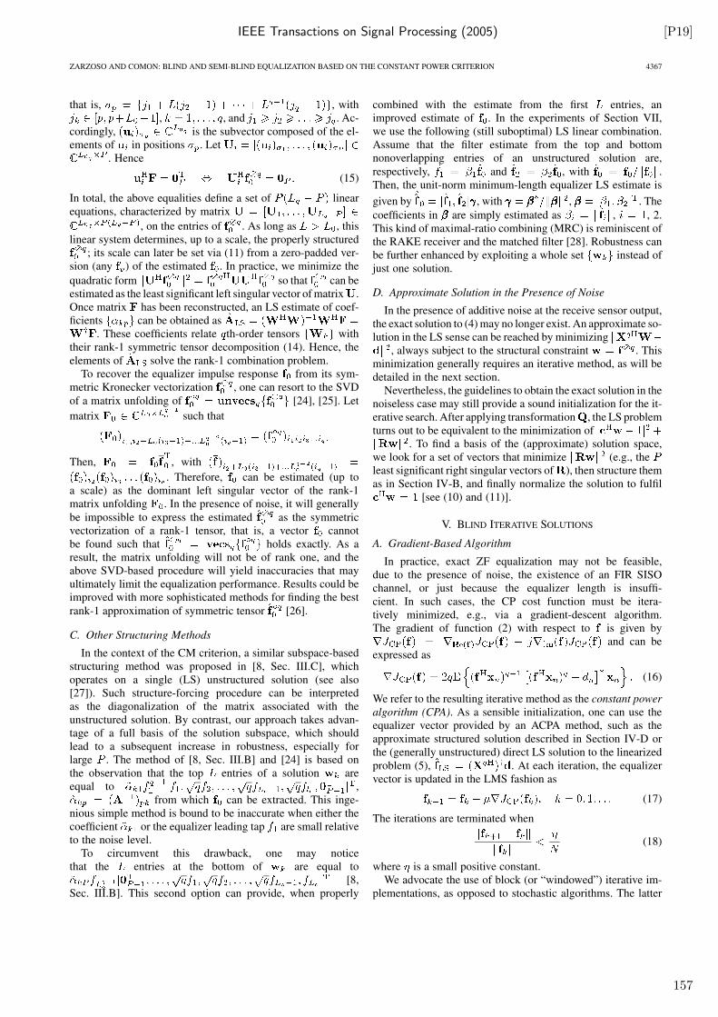
IEEE Transactions on Signal Processing (2005) [P19]
ZARZOSO AND COMON: BLIND AND SEMI-BLIND EQUALIZATION BASED ON THE CONSTANT POWER CRITERION 4367
that is, , with, , and . Ac-
cordingly, is the subvector composed of the el-ements of in positions . Let
. Hence
(15)
In total, the above equalities define a set of linearequations, characterized by matrix
, on the entries of . As long as , thislinear system determines, up to a scale, the properly structured
; its scale can later be set via (11) from a zero-padded ver-sion (any ) of the estimated . In practice, we minimize the
quadratic form so that can beestimated as the least significant left singular vector of matrix .Once matrix has been reconstructed, an LS estimate of coef-ficients can be obtained as
. These coefficients relate th-order tensors withtheir rank-1 symmetric tensor decomposition (14). Hence, theelements of solve the rank-1 combination problem.
To recover the equalizer impulse response from its sym-metric Kronecker vectorization , one can resort to the SVDof a matrix unfolding of [24], [25]. Let
matrix such that
Then, , with
. Therefore, can be estimated (up toa scale) as the dominant left singular vector of the rank-1matrix unfolding . In the presence of noise, it will generallybe impossible to express the estimated as the symmetricvectorization of a rank-1 tensor, that is, a vector cannotbe found such that holds exactly. As aresult, the matrix unfolding will not be of rank one, and theabove SVD-based procedure will yield inaccuracies that mayultimately limit the equalization performance. Results could beimproved with more sophisticated methods for finding the bestrank-1 approximation of symmetric tensor [26].
C. Other Structuring Methods
In the context of the CM criterion, a similar subspace-basedstructuring method was proposed in [8, Sec. III.C], whichoperates on a single (LS) unstructured solution (see also[27]). Such structure-forcing procedure can be interpretedas the diagonalization of the matrix associated with theunstructured solution. By contrast, our approach takes advan-tage of a full basis of the solution subspace, which shouldlead to a subsequent increase in robustness, especially forlarge . The method of [8, Sec. III.B] and [24] is based onthe observation that the top entries of a solution areequal to ,
from which can be extracted. This inge-nious simple method is bound to be inaccurate when either thecoefficient or the equalizer leading tap are small relativeto the noise level.
To circumvent this drawback, one may noticethat the entries at the bottom of are equal to
[8,Sec. III.B]. This second option can provide, when properly
combined with the estimate from the first entries, animproved estimate of . In the experiments of Section VII,we use the following (still suboptimal) LS linear combination.Assume that the filter estimate from the top and bottomnonoverlapping entries of an unstructured solution are,respectively, and , with .Then, the unit-norm minimum-length equalizer LS estimate is
given by , with , . The
coefficients in are simply estimated as , , 2.This kind of maximal-ratio combining (MRC) is reminiscent ofthe RAKE receiver and the matched filter [28]. Robustness canbe further enhanced by exploiting a whole set instead ofjust one solution.
D. Approximate Solution in the Presence of Noise
In the presence of additive noise at the receive sensor output,the exact solution to (4) may no longer exist. An approximate so-lution in the LS sense can be reached by minimizing
, always subject to the structural constraint . Thisminimization generally requires an iterative method, as will bedetailed in the next section.
Nevertheless, the guidelines to obtain the exact solution in thenoiseless case may still provide a sound initialization for the it-erative search. After applying transformation , the LS problemturns out to be equivalent to the minimization of
. To find a basis of the (approximate) solution space,we look for a set of vectors that minimize (e.g., theleast significant right singular vectors of ), then structure themas in Section IV-B, and finally normalize the solution to fulfil
[see (10) and (11)].
V. BLIND ITERATIVE SOLUTIONS
A. Gradient-Based Algorithm
In practice, exact ZF equalization may not be feasible,due to the presence of noise, the existence of an FIR SISOchannel, or just because the equalizer length is insuffi-cient. In such cases, the CP cost function must be itera-tively minimized, e.g., via a gradient-descent algorithm.The gradient of function (2) with respect to is given by
and can beexpressed as
(16)
We refer to the resulting iterative method as the constant power
algorithm (CPA). As a sensible initialization, one can use theequalizer vector provided by an ACPA method, such as theapproximate structured solution described in Section IV-D orthe (generally unstructured) direct LS solution to the linearizedproblem (5), . At each iteration, the equalizervector is updated in the LMS fashion as
(17)
The iterations are terminated when
(18)
where is a small positive constant.We advocate the use of block (or “windowed”) iterative im-
plementations, as opposed to stochastic algorithms. The latter
157
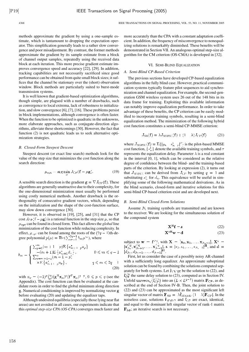
[P19] IEEE Transactions on Signal Processing (2005)
4368 IEEE TRANSACTIONS ON SIGNAL PROCESSING, VOL. 53, NO. 11, NOVEMBER 2005
methods approximate the gradient by using a one-sample es-timate, which is tantamount to dropping the expectation oper-ator. This simplification generally leads to a rather slow conver-gence and poor misadjustment. By contrast, the former methodsapproximate the gradient by its sample estimate from a blockof channel output samples, repeatedly using the received datablock at each iteration. This more precise gradient estimate im-proves convergence speed and accuracy [22], [29]. In addition,tracking capabilities are not necessarily sacrificed since goodperformance can be obtained from quite small block sizes; it suf-fices that the channel be stationary over the (short) observationwindow. Block methods are particularly suited to burst-modetransmission systems.
It is well known that gradient-based optimization algorithms,though simple, are plagued with a number of drawbacks, suchas convergence to local extrema, lack of robustness to initializa-tion, and slow convergence [6], [7], [16]. These problems persistin block implementations, although convergence is often faster.When the function to be optimized is quadratic in the unknowns,more elaborate approaches, such as conjugate-direction algo-rithms, alleviate these shortcomings [30]. However, the fact thatfunction (2) is not quadratic leads us to seek alternative opti-mization strategies.
B. Closed-Form Steepest Descent
Steepest descent (or exact line search) methods look for thevalue of the step size that minimizes the cost function along thesearch direction:
(19)
A sensible search direction is the gradient . Thesealgorithms are generally unattractive due to their complexity, forthe one-dimensional minimization must usually be performedusing costly numerical methods. Another drawback is the or-thogonality of consecutive gradient vectors, which, dependingon the initialization and the shape of the cost-function surface,may slow down convergence [30].
However, it is observed in [19], [25], and [31] that the CPcost is a rational function in the step size , so that
can be found in closed form. This fact allows the global lineminimization of the cost function while reducing complexity. Ineffect, can be found among the roots of the th-de-
gree polynomial , where
(20)
with , (see theAppendix). The cost function can then be evaluated at the can-didate roots in order to find the global minimum along direction
. Numerical conditioning is improved by normalizing vectorbefore evaluating (20) and updating the equalizer taps.
Although undesired equilibria (especially those lying near flatareas) are not avoided in all cases, our experiments indicate thatthis optimal step-size CPA (OS-CPA) converges much faster and
more accurately than the CPA with a constant adaptation coeffi-cient. In addition, the frequency of misconvergence to nonequal-izing solutions is remarkably diminished. These benefits will bedemonstrated in Section VII. An analogous optimal step-size al-gorithm for the CM criterion (OS-CMA) is developed in [32].
VI. SEMI-BLIND EQUALIZATION
A. Semi-Blind CP-Based Criterion
The previous sections have developed CP-based equalization
algorithms in the fully blind case. However, practical communi-
cation systems typically feature pilot sequences to aid synchro-
nization and channel equalization. For example, the second-gen-
eration GSM wireless system uses 26 out of the 148 bits in its
data frame for training. Exploiting this available information
can notably improve equalization performance. In order to take
advantage of these benefits, the CP criterion can be easily mod-
ified to incorporate training symbols, resulting in a semi-blind
equalization method. The minimization of the following hybrid
cost function constitutes a semi-blind CP-MMSE criterion:
(21)
where is the pilot-based MMSE
cost function, denote the available training symbols, and
represents the equalization delay. Parameter is a real constant
in the interval [0, 1], which can be considered as the relative
degree of confidence between the blind- and the training-based
parts of the criterion. By looking at expression (2), it turns out
that can be derived from by setting and
substituting for . This equivalence will be useful in sim-
plifying some of the following mathematical derivations. As in
the blind scenario, closed-form and iterative solutions for this
semi-blind CP-based criterion exist and are developed next.
B. Semi-Blind Closed-Form Solutions
Assume training symbols are transmitted and are known
to the receiver. We are looking for the simultaneous solution of
the compound system
(22)
(23)
subject to , with ,
, , and
.
First, let us consider the case of a possibly noisy AR-channel
with a sufficiently long equalizer. An approximate suboptimal
solution can be found by combining the solutions computed sep-
arately for both systems. Let be the solution to (22), and
the same delay solution to (23), computed as in Section IV.
Unfold into an matrix , as de-
scribed at the end of Section IV-B. Then, the joint solution to
(22) and (23) can be approximated as the most significant left
singular vector of matrix . In the
noiseless case, solutions and are exact, identical,
and equal to the dominant left singular vector of rank-1 matrix
; an iterative search is not necessary.
158
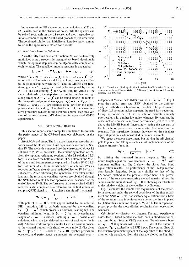
IEEE Transactions on Signal Processing (2005) [P19]
ZARZOSO AND COMON: BLIND AND SEMI-BLIND EQUALIZATION BASED ON THE CONSTANT POWER CRITERION 4369
In the case of an FIR channel, no exact solution to (22) and(23) exists, even in the absence of noise. Still, the systems canbe solved separately in the LS sense, and their respective so-lutions combined by the SVD-based procedure just described.The combined solution can initialize an iterative search aimingto refine the approximate closed-form result.
C. Semi-Blind Iterative Solutions
As in the fully blind case, cost function (21) can be iterativelyminimized using a steepest-descent gradient-based algorithm inwhich the optimal step size can be algebraically computed ateach iteration. The equalizer impulse response is updated as
(24)
where . Cri-terion (18) still remains valid for checking convergence. Dueto the relationship between the CP and the MMSE cost func-tions, gradient can readily be computed by setting
and substituting for in (16). By virtue of thesame relationship, the step size that minimizes functionalong direction can be found among the roots ofthe composite polynomial ,where and are obtained as in (20) from the appro-priate values of and . Note that for , the above iter-ative procedure reduces to the algebraic optimal step-size ver-sion of the well-known LMS algorithm for supervised MMSEequalization.
VII. EXPERIMENTAL RESULTS
This section reports some computer simulations to evaluatethe performance of the CP-based methods elaborated in thispaper.
Blind ACPA solutions. The first experiment compares the per-formance of the closed-form blind equalization methods of Sec-tion IV. The methods compared are the unstructured direct LSsolution to (5) (“LS, no struct”); the structuring method of [24]from the top nonoverlapping sections of the LS solution (“LS,top”); idem, from the bottom sections (“LS, bottom”); the MRCof the top and bottom parts as explained in Section IV-C (“LS,top+bottom”); idem, from the whole basis of solutions (“basis,top+bottom”); and the subspace method of Section IV-B (“basis,subspace”). After estimating the symmetric Kronecker vector-izations, the respective equalizer vectors are obtained throughthe SVD-based rank-1 tensor approximation described at theend of Section IV-B. The performance of the supervised MMSEreceiver is also computed as a reference. In the first simulationsetup, a QPSK signal excites a simple AR-1 channel
(25)
with pole at , well approximated by an order-50FIR truncation. ISI is perfectly removed by the equalizer
, which presents a dominant leading tap. Theequalizer minimum length is , but an overestimatedlength of is chosen, yielding possible ZFsolutions, which are just delayed versions of each other [as in(6)]. Additive white complex circular Gaussian noise is presentat the channel output, with signal-to-noise ratio (SNR) givenby . Blocks of symbol periods areobserved, and performance parameters are averaged over
Fig. 1. Closed-form blind equalization based on the CP criterion for severalstructuring methods. ChannelH (z), QPSK input (q = 4),N = 100 symbolperiods, 1000 MC runs.
independent Monte Carlo (MC) runs, with . Fig. 1plots the symbol error rate (SER) obtained by the differentanalytic methods as a function of the SNR. The performanceof direct LS solution makes apparent the need for structuring.Using the bottom part of the LS solution exhibits similarlypoor results, with a rather low noise tolerance. By contrast, theother methods present a superior performance, just 2 to 3 dBabove the MMSE bound. Interestingly, taking the top part ofthe LS solution proves best for moderate SNR values in thisscenario. This superiority depends, however, on the equalizertap configuration, as demonstrated in the next example.
We repeat the above experiment, but moving the AR channelpole to , and taking a stable causal implementation of thechannel transfer function
(26)
by shifting the truncated impulse response. The min-imum-length equalizer now becomes , withdominant trailing tap. Fig. 2 shows the closed-form blindequalization results. The performance of the LS-top methodconsiderably degrades, being very similar to that of theLS-bottom method in the previous experiment. The perfor-mance of the subspace structuring method remains almost thesame as in the simulation of Fig. 1, thus showing its robustnessto the relative weights of the equalizer coefficients.
Fig. 3 evaluates the sample size requirements of the closed-form solutions under the general conditions of the first experi-ment and SNR dB. Satisfactory equalization from a basisof the solution space is achieved even below the limit imposedby (12) for this simulation example, . The subspace ap-proach provides the most efficient results for short observationwindows.
CPA Solutions—Basins of Attraction. The next experimentsassess the CP-based iterative methods, both in blind (Section V)and semi-blind (Section VI-C) operation. We observe a burstof symbols with SNR dB at the output ofchannel excited by a BPSK input. The contour lines (inthe equalizer parameter space) of the logarithm of the blind CPcriterion (2) calculated from the data are plotted in Fig. 4(a).
159
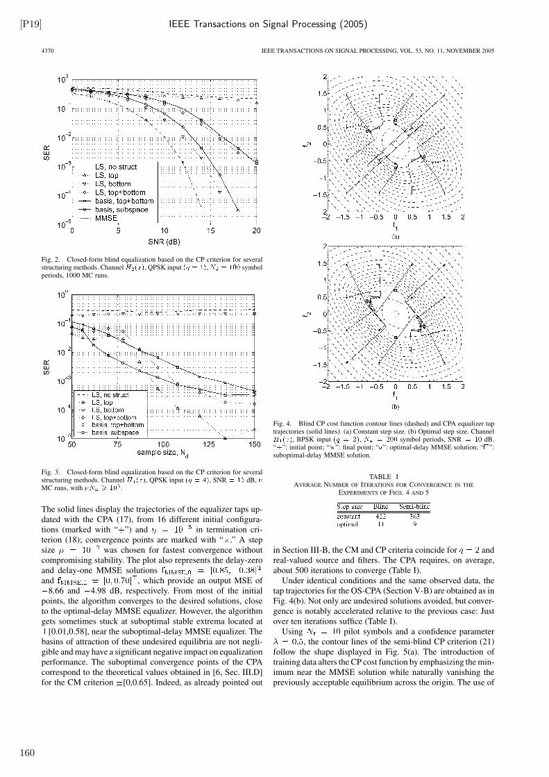
[P19] IEEE Transactions on Signal Processing (2005)
4370 IEEE TRANSACTIONS ON SIGNAL PROCESSING, VOL. 53, NO. 11, NOVEMBER 2005
Fig. 2. Closed-form blind equalization based on the CP criterion for severalstructuring methods. ChannelH (z), QPSK input (q = 4),N = 100 symbolperiods, 1000 MC runs.
Fig. 3. Closed-form blind equalization based on the CP criterion for severalstructuring methods. Channel H (z), QPSK input (q = 4), SNR = 15 dB, �MC runs, with �N 10 .
The solid lines display the trajectories of the equalizer taps up-dated with the CPA (17), from 16 different initial configura-tions (marked with “ ”) and in termination cri-terion (18); convergence points are marked with “ .” A stepsize was chosen for fastest convergence withoutcompromising stability. The plot also represents the delay-zeroand delay-one MMSE solutionsand , which provide an output MSE of
8.66 and 4.98 dB, respectively. From most of the initialpoints, the algorithm converges to the desired solutions, closeto the optimal-delay MMSE equalizer. However, the algorithmgets sometimes stuck at suboptimal stable extrema located at
[0.01,0.58], near the suboptimal-delay MMSE equalizer. Thebasins of attraction of these undesired equilibria are not negli-gible and may have a significant negative impact on equalizationperformance. The suboptimal convergence points of the CPAcorrespond to the theoretical values obtained in [6, Sec. III.D]for the CM criterion [0,0.65]. Indeed, as already pointed out
Fig. 4. Blind CP cost function contour lines (dashed) and CPA equalizer taptrajectories (solid lines). (a) Constant step size. (b) Optimal step size. ChannelH (z), BPSK input (q = 2), N = 200 symbol periods, SNR = 10 dB.“+”: initial point; “�”: final point; “�”: optimal-delay MMSE solution; “ ”:suboptimal-delay MMSE solution.
TABLE IAVERAGE NUMBER OF ITERATIONS FOR CONVERGENCE IN THE
EXPERIMENTS OF FIGS. 4 AND 5
in Section III-B, the CM and CP criteria coincide for andreal-valued source and filters. The CPA requires, on average,about 500 iterations to converge (Table I).
Under identical conditions and the same observed data, thetap trajectories for the OS-CPA (Section V-B) are obtained as inFig. 4(b). Not only are undesired solutions avoided, but conver-gence is notably accelerated relative to the previous case: Justover ten iterations suffice (Table I).
Using pilot symbols and a confidence parameter, the contour lines of the semi-blind CP criterion (21)
follow the shape displayed in Fig. 5(a). The introduction oftraining data alters the CP cost function by emphasizing the min-imum near the MMSE solution while naturally vanishing thepreviously acceptable equilibrium across the origin. The use of
160
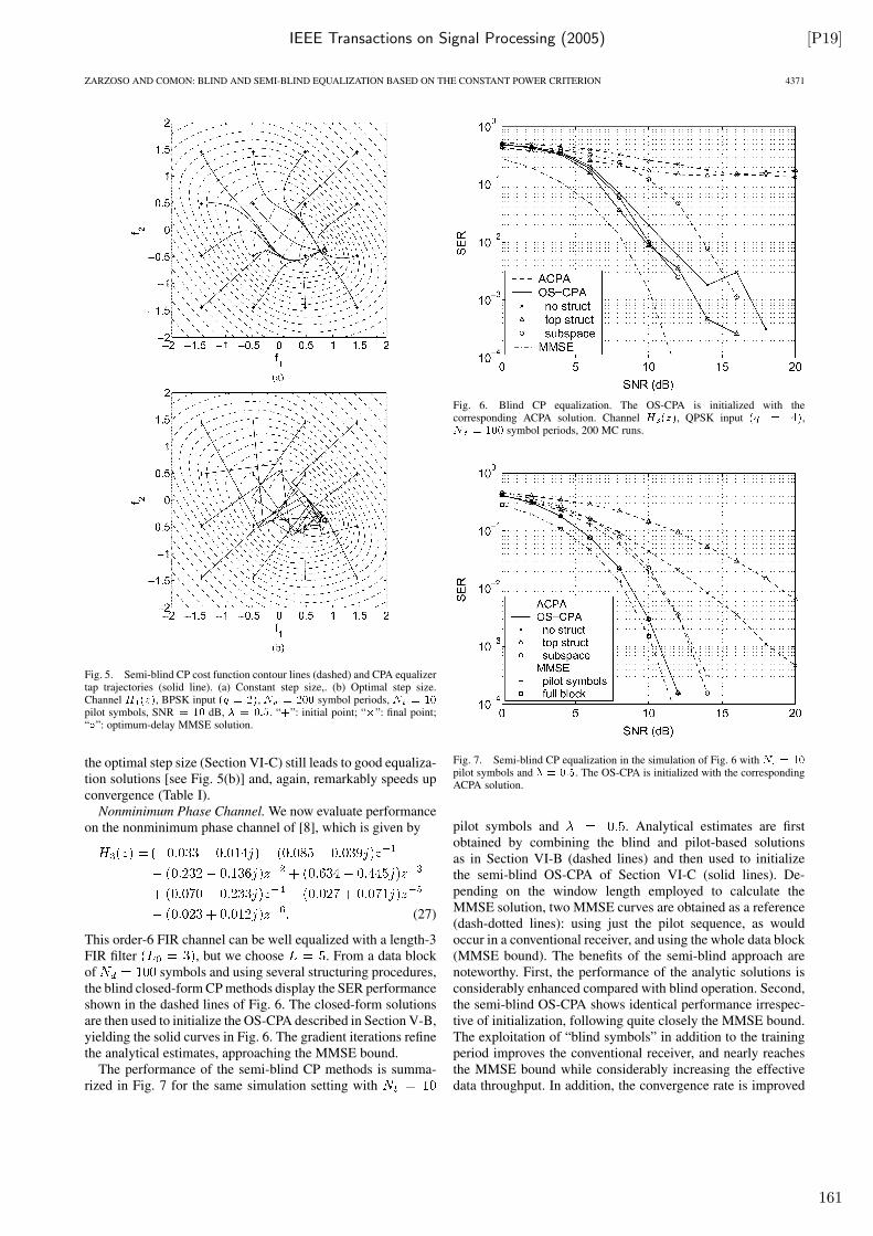
IEEE Transactions on Signal Processing (2005) [P19]
ZARZOSO AND COMON: BLIND AND SEMI-BLIND EQUALIZATION BASED ON THE CONSTANT POWER CRITERION 4371
Fig. 5. Semi-blind CP cost function contour lines (dashed) and CPA equalizertap trajectories (solid line). (a) Constant step size,. (b) Optimal step size.Channel H (z), BPSK input (q = 2), N = 200 symbol periods, N = 10pilot symbols, SNR = 10 dB, � = 0:5. “+”: initial point; “�”: final point;“�”: optimum-delay MMSE solution.
the optimal step size (Section VI-C) still leads to good equaliza-tion solutions [see Fig. 5(b)] and, again, remarkably speeds upconvergence (Table I).
Nonminimum Phase Channel. We now evaluate performanceon the nonminimum phase channel of [8], which is given by
(27)
This order-6 FIR channel can be well equalized with a length-3FIR filter , but we choose . From a data blockof symbols and using several structuring procedures,the blind closed-form CP methods display the SER performanceshown in the dashed lines of Fig. 6. The closed-form solutionsare then used to initialize the OS-CPA described in Section V-B,yielding the solid curves in Fig. 6. The gradient iterations refinethe analytical estimates, approaching the MMSE bound.
The performance of the semi-blind CP methods is summa-rized in Fig. 7 for the same simulation setting with
Fig. 6. Blind CP equalization. The OS-CPA is initialized with thecorresponding ACPA solution. Channel H (z), QPSK input (q = 4),N = 100 symbol periods, 200 MC runs.
Fig. 7. Semi-blind CP equalization in the simulation of Fig. 6 with N = 10pilot symbols and � = 0:5. The OS-CPA is initialized with the correspondingACPA solution.
pilot symbols and . Analytical estimates are firstobtained by combining the blind and pilot-based solutionsas in Section VI-B (dashed lines) and then used to initializethe semi-blind OS-CPA of Section VI-C (solid lines). De-pending on the window length employed to calculate theMMSE solution, two MMSE curves are obtained as a reference(dash-dotted lines): using just the pilot sequence, as wouldoccur in a conventional receiver, and using the whole data block(MMSE bound). The benefits of the semi-blind approach arenoteworthy. First, the performance of the analytic solutions isconsiderably enhanced compared with blind operation. Second,the semi-blind OS-CPA shows identical performance irrespec-tive of initialization, following quite closely the MMSE bound.The exploitation of “blind symbols” in addition to the trainingperiod improves the conventional receiver, and nearly reachesthe MMSE bound while considerably increasing the effectivedata throughput. In addition, the convergence rate is improved
161
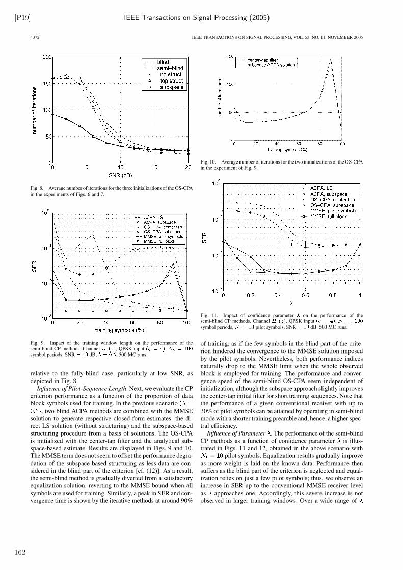
[P19] IEEE Transactions on Signal Processing (2005)
4372 IEEE TRANSACTIONS ON SIGNAL PROCESSING, VOL. 53, NO. 11, NOVEMBER 2005
Fig. 8. Average number of iterations for the three initializations of the OS-CPAin the experiments of Figs. 6 and 7.
Fig. 9. Impact of the training window length on the performance of thesemi-blind CP methods. Channel H (z), QPSK input (q = 4), N = 100symbol periods, SNR = 10 dB, � = 0:5, 500 MC runs.
relative to the fully-blind case, particularly at low SNR, asdepicted in Fig. 8.
Influence of Pilot-Sequence Length. Next, we evaluate the CPcriterion performance as a function of the proportion of datablock symbols used for training. In the previous scenario
, two blind ACPA methods are combined with the MMSEsolution to generate respective closed-form estimates: the di-rect LS solution (without structuring) and the subspace-basedstructuring procedure from a basis of solutions. The OS-CPAis initialized with the center-tap filter and the analytical sub-space-based estimate. Results are displayed in Figs. 9 and 10.The MMSE term does not seem to offset the performance degra-dation of the subspace-based structuring as less data are con-sidered in the blind part of the criterion [cf. (12)]. As a result,the semi-blind method is gradually diverted from a satisfactoryequalization solution, reverting to the MMSE bound when allsymbols are used for training. Similarly, a peak in SER and con-vergence time is shown by the iterative methods at around 90%
Fig. 10. Average number of iterations for the two initializations of the OS-CPAin the experiment of Fig. 9.
Fig. 11. Impact of confidence parameter � on the performance of thesemi-blind CP methods. Channel H (z), QPSK input (q = 4), N = 100symbol periods, N = 10 pilot symbols, SNR = 10 dB, 500 MC runs.
of training, as if the few symbols in the blind part of the crite-rion hindered the convergence to the MMSE solution imposedby the pilot symbols. Nevertheless, both performance indicesnaturally drop to the MMSE limit when the whole observedblock is employed for training. The performance and conver-gence speed of the semi-blind OS-CPA seem independent ofinitialization, although the subspace approach slightly improvesthe center-tap initial filter for short training sequences. Note thatthe performance of a given conventional receiver with up to30% of pilot symbols can be attained by operating in semi-blindmode with a shorter training preamble and, hence, a higher spec-tral efficiency.
Influence of Parameter . The performance of the semi-blindCP methods as a function of confidence parameter is illus-trated in Figs. 11 and 12, obtained in the above scenario with
pilot symbols. Equalization results gradually improveas more weight is laid on the known data. Performance thensuffers as the blind part of the criterion is neglected and equal-ization relies on just a few pilot symbols; thus, we observe anincrease in SER up to the conventional MMSE receiver levelas approaches one. Accordingly, this severe increase is notobserved in larger training windows. Over a wide range of
162
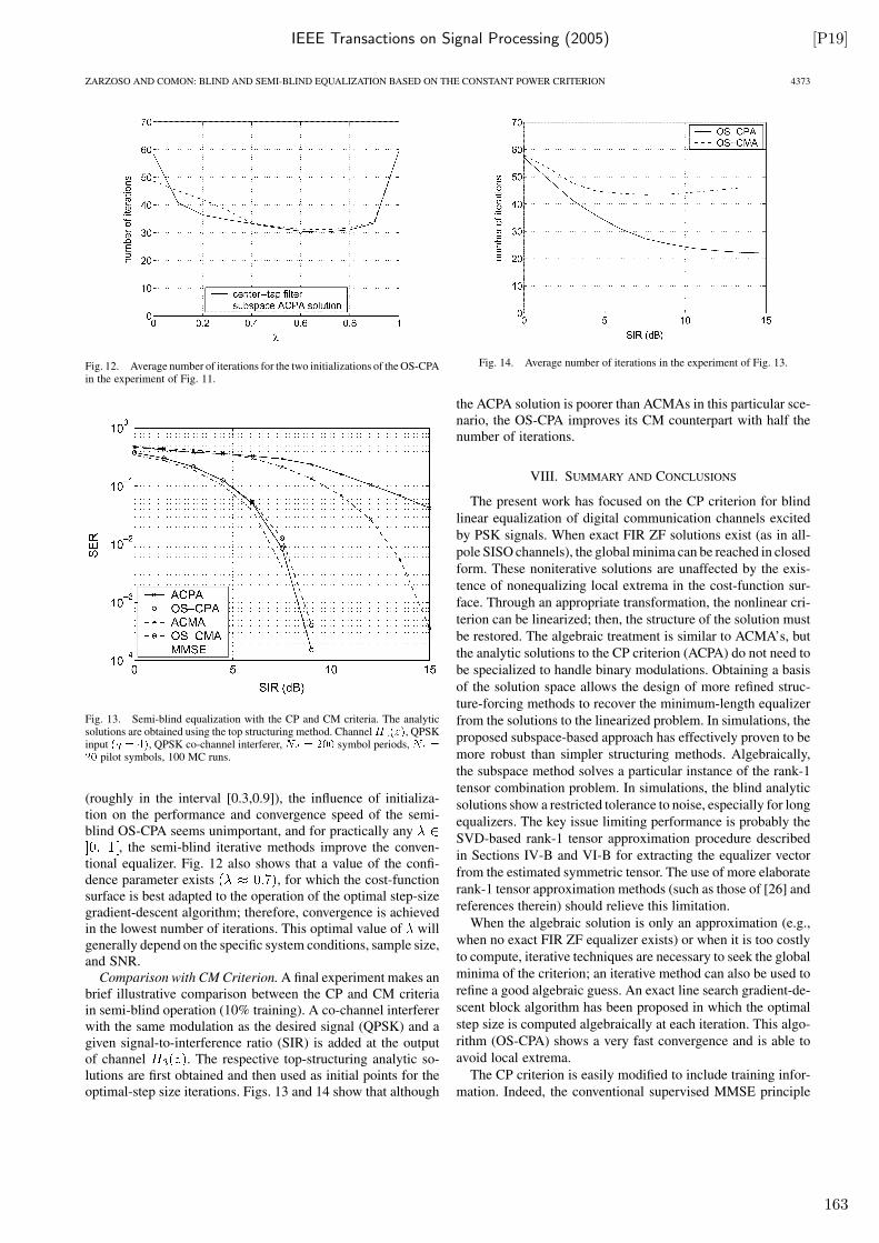
IEEE Transactions on Signal Processing (2005) [P19]
ZARZOSO AND COMON: BLIND AND SEMI-BLIND EQUALIZATION BASED ON THE CONSTANT POWER CRITERION 4373
Fig. 12. Average number of iterations for the two initializations of the OS-CPAin the experiment of Fig. 11.
Fig. 13. Semi-blind equalization with the CP and CM criteria. The analyticsolutions are obtained using the top structuring method. ChannelH (z), QPSKinput (q = 4), QPSK co-channel interferer, N = 200 symbol periods, N =20 pilot symbols, 100 MC runs.
(roughly in the interval [0.3,0.9]), the influence of initializa-tion on the performance and convergence speed of the semi-blind OS-CPA seems unimportant, and for practically any
, the semi-blind iterative methods improve the conven-tional equalizer. Fig. 12 also shows that a value of the confi-dence parameter exists , for which the cost-functionsurface is best adapted to the operation of the optimal step-sizegradient-descent algorithm; therefore, convergence is achievedin the lowest number of iterations. This optimal value of willgenerally depend on the specific system conditions, sample size,and SNR.
Comparison with CM Criterion. A final experiment makes anbrief illustrative comparison between the CP and CM criteriain semi-blind operation (10% training). A co-channel interfererwith the same modulation as the desired signal (QPSK) and agiven signal-to-interference ratio (SIR) is added at the outputof channel . The respective top-structuring analytic so-lutions are first obtained and then used as initial points for theoptimal-step size iterations. Figs. 13 and 14 show that although
Fig. 14. Average number of iterations in the experiment of Fig. 13.
the ACPA solution is poorer than ACMAs in this particular sce-nario, the OS-CPA improves its CM counterpart with half thenumber of iterations.
VIII. SUMMARY AND CONCLUSIONS
The present work has focused on the CP criterion for blind
linear equalization of digital communication channels excited
by PSK signals. When exact FIR ZF solutions exist (as in all-
pole SISO channels), the global minima can be reached in closed
form. These noniterative solutions are unaffected by the exis-
tence of nonequalizing local extrema in the cost-function sur-
face. Through an appropriate transformation, the nonlinear cri-
terion can be linearized; then, the structure of the solution must
be restored. The algebraic treatment is similar to ACMA’s, but
the analytic solutions to the CP criterion (ACPA) do not need to
be specialized to handle binary modulations. Obtaining a basis
of the solution space allows the design of more refined struc-
ture-forcing methods to recover the minimum-length equalizer
from the solutions to the linearized problem. In simulations, the
proposed subspace-based approach has effectively proven to be
more robust than simpler structuring methods. Algebraically,
the subspace method solves a particular instance of the rank-1
tensor combination problem. In simulations, the blind analytic
solutions show a restricted tolerance to noise, especially for long
equalizers. The key issue limiting performance is probably the
SVD-based rank-1 tensor approximation procedure described
in Sections IV-B and VI-B for extracting the equalizer vector
from the estimated symmetric tensor. The use of more elaborate
rank-1 tensor approximation methods (such as those of [26] and
references therein) should relieve this limitation.
When the algebraic solution is only an approximation (e.g.,
when no exact FIR ZF equalizer exists) or when it is too costly
to compute, iterative techniques are necessary to seek the global
minima of the criterion; an iterative method can also be used to
refine a good algebraic guess. An exact line search gradient-de-
scent block algorithm has been proposed in which the optimal
step size is computed algebraically at each iteration. This algo-
rithm (OS-CPA) shows a very fast convergence and is able to
avoid local extrema.
The CP criterion is easily modified to include training infor-
mation. Indeed, the conventional supervised MMSE principle
163
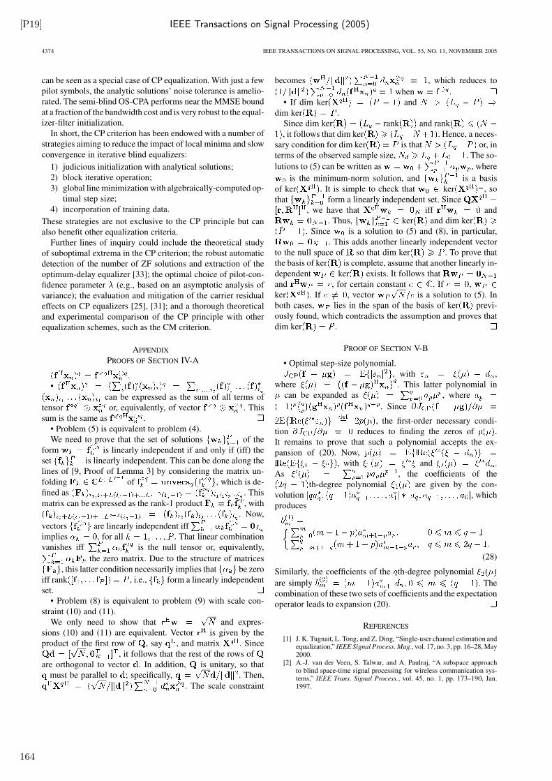
[P19] IEEE Transactions on Signal Processing (2005)
4374 IEEE TRANSACTIONS ON SIGNAL PROCESSING, VOL. 53, NO. 11, NOVEMBER 2005
can be seen as a special case of CP equalization. With just a few
pilot symbols, the analytic solutions’ noise tolerance is amelio-
rated. The semi-blind OS-CPA performs near the MMSE bound
at a fraction of the bandwidth cost and is very robust to the equal-
izer-filter initialization.
In short, the CP criterion has been endowed with a number of
strategies aiming to reduce the impact of local minima and slow
convergence in iterative blind equalizers:
1) judicious initialization with analytical solutions;
2) block iterative operation;
3) global line minimization with algebraically-computed op-
timal step size;
4) incorporation of training data.
These strategies are not exclusive to the CP principle but can
also benefit other equalization criteria.
Further lines of inquiry could include the theoretical study
of suboptimal extrema in the CP criterion; the robust automatic
detection of the number of ZF solutions and extraction of the
optimum-delay equalizer [33]; the optimal choice of pilot-con-
fidence parameter (e.g., based on an asymptotic analysis of
variance); the evaluation and mitigation of the carrier residual
effects on CP equalizers [25], [31]; and a thorough theoretical
and experimental comparison of the CP principle with other
equalization schemes, such as the CM criterion.
APPENDIX
PROOFS OF SECTION IV-A
•
can be expressed as the sum of all terms of
tensor or, equivalently, of vector . This
sum is the same as .
• Problem (5) is equivalent to problem (4).
We need to prove that the set of solutions of the
form is linearly independent if and only if (iff) the
set is linearly independent. This can be done along the
lines of [9, Proof of Lemma 3] by considering the matrix un-
folding of , which is de-
fined as . This
matrix can be expressed as the rank-1 product , with
. Now,
vectors are linearly independent iff
implies , for all . That linear combination
vanishes iff is the null tensor or, equivalently,
the zero matrix. Due to the structure of matrices
, this latter condition necessarily implies that be zero
iff rank , i.e., form a linearly independent
set.
• Problem (8) is equivalent to problem (9) with scale con-
straint (10) and (11).
We only need to show that and expres-
sions (10) and (11) are equivalent. Vector is given by the
product of the first row of , say , and matrix . Since
, it follows that the rest of the rows of
are orthogonal to vector . In addition, is unitary, so that
must be parallel to ; specifically, . Then,
. The scale constraint
becomes , which reduces to
when .
• If dim ker and
dim ker .
Since dim ker rank and rank
, it follows that dim ker . Hence, a neces-
sary condition for dim ker is that or, in
terms of the observed sample size, . The so-
lutions to (5) can be written as , where
is the minimum-norm solution, and is a basis
of ker . It is simple to check that ker , so
that form a linearly independent set. Since
, we have that iff and
. Thus, ker and dim ker
. Since is a solution to (5) and (8), in particular,
. This adds another linearly independent vector
to the null space of so that dim ker . To prove that
the basis of ker is complete, assume that another linearly in-
dependent ker exists. It follows that
and , for certain constant . If ,
ker . If , vector is a solution to (5). In
both cases, lies in the span of the basis of ker previ-
ously found, which contradicts the assumption and proves that
dim ker .
PROOF OF SECTION V-B
• Optimal step-size polynomial.
, with ,
where . This latter polynomial in
can be expanded as , where
. Since
, the first-order necessary condi-
tion reduces to finding the zeros of .
It remains to prove that such a polynomial accepts the ex-
pansion of (20). Now,
, with and .
As , the coefficients of the
th-degree polynomial are given by the con-
volution , which
produces
(28)
Similarly, the coefficients of the th-degree polynomial
are simply . The
combination of these two sets of coefficients and the expectation
operator leads to expansion (20).
REFERENCES
[1] J. K. Tugnait, L. Tong, and Z. Ding, “Single-user channel estimation andequalization,” IEEE Signal Process. Mag., vol. 17, no. 3, pp. 16–28, May2000.
[2] A.-J. van der Veen, S. Talwar, and A. Paulraj, “A subspace approachto blind space-time signal processing for wireless communication sys-tems,” IEEE Trans. Signal Process., vol. 45, no. 1, pp. 173–190, Jan.1997.
164
IEEE Transactions on Signal Processing (2005) [P19]
ZARZOSO AND COMON: BLIND AND SEMI-BLIND EQUALIZATION BASED ON THE CONSTANT POWER CRITERION 4375
[3] Y. Sato, “A method of self-recovering equalization for multi-level am-plitude modulation,” IEEE Trans. Commun., vol. COM-23, no. 6, pp.679–682, Jun. 1975.
[4] D. N. Godard, “Self-recovering equalization and carrier tracking in two-dimensional data communication systems,” IEEE Trans. Commun., vol.COM-28, no. 11, pp. 1867–1875, Nov. 1980.
[5] J. R. Treichler and B. G. Agee, “A new approach to multipath correc-tion of constant modulus signals,” IEEE Trans. Acoust., Speech, Signal
Process., vol. ASSP-31, no. 2, pp. 459–472, Apr. 1983.[6] Z. Ding, R. A. Kennedy, B. D. O. Anderson, and C. R. Johnson, “Ill-con-
vergence of Godard blind equalizers in data communication systems,”IEEE Trans. Commun., vol. 39, no. 9, pp. 1313–1327, Sep. 1991.
[7] Z. Ding, C. R. Johnson, and R. A. Kennedy, “On the (non)existence ofundesirable equilibria of Godard blind equalizers,,” IEEE Trans. Signal
Process., vol. 40, no. 10, pp. 2425–2432, Oct. 1992.[8] K. Dogançay and R. A. Kennedy, “Least squares approach to blind
channel equalization,” IEEE Trans. Signal Process., vol. 47, no. 11, pp.1678–1687, Nov. 1999.
[9] A.-J. van der Veen and A. Paulraj, “An analytical constant modulus al-gorithm,” IEEE Trans. Signal Process., vol. 44, no. 5, pp. 1136–1155,May 1996.
[10] G. H. Golub and C. F. Van Loan, Matrix Computations, Third ed. Bal-timore, MD: Johns Hopkins Univ. Press, 1996.
[11] A.-J. van der Veen, “Analytical method for blind binary signal separa-tion,” IEEE Trans. Signal Process., vol. 45, no. 4, pp. 1078–1082, Apr.1997.
[12] D. T. M. Slock, “Blind fractionally-spaced equalization, perfect-re-construction filter banks and multichannel linear prediction,” in Proc.
ICASSP-94, 19th Int. Conf. Acoust., Speech Signal Process., vol. IV,Adelaide, Australia, Apr. 19–22, 1994, pp. 585–588.
[13] L. Tong, G. Xu, and T. Kailath, “Blind identification and equalizationbased on second-order statistics: a time domain approach,” IEEE Trans.
Inf. Theory, vol. 40, no. 2, pp. 340–349, Mar. 1994.[14] E. Moulines, P. Duhamel, J.-F. Cardoso, and S. Mayrargue, “Subspace
methods for the blind identification of multichannel FIR filters,” IEEE
Trans. Signal Process., vol. 43, no. 2, pp. 516–525, Feb. 1995.[15] Y. Li and Z. Ding, “Global convergence of fractionally spaced Godard
(CMA) adaptive equalizers,” IEEE Trans. Signal Processing, vol. 44, no.4, pp. 818–826, Apr. 1996.
[16] C. R. Johnson, P. Schniter, I. Fijalkow, and L. Tong et al., “The coreof FSE-CMA behavior theory,” in Unsupervised Adaptive Filtering II:
Blind Deconvolution, S. S. Haykin et al., Ed. New York: Wiley, 2000,ch. 2, pp. 13–112.
[17] P. Comon, “Tensor decompositions: state of the art and applications,” inMathematics in Signal Processing V, J. G. McWhirter and I. K. Proudler,Eds. Oxford, U.K.: Clarendon, 2002, pp. 1–24.
[18] O. Grellier and P. Comon, “Blind equalization and source separationwith MSK inputs,” in Proc. SPIE Conf. Adv. Signal Process., Jul. 19–24,1998, pp. 26–34.
[19] P. Comon, “Contrasts, independent component analysis, and blind de-convolution,” Int. J. Adaptive Contr. Signal Process. (Special Issue on
Blind Signal Separation), vol. 18, no. 3, pp. 225–243, Apr. 2004.[20] L. Rota and P. Comon, “Blind equalizers based on polynomial criteria,”
in Proc. ICASSP-2004, 29th Int. Conf. Acoust., Speech, Signal Process.,vol. IV, Montreal, QC, Canada, May 17–21, 2004, pp. 441–444.
[21] O. Grellier and P. Comon, “Blind separation of discrete sources,” IEEE
Signal Process. Lett., vol. 5, no. 8, pp. 212–214, Aug. 1998.[22] P. Comon, “Block methods for channel identification and source sepa-
ration,” in Proc. IEEE Symp. Adaptive Syst. Signal Process., Commun.
Contr., Calgary, AB, Canada, Oct. 1–4, 2000, pp. 87–92.[23] P. Comon and B. Mourrain, “Decomposition of quantics in sums of
powers of linear forms,” Signal Process. (Special Issue on Higher Order
Statistics), vol. 53, no. 2, pp. 93–107, Sept. 1996.[24] O. Grellier and P. Comon, “Closed-form equalization,” in Proc.
SPAWC-99, 2nd IEEE Workshop Signal Process. Adv. Wireless
Commun., May 9–12, 1999, pp. 219–222.[25] P. Comon, “Blind equalization with discrete inputs in the presence of car-
rier residual,” in Proc. 2nd IEEE Int. Symp. Signal Process. Inf. Theory,Marrakech, Morocco, Dec. 2002.
[26] E. Kofidis and P. A. Regalia, “On the best rank-1 approximation ofhigher-order supersymmetric tensors,” SIAM J. Matrix Anal. Appl., vol.23, no. 3, pp. 863–884, Jul. 2002.
[27] K. Dogançay, K. Abed-Meraim, and Y. Hua, “Convex optimization forblind equalization,” in Proc. ICOTA-98, 4th Int. Conf. Optimization:
Techniques Appl., Perth, Australia, July 3–5, 1998, pp. 1017–1023.
[28] J. G. Proakis, Digital Communications, Fourth ed. New York: Mc-Graw-Hill, 2000.
[29] P. A. Regalia, “A finite-interval constant modulus algorithm,” in Proc.
ICASSP-2002, 27th Int. Conf. Acoust., Speech, Signal Process., vol. III,Orlando, FL, May 13–17, 2002, pp. 2285–2288.
[30] W. H. Press, S. A. Teukolsky, W. T. Vetterling, and B. P. Flannery,Numerical Recipes in C. The Art of Scientific Computing, Seconded. Cambridge, U.K.: Cambridge Univ. Press, 1992.
[31] P. Comon, “Independent component analysis, contrasts, and convolutivemixtures,” in Proc. 2nd IMA Int. Conf. Math. Commun.. Lancaster, U.K.,Dec. 16–18, 2002.
[32] V. Zarzoso and P. Comon, “Blind channel equalization with algebraicoptimal step size,” in Proc. XIII Eur. Signal Process. Conf., Antalya,Turkey, Sep. 2005.
[33] V. Zarzoso and A. K. Nandi, “Blind MIMO equalization with optimumdelay using independent component analysis,” Int. J. Adaptive Contr.
Signal Process. (Special Issue on Blind Signal Separation), vol. 18, no.3, pp. 245–263, Apr. 2004.
Vicente Zarzoso (S’94–M’03) was born in Valencia,Spain, in 1973. He graduated with the highest dis-tinction in telecommunications engineering fromthe Universidad Politecnica de Valencia in 1996. Hewas then awarded a scholarship by the Universityof Strathclyde, Glasgow, U.K., to study with theDepartment of Electronic and Electrical Engineeringtoward the Ph.D. degree, which was also partlysupported by the Defence Evaluation and ResearchAgency (DERA) of the U.K. He received the Ph.D.degree from the Department of Electrical Engi-
neering and Electronics, The University of Liverpool, Liverpool, U.K., in 1999,where he subsequently held a five-year Research Fellowship awarded by theRoyal Academy of Engineering of the U.K.
Since September 2005, he has been a lecturer with the Université de Nice,Sophia Antipolis, France, and a researcher with the Laboratoire d’Informatique,Signaux et Systèmes de Sophia Antipolis. His research interests include blindstatistical signal and array processing and its application to biomedical problemsand communications.
Pierre Comon (M’87–SM’95) graduated in 1982,and received the Doctorate degree in 1985, both fromthe University of Grenoble, Grenoble, France. Helater received the Habilitation to Lead Researches in1995 from the University of Nice, Sophia Antipolis,France.
For nearly 13 years, he has been in industry, firstwith Crouzet-Sextant, Valence, France, between1982 and 1985, and then with Thomson Marconi,Sophia-Antipolis, France, between 1988 and 1997.He spent 1987 with the ISL Laboratory, Stanford
University, Stanford, CA. He joined the Eurecom Institute, Sophia Antipolis, in1997 and left during the Fall of 1998. He was an Associate Research Directorwith CNRS, Sophia-Antipolis, from 1994 to 1998. He has been Research Di-rector at Laboratory I3S, CNRS, since 1998. His research interests include highorder statistics, blind deconvolution and equalization, digital communications,and statistical signal and array processing.
Dr. Comon was Associate Editor of the IEEE TRANSACTIONS ON SIGNAL
PROCESSING from 1995 to 1998 and a member of the French National Com-mittee of Scientific Research from 1995 to 2000. He was the coordinator ofthe European Basic Research Working Group ATHOS from 1992 to 1995.Between 1992 and 1998, he was a member of the Technical and ScientificCouncil of the Thomson Group. Between July 2001 and January 2004, he actedas the launching Associate Editor of the IEEE TRANSACTIONS ON CIRCUITS
AND SYSTEMS I in the area of Blind Techniques. He was IEEE DistinguishedLecturer from 2002 to 2003. He is currently a member of the SAM TechnicalCommittee.
165

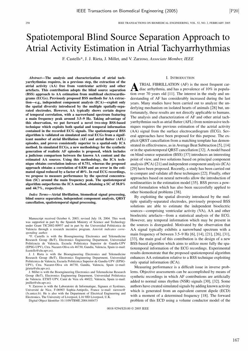
IEEE Transactions on Biomedical Engineering (2005) [P20]
258 IEEE TRANSACTIONS ON BIOMEDICAL ENGINEERING, VOL. 52, NO. 2, FEBRUARY 2005
Spatiotemporal Blind Source Separation Approach toAtrial Activity Estimation in Atrial Tachyarrhythmias
F. Castells*, J. J. Rieta, J. Millet, and V. Zarzoso, Associate Member, IEEE
Abstract—The analysis and characterization of atrial tach-yarrhythmias requires, in a previous step, the extraction of theatrial activity (AA) free from ventricular activity and otherartefacts. This contribution adopts the blind source separation(BSS) approach to AA estimation from multilead electrocardio-grams (ECGs). Previously proposed BSS methods for AA extrac-tion—e.g., independent component analysis (ICA)—exploit onlythe spatial diversity introduced by the multiple spatially-sepa-rated electrodes. However, AA typically shows certain degreeof temporal correlation, with a narrowband spectrum featuringa main frequency peak around 3.5–9 Hz. Taking advantage ofthis observation, we put forward a novel two-step BSS-basedtechnique which exploits both spatial and temporal informationcontained in the recorded ECG signals. The spatiotemporal BSSalgorithm is validated on simulated and real ECGs from a signif-icant number of atrial fibrillation (AF) and atrial flutter (AFL)episodes, and proves consistently superior to a spatial-only ICAmethod. In simulated ECGs, a new methodology for the syntheticgeneration of realistic AF episodes is proposed, which includesa judicious comparison between the known AA content and theestimated AA sources. Using this methodology, the ICA tech-nique obtains correlation indexes of 0.751, whereas the proposed
approach obtains a correlation of 0.830 and an error in the esti-mated signal reduced by a factor of 40%. In real ECG recordings,we propose to measure performance by the spectral concentra-tion (SC) around the main frequency peak. The spatiotemporalalgorithm outperforms the ICA method, obtaining a SC of 58.8%and 44.7%, respectively.
Index Terms—Atrial fibrillation, biomedical signal processing,blind source separation, independent component analysis, QRSTcancellation, spatiotemporal signal processing.
Manuscript received October 6, 2003; revised July 18, 2004. This workwas supported in part by the Spanish Ministry of Science and Technologyunder Grant TIC2002-00957 and in part by the Universidad Politécnica deValencia through a research incentive program. Asterisk indicates corre-
sponding author.
*F. Castells is with the Bioengineering Electronics and TelemedicineResearch Group (BeT), Electronics Engineering Department, UniversidadPolitécncia de Valencia, Escuela Politécnica Superior de Gandía-UPV(EPSG-UPV), Ctra. Nazaret-Oliva s/n 46730, Gandía, Valencia, Spain (e-mail:[email protected]).
J. J. Rieta is with the Bioengineering Electronics and TelemedicineResearch Group (BeT), Electronics Engineering Department, UniversidadPolitécnica de Valencia, Escuela Politécnica Superior de Gandía-UPV (EPSG-UPV), Ctra. Nazaret-Oliva s/n 46730, Gandía, Valencia, Spain (e-mail:[email protected]).
J. Millet is with the Bioengineering Electronics and Telemedicine ResearchGroup (BeT), Electronics Engineering Deparment, Universidad Politécnicade Valencia. ETSIT-UPV, Camí de Vera s/n 46022, Valencia, Spain (e-mail:[email protected]).
V. Zarzoso is with the Laboratoire de Informatique, Signaux et Systèmes,Université de Nice, F-06903 Sophia-Antipolis, France (e-mail: [email protected]). He is also with the Department of Electrical Engineering andElectronics, The University of Liverpool, L16 9JD Liverpool, U.K.
Digital Object Identifier 10.1109/TBME.2004.840473
I. INTRODUCTION
ATRIAL FIBRILLATION (AF) is the most frequent car-diac arrhythmia, and has a prevalence of 10% in popula-
tion over 70 years old [11]. The interest in the study and un-derstanding of AF has considerably increased during the lastyears. Many studies have been carried out to analyze the un-derlying mechanism on isolated hearts of animals [28] but, un-fortunately, these results are not directly applicable to humans.The analysis and characterization of AF and other atrial tach-yarrhythmias such as atrial flutter (AFL) from noninvasive tech-niques requires the previous estimation of the actrial activity(AA) signal from the surface electrocardiogram (ECG). Sev-eral approaches have been proposed for this purpose. The ex-plicit QRST cancellation from a matching template has demon-strated its effectiveness, as in Average Beat Subtraction [5], [14]or in the spatiotemporal QRST cancellation [32]. A model basedon blind source separation (BSS) [37] introduces an interestingpoint of view, and two solutions based on principal componentanalysis (PCA) [21] and independent component analysis (ICA)[29] have been proposed. Recently, a study has been carried outto compare and validate all these techniques [22]. Finally, otherapproaches based on neural networks allow the introduction ofnonlinearities in the estimation model [35]. BSS proves a pow-erful formulation which has also been successfully applied toother biomedical problems [38].
By exploiting the spatial diversity introduced by the mul-tiple spatially-separated electrodes, previously proposed BSSsolutions are able to estimate the independent bioelectricsources—comprising ventricular activity (VA), AA and otherbioelectric artefacts—from a statistical analysis of the ECG.However, any temporal information which may be present inthe sources is disregarded. Motivated by the observation thatAA signal typically exhibits a narrowband spectrum with amain frequency of between 3.5–9 Hz [6], [14], [21], [26], [31],[33], the main goal of this contribution is the design of a newBSS-based algorithm which aims to utilize more fully the spa-tiotemporal information of the ECG recordings. Experimentalresults demonstrate that the proposed spatiotemporal algorithmenhances AA estimation relative to a BSS technique exploitingonly spatial information (ICA).
Measuring performance is a difficult issue in inverse prob-
lems. Objective assessments can be accomplished by means of
synthetic recordings in which AF contributions are artificially
added to normal sinus rhythm (NSR) signals [30], [32]. Some
authors have created simulated signals by adding known activity
which is generated from an equivalent current dipole (ECD)
with a moment of a determined frequency [18]. The forward
problem of this ECD using a volume conductor model of the
0018-9294/$20.00 © 2005 IEEE
167
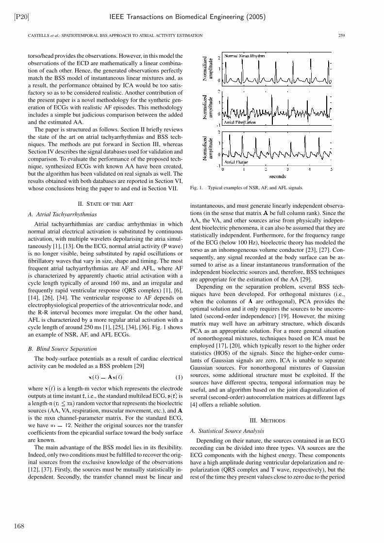
[P20] IEEE Transactions on Biomedical Engineering (2005)
CASTELLS et al.: SPATIOTEMPORAL BSS APPROACH TO ATRIAL ACTIVITY ESTIMATION 259
torso/head provides the observations. However, in this model the
observations of the ECD are mathematically a linear combina-
tion of each other. Hence, the generated observations perfectly
match the BSS model of instantaneous linear mixtures and, as
a result, the performance obtained by ICA would be too satis-
factory so as to be considered realistic. Another contribution of
the present paper is a novel methodology for the synthetic gen-
eration of ECGs with realistic AF episodes. This methodology
includes a simple but judicious comparison between the added
and the estimated AA.
The paper is structured as follows. Section II briefly reviews
the state of the art on atrial tachyarrhythmias and BSS tech-
niques. The methods are put forward in Section III, whereas
Section IV describes the signal databases used for validation and
comparison. To evaluate the performance of the proposed tech-
nique, synthesized ECGs with known AA have been created,
but the algorithm has been validated on real signals as well. The
results obtained with both databases are reported in Section VI,
whose conclusions bring the paper to and end in Section VII.
II. STATE OF THE ART
A. Atrial Tachyarrhythmias
Atrial tachyarrhithmias are cardiac arrhythmias in which
normal atrial electrical activation is substituted by continuous
activation, with multiple wavelets depolarising the atria simul-
taneously [1], [13]. On the ECG, normal atrial activity (P wave)
is no longer visible, being substituted by rapid oscillations or
fibrillatory waves that vary in size, shape and timing. The most
frequent atrial tachyarrhythmias are AF and AFL, where AF
is characterized by apparently chaotic atrial activation with a
cycle length typically of around 160 ms, and an irregular and
frequently rapid ventricular response (QRS complex) [1], [6],
[14], [26], [34]. The ventricular response to AF depends on
electrophysiological properties of the atrioventricular node, and
the R-R interval becomes more irregular. On the other hand,
AFL is characterized by a more regular atrial activation with a
cycle length of around 250 ms [1], [25], [34], [36]. Fig. 1 shows
an example of NSR, AF, and AFL ECGs.
B. Blind Source Separation
The body-surface potentials as a result of cardiac electrical
activity can be modeled as a BSS problem [29]
(1)
where is a length-m vector which represents the electrode
outputs at time instant , i.e., the standard multilead ECG, is
a length-n random vector that represents the bioelectric
sources (AA, VA, respiration, muscular movement, etc.), and
is the mxn channel-parameter matrix. For the standard ECG,
we have . Neither the original sources nor the transfer
coefficients from the epicardial surface toward the body surface
are known.
The main advantage of the BSS model lies in its flexibility.
Indeed, only two conditions must be fulfilled to recover the orig-
inal sources from the exclusive knowledge of the observations
[12], [37]. Firstly, the sources must be mutually statistically in-
dependent. Secondly, the transfer channel must be linear and
Fig. 1. Typical examples of NSR, AF, and AFL signals.
instantaneous, and must generate linearly independent observa-
tions (in the sense that matrix be full column rank). Since the
AA, the VA, and other sources arise from physically indepen-
dent bioelectric phenomena, it can also be assumed that they are
statistically independent. Furthermore, for the frequency range
of the ECG (below 100 Hz), bioelectric theory has modeled the
torso as an inhomogeneous volume conductor [23], [27]. Con-
sequently, any signal recorded at the body surface can be as-
sumed to arise as a linear instantaneous transformation of the
independent bioelectric sources and, therefore, BSS techniques
are appropriate for the estimation of the AA [29].
Depending on the separation problem, several BSS tech-
niques have been developed. For orthogonal mixtures (i.e.,
when the columns of are orthogonal), PCA provides the
optimal solution and it only requires the sources to be uncorre-
lated (second-order independence) [19]. However, the mixing
matrix may well have an arbitrary structure, which discards
PCA as an appropriate solution. For a more general situation
of nonorthogonal mixtures, techniques based on ICA must be
employed [17], [20], which typically resort to the higher order
statistics (HOS) of the signals. Since the higher-order cumu-
lants of Gaussian signals are zero, ICA is unable to separate
Gaussian sources. For nonorthogonal mixtures of Gaussian
sources, some additional structure must be exploited. If the
sources have different spectra, temporal information may be
useful, and an algorithm based on the joint diagonalization of
several (second-order) autocorrelation matrices at different lags
[4] offers a reliable solution.
III. METHODS
A. Statistical Source Analysis
Depending on their nature, the sources contained in an ECGrecording can be divided into three types. VA sources are theECG components with the highest energy. These componentshave a high amplitude during ventricular depolarization and re-polarization (QRS complex and T wave, respectively), but therest of the time they present values close to zero due to the period
168
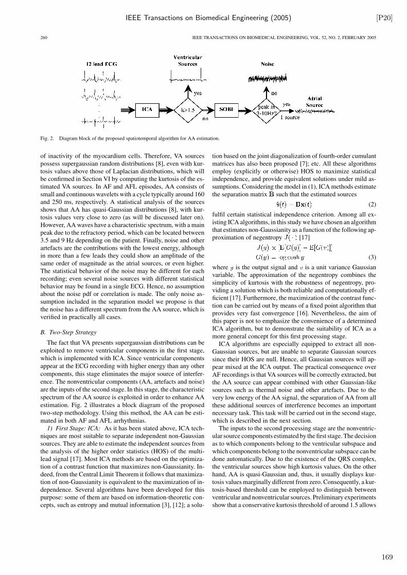
IEEE Transactions on Biomedical Engineering (2005) [P20]
260 IEEE TRANSACTIONS ON BIOMEDICAL ENGINEERING, VOL. 52, NO. 2, FEBRUARY 2005
Fig. 2. Diagram block of the proposed spatiotemporal algorithm for AA estimation.
of inactivity of the myocardium cells. Therefore, VA sourcespossess supergaussian random distributions [8], even with kur-tosis values above those of Laplacian distributions, which willbe confirmed in Section VI by computing the kurtosis of the es-timated VA sources. In AF and AFL episodes, AA consists ofsmall and continuous wavelets with a cycle typically around 160and 250 ms, respectively. A statistical analysis of the sourcesshows that AA has quasi-Gaussian distributions [8], with kur-tosis values very close to zero (as will be discussed later on).However, AA waves have a characteristic spectrum, with a mainpeak due to the refractory period, which can be located between3.5 and 9 Hz depending on the patient. Finally, noise and otherartefacts are the contributions with the lowest energy, althoughin more than a few leads they could show an amplitude of thesame order of magnitude as the atrial sources, or even higher.The statistical behavior of the noise may be different for eachrecording; even several noise sources with different statisticalbehavior may be found in a single ECG. Hence, no assumptionabout the noise pdf or correlation is made. The only noise as-sumption included in the separation model we propose is thatthe noise has a different spectrum from the AA source, which isverified in practically all cases.
B. Two-Step Strategy
The fact that VA presents supergaussian distributions can be
exploited to remove ventricular components in the first stage,
which is implemented with ICA. Since ventricular components
appear at the ECG recording with higher energy than any other
components, this stage eliminates the major source of interfer-
ence. The nonventricular components (AA, artefacts and noise)
are the inputs of the second stage. In this stage, the characteristic
spectrum of the AA source is exploited in order to enhance AA
estimation. Fig. 2 illustrates a block diagram of the proposed
two-step methodology. Using this method, the AA can be esti-
mated in both AF and AFL arrhythmias.1) First Stage: ICA: As it has been stated above, ICA tech-
niques are most suitable to separate independent non-Gaussiansources. They are able to estimate the independent sources fromthe analysis of the higher order statistics (HOS) of the multi-lead signal [17]. Most ICA methods are based on the optimiza-tion of a contrast function that maximizes non-Gaussianity. In-deed, from the Central Limit Theorem it follows that maximiza-tion of non-Gaussianity is equivalent to the maximization of in-dependence. Several algorithms have been developed for thispurpose: some of them are based on information-theoretic con-cepts, such as entropy and mutual information [3], [12]; a solu-
tion based on the joint diagonalization of fourth-order cumulantmatrices has also been proposed [7]; etc. All these algorithmsemploy (explicitly or otherwise) HOS to maximize statisticalindependence, and provide equivalent solutions under mild as-sumptions. Considering the model in (1), ICA methods estimatethe separation matrix such that the estimated sources
(2)
fulfil certain statistical independence criterion. Among all ex-isting ICA algorithms, in this study we have chosen an algorithmthat estimates non-Gaussianity as a function of the following ap-proximation of negentropy [17]
(3)
where is the output signal and is a unit variance Gaussianvariable. The approximation of the negentropy combines thesimplicity of kurtosis with the robustness of negentropy, pro-viding a solution which is both reliable and computationally ef-ficient [17]. Furthermore, the maximization of the contrast func-tion can be carried out by means of a fixed point algorithm thatprovides very fast convergence [16]. Nevertheless, the aim ofthis paper is not to emphasize the convenience of a determinedICA algorithm, but to demonstrate the suitability of ICA as amore general concept for this first processing stage.
ICA algorithms are especially equipped to extract all non-Gaussian sources, but are unable to separate Gaussian sourcessince their HOS are null. Hence, all Gaussian sources will ap-pear mixed at the ICA output. The practical consequence overAF recordings is that VA sources will be correctly extracted, butthe AA source can appear combined with other Gaussian-likesources such as thermal noise and other artefacts. Due to thevery low energy of the AA signal, the separation of AA from allthese additional sources of interference becomes an importantnecessary task. This task will be carried out in the second stage,which is described in the next section.
The inputs to the second processing stage are the nonventric-ular source components estimated by the first stage. The decisionas to which components belong to the ventricular subspace andwhich components belong to the nonventricular subspace can bedone automatically. Due to the existence of the QRS complex,the ventricular sources show high kurtosis values. On the otherhand, AA is quasi-Gaussian and, thus, it usually displays kur-tosis values marginally different from zero. Consequently, a kur-tosis-based threshold can be employed to distinguish betweenventricular and nonventricular sources. Preliminary experimentsshow that a conservative kurtosis threshold of around 1.5 allows
169
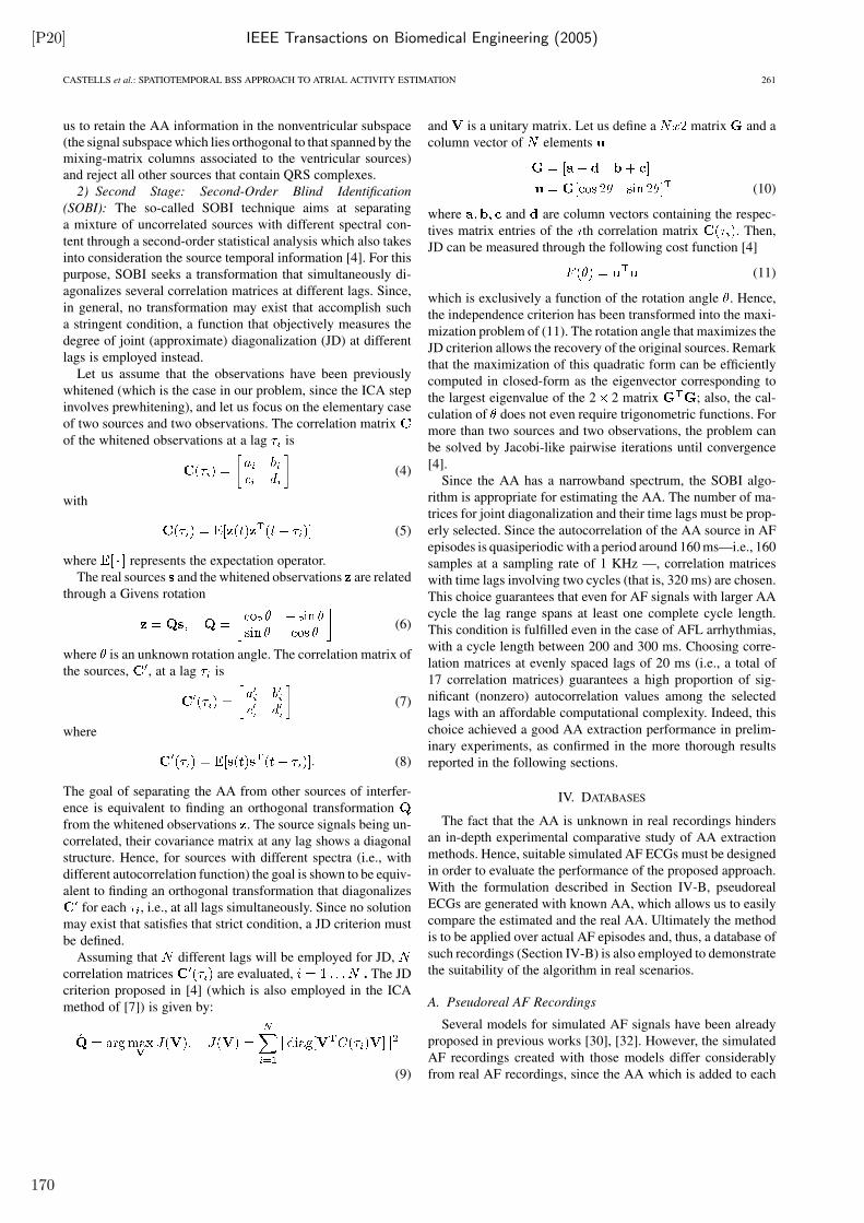
[P20] IEEE Transactions on Biomedical Engineering (2005)
CASTELLS et al.: SPATIOTEMPORAL BSS APPROACH TO ATRIAL ACTIVITY ESTIMATION 261
us to retain the AA information in the nonventricular subspace(the signal subspace which lies orthogonal to that spanned by themixing-matrix columns associated to the ventricular sources)and reject all other sources that contain QRS complexes.
2) Second Stage: Second-Order Blind Identification
(SOBI): The so-called SOBI technique aims at separating
a mixture of uncorrelated sources with different spectral con-
tent through a second-order statistical analysis which also takes
into consideration the source temporal information [4]. For this
purpose, SOBI seeks a transformation that simultaneously di-
agonalizes several correlation matrices at different lags. Since,
in general, no transformation may exist that accomplish such
a stringent condition, a function that objectively measures the
degree of joint (approximate) diagonalization (JD) at different
lags is employed instead.
Let us assume that the observations have been previously
whitened (which is the case in our problem, since the ICA step
involves prewhitening), and let us focus on the elementary case
of two sources and two observations. The correlation matrix
of the whitened observations at a lag is
(4)
with
(5)
where represents the expectation operator.
The real sources and the whitened observations are related
through a Givens rotation
(6)
where is an unknown rotation angle. The correlation matrix of
the sources, , at a lag is
(7)
where
(8)
The goal of separating the AA from other sources of interfer-
ence is equivalent to finding an orthogonal transformation
from the whitened observations . The source signals being un-
correlated, their covariance matrix at any lag shows a diagonal
structure. Hence, for sources with different spectra (i.e., with
different autocorrelation function) the goal is shown to be equiv-
alent to finding an orthogonal transformation that diagonalizes
for each , i.e., at all lags simultaneously. Since no solution
may exist that satisfies that strict condition, a JD criterion must
be defined.
Assuming that different lags will be employed for JD,
correlation matrices are evaluated, . The JD
criterion proposed in [4] (which is also employed in the ICA
method of [7]) is given by:
(9)
and is a unitary matrix. Let us define a matrix and a
column vector of elements
(10)
where and are column vectors containing the respec-
tives matrix entries of the th correlation matrix . Then,
JD can be measured through the following cost function [4]
(11)
which is exclusively a function of the rotation angle . Hence,
the independence criterion has been transformed into the maxi-
mization problem of (11). The rotation angle that maximizes the
JD criterion allows the recovery of the original sources. Remark
that the maximization of this quadratic form can be efficiently
computed in closed-form as the eigenvector corresponding to
the largest eigenvalue of the 2 2 matrix ; also, the cal-
culation of does not even require trigonometric functions. For
more than two sources and two observations, the problem can
be solved by Jacobi-like pairwise iterations until convergence
[4].
Since the AA has a narrowband spectrum, the SOBI algo-
rithm is appropriate for estimating the AA. The number of ma-
trices for joint diagonalization and their time lags must be prop-
erly selected. Since the autocorrelation of the AA source in AF
episodes is quasiperiodic with a period around 160 ms—i.e., 160
samples at a sampling rate of 1 KHz —, correlation matrices
with time lags involving two cycles (that is, 320 ms) are chosen.
This choice guarantees that even for AF signals with larger AA
cycle the lag range spans at least one complete cycle length.
This condition is fulfilled even in the case of AFL arrhythmias,
with a cycle length between 200 and 300 ms. Choosing corre-
lation matrices at evenly spaced lags of 20 ms (i.e., a total of
17 correlation matrices) guarantees a high proportion of sig-
nificant (nonzero) autocorrelation values among the selected
lags with an affordable computational complexity. Indeed, this
choice achieved a good AA extraction performance in prelim-
inary experiments, as confirmed in the more thorough results
reported in the following sections.
IV. DATABASES
The fact that the AA is unknown in real recordings hinders
an in-depth experimental comparative study of AA extraction
methods. Hence, suitable simulated AF ECGs must be designed
in order to evaluate the performance of the proposed approach.
With the formulation described in Section IV-B, pseudoreal
ECGs are generated with known AA, which allows us to easily
compare the estimated and the real AA. Ultimately the method
is to be applied over actual AF episodes and, thus, a database of
such recordings (Section IV-B) is also employed to demonstrate
the suitability of the algorithm in real scenarios.
A. Pseudoreal AF Recordings
Several models for simulated AF signals have been already
proposed in previous works [30], [32]. However, the simulated
AF recordings created with those models differ considerably
from real AF recordings, since the AA which is added to each
170
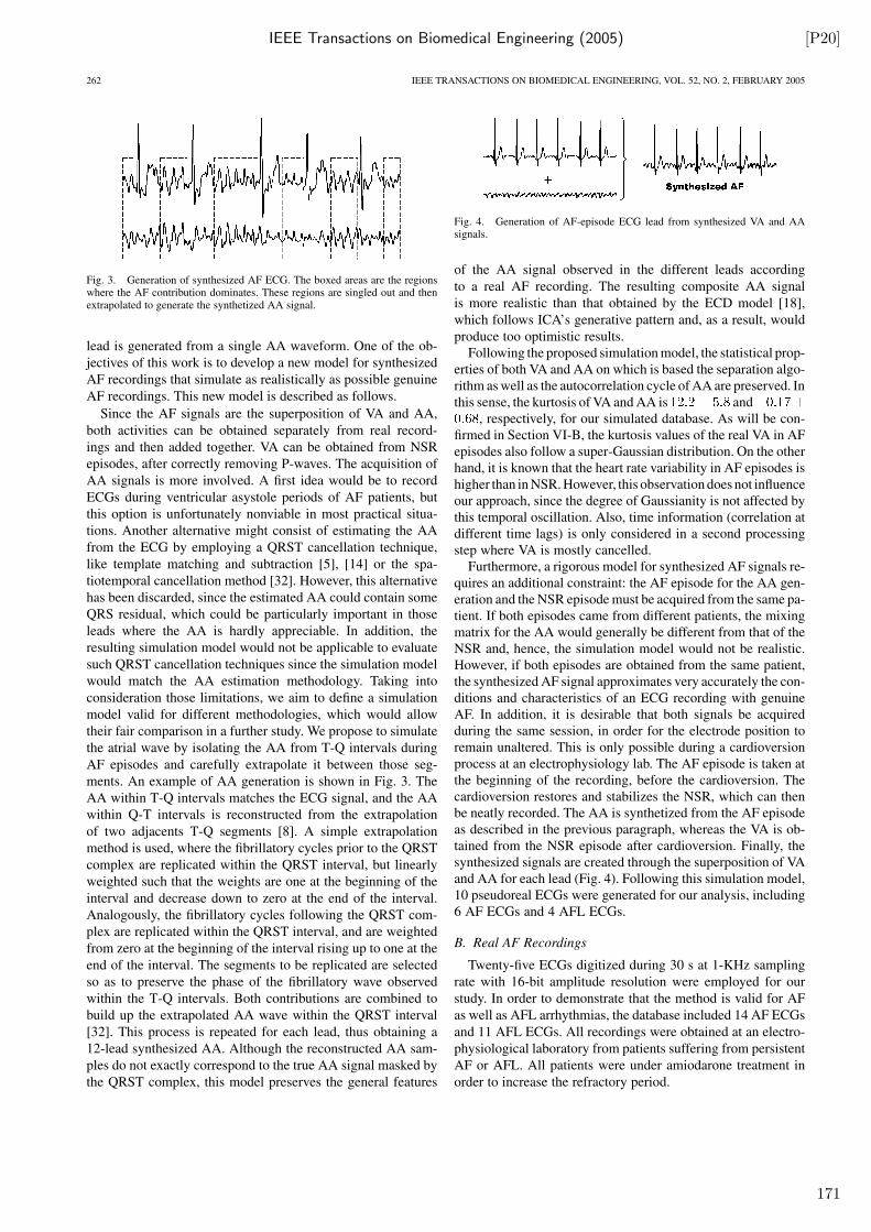
IEEE Transactions on Biomedical Engineering (2005) [P20]
262 IEEE TRANSACTIONS ON BIOMEDICAL ENGINEERING, VOL. 52, NO. 2, FEBRUARY 2005
Fig. 3. Generation of synthesized AF ECG. The boxed areas are the regionswhere the AF contribution dominates. These regions are singled out and thenextrapolated to generate the synthetized AA signal.
lead is generated from a single AA waveform. One of the ob-
jectives of this work is to develop a new model for synthesized
AF recordings that simulate as realistically as possible genuine
AF recordings. This new model is described as follows.
Since the AF signals are the superposition of VA and AA,
both activities can be obtained separately from real record-
ings and then added together. VA can be obtained from NSR
episodes, after correctly removing P-waves. The acquisition of
AA signals is more involved. A first idea would be to record
ECGs during ventricular asystole periods of AF patients, but
this option is unfortunately nonviable in most practical situa-
tions. Another alternative might consist of estimating the AA
from the ECG by employing a QRST cancellation technique,
like template matching and subtraction [5], [14] or the spa-
tiotemporal cancellation method [32]. However, this alternative
has been discarded, since the estimated AA could contain some
QRS residual, which could be particularly important in those
leads where the AA is hardly appreciable. In addition, the
resulting simulation model would not be applicable to evaluate
such QRST cancellation techniques since the simulation model
would match the AA estimation methodology. Taking into
consideration those limitations, we aim to define a simulation
model valid for different methodologies, which would allow
their fair comparison in a further study. We propose to simulate
the atrial wave by isolating the AA from T-Q intervals during
AF episodes and carefully extrapolate it between those seg-
ments. An example of AA generation is shown in Fig. 3. The
AA within T-Q intervals matches the ECG signal, and the AA
within Q-T intervals is reconstructed from the extrapolation
of two adjacents T-Q segments [8]. A simple extrapolation
method is used, where the fibrillatory cycles prior to the QRST
complex are replicated within the QRST interval, but linearly
weighted such that the weights are one at the beginning of the
interval and decrease down to zero at the end of the interval.
Analogously, the fibrillatory cycles following the QRST com-
plex are replicated within the QRST interval, and are weighted
from zero at the beginning of the interval rising up to one at the
end of the interval. The segments to be replicated are selected
so as to preserve the phase of the fibrillatory wave observed
within the T-Q intervals. Both contributions are combined to
build up the extrapolated AA wave within the QRST interval
[32]. This process is repeated for each lead, thus obtaining a
12-lead synthesized AA. Although the reconstructed AA sam-
ples do not exactly correspond to the true AA signal masked by
the QRST complex, this model preserves the general features
Fig. 4. Generation of AF-episode ECG lead from synthesized VA and AAsignals.
of the AA signal observed in the different leads according
to a real AF recording. The resulting composite AA signal
is more realistic than that obtained by the ECD model [18],
which follows ICA’s generative pattern and, as a result, would
produce too optimistic results.Following the proposed simulation model, the statistical prop-
erties of both VA and AA on which is based the separation algo-rithm as well as the autocorrelation cycle of AA are preserved. Inthis sense, the kurtosis of VA and AA is and
, respectively, for our simulated database. As will be con-firmed in Section VI-B, the kurtosis values of the real VA in AFepisodes also follow a super-Gaussian distribution. On the otherhand, it is known that the heart rate variability in AF episodes ishigher than in NSR. However, this observation does not influenceour approach, since the degree of Gaussianity is not affected bythis temporal oscillation. Also, time information (correlation atdifferent time lags) is only considered in a second processingstep where VA is mostly cancelled.
Furthermore, a rigorous model for synthesized AF signals re-quires an additional constraint: the AF episode for the AA gen-eration and the NSR episode must be acquired from the same pa-tient. If both episodes came from different patients, the mixingmatrix for the AA would generally be different from that of theNSR and, hence, the simulation model would not be realistic.However, if both episodes are obtained from the same patient,the synthesized AF signal approximates very accurately the con-ditions and characteristics of an ECG recording with genuineAF. In addition, it is desirable that both signals be acquiredduring the same session, in order for the electrode position toremain unaltered. This is only possible during a cardioversionprocess at an electrophysiology lab. The AF episode is taken atthe beginning of the recording, before the cardioversion. Thecardioversion restores and stabilizes the NSR, which can thenbe neatly recorded. The AA is synthetized from the AF episodeas described in the previous paragraph, whereas the VA is ob-tained from the NSR episode after cardioversion. Finally, thesynthesized signals are created through the superposition of VAand AA for each lead (Fig. 4). Following this simulation model,10 pseudoreal ECGs were generated for our analysis, including6 AF ECGs and 4 AFL ECGs.
B. Real AF Recordings
Twenty-five ECGs digitized during 30 s at 1-KHz sampling
rate with 16-bit amplitude resolution were employed for our
study. In order to demonstrate that the method is valid for AF
as well as AFL arrhythmias, the database included 14 AF ECGs
and 11 AFL ECGs. All recordings were obtained at an electro-
physiological laboratory from patients suffering from persistent
AF or AFL. All patients were under amiodarone treatment in
order to increase the refractory period.
171
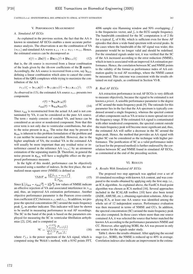
[P20] IEEE Transactions on Biomedical Engineering (2005)
CASTELLS et al.: SPATIOTEMPORAL BSS APPROACH TO ATRIAL ACTIVITY ESTIMATION 263
V. PERFORMANCE MEASUREMENT
A. Simulated AF ECGs
As explained in the previous section, the fact that the AA is
known in simulated AF ECGs enables a more accurate perfor-
mance analysis. The observations are the combination of VA
and simulated AA waves . Hence,
the estimated sources can be decomposed as
(12)
that is, the th source is recovered from a linear combination
of the leads given by the th-row coefficients of the matrix.
Accordingly, the AA source is recovered from a row, say ,
defining a linear combination which aims to cancel the contri-
bution of the QRS complexes while trying to maximize the con-
tribution of the AA
(13)
As observed in (13), the estimated AA source presents two
components
(14)
Since is reconstructed from the actual AA and is not con-
taminated by VA, it can be considered as the pure AA source.
The term mainly consists of residual VA, and hence can be
considered as an error or nondesired component. Note that this
error term is not only due to ventricular contributions, but also
to the noise present in . The noise that may be present in
is inherent to this problem formulation of the problem and
it can neither be measured nor cancelled. However, due to the
higher amplitude of VA, the residual VA in the estimated AA
will usually be more important than any residual noise or in-
terference caused in the reference AA by an erroneous
estimation of the separating matrix . Therefore, in general the
noise present in will have a negligible effect on the pro-
posed performance measure.
In the light of this model, performance can be objectively
measured using a number of indexes. In the first place, the nor-
malized mean square error (NMSE) is defined as
(15)
Since , low values of NMSE indicate
an effective rejection of VA and associated interference in
and, thus, an improved AA estimation performance. Another
objective performance parameter is the Pearson cross-correla-
tion coefficient (CC) between and . In addition, we pro-
pose the spectral concentration (SC) around the main frequency
peak as another indicator. This indicator will later be shown
to be useful in measuring performance in real AF recordings.
The SC in the band of the peak is based on the parameters em-
ployed for measuring the SC in ventricular fibrillation arrhyth-
mias [2], [24], and is computed as
(16)
where is the power spectrum of the AA signal, which is
computed using the Welch’s method, with a 8192 points FFT,
4096 sample size Hamming window and 50% overlapping;
is the frequencies vector, and is the ECG sample frequency.
The bandwidth considered for the SC computation is of 2 Hz
for a typical of 6 Hz, which is sufficient even for those AF
episodes that show a wide-band spectrum with several peaks. In
the cases where the bandwidth of the AF signal was wider, this
parameter would be no longer valid and should be redefined.
For the simulated signals under test, it was verified that the SC
of the AA increased according to the error reduction (NMSE),
which in turn is associated with an improved AA estimation per-
formance. Hence, the correlation between SC and NMSE points
to the validity of the former as performance index of AA esti-
mation quality in real AF recordings, where the NMSE cannot
be measured. This outcome was consistent with the results ob-
tained on real signals, as confirmed in Section VI-B.
B. Real AF ECGs
AA extraction performance in real AF ECGs is very difficult
to measure objectively, because the signal to be estimated is not
known a priori. A sensible performance parameter is the degree
of SC around the main frequency peak [9]. The rationale for this
parameter lies in the fact that the AA spectrum is typically con-
densed around a single frequency, whereas the spectral content
of other components such as VA or noise is more spread out over
the frequency range. If the estimated AA signal is contaminated
with other nondesired components, the spectral content outside
the main frequency peak will become more significant and, thus,
the estimated AA will suffer a decrease in the SC around the
main peak. Hence, the method that provides an AA signal with
higher SC can be considered as the technique with higher per-
formance. The justification of SC as a valid performance index
(at least for the proposed method) is further endorsed by the cor-
relation between SC and NMSE found in simulated AF ECGs,
as commented at the end of the preceding section.
VI. RESULTS
A. Results With Simulated AF ECGs
The proposed two step approach was applied over a set of
10 simulated recordings with known AA content, and was com-
pared to the results obtained by applying only the first step, i.e.,
an ICA algorithm. As explained above, the FastICA fixed-point
algorithm was chosen as ICA method [16]. Several approaches
included in the ICALAB toolbox [10] have also been tested
(JADE, AMUSE, etc.), obtaining equivalent solutions. After ap-
plying ICA, at least one AA source was identified among the
whole set of 12 independent sources. Performance evaluation
was then measured in terms of NMSE and CCs. In addition,
the spectral concentration (SC) around the main frequency peak
was also computed. In those cases where more than one source
contained AA, it was selected the source that better matched the
known AA according to the performance parameters NMSE and
CC. However, after applying SOBI, the AA was present in only
one source for the signals under study.
Table I. shows the results obtained. After applying the second
stage (i.e., SOBI), the NMSE is reduced up to 40% in average.
Correlation indexes also indicate an improvement in the estima-
172
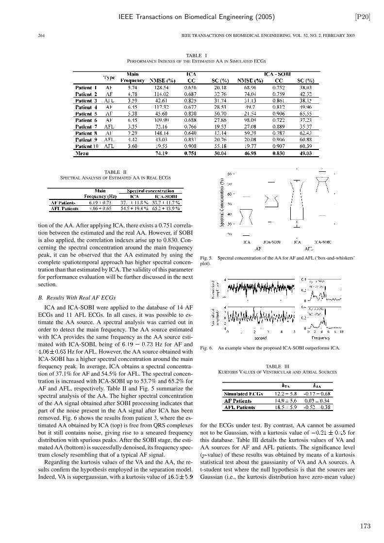
IEEE Transactions on Biomedical Engineering (2005) [P20]
264 IEEE TRANSACTIONS ON BIOMEDICAL ENGINEERING, VOL. 52, NO. 2, FEBRUARY 2005
TABLE IPERFORMANCE INDEXES OF THE ESTIMATED AA IN SIMULATED ECGS
TABLE IISPECTRAL ANALYSIS OF ESTIMATED AA IN REAL ECGS
tion of the AA. After applying ICA, there exists a 0.751 correla-
tion between the estimated and the real AA. However, if SOBI
is also applied, the correlation indexes arise up to 0.830. Con-
cerning the spectral concentration around the main frequency
peak, it can be observed that the AA estimated by using the
complete spatiotemporal approach has higher spectral concen-
tration than that estimated by ICA. The validity of this parameter
for performance evaluation will be further discussed in the next
section.
B. Results With Real AF ECGs
ICA and ICA-SOBI were applied to the database of 14 AF
ECGs and 11 AFL ECGs. In all cases, it was possible to es-
timate the AA source. A spectral analysis was carried out in
order to detect the main frequency. The AA source estimated
with ICA provides the same frequency as the AA source esti-
mated with ICA-SOBI, being of Hz for AF and
Hz for AFL. However, the AA source obtained with
ICA-SOBI has a higher spectral concentration around the main
frequency peak. In average, ICA obtains a spectral concentra-
tion of 37.1% for AF and 54.5% for AFL. The spectral concen-
tration is increased with ICA-SOBI up to 53.7% and 65.2% for
AF and AFL, respectively. Table II and Fig. 5 summarize the
spectral analysis of the AA. The higher spectral concentration
of the AA signal obtained after SOBI processing indicates that
part of the noise present in the AA signal after ICA has been
removed. Fig. 6 shows the results from patient 3, where the es-
timated AA obtained by ICA (top) is free from QRS complexes
but it still contains noise, giving rise to a smeared frequency
distribution with spurious peaks. After the SOBI stage, the esti-
mated AA (bottom) is successfully denoised, its frequency spec-
trum closely resembling that of a typical AF signal.
Regarding the kurtosis values of the VA and the AA, the re-
sults confirm the hypothesis employed in the separation model.
Indeed, VA is supergaussian, with a kurtosis value of
Fig. 5. Spectral concentration of the AA for AF and AFL (‘box-and-whiskers’plot).
Fig. 6. An example where the proposed ICA-SOBI outperforms ICA.
TABLE IIIKURTOSIS VALUES OF VENTRICULAR AND ATRIAL SOURCES
for the ECGs under test. By contrast, AA cannot be assumed
not to be Gaussian, with a kurtosis value of for
this database. Table III details the kurtosis values of VA and
AA sources for AF and AFL patients. The significance level
( -value) of these results was obtained by means of a kurtosis
statistical test about the gaussianity of VA and AA sources. A
t-student test where the null hypothesis is that the sources are
Gaussian (i.e., the kurtosis distribution have zero-mean value)
173
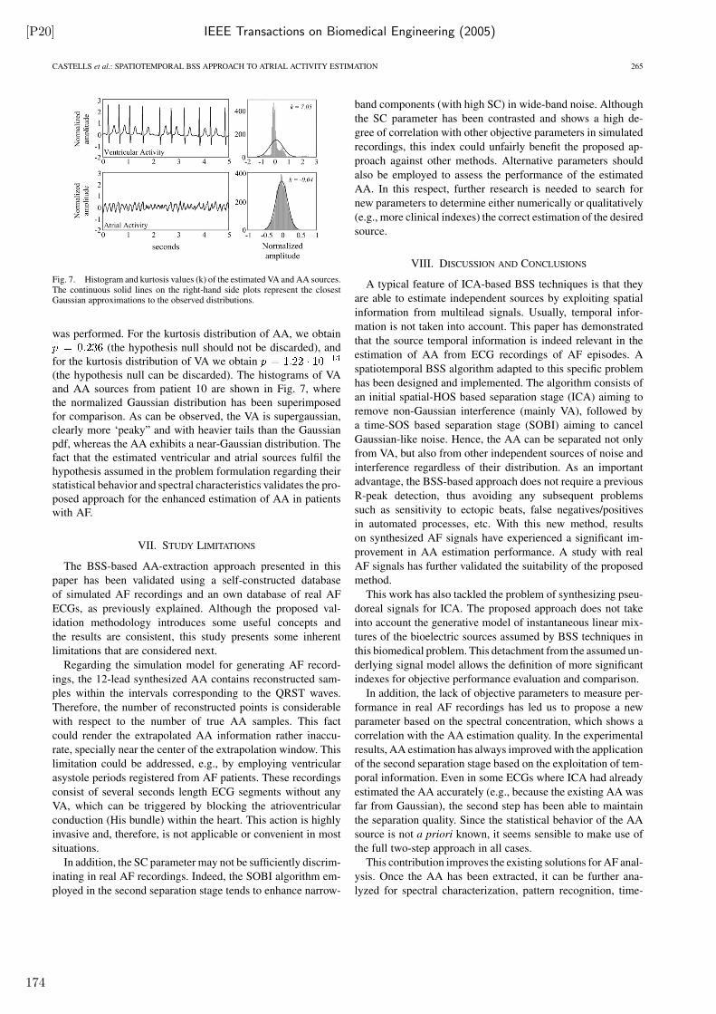
[P20] IEEE Transactions on Biomedical Engineering (2005)
CASTELLS et al.: SPATIOTEMPORAL BSS APPROACH TO ATRIAL ACTIVITY ESTIMATION 265
Fig. 7. Histogram and kurtosis values (k) of the estimated VA and AA sources.The continuous solid lines on the right-hand side plots represent the closestGaussian approximations to the observed distributions.
was performed. For the kurtosis distribution of AA, we obtain
(the hypothesis null should not be discarded), and
for the kurtosis distribution of VA we obtain
(the hypothesis null can be discarded). The histograms of VA
and AA sources from patient 10 are shown in Fig. 7, where
the normalized Gaussian distribution has been superimposed
for comparison. As can be observed, the VA is supergaussian,
clearly more ‘peaky” and with heavier tails than the Gaussian
pdf, whereas the AA exhibits a near-Gaussian distribution. The
fact that the estimated ventricular and atrial sources fulfil the
hypothesis assumed in the problem formulation regarding their
statistical behavior and spectral characteristics validates the pro-
posed approach for the enhanced estimation of AA in patients
with AF.
VII. STUDY LIMITATIONS
The BSS-based AA-extraction approach presented in this
paper has been validated using a self-constructed database
of simulated AF recordings and an own database of real AF
ECGs, as previously explained. Although the proposed val-
idation methodology introduces some useful concepts and
the results are consistent, this study presents some inherent
limitations that are considered next.
Regarding the simulation model for generating AF record-
ings, the 12-lead synthesized AA contains reconstructed sam-
ples within the intervals corresponding to the QRST waves.
Therefore, the number of reconstructed points is considerable
with respect to the number of true AA samples. This fact
could render the extrapolated AA information rather inaccu-
rate, specially near the center of the extrapolation window. This
limitation could be addressed, e.g., by employing ventricular
asystole periods registered from AF patients. These recordings
consist of several seconds length ECG segments without any
VA, which can be triggered by blocking the atrioventricular
conduction (His bundle) within the heart. This action is highly
invasive and, therefore, is not applicable or convenient in most
situations.
In addition, the SC parameter may not be sufficiently discrim-
inating in real AF recordings. Indeed, the SOBI algorithm em-
ployed in the second separation stage tends to enhance narrow-
band components (with high SC) in wide-band noise. Although
the SC parameter has been contrasted and shows a high de-
gree of correlation with other objective parameters in simulated
recordings, this index could unfairly benefit the proposed ap-
proach against other methods. Alternative parameters should
also be employed to assess the performance of the estimated
AA. In this respect, further research is needed to search for
new parameters to determine either numerically or qualitatively
(e.g., more clinical indexes) the correct estimation of the desired
source.
VIII. DISCUSSION AND CONCLUSIONS
A typical feature of ICA-based BSS techniques is that they
are able to estimate independent sources by exploiting spatial
information from multilead signals. Usually, temporal infor-
mation is not taken into account. This paper has demonstrated
that the source temporal information is indeed relevant in the
estimation of AA from ECG recordings of AF episodes. A
spatiotemporal BSS algorithm adapted to this specific problem
has been designed and implemented. The algorithm consists of
an initial spatial-HOS based separation stage (ICA) aiming to
remove non-Gaussian interference (mainly VA), followed by
a time-SOS based separation stage (SOBI) aiming to cancel
Gaussian-like noise. Hence, the AA can be separated not only
from VA, but also from other independent sources of noise and
interference regardless of their distribution. As an important
advantage, the BSS-based approach does not require a previous
R-peak detection, thus avoiding any subsequent problems
such as sensitivity to ectopic beats, false negatives/positives
in automated processes, etc. With this new method, results
on synthesized AF signals have experienced a significant im-
provement in AA estimation performance. A study with real
AF signals has further validated the suitability of the proposed
method.
This work has also tackled the problem of synthesizing pseu-
doreal signals for ICA. The proposed approach does not take
into account the generative model of instantaneous linear mix-
tures of the bioelectric sources assumed by BSS techniques in
this biomedical problem. This detachment from the assumed un-
derlying signal model allows the definition of more significant
indexes for objective performance evaluation and comparison.
In addition, the lack of objective parameters to measure per-
formance in real AF recordings has led us to propose a new
parameter based on the spectral concentration, which shows a
correlation with the AA estimation quality. In the experimental
results, AA estimation has always improved with the application
of the second separation stage based on the exploitation of tem-
poral information. Even in some ECGs where ICA had already
estimated the AA accurately (e.g., because the existing AA was
far from Gaussian), the second step has been able to maintain
the separation quality. Since the statistical behavior of the AA
source is not a priori known, it seems sensible to make use of
the full two-step approach in all cases.
This contribution improves the existing solutions for AF anal-
ysis. Once the AA has been extracted, it can be further ana-
lyzed for spectral characterization, pattern recognition, time-
174
IEEE Transactions on Biomedical Engineering (2005) [P20]
266 IEEE TRANSACTIONS ON BIOMEDICAL ENGINEERING, VOL. 52, NO. 2, FEBRUARY 2005
frequency parameter extraction, etc. Some clinical applications
derived from the AA analysis could involve, e.g., the prediction
of AF recurrence after successful cardioversion. A significant
number of patients return to sustained AF in few days after elec-
trical cardioversion. The analysis of the AA could contribute to
the prediction of AF recurrence in order to prevent some pa-
tients from suffering ineffective electrical discharges. Other in-
teresting application could be based on the analysis of parox-
ysmal AF (PAF), which appears and terminates spontaneously.
It is commonly accepted that PAF is a precursor of persistent
AF. Improved knowledge about the mechanisms that cause PAF
and its spontaneous termination may introduce improvements in
the treatment of AF. The proposed methodology, thus, emerges
as a helpful tool in clinical diagnosis.
ACKNOWLEDGMENT
The authors would like to acknowledge the helpful support
received from Servicio de Hemodinámica of the Hospital
Clínico Universitario the Valencia, and specially from R. Ruiz,
S. Morell, and R. García Civera, for providing signals and for
the high quality of their clinical advice. V. Zarzoso has carried
out part of this research work while on leave at Laboratoire I3S,
Universite de Nice—Sophia Antipolis, France. He gratefully
acknowledges Dr. P. Comon for his kind hospitality.
REFERENCES
[1] M. Allessie, K. Konings, and M. Wijffels, Atrial Arrhythmias—State
of the Art: Electrophysiological Mechanism of Atrial Fibrillation, J. P.DiMarco and E. N. Prystowsky, Eds. Armonk, NY: Futura, 1995.
[2] S. Barro, R. Ruiz, D. Cabello, and J. Mira, “Algorithmic sequential de-cision-making in the frequency domain for life threatening ventriculararrhythmias and imitative artefacts: A diagnostic system,” J. Biomed.
Eng., vol. 11, pp. 320–328, 1989.[3] A. J. Bell and T. J. Sejnowsky, “An information maximization approach
to blind separation and blind deconvolution,” Neural Computation, vol.7, pp. 1129–1159, 1995.
[4] A. Belouchrani, K. Abed-Meraim, J. F. Cardoso, and E. Moulines, “Ablind source separation technique using second-order statistics,” IEEE
Trans. Signal Process., vol. 45, no. 2, pp. 434–444, Feb. 1997.[5] A. Bollmann, N. K. Kanuru, K. K. McTeague, P. F. Walter, D. B.
DeLurgio, and J. J. Langberg, “Frequency analysis of human atrialfibrillation using the surface electrocardiogram and its response toibutilide,” Am. J. Cardiol., vol. 81, pp. 1439–1445, 1998.
[6] A. Bollmann, K. Sonne, H. D. Esperer, I. Toepffer, J. J. Langberg, andH. U. Klein, “Non-invasive assessment of fibrillatory activity in patientswith paroxysmal and persistent atrial fibrillation using the Holter ECG,”Cardiovasc Res., vol. 44, pp. 60–6, 1999.
[7] J. F. Cardoso and A. Souloumiac, “Blind beamforming for non Gaussiansignals,” Inst. Elect. Eng. Proc.-F, vol. 140, pp. 362–370, 1993.
[8] F. Castells, J. Igual, J. J. Rieta, C. Sánchez, and J. Millet, “Atrial fib-rillation análisis based on ICA including statistical and temporal sourceinformation,” in Proc ICASSP, Hong Kong, 2003. V-94-96.
[9] F. Castells, R. Ruiz, J. J. Rieta, and J. Millet, “An integral atrial waveidentification based on spatiotemporal source separation: Clinical vali-dation,” Comput. Cardiol., pp. 717–720, 2003.
[10] A. Cichocki, S. Amari, and K. Siwek, “ICALAB Toolboxes,”, [Online].Available: http://www.bsp.brain.riken.go.jp/ICALAB, 2003.
[11] S. S. Chugh, J. L. Blackshear, W. K. Shen, S. C. Hammill, and B. J.Gersh, “Epidemiology and natural history of atrial fibrillation: Clinicalimplications,” J. Am. Coll. Cardiol., vol. 37, pp. 371–378, 2001.
[12] P. Comon, “Independent component analysis—A new concept?,” inSignal Process., vol. 36, 1994, pp. 287–314.
[13] V. Fuster et al., “ACC/AHA/ESC guidelines for the management ofpatients with atrial fibrillation,” J. Am. Coll. Cardiol., vol. 38, pp.1231–1265, 2001.
[14] M. Holm, S. Pehrson, M. Ingemansson, L. Sornmo, R. Jahansson, L.Sandhall, M. Sunemark, B. Smideberg, C. Olsson, and S. B. Olsson,“Non-invasive assessment of the atrial cycle length during atrial fib-rillation in man: Introducing, validating, and illustrating a new ECGmethod,” Cardiovasc Res., vol. 38, pp. 69–81, 1998.
[15] The FastICA Package, [Online]. Available: http://www.cis.hut.fi/projects/ica/fastica/, 1998.
[16] A. Hyvärinen, “Fast and robust fixed-point algorithms for independentcomponent analysis,” IEEE Trans. Neural Networks, vol. 10, no. 3, pp.626–634, May 1999.
[17] A. Hyvärinen, J. Karhunen, and E. Oja, Independent Component Anal-
ysis. New York: Wiley, 2001.[18] C. James, D. Lowe, and O. Gibson, “An objective study into single vs
multiple channel brain signal analysis using realistic ictal EEG,” in Proc.
NNESMED, Sheffield, 2003, pp. 139–144.[19] I. T. Joliffe, Principal Component Analysis. Berlin, Germany:
Springer-Verlag, 2002.[20] C. Jutten and J. Hérault, “Blind separation of sources, part I: An adaptive
algorithm based on neuromimetic architecture,” Signal Process., vol. 24,pp. 1–10, 1991.
[21] P. Langley, J. P. Bourke, and A. Murray, “Frequency analysis of atrialfibrillation,” Comput. Cardiol., pp. 65–68, 2000.
[22] P. Langley, J. J. Rieta, M. Stridh, J. Millet, L. Sornmo, and A. Murray,“Comparison of atrial signals derived from the 12-lead ECG using atrialsignal extraction techniques,” Comput. Cardiol., pp. 129–132, 2003.
[23] J. Malmivuo and R. Plonsey, Bioelectromagnetism. New York: OxfordUniv. Press, 1995.
[24] F. M. Nolle, R. W. Bowser, and F. K. Badura, “Evaluation of a fre-quency-domain algorithm to detect ventricular fibrillation in the surfaceelectrocardiogram,” Comput. Cardiol., pp. 337–340, 1989.
[25] B. Olshansky, K. Okumura, R. W. Henthorn, and A. L. Waldo, “Char-acterization of double potentials in human atrial flutter: Studies duringtransient entrainment,” J Am. Coll. Cardiol., vol. 15, no. 4, pp. 833–841,Mar. 15, 1990.
[26] S. Pehrson, M. Holm, C. Meurling, M. Ingemansson, B. Smideberg, L.Sornmo, and S. B. Olsson, “Non-invasive assessment of magnitude anddispersion of atrial cycle length during chronic atrial fibrillation in man,”Eur. Heart J., vol. 19, pp. 1836–1844, 1998.
[27] R. Plonsey, Bioelectric Phenomena. New York: McGraw-Hill, 1969.[28] P. L. Rensma, M. A. Allessie, W. J. E. P. Lammers, F. I. M. Bonke, and
M. J. Schalij, “Length of excitation wave and susceptibility to reentrantatrial arrhythmias in normal conscious dogs,” Circ. Res., vol. 62, pp.395–410, 1988.
[29] J. J. Rieta, F. Castells, C. Sánchez, and V. Zarzoso, “Atrial activityextraction for atrial fibrillation analysis using blind source separa-tion,” IEEE Trans. Biomed. Eng., vol. 51, no. 7, pp. 1176–1186, Jul.2004.
[30] J. J. Rieta, V. Zarzoso, J. Millet-Roig, R. García-Civera, and R. Ruiz-Granell, “Atrial activity extraction based on blind source separation as analternative to QRST cancellation for atrial fibrillation analysis,” Comput.
Cardiol., pp. 69–72, Sep. 2000.[31] J. Slocum, A. Sahakian, and S. Swiryn, “Diagnosis of atrial fibrillation
from surface electrocardiograms based on computer-detected atrial ac-tivity,” J. Electrocardiol., vol. 25, pp. 1–8, 1992.
[32] M. Stridh and L. Sörnmo, “Spatiotemporal QRST cancellation tech-niques for analysis of atrial fibrillation,” IEEE Trans. Biomed. Eng., vol.48, no. 1, pp. 105–111, Jan. 2001.
[33] M. Stridh, L. Sörnmo, C. Meurling, and B. Olsson, “Characterizationof atrial fibrillation using the surface ECG: time-dependent spectralproperties,” IEEE Trans. Biomed. Eng., vol. 48, no. 1, pp. 19–27, Jan.2001.
[34] M. Stridh, “Signal Characterization of Atrial Arrhythmias Using the Sur-face ECG,” Ph.D. dissertation, Lund Univ., Lund, Sweden, 2003.
[35] A. Vasquez, A. Hernandez, F. Mora, G. Carrault, and G. Passariello,“Atrial activity enhancement by wiener filtering using an artificial neuralnetwork,” IEEE Trans. Biomed. Eng., vol. 48, no. 8, pp. 940–944, Aug.2001.
[36] J. L. Wells Jr., W. A. McLean, T. N. James, and A. L. Waldo, “Charac-terization of atrial flutter. Studies in man after open heart surgery usingfixed atrial electrodes,” Circulation, vol. 60, no. 3, pp. 665–673, Sep.1979.
[37] V. Zarzoso and A. K. Nandi, “Blind source separation,” in Blind Esti-
mation Using Higher-Order Statistics, A. K. Nandi, Ed. Boston, MA:Kluwer, 1999, pp. 167–252.
[38] , “Noninvasive fetal electrocardiogram extraction: Blind separationversus adaptive noise cancellation,” IEEE Trans. Biomed. Eng., vol. 48,no. 1, pp. 12–18, Jan. 2001.
175
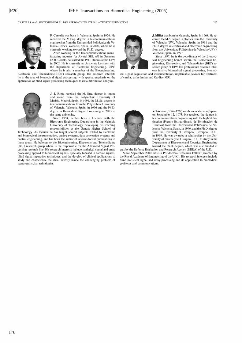
[P20] IEEE Transactions on Biomedical Engineering (2005)
CASTELLS et al.: SPATIOTEMPORAL BSS APPROACH TO ATRIAL ACTIVITY ESTIMATION 267
F. Castells was born in Valencia, Spain in 1976. Hereceived the M.Eng. degree in telecommunicationsengineering from the Universidad Politécnica de Va-lencia (UPV), Valencia, Spain, in 2000, where he iscurrently working toward the Ph.D. degree.
After working in the telecommunications manu-facturing industry for Alcatel SEL AG in Germany(2000–2001), he started his PhD. studies at the UPVin 2002. He is currently an Associate Lecturer withthe Department of Electronic Engineering, UPV,where he is also a member of the Bioengineering,
Electronic and Telemedicine (BeT) research group. His research interestslie in the area of biomedical signal processing, with special emphasis on theapplication of blind signal processing techniques to atrial fibrillation analysis.
J. J. Rieta received the M. Eng. degree in imageand sound from the Polytechnic University ofMadrid, Madrid, Spain, in 1991, the M. Sc. degree intelecommunications from the Polytechnic Universityof Valencia, Valencia, Spain, in 1996 and the Ph.D.degree in Biomedical Signal Processing in 2003 inthe same university.
Since 1994, he has been a Lecturer with theElectronic Engineering Department in the ValenciaUniversity of Technology, developing his teachingresponsibilities at the Gandía Higher School of
Technology. As lecturer he has taught several subjects related to electronicand biomedical instrumentation, analog systems, data conversion systems andcontrol engineering, and has been the author of several docent publications inthese areas. He belongs to the Bioengineering, Electronic and Telemedicine(BeT) research group where is the responsible for the Advanced Signal Pro-cessing research line. His research interests include statistical signal and arrayprocessing applied to biomedical signals, specially focused in cardiac signals,blind signal separation techniques, and the develop of clinical applications tostudy and characterize the atrial activity inside the challenging problem ofsupraventricular arrhythmias.
J. Millet was born in Valencia, Spain, in 1968. He re-ceived the M.S. degree in physics from the Universityof Valencia (UV), Valencia, Spain, in 1991 and thePh.D. degree in electrical and electronic engineeringfrom the Universidad Politécnica de Valencia (UPV),Valencia, Spain, in 1997.
Since 1997, he is the coordinator of the Biomed-ical Engineering branch within the Biomedical En-gineering, Electronics, and Telemedicine (BET) re-search group of UPV. His professional research inter-ests involve biomedical signal processing, biomed-
ical signal acquisition and instrumentation, implantable devices for treatmentof cardiac arrhythmias and Cardiac MRI.
V. Zarzoso (S’94–A’99) was born in Valencia, Spain,on September 12, 1973. He received the degree intelecommunications engineering with the highest dis-tinction (Premio Extraordinario de Terminación deEstudios) from the Universidad Politécnica de Va-lencia, Valencia, Spain, in 1996, and the Ph.D. degreefrom the University of Liverpool, Liverpool, U.K.,in 1999. He was awarded a scholarship by the Uni-versity of Strathclyde, Glasgow, U.K., to study in theDepartment of Electronic and Electrical Engineeringtoward the Ph.D. degree, which was also funded in
part by the Defence Evaluation and Research Agency (DERA) of the U.K.Since September 2000, he is a Postdoctoral Research Fellow (awarded by
the Royal Academy of Engineering of the U.K.). His research interests includeblind statistical signal and array processing and its application to biomedicalproblems and communications.
176
IEEE Transactions on Biomedical Engineering (2004) [P21]
1176 IEEE TRANSACTIONS ON BIOMEDICAL ENGINEERING, VOL. 51, NO. 7, JULY 2004
Atrial Activity Extraction for Atrial FibrillationAnalysis Using Blind Source Separation
José Joaquín Rieta*, Francisco Castells, César Sánchez, Vicente Zarzoso, Associate Member, IEEE, and José Millet
Abstract—This contribution addresses the extraction of atrialactivity (AA) from real electrocardiogram (ECG) recordings ofatrial fibrillation (AF). We show the appropriateness of indepen-dent component analysis (ICA) to tackle this biomedical challengewhen regarded as a blind source separation (BSS) problem. ICA isa statistical tool able to reconstruct the unobservable independentsources of bioelectric activity which generate, through instanta-neous linear mixing, a measurable set of signals. The three keyhypothesis that make ICA applicable in the present scenario arediscussed and validated: 1) AA and ventricular activity (VA) aregenerated by sources of independent bioelectric activity; 2) AAand VA present non-Gaussian distributions; and 3) the generationof the surface ECG potentials from the cardioelectric sources canbe regarded as a narrow-band linear propagation process. Toempirically endorse these claims, an ICA algorithm is applied torecordings from seven patients with persistent AF. We demon-strate that the AA source can be identified using a kurtosis-basedreordering of the separated signals followed by spectral analysisof the sub-Gaussian sources. In contrast to traditional methods,the proposed BSS-based approach is able to obtain a unified AAsignal by exploiting the atrial information present in every ECGlead, which results in an increased robustness with respect toelectrode selection and placement.
Index Terms—Atrial fibrillation, blind source separation, ECG,forward electrocardiography problem, independent componentanalysis, QRS cancellation.
I. INTRODUCTION
ATRIAL fibrillation (AF) is the most common sustained ar-
rhythmia encountered by clinicians and occurs in approx-
imately 0.4%–1.0% of the general population. Its prevalence in-
creases with age, and up to 10% of the population older than 80
years has been diagnosed with AF. With the projected growth
of the elderly population, the prevalence of AF will certainly
increase [1]. There is also increasing awareness that AF is a
major cause of embolic events which in 75% of cases are com-
plicated by cerebrovascular accidents [2], [3]. AF is often asso-
Manuscript received February 21, 2003; revised July 28, 2003. This work wassupported in part by TIC2002-00957 and the research incentive program of thePolytechnic University of Valencia. Asterisk indicates corresponding author.
*J. J. Rieta is with the Bioengineering Electronic and Telemedicine ResearchGroup, Electronic Engineering Department, Polytechnic University of Valencia.EPSG, Carretera Nazaret Oliva s/n, 46730, Gandía, Valencia, Spain (e-mail:[email protected]).
F. Castells and J. Millet are with the Bioengineering Electronic andTelemedicine Research Group, Electronic Engineering Department, Poly-technic University of Valencia. EPSG, Carretera Nazaret Oliva s/n, 46730,Gandía, Valencia, Spain.
C. Sánchez is with the Bioengineering Electronic and Telemedicine ResearchGroup, University of Castilla-La Mancha, 16071 Cuenca, Spain.
V. Zarzoso is with the Signal Processing and Communications Group, De-partment of Electrical Engineering and Electronics, The University of Liver-pool, L69 3GJ Liverpool, U.K.
Digital Object Identifier 10.1109/TBME.2004.827272
ciated with heart disease but a significant proportion of patients
(about 30%) have no detectable heart disease. Symptoms such
as occasionally disabling haemo-dynamic impairment and a de-
crease in life expectancy are among the untoward effects of atrial
fibrillation, resulting in an important morbidity, mortality, and
an increased cost for the health care provider [1], [2]. In this re-
spect, AF has been the subject of arousing interest and intensive
clinical research in recent years.
The proper analysis and characterization of AF from elec-
trocardiogram (ECG) recordings—regardless of the leads con-
sidered—requires the extraction or cancellation of the signal
components associated with ventricular activity (VA), that is,
the QRS complex and the T-wave (QRS-T). Unfortunately, a
number of facts hinder this operation. First, atrial activity (AA)
presents in the ECG much lower amplitude—in some cases well
under the noise level—than its ventricular counterpart. Addi-
tionally, both phenomena possess spectral distributions that no-
tably overlap, rendering linear filtering solutions unsuccessful.
Methods reported in the literature to cancel out VA in the ECG
involve direct suppression of the QRS complex and T-wave
through the subtraction of a fixed template [4]–[6]. Also, the use
of an adaptive template in conjunction with the correct spatio-
temporal alignment of every QRS complex has proven to be very
effective [7]. All of these methods—though different in their
performance—share similar limitations such as high sensitivity
to QRS morphological changes in [4]–[6] and their inability to
eliminate artifacts from electrode movement or ectopic beats in
[4]–[7]. More recent methods have focused on extracting the VA
using artificial neural networks and subtracting it from the ECG
[8] or on the decomposition of the original ECG in a set of coef-
ficients that obtain the AA using discrete packet wavelet trans-
form [9]. A common limitation of all of the previously men-
tioned methods is their inability to exploit the spatial diversity
of an ECG recording.
However, the key observation that AA and VA are decoupled
[1], [6] introduces a new interesting perspective which does not
rely on direct QRS-T elimination. Under certain assumptions,
the AA extraction problem accepts a formulation based on blind
source separation (BSS) of instantaneous linear mixtures [10],
in which atrial and ventricular source contributions to be appear
mixed at the electrode outputs in the ECG. Hence, the separation
of AA sources through a suitable BSS method would allow the
reconstruction of atrial contribution to each electrode free from
VA and other disturbances. The multichannel signal processing
standpoint adopted in the BSS approach aims at an effective uti-
lization of the atrial information present in all ECG leads. Two
main families of BSS techniques for AA extraction have been
proposed, based on principal component analysis (PCA) [11],
0018-9294/04$20.00 © 2004 IEEE
177
[P21] IEEE Transactions on Biomedical Engineering (2004)
RIETA et al.: ATRIAL ACTIVITY EXTRACTION FOR ATRIAL FIBRILLATION ANALYSIS USING BLIND SOURCE SEPARATION 1177
[12] and independent component analysis (ICA) [13], [14], re-
spectively. PCA methods search for a solution, using second-
order statistics (SOSs), that decorrelates the input signals. By
contrast, the assumptions that AA and VA are independent at
orders higher than two and do not present random Gaussian dis-
tributions [6], [7] may be exploited to separate AA from VA
by imposing the necessary higher order statistical conditions.
If such assumptions are fulfilled, the application of ICA-based
methods makes it possible to reconstruct the atrial contribution
to each electrode free from VA and other large-amplitude nui-
sance signals, like respiration artifacts, ectopic beats, or mus-
cular noise.
One of the most important research areas where ICA tech-
niques have proven their success is precisely in biomedical
engineering. Today the use of BSS is well known in elec-
troencephalogram and magnetoencephalogram applications
[15], [16] or in the extraction of the fetal ECG from maternal
cutaneous recordings [17]. Regarding the ECG, examples of
the application of BSS-based methods are the separation of
breathing artifacts, muscular noise, and other disturbances
[18], [19], analysis of ST segments for ischemia detection [20],
identification of humans using the ECG [21], and ventricular
arrhythmia detection and classification [22].
In the present contribution, a new application of BSS to the
multilead ECG is presented. We show the suitability of ICA
techniques to extract the AA present in the ECG of patients
with persistent AF episodes. It is argued that AA and VA are
generated by independent sources of bioelectric activity, that
this activity exhibits non-Gaussian character, and that the ECG
recordings fulfil the instantaneous linear model. To empirically
validate these claims, an ICA method is applied to real record-
ings obtained from patients suffering from AF. A simple yet ef-
fective method for the identification of AA from the estimated
sources is put forward, based on higher order statistics (HOS)
(more specifically, the fourth-order marginal cumulant or kur-
tosis) and spectral analysis [14], [23].
The paper is structured as follows. Section II justifies the
assumptions that lead to the suitability of the ICA-based BSS
approach to the AA extraction problem. Section III develops
a method for the identification and reconstruction of AA from
the separated sources of cardioelectric activity. Section IV sum-
marizes the results obtained from the application of the ICA-
based AA extraction technique on real multilead ECG signals
recorded from AF patients, and the results are discussed in Sec-
tion V. Section VI presents the concluding remarks.
II. AF BSS MODEL
If BSS methods based on ICA are to be applied to the AA
extraction from the 12-lead ECG, the fulfillment of three basic
considerations regarding AA, VA and the fashion in which
both activities arise on the body surface must first be justified:
independence of the sources, non-Gaussianity, and observations
generated by instantaneous linear mixing of the bioelectric
sources [24]. This section begins with an outline of the basic
mathematical principles behind the BSS of instantaneous linear
mixtures. Then, physical mechanisms of AF generation give
strong support to the independence and non-Gaussianity of AA
and VA. Next, the validity of the instantaneous linear mixing
model for the ECG is endorsed through the matrix solution for
the forward problem of electrocardiography. The corroboration
of these conditions make it possible to assume that the ECG of
a patient in AF satisfies the BSS instantaneous linear mixture
model, thus justifying the application of ICA.
A. BSS Principles
The BSS consists of recovering a set of source signals from
the observation of linear mixtures of the sources [10], [25]. The
term “blind” emphasizes that nothing is known about the source
signals or the mixing structure, the only hypothesis being the
source mutual independence [24]. Mathematically, let us de-
note by ( stands for
the transpose operator) the vector that represents the source
signals and the
sensor output vector, i.e., the observation vector. It is assumed
that , so that there are at least as many sensors as
sources. In the noiseless case, the BSS model for instantaneous
linear mixtures reads
(1)
where is the unknown mixing matrix. The objec-
tive of BSS is to estimate and from the exclusive knowl-
edge of . To achieve the source separation, a linear transfor-
mation is sought such that the components of the
output signal vector become statistically independent, thus
representing an estimate of the sources
(2)
except for (perhaps) scaling and permutation, which are consid-
ered admissible indeterminacies.
Some authors have proposed the use of PCA to solve the
model of (1) [11]. However, it is important to remark that
the success of PCA relies heavily on the orthogonality of the
columns of the mixing matrix. However, in general, there is no
reason why bioelectrical sources of the heart should be spatially
orthogonal to one another in the ECG. This orthogonality
condition can only be forced through appropriate electrode
placement, as was previously emphasized in the context of the
fetal ECG extraction problem [26], [27] and the cancellation of
artifacts in the electroencephalogram [16]. As a consequence,
PCA is not expected to separate each source from the ECG
with a quality similar to that of ICA. Moreover, PCA methods
assume sources with a Gaussian distribution, which is not the
case for AA and VA in the AF problem (as will be justified in
Section II-C). In general, the measurement of independence for
non-Gaussian signals can be carried out more accurately using
HOS, rather than SOS, like PCA methods do.
By contrast, ICA does not introduce any restriction on the ge-
ometrical structure of the mixing matrix (apart from the linear
independence of its columns) and, in addition, takes into ac-
count the non-Gaussian nature of the source signals. Conse-
quently, ICA arises as a more sensible approach to this problem.
Several ICA techniques have been proposed mainly based on
HOS and information theory [28], due to their ability to mea-
sure statistical independence. In practice, additive measurement
178
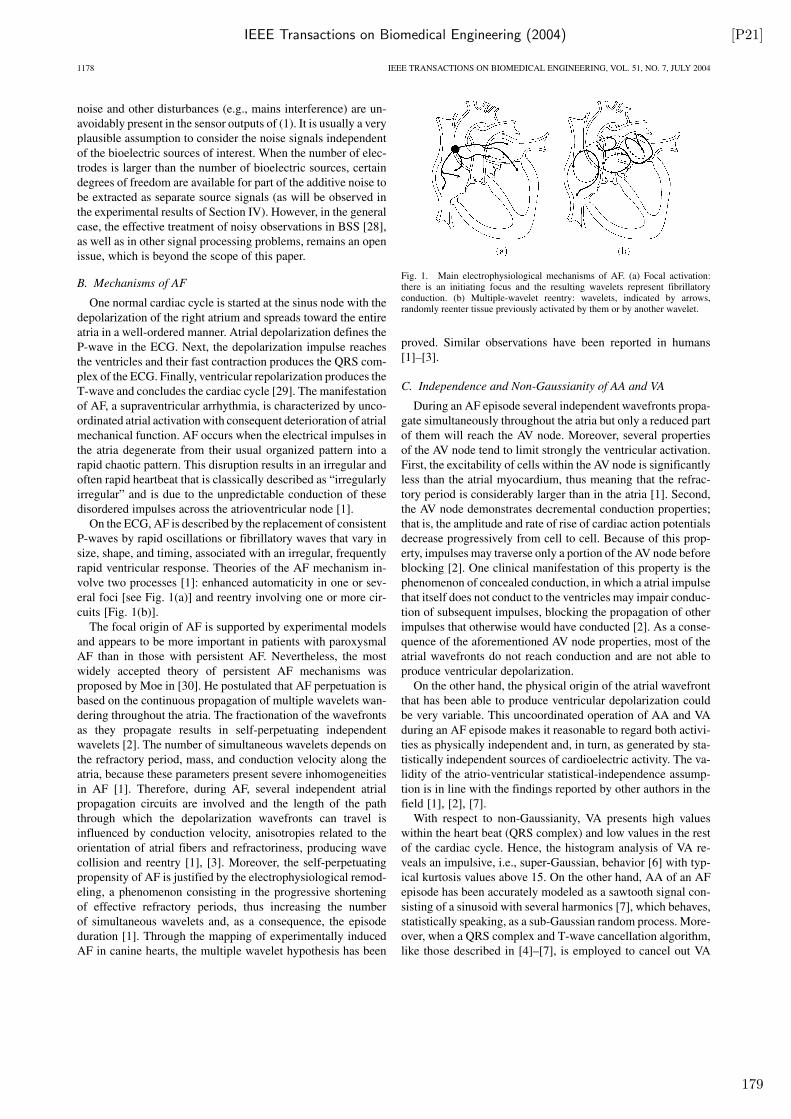
IEEE Transactions on Biomedical Engineering (2004) [P21]
1178 IEEE TRANSACTIONS ON BIOMEDICAL ENGINEERING, VOL. 51, NO. 7, JULY 2004
noise and other disturbances (e.g., mains interference) are un-
avoidably present in the sensor outputs of (1). It is usually a very
plausible assumption to consider the noise signals independent
of the bioelectric sources of interest. When the number of elec-
trodes is larger than the number of bioelectric sources, certain
degrees of freedom are available for part of the additive noise to
be extracted as separate source signals (as will be observed in
the experimental results of Section IV). However, in the general
case, the effective treatment of noisy observations in BSS [28],
as well as in other signal processing problems, remains an open
issue, which is beyond the scope of this paper.
B. Mechanisms of AF
One normal cardiac cycle is started at the sinus node with the
depolarization of the right atrium and spreads toward the entire
atria in a well-ordered manner. Atrial depolarization defines the
P-wave in the ECG. Next, the depolarization impulse reaches
the ventricles and their fast contraction produces the QRS com-
plex of the ECG. Finally, ventricular repolarization produces the
T-wave and concludes the cardiac cycle [29]. The manifestation
of AF, a supraventricular arrhythmia, is characterized by unco-
ordinated atrial activation with consequent deterioration of atrial
mechanical function. AF occurs when the electrical impulses in
the atria degenerate from their usual organized pattern into a
rapid chaotic pattern. This disruption results in an irregular and
often rapid heartbeat that is classically described as “irregularly
irregular” and is due to the unpredictable conduction of these
disordered impulses across the atrioventricular node [1].
On the ECG, AF is described by the replacement of consistent
P-waves by rapid oscillations or fibrillatory waves that vary in
size, shape, and timing, associated with an irregular, frequently
rapid ventricular response. Theories of the AF mechanism in-
volve two processes [1]: enhanced automaticity in one or sev-
eral foci [see Fig. 1(a)] and reentry involving one or more cir-
cuits [Fig. 1(b)].
The focal origin of AF is supported by experimental models
and appears to be more important in patients with paroxysmal
AF than in those with persistent AF. Nevertheless, the most
widely accepted theory of persistent AF mechanisms was
proposed by Moe in [30]. He postulated that AF perpetuation is
based on the continuous propagation of multiple wavelets wan-
dering throughout the atria. The fractionation of the wavefronts
as they propagate results in self-perpetuating independent
wavelets [2]. The number of simultaneous wavelets depends on
the refractory period, mass, and conduction velocity along the
atria, because these parameters present severe inhomogeneities
in AF [1]. Therefore, during AF, several independent atrial
propagation circuits are involved and the length of the path
through which the depolarization wavefronts can travel is
influenced by conduction velocity, anisotropies related to the
orientation of atrial fibers and refractoriness, producing wave
collision and reentry [1], [3]. Moreover, the self-perpetuating
propensity of AF is justified by the electrophysiological remod-
eling, a phenomenon consisting in the progressive shortening
of effective refractory periods, thus increasing the number
of simultaneous wavelets and, as a consequence, the episode
duration [1]. Through the mapping of experimentally induced
AF in canine hearts, the multiple wavelet hypothesis has been
Fig. 1. Main electrophysiological mechanisms of AF. (a) Focal activation:there is an initiating focus and the resulting wavelets represent fibrillatoryconduction. (b) Multiple-wavelet reentry: wavelets, indicated by arrows,randomly reenter tissue previously activated by them or by another wavelet.
proved. Similar observations have been reported in humans
[1]–[3].
C. Independence and Non-Gaussianity of AA and VA
During an AF episode several independent wavefronts propa-
gate simultaneously throughout the atria but only a reduced part
of them will reach the AV node. Moreover, several properties
of the AV node tend to limit strongly the ventricular activation.
First, the excitability of cells within the AV node is significantly
less than the atrial myocardium, thus meaning that the refrac-
tory period is considerably larger than in the atria [1]. Second,
the AV node demonstrates decremental conduction properties;
that is, the amplitude and rate of rise of cardiac action potentials
decrease progressively from cell to cell. Because of this prop-
erty, impulses may traverse only a portion of the AV node before
blocking [2]. One clinical manifestation of this property is the
phenomenon of concealed conduction, in which a atrial impulse
that itself does not conduct to the ventricles may impair conduc-
tion of subsequent impulses, blocking the propagation of other
impulses that otherwise would have conducted [2]. As a conse-
quence of the aforementioned AV node properties, most of the
atrial wavefronts do not reach conduction and are not able to
produce ventricular depolarization.
On the other hand, the physical origin of the atrial wavefront
that has been able to produce ventricular depolarization could
be very variable. This uncoordinated operation of AA and VA
during an AF episode makes it reasonable to regard both activi-
ties as physically independent and, in turn, as generated by sta-
tistically independent sources of cardioelectric activity. The va-
lidity of the atrio-ventricular statistical-independence assump-
tion is in line with the findings reported by other authors in the
field [1], [2], [7].
With respect to non-Gaussianity, VA presents high values
within the heart beat (QRS complex) and low values in the rest
of the cardiac cycle. Hence, the histogram analysis of VA re-
veals an impulsive, i.e., super-Gaussian, behavior [6] with typ-
ical kurtosis values above 15. On the other hand, AA of an AF
episode has been accurately modeled as a sawtooth signal con-
sisting of a sinusoid with several harmonics [7], which behaves,
statistically speaking, as a sub-Gaussian random process. More-
over, when a QRS complex and T-wave cancellation algorithm,
like those described in [4]–[7], is employed to cancel out VA
179
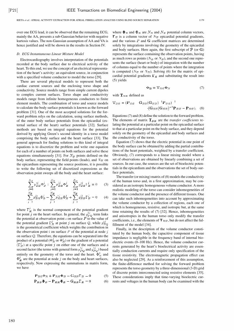
[P21] IEEE Transactions on Biomedical Engineering (2004)
RIETA et al.: ATRIAL ACTIVITY EXTRACTION FOR ATRIAL FIBRILLATION ANALYSIS USING BLIND SOURCE SEPARATION 1179
over one ECG lead, it can be observed that the remaining ECG,
mainly the AA, presents a sub-Gaussian behavior with negative
kurtosis values. The non-Gaussian assumption of AA and VA is
hence justified and will be shown in the results in Section IV.
D. ECG Instantaneous Linear Mixture Model
Electrocardiography involves interpretation of the potentials
recorded at the body surface due to electrical activity of the
heart. To this end, we use the concept of an electrical representa-
tion of the heart’s activity: an equivalent source, in conjunction
with a specified volume conductor to model the torso [29].
There are several physical models to represent both the
cardiac current sources and the enclosing torso shape and
conductivity. Source models range from simple current dipoles
to complex current surfaces. Torso shape and conductivity
models range from infinite homogeneous conductors to finite
element models. The combination of torso and source models
to calculate the body surface potentials is known as the forward
problem [31]. One of the most accepted solutions for the for-
ward problem relys on the calculation, using surface methods,
of the outer body surface potentials from the epicardial (ex-
ternal surface of the heart) surface potentials [32]. Surface
methods are based on integral equations for the potential
derived by applying Green’s second identity in a torso model
comprising the body surface and the heart surface [33]. The
general approach for finding solutions to this kind of integral
equations is to discretize the problem and write one equation
for each of a number of points on both surfaces and solve these
equations simultaneously [31]. For points defined on the
body surface, representing the field points (leads), and on
the epicardium representing the source positions, it is possible
to write the following set of discretized expressions as the
observation point sweeps all the body and the heart surface:
(3)
(4)
where is the normal component of the potential gradient
for point on the heart surface. In general, the term links
the potential at observation point on surface to the value of
the potential gradient at point on surface , while
is the geometrical coefficient which weights the contribution in
the observation point on surface of the potential at node
on surface . Therefore, the equations can be separated into the
product of a potential ( or ) or the gradient of a potential
at a specific point on either one of the surfaces and a
second factor (the terms with general form and ) based
entirely on the geometry of the torso and the heart. and
are the potential at node on the body and heart surfaces,
respectively. Now expressing the summations in matrix form,
we have
(5)
(6)
where and are and potential column vectors,
is a column vector of epicardial potential gradients,
and the various and coefficient matrices are determined
solely by integrations involving the geometry of the epicardial
and body surfaces. Here again, the first subscript of (or )
represents the surface containing the observation points, having
as much rows as points ( or ), and the second one repre-
sents the surface (heart or body) of integration with the number
of columns equal to the number of points where the integration
is computed ( or ). Solving (6) for the matrix of epi-
cardial potential gradients and substituting the result into
(5) yields
(7)
with defined as
(8)
Equations (7) and (8) define the solution to the forward problem.
The elements of matrix are the transfer coefficients re-
lating the potential at a particular point on the epicardial surface
to that at a particular point on the body surface, and they depend
solely on the geometry of the epicardial and body surfaces and
the conductivity of the torso.
Equation (7) shows that the electric potential in one point of
the body surface can be obtained by adding the partial contribu-
tions of the heart potentials, weighted by a transfer coefficient.
Obviously, (7) corresponds to a linear mixing model where a
set of observations are obtained by linearly combining a set of
sources. In our case, the sources are the set of bioelectric poten-
tials in the epicardium and the observations the set of body-sur-
face potentials.
The transfer (or mixing) matrix of (8) models the conductivity
of the human torso and, in a first approximation, may be con-
sidered as an isotropic homogeneous volume conductor. A more
realistic modeling of the torso can consider inhomogeneities of
the volume conductor and the presence of different tissues. One
can take such inhomogeneities into account by approximating
the volume conductor by a collection of regions, each one of
which is homogeneous, resistive, and isotropic but, at the same
time retaining the results of (7) [32]. Hence, inhomogeneities
and anisotropies in the human torso only modify the transfer
coefficients, i.e., the elements of , but do not affect the ful-
fillment of the model [34].
Finally, in the description of the volume conductor consti-
tuted by the human body, the capacitive component of tissue
impedance is negligible in the frequency band of internal bio-
electric events (0–100 Hz). Hence, the volume conductor cur-
rents generated by the heart’s bioelectrical activity are essen-
tially conduction currents and require only specification of the
tissue resistivity. The electromagnetic propagation effect can
also be neglected [29]. As a reinforcement of this assumption,
the finite-difference method for solving the forward problem
represents the torso geometry by a three-dimensional (3-D) grid
of discrete points interconnected using resistive elements [35].
These considerations imply that time-varying bioelectric cur-
rents and voltages in the human body can be examined with the
180
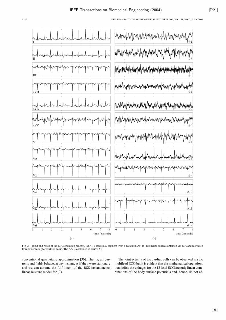
IEEE Transactions on Biomedical Engineering (2004) [P21]
1180 IEEE TRANSACTIONS ON BIOMEDICAL ENGINEERING, VOL. 51, NO. 7, JULY 2004
Fig. 2. Input and result of the ICA separation process. (a) A 12-lead ECG segment from a patient in AF. (b) Estimated sources obtained via ICA and reorderedfrom lower to higher kurtosis value. The AA is contained in source #1.
conventional quasi-static approximation [36]. That is, all cur-
rents and fields behave, at any instant, as if they were stationary
and we can assume the fulfillment of the BSS instantaneous
linear mixture model for (7).
The joint activity of the cardiac cells can be observed via the
multilead ECG but it is evident that the mathematical operations
that define the voltages for the 12-lead ECG are only linear com-
binations of the body surface potentials and, hence, do not af-
181
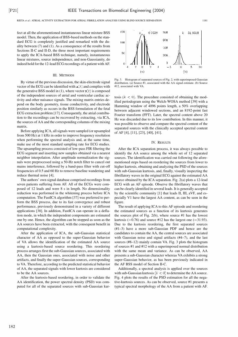
[P21] IEEE Transactions on Biomedical Engineering (2004)
RIETA et al.: ATRIAL ACTIVITY EXTRACTION FOR ATRIAL FIBRILLATION ANALYSIS USING BLIND SOURCE SEPARATION 1181
fect at all the aforementioned instantaneous linear mixture BSS
model. Then, the application of BSS-based methods on the stan-
dard ECG is completely justified and remarked with the du-
ality between (7) and (1). As a consequence of the results from
Sections II-C and II-D, the three most important requirements
to apply the ICA-based BSS technique, namely, instantaneous
linear mixtures, source independence, and non-Gaussianity, do
indeed hold for the 12-lead ECG recordings of a patient with AF.
III. METHODS
By virtue of the previous discussion, the skin-electrode signal
vector of the ECG can be identified with and complies with
the generative BSS model in (1), where vector is composed
of the independent sources of atrial and ventricular cardiac ac-
tivity and other nuisance signals. The mixing matrix entries de-
pend on the body geometry, tissue conductivity, and electrode
position similarly as occurs in the BSS formulation of the fetal
ECG extraction problem [17]. Consequently, the atrial contribu-
tion to the recordings can be recovered by extracting, via ICA,
the sources of AA and the corresponding columns of the mixing
matrix.
Before applying ICA, all signals were sampled (or upsampled
from 500 Hz) at 1 kHz in order to improve frequency resolution
when performing the spectral analysis and, at the same time,
make use of the most standard sampling rate for ECG studies.
The upsampling process consisted of low-pass FIR filtering the
ECG segment and inserting new samples obtained via a nearest
neighbor interpolation. After amplitude normalization the sig-
nals were preprocessed using a 50-Hz notch filter to cancel out
mains interference, followed by a band-pass filter with cut-off
frequencies of 0.5 and 60 Hz to remove baseline wandering and
reduce thermal noise [4].
The authors’ own signal database comprised recordings from
seven patients suffering from AF. All of the ECGs were com-
posed of 12 leads and were 8 s in length. No dimensionality
reduction was performed in the whitening process before ICA
computation. The FastICA algorithm [37] was preferred to per-
form the BSS process, due to its fast convergence and robust
performance, previously demonstrated in a variety of different
applications [38]. In addition, FastICA can operate in a defla-
tion mode, in which the independent components are estimated
one by one. Hence, the algorithm can be stopped as soon as the
AA sources have been extracted, with the consequent benefit in
computational complexity.
After the application of ICA, the sub-Gaussian statistical
character of AA as opposed to the super-Gaussian behavior
of VA allows the identification of the estimated AA source
using a kurtosis-based source reordering. This reordering
process arranges first the sub-Gaussian sources, associated with
AA, then the Gaussian ones, associated with noise and other
artifacts, and finally the super-Gaussian sources, corresponding
to VA. Therefore, according to the predicted statistical behavior
of AA, the separated signals with lower kurtosis are considered
to be the AA sources.
After the kurtosis-based reordering, in order to validate the
AA identification, the power spectral density (PSD) was com-
puted for all of the separated sources with sub-Gaussian kur-
Fig. 3. Histogram of separated sources of Fig. 2, with superimposed Gaussiandistribution. (a) Source #1, associated with the AA signal estimate. (b) Source#12, associated with VA.
tosis . The procedure consisted of obtaining the mod-
ified periodogram using the Welch-WOSA method [39] with a
Hamming window of 4096 points length, a 50% overlapping
between adjacent windowed sections, and an 8192-point fast
Fourier transform (FFT). Later, the spectral content above 20
Hz was discarded due to its low contribution. In this manner, it
was possible to observe and compare the spectral content of the
separated sources with the clinically accepted spectral content
of AF [4], [11], [23], [40], [41].
IV. RESULTS
After the ICA separation process, it was always possible to
identify the AA source among the whole set of 12 separated
sources. The identification was carried out following the afore-
mentioned steps based on reordering the sources from lower to
higher kurtosis, obtaining and analyzing the PSD of the sources
with sub-Gaussian kurtosis, and, finally, visually inspecting the
fibrillatory waves in the original ECG against the estimated AA
source obtained by the ICA separation. Fig. 2(a) plots a 12-lead
ECG with an AF episode. Observe the fibrillatory waves that
can be clearly identified in several leads. It is generally accepted
by the scientific community [1] that leads II, III, aVF, and es-
pecially V1 have the largest AA content, as can be seen in the
figure.
The result of applying ICA to this AF episode and reordering
the estimated sources as a function of its kurtosis generates
the sources plot of Fig. 2(b), where source #1 has the lowest
kurtosis ( 0.76) and source #12 has the largest one ( 31.93).
Due to the kurtosis reordering, the first separated sources
(#1–3) have a more sub-Gaussian PDF and hence are the
candidates to contain the AA, the central sources are associated
with Gaussian noise and signal artifacts (#4–7), and the last
sources (#8–12) mainly contain VA. Fig. 3 plots the histogram
of sources #1 and #12 with a superimposed normal distribution
with the same mean and variance. As can be observed, AA
presents a sub-Gaussian character whereas VA exhibits a strong
super-Gaussian behavior, as has been previously indicated in
the AF BSS model of Section II-C.
Additionally, a spectral analysis is applied over the sources
with sub-Gaussian kurtosis to determine the AA source.
Fig. 4 plots the results of the PSD estimation for all the nega-
tive-kurtosis sources. As can be observed, source #1 presents a
typical spectral morphology of the AA from a patient with AF.
182
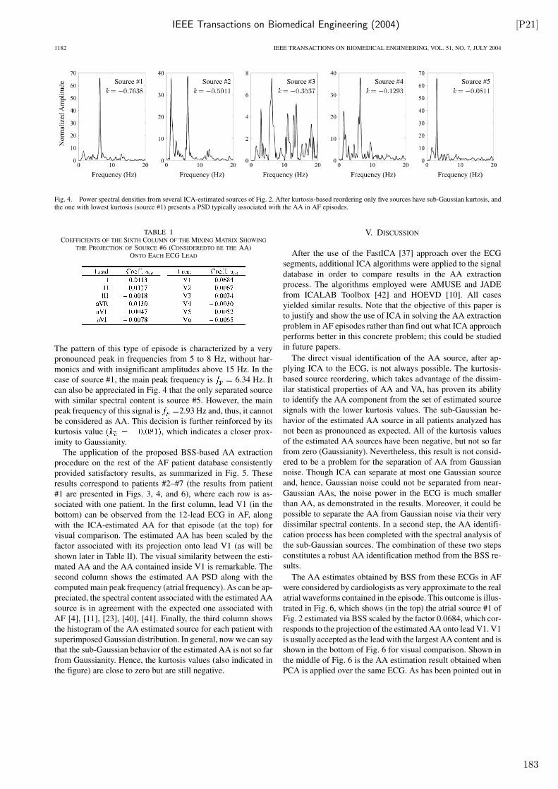
IEEE Transactions on Biomedical Engineering (2004) [P21]
1182 IEEE TRANSACTIONS ON BIOMEDICAL ENGINEERING, VOL. 51, NO. 7, JULY 2004
Fig. 4. Power spectral densities from several ICA-estimated sources of Fig. 2. After kurtosis-based reordering only five sources have sub-Gaussian kurtosis, andthe one with lowest kurtosis (source #1) presents a PSD typically associated with the AA in AF episodes.
TABLE ICOEFFICIENTS OF THE SIXTH COLUMN OF THE MIXING MATRIX SHOWING
THE PROJECTION OF SOURCE #6 (CONSIDEREDTO BE THE AA)ONTO EACH ECG LEAD
The pattern of this type of episode is characterized by a very
pronounced peak in frequencies from 5 to 8 Hz, without har-
monics and with insignificant amplitudes above 15 Hz. In the
case of source #1, the main peak frequency is 6.34 Hz. It
can also be appreciated in Fig. 4 that the only separated source
with similar spectral content is source #5. However, the main
peak frequency of this signal is 2.93 Hz and, thus, it cannot
be considered as AA. This decision is further reinforced by its
kurtosis value , which indicates a closer prox-
imity to Gaussianity.
The application of the proposed BSS-based AA extraction
procedure on the rest of the AF patient database consistently
provided satisfactory results, as summarized in Fig. 5. These
results correspond to patients #2–#7 (the results from patient
#1 are presented in Figs. 3, 4, and 6), where each row is as-
sociated with one patient. In the first column, lead V1 (in the
bottom) can be observed from the 12-lead ECG in AF, along
with the ICA-estimated AA for that episode (at the top) for
visual comparison. The estimated AA has been scaled by the
factor associated with its projection onto lead V1 (as will be
shown later in Table II). The visual similarity between the esti-
mated AA and the AA contained inside V1 is remarkable. The
second column shows the estimated AA PSD along with the
computed main peak frequency (atrial frequency). As can be ap-
preciated, the spectral content associated with the estimated AA
source is in agreement with the expected one associated with
AF [4], [11], [23], [40], [41]. Finally, the third column shows
the histogram of the AA estimated source for each patient with
superimposed Gaussian distribution. In general, now we can say
that the sub-Gaussian behavior of the estimated AA is not so far
from Gaussianity. Hence, the kurtosis values (also indicated in
the figure) are close to zero but are still negative.
V. DISCUSSION
After the use of the FastICA [37] approach over the ECG
segments, additional ICA algorithms were applied to the signal
database in order to compare results in the AA extraction
process. The algorithms employed were AMUSE and JADE
from ICALAB Toolbox [42] and HOEVD [10]. All cases
yielded similar results. Note that the objective of this paper is
to justify and show the use of ICA in solving the AA extraction
problem in AF episodes rather than find out what ICA approach
performs better in this concrete problem; this could be studied
in future papers.
The direct visual identification of the AA source, after ap-
plying ICA to the ECG, is not always possible. The kurtosis-
based source reordering, which takes advantage of the dissim-
ilar statistical properties of AA and VA, has proven its ability
to identify the AA component from the set of estimated source
signals with the lower kurtosis values. The sub-Gaussian be-
havior of the estimated AA source in all patients analyzed has
not been as pronounced as expected. All of the kurtosis values
of the estimated AA sources have been negative, but not so far
from zero (Gaussianity). Nevertheless, this result is not consid-
ered to be a problem for the separation of AA from Gaussian
noise. Though ICA can separate at most one Gaussian source
and, hence, Gaussian noise could not be separated from near-
Gaussian AAs, the noise power in the ECG is much smaller
than AA, as demonstrated in the results. Moreover, it could be
possible to separate the AA from Gaussian noise via their very
dissimilar spectral contents. In a second step, the AA identifi-
cation process has been completed with the spectral analysis of
the sub-Gaussian sources. The combination of these two steps
constitutes a robust AA identification method from the BSS re-
sults.
The AA estimates obtained by BSS from these ECGs in AF
were considered by cardiologists as very approximate to the real
atrial waveforms contained in the episode. This outcome is illus-
trated in Fig. 6, which shows (in the top) the atrial source #1 of
Fig. 2 estimated via BSS scaled by the factor 0.0684, which cor-
responds to the projection of the estimated AA onto lead V1. V1
is usually accepted as the lead with the largest AA content and is
shown in the bottom of Fig. 6 for visual comparison. Shown in
the middle of Fig. 6 is the AA estimation result obtained when
PCA is applied over the same ECG. As has been pointed out in
183
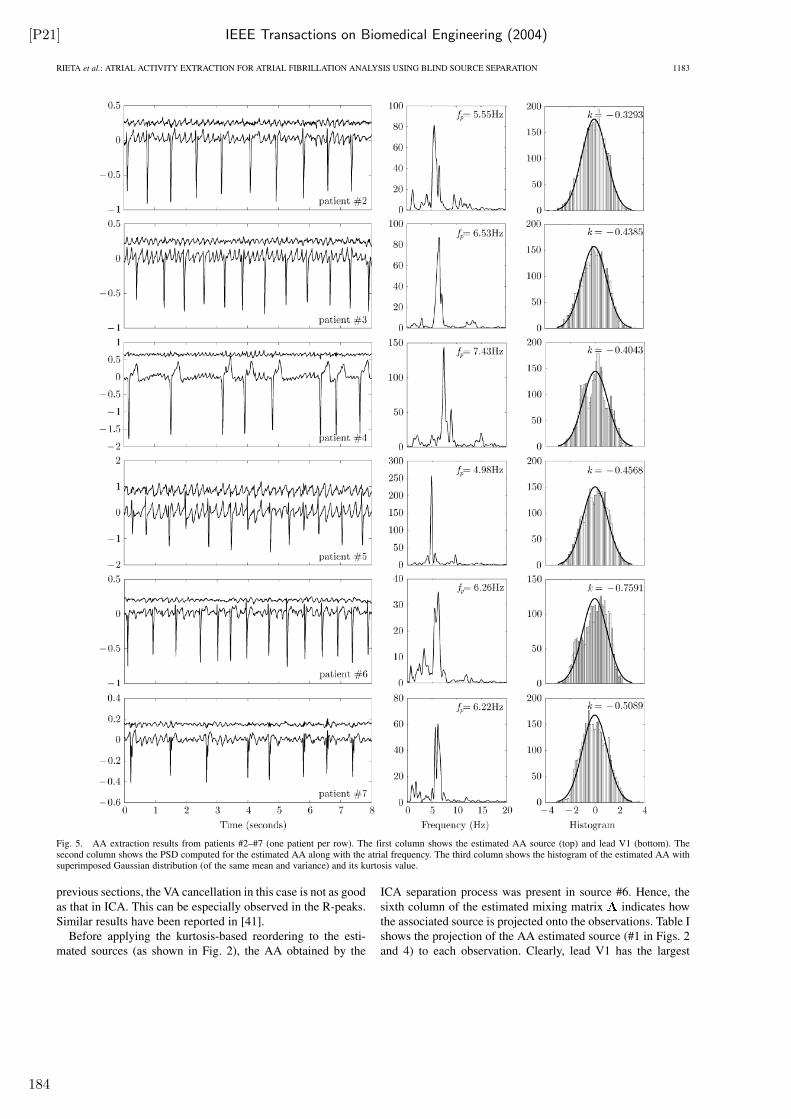
[P21] IEEE Transactions on Biomedical Engineering (2004)
RIETA et al.: ATRIAL ACTIVITY EXTRACTION FOR ATRIAL FIBRILLATION ANALYSIS USING BLIND SOURCE SEPARATION 1183
Fig. 5. AA extraction results from patients #2–#7 (one patient per row). The first column shows the estimated AA source (top) and lead V1 (bottom). Thesecond column shows the PSD computed for the estimated AA along with the atrial frequency. The third column shows the histogram of the estimated AA withsuperimposed Gaussian distribution (of the same mean and variance) and its kurtosis value.
previous sections, the VA cancellation in this case is not as good
as that in ICA. This can be especially observed in the R-peaks.
Similar results have been reported in [41].
Before applying the kurtosis-based reordering to the esti-
mated sources (as shown in Fig. 2), the AA obtained by the
ICA separation process was present in source #6. Hence, the
sixth column of the estimated mixing matrix indicates how
the associated source is projected onto the observations. Table I
shows the projection of the AA estimated source (#1 in Figs. 2
and 4) to each observation. Clearly, lead V1 has the largest
184
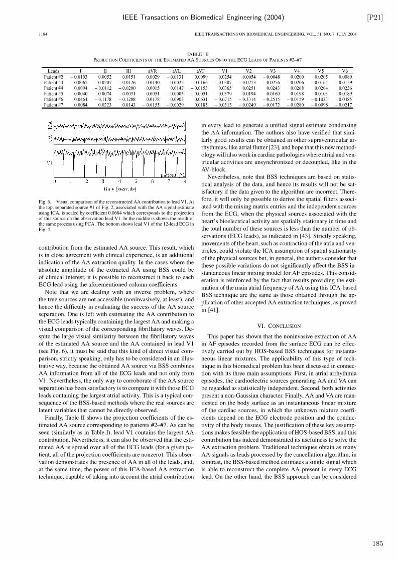
IEEE Transactions on Biomedical Engineering (2004) [P21]
1184 IEEE TRANSACTIONS ON BIOMEDICAL ENGINEERING, VOL. 51, NO. 7, JULY 2004
TABLE IIPROJECTION COEFFICIENTS OF THE ESTIMATED AA SOURCES ONTO THE ECG LEADS OF PATIENTS #2–#7
Fig. 6. Visual comparison of the reconstructed AA contribution to lead V1. Atthe top, separated source #1 of Fig. 2, associated with the AA signal estimateusing ICA, is scaled by coefficient 0.0684 which corresponds to the projectionof this source on the observation lead V1. In the middle is shown the result ofthe same process using PCA. The bottom shows lead V1 of the 12-lead ECG inFig. 2.
contribution from the estimated AA source. This result, which
is in close agreement with clinical experience, is an additional
indication of the AA extraction quality. In the cases where the
absolute amplitude of the extracted AA using BSS could be
of clinical interest, it is possible to reconstruct it back to each
ECG lead using the aforementioned column coefficients.
Note that we are dealing with an inverse problem, where
the true sources are not accessible (noninvasively, at least), and
hence the difficulty in evaluating the success of the AA source
separation. One is left with estimating the AA contribution to
the ECG leads typically containing the largest AA and making a
visual comparison of the corresponding fibrillatory waves. De-
spite the large visual similarity between the fibrillatory waves
of the estimated AA source and the AA contained in lead V1
(see Fig. 6), it must be said that this kind of direct visual com-
parison, strictly speaking, only has to be considered in an illus-
trative way, because the obtained AA source via BSS combines
AA information from all of the ECG leads and not only from
V1. Nevertheless, the only way to corroborate if the AA source
separation has been satisfactory is to compare it with those ECG
leads containing the largest atrial activity. This is a typical con-
sequence of the BSS-based methods where the real sources are
latent variables that cannot be directly observed.
Finally, Table II shows the projection coefficients of the es-
timated AA source corresponding to patients #2–#7. As can be
seen (similarly as in Table I), lead V1 contains the largest AA
contribution. Nevertheless, it can also be observed that the esti-
mated AA is spread over all of the ECG leads (for a given pa-
tient, all of the projection coefficients are nonzero). This obser-
vation demonstrates the presence of AA in all of the leads, and,
at the same time, the power of this ICA-based AA extraction
technique, capable of taking into account the atrial contribution
in every lead to generate a unified signal estimate condensing
the AA information. The authors also have verified that simi-
larly good results can be obtained in other supraventricular ar-
rhythmias, like atrial flutter [23], and hope that this new method-
ology will also work in cardiac pathologies where atrial and ven-
tricular activities are unsynchronized or decoupled, like in the
AV-block.
Nevertheless, note that BSS techniques are based on statis-
tical analysis of the data, and hence its results will not be sat-
isfactory if the data given to the algorithm are incorrect. There-
fore, it will only be possible to derive the spatial filters associ-
ated with the mixing matrix entries and the independent sources
from the ECG, when the physical sources associated with the
heart’s bioelectrical activity are spatially stationary in time and
the total number of these sources is less than the number of ob-
servations (ECG leads), as indicated in [43]. Strictly speaking,
movements of the heart, such as contraction of the atria and ven-
tricles, could violate the ICA assumption of spatial stationarity
of the physical sources but, in general, the authors consider that
these possible variations do not significantly affect the BSS in-
stantaneous linear mixing model for AF episodes. This consid-
eration is reinforced by the fact that results providing the esti-
mation of the main atrial frequency of AA using this ICA-based
BSS technique are the same as those obtained through the ap-
plication of other accepted AA extraction techniques, as proved
in [41].
VI. CONCLUSION
This paper has shown that the noninvasive extraction of AA
in AF episodes recorded from the surface ECG can be effec-
tively carried out by HOS-based BSS techniques for instanta-
neous linear mixtures. The applicability of this type of tech-
nique in this biomedical problem has been discussed in connec-
tion with its three main assumptions. First, in atrial arrhythmia
episodes, the cardioelectric sources generating AA and VA can
be regarded as statistically independent. Second, both activities
present a non-Gaussian character. Finally, AA and VA are man-
ifested on the body surface as an instantaneous linear mixture
of the cardiac sources, in which the unknown mixture coeffi-
cients depend on the ECG electrode position and the conduc-
tivity of the body tissues. The justification of these key assump-
tions makes feasible the application of HOS-based BSS, and this
contribution has indeed demonstrated its usefulness to solve the
AA extraction problem. Traditional techniques obtain as many
AA signals as leads processed by the cancellation algorithm; in
contrast, the BSS-based method estimates a single signal which
is able to reconstruct the complete AA present in every ECG
lead. On the other hand, the BSS approach can be considered
185
[P21] IEEE Transactions on Biomedical Engineering (2004)
RIETA et al.: ATRIAL ACTIVITY EXTRACTION FOR ATRIAL FIBRILLATION ANALYSIS USING BLIND SOURCE SEPARATION 1185
as an alternative procedure for (indirect) QRST cancellation in
atrial arrhythmia analysis.
The positive results reported in this paper mean the advent
of novel noninvasive techniques for AF analysis and are the
first step in the development and future improvement of new
diagnostic strategies, pathology prediction methodologies, and
aid tools based on AA-wave analysis in the management of pa-
tients with AF. In fact, most of the actual diagnosis and man-
agement of patients with AF are judged on the basis of clinical
symptoms and ECG recordings. Therefore, the development and
availability of suitable techniques allowing the knowledge of AF
patterns (paroxysmal, persistent, or permanent) and aiding in
the decision making about restoration and maintenance of sinus
rhythm or control of the ventricular rate may be a tool of fun-
damental importance for the treatment of AF, a commonly en-
countered arrhythmia in permanent expansion.
ACKNOWLEDGMENT
The authors would like to thank cardiologists R. Ruiz Granell,
S. Morell, F. J. Chorro, and R. García Civera, from the Electro-
physiology Laboratory of the Universitary Clinical Hospital of
Valencia, Spain, for their clinical advice and kind help in ob-
taining the signals.
REFERENCES
[1] V. Fuster, L. E. Ryden, R. W. Asinger, D. S. Cannom, H. J. Crijns, R. L.Frye, J. L. Halperin, G. N. Kay, W. W. Klein, S. Levy, R. L. McNamara,E. N. Prystowsky, L. S. Wann, and D. G. Wyse, “ACC/AHA/ESC guide-lines for the management of patients with atrial fibrillation: a report ofthe American College of Cardiology/American Heart Association TaskForce on Practice Guidelines and the European Society of CardiologyCommittee for Practice Guidelines and Policy Conferences (Committeeto Develop Guidelines for the Management of Patients With Atrial Fib-rillation),” J. Amer. Coll. Cardiol., vol. 38, pp. 1266 i–1266 lxx, 2001.
[2] S. Levy et al., “Atrial fibrillation: Current knowledge and recommen-dations for management,” Eur. Heart J., vol. 19, no. 9, pp. 1294–1320,1998.
[3] R. H. Falk, “Medical progress: Atrial fibrillation,” New Eng. J. Med.,vol. 344, no. 14, pp. 1067–1078, 2001.
[4] A. Bollmann, N. K. Kanuru, K. K. McTeague, P. F. Walter, D. B.DeLurgio, and J. J. Langberg, “Frequency analysis of human atrialfibrillation using the surface electrocardiogram and its response toibutilide,” Amer. J. Cardiol., vol. 81, no. 12, pp. 1439–1445, 1998.
[5] N. V. Thakor and Y. S. Zhu, “Applications of adaptive filtering toecganalysis: Noise cancellation and arrhytmia detection,” IEEE Trans.
Biomed. Eng., vol. 38, pp. 785–794, Aug. 1991.[6] S. Shkurovich, A. V. Sahakian, and S. Swiryn, “Detection of atrial ac-
tivity from high-voltage leads of implantable ventricular defibrillatorsusing a cancellation technique,” IEEE Trans. Biomed. Eng., vol. 45, pp.229–234, Feb. 1998.
[7] M. Stridh and L. Sörnmo, “Spatiotemporal QRST cancellation techniquesfor analysis of atrial fibrillation,” IEEE Trans. Biomed. Eng., vol. 48, pp.105–111, Jan. 2001.
[8] C. Vasquez, A. Hernandez, F. Mora, G. Carrault, and G. Passariello,“Atrial activity enhancement by wiener filtering using an artificial neuralnetwork,” IEEE Trans. Biomed. Eng., vol. 48, pp. 940–944, Aug. 2001.
[9] C. Sanchez, J. Millet, J. J. Rieta, J. Rodenas, F. Castells, R. Ruiz, andV. Ruiz, “Packet wavelet decomposition: An approach for atrial activityextraction,” IEEE Comput. Cardiol., vol. 29, pp. 33–36, Sept. 2001.
[10] V. Zarzoso and A. K. Nandi, “Blind source separation,” in Blind Esti-
mation Using Higher-Order Statistics, A. K. Nandi, Ed. Boston, MA:Kluwer, 1999, pp. 167–252.
[11] P. Langley, J. P. Bourke, and A. Murray, “Frequency analysis of atrialfibrillation,” IEEE Comput. Cardiol., vol. 27, pp. 65–68, Sept. 2000.
[12] L. Faes, G. Nollo, M. Kirchner, E. Olivetti, F. Gaita, R. Riccardi, and R.Antolini, “Principal component analysis and cluster analysis for mea-suring the local organization of human atrial fibrillation,” Med. Biol.
Eng. Comput., vol. 39, pp. 656–663, 2001.
[13] J. J. Rieta, V. Zarzoso, J. Millet, R. Garcia, and R. Ruiz, “Atrial activityextraction based on blind source separation as an alternative to QRSTcancellation for atrial fibrillation analysis,” IEEE Comput. Cardiol., vol.27, pp. 69–72, Sept. 2000.
[14] J. J. Rieta, F. Castells, C. Sanchez, and J. Igual, “ICA applied to atrialfibrillation analysis,” in Proc. Int. Conf. Independent Component Anal-ysis and Blind Signal Separation (ICA), vol. 4, Nara, Japan, 2003, pp.59–64.
[15] R. Vigario, J. Sarela, V. Jousmaki, M. Hamalainen, and E. Oja, “Indepen-dent component approach to the analysis of EEG and MEG recordings,”IEEE Trans. Biomed. Eng., vol. 47, pp. 589–593, May 2000.
[16] T. P. Jung, S. Makeig, C. Humphries, T. W. Lee, M. J. McKeown, V.Iragui, and T. J. Sejnowski, “Removing electroencephalographic arti-facts by blind source separation,” Psychophysiol., vol. 37, no. 2, pp.163–178, 2000.
[17] V. Zarzoso and A. K. Nandi, “Noninvasive fetal electrocardiogramextraction: Blind separation versus adaptive noise cancellation,” IEEETrans. Biomed. Eng., vol. 48, pp. 12–18, Jan. 2001.
[18] J. O. Wisbeck, A. K. Barros, and R. C. Ojeda, “Application of ica in theseparation of breathing artifacts in ECG signals,” in Proc. 5th Int. Conf.Neural Information Processing (ICONIP’98), vol. 1, pp. 211–214.
[19] A. K. Barros, A. Mansour, and N. Ohnishi, “Adaptive blind eliminationof artifacts in ECG signals,” in Proc. Int. Workshop Independence &Artificial Neural Networks (I&ANN’98), pp. 1380–1386.
[20] T. Stamkopoulos, K. Diamantaras, N. Maglaveras, and M. Strintzis,“ECG analysis using nonlinear PCA neural networks for ischemiadetection,” IEEE Trans. Signal Processing, vol. 46, pp. 3058–3067,Nov. 1998.
[21] L. Biel, O. Pettersson, L. Philipson, and P. Wide, “ECG analysis: A newapproach in human identification,” IEEE Trans. Instrum. Meas., vol. 50,pp. 808–812, June 2001.
[22] M. I. Owis, A. B. M. Youssef, and Y. M. Kadah, “Characterization ofelectrocardiogram signals based on blind source separation,” Med. Biol.Eng. Comput., vol. 40, no. 5, pp. 557–564, 2002.
[23] J. J. Rieta, J. Millet, V. Zarzoso, F. Castells, C. Sanchez, R. Garcia, andS. Morell, “Atrial fibrillation, atrial flutter and normal sinus rhythm dis-crimination by means of blind source separation and spectral parametersextraction,” IEEE Comput. Cardiol., vol. 29, pp. 25–28, 2002.
[24] J. F. Cardoso, “Blind signal separation: Statistical principles,” Proc.IEEE, vol. 86, pp. 2009–2025, Oct. 1998.
[25] P. Comon, “Independent component analysis, a new concept?,” SignalProcessing, vol. 36, no. 3, pp. 287–314, 1994.
[26] J. Vanderschoot, D. Callaerts, W. Sansen, J. Vandewalle, G. Vantrappen,and J. Janssens, “Two methods for optimal MECG elimination and FECGdetection from skin electrode signals,” IEEE Trans. Biomed. Eng., vol.34, pp. 233–243, Mar. 1987.
[27] D. Callaerts, B. Demoor, J. Vandewalle, W. Sansen, G. Vantrappen, andJ. Janssens, “Comparison of SVD methods to extract the fetal electrocar-diogram from cutaneous electrode signals,” Med. Biol. Eng. Comput.,vol. 28, no. 3, pp. 217–224, 1990.
[28] A. Hyvarinen, J. Karhunen, and E. Oja, Independent Component Anal-ysis. New York: Wiley, 2001.
[29] J. Malmivuo and R. Plonsey, Bioelectromagnetism: Principles and Ap-plications of Bioelectric and Biomagnetic Fields. Oxford, U.K.: Ox-ford Univ. Press, 1995.
[30] G. K. Moe, “On multiple wavelet hypothesis of atrial fibrillation,”Archives Internationales de Pharmacodynamie et de Therapie, vol.140, no. 1–2, pp. 183–188, 1962.
[31] R. M. Gulrajani, “The forward and inverse problems of electrocardiog-raphy,” IEEE Eng. Med. Biol. Mag., vol. 17, pp. 84–101, May 1998.
[32] R. C. Barr, T. C. Pilkington, J. P. Boineau, and M. S. Spach, “Deter-mining surface potentials from current dipoles, with application to elec-trocardiography,” IEEE Trans. Biomed. Eng., vol. BME-13, pp. 88–92,1966.
[33] R. C. Barr, M. Ramsey, and M. S. Spach, “Relating epicardial to bodysurface potential distribution by means of transfer coefficients based ongeometry measurements,” IEEE Trans. Biomed. Eng., vol. BME-24, pp.1–11, Jan. 1977.
[34] R. N. Klepfer, C. R. Johnson, and R. S. MacLeod, “The effects of in-homogeneities and anisotropies on electrocardiographic fields: A 3-d fi-nite-element study,” IEEE Trans. Biomed. Eng., vol. 44, pp. 706–719,Aug. 1997.
[35] S. J. Walker and D. Kilpatrick, “Forward and inverse electrocardio-graphic calculations using resistor network models of the human torso,”Circ. Res., vol. 61, no. 4, pp. 504–513, 1987.
[36] R. Plonsey and D. B. Heppner, “Considerations of quasistationarity inelectrophysiological systems,” Bull. Math. Biophys., vol. 29, no. 4, pp.657–664, 1967.
186
IEEE Transactions on Biomedical Engineering (2004) [P21]
1186 IEEE TRANSACTIONS ON BIOMEDICAL ENGINEERING, VOL. 51, NO. 7, JULY 2004
[37] The Fastica Package for Matlab, J. Hurri, J. Gavert, J. Sarela, andA. Hyvarinen. (1998). [Online]. Available: http://www.cis.hut.fi/projects/ica/fastica
[38] A. Hyvarinen, “Fast and robust fixed-point algorithms for independentcomponent analysis,,” IEEE Trans. Neural Networks, vol. 10, pp.626–634, May 1999.
[39] P. D. Welch, “Use of fast fourier transform for estimation of powerspectra: A method based on time averaging over short modified peri-odograms,” IEEE Trans. Audio Electroacoust., vol. AE-15, no. 2, pp.70–73, 1967.
[40] M. Stridh, L. Sörnmo, C. J. Meurling, and S. B. Olsson, “Characteriza-tion of atrial fibrillation using the surface ECG: Time-dependent spectralproperties,” IEEE Trans. Biomed. Eng., vol. 48, pp. 19–27, Jan. 2001.
[41] P. Langley, M. Stridh, J. J. Rieta, L. Sörnmo, J. Millet, and A. Murray,“Comparison of atrial rhythm extraction techniques for the detection ofthe main atrial frequency from the 12-lead ECG in atrial fibrillation,”IEEE Comput. Cardiol., vol. 29, pp. 29–32, Sept. 2002.
[42] Icalab Toolboxes, A. Cichocki, S. Amari, K. Siwek, T. Tanaka, andT. Rutkowski. (2003). [Online]. Available: http://www.bsp.brain.riken.go.jp/ICALAB
[43] T. P. Jung, S. Makeig, T. W. Lee, M. J. McKeown, G. Brown, A. J. Bell,and T. J. Sejnowski, “Independent component analysis of biomedicalsignals,” in Proc. Int. Conf. Independent Component Analysis and Blind
Signal Separation (ICA), vol. 2, 2000, pp. 633–644.
José Joaquín Rieta received the M. Eng. degree inimage and sound from the Polytechnic University ofMadrid, Madrid, Spain, in 1991, the M. Sc. degree intelecommunications from the Polytechnic Universityof Valencia, Valencia, Spain, in 1996 and the Ph.D.degree in Biomedical Signal Processing in 2003 inthe same university.
Since 1994, he has been a Lecturer with theElectronic Engineering Department in the ValenciaUniversity of Technology, developing his teachingresponsibilities at the Gandía Higher School of
Technology. As lecturer he has taught several subjects related to electronicand biomedical instrumentation, analog systems, data conversion systems andcontrol engineering, and has been the author of several docent publications inthese areas. He belongs to the Bioengineering, Electronic and Telemedicine(BeT) research group where is the responsible for the Advanced Signal Pro-cessing research line. His research interests include statistical signal and arrayprocessing applied to biomedical signals, specially focused in cardiac signals,blind signal separation techniques, and the develop of clinical applicationsto study and characterize the atrial activity inside the challenging problem ofsupraventricular arrhythmias.
Francisco Castells was born in Spain in 1976. Hereceived the M.Eng. degree in telecommunicationsengineering from the Universidad Politécnica de Va-lencia (UPV), Valencia, Spain, in 2000, where he iscurrently working toward the Ph.D. degree.
After working in the telecommunications manu-facturing industry for Alcatel SEL AG in Germany(2000–2001), he started his PhD. studies at the UPVin 2002. He is currently an Associate Lecturer withthe Department of Electronic Engineering, UPV,where he is also a member of the Bioengineering,
Electronic and Telemedicine (BeT) research group. His research interests liein the area of biomedical signal processing, with special emphasis on theapplication of blind signal processing techniques to atrial fibrillation analysis.
César Sánchez was born in Albacete, Spain, in 1973.He received the M.Eng. degree in telecommunica-tions engineering from the Universidad Politécnicade Madrid, Madrid, Spain, in 1998 and he is currentlyworking toward the Ph.D. degree at the UniversidadPolitécnica de Valencia (UPV), Valencia, Spain, in2000.
He is currently a Lecturer with the Universidadde Castilla—La Mancha (UCLM), Spain, andworks as an external member of the Bioengineering,Electronic and Telemedicine (BeT) research group
of the UPV. His research interests are centered on the application of advancedsignal processing techiques such as the wavelet transform to cardiac signals.
Vicente Zarzoso (S’94–A’99) was born in Valencia,Spain, on September 12, 1973. He received thedegree in telecommunications engineering withthe highest distinction (Premio Extraordinario deTerminación de Estudios) from the UniversidadPolitécnica de Valencia, Valencia, Spain, in 1996,and the Ph.D. degree from the University ofLiverpool, Liverpool, U.K., in 1999.
He was awarded a scholarship by the University ofStrathclyde, Glasgow, U.K., to study in the Depart-ment of Electronic and Electrical Engineering toward
his Ph.D. degree, which was also funded in part by the Defence Evaluation andResearch Agency (DERA) of the U.K. Since September 2000, he is in receipt ofa Post-doctoral Research Fellowship awarded by the Royal Academy of Engi-neering of the U.K. He is currently on leave at the Laboratoire de Informatique,Signaux et Systèmes (I3S), Université de Nice, Sophia-Antipolis, France. Hisresearch interests include blind statistical signal and array processing and its ap-plication to biomedical problems and communications.
José Millet was born in Valencia, Spain, in 1968. Hereceived the M.S. degree in physics from the Uni-versity of Valencia (UV), Valencia, Spain, in 1991and the Ph.D. degree in electrical and electronic engi-neering from the Universidad Politécnica de Valencia(UPV), Valencia, Spain, in 1997.
He is currently an Associate Professor of Elec-tronics and Biomedical Signal Processing with theElectronic Engineering Department, UPV. From1991 to 1999, he worked as Assistant Professor inthe same department. Since 1997, he has been the
coordinator of the Biomedical Engineering branch within the Bioengineering,Electronic and Telemedicine (BeT) research group of UPV. His professionalresearch interests are in biomedical signal processing, biomedical signalacquisition and instrumentation, implantable devices for treatment of cardiacarrhythmias, and cardiac MRI.
187

Journal of Optical Networking (2004) [P22]
189
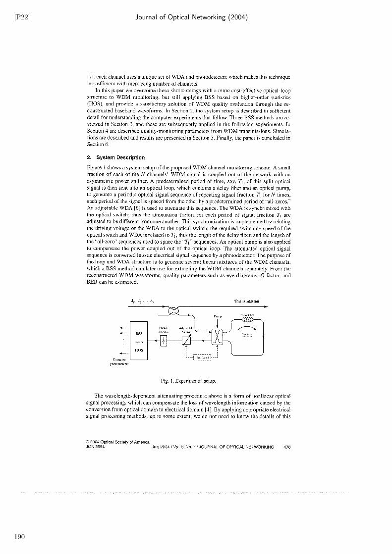
[P22] Journal of Optical Networking (2004)
190
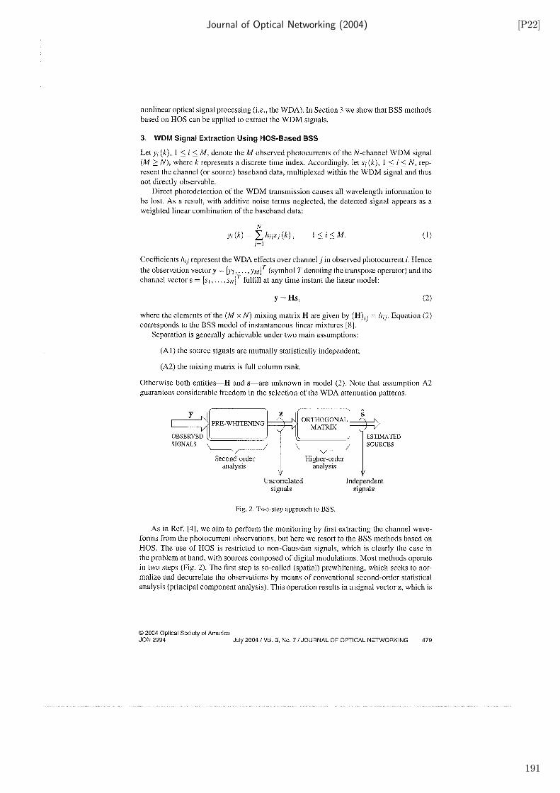
Journal of Optical Networking (2004) [P22]
191
[P22] Journal of Optical Networking (2004)
192
Journal of Optical Networking (2004) [P22]
193
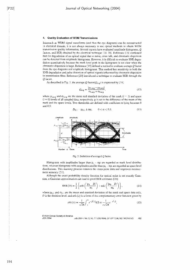
[P22] Journal of Optical Networking (2004)
194
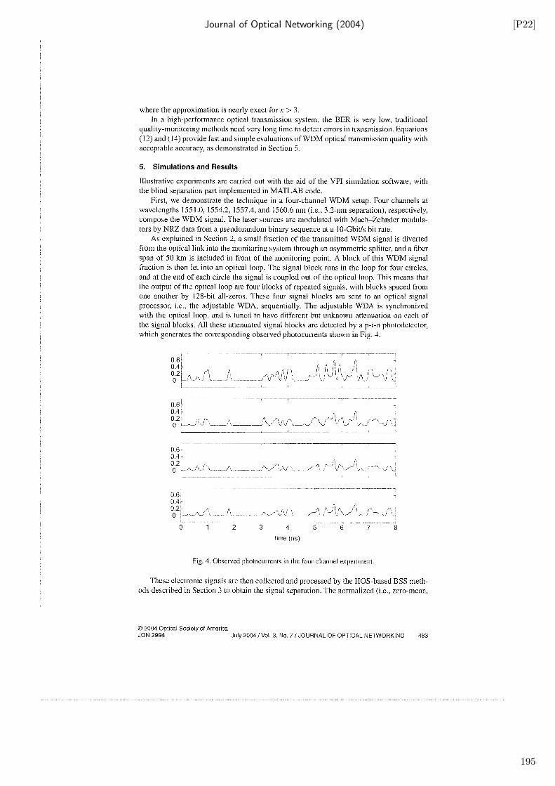
Journal of Optical Networking (2004) [P22]
195
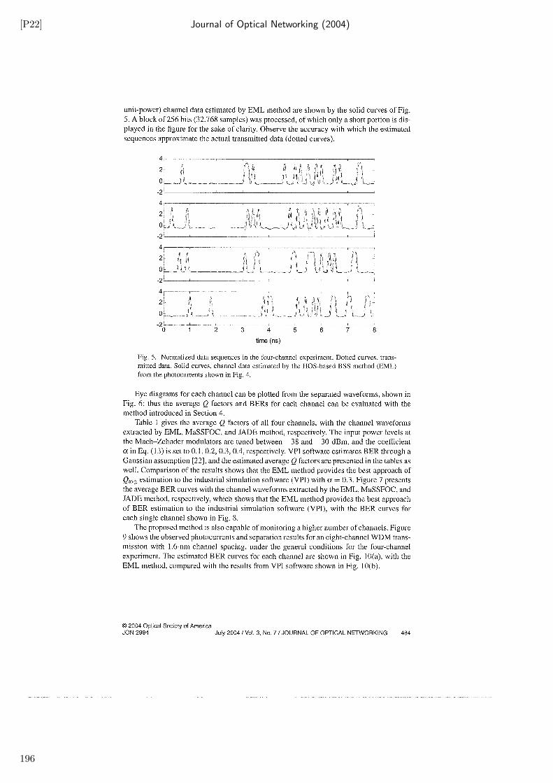
[P22] Journal of Optical Networking (2004)
196
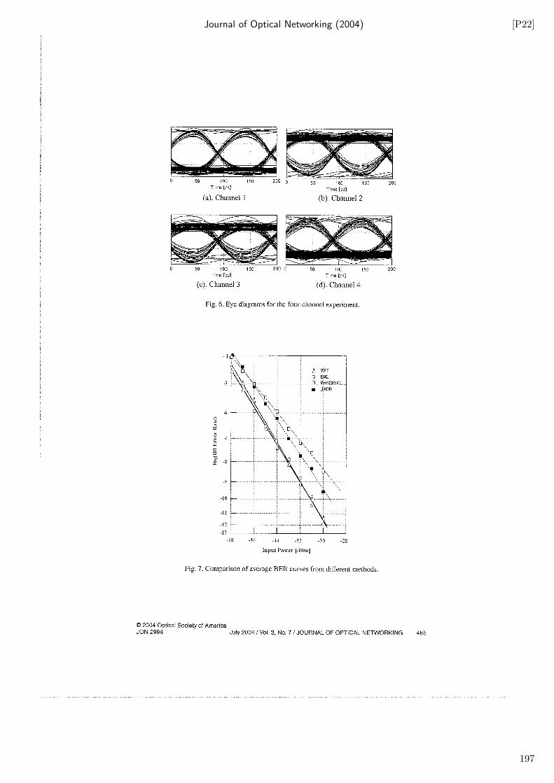
Journal of Optical Networking (2004) [P22]
197
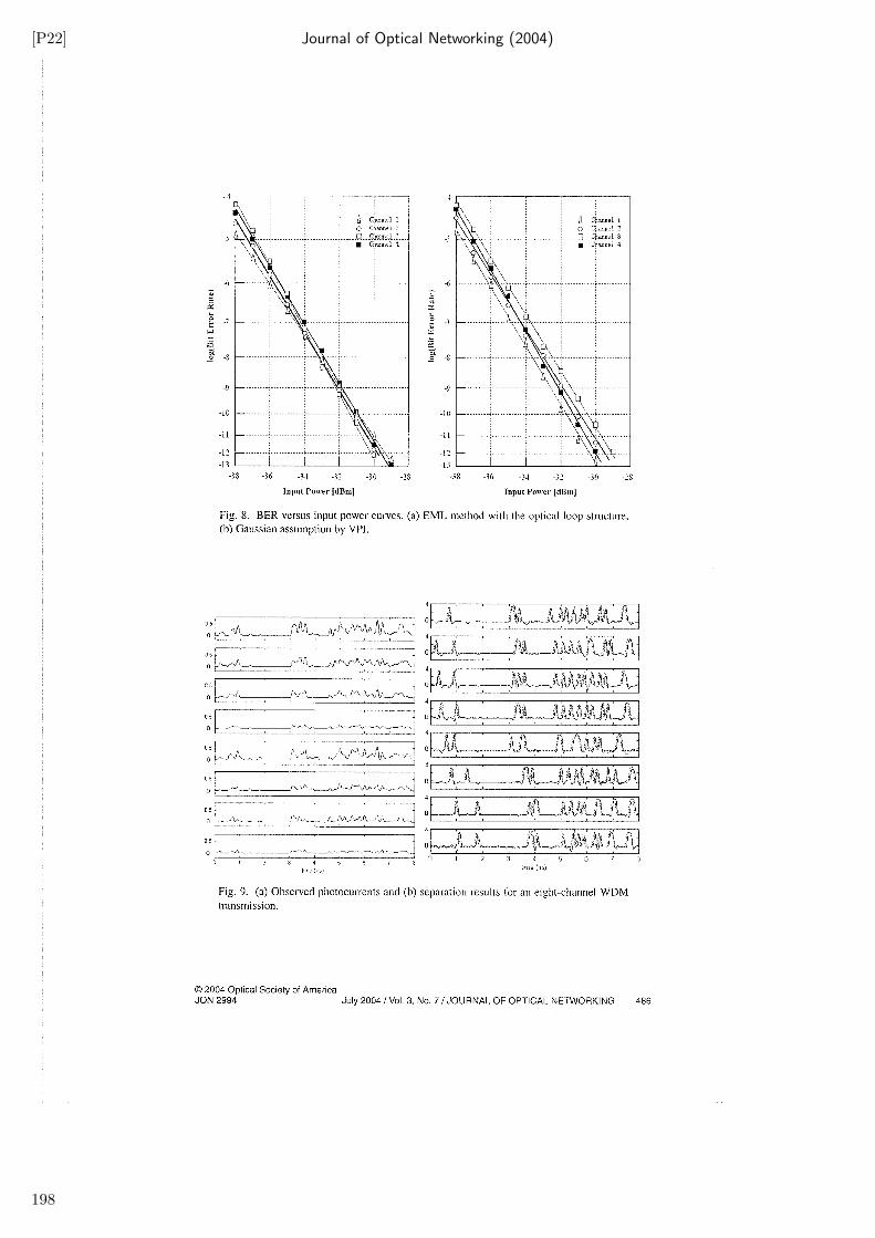
[P22] Journal of Optical Networking (2004)
198
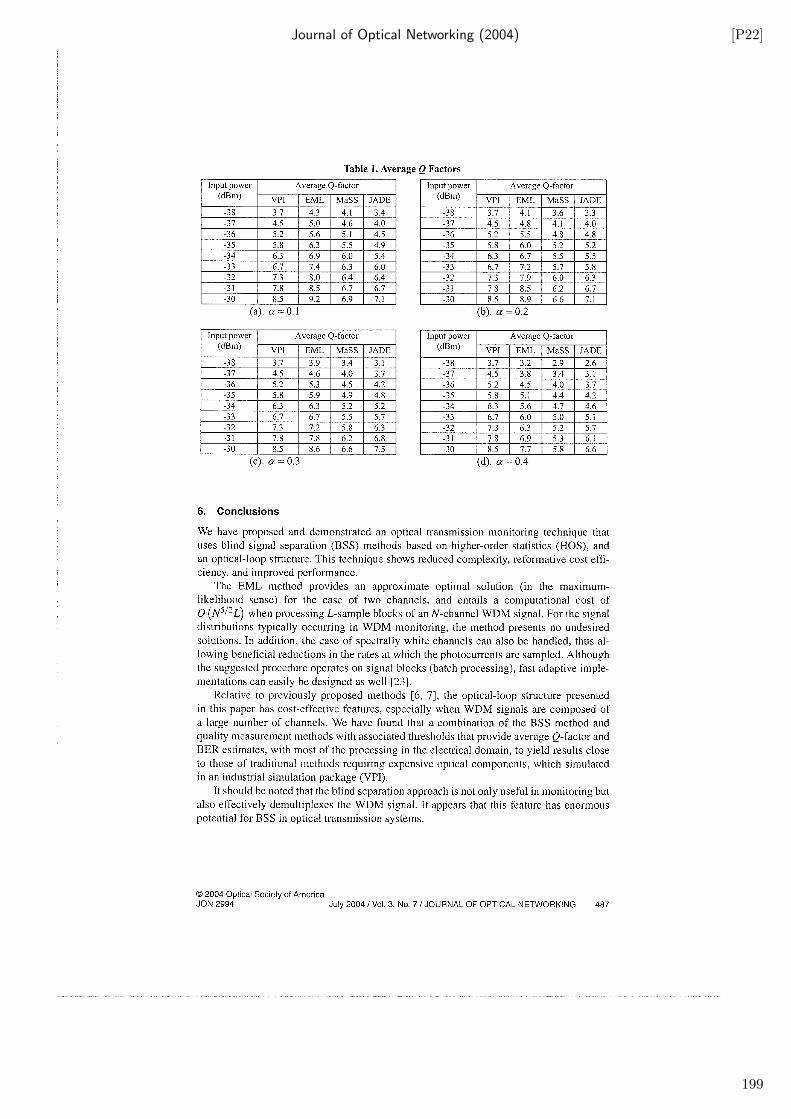
Journal of Optical Networking (2004) [P22]
199
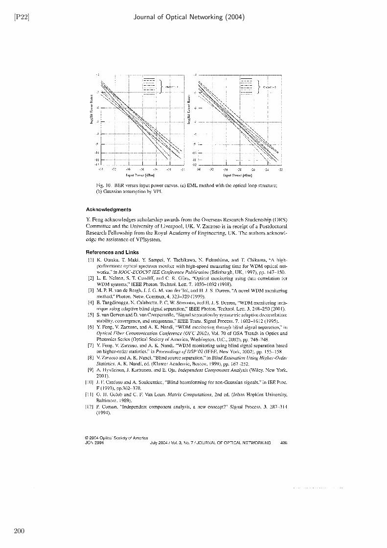
[P22] Journal of Optical Networking (2004)
200
Journal of Optical Networking (2004) [P22]
201

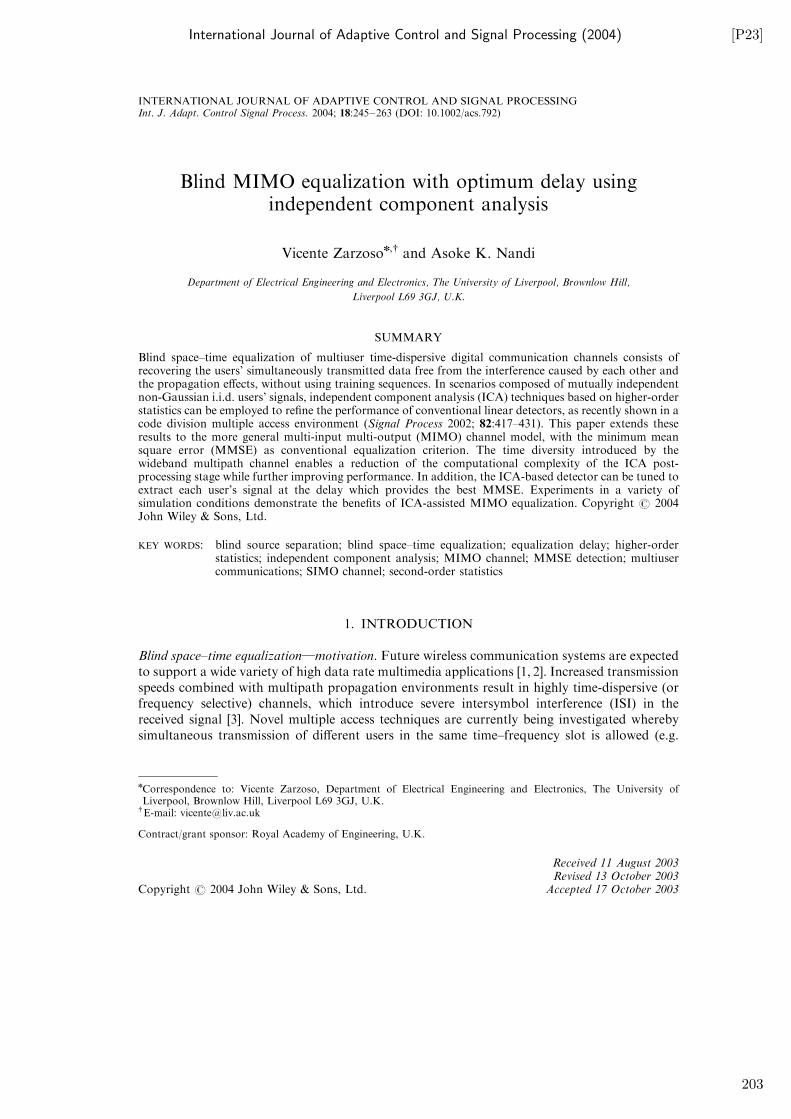
International Journal of Adaptive Control and Signal Processing (2004) [P23]
INTERNATIONAL JOURNAL OF ADAPTIVE CONTROL AND SIGNAL PROCESSINGInt. J. Adapt. Control Signal Process. 2004; 18:245–263 (DOI: 10.1002/acs.792)
Blind MIMO equalization with optimum delay usingindependent component analysis
Vicente Zarzoson,y and Asoke K. Nandi
Department of Electrical Engineering and Electronics, The University of Liverpool, Brownlow Hill,
Liverpool L69 3GJ, U.K.
SUMMARY
Blind space–time equalization of multiuser time-dispersive digital communication channels consists ofrecovering the users’ simultaneously transmitted data free from the interference caused by each other andthe propagation effects, without using training sequences. In scenarios composed of mutually independentnon-Gaussian i.i.d. users’ signals, independent component analysis (ICA) techniques based on higher-orderstatistics can be employed to refine the performance of conventional linear detectors, as recently shown in acode division multiple access environment (Signal Process 2002; 82:417–431). This paper extends theseresults to the more general multi-input multi-output (MIMO) channel model, with the minimum meansquare error (MMSE) as conventional equalization criterion. The time diversity introduced by thewideband multipath channel enables a reduction of the computational complexity of the ICA post-processing stage while further improving performance. In addition, the ICA-based detector can be tuned toextract each user’s signal at the delay which provides the best MMSE. Experiments in a variety ofsimulation conditions demonstrate the benefits of ICA-assisted MIMO equalization. Copyright # 2004John Wiley & Sons, Ltd.
KEY WORDS: blind source separation; blind space–time equalization; equalization delay; higher-orderstatistics; independent component analysis; MIMO channel; MMSE detection; multiusercommunications; SIMO channel; second-order statistics
1. INTRODUCTION
Blind space–time equalization}motivation. Future wireless communication systems are expected
to support a wide variety of high data rate multimedia applications [1, 2]. Increased transmission
speeds combined with multipath propagation environments result in highly time-dispersive (or
frequency selective) channels, which introduce severe intersymbol interference (ISI) in the
received signal [3]. Novel multiple access techniques are currently being investigated whereby
simultaneous transmission of different users in the same time–frequency slot is allowed (e.g.
Contract/grant sponsor: Royal Academy of Engineering, U.K.
Received 11 August 2003Revised 13 October 2003
Accepted 17 October 2003Copyright # 2004 John Wiley & Sons, Ltd.
yE-mail: [email protected]
nCorrespondence to: Vicente Zarzoso, Department of Electrical Engineering and Electronics, The University ofLiverpool, Brownlow Hill, Liverpool L69 3GJ, U.K.
203
[P23] International Journal of Adaptive Control and Signal Processing (2004)
spatial division multiple access, SDMA). This overlapped sharing of channel resources enhances
bandwidth utilization at the expense of an increased level of co-channel interference (CCI).
Signal processing techniques for space–time equalization aim at the cancellation of CCI and ISI
at the receive antenna output, and the recovery of the transmitted users’ data [4]. Traditionally,
equalization is aided with the transmission of training or pilot sequences, which makes a poor
use of the available bandwidth and is not feasible or practical in certain scenarios [5, 6]; hence
the enormous research interest aroused by blind equalization techniques since the seminal works
of References [7–11].
SIMO model. In the single-user case, the use of receivers with spatially separated multiple
antenna elements and/or oversampling (i.e. sampling faster than the baud rate) leads to the
single-input multiple-output (SIMO) signal model. Compared to the conventional single-output
(SISO) case, SIMO systems exhibit two remarkable features [12–14]: first, non-minimum phase
channels can be blindly identified using only second-order statistics (SOS); second, finite impulse
response (FIR) channels can be perfectly equalized, in the noiseless case, using FIR filters.
MIMO model}ICA-based CCI-cancellation. The multiuser scenario is naturally described by
the multiple-input multiple-output (MIMO) signal model. This model also arises in systems with
multiple transmitter antennas (using, e.g. spatial multiplexing), even if just a single user is
present. The MIMO extensions of SIMO equalization techniques are able to suppress ISI,
resulting in a memoryless CCI-only cancellation problem [5, 15–17]. This latter can then be
resolved using source separation techniques based on the finite alphabet or constant modulus
properties of digital modulations [5,18–20]. Alternatively, the mutual statistical independence
between the users’ signals can be exploited through the use of independent component analysis
(ICA) [21] based on higher-order statistics (HOS) [15, 22–24]. The main advantage of HOS-
based ICA techniques is that, under mild conditions (typically, that at most one of the sources
be Gaussian [23]), signal recovery is guaranteed regardless of the source constellation and
spectral characteristics [24].
Channel identification and optimum-delay estimation. Blind multichannel equalization can be
performed with (e.g. References [12, 13, 25]) or without (e.g. References [5, 26, 27]) previous
channel identification. Channel identification-based equalization presents the main drawback
that inaccuracies in the channel estimate have a detrimental effect on the signal detection stage.
However, a channel estimate may prove useful in a variety of tasks such as power control,
propagation characterization, or source localization and tracking. More importantly, knowl-
edge of the channel structure makes it possible to select the equalization delay which yields
optimum performance. The equalized signal mean square error (MSE) for a given delay depends
on the corresponding column of the channel matrix, as shown in the exact MSE expression for
the linear minimum mean square error (MMSE) equalizer [28] as well as in the approximated
Cram!eer–Rao lower bound of Reference [29]. Even direct equalization methods require to
estimate the channel response from the equalized output in order to perform optimum delay
selection [27, 30]. In addition, Reference [27] needs to compute the equalizers for all delays
before discerning the optimum solution. The iterative procedure described in Reference [31]
avoids channel estimation, but its convergence to the optimum-delay equalizer is only
conjectured and is not theoretically guaranteed; the procedure is also computationally
expensive.
ICA-based detection. The exploitation of HOS through ICA proves useful in refining
conventional linear detection, as recently demonstrated in Reference [1] in a particular code
division multiple access (CDMA) model. The ICA refinement alleviates the negative impact of
Copyright # 2004 John Wiley & Sons, Ltd. Int. J. Adapt. Control Signal Process. 2004; 18:245–263
V. ZARZOSO AND A. K. NANDI246
204
International Journal of Adaptive Control and Signal Processing (2004) [P23]
channel estimation errors on the equalization performance. Similar results are obtained in
Reference [32] in the more generic MIMO model, where it is shown that ICA-aided MMSE
equalization outperforms the conventional MMSE receiver. Furthermore, the time redundan-
cies of the MIMO model allow certain simplifications which yield considerable performance
improvements with significant computational savings.
Contribution. The purpose of this paper is to elaborate on the findings of Reference [32]. We
propose the use of ICA for the simultaneous extraction of the users’ signals at their respective
optimal MMSE equalization delays. The subsequent performance gains are achieved at only a
modest increase in computational load relative to the conventional receiver. We also intend to
carry out, through simulation, a more rigorous experimental analysis of ICA-assisted blind
detection in MIMO digital communication systems.
Outline of the paper. Section 2 summarizes the signal model and mathematical preliminaries.
Section 3 presents the theory behind ICA-aided optimum-delay equalization, which is the core
of our contribution. An experimental study is reported in Section 4. The concluding remarks of
Section 5 bring the paper to an end.
Notations. Vectors and matrices are denoted by boldface lowercase and uppercase symbols,
respectively; C is the set of complex numbers; In refers to the n� n identity matrix; ð�ÞT; ð�ÞH,ð�Þ�1 and ð�Þy indicate the transpose, Hermitian (conjugate-transpose), inverse and Moore-
Penrose pseudoinverse matrix operators, respectively; ðaÞi is ith component of vector a; jjAjj2F ¼
traceðAAHÞ ¼ traceðAHAÞ denotes the Frobenius norm of matrix A; Reð�Þ denotes the real part
of its complex argument; Ef�g represents the mathematical expectation;� and� stand for the
Kronecker and elementwise product, respectively.
2. SIGNAL MODEL
Let us consider a multiuser communication system composed of
(A1) K users transmitting, at a known constant baud rate, zero-mean unit-variance mutually
independent non-Gaussian i.i.d. data symbols sðnÞ ¼ ½s1ðnÞ; . . . ; sK ðnÞ�T 2 CK ;
(A2) a receiver with vector output xðnÞ ¼ ½x1ðnÞ; . . . ; xLðnÞ�T 2 CL;
(A3) FIR channels (including pulse-shaping and receive filter effects) spanning at most M þ 1
symbols, with matrix coefficients HðkÞ 2 CL�K ; k ¼ 0; 1; . . . ;M ; where the channel order Mis assumed to be known and the channel taps fixed over the observation window,
(A4) zero-mean additive noise vðnÞ 2 CL independent of the data sources.
Symbols n and k above represent discrete-time indices relative to the baud period. The
receiver output components in (A2) are not necessarily associated with spatially separated
physical devices. Since digital signals are cyclostationary, oversampling or fractionally spaced
sampling (i.e. taking more than a sample per baud period) can induce extra ‘virtual’ sensors
[12, 13]. The virtual channels are given by the phases of the physical channels, a phase
corresponding to a baud-sampled sequence of the impulse response with a different time origin.
Space–time processing operates on the spatial (physically separated sensors) as well as the
temporal dimension [4, 5]. Although time- or space-only processing may suffice in theory,
improved ISI-CCI suppression can be achieved by joint space–time processing [4]. Assumptions
(A3) model block (or time-non-selective or slowly) fading channels, typical of low mobility
systems, with small to moderate Doppler spread values.
Copyright # 2004 John Wiley & Sons, Ltd. Int. J. Adapt. Control Signal Process. 2004; 18:245–263
BLIND MIMO EQUALIZATION 247
205
[P23] International Journal of Adaptive Control and Signal Processing (2004)
Under the above assumptions, the MIMO model can be expressed as
xðnÞ ¼X
M
k¼0
HðkÞsðn� kÞ þ vðnÞ ð1Þ
Stacking N consecutive received signal vector samples leads to the matrix model
xn ¼ Hsn þ vn ð2Þ
with sn ¼ ½sðnÞT; sðn� 1ÞT; . . . ; sðn�M � N þ 1ÞT�T 2 CKðMþNÞ
H ¼
Hð0Þ � � � HðMÞ 0 � � � 0
0 Hð0Þ � � � HðMÞ � � � 0
..
. . .. . .
. . .. . .
. ...
0 . . . 0 Hð0Þ � � � HðMÞ
2
6
6
6
6
6
6
4
3
7
7
7
7
7
7
5
ð3Þ
xn ¼ ½xðnÞT;xðn� 1ÞT; . . . ;xðn� N þ 1ÞT�T 2 CLN ; and analogous definition for vn: For conve-
nience, we call P ¼ LN ; C ¼ M þ N ; and D ¼ KC:The objective of blind MIMO equalization is to estimate the source signals sðnÞ from the only
observation of the receiving sensor output xðnÞ: This process involves ISI cancellation (time
equalization) and CCI suppression (space equalization). These tasks can be performed by first
identifying the channel taps
H ¼ ½Hð0Þ; Hð1Þ; . . . ;HðMÞ� ð4Þ
which are then ‘inverted’ to estimate the sources. The block-Toeplitz channel matrix H 2 CP�D
in Equation (2) must be full column rank. An obvious necessary condition is that L > K: the
number of sensors must be strictly higher than the number of sources, i.e. sufficient spatio-
temporal diversity must be available; also, N5KM=ðL� KÞ; which sets a lower bound on the
equalizer length. A sufficient condition for the invertibility of H is that the subchannels be
coprime, that is, that they do not share any common zeros [12]. More elaborate sufficient
conditions are given in Reference [33].
Even if the channel matrix is invertible, inherent indeterminacies exist. Without any further
prior knowledge on the sources or the mixing system besides assumptions (A1) and (A3), the
channel matrix tapsHðkÞ can at best be identified up to a common post-multiplicative factor KC;where C 2 CK�K is a permutation matrix and K 2 CK�K a non-singular diagonal matrix with
unit-norm diagonal elements. These phase and permutation indeterminacies are unavoidable
but admissible ambiguities in blind estimation.
In the sequel, it is assumed that the channel matrix H (or, equivalently, the channel tap matrix
H) has been estimated through a suitable blind MIMO identification method (as those of, e.g.
References [5, 16, 17, 32]). Our primary concern is the estimation (i.e. detection or equalization)
of the source signals s from the sensor output x by using the identified channel. In blind space–
time equalization techniques based on previous channel identification, ISI-CCI suppression is
implicitly carried out during channel estimation, and actually takes effect at the detection stage.
Copyright # 2004 John Wiley & Sons, Ltd. Int. J. Adapt. Control Signal Process. 2004; 18:245–263
V. ZARZOSO AND A. K. NANDI248
206
International Journal of Adaptive Control and Signal Processing (2004) [P23]
3. ICA-AIDED DETECTION
3.1. Linear detection
Even if the channel is perfectly known, the estimation of the source signals in a noisy model like
(1)–(2) is not a trivial task. The maximum likelihood sequence estimator is the optimal detector,
but its computational load can be prohibitive in scenarios involving a large number of users and
highly dispersive channels [3]. Trading off complexity for performance, linear receivers are based
on the estimation of a linear transformation G 2 CP�D fulfilling certain (sub)optimality
criterion; data are then detected as #ssn ¼ GHxn: The zero forcing (ZF) detector aims at the joint
minimization of ISI and CCI in the absence of noise, and can thus be expressed as the least-
squares problem
GZF ¼ arg minG
jjGHH� IDjj
2F ð5Þ
The solution to (5) is readily computed as GZF ¼ ðHHHÞ�1H ¼ ðHyÞH: The ZF detector can lead
to severe noise amplification in noisy scenarios. This drawback is avoided by the minimum mean
square error (MMSE) equalizer
GMMSE ¼ arg minG
E jjGHxn � snjj
2� �
ð6Þ
with closed-form solution GMMSE ¼ R�1x H; where Rx ¼ EfxxHg represents the sensor-output
covariance matrix. Due to its enhanced properties at low signal-to-noise ratio (SNR), we adhere
to the MMSE detector in the following. The development is analogous for ZF equalization.
3.2. ICA refinement
Imprecisions, e.g. due to finite sample size, in the estimation of the channel matrix or the sensor
covariance matrix have a negative impact on the detection of the transmitted data symbols. To
alleviate this detrimental effect, the higher-order statistical independence of the users’ signals can
be exploited. Under the spatio-temporal independence assumption of (A1), model (2)
corresponds to a problem of blind separation of independent sources in instantaneous linear
mixtures, which can be solved with the statistical tool of ICA based on HOS [21]. From this
perspective, the source estimation can be carried out without previous channel identification by
applying an ICA method directly and then using a simple algorithm to identify and group each
user’s delays [24, 34, 35]. Although this fully blind ICA approach is conceptually simple, the
computational complexity of separating D ¼ KðM þ N Þ independent components can become
excessive, even with a moderate number of users, in systems with long delay spreads as a result
of high data rates [24].
The rationale behind ICA-assisted detection consists of taking advantage of the available
channel estimate as an initial point in the ICA search. Two main benefits can be derived from
this refinement. Firstly, since conventional detection (Equations (5)–(6)) only makes use
(implicitly) of SOS, the exploitation of HOS by ICA is expected to mitigate performance drops
caused by estimation errors at the channel identification stage. Secondly, if these channel
identification errors are moderate, the initialization provided by the channel estimate may
already be quite close to the ICA solution, thus decreasing the convergence time and
computational complexity of the ICA post-processing block. The idea of ICA-refined detection
was originally proposed in Reference [1] in the context of a DS-CDMA signal model. In
Copyright # 2004 John Wiley & Sons, Ltd. Int. J. Adapt. Control Signal Process. 2004; 18:245–263
BLIND MIMO EQUALIZATION 249
207
[P23] International Journal of Adaptive Control and Signal Processing (2004)
Reference [32], the ICA-based MMSE refinement was extended to the more general MIMO
model, and is reproduced below for the sake of completeness.
Consider the whitened sensor output zn ¼Wxn; in which the whitening matrix W 2 CD�P
constrains Rz ¼ ID: Matrix W can easily be computed from the eigenvalue decomposition
(EVD) of Rx; and involves second-order space–time decorrelation, power normalization and
projection on the signal subspace. The MMSE estimate of sn accepts the equivalent expression
#ssn ¼ *GGHzn; with
*GG ¼W #HH ð7Þ
In the noiseless case, detection matrix *GG is unitary. Hence, the whitened outputs can be regarded
as a spatio-temporal unitary linear mixture of the users’ data. To exploit the source statistical
independence, an ICA method can operate on the whitened signals zn with a separating matrix
initialized at the conventional MMSE detection matrix *GG: Final detection is then performed
with the separating matrix #GG provided by the ICA algorithm at convergence. The use of HOS
constrains the users’ data to be non-Gaussian (Assumption (A1)), which is verified by most
digital modulations of practical significance. We select the fixed-point FastICA algorithm based
on kurtosis optimization [21, 36] for its robustness and rapid (cubic) convergence properties.
Assume that T consecutive whitened column vectors are stored in matrix Z ¼ ½z0; z1; . . . ; zT�1� 2C
D�T : The FastICA algorithm can be outlined as follows [1, 21, 36]:
1. Initialize #GG0 as the projection of *GG onto the set of unitary matrices.
2. For k50; repeat steps below until convergence.
3. #SSk ¼ #GGHk Z:
4. Update #GGkþ1 ¼1TZðj #SSk j
2� #SSkÞH � g #GGk :
5. Symmetric decorrelation #GGkþ1 #GGkþ1ð #GGHkþ1
#GGkþ1Þ�1=2:
In Step 4, g ¼ 3 for real-valued sources (e.g. BPSK modulations) and g ¼ 2 for complex-
valued sources. The orthogonal projection on the set of unitary matrices of Steps 1 and 5 admits
an efficient implementation in terms of the singular value decomposition (SVD) #GG ¼ URVH as
#GG UVH: As a statistically significant termination criterion we choose
1
Dtraceðj #GGH
kþ1#GGk jÞ � 1
�
�
�
�
�
�
�
�
5
10�3
Tð8Þ
That is, iterations are stopped when the column vectors of #GGkþ1 and #GGk lie in directions which
are sufficiently close (in terms of a sample-size based threshold). In preliminary experiments, less
than 2D iterations are typically required for convergence in high SNR environments and
sufficient sample size. For low SNR or insufficient sample length, the algorithm may not
converge, so the above maximum number of iterations is set as an additional termination test.
Excluding the symmetric decorrelation step, the computational complexity of the FastICA
algorithm is of order OðDT Þ floating point operations (flops) per column of #GG per iteration.
Note that the authors of Reference [1] were involved in extracting the signal of a single user of
interest, whereas we aim at the simultaneous demodulation of all existing users (including all the
spatially multiplexed data substreams of each user, if multiple transmit antennas are employed).
Furthermore, the parameterization in the CDMA model of Reference [1] only accounts for
channels with short delay spreads (more precisely, a delay spread of less than half the symbol
period is considered in that reference). By contrast, the more general MIMO model of
Equations (1)–(2) enables a more realistic characterization of wideband channels with longer
Copyright # 2004 John Wiley & Sons, Ltd. Int. J. Adapt. Control Signal Process. 2004; 18:245–263
V. ZARZOSO AND A. K. NANDI250
208
International Journal of Adaptive Control and Signal Processing (2004) [P23]
delay spreads.z More importantly, Reference [1] extracts the user-of-interest’s signal at a fixed
delay. However, long delay spreads make it possible to extract the users’ data at alternative
delays, which can lead to potential performance improvements. Unlike fully blind ICA, where
no control over the extracted delay is possible, we will see next that ICA-based MIMO
equalization can be fine-tuned to carry out detection at the best delay for each user, thus
improving performance while reducing computational cost.
3.3. Optimal delay selection
The previous sections have reviewed linear detectors that estimate all the components of the
source vector sn simultaneously, and how this conventional detection can be enhanced with the
use of ICA. However, most of the detected signals are redundant, since C ¼ M þ N time-shifted
versions of each of the K users are recovered, whereas a single time delay suffices in practice. The
time redundancy introduced by the multipath channel in the MIMO model (2) enables the
choice of the equalization delay providing the best MMSE performance for each user. This
choice is simplified thanks to the channel matrix estimate obtained in the blind identification
stage.
The MMSE detector of the ith source signal, 14i4K; with delay 04d4ðC � 1Þ; is given by
the corresponding column of GMMSE:
Gi;d ¼ R�1x hi;d ð9Þ
in which hi;d denotes the ðKd þ iÞth column vector of channel matrix H: The resulting MMSE
can be obtained analytically as [28]
MMSEi;d ¼ Efj#ssiðn� dÞ � siðn� dÞj2g ¼ 1� hHi;dR
�1x hi;d ð10Þ
Optimum MMSE equalization for the ith user is achieved at delay
di ¼ argmind
MMSEi;d ð11Þ
Hence, from the available estimate of the channel matrix and the sensor output covariance
matrix, it is possible to compute the equalizer that will detect each source signal with the lowest
MMSE.
In practice, estimation errors caused by finite sample length may produce negative values of
MMSE in Equation (10). However, in our experience the shape of the MMSE performance
variation as a function of the equalization delay as well as the position of the optimum delay do
not suffer significant changes relative to the theoretical solution.
3.4. Simplified ICA refinement
Once the optimal delay of each source has been selected, the corresponding columns of the
estimated channel can be used to initalize the ICA post-processing stage. Let those columns be
stored in matrix #HHK ¼ ½h1;d1 ; h2;d2 ; . . . ; hK;dK �: Then
*GGK ¼W #HHK ð12Þ
zMore details about the differences and relationships between channel models based on physical multipath parametersand on the channel impulse response can be found in Reference [4].
Copyright # 2004 John Wiley & Sons, Ltd. Int. J. Adapt. Control Signal Process. 2004; 18:245–263
BLIND MIMO EQUALIZATION 251
209
[P23] International Journal of Adaptive Control and Signal Processing (2004)
is the associated MMSE detector, which can serve as starting point for the ICA refinement
(with the obvious modification of K for D in termination test (8)). In this manner, the ICA
algorithm searches only for the K independent components associated with the users’ signals at
their respective optimum MMSE delay. This search for the optimum-delay components not
only improves performance, but also leads to a reduction in computational complexity by a
factor of C per iteration, which can be remarkable in highly time dispersive channels. In
addition, since fewer independent components are sought, the ICA algorithm would also be
expected to take fewer iterations to converge. These benefits will be put to the test in the
experiments of Section 4.
This simplified MMSE-ICA detection scheme, which arises from the time redundancy
induced by wideband multipath propagation, was originally proposed in Reference [32] for zero-
delay equalization only. Herein, we improve on the original definition by allowing arbitrary
delays and, in particular, those providing optimum MMSE performance for each user
transmission.
3.5. Switching
The ICA refinement may converge to a solution far from optimal, worsening rather
than improving the results of the conventional detector. Experimental results indicate
that this undesirable outcome only occurs in low SNR scenarios or when processing
short sample sizes. At low SNR, noise becomes dominant relative to the users’ data
in signal model (1)–(2). As a result, ICA will ‘perceive’ the noise as the actual sources,
and thus will seek independence among the noise components. This misguided search
will most probably yield a wrong equalization solution. Erroneous HOS estimation
due to short observation windows can cause analogous adverse effects in the ICA
refinement.
To avoid this degeneracy, a ‘branch switching’ criterion can be proposed along the
lines of Reference [1]. By virtue of this criterion, the MMSE-ICA solution is deemed
as favourable when the prior information provided by the conventional receiver is fairly
preserved at the output of the ICA stage, that is, when the initial and final separating
vectors (the columns of #GG0 and #GG; respectively) are sufficiently correlated. This criterion can
easily be extended to the MIMO model by switching to the MMSE-ICA solution of Section 3.2
whenever [32]
x¼4 1
DReðtraceð #GGH #GG0ÞÞ > t ð13Þ
where t 2�0; 1½ is a suitably selected threshold (e.g. Reference [1] chooses t ¼ 0:8); the
conventional MMSE detector is otherwise employed. Using K instead of D in the above
expression, the switching rule is readily made applicable to the simplified MMSE-ICA solution
of Section 3.4.
The usefulness of this switching strategy is arguable if the accuracy of the prior information
acquired before detection (e.g. the proximity between the true and the identified channel)
is poor. In such an event, the proposed switching could wrongly rule out ICA solutions that
are actually advantageous compared to those of the linear MMSE receiver, which would
be operating on erroneous information. This switching rule is tested in the simulations of
next section.
Copyright # 2004 John Wiley & Sons, Ltd. Int. J. Adapt. Control Signal Process. 2004; 18:245–263
V. ZARZOSO AND A. K. NANDI252
210
International Journal of Adaptive Control and Signal Processing (2004) [P23]
4. EXPERIMENTAL RESULTS AND ANALYSIS
This section evaluates the comparative performance of the ICA-assisted equalizers under a
variety of simulation conditions, and illustrates some points of the previous theoretical
exposition. A communication system composed of K ¼ 5 simultaneous QPSK-modulated users
is simulated in a frequency-selective block fading channel introducing ISI from a maximum of
M ¼ 4 consecutive baud periods. The channel filter taps are randomly drawn from a complex
Gaussian distribution and hence model (up to the pulse-shaping and receive filters) a Rayleigh
propagation environment. A spatio-temporal oversampling level of L ¼ 10 and a smoothing
factor of N ¼ 5 result in a 50� 45 channel matrix H: Additive white Gaussian noise with
covariance matrix Rv ¼ s2IL is present at the sensor output; the SNR is given by
SNR ¼traceðHH
HÞ
s2Lð14Þ
Equalization performance is measured by the signal mean square error (SMSE)
SMSE ¼1
K
X
K
i¼1
Efj#ssiðn� #dd iÞ � siðn� #dd iÞj2g ð15Þ
where #dd i represents the equalization delay selected for the ith user, which is obtained by the
optimality criteria of Section 3.3 from the channel and covariance matrix estimates. Similarly,
the channel identification accuracy can be assessed with the channel normalized mean square
error (CMSE)
CMSE ¼jj #HH�Hjj2F
jjHjj2Fð16Þ
where #HH is the estimated channel tap matrix. Performance parameters are averaged over n
independent Monte Carlo (MC) iterations, with nNd5105; where Nd is the observation length in
baud periods. As a quality index for the optimum-delay estimation performance we define the
delay root mean square error (DRMSE)
DRMSE ¼
ffiffiffiffiffiffiffiffiffiffiffiffiffiffiffiffiffiffiffiffiffiffiffiffiffiffiffiffiffiffiffiffiffiffiffiffiffiffiffiffiffiffiffiffiffiffiffiffiffiffiffiffiffiffiffiffiffiffiffi
1
n
Xn
j¼1
1
K
XK
i¼1ð #ddðjÞi � diÞ
2
r
ð17Þ
where #ddðjÞi represents the ith-source delay estimate at MC iteration j; and theoretical values di are
obtained from Equation (11) by plugging the true channel and covariance matrices in Equation (10).
4.1. Perfect channel knowledge
We first consider the scenario where the channel is assumed to be perfectly known or estimated,
i.e. CMSE ¼ 0: As a result, all errors in the MMSE equalizer are due exclusively to the finite-
sample estimation of the sensor covariance matrix (or, equivalently in this case, of the noise
variance), which is computed from Nd observed symbol periods. For instance, this scenario
could simulate a training-based channel estimation preamble during transmission.
Performance vs sample size. Figure 1 shows the performance of the conventional MMSE, the
MMSE-ICA and the simplified MMSE-ICA receivers against the sample size Nd ; for SNR ¼
20 dB and a fixed channel matrix with condition number around 100. The ICA post-processing
has difficulties to converge at low sample size, as shown by the number of FastICA iterations in
Figure 2. A performance degradation is consequently observed when the switching criterion of
Copyright # 2004 John Wiley & Sons, Ltd. Int. J. Adapt. Control Signal Process. 2004; 18:245–263
BLIND MIMO EQUALIZATION 253
211
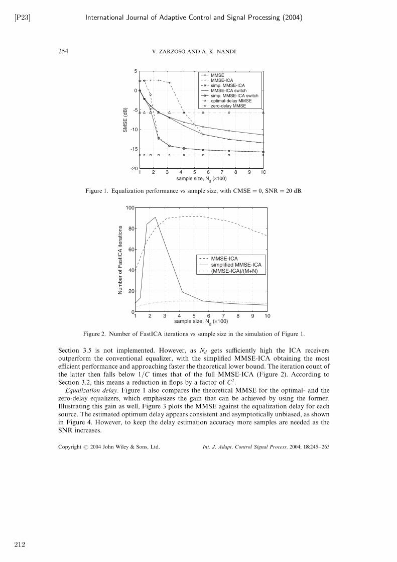
[P23] International Journal of Adaptive Control and Signal Processing (2004)
Section 3.5 is not implemented. However, as Nd gets sufficiently high the ICA receivers
outperform the conventional equalizer, with the simplified MMSE-ICA obtaining the most
efficient performance and approaching faster the theoretical lower bound. The iteration count of
the latter then falls below 1=C times that of the full MMSE-ICA (Figure 2). According to
Section 3.2, this means a reduction in flops by a factor of C2:Equalization delay. Figure 1 also compares the theoretical MMSE for the optimal- and the
zero-delay equalizers, which emphasizes the gain that can be achieved by using the former.
Illustrating this gain as well, Figure 3 plots the MMSE against the equalization delay for each
source. The estimated optimum delay appears consistent and asymptotically unbiased, as shown
in Figure 4. However, to keep the delay estimation accuracy more samples are needed as the
SNR increases.
1 2 3 4 5 6 7 8 9 10-20
-15
-10
-5
0
5
sample size, Nd (×100)
SM
SE
(dB
)
MMSEMMSE-ICAsimp. MMSE-ICAMMSE-ICA switchsimp. MMSE-ICA switchoptimal-delay MMSEzero-delay MMSE
Figure 1. Equalization performance vs sample size, with CMSE ¼ 0; SNR ¼ 20 dB:
1 2 3 4 5 6 7 8 9 100
20
40
60
80
100
sample size, Nd (×100)
Num
ber
of F
astIC
A ite
rations
MMSE-ICAsimplified MMSE-ICA(MMSE-ICA)/(M+N)
Figure 2. Number of FastICA iterations vs sample size in the simulation of Figure 1.
Copyright # 2004 John Wiley & Sons, Ltd. Int. J. Adapt. Control Signal Process. 2004; 18:245–263
V. ZARZOSO AND A. K. NANDI254
212
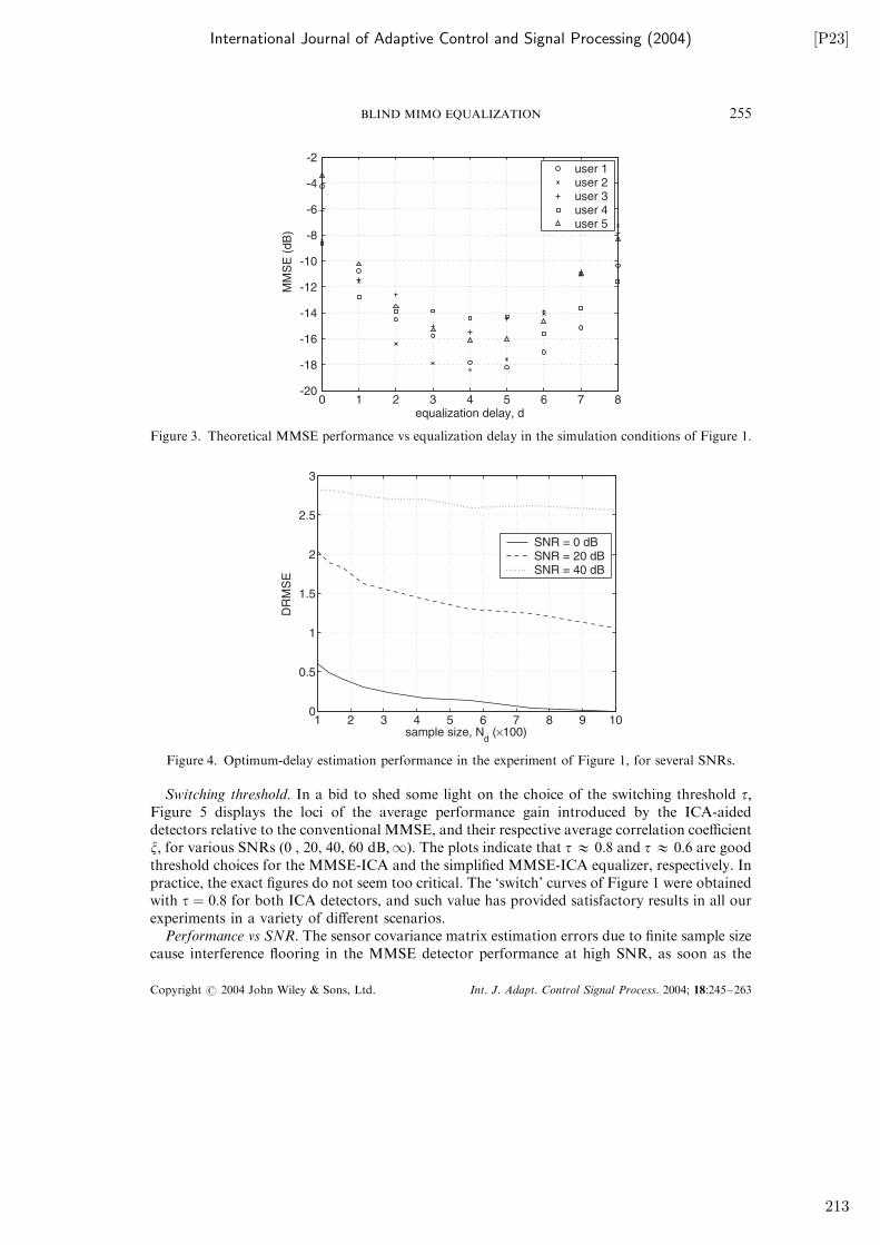
International Journal of Adaptive Control and Signal Processing (2004) [P23]
Switching threshold. In a bid to shed some light on the choice of the switching threshold t;Figure 5 displays the loci of the average performance gain introduced by the ICA-aided
detectors relative to the conventional MMSE, and their respective average correlation coefficient
x; for various SNRs (0 , 20, 40, 60 dB;1). The plots indicate that t� 0:8 and t� 0:6 are good
threshold choices for the MMSE-ICA and the simplified MMSE-ICA equalizer, respectively. In
practice, the exact figures do not seem too critical. The ‘switch’ curves of Figure 1 were obtained
with t ¼ 0:8 for both ICA detectors, and such value has provided satisfactory results in all our
experiments in a variety of different scenarios.
Performance vs SNR. The sensor covariance matrix estimation errors due to finite sample size
cause interference flooring in the MMSE detector performance at high SNR, as soon as the
0 1 2 3 4 5 6 7 8-20
-18
-16
-14
-12
-10
-8
-6
-4
-2
equalization delay, d
MM
SE
(dB
)
user 1user 2user 3user 4user 5
Figure 3. Theoretical MMSE performance vs equalization delay in the simulation conditions of Figure 1.
1 2 3 4 5 6 7 8 9 100
0.5
1
1.5
2
2.5
3
sample size, Nd
(×100)
DR
MS
E
SNR = 0 dBSNR = 20 dBSNR = 40 dB
Figure 4. Optimum-delay estimation performance in the experiment of Figure 1, for several SNRs.
Copyright # 2004 John Wiley & Sons, Ltd. Int. J. Adapt. Control Signal Process. 2004; 18:245–263
BLIND MIMO EQUALIZATION 255
213
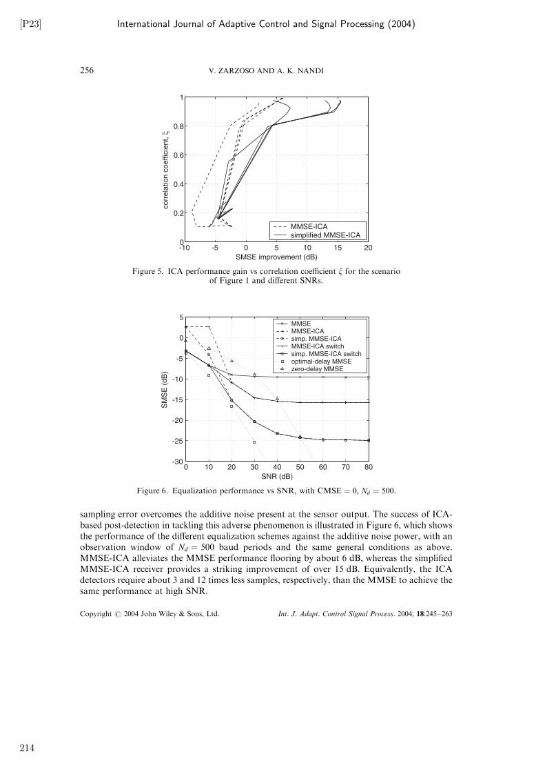
[P23] International Journal of Adaptive Control and Signal Processing (2004)
sampling error overcomes the additive noise present at the sensor output. The success of ICA-
based post-detection in tackling this adverse phenomenon is illustrated in Figure 6, which shows
the performance of the different equalization schemes against the additive noise power, with an
observation window of Nd ¼ 500 baud periods and the same general conditions as above.
MMSE-ICA alleviates the MMSE performance flooring by about 6 dB; whereas the simplified
MMSE-ICA receiver provides a striking improvement of over 15 dB: Equivalently, the ICA
detectors require about 3 and 12 times less samples, respectively, than the MMSE to achieve the
same performance at high SNR.
-10 -5 0 5 10 15 200
0.2
0.4
0.6
0.8
1
SMSE improvement (dB)
co
rre
latio
n c
oe
ffic
ien
t, ξ
MMSE-ICAsimplified MMSE-ICA
Figure 5. ICA performance gain vs correlation coefficient x for the scenarioof Figure 1 and different SNRs.
0 10 20 30 40 50 60 70 80-30
-25
-20
-15
-10
-5
0
5
SNR (dB)
SM
SE
(d
B)
MMSEMMSE-ICAsimp. MMSE-ICAMMSE-ICA switchsimp. MMSE-ICA switchoptimal-delay MMSEzero-delay MMSE
Figure 6. Equalization performance vs SNR, with CMSE ¼ 0; Nd ¼ 500:
Copyright # 2004 John Wiley & Sons, Ltd. Int. J. Adapt. Control Signal Process. 2004; 18:245–263
V. ZARZOSO AND A. K. NANDI256
214
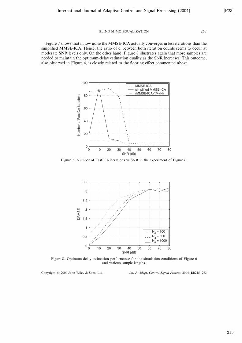
International Journal of Adaptive Control and Signal Processing (2004) [P23]
Figure 7 shows that in low noise the MMSE-ICA actually converges in less iterations than the
simplified MMSE-ICA. Hence, the ratio of C between both iteration counts seems to occur at
moderate SNR levels only. On the other hand, Figure 8 illustrates again that more samples are
needed to maintain the optimum-delay estimation quality as the SNR increases. This outcome,
also observed in Figure 4, is closely related to the flooring effect commented above.
0 10 20 30 40 50 60 70 800
20
40
60
80
100
SNR (dB)
Nu
mb
er
of
Fa
stI
CA
ite
ratio
ns
MMSE-ICAsimplified MMSE-ICA(MMSE-ICA)/(M+N)
Figure 7. Number of FastICA iterations vs SNR in the experiment of Figure 6.
0 10 20 30 40 50 60 70 800
0.5
1
1.5
2
2.5
3
3.5
SNR (dB)
DR
MS
E
Nd = 100
Nd = 500
Nd = 1000
Figure 8. Optimum-delay estimation performance for the simulation conditions of Figure 6and various sample lengths.
Copyright # 2004 John Wiley & Sons, Ltd. Int. J. Adapt. Control Signal Process. 2004; 18:245–263
BLIND MIMO EQUALIZATION 257
215
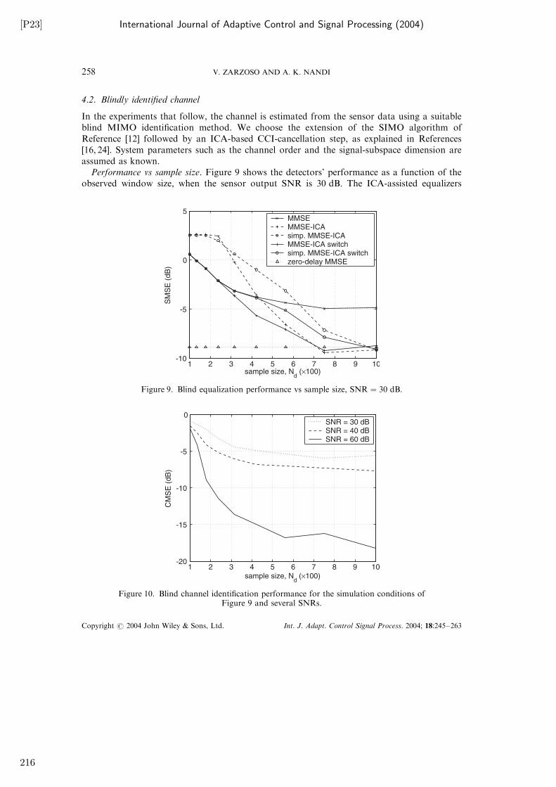
[P23] International Journal of Adaptive Control and Signal Processing (2004)
4.2. Blindly identified channel
In the experiments that follow, the channel is estimated from the sensor data using a suitable
blind MIMO identification method. We choose the extension of the SIMO algorithm of
Reference [12] followed by an ICA-based CCI-cancellation step, as explained in References
[16, 24]. System parameters such as the channel order and the signal-subspace dimension are
assumed as known.
Performance vs sample size. Figure 9 shows the detectors’ performance as a function of the
observed window size, when the sensor output SNR is 30 dB: The ICA-assisted equalizers
1 2 3 4 5 6 7 8 9 10-10
-5
0
5
sample size, Nd (×100)
SM
SE
(dB
)
MMSEMMSE-ICAsimp. MMSE-ICAMMSE-ICA switchsimp. MMSE-ICA switchzero-delay MMSE
Figure 9. Blind equalization performance vs sample size, SNR ¼ 30 dB:
1 2 3 4 5 6 7 8 9 10-20
-15
-10
-5
0
sample size, Nd
(×100)
CM
SE
(d
B)
SNR = 30 dBSNR = 40 dBSNR = 60 dB
Figure 10. Blind channel identification performance for the simulation conditions ofFigure 9 and several SNRs.
Copyright # 2004 John Wiley & Sons, Ltd. Int. J. Adapt. Control Signal Process. 2004; 18:245–263
V. ZARZOSO AND A. K. NANDI258
216

International Journal of Adaptive Control and Signal Processing (2004) [P23]
require around 500 samples to improve the conventional detector. This minimum sample length
reduces for higher SNR (results for the noiseless case under similar simulation conditions can be
found in Reference [32]). The theoretical optimal-delay MMSE lies around �25 dB; which the
ICA methods are unable to reach due to an erroneous delay estimation (dashed line of
Figure 11). Channel identification errors now join covariance matrix imprecisions in hindering
an accurate delay detection. Indeed, the CMSE reaches only around �6 dB from about 700
samples in this simulation (dotted line in Figure 10). Despite the higher iteration count shown
by the simplified MMSE-ICA in Figure 12, further experiments demonstrate that for high Nd
and SNR both methods require approximately the same number of FastICA iterations.
1 2 3 4 5 6 7 8 9 102
2.5
3
3.5
4
4.5
5
sample size, Nd (×100)
DR
MS
E
SNR = 20 dBSNR = 30 dBSNR = 40 dB
Figure 11. Delay estimation performance for the simulation conditions of Figure 9 and different SNRs.
1 2 3 4 5 6 7 8 9 100
20
40
60
80
100
sample size, Nd (×100)
Nu
mb
er
of
Fa
stI
CA
ite
ratio
ns
MMSE-ICAsimplified MMSE-ICA(MMSE-ICA)/(M+N)
Figure 12. Number of FastICA iterations vs sample size in the simulation of Figure 9.
Copyright # 2004 John Wiley & Sons, Ltd. Int. J. Adapt. Control Signal Process. 2004; 18:245–263
BLIND MIMO EQUALIZATION 259
217
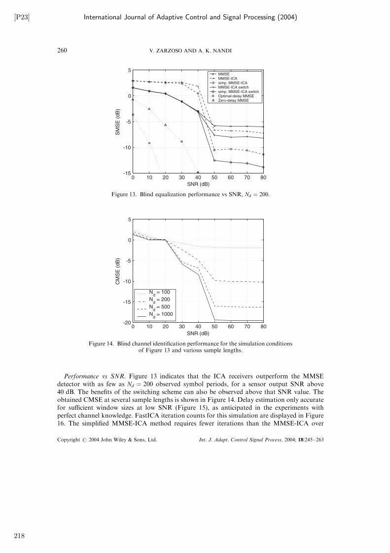
[P23] International Journal of Adaptive Control and Signal Processing (2004)
Performance vs SNR. Figure 13 indicates that the ICA receivers outperform the MMSE
detector with as few as Nd ¼ 200 observed symbol periods, for a sensor output SNR above
40 dB: The benefits of the switching scheme can also be observed above that SNR value. The
obtained CMSE at several sample lengths is shown in Figure 14. Delay estimation only accurate
for sufficient window sizes at low SNR (Figure 15), as anticipated in the experiments with
perfect channel knowledge. FastICA iteration counts for this simulation are displayed in Figure
16. The simplified MMSE-ICA method requires fewer iterations than the MMSE-ICA over
0 10 20 30 40 50 60 70 80-15
-10
-5
0
5
SNR (dB)
SM
SE
(d
B)
MMSEMMSE-ICAsimp. MMSE-ICAMMSE-ICA switchsimp. MMSE-ICA switchOptimal-delay MMSEZero-delay MMSE
Figure 13. Blind equalization performance vs SNR, Nd ¼ 200:
0 10 20 30 40 50 60 70 80-20
-15
-10
-5
0
5
SNR (dB)
CM
SE
(d
B)
Nd = 100
Nd = 200
Nd = 500
Nd = 1000
Figure 14. Blind channel identification performance for the simulation conditionsof Figure 13 and various sample lengths.
Copyright # 2004 John Wiley & Sons, Ltd. Int. J. Adapt. Control Signal Process. 2004; 18:245–263
V. ZARZOSO AND A. K. NANDI260
218
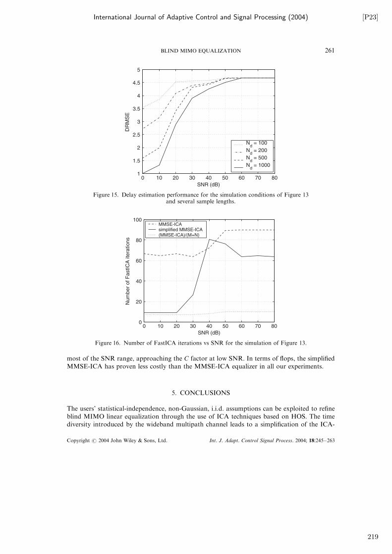
International Journal of Adaptive Control and Signal Processing (2004) [P23]
most of the SNR range, approaching the C factor at low SNR. In terms of flops, the simplified
MMSE-ICA has proven less costly than the MMSE-ICA equalizer in all our experiments.
5. CONCLUSIONS
The users’ statistical-independence, non-Gaussian, i.i.d. assumptions can be exploited to refine
blind MIMO linear equalization through the use of ICA techniques based on HOS. The time
diversity introduced by the wideband multipath channel leads to a simplification of the ICA-
0 10 20 30 40 50 60 70 800
20
40
60
80
100
SNR (dB)
Num
ber
of F
astIC
A ite
rations
MMSE-ICAsimplified MMSE-ICA(MMSE-ICA)/(M+N)
Figure 16. Number of FastICA iterations vs SNR for the simulation of Figure 13.
0 10 20 30 40 50 60 70 801
1.5
2
2.5
3
3.5
4
4.5
5
SNR (dB)
DR
MS
E
Nd = 100
Nd = 200
Nd = 500
Nd = 1000
Figure 15. Delay estimation performance for the simulation conditions of Figure 13and several sample lengths.
Copyright # 2004 John Wiley & Sons, Ltd. Int. J. Adapt. Control Signal Process. 2004; 18:245–263
BLIND MIMO EQUALIZATION 261
219
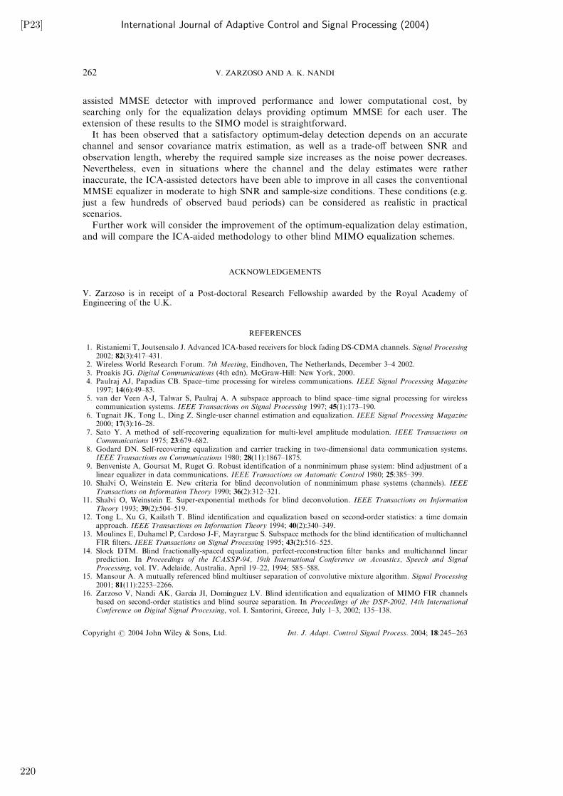
[P23] International Journal of Adaptive Control and Signal Processing (2004)
assisted MMSE detector with improved performance and lower computational cost, by
searching only for the equalization delays providing optimum MMSE for each user. The
extension of these results to the SIMO model is straightforward.
It has been observed that a satisfactory optimum-delay detection depends on an accurate
channel and sensor covariance matrix estimation, as well as a trade-off between SNR and
observation length, whereby the required sample size increases as the noise power decreases.
Nevertheless, even in situations where the channel and the delay estimates were rather
inaccurate, the ICA-assisted detectors have been able to improve in all cases the conventional
MMSE equalizer in moderate to high SNR and sample-size conditions. These conditions (e.g.
just a few hundreds of observed baud periods) can be considered as realistic in practical
scenarios.
Further work will consider the improvement of the optimum-equalization delay estimation,
and will compare the ICA-aided methodology to other blind MIMO equalization schemes.
ACKNOWLEDGEMENTS
V. Zarzoso is in receipt of a Post-doctoral Research Fellowship awarded by the Royal Academy ofEngineering of the U.K.
REFERENCES
1. Ristaniemi T, Joutsensalo J. Advanced ICA-based receivers for block fading DS-CDMA channels. Signal Processing2002; 82(3):417–431.
2. Wireless World Research Forum. 7th Meeting, Eindhoven, The Netherlands, December 3–4 2002.3. Proakis JG. Digital Communications (4th edn). McGraw-Hill: New York, 2000.4. Paulraj AJ, Papadias CB. Space–time processing for wireless communications. IEEE Signal Processing Magazine
1997; 14(6):49–83.5. van der Veen A-J, Talwar S, Paulraj A. A subspace approach to blind space–time signal processing for wireless
communication systems. IEEE Transactions on Signal Processing 1997; 45(1):173–190.6. Tugnait JK, Tong L, Ding Z. Single-user channel estimation and equalization. IEEE Signal Processing Magazine
2000; 17(3):16–28.7. Sato Y. A method of self-recovering equalization for multi-level amplitude modulation. IEEE Transactions on
Communications 1975; 23:679–682.8. Godard DN. Self-recovering equalization and carrier tracking in two-dimensional data communication systems.
IEEE Transactions on Communications 1980; 28(11):1867–1875.9. Benveniste A, Goursat M, Ruget G. Robust identification of a nonminimum phase system: blind adjustment of a
linear equalizer in data communications. IEEE Transactions on Automatic Control 1980; 25:385–399.10. Shalvi O, Weinstein E. New criteria for blind deconvolution of nonminimum phase systems (channels). IEEE
Transactions on Information Theory 1990; 36(2):312–321.11. Shalvi O, Weinstein E. Super-exponential methods for blind deconvolution. IEEE Transactions on Information
Theory 1993; 39(2):504–519.12. Tong L, Xu G, Kailath T. Blind identification and equalization based on second-order statistics: a time domain
approach. IEEE Transactions on Information Theory 1994; 40(2):340–349.13. Moulines E, Duhamel P, Cardoso J-F, Mayrargue S. Subspace methods for the blind identification of multichannel
FIR filters. IEEE Transactions on Signal Processing 1995; 43(2):516–525.14. Slock DTM. Blind fractionally-spaced equalization, perfect-reconstruction filter banks and multichannel linear
prediction. In Proceedings of the ICASSP-94, 19th International Conference on Acoustics, Speech and SignalProcessing, vol. IV. Adelaide, Australia, April 19–22, 1994; 585–588.
15. Mansour A. A mutually referenced blind multiuser separation of convolutive mixture algorithm. Signal Processing2001; 81(11):2253–2266.
16. Zarzoso V, Nandi AK, Garc!ııa JI, Dom!ıınguez LV. Blind identification and equalization of MIMO FIR channelsbased on second-order statistics and blind source separation. In Proceedings of the DSP-2002, 14th InternationalConference on Digital Signal Processing, vol. I. Santorini, Greece, July 1–3, 2002; 135–138.
Copyright # 2004 John Wiley & Sons, Ltd. Int. J. Adapt. Control Signal Process. 2004; 18:245–263
V. ZARZOSO AND A. K. NANDI262
220
International Journal of Adaptive Control and Signal Processing (2004) [P23]
17. Zarzoso V, Nandi AK, Igual-Garc!ııa J, Vergara-Dom!ıınguez L. Blind identification and equalization of MIMO FIRchannels based on subspace decomposition and independent component analysis. In Proceedings of the 2nd IMAInternational Conference on Mathematics in Communications, University of Lancaster, UK, December 16–18, 2002.
18. Talwar S, Viberg M, Paulraj A. Blind separation of synchronous co-channel digital signals using an antenna array.Part I: Algorithms. IEEE Transactions on Signal Processing 1996; 44(5):1184–1197.
19. van der Veen A-J, Paulraj A. An analytical constant modulus algorithm. IEEE Transactions on Signal Processing1996; 44(5):1136–1155.
20. van der Veen A-J. Analytical method for blind binary signal separation. IEEE Transactions on Signal Processing1997; 45(4):1078–1082.
21. Hyv.aarinen A, Karhunen J, Oja E. Independent Component Analysis. John Wiley & Sons: New York, 2001.22. Cardoso J-F, Souloumiac A. Blind beamforming for non-Gaussian signals. IEE Proceedings-F 1993; 140(6):362–370.23. Comon P. Independent component analysis, a new concept? Signal Processing 1994; 36(3):287–314.24. Zarzoso V, Nandi AK. Exploiting non-Gaussianity in blind identification and equalization of MIMO FIR channels.
IEE Proceedings}Vision, Image and Signal Processing (Special Issue on Nonlinear and non-Gaussian SignalProcessing) 2004;151(1):69–75.
25. Xu G, Liu H, Tong L, Kailath T. A least-squares approach to blind channel identification. IEEE Transactions onSignal Processing 1995; 43(12):2982–2993.
26. Gesbert D, Duhamel P, Mayrargue S. On-line blind multichannel equalization based on mutually referenced filters.IEEE Transactions on Signal Processing 1997; 45(9):2307–2317.
27. Giannakis GB, Halford SD. Blind fractionally spaced equalization of noisy FIR channels: direct and adaptivesolutions. IEEE Transactions on Signal Processing 1997; 45(9):2277–2291.
28. Shen J, Ding Z. Direct blind MMSE channel equalization based on second-order statistics. IEEE Transactions onSignal Processing 2000; 48(4):1015–1022.
29. Gesbert D, Duhamel P, Mayrargue S. Blind multichannel adaptive MMSE equalization with controlled delay. InProceedings of the SSAP-1996, IEEE Statistical Signal and Array Processing Workshop, Corfu, Greece, June 24–26,1996; 172–175.
30. Gazzah H, Abed-Meraim K. Blind ZF equalization with controlled delay robust to order over estimation. SignalProcessing 2003; 83(7):1505–1518.
31. Prandini M, Campi MC, Leonardi R. Optimal delay estimation and performance evaluation in blind equalization.International Journal of Adaptive Control and Signal Processing 1997; 11(7):621–640.
32. Zarzoso V. Exploiting independence for co-channel interference cancellation and symbol detection in multiuserdigital communications. In Proceedings of the ISSPA-2003, 7th International Symposium on Signal Processing and itsApplications, Paris, France, July 1–4, 2003.
33. Abed-Meraim K, Loubaton P, Moulines E. A subspace algorithm for certain blind identification problems. IEEETransactions on Information Theory 1997; 43(2):499–511.
34. Yang HH. On-line blind equalization via on-line blind separation. Signal Processing 1998; 68(3):271–281.35. Zhang Y, Kassam SA. Blind separation and equalization using fractional sampling of digital communications
signals. Signal Processing 2001; 81(12):2591–2608.36. Hyv.aarinen A, Oja E. A fast fixed-point algorithm for independent component analysis. Neural Computation 1997;
9(7):1483–1492.
Copyright # 2004 John Wiley & Sons, Ltd. Int. J. Adapt. Control Signal Process. 2004; 18:245–263
BLIND MIMO EQUALIZATION 263
221

IEE Proceedings – Vision, Image and Signal Processing (2004) [P24]
NONLINEAR AND NON-GAUSSIAN SIGNAL PROCESSING
Exploiting non-Gaussianity in blind identification andequalisation of MIMO FIR channels
V. Zarzoso and A.K. Nandi
Abstract: The problem of blind identification and equalisation (BIE) of finite impulse response(FIR) channels in multiuser digital communications is investigated. The non-Gaussian nature andstatistical independence of the users’ data streams is exploited by resorting to blind signalseparation (BSS) based on higher-order statistics (HOS). Two such techniques are put forward. Thefirst technique is composed of an extension to the multiuser case of a second-order BIE method,followed by a BSS-based space-equalisation step. The second technique achieves joint space–timeequalisation through the direct application of a HOS-based BSS method followed by a blindidentification algorithm. In a number of numerical experiments, the first procedure proves lesscostly and more effective for short data records. Despite their computational complexity, interestingfeatures such as constellation-independent channel identification and symbol recovery, androbustness to ill-conditioned channels in high SNR environments render HOS-BSS based BIEmethods an effective alternative to BIE techniques exploiting other spatio-temporal structures.
1 Introduction
In digital communications, linear distortion effects such asmultipath propagation and limited bandwidth cause inter-symbol interference (ISI) in the received signal, producingerrors in symbol detection. A variety of equaliser designscan be employed to compensate for the channel effects [1].As opposed to traditional techniques, blind channelidentification and equalisation (BIE) methods do not requiretraining sequences, and are thus able to use the bandwidthresources more efficiently and to perform in a wider range ofcommunication environments. Due to their many desirableproperties [2], blind methods have aroused great researchinterest.Tong et al. first proved [3] that non-minimum phase
(NMP) finite-impulse response (FIR) channels can beidentified using only second-order statistics (SOS) if thereceived signal exhibits cyclostationarity. Cyclostationaritynaturally leads to the so-called single-input multiple-output(SIMO) model, a multichannel signal structure with oneinput (the transmitted symbol sequence) and severaloutputs. By relying only on the subspace informationcontained within the sensor second-order correlation matrix,BIE is possible in SIMO systems [3, 4].In multiuser communication environments (e.g. cellular
wireless systems) the co-channel interference (CCI) causedby other users simultaneously transmitting across the samemedium adds to multipath-induced ISI. To ensure reliabledetection, space–time equalisation must be performed.Time equalisation aims at ISI removal, whereas space
equalisation involves CCI elimination and the extraction ofthe signal(s) of interest. The exploitation of temporal and/orspatial diversity (fractional sampling and/or multiplesensors) results in multiple-input multiple-output (MIMO)signal models. Direct extensions of subspace-based SIMOmethods to the MIMO case achieve time equalisation butare generally unable to separate the different source datastreams, i.e. CCI remains in the form of an instantaneouslinear mixture of the transmitted symbols [2, 5, 6].To separate this spatial mixture, the fact that digitalcommunication signals possess a finite alphabet (FA) canbe exploited [2]. In a direct-sequence code-division multipleaccess (DS/CDMA) system, [6] reports an unsatisfactoryperformance of one such FA-based method, with probabilityof error well above 10% even in the noise-free case.Nevertheless, the spatial mixture can be resolved with theaid of the users’ signature sequences [6], which are typicallyknown in a CDMA scenario. This semi-blind method is notapplicable to a general (i.e. using a multiple-accesstechnique other than DS/CDMA) multiuser digital com-munication environment. The method of [6] is blind in thatit spares training sequences. However, the use of signaturesequences leads to a particular factorisation of the channelmatrix, whereas fully blind methods generally avoid suchparameterisations. Precisely there lies the robustness ofthese methods to deviations from the assumed priorinformation (e.g. calibration errors in beamforming) [7].
A more generic, fully blind approach sparing the priorknowledge of the users’ signature sequences or FAs followsfrom the plausible hypothesis that the signals transmitted bydifferent users are statistically independent. Hence, theremaining spatial mixture after the SOS-MIMO stage adoptsa model of blind source separation (BSS) of instantaneouslinear mixtures. In addition, digital communication signalsare non-Gaussian, typically showing sub-Gaussian (orplatykurtic [8]) probability density functions (pdfs), soBSS methods based on higher-order statistics (HOS) areapplicable. In the case where the transmitted symbols areindependent and identically distributed (i.i.d.), the sourceextraction can directly be solved by HOS-based BSS
q IEE, 2004
IEE Proceedings online no. 20040278
doi: 10.1049/ip-vis:20040278
The authors are with the Signal Processing and Communications Group,Department of Electrical Engineering and Electronics, The University ofLiverpool, Brownlow Hill, Liverpool L69 3GJ, UK
Paper received 4th September 2002 and in revised form 28th March 2003
IEE Proc.-Vis. Image Signal Process., Vol. 151, No. 1, February 2004 69
223
[P24] IEE Proceedings – Vision, Image and Signal Processing (2004)
techniques, as shown in [9–11]. However, the methodspresented therein are not designed to identify the channel.A channel estimate may prove useful in a variety of tasks,such as power control, source localisation, propagationcharacterisation, or as a sensible initialisation for anadaptive receiver.
This contribution discusses the exploitation of the non-Gaussian i.i.d. source property in the FIR–MIMO BIEproblem. In particular, we study two techniques which relyon such an assumption through the application of BSS. Thefirst technique is composed of the extension to the MIMOcase of a SOS-based SIMO method, completed by a BSS-based space-equalisation stage. The second techniqueconsists of joint space–time equalisation through the directapplication HOS-based BSS followed by a suitablealgorithm for channel identification. The benefits anddrawbacks of exploiting non-Gaussianity are also high-lighted throughout.
A signal model is presented which will be used in themathematical developments. The two BIE methods are putforward and simulation results are reported. Other relevantissues are also discussed.
NotationsC is the set of complex numbers. Vectors and matrices arerepresented, respectively, by boldface lower-case andupper-case symbols. ðAÞij denotes the (i, j)-element ofmatrix A. Symbol In refers to the n� n identity matrix, and
eðnÞi ¼ ½0; . . . ; 0;
|fflfflfflfflffl{zfflfflfflfflffl}
i�1
1; 0; . . . ; 0�|fflfflfflffl{zfflfflfflffl}
n�i
T
is the ith canonic basis vector of Cn: Superindices ð·Þ�; ð·ÞT;ð·ÞH; ð·Þ�1 and ð·Þy indicate the complex conjugate, transpose,Hermitian (conjugate-transpose), inverse and Moore–Pen-rose pseudoinverse operators, respectively. E[·] stands formathematical expectation, and ^ denotes the Kroneckerproduct.
2 Signal model
The signal model of [4] is extended to the multiple-inputcase. An oversampled single-sensor receiver is considered,although the model also holds for spatially separatedmultiple physical sensors. The system assumptions are:
(i) K data sources simultaneously transmit mutually-inde-pendent information-bearing non-Gaussian i.i.d. symbolsfsk;mg
Kk¼1 2 C at a known rate 1/T bauds, with E½sk; � ¼ 0
and E½jsk; j2� ¼ 1:
(ii) The impulse responses hkðtÞ representing the propa-gation between the kth source and the sensor (including theeffects of the transmitter and receiver filters, carrier-pulseshaping, etc.) span at most M þ 1 data symbols.(iii) The additive measurement noise v(t) is white, zero-mean and uncorrelated with the data sequences; its varianceis �2:
The implicit source power normalisation in assumption (i)stems from the fact that a complex scalar can beinterchanged between the channel and the data withoutaltering the received signal. This scalar factor is anadmissible indeterminacy in blind equalisation, and cannotbe resolved without resorting to further prior information.
In contrast to [2], herein source alphabets can be assumedunknown and not necessarily identical for all users; neitherthe alphabets need be constant modulus. The source dataneed not even be discrete. We only require that their kurtosis[8] be different from zero (at most one non-kurtic source is
allowed [12]). Assumption (ii) demands channel stationar-ity, at least over the observation window. This hypothesis isverified in time non-selective scenarios, such as block-fading multipath channels, whose coherence time is largecompared to the baud period [13].
With the above assumptions, the continuous-time com-plex baseband received signal can be expressed as
xðtÞ ¼XK
k¼1
X1
m¼�1
sk;mhkðt � mTÞ þ vðtÞ ð1Þ
Sampling at a rate 1=Ts ¼ L=T ; with L integer, from aninitial instant t0 ¼ 0 s (without loss of generality) yields
xðiÞn ¼
XK
k¼1
XM
m¼0
sk;n�mhðiÞk;m þ v
ðiÞn ; i ¼ 0; . . . ; L� 1 ð2Þ
in which xðiÞn ¼ xðiTs þ nTÞ; h
ðiÞk;n ¼ hkðiTs þ nTÞ and
vðiÞn ¼ vðiTs þ nTÞ: Hence, fractionally-spaced samplingeffectively generates L virtual channels excited by thesame input. Let us now store N consecutive output samplesof virtual channel i in vector x
ðiÞn ¼ ½x
ðiÞn ; . . . ; x
ðiÞn�Nþ1�
T:Parameter N is referred to as the smoothing factor [14] orstacking level [9]. Similarly, gather the N samples of the L
virtual channel outputs in vector xn ¼ ½xð0ÞT
n ; . . . ; xðL�1ÞT
n �T
(with similar notations for the noise vector vn). Then, thefollowing matrix model holds:
xn ¼ Hsn þ vn ð3Þ
where sn ¼ ½sT1;n; . . . ; sTK;n�
T; sk;n ¼ ½sk;n; . . . ; sk;n�N�Mþ1�T;
H ¼ ½H1; . . . ;HK � is the LN � KðM þ NÞ channel filtering
matrix, with Hk ¼ ½Hð0ÞT
k ; . . . ;HðL�1ÞT
k �T; HðiÞk representing
the N � ðM þ NÞ Toeplitz convolution matrix asso-ciated with the linear filter h
ðiÞk ¼ ½h
ðiÞk;0; . . . ; h
ðiÞk;M�
T: To abbre-
viate, in the sequel we denote P¼DLN; C¼
DM þ N and
D¼DKðM þ NÞ ¼ KC:
The objective of BIE is to estimate H (blind channelidentification) and sn (blind channel equalisation [ISIcancellation] and source separation [CCI cancellation])from the only observation of the received vector xn: Thesetasks are equivalent to recovering the channel coefficient
vector h ¼ ½hT1 ; . . . ; hTK �
T; with hk ¼ ½hð0ÞT
k ; . . . ; hðL�1ÞT
k �T;and the source vector
s ¼ EH1 sn ¼ ½s1;n; . . . ; sK;n�
T ð4Þ
where Ei ¼ IK � eðCÞi :
A necessary condition for blind identifiability is that thefiltering matrix be full column rank, which can occur only ifH has more rows than columns, P � D; or, equivalently,L > K and N � KM=ðL� KÞ: This condition is notsufficient. It is required that polynomial matrix H(z) be‘irreducible and column reduced’, where ðHðzÞÞij is thez-transform of h
ðiÞj [5].
Note that with the information of assumptions (i)–(iii) we
can obtain at best a channel estimate HH such that HHyH ¼GK � IC; where GK is an arbitrary K � K permutationmatrix with unit-norm nonzero entries; signal blocks ofdifferent users present an order indeterminacy, which canonly be surmounted if further information is available(e.g. users’ signature sequences in a CDMA system).
3 SOS-based time equalisation and BSS-basedspace equalisation
3.1 Multiuser extension of SIMO methods
Tong et al. [3] realised that blind channel identification ofNMP FIR channels is possible from SOS alone in the
IEE Proc.-Vis. Image Signal Process., Vol. 151, No. 1, February 200470
224
IEE Proceedings – Vision, Image and Signal Processing (2004) [P24]
single-user cyclostationary case, which results in the SIMOsignal model. (The signal model in [3] is slightly differentfrom that presented in the previous Section (with K ¼ 1).Tong’s signal model involves a different arrangement forthe signal vectors and channel matrix, and allows fornoninteger (fractional) values for the stacking level.However, both models are totally analogous, so that wecan use the model of Section 2 without loss of generality.)Their approach takes advantage of the particular structure ofthe observed-vector correlation matrix RxðmÞ ¼ E½xnx
Hn�m�
at two different lags ðm ¼ 0; 1Þ. The direct application ofthis blind identification method to the MIMO case yields thefollowing identifiability result [15].
Theorem 1: Suppose that H and sn satisfy the linear model(3) and its constraints (i)–(iii). Then H is determined fromRxð0Þ and Rxð1Þ up to a post-multiplicative factor of theform Q� IC; where Q 2 CK�K is a K � K unitary matrix.
A similar indeterminacy is observed in the multiuserextension [2, 16] of the subspace method of [4], in whichQ becomes an arbitrary K � K invertible matrix. Indeed,theorem 1 may be generalised to the MIMO extension ofany SIMO BIE method [2].According to the above result, the channel estimated by
the extended Tong’s method is of the form ~HH ¼ HðQ� ICÞ;with Q an unknown K � K unitary matrix. Should we wantto carry out soft-symbol detection at this stage, the resultingzero-forcing (ZF) equaliser output would be
yn ¼ ~HHyxn ¼ ðQH � ICÞsn þ ~vvn ð5Þ
in which
~vvn ¼ ~HHyvn ð6Þ
Now, defining y ¼ EH1 yn; system (5) becomes
y ¼ QHsþ ~vv ð7Þ
where ~vv ¼ EH1 ~vvn; and s is given by (4).
3.2 BSS-based space equalisation
Equation (7) represents a noisy unitary instantaneous linearmixture of the source symbols. That is, CCI eliminationrequires further processing. Since the components of s arestatistically independent [assumption (i)], (7) corresponds toa BSS problem of instantaneous linear mixtures [17, 18].Due to the i.i.d. assumption, SOS-based BSS methods fail,but the source non-Gaussianity can still be exploitedthrough HOS. A few remarks indicate that HOS-basedBSS seems well suited as a second processing step:
3.2.1 Complexity reduction: The BSS problemat this second stage has size K � K, which is considerablyreduced compared with the original dimensions of the BIEsystem (3).
3.2.2 Robustness to ill-conditioned channels:In the single-user case, the so-called uniform performanceproperty enjoyed by many BSS methods [19] translates intoa robust performance for ill-conditioned channels [9]. Note,however, that uniform performance is only expected to holdin the noiseless case [19].
3.2.3 Noise ‘Gaussianisation’: The central limittheorem and (6) guarantee that the equalised noise ~vv will beclose to Gaussian, even if the actual sensor noise vn is not.The well known HOS immunity to Gaussian noise would
then result in an increased robustness of the BIE method notonly to Gaussian noise but also to other kinds of non-Gaussian noise, such as impulsive interference.
In the simulations of Section 5, we employ the jointapproximate diagonalisation of eigenmatrices (JADE) BSSmethod [7]. This choice is somewhat arbitrary; we areconcerned with the application of BSS as a general strategy,rather than assessing which particular BSS method providesthe best performance. JADE optimises a HOS cost functionthrough the joint diagonalisation of a particular set of fourth-order cumulant tensor ‘slices’.
Once Q has been obtained via a HOS–BSS method, thefull channel estimate can be calculated as HH ¼ ~HHðQH � ICÞ:From the channel estimate, soft-symbol detection can thenbe accomplished from (3) as ssn ¼ GHxn with the ZF andminimum mean square error (MMSE) equalisers
GZF ¼ ðHHHHHÞ�1HH ð8Þ
GMMSE ¼ Rxð0Þ�1HH ð9Þ
whose subspace version from the channel matrix singularvalue decomposition is given in [6].
Steps 2–5 of Table 1 summarise the BSS and detectionstages, which, in combination with the extended Tongmethod, complete the first FIR–MIMO BIE algorithmproposed in this paper.
4 BSS-based joint space–time equalisation andchannel identification
The i.i.d. assumption in (i) makes the components of thesource vector sn in (3) statistically independent. From thisperspective, (3) itself can also be considered as a BSS modelof instantaneous linear mixtures, and thus BSS techniquesmay be directly applied to resolve it [11].
The whitening step of Tong’s method provides theoutputs [15]
zn ¼ Wxn ¼ Vsn þ wn ð10Þ
where wn ¼ Wvn and W represents the whitening matrix. Ina second step, a HOS-based BSS method, such as JADE [7],can estimate the unitary mixing matrix V. Detection can becarried out through ZF/MMSE equalisers (8)=(9).
Since in this case the BSS method operates over all the Dwhitened components, the complexity reduction remarkedin the previous Section is lost. However, the key point tonote in the direct application of BSS techniques to the BIEmodel is related to the source scale and order indetermi-nacies inherent to the BSS problem [17, 18]. Theseindeterminacies mean that a blind separation method
can provide any solution VV such that VVyV is an arbitrary
permutation matrix with unit-norm non-zero entries. In ourparticular model (3), the arrangement and scale of therecovered source components as well as the correspondingcolumns of the filtering matrix are crucial, especially for
Table 1: Algorithm for SOS-based time equalisation andBSS-based space equalisation
1. Obtain first estimate of the filtering matrix ~HH from the
extended Tong method [15].
2. Compute ISI-free output (5).
3. Estimate matrixQ from (7) with a HOS-based BSSmethod.
4. Update estimate of channel matrix as HH ¼ ~HHðQH � IC Þ:
5. Detect CCI-free source symbols [(8) and (9)].
IEE Proc.-Vis. Image Signal Process., Vol. 151, No. 1, February 2004 71
225
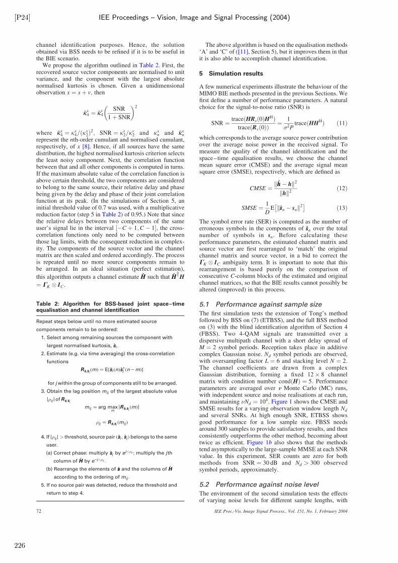
[P24] IEE Proceedings – Vision, Image and Signal Processing (2004)
channel identification purposes. Hence, the solutionobtained via BSS needs to be refined if it is to be useful inthe BIE scenario.
We propose the algorithm outlined in Table 2. First, therecovered source vector components are normalised to unitvariance, and the component with the largest absolutenormalised kurtosis is chosen. Given a unidimensionalobservation x ¼ sþ v; then
~kkx4 ¼ ~kks4SNR
1þ SNR
� �2
where ~kkx4 ¼ kx4=ðkx2Þ
2; SNR ¼ ks2=kv2 and kxn and ~kkxn
represent the nth-order cumulant and normalised cumulant,respectively, of x [8]. Hence, if all sources have the samedistribution, the highest normalised kurtosis criterion selectsthe least noisy component. Next, the correlation functionbetween that and all other components is computed in turns.If the maximum absolute value of the correlation function isabove certain threshold, the two components are consideredto belong to the same source, their relative delay and phasebeing given by the delay and phase of their joint correlationfunction at its peak. (In the simulations of Section 5, aninitial threshold value of 0.7 was used, with a multiplicativereduction factor (step 5 in Table 2) of 0.95.) Note that sincethe relative delays between two components of the sameuser’s signal lie in the interval ½�C þ 1;C � 1�; the cross-correlation functions only need to be computed betweenthose lag limits, with the consequent reduction in complex-ity. The components of the source vector and the channelmatrix are then scaled and ordered accordingly. The processis repeated until no more source components remain tobe arranged. In an ideal situation (perfect estimation),
this algorithm outputs a channel estimate HH such that HHyH
¼ GK � IC:
The above algorithm is based on the equalisation methods‘A’ and ‘C’ of ([11], Section 5), but it improves them in thatit is also able to accomplish channel identification.
5 Simulation results
A few numerical experiments illustrate the behaviour of theMIMO BIE methods presented in the previous Sections. Wefirst define a number of performance parameters. A naturalchoice for the signal-to-noise ratio (SNR) is
SNR ¼traceðHRsð0ÞH
HÞ
traceðRvð0ÞÞ¼
1
�2PtraceðHHHÞ ð11Þ
which corresponds to the average source power contributionover the average noise power in the received signal. Tomeasure the quality of the channel identification and thespace–time equalisation results, we choose the channelmean square error (CMSE) and the average signal meansquare error (SMSE), respectively, which are defined as
CMSE ¼khh� hk2
khk2ð12Þ
SMSE ¼1
DEkssn � snk
2
ð13Þ
The symbol error rate (SER) is computed as the number oferroneous symbols in the components of ssn over the totalnumber of symbols in sn. Before calculating theseperformance parameters, the estimated channel matrix andsource vector are first rearranged to ‘match’ the originalchannel matrix and source vector, in a bid to correct theGK � IC ambiguity term. It is important to note that thisrearrangement is based purely on the comparison ofconsecutive C-column blocks of the estimated and originalchannel matrices, so that the BIE results cannot possibly bealtered (improved) in this process.
5.1 Performance against sample size
The first simulation tests the extension of Tong’s methodfollowed by BSS on (7) (ETBSS), and the full BSS methodon (3) with the blind identification algorithm of Section 4(FBSS). Two 4-QAM signals are transmitted over adispersive multipath channel with a short delay spread ofM ¼ 2 symbol periods. Reception takes place in additivecomplex Gaussian noise. Nd symbol periods are observed,with oversampling factor L ¼ 6 and stacking level N ¼ 2:The channel coefficients are drawn from a complexGaussian distribution, forming a fixed 12� 8 channelmatrix with condition number condðHÞ ¼ 5: Performanceparameters are averaged over n Monte Carlo (MC) runs,with independent source and noise realisations at each run,and maintaining �Nd ¼ 104. Figure 1 shows the CMSE andSMSE results for a varying observation window length Nd
and several SNRs. At high enough SNR, ETBSS showsgood performance for a low sample size. FBSS needsaround 300 samples to provide satisfactory results, and thenconsistently outperforms the other method, becoming abouttwice as efficient. Figure 1b also shows that the methodstend asymptotically to the large-sample MMSE at each SNRvalue. In this experiment, SER counts are zero for bothmethods from SNR ¼ 30 dB and Nd > 300 observedsymbol periods, approximately.
5.2 Performance against noise level
The environment of the second simulation tests the effectsof varying noise levels for different sample lengths, with
Table 2: Algorithm for BSS-based joint space–timeequalisation and channel identification
Repeat steps below until no more estimated source
components remain to be ordered:
1. Select among remaining sources the component with
largest normalised kurtosis, ssi :
2. Estimate (e.g. via time averaging) the cross-correlation
functions
R ssi ssjðmÞ ¼ E½ssi ðnÞss
�j ðn �mÞ�
for jwithin the group of components still to be arranged.
3. Obtain the lag position mij of the largest absolute value
j�ij jofR ssi ssj
mij ¼ arg maxm
jR ssi ssjðmÞj
�ij ¼ R ssi ssjðmij Þ
4. If j�ij j > threshold, source pair ðssi ; ssj Þ belongs to the same
user.
(a) Correct phase: multiply ssj by e j<�ij ; multiply the j th
column of HH by e�j<�ij :
(b) Rearrange the elements of ss and the columns of HH
according to the ordering of mij :
5. If no source pair was detected, reduce the threshold and
return to step 4.
IEE Proc.-Vis. Image Signal Process., Vol. 151, No. 1, February 200472
226
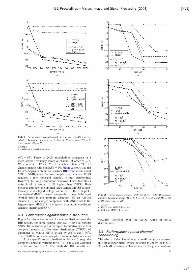
IEE Proceedings – Vision, Image and Signal Processing (2004) [P24]
�Nd ¼ 105: Three 16-QAM modulations propagate in amore severe frequency-selective channel of order M ¼ 5:We choose L ¼ 12 and N ¼ 2; which result in a 24� 21channel matrix with condðHÞ ¼ 30: Figure 2 shows that theETBSS begins to obtain satisfactory BIE results from aboutSNR ¼ 20 dB; even for low sample size, whereas FBSSrequires a few thousand samples to start performing.However, for long observation windows, FBSS tolerates anoise level of around 10 dB higher than ETBSS. Bothmethods approach the optimal large-sample MMSE asymp-totically, as displayed in Figs. 2b and 2c. In the SER plots,the ‘optimal MMSE’ curve corresponds to the probability ofsymbol error in the optimum detection (for an AWGNchannel [13]) of a single component with MSE equal to thelarge-sample MMSE in the given simulation conditions(channel matrix and SNR).
5.3 Performance against noise distribution
Figure 3 explores the impact of the noise distribution on theBIE results, for large sample size ðNd ¼ 104Þ at variousSNRs. The sensor output is corrupted by additive noise withcomplex generalised Gaussian distribution (CGGD) ofparameter a, whose pdf is given by pðzÞ! expð�jzjaÞ:The CGGD becomes the complex Gaussian distribution fora ¼ 2; a super-Gaussian distribution for a < 2 (e.g. thecomplex Laplacian variable for a ¼ 1), and a sub-Gaussiandistribution for a > 2: The methods’ BIE results are
virtually identical over the tested range of noisedistributions.
5.4 Performance against channelconditioning
The effects of the channel matrix conditioning are assessedin a final experiment, whose outcome is shown in Fig. 4.At each MC iteration, a channel matrix of a given condition
Fig. 1 Performance against sample size for two 4-QAM sources,additive Gaussian noise, M ¼ 2, L ¼ 6, N ¼ 2, condðHÞ ¼ 5,
� MC runs, �Nd ¼ 104
a CMSEb SMSE with MMSE detection
Fig. 2 Performance against SNR for three 16-QAM sources,additive Gaussian noise, M ¼ 5, L ¼ 12, N ¼ 2, condðHÞ ¼ 30,
� MC runs, �Nd ¼ 105
a CMSEb SMSE with MMSE detectionc SER with MMSE detection
IEE Proc.-Vis. Image Signal Process., Vol. 151, No. 1, February 2004 73
227
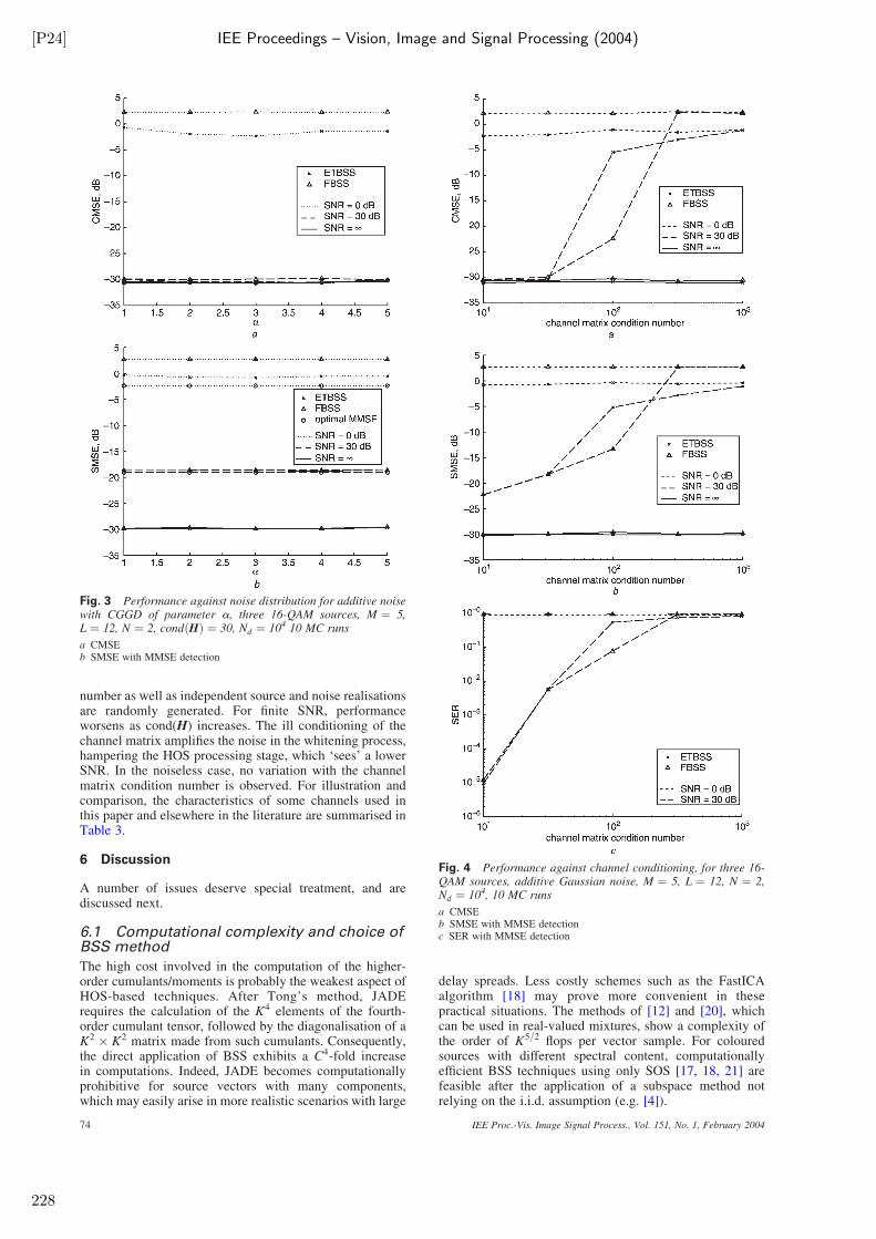
[P24] IEE Proceedings – Vision, Image and Signal Processing (2004)
number as well as independent source and noise realisationsare randomly generated. For finite SNR, performanceworsens as cond(H) increases. The ill conditioning of thechannel matrix amplifies the noise in the whitening process,hampering the HOS processing stage, which ‘sees’ a lowerSNR. In the noiseless case, no variation with the channelmatrix condition number is observed. For illustration andcomparison, the characteristics of some channels used inthis paper and elsewhere in the literature are summarised inTable 3.
6 Discussion
A number of issues deserve special treatment, and arediscussed next.
6.1 Computational complexity and choice ofBSS method
The high cost involved in the computation of the higher-order cumulants/moments is probably the weakest aspect ofHOS-based techniques. After Tong’s method, JADErequires the calculation of the K4 elements of the fourth-order cumulant tensor, followed by the diagonalisation of aK2 � K2 matrix made from such cumulants. Consequently,the direct application of BSS exhibits a C4-fold increasein computations. Indeed, JADE becomes computationallyprohibitive for source vectors with many components,which may easily arise in more realistic scenarios with large
delay spreads. Less costly schemes such as the FastICAalgorithm [18] may prove more convenient in thesepractical situations. The methods of [12] and [20], whichcan be used in real-valued mixtures, show a complexity ofthe order of K5=2 flops per vector sample. For colouredsources with different spectral content, computationallyefficient BSS techniques using only SOS [17, 18, 21] arefeasible after the application of a subspace method notrelying on the i.i.d. assumption (e.g. [4]).
Fig. 3 Performance against noise distribution for additive noisewith CGGD of parameter a, three 16-QAM sources, M ¼ 5,
L ¼ 12, N ¼ 2, condðHÞ ¼ 30, Nd ¼ 104 10 MC runs
a CMSEb SMSE with MMSE detection
Fig. 4 Performance against channel conditioning, for three 16-QAM sources, additive Gaussian noise, M ¼ 5, L ¼ 12, N ¼ 2,
Nd ¼ 104, 10 MC runs
a CMSEb SMSE with MMSE detectionc SER with MMSE detection
IEE Proc.-Vis. Image Signal Process., Vol. 151, No. 1, February 200474
228
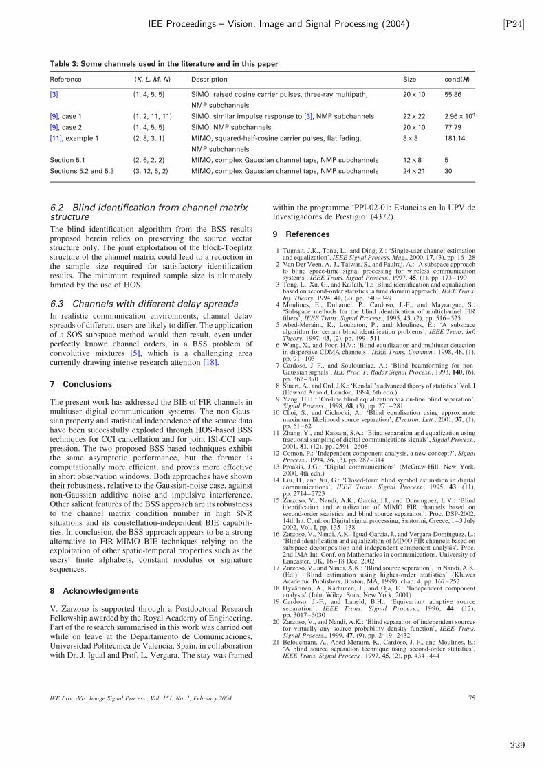
IEE Proceedings – Vision, Image and Signal Processing (2004) [P24]
6.2 Blind identification from channel matrixstructure
The blind identification algorithm from the BSS resultsproposed herein relies on preserving the source vectorstructure only. The joint exploitation of the block-Toeplitzstructure of the channel matrix could lead to a reduction inthe sample size required for satisfactory identificationresults. The minimum required sample size is ultimatelylimited by the use of HOS.
6.3 Channels with different delay spreads
In realistic communication environments, channel delayspreads of different users are likely to differ. The applicationof a SOS subspace method would then result, even underperfectly known channel orders, in a BSS problem ofconvolutive mixtures [5], which is a challenging areacurrently drawing intense research attention [18].
7 Conclusions
The present work has addressed the BIE of FIR channels inmultiuser digital communication systems. The non-Gaus-sian property and statistical independence of the source datahave been successfully exploited through HOS-based BSStechniques for CCI cancellation and for joint ISI-CCI sup-pression. The two proposed BSS-based techniques exhibitthe same asymptotic performance, but the former iscomputationally more efficient, and proves more effectivein short observation windows. Both approaches have showntheir robustness, relative to the Gaussian-noise case, againstnon-Gaussian additive noise and impulsive interference.Other salient features of the BSS approach are its robustnessto the channel matrix condition number in high SNRsituations and its constellation-independent BIE capabili-ties. In conclusion, the BSS approach appears to be a strongalternative to FIR-MIMO BIE techniques relying on theexploitation of other spatio-temporal properties such as theusers’ finite alphabets, constant modulus or signaturesequences.
8 Acknowledgments
V. Zarzoso is supported through a Postdoctoral ResearchFellowship awarded by the Royal Academy of Engineering.Part of the research summarised in this work was carried outwhile on leave at the Departamento de Comunicaciones,Universidad Politecnica de Valencia, Spain, in collaborationwith Dr. J. Igual and Prof. L. Vergara. The stay was framed
within the programme ‘PPI-02-01: Estancias en la UPV deInvestigadores de Prestigio’ (4372).
9 References
1 Tugnait, J.K., Tong, L., and Ding, Z.: ‘Single-user channel estimationand equalization’, IEEE Signal Process. Mag., 2000, 17, (3), pp. 16–28
2 Van Der Veen, A.-J., Talwar, S., and Paulraj, A.: ‘A subspace approachto blind space-time signal processing for wireless communicationsystems’, IEEE Trans. Signal Process., 1997, 45, (1), pp. 173–190
3 Tong, L., Xu, G., and Kailath, T.: ‘Blind identification and equalizationbased on second-order statistics: a time domain approach’, IEEE Trans.Inf. Theory, 1994, 40, (2), pp. 340–349
4 Moulines, E., Duhamel, P., Cardoso, J.-F., and Mayrargue, S.:‘Subspace methods for the blind identification of multichannel FIRfilters’, IEEE Trans. Signal Process., 1995, 43, (2), pp. 516–525
5 Abed-Meraim, K., Loubaton, P., and Moulines, E.: ‘A subspacealgorithm for certain blind identification problems’, IEEE Trans. Inf.Theory, 1997, 43, (2), pp. 499–511
6 Wang, X., and Poor, H.V.: ‘Blind equalization and multiuser detectionin dispersive CDMA channels’, IEEE Trans. Commun., 1998, 46, (1),pp. 91–103
7 Cardoso, J.-F., and Souloumiac, A.: ‘Blind beamforming for non-Gaussian signals’, IEE Proc. F, Radar Signal Process., 1993, 140, (6),pp. 362–370
8 Stuart, A., and Ord, J.K.: ‘Kendall’s advanced theory of statistics’ Vol. I(Edward Arnold, London, 1994, 6th edn.)
9 Yang, H.H.: ‘On-line blind equalization via on-line blind separation’,Signal Process., 1998, 68, (3), pp. 271–281
10 Choi, S., and Cichocki, A.: ‘Blind equalisation using approximatemaximum likelihood source separation’, Electron. Lett., 2001, 37, (1),pp. 61–62
11 Zhang, Y., and Kassam, S.A.: ‘Blind separation and equalization usingfractional sampling of digital communications signals’, Signal Process.,2001, 81, (12), pp. 2591–2608
12 Comon, P.: ‘Independent component analysis, a new concept?’, SignalProcess., 1994, 36, (3), pp. 287–314
13 Proakis, J.G.: ‘Digital communications’ (McGraw-Hill, New York,2000, 4th edn.)
14 Liu, H., and Xu, G.: ‘Closed-form blind symbol estimation in digitalcommunications’, IEEE Trans. Signal Process., 1995, 43, (11),pp. 2714–2723
15 Zarzoso, V., Nandi, A.K., Garcıa, J.I., and Domınguez, L.V.: ‘Blindidentification and equalization of MIMO FIR channels based onsecond-order statistics and blind source separation’. Proc. DSP-2002,14th Int. Conf. on Digital signal processing, Santorini, Greece, 1–3 July2002, Vol. I, pp. 135–138
16 Zarzoso, V., Nandi, A.K., Igual-Garcıa, J., and Vergara-Domınguez, L.:‘Blind identification and equalization of MIMO FIR channels based onsubspace decomposition and independent component analysis’. Proc.2nd IMA Int. Conf. on Mathematics in communications, University ofLancaster, UK, 16–18 Dec. 2002
17 Zarzoso, V., and Nandi, A.K.: ‘Blind source separation’, in Nandi, A.K.(Ed.): ‘Blind estimation using higher-order statistics’ (KluwerAcademic Publishers, Boston, MA, 1999), chap. 4, pp. 167–252
18 Hyvarinen, A., Karhunen, J., and Oja, E.: ‘Independent componentanalysis’ (John Wiley Sons, New York, 2001)
19 Cardoso, J.-F., and Laheld, B.H.: ‘Equivariant adaptive sourceseparation’, IEEE Trans. Signal Process., 1996, 44, (12),pp. 3017–3030
20 Zarzoso, V., and Nandi, A.K.: ‘Blind separation of independent sourcesfor virtually any source probability density function’, IEEE Trans.Signal Process., 1999, 47, (9), pp. 2419–2432
21 Belouchrani, A., Abed-Meraim, K., Cardoso, J.-F., and Moulines, E.:‘A blind source separation technique using second-order statistics’,IEEE Trans. Signal Process., 1997, 45, (2), pp. 434–444
Table 3: Some channels used in the literature and in this paper
Reference (K, L, M, N) Description Size cond(H)
[3] (1, 4, 5, 5) SIMO, raised cosine carrier pulses, three-ray multipath,
NMP subchannels
20 10 55.86
[9], case 1 (1, 2, 11, 11) SIMO, similar impulse response to [3], NMP subchannels 22 22 2:96 104
[9], case 2 (1, 4, 5, 5) SIMO, NMP subchannels 20 10 77.79
[11], example 1 (2, 8, 3, 1) MIMO, squared-half-cosine carrier pulses, flat fading,
NMP subchannels
8 8 181.14
Section 5.1 (2, 6, 2, 2) MIMO, complex Gaussian channel taps, NMP subchannels 12 8 5
Sections 5.2 and 5.3 (3, 12, 5, 2) MIMO, complex Gaussian channel taps, NMP subchannels 24 21 30
IEE Proc.-Vis. Image Signal Process., Vol. 151, No. 1, February 2004 75
229

EUSIPCO-2008 [P29]
ATRIAL SIGNAL EXTRACTION IN ATRIAL FIBRILLATION ECGS EXPLOITINGSPATIAL CONSTRAINTS
P. Bonizzi1, R. Phlypo3, V. Zarzoso1, O. Meste1 and A. Fred2
1I3S - UNSA/CNRS, 2000 Route des Lucioles, Les Algorithmes Euclide B, B.P. 121, 06903 Sophia Antipolis Cedex, France2Instituto Superior Tecnico - Torre Norte, Av. Rovisco Pais, 1, 1049-001, Lisbon, Portugal
3MEDISIP - IBBT, Ghent University, De Pintelaan 185, 9000 Ghent, [email protected]
ABSTRACT
The accuracy in the extraction of the atrial activity (AA) fromelectrocardiogram (ECG) signals recorded during atrial fib-rillation (AF) episodes plays an important role in the analy-sis and characterization of atrial arrhhythmias. The presentcontribution puts forward a new method for AA signal au-tomatic extraction based on a blind source separation (BSS)formulation that exploits spatial information about the AAduring the T-Q segments. This prior knowledge is used to op-timize the spectral content of the AA signal estimated by BSSon the full ECG recording. The comparative performance ofthe method is evaluated on real data recorded from AF suf-ferers. The AA extraction quality of the proposed technique iscomparable to that of previous algorithms, but is achieved ata reduced cost and without manual selection of parameters.
1. INTRODUCTION
Atrial Fibrillation (AF) represents the most common sus-tained cardiac arrhythmia in adults. It consists of a mis-function of the atrium characterized by a modification ofthe normal atrial activity (AA) pattern on the electrocardio-gram (ECG) signal. Epidemiologic studies have shown thatits prevalence and incidence doubles with each advancingdecade beyond 50 years reaching 10% in people over 80 andhas direct impact on mortality and morbidity [1, 2].
The accurate extraction of the AA signal from the ECG ofAF is of great interest for subsequent analysis. For instance,when the behaviour of the atrioventricular node during AFis addressed, the precision in the relative amplitude of theAF estimated signal plays a critical role. A good estimateof the AA signal is also important for an accurate analysisof the temporal evolution of the spectral content of the AAsignal. This analysis is justified by the evident correlationbetween the spontaneous termination of the episode and thedecreasing trend of the AA signal main frequency [3].
It follows that the proper analysis and characterizationof AF from ECG recordings requires the cancellation of thesignal components associated with ventricular activity (VA),that is, the QRS-T complex. However, this is not a simpletask. Indeed, a lot of facts hinder this operation. In partic-ular, the much lower amplitude of the AA signal comparedto the ventricular one and the spectral overlapping of the twophenomena, so that linear filtering solutions in the frequencydomain are unsuccessful [4].
There exist in the literature two different families ofmethods applied to cancel out VA in the ECG. The first in-volves methods that aim for a direct suppression of the QRS-T complex, e.g., using an adaptive template in conjunction
with the correct spatio-temporal alignment of every QRS-Tcomplex [5, 6]. The second involves all the methods basedon the blind source separation (BSS) approach. All the meth-ods belonging to the first class share similar limitations suchas high sensitivity to QRS morphological changes over timeand inability to eliminate artifacts other than VA. Moreover,a common limitation to these methods is their inability to ex-ploit the global spatial diversity of an ECG recording.
Starting from the key observation that AA and VA are de-coupled, a new interesting perspective has been introducedrecently which does not rely on direct elimination of theQRS-T complex [4]. Under this assumptions, the AA ex-traction problem accepts a formulation based on BSS of in-stantaneous linear mixtures, in which atrial and ventricularsource contributions appear mixed at the electrode outputs inthe ECG. First hopeful results obtained in the separation ofAA sources through a BSS method gave rise to the defini-tion of more suitable methods exploiting a priori informationinside the BSS model.
The method proposed by Castells et al. in [7] used onecomplete independent component analysis (ICA) of the ob-served signals, followed by a second-order blind identifica-tion (SOBI). SOBI exploits the time coherence of the sourcesignals and relies on stationary second-order statistics by per-forming a joint diagonalization of a set of covariance matri-ces. A limitation of this method is the presence of two param-eters that are to be manually defined. Indeed, sources givenby ICA are selected in relation with their kurtosis value, thefirst parameter. Only sources that satisfy a particular thresh-old are kept and introduced in SOBI. Moreover, also suit-able correlation matrices’ time lags must be manually de-fined. Our method, inspired to that presented by Hesse andJames in [8], uses a spatial constraint as an a priori informa-tion inside the model. The spatial constraint used is basedon an initial estimation of the AA source direction or spatialtopography from the T-Q segments. Differently from [8], weuse this spatial constraint not directly inside a suitable ICAmodel, but after a conventional ICA. In conjunction with aspectral concentration criterion, this topography is employedto enhance the separation of AA from VA and other artifactsin the whole recording.
2. METHODS
2.1 Data and Preprocessing
A dataset composed of 22 recordings (all presenting AF) wasemployed to analyze the proposed idea. All signals wererecorded and digitized at a sampling rate of 1KHz. Amongthe segments employed in this analysis 20 were recorded us-
231
[P29] EUSIPCO-2008
ing a standard 12-lead system while 2 were recorded using a9-lead system. Pre-processing was done by applying a zero-phase high pass filter with a cut off frequency of 0.5Hz toremove physiologically irrelevant low frequency signal vari-ations (<1Hz) [9], while a notch filter was implemented tosuppress power line noise at 50Hz, applying it in a forward-backward way to eliminate any phase jump [10].
2.2 Blind Source Separation
The BSS consists of recovering a set of source signals fromthe observation of linear mixtures of the sources. The termblind underlines that little is known about the source sig-nals or the mixing structure, the only hypothesis being thesources’ mutual independence [11, 12]. Under this hypoth-esis, BSS can be carried out by ICA, a technique used totransform multisensor signals into statistically independentcomponents [11]. Mathematically, given N observations of ntime series y(t) ∈ ℜn, the observed signals, it is possible towrite them as a linear combination M ∈ ℜn×m of the origi-nal sources s(t) ∈ ℜm (m ≤ n). BSS searches for this linearcombination and the corresponding sources given the obser-vations. In the noiseless case, the BSS model for an instan-taneous linear mixtures is:
y(t) = Ms(t) (1)
where the ith column of M represents the spatial topographythat links the ith source with the observed signals. ICA aims
to estimate the sources s(t) and the separating matrix W:
s(t) = Wy(t) (2)
with W ≈M♯, and where the ♯ operator stands for pseudo-inverse of the matrix.
Spatial whitening involves a linear transformation of themean corrected observed signals y(t), which produces a setof uncorrelated waveforms with unit variance z(t):
z(t) = Vy(t) = VMs(t) = Hs(t) (3)
The whitening matrix V can be obtained from the singu-lar value decomposition (SVD) of the observation matrix
y(t) = USRT, and V =√
NS−1UT. Since whiteningidentifies the independent components up to a rotation, themixing matrix H = VM for whitened data is orthonormal,i.e. H−1 = HT with unit norm columns. Therefore, sourcesestimated from whitened data s(t) = HT z(t) (with H ≈H
and z(t) = Vy(t)) do not involve matrix inversion. This
gives the possibility to apply the transpose of matrix H onz(t) directly, withouth further computations.
For the estimate of the a priori information that is usedin the proposed method, a further model based only on thetemporal segments in the observations free from any VA isneeded. This model is obtained in the following way. Firstly,the set of ECG recordings under analysis (e.g. Fig. 1(a))is taken and, after the QRS-T complexes detection, onlythe T-Q segments are isolated, so that yAA(t) = {y(ti) | ti /∈QRS−T}. This new set of signals contains only AA andpossible noise, but it is quite reasonable to suppose it freefrom any VA, confined in the QRS-T segment. Secondly,the BSS model for this new set is generated in two differentways, that is, applying either ICA or principal componentanalysis (PCA) (e.g., through SVD):
yAA(t) = MAAsAA(t) (4)
yAA(t) = BAAzAA(t) (5)
where B♯AA is the whitening matrix and zAA(t) the set of
decorrelated sources. In this way, two sets of independent (4)or simply decorrelated (5) sources respectively, formed bythe components present in T-Q segments only, are obtained.
2.3 ICA and Spatial Constraint
In many BSS problems exploiting independence, one mayonly have particular interest in a component or a set of de-sired sources, and automatically discard the remainder of un-interesting signals or noise. To this end, ICA methods ex-ploiting some a priori information as a referential constraintinside the problem have been presented in the literature. Bothsignal extraction and noise rejection essentially involve theestimation of a target source, in a more precise way thanconventional ICA. Therefore, the achievement of a suitableconstraint becomes a crucial task.
The observation that AA and VA are decoupled under-lines the idea that their electrical vectors inside the heartshould be different, and so their topographies. This naturallydraws our attention to their spatial differences, rather thanon their temporal ones. The importance of exploiting spatialdiversity of an ECG recording is then clear. Therefore, a par-ticular AA spatial constraint, as the AA spatial topography,can be used as a tool to get rid of the VA present in the ECG.
A spatial constraint can be defined either as an abstractprior knowledge (e.g., all the constraints defined on the mix-ing matrix structure, as orthogonality, orthonormality etc.) orin a more specific way. We use a specific spatial constraint,for each particular subject under analysis: the estimation ofthe AA spatial topography mAA. As said before, this spa-tial constraint can be generated applying either ICA (4) orPCA (5) to the set yAA(t). When the spatial constraint isconstructed using ICA, as in the model described in (4), thesecond step is to search for the best AA source that describesthe AF, sAA, inside the set of the estimated output sourcessAA(t). The criterion used for selecting the best AA source isSpectral Concentration (SC) of the AA around its main peak,computed according to the following expression [7]:
SC =
∫ 1.17 fc0.82 fc
PAA( f )d f∫ fs/2
0 PAA( f )d f(6)
The above equation is a measure for the compactness of thespectrum around the central frequency fc, that is the modalfrequency in the 3-12Hz interval. PAA is the power spectrumof the AA signal, fs/2 is the half of the sampling frequency
[7]. The column of the estimated mixing matrix MAA asso-ciated to the selected source is the topography of interest anddefines the spatial constraint mAA.
Alternatively, when the spatial constraint is constructedusing PCA, as in the model described in (5), we can takeas reference topography mAA the first column of the esti-
mated matrix BAA, that is the column associated with thedecorrelated source with the highest energy. This is be-cause AA is expected to be the component contributing toyAA(t) with the highest variance. Moreover, it is possible todistinguish between spatial constraints of different severity,namely hard and soft spatial constraints, according to the un-certainty about their constraint topographies.
232
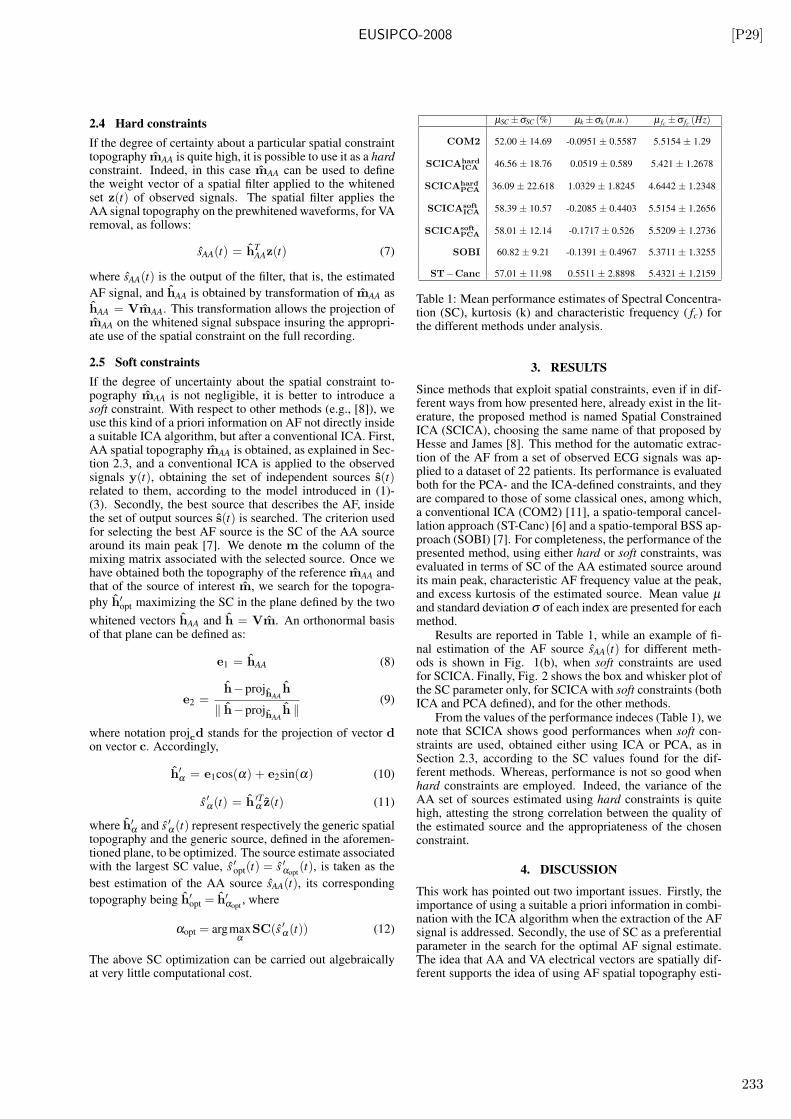
EUSIPCO-2008 [P29]
2.4 Hard constraints
If the degree of certainty about a particular spatial constrainttopography mAA is quite high, it is possible to use it as a hardconstraint. Indeed, in this case mAA can be used to definethe weight vector of a spatial filter applied to the whitenedset z(t) of observed signals. The spatial filter applies theAA signal topography on the prewhitened waveforms, for VAremoval, as follows:
sAA(t) = hTAAz(t) (7)
where sAA(t) is the output of the filter, that is, the estimated
AF signal, and hAA is obtained by transformation of mAA as
hAA = VmAA. This transformation allows the projection ofmAA on the whitened signal subspace insuring the appropri-ate use of the spatial constraint on the full recording.
2.5 Soft constraints
If the degree of uncertainty about the spatial constraint to-pography mAA is not negligible, it is better to introduce asoft constraint. With respect to other methods (e.g., [8]), weuse this kind of a priori information on AF not directly insidea suitable ICA algorithm, but after a conventional ICA. First,AA spatial topography mAA is obtained, as explained in Sec-tion 2.3, and a conventional ICA is applied to the observedsignals y(t), obtaining the set of independent sources s(t)related to them, according to the model introduced in (1)-(3). Secondly, the best source that describes the AF, insidethe set of output sources s(t) is searched. The criterion usedfor selecting the best AF source is the SC of the AA sourcearound its main peak [7]. We denote m the column of themixing matrix associated with the selected source. Once wehave obtained both the topography of the reference mAA andthat of the source of interest m, we search for the topogra-
phy h′opt maximizing the SC in the plane defined by the two
whitened vectors hAA and h = Vm. An orthonormal basisof that plane can be defined as:
e1 = hAA (8)
e2 =h−proj
hAAh
‖ h−projhAA
h ‖(9)
where notation projcd stands for the projection of vector don vector c. Accordingly,
h′α = e1cos(α) + e2sin(α) (10)
s ′α(t) = h ′Tα z(t) (11)
where h′α and s ′α(t) represent respectively the generic spatialtopography and the generic source, defined in the aforemen-tioned plane, to be optimized. The source estimate associatedwith the largest SC value, s ′opt(t) = s ′αopt
(t), is taken as the
best estimation of the AA source sAA(t), its corresponding
topography being h′opt = h′αopt, where
αopt = argmaxα
SC(s ′α(t)) (12)
The above SC optimization can be carried out algebraicallyat very little computational cost.
µSC±σSC (%) µk±σk (n.u.) µ fc ±σ fc (Hz)
COM2 52.00 ± 14.69 -0.0951 ± 0.5587 5.5154 ± 1.29
SCICAhardICA 46.56 ± 18.76 0.0519 ± 0.589 5.421 ± 1.2678
SCICAhardPCA 36.09 ± 22.618 1.0329 ± 1.8245 4.6442 ± 1.2348
SCICAsoftICA 58.39 ± 10.57 -0.2085 ± 0.4403 5.5154 ± 1.2656
SCICAsoftPCA 58.01 ± 12.14 -0.1717 ± 0.526 5.5209 ± 1.2736
SOBI 60.82 ± 9.21 -0.1391 ± 0.4967 5.3711 ± 1.3255
ST−Canc 57.01 ± 11.98 0.5511 ± 2.8898 5.4321 ± 1.2159
Table 1: Mean performance estimates of Spectral Concentra-tion (SC), kurtosis (k) and characteristic frequency ( fc) forthe different methods under analysis.
3. RESULTS
Since methods that exploit spatial constraints, even if in dif-ferent ways from how presented here, already exist in the lit-erature, the proposed method is named Spatial ConstrainedICA (SCICA), choosing the same name of that proposed byHesse and James [8]. This method for the automatic extrac-tion of the AF from a set of observed ECG signals was ap-plied to a dataset of 22 patients. Its performance is evaluatedboth for the PCA- and the ICA-defined constraints, and theyare compared to those of some classical ones, among which,a conventional ICA (COM2) [11], a spatio-temporal cancel-lation approach (ST-Canc) [6] and a spatio-temporal BSS ap-proach (SOBI) [7]. For completeness, the performance of thepresented method, using either hard or soft constraints, wasevaluated in terms of SC of the AA estimated source aroundits main peak, characteristic AF frequency value at the peak,and excess kurtosis of the estimated source. Mean value µand standard deviation σ of each index are presented for eachmethod.
Results are reported in Table 1, while an example of fi-nal estimation of the AF source sAA(t) for different meth-ods is shown in Fig. 1(b), when soft constraints are usedfor SCICA. Finally, Fig. 2 shows the box and whisker plot ofthe SC parameter only, for SCICA with soft constraints (bothICA and PCA defined), and for the other methods.
From the values of the performance indeces (Table 1), wenote that SCICA shows good performances when soft con-straints are used, obtained either using ICA or PCA, as inSection 2.3, according to the SC values found for the dif-ferent methods. Whereas, performance is not so good whenhard constraints are employed. Indeed, the variance of theAA set of sources estimated using hard constraints is quitehigh, attesting the strong correlation between the quality ofthe estimated source and the appropriateness of the chosenconstraint.
4. DISCUSSION
This work has pointed out two important issues. Firstly, theimportance of using a suitable a priori information in combi-nation with the ICA algorithm when the extraction of the AFsignal is addressed. Secondly, the use of SC as a preferentialparameter in the search for the optimal AF signal estimate.The idea that AA and VA electrical vectors are spatially dif-ferent supports the idea of using AF spatial topography esti-
233
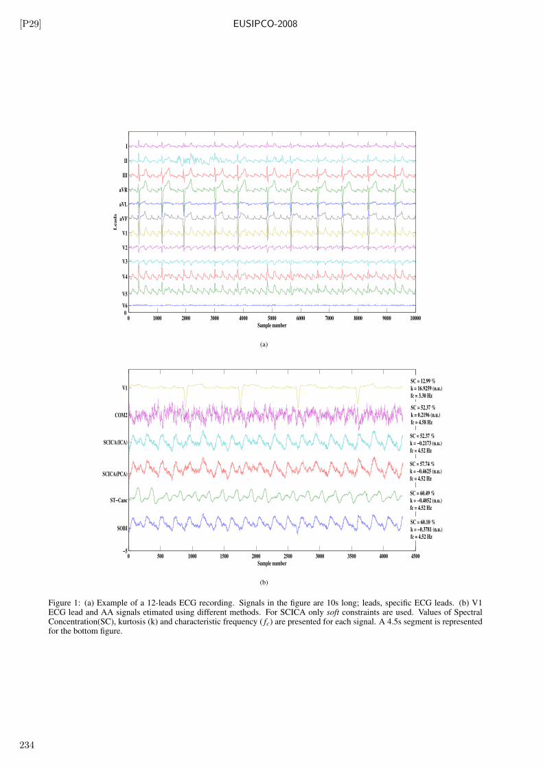
[P29] EUSIPCO-2008
0 1000 2000 3000 4000 5000 6000 7000 8000 9000 100000
V6
V5
V4
V3
V2
V1
aVF
aVL
aVR
III
II
I
Sample number
Lead
s
(a)
0 500 1000 1500 2000 2500 3000 3500 4000 4500−5
SOBI
ST−Canc
SCICA(PCA)
SCICA(ICA)
COM2
V1
Sample number
SC = 52.37 %
k = −0.2173 (n.u.)
fc = 4.52 Hz
SC = 52.37 %
k = 0.2196 (n.u.)
fc = 4.58 Hz
SC = 57.74 %
k = −0.4625 (n.u.)
fc = 4.52 Hz
SC = 60.49 %
k = −0.4052 (n.u.)
fc = 4.52 Hz
SC = 60.10 %
k = −0.3781 (n.u.)
fc = 4.52 Hz
SC = 12.99 %
k = 16.9259 (n.u.)
fc = 3.30 Hz
(b)
Figure 1: (a) Example of a 12-leads ECG recording. Signals in the figure are 10s long; leads, specific ECG leads. (b) V1ECG lead and AA signals etimated using different methods. For SCICA only soft constraints are used. Values of SpectralConcentration(SC), kurtosis (k) and characteristic frequency ( fc) are presented for each signal. A 4.5s segment is representedfor the bottom figure.
234
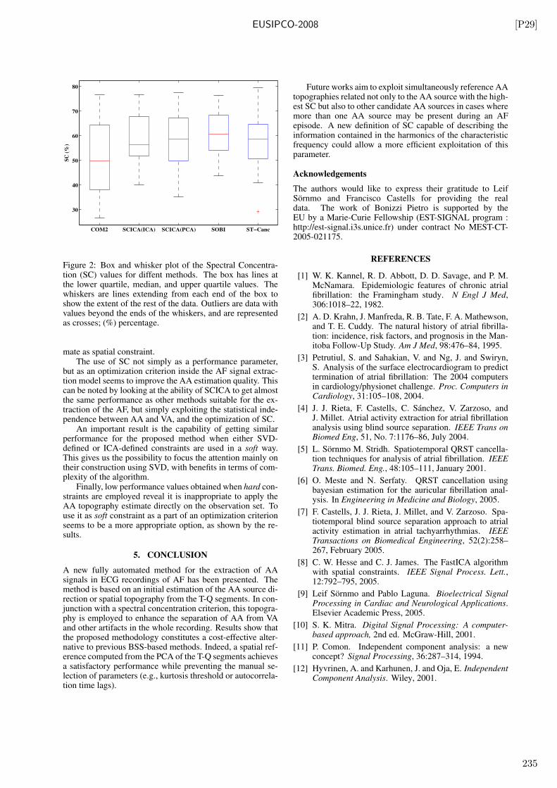
EUSIPCO-2008 [P29]
COM2 SCICA(ICA) SCICA(PCA) SOBI ST−Canc
30
40
50
60
70
80
SC
(%
)
Figure 2: Box and whisker plot of the Spectral Concentra-tion (SC) values for diffent methods. The box has lines atthe lower quartile, median, and upper quartile values. Thewhiskers are lines extending from each end of the box toshow the extent of the rest of the data. Outliers are data withvalues beyond the ends of the whiskers, and are representedas crosses; (%) percentage.
mate as spatial constraint.The use of SC not simply as a performance parameter,
but as an optimization criterion inside the AF signal extrac-tion model seems to improve the AA estimation quality. Thiscan be noted by looking at the ability of SCICA to get almostthe same performance as other methods suitable for the ex-traction of the AF, but simply exploiting the statistical inde-pendence between AA and VA, and the optimization of SC.
An important result is the capability of getting similarperformance for the proposed method when either SVD-defined or ICA-defined constraints are used in a soft way.This gives us the possibility to focus the attention mainly ontheir construction using SVD, with benefits in terms of com-plexity of the algorithm.
Finally, low performance values obtained when hard con-straints are employed reveal it is inappropriate to apply theAA topography estimate directly on the observation set. Touse it as soft constraint as a part of an optimization criterionseems to be a more appropriate option, as shown by the re-sults.
5. CONCLUSION
A new fully automated method for the extraction of AAsignals in ECG recordings of AF has been presented. Themethod is based on an initial estimation of the AA source di-rection or spatial topography from the T-Q segments. In con-junction with a spectral concentration criterion, this topogra-phy is employed to enhance the separation of AA from VAand other artifacts in the whole recording. Results show thatthe proposed methodology constitutes a cost-effective alter-native to previous BSS-based methods. Indeed, a spatial ref-erence computed from the PCA of the T-Q segments achievesa satisfactory performance while preventing the manual se-lection of parameters (e.g., kurtosis threshold or autocorrela-tion time lags).
Future works aim to exploit simultaneously reference AAtopographies related not only to the AA source with the high-est SC but also to other candidate AA sources in cases wheremore than one AA source may be present during an AFepisode. A new definition of SC capable of describing theinformation contained in the harmonics of the characteristicfrequency could allow a more efficient exploitation of thisparameter.
Acknowledgements
The authors would like to express their gratitude to LeifSornmo and Francisco Castells for providing the realdata. The work of Bonizzi Pietro is supported by theEU by a Marie-Curie Fellowship (EST-SIGNAL program :http://est-signal.i3s.unice.fr) under contract No MEST-CT-2005-021175.
REFERENCES
[1] W. K. Kannel, R. D. Abbott, D. D. Savage, and P. M.McNamara. Epidemiologic features of chronic atrialfibrillation: the Framingham study. N Engl J Med,306:1018–22, 1982.
[2] A. D. Krahn, J. Manfreda, R. B. Tate, F. A. Mathewson,and T. E. Cuddy. The natural history of atrial fibrilla-tion: incidence, risk factors, and prognosis in the Man-itoba Follow-Up Study. Am J Med, 98:476–84, 1995.
[3] Petrutiul, S. and Sahakian, V. and Ng, J. and Swiryn,S. Analysis of the surface electrocardiogram to predicttermination of atrial fibrillation: The 2004 computersin cardiology/physionet challenge. Proc. Computers inCardiology, 31:105–108, 2004.
[4] J. J. Rieta, F. Castells, C. Sanchez, V. Zarzoso, andJ. Millet. Atrial activity extraction for atrial fibrillationanalysis using blind source separation. IEEE Trans onBiomed Eng, 51, No. 7:1176–86, July 2004.
[5] L. Sornmo M. Stridh. Spatiotemporal QRST cancella-tion techniques for analysis of atrial fibrillation. IEEETrans. Biomed. Eng., 48:105–111, January 2001.
[6] O. Meste and N. Serfaty. QRST cancellation usingbayesian estimation for the auricular fibrillation anal-ysis. In Engineering in Medicine and Biology, 2005.
[7] F. Castells, J. J. Rieta, J. Millet, and V. Zarzoso. Spa-tiotemporal blind source separation approach to atrialactivity estimation in atrial tachyarrhythmias. IEEETransactions on Biomedical Engineering, 52(2):258–267, February 2005.
[8] C. W. Hesse and C. J. James. The FastICA algorithmwith spatial constraints. IEEE Signal Process. Lett.,12:792–795, 2005.
[9] Leif Sornmo and Pablo Laguna. Bioelectrical SignalProcessing in Cardiac and Neurological Applications.Elsevier Academic Press, 2005.
[10] S. K. Mitra. Digital Signal Processing: A computer-based approach, 2nd ed. McGraw-Hill, 2001.
[11] P. Comon. Independent component analysis: a newconcept? Signal Processing, 36:287–314, 1994.
[12] Hyvrinen, A. and Karhunen, J. and Oja, E. IndependentComponent Analysis. Wiley, 2001.
235

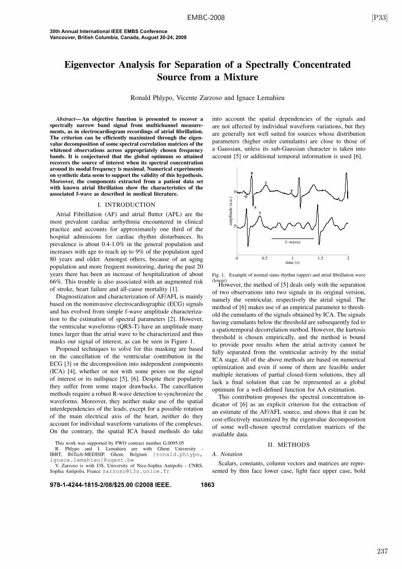
EMBC-2008 [P33]
Eigenvector Analysis for Separation of a Spectrally Concentrated
Source from a Mixture
Ronald Phlypo, Vicente Zarzoso and Ignace Lemahieu
Abstract— An objective function is presented to recover aspectrally narrow band signal from multichannel measure-ments, as in electrocardiogram recordings of atrial fibrillation.The criterion can be efficiently maximized through the eigen-value decomposition of some spectral correlation matrices of thewhitened observations across appropriately chosen frequencybands. It is conjectured that the global optimum so attainedrecovers the source of interest when its spectral concentrationaround its modal frequency is maximal. Numerical experimentson synthetic data seem to support the validity of this hypothesis.Moreover, the components extracted from a patient data setwith known atrial fibrillation show the characteristics of theassociated f-wave as described in medical literature.
I. INTRODUCTION
Atrial Fibrillation (AF) and atrial flutter (AFL) are the
most prevalent cardiac arrhythmia encountered in clinical
practice and accounts for approximately one third of the
hospital admissions for cardiac rhythm disturbances. Its
prevalence is about 0.4-1.0% in the general population and
increases with age to reach up to 9% of the population aged
80 years and older. Amongst others, because of an aging
population and more frequent monitoring, during the past 20
years there has been an increase of hospitalization of about
66%. This trouble is also associated with an augmented risk
of stroke, heart failure and all-cause mortality [1].
Diagnostization and characterization of AF/AFL is mainly
based on the noninvasive electrocardiographic (ECG) signals
and has evolved from simple f-wave amplitude characteriza-
tion to the estimation of spectral parameters [2]. However,
the ventricular waveforms (QRS-T) have an amplitude many
times larger than the atrial wave to be characterized and thus
masks our signal of interest, as can be seen in Figure 1.
Proposed techniques to solve for this masking are based
on the cancellation of the ventricular contribution in the
ECG [3] or the decomposition into independent components
(ICA) [4], whether or not with some priors on the signal
of interest or its nullspace [5], [6]. Despite their popularity
they suffer from some major drawbacks. The cancellation
methods require a robust R-wave detection to synchronize the
waveforms. Moreover, they neither make use of the spatial
interdependencies of the leads, except for a possible rotation
of the main electrical axis of the heart, neither do they
account for individual waveform variations of the complexes.
On the contrary, the spatial ICA based methods do take
This work was supported by FWO contract number G.0095.05R. Phlypo and I. Lemahieu are with Ghent University -
IBBT, IbiTech-MEDISIP, Ghent, Belgium {ronald.phlypo,ignace.lemahieu}@ugent.be
V. Zarzoso is with I3S, University of Nice-Sophia Antipolis - CNRS,Sophia Antipolis, France [email protected]
into account the spatial dependencies of the signals and
are not affected by individual waveform variations, but they
are generally not well suited for sources whose distribution
parameters (higher order cumulants) are close to those of
a Gaussian, unless its sub-Gaussian character is taken into
account [5] or additional temporal information is used [6].
0 0.5 1 1.5 2
0
0
time (s)
amp
litu
de
(a.u
.)
f−waves
S
T
R
T
P
Q
Fig. 1. Example of normal sinus rhythm (upper) and atrial fibrillation wave(lower)
However, the method of [5] deals only with the separation
of two observations into two signals in its original version,
namely the ventricular, respectively the atrial signal. The
method of [6] makes use of an empirical parameter to thresh-
old the cumulants of the signals obtained by ICA. The signals
having cumulants below the threshold are subsequently fed to
a spatiotemporal decorrelation method. However, the kurtosis
threshold is chosen empirically, and the method is bound
to provide poor results when the atrial activity cannot be
fully separated from the ventricular activity by the initial
ICA stage. All of the above methods are based on numerical
optimization and even if some of them are feasible under
multiple iterations of partial closed-form solutions, they all
lack a final solution that can be represented as a global
optimum for a well-defined function for AA estimation.
This contribution proposes the spectral concentration in-
dicator of [6] as an explicit criterion for the extraction of
an estimate of the AF/AFL source, and shows that it can be
cost-effectively maximized by the eigenvalue decomposition
of some well-chosen spectral correlation matrices of the
available data.
II. METHODS
A. Notation
Scalars, constants, column vectors and matrices are repre-
sented by thin face lower case, light face upper case, bold
30th Annual International IEEE EMBS ConferenceVancouver, British Columbia, Canada, August 20-24, 2008
978-1-4244-1815-2/08/$25.00 ©2008 IEEE. 1863
237
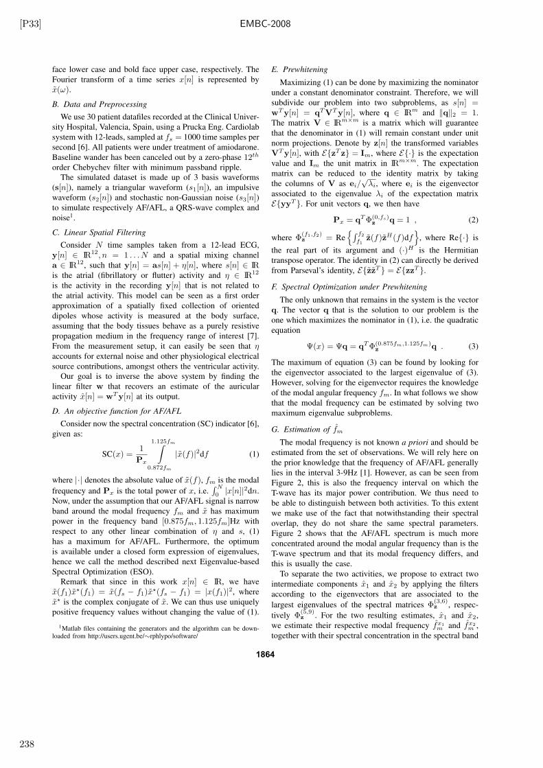
[P33] EMBC-2008
face lower case and bold face upper case, respectively. The
Fourier transform of a time series x[n] is represented by
x(ω).
B. Data and Preprocessing
We use 30 patient datafiles recorded at the Clinical Univer-
sity Hospital, Valencia, Spain, using a Prucka Eng. Cardiolab
system with 12-leads, sampled at fs = 1000 time samples per
second [6]. All patients were under treatment of amiodarone.
Baseline wander has been canceled out by a zero-phase 12th
order Chebychev filter with minimum passband ripple.
The simulated dataset is made up of 3 basis waveforms
(s[n]), namely a triangular waveform (s1[n]), an impulsive
waveform (s2[n]) and stochastic non-Gaussian noise (s3[n])to simulate respectively AF/AFL, a QRS-wave complex and
noise1.
C. Linear Spatial Filtering
Consider N time samples taken from a 12-lead ECG,
y[n] ∈ IR12, n = 1 . . . N and a spatial mixing channel
a ∈ IR12, such that y[n] = as[n] + η[n], where s[n] ∈ IRis the atrial (fibrillatory or flutter) activity and η ∈ IR12
is the activity in the recording y[n] that is not related to
the atrial activity. This model can be seen as a first order
approximation of a spatially fixed collection of oriented
dipoles whose activity is measured at the body surface,
assuming that the body tissues behave as a purely resistive
propagation medium in the frequency range of interest [7].
From the measurement setup, it can easily be seen that ηaccounts for external noise and other physiological electrical
source contributions, amongst others the ventricular activity.
Our goal is to inverse the above system by finding the
linear filter w that recovers an estimate of the auricular
activity x[n] = wT y[n] at its output.
D. An objective function for AF/AFL
Consider now the spectral concentration (SC) indicator [6],
given as:
SC(x) =1
Px
1.125fm∫
0.872fm
|x(f)|2df (1)
where |·| denotes the absolute value of x(f), fm is the modal
frequency and Px is the total power of x, i.e.∫ N
0|x[n]|2dn.
Now, under the assumption that our AF/AFL signal is narrow
band around the modal frequency fm and x has maximum
power in the frequency band [0.875fm, 1.125fm]Hz with
respect to any other linear combination of η and s, (1)
has a maximum for AF/AFL. Furthermore, the optimum
is available under a closed form expression of eigenvalues,
hence we call the method described next Eigenvalue-based
Spectral Optimization (ESO).
Remark that since in this work x[n] ∈ IR, we have
x(f1)x⋆(f1) = x(fs − f1)x
⋆(fs − f1) = |x(f1)|2, where
x⋆ is the complex conjugate of x. We can thus use uniquely
positive frequency values without changing the value of (1).
1Matlab files containing the generators and the algorithm can be down-loaded from http://users.ugent.be/∼rphlypo/software/
E. Prewhitening
Maximizing (1) can be done by maximizing the nominator
under a constant denominator constraint. Therefore, we will
subdivide our problem into two subproblems, as s[n] =wT y[n] = qT VT y[n], where q ∈ IRm and ‖q‖2 = 1.
The matrix V ∈ IRm×m is a matrix which will guarantee
that the denominator in (1) will remain constant under unit
norm projections. Denote by z[n] the transformed variables
VT y[n], with E{zT z} = Im, where E{·} is the expectation
value and Im the unit matrix in IRm×m. The expectation
matrix can be reduced to the identity matrix by taking
the columns of V as ei/√
λi, where ei is the eigenvector
associated to the eigenvalue λi of the expectation matrix
E{yyT }. For unit vectors q, we then have
Px = qT Φ(0,fs)z
q = 1 , (2)
where Φ(f1,f2)z = Re
{
∫ f2
f1
z(f)zH(f)df}
, where Re{·} is
the real part of its argument and (·)H is the Hermitian
transpose operator. The identity in (2) can directly be derived
from Parseval’s identity, E{zzT } = E{zzT }.
F. Spectral Optimization under Prewhitening
The only unknown that remains in the system is the vector
q. The vector q that is the solution to our problem is the
one which maximizes the nominator in (1), i.e. the quadratic
equation
Ψ(x) = Ψq = qT Φ(0.875fm,1.125fm)z
q . (3)
The maximum of equation (3) can be found by looking for
the eigenvector associated to the largest eigenvalue of (3).
However, solving for the eigenvector requires the knowledge
of the modal angular frequency fm. In what follows we show
that the modal frequency can be estimated by solving two
maximum eigenvalue subproblems.
G. Estimation of fm
The modal frequency is not known a priori and should be
estimated from the set of observations. We will rely here on
the prior knowledge that the frequency of AF/AFL generally
lies in the interval 3-9Hz [1]. However, as can be seen from
Figure 2, this is also the frequency interval on which the
T-wave has its major power contribution. We thus need to
be able to distinguish between both activities. To this extent
we make use of the fact that notwithstanding their spectral
overlap, they do not share the same spectral parameters.
Figure 2 shows that the AF/AFL spectrum is much more
concentrated around the modal angular frequency than is the
T-wave spectrum and that its modal frequency differs, and
this is usually the case.
To separate the two activities, we propose to extract two
intermediate components x1 and x2 by applying the filters
according to the eigenvectors that are associated to the
largest eigenvalues of the spectral matrices Φ(3,6)z , respec-
tively Φ(5,9)z . For the two resulting estimates, x1 and x2,
we estimate their respective modal frequency fx1
m and fx2
m ,
together with their spectral concentration in the spectral band
1864
238
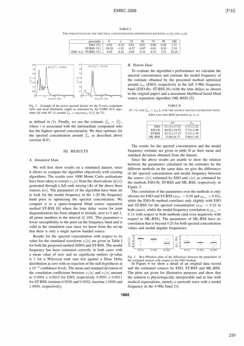
EMBC-2008 [P33]
TABLE I
THE PERCENTILES OF THE SPECTRAL CONCENTRATION DIFFERENCES BETWEEN x1[n] AND s1[n]
percentile 0 1 25 50 75 99 100
ESO (%) -4.93 -0.18 0.01 0.03 0.08 0.48 1.31ST-BSS (%) -26.20 -1.93 -0.27 -0.07 -0.01 0.20 2.10
ESO w.r.t. ST-BSS (%) -4.84 -0.22 0.04 0.10 0.33 2.21 26.18
0 5 10 15 200
0.05
0.1
0.15
0.2
0.25
0.3
0.35
frequency [Hz]
x[µ
V]
SC(xICAT ) = 25.0618
0 5 10 15 200
0.1
0.2
0.3
0.4
0.5
0.6
0.7
frequency [Hz]
x[µ
V]
SC(xICAAA ) = 46.4748
Fig. 2. Example of the power spectral density for the T-wave component(left) and atrial fibrillation (right) as estimated by the COM2 ICA algo-
rithm [8] with SC (1) around fm = arg maxf x(f) [in %].
as defined in (1). Finally, we use the estimate fm = fxi
m ,
where i is associated with the intermediate component who
has the highest spectral concentration. We then optimize for
the spectral concentration around fm as described above
(section II-F).
III. RESULTS
A. Simulated Data
We will first show results on a simulated dataset, since
it allows to compare the algorithm objectively with existing
algorithms. The results over 1000 Monte Carlo realisations
have been taken to extract x1[n] from the observations (y[n])generated through a full rank mixing (A) of the above three
sources s[n]. The parameters of the algorithm have been set
to look for the modal frequency in the 1-20 Hz frequency
band prior to optimizing the spectral concentration. We
compare it to a spatio-temporal blind source separation
method ST-BSS [6] where the time delay vector for joint
diagonalization has been adapted to include, next to 0 and 1,
all prime numbers in the interval [0, 100]. This guarantees a
lower susceptibility to the prior on the frequency band and is
valid in the simulation case since we know from the set-up
that there is only a single narrow banded source.
Results for the spectral concentration with respect to its
value for the simulated waveform s1[n] are given in Table I
for both the proposed method (ESO) and ST-BSS. The modal
frequency has been estimated correctly in both cases with
a mean value of zero and no significant outliers (p-value
is 1 for a Wilcoxon rank sum test against a Dirac Delta
distribution at zero with no rejection of the null-hypothesis at
a 10−6 confidence level). The mean and standard deviation of
the correlation coefficients between x1[n] and s1[n] amount
to 0.9994 ± 0.0010 for ESO, respectively 0.9991 ± 0.0011for ST-BSS (minima 0.9928 and 0.9933, maxima 1.0000 and
1.0000, respectively).
B. Patient Data
To evaluate the algorithm’s performance we calculate the
spectral concentration and estimate the modal frequency of
the estimate obtained by the presented method optimized
around ωm (ESO), respectively in the full 3-9Hz frequency
band (ESO-fb), ST-BSS [6] (with the time delays as chosen
in the original paper) and a maximum likelihood based blind
source separation algorithm (ML-BSS) [5].
TABLE II
SC (1) AND fm = ωmfs FOR THE SOURCE SIGNALS ESTIMATED WITH
ESO AND TWO BSS METHODS (µ ± σ).
SC fm
ESO 51.11±17.25 5.31±1.22ESO-fb 40.82±18.55 5.72±1.08ST-BSS 42.21±17.15 5.13±1.39
ML-BSS 13.66±6.37 5.06±1.44
The results for the spectral concentration and the modal
frequency estimate are given in table II as their mean and
standard deviation obtained from the dataset.
Since the above results are unable to show the relation
between the parameters calculated on the estimates by the
different methods on the same data, we give the differences
of the spectral concentration and modal frequency between
the source x[n] estimated by ESO and x[n] as estimated by
the methods ESO-fb, ST-BSS and ML-BSS, respectively, in
Figure 3.
The correlation of the parameters over the methods is only
obvious for ESO and ST-BSS (ρSC = 0.88 and ρωm= 0.85),
while the ESO-fb method correlates only slightly with ESO
and ST-BSS for the spectral concentration (ρSC = 0.52 in
both cases), whilst the modal frequency correlation is ρωm=
0.14 with respect to both methods (and even negatively with
respect to ML-BSS). The parameters of ML-BSS have no
correlation that is beyond 0.25 for both spectral concentration
values and modal angular frequencies.
ESO−fb ST−BSS ML−BSS
−60
−40
−20
0
20
∆S
C(%
)
ESO−fb ST−BSS ML−BSS
−2
0
2
4
∆f m
(Hz)
Fig. 3. Box-Whiskers plots of the differences between the parameters ofthe estimated sources with respect to the ESO method.
In Figure 4 we show a detail of an original data record
and the estimated sources by ESO, ST-BSS and ML-BSS.
The plots are given for illustrative purposes and show that
the solution is physiologically interpretable and in line with
medical expectations, namely a sawtooth wave with a modal
frequency in the 4-9Hz band [1].
1865
239
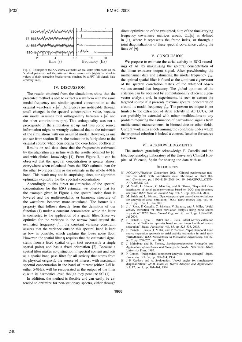
[P33] EMBC-2008
2 4 6
ESO−fb
ML−BSS
ST−BSS
ESO
time (s)0 10 20
frequency (Hz)
Fig. 4. Example of the AA source estimates on real data: (left) zoom on theV1-lead potentials and the estimated time courses with (right) the absolutevalues of their respective Fourier terms obtained by a FFT (all signals havearbitrary units).
IV. DISCUSSION
The results obtained from the simulations show that the
presented method is able to extract a waveform with the same
modal frequency and similar spectral concentration as the
original waveform s1[n]. Differences are noticeable through
small changes in the spectral concentration value, because
our model assumes total orthogonality between s1[n] and
the other contributions η[n]. This orthogonality was not a
prerequisite in the simulation set up and thus some source
information might be wrongly estimated due to the mismatch
of the simulations with our assumed model. However, as one
can see from section III-A, the estimation is fairly close to the
original source when considering the correlation coefficient.
Results on real data show that the frequencies estimated
by the algorithm are in line with the results obtained by [6]
and with clinical knowledge [1]. From Figure 3, it can be
observed that the spectral concentration is greater almost
everywhere when calculated from the ESO estimate than for
the other two algorithms or the estimate in the whole 4-9Hz
band. This result may not be surprising, since our algorithm
optimizes explicitly for the spectral concentration.
Accordingly to this direct maximization of the spectral
concentration for the ESO estimate, we observe that for
the example given in Figure 4 the spectral noise floor is
lowered and the multi-modality, or harmonic structure of
the waveform, becomes more articulated. The former is a
property that follows directly from the definition of our
function (1) under a constant denominator, while the latter
is connected to the application of a spatial filter. Since we
optimize for the variance in the narrow band around the
estimated frequency fm, the constant variance constraint
assures that the variance outside this spectral band is kept
as low as possible, which explains the lower noise floor.
However, the spatial filter q requires that the estimated signal
stems from a fixed spatial origin (not necessarily a single
spatial point) and has a fixed orientation [7]. Because a
spatial filter makes no distinction in spectral content and acts
as a spatial band pass filter for all activity that stems from
its physical origin(s), the source of interest with maximum
spectral concentration in the band of interest (either 3-6Hz,
either 5-9Hz), will be recuperated at the output of the filter
q with its harmonics, even though they penalize SC (1).
In addition, the method is flexible and can easily be ex-
tended to optimize for non-stationary spectra, either through
direct optimization of the (weighted) sum of the time-varying
frequency covariance matrices around ωm[k] as defined
in (1), where k represents the frame index, or through a
joint diagonalization of these spectral covariance , along the
lines of [9].
V. CONCLUSION
We propose to estimate the atrial activity in ECG record-
ings of AF by maximizing the spectral concentration of
the linear extractor output signal. After prewhitening the
multichannel data and estimating the modal frequency fm,
the optimal spatial filter is found as the dominant eigenvector
of the spectral correlation matrix of the whitened obser-
vations around that frequency. The global optimum of the
criterion can be obtained by computationally efficient eigen-
vector analysis and, in experiments, is seen to extract the
targeted source if it presents maximal spectral concentration
around its modal frequency fm. The present technique is not
limited to the extraction of atrial activity in AF ECGs, but
can probably be extended with minor modifications to any
problem requiring the estimation of narrowband signals from
multichannel measurements, in biomedicine or other fields.
Current work aims at determining the conditions under which
the proposed criterion is indeed a contrast function for source
extraction.
VI. ACKNOWLEDGMENTS
The authors gratefully acknowledge F. Castells and the
Electrophysiology Laboratory of the University Clinical Hos-
pital of Valencia, Spain for sharing the data with us.
REFERENCES
[1] ACC/AHA/Physician Consortium 2008, “Clinical performance mea-sure for adults with nonvalvular atrial fibrillation or atrial flut-ter,” Circulation, pp. 1100–1120, 2008 doi: 10.1161/CIRCULATION-AHA.107.187192.
[2] M. Stridh, L. Sörnmo, C. Meurling, and B. Olsson, “Sequential char-acterization of atrial tachyarrhythmias based on ECG time-frequencyanalysis,” IEEE Trans on Biomed Eng, vol. 51, pp. 100–114, 2004.
[3] M. Stridh and L. Sörnmo, “Spatiotemporal qrst cancellation techniquesfor analysis of atrial fibrillation.” IEEE Trans Biomed Eng, vol. 48,no. 1, pp. 105–111, Jan 2001.
[4] J. J. Rieta, F. Castells, C. Sánchez, V. Zarzoso, and J. Millet, “Atrialactivity extraction for atrial fibrillation analysis using blind sourceseparation.” IEEE Trans Biomed Eng, vol. 51, no. 7, pp. 1176–1186,Jul 2004.
[5] F. Castells, J. Igual, J. Millet, and J. Rieta, “Atrial activity extractionfrom atrial fibrillation episodes based on maximum likelihood sourceseparation,” Signal Processing, vol. 85, pp. 523–535, 2005.
[6] F. Castells, J. Rieta, J. Millet, and V. Zarzoso, “Spatiotemporal blindsource separation approach to atrial activity estimation in atrial tach-yarrhythmias,” IEEE Transactions on Biomedical Engineering, vol. 52,no. 2, pp. 258–267, Feb. 2005.
[7] J. Malmivuo and R. Plonsey, Bioelectromagnetism: Principles and
Applications of Bioelectric and Biomagnetic Fields. New York: OxfordUniversity Press, 1995.
[8] P. Comon, “Independent component analysis, a new concept?” Signal
Processing, vol. 36, pp. 287–314, 1994.[9] J.-F. Cardoso and A. Souloumiac, “Jacobi angles for simultaneous
diagonalization.” SIAM Journ on Matrix Analysis and Applications,vol. 17, no. 1, pp. 161–164, 1996.
1866
240
CINC-2007 [P35]
Atrio-Ventricular Junction Behaviour
During Atrial Fibrillation
P Bonizzi, V Zarzoso, O Meste
I3S Laboratory, University of Nice - Sophia Antipolis, France
Abstract
Up to now the functioning of the Atrio-Ventricular Junc-
tion (AVJ) during Atrial Fibrillation (AF) is still not com-
pletely understood. To shed some light on the AVJ behav-
ior during AF episodes, this study analyses the existence of
a possible relationship between the occurrence of a heart
beat and the power of the atrial activity (AA) preceding
this heart beat in an electrocardiogram (ECG) signal. AA
power is measured in the interval of the ECG between the
onset of the heart beat under analysis and the ending of
the previous heart beat (T-Q interval). Our analysis has
shown a difference in the distributions of AA power versus
cardiac cycle length (RR interval on the ECG) between
healthy and pathological subjects. In particular, a nega-
tive trend between these two parameters is discovered in
pathological subjects. This negative relation shows a pos-
sible coherence between power arriving at the AVJ and the
triggering of the heart beat, which is in line with the as-
sumptions made in the quantitative model for the ventricu-
lar response during AF by Cohen [1].
1. Introduction
Atrial Fibrillation (AF) represents the most common
sustained cardiac arrhythmia in adults. It consists of a mis-
function of the atrium characterized by a modification of
the normal atrial activity (AA) pattern on the electrocar-
diogram (ECG) signal. Epidemiologic studies have shown
that its prevalence and incidence doubles with each ad-
vancing decade beyond 50 years reaching 10% in people
over 80 and has direct impact on mortality and morbidity
[2, 3].
Although the mechanism and effective treatments for
most other supraventricular tachyarrhythmia have been
discovered, the understanding of AF remains incomplete.
In particular, no unifying mechanism has been found yet
to explain the behaviour of the atrio-ventricular junction
(AVJ) during AF. It is well known that heart rate vari-
ability is enhanced during AF [1, 4], while other studies
have revealed a more complex relationship between AVJ
behaviour and AF [5]. In addition, the variation of the RR
interval during AF has been thought to result mainly from
autonomic modulation of the electrophysiological proper-
ties of the atria and the AVJ [6]. Therefore, the character-
ization of the ventricular rhythm in AF has been contro-
versial and its mechanism has been a subject of debate for
decades [7], thus revealing that the prevailing ventricular
rate during high atrial rate is a complex dynamic parame-
ter.
Different hypothesis were introduced to explain the ir-
regular ventricular response during AF, i.e., the depen-
dence of the decremental conduction and repetitive con-
cealment on the AF impulses within the AVJ [8], or yet
the dependence of the electrotonic modulation on the AVJ
propagation by concealed AF impulses [9].
Several quantitative models for the ventricular response
during AF were developed [1, 7, 10] to deal with this prob-
lem. The AVJ model presented by Cohen et al. [1] in-
troduced the hyphotesis that it can be treated as a lumped
structure with well defined electrical properties, including
the refractory period, the automaticity and a defined de-
polarization threshold. From this point, the present work
analyzes the presence of a possible correlation between the
occurrence of a heart beat and the power of the AA observ-
able in the ECG signal during the T-Q interval preceding
this heart beat. This analysis aims to test the presence of
a dependence between the AA power arriving at the AVJ
and the RR period, following the idea that the AVJ gener-
ates an activation wave when the AA power arriving at it
exceeds a threshold value, intrinsic to the AVJ.
The study of AF and its characteristics can to a large
extent be carried out through the analysis of the surface
electrocardiogram (ECG), which has the advantage to be a
noninvasive technique and is already reported to be useful
[11].
2. Methods
A dataset composed of 23 real recordings (2 healthy
subjects and 21 presenting AF) was employed to analyze
the proposed idea. All signals were recorded and digitized
at a sampling rate of 1 KHz. Among the segments em-
ISSN 0276−6574 561 Computers in Cardiology 2007;34:561−564.
241
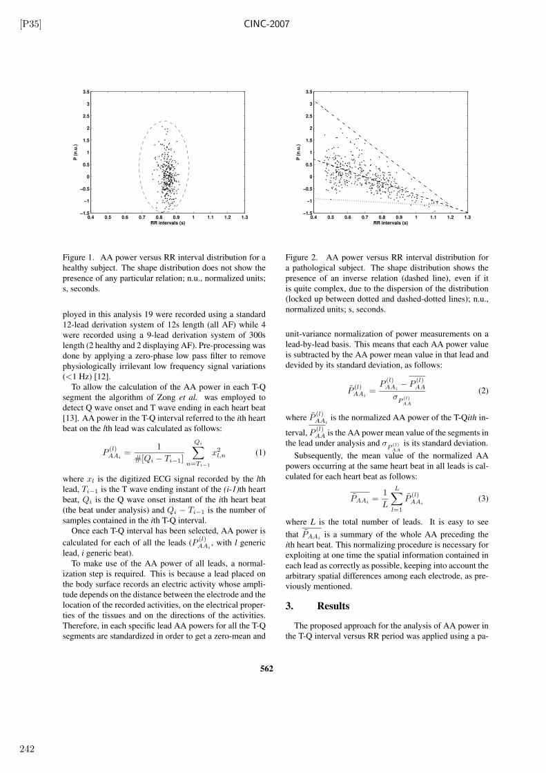
[P35] CINC-2007
0.4 0.5 0.6 0.7 0.8 0.9 1 1.1 1.2 1.3−1.5
−1
−0.5
0
0.5
1
1.5
2
2.5
3
3.5
RR intervals (s)
P (
n.u
.)
Figure 1. AA power versus RR interval distribution for a
healthy subject. The shape distribution does not show the
presence of any particular relation; n.u., normalized units;
s, seconds.
ployed in this analysis 19 were recorded using a standard
12-lead derivation system of 12s length (all AF) while 4
were recorded using a 9-lead derivation system of 300s
length (2 healthy and 2 displaying AF). Pre-processing was
done by applying a zero-phase low pass filter to remove
physiologically irrilevant low frequency signal variations
(<1 Hz) [12].
To allow the calculation of the AA power in each T-Q
segment the algorithm of Zong et al. was employed to
detect Q wave onset and T wave ending in each heart beat
[13]. AA power in the T-Q interval referred to the ith heart
beat on the lth lead was calculated as follows:
P(l)AAi
=1
#[Qi − Ti−1]
Qi∑
n=Ti−1
x2l,n (1)
where xl is the digitized ECG signal recorded by the lth
lead, Ti−1 is the T wave ending instant of the (i-1)th heart
beat, Qi is the Q wave onset instant of the ith heart beat
(the beat under analysis) and Qi − Ti−1 is the number of
samples contained in the ith T-Q interval.
Once each T-Q interval has been selected, AA power is
calculated for each of all the leads (P(l)AAi
, with l generic
lead, i generic beat).
To make use of the AA power of all leads, a normal-
ization step is required. This is because a lead placed on
the body surface records an electric activity whose ampli-
tude depends on the distance between the electrode and the
location of the recorded activities, on the electrical proper-
ties of the tissues and on the directions of the activities.
Therefore, in each specific lead AA powers for all the T-Q
segments are standardized in order to get a zero-mean and
0.4 0.5 0.6 0.7 0.8 0.9 1 1.1 1.2 1.3−1.5
−1
−0.5
0
0.5
1
1.5
2
2.5
3
3.5
RR intervals (s)
P (
n.u
.)
Figure 2. AA power versus RR interval distribution for
a pathological subject. The shape distribution shows the
presence of an inverse relation (dashed line), even if it
is quite complex, due to the dispersion of the distribution
(locked up between dotted and dashed-dotted lines); n.u.,
normalized units; s, seconds.
unit-variance normalization of power measurements on a
lead-by-lead basis. This means that each AA power value
is subtracted by the AA power mean value in that lead and
devided by its standard deviation, as follows:
P(l)AAi
=P
(l)AAi− P (l)
AA
σP
(l)
AA
(2)
where P(l)AAi
is the normalized AA power of the T-Qith in-
terval, P(l)AA is the AA power mean value of the segments in
the lead under analysis and σP
(l)
AA
is its standard deviation.
Subsequently, the mean value of the normalized AA
powers occurring at the same heart beat in all leads is cal-
culated for each heart beat as follows:
PAAi=
1
L
L∑
l=1
P(l)AAi
(3)
where L is the total number of leads. It is easy to see
that PAAiis a summary of the whole AA preceding the
ith heart beat. This normalizing procedure is necessary for
exploiting at one time the spatial information contained in
each lead as correctly as possible, keeping into account the
arbitrary spatial differences among each electrode, as pre-
viously mentioned.
3. Results
The proposed approach for the analysis of AA power in
the T-Q interval versus RR period was applied using a pa-
562
242
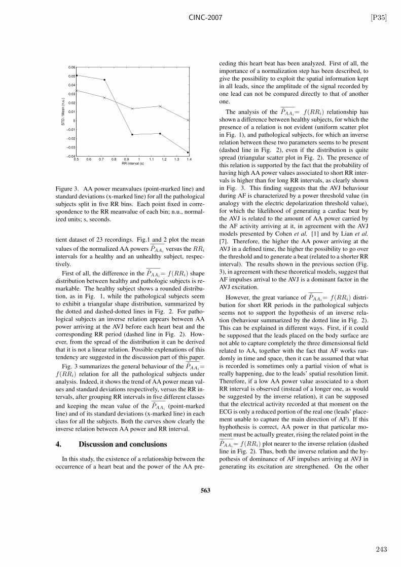
CINC-2007 [P35]
0.5 0.6 0.7 0.8 0.9 1 1.1 1.2 1.3 1.4−0.04
−0.03
−0.02
−0.01
0
0.01
0.02
0.03
0.04
0.05
0.06
RR interval (s)
ST
D / M
ean (
n.u
.)
Figure 3. AA power meanvalues (point-marked line) and
standard deviations (x-marked line) for all the pathological
subjects split in five RR bins. Each point fixed in corre-
spondence to the RR meanvalue of each bin; n.u., normal-
ized units; s, seconds.
tient dataset of 23 recordings. Fig.1 and 2 plot the mean
values of the normalized AA powers PAAiversus the RRi
intervals for a healthy and an unhealthy subject, respec-
tively.
First of all, the difference in the PAAi= f(RRi) shape
distribution between healthy and pathologic subjects is re-
markable. The healthy subject shows a rounded distribu-
tion, as in Fig. 1, while the pathological subjects seem
to exhibit a triangular shape distribution, summarized by
the dotted and dashed-dotted lines in Fig. 2. For patho-
logical subjects an inverse relation appears between AA
power arriving at the AVJ before each heart beat and the
corresponding RR period (dashed line in Fig. 2). How-
ever, from the spread of the distribution it can be derived
that it is not a linear relation. Possible explenations of this
tendency are suggested in the discussion part of this paper.
Fig. 3 summarizes the general behaviour of the PAAi=
f(RRi) relation for all the pathological subjects under
analysis. Indeed, it shows the trend of AA power mean val-
ues and standard deviations respectively, versus the RR in-
tervals, after grouping RR intervals in five different classes
and keeping the mean value of the PAAi(point-marked
line) and of its standard deviations (x-marked line) in each
class for all the subjects. Both the curves show clearly the
inverse relation between AA power and RR interval.
4. Discussion and conclusions
In this study, the existence of a relationship between the
occurrence of a heart beat and the power of the AA pre-
ceding this heart beat has been analyzed. First of all, the
importance of a normalization step has been described, to
give the possibility to exploit the spatial information kept
in all leads, since the amplitude of the signal recorded by
one lead can not be compared directly to that of another
one.
The analysis of the PAAi= f(RRi) relationship has
shown a difference between healthy subjects, for which the
presence of a relation is not evident (uniform scatter plot
in Fig. 1), and pathological subjects, for which an inverse
relation between these two parameters seems to be present
(dashed line in Fig. 2), even if the distribution is quite
spread (triangular scatter plot in Fig. 2). The presence of
this relation is supported by the fact that the probability of
having high AA power values associated to short RR inter-
vals is higher than for long RR intervals, as clearly shown
in Fig. 3. This finding suggests that the AVJ behaviour
during AF is characterized by a power threshold value (in
analogy with the electric depolarization threshold value),
for which the likelihood of generating a cardiac beat by
the AVJ is related to the amount of AA power carried by
the AF activity arriving at it, in agreement with the AVJ
models presented by Cohen et al. [1] and by Lian et al.
[7]. Therefore, the higher the AA power arriving at the
AVJ in a defined time, the higher the possibility to go over
the threshold and to generate a beat (related to a shorter RR
interval). The results shown in the previous section (Fig.
3), in agreement with these theoretical models, suggest that
AF impulses arrival to the AVJ is a dominant factor in the
AVJ excitation.
However, the great variance of PAAi= f(RRi) distri-
bution for short RR periods in the pathological subjects
seems not to support the hypothesis of an inverse rela-
tion (behaviour summarized by the dotted line in Fig. 2).
This can be explained in different ways. First, if it could
be supposed that the leads placed on the body surface are
not able to capture completely the three dimensionsal field
related to AA, together with the fact that AF works ran-
domly in time and space, then it can be assumed that what
is recorded is sometimes only a partial vision of what is
really happening, due to the leads’ spatial resolution limit.
Therefore, if a low AA power value associated to a short
RR interval is observed (instead of a longer one, as would
be suggested by the inverse relation), it can be supposed
that the electrical activity recorded at that moment on the
ECG is only a reduced portion of the real one (leads’ place-
ment unable to capture the main direction of AF). If this
hyphothesis is correct, AA power in that particular mo-
ment must be actually greater, rising the related point in the
PAAi= f(RRi) plot nearer to the inverse relation (dashed
line in Fig. 2). Thus, both the inverse relation and the hy-
pothesis of dominance of AF impulses arriving at AVJ in
generating its excitation are strengthened. On the other
563
243
[P35] CINC-2007
hand, we could think the opposite,i.e., that leads place-
ment works well in capturing all the AF electrical activity
in any direction. Consequently, power variance trend in the
PAAi= f(RRi) distribution could be due to the amount of
noise present in the AA signal and to the way the power
is computed (the longer the RR periods for which AA en-
ergy is divided the lesser the variance of the estimator of
the AA power mean). On the contrary, if the amount of
noise in the AA signal is unimportant, it means that other
factors must be taken into account for the understanding of
the spread of the variance and the AVJ way of functioning.
Also, it must be taken into account that there is no cer-
tainty about the fact that AA recorded in the ECG before a
heart beat is effectively what reachs the AVJ. Indeed, it is
the global activity of the heart in a particular moment. The
portion of this global activity that really arrives at the AVJ
depends on the AA waves interaction, and so on their level
of spatial and temporal organization.
In conclusion, the frequency content of AA is known to
provide important physiological and clinical informations
about AF [11]. This study has evidenced that alternative
information such as the amplitude (power) of the AA sig-
nal can also shed some light on the understanding of the
physiological mechanism behind this condition. Future
work aims to analyze more deeply this finding, trying to
exploit also the AA masked by the QRS complex [14, 15].
Acknowledgements
The authors would like to express their gratitude to
Leif Sornmo and Francisco Castells for providing the real
data. The work of Bonizzi Pietro is supported by the
EU by a Marie-Curie Fellowship (EST-SIGNAL program :
http://est-signal.i3s.unice.fr) under contract No MEST-CT-
2005-021175.
References
[1] Cohen RJ, Berger RD, Dushane TE. A quantitative model
for the ventricular response during atrial fibrillation. IEEE
1983;781–796.
[2] Kannel WK, Abbott RD, Savage DD, McNamara PM. Epi-
demiologic features of chronic atrial fibrillation: the fram-
ingham study. N Engl J Med 1982;306:1018–22.
[3] Krahn AD, Manfreda J, Tate RB, Mathewson FA, Cuddy
TE. The natural history of atrial fibrillation: incidence, risk
factors, and prognosis in the Manitoba Follow-Up Study.
Am J Med 1995;98:476–84.
[4] Fuster V, Ryden LE, Asinger RW. ACC/AHA/ESC guide-
lines for the management of patients with atrial fibrillation.
JACC 2001;38:1266i–1266lxx.
[5] Garrigue S, Tchou PJ, Mazgalev TN. Role of the differ-
ential bombardment of atrial inputs to the atrioventricular
node as a factor influencing ventricular rate during high
atrial rate. Cardiovasc Res 1999;44:344–355.
[6] Toivonen L, Kadish A, Kou W, Morady F. Determinants
of the ventricular rate during atrial fibrillation. J Am Coll
Cardiol 1990;16:1194–1200.
[7] Lian J, Mussig D, Lang V. Computer modeling of ventric-
ular rhythm during atrial fibrillation and ventricular pacing.
IEEE Trans Biomed Eng 2006;53:1512–20.
[8] Watanabe Y, Watanabe M. Impulse formation and conduc-
tion of excitation in the atrioventricular node. J Cardiovasc
Electrophysiol 1994;5:517–531.
[9] Meijler FL, Jalife J, Beaumont J, Vaidya D. AV nodal func-
tion during atrial fibrillation: The role of electrotonic mod-
ulation of propagation. J Cardiovasc Electrophysiol 1996;
7:843–861.
[10] Jorgensen P, Schafer C, Guerra PG, Talajic M, Nattel S. A
mathematical model of human atrioventricular nodal func-
tion incorporating cocealed conduction. Bull Math Biol
2002;64:1083–1099.
[11] Bollmann A, Husser D, Mainardi L, Lombardi F, Langley
P, Murray A, Rieta JJ, Millet J, Bertil Olsson S, Stridh M,
Sornmo L. Analysis of surface electrocardiograms in atrial
fibrillation: techniques, research, and clinical applications.
Europace 2006;8:911–926.
[12] Sornmo L, Laguna P. Bioelectrical Signal Processing in
Cardiac and Neurological Applications. Elsevier Academic
Press, 2005.
[13] Zong W, Saeed M, Heldt T. A QT interval detection algo-
rithm based on ecg curve length transform. In Computers
in Cardiology. 2006; .
[14] Zarzoso V, Nandi AK. Noninvasive fetal electrocardiogram
extraction: blind separation versus adaptive noise cancella-
tion. IEEE Trans Biomed Eng 48;January 2001:12–18.
[15] Meste O, Serfaty N. QRST cancellation using bayesian esti-
mation for the auricular fibrillation analysis. In Engineering
in Medicine and Biology. 2005; .
Address for correspondence:
Pietro Bonizzi, Ph.D. Student
Laboratoire I3S - BIOMED UNSA - CNRS
2000, Route des Lucioles Les Algorithmes - bat. Euclide B
B.P. 121
06903 Sophia Antipolis - Cedex, France
E-mail: [email protected]
564
244
EMBC-2007 [P36]
Extraction of the Atrial Activity from the ECG based on Independent
Component Analysis with Prior Knowledge of the Source Kurtosis Signs
Ronald Phlypo, Yves D’Asseler, Ignace
Lemahieu
MEDISIP - IBiTech
University of Ghent
De Pintelaan 185, Blok B
9000 Ghent, Belgium
{ronald.phlypo, yves.dasseler,
ignace.lemahieu}@ugent.be
Vicente Zarzoso
Laboratoire I3S
CNRS/UNSA
Les Algorithmes Euclides-B
2000, Route des Lucioles
06903 Sophia Antipolis Cedex
France
{phlypo, zarzoso}@i3s.unice.fr
Abstract— In this work it will be shown that a contrastfor independent component analysis based on prior knowledgeof the source kurtosis signs (ica-sks) is able to extract atrialactivity from the electrocardiogram when a constrained updat-ing is introduced. A spectral concentration measure is used,only allowing signal pair updates when spectral concentrationaugments. This strategy proves to be valid for independentsource extraction with priors on the spectral concentration.Moreover, the method is computationally attractive with a verylow complexity compared to the recently proposed methodsbased on spatiotemporal extraction of the atrial fibrillationsignal.
I. INTRODUCTION
With a prevalence as high as 10% for people over the age
of 70, atrial fibrillation (AF) and atrial flutter (AFL) are the
most commonly encountered forms of cardiac arrhythmia.
Since the origin and model of AF and AFL are barely
understood until now [14], extraction of the electrical activity
from the electrocardiogram (ECG) attributed to the AF/AFL
is of great value for further understanding its underlying
mechanisms. Therefore we propose a fully automated low
complexity AF extraction technique. Contrary to the majority
of the algorithms which try to unveil the atrial activity (AA)
during AF periods by suppression of the QRS(-T) complex,
the proposed method envisages the isolation of the AA as
has been proposed in [5, and references therein].
However, most signal extraction techniques, whether in
a single stage or in multiple stages are computationally
expensive and are seldom fully automated, leaving the final
component selection to the user. Moreover, there are only
few methods that combine successfully both the spatial
and temporal information without turning to an excessive
computational cost.
The last point to tackle is surely the validation of the algo-
rithms. The extraction of AF from the ECG is essentially an
inverse problem where the unknown source is to be estimated
from the total measurement. Hence, there is no objective
performance index (i.e. based on the original sources or any
a priori information about them) to compare against.
Ronald Phlypo would like to thank Vicente Zarzoso and the BIOMEDresearch group at I3S for their kind hospitality
In this contribution we will compare a spatio-temporal
two stage method for extraction of AA during AF/AFL
episodes [5] against a novel single stage AA extraction
technique based on limited a priori knowledge about its
spectrum and source kurtosis signs (sks). The method is
based on the contrast function in [11] and the adapted version
in [10] to extract AF signals. It uses the prior information
that in the 3-12Hz band the AF is characterised by a single
frequency waveform and its harmonics with slow frequency
and amplitude modulation [13]. Since the AA exhibits quasi-
sinusoidal behaviour, we may thus use the contrast proposed
in [11] with a negative sign for the AA kurtosis and a positive
sign for the other sources.
II. DATA & METHODS
A. Data
For a validation of the results we turned to both sim-
ulations (of which the results are published in [11]) and
real data. The dataset consisted of 51 patients, all being
diagnosed with AF. The recordings were registered with a
standard 12-lead ECG, including the bipolar limb leads I-III,
the augmented unipolar limb leads aVR, aVF and aVL and
the six unipolar chest leads V1-V6. Since there is abundance
in the information in the leads, a second set was constructed
with 8 leads including all six chest leads and recalculations
from the limb leads to the electrode potentials between LL
and LA, respectively RA. The latter set of potentials will be
called the 8-lead system from hereon.
B. Independent Component Analysis
Solving the biomedical inverse problems often relies on
the statistical properties of the underlying sources [9], [1].
Independent Component Analysis (ICA) has already proven
to be an appropriate measure for decomposition of an ECG
dataset into its source contributions according to a linear
model [12]
y = Hx+η , (1)
where the projection of the source activities x ∈ IRn onto
the measurements y ∈ IRm is determined by a linear mixing
Proceedings of the 29th Annual InternationalConference of the IEEE EMBSCité Internationale, Lyon, FranceAugust 23-26, 2007.
SuB02.1
1-4244-0788-5/07/$20.00 ©2007 IEEE 6499
245
[P36] EMBC-2007
matrix H ∈ IRm×n up to some noise η ∈ IRm. To solve Eq. 1,
we need some a priori assumptions on the sources, e.g.
statistical independence. In this paper, the noise η will be
neglected or be taken as a source signal, reducing Eq. 1 to
y = Hx. The system of equations is then solved by searching
for W in x = W−1y 1 which yields estimates x = W−1Hx =Qx that are as independent as possible. From hereon, x is
considered a decorrelated version of y. Left to estimate is the
rotation matrix Q, since they are the only group of matrices
that preserve orthogonality in x. This paper presents the
application of ICA based on sks (ica-sks) constrained in its
updating by spectral concentration.
Any function Ψ(Q) that can be optimised such that (1)
Ψ is invariant under permutation and scaling and (2) it
reaches its maximum if and only if Q yields maximally
independent components x is a contrast for independent
component analysis (ICA) [6].
C. 2×2 Source Separation
For the case of 2 sources and 2 observations, an ICA
contrast can be defined as a single planar rotation of the
prewhitened data x. Since any rotation in a two dimensional
plane can be expressed in matrix format as a Givens rotation
x = QT x ,where Q(θ) =
(
cosθ sinθ
−sinθ cosθ
)
, (2)
the estimation is reduced to a single parameter and can be
expressed in analytical form. The contrast that will be used
here is based on independence and prior knowledge of source
kurtosis signs and reads Ψ(Q) = ε1κ1111 + ε2κ2222, where
κiiii =⟨
x4i
⟩
/⟨
x2i
⟩2 − 3 is the standardised kurtosis of xi. ε1
is chosen negative and ε2 is chosen positive. This yields as
the solution for θ [11], [16]:
θopt = 0.5arctan2(κ1112 +κ2221)(κ2222 −κ1111)−1 , (3)
where κi j j j is the bivariate moment defined as⟨
xix3j
⟩
.
D. Higher Dimensional Data
For higher dimensional data (n > 2), it is possible to ex-
press the orthogonal mixing matrix Q as subsequent Givens
rotations, updating the current source estimate x. Since for
plane rotations in higher dimensional data it suffices to
fix all axes but two, we can express the rotation of the
subspace spanned by two components in x by Eq. 2 while
the other components undergo a identity transformation.
Based on the fact that maximal mutual independence of each
pair guarantees maximal independence of the set, pairwise
rotations with a fixed updating order will yield a solution to
ICA [7]. Being interested in a single component only - the
one that contains the atrial fibrillation - we define one sweep
as such that it will compare our best current estimate x(k)i to
every other x(k)j 6=i
and process these pairs according to[
x(k+1)i
x(k+1)j
]
= QT
[
x(k)i
x(k)j
]
. (4)
1Since W−1 is defined as the inverse of H, m is limited to be equal ton, and H and W must be full column rank.
However, there is no guarantee that the source of interest is
the only source with negative kurtosis, nor is it guaranteed
that the algorithm will return the source with a basic
frequency in the 3-12Hz band, the band of interest for AF
signals. Hence the need to use a constrained optimisation
criterion as given in the next paragraph.
E. Constrained Optimisation
To further optimise the algorithm for the extraction of AA
we include a constraint in the update rule in the form of a
decision rule. This decision rule will allow for rotation at
step k + 1 if and only if the rotation augments the spectral
concentration of the best estimate found in iteration k. After
calculating our potential candidates for x(k+1)i and x
(k+1)j
we apply a decision rule characterised by the detection of
augmentation in spectral concentration:
max(
SC(
x⋆(k)i
)
,SC(
x⋆(k)j
))
> SC(
x(k)i
)
, (5)
where the function SC calculates the ratio of the power
spectral density (PSD) in the 90-110% range of the frequency
with maximal power in the 3-12Hz band to the PSD of half
the spectrum (i.e. from 0Hz to half the sampling frequency
Fs) given by:
SC(a) =
1.1 fc∫
0.9 fc
Pa (τ)e−2πτ f d f
0.5Fs∫
0
Pa (τ)e−2πτ f d f
. (6)
If the decision rule of Eq. (5) is fulfilled, the new estimate
[x(k+1)i x
(k+1)j ]T is replaced by the candidates [x⋆
i x⋆j ]
T the
component with the highest SC as the new reference. If
not fulfilled the estimates do not get updated and the pair(
xi, x j+1
)
is processed. The updating process is finished
when a full sweep has passed without finding candidates
augmenting the spectral concentration, which is generally of
the order of 3 sweeps.
F. Spatio-temporal Source Separation
As a reference technique we will use the technique
proposed by Castells et al. [5] based on spatio-temporal
source decomposition. The algorithm consists essentially
out of an ICA step (FastICA [8]) with elimination of the
components with a kurtosis higher than the threshold of 1.5
followed by a temporal decorrelation step, namely Second
Order Blind Identification (SOBI) [3]. The iterative algorithm
RobustICA [15] was used here as an implementation of
FastICA. SOBI is known to be quite robust to estimation
errors in the used time lags, but there is no rule on how to
choose the optimal set. Therefore we also include a tempo-
ral decorrelation algorithm known as Canonical Correlation
Analysis (CCA) [2] based solely on a single sample shift, to
compare with.
6500
246
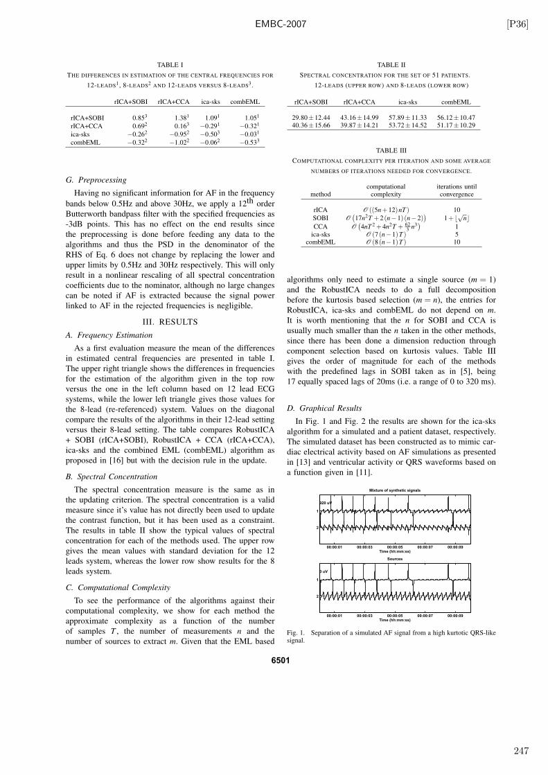
EMBC-2007 [P36]
TABLE I
THE DIFFERENCES IN ESTIMATION OF THE CENTRAL FREQUENCIES FOR
12-LEADS1 , 8-LEADS
2AND 12-LEADS VERSUS 8-LEADS
3 .
rICA+SOBI rICA+CCA ica-sks combEML
rICA+SOBI 0.853 1.381 1.091 1.051
rICA+CCA 0.692 0.163 −0.291 −0.321
ica-sks −0.262 −0.952 −0.503 −0.031
combEML −0.322 −1.022 −0.062 −0.533
G. Preprocessing
Having no significant information for AF in the frequency
bands below 0.5Hz and above 30Hz, we apply a 12th order
Butterworth bandpass filter with the specified frequencies as
-3dB points. This has no effect on the end results since
the preprocessing is done before feeding any data to the
algorithms and thus the PSD in the denominator of the
RHS of Eq. 6 does not change by replacing the lower and
upper limits by 0.5Hz and 30Hz respectively. This will only
result in a nonlinear rescaling of all spectral concentration
coefficients due to the nominator, although no large changes
can be noted if AF is extracted because the signal power
linked to AF in the rejected frequencies is negligible.
III. RESULTS
A. Frequency Estimation
As a first evaluation measure the mean of the differences
in estimated central frequencies are presented in table I.
The upper right triangle shows the differences in frequencies
for the estimation of the algorithm given in the top row
versus the one in the left column based on 12 lead ECG
systems, while the lower left triangle gives those values for
the 8-lead (re-referenced) system. Values on the diagonal
compare the results of the algorithms in their 12-lead setting
versus their 8-lead setting. The table compares RobustICA
+ SOBI (rICA+SOBI), RobustICA + CCA (rICA+CCA),
ica-sks and the combined EML (combEML) algorithm as
proposed in [16] but with the decision rule in the update.
B. Spectral Concentration
The spectral concentration measure is the same as in
the updating criterion. The spectral concentration is a valid
measure since it’s value has not directly been used to update
the contrast function, but it has been used as a constraint.
The results in table II show the typical values of spectral
concentration for each of the methods used. The upper row
gives the mean values with standard deviation for the 12
leads system, whereas the lower row show results for the 8
leads system.
C. Computational Complexity
To see the performance of the algorithms against their
computational complexity, we show for each method the
approximate complexity as a function of the number
of samples T , the number of measurements n and the
number of sources to extract m. Given that the EML based
TABLE II
SPECTRAL CONCENTRATION FOR THE SET OF 51 PATIENTS.
12-LEADS (UPPER ROW) AND 8-LEADS (LOWER ROW)
rICA+SOBI rICA+CCA ica-sks combEML
29.80±12.44 43.16±14.99 57.89±11.33 56.12±10.4740.36±15.66 39.87±14.21 53.72±14.52 51.17±10.29
TABLE III
COMPUTATIONAL COMPLEXITY PER ITERATION AND SOME AVERAGE
NUMBERS OF ITERATIONS NEEDED FOR CONVERGENCE.
computational iterations untilmethod complexity convergence
rICA O ((5n+12)nT ) 10
SOBI O(
17n2T +2(n−1)(n−2))
1+ ⌊√n⌋CCA O
(
4nT 2 +4n2T + 623
n3)
1
ica-sks O (7(n−1)T ) 5combEML O (8(n−1)T ) 10
algorithms only need to estimate a single source (m = 1)
and the RobustICA needs to do a full decomposition
before the kurtosis based selection (m = n), the entries for
RobustICA, ica-sks and combEML do not depend on m.
It is worth mentioning that the n for SOBI and CCA is
usually much smaller than the n taken in the other methods,
since there has been done a dimension reduction through
component selection based on kurtosis values. Table III
gives the order of magnitude for each of the methods
with the predefined lags in SOBI taken as in [5], being
17 equally spaced lags of 20ms (i.e. a range of 0 to 320 ms).
D. Graphical Results
In Fig. 1 and Fig. 2 the results are shown for the ica-sks
algorithm for a simulated and a patient dataset, respectively.
The simulated dataset has been constructed as to mimic car-
diac electrical activity based on AF simulations as presented
in [13] and ventricular activity or QRS waveforms based on
a function given in [11].
00:00:01 00:00:03 00:00:05 00:00:07 00:00:09
2
1
0 uV
Sources
Time (hh:mm:ss)
00:00:01 00:00:03 00:00:05 00:00:07 00:00:09
2
1
920 uV
Mixture of synthetic signals
Time (hh:mm:ss)
Fig. 1. Separation of a simulated AF signal from a high kurtotic QRS-likesignal.
6501
247
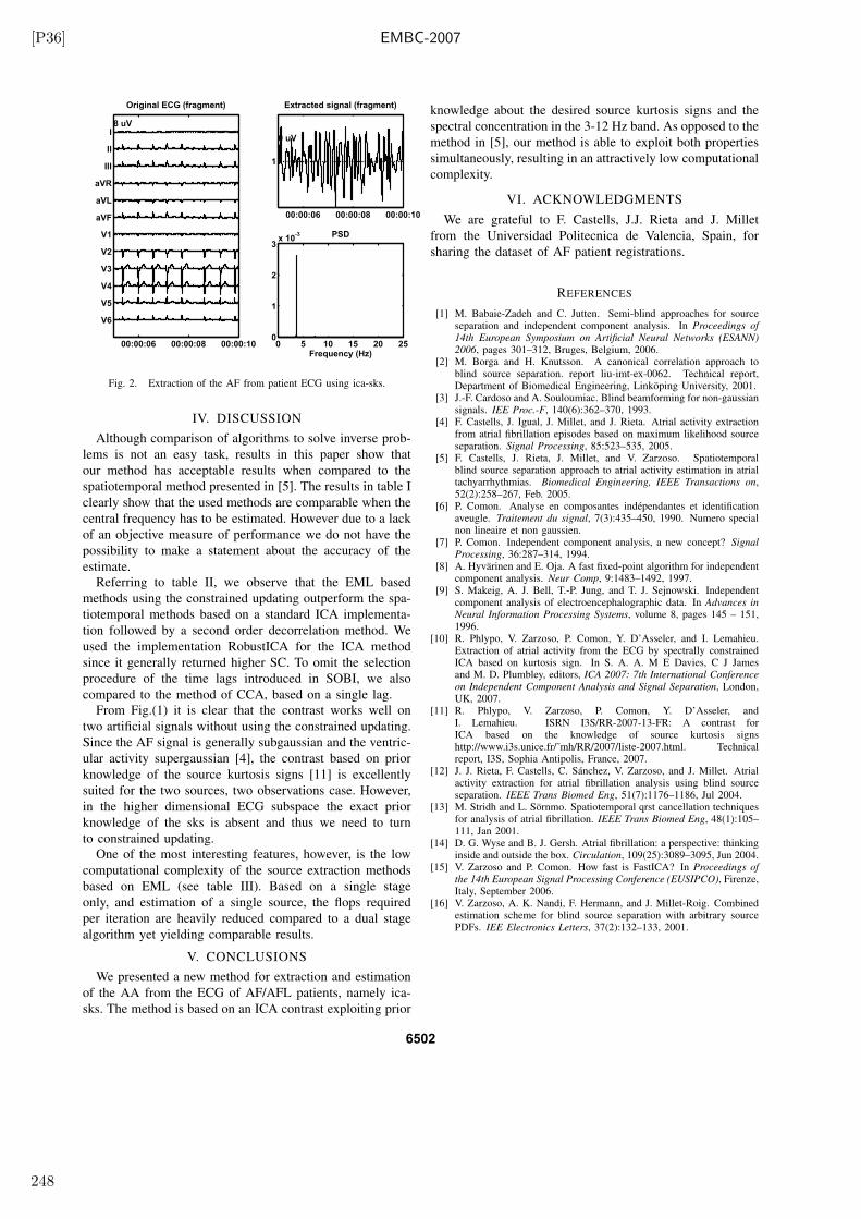
[P36] EMBC-2007
00:00:06 00:00:08 00:00:10
V6
V5
V4
V3
V2
V1
aVF
aVL
aVR
III
II
I8 uV
Original ECG (fragment)
00:00:06 00:00:08 00:00:10
1
0 uV
Extracted signal (fragment)
0 5 10 15 20 250
1
2
3x 10
-3
Frequency (Hz)
PSD
Fig. 2. Extraction of the AF from patient ECG using ica-sks.
IV. DISCUSSION
Although comparison of algorithms to solve inverse prob-
lems is not an easy task, results in this paper show that
our method has acceptable results when compared to the
spatiotemporal method presented in [5]. The results in table I
clearly show that the used methods are comparable when the
central frequency has to be estimated. However due to a lack
of an objective measure of performance we do not have the
possibility to make a statement about the accuracy of the
estimate.
Referring to table II, we observe that the EML based
methods using the constrained updating outperform the spa-
tiotemporal methods based on a standard ICA implementa-
tion followed by a second order decorrelation method. We
used the implementation RobustICA for the ICA method
since it generally returned higher SC. To omit the selection
procedure of the time lags introduced in SOBI, we also
compared to the method of CCA, based on a single lag.
From Fig.(1) it is clear that the contrast works well on
two artificial signals without using the constrained updating.
Since the AF signal is generally subgaussian and the ventric-
ular activity supergaussian [4], the contrast based on prior
knowledge of the source kurtosis signs [11] is excellently
suited for the two sources, two observations case. However,
in the higher dimensional ECG subspace the exact prior
knowledge of the sks is absent and thus we need to turn
to constrained updating.
One of the most interesting features, however, is the low
computational complexity of the source extraction methods
based on EML (see table III). Based on a single stage
only, and estimation of a single source, the flops required
per iteration are heavily reduced compared to a dual stage
algorithm yet yielding comparable results.
V. CONCLUSIONS
We presented a new method for extraction and estimation
of the AA from the ECG of AF/AFL patients, namely ica-
sks. The method is based on an ICA contrast exploiting prior
knowledge about the desired source kurtosis signs and the
spectral concentration in the 3-12 Hz band. As opposed to the
method in [5], our method is able to exploit both properties
simultaneously, resulting in an attractively low computational
complexity.
VI. ACKNOWLEDGMENTS
We are grateful to F. Castells, J.J. Rieta and J. Millet
from the Universidad Politecnica de Valencia, Spain, for
sharing the dataset of AF patient registrations.
REFERENCES
[1] M. Babaie-Zadeh and C. Jutten. Semi-blind approaches for sourceseparation and independent component analysis. In Proceedings of
14th European Symposium on Artificial Neural Networks (ESANN)
2006, pages 301–312, Bruges, Belgium, 2006.[2] M. Borga and H. Knutsson. A canonical correlation approach to
blind source separation. report liu-imt-ex-0062. Technical report,Department of Biomedical Engineering, Linkoping University, 2001.
[3] J.-F. Cardoso and A. Souloumiac. Blind beamforming for non-gaussiansignals. IEE Proc.-F, 140(6):362–370, 1993.
[4] F. Castells, J. Igual, J. Millet, and J. Rieta. Atrial activity extractionfrom atrial fibrillation episodes based on maximum likelihood sourceseparation. Signal Processing, 85:523–535, 2005.
[5] F. Castells, J. Rieta, J. Millet, and V. Zarzoso. Spatiotemporalblind source separation approach to atrial activity estimation in atrialtachyarrhythmias. Biomedical Engineering, IEEE Transactions on,52(2):258–267, Feb. 2005.
[6] P. Comon. Analyse en composantes independantes et identificationaveugle. Traitement du signal, 7(3):435–450, 1990. Numero specialnon lineaire et non gaussien.
[7] P. Comon. Independent component analysis, a new concept? Signal
Processing, 36:287–314, 1994.[8] A. Hyvarinen and E. Oja. A fast fixed-point algorithm for independent
component analysis. Neur Comp, 9:1483–1492, 1997.[9] S. Makeig, A. J. Bell, T.-P. Jung, and T. J. Sejnowski. Independent
component analysis of electroencephalographic data. In Advances in
Neural Information Processing Systems, volume 8, pages 145 – 151,1996.
[10] R. Phlypo, V. Zarzoso, P. Comon, Y. D’Asseler, and I. Lemahieu.Extraction of atrial activity from the ECG by spectrally constrainedICA based on kurtosis sign. In S. A. A. M E Davies, C J Jamesand M. D. Plumbley, editors, ICA 2007: 7th International Conference
on Independent Component Analysis and Signal Separation, London,UK, 2007.
[11] R. Phlypo, V. Zarzoso, P. Comon, Y. D’Asseler, andI. Lemahieu. ISRN I3S/RR-2007-13-FR: A contrast forICA based on the knowledge of source kurtosis signshttp://www.i3s.unice.fr/˜mh/RR/2007/liste-2007.html. Technicalreport, I3S, Sophia Antipolis, France, 2007.
[12] J. J. Rieta, F. Castells, C. Sanchez, V. Zarzoso, and J. Millet. Atrialactivity extraction for atrial fibrillation analysis using blind sourceseparation. IEEE Trans Biomed Eng, 51(7):1176–1186, Jul 2004.
[13] M. Stridh and L. Sornmo. Spatiotemporal qrst cancellation techniquesfor analysis of atrial fibrillation. IEEE Trans Biomed Eng, 48(1):105–111, Jan 2001.
[14] D. G. Wyse and B. J. Gersh. Atrial fibrillation: a perspective: thinkinginside and outside the box. Circulation, 109(25):3089–3095, Jun 2004.
[15] V. Zarzoso and P. Comon. How fast is FastICA? In Proceedings of
the 14th European Signal Processing Conference (EUSIPCO), Firenze,Italy, September 2006.
[16] V. Zarzoso, A. K. Nandi, F. Hermann, and J. Millet-Roig. Combinedestimation scheme for blind source separation with arbitrary sourcePDFs. IEE Electronics Letters, 37(2):132–133, 2001.
6502
248

ICARNW-2006 [P40]
ALPHABET-BASED DEFLATION FOR BLIND SOURCE EXTRACTIONIN UNDERDETERMINED MIXTURES
Vicente Zarzoso and Pierre ComonLaboratoire I3S, Universite de Nice – Sophia Antipolis / CNRSLes Algorithmes – Euclide-B, 2000 route des Lucioles, BP 121
06903 Sophia Antipolis Cedex, France{zarzoso, pcomon }@i3s.unice.fr
ABSTRACT
The deflation approach to blind source extraction esti-mates the source signals one by one. The contribution ofthe latest source estimate is computed via linear regressionand subtracted from the observations before performing anew extraction. In the context of digital communications,novel alphabet-based contrast criteria can naturally be de-fined, leading to the recently proposed parallel deflationconcept. We analyse the use of such criteria in the chal-lenging scenario of underdetermined mixtures, where thesources outnumber the sensors. Due to the limitations oflinear extraction, projection on the signal alphabet beforethe regression-subtraction stage is shown to be capital fora successful source estimation. It is also demonstrated thatalphabet-based criteria outperform the constant modulus(CM) principle, even for CM-type sources. More interest-ingly, classical deflation can improve on parallel deflation,but requires a refinement to render its performance robustto the extraction ordering.
Keywords: alphabet-based criteria, blind source separa-tion, deflation, digital communications, MIMO transmis-sion, underdetermined mixtures.
1 INTRODUCTION
The goal of blind source separation (BSS) is to recoverthe unknown source signals from their observed mixtures.The deflation approach to BSS consists of estimating thesource signals one after another. Originally proposed byDelfosse-Loubaton [3] in the context of instantaneous lin-ear mixtures, deflation was later applied with success byTugnait in the convolutive scenario [10]. After estimat-ing a single source signal using a suitable cost or con-trast function, its contribution to the sensor output is esti-mated (via linear regression, for instance) and subtractedfrom the observations. The process is then repeated un-
Permission to make digital or hard copies of all or part of thiswork for personal or classroom use is granted without fee pro-vided that copies are not made or distributed for profit or com-mercial advantage and that copies bear this notice and the fullcitation on the first page.
c©2006 The University of Liverpool
In Proc. ICA Research Network International Workshop, Liverpool, UK, Sept. 18-19, 2006, pp. 21-24.
til all sources have been extracted. In multiple-inputmultiple-output (MIMO) digital communications, defla-tion (or symbol cancellation) has also been employed bythe popular V-BLAST detection algorithm [5], which re-quires an accurate channel matrix estimate and is thusnon-blind.
Despite its appealing simplicity, deflation presents twomain drawbacks. Firstly, estimation errors caused in eachextraction-deflation stage accumulate through successivestages. As a result, the source estimation quality deteri-orates progressively as more sources are obtained. Sec-ondly, since a linear extractor is usually employed, themaximum number of sources that can be separated is lim-ited by the available spatial diversity, i.e., it is generallyimpossible to extract more sources than sensors. This lim-its the applicability of deflation in the interesting scenarioof underdetermined mixtures.
The discrete nature of digital modulation sources,characterized by a finite number of symbols compos-ing the signal alphabet or constellation, can help allevi-ate these shortcomings. The present contribution anal-yses and compares these alphabet-exploiting techniquesfor deflation-based source extraction in underdeterminedmixtures. A simple modification improves the robustnessof classical deflation to the source extraction ordering, andoutperforms the recently proposed parallel deflation [8] inestimating all sources with low error probability more of-ten.
2 PROBLEM AND ASSUMPTIONS
A noisy mixturex = [x1, x2, . . . , xL]T ∈ CL of K un-
correlated sourcess = [s1, s2, . . . , sK ]T ∈ CK is ob-
served at the output of anL-sensor array, whereT denotestransposition. In matrix form, the sensor output can beexpressed as:
x = Hs + n =K∑
k=1
hksk + n (1)
whereH ∈ CL×K represents the unknown full-rank mix-
ing matrix with columns{hk}Kk=1, andn ∈ CL the addi-
tive noise, which is also unknown, uncorrelated with thesources, and has covariance matrixσ2
nIL. Eqn. (1) mod-els (but is not limited to) a flat-fading MIMO transmissionsystem. BSS aims at estimating the realizations of random
249
[P40] ICARNW-2006
vectors from the observation of the corresponding realiza-tions of the mixturex. To this end, we seek an extractingvectorw ∈ C
L so that the linear extractor output
y = wHx (2)
optimises some cost function or contrast criterion. Sym-bol H represents the Hermitian (conjugate-transpose) op-erator. After a source signal has been estimated in thisfashion, its contribution is computed and subtracted (can-celled) from the observations, which then become ‘de-flated’. The source estimation and deflation process is re-peated until all signals have been extracted.
In the challenging underdetermined mixture scenario,the number of sources is higher than the number of sen-sors,K > L. In that case, it is generally not possibleto estimate all sources linearly, even in the absence ofnoise, as the rows of the mixing matrix only span anL-dimensional subspace ofC
K . Similarly, linear extractionseverely limits the capabilities of conventional deflation,as will be seen later, calling for the design of alternativeextraction and/or deflation criteria.
The novelty of the present approach lies in the ex-ploitation of the discrete character of digital commu-nication signals. In the sequel, it will be assumedthat the sources can be divided intoR different groups,∑R
r=1Kr = K, where groupr containsKr sources withthe same digital modulationAr. Each digital modula-tion is characterized by its alphabet or constellationAr ={ar,m}Mm=1, whose discrete symbols can be representedby the roots of a polynomialψr(z) =
∏Mm=1(z − ar,m).
3 ALPHABET-BASED EXTRACTION
Under the signal model and assumptions of the previoussection, it follows that functional
Jr(y) = E{|ψr(y)|2}
is a contrast function for sources with alphabetAr underrather general assumptions [2]. In particular, a constella-tion may not be a subset of another. This criterion, origi-nally proposed in [6], is known as alphabet polynomial fit-ting (APF) and becomes the so-called constant power (CP)criterion forM -PSK modulations [11]. The APF presentsthe advantage of targeting a specific signal modulation, incontrast to alternative criteria typically used in the sepa-ration of digital communication sources such as the con-stant modulus (CM) or the kurtosis maximisation (KM)principles [4, 9]. As opposed to independence-based con-trast criteria, the APF can separate spatially correlated andspectrally coloured sources. To estimate a source signal ofgiven modulation, a simple yet efficient gradient-descentprocedure with optimal step size can drive a linear ex-tractor in the search of the corresponding APF contrast-function minima [11].
4 CLASSICAL DEFLATION
At the end of a successful iterative search (leading to theoptimisation of the corresponding contrast functionJr),the extractor outputy contains an estimates of a source
signals with alphabetAr. In regression-based classicaldeflation, the contribution of the extracted source to theobservations is estimated as:
h = arg minh
E{‖x− hs‖2} ⇒ h =E{xs∗}E{|s|2} (3)
symbol ∗ denoting complex conjugation, and then sub-tracted to yield the deflated sensor output:
x ← x− hs. (4)
If a linear extractor is employed, as in eqn. (2), it iseasy to prove that the rank of the sensor-output covariancematrix (related to the available spatial diversity) necessar-ily decreases by one at each deflation step, regardless ofthe achieved source estimation quality. As a result, onlyL out of theK sources can at most be estimated by thisprocedure. This fundamental limitation renders plain clas-sical deflation inappropriate in the underdetermined case.
5 ALPHABET-BASED DEFLATION
5.1 Parallel Deflation
Estimation errors accumulate through successive stages inclassical deflation. Parallel deflation [8] tries to overcomethis limitation by exploiting the discrete nature of digitalsources and alphabet diversity, which arises whenR > 1.Sources from alphabetAr are extracted using the corre-sponding APF criterion. To minimise the impact of erroraccumulation, the deflation process used for the sourceswith a given modulation is carried out from the originalobservations, that can be processed in parallel by the ap-propriate APF contrasts. As a result, one such paralleldeflation processes ‘perceives’ a mixture ofKr sourcesonL sensors, which should be easier to deal with than theL mixtures ofK sources ‘seen’ by conventional deflationover all sources. Nevertheless, the extraction of sourcesfrom groupr may be severely hampered by the interfer-ing sources from the other groups.
5.2 Projection on the Source Alphabet
As pointed out earlier, the linear estimate of a source sig-nal reduces the rank of the deflated sensor-output covari-ance matrix, making it impossible to extract all sourcesin an underdetermined mixture. To circumvent this diffi-culty, let us assume that the source has been perfectly es-timated: s = sk, for somek ∈ {1, . . . ,K}. Then, underthe source uncorrelation assumption, the deflation proce-dure described by eqns. (3)–(4) would produceh = hk
and the new set of observationsx =∑
p6=k hpsp +n; thatis, the interference caused by that source to the remain-ing sources would be perfectly cancelled. Since the rankof the deflated sensor-output covariance matrix would notnecessarily decrease, the rest of the sources might still beextracted at later stages.
Obviously, it will generally be difficult to haves =sk. A simple manner to try to obtain this perfect estimateis by projecting the linear extractor output on the knownsource constellation before deflation, as in the V-BLASTdetection algorithm [5]. This non-linear processing can
22
250
ICARNW-2006 [P40]
be carried out cost-effectively by the minimum-distancedetector.
5.3 Optimal Ordering in Classical Deflation
Classical deflation reduces the remaining interference asmore sources are extracted. The amount of interferencereduction depends on the quality of the source estimate.To minimise error accumulation, the ‘strongest’ or bestestimated sources should be extracted and deflated first.The prior knowledge of the channel matrix simplifies theoptimal ordering in terms of the output signal-to-noise ra-tion (SNR), as in the V-BLAST algorithm [5]. For theblind scenario, we propose the following ordering methodwhich, for simplicity but without loss of generality, is de-veloped forM -PSK modulations.
The symbol error probability in the detection of aM -PSK signal contaminated by complex Gaussian noise canbe accurately approximated by [7]:
Pe = 2Q(√
SNR sin( πM
))
, M > 2 (5)
whereQ(x) = 1√2π
∫ ∞x
e−t2/2dt. Now, given the set
{sp, hp,wp}Kp=1 provided by an initial deflation sweep,the signal-to-interference-and-noise ratio (SINR) in theestimation of sourcek can be computed as:
SINRk =|wH
k hk|2∑
p6=k |wHk hp|2 + σ2
n‖wk‖2. (6)
The noise variance estimateσ2n can be obtained from the
sensor-output residual after all sources have been deflated.To estimate the probability of errorPe in (5), the SNRcan be replaced with the SINR given above. Deflationcan then be repeated in ascending order ofPe or, equiva-lently, descending order of
√SINR sin(π/M). To target
a specific source while trying to alleviate the increasedcomputational cost, the linear extractor found in the origi-nal deflation is used to initialise the iterative optimisationof the corresponding alphabet-matched contrast function(the CP criterion forM -PSK signals). The whole processmay be repeated until the ordering converges, or just for afixed number of deflation iterations.
6 EXPERIMENTAL STUDY
Influence of extraction criterion and alphabet projection.An underdetermined instantaneous linear mixture of 4sources with QPSK modulation is observed at the outputof a 3-sensor array in blocks of 150 data symbols. Thesensor output is corrupted by additive white complex cir-cular Gaussian noise, with a varying spatially averagedreceived SNR defined as in [5], which can be expressedasSNR = trace(HHH)/(Lσ2
n). The mixing matrix el-ements are randomly drawn from a normalised complexGaussian distribution at each of the 200 Monte Carlo iter-ations. In the first experiment, two extraction criteria (CMand CP) together with two deflation methods (classical de-flation and classical deflation with projection), giving riseto the methods labelled as CM-D, CM-P-D (projection on
|s| = 1), CP-D and CP-P-D (projection on the alphabet).The search for the CM and the CP contrast function min-ima is carried out with the optimal step-size technique of[11]. ZF V-BLAST with perfect channel estimate is im-plemented as in [5]. The linear MMSE detector and thenon-linear MAP detector serve as performance bounds.
Figure 1 (top) shows the symbol-error-rate (SER) av-eraged over the 4 estimated sources. Figure 1(bottom)displays the probability of extracting all 4 sources withan SER below 10%. The CM-D and the CP-D, wheredeflation is based on conventional linear regression, areunable to extract the four sources satisfactorily. Likewise,the MMSE extractor and V-BLAST are also severely lim-ited by the lack of linear invertibility of the channel ma-trix. Although the CM-P-D visibly improves on the CM-D, the combination of alphabet projection and alphabet-based extraction appears most effective. Indeed, the CP-P-D approaches the MAP bound and, for sufficient SNR,is able to extract all four sources at low SER with proba-bility close to one.
Classical vs. parallel deflation. Influence of extractionordering. The second experiment simulates a mixture of6 sources, three with BPSK and three with 3-PSK mod-ulation, observed at the output of 4 sensors, in the samegeneral conditions as above and 150 Monte Carlo itera-tions. Only CP-based extraction is considered: classicaldeflation with direct ordering (targeting the BPSK sourcesfirst), with inverse ordering (aiming at the 3-PSK sourcesfirst), and with the optimal ordering presented in the pre-vious section (with a single extra deflation sweep after or-dering). These methods are also compared with the paral-lel deflation approach of [8] with alphabet projection.
As observed in Fig. 2, the performance of classical de-flation depends strongly on the extraction ordering, withthe proposed optimal ordering achieving the best resultsat almost twice the average number of optimal step-sizegradient-descent iterations (around 550) required by thetwo other classical deflation methods (300). Parallel de-flation entails the lowest computational cost (just over 200iterations) but shows a performance near classical defla-tion with inverse ordering, marginally improving on theMMSE’s average SER at high SNR.
7 CONCLUSIONS
We have exploited the discrete nature of digital communi-cation signals to address the deflation-based blind sourceextraction in underdetermined mixtures. As already no-ticed in other works (e.g., [1]), some type of non-linearprocessing is necessary to extract all sources satisfacto-rily. Herein, projection on the signal alphabet before de-flation has been shown to ameliorate the performance oflinear extraction, with an alphabet-based criterion (CP)clearly outperforming the traditional CM principle, evenfor sources verifying the CM assumption. An alphabet-matched linear extraction criterion followed by projec-tion on the signal alphabet can considerably improve theperformance of classical regression-based deflation in ex-tracting all sources from an underdetermined mixture witha reasonably low probability of error. Also, the gradual in-terference suppression of classical deflation seems to have
23
251
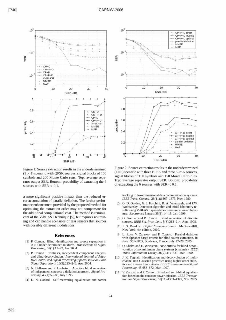
[P40] ICARNW-2006
0 10 20 30 40
10−2
10−1
100
SNR (dB)
SE
R
CM−DCM−P−DCP−DCP−P−DV−BLASTMMSEMAP
0 10 20 30 400
0.2
0.4
0.6
0.8
1
SNR (dB)
prob
abili
ty
CM−DCM−P−DCP−DCP−P−DV−BLASTMMSEMAP
Figure 1: Source extraction results in the underdetermined(3× 4) scenario with QPSK sources, signal blocks of 150symbols and 200 Monte Carlo runs. Top: average sepa-rator output SER. Bottom: probability of extracting the 4sources with SER< 0.1.
a more significant positive impact than the reduced er-ror accumulation of parallel deflation. The further perfor-mance enhancement provided by the proposed method foroptimising the extraction order may not compensate forthe additional computational cost. The method is reminis-cent of the V-BLAST technique [5], but requires no train-ing and can handle scenarios of less sensors that sourceswith possibly different modulations.
References[1] P. Comon. Blind identification and source separation in
2 × 3 under-determined mixtures.Transactions on SignalProcessing, 52(1):11–22, Jan. 2004.
[2] P. Comon. Contrasts, independent component analysis,and blind deconvolution.International Journal of Adap-tive Control and Signal Processing (Special Issue on BlindSignal Separation), 18(3):225–243, Apr. 2004.
[3] N. Delfosse and P. Loubaton. Adaptive blind separationof independent sources: a deflation approach.Signal Pro-cessing, 45(1):59–83, July 1995.
[4] D. N. Godard. Self-recovering equalization and carrier
0 10 20 30 40
10−2
10−1
100
SNR (dB)
SE
R
CP−P−D directCP−P−D inverseCP−P−D optimalparallel deflationMMSEMAP
0 10 20 30 400
0.2
0.4
0.6
0.8
1
SNR (dB)
prob
abili
ty
CP−P−D directCP−P−D inverseCP−P−D optimalparallel deflationMMSEMAP
Figure 2: Source extraction results in the underdetermined(4×6) scenario with three BPSK and three 3-PSK sources,signal blocks of 150 symbols and 150 Monte Carlo runs.Top: average separator output SER. Bottom: probabilityof extracting the 6 sources with SER< 0.1.
tracking in two-dimensional data communication systems.IEEE Trans. Comms., 28(11):1867–1875, Nov. 1980.
[5] G. D. Golden, G. J. Foschini, R. A. Valenzuela, and P.W.Wolniansky. Detection algorithm and initial laboratory re-sults using V-BLAST space-time communication architec-ture. Electronics Letters, 35(1):14–15, Jan. 1999.
[6] O. Grellier and P. Comon. Blind separation of discretesources.IEEE Sig. Proc. Lett., 5(8):212–214, Aug. 1998.
[7] J. G. Proakis. Digital Communications. McGraw-Hill,New York, 4th edition, 2000.
[8] L. Rota, V. Zarzoso, and P. Comon. Parallel deflationwith alphabet-based criteria for blind source extraction. InProc. SSP-2005, Bordeaux, France, July 17–20, 2005.
[9] O. Shalvi and E. Weinstein. New criteria for blind decon-volution of nonminimum phase systems (channels).IEEETrans. Information Theory, 36(2):312–321, Mar. 1990.
[10] J. K. Tugnait. Identification and deconvolution of multi-channel non-Gaussian processes using higher order statis-tics and inverse filter criteria.IEEE Transactions on SignalProcessing, 45:658–672, Mar. 1997.
[11] V. Zarzoso and P. Comon. Blind and semi-blind equaliza-tion based on the constant power criterion.IEEE Transac-tions on Signal Processing, 53(11):4363–4375, Nov. 2005.
24
252
EUSIPCO-2006 [P41]
HOW FAST IS FASTICA?
Vicente Zarzoso, Pierre Comon Mariem Kallel
Laboratoire I3S, CNRS/UNSALes Algorithmes – Euclide-B, BP 12106903 Sophia Antipolis Cedex, France{zarzoso, comon}@i3s.unice.fr
Departement TIC, Laboratoire U2S, ENITCampus Universitaire “Le Belvedere”
1002 Tunis, Tunisia
ABSTRACTThe present contribution deals with the statistical toolof Independent Component Analysis (ICA). The fo-cus is on the deflation approach, whereby the inde-pendent components are extracted one after another.The kurtosis-based FastICA is arguably one of the mostwidespread methods of this kind. However, its features,particularly its speed, have not been thoroughly eval-uated or compared, so that its popularity seems some-what unfounded. To substantiate this claim, a simplequite natural modification is put forward and assessedin this paper. It merely consists of performing exactline search optimization of the contrast function. Speedis objectively measured in terms of the computationalcomplexity required to reach a given source extractionperformance. Illustrative numerical results demonstratethe faster convergence and higher robustness to initial-ization of the proposed approach, which is thus referredto as RobustICA.
1. INTRODUCTION
Independent Component Analysis (ICA) transforms anobserved random vector into mutually statistically inde-pendent components [1]. Its numerous applications havespurred an increasing research interest in this technique;for instance, ICA is the basic statistical tool to performBlind Source Separation (BSS) [1, 2, 3]. In its originaldefinition (see [1, 4], among other early works), ICA ex-tracts all the sources jointly or simultaneously; this isthe so-called “symmetric” approach. ICA can also beperformed by estimating the sources sequentially or oneby one. This alternative procedure, referred to as defla-tion, was originally proposed in [5], and used successfullyin the separation of convolutive mixtures [6]. Deflationhas later been widely promoted in the machine learningcommunity [3]. Joint algorithms are usually thought tooutperform deflationary algorithms due to errors accu-mulated in successive subtractions (regressions) of theestimated source contribution to the observation. Thisshortcoming is generally claimed to be compensated bya significant gain in computations, although this claimstill requires closer examination.
The FastICA [7, 8], originally put forward in defla-tion mode, features among the most popular ICA algo-rithms. Although it appeared when many other ICAmethods had already been proposed, the deflationaryFastICA has never been compared by the authors of [3]with earlier joint algorithms such as COM2 [1], JADE[4], COM1 [9], or the deflation methods by Tugnait [6]or Delfosse-Loubaton [5]. In fact, to our knowledge,
FastICA (both in its deflation and symmetric imple-mentations) has only been compared with neural-basedadaptive algorithms and principal component analysis(PCA), that most ICA algorithms are known to outper-form. Its popularity has been justified on the grounds ofthe satisfactory performance offered by the method inseveral applications, as well as its simplicity. However,these features, and in particular its speed, have neverbeen substantiated by a thorough comparison with othertechniques. A first serious attempt has been made in[10], where FastICA is found to fail for weak or highlyspatially correlated sources. In spite of its comprehen-siveness, the comparative analysis of [10] is perhaps un-fortunate in contrasting the deflationary FastICA withjoint methods such as COM2, JADE and COM1. Onthe other hand, recent studies have put in evidence somedeficiencies of FastICA, such as the detrimental effectsof saddle points on its performance [11].
Given the assiduous attention the method has re-ceived over the last decade, these gaps are somewhatsurprising. Indeed, it does not seem difficult to envis-age a very simple, quite natural deflation algorithm thatwould outperform FastICA. The goal of this work is toput forward such a method, which we refer to as Robus-tICA, and compare it with FastICA. The new methodsimply consists of carrying out exact line search of thecontrast function, the normalized kurtosis [12]. Exactline search is achieved at low cost, since the optimalstep size (OS) leading to the global maximum along thesearch direction can algebraically be found at each iter-ation among the roots of a low-degree polynomial. TheOS methodology, which has already been proposed inthe time equalization context [13, 14, 15, 16], can beused in conjunction with a variety of alternative crite-ria such as the constant modulus [17] and the constantpower [14, 18]. As part of our experimental study, weevaluate the computational complexity required to reacha given source extraction performance. The algorithms’speed and efficiency can thus be compared objectively.
It is now generally acknowledged that adaptive (alsoknown as on-line, recursive or sample-by-sample) al-gorithms are not always computationally cheaper thanblock (off-line, windowed) algorithms, and that they arerarely better in terms of precision. On this account,block implementations are the focus of this paper.
2. MODEL AND NOTATION
Let an L-dimensional random vector x denote the ob-servation, which is assumed to stem from the linear sta-
In Proc. EUSIPCO-2006, Florence, Italy, Sept. 4-8, 2006.
253

[P41] EUSIPCO-2006
tistical model:x = Hs + v. (1)
The source vector s = [s1, s2, . . . , sK ]T is made of K sta-tistically mutually independent components. The noiseterm v will be ignored throughout, except in the nu-merical experiments. In fact, its distribution is assumedto be unknown, so that it can at most be considered asa nuisance; otherwise, a maximum likelihood approachcould be employed, which is beyond the scope of thepresent comparison. The goal of ICA can be expressedas follows: given a sensor-output signal block composedof T samples, estimate the corresponding T -sample re-alization of the source vector.
Vectors and matrices will be typeset in boldface low-ercase and boldface uppercase symbols, respectively; su-perscripts (T), (H), and (∗) denote respectively transpo-sition, conjugate transposition, and complex conjuga-tion. Unless otherwise specified, the components of ran-dom vectors x, s and v take their values in the complexfield.
3. OPTIMALITY CRITERIA
The deflation approach to ICA consists of searching foran extracting vector w so that its scalar output
zdef= wHx (2)
maximizes some optimality criterion or contrast func-tion. A widely used contrast is the normalized kurtosisof the separator output:
K(w) =E{|z|4} − 2E2{|z|2} − |E{z2}|2
E2{|z|2} . (3)
This criterion is easily seen to be insensitive to scale, i.e.,K(λw) = K(w), ∀λ 6= 0. This scale indeterminacy is in-herent in BSS, and we can thus impose ‖w‖ = 1 for nu-merical convenience. Other criteria are the widespreadconstant modulus (CM) [17]:
C(w) = E{(|z|2 − 1
)2} (4)
and the constant power (CP) [14, 18]:
Pr(w) = E{|zr − 1|2}. (5)
Another type of objective functions need the data tobe prewhitened, so that the sensor outputs are assumed
to have an identity covariance matrix, Rxdef= E{xxH} =
I. One criterion that we shall be particularly interestedin is the separator-output fourth-order moment:
M(w) = E{|z|4}. (6)
This criterion must be optimized under a constraint toavoid arbitrarily large values of z. Assuming ‖w‖ = 1,it is simple to realize that (6) is equivalent to (3) afterprewhitening in two cases: if all sources and mixturesare real-valued, and if the sources are complex-valuedbut second-order circular, i.e., the non-circular second-
moment matrix Cxdef= E{xxT} is null. For instance,
in the case where the mixture and noise are complexbut the sources are real, criteria (6) and (3) are notequivalent.
4. KURTOSIS-BASED FASTICA
The stationary values of the kurtosis contrast K(w) aregiven by the cancellation of its gradient, which is pro-portional to:
E{xzz∗2} − (wTC∗xw)Cxw
∗
− (wHRxw)−1[E{|z|4} − |wHCxw
∗|2]Rxw. (7)
Under the constraint ‖w‖ = 1, the stationary pointsof M(w) are obtained for the collinearity condition onE{xzz∗2}:
E{(wHxxHw)xxH}w = λw (8)
where λ is some Lagrangian multiplier. It is easy toverify that the same result is obtained by performingthe unconstrained optimization ofM(w)/‖w‖4.
Equation (8) is a fixed-point equation as claimed in[7] only when λ is known, which is not the case here; λmust be determined so as to satisfy the constraint, andthus unfortunately it depends again on x and w. In[3, 7], λ is arbitrarily set to a deterministic fixed value,which allows to spare computations. For this reason,as eventually pointed out in [8], FastICA is actually anapproximate standard Newton algorithm rather than afixed-point algorithm. As a result of the Hessian matrixapproximation carried out under the prewhitening as-sumption, the kurtosis-based FastICA reduces to a con-ventional gradient-descent algorithm with a fixed stepsize, and is hence a particular case of [6]. In the real-valued scenario, FastICA’s update rule reads:
w+ = w − 1
3E{x(wTx)3} (9)
w+ ← w+/‖w+‖. (10)
The Hessian matrix approximation is somewhat for-tunate in that, under the source statistical indepen-dence assumption, it theoretically endows the result-ing method with global cubic convergence. It is likelythat the algorithms described in the next section in-herit analogous convergence properties. Nevertheless,the FastICA algorithm sometimes gets stuck at saddlepoints, particularly for short sample sizes [11].
5. OPTIMAL STEP SIZE: ROBUSTICA
As we have just recalled, FastICA attempts to maxi-mize the normalized kurtosis of the extractor output bymeans of a approximate Newton algorithm. The Hessiansimplification reduces the Newton update to a gradient-based update with fixed step size. For the kurtosis aswell as analogous contrast functions commonly encoun-tered in blind signal processing, a more efficient opti-mization method exists that can improve performancewhile accelerating convergence. This method, theoret-ically straightforward yet effective in practice, is exactline maximization.
Line maximization of a generic cost function J (w)consists of finding its global maximum along a given
2
254
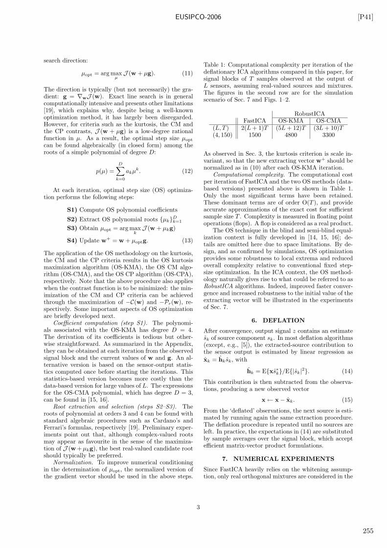
EUSIPCO-2006 [P41]
search direction:
µopt = arg maxµJ (w + µg). (11)
The direction is typically (but not necessarily) the gra-dient: g = ∇wJ (w). Exact line search is in generalcomputationally intensive and presents other limitations[19], which explains why, despite being a well-knownoptimization method, it has largely been disregarded.However, for criteria such as the kurtosis, the CM andthe CP contrasts, J (w + µg) is a low-degree rationalfunction in µ. As a result, the optimal step size µopt
can be found algebraically (in closed form) among theroots of a simple polynomial of degree D:
p(µ) =
D∑
k=0
akµk. (12)
At each iteration, optimal step size (OS) optimiza-tion performs the following steps:
S1) Compute OS polynomial coefficients
S2) Extract OS polynomial roots {µk}Dk=1
S3) Obtain µopt = arg maxkJ (w + µkg)
S4) Update w+ = w + µoptg. (13)
The application of the OS methodology on the kurtosis,the CM and the CP criteria results in the OS kurtosismaximization algorithm (OS-KMA), the OS CM algo-rithm (OS-CMA), and the OS CP algorithm (OS-CPA),respectively. Note that the above procedure also applieswhen the contrast function is to be minimized: the min-imization of the CM and CP criteria can be achievedthrough the maximization of −C(w) and −Pr(w), re-spectively. Some important aspects of OS optimizationare briefly developed next.
Coefficient computation (step S1). The polynomi-als associated with the OS-KMA has degree D = 4.The derivation of its coefficients is tedious but other-wise straightforward. As summarized in the Appendix,they can be obtained at each iteration from the observedsignal block and the current values of w and g. An al-ternative version is based on the sensor-output statis-tics computed once before starting the iterations. Thisstatistics-based version becomes more costly than thedata-based version for large values of L. The expressionsfor the OS-CMA polynomial, which has degree D = 3,can be found in [15, 16].
Root extraction and selection (steps S2–S3). Theroots of polynomial at orders 3 and 4 can be found withstandard algebraic procedures such as Cardano’s andFerrari’s formulas, respectively [19]. Preliminary exper-iments point out that, although complex-valued rootsmay appear as favourite in the sense of the maximiza-tion of J (w+µkg), the best real-valued candidate rootshould typically be preferred.
Normalization. To improve numerical conditioningin the determination of µopt, the normalized version ofthe gradient vector should be used in the above steps.
Table 1: Computational complexity per iteration of thedeflationary ICA algorithms compared in this paper, forsignal blocks of T samples observed at the output ofL sensors, assuming real-valued sources and mixtures.The figures in the second row are for the simulationscenario of Sec. 7 and Figs. 1–2.
RobustICAFastICA OS-KMA OS-CMA
(L, T ) 2(L + 1)T (5L + 12)T (3L + 10)T(4, 150) 1500 4800 3300
As observed in Sec. 3, the kurtosis criterion is scale in-variant, so that the new extracting vector w+ should benormalized as in (10) after each OS-KMA iteration.
Computational complexity. The computational costper iteration of FastICA and the two OS methods (data-based versions) presented above is shown in Table 1.Only the most significant terms have been retained.These dominant terms are of order O(T ), and provideaccurate approximations of the exact cost for sufficientsample size T . Complexity is measured in floating pointoperations (flops). A flop is considered as a real product.
The OS technique in the blind and semi-blind equal-ization context is fully developed in [14, 15, 16]; de-tails are omitted here due to space limitations. By de-sign, and as confirmed by simulations, OS optimizationprovides some robustness to local extrema and reducedoverall complexity relative to conventional fixed step-size optimization. In the ICA context, the OS method-ology naturally gives rise to what could be referred to asRobustICA algorithms. Indeed, improved faster conver-gence and increased robustness to the initial value of theextracting vector will be illustrated in the experimentsof Sec. 7.
6. DEFLATION
After convergence, output signal z contains an estimatesk of source component sk. In most deflation algorithms(except, e.g., [5]), the extracted-source contribution tothe sensor output is estimated by linear regression as
xk = hksk, with
hk = E{xs∗k}/E{|sk|2}. (14)
This contribution is then subtracted from the observa-tions, producing a new observed vector
x← x− xk. (15)
From the ‘deflated’ observations, the next source is esti-mated by running again the same extraction procedure.The deflation procedure is repeated until no sources areleft. In practice, the expectations in (14) are substitutedby sample averages over the signal block, which acceptefficient matrix-vector product formulations.
7. NUMERICAL EXPERIMENTS
Since FastICA heavily relies on the whitening assump-tion, only real orthogonal mixtures are considered in the
3
255
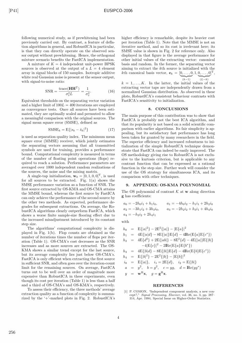
[P41] EUSIPCO-2006
following numerical study, as if prewhitening had beenpreviously carried out. By contrast, a feature of defla-tion algorithms in general, and RobustICA in particular,is that they can directly operate on the observed sen-sor output without prewhitening. Hence, the orthogonalmixture scenario benefits the FastICA implementation.
A mixture of K = 4 independent unit-power BPSKsources is observed at the output of a L = 4 elementarray in signal blocks of 150 samples. Isotropic additivewhite real Gaussian noise is present at the sensor output,with signal-to-noise ratio:
SNR =trace(HHT)
σ2vL
=1
σ2v
. (16)
Equivalent thresholds on the separating vector variationand a higher limit of 100L = 400 iterations are employedas convergence tests. Once all sources have been esti-mated, they are optimally scaled and permuted to allowa meaningful comparison with the original sources. Thesignal mean square error (SMSE), defined as
SMSEk = E{|sk − sk|2} (17)
is used as separation quality index. The minimum meansquare error (MMSE) receiver, which jointly estimatesthe separating vectors assuming that all transmittedsymbols are used for training, provides a performancebound. Computational complexity is measured in termsof the number of floating point operations (flops) re-quired to reach a solution. Performance parameters areaveraged over 1000 independent random realizations ofthe sources, the noise and the mixing matrix.
A single-tap initialization, w0 = [0, 1, 0, 0]T, is usedfor all sources to be extracted. Fig. 1(a) shows theSMSE performance variation as a function of SNR. Thefirst source extracted by OS-KMA and OS-CMA attainsthe MMSE bound, whereas the first source by FastICAcan only achieve the performance of the second source bythe other two methods. As expected, performance de-grades for subsequent extractions. On average, the Ro-bustICA algorithms clearly outperform FastICA, whichshows a worse finite sample-size flooring effect due tothe increased misadjustment introduced by its constantstep size.
The algorithms’ computational complexity is dis-played in Fig. 1(b). Flop counts are obtained as thenumber of iterations times the number of flops per iter-ation (Table 1). OS-CMA’s cost decreases as the SNRincreases and as more sources are extracted. The OS-KMA shows a similar trend except for the last source,but its average complexity lies just below OS-CMA’s.FastICA is only efficient when extracting the first sourcein sufficient SNR, and often goes over the iteration-countlimit for the remaining sources. On average, FastICAturns out to be well over an order of magnitude moreexpensive than RobustICA in these experiments, eventhough its cost per iteration (Table 1) is less than a halfand a third of OS-CMA’s and OS-KMA’s, respectively.
To assess their efficiency, the three methods’ averageextraction quality as a function of complexity is summa-rized by the ‘+’-marked plots in Fig. 2. RobustICA’s
higher efficiency is remarkable, despite its heavier costper iteration (Table 1). Note that the MMSE is not aniterative method, and so its cost is irrelevant here; itsSMSE value is shown in Fig. 2 for reference only. Alsodisplayed in that figure is the average performance forother initial values of the extracting vector: canonicalbasis and random. In the former, the separating vectoraiming to extract the kth source is initialized with thekth canonical basis vector, ek = [0, . . . , 0︸ ︷︷ ︸
(k−1)
, 1, 0, . . . , 0︸ ︷︷ ︸(L−k)
]T,
k = 1, . . . ,K. In the latter, the initial values of theextracting vector taps are independently drawn from anormalized Gaussian distribution. As observed in theseplots, RobustICA’s consistent behaviour contrasts withFastICA’s sensitivity to initialization.
8. CONCLUSIONS
The main purpose of this contribution was to show thatFastICA is probably not the best ICA algorithm, andthat its popularity is not based on a solid scientific com-parison with earlier algorithms. Its fair simplicity is ap-pealing, but its satisfactory fast performance has longbeen taken for granted by many researchers in the field.The superior efficiency and increased robustness to ini-tialization of the simple RobustICA technique demon-strate that FastICA can indeed be easily improved. TheOS methodology giving rise to RobustICA is not exclu-sive to the kurtosis criterion, but is applicable to anycontrast function that can be expressed as a rationalfunction in the step size. Further work will consider theuse of the OS strategy for simultaneous ICA, and itscomparison with other techniques.
9. APPENDIX: OS-KMA POLYNOMIAL
The OS polynomial of contrast K at w along directiong has coefficients:
a0 = −2h0i1 + h1i0, a1 = −4h0i2 − h1i1 + 2h2i0
a2 = −3h1i2 + 3h3i0, a3 = −2h2i2 + h3i1 + 4h4i0
a4 = −h3i2 + 2h4i1
with
h0 = E{|a|2} − 2E2{|a|} − |E{a}|2h1 = 4E{|a|d} − 8E{|a|}E{d} − 4IRe(E{a}E{c∗})h2 = 4E{d2}+ 2E{|ab|} − 8E2{d} − 4E{|a|}E{|b|}
−4|E{c}|2 − 2IRe(E{a}E{b∗})h3 = 4E{|b|d} − 8E{|b|}E{d} − 4IRe(E{b}E{c∗})h4 = E{|b|2} − 2E2{|b|} − |E{b}|2i0 = E{|a|}, i1 = 2E{d}, i2 = E{|b|}a = y2, b = g2, c = yg, d = IRe(yg∗)
y = wHx, g = gHx.
REFERENCES
[1] P. COMON, “Independent component analysis, a new con-cept?,” Signal Processing, Elsevier, vol. 36, no. 3, pp. 287–314, Apr. 1994, Special Issue on Higher-Order Statistics.
4
256
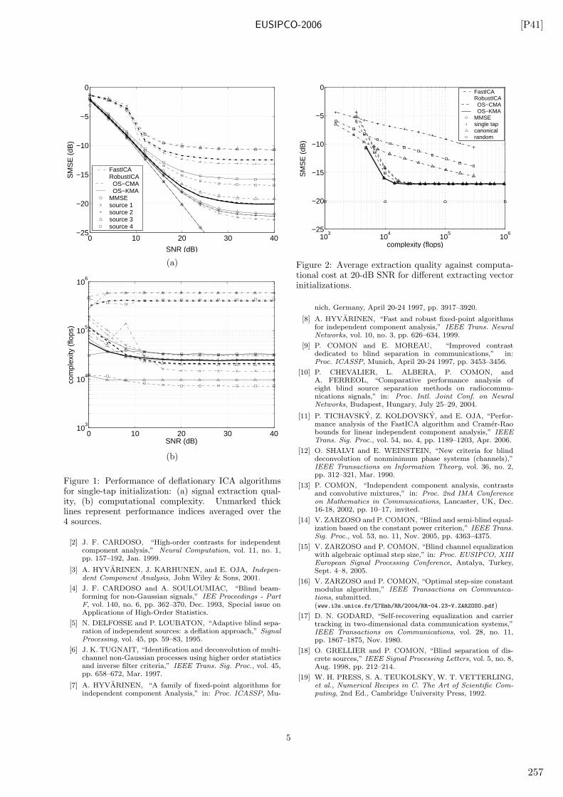
EUSIPCO-2006 [P41]
0 10 20 30 40−25
−20
−15
−10
−5
0
SM
SE
(dB
)
SNR (dB)
FastICARobustICA OS−CMA OS−KMAMMSEsource 1source 2source 3source 4
(a)
0 10 20 30 4010
3
104
105
106
SNR (dB)
com
plex
ity (
flops
)
(b)
Figure 1: Performance of deflationary ICA algorithmsfor single-tap initialization: (a) signal extraction qual-ity, (b) computational complexity. Unmarked thicklines represent performance indices averaged over the4 sources.
[2] J. F. CARDOSO, “High-order contrasts for independentcomponent analysis,” Neural Computation, vol. 11, no. 1,pp. 157–192, Jan. 1999.
[3] A. HYVARINEN, J. KARHUNEN, and E. OJA, Indepen-dent Component Analysis, John Wiley & Sons, 2001.
[4] J. F. CARDOSO and A. SOULOUMIAC, “Blind beam-forming for non-Gaussian signals,” IEE Proceedings - PartF, vol. 140, no. 6, pp. 362–370, Dec. 1993, Special issue onApplications of High-Order Statistics.
[5] N. DELFOSSE and P. LOUBATON, “Adaptive blind sepa-ration of independent sources: a deflation approach,” SignalProcessing, vol. 45, pp. 59–83, 1995.
[6] J. K. TUGNAIT, “Identification and deconvolution of multi-channel non-Gaussian processes using higher order statisticsand inverse filter criteria,” IEEE Trans. Sig. Proc., vol. 45,pp. 658–672, Mar. 1997.
[7] A. HYVARINEN, “A family of fixed-point algorithms forindependent component Analysis,” in: Proc. ICASSP, Mu-
103
104
105
106
−25
−20
−15
−10
−5
0
complexity (flops)
SM
SE
(dB
)
FastICARobustICA OS−CMA OS−KMAMMSEsingle tapcanonicalrandom
Figure 2: Average extraction quality against computa-tional cost at 20-dB SNR for different extracting vectorinitializations.
nich, Germany, April 20-24 1997, pp. 3917–3920.
[8] A. HYVARINEN, “Fast and robust fixed-point algorithmsfor independent component analysis,” IEEE Trans. NeuralNetworks, vol. 10, no. 3, pp. 626–634, 1999.
[9] P. COMON and E. MOREAU, “Improved contrastdedicated to blind separation in communications,” in:Proc. ICASSP, Munich, April 20-24 1997, pp. 3453–3456.
[10] P. CHEVALIER, L. ALBERA, P. COMON, andA. FERREOL, “Comparative performance analysis ofeight blind source separation methods on radiocommu-nications signals,” in: Proc. Intl. Joint Conf. on NeuralNetworks, Budapest, Hungary, July 25–29, 2004.
[11] P. TICHAVSKY, Z. KOLDOVSKY, and E. OJA, “Perfor-mance analysis of the FastICA algorithm and Cramer-Raobounds for linear independent component analysis,” IEEETrans. Sig. Proc., vol. 54, no. 4, pp. 1189–1203, Apr. 2006.
[12] O. SHALVI and E. WEINSTEIN, “New criteria for blinddeconvolution of nonminimum phase systems (channels),”IEEE Transactions on Information Theory, vol. 36, no. 2,pp. 312–321, Mar. 1990.
[13] P. COMON, “Independent component analysis, contrastsand convolutive mixtures,” in: Proc. 2nd IMA Conferenceon Mathematics in Communications, Lancaster, UK, Dec.16-18, 2002, pp. 10–17, invited.
[14] V. ZARZOSO and P. COMON, “Blind and semi-blind equal-ization based on the constant power criterion,” IEEE Trans.Sig. Proc., vol. 53, no. 11, Nov. 2005, pp. 4363–4375.
[15] V. ZARZOSO and P. COMON, “Blind channel equalizationwith algebraic optimal step size,” in: Proc. EUSIPCO, XIIIEuropean Signal Processing Conference, Antalya, Turkey,Sept. 4–8, 2005.
[16] V. ZARZOSO and P. COMON, “Optimal step-size constantmodulus algorithm,” IEEE Transactions on Communica-tions, submitted.(www.i3s.unice.fr/%7Emh/RR/2004/RR-04.23-V.ZARZOSO.pdf)
[17] D. N. GODARD, “Self-recovering equalization and carriertracking in two-dimensional data communication systems,”IEEE Transactions on Communications, vol. 28, no. 11,pp. 1867–1875, Nov. 1980.
[18] O. GRELLIER and P. COMON, “Blind separation of dis-crete sources,” IEEE Signal Processing Letters, vol. 5, no. 8,Aug. 1998, pp. 212–214.
[19] W. H. PRESS, S. A. TEUKOLSKY, W. T. VETTERLING,et al., Numerical Recipes in C. The Art of Scientific Com-puting, 2nd Ed., Cambridge University Press, 1992.
5
257

EUSIPCO-2005 [P43]
BLIND CHANNEL EQUALIZATION WITH ALGEBRAIC OPTIMAL STEP SIZE
Vicente Zarzoso1∗ and Pierre Comon2
1 Department of Electrical Engineering and Electronics, The University of Liverpool, Liverpool L69 3GJ, [email protected]
2 Laboratoire I3S, Les Algorithmes – Euclide-B, BP 121, 06903, Sophia Antipolis, [email protected]
ABSTRACT
The constant modulus algorithm (CMA) is arguably themost widespread iterative method for blind equalization ofdigital communication channels. The present contributionstudies a recently proposed technique aiming at avoiding theshortcomings of conventional gradient-descent implementa-tions. This technique is based on the computation of thestep size leading to the absolute minimum of the CM crite-rion along the search direction. For the CM as well as otherequalization criteria, this optimal step size can be calculatedalgebraically at each iteration by finding the roots of a low-degree polynomial. After developing the resulting optimalstep-size CMA (OS-CMA), the algorithm is compared to itsconventional constant step-size counterpart and more recentalternative CM-based methods. The optimal step size seemsto improve the conditioning of the equalization problem as inprewhitening (e.g., via a prior QR decomposition of the datamatrix), although it becomes more costly for long equalizers.The additional exploitation of the i.i.d. assumption throughprewhitening can further improve performance, an outcomethat had not been clearly interpreted in former works.
1. INTRODUCTION
An important problem in digital communications is the re-covery of the data symbols transmitted through a distortingmedium. The constant modulus (CM) criterion is proba-bly the most widespread blind channel equalization princi-ple [1]. The CM criterion generally presents local extrema— often associated with different equalization delays — inthe equalizer parameter space [2]. This shortcoming rendersthe performance of gradient-based implementations, such asthe well-known constant modulus algorithm (CMA), verydependent on the equalizer impulse response initialization.Even when the absolute minimum is found, convergence canbe severely slowed down for initial equalizer settings withtrajectories in the vicinity of saddle points [3, 4]. Also, theconstant value of the step-size parameter (or adaption coeffi-cient) must be carefully selected to ensure a stable operationwhile balancing convergence rate and final accuracy (misad-justment or excess mean square error). The stochastic gra-dient CMA (SG-CMA) drops the expectation operator andapproximates the gradient of the criterion by a one-sampleestimate, much in the LMS fashion. This rough approxima-tion generally leads to slow convergence and poor misadjust-ment, even if the step size is carefully selected.
Block (or fixed-window) methods obtain a more precisegradient estimate from a batch of channel output samples,improving convergence speed and accuracy [5]. Tracking ca-pabilities are preserved as long as the channel remains sta-tionary over the observation window. The block-gradientCMA (simply denoted as CMA hereafter) is particularlysuited to burst-mode transmission systems. Unfortunately,the multimodal nature of the CM criterion sustains the neg-ative impact of local extrema in block implementations. The
* Royal Academy of Engineering Research Fellow.
block CMA method of [5] is based on a preliminary QR de-composition of the data matrix, followed by power iterationson an equivalent kurtosis minimization criterion. An ap-propriate choice of the step size ensures the monotonic con-vergence of this algorithm (referred to as QR-CMA herein),although global convergence is not guaranteed. The recur-sive least squares CMA (RLS-CMA) [6], which operates on asample-by-sample basis, also proves notably faster and morerobust than the SG-CMA. The derivation of the RLS-CMArelies on an approximation to the CM cost function in sta-tionary or slowly varying environments, where block imple-mentations may actually prove more efficient in exploitingthe available information (the received signal burst). More-over, the problems posed by local extrema are not explic-itly addressed by the RLS approach. Another attempt toimprove convergence is based on an adaptive control tunerthat adjusts the second derivative of the equalizer tap esti-mates [7]. This accelerating adaptive filtering CMA (AAF-CMA) presents enhanced convergence rate and tracking ca-pabilities relative to the SG-CMA, and is able to avoid shal-low local extrema.
A recently proposed methodology to avoid the short-comings derived from the multimodality of the CM criterionconsists of performing consecutive one-dimensional absoluteminimizations of the cost function. This technique, known asexact line search or steepest descent, is generally consideredinefficient [8]. However, it was first observed in [9] that thevalue of the adaption coefficient that leads to the absoluteminimum of most blind cost functions along a given searchdirection can be computed algebraically. It was conjecturedthat the use of this algebraic optimal step size could notonly accelerate convergence but also avoid local extrema insome cases. The present contribution carries out the theoret-ical development and experimental evaluation of the optimalstep-size CMA (OS-CMA) derived from this idea, which wasbriefly presented in [10] under a different name. The OS-CMA is then compared to other CM-based implementationssuch as the CMA, the QR-CMA, the RLS-CMA and theAAF-CMA.
2. CONSTANT MODULUS EQUALIZATION
Zero-mean data symbols {sn} are transmitted at a knownbaud-rate 1/T through a time dispersive channel with im-pulse response h(t). The channel is assumed linear andtime-invariant (at least over the observation window), witha stable, causal and possibly non-minimum phase transferfunction, and comprises the transmitter pulse-shaping andreceiver front-end filters. Assuming perfect synchroniza-tion and carrier-residual elimination, baud-spaced samplingyields the discrete-time channel output
xn =∑
k
hksn−k + vn (1)
in which xn = x(nT ), x(t) denoting the continuous-timebaseband received signal. Similar definitions hold for hk
In Proc. EUSIPCO, Antalya, Turkey, Sept. 4-8, 2005.
259
[P43] EUSIPCO-2005
and the additive noise vn. Eqn. (1) represents the so-calledsingle-input single-output (SISO) signal model. This modelapplies to scenarios where diversity in the form of time over-sampling or multiple receive sensors is not available. Theinterest in the SISO model lies in its ‘hardness’: in gen-eral, FIR channels cannot be perfectly equalized using FIRfilters. By contrast, in multichannel configurations, givingrise to multiple-output models (SIMO, MIMO), FIR chan-nels accept zero-forcing FIR equalizers under relatively mildlength-and-zero conditions [11]. The results presented in thispaper are easily transposable to multichannel models [10,13].
To recover the original data symbols from the receivedsignal, a linear equalizer is employed with finite impulse re-sponse spanning L baud periods f = [f1, f2, . . . , fL]T ∈ C
L,This filter produces the output signal yn = fHxn, wherexn = [xn, xn−1, . . . , xn−L+1]
T ∈ CL. The equalizer vector
can be blindly estimated by minimizing the CM cost func-tion [1]:
JCM(f) = E{(
|yn|2 − γ)2}
(2)
where γ = E{|sn|4}/E{|sn|2} is a constellation-dependentparameter. The CMA is a gradient-descent iterative proce-dure to minimize the CM cost. Its update rule reads
f′ = f − µg (3)
where gdef= ∇JCM(f) = 4E
{(|yn|2 − γ)y∗
nxn} is the gradientvector at point f , and µ represents the step-size parameter.In the sequel, we assume that a block of length Nd baudperiods xn is observed at the channel output, from whichN = (Nd − L + 1) vectors xn can be constructed.
3. OPTIMAL STEP-SIZE CMA
3.1 Steepest-Descent Minimization
Steepest-descent minimization consists of finding the abso-lute minimum of the cost function along the line defined bythe search direction (typically the gradient) [8]:
µopt = arg minµ
JCM(f − µg). (4)
In general, exact line search algorithms are unattractive be-cause of their relatively high complexity. Even in the one-dimensional case, function minimization must usually be per-formed using costly numerical methods. However, it wasoriginally observed in [9] that the CM cost JCM(f − µg) is alow-degree rational function in the step size µ. Consequently,it is possible to find the optimal step size µopt in closed formamong the roots of a simple polynomial in µ. Exact line min-imization of function (2) can thus be performed at relativelylow complexity.
3.2 Algebraic Optimal Step Size: the OS-CMA
In effect, some algebraic manipulations show that the deriva-tive of JCM(f −µg) with respect to µ is the 3rd-degree poly-nomial
p(µ) = d3µ3 + d2µ
2 + d1µ + d0 (5)
with real-valued coefficients given by
d3 = 2E{a2n}, d2 = 3E{anbn}
d1 = E{2ancn + b2n}, d0 = E{bncn} (6)
where an = |gn|2, bn = −2IRe(yng∗
n), and cn = (|yn|2 − γ),with gn = gHxn.
Alternatively, the coefficients of the OS-CMA polynomialcan be obtained as a function of the sensor-output statisticsas:
d3 = Cgggg, d2 = −3IRe(Cgggf )d1 = 2Cffgg + IRe(Cfgfg) − γCgg, d0 = IRe(γCfg − Cfffg)
(7)
where
Cabcddef= E{aH
xxHbc
Hxx
Hd} =
∑
ijkl
E{xix∗
j xkx∗
l }a∗
i bjc∗
kdl
and Cabdef= aHRxb, with Rx = E{xxH} denoting the
sensor-output covariance matrix. This second procedureneeds to compute in advance the sensor-output covari-ance matrix Rx and 4th-order moments E{xix
∗
j xkx∗
l }, 1 6
i, j, k, l 6 L. Coefficients (6)–(7) are derived in the Ap-pendix.
Having obtained its coefficients through any of the aboveequivalent procedures, the roots of polynomial (5) can beextracted as explained in Sec. 3.3. The optimal step sizecorresponds to the root attaining the lowest value of thecost function, thus accomplishing the global minimization ofJCM in the gradient direction. Once µopt has been deter-mined, the filter taps are updated as in (3), and the processis repeated with the new filter and gradient vectors, untilconvergence. This algorithm is referred to as optimal step-size CMA (OS-CMA). Specifically, we call OS-CMA-1 themethod resulting from coefficient computation (6), and OS-CMA-2 that obtained from (7). Note that both methods areequivalent in equalization performance and convergence ratemeasured in terms of iterations. The only difference lies intheir computational cost in number of operations (Sec. 3.5).
To improve numerical conditioning in the determina-tion of µopt, gradient vector g should be normalized before-hand. Since the relevant parameter is the search directiong = g/‖g‖, this normalization does not cause any adverseeffects. Accordingly, vector g is substituted by g when com-puting the polynomial coefficients (6)–(7) and in the updaterule (3).
3.3 Root Extraction
Standard analytical procedures such as Cardano’s formula,or more efficient iterative methods [12], are readily availablefor obtaining the roots of 3rd-degree polynomial (5); an effi-cient MATLAB implementation, valid for polynomials withreal or complex coefficients, is given in [13]. Concerning thenature of the roots, two options are possible: either all threeroots are real, or one is real and the other two form a com-plex conjugate pair. If all three roots are real valued, wecheck which of the three real roots provides the lowest valueof JCM(f −µg). In our experiments, when one root was realand the other two formed a complex conjugate pair, the realroot typically provided the lowest value of the cost function.Even when the real root did not yield the lowest JCM, it gen-erally produced better output mean square error (MSE) thanthe complex roots. Hence, the real root should be preferred.
3.4 Preliminary Convergence Analysis
By design of steepest-descent methods, gradient vectors atconsecutive iterations are orthogonal, which, depending onthe initialization and the shape of the cost-function surface,may slow down convergence [8]. In the OS-CMA, gradi-ent orthogonality is mathematically represented by relationIRe(gHg′) = 0, with g′ = ∇JCM(f ′). In our experiments, theOS-CMA always converged in less iterations than its con-stant step-size counterpart [13]. Likewise, fast convergeceand improved stability have been independently reportedin [10]. In addition, the frequency of misconvergence to localextrema is diminished with the use of the optimal step-sizestrategy, as empirically demonstrated in [13] and briefly inSection 4.
3.5 Computational Complexity
The computational load of the OS-CMA is mainly due to thecalculation of the polynomial coefficients (6) or (7). Mathe-
2
260
EUSIPCO-2005 [P43]
Table 1: Computational cost in number of flops for severalCM-based algorithms (single-input case). L: number of tapsin equalizer vector; N : number of data vectors in observedsignal burst.
initialization per iteration
SG-CMA — 2(L + 1)CMA — 2N(L + 1)OS-CMA-1 — N(6L + 15)
OS-CMA-2 N[(L+3
4
)+
(L+12
)]
6L4 + 3L2 + 2L
QR-CMA 4L2N 2(L + 2)NRLS-CMA — L(4L + 7)AAF-CMA — 6L
matical expectations are in practice approximated by sampleaveraging across the observed signal burst. The computa-tional cost of these averages in (6) is of order O(NL) periteration, for data blocks composed of N sensor vectors xn.The cost per iteration of the alternative procedure (7) is ap-proximately of order O(L4). However, the second procedureneeds to compute in advance the sensor-output 4th-orderstatistics, E{xix
∗
j xkx∗
l }, 1 6 i, j, k, l 6 L, incurring in an
additional cost of O(NL4) operations. Depending on thenumber of iterations for convergence and the relative valuesof N and L, this initial load may render the second methodmore costly.
Table 1 provides the figures for the OS-CMA compu-tational cost in terms of the number of real floating pointoperations or flops (a flop represents a multiplication or a di-vision followed by an addition or a subtraction). Also shownare the values for other CM-based methods. Only dominantterms in the relevant parameters (L, N) are retained in theflop-count calculations. Real-valued signals and filters are as-sumed, although analogous values can similarly be obtainedfor the complex-valued scenario. The cost of extracting theroots of the step-size polynomial does not depend on (L, N)and can thus be considered negligible (see Section 3.3).
3.6 Variants
The algebraic optimal step-size technique can also be appliedto other blind equalization criteria. The kurtosis maximiza-tion (KM, also known as Shalvi-Weinstein) criterion [14] canbe globally minimized along a given direction by rooting apolynomial of degree 4 in µ (details are omitted due to thelack of space). This would give rise to the OS-KMA, with acomputational cost per iteration similar to that of the OS-CMA. The optimal step-size technique remains applicable ifthe received data are prewhitened, e.g., using a QR decom-position of the data matrix, as in the QR-CMA method of [5].Accordingly, we refer to the optimal step-size KM algorithmwith prewhitening as OS-QR-KMA. Prewhitening improvesconditioning and may lead to faster convergence under thei.i.d. input assumption.
4. EXPERIMENTAL RESULTS
The following experiments evaluate the comparative perfor-mance of the OS-CMA. Bursts of Nd = 200 baud periodsare observed at the output of a baud-spaced order-4 channelexcited by an i.i.d. BPSK source (γ = 1) and corrupted byAWGN with 10-dB SNR. To test robustness to the channelconfiguration, the channel impulse response coefficients arerandomly drawn from a zero-mean unit-variance real-valuedGaussian distribution before processing each of 500 inde-pendent signal bursts. The typical center-tap filter servesas equalizer tap vector initialization. Iterations are stoppedwhen ‖f ′ − f‖/‖f‖ < 0.1µ/
√N , where ‖ · ‖ denotes the Eu-
clidean norm, and µ is the constant step size chosen for the
conventional CMA. To limit complexity, a higher bound of500L iterations is set. The final equalizer vector is scaled toprovide the lowest MSE value among all possible extractiondelays. The same signal bursts, channel impulse response,and termination test are used for all methods under study.Regarding the methods’ parameters, an adaption coefficientµ = 10−4 is chosen in a bid to prevent divergence of theconventional block CMA. The QR-CMA operates with theoptimal value of [5, Secs. 4–5] (α = 2/3). The RLS-CMA isrun with the typical forgetting factor λ = 0.99 and inversecovariance matrix initialized at the identity (δ = 1). The val-ues m1 = 0.15, κ = 100, µ = 0.5 are used for the AAF-CMA,as suggested in [7]. In the latter two methods, which oper-ate on a sample-by-sample basis, the received signal block isre-used as many times as required.
The average output MSE after convergence as a functionof the equalizer length L is shown in Fig. 1, where the same500 signal bursts are used at each value of L. Also plot-ted as a reference is the performance of the minimum MSE(MMSE) equalizer with optimum delay. Since the optimum-delay MMSE equalizer typically lies close to the CM-costglobal extrema [4], the distance to the MMSE-bound curveprovides an indication of global convergence. The averageoverall computational complexity (flops) for convergence inthe same experiment appears in Fig. 2. The complexity ofthe OS-QR-KMA is very close to that of the OS-CMA (witha small extra cost due to prewhitening) and has not beenplotted for the sake of clarity.
The OS-CMA considerably improves its conventionalconstant-step counterpart and the AAF-CMA; also, itslightly outperforms the RLS-CMA over the whole equalizer-length range, and the QR-CMA for short equalizer lengths.Hence, the OS-CMA ability to escape local extrema [9, 13]seems more evident in lower-dimensional equalizer spaces.As expected, the OS-CMA-2 is more complex than the OS-CMA-1 for long equalizers, due to the extra complexity in-troduced by the computation of the sensor-output 4th-ordermoments before starting the iterations. The OS-CMA-1complexity remains above that of the other non-conventionalmethods in this scenario. Nevertheless, the OS-CMA ap-pears less complex than the conventional CMA, as it con-verges in over an order of magnitude fewer iterations. Justlike the QR-CMA, the OS-QR-KMA takes advantage of boththe constellation and the i.i.d. character of the input signal.With the incorporation of the algebraic optimal step-size,the OS-QR-KMA is able to outperform the QR-CMA, get-ting closer to the MMSE bound and requiring up to an orderof magnitude less iterations, yet becoming more costly forlonger equalizers.
5. CONCLUSIONS
Global line minimization of the CM cost function can becarried out algebraically by finding the roots of a 3rd-degreepolynomial with real coefficients. The resulting blind equal-ization algorithm, the OS-CMA, has been studied in thiscontribution, which expands the brief description of thistechnique independently developed in [10]. The OS-CMAclearly outperforms in equalization quality and cost the con-ventional constant step-size CMA; it is also able to improveother non-conventional methods for short equalizer lengths.The exploitation of the i.i.d. assumption through prewhiten-ing (e.g., based on a QR decomposition of the data matrix)can further improve performance regardless of the criterionemployed (CM, KM); this feature has not been clearly inter-preted in previous works [5]. The optimal step size seemsto have a conditioning effect similar to prewhitening, asboth techniques yield very similar results, the former be-coming less costly for short equalizer settings. The optimalstep-size strategy, which is not exclusive to the CM crite-rion [15, 16], can also be easily implemented in semi-blind
3
261

[P43] EUSIPCO-2005
2 3 4 5 6 7−7
−6
−5
−4
−3
equalizer length, L
equa
lizer
out
put M
SE
(dB
)
CMAQR−CMARLS−CMAAAF−CMAOS−CMAOS−QR−KMAMMSE bound
Figure 1: Equalizer output MSE after convergence.
operation [16, 17], and its extension to multichannel config-urations (e.g., the SIMO model) is straightforward [13]. Inconsequence, this strategy arises as a promising approach toimproving the performance of blind equalizers in burst-modetransmission systems. Further work should include a morecomprehensive performance evaluation and comparison in awider variety of equalization scenarios, and the search fornew variants aiming at a reduced complexity in large equal-izer spaces.
Appendix: Coefficients of Step-Size Polynomial
Method 1: Let f ′ = f − µg. Then JCM(f ′) = E{(|f ′Hxn|2 − γ)2}.Calling yn = fHxn and gn = gHxn, we have |f ′Hxn|2 = µ2|gn|2−2µIRe(yng∗n) + |yn|2. Hence, JCM(f ′) = E{(anµ2 + bnµ + cn)2},with an = |gn|2, bn = −2IRe(yng∗n) and cn = (|yn|2 − γ). Ex-panding the square results in JCM(f ′) = µ4E{a2
n}+2µ3E{anbn}+µ2E{b2n + 2ancn} + 2µE{bncn} + E{c2n}. Taking the derivativewith respect to µ and eliminating common constant factors, wefinally arrive at the polynomial with the coefficients shown in (6).
Method 2: JCM(f ′) = E{(
|f ′Hx|2 − γ)2}
= E{|f ′Hx|4} −2γE{|f ′Hx|2} + γ2. In the first place, E{|f ′Hx|2} =
E{f ′HxxHf ′} = µ2Cgg−2µIRe(Cfg)+Cff , where Cab = aHRxb,
Rx = E{xxH}, a, b ∈ CL. Similarly, let us denote
Cabcd = E{aHxxHbcHxxHd} =
L∑
ijkl=1
E{xix∗
j xkx∗
l }a∗
i bjc∗kdl
with a ,b, c, d ∈ CL, which shows the symmetry propertiesCabcd = Ccdab = Ccbad = Cadcb = C∗
badc. Then, after some
algebraic simplifications, we can express
E{|f ′Hx|4} = µ4Cgggg − 4µ3IRe(Cgggf )
+ 2µ2[2Cffgg + IRe(Cfgfg)] − 4µIRe(Cfffg) + Cffff .
Combining the previous expressions, taking the derivative withrespect to variable µ and eliminating common constant factors,one arrives at the polynomial with the coefficients given in (7).
Acknowledgement. The authors would like to thank oneof the reviewers for pointing out reference [10].
REFERENCES
[1] D. N. Godard, “Self-recovering equalization and carrier trackingin two-dimensional data communication systems,” IEEE Trans-actions on Communications, vol. 28, no. 11, pp. 1867–1875,Nov. 1980.
2 3 4 5 6 710
3
104
105
106
107
108
equalizer length, L
flops
CMAQR−CMARLS−CMAAAF−CMAOS−CMA−1OS−CMA−2
Figure 2: Computational cost for convergence.
[2] Z. Ding, C. R. Johnson, and R. A. Kennedy, “On the(non)existence of undesirable equilibria of Godard blind equaliz-ers,” IEEE Transactions on Signal Processing, vol. 40, no. 10,pp. 2425–2432, Oct. 1992.
[3] S. Lambotharan, J. Chambers, and C. R. Johnson, “Attractionof saddles and slow convergence in CMA adaptation,” SignalProcessing, vol. 59, no. 3, pp. 335–340, June 1997.
[4] C. R. Johnson, P. Schniter, I. Fijalkow, L. Tong, et al., “Thecore of FSE-CMA behavior theory,” in Unsupervised AdaptiveFiltering, Vol. II: Blind Deconvolution, S. S. Haykin, Ed. NewYork: John Wiley & Sons, 2000, ch. 2, pp. 13–112.
[5] P. A. Regalia, “A finite-interval constant modulus algorithm,”in Proc. ICASSP-2002, vol. III, Orlando, FL, May 13–17, 2002,pp. 2285–2288.
[6] Y. Chen, T. Le-Ngoc, B. Champagne, and C. Xu, “Recursiveleast squares constant modulus algorithm for blind adaptive ar-ray,” IEEE Transactions on Signal Processing, vol. 52, no. 5,pp. 1452–1456, May 2004.
[7] M. T. M. Silva, M. Gerken, and M. D. Miranda, “An acceleratedconstant modulus algorithm for space-time blind equalization,”in Proc. EUSIPCO-2004, Vienna, Austria, Sept. 6–10, 2004, pp.1853–1856.
[8] W. H. Press, S. A. Teukolsky, W. T. Vetterling, and B. P. Flan-nery, Numerical Recipes in C. The Art of Scientific Comput-ing, 2nd ed. Cambridge, UK: Cambridge University Press, 1992.
[9] P. Comon, “Contrasts, independent component analysis, andblind deconvolution,” International Journal of Adaptive Con-trol and Signal Processing (Special Issue on Blind Signal Sep-aration), vol. 18, no. 3, pp. 225–243, Apr. 2004.
[10] C. Xu and J. Li, “A batch processing constant modulus algo-rithm,” IEEE Communications Letters, vol. 8, no. 9, pp. 582–584, Sept. 2004.
[11] Y. Li and Z. Ding, “Global convergence of fractionally spacedGodard (CMA) adaptive equalizers,” IEEE Transactions onSignal Processing, vol. 44, no. 4, pp. 818–826, Apr. 1996.
[12] C. Lanczos, Applied Analysis. New York: Dover, 1988.
[13] V. Zarzoso and P. Comon, “Optimal step-size constant modu-lus algorithm,” IEEE Transactions on Communications, Oct.2004, submitted.
[14] O. Shalvi and E. Weinstein, “New criteria for blind deconvolu-tion of nonminimum phase systems (channels),” IEEE Trans.on Information Theory, vol. 36, no. 2, pp. 312–321, Mar. 1990.
[15] L. Rota and P. Comon, “Blind equalizers based on polynomialcriteria,” in Proc. ICASSP-2004, vol. IV, Montreal, Canada,May 17–21, 2004, pp. 441–444.
[16] V. Zarzoso and P. Comon, “Blind and semi-blind equalizationbased on the constant power criterion,” IEEE Transactions onSignal Processing, 2005, to appear in Oct.–Nov. 2005.
[17] ——, “Semi-blind constant modulus equalization with optimalstep size,” in ICASSP-2005, vol. III, Philadelphia, PA, Mar. 18–23, 2005, pp. 577–580.
4
262
SSP-2005 [P45]
PARALLEL DEFLATION WITH ALPHABET-BASED CRITERIA FOR BLIND SOURCEEXTRACTION
Ludwig Rota†, Vicente Zarzoso‡∗, Pierre Comon†
†Laboratoire I3S, UNSA/CNRS ‡Dept. of Electrical Eng. & Electronics2000 route des Lucioles, BP 121 The University of Liverpool
06903 Sophia Antipolis Cedex, France Brownlow Hill, Liverpool L69 3GJ, UK{rota, comon }@i3s.unice.fr [email protected]
ABSTRACT
Blind source extraction aims at estimating the sourcesignals which appear mixed at the output of a sensor array.A novel approach to blind source extraction is presented inthis contribution, which exploits the discrete character (fi-nite alphabet property) of digital modulations in the casewhere sources with different alphabet exist. An alphabetpolynomial fitting (APF) criterion matched to the specificsignal constellation is employed to extract, through defla-tion, the sources with the same modulation. Using the ap-propriate APF criteria, the sources with different modula-tions can be extracted in parallel. This new concept, referredto as parallel deflation, presents the potential of reducingboth the signal estimation errors that typically accumulatein the conventional deflationary approach and the spatio-temporal diversity required for a satisfactory source extrac-tion. In addition, APF criteria can be optimized througha cost-effective optimal step-size technique that can escapelocal extrema.
Keywords: blind equalization, deflation, finite alphabet,MIMO, parallel processing, underdetermined mixtures.
1. INTRODUCTION
Channel equalization aims to reconstruct the transmitted sig-nals that have distorted by the propagation medium. Blindequalization has been the subject of intense research interestsince the pioneering work of Sato [1] and Godard [2]. Themain advantage of blind techniques is arguably that trainingsequences are not required, so that the effective transmis-sion rate, and thus the spectral efficiency, are increased. Inmultiple-input multiple-output (MIMO) scenarios, the spa-tial mixing of several transmitted sources adds to the inter-symbol interference introduced by the time dispersive chan-nel. Blind signal extraction can be accomplished through adeflation approach, where the input signals are estimatedone after another [3, 4]. The major limitation of classical
∗Royal Academy of Engineering Research Fellow.
deflation is that estimation errors accumulate along succes-sive extraction stages. Also, sufficient diversity must beavailable in general; i.e., for a satisfactory equalization, thenumber of sensors needs to be higher than the number ofsources.
The present contribution addresses the problem of blindextraction of discrete signals, particularly in the underdeter-mined case where there are less sensors than sources. Theoriginality of this work lies in the use of a polynomial cri-terion namedalphabet polynomial fitting (APF), which ex-ploits the knowledge of the modulation alphabet in order toaccomplish the source extraction [5, 6]. In contrast to tra-ditional source-distribution independent principles such asconstant modulus [2] or kurtosis maximization (KM) [7],the APF criterion targets a specific modulation. This fea-ture leads to the novel concept of parallel deflation: a poly-nomial criterion can be used in a deflationary process to ex-tract the signals of each modulation. Parallel deflation canthus reduce the diversity required for the extraction of allsources from a mixture while extracting different modula-tions simultaneously. As a result, this new approach can in-crease the extraction performance while reducing the com-putational cost compared to classical deflation.
Moreover, APF criteria can be optimized by efficientgradient- or Newton-descent procedures based on an opti-mal step size computed algebraically at each iteration. Theoptimal step-size strategy is able to avoid local extrema atan affordable computational cost.
2. BLIND SOURCE EXTRACTION
2.1. Problem and Signal model
We consider a time-dispersive MIMO linear time-invariant(LTI) system with the input-output relationship
w(n) =
Lc∑
k=0
Cks(n− k) + b(n), n ∈ N
In Proc. SSP-2005, 13th IEEE Workshop on Statistical Signal Processing, Bordeaux, France, July 17-20, 2005.
263
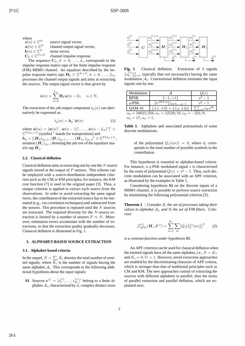
[P45] SSP-2005
wheres(n) ∈ CN source signal vector,w(n) ∈ CP channel output signal vector,b(n) ∈ CP noise vector,Ck ∈ C
P×N channel impulse response.The sequenceCk, k = 0, . . . , Lc corresponds to the
impulse response matrix taps of the finite impulse response(FIR) MIMO channel. An equalizer described by the im-pulse response matrix tapsHk ∈ CN×P , k = 0, . . . , Lh,processes the channel output signals and aims at extractingthe sources. The output signal vector is thus given by
s(n) =
Lh∑
k=0
Hkw(n− k), n ∈ N.
The extraction of thepth output componentsp(n) can alter-natively be expressed as:
sp(n) = hpTw(n) (1)
wherew(n) = [w(n)T, w(n − 1)T, . . . , w(n − Lh)T]T ∈CP (Lh+1) (symbolT stands for transposition) andhp = [(H0)(p,:), (H1)(p,:), . . . , (HLh
)(p,:)]T ∈ CP (Lh+1),
notation(Hj)(p,:) denoting thepth row of the equalizer ma-trix tapHj .
2.2. Classical deflation
Classical deflation aims at extracting one by one theN sourcesignals mixed at the output ofP sensors. This scheme canbe employed with a source-distribution independent crite-rion such as the CM or KM principles; for instance, the KMcost function [7] is used in the original paper [3]. Thus, aunique criterion is applied to extract each source from theobservations. In order to avoid extracting the same signaltwice, the contribution of the extracted source has to be esti-mated (e.g., via correlation techniques) and subtracted fromthe sensors. This procedure is repeated until theN sourcesare extracted. The required diversity for theN -source ex-traction is limited by a number of sensorsP ≈ N . More-over, estimation errors accumulate with the number of ex-tractions, so that the extraction quality gradually decreases.Classical deflation is illustrated in Fig. 1.
3. ALPHABET-BASED SOURCE EXTRACTION
3.1. Alphabet-based criteria
In the sequel,N =∑
iKi denotes the total number of emit-ted signals, whereKi is the number of signals having thesame alphabetAi. This corresponds to the following addi-tional hypothesis about the input signals:
S1. Sourcess(i) = [s(i)1 , . . . , s
(i)Ki
]T belong to a finite al-phabetAi, characterized bydi complex distinct roots
s(1)3
w(1,1,1)1
w(1,1,1)2
w(1,1,1)3
s(1)1
s(1)2
s(1)3
C
w(1,1)1 w
(1)1
w(1,1)3 w
(1)3
w(1)2
H3H2H1
w(1,1)2
s(1)2s
(1)1
Fig. 1. Classical deflation. Extraction of 3 signals{s(1)p }3p=1, typically (but not necessarily) having the samemodulationA1. Conventional deflation estimates the inputsignals one by one.
Modulation A Q(s)BPSK {−1,+1} s2 − 1
q-PSK {e2kπ/q}|k∈0,...,q−1 sq − 1
QAM-16 {±1,±3}+ {±,±3} ∑4k=0 αks
4k
α0 = 50625/256, α1 = 12529/16, α2 = −221/8,α3 = 17, α4 = 1.
Table 1. Alphabets and associated polynomials of somediscrete modulations.
of the polynomialQi(s(n)) = 0, wheredi corre-sponds to the total number of possible symbols in theconstellation.
This hypothesis is essential to alphabet-based criteria.For instance, aq-PSK modulated signals is characterizedby the roots of polynomialQ(s) = sq − 1. Thus, each dis-crete modulation can be associated with an APF criterion,as illustrated by the examples in Table 1.
Considering hypothesisS1 on the discrete inputs of aMIMO channel, it is possible to perform source extractionby minimizing the following polynomial criterion [5]:
Theorem 1 : ConsiderSi the set of processes taking theirvalues in alphabetAi, andH the set of FIR filters. Crite-rion:
J (i)APF (H i, s
(i)) =
Ki∑
n=1
∑
m
∣∣Qi
(s(i)n (m)
)∣∣2
(2)
is a contrast function under hypothesisS1.
An APF criterion can be used for classical deflation whenthe emitted signals have all the same alphabet, i.e.,N = K1
andKi = 0, ∀i > 1. However, novel extraction approachesare enabled by the discriminating character of APF criteria,which is stronger than that of traditional principles such asCM and KM. The new approaches consist of extracting thesources with different alphabets in parallel, thus the termsof parallel extraction and parallel deflation, which are ex-plained next.
2
264
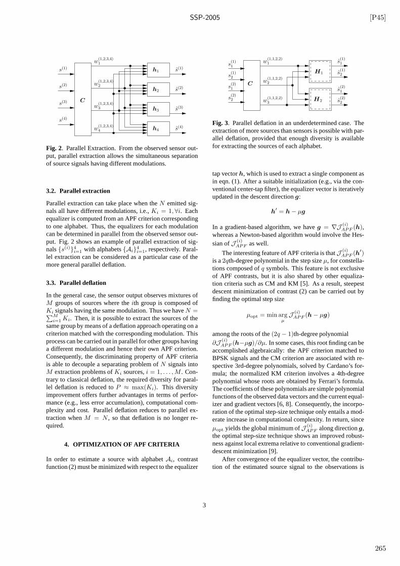
SSP-2005 [P45]
s(4)
h1
h2
h3
h4 s(4)
s(3)
s(2)
s(1)
w(1,2,3,4)4
w(1,2,3,4)3
w(1,2,3,4)2
w(1,2,3,4)1
C
s(1)
s(2)
s(3)
Fig. 2. Parallel Extraction. From the observed sensor out-put, parallel extraction allows the simultaneous separationof source signals having different modulations.
3.2. Parallel extraction
Parallel extraction can take place when theN emitted sig-nals all have different modulations, i.e.,Ki = 1, ∀i. Eachequalizer is computed from an APF criterion correspondingto one alphabet. Thus, the equalizers for each modulationcan be determined in parallel from the observed sensor out-put. Fig. 2 shows an example of parallel extraction of sig-nals{s(i)}4i=1 with alphabets{Ai}4i=1, respectively. Paral-lel extraction can be considered as a particular case of themore general parallel deflation.
3.3. Parallel deflation
In the general case, the sensor output observes mixtures ofM groups of sources where theith group is composed ofKi signals having the same modulation. Thus we haveN =∑M
i=1Ki. Then, it is possible to extract the sources of thesame group by means of a deflation approach operating on acriterion matched with the corresponding modulation. Thisprocess can be carried out in parallel for other groups havinga different modulation and hence their own APF criterion.Consequently, the discriminating property of APF criteriais able to decouple a separating problem ofN signals intoM extraction problems ofKi sources,i = 1, . . . ,M . Con-trary to classical deflation, the required diversity for paral-lel deflation is reduced toP ≈ max(Ki). This diversityimprovement offers further advantages in terms of perfor-mance (e.g., less error accumulation), computational com-plexity and cost. Parallel deflation reduces to parallel ex-traction whenM = N , so that deflation is no longer re-quired.
4. OPTIMIZATION OF APF CRITERIA
In order to estimate a source with alphabetAi, contrastfunction (2) must be minimized with respect to the equalizer
w(1,1,2,2)3
H1
H2 s(2)2
s(2)1
s(1)2
s(1)1
s(1)1
s(1)2
s(2)2
Cs(2)1
w(1,1,2,2)1
w(1,1,2,2)2
Fig. 3. Parallel deflation in an underdetermined case. Theextraction of more sources than sensors is possible with par-allel deflation, provided that enough diversity is availablefor extracting the sources of each alphabet.
tap vectorh, which is used to extract a single component asin eqn. (1). After a suitable initialization (e.g., via the con-ventional center-tap filter), the equalizer vector is iterativelyupdated in the descent directiong:
h′ = h− µg
In a gradient-based algorithm, we haveg = ∇J (i)APF (h),
whereas a Newton-based algorithm would involve the Hes-sian ofJ (i)
APF as well.
The interesting feature of APF criteria is thatJ (i)APF (h′)
is a2qth-degree polynomial in the step sizeµ, for constella-tions composed ofq symbols. This feature is not exclusiveof APF contrasts, but it is also shared by other equaliza-tion criteria such as CM and KM [5]. As a result, steepestdescent minimization of contrast (2) can be carried out byfinding the optimal step size
µopt = min argµJ (i)
APF (h− µg)
among the roots of the(2q − 1)th-degree polynomial∂J (i)
APF (h−µg)/∂µ. In some cases, this root finding can beaccomplished algebraically: the APF criterion matched toBPSK signals and the CM criterion are associated with re-spective 3rd-degree polynomials, solved by Cardano’s for-mula; the normalized KM criterion involves a 4th-degreepolynomial whose roots are obtained by Ferrari’s formula.The coefficients of these polynomials are simple polynomialfunctions of the observed data vectors and the current equal-izer and gradient vectors [6, 8]. Consequently, the incorpo-ration of the optimal step-size technique only entails a mod-erate increase in computational complexity. In return, sinceµopt yields the global minimum ofJ (i)
APF along directiong,the optimal step-size technique shows an improved robust-ness against local extrema relative to conventional gradient-descent minimization [9].
After convergence of the equalizer vector, the contribu-tion of the estimated source signal to the observations is
3
265

[P45] SSP-2005
0 5 10 15 20 25 3010
−5
10−4
10−3
10−2
10−1
100
Lc=2, Lh=13
Signal to Noise ratio (dB)
Sym
bol E
rror
Rat
e (%
)
QAM16QPSKPSK−6
Fig. 4. Parallel extraction of 3 different sources for variousSNRs.
calculated and subtracted from the sensor output, to pre-vent extracting the same source twice. This contributionis easily obtained as the cross-correlation between the esti-mated source signal and the sensor output vector. To extractthe next source, the APF criterion needs to be minimizedagain, but using the sensor output data without the contri-bution from the source previously extracted. This processis repeated until all sources with the same modulation havebeen obtained In parallel deflation, the deflation processesof the different APF criteria can be executed in parallel.
5. PRELIMINARY EXPERIMENTAL RESULTS
5.1. Parallel extraction
In this experiment,N = 3 sources with different modu-lations (QPSK, QAM-16, PSK-6) are mixed by a length-3channel (Lc = 2). P = 3 noisy observations are processedby a parallel extraction algorithm made up of the APF cri-teria associated with each modulation. The channel coeffi-cients are randomly drawn from a Gaussian distribution, andso is the noise added to the observations. Fig. 4 summarizesthe parallel extraction performance for different signal-to-noise ratios (SNRs).
5.2. Parallel deflation
The second experiment tests a channel spanning two baudperiods (Lc = 1) and mixingN = 4 source signals (2QPSK and 2 QAM16, i.e.,M = 2) at the output of onlyP = 3 sensors:
C(z) = C0 + C1z−1
0 2 4 6 8 10 12 14 16 18 2010
−2
10−1
100
101
SNR(dB)
MS
E
Underdetermined mixture (4 inputs − 3 ouputs), 600 samples
APF extraction filterMMSE filter
Fig. 5. APF extraction of a QPSK signal from an underde-termined mixture.
with
C0 =
−0.66 −0.19 0.65 0.920.22 −0.96 0.43 −0.85−0.30 −0.76 0.95 0.85
C1 =
0.75 −0.98 −0.75 −0.38−0.97 0.27 0.90 0.530.95 0.65 0.30 −0.52
Hence, this situation describes the underdetermined mixturecontext. The extraction of one of the QPSK signals is il-lustrated in Fig. 5. Note that, despite the hardness of theunderdetermined scenario, the APF extraction performancelies very close to the MMSE bound.
6. CONCLUSIONS
The use of contrast functions matched to the signal mod-ulation enables the definition of a novel approach to blindsource extraction whereby sources with different constella-tions can be extracted in parallel, provided that no alphabetbe a subset of another. Parallel deflation may prove use-ful when different modulations coexist in the same trans-mission environment. Such a scenario is likely in future-generation wireless communication networks, where sig-nal constellations will be dynamically allocated accordingto the service required and the channel conditions, analo-gously to the bit-loading schemes used in multicarrier com-munications [10]. The preliminary experiments reported inthis paper are encouraging. More detailed experimental re-sults illustrating the performance of the parallel deflationapproach will be presented at the conference.
4
266
SSP-2005 [P45]
7. REFERENCES
[1] Y. SATO, “A method of self recovering equalizationfor multilevel amplitude-modulation systems,”IEEETrans. on Com., vol. 23, pp. 679–682, June 1975.
[2] D. GODARD, “Self recovering equalization and car-rier tracking in two dimensional data communicationsystems,”IEEE Trans. on Signal Processing, vol. 28,no. 11, pp. 1867–1875, Nov. 1980.
[3] N. DELFOSSE and P. LOUBATON, “Adaptive blindseparation of independent sources: A deflation ap-proach,”Signal Processing, vol. 45, pp. 59–83, 1995.
[4] J.R. TREICHLER and M.G. LARIMORE, “New pro-cessing techniques based on the constant modulus al-gorithm,” IEEE Trans. on Acoust. Speech Sig. Proc.,vol. 33, no. 2, pp. 420–431, April 1985.
[5] P. COMON, “Contrasts, independent component anal-ysis, and blind deconvolution,”International Journalof Adaptive Control and Signal Processing (Special Is-sue on Blind Signal Separation), vol. 18, no. 3, pp.225–243, Apr. 2004.
[6] L. ROTA and P. COMON, “Blind Equalizers Basedon Polynomial Criteria,” inProc. ICASSP, Montreal,Quebec, 17-21 May 2004.
[7] O. SHALVI and E. WEINSTEIN, “New criteria forblind deconvolution of nonminimum phase systems(channels),”IEEE Trans. on Information Theory, vol.36, no. 2, pp. 312–321, Mar. 1990.
[8] V. ZARZOSO and P. COMON, “Blind channelequalization with algebraic optimal step size,” inEUSIPCO-2005, XIII European Signal ProcessingConference, Antalya, Turkey, Sept. 4–8, 2005.
[9] V. ZARZOSO and P. COMON, “Optimal step-size constant modulus algorithm,” IEEE Trans-actions on Communications, Oct. 2004, submit-ted(http://www.i3s.unice.fr/%7Emh/RR/2004/RR-
04.23-V.ZARZOSO.pdf) .
[10] Z. WANG and G. B. GIANNAKIS, “Wireless mul-ticarrier communications,” IEEE Signal ProcessingMagazine, vol. 17, no. 3, pp. 29–48, May 2000.
5
267

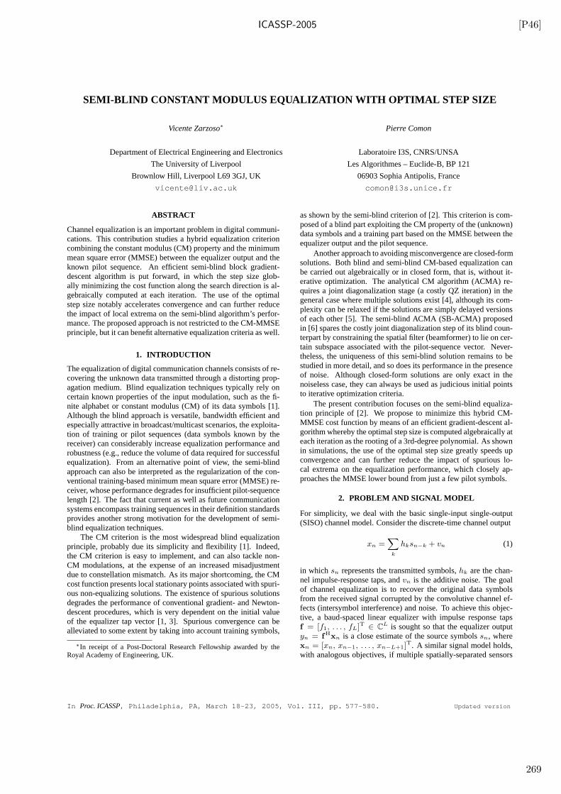
ICASSP-2005 [P46]
SEMI-BLIND CONSTANT MODULUS EQUALIZATION WITH OPTIMAL STEP SIZE
Vicente Zarzoso∗
Department of Electrical Engineering and Electronics
The University of Liverpool
Brownlow Hill, Liverpool L69 3GJ, UK
Pierre Comon
Laboratoire I3S, CNRS/UNSA
Les Algorithmes – Euclide-B, BP 121
06903 Sophia Antipolis, France
ABSTRACT
Channel equalization is an important problem in digital communi-cations. This contribution studies a hybrid equalization criterioncombining the constant modulus (CM) property and the minimummean square error (MMSE) between the equalizer output and theknown pilot sequence. An efficient semi-blind block gradient-descent algorithm is put forward, in which the step size glob-ally minimizing the cost function along the search direction is al-gebraically computed at each iteration. The use of the optimalstep size notably accelerates convergence and can further reducethe impact of local extrema on the semi-blind algorithm’s perfor-mance. The proposed approach is not restricted to the CM-MMSEprinciple, but it can benefit alternative equalization criteria as well.
1. INTRODUCTION
The equalization of digital communication channels consists of re-covering the unknown data transmitted through a distorting prop-agation medium. Blind equalization techniques typically rely oncertain known properties of the input modulation, such as the fi-nite alphabet or constant modulus (CM) of its data symbols [1].Although the blind approach is versatile, bandwidth efficient andespecially attractive in broadcast/multicast scenarios, the exploita-tion of training or pilot sequences (data symbols known by thereceiver) can considerably increase equalization performance androbustness (e.g., reduce the volume of data required for successfulequalization). From an alternative point of view, the semi-blindapproach can also be interpreted as the regularization of the con-ventional training-based minimum mean square error (MMSE) re-ceiver, whose performance degrades for insufficient pilot-sequencelength [2]. The fact that current as well as future communicationsystems encompass training sequences in their definition standardsprovides another strong motivation for the development of semi-blind equalization techniques.
The CM criterion is the most widespread blind equalizationprinciple, probably due its simplicity and flexibility [1]. Indeed,the CM criterion is easy to implement, and can also tackle non-CM modulations, at the expense of an increased misadjustmentdue to constellation mismatch. As its major shortcoming, the CMcost function presents local stationary points associated with spuri-ous non-equalizing solutions. The existence of spurious solutionsdegrades the performance of conventional gradient- and Newton-descent procedures, which is very dependent on the initial valueof the equalizer tap vector [1, 3]. Spurious convergence can bealleviated to some extent by taking into account training symbols,
∗In receipt of a Post-Doctoral Research Fellowship awarded by theRoyal Academy of Engineering, UK.
as shown by the semi-blind criterion of [2]. This criterion is com-posed of a blind part exploiting the CM property of the (unknown)data symbols and a training part based on the MMSE between theequalizer output and the pilot sequence.
Another approach to avoiding misconvergence are closed-formsolutions. Both blind and semi-blind CM-based equalization canbe carried out algebraically or in closed form, that is, without it-erative optimization. The analytical CM algorithm (ACMA) re-quires a joint diagonalization stage (a costly QZ iteration) in thegeneral case where multiple solutions exist [4], although its com-plexity can be relaxed if the solutions are simply delayed versionsof each other [5]. The semi-blind ACMA (SB-ACMA) proposedin [6] spares the costly joint diagonalization step of its blind coun-terpart by constraining the spatial filter (beamformer) to lie on cer-tain subspace associated with the pilot-sequence vector. Never-theless, the uniqueness of this semi-blind solution remains to bestudied in more detail, and so does its performance in the presenceof noise. Although closed-form solutions are only exact in thenoiseless case, they can always be used as judicious initial pointsto iterative optimization criteria.
The present contribution focuses on the semi-blind equaliza-tion principle of [2]. We propose to minimize this hybrid CM-MMSE cost function by means of an efficient gradient-descent al-gorithm whereby the optimal step size is computed algebraically ateach iteration as the rooting of a 3rd-degree polynomial. As shownin simulations, the use of the optimal step size greatly speeds upconvergence and can further reduce the impact of spurious lo-cal extrema on the equalization performance, which closely ap-proaches the MMSE lower bound from just a few pilot symbols.
2. PROBLEM AND SIGNAL MODEL
For simplicity, we deal with the basic single-input single-output(SISO) channel model. Consider the discrete-time channel output
xn =∑
k
hksn−k + vn (1)
in which sn represents the transmitted symbols,hk are the chan-nel impulse-response taps, andvn is the additive noise. The goalof channel equalization is to recover the original data symbolsfrom the received signal corrupted by the convolutive channel ef-fects (intersymbol interference) and noise. To achieve this objec-tive, a baud-spaced linear equalizer with impulse response tapsf = [f1, . . . , fL]T ∈ C
L is sought so that the equalizer outputyn = fHxn is a close estimate of the source symbolssn, wherexn = [xn, xn−1, . . . , xn−L+1]
T. A similar signal model holds,with analogous objectives, if multiple spatially-separated sensors
In Proc. ICASSP, Philadelphia, PA, March 18-23, 2005, Vol. III, pp. 577-580. Updated version
269
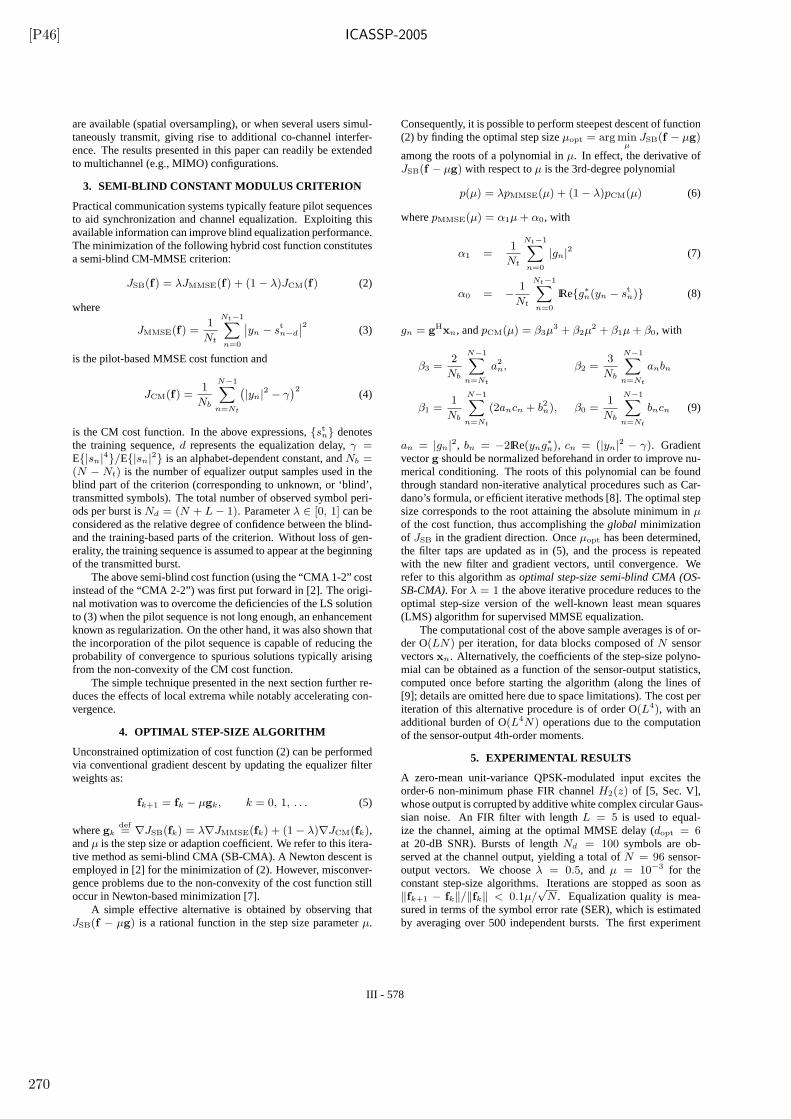
[P46] ICASSP-2005
are available (spatial oversampling), or when several users simul-taneously transmit, giving rise to additional co-channel interfer-ence. The results presented in this paper can readily be extendedto multichannel (e.g., MIMO) configurations.
3. SEMI-BLIND CONSTANT MODULUS CRITERION
Practical communication systems typically feature pilot sequencesto aid synchronization and channel equalization. Exploiting thisavailable information can improve blind equalization performance.The minimization of the following hybrid cost function constitutesa semi-blind CM-MMSE criterion:
JSB(f) = λJMMSE(f) + (1 − λ)JCM(f) (2)
where
JMMSE(f) =1
Nt
Nt−1∑
n=0
∣∣yn − stn−d
∣∣2 (3)
is the pilot-based MMSE cost function and
JCM(f) =1
Nb
N−1∑
n=Nt
(|yn|2 − γ
)2(4)
is the CM cost function. In the above expressions,{stn} denotes
the training sequence,d represents the equalization delay,γ =E{|sn|4}/E{|sn|2} is an alphabet-dependent constant, andNb =(N − Nt) is the number of equalizer output samples used in theblind part of the criterion (corresponding to unknown, or ‘blind’,transmitted symbols). The total number of observed symbol peri-ods per burst isNd = (N + L − 1). Parameterλ ∈ [0, 1] can beconsidered as the relative degree of confidence between the blind-and the training-based parts of the criterion. Without loss of gen-erality, the training sequence is assumed to appear at the beginningof the transmitted burst.
The above semi-blind cost function (using the “CMA 1-2” costinstead of the “CMA 2-2”) was first put forward in [2]. The origi-nal motivation was to overcome the deficiencies of the LS solutionto (3) when the pilot sequence is not long enough, an enhancementknown as regularization. On the other hand, it was also shown thatthe incorporation of the pilot sequence is capable of reducing theprobability of convergence to spurious solutions typically arisingfrom the non-convexity of the CM cost function.
The simple technique presented in the next section further re-duces the effects of local extrema while notably accelerating con-vergence.
4. OPTIMAL STEP-SIZE ALGORITHM
Unconstrained optimization of cost function (2) can be performedvia conventional gradient descent by updating the equalizer filterweights as:
fk+1 = fk − µgk, k = 0, 1, . . . (5)
wheregkdef= ∇JSB(fk) = λ∇JMMSE(fk) + (1 − λ)∇JCM(fk),
andµ is the step size or adaption coefficient. We refer to this itera-tive method as semi-blind CMA (SB-CMA). A Newton descent isemployed in [2] for the minimization of (2). However, misconver-gence problems due to the non-convexity of the cost function stilloccur in Newton-based minimization [7].
A simple effective alternative is obtained by observing thatJSB(f − µg) is a rational function in the step size parameterµ.
Consequently, it is possible to perform steepest descent of function(2) by finding the optimal step sizeµopt = arg min
µJSB(f − µg)
among the roots of a polynomial inµ. In effect, the derivative ofJSB(f − µg) with respect toµ is the 3rd-degree polynomial
p(µ) = λpMMSE(µ) + (1 − λ)pCM(µ) (6)
wherepMMSE(µ) = α1µ + α0, with
α1 =1
Nt
Nt−1∑
n=0
|gn|2 (7)
α0 = − 1
Nt
Nt−1∑
n=0
IRe{g∗
n(yn − stn)} (8)
gn = gHxn, andpCM(µ) = β3µ3 + β2µ
2 + β1µ + β0, with
β3 =2
Nb
N−1∑
n=Nt
a2n, β2 =
3
Nb
N−1∑
n=Nt
anbn
β1 =1
Nb
N−1∑
n=Nt
(2ancn + b2n), β0 =
1
Nb
N−1∑
n=Nt
bncn (9)
an = |gn|2, bn = −2IRe(yng∗
n), cn = (|yn|2 − γ). Gradientvectorg should be normalized beforehand in order to improve nu-merical conditioning. The roots of this polynomial can be foundthrough standard non-iterative analytical procedures such as Car-dano’s formula, or efficient iterative methods [8]. The optimal stepsize corresponds to the root attaining the absolute minimum inµof the cost function, thus accomplishing theglobal minimizationof JSB in the gradient direction. Onceµopt has been determined,the filter taps are updated as in (5), and the process is repeatedwith the new filter and gradient vectors, until convergence. Werefer to this algorithm asoptimal step-size semi-blind CMA (OS-SB-CMA). Forλ = 1 the above iterative procedure reduces to theoptimal step-size version of the well-known least mean squares(LMS) algorithm for supervised MMSE equalization.
The computational cost of the above sample averages is of or-der O(LN) per iteration, for data blocks composed ofN sensorvectorsxn. Alternatively, the coefficients of the step-size polyno-mial can be obtained as a function of the sensor-output statistics,computed once before starting the algorithm (along the lines of[9]; details are omitted here due to space limitations). The cost periteration of this alternative procedure is of order O(L4), with anadditional burden of O(L4N) operations due to the computationof the sensor-output 4th-order moments.
5. EXPERIMENTAL RESULTS
A zero-mean unit-variance QPSK-modulated input excites theorder-6 non-minimum phase FIR channelH2(z) of [5, Sec. V],whose output is corrupted by additive white complex circular Gaus-sian noise. An FIR filter with lengthL = 5 is used to equal-ize the channel, aiming at the optimal MMSE delay (dopt = 6at 20-dB SNR). Bursts of lengthNd = 100 symbols are ob-served at the channel output, yielding a total ofN = 96 sensor-output vectors. We chooseλ = 0.5, and µ = 10−3 for theconstant step-size algorithms. Iterations are stopped as soon as‖fk+1 − fk‖/‖fk‖ < 0.1µ/
√N . Equalization quality is mea-
sured in terms of the symbol error rate (SER), which is estimatedby averaging over 500 independent bursts. The first experiment
III - 578
270
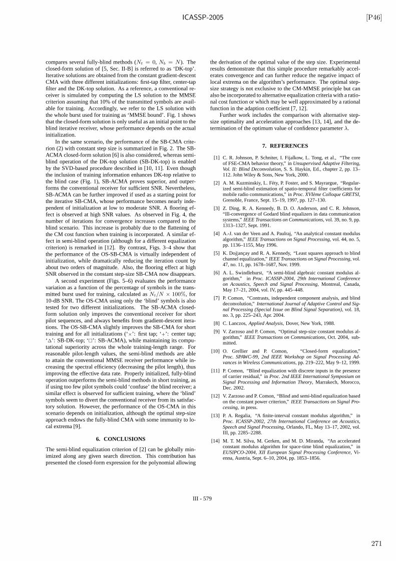
ICASSP-2005 [P46]
compares several fully-blind methods (Nt = 0, Nb = N ). Theclosed-form solution of [5, Sec. II-B] is referred to as ‘DK-top’.Iterative solutions are obtained from the constant gradient-descentCMA with three different initializations: first-tap filter, center-tapfilter and the DK-top solution. As a reference, a conventional re-ceiver is simulated by computing the LS solution to the MMSEcriterion assuming that 10% of the transmitted symbols are avail-able for training. Accordingly, we refer to the LS solution withthe whole burst used for training as ‘MMSE bound’. Fig. 1 showsthat the closed-form solution is only useful as an initial point to theblind iterative receiver, whose performance depends on the actualinitialization.
In the same scenario, the performance of the SB-CMA crite-rion (2) with constant step size is summarized in Fig. 2. The SB-ACMA closed-form solution [6] is also considered, whereas semi-blind operation of the DK-top solution (SB-DK-top) is enabledby the SVD-based procedure described in [10, 11]. Even thoughthe inclusion of training information enhances DK-top relative tothe blind case (Fig. 1), SB-ACMA proves superior, and outper-forms the conventional receiver for sufficient SNR. Nevertheless,SB-ACMA can be further improved if used as a starting point forthe iterative SB-CMA, whose performance becomes nearly inde-pendent of initialization at low to moderate SNR. A flooring ef-fect is observed at high SNR values. As observed in Fig. 4, thenumber of iterations for convergence increases compared to theblind scenario. This increase is probably due to the flattening ofthe CM cost function when training is incorporated. A similar ef-fect in semi-blind operation (although for a different equalizationcriterion) is remarked in [12]. By contrast, Figs. 3–4 show thatthe performance of the OS-SB-CMA is virtually independent ofinitialization, while dramatically reducing the iteration count byabout two orders of magnitude. Also, the flooring effect at highSNR observed in the constant step-size SB-CMA now disappears.
A second experiment (Figs. 5–6) evaluates the performancevariation as a function of the percentage of symbols in the trans-mitted burst used for training, calculated asNt/N × 100%, for10-dB SNR. The OS-CMA using only the ‘blind’ symbols is alsotested for two different initializations. The SB-ACMA closed-form solution only improves the conventional receiver for shortpilot sequences, and always benefits from gradient-descent itera-tions. The OS-SB-CMA slightly improves the SB-CMA for shorttraining and for all initializations (‘×’: first tap; ‘+’: center tap;‘∆’: SB-DK-top; ‘�’: SB-ACMA), while maintaining its compu-tational superiority across the whole training-length range. Forreasonable pilot-length values, the semi-blind methods are ableto attain the conventional MMSE receiver performance while in-creasing the spectral efficiency (decreasing the pilot length), thusimproving the effective data rate. Properly initialized, fully-blindoperation outperforms the semi-blind methods in short training, asif using too few pilot symbols could ‘confuse’ the blind receiver; asimilar effect is observed for sufficient training, where the ‘blind’symbols seem to divert the conventional receiver from its satisfac-tory solution. However, the performance of the OS-CMA in thisscenario depends on initialization, although the optimal step-sizeapproach endows the fully-blind CMA with some immunity to lo-cal extrema [9].
6. CONCLUSIONS
The semi-blind equalization criterion of [2] can be globally min-imized along any given search direction. This contribution haspresented the closed-form expression for the polynomial allowing
the derivation of the optimal value of the step size. Experimentalresults demonstrate that this simple procedure remarkably accel-erates convergence and can further reduce the negative impact oflocal extrema on the algorithm’s performance. The optimal step-size strategy is not exclusive to the CM-MMSE principle but canalso be incorporated to alternative equalization criteria with a ratio-nal cost function or which may be well approximated by a rationalfunction in the adaption coefficient [7, 12].
Further work includes the comparison with alternative step-size optimality and acceleration approaches [13, 14], and the de-termination of the optimum value of confidence parameterλ.
7. REFERENCES
[1] C. R. Johnson, P. Schniter, I. Fijalkow, L. Tong, et al., “The coreof FSE-CMA behavior theory,” inUnsupervised Adaptive Filtering,Vol. II: Blind Deconvolution, S. S. Haykin, Ed., chapter 2, pp. 13–112. John Wiley & Sons, New York, 2000.
[2] A. M. Kuzminskiy, L. Fety, P. Foster, and S. Mayrargue, “Regular-ized semi-blind estimation of spatio-temporal filter coefficients formobile radio communications,” inProc. XVIeme Colloque GRETSI,Grenoble, France, Sept. 15–19, 1997, pp. 127–130.
[3] Z. Ding, R. A. Kennedy, B. D. O. Anderson, and C. R. Johnson,“Ill-convergence of Godard blind equalizers in data communicationsystems,”IEEE Transactions on Communications, vol. 39, no. 9, pp.1313–1327, Sept. 1991.
[4] A.-J. van der Veen and A. Paulraj, “An analytical constant modulusalgorithm,” IEEE Transactions on Signal Processing, vol. 44, no. 5,pp. 1136–1155, May 1996.
[5] K. Dogancay and R. A. Kennedy, “Least squares approach to blindchannel equalization,”IEEE Transactions on Signal Processing, vol.47, no. 11, pp. 1678–1687, Nov. 1999.
[6] A. L. Swindlehurst, “A semi-blind algebraic constant modulus al-gorithm,” in Proc. ICASSP-2004, 29th International Conferenceon Acoustics, Speech and Signal Processing, Montreal, Canada,May 17–21, 2004, vol. IV, pp. 445–448.
[7] P. Comon, “Contrasts, independent component analysis, and blinddeconvolution,”International Journal of Adaptive Control and Sig-nal Processing (Special Issue on Blind Signal Separation), vol. 18,no. 3, pp. 225–243, Apr. 2004.
[8] C. Lanczos,Applied Analysis, Dover, New York, 1988.
[9] V. Zarzoso and P. Comon, “Optimal step-size constant modulus al-gorithm,” IEEE Transactions on Communications, Oct. 2004, sub-mitted.
[10] O. Grellier and P. Comon, “Closed-form equalization,”Proc. SPAWC-99, 2nd IEEE Workshop on Signal Processing Ad-vances in Wireless Communications, pp. 219–222, May 9–12, 1999.
[11] P. Comon, “Blind equalization with discrete inputs in the presenceof carrier residual,” inProc. 2nd IEEE International Symposium onSignal Processing and Information Theory, Marrakech, Morocco,Dec. 2002.
[12] V. Zarzoso and P. Comon, “Blind and semi-blind equalization basedon the constant power criterion,”IEEE Transactions on Signal Pro-cessing, in press.
[13] P. A. Regalia, “A finite-interval constant modulus algorithm,” inProc. ICASSP-2002, 27th International Conference on Acoustics,Speech and Signal Processing, Orlando, FL, May 13–17, 2002, vol.III, pp. 2285–2288.
[14] M. T. M. Silva, M. Gerken, and M. D. Miranda, “An acceleratedconstant modulus algorithm for space-time blind equalization,” inEUSIPCO-2004, XII European Signal Processing Conference, Vi-enna, Austria, Sept. 6–10, 2004, pp. 1853–1856.
III - 579
271
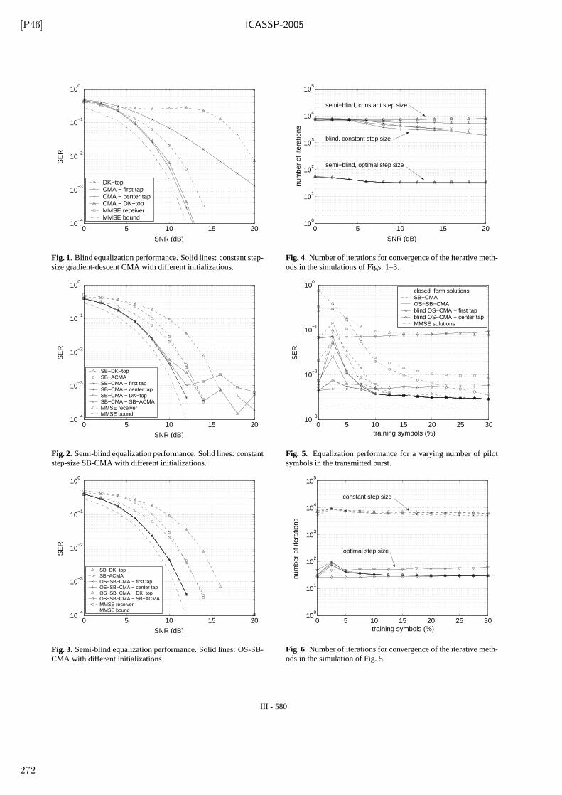
[P46] ICASSP-2005
0 5 10 15 2010
−4
10−3
10−2
10−1
100
SNR (dB)
SE
R
DK−topCMA − first tapCMA − center tapCMA − DK−topMMSE receiverMMSE bound
Fig. 1. Blind equalization performance. Solid lines: constant step-size gradient-descent CMA with different initializations.
0 5 10 15 2010
−4
10−3
10−2
10−1
100
SNR (dB)
SE
R
SB−DK−topSB−ACMASB−CMA − first tapSB−CMA − center tapSB−CMA − DK−topSB−CMA − SB−ACMAMMSE receiverMMSE bound
Fig. 2. Semi-blind equalization performance. Solid lines: constantstep-size SB-CMA with different initializations.
0 5 10 15 2010
−4
10−3
10−2
10−1
100
SNR (dB)
SE
R
SB−DK−topSB−ACMAOS−SB−CMA − first tapOS−SB−CMA − center tapOS−SB−CMA − DK−topOS−SB−CMA − SB−ACMAMMSE receiverMMSE bound
Fig. 3. Semi-blind equalization performance. Solid lines: OS-SB-CMA with different initializations.
0 5 10 15 2010
0
101
102
103
104
105
SNR (dB)
num
ber
of it
erat
ions
blind, constant step size
semi−blind, optimal step size
semi−blind, constant step size
Fig. 4. Number of iterations for convergence of the iterative meth-ods in the simulations of Figs. 1–3.
0 5 10 15 20 25 3010
−3
10−2
10−1
100
training symbols (%)
SE
Rclosed−form solutionsSB−CMAOS−SB−CMAblind OS−CMA − first tapblind OS−CMA − center tapMMSE solutions
Fig. 5. Equalization performance for a varying number of pilotsymbols in the transmitted burst.
0 5 10 15 20 25 3010
0
101
102
103
104
105
training symbols (%)
num
ber
of it
erat
ions
optimal step size
constant step size
Fig. 6. Number of iterations for convergence of the iterative meth-ods in the simulation of Fig. 5.
III - 580
272
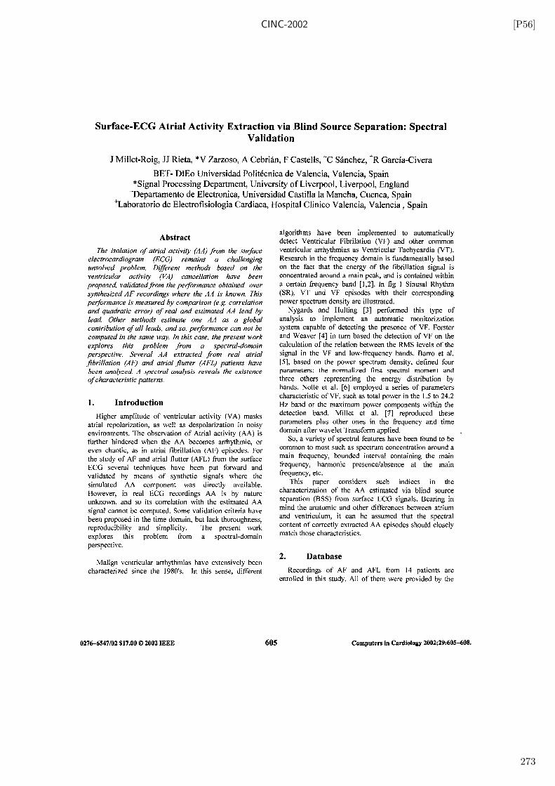
CINC-2002 [P56]
273
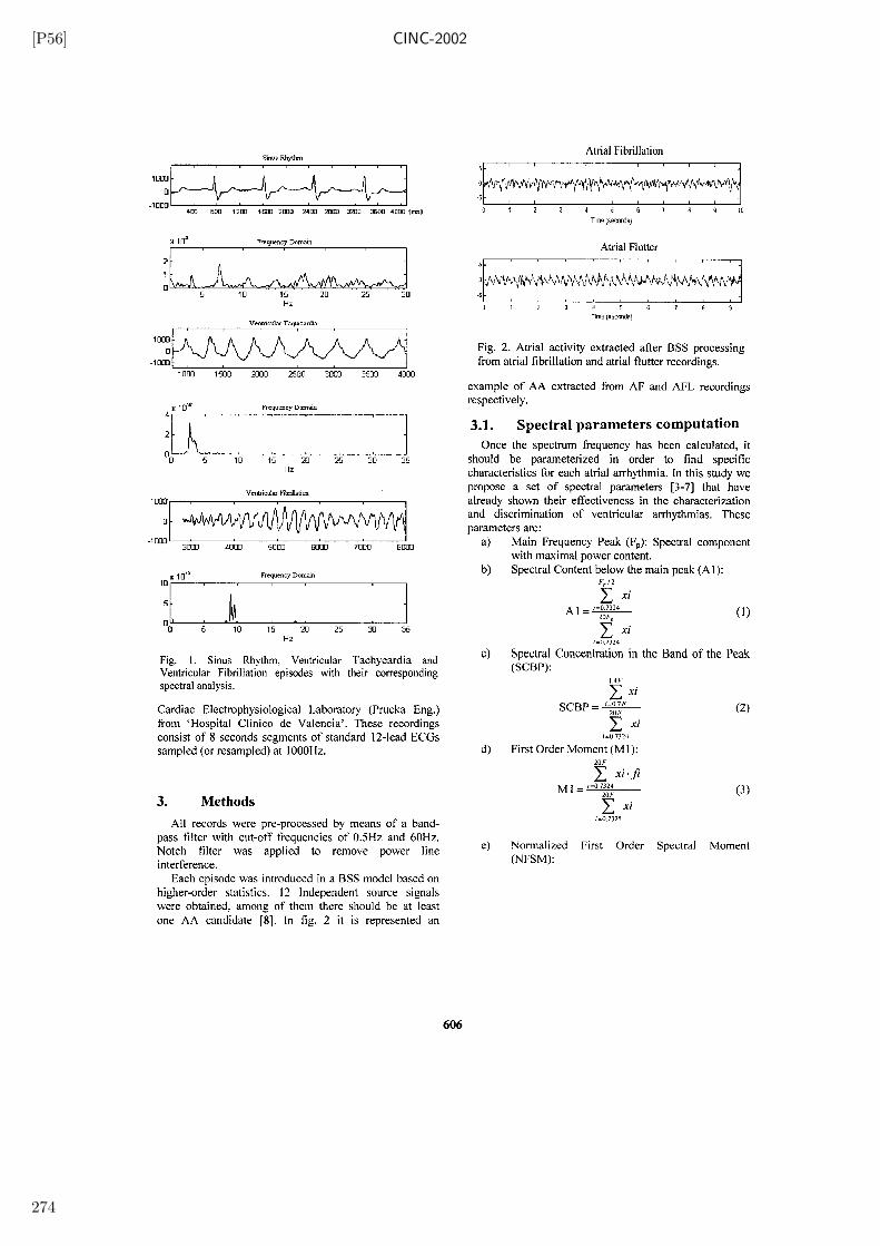
[P56] CINC-2002
274
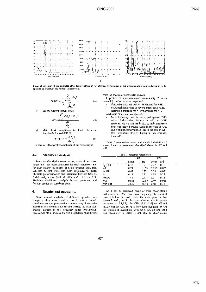
CINC-2002 [P56]
275
[P56] CINC-2002
276
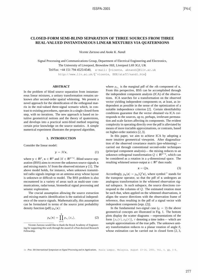
ISSPA-2001 [P64]
CLOSED-FORM SEMI-BLIND SEPARATION OF THREE SOURCES FROM THREEREAL-VALUED INSTANTANEOUS LINEAR MIXTURES VIA QUATERNIONS
Vicente Zarzoso and Asoke K. Nandi
Signal Processing and Communications Group, Department of Electrical Engineering and Electronics,
The University of Liverpool, Brownlow Hill, Liverpool L69 3GJ, UK
Tel/Fax: +44 151 794 4525/4540,e-mail: {vicente, aknandi }@liv.ac.uk
http://www.liv.ac.uk/ {˜vicente, EEE/staff/nandi.htm }
ABSTRACT
In the problem of blind source separation from instantan-eous linear mixtures, a unitary transformation remains un-known after second-order spatial whitening. We present anovel approach for the identification of the orthogonal mat-rix in the real-valued three-signal scenario which, in con-trast to existing procedures, operates in a single closed-formstep, with no iterations. The new approach is based on in-tuitive geometrical notions and the theory of quaternions,and develops into a practical semi-blind method requiringcertain prior knowledge on the source statistics. A simplenumerical experiment illustrates the proposed algorithm.
1. INTRODUCTION
Consider the linear model:
y = Mx, (1)
wherey ∈ IRp, x ∈ IRq andM ∈ IRp×q. Blind source sep-aration (BSS) aims to recover the unknown source signalsxand mixing matrixM from the observed mixturey [1]. Theabove model holds, for instance, when unknown transmit-ted radio signals impinge on an antenna array whose layoutis unknown or difficult to model. The BSS problem is alsoencountered in a variety of areas such as multi-user com-munications, radar/sonar, biomedical signal processing andseismic exploration.
The crucial assumption allowing the source extractionand mixing-matrix identification is the statistical independ-ence of the source signals. Mathematically, this assumptioncan be formulated in terms of the source joint probabilitydensity function (pdf)px(x):
px(x) =
q∏
s=1
pxs(xs), (2)
Vicente Zarzoso would like to thank the Royal Academy of Engineer-ing for supporting this work through the award of a Post-doctoral ResearchFellowship.
wherepxsis the marginal pdf of thesth component ofx.
From this perspective, BSS can be accomplished throughthe independent component analysis (ICA) of the observa-tions. ICA searches for a transformation on the observedvector yielding independent components or, at least, as in-dependent as possible in the sense of the optimization of asuitable independence criterion [2]. Certain identifiabilityconditions guarantee that the vector obtained via ICA cor-responds to the sources, up to, perhaps, irrelevant permuta-tion and scale factors affecting its components. The evidentcomplexity in operating directly over the pdf is alleviated bymeans of more tractable approximations, or contrasts, basedon higher-order statistics [2,3].
In this paper, we aim to achieve ICA by adopting amore intuitive geometrical viewpoint. After diagonaliza-tion of the observed covariance matrix (pre-whitening) —carried out through conventional second-order techniques(principal component analysis)— the mixing reduces to anunknown orthogonal transformationQ ∈ IRq×q, which canbe considered as a rotation in aq-dimensional space. Theresulting whitened sensor-outputz ∈ IRq then reads:
z = Qx. (3)
Accordingly,pz(z) = px(Q†z), where symbol† stands forthe transpose operator, so that the pdf ofx undergoes ananalogous transformation in the whitened observation sig-nal subspace. In such subspace, the source directions cor-respond to the columns ofQ. The estimated rotation mustbe such that, when applied on the whitened observations, italigns the source directions with the observation frame ofreference, thus resulting in the pdf of a signal vector withindependent components [eqn. (2)].
In the fundamental two-signal case (q = 2) the abovegeometrical concepts are illustrated in Fig. 1. The bottomplots display the scatter diagrams —representations of theform
(x1(τ), x2(τ)
), τ denoting a time index— which are
sample approximations of the true pdfs. The unknown unit-ary transformation reduces to a planar rotation of angleθ,whose estimation can be carried out in closed form [2, 3,
In Proc. 6th International Symposium on Signal Processing and its Applications, Kuala Lumpur, Malaysia, August 13-16, 2001, Vol. I, pp. 1-4.
277
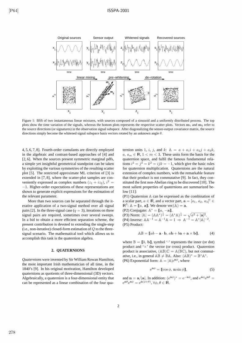
[P64] ISSPA-2001
Original sources
time
x1
x 2
Sensor output
time
y1
y 2
Whitened signals
time
z1
z 2
Recovered sources
time
s1
s 2θ
m1
m2
linear mixing pre−whitening de−rotation
x1
x2
y1
y2
z1
z2
s1
s2
Figure 1: BSS of two instantaneous linear mixtures, with sources composed of a sinusoid and a uniformly distributed process. The topplots show the time variation of the signals, whereas the bottom plots represents the respective scatter plots. Vectorsm1 andm2 refer tothe source directions (or signatures) in the observation signal subspace. After diagonalizing the sensor-output covariance matrix, the sourcedirections simply become the whitened signal subspace basis vectors rotated by an unknown angleθ.
4, 5, 6, 7, 8]. Fourth-order cumulants are directly employedin the algebraic and contrast-based approaches of [4] and[2, 6]. When the sources present symmetric marginal pdfs,a simple yet insightful geometrical standpoint can be takenby exploiting the various symmetries of the resulting scatterplot [5]. The restricted approximate ML criterion of [3] isextended in [7, 8], where the scatter-plot samples are con-veniently expressed as complex numbers(z1 + iz2), i2 =−1. Higher-order expectations of these representations areshown to generate explicit expressions for the estimation ofthe relevant parameter.
More than two sources can be separated through the it-erative application of a two-signal method over all signalpairs [2]. In the three-signal case (q = 3), iterations on threesignal pairs are required, sometimes over several sweeps.In a bid to obtain a more efficient separation scheme, thepresent contribution is devoted to extending the single-step(i.e., non-iterative) closed-form estimation ofQ to the three-signal scenario. The mathematical tool which allows us toaccomplish this task is the quaternion algebra.
2. QUATERNIONS
Quaternionswere invented by Sir William Rowan Hamilton,the most important Irish mathematician of all time, in the1840’s [9]. In his original motivation, Hamilton developedquaternions as quotients of three-dimensional (3D) vectors.Algebraically, a quaternion is a four-dimensional entity thatcan be represented as a linear combination of the four qua-
ternion units1, i, j, andk: A = a + a1i + a2j + a3k,a, am ∈ IR, 1 < m < 3. These units form the basis for thequaternion space, and fulfil the famous fundamental rela-tionsi2 = j2 = k2 = ijk = −1, which give the basic rulesfor quaternion multiplication. Quaternions are the naturalextension of complex numbers, with the remarkable featurethat their product is not commutative [9]. In fact, they con-stituted the first non-Abelian ring to be discovered [10]. Themost salient properties of quaternions are summarized be-low [11]:(P1) QuaternionA can be expressed as the combination ofa scalar part,a ∈ IR, and a vector part,a = [a1, a2, a3]
† ∈IR3: A = [[a, a]]. We denote vec(A) = a.(P2) Conjugate:A∗ = [[a, −a]].(P3) Norm:|A| = (AA
∗)12 = (A∗
A)12 =
√a2 + |a|2.
(P4) Inverse:AA−1 = A
−1A = 1 ⇒ A
−1 = A∗|A|−2.
(P5) Product:
AB = [[ab− a · b, ab + ba + a× b]] , (4)
whereB = [[b, b]], symbol ‘·’ represents the inner (or dot)product and ‘×’ the vector (or cross) product. Quaternionproduct is associative,(AB)C = A(BC), but not commut-ative, i.e., in generalAB 6= BA. Also: (AB)∗ = B
∗A
∗.(P6) Exponential form:A = |A|enφ, where
enφ = [[cos φ, n sin φ]] , (5)
andn = a/|a|. In addition:(enφ)∗ = e−nφ, andenφenθ =enθenφ = en(φ+θ), ∀φ, θ ∈ IR.
2
278
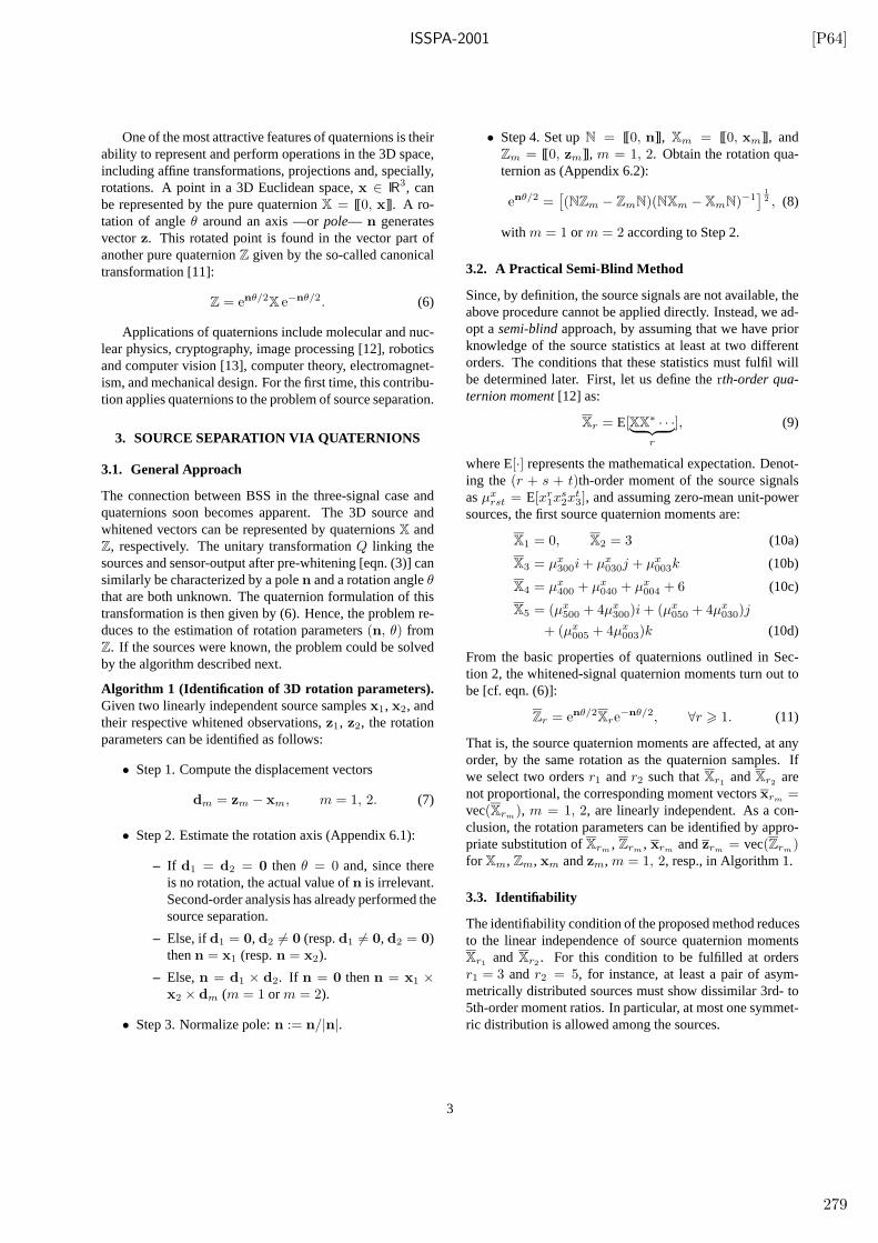
ISSPA-2001 [P64]
One of the most attractive features of quaternions is theirability to represent and perform operations in the 3D space,including affine transformations, projections and, specially,rotations. A point in a 3D Euclidean space,x ∈ IR3, canbe represented by the pure quaternionX = [[0, x]]. A ro-tation of angleθ around an axis —orpole— n generatesvectorz. This rotated point is found in the vector part ofanother pure quaternionZ given by the so-called canonicaltransformation [11]:
Z = enθ/2X e−nθ/2. (6)
Applications of quaternions include molecular and nuc-lear physics, cryptography, image processing [12], roboticsand computer vision [13], computer theory, electromagnet-ism, and mechanical design. For the first time, this contribu-tion applies quaternions to the problem of source separation.
3. SOURCE SEPARATION VIA QUATERNIONS
3.1. General Approach
The connection between BSS in the three-signal case andquaternions soon becomes apparent. The 3D source andwhitened vectors can be represented by quaternionsX andZ, respectively. The unitary transformationQ linking thesources and sensor-output after pre-whitening [eqn. (3)] cansimilarly be characterized by a polen and a rotation angleθthat are both unknown. The quaternion formulation of thistransformation is then given by (6). Hence, the problem re-duces to the estimation of rotation parameters(n, θ) fromZ. If the sources were known, the problem could be solvedby the algorithm described next.
Algorithm 1 (Identification of 3D rotation parameters).Given two linearly independent source samplesx1, x2, andtheir respective whitened observations,z1, z2, the rotationparameters can be identified as follows:
• Step 1. Compute the displacement vectors
dm = zm − xm, m = 1, 2. (7)
• Step 2. Estimate the rotation axis (Appendix 6.1):
– If d1 = d2 = 0 thenθ = 0 and, since thereis no rotation, the actual value ofn is irrelevant.Second-order analysis has already performed thesource separation.
– Else, ifd1 = 0, d2 6= 0 (resp.d1 6= 0, d2 = 0)thenn = x1 (resp.n = x2).
– Else,n = d1 × d2. If n = 0 thenn = x1 ×x2 × dm (m = 1 or m = 2).
• Step 3. Normalize pole:n := n/|n|.
• Step 4. Set upN = [[0, n]], Xm = [[0, xm]], andZm = [[0, zm]], m = 1, 2. Obtain the rotation qua-ternion as (Appendix 6.2):
enθ/2 =[(NZm − ZmN)(NXm − XmN)−1
] 12 , (8)
with m = 1 or m = 2 according to Step 2.
3.2. A Practical Semi-Blind Method
Since, by definition, the source signals are not available, theabove procedure cannot be applied directly. Instead, we ad-opt asemi-blindapproach, by assuming that we have priorknowledge of the source statistics at least at two differentorders. The conditions that these statistics must fulfil willbe determined later. First, let us define therth-order qua-ternion moment[12] as:
Xr = E[XX∗ · · ·
︸ ︷︷ ︸
r
], (9)
where E[·] represents the mathematical expectation. Denot-ing the (r + s + t)th-order moment of the source signalsasµx
rst = E[xr1x
s2x
t3], and assuming zero-mean unit-power
sources, the first source quaternion moments are:
X1 = 0, X2 = 3 (10a)
X3 = µx300i + µx
030j + µx003k (10b)
X4 = µx400 + µx
040 + µx004 + 6 (10c)
X5 = (µx500 + 4µx
300)i + (µx050 + 4µx
030)j
+ (µx005 + 4µx
003)k (10d)
From the basic properties of quaternions outlined in Sec-tion 2, the whitened-signal quaternion moments turn out tobe [cf. eqn. (6)]:
Zr = enθ/2Xre
−nθ/2, ∀r > 1. (11)
That is, the source quaternion moments are affected, at anyorder, by the same rotation as the quaternion samples. Ifwe select two ordersr1 andr2 such thatXr1
andXr2are
not proportional, the corresponding moment vectorsxrm=
vec(Xrm), m = 1, 2, are linearly independent. As a con-
clusion, the rotation parameters can be identified by appro-priate substitution ofXrm
, Zrm, xrm
andzrm= vec(Zrm
)for Xm, Zm, xm andzm, m = 1, 2, resp., in Algorithm 1.
3.3. Identifiability
The identifiability condition of the proposed method reducesto the linear independence of source quaternion momentsXr1
and Xr2. For this condition to be fulfilled at orders
r1 = 3 and r2 = 5, for instance, at least a pair of asym-metrically distributed sources must show dissimilar 3rd- to5th-order moment ratios. In particular, at most one symmet-ric distribution is allowed among the sources.
3
279
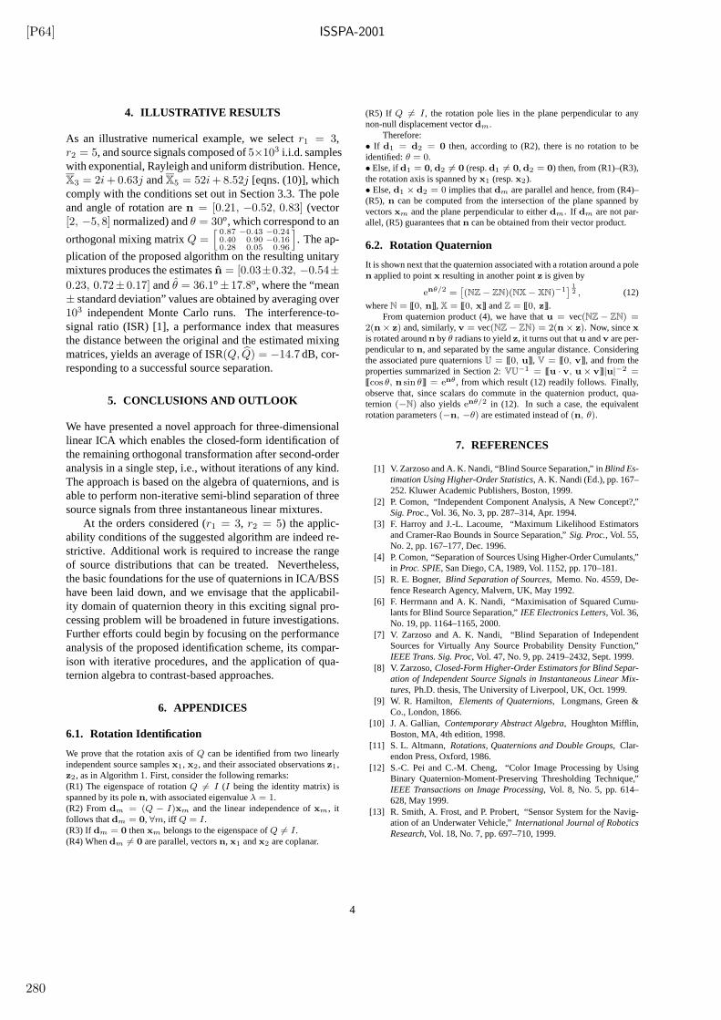
[P64] ISSPA-2001
4. ILLUSTRATIVE RESULTS
As an illustrative numerical example, we selectr1 = 3,r2 = 5, and source signals composed of5×103 i.i.d. sampleswith exponential, Rayleigh and uniform distribution. Hence,X3 = 2i+ 0.63j andX5 = 52i + 8.52j [eqns. (10)], whichcomply with the conditions set out in Section 3.3. The poleand angle of rotation aren = [0.21, −0.52, 0.83] (vector[2, −5, 8] normalized) andθ = 30o, which correspond to an
orthogonal mixing matrixQ =[
0.87 −0.43 −0.240.40 0.90 −0.160.28 0.05 0.96
]. The ap-
plication of the proposed algorithm on the resulting unitarymixtures produces the estimatesn = [0.03±0.32, −0.54±0.23, 0.72± 0.17] andθ = 36.1o± 17.8o, where the “mean± standard deviation” values are obtained by averaging over103 independent Monte Carlo runs. The interference-to-signal ratio (ISR) [1], a performance index that measuresthe distance between the original and the estimated mixingmatrices, yields an average of ISR(Q, Q) = −14.7 dB, cor-responding to a successful source separation.
5. CONCLUSIONS AND OUTLOOK
We have presented a novel approach for three-dimensionallinear ICA which enables the closed-form identification ofthe remaining orthogonal transformation after second-orderanalysis in a single step, i.e., without iterations of any kind.The approach is based on the algebra of quaternions, and isable to perform non-iterative semi-blind separation of threesource signals from three instantaneous linear mixtures.
At the orders considered (r1 = 3, r2 = 5) the applic-ability conditions of the suggested algorithm are indeed re-strictive. Additional work is required to increase the rangeof source distributions that can be treated. Nevertheless,the basic foundations for the use of quaternions in ICA/BSShave been laid down, and we envisage that the applicabil-ity domain of quaternion theory in this exciting signal pro-cessing problem will be broadened in future investigations.Further efforts could begin by focusing on the performanceanalysis of the proposed identification scheme, its compar-ison with iterative procedures, and the application of qua-ternion algebra to contrast-based approaches.
6. APPENDICES
6.1. Rotation Identification
We prove that the rotation axis ofQ can be identified from two linearlyindependent source samplesx1, x2, and their associated observationsz1,z2, as in Algorithm 1. First, consider the following remarks:(R1) The eigenspace of rotationQ 6= I (I being the identity matrix) isspanned by its polen, with associated eigenvalueλ = 1.(R2) Fromdm = (Q − I)xm and the linear independence ofxm, itfollows thatdm = 0, ∀m, iff Q = I.(R3) If dm = 0 thenxm belongs to the eigenspace ofQ 6= I.(R4) Whendm 6= 0 are parallel, vectorsn, x1 andx2 are coplanar.
(R5) If Q 6= I, the rotation pole lies in the plane perpendicular to anynon-null displacement vectordm.
Therefore:• If d1 = d2 = 0 then, according to (R2), there is no rotation to beidentified:θ = 0.• Else, ifd1 = 0, d2 6= 0 (resp.d1 6= 0, d2 = 0) then, from (R1)–(R3),the rotation axis is spanned byx1 (resp.x2).• Else,d1 × d2 = 0 implies thatdm are parallel and hence, from (R4)–(R5), n can be computed from the intersection of the plane spanned byvectorsxm and the plane perpendicular to eitherdm. If dm are not par-allel, (R5) guarantees thatn can be obtained from their vector product.
6.2. Rotation Quaternion
It is shown next that the quaternion associated with a rotation around a polen applied to pointx resulting in another pointz is given by
enθ/2 =[(NZ − ZN)(NX − XN)−1
] 12 , (12)
whereN = [[0, n]], X = [[0, x]] andZ = [[0, z]].From quaternion product (4), we have thatu = vec(NZ − ZN) =
2(n × z) and, similarly,v = vec(NZ − ZN) = 2(n × z). Now, sincexis rotated aroundn by θ radians to yieldz, it turns out thatu andv are per-pendicular ton, and separated by the same angular distance. Consideringthe associated pure quaternionsU = [[0, u]], V = [[0, v]], and from theproperties summarized in Section 2:VU−1 = [[u · v, u × v]] |u|−2 =[[cos θ, n sin θ]] = enθ , from which result (12) readily follows. Finally,observe that, since scalars do commute in the quaternion product, qua-ternion (−N) also yieldsenθ/2 in (12). In such a case, the equivalentrotation parameters(−n, −θ) are estimated instead of(n, θ).
7. REFERENCES
[1] V. Zarzoso and A. K. Nandi, “Blind Source Separation,” inBlind Es-timation Using Higher-Order Statistics, A. K. Nandi (Ed.), pp. 167–252. Kluwer Academic Publishers, Boston, 1999.
[2] P. Comon, “Independent Component Analysis, A New Concept?,”Sig. Proc., Vol. 36, No. 3, pp. 287–314, Apr. 1994.
[3] F. Harroy and J.-L. Lacoume, “Maximum Likelihood Estimatorsand Cramer-Rao Bounds in Source Separation,”Sig. Proc., Vol. 55,No. 2, pp. 167–177, Dec. 1996.
[4] P. Comon, “Separation of Sources Using Higher-Order Cumulants,”in Proc. SPIE, San Diego, CA, 1989, Vol. 1152, pp. 170–181.
[5] R. E. Bogner,Blind Separation of Sources, Memo. No. 4559, De-fence Research Agency, Malvern, UK, May 1992.
[6] F. Herrmann and A. K. Nandi, “Maximisation of Squared Cumu-lants for Blind Source Separation,”IEE Electronics Letters, Vol. 36,No. 19, pp. 1164–1165, 2000.
[7] V. Zarzoso and A. K. Nandi, “Blind Separation of IndependentSources for Virtually Any Source Probability Density Function,”IEEE Trans. Sig. Proc, Vol. 47, No. 9, pp. 2419–2432, Sept. 1999.
[8] V. Zarzoso,Closed-Form Higher-Order Estimators for Blind Separ-ation of Independent Source Signals in Instantaneous Linear Mix-tures, Ph.D. thesis, The University of Liverpool, UK, Oct. 1999.
[9] W. R. Hamilton, Elements of Quaternions, Longmans, Green &Co., London, 1866.
[10] J. A. Gallian, Contemporary Abstract Algebra, Houghton Mifflin,Boston, MA, 4th edition, 1998.
[11] S. L. Altmann, Rotations, Quaternions and Double Groups, Clar-endon Press, Oxford, 1986.
[12] S.-C. Pei and C.-M. Cheng, “Color Image Processing by UsingBinary Quaternion-Moment-Preserving Thresholding Technique,”IEEE Transactions on Image Processing, Vol. 8, No. 5, pp. 614–628, May 1999.
[13] R. Smith, A. Frost, and P. Probert, “Sensor System for the Navig-ation of an Underwater Vehicle,”International Journal of RoboticsResearch, Vol. 18, No. 7, pp. 697–710, 1999.
4
280
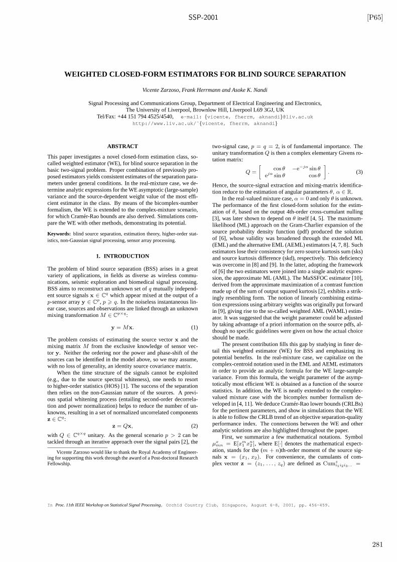
SSP-2001 [P65]
WEIGHTED CLOSED-FORM ESTIMATORS FOR BLIND SOURCE SEPARATION
Vicente Zarzoso, Frank Herrmann and Asoke K. Nandi
Signal Processing and Communications Group, Department of Electrical Engineering and Electronics,The University of Liverpool, Brownlow Hill, Liverpool L69 3GJ, UK
Tel/Fax: +44 151 794 4525/4540,e-mail: {vicente, fherrm, aknandi }@liv.ac.ukhttp://www.liv.ac.uk/˜ {vicente, fherrm, aknandi }
ABSTRACT
This paper investigates a novel closed-form estimation class, so-called weighted estimator (WE), for blind source separation in thebasic two-signal problem. Proper combination of previously pro-posed estimators yields consistent estimates of the separation para-meters under general conditions. In the real-mixture case, we de-termine analytic expressions for the WE asymptotic (large-sample)variance and the source-dependent weight value of the most effi-cient estimator in the class. By means of the bicomplex-numberformalism, the WE is extended to the complex-mixture scenario,for which Cramer-Rao bounds are also derived. Simulations com-pare the WE with other methods, demonstrating its potential.
Keywords: blind source separation, estimation theory, higher-order stat-istics, non-Gaussian signal processing, sensor array processing.
1. INTRODUCTION
The problem of blind source separation (BSS) arises in a greatvariety of applications, in fields as diverse as wireless commu-nications, seismic exploration and biomedical signal processing.BSS aims to reconstruct an unknown set ofq mutually independ-ent source signalsx ∈ C
q which appear mixed at the output of ap-sensor arrayy ∈ C
p, p > q. In the noiseless instantaneous lin-ear case, sources and observations are linked through an unknownmixing transformationM ∈ C
p×q:
y = Mx. (1)
The problem consists of estimating the source vectorx and themixing matrix M from the exclusive knowledge of sensor vec-tor y. Neither the ordering nor the power and phase-shift of thesources can be identified in the model above, so we may assume,with no loss of generality, an identity source covariance matrix.
When the time structure of the signals cannot be exploited(e.g., due to the source spectral whiteness), one needs to resortto higher-order statistics (HOS) [1]. The success of the separationthen relies on the non-Gaussian nature of the sources. A previ-ous spatial whitening process (entailing second-order decorrela-tion and power normalization) helps to reduce the number of un-knowns, resulting in a set of normalized uncorrelated componentsz ∈ C
q:z = Qx, (2)
with Q ∈ Cq×q unitary. As the general scenariop > 2 can be
tackled through an iterative approach over the signal pairs [2], the
Vicente Zarzoso would like to thank the Royal Academy of Engineer-ing for supporting this work through the award of a Post-doctoral ResearchFellowship.
two-signal case,p = q = 2, is of fundamental importance. Theunitary transformationQ is then a complex elementary Givens ro-tation matrix:
Q =
[cos θ −e−jα sin θ
ejα sin θ cos θ
]. (3)
Hence, the source-signal extraction and mixing-matrix identifica-tion reduce to the estimation of angular parametersθ, α ∈ R.
In the real-valued mixture case,α = 0 and onlyθ is unknown.The performance of the first closed-form solution for the estim-ation of θ, based on the output 4th-order cross-cumulant nulling[3], was later shown to depend onθ itself [4, 5]. The maximum-likelihood (ML) approach on the Gram-Charlier expansion of thesource probability density function (pdf) produced the solutionof [6], whose validity was broadened through the extended ML(EML) and the alternative EML (AEML) estimators [4, 7, 8]. Suchestimators lose their consistency for zero source kurtosis sum (sks)and source kurtosis difference (skd), respectively. This deficiencywas overcome in [8] and [9]. In the latter, adopting the frameworkof [6] the two estimators were joined into a single analytic expres-sion, the approximate ML (AML). The MaSSFOC estimator [10],derived from the approximate maximization of a contrast functionmade up of the sum of output squared kurtosis [2], exhibits a strik-ingly resembling form. The notion of linearly combining estima-tion expressions using arbitrary weights was originally put forwardin [9], giving rise to the so-called weighted AML (WAML) estim-ator. It was suggested that the weight parameter could be adjustedby taking advantage of a priori information on the source pdfs, al-though no specific guidelines were given on how the actual choiceshould be made.
The present contribution fills this gap by studying in finer de-tail this weighted estimator (WE) for BSS and emphasizing itspotential benefits. In the real-mixture case, we capitalize on thecomplex-centroid notation used in the EML and AEML estimatorsin order to provide an analytic formula for the WE large-samplevariance. From this formula, the weight parameter of the asymp-totically most efficient WE is obtained as a function of the sourcestatistics. In addition, the WE is neatly extended to the complex-valued mixture case with the bicomplex number formalism de-veloped in [4, 11]. We deduce Cramer-Rao lower bounds (CRLBs)for the pertinent parameters, and show in simulations that the WEis able to follow the CRLB trend of an objective separation-qualityperformance index. The connections between the WE and otheranalytic solutions are also highlighted throughout the paper.
First, we summarize a few mathematical notations. Symbolµx
mn = E[xm1 xn
2 ], where E[·] denotes the mathematical expect-ation, stands for the (m + n)th-order moment of the source sig-nals x = (x1, x2). For convenience, the cumulants of com-plex vectorz = (z1, . . . , zq) are defined asCumz
i1i2i3... =
In Proc. 11th IEEE Workshop on Statistical Signal Processing, Orchid Country Club, Singapore, August 6-8, 2001, pp. 456-459.
281
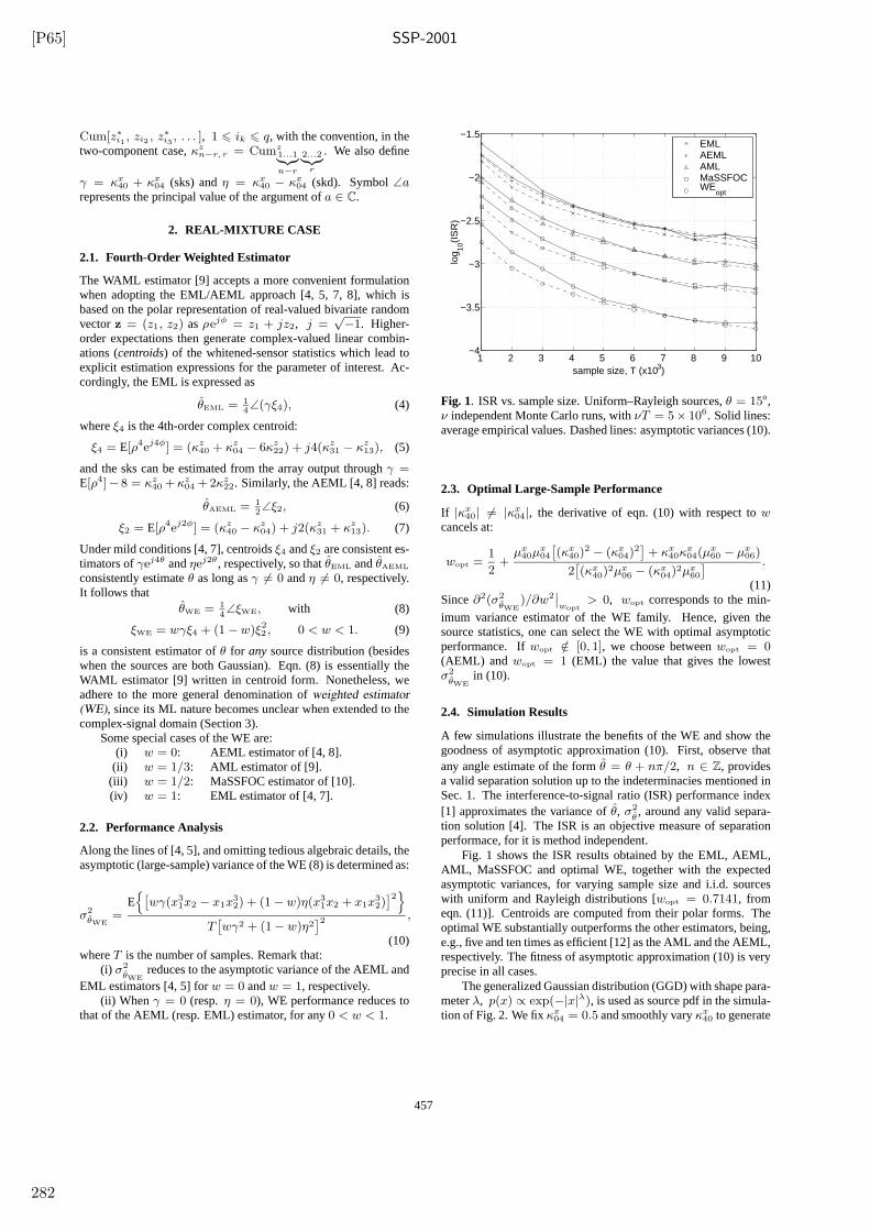
[P65] SSP-2001
Cum[z∗
i1 , zi2 , z∗
i3 , . . . ], 1 6 ik 6 q, with the convention, in thetwo-component case,κz
n−r, r = Cumz1...1︸︷︷︸n−r
2...2︸︷︷︸r
. We also define
γ = κx40 + κx
04 (sks) andη = κx40 − κx
04 (skd). Symbol∠arepresents the principal value of the argument ofa ∈ C.
2. REAL-MIXTURE CASE
2.1. Fourth-Order Weighted Estimator
The WAML estimator [9] accepts a more convenient formulationwhen adopting the EML/AEML approach [4, 5, 7, 8], which isbased on the polar representation of real-valued bivariate randomvectorz = (z1, z2) asρejφ = z1 + jz2, j =
√−1. Higher-
order expectations then generate complex-valued linear combin-ations (centroids) of the whitened-sensor statistics which lead toexplicit estimation expressions for the parameter of interest. Ac-cordingly, the EML is expressed as
θEML = 14∠(γξ4), (4)
whereξ4 is the 4th-order complex centroid:
ξ4 = E[ρ4ej4φ] = (κz40 + κz
04 − 6κz22) + j4(κz
31 − κz13), (5)
and the sks can be estimated from the array output throughγ =E[ρ4]− 8 = κz
40 + κz04 + 2κz
22. Similarly, the AEML [4, 8] reads:
θAEML = 12∠ξ2, (6)
ξ2 = E[ρ4ej2φ] = (κz40 − κz
04) + j2(κz31 + κz
13). (7)
Under mild conditions [4, 7], centroidsξ4 andξ2 are consistent es-timators ofγej4θ andηej2θ, respectively, so thatθEML andθAEML
consistently estimateθ as long asγ 6= 0 andη 6= 0, respectively.It follows that
θWE = 14∠ξWE, with (8)
ξWE = wγξ4 + (1 − w)ξ22 , 0 < w < 1. (9)
is a consistent estimator ofθ for any source distribution (besideswhen the sources are both Gaussian). Eqn. (8) is essentially theWAML estimator [9] written in centroid form. Nonetheless, weadhere to the more general denomination ofweighted estimator
(WE), since its ML nature becomes unclear when extended to thecomplex-signal domain (Section 3).
Some special cases of the WE are:(i) w = 0: AEML estimator of [4, 8].
(ii) w = 1/3: AML estimator of [9].(iii) w = 1/2: MaSSFOC estimator of [10].(iv) w = 1: EML estimator of [4, 7].
2.2. Performance Analysis
Along the lines of [4, 5], and omitting tedious algebraic details, theasymptotic (large-sample) variance of the WE (8) is determined as:
σ2θWE
=E{[
wγ(x31x2 − x1x
32) + (1 − w)η(x3
1x2 + x1x32)
]2}
T[wγ2 + (1 − w)η2
]2 ,
(10)whereT is the number of samples. Remark that:
(i) σ2θWE
reduces to the asymptotic variance of the AEML andEML estimators [4, 5] forw = 0 andw = 1, respectively.
(ii) When γ = 0 (resp.η = 0), WE performance reduces tothat of the AEML (resp. EML) estimator, for any0 < w < 1.
1 2 3 4 5 6 7 8 9 10−4
−3.5
−3
−2.5
−2
−1.5
sample size, T (x103)
log 10
(IS
R)
EML AEML AML MaSSFOC WE
opt
Fig. 1. ISR vs. sample size. Uniform–Rayleigh sources,θ = 15o,ν independent Monte Carlo runs, withνT = 5× 10⁶. Solid lines:average empirical values. Dashed lines: asymptotic variances (10).
2.3. Optimal Large-Sample Performance
If |κx40| 6= |κx
04|, the derivative of eqn. (10) with respect towcancels at:
wopt =1
2+
µx40µ
x04
[(κx
40)2 − (κx
04)2]+ κx
40κx04(µ
x60 − µx
06)
2[(κx
40)2µx
06 − (κx04)
2µx60
] .
(11)Since∂2(σ2
θWE)/∂w2
∣∣wopt
> 0, wopt corresponds to the min-
imum variance estimator of the WE family. Hence, given thesource statistics, one can select the WE with optimal asymptoticperformance. Ifwopt /∈ [0, 1], we choose betweenwopt = 0(AEML) and wopt = 1 (EML) the value that gives the lowestσ2
θWEin (10).
2.4. Simulation Results
A few simulations illustrate the benefits of the WE and show thegoodness of asymptotic approximation (10). First, observe thatany angle estimate of the formθ = θ + nπ/2, n ∈ Z, providesa valid separation solution up to the indeterminacies mentioned inSec. 1. The interference-to-signal ratio (ISR) performance index[1] approximates the variance ofθ, σ2
θ, around any valid separa-
tion solution [4]. The ISR is an objective measure of separationperformace, for it is method independent.
Fig. 1 shows the ISR results obtained by the EML, AEML,AML, MaSSFOC and optimal WE, together with the expectedasymptotic variances, for varying sample size and i.i.d. sourceswith uniform and Rayleigh distributions [wopt = 0.7141, fromeqn. (11)]. Centroids are computed from their polar forms. Theoptimal WE substantially outperforms the other estimators, being,e.g., five and ten times as efficient [12] as the AML and the AEML,respectively. The fitness of asymptotic approximation (10) is veryprecise in all cases.
The generalized Gaussian distribution (GGD) with shape para-meterλ, p(x) ∝ exp(−|x|λ), is used as source pdf in the simula-tion of Fig. 2. We fixκx
04 = 0.5 and smoothly varyκx40 to generate
457
282
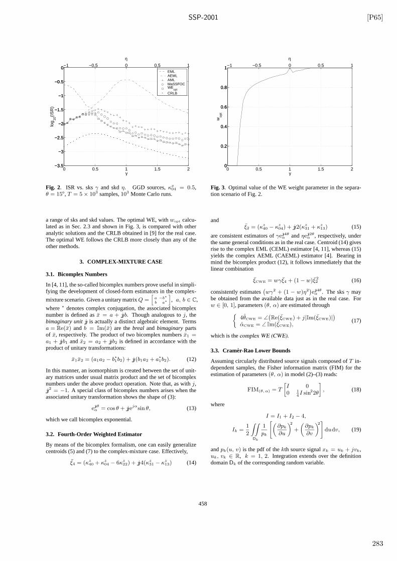
SSP-2001 [P65]
0 0.5 1 1.5 2−3.5
−3
−2.5
−2
−1.5
−1
−0.5
0
γ
log 10
(IS
R)
EMLAEMLAMLMaSSFOCWE
optCRLB
−1 −0.5 0 0.5 1
−3.5
−3
−2.5
−2
−1.5
−1
−0.5
0
η
Fig. 2. ISR vs. sksγ and skdη. GGD sources,κx04 = 0.5,
θ = 15o, T = 5 × 10³ samples,103 Monte Carlo runs.
a range of sks and skd values. The optimal WE, withwopt calcu-lated as in Sec. 2.3 and shown in Fig. 3, is compared with otheranalytic solutions and the CRLB obtained in [9] for the real case.The optimal WE follows the CRLB more closely than any of theother methods.
3. COMPLEX-MIXTURE CASE
3.1. Bicomplex Numbers
In [4, 11], the so-called bicomplex numbers prove useful in simpli-fying the development of closed-form estimators in the complex-
mixture scenario. Given a unitary matrixQ =[
a −b∗
b a∗
], a, b ∈ C,
where∗ denotes complex conjugation, the associated bicomplexnumber is defined asx = a + jb. Though analogous toj, thebimaginary unitj is actually a distinct algebraic element. Termsa = Re(x) and b = Im(x) are thebreal and bimaginarypartsof x, respectively. The product of two bicomplex numbersx1 =a1 + jb1 and x2 = a2 + jb2 is defined in accordance with theproduct of unitary transformations:
x1x2 = (a1a2 − b∗1b2) + j(b1a2 + a∗
1b2). (12)
In this manner, an isomorphism is created between the set of unit-ary matrices under usual matrix product and the set of bicomplexnumbers under the above product operation. Note that, as withj,j2 = −1. A special class of bicomplex numbers arises when theassociated unitary transformation shows the shape of (3):
ejθα = cos θ + jejαsin θ, (13)
which we call bicomplex exponential.
3.2. Fourth-Order Weighted Estimator
By means of the bicomplex formalism, one can easily generalizecentroids (5) and (7) to the complex-mixture case. Effectively,
ξ4 = (κz40 + κz
04 − 6κz22) + j4(κz
31 − κz13) (14)
0 0.5 1 1.5 20
0.2
0.4
0.6
0.8
1
γ
wop
t
−1 −0.5 0 0.5 1
0
0.2
0.4
0.6
0.8
1
η
Fig. 3. Optimal value of the WE weight parameter in the separa-tion scenario of Fig. 2.
andξ2 = (κz
40 − κz04) + j2(κz
31 + κz13) (15)
are consistent estimators ofγej4θα andηej2θ
α , respectively, underthe same general conditions as in the real case. Centroid (14) givesrise to the complex EML (CEML) estimator [4, 11], whereas (15)yields the complex AEML (CAEML) estimator [4]. Bearing inmind the bicomplex product (12), it follows immediately that thelinear combination
ξCWE = wγξ4 + (1 − w)ξ22 (16)
consistently estimates(wγ2 + (1 − w)η2
)ej4θ
α . The sksγ maybe obtained from the available data just as in the real case. Forw ∈ [0, 1], parameters(θ, α) are estimated through
{
4θCWE = ∠(Re(ξCWE) + j|Im(ξCWE)|
)
αCWE = ∠ Im(ξCWE),(17)
which is thecomplex WE (CWE).
3.3. Cramer-Rao Lower Bounds
Assuming circularly distributed source signals composed ofT in-dependent samples, the Fisher information matrix (FIM) for theestimation of parameters(θ, α) in model (2)–(3) reads:
FIM(θ, α) = T
[I 00 1
4I sin22θ
]
, (18)
where
I = I1 + I2 − 4,
Ik =1
2
∫∫
Dk
1
pk
[(∂pk
∂u
)2
+
(∂pk
∂v
)2]
dudv, (19)
andpk(u, v) is the pdf of thekth source signalxk = uk + jvk,uk, vk ∈ R, k = 1, 2. Integration extends over the definitiondomainDk of the corresponding random variable.
458
283
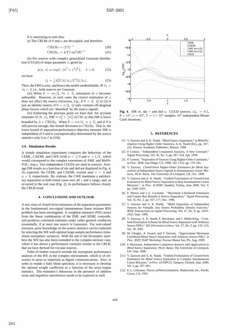
[P65] SSP-2001
It is interesting to note that:(i) The CRLBs ofθ andα are decoupled, and therefore:
CRLBθ = (TI)−1 (20)
CRLBα = 4(TI sin22θ)−1 (21)
(ii) For sources with complex generalized Gaussian distribu-tion (CGGD) of shape parameterλ, given by
p(u, v) ∝ exp{−(u2 + v2)λ2 }, λ > 0, (22)
we haveIk = 1
2λ2
kΓ(4/λk)/Γ2(2/λk). (23)
Then, the FIM is zero, and hence the model unidentifiable, iffλ1 =λ2 = 2, i.e., both sources are Gaussian.
(iii) When θ = nπ/2, ∀n ∈ Z, estimation ofα becomesunfeasible. However, in such cases the correct estimation ofαdoes not affect the source extraction, e.g., ifθ = 0, Q in (3) isjust an identity matrix; ifθ = π/2, Q only contains off-diagonalphase factors which are ‘absorbed’ by the source signals.
(iv) Endorsing the previous point we have that, for accurateestimates of(θ, α), ISR≈ σ2
θ+ 1
4σ2
α sin22θ, so that ISR is lower
bounded by2 × CRLBθ. Whenθ = nπ/2, n ∈ Z, and if θ isstill precise enough, this bound decreases toCRLBθ. That is, thelower bound of separation-performance objective measure ISR isindependent ofθ and is (asymptotically) determined by the sourcestatistics only [viaI in (19)].
3.4. Simulation Results
A simple simulation experiment compares the behaviour of theCEML, CAEML and CWE (withw = 1/3 andw = 1/2 , whichwould correspond to the complex extensions of AML and MaSS-FOC, resp.). Two independent CGGDs are used as sources. Aver-age ISR results as a function of sks and skd are displayed in Fig. 4.As expected, the CEML and CAEML worsen nearγ = 0 andη = 0, respectively. By contrast, the CWE maintains a satisfact-ory separation in both tested cases over allγ andη range, and, asoccurred in the real case (Fig. 2), its performance follows closelythe CRLB trend.
4. CONCLUSIONS AND OUTLOOK
A new class of closed-form estimators of the separation parametersin the fundamental two-signal instantaneous linear mixture BSSproblem has been investigated. A weighted estimator (WE) arisesfrom the linear combination of the EML and AEML centroids,and produces consistent estimates under rather general conditions(essentially, if at most one source is Gaussian). For real-valuedmixtures, prior knowledge on the source statistics can be exploitedby selecting the WE with optimal large-sample performance (min-imum asymptotic variance). With the aid of the bicomplex num-bers the WE has also been extended to the complex-mixture case,where it has shown a performance variation similar to the CRLB,that we have derived for circular sources.
Paths of further research include the asymptotic performanceanalysis of the WE in the complex environment, which is of rel-evance in areas as important as digital communications. Also, inorder to enable a fully blind operation, it is necessary to developthe optimal weight coefficient as a function of the array-outputstatistics. The estimator’s behaviour in the presence of additivenoise and impulsive interference needs to be explored as well.
0 0.5 1 1.5 2−4
−3.5
−3
−2.5
−2
−1.5
−1
−0.5
0
γ
log 10
(IS
R)
CEMLCAEMLCWE (w=1/3)CWE (w=1/2)CRLB
−1 −0.5 0 0.5 1
−4
−3.5
−3
−2.5
−2
−1.5
−1
−0.5
0
η
Fig. 4. ISR vs. sksγ and skdη. CGGD sources,κx04 = 0.5,
θ = 15o, α = 65o, T = 5× 10³ samples,103 independent MonteCarlo iterations.
5. REFERENCES
[1] V. Zarzoso and A. K. Nandi, “Blind Source Separation,” inBlind Es-timation Using Higher-Order Statistics, A. K. Nandi (Ed.), pp. 167–252. Kluwer Academic Publishers, Boston, 1999.
[2] P. Comon, “Independent Component Analysis, A New Concept?,”Signal Processing, Vol. 36, No. 3, pp. 287–314, Apr. 1994.
[3] P. Comon, “Separation of Sources Using Higher-Order Cumulants,”in Proc. SPIE, San Diego, CA, 1989, Vol. 1152, pp. 170–181.
[4] V. Zarzoso, Closed-Form Higher-Order Estimators for Blind Sep-aration of Independent Source Signals in Instantaneous Linear Mix-tures, Ph.D. thesis, The University of Liverpool, UK, Oct. 1999.
[5] V. Zarzoso and A. K. Nandi, “Unified Formulation of Closed-FormEstimators for Blind Source Separation in Real Instantaneous LinearMixtures,” in Proc. ICASSP, Istanbul, Turkey, June 2000, Vol. V,pp. 3160–3163.
[6] F. Harroy and J.-L. Lacoume, “Maximum Likelihood Estimatorsand Cramer-Rao Bounds in Source Separation,”Signal Processing,Vol. 55, No. 2, pp. 167–177, Dec. 1996.
[7] V. Zarzoso and A. K. Nandi, “Blind Separation of IndependentSources for Virtually Any Source Probability Density Function,”IEEE Transactions on Signal Processing, Vol. 47, No. 9, pp. 2419–2432, Sept. 1999.
[8] V. Zarzoso, A. K. Nandi, F. Herrmann, and J. Millet-Roig, “Com-bined Estimation Scheme for Blind Source Separation with ArbitrarySource PDFs,”IEE Electronics Letters, Vol. 37, No. 2, pp. 132–133,Jan. 18, 2001.
[9] M. Ghogho, A. Swami, and T. Durrani, “Approximate MaximumLikelihood Blind Source Separation with Arbitrary Source Pdfs,” inProc. IEEE SSAP Workshop, Pocono Manor Inn, PA, Aug. 2000.
[10] F. Herrmann,Independent Component Analysis with Applications toBlind Source Separation, Ph.D. thesis, The University of Liverpool,UK, Sept. 2000.
[11] V. Zarzoso and A. K. Nandi, “Unified Formulation of Closed-FormEstimators for Blind Source Separation in Complex InstantaneousLinear Mixtures,” inProc. EUSIPCO, Tampere, Finland, Sept. 2000,Vol. I, pp. 597–601.
[12] E. L. Lehmann,Theory of Point Estimation, Wadsworth, Inc., PacificGrove, CA, 1991.
459
284

c© 2009 Vicente Zarzoso

Related Documents