CARDIFF UNIVERSITY School Of Physics and Astronomy BLAST: studying cosmic and Galactic star formation from a stratospheric balloon PhD in Physics and Astronomy Academic Year 2010/2011 Author Supervisor Lorenzo Moncelsi Dr. Enzo Pascale Student Number: 0829637 Co-supervisor Prof. Philip Mauskopf

Welcome message from author
This document is posted to help you gain knowledge. Please leave a comment to let me know what you think about it! Share it to your friends and learn new things together.
Transcript
CARDIFF UNIVERSITY
School Of Physics and Astronomy
BLAST: studying cosmic and Galactic star
formation from a stratospheric balloon
PhD in Physics and Astronomy
Academic Year 2010/2011
Author Supervisor
Lorenzo Moncelsi Dr. Enzo Pascale
Student Number: 0829637 Co-supervisor
Prof. Philip Mauskopf
I
Published Work
Refereed Publications
1. Moncelsi, L., Ade, P. A. R., et al. 2011, ApJ, 727, 83
2. Viero, M. P., Moncelsi, L., et al. 2011, ArXiv 1008.4359
3. Zhang, J., Ade, P. A. R., Mauskopf, P., Savini, G., Moncelsi,
L., & Whitehouse, N. 2011, Appl. Opt., 50, 3750
4. Chapin, E. L., Chapman, S. C., et al. 2011, MNRAS, 411, 505
5. Braglia, F. G., Ade, P. A. R., et al. 2011, MNRAS, 412, 1187
6. Dye, S., Eales, S., Moncelsi, L., & Pascale, E. 2010b, MNRAS,
407, L69
7. Ivison, R. J., Alexander, D. M., et al. 2010a, MNRAS, 402, 245
8. Zhang, J., Ade, P. A. R., Mauskopf, P., Moncelsi, L., Savini, G.,
& Whitehouse, N. 2009, Appl. Opt., 48, 6635
9. Eales, S., Chapin, E. L., et al. 2009, ApJ, 707, 1779
10. Viero, M. P., Ade, P. A. R., et al. 2009, ApJ, 707, 1766
11. Patanchon, G., Ade, P. A. R., et al. 2009, ApJ, 707, 1750
12. Pascale, E., Ade, P. A. R., et al. 2009, ApJ, 707, 1740
13. Marsden, G., Ade, P. A. R., et al. 2009, ApJ, 707, 1729
14. Truch, M. D. P., Ade, P. A. R., et al. 2009, ApJ, 707, 1723
15. Dye, S., Ade, P. A. R., et al. 2009, ApJ, 703, 285
16. Devlin, M. J., Ade, P. A. R., et al. 2009, Nature, 458, 737
II
Notes on Refereed Publications
Where not explicitly highlighted, Moncelsi appears as co-author in
alphabetical order, in concordance with BLAST’s publication policy,
albeit he is not part of the BLAST core team. We point out that
Moncelsi is a major contributor to the analyses carried out in papers
# 1, 2, 9, 12, and 13. As of this thesis’ submission date, the refereed
publications listed above have been cited 462 times.
Conference Proceedings
17. Fissel, L. M., Ade, P. A. R., et al. 2010, in Proceedings of SPIE,
Vol. 7741, Society of Photo-Optical Instrumentation Engineers
(SPIE) Conference Series
18. Bintley, D., Macintosh, M. J., et al. 2010, in Proceedings of SPIE,
Vol. 7741, Society of Photo-Optical Instrumentation Engineers
(SPIE) Conference Series
19. Marsden, G., Ade, P. A. R., et al. 2008, in Proceedings of SPIE,
Vol. 7020, Society of Photo-Optical Instrumentation Engineers
(SPIE) Conference Series
20. Masi, S., Brienza, D., et al. 2007, in 18th ESA Symposium on
European Rocket and Balloon Programmes and Related Research
(ESA)
III
Preface
This thesis is the result of work I have undertaken as a research stu-
dent in the Astronomy Instrumentation Group, School of Physics and
Astronomy, Cardiff University between October 2008 and September
2011. As part of my research, during these three years I have been
deployed on observation and instrument integration campaigns three
times: at the Anglo-Australian Telescope, Siding Spring Observatory,
Australia in November 2008; at the Columbia Scientific Balloon Fa-
cility, Palestine, Texas, USA, in June and July 2010; and at the Long
Duration Balloon (LDB) facility near McMurdo Station, Antarctica,
from November 2010 to January 2011.
Except where otherwise stated and referenced, this thesis solely in-
cludes research carried out by myself in its entirety, or for the most part
if the work was done in collaboration with the BLAST and BLAST-
Pol teams. Neither this thesis nor any similar dissertation has been
submitted for a degree, diploma or other qualification at this or any
other university. This thesis does not exceed 80,000 words in length.
Chapters 2 and 3 of this thesis are largely based on papers # 1
and 2 (as listed in Published Work), respectively. These scientific pro-
ductions are my intellectual property, as I have conducted the largest
part of the analyses described in them. In particular, in paper # 2,
I have performed the stacking analysis, SED fitting, noise estimation
and propagation, which led to the estimates of SFRs and their uncer-
tainties; I have also been a major contributor to the text.
Finally, where applicable, I adopt American English spelling for
consistency with most of the published work.
Lorenzo Moncelsi
IV
Declaration and Statements
Declaration
This work has not previously been accepted in substance for any degree
and is not concurrently submitted in candidature for any degree.
Signed (candidate) Date
Statement 1
This thesis is being submitted in partial fulfillment of the requirements
for the degree of PhD.
Signed (candidate) Date
Statement 2
This thesis is the result of my own independent work/investigation,
except where otherwise stated. Other sources are acknowledged by
explicit references.
Signed (candidate) Date
Statement 3
I hereby give consent for my thesis, if accepted, to be available for
photocopying and for inter-library loan, and for the title and summary
to be made available to outside organizations.
Signed (candidate) Date
V
Acknowledgments
This work is dedicated to Alceo’s son, to whom I am endlessly grateful
for being a stainless example of how to be a man and a father. I extend
my perpetual gratitude to my mother, my sister, my whole family and
Steffi for their never-ending support.
A special appreciation goes to my supervisor Enzo Pascale and to
Giorgio Savini, for never allowing my learning curve to flatten and for
constituting important role models of scientists and expatriates to me.
I thank Peter Ade for having repeatedly instilled in me knowledge
of experimental physics, techniques and crafts. I also wish to thank
him for a very effective catalytic action in my process of integration
with the British (Welsh in particular) idioms, mores and habits.
I also thank Phil Mauskopf, Jin Zhang, Locke Spencer, Frederick
Poidevin, David Nutter, Derek Ward-Thompson, Anthony Whitworth,
Peter Coles, Leonid Grishchuk, Luca Cortese, Simon Dye, Steve Eales,
Matthew Smith, Rashmi Sudiwala, Peter Hargrave, Will Grainger,
Chris North, Ian Walker, Richard Frewin , Nicola Whitehouse, Chris
Dunscombe, Brian Kiernan, Julian House, and Chris Dodd.
I am grateful to the members of the BLAST and BLAST-Pol teams,
and in particular to Marco Viero, Giles Novak, Mark Devlin, Barth
Netterfield, Elio Angile, Jeff Klein, Marie Rex, Matthew Truch, Ed
Chapin, Mark Halpern, Gaelen Marsden, Douglas Scott, Don Wiebe,
Henry Ngo, Juan Diego Soler, Steve Benton, Natalie Gandilo, Laura
Fissel, Jamil Shariff, Guillaume Patanchon, Tristan Matthews, Nick
Thomas, Greg Tucker, and Andrei Korotkov.
I thank all my friends that have brightened up my 3-year-and-a-bit
stay in Cardiff, and in particular Diego Pizzocaro, Giancarlo Russo,
Stefano Larsen, Michele de Benedetti, Riccardo Montana, Piero Volta,

VI
Hillel Raz, Inaki Grau, Panos Papadopoulos, Nasos Dimopoulos,
Achilleas Tziatzios, Tullio Buccellato, Piers Horner, Eduardo Della
Pia, Nicolo Accanto, Daniele Pranzetti, Massimo Granata, Daniele
Carazzo, Matt Williams, Ahmed Alazzawi, Konrad Borowiecki, Feder-
ica Pinto, Baljinder Bains, Barbara Torrisi, Lydia Lagartija, Ieva Bisi-
girskaite, Pilar Clemente-Fernandez, Vanessa Stroud, Carolyn Mur-
phy, Raul Gonzalez, and Yiannis Kouropalatis.
Thanks to all the metal bands I listen to, for the energy they instill
in me every day and for sparing me from useless chatters and noisy
machines in the lab. A special appreciation goes to Kai Hansen and
Gamma Ray for accompanying my “journey through space and time”
since 1997.
Thanks to atheists, basketball, ShopRight, coffee, NBA Live 2007,
Skype, and VLC. Thanks to Lenovo for my fellow traveler T61, which
has endured years of hard work, even if I needed to swap its mother-
board a couple of months before finishing.

VII
To my fellow time-travelers
If there’s a possible chance for something that can be
called future behind the spiral
the only way to find out is to leave the final frontier
to eternity and fly
I will fly - beyond the gates of space and time
I leave the Universe behind
and I can’t wait until tomorrow
Fly - beyond the gates of space and time
I know the Universe is mine
’cause I will dive into the black hole
Ride - and there’s a call from deep within
I know I won’t return again
’cause I will dive into the black hole
from “Beyond the black hole”
“Somewhere out in space”
Gamma Ray (1997)
VIII
Thesis Summary/Abstract
Understanding the history of the formation of stars and evolution of
galaxies is one of the foremost goals of astrophysics. While stars emit
most of their energy at visible and ultraviolet wavelengths, during the
early stages of star formation these photons are absorbed by the dusty
molecular clouds that host and fuel the emerging stars, and re-emitted
as thermal radiation at infrared and submillimeter wavelengths.
The Balloon-borne Large Aperture Submillimeter Telescope
(BLAST) was designed to study the history of obscured star forma-
tion in galaxies at cosmological distances and witness the details of
the star-formation processes in our own Galaxy, by conducting large-
area surveys of the sky at 250, 350, and 500�m from a long-duration
stratospheric balloon platform. Its polarimetric adaptation, BLAST-
Pol, will allow us to further probe the strength and morphology of
magnetic fields in dust-enshrouded star-forming molecular clouds in
our Galaxy. The study of these two diverse, yet highly complemen-
tary, topics is the primary scientific motivation for this thesis, which
is in two parts.
Part One is concerned with the analysis of a combination of the
extragalactic dataset collected by BLAST in the 2006 Antarctic cam-
paign, which comprises maps containing hundreds of distant, highly
dust-obscured, and actively star-forming galaxies, with a wealth of
ancillary multi-wavelength data spanning the radio to the ultravio-
let. The star-formation rates we observe in massive galaxies at high
redshift support downsizing and size evolution.
Part Two describes the BLAST-Pol instrument. In particular, we
focus on the gondola’s primary pointing sensors, the star cameras, and
on the design, manufacture and characterization of a polarization
IX
modulation scheme, comprising a cryogenic achromatic half-wave plate
and photolithographed polarizing grids, which has been effectively
retrofitted on BLAST-Pol.
We report on the construction and deployment of BLAST-Pol,
which completed its first successful 9.5-day flight over Antarctica in
January 2011 and mapped ten science targets with unprecedented
combined mapping speed, sensitivity, and resolution.
X
List of Abbreviations and Acronyms
AAO: AAOmega, spectrograph at the Anglo-Australian telescope
ADC: analog-to-digital converter
ADM: artificial dielectric metamaterial
ADU: analog-to-digital unit
ARC: anti-reflection coating
AGN: active galactic nucleus
BDA: bolometer detector array
BLAST: balloon-borne large aperture submillimeter telescope
CCD: charge-coupled device
CDFS: Chandra deep-field south
CSBF: Columbia scientific balloon facility
CIB: cosmic infrared background
CMF: prestellar core mass function
COB: cosmic optical background
CMB: cosmic microwave background
Dec: declination, �
ECDFS: extended Chandra deep-field South
EBL: extragalactic background light
EW: equivalent width
FIR: far-infrared
FOV: field of view
FTS: Fourier transform spectrometer
FUV: far-ultraviolet
FWHM: full width at half maximum
GMC: giant molecular cloud
HWP: half-wave plate
ID: counterpart
XI
IMF: stellar initial mass function
ISM: interstellar medium
L⊙ = 3.839× 1026W: solar luminosity
LDB: long duration balloon
LIRG: luminous infrared galaxy
LM: Lorenzo Moncelsi
M★: stellar mass
M⊙ = 1.98892× 1030 kg: solar mass
MIR: mid-infrared
mm: millimeter
NEP: noise equivalent power
NEFD: noise equivalent flux density
NIR: near-infrared
NUV: near-ultraviolet
P10: photolithographed polarizer (5�m copper strips and 5�m gaps)
PAH: polycyclic aromatic hydrocarbon
PSF: point-spread function
PTFE: polytetrafluoroethylene
QSO: quasi-stellar object
RA: right ascension, �
ROI: region of interest
rms: root mean square
SCUBA: submillimetre common-user bolometer array
SED: spectral energy distribution
SFR: star-formation rate
SNR: signal-to-noise ratio
SSFR: specific star-formation rate
submm: submillimeter
ULIRG: ultra-luminous infrared galaxy
CONTENTS
Published Work . . . . . . . . . . . . . . . . . . . . . . . . . . . I
Preface . . . . . . . . . . . . . . . . . . . . . . . . . . . . . . . III
Declaration and Statements . . . . . . . . . . . . . . . . . . . . IV
Acknowledgements . . . . . . . . . . . . . . . . . . . . . . . . . V
Thesis Summary/Abstract . . . . . . . . . . . . . . . . . . . . . VIII
List of Abbreviations and Acronyms . . . . . . . . . . . . . . . X
Contents . . . . . . . . . . . . . . . . . . . . . . . . . . . . . . . XII
1. Introduction . . . . . . . . . . . . . . . . . . . . . . . . . . . 1
1.1 Extragalactic Science Case . . . . . . . . . . . . . . . . 5
1.1.1 The dust-obscured Universe . . . . . . . . . . . 5
1.1.2 Galaxy formation and evolution . . . . . . . . . 6
1.1.3 Resolving the FIR background . . . . . . . . . . 8
1.1.4 A luminous population of submm galaxies at
high-z . . . . . . . . . . . . . . . . . . . . . . . 9
1.1.5 The assembly of massive galaxies . . . . . . . . 10
1.2 Galactic Science Case . . . . . . . . . . . . . . . . . . . 12
1.2.1 Background . . . . . . . . . . . . . . . . . . . . 12
Contents XIII
1.2.2 Previous work: Zeeman measurements, stellar
polarimetry, FIR and submm–mm polarimetry . 16
1.2.3 Mapping the large-scale magnetic fields in star-
forming clouds with BLAST-Pol . . . . . . . . . 20
1.2.3.1 Structure lifetimes . . . . . . . . . . . 20
1.2.3.2 Core morphology . . . . . . . . . . . . 22
1.2.3.3 Magnetic field strength . . . . . . . . . 22
1.2.4 The FIR/submm polarization spectrum . . . . . 24
1.2.5 Overview of the BLAST-Pol observations . . . . 27
1.3 Thesis Overview . . . . . . . . . . . . . . . . . . . . . . 28
1.3.1 LM’s contribution to the BLAST and BLAST-
Pol projects . . . . . . . . . . . . . . . . . . . . 32
1.3.2 Other work . . . . . . . . . . . . . . . . . . . . 34
Part One . . . . . . . . . . . . . . . . . . . . . . . . . . . . . . 36
2. A multi-wavelength study of BLAST counterparts . . . . . . 37
2.1 Introduction . . . . . . . . . . . . . . . . . . . . . . . . 37
2.2 Data . . . . . . . . . . . . . . . . . . . . . . . . . . . . 43
2.2.1 Submillimeter data . . . . . . . . . . . . . . . . 43
2.2.2 Optical spectroscopy . . . . . . . . . . . . . . . 44
2.2.3 UV data . . . . . . . . . . . . . . . . . . . . . . 50
2.2.4 SWIRE 70 and 160�m MIPS maps . . . . . . . 51
2.2.5 MIR/NIR/optical images and catalogs . . . . . 51
2.2.6 Redshifts . . . . . . . . . . . . . . . . . . . . . 52
2.3 FIR Luminosities and SFRs . . . . . . . . . . . . . . . 56
2.3.1 Deboosting the BLAST fluxes . . . . . . . . . . 56
2.3.2 SED fitting and FIR luminosities . . . . . . . . 59
2.3.3 FIR star-formation rates . . . . . . . . . . . . . 63
2.4 UV Luminosities and SFRs . . . . . . . . . . . . . . . 66
Contents XIV
2.4.1 UV fluxes and rest-frame luminosities . . . . . . 66
2.4.2 UV star-formation rates . . . . . . . . . . . . . 67
2.5 Total SFRs . . . . . . . . . . . . . . . . . . . . . . . . 69
2.6 AGN Fraction and Quasars . . . . . . . . . . . . . . . 73
2.7 Morphology . . . . . . . . . . . . . . . . . . . . . . . . 75
2.8 Stellar Masses . . . . . . . . . . . . . . . . . . . . . . . 77
2.9 Concluding Remarks . . . . . . . . . . . . . . . . . . . 85
3. Measuring star formation in massive high-z galaxies . . . . . 89
3.1 Introduction . . . . . . . . . . . . . . . . . . . . . . . . 89
3.2 Data . . . . . . . . . . . . . . . . . . . . . . . . . . . . 91
3.2.1 Mass-selected catalog . . . . . . . . . . . . . . . 91
3.2.2 Spitzer . . . . . . . . . . . . . . . . . . . . . . . 93
3.2.3 PACS . . . . . . . . . . . . . . . . . . . . . . . 93
3.2.4 BLAST . . . . . . . . . . . . . . . . . . . . . . 95
3.2.5 LABOCA . . . . . . . . . . . . . . . . . . . . . 95
3.3 Method . . . . . . . . . . . . . . . . . . . . . . . . . . 95
3.3.1 Stacking formalism . . . . . . . . . . . . . . . . 95
3.3.2 Testing the Poisson hypothesis . . . . . . . . . . 97
3.3.3 SED fitting, IR luminosities, and star-formation
rates . . . . . . . . . . . . . . . . . . . . . . . . 100
3.4 Results . . . . . . . . . . . . . . . . . . . . . . . . . . . 102
3.4.1 Stacking results . . . . . . . . . . . . . . . . . . 102
3.4.2 Contribution of stellar emission . . . . . . . . . 103
3.4.3 Best-fit SEDs and star-formation rates . . . . . 104
3.5 Discussion . . . . . . . . . . . . . . . . . . . . . . . . . 107
3.5.1 Consequences for galaxy growth . . . . . . . . . 107
3.5.2 Potential contribution from other sources of dust
heating . . . . . . . . . . . . . . . . . . . . . . . 108
Contents XV
3.5.3 Red and dead? . . . . . . . . . . . . . . . . . . 108
3.6 Concluding Remarks . . . . . . . . . . . . . . . . . . . 110
Part Two . . . . . . . . . . . . . . . . . . . . . . . . . . . . . . 112
4. The BLAST-Pol Instrument . . . . . . . . . . . . . . . . . . 113
4.1 Introduction . . . . . . . . . . . . . . . . . . . . . . . . 113
4.2 Optical Design . . . . . . . . . . . . . . . . . . . . . . 115
4.3 Detectors . . . . . . . . . . . . . . . . . . . . . . . . . 119
4.4 Cryogenics . . . . . . . . . . . . . . . . . . . . . . . . . 121
4.5 Polarimetry . . . . . . . . . . . . . . . . . . . . . . . . 121
4.5.1 Polarization recovery strategy . . . . . . . . . . 122
4.5.2 Polarimeter design . . . . . . . . . . . . . . . . 124
4.6 Gondola . . . . . . . . . . . . . . . . . . . . . . . . . . 129
4.7 Star Cameras . . . . . . . . . . . . . . . . . . . . . . . 132
4.7.1 Overview . . . . . . . . . . . . . . . . . . . . . 132
4.7.2 Bad/hot pixels . . . . . . . . . . . . . . . . . . 139
4.7.3 Noise model . . . . . . . . . . . . . . . . . . . . 140
4.7.4 Post-flight pointing reconstruction . . . . . . . . 146
4.8 Concluding Remarks . . . . . . . . . . . . . . . . . . . 150
5. Half Wave Plate and Polarimetry . . . . . . . . . . . . . . . 153
5.1 Introduction . . . . . . . . . . . . . . . . . . . . . . . . 153
5.2 The BLAST-Pol Half-Wave Plate . . . . . . . . . . . . 154
5.2.1 Birefringent wave plates . . . . . . . . . . . . . 154
5.2.2 Achromatic half-wave plate design . . . . . . . . 156
5.2.3 HWP manufacture . . . . . . . . . . . . . . . . 160
5.2.4 Anti-reflection coating . . . . . . . . . . . . . . 167
5.2.4.1 Old recipes: high-n powders and loaded
ceramics . . . . . . . . . . . . . . . . . 168
Contents XVI
5.2.4.2 New recipes: artificial dielectric meta-
materials . . . . . . . . . . . . . . . . 169
5.2.5 Spectral characterization . . . . . . . . . . . . . 170
5.2.5.1 Introduction . . . . . . . . . . . . . . 170
5.2.5.2 Room-temperature measurements . . . 171
5.2.5.3 Cold measurements . . . . . . . . . . . 177
5.2.6 Mueller matrix characterization . . . . . . . . . 187
5.3 Polarizing Grids . . . . . . . . . . . . . . . . . . . . . . 205
5.4 Concluding Remarks . . . . . . . . . . . . . . . . . . . 209
6. The BLAST-Pol map-maker . . . . . . . . . . . . . . . . . . 214
6.1 Introduction . . . . . . . . . . . . . . . . . . . . . . . . 214
6.2 Maximum Likelihood Map-making . . . . . . . . . . . 215
6.3 Naive Binning . . . . . . . . . . . . . . . . . . . . . . . 220
6.4 Weights and Uncertainties . . . . . . . . . . . . . . . . 224
6.5 Preliminary Maps . . . . . . . . . . . . . . . . . . . . . 225
6.6 Concluding Remarks . . . . . . . . . . . . . . . . . . . 227
6.7 Future Work . . . . . . . . . . . . . . . . . . . . . . . . 228
7. Conclusions . . . . . . . . . . . . . . . . . . . . . . . . . . . 234
7.1 Future Work . . . . . . . . . . . . . . . . . . . . . . . . 238
Appendix 239
A. Stacking Analysis . . . . . . . . . . . . . . . . . . . . . . . . 240
A.1 Introduction . . . . . . . . . . . . . . . . . . . . . . . . 240
A.2 Mathematical Formalism . . . . . . . . . . . . . . . . . 242
A.3 Aperture Photometry Method . . . . . . . . . . . . . . 245
A.4 Uncertainties . . . . . . . . . . . . . . . . . . . . . . . 249
A.5 Catalogs . . . . . . . . . . . . . . . . . . . . . . . . . . 251
Contents XVII
A.6 Post-flight Pointing Verification . . . . . . . . . . . . . 252
B. Postage Stamps of BLAST Counterparts . . . . . . . . . . . 256
C. Catalogs of BLAST Counterparts . . . . . . . . . . . . . . . 262
Bibliography . . . . . . . . . . . . . . . . . . . . . . . . . . . . 281
1. INTRODUCTION
Understanding how the early Universe evolved into the structures that
are observed today is one of the foremost goals of astrophysics and
experimental cosmology. In particular, the history of the formation
of stars and evolution of galaxies is not fully understood yet. While
stars emit most of their energy in the visible (optical) and ultraviolet
(UV) part of the electromagnetic spectrum, during the early stages of
star formation this radiation is absorbed and obscured by the dusty
molecular clouds that host and fuel the emerging stars. The dust
is heated to tens of kelvin, generating thermal emission at infrared
(IR) wavelengths. Regions that are luminous at these wavelengths
indicate active in-situ star formation, which in turn is often associated
with dynamical stages in galactic evolution. When this thermal IR
emission has originated in distant galaxies, the light is stretched by
the expansion of the Universe and reaches an observer on Earth as
submillimeter (submm) and millimeter (mm) radiation.
From an observational point of view, surveys in the optical have
enjoyed a head-start of several decades, and pioneered the field since
the derivation of Hubble’s (1929) law. However, thanks to the rela-
tively recent advances in IR and submm–mm instrumentation, Galac-
tic and extragalactic observations have started to incorporate these
longer wavelengths in the search for a more complete understanding
of the formation of structures in the Universe. Impressive headway
has been made in the past three decades by conducting surveys of
1. Introduction 2
the sky at IR and submm–mm wavelengths within our Galaxy, in
nearby galaxies that populate the local Universe, and in galaxies at
cosmological distances. These observations provide a highly comple-
mentary picture to those carried out at much shorter wavelengths in
the optical, and have been proven to be fundamental to investigate the
physical processes associated with star formation and galaxy evolution
(e.g., Hildebrand 1983, Helou et al. 1985, Rowan-Robinson et al. 1991,
Puget et al. 1996, Smail et al. 1997, Schlegel et al. 1998, Fixsen et al.
1998, Hughes et al. 1998, Genzel et al. 1998, Calzetti et al. 2000).
Most of these ground-breaking findings resulted from data acquired
with space-based observatories, namely the Infrared Astronomical Satel-
lite (IRAS; Neugebauer et al. 1984), the Cosmic Background Explorer
(COBE; Boggess et al. 1992), and the Infrared Space Observatory
(ISO; Kessler et al. 1996). The necessity for geocentrically orbiting
telescopes was dictated by the fact that observations from the ground
are impaired by the atmosphere being opaque over much of the wave-
length range from 20�m to 1mm, with only the 850�m atmospheric
window having routine transmission of over 50%. In fact, this band
has been effectively exploited with the Submillimetre Common-User
Bolometer Array (SCUBA; Holland et al. 1999) to discover a popu-
lation of distant, extremely luminous, heavily dust-enshrouded, star-
burst galaxies (Hughes et al. 1998, Barger et al. 1998).
In the last decade, three other IR and submm–mm space obser-
vatories have started operations in far-Earth orbits, which expose
the telescopes much less to Earth’s heat load hence prolonging their
mission lifetimes: the Spitzer Space Telescope (Werner et al. 2004),
placed in heliocentric Earth-trailing orbit since 2003; and the Her-
schel Space Observatory (Pilbratt et al. 2010) along with the Planck
satellite (Planck Collaboration 2011), which entered a Lissajous orbit
1. Introduction 3
around the second Lagrangian point (L2) of the Earth-Sun system in
mid-2009. Some of the data and results obtained by the former two
observatories are used and referenced, respectively, in this thesis, as
they are highly relevant to our study.
Naturally, space-based missions bring economic burden on the space
agencies, and typically require two decades of work between concep-
tion and deployment; as a consequence, state-of-the-art technologies
and components are not easily implemented aboard these payloads,
because they increase the risk of jeopardizing the entire mission. A
much less expensive alternative to satellites are long-duration balloon
(LDB) platforms, which float for 4–15 days at stratospheric altitudes
of ∼40 km to provide > 99% atmospheric transparency in the far-IR
(FIR) and submm bands. Balloon-borne payloads have been used
since the 1960s as precursors to space-based instruments, since the
much shorter timescales of realization as well as the limited budget
requirements allow greater flexibility in terms of components used and
experimental proofs of concept.
The Balloon-borne Large Aperture Submillimeter Telescope (BLAST;
Devlin et al. 2004, Pascale et al. 2008), a forerunner of the SPIRE pho-
tometer (Griffin et al. 2010) aboard Herschel, was designed to conduct
confusion-limited and wide-area extragalactic and Galactic surveys at
submm wavelengths from a LDB platform. The sky is mapped by
BLAST with a 1.8m primary mirror and re-imaged onto the focal-
plane arrays, composed of 280 bolometric detectors; these provide si-
multaneous photometric measurements at 250, 350, and 500�m with
diffraction-limited resolutions of 30–60′′, over an 88 square arcminute
field of view. The recent conversion of BLAST into a polarimeter,
BLAST-Pol (see Chapter 4), will allow us to further probe the ear-
liest, highly obscured stages of star formation, and in particular the
1. Introduction 4
inherent role of magnetic fields, via the polarized submm emission
from aligned elongated dust grains. As described in more detail in
Section 4.1, BLAST has had three LDB flights: a 4-day flight from
Kiruna, Sweden in June 2005 (BLAST05); a 11-day flight over Antarc-
tica in December 2006 (BLAST06); and a 9.5-day flight, again over
Antarctica, in December 2010 (BLAST-Pol).
BLAST has had and will continue to have a cardinal impact on
the scientific community since the publication of its first results in
2008. Not only have the BLAST analyses provided a very valuable
benchmark for those that are emerging from space observatories such
as Herschel, but its results and some of the state-of-the-art technologies
implemented on the payload will probably stand the test of time.
The research presented in this thesis combines the reduction and
interpretation of astrophysical data with the design, manufacture and
characterization of astronomical instrumentation. We therefore divide
the thesis in two Parts.
Part One is concerned with the analysis and interpretation of a
combination of the BLAST06 primary extragalactic dataset, which
comprises maps containing hundreds of distant, highly dust-obscured,
and actively star-forming galaxies, with a series of multi-wavelength
data spanning the radio to the UV. Part One also reports a challenging
mid-IR (MIR) to submm measurement of the level of star formation
in optically-selected compact massive galaxies at high redshift.
Part Two describes the experimental work carried out during the
construction and deployment of BLAST-Pol, which is aimed at prob-
ing the earliest stages of star formation by measuring the strength and
morphology of magnetic fields in dust-enshrouded star-forming regions
in our own Galaxy. The study of these two diverse, yet highly com-
plementary, topics is the primary scientific motivation for this thesis.
1. Introduction 5
In the following, we outline in greater detail the scientific moti-
vations for the BLAST extragalactic survey (Section 1.1) and the
BLAST-Pol Galactic survey (Section 1.2); finally, Section 1.3 gives
an overview of the thesis’ structure and content, as well as a brief ac-
count of the contribution brought by Lorenzo Moncelsi (LM) to the
BLAST and BLAST-Pol projects.
1.1 Extragalactic Science Case
1.1.1 The dust-obscured Universe
Observational evidence suggests that much of the ongoing star forma-
tion in the Universe takes place in a dusty, heavily-obscured interstel-
lar medium (ISM), at all epochs (Rowan-Robinson et al. 1997, Hauser
et al. 1998, Dwek et al. 1998, Blain et al. 1999b, Chary & Elbaz 2001,
Le Floc’h et al. 2005, Chapman et al. 2005, Dye et al. 2008, Pascale
et al. 2009). When the Universe was less than 10% of its current-age,
galaxies had already formed from the first generations of stars, which
then proceeded to enrich (pollute) the primeval ISM with metals and
the other by-products of star formation, such as amorphous silicate
and carbonaceous dust grains (Rowan-Robinson 1986, Draine 2003).
The prime observable for understanding galaxy formation and evo-
lution is the star-formation rate (SFR). In particular, the most sensible
approach to measure the SFR of a galaxy is to estimate the number of
massive stars, as they are short-lived and thus only present during the
phases of active star formation in a galactic system. The rest-frame
optical–UV emission from young, massive stars is usually “reddened”
by dust, often partially extinguished, and sometimes even completely
obscured (optically thick; Savage & Mathis 1979, Mathis 1990, Calzetti
et al. 2000). On the other hand, observations at rest-frame FIR wave-
1. Introduction 6
lengths provide an almost transparent view (optically thin) into the
cores of star-forming molecular clouds by tracing the thermal signature
of heated dust. The FIR has opened a new window on the Universe,
with its ability to detect violent star-formation activity in dusty and
gas1-rich galaxies (Genzel et al. 1998), which can be missed in even the
most sensitive rest-frame optical–UV searches with the Hubble Space
Telescope (HST) and ground-based 10-m class telescopes.
In addition, at high redshift (z) the effect of cosmological dimming
is partially compensated in the submm–mm bands by the shift in peak
wavelength of a galaxy’s spectral energy distribution (SED), an effect
referred to as “negative K-correction” (e.g., Blain et al. 2002; see also
Figure 2.7); this allows submm–mm wavelength observations to trace
the evolution of star formation in dusty galaxies throughout a large
volume of the high-redshift Universe.
1.1.2 Galaxy formation and evolution
In the original optical morphological classification scheme (or sequence)
of galaxies introduced by Hubble (1926), there are two main types
of galaxies: the ellipticals (or “early-type”) and the spirals (or “late-
type”). While elliptical galaxies are typically red, gas-poor and harbor
an old, evolved stellar population, spiral galaxies are blue, with a dom-
inant population of young stars, and contain large amounts of gas and
dust (“red” and “blue” refer to the galaxy’s optical colors; see e.g.,
Bell et al. 2004). Although this is a rather simplistic scheme, it does
suggest that galaxies of distinct morphologies have different ages and
have likely formed and evolved diversely.
The currently most successful picture for galaxy formation and evo-
1 In the context of galaxy structure, we refer to “gas” as interstellar gas, which by mass iscomposed of about 75% hydrogen (either in ionic [H II], atomic [H I], or molecular [H2] form), andof ∼23–24% helium plus a few percent of heavier elements (“metals”).
1. Introduction 7
lution is the model of hierarchical structure formation (e.g., Press &
Schechter 1974), where galaxies are assembled through mergers and
accretion of smaller galaxies. This paradigm is often realized through
N-body simulations and “semi-analytic” models, which make assump-
tions about the astrophysical processes at work in galaxy evolution
and then predict the observational consequences. These models were
initially developed to explain optical and near-IR (NIR) observations,
take a representative set of dark-matter halos that evolve and merge
over cosmic time, and determine their star-formation histories using a
set of indicators for star formation and feedback from active galactic
nuclei (AGN) and supernovae (e.g., White & Frenk 1991, Kauffmann
et al. 1993, Guiderdoni et al. 1998, Somerville & Primack 1999, Cole
et al. 2000, Khochfar & Burkert 2003, Khochfar & Silk 2006).
Submm astronomy offers unique advantages and opportunities to
confront the competing theoretical models (accretion by cold gas streams
[Dekel et al. 2009] and minor mergers [e.g., Dave et al. 2010], versus
major mergers [e.g., Narayanan et al. 2010, Engel et al. 2010]), refine
the empirical relationships (e.g., Ivison et al. 2010a,b), and test the
accepted scenarios that compose our current knowledge of the physi-
cal processes that drive the initial formation of structure and control
its subsequent evolution into the galaxies and clusters that we see
today (e.g., Amblard et al. 2011, Marsden et al. 2011). In particu-
lar, some authors have recently started to incorporate in their semi-
analytic models observables from submm astronomy, such as average
galaxy SEDs, luminosity functions, galaxy counts, and redshift distri-
butions (e.g., Hatton et al. 2003, Lacey et al. 2008, Swinbank et al.
2008, Gonzalez et al. 2011). As more information becomes available,
the full capabilities of semi-analytic models will hopefully be applied
to derive stronger constraints on dusty galaxy evolution.
1. Introduction 8
1.1.3 Resolving the FIR background
Further constraints to the above models can be imposed by the ob-
servational evidence that a major fraction (∼50%) of the energy in
the Extragalactic Background Light (EBL; excluding the Cosmic Mi-
crowave Background [CMB] that permeates the Universe with a pho-
ton density of about 410 cm−3) is emitted at MIR to mm wavelengths
(Puget et al. 1996, Fixsen et al. 1998). The EBL arises from the in-
tegrated luminosity due to star formation and AGN activity within
all galaxies over the entire history of the Universe. The IR portion of
the EBL, usually referred to as Cosmic Infrared Background (CIB),
is broadly interpreted as evidence that half of the total UV–optical
emission from stars and nuclear accretion disks, which in turn makes
up the Cosmic Optical Background (COB; Bernstein et al. 2002), is
effectively absorbed by dust grains in the ISM of galaxies over a wide
range of redshifts, and then re-radiated at longer wavelengths (Hauser
et al. 1998, Dwek et al. 1998). This produces a broad peak in the SED
of the EBL at about 200�m, whose integrated energy budget equals
that of the COB at shorter wavelengths (e.g., Dole et al. 2006).
One of the main goals of FIR–mm cosmological surveys, including
those undertaken with BLAST, is to “resolve” this diffuse extragalac-
tic FIR–mm background by identifying the individual dusty galaxies
that contribute to the integrated CIB emission. Studying the sources
that make up the CIB can help us determine the evolutionary history
of obscured star formation at high-z and the mechanism of the as-
sembly of massive galaxies, their nature and physical properties. As
detailed in the introduction to Chapter 2, the analyses performed by
the BLAST team by combining submm maps with external multi-
wavelength source catalogs have in fact resolved the long-wavelength
side of the CIB into individual sources detected at 24�m with flux
1. Introduction 9
density2 ≳ 20�Jy (Devlin et al. 2009, Marsden et al. 2009, Pascale
et al. 2009). The methodology used to achieve these results goes un-
der the name of “stacking analysis”, for which we extensively describe
the mathematical formalism and the perfected technicalities in Ap-
pendix A; we also employ this technique in Chapter 3 to make a chal-
lenging measurement of the level of star formation in optically-selected
massive galaxies at high-z.
1.1.4 A luminous population of submm galaxies at high-z
During the last 15 years, the SCUBA camera on the 15-m James Clerk
Maxwell Telescope (JCMT) and the Max Planck Millimetre Bolome-
ter Array (MAMBO; Kreysa et al. 1998) on the 30-m Institut de Ra-
dio Astronomie Millimetrique (IRAM) telescope have allowed a series
of ground-breaking surveys of the extragalactic sky at 850�m and
1.2mm, respectively, covering a combined area < 1 deg2.
These observations led to the important discovery of a luminous
population of high-redshift, optically-obscured, dusty starburst galax-
ies (e.g., Smail et al. 1997, Hughes et al. 1998, Scott et al. 2002, Greve
et al. 2004). Preliminary measurements of the redshift distribution of
this new dust-enshrouded submm population, based on optical and IR
spectroscopic and rest-frame radio–FIR photometric data (e.g., Chap-
man et al. 2003, 2005, Aretxaga et al. 2003, 2005), confirmed the ex-
pected high-redshifts of these galaxies (zmedian ∼2.4, with 50% of the
sources between 1.9 < z < 2.8). The inherent bias in the method by
which the faint optical and/or IR counterparts are frequently identi-
fied leaves open the possibility that a significant fraction of the submm
population could reside at z ≳ 3. The demonstration that the major-
2 Throughout this thesis we make use of the Jansky (Jy) as a (non-SI) unit of flux density,expressed as Jy = 10−26 W
m2 Hz .
1. Introduction 10
ity of the submm population are at z > 1 implies that these galaxies
are extremely luminous in the rest-frame FIR (LFIR ≳ 1012L⊙).
Therefore, these extragalactic submm surveys have identified sites
of powerful star formation (with rates ≫ 200M⊙ yr−1) in the early
Universe, which are believed to be associated with an epoch during
which massive galaxies were assembled. The integrated resolved emis-
sion from these individual submm sources contributes ∼30–100% of
the extragalactic background at 850�m (Blain et al. 1999a) and 20–
30% of the diffuse FIR background that peaks at ∼200�m (Coppin
et al. 2006, Dye et al. 2007). A key goal of observational cosmology in
recent years has been to understand the evolutionary history of this
newly discovered high-redshift submm galaxy population.
1.1.5 The assembly of massive galaxies
It has become clear in recent years (Marchesini et al. 2009) that about
half of the stellar mass (M★) in galaxies in our Universe has formed
over the last 7.5Gyr (0 < z < 1). However, the details of how the mass
has been assembled and what physical processes were involved at early
stages of galaxy evolution remain unclear. Although models of galaxy
formation predict that galaxies form hierarchically, observations in
the optical indicate “downsizing”, with high-mass galaxies assembling
their stellar mass earlier than low-mass systems, and that the redshift
at which star-formation activity peaks is a monotonically increasing
function of the final stellar mass (Heavens et al. 2004). The best
observable known to date for studying downsizing and mass assembly
is the Specific Star-Formation Rate (SSFR; Brinchmann et al. 2004),
the ratio between the instantaneous SFR in a galaxy and the stellar
mass integrated over the galaxy’s history. The SSFR, as observed
in the optical and NIR, increases with z at a rate independent of
1. Introduction 11
mass (Damen et al. 2009). Also, SSFRs of more massive galaxies are
typically lower than those of less massive galaxies out to redshift z ∼ 2.
This behavior has been very recently observed in FIR/submm-
selected galaxies with BLAST (see Chapter 2) andHerschel (Rodighiero
et al. 2010), again out to z ∼ 2. Therefore, the downsizing pattern
seems to be at work up to relatively high redshift, for samples of
galaxies selected both in the optical/NIR and in the FIR/submm. We
are urged to study whether downsizing still occurs in mass-assembling
galaxies at very high redshift (z ≳ 3). Could it be just a selection
effect? How does it relate to the high molecular gas fractions observed
in distant massive star-forming galaxies (Genzel et al. 2006, Tacconi
et al. 2006, 2008, 2010)?
At slightly higher redshift (1.7 < z < 2.9), recent follow-up obser-
vations at submm wavelengths of an optically-selected sample of mas-
sive galaxies (M★ ≥ 1011M⊙), detected with the Near Infrared Camera
and Multi-Object Spectrometer (NICMOS; Schneider 2004) camera on
HST, estimate SFRs of the order of a hundred M⊙ yr−1. Yet, these
SFRs are significantly lower than the ones measured for equally mas-
sive and distant, but heavily obscured, submm galaxies. This result
has been reported independently, and using different methodologies,
by the BLAST (see Chapter 3) and Herschel (Cava et al. 2010) teams.
In addition, when this sample of optically-selected, massive galaxies is
morphologically divided into spheroid-like and disk-like systems, the
latter show an average SFR that is at least 3–4 times higher than that
of the spheroids. What is the nature of these different populations of
massive galaxies at high-z? Do they really undergo a morphological
transition as per the Hubble sequence? Are they linked through dis-
sipative major mergers (Mihos & Hernquist 1994, 1996, Tacconi et al.
2008, Bournaud et al. 2011), or are they following separate evolution-
1. Introduction 12
ary paths leading to differences in the structural parameters?
There are indications that massive galaxies at high redshift are the
cores of present-day massive ellipticals (Hopkins et al. 2009, Bezanson
et al. 2009), and that the growth of these galaxies takes place mostly
in the outskirts via star formation and minor mergers (Hopkins et al.
2009, van Dokkum et al. 2010) — a process sometimes referred to as
“inside-out” growth, which has also been observed in hydrodynamical
cosmological simulations (Naab et al. 2009, Johansson et al. 2009, Oser
et al. 2010). In Chapter 3, we discuss how our findings are qualitatively
consistent with a picture of gradual growth in the outer regions.
1.2 Galactic Science Case
1.2.1 Background
The extragalactic emission detected by BLAST, whether from star-
burst galaxies, buried AGNs, or the diffuse CIB, results from higher-
frequency photons reprocessed by dust. In the previous section, we
have outlined how measurements of the global level of star formation
in galaxies at cosmological distances can lead to a better understand-
ing of the formation and evolution of the structures in our Universe.
In our Galaxy, we have the opportunity to witness the details of
how starlight is reprocessed and thereby probe the physics of diverse
environments. Star formation in the Milky Way takes place in clouds
of dense dust and gas (sometimes called “stellar nurseries”) with tem-
peratures of 10–30K, which glow at FIR and submm wavelengths.
The dynamics, temperature distribution and masses of the prestellar
regions, as well as the strength and morphology of the local magnetic
fields provide a probe of the earliest stages of star formation.
These stellar nurseries are overdensities in the cold ISM where the
1. Introduction 13
gas is mostly found in molecular form; hence they go under the name
of molecular clouds3. Vast assemblages of molecular gas with masses of
104–106M⊙ are called giant molecular clouds (GMCs). These clouds
can reach tens of parsecs4 in diameter and have an average parti-
cle density of n ∼ 102–103 cm−3 (see e.g., Lada 2005). GMCs are
highly structured; in particular, they contain dense gas in the form
of identifiable clumps, called “pre-protostellar” (or “prestellar”) cores,
which are gravitationally-bound and have mean particle densities of
n ∼ 104 cm−3, with peaks as high as ∼106 cm−3. These dense cores
have masses ranging from ∼1–1000M⊙, and typically spawn one or
more young protostars, which eventually develop into main sequence
stars. However, the quantitative details of these early stages of star
birth are far from being well understood.
Significant progress has been made in recent years on the knowl-
edge of the spectrum of masses of prestellar cores, and its apparent
connection to the distribution of stellar masses. Observations of dust
emission and extinction (e.g., Motte et al. 1998, Johnstone et al. 2000,
Reid & Wilson 2006, Alves et al. 2007, Nutter & Ward-Thompson
2007, Andre et al. 2010, Konyves et al. 2010) show that the over-
all distribution of core masses (usually referred to as “prestellar core
mass function” [CMF]) bears a striking resemblance to the stellar ini-
tial mass function (IMF; Salpeter 1955, Miller & Scalo 1979, Kennicutt
1983, Kroupa 2001, Chabrier 2003). This suggests that the origin of
the IMF lies in the power spectrum of density fluctuations in turbulent
molecular clouds (e.g., Hennebelle & Chabrier 2008).
3 Besides the vast majority of cold molecular hydrogen (H2), a notable constituent in molecularclouds is carbon monoxide (CO). CO is the species most easily detected through its rotationalemission lines, and is a reliable tracer of H2 because the ratio between CO luminosity and H2 massis observed to be nearly constant.
4 Throughout this thesis we make use of the parsec [pc] as a (non-SI) unit of distance, expressedas 1 pc = 3.0857× 10¹⁶ m= 3.26156 light years [ly]= 206.26× 10³ astronomical units [AU].
1. Introduction 14
GMCs generally host many Jeans (1902) masses (MJ ≈ 20–80M⊙)
and have free-fall (or dynamical) timescales of 1–3Myr. The actual
lifetimes of GMCs have been a matter of long debate, with estimates
ranging from one to ten or more free-fall times (e.g., Murray 2011).
If GMCs are long-lived, the question arises as to what holds them
up. The thermal pressure, along with either the energy stored in the
local magnetic field or carried by supersonic turbulent gas motions,
can provide the necessary support against gravitational collapse.
A small fraction, typically 10−6, of gas particles ionized by cosmic
rays provide strong coupling between the cold gas and the magnetic
field within molecular clouds. Thus, magnetic fields might play an
important role in the evolution of star-forming clouds, perhaps con-
trolling the rate at which stars form and even determining the masses
of stars (Crutcher 2004, McKee & Ostriker 2007). Many theories and
models have been developed in which magnetism plays a crucial role
in star formation (e.g., Galli & Shu 1993a,b, Allen et al. 2003).
On the other hand, the last decade has seen models leaning more
towards the control of star formation by supersonic, super-Alfvenic
turbulent gas flows (Elmegreen & Scalo 2004, Mac Low & Klessen
2004, Padoan et al. 2004), in which case the local magnetic field is
too weak to have a decisive influence. Impressive advances in com-
puter hardware and magnetohydrodynamic (MHD) algorithms have
led to the widespread use of detailed numerical simulations of turbu-
lent molecular clouds (e.g., Ostriker et al. 2001, Nakamura & Li 2008),
which are highly dynamical structures and not necessarily long-lived.
Recent observations undertaken with Herschel reveal the presence
of highly filamentary structures in the ISM (Men’shchikov et al. 2010,
Andre et al. 2010, Ward-Thompson et al. 2010, Molinari et al. 2010);
several possible models for the formation of filamentary cloud struc-
1. Introduction 15
tures have been proposed in the literature. In particular, numeri-
cal simulations of supersonic MHD turbulence in weakly magnetized
clouds always generate complex systems of shocks, which fragment
the gas into high-density sheets, filaments, and cores (e.g., Padoan
et al. 2001). Filaments are also produced in turbulent simulations of
more strongly magnetized molecular clouds, whereby the gas can be
channeled and collapse along the field lines (Nakamura & Li 2008).
Since Galactic magnetic fields are difficult to observe, especially in
obscured molecular clouds (see e.g., Crutcher et al. 2004, Whittet et al.
2008), it has not yet been possible to clearly establish the influence of
magnetic fields on GMCs and star formation. One promising method
for probing them is to observe clouds with a far-IR/submm polarime-
ter (Hildebrand et al. 2000, Ward-Thompson et al. 2000). By trac-
ing the linearly polarized thermal emission from dust grains aligned
with respect to the local magnetic fields, we can measure direction
and strength of the plane-of-the-sky component of the field within the
cloud. FIR/submm polarimetry is an emerging area of star formation
research, with many upcoming experiments that have already and will
map fields on different scales.
Ground-based observations with the SCUBA polarimeter (Murray
et al. 1997) and the Submillimeter Polarimeter for Antarctic Remote
Observations (SPARO; Novak et al. 2003) show that the submm emis-
sion from, respectively, prestellar cores and GMCs is indeed polarized
to a few percent (Ward-Thompson et al. 2000, Li et al. 2006). Planck
(Planck Collaboration 2011) will provide coarse resolution (FWHM
∼5′) submm polarimetry maps of the entire Galaxy. The Atacama
Large Millimeter/submillimeter Array (ALMA; Wootten & Thompson
2009) will provide sub-arcsecond resolution mm/submm polarimetry,
capable of resolving fields within cores and circumstellar disks, but
1. Introduction 16
will not be sensitive to cloud-scale fields.
BLAST-Pol, with its arcminute resolution, will be the first submm
polarimeter to map the large-scale magnetic fields within molecular
clouds with high sensitivity and mapping speed, and sufficient angu-
lar resolution to observe into the dense cores (∼0.1 pc). BLAST-Pol
will produce maps of polarized dust emission over a wide range of col-
umn densities corresponding to Av ≳ 4mag (see Table 4.2), yielding
hundreds of independent polarization vectors per cloud, for a dozen
clouds (see Table 1.1). Moreover, the polarimetric observations of
BLAST-Pol complement those planned for SCUBA-2 (Bastien et al.
2005, Holland et al. 2006). In particular, BLAST-Pol will have bet-
ter sensitivity to degree-scale polarized emission. Core maps to be
obtained using SCUBA-2 can be combined with those produced by
BLAST-Pol to trace magnetic structures in the cold ISM from scales
of 0.01 pc out to 5 pc, thus providing a much needed bridge between
the large-area but coarse-resolution polarimetry provided by Planck
and the high-resolution but limited field-of-view maps of ALMA.
Although the reduction of the dataset collected by BLAST-Pol dur-
ing its 2010 Antarctic campaign (see Section 1.2.5) has not yet been
finalized, we show a sample of preliminary polarization maps in Chap-
ter 6, which result as the culmination of the whole data analysis process
and qualitatively demonstrate the overall success of the mission.
1.2.2 Previous work: Zeeman measurements, stellar polarimetry,
FIR and submm–mm polarimetry
We have mentioned that Galactic magnetic fields are difficult to mea-
sure, especially those embedded in dark clouds. In the following, we
briefly describe the three main methods that have been used in the
literature to measure magnetic fields in molecular clouds.
1. Introduction 17
Measurements of the Zeeman (1897) effect in molecular clouds allow
one to estimate the line-of-sight field properties using the line splitting
of different electronic magnetic moment states in the presence of a
magnetic field. In particular, radio observations of Zeeman splitting
in atomic (H I 21 cm line) or thermally excited molecular lines (such
as the hydroxyl [OH], cyano [CN], and sulfur monoxide [SO] radicals)
provide the strength and direction of the line-of-sight component of
the field (Crutcher 1999). However, most measurements with H I and
OH transitions are restricted to low or moderate densities (n(H2) ≲
103 cm−3); on the other hand, successful measurements on the dense
core gas using suitable molecules like CN and SO are still rare (see
reviews by Crutcher 1999, 2004). Thus, Zeeman measurements do
not reliably probe the density range n(H2) ∼ 103–106 cm−3, within
which the most important phenomena in star formation take place.
The FIR/submm thermal emission from magnetically aligned dust
grains (see later in this section and Section 1.2.4 for more details on
the possible alignment mechanisms) is partially polarized in a direction
perpendicular to that of the sky-plane projection of the aligning field
(e.g., Hildebrand et al. 2000, Ward-Thompson et al. 2000). Polarized
dust emission has been mapped in dozens of clouds, with up to a few
hundred points per cloud. Moreover, field strength estimates can be
obtained from the dispersion of measured dust emission polarization
angles (Chandrasekhar & Fermi [CF; 1953] technique; see Section 1.2.3
for details). However, most dust polarization studies have been limited
so far to dense cloud cores (e.g., Crutcher et al. 2004, Kirk et al. 2006).
Crutcher (2004) compares these CF estimates with those obtained
with the Zeeman measurements, finding that molecular cloud cores
are in approximate equipartition between magnetic flux density and
turbulent kinetic energy. He writes that “a strong conclusion does
1. Introduction 18
come from the observations: both turbulence and strong magnetic
fields are important in the physics of molecular clouds. There does not
seem to be a single driver of star formation.” He further notes that
the fields in the cloud envelopes are almost completely unexplored.
In particular, it remains to be determined how the field in the cores
connects with that in its surroundings.
We have said that the collisional coupling between the neutral gas
and the ions frozen into the magnetic field lines may provide sup-
port against the gravitational collapse of a cloud. A class of theoreti-
cal models invokes ambipolar diffusion as the mechanism that acts to
change the mass distribution against the magnetic flux tube; because
the ambipolar diffusion timescale is several times longer than the dy-
namical contraction (or free-fall) timescale, neutral particles can drift
into the core without significant increase in the magnetic flux, eventu-
ally leading to a gravitational instability and dynamical collapse of the
core (see e.g., Mouschovias 1976, Shu et al. 1987, Basu & Mouschovias
1994, Tassis & Mouschovias 2004). Evidence for an increase in ratio
of the mass in a magnetic flux tube to the magnitude of the magnetic
flux (mass-to-flux ratio) from envelope to core would support these
ambipolar diffusion models.
In principle, such large-scale cloud fields can be probed by opti-
cal/NIR polarimetry of background stars; starlight experiences differ-
ential extinction by aligned dust grains and hence becomes partially
polarized in a direction parallel to that of the sky-plane projection
of the aligning field (see e.g., Draine 2003). In practice, however,
stellar polarization measurements seem to be primarily sensitive to
fields in the clouds’ outermost skins, because the grain alignment effi-
ciency is high at the cloud’s surface, but much lower in the interiors of
clouds (Lazarian 2007); in fact, in even moderately obscured regions
1. Introduction 19
(Av ≳ 1–2mag) the polarization efficiency (an observational tracer of
the alignment efficiency) at NIR and optical wavelengths is found to
be very much reduced (Whittet et al. 2001, 2008). On the other hand,
the submm emission from highly obscured (Av ∼ 30mag) quiescent
cores is indeed polarized (Crutcher et al. 2004, Kirk et al. 2006).
A possible explanation for this apparent inconsistency is provided
by the theoretical studies of Cho & Lazarian (2005) and Lazarian &
Cho (2005), who calculate alignment efficiencies under the assump-
tion that grains are brought into alignment with magnetic fields via
the radiative torque mechanism: anisotropic and unpolarized starlight
can both spin the grains up and align them, provided that the dust
grains have some degree of helicity, i.e. they possess a well defined
rotation axis but are irregular in shape. When a helical grain is sub-
ject to an unpolarized and anisotropic radiation field, it undergoes a
systematic torque such that its longer axis aligns perpendicularly to
the magnetic field (see review by Lazarian 2007). This mechanism has
gained significant observational support (e.g., Hildebrand et al. 1999),
and has superseded the Davis–Greenstein (1951) mechanism, which
is based on the paramagnetic dissipation that is experienced by a ro-
tating grain. Paramagnetic materials contain unpaired electrons that
get oriented by the interstellar magnetic field. The orientation of the
electron spins causes grain magnetization, which varies as the vector
of magnetization rotates in the grain body coordinates. This causes
paramagnetic losses at the expense of the grain rotation energy. Thus
paramagnetic dissipation acts to decrease the component of the grain
rotational velocity perpendicular to the local magnetic field, eventually
causing the grains to rotate with velocity parallel to the field lines, pro-
vided that the Davis–Greenstein relaxation time is much shorter than
the time of randomization through chaotic gaseous bombardment. In
1. Introduction 20
practice, this condition is difficult to satisfy for typical ISM grains (of
size ∼ 0.1�m), and paramagnetic alignment becomes inefficient.
For regions that are shielded from the interstellar radiation field,
Lazarian and Cho find that the efficiency of radiative torques increases
rapidly with grain size. Because submillimeter emission is relatively
more sensitive to large grains (emission is proportional to grain vol-
ume) while optical/NIR extinction is relatively more sensitive to small
grains (extinction is proportional to grain cross-section), one sees that
the long-wavelength technique is more sensitive to the grain popula-
tion that is better aligned. Grains that are near the upper end of the
size distribution can become aligned even for cloud optical depths as
high as Av ∼ 10mag (Whittet et al. 2008). Because clouds are likely to
be inhomogeneous and thus partially permeable to outside radiation,
the results of Cho & Lazarian (2005) can also explain the observed
grain alignment for clouds with Av ≲ 30mag (Crutcher et al. 2004).
Finally, we also mention for completeness that a different mani-
festation of the magnetic field can be directly observed by means of
a comparison of the spectra of molecular ions with those of neutral
molecules (Li & Houde 2008).
1.2.3 Mapping the large-scale magnetic fields in star-forming clouds
with BLAST-Pol
1.2.3.1 Structure lifetimes
Despite the recent advances discussed in the previous sections, funda-
mental questions regarding molecular cloud structure are still open.
We have mentioned that GMC lifetimes have been a subject of long
debate; in fact, the problem extends also to cloud sub-structures.
Some authors argue that molecular clouds, as well as cores, clumps,
1. Introduction 21
and filaments inside the clouds, are dynamical structures, with life-
times approximately equal to their turbulent crossing times (Vazquez-
Semadeni et al. 2006; and references therein). This relatively recent
point of view is opposed by those who favor longer lifetimes, of the
order of several crossing times, which has recently gained some obser-
vational support (e.g., Goldsmith & Li 2005, Netterfield et al. 2009;
the latter find core lifetimes of ∼4Myr, whereas typical core dynam-
ical times are of the order of 0.1–0.3Myr). If clouds and cloud sub-
structures do live longer than a crossing time, they may be supported
against gravity by large-scale magnetic fields (e.g., Basu 2000).
However, the 1980’s view of star formation, in which magnetically
supported cores were presumed to live for about ten dynamical times
(e.g., Shu et al. 1987) is not well supported by all current observations
(see review by Mac Low & Klessen 2004). Nevertheless, a version
of this theoretical picture can be salvaged by invoking a faster rate of
ambipolar diffusion, thereby shortening core lifetimes (Basu 2000). In-
deed, very high angular resolution submillimeter polarimetry obtained
using the Submillimeter Array (SMA; Ho et al. 2004) interferometer
on Mauna Kea has revealed hourglass-shaped field lines (Girart et al.
2006; see also the complementary observations by Attard et al. 2009,
obtained with the Submillimeter High Angular Resolution Polarimeter
[SHARP; Li et al. 2008]), a key prediction of magnetically-regulated
models (Galli & Shu 1993a,b, Allen et al. 2003).
A combination of the polarimetric observations from BLAST-Pol
and SCUBA-2 will allow us to trace magnetic structures in the cold
ISM from scales of 0.01 pc out to 5 pc, and hence investigate the rates
of ambipolar diffusion by searching for an increase in the mass-to-flux
ratio from envelope to core.
1. Introduction 22
1.2.3.2 Core morphology
Another prediction of models invoking magnetic support for the cores
is the predominance of oblate cores in molecular clouds, which seems
to be endorsed by observations (e.g., Jones & Basu 2002). In addition,
such models also require that the core be embedded in a large-scale
cloud field running parallel to the core minor axis. Submm polarime-
try of quiescent cloud cores by Ward-Thompson et al. (2000), Kirk
et al. (2006), and Ward-Thompson et al. (2009) shows significant off-
sets between core minor axes and core fields (∼30±3∘), confirming
that turbulence and magnetic fields play roughly equal roles in the
dynamics of molecular clouds. From a theoretical point of view, while
Basu (2000) predicts such large offsets for triaxial cores, none of the
current models can explain how a triaxial core would collapse in the
presence of a magnetic field.
BLAST-Pol and SCUBA-2 will probe the linkages between core and
cloud fields predicted by the magnetically-regulated models. Such tests
will complement the smaller-scale ones carried out at SMA and ALMA.
These observations will address the formation mechanism for the cores
themselves: are they just density peaks in a turbulent medium, or are
they formed in a more quiescent, magnetically-controlled manner?
1.2.3.3 Magnetic field strength
In order to assess what are the relative contributions of magnetic fields
and turbulent motions to the total energy budget of molecular clouds,
we need to quantify the magnetic flux density in GMCs and cores.
As previously mentioned, the field strength can be estimated by mea-
suring a specific observable via the Chandrasekhar-Fermi (CF; 1953)
technique, the degree of order of cloud-scale magnetic fields; the mean
1. Introduction 23
plane-of-sky magnetic field strength, ∣Bpos∣, can be written as:
∣Bpos∣ =√
4��
3
vturb��
, (1.1)
where � is the density of the diffuse ISM, �� is the mean dispersion
in the measured dust emission polarization angles, and vturb is rms
velocity of the gas turbulent motion. This method has been employed
by many authors in the literature (see e.g., Crutcher et al. 2004, Girart
et al. 2006, Novak et al. 2009); indeed, submillimeter CF estimates
have been obtained for molecular cloud cores, and the results are in
rough agreement with values given by Zeeman observations (Crutcher
2004). Novak et al. (2009) used SPARO data to obtain field strength
estimates for large-scale GMC fields, but were hampered by small
survey size (four clouds) and poor spatial resolution (4′).
Numerical MHD turbulence simulations have been used to con-
firm the reliability of molecular cloud CF estimates (Ostriker et al.
2001, Padoan et al. 2001, Pelkonen et al. 2007, Falceta-Goncalves et al.
2008). These simulations indicate that clouds having magnetic fields
that are strong enough to play an important role in supporting them
against gravitational collapse tend to have aligned polarization angles,
whereas clouds with weaker fields show more randomly oriented po-
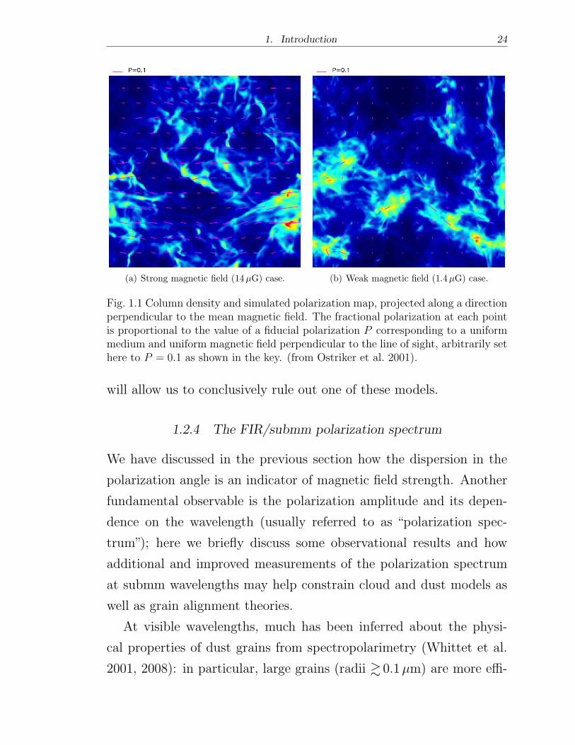
larization angles. In particular, Figure 1.1 (from Ostriker et al. 2001)
shows the result of 3D MHD simulations of turbulent, self-gravitating
molecular clouds, one with strong magnetic field (14�G5), the other
with a weak field (1.4�G); the former has a dispersion of only �� ∼ 9∘
in the distribution of polarization angles, while the latter has �� ∼ 45∘
(for a magnetic field that is parallel to the plane of the sky).
Observations of large-scale molecular cloud fields with BLAST-Pol
5 Throughout this thesis we make use of the gauss [G] as a (non-SI) unit of magnetic flux density,expressed as 1G = 10−4 kgC−1 s−1 = 10−4 tesla [T].
1. Introduction 24
(a) Strong magnetic field (14�G) case. (b) Weak magnetic field (1.4�G) case.
Fig. 1.1 Column density and simulated polarization map, projected along a directionperpendicular to the mean magnetic field. The fractional polarization at each pointis proportional to the value of a fiducial polarization P corresponding to a uniformmedium and uniform magnetic field perpendicular to the line of sight, arbitrarily sethere to P = 0.1 as shown in the key. (from Ostriker et al. 2001).
will allow us to conclusively rule out one of these models.
1.2.4 The FIR/submm polarization spectrum
We have discussed in the previous section how the dispersion in the
polarization angle is an indicator of magnetic field strength. Another
fundamental observable is the polarization amplitude and its depen-
dence on the wavelength (usually referred to as “polarization spec-
trum”); here we briefly discuss some observational results and how
additional and improved measurements of the polarization spectrum
at submm wavelengths may help constrain cloud and dust models as
well as grain alignment theories.
At visible wavelengths, much has been inferred about the physi-
cal properties of dust grains from spectropolarimetry (Whittet et al.
2001, 2008): in particular, large grains (radii ≳ 0.1�m) are more effi-
1. Introduction 25
cient polarizers than small grains (radii ≲ 0.01�m), which are appar-
ently minimally aligned; amorphous silicate grains are better aligned
than carbonaceous grains (including polycyclic aromatic hydrocarbons
[PAHs]); and the shape of aligned grains is more that of an oblate
(disc-like) rather than prolate (needle-like) spheroid, with its short
axis aligned with the magnetic field (see also Draine 2003, Draine &
Fraisse 2009).
Observations at FIR and submm–mm wavelengths have found that
in the densest cores of molecular clouds the polarization spectrum in-
creases with wavelength (in the range 100�m–1mm; Schleuning 1998,
Coppin et al. 2000). This rise is consistent with an opacity effect; as
the opacity increases towards shorter wavelengths the emitted polar-
ization must decrease, approaching zero as the emission becomes opti-
cally thick (Vaillancourt 2009). In cloud envelopes, where the emission
is typically optically thin, the spectrum falls with wavelength below
350�m, but rises at longer wavelengths (Hildebrand et al. 2000, Vail-
lancourt 2002, Vaillancourt et al. 2008).
The submm rise can be explained by a model in which the colder
grains are better aligned than the warmer grains. Bethell et al. (2007)
have shown that this can be achieved by applying the radiative torque
model of grain alignment (Lazarian 2007) to starless clouds. In their
model the cloud structure is clumpy, such that external photons can
penetrate deep into the cloud. These photons heat all grains, but the
larger grains tend to be cooler as they are more efficient emitters. At
the same time, the alignment mechanism is more efficient at aligning
the larger grains (Cho & Lazarian 2005). Therefore, their model pre-
dicts that the cooler grains are better aligned and that the polarization
spectrum rises with wavelength. Similarly, Draine & Fraisse (2009)
reproduce the submm rise, under the assumption that carbonaceous
1. Introduction 26
grains are not aligned. Their explanation is that the silicate grains
contribute an increasing fraction of the emission as the wavelength in-
creases, in part because the silicate grains are slightly cooler than the
carbonaceous grains (� ≲ 200�m), and in part because the ratio of
the silicate opacity to the graphite opacity increases with increasing
wavelength for � ≳ 100�m.
Nevertheless, to our knowledge the FIR fall and the submm rise
have yet to be connected by a theoretical dust model. Hildebrand
et al. (1999) and Vaillancourt et al. (2008) claim that the observed
behavior is not consistent with a simple isothermal dust model but
requires multiple grain populations, where each population’s polariza-
tion efficiency is correlated with either the dust temperature or spec-
tral index. While Bethell et al. (2007) work under the assumption
of starless clouds, in real molecular clouds there exist embedded stars
that provide an additional source of photons, which will both heat and
align dust grains. One can expect that grains closer to these stars will
be warmer and better aligned than grains that are either further from
stars or shielded from photons in optically thick clumps. This natu-
rally produces grain populations in which the warmer grains are better
aligned (Hildebrand et al. 1999). The result is a polarization spectrum
that falls with wavelength. The observed polarization spectrum with a
minimum between 100 and 850�m can in fact be modeled by incorpo-
rating embedded stars into the models of starless cores (Vaillancourt
2009, Hildebrand & Vaillancourt 2009).
BLAST-Pol will measure polarization spectra at 250, 350, and 500�m
(bracketing the minimum) for a number of cloud envelopes, and will
map its spatial variations. By testing the simulations against such
observational data sets, we will help improve the models, leading also
to a greater reliability of the CF field strength estimates.
1. Introduction 27
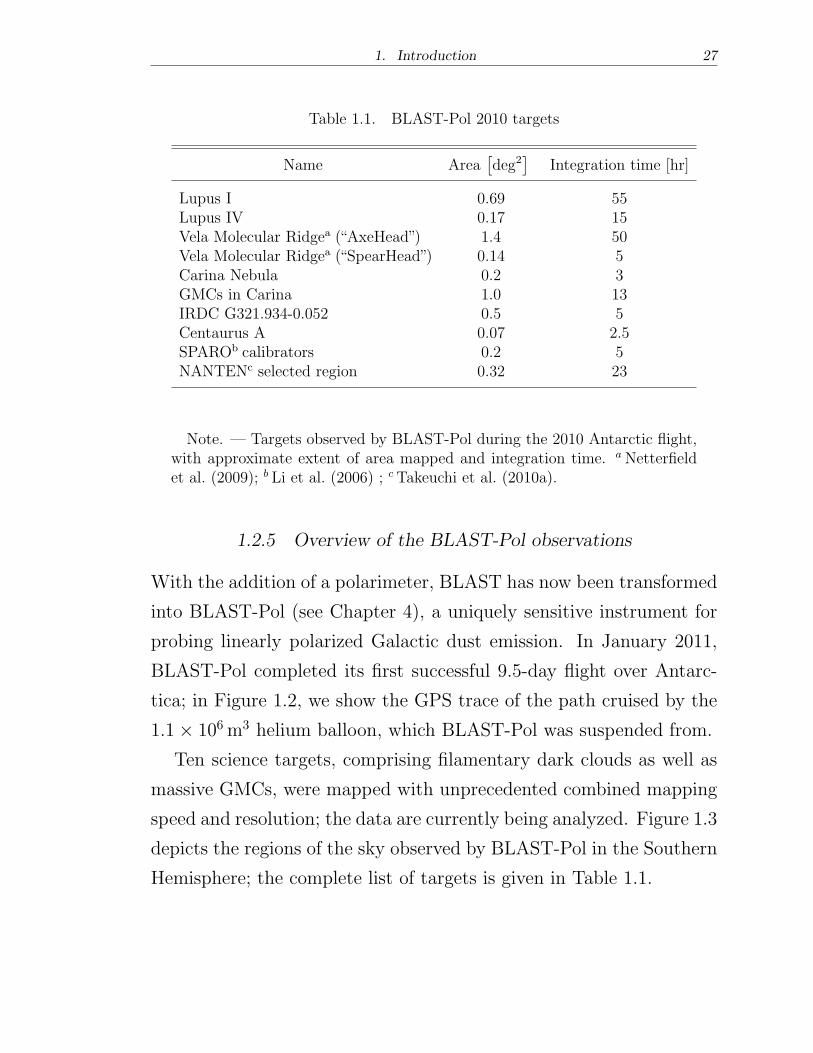
Table 1.1. BLAST-Pol 2010 targets
Name Area[
deg2]
Integration time [hr]
Lupus I 0.69 55Lupus IV 0.17 15Vela Molecular Ridgea (“AxeHead”) 1.4 50Vela Molecular Ridgea (“SpearHead”) 0.14 5Carina Nebula 0.2 3GMCs in Carina 1.0 13IRDC G321.934-0.052 0.5 5Centaurus A 0.07 2.5SPAROb calibrators 0.2 5NANTENc selected region 0.32 23
Note. — Targets observed by BLAST-Pol during the 2010 Antarctic flight,with approximate extent of area mapped and integration time. aNetterfieldet al. (2009); b Li et al. (2006) ; cTakeuchi et al. (2010a).
1.2.5 Overview of the BLAST-Pol observations
With the addition of a polarimeter, BLAST has now been transformed
into BLAST-Pol (see Chapter 4), a uniquely sensitive instrument for
probing linearly polarized Galactic dust emission. In January 2011,
BLAST-Pol completed its first successful 9.5-day flight over Antarc-
tica; in Figure 1.2, we show the GPS trace of the path cruised by the
1.1× 10⁶m3 helium balloon, which BLAST-Pol was suspended from.
Ten science targets, comprising filamentary dark clouds as well as
massive GMCs, were mapped with unprecedented combined mapping
speed and resolution; the data are currently being analyzed. Figure 1.3
depicts the regions of the sky observed by BLAST-Pol in the Southern
Hemisphere; the complete list of targets is given in Table 1.1.
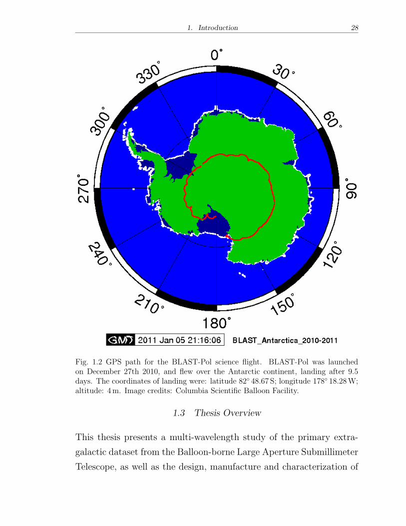
1. Introduction 28
Fig. 1.2 GPS path for the BLAST-Pol science flight. BLAST-Pol was launchedon December 27th 2010, and flew over the Antarctic continent, landing after 9.5days. The coordinates of landing were: latitude 82∘ 48.67 S; longitude 178∘ 18.28W;altitude: 4m. Image credits: Columbia Scientific Balloon Facility.
1.3 Thesis Overview
This thesis presents a multi-wavelength study of the primary extra-
galactic dataset from the Balloon-borne Large Aperture Submillimeter
Telescope, as well as the design, manufacture and characterization of
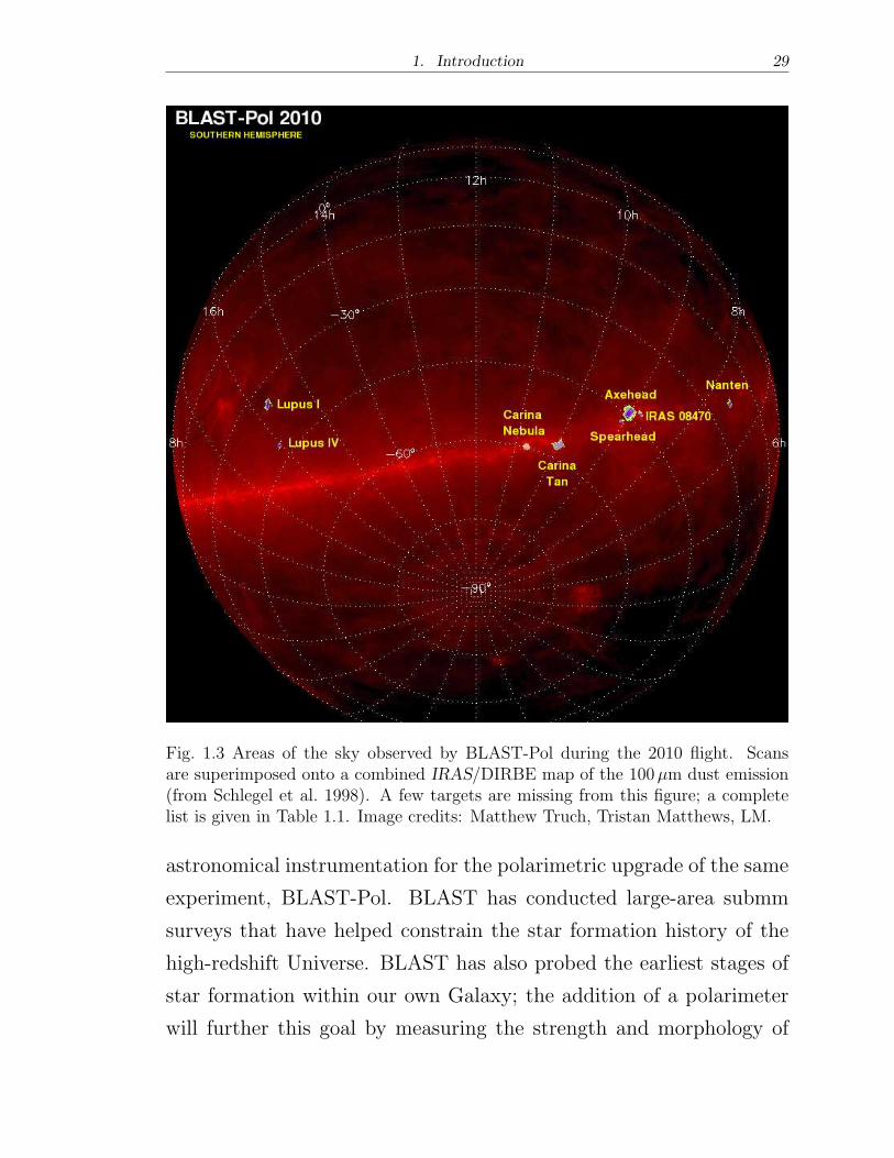
1. Introduction 29
Fig. 1.3 Areas of the sky observed by BLAST-Pol during the 2010 flight. Scansare superimposed onto a combined IRAS/DIRBE map of the 100�m dust emission(from Schlegel et al. 1998). A few targets are missing from this figure; a completelist is given in Table 1.1. Image credits: Matthew Truch, Tristan Matthews, LM.
astronomical instrumentation for the polarimetric upgrade of the same
experiment, BLAST-Pol. BLAST has conducted large-area submm
surveys that have helped constrain the star formation history of the
high-redshift Universe. BLAST has also probed the earliest stages of
star formation within our own Galaxy; the addition of a polarimeter
will further this goal by measuring the strength and morphology of
1. Introduction 30
magnetic fields in nearby star-forming regions. The study of these two
diverse, yet highly connected, topics is the main scientific motivation
for this thesis.
In this chapter, we have introduced the reader to submm Galactic
and extragalactic astronomy, highlighting the state-of-the-art theoret-
ical models and observational findings, pinpointing the questions and
problems that are still open, and defining the role that BLAST and
BLAST-Pol, respectively, has played and will play in advancing our
current understanding of the cosmic and Galactic star-formation pro-
cesses, through observations that uniquely combine elevated mapping
speed, sensitivity and resolution.
Chapter 2 (Part One) describes a multi-wavelength study of the ex-
tragalactic sources detected by BLAST in its survey of the Extended
Chandra Deep-Field South (ECDFS), using data spanning the radio
to the UV. We develop a Monte Carlo method to account for flux
boosting, source blending, and correlations among bands, which we
use to derive deboosted FIR luminosities for our sample. We estimate
total (obscured plus unobscured) star-formation rates for the BLAST
counterparts by combining their FIR and UV luminosities. We capi-
talize on the multi-wavelength data at our disposal to derive a broad
morphological classification of our galaxies, their AGN fraction and
stellar masses. We use the combined estimates of SFRs and stellar
masses to compare our sample to those selected with other submm
facilities such as SCUBA and Herschel. Finally, we contextualize our
results in the current framework of galaxy formation and evolution.
Chapter 3 (Part One) presents a challenging measurement of the
star-formation level in massive, high-redshift galaxies selected in the
optical with the NICMOS camera on HST. Because the emission from
each galaxy is too faint to be individually detected in the BLAST
1. Introduction 31
maps, we use a technique that goes under the name of “stacking anal-
ysis” (extensively described in Appendix A of this thesis) to estimate
the average brightness of our externally-selected population of galax-
ies at the BLAST frequencies. Subsequently, the galaxies are divided
into two groups, disk-like and spheroid-like, according to their surface
brightness profile, and separate measurements of SFR are performed.
We show that star formation is a plausible mechanism for size evo-
lution in this population as a whole, but find only marginal evidence
that it is what drives the expansion of the spheroid-like galaxies.
Chapter 4 (Part Two) describes the BLAST-Pol instrument. We
focus on the important subsystems of the gondola, including the op-
tics, cryogenic system, bolometric detectors, polarization-sensitive el-
ements, readout electronics, pointing sensors and control. We also
provide the nominal sensitivities for BLAST-Pol, and describe the
scanning strategy adopted to optimally recover the Stokes Q and U in
the sky. The second part of the chapter is devoted specifically to the
primary pointing sensors for BLAST-Pol, two redundant optical star
cameras. The principles of operation, design, control software, and
preliminary in-flight performance are presented.
Chapter 5 (Part Two) illustrates in full detail the theoretical frame-
work, principles of operation and manufacturing process for the optical
components of the BLAST-Pol polarimeter, an achromatic cryogenic
half-wave plate (HWP) and photolithographed polarizing grids acting
as analyzers, as well as their pre-flight performance. We identify and
measure the parameters that characterize the optical properties and
efficiency of these polarizing elements. In particular, we perform a full
spectral characterization, both at room and cryogenic temperatures,
of the five-plate sapphire HWP, which is, to our knowledge, the most
achromatic ever built at mm and submm wavelengths.
1. Introduction 32
Chapter 6 (Part Two) focuses on the most important aspect of the
BLAST-Pol data analysis pipeline that is used to transform raw detec-
tor time streams into usable sky maps of Stokes parameter [I,Q, U ]:
the map-maker. We develop the mathematical formalism of map-
making, and describe the algorithmic implementation of a naive bin-
ning technique for the case of BLAST-Pol. As a proof of concept, we
present a sample of preliminary polarization maps, which result as the
culmination of the whole data analysis process and demonstrate the
overall success of the mission.
Chapter 7 concludes the thesis with an outlook on future work.
1.3.1 LM’s contribution to the BLAST and BLAST-Pol projects
LM joined the BLAST team at the beginning of 2008. Here we briefly
summarize the main contributions brought by LM to the BLAST and
BLAST-Pol projects.
The very first task has been the design, optimization and imple-
mentation of a whitening filter for the BLAST extragalactic maps of
the ECDFS, which is not explicitly reported in this thesis. The raw
maps present large-scale noise that hampers the detection of individual
point sources. It is common habit to apply to the maps a whitening
filter in order to suppress such large-scale structure, which in our case
is primarily noise. The bi-dimensional Fourier transform of the maps
is thus filtered on spatial scales larger than the size of the BLAST
array projected onto the sky (roughly 14’ × 7’). The filtered BLAST
maps reveal the presence of hundreds of ≥ 5� submm galaxies, the
largest sample in the pre-Herschel era (Devlin et al. 2009).
The second important task within the context of the analysis of
the BLAST extragalactic dataset has been developing the algorithm
and perfecting the technicalities of the stacking methodology (see Ap-
1. Introduction 33
pendix A), as well as optimizing and implementing a large number of
simulations to evaluate stacking as an unbiased technique to estimate
the average brightness of an externally-selected population of galaxies
at submm wavelengths. Stacking analyses have enabled the statis-
tical resolution of the full CIB intensity into flux density produced
by identifiable 24�m-selected galaxies (Marsden et al. 2009), and the
measurement of the history of obscured star formation in the Universe
(Pascale et al. 2009), as well as the results presented in Chapter 3.
In November 2008, LM carried out follow-up observations of the
BLAST galaxies with AAOmega, the spectrograph on the Anglo-Australian
telescope. LM has been heavily involved in the subsequent data reduc-
tion, which resulted in spectroscopic redshifts for about two hundred
BLAST sources. The BLAST redshift survey has enabled the first di-
rect measurement of the luminosity function at 250, 350, and 500�m
(Eales et al. 2009), as well as the results presented in Chapter 2.
These contributions to the BLAST data analysis have granted LM
co-authorship in most of the BLAST extragalactic scientific production
(including a paper on the Nature journal; see Published Work), albeit
he is not part of the BLAST core team.
On the instrumentation front, LM has been part of the BLAST-Pol
team since the very beginning in 2008.
The first task has been to manufacture, test, and fully characterize
the BLAST-Pol cryogenic HWP, the most achromatic ever built to
date. In the same context, LM has participated in the tests and spec-
tral measurements of a novel artificial dielectric metamaterial (Zhang
et al. 2009), which has found its first successful application as anti-
reflection coating for the BLAST-Pol HWP. In addition, the BLAST-
Pol photolithographed analyzers, have been designed, manufactured
and extensively tested in Cardiff; LM has been directly involved in
1. Introduction 34
every step of their deployment.
The second important task has been the hardware/software opti-
mization, testing and deployment of two optical star cameras, which
constitute BLAST-Pol’s primary pointing sensors. The star cam-
eras have performed successfully during BLAST-Pol’s first flight over
Antarctica in December 2010. LM is also in charge of the post-flight
pointing reconstruction; preliminary analysis suggests that the abso-
lute pointing accuracy will equal that of BLAST06 (≲ 3′′ rms).
The third major task has been the design, optimization and imple-
mentation of the BLAST-Pol polarized map-maker. A big challenge
has been to finalize this fundamental piece of software before the de-
ployment to Antarctica for the flight campaign. LM has been using
the map-maker during the first two days of the BLAST-Pol flight to
produce“on-the-fly”maps of the bright calibrators to assess the overall
performance of the telescope.
LM has participated in the two BLAST-Pol integration campaign,
at the University of Toronto in April 2010 and at the Columbia Scien-
tific Balloon Facility, Palestine, Texas, USA, in June and July 2010.
Finally, LM has partaken in the BLAST-Pol flight campaign at the
Long Duration Balloon (LDB) facility near McMurdo Station, Antarc-
tica, from November 2010 to January 2011.
1.3.2 Other work
During the three years at Cardiff University, LM has gained valuable
laboratory experience in several occasions beyond the PhD project.
Most notably, LM has participated in tests of the SCUBA-2 arrays
(both electronics modules and science grade) in the Cardiff test-bed
cryostat, which earned LM co-authorship in Bintley et al. (2010).
LM has also participated in the anechoic-chamber measurements of
1. Introduction 35
the beam patterns of the multi-mode Planck High Frequency Instru-
ment (HFI) horns at 857 and 545GHz.
In addition, LM has participated in the spectral measurements of
a novel prototype of polypropylene-embedded metal-mesh broadband
achromatic HWP for millimeter wavelengths, which earned LM co-
authorship in Zhang et al. (2011).
The design and manufacture of the HWP for the PILOT experiment
(with similar photometric bands to BLAST-Pol; Bernard et al. 2007)
has gone hand in hand with that of BLAST-Pol; LM has participated
in its fabrication, spectral characterization and cryogenic testing.
Finally, LM has participated in the software deployment and perfor-
mance characterization of one star camera for the E and B Experiment
(EBEX; Reichborn-Kjennerud et al. 2010).

Part One
2. A MULTI-WAVELENGTH STUDY OF BLAST
COUNTERPARTS
2.1 Introduction
The physical processes associated with the evolution of the Universe
have left an imprint in the extragalactic background light. The far-
infrared (FIR) portion of the background is associated with forming
galaxies in which the ultraviolet (UV) photons emitted by newborn
stars are absorbed and re-radiated by dust in the IR. Roughly half
of the energy content of the starlight integrated over the age of the
Universe is stored in the Cosmic Infrared Background (CIB), glowing
with a broad peak at around 200�m (Puget et al. 1996, Fixsen et al.
1998, Hauser et al. 1998, Dwek et al. 1998). The tight connection
between star formation and FIR luminosity provides a route to under-
standing the history of star formation in the Universe, by means of
studying the CIB at wavelengths close to its peak (Gispert et al. 2000,
Rowan-Robinson 2001, Chary & Elbaz 2001, Hauser & Dwek 2001).
The first leg on this route is to identify the sources contributing
to the CIB. Ground-based surveys with the Submillimetre Common-
User Bolometer Array (SCUBA; Holland et al. 1999) have revealed
the existence of a population of distant, highly dust-obscured galaxies,
similar to the Ultra Luminous Infrared Galaxies (ULIRGs) detected by
IRAS (Smail et al. 1997, Hughes et al. 1998, Barger et al. 1998), which
make up all the background at 850�m (Blain et al. 1999a). However,
at these wavelengths the energy in the CIB is only one-thirtieth of the
2. A multi-wavelength study of BLAST counterparts 38
value at its peak, and the SCUBA population only contributes 20–30%
to the CIB at its peak (Coppin et al. 2006, Dye et al. 2007).
Recent progress has been made through new observations obtained
at 24, 70, and 160�m by the MIPS instrument aboard the Spitzer
Space Telescope (Rieke et al. 2004), and at 250, 350, and 500�m by
the Balloon-borne Large Aperture Submillimeter Telescope (BLAST;
Devlin et al. 2004, Pascale et al. 2008), a forerunner of the SPIRE
photometer (Griffin et al. 2010) on the Herschel Space Observatory
(Pilbratt et al. 2010). These wavelengths bracket the CIB peak; sev-
eral authors have shown through stacking analyses that 24�m-selected
galaxies resolve the CIB background, both on the short-wavelength
side of the peak (Dole et al. 2006) and on its long-wavelength side
(Devlin et al. 2009, Marsden et al. 2009).
Sources identified at 24�m are mostly unresolved in the FIR, and
have a redshift distribution with a median of 0.9 (Pascale et al. 2009).
A detailed multi-wavelength study of these sources is the necessary
next step. Starting from a catalog of ≥ 5� BLAST sources, Dye et al.
(2009; hereafter D09) identify counterparts in 24�m and radio cata-
logs (BLAST IDs). These tend to be relatively nearby sources (median
z of 0.6, interquartile range of 0.2–1.0), with a median dust tempera-
ture of 26K and a median bolometric FIR luminosity of 4 × 10¹¹L⊙,
which contribute 20% to the CIB at 250�m. Identified BLAST sources
typically lie at lower redshifts and have lower rest-frame dust tempera-
tures compared to submillimeter (submm) sources detected in surveys
conducted with SCUBA (Chapman et al. 2005, Pope et al. 2005).
However, D09 also note that the ∼40% of BLAST sources without
identified counterparts probably lie at higher redshifts on average. Fi-
nally, D09 illustrate how the apparent increase in dust temperature
and FIR luminosity with redshift occurs as a result of selection effects.
2. A multi-wavelength study of BLAST counterparts 39
We also note that three other multi-wavelength studies of fainter
BLAST sources discovered in the deepest part of the map have been
undertaken. Dunlop et al. (2010) concentrate on 250�m radio-identified
sources within Great Observatory Origins Deep Survey-South (GOODS-
S; Dickinson et al. 2003; see Section 2.2.1) where the deepest an-
cillary data coincide. Chapin et al. (2011) use overlapping BLAST
250–500�m and LABOCA 870�m (Weiß et al. 2009) data in the
larger Extended Chandra Deep-Field South (ECDFS) to constrain the
Rayleigh–Jeans tail more accurately than is possible in D09. Finally,
Ivison et al. (2010a) study the FIR/radio correlation for a catalog of
BLAST 250�m-selected galaxies in the ECDFS; this sample is deeper
than the D09 one, and yet slightly shallower than the selection in Dun-
lop et al. (2010). There is little overlap between the sources used in
these studies and the shallower/wider area sample from D09.
The basis of our present study is the D09 sample as its brighter,
and lower-redshift objects are most easily followed-up in the optical
and UV. However, we first extend the submm analysis of D09 by ac-
counting for flux boosting, source blending, and correlations among
BLAST bands that inevitably arise in IR surveys as a consequence
of finite instrumental angular resolution and source confusion (Cop-
pin et al. 2005). We then identify counterparts to the BLAST IDs
in the near- and far-UV Galaxy Evolution Explorer (GALEX) maps,
in order to quantify the total dust-obscured and unobscured star for-
mation, as described by several authors (Bell 2003, Hirashita et al.
2003, Iglesias-Paramo et al. 2006, Buat et al. 2007). We also extend
the analysis of Eales et al. (2009; hereafter E09) to combine spectro-
scopic data of BLAST IDs with optical, near-IR (NIR) and mid-IR
(MIR) photometry in order to place firmer constraints on source red-
shifts, morphology, active galactic nucleus (AGN) fraction, and stellar
2. A multi-wavelength study of BLAST counterparts 40
masses.
We are able to assign spectroscopic and photometric redshifts to
∼62% of the BLAST IDs. We use this information to estimate the
rest-frame total FIR luminosity from the combined BLAST and MIPS
photometry. We compare our FIR luminosities with those obtained
from MIPS photometry only, finding a significant discrepancy for high
luminosity sources (LFIR ≳ 5× 10¹¹L⊙) at z ≳ 0.5. The BLAST and
SPIRE wavebands are therefore fundamental in constraining the peak
of hidden star formation at high redshift (see also e.g., Schulz et al.
2010, Elbaz et al. 2010).
In addition, UV counterparts are found for about 60% of the BLAST
IDs. This allows us to estimate the fraction of UV photons that man-
age to escape the dust shroud, which is then combined with FIR data
to build an estimator of the total star-formation rate (SFRtot) ongo-
ing in these sources. Recent observations at the same wavelengths
(Rodighiero et al. 2010) delineate the UV contribution as marginal
at all redshifts. We find that star formation is heavily obscured at
LFIR ≳ 1011L⊙, z ≳ 0.5, but unobscured starlight plays an im-
portant role in low-redshift, low FIR luminosity sources (z ≲ 0.25,
LFIR ≲ 1011L⊙), in agreement with Buat et al. (2010).
We reanalyze the optical spectroscopy data from the AAOmega
survey presented in E09 to obtain H� equivalent widths (EWs) and
[N II]/H� line ratios. This spectral analysis, combined with a qual-
itative study of the radio, MIR, and optical emission, allows us to
assess whether or not a BLAST galaxy is hosting an active nucleus:
roughly 20% of the objects in our sample show evidence of AGN pres-
ence. Recent observations of FIR-selected samples (Wiebe et al. 2009,
Coppin et al. 2010, Muzzin et al. 2010, Hatziminaoglou et al. 2010,
Shao et al. 2010, Elbaz et al. 2010) show that the submm emission
2. A multi-wavelength study of BLAST counterparts 41
of such objects is mainly due to star formation ongoing in the host
galaxy, rather than due to the AGN. Therefore, we do not to ex-
plicitly exclude AGNs from our analysis, unlike other authors (Bell
2003, Iglesias-Paramo et al. 2006, Buat et al. 2007), but rather flag
them as such. Visual examination of BLAST IDs in UV, optical, and
MIR images (see Appendix B) is used to derive a broad morphological
classification of these objects: at low redshift we find predominantly
spirals, whereas most of the BLAST sources identified at high redshift
are compact and show AGN signatures. This is probably a selection
bias, as the fraction of submm sources identified at other wavelengths
gradually decreases with z (see D09), and the farthest objects can of-
ten be identified only if they are particularly bright in the radio or
in the optical, frequently an indication of AGN presence. As a mat-
ter of fact, the analysis carried out by Dunlop et al. (2010) shows
that a deep survey at 250�m not only contains low-z spirals, but also
extreme dust-enshrouded starburst galaxies at z ∼ 2. Our analysis
tends to miss the latter because they are typically extremely faint in
the optical/UV, unless they also host an AGN.
Finally, stellar masses (M★) are estimated using the method de-
tailed in Dye (2008), in order to study whether or not specific star-
formation rates (SSFR ≡ SFR/M★) depend on stellar mass and LFIR.
The SSFR plays an important role as it measures the timescale of
recent star formation in a galaxy, as compared to the star-formation
rate integrated over the galaxy’s history. Several studies (Santini et al.
2009, Rodighiero et al. 2010; and references therein) report that the
SSFR increases with redshift at all masses, whereas the dependence
of SSFR on mass is one of the most debated questions. In particu-
lar, we aim to understand whether or not sources selected at wave-
lengths longward of 200�m are experiencing a major episode of star
2. A multi-wavelength study of BLAST counterparts 42
formation, forming stars more actively than in their recent past and
building up a substantial fraction of their final stellar mass. We high-
light a dichotomy in the BLAST population: sources at z ≲ 1 appear
to be run-of-the-mill star-forming galaxies with intermediate stellar
masses (median M★ ∼ 7 × 10¹⁰M⊙) and approximately constant SS-
FRs, whereas the high-z tail of the BLAST counterparts significantly
encroaches on the SCUBA population detected in the SHADES survey
(Dye et al. 2008), in terms of both stellar masses and SSFRs. This is
expected since there is good overlap between fainter BLAST sources
and 870�m-selected galaxies (Dunlop et al. 2010, Chapin et al. 2011),
but it is also important to establish an additional link with a shallower
BLAST sample, using a methodology equivalent to that of SHADES.
In addition, since the more massive BLAST galaxies at intermediate
redshifts (0 < z < 1) seem to form stars more vividly than the equally
massive and aged 24�m sources detected in the GOODS survey, we
suggest that the BLAST counterparts may act as linking population
between the 24�m-selected sources and the SCUBA starbursts.
The layout of this chapter is as follows. In Section 2.2, we describe
in detail the maps, images, and catalogs used throughout this work.
Sections 2.3 and 2.4 are concerned with luminosities and SFRs in the
FIR and UV, respectively. In Section 2.5, we build a unified estimator
of total star formation and discuss the first results. In Section 2.6,
we estimate the AGN content of our sample, while in Section 2.7 we
outline a broad morphological scheme for our sources. In Section 2.8,
we compute the stellar masses and present the main results. Section
2.9 contains our conclusions. Throughout this thesis, we adopt the
concordance flat ΛCDM cosmological model, with ΩM = 0.274, ΩΛ =
0.726, and H0 = 70.5 km s−1Mpc−1 (Hinshaw et al. 2009).
2. A multi-wavelength study of BLAST counterparts 43
2.2 Data
This section describes the data sets used for our analysis, spanning
from the UV to the submillimeter.
2.2.1 Submillimeter data
We use data from the wide-area extragalactic survey of BLAST de-
scribed by Devlin et al. (2009), and centered on the GOODS-S (Dick-
inson et al. 2003; which in turn is centered on the Chandra Deep-Field
South, CDFS) region. The maps1 cover an area of 8.7 deg2 with a 1 �
depth of 36, 31, and 20mJy at 250, 350, and 500�m, respectively. We
refer to this region as the BLAST GOODS-S Wide (BGS-Wide). A
smaller region of 0.8 deg2, nested inside BGS-Wide and referred to as
BLAST GOODS-S Deep (BGS-Deep), has a 1 � depth of 11, 9, and
6mJy at 250, 350, and 500�m, respectively; these depths account
for the instrumental noise only. Due to large instrumental beams
(36, 42, and 60′′) and steep source counts (approximately following
dN/dS ∝ S−3; Patanchon et al. 2009), source confusion contributes
substantially to the noise in these maps. Marsden et al. (2009) esti-
mate that fluctuations arising from unresolved sources in BGS-Deep
are �confusion ≈ 21, 17, and 15mJy at 250, 350, and 500�m, respec-
tively. The BLAST maps are made using both an optimal mapmaker
(Patanchon et al. 2008) and a naive mapmaker (Pascale et al. 2011),
and are found to be in excellent quantitative agreement. Further de-
tails on the instrument may be found in Pascale et al. (2008), while
flight performance and calibration are provided in Truch et al. (2009).
Catalogs of sources detected at each wavelength in BGS-Deep and
BGS-Wide are presented by Devlin et al. (2009).
1 Available at: http://blastexperiment.info/results.php
2. A multi-wavelength study of BLAST counterparts 44
D09 combine these single-wavelength catalogs by selecting sources
with a ≥ 5� (instrumental only, no confusion noise) significance in at
least one of the bands. They use this multi-band catalog to identify
counterparts (BLAST primary IDs) in deep radio (ACTA and Very
Large Array, VLA; Norris et al. 2006, Miller et al. 2008) and 24�m
(SWIRE and FIDEL; Lonsdale et al. 2004, Dickinson & FIDEL team
2007, Magnelli et al. 2009) surveys. The BLAST primary IDs all have
≤ 5% probability of being a chance alignment. They also compile a
list of secondary IDs, with different counterparts associated with the
same BLAST source as the primary ID, but with larger probability of
being a chance alignment.
In this work, we present an extended version of the D09 catalog
of the BLAST primary IDs which contains 227 BLAST sources. In
the following sections, we update this list to include UV data, recent
redshifts, corrections for submm flux boosting and blending, morphol-
ogy, AGN features, and SFRs (see Appendix C for data tables). The
list of secondary IDs is extensively discussed in E09, and we do not
investigate them further.
We emphasize again that the sample studied in this work comprises
the subset of BLAST-selected bright sources for which optical spec-
troscopy/photometry is available, and/or for which we find a clear
counterpart in the UV. Naturally, this is only a fraction of sources
that would be in a purely BLAST-selected catalog, skewed toward
lower redshifts and strong optical/UV fluxes.
2.2.2 Optical spectroscopy
A spectroscopic follow-up of the BLAST IDs is carried out with the
AAOmega optical spectrograph at the Anglo-Australian Telescope.
The BLAST spectroscopic redshift survey is discussed in E09, as well
2. A multi-wavelength study of BLAST counterparts 45
as the reduction of the spectral data; here we extend their analysis
and results (see Sections 2.6, 2.7 and Tables 2.2, C1).
AAOmega (AAO; Sharp et al. 2006) consists of 392, 2′′-wide fibers
feeding light from targets within a 2∘ field of view; the configuration of
diffraction gratings is chosen to yield a wavelength coverage from 370
to 880 nm, with spectral resolution �/�� ≃ 1300. At redshifts lower
than 1, this allows us to detect two or more of the following lines: [O II]
372.7, calcium H and K, H�, [O III] 495.9 and 500.7, H�, [N II] 658.3,
and [S II] 671.6 and 673.1. At redshifts greater than 1, we only rely on
broad emission lines, such as Lyman �, Si IV 140.3, C III] 190.9, and
C IV 154.9.
We have produced two prioritized lists of targets. The first list
comprises ≥ 3.5� BLAST sources with primary radio or 24�m coun-
terparts2. Sources selected at 24�m are also included in the target list
to use all the available fibers. The second list contains the secondary
BLAST IDs, plus 24 �m sources. The positions of the primary and
secondary targets are shown in Figure 2.1.
The net observing time for the list of primary targets is 7 hr, obtain-
ing spectra for 669 sources (316 BLAST IDs and 356 SWIRE sources).
The list of secondary targets is observed for only 1 hr (due to poor
weather), obtaining 335 spectra (77 BLAST IDs, and 258 SWIRE
sources). Spectroscopic redshifts are consequently obtained by E09
for 212 BLAST IDs in the primary list, 193 of which have ≥ 75% con-
fidence level (c.l.), and for 11 BLAST IDs in the secondary list (all with
≥ 75% c.l.). Figure 2.2 shows three representative spectra of primary
BLAST counterparts, while Figure 2.3 (which we choose to display
full-page and rotated for visual clarity) compares the spectroscopic
redshifts of primary and secondary targets measured with AAOmega
2 If only the 24�m counterpart is present, we refine the position of the source by matching itwith optical or IRAC 3.6�m coordinates.
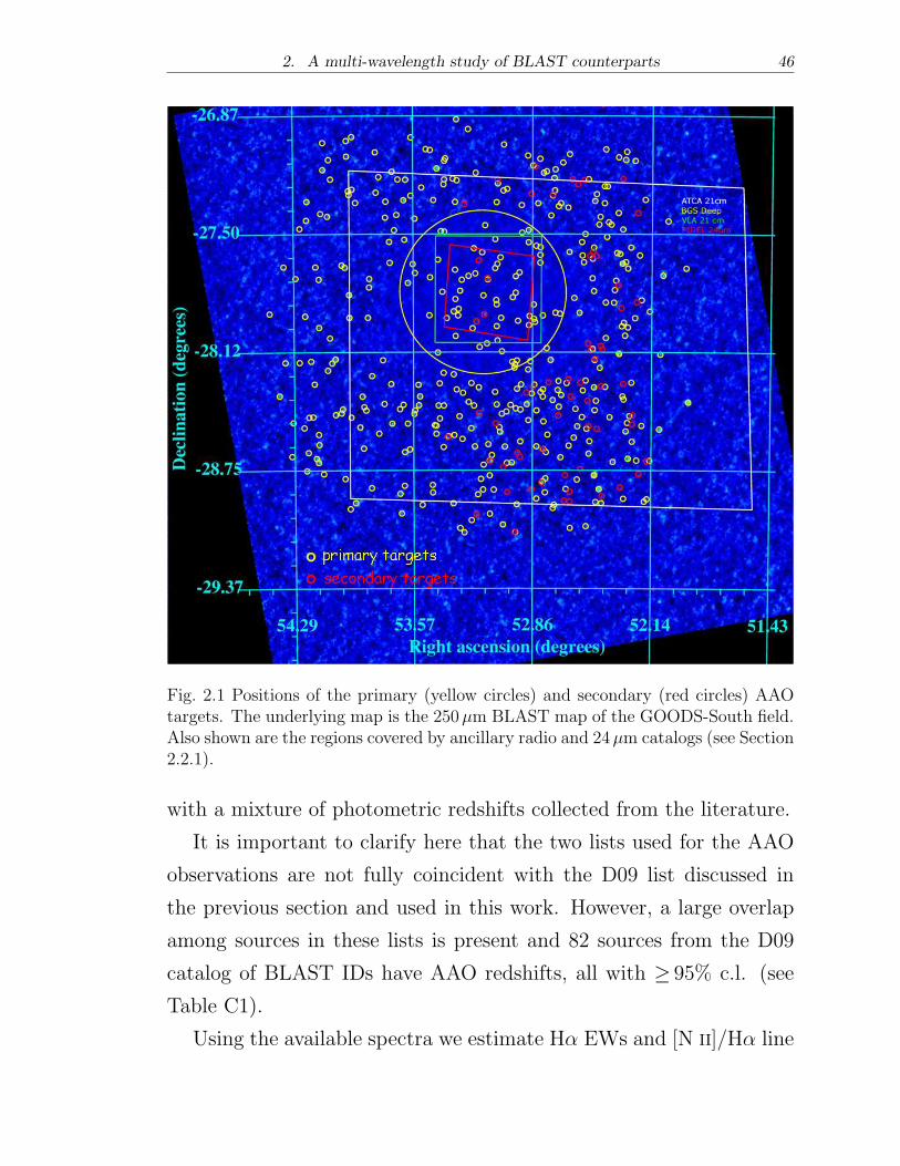
2. A multi-wavelength study of BLAST counterparts 46
Fig. 2.1 Positions of the primary (yellow circles) and secondary (red circles) AAOtargets. The underlying map is the 250�m BLAST map of the GOODS-South field.Also shown are the regions covered by ancillary radio and 24�m catalogs (see Section2.2.1).
with a mixture of photometric redshifts collected from the literature.
It is important to clarify here that the two lists used for the AAO
observations are not fully coincident with the D09 list discussed in
the previous section and used in this work. However, a large overlap
among sources in these lists is present and 82 sources from the D09
catalog of BLAST IDs have AAO redshifts, all with ≥ 95% c.l. (see
Table C1).
Using the available spectra we estimate H� EWs and [N II]/H� line
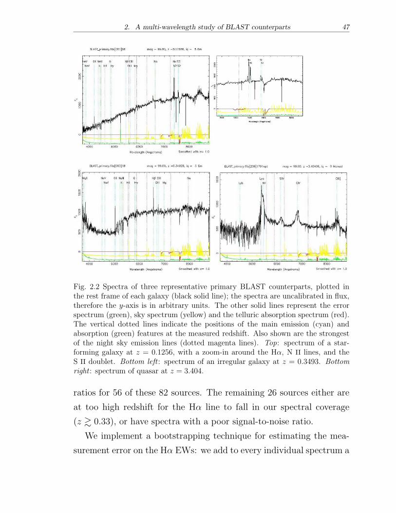
2. A multi-wavelength study of BLAST counterparts 47
Fig. 2.2 Spectra of three representative primary BLAST counterparts, plotted inthe rest frame of each galaxy (black solid line); the spectra are uncalibrated in flux,therefore the y-axis is in arbitrary units. The other solid lines represent the errorspectrum (green), sky spectrum (yellow) and the telluric absorption spectrum (red).The vertical dotted lines indicate the positions of the main emission (cyan) andabsorption (green) features at the measured redshift. Also shown are the strongestof the night sky emission lines (dotted magenta lines). Top: spectrum of a star-forming galaxy at z = 0.1256, with a zoom-in around the H�, N II lines, and theS II doublet. Bottom left : spectrum of an irregular galaxy at z = 0.3493. Bottom
right : spectrum of quasar at z = 3.404.
ratios for 56 of these 82 sources. The remaining 26 sources either are
at too high redshift for the H� line to fall in our spectral coverage
(z ≳ 0.33), or have spectra with a poor signal-to-noise ratio.
We implement a bootstrapping technique for estimating the mea-
surement error on the H� EWs: we add to every individual spectrum a
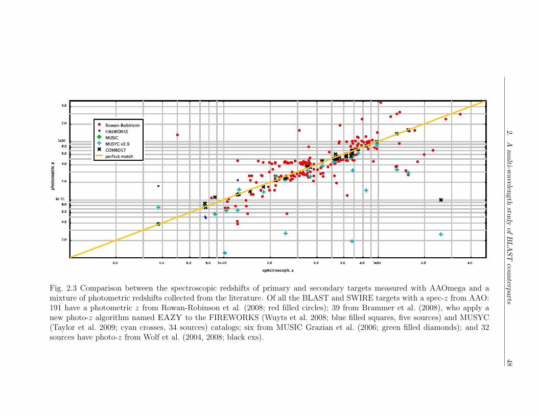
2.
Amulti-w
avelen
gth
studyofBLAST
counterp
arts
48
Fig. 2.3 Comparison between the spectroscopic redshifts of primary and secondary targets measured with AAOmega and amixture of photometric redshifts collected from the literature. Of all the BLAST and SWIRE targets with a spec-z from AAO:191 have a photometric z from Rowan-Robinson et al. (2008; red filled circles); 39 from Brammer et al. (2008), who apply anew photo-z algorithm named EAZY to the FIREWORKS (Wuyts et al. 2008; blue filled squares, five sources) and MUSYC(Taylor et al. 2009; cyan crosses, 34 sources) catalogs; six from MUSIC Grazian et al. (2006; green filled diamonds); and 32sources have photo-z from Wolf et al. (2004, 2008; black exs).
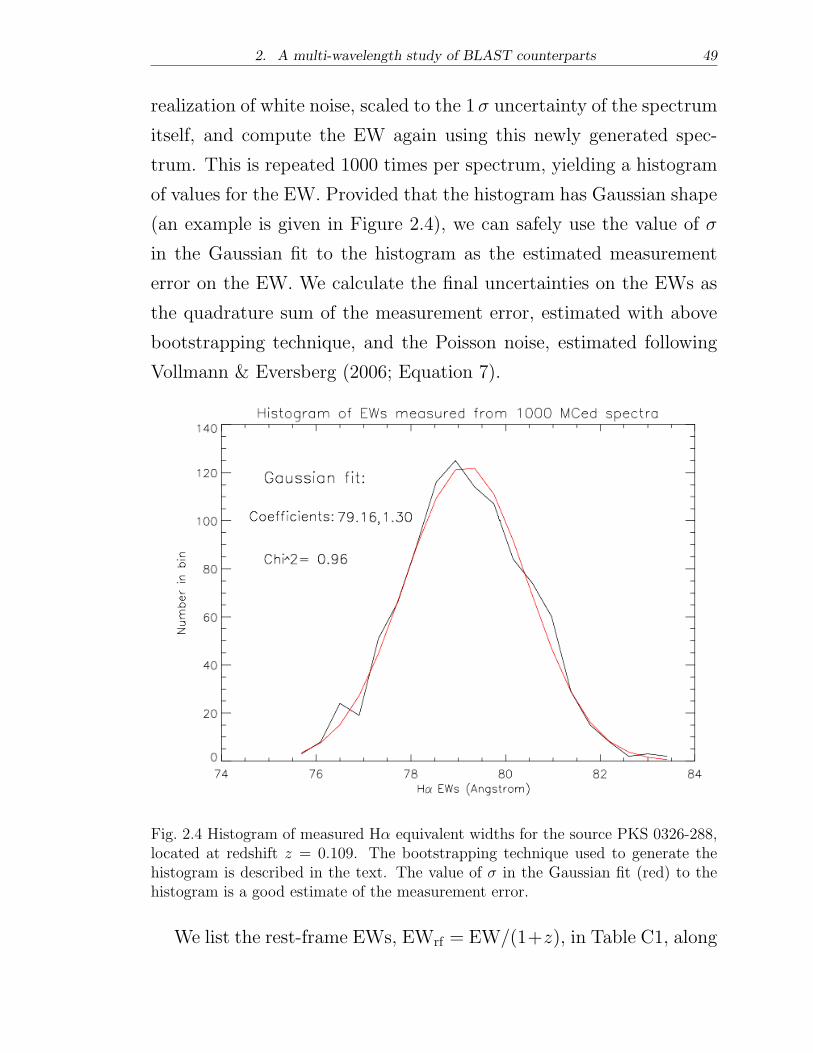
2. A multi-wavelength study of BLAST counterparts 49
realization of white noise, scaled to the 1 � uncertainty of the spectrum
itself, and compute the EW again using this newly generated spec-
trum. This is repeated 1000 times per spectrum, yielding a histogram
of values for the EW. Provided that the histogram has Gaussian shape
(an example is given in Figure 2.4), we can safely use the value of �
in the Gaussian fit to the histogram as the estimated measurement
error on the EW. We calculate the final uncertainties on the EWs as
the quadrature sum of the measurement error, estimated with above
bootstrapping technique, and the Poisson noise, estimated following
Vollmann & Eversberg (2006; Equation 7).
Fig. 2.4 Histogram of measured H� equivalent widths for the source PKS 0326-288,located at redshift z = 0.109. The bootstrapping technique used to generate thehistogram is described in the text. The value of � in the Gaussian fit (red) to thehistogram is a good estimate of the measurement error.
We list the rest-frame EWs, EWrf = EW/(1+z), in Table C1, along
2. A multi-wavelength study of BLAST counterparts 50
with their uncertainties and the [N II]/H� line ratios. Note that we
apply a 1 A correction to the H� EWrf for underlying stellar absorption
(Hopkins et al. 2003, Balogh et al. 2004).
2.2.3 UV data
We identify near-UV (NUV) and far-UV (FUV) counterparts to BLAST
IDs by searching for GALEX sources in the Deep Imaging Survey
(DIS; Martin et al. 2005; data release GR–4/5) within 6′′ of the ra-
dio or 24�m counterpart3, a separation just slightly larger than the
GALEX point-spread function (PSF) FWHM (Morrissey et al. 2007).
This choice is justified by the presence of a few extended objects,
unresolved by the submillimetric beam, that contribute to the same
BLAST source (see Section 2.7). After visual inspection of the UV
images, we add one additional interacting system extending beyond
6′′ from the BLAST ID (#2); in this case we integrate the UV mag-
nitude from both the interacting objects, because they fall within the
same BLAST beam. We estimate FUV and NUV magnitudes using
the standard GALEX pipeline (Morrissey et al. 2007) for most IDs,
whereas we perform aperture photometry on 13 extended objects. A
magnitude is considered to be unreliable if the source is either confused
or blended with a star.
We find that 144 BLAST IDs have an NUV counterpart (136 with
reliable magnitude), and 113 have an FUV counterpart (107 with re-
liable magnitude). Three sources are outside the area covered by the
DIS, and the remaining 80 BLAST IDs have no obvious counterpart.
By comparing the flux estimates for objects detected in more than one
GALEX tile (pointing), we find that the average uncertainty associ-
3 If both counterparts are present, we use the arithmetic mean between the two sets of coordi-nates: [�BLAST, �BLAST].
2. A multi-wavelength study of BLAST counterparts 51
ated with the reproducibility of the measurement is 0.06 and 0.11mag
in NUV and FUV, respectively. For bright galaxies, these values are
larger than the uncertainty in the calibration (0.03 and 0.05mag in the
NUV and FUV, respectively; Morrissey et al. 2007), and in the source
extraction procedure (≤ 0.02mag). The uncertainty on a quoted UV
magnitude is therefore the sum in quadrature of these three terms,
and it lies in the 1 � range of 0.07–0.25mag and 0.12–0.5mag in NUV
and FUV, respectively.
GALEX postage-stamp images, 2′ × 2′ wide, are used to study the
UV morphology of the BLAST IDs; a selection4 of these is shown in
Figure B1. UV magnitudes and uncertainties are listed in Table C2.
2.2.4 SWIRE 70 and 160�m MIPS maps
We use 70 and 160�m fluxes extracted from SWIRE maps (Lonsdale
et al. 2004) at positions [�BLAST, �BLAST] to constrain the spectral en-
ergy distribution (SED) of each BLAST source at wavelengths shorter
than the emission peak (see Section 2.3.2). These maps overlap almost
completely with BGS-Wide, and all the ≥ 5� BLAST sources investi-
gated in this work lie within them. The 1 � depth of the maps is 3.6
and 20.8mJy at 70 and 160�m, respectively.
2.2.5 MIR/NIR/optical images and catalogs
In addition to the aforementioned UV GALEX images, we investigate
BLAST source morphology using optical and IR images. The latter
are 3.6, 4.5, 5.8, and 8�m IRAC (Fazio et al. 2004) images from the
SWIRE survey. In the optical, we examine (U g r)-band images, ac-
quired with the 4m Cerro Tololo Inter-American Observatory (CTIO)
4 The complete set of full-color cutouts can be found athttp://blastexperiment.info/results images/moncelsi/
2. A multi-wavelength study of BLAST counterparts 52
as part of the SWIRE survey, and R-band images from the COMBO–
17 survey (Wolf et al. 2004, 2008). In Figure B1, we show 2′ × 2′
cutouts for a selection4 of BLAST IDs.
For the purpose of studying the morphology, AGN fraction and
stellar mass, we also match, using a search radius of 3′′ as in D09, the
catalog of BLAST IDs to the following catalogs:
1. the SWIRE band-merged catalog consisting of optical (U g r i z)
and MIR IRAC fluxes5 (Surace & SWIRE Team 2005);
2. the 17 band COMBO–17 optical catalog (Wolf et al. 2004, 2008);
3. the Multi-wavelength Survey by Yale-Chile (MUSYC; Gawiser
et al. 2006) catalog for NIR photometry (J and K bands).
As a result of this analysis, out of 227 BLAST IDs:
∙ 205 (90%) have an IRAC counterpart from the SWIRE survey;
∙ 114 (50%) have an optical (SWIRE and/or COMBO–17), and
either an NIR (MUSYC) or MIR (3.6 or 4.5�m, IRAC) counter-
part6;
∙ 102 of the above 114 are detected in a minimum of five bands
(optical, NIR, and MIR);
∙ 52 of the above 102 have J- andK-band photometry fromMUSYC.
We use the wealth of ancillary information for a variety of purposes:
we refer to Sections 2.6, 2.7, and 2.8 for discussions on AGN fraction,
morphology, and stellar masses.
2.2.6 Redshifts
In addition to the 82 spectroscopic redshifts obtained with AAO for
the BLAST primary IDs, we find five additional spectroscopic red-5 The lower limits for inclusion in the catalog are 7 (10�), 7 (5�), 41.8 (5�) and 48.6�Jy (5�)
at 3.6, 4.5, 5.8 and 8�m, respectively.6 We note that the sky overlap among BGS, SWIRE, COMBO–17, and MUSYC is limited to a
∼4.15 deg2 region.
2. A multi-wavelength study of BLAST counterparts 53
shifts by exploring the NASA/IPAC Extragalactic Database (NED)
with a 1′′ search radius around each ID. For the other sources, we use
photometric redshifts from the MUSYC-EAZY (Brammer et al. 2008,
Taylor et al. 2009), COMBO–17 (Wolf et al. 2004, 2008; only sources
with R ≤ 24) and Rowan-Robinson et al. (2008; RR08) catalogs, using
again a 1′′ search radius. We carefully inspect each individual align-
ment by taking into account the imaging data in Figure B1, the UV
photometry, the SED in the FIR/submm, and any additional infor-
mation available from NED. In the cases of BLAST IDs with more
than one associated photometric redshift, priority is given in the or-
der: EAZY, COMBO–17, and RR08. We thereby acquire 53 addi-
tional photometric redshifts, of which 20 are from EAZY, six from
COMBO–17, and 27 from RR08.
We have succeeded in assigning 140 redshifts out of 227 (∼62%)
objects in our sample. The redshifts are listed in Table C1, along
with their provenance. Figure 2.5 shows the redshift distribution of
the whole BLAST ID catalog, and of the UV subset used in Section
2.5 for the discussion on the total SFRs. The number of sources with
redshift is doubled with respect to the robust sample of D09,7 but the
median redshift is roughly halved. This apparent pronounced discrep-
ancy, limited to the z ≲ 0.2 bin, amounts to 40 sources and is due to
the combination of two selection effects. First, roughly 15 sources in
D09 with z ≲ 0.2 (mostly from RR08) do not make it into the robust
sample, mainly because the photometric redshift is intrinsically unre-
liable or, in a handful of cases, because the BLAST source has been
spuriously identified with the counterpart. Second, 27 other sources
with redshifts estimated in this work have no redshift in D09, because
they have neither sky coverage from COMBO–17 nor from RR08; of
7 The robustness of a source is assessed by D09 based solely on the goodness of the SED fit.
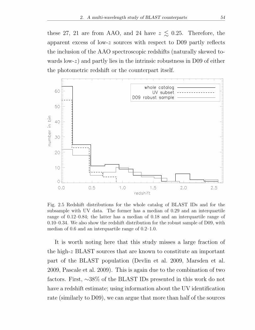
2. A multi-wavelength study of BLAST counterparts 54
these 27, 21 are from AAO, and 24 have z ≲ 0.25. Therefore, the
apparent excess of low-z sources with respect to D09 partly reflects
the inclusion of the AAO spectroscopic redshifts (naturally skewed to-
wards low-z) and partly lies in the intrinsic robustness in D09 of either
the photometric redshift or the counterpart itself.
Fig. 2.5 Redshift distributions for the whole catalog of BLAST IDs and for thesubsample with UV data. The former has a median of 0.29 and an interquartilerange of 0.12–0.84; the latter has a median of 0.18 and an interquartile range of0.10–0.34. We also show the redshift distribution for the robust sample of D09, withmedian of 0.6 and an interquartile range of 0.2–1.0.
It is worth noting here that this study misses a large fraction of
the high-z BLAST sources that are known to constitute an important
part of the BLAST population (Devlin et al. 2009, Marsden et al.
2009, Pascale et al. 2009). This is again due to the combination of two
factors. First, ∼38% of the BLAST IDs presented in this work do not
have a redshift estimate; using information about the UV identification
rate (similarly to D09), we can argue that more than half of the sources
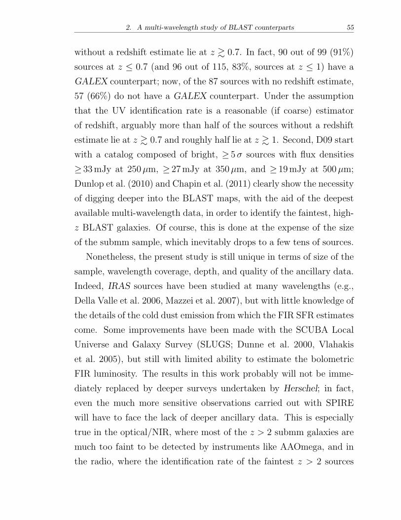
2. A multi-wavelength study of BLAST counterparts 55
without a redshift estimate lie at z ≳ 0.7. In fact, 90 out of 99 (91%)
sources at z ≤ 0.7 (and 96 out of 115, 83%, sources at z ≤ 1) have a
GALEX counterpart; now, of the 87 sources with no redshift estimate,
57 (66%) do not have a GALEX counterpart. Under the assumption
that the UV identification rate is a reasonable (if coarse) estimator
of redshift, arguably more than half of the sources without a redshift
estimate lie at z ≳ 0.7 and roughly half lie at z ≳ 1. Second, D09 start
with a catalog composed of bright, ≥ 5� sources with flux densities
≥ 33mJy at 250�m, ≥ 27mJy at 350�m, and ≥ 19mJy at 500�m;
Dunlop et al. (2010) and Chapin et al. (2011) clearly show the necessity
of digging deeper into the BLAST maps, with the aid of the deepest
available multi-wavelength data, in order to identify the faintest, high-
z BLAST galaxies. Of course, this is done at the expense of the size
of the submm sample, which inevitably drops to a few tens of sources.
Nonetheless, the present study is still unique in terms of size of the
sample, wavelength coverage, depth, and quality of the ancillary data.
Indeed, IRAS sources have been studied at many wavelengths (e.g.,
Della Valle et al. 2006, Mazzei et al. 2007), but with little knowledge of
the details of the cold dust emission from which the FIR SFR estimates
come. Some improvements have been made with the SCUBA Local
Universe and Galaxy Survey (SLUGS; Dunne et al. 2000, Vlahakis
et al. 2005), but still with limited ability to estimate the bolometric
FIR luminosity. The results in this work probably will not be imme-
diately replaced by deeper surveys undertaken by Herschel; in fact,
even the much more sensitive observations carried out with SPIRE
will have to face the lack of deeper ancillary data. This is especially
true in the optical/NIR, where most of the z > 2 submm galaxies are
much too faint to be detected by instruments like AAOmega, and in
the radio, where the identification rate of the faintest z > 2 sources
2. A multi-wavelength study of BLAST counterparts 56
drops drastically, even when using the deepest available data (VLA).
2.3 FIR Luminosities and SFRs
2.3.1 Deboosting the BLAST fluxes
The sources in the BLAST catalog used by D09 to identify counter-
parts in the radio and 24�m are detected directly from the maps of
BGS-Deep and BGS-Wide. While the details of the catalog are dis-
cussed there, it is useful to summarize here the procedure to clarify
what are the potential biases.
First, a catalog of BLAST sources with detection significance higher
than 3 � is made at each wavelength, independently. Each entry in the
catalog is then positionally matched across the three bands, with the
requirement of a 5 � detection in at least one band. The significance
here is relative to instrumental noise, and does not include confusion
noise. A new position is assigned to the source by averaging its posi-
tions in the original single-wavelength catalogs, with weights estimated
by taking into account the beam sizes and the signal-to-noise ratios
(SNRs) of the detections at each wavelength. This combined catalog
is then used to identify counterparts in the radio and at 24�m, and
a new flux density is measured from the 70 to 500�m maps at the
accurate position of the counterpart.
The BLAST differential source counts fall very rapidly with flux
density (approximately following dN/dS ∝ S−3; Patanchon et al.
2009), thus Eddington bias as well as source confusion will cause the
fluxes to be boosted. This effect has to be estimated to properly com-
pute the FIR luminosity of each source. Coppin et al. (2005) have
proposed a Bayesian approach that can be applied to estimate the
most likely flux distribution when the noise properties of the detection
2. A multi-wavelength study of BLAST counterparts 57
and the underlying source distribution are known. Their method is
derived under the assumption that the flux density comes from just
one source, plus noise. This cannot be applied to BLAST sources be-
cause of blending: the measured flux density can either come from just
one source, or more likely from several sources blended together by the
beam, which then appear as one single source of larger flux density.
We develop a different method to account for boosting of BLAST
fluxes, which is entirely based on Monte Carlo simulations. We gener-
ate 100 noiseless sky maps using the BLAST measured count models
(Patanchon et al. 2009), and no clustering8. Noise is added to each
simulated map to a realistic level for the BGS-Deep and BGS-Wide
regions. Sources are then retrieved with the same method used on the
real maps (Devlin et al. 2009). Considering all the input components
within an FWHM beam distance from each retrieved source, we stip-
ulate that the input component with largest flux density is the actual
counterpart9 (ID). The source flux density is then remeasured at the
position of the ID. Finally, we compare this flux density with that of
the input source. By repeating this for each source detected in each
simulation, we generate distributions of input/output SNR, where the
relevant noise is the instrumental noise at the position of the ID. These
simulations are similar to those used in Chapin et al. (2011) to study
the effects of confusion for their deeper sample.
Figure 2.6 shows the result of this analysis. In each bin, we display
the median of the distribution of input SNR (labeled SNRID) corre-
sponding to the measured SNR. The error bars define the first and
third interquartiles. To obtain the deboosted flux density likelihood,
8 Here we refer to the source clustering detected in the BLAST maps by Viero et al. (2009).9 We know that this assumption is always verified in BGS-Wide but less so in BGS-Deep, where
in 21% of the cases the second brightest component contributes to more than 50% of the retrievedflux (see E09, Appendix B).
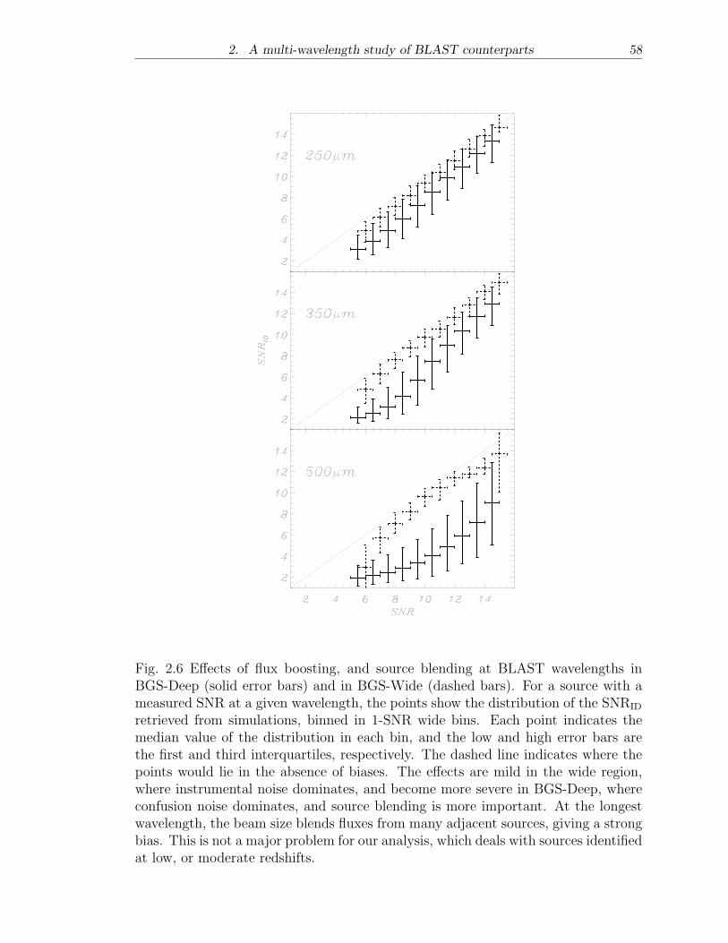
2. A multi-wavelength study of BLAST counterparts 58
Fig. 2.6 Effects of flux boosting, and source blending at BLAST wavelengths inBGS-Deep (solid error bars) and in BGS-Wide (dashed bars). For a source with ameasured SNR at a given wavelength, the points show the distribution of the SNRID
retrieved from simulations, binned in 1-SNR wide bins. Each point indicates themedian value of the distribution in each bin, and the low and high error bars arethe first and third interquartiles, respectively. The dashed line indicates where thepoints would lie in the absence of biases. The effects are mild in the wide region,where instrumental noise dominates, and become more severe in BGS-Deep, whereconfusion noise dominates, and source blending is more important. At the longestwavelength, the beam size blends fluxes from many adjacent sources, giving a strongbias. This is not a major problem for our analysis, which deals with sources identifiedat low, or moderate redshifts.
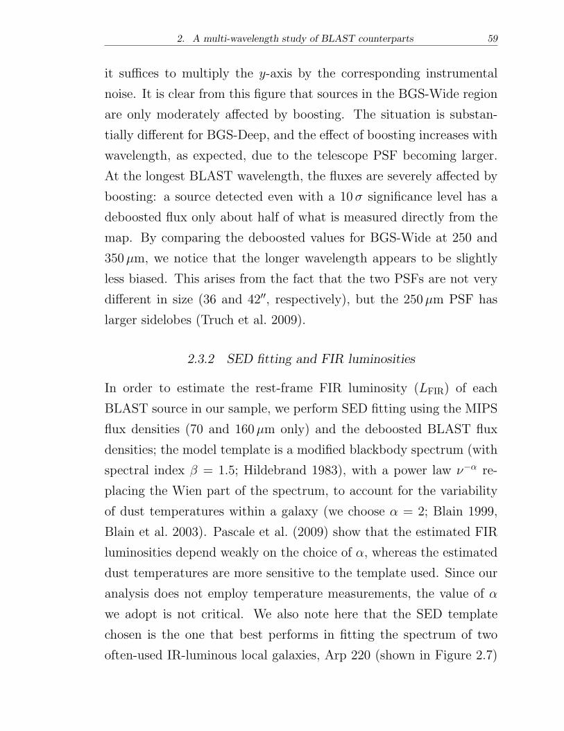
2. A multi-wavelength study of BLAST counterparts 59
it suffices to multiply the y-axis by the corresponding instrumental
noise. It is clear from this figure that sources in the BGS-Wide region
are only moderately affected by boosting. The situation is substan-
tially different for BGS-Deep, and the effect of boosting increases with
wavelength, as expected, due to the telescope PSF becoming larger.
At the longest BLAST wavelength, the fluxes are severely affected by
boosting: a source detected even with a 10 � significance level has a
deboosted flux only about half of what is measured directly from the
map. By comparing the deboosted values for BGS-Wide at 250 and
350�m, we notice that the longer wavelength appears to be slightly
less biased. This arises from the fact that the two PSFs are not very
different in size (36 and 42′′, respectively), but the 250�m PSF has
larger sidelobes (Truch et al. 2009).
2.3.2 SED fitting and FIR luminosities
In order to estimate the rest-frame FIR luminosity (LFIR) of each
BLAST source in our sample, we perform SED fitting using the MIPS
flux densities (70 and 160�m only) and the deboosted BLAST flux
densities; the model template is a modified blackbody spectrum (with
spectral index � = 1.5; Hildebrand 1983), with a power law �−� re-
placing the Wien part of the spectrum, to account for the variability
of dust temperatures within a galaxy (we choose � = 2; Blain 1999,
Blain et al. 2003). Pascale et al. (2009) show that the estimated FIR
luminosities depend weakly on the choice of �, whereas the estimated
dust temperatures are more sensitive to the template used. Since our
analysis does not employ temperature measurements, the value of �
we adopt is not critical. We also note here that the SED template
chosen is the one that best performs in fitting the spectrum of two
often-used IR-luminous local galaxies, Arp 220 (shown in Figure 2.7)
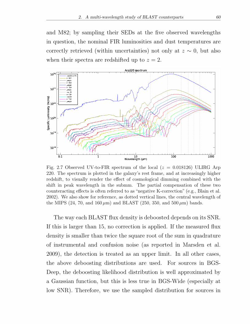
2. A multi-wavelength study of BLAST counterparts 60
and M82; by sampling their SEDs at the five observed wavelengths
in question, the nominal FIR luminosities and dust temperatures are
correctly retrieved (within uncertainties) not only at z ∼ 0, but also
when their spectra are redshifted up to z = 2.
Wavelength (m)S pecifi cL umi nosi t y( W/H z)
Arp220 spectrum
0.1 1 10 100 1000101610181020102210241026 z=0.018126z=0.2z=0.4z=0.6z=0.8z=1.0z=1.5z=2.0z=3.0z=4.0z=5.0z=6.0
Fig. 2.7 Observed UV-to-FIR spectrum of the local (z = 0.018126) ULIRG Arp220. The spectrum is plotted in the galaxy’s rest frame, and at increasingly higherredshift, to visually render the effect of cosmological dimming combined with theshift in peak wavelength in the submm. The partial compensation of these twocounteracting effects is often referred to as “negative K-correction” (e.g., Blain et al.2002). We also show for reference, as dotted vertical lines, the central wavelength ofthe MIPS (24, 70, and 160�m) and BLAST (250, 350, and 500�m) bands.
The way each BLAST flux density is deboosted depends on its SNR.
If this is larger than 15, no correction is applied. If the measured flux
density is smaller than twice the square root of the sum in quadrature
of instrumental and confusion noise (as reported in Marsden et al.
2009), the detection is treated as an upper limit. In all other cases,
the above deboosting distributions are used. For sources in BGS-
Deep, the deboosting likelihood distribution is well approximated by
a Gaussian function, but this is less true in BGS-Wide (especially at
low SNR). Therefore, we use the sampled distribution for sources in
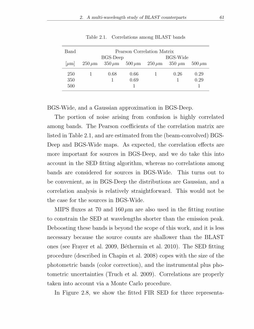
2. A multi-wavelength study of BLAST counterparts 61
Table 2.1. Correlations among BLAST bands
Band Pearson Correlation MatrixBGS-Deep BGS-Wide
[�m] 250�m 350�m 500�m 250�m 350 �m 500�m
250 1 0.68 0.66 1 0.26 0.29350 1 0.69 1 0.29500 1 1
BGS-Wide, and a Gaussian approximation in BGS-Deep.
The portion of noise arising from confusion is highly correlated
among bands. The Pearson coefficients of the correlation matrix are
listed in Table 2.1, and are estimated from the (beam-convolved) BGS-
Deep and BGS-Wide maps. As expected, the correlation effects are
more important for sources in BGS-Deep, and we do take this into
account in the SED fitting algorithm, whereas no correlations among
bands are considered for sources in BGS-Wide. This turns out to
be convenient, as in BGS-Deep the distributions are Gaussian, and a
correlation analysis is relatively straightforward. This would not be
the case for the sources in BGS-Wide.
MIPS fluxes at 70 and 160�m are also used in the fitting routine
to constrain the SED at wavelengths shorter than the emission peak.
Deboosting these bands is beyond the scope of this work, and it is less
necessary because the source counts are shallower than the BLAST
ones (see Frayer et al. 2009, Bethermin et al. 2010). The SED fitting
procedure (described in Chapin et al. 2008) copes with the size of the
photometric bands (color correction), and the instrumental plus pho-
tometric uncertainties (Truch et al. 2009). Correlations are properly
taken into account via a Monte Carlo procedure.
In Figure 2.8, we show the fitted FIR SED for three representa-
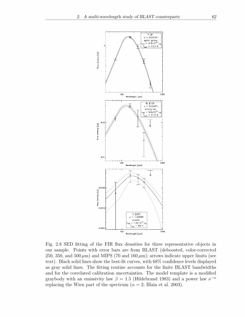
2. A multi-wavelength study of BLAST counterparts 62
Fig. 2.8 SED fitting of the FIR flux densities for three representative objects inour sample. Points with error bars are from BLAST (deboosted, color-corrected250, 350, and 500�m) and MIPS (70 and 160�m); arrows indicate upper limits (seetext). Black solid lines show the best-fit curves, with 68% confidence levels displayedas gray solid lines. The fitting routine accounts for the finite BLAST bandwidthsand for the correlated calibration uncertainties. The model template is a modifiedgraybody with an emissivity law � = 1.5 (Hildebrand 1983) and a power law �−�
replacing the Wien part of the spectrum (� = 2; Blain et al. 2003).
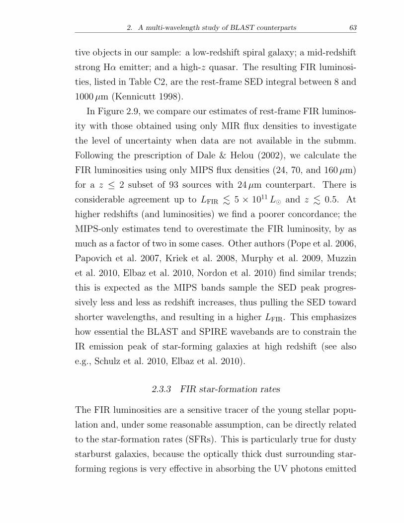
2. A multi-wavelength study of BLAST counterparts 63
tive objects in our sample: a low-redshift spiral galaxy; a mid-redshift
strong H� emitter; and a high-z quasar. The resulting FIR luminosi-
ties, listed in Table C2, are the rest-frame SED integral between 8 and
1000�m (Kennicutt 1998).
In Figure 2.9, we compare our estimates of rest-frame FIR luminos-
ity with those obtained using only MIR flux densities to investigate
the level of uncertainty when data are not available in the submm.
Following the prescription of Dale & Helou (2002), we calculate the
FIR luminosities using only MIPS flux densities (24, 70, and 160�m)
for a z ≤ 2 subset of 93 sources with 24�m counterpart. There is
considerable agreement up to LFIR ≲ 5 × 10¹¹L⊙ and z ≲ 0.5. At
higher redshifts (and luminosities) we find a poorer concordance; the
MIPS-only estimates tend to overestimate the FIR luminosity, by as
much as a factor of two in some cases. Other authors (Pope et al. 2006,
Papovich et al. 2007, Kriek et al. 2008, Murphy et al. 2009, Muzzin
et al. 2010, Elbaz et al. 2010, Nordon et al. 2010) find similar trends;
this is expected as the MIPS bands sample the SED peak progres-
sively less and less as redshift increases, thus pulling the SED toward
shorter wavelengths, and resulting in a higher LFIR. This emphasizes
how essential the BLAST and SPIRE wavebands are to constrain the
IR emission peak of star-forming galaxies at high redshift (see also
e.g., Schulz et al. 2010, Elbaz et al. 2010).
2.3.3 FIR star-formation rates
The FIR luminosities are a sensitive tracer of the young stellar popu-
lation and, under some reasonable assumption, can be directly related
to the star-formation rates (SFRs). This is particularly true for dusty
starburst galaxies, because the optically thick dust surrounding star-
forming regions is very effective in absorbing the UV photons emitted
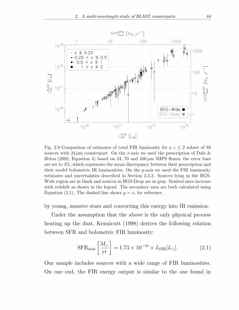
2. A multi-wavelength study of BLAST counterparts 64
Fig. 2.9 Comparison of estimates of total FIR luminosity for a z ≤ 2 subset of 93sources with 24�m counterpart. On the x-axis we used the prescription of Dale &Helou (2002; Equation 4) based on 24, 70 and 160�m MIPS fluxes; the error barsare set to 4%, which represents the mean discrepancy between their prescription andtheir model bolometric IR luminosities. On the y-axis we used the FIR luminosityestimates and uncertainties described in Section 2.3.2. Sources lying in the BGS-Wide region are in black and sources in BGS-Deep are in gray. Symbol sizes increasewith redshift as shown in the legend. The secondary axes are both calculated usingEquation (2.1). The dashed line shows y = x, for reference.
by young, massive stars and converting this energy into IR emission.
Under the assumption that the above is the only physical process
heating up the dust, Kennicutt (1998) derives the following relation
between SFR and bolometric FIR luminosity:
SFRdust
[
M⊙yr
]
= 1.73× 10⁻¹⁰ × LFIR[L⊙]. (2.1)
Our sample includes sources with a wide range of FIR luminosities.
On one end, the FIR energy output is similar to the one found in
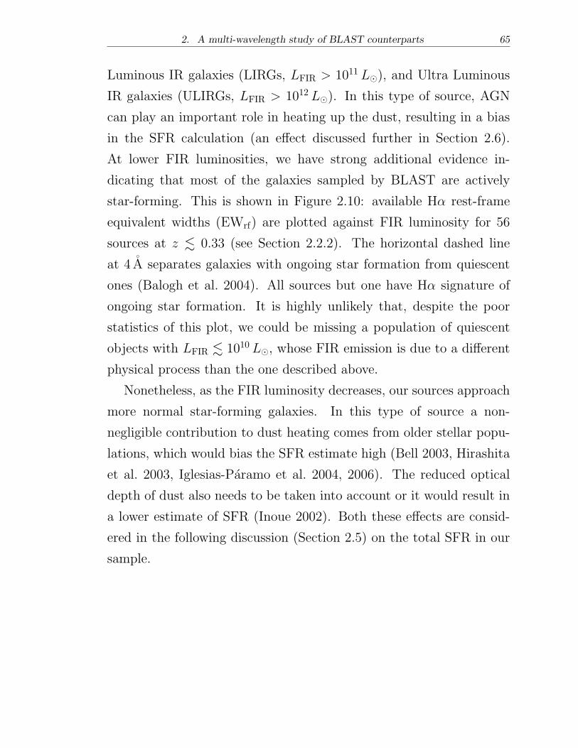
2. A multi-wavelength study of BLAST counterparts 65
Luminous IR galaxies (LIRGs, LFIR > 1011L⊙), and Ultra Luminous
IR galaxies (ULIRGs, LFIR > 1012L⊙). In this type of source, AGN
can play an important role in heating up the dust, resulting in a bias
in the SFR calculation (an effect discussed further in Section 2.6).
At lower FIR luminosities, we have strong additional evidence in-
dicating that most of the galaxies sampled by BLAST are actively
star-forming. This is shown in Figure 2.10: available H� rest-frame
equivalent widths (EWrf) are plotted against FIR luminosity for 56
sources at z ≲ 0.33 (see Section 2.2.2). The horizontal dashed line
at 4 A separates galaxies with ongoing star formation from quiescent
ones (Balogh et al. 2004). All sources but one have H� signature of
ongoing star formation. It is highly unlikely that, despite the poor
statistics of this plot, we could be missing a population of quiescent
objects with LFIR ≲ 1010L⊙, whose FIR emission is due to a different
physical process than the one described above.
Nonetheless, as the FIR luminosity decreases, our sources approach
more normal star-forming galaxies. In this type of source a non-
negligible contribution to dust heating comes from older stellar popu-
lations, which would bias the SFR estimate high (Bell 2003, Hirashita
et al. 2003, Iglesias-Paramo et al. 2004, 2006). The reduced optical
depth of dust also needs to be taken into account or it would result in
a lower estimate of SFR (Inoue 2002). Both these effects are consid-
ered in the following discussion (Section 2.5) on the total SFR in our
sample.
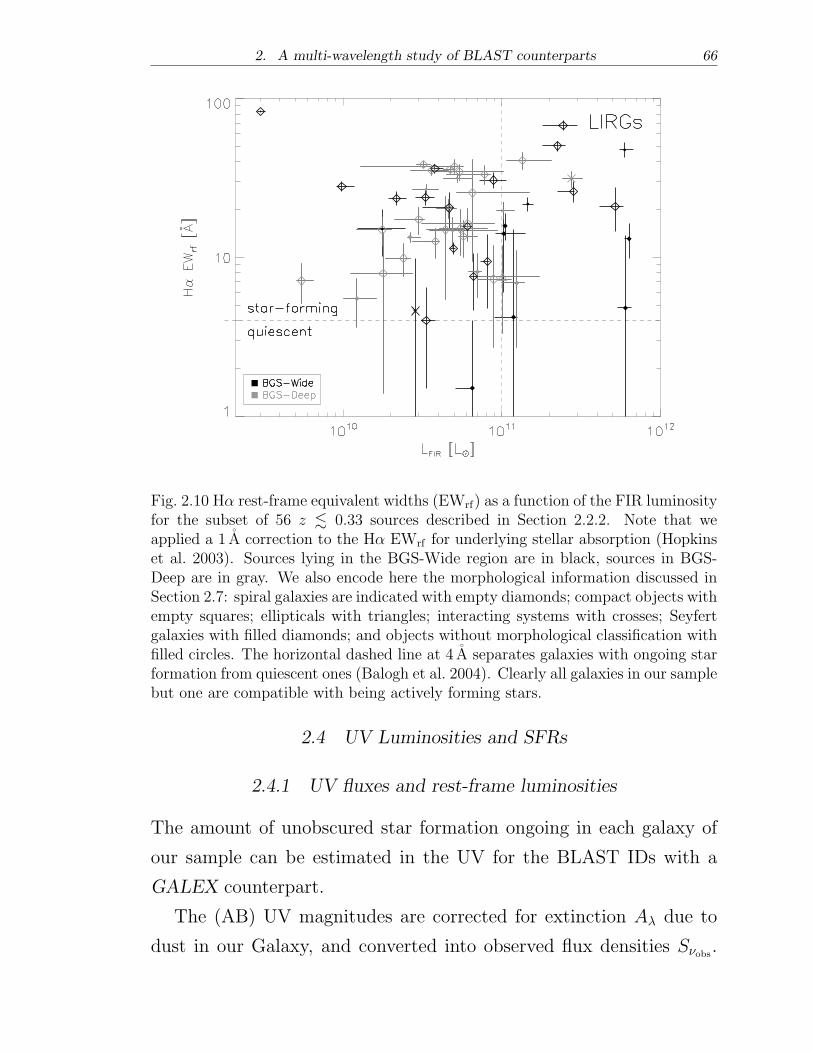
2. A multi-wavelength study of BLAST counterparts 66
Fig. 2.10 H� rest-frame equivalent widths (EWrf) as a function of the FIR luminosityfor the subset of 56 z ≲ 0.33 sources described in Section 2.2.2. Note that weapplied a 1 A correction to the H� EWrf for underlying stellar absorption (Hopkinset al. 2003). Sources lying in the BGS-Wide region are in black, sources in BGS-Deep are in gray. We also encode here the morphological information discussed inSection 2.7: spiral galaxies are indicated with empty diamonds; compact objects withempty squares; ellipticals with triangles; interacting systems with crosses; Seyfertgalaxies with filled diamonds; and objects without morphological classification withfilled circles. The horizontal dashed line at 4 A separates galaxies with ongoing starformation from quiescent ones (Balogh et al. 2004). Clearly all galaxies in our samplebut one are compatible with being actively forming stars.
2.4 UV Luminosities and SFRs
2.4.1 UV fluxes and rest-frame luminosities
The amount of unobscured star formation ongoing in each galaxy of
our sample can be estimated in the UV for the BLAST IDs with a
GALEX counterpart.
The (AB) UV magnitudes are corrected for extinction A� due to
dust in our Galaxy, and converted into observed flux densities S�obs.
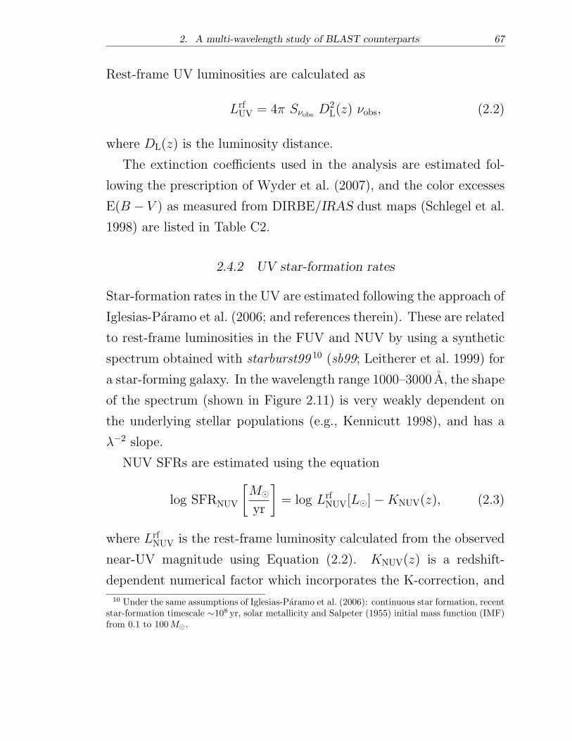
2. A multi-wavelength study of BLAST counterparts 67
Rest-frame UV luminosities are calculated as
LrfUV = 4� S�obs D
2L(z) �obs, (2.2)
where DL(z) is the luminosity distance.
The extinction coefficients used in the analysis are estimated fol-
lowing the prescription of Wyder et al. (2007), and the color excesses
E(B − V ) as measured from DIRBE/IRAS dust maps (Schlegel et al.
1998) are listed in Table C2.
2.4.2 UV star-formation rates
Star-formation rates in the UV are estimated following the approach of
Iglesias-Paramo et al. (2006; and references therein). These are related
to rest-frame luminosities in the FUV and NUV by using a synthetic
spectrum obtained with starburst99 10 (sb99; Leitherer et al. 1999) for
a star-forming galaxy. In the wavelength range 1000–3000 A, the shape
of the spectrum (shown in Figure 2.11) is very weakly dependent on
the underlying stellar populations (e.g., Kennicutt 1998), and has a
�−2 slope.
NUV SFRs are estimated using the equation
log SFRNUV
[
M⊙yr
]
= log LrfNUV[L⊙]−KNUV(z), (2.3)
where LrfNUV is the rest-frame luminosity calculated from the observed
near-UV magnitude using Equation (2.2). KNUV(z) is a redshift-
dependent numerical factor which incorporates the K-correction, and
10 Under the same assumptions of Iglesias-Paramo et al. (2006): continuous star formation, recentstar-formation timescale ∼108 yr, solar metallicity and Salpeter (1955) initial mass function (IMF)from 0.1 to 100M⊙.
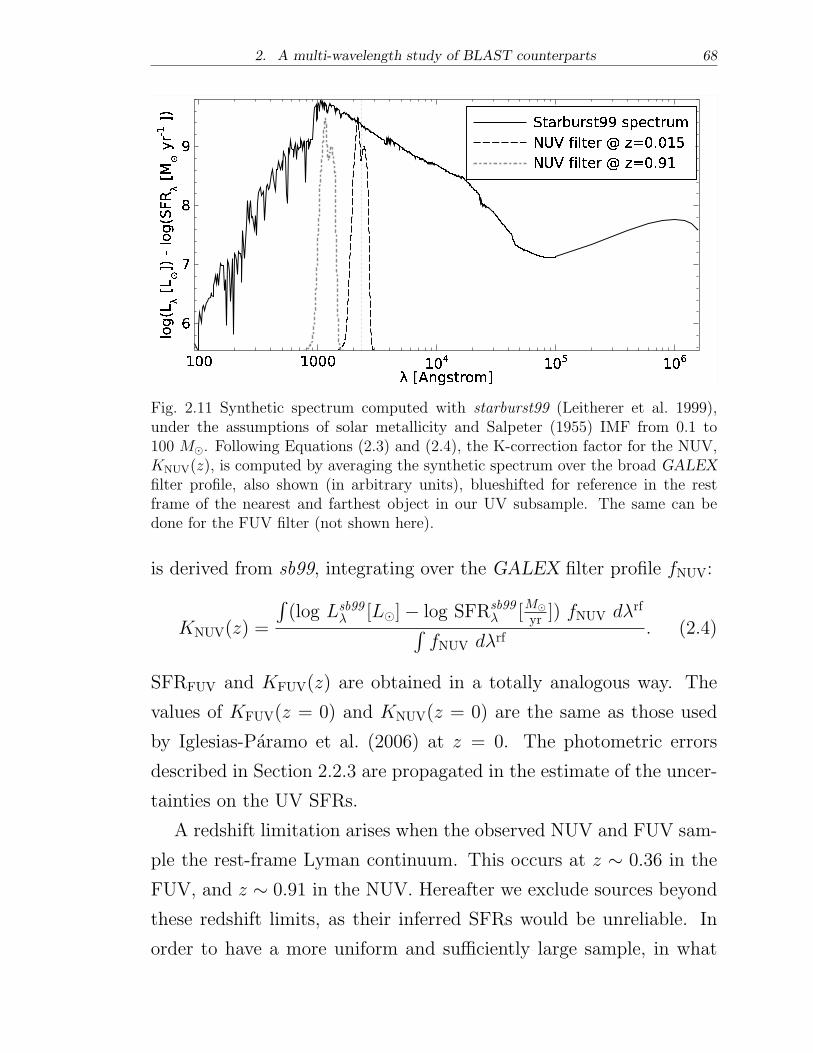
2. A multi-wavelength study of BLAST counterparts 68
λ [Angstrom]l og( L λ[ L N]) Ql og( S FR λ[ M NyrX1 ])
100 1000 104 105 1066789 Starburst99 spectrumNUV filter @ z=0.015NUV filter @ z=0.91
Fig. 2.11 Synthetic spectrum computed with starburst99 (Leitherer et al. 1999),under the assumptions of solar metallicity and Salpeter (1955) IMF from 0.1 to100 M⊙. Following Equations (2.3) and (2.4), the K-correction factor for the NUV,KNUV(z), is computed by averaging the synthetic spectrum over the broad GALEXfilter profile, also shown (in arbitrary units), blueshifted for reference in the restframe of the nearest and farthest object in our UV subsample. The same can bedone for the FUV filter (not shown here).
is derived from sb99, integrating over the GALEX filter profile fNUV:
KNUV(z) =
∫
(log Lsb99� [L⊙]− log SFRsb99
� [M⊙
yr ]) fNUV d�rf∫
fNUV d�rf. (2.4)
SFRFUV and KFUV(z) are obtained in a totally analogous way. The
values of KFUV(z = 0) and KNUV(z = 0) are the same as those used
by Iglesias-Paramo et al. (2006) at z = 0. The photometric errors
described in Section 2.2.3 are propagated in the estimate of the uncer-
tainties on the UV SFRs.
A redshift limitation arises when the observed NUV and FUV sam-
ple the rest-frame Lyman continuum. This occurs at z ∼ 0.36 in the
FUV, and z ∼ 0.91 in the NUV. Hereafter we exclude sources beyond
these redshift limits, as their inferred SFRs would be unreliable. In
order to have a more uniform and sufficiently large sample, in what
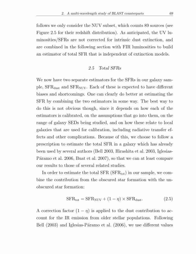
2. A multi-wavelength study of BLAST counterparts 69
follows we only consider the NUV subset, which counts 89 sources (see
Figure 2.5 for their redshift distribution). As anticipated, the UV lu-
minosities/SFRs are not corrected for intrinsic dust extinction, and
are combined in the following section with FIR luminosities to build
an estimator of total SFR that is independent of extinction models.
2.5 Total SFRs
We now have two separate estimators for the SFRs in our galaxy sam-
ple, SFRdust and SFRNUV. Each of these is expected to have different
biases and shortcomings. One can clearly do better at estimating the
SFR by combining the two estimators in some way. The best way to
do this is not obvious though, since it depends on how each of the
estimators is calibrated, on the assumptions that go into them, on the
range of galaxy SEDs being studied, and on how these relate to local
galaxies that are used for calibration, including radiative transfer ef-
fects and other complications. Because of this, we choose to follow a
prescription to estimate the total SFR in a galaxy which has already
been used by several authors (Bell 2003, Hirashita et al. 2003, Iglesias-
Paramo et al. 2006, Buat et al. 2007), so that we can at least compare
our results to those of several related studies.
In order to estimate the total SFR (SFRtot) in our sample, we com-
bine the contribution from the obscured star formation with the un-
obscured star formation:
SFRtot = SFRNUV + (1− �)× SFRdust. (2.5)
A correction factor (1 − �) is applied to the dust contribution to ac-
count for the IR emission from older stellar populations. Following
Bell (2003) and Iglesias-Paramo et al. (2006), we use different values
2. A multi-wavelength study of BLAST counterparts 70
of � depending on whether the object in question is more likely to be
a starburst (� ∼ 0.09 for LFIR > 1011L⊙) or a normal star-forming
galaxy (� ∼ 0.32 for LFIR ≤ 1011L⊙). As anticipated in Section 2.3.3,
this method can account for both the contrasting effects that come into
play when we try to estimate the total SFR budget for an inhomoge-
neous sample of objects. Namely, � parameterizes the contribution
to dust heating from older stellar populations as a function of the
integrated FIR luminosity, whereas the contribution from the UV lu-
minosity guarantees that all the UV photons that manage to escape
the galaxy, due to the reduced optical depth of the dust, are actually
taken into account.
We briefly recall here that the main selection effects of our sample
are, on the one hand, that the rest-frame LFIR increases steadily with
redshift (see Figure 2.9 and D09), and on the other hand that the
UV luminosity estimates are not reliable beyond z ∼ 0.9. Moreover,
we stress the importance of the blending effects reported in Section
2.3.1, which may lead to misidentifications, particularly in BGS-Deep
(sources in gray).
The results of this analysis are shown in Figure 2.12. In the top
panel, we plot the ratio of SFRNUV to (1−�)SFRdust as a function of the
FIR luminosity. With the exception of a few outliers,11 there is a clear
trend, namely the NUV contribution is more important at low LFIR
(low-z), whereas star formation is mainly obscured at LFIR ≳ 1011L⊙,
z ≳ 0.5. The same effect is evident in the bottom panel, where we
plot SFRtot as a function of redshift. The gray shaded area shows the
1 � confidence interval of a power-law fit SFRNUV ∝ z1.6. Most sources
with SFRtot larger than a few M⊙ yr−1 have negligible contribution
from the UV. This is consistent with what Takeuchi et al. (2010b)
11 In particular, ID#55 could be a misidentification because there is a secondary counterpart, seeE09.
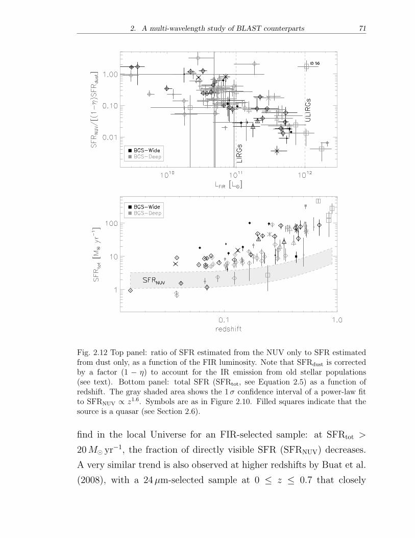
2. A multi-wavelength study of BLAST counterparts 71
Fig. 2.12 Top panel: ratio of SFR estimated from the NUV only to SFR estimatedfrom dust only, as a function of the FIR luminosity. Note that SFRdust is correctedby a factor (1 − �) to account for the IR emission from old stellar populations(see text). Bottom panel: total SFR (SFRtot, see Equation 2.5) as a function ofredshift. The gray shaded area shows the 1� confidence interval of a power-law fitto SFRNUV ∝ z1.6. Symbols are as in Figure 2.10. Filled squares indicate that thesource is a quasar (see Section 2.6).
find in the local Universe for an FIR-selected sample: at SFRtot >
20M⊙ yr−1, the fraction of directly visible SFR (SFRNUV) decreases.
A very similar trend is also observed at higher redshifts by Buat et al.
(2008), with a 24�m-selected sample at 0 ≤ z ≤ 0.7 that closely
2. A multi-wavelength study of BLAST counterparts 72
resembles our sample at those redshifts, in terms of dynamic ranges
and FIR-to-UV ratios.
Such a behavior in the individual BLAST IDs can be related to the
greater evolution of the total FIR luminosity density with respect to
the optical–UV one, as reported for instance by Pascale et al. (2009).
On the other hand, we stress that at LFIR ≲ 1011L⊙, z ≲ 0.25, FIR-
only observations would lead to underestimates of the total SFR of at
least a factor of two.
By comparing our sample in Figure 2.12 with the IRAS/FIR-selected
local sample of Iglesias-Paramo et al. (2006), we notice that the over-
lap is quite modest and limited to LFIR ≲ 1010L⊙, z ≲ 0.1 sources.
We point out that this conclusion should not be diminished by con-
siderations on the extent of the local volume sampled by the BLAST
survey.
At the very high luminosity end, only two objects (one of which is
flagged as quasar, see Section 2.6) with z ≤ 0.91 have a UV counter-
part. We thus investigate the 30 galaxies with LFIR ≥ 1012L⊙ in the
full set of BLAST IDs, finding that 16 are flagged as quasars, most of
which are optically bright. At z > 1, the optical U and g bands probe
the rest-frame UV, and we calculate that these objects would virtually
populate the top right corner of the upper panel of Figure 2.12. How-
ever, the UV emission from quasars is strongly contaminated by the
active nucleus, and cannot be directly associated with recent star for-
mation. Of the remaining 14 ULIRGs with no AGN signatures, only
four have optical magnitudes, and would occupy the bottom right cor-
ner, indicating severe dust attenuation. We can therefore argue that,
even if our subset of objects lacks the abundance of most luminous
IR galaxies detected in the SHADES survey (see Coppin et al. 2008,
Serjeant et al. 2008), SCUBA-like sources will likely lie in the bot-
2. A multi-wavelength study of BLAST counterparts 73
tom right corner and beyond, following the same trend of increasing
dust attenuation at higher FIR luminosities. This is a first hint that
our analysis begins to detect SCUBA galaxies, which are known to
overlap considerably with the fainter BLAST galaxy population, fol-
lowing joint studies of LABOCA 870�m and BLAST data (Dunlop
et al. 2010, Chapin et al. 2011). We will discuss this in more detail in
Section 2.8.
The 24�m-selected sample described by Le Floc’h et al. (2005)
most resembles our z ≤ 0.9 sample in terms of LFIR–z parameter
space, although our objects are in general more massive, as we will
see in Section 2.8. This, in combination with Figure 2.10, points to
the conclusion that the BLAST counterparts detected in this survey
at z ≲ 1 are mostly run-of-the-mill star-forming galaxies. Finally,
given the steep number counts at the BLAST wavelengths (Patanchon
et al. 2009) and the smaller beam sizes of Herschel, we expect SPIRE
to detect roughly a factor of 10 more sources than BLAST, probing
fainter fluxes and therefore higher redshifts. Figure 2.12 suggests that
SPIRE will likely fill the 1011 ≲ LFIR ≲ 2 × 10¹²L⊙ region (see e.g.,
Chapin et al. 2011), but probably will not be dominated by SCUBA-
like sources.
2.6 AGN Fraction and Quasars
In this section, we describe the AGN and quasar content of our sample
and investigate whether the submm emission that we see with BLAST
is mainly due to the host galaxy or to the active nucleus.
AGNs are identified using spectroscopic and photometric methods,
and the information is listed in Table C1. Of the 82 sources in our
sample with optical spectra, 56 have a measurement of the line ratio
2. A multi-wavelength study of BLAST counterparts 74
[N II]/H�; 14 of these have [N II]/H�≳ 0.6, and we flag them as AGNs
(Kauffmann et al. 2003, Miller et al. 2003; and references therein).
Broad emission lines, such as C III] 190.9 and C IV 154.9, which appear
in the accessible waveband at z > 1, are used to identify five additional
sources as quasars. A search on NED yields that 10 more sources in
our sample are classified as AGNs by other authors.
Active galaxies can also be identified using a number of photometric
empirical methods. Quasars occupy a distinct region in the IRAC color
space by virtue of their strong, red continua in the MIR (Lacy et al.
2004). IRAC fluxes are available for 205 sources, and we use the three
color–color cut prescriptions of Hatziminaoglou et al. (2005), Stern
et al. (2005), and Marsden et al. (2009). Optical magnitudes and
postage-stamp images are also available for 114 sources, along with
radio fluxes for 107 sources from D09. A source is considered a quasar
when it is compact12 and satisfies the three aforementioned color–
color cut prescriptions. If only two color–color cuts prescriptions are
satisfied, we also require the source to be either radio-loud (L1.4GHz ≳
1039 W), optically bright (LU /g ≳ 1011L⊙), or one of the 10 NED
AGNs.
Using these empirical methods, we find 24 quasars plus 10 addi-
tional sources showing weaker yet significant quasar activity, when the
above conditions are near the threshold. The five quasars identified
spectroscopically are all contained in this photometric list. Of the 14
spectroscopically identified AGNs, 10 are definitely not compact, but
rather spiral in shape (see the following section on morphology), and
mostly radio-quiet. We believe that these objects are Seyfert galaxies
(e.g., Cid Fernandes et al. 2010).
In conclusion, we have assessed that about 15% of the galaxies in
12 By “compact” we mean objects unresolved in the optical and MIR, with linear sizes ≲ 3 kpc atz ≳ 1.
2. A multi-wavelength study of BLAST counterparts 75
our sample show strong indication of having an active nucleus and
an additional 6% have weaker yet significant evidence. Chapin et al.
(2011) found a comparable proportion13 of sources with excess radio
and/or MIR that can be interpreted as an AGN signature. Several re-
cent observations find close association of AGN activity and young star
formation (Silverman et al. 2009), consistent with a scenario in which
the FIR/submm emission is mainly due to star formation ongoing in
the host galaxy, rather than to emission from a dusty torus obscuring
the inner regions of the active nucleus (Wiebe et al. 2009, Coppin et al.
2010, Muzzin et al. 2010, Hatziminaoglou et al. 2010, Shao et al. 2010,
Elbaz et al. 2010). In addition, our AGN selection criteria, which use
optical and MIR data, tend to favor type-1 AGNs, i.e., unobscured
Seyfert galaxies and quasars. This is definitely the case for the IRAC
color–color selection methods, as reported by Hatziminaoglou et al.
(2005) and Stern et al. (2005), but it is also corroborated by the fact
that most of the quasars we identify are optically bright. We aim to
address this issue in greater detail in a future paper.
2.7 Morphology
We assign a broad morphological classification to 137 (60%) of the
BLAST IDs presented in this work, based upon visual inspection of
UV, optical and MIR postage-stamp images (see Section 2.2.5) cen-
tered at [�BLAST, �BLAST]. A selection of cutouts is shown in Figure B1.
In addition to the visual examination of the multi-wavelength im-
ages, we corroborated our choice with ancillary information (when
available), such as: (1) location on the color–magnitude diagram, typ-
ically (U − r) versus Mr; (2) spectral features; (3) UV detection; (4)
FIR luminosity. Our findings are listed in the “morphology” column13 Only sources with a redshift estimate.
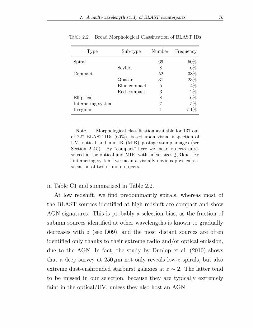
2. A multi-wavelength study of BLAST counterparts 76
Table 2.2. Broad Morphological Classification of BLAST IDs
Type Sub-type Number Frequency
Spiral 69 50%Seyfert 8 6%
Compact 52 38%Quasar 31 23%Blue compact 5 4%Red compact 3 2%
Elliptical 8 6%Interacting system 7 5%Irregular 1 < 1%
Note. — Morphological classification available for 137 outof 227 BLAST IDs (60%), based upon visual inspection ofUV, optical and mid-IR (MIR) postage-stamp images (seeSection 2.2.5). By “compact” here we mean objects unre-solved in the optical and MIR, with linear sizes ≲ 3 kpc. By“interacting system” we mean a visually obvious physical as-sociation of two or more objects.
in Table C1 and summarized in Table 2.2.
At low redshift, we find predominantly spirals, whereas most of
the BLAST sources identified at high redshift are compact and show
AGN signatures. This is probably a selection bias, as the fraction of
submm sources identified at other wavelengths is known to gradually
decreases with z (see D09), and the most distant sources are often
identified only thanks to their extreme radio and/or optical emission,
due to the AGN. In fact, the study by Dunlop et al. (2010) shows
that a deep survey at 250�m not only reveals low-z spirals, but also
extreme dust-enshrouded starburst galaxies at z ∼ 2. The latter tend
to be missed in our selection, because they are typically extremely
faint in the optical/UV, unless they also host an AGN.
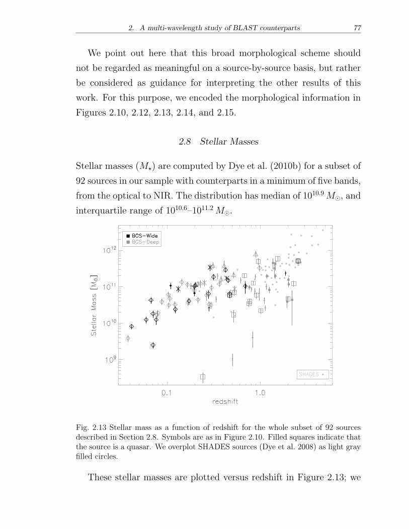
2. A multi-wavelength study of BLAST counterparts 77
We point out here that this broad morphological scheme should
not be regarded as meaningful on a source-by-source basis, but rather
be considered as guidance for interpreting the other results of this
work. For this purpose, we encoded the morphological information in
Figures 2.10, 2.12, 2.13, 2.14, and 2.15.
2.8 Stellar Masses
Stellar masses (M★) are computed by Dye et al. (2010b) for a subset of
92 sources in our sample with counterparts in a minimum of five bands,
from the optical to NIR. The distribution has median of 1010.9M⊙, and
interquartile range of 1010.6–1011.2M⊙.
Fig. 2.13 Stellar mass as a function of redshift for the whole subset of 92 sourcesdescribed in Section 2.8. Symbols are as in Figure 2.10. Filled squares indicate thatthe source is a quasar. We overplot SHADES sources (Dye et al. 2008) as light grayfilled circles.
These stellar masses are plotted versus redshift in Figure 2.13; we
2. A multi-wavelength study of BLAST counterparts 78
also show for comparison the stellar masses of SCUBA sources in
SHADES, computed by Dye et al. (2008) using a methodology and
photometry almost identical to ours.
Except for three outliers (that may well be misidentifications as they
all lie in BGS-Deep), the monotonic trend of increasing stellar masses
is the result of multiple selection effects; sources at a given redshift are
not detected with arbitrarily low, or arbitrarily high stellar masses. As
we discuss later in this section, there is an approximately constant re-
lation between LFIR and stellar masses in our sample. Low-luminosity
sources (with low stellar masses) are excluded at a given redshift be-
cause of sensitivity. On the other hand, sources with LFIR (and stellar
masses) above a certain threshold are excluded from our sample de-
spite the well-documented strongly evolving FIR luminosity function
(E09, Dye et al. 2010a, Eales et al. 2010b); our present study simply
does not go deep enough to start detecting the bulk of high-z (and
higher volume density) K-corrected sources. In particular, sources
with M★ ≳ 1012M⊙, which are present in the SHADES sample, are
absent from ours. Indeed, these very massive sources are not detected
among 24�m-selected samples, down to a flux density level of ∼20�Jy
(GOODS survey; see e.g., Le Floc’h et al. 2005, Perez-Gonzalez et al.
2005, Caputi et al. 2006, Elbaz et al. 2007, Santini et al. 2009)14. The
24�m catalog used by D09 to find counterparts to the BLAST sources
goes down to the same depth; therefore, we are only left with the radio
catalogs. It is indeed possible that our analysis is missing very massive
galaxies that, though having a radio ID, do not have an estimate of
14 All the authors cited above adopt a Salpeter (1955) IMF. Caputi et al. (2006), Santini et al.(2009), and Dye et al. (2008, 2010b) estimate the stellar masses by means of an optical–to–NIRSED fit of each galaxy at the determined redshift. Le Floc’h et al. (2005) and Perez-Gonzalezet al. (2005) simply convert, respectively, V - and K-band luminosities into stellar masses. Finally,Elbaz et al. (2007) compute stellar masses by modeling the stellar populations of each galaxy usingstellar absorption-line indices.
2. A multi-wavelength study of BLAST counterparts 79
stellar mass because measurements are not available in a minimum of
5 optical/NIR bands. An accurate account of the selection effects at
work forM★ ≳ 1012M⊙, which is beyond the scope of this work, would
not invalidate the results of the rest of this chapter.
Our subsample is composed of relatively massive objects, with a
significant fraction of sources (45%) with stellar masses greater than
1011M⊙. This fraction soars to 84% in the SHADES survey, whereas
the majority of sources detected at 24�m in deep surveys of the CDFS
(down to a flux density level of ∼20�Jy) have M★ ≤ 1011M⊙ (e.g.,
Le Floc’h et al. 2005, Perez-Gonzalez et al. 2005, Caputi et al. 2006,
Elbaz et al. 2007, Santini et al. 2009). However, a direct comparison
of the detection rates of massive galaxies among these surveys is very
difficult because of the dissimilar comoving volumes probed; in fact,
BLAST samples a volume roughly 14 (57) times larger than SHADES
(GOODS)15. Furthermore, it would be necessary to quantify the nu-
merous selection effects and the different shape of the stellar mass
function at the wavelengths in question.
Nevertheless, BLAST observes a significant number of large, mas-
sive and actively star-forming galaxies (typically spirals, see Section
2.7), which qualitatively appear to link the 24�m and SCUBA pop-
ulations at 0 < z < 2. With the deep 24�m GOODS survey, other
authors seem to be already detecting this linking population (in partic-
ular Caputi et al. 2006 and Elbaz et al. 2007), but their most massive
sources at 0 < z < 1 all have long (≥ 4Gyr) star-formation timescales
(defined as the ratio of already assembled stellar mass over the recent
SFR, see later in this section), indicating prolonged star formation his-
tories. In contrast, about 60% of our galaxies in the same M★–z range
15 Based on the following redshift depth and sky area covered by, respectively, the GOODS survey,the SHADES survey and the present BLAST study: ∼140 arcmin2 out to z ∼ 3; ∼320 arcmin2 outto z ∼ 5; and ∼4.15 deg2 out to z ∼ 2.
2. A multi-wavelength study of BLAST counterparts 80
have star-formation timescales shorter than 4Gyr, consistent with the
findings that submm-selected M★ ≳ 1011M⊙ systems at z ≥ 0.5 form
their stellar mass predominantly at late and at early times, but less
so when the galaxies are middle-aged (Dye et al. 2010b, 2008). These
figures indicate that the moderately massive population detected at
0 < z < 1 by BLAST is more actively forming stars than the equally
massive 24�m-selected galaxies in the same redshift range. One might
wonder whether this observation arises just as a consequence of a se-
lection effect in the shallower BLAST sample; although our data do
not allow us to investigate the stellar masses of fainter BLAST galax-
ies, a thorough examination of theM★ distribution at 0 < z < 1 in the
GOODS survey (e.g., Figure 7 of Caputi et al. 2006) does not suggest
that the exclusion of the fainter 24�m sources (below e.g., 83�Jy, the
80% completeness limit in the CDFS) would dramatically alter the
proportions of galaxies with stellar mass above and below 1011M⊙. It
is certainly possible that a cut at a brighter 24�m flux density would
bias high the detection rate of massive galaxies; however, the mas-
sive BLAST galaxies at z ≤ 1 have a median SFR of ∼70M⊙ yr−1
that equals the maximum SFR among the likewise massive and aged
galaxies in GOODS. This would still be true if the 24�m sample were
shallower.
Moreover, Figure 2.13 exhibits, in the range 1 < z < 2, a substan-
tial overlap between BLAST and SCUBA sources. Therefore, assum-
ing that the BGS is a representative field, our data suggest that the
BLAST galaxies seem to connect the 24�m and SCUBA populations,
in terms of both stellar mass and star-formation activity. Figures 2.14
and 2.15 further corroborate this conclusion. It is worth reminding
the reader that the M★ estimates are based on the optical/NIR fluxes
of BLAST IDs and do not employ any BLAST-specific photometric
2. A multi-wavelength study of BLAST counterparts 81
data.
Figure 2.14 plots stellar masses (top panel) and SSFRtot (bottom
panel) versus LFIR for the subset of 55 sources at z ≤ 0.9 that have
an estimate of both these quantities. There are 37 additional sources
in our catalog with LFIR ≳ 1011L⊙ and stellar mass estimates, but
no reliable SFRNUV. These are included in Figure 2.14, because in
this case SFRtot ≃ (1− �) SFRdust (see Section 2.5). SHADES sources
are also shown in this figure. S. Dye (2010, private communication)
estimates their FIR luminosities using a two-component SED fit from
Dunne & Eales (2001) that has cold/hot ratio of 186, with Thot =
44K and Tcold = 20K. SFRs are estimated using Equation (2.1) and
corrected by (1 − �). Finally, star-formation timescales, defined as
�SF = SSFR−1, are shown as the secondary y-axis.
BLAST IDs selected in BGS-Wide show a positive correlation be-
tween their stellar masses and LFIR, but there is no strong evidence
for a correlation between SSFRtot and FIR luminosities. Although
BLAST IDs selected in BGS-Deep appear to have different trends,
one should be cautious as the they are, in general, less reliable than
the IDs in BGS-Wide. However, BGS-Deep sources can be used to
study bulk properties under appropriate caveats. The emerging pic-
ture appears to confirm Figure 2.13, in which there is a non-negligible
overlap between the BLAST and SCUBA populations in the range
1 < z < 2. In particular, the high luminosity tail of the BLAST sam-
ple appears to encroach on the SHADES sources in terms of both LFIR
and M★, bridging the gap with the lower-redshift Universe populated
by 24�m sources and by run-of-the-mill star-forming BLAST galaxies,
with �SF spanning the interval 1–10Gyr. A considerable overlap be-
tween fainter BLAST sources and 870�m-selected galaxies has already
been established by Dunlop et al. (2010) and Chapin et al. (2011), but
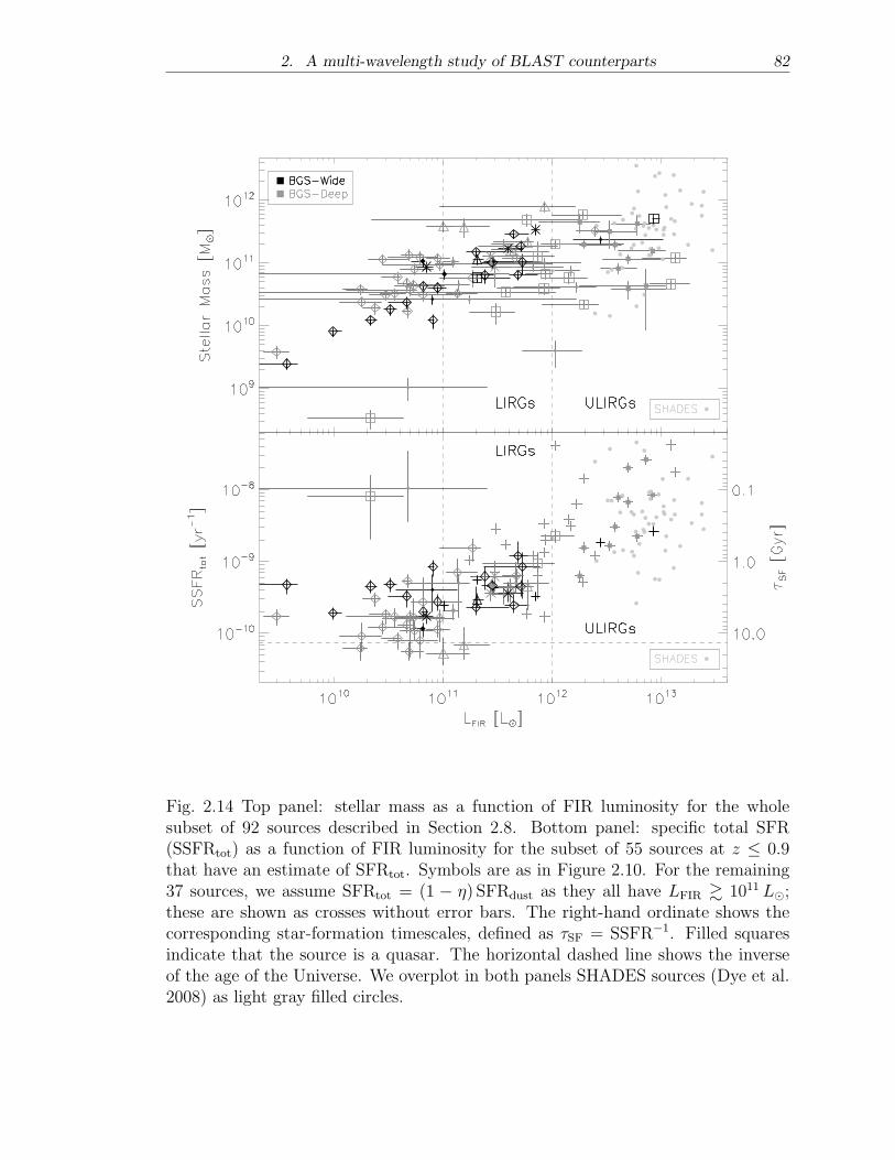
2. A multi-wavelength study of BLAST counterparts 82
Fig. 2.14 Top panel: stellar mass as a function of FIR luminosity for the wholesubset of 92 sources described in Section 2.8. Bottom panel: specific total SFR(SSFRtot) as a function of FIR luminosity for the subset of 55 sources at z ≤ 0.9that have an estimate of SFRtot. Symbols are as in Figure 2.10. For the remaining37 sources, we assume SFRtot = (1 − �) SFRdust as they all have LFIR ≳ 1011 L⊙;these are shown as crosses without error bars. The right-hand ordinate shows thecorresponding star-formation timescales, defined as �SF = SSFR−1. Filled squaresindicate that the source is a quasar. The horizontal dashed line shows the inverseof the age of the Universe. We overplot in both panels SHADES sources (Dye et al.2008) as light gray filled circles.
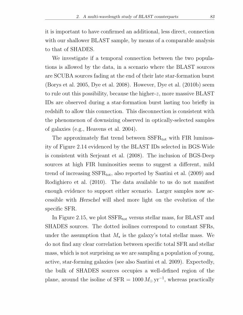
2. A multi-wavelength study of BLAST counterparts 83
it is important to have confirmed an additional, less direct, connection
with our shallower BLAST sample, by means of a comparable analysis
to that of SHADES.
We investigate if a temporal connection between the two popula-
tions is allowed by the data, in a scenario where the BLAST sources
are SCUBA sources fading at the end of their late star-formation burst
(Borys et al. 2005, Dye et al. 2008). However, Dye et al. (2010b) seem
to rule out this possibility, because the higher-z, more massive BLAST
IDs are observed during a star-formation burst lasting too briefly in
redshift to allow this connection. This disconnection is consistent with
the phenomenon of downsizing observed in optically-selected samples
of galaxies (e.g., Heavens et al. 2004).
The approximately flat trend between SSFRtot with FIR luminos-
ity of Figure 2.14 evidenced by the BLAST IDs selected in BGS-Wide
is consistent with Serjeant et al. (2008). The inclusion of BGS-Deep
sources at high FIR luminosities seems to suggest a different, mild
trend of increasing SSFRtot, also reported by Santini et al. (2009) and
Rodighiero et al. (2010). The data available to us do not manifest
enough evidence to support either scenario. Larger samples now ac-
cessible with Herschel will shed more light on the evolution of the
specific SFR.
In Figure 2.15, we plot SSFRtot versus stellar mass, for BLAST and
SHADES sources. The dotted isolines correspond to constant SFRs,
under the assumption that M★ is the galaxy’s total stellar mass. We
do not find any clear correlation between specific total SFR and stellar
mass, which is not surprising as we are sampling a population of young,
active, star-forming galaxies (see also Santini et al. 2009). Expectedly,
the bulk of SHADES sources occupies a well-defined region of the
plane, around the isoline of SFR = 1000M⊙ yr−1, whereas practically
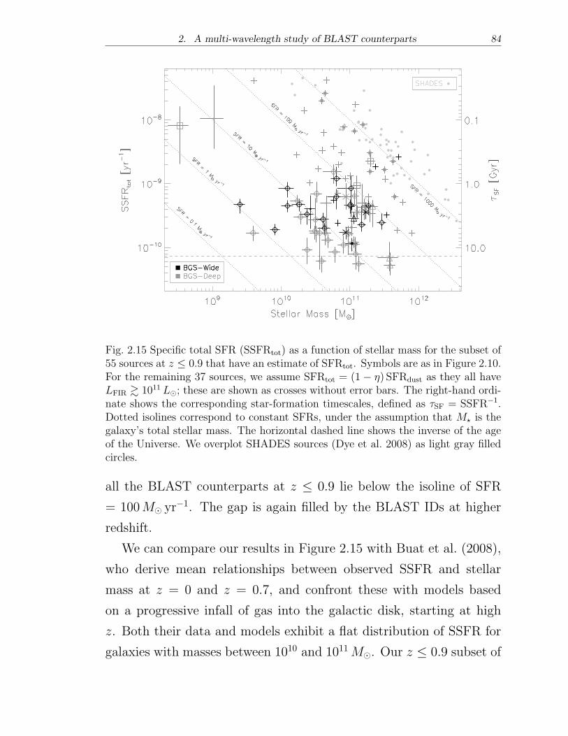
2. A multi-wavelength study of BLAST counterparts 84
Fig. 2.15 Specific total SFR (SSFRtot) as a function of stellar mass for the subset of55 sources at z ≤ 0.9 that have an estimate of SFRtot. Symbols are as in Figure 2.10.For the remaining 37 sources, we assume SFRtot = (1− �) SFRdust as they all haveLFIR ≳ 1011 L⊙; these are shown as crosses without error bars. The right-hand ordi-nate shows the corresponding star-formation timescales, defined as �SF = SSFR−1.Dotted isolines correspond to constant SFRs, under the assumption that M★ is thegalaxy’s total stellar mass. The horizontal dashed line shows the inverse of the ageof the Universe. We overplot SHADES sources (Dye et al. 2008) as light gray filledcircles.
all the BLAST counterparts at z ≤ 0.9 lie below the isoline of SFR
= 100M⊙ yr−1. The gap is again filled by the BLAST IDs at higher
redshift.
We can compare our results in Figure 2.15 with Buat et al. (2008),
who derive mean relationships between observed SSFR and stellar
mass at z = 0 and z = 0.7, and confront these with models based
on a progressive infall of gas into the galactic disk, starting at high
z. Both their data and models exhibit a flat distribution of SSFR for
galaxies with masses between 1010 and 1011M⊙. Our z ≤ 0.9 subset of
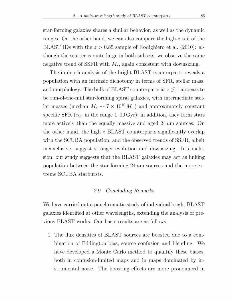
2. A multi-wavelength study of BLAST counterparts 85
star-forming galaxies shares a similar behavior, as well as the dynamic
ranges. On the other hand, we can also compare the high-z tail of the
BLAST IDs with the z > 0.85 sample of Rodighiero et al. (2010): al-
though the scatter is quite large in both subsets, we observe the same
negative trend of SSFR with M★, again consistent with downsizing.
The in-depth analysis of the bright BLAST counterparts reveals a
population with an intrinsic dichotomy in terms of SFR, stellar mass,
and morphology. The bulk of BLAST counterparts at z ≲ 1 appears to
be run-of-the-mill star-forming spiral galaxies, with intermediate stel-
lar masses (median M★ ∼ 7 × 10¹⁰M⊙) and approximately constant
specific SFR (�SF in the range 1–10Gyr); in addition, they form stars
more actively than the equally massive and aged 24�m sources. On
the other hand, the high-z BLAST counterparts significantly overlap
with the SCUBA population, and the observed trends of SSFR, albeit
inconclusive, suggest stronger evolution and downsizing. In conclu-
sion, our study suggests that the BLAST galaxies may act as linking
population between the star-forming 24�m sources and the more ex-
treme SCUBA starbursts.
2.9 Concluding Remarks
We have carried out a panchromatic study of individual bright BLAST
galaxies identified at other wavelengths, extending the analysis of pre-
vious BLAST works. Our basic results are as follows.
1. The flux densities of BLAST sources are boosted due to a com-
bination of Eddington bias, source confusion and blending. We
have developed a Monte Carlo method to quantify these biases,
both in confusion-limited maps and in maps dominated by in-
strumental noise. The boosting effects are more pronounced in
2. A multi-wavelength study of BLAST counterparts 86
the confusion-limited regime, and become more important as the
wavelength increases. In addition, flux densities are heavily corre-
lated among the BLAST bands, again more prominently in BGS-
Deep. We have accounted for all these effects coherently while
calculating the FIR luminosities of BLAST galaxies. We have
also shown how crucial the BLAST/SPIRE photometry is to es-
timate without bias the FIR luminosity of a galaxy, especially at
high redshift.
2. We have measured that star formation is predominantly obscured
at LFIR ≳ 1011L⊙, z ≳ 0.5. On the other hand, unobscured star
formation is important at LFIR ≲ 1011L⊙, z ≲ 0.25 and FIR-only
evaluations of SFR would lead to underestimates up to a factor of
two. This is probably a direct consequence of the well documented
stronger evolution of the FIR luminosity density with respect to
the optical–UV one.
3. We have compared, in terms of LFIR–z parameter space, the
BLAST counterparts to the IRAS/FIR-selected sample of local
galaxies, to the 24�m-selected sample observed by Spitzer, and to
the SCUBA 850�m-selected sample. The overlap with the local
IRAS sample is minimal and this conclusion should not be belit-
tled by the extent of local volume surveyed by BLAST. Similarly,
our sample lacks the abundance of most luminous IR galaxies de-
tected in the SHADES survey, but the high-LFIR, high-z tail of
the BLAST counterparts seems to overlap with the SCUBA pop-
ulation. The 24�m-selected sample most resembles the bulk of
BLAST IDs in terms of LFIR and redshift distribution.
4. We have assessed that 15% of the galaxies in our sample show
strong indication of an active nucleus and an additional 6% have
weaker yet significant evidence. In particular, these are pre-
2. A multi-wavelength study of BLAST counterparts 87
dominantly type-1 AGNs, i.e., unobscured Seyfert galaxies and
quasars. The AGN fraction and the SFRs inferred for these ob-
jects are comparable to recent observations at similar wavelengths
and point to a scenario in which the submillimeter emission de-
tected by BLAST is mainly due to star formation ongoing in the
host galaxy, rather than to emission from a dusty torus obscuring
the inner regions of the active nucleus.
5. We have computed stellar masses for a subset of 92 BLAST coun-
terparts. These appear to be relatively massive objects, with a
median mass of 1010.9M⊙, and an interquartile range of 1010.6–
1011.2M⊙. In particular, a significant fraction of them fill the
region of M★ ∼ 1011M⊙ at z ≲ 1 that is practically vacant in the
SCUBA surveys, and sparsely populated by 24�m-selected sam-
ples. Although the dissimilar volumes sampled by these surveys
discourage a direct comparison of the detection rates of massive
galaxies, our study suggests that the BLAST counterparts seem
to link the 24�m and SCUBA populations, in terms of both stel-
lar mass and star-formation activity.
6. We have highlighted a dichotomy in the BLAST population in
terms of star-formation rate, stellar mass and morphology. The
bulk of BLAST counterparts at z ≲ 1 comprises run-of-the-mill
star-forming galaxies, typically spiral in shape, with interme-
diate stellar masses and nearly constant specific SFR. On the
other hand, the higher redshift BLAST counterparts significantly
overlap with the SCUBA population, and the observed trends
of SSFR, albeit inconclusive, suggest stronger evolution. Other
BLAST studies have already described the significant overlap ex-
isting between fainter BLAST sources and 870�m-selected galax-
ies, but here we have established an additional link with a shal-
2. A multi-wavelength study of BLAST counterparts 88
lower BLAST sample, via an analysis equivalent to that of SHADES.
7. We rule out a temporal connection between the BLAST and
SCUBA populations, in a scenario where BLAST sources would
correspond to SCUBA galaxies whose burst of star formation is
ceasing. This disconnection is consistent with the downsizing ob-
served in optical samples.
The findings described in this work represent a taste of what should
be possible with a significantly larger sample of sources. The increased
sensitivity and resolution of the Herschel Space Observatory, which
recently started operation, will soon provide vastly increased numbers
of sources. This will enable significantly reduced uncertainties and
therefore much improved constraints on models of galaxy evolution
and formation. Nevertheless, the BLAST data have provided a very
valuable benchmark for the Herschel data and the various analyses
that will emerge for some time to come. Furthermore, the results
in this work probably will not immediately become obsolete, as even
the much more sensitive SPIRE surveys will have to face the lack of
deeper ancillary data, especially in the optical/NIR and in the radio.
Identifying the precise location of the submm sources will require either
deep and very wide-area VLA data, or a combination of MIPS 24�m
and PACS, or ultimately ALMA and the Space Infra-Red Telescope for
Cosmology and Astrophysics (SPICA; Swinyard & Nakagawa 2009).
Finally, in order to study the rest-frame optical/NIR of the z > 2
submm galaxies in much more detail than BLAST or SCUBA, future
studies will really require instruments like the Wide Field Camera
3 (WFC3; Kimble et al. 2008) or the James Webb Space Telescope
(JWST; Gardner et al. 2006).
3. MEASURING STAR FORMATION IN MASSIVE HIGH-z
GALAXIES
3.1 Introduction
The observed structural properties of massive galaxies (M★ ≳ 1011M⊙)
at high redshift (z ≳ 1) are difficult to reconcile with those of galaxies
that populate the local Universe. Most strikingly, they are much more
compact in size than local galaxies of similar mass (Daddi et al. 2005,
Trujillo et al. 2006). For the spheroid-like galaxy population, the size
evolution has been particularly dramatic (a factor of 4–5 since z ∼ 2,
see e.g., Trujillo et al. 2007, Buitrago et al. 2008, Damjanov et al.
2009), with subsequent observations confirming these findings (e.g.,
Muzzin et al. 2009, Trujillo et al. 2011). Only a tiny fraction of massive
galaxies in the local Universe have sizes comparable to those found
at high redshift (Trujillo et al. 2009). The absence of similar mass
counterparts in the local Universe (Trujillo et al. 2009) implies that
some mechanism is acting on those high-redshift galaxies to make them
grow in size (Hopkins et al. 2009, Bezanson et al. 2009).
In order to understand the mechanism responsible for this galaxy
growth, a crucial point that needs to be addressed is the level of star
formation (or star-formation rate [SFR]) in this population. From
an observational point of view, evidence for star formation in mas-
sive galaxies at high redshift is unclear, especially for the spheroid-like
population. For example, small samples of high-quality spectroscopy
(Kriek et al. 2006, 2009a) find little or no star formation in this pop-
3. Measuring star formation in massive high-z galaxies 90
ulation; whereas, about 50% of these galaxies appear to have 24�m
counterparts (Perez-Gonzalez et al. 2008), indicating an elevated level
of star formation. This discrepancy may be due to biases inherent to
their respective SFR estimators, which are either susceptible to errors
in extinction correction and require deep spectroscopic observations,
or probe emission from polycyclic aromatic hydrocarbons (PAHs), and
thus provide a poor constraint on the thermal spectral energy distri-
bution (SED).
An alternative probe of star formation is to observe in the far-
infrared/submillimeter bands (FIR/submm), where emission is pri-
marily from heated dust. It is known that in the local Universe the
dust luminosity in star-forming regions is correlated with SFR (e.g.,
Kennicutt 1998, Chary & Elbaz 2001, Buat et al. 2007), with the most
actively star-forming galaxies often the most dust obscured or even op-
tically thick in the optical/UV (Genzel et al. 1998). Therefore, it is
reasonable to expect that if high-redshift, compact, massive galaxies
are vigorously forming stars, then they should be observable in the
rest-frame FIR/submm.
However, due to the large beams of current submm telescopes,
source confusion and flux boosting present significant obstacles to
studying the star formation properties of anything other than the
most luminous galaxies at high redshift (see Chapter 2). For example,
the 1 � noise limit in the 250�m band of Herschel/SPIRE is 5.8mJy
(Nguyen et al. 2010), which corresponds to the flux from galaxies at
z ∼ 2 with bolometric FIR luminosities of LFIR ∼ 2 × 10¹²L⊙, i.e.,
ultra-luminous infrared galaxies (ULIRGs). As a result, a catalog of
galaxies at z > 2 robustly detected above the confusion noise (5�) in
the submm can only probe the bright end of the luminosity distribu-
tion. Stacking provides a mechanism to examine the full distribution,
3. Measuring star formation in massive high-z galaxies 91
provided a reliable external catalog extending to faint fluxes is avail-
able (see e.g., Marsden et al. 2009, Pascale et al. 2009).
In this work we perform a stacking analysis using a catalog of dis-
tant massive galaxies from the GOODS NICMOS Survey (GNS; Con-
selice et al. 2011) — which we select to have stellar masses M★ ≥1011M⊙ and redshifts 1.7 < z < 2.9 — on maps from: Spitzer/MIPS
(Rieke et al. 2004) at 24�m; Herschel/PACS (Poglitsch et al. 2010) at
70, 100, and 160�m; the Balloon-borne Large Aperture Submillime-
ter Telescope (BLAST; Devlin et al. 2004, Pascale et al. 2008) at 250,
350, and 500�m; and the Large APEX Bolometer Camera (LABOCA;
Weiß et al. 2009) at 870�m. Our objective is to estimate the aver-
age SFRs of high-redshift massive galaxies, and to look for differences
between the disk-like and spheroid-like galaxies.
An alternative approach, based on counterpart identification of sim-
ilar GNS catalog sources, is carried out by Cava et al. (2010); we
discuss how their results compare to ours in Section 3.5.3.
3.2 Data
We perform our analysis on the Great Observatories Origins Deep Sur-
vey South field (GOODS-South), also known as the Extended Chan-
dra Deep Field South (E-CDFS), which has field center coordinates
3h32m30s,−27∘48′20′′. Here we briefly describe the catalog and maps.
3.2.1 Mass-selected catalog
Our catalog is the Buitrago et al. (2008) subset of the publicly available
GOODS NICMOS Survey1 (Conselice et al. 2011). Here we summarize
its main features; for a more detailed description see Buitrago et al.
1 http://www.nottingham.ac.uk/astronomy/gns/index.html
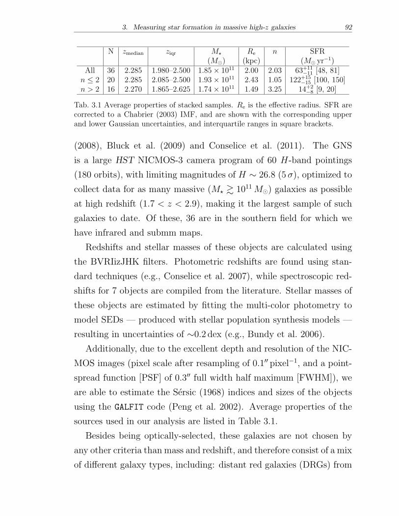
3. Measuring star formation in massive high-z galaxies 92
N zmedian ziqr M★ Re n SFR(M⊙) (kpc) (M⊙ yr−1)
All 36 2.285 1.980–2.500 1.85× 10¹¹ 2.00 2.03 63+11−11 [48, 81]
n ≤ 2 20 2.285 2.085–2.500 1.93× 10¹¹ 2.43 1.05 122+15−15 [100, 150]
n > 2 16 2.270 1.865–2.625 1.74× 10¹¹ 1.49 3.25 14+2−8 [9, 20]
Tab. 3.1 Average properties of stacked samples. Re is the effective radius. SFR arecorrected to a Chabrier (2003) IMF, and are shown with the corresponding upperand lower Gaussian uncertainties, and interquartile ranges in square brackets.
(2008), Bluck et al. (2009) and Conselice et al. (2011). The GNS
is a large HST NICMOS-3 camera program of 60 H-band pointings
(180 orbits), with limiting magnitudes of H ∼ 26.8 (5 �), optimized to
collect data for as many massive (M★ ≳ 1011M⊙) galaxies as possible
at high redshift (1.7 < z < 2.9), making it the largest sample of such
galaxies to date. Of these, 36 are in the southern field for which we
have infrared and submm maps.
Redshifts and stellar masses of these objects are calculated using
the BVRIizJHK filters. Photometric redshifts are found using stan-
dard techniques (e.g., Conselice et al. 2007), while spectroscopic red-
shifts for 7 objects are compiled from the literature. Stellar masses of
these objects are estimated by fitting the multi-color photometry to
model SEDs — produced with stellar population synthesis models —
resulting in uncertainties of ∼0.2 dex (e.g., Bundy et al. 2006).
Additionally, due to the excellent depth and resolution of the NIC-
MOS images (pixel scale after resampling of 0.1′′ pixel−1, and a point-
spread function [PSF] of 0.3′′ full width half maximum [FWHM]), we
are able to estimate the Sersic (1968) indices and sizes of the objects
using the GALFIT code (Peng et al. 2002). Average properties of the
sources used in our analysis are listed in Table 3.1.
Besides being optically-selected, these galaxies are not chosen by
any other criteria than mass and redshift, and therefore consist of a mix
of different galaxy types, including: distant red galaxies (DRGs) from
3. Measuring star formation in massive high-z galaxies 93
Papovich et al. (2006), IRAC-selected extremely red objects (IEROs)
from Yan et al. (2004), and BzK galaxies from Daddi et al. (2007). Fur-
thermore, the deep limiting H-band magnitude greatly exceeds that
of the expected upper bound for dusty submm galaxies (∼23.3mag,
Frayer et al. 2004), so that we are confident that we are not missing
the dustiest galaxies due to attenuation. Lastly, it is expected that
this selection of galaxies closely approximates the true ratio of red to
blue galaxies in these mass and redshift ranges.
3.2.2 Spitzer
We use the publicly available Spitzer/MIPS map at 24�m from the
Far Infrared Deep Extragalactic Legacy Survey (FIDEL; Dickinson
& FIDEL team 2007), data release 22 (DR2). The 5� point source
sensitivity of this map is 0.03mJy.
3.2.3 PACS
We use publicly available Herschel/PACS (Poglitsch et al. 2010) ob-
servations of the GOODS-South field from the PACS Evolutionary
Probe (PEP3; Lutz et al. 2011) survey. The data is re-processed with
the Herschel Processing Environment (HIPE, continuous integration
build number 6.0.2110; see Ott 2010). The PEP survey is designed
to provide data in all three PACS bands; since PACS can only ob-
serve in two bands simultaneously — at 160�m (red) and either 70
(blue) or 100�m (green) — we use two sets of observations to pro-
duce maps at all three wavelengths. We combine the available deep
observations using the standard PACS pipeline, choosing a high-pass
filter parameter of 20 for the blue and green bands, and 30 for the red
2 http://data.spitzer.caltech.edu/popular/fidel/20070917 enhanced/docs/fidel dr2.html3 http://www.mpe.mpg.de/ir/Research/PEP/
3. Measuring star formation in massive high-z galaxies 94
band (corresponding to suppression of scales larger than 40 and 60′′
on the sky, respectively; see Muller et al. 2011a). In order to prevent
ringing effects around bright sources caused by the high-pass filter, the
pipeline performs an initial crude reduction and automatically masks
out the brightest sources in the subsequent iterations of de-glitching
and filtering. The rms depths of the final maps are 0.31, 0.44, and
1.5mJy at 70, 100, and 160�m, respectively.
As reported by Muller et al. (2011a), the relatively strong high-
pass filter adopted along with the masking of the bright sources may
attenuate the final photometry of faint sources. To test and account
for the combination of these effects in our specific case, we produce
maps of a few, isolated, unmasked, faint point sources of different flux
density, using the same parameters employed in the reduction of the
GOODS-South maps; we then mask these sources out, and create new
maps. We use the average ratio of the flux densities of the same sources
in the two maps as our estimate of the attenuation factor due to the
high-pass filter. We find that the magnitude of the attenuation mildly
increases for increasing wavelengths, as expected given the shape of the
1/f noise over the relevant frequency range (∝ f−0.5; Lutz et al. 2011).
The estimated attenuation factors are 0.80, 0.78, and 0.75 at 70, 100,
and 160�m, respectively. Note that a slightly different approach is
followed by Lutz et al. (2011), who perform tests on the red band by
adding simulated sources to the timelines before masking and high-
pass filtering; they find that the filtering modifies the fluxes by 16%
for very faint unmasked point sources. Despite the slight disagreement
with our finding at 160�m, and because of the lack of an estimate for
the blue and green bands from the PEP team, we choose to adopt
our three estimated factors for consistency. The above attenuation
factors are therefore used in our subsequent analysis to correct the
3. Measuring star formation in massive high-z galaxies 95
measured PACS flux densities and their uncertainties for attenuation
due to filtering and source masking.
3.2.4 BLAST
We refer to Section 2.2.1 of this thesis for a description of the BLAST
dataset. Figure 3.1 depicts how the BGS-Deep region completely en-
compasses the southern sources in the Buitrago et al. (2008) catalog.
3.2.5 LABOCA
The LABOCA E-CDFS Submm Survey (LESS; Weiß et al. 2009) pro-
vides deep 870�m data, with an rms depth to better than 1.2mJy
across the full 30′×30′ field, with an effective resolution of 27′′ FWHM.
For a detailed description of the instrument see Siringo et al. (2009).
3.3 Method
3.3.1 Stacking formalism
Stacking is a well established technique for finding the average prop-
erties of objects which individually are undetectable by using external
knowledge of their positions in a map (e.g., Dole et al. 2006, Wang
et al. 2006, Marsden et al. 2009, Pascale et al. 2009). We follow the
formalism of Marsden et al. (2009; hereafter M09), which we review
and expand in Appendix A. Here we summarize the salient features
of the technique.
M09 show that the mean flux density of an external catalog is sim-
ply the covariance of the mean-subtracted map with the catalog, di-
vided by the variance of the catalog density. If the catalog is Poisson-
distributed, then a powerful diagnostic is that the variance of the
source density should equal the mean, and the average flux density
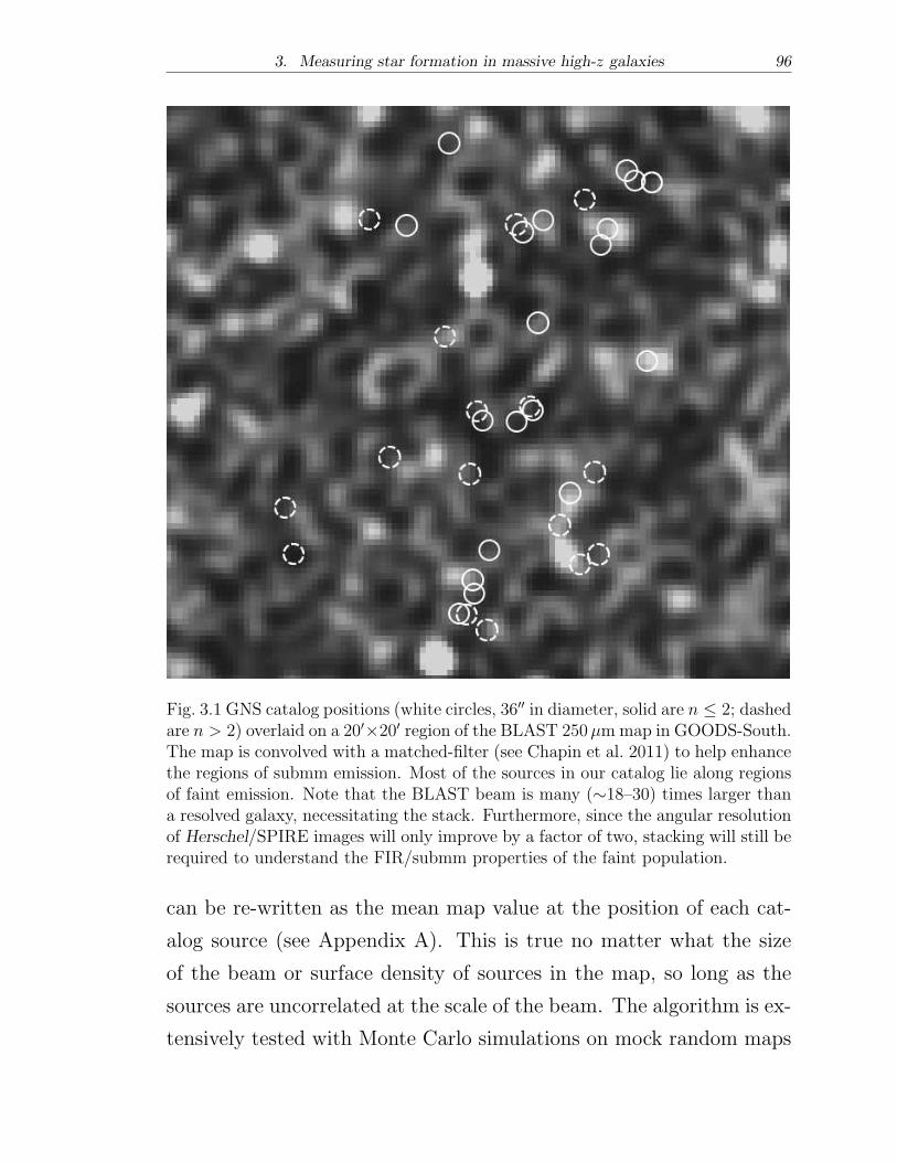
3. Measuring star formation in massive high-z galaxies 96
Fig. 3.1 GNS catalog positions (white circles, 36′′ in diameter, solid are n ≤ 2; dashedare n > 2) overlaid on a 20′×20′ region of the BLAST 250�mmap in GOODS-South.The map is convolved with a matched-filter (see Chapin et al. 2011) to help enhancethe regions of submm emission. Most of the sources in our catalog lie along regionsof faint emission. Note that the BLAST beam is many (∼18–30) times larger thana resolved galaxy, necessitating the stack. Furthermore, since the angular resolutionof Herschel/SPIRE images will only improve by a factor of two, stacking will still berequired to understand the FIR/submm properties of the faint population.
can be re-written as the mean map value at the position of each cat-
alog source (see Appendix A). This is true no matter what the size
of the beam or surface density of sources in the map, so long as the
sources are uncorrelated at the scale of the beam. The algorithm is ex-
tensively tested with Monte Carlo simulations on mock random maps
3. Measuring star formation in massive high-z galaxies 97
with increasing source densities, and is shown to consistently recover
the correct mean flux density, with no dependence on the number of
sources per beam (Figure 3.2). If however the catalog is clustered on
the beam scale, the stacked flux will be biased high, compared to the
properly normalized covariance, by a factor equal to the catalog vari-
ance at the beam scale divided by the mean source density. In the
following section we show that this factor is consistent with unity for
our data.
Uncertainties and possible biases of our measurement are estimated
by generating random catalogs and stacking them on the actual maps
themselves. We find that the uncertainties are Gaussian-distributed
and scale as the map rms (including confusion noise) divided by the
square root of the number of catalog entries (see Appendix A).
3.3.2 Testing the Poisson hypothesis
Stacking provides an unbiased estimate of the mean flux only when the
sources in the sky are uncorrelated. While massive galaxies have been
shown to cluster quite strongly (e.g., Foucaud et al. 2010), we find
that on scales relevant for this analysis they are essentially Poisson-
distributed, as we show with the following tests:
1) In the presence of clustering, the FWHM of the postage-stamp of
stacked sources would be larger than the nominal instrumental PSF.
We compare our measured stacked 24�m PSF to that measured from
stacking the sources used in M09 (Magnelli et al. 2009), which are
shown to be Poisson-distributed (see Figure 3 of M09), and find that
they are identical to within ∼0.6′′ (one tenth of the PSF FWHM).
2) If the sources are Poisson-distributed over a given scale, then by
definition the average number of sources in a cell of that size should
equal the variance. We test that by dividing the field into equal sized
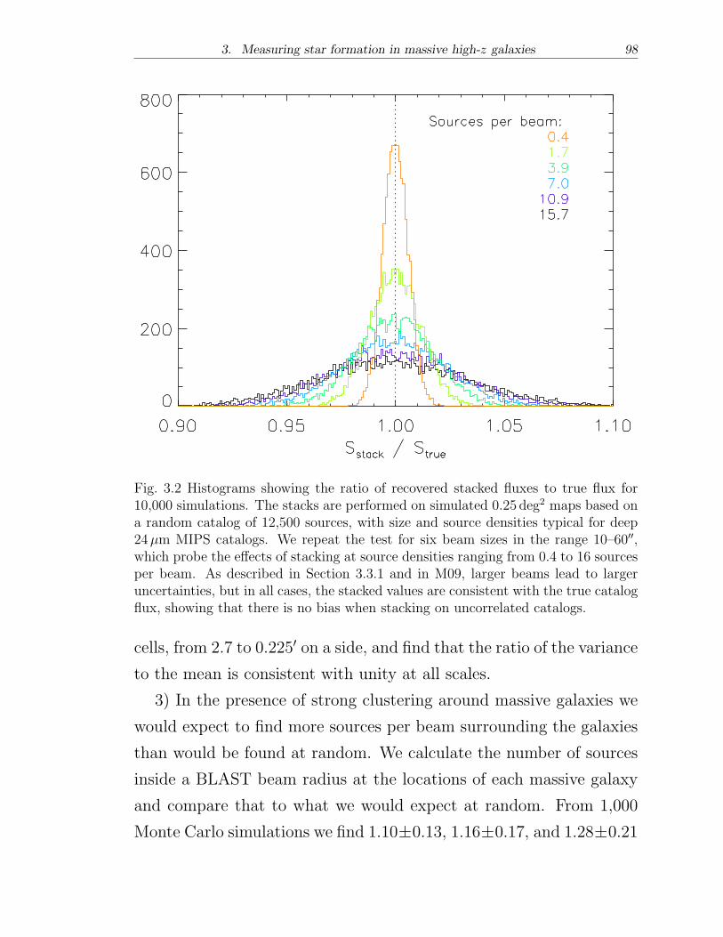
3. Measuring star formation in massive high-z galaxies 98
Fig. 3.2 Histograms showing the ratio of recovered stacked fluxes to true flux for10,000 simulations. The stacks are performed on simulated 0.25 deg2 maps based ona random catalog of 12,500 sources, with size and source densities typical for deep24�m MIPS catalogs. We repeat the test for six beam sizes in the range 10–60′′,which probe the effects of stacking at source densities ranging from 0.4 to 16 sourcesper beam. As described in Section 3.3.1 and in M09, larger beams lead to largeruncertainties, but in all cases, the stacked values are consistent with the true catalogflux, showing that there is no bias when stacking on uncorrelated catalogs.
cells, from 2.7 to 0.225′ on a side, and find that the ratio of the variance
to the mean is consistent with unity at all scales.
3) In the presence of strong clustering around massive galaxies we
would expect to find more sources per beam surrounding the galaxies
than would be found at random. We calculate the number of sources
inside a BLAST beam radius at the locations of each massive galaxy
and compare that to what we would expect at random. From 1,000
Monte Carlo simulations we find 1.10±0.13, 1.16±0.17, and 1.28±0.21
3. Measuring star formation in massive high-z galaxies 99
sources per beam at 250, 350, and 500�m, compared to the measured
1.04, 1.13, and 1.17, respectively. We extend this test to galaxies with
log(M★/M⊙)> 9 (catalog provided by Kevin Bundy, private commu-
nication), to account for the possibility of less massive galaxies clus-
tering around our more massive ones. We find there are 2.85 ± 0.40,
3.83±0.51, and 5.97±0.73 sources per beam at 250, 350, and 500�m,
compared to the measured 2.53, 4.04, and 5.87, respectively. Thus,
while there are multiple sources per beam at all wavelengths, because
their distribution is consistent with a Poissonian, they do not bias the
result.
There still remains the possibility, however, that even fainter, un-
detected sources (with flux densities < 13�Jy at 24�m) may cluster
around detected ones. We can estimate their potential contribution in
the following way. If clustered, faint sources contribute significantly
to the stacked flux density for large beams, then after convolving the
24�m map (whose beam FWHM is 6′′) with a much larger beam, we
would expect the stacked flux density to increase. On the other hand,
as described in the previous section, if the faint sources are Poisson-
distributed, then we would expect only the noise to increase. We find
that after convolving the 24�m map with a 60′′ beam, the stacked
flux density per source is 0.08 ± 0.11mJy, compared to the original
0.081 ± 0.005mJy (see Table 3.3). Thus, the stacked signal does not
change, but the errors increase substantially, which is consistent with
what we would expect from additional, Poisson-distributed sources in
the beam. We therefore conclude that the contribution from faint
clustered sources is negligible.
3. Measuring star formation in massive high-z galaxies 100
3.3.3 SED fitting, IR luminosities, and star-formation rates
We model the thermal dust emission as a modified blackbody with an
SED of the form:
S� = A��B(�, T ), (3.1)
where B(�, T ) is the blackbody spectrum, of amplitude A, and � is
the emissivity index, which we fix to 1.5 (Hildebrand 1983). Further-
more, we replace the mid-infrared exponential on the Wien side of
the spectrum with a power-law of the form f� ∝ �−� (with � = 2,
following Blain 1999, Blain et al. 2003) to account for the variability
of dust temperatures within a single galaxy (see also Section 2.3.2 of
this thesis). Our SED fitting procedure estimates the amplitude and
temperature of the above template, keeping � and � fixed.
For the BLAST points, the SED fitting procedure (described in de-
tail in Chapin et al. 2008) takes the width and shape of the photomet-
ric bands into account, as well as the absolute photometric calibration
uncertainty in each band (see Truch et al. 2009). Correlations due
to instrumental noise are estimated and accounted for with a Monte
Carlo procedure. Because we do not possess similar detailed data for
Spitzer/MIPS and LABOCA, these photometric points are not color-
corrected, whereas we do apply a color-correction to the PACS points,
following the standard procedure described in Muller et al. (2011b; see
their Table 4.2, for a power law �−2); the color-correction factors are
1.016, 1.012, 1.017 at 70, 100, and 160 um, respectively, and have a
negligible impact on the final results. The PACS points are assumed
to have completely uncorrelated instrumental noise among bands.
The portion of noise arising from source confusion may be highly
correlated among bands; if that is in fact the case, correlated confusion
noise must be accounted for in the fit, as these correlations reduce the
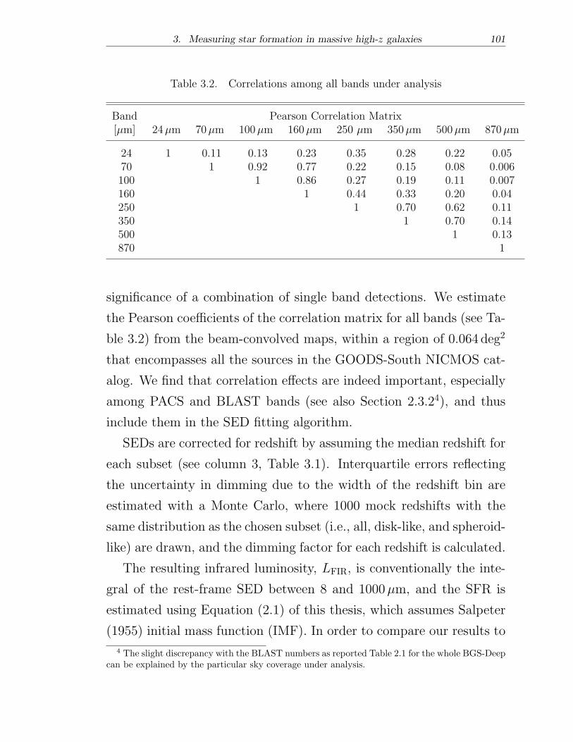
3. Measuring star formation in massive high-z galaxies 101
Table 3.2. Correlations among all bands under analysis
Band Pearson Correlation Matrix[�m] 24�m 70�m 100�m 160�m 250 �m 350�m 500�m 870�m
24 1 0.11 0.13 0.23 0.35 0.28 0.22 0.0570 1 0.92 0.77 0.22 0.15 0.08 0.006100 1 0.86 0.27 0.19 0.11 0.007160 1 0.44 0.33 0.20 0.04250 1 0.70 0.62 0.11350 1 0.70 0.14500 1 0.13870 1
significance of a combination of single band detections. We estimate
the Pearson coefficients of the correlation matrix for all bands (see Ta-
ble 3.2) from the beam-convolved maps, within a region of 0.064 deg2
that encompasses all the sources in the GOODS-South NICMOS cat-
alog. We find that correlation effects are indeed important, especially
among PACS and BLAST bands (see also Section 2.3.24), and thus
include them in the SED fitting algorithm.
SEDs are corrected for redshift by assuming the median redshift for
each subset (see column 3, Table 3.1). Interquartile errors reflecting
the uncertainty in dimming due to the width of the redshift bin are
estimated with a Monte Carlo, where 1000 mock redshifts with the
same distribution as the chosen subset (i.e., all, disk-like, and spheroid-
like) are drawn, and the dimming factor for each redshift is calculated.
The resulting infrared luminosity, LFIR, is conventionally the inte-
gral of the rest-frame SED between 8 and 1000�m, and the SFR is
estimated using Equation (2.1) of this thesis, which assumes Salpeter
(1955) initial mass function (IMF). In order to compare our results to
4 The slight discrepancy with the BLAST numbers as reported Table 2.1 for the whole BGS-Deepcan be explained by the particular sky coverage under analysis.
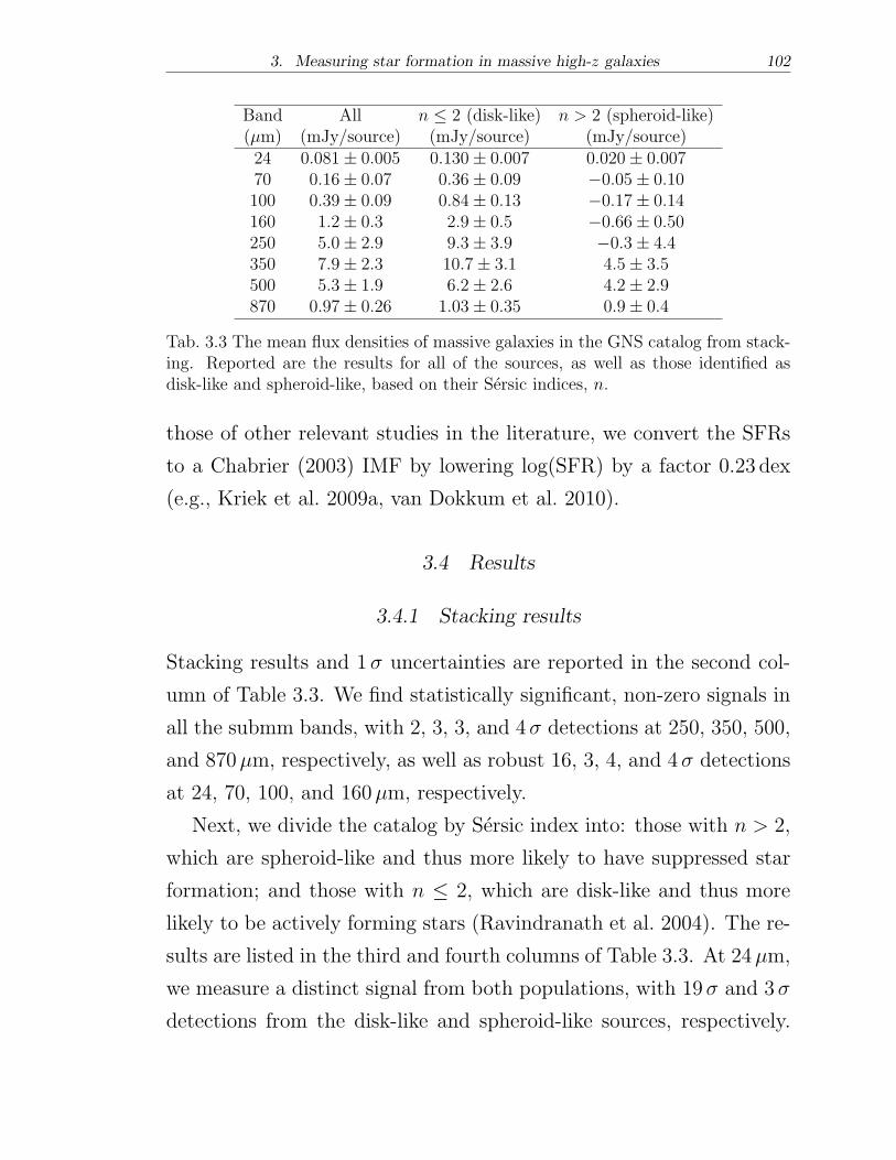
3. Measuring star formation in massive high-z galaxies 102
Band All n ≤ 2 (disk-like) n > 2 (spheroid-like)(�m) (mJy/source) (mJy/source) (mJy/source)24 0.081± 0.005 0.130± 0.007 0.020± 0.00770 0.16± 0.07 0.36± 0.09 −0.05± 0.10100 0.39± 0.09 0.84± 0.13 −0.17± 0.14160 1.2± 0.3 2.9± 0.5 −0.66± 0.50250 5.0± 2.9 9.3± 3.9 −0.3± 4.4350 7.9± 2.3 10.7± 3.1 4.5± 3.5500 5.3± 1.9 6.2± 2.6 4.2± 2.9870 0.97± 0.26 1.03± 0.35 0.9± 0.4
Tab. 3.3 The mean flux densities of massive galaxies in the GNS catalog from stack-ing. Reported are the results for all of the sources, as well as those identified asdisk-like and spheroid-like, based on their Sersic indices, n.
those of other relevant studies in the literature, we convert the SFRs
to a Chabrier (2003) IMF by lowering log(SFR) by a factor 0.23 dex
(e.g., Kriek et al. 2009a, van Dokkum et al. 2010).
3.4 Results
3.4.1 Stacking results
Stacking results and 1� uncertainties are reported in the second col-
umn of Table 3.3. We find statistically significant, non-zero signals in
all the submm bands, with 2, 3, 3, and 4� detections at 250, 350, 500,
and 870�m, respectively, as well as robust 16, 3, 4, and 4� detections
at 24, 70, 100, and 160�m, respectively.
Next, we divide the catalog by Sersic index into: those with n > 2,
which are spheroid-like and thus more likely to have suppressed star
formation; and those with n ≤ 2, which are disk-like and thus more
likely to be actively forming stars (Ravindranath et al. 2004). The re-
sults are listed in the third and fourth columns of Table 3.3. At 24�m,
we measure a distinct signal from both populations, with 19� and 3�
detections from the disk-like and spheroid-like sources, respectively.
3. Measuring star formation in massive high-z galaxies 103
At longer wavelengths, for the disk-like population we detect signals
with greater significance than that of the combined catalog, between
2.5 and 6.5� in each FIR/submm band; whereas for the spheroid-like
population we find a much weaker signal, with four bands consistent
with zero.
While the error on the stacks is Gaussian, the uncertainty associated
with the average rest-frame LFIR is dominated by the width of the
redshift distribution, which is not Gaussian. Hence, as anticipated in
the previous section, we choose to adopt for T , LFIR, and SFR the
median value as our best estimate and the interquartile range as the
associated error, because these best reflect the asymmetric shape of the
redshift distribution, which ultimately determines the uncertainty of
our measurement. However, we also quote the Gaussian uncertainties.
We anticipate that the lower Gaussian errors on T , LFIR, and SFR for
the spheroid-like subset exceed the lower bound of the interquartile
range, and reflect the elevated level of uncertainty in our measurement.
3.4.2 Contribution of stellar emission
At z ∼ 2.3 the observed 24�m band probes rest-frame wavelengths
of 6–8�m, which in addition to PAH emission, is where the Rayleigh-
Jeans tail of stellar emission lies. Thus it is possible that stellar emis-
sion could contaminate our measurement, considering the nature and
stellar masses of our sample. To investigate this potential bias in our
analysis, we calculate the predicted 24�m observed flux densities due
to stellar emission using the redshifts and stellar masses as per our cat-
alog (see Section 3.2.1). We opt to use a galaxy template with solar
metallicity and an exponentially declining SFR with an e-folding time
of 500Myr, generated with the stellar population synthesis code PE-
GASE.2 (Fioc & Rocca-Volmerange 1997). Output from non-stellar
3. Measuring star formation in massive high-z galaxies 104
emission or evolving main-sequence stars is not included, as the source
of non-stellar emission at 7�m is assumed to be the same as that of
the FIR emission. Assuming a formation redshift of z = 9, the galaxy
ages range from 1.5 to 3Gyr and the predicted 24�m flux densities
due to stellar emission range from 1.3 to 8.8�Jy, depending primarily
on the galaxy’s redshift. For each stacked sample, we find the pre-
dicted contamination per galaxy from stellar emission to be at most
∼50% of our error on the stacks (Table 3.3), with amounts of 3.0,
2.9, and 3.9�Jy for the entire sample, the disk-like and spheroid-like
populations, respectively. Therefore, the 24�m flux densities included
in our analysis are primarily dominated by non-stellar emission (dust
and PAH), and we choose not apply any correction to them.
3.4.3 Best-fit SEDs and star-formation rates
The best-fit SED and interquartile range to the stacked values of the
complete catalog are shown in the left panel of Figure 3.3 (which we
choose to display full-page and rotated for visual clarity), correspond-
ing to a median (plus/minus Gaussian) [interquartile] temperature of
T = 29.4+1.4−0.8 [27.3, 31.6]K, luminosity of LFIR = 6.2+1.1
−1.0 [4.7, 8.0] ×1011L⊙ , and SFR = 63+11
−11 [48, 81]M⊙ yr−1.
We check the validity of our modified blackbody approximation by
comparing to the templates of Chary & Elbaz (2001; hereafter CE01).
For each of the 101 templates, we approximate the stacked SED by
taking the average of templates shifted to the redshift of each galaxy
in the catalog; this acts to smear out the otherwise highly-variable
PAH region of the rest-frame SED probed by the 24�m band. We fit
the resulting template to our photometric points without accounting
for calibration uncertainties, color corrections, or correlations among
bands. The best-fit template is shown as a 3-dot-dashed line in Fig-
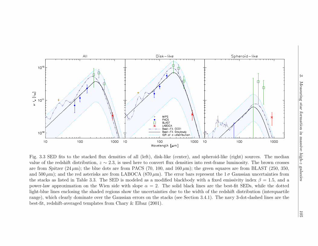
3.
Measurin
gsta
rform
atio
nin
massiv
ehigh-z
galaxies
105
Fig. 3.3 SED fits to the stacked flux densities of all (left), disk-like (center), and spheroid-like (right) sources. The medianvalue of the redshift distribution, z ∼ 2.3, is used here to convert flux densities into rest-frame luminosity. The brown crossesare from Spitzer (24�m); the blue dots are from PACS (70, 100, and 160�m); the green squares are from BLAST (250, 350,and 500�m); and the red asterisks are from LABOCA (870�m). The error bars represent the 1� Gaussian uncertainties fromthe stacks as listed in Table 3.3. The SED is modeled as a modified blackbody with a fixed emissivity index � = 1.5, and apower-law approximation on the Wien side with slope � = 2. The solid black lines are the best-fit SEDs, while the dottedlight-blue lines enclosing the shaded regions show the uncertainties due to the width of the redshift distribution (interquartilerange), which clearly dominate over the Gaussian errors on the stacks (see Section 3.4.1). The navy 3-dot-dashed lines are thebest-fit, redshift-averaged templates from Chary & Elbaz (2001).
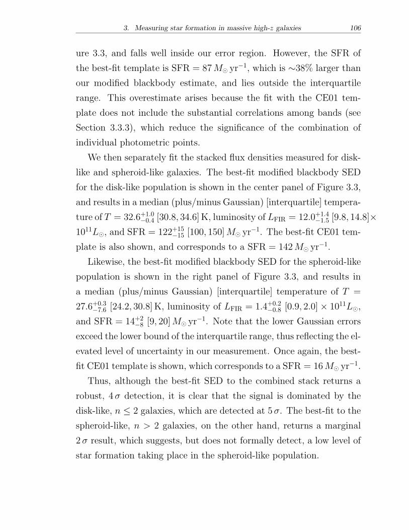
3. Measuring star formation in massive high-z galaxies 106
ure 3.3, and falls well inside our error region. However, the SFR of
the best-fit template is SFR = 87M⊙ yr−1, which is ∼38% larger than
our modified blackbody estimate, and lies outside the interquartile
range. This overestimate arises because the fit with the CE01 tem-
plate does not include the substantial correlations among bands (see
Section 3.3.3), which reduce the significance of the combination of
individual photometric points.
We then separately fit the stacked flux densities measured for disk-
like and spheroid-like galaxies. The best-fit modified blackbody SED
for the disk-like population is shown in the center panel of Figure 3.3,
and results in a median (plus/minus Gaussian) [interquartile] tempera-
ture of T = 32.6+1.0−0.4 [30.8, 34.6]K, luminosity of LFIR = 12.0+1.4
−1.5 [9.8, 14.8]×1011L⊙, and SFR = 122+15
−15 [100, 150]M⊙ yr−1. The best-fit CE01 tem-
plate is also shown, and corresponds to a SFR = 142M⊙ yr−1.
Likewise, the best-fit modified blackbody SED for the spheroid-like
population is shown in the right panel of Figure 3.3, and results in
a median (plus/minus Gaussian) [interquartile] temperature of T =
27.6+0.3−7.6 [24.2, 30.8]K, luminosity of LFIR = 1.4+0.2
−0.8 [0.9, 2.0]× 1011L⊙,
and SFR = 14+2−8 [9, 20]M⊙ yr−1. Note that the lower Gaussian errors
exceed the lower bound of the interquartile range, thus reflecting the el-
evated level of uncertainty in our measurement. Once again, the best-
fit CE01 template is shown, which corresponds to a SFR = 16M⊙ yr−1.
Thus, although the best-fit SED to the combined stack returns a
robust, 4� detection, it is clear that the signal is dominated by the
disk-like, n ≤ 2 galaxies, which are detected at 5�. The best-fit to the
spheroid-like, n > 2 galaxies, on the other hand, returns a marginal
2� result, which suggests, but does not formally detect, a low level of
star formation taking place in the spheroid-like population.
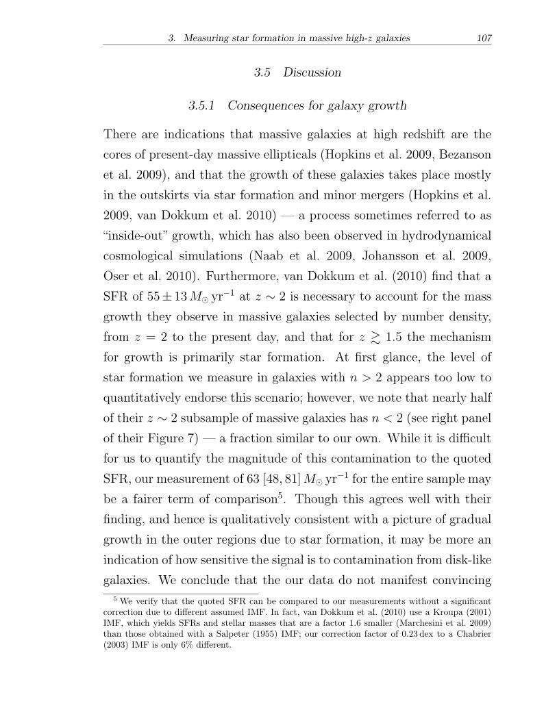
3. Measuring star formation in massive high-z galaxies 107
3.5 Discussion
3.5.1 Consequences for galaxy growth
There are indications that massive galaxies at high redshift are the
cores of present-day massive ellipticals (Hopkins et al. 2009, Bezanson
et al. 2009), and that the growth of these galaxies takes place mostly
in the outskirts via star formation and minor mergers (Hopkins et al.
2009, van Dokkum et al. 2010) — a process sometimes referred to as
“inside-out” growth, which has also been observed in hydrodynamical
cosmological simulations (Naab et al. 2009, Johansson et al. 2009,
Oser et al. 2010). Furthermore, van Dokkum et al. (2010) find that a
SFR of 55± 13M⊙ yr−1 at z ∼ 2 is necessary to account for the mass
growth they observe in massive galaxies selected by number density,
from z = 2 to the present day, and that for z ≳ 1.5 the mechanism
for growth is primarily star formation. At first glance, the level of
star formation we measure in galaxies with n > 2 appears too low to
quantitatively endorse this scenario; however, we note that nearly half
of their z ∼ 2 subsample of massive galaxies has n < 2 (see right panel
of their Figure 7) — a fraction similar to our own. While it is difficult
for us to quantify the magnitude of this contamination to the quoted
SFR, our measurement of 63 [48, 81]M⊙ yr−1 for the entire sample may
be a fairer term of comparison5. Though this agrees well with their
finding, and hence is qualitatively consistent with a picture of gradual
growth in the outer regions due to star formation, it may be more an
indication of how sensitive the signal is to contamination from disk-like
galaxies. We conclude that the our data do not manifest convincing
5 We verify that the quoted SFR can be compared to our measurements without a significantcorrection due to different assumed IMF. In fact, van Dokkum et al. (2010) use a Kroupa (2001)IMF, which yields SFRs and stellar masses that are a factor 1.6 smaller (Marchesini et al. 2009)than those obtained with a Salpeter (1955) IMF; our correction factor of 0.23 dex to a Chabrier(2003) IMF is only 6% different.
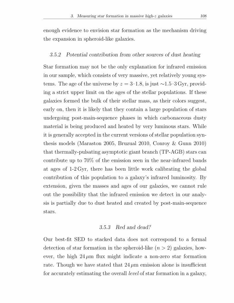
3. Measuring star formation in massive high-z galaxies 108
enough evidence to envision star formation as the mechanism driving
the expansion in spheroid-like galaxies.
3.5.2 Potential contribution from other sources of dust heating
Star formation may not be the only explanation for infrared emission
in our sample, which consists of very massive, yet relatively young sys-
tems. The age of the universe by z = 3–1.8, is just ∼1.5–3Gyr, provid-
ing a strict upper limit on the ages of the stellar populations. If these
galaxies formed the bulk of their stellar mass, as their colors suggest,
early on, then it is likely that they contain a large population of stars
undergoing post-main-sequence phases in which carbonaceous dusty
material is being produced and heated by very luminous stars. While
it is generally accepted in the current versions of stellar population syn-
thesis models (Maraston 2005, Bruzual 2010, Conroy & Gunn 2010)
that thermally-pulsating asymptotic giant branch (TP-AGB) stars can
contribute up to 70% of the emission seen in the near-infrared bands
at ages of 1-2Gyr, there has been little work calibrating the global
contribution of this population to a galaxy’s infrared luminosity. By
extension, given the masses and ages of our galaxies, we cannot rule
out the possibility that the infrared emission we detect in our analy-
sis is partially due to dust heated and created by post-main-sequence
stars.
3.5.3 Red and dead?
Our best-fit SED to stacked data does not correspond to a formal
detection of star formation in the spheroid-like (n > 2) galaxies, how-
ever, the high 24�m flux might indicate a non-zero star formation
rate. Though we have stated that 24�m emission alone is insufficient
for accurately estimating the overall level of star formation in a galaxy,
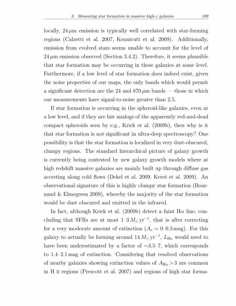
3. Measuring star formation in massive high-z galaxies 109
locally, 24�m emission is typically well correlated with star-forming
regions (Calzetti et al. 2007, Kennicutt et al. 2009). Additionally,
emission from evolved stars seems unable to account for the level of
24�m emission observed (Section 3.4.2). Therefore, it seems plausible
that star formation may be occurring in these galaxies at some level.
Furthermore, if a low level of star formation does indeed exist, given
the noise properties of our maps, the only bands which would permit
a significant detection are the 24 and 870�m bands — those in which
our measurements have signal-to-noise greater than 2.5.
If star formation is occurring in the spheroid-like galaxies, even at
a low level, and if they are fair analogs of the apparently red-and-dead
compact spheroids seen by e.g., Kriek et al. (2009b), then why is it
that star formation is not significant in ultra-deep spectroscopy? One
possibility is that the star formation is localized in very dust-obscured,
clumpy regions. The standard hierarchical picture of galaxy growth
is currently being contested by new galaxy growth models where at
high redshift massive galaxies are mainly built up through diffuse gas
accreting along cold flows (Dekel et al. 2009, Keres et al. 2009). An
observational signature of this is highly clumpy star formation (Bour-
naud & Elmegreen 2009), whereby the majority of the star formation
would be dust obscured and emitted in the infrared.
In fact, although Kriek et al. (2009b) detect a faint H� line, con-
cluding that SFRs are at most 1–3M⊙ yr−1, that is after correcting
for a very moderate amount of extinction (Av = 0–0.3mag). For this
galaxy to actually be forming around 14M⊙ yr−1, LH� would need to
have been underestimated by a factor of ∼3.5–7, which corresponds
to 1.4–2.1mag of extinction. Considering that resolved observations
of nearby galaxies showing extinction values of AH�> 3 are common
in H II regions (Prescott et al. 2007) and regions of high star forma-
3. Measuring star formation in massive high-z galaxies 110
tion (Mentuch et al. 2010), this amount of extinction is not unreal-
istic. However, this does not mean that we expect star formation to
be ubiquitous across these galaxies. Had star formation been more
widespread, and ongoing over 10–500Myr, then it would have been
detected in optical images, but the rest-frame UV and optical colors
do not support that scenario. Rather, we interpret the signal as galax-
ies having clumpy regions of star formation, on timescales of ∼10Myr,
which lead to the low observed H� line emission, but stronger infrared
emission. Overall, these galaxies are red and evolved, with most of
their stellar mass set in place long ago. This picture is consistent with
the recent findings of Bauer et al. (2011).
Lastly, we report that our results are in slight disagreement with
Cava et al. (2010), who (after correcting by 0.23 dex due to differences
in assumed IMF) find average SFRs of 147–178M⊙ yr−1 for disk-like
galaxies and 30–60M⊙ yr−1 for spheroid-like galaxies. Note that their
average SFRs are based on photometry of individual galaxies at 24�m,
and at 250, 350, and 500�m from Herschel/SPIRE; however, we point
out that their mean detection fraction for the spheroid-like population
is ∼0.4 at 24�m and ∼0.15 at 250�m. Furthermore, their SED fitting
routine does not account for correlations among bands due to source
confusion, which, albeit certainly smaller for SPIRE than for BLAST,
undoubtedly reduce the significance of the combined detection.
3.6 Concluding Remarks
Our goal was to search for evidence of star formation in high-redshift
massive galaxies, with the hope of leading to a better understanding
of the mechanisms responsible for their growth. We found that on
average the full catalog of sources are forming stars with a median
3. Measuring star formation in massive high-z galaxies 111
(plus/minus Gaussian) [interquartile] SFR = 63+11−11 [48, 81]M⊙ yr−1,
which can be decomposed into a relatively strong signal for the disk-
like galaxies, with a median [interquartile] SFR = 122+15−15 [100, 150]M⊙ yr−1,
and a marginal signal for the spheroid-like population, with a median
[interquartile] SFR = 14+2−8 [9, 20]M⊙ yr−1.
The level of star-formation detected for the full catalog is in good
agreement with other measurements of galaxy growth (e.g., van Dokkum
et al. 2010), which show that star formation can account for most of the
growth at these redshifts. However, despite having detected stacked
emission at 24 and 870�m, we are unable to say convincingly that
star formation is responsible for the dramatic size evolution of the
spheroid-like population.
Lastly, though a red sequence appears to already be in place by
z ∼ 2 (Kriek et al. 2009a), we found hints that perhaps the red,
compact, spheroid-like galaxies may not be completely dead. Future
stacking work with larger catalogs and better maps will go a long way
to further understanding this question. Deeper and higher resolution
data bracketing the peak with Herschel/SPIRE (Griffin et al. 2010),
will make more robust estimates of the SED possible, and will greatly
increase our understanding of star formation in high-redshift massive
galaxies.

Part Two
4. THE BLAST-POL INSTRUMENT
4.1 Introduction
BLAST-Pol, the Balloon-borne Large Aperture Submillimeter Tele-
scope for Polarimetry, is a stratospheric 1.8m telescope which maps
linearly polarized submillimeter (submm) emission with bolometric de-
tectors operating in three 30% wide bands at 250, 350, and 500�m.
BLAST-Pol’s diffraction-limited optics are designed to provide a res-
olution of 36′′, 42′′, and 60′′ at the three wavebands, respectively. The
detectors and cold optics are adapted from those of the SPIRE instru-
ment (Griffin et al. 2010) on Herschel (Pilbratt et al. 2010).
BLAST-Pol is a rebuilt and enhanced version of the BLAST tele-
scope (Pascale et al. 2008), with added linear polarization capability.
As described elsewhere in this thesis (see Chapters 2 and 3), BLAST
was designed to conduct confusion-limited, wide-area extragalactic and
Galactic surveys at submm wavelengths from a balloon platform.
BLAST had two Long Duration Balloon (LDB) flights. The first
was a 4-day flight from Kiruna, Sweden in June 2005 (BLAST05). Un-
fortunately the telescope was found to be out of focus, due to a possi-
ble damage of the primary mirror during the launch or ascent, so the
telescope was restricted to observing bright Galactic targets. BLAST
was repaired and flown again over Antarctica in December 2006 for
11 days (BLAST06). In a rather eventful landing, the telescope was
largely destroyed, but the pressure vessel containing the hard drives,
which stored all of the experiment data, was recovered. During the
4. The BLAST-Pol Instrument 114
very successful BLAST06 flight, multiple deep, large-area maps were
obtained for Galactic and extragalactic fields. The BLAST06 cam-
paign has left a legacy of fantastic science results, some of which we
have first-handedly derived in the first part of this thesis. In addi-
tion to the hard drives, the mirrors, detectors and receiver were all
recovered, and have been used in the construction of BLAST-Pol.
With the addition of a polarimeter, BLAST has now been trans-
formed into BLAST-Pol, a uniquely sensitive instrument for probing
linearly polarized Galactic dust emission. In January 2011, BLAST-
Pol successfully completed its first 9.5-day flight over Antarctica. Ten
science targets were mapped with unprecedented combined mapping
speed and resolution; the data are currently being analyzed. These
observations comprise an exciting dataset for studying the role played
by magnetic fields in star formation (see Chapter 1).
BLAST-Pol will ultimately yield maps of the inferred magnetic
fields across entire Giant Molecular Clouds (GMCs), with sufficient
resolution to probe fields in dense filamentary sub-structures and molec-
ular cores. The experiment provides a crucial bridge between the
large-area but coarse-resolution polarimetry provided by experiments
such as Planck (5′ resolution; Planck Collaboration 2011) and the
high-resolution but limited field-of-view (FOV) maps of the Atacama
Large Millimeter/submillimeter Array (ALMA; Wootten & Thomp-
son 2009). Finally, the BLAST-Pol observations are complementary
to those planned with the SCUBA-2 polarimeter (Bastien et al. 2005)
at 850�m, as the disadvantage in mapping speed due to the smaller
pixel count of BLAST-Pol is almost completely compensated by the
increasing flux density at shorter wavelengths.
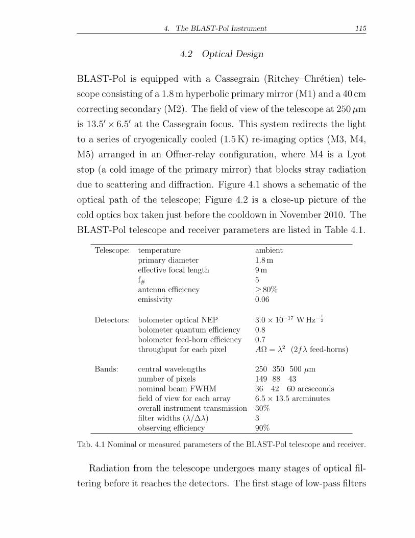
4. The BLAST-Pol Instrument 115
4.2 Optical Design
BLAST-Pol is equipped with a Cassegrain (Ritchey–Chretien) tele-
scope consisting of a 1.8m hyperbolic primary mirror (M1) and a 40 cm
correcting secondary (M2). The field of view of the telescope at 250�m
is 13.5′× 6.5′ at the Cassegrain focus. This system redirects the light
to a series of cryogenically cooled (1.5K) re-imaging optics (M3, M4,
M5) arranged in an Offner-relay configuration, where M4 is a Lyot
stop (a cold image of the primary mirror) that blocks stray radiation
due to scattering and diffraction. Figure 4.1 shows a schematic of the
optical path of the telescope; Figure 4.2 is a close-up picture of the
cold optics box taken just before the cooldown in November 2010. The
BLAST-Pol telescope and receiver parameters are listed in Table 4.1.
Telescope: temperature ambientprimary diameter 1.8meffective focal length 9mf# 5antenna efficiency ≥ 80%emissivity 0.06
Detectors: bolometer optical NEP 3.0× 10⁻¹⁷ WHz−1
2
bolometer quantum efficiency 0.8bolometer feed-horn efficiency 0.7throughput for each pixel AΩ = �2 (2f� feed-horns)
Bands: central wavelengths 250 350 500 �mnumber of pixels 149 88 43nominal beam FWHM 36 42 60 arcsecondsfield of view for each array 6.5× 13.5 arcminutesoverall instrument transmission 30%filter widths (�/Δ�) 3observing efficiency 90%
Tab. 4.1 Nominal or measured parameters of the BLAST-Pol telescope and receiver.
Radiation from the telescope undergoes many stages of optical fil-
tering before it reaches the detectors. The first stage of low-pass filters
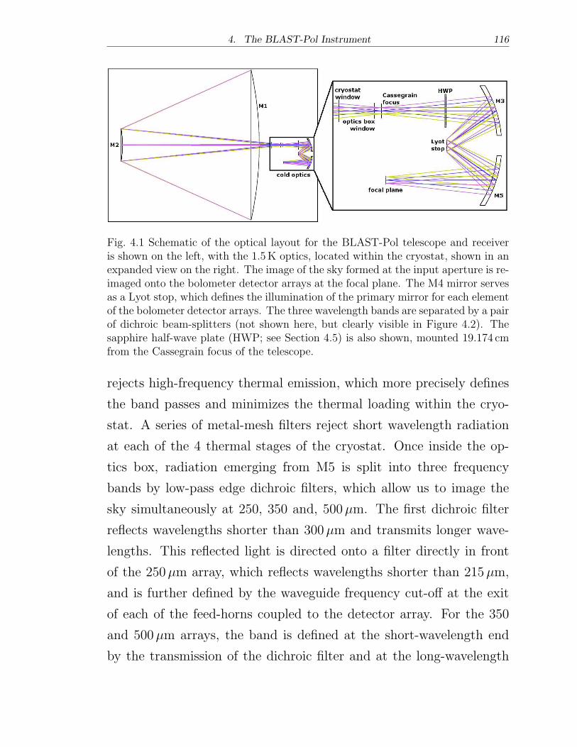
4. The BLAST-Pol Instrument 116
Fig. 4.1 Schematic of the optical layout for the BLAST-Pol telescope and receiveris shown on the left, with the 1.5K optics, located within the cryostat, shown in anexpanded view on the right. The image of the sky formed at the input aperture is re-imaged onto the bolometer detector arrays at the focal plane. The M4 mirror servesas a Lyot stop, which defines the illumination of the primary mirror for each elementof the bolometer detector arrays. The three wavelength bands are separated by a pairof dichroic beam-splitters (not shown here, but clearly visible in Figure 4.2). Thesapphire half-wave plate (HWP; see Section 4.5) is also shown, mounted 19.174 cmfrom the Cassegrain focus of the telescope.
rejects high-frequency thermal emission, which more precisely defines
the band passes and minimizes the thermal loading within the cryo-
stat. A series of metal-mesh filters reject short wavelength radiation
at each of the 4 thermal stages of the cryostat. Once inside the op-
tics box, radiation emerging from M5 is split into three frequency
bands by low-pass edge dichroic filters, which allow us to image the
sky simultaneously at 250, 350 and, 500�m. The first dichroic filter
reflects wavelengths shorter than 300�m and transmits longer wave-
lengths. This reflected light is directed onto a filter directly in front
of the 250�m array, which reflects wavelengths shorter than 215�m,
and is further defined by the waveguide frequency cut-off at the exit
of each of the feed-horns coupled to the detector array. For the 350
and 500�m arrays, the band is defined at the short-wavelength end
by the transmission of the dichroic filter and at the long-wavelength
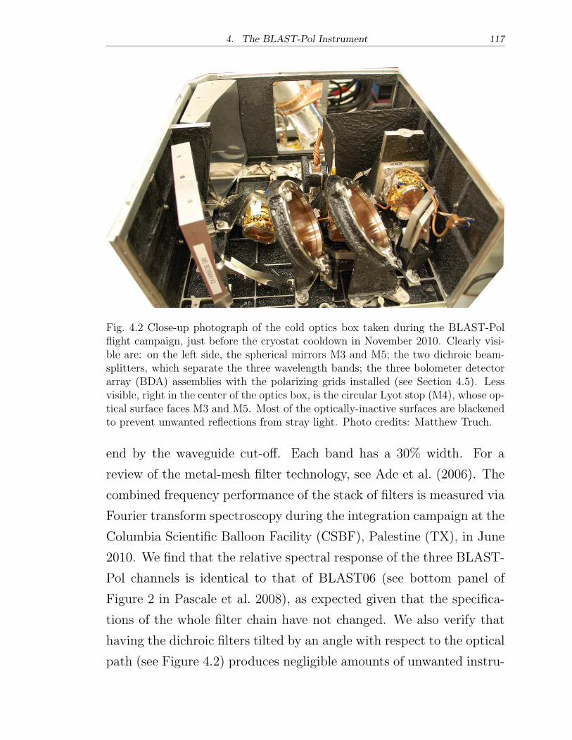
4. The BLAST-Pol Instrument 117
Fig. 4.2 Close-up photograph of the cold optics box taken during the BLAST-Polflight campaign, just before the cryostat cooldown in November 2010. Clearly visi-ble are: on the left side, the spherical mirrors M3 and M5; the two dichroic beam-splitters, which separate the three wavelength bands; the three bolometer detectorarray (BDA) assemblies with the polarizing grids installed (see Section 4.5). Lessvisible, right in the center of the optics box, is the circular Lyot stop (M4), whose op-tical surface faces M3 and M5. Most of the optically-inactive surfaces are blackenedto prevent unwanted reflections from stray light. Photo credits: Matthew Truch.
end by the waveguide cut-off. Each band has a 30% width. For a
review of the metal-mesh filter technology, see Ade et al. (2006). The
combined frequency performance of the stack of filters is measured via
Fourier transform spectroscopy during the integration campaign at the
Columbia Scientific Balloon Facility (CSBF), Palestine (TX), in June
2010. We find that the relative spectral response of the three BLAST-
Pol channels is identical to that of BLAST06 (see bottom panel of
Figure 2 in Pascale et al. 2008), as expected given that the specifica-
tions of the whole filter chain have not changed. We also verify that
having the dichroic filters tilted by an angle with respect to the optical
path (see Figure 4.2) produces negligible amounts of unwanted instru-
4. The BLAST-Pol Instrument 118
mental polarization. To this end, we measure with a polarizing Fourier
transform spectrometer (pFTS; briefly described in Section 5.2.5.1) the
spectral performance of the dichroic filters tilted by 45∘, and find that
to first order they do not induce significant spurious polarization in a
polarization-sensitive receiver.
Although the primary mirror was recovered after the destruction of
BLAST06, we decided that a new primary mirror was needed. The sur-
face of the new mirror has an rms of ∼1.0�m, with the overall shape of
the mirror good to ∼10�m. The secondary mirror was also recovered
after BLAST06, and has been reused for BLAST-Pol (after resurfacing
to remove some scratches). The estimated antenna efficiency of the
telescope is > 80%, with losses caused by both the roughness of the
primary and the quality of the re-imaging optics. More information
about the optical design and performance of the BLAST telescope can
be found in Olmi (2002) and Pascale et al. (2008).
Temperatures of the primary and secondary mirrors do not remain
constant throughout the flight. Diurnal temperature variations of
∼10∘C have been observed in previous BLAST flights (Pascale et al.
2008). These thermal variations result in changes to the radii of cur-
vature of various optical surfaces. To compensate, the position of the
secondary mirror with respect to the primary can be changed in flight
by three stepper motor actuators. These actuators are also used to set
the original tip/tilt alignment of the secondary (see Rex 2007). Anal-
ysis of the BLAST optical system indicates that the distance between
the primary and secondary mirrors must be kept to within 100�m to
avoid significant image degradation at the shortest wavelength band.
Because of the insertion of a ∼2.5mm-thick sapphire half-wave
plate (HWP; see Section 4.5 and Chapter 5) in the optical path,
we have to compensate for the fact that submm light propagates for
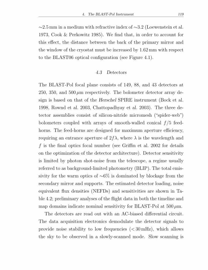
4. The BLAST-Pol Instrument 119
∼2.5mm in a medium with refractive index of ∼3.2 (Loewenstein et al.
1973, Cook & Perkowitz 1985). We find that, in order to account for
this effect, the distance between the back of the primary mirror and
the window of the cryostat must be increased by 1.62mm with respect
to the BLAST06 optical configuration (see Figure 4.1).
4.3 Detectors
The BLAST-Pol focal plane consists of 149, 88, and 43 detectors at
250, 350, and 500�m respectively. The bolometer detector array de-
sign is based on that of the Herschel SPIRE instrument (Bock et al.
1998, Rownd et al. 2003, Chattopadhyay et al. 2003). The three de-
tector assemblies consist of silicon-nitride micromesh (“spider-web”)
bolometers coupled with arrays of smooth-walled conical f/5 feed-
horns. The feed-horns are designed for maximum aperture efficiency,
requiring an entrance aperture of 2f�, where � is the wavelength and
f is the final optics focal number (see Griffin et al. 2002 for details
on the optimization of the detector architecture). Detector sensitivity
is limited by photon shot-noise from the telescope, a regime usually
referred to as background-limited photometry (BLIP). The total emis-
sivity for the warm optics of ∼6% is dominated by blockage from the
secondary mirror and supports. The estimated detector loading, noise
equivalent flux densities (NEFDs) and sensitivities are shown in Ta-
ble 4.2; preliminary analyses of the flight data in both the timeline and
map domains indicate nominal sensitivity for BLAST-Pol at 500�m.
The detectors are read out with an AC-biased differential circuit.
The data acquisition electronics demodulate the detector signals to
provide noise stability to low frequencies (< 30mHz), which allows
the sky to be observed in a slowly-scanned mode. Slow scanning is
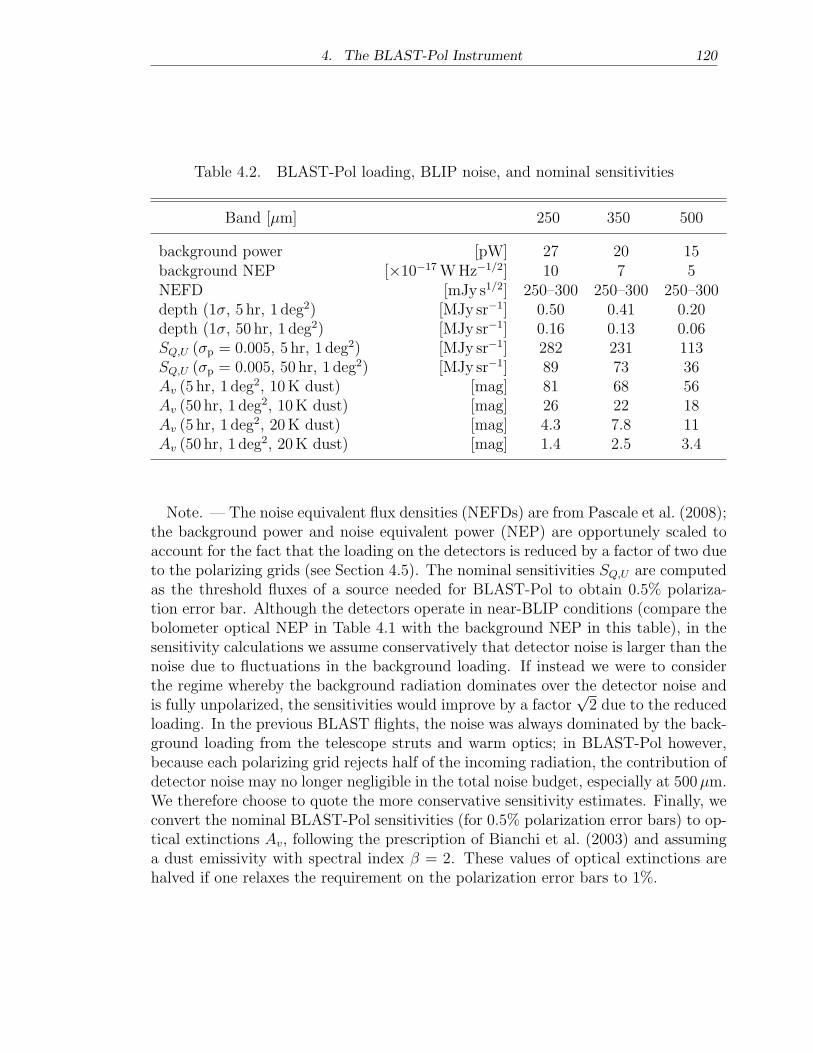
4. The BLAST-Pol Instrument 120
Table 4.2. BLAST-Pol loading, BLIP noise, and nominal sensitivities
Band [�m] 250 350 500
background power [pW] 27 20 15background NEP [×10−17WHz−1/2] 10 7 5NEFD [mJy s1/2] 250–300 250–300 250–300depth (1�, 5 hr, 1 deg2) [MJy sr−1] 0.50 0.41 0.20depth (1�, 50 hr, 1 deg2) [MJy sr−1] 0.16 0.13 0.06SQ,U (�p = 0.005, 5 hr, 1 deg2) [MJy sr−1] 282 231 113SQ,U (�p = 0.005, 50 hr, 1 deg2) [MJy sr−1] 89 73 36Av (5 hr, 1 deg
2, 10K dust) [mag] 81 68 56Av (50 hr, 1 deg
2, 10K dust) [mag] 26 22 18Av (5 hr, 1 deg
2, 20K dust) [mag] 4.3 7.8 11Av (50 hr, 1 deg
2, 20K dust) [mag] 1.4 2.5 3.4
Note. — The noise equivalent flux densities (NEFDs) are from Pascale et al. (2008);the background power and noise equivalent power (NEP) are opportunely scaled toaccount for the fact that the loading on the detectors is reduced by a factor of two dueto the polarizing grids (see Section 4.5). The nominal sensitivities SQ,U are computedas the threshold fluxes of a source needed for BLAST-Pol to obtain 0.5% polariza-tion error bar. Although the detectors operate in near-BLIP conditions (compare thebolometer optical NEP in Table 4.1 with the background NEP in this table), in thesensitivity calculations we assume conservatively that detector noise is larger than thenoise due to fluctuations in the background loading. If instead we were to considerthe regime whereby the background radiation dominates over the detector noise andis fully unpolarized, the sensitivities would improve by a factor
√2 due to the reduced
loading. In the previous BLAST flights, the noise was always dominated by the back-ground loading from the telescope struts and warm optics; in BLAST-Pol however,because each polarizing grid rejects half of the incoming radiation, the contribution ofdetector noise may no longer negligible in the total noise budget, especially at 500�m.We therefore choose to quote the more conservative sensitivity estimates. Finally, weconvert the nominal BLAST-Pol sensitivities (for 0.5% polarization error bars) to op-tical extinctions Av, following the prescription of Bianchi et al. (2003) and assuminga dust emissivity with spectral index � = 2. These values of optical extinctions arehalved if one relaxes the requirement on the polarization error bars to 1%.
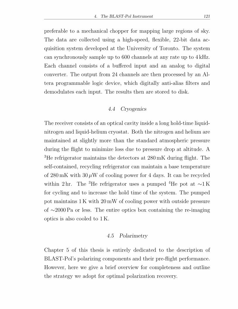
4. The BLAST-Pol Instrument 121
preferable to a mechanical chopper for mapping large regions of sky.
The data are collected using a high-speed, flexible, 22-bit data ac-
quisition system developed at the University of Toronto. The system
can synchronously sample up to 600 channels at any rate up to 4 kHz.
Each channel consists of a buffered input and an analog to digital
converter. The output from 24 channels are then processed by an Al-
tera programmable logic device, which digitally anti-alias filters and
demodulates each input. The results then are stored to disk.
4.4 Cryogenics
The receiver consists of an optical cavity inside a long hold-time liquid-
nitrogen and liquid-helium cryostat. Both the nitrogen and helium are
maintained at slightly more than the standard atmospheric pressure
during the flight to minimize loss due to pressure drop at altitude. A3He refrigerator maintains the detectors at 280mK during flight. The
self-contained, recycling refrigerator can maintain a base temperature
of 280mK with 30�W of cooling power for 4 days. It can be recycled
within 2 hr. The 3He refrigerator uses a pumped 4He pot at ∼1K
for cycling and to increase the hold time of the system. The pumped
pot maintains 1K with 20mW of cooling power with outside pressure
of ∼2000Pa or less. The entire optics box containing the re-imaging
optics is also cooled to 1K.
4.5 Polarimetry
Chapter 5 of this thesis is entirely dedicated to the description of
BLAST-Pol’s polarizing components and their pre-flight performance.
However, here we give a brief overview for completeness and outline
the strategy we adopt for optimal polarization recovery.
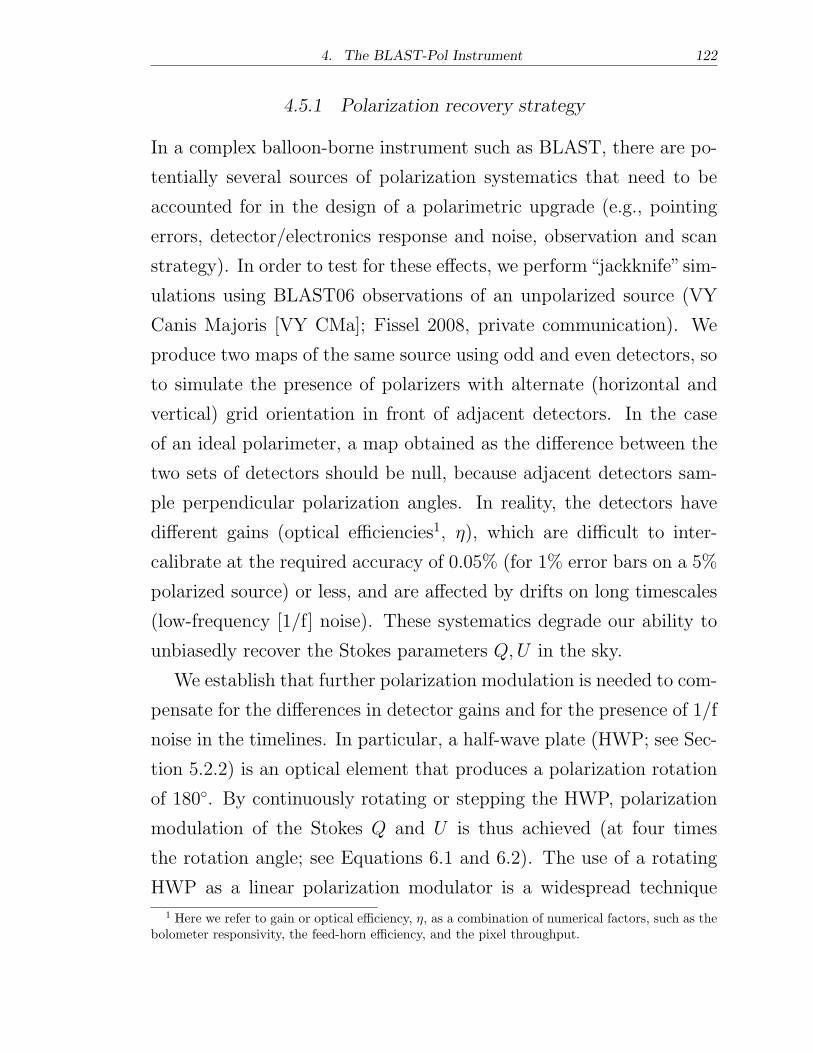
4. The BLAST-Pol Instrument 122
4.5.1 Polarization recovery strategy
In a complex balloon-borne instrument such as BLAST, there are po-
tentially several sources of polarization systematics that need to be
accounted for in the design of a polarimetric upgrade (e.g., pointing
errors, detector/electronics response and noise, observation and scan
strategy). In order to test for these effects, we perform“jackknife”sim-
ulations using BLAST06 observations of an unpolarized source (VY
Canis Majoris [VY CMa]; Fissel 2008, private communication). We
produce two maps of the same source using odd and even detectors, so
to simulate the presence of polarizers with alternate (horizontal and
vertical) grid orientation in front of adjacent detectors. In the case
of an ideal polarimeter, a map obtained as the difference between the
two sets of detectors should be null, because adjacent detectors sam-
ple perpendicular polarization angles. In reality, the detectors have
different gains (optical efficiencies1, �), which are difficult to inter-
calibrate at the required accuracy of 0.05% (for 1% error bars on a 5%
polarized source) or less, and are affected by drifts on long timescales
(low-frequency [1/f] noise). These systematics degrade our ability to
unbiasedly recover the Stokes parameters Q,U in the sky.
We establish that further polarization modulation is needed to com-
pensate for the differences in detector gains and for the presence of 1/f
noise in the timelines. In particular, a half-wave plate (HWP; see Sec-
tion 5.2.2) is an optical element that produces a polarization rotation
of 180∘. By continuously rotating or stepping the HWP, polarization
modulation of the Stokes Q and U is thus achieved (at four times
the rotation angle; see Equations 6.1 and 6.2). The use of a rotating
HWP as a linear polarization modulator is a widespread technique
1 Here we refer to gain or optical efficiency, �, as a combination of numerical factors, such as thebolometer responsivity, the feed-horn efficiency, and the pixel throughput.
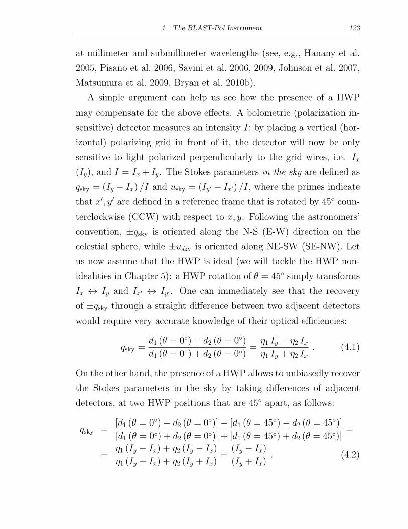
4. The BLAST-Pol Instrument 123
at millimeter and submillimeter wavelengths (see, e.g., Hanany et al.
2005, Pisano et al. 2006, Savini et al. 2006, 2009, Johnson et al. 2007,
Matsumura et al. 2009, Bryan et al. 2010b).
A simple argument can help us see how the presence of a HWP
may compensate for the above effects. A bolometric (polarization in-
sensitive) detector measures an intensity I; by placing a vertical (hor-
izontal) polarizing grid in front of it, the detector will now be only
sensitive to light polarized perpendicularly to the grid wires, i.e. Ix
(Iy), and I = Ix + Iy. The Stokes parameters in the sky are defined as
qsky = (Iy − Ix) /I and usky = (Iy′ − Ix′) /I, where the primes indicate
that x′, y′ are defined in a reference frame that is rotated by 45∘ coun-
terclockwise (CCW) with respect to x, y. Following the astronomers’
convention, ±qsky is oriented along the N-S (E-W) direction on the
celestial sphere, while ±usky is oriented along NE-SW (SE-NW). Let
us now assume that the HWP is ideal (we will tackle the HWP non-
idealities in Chapter 5): a HWP rotation of � = 45∘ simply transforms
Ix ↔ Iy and Ix′ ↔ Iy′. One can immediately see that the recovery
of ±qsky through a straight difference between two adjacent detectors
would require very accurate knowledge of their optical efficiencies:
qsky =d1 (� = 0∘)− d2 (� = 0∘)
d1 (� = 0∘) + d2 (� = 0∘)=�1 Iy − �2 Ix�1 Iy + �2 Ix
. (4.1)
On the other hand, the presence of a HWP allows to unbiasedly recover
the Stokes parameters in the sky by taking differences of adjacent
detectors, at two HWP positions that are 45∘ apart, as follows:
qsky =[d1 (� = 0∘)− d2 (� = 0∘)]− [d1 (� = 45∘)− d2 (� = 45∘)]
[d1 (� = 0∘) + d2 (� = 0∘)] + [d1 (� = 45∘) + d2 (� = 45∘)]=
=�1 (Iy − Ix) + �2 (Iy − Ix)
�1 (Iy + Ix) + �2 (Iy + Ix)=
(Iy − Ix)
(Iy + Ix). (4.2)
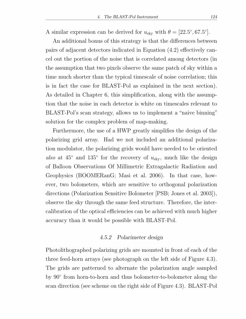
4. The BLAST-Pol Instrument 124
A similar expression can be derived for usky with � = [22.5∘, 67.5∘].
An additional bonus of this strategy is that the differences between
pairs of adjacent detectors indicated in Equation (4.2) effectively can-
cel out the portion of the noise that is correlated among detectors (in
the assumption that two pixels observe the same patch of sky within a
time much shorter than the typical timescale of noise correlation; this
is in fact the case for BLAST-Pol as explained in the next section).
As detailed in Chapter 6, this simplification, along with the assump-
tion that the noise in each detector is white on timescales relevant to
BLAST-Pol’s scan strategy, allows us to implement a “naive binning”
solution for the complex problem of map-making.
Furthermore, the use of a HWP greatly simplifies the design of the
polarizing grid array. Had we not included an additional polariza-
tion modulator, the polarizing grids would have needed to be oriented
also at 45∘ and 135∘ for the recovery of usky, much like the design
of Balloon Observations Of Millimetric Extragalactic Radiation and
Geophysics (BOOMERanG; Masi et al. 2006). In that case, how-
ever, two bolometers, which are sensitive to orthogonal polarization
directions (Polarization Sensitive Bolometer [PSB; Jones et al. 2003]),
observe the sky through the same feed structure. Therefore, the inter-
calibration of the optical efficiencies can be achieved with much higher
accuracy than it would be possible with BLAST-Pol.
4.5.2 Polarimeter design
Photolithographed polarizing grids are mounted in front of each of the
three feed-horn arrays (see photograph on the left side of Figure 4.3).
The grids are patterned to alternate the polarization angle sampled
by 90∘ from horn-to-horn and thus bolometer-to-bolometer along the
scan direction (see scheme on the right side of Figure 4.3). BLAST-Pol
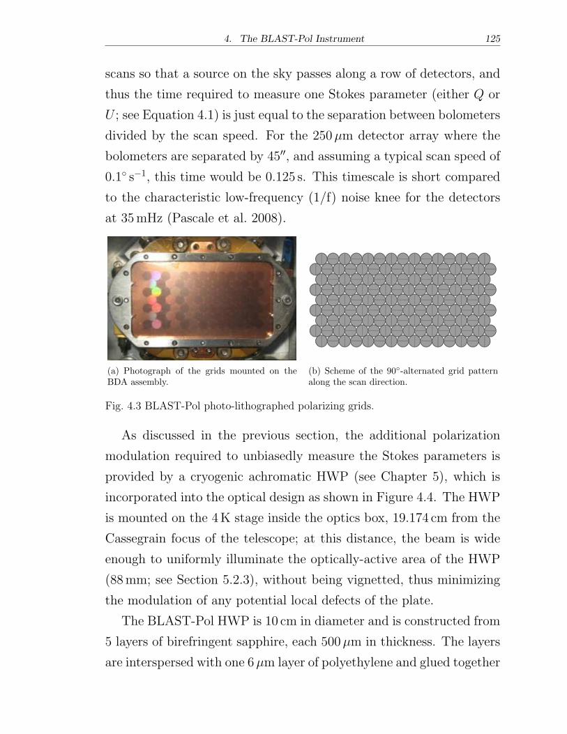
4. The BLAST-Pol Instrument 125
scans so that a source on the sky passes along a row of detectors, and
thus the time required to measure one Stokes parameter (either Q or
U ; see Equation 4.1) is just equal to the separation between bolometers
divided by the scan speed. For the 250�m detector array where the
bolometers are separated by 45′′, and assuming a typical scan speed of
0.1∘ s−1, this time would be 0.125 s. This timescale is short compared
to the characteristic low-frequency (1/f) noise knee for the detectors
at 35mHz (Pascale et al. 2008).
(a) Photograph of the grids mounted on theBDA assembly.
(b) Scheme of the 90∘-alternated grid patternalong the scan direction.
Fig. 4.3 BLAST-Pol photo-lithographed polarizing grids.
As discussed in the previous section, the additional polarization
modulation required to unbiasedly measure the Stokes parameters is
provided by a cryogenic achromatic HWP (see Chapter 5), which is
incorporated into the optical design as shown in Figure 4.4. The HWP
is mounted on the 4K stage inside the optics box, 19.174 cm from the
Cassegrain focus of the telescope; at this distance, the beam is wide
enough to uniformly illuminate the optically-active area of the HWP
(88mm; see Section 5.2.3), without being vignetted, thus minimizing
the modulation of any potential local defects of the plate.
The BLAST-Pol HWP is 10 cm in diameter and is constructed from
5 layers of birefringent sapphire, each 500�m in thickness. The layers
are interspersed with one 6�m layer of polyethylene and glued together
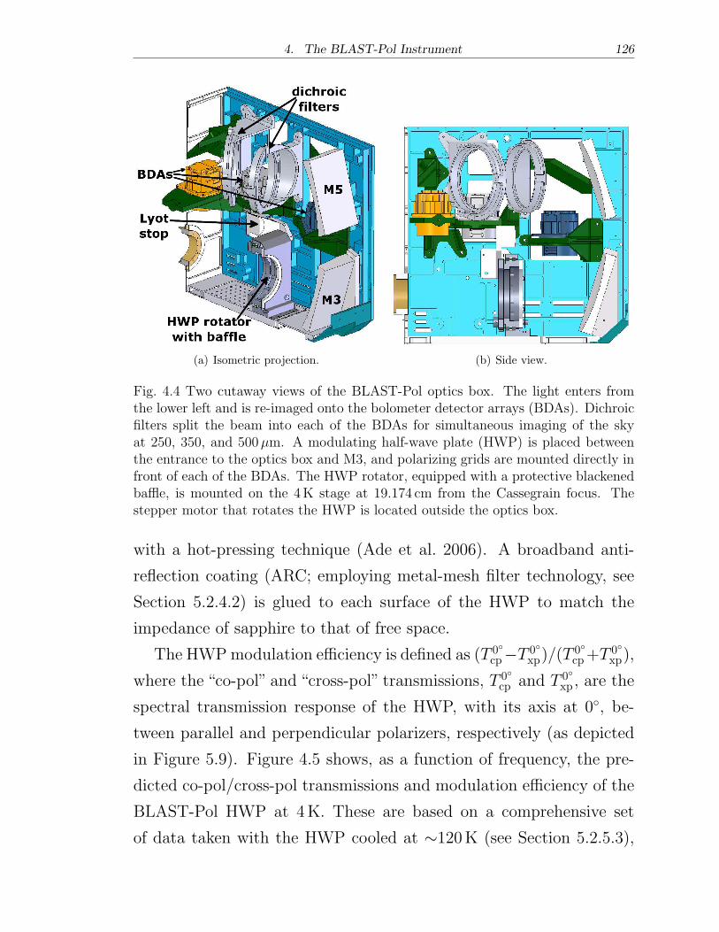
4. The BLAST-Pol Instrument 126
(a) Isometric projection. (b) Side view.
Fig. 4.4 Two cutaway views of the BLAST-Pol optics box. The light enters fromthe lower left and is re-imaged onto the bolometer detector arrays (BDAs). Dichroicfilters split the beam into each of the BDAs for simultaneous imaging of the skyat 250, 350, and 500�m. A modulating half-wave plate (HWP) is placed betweenthe entrance to the optics box and M3, and polarizing grids are mounted directly infront of each of the BDAs. The HWP rotator, equipped with a protective blackenedbaffle, is mounted on the 4K stage at 19.174 cm from the Cassegrain focus. Thestepper motor that rotates the HWP is located outside the optics box.
with a hot-pressing technique (Ade et al. 2006). A broadband anti-
reflection coating (ARC; employing metal-mesh filter technology, see
Section 5.2.4.2) is glued to each surface of the HWP to match the
impedance of sapphire to that of free space.
The HWPmodulation efficiency is defined as (T 0∘cp−T 0∘
xp)/(T0∘cp+T
0∘xp),
where the “co-pol” and “cross-pol” transmissions, T 0∘cp and T 0∘
xp , are the
spectral transmission response of the HWP, with its axis at 0∘, be-
tween parallel and perpendicular polarizers, respectively (as depicted
in Figure 5.9). Figure 4.5 shows, as a function of frequency, the pre-
dicted co-pol/cross-pol transmissions and modulation efficiency of the
BLAST-Pol HWP at 4K. These are based on a comprehensive set
of data taken with the HWP cooled at ∼120K (see Section 5.2.5.3),
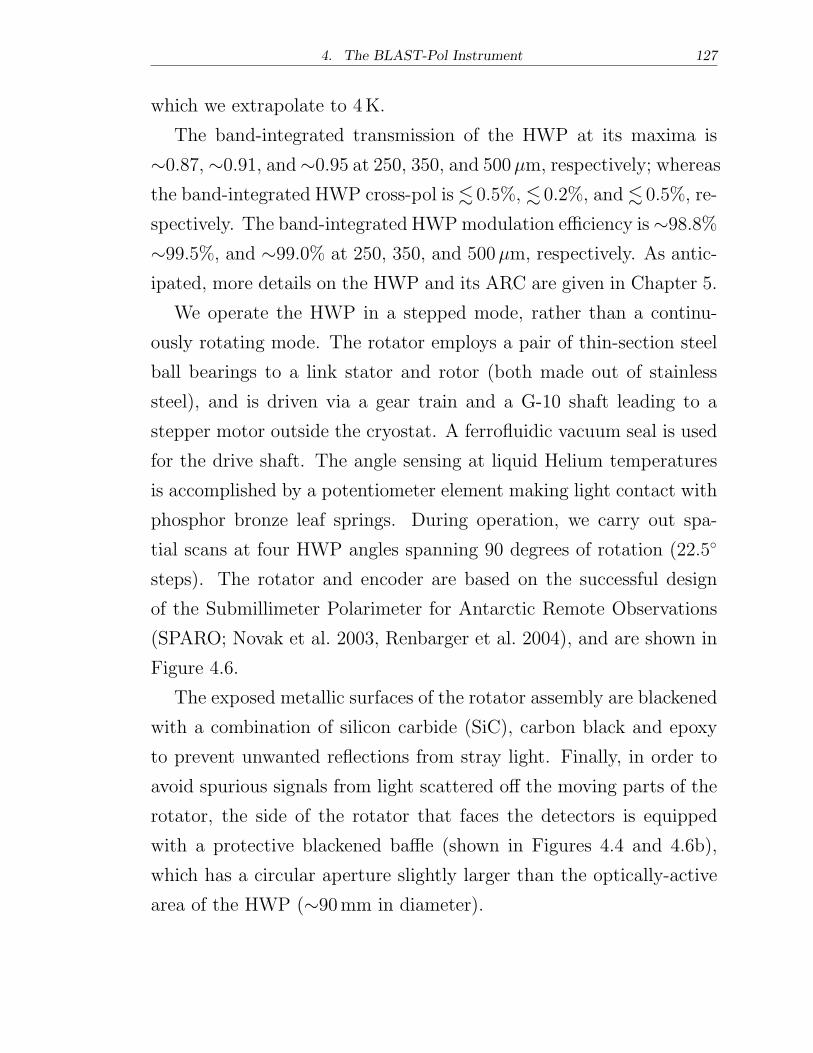
4. The BLAST-Pol Instrument 127
which we extrapolate to 4K.
The band-integrated transmission of the HWP at its maxima is
∼0.87, ∼0.91, and∼0.95 at 250, 350, and 500�m, respectively; whereas
the band-integrated HWP cross-pol is ≲ 0.5%, ≲ 0.2%, and ≲ 0.5%, re-
spectively. The band-integrated HWPmodulation efficiency is∼98.8%
∼99.5%, and ∼99.0% at 250, 350, and 500�m, respectively. As antic-
ipated, more details on the HWP and its ARC are given in Chapter 5.
We operate the HWP in a stepped mode, rather than a continu-
ously rotating mode. The rotator employs a pair of thin-section steel
ball bearings to a link stator and rotor (both made out of stainless
steel), and is driven via a gear train and a G-10 shaft leading to a
stepper motor outside the cryostat. A ferrofluidic vacuum seal is used
for the drive shaft. The angle sensing at liquid Helium temperatures
is accomplished by a potentiometer element making light contact with
phosphor bronze leaf springs. During operation, we carry out spa-
tial scans at four HWP angles spanning 90 degrees of rotation (22.5∘
steps). The rotator and encoder are based on the successful design
of the Submillimeter Polarimeter for Antarctic Remote Observations
(SPARO; Novak et al. 2003, Renbarger et al. 2004), and are shown in
Figure 4.6.
The exposed metallic surfaces of the rotator assembly are blackened
with a combination of silicon carbide (SiC), carbon black and epoxy
to prevent unwanted reflections from stray light. Finally, in order to
avoid spurious signals from light scattered off the moving parts of the
rotator, the side of the rotator that faces the detectors is equipped
with a protective blackened baffle (shown in Figures 4.4 and 4.6b),
which has a circular aperture slightly larger than the optically-active
area of the HWP (∼90mm in diameter).
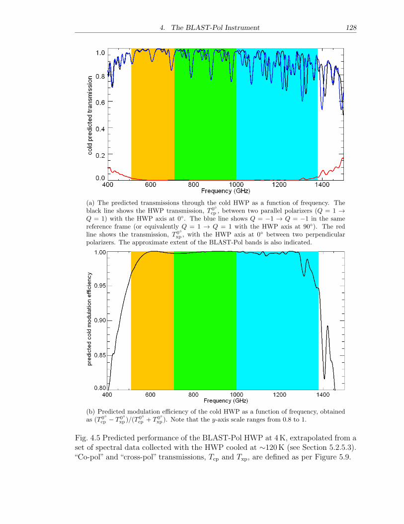
4. The BLAST-Pol Instrument 128
(a) The predicted transmissions through the cold HWP as a function of frequency. Theblack line shows the HWP transmission, T 0∘
cp , between two parallel polarizers (Q = 1 →Q = 1) with the HWP axis at 0∘. The blue line shows Q = −1 → Q = −1 in the samereference frame (or equivalently Q = 1 → Q = 1 with the HWP axis at 90∘). The redline shows the transmission, T 0∘
xp , with the HWP axis at 0∘ between two perpendicularpolarizers. The approximate extent of the BLAST-Pol bands is also indicated.
(b) Predicted modulation efficiency of the cold HWP as a function of frequency, obtainedas (T 0∘
cp − T 0∘
xp )/(T0∘
cp + T 0∘
xp ). Note that the y-axis scale ranges from 0.8 to 1.
Fig. 4.5 Predicted performance of the BLAST-Pol HWP at 4K, extrapolated from aset of spectral data collected with the HWP cooled at ∼120K (see Section 5.2.5.3).“Co-pol” and “cross-pol” transmissions, Tcp and Txp, are defined as per Figure 5.9.
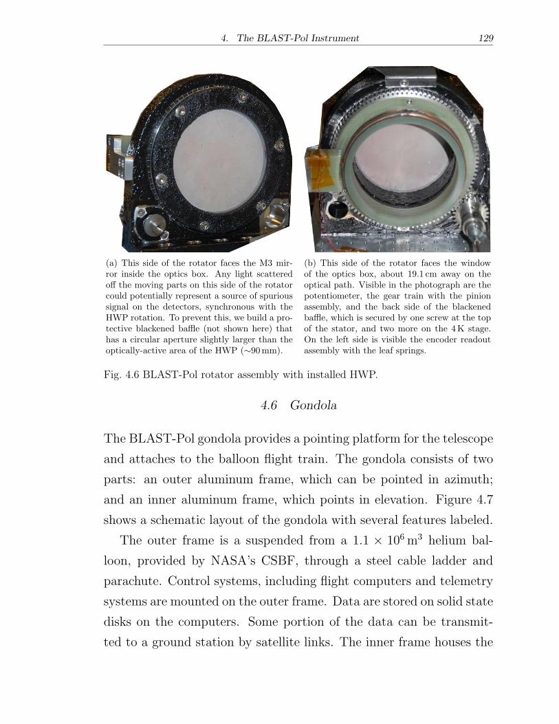
4. The BLAST-Pol Instrument 129
(a) This side of the rotator faces the M3 mir-ror inside the optics box. Any light scatteredoff the moving parts on this side of the rotatorcould potentially represent a source of spurioussignal on the detectors, synchronous with theHWP rotation. To prevent this, we build a pro-tective blackened baffle (not shown here) thathas a circular aperture slightly larger than theoptically-active area of the HWP (∼90mm).
(b) This side of the rotator faces the windowof the optics box, about 19.1 cm away on theoptical path. Visible in the photograph are thepotentiometer, the gear train with the pinionassembly, and the back side of the blackenedbaffle, which is secured by one screw at the topof the stator, and two more on the 4K stage.On the left side is visible the encoder readoutassembly with the leaf springs.
Fig. 4.6 BLAST-Pol rotator assembly with installed HWP.
4.6 Gondola
The BLAST-Pol gondola provides a pointing platform for the telescope
and attaches to the balloon flight train. The gondola consists of two
parts: an outer aluminum frame, which can be pointed in azimuth;
and an inner aluminum frame, which points in elevation. Figure 4.7
shows a schematic layout of the gondola with several features labeled.
The outer frame is a suspended from a 1.1 × 10⁶m3 helium bal-
loon, provided by NASA’s CSBF, through a steel cable ladder and
parachute. Control systems, including flight computers and telemetry
systems are mounted on the outer frame. Data are stored on solid state
disks on the computers. Some portion of the data can be transmit-
ted to a ground station by satellite links. The inner frame houses the
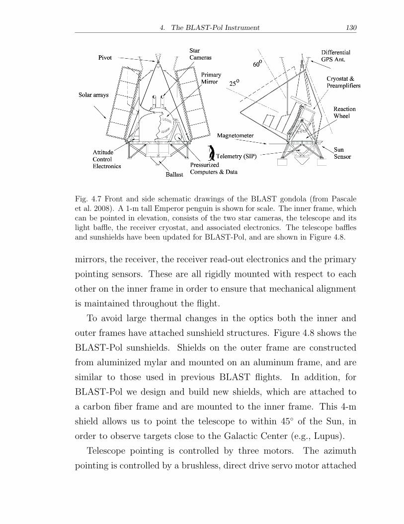
4. The BLAST-Pol Instrument 130
Fig. 4.7 Front and side schematic drawings of the BLAST gondola (from Pascaleet al. 2008). A 1-m tall Emperor penguin is shown for scale. The inner frame, whichcan be pointed in elevation, consists of the two star cameras, the telescope and itslight baffle, the receiver cryostat, and associated electronics. The telescope bafflesand sunshields have been updated for BLAST-Pol, and are shown in Figure 4.8.
mirrors, the receiver, the receiver read-out electronics and the primary
pointing sensors. These are all rigidly mounted with respect to each
other on the inner frame in order to ensure that mechanical alignment
is maintained throughout the flight.
To avoid large thermal changes in the optics both the inner and
outer frames have attached sunshield structures. Figure 4.8 shows the
BLAST-Pol sunshields. Shields on the outer frame are constructed
from aluminized mylar and mounted on an aluminum frame, and are
similar to those used in previous BLAST flights. In addition, for
BLAST-Pol we design and build new shields, which are attached to
a carbon fiber frame and are mounted to the inner frame. This 4-m
shield allows us to point the telescope to within 45∘ of the Sun, in
order to observe targets close to the Galactic Center (e.g., Lupus).
Telescope pointing is controlled by three motors. The azimuth
pointing is controlled by a brushless, direct drive servo motor attached
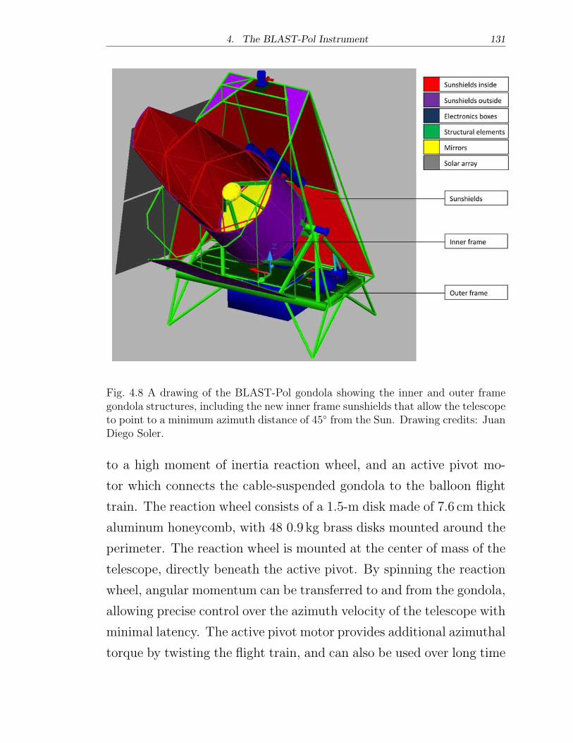
4. The BLAST-Pol Instrument 131
Fig. 4.8 A drawing of the BLAST-Pol gondola showing the inner and outer framegondola structures, including the new inner frame sunshields that allow the telescopeto point to a minimum azimuth distance of 45∘ from the Sun. Drawing credits: JuanDiego Soler.
to a high moment of inertia reaction wheel, and an active pivot mo-
tor which connects the cable-suspended gondola to the balloon flight
train. The reaction wheel consists of a 1.5-m disk made of 7.6 cm thick
aluminum honeycomb, with 48 0.9 kg brass disks mounted around the
perimeter. The reaction wheel is mounted at the center of mass of the
telescope, directly beneath the active pivot. By spinning the reaction
wheel, angular momentum can be transferred to and from the gondola,
allowing precise control over the azimuth velocity of the telescope with
minimal latency. The active pivot motor provides additional azimuthal
torque by twisting the flight train, and can also be used over long time
4. The BLAST-Pol Instrument 132
scales to transfer angular momentum to the balloon.
The elevation of the inner frame is controlled by a servo motor
mounted on one side of the inner frame at the attachment point to the
outer frame. A free bearing provides the connection point between the
inner and outer frames, on the other side.
In-flight pointing is measured to an accuracy of∼30′′ by a number of
fine and coarse pointing sensors. These include fiber optic gyroscopes,
two optical star cameras, a differential GPS, an elevation encoder,
inclinometers, a magnetometer and a Sun sensor (a description of these
devices can be found in Pascale et al. 2008). The star cameras are the
primary pointing sensor for BLAST-Pol; LM was responsible for the
hardware/software testing and deployment of both of them, as well as
for the flight operations and post-flight pointing reconstruction. In the
following section we briefly describe the components of the star-camera
assembly, the principles of operation, and the in-flight performance.
Incidentally, we mention that LM has participated in the software
deployment and performance characterization of one star camera for
the E and B Experiment (EBEX; Reichborn-Kjennerud et al. 2010).
4.7 Star Cameras
4.7.1 Overview
The BLAST-Pol star cameras are closely based on the successful BLAST
design, and therefore we refer elsewhere for a thorough description of
the theory, principles of operation and pattern-matching algorithms of
these sensors (Pascale et al. 2008), their hardware implementation and
overall performance (Rex et al. 2006, Rex 2007). Nevertheless, it is
useful to review here the design requirements and the basic equations
that allow an optimization of the optics.
4. The BLAST-Pol Instrument 133
Four primary factors drive the design of the star cameras:
1. an absolute pointing accuracy of ∼5′′ is required to over-sample
the diffraction-limited size of the 250�m beam;
2. integration times have to be short enough to avoid significant
smearing of stars in each frame taken at the typical scan angular
velocity of the gondola (0.1∘ s−1);
3. the system must always detect stars to calibrate gyroscope drifts;
4. the frequency of the solutions must be high enough to control
the 1/f random walk noise in the integrated gyroscopes (4′′ s−0.5;
Pascale et al. 2008).
We incorporate two star cameras for redundancy, and to enable
increased positional accuracy in the post-flight processing. In order to
meet the above requirements, each star camera is designed to detect in
each frame several stars2 with significance ≥ 5�. The signal-to-noise
ratio (SNR) of a star detection depends upon its effective temperature
(color), the brightness of the sky background at balloon float altitude,
and the optical properties of the camera itself.
The flux of a star of visual magnitude mv can be written as Itot =
I0 10−0.4mv [Wm−2], where I0 is the reference zero-magnitude flux. As-
suming that stars radiate with a blackbody spectrum at temperature
Teff , the flux density reads:
I� = ItotB (Teff , �)
∫
B (Teff , �) d�
= I0 � 10−0.4mv
B (Teff , �)
�SB T 4eff
[
W
m2 nm
]
, (4.3)
2 At the very least 1–2 stars per frame are necessary for the post-flight pointing reconstruction.
4. The BLAST-Pol Instrument 134
whereB (Teff , �) is the Planck function, and �SB is the Stefan–Boltzmann
constant.
The actual signal from a star received by a CCD pixel on the star
camera depends upon several parameters, as follows:
Sstar =� d2l4P
� t
∫
Qe T� I��
ℎ cd�
[
e− pix−1]
(4.4)
where: dl is the diameter of the lens coupled to the CCD; P is the size
of the lens PSF in number of pixels (the lens is not diffraction-limited
and typically P = 2–4); � is the total optical transmission of the op-
tics (we estimate � ∼ 0.95 using Equation 4.4, by performing aperture
photometry on star-camera frames of a bright star of known Teff , after
having measured all the other unknown parameters independently); t
is the exposure time in seconds; Qe� is the quantum efficiency of the
device, expressed as electrons generated per incident photon, where
1 represents 100% efficiency (see Table 4.3 for its wavelength depen-
dence); and T� is the optical filter response (see Table 4.3).
The star cameras are operated during the daytime; even at balloon
float altitudes, the noise in each star-camera frame is dominated by the
background flux from the sky (see also Section 4.7.3). The background
signal from the sky in one pixel can be written as:
Ssky =� d2l4
�Ωp t
∫
Qe T�Bsky�
�
ℎ cd�
[
e− pix−1]
(4.5)
where Ωp is the solid angle of one pixel projected onto the sky, and
Bsky� is the sky brightness, which at balloon altitudes approaches a few
tens of nWsr−1 cm−2 nm−1 (Rex 2007). In this photon-noise limited
regime (see Section 4.7.3), the noise from Ssky is Poissonian is nature,
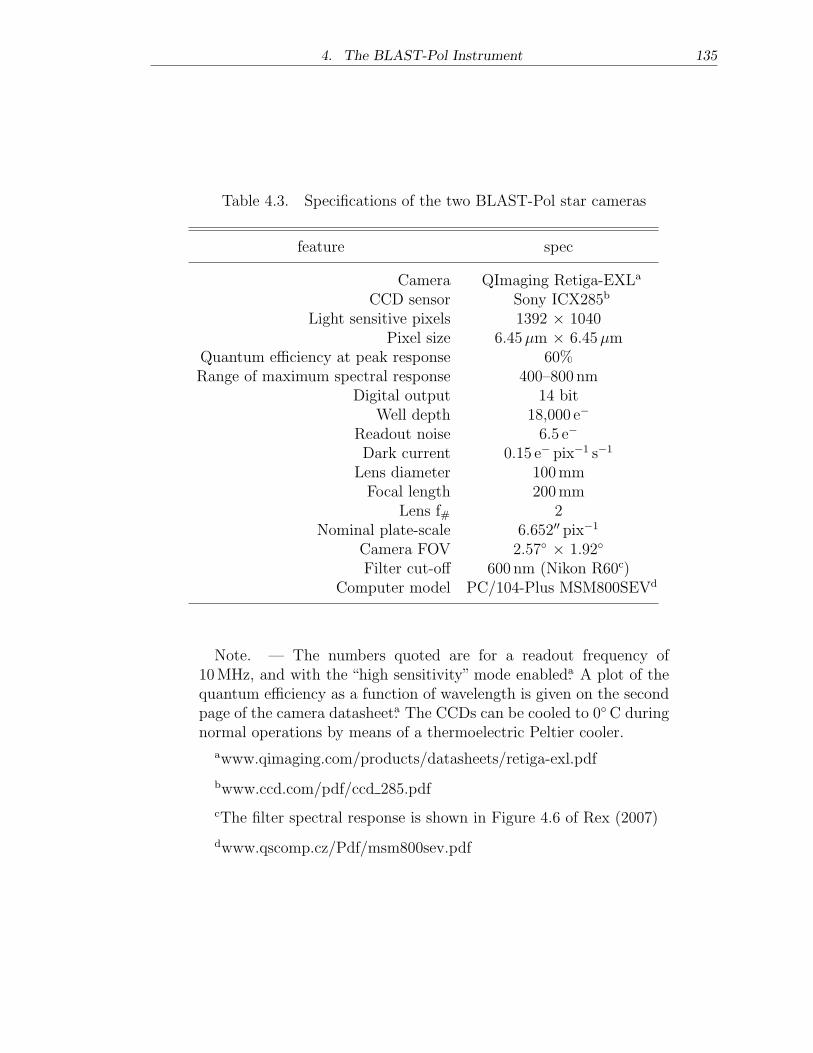
4. The BLAST-Pol Instrument 135
Table 4.3. Specifications of the two BLAST-Pol star cameras
feature spec
Camera QImaging Retiga-EXLa
CCD sensor Sony ICX285b
Light sensitive pixels 1392 × 1040Pixel size 6.45�m × 6.45�m
Quantum efficiency at peak response 60%Range of maximum spectral response 400–800 nm
Digital output 14 bitWell depth 18,000 e−
Readout noise 6.5 e−
Dark current 0.15 e− pix−1 s−1
Lens diameter 100mmFocal length 200mm
Lens f# 2Nominal plate-scale 6.652′′ pix−1
Camera FOV 2.57∘ × 1.92∘
Filter cut-off 600 nm (Nikon R60c)Computer model PC/104-Plus MSM800SEVd
Note. — The numbers quoted are for a readout frequency of10MHz, and with the “high sensitivity” mode enableda. A plot of thequantum efficiency as a function of wavelength is given on the secondpage of the camera datasheeta. The CCDs can be cooled to 0∘C duringnormal operations by means of a thermoelectric Peltier cooler.
awww.qimaging.com/products/datasheets/retiga-exl.pdf
bwww.ccd.com/pdf/ccd 285.pdf
cThe filter spectral response is shown in Figure 4.6 of Rex (2007)
dwww.qscomp.cz/Pdf/msm800sev.pdf
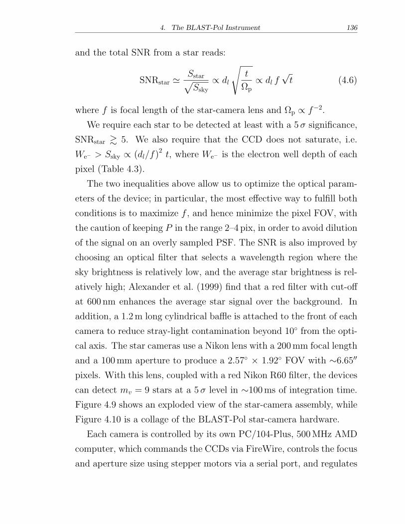
4. The BLAST-Pol Instrument 136
and the total SNR from a star reads:
SNRstar ≃Sstar√
Ssky
∝ dl
√
t
Ωp∝ dl f
√t (4.6)
where f is focal length of the star-camera lens and Ωp ∝ f−2.
We require each star to be detected at least with a 5� significance,
SNRstar ≳ 5. We also require that the CCD does not saturate, i.e.
We− > Ssky ∝ (dl/f)2 t, where We− is the electron well depth of each
pixel (Table 4.3).
The two inequalities above allow us to optimize the optical param-
eters of the device; in particular, the most effective way to fulfill both
conditions is to maximize f , and hence minimize the pixel FOV, with
the caution of keeping P in the range 2–4 pix, in order to avoid dilution
of the signal on an overly sampled PSF. The SNR is also improved by
choosing an optical filter that selects a wavelength region where the
sky brightness is relatively low, and the average star brightness is rel-
atively high; Alexander et al. (1999) find that a red filter with cut-off
at 600 nm enhances the average star signal over the background. In
addition, a 1.2m long cylindrical baffle is attached to the front of each
camera to reduce stray-light contamination beyond 10∘ from the opti-
cal axis. The star cameras use a Nikon lens with a 200mm focal length
and a 100mm aperture to produce a 2.57∘ × 1.92∘ FOV with ∼6.65′′
pixels. With this lens, coupled with a red Nikon R60 filter, the devices
can detect mv = 9 stars at a 5� level in ∼100ms of integration time.
Figure 4.9 shows an exploded view of the star-camera assembly, while
Figure 4.10 is a collage of the BLAST-Pol star-camera hardware.
Each camera is controlled by its own PC/104-Plus, 500MHz AMD
computer, which commands the CCDs via FireWire, controls the focus
and aperture size using stepper motors via a serial port, and regulates
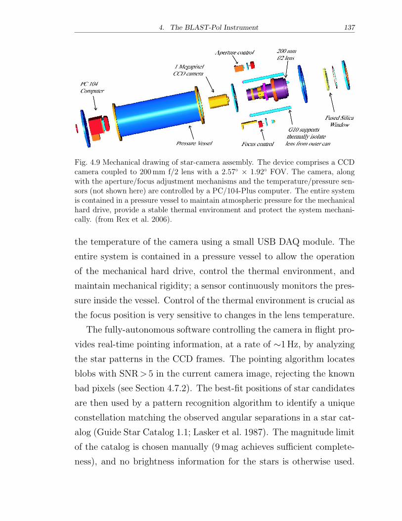
4. The BLAST-Pol Instrument 137
Fig. 4.9 Mechanical drawing of star-camera assembly. The device comprises a CCDcamera coupled to 200mm f/2 lens with a 2.57∘ × 1.92∘ FOV. The camera, alongwith the aperture/focus adjustment mechanisms and the temperature/pressure sen-sors (not shown here) are controlled by a PC/104-Plus computer. The entire systemis contained in a pressure vessel to maintain atmospheric pressure for the mechanicalhard drive, provide a stable thermal environment and protect the system mechani-cally. (from Rex et al. 2006).
the temperature of the camera using a small USB DAQ module. The
entire system is contained in a pressure vessel to allow the operation
of the mechanical hard drive, control the thermal environment, and
maintain mechanical rigidity; a sensor continuously monitors the pres-
sure inside the vessel. Control of the thermal environment is crucial as
the focus position is very sensitive to changes in the lens temperature.
The fully-autonomous software controlling the camera in flight pro-
vides real-time pointing information, at a rate of ∼1Hz, by analyzing
the star patterns in the CCD frames. The pointing algorithm locates
blobs with SNR> 5 in the current camera image, rejecting the known
bad pixels (see Section 4.7.2). The best-fit positions of star candidates
are then used by a pattern recognition algorithm to identify a unique
constellation matching the observed angular separations in a star cat-
alog (Guide Star Catalog 1.1; Lasker et al. 1987). The magnitude limit
of the catalog is chosen manually (9mag achieves sufficient complete-
ness), and no brightness information for the stars is otherwise used.
4. The BLAST-Pol Instrument 138
Fig. 4.10 A collage of photographs of the BLAST-Pol star-camera hardware. Left :view from behind of the pressure vessel, with back flange open to show the PC/104-Plus computer assembly. Top right : a closeup view of the Nikon lens, with retrofittedbelts and gears for the focus and aperture adjustment mechanisms. Bottom right :side view of the star-camera body, whose exploded mechanical drawing is shown inFigure 4.9. Photo credits: Steve Benton.
The algorithm is aided by an approximate “guess” pointing solution
from the flight computer (a combination of the pointing information
registered by the several coarse sensors on board, see Section 4.6), re-
quired to be accurate to about 5∘ in order to reduce the number of
candidate star identifications. A “Lost in Space” algorithm based on
the Pyramid technique (Mortari et al. 2004) is also implemented to be
used if the guess solution is found to be unreliable; however, such an
instance never occurred during the three BLAST flights.
Once the CCD blob centroids are matched to i stars with known
coordinates [�i, �i], the pointing solution is calculated in terms of the
celestial coordinates of the center pixel [�0, �0], and the roll of the
4. The BLAST-Pol Instrument 139
camera, �0. A star-camera frame is modeled to be a perfect gnomic
tangent-plane projection, with the tangent point at [�0, �0], and ro-
tation �0 with respect to the local meridian; the coordinates of each
matched star, [�i, �i], are projected into the plane of the CCD. The
rms distance between the CCD and model star coordinates is then
minimized using an iterative Newton solver with respect to the three
model parameters, [�0, �0,�0]. This procedure produces pointing so-
lutions with uncertainties of ∼3.5′′ and ∼200′′ for the position of the
tangent point and of the roll, respectively. A post-flight comparison
of simultaneous pointing solutions from both cameras will result in an
rms uncertainty of ≲ 2′′ (see Section 4.7.4).
4.7.2 Bad/hot pixels
As with every CCD, we need to exclude some bad (or, more appropri-
ately, “hot”) pixels, whose brightness increases steadily with integra-
tion time on dark frames. In general, this is true for all active pixels,
because of dark currents (see next section); however, the brightness of
hot pixels increases with time much more rapidly than that of other
pixels. An overdensity of a few adjacent hot pixels in a star-camera
frame could lead to a spurious star detection.
Hot pixels are individual sensors on the CCD with higher than
normal rates of charge leakage. They can appear as small pixel-sized
bright points of light on longer exposures. Because the rate of charge
leakage is the same for a given pixel over time, the longer the exposure,
the brighter they appear, even on dark frames. This charge leakage
is worse at higher temperatures, even a 10∘C difference can cause a
noticeable increase in the number of hot pixels (on frames taken with
the same exposure time).
It is worth making here a clear distinction between hot, stuck, and
4. The BLAST-Pol Instrument 140
dead pixels. Stuck pixels always read high (maximum) on all expo-
sures, whereas dead pixels read zero on all exposures. The BLAST-Pol
star-camera CCDs appear to have neither stuck nor dead pixels, only
hot pixels. Here we describe our methodology to isolate them.
We take several dark frame, with exposure times ranging from
100ms to 10 s. We then create a synthetic image which is the weighted
mean of all the dark frames taken, where the weights are the inverse
of the exposure time. We normalize such a synthetic image with the
image with shortest integration time (100ms). This image should now
contain information on the relative rate of charge leakage in every
pixel, averaged over several frames. We perform a weighted mean be-
cause otherwise only the long-exposure frames would dominate. We
can now make a histogram of such image (see Figure 4.11) and isolate
the pixels with counts ≥ 5�, where � is the standard deviation calcu-
lated across all the synthetic image. 5� is a somewhat arbitrary but
very conservative choice. We find about ∼ 70 hot pixels per camera,
which is a mere 0.005% of the whole frame and is expected in every
CCD. This method is found to be in extremely good agreement with
a visual inspection of a long-exposure dark frame.
4.7.3 Noise model
In a CCD image sensor, the noise consists of undesirable signal compo-
nents arising in the electronic system, and inherent natural variation
of the incident photon flux. The three primary sources of noise in a
CCD imaging system are photon noise, dark-current noise, and read-
out noise.
Photon noise (sometimes referred to as shot noise) results from the
intrinsic statistical variation in the arrival rate of photons incident on
the CCD. Photoelectrons generated within the semiconductor device
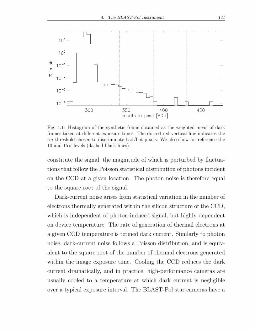
4. The BLAST-Pol Instrument 141
Fig. 4.11 Histogram of the synthetic frame obtained as the weighted mean of darkframes taken at different exposure times. The dotted red vertical line indicates the5� threshold chosen to discriminate bad/hot pixels. We also show for reference the10 and 15� levels (dashed black lines).
constitute the signal, the magnitude of which is perturbed by fluctua-
tions that follow the Poisson statistical distribution of photons incident
on the CCD at a given location. The photon noise is therefore equal
to the square-root of the signal.
Dark-current noise arises from statistical variation in the number of
electrons thermally generated within the silicon structure of the CCD,
which is independent of photon-induced signal, but highly dependent
on device temperature. The rate of generation of thermal electrons at
a given CCD temperature is termed dark current. Similarly to photon
noise, dark-current noise follows a Poisson distribution, and is equiv-
alent to the square-root of the number of thermal electrons generated
within the image exposure time. Cooling the CCD reduces the dark
current dramatically, and in practice, high-performance cameras are
usually cooled to a temperature at which dark current is negligible
over a typical exposure interval. The BLAST-Pol star cameras have a
4. The BLAST-Pol Instrument 142
nominal dark current, Dc, of 0.15 e− pix−1 s−1 at 0∘C. Their operating
temperature is typically around 20∘C in flight. Although the CCDs
may be cooled to 0∘C via a thermoelectric Peltier cooler, we do not
make use of this feature because at 20∘C dark currents are negligible
compared to the sky background, as explained later in this section.
Readout noise is a combination of electronic noise components in-
herent to the process of converting CCD charge carriers into a voltage
signal for quantification, and the subsequent processing and analog-to-
digital conversion. The major contribution to readout noise is usually
due to the on-chip preamplifier, and this noise is added uniformly
to every image pixel. High-performance camera systems utilize de-
sign enhancements that greatly reduce the level of readout noise. The
BLAST-Pol star cameras have nominal readout noise, R, of 6.5 e− pix−1
(rms) when using a readout frequency of 10MHz (see Table 4.3).
The photon noise contribution to the total noise budget is a function
of the signal level. The measured signal, S, depends upon several
parameters, as described in Section 4.7.1. In a CCD imaging system,
the number of photoelectrons generated per pixel, Ne− = Sstar + Ssky
(as given by Equations 4.4 and 4.5), is converted in analog-to-digital
units (ADUs) per pixel as follows:
S = ℜ×Ne−, (4.7)
where ℜ is the intrinsic responsivity (or gain) of the camera, which
is nominally the ratio between the analog-to-digital converter (ADC)
output resolution (the ADC has a maximum resolution of 14-bit, thus
214ADU) and the electron well depth of each pixel (We− = 18, 000 e−,
see Table 4.3), and therefore is expressed in ADU/e−.
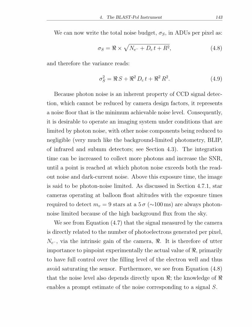
4. The BLAST-Pol Instrument 143
We can now write the total noise budget, �S, in ADUs per pixel as:
�S = ℜ×√
Ne− +Dc t+R2, (4.8)
and therefore the variance reads:
�2S = ℜS + ℜ2Dc t+ ℜ2R2. (4.9)
Because photon noise is an inherent property of CCD signal detec-
tion, which cannot be reduced by camera design factors, it represents
a noise floor that is the minimum achievable noise level. Consequently,
it is desirable to operate an imaging system under conditions that are
limited by photon noise, with other noise components being reduced to
negligible (very much like the background-limited photometry, BLIP,
of infrared and submm detectors; see Section 4.3). The integration
time can be increased to collect more photons and increase the SNR,
until a point is reached at which photon noise exceeds both the read-
out noise and dark-current noise. Above this exposure time, the image
is said to be photon-noise limited. As discussed in Section 4.7.1, star
cameras operating at balloon float altitudes with the exposure times
required to detect mv = 9 stars at a 5� (∼100ms) are always photon-
noise limited because of the high background flux from the sky.
We see from Equation (4.7) that the signal measured by the camera
is directly related to the number of photoelectrons generated per pixel,
Ne−, via the intrinsic gain of the camera, ℜ. It is therefore of utter
importance to pinpoint experimentally the actual value of ℜ, primarily
to have full control over the filling level of the electron well and thus
avoid saturating the sensor. Furthermore, we see from Equation (4.8)
that the noise level also depends directly upon ℜ; the knowledge of ℜenables a prompt estimate of the noise corresponding to a signal S.
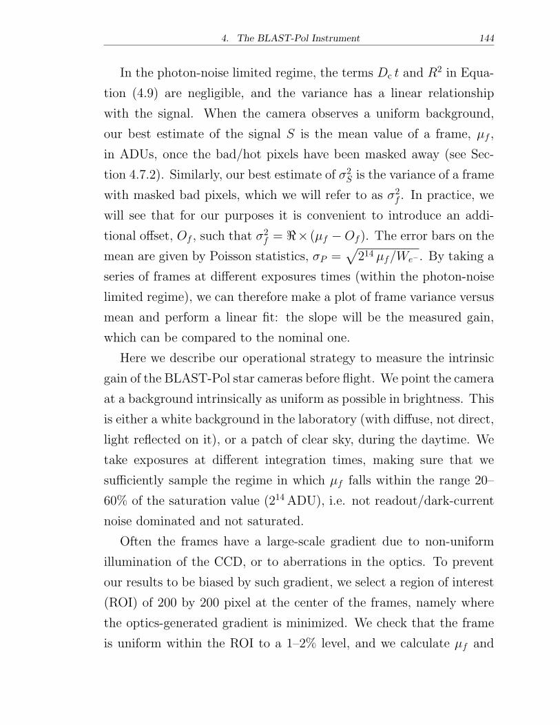
4. The BLAST-Pol Instrument 144
In the photon-noise limited regime, the terms Dc t and R2 in Equa-
tion (4.9) are negligible, and the variance has a linear relationship
with the signal. When the camera observes a uniform background,
our best estimate of the signal S is the mean value of a frame, �f ,
in ADUs, once the bad/hot pixels have been masked away (see Sec-
tion 4.7.2). Similarly, our best estimate of �2S is the variance of a frame
with masked bad pixels, which we will refer to as �2f . In practice, we
will see that for our purposes it is convenient to introduce an addi-
tional offset, Of , such that �2f = ℜ× (�f −Of). The error bars on the
mean are given by Poisson statistics, �P =√
214 �f/We−. By taking a
series of frames at different exposures times (within the photon-noise
limited regime), we can therefore make a plot of frame variance versus
mean and perform a linear fit: the slope will be the measured gain,
which can be compared to the nominal one.
Here we describe our operational strategy to measure the intrinsic
gain of the BLAST-Pol star cameras before flight. We point the camera
at a background intrinsically as uniform as possible in brightness. This
is either a white background in the laboratory (with diffuse, not direct,
light reflected on it), or a patch of clear sky, during the daytime. We
take exposures at different integration times, making sure that we
sufficiently sample the regime in which �f falls within the range 20–
60% of the saturation value (214ADU), i.e. not readout/dark-current
noise dominated and not saturated.
Often the frames have a large-scale gradient due to non-uniform
illumination of the CCD, or to aberrations in the optics. To prevent
our results to be biased by such gradient, we select a region of interest
(ROI) of 200 by 200 pixel at the center of the frames, namely where
the optics-generated gradient is minimized. We check that the frame
is uniform within the ROI to a 1–2% level, and we calculate �f and
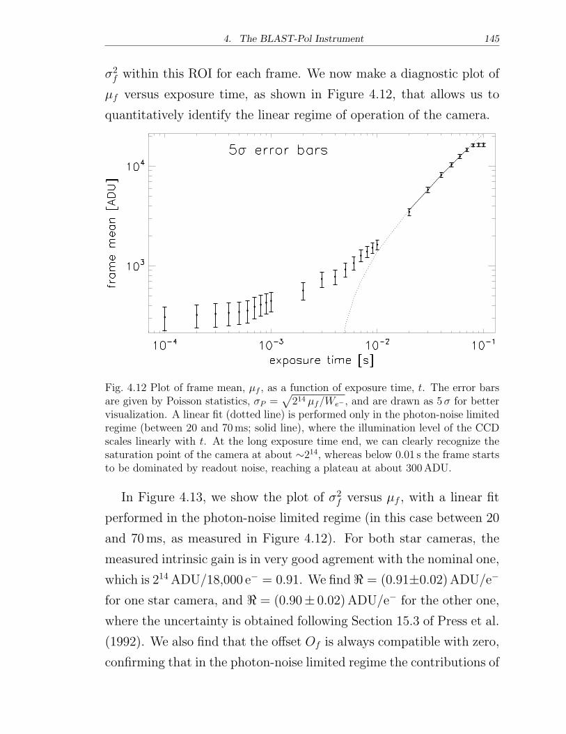
4. The BLAST-Pol Instrument 145
�2f within this ROI for each frame. We now make a diagnostic plot of
�f versus exposure time, as shown in Figure 4.12, that allows us to
quantitatively identify the linear regime of operation of the camera.
Fig. 4.12 Plot of frame mean, �f , as a function of exposure time, t. The error barsare given by Poisson statistics, �P =
√
214 �f/We− , and are drawn as 5� for bettervisualization. A linear fit (dotted line) is performed only in the photon-noise limitedregime (between 20 and 70ms; solid line), where the illumination level of the CCDscales linearly with t. At the long exposure time end, we can clearly recognize thesaturation point of the camera at about ∼214, whereas below 0.01 s the frame startsto be dominated by readout noise, reaching a plateau at about 300ADU.
In Figure 4.13, we show the plot of �2f versus �f , with a linear fit
performed in the photon-noise limited regime (in this case between 20
and 70ms, as measured in Figure 4.12). For both star cameras, the
measured intrinsic gain is in very good agrement with the nominal one,
which is 214ADU/18,000 e− = 0.91. We find ℜ = (0.91±0.02)ADU/e−
for one star camera, and ℜ = (0.90± 0.02)ADU/e− for the other one,
where the uncertainty is obtained following Section 15.3 of Press et al.
(1992). We also find that the offset Of is always compatible with zero,
confirming that in the photon-noise limited regime the contributions of
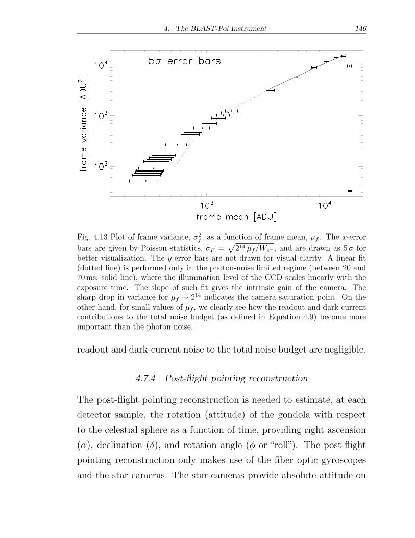
4. The BLAST-Pol Instrument 146
Fig. 4.13 Plot of frame variance, �2f , as a function of frame mean, �f . The x-error
bars are given by Poisson statistics, �P =√
214 �f/We− , and are drawn as 5� forbetter visualization. The y-error bars are not drawn for visual clarity. A linear fit(dotted line) is performed only in the photon-noise limited regime (between 20 and70ms; solid line), where the illumination level of the CCD scales linearly with theexposure time. The slope of such fit gives the intrinsic gain of the camera. Thesharp drop in variance for �f ∼ 214 indicates the camera saturation point. On theother hand, for small values of �f , we clearly see how the readout and dark-currentcontributions to the total noise budget (as defined in Equation 4.9) become moreimportant than the photon noise.
readout and dark-current noise to the total noise budget are negligible.
4.7.4 Post-flight pointing reconstruction
The post-flight pointing reconstruction is needed to estimate, at each
detector sample, the rotation (attitude) of the gondola with respect
to the celestial sphere as a function of time, providing right ascension
(�), declination (�), and rotation angle (� or “roll”). The post-flight
pointing reconstruction only makes use of the fiber optic gyroscopes
and the star cameras. The star cameras provide absolute attitude on
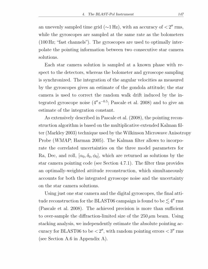
4. The BLAST-Pol Instrument 147
an unevenly sampled time grid (∼1Hz), with an accuracy of < 2′′ rms,
while the gyroscopes are sampled at the same rate as the bolometers
(100Hz; “fast channels”). The gyroscopes are used to optimally inter-
polate the pointing information between two consecutive star camera
solutions.
Each star camera solution is sampled at a known phase with re-
spect to the detectors, whereas the bolometer and gyroscope sampling
is synchronized. The integration of the angular velocities as measured
by the gyroscopes gives an estimate of the gondola attitude; the star
camera is used to correct the random walk drift induced by the in-
tegrated gyroscope noise (4′′ s−0.5; Pascale et al. 2008) and to give an
estimate of the integration constant.
As extensively described in Pascale et al. (2008), the pointing recon-
struction algorithm is based on the multiplicative extended Kalman fil-
ter (Markley 2003) technique used by theWilkinson Microwave Anisotropy
Probe (WMAP; Harman 2005). The Kalman filter allows to incorpo-
rate the correlated uncertainties on the three model parameters for
Ra, Dec, and roll, [�0, �0,�0], which are returned as solutions by the
star camera pointing code (see Section 4.7.1). The filter thus provides
an optimally-weighted attitude reconstruction, which simultaneously
accounts for both the integrated gyroscope noise and the uncertainty
on the star camera solutions.
Using just one star camera and the digital gyroscopes, the final atti-
tude reconstruction for the BLAST06 campaign is found to be≲ 4′′ rms
(Pascale et al. 2008). The achieved precision is more than sufficient
to over-sample the diffraction-limited size of the 250�m beam. Using
stacking analysis, we independently estimate the absolute pointing ac-
curacy for BLAST06 to be < 2′′, with random pointing errors < 3′′ rms
(see Section A.6 in Appendix A).
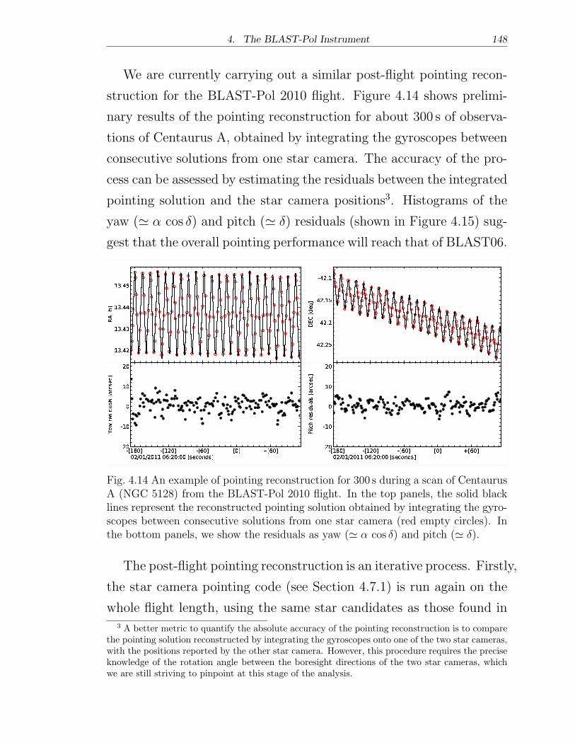
4. The BLAST-Pol Instrument 148
We are currently carrying out a similar post-flight pointing recon-
struction for the BLAST-Pol 2010 flight. Figure 4.14 shows prelimi-
nary results of the pointing reconstruction for about 300 s of observa-
tions of Centaurus A, obtained by integrating the gyroscopes between
consecutive solutions from one star camera. The accuracy of the pro-
cess can be assessed by estimating the residuals between the integrated
pointing solution and the star camera positions3. Histograms of the
yaw (≃ � cos �) and pitch (≃ �) residuals (shown in Figure 4.15) sug-
gest that the overall pointing performance will reach that of BLAST06.
RA[h] 13.4213.4313.4413.45 DEC[d eg] �42.25�42.2�42.15�42.1
Y a wresid ual s[ arcsec] 02/01/2011 06:20:00 [seconds]�[180] �[120] �[60] [0] +[60]�20�1001020 Pi t ch resid ual s[ arcsec] 02/01/2011 06:20:00 [seconds]�[180] �[120] �[60] [0] +[60]�20�100
1020Fig. 4.14 An example of pointing reconstruction for 300 s during a scan of CentaurusA (NGC 5128) from the BLAST-Pol 2010 flight. In the top panels, the solid blacklines represent the reconstructed pointing solution obtained by integrating the gyro-scopes between consecutive solutions from one star camera (red empty circles). Inthe bottom panels, we show the residuals as yaw (≃ � cos �) and pitch (≃ �).
The post-flight pointing reconstruction is an iterative process. Firstly,
the star camera pointing code (see Section 4.7.1) is run again on the
whole flight length, using the same star candidates as those found in3 A better metric to quantify the absolute accuracy of the pointing reconstruction is to compare
the pointing solution reconstructed by integrating the gyroscopes onto one of the two star cameras,with the positions reported by the other star camera. However, this procedure requires the preciseknowledge of the rotation angle between the boresight directions of the two star cameras, whichwe are still striving to pinpoint at this stage of the analysis.
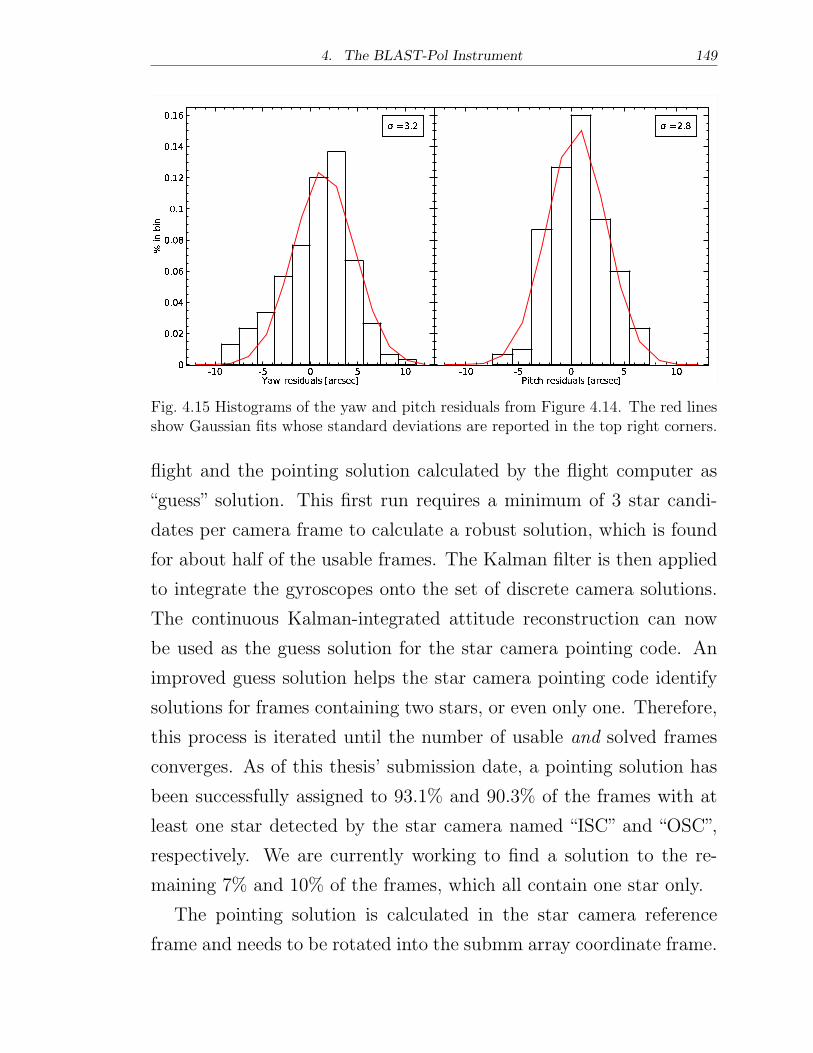
4. The BLAST-Pol Instrument 149
Yaw residuals [arcsec]%i nbi n
±10 ±5 0 5 1000.020.040.060.080.10.120.140.16 σ =3.2
Pitch residuals [arcsec]±10 ±5 0 5 10
σ =2.8
Fig. 4.15 Histograms of the yaw and pitch residuals from Figure 4.14. The red linesshow Gaussian fits whose standard deviations are reported in the top right corners.
flight and the pointing solution calculated by the flight computer as
“guess” solution. This first run requires a minimum of 3 star candi-
dates per camera frame to calculate a robust solution, which is found
for about half of the usable frames. The Kalman filter is then applied
to integrate the gyroscopes onto the set of discrete camera solutions.
The continuous Kalman-integrated attitude reconstruction can now
be used as the guess solution for the star camera pointing code. An
improved guess solution helps the star camera pointing code identify
solutions for frames containing two stars, or even only one. Therefore,
this process is iterated until the number of usable and solved frames
converges. As of this thesis’ submission date, a pointing solution has
been successfully assigned to 93.1% and 90.3% of the frames with at
least one star detected by the star camera named “ISC” and “OSC”,
respectively. We are currently working to find a solution to the re-
maining 7% and 10% of the frames, which all contain one star only.
The pointing solution is calculated in the star camera reference
frame and needs to be rotated into the submm array coordinate frame.
4. The BLAST-Pol Instrument 150
This rotation is evaluated by observing bright optical and submm point
sources (calibrators) simultaneously and repeatedly throughout the
flight. For all the BLAST flights, the relative pointing between the
star cameras and telescope is found to vary as a function of the inner
frame elevation and temperatures, requiring corrections to yaw and
pitch of ∼20′′ and ∼125′′, respectively.
Both star cameras performed well during the BLAST-Pol 2010
flight, being able to detect mv = 9 stars with ∼100ms integration
times. Figure 4.16 shows histograms of the magnitude of the stars
observed by each of the two star cameras during the whole flight. In
Figure 4.17 we show histograms of the total number of stars detected
in one frame by each star camera, throughout the whole flight. Two to
five stars were observed on average, with less than 10% of the frames
having no candidate stars. We investigate how frequently it occurs
that both star cameras simultaneously detect no stars; we find that
zero-star frames usually result as sporadic episodes of desynchroniza-
tion between one star camera computer and the flight computer, and
do not affect both cameras together.
4.8 Concluding Remarks
In this chapter, we have given an overview of the BLAST-Pol instru-
ment, collecting and updating all the information available as of the
2010 Antarctic flight campaign. In particular, we have delved into
the strategy adopted for optimal polarization recovery, as well as the
hardware and software characteristics of the primary pointing sensors,
the star cameras. Finally, we have given an outline of the post-flight
pointing reconstruction process; albeit preliminary, the results pre-
sented here suggest that BLAST-Pol’s absolute pointing accuracy will
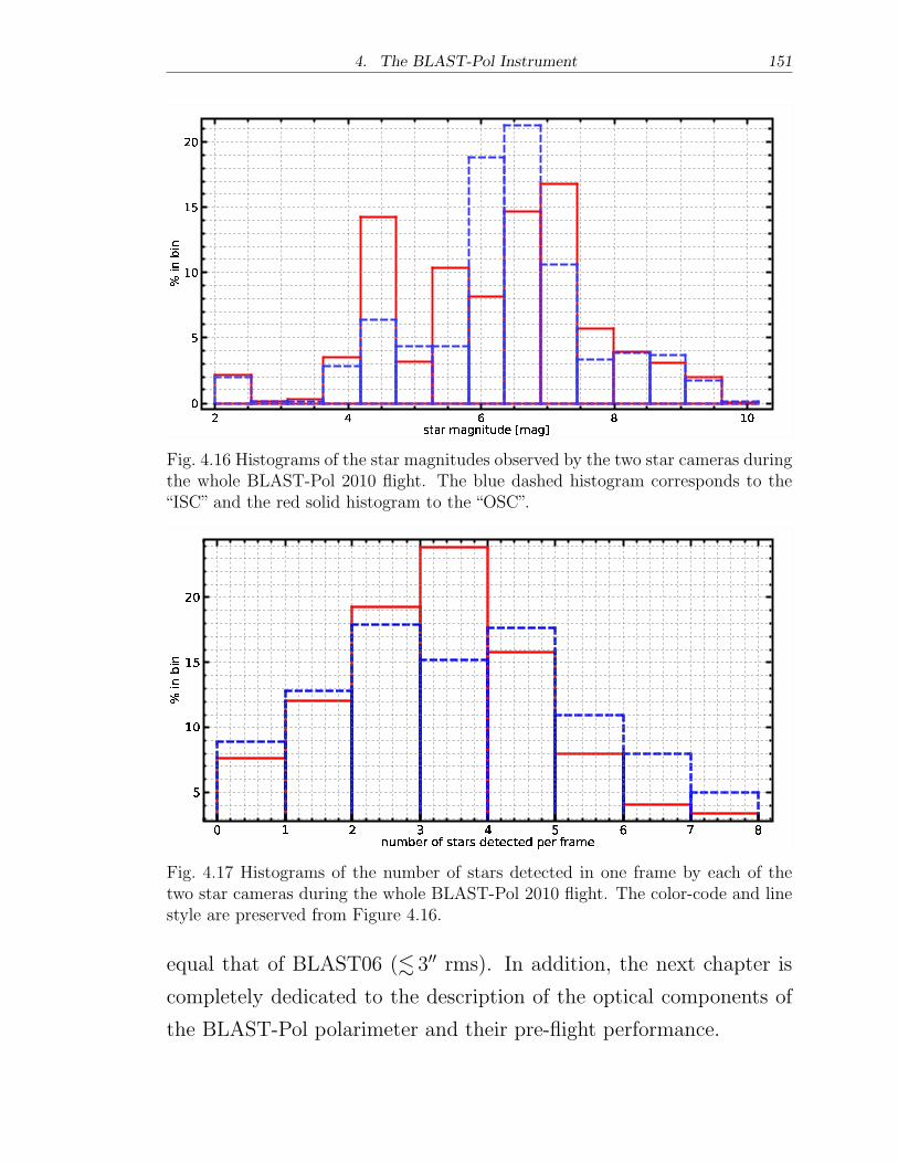
4. The BLAST-Pol Instrument 151
star magnitude [mag]%i nbi n
2 4 6 8 1005101520
Fig. 4.16 Histograms of the star magnitudes observed by the two star cameras duringthe whole BLAST-Pol 2010 flight. The blue dashed histogram corresponds to the“ISC” and the red solid histogram to the “OSC”.
number of stars detected per frame%i nbi n
0 1 2 3 4 5 6 7 85101520
Fig. 4.17 Histograms of the number of stars detected in one frame by each of thetwo star cameras during the whole BLAST-Pol 2010 flight. The color-code and linestyle are preserved from Figure 4.16.
equal that of BLAST06 (≲ 3′′ rms). In addition, the next chapter is
completely dedicated to the description of the optical components of
the BLAST-Pol polarimeter and their pre-flight performance.
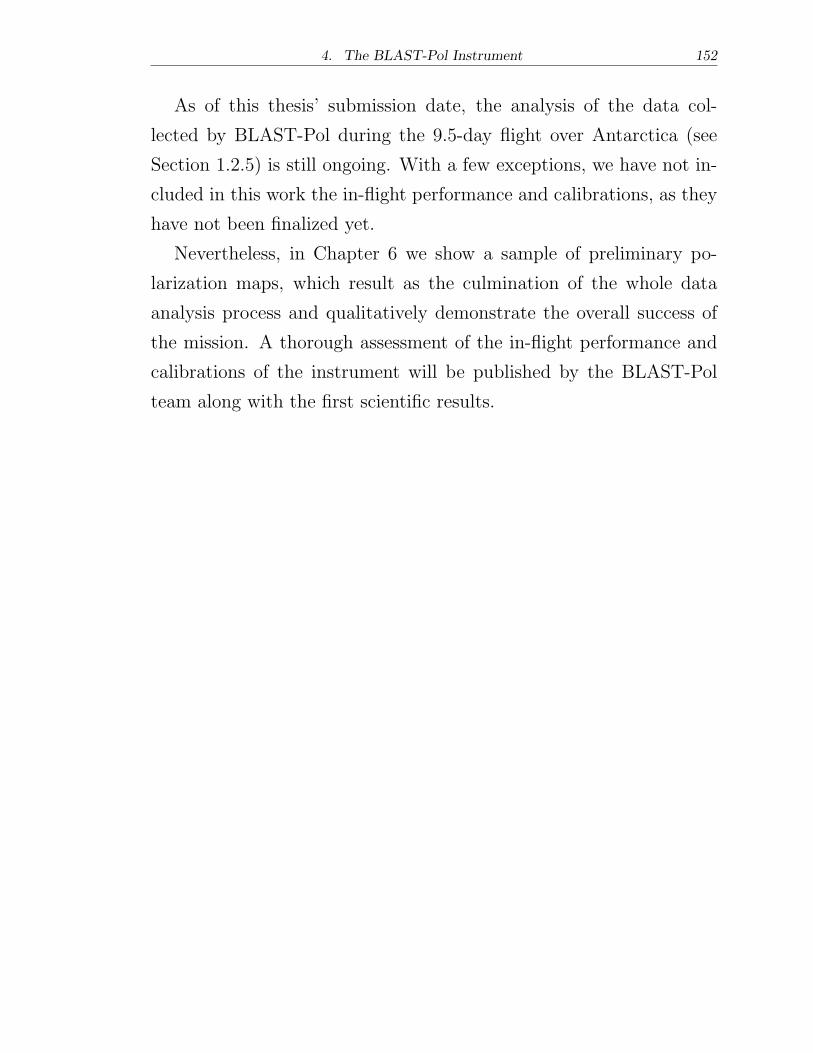
4. The BLAST-Pol Instrument 152
As of this thesis’ submission date, the analysis of the data col-
lected by BLAST-Pol during the 9.5-day flight over Antarctica (see
Section 1.2.5) is still ongoing. With a few exceptions, we have not in-
cluded in this work the in-flight performance and calibrations, as they
have not been finalized yet.
Nevertheless, in Chapter 6 we show a sample of preliminary po-
larization maps, which result as the culmination of the whole data
analysis process and qualitatively demonstrate the overall success of
the mission. A thorough assessment of the in-flight performance and
calibrations of the instrument will be published by the BLAST-Pol
team along with the first scientific results.
5. HALF WAVE PLATE AND POLARIMETRY
5.1 Introduction
In this chapter we describe in detail the components of the BLAST-
Pol polarimeter, a cryogenic achromatic half-wave plate (HWP) and
photolithographed polarizing grids acting as analyzers. The use of a
continuously rotating or stepped HWP as a polarization modulator is a
widespread technique at millimeter (mm) and submillimeter (submm)
wavelengths (e.g., Renbarger et al. 2004, Hanany et al. 2005, Pisano
et al. 2006, Savini et al. 2006, 2009, Johnson et al. 2007, Li et al. 2008,
Matsumura et al. 2009, Bryan et al. 2010a,b, Dowell et al. 2010).
In Section 4.5 we have given an overview of the BLAST-Pol po-
larization modulation scheme and outlined our strategy for optimal
polarization recovery. The final goal of this chapter is to provide a set
of usable parameters that completely characterize the optical proper-
ties and efficiency of the HWP (see Section 5.2.6) and the polarizing
grids (see Section 5.3), as measured in the laboratory.
We delve into the theoretical framework, principles of operation,
and manufacturing process of a five-plate sapphire HWP, which is,
to our knowledge, the most achromatic ever built at mm and submm
wavelengths. We include a brief account of the various solutions con-
sidered for the anti-reflection coating (ARC), and highlight the tech-
nical challenges of a broadband design at submm wavelengths. We
discuss how the ARC applied to the BLAST-Pol HWP represents the
first successful application of a novel artificial dielectric metamaterial.
5. Half Wave Plate and Polarimetry 154
Using a polarizing Fourier transform spectrometer, we fully charac-
terize the spectral response of the coated BLAST-Pol HWP at room
temperature and at 120K. We present the pre-flight performance of
the HWP in terms of its measured Mueller matrix and phase shift as a
function of frequency and extrapolated at 4K. We show that most of
the HWP non-idealities can be more easily modeled by quantifying one
wavelength-dependent parameter, which is then readily implemented
in the map-making algorithm described in Chapter 6. We also derive
this parameter for a range of spectral signatures of an input astro-
nomical source, including that of a blackbody and of dust emission;
we discuss the possible implications for BLAST-Pol.
In the following, we adopt the Stokes (1852) formalism to represent
the time-averaged polarization state of electromagnetic radiation; for
a review of polarization basics we refer the reader to Appendix A of
Moncelsi (2007), which in turn follows the notation of Collett (1993).
5.2 The BLAST-Pol Half-Wave Plate
5.2.1 Birefringent wave plates
Wave plates (or retarders), are optical elements used to change the
polarization state of an incident wave, by inducing a predetermined
phase difference between two perpendicular polarization components.
A (monochromatic) wave plate can be simply obtained with a single
slab of uniaxial birefringent crystal of specific thickness, which depends
upon the wavelength and the index of refraction of the crystal.
Birefringence results from the anisotropy in the binding forces be-
tween the atoms forming a crystal. Such anisotropy originates from
an asymmetric spatial distribution of the atoms in some crystals. An
anisotropy in the binding forces in the lattice will manifest itself as an
5. Half Wave Plate and Polarimetry 155
anisotropy in the refractive index. Crystals belonging to the trigonal
(e.g., calcite, quartz, sapphire) or tetragonal (e.g., rutile) systems are
uniaxial, in that they possess a unique optic axis, most often coincident
with the crystallographic axis.
Light propagating through a uniaxial birefringent material experi-
ences different refraction indices depending on its propagation direc-
tion and polarization orientation inside the crystal: light propagating
along the birefringent optic axis (extraordinary axis) will see an ordi-
nary refraction index regardless of the polarization orientation. Light
propagating orthogonally to the optic axis will see extraordinary or
ordinary refraction indices depending on whether the polarization is,
respectively, aligned or perpendicular to the optic axis.
In wave plates, the crystal is cut so that the extraordinary axis is
parallel to the surfaces of the plate; light polarized along this axis trav-
els through the crystal at a different speed than light with the perpen-
dicular polarization, creating a phase difference. When the extraor-
dinary index is larger than the ordinary index, as in (cold) sapphire,
the extraordinary axis is called the “slow axis” and the perpendicular
direction in the plane of the surfaces is called the “fast axis”.
A birefringent crystal is characterized by four parameters, ne, no,
�e, �o, the real part of the indices of refraction and the absorption
coefficient (in cm−1) for the extraordinary and ordinary axes of the
crystal. At a specific wavelength �0, the phase shift induced by a slab
is determined uniquely by its thickness d, and reads:
Δ' (�0) =2 � d
�0(ne − no) (5.1)
Given the operating wavelength �0, the required phase shift for the
wave plate is achieved by tuning the thickness d.
5. Half Wave Plate and Polarimetry 156
5.2.2 Achromatic half-wave plate design
While monochromatic wave plates have been (and are still being) used
in mm and submm astronomical polarimeters (see e.g.,1 Renbarger
et al. 2004, Li et al. 2008, Bryan et al. 2010a,b, Dowell et al. 2010), the
inherent dependence of the phase shift with wavelength expressed in
Equation (5.1) constitutes an intrinsic limit in designing a polarization
modulator that operates in a broad spectral range (i.e., achromatic).
Achromaticity is necessary for wave plates that are designed for
use with multi-band bolometric receivers, such as BLAST-Pol (see
Chapter 4 of this thesis), PILOT (Bernard et al. 2007), or SCUBA-
2 (Bastien et al. 2005, Savini et al. 2009). To achieve a broadband
performance, multiple-plate solutions have been conceived in the past
(Pancharatnam 1955, Title & Rosenberg 1981) to compensate and to
keep the phase shift approximately constant across the bandwidth, by
stacking an odd number (usually 3 or 5) of birefringent plates of the
same material, which are rotated with respect to each other about
their optical2 axes by a frequency-dependent set of angles.
Achromatic wave plates have been designed and built for astronom-
ical polarimeters at mm and submm wavelengths by many authors in
the last decade (Hanany et al. 2005, Pisano et al. 2006, Savini et al.
2006, 2009, Matsumura et al. 2009), following the Poincare sphere (PS)
method first introduced by Pancharatnam (1955). We briefly recall it
here for completeness (see also Appendix A of Moncelsi 2007). The po-
larization state of a monochromatic wave in a given reference frame can
1 The references listed here describe instruments with wave plates optimized to operate in a singlephotometric waveband, centered at �0 and typically 10–30% wide; hence, these are not strictlymonochromatic. However, these wave plates are referred to as monochromatic in astronomicaljargon, because they cover a single waveband, within which Equation (5.1) is a good approximation.
2 We distinguish between “optic” axis of a crystal, that is the direction in which a ray of trans-mitted light experiences no birefringence, and “optical” axis, that is the imaginary line along whichthere is some degree of rotational symmetry in the optical system described.
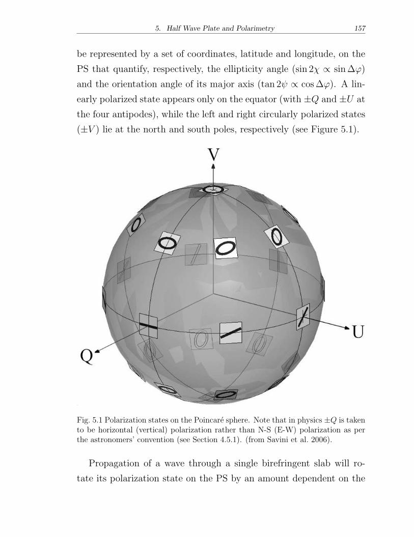
5. Half Wave Plate and Polarimetry 157
be represented by a set of coordinates, latitude and longitude, on the
PS that quantify, respectively, the ellipticity angle (sin 2� ∝ sinΔ')
and the orientation angle of its major axis (tan 2 ∝ cosΔ'). A lin-
early polarized state appears only on the equator (with ±Q and ±U at
the four antipodes), while the left and right circularly polarized states
(±V ) lie at the north and south poles, respectively (see Figure 5.1).
Fig. 5.1 Polarization states on the Poincare sphere. Note that in physics ±Q is takento be horizontal (vertical) polarization rather than N-S (E-W) polarization as perthe astronomers’ convention (see Section 4.5.1). (from Savini et al. 2006).
Propagation of a wave through a single birefringent slab will ro-
tate its polarization state on the PS by an amount dependent on the
5. Half Wave Plate and Polarimetry 158
relation between wavelength and thickness (Equation 5.1), about an
axis whose orientation depends upon the position of the optic axis of
the wave plate with respect to the reference frame of the incoming po-
larization state. Specifically, an ideal monochromatic half-wave plate
produces one PS rotation of 180∘, changing a linear polarization state
to another one on the equator.
When a polychromatic wave packet enters a multiple-plate HWP,
the input polarized states of all wavelengths overlap in a single point
on the PS (see point 1 in Figure 5.2). After the rotation due to the
first plate, the polarization states of different wavelengths will be scat-
tered along an arc on the PS (point 2 in Figure 5.2), with separations
that depend on the bandwidth Δ� of the wave packet. As antici-
pated, this effect can be compensated for by stacking together an odd
number of birefringent slabs, rotated with respect to each other by a
symmetric pattern of angles (�, �, , �, and � for 5 slabs) about their
optical axes (as derived by e.g., Pancharatnam 1955, Title & Rosen-
berg 1981). Figure 5.2 visually illustrates how the various polarization
states regroup in a small area of the PS surface, thus achieving a nearly
frequency-independent output polarization state, within a certain Δ�.
We note that, strictly speaking, all the four parameters that char-
acterize a crystal, ne, no, �e, �o, depend upon wavelength (as we will
illustrate in detail for sapphire); in particular, the different frequency-
dependence of the ordinary and extraordinary refraction indices enters
Equation (5.1) in a non-trivial way, thus rendering the design of an
achromatic HWP increasingly difficult as Δ� broadens.
Using the above PS method, we design and manufacture a HWP
for the BLAST-Pol instrument, which is successfully used as a polar-
ization modulator to study the role of magnetic fields in the earliest,
highly obscured stages of star formation, via the polarized submm
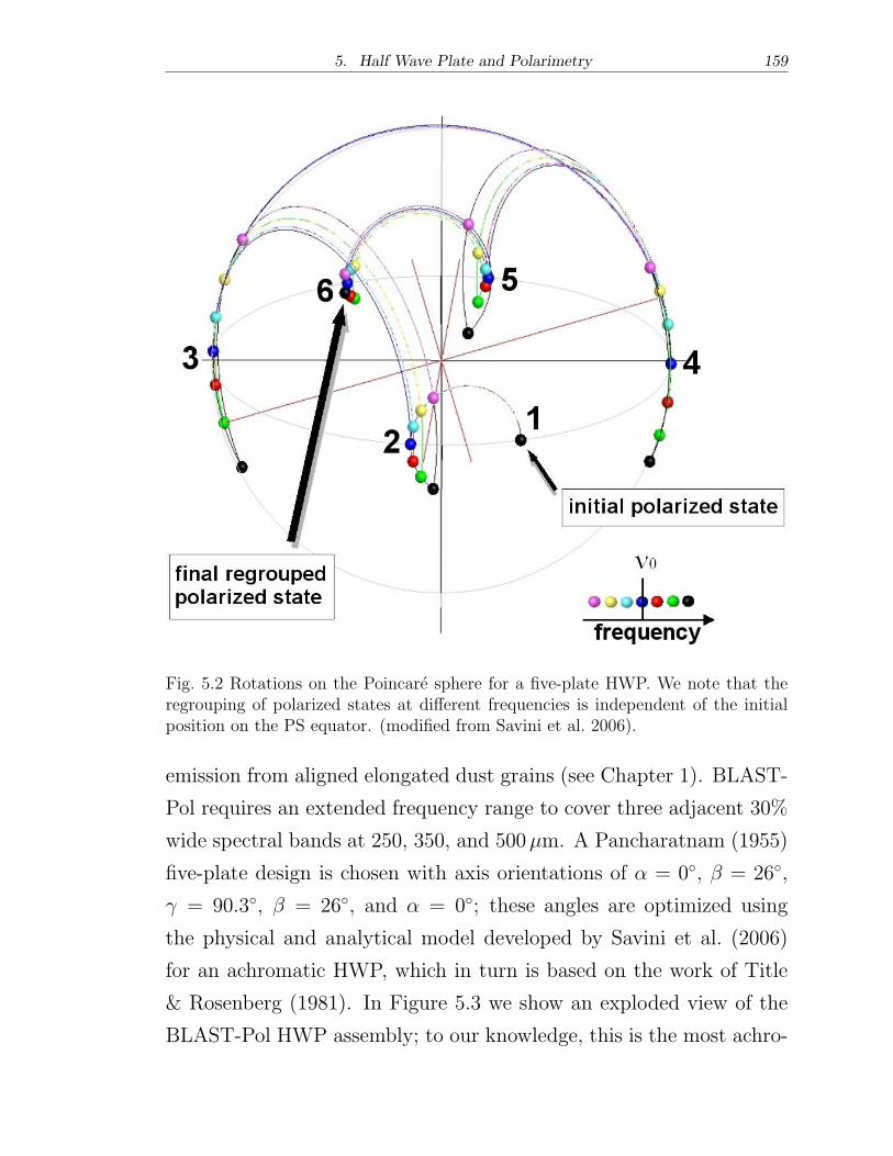
5. Half Wave Plate and Polarimetry 159
Fig. 5.2 Rotations on the Poincare sphere for a five-plate HWP. We note that theregrouping of polarized states at different frequencies is independent of the initialposition on the PS equator. (modified from Savini et al. 2006).
emission from aligned elongated dust grains (see Chapter 1). BLAST-
Pol requires an extended frequency range to cover three adjacent 30%
wide spectral bands at 250, 350, and 500�m. A Pancharatnam (1955)
five-plate design is chosen with axis orientations of � = 0∘, � = 26∘,
= 90.3∘, � = 26∘, and � = 0∘; these angles are optimized using
the physical and analytical model developed by Savini et al. (2006)
for an achromatic HWP, which in turn is based on the work of Title
& Rosenberg (1981). In Figure 5.3 we show an exploded view of the
BLAST-Pol HWP assembly; to our knowledge, this is the most achro-
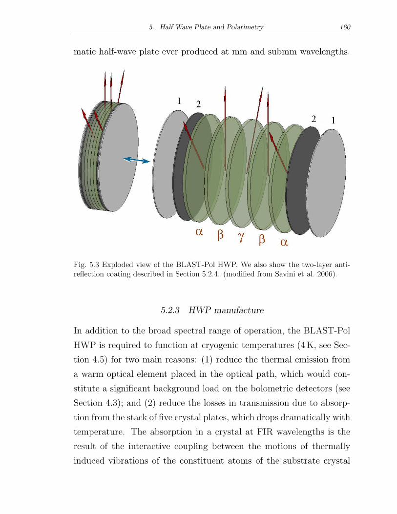
5. Half Wave Plate and Polarimetry 160
matic half-wave plate ever produced at mm and submm wavelengths.
Fig. 5.3 Exploded view of the BLAST-Pol HWP. We also show the two-layer anti-reflection coating described in Section 5.2.4. (modified from Savini et al. 2006).
5.2.3 HWP manufacture
In addition to the broad spectral range of operation, the BLAST-Pol
HWP is required to function at cryogenic temperatures (4K, see Sec-
tion 4.5) for two main reasons: (1) reduce the thermal emission from
a warm optical element placed in the optical path, which would con-
stitute a significant background load on the bolometric detectors (see
Section 4.3); and (2) reduce the losses in transmission due to absorp-
tion from the stack of five crystal plates, which drops dramatically with
temperature. The absorption in a crystal at FIR wavelengths is the
result of the interactive coupling between the motions of thermally
induced vibrations of the constituent atoms of the substrate crystal
5. Half Wave Plate and Polarimetry 161
lattice (which propagate as waves called phonons) and the incident
radiation. Because the phonon population is much reduced at low
temperatures, cooling the crystal effectively reduces the absorption.
The two obvious candidates (uniaxial birefringent) crystals are sap-
phire and quartz, because of their favorable optical properties in the
FIR/submm (Loewenstein et al. 1973). Sapphire is chosen over quartz
due to its larger difference between ordinary and extraordinary refrac-
tion index (Δne−o ≈ 0.34 for sapphire, and ≈ 0.13 for quartz Loewen-
stein et al. 1973; see also Figures 5.4, 5.5), which implies a smaller
thickness for the plates (see Equation 5.1). Since quartz and sapphire
have a comparable level of absorption at cryogenic temperatures in
the wavelength range of 200–600�m (Loewenstein et al. 1973), thinner
substrates are desirable to minimize absorption losses (∝ 1− e−�d).
Nonetheless, the thin sapphire substrates chosen for the BLAST-
Pol HWP do indeed show appreciable absorption, especially at the
shortest wavelengths (250�m band; see Section 5.2.5). We have high-
lighted how the frequency dependence of both the refractive index and
absorption coefficient for the chosen birefringent crystal is crucial to
the overall performance of the HWP. Therefore, in Figures 5.4, 5.5,
5.6, and 5.7 we graphically report a collection of spectral measure-
ments3 and analytical expressions from the literature of the indices of
refraction and the absorption coefficient at the wavelengths relevant
to BLAST-Pol, for the extraordinary and ordinary axes of sapphire,
both at room and cryogenic temperatures. The details and relevant
references are given in the captions. Albeit not necessarily complete,
to our knowledge this collection represents the most comprehensive
3 Throughout this Chapter we make use of the wavenumber, k, as a unit of frequency, ex-
pressed in cm−1 as customary in spectroscopy, with k[
cm−1]
= � [Hz]100 c [m s−1] =
0.01� [m] , or k
[
cm−1]
=107 � [GHz]c [m s−1] = 104
� [�m] , where c is the speed of light in vacuum. Furthermore, we adopt a color code in
the plots whereby curves referring to the three BLAST-Pol bands, 250, 350, and 500�m are drawnin blue, green, and red, respectively.
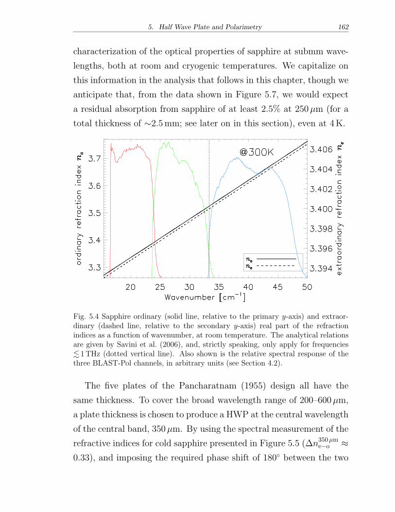
5. Half Wave Plate and Polarimetry 162
characterization of the optical properties of sapphire at submm wave-
lengths, both at room and cryogenic temperatures. We capitalize on
this information in the analysis that follows in this chapter, though we
anticipate that, from the data shown in Figure 5.7, we would expect
a residual absorption from sapphire of at least 2.5% at 250�m (for a
total thickness of ∼2.5mm; see later on in this section), even at 4K.
Fig. 5.4 Sapphire ordinary (solid line, relative to the primary y-axis) and extraor-dinary (dashed line, relative to the secondary y-axis) real part of the refractionindices as a function of wavenumber, at room temperature. The analytical relationsare given by Savini et al. (2006), and, strictly speaking, only apply for frequencies≲ 1THz (dotted vertical line). Also shown is the relative spectral response of thethree BLAST-Pol channels, in arbitrary units (see Section 4.2).
The five plates of the Pancharatnam (1955) design all have the
same thickness. To cover the broad wavelength range of 200–600�m,
a plate thickness is chosen to produce a HWP at the central wavelength
of the central band, 350�m. By using the spectral measurement of the
refractive indices for cold sapphire presented in Figure 5.5 (Δn350�me−o ≈0.33), and imposing the required phase shift of 180∘ between the two
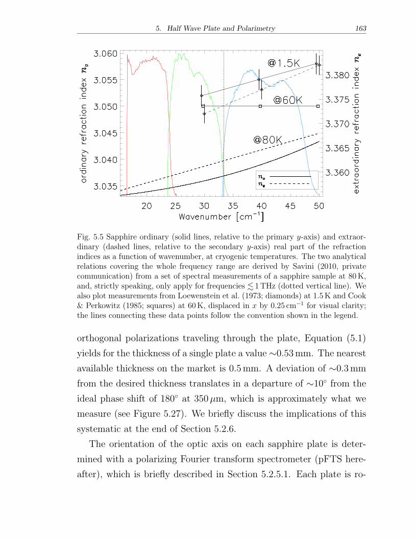
5. Half Wave Plate and Polarimetry 163
Fig. 5.5 Sapphire ordinary (solid lines, relative to the primary y-axis) and extraor-dinary (dashed lines, relative to the secondary y-axis) real part of the refractionindices as a function of wavenumber, at cryogenic temperatures. The two analyticalrelations covering the whole frequency range are derived by Savini (2010, privatecommunication) from a set of spectral measurements of a sapphire sample at 80K,and, strictly speaking, only apply for frequencies ≲ 1THz (dotted vertical line). Wealso plot measurements from Loewenstein et al. (1973; diamonds) at 1.5K and Cook& Perkowitz (1985; squares) at 60K, displaced in x by 0.25 cm−1 for visual clarity;the lines connecting these data points follow the convention shown in the legend.
orthogonal polarizations traveling through the plate, Equation (5.1)
yields for the thickness of a single plate a value ∼0.53mm. The nearest
available thickness on the market is 0.5mm. A deviation of ∼0.3mm
from the desired thickness translates in a departure of ∼10∘ from the
ideal phase shift of 180∘ at 350�m, which is approximately what we
measure (see Figure 5.27). We briefly discuss the implications of this
systematic at the end of Section 5.2.6.
The orientation of the optic axis on each sapphire plate is deter-
mined with a polarizing Fourier transform spectrometer (pFTS here-
after), which is briefly described in Section 5.2.5.1. Each plate is ro-
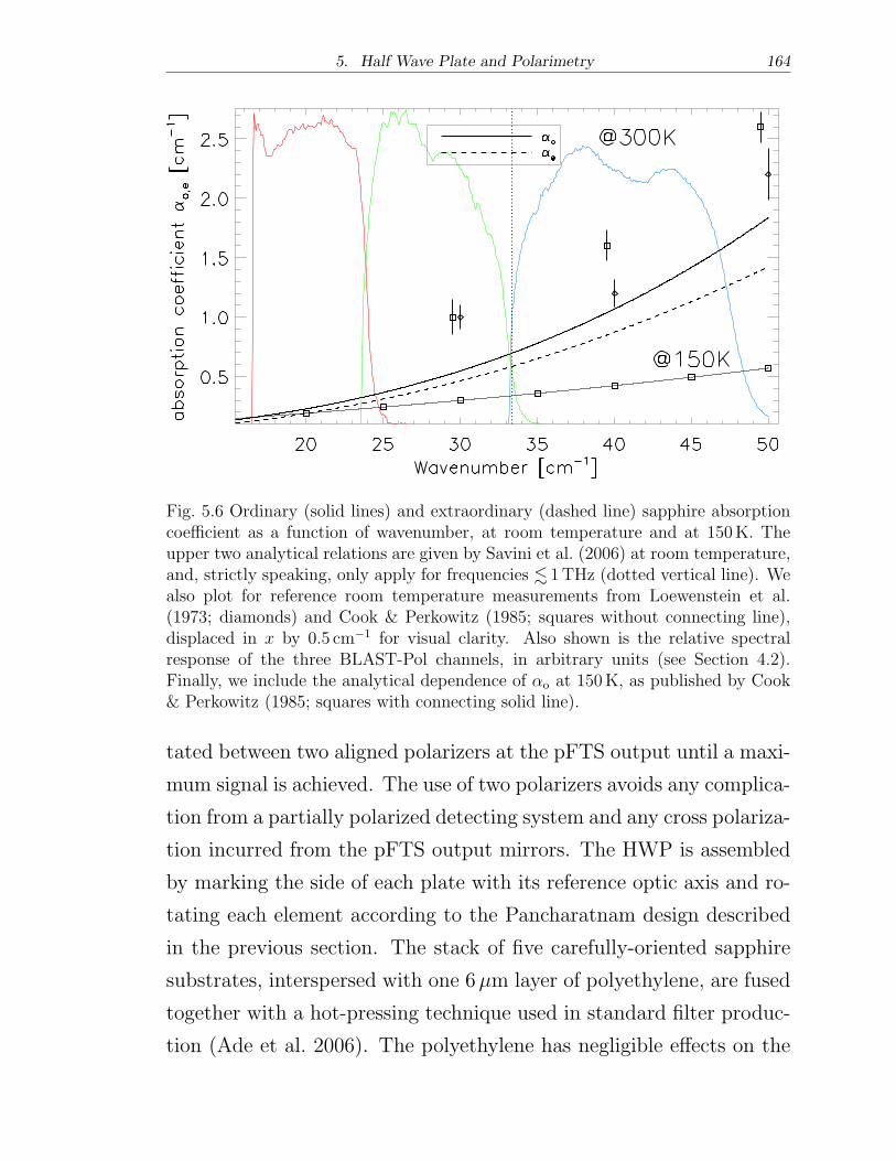
5. Half Wave Plate and Polarimetry 164
Fig. 5.6 Ordinary (solid lines) and extraordinary (dashed line) sapphire absorptioncoefficient as a function of wavenumber, at room temperature and at 150K. Theupper two analytical relations are given by Savini et al. (2006) at room temperature,and, strictly speaking, only apply for frequencies ≲ 1THz (dotted vertical line). Wealso plot for reference room temperature measurements from Loewenstein et al.(1973; diamonds) and Cook & Perkowitz (1985; squares without connecting line),displaced in x by 0.5 cm−1 for visual clarity. Also shown is the relative spectralresponse of the three BLAST-Pol channels, in arbitrary units (see Section 4.2).Finally, we include the analytical dependence of �o at 150K, as published by Cook& Perkowitz (1985; squares with connecting solid line).
tated between two aligned polarizers at the pFTS output until a maxi-
mum signal is achieved. The use of two polarizers avoids any complica-
tion from a partially polarized detecting system and any cross polariza-
tion incurred from the pFTS output mirrors. The HWP is assembled
by marking the side of each plate with its reference optic axis and ro-
tating each element according to the Pancharatnam design described
in the previous section. The stack of five carefully-oriented sapphire
substrates, interspersed with one 6�m layer of polyethylene, are fused
together with a hot-pressing technique used in standard filter produc-
tion (Ade et al. 2006). The polyethylene has negligible effects on the
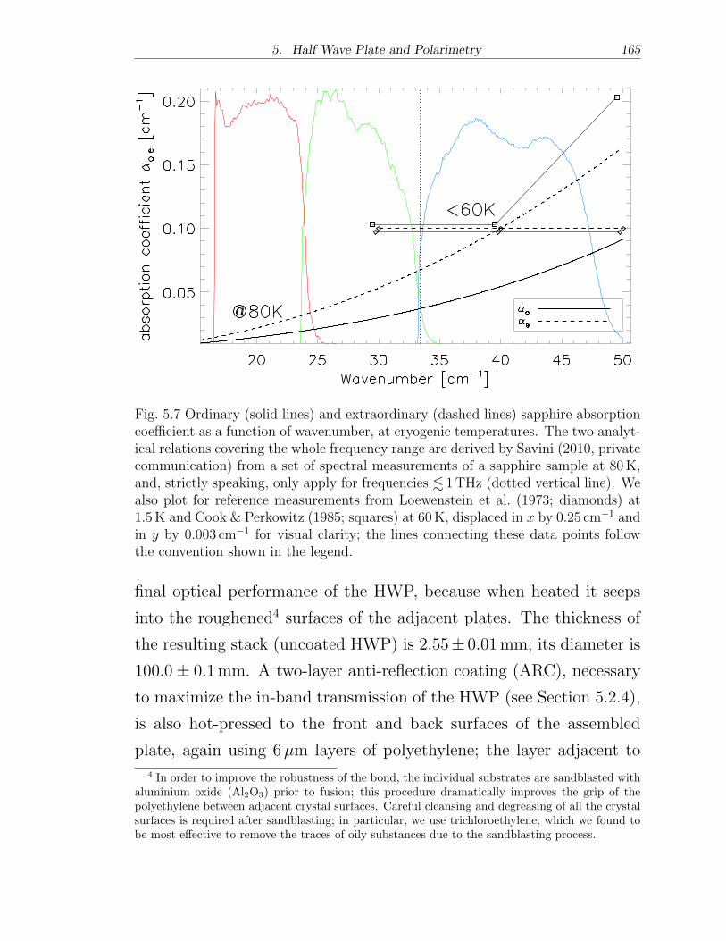
5. Half Wave Plate and Polarimetry 165
Fig. 5.7 Ordinary (solid lines) and extraordinary (dashed lines) sapphire absorptioncoefficient as a function of wavenumber, at cryogenic temperatures. The two analyt-ical relations covering the whole frequency range are derived by Savini (2010, privatecommunication) from a set of spectral measurements of a sapphire sample at 80K,and, strictly speaking, only apply for frequencies ≲ 1THz (dotted vertical line). Wealso plot for reference measurements from Loewenstein et al. (1973; diamonds) at1.5K and Cook & Perkowitz (1985; squares) at 60K, displaced in x by 0.25 cm−1 andin y by 0.003 cm−1 for visual clarity; the lines connecting these data points followthe convention shown in the legend.
final optical performance of the HWP, because when heated it seeps
into the roughened4 surfaces of the adjacent plates. The thickness of
the resulting stack (uncoated HWP) is 2.55± 0.01mm; its diameter is
100.0± 0.1mm. A two-layer anti-reflection coating (ARC), necessary
to maximize the in-band transmission of the HWP (see Section 5.2.4),
is also hot-pressed to the front and back surfaces of the assembled
plate, again using 6�m layers of polyethylene; the layer adjacent to
4 In order to improve the robustness of the bond, the individual substrates are sandblasted withaluminium oxide (Al2O3) prior to fusion; this procedure dramatically improves the grip of thepolyethylene between adjacent crystal surfaces. Careful cleansing and degreasing of all the crystalsurfaces is required after sandblasting; in particular, we use trichloroethylene, which we found tobe most effective to remove the traces of oily substances due to the sandblasting process.
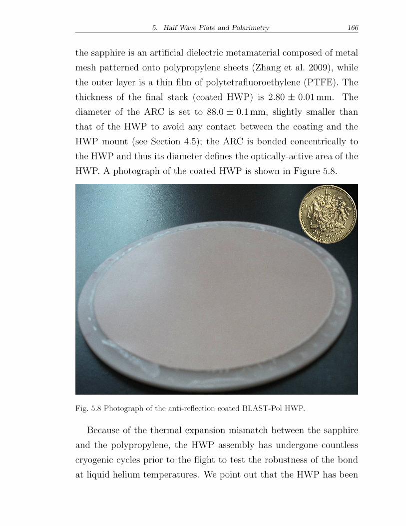
5. Half Wave Plate and Polarimetry 166
the sapphire is an artificial dielectric metamaterial composed of metal
mesh patterned onto polypropylene sheets (Zhang et al. 2009), while
the outer layer is a thin film of polytetrafluoroethylene (PTFE). The
thickness of the final stack (coated HWP) is 2.80 ± 0.01mm. The
diameter of the ARC is set to 88.0 ± 0.1mm, slightly smaller than
that of the HWP to avoid any contact between the coating and the
HWP mount (see Section 4.5); the ARC is bonded concentrically to
the HWP and thus its diameter defines the optically-active area of the
HWP. A photograph of the coated HWP is shown in Figure 5.8.
Fig. 5.8 Photograph of the anti-reflection coated BLAST-Pol HWP.
Because of the thermal expansion mismatch between the sapphire
and the polypropylene, the HWP assembly has undergone countless
cryogenic cycles prior to the flight to test the robustness of the bond
at liquid helium temperatures. We point out that the HWP has been
5. Half Wave Plate and Polarimetry 167
successfully installed in the BLAST-Pol cryogenic receiver and flown
from balloon platform for about ten days, without delamination of the
ARC or damage to the assembly.
5.2.4 Anti-reflection coating
The presence of an anti-reflection coating (ARC) on both sides of
the HWP is required to minimize the reflections due to the impedance
mismatch between the high-n birefringent crystal and free space, which
would substantially degrade the overall optical efficiency of the system.
As a consequence of the inclusion of an ARC, the in-band transmission
is maximized and very little radiation is reflected off the HWP, which
would otherwise be scattered inside the optics box and could eventually
end up on the detectors. The large bandwidth of BLAST-Pol dictates
the need for an ARC solution that is at least as achromatic as the
HWP. Furthermore, the materials employed must be suitable for use
at liquid helium temperatures.
Before describing the particular solution adopted for the BLAST-
Pol HWP, we briefly review here the principles of operation of an
ARC. In propagating from one medium (air) with refractive index
n1 into another one with refractive index n2 (sapphire), a fraction
R =(
n2−n1
n2+n1
)2of the light will be reflected off the boundary surface
between the two media. By applying a coating, with refractive index
n3 and thickness t, on the sapphire plate, the light is reflected twice
at the two boundary surfaces; if the optical path difference between
the two reflections is a half-integer number of wavelengths, the two
reflections interfere destructively and the reflection is minimized. This
condition is satisfied when
t =�
4n3(5.2)
5. Half Wave Plate and Polarimetry 168
For fully destructive interference the amplitudes of the two reflec-
tions should be equal; this is achieved by choosing n3 =√n1 n2. It is
clear from Equation (5.2) that a single layer of ARC is effective only at
one wavelength. Broadband performance can be achieved by stacking
multiple layers of materials with progressively higher refractive indices,
which create a smoother impedance match between n1 and n2.
5.2.4.1 Old recipes: high-n powders and loaded ceramics
ARC solutions at mm wavelengths use multiple layers of either spe-
cially prepared polypropylene layers loaded with high refractive index
powders (TiO2; Pisano et al. 2006, Savini et al. 2006) or ceramic-based
materials (e.g., Rogers TMM material5; Savini et al. 2009) to create
a particular refractive index. These ARC recipes need usually three
layers to achieve a flat response across the band. Each layer requires
hot-pressing onto the HWP stack, and subsequent grinding to the
required thickness. There are several disadvantages to both these ap-
proaches: the loaded powder layers are slow to manufacture because
the powder needs to be uniformly mixed in the polypropylene, and
then the layers have to be hot-pressed to the appropriate thickness;
the ceramics are brittle and can only be thinned with a grinding tech-
nique, which is time-consuming and unreliable for thicknesses below
∼100�m. Among all the drawbacks listed, this latter point is the one
that engages us to design a new ARC solution (described in the next
section), as at submm wavelengths the required thicknesses of high
refractive index materials (n ≈ 1.2–2.75) are of the order of tens of
microns (see Equation 5.2).
5 Rogers Corporation supply TMM high-frequency laminate materials: www.rogerscorp.com.
5. Half Wave Plate and Polarimetry 169
5.2.4.2 New recipes: artificial dielectric metamaterials
As anticipated in the previous sections, the technical difficulties in the
manufacture of conventional ARC solutions at submm wavelengths led
us to develop a novel artificial dielectric metamaterial (ADM), which
is thoroughly described in Zhang et al. (2009); we briefly review here
its salient features.
The material is manufactured from layers of photolithographed
metal mesh (copper; Tucker & Ade 2007) patterned onto thin polypropy-
lene sheets, which act as embedding dielectric. Specifically, two metal-
mesh layers (periodic structures of square grids patterns) are immersed
in the polypropylene substrate at a distance of 8�m from the top and
bottom surfaces and with a spacing of 24�m between the two layers.
The 40�m multi-layer structure is assembled and then hot-pressed at
temperatures close to the polypropylene melting point (160∘C).
The artificial material thus created has the consistency of a solid
plastic film that can be easily handled, cut to the desired size, and
reliably cycled to liquid helium temperatures. The refractive index of
this metamaterial can be tuned by adjusting the geometry and spacing
of the metal-mesh layers. The particular ADM prototype that Zhang
et al. (2009) describe and fully characterize is applied as an ARC to
a quartz substrate; subsequently, the recipe has been optimized for
sapphire substrates in the wavelength range 200–600�m.
As anticipated, a second layer of coating is necessary to achieve
the required broadband performance. We use a 54�m layer of porous
PTFE6, which has refractive index n = 1.375; its thermal expansion
coefficient is closely matched to that of polypropylene, so it represents
an ideal solution for our application at cryogenic temperatures.
Finally, the two ARC layers are interspersed by 6�m layers of
6 http://www.porex.com/porous.cfm
5. Half Wave Plate and Polarimetry 170
polyethylene and hot-pressed concentrically to the top and bottom
surfaces of the HWP stack (the two layers can in fact be bonded in
one single press cycle). The final ARC assembly has a thickness of
125± 15�m and an outer diameter of 88mm.
Such a metal-mesh ADM design has complete control over the thick-
ness of the coating layer and the embedding material is not brittle,
hence it has better performance in thermal cycling. The BLAST-Pol
coated HWP represents the first successful application of the new-
concept THz coating. Incidentally, we mention that the design and
manufacture of the HWP for the PILOT experiment (with similar
photometric bands to those of BLAST-Pol; Bernard et al. 2007) has
gone hand in hand with that of BLAST-Pol; LM has participated in
its fabrication, spectral characterization and cryogenic testing.
Because of the thermal expansion mismatch between polypropylene
and sapphire (or quartz), the application of this metal-mesh ADM as
an ARC is challenging for large-aperture cryogenic HWPs. Extending
previous work by Pisano et al. (2008), we have recently designed and
realized a prototype polypropylene-embedded metal-mesh broadband
achromatic HWP for millimeter wavelengths (Zhang et al. 2011); this
will allow next generation experiments with large-aperture detector
arrays to be equipped with large-format (≳ 20 cm in diameter) HWPs
for broadband polarization modulation.
5.2.5 Spectral characterization
5.2.5.1 Introduction
We fully characterize the spectral performance of the BLAST-Pol
HWP by using a pFTS of the Martin–Puplett (1970) type. The
source is an incoherent mercury arc lamp with an aperture of 10mm,
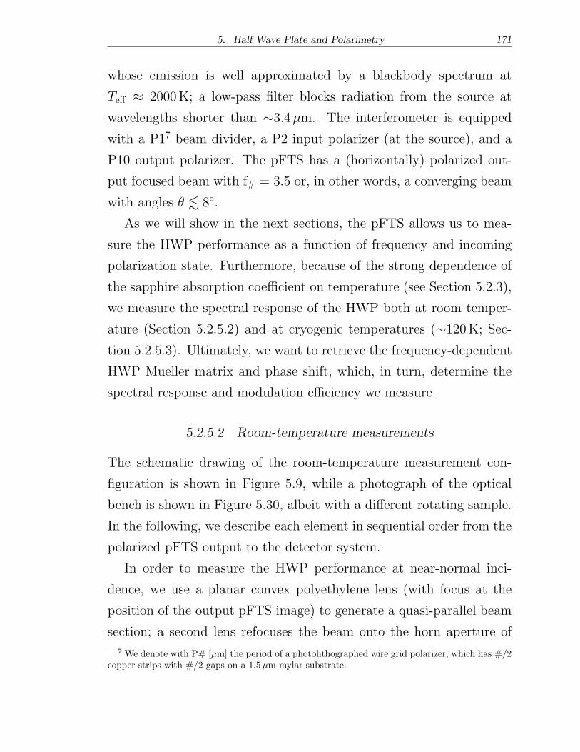
5. Half Wave Plate and Polarimetry 171
whose emission is well approximated by a blackbody spectrum at
Teff ≈ 2000K; a low-pass filter blocks radiation from the source at
wavelengths shorter than ∼3.4�m. The interferometer is equipped
with a P17 beam divider, a P2 input polarizer (at the source), and a
P10 output polarizer. The pFTS has a (horizontally) polarized out-
put focused beam with f# = 3.5 or, in other words, a converging beam
with angles � ≲ 8∘.
As we will show in the next sections, the pFTS allows us to mea-
sure the HWP performance as a function of frequency and incoming
polarization state. Furthermore, because of the strong dependence of
the sapphire absorption coefficient on temperature (see Section 5.2.3),
we measure the spectral response of the HWP both at room temper-
ature (Section 5.2.5.2) and at cryogenic temperatures (∼120K; Sec-
tion 5.2.5.3). Ultimately, we want to retrieve the frequency-dependent
HWP Mueller matrix and phase shift, which, in turn, determine the
spectral response and modulation efficiency we measure.
5.2.5.2 Room-temperature measurements
The schematic drawing of the room-temperature measurement con-
figuration is shown in Figure 5.9, while a photograph of the optical
bench is shown in Figure 5.30, albeit with a different rotating sample.
In the following, we describe each element in sequential order from the
polarized pFTS output to the detector system.
In order to measure the HWP performance at near-normal inci-
dence, we use a planar convex polyethylene lens (with focus at the
position of the output pFTS image) to generate a quasi-parallel beam
section; a second lens refocuses the beam onto the horn aperture of
7 We denote with P# [�m] the period of a photolithographed wire grid polarizer, which has #/2copper strips with #/2 gaps on a 1.5�m mylar substrate.
5. Half Wave Plate and Polarimetry 172
Fig. 5.9 Schematic drawing of the room-temperature spectral measurements setup.The horizontally polarized output of a pFTS feeds into a polyethylene lens thatcreates a quasi-parallel beam and is then refocused onto the horn aperture of thebolometric detector. Two polarizers alternatively parallel and perpendicular createthe necessary polarization selection for the “co-pol” and “cross-pol” sets of measure-ments. The arrows for PP1 and PP2 indicate the selected polarization, so that thewire grid orientations are perpendicular to the arrows. (from Zhang et al. 2011).
the detector system. The maximum range of incident angles is thus
limited by the input source aperture (10mm), a beam spread of only
1.6∘. This allows to evenly illuminate the entire optically-active area
of the HWP, as if it would be inside the BLAST-Pol optics box (see
Section 4.5.2).
The HWP is placed centrally in the collimated beam section be-
tween two P10 polarizers (the output polarizer is usually referred to
as “analyzer”), which are tilted by 45∘ with respect to the optical axis
to avoid standing waves between the optical elements. This tilt in-
troduces four ports that are optically terminated with a close to ideal
5. Half Wave Plate and Polarimetry 173
blackbody, Eccosorb AN72 absorber8. The efficiency of these polar-
izers is separately determined to exceed 99.8% over the range of fre-
quencies of interest, with a cross-polarization of less than 0.1%. The
polarizers are initially aligned with respect to each other with the grid
wires vertical (thus selecting horizontal polarization) with respect to
the optical bench, in order to avoid any projection effect when tilted.
Following the convention depicted in Figure 5.9, measurements with
aligned polarizers are referred to as “co-pol” transmission, Tcp. As
shown in the next section, the HWP has a complementary response
when the output polarizer (analyzer) is rotated by 90∘ about the op-
tical axis of the system (i.e., horizontal wires, selecting vertical po-
larization); data taken with this configuration are also necessary to
completely characterize the HWP, and are referred to as “cross-pol”
transmission9, Txp.
Common to both the warm and cold measurements is the require-
ment to position and rotate the HWP accurately with respect to its
optical axis. When at room temperature, the HWP is held and rotated
by a motorized rotating mount positioned centrally between the two
tilted polarizers. The mount has a fixed orientation with respect to the
optical axis of the system; we position it so that the collimated beam
has normal incidence on the HWP (within 1∘), and evenly illuminates
its surface. The electronically-controlled rotating mount can rotate
the HWP about its optical axis to obtain the polarization modulation;
the resolution of the digital angular encoder on the rotation angle is
0.001∘. Besides Figures 5.9 and 5.30, a CAD drawing of the optical
bench setup, including the motorized rotating mount, can be found in
Figure 1 of Pisano et al. (2006).
8 Emerson and Cuming, Microwave Products, http://www. eccosorb.com/.9 We note that this definition of cross-pol may differ from other conventions adopted in the
literature (e.g., that of Masi et al. 2006, who operate without a HWP).
5. Half Wave Plate and Polarimetry 174
Finally, the detecting system used is a 4.2K liquid helium cooled
indium antimonide (InSb) detector, which is cryogenically filtered to
minimize photon noise. The spectral coverage of the data is thus de-
fined by the cut-off frequency of the light collector waveguide (5 cm−1)
and by two low-pass filters in the cryostat housing the bolometric de-
tector (60 cm−1). We pay particular attention to ensure the absorption
of any diffracted or reflected stray radiation. Besides terminating all
unused optical ports as described above, additional Eccosorb AN72
covers all the exposed metallic surfaces close to the optical path.
The rapid scan system records interferograms with a 8�m sam-
pling interval over a 10 cm optical path difference, at a scan speed of
1 cm s−1; this results in a Nyquist frequency of 625 cm−1 and a spectral
resolution of 0.05 cm−1.
A first dataset is obtained in co-pol configuration by scanning the
spectrometer in the absence of the HWP, which we refer to as the
background spectrum. This dataset defines the pFTS reference spec-
tral envelope, and it is the set against which all the following spectra
are divided in order to account for the spectral features of the source,
pFTS optics, detector system, and laboratory environment (i.e., wa-
ter vapor). Subsequently, the HWP is inserted in between the tilted
polarizers in co-pol configuration, and spectra are acquired at many
different HWP rotation angles (resulting in a data cube). To enhance
the spectral signal-to-noise ratio, each dataset at a given angle consists
of an average of two spectra, each obtained by computing the Fourier
transform of an (apodized and phase-corrected) average of 30 interfer-
ograms10 with the mirror scanned in both the forward and backward
directions. As anticipated, the resulting spectra are divided by the
background dataset, which in turn is the average of three spectra, to
10 This is to all intens and purposes equivalent to averaging 60 interferograms together. However,we proceed as described in the text for operative convenience.
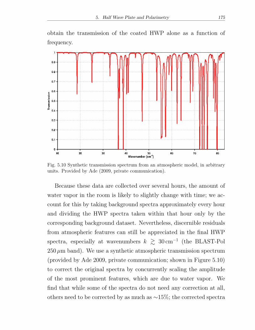
5. Half Wave Plate and Polarimetry 175
obtain the transmission of the coated HWP alone as a function of
frequency.
Fig. 5.10 Synthetic transmission spectrum from an atmospheric model, in arbitraryunits. Provided by Ade (2009, private communication).
Because these data are collected over several hours, the amount of
water vapor in the room is likely to slightly change with time; we ac-
count for this by taking background spectra approximately every hour
and dividing the HWP spectra taken within that hour only by the
corresponding background dataset. Nevertheless, discernible residuals
from atmospheric features can still be appreciated in the final HWP
spectra, especially at wavenumbers k ≳ 30 cm−1 (the BLAST-Pol
250�m band). We use a synthetic atmospheric transmission spectrum
(provided by Ade 2009, private communication; shown in Figure 5.10)
to correct the original spectra by concurrently scaling the amplitude
of the most prominent features, which are due to water vapor. We
find that while some of the spectra do not need any correction at all,
others need to be corrected by as much as ∼15%; the corrected spectra
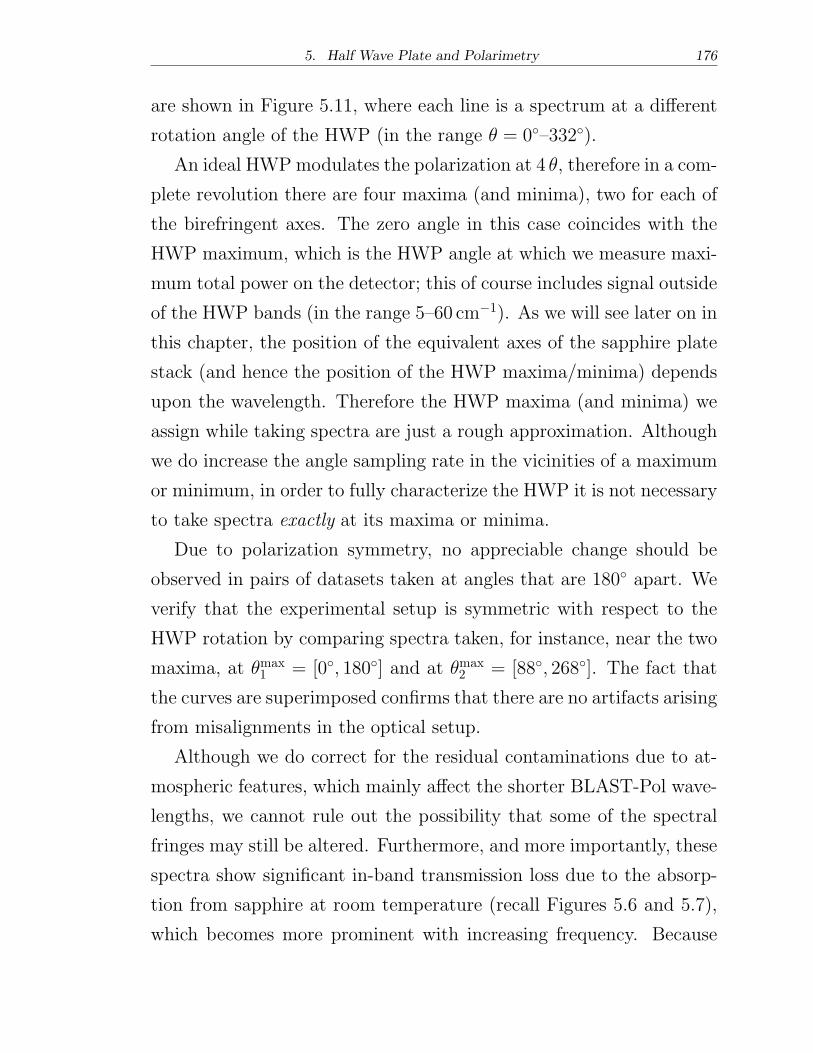
5. Half Wave Plate and Polarimetry 176
are shown in Figure 5.11, where each line is a spectrum at a different
rotation angle of the HWP (in the range � = 0∘–332∘).
An ideal HWPmodulates the polarization at 4 �, therefore in a com-
plete revolution there are four maxima (and minima), two for each of
the birefringent axes. The zero angle in this case coincides with the
HWP maximum, which is the HWP angle at which we measure maxi-
mum total power on the detector; this of course includes signal outside
of the HWP bands (in the range 5–60 cm−1). As we will see later on in
this chapter, the position of the equivalent axes of the sapphire plate
stack (and hence the position of the HWP maxima/minima) depends
upon the wavelength. Therefore the HWP maxima (and minima) we
assign while taking spectra are just a rough approximation. Although
we do increase the angle sampling rate in the vicinities of a maximum
or minimum, in order to fully characterize the HWP it is not necessary
to take spectra exactly at its maxima or minima.
Due to polarization symmetry, no appreciable change should be
observed in pairs of datasets taken at angles that are 180∘ apart. We
verify that the experimental setup is symmetric with respect to the
HWP rotation by comparing spectra taken, for instance, near the two
maxima, at �max1 = [0∘, 180∘] and at �max
2 = [88∘, 268∘]. The fact that
the curves are superimposed confirms that there are no artifacts arising
from misalignments in the optical setup.
Although we do correct for the residual contaminations due to at-
mospheric features, which mainly affect the shorter BLAST-Pol wave-
lengths, we cannot rule out the possibility that some of the spectral
fringes may still be altered. Furthermore, and more importantly, these
spectra show significant in-band transmission loss due to the absorp-
tion from sapphire at room temperature (recall Figures 5.6 and 5.7),
which becomes more prominent with increasing frequency. Because
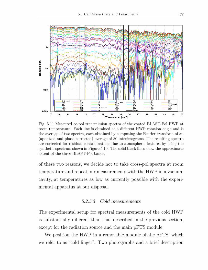
5. Half Wave Plate and Polarimetry 177
Fig. 5.11 Measured co-pol transmission spectra of the coated BLAST-Pol HWP atroom temperature. Each line is obtained at a different HWP rotation angle and isthe average of two spectra, each obtained by computing the Fourier transform of an(apodized and phase-corrected) average of 30 interferograms. The resulting spectraare corrected for residual contaminations due to atmospheric features by using thesynthetic spectrum shown in Figure 5.10. The solid black lines show the approximateextent of the three BLAST-Pol bands.
of these two reasons, we decide not to take cross-pol spectra at room
temperature and repeat our measurements with the HWP in a vacuum
cavity, at temperatures as low as currently possible with the experi-
mental apparatus at our disposal.
5.2.5.3 Cold measurements
The experimental setup for spectral measurements of the cold HWP
is substantially different than that described in the previous section,
except for the radiation source and the main pFTS module.
We position the HWP in a removable module of the pFTS, which
we refer to as “cold finger”. Two photographs and a brief description
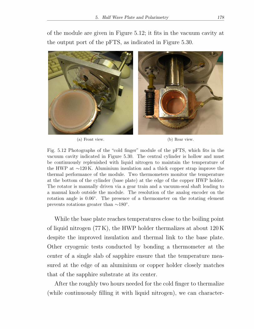
5. Half Wave Plate and Polarimetry 178
of the module are given in Figure 5.12; it fits in the vacuum cavity at
the output port of the pFTS, as indicated in Figure 5.30.
(a) Front view. (b) Rear view.
Fig. 5.12 Photographs of the “cold finger” module of the pFTS, which fits in thevacuum cavity indicated in Figure 5.30. The central cylinder is hollow and mustbe continuously replenished with liquid nitrogen to maintain the temperature ofthe HWP at ∼120K. Aluminium insulation and a thick copper strap improve thethermal performance of the module. Two thermometers monitor the temperatureat the bottom of the cylinder (base plate) at the edge of the copper HWP holder.The rotator is manually driven via a gear train and a vacuum-seal shaft leading toa manual knob outside the module. The resolution of the analog encoder on therotation angle is 0.06∘. The presence of a thermometer on the rotating elementprevents rotations greater than ∼180∘.
While the base plate reaches temperatures close to the boiling point
of liquid nitrogen (77K), the HWP holder thermalizes at about 120K
despite the improved insulation and thermal link to the base plate.
Other cryogenic tests conducted by bonding a thermometer at the
center of a single slab of sapphire ensure that the temperature mea-
sured at the edge of an aluminium or copper holder closely matches
that of the sapphire substrate at its center.
After the roughly two hours needed for the cold finger to thermalize
(while continuously filling it with liquid nitrogen), we can character-
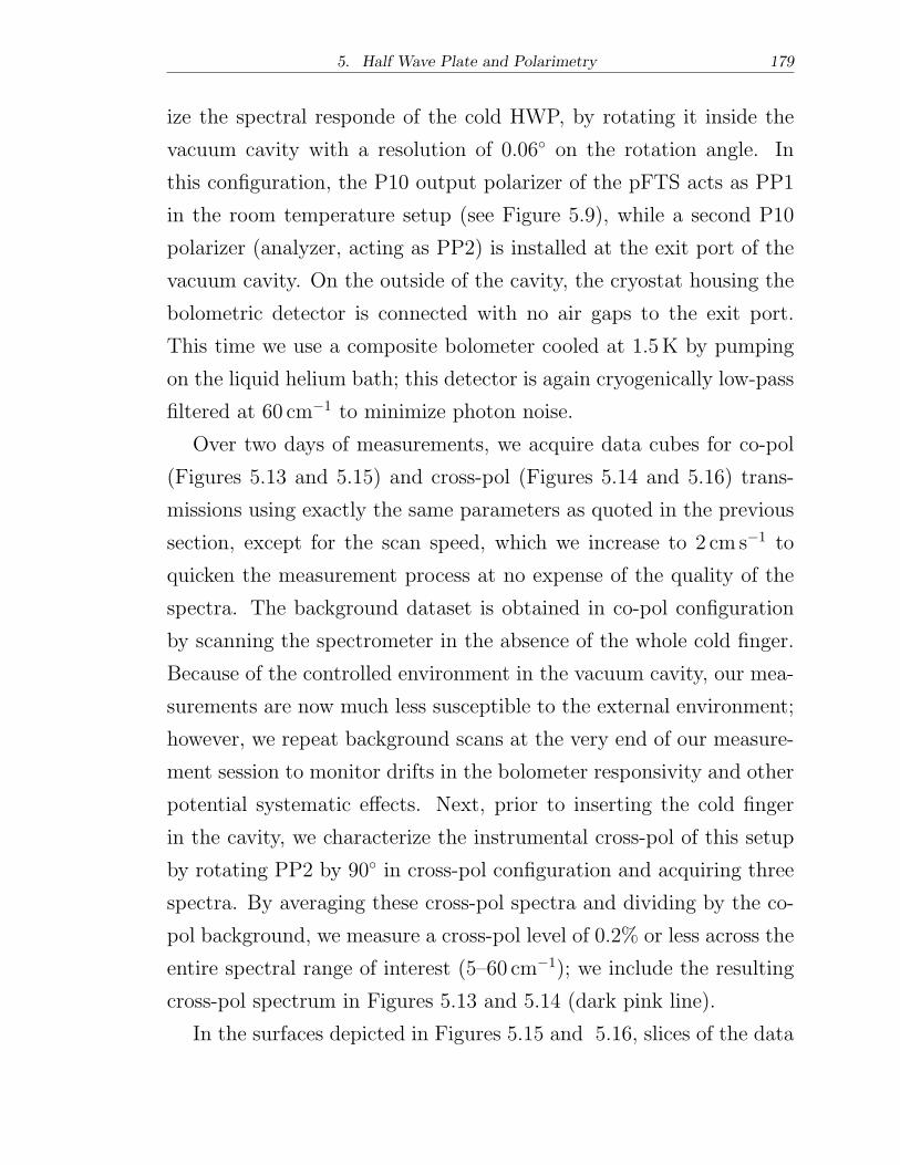
5. Half Wave Plate and Polarimetry 179
ize the spectral responde of the cold HWP, by rotating it inside the
vacuum cavity with a resolution of 0.06∘ on the rotation angle. In
this configuration, the P10 output polarizer of the pFTS acts as PP1
in the room temperature setup (see Figure 5.9), while a second P10
polarizer (analyzer, acting as PP2) is installed at the exit port of the
vacuum cavity. On the outside of the cavity, the cryostat housing the
bolometric detector is connected with no air gaps to the exit port.
This time we use a composite bolometer cooled at 1.5K by pumping
on the liquid helium bath; this detector is again cryogenically low-pass
filtered at 60 cm−1 to minimize photon noise.
Over two days of measurements, we acquire data cubes for co-pol
(Figures 5.13 and 5.15) and cross-pol (Figures 5.14 and 5.16) trans-
missions using exactly the same parameters as quoted in the previous
section, except for the scan speed, which we increase to 2 cm s−1 to
quicken the measurement process at no expense of the quality of the
spectra. The background dataset is obtained in co-pol configuration
by scanning the spectrometer in the absence of the whole cold finger.
Because of the controlled environment in the vacuum cavity, our mea-
surements are now much less susceptible to the external environment;
however, we repeat background scans at the very end of our measure-
ment session to monitor drifts in the bolometer responsivity and other
potential systematic effects. Next, prior to inserting the cold finger
in the cavity, we characterize the instrumental cross-pol of this setup
by rotating PP2 by 90∘ in cross-pol configuration and acquiring three
spectra. By averaging these cross-pol spectra and dividing by the co-
pol background, we measure a cross-pol level of 0.2% or less across the
entire spectral range of interest (5–60 cm−1); we include the resulting
cross-pol spectrum in Figures 5.13 and 5.14 (dark pink line).
In the surfaces depicted in Figures 5.15 and 5.16, slices of the data
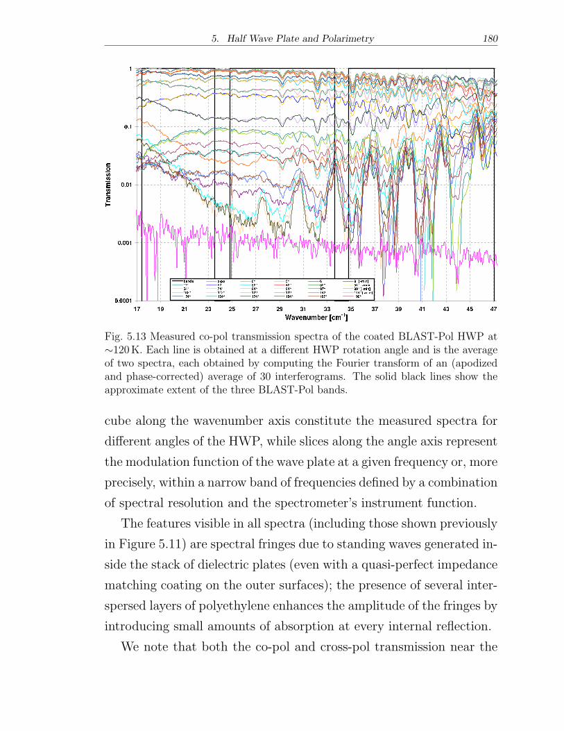
5. Half Wave Plate and Polarimetry 180
Fig. 5.13 Measured co-pol transmission spectra of the coated BLAST-Pol HWP at∼120K. Each line is obtained at a different HWP rotation angle and is the averageof two spectra, each obtained by computing the Fourier transform of an (apodizedand phase-corrected) average of 30 interferograms. The solid black lines show theapproximate extent of the three BLAST-Pol bands.
cube along the wavenumber axis constitute the measured spectra for
different angles of the HWP, while slices along the angle axis represent
the modulation function of the wave plate at a given frequency or, more
precisely, within a narrow band of frequencies defined by a combination
of spectral resolution and the spectrometer’s instrument function.
The features visible in all spectra (including those shown previously
in Figure 5.11) are spectral fringes due to standing waves generated in-
side the stack of dielectric plates (even with a quasi-perfect impedance
matching coating on the outer surfaces); the presence of several inter-
spersed layers of polyethylene enhances the amplitude of the fringes by
introducing small amounts of absorption at every internal reflection.
We note that both the co-pol and cross-pol transmission near the
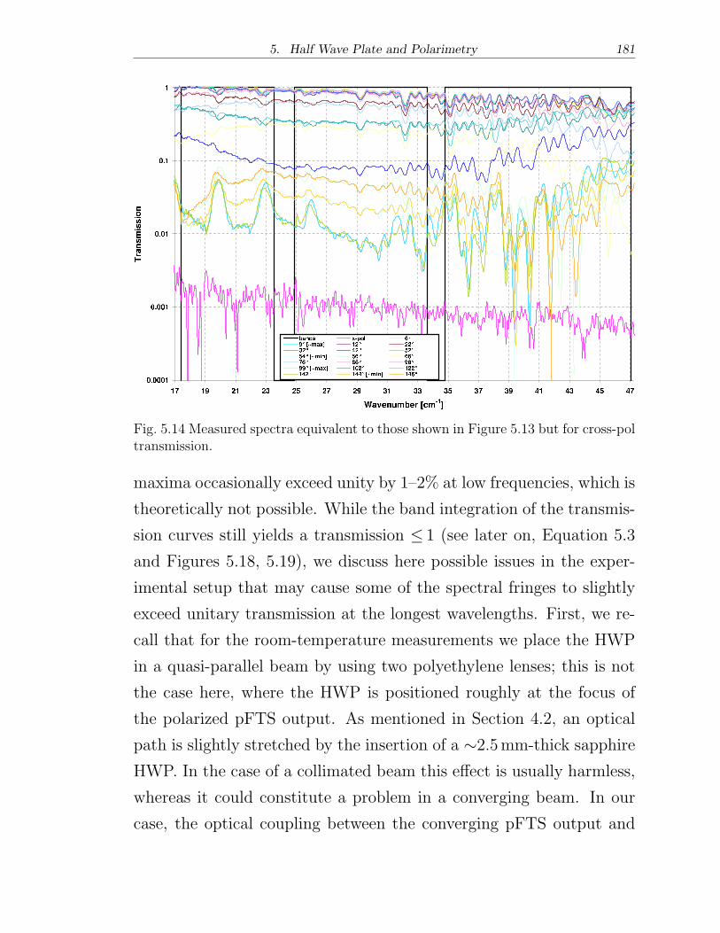
5. Half Wave Plate and Polarimetry 181
Fig. 5.14 Measured spectra equivalent to those shown in Figure 5.13 but for cross-poltransmission.
maxima occasionally exceed unity by 1–2% at low frequencies, which is
theoretically not possible. While the band integration of the transmis-
sion curves still yields a transmission ≤ 1 (see later on, Equation 5.3
and Figures 5.18, 5.19), we discuss here possible issues in the exper-
imental setup that may cause some of the spectral fringes to slightly
exceed unitary transmission at the longest wavelengths. First, we re-
call that for the room-temperature measurements we place the HWP
in a quasi-parallel beam by using two polyethylene lenses; this is not
the case here, where the HWP is positioned roughly at the focus of
the polarized pFTS output. As mentioned in Section 4.2, an optical
path is slightly stretched by the insertion of a ∼2.5mm-thick sapphire
HWP. In the case of a collimated beam this effect is usually harmless,
whereas it could constitute a problem in a converging beam. In our
case, the optical coupling between the converging pFTS output and
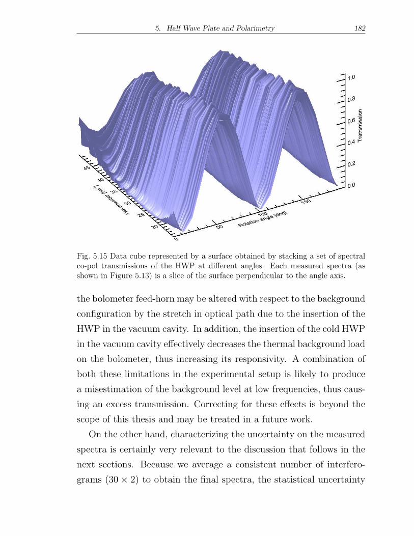
5. Half Wave Plate and Polarimetry 182
Fig. 5.15 Data cube represented by a surface obtained by stacking a set of spectralco-pol transmissions of the HWP at different angles. Each measured spectra (asshown in Figure 5.13) is a slice of the surface perpendicular to the angle axis.
the bolometer feed-horn may be altered with respect to the background
configuration by the stretch in optical path due to the insertion of the
HWP in the vacuum cavity. In addition, the insertion of the cold HWP
in the vacuum cavity effectively decreases the thermal background load
on the bolometer, thus increasing its responsivity. A combination of
both these limitations in the experimental setup is likely to produce
a misestimation of the background level at low frequencies, thus caus-
ing an excess transmission. Correcting for these effects is beyond the
scope of this thesis and may be treated in a future work.
On the other hand, characterizing the uncertainty on the measured
spectra is certainly very relevant to the discussion that follows in the
next sections. Because we average a consistent number of interfero-
grams (30 × 2) to obtain the final spectra, the statistical uncertainty
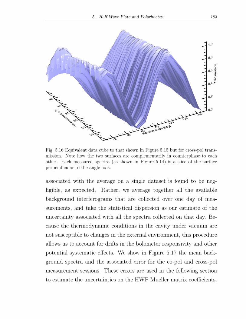
5. Half Wave Plate and Polarimetry 183
Fig. 5.16 Equivalent data cube to that shown in Figure 5.15 but for cross-pol trans-mission. Note how the two surfaces are complementarily in counterphase to eachother. Each measured spectra (as shown in Figure 5.14) is a slice of the surfaceperpendicular to the angle axis.
associated with the average on a single dataset is found to be neg-
ligible, as expected. Rather, we average together all the available
background interferograms that are collected over one day of mea-
surements, and take the statistical dispersion as our estimate of the
uncertainty associated with all the spectra collected on that day. Be-
cause the thermodynamic conditions in the cavity under vacuum are
not susceptible to changes in the external environment, this procedure
allows us to account for drifts in the bolometer responsivity and other
potential systematic effects. We show in Figure 5.17 the mean back-
ground spectra and the associated error for the co-pol and cross-pol
measurement sessions. These errors are used in the following section
to estimate the uncertainties on the HWP Mueller matrix coefficients.
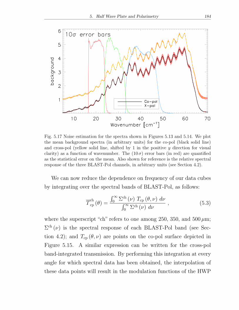
5. Half Wave Plate and Polarimetry 184
Fig. 5.17 Noise estimation for the spectra shown in Figures 5.13 and 5.14. We plotthe mean background spectra (in arbitrary units) for the co-pol (black solid line)and cross-pol (yellow solid line, shifted by 1 in the positive y direction for visualclarity) as a function of wavenumber. The (10�) error bars (in red) are quantifiedas the statistical error on the mean. Also shown for reference is the relative spectralresponse of the three BLAST-Pol channels, in arbitrary units (see Section 4.2).
We can now reduce the dependence on frequency of our data cubes
by integrating over the spectral bands of BLAST-Pol, as follows:
Tchcp (�) =
∫∞0 Σch (�) Tcp (�, �) d�
∫∞0 Σch (�) d�
, (5.3)
where the superscript “ch” refers to one among 250, 350, and 500�m;
Σch (�) is the spectral response of each BLAST-Pol band (see Sec-
tion 4.2); and Tcp (�, �) are points on the co-pol surface depicted in
Figure 5.15. A similar expression can be written for the cross-pol
band-integrated transmission. By performing this integration at every
angle for which spectral data has been obtained, the interpolation of
these data points will result in the modulation functions of the HWP
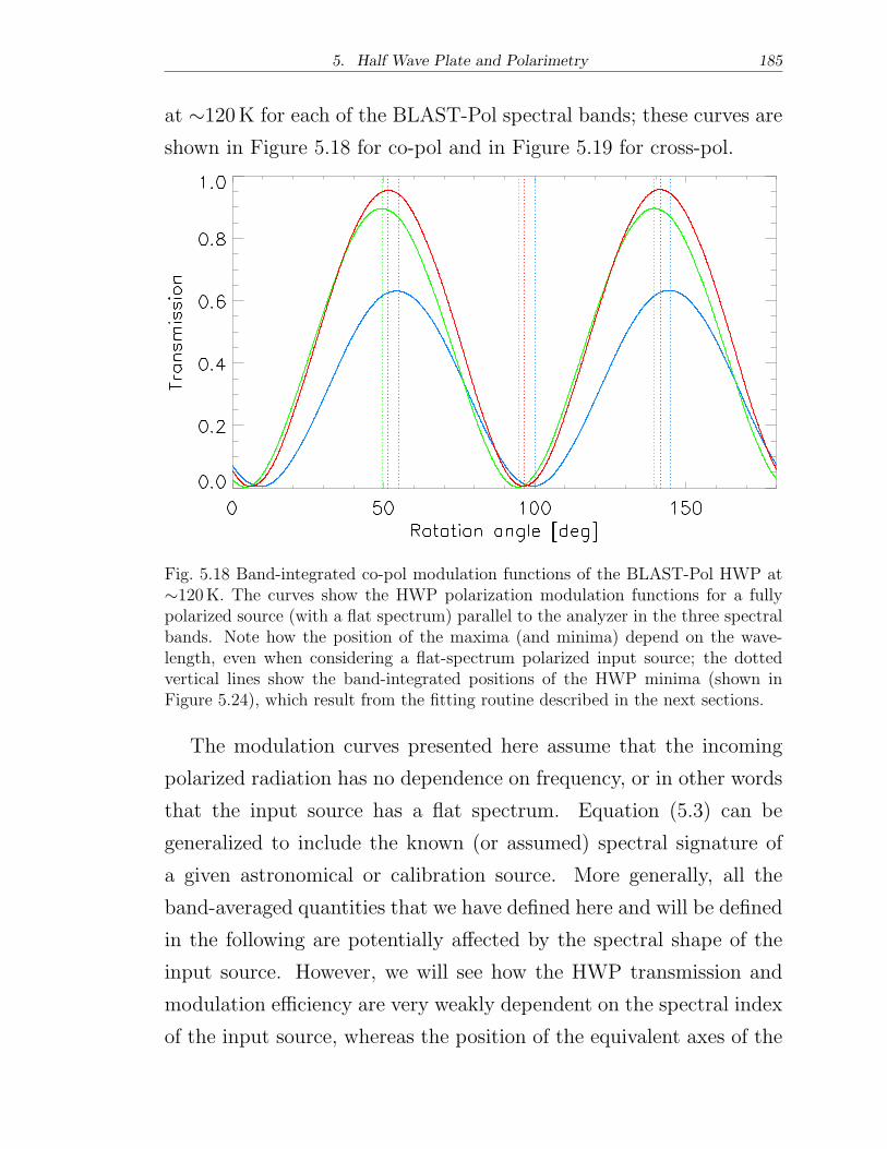
5. Half Wave Plate and Polarimetry 185
at ∼120K for each of the BLAST-Pol spectral bands; these curves are
shown in Figure 5.18 for co-pol and in Figure 5.19 for cross-pol.
Fig. 5.18 Band-integrated co-pol modulation functions of the BLAST-Pol HWP at∼120K. The curves show the HWP polarization modulation functions for a fullypolarized source (with a flat spectrum) parallel to the analyzer in the three spectralbands. Note how the position of the maxima (and minima) depend on the wave-length, even when considering a flat-spectrum polarized input source; the dottedvertical lines show the band-integrated positions of the HWP minima (shown inFigure 5.24), which result from the fitting routine described in the next sections.
The modulation curves presented here assume that the incoming
polarized radiation has no dependence on frequency, or in other words
that the input source has a flat spectrum. Equation (5.3) can be
generalized to include the known (or assumed) spectral signature of
a given astronomical or calibration source. More generally, all the
band-averaged quantities that we have defined here and will be defined
in the following are potentially affected by the spectral shape of the
input source. However, we will see how the HWP transmission and
modulation efficiency are very weakly dependent on the spectral index
of the input source, whereas the position of the equivalent axes of the
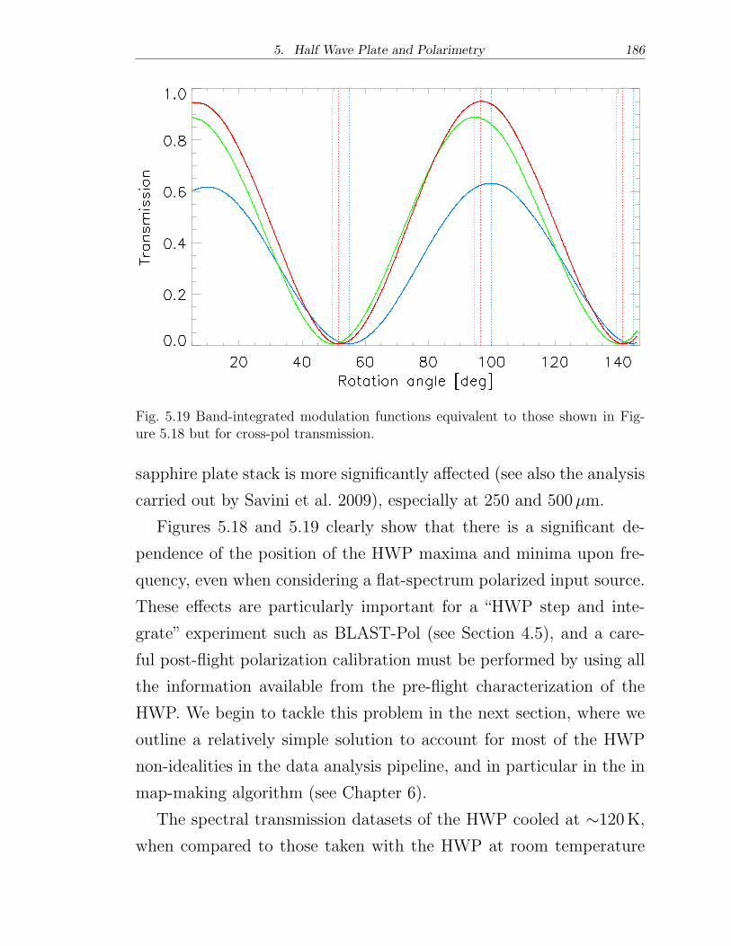
5. Half Wave Plate and Polarimetry 186
Fig. 5.19 Band-integrated modulation functions equivalent to those shown in Fig-ure 5.18 but for cross-pol transmission.
sapphire plate stack is more significantly affected (see also the analysis
carried out by Savini et al. 2009), especially at 250 and 500�m.
Figures 5.18 and 5.19 clearly show that there is a significant de-
pendence of the position of the HWP maxima and minima upon fre-
quency, even when considering a flat-spectrum polarized input source.
These effects are particularly important for a “HWP step and inte-
grate” experiment such as BLAST-Pol (see Section 4.5), and a care-
ful post-flight polarization calibration must be performed by using all
the information available from the pre-flight characterization of the
HWP. We begin to tackle this problem in the next section, where we
outline a relatively simple solution to account for most of the HWP
non-idealities in the data analysis pipeline, and in particular in the in
map-making algorithm (see Chapter 6).
The spectral transmission datasets of the HWP cooled at ∼120K,
when compared to those taken with the HWP at room temperature
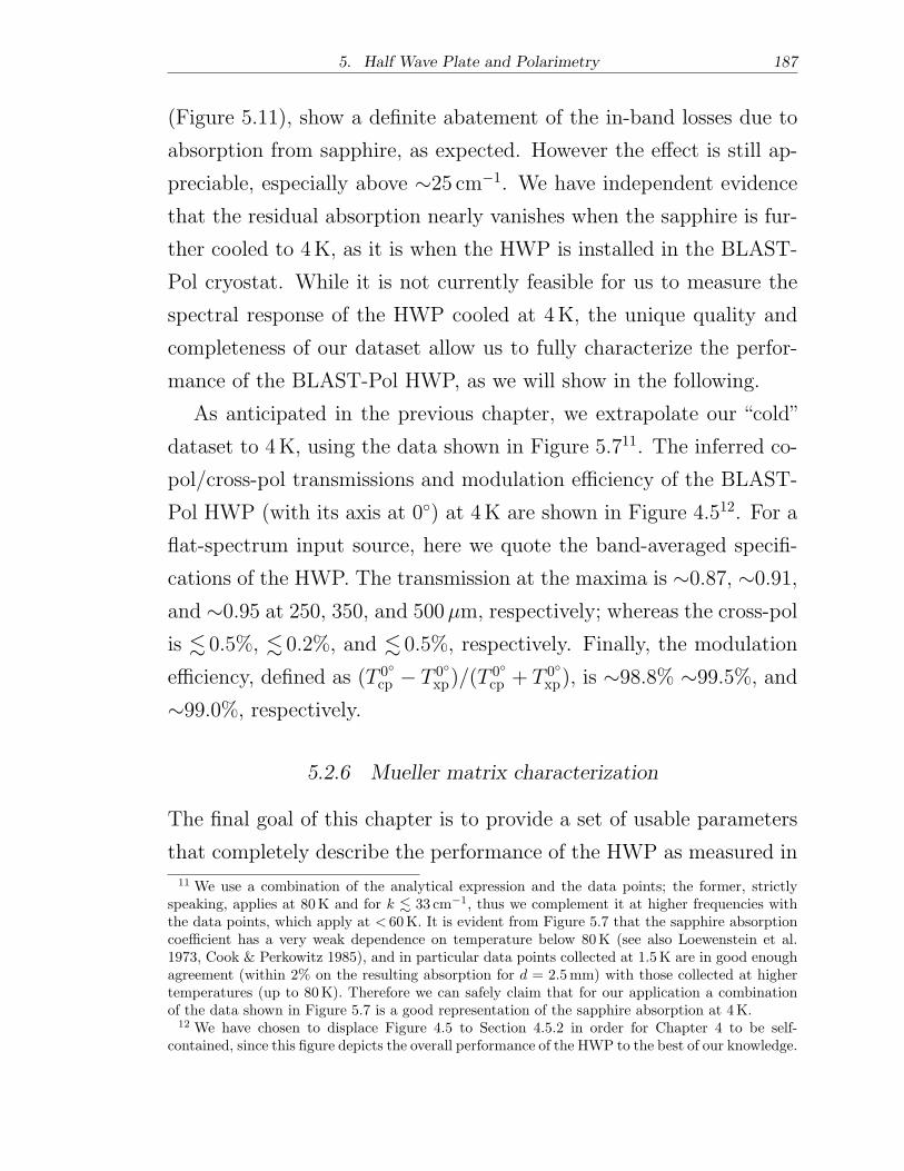
5. Half Wave Plate and Polarimetry 187
(Figure 5.11), show a definite abatement of the in-band losses due to
absorption from sapphire, as expected. However the effect is still ap-
preciable, especially above ∼25 cm−1. We have independent evidence
that the residual absorption nearly vanishes when the sapphire is fur-
ther cooled to 4K, as it is when the HWP is installed in the BLAST-
Pol cryostat. While it is not currently feasible for us to measure the
spectral response of the HWP cooled at 4K, the unique quality and
completeness of our dataset allow us to fully characterize the perfor-
mance of the BLAST-Pol HWP, as we will show in the following.
As anticipated in the previous chapter, we extrapolate our “cold”
dataset to 4K, using the data shown in Figure 5.711. The inferred co-
pol/cross-pol transmissions and modulation efficiency of the BLAST-
Pol HWP (with its axis at 0∘) at 4K are shown in Figure 4.512. For a
flat-spectrum input source, here we quote the band-averaged specifi-
cations of the HWP. The transmission at the maxima is ∼0.87, ∼0.91,
and ∼0.95 at 250, 350, and 500�m, respectively; whereas the cross-pol
is ≲ 0.5%, ≲ 0.2%, and ≲ 0.5%, respectively. Finally, the modulation
efficiency, defined as (T 0∘cp − T 0∘
xp)/(T0∘cp + T 0∘
xp), is ∼98.8% ∼99.5%, and
∼99.0%, respectively.
5.2.6 Mueller matrix characterization
The final goal of this chapter is to provide a set of usable parameters
that completely describe the performance of the HWP as measured in
11 We use a combination of the analytical expression and the data points; the former, strictlyspeaking, applies at 80K and for k ≲ 33 cm−1, thus we complement it at higher frequencies withthe data points, which apply at < 60K. It is evident from Figure 5.7 that the sapphire absorptioncoefficient has a very weak dependence on temperature below 80K (see also Loewenstein et al.1973, Cook & Perkowitz 1985), and in particular data points collected at 1.5K are in good enoughagreement (within 2% on the resulting absorption for d = 2.5mm) with those collected at highertemperatures (up to 80K). Therefore we can safely claim that for our application a combinationof the data shown in Figure 5.7 is a good representation of the sapphire absorption at 4K.
12 We have chosen to displace Figure 4.5 to Section 4.5.2 in order for Chapter 4 to be self-contained, since this figure depicts the overall performance of the HWP to the best of our knowledge.
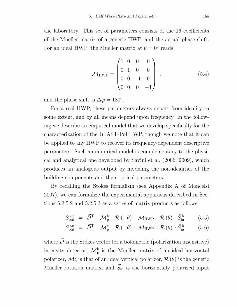
5. Half Wave Plate and Polarimetry 188
the laboratory. This set of parameters consists of the 16 coefficients
of the Mueller matrix of a generic HWP, and the actual phase shift.
For an ideal HWP, the Mueller matrix at � = 0∘ reads
ℳHWP =
⎛
⎜
⎜
⎜
⎜
⎝
1 0 0 0
0 1 0 0
0 0 −1 0
0 0 0 −1
⎞
⎟
⎟
⎟
⎟
⎠
, (5.4)
and the phase shift is Δ' = 180∘.
For a real HWP, these parameters always depart from ideality to
some extent, and by all means depend upon frequency. In the follow-
ing we describe an empirical model that we develop specifically for the
characterization of the BLAST-Pol HWP, though we note that it can
be applied to any HWP to recover its frequency-dependent descriptive
parameters. Such an empirical model is complementary to the physi-
cal and analytical one developed by Savini et al. (2006, 2009), which
produces an analogous output by modeling the non-idealities of the
building components and their optical parameters.
By recalling the Stokes formalism (see Appendix A of Moncelsi
2007), we can formalize the experimental apparatus described in Sec-
tions 5.2.5.2 and 5.2.5.3 as a series of matrix products as follows:
S cpout = DT ⋅ ℳh
p ⋅ ℛ (−�) ⋅ ℳHWP ⋅ ℛ (�) ⋅ S hin (5.5)
S xpout = DT ⋅ ℳv
p ⋅ ℛ (−�) ⋅ ℳHWP ⋅ ℛ (�) ⋅ S hin , (5.6)
where D is the Stokes vector for a bolometric (polarization insensitive)
intensity detector, ℳhp is the Mueller matrix of an ideal horizontal
polarizer, ℳvp is that of an ideal vertical polarizer, ℛ (�) is the generic
Mueller rotation matrix, and Sin is the horizontally polarized input
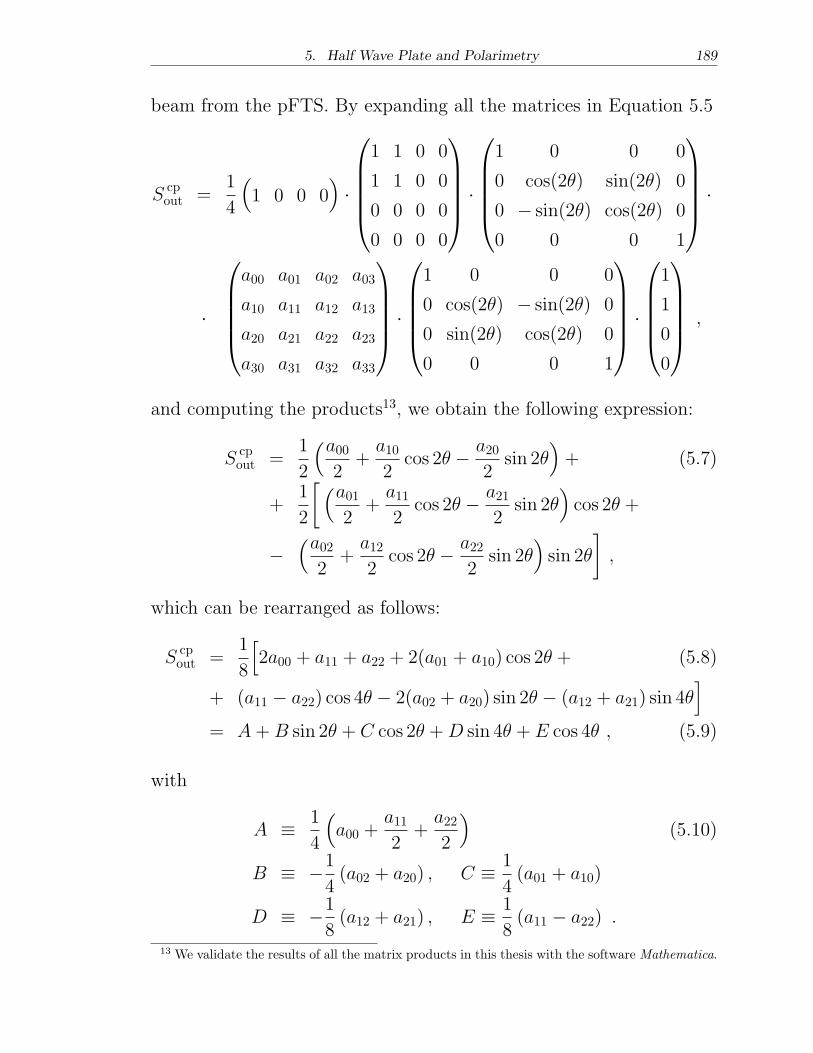
5. Half Wave Plate and Polarimetry 189
beam from the pFTS. By expanding all the matrices in Equation 5.5
S cpout =
1
4
(
1 0 0 0)
⋅
⎛
⎜
⎜
⎜
⎜
⎝
1 1 0 0
1 1 0 0
0 0 0 0
0 0 0 0
⎞
⎟
⎟
⎟
⎟
⎠
⋅
⎛
⎜
⎜
⎜
⎜
⎝
1 0 0 0
0 cos(2�) sin(2�) 0
0 − sin(2�) cos(2�) 0
0 0 0 1
⎞
⎟
⎟
⎟
⎟
⎠
⋅
⋅
⎛
⎜
⎜
⎜
⎜
⎝
a00 a01 a02 a03
a10 a11 a12 a13
a20 a21 a22 a23
a30 a31 a32 a33
⎞
⎟
⎟
⎟
⎟
⎠
⋅
⎛
⎜
⎜
⎜
⎜
⎝
1 0 0 0
0 cos(2�) − sin(2�) 0
0 sin(2�) cos(2�) 0
0 0 0 1
⎞
⎟
⎟
⎟
⎟
⎠
⋅
⎛
⎜
⎜
⎜
⎜
⎝
1
1
0
0
⎞
⎟
⎟
⎟
⎟
⎠
,
and computing the products13, we obtain the following expression:
S cpout =
1
2
(a002
+a102
cos 2� − a202
sin 2�)
+ (5.7)
+1
2
[
(a012
+a112
cos 2� − a212
sin 2�)
cos 2� +
−(a02
2+a122
cos 2� − a222
sin 2�)
sin 2�
]
,
which can be rearranged as follows:
S cpout =
1
8
[
2a00 + a11 + a22 + 2(a01 + a10) cos 2� + (5.8)
+ (a11 − a22) cos 4� − 2(a02 + a20) sin 2� − (a12 + a21) sin 4�]
= A+B sin 2� + C cos 2� +D sin 4� + E cos 4� , (5.9)
with
A ≡ 1
4
(
a00 +a112
+a222
)
(5.10)
B ≡ −1
4(a02 + a20) , C ≡ 1
4(a01 + a10)
D ≡ −1
8(a12 + a21) , E ≡ 1
8(a11 − a22) .
13 We validate the results of all the matrix products in this thesis with the software Mathematica.
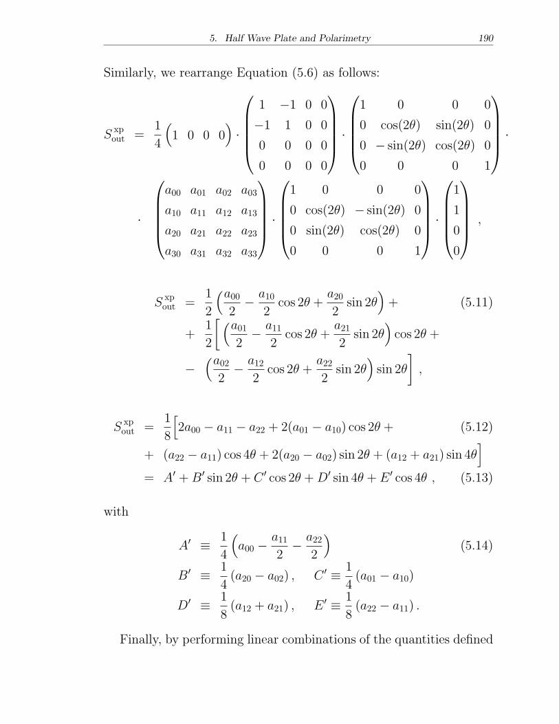
5. Half Wave Plate and Polarimetry 190
Similarly, we rearrange Equation (5.6) as follows:
S xpout =
1
4
(
1 0 0 0)
⋅
⎛
⎜
⎜
⎜
⎜
⎝
1 −1 0 0
−1 1 0 0
0 0 0 0
0 0 0 0
⎞
⎟
⎟
⎟
⎟
⎠
⋅
⎛
⎜
⎜
⎜
⎜
⎝
1 0 0 0
0 cos(2�) sin(2�) 0
0 − sin(2�) cos(2�) 0
0 0 0 1
⎞
⎟
⎟
⎟
⎟
⎠
⋅
⋅
⎛
⎜
⎜
⎜
⎜
⎝
a00 a01 a02 a03
a10 a11 a12 a13
a20 a21 a22 a23
a30 a31 a32 a33
⎞
⎟
⎟
⎟
⎟
⎠
⋅
⎛
⎜
⎜
⎜
⎜
⎝
1 0 0 0
0 cos(2�) − sin(2�) 0
0 sin(2�) cos(2�) 0
0 0 0 1
⎞
⎟
⎟
⎟
⎟
⎠
⋅
⎛
⎜
⎜
⎜
⎜
⎝
1
1
0
0
⎞
⎟
⎟
⎟
⎟
⎠
,
S xpout =
1
2
(a002
− a102
cos 2� +a202
sin 2�)
+ (5.11)
+1
2
[
(a012
− a112
cos 2� +a212
sin 2�)
cos 2� +
−(a02
2− a12
2cos 2� +
a222
sin 2�)
sin 2�
]
,
S xpout =
1
8
[
2a00 − a11 − a22 + 2(a01 − a10) cos 2� + (5.12)
+ (a22 − a11) cos 4� + 2(a20 − a02) sin 2� + (a12 + a21) sin 4�]
= A′ +B′ sin 2� + C ′ cos 2� +D′ sin 4� + E ′ cos 4� , (5.13)
with
A′ ≡ 1
4
(
a00 −a112
− a222
)
(5.14)
B′ ≡ 1
4(a20 − a02) , C ′ ≡ 1
4(a01 − a10)
D′ ≡ 1
8(a12 + a21) , E ′ ≡ 1
8(a22 − a11) .
Finally, by performing linear combinations of the quantities defined
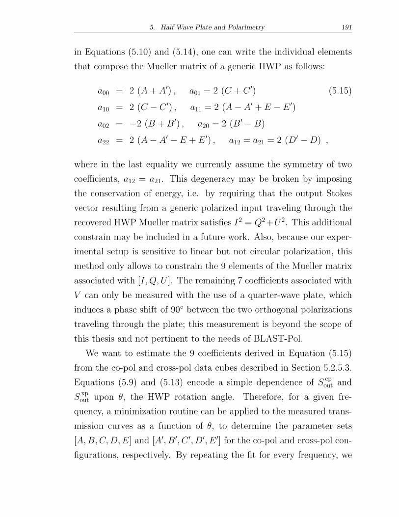
5. Half Wave Plate and Polarimetry 191
in Equations (5.10) and (5.14), one can write the individual elements
that compose the Mueller matrix of a generic HWP as follows:
a00 = 2 (A+ A′) , a01 = 2 (C + C ′) (5.15)
a10 = 2 (C − C ′) , a11 = 2 (A− A′ + E − E ′)
a02 = −2 (B +B′) , a20 = 2 (B′ − B)
a22 = 2 (A− A′ − E + E ′) , a12 = a21 = 2 (D′ −D) ,
where in the last equality we currently assume the symmetry of two
coefficients, a12 = a21. This degeneracy may be broken by imposing
the conservation of energy, i.e. by requiring that the output Stokes
vector resulting from a generic polarized input traveling through the
recovered HWP Mueller matrix satisfies I2 = Q2+U 2. This additional
constrain may be included in a future work. Also, because our exper-
imental setup is sensitive to linear but not circular polarization, this
method only allows to constrain the 9 elements of the Mueller matrix
associated with [I,Q, U ]. The remaining 7 coefficients associated with
V can only be measured with the use of a quarter-wave plate, which
induces a phase shift of 90∘ between the two orthogonal polarizations
traveling through the plate; this measurement is beyond the scope of
this thesis and not pertinent to the needs of BLAST-Pol.
We want to estimate the 9 coefficients derived in Equation (5.15)
from the co-pol and cross-pol data cubes described in Section 5.2.5.3.
Equations (5.9) and (5.13) encode a simple dependence of S cpout and
S xpout upon �, the HWP rotation angle. Therefore, for a given fre-
quency, a minimization routine can be applied to the measured trans-
mission curves as a function of �, to determine the parameter sets
[A,B,C,D,E] and [A′, B′, C ′, D′, E ′] for the co-pol and cross-pol con-
figurations, respectively. By repeating the fit for every frequency, we
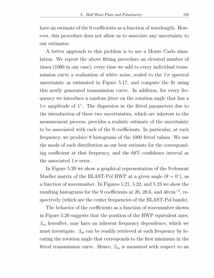
5. Half Wave Plate and Polarimetry 192
have an estimate of the 9 coefficients as a function of wavelength. How-
ever, this procedure does not allow us to associate any uncertainty to
our estimates.
A better approach to this problem is to use a Monte Carlo simu-
lation. We repeat the above fitting procedure an elevated number of
times (1000 in our case); every time we add to every individual trans-
mission curve a realization of white noise, scaled to the 1� spectral
uncertainty as estimated in Figure 5.17, and compute the fit using
this newly generated transmission curve. In addition, for every fre-
quency we introduce a random jitter on the rotation angle that has a
1� amplitude of 1∘. The dispersion in the fitted parameters due to
the introduction of these two uncertainties, which are inherent to the
measurement process, provides a realistic estimate of the uncertainty
to be associated with each of the 9 coefficients. In particular, at each
frequency, we produce 9 histograms of the 1000 fitted values. We use
the mode of each distribution as our best estimate for the correspond-
ing coefficient at that frequency, and the 68% confidence interval as
the associated 1� error.
In Figure 5.20 we show a graphical representation of the 9-element
Mueller matrix of the BLAST-Pol HWP at a given angle (� = 0∘), as
a function of wavenumber. In Figures 5.21, 5.22, and 5.23 we show the
resulting histograms for the 9 coefficients at 20, 28.6, and 40 cm−1, re-
spectively (which are the center frequencies of the BLAST-Pol bands).
The behavior of the coefficients as a function of wavenumber shown
in Figure 5.20 suggests that the position of the HWP equivalent axes,
�ea hereafter, may have an inherent frequency dependence, which we
must investigate. �ea can be readily retrieved at each frequency by lo-
cating the rotation angle that corresponds to the first minimum in the
fitted transmission curve. Hence, �ea is measured with respect to an
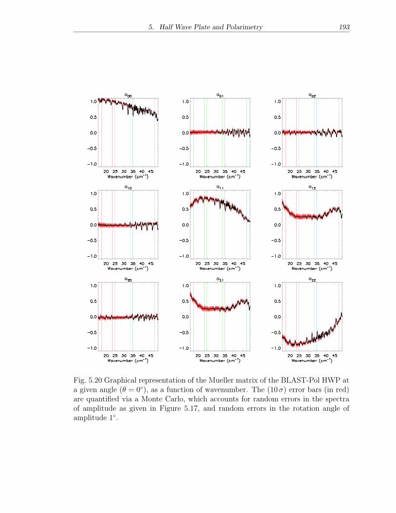
5. Half Wave Plate and Polarimetry 193
Fig. 5.20 Graphical representation of the Mueller matrix of the BLAST-Pol HWP ata given angle (� = 0∘), as a function of wavenumber. The (10�) error bars (in red)are quantified via a Monte Carlo, which accounts for random errors in the spectraof amplitude as given in Figure 5.17, and random errors in the rotation angle ofamplitude 1∘.
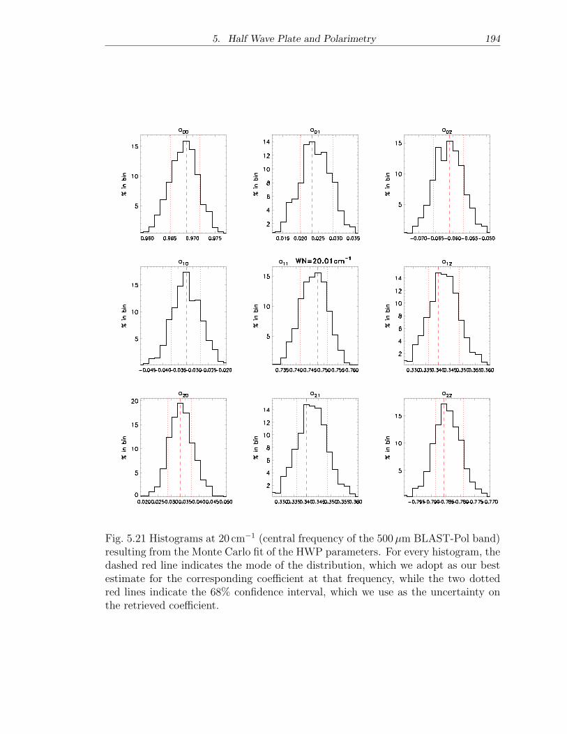
5. Half Wave Plate and Polarimetry 194
Fig. 5.21 Histograms at 20 cm−1 (central frequency of the 500�m BLAST-Pol band)resulting from the Monte Carlo fit of the HWP parameters. For every histogram, thedashed red line indicates the mode of the distribution, which we adopt as our bestestimate for the corresponding coefficient at that frequency, while the two dottedred lines indicate the 68% confidence interval, which we use as the uncertainty onthe retrieved coefficient.
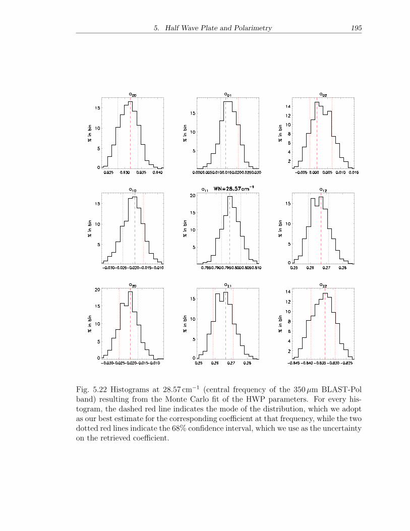
5. Half Wave Plate and Polarimetry 195
Fig. 5.22 Histograms at 28.57 cm−1 (central frequency of the 350�m BLAST-Polband) resulting from the Monte Carlo fit of the HWP parameters. For every his-togram, the dashed red line indicates the mode of the distribution, which we adoptas our best estimate for the corresponding coefficient at that frequency, while the twodotted red lines indicate the 68% confidence interval, which we use as the uncertaintyon the retrieved coefficient.
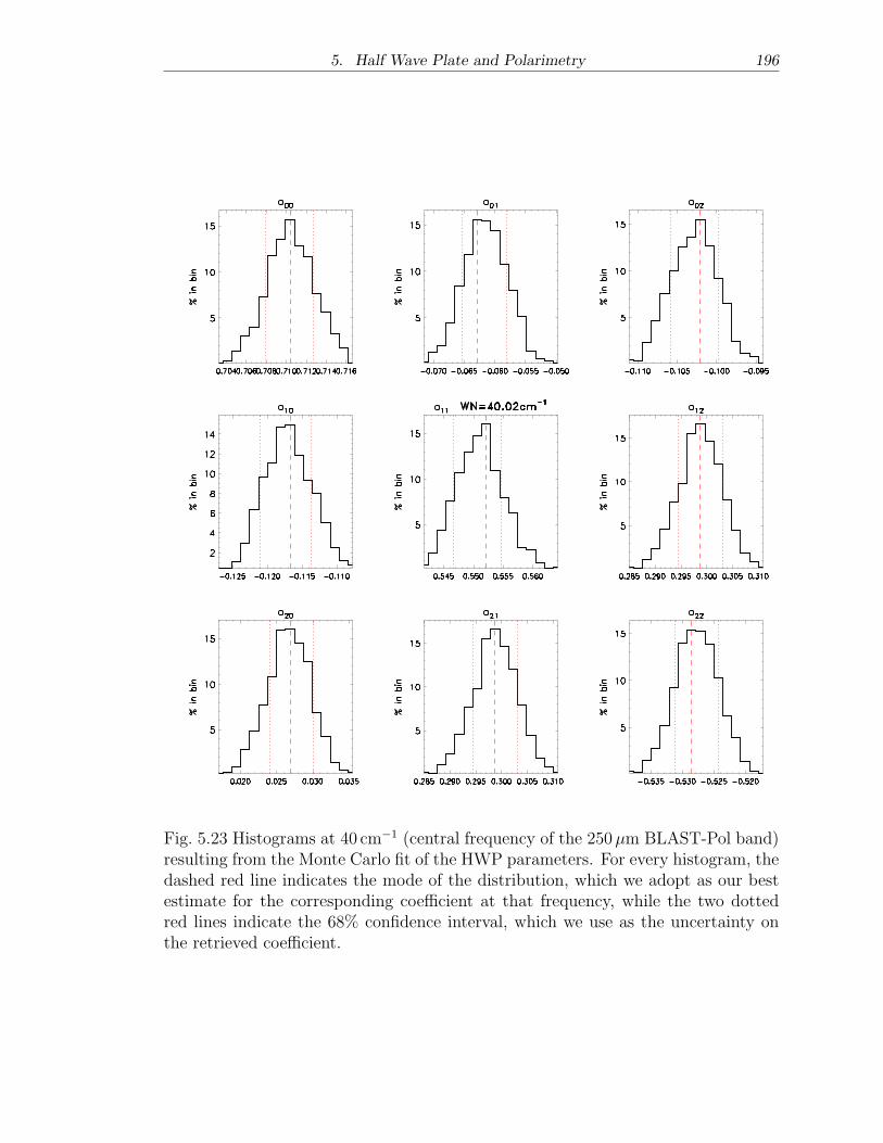
5. Half Wave Plate and Polarimetry 196
Fig. 5.23 Histograms at 40 cm−1 (central frequency of the 250�m BLAST-Pol band)resulting from the Monte Carlo fit of the HWP parameters. For every histogram, thedashed red line indicates the mode of the distribution, which we adopt as our bestestimate for the corresponding coefficient at that frequency, while the two dottedred lines indicate the 68% confidence interval, which we use as the uncertainty onthe retrieved coefficient.
5. Half Wave Plate and Polarimetry 197
arbitrary constant offset that is inherent to the specific experimental
setup; we set this offset to be zero at 25 cm−1. Operatively, this means
that the HWP zero angle in the instrument reference frame (�0; see
Equation 6.2) must be calibrated using the 350�m band. A plot of
�ea as a function of wavenumber is given in Figure 5.24.
As anticipated, it is of crucial importance to derive the band-
averaged value of �ea for input sources with different spectral signature,
as follows:
�ch
ea =
∫∞0 Σch (�) �ea (�) & (�) d�
∫∞0 Σch (�) & (�) d�
, (5.16)
where we adopt the same notation as in Equation (5.3) and the known
(or assumed) spectrum of an astronomical or calibration source is mod-
eled as & (�) ∝ ��. We compute Equation (5.16) for a range of spectral
indices of interest: � = 0 for a flat spectrum; � = 2 for the Raleigh-
Jeans tail of a blackbody; � = 4 for interstellar dust, modeled as a
modified blackbody with emissivity � = 2 (Hildebrand 1983); and fi-
nally � = −2 as a replacement for the mid-infrared exponential on
the Wien side of a blackbody to account for the variability of dust
temperatures within a galaxy (Blain 1999, Blain et al. 2003; see also
Sections 2.3.2 and 3.3.3). The results of this analysis are shown in
Figure 5.24 and in Table 5.1.
Expectedly, the impact of different input spectral signatures is min-
imal at 350�m, where the HWP has been designed to function opti-
mally (see Section 5.2.3); whereas the spectral dependence is more
pronounced at 250 and 500�m, and, if neglected, it may lead to an
arbitrary rotation of the retrieved polarization angle on the sky of
magnitude 2 �ea = 10–15∘ (3–5∘) at 250 (500)�m (see Equation 6.2).
We have thus confirmed that the dependence of the HWP equiva-
lent axes upon wavelength is inherent to the achromatic design. We
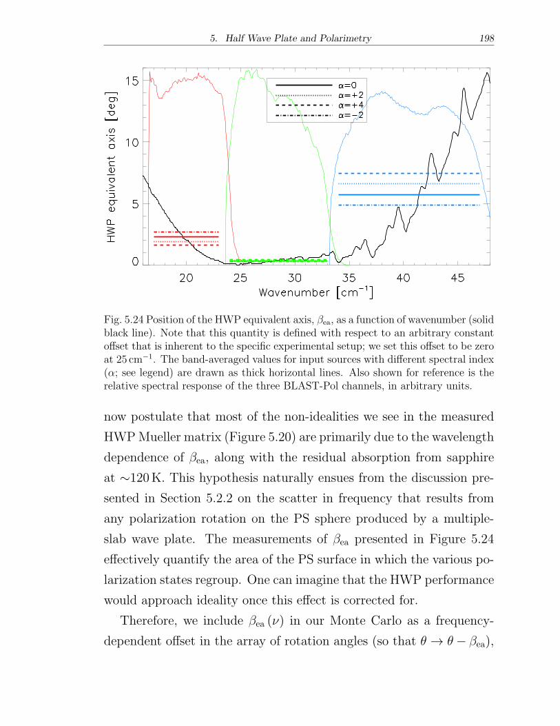
5. Half Wave Plate and Polarimetry 198
Fig. 5.24 Position of the HWP equivalent axis, �ea, as a function of wavenumber (solidblack line). Note that this quantity is defined with respect to an arbitrary constantoffset that is inherent to the specific experimental setup; we set this offset to be zeroat 25 cm−1. The band-averaged values for input sources with different spectral index(�; see legend) are drawn as thick horizontal lines. Also shown for reference is therelative spectral response of the three BLAST-Pol channels, in arbitrary units.
now postulate that most of the non-idealities we see in the measured
HWPMueller matrix (Figure 5.20) are primarily due to the wavelength
dependence of �ea, along with the residual absorption from sapphire
at ∼120K. This hypothesis naturally ensues from the discussion pre-
sented in Section 5.2.2 on the scatter in frequency that results from
any polarization rotation on the PS sphere produced by a multiple-
slab wave plate. The measurements of �ea presented in Figure 5.24
effectively quantify the area of the PS surface in which the various po-
larization states regroup. One can imagine that the HWP performance
would approach ideality once this effect is corrected for.
Therefore, we include �ea (�) in our Monte Carlo as a frequency-
dependent offset in the array of rotation angles (so that � → �− �ea),
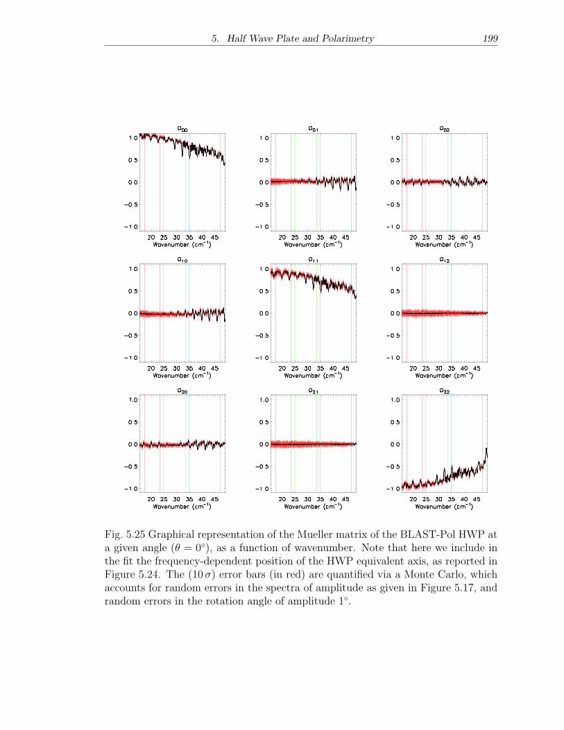
5. Half Wave Plate and Polarimetry 199
Fig. 5.25 Graphical representation of the Mueller matrix of the BLAST-Pol HWP ata given angle (� = 0∘), as a function of wavenumber. Note that here we include inthe fit the frequency-dependent position of the HWP equivalent axis, as reported inFigure 5.24. The (10�) error bars (in red) are quantified via a Monte Carlo, whichaccounts for random errors in the spectra of amplitude as given in Figure 5.17, andrandom errors in the rotation angle of amplitude 1∘.
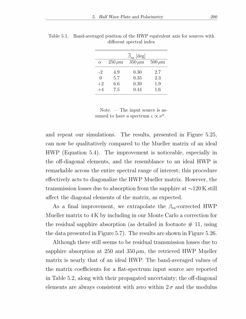
5. Half Wave Plate and Polarimetry 200
Table 5.1. Band-averaged position of the HWP equivalent axis for sources withdifferent spectral index
�ea [deg]� 250�m 350�m 500�m
-2 4.9 0.30 2.70 5.7 0.35 2.3+2 6.6 0.39 1.9+4 7.5 0.44 1.6
Note. — The input source is as-sumed to have a spectrum & ∝ ��.
and repeat our simulations. The results, presented in Figure 5.25,
can now be qualitatively compared to the Mueller matrix of an ideal
HWP (Equation 5.4). The improvement is noticeable, especially in
the off-diagonal elements, and the resemblance to an ideal HWP is
remarkable across the entire spectral range of interest; this procedure
effectively acts to diagonalize the HWP Mueller matrix. However, the
transmission losses due to absorption from the sapphire at ∼120K still
affect the diagonal elements of the matrix, as expected.
As a final improvement, we extrapolate the �ea-corrected HWP
Mueller matrix to 4K by including in our Monte Carlo a correction for
the residual sapphire absorption (as detailed in footnote # 11, using
the data presented in Figure 5.7). The results are shown in Figure 5.26.
Although there still seems to be residual transmission losses due to
sapphire absorption at 250 and 350�m, the retrieved HWP Mueller
matrix is nearly that of an ideal HWP. The band-averaged values of
the matrix coefficients for a flat-spectrum input source are reported
in Table 5.2, along with their propagated uncertainty; the off-diagonal
elements are always consistent with zero within 2� and the modulus
5. Half Wave Plate and Polarimetry 201
Fig. 5.26 Graphical representation of the Mueller matrix of the cold BLAST-PolHWP at a given angle (� = 0∘), as a function of wavenumber. Note that here wecorrect for the temperature dependence of the sapphire absorption coefficient, asdescribed in footnote # 11, using the data presented in Figure 5.7. The (10�) errorbars (in red) are quantified via a Monte Carlo, which accounts for random errors inthe spectra of amplitude as given in Figure 5.17, and random errors in the rotationangle of amplitude 1∘.
5. Half Wave Plate and Polarimetry 202
Table 5.2. Band-averaged Mueller matrix coefficients
Band 250�m 350�m 500�m
a00 0.905 ± 0.006 1.001 ± 0.006 1.008 ± 0.007a01 0.012 ± 0.010 0.017 ± 0.010 0.014 ± 0.011a02 -0.002 ± 0.008 0.006 ± 0.009 0.001 ± 0.009a10 -0.016 ± 0.010 -0.021 ± 0.010 -0.020 ± 0.011a11 0.806 ± 0.011 0.928 ± 0.010 0.935 ± 0.012a12 -0.007 ± 0.011 -0.009 ± 0.014 -0.011 ± 0.014a20 -0.008 ± 0.008 -0.022 ± 0.010 -0.021 ± 0.010a21 -0.007 ± 0.011 -0.009 ± 0.014 -0.011 ± 0.014a22 -0.808 ± 0.008 -0.960 ± 0.009 -0.979 ± 0.010
Note. — These values are relative to Figure 5.26. Theinput source is assumed to have a flat spectrum.
of the three diagonal coefficients is always > 0.8. The combination of
these coefficients with the band-averaged values of �ea given in Ta-
ble 5.1 gives a complete account of the HWP non-idealities to the best
of our ability.
We repeat the calculation of the band-averaged coefficients for the
other spectral indices discussed in Figure 5.24; we find values that are
always within 1–2% of those reported in Table 5.2, and thus we do not
explicitly report them here. Because the three diagonal elements of
the HWP Mueller matrix effectively determine the HWP co-pol/cross-
pol transmission and modulation efficiency, this analysis confirms that
these quantities are very weakly dependent on the spectral index of
the input source; these findings are in very good agreement with those
of Savini et al. (2009). We will see in the next Chapter how a00, a11,
and a22 can be incorporated in the map-making algorithm in terms of
optical efficiency, �, and polarization efficiency, ", of each detector.
Finally, we discuss a potential limitation to any linear polarization
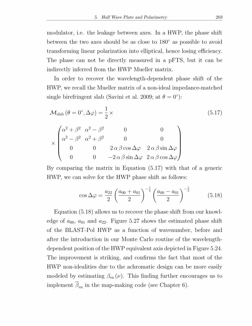
5. Half Wave Plate and Polarimetry 203
modulator, i.e. the leakage between axes. In a HWP, the phase shift
between the two axes should be as close to 180∘ as possible to avoid
transforming linear polarization into elliptical, hence losing efficiency.
The phase can not be directly measured in a pFTS, but it can be
indirectly inferred from the HWP Mueller matrix.
In order to recover the wavelength-dependent phase shift of the
HWP, we recall the Mueller matrix of a non-ideal impedance-matched
single birefringent slab (Savini et al. 2009; at � = 0∘):
ℳslab (� = 0∘,Δ') =1
2× (5.17)
×
⎛
⎜
⎜
⎜
⎜
⎝
�2 + �2 �2 − �2 0 0
�2 − �2 �2 + �2 0 0
0 0 2�� cosΔ' 2�� sinΔ'
0 0 −2�� sinΔ' 2�� cosΔ'
⎞
⎟
⎟
⎟
⎟
⎠
By comparing the matrix in Equation (5.17) with that of a generic
HWP, we can solve for the HWP phase shift as follows:
cosΔ' =a222
(
a00 + a012
)− 12(
a00 − a012
)− 12
(5.18)
Equation (5.18) allows us to recover the phase shift from our knowl-
edge of a00, a01 and a22. Figure 5.27 shows the estimated phase shift
of the BLAST-Pol HWP as a function of wavenumber, before and
after the introduction in our Monte Carlo routine of the wavelength-
dependent position of the HWP equivalent axis depicted in Figure 5.24.
The improvement is striking, and confirms the fact that most of the
HWP non-idealities due to the achromatic design can be more easily
modeled by estimating �ea (�). This finding further encourages us to
implement �ea in the map-making code (see Chapter 6).
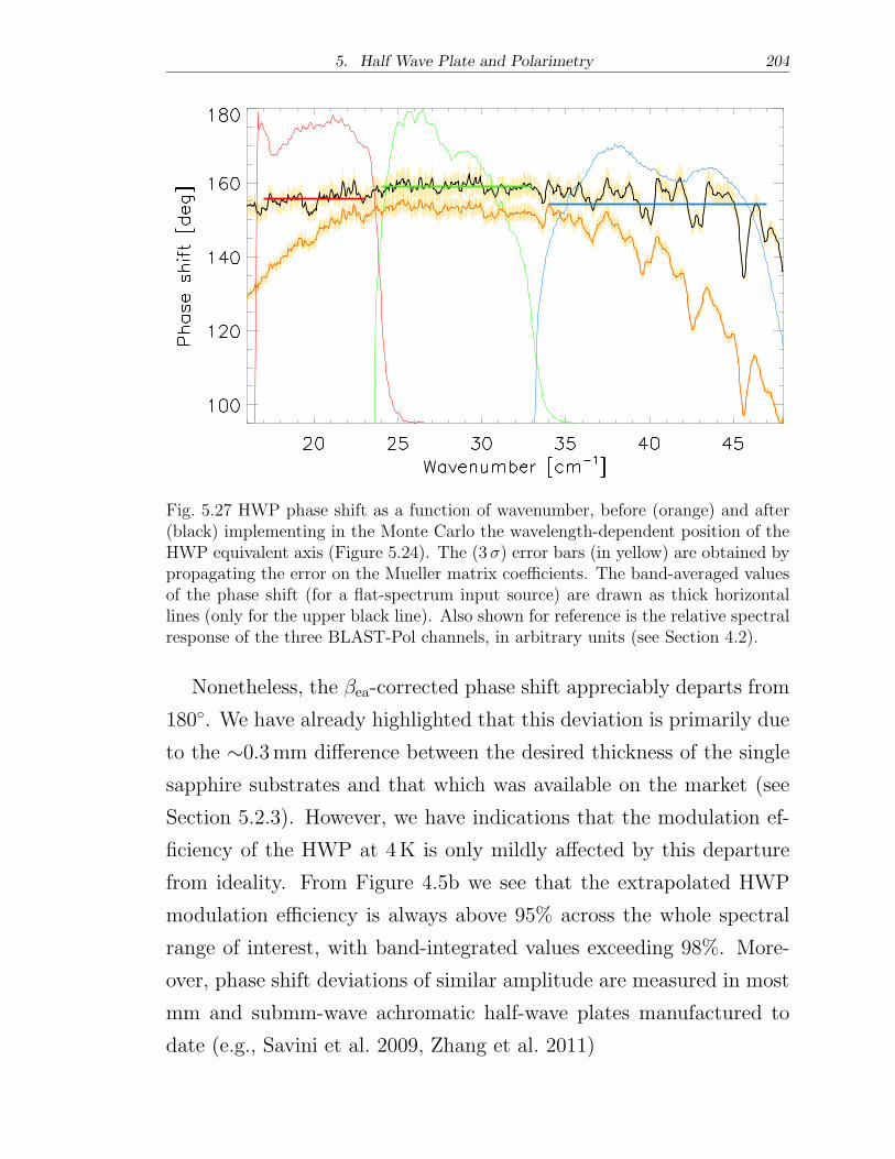
5. Half Wave Plate and Polarimetry 204
Fig. 5.27 HWP phase shift as a function of wavenumber, before (orange) and after(black) implementing in the Monte Carlo the wavelength-dependent position of theHWP equivalent axis (Figure 5.24). The (3�) error bars (in yellow) are obtained bypropagating the error on the Mueller matrix coefficients. The band-averaged valuesof the phase shift (for a flat-spectrum input source) are drawn as thick horizontallines (only for the upper black line). Also shown for reference is the relative spectralresponse of the three BLAST-Pol channels, in arbitrary units (see Section 4.2).
Nonetheless, the �ea-corrected phase shift appreciably departs from
180∘. We have already highlighted that this deviation is primarily due
to the ∼0.3mm difference between the desired thickness of the single
sapphire substrates and that which was available on the market (see
Section 5.2.3). However, we have indications that the modulation ef-
ficiency of the HWP at 4K is only mildly affected by this departure
from ideality. From Figure 4.5b we see that the extrapolated HWP
modulation efficiency is always above 95% across the whole spectral
range of interest, with band-integrated values exceeding 98%. More-
over, phase shift deviations of similar amplitude are measured in most
mm and submm-wave achromatic half-wave plates manufactured to
date (e.g., Savini et al. 2009, Zhang et al. 2011)
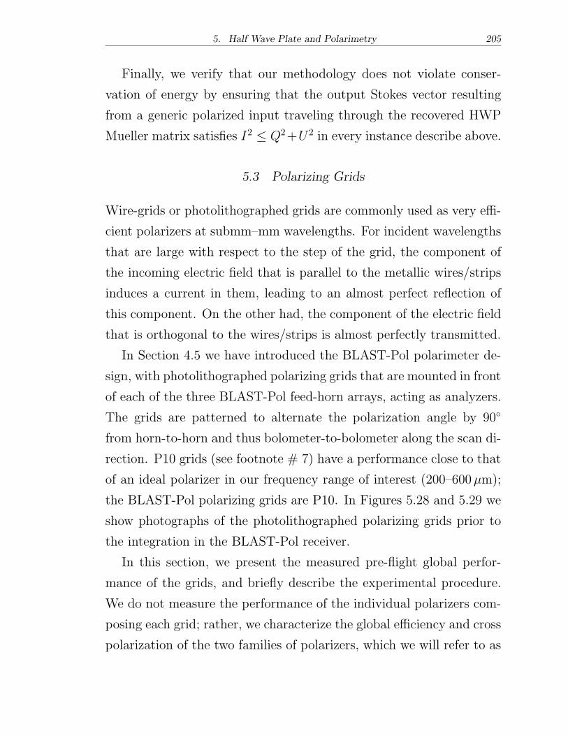
5. Half Wave Plate and Polarimetry 205
Finally, we verify that our methodology does not violate conser-
vation of energy by ensuring that the output Stokes vector resulting
from a generic polarized input traveling through the recovered HWP
Mueller matrix satisfies I2 ≤ Q2+U 2 in every instance describe above.
5.3 Polarizing Grids
Wire-grids or photolithographed grids are commonly used as very effi-
cient polarizers at submm–mm wavelengths. For incident wavelengths
that are large with respect to the step of the grid, the component of
the incoming electric field that is parallel to the metallic wires/strips
induces a current in them, leading to an almost perfect reflection of
this component. On the other had, the component of the electric field
that is orthogonal to the wires/strips is almost perfectly transmitted.
In Section 4.5 we have introduced the BLAST-Pol polarimeter de-
sign, with photolithographed polarizing grids that are mounted in front
of each of the three BLAST-Pol feed-horn arrays, acting as analyzers.
The grids are patterned to alternate the polarization angle by 90∘
from horn-to-horn and thus bolometer-to-bolometer along the scan di-
rection. P10 grids (see footnote # 7) have a performance close to that
of an ideal polarizer in our frequency range of interest (200–600�m);
the BLAST-Pol polarizing grids are P10. In Figures 5.28 and 5.29 we
show photographs of the photolithographed polarizing grids prior to
the integration in the BLAST-Pol receiver.
In this section, we present the measured pre-flight global perfor-
mance of the grids, and briefly describe the experimental procedure.
We do not measure the performance of the individual polarizers com-
posing each grid; rather, we characterize the global efficiency and cross
polarization of the two families of polarizers, which we will refer to as
5. Half Wave Plate and Polarimetry 206
Fig. 5.28 Photolithographed polarizing grids for the 500�m feed-horn array.
(a) (b)
Fig. 5.29 Two high-resolution images of the P10 photolithographed polarizing gridsfor the 500�m channel, obtained with a digital microscope.
“Q mask”and“-Q mask”in direct reference to the vertical or horizontal
orientation of the wires, respectively.
Although we do not record spectra, the experimental setup is very
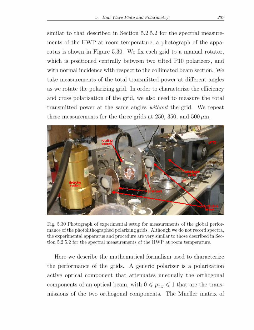
5. Half Wave Plate and Polarimetry 207
similar to that described in Section 5.2.5.2 for the spectral measure-
ments of the HWP at room temperature; a photograph of the appa-
ratus is shown in Figure 5.30. We fix each grid to a manual rotator,
which is positioned centrally between two tilted P10 polarizers, and
with normal incidence with respect to the collimated beam section. We
take measurements of the total transmitted power at different angles
as we rotate the polarizing grid. In order to characterize the efficiency
and cross polarization of the grid, we also need to measure the total
transmitted power at the same angles without the grid. We repeat
these measurements for the three grids at 250, 350, and 500�m.
Fig. 5.30 Photograph of experimental setup for measurements of the global perfor-mance of the photolithographed polarizing grids. Although we do not record spectra,the experimental apparatus and procedure are very similar to those described in Sec-tion 5.2.5.2 for the spectral measurements of the HWP at room temperature.
Here we describe the mathematical formalism used to characterize
the performance of the grids. A generic polarizer is a polarization
active optical component that attenuates unequally the orthogonal
components of an optical beam, with 0 ⩽ px,y ⩽ 1 that are the trans-
missions of the two orthogonal components. The Mueller matrix of
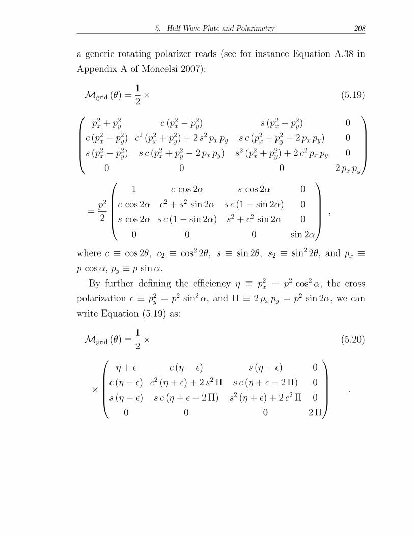
5. Half Wave Plate and Polarimetry 208
a generic rotating polarizer reads (see for instance Equation A.38 in
Appendix A of Moncelsi 2007):
ℳgrid (�) =1
2× (5.19)
⎛
⎜
⎜
⎜
⎜
⎝
p2x + p2y c (p2x − p2y) s (p2x − p2y) 0
c (p2x − p2y) c2 (p2x + p2y) + 2 s2 px py s c (p2x + p2y − 2 px py) 0
s (p2x − p2y) s c (p2x + p2y − 2 px py) s2 (p2x + p2y) + 2 c2 px py 0
0 0 0 2 px py
⎞
⎟
⎟
⎟
⎟
⎠
=p2
2
⎛
⎜
⎜
⎜
⎜
⎝
1 c cos 2� s cos 2� 0
c cos 2� c2 + s2 sin 2� s c (1− sin 2�) 0
s cos 2� s c (1− sin 2�) s2 + c2 sin 2� 0
0 0 0 sin 2�
⎞
⎟
⎟
⎟
⎟
⎠
,
where c ≡ cos 2�, c2 ≡ cos2 2�, s ≡ sin 2�, s2 ≡ sin2 2�, and px ≡p cos�, py ≡ p sin�.
By further defining the efficiency � ≡ p2x = p2 cos2 �, the cross
polarization � ≡ p2y = p2 sin2 �, and Π ≡ 2 px py = p2 sin 2�, we can
write Equation (5.19) as:
ℳgrid (�) =1
2× (5.20)
×
⎛
⎜
⎜
⎜
⎜
⎝
� + � c (� − �) s (� − �) 0
c (� − �) c2 (� + �) + 2 s2Π s c (� + �− 2Π) 0
s (� − �) s c (� + �− 2Π) s2 (� + �) + 2 c2Π 0
0 0 0 2Π
⎞
⎟
⎟
⎟
⎟
⎠
.
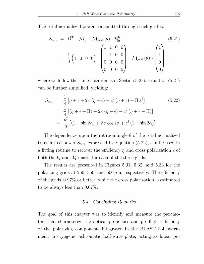
5. Half Wave Plate and Polarimetry 209
The total normalized power transmitted through each grid is:
Sout = DT ⋅ ℳhp ⋅ ℳgrid (�) ⋅ S h
in (5.21)
=1
8
(
1 0 0 0)
⋅
⎛
⎜
⎜
⎜
⎜
⎝
1 1 0 0
1 1 0 0
0 0 0 0
0 0 0 0
⎞
⎟
⎟
⎟
⎟
⎠
⋅ ℳgrid (�) ⋅
⎛
⎜
⎜
⎜
⎜
⎝
1
1
0
0
⎞
⎟
⎟
⎟
⎟
⎠
,
where we follow the same notation as in Section 5.2.6. Equation (5.21)
can be further simplified, yielding:
Sout =1
8
[
� + �+ 2 c (� − �) + c2 (� + �) + Π s2]
(5.22)
=1
8
[
(� + �+Π) + 2 c (� − �) + c2 (� + �− Π)]
=p2
8
[
(1 + sin 2�) + 2 c cos 2� + c2 (1− sin 2�)]
The dependency upon the rotation angle � of the total normalized
transmitted power Sout, expressed by Equation (5.22), can be used in
a fitting routine to recover the efficiency � and cross polarization � of
both the Q and -Q masks for each of the three grids.
The results are presented in Figures 5.31, 5.32, and 5.33 for the
polarizing grids at 250, 350, and 500�m, respectively. The efficiency
of the grids is 97% or better, while the cross polarization is estimated
to be always less than 0.07%.
5.4 Concluding Remarks
The goal of this chapter was to identify and measure the parame-
ters that characterize the optical properties and pre-flight efficiency
of the polarizing components integrated in the BLAST-Pol instru-
ment: a cryogenic achromatic half-wave plate, acting as linear po-
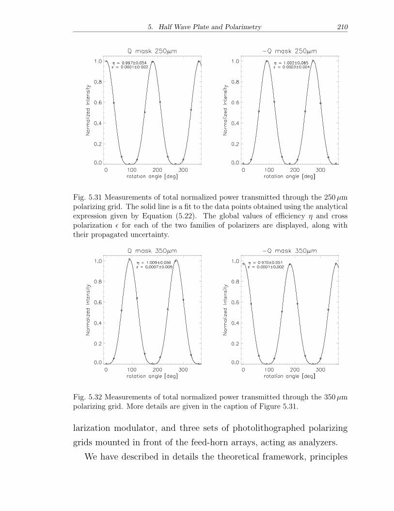
5. Half Wave Plate and Polarimetry 210
Fig. 5.31 Measurements of total normalized power transmitted through the 250�mpolarizing grid. The solid line is a fit to the data points obtained using the analyticalexpression given by Equation (5.22). The global values of efficiency � and crosspolarization � for each of the two families of polarizers are displayed, along withtheir propagated uncertainty.
Fig. 5.32 Measurements of total normalized power transmitted through the 350�mpolarizing grid. More details are given in the caption of Figure 5.31.
larization modulator, and three sets of photolithographed polarizing
grids mounted in front of the feed-horn arrays, acting as analyzers.
We have described in details the theoretical framework, principles
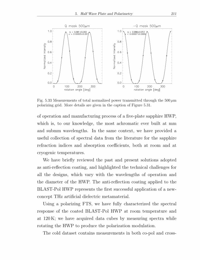
5. Half Wave Plate and Polarimetry 211
Fig. 5.33 Measurements of total normalized power transmitted through the 500�mpolarizing grid. More details are given in the caption of Figure 5.31.
of operation and manufacturing process of a five-plate sapphire HWP,
which is, to our knowledge, the most achromatic ever built at mm
and submm wavelengths. In the same context, we have provided a
useful collection of spectral data from the literature for the sapphire
refraction indices and absorption coefficients, both at room and at
cryogenic temperatures.
We have briefly reviewed the past and present solutions adopted
as anti-reflection coating, and highlighted the technical challenges for
all the designs, which vary with the wavelengths of operation and
the diameter of the HWP. The anti-reflection coating applied to the
BLAST-Pol HWP represents the first successful application of a new-
concept THz artificial dielectric metamaterial.
Using a polarizing FTS, we have fully characterized the spectral
response of the coated BLAST-Pol HWP at room temperature and
at 120K; we have acquired data cubes by measuring spectra while
rotating the HWP to produce the polarization modulation.
The cold dataset contains measurements in both co-pol and cross-
5. Half Wave Plate and Polarimetry 212
pol configurations; we have used these two data cubes to estimate 9
out of 16 elements of the Mueller matrix of the HWP as a function of
frequency. We have developed an ad-hoc Monte Carlo algorithm that
returns for every frequency the best estimate of each matrix element
and the associated error, which is a combination of the uncertainty on
the measured spectra and a random jitter on the rotation angle.
We have measured how the position of the equivalent axes of the
HWP, �ea, changes as a function of frequency, an effect that is inherent
to any achromatic design. Once this dependence is accounted for in
the Monte Carlo, and a correction is implemented for the residual
absorption from sapphire, the Mueller matrix of the HWP approaches
that of an ideal HWP, at all wavelengths of interest. In particular,
the (band-averaged) off-diagonal elements are always consistent with
zero within 2� and the modulus of the three diagonal coefficients is
always > 0.8. Therefore, we have introduced in the BLAST-Pol map-
making algorithm (Chapter 6) the band-integrated values of �ea as an
additional parameter in the evaluation of the polarization angle. To
first order, this approach allows us to account for most of the non-
idealities in the HWP.
We have investigated the impact of input sources with different
spectral signatures on �ea and on the HWPMueller matrix coefficients.
We find that the HWP transmission and modulation efficiency are very
weakly dependent on the spectral index of the input source, whereas
the position of the equivalent axes of the sapphire plate stack is more
significantly affected. This latter dependence, if neglected, may lead to
an arbitrary rotation of the retrieved polarization angle on the sky of
magnitude 2 �ea = 10–15∘ (3–5∘) at 250 (500)�m. The 350�m band,
however, is minimally perturbed by this effect.
In principle, the measured Mueller matrix can be used to gener-
5. Half Wave Plate and Polarimetry 213
ate a synthetic time-ordered template of the polarization modulation
produced by the HWP as if it were continuously rotated at � = ! t.
Continuous rotation of the HWP allows to reject all the noise com-
ponents modulated at harmonics different than 4 � (synchronous de-
modulation) and is typically employed by experiments optimized to
measure the polarization of the Cosmic Microwave Background (e.g.,
Johnson et al. 2007, Reichborn-Kjennerud et al. 2010). In such ex-
periments, the HWP modulation curve leaves a definite synchronous
imprint on the time-ordered bolometer data streams (timelines), hence
it is of utter importance to characterize the template and remove it
from the raw data. However, a time-ordered HWP template would
be of no use to a step-and-integrate experiment such as BLAST-Pol,
whose timelines are not dominated by the HWP synchronous signal.
We have measured the phase shift of the HWP across the wave-
length range of interest to be ∼160∘, which appreciably deviates from
the ideal 180∘; this is primarily due to the unavailability on the mar-
ket of sapphire substrates with the exact desired thickness. How-
ever, the modulation efficiency of the HWP is only mildly affected by
this departure from ideality, being above 98% in all three BLAST-Pol
bands. Moreover, departures of similar amplitude are not uncommon
for HWPs at mm and submm wavelengths.
Finally, we have measured the efficiency the BLAST-Pol analyzers
to be at least 97%, and their cross polarization to be at most 0.07%.
6. THE BLAST-POL MAP-MAKER
6.1 Introduction
Map-making is the operation that generates an astronomical map,
which contains in every pixel an estimate of the sky emission, and
is obtained by combining data from all detectors available at a given
wavelength channel, their noise properties and the pointing informa-
tion. The raw data consist of bolometer time-ordered streams (or time-
lines), which are cleaned and pre-processed before being fed into the
map-maker: in order, cosmic rays are flagged and removed, the known
electronics transfer function is deconvolved from the data streams,
an elevation-dependent common-mode signal due to the residual at-
mosphere is removed concurrently with a polynomial fit to the data,
and finally the timelines are high-pass filtered to suppress the low-
frequency (1/f) noise. The details of the pre-processing of the BLAST
timelines are extensively described elsewhere (Rex 2007, Truch 2007,
Wiebe 2008, Pascale et al. 2008), and we refer to these works for a com-
plete account of the low-level data reduction. Note that the process
of cleaning and preparing the bolometer time-streams for map-making
in BLAST-Pol has closely followed that of BLAST, exception made
for the removal of discontinuities in the DC level of the bolometer,
caused by the half-wave plate (HWP; see Section 4.5) being stepped
approximately every 15 minutes (this operation is performed before
the high-pass filtering); also, the subtraction of an elevation-dependent
term from the timelines was not needed in BLAST.
6. The BLAST-Pol map-maker 215
In the following, we focus on the mathematical formalism of the
map-making technique, and its algorithmic implementation in the spe-
cific case of BLAST-Pol. As a proof of concept, we produce preliminary
intensity and polarization maps for a sample of the scientific targets
observed by BLAST-Pol during its 9.5-day flight over Antarctica, com-
pleted in January 2011 (see Section 1.2.5). Although the reduction of
this dataset has not yet been finalized, the maps presented here result
as the culmination of the whole data analysis process and demonstrate
the overall success of the mission.
6.2 Maximum Likelihood Map-making
For a non-ideal polarization experiment, by adopting the Stokes for-
malism1 and assuming that no circular (V ) polarization is present, we
can model the data as follows:
dit =�i
2Ai
tp
[
Ip + "i(
Qp cos 2 it + Up sin 2 it)]
+ nit . (6.1)
Here, i, t and p label detector index, time, and map pixel respec-
tively; dit are the time-ordered data for a given channel, related to the
sky maps [Ip, Qp, Up] by the pointing operator Aitp; �
i is the optical effi-
ciency of each detector; "i is the polarization efficiency of each detector
with its polarizing grid (analyzer); and nit represents a generic time-
dependent noise term. Throughout this discussion it is assumed that
the term within square brackets is the convolution of the sky emission
with the telescope point-spread function (PSF). it is the time-ordered
vector of the observed polarization angle, defined as the angle between
the polarization reference vector at the sky pixel p (in the chosen ce-
1 We refer to Appendix A of Moncelsi (2007) for a review of polarization basics.
6. The BLAST-Pol map-maker 216
lestial frame) and the polarimeter transmission axis. it is given by:
it = �it + 2
[
�t − �0 − �ea
]
+ �igrid , (6.2)
where �it is the angle between the reference vector at pixel p and a vec-
tor pointing from p to the zenith along a great circle; �t is the HWP
orientation angle in the instrument frame; �0 is the HWP zero angle in
the instrument frame; �ea is the band-averaged position of the equiv-
alent axes of the HWP (dependent on the known or assumed spectral
signature of the input source; see Section 5.2.6); and �igrid = [0, �/2]
accounts for the transmission axis of the polarizing grids (analyzers;
see Section 4.5) being parallel/perpendicular to the zenith angle.
The notation outlined above can be connected to the Mueller for-
malism developed in Chapter 5 to determine under which circum-
stances Equation (6.1) is valid in the presence of a real (i.e., non-ideal)
HWP. Because we have included in Equation (6.2) the band-averaged
position of the equivalent axes of the HWP, �ea, the Mueller matrix of
the BLAST-Pol HWP can be considered almost that of an ideal HWP,
as discussed in Section 5.2.6. Nonetheless, we have shown that the
band-averaged values of the three diagonal matrix coefficients are not
identically unity (but always > 0.8 in modulus), probably as a result
of residual absorption from sapphire, especially in the 250 and 350�m
bands, albeit we have corrected for it to the best of our knowledge.
In the light of these considerations, we now want to compare Equa-
tion (6.1) to Equation (5.9), which both represent the signal measured
by a polarization insensitive intensity detector when illuminated by
a polarized input that propagates through a rotating HWP and an
analyzer. A term-by-term comparison yields that these two expres-
sions are equivalent when the coefficients B and C (defined in Equa-
tion 5.10) are zero, i.e. when the HWP modulates the polarization
6. The BLAST-Pol map-maker 217
purely at four times the rotation angle, with no leakage in the second
harmonic (twice the rotation angle) and thus no leakage of I into Q
and U . These two coefficients are linear combinations of the HWP
Mueller matrix elements a01, a10, a02, a20, which we have shown in Ta-
ble 5.2 to be all compatible with zero within 2�. In addition, their
amplitude is at most ∼2% of that of the diagonal matrix elements, and
in the limit of elevated angle coverage, ⟨cos 2 ⟩2 + ⟨sin 2 ⟩2 ≈ 0, these
terms (in twice the rotation angle) effectively average out in the sums.
Therefore, the coefficients B and C can be neglected to first order,
and the two expressions can be considered equivalent. Nonetheless,
these generally moderate levels of I → Q,U leakage can be readily ac-
counted for by incorporating in the map-making algorithm a correction
for the “instrumental polarization” (IP). We further this discussion in
Section 6.7.
In addition, after some elementary algebra, it results that � =
a00 +a112 + a22
2 , and that � " = a112 − a22
2 . As anticipated in the pre-
vious chapter, the knowledge of the band-averaged values of the three
diagonal matrix elements, a00, a11, a22 (which we have shown to de-
pend weakly on the spectral index of the input source), can be readily
incorporated in the map-making algorithm in terms of optical effi-
ciency, �, and polarization efficiency, ", of the HWP; these can be
factored in the overall optical efficiency and polarization efficiency
of each detector. From the values listed in Table 5.2, in our case
we find [�hwp, "hwp] = [0.904, 0.893], [0.985, 0.958], and [0.986, 0.971] at
250, 350, and 500�m, respectively.
Finally, the comparison of Equations (6.1) and (5.9) also yields
� " � = −a12 = −a21, where we have introduced a new parameter,
�, which quantifies the amplitude of the mixing of Q and U . From
Table 5.2, we see that a12 = a21 are always compatible with zero
6. The BLAST-Pol map-maker 218
within 1�, and their amplitude is at most ∼1% of that of the diag-
onal matrix elements. Nonetheless we quantify the amplitude of the
Q ↔ U mixing to be �hwp = 0.009, 0.010, and 0.011 at 250, 350, and
500�m, respectively. While this correction is not currently included
in our algorithm, we indicate that it can be implemented in a rela-
tively straightforward way by modifying Equation (6.1) with a double
change of variable, i.e. Q → Q + �U and U → U + �Q. If � is
estimated to the required accuracy, the unmixed Q and U can be re-
trieved unbiasedly. This correction may be very relevant to Cosmic
Microwave Background (CMB) polarization experiments, where any
Q↔ U leakage leads to a spurious mixing of the EE and BB modes.
We remind the reader that the above factors have been computed di-
rectly from the band-averaged coefficients of the inferred HWPMueller
matrix extrapolated at 4K, and offer a direct way to include the mod-
eled HWP non-idealities in a map-making algorithm. On the other
hand, the band-averaged HWP maximum transmission, polarization
efficiency and cross-pol quoted at the end of Sections 4.5.2 and 5.2.5.3
are estimated directly from the spectra extrapolated at 4K, and are
only informative from an experimental point of view rather than for
data analysis purposes.
Consider now one map pixel p that is observed in one band by k
detectors (i = 1, ..., k); let us define the generalised pointing matrix
Atp, which includes the trigonometric functions and the efficiencies,
Atp ≡1
2
⎛
⎜
⎜
⎜
⎜
⎜
⎜
⎜
⎝
�1A1tp �1 "1A1
tp cos 2 1t �1 "1A1tp sin 2 1t
......
...
�iAitp �i "iAi
tp cos 2 it �i "iAitp sin 2 it
......
...
�k Aktp �k "k Ak
tp cos 2 kt �k "k Aktp sin 2 kt
⎞
⎟
⎟
⎟
⎟
⎟
⎟
⎟
⎠
, (6.3)
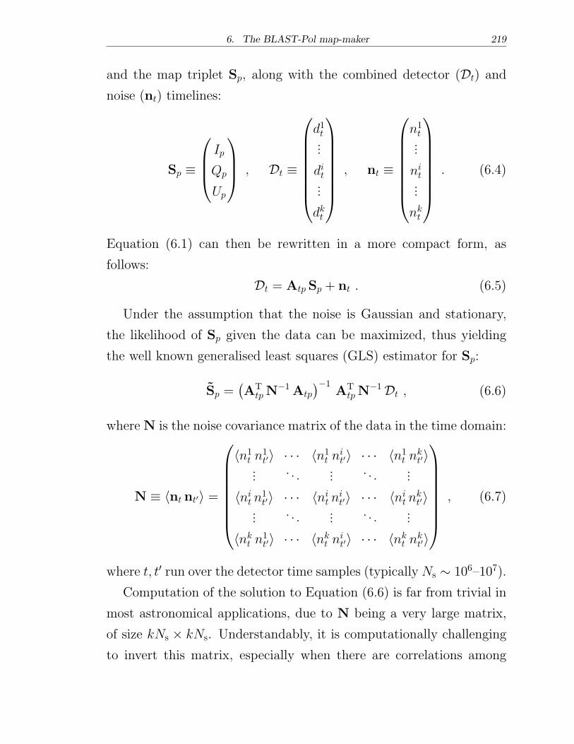
6. The BLAST-Pol map-maker 219
and the map triplet Sp, along with the combined detector (Dt) and
noise (nt) timelines:
Sp ≡
⎛
⎜
⎜
⎝
Ip
Qp
Up
⎞
⎟
⎟
⎠
, Dt ≡
⎛
⎜
⎜
⎜
⎜
⎜
⎜
⎜
⎝
d1t...
dit...
dkt
⎞
⎟
⎟
⎟
⎟
⎟
⎟
⎟
⎠
, nt ≡
⎛
⎜
⎜
⎜
⎜
⎜
⎜
⎜
⎝
n1t...
nit...
nkt
⎞
⎟
⎟
⎟
⎟
⎟
⎟
⎟
⎠
. (6.4)
Equation (6.1) can then be rewritten in a more compact form, as
follows:
Dt = Atp Sp + nt . (6.5)
Under the assumption that the noise is Gaussian and stationary,
the likelihood of Sp given the data can be maximized, thus yielding
the well known generalised least squares (GLS) estimator for Sp:
Sp =(
ATtpN
−1Atp
)−1A
TtpN
−1Dt , (6.6)
where N is the noise covariance matrix of the data in the time domain:
N ≡ ⟨nt nt′⟩ =
⎛
⎜
⎜
⎜
⎜
⎜
⎜
⎜
⎝
⟨n1t n1t′⟩ ⋅ ⋅ ⋅ ⟨n1t nit′⟩ ⋅ ⋅ ⋅ ⟨n1t nkt′⟩... . . . ... . . . ...
⟨nit n1t′⟩ ⋅ ⋅ ⋅ ⟨nit nit′⟩ ⋅ ⋅ ⋅ ⟨nit nkt′⟩... . . . ... . . . ...
⟨nkt n1t′⟩ ⋅ ⋅ ⋅ ⟨nkt nit′⟩ ⋅ ⋅ ⋅ ⟨nkt nkt′⟩
⎞
⎟
⎟
⎟
⎟
⎟
⎟
⎟
⎠
, (6.7)
where t, t′ run over the detector time samples (typically Ns ∼ 106–107).
Computation of the solution to Equation (6.6) is far from trivial in
most astronomical applications, due to N being a very large matrix,
of size kNs × kNs. Understandably, it is computationally challenging
to invert this matrix, especially when there are correlations among
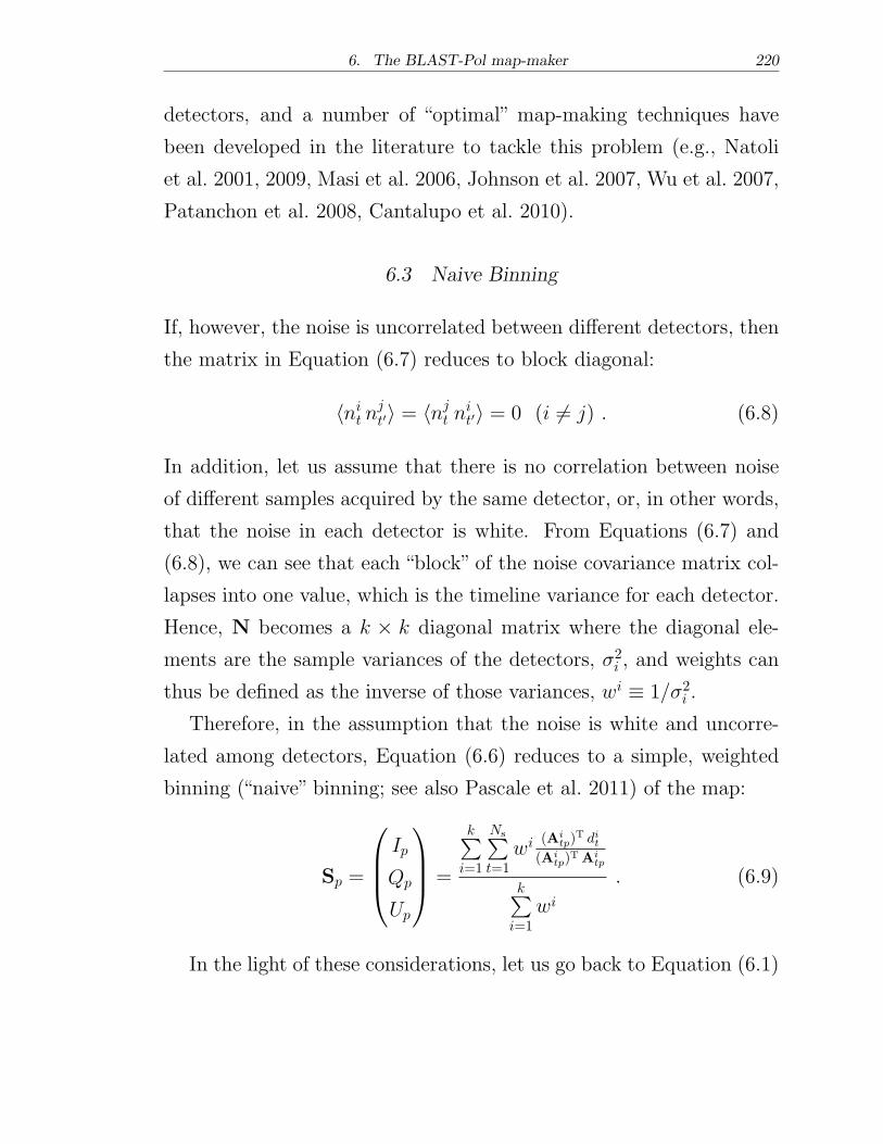
6. The BLAST-Pol map-maker 220
detectors, and a number of “optimal” map-making techniques have
been developed in the literature to tackle this problem (e.g., Natoli
et al. 2001, 2009, Masi et al. 2006, Johnson et al. 2007, Wu et al. 2007,
Patanchon et al. 2008, Cantalupo et al. 2010).
6.3 Naive Binning
If, however, the noise is uncorrelated between different detectors, then
the matrix in Equation (6.7) reduces to block diagonal:
⟨nit njt′⟩ = ⟨njt nit′⟩ = 0 (i ∕= j) . (6.8)
In addition, let us assume that there is no correlation between noise
of different samples acquired by the same detector, or, in other words,
that the noise in each detector is white. From Equations (6.7) and
(6.8), we can see that each “block” of the noise covariance matrix col-
lapses into one value, which is the timeline variance for each detector.
Hence, N becomes a k × k diagonal matrix where the diagonal ele-
ments are the sample variances of the detectors, �2i , and weights can
thus be defined as the inverse of those variances, wi ≡ 1/�2i .
Therefore, in the assumption that the noise is white and uncorre-
lated among detectors, Equation (6.6) reduces to a simple, weighted
binning (“naive” binning; see also Pascale et al. 2011) of the map:
Sp =
⎛
⎜
⎜
⎝
Ip
Qp
Up
⎞
⎟
⎟
⎠
=
k∑
i=1
Ns∑
t=1wi (Ai
tp)T dit
(Aitp)
T Aitp
k∑
i=1
wi
. (6.9)
In the light of these considerations, let us go back to Equation (6.1)
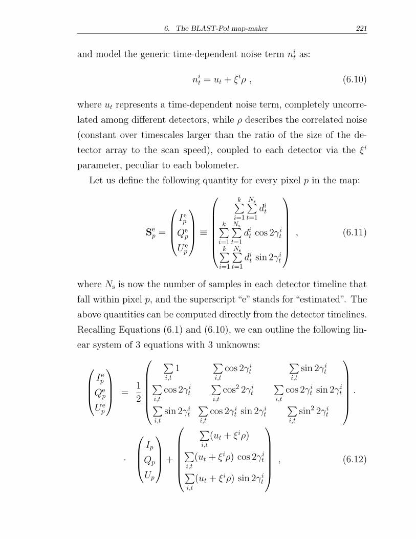
6. The BLAST-Pol map-maker 221
and model the generic time-dependent noise term nit as:
nit = ut + �i� , (6.10)
where ut represents a time-dependent noise term, completely uncorre-
lated among different detectors, while � describes the correlated noise
(constant over timescales larger than the ratio of the size of the de-
tector array to the scan speed), coupled to each detector via the �i
parameter, peculiar to each bolometer.
Let us define the following quantity for every pixel p in the map:
Sep =
⎛
⎜
⎜
⎝
Iep
Qep
U ep
⎞
⎟
⎟
⎠
≡
⎛
⎜
⎜
⎜
⎜
⎜
⎜
⎝
k∑
i=1
Ns∑
t=1dit
k∑
i=1
Ns∑
t=1dit cos 2
it
k∑
i=1
Ns∑
t=1dit sin 2
it
⎞
⎟
⎟
⎟
⎟
⎟
⎟
⎠
, (6.11)
where Ns is now the number of samples in each detector timeline that
fall within pixel p, and the superscript “e” stands for “estimated”. The
above quantities can be computed directly from the detector timelines.
Recalling Equations (6.1) and (6.10), we can outline the following lin-
ear system of 3 equations with 3 unknowns:
⎛
⎜
⎜
⎝
Iep
Qep
U ep
⎞
⎟
⎟
⎠
=1
2
⎛
⎜
⎜
⎜
⎜
⎜
⎝
∑
i,t
1∑
i,t
cos 2 it∑
i,t
sin 2 it∑
i,t
cos 2 it∑
i,t
cos2 2 it∑
i,t
cos 2 it sin 2 it
∑
i,t
sin 2 it∑
i,t
cos 2 it sin 2 it
∑
i,t
sin2 2 it
⎞
⎟
⎟
⎟
⎟
⎟
⎠
⋅
⋅
⎛
⎜
⎜
⎝
Ip
Qp
Up
⎞
⎟
⎟
⎠
+
⎛
⎜
⎜
⎜
⎜
⎜
⎝
∑
i,t
(ut + �i�)
∑
i,t
(ut + �i�) cos 2 it∑
i,t
(ut + �i�) sin 2 it
⎞
⎟
⎟
⎟
⎟
⎟
⎠
, (6.12)
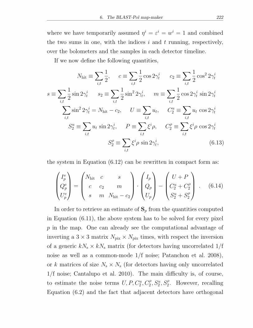
6. The BLAST-Pol map-maker 222
where we have temporarily assumed �i = "i = wi = 1 and combined
the two sums in one, with the indices i and t running, respectively,
over the bolometers and the samples in each detector timeline.
If we now define the following quantities,
Nhit ≡∑
i,t
1
2, c ≡
∑
i,t
1
2cos 2 it c2 ≡
∑
i,t
1
2cos2 2 it
s ≡∑
i,t
1
2sin 2 it s2 ≡
∑
i,t
1
2sin2 2 it, m ≡
∑
i,t
1
2cos 2 it sin 2
it
∑
i,t
sin2 2 it = Nhit − c2, U ≡∑
i,t
ut, Cu2 ≡
∑
i,t
ut cos 2 it
Su2 ≡
∑
i,t
ut sin 2 it, P ≡
∑
i,t
�i�, C�2 ≡
∑
i,t
�i� cos 2 it
S�2 ≡
∑
i,t
�i� sin 2 it, (6.13)
the system in Equation (6.12) can be rewritten in compact form as:
⎛
⎜
⎜
⎝
Iep
Qep
U ep
⎞
⎟
⎟
⎠
=
⎛
⎜
⎜
⎝
Nhit c s
c c2 m
s m Nhit − c2
⎞
⎟
⎟
⎠
⋅
⎛
⎜
⎜
⎝
Ip
Qp
Up
⎞
⎟
⎟
⎠
−
⎛
⎜
⎜
⎝
U + P
Cu2 + C�
2
Su2 + S�
2
⎞
⎟
⎟
⎠
. (6.14)
In order to retrieve an estimate of Sp from the quantities computed
in Equation (6.11), the above system has to be solved for every pixel
p in the map. One can already see the computational advantage of
inverting a 3× 3 matrix Npix ×Npix times, with respect the inversion
of a generic kNs × kNs matrix (for detectors having uncorrelated 1/f
noise as well as a common-mode 1/f noise; Patanchon et al. 2008),
or k matrices of size Ns × Ns (for detectors having only uncorrelated
1/f noise; Cantalupo et al. 2010). The main difficulty is, of course,
to estimate the noise terms U, P, Cu2 , C
�2 , S
u2 , S
�2 . However, recalling
Equation (6.2) and the fact that adjacent detectors have orthogonal
6. The BLAST-Pol map-maker 223
polarizing grids (�igrid = [0, �/2]), we note that, in the sum over i,
adjacent detectors have equal and opposite contributions to C�2 and
S�2 (as anticipated in Section 4.5.1), under the following assumptions:
∙ the timescale over which the correlated noise is approximately
constant is larger than the time elapsed while scanning the same
patch of sky with two adjacent detectors;
∙ �i is not too dissimilar between adjacent bolometers.
This means that the terms C�2 and S�
2 can be neglected, under the
above assumptions, while estimating the [Q,U ] maps. In particular, as
a first step, we can solve for I only by high-pass filtering the timelines,
in order to suppress the correlated noise term in I, P . Subsequently, I
can be assumed known, and the [Q,U ] maps can be computed without
filtering the timelines, so that polarized signal at large angular scales
is not suppressed. In fact, we see from Equation (6.1) that in the limit
of elevated angle coverage, the term in I, not being modulated at four
times the HWP rotation angle, effectively averages out in the sums.
The other assumption required for the naive binning is that the
noise is white, at least on the timescales relevant to BLAST-Pol’s scan
strategy (see Section 4.5). As a matter of fact, preliminary analysis of
the bolometer timelines from the 2010 campaign shows that the knee
of the 1/f noise in the difference between two adjacent detectors is
typically located at frequencies≲ 0.1Hz; assuming a typical scan speed
of 0.1∘ s−1, this corresponds to angular scales of ≳ 1 deg in the sky.
The regions mapped by BLAST-Pol hardly exceed 1 deg in size (see
Section 1.2.5), hence here we stipulate that the noise in the difference
between pairs of adjacent detectors is white.
Therefore, under the assumptions above, we can solve the linear
system outlined in Equation (6.14); by defining the following quanti-
6. The BLAST-Pol map-maker 224
ties:
Δ ≡ c2 (c2 −Nh)−Nh
(
c22 +m2 − c2Nh
)
+ 2 c sm− c2 s2 ,
A ≡ −(
c22 +m2 − c2Nh
)
, B ≡ c (c2 −Nh) + sm ,
C ≡ cm− s c2, D ≡ −[
(c2 −Nh)Nh + s2]
, (6.15)
E ≡ c s−mNh, F ≡ c2Nh − c2 ,
the solution to the system can be written in compact form, as follows:
Sp =
⎛
⎜
⎜
⎝
Ip
Qp
Up
⎞
⎟
⎟
⎠
=
⎛
⎜
⎜
⎝
AIep+BQep+C U e
p
ΔB Iep+DQe
p+E U ep
ΔC Iep+EQe
p+F U ep
Δ
⎞
⎟
⎟
⎠
, (6.16)
where we have renamed Nhit → Nh for brevity.
6.4 Weights and Uncertainties
The solution for Sp given in Equation (6.16) is a simple, unweighed
binning of the data into the map pixels. In reality, as anticipated in
Equation (6.9), we want to perform a weighted binning, where the
weight of each detector is given by the inverse of its timeline variance,
which can be easily measured as the bolometer’s white noise floor level.
In our formalism, the weighted binning is simply achieved by defining
[Iep, Qep, U
ep ] in Equation (6.11), as well as each of the quantities Nh, c,
s, c2, s2, and m introduced in Equation (6.13), to include wi in the
sums. Similarly, the measured values of the optical efficiencies �i and
polarization efficiencies "i can readily be inserted in Equations (6.12)
and (6.13) to account for the non-idealities of the optical system.
The introduction of the weights allows us to derive the expression
for the statistical error on Sp, in the continued assumption of uncorre-
lated noise, following the usual error propagation formula (e.g., Press

6. The BLAST-Pol map-maker 225
et al. 1992; here we omit the sum over t for simplicity):
�2p =∑
i
1
wi
(
∂Sp
∂di
)2
. (6.17)
After some tedious algebra, the expression for the statistical error is:
�2p =
⎛
⎜
⎜
⎝
VarIp
VarQp
VarUp
⎞
⎟
⎟
⎠
= (6.18)
=
⎛
⎜
⎜
⎝
2Δ2
(
A2Nh + B2 c2 + C2 s2 + 2AB c+ 2AC s+ 2B C m)
2Δ2
(
B2Nh +D2 c2 + E2 s2 + 2BD c+ 2BE s+ 2DEm)
2Δ2
(
C2Nh + E2 c2 + F 2 s2 + 2C E c+ 2C F s+ 2E F m)
⎞
⎟
⎟
⎠
,
where s2 ≡ Nh − c2, as noted in Equation (6.13). To first order, these
expression can be used to quantify the uncertainty of [I,Q, U ] in each
map pixel p. A more comprehensive account of the correlations in the
noise, as well as a thorough validation of the assumptions made here,
is beyond the scope of this thesis and will be treated in a future work.
Finally, we note that a better approach to estimating the uncertainties
on the [I,Q, U ] maps would be a Monte Carlo simulation, which more
effectively accounts for the well known biases inherent to the direct
error propagation method.
6.5 Preliminary Maps
Firstly, we want to test the ability of the algorithm to genuinely re-
trieve the correct polarization on the sky, i.e. without introducing
artifacts. In order to do so, we produce simulated polarization maps
using observations of VY Canis Majoris (VY CMa) from the BLAST06
dataset. The total intensity I map is shown in the top panel of Fig-
6. The BLAST-Pol map-maker 226
ure 6.1. We then simulate a p% = 50 polarized Q and U input,
obtained from the BLAST06 timelines as d50%Q = d (1 + 0.5 cos 2 )
and d50%U = d (1 + 0.5 sin 2 ), respectively. These synthetic timelines,
along with a simulated timeline containing the HWP angles, are then
fed into the map-making code as if they had been observed by BLAST-
Pol. The resulting polarization maps are shown in the four bottom
panels of Figure 6.1. In the case of a simulated Q input, the Q map is
retrieved correctly with a value at the source peak that is half of that
in the corresponding pixel in the I map, while the U map is practi-
cally featureless, indicating that there are no artifacts introduced by
the map-maker; a similar result is found for the simulated U input.
Therefore, these maps qualitatively demonstrate the effectiveness of
the algorithm in retrieving the polarization signal.
In addition, as a proof of concept of the naive binning technique for
the BLAST-Pol polarized map-maker, we present preliminary inten-
sity and polarization maps at 500�m for a sample of three scientific
targets observed by BLAST-Pol during its first Antarctic flight, com-
pleted in January 2011 (see Section 1.2.5). The original maps have
been smoothed with a kernel of 3′ (FWHM; about three times that of
the nominal BLAST-Pol beam at 500�m) to mitigate the effects due
to the uncertainty on the shape of the instrumental PSF, which are
still being investigated.
The maps (shown in Figures 6.2, 6.4, and 6.6) are presented as
contour levels of the intensity map I, upon which we superimpose
vectors indicating the polarization direction in the sky; the length of
each vector is proportional to the polarization degree (a vector corre-
sponding to p% = 5 is shown for reference). The polarization degree
is obtained as p% =√
Q2 + U 2/I, and the sky polarization angle is
given by � = 12 arctan
UQ . Because the absolute flux calibration has not
6. The BLAST-Pol map-maker 227
been finalized yet, we choose not to report here the intensity values
corresponding to each contour level. These map should not be consid-
ered of any scientific value as they are not calibrated in flux and the
polarization angles may be rotated by an offset, as summarized later
on in Section 6.7. Nonetheless, we note that the BLAST-Pol map of
the Carina Nebula shown in Figure 6.4 bears a promising resemblance
to the map produced by the Submillimeter Polarimeter for Antarctic
Remote Observations (SPARO; Novak et al. 2003) at 450�m, which
is shown in Figure 1 of Li et al. (2006).
The polarization degree and position angle in the sky are two of the
most important observables that BLAST-Pol will yield; in particular,
as detailed in Section 1.2, the degree of dispersion in the polarization
angle is an indicator of magnetic field strength, while the variation
of the polarization amplitude as a function of wavelength can help
constrain models of grain alignment. In addition to the maps, we show
for each source preliminary histograms of the polarization degree and
the polarization angle in the sky (Figures 6.3, 6.5, and 6.7), which are
measured from the maps for each 3′ resolution element.
6.6 Concluding Remarks
In this chapter we have introduced the problem of producing astro-
nomical maps from raw bolometric data collected by an experiment
with hundreds of detectors. We have focused on the mathematical
formalism of map-making, and the algorithmic implementation of a
naive binning technique for the case of BLAST-Pol, in the assump-
tion of white and uncorrelated noise. By using a simulated polarized
input synthesized from the timelines of a bright calibrator from the
BLAST06 dataset, we have successfully tested the ability of the algo-
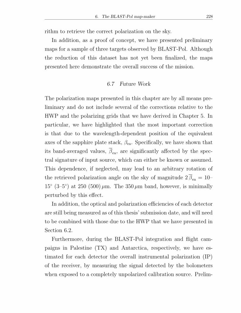
6. The BLAST-Pol map-maker 228
rithm to retrieve the correct polarization on the sky.
In addition, as a proof of concept, we have presented preliminary
maps for a sample of three targets observed by BLAST-Pol. Although
the reduction of this dataset has not yet been finalized, the maps
presented here demonstrate the overall success of the mission.
6.7 Future Work
The polarization maps presented in this chapter are by all means pre-
liminary and do not include several of the corrections relative to the
HWP and the polarizing grids that we have derived in Chapter 5. In
particular, we have highlighted that the most important correction
is that due to the wavelength-dependent position of the equivalent
axes of the sapphire plate stack, �ea. Specifically, we have shown that
its band-averaged values, �ea, are significantly affected by the spec-
tral signature of input source, which can either be known or assumed.
This dependence, if neglected, may lead to an arbitrary rotation of
the retrieved polarization angle on the sky of magnitude 2 �ea = 10–
15∘ (3–5∘) at 250 (500)�m. The 350�m band, however, is minimally
perturbed by this effect.
In addition, the optical and polarization efficiencies of each detector
are still being measured as of this thesis’ submission date, and will need
to be combined with those due to the HWP that we have presented in
Section 6.2.
Furthermore, during the BLAST-Pol integration and flight cam-
paigns in Palestine (TX) and Antarctica, respectively, we have es-
timated for each detector the overall instrumental polarization (IP)
of the receiver, by measuring the signal detected by the bolometers
when exposed to a completely unpolarized calibration source. Prelim-
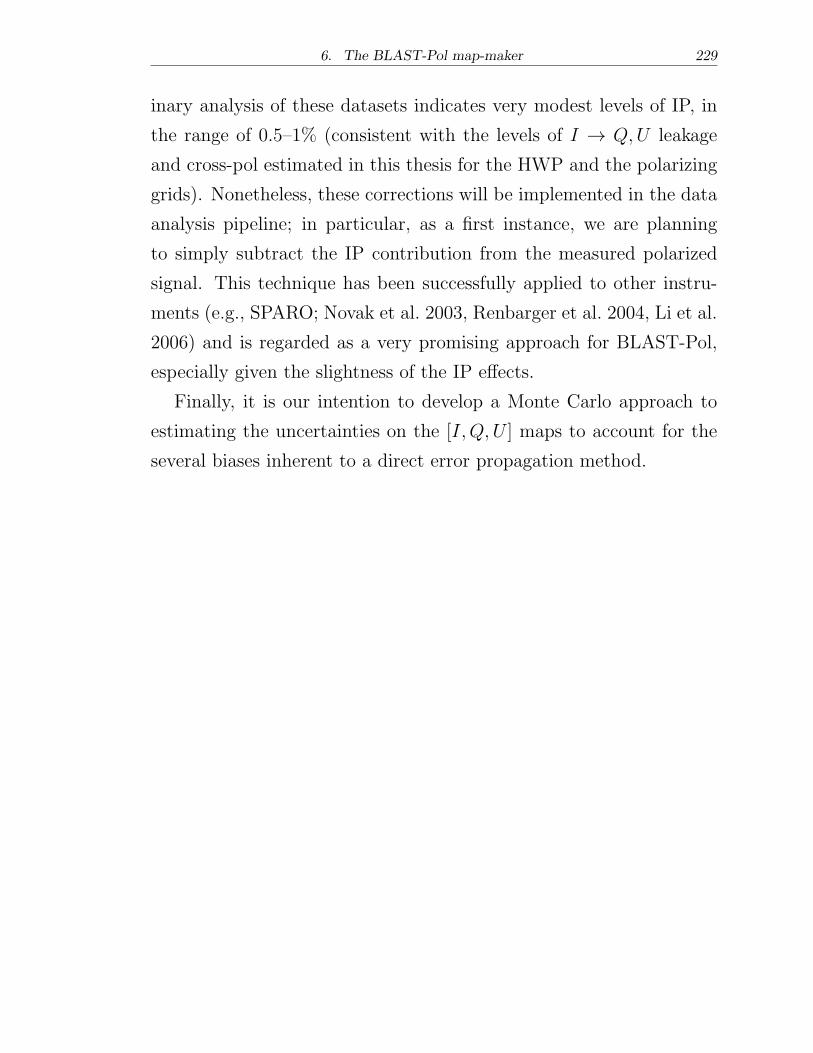
6. The BLAST-Pol map-maker 229
inary analysis of these datasets indicates very modest levels of IP, in
the range of 0.5–1% (consistent with the levels of I → Q,U leakage
and cross-pol estimated in this thesis for the HWP and the polarizing
grids). Nonetheless, these corrections will be implemented in the data
analysis pipeline; in particular, as a first instance, we are planning
to simply subtract the IP contribution from the measured polarized
signal. This technique has been successfully applied to other instru-
ments (e.g., SPARO; Novak et al. 2003, Renbarger et al. 2004, Li et al.
2006) and is regarded as a very promising approach for BLAST-Pol,
especially given the slightness of the IP effects.
Finally, it is our intention to develop a Monte Carlo approach to
estimating the uncertainties on the [I,Q, U ] maps to account for the
several biases inherent to a direct error propagation method.
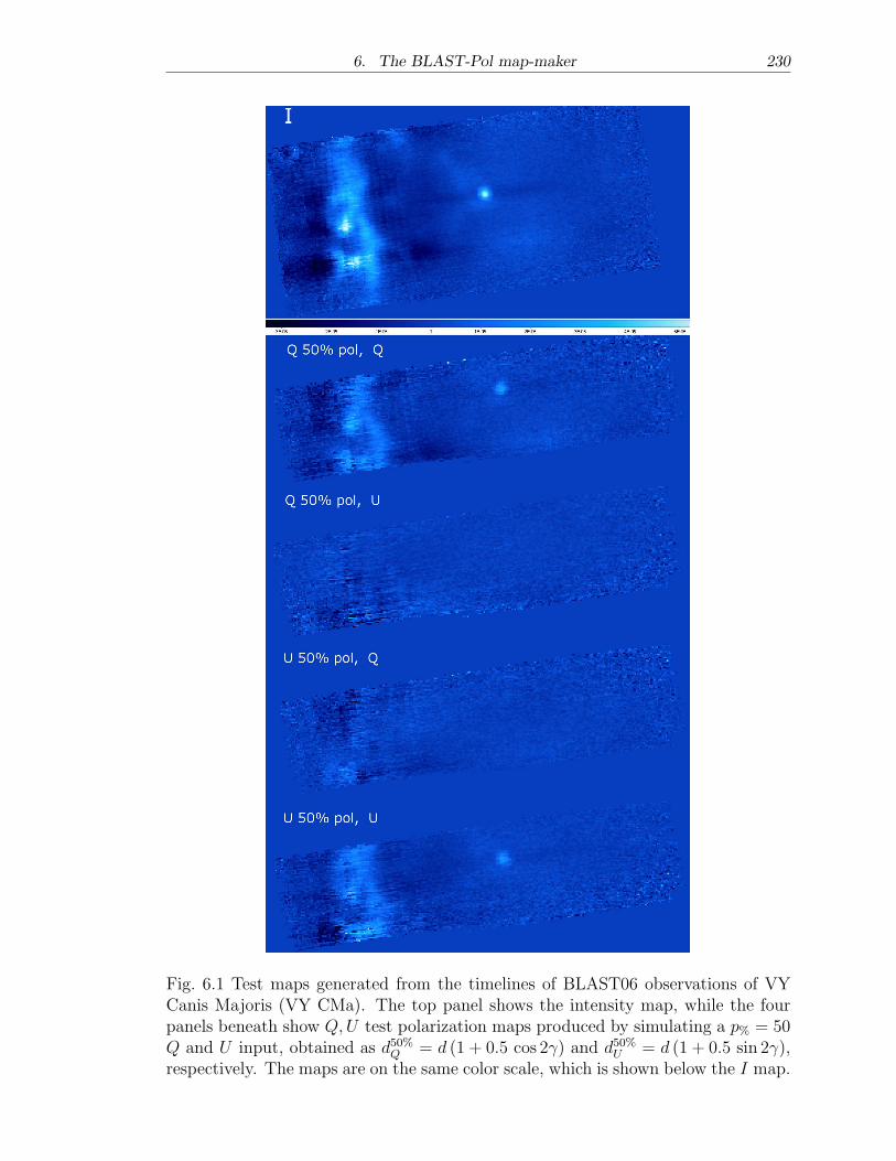
6. The BLAST-Pol map-maker 230
Fig. 6.1 Test maps generated from the timelines of BLAST06 observations of VYCanis Majoris (VY CMa). The top panel shows the intensity map, while the fourpanels beneath show Q,U test polarization maps produced by simulating a p% = 50Q and U input, obtained as d50%Q = d (1 + 0.5 cos 2 ) and d50%U = d (1 + 0.5 sin 2 ),respectively. The maps are on the same color scale, which is shown below the I map.
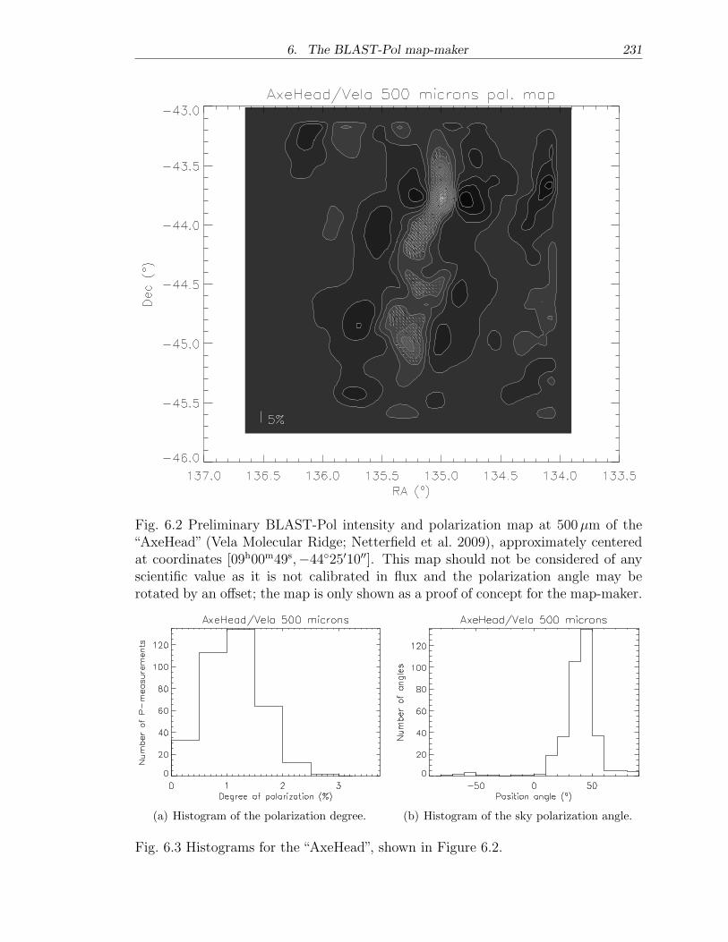
6. The BLAST-Pol map-maker 231
Fig. 6.2 Preliminary BLAST-Pol intensity and polarization map at 500�m of the“AxeHead” (Vela Molecular Ridge; Netterfield et al. 2009), approximately centeredat coordinates [09h00m49s,−44∘25′10′′]. This map should not be considered of anyscientific value as it is not calibrated in flux and the polarization angle may berotated by an offset; the map is only shown as a proof of concept for the map-maker.
(a) Histogram of the polarization degree. (b) Histogram of the sky polarization angle.
Fig. 6.3 Histograms for the “AxeHead”, shown in Figure 6.2.
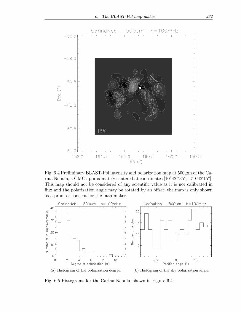
6. The BLAST-Pol map-maker 232
Fig. 6.4 Preliminary BLAST-Pol intensity and polarization map at 500�m of the Ca-rina Nebula, a GMC approximately centered at coordinates [10h42m35s,−59∘42′15′′].This map should not be considered of any scientific value as it is not calibrated influx and the polarization angle may be rotated by an offset; the map is only shownas a proof of concept for the map-maker.
(a) Histogram of the polarization degree. (b) Histogram of the sky polarization angle.
Fig. 6.5 Histograms for the Carina Nebula, shown in Figure 6.4.
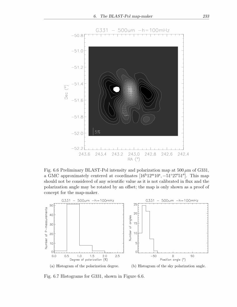
6. The BLAST-Pol map-maker 233
Fig. 6.6 Preliminary BLAST-Pol intensity and polarization map at 500�m of G331,a GMC approximately centered at coordinates [16h12m10s,−51∘27′51′′]. This mapshould not be considered of any scientific value as it is not calibrated in flux and thepolarization angle may be rotated by an offset; the map is only shown as a proof ofconcept for the map-maker.
(a) Histogram of the polarization degree. (b) Histogram of the sky polarization angle.
Fig. 6.7 Histograms for G331, shown in Figure 6.6.
7. CONCLUSIONS
The primary scientific motivation for this thesis is the study of the star-
formation processes in galaxies at cosmological distances and in molec-
ular clouds in our own Galaxy. We have discussed how fundamental
it is to conduct surveys of the sky at FIR and submm wavelengths, in
order to achieve a more complete understanding of the formation of
stars and the evolution of galaxies in the Universe. In particular, we
have introduced the reader to submm extragalactic and Galactic as-
tronomy, referencing the leading theoretical models and observational
findings as well as pinpointing the questions and issues that are still
being debated. We have outlined the role that BLAST and its polari-
metric upgrade, BLAST-Pol, respectively, has played and will play in
making significant headway on these fronts, through large-area submm
surveys conducted from long-duration stratospheric balloon platform.
In the first part of this thesis, we have presented a multi-wavelength
study of a subset of the hundreds of distant, highly dust-obscured, and
actively star-forming galaxies detected by BLAST in its survey of the
Extended Chandra Deep-Field South (ECDFS), using data spanning
the radio to the UV. We have developed a Monte Carlo method to
account for flux boosting, source blending, and correlations among
bands, which we have used to derive deboosted FIR luminosities for
our sample. We have shown how crucial the BLAST/SPIRE photom-
etry is to estimate the FIR luminosity of a galaxy without bias, espe-
cially at high redshift. We have estimated total (obscured plus unob-
7. Conclusions 235
scured) star-formation rates for the BLAST counterparts by combining
their FIR and UV luminosities. We have shown that star formation is
heavily obscured at LFIR ≳ 1011L⊙, z ≳ 0.5, but the contribution from
unobscured starlight cannot be neglected at LFIR ≲ 1011L⊙, z ≲ 0.25.
We have capitalized on the multi-wavelength data at our disposal to
derive a broad morphological classification of our galaxies, their AGN
fraction and stellar masses. We have assessed that about 20% of the
galaxies in our sample harbor a type-1 AGN, but their submillimeter
emission is mainly due to star formation in the host galaxy. We have
used the combined estimates of SFRs and stellar masses to determine
that the bulk of the BLAST counterparts at z ≲ 1 are normal star-
forming galaxies, typically spiral in shape, with intermediate stellar
masses (M★ ∼ 7 × 10¹⁰M⊙) and approximately constant SSFRs (�SF
in the range 1–10Gyr). On the other hand, the high-z tail of the
BLAST counterparts significantly overlaps with the SCUBA starburst
population, in terms of both SFRs and stellar masses, with observed
trends of SSFRs that support strong evolution and downsizing.
In Part One of this thesis we have also presented a challenging
measurement of the star-formation level in massive (M★ ≥ 1011M⊙),
high-redshift (1.7 < z < 2.9) galaxies selected in the optical with the
NICMOS camera on HST. Because the emission from each galaxy is
too faint to be individually detected in the MIR–to–submm maps at
our disposal, we have performed stacking analysis to unbiasedly mea-
sure their mean flux density. We have fitted a modified blackbody
spectrum to the stacked flux densities and measured a median [in-
terquartile] star-formation rate of SFR = 63 [48, 81]M⊙ yr−1. When
the galaxies are divided into two groups, disk-like and spheroid-like,
according to their Sersic indices, we have found evidence that most
of the star formation is occurring in disk-like galaxies, with SFR =
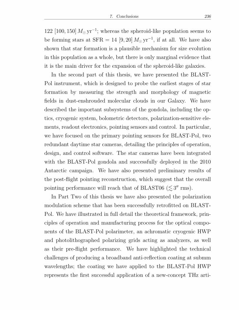
7. Conclusions 236
122 [100, 150]M⊙ yr−1; whereas the spheroid-like population seems to
be forming stars at SFR = 14 [9, 20]M⊙ yr−1, if at all. We have also
shown that star formation is a plausible mechanism for size evolution
in this population as a whole, but there is only marginal evidence that
it is the main driver for the expansion of the spheroid-like galaxies.
In the second part of this thesis, we have presented the BLAST-
Pol instrument, which is designed to probe the earliest stages of star
formation by measuring the strength and morphology of magnetic
fields in dust-enshrouded molecular clouds in our Galaxy. We have
described the important subsystems of the gondola, including the op-
tics, cryogenic system, bolometric detectors, polarization-sensitive ele-
ments, readout electronics, pointing sensors and control. In particular,
we have focused on the primary pointing sensors for BLAST-Pol, two
redundant daytime star cameras, detailing the principles of operation,
design, and control software. The star cameras have been integrated
with the BLAST-Pol gondola and successfully deployed in the 2010
Antarctic campaign. We have also presented preliminary results of
the post-flight pointing reconstruction, which suggest that the overall
pointing performance will reach that of BLAST06 (≲ 3′′ rms).
In Part Two of this thesis we have also presented the polarization
modulation scheme that has been successfully retrofitted on BLAST-
Pol. We have illustrated in full detail the theoretical framework, prin-
ciples of operation and manufacturing process for the optical compo-
nents of the BLAST-Pol polarimeter, an achromatic cryogenic HWP
and photolithographed polarizing grids acting as analyzers, as well
as their pre-flight performance. We have highlighted the technical
challenges of producing a broadband anti-reflection coating at submm
wavelengths; the coating we have applied to the BLAST-Pol HWP
represents the first successful application of a new-concept THz arti-
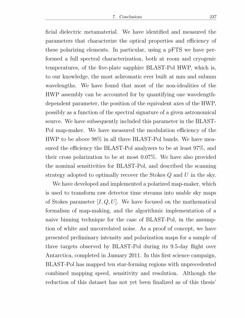
7. Conclusions 237
ficial dielectric metamaterial. We have identified and measured the
parameters that characterize the optical properties and efficiency of
these polarizing elements. In particular, using a pFTS we have per-
formed a full spectral characterization, both at room and cryogenic
temperatures, of the five-plate sapphire BLAST-Pol HWP, which is,
to our knowledge, the most achromatic ever built at mm and submm
wavelengths. We have found that most of the non-idealities of the
HWP assembly can be accounted for by quantifying one wavelength-
dependent parameter, the position of the equivalent axes of the HWP,
possibly as a function of the spectral signature of a given astronomical
source. We have subsequently included this parameter in the BLAST-
Pol map-maker. We have measured the modulation efficiency of the
HWP to be above 98% in all three BLAST-Pol bands. We have mea-
sured the efficiency the BLAST-Pol analyzers to be at least 97%, and
their cross polarization to be at most 0.07%. We have also provided
the nominal sensitivities for BLAST-Pol, and described the scanning
strategy adopted to optimally recover the Stokes Q and U in the sky.
We have developed and implemented a polarized map-maker, which
is used to transform raw detector time streams into usable sky maps
of Stokes parameter [I,Q, U ]. We have focused on the mathematical
formalism of map-making, and the algorithmic implementation of a
naive binning technique for the case of BLAST-Pol, in the assump-
tion of white and uncorrelated noise. As a proof of concept, we have
presented preliminary intensity and polarization maps for a sample of
three targets observed by BLAST-Pol during its 9.5-day flight over
Antarctica, completed in January 2011. In this first science campaign,
BLAST-Pol has mapped ten star-forming regions with unprecedented
combined mapping speed, sensitivity and resolution. Although the
reduction of this dataset has not yet been finalized as of this thesis’
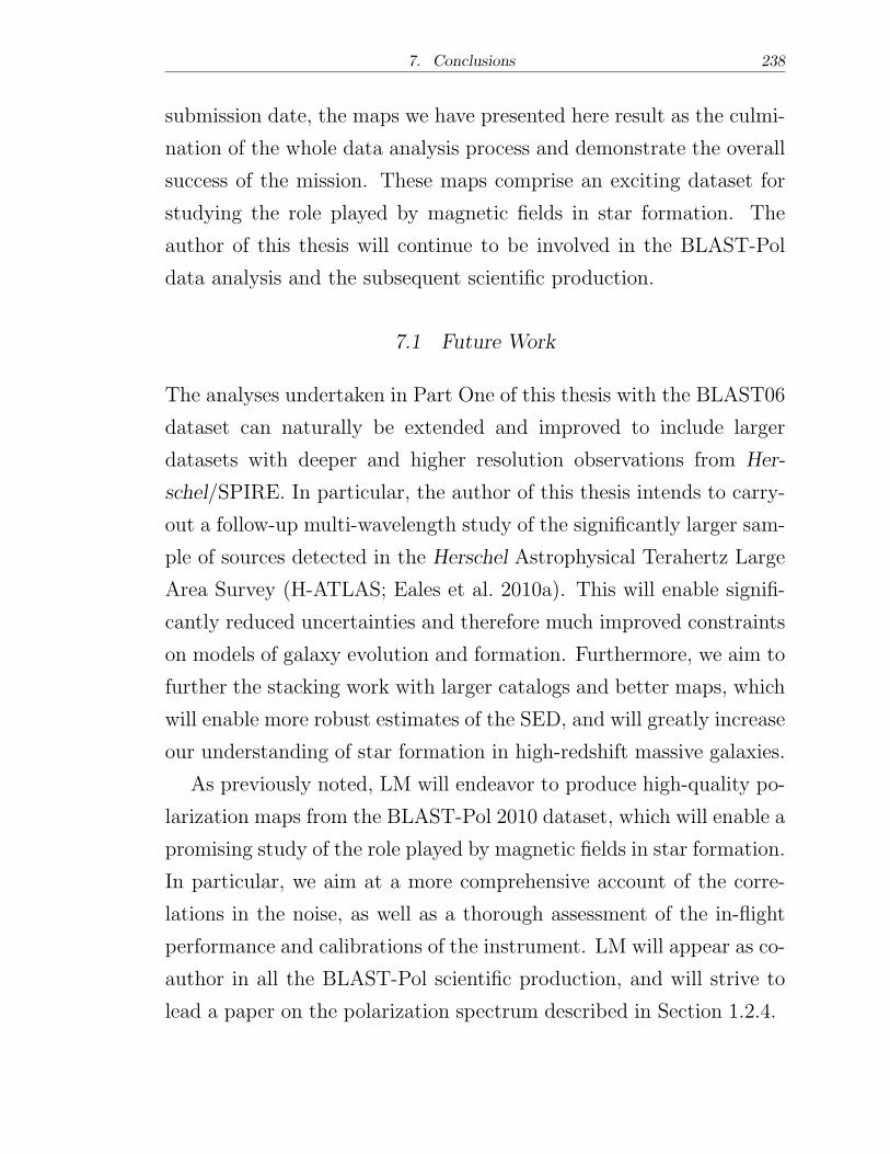
7. Conclusions 238
submission date, the maps we have presented here result as the culmi-
nation of the whole data analysis process and demonstrate the overall
success of the mission. These maps comprise an exciting dataset for
studying the role played by magnetic fields in star formation. The
author of this thesis will continue to be involved in the BLAST-Pol
data analysis and the subsequent scientific production.
7.1 Future Work
The analyses undertaken in Part One of this thesis with the BLAST06
dataset can naturally be extended and improved to include larger
datasets with deeper and higher resolution observations from Her-
schel/SPIRE. In particular, the author of this thesis intends to carry-
out a follow-up multi-wavelength study of the significantly larger sam-
ple of sources detected in the Herschel Astrophysical Terahertz Large
Area Survey (H-ATLAS; Eales et al. 2010a). This will enable signifi-
cantly reduced uncertainties and therefore much improved constraints
on models of galaxy evolution and formation. Furthermore, we aim to
further the stacking work with larger catalogs and better maps, which
will enable more robust estimates of the SED, and will greatly increase
our understanding of star formation in high-redshift massive galaxies.
As previously noted, LM will endeavor to produce high-quality po-
larization maps from the BLAST-Pol 2010 dataset, which will enable a
promising study of the role played by magnetic fields in star formation.
In particular, we aim at a more comprehensive account of the corre-
lations in the noise, as well as a thorough assessment of the in-flight
performance and calibrations of the instrument. LM will appear as co-
author in all the BLAST-Pol scientific production, and will strive to
lead a paper on the polarization spectrum described in Section 1.2.4.

APPENDIX
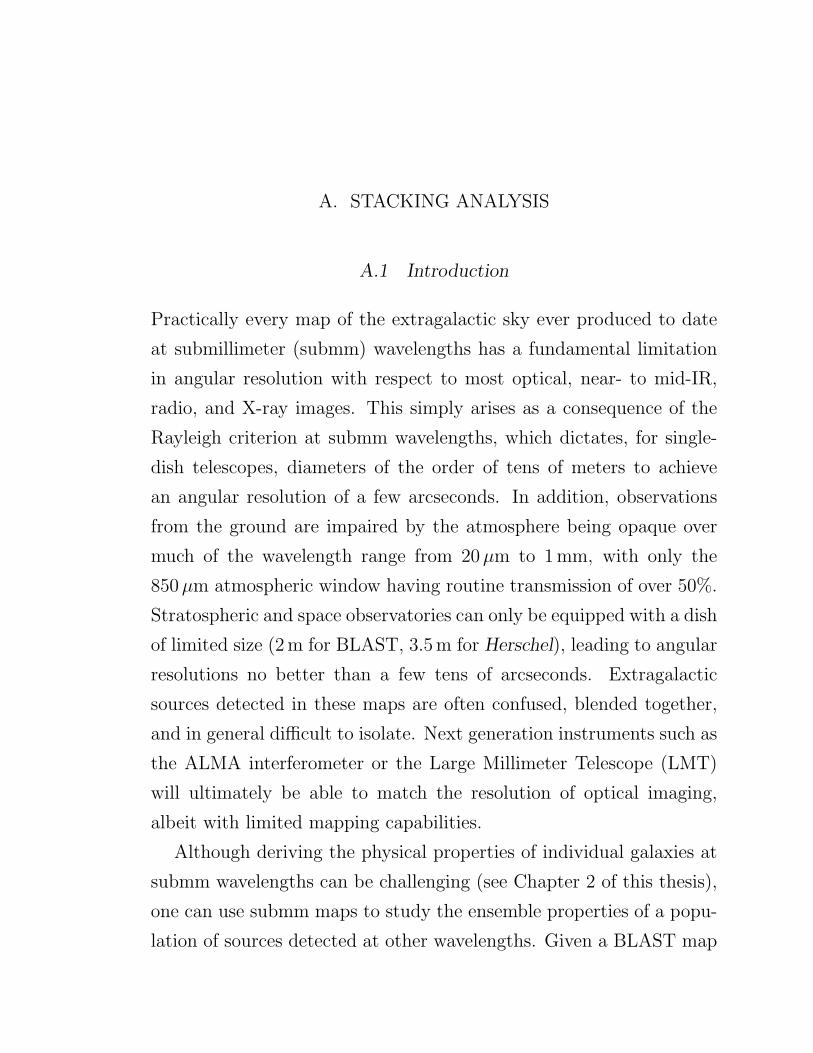
A. STACKING ANALYSIS
A.1 Introduction
Practically every map of the extragalactic sky ever produced to date
at submillimeter (submm) wavelengths has a fundamental limitation
in angular resolution with respect to most optical, near- to mid-IR,
radio, and X-ray images. This simply arises as a consequence of the
Rayleigh criterion at submm wavelengths, which dictates, for single-
dish telescopes, diameters of the order of tens of meters to achieve
an angular resolution of a few arcseconds. In addition, observations
from the ground are impaired by the atmosphere being opaque over
much of the wavelength range from 20�m to 1mm, with only the
850�m atmospheric window having routine transmission of over 50%.
Stratospheric and space observatories can only be equipped with a dish
of limited size (2m for BLAST, 3.5m for Herschel), leading to angular
resolutions no better than a few tens of arcseconds. Extragalactic
sources detected in these maps are often confused, blended together,
and in general difficult to isolate. Next generation instruments such as
the ALMA interferometer or the Large Millimeter Telescope (LMT)
will ultimately be able to match the resolution of optical imaging,
albeit with limited mapping capabilities.
Although deriving the physical properties of individual galaxies at
submm wavelengths can be challenging (see Chapter 2 of this thesis),
one can use submm maps to study the ensemble properties of a popu-
lation of sources detected at other wavelengths. Given a BLAST map
A. Stacking Analysis 241
and an external catalog, we can estimate the average brightness of
an externally-selected population of galaxies at the BLAST frequen-
cies by taking postage-stamps of the BLAST map, at the positions
of the external catalog, and stacking them together to form a unique,
higher signal-to-noise image. This technique is often referred to as
“stacking analysis”. As we will show in the following sections, not
only does stacking naturally provide a way around the poor resolution
of submm maps, but also greatly enhances the signal-to-noise ratio
of objects too faint to be individually detected; the combination of
these two virtues effectively allows stacking to push flux density mea-
surements beyond the confusion limit. Technical questions often arise
about the generalization of this technique to very high source density
or about the exclusion of bright sources: we review the mathematical
formalism in Section A.2, and find that many of these misconceptions
are avoided when one realizes that the technique is really one of tak-
ing the covariance of the map with the catalog. In Section A.3, we
formally show how aperture photometry can be safely performed to
measure the stacked flux density. In Section A.4, we detail how to
estimate uncertainties on the measured stacked values that include
both instrumental and confusion noise. In Section A.5, we describe
the catalogs used and present some of the stacked images. Finally,
in Section A.6, we show how stacking analysis can provide additional
information on the effective shape of the point-spread function (PSF)
of BLAST, as well as being an effective diagnostic tool for pointing
errors and astrometry registration.
For brevity, we choose not to report in this thesis all of the scientific
results of this analysis, except for those presented in Chapter 3. In
particular, we omit here the findings based on splitting up a catalog
in bins of, e.g., 24�m flux density or redshift, which are extensively
A. Stacking Analysis 242
described in Devlin et al. (2009), Pascale et al. (2009) and Marsden
et al. (2009).
A.2 Mathematical Formalism
Imagine we have a map of the sky where Mj is the flux density in
each pixel j. Suppose also that we have one or several independent
catalogs of sources made from other experiments, potentially at dif-
ferent wavelengths; catalog C� has N j� sources in pixel j, and we want
to measure the mean flux density, S�, of the sources in C�. Let us
denote the mean of N j� as ��, the average number of sources per pixel
in list C�. If objects in the catalog produce flux densities that are S�
on average, then, along with whatever else is in the sky, there will be
a contribution Sj� = S�N
j� to each pixel.
If a sky containing this signal were observed with BLAST, the re-
sulting map would be the convolution of Sj� with the instrumental PSF,
and with a mean of zero (because BLAST is a relative photometer).
We can write the flux density in the map as
Mj = nj +∑
�
S�
(
N j� − ��
)
, (A.1)
where nj is the contribution of detector noise in pixel j, and, strictly
speaking, the S� form the complete set of all objects in the Universe.
The mean in the map is removed by subtracting S� �� for each catalog
from every pixel. We additionally require that nj has a mean of zero.
In order for stacking analysis to provide an unbiased estimate of
the average brightness of an externally-selected population of galax-
ies at the BLAST wavelengths, we postulate that the sources in the
catalog are not spatially correlated (or “clustered”, as often referred
to in the literature), such that N j� is a random, Poisson-distributed
A. Stacking Analysis 243
number1. Furthermore, we assume that no two lists are correlated, so
that⟨
(
N j� − ��
) (
N j� − ��
)
⟩
= 0, ∀� ∕= �.
We emphasize here that our goal is to determine the mean flux
density per source in a catalog, from knowledge of the submm map,
Mj, and the locations, N j�, of the sources in C�, but without any
other information. This problem can be approached by considering
our map and our external catalog distribution as shapes on the sky;
the amplitude, S�, of Nj� that matchesMj can be quantified by writing
their covariance:
Cov(Mj, Nj�) =
1
Npix
∑
j
MjNj�
=S�
Npix
[
∑
j
(
N j�
)2 − ��∑
j
N j�
]
, (A.2)
where Npix is the total number of pixels in the map, and the terms
in N j�N
j� and N j
� nj vanish in the sum. We notice that the term in
square parentheses in Equation (A.2) divided by Npix is nothing else
but the definition of variance for N j�, and therefore equals �� for a
Poisson-distributed source list.
The net result is that the zero-lag cross-correlation (covariance)
of a catalog with the map divided by the mean number of sources
per pixel is an estimate of the average flux density per source. An
additional re-arrangement of Equation (A.2) makes this result more
useful. Notice that the sum runs over all pixels, with the weight of
each pixel proportional to the number of catalog sources found in it,
and that zero weight is given to pixels that do not contain a source
(N j� = 0). This can be written as a sum over all catalog entries with
1 We refer to Section 3.3 and Figure 3 of Marsden et al. (2009) for an exhaustive test of thisassumption. We also point out that the “catalog clustering” discussed here should not be confusedwith the source clustering detected in the BLAST maps by Viero et al. (2009).
A. Stacking Analysis 244
unit weight:
S� =Cov(Mj, N
j�)
��=
1
Npix ��
∑
j
MjNj� =
1
n�
∑
k
Mk, (A.3)
where k is the index of sources in catalog C�, Mk is the measured
flux density in the map pixel that contains the kth catalog entry, and
n� is the total number of catalog entries, n� = Npix ��. This expres-
sion is the simple average flux density in the map over all positions
in the source catalog; as anticipated above, it can be used to probe
the ensemble properties of sources much too crowded to be detected
individually, and also those with flux densities that are much fainter
than the typical thresholds of source catalogs derived only from the
map itself.
Perhaps counterintuitively, in the absence of clustering of the source
catalog, no additional correction is needed, even for cases in which the
catalog has a very high source density (e.g., a few sources per submm
beam). One other assumption made is that the instrumental noise
is well-behaved, i.e. ⟨nj = 0⟩. Since the map pixel noises nj are not
uniform across the map, we weight the mean in Equation (A.3) by the
inverse pixel variance to maximize the S/N ratio of S�. We will show
in Section A.4 how to estimate the uncertainty on S� by repeating the
stacking for a set of random locations in the map, and by measuring
the sample standard deviation of the resulting stacks. This procedure
accounts for uncertainties caused both by instrumental and confusion
noise.
Equation (A.3) provides a robust estimate of the mean brightness
per source even when there are other, possibly substantial, contrib-
utors to the flux density present, C�. This is provided that N j� is
Poisson distributed, and N j� is not correlated with either the detector

A. Stacking Analysis 245
noise or sources in C�. In other words, the effect of other sources on
the estimator S� is to provide an additional source of noise. This noise
may potentially be asymmetric, but it has a mean of zero, such that
S� is unbiased. Similarly, a catalog C� can be subdivided into disjoint
subsets, and the mean brightness due to each subset can be measured
without bias. We use this fact to split up our catalogs based on 24�m
flux density or redshift (see Pascale et al. 2009).
We are now in a position to address the proper handling of sources
that are bright enough to be easily recognized in the maps, for example
the sources in a BLAST 5 � catalog. We have shown that S�, our esti-
mate of S�, is not affected by either the presence or the removal of flux
density from other source lists C� that are uncorrelated with C�. How-
ever, since the sum of confusion noise and detector noise, S�Nj� + nj,
will cause sources near the threshold to be accidentally included or ex-
cluded from the BLAST catalog, any list made from the BLAST maps
themselves will be artificially correlated with all the terms in Equa-
tion (A.1). Furthermore, since the BLAST-generated bright source
catalog depends on the sum of the other terms in Equation (A.1), ex-
cision of the flux density from such a catalog will artificially correlate
the remaining terms, such as (N j�−��) and nj. This introduces a bias
in our estimator S� that is difficult to quantify. Therefore, stacking is
performed on the full BLAST maps, including any bright sources they
contain.
A.3 Aperture Photometry Method
In the previous section, we have outlined the mathematical formalism
behind stacking analysis, starting from a catalog of sources and a map
of the sky in units of flux density (Jy). Such a map is presumably the
A. Stacking Analysis 246
result of the cross-correlation (convolution) of the raw map with the
instrumental PSF: this operation is optimal for the case of an isolated
point source in a field of statistically uncorrelated noise, and gives the
maximum-likelihood flux density of a point-source fit to every position
in the map (see, e.g., Stetson 1987). Alternatively, the flux density
of a stack of postage-stamps, centered at the catalog positions and
extracted from a raw submm map (with units of MJy/sr or Jy/pixel),
can be measured via aperture photometry.
Let Mij be our submm map and c�ij a list of positions from the
catalog C�. In the previous section, we have shown that the total flux,
F , in Mij associated with C� can be written as
F =∑
�
∑
ij
c�ijMi+ , j+�, (A.4)
where the indices [ , �] indicate the sum over a circular aperture of
some radius (i.e., aperture photometry), while [i, j] run over the map’s
pixels.
If the sources from C� have a mean flux S� in our map, then Mij
can be expressed as a PSF-convolution of the c�ij, as follows:
Mij = S�
∑
kw
c�kwBi−k, j−w, (A.5)
where Bkw is our best-estimate, pixelated instrumental PSF (or beam).
Consequently, Equation (A.4) becomes
F = S�
∑
�
∑
ij
∑
kw
c�ij c�kwBi+ −k, j+�−w. (A.6)
A. Stacking Analysis 247
The mean flux, ⟨F ⟩, is then
⟨F ⟩ = S�
∑
�
∑
ij
∑
kw
⟨
c�ij c�kw
⟩
Bi+ −k, j+�−w
= S�
∑
�
∑
ij ∕=kw
⟨
c�ij c�kw
⟩
Bi+ −k, j+�−w +
+ S�
∑
�
∑
ij=kw
⟨
c�ij c�kw
⟩
Bi+ −k, j+�−w, (A.7)
which can be rearranged as
⟨F ⟩ = S�
∑
�
∑
ij ∕=kw
⟨
c�ij c�kw
⟩
Bi+ −k, j+�−w +
+ S�
∑
�
∑
ij=kw
⟨
c�ij c�ij
⟩
B �. (A.8)
In the assumption of no clustering, we have
⟨
c�ij c�kw
⟩
=⟨
c�ij⟩
⟨c�kw⟩ = �2�, ij ∕= kw,⟨
c�ij c�ij
⟩
= Var(
c�ij)
+⟨
c�ij⟩2
= �� + �2�, ij = kw,(A.9)
where �� =⟨
c�ij⟩
is the expected value of the Poisson-distributed
stochastic variable c�ij. Therefore Equation (A.8) becomes
⟨F ⟩ = S� �2�
∑
�
∑
ij ∕=kw
Bi+ −k, j+�−w +
+ S�
(
�� + �2�)
∑
�
∑
ij=kw
B �
= S� �2�
∑
�
∑
ij
∑
kw
Bi+ −k, j+�−w +
+ S� ��∑
�
∑
ij
B �. (A.10)
A. Stacking Analysis 248
Because the beam integrates to unity, we obtain
⟨F ⟩ = S� �2�NpixA+ S� ��NpixAc
= �� S�Npix (��A+ Ac) (A.11)
where A is the area size of the aperture (in pixel) and Ac the aperture
correction (dimensionless number).
We can now account for the fact that BLAST maps have zero mean,
by modifying Equation (A.4), which becomes
⟨F ⟩ =∑
�
∑
ij
c�ij
[
Mi+ , j+� −1
Npix
∑
��
M��
]
(A.12)
Equation (A.5) changes as follows:
Mij −1
Npix
∑
��
M�� = (A.13)
= S�
∑
kw
c�kwBi−k, j−w − S�1
Npix
∑
��
∑
kw
c�kwB�−k, �−w
= S�
∑
kw
c�kwBi−k, j−w − S� ��,
where the last equality holds, again, because the beam integrates to
unity. Inserting Equation (A.13) into Equation (A.12), we easily ob-
tain the equivalent of Equation (A.11), which now finally reads
⟨F ⟩ = �� S�NpixAc. (A.14)
Equation (A.14), analogous and equally simple to Equation (A.3),
gives the expression for the average flux density at submm wavelengths
of an externally-selected population of sources as a function of the
total stacked flux retrieved (and appropriately corrected) via aperture
photometry.
A. Stacking Analysis 249
Finally, there are a few important technicalities worth mentioning
here about aperture photometry applied to our case. First, we de-
liberately set the value of the sky background to zero, since we have
ensured that the region where the stacking is performed has zero mean.
Second, the aperture radii chosen at the different channels are those
maximizing the signal-to-noise2 ratio, as computed by performing the
stacking on BLAST noise maps, in a totally analogous way to the pre-
viously discussed signal maps. For BLAST, these turn out to be 30,
30, and 40′′ at 250, 350, and 500�m, respectively. Third, the aper-
ture corrections are evaluated by performing aperture photometry on
the PSFs themselves, with the same aperture radii as above. The re-
sulting values are, 1.985, 1.906 and 1.966 at 250, 350, and 500�m,
respectively.
A.4 Uncertainties
In order to estimate the uncertainty of Equation (A.3) (and A.14)
algebraically for a catalog C�, one would need to know the scatter
produced by the catalog of all sources not in C� that contribute to
the background (in addition to sources of instrumental noise) in the
submm maps. In practice, such a catalog is not known, so we estab-
lish the uncertainties and possible biases of our measurements via a
Monte Carlo technique, by generating random catalogs and stacking
them on the submm maps under analysis. Namely, we stack N� (the
actual number of sources in the catalog or sub-catalog under analysis)
postage-stamps centered at random positions within the region of sky
under consideration; we then measure the mean flux density of such
2 Note that here“noise” is just estimated by co-adding the BLAST variance map, which is not themost appropriate estimate of the noise associated with the measured average flux density, becauseit does not account for the confusion noise in the map (see Section A.4)
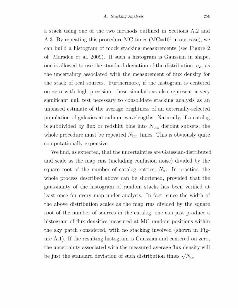
A. Stacking Analysis 250
a stack using one of the two methods outlined in Sections A.2 and
A.3. By repeating this procedure MC times (MC=105 in our case), we
can build a histogram of mock stacking measurements (see Figure 2
of Marsden et al. 2009). If such a histogram is Gaussian in shape,
one is allowed to use the standard deviation of the distribution, ��, as
the uncertainty associated with the measurement of flux density for
the stack of real sources. Furthermore, if the histogram is centered
on zero with high precision, these simulations also represent a very
significant null test necessary to consolidate stacking analysis as an
unbiased estimate of the average brightness of an externally-selected
population of galaxies at submm wavelengths. Naturally, if a catalog
is subdivided by flux or redshift bins into Nbin disjoint subsets, the
whole procedure must be repeated Nbin times. This is obviously quite
computationally expensive.
We find, as expected, that the uncertainties are Gaussian-distributed
and scale as the map rms (including confusion noise) divided by the
square root of the number of catalog entries, N�. In practice, the
whole process described above can be shortened, provided that the
gaussianity of the histogram of random stacks has been verified at
least once for every map under analysis. In fact, since the width of
the above distribution scales as the map rms divided by the square
root of the number of sources in the catalog, one can just produce a
histogram of flux densities measured at MC random positions within
the sky patch considered, with no stacking involved (shown in Fig-
ure A.1). If the resulting histogram is Gaussian and centered on zero,
the uncertainty associated with the measured average flux density will
be just the standard deviation of such distribution times√N�.
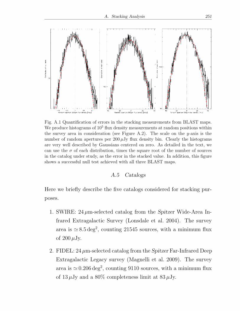
A. Stacking Analysis 251
Fig. A.1 Quantification of errors in the stacking measurements from BLAST maps.We produce histograms of 105 flux density measurements at random positions withinthe survey area in consideration (see Figure A.2). The scale on the y-axis is thenumber of random apertures per 200�Jy flux density bin. Clearly the histogramsare very well described by Gaussians centered on zero. As detailed in the text, wecan use the � of each distribution, times the square root of the number of sourcesin the catalog under study, as the error in the stacked value. In addition, this figureshows a successful null test achieved with all three BLAST maps.
A.5 Catalogs
Here we briefly describe the five catalogs considered for stacking pur-
poses.
1. SWIRE: 24�m-selected catalog from the Spitzer Wide-Area In-
frared Extragalactic Survey (Lonsdale et al. 2004). The survey
area is ≃ 8.5 deg2, counting 21545 sources, with a minimum flux
of 200�Jy.
2. FIDEL: 24�m-selected catalog from the Spitzer Far-Infrared Deep
Extragalactic Legacy survey (Magnelli et al. 2009). The survey
area is ≃ 0.206 deg2, counting 9110 sources, with a minimum flux
of 13�Jy and a 80% completeness limit at 83�Jy.
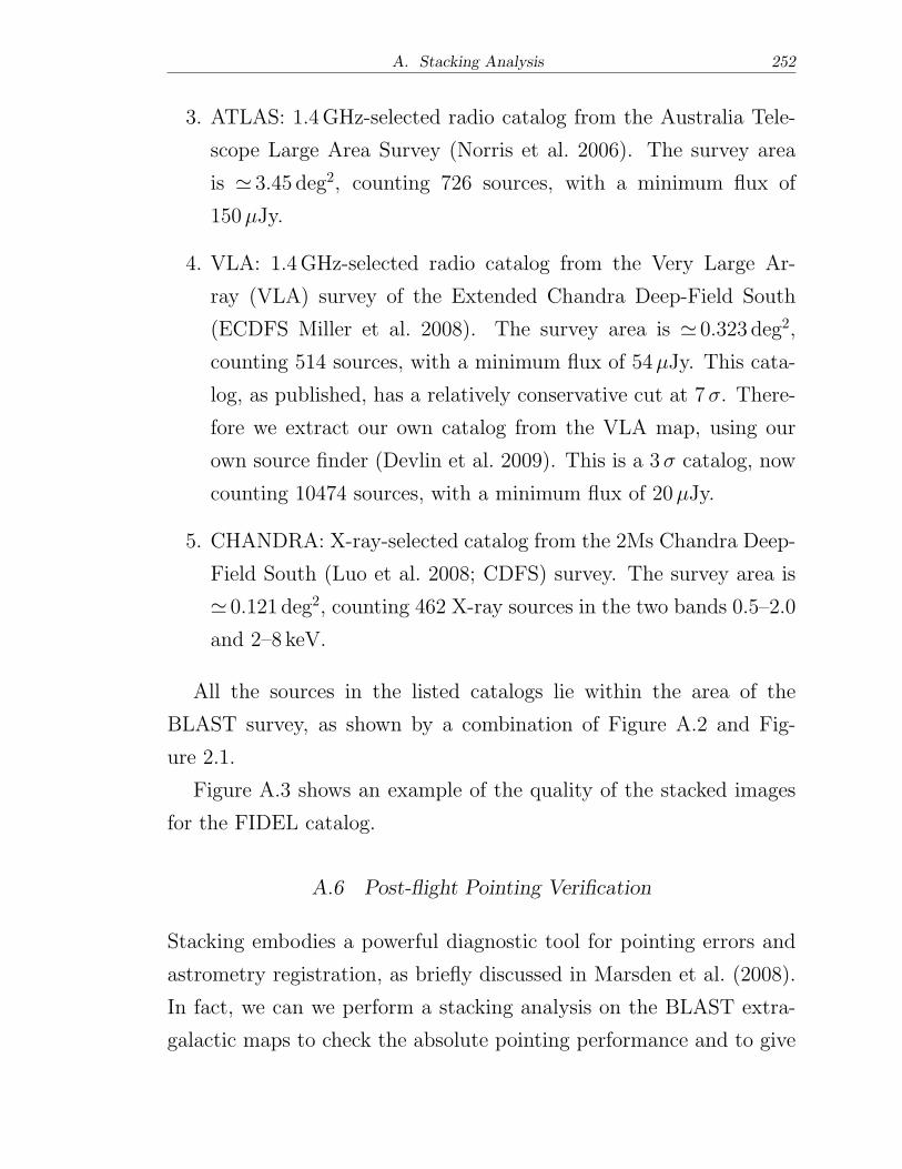
A. Stacking Analysis 252
3. ATLAS: 1.4GHz-selected radio catalog from the Australia Tele-
scope Large Area Survey (Norris et al. 2006). The survey area
is ≃ 3.45 deg2, counting 726 sources, with a minimum flux of
150�Jy.
4. VLA: 1.4GHz-selected radio catalog from the Very Large Ar-
ray (VLA) survey of the Extended Chandra Deep-Field South
(ECDFS Miller et al. 2008). The survey area is ≃ 0.323 deg2,
counting 514 sources, with a minimum flux of 54�Jy. This cata-
log, as published, has a relatively conservative cut at 7�. There-
fore we extract our own catalog from the VLA map, using our
own source finder (Devlin et al. 2009). This is a 3� catalog, now
counting 10474 sources, with a minimum flux of 20�Jy.
5. CHANDRA: X-ray-selected catalog from the 2Ms Chandra Deep-
Field South (Luo et al. 2008; CDFS) survey. The survey area is
≃ 0.121 deg2, counting 462 X-ray sources in the two bands 0.5–2.0
and 2–8 keV.
All the sources in the listed catalogs lie within the area of the
BLAST survey, as shown by a combination of Figure A.2 and Fig-
ure 2.1.
Figure A.3 shows an example of the quality of the stacked images
for the FIDEL catalog.
A.6 Post-flight Pointing Verification
Stacking embodies a powerful diagnostic tool for pointing errors and
astrometry registration, as briefly discussed in Marsden et al. (2008).
In fact, we can we perform a stacking analysis on the BLAST extra-
galactic maps to check the absolute pointing performance and to give
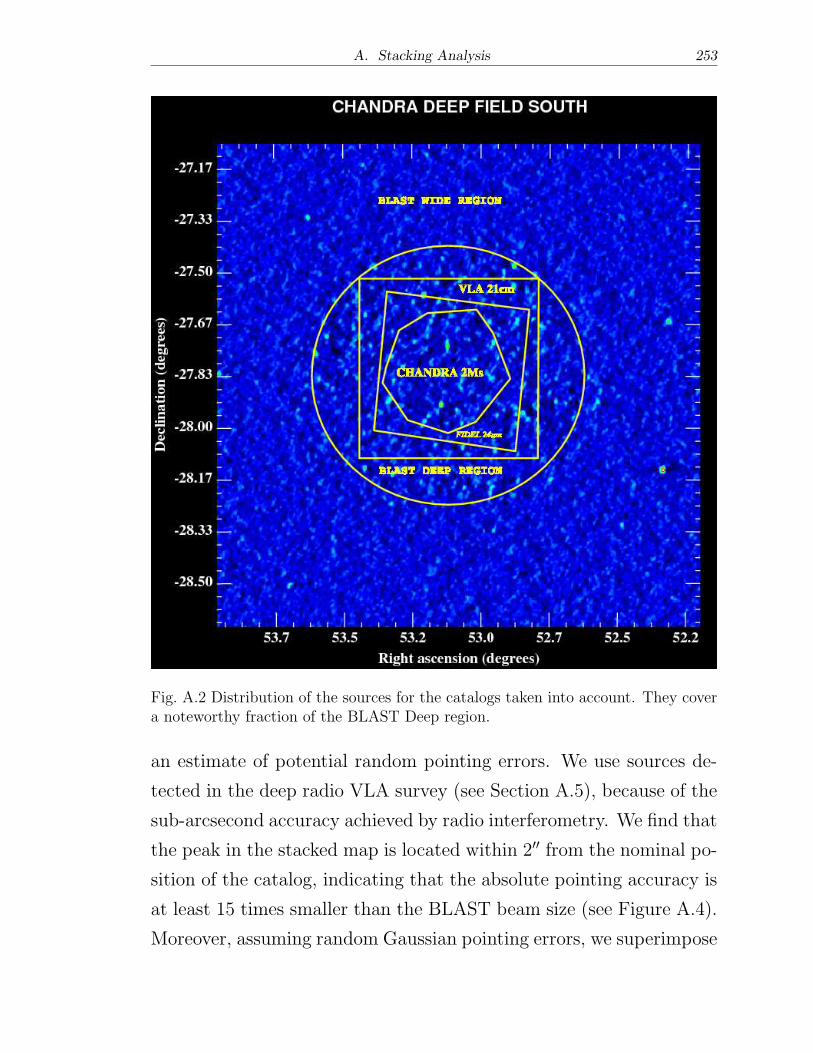
A. Stacking Analysis 253
Fig. A.2 Distribution of the sources for the catalogs taken into account. They covera noteworthy fraction of the BLAST Deep region.
an estimate of potential random pointing errors. We use sources de-
tected in the deep radio VLA survey (see Section A.5), because of the
sub-arcsecond accuracy achieved by radio interferometry. We find that
the peak in the stacked map is located within 2′′ from the nominal po-
sition of the catalog, indicating that the absolute pointing accuracy is
at least 15 times smaller than the BLAST beam size (see Figure A.4).
Moreover, assuming random Gaussian pointing errors, we superimpose
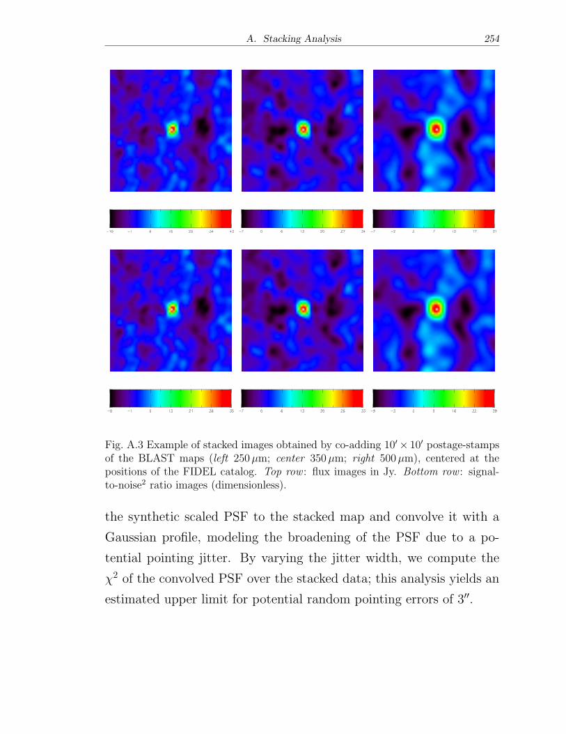
A. Stacking Analysis 254
Fig. A.3 Example of stacked images obtained by co-adding 10′× 10′ postage-stampsof the BLAST maps (left 250�m; center 350�m; right 500�m), centered at thepositions of the FIDEL catalog. Top row : flux images in Jy. Bottom row : signal-to-noise2 ratio images (dimensionless).
the synthetic scaled PSF to the stacked map and convolve it with a
Gaussian profile, modeling the broadening of the PSF due to a po-
tential pointing jitter. By varying the jitter width, we compute the
�2 of the convolved PSF over the stacked data; this analysis yields an
estimated upper limit for potential random pointing errors of 3′′.
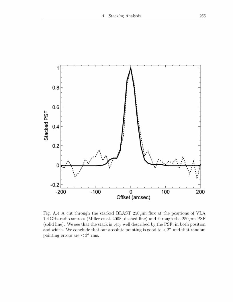
A. Stacking Analysis 255
Fig. A.4 A cut through the stacked BLAST 250�m flux at the positions of VLA1.4GHz radio sources (Miller et al. 2008; dashed line) and through the 250�m PSF(solid line). We see that the stack is very well described by the PSF, in both positionand width. We conclude that our absolute pointing is good to < 2′′ and that randompointing errors are < 3′′ rms.
B. POSTAGE STAMPS OF BLAST COUNTERPARTS
The broad morphological classification of the BLAST IDs presented
in this work is based upon visual inspection of UV, optical, and MIR
postage-stamp images (see Sections 2.2.5 and 2.7). A selection of 2′×2′
cutouts is shown in Figure B1. The complete set of full-color cutouts
can be found at:
http://blastexperiment.info/results images/moncelsi/.
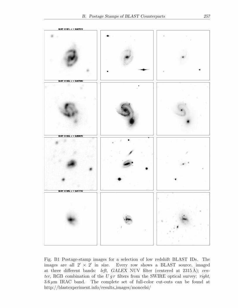
B. Postage Stamps of BLAST Counterparts 257
Fig. B1 Postage-stamp images for a selection of low redshift BLAST IDs. Theimages are all 2′ × 2′ in size. Every row shows a BLAST source, imagedat three different bands: left, GALEX NUV filter (centered at 2315 A); cen-
ter, RGB combination of the U g r filters from the SWIRE optical survey; right,3.6�m IRAC band. The complete set of full-color cut-outs can be found athttp://blastexperiment.info/results images/moncelsi/
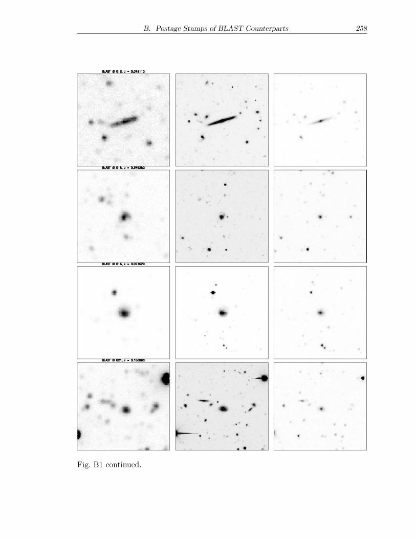
B. Postage Stamps of BLAST Counterparts 258
Fig. B1 continued.
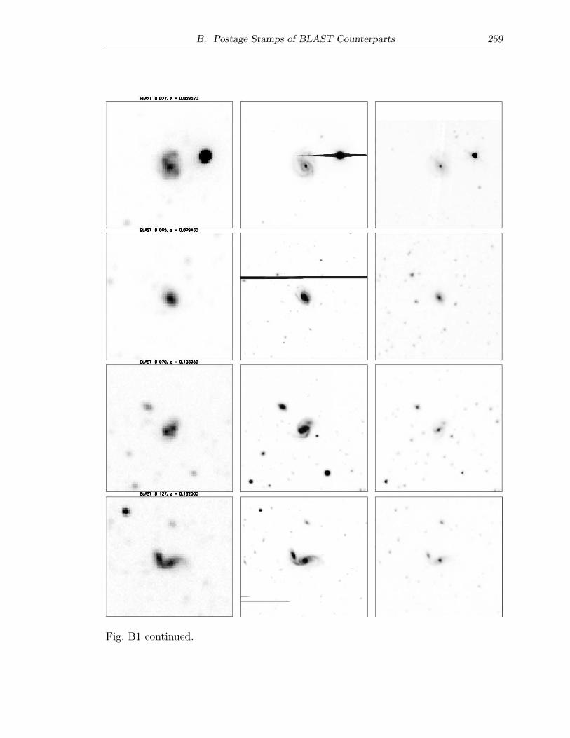
B. Postage Stamps of BLAST Counterparts 259
Fig. B1 continued.
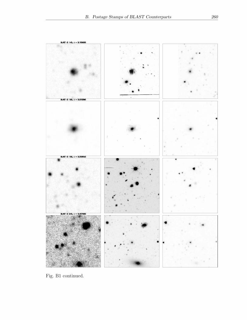
B. Postage Stamps of BLAST Counterparts 260
Fig. B1 continued.
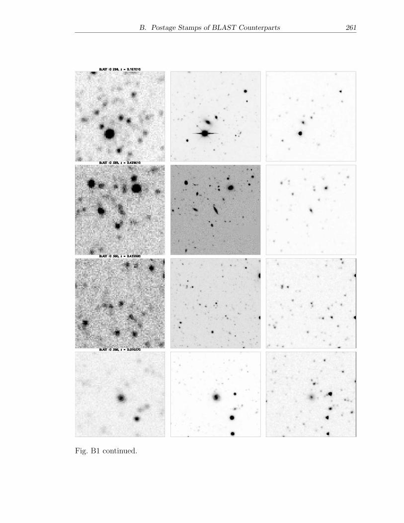
B. Postage Stamps of BLAST Counterparts 261
Fig. B1 continued.
C. CATALOGS OF BLAST COUNTERPARTS
We present here the catalogs of the primary counterparts to ≥ 5�
BLAST sources. Table C1 contains the redshifts, the spectral infor-
mation and the morphology while Table C2 lists the UV and FIR
properties.
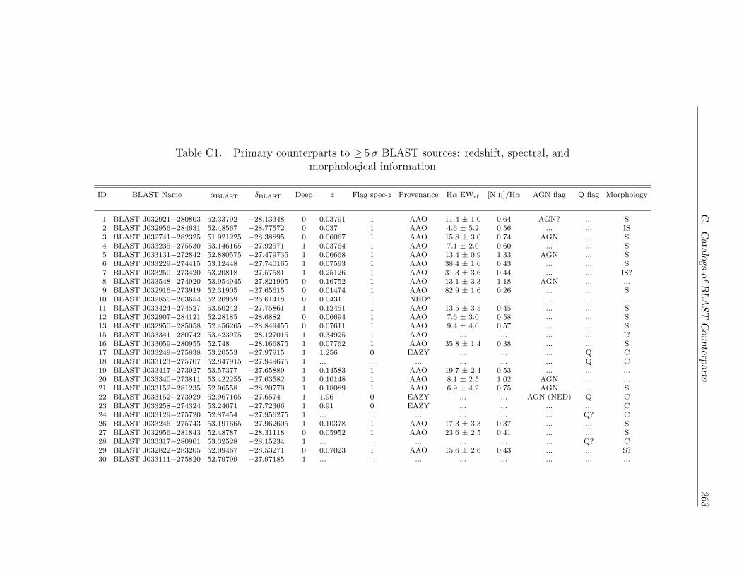
C.CatalogsofBLAST
Counterp
arts
263
Table C1. Primary counterparts to ≥ 5� BLAST sources: redshift, spectral, andmorphological information
ID BLAST Name �BLAST �BLAST Deep z Flag spec-z Provenance H� EWrf [N II]/H� AGN flag Q flag Morphology
1 BLAST J032921−280803 52.33792 −28.13348 0 0.03791 1 AAO 11.4 ± 1.0 0.64 AGN? ... S2 BLAST J032956−284631 52.48567 −28.77572 0 0.037 1 AAO 4.6 ± 5.2 0.56 ... ... IS3 BLAST J032741−282325 51.921225 −28.38895 0 0.06067 1 AAO 15.8 ± 3.0 0.74 AGN ... S4 BLAST J033235−275530 53.146165 −27.92571 1 0.03764 1 AAO 7.1 ± 2.0 0.60 ... ... S5 BLAST J033131−272842 52.880575 −27.479735 1 0.06668 1 AAO 13.4 ± 0.9 1.33 AGN ... S6 BLAST J033229−274415 53.12448 −27.740165 1 0.07593 1 AAO 38.4 ± 1.6 0.43 ... ... S7 BLAST J033250−273420 53.20818 −27.57581 1 0.25126 1 AAO 31.3 ± 3.6 0.44 ... ... IS?8 BLAST J033548−274920 53.954945 −27.821905 0 0.16752 1 AAO 13.1 ± 3.3 1.18 AGN ... ...9 BLAST J032916−273919 52.31905 −27.65615 0 0.01474 1 AAO 82.9 ± 1.6 0.26 ... ... S
10 BLAST J032850−263654 52.20959 −26.61418 0 0.0431 1 NEDa ... ... ... ... ...11 BLAST J033424−274527 53.60242 −27.75861 1 0.12451 1 AAO 13.5 ± 3.5 0.45 ... ... S12 BLAST J032907−284121 52.28185 −28.6882 0 0.06694 1 AAO 7.6 ± 3.0 0.58 ... ... S13 BLAST J032950−285058 52.456265 −28.849455 0 0.07611 1 AAO 9.4 ± 4.6 0.57 ... ... S15 BLAST J033341−280742 53.423975 −28.127015 1 0.34925 1 AAO ... ... ... ... I?16 BLAST J033059−280955 52.748 −28.166875 1 0.07762 1 AAO 35.8 ± 1.4 0.38 ... ... S17 BLAST J033249−275838 53.20553 −27.97915 1 1.256 0 EAZY ... ... ... Q C18 BLAST J033123−275707 52.847915 −27.949675 1 ... ... ... ... ... ... Q C19 BLAST J033417−273927 53.57377 −27.65889 1 0.14583 1 AAO 19.7 ± 2.4 0.53 ... ... ...20 BLAST J033340−273811 53.422255 −27.63582 1 0.10148 1 AAO 8.1 ± 2.5 1.02 AGN ... ...21 BLAST J033152−281235 52.96558 −28.20779 1 0.18089 1 AAO 6.9 ± 4.2 0.75 AGN ... S22 BLAST J033152−273929 52.967105 −27.6574 1 1.96 0 EAZY ... ... AGN (NED) Q C23 BLAST J033258−274324 53.24671 −27.72366 1 0.91 0 EAZY ... ... ... ... C24 BLAST J033129−275720 52.87454 −27.956275 1 ... ... ... ... ... ... Q? C26 BLAST J033246−275743 53.191665 −27.962605 1 0.10378 1 AAO 17.3 ± 3.3 0.37 ... ... S27 BLAST J032956−281843 52.48787 −28.31118 0 0.05952 1 AAO 23.6 ± 2.5 0.41 ... ... S28 BLAST J033317−280901 53.32528 −28.15234 1 ... ... ... ... ... ... Q? C29 BLAST J032822−283205 52.09467 −28.53271 0 0.07023 1 AAO 15.6 ± 2.6 0.43 ... ... S?30 BLAST J033111−275820 52.79799 −27.97185 1 ... ... ... ... ... ... ... ...
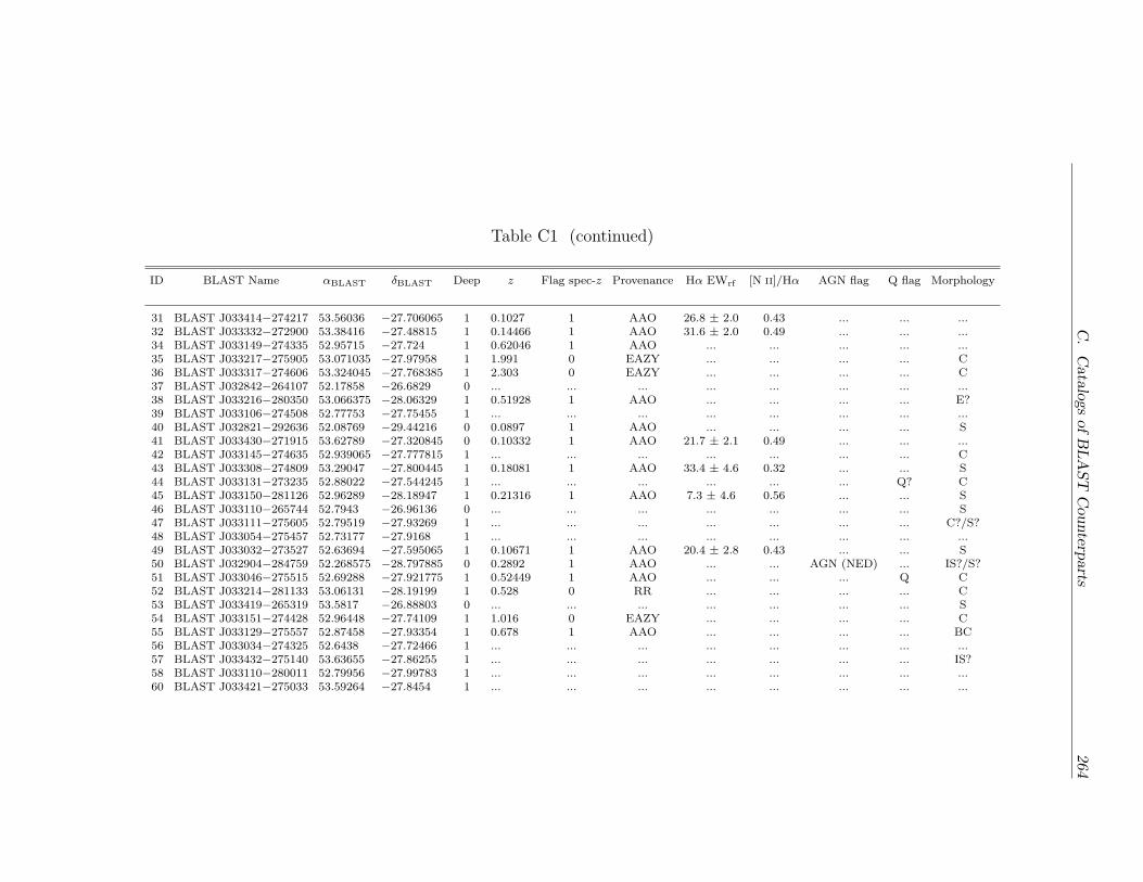
C.CatalogsofBLAST
Counterp
arts
264
Table C1 (continued)
ID BLAST Name �BLAST �BLAST Deep z Flag spec-z Provenance H� EWrf [N II]/H� AGN flag Q flag Morphology
31 BLAST J033414−274217 53.56036 −27.706065 1 0.1027 1 AAO 26.8 ± 2.0 0.43 ... ... ...32 BLAST J033332−272900 53.38416 −27.48815 1 0.14466 1 AAO 31.6 ± 2.0 0.49 ... ... ...34 BLAST J033149−274335 52.95715 −27.724 1 0.62046 1 AAO ... ... ... ... ...35 BLAST J033217−275905 53.071035 −27.97958 1 1.991 0 EAZY ... ... ... ... C36 BLAST J033317−274606 53.324045 −27.768385 1 2.303 0 EAZY ... ... ... ... C37 BLAST J032842−264107 52.17858 −26.6829 0 ... ... ... ... ... ... ... ...38 BLAST J033216−280350 53.066375 −28.06329 1 0.51928 1 AAO ... ... ... ... E?39 BLAST J033106−274508 52.77753 −27.75455 1 ... ... ... ... ... ... ... ...40 BLAST J032821−292636 52.08769 −29.44216 0 0.0897 1 AAO ... ... ... ... S41 BLAST J033430−271915 53.62789 −27.320845 0 0.10332 1 AAO 21.7 ± 2.1 0.49 ... ... ...42 BLAST J033145−274635 52.939065 −27.777815 1 ... ... ... ... ... ... ... C43 BLAST J033308−274809 53.29047 −27.800445 1 0.18081 1 AAO 33.4 ± 4.6 0.32 ... ... S44 BLAST J033131−273235 52.88022 −27.544245 1 ... ... ... ... ... ... Q? C45 BLAST J033150−281126 52.96289 −28.18947 1 0.21316 1 AAO 7.3 ± 4.6 0.56 ... ... S46 BLAST J033110−265744 52.7943 −26.96136 0 ... ... ... ... ... ... ... S47 BLAST J033111−275605 52.79519 −27.93269 1 ... ... ... ... ... ... ... C?/S?48 BLAST J033054−275457 52.73177 −27.9168 1 ... ... ... ... ... ... ... ...49 BLAST J033032−273527 52.63694 −27.595065 1 0.10671 1 AAO 20.4 ± 2.8 0.43 ... ... S50 BLAST J032904−284759 52.268575 −28.797885 0 0.2892 1 AAO ... ... AGN (NED) ... IS?/S?51 BLAST J033046−275515 52.69288 −27.921775 1 0.52449 1 AAO ... ... ... Q C52 BLAST J033214−281133 53.06131 −28.19199 1 0.528 0 RR ... ... ... ... C53 BLAST J033419−265319 53.5817 −26.88803 0 ... ... ... ... ... ... ... S54 BLAST J033151−274428 52.96448 −27.74109 1 1.016 0 EAZY ... ... ... ... C55 BLAST J033129−275557 52.87458 −27.93354 1 0.678 1 AAO ... ... ... ... BC56 BLAST J033034−274325 52.6438 −27.72466 1 ... ... ... ... ... ... ... ...57 BLAST J033432−275140 53.63655 −27.86255 1 ... ... ... ... ... ... ... IS?58 BLAST J033110−280011 52.79956 −27.99783 1 ... ... ... ... ... ... ... ...60 BLAST J033421−275033 53.59264 −27.8454 1 ... ... ... ... ... ... ... ...
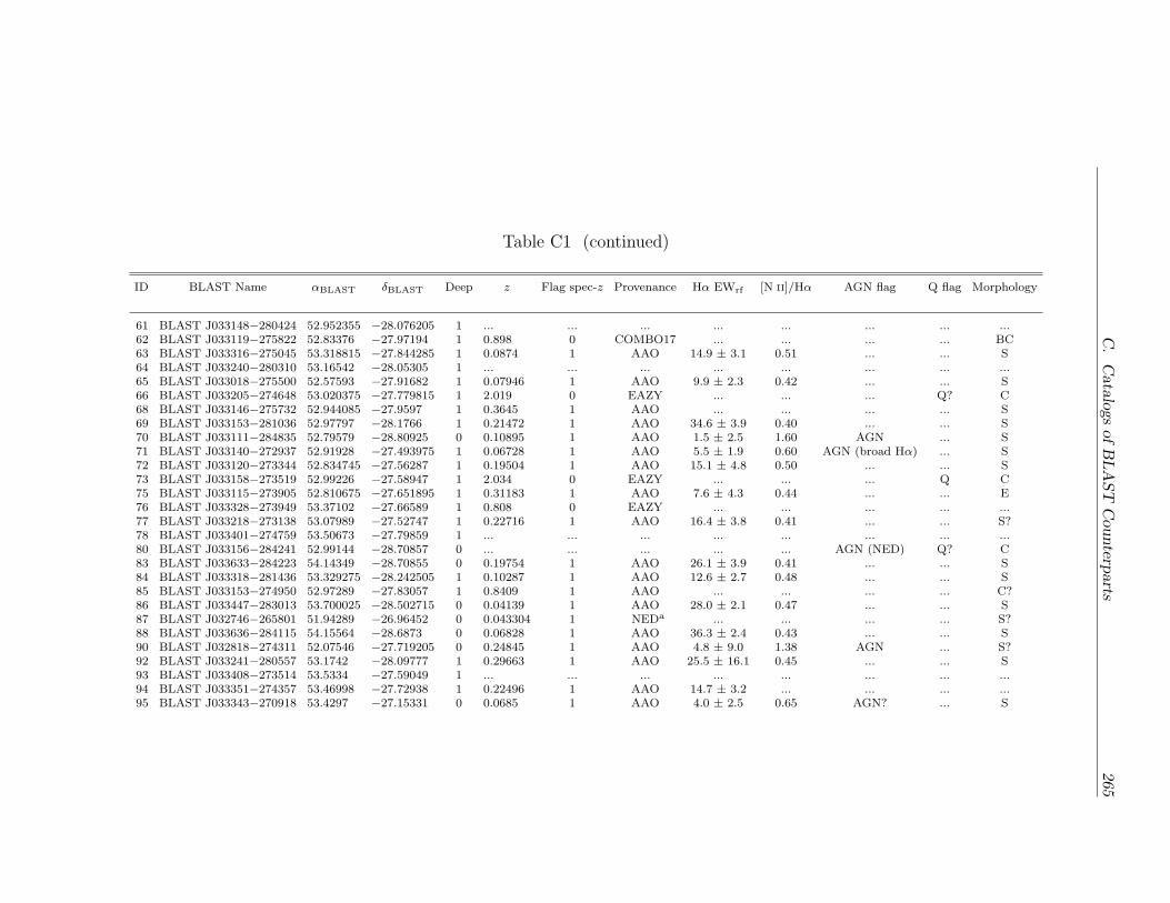
C.CatalogsofBLAST
Counterp
arts
265
Table C1 (continued)
ID BLAST Name �BLAST �BLAST Deep z Flag spec-z Provenance H� EWrf [N II]/H� AGN flag Q flag Morphology
61 BLAST J033148−280424 52.952355 −28.076205 1 ... ... ... ... ... ... ... ...62 BLAST J033119−275822 52.83376 −27.97194 1 0.898 0 COMBO17 ... ... ... ... BC63 BLAST J033316−275045 53.318815 −27.844285 1 0.0874 1 AAO 14.9 ± 3.1 0.51 ... ... S64 BLAST J033240−280310 53.16542 −28.05305 1 ... ... ... ... ... ... ... ...65 BLAST J033018−275500 52.57593 −27.91682 1 0.07946 1 AAO 9.9 ± 2.3 0.42 ... ... S66 BLAST J033205−274648 53.020375 −27.779815 1 2.019 0 EAZY ... ... ... Q? C68 BLAST J033146−275732 52.944085 −27.9597 1 0.3645 1 AAO ... ... ... ... S69 BLAST J033153−281036 52.97797 −28.1766 1 0.21472 1 AAO 34.6 ± 3.9 0.40 ... ... S70 BLAST J033111−284835 52.79579 −28.80925 0 0.10895 1 AAO 1.5 ± 2.5 1.60 AGN ... S71 BLAST J033140−272937 52.91928 −27.493975 1 0.06728 1 AAO 5.5 ± 1.9 0.60 AGN (broad H�) ... S72 BLAST J033120−273344 52.834745 −27.56287 1 0.19504 1 AAO 15.1 ± 4.8 0.50 ... ... S73 BLAST J033158−273519 52.99226 −27.58947 1 2.034 0 EAZY ... ... ... Q C75 BLAST J033115−273905 52.810675 −27.651895 1 0.31183 1 AAO 7.6 ± 4.3 0.44 ... ... E76 BLAST J033328−273949 53.37102 −27.66589 1 0.808 0 EAZY ... ... ... ... ...77 BLAST J033218−273138 53.07989 −27.52747 1 0.22716 1 AAO 16.4 ± 3.8 0.41 ... ... S?78 BLAST J033401−274759 53.50673 −27.79859 1 ... ... ... ... ... ... ... ...80 BLAST J033156−284241 52.99144 −28.70857 0 ... ... ... ... ... AGN (NED) Q? C83 BLAST J033633−284223 54.14349 −28.70855 0 0.19754 1 AAO 26.1 ± 3.9 0.41 ... ... S84 BLAST J033318−281436 53.329275 −28.242505 1 0.10287 1 AAO 12.6 ± 2.7 0.48 ... ... S85 BLAST J033153−274950 52.97289 −27.83057 1 0.8409 1 AAO ... ... ... ... C?86 BLAST J033447−283013 53.700025 −28.502715 0 0.04139 1 AAO 28.0 ± 2.1 0.47 ... ... S87 BLAST J032746−265801 51.94289 −26.96452 0 0.043304 1 NEDa ... ... ... ... S?88 BLAST J033636−284115 54.15564 −28.6873 0 0.06828 1 AAO 36.3 ± 2.4 0.43 ... ... S90 BLAST J032818−274311 52.07546 −27.719205 0 0.24845 1 AAO 4.8 ± 9.0 1.38 AGN ... S?92 BLAST J033241−280557 53.1742 −28.09777 1 0.29663 1 AAO 25.5 ± 16.1 0.45 ... ... S93 BLAST J033408−273514 53.5334 −27.59049 1 ... ... ... ... ... ... ... ...94 BLAST J033351−274357 53.46998 −27.72938 1 0.22496 1 AAO 14.7 ± 3.2 ... ... ... ...95 BLAST J033343−270918 53.4297 −27.15331 0 0.0685 1 AAO 4.0 ± 2.5 0.65 AGN? ... S
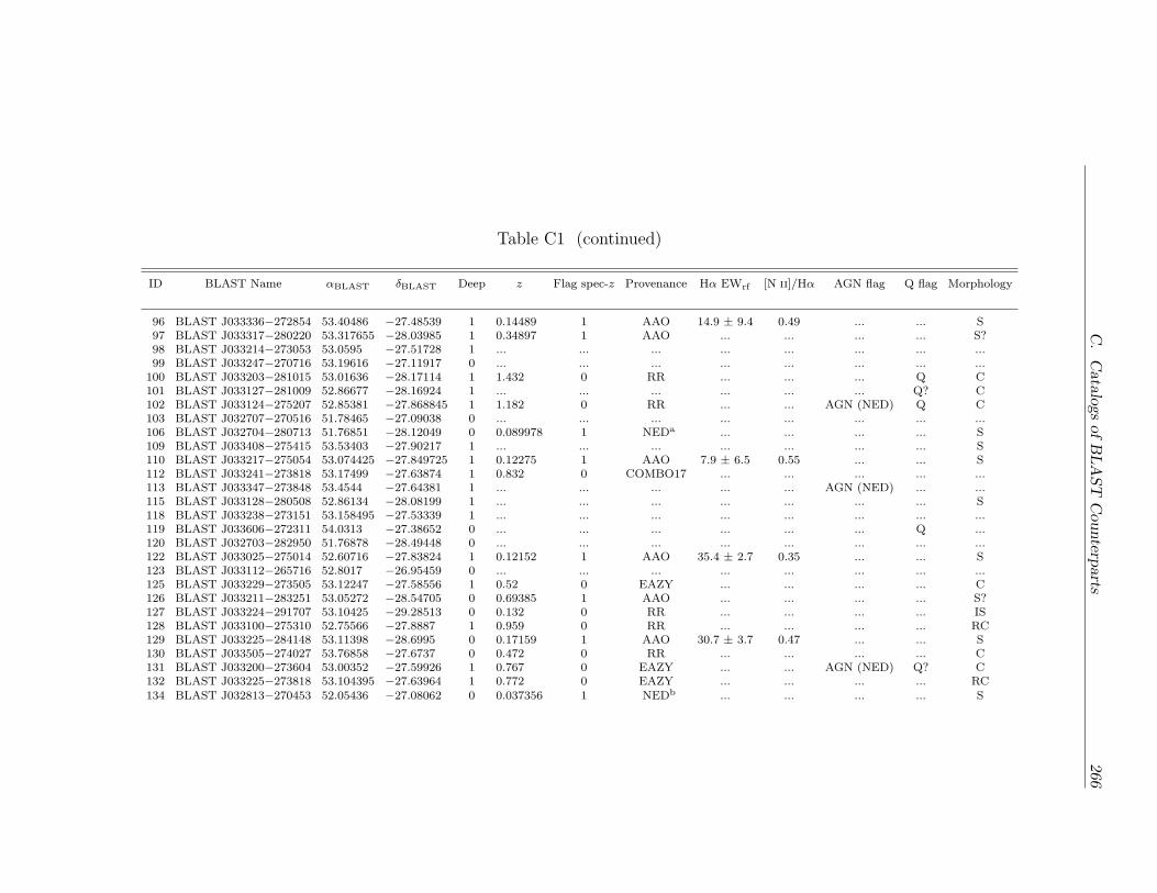
C.CatalogsofBLAST
Counterp
arts
266
Table C1 (continued)
ID BLAST Name �BLAST �BLAST Deep z Flag spec-z Provenance H� EWrf [N II]/H� AGN flag Q flag Morphology
96 BLAST J033336−272854 53.40486 −27.48539 1 0.14489 1 AAO 14.9 ± 9.4 0.49 ... ... S97 BLAST J033317−280220 53.317655 −28.03985 1 0.34897 1 AAO ... ... ... ... S?98 BLAST J033214−273053 53.0595 −27.51728 1 ... ... ... ... ... ... ... ...99 BLAST J033247−270716 53.19616 −27.11917 0 ... ... ... ... ... ... ... ...
100 BLAST J033203−281015 53.01636 −28.17114 1 1.432 0 RR ... ... ... Q C101 BLAST J033127−281009 52.86677 −28.16924 1 ... ... ... ... ... ... Q? C102 BLAST J033124−275207 52.85381 −27.868845 1 1.182 0 RR ... ... AGN (NED) Q C103 BLAST J032707−270516 51.78465 −27.09038 0 ... ... ... ... ... ... ... ...106 BLAST J032704−280713 51.76851 −28.12049 0 0.089978 1 NEDa ... ... ... ... S109 BLAST J033408−275415 53.53403 −27.90217 1 ... ... ... ... ... ... ... S110 BLAST J033217−275054 53.074425 −27.849725 1 0.12275 1 AAO 7.9 ± 6.5 0.55 ... ... S112 BLAST J033241−273818 53.17499 −27.63874 1 0.832 0 COMBO17 ... ... ... ... ...113 BLAST J033347−273848 53.4544 −27.64381 1 ... ... ... ... ... AGN (NED) ... ...115 BLAST J033128−280508 52.86134 −28.08199 1 ... ... ... ... ... ... ... S118 BLAST J033238−273151 53.158495 −27.53339 1 ... ... ... ... ... ... ... ...119 BLAST J033606−272311 54.0313 −27.38652 0 ... ... ... ... ... ... Q ...120 BLAST J032703−282950 51.76878 −28.49448 0 ... ... ... ... ... ... ... ...122 BLAST J033025−275014 52.60716 −27.83824 1 0.12152 1 AAO 35.4 ± 2.7 0.35 ... ... S123 BLAST J033112−265716 52.8017 −26.95459 0 ... ... ... ... ... ... ... ...125 BLAST J033229−273505 53.12247 −27.58556 1 0.52 0 EAZY ... ... ... ... C126 BLAST J033211−283251 53.05272 −28.54705 0 0.69385 1 AAO ... ... ... ... S?127 BLAST J033224−291707 53.10425 −29.28513 0 0.132 0 RR ... ... ... ... IS128 BLAST J033100−275310 52.75566 −27.8887 1 0.959 0 RR ... ... ... ... RC129 BLAST J033225−284148 53.11398 −28.6995 0 0.17159 1 AAO 30.7 ± 3.7 0.47 ... ... S130 BLAST J033505−274027 53.76858 −27.6737 0 0.472 0 RR ... ... ... ... C131 BLAST J033200−273604 53.00352 −27.59926 1 0.767 0 EAZY ... ... AGN (NED) Q? C132 BLAST J033225−273818 53.104395 −27.63964 1 0.772 0 EAZY ... ... ... ... RC134 BLAST J032813−270453 52.05436 −27.08062 0 0.037356 1 NEDb ... ... ... ... S
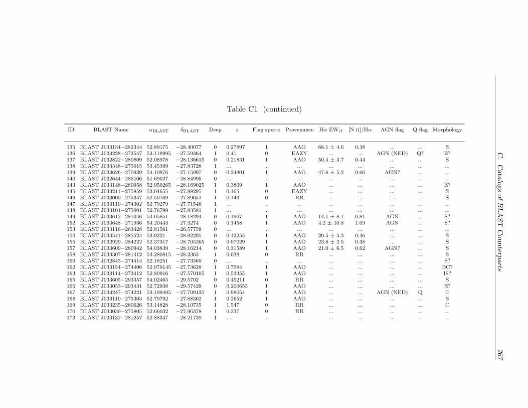
C.CatalogsofBLAST
Counterp
arts
267
Table C1 (continued)
ID BLAST Name �BLAST �BLAST Deep z Flag spec-z Provenance H� EWrf [N II]/H� AGN flag Q flag Morphology
135 BLAST J033134−282344 52.89175 −28.40077 0 0.27897 1 AAO 68.1 ± 4.6 0.38 ... ... S136 BLAST J033228−273547 53.118995 −27.59364 1 0.41 0 EAZY ... ... AGN (NED) Q? E?137 BLAST J032822−280809 52.08978 −28.136615 0 0.21831 1 AAO 50.4 ± 3.7 0.44 ... ... S138 BLAST J033348−275015 53.45399 −27.83728 1 ... ... ... ... ... ... ... ...139 BLAST J033626−270939 54.10876 −27.15997 0 0.24401 1 AAO 47.6 ± 5.2 0.66 AGN? ... ...140 BLAST J032644−285106 51.69027 −28.84995 0 ... ... ... ... ... ... ... ...143 BLAST J033148−280958 52.950265 −28.169025 1 0.3809 1 AAO ... ... ... ... E?145 BLAST J033211−275859 53.04655 −27.98295 1 0.165 0 EAZY ... ... ... ... S146 BLAST J033000−275347 52.50169 −27.89651 1 0.143 0 RR ... ... ... ... S147 BLAST J033110−274302 52.79279 −27.71546 1 ... ... ... ... ... ... ... ...148 BLAST J033104−275001 52.76799 −27.83581 1 ... ... ... ... ... ... ... ...149 BLAST J033612−281046 54.05851 −28.18294 0 0.1967 1 AAO 14.1 ± 8.1 0.81 AGN ... S?152 BLAST J033648−271936 54.20443 −27.3274 0 0.1458 1 AAO 4.2 ± 10.8 1.09 AGN ... S?153 BLAST J033116−263428 52.81561 −26.57759 0 ... ... ... ... ... ... ... ...154 BLAST J033541−285524 53.9221 −28.92295 0 0.12255 1 AAO 20.5 ± 5.3 0.46 ... ... S155 BLAST J032929−284222 52.37317 −28.705265 0 0.07029 1 AAO 23.8 ± 2.5 0.38 ... ... S157 BLAST J033609−280942 54.03839 −28.16214 0 0.31589 1 AAO 21.0 ± 6.5 0.62 AGN? ... S158 BLAST J033307−281412 53.280815 −28.2363 1 0.038 0 RR ... ... ... ... S160 BLAST J032843−274414 52.18251 −27.73569 0 ... ... ... ... ... ... ... S?162 BLAST J033154−274406 52.979145 −27.73628 1 0.7584 1 AAO ... ... ... ... BC?163 BLAST J033114−273412 52.80916 −27.570105 1 0.53355 1 AAO ... ... ... ... IS?165 BLAST J033605−293357 54.02465 −29.5702 0 0.45211 0 RR ... ... ... ... S166 BLAST J033053−293431 52.72938 −29.57429 0 0.200653 1 AAO ... ... ... ... E?167 BLAST J033247−274221 53.199495 −27.709135 1 0.98054 1 AAO ... ... AGN (NED) Q C168 BLAST J033110−275303 52.79792 −27.88302 1 0.2652 1 AAO ... ... ... ... S169 BLAST J033235−280626 53.14828 −28.10735 1 1.547 0 RR ... ... ... ... C170 BLAST J033039−275805 52.66032 −27.96378 1 0.337 0 RR ... ... ... ... ...173 BLAST J033132−281257 52.88347 −28.21739 1 ... ... ... ... ... ... ... ...
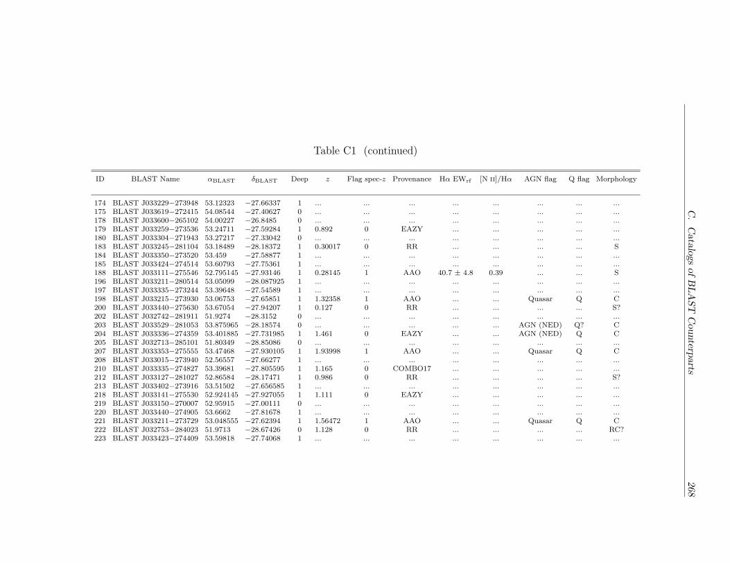
C.CatalogsofBLAST
Counterp
arts
268
Table C1 (continued)
ID BLAST Name �BLAST �BLAST Deep z Flag spec-z Provenance H� EWrf [N II]/H� AGN flag Q flag Morphology
174 BLAST J033229−273948 53.12323 −27.66337 1 ... ... ... ... ... ... ... ...175 BLAST J033619−272415 54.08544 −27.40627 0 ... ... ... ... ... ... ... ...178 BLAST J033600−265102 54.00227 −26.8485 0 ... ... ... ... ... ... ... ...179 BLAST J033259−273536 53.24711 −27.59284 1 0.892 0 EAZY ... ... ... ... ...180 BLAST J033304−271943 53.27217 −27.33042 0 ... ... ... ... ... ... ... ...183 BLAST J033245−281104 53.18489 −28.18372 1 0.30017 0 RR ... ... ... ... S184 BLAST J033350−273520 53.459 −27.58877 1 ... ... ... ... ... ... ... ...185 BLAST J033424−274514 53.60793 −27.75361 1 ... ... ... ... ... ... ... ...188 BLAST J033111−275546 52.795145 −27.93146 1 0.28145 1 AAO 40.7 ± 4.8 0.39 ... ... S196 BLAST J033211−280514 53.05099 −28.087925 1 ... ... ... ... ... ... ... ...197 BLAST J033335−273244 53.39648 −27.54589 1 ... ... ... ... ... ... ... ...198 BLAST J033215−273930 53.06753 −27.65851 1 1.32358 1 AAO ... ... Quasar Q C200 BLAST J033440−275630 53.67054 −27.94207 1 0.127 0 RR ... ... ... ... S?202 BLAST J032742−281911 51.9274 −28.3152 0 ... ... ... ... ... ... ... ...203 BLAST J033529−281053 53.875965 −28.18574 0 ... ... ... ... ... AGN (NED) Q? C204 BLAST J033336−274359 53.401885 −27.731985 1 1.461 0 EAZY ... ... AGN (NED) Q C205 BLAST J032713−285101 51.80349 −28.85086 0 ... ... ... ... ... ... ... ...207 BLAST J033353−275555 53.47468 −27.930105 1 1.93998 1 AAO ... ... Quasar Q C208 BLAST J033015−273940 52.56557 −27.66277 1 ... ... ... ... ... ... ... ...210 BLAST J033335−274827 53.39681 −27.805595 1 1.165 0 COMBO17 ... ... ... ... ...212 BLAST J033127−281027 52.86584 −28.17471 1 0.986 0 RR ... ... ... ... S?213 BLAST J033402−273916 53.51502 −27.656585 1 ... ... ... ... ... ... ... ...218 BLAST J033141−275530 52.924145 −27.927055 1 1.111 0 EAZY ... ... ... ... ...219 BLAST J033150−270007 52.95915 −27.00111 0 ... ... ... ... ... ... ... ...220 BLAST J033440−274905 53.6662 −27.81678 1 ... ... ... ... ... ... ... ...221 BLAST J033211−273729 53.048555 −27.62394 1 1.56472 1 AAO ... ... Quasar Q C222 BLAST J032753−284023 51.9713 −28.67426 0 1.128 0 RR ... ... ... ... RC?223 BLAST J033423−274409 53.59818 −27.74068 1 ... ... ... ... ... ... ... ...
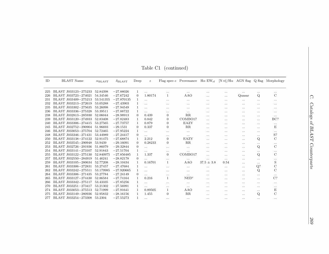
C.CatalogsofBLAST
Counterp
arts
269
Table C1 (continued)
ID BLAST Name �BLAST �BLAST Deep z Flag spec-z Provenance H� EWrf [N II]/H� AGN flag Q flag Morphology
225 BLAST J033123−275233 52.84398 −27.88026 1 ... ... ... ... ... ... ... ...226 BLAST J033723−274021 54.34546 −27.67242 0 1.80174 1 AAO ... ... Quasar Q C231 BLAST J033409−275213 53.541355 −27.870135 1 ... ... ... ... ... ... ... ...232 BLAST J033213−272619 53.05288 −27.43903 1 ... ... ... ... ... ... ... ...235 BLAST J033302−275635 53.26098 −27.94549 1 ... ... ... ... ... ... ... ...236 BLAST J033336−275328 53.39511 −27.88722 1 ... ... ... ... ... ... ... ...238 BLAST J032813−285930 52.06044 −28.98913 0 0.439 0 RR ... ... ... ... ...239 BLAST J033120−274933 52.83408 −27.82483 1 0.842 0 COMBO17 ... ... ... ... BC?240 BLAST J033306−274415 53.27565 −27.73757 1 0.879 0 EAZY ... ... ... ... ...245 BLAST J032752−290904 51.96693 −29.1531 0 0.337 0 RR ... ... ... ... E246 BLAST J033053−275704 52.72465 −27.95224 1 ... ... ... ... ... ... ... ...248 BLAST J033346−271431 53.44989 −27.24417 0 ... ... ... ... ... ... ... S?250 BLAST J033138−274122 52.91475 −27.68874 1 2.212 0 EAZY ... ... ... Q C252 BLAST J033545−290948 53.9439 −29.16091 0 0.28233 0 RR ... ... ... ... ...253 BLAST J032726−291936 51.86079 −29.32844 0 ... ... ... ... ... ... Q C254 BLAST J033141−273107 52.91843 −27.51704 1 ... ... ... ... ... ... ... ...255 BLAST J033122−275130 52.840975 −27.856485 1 1.337 0 COMBO17 ... ... ... Q C257 BLAST J032550−284919 51.46241 −28.82178 0 ... ... ... ... ... ... ... ...259 BLAST J033105−280634 52.77208 −28.10434 1 0.16701 1 AAO 37.5 ± 3.8 0.54 ... ... S261 BLAST J033306−272831 53.27457 −27.47684 1 ... ... ... ... ... ... Q? C262 BLAST J033242−275511 53.179985 −27.920665 1 ... ... ... ... ... ... Q C264 BLAST J033306−271435 53.27784 −27.24149 0 ... ... ... ... ... ... ... ...265 BLAST J033127−274430 52.86584 −27.74164 1 0.216 1 NEDc ... ... ... ... C?266 BLAST J033342−275117 53.43335 −27.85256 1 ... ... ... ... ... ... ... ...270 BLAST J033251−273417 53.21302 −27.56991 1 ... ... ... ... ... ... ... ...274 BLAST J033053−275513 52.71999 −27.91641 1 0.89505 1 AAO ... ... ... ... E275 BLAST J033149−280936 52.95832 −28.16156 1 1.455 0 RR ... ... ... Q C277 BLAST J033254−273308 53.2304 −27.55273 1 ... ... ... ... ... ... ... ...
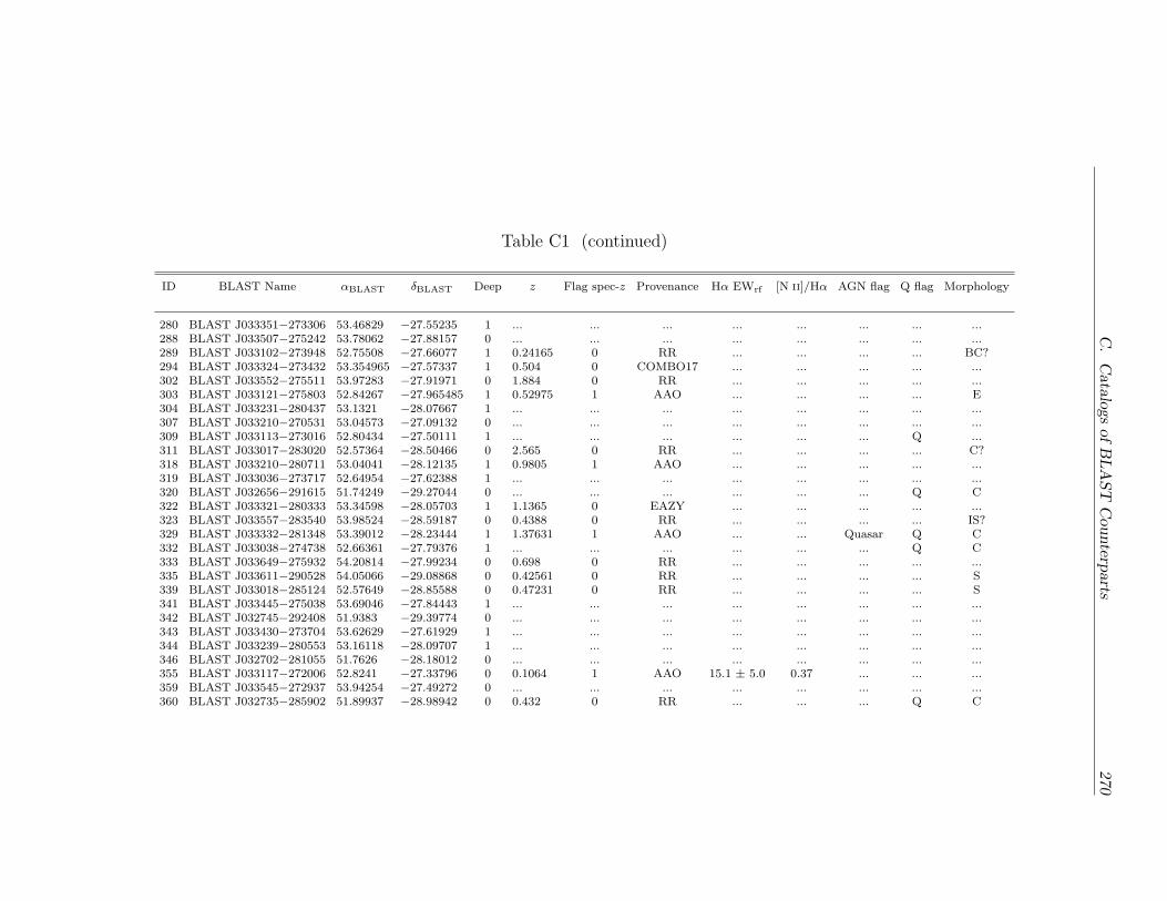
C.CatalogsofBLAST
Counterp
arts
270
Table C1 (continued)
ID BLAST Name �BLAST �BLAST Deep z Flag spec-z Provenance H� EWrf [N II]/H� AGN flag Q flag Morphology
280 BLAST J033351−273306 53.46829 −27.55235 1 ... ... ... ... ... ... ... ...288 BLAST J033507−275242 53.78062 −27.88157 0 ... ... ... ... ... ... ... ...289 BLAST J033102−273948 52.75508 −27.66077 1 0.24165 0 RR ... ... ... ... BC?294 BLAST J033324−273432 53.354965 −27.57337 1 0.504 0 COMBO17 ... ... ... ... ...302 BLAST J033552−275511 53.97283 −27.91971 0 1.884 0 RR ... ... ... ... ...303 BLAST J033121−275803 52.84267 −27.965485 1 0.52975 1 AAO ... ... ... ... E304 BLAST J033231−280437 53.1321 −28.07667 1 ... ... ... ... ... ... ... ...307 BLAST J033210−270531 53.04573 −27.09132 0 ... ... ... ... ... ... ... ...309 BLAST J033113−273016 52.80434 −27.50111 1 ... ... ... ... ... ... Q ...311 BLAST J033017−283020 52.57364 −28.50466 0 2.565 0 RR ... ... ... ... C?318 BLAST J033210−280711 53.04041 −28.12135 1 0.9805 1 AAO ... ... ... ... ...319 BLAST J033036−273717 52.64954 −27.62388 1 ... ... ... ... ... ... ... ...320 BLAST J032656−291615 51.74249 −29.27044 0 ... ... ... ... ... ... Q C322 BLAST J033321−280333 53.34598 −28.05703 1 1.1365 0 EAZY ... ... ... ... ...323 BLAST J033557−283540 53.98524 −28.59187 0 0.4388 0 RR ... ... ... ... IS?329 BLAST J033332−281348 53.39012 −28.23444 1 1.37631 1 AAO ... ... Quasar Q C332 BLAST J033038−274738 52.66361 −27.79376 1 ... ... ... ... ... ... Q C333 BLAST J033649−275932 54.20814 −27.99234 0 0.698 0 RR ... ... ... ... ...335 BLAST J033611−290528 54.05066 −29.08868 0 0.42561 0 RR ... ... ... ... S339 BLAST J033018−285124 52.57649 −28.85588 0 0.47231 0 RR ... ... ... ... S341 BLAST J033445−275038 53.69046 −27.84443 1 ... ... ... ... ... ... ... ...342 BLAST J032745−292408 51.9383 −29.39774 0 ... ... ... ... ... ... ... ...343 BLAST J033430−273704 53.62629 −27.61929 1 ... ... ... ... ... ... ... ...344 BLAST J033239−280553 53.16118 −28.09707 1 ... ... ... ... ... ... ... ...346 BLAST J032702−281055 51.7626 −28.18012 0 ... ... ... ... ... ... ... ...355 BLAST J033117−272006 52.8241 −27.33796 0 0.1064 1 AAO 15.1 ± 5.0 0.37 ... ... ...359 BLAST J033545−272937 53.94254 −27.49272 0 ... ... ... ... ... ... ... ...360 BLAST J032735−285902 51.89937 −28.98942 0 0.432 0 RR ... ... ... Q C
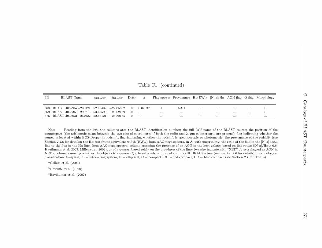
C.CatalogsofBLAST
Counterp
arts
271
Table C1 (continued)
ID BLAST Name �BLAST �BLAST Deep z Flag spec-z Provenance H� EWrf [N II]/H� AGN flag Q flag Morphology
368 BLAST J032957−290321 52.48499 −29.05382 0 0.07037 1 AAO ... ... ... ... S369 BLAST J033359−293715 53.49599 −29.62169 0 ... ... ... ... ... ... ... S376 BLAST J033031−264922 52.63121 −26.82185 0 ... ... ... ... ... ... ... ...
Note. — Reading from the left, the columns are: the BLAST identification number; the full IAU name of the BLAST source; the position of thecounterpart (the arithmetic mean between the two sets of coordinates if both the radio and 24�m counterparts are present); flag indicating whether thesource is located within BGS-Deep; the redshift; flag indicating whether the redshift is spectroscopic or photometric; the provenance of the redshift (see
Section 2.2.6 for details); the H� rest-frame equivalent width (EWrf) from AAOmega spectra, in A, with uncertainty; the ratio of the flux in the [N II] 658.3line to the flux in the H� line, from AAOmega spectra; column assessing the presence of an AGN in the host galaxy, based on line ratios ([N II]/H�> 0.6,Kauffmann et al. 2003, Miller et al. 2003), or of a quasar, based solely on the broadness of the lines (we also indicate with “NED” objects flagged as AGN inNED); column assessing whether the objects is a quasar (Q), based solely on optical and mid-IR (IRAC) colors (see Section 2.6 for details); morphologicalclassification: S=spiral, IS = interacting system, E = elliptical, C = compact, RC = red compact, BC = blue compact (see Section 2.7 for details).
aColless et al. (2003)
bRatcliffe et al. (1998)
cRavikumar et al. (2007)
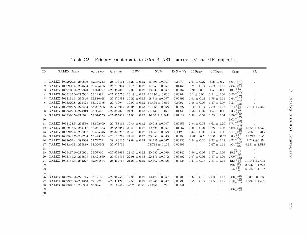
C.CatalogsofBLAST
Counterp
arts
272
Table C2. Primary counterparts to ≥ 5� BLAST sources: UV and FIR properties
ID GALEX Name �GALEX �GALEX FUV NUV E(B − V ) SFRFUV SFRNUV LFIR M★
1 GALEX J032920.6−280800 52.336213 −28.133591 17.23 ± 0.12 16.795 ±0.067 0.0071 2.01 ± 0.22 3.25 ± 0.2 4.94+0.17−0.16 ...
2 GALEX J032956.4−284633 52.485265 −28.775954 17.78 ± 0.12 17.051 ±0.067 0.01456 1.22 ± 0.14 2.59 ± 0.16 2.85+0.06−0.10 ...
3 GALEX J032740.9−282320 51.920727 −28.389056 19.09 ± 0.12 18.637 ±0.067 0.00862 0.94 ± 0.1 1.55 ± 0.1 10.5+0.2−0.4 ...
4 GALEX J033235.0−275532 53.14599 −27.925756 20.49 ± 0.12 20.176 ± 0.068 0.00864 0.1 ± 0.01 0.14 ± 0.01 0.55+0.10−0.04 ...
5 GALEX J033131.3−272846 52.880468 −27.479551 19.23 ± 0.12 18.716 ±0.067 0.00995 1.01 ± 0.11 1.76 ± 0.11 2.64+0.44−0.11 ...
6 GALEX J033229.8−274423 53.124378 −27.73994 19.97 ± 0.12 19.435 ± 0.067 0.0092 0.66 ± 0.07 1.17 ± 0.07 3.21+0.37−0.31 ...
7 GALEX J033249.8−273433 53.207886 −27.575957 22.08 ± 0.13 21.065 ±0.068 0.00827 1.16 ± 0.14 2.89 ± 0.18 27.4+4.9−3.3 12.791 ±2.442
8 GALEX J033549.0−274919 53.95423 −27.822048 21.95 ± 0.13 20.976 ± 0.073 0.01343 0.56 ± 0.07 1.43 ± 0.1 63.2+1.2−4.4 ...
9 GALEX J032916.5−273921 52.318753 −27.655832 17.01 ± 0.12 16.65 ± 0.067 0.01112 0.38 ± 0.04 0.58 ± 0.04 0.30+0.02−0.01 ...
10 ... ... ... ... ... ... ... ... 3.02+0.27−0.28 ...
11 GALEX J033424.5−274530 53.602409 −27.758395 19.44 ± 0.12 19.018 ±0.067 0.00853 2.94 ± 0.33 4.61 ± 0.29 5.71+1.29−0.42 ...
12 GALEX J032907.6−284117 52.281953 −28.688087 20.41 ± 0.12 19.625 ±0.067 0.01167 0.35 ± 0.04 0.78 ± 0.05 6.62+0.40−0.32 4.253 ±0.837
13 GALEX J032949.4−285057 52.455946 −28.849296 20.45 ± 0.12 19.843 ±0.068 0.0121 0.44 ± 0.05 0.83 ± 0.05 8.11+0.22−0.81 1.228 ± 0.315
15 GALEX J033341.7−280736 53.423854 −28.126769 21.42 ± 0.12 20.352 ±0.068 0.00853 4.47 ± 0.5 10.97 ± 0.69 36.2+8.3−8.2 19.742 ±3.56
16 GALEX J033059.4−281000 52.74774 −28.166835 18.64 ± 0.12 18.225 ±0.067 0.00926 2.34 ± 0.26 3.73 ± 0.23 4.72+0.31−0.46 1.718 ±0.35
17 GALEX J033249.5−275839 53.206398 −27.977736 ... 23.738 ± 0.125 0.00806 ... 9.67 ± 1.11 404+190−127 8.151 ± 1.516
18 ... ... ... ... ... ... ... ... ... ...
19 GALEX J033417.6−273931 53.57366 −27.658699 21.42 ± 0.12 20.682 ±0.068 0.00846 0.66 ± 0.07 1.37 ± 0.09 10.2+1.8−0.9 ...
20 GALEX J033341.2−273808 53.421869 −27.635593 22.98 ± 0.13 22.176 ±0.072 0.00802 0.07 ± 0.01 0.17 ± 0.01 7.00+0.47−0.84 ...
21 GALEX J033151.5−281227 52.964884 −28.207763 21.05 ± 0.12 20.562 ±0.068 0.00938 1.47 ± 0.16 2.37 ± 0.15 12.4+1.5−2.5 10.541 ±2.014
22 ... ... ... ... ... ... ... ... 498+582−148 3.896 ± 1.228
23 ... ... ... ... ... ... ... ... 142+68−64 5.825 ± 1.132
24 ... ... ... ... ... ... ... ... ... ...
26 GALEX J033245.9−275745 53.191281 −27.962535 19.88 ± 0.12 19.477 ±0.067 0.00806 1.34 ± 0.15 2.09 ± 0.13 3.00+0.25−0.89 3.08 ±0.536
27 GALEX J032957.0−281840 52.48763 −28.311293 18.52 ± 0.12 17.865 ±0.067 0.00898 1.53 ± 0.17 3.05 ± 0.19 2.18+0.32−0.24 1.238 ±0.246
28 GALEX J033318.1−280908 53.3254 −28.152402 25.7 ± 0.33 25.746 ± 0.246 0.00841 ... ... ... ...
29 ... ... ... ... ... ... ... ... 6.06+0.39−0.49 ...
30 ... ... ... ... ... ... ... ... ... ...
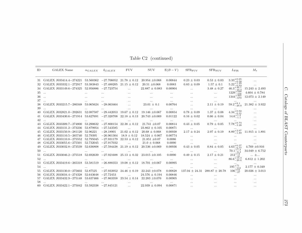
C.CatalogsofBLAST
Counterp
arts
273
Table C2 (continued)
ID GALEX Name �GALEX �GALEX FUV NUV E(B − V ) SFRFUV SFRNUV LFIR M★
31 GALEX J033414.4−274221 53.560362 −27.706052 21.78 ± 0.12 20.954 ±0.068 0.00844 0.23 ± 0.03 0.53 ± 0.03 3.33+0.65−0.58 ...
32 GALEX J033332.1−272917 53.383843 −27.488205 21.15 ± 0.12 20.51 ±0.068 0.0083 0.83 ± 0.09 1.57 ± 0.1 5.22+1.29−0.93 ...
34 GALEX J033149.6−274325 52.956886 −27.723754 ... 22.887 ± 0.083 0.00904 ... 3.48 ± 0.27 46.3+46.1−10.4 15.243 ± 2.493
35 ... ... ... ... ... ... ... ... 1229+599−436 4.604 ± 0.784
36 ... ... ... ... ... ... ... ... 1344+365−670 12.073 ± 2.149
37 ... ... ... ... ... ... ... ... ... ...
38 GALEX J033215.7−280348 53.065624 −28.063464 ... 23.01 ± 0.1 0.00764 ... 2.11 ± 0.19 59.2+8.1−29.8 21.382 ± 3.922
39 ... ... ... ... ... ... ... ... ... ...
40 GALEX J032821.0−292631 52.087587 −29.442053 19.67 ± 0.12 19.146 ±0.067 0.00854 0.78 ± 0.09 1.37 ± 0.08 4.34+0.92−0.31 ...
41 GALEX J033430.6−271914 53.627691 −27.320708 22.18 ± 0.13 20.743 ±0.069 0.01122 0.16 ± 0.02 0.66 ± 0.04 14.6+1.2−1.1 ...
42 ... ... ... ... ... ... ... ... ... ...
43 GALEX J033309.7−274800 53.290632 −27.800154 22.38 ± 0.12 21.741 ±0.07 0.00814 0.43 ± 0.05 0.79 ± 0.05 7.78+0.73−3.28 ...
44 GALEX J033131.2−273236 52.879954 −27.543585 ... 23.862 ± 0.105 0.00871 ... ... ... ...
45 GALEX J033150.9−281120 52.96221 −28.18901 21.02 ± 0.12 20.68 ± 0.068 0.00938 2.17 ± 0.24 2.97 ± 0.19 8.89+2.67−1.89 11.915 ± 1.891
46 GALEX J033110.5−265740 52.79395 −26.961304 18.9 ± 0.12 18.524 ± 0.067 0.00774 ... ... ... ...47 GALEX J033110.8−275552 52.795045 −27.931179 22.53 ± 0.12 21.851 ±0.07 0.0086 ... ... ... ...48 GALEX J033055.6−275501 52.732045 −27.917032 ... 21.0 ± 0.068 0.0090 ... ... ... ...
49 GALEX J033032.8−273539 52.636808 −27.594438 21.19 ± 0.12 20.536 ±0.069 0.00936 0.43 ± 0.05 0.84 ± 0.05 4.63+0.57−0.77 4.769 ±0.916
50 ... ... ... ... ... ... ... ... 70.1+7.3−6.3 34.049 ± 6.752
51 GALEX J033046.2−275518 52.692639 −27.921688 25.13 ± 0.32 23.015 ±0.105 0.0090 0.49 ± 0.15 2.17 ± 0.21 212+12−41 ... ±...
52 ... ... ... ... ... ... ... ... 86.6+13.3−29.6 6.812 ± 1.202
53 GALEX J033419.6−265318 53.581519 −26.888353 19.08 ± 0.12 18.701 ±0.067 0.00995 ... ... ... ...
54 ... ... ... ... ... ... ... ... 195+71−114 2.177 ± 0.349
55 GALEX J033130.0−275602 52.87525 −27.933952 24.46 ± 0.19 22.243 ±0.078 0.00828 137.04 ± 24.31 288.87 ± 20.78 106+52−27 20.026 ± 3.013
56 GALEX J033034.4−274328 52.643648 −27.72453 ... 24.576 ± 0.194 0.00846 ... ... ... ...57 GALEX J033432.9−275148 53.637466 −27.863358 23.54 ± 0.14 22.283 ±0.076 0.00905 ... ... ... ...58 ... ... ... ... ... ... ... ... ... ...60 GALEX J033422.1−275042 53.592338 −27.845121 ... 22.939 ± 0.094 0.00871 ... ... ... ...
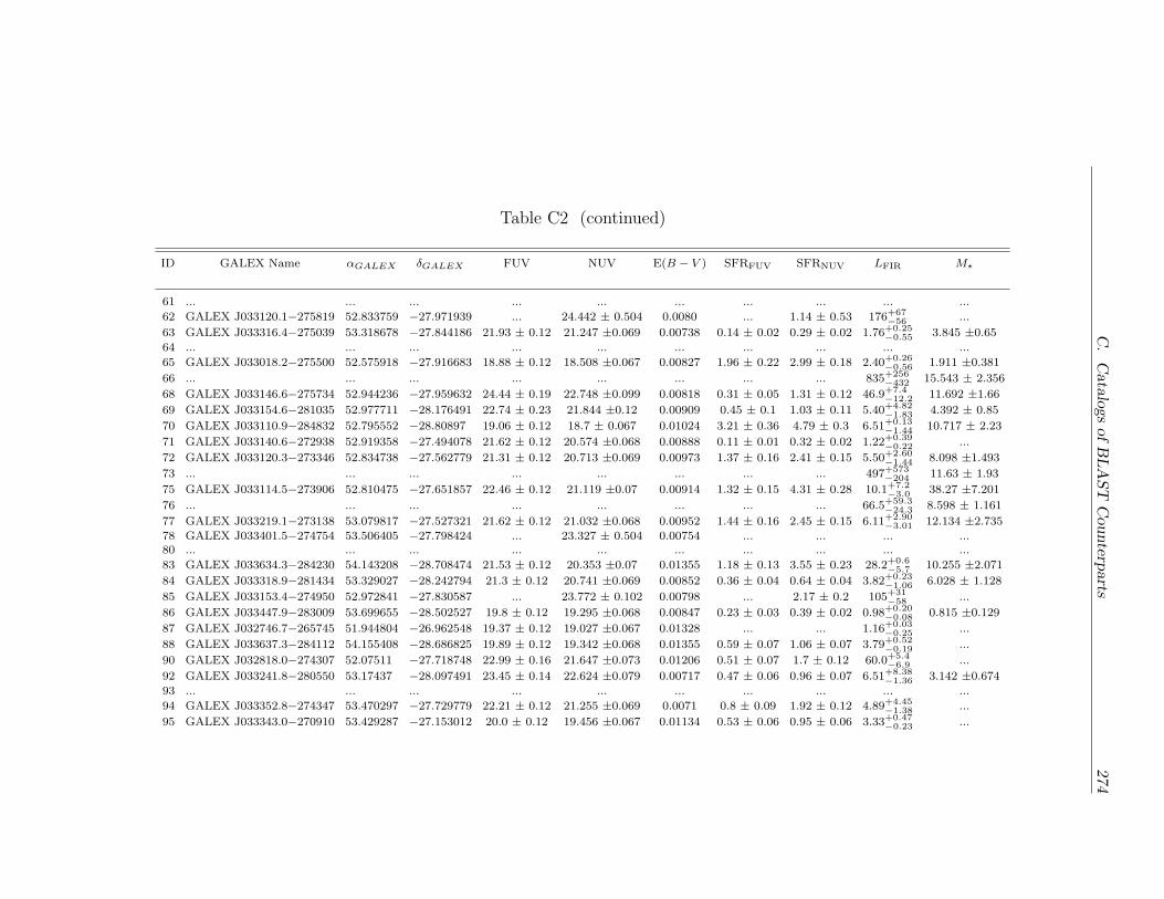
C.CatalogsofBLAST
Counterp
arts
274
Table C2 (continued)
ID GALEX Name �GALEX �GALEX FUV NUV E(B − V ) SFRFUV SFRNUV LFIR M★
61 ... ... ... ... ... ... ... ... ... ...
62 GALEX J033120.1−275819 52.833759 −27.971939 ... 24.442 ± 0.504 0.0080 ... 1.14 ± 0.53 176+67−56 ...
63 GALEX J033316.4−275039 53.318678 −27.844186 21.93 ± 0.12 21.247 ±0.069 0.00738 0.14 ± 0.02 0.29 ± 0.02 1.76+0.25−0.55 3.845 ±0.65
64 ... ... ... ... ... ... ... ... ... ...
65 GALEX J033018.2−275500 52.575918 −27.916683 18.88 ± 0.12 18.508 ±0.067 0.00827 1.96 ± 0.22 2.99 ± 0.18 2.40+0.26−0.56 1.911 ±0.381
66 ... ... ... ... ... ... ... ... 835+256−432 15.543 ± 2.356
68 GALEX J033146.6−275734 52.944236 −27.959632 24.44 ± 0.19 22.748 ±0.099 0.00818 0.31 ± 0.05 1.31 ± 0.12 46.9+7.4−12.2 11.692 ±1.66
69 GALEX J033154.6−281035 52.977711 −28.176491 22.74 ± 0.23 21.844 ±0.12 0.00909 0.45 ± 0.1 1.03 ± 0.11 5.40+4.82−1.83 4.392 ± 0.85
70 GALEX J033110.9−284832 52.795552 −28.80897 19.06 ± 0.12 18.7 ± 0.067 0.01024 3.21 ± 0.36 4.79 ± 0.3 6.51+0.13−1.44 10.717 ± 2.23
71 GALEX J033140.6−272938 52.919358 −27.494078 21.62 ± 0.12 20.574 ±0.068 0.00888 0.11 ± 0.01 0.32 ± 0.02 1.22+0.39−0.22 ...
72 GALEX J033120.3−273346 52.834738 −27.562779 21.31 ± 0.12 20.713 ±0.069 0.00973 1.37 ± 0.16 2.41 ± 0.15 5.50+2.60−1.44 8.098 ±1.493
73 ... ... ... ... ... ... ... ... 497+573−204 11.63 ± 1.93
75 GALEX J033114.5−273906 52.810475 −27.651857 22.46 ± 0.12 21.119 ±0.07 0.00914 1.32 ± 0.15 4.31 ± 0.28 10.1+7.2−3.0 38.27 ±7.201
76 ... ... ... ... ... ... ... ... 66.5+59.3−24.3 8.598 ± 1.161
77 GALEX J033219.1−273138 53.079817 −27.527321 21.62 ± 0.12 21.032 ±0.068 0.00952 1.44 ± 0.16 2.45 ± 0.15 6.11+2.90−3.01 12.134 ±2.735
78 GALEX J033401.5−274754 53.506405 −27.798424 ... 23.327 ± 0.504 0.00754 ... ... ... ...80 ... ... ... ... ... ... ... ... ... ...
83 GALEX J033634.3−284230 54.143208 −28.708474 21.53 ± 0.12 20.353 ±0.07 0.01355 1.18 ± 0.13 3.55 ± 0.23 28.2+0.6−5.7 10.255 ±2.071
84 GALEX J033318.9−281434 53.329027 −28.242794 21.3 ± 0.12 20.741 ±0.069 0.00852 0.36 ± 0.04 0.64 ± 0.04 3.82+0.23−1.06 6.028 ± 1.128
85 GALEX J033153.4−274950 52.972841 −27.830587 ... 23.772 ± 0.102 0.00798 ... 2.17 ± 0.2 105+31−58 ...
86 GALEX J033447.9−283009 53.699655 −28.502527 19.8 ± 0.12 19.295 ±0.068 0.00847 0.23 ± 0.03 0.39 ± 0.02 0.98+0.20−0.08 0.815 ±0.129
87 GALEX J032746.7−265745 51.944804 −26.962548 19.37 ± 0.12 19.027 ±0.067 0.01328 ... ... 1.16+0.03−0.25 ...
88 GALEX J033637.3−284112 54.155408 −28.686825 19.89 ± 0.12 19.342 ±0.068 0.01355 0.59 ± 0.07 1.06 ± 0.07 3.79+0.52−0.19 ...
90 GALEX J032818.0−274307 52.07511 −27.718748 22.99 ± 0.16 21.647 ±0.073 0.01206 0.51 ± 0.07 1.7 ± 0.12 60.0+5.4−6.9 ...
92 GALEX J033241.8−280550 53.17437 −28.097491 23.45 ± 0.14 22.624 ±0.079 0.00717 0.47 ± 0.06 0.96 ± 0.07 6.51+8.38−1.36 3.142 ±0.674
93 ... ... ... ... ... ... ... ... ... ...
94 GALEX J033352.8−274347 53.470297 −27.729779 22.21 ± 0.12 21.255 ±0.069 0.0071 0.8 ± 0.09 1.92 ± 0.12 4.89+4.45−1.38 ...
95 GALEX J033343.0−270910 53.429287 −27.153012 20.0 ± 0.12 19.456 ±0.067 0.01134 0.53 ± 0.06 0.95 ± 0.06 3.33+0.47−0.23 ...
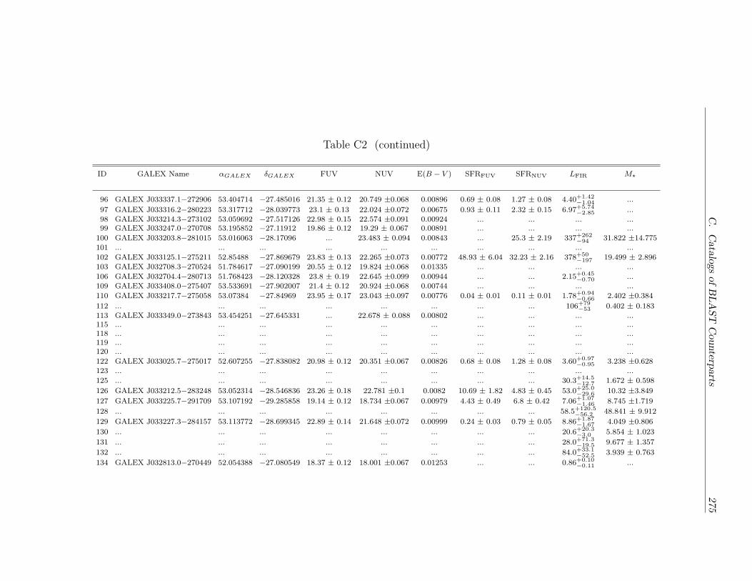
C.CatalogsofBLAST
Counterp
arts
275
Table C2 (continued)
ID GALEX Name �GALEX �GALEX FUV NUV E(B − V ) SFRFUV SFRNUV LFIR M★
96 GALEX J033337.1−272906 53.404714 −27.485016 21.35 ± 0.12 20.749 ±0.068 0.00896 0.69 ± 0.08 1.27 ± 0.08 4.40+1.42−1.04 ...
97 GALEX J033316.2−280223 53.317712 −28.039773 23.1 ± 0.13 22.024 ±0.072 0.00675 0.93 ± 0.11 2.32 ± 0.15 6.97+5.74−2.85 ...
98 GALEX J033214.3−273102 53.059692 −27.517126 22.98 ± 0.15 22.574 ±0.091 0.00924 ... ... ... ...99 GALEX J033247.0−270708 53.195852 −27.11912 19.86 ± 0.12 19.29 ± 0.067 0.00891 ... ... ... ...
100 GALEX J033203.8−281015 53.016063 −28.17096 ... 23.483 ± 0.094 0.00843 ... 25.3 ± 2.19 337+262−94 31.822 ±14.775
101 ... ... ... ... ... ... ... ... ... ...
102 GALEX J033125.1−275211 52.85488 −27.869679 23.83 ± 0.13 22.265 ±0.073 0.00772 48.93 ± 6.04 32.23 ± 2.16 378+50−197 19.499 ± 2.896
103 GALEX J032708.3−270524 51.784617 −27.090199 20.55 ± 0.12 19.824 ±0.068 0.01335 ... ... ... ...
106 GALEX J032704.4−280713 51.768423 −28.120328 23.8 ± 0.19 22.645 ±0.099 0.00944 ... ... 2.15+0.45−0.70 ...
109 GALEX J033408.0−275407 53.533691 −27.902007 21.4 ± 0.12 20.924 ±0.068 0.00744 ... ... ... ...
110 GALEX J033217.7−275058 53.07384 −27.84969 23.95 ± 0.17 23.043 ±0.097 0.00776 0.04 ± 0.01 0.11 ± 0.01 1.78+0.94−0.66 2.402 ±0.384
112 ... ... ... ... ... ... ... ... 106+79−53 0.402 ± 0.183
113 GALEX J033349.0−273843 53.454251 −27.645331 ... 22.678 ± 0.088 0.00802 ... ... ... ...115 ... ... ... ... ... ... ... ... ... ...118 ... ... ... ... ... ... ... ... ... ...119 ... ... ... ... ... ... ... ... ... ...120 ... ... ... ... ... ... ... ... ... ...
122 GALEX J033025.7−275017 52.607255 −27.838082 20.98 ± 0.12 20.351 ±0.067 0.00826 0.68 ± 0.08 1.28 ± 0.08 3.60+0.97−0.95 3.238 ±0.628
123 ... ... ... ... ... ... ... ... ... ...
125 ... ... ... ... ... ... ... ... 30.3+14.5−12.7 1.672 ± 0.598
126 GALEX J033212.5−283248 53.052314 −28.546836 23.26 ± 0.18 22.781 ±0.1 0.0082 10.69 ± 1.82 4.83 ± 0.45 53.0+25.0−29.6 10.32 ±3.849
127 GALEX J033225.7−291709 53.107192 −29.285858 19.14 ± 0.12 18.734 ±0.067 0.00979 4.43 ± 0.49 6.8 ± 0.42 7.06+1.07−1.46 8.745 ±1.719
128 ... ... ... ... ... ... ... ... 58.5+120.5−56.2 48.841 ± 9.912
129 GALEX J033227.3−284157 53.113772 −28.699345 22.89 ± 0.14 21.648 ±0.072 0.00999 0.24 ± 0.03 0.79 ± 0.05 8.86+1.87−1.67 4.049 ±0.806
130 ... ... ... ... ... ... ... ... 20.6+20.3−3.0 5.854 ± 1.023
131 ... ... ... ... ... ... ... ... 28.0+71.3−19.5 9.677 ± 1.357
132 ... ... ... ... ... ... ... ... 84.0+33.1−52.5 3.939 ± 0.763
134 GALEX J032813.0−270449 52.054388 −27.080549 18.37 ± 0.12 18.001 ±0.067 0.01253 ... ... 0.86+0.10−0.11 ...
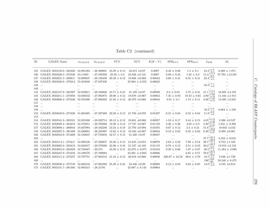
C.CatalogsofBLAST
Counterp
arts
276
Table C2 (continued)
ID GALEX Name �GALEX �GALEX FUV NUV E(B − V ) SFRFUV SFRNUV LFIR M★
135 GALEX J033133.9−282403 52.891282 −28.400861 23.29 ± 0.14 22.015 ±0.07 0.0087 0.48 ± 0.06 1.5 ± 0.1 24.3+5.6−6.3 6.369 ± 1.671
136 GALEX J033228.5−273536 53.11883 −27.593592 25.92 ± 0.3 23.828 ±0.121 0.0097 0.89 ± 0.24 1.82 ± 0.2 15.4+11.2−2.9 37.782 ±12.281
137 GALEX J032821.5−280811 52.089837 −28.136439 20.49 ± 0.12 19.866 ±0.068 0.00842 3.69 ± 0.41 6.55 ± 0.41 22.4+2.9−4.5 ...
138 GALEX J033348.9−275014 53.453949 −27.837456 ... 25.064 ± 0.252 0.00622 ... ... ... ...
139 ... ... ... ... ... ... ... ... 59.3+7.7−4.2 ...
140 ... ... ... ... ... ... ... ... ... ...
143 GALEX J033147.9−281007 52.949911 −28.168868 24.71 ± 0.24 21.189 ±0.07 0.00939 0.2 ± 0.04 4.75 ± 0.31 41.1+12.0−13.5 16.095 ±3.185
145 GALEX J033211.1−275858 53.046532 −27.982875 20.08 ± 0.12 19.678 ±0.067 0.00852 7.45 ± 0.83 10.53 ± 0.65 2.80+1.92−0.76 11.444 ±1.915
146 GALEX J033000.4−275346 52.501809 −27.896302 21.02 ± 0.12 20.379 ±0.068 0.00844 0.91 ± 0.1 1.74 ± 0.11 4.90+1.64−0.79 13.495 ±2.621
147 ... ... ... ... ... ... ... ... ... ...148 ... ... ... ... ... ... ... ... ... ...
149 ... ... ... ... ... ... ... ... 10.3+3.8−1.1 6.664 ± 1.246
152 GALEX J033649.0−271938 54.204385 −27.327469 22.28 ± 0.13 21.756 ±0.078 0.01227 0.31 ± 0.04 0.52 ± 0.04 11.8+0.8−2.9 ...
153 ... ... ... ... ... ... ... ... ... ...
154 GALEX J033541.2−285521 53.921886 −28.922714 20.12 ± 0.12 19.681 ±0.068 0.00957 1.53 ± 0.17 2.44 ± 0.15 4.65+0.33−1.50 2.386 ±0.537
155 GALEX J032929.4−284218 52.372851 −28.705028 18.09 ± 0.12 17.747 ±0.067 0.01159 3.26 ± 0.36 4.83 ± 0.3 3.30+0.47−0.45 1.821 ± 0.392
157 GALEX J033609.1−280944 54.037984 −28.162246 23.24 ± 0.19 21.793 ±0.094 0.01055 0.67 ± 0.12 2.4 ± 0.21 51.6+6.4−10.8 18.643 ±3.62
158 GALEX J033307.3−281409 53.280691 −28.235987 19.82 ± 0.12 19.343 ±0.067 0.00824 0.19 ± 0.02 0.32 ± 0.02 0.30+0.09−0.07 0.389 ±0.081
160 GALEX J032843.6−274409 52.182047 −27.735859 22.57 ± 0.13 21.426 ±0.07 0.00847 ... ... ... ...
162 ... ... ... ... ... ... ... ... 37.7+68.2−39.8 3.452 ± 0.616
163 GALEX J033114.1−273411 52.809126 −27.569857 23.38 ± 0.13 21.643 ±0.073 0.00979 2.63 ± 0.33 7.99 ± 0.54 29.7+20.2−11.2 8.753 ±1.525
165 GALEX J033605.9−293413 54.024817 −29.570388 22.86 ± 0.16 21.547 ±0.102 0.01119 0.78 ± 0.12 2.51 ± 0.23 20.2+20.4−3.8 14.919 ±2.152
166 GALEX J033055.0−293426 52.729487 −29.574 23.39 ± 0.15 22.279 ± 0.075 0.01019 0.39 ± 0.06 1.07 ± 0.07 20.5+3.3−1.9 11.484 ± 2.099
167 GALEX J033247.9−274232 53.199576 −27.709084 ... 23.291 ± 0.093 0.00866 ... 6.65 ± 0.57 76.6+86.0−60.1 ...
168 GALEX J033111.4−275257 52.797751 −27.882512 21.24 ± 0.12 20.616 ±0.068 0.00836 220.07 ± 24.58 60.6 ± 3.79 18.5+3.6−9.1 5.826 ±1.729
169 ... ... ... ... ... ... ... ... 190+243−89 58.348 ± 8.475
170 GALEX J033038.4−275748 52.660132 −27.963382 25.29 ± 0.24 23.346 ±0.09 0.00808 0.12 ± 0.03 0.64 ± 0.05 14.0+3.5−9.3 4.535 ±0.814
173 GALEX J033131.7−281304 52.882415 −28.21781 ... 23.887 ± 0.145 0.00964 ... ... ... ...
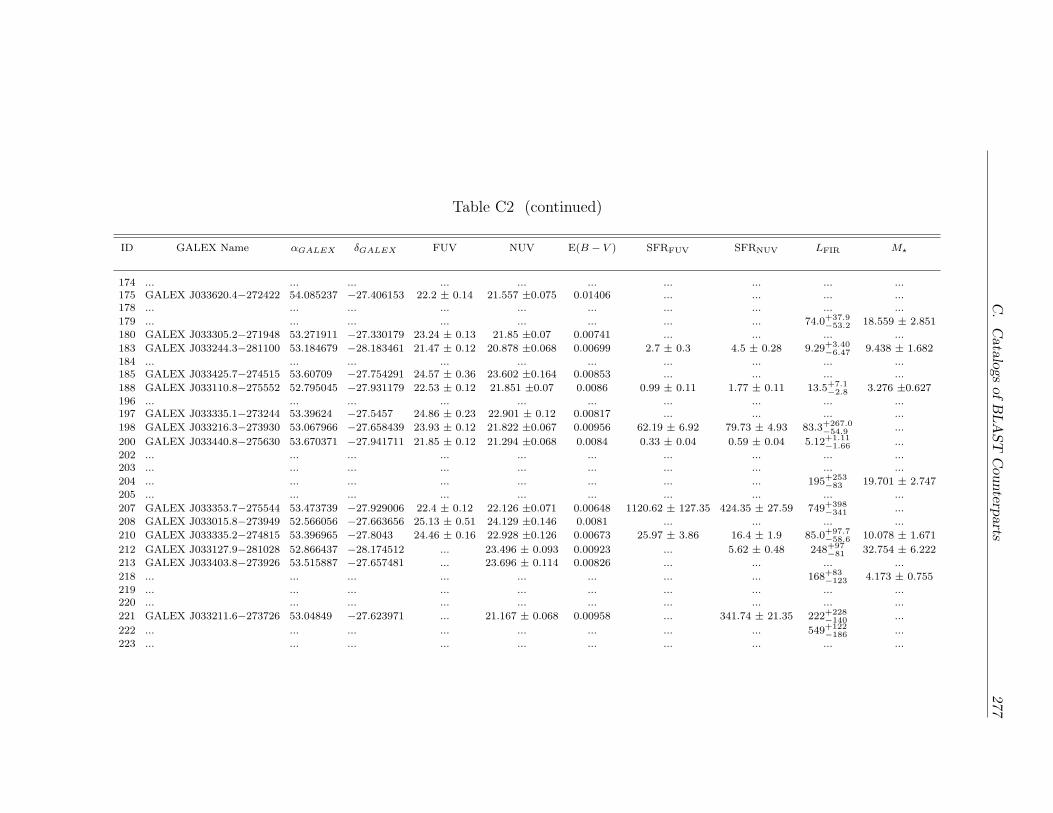
C.CatalogsofBLAST
Counterp
arts
277
Table C2 (continued)
ID GALEX Name �GALEX �GALEX FUV NUV E(B − V ) SFRFUV SFRNUV LFIR M★
174 ... ... ... ... ... ... ... ... ... ...175 GALEX J033620.4−272422 54.085237 −27.406153 22.2 ± 0.14 21.557 ±0.075 0.01406 ... ... ... ...178 ... ... ... ... ... ... ... ... ... ...
179 ... ... ... ... ... ... ... ... 74.0+37.9−53.2 18.559 ± 2.851
180 GALEX J033305.2−271948 53.271911 −27.330179 23.24 ± 0.13 21.85 ±0.07 0.00741 ... ... ... ...
183 GALEX J033244.3−281100 53.184679 −28.183461 21.47 ± 0.12 20.878 ±0.068 0.00699 2.7 ± 0.3 4.5 ± 0.28 9.29+3.40−6.47 9.438 ± 1.682
184 ... ... ... ... ... ... ... ... ... ...185 GALEX J033425.7−274515 53.60709 −27.754291 24.57 ± 0.36 23.602 ±0.164 0.00853 ... ... ... ...
188 GALEX J033110.8−275552 52.795045 −27.931179 22.53 ± 0.12 21.851 ±0.07 0.0086 0.99 ± 0.11 1.77 ± 0.11 13.5+7.1−2.8 3.276 ±0.627
196 ... ... ... ... ... ... ... ... ... ...197 GALEX J033335.1−273244 53.39624 −27.5457 24.86 ± 0.23 22.901 ± 0.12 0.00817 ... ... ... ...
198 GALEX J033216.3−273930 53.067966 −27.658439 23.93 ± 0.12 21.822 ±0.067 0.00956 62.19 ± 6.92 79.73 ± 4.93 83.3+267.0−54.9 ...
200 GALEX J033440.8−275630 53.670371 −27.941711 21.85 ± 0.12 21.294 ±0.068 0.0084 0.33 ± 0.04 0.59 ± 0.04 5.12+1.11−1.66 ...
202 ... ... ... ... ... ... ... ... ... ...203 ... ... ... ... ... ... ... ... ... ...
204 ... ... ... ... ... ... ... ... 195+253−83 19.701 ± 2.747
205 ... ... ... ... ... ... ... ... ... ...
207 GALEX J033353.7−275544 53.473739 −27.929006 22.4 ± 0.12 22.126 ±0.071 0.00648 1120.62 ± 127.35 424.35 ± 27.59 749+398−341 ...
208 GALEX J033015.8−273949 52.566056 −27.663656 25.13 ± 0.51 24.129 ±0.146 0.0081 ... ... ... ...
210 GALEX J033335.2−274815 53.396965 −27.8043 24.46 ± 0.16 22.928 ±0.126 0.00673 25.97 ± 3.86 16.4 ± 1.9 85.0+97.7−58.6 10.078 ± 1.671
212 GALEX J033127.9−281028 52.866437 −28.174512 ... 23.496 ± 0.093 0.00923 ... 5.62 ± 0.48 248+97−81 32.754 ± 6.222
213 GALEX J033403.8−273926 53.515887 −27.657481 ... 23.696 ± 0.114 0.00826 ... ... ... ...
218 ... ... ... ... ... ... ... ... 168+83−123 4.173 ± 0.755
219 ... ... ... ... ... ... ... ... ... ...220 ... ... ... ... ... ... ... ... ... ...
221 GALEX J033211.6−273726 53.04849 −27.623971 ... 21.167 ± 0.068 0.00958 ... 341.74 ± 21.35 222+228−140 ...
222 ... ... ... ... ... ... ... ... 549+122−186 ...
223 ... ... ... ... ... ... ... ... ... ...
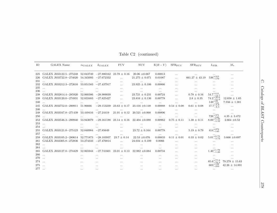
C.CatalogsofBLAST
Counterp
arts
278
Table C2 (continued)
ID GALEX Name �GALEX �GALEX FUV NUV E(B − V ) SFRFUV SFRNUV LFIR M★
225 GALEX J033122.5−275248 52.843749 −27.880162 23.78 ± 0.16 20.06 ±0.067 0.00813 ... ... ... ...
226 GALEX J033722.8−274020 54.345093 −27.672332 ... 21.275 ± 0.071 0.01087 ... 661.27 ± 43.19 536+315−176 ...
231 ... ... ... ... ... ... ... ... ... ...232 GALEX J033212.3−272616 53.051583 −27.437917 ... 23.925 ± 0.106 0.00866 ... ... ... ...235 ... ... ... ... ... ... ... ... ... ...236 ... ... ... ... ... ... ... ... ... ...
238 GALEX J032814.4−285920 52.060386 −28.989039 ... 23.721 ± 0.231 0.00724 ... 0.78 ± 0.16 54.7+4.0−12.7 ...
239 GALEX J033120.0−274931 52.833483 −27.825427 ... 23.816 ± 0.136 0.00778 ... 2.8 ± 0.35 74.2+30.6−51.0 12.658 ± 1.65
240 ... ... ... ... ... ... ... ... 149+29−101 7.556 ± 1.381
245 GALEX J032752.0−290911 51.96666 −29.153239 23.63 ± 0.17 23.416 ±0.148 0.00888 0.54 ± 0.08 0.61 ± 0.08 17.7+4.8−8.5 ...
246 ... ... ... ... ... ... ... ... ... ...248 GALEX J033347.8−271439 53.449416 −27.24419 21.01 ± 0.12 20.521 ±0.068 0.00896 ... ... ... ...
250 ... ... ... ... ... ... ... ... 726+371−546 4.35 ± 3.472
252 GALEX J033546.3−290940 53.943079 −29.161188 23.14 ± 0.16 22.404 ±0.088 0.00962 0.75 ± 0.11 1.38 ± 0.11 8.00+5.49−4.32 2.664 ±0.52
253 ... ... ... ... ... ... ... ... ... ...254 ... ... ... ... ... ... ... ... ... ...
255 GALEX J033121.8−275123 52.840984 −27.85649 ... 23.72 ± 0.164 0.00778 ... 5.19 ± 0.79 414+272−145 ...
257 ... ... ... ... ... ... ... ... ... ...
259 GALEX J033105.2−280614 52.771873 −28.103937 23.7 ± 0.14 22.53 ±0.076 0.00833 0.11 ± 0.01 0.33 ± 0.02 5.01+0.72−3.72 3.666 ±0.697
261 GALEX J033305.8−272836 53.274333 −27.476814 ... 24.034 ± 0.109 0.0066 ... ... ... ...262 ... ... ... ... ... ... ... ... ... ...264 ... ... ... ... ... ... ... ... ... ...
265 GALEX J033127.8−274429 52.865944 −27.741601 23.01 ± 0.13 22.982 ±0.084 0.00734 ... ... 1.40+1.78−1.29 ...
266 ... ... ... ... ... ... ... ... ... ...270 ... ... ... ... ... ... ... ... ... ...
274 ... ... ... ... ... ... ... ... 85.6+77.9−76.3 79.278 ± 15.63
275 ... ... ... ... ... ... ... ... 603+192−250 42.26 ± 14.891
277 ... ... ... ... ... ... ... ... ... ...
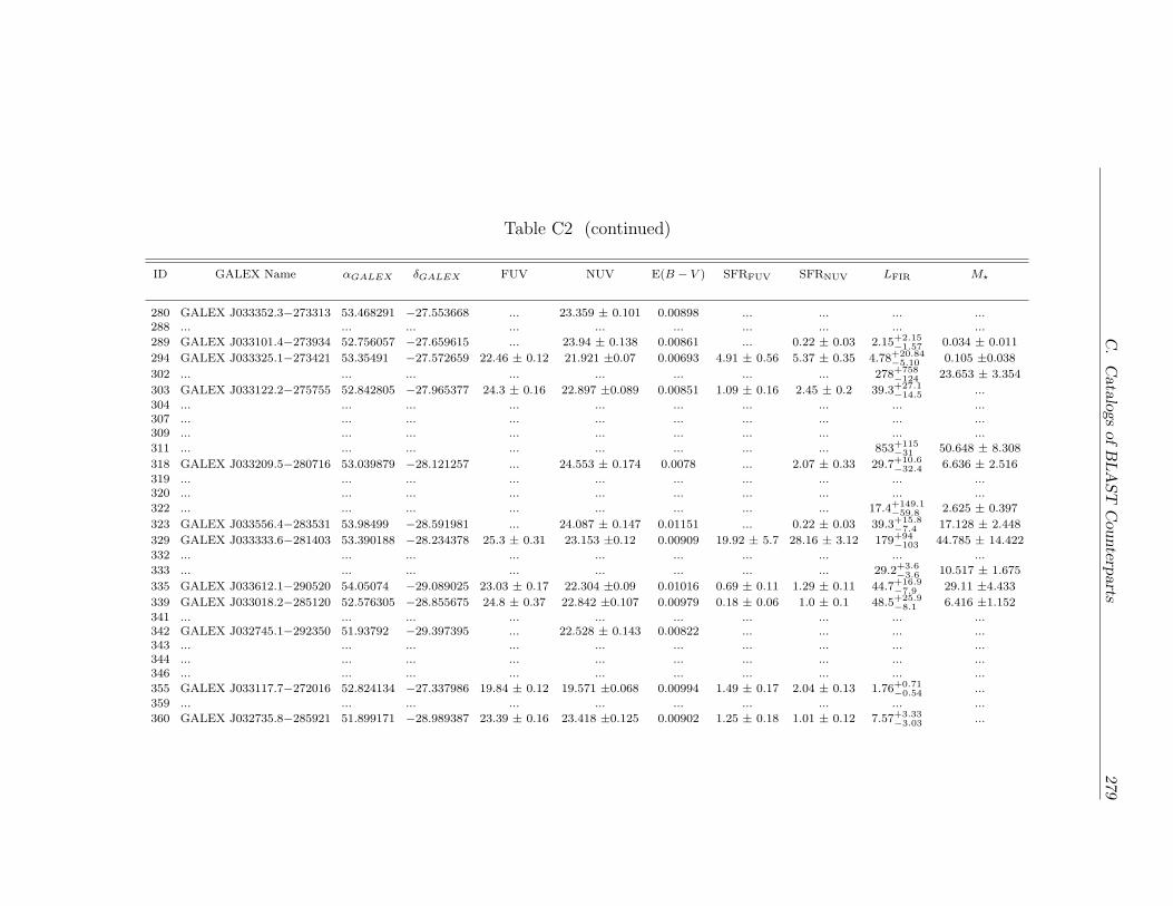
C.CatalogsofBLAST
Counterp
arts
279
Table C2 (continued)
ID GALEX Name �GALEX �GALEX FUV NUV E(B − V ) SFRFUV SFRNUV LFIR M★
280 GALEX J033352.3−273313 53.468291 −27.553668 ... 23.359 ± 0.101 0.00898 ... ... ... ...288 ... ... ... ... ... ... ... ... ... ...
289 GALEX J033101.4−273934 52.756057 −27.659615 ... 23.94 ± 0.138 0.00861 ... 0.22 ± 0.03 2.15+2.15−1.57 0.034 ± 0.011
294 GALEX J033325.1−273421 53.35491 −27.572659 22.46 ± 0.12 21.921 ±0.07 0.00693 4.91 ± 0.56 5.37 ± 0.35 4.78+20.84−5.10 0.105 ±0.038
302 ... ... ... ... ... ... ... ... 278+758−124 23.653 ± 3.354
303 GALEX J033122.2−275755 52.842805 −27.965377 24.3 ± 0.16 22.897 ±0.089 0.00851 1.09 ± 0.16 2.45 ± 0.2 39.3+27.1−14.5 ...
304 ... ... ... ... ... ... ... ... ... ...307 ... ... ... ... ... ... ... ... ... ...309 ... ... ... ... ... ... ... ... ... ...
311 ... ... ... ... ... ... ... ... 853+115−31 50.648 ± 8.308
318 GALEX J033209.5−280716 53.039879 −28.121257 ... 24.553 ± 0.174 0.0078 ... 2.07 ± 0.33 29.7+10.6−32.4 6.636 ± 2.516
319 ... ... ... ... ... ... ... ... ... ...320 ... ... ... ... ... ... ... ... ... ...
322 ... ... ... ... ... ... ... ... 17.4+149.1−59.8 2.625 ± 0.397
323 GALEX J033556.4−283531 53.98499 −28.591981 ... 24.087 ± 0.147 0.01151 ... 0.22 ± 0.03 39.3+15.8−7.4 17.128 ± 2.448
329 GALEX J033333.6−281403 53.390188 −28.234378 25.3 ± 0.31 23.153 ±0.12 0.00909 19.92 ± 5.7 28.16 ± 3.12 179+94−103 44.785 ± 14.422
332 ... ... ... ... ... ... ... ... ... ...
333 ... ... ... ... ... ... ... ... 29.2+3.6−3.6 10.517 ± 1.675
335 GALEX J033612.1−290520 54.05074 −29.089025 23.03 ± 0.17 22.304 ±0.09 0.01016 0.69 ± 0.11 1.29 ± 0.11 44.7+16.9−7.9 29.11 ±4.433
339 GALEX J033018.2−285120 52.576305 −28.855675 24.8 ± 0.37 22.842 ±0.107 0.00979 0.18 ± 0.06 1.0 ± 0.1 48.5+25.9−8.1 6.416 ±1.152
341 ... ... ... ... ... ... ... ... ... ...342 GALEX J032745.1−292350 51.93792 −29.397395 ... 22.528 ± 0.143 0.00822 ... ... ... ...343 ... ... ... ... ... ... ... ... ... ...344 ... ... ... ... ... ... ... ... ... ...346 ... ... ... ... ... ... ... ... ... ...
355 GALEX J033117.7−272016 52.824134 −27.337986 19.84 ± 0.12 19.571 ±0.068 0.00994 1.49 ± 0.17 2.04 ± 0.13 1.76+0.71−0.54 ...
359 ... ... ... ... ... ... ... ... ... ...
360 GALEX J032735.8−285921 51.899171 −28.989387 23.39 ± 0.16 23.418 ±0.125 0.00902 1.25 ± 0.18 1.01 ± 0.12 7.57+3.33−3.03 ...
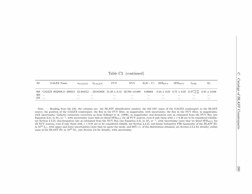
C.CatalogsofBLAST
Counterp
arts
280
Table C2 (continued)
ID GALEX Name �GALEX �GALEX FUV NUV E(B − V ) SFRFUV SFRNUV LFIR M★
368 GALEX J032956.2−290313 52.484512 −29.053836 21.28 ± 0.12 20.769 ±0.069 0.00904 0.44 ± 0.05 0.75 ± 0.05 0.37+0.10−0.19 0.25 ± 0.048
369 ... ... ... ... ... ... ... ... ... ...376 ... ... ... ... ... ... ... ... ... ...
Note. — Reading from the left, the columns are: the BLAST identification number; the full IAU name of the GALEX counterpart to the BLASTsource; the position of the GALEX counterpart; the flux in the FUV filter, in magnitudes, with uncertainty; the flux in the NUV filter, in magnitudes,with uncertainty; Galactic extinction correction as from Schlegel et al. (1998), in magnitudes; star-formation rate as estimated from the FUV flux (seeEquation 2.3), in M⊙ yr−1, with uncertainty (note that we listed SFRFUV for all FUV sources, even if only those with z < 0.36 are to be considered reliable,see Section 2.4.2); star-formation rate as estimated from the NUV flux (see Equation 2.3), in M⊙ yr−1, with uncertainty (note that we listed SFRNUV forall NUV sources, even if only those with z < 0.91 are to be considered reliable, see Section 2.4.2); rest-frame bolometric FIR luminosity of the BLAST ID,in 1010 L⊙, with upper and lower uncertainties (note that we quote the mode, and 68% c.l. of the distribution obtained, see Section 2.3.2 for details); stellarmass of the BLAST ID, in 1010 M⊙ (see Section 2.8 for details), with uncertainty.
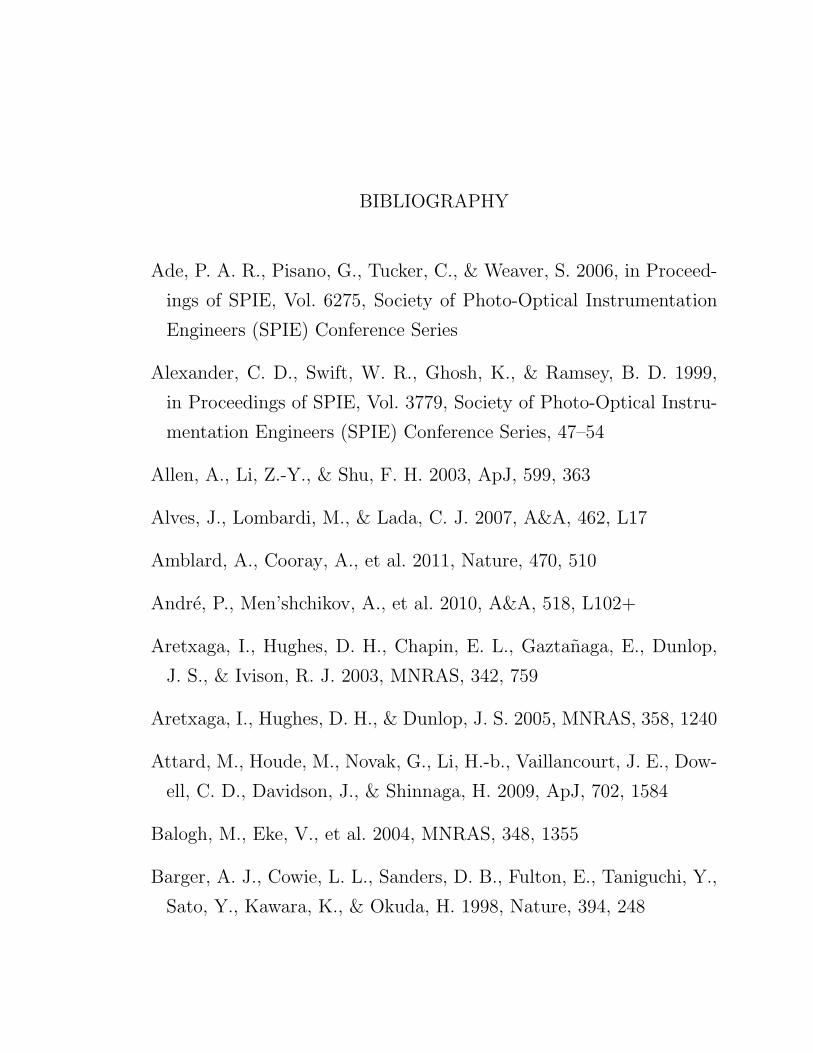
BIBLIOGRAPHY
Ade, P. A. R., Pisano, G., Tucker, C., & Weaver, S. 2006, in Proceed-
ings of SPIE, Vol. 6275, Society of Photo-Optical Instrumentation
Engineers (SPIE) Conference Series
Alexander, C. D., Swift, W. R., Ghosh, K., & Ramsey, B. D. 1999,
in Proceedings of SPIE, Vol. 3779, Society of Photo-Optical Instru-
mentation Engineers (SPIE) Conference Series, 47–54
Allen, A., Li, Z.-Y., & Shu, F. H. 2003, ApJ, 599, 363
Alves, J., Lombardi, M., & Lada, C. J. 2007, A&A, 462, L17
Amblard, A., Cooray, A., et al. 2011, Nature, 470, 510
Andre, P., Men’shchikov, A., et al. 2010, A&A, 518, L102+
Aretxaga, I., Hughes, D. H., Chapin, E. L., Gaztanaga, E., Dunlop,
J. S., & Ivison, R. J. 2003, MNRAS, 342, 759
Aretxaga, I., Hughes, D. H., & Dunlop, J. S. 2005, MNRAS, 358, 1240
Attard, M., Houde, M., Novak, G., Li, H.-b., Vaillancourt, J. E., Dow-
ell, C. D., Davidson, J., & Shinnaga, H. 2009, ApJ, 702, 1584
Balogh, M., Eke, V., et al. 2004, MNRAS, 348, 1355
Barger, A. J., Cowie, L. L., Sanders, D. B., Fulton, E., Taniguchi, Y.,
Sato, Y., Kawara, K., & Okuda, H. 1998, Nature, 394, 248
BIBLIOGRAPHY 282
Bastien, P., Bissonnette, E., Ade, P., Pisano, G., Savini, G., Jenness,
T., Johnstone, D., & Matthews, B. 2005, JRASC, 99, 133
Basu, S. 2000, ApJ, 540, L103
Basu, S. & Mouschovias, T. C. 1994, ApJ, 432, 720
Bauer, A. E., Conselice, C. J., Perez-Gonzalez, P. G., Grutzbauch, R.,
Bluck, A. F. L., Buitrago, F., & Mortlock, A. 2011, MNRAS, 417,
289
Bell, E. F. 2003, ApJ, 586, 794
Bell, E. F., Wolf, C., et al. 2004, ApJ, 608, 752
Bernard, J.-P., Ade, P., et al. 2007, in EAS Publications Series,
Vol. 23, EAS Publications Series, ed. M.-A. Miville-Deschenes &
F. Boulanger, 189–203
Bernstein, R. A., Freedman, W. L., & Madore, B. F. 2002, ApJ, 571,
56
Bethell, T. J., Chepurnov, A., Lazarian, A., & Kim, J. 2007, ApJ, 663,
1055
Bethermin, M., Dole, H., Beelen, A., & Aussel, H. 2010, A&A, 512,
A78+
Bezanson, R., van Dokkum, P. G., Tal, T., Marchesini, D., Kriek, M.,
Franx, M., & Coppi, P. 2009, ApJ, 697, 1290
Bianchi, S., Goncalves, J., Albrecht, M., Caselli, P., Chini, R., Galli,
D., & Walmsley, M. 2003, A&A, 399, L43
Bintley, D., Macintosh, M. J., et al. 2010, in Proceedings of SPIE, Vol.
7741, Society of Photo-Optical Instrumentation Engineers (SPIE)
Conference Series
BIBLIOGRAPHY 283
Blain, A. W. 1999, MNRAS, 304, 669
Blain, A. W., Barnard, V. E., & Chapman, S. C. 2003, MNRAS, 338,
733
Blain, A. W., Kneib, J., Ivison, R. J., & Smail, I. 1999a, ApJ, 512,
L87
Blain, A. W., Smail, I., Ivison, R. J., & Kneib, J.-P. 1999b, MNRAS,
302, 632
Blain, A. W., Smail, I., Ivison, R. J., Kneib, J.-P., & Frayer, D. T.
2002, Phys. Rep., 369, 111
Bluck, A. F. L., Conselice, C. J., Bouwens, R. J., Daddi, E., Dickinson,
M., Papovich, C., & Yan, H. 2009, MNRAS, 394, L51
Bock, J. J., Glenn, J., Grannan, S. M., Irwin, K. D., Lange, A. E.,
Leduc, H. G., & Turner, A. D. 1998, in Proceedings of SPIE, Vol.
3357, Society of Photo-Optical Instrumentation Engineers (SPIE)
Conference Series, 297–304
Boggess, N. W., Mather, J. C., et al. 1992, ApJ, 397, 420
Borys, C., Smail, I., Chapman, S. C., Blain, A. W., Alexander, D. M.,
& Ivison, R. J. 2005, ApJ, 635, 853
Bournaud, F., Chapon, D., et al. 2011, ApJ, 730, 4
Bournaud, F. & Elmegreen, B. G. 2009, ApJ, 694, L158
Braglia, F. G., Ade, P. A. R., et al. 2011, MNRAS, 412, 1187
Brammer, G. B., van Dokkum, P. G., & Coppi, P. 2008, ApJ, 686,
1503
BIBLIOGRAPHY 284
Brinchmann, J., Charlot, S., White, S. D. M., Tremonti, C., Kauff-
mann, G., Heckman, T., & Brinkmann, J. 2004, MNRAS, 351, 1151
Bruzual, G. 2010, in IAU Symposium, Vol. 262, IAU Symposium, ed.
G. Bruzual & S. Charlot, 55–64
Bryan, S. A., Ade, P. A. R., et al. 2010a, in Proceedings of SPIE, Vol.
7741, Society of Photo-Optical Instrumentation Engineers (SPIE)
Conference Series
Bryan, S. A., Montroy, T. E., & Ruhl, J. E. 2010b, Appl. Opt., 49,
6313
Buat, V., Boissier, S., et al. 2008, A&A, 483, 107
Buat, V., Giovannoli, E., et al. 2010, MNRAS, 409, L1
Buat, V., Takeuchi, T. T., et al. 2007, ApJS, 173, 404
Buitrago, F., Trujillo, I., Conselice, C. J., Bouwens, R. J., Dickinson,
M., & Yan, H. 2008, ApJ, 687, L61
Bundy, K., Ellis, R. S., et al. 2006, ApJ, 651, 120
Calzetti, D., Armus, L., Bohlin, R. C., Kinney, A. L., Koornneef, J.,
& Storchi-Bergmann, T. 2000, ApJ, 533, 682
Calzetti, D., Kennicutt, R. C., et al. 2007, ApJ, 666, 870
Cantalupo, C. M., Borrill, J. D., Jaffe, A. H., Kisner, T. S., & Stompor,
R. 2010, ApJS, 187, 212
Caputi, K. I., Dole, H., et al. 2006, ApJ, 637, 727
Cava, A., Rodighiero, G., et al. 2010, MNRAS, 409, L19
Chabrier, G. 2003, PASP, 115, 763
BIBLIOGRAPHY 285
Chandrasekhar, S. & Fermi, E. 1953, ApJ, 118, 113
Chapin, E. L., Ade, P. A. R., et al. 2008, ApJ, 681, 428
Chapin, E. L., Chapman, S. C., et al. 2011, MNRAS, 411, 505
Chapman, S. C., Blain, A. W., Ivison, R. J., & Smail, I. R. 2003,
Nature, 422, 695
Chapman, S. C., Blain, A. W., Smail, I., & Ivison, R. J. 2005, ApJ,
622, 772
Chary, R. & Elbaz, D. 2001, ApJ, 556, 562
Chattopadhyay, G., Glenn, J., Bock, J. J., Rownd, B. K., Caldwell,
M., & Griffin, M. J. 2003, IEEE Transactions on Microwave Theory
Techniques, 51, 2139
Cho, J. & Lazarian, A. 2005, ApJ, 631, 361
Cid Fernandes, R., Stasinska, G., Schlickmann, M. S., Mateus, A.,
Vale Asari, N., Schoenell, W., & Sodre, L. 2010, MNRAS, 403, 1036
Cole, S., Lacey, C. G., Baugh, C. M., & Frenk, C. S. 2000, MNRAS,
319, 168
Colless, M., Peterson, B. A., et al. 2003, ArXiv astro-ph/0306581
Collett, E. 1993, Polarized light: fundamentals and applications (Mar-
cel Dekker)
Conroy, C. & Gunn, J. E. 2010, ApJ, 712, 833
Conselice, C. J., Bluck, A. F. L., et al. 2011, MNRAS, 413, 80
Conselice, C. J., Bundy, K., et al. 2007, MNRAS, 381, 962
Cook, W. B. & Perkowitz, S. 1985, Appl. Opt., 24, 1773
BIBLIOGRAPHY 286
Coppin, K., Chapin, E. L., et al. 2006, MNRAS, 372, 1621
Coppin, K., Halpern, M., Scott, D., Borys, C., & Chapman, S. 2005,
MNRAS, 357, 1022
Coppin, K., Halpern, M., et al. 2008, MNRAS, 384, 1597
Coppin, K., Pope, A., et al. 2010, ApJ, 713, 503
Coppin, K. E. K., Greaves, J. S., Jenness, T., & Holland, W. S. 2000,
A&A, 356, 1031
Crutcher, R. M. 1999, ApJ, 520, 706
—. 2004, Ap&SS, 292, 225
Crutcher, R. M., Nutter, D. J., Ward-Thompson, D., & Kirk, J. M.
2004, ApJ, 600, 279
Daddi, E., Dickinson, M., et al. 2005, ApJ, 631, L13
—. 2007, ApJ, 670, 156
Dale, D. A. & Helou, G. 2002, ApJ, 576, 159
Damen, M., Labbe, I., Franx, M., van Dokkum, P. G., Taylor, E. N.,
& Gawiser, E. J. 2009, ApJ, 690, 937
Damjanov, I., McCarthy, P. J., et al. 2009, ApJ, 695, 101
Dave, R., Finlator, K., Oppenheimer, B. D., Fardal, M., Katz, N.,
Keres, D., & Weinberg, D. H. 2010, MNRAS, 404, 1355
Davis, Jr., L. & Greenstein, J. L. 1951, ApJ, 114, 206
Dekel, A., Birnboim, Y., et al. 2009, Nature, 457, 451
Della Valle, A., Mazzei, P., Bettoni, D., Aussel, H., & de Zotti, G.
2006, A&A, 454, 453
BIBLIOGRAPHY 287
Devlin, M. J., Ade, P. A. R., et al. 2009, Nature, 458, 737
Devlin, M. J., Ade, P. A. R., et al. 2004, in Proceedings of SPIE, Vol.
5498, Society of Photo-Optical Instrumentation Engineers (SPIE)
Conference Series, 42–54
Dickinson, M. & FIDEL team. 2007, in Bulletin of the American As-
tronomical Society, Vol. 38, BAAS, 822–+
Dickinson, M., Giavalisco, M., & The Goods Team. 2003, in The Mass
of Galaxies at Low and High Redshift, 324–+
Dole, H., Lagache, G., et al. 2006, A&A, 451, 417
Dowell, C. D., Cook, B. T., et al. 2010, in Proceedings of SPIE, Vol.
7735, Society of Photo-Optical Instrumentation Engineers (SPIE)
Conference Series
Draine, B. T. 2003, ARA&A, 41, 241
Draine, B. T. & Fraisse, A. A. 2009, ApJ, 696, 1
Dunlop, J. S., Ade, P. A. R., et al. 2010, MNRAS, 408, 2022
Dunne, L., Eales, S., Edmunds, M., Ivison, R., Alexander, P., &
Clements, D. L. 2000, MNRAS, 315, 115
Dunne, L. & Eales, S. A. 2001, MNRAS, 327, 697
Dwek, E., Arendt, R. G., et al. 1998, ApJ, 508, 106
Dye, S. 2008, MNRAS, 389, 1293
Dye, S., Ade, P. A. R., et al. 2009, ApJ, 703, 285
Dye, S., Dunne, L., et al. 2010a, A&A, 518, L10+
BIBLIOGRAPHY 288
Dye, S., Eales, S., Moncelsi, L., & Pascale, E. 2010b, MNRAS, 407,
L69
Dye, S., Eales, S. A., et al. 2008, MNRAS, 386, 1107
Dye, S., Eales, S. A., Ashby, M. L. N., Huang, J., Egami, E., Brodwin,
M., Lilly, S., & Webb, T. 2007, MNRAS, 375, 725
Eales, S., Chapin, E. L., et al. 2009, ApJ, 707, 1779
Eales, S., Dunne, L., et al. 2010a, PASP, 122, 499
Eales, S. A., Raymond, G., et al. 2010b, A&A, 518, L23+
Elbaz, D., Daddi, E., et al. 2007, A&A, 468, 33
Elbaz, D., Hwang, H. S., et al. 2010, A&A, 518, L29+
Elmegreen, B. G. & Scalo, J. 2004, ARA&A, 42, 211
Engel, H., Tacconi, L. J., et al. 2010, ApJ, 724, 233
Falceta-Goncalves, D., Lazarian, A., & Kowal, G. 2008, ApJ, 679, 537
Fazio, G. G., Hora, J. L., et al. 2004, ApJS, 154, 10
Fioc, M. & Rocca-Volmerange, B. 1997, A&A, 326, 950
Fissel, L. M., Ade, P. A. R., et al. 2010, in Proceedings of SPIE, Vol.
7741, Society of Photo-Optical Instrumentation Engineers (SPIE)
Conference Series
Fixsen, D. J., Dwek, E., Mather, J. C., Bennett, C. L., & Shafer, R. A.
1998, ApJ, 508, 123
Foucaud, S., Conselice, C. J., Hartley, W. G., Lane, K. P., Bamford,
S. P., Almaini, O., & Bundy, K. 2010, MNRAS, 406, 147
BIBLIOGRAPHY 289
Frayer, D. T., Reddy, N. A., Armus, L., Blain, A. W., Scoville, N. Z.,
& Smail, I. 2004, AJ, 127, 728
Frayer, D. T., Sanders, D. B., et al. 2009, AJ, 138, 1261
Galli, D. & Shu, F. H. 1993a, ApJ, 417, 220
—. 1993b, ApJ, 417, 243
Gardner, J. P., Mather, J. C., et al. 2006, Space Sci. Rev., 123, 485
Gawiser, E., van Dokkum, P. G., et al. 2006, ApJS, 162, 1
Genzel, R., Lutz, D., et al. 1998, ApJ, 498, 579
Genzel, R., Tacconi, L. J., et al. 2006, Nature, 442, 786
Girart, J. M., Rao, R., & Marrone, D. P. 2006, Science, 313, 812
Gispert, R., Lagache, G., & Puget, J. L. 2000, A&A, 360, 1
Goldsmith, P. F. & Li, D. 2005, ApJ, 622, 938
Gonzalez, J. E., Lacey, C. G., Baugh, C. M., & Frenk, C. S. 2011,
MNRAS, 413, 749
Grazian, A., Fontana, A., et al. 2006, A&A, 449, 951
Greve, T. R., Ivison, R. J., Bertoldi, F., Stevens, J. A., Dunlop, J. S.,
Lutz, D., & Carilli, C. L. 2004, MNRAS, 354, 779
Griffin, M. J., Abergel, A., et al. 2010, A&A, 518, L3+
Griffin, M. J., Bock, J. J., & Gear, W. K. 2002, Appl. Opt., 41, 6543
Guiderdoni, B., Hivon, E., Bouchet, F. R., & Maffei, B. 1998, MNRAS,
295, 877
BIBLIOGRAPHY 290
Hanany, S., Hubmayr, J., Johnson, B. R., Matsumura, T., Oxley, P.,
& Thibodeau, M. 2005, Appl. Opt., 44, 4666
Harman, R. R. 2005, Wilkinson Microwave Anisotropy Probe
(WMAP) Attitude Estimation Filter Comparison, Tech. Rep.
20060002447
Hatton, S., Devriendt, J. E. G., Ninin, S., Bouchet, F. R., Guiderdoni,
B., & Vibert, D. 2003, MNRAS, 343, 75
Hatziminaoglou, E., Omont, A., et al. 2010, A&A, 518, L33+
Hatziminaoglou, E., Perez-Fournon, I., et al. 2005, AJ, 129, 1198
Hauser, M. G., Arendt, R. G., et al. 1998, ApJ, 508, 25
Hauser, M. G. & Dwek, E. 2001, ARA&A, 39, 249
Heavens, A., Panter, B., Jimenez, R., & Dunlop, J. 2004, Nature, 428,
625
Helou, G., Soifer, B. T., & Rowan-Robinson, M. 1985, ApJ, 298, L7
Hennebelle, P. & Chabrier, G. 2008, ApJ, 684, 395
Hildebrand, R. H. 1983, QJRAS, 24, 267
Hildebrand, R. H., Davidson, J. A., Dotson, J. L., Dowell, C. D.,
Novak, G., & Vaillancourt, J. E. 2000, PASP, 112, 1215
Hildebrand, R. H., Dotson, J. L., Dowell, C. D., Schleuning, D. A., &
Vaillancourt, J. E. 1999, ApJ, 516, 834
Hildebrand, R. H. & Vaillancourt, J. E. 2009, in Revista Mexicana
de Astronomia y Astrofisica, vol. 27, Vol. 36, Revista Mexicana de
Astronomia y Astrofisica Conference Series, 137–141
BIBLIOGRAPHY 291
Hinshaw, G., Weiland, J. L., et al. 2009, ApJS, 180, 225
Hirashita, H., Buat, V., & Inoue, A. K. 2003, A&A, 410, 83
Ho, P. T. P., Moran, J. M., & Lo, K. Y. 2004, ApJ, 616, L1
Holland, W., MacIntosh, M., et al. 2006, in Proceedings of SPIE, Vol.
6275, Society of Photo-Optical Instrumentation Engineers (SPIE)
Conference Series
Holland, W. S., Robson, E. I., et al. 1999, MNRAS, 303, 659
Hopkins, A. M., Miller, C. J., et al. 2003, ApJ, 599, 971
Hopkins, P. F., Bundy, K., Murray, N., Quataert, E., Lauer, T. R., &
Ma, C. 2009, MNRAS, 398, 898
Hubble, E. 1929, Proceedings of the National Academy of Science, 15,
168
Hubble, E. P. 1926, ApJ, 64, 321
Hughes, D. H., Serjeant, S., et al. 1998, Nature, 394, 241
Iglesias-Paramo, J., Buat, V., Donas, J., Boselli, A., & Milliard, B.
2004, A&A, 419, 109
Iglesias-Paramo, J., Buat, V., et al. 2006, ApJS, 164, 38
Inoue, A. K. 2002, ApJ, 570, L97
Ivison, R. J., Alexander, D. M., et al. 2010a, MNRAS, 402, 245
Ivison, R. J., Magnelli, B., et al. 2010b, A&A, 518, L31+
Jeans, J. H. 1902, Royal Society of London Philosophical Transactions
Series A, 199, 1
BIBLIOGRAPHY 292
Johansson, P. H., Naab, T., & Ostriker, J. P. 2009, ApJ, 697, L38
Johnson, B. R., Collins, J., et al. 2007, ApJ, 665, 42
Johnstone, D., Wilson, C. D., Moriarty-Schieven, G., Joncas, G.,
Smith, G., Gregersen, E., & Fich, M. 2000, ApJ, 545, 327
Jones, C. E. & Basu, S. 2002, ApJ, 569, 280
Jones, W. C., Bhatia, R., Bock, J. J., & Lange, A. E. 2003, in Proceed-
ings of SPIE, Vol. 4855, Society of Photo-Optical Instrumentation
Engineers (SPIE) Conference Series, 227–238
Kauffmann, G., Heckman, T. M., et al. 2003, MNRAS, 346, 1055
Kauffmann, G., White, S. D. M., & Guiderdoni, B. 1993, MNRAS,
264, 201
Kennicutt, Jr., R. C. 1983, ApJ, 272, 54
—. 1998, ARA&A, 36, 189
Kennicutt, Jr., R. C., Hao, C.-N., et al. 2009, ApJ, 703, 1672
Keres, D., Katz, N., Fardal, M., Dave, R., & Weinberg, D. H. 2009,
MNRAS, 395, 160
Kessler, M. F., Steinz, J. A., et al. 1996, A&A, 315, L27
Khochfar, S. & Burkert, A. 2003, ApJ, 597, L117
Khochfar, S. & Silk, J. 2006, ApJ, 648, L21
Kimble, R. A., MacKenty, J. W., O’Connell, R. W., & Townsend, J. A.
2008, in Proceedings of SPIE, Vol. 7010, Society of Photo-Optical
Instrumentation Engineers (SPIE) Conference Series
BIBLIOGRAPHY 293
Kirk, J. M., Ward-Thompson, D., & Crutcher, R. M. 2006, MNRAS,
369, 1445
Konyves, V., Andre, P., et al. 2010, A&A, 518, L106+
Kreysa, E., Gemuend, H.-P., et al. 1998, in Proceedings of SPIE, Vol.
3357, Society of Photo-Optical Instrumentation Engineers (SPIE)
Conference Series, ed. T. G. Phillips, 319–325
Kriek, M., van Dokkum, P. G., Franx, M., Illingworth, G. D., & Magee,
D. K. 2009a, ApJ, 705, L71
Kriek, M., van Dokkum, P. G., et al. 2008, ApJ, 677, 219
—. 2006, ApJ, 649, L71
Kriek, M., van Dokkum, P. G., Labbe, I., Franx, M., Illingworth,
G. D., Marchesini, D., & Quadri, R. F. 2009b, ApJ, 700, 221
Kroupa, P. 2001, MNRAS, 322, 231
Lacey, C. G., Baugh, C. M., Frenk, C. S., Silva, L., Granato, G. L., &
Bressan, A. 2008, MNRAS, 385, 1155
Lacy, M., Storrie-Lombardi, L. J., et al. 2004, ApJS, 154, 166
Lada, C. J. 2005, Progress of Theoretical Physics Supplement, 158, 1
Lasker, B. M., Jenkner, H., & Russell, J. L. 1987, NASA STI/Recon
Technical Report N, 88, 30547
Lazarian, A. 2007, J. Quant. Spec. Radiat. Transf., 106, 225
Lazarian, A. & Cho, J. 2005, in Astronomical Society of the Pacific
Conference Series, Vol. 343, Astronomical Polarimetry: Current Sta-
tus and Future Directions, ed. A. Adamson, C. Aspin, C. Davis, &
T. Fujiyoshi, 333–+
BIBLIOGRAPHY 294
Le Floc’h, E., Papovich, C., et al. 2005, ApJ, 632, 169
Leitherer, C., Schaerer, D., et al. 1999, ApJS, 123, 3
Li, H., Dowell, C. D., Kirby, L., Novak, G., & Vaillancourt, J. E. 2008,
Appl. Opt., 47, 422
Li, H., Griffin, G. S., Krejny, M., Novak, G., Loewenstein, R. F.,
Newcomb, M. G., Calisse, P. G., & Chuss, D. T. 2006, ApJ, 648,
340
Li, H. & Houde, M. 2008, ApJ, 677, 1151
Loewenstein, E. V., Smith, D. R., & Morgan, R. L. 1973, Appl. Opt.,
12, 398
Lonsdale, C., Polletta, M. d. C., et al. 2004, ApJS, 154, 54
Luo, B., Bauer, F. E., et al. 2008, ApJS, 179, 19
Lutz, D., Poglitsch, A., et al. 2011, A&A, 532, A90+
Mac Low, M.-M. & Klessen, R. S. 2004, Reviews of Modern Physics,
76, 125
Magnelli, B., Elbaz, D., Chary, R. R., Dickinson, M., Le Borgne, D.,
Frayer, D. T., & Willmer, C. N. A. 2009, A&A, 496, 57
Maraston, C. 2005, MNRAS, 362, 799
Marchesini, D., van Dokkum, P. G., Forster Schreiber, N. M., Franx,
M., Labbe, I., & Wuyts, S. 2009, ApJ, 701, 1765
Markley, F. L. 2003, Journal of Guidance, Control, and Dynamics, 26,
311
BIBLIOGRAPHY 295
Marsden, G., Ade, P. A. R., et al. 2008, in Proceedings of SPIE, Vol.
7020, Society of Photo-Optical Instrumentation Engineers (SPIE)
Conference Series
Marsden, G., Ade, P. A. R., et al. 2009, ApJ, 707, 1729
Marsden, G., Chapin, E. L., et al. 2011, MNRAS, 417, 1192
Martin, D. C., Fanson, J., et al. 2005, ApJ, 619, L1
Martin, D. H. & Puplett, E. 1970, Infrared Physics, 10, 105
Masi, S., Ade, P. A. R., et al. 2006, A&A, 458, 687
Masi, S., Brienza, D., et al. 2007, in 18th ESA Symposium on Euro-
pean Rocket and Balloon Programmes and Related Research (ESA)
Mathis, J. S. 1990, ARA&A, 28, 37
Matsumura, T., Hanany, S., Ade, P. A. R., Johnson, B. R., Jones,
T. J., Jonnalagadda, P., & Savini, G. 2009, Appl. Opt., 48, 3614
Mazzei, P., Della Valle, A., & Bettoni, D. 2007, A&A, 462, 21
McKee, C. F. & Ostriker, E. C. 2007, ARA&A, 45, 565
Men’shchikov, A., Andre, P., et al. 2010, A&A, 518, L103+
Mentuch, E., Abraham, R. G., & Zibetti, S. 2010, ApJ, 725, 1971
Mihos, J. C. & Hernquist, L. 1994, ApJ, 431, L9
—. 1996, ApJ, 464, 641
Miller, C. J., Nichol, R. C., Gomez, P. L., Hopkins, A. M., & Bernardi,
M. 2003, ApJ, 597, 142
Miller, G. E. & Scalo, J. M. 1979, ApJS, 41, 513
BIBLIOGRAPHY 296
Miller, N. A., Fomalont, E. B., Kellermann, K. I., Mainieri, V., Nor-
man, C., Padovani, P., Rosati, P., & Tozzi, P. 2008, ApJS, 179,
114
Molinari, S., Swinyard, B., et al. 2010, A&A, 518, L100+
Moncelsi, L. 2007, Master thesis, La Sapienza University,
Rome, Italy, a pdf version of the thesis can be found here:
www.astro.cardiff.ac.uk/pub/Lorenzo.Moncelsi/Master Thesis.pdf
Moncelsi, L., Ade, P. A. R., et al. 2011, ApJ, 727, 83
Morrissey, P., Conrow, T., et al. 2007, ApJS, 173, 682
Mortari, D., Samaan, M. A., & Bruccoleri, C. 2004, Navigation, 51,
171–183
Motte, F., Andre, P., & Neri, R. 1998, A&A, 336, 150
Mouschovias, T. C. 1976, ApJ, 207, 141
Muller, T., Nielbock, M., Balog, Z., Klaas, U., & Vilenius, E. 2011a,
PACS Photometer - Point-Source Flux Calibration, Tech. Rep.
PICC-ME-TN-037 v1.0
Muller, T., Okumura, K., & Klaas, U. 2011b, PACS Photometer -
Passbands and Colour Correction Factors for Various Source SEDs,
Tech. Rep. PICC-ME-TN-038 v1.0
Murphy, E. J., Chary, R., Alexander, D. M., Dickinson, M., Magnelli,
B., Morrison, G., Pope, A., & Teplitz, H. I. 2009, ApJ, 698, 1380
Murray, A. G., Nartallo, R., Haynes, C. V., Gannaway, F., & Ade,
P. A. R. 1997, in ESA Special Publication, Vol. 401, The Far Infrared
and Submillimetre Universe., ed. A. Wilson, 405–+
BIBLIOGRAPHY 297
Murray, N. 2011, ApJ, 729, 133
Muzzin, A., van Dokkum, P., Franx, M., Marchesini, D., Kriek, M., &
Labbe, I. 2009, ApJ, 706, L188
Muzzin, A., van Dokkum, P., Kriek, M., Labbe, I., Cury, I., March-
esini, D., & Franx, M. 2010, ApJ, 725, 742
Naab, T., Johansson, P. H., & Ostriker, J. P. 2009, ApJ, 699, L178
Nakamura, F. & Li, Z.-Y. 2008, ApJ, 687, 354
Narayanan, D., Hayward, C. C., Cox, T. J., Hernquist, L., Jonsson,
P., Younger, J. D., & Groves, B. 2010, MNRAS, 401, 1613
Natoli, P., Botti, M., de Gasperis, G., De Troia, G., & Massaioli, F.
2009, Memorie della Societa Astronomica Italiana Supplementi, 13,
84
Natoli, P., de Gasperis, G., Gheller, C., & Vittorio, N. 2001, A&A,
372, 346
Netterfield, C. B., Ade, P. A. R., et al. 2009, ApJ, 707, 1824
Neugebauer, G., Habing, H. J., et al. 1984, ApJ, 278, L1
Nguyen, H. T., Schulz, B., et al. 2010, A&A, 518, L5+
Nordon, R., Lutz, D., et al. 2010, A&A, 518, L24+
Norris, R. P., Afonso, J., et al. 2006, AJ, 132, 2409
Novak, G., Chuss, D. T., et al. 2003, ApJ, 583, L83
Novak, G., Dotson, J. L., & Li, H. 2009, ApJ, 695, 1362
Nutter, D. & Ward-Thompson, D. 2007, MNRAS, 374, 1413
BIBLIOGRAPHY 298
Olmi, L. 2002, in Proceedings of SPIE, Vol. 4849, Society of Photo-
Optical Instrumentation Engineers (SPIE) Conference Series, 245–
256
Oser, L., Ostriker, J. P., Naab, T., Johansson, P. H., & Burkert, A.
2010, ApJ, 725, 2312
Ostriker, E. C., Stone, J. M., & Gammie, C. F. 2001, ApJ, 546, 980
Ott, S. 2010, in Astronomical Society of the Pacific Conference Series,
Vol. 434, Astronomical Data Analysis Software and Systems XIX,
139–+
Padoan, P., Goodman, A., Draine, B. T., Juvela, M., Nordlund, A.,
& Rognvaldsson, O. E. 2001, ApJ, 559, 1005
Padoan, P., Jimenez, R., Juvela, M., & Nordlund, A. 2004, ApJ, 604,
L49
Pancharatnam, S. 1955, Memoirs of the Raman Research Institute
Bangalore, 71, 137
Papovich, C., Moustakas, L. A., et al. 2006, ApJ, 640, 92
Papovich, C., Rudnick, G., et al. 2007, ApJ, 668, 45
Pascale, E., Ade, P. A. R., et al. 2008, ApJ, 681, 400
—. 2009, ApJ, 707, 1740
Pascale, E., Auld, R., et al. 2011, MNRAS, 415, 911
Patanchon, G., Ade, P. A. R., et al. 2008, ApJ, 681, 708
—. 2009, ApJ, 707, 1750
Pelkonen, V.-M., Juvela, M., & Padoan, P. 2007, A&A, 461, 551
BIBLIOGRAPHY 299
Peng, C. Y., Ho, L. C., Impey, C. D., & Rix, H. 2002, AJ, 124, 266
Perez-Gonzalez, P. G., Rieke, G. H., et al. 2005, ApJ, 630, 82
Perez-Gonzalez, P. G., Trujillo, I., Barro, G., Gallego, J., Zamorano,
J., & Conselice, C. J. 2008, ApJ, 687, 50
Pilbratt, G. L., Riedinger, J. R., et al. 2010, A&A, 518, L1+
Pisano, G., Savini, G., Ade, P. A. R., & Haynes, V. 2008, Appl. Opt.,
47, 6251
Pisano, G., Savini, G., Ade, P. A. R., Haynes, V., & Gear, W. K. 2006,
Appl. Opt., 45, 6982
Planck Collaboration. 2011, ArXiv 1101.2022
Poglitsch, A., Waelkens, C., et al. 2010, A&A, 518, L2+
Pope, A., Borys, C., Scott, D., Conselice, C., Dickinson, M., &
Mobasher, B. 2005, MNRAS, 358, 149
Pope, A., Scott, D., et al. 2006, MNRAS, 370, 1185
Prescott, M. K. M., Kennicutt, Jr., R. C., et al. 2007, ApJ, 668, 182
Press, W. H. & Schechter, P. 1974, ApJ, 187, 425
Press, W. H., Teukolsky, S. A., Vetterling, W. T., & Flannery, B. P.
1992, Numerical recipes in C (2nd ed.): the art of scientific comput-
ing (New York, NY, USA: Cambridge University Press)
Puget, J.-L., Abergel, A., Bernard, J.-P., Boulanger, F., Burton,
W. B., Desert, F.-X., & Hartmann, D. 1996, A&A, 308, L5+
Ratcliffe, A., Shanks, T., Parker, Q. A., Broadbent, A., Watson, F. G.,
Oates, A. P., Collins, C. A., & Fong, R. 1998, MNRAS, 300, 417
BIBLIOGRAPHY 300
Ravikumar, C. D., Puech, M., et al. 2007, A&A, 465, 1099
Ravindranath, S., Ferguson, H. C., et al. 2004, ApJ, 604, L9
Reichborn-Kjennerud, B., Aboobaker, A. M., et al. 2010, in Proceed-
ings of SPIE, Vol. 7741, Society of Photo-Optical Instrumentation
Engineers (SPIE) Conference Series
Reid, M. A. & Wilson, C. D. 2006, ApJ, 650, 970
Renbarger, T., Chuss, D. T., et al. 2004, PASP, 116, 415
Rex, M. 2007, PhD thesis, University of Pennsylvania
Rex, M., Chapin, E., Devlin, M. J., Gundersen, J., Klein, J., Pascale,
E., & Wiebe, D. 2006, in Proceedings of SPIE, Vol. 6269, Society of
Photo-Optical Instrumentation Engineers (SPIE) Conference Series
Rieke, G. H., Young, E. T., et al. 2004, ApJS, 154, 25
Rodighiero, G., Cimatti, A., et al. 2010, A&A, 518, L25+
Rowan-Robinson, M. 1986, MNRAS, 219, 737
—. 2001, ApJ, 549, 745
Rowan-Robinson, M., Babbedge, T., et al. 2008, MNRAS, 386, 697
Rowan-Robinson, M., Broadhurst, T., et al. 1991, Nature, 351, 719
Rowan-Robinson, M., Mann, R. G., et al. 1997, MNRAS, 289, 490
Rownd, B., Bock, J. J., Chattopadhyay, G., Glenn, J., & Griffin, M. J.
2003, in Proceedings of SPIE, Vol. 4855, Society of Photo-Optical
Instrumentation Engineers (SPIE) Conference Series, 510–519
Salpeter, E. E. 1955, ApJ, 121, 161
BIBLIOGRAPHY 301
Santini, P., Fontana, A., et al. 2009, A&A, 504, 751
Savage, B. D. & Mathis, J. S. 1979, ARA&A, 17, 73
Savini, G., Ade, P. A. R., House, J., Pisano, G., Haynes, V., & Bastien,
P. 2009, Appl. Opt., 48, 2006
Savini, G., Pisano, G., & Ade, P. A. R. 2006, Appl. Opt., 45, 8907
Schlegel, D. J., Finkbeiner, D. P., & Davis, M. 1998, ApJ, 500, 525
Schleuning, D. A. 1998, ApJ, 493, 811
Schneider, G. 2004, Advances in Space Research, 34, 543
Schulz, B., Pearson, C. P., et al. 2010, A&A, 518, L32+
Scott, S. E., Fox, M. J., et al. 2002, MNRAS, 331, 817
Serjeant, S., Dye, S., et al. 2008, MNRAS, 386, 1907
Sersic, J. L. 1968, Atlas de galaxias australes (Observatorio As-
tronomico)
Shao, L., Lutz, D., et al. 2010, A&A, 518, L26+
Sharp, R., Saunders, W., et al. 2006, in Proceedings of SPIE, Vol.
6269, Society of Photo-Optical Instrumentation Engineers (SPIE)
Conference Series
Shu, F. H., Adams, F. C., & Lizano, S. 1987, ARA&A, 25, 23
Silverman, J. D., Lamareille, F., et al. 2009, ApJ, 696, 396
Siringo, G., Kreysa, E., et al. 2009, A&A, 497, 945
Smail, I., Ivison, R. J., & Blain, A. W. 1997, ApJ, 490, L5+
Somerville, R. S. & Primack, J. R. 1999, MNRAS, 310, 1087
BIBLIOGRAPHY 302
Stern, D., Eisenhardt, P., et al. 2005, ApJ, 631, 163
Stetson, P. B. 1987, PASP, 99, 191
Stokes, G. G. 1852, Annalen der Physik, 163, 480
Surace, J. A. & SWIRE Team. 2005, in Bulletin of the American
Astronomical Society, Vol. 37, BAAS, 1246–+
Swinbank, A. M., Lacey, C. G., et al. 2008, MNRAS, 391, 420
Swinyard, B. & Nakagawa, T. 2009, Experimental Astronomy, 23, 193
Tacconi, L. J., Genzel, R., et al. 2010, Nature, 463, 781
—. 2008, ApJ, 680, 246
Tacconi, L. J., Neri, R., et al. 2006, ApJ, 640, 228
Takeuchi, T., Yamamoto, H., et al. 2010a, PASJ, 62, 557
Takeuchi, T. T., Buat, V., Heinis, S., Giovannoli, E., Yuan, F.,
Iglesias-Paramo, J., Murata, K. L., & Burgarella, D. 2010b, A&A,
514, A4+
Tassis, K. & Mouschovias, T. C. 2004, ApJ, 616, 283
Taylor, E. N., Franx, M., et al. 2009, ApJS, 183, 295
Title, A. M. & Rosenberg, W. J. 1981, in Proceedings of SPIE, Vol.
307, Society of Photo-Optical Instrumentation Engineers (SPIE)
Conference Series, ed. G. Trapani, 120
Truch, M. D. P. 2007, PhD thesis, Brown University
Truch, M. D. P., Ade, P. A. R., et al. 2009, ApJ, 707, 1723
Trujillo, I., Cenarro, A. J., de Lorenzo-Caceres, A., Vazdekis, A., de
la Rosa, I. G., & Cava, A. 2009, ApJ, 692, L118
BIBLIOGRAPHY 303
Trujillo, I., Conselice, C. J., Bundy, K., Cooper, M. C., Eisenhardt,
P., & Ellis, R. S. 2007, MNRAS, 382, 109
Trujillo, I., Ferreras, I., & de La Rosa, I. G. 2011, MNRAS, 415, 3903
Trujillo, I., Feulner, G., et al. 2006, MNRAS, 373, L36
Tucker, C. & Ade, P. 2007, in IR/mm Waves and 15th International
Conference on THz Electronics, IRMMW-THz, 973 –975
Vaillancourt, J. E. 2002, ApJS, 142, 53
—. 2009, ArXiv 0904.1979
Vaillancourt, J. E., Dowell, C. D., et al. 2008, ApJ, 679, L25
van Dokkum, P. G., Whitaker, K. E., et al. 2010, ApJ, 709, 1018
Vazquez-Semadeni, E., Ryu, D., Passot, T., Gonzalez, R. F., & Gazol,
A. 2006, ApJ, 643, 245
Viero, M. P., Ade, P. A. R., et al. 2009, ApJ, 707, 1766
Viero, M. P., Moncelsi, L., et al. 2011, ArXiv 1008.4359
Vlahakis, C., Dunne, L., & Eales, S. 2005, MNRAS, 364, 1253
Vollmann, K. & Eversberg, T. 2006, Astronomische Nachrichten, 327,
862
Wang, W., Cowie, L. L., & Barger, A. J. 2006, ApJ, 647, 74
Ward-Thompson, D., Kirk, J. M., et al. 2010, A&A, 518, L92+
Ward-Thompson, D., Kirk, J. M., Crutcher, R. M., Greaves, J. S.,
Holland, W. S., & Andre, P. 2000, ApJ, 537, L135
Ward-Thompson, D., Sen, A. K., Kirk, J. M., & Nutter, D. 2009,
MNRAS, 398, 394
BIBLIOGRAPHY 304
Weiß, A., Kovacs, A., et al. 2009, ApJ, 707, 1201
Werner, M. W., Roellig, T. L., et al. 2004, ApJS, 154, 1
White, S. D. M. & Frenk, C. S. 1991, ApJ, 379, 52
Whittet, D. C. B., Gerakines, P. A., Hough, J. H., & Shenoy, S. S.
2001, ApJ, 547, 872
Whittet, D. C. B., Hough, J. H., Lazarian, A., & Hoang, T. 2008,
ApJ, 674, 304
Wiebe, D. V. 2008, PhD thesis, University of Toronto, Canada
Wiebe, D. V., Ade, P. A. R., et al. 2009, ApJ, 707, 1809
Wolf, C., Hildebrandt, H., Taylor, E. N., & Meisenheimer, K. 2008,
A&A, 492, 933
Wolf, C., Meisenheimer, K., et al. 2004, A&A, 421, 913
Wootten, A. & Thompson, A. R. 2009, IEEE Proceedings, 97, 1463
Wu, J. H. P., Zuntz, J., et al. 2007, ApJ, 665, 55
Wuyts, S., Labbe, I., Schreiber, N. M. F., Franx, M., Rudnick, G.,
Brammer, G. B., & van Dokkum, P. G. 2008, ApJ, 682, 985
Wyder, T. K., Martin, D. C., et al. 2007, ApJS, 173, 293
Yan, H., Dickinson, M., et al. 2004, ApJ, 616, 63
Zeeman, P. 1897, ApJ, 5, 332
Zhang, J., Ade, P. A. R., Mauskopf, P., Moncelsi, L., Savini, G., &
Whitehouse, N. 2009, Appl. Opt., 48, 6635
Zhang, J., Ade, P. A. R., Mauskopf, P., Savini, G., Moncelsi, L., &
Whitehouse, N. 2011, Appl. Opt., 50, 3750
Related Documents