Technische Universit ¨ at Berlin Fakult¨atII Institut f¨ ur Mathematik Black box factorization of multivariate polynomials Bachelorarbeit zur Erlangung des Grades Bachelor of Science im Studiengang Mathematik vorgelegt von Sascha Timme (Matrikelnummer 348922) Berlin, August 2015 Erstgutachter: Prof. Dr. Peter B¨ urgisser Zweitgutachter: Prof. Dr. Martin Skutella

Welcome message from author
This document is posted to help you gain knowledge. Please leave a comment to let me know what you think about it! Share it to your friends and learn new things together.
Transcript

Technische Universitat Berlin
Fakultat II
Institut fur Mathematik
Black box factorization of multivariate polynomials
Bachelorarbeit
zur Erlangung des Grades
Bachelor of Science
im Studiengang Mathematik
vorgelegt von
Sascha Timme
(Matrikelnummer 348922)
Berlin, August 2015
Erstgutachter: Prof. Dr. Peter Burgisser
Zweitgutachter: Prof. Dr. Martin Skutella

Hiermit erklare ich, dass ich die vorliegende Arbeit selbststandig und eigenhandig sowie
ohne unerlaubte fremde Hilfe und ausschließlich unter Verwendung der aufgefuhrten
Quellen und Hilfsmittel angefertigt habe.
Die selbstandige und eigenstandige Anfertigung versichert an Eides statt:
Berlin, den 31. August 2015
ii

Deutsche Zusammenfassung
Das Thema dieser Arbeit ist ein von Kaltofen und Trager [13] entwickelter Monte
Carlo Algorithmus zur Faktorisierung multivariater Polyonome, die durch eine black
box gegeben sind. Dabei ist die black box eines Polynoms f ∈ k[X1, . . . , Xn] uber
einem Korper k ein Programm, welches als Eingabe p1, . . . , pn ∈ k hat und den Wert
f(p1, . . . , pn) ausgibt:
-p1, . . . , pn ∈ k f(p1, . . . , pn)-
Das bemerkenswerte an dem Algorithmus ist, dass die Laufzeit polynomiell in dem
Grad des Eingabepolynoms, der Anzahl der black box Aufrufe und der Anzahl der
Unbekannten ist. Zum Verstandnis des Algorithmus werden in dieser Arbeit zunachst
die wesentlichen theoretischen Grundlagen erarbeitet. Diese sind Hensel Lifting und eine
effektive Version von Hilberts Irreduzibilitatstheorem.
Dabei ist Hensel Lifting ein Verfahren mit dem die Faktorisierung eines Polynoms uber
einem vollstandigen lokalen noetherschen Ring aus der Faktorisierung im Quotientenring
bezuglich des maximalen Ideals rekonstruiert werden kann. Dafur werden zunachst die
Konzepte eines bewerteten Rings und der Vervollstandigung eines Rings prasentiert.
Ein besonderes Augenmerk liegt dabei auf der Vervollstandigung von noetherschen
Ringen bezuglich eines maximalen Ideals. Mit Hilfe dieser Konzepte wird dann rein
algebraisch die Taylorentwicklung eines Polynoms hergeleitet und anschließend eine
algebraische Version des (mehrdimensionalen) Newton-Verfahrens uber bestimmten
bewerteten Ringen entwickelt. Dieses hat wie die aus der Analysis bekannte Variante
des Newtons-Verfahrens fur einen geeigneten Startwert eine quadratische Konvergenz.
Zusatzlich kann jedoch auch garantiert werden, dass die Jacobi Matrix in allen Itera-
tionsschritten invertierbar bleibt. Anschließend wird das Konzept der Resultante und
der Sylvester Matrix zweier Polynome prasentiert. Mit diesem wird dann das Hensel
Lifting als ein Spezialfall des Newton-Verfahrens uber vollstandigen lokalen noetherschen
Ringen hergeleitet und ein Hensel Lifting Algorithmus fur noethersche Ringe entwickelt.
Zudem wird eine von Kaltofen entwickelte effektive Version von Hilberts
Irreduzibilitatstheorem prasentiert. Mit Hilfe dieses Ergebnisses wird dann gezeigt,
dass fur ein multivariates Polynoms uber einem perfekten Korper durch eine bestimmte
iii

iv
Substitution ein bivariates Polynom konstruiert werden kann, welches mit kontrollier-
barer hoher Wahrscheinlichkeit das gleiche Faktorisierungsmuster wie das ursprungliche
multivariate Polynom aufweist.
Abschließend wird der detaillierte Faktorisierungsalgorithmus prasentiert und die
Korrektheit, die Fehlschlagswahrscheinlichkeit und die polynomielle Laufzeit des
Algorithmus bewiesen.
iv

Contents
Deutsche Zusammenfassung iii
1 Introduction 1
1.1 The problem of factoring polynomials . . . . . . . . . . . . . . . . . . . . 1
1.2 The representation problem . . . . . . . . . . . . . . . . . . . . . . . . . . 2
1.3 Black box factorization . . . . . . . . . . . . . . . . . . . . . . . . . . . . . 4
2 Hensel lifting 7
2.1 Valuation on a ring . . . . . . . . . . . . . . . . . . . . . . . . . . . . . . . 8
2.2 Taylor’s formula . . . . . . . . . . . . . . . . . . . . . . . . . . . . . . . . 14
2.3 Newton iteration . . . . . . . . . . . . . . . . . . . . . . . . . . . . . . . . 19
2.4 Sylvester matrix and resultant . . . . . . . . . . . . . . . . . . . . . . . . 24
2.5 Hensel lifting . . . . . . . . . . . . . . . . . . . . . . . . . . . . . . . . . . 30
3 Evaluations of multivariate polynomials 41
3.1 Effective Hilbert irreducibility . . . . . . . . . . . . . . . . . . . . . . . . . 41
3.2 Factor degree pattern . . . . . . . . . . . . . . . . . . . . . . . . . . . . . 47
4 Black box factorization 53
5 Closing remarks 57
Bibliography 59
v


Chapter 1
Introduction
1.1 The problem of factoring polynomials
The problem of factoring polynomials is centuries old. In 1673 Newton already taught
about computing factors of polynomials and this method was subsequently
published in his Arithmetica Universalis [17]. In 1882 Kronecker [14] reduced the prob-
lem of factoring multivariate polynomials over finite extensions of the rational numbers
(algebraic number fields) to factoring univariate polynomials over the integers, for which
he then applied Newton’s method. But implementations in early computer programs
showed that these algorithms are not very practical for large problems which van der
Waerden already discussed in his influential text Modern Algebra [18] in 1953. A the-
oretical and practical breakthrough was achieved by Elwyn Berlekamp during his time
as a mathematical researcher at Bell Labs. He invented in 1967 [2] and improved in
1970 [3] an algorithm to factor univariate polynomials over finite fields. This algorithm
was remarkable in several aspects. Firstly, it factors polynomials in time proportional
to the cube of the input degree and was therefore the first algorithm which was suitable
for use in applications. This also gave the first evidence that the problem of factoring
polynomials is not as hard as the problem of factoring integers. In addition Berlekamp
introduced the concept of probabilistic algorithms. He discovered that if one allows an
algorithm to make random choices, e.g. pick a randomly chosen element out of a set,
the algorithm could be sped up exponentially. The downside of this randomization is
that the algorithm can fail or return a wrong result. If one can prove that the algorithm
returns the correct output with a controllable high probability, it is called a Monte Carlo
algorithm. In practice the performance of randomized algorithms to factor univariate
polynomials over finite fields is far superior to any known deterministic algorithm.
The progress in factoring polynomials over finite fields suggested to apply these al-
gorithms to the problem of factoring polynomials with integer coefficients. The idea is
to factor the polynomial over a suitable finite field and then to reconstruct the integral
factors from the modular images. One approach is to consider a finite field with a suf-
ficiently large characteristic and another one is to make use of the Chinese remainder
1

2 1. INTRODUCTION
theorem and to consider different modular images. Another approach was introduced
by Zassenhaus [21] in 1969. He pointed to the p-adic numbers and “Hensel’s Lemma”,
which were introduced by Hensel [8] in 1908. The described procedure is now called
Hensel lifting and one of the standard techniques in computer algebra. But actually
Gauß has preempted them all. In his Nachlass we can find an explicit description of a
lifting procedure modulo prime powers 1, which is the core idea of Hensel’s procedure.
While the algorithm introduced by Zassenhaus has for most of the input polynomials a
polynomially runtime, for some polynomials the algorithm has an exponential complex-
ity due to “combinatorial explosion” in the lifting procedure. Nevertheless, the algorithm
works well in practice and is implemented in many computer algebra systems. In 1982
A. Lenstra, H. Lenstra and L. Lovasz [16] published a remarkable algorithm, called
LLL algorithm, in which they solved the combinatorial explosion problem in the case
of rational coefficients. This led to the development of algorithms to factor univariate
polynomials over algebraic number fields in polynomial time [15].
1.2 The representation problem
In order to compute with polynomials we have to answer the question of how we uniquely
represent a polynomial in our computer program. We call this the data structure or rep-
resentation of a polynomial. For a polynomial the list of all terms with total degree less
or equal than the degree of the polynomial is the dense representation of this polynomial.
Consider the polynomial
f = X3 + 2Y 2 − Z2 ∈ Q[X,Y, Z] . (1.1)
It has the dense representation
f = 1 ·X3 + 0 ·X2Y + 0 ·X2Z + +0 ·X2 + 0 ·XY 2 + 0 ·XY Z + 0 ·XY
+ 0 ·XZ2 + 0 ·XZ + 0 ·X + 0 · Y 3 + 0 · Y 2Z + 2 · Y 2 + 0 · Y Z2
+ 0 · Y Z + 0 · Y + 0 · Z3 + (−1) · Z2 + 0 · Z + 0 · 1 .
All algorithms so far assumed that the input polynomial has as a representation the
dense representation. In 1985 Kaltofen [11] showed that the problem of factoring a mul-
tivariate polynomial can be reduced to the problem of factoring an univariate polynomial
in polynomial time in the length of the dense representation. Therefore we can factor a
multivariate polynomial over an algebraic number field in polynomial time in the length
of its dense representation. But is this a satisfying result? Even for our previous poly-
nomial (1.1) the dense representation has already 20 entries. In fact a polynomial in n
indeterminates and with total degree d has
σn,d :=
(n+ d
n
)1more details can be found in [19], p. 460
1.2. THE REPRESENTATION PROBLEM 3
terms of total degree less than or equal d. Since σn,d grows exponentially it follows
that the length of the dense representation of a multivariate polynomial also grows
exponentially! Thus the problem of factoring multivariate polynomials is obviously not
satisfactorily solved.
Can we get a better result if we consider another representation? A more concise
and readable representation is the sparse representation of a polynomial as in (1.1). It
consists in general of a list of coefficients and exponents (ak, ek,1, . . . , ek,n) of the non-
zero terms of the polynomial. We also have to consider the degree of the polynomial
in the length of the sparse representation. Thus the convention is that the length of a
list entry (ak, ek,1, . . . , ek,n) is the sum of the lengths of the exponents and the length
of ak. While this representation is elegant and the natural mathematical notation; it is
unfortunately less suitable for computation.
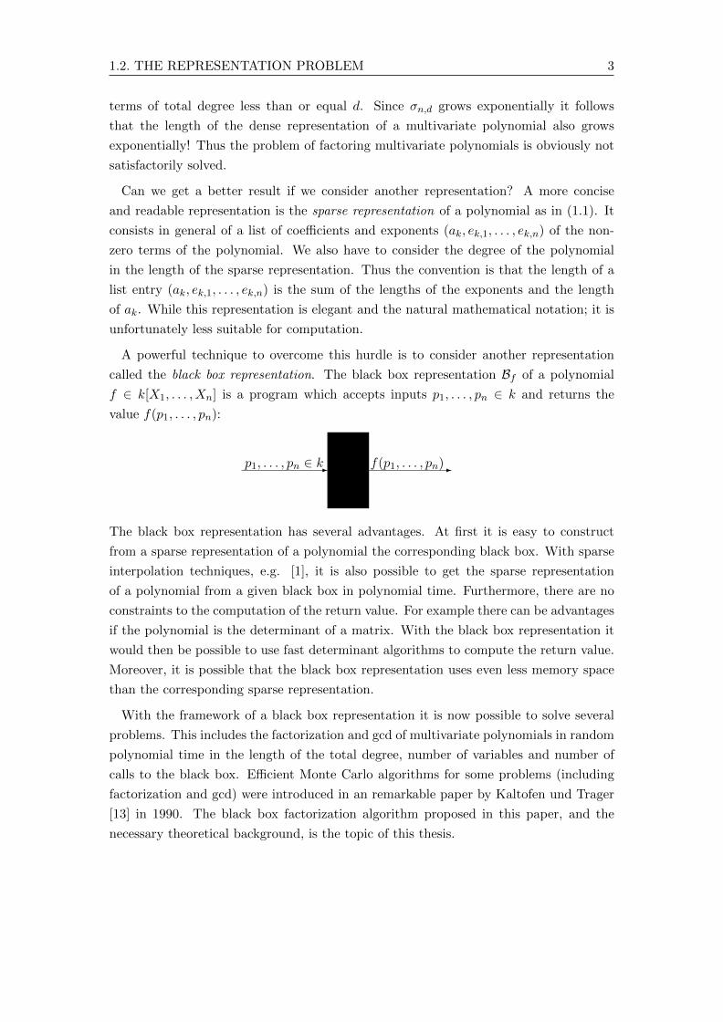
A powerful technique to overcome this hurdle is to consider another representation
called the black box representation. The black box representation Bf of a polynomial
f ∈ k[X1, . . . , Xn] is a program which accepts inputs p1, . . . , pn ∈ k and returns the
value f(p1, . . . , pn):
-p1, . . . , pn ∈ k f(p1, . . . , pn)-
The black box representation has several advantages. At first it is easy to construct
from a sparse representation of a polynomial the corresponding black box. With sparse
interpolation techniques, e.g. [1], it is also possible to get the sparse representation
of a polynomial from a given black box in polynomial time. Furthermore, there are no
constraints to the computation of the return value. For example there can be advantages
if the polynomial is the determinant of a matrix. With the black box representation it
would then be possible to use fast determinant algorithms to compute the return value.
Moreover, it is possible that the black box representation uses even less memory space
than the corresponding sparse representation.
With the framework of a black box representation it is now possible to solve several
problems. This includes the factorization and gcd of multivariate polynomials in random
polynomial time in the length of the total degree, number of variables and number of
calls to the black box. Efficient Monte Carlo algorithms for some problems (including
factorization and gcd) were introduced in an remarkable paper by Kaltofen und Trager
[13] in 1990. The black box factorization algorithm proposed in this paper, and the
necessary theoretical background, is the topic of this thesis.

4 1. INTRODUCTION
1.3 Black box factorization
We want to have a first glimpse on the factorization algorithm to motivative the following
theoretical chapters.
Assume we have a multivariate polynomial f ∈ k[X1, . . . , Xn] over a field k with char-
acteristic 0 and write he11 · · ·herr for the factorization of f . The factorization algorithm
has as its input the black box Bf and it returns the multiplicities e1, . . . , er and the
following program.
For input p1, . . . , pn ∈ k it returns the values h1(p1, . . . , pn), . . . , hr(p1, . . . , pn).
-p1, . . . , pn
h1(p1, . . . , pn)-
h2(p1, . . . , pn)-...
hr(p1, . . . , pn)-
Figure 1.1: Output program
Furthermore, we assume that we can efficiently factor polynomials in k[X1, X2].
The algorithm combines two ideas. The first idea is to use an effective version of the
Hilbert irreducibility theorem which was first stated and proved by Hilbert [9] in 1892.
The theorem states that for an irreducible polynomial g(X,Y ) ∈ Q[X,Y ], for almost
all a ∈ Q, the polynomial g(a, Y ) ∈ Q[Y ] is also irreducible. This can be generalized
for irreducible multivariate polynomials g ∈ Q[X1, . . . , Xn, Y ] such that for almost all
a1, . . . , an ∈ Q the evaluation g(a1, . . . , an, Y ) remains irreducible in Q[Y ]. We need
to quantify the “for almost all’ part, i.e., an effective version, of the theorem and we
have to be able to apply the theorem not only to polynomials over Q. Unfortunately
there is no known effective univariate version and the statement is clearly not applicable
for important fields like finite fields or the complex numbers. But the situation can be
rescued. In 1985 Kaltofen [10] constructed a substitution such that for an irreducible
multivariate polynomial over a perfect field k the resulting bivariate polynomial remains
irreducible with a controllable high probability. As a consequence for a multivariate
polynomial f ∈ k[X1, . . . , Xn] we can create a bivariate polynomial f2 ∈ k[X1, X2]
such that each irreducible factor hi of f has with a high probability a corresponding
irreducible factor g2,i of f2.
The second idea could be interpreted as an ansatz in homotopy continuation methods.
We can construct a bivariate polynomial f ∈ k[X1, Y ] such that for p1, . . . , pn ∈ k and
a known α ∈ k we have f(α, 1) = f(p1, . . . , pn) and f(X1, 0) = f2(X1, 0). Since we can
efficiently compute the factors g2,i of f2 we have a factorization of f2(X1, 0). With this
factorization we can reconstruct the factors gi of f with the by Zassenhaus introduced
Hensel lifting. By construction we have then gi(α, 1) = hi(p1, . . . , pn).

1.3. BLACK BOX FACTORIZATION 5
This causes the following structure of this thesis. At first we derive the Hensel lifting
algorithm in chapter 2 and then an effective version of Hilbert’s irreducibility theorem
in chapter 3. Finally we formulate the detailed black box factorization algorithm in
chapter 4.


Chapter 2
Hensel lifting
Assume we want to factor the bivariate polynomial
f(X,Y ) = Y 3 + (X − 1)Y 2 + (−X + 1)Y − 1 ∈ Q[X][Y ] .
The homotopy continuation ansatz is to transform this problem into a simpler one which
we can easily solve, i.e., an univariate factorization problem. Hence consider
f(0, Y ) = Y 3 − Y 2 + Y − 1 ∈ Q[Y ]
and in fact we can see that f(0, Y ) = (Y 2+1)(Y−1). Thus we are looking for polynomials
g(X,Y ) = Y 2 + g1(X)Y + g0(X) and h(X,Y ) = Y + h0(X)
such that f(X,Y ) = g(X,Y )h(X,Y ), g(0, Y ) = Y 2 + 1 and h(0, Y ) = Y − 1. This is the
same as solving the (non-linear) system of polynomial coefficient equations
1 = 1 · 1 (Y 3)
X − 1 = g1 + h0 (Y 2)
−X + 1 = g1h0 + g0 (Y )
−1 = g0h0 (1)
in Q[X].
A well-known method in numerical analysis to solve a system of non-linear functions
is the Newton iteration (or Newton’s method). It states
Let F : Rn → Rn be a differentiable function and x(0) ∈ Rn a suitable start approxi-
mation such that ‖F (x(0))‖ ≤ ε < 1 and JF (x(0)) invertible. Define the iteration
x(k+1) := x(k) − JF(x(k)
)−1F(x(k)
)(if well defined) then ‖F (x(k))‖ ≤ ε2k and ‖F ( lim
k→∞x(k))‖ = 0
7
8 2. HENSEL LIFTING
If we were now able to give a corresponding method in our algebraic setting we could
solve our system of coefficient equations and in fact this is possible. In order to do this
we have to answer the following questions:
1. Can we define a notion of “closeness” or even a metric space over rings / modules?
2. Can we even define a notion of convergence? Do we also have a quadratic conver-
gence?
3. Can we replace the analytical derivation?
4. Can we formulate an algebraic version of Taylor’s formula?
5. What is a suitable initial approximate solution?
6. Can we guarantee that the Jacobian remains invertible?
7. Is the result also unique?
We will derive the Hensel lifting theorem for polynomials over an arbitrary Noetherian
ring, although we only apply it in the concrete case that we have multivariate polynomials
over a field of characteristic 0. I chose this approach because I derived on my own an
algebraic version of the multivariate Newton iteration and the Hensel lifting theorem
and it felt “natural” to make this in a more general setting. A drawback is that I needed
some advanced results from commutative algebra in section 2.1 so that this thesis is not
self-contained. But we will, as often as possible, refer to the concrete case of polynomial
rings.
2.1 Valuation on a ring
First, all rings in this thesis are assumed to be commutative with identity 1.
We start with the fundamental question when two elements are “close”. If not other
mentioned we follow Bourbaki [5] in this section.
Definition 2.1 (Valuation). Let A be a ring and Γ a totally ordered abelian groupwritten multiplicatively. A valuation is a surjective map ν : A 7→ Γ ∪ {0} =: Γ0 whichsatisfies for all a, b ∈ A:
(1) ν(ab) = ν(a)ν(b) (multiplicative)
(2) ν(a+ b) ≤ max {ν(a), ν(b)} (ultra-metric inequality)
(3) ν(1) = 1 and ν(a) = 0 if and only if a = 0
A valuation is called discrete if Γ is isomorph to Z.
Remark 2.2. Q>0 with the usual multiplication is an example for Γ.
Remark 2.3. From the definition it follows that A has to be an integral domain.
2.1. VALUATION ON A RING 9
Remark 2.4. It is possible to give a equivalent definition (and more common definition)for a valuation with a totally ordered additive abelian group Γ adjoined with∞. In thiscase we have for all a, b ∈ A:
(1) ν(ab) = ν(a) + ν(b) (additive)
(2) ν(a+ b) ≥ inf {ν(a), ν(b)}
(3) ν(1) = 0 and ν(a) =∞ if and only if a = 0
Remark 2.5. If a ∈ A such that an = 1 for some integer n ≥ 1, we have ν(an) = ν(a)n = 1by (1) and since Γ is a totally ordered multiplicative group we have ν(a) = 1 for everyvaluation ν on A. In particular ν(−1) = 1 and thus ν(−a) = ν(a) for all a ∈ A. Since fora ∈ A we have 0 = ν(0) = ν(a+ (−a)) ≤ max{ν(a), ν(−a)} = max{ν(a), ν(a)} by (2) itfollows ν(a) ≥ 0 for all a ∈ A. If a ∈ A is not zero then ν(a)ν(a−1) = ν(aa−1) = ν(1) = 1and thus ν(a−1) = 1/ν(a).
Now we consider an important valuation, the m-adic valuation. Let A be a ring,
m ⊂ A a proper ideal. The sequence (mn)n≥0 of additive subgroups of A is called the
m-adic filtration of A. Then the order function ω : A→ N ∪ {∞}, a 7→ ω(a) with
ω(a) = n ⇔ a ∈ mn and a /∈ mn+1 (2.1)
ω(a) =∞⇔ a ∈⋂n≥0
mn (2.2)
is well defined.
The fact that the mn are additive subgroups of A implies that for a, b ∈ A
ω(a+ b) ≥ inf{ω(a), ω(b)} . (2.3)
Since A is an integral domain it follows for a, b 6= 0 with a ∈ mr, a /∈ mr+1 and b ∈ ms,
b /∈ ms+1 that ab /∈ mr+s+1 but ab ∈ mr+s and thus
ω(a+ b) = ω(a) + ω(b) . (2.4)
Consider now the map
ν : A→ {2−k | k ∈ N} ∪ {0}, a 7→ 2−ω(a) ,
then it follows from the equations (2.1) - (2.4) that, if⋂n≥0 m
n = {0}, ν is a valua-
tion map on A, called the m-adic valuation of A. In the concrete case of multivariate
polynomials over a field this is clearly satisfied for every m.
A theorem from Krull [6] states that the ideal⋂n≥0 m
n is {0} if A is a Noetherian
ring and no element of 1 + m is a divisor of 0 in A. In particular this is satisfied by
Noetherian local rings.
Example 2.6. Let A = Q[X] and m = (X). Then the order function is
ω(a) = n⇔ a ≡ 0 mod Xn and a 6≡ 0 mod Xn+1
ω(0) = 0

10 2. HENSEL LIFTING
With ν as the m-adic valuation we have
ν(X − 1) = 1, ν(X) =1
2and ν(X6 −X3) =
1
8.
Lemma 2.7 ([6]). Let A be a ring, Γ a totally ordered abelian group written multi-plicatively and ν : A 7→ Γ0 a valuation map. Then for a1, . . . , an ∈ A
ν( n∑j=1
aj
)≤ max
1≤j≤nν(aj) . (2.5)
Moreover, equality holds if there exists only a single index i such thatν(ai) = max1≤j≤n ν(aj).In particular we have for a, b ∈ A with ν(a) 6= ν(b) that ν(a+ b) = max{ν(a), ν(b)}.
Proof. The inequality (2.5) follows with axiom (2) easily by induction over n. Now ifthere exists only a single index i such that ν(ai) = max1≤j≤n ν(aj) then it follows withx :=
∑j 6=i ai and y :=
∑nj=1 aj by (2.5) that ν(x) < ν(ai) and ν(y) ≤ ν(ai). Assume
ν(y) < ν(ai). Since ai = y − x it follows that ν(ai) ≤ max{ν(y), ν(x)} < ν(ai). This isclearly a contradiction. Hence ν(y) = ν(ai).
Now consider again general valuations ν : A 7→ Γ0 on a ring A. For a = (ai) ∈ An
define
‖a‖ν := max1≤i≤n
ν(ai) . (2.6)
Then
d : An ×An → Γ0, (a, b) 7→ ‖a− b‖ν (2.7)
is an ultra-metric on An.
Proof. For a, b, c ∈ An we have d(a, b) = ‖a− b‖ν = maxi ν(ai−bi) ≥ 0 and d(a, b) = 0if and only if a− b = 0. Obviously d(a, b) = d(b, a) and
d(a, c) = ‖a− c‖ν = ‖a− b+ b− c‖ν= max
iν(ai − bi + bi − ci)
≤ maxi
max{ν(ai − bi), ν(bi − ci)}
= max{‖a− b‖ν , ‖b− c‖ν} = max{d(a, b), d(b, c)}
If we identify Am,n with Amn then (2.7) is also a metric on Am,n. For C = (ci,j) ∈ Am,n
we set ‖C‖ν := max1≤i≤m1≤j≤n
ν(ci,j).
Therefore every valuation ν induces a metric and thus a topology on the A-module
An, n ∈ N≥1. If ν is the m-adic valuation on A then the topology on An, induced by
(2.7), is called the m-adic topology and we write ‖ · ‖m instead of ‖·‖ν .
Now we introduce the concept of the completion of a ring which will prove to be
very useful. Following Eisenbud [7] the completion Am of A with respect to the m-adic
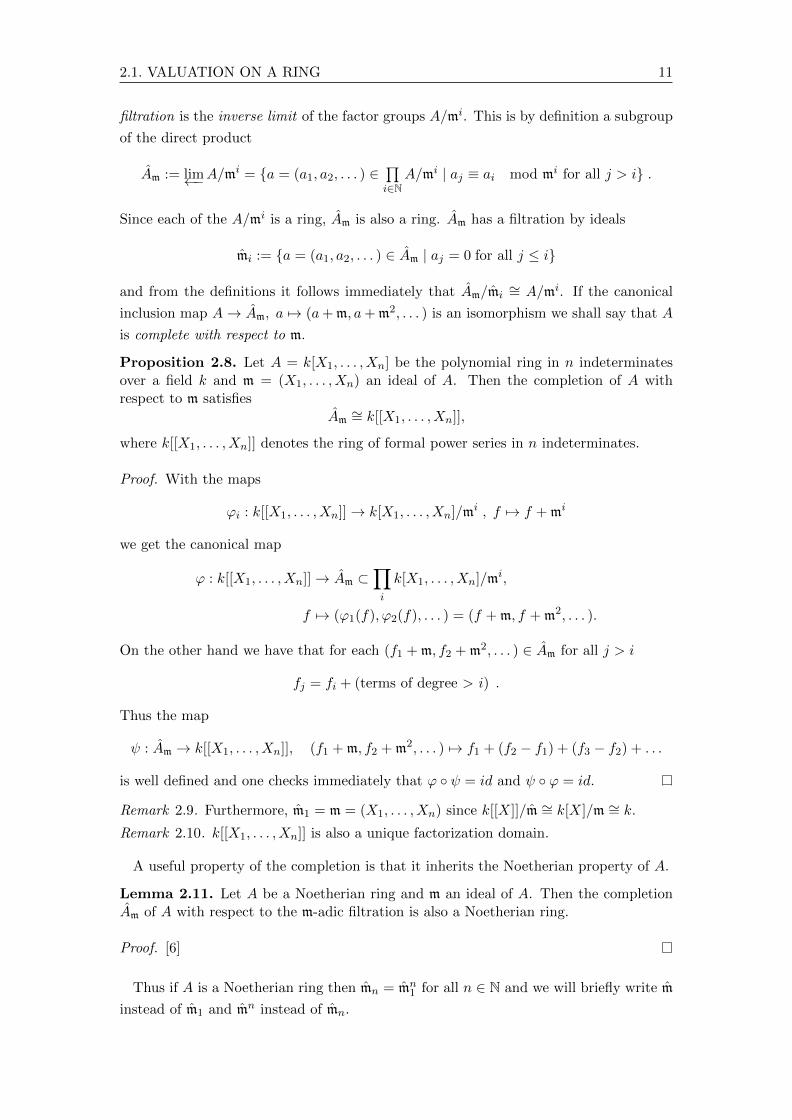
2.1. VALUATION ON A RING 11
filtration is the inverse limit of the factor groups A/mi. This is by definition a subgroup
of the direct product
Am := lim←−A/mi = {a = (a1, a2, . . . ) ∈
∏i∈N
A/mi | aj ≡ ai mod mi for all j > i} .
Since each of the A/mi is a ring, Am is also a ring. Am has a filtration by ideals
mi := {a = (a1, a2, . . . ) ∈ Am | aj = 0 for all j ≤ i}
and from the definitions it follows immediately that Am/mi∼= A/mi. If the canonical
inclusion map A→ Am, a 7→ (a+ m, a+ m2, . . . ) is an isomorphism we shall say that A
is complete with respect to m.
Proposition 2.8. Let A = k[X1, . . . , Xn] be the polynomial ring in n indeterminatesover a field k and m = (X1, . . . , Xn) an ideal of A. Then the completion of A withrespect to m satisfies
Am∼= k[[X1, . . . , Xn]],
where k[[X1, . . . , Xn]] denotes the ring of formal power series in n indeterminates.
Proof. With the maps
ϕi : k[[X1, . . . , Xn]]→ k[X1, . . . , Xn]/mi , f 7→ f + mi
we get the canonical map
ϕ : k[[X1, . . . , Xn]]→ Am ⊂∏i
k[X1, . . . , Xn]/mi,
f 7→ (ϕ1(f), ϕ2(f), . . . ) = (f + m, f + m2, . . . ).
On the other hand we have that for each (f1 + m, f2 + m2, . . . ) ∈ Am for all j > i
fj = fi + (terms of degree > i) .
Thus the map
ψ : Am → k[[X1, . . . , Xn]], (f1 + m, f2 + m2, . . . ) 7→ f1 + (f2 − f1) + (f3 − f2) + . . .
is well defined and one checks immediately that ϕ ◦ ψ = id and ψ ◦ ϕ = id.
Remark 2.9. Furthermore, m1 = m = (X1, . . . , Xn) since k[[X]]/m ∼= k[X]/m ∼= k.
Remark 2.10. k[[X1, . . . , Xn]] is also a unique factorization domain.
A useful property of the completion is that it inherits the Noetherian property of A.
Lemma 2.11. Let A be a Noetherian ring and m an ideal of A. Then the completionAm of A with respect to the m-adic filtration is also a Noetherian ring.
Proof. [6]
Thus if A is a Noetherian ring then mn = mn1 for all n ∈ N and we will briefly write m
instead of m1 and mn instead of mn.

12 2. HENSEL LIFTING
Assume now that A is a Noetherian ring with ideal m. We want to determine when the
m-adic valuation on the completion Am is well defined, i.e.⋂n≥0 m
n = {0}. By Krull’s
theorem this condition is satisfied if Am is a local ring. Remember that a characterization
of a local ring B is that for every element b ∈ B is b or 1− b a unit.
Lemma 2.12. Let A be a ring, m ⊂ A an ideal and a ∈ A. For positive integers i and j
a unit in A/mi ⇐⇒ a unit in A/mj .
Proof. Let a be a unit in A/mi and first assume i ≥ j. Then there exists a b ∈ A suchthat ab ≡ 1 mod mi and since mj ⊂ mi we have ab ≡ 1 mod mj .
Now assume i < j and without loss of generality i = 1 and j = 2k for some integer k.Then there exists a b0 ∈ A such that ab0 ≡ 1 mod m. Now we can recursively define asequence (bl) ⊂ A such that for l ≥ 1
bl ≡ 2bl−1 − ab2l−1 mod m2l . (2.8)
We claim that then abl ≡ 1 mod m2l for all l ≥ 0. We prove the claim by induction overl. The induction start is already done and for the induction step (l − 1→ l) consider
1− abl(2.8)≡ 1− a(2bl−1 − ab2l−1) ≡ 1− 2abl−1 + a2b2l−1 ≡ (1− abl−1)2 ≡ 0 mod m2l .
Hence abk ≡ 1 mod mj .
Remark 2.13. Equation (2.8) gives an algorithm to efficiently compute the inverse of anelement.
Lemma 2.14. Let A be a ring with maximal ideal m and Am its completion. Thena = (a1, a2, . . . ) ∈ Am is a unit if and only if a1 6= 0.
Proof. If a1 6= 0 each ai is a unit in A/m and therefore a unit in A/mi by lemma 2.12.Now it follows from aj ≡ ai mod mi for all j > i that a−1
j ≡ a−1i mod mi for all j > i
and we conclude that b := (a−11 , a−1
2 , . . . ) ∈ Am is the inverse of a.
Now suppose that a ∈ Am is a unit. Then there exists a b ∈ Am such that ab = 1 andin particular a1b1 = 1 and thus a1 6= 0.
Hence the completion of a ring with respect to a maximal ideal is a local ring and we
can conclude
Lemma 2.15. Let A be a Noetherian ring with maximal ideal m. Then the completionAm of A with respect to the m-adic filtration is a Noetherian local ring with maximalideal m.
Proof. Since m is a maximal ideal Am/m ∼= A/m is a field and hence m a maximal ideal.Moreover, if a = (a1, a2, . . . ) ∈ Am not in m, a1 6= 0 and by lemma 2.14 a unit. Thisshows that Am is a local ring and Am is also Noetherian by lemma 2.11.
Remark 2.16. In particular k[[X1, . . . , Xn]] is a complete Noetherian local ring by ourlemma and proposition 2.8.

2.1. VALUATION ON A RING 13
The completion Am of a Noetherian ring A with respect to a maximal ideal m has
therefore the m-adic topology. Now we show that this notion of completion coincides
with the notion of a complete metric space in the sense that every Cauchy sequence in
Am converges in Am.
Since Am is a metric space, a series (a1, a2, . . . ) ⊂ Am converges in the m-adic topol-
ogy to an element a ∈ Am if for every integer n there is an integer i(n) such that
‖a− ai(n)‖m ≤ 2−n. This is equivalent to that for every integer n there is an integer i(n)
such that a − ai(n) ∈ mn. Let (ai) ⊂ Am be a Cauchy sequence in the m-adic topology.
This means that for every integer n there exists an integer N such that
ai − aj ∈ mn for all i, j ≥ N .
This implies that for every integer n there exists an integer N such that ai ≡ aN mod m
for i ≥ N and it follows immediately immediately that every Cauchy sequence converges
in Am. Thus Anm is also complete since every sequence Anm is Cauchy if and only if the
coordinate sequences (a(i)j ) are Cauchy.
We have seen that every Noetherian local ring yields in a natural way a valuation, the
m-adic valuation. But it is of course possible to define valuations on other rings as well.
This leads to the following definition.
Definition 2.17 (Valuation ring). Let A be an integral domain and k its field of frac-tions. A is a valuation ring (or valued ring) if there exists a totally ordered multiplicativeabelian group Γ and a valuation ν : k 7→ Γ0 such that A = {ν(x) ≤ 1 |x ∈ k}. By defi-nition, a field is not a valuation ring.
If ν is a discrete valuation A is called a discrete valuation ring.
Remark 2.18. It’s again possible to give an equivalent definition for a valuation with atotally ordered additive abelian group Γ adjoined with ∞. Then the valuation ring isdefined as A := {ν(x) ≥ 0 |x ∈ k}.Remark 2.19. Let A be an integral domain and ν : A 7→ Γ0 a valuation map. Denoteby k the field of fractions of A and let a/b be an element of k. Then ν can easily beextended to a valuation of k with ν(a/b) := ν(a)/ν(b) and A is a subring of the valuationring Aν = {ν(x) ≤ 1 |x ∈ k}.
Example 2.20. Let k[[X]] be the ring of formal power series in one indeterminate overa field k. From proposition 2.8 it follows that k[[X]] is a complete Noetherian local ringwith maximal ideal m = (X). We claim that k[[X]] with the m-adic valuation ν is avaluation ring.The field of fractions of k[[X]] is k((X)) = {f/g | f, g ∈ k[[X]] with g 6= 0} and we canextend the m-adic valuation to k((X)) with ν(f/g) := ν(f)/ν(g) = 2−(ω(f)−ω(g)). Thenthe corresponding valuation ring is
{f/g ∈ k((X)) | ν(f/g) ≤ 1} = {f/g ∈ k((X)) | ω(f)− ω(g) ≥ 0} .
For f/g ∈ k((X)) with ν(f/g) ≤ 1 we can assume that gcd(f, g) = 1. Hence theonly case that, at the first sight, f/g is not in k[[X]] is ω(f) ≥ ω(g) = 0. Butthen g has a non-zero constant coefficient g0 and by lemma 2.14 g is a unit in k[[X]].Therefore f/g = (fg−1)/(gg−1) = fg−1 ∈ k[[X]] and k[[X]] is a valuation ring.

14 2. HENSEL LIFTING
A valuation ring has the following useful property.
Lemma 2.21. Let A be a valuation ring with valuation map ν. Then a ∈ A is a unitif and only if ν(a) = 1.
Proof. Let a ∈ A be a unit. Then there exists a−1 ∈ A and ν(a) = 1/ν(a−1). Sincea ∈ A, ν(a) ≤ 1 implies ν(a−1) ≥ 1 and with a−1 ∈ A it follows ν(a−1) = 1 and thusν(a) = 1.Now let a be in A with ν(a) = 1. Denote by k the field of fractions of A and interpreta as an element of k. Then there exists a−1 ∈ k and ν(a−1) = 1/ν(a) = 1. Thereforea−1 ∈ A and a is a unit.
But this statement is not only true for valuation rings but also for Noetherian local
rings A with maximal ideal m and the m-adic valuation. Consider a ∈ A. Then ν(a) = 1
if and only if a /∈ m and a characterization of a local ring is that every element not in m
is a unit.
This property yields also to the following valuable statement.
Lemma 2.22. Let A be a ring with valuation map ν such that a ∈ A is a unit if andonly if ν(a) = 1. Let a, b ∈ A with ν(b − a) < 1. Then a is a unit if and only if b is aunit.
Proof. It is sufficient to show that ν(a) = 1 if and only if ν(b) = 1. If ν(a) = 1 then
ν(b) = ν(a+(b−a))2.5= max{ν(a), ν(b−a)} = 1 and by an analogous argument it follows
that ν(a) = 1 if ν(b) = 1.
2.2 Taylor’s formula
As a next step we derive an algebraic version of Taylor’s formula (following Bourbaki’s
[4] neat derivation) and introduce the concept of a formal derivative as an replacement
for the analytical derivative. But at first we have to fix some multi-index notation.
Let n ∈ N, α = (α1, . . . , αn), β = (β1, . . . , βn) ∈ Nn and X = (X1, . . . , Xn) and
Y = (Y1, . . . , Yn) two families of indeterminates. We set X + Y := (X1 + Y1, . . . ,
Xn + Yn), Xα := X1α1 · . . . ·Xn
αn , α! := α1!α2! . . . αn!, |α| := α1 + α2 + . . . + αn and(αβ
):=(α1
β1
). . .(αnβn
)where
(αiβi
)denotes the binomial coefficient.
Lemma 2.23 (Multi-index binomial theorem). Let n ∈ N, X = (X1, . . . , Xn) andY = (Y1, . . . , Yn) two families of indeterminates and α ∈ Nn. Then
(X + Y )α =∑
0≤β≤α
(α
β
)XβY α−β .

2.2. TAYLOR’S FORMULA 15
Proof. We have
(X + Y )α =
n∏i=0
(Xi + Yi)αi
=n∏i=0
αi∑βi=0
(αiβi
)Xβii Y
αi−βii
=( α1∑β1=0
(α1
β1
)Xβ1
1 Y α1−β11
)· · ·( αn∑βn=0
(αnβn
)Xβnn Y αn−βn
n
).
Now we can expand and rearrange the product:
=
α1∑β1=0
· · ·αn∑βn=0
(α1
β1
). . .
(αnβn
)Xβ1
1 . . . Xβnn Y α1−β1
1 . . . Y αn−βnn
=∑
0≤β≤α
(α
β
)XβY α−β .
Definition 2.24. Let n be an integer, A an integral domain and X = (X1, . . . , Xn)and Y = (Y1, . . . , Yn) two families of indeterminates. For f ∈ A[X] = A[X1, . . . , Xn]we can consider f(X + Y ) as a polynomial in A[X][Y ] and denote for all α ∈ Nn by∆αf ∈ A[X] the coefficient of Y α in f(X + Y ).
Remark 2.25. From the definition of ∆αf it follows immediately that ∆α ∈ End(A[X])where A[X] is considered as an A-module.
Example 2.26. Consider again our example
f(X,Y ) = Y 3 + (X − 1)Y 2 + (−X + 1)Y − 1
= Y 3 +XY 2 − Y 2 −XY + Y − 1 .
Then
f(X + Z1, Y + Z2) = (Y + Z2)3 − (Y + Z2)2 + (X + Z1)(Y + Z2)2 + (Y + Z2)
− (X + Z1)(Y + Z2)− 1
= Z32 + Z2
2Z1 + (3Y +X − 1)Z22 + (2Y − 1)Z1Z2
+ (3Y 2 + 2XY − 2Y −X + 1)Z2 + (Y 2 − Y )Z1
+ Y 3 +XY 2 − Y 2 −XY + Y − 1
Hence, ∆0,1f(X,Y ) = 3Y 2 + 2XY − 2Y −X + 1 and ∆1,1f(X) = 2Y − 1.
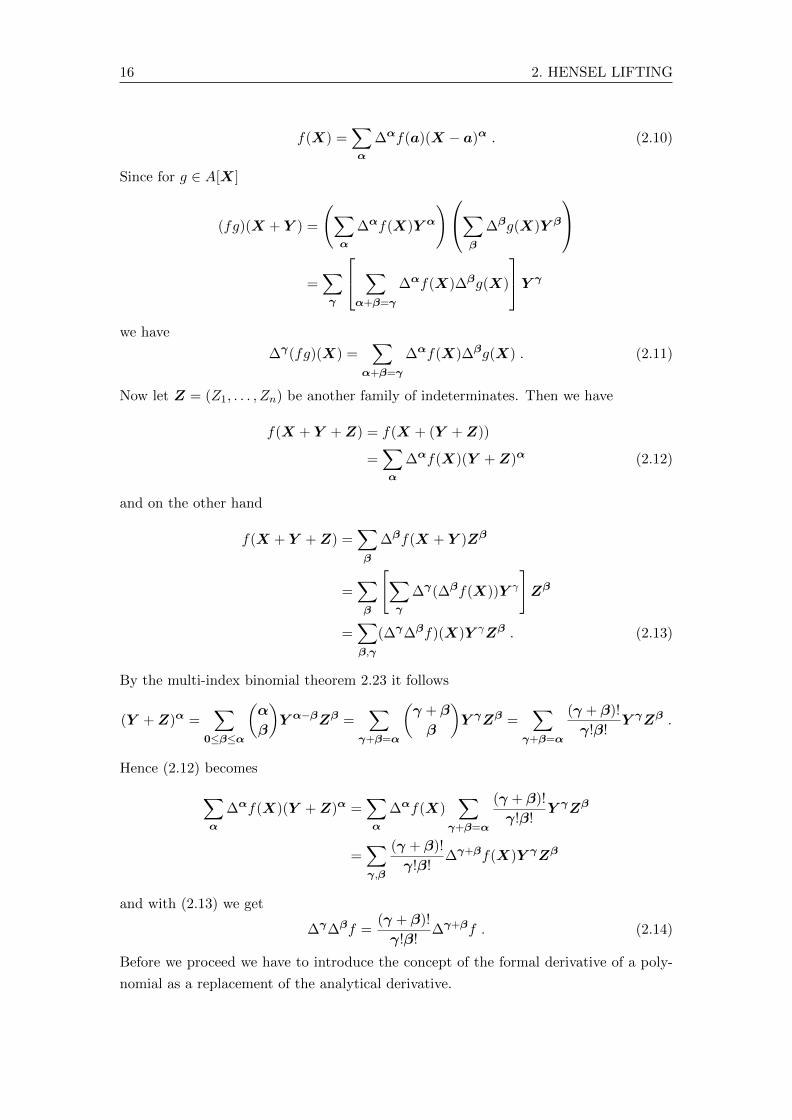
In the following all summations are about Nn. Let f ∈ A[X] = A[X1, . . . , Xn] be a
multivariate polynomial and by definition
f(X + Y ) =∑α
∆αf(X)Y α . (2.9)
If we substitute X 7→ a and Y 7→X − a for a ∈ An we have
16 2. HENSEL LIFTING
f(X) =∑α
∆αf(a)(X − a)α . (2.10)
Since for g ∈ A[X]
(fg)(X + Y ) =
(∑α
∆αf(X)Y α
)∑β
∆βg(X)Y β
=∑γ
∑α+β=γ
∆αf(X)∆βg(X)
Y γ
we have
∆γ(fg)(X) =∑
α+β=γ
∆αf(X)∆βg(X) . (2.11)
Now let Z = (Z1, . . . , Zn) be another family of indeterminates. Then we have
f(X + Y +Z) = f(X + (Y +Z))
=∑α
∆αf(X)(Y +Z)α (2.12)
and on the other hand
f(X + Y +Z) =∑β
∆βf(X + Y )Zβ
=∑β
[∑γ
∆γ(∆βf(X))Y γ
]Zβ
=∑β,γ
(∆γ∆βf)(X)Y γZβ . (2.13)
By the multi-index binomial theorem 2.23 it follows
(Y +Z)α =∑
0≤β≤α
(α
β
)Y α−βZβ =
∑γ+β=α
(γ + β
β
)Y γZβ =
∑γ+β=α
(γ + β)!
γ!β!Y γZβ .
Hence (2.12) becomes∑α
∆αf(X)(Y +Z)α =∑α
∆αf(X)∑
γ+β=α
(γ + β)!
γ!β!Y γZβ
=∑γ,β
(γ + β)!
γ!β!∆γ+βf(X)Y γZβ
and with (2.13) we get
∆γ∆βf =(γ + β)!
γ!β!∆γ+βf . (2.14)
Before we proceed we have to introduce the concept of the formal derivative of a poly-
nomial as a replacement of the analytical derivative.
2.2. TAYLOR’S FORMULA 17
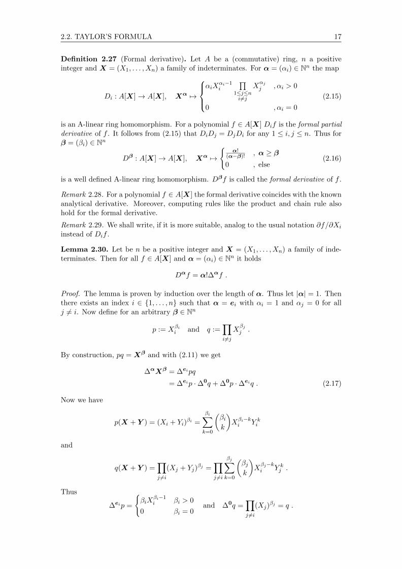
Definition 2.27 (Formal derivative). Let A be a (commutative) ring, n a positiveinteger and X = (X1, . . . , Xn) a family of indeterminates. For α = (αi) ∈ Nn the map
Di : A[X]→ A[X], Xα 7→
αiX
αi−1i
∏1≤j≤ni 6=j
Xαjj , αi > 0
0 , αi = 0
(2.15)
is an A-linear ring homomorphism. For a polynomial f ∈ A[X] Dif is the formal partialderivative of f . It follows from (2.15) that DiDj = DjDi for any 1 ≤ i, j ≤ n. Thus forβ = (βi) ∈ Nn
Dβ : A[X]→ A[X], Xα 7→
{α!
(α−β)! , α ≥ β0 , else
(2.16)
is a well defined A-linear ring homomorphism. Dβf is called the formal derivative of f .
Remark 2.28. For a polynomial f ∈ A[X] the formal derivative coincides with the knownanalytical derivative. Moreover, computing rules like the product and chain rule alsohold for the formal derivative.
Remark 2.29. We shall write, if it is more suitable, analog to the usual notation ∂f/∂Xi
instead of Dif .
Lemma 2.30. Let be n be a positive integer and X = (X1, . . . , Xn) a family of inde-terminates. Then for all f ∈ A[X] and α = (αi) ∈ Nn it holds
Dαf = α!∆αf .
Proof. The lemma is proven by induction over the length of α. Thus let |α| = 1. Thenthere exists an index i ∈ {1, . . . , n} such that α = ei with αi = 1 and αj = 0 for allj 6= i. Now define for an arbitrary β ∈ Nn
p := Xβii and q :=
∏i 6=j
Xβjj .
By construction, pq = Xβ and with (2.11) we get
∆αXβ = ∆eipq
= ∆eip ·∆0q + ∆0p ·∆eiq . (2.17)
Now we have
p(X + Y ) = (Xi + Yi)βi =
βi∑k=0
(βik
)Xβi−ki Y k
i
and
q(X + Y ) =∏j 6=i
(Xj + Yj)βj =
∏j 6=i
βj∑k=0
(βjk
)Xβj−ki Y k
j .
Thus
∆eip =
{βiX
βi−1i βi > 0
0 βi = 0and ∆0q =
∏j 6=i
(Xj)βj = q .

18 2. HENSEL LIFTING
Since Yi doesn’t appear in q(X + Y ) we have ∆eiq = 0. With (2.17) it follows that
∆αXβ = ∆eiXβ =
βiXβi−1i
∏j 6=i
(Xj)βj , βi > 0
0 , βi = 0
= DeiXβ = ∆αXβ .
Since ∆α ∈ End(A[X]) it follows that ∆αf = Dαf = α!Dαf.
Now let us assume that our induction hypothesis holds for m ∈ N and let α ∈ Nnwith |α| = m+ 1. Notice that we obtain for β,γ ∈ Nn by (2.14)
(γ!∆γ)(β!∆β) = (γ + β)!∆γ+β ∈ End(A[X]) . (2.18)
Then there exists i ∈ {1, . . . , n} such that α− ei ∈ Nn and by (2.18) we obtain
α!∆α = ((α− ei) + ei)!∆(α−ei)+ei = (α− ei)!∆(α−ei) ◦ ei!∆ei .
Therefore it follows together with the induction hypothesis:
α!∆αf = ((α− ei)!∆(α−ei) ◦ ei!∆ei)f
= (α− ei)!∆(α−ei)(ei!∆eif)
= (α− ei)!∆(α−ei)(Deif)
= D(α−ei)(Deif)
= Dαf
Now everything is in place to formulate Taylor’s formula in our algebraic setting.
Theorem 2.31 (Taylor’s formula). LetA be an integral domain, n ∈ N,X = (X1, . . . , Xn)a family of indeterminates and f ∈ A[X]. Then we have for another family of indeter-minates Y = (Y1, . . . , Yn)
f(X + Y ) =∑α
1
α!(Dαf)(X)Y α
and for a ∈ An
f(X) =∑α
1
α!(Dαf)(a)(X − a)α .
Proof. By (2.9) f(X + Y ) =∑α
∆αf(X)Y α and by lemma 2.30 it follows the first
statement. By (2.10) f(X) =∑α
∆αf(a)(X − a)α and again by lemma 2.30 it follows
the second statement.
Finally, in preparation for the Newton iteration, we formulate a version of Taylor’s
formula for systems of polynomials.
Corollary 2.32. Let A be an integral domain, n a positive integer, X = (X1, . . . , Xn)
a family of indeterminates and F (X) =
[f1(X)
...fn(X)
]∈ A[X]n a system of polynomials. For
2.3. NEWTON ITERATION 19
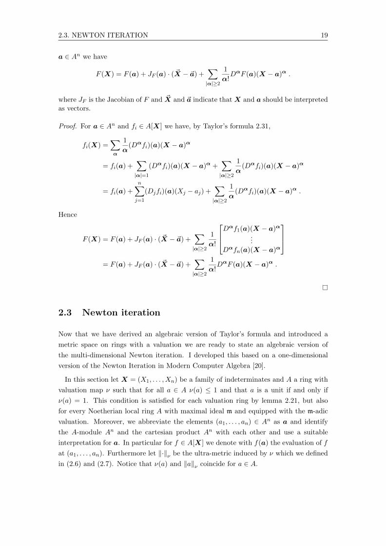
a ∈ An we have
F (X) = F (a) + JF (a) · ( ~X − ~a) +∑|α|≥2
1
α!DαF (a)(X − a)α .
where JF is the Jacobian of F and ~X and ~a indicate that X and a should be interpretedas vectors.
Proof. For a ∈ An and fi ∈ A[X] we have, by Taylor’s formula 2.31,
fi(X) =∑α
1
α(Dαfi)(a)(X − a)α
= fi(a) +∑|α|=1
(Dαfi)(a)(X − a)α +∑|α|≥2
1
α(Dαfi)(a)(X − a)α
= fi(a) +
n∑j=1
(Djfi)(a)(Xj − aj) +∑|α|≥2
1
α(Dαfi)(a)(X − a)α .
Hence
F (X) = F (a) + JF (a) · ( ~X − ~a) +∑|α|≥2
1
α!
Dαf1(a)(X − a)α
...Dαfn(a)(X − a)α
= F (a) + JF (a) · ( ~X − ~a) +
∑|α|≥2
1
α!DαF (a)(X − a)α .
2.3 Newton iteration
Now that we have derived an algebraic version of Taylor’s formula and introduced a
metric space on rings with a valuation we are ready to state an algebraic version of
the multi-dimensional Newton iteration. I developed this based on a one-dimensional
version of the Newton Iteration in Modern Computer Algebra [20].
In this section let X = (X1, . . . , Xn) be a family of indeterminates and A a ring with
valuation map ν such that for all a ∈ A ν(a) ≤ 1 and that a is a unit if and only if
ν(a) = 1. This condition is satisfied for each valuation ring by lemma 2.21, but also
for every Noetherian local ring A with maximal ideal m and equipped with the m-adic
valuation. Moreover, we abbreviate the elements (a1, . . . , an) ∈ An as a and identify
the A-module An and the cartesian product An with each other and use a suitable
interpretation for a. In particular for f ∈ A[X] we denote with f(a) the evaluation of f
at (a1, . . . , an). Furthermore let ‖·‖ν be the ultra-metric induced by ν which we defined
in (2.6) and (2.7). Notice that ν(a) and ‖a‖ν coincide for a ∈ A.

20 2. HENSEL LIFTING
At first we note the following useful estimate.
Lemma 2.33. For C ∈ Am,n and a ∈ An we have ‖Ca‖ν ≤ ‖C‖ν ‖a‖ν
Proof. Let C = (ci,j) ∈ An,n be a matrix and a ∈ An. Then
‖Ca‖ν = max1≤i≤m
(∑j=1
ci,jaj
)≤ max
1≤i≤mmax
1≤i≤m1≤j≤n
ν(ci,jaj)
= max1≤i≤m1≤j≤n
ν(ci,j)ν(aj) ≤ max1≤i≤m1≤j≤n
ν(ci,j) max1≤j≤n
ν(aj) = ‖C‖ν ‖a‖ν .
The construction of the Newton iteration is mostly identical to the analytical version.
Lemma 2.34. Let F ∈ A[X]n be a system of polynomials. For all a, b ∈ An with‖b− a‖ν ≤ ε we have
‖F (b)− F (a)− JF (a)(b− a)‖ν ≤ ε2 .
Proof. By corollary 2.32 to Taylor’s formula we have
F (b) = F (a) + JF (a) · (b− a) +∑|α|≥2
1
α!DαF (a)(b− a)α
and therefore
‖F (b)− F (a)− JF (a)(b− a)‖ν =∥∥∥∑|α|≥2
1
α!DαF (a)(b− a)α
∥∥∥ν. (2.19)
To prove the lemma we now look at the right side of equation (2.19). From ‖b− a‖ν ≤ εit follows that for i = 1, . . . , n, ν(bi − ai) ≤ ε and thus for all α ∈ Nn with |α| ≥ 2
ν((b− a)α) = ν( n∏i=1
(bi − ai)αi)
=
n∏i=1
ν(bi − ai)αi ≤ ε2 .
Hence ∥∥∥∑|α|≥2
1
α!DαF (a)(b− a)α
∥∥∥ν≤ ε2
and the lemma follows.
A notable difference to the analytical case is that we can guarantee that the Jacobian
of a system remains invertible.
Lemma 2.35. Let F ∈ A[X]n be a system of polynomials, a ∈ An such that‖det(JF (a))‖ν = 1 and b ∈ An with ‖b− a‖ν < 1. Then
‖det(JF (b))‖ν = 1 .

2.3. NEWTON ITERATION 21
Proof. det(JF (X)) is a polynomial in A[X] and therefore there exists a finite indexfamily I ⊂ Nn such that det(JF (X)) =
∑α∈I cαX
α with cα ∈ A. Now we have
det(JF (b)) =∑α∈I
cαbα =
∑α∈I
cα (a+ (b− a))α
and by the multi-index binomial theorem 2.23
=∑α∈I
cα
( ∑0≤β≤α
(α
β
)aβ(b− a)α−β
)=∑α∈I
cαaα
︸ ︷︷ ︸det(JF (a))
+∑α∈I
∑0≤β<α
cα
(α
β
)aβ(b− a)α−β .
Since ‖det(JF (a))‖ν = 1 and∥∥∥∑α∈I
∑0≤β<α
cα
(α
β
)aβ(b− a)α−β
∥∥∥ν≤ max
α∈Imax
0≤β<αν
(cα
(α
β
)aβ(b− a)α−β
)≤ max
α∈Imax
0≤β<αν(
(b− a)α−β)
|α−β|>0 ∧ ‖b−a‖ν<1< 1
we conclude ‖det(JF (b))‖ν = 1 by lemma 2.7.
Now assume that for a system of polynomials F ∈ A[X]n we have an approximation
a ∈ An with ‖F (a)‖ν ≤ ε < 1. If additionally the Jacobian of F , JF , is invertible in a
we get ∥∥(a− JF (a)−1F (a))− a∥∥ν
=∥∥−JF (a)−1F (a)
∥∥ν≤ ‖F (a)‖ν ≤ ε (2.20)
by lemma 2.33. With b := a − JF (a)−1F (a) we have then found a suitable b for
lemma 2.34 and we can formulate the following theorem:
Theorem 2.36 (Quadratic Convergence). Let F ∈ A[X]n be a system of polynomials,a ∈ An an approximation of F with ‖F (a)‖ν ≤ ε < 1 and ‖det(JF (a))‖ν = 1. Thenb := a− JF (a)−1F (a) is well defined and
‖b− a‖ν ≤ ε , ‖F (b)‖ν ≤ ε2 and ‖det(JF (b))‖ν = 1 .
Proof. Since ‖det(JF (a))‖ν = 1 it follows by lemma 2.21 that det(JF (a)) is a unitin A. Hence JF (a) is invertible and b well defined.
By (2.20) ‖b− a‖ν ≤ ε < 1 and thus ‖det(JF (b))‖ν = 1 by lemma 2.35. Finally weobtain by lemma 2.34
ε2 ≥ ‖F (b)− F (a)− JF (a)(b− a)‖ν=∥∥F (b)− F (a)− JF (a)(a− JF (a)−1F (a)− a)
∥∥ν
=∥∥F (b)− F (a) + JF (a)JF (a)−1F (a)
∥∥ν
(2.21)
= ‖F (b)‖ν .

22 2. HENSEL LIFTING
Remark 2.37. Instead of computing JF (a)−1 it is sufficient to compute J∗ such that‖J∗JF (a)− In‖ν ≤ ε2 and to set b = a − J∗F (a). By lemma 2.33 we have‖(J∗JF (a)− In)F (a)‖ν ≤ ε2 and the inequality (2.21) would then be
‖F (b) + J∗JF (a)F (a)− F (a)‖ν ≤ ε2
and on the other hand
‖F (b) + J∗JF (a)F (a)− F (a)‖ν ≤ max{‖F (b)‖ν , ε2} .
Hence ‖F (b)‖ν ≤ ε2.
We have seen how we can get from an approximate solution a with ‖F (a)‖ν ≤ ε < 1
and ‖det(JF (a))‖ν to a better approximation b with ‖F (b)‖ν ≤ ε2 and ‖b− a‖ν ≤ ε.
The following theorem shows that b is even unique.
Theorem 2.38 (Uniqueness). Let F ∈ A[X]n be a system of polynomials, a ∈ An suchthat ‖F (a)‖ν = ε < 1 and ‖det(JF (a))‖ν = 1. If there exists b and b∗ ∈ An such that
‖b− a‖ν ≤ ε‖F (b)‖ν ≤ ε2 and
‖b∗ − a‖ν ≤ ε‖F (b∗)‖ν ≤ ε2
then‖b∗ − b‖ν ≤ ε
2 .
Proof. By corollary 2.32 to Taylor’s formula we have
F (b∗) = F (b) + JF (b) · (b∗ − b) +∑|α|≥2
1
α!DαF (b)(b∗ − b)α (2.22)
and by lemma 2.34 ∥∥∥∑|α|≥2
1
α!DαF (b)(b∗ − b)α
∥∥∥ν≤ ‖b∗ − b‖2ν . (2.23)
Since‖b− a‖ν ≤ ε < 1 it follows ‖det(JF (b))‖ν = 1 by lemma 2.35. Hence det(JF (b))is a unit in A and JF (b) is invertible. Now it follows with (2.22)
‖b∗ − b‖ν =∥∥∥JF (b)−1
(F (b∗)− F (b)−
∑|α|≥2
1
α!DαF (b)(b∗ − b)α
)∥∥∥ν
≤∥∥∥F (b∗)− F (b)−
∑|α|≥2
1
α!DαF (b)(b∗ − b)α
∥∥∥ν
≤ max{‖F (b∗)‖ν , ‖F (b)‖ν ,
∥∥∥∑|α|≥2
1
α!DαF (b)(b∗ − b)α
∥∥∥ν
}(2.23)
≤ max{ε2, ε2, ‖b∗ − b‖2ν
}.
2.3. NEWTON ITERATION 23
Since ‖b∗ − b‖ν = ‖b∗ − a− (b− a)‖ν ≤ max{‖b∗ − a‖ν , ‖b− a‖ν} ≤ ε < 1 it fol-lows that ‖b∗ − b‖2ν < ‖b∗ − b‖ν . Therefore we conclude
‖b∗ − b‖ν ≤ max{ε2, ε2, ‖b∗ − b‖2ν
}≤ ε2
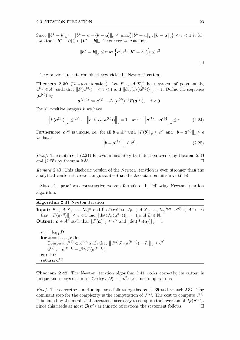
The previous results combined now yield the Newton iteration.
Theorem 2.39 (Newton iteration). Let F ∈ A[X]n be a system of polynomials,a(0) ∈ An such that
∥∥F (a(0))∥∥ν≤ ε < 1 and
∥∥det(Jf (a(0)))∥∥ν
= 1. Define the sequence
(a(k)) bya(j+1) := a(j) − JF (a(j))−1F (a(j)), j ≥ 0 .
For all positive integers k we have∥∥∥F (a(k))∥∥∥ν≤ ε2k ,
∥∥∥det(JF (a(k)))∥∥∥ν
= 1 and∥∥∥a(k) − a(0)
∥∥∥ν≤ ε . (2.24)
Furthermore, a(k) is unique, i.e., for all b ∈ An with ‖F (b)‖ν ≤ ε2k
and∥∥b− a(0)
∥∥ν≤ ε
we have ∥∥∥b− a(k)∥∥∥ν≤ ε2k . (2.25)
Proof. The statement (2.24) follows immediately by induction over k by theorem 2.36and (2.25) by theorem 2.38.
Remark 2.40. This algebraic version of the Newton iteration is even stronger than theanalytical version since we can guarantee that the Jacobian remains invertible!
Since the proof was constructive we can formulate the following Newton iteration
algorithm:
Algorithm 2.41 Newton iteration
Input: F ∈ A[X1, . . . , Xn]n and its Jacobian JF ∈ A[X1, . . . , Xn]n,n, a(0) ∈ An suchthat
∥∥F (a(0))∥∥ν≤ ε < 1 and
∥∥det(JF (a(0)))∥∥ν
= 1 and D ∈ N.
Output: a ∈ An such that ‖F (a)‖ν ≤ εD and ‖det(JF (a))‖ν = 1
r := dlog2Defor k := 1, . . . , r do
Compute J (k) ∈ An,n such that∥∥J (k)JF (a(k−1))− In
∥∥ν≤ ε2k
a(k) := a(k−1) − J (k)F (a(k−1))end forreturn a(r)
Theorem 2.42. The Newton iteration algorithm 2.41 works correctly, its output isunique and it needs at most O((log2(D) + 1)n3) arithmetic operations.
Proof. The correctness and uniqueness follows by theorem 2.39 and remark 2.37. Thedominant step for the complexity is the computation of J (k). The cost to compute J (k)
is bounded by the number of operations necessary to compute the inversion of JF (a(k)).Since this needs at most O(n3) arithmetic operations the statement follows.

24 2. HENSEL LIFTING
Finally we state that if A is a complete Noetherian local ring and ν the m-adic valu-
ation, the Newton iteration always converges to a unique limit.
Corollary 2.43. Let A be a complete Noetherian local ring with maximal ideal m andequipped with the m-adic valuation. If for a system of polynomials F ∈ A[X]n ana = (ai) ∈ An exists such that
‖F (a)‖m < 1 and ‖ det(JF (a))‖m = 1
then there exists an unique a ∈ An such that
F (a) = 0 , det(JF (a)) unit and ‖a− a‖m < 1 .
Proof. With a(0) := a the sequence
a(k+1) := a(k) − JF (a(k))−1F (a(k)) , k ≥ 0 (2.26)
is well defined and a Cauchy sequence as, by theorem 2.39, for i = 1, . . . , n and allintegers N
a(j)i − a
(k)i ∈ mN for all j, k > dlog2Ne.
Define a := lima(i) ∈ A. By theorem 2.39 a is unique, F (a) = 0, det(JF (a)) a unit and‖a− a‖m < 1.
Remark 2.44. Remember that ‖F (a)‖m < 1 if and only if fi(a) ≡ 0 mod m for 1 ≤ i ≤ nand ‖ det(JF (a))‖m = 1 if and only if det(JF (a)) is a unit.
2.4 Sylvester matrix and resultant
This section is based on Chapter 6 in Modern Computer Algebra [19]. Let us now take
a look at our original problem. We want to factor the polynomial
f(X,Y ) = Y 3 + (X − 1)Y 2 + (−X + 1)Y − 1 ∈ Q[X][Y ]
and already derived that this is equivalent to a solution g1, g0, h0 ∈ Q[X] such that
F (h0, g1, g0) =
g1 + h0 − (X − 1)
g1h0 + g0 − (−X + 1)
g0h0 − (−1)
= 0 .
Since f(0, Y ) = (Y 2 + 1)(Y − 1) we have
F (−1, 0, 1) =
−XX0
.
If we now interpret f, g1, g0 and h0 as elements of Q[[X]] F is a system over the complete
Noetherian local ring Q[[X]] with maximal ideal m = (X). Then ‖F (−1, 0, 1)‖m = 1/2
and if JF (−1, 0, 1) is invertible we can obtain a solution for F by Newton iteration.
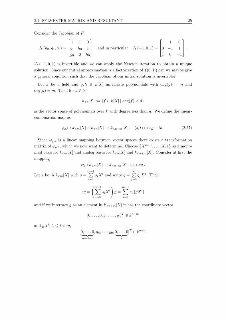
2.4. SYLVESTER MATRIX AND RESULTANT 25
Consider the Jacobian of F
JF (h0, g1, g0) =
1 1 0
g1 h0 1
g0 0 h0
and in particular JF (−1, 0, 1) =
1 1 0
0 −1 1
1 0 −1
.
JF (−1, 0, 1) is invertible and we can apply the Newton iteration to obtain a unique
solution. Since our initial approximation is a factorization of f(0, Y ) can we maybe give
a general condition such that the Jacobian of our initial solution is invertible?
Let k be a field and g, h ∈ k[X] univariate polynomials with deg(g) = n and
deg(h) = m. Then for d ∈ N
k<d[X] := {f ∈ k[X] | deg(f) < d}
is the vector space of polynomials over k with degree less than d. We define the linear-
combination map as
ϕg,h : k<m[X]× k<n[X]→ k<n+m[X], (s, t) 7→ sg + th . (2.27)
Since ϕg,h is a linear mapping between vector spaces there exists a transformation
matrix of ϕg,h, which we now want to determine. Choose {Xm−1, . . . , X, 1} as a mono-
mial basis for k<m[X] and analog bases for k<n[X] and k<n+m[X]. Consider at first the
mapping
ϕg : k<m[X]→ k<n+m[X], s 7→ sg .
Let s be in k<m[X] with s =m−1∑i=0
siXi and write g =
n∑j=0
gjXj . Then
sg =
(m−1∑i=0
siXi
)g =
m−1∑i=0
si(gXi
)and if we interpret g as an element in k<n+m[X] it has the coordinate vector
[0, . . . , 0, gn, . . . , g0]T ∈ kn+m
and gXi, 1 ≤ i < m,
[0, . . . , 0︸ ︷︷ ︸m−1−i
, gn, . . . , g0, 0, . . . , 0︸ ︷︷ ︸i
]T ∈ kn+m

26 2. HENSEL LIFTING
Now we can obtain the (n+m)×m transformation matrix of ϕg by
gn 0 . . . 0
gn−1 gn. . .
...... gn−1
. . . 0...
. . .. . . gn
.... . .
. . . gn−1
g1. . .
. . ....
g0 g1. . .
...
0 g0. . .
......
. . .. . . g1
0 . . . 0 g0
.
We can analogous obtain the (n+m)× n transformation matrix of
ϕh : k<n[X]→ k<n+m[X], t 7→ th .
The transformation matrix of ϕg,h is thus
gn 0 . . . 0 hm 0 . . . . . . 0
gn−1 gn. . .
... hm−1 hm. . .
...... gn−1
. . . 0... hm−1
. . .. . .
......
. . .. . . gn
.... . .
. . .. . . 0
.... . .
. . . gn−1...
. . .. . .
. . . hm
g2. . .
. . .... h1
. . .. . .
. . . hm−1
g1 g2. . .
... h0 h1. . .
. . ....
g0 g1. . .
... 0 h0. . .
. . ....
0 g0. . . g2
.... . .
. . .. . .
......
. . .. . . g1
.... . .
. . . h1
0 . . . 0 g0 0 . . . . . . 0 h0
. (2.28)
For the construction of (2.28) we did not use the fact that k is a field. Therefore we can
give the following more general definition.
Definition 2.45 (Sylvester matrix and resultant). Let A be a commutative ring andg, h ∈ A[X] two polynomials with g =
∑ni=0 giX
i and h =∑m
i=0 hiXi. Then the
(n+m)× (n+m) matrix (2.28) is the Sylvester matrix of g and h denoted by Syl(g, h).The determinant of Syl(g, h) is called the resultant of g and h denoted byres(g, h).
Example 2.46. We continue our example. Consider the initial factorization
f(0, Y ) = Y 3 − Y 2 + Y − 1 = (Y 2 + 1)(Y − 1) ∈ Q[[X]][Y ] .

2.4. SYLVESTER MATRIX AND RESULTANT 27
Then
Syl(Y 2 + 1, Y − 1) =
1 1 00 −1 11 0 −1
and res(Y 2 + 1, Y − 1) = 2 .
Notice that Syl(Y 2 + 1, Y − 1) and JF (−1, 0, 1) coincide!
Let g and h be univariate polynomials over a (commutative) ring A. With the Sylvester
matrix we can reformulate the linear-combination mapping ϕg,h as the corresponding
linear transformation mapping:
Φg,h : Am ×An → An+m,
sm−1
...s0
, tn−1
...t0
7→ Syl(g, h)
sm−1
...s0
tn−1
...t0
(2.29)
With the linear combination mapping ϕg,h and the Sylvester matrix we can now prove
(based on [19]) the following astonishing theorem which links the questions whether g
and h are strongly relatively prime to the resultant of g and h.
Theorem 2.47. Let A be a (commutative) ring and g, h ∈ A[X] univariate polynomials
with g =n∑i=0
giXi and h =
m∑i=0
hiXi such that gn and hm are units in A. Let ϕg,h be the
linear combination mapping
ϕg,h : A<m[X]×A<n[X]→ A<n+m[X], (s, t) 7→ sg + th.
Then the following statements are equivalent:
(1) There exists (s, t) ∈ A<m[X]×A<n[X] such that sg + th = 1
(2) ϕg,h is an isomorphism
(3) res(g, h) is a unit in A
Proof. Let Φg,h be defined as in (2.29). Then
ϕg,h isomorphism ⇐⇒ Φg,h isomorphism
⇐⇒ Syl(g, h) invertible
⇐⇒ res(g, h) = det(Syl(g, h)) unit in A .
This shows the equivalence of (2) and (3). Now let ϕg,h be an isomorphism. Thenϕ−1g,h(1) = (s, t) such that sg + th = 1. Hence (2) implies (1).
Finally let (s, t) ∈ A<m[X] × A<n[X] such that sg + th = 1. We claim that thenexists (sk, tk) ∈ A<m[X] × A<n[X] such that skg + tkh = Xk for 0 ≤ k < n + m.We prove this by induction over k. For k = 0 set s0 = s and t0 = t. Now assumethe induction hypothesis holds for some k − 1 < n + m − 1. Then there exists(sk−1, tk−1) ∈ A<m[X]×A<n[X] such that sk−1g + tk−1h = Xk−1 and
Xk = (sk−1g + tk−1h)X = sk−1Xg + tk−1Xh .

28 2. HENSEL LIFTING
Since hm is a unit there exists a ∈ A such that sk−1X = ah + sk with deg(sk) < m.Then
Xk = sk−1Xg + tk−1Xh
= sk−1Xg + tk−1Xh− ahg + ahg
= (sk−1X − ah)g + (tk−1X + ag)h
= skg + (tk−1X + ag)h
Now deg(skg) < n+m and deg((tk−1X+ag)h) ≤ deg(tk−1X+ag)+m. Since k < n+mis deg(tk−1X+ag)+m < n+m and hence deg(tk−1X+ag) < n. With tk := tk−1X+agit follows the hypothesis.
As a result there exists for 0 ≤ k < n + m (sk, tk) ∈ A<m[X] × A<n[X] such thatϕg,h(sk, tk) = Xk and therefore is ϕg,h surjective and hence an isomorphism whichcompletes the proof.
Remark 2.48. The equivalence of (2) and (3) is valid for any g, h ∈ A[X].
Definition 2.49. Let A be a ring and g and h ∈ A[X] polynomials with deg(g) = nand deg(h) = m. If there exists s ∈ A<m[X] and t ∈ A<n[X] such that sg + th = 1 wecall g and h strongly relatively prime.
Remark 2.50. If A[X] is a unique factorization domain and g and h are strongly relativelyprime then g and h are also relatively prime in the sense that gcd(g, h) = 1. Supposethis were not the case, then gcd(g, h) divides 1 = sg + th. Since gcd(g, h) it not a unitand A an integral domain this is a contradiction. If A[X] is a principal ideal domainthen, by Bezout’s identity, relatively prime g and h are also strongly relatively prime.
We can also obtain the following useful corollary
Corollary 2.51. Let A be an unique factorization domain and g, h ∈ A[X]. Thenres(g, h) 6= 0 if and only if gcd(g, h) constant.
Proof. Let k be the field of fractions of A. Then k[X] is a principal ideal domain. Henceg, h are strongly relatively prime in k if and only if gcd(g, h) = 1 in k by Bezout’sidentity. Thus res(g, h) is a unit, i.e. res(g, h) 6= 0, if and only if gcd(g, h) = 1 in k bytheorem 2.47. Since gcd(g, h) = 1 in k if and only if gcd(g, h) constant in A we concludethe proof.
With the resultant we have a powerful (theoretical) tool to determine whether two
polynomials are (strongly) relatively prime. In the following we are particularly inter-
ested whether polynomials g, h ∈ A[X] remain (strongly) relatively prime in A/m for
some proper ideal m. Since res(g, h) is a polynomial in A[X] one might assume that there
is no difference whether we first include g, h in A/m and then compute the resultant or
include res(g, h) in A/m. But consider the following example
Example 2.52. For g = Y 2X3 −X and h = Y X + 1 ∈ Q[Y ][X] and m = (Y ) we have
Syl(g, h) =
Y 2 Y 0 00 1 Y 00 0 1 Y−1 0 0 1
and Syl(g, h) = Syl(−X, 1) =[−1].

2.4. SYLVESTER MATRIX AND RESULTANT 29
Hence res(g, h) = Y 2(Y + 1) ≡ 0 mod Y but res(g, h) ≡ −1 mod Y .
The reason is that the Sylvester matrices are rather different. Thus we have to find a
sufficient condition that ensures that the resultants coincide. But at first we need some
notation.
Definition 2.53. For a polynomial f ∈ A[X] denote by lt(f) the leading term of f , i.e.the term with highest degree of f . Moreover, denote by lc(f) the leading coefficient off , i.e. the coefficient of the monomial of lt(f).
Lemma 2.54. Let A be a integral domain, m ⊂ A a proper ideal and g, h ∈ A[X]non-zero polynomials. If lc(g) and lc(h) are units in A then
res(g mod m, h mod m) ≡ res(g, h) mod m .
Proof. Since lc(g) and lc(h) are units in A it follows that deg(g) = deg(g mod m) anddeg(h) = deg(h mod m). The construction of Syl(g, h) depends on the degree of g andh. Thus Syl(g, h) and Syl(g mod m, h mod m) have the same size. Since the resultant isa polynomial in the coefficients of g and h the statement follows.
For the case that A is an Noetherian domain we can now give the following useful
connection between (strongly) relatively prime polynomials.
Corollary 2.55. Let A be a Noetherian domain with maximal ideal m, Am its com-pletion and g, h ∈ A[X] non-zero polynomials with lc(g) and lc(h) not in m. Then thefollowing statements are equivalent:
(1) gcd(g mod m, h mod m) /∈ m
(2) g and h are relatively prime in A/m[X]
(3) g and h are strongly relatively prime in A/mk[X] for all k ∈ N≥1
(4) g and h are strongly relatively prime in Am[X]
Proof. Since m is a maximal ideal, A/m is a field and thus lc(g) and lc(h) are units inA/m. This also implies the equivalence of (1) and (2).
Moreover, A/m[X] is a principal ideal domain. Therefore g and h are relatively primein A/m if and only if g and h are strongly relatively prime in A/m by Bezout’s iden-tity. By theorem 2.47 it follows that g and h are relatively prime in A/m if and onlyif res(g, h) is a unit in A/m. Let k be a positive integer. By lemma 2.54 we haveres(g mod mk, h mod mk) ≡ res(g, h) mod mk and by lemma 2.12 res(g, h) unit in A/mif and only if res(g, h) unit in A/mk. This combined implies the equivalence of (2) and(3). From the construction of Am it follows immediately the equivalence of (3) and(4).
30 2. HENSEL LIFTING
2.5 Hensel lifting
The content of this section was derived on my own. In example 2.46 we have seen that
the Jacobian of our initial approximation and the Sylvester matrix of the polynomials of
the corresponding factorization of f(0, Y ) coincide. This is in fact always the case and
therefore the Jacobian is invertible if and only if the polynomials of the corresponding
factorization are strongly relatively prime by our previous result. This can be seen as
follows:
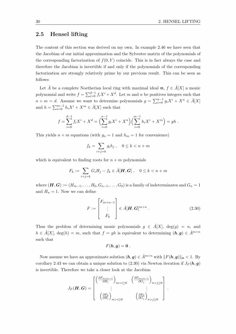
Let A be a complete Noetherian local ring with maximal ideal m, f ∈ A[X] a monic
polynomial and write f =∑d−1
i=0 fiXi+Xd. Let m and n be positives integers such that
n + m = d. Assume we want to determine polynomials g =∑n−1
i=0 giXi + Xn ∈ A[X]
and h =∑m−1
i=0 hiXi +Xm ∈ A[X] such that
f =
d−1∑i=0
fiXi +Xd =
(n−1∑i=0
giXi +Xn
)(m−1∑i=0
hiXi +Xm
)= gh .
This yields n+m equations (with gn = 1 and hm = 1 for convenience)
fk =∑i+j=k
gihj , 0 ≤ k < n+m
which is equivalent to finding roots for n+m polynomials
Fk :=∑i+j=k
GiHj − fk ∈ A[H,G] , 0 ≤ k < n+m
where (H,G) := (Hm−1, . . . ,H0, Gn−1, . . . , G0) is a family of indeterminates and Gn = 1
and Hn = 1. Now we can define
F :=
Fm+n−1
...
F0
∈ A[H,G]m+n . (2.30)
Thus the problem of determining monic polynomials g ∈ A[X], deg(g) = n, and
h ∈ A[X], deg(h) = m, such that f = gh is equivalent to determining (h, g) ∈ Am+n
such that
F (h, g) = 0 .
Now assume we have an approximate solution (h, g) ∈ Am+n with ‖F (h, g)‖m < 1. By
corollary 2.43 we can obtain a unique solution to (2.30) via Newton iteration if JF (h, g)
is invertible. Therefore we take a closer look at the Jacobian
JF (H,G) =
(∂Fm+n−1
∂Hi
)m>i≥0
(∂Fm+n−1
∂Gj
)n>j≥0
......(
∂F0∂Hi
)m>i≥0
(∂F0∂Gj
)n>j≥0
.

2.5. HENSEL LIFTING 31
For 0 ≤ k < m+ n and 0 ≤ i < m we have
∂Fk∂Hi
=∂
∂Hi
( ∑i+j=k
GiHj − fk
)
=∑i+j=k
∂(GiHj)
∂Hi
=
min{m,k}∑j=max{0,−n+k}
∂(Gk−jHj)
∂Hi=
Gk−i , max{0,−n+ k} ≤ i ≤ min{m, k}
0 , else
and by an analogous computation for 0 ≤ j < n
∂Fk∂Gj
=
Hk−j , max{0,−m+ k} ≤ j ≤ min{n, k}
0 , else.
In particular
∂Fm+n−1
∂Hi...
∂F0∂Hi
=
0...0
1
Gn−1
...G0
0...0
m− 1− i
}i
and
∂Fm+n−1
∂Gj...
∂F0∂Gj
=
0...0
1
Hm−1
...H0
0...0
n− 1− j
}j
Hence
JF (h, g) = Syl(g, h) (2.31)
and thus JF is invertible if and only if res(g, h) is a unit in A. To obtain a unique
solution for F it is therefore sufficient that we have strongly relatively prime polynomials
g, h ∈ A[X] such that f ≡ gh mod m by theorem 2.47!
Proposition 2.56 (Hensel lifting). Let A be a complete Noetherian local ring withmaximal ideal m and f ∈ A[X] a non-zero polynomial with lc(f) /∈ m. If there existsg, h ∈ A[X] such that g and h are strongly relatively prime and
f ≡ gh mod m
then there exists unique strongly relatively prime polynomials g and h ∈ A[X] such that
f = gh andg ≡ g mod m
h ≡ h mod m. (2.32)
Proof. Since lc(f) /∈ m we have also lc(g) /∈ m and lc(h) /∈ m. Thus lc(f), lc(g) and lc(h)are units in A. Therefore we assume without loss of generality that f, g and h are monic(see remark 2.58 for details) and write g =
∑n−1i=0 giX
i+Xn and h =∑m−1
i=0 hiXi+Xm.

32 2. HENSEL LIFTING
Now we can construct system (2.30) with F ∈ A[H,G]m+n. As f ≡ gh mod m,F has an approximate solution (h, g) := (hm−1, . . . , h0, gn−1, . . . , g0) ∈ Am+n with‖F (h, g)‖m < 1 and JF (h, g) = Syl(g, h) by (2.31). Furthermore, g and h are stronglyrelatively prime and thus res(g, h) = det(JF (h, g)) is a unit by theorem 2.47. Thus allconditions for the corollary 2.43 to the Newton iteration are satisfied. Therefore thereexists a unique (h, g) = (hm−1, . . . , h0, gn−1, . . . , g0) ∈ Am+n such that
F (h, g) = 0, det(Jf (h, g)) unit and ‖(h, g)− (h, g)‖m < 1.
Define the polynomials
g :=
n−1∑i=0
giXi +Xn and h :=
m−1∑i=0
hiXi +Xm .
Then g and h satisfy (2.32) and since det(Jf (h, g)) = res(g, h), g and h are stronglyrelatively prime by theorem 2.47.
Remark 2.57. We call the polynomials g and h lifted.
Remark 2.58. Since lc(f), lc(g) and lc(h) are units we can write lc(f)f ′ = f ,lc(g)g′ ≡ g mod m and lc(h)h′ ≡ h mod m with monic polynomials f ′, g′ and h′. Itis therefore sufficient to apply our lifting procedure to the monic polynomials such thatwe obtain lifted polynomial g′ and h′ and then to return lc(g)g and lc(h)h.
For the rest of this section let f ∈ A[X] be a monic polynomial with deg(f) = n. We
have seen that it is possible to lift a factorization f ≡ gh mod m with strongly relatively
prime polynomials g, h ∈ A[X] uniquely to a factorization f = gh with g, h ∈ A[X]. To
be useful in practice we have to generalize the statement in such a way that we can lift
strongly relatively prime monic polynomials g1, . . . , gr ∈ A[X] with deg(gi) = ni and
f ≡r∏i=1
geii mod m, ei ≥ 1 (2.33)
to unique polynomials g1, . . . , gr ∈ A[X] such that
f =∏ri=1 g
eii and gi ≡ gi mod m , i = 1, . . . , r .
We make the generalization in two steps. First we consider the case that ei = 1 for
i = 1, . . . , n and then the general case (2.33).
Therefore suppose that f ≡∏ri=1 gi mod m with gi =
∑ni−1j=0 gi,jX
j +Xni . If we define
the families of indeterminates Gi := (Gi,ni−1, . . . , Gi,0) for i = 1, . . . , r we can extend
our system (2.30) to
F (1) :=
F
(1)n−1...
F(1)0
∈ A[Gr, . . . ,G1]n (2.34)
where (again with Gi,ni = 1)
F(1)k :=
∑k1+...+kr=k
G1,k1 · · ·Gr,kr − fk , 0 ≤ k < n .
2.5. HENSEL LIFTING 33
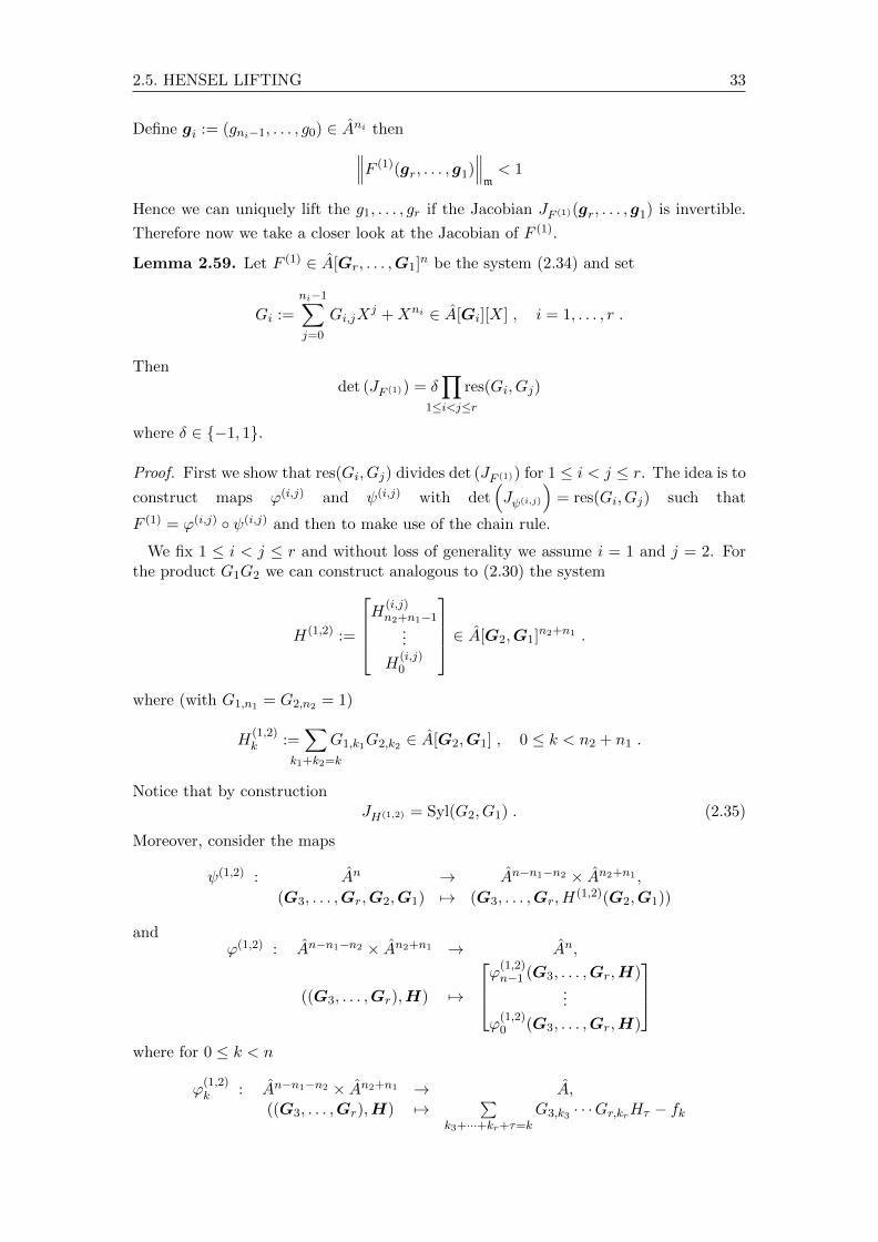
Define gi := (gni−1, . . . , g0) ∈ Ani then∥∥∥F (1)(gr, . . . , g1)∥∥∥m< 1
Hence we can uniquely lift the g1, . . . , gr if the Jacobian JF (1)(gr, . . . , g1) is invertible.
Therefore now we take a closer look at the Jacobian of F (1).
Lemma 2.59. Let F (1) ∈ A[Gr, . . . ,G1]n be the system (2.34) and set
Gi :=
ni−1∑j=0
Gi,jXj +Xni ∈ A[Gi][X] , i = 1, . . . , r .
Thendet (JF (1)) = δ
∏1≤i<j≤r
res(Gi, Gj)
where δ ∈ {−1, 1}.
Proof. First we show that res(Gi, Gj) divides det (JF (1)) for 1 ≤ i < j ≤ r. The idea is to
construct maps ϕ(i,j) and ψ(i,j) with det(Jψ(i,j)
)= res(Gi, Gj) such that
F (1) = ϕ(i,j) ◦ ψ(i,j) and then to make use of the chain rule.
We fix 1 ≤ i < j ≤ r and without loss of generality we assume i = 1 and j = 2. Forthe product G1G2 we can construct analogous to (2.30) the system
H(1,2) :=
H
(i,j)n2+n1−1
...
H(i,j)0
∈ A[G2,G1]n2+n1 .
where (with G1,n1 = G2,n2 = 1)
H(1,2)k :=
∑k1+k2=k
G1,k1G2,k2 ∈ A[G2,G1] , 0 ≤ k < n2 + n1 .
Notice that by constructionJH(1,2) = Syl(G2, G1) . (2.35)
Moreover, consider the maps
ψ(1,2) : An → An−n1−n2 × An2+n1 ,
(G3, . . . ,Gr,G2,G1) 7→ (G3, . . . ,Gr, H(1,2)(G2,G1))
andϕ(1,2) : An−n1−n2 × An2+n1 → An,
((G3, . . . ,Gr),H) 7→
ϕ(1,2)n−1 (G3, . . . ,Gr,H)
...
ϕ(1,2)0 (G3, . . . ,Gr,H)
where for 0 ≤ k < n
ϕ(1,2)k : An−n1−n2 × An2+n1 → A,
((G3, . . . ,Gr),H) 7→∑
k3+···+kr+τ=k
G3,k3 · · ·Gr,krHτ − fk

34 2. HENSEL LIFTING
with H = (Hn2+n1−1, . . . ,H0) and Hn2+n1 = 1. Then
F (1)(Gr, . . . ,G1) = ϕ(1,2) ◦ ψ(1,2)(G3, . . . ,Gr,G2,G1)
and by the chain rule it follows with δ ∈ {−1, 1}
det (JF (1)) = δ det(Jϕ(1,2)◦ψ(1,2)
)= δ det
((Jϕ(1,2) ◦ ψ(1,2)
)Jψ(1,2)
).
Finally we obtain
det(Jψ(1,2)
)= det
([In−n1−n2
JH(1,2)
])= det (JH(1,2))
(2.35)= det(Syl(G2, G1)) = res(G2, G1) .
Therefore res(Gi, Gj) divides det(JF (1)) for all 1 ≤ i < j ≤ r.From Syl(Gi, Gj) it follows easily that deg(res(Gi, Gj)) = ni + nj − 1 (remember that
Gi and Gj are monic). Since the res(Gi, Gj) are clearly pairwise relatively prime weobtain
deg(det(JF (1))) ≥∑
1≤i<j≤r(ni + nj − 1) = (r − 1)n−
∑1≤i<j≤r
1 = (r − 1)n− 1
2(r − 1)r .
On the other hand, for k = 1, . . . , r, the term with highest degree in F(1)n−k is
∏s∈S Gs,ns−1
for a subset S ⊂ {1, . . . , r} with |S| = k (again the Gi are monic). For k > r the degree
of F(1)n−k is at most r. Hence
deg(det(JF (1))) ≤r∑
k=1
(k − 1) + (n− r)(r − 1) =r−1∑k=1
k + (n− r)(r − 1)
=1
2(r − 1)r + n(r − 1)− r(r − 1)
= (r − 1)n− 1
2(r − 1)r
and we conclude det(JF (1)) = δ∏
1≤i<j≤r res(Gi, Gj).
With the help of this lemma we can state the first generalization of the Hensel lifting
theorem.
Proposition 2.60. Let A be a complete Noetherian local ring with maximal ideal mand f ∈ A[X] a non-zero polynomial such that lc(f) /∈ m. Let g1, . . . , gr ∈ A[X] bepairwise strongly relatively prime polynomials such that
f ≡r∏i=1
gi mod m .
Then there exists unique pairwise strongly relatively prime polynomials gi ∈ A[X],i = 1, . . . , r, such that
f =r∏i=1
gi and gi ≡ gi mod m , 1 ≤ i ≤ r . (2.36)

2.5. HENSEL LIFTING 35
Proof. With the system (2.34) the proof is largely analog to the previous proof of ourHensel lifting theorem 2.56. Assume again without loss of generality that f and g1, . . . , grare monic. Considering the previous notation the only thing that remains to show isthat det(JF (1)(gr, . . . , g1)) is a unit and that the lifted polynomials are pairwise stronglyrelatively prime.
Since the gi are pairwise strongly relatively prime res(gi, gj) is a unit for 1 ≤ i < j ≤ rby theorem 2.47 and thus det(JF (1)(gr, . . . , g1)) is a unit by lemma 2.59. Therefore bycorollary 2.43 to the Newton iteration we can obtain a unique (gr, . . . , g1) ∈ Anr+...+n1
such that
F (1)(gr, . . . , g1) = 0, ‖(gr, . . . , g1)− (gr, . . . , g1)‖m < 1 and det(J(1)F (gr, . . . , g1)) unit.
If we write gi = (gi,ni−1, . . . , gi,0) for i = 1, . . . , r we can define the unique polynomials
gi :=
ni−1∑j=0
gi,jXj +Xni ∈ A[X] , 1 ≤ i ≤ r
which satisfy (2.36). Furthermore, by lemma 2.59 it follows that
δ∏
1≤i<j≤rres(gi, gj) = det (JF (1)(gr, . . . , g1)) , δ ∈ {−1, 1}
is a unit. Therefore g1, . . . , gr are pairwise strongly relatively prime by theorem 2.47
Now we are ready to handle the general case. Unless otherwise stated we continue the
notation of the previous case. Suppose we have pairwise strongly relatively prime monic
polynomials g1, . . . , gr ∈ A[X] with mi := deg(gi), m :=∑r
i=1mi and positive integers
e1, . . . , er such that
f ≡∏
geii mod m
and assume that there exists an index i with ei ≥ 2. To simplify the notation define the
polynomials
Hi :=(mi−1∑j=0
Gi,jXj +Xmi
)ei∈ A[Gr, . . . ,G1][X]
and write Hi =∑ni−1
k=0 Hi,kXk +Xni with ni := miei. Then (again with Gi,mi = 1)
Hi,k =∑
k1+...+kei=k
Gi,k1 . . . Gi,kei ∈ A[Gr, . . . ,G1] , 0 ≤ k < ni
for i = 1, . . . , r. Now we can extend our previous system (2.34) to
F (2) :=
F
(2)n−1...
F(2)0
∈ A[Gr, . . . ,G1]n (2.37)

36 2. HENSEL LIFTING
where (again with Hi,ni = 1)
F(2)k :=
∑k1+...+kr=k
H1,k1H2,k2 · · ·Hr,kr − fk , 0 ≤ k < n .
But in contrast to the previous case the system F (2) is overdetermined since
deg(f) = n =r∑i=1
ni =r∑i=1
miei >r∑i=1
mi .
Therefore we have to show that there exists a consistent subsystem of F (2) such that
the Jacobian of this subsystem is invertible for (gr, . . . , g1).
In preparation of the proof we take a closer look at F (2). Consider the map
ϕ : Am → An,
gr...
g1
7→ϕ(r)(gr)
...
ϕ(1)(g1)
where
ϕ(i) : Ami → Ani , g 7→
Hi,ni−1(g)
...
Hi,0(g)
for 1 ≤ i ≤ r. Then
F (2) = F (1) ◦ ϕ
and by the chain rule
JF (2) = (JF (1) ◦ ϕ) Jϕ . (2.38)
To determine a consistent subsystem of F (2) it is therefore sufficient to consider F (1) ◦ϕand (JF (1) ◦ ϕ) Jϕ respectively.
Theorem 2.61 (Generalized Hensel lifting). Let A be a complete Noetherian localring with maximal ideal m and f ∈ A[X] a non-zero polynomial such that lc(f) /∈ m.Let g1, . . . , gr ∈ A[X] be pairwise strongly relatively prime polynomials and e1, . . . , erpositive integers such that
f ≡r∏i=1
geii mod m
and ei 6≡ 0 mod m, i = 1, . . . , r. Then there exists unique pairwise strongly relativelyprime polynomials g1, . . . , gr ∈ A[X] such that
f =r∏i=1
geii and gi ≡ gi mod m , 1 ≤ i ≤ r .
Proof. We make again use of the previous introduced notation and assume again that,without loss of generality, f and g1 . . . , gr are monic. If we can show that the system(2.37) has a consistent subsystem G such that det(JG(gr, . . . , g1)) is a unit, the proof islargely identical to the proof of the previous corollary. The only thing that remains toshow is that the lifted polynomials are pairwise strongly relatively prime and unique.

2.5. HENSEL LIFTING 37
For i = 1, . . . , r set hi := (hi,ni−1, . . . , hi,0) := ϕ(i)(gi) and define the polynomialshi :=
∑ni−1k=0 hi,kX
k +Xni . Then we have hi = geii and by (2.38)
JF (2)(gr, . . . , g1) = JF (1)◦ϕ(gr, . . . , g1)
= JF (1)(hr, . . . ,h1)Jϕ(gr, . . . , g1) .
Since the gi are strongly relatively prime the hi are also strongly relatively prime. Thusit follows that
det(JF (1)(hr, . . . ,h1)) = δ∏
1≤i<j≤rres(hi, hj) , δ ∈ {−1, 1}
is a unit by theorem 2.47 and lemma 2.59 and in particular that JF (1)(hr, . . . ,h1) isinvertible. Now by construction
Jϕ(gr, . . . , g1) =
Jϕ(r)(gr). . .
Jϕ(1)(g1)
where Jϕ(i)(gr) ∈ Ani,mi for i = 1, . . . , r. Since the gi are assumed to be monic we have
∂Hi,ni−k∂Gi,mi−j
=
ei , k = j
0 , k < j
∗ , else
for 1 ≤ i ≤ r, 1 ≤ k ≤ ni and 1 ≤ j ≤ mi. Therefore it follows that
Jϕ(i) =
ei
∗ . . ....
. . . ei...
. . . ∗...
. . ....
∗ . . . ∗
.
Consider JF (1)(hr, . . . ,h1)Jϕ(gr, . . . , g1) as an element in (A/m)n,m. Due to the factthat A/m is a field we can apply vector space theory:
Since JF (1)(hr, . . . ,h1) is invertible it has full rank and by our previous observationrank(Jϕ(gr, . . . , g1)) = m. Thus
rank(JF (2)(gr, . . . , g1))(2.38)
= rank(JF (1)(hr, . . . ,h1)Jϕ(gr, . . . , g1)) = m
and we can determine a consistent subsystem G with det(JG)(gr, . . . , g1) 6∈ m. This alsoimplies that det(JG)(gr, . . . , g1)) is a unit in A.
Hence we can analogous to the previous proof apply the Newton iteration on the systemG to determine polynomials g1, . . . , gr ∈ A[X] such that f =
∏ri=1 g
eii and gi ≡ gi mod m
for i = 1, . . . , r. If we define hi := gei =∑ni−1
k=0 hi,kXk+Xni and hi := (hi,ni−1, . . . , hi,0)

38 2. HENSEL LIFTING
for i = 1, . . . , r we have that
det(JF (1)(hr, . . . , h1)) = δ∏
1≤i<j≤rres(hi, hj) , δ ∈ {−1, 1}
is a unit. Therefore hr, . . . , h1 are pairwise strongly relatively prime by theorem 2.47and thus the gi are also pairwise strongly relatively prime.
Finally we have to show that the gr, . . . , g1 are unique. As gi ≡ gi mod m fori = 1, . . . , r we also have hi ≡ hi mod m for i = 1, . . . , r. Since also f =
∏ri=1 hi and
f ≡∏ri=1 hi mod m it follows that hr, . . . , h1 are unique by our previous proposition
2.60 and thus gr, . . . , g1 are also unique.
We have seen that we can uniquely lift a factorization in a complete Noetherican local
ring A. A downside is that since each element in A is a possibly infinite series it is not
possible to compute exactly in A. But the situation can be rescued.
Corollary 2.62. Let A be a Noetherian ring with maximal ideal m andf ∈ A[X] a non-zero polynomial such that lc(f) /∈ m. Let g1, . . . , gr ∈ A[X] be polyno-mials and e1, . . . , er positive integers such that
f ≡r∏i=1
geii mod m and gcd(gi mod m, gj mod m) /∈ m for 1 ≤ i < j ≤ r
and ei 6≡ 0 mod m, i = 1, . . . , r. Then there exists for all positive integers D polynomials
g(D)1 , . . . , g
(D)r ∈ A[X] such that the g
(D)i are pairwise strongly relatively prime in A/mD,
f ≡r∏i=1
(g
(D)i
)eimod mD and g
(D)i ≡ g mod m for 1 ≤ i ≤ r. (2.39)
Furthermore, the g(D)1 , . . . , g
(D)r are unique, i.e., for all g∗1, . . . , g
∗r ∈ A[X] with
f ≡∏ri=1(g∗i )
ei mod mD and g∗i ≡ g mod m, for 1 ≤ i ≤ r, we have
g∗i − g(D)i ≡ 0 mod mD , i = 1, . . . , r . (2.40)
Moreover, there exists unique strongly relatively prime polynomials g1, . . . , gr ∈ Am[X]such that
f =r∏i=1
geii and gi ≡ gi mod m for 1 ≤ i ≤ r
where Am is the completion of A with respect to m with maximal ideal m.
Proof. By corollary 2.55 the gi are pairwise strongly relatively prime in Am. Thereforeby theorem 2.61 there exists unique strongly relatively prime polynomials
gi =
ni∑j=0
g(i)j Xj ∈ Am[X] , 1 ≤ i ≤ r,
such that f =∏ri=1 g
eii and gi ≡ gi mod m for 1 ≤ i ≤ r. If we write for i = 1, . . . , r
g(i)j = (g
(i)j,1 + m, g
(i)j,2 + m2, . . . ) , 0 ≤ j ≤ ni ,
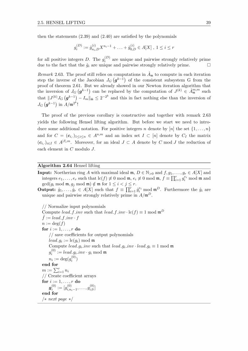
2.5. HENSEL LIFTING 39
then the statements (2.39) and (2.40) are satisfied by the polynomials
g(D)i := g
(i)ni,D
Xni−1 + . . .+ g(i)0,D ∈ A[X] , 1 ≤ i ≤ r
for all positive integers D. The g(D)i are unique and pairwise strongly relatively prime
due to the fact that the gi are unique and pairwise strongly relatively prime.
Remark 2.63. The proof still relies on computations in Am to compute in each iterationstep the inverse of the Jacobian JG
(gk−1
)of the consistent subsystem G from the
proof of theorem 2.61. But we already showed in our Newton iteration algorithm thatthe inversion of JG
(gk−1
)can be replaced by the computation of J (k) ∈ Am,mm such
that ‖J (k)JG(gk−1
)− Im‖m ≤ 2−2k and this in fact nothing else than the inversion of
JG(gk−1
)in A/m2k !
The proof of the previous corollary is constructive and together with remark 2.63
yields the following Hensel lifting algorithm. But before we start we need to intro-
duce some additional notation. For positive integers n denote by [n] the set {1, . . . , n}and for C = (ci,·)1≤i≤n ∈ An,m and an index set I ⊂ [n] denote by CI the matrix
(ci,·)i∈I ∈ A|I|,m. Moreover, for an ideal J ⊂ A denote by C mod J the reduction of
each element in C modulo J .
Algorithm 2.64 Hensel lifting
Input: Noetherian ring A with maximal ideal m, D ∈ N>0 and f, g1, . . . , gr ∈ A[X] andintegers e1, . . . , er such that lc(f) 6≡ 0 mod m, ei 6≡ 0 mod m, f ≡
∏ri=1 g
eii mod m and
gcd(gi mod m, gj mod m) /∈ m for 1 ≤ i < j ≤ r.Output: g1, . . . , gr ∈ A[X] such that f ≡
∏ri=1 g
eii mod mD. Furthermore the gi are
unique and pairwise strongly relatively prime in A/mD.
// Normalize input polynomialsCompute lead f inv such that lead f inv · lc(f) ≡ 1 mod mD
f := lead f inv · fn := deg(f)for i := 1, . . . , r do
// save coefficients for output polynomialslead gi := lc(gi) mod mCompute lead gi inv such that lead gi inv · lead gi ≡ 1 mod m
g(0)i := lead gi inv · gi mod m
ni := deg(g(0)i )
end form :=
∑ri=1 ni
// Create coefficient arraysfor i := 1, . . . , r do
g(0)i := [g
(0)i,ni−1, . . . , g
(0)i,0 ]
end for/∗ next page ∗/

40 2. HENSEL LIFTING
// Preparation for Newton iterationCreate F (2) ∈ A[Gr, . . . ,G1]n as defined in (2.37)Create the corresponding Jacobian JF (2) ∈ A[Gr, . . . ,G1]n,m
/∗ continue Hensel lifting algorithm ∗/if m 6= n then //F (2) overdetermined
Determine I ⊂ [n], |I| = m, s.th. rank(
(JF (2))I (g(0)r , . . . , g
(0)1 ))
= m in A/m
G := F(2)I
JG := (JF (2))Ielse
G := F (2)
JG := JF (2)
end if// Newton Iterationd := dlog2Defor k := 1, . . . , d do
Compute J (k) ∈ Am,m such that J (k)JG(g(k−1)r , . . . , g
(k−1)1 ) ≡ Im mod m2k(
g(k)r , . . . , g
(k)1
):=(g
(k−1)r , . . . , g
(k−1)1
)− J (k)G
(g
(k−1)r , . . . , g
(k−1)1
)mod m2k
end for// Create output polynomialsfor i := 1, . . . , r do
gi :=∑ni−1
k=0 lead gi · g(d)i,kX
k + lead giXni
end forreturn g1, . . . , gr
Theorem 2.65. The Hensel lifting algorithm 2.64 works correctly and needs at mostO((log2(D) + 1) deg(f)3) arithmetic operations.
Proof. The correctness of the algorithm follows from corollary 2.62, remark 2.63, theproof of theorem 2.61 and the correctness of the Newton iteration algorithm 2.41. Sincethe dominant step is the Newton iteration it follows that the algorithm needs at mostO((log2(D) + 1) deg(f)3) arithmetic operations.

Chapter 3
Evaluations of multivariatepolynomials
Before we start with this chapter, we have to fix some notation. We denote for a
finite set S by card(S) the cardinality of S. For a field k consider the polynomial
f ∈ k[X1, . . . , Xn]. We denote by deg(f) the total degree of f and for a family I ⊂{X1, . . . , Xn} of indeterminates we denote by degI(f) the (total) degree of f with respect
to I. Moreover, we denote for an indeterminate Xi by lcXi(f) the leading coefficient of
f with respect to Xi. Similarly we denote for polynomials g, h ∈ k[X1, . . . , Xn, Y ] by
resY (g, h) and SylY (g, h) the resultant / Sylvester matrix of g and h where g and h are
considered as polynomials in k[X1, . . . , Xn][Y ].
Example 3.1. Let f = 3X2Y 2Z3 − 2XY 4Z ∈ Q[X,Y, Z]. Then
deg(f) = 7, degY (f) = 4 and lcY (f) = −2XZ .
3.1 Effective Hilbert irreducibility
Our goal in this section is to derive an effective version of Hilbert’s Irreducibility theorem.
We will follow the original publication from Kaltofen [10]. We show that a certain
bivariate image of an irreducible polynomial f ∈ k[X1, . . . , Xn] remains irreducible with
a controllable high probability.
We start with the fundamental Schwartz-Zippel lemma. This lemma will be used in
nearly every proof of this chapter.
Lemma 3.2 (Schwartz-Zippel lemma). Let A be an integral domain, f a non-zeropolynomial in A[X1, . . . , Xn] with total degree D. Let S ⊂ A be a finite subset. Thenthe probability
Prob(f(a1, . . . , an) = 0 | a1, . . . , an ∈ S
)≤ D
card(S).
Proof. We prove the lemma by induction over the number of indeterminates. Let n = 1and f ∈ A[X1]. Since an univariate polynomial with degree D has at most D roots it
41
42 3. EVALUATIONS OF MULTIVARIATE POLYNOMIALS
follows Prob(f(a1) = 0 | a1 ∈ S
)≤ D/card(S).
Now assume the hypothesis holds for all polynomials in A[X1, . . . , Xn−1] and let f be apolynomial in A[X1, . . . , Xn]. Set d = degXn(f) and fd = lcXn(f) ∈ A[X1, . . . , Xn−1].Then deg(fd) ≤ D − d and by our induction hypothesis
Prob(fd(a1, . . . , an−1) = 0 | a1, . . . , an−1 ∈ S
)≤ D − d
card(S).
If we have fd(a1, . . . , an−1) 6= 0 for a1, . . . , an−1 ∈ S it follows thatdeg f(a1, . . . , an−1, Xn) = d and thus that there are at most d roots of f(a1, . . . , an−1, Xn)in S. Hence, by our induction hypothesis
Prob( f(a1, . . . , an) = 0 | fd(a1, . . . , an−1) 6= 0, an ∈ S ) ≤ d
card(S).
We can now conclude that for arbitrary a1, . . . , an ∈ S with a := (a1, . . . , an)
Prob(f(a) = 0
)= Prob
(f(a) = 0 | fd(a1, . . . , an−1) = 0
)Prob
(fd(a1, . . . , an−1) = 0
)+ Prob
(f(a) = 0 | fd(a1, . . . , an−1) 6= 0
)Prob
(fd(a1, . . . , an−1) 6= 0
)≤ Prob
(fd(a1, . . . , an−1) = 0
)+ Prob
(f(a) = 0 | fd(a1, . . . , an−1) 6= 0
)≤ D − d
card(S)+
d
card(S)
=D
card(S)
Remark 3.3. Note that the probability only depends on the degree of f and on thecardinality of S and not on the number of indeterminates!
Lemma 3.4 ([10]). Let k be a field and f ∈ k[X1, . . . , Xn, Y ] an irreducible polynomialwith ∂f/∂Y 6= 0, d = degY (f) and D = degX1,...,Xn(f). Pick random elements a1, . . . , anfrom a finite subset S ⊂ k. Then
Prob(f(a1, . . . , an, Y ) square free ∧ lcY (f)(a1, . . . , an) 6= 0
)≥ 1− (2d+ 1)D
card(S).
Proof. Since f is irreducible and ∂f/∂Y 6= 0 we have gcd(f, ∂f/∂Y ) = 1. Therefore theresultant
rf (X1, . . . , Xn) := resY
(f,∂f
∂Y
)= det
(SylY
(f,∂f
∂Y
))6= 0
by corollary 2.51. Since every term of rf is a product of d+(d−1) coefficients fi of f withdegree at most D it follows deg(rf ) ≤ (2d−1)D. We write ∂f/∂Y = kfkY
k−1 + . . .+f1
with fi ∈ k[X1, . . . , Xn], kfk 6= 0 and deg(fi) ≤ D, 1 ≤ i ≤ k.
We claim that if we select elements a1, . . . , an ∈ S such that(lcY (f)kfkrf )(a1, . . . , an) 6= 0 then f(Y ) := f(a1, . . . , an, Y ) is square free. Assumethis were not the case. Then gcd(f , ∂f/∂Y ) 6= 1 and thus resY (f , ∂f/∂Y ) = 0 by corol-lary 2.51. But resY (f , ∂f/∂Y ) = rf (a1, . . . , an) 6= 0, a contradiction. Hence f is squarefree if (lcY (f)kfkrf )(a1, . . . , an) 6= 0.

3.1. EFFECTIVE HILBERT IRREDUCIBILITY 43
Since deg(lcY (f)kfkrf ) ≤ D +D + (2d− 1)D = (2d+ 1)D it follows that
Prob(
(lcY (f)kfkrf )(a1, . . . , an) 6= 0 | a1, . . . , an ∈ S)≥ 1− (2d+ 1)D
card(S)
by the Schwartz-Zippel lemma 3.2.
Before we prove the main theorem of this section we prove that the substitutions rarely
allow that a gcd of higher degree occurs.
Lemma 3.5 ([10]). Let k be a field, f1, . . . , fr ∈ k[X1, . . . , Xn] polynomials withdeg(fi) ≤ D for 1 ≤ i ≤ r and gcd(f1, . . . , fr) = 1. Furthermore, assume thatf1(0, . . . , 0) 6= 0. Then there exists a polynomial ∆ ∈ k[Z2, . . . , Zn] with deg(∆) ≤ 2D2
such that for any elements b2, . . . , bn ∈ k with ∆(b2, . . . , bn) 6= 0 we have
gcd1≤i≤r
(fi(X1, b2X1, . . . , bnX1)) = 1 .
Proof. Since f1(0, . . . , 0) 6= 0 it follows that X1 doesn’t divide f1(X1, Z2X1, . . . , ZnX1).Furthermore, we have gcd(f1, . . . , fr) = 1 by assumption. Thus it follows
gcd1≤i≤r
(fi(X1, Z2X1, . . . , ZnX1)) = 1
in k[X1, Z2, . . . , Zn]. Therefore there exists, by Bezout’s identity, polynomialss1, . . . , sr ∈ k(Z2, . . . , Zn)[X1] with deg(si) < D such that
1 =r∑i=1
sifi(X1, Z2X1, . . . , ZnX1) .
This yields a linear system over k(Z2, . . . , Zn) in 2D equations and rD unknowns. ByCramer’s rule we can find a solution in 1
∆(Z2,...,Zn)k[Z2, . . . , Zn] where ∆ is a determinant
of a m×m-Matrix, m ≤ 2D, of coefficients of powers of X1 in fi(X1, Z2X1, . . . , ZnX1).Hence deg(∆) ≤ 2D2 and b2, . . . , bn ∈ k with ∆(b2, . . . , bn) 6= 0 implies
1 =
r∑i=1
si(b2, . . . , bn, X1)fi(X1, b2X1, . . . , bnX1)
and thus gcd1≤i≤r(fi(X1, b2X1, . . . , bnX1)).
Moreover, substitutions of the form Xi 7→ Xi+ai have no influence on the irreducibility
of polynomials.
Lemma 3.6. Let f ∈ k[X1, . . . , Xn, Y ] be a non-zero polynomial over a field k. Forelements a1, . . . , an ∈ k the polynomial
f(X1 + a1, . . . , Xn + an, Y )
is irreducible if and only if f is irreducible.
Proof. The statement follows immediately from the fact that the map
k[X1, . . . , Xn, Y ]→ k[X1, . . . , Xn, Y ],Xi 7→ Xi + aiY 7→ Y
(3.1)
44 3. EVALUATIONS OF MULTIVARIATE POLYNOMIALS
is a k-algebra automorphism.
In preparation of the proof of the effective Hilbert irreducibility theorem we state the
following application of the Hensel lifting theorem.
Proposition 3.7. Let g ∈ k[X1, . . . , Xn, Y ] be an irreducible polynomial. Assume thatg(0, . . . , 0, Y ) is square free and lcY (g)(0, . . . , 0) 6= 0. Define for elements b2, . . . , bn ∈ k
gb(X1, Y ) := g(X1, b2X1, . . . , bnX1, Y ) .
Then there exists for each factor hb ∈ k[[X1]][Y ] of gb with lcY (hb) = lcY (gb) a factorh ∈ k[[X1, . . . , Xn]][Y ] of g with lcY (h) = lcY (g) such that
h(X1, b2X1, . . . , bnX1, Y ) = hb(X1, Y ) .
Proof. Remember that k[[X1, . . . , Xn]] is a complete Noetherian local ring withmaximal ideal m = (X1, . . . , Xn). Let hb(X1, Y ) ∈ k[[X1]][Y ] be a factor of gb withlcY (hb) = lcY (gb). Notice that
gb(0, Y ) = g(0, . . . , 0, Y ) ≡ g mod m (3.2)
and that lcY (g)(0, . . . , 0) 6= 0 implies lcY (g) /∈ m. Furthermore, hb(0, Y ) is a non-zerofactor of g(0, . . . , 0, Y ). We write g(0, . . . , 0, Y ) = hb(0, Y )hb where hb is the corre-sponding cofactor. Since g(0, . . . , 0, Y ) is square free hb(0, Y ) and hb are relativelyprime. Therefore we can obtain by corollary 2.62 to the Hensel lifting a unique factorh ∈ k[[X1, . . . , Xn]][Y ] of g with h(0, . . . , 0, Y ) = hb(0, Y ) and lcY (h) = lcY (g).
We claim thath(X1, b2X1, . . . , bnX1, Y ) = hb(X1, Y ) .
This can be seen as follows. Since gb(0, Y ) = g(0, . . . , 0, Y ) we can also consider thefactorization gb(0, Y ) = hb(0, Y )hb and apply on this factorization the Hensel lift-ing theorem. Since the lifted polynomials are unique we obtain as the lifted poly-nomial hb. Assume now that h(X1, b2X1, . . . , bnX1, Y ) 6= hb(X1, Y ). Then wouldh(X1, b2X1, . . . , bnX1, Y ) be another factor of gb with
h(X1, b2X1, . . . , bnX1, Y ) ≡ hb(0, Y ) mod X1
in contradiction to the uniqueness of the lifted polynomials!
Now we can state the effective Hilbert irreducibility theorem under the additional
constraint that for f ∈ k[X1, . . . , Xn, Y ] we have ∂f/∂Y 6= 0. This is always satisfied
if degY (f) ≥ 1 and char(k) = 0. The proof is based on the original paper by Kaltofen
[10].
Theorem 3.8. Let k be a field, f ∈ k[X1, . . . , Xn, Y ] an irreducible polynomial with∂f/∂Y 6= 0 and δ the total degree of f . Pick random elements a1, . . . , an, b2, . . . , bn froma finite subset S ⊂ k. Then the probability
Prob(f(a1 +X1, a2 + b2X1, . . . , an + bnX1, Y ) irreducible in k[X1, Y ]
)≥ 1− 4δ2δ
card(S).
3.1. EFFECTIVE HILBERT IRREDUCIBILITY 45
Proof. By lemma 3.4 the probability that f(a1, . . . , an, Y ) is square free andlcY (f)(a1, . . . , an) 6= 0 is at least 1 − (2d+ 1)D/card(S) where D := degX1,...,Xn(f)and d := degY (f). Fix a1, . . . , an such that this is the case and set
g(X1, . . . , Xn, Y ) := f(X1 + a1, . . . , Xn + an, Y ) .
Notice that g is irreducible if and only if f is irreducible by lemma 3.6. For elementsb2, . . . , bn ∈ S set
gb(X1, Y ) := g(X1, b2X1, . . . , bnX1, Y )
= f(a1 +X1, a2 + b2X1, . . . , an + bnX1, Y ) .
We have to prove that gb is irreducible in k[X1, Y ] with a probability of at least1− 4δ2δ/card(S).
First we determine the probability that gb remains irreducible in k(X1)[Y ].By our assumption g(0, . . . , 0, Y ) = f(a1, . . . , an, Y ) is square free andlcY (g)(0, . . . , 0) = lcY (f)(a1, . . . , an) 6= 0. Therefore by proposition 3.7 there exists foreach factor hb ∈ k[[X1]][Y ] of gb with lcY (hb) = lcY (gb) a factor h ∈ k[[X1, . . . , Xn]][Y ]of g with lcY (h) = lcY (g) such that
h(X1, b2X1, . . . , bnX1, Y ) = hb(X1, Y ) .
Thus it is sufficient to show that for each factor h ∈ k[[X1, . . . , Xn]][Y ] of g the polyno-mial hb(X1, Y ) := h(X1, b2X1, . . . , bnX1, Y ) does not divide gb in k[X1][Y ]. A sufficientcondition is that degX1
(hb) > D = degX1(gb). Then gb remains irreducible in k(X1)[Y ].
We show that this is the case if a certain polynomial π ∈ k[Z2, . . . , Zn] with degree atmost 2D(2d−1 − 1) does not vanish at b2, . . . , bn ∈ S. We fix the lead coefficients of thefactors since lcY (g) and lcY (gb) are units in k[[X1, . . . , Xn]] and k[[X1]] respectively andwe are only interested in non-associated factors.
Let h ∈ k[[X1, . . . , Xn]][Y ] be a factor of g with lcY (h) = lcY (g) and let h be thecorresponding cofactor such that g = hh. We write with X := (X1, . . . , Xn)
h =r∑i=0
∑α∈Nn
hi,αXαY i and h =
s∑i=0
∑α∈Nn
hi,αXαY i
where s < d and s + r = d. We claim that there must exist a coefficient hi,α of h or acoefficient hi,α of h for an index i with
D < |α| ≤ 2D and(hi,α 6= 0 or hi,α 6= 0
).
Assume this were not the case. Then
g =
(r∑i=0
∑|α|≤D
hi,αXαY i
)(s∑i=0
∑|α|≤D
hi,αXαY i
)+
d∑i=0
∑|β|≥2D+1α1+α2=β
hi,α1 hi,α2XβY i .
Since degX(g) ≤ D the right sum vanishes and h and h can be considered as elementsof k[X1, . . . , Xn][Y ]. Then g is reducible in k[X1, . . . , Xn][Y ] in contradiction to f irre-ducible. Hence we can assume without loss of generality that there exists an α ∈ Nn andan integer i such that hi,α 6= 0 with D < |α| ≤ 2D and 0 ≤ i ≤ r. Then we can define

46 3. EVALUATIONS OF MULTIVARIATE POLYNOMIALS
the polynomial
δi,α :=∑|β|=|α|
hi,βXβ 6= 0
which is the coefficient of Y i in h of degree 2D ≥ |α| > D in X.
If b2, . . . , bn ∈ S satisfy
δi,α(X1, b2X1, . . . , bnX1) 6= 0
we can guarantee that hb has a non-zero coefficient of order 2D ≥ |α| > D in X1.Therefore hb cannot be a polynomial dividing gb in k[X1][Y ]. Thus the polynomialπ(Z2, . . . , Zn) can be chosen as the product of the δi,α(1, Z2, . . . , Zn) 6= 0 over all possiblefactor candidates of h. Since g has at most d irreducible factors in k[[X1, . . . , Xn]][Y ]and we do not need to consider complementary factor combinations there are at most
d−1∑i=1
(d− 1
i
)= 2d−1 − 1
factors to refute. Hence deg(π) ≤ 2D(2d−1 − 1) and we know that π(b2, . . . , bn) 6= 0guarantees that gb has no factor hb in k[[X1]][Y ] with degX1
(hb) ≤ degX1(gb). Therefore
gb is irreducible in k(X1)[Y ] if π(b2, . . . , bn) 6= 0.
Finally we must refute a possible content in k[X1][Y ]. Let li(X1, . . . , Xn) be the coeffi-cient of Y i in g(X1, . . . , Xn, Y ), deg(li) ≤ D. Then ld = lcY (g) and thus ld(0, . . . , 0) 6= 0.Since f is irreducible we have gcd0≤i≤d(li) = 1. By lemma 3.5 there exists a polynomial∆ ∈ k[Z2, . . . , Zn] with deg(∆) ≤ 2D2 such that for b2, . . . , bn ∈ S with∆(b2, . . . , bn) 6= 0 it follows that gcd0≤i≤d(li(X1, b2X1, . . . , bnX1)) = 1. For suchb2, . . . , bn ∈ S it follows that gb cannot have a non-trivial content with respect to Y , i.e.,a factor in k[X1].
We conclude that we have to avoid zeros of π∆. For randomly chosen b2, · · · , bn ∈ Swe have π∆(b2, · · · , bn) 6= 0 with a probability of at least 1− (deg(π) + deg(∆))/card(S)by the Schwartz-Zippel lemma 3.2. Together with the probability that f(a1, . . . , an, Y ) issquare free and lcY (f)(a1, . . . , an) 6= 0 it follows that gb is irreducible with a probabilityof at least(
1− (2d+ 1)D
card(S)
)(1− 2D(2D−1 − 1) + 2D2
card(S)
)≥ 1− 4δ2δ − 3d
card(S)≥ 1− 4δ2δ
card(S)
where δ := dD = deg(f).
For every non-zero polynomial f the condition ∂f/∂Y 6= 0 is satisfied if k is a field
of characteristic 0. For characteristic p > 0 one can prove that without the assumption
about the derivative the theorem is still correct if k is a perfect field, in particular if
every element of k is a pth power. But our black box factorization algorithm succeeds
only with a controllably high probability if k is an field of characteristic zero. Therefore
we only state the general theorem and skip the proof.

3.2. FACTOR DEGREE PATTERN 47
Theorem 3.9 (Effective Hilbert irreducibility theorem). Let k be a perfect field,f ∈ k[X1, . . . , Xn, Y ] an irreducible polynomial with degree δ. Pick random elementsa1, . . . , an, b2, . . . , bn from a finite subset S ⊂ k. Then
Prob(f(a1 +X1, a2 + b2X1, . . . , an + bnX1, Y ) irreducible in k[X1, Y ]
)≥ 1− 4δ2δ
card(S).
Proof. If char(k) = 0 this is theorem 3.8. If char(k) > 0 see [10].
3.2 Factor degree pattern
In the previous section we determined the probability that for randomly chosen elements
a1, . . . , an, b2, . . . , bn the image f(a1 +X1, a2 + b2X1, . . . , an + bnX1, Y ) of an irreducible
polynomial f ∈ k[X1, . . . , Xn, Y ] remains irreducible. The question that now arises is
what happens with the image f(a1 + X1, a2 + b2X1, . . . , an + bnX1, Y ) of a reducible
polynomial?
Consider the factorization f = ge11 · · · gerr of f in pairwise non-associated irreducible
factors gi with di = deg(gi) ≥ 1 and ei ≥ 1. We call the lexicographically ordered
n-tuple ((di1 , ei1), . . . , (dir , eir)) the factor degree pattern of f .
The images gi(a1 +X1, a2 + b2X1, . . . , an+ bnX1, Y ) remain irreducible if they depend
on Y by the effective Hilbert irreducibility theorem 3.9. But they have not necessarily the
same degree and they can become associated. Thus the interesting question is whether
the factor degree pattern of the image f(a1 + b1X1, . . . , an + bnX1, Y ) coincides with
the factor degree pattern of f(X1, . . . , Xn, Y ). Since we can only apply the effective
Hilbert irreducibility theorem on those factors that depend on Y we need the following
notation. The primitive part of a polynomial f with respect to some indeterminate Y
is the polynomial divided by the gcd of all coefficients with respect to Y (the content)
and denoted by ppY (f). If the content of a f is an unit then f is called primitive.
Theorem 3.10 (Factor degree pattern [12]). Let f ∈ k[X1, . . . , Xn, Y ] be a polynomialover a perfect field k. Denote by δ the total degree of f and pick random elementsa1, . . . , an, b2, . . . , bn from a finite subset S ⊂ k and set
f2 := f(a1 +X1, a2 + b2X1, . . . , an + bnX1, Y ) .
Then
Prob(
ppY (f) and ppY (f2) have the same factor degree pattern)≥ 1− 4δ2δ + δ3
card(S).
Proof. Let f =∏ri=1 g
eii be a factorization of f in pairwise non-associated irreducible
factors gi with δi = deg(gi) and ei ≥ 1 for i = 1, . . . , r. First consider the factors gi withdegY (gi) > 0. By the effective Hilbert irreducibility theorem 3.9
gi,2 := gi(a1 +X1, a2 + b2X1, . . . , an + bnX1, Y )

48 3. EVALUATIONS OF MULTIVARIATE POLYNOMIALS
remains irreducible in k[X1, Y ] with a probability of at least 1 − 4δi2δi/card(S). It
remains to determine the probability that deg(gi,2) = δi and that the gi,2 are pairwisenon-associated.
We start with the degree. Let A := (A1, . . . , An) and B := (B2, . . . , Bn) be twofamilies of indeterminates and define
hi(X1, Y,A,B) := gi(A1 +X1, A2 +B2X1, . . . , An +BnX1, Y ) .
Notice that hi(X1, Y, a1, . . . , an, b2, . . . , bn) = gi,2. Clearly degX1,Y (hi) = δi fori = 1, . . . , r and thus there exists in each hi a non-zero coefficient πi(B2, . . . , Bn) ofa monomial Xj
1Yk with j + k = δi. Then deg(πi) ≤ δi and πi(b2, . . . , bn) 6= 0 implies
deg(gi,2) = δi. The probability that πi(b2, . . . , bn) 6= 0 is at least
1− deg(πi)/card(S) ≥ 1− δi/card(S)
by the Schwartz-Zippel lemma 3.2.
Now we have to determine the probability that the gi are pairwise non-associated. Weclaim that the hi are pairwise non-associated in k(A,B)[X1, Y ]. Assume this were notthe case. Then there exists integers i and j, i 6= j, and polynomials si, sj ∈ k[A,B]with gcd(si, sj) = 1 such that sihi = sjhj . Since deg si ≥ 1 it follows that si divides hj
and thus hj is reducible in k[X1, Y,A,B]. We write hj = h(1)j h
(2)j . But then would
gj(X1, . . . , Xn, Y ) = hj(X1, Y, 0, X2 −B2X1, . . . , Xn −BnX1, B2, . . . , Bn)
= (h(1)j h
(2)j )(X1, Y, 0, X2 −B2X1, . . . , Xn −BnX1, B2, . . . , Bn)
be a non-trivial factorization of gj in k[X1 . . . , Xn, Y ] in contradiction to gj irreducible.Therefore the hk are pairwise non-associated in k(A,B)[X1, Y ].
Hence there exists in hi and hj , i 6= j, coefficients h(α1,α2)i and h
(α1,α2)j of Xα1
1 Y α2 suchthat
h(α1,α2)j hi − h(α1,α2)
i hj 6= 0
(otherwise hi and hj would be associated). In particular there exists two additional
coefficients h(β1,β2)i and h
(β1,β2)j of Xβ1
1 Y β2 in hi and hj such that
τi,j := h(α1,α2)j h
(β1,β2)i − h(α1,α2)
i h(β1,β2)j 6= 0 .
τi,j is a polynomial in k[A,B] and τi,j(a1, . . . , an, b2, . . . , bn) 6= 0 implies that gi,2 andgj,2 are not associated. Since deg(τi,j) ≤ δi + δj the probability that gi,2 and gj,2 are notassociated is at least 1− (δi + δj)/card(S) by the Schwartz-Zippel lemma 3.2.
Finally we consider the case degY (gi) = 0. Then gi,2 is a divisor of the content of f2
with respect to Y. Thus it is sufficient that gi,2 is not identical zero. A condition forthis is that the total degree of gi,2 gets preserved. By the same arguments as in the firstcase this happens with a probability of at least 1− δi/card(S).

3.2. FACTOR DEGREE PATTERN 49
In summary it follows that that the factor degree pattern is preserved with a proba-bility not less than
1−
(r∑i=1
4δi2δi
card(S)︸ ︷︷ ︸irreducible
+r∑i=1
δicard(S)︸ ︷︷ ︸
degree preserved
+∑
1≤i<j≤r
δi + δjcard(S)︸ ︷︷ ︸
non-associated
)
≥1− 1
card(S)
(4δ2δ + δ +
δ(δ − 1)
2δ
)≥1− 4δ2δ + δ3
card(S)
With this theorem we can probabilistically guarantee that the factor degree patterns
of f and f(a1 +X1, a2 + b2X1, . . . , an + bnX1, Y ) coincide if f is primitive with respect
to Y. But what happens if f is not primitive? The idea is that we modify f in such a
way that the image is primitive with a high probability and has the same factor degree
pattern as f . The following lemmas show that we can in fact define such an image of f .
Lemma 3.11. Let f ∈ k[X1, . . . , Xn, Y ] be a polynomial over a field k with total degreeδ and pick random elements c1, . . . , cn from a finite subset S ⊂ k. Then
Prob(
lcY (f(X1 + c1Y, . . . ,Xn + cnY, Y )) ∈ k)≥ 1− δ
card(S).
Proof. For indeterminates C1, . . . , Cn we define
f(C1, . . . , Cn, X1, . . . , Xn, Y ) := f(X1 + C1Y, . . . ,Xn + CnY, Y )
and π := lcY (f) ∈ k[C1, . . . , Cn]. Then deg(π) ≤ δ and if π(c1, . . . , cn) 6= 0 forc1, . . . , cn ∈ S it follows lcY (f(X1 + c1Y, . . . ,Xn + cnY, Y )) ∈ k and by the Schwartz-Zippel lemma 3.2 it follows the statement.
Moreover, substitutions of the form Xi 7→ Xi+biY +ai have no influence on the factor
degree pattern of f .
Lemma 3.12. Let f ∈ k[X1, . . . , Xn, Y ] be a non-zero polynomial over a field k. Forelements ai, bi ∈ k, i = 1, . . . , n
f(X1 + b1Y + a1, . . . , Xn + bnY + an, Y )
and f have the same factor degree patterns.
Proof. The statement follows immediately from the fact that the map
k[X1, . . . , Xn, Y ]→ k[X1, . . . , Xn, Y ],Xi 7→ Xi + biY + aiY 7→ Y
(3.3)
is a k-algebra automorphism.
50 3. EVALUATIONS OF MULTIVARIATE POLYNOMIALS
Therefore we can construct for a multivariate polynomial f a bivariate polynomial
f2 such that the factor degree patterns of f and f2 coincide with a controllable high
probability.
As a final result we state the substitution which is used in our factorization algorithm
and the probability that the factor degree patterns coincide for this substitution.
Corollary 3.13. Let f ∈ k[X1, . . . , Xn, Y ] be a non-zero polynomial over a perfect fieldk. Denote by δ the total degree of f and pick randomly chosen elements a1, . . . , an,b2, . . . , bn, c1, . . . , cn and aY , bY from a finite subset S ⊂ k and set
f2 = f(a1 +X1 + c1Y, a2 + b2X1 + c2Y, . . . , an + bnX1 + cnY, aY + bYX1 + Y )
Then
Prob(f and f2 have the same factor degree pattern
)≥ 1− δ + 4δ2δ + δ3
card(S). (3.4)
Furthermore, for the factorization∏ri=1 g
ei2,i of f2 with g2,i ∈ k[X1, Y ] we have
Prob( deg(g2,i(X1, 0)) = deg(g2,i) for i = 1, . . . , r and
gcd(g2,i(X1, 0), g2,j(X1, 0)) = 1 for 1 ≤ i < j ≤ r
)≥ 1− δ2
card(S). (3.5)
Proof. First set f1(X1, . . . , Xn, Y ) := f(X1 + c1Y, . . . ,Xn + cnY, Y ). By lemma 3.11 wehave lcY (f1) ∈ k with a probability of at least 1−δ/card(S) and therefore f1 is primitivein Y with the same probability. Assume now that is true. By lemma 3.12 the factordegree patterns of f and f1 coincide and if we set
f2(X1, Y ) := f1(a1 +X1, a2 + b2X1, . . . , an + bnX1, Y )
= f(a1 +X1 + c1Y, a2 + b2X1 + c2Y, . . . , an + bnX1 + cnY, Y )
it follows that the factor degree patterns of f1 and f2 coincide with a probability of atleast 1− (4δ2δ + δ3)/card(S) by theorem 3.10. Hence
Prob(f and f2 have the same factor degree pattern
)≥ 1− δ + 4δ2δ + δ3
card(S).
Again assume that this is true and write f2 =∏ri=1 g
ei2,i for the factorization of f2. Then
g2,i = gi(a1 +X1 + c1Y, a2 + b2X1 + c2Y, . . . , an + bnX1 + cnY, Y )
where gi is the corresponding factor of f . For i = 1, . . . , r define
h2,i(X1, Y, AY , BY ) := gi(a1+X1+c1Y, a2+b2X1+c2Y, . . . , an+bnX1+cnY,AY +BYX1+Y ) .
For g2,i := h2,i(X1, Y, aY , bY ) ∈ k[X1, Y ] it follows easily that the g2,i are irreducibleand pairwise not associated. Therefore
∏ri=1 g
ei2,i is the factorization of f2 and the factor
degree patterns of f2 and f2 coincide. This shows statement (3.4).
Now we want to show statement (3.5). By our previous construction we haveg2,i(X1, 0) = h2,i(X1, 0, aY , bY ) for 1 ≤ i ≤ r. Set πi(BY ) := lcX1(h2,i) for i = 1, . . . , rand
σi,j(AY , BY ) := resX1(h2,i(X1, 0, AY , BY ), h2,j(X1, 0, AY , BY ))

3.2. FACTOR DEGREE PATTERN 51
for 1 ≤ i < j ≤ r. Then πi(bY ) 6= 0 implies deg(g1,i) = deg(g2,i) and σi,j(aY , bY ) 6= 0implies resX1(g2,i(X1, 0), g2,j(X1, 0)) 6= 0 and thus gcd(g2,i(X1, 0), g2,j(X1, 0)) = 1 bycorollary 2.51. Therefore it is sufficient to determine the probability that
r∏i=1
πi(bY )∏
1≤i<j≤rσi,j(aY , bY ) = 0 .
Set δi := deg(g2,i) for i = 1, . . . , r. Now deg(πi) ≤ δi for i = 1, . . . , r and deg(σi,j) ≤ 2δiδjfor 1 ≤ i < j ≤ r. Therefore
deg( r∏i=1
πi∏
1≤i<j≤rσi,j
)≤
r∑i=1
δi +∑
1≤i<j≤r2δiδj ≤ (δ1 + · · ·+ δr)
2 ≤ δ2 .
Hence it follows statement (3.5) by the Schwartz-Zippel lemma 3.2.
Remark 3.14. The proof of statement (3.5) is based on [12], proof of theorem 6.1.

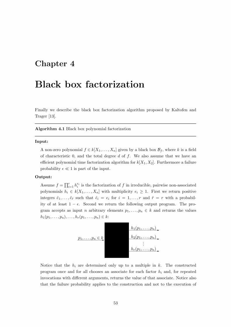
Chapter 4
Black box factorization
Finally we describe the black box factorization algorithm proposed by Kaltofen and
Trager [13].
Algorithm 4.1 Black box polynomial factorization
Input:
A non-zero polynomial f ∈ k[X1, . . . , Xn] given by a black box Bf , where k is a field
of characteristic 0, and the total degree d of f . We also assume that we have an
efficient polynomial time factorization algorithm for k[X1, X2]. Furthermore a failure
probability ε� 1 is part of the input.
Output:
Assume f =∏ri=1 h
eii is the factorization of f in irreducible, pairwise non-associated
polynomials hi ∈ k[X1, . . . , Xn] with multiplicity ei ≥ 1. First we return positive
integers e1, . . . , er such that ei = ei for i = 1, . . . , r and r = r with a probabil-
ity of at least 1 − ε. Second we return the following output program. The pro-
gram accepts as input n arbitrary elements p1, . . . , pn ∈ k and returns the values
h1(p1, . . . , pn), . . . , hr(p1, . . . , pn) ∈ k:
-p1, . . . , pn ∈ k
h1(p1, . . . , pn)-
h2(p1, . . . , pn)-...
hr(p1, . . . , pn)-
Notice that the hi are determined only up to a multiple in k. The constructed
program once and for all chooses an associate for each factor hi and, for repeated
invocations with different arguments, returns the value of that associate. Notice also
that the failure probability applies to the construction and not to the execution of
53
54 4. BLACK BOX FACTORIZATION
the program. That is, with probability of at least 1−ε the output program is correct;
a correct program always produces the true values of the factors.
Step 1:
Pick randomly chosen elements a1, . . . , an, b2, . . . , bn, c1, c3, . . . , cn from a sufficiently
large finite subset S ⊂ k and compute by standard interpolation the following inter-
polation polynomial:
f2(X1, X2) := f(X1 + c1X2 + a1, b2X1 +X2 + a2, b3X1 + c3X2 + a3,
. . . , bnX1 + cnX2 + an)
Step 2:
Factor f2(X1, X2) in k[X1, X2] such that
f2(X1, X2) =r∏i=1
g2,i(X1, X2)ei .
With a probability not less than 1 − ε we have r = r and ei = ei for all 1 ≤ i ≤ r.
Assume that this is all true. Otherwise an incorrect output program will be produced.
Step 3:
Assign
g1,i(X1) := g2,i(X1, 0) , 1 ≤ i ≤ r .
Check whether gcd(g1,i, g1,j) = 1, 1 ≤ i < j ≤ r, and deg(g2,i) = deg(g1,i), 1 ≤ i ≤ r.If one check fails, return “failure”. Then we have found that our chosen elements in
step 1 were unlucky.
Now set
f1(X1) := f2(X1, 0) = f(X1 + a1, b2X1 + a2, . . . , bnX1 + an) =
r∏i=1
g1,i(X1)ei .
We use the g1,i to uniquely enumerate the factors of f . Our associated choices (see
output specifications) then satisfy
hi(X1 + a1, b2X1 + a2, . . . , bnX1 + an) = g1,i(X1) .
Step 4:
This step constructs the output program for the evaluation of the hi at p1, . . . , pn
as described in the output specifications. First, the information computed so far
is “hardwired” into that program. Then the following steps 4.1, 4.2, and 4.3 are
appended to the program.
55
Step 4.1:
By standard interpolation compute
f(X1, Y ) := f(X1 + a1, Y (p2 − b2(p1 − a1)− a2) + b2X1 + a2,
. . . , Y (pn − bn(p1 − a1)− an) + bnX1 + an).
Notice that f(p1 − a1, 1) = f(p1, . . . , pn) and f(X1, 0) = f1(X1).
Step 4.2:
By Hensel lifting we obtain a factorization
f(X1, Y ) ≡r∏i=1
gi(X1, Y )ei mod Y d+1 with gi(X1, 0) = g1,i(X1) (4.1)
For all 1 ≤ i ≤ r test whether gi divides f . If at least one test fails return “failure”.
We have then discovered that the factor degree pattern of f and f2 disagree.
Step 4.3:
For i := 1, . . . , r do:
return gi(p1 − a1, 1) as hi(p1, . . . , pn)
Step 5:
return (e1, . . . , er) and the program constructed in step 4.
Remark 4.2. The Black box polynomial factorization algorithm is a Monte Carlo algo-rithm.
First we prove the correctness, analyze the failure probability of the algorithm and
then we prove the running time of the algorithm.
Theorem 4.3 (Correctness and failure probability). The black box polynomial factor-ization algorithm 4.1 works correctly and if the cardinality of the set S in step 1 ischosen
card(S) ≥ 6 deg(f)2deg(f)/ε,
then the algorithm succeeds with probability not less than 1−ε and the resulting programalways correctly evaluates all irreducible factors of f .
Proof. Denote by δ the total degree of f . By corollary 3.13 the factor degree patternsof f and f2 coincide in step 2 with a probability of at least 1− (δ+ 4δ2δ + δ3)/card(S).By the same corollary it follows that the probability that one of the checks in step 3returns “failure” is less than δ2/card(S). Assume all this is true. Notice that thendeg(g2,i) = deg(g1,i) for i = 1, . . . , r and this implies lcX1(f2) ∈ k and thus alsolcX1(f) ∈ k. Since k[Y ] is a Noetherian domain with maximal ideal (Y ) we can ap-ply our Hensel lifting algorithm 2.64 to the factorization
f(X1, Y ) ≡ f1(X1) ≡r∏i=1
g1,i(X1)ei mod Y

56 4. BLACK BOX FACTORIZATION
such that we obtain the factorization (4.1). If we now choose card(S) such that
δ + 4δ2δ + δ3 + δ2
ε=
4δ2δ + δ(1 + δ) + δ(δ2)
ε≤ 6δ2δ
ε≤ card(S)
we can guarantee that the output program is correct (and step B returns never a failure)with a probability of at least 1− ε.
Theorem 4.4. The black box polynomial factorization algorithm 4.1 can construct itsoutput program in polynomially many arithmetic steps as a function of n and deg(f) andan additional single polynomial factorization in k[X1, X2]. It requires O(deg(f)2) calls tothe black box for f . The output program can be executed in O((log(deg(f))+1) deg(f)3)arithmetic steps and O(deg(f)2) calls to the black box for f .
Proof. Each bivariate interpolation of f2 and f requires O(deg(f)2) black box eval-uations. Then the algorithm needs to factor f2 which can be accomplished by ourassumption in polynomial time in the size of deg(f) and the size of the coefficientsof f . The dominating additional work of the output program is step 4.2, which can beaccomplished in O((log(deg(f))+1) deg(f)3) arithmetic operations by theorem 2.65.
Chapter 5
Closing remarks
In Mathematics it often occurs that after a novel idea gets introduced one notices that
it is in fact just a rediscovery. A very specific case of this is Hensel lifting. It was
introduced in computer algebra by Zassenhaus in 1969, who referred to the in 1908
published Hensel’s Lemma. In this thesis it has been shown that the Hensel lifting is in
fact a special case of Newton Iteration, an over 300 years old technique. But we have
to note that the necessary algebraic concepts were first introduced in the 19th and 20th
century. I hope that the link between Hensel lifting and Newton iteration was for the
reader as fascinating as it was for me.
As for the black box factorization algorithm I believe it is not only a theoretically
efficient solution for the problem of factoring multivariate polynomials but also very
suitable for use in practice. For example the output program can be easily distributed,
due to the small space requirement of a black box, to a network of asynchronous parallel
processors and therefore evaluated in parallel. This enables for instance the computation
of the sparse representation of the factors in parallel. Moreover, I want to remark
that the algorithm can also be adapted for finite coefficient fields with sufficiently high
characteristic. We just have to take into account that the failure probability is bounded
below by the characteristic of the field.
Also with the black box approach Kaltofen and Trager were able to solve the gcd and
the numerator / denominator problem for multivariate polynomials in random polyno-
mial time [13]. This suggests that the black box approach could prove beneficial for
other computational problems as well.
57

Bibliography
[1] M. Ben-Or and P. Tiwari. A deterministic algorithm for sparse multivariate polyno-
mial interpolation. Proc. 20th Annual ACM Symp. Theory Comp., pages 301–309,
1988.
[2] E. R. Berlekamp. Factoring polynomials over finite fields. Bell Systems Tech. J.,
46:1853–1859, 1967. Republished in revised form in: E. R. Berlekamp, Algebraic
Coding Theory, Chapter 6, McGraw-Hill Publ., New York 1968.
[3] E. R. Berlekamp. Factoring polynomials over large finite fields. Math. Comp.,
24:713–735, 1970.
[4] N. Bourbaki. Algebra II Chapters 4-7, chapter IV, pages 31–32. Elements of math-
ematics. Springer-Verlag, 1989.
[5] N. Bourbaki. Commutative Algebra Chapters 1-7, page 392. Elements of mathe-
matics. Springer-Verlag, 1989.
[6] N. Bourbaki. Commutative Algebra Chapters 1-7, pages 200–205 and 392. Elements
of mathematics. Springer-Verlag, 1989.
[7] D. Eisenbud. Commutative Algebra: With a View Toward Algebraic Geometry,
pages 181–182. Number 150 in Graduate Texts in Mathematics. Springer-Verlag,
1995.
[8] K. Hensel. Theorie der algebraischen Zahlen, chapter 4. Teubner, Leipzig, 1908.
[9] D. Hilbert. Uber die Irreduzibilitat ganzer rationaler Funktionen mit ganzahligen
Koeffizienten. J. reine angew. Math., 110:104–129, 1892.
[10] E. Kaltofen. Effective Hilbert Irreducibility. Information and Control, 66:123–137,
1985.
[11] E. Kaltofen. Polynomial-time reductions from multivariate to bi- and univariate
integral polynomial factorization. SIComp, 14(2):469–489, 1985.
[12] E. Kaltofen. Factorization of polynomials given by straight-line programs. In S. Mi-
cali, editor, Randomness and Computation, volume 5 of Advances in Computing
Research, pages 375–412. JAI Press Inc., 1989.
59

60 BIBLIOGRAPHY
[13] E. Kaltofen and B. Trager. Computing with polynomials given by black boxes for
their evaluations: Greatest common divisors, factorization, separation of numera-
tors and denominators. J. Symbolic Comput., 9(3):301–320, 1990.
[14] L. Kronecker. Grundzuge einer arithmetischen Theorie der algebraischen Grossen.
J. reine angew. Math, 92:1–122, 1882.
[15] S. Landau. Factoring polynomials over algebraic number fields. SIAM J. Comp.,
14:184–195, 1985.
[16] A. K. Lenstra and H. W. Lenstra. Factoring polynomials with rational coefficients.
Math. Ann., pages 515–534, 1982.
[17] I. Newton. Arithmetica Universalis, 2nd ed. 1728. Reprinted in The Mathematical
Works of Isaac Newton, vol. 2, D. T. Whiteside, ed., Johnson Reprint Corp., New
York, 1967.
[18] B. L. van der Waerden. Modern Algebra. F. Ungar Publ. Co., New York, 1953.
[19] J. von zur Gathen and J. Gerhard. Modern Computer Algebra - Third Edition,
chapter 6. Cambridge University Press, 2013.
[20] J. von zur Gathen and J. Gerhard. Modern Computer Algebra - Third Edition,
chapter 9. Cambridge University Press, 2013.
[21] H. Zassenhaus. On Hensel factorization I. J. Number Theory, 1:291–311, 1969.
Related Documents