bla6310X_chapter2

Factors: How Time and Interest Affect Money

In the previous chapter we learned the basic concepts of engineeringeconomy and their role in decision making. The cash fl ow is fundamental to every economic study. Cash fl ows occur in many confi gurations and amounts— isolated single values, series that are uniform, and series that increase or decrease by constant amounts or constant percentages. This chapter develops derivations for all the commonly used engineering econ-omy factors that take the time value of money into account. The application of factors is illustrated using their mathematical forms and a standard notation format. Spreadsheet functions are introduced in order to rapidly work with cash fl ow series and to perform sensitivity analysis. The case study focuses on the signifi cant impacts that compound interest and time make on the value and amount of money.

CH

AP

TE

R

2

Purpose: Derive and use the engineering economy factors to account for the time valueof money.

Interpolate factor values

P�G and A�G factors

Geometric gradient

F�A and A�F factors

P�A and A�P factors

F�P and P�F factors

LEARNING OBJECTIVES

This chapter will help you:

1. Derive and use the compound amount factor and present worth factor for single payments.

2. Derive and use the uniform series present worth and capital recovery factors.

3. Derive and use the uniform series compound amount and sinking fund factors.

4. Linearly interpolate to determine a factor value.

5. Derive and use the arithmetic gradient present worth and uniform series factors.

6. Derive and use the geometric gradient series formulas.

7. Determine the interest rate (rate of return) for a sequence of cash fl ows.

8. Determine the number of years required for equivalence in a cash fl ow series.

9. Develop a spreadsheet to perform basic sensitivity analysis using spreadsheet functions.

Calculate i

Calculate n

Spreadsheets

48 CHAPTER 2 Factors: How Time and Interest Affect Money

2.1 SINGLE-PAYMENT FACTORS (F/P AND P/F )

The most fundamental factor in engineering economy is the one that determines the amount of money F accumulated after n years (or periods) from a single present worth P, with interest compounded one time per year (or period). Recall that compound interest refers to interest paid on top of interest. Therefore, if an amount P is invested at time t � 0, the amount F1 accumulated 1 year hence at an interest rate of i percent per year will be

F P Pi

P i

1

1

� �

� �( )

where the interest rate is expressed in decimal form. At the end of the second year, the amount accumulated F2 is the amount after year 1 plus the interest from the end of year 1 to the end of year 2 on the entire F1.

F F Fi

P i P i i2 1 1

1 1

� �

� � � �( ) ( ) [2.1]

This is the logic used in Chapter 1 for compound interest, specifi cally inExamples 1.8 and 1.18. The amount F2 can be expressed as

F2 � � � �

� � �

� �

P i i i

P i i

P i

( )

( )

( )

1

1 2

1

2

2

2

Similarly, the amount of money accumulated at the end of year 3, usingEquation [2.1], will be

F F F i3 2 2� �

Substituting P(1 � i)2 for F2 and simplifying, we get

F P i331� �( )

From the preceding values, it is evident by mathematical induction that theformula can be generalized for n years to

F P i n� �( )1 [2.2]

The factor (1�i)n is called the single-payment compound amount factor (SPCAF), but it is usually referred to as the F�P factor. This is the conversion factor that, when multiplied by P, yields the future amount F of an initial amount P after n years at interest rate i. The cash fl ow diagram is seen in Figure 2–1a.

Reverse the situation to determine the P value for a stated amount F that occurs n periods in the future. Simply solve Equation [2.2] for P.

P F

i n�

�

11( )

⎡

⎣⎢

⎤

⎦⎥

[2.3]

The expression in brackets is known as the single-payment present worth factor (SPPWF), or the P�F factor. This expression determines the present worth P of a given future amount F after n years at interest rate i. The cash fl ow diagram is shown in Figure 2–1b.

Note that the two factors derived here are for single payments; that is, they are used to fi nd the present or future amount when only one payment or receipt is involved.

A standard notation has been adopted for all factors. The notation includes two cash fl ow symbols, the interest rate, and the number of periods. It is always in the general form (X�Y,i,n). The letter X represents what is sought, while the letter Y represents what is given. For example, F�P means fi nd F when given P. The i is the interest rate in percent, and n represents the number of periods involved. Thus, (F�P,6%,20) represents the factor that is used to calculate the future amount F accumulated in 20 periods if the interest rate is 6% per period. The P is given. The standard notation, simpler to use than formulas and factor names, will be used hereafter.

Table 2–1 summarizes the standard notation and equations for the F�P and P�F factors. This information is also included inside the front cover.

To simplify routine engineering economy calculations, tables of factor values have been prepared for interest rates from 0.25 to 50% and time periods from 1 to large n values, depending on the i value. These tables, found at the rear of the

20 1 n – 2 n – 1 n

P = ?

F = given

i = given

(b)

20 1 n – 2 n – 1 n

P = given

F = ?

i = given

(a)

Figure 2–1Cash fl ow diagrams for single-payment factors: (a) fi nd F and (b) fi nd P.

TABLE 2–1 F�P and P�F Factors: Notation and Equations

Factor Standard Notation Equation

Equation with Factor Formula

Excel FunctionsNotation Name Find/Given

(F�P,i,n) Single-paymentcompound amount

F�P F � P(F�P,i,n) F � P(1 � i)n FV(i%,n,,P)

(P�F,i,n) Single-paymentpresent worth

P�F P � F(P�F,i,n) P � F[1�(1 � i)n] PV(i%,n,,F)

SECTION 2.1 Single-Payment Factors (F�P and P�F) 49

book, are arranged with factors across the top and the number of periods n down the left. The word discrete in the title of each table emphasizes that these tables utilize the end-of-period convention and that interest is compounded once each interest period. For a given factor, interest rate, and time, the correct factor value is found at the intersection of the factor name and n. For example, the value of the factor (P�F,5%,10) is found in the P�F column of Table 10 at period 10 as 0.6139. This value is determined by using Equation [2.3].

( , %, )( )

( . )

..

P Fi n

� 5 101

1

1

1 05

1

1 62890 6139

10

��

�

� �

For solution by computer, the F value is calculated by the FV function using the format

FV(i%,n,,P)

An � sign must precede the function when it is entered. The amount P is deter-mined using the PV function with the format

PV(i%,n,,F)

These functions are included in Table 2–1. Refer to Appendix A or Excel online help for more information on the FV and PV functions. Examples 2.1 and 2.2 illustrate solutions by computer using both of these functions.

Factor values

Tables1 to 29

An industrial engineer received a bonus of $12,000 that he will invest now. He wants to calculate the equivalent value after 24 years, when he plans to use all the resulting money as the down payment on an island vacation home. Assume a rate of return of 8% per year for each of the 24 years. (a) Find the amount he can pay down, using both the standard notation and the factor formula. (b) Use a computer to fi nd the amount he can pay down.

(a) Solution by HandThe symbols and their values are

P � $12,000 F � ? i � 8% per year n � 24 years

The cash fl ow diagram is the same as that in Figure 2–1a.Standard notation: Determine F, using the F�P factor for 8% and 24 years. Table 13

provides the factor value.

F P F P i n F P� �

�

�

( , , ) , ( , %, )

, ( . )

$ , .

� �12 000 8 24

12 000 6 3412

76 094 40

EXAMPLE 2.1

Q-SOLVE


The recent enhancements made by Ipsco, Inc., to its large-diameter spiral pipe mill inRegina are estimated to save $50,000 in reduced maintenance this year.

(a) If the steel maker considers these types of savings worth 20% per year, fi nd the equivalent value of this result after 5 years.

(b) If the $50,000 maintenance savings occurs now, fi nd its equivalent value 3 years earlier with interest at 20% per year.

(c) Develop a spreadsheet to answer the two parts above at compound rates of 20% and 5% per year. Additionally develop an Excel column chart indicating the equivalent values at the three different times for both rate-of-return values.

Solution(a) The cash fl ow diagram appears as in Figure 2–1a. The symbols and their values are

P � $50,000 F � ? i � 20% per year n � 5 years

Use the F�P factor to determine F after 5 years.

F P F P i n F P� �

�

�

( , , ) $ , ( , %, )

, ( . )

$ , .

� �50 000 20 5

50 000 2 4883

124 415 00

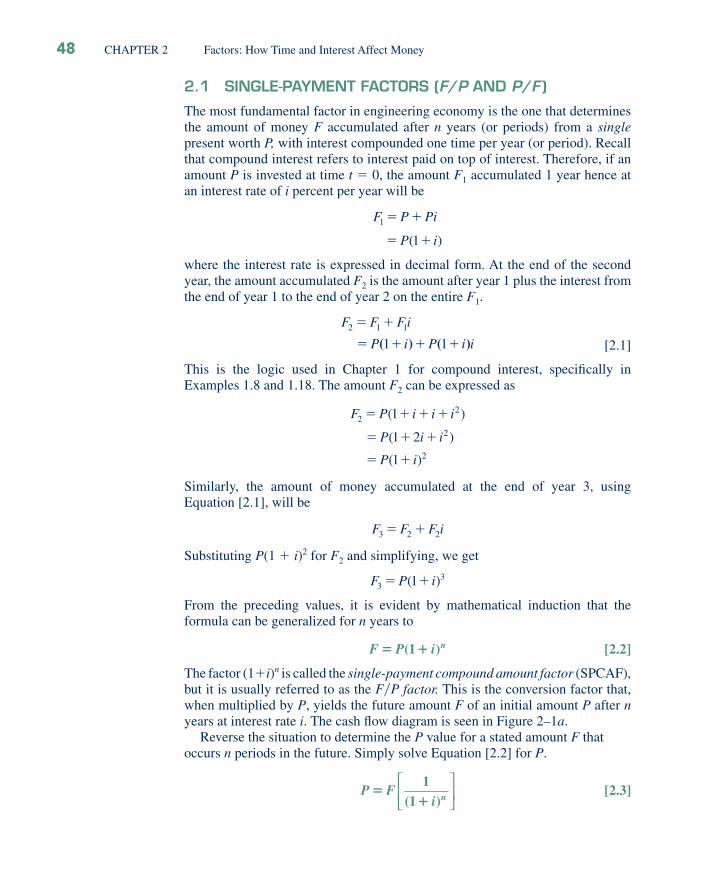
The function FV(20%,5,,50000) provides the same answer. See Figure 2–2a, cell C4.(b) In this case, the cash fl ow diagram appears as in Figure 2–1b with F placed at time

t � 0 and the P value placed 3 years earlier at t � �3. The symbols and their values are

P � ? F � $50,000 i � 20% per year n � 3 years

EXAMPLE 2.2

Q-SOLVE


Factor formula: Apply Equation [2.2] to calculate the future worth F.

F P i n� � � �

�

�

( ) , ( . )

, ( . )

$ , .

1 12 000 1 0 08

12 000 6 341181

76 094 17

24

The slight difference in answers is due to the round-off error introduced by the tabulated factor values. An equivalence interpretation of this result is that $12,000 today is worth $76,094 after 24 years of growth at 8% per year, compounded annually.

(b) Solution by ComputerTo fi nd the future value use the FV function that has the format FV(i%,n,A,P). The spreadsheet will look like the one in Figure 1–5a, except the cell entry is FV(8%,24,,12000). The F value displayed by Excel is ($76,094.17) in red to indicate a cash outfl ow. The FV function has performed the computation F � P(1 � i)n � 12,000(1 � 0.08)24 and presented the answer on the screen.

Q-SOLVE

�FV(20%,5,,50000) �PV(20%,3,,50000)

�PV(C5,3,,�50000)

�FV(C5,5,0,�50000)

�PV(D5,3,,�50000)

(b)

(a)

Figure 2–2(a) Q-Solve spreadsheet for Example 2.2(a) and (b); (b) complete spreadsheet with graphic, Example 2.2.


Use the P�F factor to determine P three years earlier.

P F P F i n P F� �

� �

( , , ) $ , ( , %, )

, ( . ) $ , .

� �50 000 20 3

50 000 0 5787 28 935 00

An equivalence statement is that $28,935 three years ago is the same as $50,000 today, which will grow to $124,415 fi ve years from now, provided a 20% per year compound interest rate is realized each year.

Use the PV function PV(i%,n,A,F) and omit the A value. Figure 2–2a shows the result of entering PV(20%,3,,50000) in cell F4 to be the same as using the P�F factor.

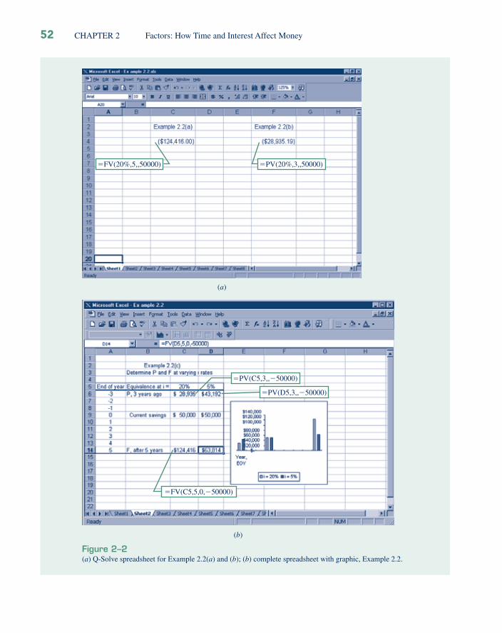
Solution by Computer(c) Figure 2–2b is a complete spreadsheet solution on one worksheet with the chart.

Two columns are used for 20% and 5% computations primarily so the graph can be developed to compare the F and P values. Row 14 shows the F values using the FV function with the format FV(i%,5,0,�50000) where the i values are taken from cells C5 and D5. The future worth F � $124,416 in cell C14 is the same (round-off considered) as that calculated above. The minus sign on 50,000 makes the result a positive number for the chart.

The PV function is used to fi nd the P values in row 6. For example, the present worth at 20% in year �3 is determined in cell C6 using the PV function. The result P � $28,935 is the same as that obtained by using the P�F factor previously. The chart graphically shows the noticeable difference that 20% versus 5% makes over the 8-year span.

Q-SOLVE

E-SOLVE

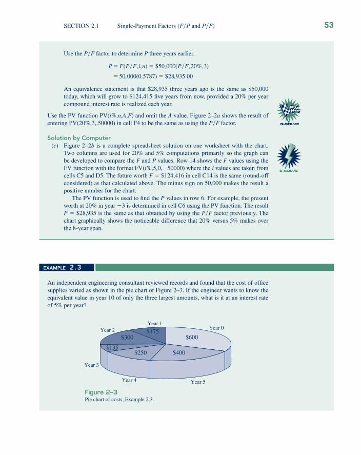
An independent engineering consultant reviewed records and found that the cost of offi ce supplies varied as shown in the pie chart of Figure 2–3. If the engineer wants to know the equivalent value in year 10 of only the three largest amounts, what is it at an interest rate of 5% per year?

Year 0 Year 1

Year 2

Year 3

Year 4 Year 5

$600

$400$250$135

$300$175

Figure 2–3Pie chart of costs, Example 2.3.

EXAMPLE 2.3


2.2 UNIFORM-SERIES PRESENT WORTH FACTOR AND CAPITAL RECOVERY FACTOR (P�A AND A�P )

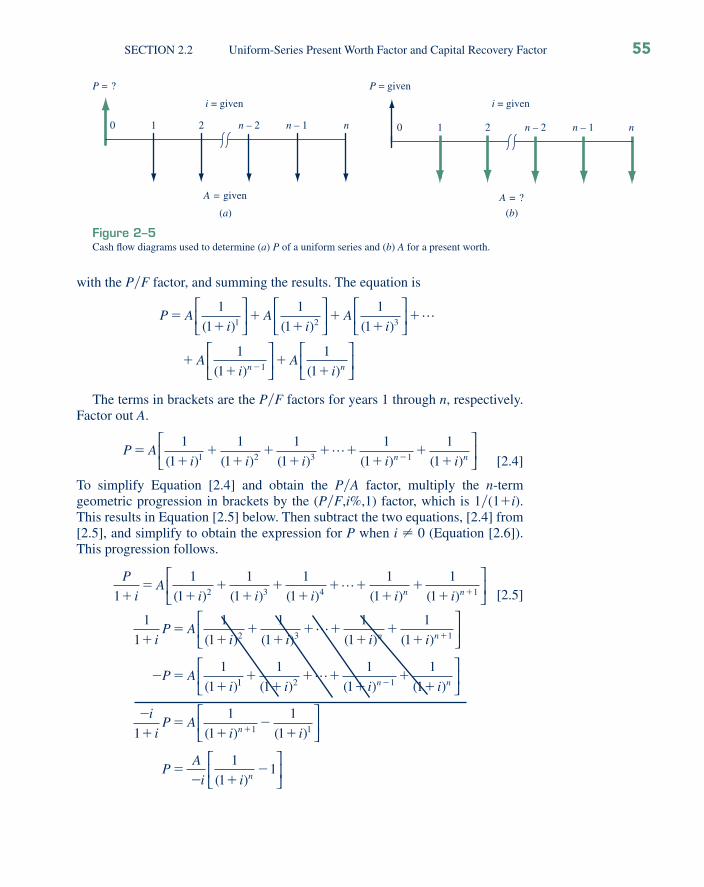
The equivalent present worth P of a uniform series A of end-of-period cash fl ows is shown in Figure 2–5a. An expression for the present worth can be determined by considering each A value as a future worth F, calculating its present worth

i = 5%

10

$600

2

$300

3 4 65 7 8 9 10

$400

F = ?

Figure 2–4Diagram for a future worth in year 10, Example 2.3.

SolutionDraw the cash fl ow diagram for the values $600, $300, and $400 from the engineer’s per-spective (Figure 2–4). Use F�P factors to fi nd F in year 10.

F F P F P F P� � �

� �

600 5 10 300 5 8 400 5 5

600 1 6289 3

( , %, ) ( , %, ) ( , %, )

( . )

� � �

00 1 4775 400 1 2763

1931 11

( . ) ( . )

$ .

�

�

The problem could also be solved by fi nding the present worth in year 0 of the $300 and $400 costs using the P�F factors and then fi nding the future worth of the total in year 10.

P P F P F� � �

� � �

600 300 5 2 400 5 5

600 300 0 9070 400 0 78

( , %, ) ( , %, )

( . ) ( .

� �

35

1185 50

1185 50 5 10 1185 50 1 6289

1931 06

)

$ .

. ( , %, ) . ( . )

$ .

�

� �

�

F F P�

CommentIt should be obvious that there are a number of ways the problem could be worked, since any year could be used to fi nd the equivalent total of the costs before fi nding the future value in year 10. As an exercise, work the problem using year 5 for the equivalent total and then determine the fi nal amount in year 10. All answers should be the same except for round-off error.


0 n – 2 n – 1 n

P = ?

1 2

i = given

A = given

(a)

n – 2 n – 1 n1 2

i = given

A = ?

0

P = given

(b)

Figure 2–5Cash fl ow diagrams used to determine (a) P of a uniform series and (b) A for a present worth.

with the P�F factor, and summing the results. The equation is

P Ai

Ai

Ai

Ai n

��

��

��

�

��

1

1

1

1

1

1

1

1

1 2 3( ) ( ) ( )

( )

⎡

⎣⎢

⎤

⎦⎥

⎡

⎣⎢

⎤

⎦⎥

⎡

⎣⎢

⎤

⎦⎥ �

1

1

1

⎡

⎣⎢

⎤

⎦⎥

⎡

⎣⎢

⎤

⎦⎥�

�A

i n( )

The terms in brackets are the P�F factors for years 1 through n, respectively. Factor out A.

P A

i i i i in n�

��

��

��

��

��

1

1

1

1

1

1

1

1

1

11 2 3 1( ) ( ) ( ) ( ) ( )�

⎡

⎣⎢

⎤

⎦⎥ [2.4]

To simplify Equation [2.4] and obtain the P�A factor, multiply the n-termgeometric progression in brackets by the (P�F,i%,1) factor, which is 1�(1�i). This results in Equation [2.5] below. Then subtract the two equations, [2.4] from [2.5], and simplify to obtain the expression for P when i � 0 (Equation [2.6]). This progression follows.

P

iA

i i i i in n1

1

1

1

1

1

1

1

1

1

12 3 4 1��

��

��

��

��

� �( ) ( ) ( ) ( ) ( )�

⎡

⎣⎢

⎤

⎦⎥

[2.5]

1

1

1

1

1

1

1

1

1

1

1

1

2 3 1��

��

��

��

�

� ��

�iP A

i i i i

P Ai

n n( ) ( ) ( ) ( )

( )

�⎡

⎣⎢

⎤

⎦⎥

11 2 1

1

1

1

1

1

1

1

1

1

1

1

1

��

� ��

��

�

��

��

�

�

�

( ) ( ) ( )

( ) (

i i i

i

iP A

i

n n

n

�⎡

⎣⎢

⎤

⎦⎥

i

PA

i i n

)

( )

1

1

11

⎡

⎣⎢

⎤

⎦⎥

⎡

⎣⎢

⎤

⎦⎥�

� ��

SECTION 2.2 Uniform-Series Present Worth Factor and Capital Recovery Factor 55

P A

ii i

n

n�

� �

�

( )( )

1 11

⎡

⎣⎢

⎤

⎦⎥ i � 0 [2.6]

The term in brackets in Equation [2.6] is the conversion factor referred to as the uniform-series present worth factor (USPWF). It is the P�A factor used to calculate the equivalent P value in year 0 for a uniform end-of-period series of A values beginning at the end of period 1 and extending for n periods. The cash fl ow diagram is Figure 2–5a.

To reverse the situation, the present worth P is known and the equivalent uniform-series amount A is sought (Figure 2–5b). The fi rst A value occurs at the end of period 1, that is, one period after P occurs. Solve Equation [2.6] for A to obtain

A P

i ii

n

n�

�

� �

( )( )

11 1

⎡

⎣⎢

⎤

⎦⎥ [2.7]

The term in brackets is called the capital recovery factor (CRF), or A�P factor. It calculates the equivalent uniform annual worth A over n years for a given P in year 0, when the interest rate is i.

These formulas are derived with the present worth P and the fi rst uni-form annual amount A one year (period) apart. That is, the present worth P must always be located one period prior to the fi rst A.

The factors and their use to fi nd P and A are summarized in Table 2–2, and inside the front cover. The standard notations for these two factors are (P�A,i%,n) and (A�P,i%,n). Tables 1 through 29 at the end of the text include the factor values. As an example, if i � 15% and n � 25 years, the P�A factor value from Table 19 is (P�A,15%,25) � 6.4641. This will fi nd the equivalent present worth at 15% per year for any amount A that occurs uniformly from years 1 through 25. When the bracketed relation in Equation [2.6] is used to calculate the P�A factor, the result is the same except for round-off errors.

( , %, )

( )

( )

( . )

. ( . )

.P A

i

i i

n

n� 15 25

1 1

1

1 15 1

0 15 1 15

31 91825

25�

�

��

��

− 95

4 937846 46415

..�

TABLE 2–2 P�A and A�P Factors: Notation and Equations

Factor Factor Formula

Standard Notation Equation

Excel FunctionNotation Name Find/Given

(P�A,i,n) Uniform-series present worth

P�A ( )

( )

1 1

1

� �

�

i

i i

n

n

P � A(P�A,i,n) PV(i%,n,A)

(A�P,i,n) Capital recovery A�P i i

i

n

n

( )

( )

1

1 1

�

� �

A � P(A�P,i,n) PMT(i%,n,P)


Spreadsheet functions are capable of determining both P and A values in lieu of applying the P�A and A�P factors. The PV function that we used in the lastsection also calculates the P value for a given A over n years, and a separateF value in year n, if it is given. The format, introduced in Section 1.8, is

PV(i%,n,A,F)

Similarly, the A value is determined using the PMT function for a given P value in year 0 and a separate F, if given. The format is

PMT(i%,n,P,F)

The PMT function was demonstrated in Section 1.18 (Figure 1–5b) and is used in later examples. Table 2–2 includes the PV and PMT functions for P and A, respectively. Example 2.4 demonstrates the PV function.

Q-SOLVE

How much money should you be willing to pay now for a guaranteed $600 per year for 9 years starting next year, at a rate of return of 16% per year?

SolutionThe cash fl ow diagram (Figure 2–6) fi ts the P�A factor. The present worth is:

P � 600(P�A,16%,9) � 600(4.6065) � $2763.90

The PV function PV(16%,9,600) entered into a single spreadsheet cell will display the answer P � $2763.93.

i = 16%

10

P = ?

2 3 4 65 987

A = $600

Figure 2–6Diagram to fi nd P using the P�A factor, Example 2.4.

CommentAnother solution approach is to use P�F factors for each of the nine receipts and add the resulting present worths to get the correct answer. Another way is to fi nd the future worth F of the $600 payments and then fi nd the present worth of the F value. There are many ways to solve an engineering economy problem. Only the most direct method is presented here.

EXAMPLE 2.4

Q-SOLVE

SECTION 2.2 Uniform-Series Present Worth Factor and Capital Recovery Factor 57

2.3 SINKING FUND FACTOR AND UNIFORM-SERIES COMPOUND AMOUNT FACTOR (A/F AND F/A)

The simplest way to derive the A�F factor is to substitute into factors already developed. If P from Equation [2.3] is substituted into Equation [2.7], the fol-lowing formula results.

A F

i

i i

in

n

n�

�

�

� �

1

1

1

1 1( )

( )

( )

⎡

⎣⎢

⎤

⎦⎥

⎡

⎣⎢

⎤

⎦⎥

A Fii n

�� ( )1 1

⎡

⎣⎢

⎤

⎦⎥

[2.8]

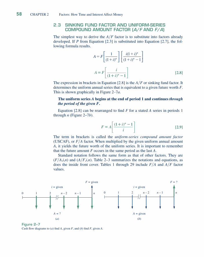
The expression in brackets in Equation [2.8] is the A�F or sinking fund factor. It determines the uniform annual series that is equivalent to a given future worth F. This is shown graphically in Figure 2–7a.

The uniform series A begins at the end of period 1 and continues through the period of the given F.

Equation [2.8] can be rearranged to fi nd F for a stated A series in periods 1 through n (Figure 2–7b).

F Aii

n

�� ( )1 1⎡

⎣⎢

⎤

⎦⎥

[2.9]

The term in brackets is called the uniform-series compound amount factor (USCAF), or F�A factor. When multiplied by the given uniform annual amount A, it yields the future worth of the uniform series. It is important to remember that the future amount F occurs in the same period as the last A.

Standard notation follows the same form as that of other factors. They are (F�A,i,n) and (A�F,i,n). Table 2–3 summarizes the notations and equations, as does the inside front cover. Tables 1 through 29 include F�A and A�F factor values.

0 n – 2 n – 1 n

F = given

1 2

i = given

A = ?

(a)

0 n – 2 n – 1 n

F = ?

1 2

i = given

A = given

(b)

Figure 2–7Cash fl ow diagrams to (a) fi nd A, given F, and (b) fi nd F, given A.


The uniform-series factors can be symbolically determined by using anabbreviated factor form. For example, F�A � (F�P)(P�A), where cancellationof the P is correct. Using the factor formulas, we have

( , , ) ( )

( )

( )

( )F A i n i

i

i i

i

in

n

n

n

� = +⎡⎣ ⎤⎦+ −

+⎡

⎣⎢

⎤

⎦⎥ = + −

11 1

1

1 1

Also the A�F factor in Equation [2.8] may be derived from the A�P factor by subtracting i.

( , , ) ( , , )A F i n A P i n i� ��

This relation can be verifi ed empirically in any interest factor table in the rear of the text, or mathematically by simplifying the equation to derive the A�F factor formula. This relation is used later to compare alternatives by the annual worth method.

For solution by computer, the FV spreadsheet function calculates F for a stated A series over n years. The format is

FV(i%,n,A,P)

The P may be omitted when no separate present worth value is given. The PMT function determines the A value for n years, given F in year n, and possibly a separate P value in year 0. The format is

PMT(i%,n,P,F)

If P is omitted, the comma must be entered so the computer knows the last entry is an F value. These functions are included in Table 2–3. The next two examples include the FV and PMT functions.

TABLE 2–3 F�A and A�F Factors: Notation and Equations

Factor Factor Formula

Standard Notation Equation

Excel FunctionsNotation Name Find/Given

(F�A,i,n) Uniform-seriescompound amount

F�A ( )1 1� �i

i

n F � A(F�A,i,n) FV(i%,n,A)

(A�F,i,n) Sinking fund A�F i

i n( )1 1+ −

A � F(A�F,i,n) PMT(i%,n,,F)

Formasa Plastics has major fabrication plants in Toronto and Hong Kong. The president wants to know the equivalent future worth of a $1 million capital investment each year for 8 years, starting 1 year from now. Formasa capital earns at a rate of 14% per year.

EXAMPLE 2.5

SECTION 2.3 Sinking Fund Factor and Uniform-Series Compound Amount Factor 59

Sec. 6.2

AW method

Q-SOLVE


SolutionThe cash fl ow diagram (Figure 2–8) shows the annual payments starting at the end of year 1 and ending in the year the future worth is desired. Cash fl ows are indicated in $1000 units. The F value in 8 years is

F � 1000(F�A,14%,8) � 1000(13.2328) � $13,232.80

The actual future worth is $13,232,800. The FV function is FV(14%,8,1000000).

i = 14%

A = $1000

10 2 3 4 65 7 8

F = ? Figure 2–8Diagram to fi nd Ffor a uniform series,Example 2.5.

Q-SOLVE

How much money must Carol deposit every year starting 1 year from now at 5 %12

per

year in order to accumulate $6000 seven years from now?

SolutionThe cash fl ow diagram from Carol’s perspective (Figure 2–9a) fi ts the A�F factor.

A � $6000(A�F,5.5%,7) � 6000(0.12096) � $725.76 per year

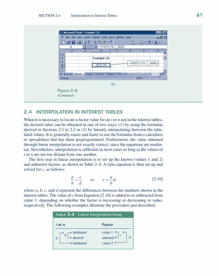
The A�F factor value of 0.12096 was computed using the factor formula in Equation [2.8]. Alternatively, use the PMT function as shown in Figure 2–9b to obtain A � $725.79per year.

1 0

F = $6000

2 3 4 6 5 7

A = ?

i = 5 % 1 2

(a)

Figure 2–9(a) Cash fl ow diagram and (b) PMT function to determine A, Example 2.6.

EXAMPLE 2.6

Q-SOLVE

2.4 INTERPOLATION IN INTEREST TABLES

When it is necessary to locate a factor value for an i or n not in the interest tables, the desired value can be obtained in one of two ways: (1) by using the formulas derived in Sections 2.1 to 2.3 or (2) by linearly interpolating between the tabu-lated values. It is generally easier and faster to use the formulas from a calculator or spreadsheet that has them preprogrammed. Furthermore, the value obtained through linear interpolation is not exactly correct, since the equations are nonlin-ear. Nevertheless, interpolation is suffi cient in most cases as long as the values of i or n are not too distant from one another.

The fi rst step in linear interpolation is to set up the known (values 1 and 2) and unknown factors, as shown in Table 2–4. A ratio equation is then set up and solved for c, as follows:

a

b

c

dor c

a

bd� �

[2.10]

where a, b, c, and d represent the differences between the numbers shown in the interest tables. The value of c from Equation [2.10] is added to or subtracted from value 1, depending on whether the factor is increasing or decreasing in value, respectively. The following examples illustrate the procedure just described.

TABLE 2–4 Linear Interpolation Setup

i or n Factor

tabulated value 1

desired unlisted

tabulated value 2b

a cd

→→

→→ →

→→→

SECTION 2.4 Interpolation in Interest Tables 61

(b)

�PMT(5.5%,7,,6000)

Figure 2–9(Continued).

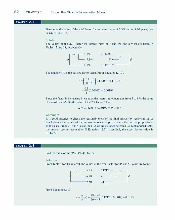
Determine the value of the A�P factor for an interest rate of 7.3% and n of 10 years, that is, (A�P,7.3%,10).

SolutionThe values of the A�P factor for interest rates of 7 and 8% and n � 10 are listed in Tables 12 and 13, respectively.

7% 0.14238

b 7.3% X d

8% 0.14903

a c→→

→

→

→

→ →

→

The unknown X is the desired factor value. From Equation [2.10],

c ��

��

� �

7 3 7

8 70 14903 0 14238

0 3

10 00665 0 00199

.( . . )

.( . ) .

⎛

⎝⎜

⎞

⎠⎟

Since the factor is increasing in value as the interest rate increases from 7 to 8%, the value of c must be added to the value of the 7% factor. Thus,

X � 0.14238 � 0.00199 � 0.14437

CommentIt is good practice to check the reasonableness of the fi nal answer by verifying that X lies between the values of the known factors in approximately the correct proportions. In this case, since 0.14437 is less than 0.5 of the distance between 0.14238 and 0.14903, the answer seems reasonable. If Equation [2.7] is applied, the exact factor value is 0.144358.

EXAMPLE 2.7

Find the value of the (P�F,4%,48) factor.

SolutionFrom Table 9 for 4% interest, the values of the P�F factor for 45 and 50 years are found.

45 0.1712

b 48 X d

50 0.1407

a c→→

→

→

→

→ →

→

From Equation [2.10],

c

a

bd� �

�

�� ( ) ( . . ) .

48 45

50 450 1712 0 1407 0 0183

EXAMPLE 2.8


2.5 ARITHMETIC GRADIENT FACTORS (P/G AND A/G )

An arithmetic gradient is a cash fl ow series that either increases or decreases by a constant amount. The cash fl ow, whether income or disbursement, changes by the same arithmetic amount each period. The amount of the increase or decrease is the gradient. For example, if a manufacturing engineer predicts that the cost of maintaining a robot will increase by $500 per year until the machine is retired, a gradient series is involved and the amount of the gradient is $500.

Formulas previously developed for an A series have year-end amounts of equal value. In the case of a gradient, each year-end cash fl ow is different, so new formulas must be derived. First, assume that the cash fl ow at the end of year 1 is not part of the gradient series, but is rather a base amount. This is convenient because in actual applications, the base amount is usually larger or smaller than the gra dient increase or decrease. For example, if you purchase a used car with a 1-year warranty, you might expect to pay the gasoline and insurance costs during the fi rst year of operation. Assume these cost $1500; that is, $1500 is the base amount. After the fi rst year, you absorb the cost of repairs, which could reasonably be expected to increase each year. If you estimate that total costs will increase by $50 each year, the amount the second year is $1550, the third $1600, and so on to year n, when the total cost is 1500 � (n�1)50. The cash fl ow diagram is shown in Figure 2–10. Note that the gradient ($50) is fi rst observed between year 1 and year 2, and the base amount ($1500 in year 1) is not equal to the gradient.

Defi ne the symbol G for gradients as

G � constant arithmetic change in the magnitude of receipts or disburse-ments from one time period to the next; G may be positive or negative.

Since the value of the factor decreases as n increases, c is subtracted from the factor value for n � 45.

X � 0.1712 � 0.0183 � 0.1529

CommentThough it is possible to perform two-way linear interpolation, it is much easier and more accurate to use the factor formula or a spreadsheet function.

0 n – 1 n1 2 3 4

$1500+ (n – 2)50 $1500

+ (n – 1)50

$1500$1550

$1600$1650

Figure 2–10Diagram of an arithmetic gradient series with a base amount of $1500 and a gradient of $50.

SECTION 2.5 Arithmetic Gradient Factors (P�G and A�G) 63

The cash fl ow in year n (CFn) may be calculated as

CF n Gn � � �base amount ( )1

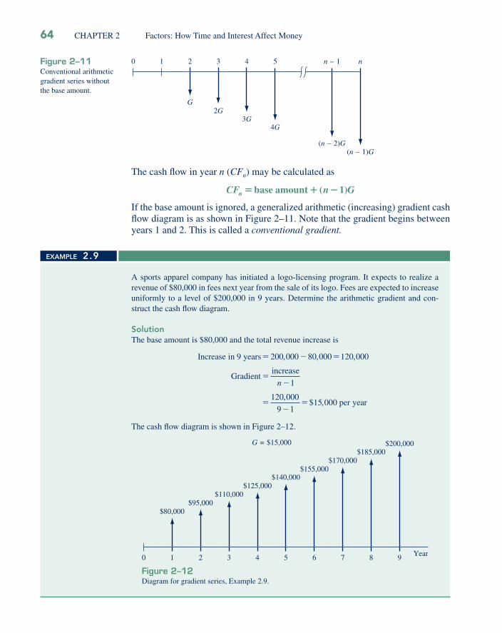
If the base amount is ignored, a generalized arithmetic (increasing) gradient cash fl ow diagram is as shown in Figure 2–11. Note that the gradient begins between years 1 and 2. This is called a conventional gradient.

0 n – 1

(n – 2)G

n

(n – 1)G

1 2

G

3

2G

4

3G

5

4G

Figure 2–11Conventional arithmetic gradient series without the base amount.

A sports apparel company has initiated a logo-licensing program. It expects to realize a revenue of $80,000 in fees next year from the sale of its logo. Fees are expected to increase uniformly to a level of $200,000 in 9 years. Determine the arithmetic gradient and con-struct the cash fl ow diagram.

SolutionThe base amount is $80,000 and the total revenue increase is

Increase in years

Gradientincrease

9 200 000 80 000 120 000� � �

�

, , ,

n �

��

�

1

120 000

9 115 000

,$ , per year

The cash fl ow diagram is shown in Figure 2–12.

0 8 9

$185,000G = $15,000

1

$80,000

2

$95,000

Year3

$110,000

4

$125,000

6

$155,000

7

$170,000

5

$140,000

$200,000

Figure 2–12Diagram for gradient series, Example 2.9.

EXAMPLE 2.9


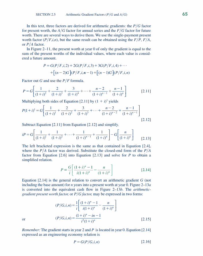
In this text, three factors are derived for arithmetic gradients: the P�G factor for present worth, the A�G factor for annual series and the F�G factor for future worth. There are several ways to derive them. We use the single-payment present worth factor (P�F,i,n), but the same result can be obtained using the F�P, F�A, or P�A factor.

In Figure 2–11, the present worth at year 0 of only the gradient is equal to the sum of the present worths of the individual values, where each value is consid-ered a future amount.

P G P F i G P F i G P F i

n G P F i

� � � �

� �

( , , ) ( , , ) ( , , ) . . .

( ) ( , ,

� � �

�

2 2 3 3 4

2⎡⎣ ⎤⎦ nn n G P F i n� � �1 1) ( ) ( , , )⎡⎣ ⎤⎦ �

Factor out G and use the P�F formula.

P Gi i i

n

i

n

in n�

��

��

��

�

��

�

��

1

1

2

1

3

1

2

1

1

12 3 4 1( ) ( ) ( ). . .

( ) ( )

⎡

⎣⎢

⎤

⎦⎥

[2.11]

Multiplying both sides of Equation [2.11] by (1 � i)1 yields

P i Gi i i

n

i

n

in n( )

( ) ( ) ( ). . .

( ) ( )1

1

1

2

1

3

1

2

1

1

11

1 2 3 2� �

��

��

��

�

��

�

�� 1

⎡

⎣⎢

⎤

⎦⎥

[2.12]

Subtract Equation [2.11] from Equation [2.12] and simplify.

iP Gi i i i

Gn

in n n�

��

��

��

��

��

1

1

1

1

1

1

1

1 11 2 1( ) ( ). . .

( ) ( ) ( )

⎡

⎣⎢

⎤

⎦⎥

⎡

⎣⎢

⎤

⎦⎥

[2.13]

The left bracketed expression is the same as that contained in Equation [2.4], where the P�A factor was derived. Substitute the closed-end form of the P�A factor from Equation [2.6] into Equation [2.13] and solve for P to obtain asimplifi ed relation.

P

Gi

ii i

ni

n

n n�

� �

��

�

( )( ) ( )

1 11 1

⎡

⎣⎢

⎤

⎦⎥

[2.14]

Equation [2.14] is the general relation to convert an arithmetic gradient G (notincluding the base amount) for n years into a present worth at year 0. Figure 2–13a is converted into the equivalent cash fl ow in Figure 2–13b. The arithmetic-gradient present worth factor, or P�G factor, may be expressed in two forms:

or

( , , )( )

( ) ( )

( , , )( )

P G i ni

i

i i

n

i

P G i ni

n

n n

n

�

�

��

��

�

��

1 1 1

1 1

1

⎡

⎣⎢

⎤

⎦⎥

in

i i n

�

�

1

12( ) [2.15]

Remember: The gradient starts in year 2 and P is located in year 0. Equation [2.14] expressed as an engineering economy relation is

P G P G i n� ( , , )� [2.16]


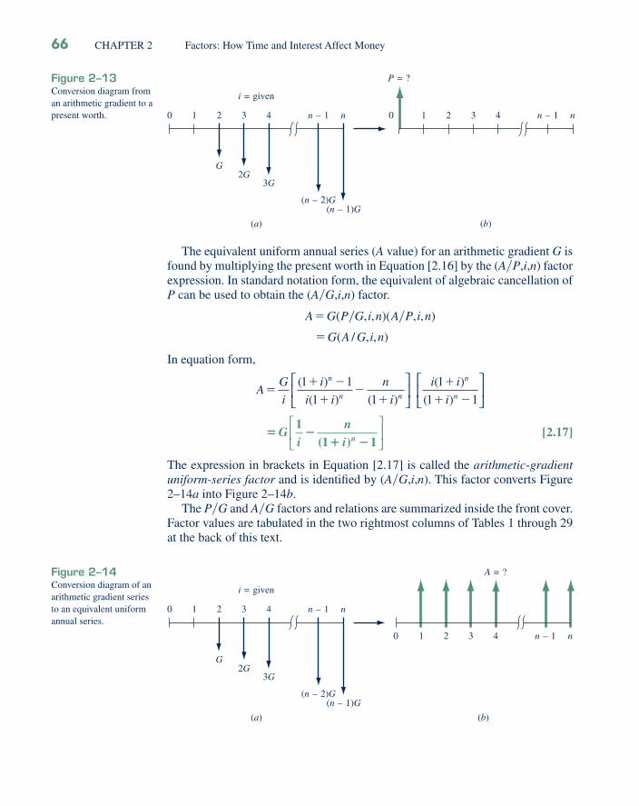
The equivalent uniform annual series (A value) for an arithmetic gradient G is found by multiplying the present worth in Equation [2.16] by the (A�P,i,n) factor expression. In standard notation form, the equivalent of algebraic cancellation of P can be used to obtain the (A�G,i,n) factor.

A G P G i n A P i n

G A G i n

�

�

( , , )( , , )

( / , , )

� �

In equation form,

A

G

i

i

i i

n

i

i i

i

n

n n

n

n�

� �

��

�

�

� �

( )

( ) ( )

( )

( )

1 1

1 1

1

1 1

⎡

⎣⎢

⎤

⎦⎥

⎡

⎣⎢

⎤

⎦⎥

� �

� �G

ini n

11 1( )

⎡

⎣⎢

⎤

⎦⎥

[2.17]

The expression in brackets in Equation [2.17] is called the arithmetic-gradient uniform-series factor and is identifi ed by (A�G,i,n). This factor converts Figure 2–14a into Figure 2–14b.

The P�G and A�G factors and relations are summarized inside the front cover. Factor values are tabulated in the two rightmost columns of Tables 1 through 29 at the back of this text.

0 n – 1

(n – 2)G

n

(n – 1)G

(a)

1 2

G

3

2G

4

3G

P = ?

n – 1 n

(b)

10 2 3 4

i = given

Figure 2–13Conversion diagram from an arithmetic gradient to a present worth.

0 n – 1

(n – 2)G

n

(n – 1)G

(a)

1 2

G

3

2G

4

3G

A = ?

n – 1 n

(b)

10 2 3 4

i = given

Figure 2–14Conversion diagram of an arithmetic gradient series to an equivalent uniform annual series.


There is no direct, single-cell spreadsheet function to calculate P or A for an arithmetic gradient. Use the NPV function for P, and the PMT function for A, after all cash fl ows are entered into cells. (The use of NPV and PMT functions for this type of cash fl ow series is illustrated in Chapter 3.)

An F�G factor (arithmetic-gradient future worth factor) can be derivedby multiplying the P�G and F�P factors. The resulting factor, (F�G,i,n), in brackets, and engineering economy relation is

F G

i

i

in

n

��

�1 1 1⎛

⎝⎜⎞⎠⎟

⎛

⎝⎜

⎞

⎠⎟

⎡

⎣⎢⎢

⎤

⎦⎥⎥

( )

The total present worth PT for a gradient series must consider the base and the gradient separately. Thus, for cash fl ow series involving conventional gradients:

The base amount is the uniform-series amount A that begins in year 1 and extends through year n. Its present worth is represented by PA.For an increasing gradient, the gradient amount must be added to theuniform-series amount. The present worth is PG.For a decreasing gradient, the gradient amount must be subtracted from the uniform-series amount. The present worth is �PG.

The general equations for calculating total present worth PT of conventional arithmetic gradients are

P P P P P PT A G T A G� � � �and [2.18]

Similarly, the equivalent total annual series are

A A A A A AT A G T A G� � � �and [2.19]

where AA is the annual base amount and AG is the equivalent annual amount of the gradient series.

•

•

•

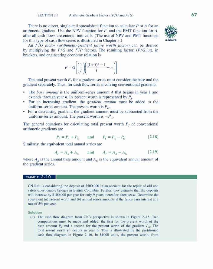
CN Rail is considering the deposit of $500,000 in an account for the repair of old and safety-questionable bridges in British Columbia. Further, they estimate that the deposits will increase by $100,000 per year for only 9 years thereafter, then cease. Determine the equivalent (a) present worth and (b) annual series amounts if the funds earn interest at a rate of 5% per year.

Solution(a) The cash fl ow diagram from CN’s perspective is shown in Figure 2–15. Two

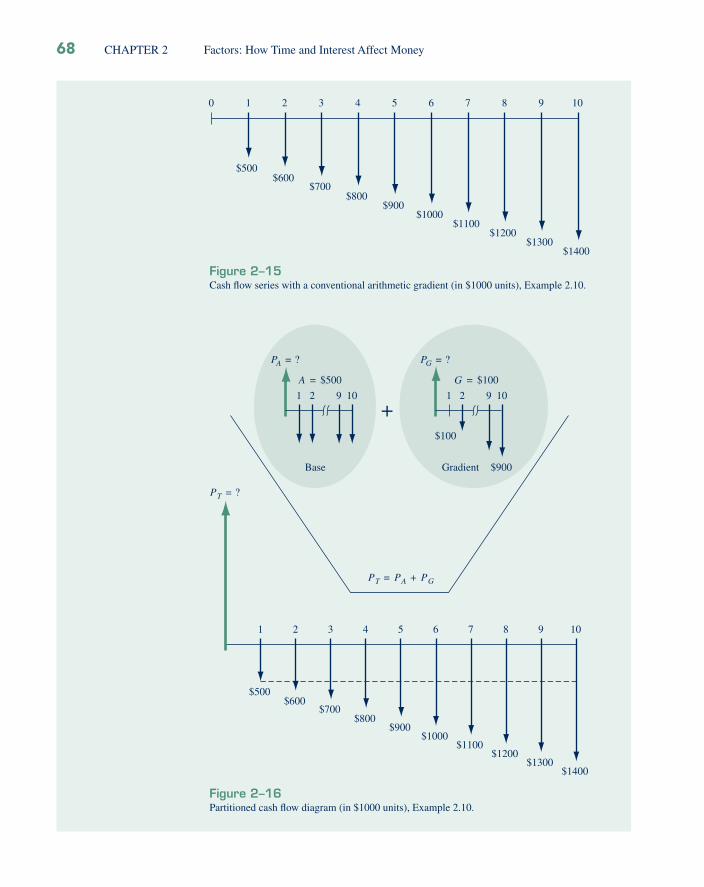
computations must be made and added: the fi rst for the present worth of the base amount PA and a second for the present worth of the gradient PG. The total resent worth PT occurs in year 0. This is illustrated by the partitioned cash fl ow diagram in Figure 2–16. In $1000 units, the present worth, from

EXAMPLE 2.10


Q-SOLVE

0

$500

2

$600

3

$700

4

$800

5

$900

6

$1000

7

$1100

8

$1200

9

$1300

10

$1400

1

Figure 2–15Cash fl ow series with a conventional arithmetic gradient (in $1000 units), Example 2.10.

PT = ?

1

$500

2

$600

3

$700

4

$800

5

$900

PT = PA + PG

6

$1000

7

$1100

8

$1200

9

$1300

10

$1400

PA = ?

109

Base

21

+

PG = ?

10

$900

9

Gradient

21

$100

G = $100A = $500

Figure 2–16Partitioned cash fl ow diagram (in $1000 units), Example 2.10.


Additional Example 2.16.

2.6 GEOMETRIC GRADIENT SERIES FACTORS

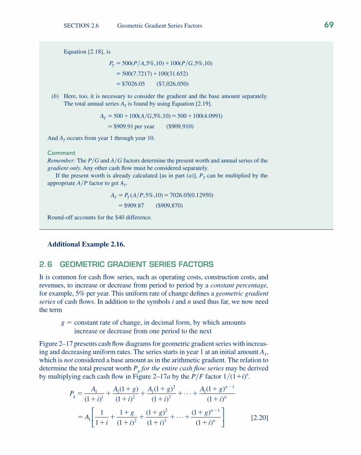
It is common for cash fl ow series, such as operating costs, construction costs, and revenues, to increase or decrease from period to period by a constant percentage, for example, 5% per year. This uniform rate of change defi nes a geometric gradient series of cash fl ows. In addition to the symbols i and n used thus far, we now need the term

g � constant rate of change, in decimal form, by which amounts increase or decrease from one period to the next

Figure 2–17 presents cash fl ow diagrams for geometric gradient series with increas-ing and decreasing uniform rates. The series starts in year 1 at an initial amount A1, which is not considered a base amount as in the arithmetic gradient. The relation to determine the total present worth Pg for the entire cash fl ow series may be derived by multiplying each cash fl ow in Figure 2–17a by the P�F factor 1�(1�i)n.

PA

i

A g

i

A g

i

A gg

n

��

��

��

�

��

�

�

�1

11

21

2

31

1

1

1

1

1

1

1

1( )

( )

( )

( )

( ). . . ( )

( i

Ai

g

i

g

i

g

i

n

n

n

)

( )

( )

( ). . . ( )

( )�

��

�

��

�

��

�

�

�

1 2

2

3

11

1

1

1

1

1

1

1

⎡

⎣⎢

⎤

⎦⎥ [2.20]

Equation [2.18], is

P P A P GT � �

� �

�

500 5 10 100 5 10

500 7 7217 100 31 652

( , %, ) ( , %, )

( . ) ( . )

$

� �

7026 05 7 026 050. ($ , , )

(b) Here, too, it is necessary to consider the gradient and the base amount separately. The total annual series AT is found by using Equation [2.19].

A A GT � � � �

�

500 100 10 500 100 4 0991

909 91 909

( , %, ) ( . )

$ . ($ ,

� 5

per year 910)

And AT occurs from year 1 through year 10.

CommentRemember: The P�G and A�G factors determine the present worth and annual series of the gradient only. Any other cash fl ow must be considered separately.

If the present worth is already calculated [as in part (a)], PT can be multiplied by the appropriate A�P factor to get AT.

A P A PT T� �

�

( , %, ) . ( . )

$ . ($ , )

� 5 10 7026 05 0 12950

909 87 909 870

Round-off accounts for the $40 difference.

SECTION 2.6 Geometric Gradient Series Factors 69

Multiply both sides by (1�g)�(1�i), subtract Equation [2.20] from the result, factor out Pg, and obtain

P

g

iA

g

i ig

n

n

1

11

1

1

1

11 1

�

��

�

��

��

⎛

⎝⎜

⎞

⎠⎟

⎡

⎣⎢

⎤

⎦⎥

( )

( )

Solve for Pg and simplify.

Pg A1

111�

� ��

�

⎛⎝⎜

⎞⎠⎟

g

i

i g

n

g i [2.21]

The term in brackets in Equation [2.21] is the geometric-gradient-series present worth factor for values of g not equal to the interest rate i. The standard notation used is (P�A,g,i,n). When g�i, substitute i for g in Equation [2.20] to obtain

P A

i i i ig ��

��

��

� ��

11

1

1

1

1

1

1

1( ) ( ) ( ) ( )�

⎛

⎝⎜

⎞

⎠⎟

The term 1�(1 � i) appears n times, so

P

nA

ig ��

1

1( ) [2.22]

In summary, the engineering economy relation and factor formulas to calcu-late Pg in period t � 0 for a geometric gradient series starting in period 1 in the amount A1 and increasing by a constant rate of g each period are

P A P A g i ng � 1( , , , )� [2.23]

( , , , )P A g i n

gi

i gg i

ni

g i

n

� ��

111

1

��

�

�

��

⎛

⎝⎜

⎞

⎠⎟

⎧

⎨

⎪⎪⎪

⎩

⎪⎪⎪

[2.24]

Pg = ?i = giveng = given

A1(1 + g)3

n

A1(1 + g)n – 1

10 2

A1

3

A1(1 + g)

4

A1(1 + g)2

(a)

Pg = ?i = giveng = given

n10 2 3 4

A1(1 – g)2

A1(1 – g)n – 1A1(1 – g)3

A1(1 – g)

A1

(b)

Figure 2–17Cash fl ow diagram of (a) increasing and (b) decreasing geometric gradient series and present worth Pg.


It is possible to derive factors for the equivalent A and F values; however, it is easier to determine the Pg amount and then multiply by the A�P or F�P factor.

As with the arithmetic gradient series, there are no direct spreadsheet func-tions for geometric gradients series. Once the cash fl ows are entered, P and A are determined by using the NPV and PMT functions, respectively. However, it is always an option to develop on the spreadsheet a function that uses thefactor equation to determine a P, F, or A value. Example 2.11 demonstratesthis approach to fi nd the present worth of a geometric gradient series usingEquations [2.24].

SECTION 2.6 Geometric Gradient Series Factors 71

Engineers at La Ronde, the large amusement park in Montreal, are considering an innova-tion on the existing Monster roller coaster to make it more exciting. The modifi cation costs only $8000 and is expected to last 6 years with a $1300 salvage value for the solenoid mechanisms. The maintenance cost is expected to be high at $1700 the fi rst year, increas-ing by 11% per year thereafter. Determine the equivalent present worth of the modifi cation and maintenance cost by hand and by computer. The interest rate is 8% per year.

Solution by HandThe cash fl ow diagram (Figure 2–18) shows the salvage value as a positive cash fl ow and all costs as negative. Use Equation [2.24] for g � i to calculate Pg. The total PT is

P P P FT g��

��

�

8000 1300 8 6

8000 17001 1 11 1 08

0 08 0

6

( , %, )

( . . )

. .

�

�11

1300 8 6

8000 1700 5 9559 819 26 17 30

⎡

⎣⎢

⎤

⎦⎥ �

��

( , %, )

( . ) . $ ,

P F�

55 85.

[2.25]

Pg = ?

PT = ?

1

$1700

$8000

2

$1700(1.11)

3

i = 8%g = 11%

$1700(1.11)2

4

$1700(1.11)3

5

$1700(1.11)4

6

$1300

$1700(1.11)5

EXAMPLE 2.11

Figure 2–18Cash fl ow diagram of ageometric gradient,Example 2.11.

2.7 DETERMINATION OF AN UNKNOWN INTEREST RATE

In some cases, the amount of money deposited and the amount of money received after a specifi ed number of years are known, and it is the interest rate or rate of return that is unknown. When single amounts, uniform series, or a uniform conven-tional gradient is involved, the unknown rate i can be determined by direct solution of the time value of money equation. When nonuniform payments or several factors are involved, the problem must be solved by a trial-and-error or numerical method. These more complicated problems are deferred until Chapter 7.

The single-payment formulas can be easily rearranged and expressed in terms of i, but for the uniform series and gradient equations, it is easier to solve for the value of the factor and determine the interest rate from interest factor tables. Both situations are illustrated in the examples that follow.

Chap.7

Sec. 2.9

Find i


Solution by ComputerFigure 2–19 presents a spreadsheet with the total present worth in cell B13. The function used to determine PT � $�17,305.89 is detailed in the cell tag. It is a rewrite of Equation [2.25]. Since it is complex, column C and D cells also contain the three elements of PT, which are summed in D13 to obtain the same result.

E-SOLVE

�((1�((1�B10)/(1�B11))^B7)/(B11�B10))

�B6�B9*((1�((1�B10)/(1�B11))^B7)/(B11�B10))�PV(B11,B7,0,�B8)

�SUM(D6:D12)

�PV(B11,B7,0,�B8)

Figure 2–19Spreadsheet used to determine present worth of a geometric gradient with g � 11%, Example 2.11.

The IRR spreadsheet function is one of the most useful of all those available. IRR means internal rate of return, which is a topic unto itself, discussed in detail in Chapter 7. However, even at this early stage of engineering economic analysis, the IRR function can be used benefi cially to fi nd the interest rate (or rate of return) for any cash fl ow series that is entered into a series of contiguous spreadsheet cells, vertical or horizontal. It is very important that any years (periods) with a zero cash fl ow have an entry of 0 in the cell. A cell left blank is not suffi cient, because an incorrect value of i will be displayed by the IRR function. The basic format is

IRR(fi rst_cell:last_cell)

If Laurel can make an investment in a friend’s business of $3000 now in order to receive $5000 fi ve years from now, determine the rate of return. If Laurel can receive 7% per year interest on a guaranteed investment certifi cate, which investment should be made?

SolutionSince only single payment amounts are involved, i can be determined directly from the P�F factor.

P F P F i n Fi

i

i

i

n� �

�

��

��

�

( , , )( )

( )

.( )

.

�1

1

3000 50001

1

0 6001

1

1

0 6

5

5

⎛⎝⎜

⎞⎠⎟

0 2

1 0 1076 10 76.

. ( . %)� �

Alternatively, the interest rate can be found by setting up the standard notation P�F relation, solving for the factor value, and interpolating in the tables.

P F P F i n

P F i

P F i

�

�

� �

( , , )

$ ( , , )

( , , ) .

�

�

�

3000 5000 5

53000

50000 60

From the interest tables, a P�F factor of 0.6000 for n � 5 lies between 10 and 11%. Interpolate between these two values to obtain i � 10.76%.

Since 10.76% is greater than the 7% available from a guaranteed investment certifi cate, Laurel should make the business investment. Since the higher rate of return would be re-ceived on the business investment, Laurel would probably select this option instead of the investment certifi cate. However, the degree of risk associated with the business investment was not specifi ed. Obviously, risk is an important parameter that may cause selection of the lower rate of return investment. Unless specifi ed to the contrary, equal risk for all alternatives is assumed in this text.

EXAMPLE 2.12

E-SOLVE

SECTION 2.7 Determination of an Unknown Interest Rate 73

The fi rst_cell and last_cell are the cell references for the start and end of the cash fl ow series. Example 2.13 illustrates the IRR function.

The RATE function, also very useful, is an alternative to IRR. RATE is a one-cell function that displays the compound interest rate (or rate of return) only when the annual cash fl ows, that is, A values, are the same. Present and future values different from the A value can be entered. The format is

RATE(number_years,A,P,F)

The F value does not include the amount A that occurs in year n. No entry into spreadsheet cells of each cash fl ow is necessary to use RATE, so it should be used whenever there is a uniform series over n years with associated P and/or F values stated. Example 2.13 illustrates the RATE function.

Q-SOLVE

Professional Engineers, Inc., requires that $500 per year be placed into a sinking fundaccount to cover any unexpected major rework on fi eld equipment. In one case, $500 was deposited for 15 years and covered a rework costing $10,000 in year 15. What rate of return did this practice provide to the company? Solve by hand and by computer.

Solution by HandThe cash fl ow diagram is shown in Figure 2–20. Either the A�F or F�A factor can be used. Using A�F,

A F A F i n

A F i

A F i

�

�

�

( , , )

, ( , , )

( , , ) .

�

�

�

500 10 000 15

15 0 0500

From interest Tables 8 and 9 under the A�F column for 15 years, the value 0.0500 lies between 3 and 4%. By interpolation, i�3.98%. (This is considered a low return for an engineering project.)

EXAMPLE 2.13

i = ?

10

A = $500

2 3 4 65 7 8 9 1110 12 13 14 15

F = $10,000 Figure 2–20Diagram to determine the rate of return, Example 2.13.

Solution by ComputerRefer to the cash fl ow diagram (Figure 2–20) while completing the spreadsheet (Figure 2–21). A single-cell solution using the RATE function can be applied since A � $�500 occurs each year and the F � $10,000 value takes place in the last year of the series. Cell A3 contains the function RATE(15,�500,,10000), and the answer displayed is 3.98%. The minus sign on


2.8 DETERMINATION OF UNKNOWN NUMBER OF YEARS

It is sometimes necessary to determine the number of years (periods) required for a cash fl ow series to provide a stated rate of return. Other times it is desirable to determine when specifi ed amounts will be available from an investment. In both cases, the unknown value is n. Techniques similar to those of the preced-ing section are used to fi nd n. Some problems can be solved directly for n by

500 indicates the annual deposit. The extra comma is necessary to indicate that no P value is present. This function is fast, but it allows only limited sensitivity analysis; all the A values have to change by the same amount. The IRR function is much better for answering “What if?” questions.

To apply the IRR function and obtain the same answer, enter the value 0 in a cell (for year 0), followed by �500 for 14 years and 9500 (from 10,000 � 500) in year 15. Figure 2–21 contains these numbers in cells D2 through D17. In any cell on the spreadsheet, enter the IRR function IRR(D2:D17). The answer i � 3.98% is displayed in cell E3. It is advisable to enter the year numbers 0 through n (15 in this example) in the column immediately to the left of the cash fl ow entries. The IRR function does not need these numbers, but it makes the cash fl ow entry activity easier and more accurate. Now any cash fl ow can be changed, and a new rate will be displayed immediately via IRR.

�IRR(D2:D17)�RATE(15,�500,,10000)

Figure 2–21Spreadsheet solution for rate of return using the RATE and IRR functions, Example 2.13.

Q-SOLVE

E-SOLVE

SECTION 2.8 Determination of Unknown Number of Years 75

manipulation of the single-payment and uniform-series formulas. In other cases, n is found through interpolation in the interest tables, as illustrated below.

The spreadsheet function NPER can be used to quickly fi nd the number of years (periods) n for given A, P, and/or F values. The format is

NPER(i%,A,P,F)

If the future value F is not involved, F is omitted; however, a present worth P and uniform amount A must be entered. The A entry can be zero when only single amounts P and F are known, as in the next example. At least one of the entries must have a sign opposite the others to obtain an answer from NPER.

Q-SOLVE

2.9 SPREADSHEET APPLICATION—BASIC SENSITIVITY ANALYSIS

We have performed engineering economy computations with the spreadsheet functions PV, FV, PMT, IRR, and NPER that were introduced in Section 1.8. Most functions took only a single spreadsheet cell to fi nd the answer. The exam-ple below illustrates how to solve a slightly more complex problem that involves sensitivity analysis; that is, it helps answer “What if?” questions.

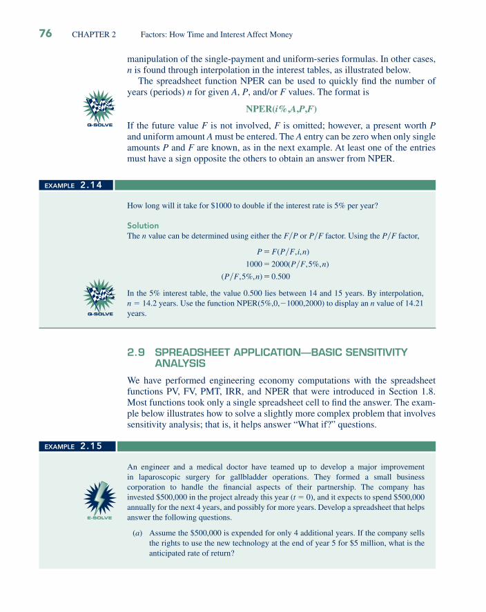
How long will it take for $1000 to double if the interest rate is 5% per year?

SolutionThe n value can be determined using either the F�P or P�F factor. Using the P�F factor,

P F P F i n

P F n

P F n

�

�

�

( , , )

( , %, )

( , %, ) .

��

�1000 2000 5

5 0 500

In the 5% interest table, the value 0.500 lies between 14 and 15 years. By interpolation, n � 14.2 years. Use the function NPER(5%,0,�1000,2000) to display an n value of 14.21 years.

EXAMPLE 2.14

Q-SOLVE

An engineer and a medical doctor have teamed up to develop a major improvementin lap aro scopic surgery for gallbladder operations. They formed a small businesscorporation to handle the fi nancial aspects of their partnership. The company hasinvested $500,000 in the project already this year (t � 0), and it expects to spend $500,000 annually for the next 4 years, and possibly for more years. Develop a spreadsheet that helps answer the following questions.

(a) Assume the $500,000 is expended for only 4 additional years. If the company sells the rights to use the new technology at the end of year 5 for $5 million, what is the anticipated rate of return?

EXAMPLE 2.15

E-SOLVE


(b) The engineer and doctor estimate that they will need $500,000 per year for more than 4 additional years. How many years from now do they have to fi nish their development work and receive the $5 million licence fee to make at least 10% per year? Assume the $500,000 per year is expended through the year immediately prior to the receipt for the $5 million.

Solution by ComputerFigure 2–22 presents the spreadsheet, with all fi nancial values in $1000 units. The IRR function is used throughout.

(a) The function IRR(B6:B11) in cell B15 displays i � 24.07%. Note there is a cash fl ow of $�500 in year 0. The equivalence statement is: Spending $500,000 now and $500,000 each year for 4 more years is equivalent to receiving $5 million at the end of year 5, when the interest rate is 24.07% per year.

(b) Find the rate of return for an increasing number of years that the $500 is expended. Columns C and D in Figure 2–22 present the results of IRR functions with the $5000 cash fl ow in different years. Cells C15 and D15 show returns on opposite sides of 10%. Therefore, the $5 million must be received some time prior to the end of year 7 to make more than the 8.93% shown in cell D15. The engineer and doctor have less than 6 years to complete their development work.

�IRR(C6:C12)�IRR(B6:B11) �IRR(D6:D13)

Figure 2–22Spreadsheet solution including sensitivity analysis, Example 2.15.

SECTION 2.9 Spreadsheet Application—Basic Sensitivity Analysis 77

ADDITIONAL EXAMPLE


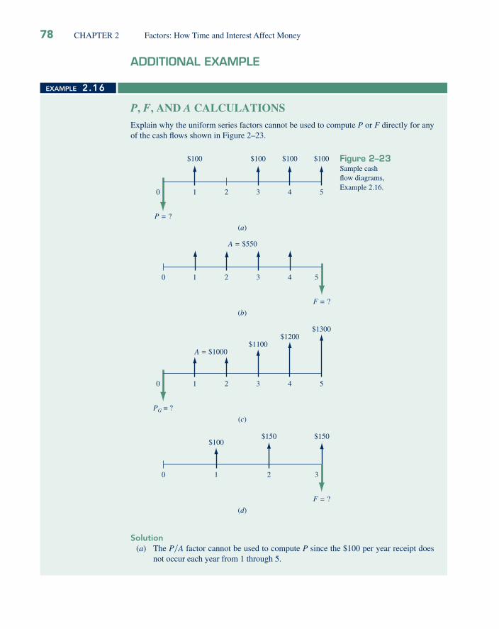
P, F, AND A CALCULATIONSExplain why the uniform series factors cannot be used to compute P or F directly for any of the cash fl ows shown in Figure 2–23.

0

P = ?

(a)

1 2 3 4 5

$100 $100 $100 $100

F = ?

(b)

10 2 3 4 5

A = $550

0

PG = ?

(c)

1 2 3 4 5

A = $1000

F = ?

(d)

10 2 3

$100$150 $150

$1100$1200

$1300

Solution(a) The P�A factor cannot be used to compute P since the $100 per year receipt does

not occur each year from 1 through 5.

EXAMPLE 2.16

Figure 2–23Sample cashfl ow diagrams,Example 2.16.

CHAPTER SUMMARYFormulas and factors derived and applied in this chapter perform equivalence calculations for present, future, annual, and gradient cash fl ows. Capability in using these formulas and their standard notation manually and with spreadsheets is critical to complete an engineering economy study. Using these formulas and spreadsheet functions, you can convert single cash fl ows into uniform cash fl ows, gradients into present worths, and much more. You can solve for rate of return i or time n. A thorough understanding of how to manipulate cash fl ows using the material in this chapter will help you address fi nancial questions in professional practice as well as in everyday living.

PROBLEMS 79

Use of Interest Tables

2.1 Find the correct numerical value for the following factors from the interest tables.

1. (F�P,8%,25) 2. (P�A,3%,8) 3. (P�G,9%,20) 4. (F�A,15%,18) 5. (A�P,30%,15)

Determination of F, P, and A

2.2 The Canadian military is considering the purchase of a new helicopter for peace-keeping operations. A similar helicopter was purchased 4 years ago at a cost of $140,000. At an interest rate of 7% per year, what would be the equivalent value today of that $140,000 expenditure?

2.3 Pressure Systems, Inc., manufactures high-accuracy liquid-level transducers. It is in-vestigating whether it should update certain equipment now or wait to do it later. If the cost now is $200,000, what will the equiv-alent amount be 3 years from now at an interest rate of 10% per year?

2.4 Petroleum Products, Inc., is a pipeline company that provides petroleum products to wholesalers in Canada and the northern United States. The company is considering purchasing insertion turbine fl owmeters to allow for better monitoring of pipelineintegrity. If these meters would prevent one major disruption (through early detection of product loss) valued at $600,000 four years from now, how much could the com-

(b) Since there is no A � $550 in year 5, the F�A factor cannot be used. The relation F � 550(F�A,i,4) would furnish the future worth in year 4, not year 5.

(c) The fi rst gradient amount G � $100 occurs in year 3. Use of the relationPG � 100(P�G,i%,4) will compute PG in year 1, not year 0. (The present worth of the base amount of $1000 is not included here.)

(d) The receipt values are unequal; thus the relation F � A(F�A,i,3) cannot be used to compute F.

PROBLEMS


pany afford to spend now at an interest rate of 12% per year?

2.5 Sensotech Inc., a maker of microelectro-mechanical systems, believes it can reduce product recalls by 10% if it purchases new software for detecting faulty parts. The cost of the new software is $225,000.(a) How much would the company have to save each year for 4 years to recover its investment if it uses a minimum attractive rate of return of 15% per year? (b) What was the cost of recalls per year before the software was purchased if the company did exactly recover its investment in 4 years from the 10% reduction?

2.6 Thompson Mechanical Products is plan-ning to set aside $150,000 now for possi-bly replacing its large synchronous refi ner motors whenever it becomes necessary. If the replacement isn’t needed for 7 years, how much will the company have in itsinvestment set-aside account if it achieves a rate of return of 18% per year?

2.7 French car maker Renault signed a $75 million contract with ABB of Zurich, Switzerland, for automated underbody assembly lines, body assembly work-shops, and line control systems. If ABB will be paid in 2 years (when the systems are ready), what is the present worth of the contract at 18% per year interest?

2.8 Atlas Long-Haul Transportation is con-sidering installing Valutemp temperature loggers in all of its refrigerated trucks for monitoring temperatures during transit. If the systems will reduce insurance claims by $100,000 two years from now, how much should the company be willing to spend now if it uses an interest rate of 12% per year?

2.9 GE Marine Systems is planning to supply a Japanese shipbuilder with aero-derivative

gas turbines to power 11 DD-class destroy-ers for the Japanese Self-Defense Force. The buyer can pay the total contract price of $1,700,000 now or an equivalent amount 1 year from now (when the tur-bines will be needed). At an interest rate of 18% per year, what is the equivalent future amount?

2.10 What is the present worth of a future cost of $162,000 to Digitech, Inc., 6 years from now at an interest rate of 12% per year?

2.11 How much could Cryogenics Inc., a maker of superconducting magnetic energy stor-age systems, afford to spend now on new equipment in lieu of spending $125,000 fi ve years from now if the company’s rate of return is 14% per year?

2.12 V-Tek Systems is a manufacturer of verti-cal compactors, and it is examining its cash fl ow requirements for the next 5 years. The company expects to replace offi ce machines and computer equipment at various times over the 5-year planning period. Specifi -cally, the company expects to spend $9000 two years from now, $8000 three years from now, and $5000 fi ve years from now. What is the present worth of the planned expendi-tures at an interest rate of 10% per year?

2.13 A manufacturer of toilet fl ush valves wants to have $2,800,000 available 10 years from now so that a new product line can be initiated. If the company plans to deposit money each year, starting 1 year from now, how much will it have to deposit each year at 6% per year interest in order to have the $2,800,000 available immediately after the last deposit is made?

2.14 The current cost of liability insurance for a certain consulting fi rm is $65,000. If the insurance cost is expected to increase by 4% each year, what will be the cost 5 years from now?

PROBLEMS 81

2.15 Grand Bay Gas Products manufactures a device that empties the contents of old aerosol cans in 2 to 3 seconds. This elimi-nates having to dispose of the cans as haz-ardous wastes. If a certain paint company can save $75,000 per year in waste dis-posal costs, how much could the company afford to spend now on the device if it wants to recover its investment in 3 years at an interest rate of 20% per year?

2.16 Atlantic Metals and Plastic uses austenitic nickel-chromium alloys to manufacture resistance heating wire. The company is considering a new annealing-drawing process to reduce costs. If the new pro-cess will cost $1.8 million now, how much must be saved each year to recover the investment in 6 years at an interest rate of 12% per year?

2.17 A green algae, Chlamydomonas rein-hardtii, can produce hydrogen when temporarily deprived of sulfur for up to 2 days at a time. A small company needs to purchase equipment costing $3.4 mil-lion to commercialize the process. If the company wants to earn a rate of return of 20% per year and recover its investments in 8 years, what must be the net value of the hydrogen produced each year?

2.18 How much money could RTT Environ-mental Services borrow to fi nance a site reclamation project if it expects revenues of $280,000 per year over a 5-year cleanup period? Expenses associated with the proj-ect are expected to be $90,000 per year. Assume the interest rate is 10% per year.

2.19 Edmonton Playland and Aquatics Park spends $75,000 each year in consulting services for ride inspection. New actua-tor element technology enables engineers to simulate complex computer-controlled movements in any direction. How much could the amusement park afford to spend

now on the new technology if the an-nual consulting services will no longer be needed? Assume the park uses an interest rate of 15% per year and it wants to re-cover its investment in 5 years.

2.20 Under an agreement with the Internet Service Providers (ISPs) Association, SBC Communications reduced the price it charges ISPs to resell its high-speed digital subscriber line (DSL) service from $458 to $360 per year per customer line. A particular ISP, which has 20,000 customers, plans to pass 90% of the sav-ings along to its customers. What is the total future worth of these savings over a 5-year horizon at an interest rate of 8% per year?

2.21 A civil engineer deposits $10,000 per year into a retirement account that achieves a rate of return of 12% per year. Determine the amount of money in the account at the end of 25 years.

2.22 A recent engineering graduate was given a raise (beginning in year 1) of $2000. At an interest rate of 8% per year, what is the present value of the $2000 per year over her expected 35-year career?

2.23 Ontario Moving and Storage wants to have enough money to purchase a new trac-tor-trailer in 3 years. If the unit will cost $250,000, how much should the company set aside each year if the account earns 9% per year?

2.24 Vision Technologies, Inc., is a small com-pany that uses ultra-wideband technology to develop devices that can detect objects (including people) inside buildings, be-hind walls, or below ground. The company expects to spend $100,000 per year for labour and $125,000 per year for supplies before a product can be marketed. At an interest rate of 15% per year, what is the


total equivalent future amount of the com-pany’s expenses at the end of 3 years?

Factor Values

2.25 Find the numerical value of the following factors by (a) interpolation and (b) using the appropriate formula.

1. (P�F,18%,33) 2. (A�G,12%,54)

2.26 Find the numerical value of the following factors by (a) interpolation and (b) using the appropriate formula.

1. (F�A,19%,20) 2. (P�A,26%,15)

Arithmetic Gradient

2.27 A cash fl ow sequence starts in year 1 at $3000 and decreases by $200 each year through year 10. (a) Determine the value of the gradient G; (b) determine the amount of cash fl ow in year 8; and (c) determine the value of n for the gradient.

2.28 Manulife expects sales to be described by the cash fl ow sequence (6000 � 5k), where k is in years and cash fl ow is in millions. Determine (a) the value of the gradient G; (b) the amount of cash fl ow in year 6; and (c) the value of n for the gradi-ent if the cash fl ow ends in year 12.

2.29 For the cash fl ow sequence that starts in year 1 and is described by 900 � 100k, where k represents years 1 through 5, (a) determine the value of the gradient G and (b) determine the cash fl ow in year 5.

2.30 Omega Instruments has budgeted $300,000 per year to pay for certain ceramic parts over the next 5 years. If the company expects the cost of the parts to increase uniformly according to an arith-metic gradient of $10,000 per year, what is

it expecting the cost to be in year 1, if the interest rate is 10% per year?

2.31 Petro-Canada expects receipts from a group of stripper wells (wells that pro-duce less than 10 barrels per day) to de-cline according to an arithmetic gradient of $50,000 per year. This year’s receipts are expected to be $280,000 (i.e., end of year 1), and the company expects the use-ful life of the wells to be 5 years. (a) What is the amount of the cash fl ow in year 3, and (b) what is the equivalent uniform annual worth in years 1 through 5 of the income from the wells at an interest rate of 12% per year?

2.32 Income from cardboard recycling at Moose Jaw has been increasing at a constant rate of $1000 in each of the last 3 years. If this year’s income (i.e., end of year 1) is expected to be $4000 and the increased income trend continues through year 5, (a) what will the income be 3 years from now (i.e., end of year 3) and (b) what is the present worth of the income over that 5-year period at an interest rate of 10% per year?

2.33 Amazon is considering purchasing a sophisticated computer system to “cube” a book’s dimensions—measure its height, length, and width so that the proper box size will be used for shipment. This will save packing material, cardboard, and labour. If the savings will be $150,000 the fi rst year, $160,000 the second year, and amounts increasing by $10,000 each year for 8 years, what is the present worth of the system at an interest rate of 15% per year?

2.34 West Coast Marine and RV is considering replacing its wired pendant controllers on its heavy-duty cranes with new portable infrared keypad controllers. The company expects to achieve cost savings of $14,000 the fi rst year and amounts increasing by

PROBLEMS 83

$1500 each year thereafter for the next 4 years. At an interest rate of 12% per year, what is the equivalent annual worth of the savings?

2.35 Ford Motor Company was able to reduce by 80% the cost required for installing data acquisition instrumentation on test vehicles by using MTS-developed spin-ning wheel force transducers. (a) If this year’s cost (i.e., end of year 1) is expected to be $2000, what was the cost the year before installation of the transducers? (b) If the costs are expected to increase by $250 each year for the next 4 years (i.e., through year 5), what is the equivalent an-nual worth of the costs (years 1 through 5) at an interest rate of 18% per year?

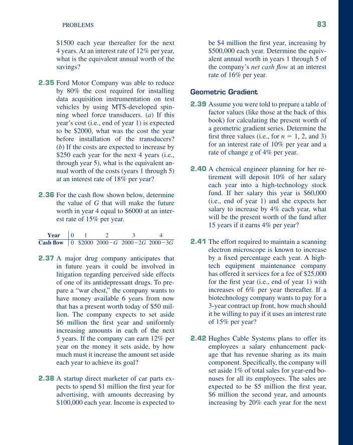
2.36 For the cash fl ow shown below, determine the value of G that will make the future worth in year 4 equal to $6000 at an inter-est rate of 15% per year.

Year 0 1 2 3 4Cash fl ow 0 $2000 2000�G 2000�2G 2000�3G

2.37 A major drug company anticipates that in future years it could be involved in litigation regarding perceived side effects of one of its antidepressant drugs. To pre-pare a “war chest,” the company wants to have money available 6 years from now that has a present worth today of $50 mil-lion. The company expects to set aside $6 million the fi rst year and uniformly increasing amounts in each of the next 5 years. If the company can earn 12% per year on the money it sets aside, by how much must it increase the amount set aside each year to achieve its goal?

2.38 A startup direct marketer of car parts ex-pects to spend $1 million the fi rst year for advertising, with amounts decreasing by $100,000 each year. Income is expected to

be $4 million the fi rst year, increasing by $500,000 each year. Determine the equiv-alent annual worth in years 1 through 5 of the company’s net cash fl ow at an interest rate of 16% per year.

Geometric Gradient

2.39 Assume you were told to prepare a table of factor values (like those at the back of this book) for calculating the present worth of a geometric gradient series. Determine the fi rst three values (i.e., for n � 1, 2, and 3) for an interest rate of 10% per year and a rate of change g of 4% per year.

2.40 A chemical engineer planning for her re-tirement will deposit 10% of her salary each year into a high-technology stock fund. If her salary this year is $60,000 (i.e., end of year 1) and she expects her salary to increase by 4% each year, what will be the present worth of the fund after 15 years if it earns 4% per year?

2.41 The effort required to maintain a scanning electron microscope is known to increase by a fi xed percentage each year. A high-tech equipment maintenance company has offered it services for a fee of $25,000 for the fi rst year (i.e., end of year 1) with increases of 6% per year thereafter. If a biotechnology company wants to pay for a 3-year contract up front, how much should it be willing to pay if it uses an interest rate of 15% per year?

2.42 Hughes Cable Systems plans to offer its employees a salary enhancement pack-age that has revenue sharing as its main component. Specifi cally, the company will set aside 1% of total sales for year-end bo-nuses for all its employees. The sales are expected to be $5 million the fi rst year, $6 million the second year, and amounts increasing by 20% each year for the next


5 years. At an interest rate of 10% per year, what is the equivalent annual worth in years 1 through 5 of the bonus package?

2.43 Determine how much money would be in a savings account that started with a deposit of $2000 in year 1 with each succeeding amount increasing by 10% per year. Use an interest rate of 15% per year and a 7-year period.

2.44 The future worth in year 10 of a geomet-ric gradient series of cash fl ows was found to be $80,000. If the interest rate was 15% per year and the annual rate of in-crease was 9% per year, what was the cash fl ow amount in year 1?

2.45 Frederiction Furniture Industries offers several types of high-performance fabrics that are capable of withstanding chemi-cals as harsh as chlorine. A certain New Brunswick manufacturing company that uses fabric in several products has a report showing that the present worth of fabric purchases over a certain 5-year period was $900,000. If the costs were known to geo-metrically increase by 5% per year during that time and the company used an interest rate of 15% per year for investments, what was the cost of the fabric in year 2?

2.46 Find the present worth of a series of investments that starts at $1000 in year 1 and increases by 10% per year for 20 years. Assume the interest rate is 10% per year.

2.47 A Windsor consulting fi rm wants to start saving money for replacement of net-work servers. If the company invests $3000 at the end of year 1 and increases the amount invested by 5% each year, how much will be in the account 4 years from now if it earns interest at a rate of 8% per year?

2.48 A company that manufactures purgable hydrogen sulfi de monitors is planning to make deposits such that each one is 5% larger than the preceding one. How large must the fi rst deposit be (at the end of year 1) if the deposits extend through year 10 and the fourth deposit is $1250? Use an interest rate of 10% per year.

Interest Rate and Rate of Return

2.49 What compound interest rate per year is equivalent to a 12% per year simple inter-est rate over a 15-year period?

2.50 A publicly traded consulting engineering fi rm pays a bonus to each engineer at the end of the year based on the company’s profi t for that year. If the company’s initial investment was $1.2 million, what rate of return has it made on its investment if each engineer’s bonus has been $3000 per year for the past 10 years? Assume the com-pany has six engineers and that the bonus money represents 5% of the company’s profi t.

2.51 Danson Iron Works, Inc., manufactures angular contact ball bearings for pumps that operate in harsh environments. If the company invested $2.4 million in a pro-cess that resulted in profi ts of $760,000 per year for 5 years, what rate of return did the company make on its investment?

2.52 An investment of $600,000 increased to $1,000,000 over a 5-year period. What was the rate of return on the investment?

2.53 A small company that specializes in powder coating expanded its building and purchased a new oven that is large enough to handle automobile frames. The building and oven cost $125,000, but new business from hot-rodders has increased annual

PROBLEMS 85

income by $520,000. If operating expenses for gas, materials, labour, etc., amount to $470,000 per year, what rate of return will be made on the investment if only the cash fl ows that occur over the next 4 years are included in the calculation?

2.54 The business plan for a startup company that manufactures multigas portable de-tectors showed equivalent annual cash fl ows of $400,000 for the fi rst 5 years. If the cash fl ow in year 1 was $320,000 and the increase thereafter was $50,000 per year, what interest rate was used in the calculation?

2.55 A new company that makes medium- voltage soft starters spent $85,000 to build a new website. Net income was $60,000 the fi rst year, increasing by $15,000 each year. What rate of return did the company make in its fi rst 5 years?

Number of Years

2.56 A company that manufactures plastic control valves has a fund for equipment replacement that contains $500,000. If the company spends $75,000 per year on new equipment, how many years will it take to reduce the fund to less than $75,000 at an interest rate of 10% per year?

2.57 An engineering consulting fi rm is consid-ering purchasing the building it currently occupies under a long-term lease because the owner of the building suddenly put it up for sale. The building is being offered at a price of $170,000. Since the lease is already paid for this year, the next annual lease payment of $30,000 isn’t due until the end of this year. Because the fi rm has been a good tenant, the owner has offered to sell to them for $160,000. If the fi rm purchases the building with no down payment, how long will it be before the

company recovers its investment at an interest rate of 12% per year?

2.58 An engineer who invested very well plans to retire now because she has $2,000,000 in her retirement account. How long will she be able to withdraw $100,000 per year (beginning 1 year from now) if her account earns interest at a rate of 4% per year?

2.59 A company that manufactures ultra-sonic wind sensors invested $1.5 million 2 years ago to acquire part ownership in an innovative chip-making company. How long would it take (from the date of the initial investment) for its share of the chip company to be worth $3 million if that company is growing at a rate of 20% per year?

2.60 Roger Lareveur owns a mutual fund that has averaged an 18% annual rate of re-turn since he bought it two years ago with $100,000. In the unlikely event that these stellar results should continue, how long will it be (from the time he started) before he can retire with $1.6 million?

2.61 How many years will it take for a uniform annual deposit of size A to accumulate to 10 times the size of a single deposit if the rate of return is 10% per year?

2.62 How many years would it take for an investment of $10,000 in year 1 with in-creases of 10% per year to have a present worth of $1,000,000 at an interest rate of 7% per year?

2.63 You were told that a certain cash fl ow sequence started at $3000 in year 1 and increased by $2000 each year. How many years were required for the equivalent annual worth of the sequence to be $12,000 at an interest rate of 10% per year?


Stock Option Program Purchase

A young B.Eng. graduate from the Dalhousie Faculty of Engineering went to work for a microelectronics com-pany at the age of 22 and placed $50 per month into the stock purchase option. He left the company after a full 60 months of employment at age 27, and he did not sell the stock. The engineer did not inquire about the value of the stock until age 57, some 30 years later.

1. Construct the cash fl ow diagram for ages 22 through 57.

2. The engineer has learned that over the 35 interven-ing years, the stock earned at a rate of 1.25% per month. Determine the value of the $50 per month when the engineer left the company after a total of 60 purchases.

3. Determine the value of the engineer’s company stock at age 57. Again, observe the signifi cant dif-ference that 30 years have made at a 15% per year compound rate.

4. Assume the engineer did not leave the funds in-vested in the stock at age 27. Now determine the amount he would have to deposit each year, start-ing at age 50, to be equivalent to the value at age 57 you calculated in (3) above. Assume the 7 years of deposits make a return of 15% per year.

5. Finally, compare the total amount of money depos-ited during the 5 years when the engineer was in his twenties with the total amount he would have to deposit during the 7 years in his fi fties to have the equal and equivalent amount at age 57, as de-termined in (3) above.

CASE STUDY

WHAT A DIFFERENCE THE YEARS AND COMPOUND INTEREST CAN MAKE

bla6310X_chapter2

Documents

cash ow diagram

capital recovery factor

cash ow series

interest affect money

cash ow sequence

engineering economy relation

pv function pv

engineering economy factors