Bivariate Density Classification by the Geometry of the Marginals

c© Heldermann Verlag Economic Quality ControlISSN 0940-5151 Vol 22 (2007), No. 1, 3 – 18

Bivariate Density Classification by the

Geometry of the Marginals

Mariela Fernandez and Nikolai Kolev

Abstract: In this work we propose a representation of a bivariate density corresponding tothe given geometrical behavior of the marginals. A continuous density with compact supportcan be approximated by the exponential of an infinite polynomial. We find intervals for thepossible values of its coefficients in the simplest cases upon the available information aboutthe marginals.

Keywords:Bivariate density, Marginal behavior, Stone-Weierstrass approximation.

1 Introduction

In any applied statistical analysis, one needs to model the probability distribution ofhigh-dimensional random variables. Usually, one is more familiar with the marginal dis-tributions, while the dependence structure remains unknown. Practitioners, therefore,often implement marginal models and use them for the analysis of more complex multi-variate models assuming independence or some standardized dependencies. In this paperwe propose to find possible forms of a two-dimensional density, using the knowledge aboutthe marginals. The need to construct multivariate distributions with given univariate mar-ginals arises quite often, see von Collani [1]. The importance of the topic in research andpractice is reflected by the fact that a special series of conferences named “MultivariateDistributions with Given Marginals” have being organized in Rome (1990), Seattle (1993),Prague (1996), Barcelona (2000), Quebec (2004) and Tartu (2007), see Cuadras et al. [2]for a history. In this context, one should also mention Kotz and van Dorp’s study [3] onthe Fairlie-Gumbel-Morgenstern family, considering the marginals from two-sided powerdistributions. Here, we suggest a bivariate density classification corresponding to increas-ing or/and decreasing marginal behavior (most frequently observed practical situations).

By Stone-Weierstrass’ theorem, e.g. Rudin [4], a continuous density with a compactsupport can be represented as follows

h(x, y) = e

∞�

i,j=0λijxiyj

(1)

where λij (i, j = 0, 1, · · ·) are real coefficients. Using the last relation, and taking intoaccount the knowledge of the geometrical behavior of the marginals (e.g. increasing,decreasing or unimodal functions), we derive the set of possible joint density functions

https://www.researchgate.net/publication/24083344_A_versatile_bivariate_distribution_on_a_bounded_domain_Another_look_at_the_product_moment_correlation?el=1_x_8&enrichId=rgreq-cdcd8032b41a39eef9e61127c37b39fd&enrichSource=Y292ZXJQYWdlOzI1NTYzMzI1MDtBUzoxODYzMzYwMDY5MDk5NTJAMTQyMTQzNzM3NDc4Nw==

https://www.researchgate.net/publication/268617174_Defining_the_Science_of_Stochastics?el=1_x_8&enrichId=rgreq-cdcd8032b41a39eef9e61127c37b39fd&enrichSource=Y292ZXJQYWdlOzI1NTYzMzI1MDtBUzoxODYzMzYwMDY5MDk5NTJAMTQyMTQzNzM3NDc4Nw==

4 Mariela Fernandez and Nikolai Kolev

h(x, y). Specifically, we will consider the simple case when the joint bivariate densityh(x, y) can be approximatted by

h(x, y) ≈ eλ0+λ10x+λ01y+λ11xy+λ21x2y for (x, y) ∈ [a, b] × [a, b] (2)

Based on the information given about the geometrical nature of the marginals, we deter-mine sets (intervals) of possible values of the parameters λ10, λ01, λ11 and λ21 (λ0 is just anormalizing constant). In particular, we find sets for the possible values of the parametersλ10, λ01, λ11 and λ21 corresponding to the specified marginals (e.g. both being increasing,one marginal being increasing and the other one decreasing, both being decreasing, etc.).

We use the following notations for the marginals

fx(x) =∫ b

ah(x, y)dy

and

gy(y) =∫ b

ah(x, y)dx

(3)

In the remainder the following notations are used:

• f cx and gc

y, for constant marginals;

• f ix and gi

y, for increasing marginals;

• fdx and gd

y , for decreasing marginals;

• fmx and gm

y , for marginals with a minimum.

In Sections 2 and 3 we consider the approximation (2) with λ21 = 0 and with λ21 �= 0,respectively. Several conclusions are given at the end.

2 The Case λ21 = 0

In this section the following approximation is considered:

h(x, y) ≈ eλ0+λ10x+λ01y+λ11xy for (x, y) ∈ [a, b] × [a, b] (4)

If additionally λ11 = 0, then the sets of possible values of the parameters λ10 and λ01 areeasily found depending on the geometrical nature of the marginals. For this simple case,our findings for the different types of marginal densities are summarized in Table 1.

gcy gi

y gdy

f cx λ10 = 0 and λ01 = 0 λ10 = 0 and λ01 > 0 λ10 = 0 and λ01 < 0f i

x λ10 > 0 and λ01 = 0 λ10>0 and λ01>0 λ10 > 0 and λ01 < 0fd

x λ10 < 0 and λ01 = 0 λ10 < 0 and λ01 > 0 λ10 < 0 and λ01 < 0

Table 1: Conditions on the coefficients λ10 and λ01 for h(x, y) = eλ0+λ10x+λ01y

Bivariate Density Classification by the Geometry of the Marginals 5

For example, for the case of increasing marginals, i.e. f ix and gi

y, the possible values forthe parameters are λ10 > 0 and λ01 > 0.

Next, let λ11 �= 0 and −∞ < a < b <∞. Then:

h(x, y) = eλ0+λ10x+λ01y+λ11xy for (x, y) ∈ [a, b] × [a, b] (5)

and

fx(x) =

{eλ0+λ10xe(λ01+λ11x)a

(e(λ01+λ11x)(b−a)−1

λ01+λ11x

)for λ01 + λ11x �= 0

eλ0+λ10x(b− a) for λ01 + λ11x = 0(6)

gy(y) =

{eλ0+λ01ye(λ10+λ11y)a

(e(λ10+λ11y)(b−a)−1

λ10+λ11y

)for λ10 + λ11y �= 0

eλ0+λ01y(b− a) for λ10 + λ11y = 0.(7)

We are interested in the sign of the derivatives of fx(x) and gy(y), which can be studiedby using the functions:

ψλ10(x)def=

{(b−a)e(λ10+λ11x)(b−a)

e(λ10+λ11x)(b−a)−1− 1

λ10+λ11xfor x �= −λ10

λ11b−a2

for x = −λ10

λ11

(8)

and

ψλ01(x)def=

{(b−a)e(λ01+λ11x)(b−a)

e(λ01+λ11x)(b−a)−1− 1

λ01+λ11xfor x �= −λ01

λ11b−a2

for x = −λ01

λ11.

(9)

The continuous functions ψλ10 and ψλ01 are increasing, if λ11 > 0, and decreasing, ifλ11 < 0. Moreover, it can be shown that ψλ10 and ψλ01 are bounded. For x ∈ (−∞,∞)we obtain:

0 < ψλ10(x) and ψλ01(x) < b− a (10)

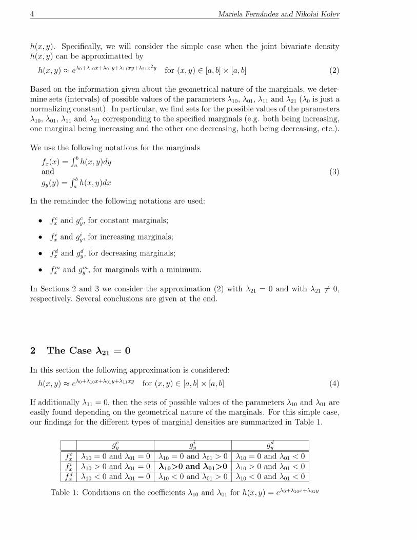
Using these functions in the expressions of the derivatives of the marginals we get theconditions given in Table 2. For instance, it can be seen that in the case (fd

x , giy) with

resepect to the marginals, the parameters λ10, λ01 and λ11 satisfy the following inequalities(where sgn(a) denotes the sign of a):

sgn(λ11)ψλ01(b) ≤−λ10 − aλ11

|λ11| and sgn(λ11)ψλ10(a) ≥−λ01 − aλ11

|λ11| (11)

giy gd

y

sgn(λ11)ψλ01(a) ≥ −λ10−aλ11

|λ11| sgn(λ11)ψλ01(a) ≥ −λ10−aλ11

|λ11|f i

x and andsgn(λ11)ψλ10(a) ≥ −λ01−aλ11

|λ11| sgn(λ11)ψλ10(b) ≤ −λ01−aλ11

|λ11|sgn(λ11)ψλ01(b)≤−λ10−aλ11

|λ11| sgn(λ11)ψλ01(b) ≤ −λ10−aλ11

|λ11|fd

x and andsgn(λ11)ψλ10(a)≥−λ01−aλ11

|λ11| sgn(λ11)ψλ10(b) ≤ −λ01−aλ11

|λ11|

Table 2: Conditions on λ10, λ01 and λ11 for (fdx , g

iy) with h(x, y) = eλ0+λ10x+λ01y+λ11xy.


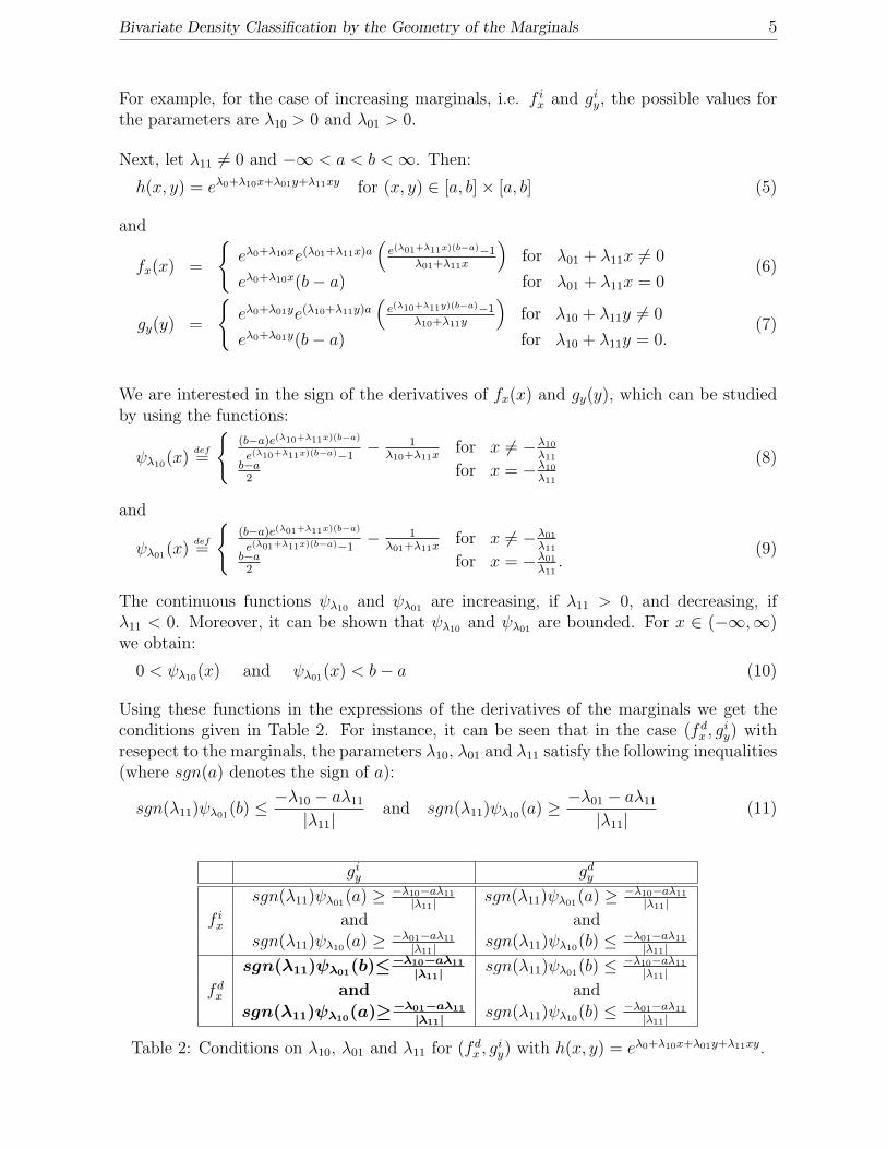
In fact, the inequalities in Table 2 give the possible range of values of the parametersof the joint density (2 with λ21 = 0, given the information about monotonicity of themarginals. In Figure 1 two examples are shown for this type of representation when(x, y) ∈ [−1, 1] × [−1, 1].

Figure 1: Joint density h(x, y) = exp{λ0 + λ10x+ λ01y + λ11xy}.

-1

-0.5

0

0.5

1

x

-1

-0.5

0

0.5

1

y

0

0.2

0.4

0.6

0.8

h

-1

-0.5

0

0.5x

Figure 1a: λ0 = −2.927, λ10 = 2, λ01 = 2 and λ11 = 1.

-1

-0.5

0

0.5

1

x

-1

-0.5

0

0.5

1

y

0

0.2

0.4

0.6

0.8

h

-1

-0.5

0

0.5x

Figure 1b: λ0 = −2.927, λ10 = 2 λ01 = −2 and λ11 = −1.

Figure 1a displays a joint density with both marginals being increasing. It is easily verifiedthat the necessary inequalities from Table 2 are satisfied:


ψλ01(−1) = 1.31 ≥ −λ10+λ11

λ11= −1

ψλ10(−1) = 1.31 ≥ −λ01+λ11

λ11= −1

(12)

Figure 1b displays the joint density with fx being increasing and gy being decreasing.Again, the inequalities given in Table 2 are satisfied again, i.e.:

−ψλ01(−1) = −0.68 ≥ −λ10+λ11

|λ11| = −3

−ψλ10(1) = −1.31 ≤ −λ01+λ11

|λ11| = 1(13)

For both cases λ0 = −2.927 holds, which is computed such that h(x, y) has a total massequal to 1.

In the rest of this section we will assume λ11 to be fixed. Using the relation (10 and theinequalities given in Table 2, one can verify the conditions on the coefficients λij for themonotonicity of the marginals listed in the following statement.

Proposition 1 Let λ11 be fixed and −∞ < a < b <∞.

1. If λ11 > 0 and λ10 and λ01 are such that

(a) −aλ11 ≤ λ10 and −aλ11 ≤ λ01, then both marginals are increasing functions;

(b) −aλ11 ≤ λ10 and −bλ11 ≥ λ01, then the marginal fx is increasing and gy isdecreasing;

(c) −bλ11 ≥ λ10 and −aλ11 ≤ λ01, then the marginal fx is decreasing and gy isincreasing;

(d) −bλ11 ≥ λ10 and −bλ11 ≥ λ01, then both marginals are decreasing functions.

2. If λ11 < 0 and λ10 and λ01 are such that

(a) −bλ11 ≤ λ10 and −bλ11 ≤ λ01, then both marginals are increasing functions;

(b) −bλ11 ≤ λ10 and −aλ11 ≥ λ01, then the marginal fx is increasing and gy isdecreasing;

(c) −aλ11 ≥ λ10 and −bλ11 ≤ λ01, then the marginal fx is decreasing and gy isincreasing;

(d) −aλ11 ≥ λ10 and −aλ11 ≥ λ01, then both marginals are decreasing functions.

Proof. Only relation 1a is proved below. The proofs of the other relations are analogously.

Let λ11 > 0. If −aλ11 ≤ λ10 and −aλ11 ≤ λ01, then

−λ10 − aλ11

λ11

≤ 0 and−λ01 − aλ11

λ11

≤ 0 (14)

By (14) and property (10), we get

−λ10 − aλ11

λ11

< ψλ01(a) and−λ01 − aλ11

λ11

< ψλ10(a). (15)


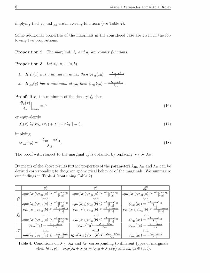
implying that fx and gy are increasing functions (see Table 2).

Some additional properties of the marginals in the considered case are given in the fol-lowing two propositions.

Proposition 2 The marginals fx and gy are convex functions.

Proposition 3 Let x0, y0 ∈ (a, b).

1. If fx(x) has a minimum at x0, then ψλ01(x0) = −λ10−aλ11

λ11;

2. If gy(y) has a minimum at y0, then ψλ10(y0) = −λ01−aλ11

λ11.

Proof: If x0 is a minimum of the density fx then

dfx(x)

dx

∣∣∣x=x0

= 0 (16)

or equivalently

fx(x)[λ11ψλ01(x0) + λ10 + aλ11] = 0, (17)

implying

ψλ01(x0) =−λ10 − aλ11

λ11

. (18)

The proof with respect to the marginal gy is obtained by replacing λ10 by λ01.

By means of the above results further properties of the parameters λ10, λ01 and λ11 can bederived corresponding to the given geometrical behavior of the marginals. We summarizeour findings in Table 4 (containing Table 2).

giy gd

y gmy

sgn(λ11)ψλ01(a) ≥ −λ10−aλ11|λ11| sgn(λ11)ψλ01(a) ≥ −λ10−aλ11

|λ11| sgn(λ11)ψλ01(a) ≥ −λ10−aλ11|λ11|

f ix and and andsgn(λ11)ψλ10(a) ≥ −λ01−aλ11

|λ11| sgn(λ11)ψλ10(b) ≤ −λ01−aλ11|λ11| ψλ10(y0) = −λ01−aλ11

λ11

sgn(λ11)ψλ01(b) ≤ −λ10−aλ11|λ11| sgn(λ11)ψλ01(b) ≤ −λ10−aλ11

|λ11| sgn(λ11)ψλ01(b) ≤ −λ10−aλ11|λ11|

fdx and and andsgn(λ11)ψλ10(a) ≥ −λ01−aλ11

|λ11| sgn(λ11)ψλ10(b) ≤ −λ01−aλ11|λ11| ψλ10(y0) = −λ01−aλ11

λ11

ψλ01(x0) = −λ10−aλ11λ11

ψλ01(x0)=−λ10−aλ11

λ11ψλ01(x0) = −λ10−aλ11

λ11

fmx and and andsgn(λ11)ψλ10(a) ≥ −λ01−aλ11

|λ11| sgn(λ11)ψλ10(b)≤−λ01−aλ11

|λ11| ψλ10(y0) = −λ01−aλ11λ11

Table 4: Conditions on λ10, λ01 and λ11 corresponding to different types of marginalswhen h(x, y) = exp{λ0 + λ10x+ λ01y + λ11xy} and x0, y0 ∈ (a, b).


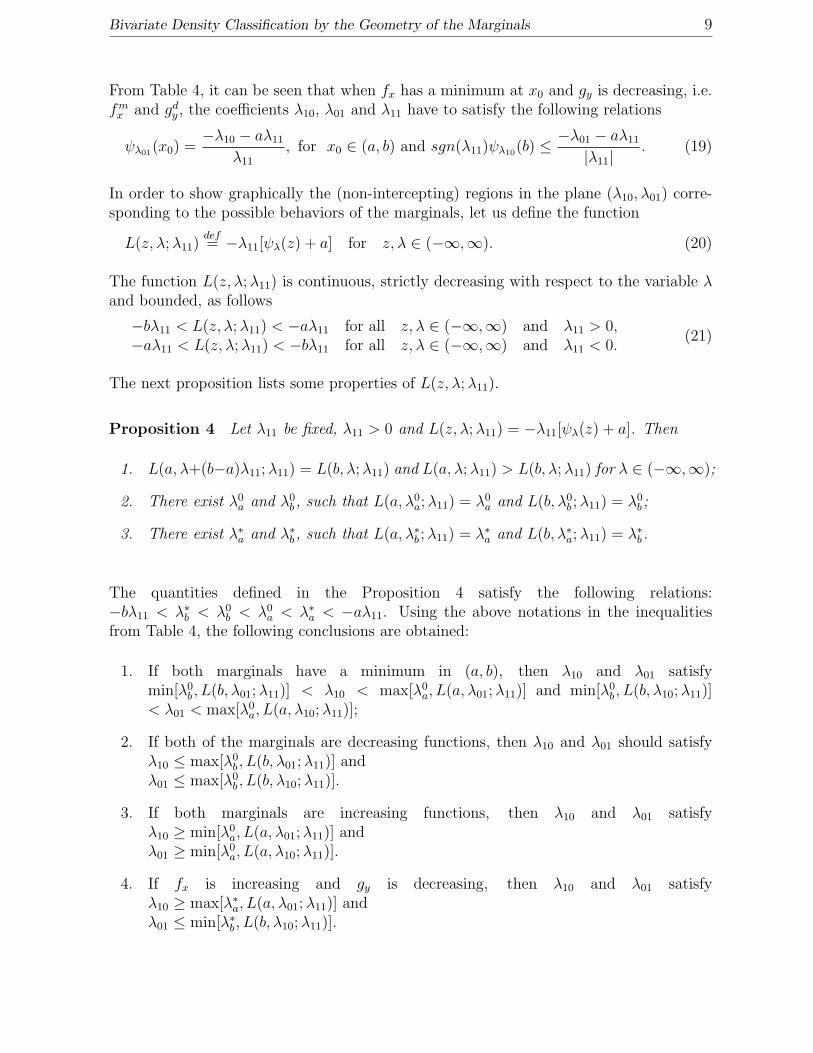
From Table 4, it can be seen that when fx has a minimum at x0 and gy is decreasing, i.e.fm

x and gdy , the coefficients λ10, λ01 and λ11 have to satisfy the following relations

ψλ01(x0) =−λ10 − aλ11

λ11

, for x0 ∈ (a, b) and sgn(λ11)ψλ10(b) ≤−λ01 − aλ11

|λ11| . (19)

In order to show graphically the (non-intercepting) regions in the plane (λ10, λ01) corre-sponding to the possible behaviors of the marginals, let us define the function

L(z, λ;λ11)def= −λ11[ψλ(z) + a] for z, λ ∈ (−∞,∞). (20)

The function L(z, λ;λ11) is continuous, strictly decreasing with respect to the variable λand bounded, as follows

−bλ11 < L(z, λ;λ11) < −aλ11 for all z, λ ∈ (−∞,∞) and λ11 > 0,−aλ11 < L(z, λ;λ11) < −bλ11 for all z, λ ∈ (−∞,∞) and λ11 < 0.

(21)

The next proposition lists some properties of L(z, λ;λ11).

Proposition 4 Let λ11 be fixed, λ11 > 0 and L(z, λ;λ11) = −λ11[ψλ(z) + a]. Then

1. L(a, λ+(b−a)λ11;λ11) = L(b, λ;λ11) and L(a, λ;λ11) > L(b, λ;λ11) for λ ∈ (−∞,∞);

2. There exist λ0a and λ0

b , such that L(a, λ0a;λ11) = λ0

a and L(b, λ0b ;λ11) = λ0

b ;

3. There exist λ∗a and λ∗b , such that L(a, λ∗b ;λ11) = λ∗a and L(b, λ∗a;λ11) = λ∗b .

The quantities defined in the Proposition 4 satisfy the following relations:−bλ11 < λ∗b < λ0

b < λ0a < λ∗a < −aλ11. Using the above notations in the inequalities

from Table 4, the following conclusions are obtained:

1. If both marginals have a minimum in (a, b), then λ10 and λ01 satisfymin[λ0

b , L(b, λ01;λ11)] < λ10 < max[λ0a, L(a, λ01;λ11)] and min[λ0

b , L(b, λ10;λ11)]< λ01 < max[λ0

a, L(a, λ10;λ11)];

2. If both of the marginals are decreasing functions, then λ10 and λ01 should satisfyλ10 ≤ max[λ0

b , L(b, λ01;λ11)] andλ01 ≤ max[λ0

b , L(b, λ10;λ11)].

3. If both marginals are increasing functions, then λ10 and λ01 satisfyλ10 ≥ min[λ0

a, L(a, λ01;λ11)] andλ01 ≥ min[λ0

a, L(a, λ10;λ11)].

4. If fx is increasing and gy is decreasing, then λ10 and λ01 satisfyλ10 ≥ max[λ∗a, L(a, λ01;λ11)] andλ01 ≤ min[λ∗b , L(b, λ10;λ11)].


5. If gy is increasing and fx is decreasing, then λ10 and λ01 satisfyλ10 ≤ min[λ∗b , L(b, λ01;λ11)] andλ01 ≥ max[λ∗a, L(a, λ10;λ11)].

6. If fx has a minimum and gy is increasing, then λ10 and λ01 satisfymin[λ∗b , L(b, λ01;λ11)] < λ10 < min[λ0

a, L(a, λ01;λ11)] andλ01 ≥ max[λ0

a, L(a, λ10;λ11)].

7. If fx has a minimum and gy is decreasing, then λ10 and λ01 satisfymax[λ0

b , L(b, λ01;λ11)] < λ10 < max[λ∗a, L(a, λ01;λ11)] andλ01 ≤ min[λ0

b , L(b, λ10;λ11)].

8. If fx is increasing and gy has a minimum, then λ10 and λ01 satisfyλ10 ≥ max[λ0

a, L(a, λ01;λ11)] andmin[λ∗b , L(b, λ10;λ11)] < λ01 < min[λ0

a, L(a, λ10;λ11)].

9. If fx is decreasing and gy has a minimum, then λ10 and λ01 satisfyλ10 ≤ min[λ0

b , L(b, λ01;λ11)] andmax[λ0

b , L(b, λ10;λ11)] < λ01 < max[λ∗a, L(a, λ10;λ11)].

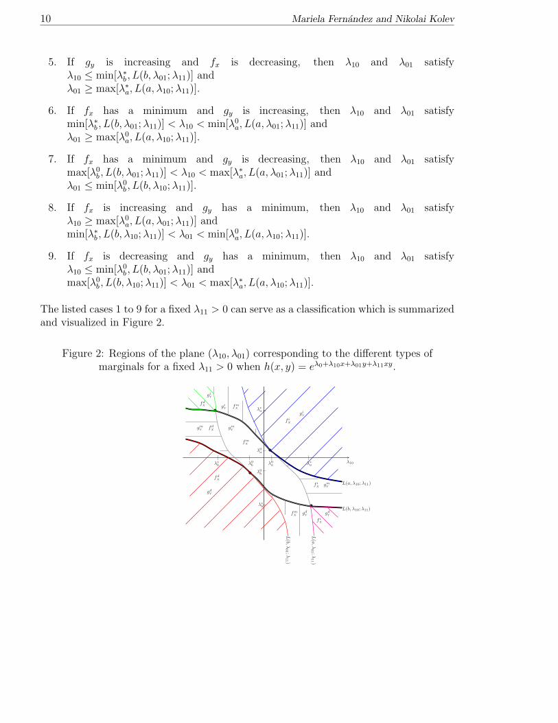
The listed cases 1 to 9 for a fixed λ11 > 0 can serve as a classification which is summarizedand visualized in Figure 2.

Figure 2: Regions of the plane (λ10, λ01) corresponding to the different types ofmarginals for a fixed λ11 > 0 when h(x, y) = eλ0+λ10x+λ01y+λ11xy.

λ10λ0a

|λ0

b

|λ∗a|

λ∗b|

λ0a−

λ0b−

λ∗a−

λ∗b−

•

•

L(a, λ10;λ11)

L(b, λ10;λ11)

•

•

L(a,λ

01 ;λ

11 )

L(b,λ

01 ;λ

11 )

fmX

gmY

fdX

gmY

f iX

gmY

fmX gd

Y

fmXgi

Y

fdX

giY

f iX

gdY

f iX

giY

fdX

gdY


If λ11 is fixed and negative, we can also get the corresponding classification of the (λ10, λ01)-plane with combinations of the three considered types of marginals. In this case, thefollowing inequalities hold:

−aλ11 < λ0b < λ∗b < λ∗a < λ0

a < −bλ11 (22)

We conclude this section with a simple example in order to show some computed valuesof λ0

a, λ0b , λ

∗a, λ

∗b , λ10 and λ01, when λ11 is fixed.

Example 1 Let a = 1, b = 2 and λ11 = 1. By means of the procedure described above,we get

λ∗a = −1.455, λ0a = −1.462, λ0

b = −1.538 and λ∗b = −1.545. (23)

Looking at Figure 2 for the computed quantities λ0a, λ

0b , λ

∗a and λ∗b , one can find the range

of the possible values of the parameters λ10 and λ01, which satisfy the given geometricalbehavior of the marginals.

If a = 1, b = 2 and λ11 = −1, we obtain

λ0a = 1.545, λ∗a = 1.538, λ∗b = 1.462 and λ0

b = 1.454. (24)

One can see that when both marginals are increasing in {x | 1 ≤ x ≤ 2}, possible valuesfor the parameters are λ11 = −1 and λ01 = 2.5 = λ10. Several additional cases are listedin Table 6 below.

fx gy λ11 λ10 λ01 λ0

fmx gm

y 1 -1.5 -1.5 2.879

fdx gi

y 1 -2 1 -1.005

fdx gd

y 1 -2 -2 3.724

f ix gi

y -1 2.5 2.5 -5.329

f ix gd

y -1 2.5 1 -3.058

Table 5: Possible values of the coefficients for different types of marginals whenh(x, y) = eλ0+λ10x+λ01y+λ11xy, (x, y) ∈ [1, 2] × [1, 2].

3 The Case λ21 �= 0

In this section we investigate the more general case considering the relation (2) withλ21 �= 0. The corresponding marginals are:

fx(x) =

eλ0+λ10x e(λ01+λ11x+λ21x2)b−e(λ01+λ11x+λ21x2)a

λ01+λ11x+λ21x2 for λ01 + λ11x+ λ21x2 �= 0

eλ0+λ10x (b− a), for λ01 + λ11x+ λ21x2 = 0

(25)


and

gy(y) = eλ0+λ01y

∫ b

a

e(λ10+λ11y)x+λ21yx2

dx. (26)

Clearly, the analysis of fx and gy will be different.

3.1 Properties of the Marginal fx

By Leibniz’s rule we have

dfx(x)

dx=

∫ b

a

h(x, y)(λ10 + λ11y + 2λ21xy)dy. (27)

The next proposition contains conditions for the increasing/decreasing nature of fx.

Proposition 5 Let Pf (x, y) = λ10 + λ11y + 2λ21xy.

1. min(x,y)∈[a,b]×[a,b]

Pf (x, y) > 0 ⇒ fx is an increasing function (28)

2. max(x,y)∈[a,b]×[a,b]

Pf (x, y) < 0 ⇒ fx is an decreasing function (29)

Proof. We prove item 1 only.

If min(x,y)∈[a,b]×[a,b] Pf (x, y) > 0, then Pf (x, y) > 0 for all (x, y) ∈ [a, b] × [a, b]. Sinceh(x, y) > 0 for all (x, y), we get:

dfx(x)

dx=

∫ b

a

h(x, y)Pf (x, y)dy > 0. (30)

Thus, fx is increasing.

As a consequence, we obtain the following statements.

Corollary 1 Let x1 = −λ11

2λ21and x2 = −λ11+2λ21(a+b)

2λ21. Then, fx is an increasing function

if one of the following conditions holds.

1. λ21 > 0, x2 ≤ a+b2

and Pf (b, a) > 0;

2. λ21 > 0, x2 >a+b2

and Pf (a, b) > 0;

3. λ21 < 0, x1 ≤ a+b2

and Pf (b, b) > 0;

4. λ21 < 0, x1 >a+b2

and Pf (a, a) > 0.

Corollary 2 Let x1 = −λ11

2λ21and x2 = −λ11+2λ21(a+b)

2λ21. Then, fx is a decreasing function

if one of the following conditions holds.


1. λ21 > 0, x1 ≤ a+b2

and Pf (b, b) < 0;

2. λ21 > 0, x1 >a+b2

and Pf (a, a) < 0;

3. λ21 < 0, x2 ≤ a+b2

and Pf (b, a) < 0;

4. λ21 < 0, x2 >a+b2

and Pf (a, b) < 0.

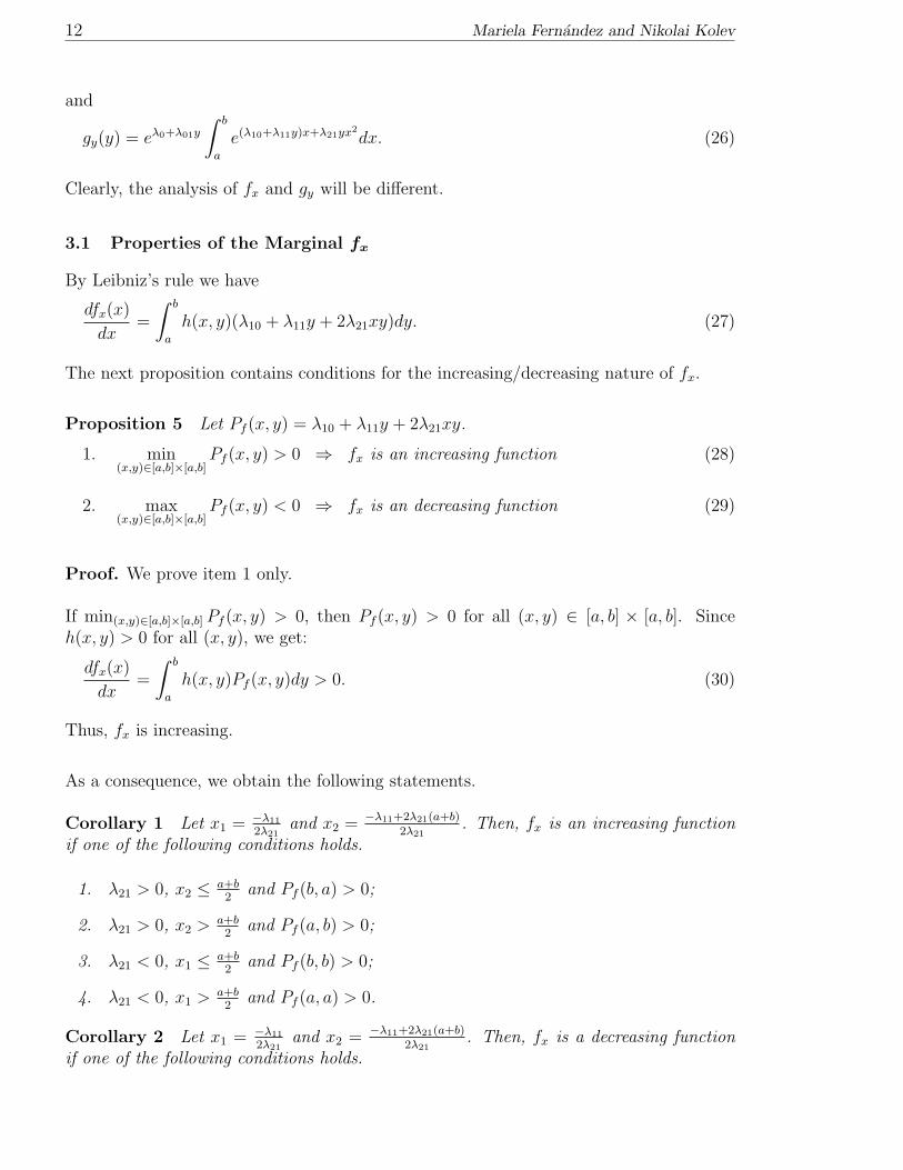
Corollaries 1 and 2 serve as a guide to find appropiate values of the coefficients λ10, λ11

and λ21. Note that the above relations do not include conditions on λ01. Table 7 containsseveral illustrative examples.

fx λ10 λ11 λ21

7 4 1f i

x 4 -1 17 -4 -1-4 1 1

fdx -4 1 -1

-4 -2 -1

Table 6: Possible values of the coefficients corresponding to increasing or decreasingmarginal fx, for (x, y) ∈ [−1, 1] × [−1, 1], when h(x, y) = eλ0+λ10x+λ01y+λ11xy+λ21x2y.

For instance, the numbers listed in the first line of Table 7 were computed using Corollary1. It means that, when fx is increasing, possible values of the coefficients are λ10 = 7,λ11 = 4 and λ21 = 1, since they satisfy the conditions

λ21 > 0,−λ11 + 2λ21(a+ b)

2λ21

≤ a+ b

2and Pf (b, a) > 0 (31)

The next three propositions show the main difference between the cases λ21 �= 0 andλ21 = 0. When λ21 �= 0, it can happen that fx has a maximum or more than one criticalpoint (a point at which the derivative is zero), which is impossible for h(x, y) with λ21 = 0(see Section 2).

Proposition 6 If λ10 = 0 and −λ11

2λ21= a+b

2, then fx is a symmetric function on [a, b].

Proposition 7 If λ10 = 0 and −λ11

2λ21∈ (a, b) then fx has a critical point at x0 = −λ11

2λ21. If

a ≥ 0, then x0 is the unique critical point of fx(x).

Proof: If λ10 = 0 and x0 = −λ11

2λ21∈ (a, b), then

dfx(x)

dx

∣∣∣x=x0

=

∫ b

a

h(x0, y)Pf (x0, y)dy

=

∫ b

a

h(x0, y)(λ11 + 2λ21x0)ydy = 0 (32)


Thus, x0 is a critical point of fx.

For proving the second part of the proposition, we compute the derivative of fx. We have

dfx(x)

dx= fx(x)

(λ11 + 2λ21x

)(Λ21(x) + a

), (33)

where

Λ21(x)def=

(b−a)e(λ01+λ11x+λ21x2)(b−a)

e(λ01+λ11x+λ21x2)(b−a)−1− 1

λ01+λ11x+λ21x2 if λ01 + λ11x+ λ21x2 �= 0

b−a2

if λ01 + λ11x+ λ21x2 = 0.

(34)

We need to prove that dfx(x)dx

�= 0 for all x �= x0. It can be done by checking that Λ21(x)+a >

0. Let us define λ10 = 0 and λ11 = 1. Thus, Λ21(x) = ψλ10(λ01 + λ11x + λ21x

2), whereψλ10

is given by (8. Relation (10 implies Λ21(x) > 0. Since a ≥ 0, then Λ21(x) + a > 0,and the derivative of fx(x) just vanishes at x = x0.

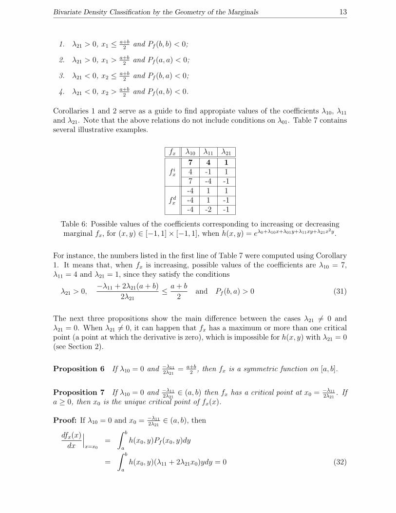
Figure 3 shows two different kinds of the marginal fx. The calculated values of λ10, λ11

and λ21 satisfy the conditions of Proposition 7, where λ01 is chosen arbitrarily.

Figure 3: Forms of the marginal fx corresponding to the joint densityh(x, y) = eλ0+λ10x+λ01y+λ11xy+λ21x2y.

-1 -0.5 0.5 1

0.7

0.75

0.8

0.85

f

Figure 3a: fx with a = −1, b = 1, λ0 = −1.055.


0.5 1 1.5 2

0.4

0.5

0.6

0.7

0.8

0.9

1

f

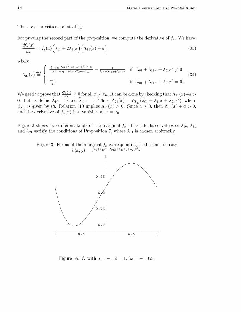
Figure 3b: λ10 = 0, λ01 = 1, λ11 = 1 and λ21 = −1.

(b) fx with a = 0, b = 2, λ0 = −1.376, λ10 = 0, λ01 = −1, λ11 = 1 and λ21 = −1.

The last two results regarding fx are related to its unimodality or convexity when λ21 > 0.

Proposition 8 If a ≥ 0, λ10 = 0, λ21 < 0 and −λ11

2λ21∈ (a, b), then fx is a unimodal

function, with mode at x0 = −λ11

2λ21.

Proposition 9 If λ21 > 0 and a ≥ 0 or if λ21 < 0 and b ≤ 0, then fx is a convexfunction.

3.2 Properties of the Marginal gy

Let gy be given by (26), where the integral has no analytical solution for y �= 0. Again,by using Leibniz’s rule we get

dgy(y)

dy=

∫ b

a

h(x, y)(λ01 + λ11x+ λ21x2)dx. (35)

The following properties of the marginal gy can be derived depending on the coefficients.

Proposition 10 Let Pg(x) = λ01 + λ11x+ λ21x2.

1. minx∈[a,b]

Pg(x) > 0 ⇒ gy is an increasing function (36)

2. maxx∈[a,b]

Pg(x) < 0 ⇒ gy is a decreasing function (37)


As an immediate consequence, we get the following two corollaries.

Corollary 3 The marginal gy is an increasing function, if one of the following conditionsholds.

1. λ21 > 0, a ≤ − λ11

2λ21≤ b and Pg(− λ11

2λ21) > 0;

2. λ21 > 0, a > − λ11

2λ21and Pg(a) > 0;

3. λ21 > 0, b < − λ11

2λ21and Pg(b) > 0;

4. λ21 < 0, − λ11

2λ21≤ a+b

2and Pg(b) > 0;

5. λ21 < 0, − λ11

2λ21> a+b

2and Pg(a) > 0.

Corollary 4 The marginal gy is a decreasing function, if one of the following conditionsholds.

1. λ21 > 0, − λ11

2λ21≤ a+b

2and Pg(b) < 0;

2. λ21 > 0, − λ11

2λ21> a+b

2and Pg(a) < 0;

3. λ21 < 0, a ≤ − λ11

2λ21≤ b and Pg(− λ11

2λ21) < 0;

4. λ21 < 0, a > − λ11

2λ21and Pg(a) < 0;

5. λ21 < 0, b < − λ11

2λ21and Pg(b) < 0.

The next proposition tells us that gy has always positive second derivative.

Proposition 11 The marginal gy is a convex function.

The following example illustrates the results of this section.

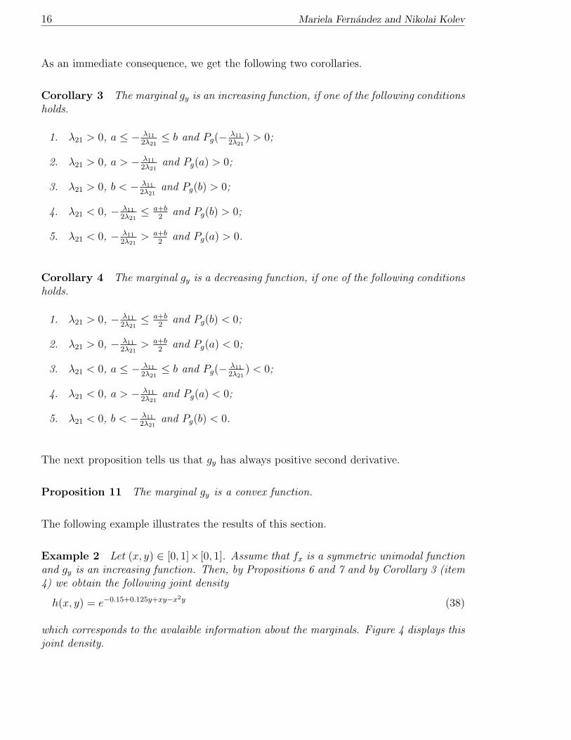
Example 2 Let (x, y) ∈ [0, 1]× [0, 1]. Assume that fx is a symmetric unimodal functionand gy is an increasing function. Then, by Propositions 6 and 7 and by Corollary 3 (item4) we obtain the following joint density

h(x, y) = e−0.15+0.125y+xy−x2y (38)

which corresponds to the avalaible information about the marginals. Figure 4 displays thisjoint density.


Figure 4: Joint density h(x, y) = e−0.15+0.125y+xy−x2y with (x, y) ∈ [0, 1] × [0, 1].

00.2

0.40.6

0.8

1

x

0

0.2

0.4

0.6

0.8

1

y

0.91

1.1

1.2

h

00.2

0.40.6

0.8x

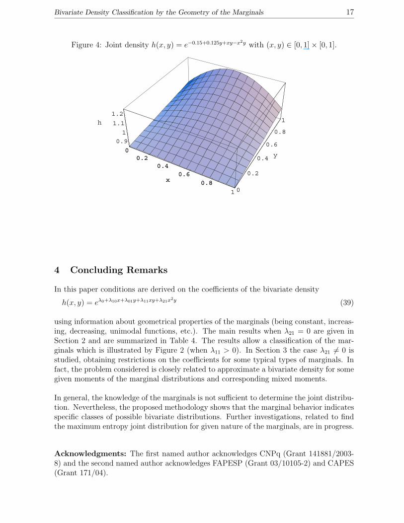
4 Concluding Remarks

In this paper conditions are derived on the coefficients of the bivariate density

h(x, y) = eλ0+λ10x+λ01y+λ11xy+λ21x2y (39)

using information about geometrical properties of the marginals (being constant, increas-ing, decreasing, unimodal functions, etc.). The main results when λ21 = 0 are given inSection 2 and are summarized in Table 4. The results allow a classification of the mar-ginals which is illustrated by Figure 2 (when λ11 > 0). In Section 3 the case λ21 �= 0 isstudied, obtaining restrictions on the coefficients for some typical types of marginals. Infact, the problem considered is closely related to approximate a bivariate density for somegiven moments of the marginal distributions and corresponding mixed moments.

In general, the knowledge of the marginals is not sufficient to determine the joint distribu-tion. Nevertheless, the proposed methodology shows that the marginal behavior indicatesspecific classes of possible bivariate distributions. Further investigations, related to findthe maximum entropy joint distribution for given nature of the marginals, are in progress.

Acknowledgments: The first named author acknowledges CNPq (Grant 141881/2003-8) and the second named author acknowledges FAPESP (Grant 03/10105-2) and CAPES(Grant 171/04).



References

[1] von Collani, E. (2004): Defining the Science of Stochastics. Heldermann Verlag.

[2] Cuadras, C. M., Fortiana, J., Rodrıguez-Lallena, J. (Eds.) (2002): DistributionsWith Given Marginals and Statistical Modelling. Kluwer Academic Publishers.

[3] Kotz, S. and van Dorp, R. (2002): A versatile bivariate distribution on a boundeddomain: another look at the product moment correlation. Journal of Applied Sta-tistics 29, 1165-1179.

[4] Rudin, W. (1976): Principles of Mathematical Analysis. International Series in Pureand Applied Mathematics. McGraw-Hill.

Mariela Fernandez Nikolai KolevDepartment of Applied Mathematics Department of StatisticsInstitute of Mathematics and Statistics Institute of Mathematics and StatisticsUniversity of Sao Paulo University of Sao PauloRua de Matao 1010 Rua de Matao 101005508-090 Sao Paulo, SP. Brazil 05508-090 Sao Paulo, SP. Brazil





Bivariate Density Classification by the Geometry of the Marginals

Documents