Digital Object Identifier (DOI) 10.1007/s00205-010-0337-3 Arch. Rational Mech. Anal. 200 (2011) 89–140 Bistable Boundary Reactions in Two Dimensions Juan Dávila, Manuel del Pino & Monica Musso Communicated by P. Rabinowitz Abstract In a bounded domain ⊂ R 2 with smooth boundary we consider the problem u = 0 in , ∂ u ∂ν = 1 ε f (u ) on ∂, where ν is the unit normal exterior vector, ε> 0 is a small parameter and f is a bistable nonlinearity such as f (u ) = sin(π u ) or f (u ) = (1 − u 2 )u . We construct solutions that develop multiple transitions from −1 to 1 and vice-versa along a connected component of the boundary ∂. We also construct an explicit solution when is a disk and f (u ) = sin(π u ). 1. Introduction In this paper we construct solutions of the following boundary value problem u = 0 in ∂ u ∂ν = 1 ε f (u ) on ∂ (1.1) where is a bounded domain in R 2 with smooth boundary ∂,ν is the unit normal exterior vector, ε> 0 is a small parameter and f is a bistable, balanced nonlinearity, namely f =−W where W (s )> W (−1) = W (1) = 0 for all s ∈ (−1, 1). (1.2) and W (−1) = W (1) = 0, W (−1)> 0, W (1)> 0. (1.3)

Welcome message from author
This document is posted to help you gain knowledge. Please leave a comment to let me know what you think about it! Share it to your friends and learn new things together.
Transcript

Digital Object Identifier (DOI) 10.1007/s00205-010-0337-3Arch. Rational Mech. Anal. 200 (2011) 89–140
Bistable Boundary Reactions in TwoDimensions
Juan Dávila, Manuel del Pino & Monica Musso
Communicated by P. Rabinowitz
Abstract
In a bounded domain � ⊂ R2 with smooth boundary we consider the problem
�u = 0 in �,∂u
∂ν= 1
εf (u) on ∂�,
where ν is the unit normal exterior vector, ε > 0 is a small parameter and f is abistable nonlinearity such as f (u) = sin(πu) or f (u) = (1 − u2)u. We constructsolutions that develop multiple transitions from −1 to 1 and vice-versa along aconnected component of the boundary ∂�. We also construct an explicit solutionwhen � is a disk and f (u) = sin(πu).
1. Introduction
In this paper we construct solutions of the following boundary value problem
{�u = 0 in �∂u∂ν
= 1ε
f (u) on ∂�(1.1)
where� is a bounded domain in R2 with smooth boundary ∂�, ν is the unit normal
exterior vector, ε > 0 is a small parameter and f is a bistable, balanced nonlinearity,namely f = −W ′ where
W (s) > W (−1) = W (1) = 0 for all s ∈ (−1, 1). (1.2)
and
W ′(−1) = W ′(1) = 0, W ′′(−1) > 0, W ′′(1) > 0. (1.3)

90 Juan Dávila, Manuel del Pino & Monica Musso
We also assume that f is of class C3. Notable examples are the Allen–Cahn andthe Peierls–Nabarro nonlinearities, respectively given by f (u) = (1 − u2)u andf (u) = sin(πu), for
W (u) = 1
4(1 − u2)2 and W (u) = 2
πcos2
(π2
u).
Problem (1.1) is the Euler–Lagrange equation for the energy functional
Eε(u) = 1
2
∫�
|∇u|2 + 1
ε
∫∂�
W (u). (1.4)
Functionals of this type arise in models for various phenomena. For instance, Kohnand Slastikov [11] proposed a model for thin soft ferromagnetic films. They estab-lished that under suitable rescalings, the micromagnetic energy �-converges to
Iε(u) = 1
2
∫�
|∇u|2 + 1
2ε
∫∂�
cos2(u − g) (1.5)
where g : ∂� → R is a given function. In this work we will focus on the caseg =constant.
Alberti et al. [1,2] studied a model for a two-phase fluid with surface andline tensions, which involved functionals with a double-well potential integrated in� and on the boundary. In [1,2] the authors calculated the �-limit of the functional
1| log ε| Eε for nonlinearities that include f (u) = u − u3 and showed that the tran-sitions of limits of local minimizers occur at finitely many points in dimension 2,and on a geodesic of the boundary in dimension 3.
Cabré and Cónsul [6] found a renormalized energy in the two-dimensionalcase: they showed that if 2k is the number of transitions in a simply connecteddomain then Eε(uε) − 4k
π| log ε| approaches a multiplicative constant times the
expression (1.9) below, which gives information on the location of the transitionpoints.
Kurzke [12,13] studied the convergence of minimizers of (1.5) by showingthat they develop transitions at finitely many points as ε → 0 and estimating theirlocation.
The shape of the transitions of local minimizers of (1.4) is related, after a suitablerescaling near a transition point, to solutions in a half plane {(x, y) : x ∈ R, y > 0}with ε = 1, for which some properties are known. Equation (1.1) in a half planewith f (u) = sin(u) and ε = 1 is known as the Peierls–Nabarro problem, whichappears as a model of dislocations in crystals. Toland [14] proved that all noncon-stant solutions to the Peierls–Nabarro problem are, except for translations in thex-direction, of the form
±2 arctanx
y + 1+ 2πn (1.6)
where n ∈ N. He achieved this by finding a relation of the Peierls–Nabarro problemwith the Benjamin–Ono equation, which is an equation of the form (1.1) in a halfplane with boundary condition f (u) = u2 − u which appears in theoretical hydro-dynamics. Uniqueness for the Benjamin–Ono equation, except for translations, was

Bistable Boundary Reactions in Two Dimensions 91
proved by Amick and Toland [3,4]. Cabré and Solà-Morales [7] analyzed (1.1)in a half plane or a half space of R
N with ε = 1 for general nonlinearities satisfyingconditions (1.2) and (1.3) below. They built and established uniqueness propertiesof solutions that are monotonically increasing in one of the tangential variables.
As we will see in Section 2, when� is the unit disk in R2 and f (u) = sin(πu),
we can find, rather surprisingly, an explicit solution with 2k transitions, for any givenk � 1. More precisely, we find a solution uε to Problem 1.1 such that uε → u∗where u∗ is harmonic inside the disk, and its boundary values alternate between+1 and −1 at the 2k vertices of a regular polygon. Our construction correspondsprecisely to the harmonic conjugate of one found by Bryan and Vogelius [5] fora boundary reaction arising in corrosion modeling.
Our main goal is to prove that in any two-dimensional domain � there aresolutions with the same qualitative behavior of the explicit solution in a disk: givenk � 1 we will find a family of solutions uε which develops 2k transitions as ε → 0between values close to +1 and −1 on ∂�. To be more precise, let �0 denote theouter component of ∂� and �1, . . . , �m denote the inner components (m � 0, withm = 0 meaning there are no inner components).
In what follows, we fix a component �i0 with index i0 ∈ {0, . . . ,m} and aninteger k � 1. For points ξ1, . . . , ξ2k in �i0 arranged increasingly with respect tosome fixed orientation, let us define the function u∗ = u∗(ξ1, . . . , ξ2k) to be thesolution of the equation
�u∗ = 0 in �
with the boundary conditions on �i0 :
u∗ = 1 on the segment from ξ j to ξ j+1 if j is odd
u∗ = −1 on the segment from ξ j to ξ j+1 if j is even
and
u∗ = 1 on �i with i �= i0.
The following is our main result.
Theorem 1.1. For all sufficiently small ε > 0, there exist at least two solutionsulε, l = 1, 2 of (1.1) such that, up to subsequences, there are two distinct arrays of
2k points of �i0ξl = (ξ l
1, . . . , ξl2k), l = 1, 2 such that
ulε → u∗ (ξ l
1, . . . , ξl2k
)as ε → 0
uniformly on compact subsets of �\{ξ l1, . . . , ξ
l2k}. Furthermore, the points ξ l ,
l = 1, 2 are critical points of the function ψk defined in (1.9).
The location of the transition points ξ1, . . . , ξ2k turns out to be accurately char-acterized as a critical point of a function ψk defined explicitly in terms of G(x, y),

92 Juan Dávila, Manuel del Pino & Monica Musso
the Green function for the following Neumann problem. For any y ∈ ∂�, let⎧⎪⎪⎪⎪⎪⎪⎪⎪⎪⎪⎨⎪⎪⎪⎪⎪⎪⎪⎪⎪⎪⎩
−�G(x, y) = 0 in �
∂G
∂νx(x, y) = 2πδy(x)− 2π
|�i0 |on �i0∫
�i0
G(x, y) = 0
∂G
∂νx(x, y) = 0 on �i , i �= i0.
(1.7)
We denote by H(x, y) its regular part:
H(x, y) = G(x, y)− log1
|x − y|2 . (1.8)
We define
ψk(ξ) = ψk(ξ1, . . . , ξ2k) =2k∑
l=1
H(ξl , ξl)+∑j �=l
(−1)l+ j G(ξ j , ξl), (1.9)
which is the renormalized energy found by Cabré and Cònsul [6], also similar tothat found by Kurzke [12,13].
The asymptotic location of the transition points of the two solutions found cor-respond, in the simply connected case, to a global maximum and a saddle point ofψk , respectively. The solutions in Theorem 1.1 do not correspond to local minimiz-ers of the energy Eε, and �-convergence methods do not appear to be suitable topredict their presence.
We remark that in the non-simply connected case we can also construct solu-tions like those in Theorem 1.1 exhibiting transitions simultaneously on any givenset of components �i of ∂�. The changes needed in the proof are minor, and wouldamount to introducing further notation. For the sake of simplicity we shall dealonly with the case of a single component.
In Section 3 we outline the proof of this result, with detailed proofs carried outin Sections 4–11.
2. Explicit solutions in the disk
Let k � 1 be an integer and consider ξ j ∈ ∂D, j = 0, . . . , 2k − 1 correspond-ing to vertices of a regular polygon, ordered counterclockwise. Given α > 1 wedefine
θ j (z) = − arg
(αξ j − z
ξ j
)j = 0, . . . , 2k − 1 (2.1)
where the argument is such that arg(eiθ ) = θ, θ ∈ (−π, π). Then θ j (z) is welldefined and harmonic in R
2 except the line segment {sξ j : s � α}. In particular θ j

Bistable Boundary Reactions in Two Dimensions 93
is harmonic in D and for z ∈ D, θ j (z) ∈ (−π/2, π/2). Define
uε = 2
π
2k−1∑j=0
(−1) jθ j where ε = 4
kπ
α2k − 1
α2k + 1. (2.2)
Then uε is harmonic in D and satisfies
ε∂uε∂ν
= sin(πuε) on ∂D. (2.3)
If ε → 0 then α → 1 and uε → u∗, which is a harmonic function in D withboundary values ±1. More precisely u∗ = 1 between ξ j and ξ j+1 if j is odd andu∗ = −1 in this range if j is even. Moreover, rescaling appropriately around atransition point we find, up to a factor, the solutions (1.6) of the Peierls–Nabarroproblem.
Next we check the validity of the boundary relation (2.3). We slightly modifythe notation above: we let ξ j ∈ ∂D, j = 0, . . . , 2k − 1 be the vertices of a regularpolygon, ordered counterclockwise, and set
uε =2k−1∑j=0
(−1) jθ j where ε = 2
k
α2k − 1
α2k + 1
and θ j is defined in (2.1).
Proposition 2.1. Then uε is harmonic in D and satisfies
ε∂uε∂ν
= sin(2uε) on ∂D. (2.4)
For the proof we follow the calculations of Bryan and Vogelius [5], who findan explicit solution to the problem
�v = 0 in �,∂v
∂ν= 2ε sinh v on ∂� (2.5)
when � = D is the unit disk and ε > 0. This solution has the form
vε(x) =2k∑j=1
(−1) j−1 log1
|x − αkξ j |2
where αk = [(k + 2ε)/(k − 2ε)] 12k . The function uε is up to a factor the harmonic
conjugate of vε.
Proof of Proposition 2.1. We write u = uε. We may assume that ξ j = eiβ j whereβ j = jπ
k , j = 0, . . . , 2k − 1. Let z = eiθ ∈ ∂B1. Then |z − αξ j |2 = 1 + α2 −2α cos(θ − β j ). We also have the following formulas
sin θ j = sin(θ − β j )(1 + α2 − 2α cos(θ − β j )
)1/2 (2.6)
cos θ j = α − cos(θ − β j )(1 + α2 − 2α cos(θ − β j )
)1/2 (2.7)

94 Juan Dávila, Manuel del Pino & Monica Musso
Let us compute sin(2u) = I m(e2iu). We write
eiu =∏2k−2
j=0, j eveneiθ j
∏2k−1j=1, j odd
eiθ j.
Using (2.6), (2.7) we have
2k−2∏j=0, j even
eiθ j =⎛⎝ 2k−2∏
j=0, j even
(1 + α2 − 2α cos(θ − β j )
)−1/2
⎞⎠
×⎛⎝ 2k−2∏
j=0, j even
(α − e−i(θ−β j ))
⎞⎠ .
It is proved in [5] that
2k−2∏j=0, j even
(1 + α2 − 2α cos(θ − β j )
)= α2k − 2αk cos(kθ)+ 1 (2.8)
2k−1∏j=1, j odd
(1 + α2 − 2α cos(θ − β j )
)= α2k + 2αk cos(kθ)+ 1 (2.9)
Hence
2k−2∏j=0, j even
(1 + α2 − 2α cos(θ − β j )
)−1/2 = (α2k − 2αk cos(kθ)+ 1)−1/2.
We also have
2k−2∏j=0, j even
(α − e−i(θ−β j )) = αk − e−ikθ .
Indeed, setting λ = αeiθ we have
2k−2∏j=0, j even
(α − e−i(θ−β j )) = e−ikθk−1∏�=0
(λ− e
2π ik �)
and the product is a polynomial in λ, of degree k, with leading coefficient equal to
1 and roots e2π i
k �, � = 0, . . . , k −1. Thus the product equals λn −1 and the formulafollows. Then
2k−2∏j=0, j even
eiθ j = αk − e−ikθ
(α2k − 2αk cos(kθ)+ 1)1/2.

Bistable Boundary Reactions in Two Dimensions 95
Similarly
2k−1∏j=1, j odd
eiθ j = αk + e−ikθ
(α2k + 2αk cos(kθ)+ 1)1/2.
It follows that
sin(2u) = 4αk(α2k − 1) sin(kθ)
(α2k − 2αk cos(kθ)+ 1)(α2k + 2αk cos(kθ)+ 1)(2.10)
To compute the normal derivative of u we begin by observing that
∂θ j
∂x(z) = I m(z − αξ j )
|z − αξ j |2∂θ j
∂y(z) = − Re(z − αξ j )
|z − αξ j |2
Taking z = eiθ we arrive at
∂u
∂ν= α
2k−1∑j=0
(−1) j sin(θ − β j )
1 + α2 − 2α cos(θ − β j ).
Taking the logarithmic derivative of (2.8) with respect to θ yields
2k−2∑j=0, j even
α sin(θ − β j )
1 + α2 − 2α cos(θ − β j )= kαk sin(kθ)
α2k − 2αk cos(kθ)+ 1
and similarly from (2.9)
2k−1∑j=1, j odd
α sin(θ − β j )
1 + α2 − 2α cos(θ − β j )= − kαk sin(kθ)
α2k + 2αk cos(kθ)+ 1
We deduce then
∂u
∂ν= 2kαk(α2k + 1) sin(kθ)
(α2k − 2αk cos(kθ)+ 1)(α2k + 2αk cos(kθ)+ 1)(2.11)
From (2.10) and (2.11) we deduce formula (2.4).

96 Juan Dávila, Manuel del Pino & Monica Musso
3. Scheme of the proof of Theorem 1.1
Let us consider the problem in the half space R2+ = {(x1, x2) ∈ R
2 : x2 > 0}{�w = 0 in R
2+∂w∂ν
= f (w) on ∂R2+(3.1)
where ∂∂ν
= − ∂∂x2
.Cabré and Solà-Morales [7] call w a layer solution of (3.1) if it satisfies
{w(x1, 0) is increasing
limx1→−∞w(x1, 0) = −1, lim
x1→∞w(x1, 0) = 1. (3.2)
They proved existence of layer solutions and uniqueness except for translations.Moreover, layer solutions satisfy
∣∣∣∣w(x1, x2)− 2
πarctan
(x1
x2 + 1
)∣∣∣∣ � C
|x |1/2 for all x = (x1, x2) ∈ R2+,
see [7] formula (6.22),
|∇w(z)| � C
1 + |z| ∀z ∈ R2+,
see [7] Theorem 1.6, and
cx2 + a
x21 + (x2 + a)2
� wx (x1, x2) � Cx2 + A
x21 + (x2 + A)2
for all (x1, x2) ∈ R2+
(3.3)
where c,C, a, A > 0 see [7] formulas (6.16) and (6.18). As a result
|w(x1, 0)− 1| � C
1 + x1∀x1 � 0 (3.4)
|w(x1, 0)+ 1| � C
1 + |x1| ∀x1 � 0. (3.5)
We will call w+ the solution to (3.1), (3.2) such that w(0, 0) = 0 and w− thesolution to (3.1) such that
{w−(x1, 0) is decreasing,
limx1→−∞w
−(x1, 0) = +1, limx1→+∞w
−(x1, 0) = −1 (3.6)
and w−(0, 0) = 0. Let us define
w±ε (z) = w±(z/ε) ∀z ∈ R
2+.
We write ∂� = �0⋃(∪m
i=1�i ), where �0 denotes the outer component of ∂� and�i the inner component. Let L denote the length of the outer component �0 of the

Bistable Boundary Reactions in Two Dimensions 97
boundary ∂� and let γ : R → R2 be an L-periodic positively oriented arclength
parametrization of �0. Then there exists δ > 0 such that
(s, t) �→ γ (s)− tν(γ (s)) (3.7)
is a smooth diffeomorphism from [0, L] × (0, δ) (identifying 0 and L) with �δ ={z ∈ � : dist(z, �0) < δ}. Therefore (s, t) can be regarded as coordinate functionsdefined in �δ .
For simplicity we assume that ξ1, . . . , ξ2k are given points in �0 ordered coun-terclockwise let s1 < s2 < . . . < s2k be their corresponding arclength parameters.We assume henceforth that
|si+1 − si | � 5δ for all i = 0, . . . , 2k − 1 (3.8)
where by convention s0 = s2k and δ is a small, fixed, positive number. Let
w+ε (s, t) = η1(s)η2(s)w
+ε (s, t)+ η1(s)− η2(s)
where η1, η2 ∈ C∞(R), 0 � η1, η2 � 1 and
η1(s) = 1 for s � −δ, η1(s) = 0 for s � −2δ
η2(s) = 1 for s � δ, η2(s) = 0 for s � 2δ
We define w−ε similarly as
w−ε (s, t) = η1(s)η2(s)w
−ε (s, t)+ η2(s)− η1(s)
Let η0 ∈ C∞(R), 0 � η0 � 1 be such that
η0(t) = 1 for t � δ/2 and η0(t) = 0 for t � δ. (3.9)
Define
Uε(s, t) = η0(t)
⎧⎪⎪⎪⎨⎪⎪⎪⎩
w+ε (s − s j , t) if s j − 2δ � s � s j + 2δ, j odd
1 if s j + 2δ � s � s j+1 − 2δ, j odd
w−ε (s − s j , t) if s j − 2δ � s � s j + 2δ, j even
−1 if s j + 2δ � s � s j+1 − 2δ, j even
where j = 1, . . . , 2k.This formula defines Uε as a smooth function in �δ . Extending it by zero to
�−�δ we obtain a smooth function in �.As initial approximation of a solution to (1.1) we take
Uε = Uε + (1 − η0)u∗ + Hε (3.10)
where u∗ = u∗[ξ1, . . . , ξ2k] is the harmonic function on� defined in the introduc-tion and Hε is the solution to{
�Hε = −�(Uε + (1 − η0)u∗) in �
Hε = 0 on ∂�.(3.11)

98 Juan Dávila, Manuel del Pino & Monica Musso
We look for a solution u of (1.1) of the form u = Uε+φ, which yields the followingequation for the new unknown φ
�φ = 0 in �
ε∂φ
∂ν− f ′(Uε)φ = N [φ] + R on ∂�
where
N [φ] = f (Uε + φ)− f (Uε)− f ′(Uε)φ
R = f (Uε)− ε∂Uε∂ν
.(3.12)
For arbitrary points ξ1, . . . , ξ2k satisfying the separation condition (3.8) we willshow in Section 9 that we can find φ, c1, . . . , c2k of order ε that solve:
⎧⎪⎪⎪⎪⎪⎪⎨⎪⎪⎪⎪⎪⎪⎩
�φ = 0 in �
ε∂φ
∂ν− f ′(Uε)φ = N [φ] + R +
2k∑j=1
c j Z j on ∂�
∫∂�
φZ j = 0 for all j = 1, . . . , 2k.
where Z j are appropriate functions defined in (7.4).A key element to prove this result is to establish the non-degeneracy of the
layer solutions w±, which we do in Section 5, by means of the estimates containedin Section 4. The non-degeneracy lets us establish an invertibility property for theassociated projected linear problem, first in the half-space (Section 6), then in thebounded domain� (Section 7). Section 8 is devoted to estimating the L∞-norm ofthe error R (3.12).
At this point, a standard argument shows Uε + φ is a real solution to (1.1),provided that the points (ξ1, . . . , ξ2k) are critical points of Eε(Uε + φ), which isclose to Eε(Uε) in an appropriate sense, see Section 10. Section 11 is devoted toexpanding the energy functional Eε at Uε and to giving the proof of Theorem 1.1.
Finally, some technical Lemmas we need throughout the paper are containedin Appendices A and B.
4. Estimates for the Laplacian with Robin Boundary condition
In this section we study existence and decay estimates for the boundary valueproblem
{�φ = 0 in R
2+∂φ∂ν
+ aφ = h on ∂R2+,(4.1)
where a > 0. For a function h : R → R and α ∈ R we define
‖h‖α = supy∈R
(1 + |y|)α|h(y)|.
Bistable Boundary Reactions in Two Dimensions 99
Let
�(x − y) = − log |x − y|, x, y ∈ R2
We recall (see [10]) that if y ∈ R2+ and a > 0, the Green function for the Robin
problem⎧⎨⎩
−�x G(x, y) = 2πδy in R2+
−∂G
∂ν+ aG = 0 on ∂R2+
is given by
G(x, y) = �(x − y)− �(x − y∗)− 2∫ 0
−∞eas ∂
∂x2�(x − y∗ − e2s
)ds, (4.2)
where y∗ is the reflection of y = (y′, y2) across ∂R2+, that is y∗ = (y′,−y2).If h is bounded on R, then a solution to (4.1) is given by
φ(x) = 1
2π
∫ ∞
−∞G((y, 0), x)h(y) dy x ∈ R
2+.
From (4.2)
G((y, 0), (x1, x2)) =∫ ∞
0
e−at (x2 + t)
(y − x1)2 + (x2 + t)2dt
and hence
φ(x1, x2) =∫ ∞
−∞ka(x1 − y, x2)h(y) dy for all (x1, x2) ∈ R
2+, (4.3)
where
ka(x1, x2) = 1
π
∫ ∞
0
e−at (x2 + t)
x21 + (x2 + t)2
dt for all (x1, x2) ∈ R2+. (4.4)
In the sequel, when the value of a > 0 is clear from the context, we will writek = ka .
Next we state some mapping properties of the operator defined by (4.3) inweighted L∞ spaces. Most of the proofs are in Appendix A. Let h : R → R with‖h‖α < ∞ where α > −1. Then (4.3) is well defined.
Lemma 4.1. Let α > −1 and h : R → R satisfy ‖h‖α < ∞. Then φ defined by(4.3) satisfies:if α < 1
|φ(x1, x2)| � C‖h‖α⎧⎨⎩
1(1+|x1|)α + 1+x2
(1+|x1|)α+1 if |x1| � x2
1(1+x2)α
if |x1| � x2
100 Juan Dávila, Manuel del Pino & Monica Musso
if α = 1,
|φ(x1, x2)| � C‖h‖α{
11+|x1| + (1+x2)max(1,log |x1|)
(1+|x1|)2 if |x1| � x21
1+x2if |x1| � x2
and if α > 1
|φ(x1, x2)| � C‖h‖α{
1(1+|x1|)α + (1+x2)
(1+|x1|)2 if |x1| � x21
1+x2if |x1| � x2
Corollary 4.1. Let α > −1. Let h : R → R be such that ‖h‖α < ∞. Then φdefined by (4.3) satisfies:if α � 2
‖φ(·, 0)‖α � C‖h‖α.if α > 2
‖φ(·, 0)‖2 � C‖h‖α.Lemma 4.2. Let α > 1 and assume that h : R → R satisfies ‖h‖α < +∞.Suppose ∫ ∞
−∞h = 0
and let φ be defined by (4.3).Then if α < 2
|φ(x1, x2)| � C‖h‖α⎧⎨⎩
1(1+|x1|)α + 1+x2
(1+|x1|)α+1 if |x1| � x2
1(1+x2)α
if |x1| � x2
if α = 2,
|φ(x1, x2)| � C‖h‖α⎧⎨⎩
1(1+|x1|)2 + (1+x2)max(1,log |x1|)
(1+|x1|)3 if |x1| � x2
max(1,log |x2|)(1+x2)2
if |x1| � x2
and if α > 2
|φ(x1, x2)| � C‖h‖α⎧⎨⎩
1(1+|x1|)α + (1+x2)
(1+|x1|)3 if |x1| � x2
1(1+x2)2
if |x1| � x2
Corollary 4.2. Let α > 2 and assume that h : R → R satisfies ‖h‖α < +∞.Suppose
∫ ∞
−∞h = 0

Bistable Boundary Reactions in Two Dimensions 101
and let φ be defined by (4.3). Then if 2 < α � 3
‖φ(·, 0)‖α � C‖h‖αand if α > 3 then
‖φ(·, 0)‖3 � C‖h‖α.Lemma 4.3. Let α > −1 and assume h : R → R satisfies ‖h‖α < ∞ andh(y) = 0 for all y � 0. Then φ defined by (4.3) satisfies:if α < 1:
|φ(x1, 0)| � C‖h‖α 1
(1 + |x1|)α+1 ∀x1 � 0,
if α = 1:
|φ(x1, 0)| � C‖h‖α max(log |x1|, 1)
(1 + |x1|)2 ∀x1 � 0,
if α > 1:
|φ(x1, 0)| � C‖h‖α 1
(1 + |x1|)2 ∀x1 � 0.
Lemma 4.4. Let α > −1 and assume h : R → R satisfies ‖h‖α < ∞, h(y) = 0for all y � 0 and
∫ ∞
0h = 0.
Then φ defined by (4.3) satisfies:if α < 2:
|φ(x1, 0)| � C‖h‖α 1
(1 + |x1|)α+1 ∀x1 � 0,
if α = 2:
|φ(x1, 0)| � C‖h‖α max(log |x1|, 1)
(1 + |x1|)3 ∀x1 � 0,
if α > 2:
|φ(x1, 0)| � C‖h‖α 1
(1 + |x1|)3 ∀x1 � 0.
Lemma 4.5. Let h ∈ L∞(∂R2+) and φ be a bounded solution to
�φ = 0 in R2+,
∂φ
∂ν+ aφ = h on ∂R2+
where a > 0. Then φ is given by (4.3).

102 Juan Dávila, Manuel del Pino & Monica Musso
Proof. Let φ1 be defined by (4.3). Then φ = φ − φ1 is a bounded solution to
�φ = 0 in R2+,
∂φ
∂ν+ aφ = 0 on ∂R2+.
By standard elliptic estimates, φ is a smooth function and ∇φ is uniformly bounded.
Let v = aφ − ∂φ∂y . Then v is a bounded function, �v = 0 in R
2+ and v vanishes on
∂R2+. Thus v can be extended by odd symmetry to R2. By Liouville’s theorem v is
constant and hence v ≡ 0. It follows that φ(x, y) = c(x)eay . Since φ is boundedφ ≡ 0.
5. Nondegeneracy of layer solutions
The main result in this section is the nondegeneracy of the layer solutionw thatsatisfies (3.1), (3.2). Consider the linear problem
�φ = 0 in R2+ (5.1)
∂φ
∂ν− f ′(w)φ = 0 on ∂R2+. (5.2)
Proposition 5.1. Suppose that φ ∈ L∞(R2+) satisfies (5.1), (5.2). Then φ = c ∂w∂x
for some constant c ∈ R.
We also establish here the following asymptotic formulas for the layer solutions.
Proposition 5.2. Suppose w is the layer solution that satisfies (3.1), (3.2). Then
w(x, 0)− 1 = 2
π f ′(1)1
x+ O
(log(x)
x2
)as x → ∞, (5.3)
and
w(x, 0)+ 1 = 2
π f ′(−1)
1
x+ O
(log(|x |)
x2
)as x → −∞. (5.4)
We start with a result that gives decay estimates for solutions with Robin bound-ary conditions, with a potential a(x) that is asymptotic to positive constants.
Lemma 5.1. Suppose φ ∈ L∞(R2+) solves
�φ = 0 in R2+
∂φ
∂ν+ a(x)φ = h on ∂R2+
where a(x) ∈ L∞(R) satisfies
a(x) = a+ + O
(1
x
)as x → ∞, a(x) = a− + O
(1
|x |)
as x → −∞
with a+, a− > 0 and ‖h‖2 < ∞ (i.e. h(x) = O(1/x2) as x → ±∞. Then
φ(x, 0) = O
(1
x2
)as x → ±∞.

Bistable Boundary Reactions in Two Dimensions 103
Proof. Let
h1 = ((a(x)− a+)φ + h)χ[x>0], h2 = ((a(x)− a+)φ + h)χ[x<0]
and let φ1, φ2 be defined by formula (4.3) with k = ka+ , h = h1 and h = h2,
respectively. Then they solve
�φi = 0 in R2+
∂φi
∂ν+ a+φi = hi on ∂R2+
By Lemma 4.5 φ = φ1 + φ2.Since φ is bounded we deduce |h1(x1)| � C(1 + |x1|)−1 for all x1 ∈ R and
Lemma 4.1 with α = 1 then implies that
|φ1(x1, 0)| � C
1 + |x1| for all x1 ∈ R. (5.5)
Since a(x) and φ are bounded, we have that h2 is bounded. Using Lemma 4.3 withα = 0, we can then deduce that φ2(x1, 0) = O(1/x1) as x1 → ∞. Combining thiswith (5.5) we deduce that φ(x1, 0) = O(1/x1) as x1 → ∞. By a similar argument,defining φ1, φ2 with a− instead of a+, we deduce that |φ(x1, 0)| � C(1 + |x1|)−1
for all x1 � 0, and therefore
|φ(x1, 0)| � C(1 + |x1|)−1 for all x1 ∈ R. (5.6)
Since a(x) is bounded we have |h1(x1)| � C(1+|x1|)−2 for all x1 ∈ R, and henceLemma 4.1 with α = 2 yields |φ1(x1, 0)| � C(1 + |x1|)−2 for all x1 ∈ R. Wealso have, thanks to (5.6), that |h2(x1)| � C(1 + |x1|)−1 for all x1 � 0. Hence byLemma 4.3 with α = 1 we obtain |φ2(x1, 0)| � C max(log |x1|, 1)(1 + |x1|)−2
for all x1 � 0. Hence |φ(x1, 0)| � C max(log |x1|, 1)(1 + |x1|)−2 for all x1 � 0.Again, through a similar argument we reach
|φ(x1, 0)| � Cmax(log |x1|, 1)
(1 + |x1|)2 for all x1 ∈ R.
Repeating the process once more, where we apply Lemma 4.3 with someα ∈ (1, 2),we find
|φ(x1, 0)| � C(1 + |x1|)−2 ∀x1 ∈ R.
Lemma 5.2. Let φ be a bounded solution to (5.1), (5.2). Then φ satisfies
|φ(x1, x2)| � C1 + x2
x21 + (1 + x2)2
∀(x1, x2) ∈ R2+ (5.7)
and
|∇φ(x)| � C
1 + |x |2 ∀x ∈ R2+. (5.8)

104 Juan Dávila, Manuel del Pino & Monica Musso
Proof. Let a± = − f ′(±1) so that a± > 0. By (3.4) and (3.5) we have that
∣∣ f ′(w(x1, 0))− a+∣∣ � C |w(x1, 0)− 1| � C
1 + x1for all x1 � 0.
and
∣∣ f ′(w(x1, 0))+ a−∣∣ � C |w(x1, 0)+ 1| � C
1 + |x1| for all x1 � 0.
By Lemma 5.1 we deduce that φ(x1, 0) = O(1/x21 ) as x1 → ±∞. We can now
write the boundary condition as
∂φ
∂ν+ a+φ = (a+ + f ′(w))φ.
Applying Lemma 4.1 with α = 2 we deduce (5.7).To prove (5.8), let us first remark that
|∇φ(x)| � C
1 + |x |2 ∀x ∈ ∂R2+. (5.9)
Indeed, (5.7) implies that |φ(x)| � C1+|x |2 for x = (x1, x2) with 0 � x2 � 1. But
f ′(w) is a smooth bounded function, with bounded derivative. By standard ellipticestimates we deduce (5.9). Now let x0 ∈ R
2+ with |x0| � 1 and R = |x0|/2. Defineψ(z) = Rφ(x0 + Rz) for z ∈ D = B1 ∩ {(z1, z2) : z2 > −x0,2/R} where wehave written x0 = (x0,1, x0,2). By (5.7) |ψ(z)| � C for z ∈ D and (5.9) impliesthat |∇ψ(z)| � C for z ∈ � where � = {(z1, z2) ∈ B1 : z2 = −x0,2/R}. UsingLemma B.1 we deduce that |∇ψ(0)| � C and this yields |∇φ(x0)| � C
|x0|2 .
Proof of Proposition 5.1. Let Z = ∂w∂x and ψ = φ
Z . Then
∇ · (Z2∇ψ) = 0 in R2+,
∂ψ
∂ν= 0 on ∂R2+.
Multiplying the equation by ψ and integrating in BR ∩ R2+ we find
0 =∫∂BR∩R
2+Z2ψ
∂ψ
∂ν−∫
BR∩R2+
Z2|∇ψ |2.
Since (3.3) holds, (5.7) shows that ψ is uniformly bounded. Since
|∇Z | � C
1 + |x |2 ∀x ∈ R2+
and using (5.8) we get
Z2|ψ ||∇ψ | � |ψ |(Z |∇φ| + |φ| |∇Z |) � C
1 + |x |3 ∀x ∈ R2+.

Bistable Boundary Reactions in Two Dimensions 105
This implies that ∣∣∣∣∣∫∂BR∩R
2+Z2ψ
∂ψ
∂ν
∣∣∣∣∣ � C
R2 .
Taking R → ∞ we find that ∫R
2+Z2|∇ψ |2 = 0
and this shows that ψ is constant. For the proof of Proposition 5.2 we need the behavior of some particular solu-
tions with explicit right-hand sides. The proofs are in Appendix A.
Lemma 5.3. Let a > 0 and u be the bounded solution of
�u = 0 in R2+
∂u
∂ν+ au = χ[x>0] on ∂R2+
Then
u(x, 0) = 1
a− 1
πa2x+ O
(1
x3
)as x → ∞
u(x, 0) = 1
πa2|x | + O
(1
|x |3)
as x → −∞.
Lemma 5.4. Let a > 0 and u be the bounded solution of
�u = 0 in R2+
∂u
∂ν+ au = χ[x>1]
1
xon ∂R2+
Then
u(x, 0) = 1
ax+ O
(log(x)
x2
)as x → ∞
u(x, 0) = O
(log(|x |)
x2
)as x → −∞
Proof of Proposition 5.2. Let a+ = − f ′(1) > 0, a− = − f ′(−1) > 0. For x > 0
∂w
∂ν= f (w) = f ′(1)(w − 1)+ O((w − 1)2) as x → ∞= −a+w + a+ + O(1/x2) as x → ∞
Similarly
∂w
∂ν= −a−w − a− + O(1/x2) as x → −∞

106 Juan Dávila, Manuel del Pino & Monica Musso
Let
a(x) = a+ for x > 0, a(x) = a− for x < 0
a(x) = a+ for x > 0, a(x) = −a− for x < 0.
Then
∂w
∂ν+ a(x)w = a(x)+ O(1/x2) as x → ±∞. (5.10)
Next we construct a function that, up to a small error, also satisfies (5.10). Defineu1 to be the bounded solution of
�u1 = 0 in R2+
∂u1
∂ν+ a+u1 = a+χ[x>0] + a+ − a−
πa−xχ[x>1] on ∂R2+
Then by Lemmas 5.3 and 5.4
u1(x, 0) = 1 − 2
πa+x+ 1
πa−x+ O
(log(x)
x2
)as x → ∞ (5.11)
and
u1(x, 0) = 1
πa+|x | + O
(log(|x |)
x2
)as x → −∞ (5.12)
Similarly define
�u2 = 0 in R2+
∂u2
∂ν+ a−u2 = −a−χ[x<0] − a− − a+
πa+|x | χ[x<−1] on ∂R2+
By Lemmas 5.3 and 5.4 we have
u2(x, 0) = −1 + 2
πa−|x | − 1
πa+|x | + O
(log(|x |)
x2
)as x → −∞ (5.13)
and
u2(x, 0) = − 1
πa−x+ O
(log(x)
x2
)as x → ∞ (5.14)
Then for x > 1
∂(u1 + u2)
∂ν+ a+(u1 + u2) = a+ + O
(log(x)
x2
)as x → ∞
and for x < −1
∂(u1 + u2)
∂ν+ a−(u1 + u2) = a− + O
(log(|x |)
x2
)as x → −∞.
Bistable Boundary Reactions in Two Dimensions 107
Therefore
∂(u1 + u2)
∂ν+ a(x)(u1 + u2) = a(x)+ O(log(|x |)/x2) as x → ±∞.
Then φ = w − (u1 + u2) satisfies
∂φ
∂ν+ a(x)φ = O
(log(|x |)
x2
)as x → ±∞
By Lemma 5.1 (really a slight variant of it):
φ(x, 0) = O
(log(|x |)
x2
)as x → ±∞.
This implies
w(x, 0) = u1(x, 0)+ u2(x, 0)+ O
(log(|x |)
x2
)as x → ±∞.
But by (5.11) and (5.14)
u1(x, 0)+ u2(x, 0) = 1 − 2
πa+x+ O
(log(x)
x2
)as x → ∞
and by (5.12) and (5.13)
u1(x, 0)+ u2(x, 0) = −1 + 2
πa−|x | + O
(log(|x |)
x2
)as x → −∞.
6. Solvability of the linearized equation in a half plane
In this section we study the solvability and decay estimates for solutions to theproblem ⎧⎨
⎩�φ = 0 in R
2+∂φ
∂ν= f ′(w)φ + h + cwxη on ∂R2+,
(6.1)
where w is the solution to (3.1), (3.2) and η ∈ C∞0 (R) is such that η � 0, η �= 0.
We will prove
Proposition 6.1. Let 2 < α � 3 and assume that ‖h‖α < +∞. Then there existunique c ∈ R and φ ∈ L∞(R2+) with ‖φ(·, 0)‖α < +∞ which solves (6.1).Moreover,
‖φ‖α � C‖h‖αfor some constant C and c is given by
c = −∫∞−∞ hwx∫∞−∞ ηw2
x
.
108 Juan Dávila, Manuel del Pino & Monica Musso
Proof. Let us prove the uniqueness. Suppose h = 0 and multiply (6.1) by wx .Integrating in a half ball B+
R = BR(0) ∩ R2+. We deduce
0 =∫∂BR∩R
2+
(∂φ
∂νwx − φ
∂wx
∂ν
)+ c
∫ R
−Rηw2
x .
By Lemma 5.1 the decay estimates (5.7) and (5.8) are valid for wx and φ. Hence∫∂BR∩R
2+
(∂φ
∂νwx − φ
∂wx
∂ν
)= O(1/R2).
Letting R → ∞ we find c = 0. Then φ = cwx by Proposition 5.1 for some c ∈ R.But since we assume that ‖φ‖α < ∞ and α > 2, we must have c = 0.
Let us show existence of a solution when 2 < α < 3. Fix 2 < γ < α and leta± = − f ′(±1) so that a± > 0. Given a > 0 and g : R → R with ‖g‖γ < ∞ wedefine φ = Ka(g) as
φ(x1) =∫ ∞
−∞ka(x1 − y, 0)(g(y)+ cη(y)wx (y))dy for all x1 ∈ R.
where
c = −∫∞−∞ g∫∞
−∞ ηwx.
In this way, the harmonic extension of φ to R2+ satisfies
∂φ
∂ν+ aφ = g + cηwx on ∂R2+.
Define the space
E = {(φ1, φ2) : φi : R → R i = 1, 2 such that ‖(φ1, φ2)‖E < ∞}where
‖(φ1, φ2)‖E = ‖φ1‖α,γ + ‖φ2‖γ,αand
‖φ1‖α,γ = supx�0
(1 + |x |)α|φ1(x)| + supx�0
(1 + x)γ |φ1(x)|
‖φ2‖γ,α = supx�0
(1 + |x |)γ |φ2(x)| + supx�0
(1 + x)α|φ2(x)|.
Let T : E → E be given by T (φ1, φ2) = (T1(φ1, φ2), T2(φ1, φ2)) where
T1(φ1, φ2) = Ka+[(a+ + f ′(w))φ1 + (a− + f ′(w))φ2)χ[x�0]
]
T2(φ1, φ2) = Ka−[(a− + f ′(w))φ2 + (a+ + f ′(w))φ1)χ[x<0]
]

Bistable Boundary Reactions in Two Dimensions 109
The operator T is well defined from E to E . Indeed, if (φ1, φ2) ∈ E , then since|w(x1, 0)− 1| � C/(1 + x1) for all x1 � 0, see (3.4), we have
∥∥∥(a+ + f ′(w))φ1 + (a− + f ′(w))φ2)χ[x�0]∥∥∥α
� C‖(φ1, φ2)‖E .
We deduce from Lemma 4.2 that
‖T1(φ1, φ2)‖α � C‖(φ1, φ2)‖E . (6.2)
Similarly
‖T2(φ1, φ2)‖α � C‖(φ1, φ2)‖E (6.3)
and hence T (φ1, φ2) ∈ E . Suppose (φ1, φ2) ∈ E satisfies{φ1 = T1(φ1, φ2)+ Ka+(hχ[x�0])φ2 = T2(φ1, φ2)+ Ka−(hχ[x<0]).
(6.4)
Then φ = φ1 + φ2 is a solution of (6.1) for some c ∈ R. We claim that T is acompact operator. Thus the Fredholm alternative implies that (6.4) has a solutionin E , because we know that when h = 0 the only solution in E of (6.4) is the trivialone. Moreover, φ = φ1 + φ2 satisfies ‖φ‖α � C‖h‖α because of (6.2), (6.3) and‖(φ1, φ2)‖E � C‖h‖α .
Let us verify that T is compact. Let (φ1,n, φ2,n) ∈ E be a bounded sequenceand let (ψ1,n, ψ2,n) = T (φ1,n, φ2,n). Define
c1,n = −∫∞−∞
((a+ + f ′(w))φ1,n + (a− + f ′(w))φ2,n)χ[x�0]
)∫∞−∞ ηwx
c2,n = −∫∞−∞
((a− + f ′(w))φ2,n + (a+ + f ′(w))φ1,n)χ[x<0]
)∫∞−∞ ηwx
.
Since c1,n, c2,n are bounded we may assume that c1,n → c1, c2,n → c2. The func-tions ψ1,n, ψ2,n are also uniformly bounded in R
2+. Hence, from standard elliptic
estimates,ψ1,n → ψ1 andψ2,n → ψ2 uniformly on compact sets of R2+. Therefore,
for any R > 0
sup−R�x�R
(1 + |x |α) |ψi,n(x)− ψi (x)| → 0 as n → ∞, i = 1, 2. (6.5)
By Lemma 4.4
supx�0
(1 + |x |)3|T1(φ1, φ2)| � C‖(φ1, φ2)‖E , (6.6)
and similarly
supx�0
(1 + |x |)3|T2(φ1, φ2)| � C‖(φ1, φ2)‖E . (6.7)

110 Juan Dávila, Manuel del Pino & Monica Musso
Using (6.6)
supx�−R
(1 + |x |)α|ψ1,n(x)− ψ1,k(x)|
� (1 + R)α−3 supx�−R
(1 + |x |)3|ψ1,n(x)− ψ1,k(x)|
� C(1 + R)α−3.
Similarly, by (6.2)
supx�R
(1 + x)γ |ψ1,n(x)− ψ1,k(x)| � (1 + R)γ−α supx�R
(1 + x)α|ψ1,n(x)− ψ1,k(x)|
� (1 + R)γ−α‖ψ1,n − ψ1,k‖α� C(1+R)γ−α‖φ1,n − φ1,k‖E �C(1+R)γ−α.
These estimates show that
‖ψ1,n − ψ1‖α,γ → 0 as n → ∞.
In a similar way we prove that ‖ψ2,n − ψ2‖γ,α → 0 as n → ∞.Finally, in the case α = 3, we fix 2 < γ < α′ < 3 and construct a solution
φ = φ1 + φ2 ∈ E with the norm ‖(φ1, φ2)‖E = ‖φ1‖α′,γ + ‖φ2‖γ,α′ . Thanks to(6.7) and |w(x1, 0)− 1| � C/(1 + x1) for all x1 � 0 we see that∥∥∥(a+ + f ′(w))φ1 + (a− + f ′(w))φ2)χ[x�0]
∥∥∥a
� C‖(φ1, φ2)‖E .
By Lemma 4.2 we deduce
‖T1(φ1, φ2)‖3 � C‖(φ1, φ2)‖E � C‖h‖3
and
‖T2(φ1, φ2)‖3 � C‖(φ1, φ2)‖E � C‖h‖3.
7. The linearized equation in a bounded domain
We study the linear problem
�φ = 0 in � (7.1)
ε∂φ
∂ν− f ′(Uε)φ = h +
2k∑j=1
c j Z j on ∂� (7.2)
with the constraints ∫∂�
φZ j = 0 for all j = 1, . . . , 2k, (7.3)
Bistable Boundary Reactions in Two Dimensions 111
where the functions Z j are defined as follows. Let s1 < s2 < · · · < s2k be thearclength parameters of ξ1, · · · , ξ2k in ∂�. Recall that (s, t) ∈ [0, L] × (0, δ) arecoordinates in a neighborhood of ∂�, with s being arclength and t distance to theboundary. We fix a function η1 ∈ C∞
0 (R) such that η1 > 0 in (−δ, δ) and define
Z j (s, t) = ∂w±ε
∂x
(s − s j
ε,
t
ε
)η1(s − s j )η0(t), (7.4)
where η0 is defined in (3.9).
Proposition 7.1. There exists ε0 > 0 such that for all 0 < ε � ε0 and h ∈ L∞(∂�)there exists unique c j ∈ R and φ ∈ L∞(∂�) solving (7.1),(7.2), (7.3). Moreover
‖φ‖L∞(∂�) +2k∑
i=1
|ci | � C‖h‖L∞(∂�) (7.5)
First we establish the following a-priori bound:
Lemma 7.1. There exists ε0 > 0 such that for all 0 < ε � ε0 we have the followingproperty: if φ ∈ L∞(�) is a solution to (7.1), (7.2), (7.3) for some h ∈ L∞(�)and ci ∈ R, then (7.5) holds.
Proof. Multiplying (7.1) by Zi and integrating we find
ci
∫∂�
Z2i = −
∫∂�
(f ′(Uε)Zi − ∂Zi
∂ν
)φ −
∫∂�
h Zi −∫�
φ�Zi .
We have ∫∂�
Z2i = ε
∫ ∞
−∞w2
xη21, f ′(Uε)Zi − ∂Zi
∂ν= 0 on ∂�
∣∣∣∣∫∂�
h Zi
∣∣∣∣ � ‖h‖L∞(∂�)ε∫ ∞
−∞|wxη1|
and ∫�
|�Zi | � Cε. (7.6)
Indeed, fix i = 1, . . . , 2k and for simplicity assume that i is odd and si = 0. Thenin the region |z| � δ, using (8.9) we have
�Zi = (2k − k2t)t
(1 − kt)2(Zi )ss − k
1 − kt(Zi )t + k′t
(1 − kt)3(Zi )s .
Let us consider the first term:
(2k − k2t)t
(1 − kt)2(Zi )ss = (2k − k2t)t
(1 − kt)2
(∂w±
ε
∂s
(s
ε,
t
ε
)η1(s − s j )η0(t)
)ss
= (2k − k2t)t
(1 − kt)2
[1
ε2
(w±
sss
(s
ε,
t
ε
)η1(s)η0(t)
+21
ε
(w±
ss
(s
ε,
t
ε
)η′
1(s)η0(t)
+ w±s
(s
ε,
t
ε
)η′′
1(s)η0(t)
]= (a)+ (b)+ (c)

112 Juan Dávila, Manuel del Pino & Monica Musso
Changing variables s = εs, t = εt we can estimate, using (8.4)
∫�
(a) � Cε∫
Bδ/ε(0)∩R2+
tw±sss dt ds � Cε.
Similarly by (8.3)
∫�
(b) � Cε2∫
Bδ/ε(0)∩R2+
tw±ss dt ds � Cε
and by (8.2)
∫�
(c) � Cε3∫
Bδ/ε(0)∩R2+
tw±s dt ds � Cε.
A similar calculation works for the other terms and we deduce the validity of (7.6).This shows that
|ci | � C(‖φ‖L∞(∂�) + ‖h‖L∞(∂�)) for all i = 1, . . . , 2k. (7.7)
In order to prove (7.5) it is then sufficient to show that there exists ε0 > 0 such thatfor all 0 < ε � ε0 if φ ∈ C(�) solves (7.1),(7.2), (7.3) then
‖φ‖L∞(∂�) � C‖h‖L∞(∂�). (7.8)
We argue by contradiction, assuming that (7.8) fails. Then there are sequences0 < εn → 0, φn ∈ C(�), hn ∈ L∞(∂�), and ci,n ∈ R such that (7.1), (7.2), (7.3)hold,
‖φn‖C(�) = 1 and ‖hn‖L∞(∂�) → 0.
By (7.7) we may assume that ci,n → ci as n → ∞. Let us fix R > 0 suffi-ciently large. Then for x ∈ ∂�\∪2k
j=1 BRε(ξ j )we have that f ′(Uε(x)) > 0. By themaximum principle and the Hopf lemma it follows that
max�\∪2k
j=1 BRε(ξ j )
|φn| = max�∩∪2k
j=1∂BRε(ξ j )
|φn|.
Extracting a subsequence we can find some fixed j0 = 1, . . . , 2k such that
max�∩∂BRε(ξ j0 )
|φn| = 1. (7.9)
After translation we can assume that ξ j0 = 0. Let �εn = �/εn and define thefunctions
φn(y) = φn(yεn), Z j (y) = Z j (yεn), y ∈ �εn
hn(y) = h(yεn), y ∈ ∂�εn
Bistable Boundary Reactions in Two Dimensions 113
so that
�φn = 0 in �εn
∂φn
∂ν− f ′(Uε)φn = hn +
2k∑j=1
c j Z j on ∂�εn .
After extracting a new subsequence we assume that�εn approaches the upper halfplane R
2+ = {(x, y) ∈ R2 : y > 0}, and that φn converges uniformly on compact
sets of �εn to a function φ. Since hn → 0 uniformly, we deduce that φ satisfies
�φ = 0 in R2+
∂φ
∂ν− f ′(w)φ = c j0wxη on ∂R2+.
As in the proof of Proposition 6.1 we deduce that c j0 = 0. Hence by Proposi-tion 5.1 we must have φ = cw±
x for some constant c ∈ R. But φn satisfies (7.3)which implies ∫
�εn
φn Z j = 0 ∀ j = 1, . . . , 2k.
Letting n → ∞ we find ∫ ∞
−∞φw±η1 = 0
This shows that c = 0 and then φ = 0. This means that φn → 0 uniformly oncompact sets of �εn , which contradicts (7.9). Proof of Proposition 7.1. Define the Hilbert space
H ={φ ∈ H1(�) :
∫∂�ε
φZ j = 0 ∀ j = 1, . . . , 2k
}
with the inner product
〈φ, ϕ〉 =∫�
∇φ∇ϕ +∫∂�
φϕ.
Given h ∈ L2(∂�), the problem (7.1), (7.2), (7.3) is equivalent to findingφ ∈ H such that
ε〈φ, ϕ〉 =∫∂�
(f ′(Uε)φ + εφ + h
)ϕ for all ϕ ∈ H.
By the Riesz representation theorem, this es equivalent to finding φ ∈ H such that
φ = Tφ + h (7.10)
where T : H → H is a linear compact operator and h ∈ H . Since in the case h = 0the unique solution to (7.1), (7.2), (7.3) is φ = 0 by Lemma 7.1, by the Fredholmalternative we conclude that (7.10) has a unique solution.

114 Juan Dávila, Manuel del Pino & Monica Musso
8. Estimate of the error
This section is devoted to proving the following
Proposition 8.1. Let R be given by (3.12). Then
‖R‖L∞(∂�) � Cε. (8.1)
For this we will need the estimates contained in the next two propositions.
Proposition 8.2. Let w denote the increasing layer solution to (3.1), (3.2) or thedecreasing one, that is, one that satisfies (3.1), (3.6). Then
|∇w(z)| � C
1 + |z| ∀z ∈ R2+ (8.2)
|D2w(z)| � C
1 + |z|2 ∀z ∈ R2+ (8.3)
|D3w(z)| � C
1 + |z|3 ∀z ∈ R2+. (8.4)
Proof. The bound (8.2) was obtained in Theorem 1.6 of [7]. Estimate (8.3) isproved in Lemma 5.2, see (5.8). It remains only to establish (8.4).
The layer solutionw is smooth in R2+ and, under the assumption that f ∈ C3, w
is C3,α for any 0 < α < 1 up to the boundary. Let v = wxx . Then v is harmonic inR
2+ and satisfies
∂v
∂ν= f ′(w)v + f ′′(w)w2
x on ∂R2+.
By standard elliptic estimates, and since by (8.3) wxx (x, 0) = O(|x |−2) for allx ∈ R and wx (x, 0) = O(|x |−2) for all x ∈ R we deduce
|∇v(x, 0)| � C
(1 + |x |)2 ∀x ∈ R. (8.5)
Multiplying �v = 0 in R2+ by wx and integrating we see that
∫ ∞
−∞f ′′(w(x, 0))wx (x, 0)3 dx = 0.
Indeed, by (8.5) and wx (x, 0) = O(|x |−2)
∫∂BR∩R2+
∂wxx
∂νwx = O(R−3)
and thanks to (8.3), we have∫∂BR∩R2+
wxx∂wx
∂ν= O(R−3).

Bistable Boundary Reactions in Two Dimensions 115
By Proposition 6.1 there exists a function φ which is harmonic in R2+, φ(x, 0) =
O(|x |−3) for all x ∈ R and satisfies
∂φ
∂ν= f ′(w)φ + f ′′(w)w2
x .
Then by Proposition 5.1, v = φ + cwx for some constant c. But by (8.3) v(x) =O(|x |−2) for x ∈ R
2+ and from Lemma 4.2 φ(x) = O(|x |−2 log |x |) for x ∈ R2+.
Since wx (0, y) decays at a rate 1/y as y → ∞ by (3.3) we conclude that c = 0.This means that v = φ and hence
|wxx (x, 0)| � C
(1 + |x |)3 ∀x ∈ R.
A standard application of elliptic estimates leads to
|∇wxx (x, 0)| � C
(1 + |x |)3 ∀x ∈ R.
Now we may use the same argument as in the proof of (5.8) to deduce that
|∇wxx (x)| � C
(1 + |x |)3 ∀x ∈ R2+.
Proposition 8.3. Let Hε be defined by (3.11). Then
‖∇Hε‖L∞(�) � C
with C independent of ε.
Proof. The function Uε = Uε + (1 − η0)u∗ + Hε is harmonic and its boundaryvalues are in the interval [−1, 1]. Thus Uε is bounded and hence Hε is uniformlybounded. Away from the points ξ j we have that�Hε is smooth. Thus we need onlyto estimate ∇Hε near ξ j . We fix j = 1, . . . , 2k and for simplicity assume that j isodd and s j = 0. Then in the region |z| � δ we have
�Hε = −�w+ε .
By (8.2), (8.3), (8.4)
∣∣∇w+ε (z)
∣∣ � C
ε + |z| (8.6)
∣∣∣D2w+ε (z)
∣∣∣ � C
ε2 + |z|2 (8.7)
∣∣∣D3w+ε (z)
∣∣∣ � C
ε3 + |z|3 ∀z ∈ R2+. (8.8)
The Laplacian expressed in the coordinates defined in (3.7) is given by
�u = uss + utt + (2k − k2t)t
(1 − kt)2uss − k
1 − ktut + k′t
(1 − kt)3us (8.9)

116 Juan Dávila, Manuel del Pino & Monica Musso
where k = k(s) is the curvature of the boundary. Sincew+ε is harmonic with respect
to (s, t) we deduce that in |z| � δ
�Hε = −[(2k − k2t)t
(1 − kt)2(w+ε
)ss − k
1 − kt
(w+ε
)t + k′t
(1 − kt)3(w+ε
)s
].
Using (8.6), (8.7) and (8.8)
�Hε = −2k(0)t(w+ε
)ss + k(0)
(w+ε
)t + O(1) (8.10)
where O(1) denotes a function which is bounded independently of ε in the regionz ∈ R
2+, |z| � δ. Let Hε(s, t) = k(0)2 t2(w+
ε )t . Using (8.9) we find
�Hε = k(0)
2
[2(w+ε
)t + 4t
(w+ε
)t t + (2k − k2t)t
(1 − kt)2
(t2 (w+
ε
)t
)ss
− k
1 − kt
(t2 (w+
ε
)t
)t+ k′t(1 − kt)3
(t2 (w+
ε
)t
)s
]
Since w+ε is harmonic and by (8.6), (8.7) and (8.8)
�Hε = k(0)((w+ε
)t − 2t
(w+ε
)ss + O(1) for all z ∈ R
2+, |z| � δ. (8.11)
Formulas (8.10), (8.11) imply that �(Hε − Hε) is uniformly bounded in z ∈R
2+, |z| � δ. Since Hε − Hε vanishes for z ∈ ∂R2+, |z| � δ and is uniformlybounded, by elliptic estimates |∇(Hε− Hε)| is uniformly bounded in z ∈ R
2+, |z| �δ/2. Now, again using (8.6), (8.7) and (8.8) we see that ∇ Hε is uniformly boundedin z ∈ R
2+, |z| � δ/2, which implies that ∇Hε is uniformly bounded in this region.
Proof of Proposition 8.1. On ∂� we have by Proposition 8.3
R = f(Uε)− ε
∂Uε∂ν
− ε∂Hε∂ν
= f(Uε)− ε
∂Uε∂ν
+ O(ε)
where O(ε) is in uniform norm. Let s1 < s2 < · · · < s2k be the correspond-ing arclength parameters of ξ1, . . . , ξ2k in ∂�, and let s ∈ [0, L] be the arclengthparameter of an arbitrary point x ∈ ∂�.
If |s − s j | � 2δ for all j = 1, . . . , 2k then f (Uε) = 0 and ∂Uε∂ν
is uniformlybounded, hence R = O(ε) is this region.
If δ � |s − s j | � 2δ for some j = 1, . . . , 2k then ∂Uε∂ν
is uniformly boundedand f (Uε) = O(ε), and therefore R = O(ε) is this region.
If |s − s j | � δ for some j = 1, . . . , 2k then f (Uε) = f (w±ε ) while ∂Uε
∂ν=
− ∂w±ε
∂t |t=0. Thus in this region f (Uε) = 1ε∂Uε∂ν
and R = O(ε).

Bistable Boundary Reactions in Two Dimensions 117
9. A nonlinear problem
We look for a solution u of (1.1) of the form u = Uε + φ. For arbitrary pointsξ1, . . . , ξ2k uniformly separated along �0 (3.8), we can find φ, c1, . . . , c2k thatsolve: ⎧⎪⎪⎪⎪⎪⎪⎨
⎪⎪⎪⎪⎪⎪⎩
�φ = 0 in �
ε∂φ
∂ν− f ′(Uε)φ = N [φ] + R +
2k∑j=1
c j Z j on ∂�
∫∂�
φZ j = 0 for all j = 1, . . . , 2k.
(9.1)
In fact, we have the following result.
Proposition 9.1. Let δ > 0. There are ρ > 0 and ε0 > 0 such that for 0 < ε � ε0and for points ξ1, . . . , ξ2k uniformly separated |ξi − ξ j | > 5δ for all i �= j , see(3.8), along �0 there is a unique solution φ ∈ C(�), c1, . . . , c2k to (9.1) with‖φ‖L∞(∂�) � ρ. This solution satisfies
‖φ‖L∞(�) � Cε. (9.2)
Moreover, the function ξ1, . . . , ξ2k �→ φ is differentiable and
‖∂ξ jφ‖L∞(�) � C. (9.3)
Proof. We define a map F : L∞(∂�) → L∞(∂�) as φ = F(ψ), where φ is theunique solution to
⎧⎪⎪⎨⎪⎪⎩
�φ = 0 in �
ε∂φ
∂ν− f ′(Uε)φ = N [ψ] + R +
2k∑j=1
c j Z j on ∂�.
Let Bρ = {φ ∈ L∞(∂�) : ‖φ‖L∞(∂�) � ρ}. We claim that if ρ > 0 is suffi-ciently small then F : Bρ → Bρ is a contraction on this set. Indeed, since f isC2 N [ψ] � C |ψ |2. Hence, using (7.5) and the estimate for R given in (8.1), forψ ∈ Bρ we have
‖F(ψ)‖L∞(∂�) � C‖ψ‖2L∞(∂�) + C‖R‖L∞(∂�) � Cρ2 + Cε. (9.4)
We can achieve ‖F(ψ)‖L∞(∂�) � ρ by fixing ρ > 0 suitably small, and then letε > 0 be small depending on ρ. That F is a contraction on Bρ for small ρ followsfrom
‖F(ψ1)− F(ψ2)‖L∞(∂�)�C‖N [ψ1] − N [ψ2]‖L∞(∂�)�Cρ‖ψ1 − ψ2‖L∞(∂�).
By the Banach fixed point theorem we deduce the existence of a unique φ ∈ Bρwhich is a fixed point of F , and hence a solution to (9.1). From (9.4) we also deducethat the fixed point φ satisfies (9.2).

118 Juan Dávila, Manuel del Pino & Monica Musso
Let us now discuss the differentiability of φ. Using the fixed point character-ization of φ, and since R depends continuously (in the L∞(∂�)-norm) on ξ =(ξ1, . . . , ξ2k), we get that the map ξ → φ is also continuous.
Formally differentiating problem (9.1) with respect to, say, ξ1, we get thatφ1 := ∂ξ1φ satisfies
�φ1 = 0 in �,
ε∂φ1
∂ν− f ′(Uε)φ1 = f ′′(Uε)
∂Uε∂ξ1
φ + ∂ξ1 N [φ] + ∂ξ1 R + c1∂ξ1 Z1 +2k∑j=1
d j Z j
where d j = ∂ξ1 c j , and∫∂�
φ1 Z j = 0, for all j �= 1,∫∂�
φ1 Z1 = −∫∂�
φ∂ξ1 Z1.
Define
φ1 = φ1 +∫∂�φ∂ξ1 Z1∫∂�
Z21
Z1. (9.5)
We have∫φ1 Z j = 0 for all j . Furthermore
�φ1 = −∫∂�φ∂ξ1 Z1∫∂�
Z21
�Z1
and, taking into account that ε ∂Z1∂ν
− f ′(Uε)Z1 = 0 on ∂�,
ε∂φ1
∂ν− f ′(Uε)φ1 = f ′′(Uε)
∂Uε∂ξ1
φ + ∂ξ1 N [φ] + ∂ξ1 R + c1∂ξ1 Z1 +2k∑j=1
d j Z j .
We write φ1 = ψ1 + ψ2, where
�ψ1 = 0 in �,
∫∂�
ψ1 Z j = 0 for all j
and
ε∂ψ1
∂ν− f ′(Uε)ψ1 = f ′′(Uε)
∂Uε∂ξ1
φ + ∂ξ1 N [φ] + ∂ξ1 R + c1∂ξ1 Z1 +2k∑j=1
d j Z j .
Using the same computations as at the beginning of the proof of Lemma 7.1, weget that
∫∂�
Z21 = O(ε), and∣∣∣∣
∫∂�
φ∂ξ1 Z1
∣∣∣∣ � ‖φ‖L∞(∂�)
∫∂�
|∂ξ1 Z1| � Cε∫
R
|wxxη1|,
and ∥∥∥∥∥∫∂�φ∂ξ1 Z1∫∂�
Z21
�Z1
∥∥∥∥∥L∞(�)
� Cε
Bistable Boundary Reactions in Two Dimensions 119
for some fixed constant C , which yields ‖ψ2‖L∞(�) � C . Concerning ψ1, giventhe validity of Lemma 7.1, we are left to estimate
∥∥∥∥ f ′′(Uε)∂Uε∂ξ1
φ + ∂ξ1 N [φ] + ∂ξ1 R + c1∂ξ1 Z1
∥∥∥∥L∞(∂�)
.
We have
∂ξ1 N [φ] = [f ′(Uε + φ)− f ′(Uε)
] [∂ξ1Uε + ∂ξ1φ
].
Since ‖∂ξ1Uε‖L∞(∂�) � Cε−1 for some fixed constant C , we get
‖∂ξ1 N [φ]‖L∞(∂�)�C‖φ‖L∞(�)(ε−1+‖∂ξ1φ‖L∞(∂�)
)�C(1+ε‖∂ξ1φ‖L∞(∂�)).
Furthermore, one has
∥∥∥∥ f ′′(Uε)∂Uε∂ξ1
φ
∥∥∥∥L∞(∂�)
�C and, since |c1|�Cε, also ‖c1∂ξ1 Z1‖L∞(∂�)�C,
where we use that ‖∂ξ1 Z1‖L∞(∂�) � Cε−1. Finally, a direct computation showsthat ‖∂ξ1 R‖L∞(∂�) � C , so we can conclude that
∥∥∥φ1
∥∥∥∞ � C.
Summing up the above information, we have (9.3).The above computation can be made rigorous by using the implicit function
theorem and the fixed point representation, which guarantees C1 regularity in ξ .
10. Variational reduction
In view of Proposition 9.1, given ξ = (ξ1, . . . , ξ2k) ∈ ∂�2k satisfying |ξi −ξ j | � 5δ ∀i �= j , we define φ(ξ) and c j (ξ) to be the unique solution to (9.1)satisfying the bounds (9.2) and (9.3).
Given ξ = (ξ1, . . . , ξ2k) ∈ ∂�2k , define
Fε(ξ) = Eε(Uε(ξ)+ φ(ξ)) (10.1)
where the energy functional Eε is defined in (1.4) and Uε(ξ) is given by (3.10).
Lemma 10.1. If ξ = (ξ1, . . . , ξm) ∈ (∂�)m satisfying |ξi − ξ j | � 5δ ∀i �= j isa critical point of Fε, then u = Uε(ξ) + φ(ξ) is a critical point of Eε, that is, asolution to (1.1).

120 Juan Dávila, Manuel del Pino & Monica Musso
Proof. We have
∂Fε∂ξl
= DEε(Uε(ξ)+ φ(ξ))
[∂Uε(ξ)
∂ξl+ ∂φ(ξ)
∂ξl
], for all l = 1, . . . , 2k.
Since Uε(ξ)+ φ(ξ) solves (9.1)
∂Fε∂ξl
=2k∑
i=1
ci
∫∂�
Zi
[∂Uε(ξ)
∂ξl+ ∂φ(ξ)
∂ξl
].
Assume that DFε(ξ) = 0. Thus
2k∑i=1
ci
∫∂�
Zi
[∂Uε(ξ)
∂ξl+ ∂φ(ξ)
∂ξl
]= 0 ∀l = 1, . . . , 2k.
From Proposition 9.1 and ∂Uε(ξ)∂ξl
= 1ε
Zl(1 + o(1)) where o(1) is in the L∞norm as a direct consequence of (7.4), it follows that
2k∑i=1
ci
∫∂�
Zi (Zl + o(1)) = 0 ∀l = 1, . . . , 2k,
which is a strictly diagonal dominant system. This implies that ci = 0∀i =1, . . . , 2k.
In order to solve for critical points of the function Fε, a key characteristic is itsexpected closeness to the function Eε(Uε(ξ)), which we will analyze in the nextsection.
Lemma 10.2. The following expansion holds
Fε(ξ) = Eε(Uε)+ θε(ξ) ,
where
|θε| → 0,
uniformly on points satisfying the constraints |ξi − ξ j | � 5δ ∀i �= j .
Proof. Taking into account that DEε(Uε + φ)[φ] = 0, a Taylor expansion and anintegration by parts give
Eε(Uε + φ)− Eε(Uε) =∫ 1
0D2 Eε(Uε + tφ)[φ]2(1 − t) dt
=∫ 1
0
(1
ε
∫∂�
[N [φ] + R]φ + 1
ε
∫∂�
[ f ′(Uε)− f ′(Uε + tφ)]φ)(1−t) dt, (10.2)
so we get
Eε(Uε + φ)− Eε(Uε) = O(ε2).
Hence |θε(ξ)| = o(1) uniformly on points satisfying |ξi − ξ j | � 5δ ∀i �= j.The continuity in ξ of all these expressions is inherited from that of φ and its
derivatives in ξ in the L∞ norm.

Bistable Boundary Reactions in Two Dimensions 121
11. Energy computations and proof of Theorem 1.1
In this section we compute the expansion of the energy functional Eε evaluatedat Uε and we give the proof of Theorem 1.1.
We have
Lemma 11.1. Let k > 0, δ > 0. Then there exists ε0 such that for all 0 < ε < ε0the following expansion holds true
Eε(Uε) = 4k
π| log ε| + 1
π[ψk(ξ)+�0(ξ)] + ε�(ξ) (11.1)
uniformly on points ξ = (ξ1, . . . , ξ2k) ∈ (∂�)2k such that |ξi − ξ j | > 5δ for alli �= j . In the previous formula, ψk(ξ) is the function introduced in (1.9), namely
ψk(ξ) = ψk(ξ1, . . . , ξ2k) =2k∑
l=1
H(ξl , ξl)+∑j �=l
(−1)l+ j G(ξ j , ξl),
�0(ξ) is an explicit function of the points ξ1, . . . , ξ2k , which is smooth and uni-formly bounded, as ε → 0, in the considered region. Finally,�(ξ) denotes a smoothand uniformly bounded, as ε → 0, function of ξ .
It is interesting to observe that for the boundary reaction ∂νu = ε sinh(u) onefinds “spike solutions” whose energy is similar to (11.1) in the simply connectedcase, but with the renormalized energy term reversed in sign, see [9].
Proof. We start with the expansion of 1ε
∫∂�
W (Uε). We claim that
1
ε
∫∂�
W (Uε) = k∫
R
W(w+(z, 0)
)+ k∫
R
W(w−(z, 0)
)+ ε�(ξ). (11.2)
Proof of (11.2). Since the function W is defined up to a constant, we assume thatW (1) = 0. We recall that ∂� = �0
⋃∪mj=1� j , where �0 is the external connected
component of ∂� and �i represents the internal connected components. For simpleconvenience, we are also assuming that the points ξ1, . . . , ξ2k are distributed along�0.
By construction, Uε = 1 on �i for all i �= 0 and = ±1 on �0\⋃2kj=1 B(ξ j , 2δ).
Thus we have
1
ε
∫∂�
W (Uε) =2k∑j=1
∫�0∩B(ξ j ,2δ)
W(Uε).
Fix some j ∈ {1, . . . , 2k}, say j = 1. Using the change of variable in (3.7) and thevery definition of Uε, we have
1
ε
∫�0∩B(ξ1,2δ)
W(Uε) = 1
ε
∫ s1+2δ
s1−2δW(w+ε (s − s1, 0)
)√1 + γ ′(s)2
= 1
ε
∫ 2δ
−2δW(w+ε (t, 0)
)√1 + γ ′(t + s1)2
= 1
ε
[∫ −δ
−2δ+∫ δ
−δ+∫ 2δ
δ
]W(w+ε (t, 0)
)√1 + γ ′(t + s1)2
= a + b + c.

122 Juan Dávila, Manuel del Pino & Monica Musso
Since W ′(1) = W ′(−1) = 0 and W ′′(1), W ′′(−1) > 0, a consequence of (3.4)and (3.5) is that
W (w+(z, 0)) ∼ 1
(1 + |z|)2 as z → ±∞.
Thus we have, expanding variables, z = tε
b =∫ δ
ε
− δε
W (w+(z, 0))√
1 + ε2γ ′(εz + s1)2 dz
=∫
R
W (w+(z, 0))+ ε�(ξ),
where�(ξ)will denote throughout the whole proof a smooth and bounded functionof the points ξ satisfying |ξi − ξ j | � 5δ ∀i �= j .
On the other hand, we have
c =∫ 2 δ
ε
δε
W(η2(εz)(w+(z, 0)− 1)+ 1
)(1 + O(ε)) .
A Taylor expansion, together with (3.4) and (3.5), W (1) = W (−1) = 0,W ′(1) =W ′(−1) = 0 and W ′′(1), W ′′(−1) > 0 we get |W (1 + η2(εz)(w+(z, 0)− 1))| �C ε2
δ2 , from which we get
c � Cε and, in a very similar way, a � Cε
for some positive constant C . This concludes the proof of (11.2). Next we estimate 1
2
∫�
|∇Uε|2. Let ρ > 0 be a fixed small number, independentof ε. We write
1
2
∫�
|∇Uε|2 = 1
2
∫�\∪2k
j=1 B(ξ j ,ρ)
|∇Uε|2 +2k∑j=1
1
2
∫B(ξ j ,ρ)
|∇Uε|2
= I +2k∑j=1
I j (11.3)
We claim that
I = −4k
πlog ρ +�0(ξ)+ 1
πψk(ξ)+ ρ�(ξ)+ ρ log ρ�(ξ)+ ε�(ξ) (11.4)
where
ψk(ξ) =2k∑j=1
H(ξ j , ξ j )+∑i �= j
(−1)i+ j G(ξi , ξ j ),
�0 is an explicit function of ξ , smooth and bounded in the region we consider, by�(ξ) we denote a smooth and bounded function of ξ in the considered region andby �(ξ) a smooth function of ξ so that |�(ξ)| � C |ψk(ξ)|.

Bistable Boundary Reactions in Two Dimensions 123
We also claim that, for all j = 1, . . . , 2k,
I j = 2
πlog
ρ
ε+ A + Bρ log ρ + Cρ log ε + ρ2�(ξ)+ O(ε), (11.5)
where A, B,C are constants and �(ξ) is a smooth and bounded function in theconsidered region.
Observe that (11.1) follows from (11.2), (11.4) and (11.5). The rest of the proofis thus devoted to proving the validity of (11.4) and (11.5). Proof of (11.4). In�\ ∪2k
j=1 B(ξ j , ρ) we write Uε = u∗ + Rε, where�Rε = 0 in
� and Rε = Uε − u∗ on �0 and Rε = 0 on �i . Thus
I = 1
2
∫�\∪2k
j=1 B(ξ j ,ρ)
|∇u∗|2+ 1
2
∫�\∪2k
j=1 B(ξ j ,ρ)
|∇ Rε|2+∫�\∪2k
j=1 B(ξ j ,ρ)
∇ Rε∇u∗
= A1 + A2 + A3.
We claim that
A2 + A3 = ρ�(ξ)+ ε�(ξ). (11.6)
and
A1 = −4k
πlog ρ +�0(ξ)
+ 1
π
⎡⎣ 2k∑
j=1
H(ξ j , ξ j )+∑i �= j
(−1)i+ j G(ξi , ξ j )
⎤⎦ (1 + O(1)ρ)
+ρ log ρ�(ξ) (11.7)
In (11.6) and (11.7) again�(ξ) denotes a smooth and bounded function of ξ in theregion |ξi − ξ j | � 5δ ∀i �= j . In (11.7)�0 is an explicit function of ξ , smooth andbounded in the region we consider, while by O(1) we denote a bounded functionof ξ . Proof of (11.6). We start with A2. Since Rε = 0 on �i , for all i = 1, . . . ,m, wehave
A2 =⎡⎣1
2
∫�0\∪2k
j=1 B(ξ j ,ρ)
+1
2
2k∑j=1
∫�∩∂B(ξ j ,ρ)
⎤⎦ ∂Rε∂ν
Rε.
On �0\ ∪2kj=1 B(ξ j , ρ), using (3.4)-(3.5) we get
|Rε(x)| � C |w± ( x
ε, 0)
± 1| � Cε
and by (8.2) ∣∣∣∣∂Rε∂ν
∣∣∣∣ � C
124 Juan Dávila, Manuel del Pino & Monica Musso
thus ∣∣∣∣∣∫�0\∪2k
j=1 B(ξ j ,ρ)
∂Rε∂ν
Rε
∣∣∣∣∣ � Cε.
Using (8.2) again, we also have∫�∩∂B(ξ j ,ρ)
∂Rε∂ν
Rε = ρ�(ξ).
Thus
A2 = ρ�(ξ)+ ε�(ξ).
Now, concerning A3, we have, using again that Rε = 0 on �i for all i = 1, . . . ,m,
A3 =∫�0\∪2k
j=1 B(ξ j ,ρ)
∂u∗
∂νRε +
2k∑j=1
∫�∩∂B(ξ j ,ρ)
∂u∗
∂νRε.
As before, we get∣∣∣∣∣∫�0\∪2k
j=1 B(ξ j ,ρ)
∂u∗
∂νRε
∣∣∣∣∣ � Cε,
∣∣∣∣∣∫�∩∂B(ξ j ,ρ)
∂u∗
∂νRε
∣∣∣∣∣ = ρ�(ξ).
We thus have the validity of (11.6). Proof of (11.7). Associated to any �i , for i = 1, . . . ,m, define the smooth andbounded function ϕi solution to⎧⎪⎪⎪⎪⎪⎪⎪⎨
⎪⎪⎪⎪⎪⎪⎪⎩
�ϕi = 0 in �
∂ϕi
∂ν= 1 on �i
∂ϕi
∂ν= 0 on � j for all j �= 1, j �= 0
ϕi = 0 on �0.
(11.8)
Furthermore, let αi = αi (ξ1, . . . , ξ2k) be defined as
αi = − 1
|�i |∫�i
∂u∗
∂ν. (11.9)
Observe that αi is a smooth function of ξ1, . . . , ξ2k in the region considered.Thus the function ϕ := ∑m
i=1 αiϕi satisfies∫�i
∂
∂ν(u∗ + ϕ) = 0 for all i = 1, . . . ,m,
and, by harmonicity, ∫�0
∂
∂ν(u∗ + ϕ) = 0.
Bistable Boundary Reactions in Two Dimensions 125
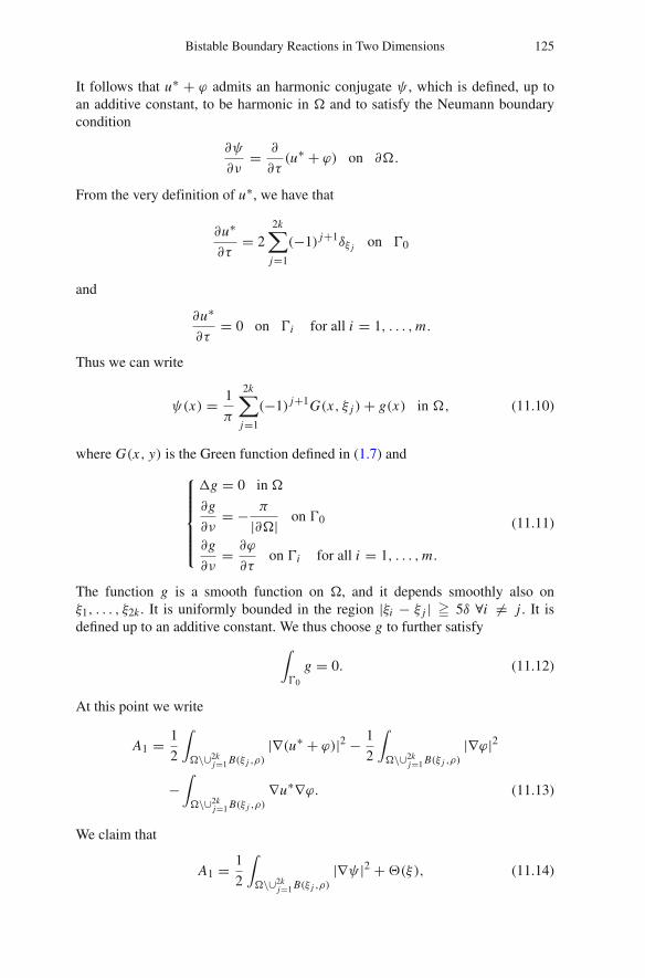
It follows that u∗ + ϕ admits an harmonic conjugate ψ , which is defined, up toan additive constant, to be harmonic in � and to satisfy the Neumann boundarycondition
∂ψ
∂ν= ∂
∂τ(u∗ + ϕ) on ∂�.
From the very definition of u∗, we have that
∂u∗
∂τ= 2
2k∑j=1
(−1) j+1δξ j on �0
and
∂u∗
∂τ= 0 on �i for all i = 1, . . . ,m.
Thus we can write
ψ(x) = 1
π
2k∑j=1
(−1) j+1G(x, ξ j )+ g(x) in �, (11.10)
where G(x, y) is the Green function defined in (1.7) and
⎧⎪⎪⎪⎪⎨⎪⎪⎪⎪⎩
�g = 0 in �
∂g
∂ν= − π
|∂�| on �0
∂g
∂ν= ∂ϕ
∂τon �i for all i = 1, . . . ,m.
(11.11)
The function g is a smooth function on �, and it depends smoothly also onξ1, . . . , ξ2k . It is uniformly bounded in the region |ξi − ξ j | � 5δ ∀i �= j . It isdefined up to an additive constant. We thus choose g to further satisfy
∫�0
g = 0. (11.12)
At this point we write
A1 = 1
2
∫�\∪2k
j=1 B(ξ j ,ρ)
|∇(u∗ + ϕ)|2 − 1
2
∫�\∪2k
j=1 B(ξ j ,ρ)
|∇ϕ|2
−∫�\∪2k
j=1 B(ξ j ,ρ)
∇u∗∇ϕ. (11.13)
We claim that
A1 = 1
2
∫�\∪2k
j=1 B(ξ j ,ρ)
|∇ψ |2 +�(ξ), (11.14)

126 Juan Dávila, Manuel del Pino & Monica Musso
for some explicit function �(ξ) which is smooth and bounded in the region ofpoints ξ = (ξ1, . . . , ξ2k) satisfying |ξi − ξ j | � 5δ ∀i �= j . Indeed estimate (11.14)follows from the following computations, based on integration by parts,
−1
2
∫�
|∇ϕ|2 −∫�
∇u∗∇ϕ = −1
2
∫∂�
∂ϕ
∂νϕ −
∫∂�
∂ϕ
∂νu∗
= −1
2
m∑i �= j
αiα j
∫�i
ϕ j −m∑
i=1
∫�i
∂u∗
∂ν−∫�0
∂ϕ
∂νu∗
where this last expression is a smooth and explicit function of ξ1, . . . , ξ2k , whichis bounded together with its derivatives in the region considered. To conclude with(11.14), we are left to observe that
2k∑j=1
[1
2
∫�∩B(ξ j ,ρ)
|∇ϕ|2 +∫�∩B(ξ j ,ρ)
∇ϕ∇u∗]
=2k∑j=1
[1
2
∫�∩B(ξ j ,ρ)
|∇ϕ|2 +∫�∩∂B(ξ j ,ρ)
∂ϕ
∂νu∗ +
∫∂�∩B(ξ j ,ρ)
∂ϕ
∂νu∗]
= ρ�(ξ).
Given (11.14) and (11.13), we are left with the expansion of 12
∫�\∪2k
j=1 B(ξ j ,ρ)|∇ψ |2.
By (11.10), we write
1
2
∫�\∪2k
j=1 B(ξ j ,ρ)
|∇ψ |2 = 1
2
∫�\∪2k
j=1 B(ξ j ,ρ)
∣∣∣∣∣∣∇⎡⎣ 1
π
2k∑j=1
(−1) j+1G(x, ξ j )
⎤⎦∣∣∣∣∣∣2
+1
2
∫�\∪2k
j=1 B(ξ j ,ρ)
|∇g|2
+∫�\∪2k
j=1 B(ξ j ,ρ)
∇⎡⎣ 1
π
2k∑j=1
(−1) j+1G(x, ξ j )
⎤⎦∇g
= A11 + A12 + A13. (11.15)
The principal part of the above expansion is contained in A11. We start with it. Wewrite
A11 = 1
2π2
⎡⎣ 2k∑
j=1
∫�\∪2k
j=1 B(ξ j ,ρ)
|∇G(x, ξ j )|2
+∑i �= j
∫�\∪2k
j=1 B(ξ j ,ρ)
∇G(x, ξ j )∇G(x, ξi )
⎤⎦ . (11.16)
We start with the first term in (11.16). Fix l ∈ {1, . . . , 2k}. Since ∂G(x,ξl )∂ν
= 0 on �i
for all i = 1, . . . ,m, ∂G(x,ξl )∂ν
= 2π|∂�| on �0\ ∪2k
j=1 B(ξ j , ρ) and∫�0
G(x, ξl) = 0,
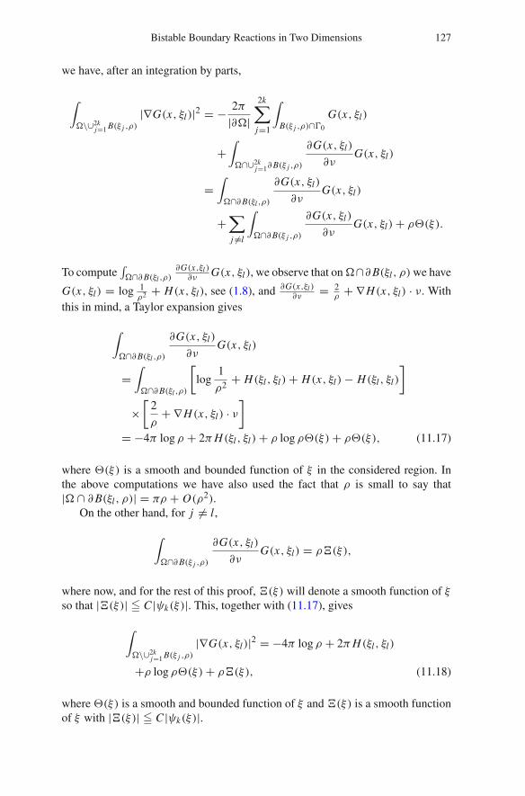
Bistable Boundary Reactions in Two Dimensions 127
we have, after an integration by parts,
∫�\∪2k
j=1 B(ξ j ,ρ)
|∇G(x, ξl)|2 = − 2π
|∂�|2k∑j=1
∫B(ξ j ,ρ)∩�0
G(x, ξl)
+∫�∩∪2k
j=1∂B(ξ j ,ρ)
∂G(x, ξl)
∂νG(x, ξl)
=∫�∩∂B(ξl ,ρ)
∂G(x, ξl)
∂νG(x, ξl)
+∑j �=l
∫�∩∂B(ξ j ,ρ)
∂G(x, ξl)
∂νG(x, ξl)+ ρ�(ξ).
To compute∫�∩∂B(ξl ,ρ)
∂G(x,ξl )∂ν
G(x, ξl), we observe that on�∩∂B(ξl , ρ)we have
G(x, ξl) = log 1ρ2 + H(x, ξl), see (1.8), and ∂G(x,ξl )
∂ν= 2
ρ+ ∇H(x, ξl) · ν. With
this in mind, a Taylor expansion gives
∫�∩∂B(ξl ,ρ)
∂G(x, ξl)
∂νG(x, ξl)
=∫�∩∂B(ξl ,ρ)
[log
1
ρ2 + H(ξl , ξl)+ H(x, ξl)− H(ξl , ξl)
]
×[
2
ρ+ ∇H(x, ξl) · ν
]
= −4π log ρ + 2πH(ξl , ξl)+ ρ log ρ�(ξ)+ ρ�(ξ), (11.17)
where �(ξ) is a smooth and bounded function of ξ in the considered region. Inthe above computations we have also used the fact that ρ is small to say that|� ∩ ∂B(ξl , ρ)| = πρ + O(ρ2).
On the other hand, for j �= l,
∫�∩∂B(ξ j ,ρ)
∂G(x, ξl)
∂νG(x, ξl) = ρ�(ξ),
where now, and for the rest of this proof, �(ξ) will denote a smooth function of ξso that |�(ξ)| � C |ψk(ξ)|. This, together with (11.17), gives
∫�\∪2k
j=1 B(ξ j ,ρ)
|∇G(x, ξl)|2 = −4π log ρ + 2πH(ξl , ξl)
+ρ log ρ�(ξ)+ ρ�(ξ), (11.18)
where �(ξ) is a smooth and bounded function of ξ and �(ξ) is a smooth functionof ξ with |�(ξ)| � C |ψk(ξ)|.
128 Juan Dávila, Manuel del Pino & Monica Musso
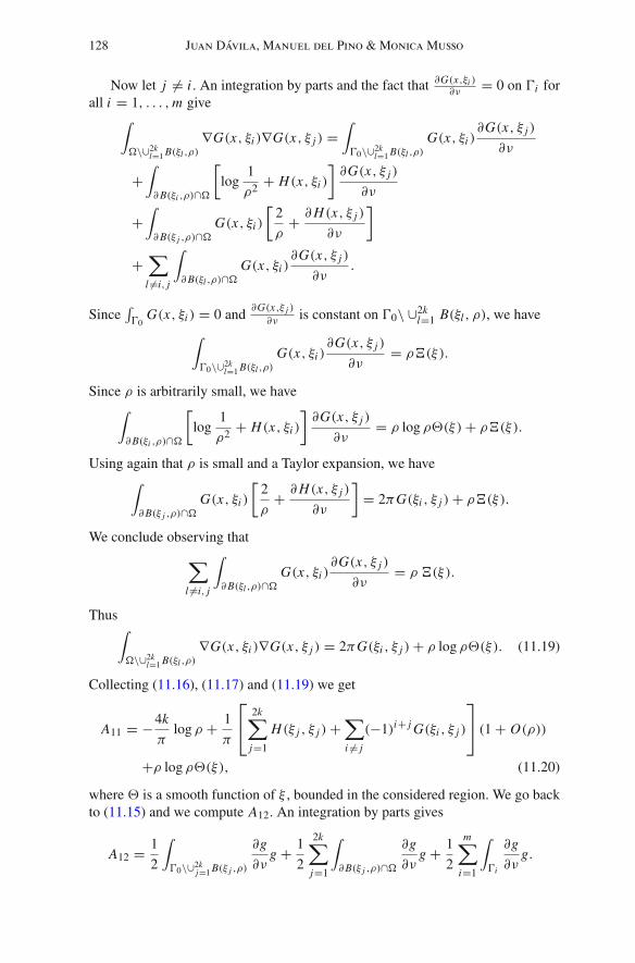
Now let j �= i . An integration by parts and the fact that ∂G(x,ξi )∂ν
= 0 on �i forall i = 1, . . . ,m give∫
�\∪2kl=1 B(ξl ,ρ)
∇G(x, ξi )∇G(x, ξ j ) =∫�0\∪2k
l=1 B(ξl ,ρ)G(x, ξi )
∂G(x, ξ j )
∂ν
+∫∂B(ξi ,ρ)∩�
[log
1
ρ2 + H(x, ξi )
]∂G(x, ξ j )
∂ν
+∫∂B(ξ j ,ρ)∩�
G(x, ξi )
[2
ρ+ ∂H(x, ξ j )
∂ν
]
+∑
l �=i, j
∫∂B(ξl ,ρ)∩�
G(x, ξi )∂G(x, ξ j )
∂ν.
Since∫�0
G(x, ξi ) = 0 and∂G(x,ξ j )
∂νis constant on �0\ ∪2k
l=1 B(ξl , ρ), we have∫�0\∪2k
l=1 B(ξl ,ρ)G(x, ξi )
∂G(x, ξ j )
∂ν= ρ�(ξ).
Since ρ is arbitrarily small, we have∫∂B(ξi ,ρ)∩�
[log
1
ρ2 + H(x, ξi )
]∂G(x, ξ j )
∂ν= ρ log ρ�(ξ)+ ρ�(ξ).
Using again that ρ is small and a Taylor expansion, we have∫∂B(ξ j ,ρ)∩�
G(x, ξi )
[2
ρ+ ∂H(x, ξ j )
∂ν
]= 2πG(ξi , ξ j )+ ρ�(ξ).
We conclude observing that
∑l �=i, j
∫∂B(ξl ,ρ)∩�
G(x, ξi )∂G(x, ξ j )
∂ν= ρ �(ξ).
Thus∫�\∪2k
l=1 B(ξl ,ρ)∇G(x, ξi )∇G(x, ξ j ) = 2πG(ξi , ξ j )+ ρ log ρ�(ξ). (11.19)
Collecting (11.16), (11.17) and (11.19) we get
A11 = −4k
πlog ρ + 1
π
⎡⎣ 2k∑
j=1
H(ξ j , ξ j )+∑i �= j
(−1)i+ j G(ξi , ξ j )
⎤⎦ (1 + O(ρ))
+ρ log ρ�(ξ), (11.20)
where � is a smooth function of ξ , bounded in the considered region. We go backto (11.15) and we compute A12. An integration by parts gives
A12 = 1
2
∫�0\∪2k
j=1 B(ξ j ,ρ)
∂g
∂νg + 1
2
2k∑j=1
∫∂B(ξ j ,ρ)∩�
∂g
∂νg + 1
2
m∑i=1
∫�i
∂g
∂νg.

Bistable Boundary Reactions in Two Dimensions 129
From (11.12) we get∫�0\∪2k
j=1 B(ξ j ,ρ)∂g∂ν
g = ρ�(ξ), from smoothness and bound-
edness of g we get∫∂B(ξ j ,ρ)∩�
∂g∂ν
g = ρ�(ξ). Thus we conclude that
A12 =m∑
i=1
∫�i
∂g
∂νg + ρ�(ξ). (11.21)
Concerning A13, an integration by parts gives
A13 = 1
π
2k∑j=1
(−1) j+1
[− 2π
|∂�|∫�0\∪2k
j=1 B(ξ j ,ρ)
g +∑
i
∫∂B(ξi ,ρ)∩�
∂G(x, ξ j )
∂νg
]
= ρ�(ξ)+ 1
π
2k∑j=1
(−1) j+1∑
i
∫∂B(ξi ,ρ)∩�
∂G(x, ξ j )
∂νg
Now, ∫∂B(ξ j ,ρ)∩�
∂G(x, ξ j )
∂νg =
∫∂B(ξi ,ρ)∩�
[2
ρ+ ∇H(x, ξ j ) · ν
]g
= −2πg(ξ j )+ ρ�(ξ)
while, for i �= j , ∫∂B(ξi ,ρ)∩�
∂G(x, ξ j )
∂νg = ρ �(ξ).
Thus we conclude that
A13 = 22k∑j=1
(−1) j g(ξ j )+ ρ(�(ξ)+�(ξ)). (11.22)
Thus expansion (11.7) follows from (11.14), (11.15), (11.20), (11.21) and (11.22).Formula (11.7) together with (11.6) gives the expansion (11.4). Proof of (11.5). We want to compute, for any j = 1, . . . , 2k,
I j = 1
2
∫�∩B(ξ j ,ρ)
|∇Uε|2.
Let us fix j , say j = 1. Take ρ < δ2 . Hence in each B(ξ j , ρ)we have Uε = Uε+Hε.
Thus
I1 = 1
2
∫B(ξ1,ρ)∩�
∣∣∇Uε∣∣2 + 1
2
∫B(ξ1,ρ)∩�
|∇Hε|2 +∫
B(ξ1,ρ)∩�∇Uε∇Hε
= a + b + c (11.23)
A direct consequence of Proposition 8.3 is that
b = ρ2�(ξ).

130 Juan Dávila, Manuel del Pino & Monica Musso
Formula (11.5) follows then from the following statements
c = Cρ logε
ρ+ ρ2�(ξ)+ O(ε2), (11.24)
where C is a constant and�(ξ) denotes a smooth and bounded function of ξ in theconsidered region, and
a = − 2
πlog
ρ
ε+ A + O(ε), (11.25)
where A is a constant. Proof of (11.24). Since Hε = 0 on ∂� we have
c = −∫�∩B(ξ1,ρ)
�UεHε +∫�∩∂B(ξ1,ρ)
∂Uε∂ν
Hε.
Again using Proposition 8.3, namely that ‖∇Hε‖L∞(�) � C , and formula (8.6),we get
∣∣∣∣∫�∩∂B(ξ1,ρ)
∂Uε∂ν
Hε
∣∣∣∣ � Cρ∫�∩∂B(ξ1,ρ)
1
ε + |z − ξ1| � Cρ.
Now using formula (8.7), we have
∣∣∣∣∫�∩B(ξ1,ρ)
�UεHε
∣∣∣∣ � Cρ∫�∩B(ξ1,ρ)
C
ε2 + |z − ξ1|2 dz � Cρ∫ ρ
ε
0
s
1 + s2 ds
� Cρ log
(1 + ρ2
ε2
).
These facts prove (11.24). Proof of (11.25). We write
a = −1
2
∫�∩B(ξ1,ρ)
Uε�Uε + 1
2
∫�∩∂B(ξ1,ρ)
∂Uε∂ν
Uε + 1
2
∫�0∩B(ξ1,ρ)
∂Uε∂ν
Uε.
(11.26)
Since ρ < δ2 , arguing as in (8.10) we have that in B(ξ1, ρ)
�Uε = �ω+ε = 2k(0)t
(w+ε
)ss − k(0)
(w+ε
)t + O(1).
Thus∣∣∣∣∫�∩B(ξ1,ρ)
Uε�Uε
∣∣∣∣ � C
[ρ
∫B(0,ρ)
∣∣∣D2ω+ε
∣∣∣+∫
B(0,ρ)
∣∣Dω+ε
∣∣+ ρ2].
Using estimate (8.7), we get
ρ
∫B(0,ρ)
∣∣∣D2ω+ε
∣∣∣ � Cρ logε
ρ+ O(ε2),

Bistable Boundary Reactions in Two Dimensions 131
while using (8.6), we get∫
B(0,ρ)
∣∣Dω+ε
∣∣ � Cρ + ε logε
ρ+ O(ε2).
Thus we have ∣∣∣∣12∫�∩B(ξ1,ρ)
Uε�Uε
∣∣∣∣ � C(ρ + ε) logε
ρ+ Cρ.
In a very similar way, one gets
∣∣∣∣12∫�∩∂B(ξ1,ρ)
∂Uε∂ν
Uε
∣∣∣∣ � Cρ
ε + ρ� C.
In order to complete the expansion of (11.26), we need to compute12
∫�0∩B(ξ1,ρ)
∂Uε∂ν
Uε. Since ρ is small and w+ is a solution to (3.1), we write
1
2
∫�0∩B(ξ1,ρ)
∂Uε∂ν
Uε = 1
2
∫�0∩B(ξ1,ρ)
∂w+ε
∂νw+ε (x − ξ1 = εz)
= 1
2
∫�0ε
∩B(0, ρε )
∂w+
∂νw+
= −1
2
(∫ ρε
− ρε
f (w+)w+ dx
)(1 + O(ε)). (11.27)
For simplicity of notation we write w+ = w. We first compute∫ ρε
0 f (w)w dx .Since f (1) = 0, f ′(1) �= 0 and (5.3) we have
∫ ρε
0f (w)w dx = 2
πlog
(ρε
)+ C + O(ε2), (11.28)
where C is a constant. In an analogous way one can prove that
∫ 0
− ρε
f (w)w dx = 2
πlog
(ρε
)+ C + O(ε2), (11.29)
for some constant C , using again that f (−1) = 0, f ′(−1) �= 0 and (5.4). From(11.27), (11.28) and (11.29) we obtain the validity of (11.25), and this concludesthe proof of the Lemma.
We now have all the ingredients needed to give the proof of Theorem 1.1.
Proof of Theorem 1.1. Define, for ξ = (ξ1, . . . , ξ2k) ∈ (�0)2k with |ξi −ξ j | � 5δ,
the function
u(x) = Uε(ξ)(x)+ φ(ξ)(x) x ∈ �

132 Juan Dávila, Manuel del Pino & Monica Musso
where Uε(ξ) is given by (3.10) and φ(ξ) is the unique solution to problem (9.1),whose existence and properties are established in Proposition 9.1. Then, accord-ing to Lemma 10.1, u is solution to (1.1) provided that ξ is a critical point of thefunction Fε(ξ) defined in (10.1), or equivalently, ξ is a critical point of
Fε(ξ) = π
(2k
πlog ε − Fε(ξ)
).
Let �0 be the set of points ξ = (ξ1, . . . , ξ2k) ∈ (�0)2k ordered clockwise and such
that |ξi − ξ j | � 5δ for all i �= j , for some δ > 0 sufficiently small so that all theprevious results hold true. Then, if we denote by p : [0, 2π ] → �0 a continuousparametrization of �0, then we can write
�0 = {ξ = (p(θ1), . . . , p(θ2k)) ∈ (�0)2k : |p(θi )− p(θ j )| � δ if i �= j}.
It is not restrictive to assume that 0 ∈ �0. Lemmas 10.2 and 11.1 guarantee that forξ ∈ �0,
Fε(ξ) = ψk(ξ)+�0(ξ)+ ε�ε(ξ) (11.30)
where �ε is uniformly bounded in the considered region as ε → 0, while �0 issmooth and uniformly bounded, as ε → 0, in the considered region. We will showthat Fε has at least two distinct critical points in this region, a fact that will proveour result. The functionψk is C1, bounded from above in �0 and if two consecutivepoints get closer it becomes unbounded from below, which implies that
ψk(ξ1, . . . , ξ2k) → −∞ as |ξi − ξ j | → 0 for some i �= j.
Hence, since δ is arbitrarily small, ψk has an absolute maximum in �0, and so doesψk +�0, since�0 is uniformly bounded in the region, as ε → 0. Let us call M0 themaximum value ofψk +�0. Thus also Fε has an absolute maximum whenever ε issufficiently small. Let us call this value Mε, so that Mε = M0 + o(1) as ε → 0. Onthe other hand, Ljusternik–Schnirelmann theory is applicable in our setting, so wecan estimate the number of critical points of ψk in �0 by cat(�0), the Ljusternik–Schnirelmann category of �0 relative to �0. We claim that cat (�0) > 1. Indeed, bycontradiction, assume that cat(�0) = 1. This means that �0 is contractible in itself,namely there exist a point ξ0 ∈ �0 and a continuous functionϒ : [0, 1]× �0 → �0such that, for all ξ ∈ �0,
ϒ(0, ξ) = ξ, ϒ(1, ξ) = ξ0.
Let f : S1 → �0 be the continuous function defined by
f (x)=(
p(θ), p
(θ+2π
1
2k
), . . . , p
(θ + 2π
2k − 1
2k
)), x =eiθ , θ ∈[0, 2π ].
Let η : [0, 1] × S1 → S1 be the well defined continuous map given by
η(t, x) = π1 ◦ ϒ(t, f (x))
‖π1 ◦ ϒ(t, f (x))‖
Bistable Boundary Reactions in Two Dimensions 133
where π1 denotes the projection on the first component. The function η is a con-traction of S1 to a point and this gives a contradiction. Thus we conclude that
c0 = supC∈�
infξ∈C
(ψk +�0)(ξ ), (11.31)
where
� = {C ⊂ �0 : C closed and cat (C) � 2},is a finite number, and a critical level for ψk +�0. Call cε the number (11.31) withψk +�0 replaced by Fε, so that cε = c0 +o(1). If cε �= Mε, we conclude that thereare at least two distinct critical points for Fε (distinct up to cyclic permutations)in �0. If cε = Mε, we get that there must be a set C , with cat (C) � 2, where thefunction Fε reaches its absolute maximum. In this case we conclude that there areinfinitely many critical points for Fε in �0. Since cyclic permutations are only infinite number, the result is thus proven.
Acknowledgments. This work has been supported by Fondecyt Grants 1070389, 1080099,1090167 Fondo Basal CMM and CAPDE-Anillo ACT-125. The authors would like to thankXavier Cabre for providing us insight on the renormalized energy of the problem.
Appendix A. Convolution estimates
First we need the following estimate for k defined in (4.4).
Lemma A.1. The kernel k satisfies
k(x1, x2) �{
C(1 + log 1|(x1,x2)| ) if |(x1, x2)| � 1
C 1+x2x2
1+(1+x2)2if |(x1, x2)| � 1
(A.1)
Proof. We write
πk(x1, x2) =∫ 1
0. . . dt +
∫ ∞
1. . . dt.
Then ∫ ∞
1
e−at (x2 + t)
x21 + (x2 + t)2
dt � 1
x21 + (x2 + 1)2
∫ ∞
1e−at (x2 + t) dt
� Cx2 + 1
x21 + (x2 + 1)2
We assume x1 > 0. The integral on the other region is estimated by∫ 1
0
e−at (x2 + t)
x21 + (x2 + t)2
dt �∫ 1
0
x2 + t
x21 + (x2 + t)2
dt =∫ x2+1
x2
t
x21 + t2
dt
=∫ (x2+1)/x1
x2/x1
r
1 + r2 dr = 1
2log
(1 + 2x2 + 1
x21 + x2
2
)
which is bounded by the right-hand side of (A.1).

134 Juan Dávila, Manuel del Pino & Monica Musso
Proof of Lemma 4.1. Using (A.1) we can estimate
|φ| � C(φ1 + φ2)‖h‖αwhere
φ1(x1, x2) =∫ ∞
−∞1 + x2
(x1 − y)2 + (1 + x2)2
1
(1 + |y|)α dy
and
φ2(x1, x2) ={∫ x1+1
x1−11+| log(x1−y)2+x2
2 )|(1+|y|)α dy if x2 � 1
0 if x2 > 1
Directly we have
φ2(x1, x2) � C
(1 + |x1|)α .
To obtain estimates for φ1 we change variables y = (1+ x2)r and define s = x11+x2
.Then
φ1(x1, x2) =∫ ∞
−∞1
(s − r)2 + 1
1
(1 + (1 + x2)|r |)α dr
We can assume x1 � 0 so that s � 0.Case 1. Assume x1 � 1 + x2, that is 0 � s � 1. Write∫ ∞
−∞1
(s − r)2 + 1
1
(1 + (1 + x2)|r |)α dr =∫
|r |� 11+x2
. . . dr +∫
|r |� 11+x2
. . . dr
We have∫|r |� 1
1+x2
1
(s − r)2 + 1
1
(1 + (1 + x2)|r |)α dr �∫
|r |� 11+x2
1
(s − r)2 + 1dr
�C∫
|r |� 11+x2
1
r2+1dr �C
1
1 + x2.
Also ∫|r |� 1
1+x2
1
(s − r)2 + 1
1
(1 + (1 + x2)|r |)α dr
� 1
(1 + x2)α
∫|r |� 1
1+x2
1
((s − r)2 + 1)|r |α dr
But
∫|r |� 1
1+x2
1
((s − r)2 + 1)|r |α dr �
⎧⎪⎨⎪⎩
C if α < 1
C(1 + log(1 + x2)) if α = 1
C(1 + x2)α−1 if α > 1
Bistable Boundary Reactions in Two Dimensions 135
Then
∫|r |� 1
1+x2
1
(s − r)2 + 1
1
(1 + (1 + x2)|r |)α dr �
⎧⎪⎪⎪⎨⎪⎪⎪⎩
C(1+x2)α
if α < 1
C(1+log(1+x2))1+x2
if α = 1
C1+x2
if α > 1
Case 2. Assume x1 � 1 + x2, that is s � 1. We make a further change of variablesr = st and obtain
φ1(x1, x2) = 1
s
∫ ∞
−∞1
(t − 1)2 + 1/s2
1
(1 + x1|t |)α dt
We split the integral in the regions
(a) : |t | � 2, (b) : |t | � 2 and |t − 1| � 1/2 (c) : |t − 1| � 1/2.
In the region (a):
1
s
∫|t |�2
1
(t − 1)2 + 1/s2
1
(1 + x1|t |)α dt � C
sxα1
∫|t |�2
1
|t |2+α dt
� C
sxα1� C
1 + x2
(1 + x1)1+α
In the region (b):
1
s
∫|t |�2, |t−1|�1/2
1
(t − 1)2 + 1/s2
1
(1 + x1|t |)α dt � C
s
∫|t |�2
1
(1 + x1|t |)α dt
� C
s
∫ 2
0
1
(1 + x1t)αdt = C
sx1
∫ 2x1
0
1
(1 + r)αdr = 1
sx1
⎧⎪⎨⎪⎩
Cx1−α1 if α < 1
C log(x1) if α = 1
C if α > 1
Thus
1
s
∫|t |�2, |t−1|�1/2
1
(t − 1)2 + 1/s2
1
(1 + x1|t |)α dt �
⎧⎪⎪⎪⎨⎪⎪⎪⎩
C 1+x2(1+x1)1+α if α < 1
C (1+x2) log(x1)
(1+x1)2if α = 1
C 1+x2(1+x1)2
if α > 1
In the region (c):
1
s
∫|t−1|�1/2
1
(t − 1)2+1/s2
1
(1 + x1|t |)α dt � C
sxα1
∫|t−1|�1/2
1
(t − 1)2 + 1/s2 dt
� C
sxα1
∫ 1/2
0
1
t2 + 1/s2 dt
= C
xα1
∫ s
0
1
1 + r2 dr = C
xα1

136 Juan Dávila, Manuel del Pino & Monica Musso
For the proof of Lemma 4.2 we need the following estimate.
Lemma A.2. If |(x1, x2)| � 1 and |(x1 − y, x2)| � 1 then
|k(x1−y, x2)−k(x1, y)|�C|y||2x1−y|(x2 + 1)(
(x1 − y)2 + (x2 + 1)2) (
x21 + (x2 + 1)2
) (A.2)
Proof.
k(x1 − y, x2)− k(x1, y) = 1
2π
∫ ∞
0e−at (x2 + t)
×[
1
(x1 − y)2 + (x2 + t)2− 1
x21 + (x2 + t)2
]dt
= 1
2π
∫ ∞
0e−at (x2 + t)
(2x1 − y)y
((x1 − y)2 + (x2 + t)2)(x21 + (x2 + t)2)
dt
= 1
2π(I1 + I2)
where I1 = ∫∞1 . . . dt and I2 = ∫ 1
0 . . . dt . We estimate
|I1| =∣∣∣∣∣∫ ∞
1e−at (x2 + t)
(2x1 − y)y((x1 − y)2 + (x2 + t)2
) (x2
1 + (x2 + t)2) dt
∣∣∣∣∣� |2x1 − y| |y|(
(x1 − y)2 + (x2 + 1)2) (
x21 + (x2 + 1)2
)∫ ∞
1e−at (x2 + t) dt
� C|2x1 − y| |y|(1 + x2)(
(x1 − y)2 + (x2 + 1)2) (
x21 + (x2 + 1)2
)
Using the above result, the proof Lemma 4.2 is similar to that of Lemma 4.1 (weomit the details).
Proof of Lemma 4.3. We need to estimate∫ ∞
0
1
(x1 − y)2 + 1
1
(1 + y)αdy =
∫ |x1|
0. . . dy +
∫ ∞
|x1|. . . dy
The first term can be bounded∫ |x1|
0
1
(x1 − y)2 + 1
1
(1 + y)αdy � 1
x21 + 1
∫ |x1|
0
1
(1 + y)αdy.
�
⎧⎪⎨⎪⎩
C if α > 1
C max(log |x1|, 1) if α = 1
C |x1|1−α if α < 1.
The second integral can be estimated as follows:∫ ∞
|x1|1
(x1 − y)2 + 1
1
(1 + y)αdy �
∫ ∞
|x1|1
y2+α dy � C |x1|−1−α.

Bistable Boundary Reactions in Two Dimensions 137
Proof of Lemma 5.3. The solution is given by
u(x, 0) =∫ ∞
0k(x − y, 0) dy
But
k(x, 0) = 1
π
∫ ∞
0
e−at t
x2 + t2 dt
and a calculation shows that ∫ ∞
−∞k(y, 0) dy = 1
a.
Expanding in powers of 1/x ,
k(x, 0) = 1
πx2
∫ ∞
0
e−at t
1 + t2/x2 dt = 1
πa2x2 + O
(1
x4
)as x → ∞.
Therefore as x → ∞∫ ∞
xk(y, 0) dy = 1
πa2x+ O
(1
x3
)
and then
u(x, 0)=∫ ∞
−∞k(y, 0) dy −
∫ ∞
xk(y, 0) dy = 1
a− 1
πa2x+ O
(1
x3
)as x →∞.
Similarly, for x → −∞
u(x, 0) =∫ x
−∞k(y, 0) dy = 1
πa2|x | + O
(1
|x |3).
Proof of Lemma 5.4. We write
u(x, 0) =∫ ∞
1k(x − y)
1
ydy =
∫ x−1
−∞k(y, 0)
1
x − ydy
so that
xu(x, 0) =∫ x−1
−∞k(y, 0)
x
x − ydy =
∫ x−1
−∞k(y, 0)
(1 + y
x − y
)dy
We know already that
∫ x−1
−∞k(y, 0) dy = 1
a+ O
(1
x
)as x → ∞

138 Juan Dávila, Manuel del Pino & Monica Musso
For x � 10 we write
∫ x−1
−∞k(y, 0)
y
x − ydy =
∫ −x
−∞k(y, 0)
y
x − ydy +
∫ √x
−xk(y, 0)
y
x − ydy
+∫ x−1
√x
k(y, 0)y
x − ydy
We estimate the first integral as follows:∣∣∣∣∫ −x
−∞k(y, 0)
y
x − ydy
∣∣∣∣ � C∫ −x
−∞k(y, 0) dy � C
x
The second integral can be bounded by∣∣∣∣∣∫ √
x
−xk(y, 0)
y
x − ydy
∣∣∣∣∣ � C
x
∫ √x
−xk(y, 0)|y| dy � C log(x)
x
Finally
∫ x−1
√x
k(y, 0)y
x − ydy � C
∫ x−1
√x
1
y2
y
x − ydy � C
xlog(
y
x − y)
∣∣∣x−1√
x� C log(x)
x.
This proves
u(x, 0) = 1
ax+ O
(log(x)
x2
)as x → ∞.
The estimate
u(x, 0) = O
(log(|x |)
x2
)as x → −∞
follows from Lemma 4.3.
Appendix B. An estimate for the gradient of a harmonic function
Let B1 be the unit ball in RN . We write x ∈ R
N as x = (x ′, t)with x ′ ∈ RN−1, t ∈
R. Define
B+1 = {(x ′, t) ∈ B1 : t > 0}� = {(x ′, t) ∈ B1 : t = 0}.
Lemma B.1. There exists C = C(N ) such that if u ∈ C2(B+1 ) is harmonic in B+
1 ,then
supB+
1/2
|∇u| � C
⎛⎝sup
�
|∇u| + supB+
1
|u|⎞⎠ .

Bistable Boundary Reactions in Two Dimensions 139
Proof. Let η ∈ C20 (R
N ) with support contained in B1, η � 0 such that η > 0 in
the ball of radius 3/4 and such that |∇η|2η
is bounded. For example, η(r) = ( 34 − r)3
for r ∈ ( 12 ,
34 ) will work. Let M > 0 be such that
2M +�η − 2|∇η|2η
> 0 in the region where η > 0. (B.1)
Let v = |∇u|2η + Mu2. We claim that either
maxB
+1
v � max�v (B.2)
or
maxB
+1
v � M maxB1
u2. (B.3)
If either of these estimates hold we obtain the conclusion of the lemma.Suppose that (B.2) fails. Then max
B+1v is attained at a point x0 ∈ ∂B1 ∩ R
2+ or a
point x0 ∈ B+1 . If x0 ∈ ∂B1 ∩ R
2+ then η(x0) = 0 and so (B.3) holds.Assume now x0 ∈ B+
1 . In this situation η(x0) > 0. Let us use the notation ui = ∂u∂xi
and the convention of summation over repeated indices. Then we may compute
v j = 2ui ui jη + u2i η j + 2Muu j
�v = v j j = 2u2i jη + 4ui ui jη j + u2
i η j j + 2Mu2j
� 2u2i jη − 2u2
i jη − 2u2i
η2j
η+ u2
i η j j + 2Mu2j
Since at x0 we have �v(x0) � 0 we deduce
0 � |∇u(x0)|2(
−|∇η(x0)|2η(x0)
+�η(x0)+ 2M
).
By (B.1) ∇u(x0) = 0 and this shows that
maxB
+1
v = v(x0) = Mu(x0)2 � M max
B1
u2.
References
1. Alberti, G., Bouchitté, G., Seppecher, P.: Un résultat de perturbations singulièresavec la norme H1/2. C. R. Acad. Sci. Paris Sér. I Math. 319(4), 333–338 (1994)
2. Alberti, G., Bouchitté, G., Seppecher, P.: Phase transition with the line-tensioneffect. Arch. Rational Mech. Anal. 144(1), 1–46 (1998)
3. Amick, C.J., Toland, J.F.: Uniqueness of Benjamin’s solitary-wave solution of theBenjamin–Ono equation. IMA J. Appl. Math. 46(1–2), 21–28 (1991)
140 Juan Dávila, Manuel del Pino & Monica Musso
4. Amick, C.J., Toland, J.F.: Uniqueness and related analytic properties for the Benja-min–Ono equation—a nonlinear Neumann problem in the plane. Acta Math. 167(1–2),107–126 (1991)
5. Bryan, K., Vogelius, M.: Singular solutions to a nonlinear elliptic boundary value prob-lem originating from corrosion modeling. Quart. Appl. Math. 60(4), 675–694 (2002)
6. Cabré, X., Cònsul, N.: Minimizers for boundary reactions: renormalized energy, loca-tion of singularities, and applications (in preparation)
7. Cabré, X., Solà-Morales, J.: Layer solutions in a half-space for boundary reactions.Comm. Pure Appl. Math. 58(12), 1678–1732 (2005)
8. Cónsul, N., Solà-Morales, J.: Stability of local minima and stable nonconstant equi-libria. J. Differential Equations 157(1), 61–81 (1999)
9. Dávila, J., del Pino, M., Musso, M., Wei, J.: Singular limits of a two-dimensionalboundary value problem arising in corrosion modeling. Arch. Ration. Mech. Anal. 182,181–221 (2006)
10. Gilbarg, D., Trudinger, N.S.: Elliptic partial differential equations of second order.Reprint of the 1998 edition. Classics in Mathematics. Springer, Berlin, 2001
11. Kohn, R.V., Slastikov, V.V.: Another thin-film limit of micromagnetics. Arch. Ration.Mech. Anal. 178(2), 227–245 (2005)
12. Kurzke, M.: A nonlocal singular perturbation problem with periodic well potential.ESAIM Control Optim. Calc. Var. 12(1), 52–63 (2006)
13. Kurzke, M.: Boundary vortices in thin magnetic films. Calc. Var. Partial DifferentialEquations 26(1), 1–28 (2006)
14. Toland, J.F.: The Peierls–Nabarro and Benjamin–Ono equations. J. Funct. Anal.145(1), 136–150 (1997)
Departamento de Ingeniería Matemática and CMM,Universidad de Chile, Casilla 170 Correo 3,
Santiago, Chile.e-mail: [email protected]
and
Departamento de Ingeniería Matemática and CMM,Universidad de Chile, Casilla 170 Correo 3,
Santiago, Chile.e-mail: [email protected]
and
Departamento de Matemáticas,P. Universidad Católica de Chile,
Santiago, Chile.e-mail: [email protected]
(Received October 27, 2009 / Accepted June 7, 2010)Published online July 7, 2010 – © Springer-Verlag (2010)
Related Documents


