Bipolar Device Modeling Bipolar Processclass.ece.iastate.edu/ee330/lectures/EE 330 Lect 19 Spring 2013.pdf · Bipolar transistor can be thought of a current amplifier with a large

EE 330

Lecture 19

Bipolar Device Modeling

Bipolar Process

Basic Devices and Device Models

• Resistor

• Diode

• Capacitor

• MOSFET

• BJT

Review from Last Lecture

Bipolar Junction Transistors

Operation and Modeling


Bipolar Transistors

npn stack pnp stack

E E

B B

C C

With proper doping and device sizing these form Bipolar Transistors

pnp transistor

B

C

E

npn transistor

B

C

E

• Bipolar Devices Show Basic

Symmetry

• Electrical Properties not

Symmetric

• Designation of C and E critical


Bipolar Operation

npn stack

E

B

C

Consider npn transistor

F1

F2

So, what will happen?

Some will recombine with holes and contribute to base current and some will

be attracted across BC junction and contribute to collector

Size and thickness of base region and relative doping levels will play key role in

percent of minority carriers injected into base contributing to collector current


Bipolar Operation

npn stack

E

B

C Under forward BE bias and reverse BC bias current flows into base region


Efficiency at which minority carriers injected into base region and contribute to

collector current is termed α

α is always less than 1 but for a good transistor, it is very close to 1

For good transistors .99 < α < .999 Making the base region very thin makes α large


Bipolar Operation

npn stack

E

B

C


In contrast to MOS devices where current flow in channel is by majority carriers,

current flow in the critical base region of bipolar transistors is by minority carriers


Bipolar Operation

IC

IE

IB

E

B

C BC II

β is typically very large

Bipolar transistor can be thought of a current amplifier with a large current gain

In contrast, MOS transistor is inherently a tramsconductance amplifier

Current flow in base is governed by the diode equation t

BE

V

V

B eI SI~

t

BE

V

V

C eI SI~

Collector current thus varies exponentially with VBE


Simple dc model IC C

E

BIB

VBE

VCE

t

BE

V

V

B eI SI~

t

BE

V

V

C eI SI~

q

kTVt

Summary:

This has the properties we are looking for but the variables we used

in introducing these relationships are not standard

SI~

It can be shown that is proportional to the emitter area AE

Define and substitute this into the above equations ESAJ1~ SI


Simple dc model

t

BE

V

V

B eI SI~

t

BE

V

V

C eI SI~

q

kTVt

t

BE

V

V

ESB e

β

AJI

t

BE

V

V

ESC eAJI

q

kTVt

JS is termed the saturation current density

Process Parameters : JS,β

Design Parameters: AE

Environmental parameters and physical constants: k,T,q

At room temperature, Vt is around 26mV

JS very small – around .25fA/u2


Simple dc model

VBE or IB

Typical Output Characteristics

0

50

100

150

200

250

300

0 1 2 3 4 5

Vds

Id

IC

VCE

Forward Active

Saturation

Cutoff

Forward Active region of BJT is analogous to Saturation region of MOSFET

Saturation region of BJT is analogous to Triode region of MOSFET


Simple dc model

0

50

100

150

200

250

300

0 1 2 3 4 5

Vds

Id

IC

VCE

VBE or IB

t

BE

V

V

ESC eAJI

Output Characteristics in Forward Active Region

Simple dc model Better Model of Output Characteristics

IC

VCE

VBE or IB

BJT and MOSFET Comparison

IC

VCE

VBE or IB

• Same general characteristics

• Spacings a bit different (Exponetial vs square law)

• Slope steeper for small VCE , VDS

ID

VDS

VGS

Simple dc model

VBE or IB

Typical Output Characteristics

0

50

100

150

200

250

300

0 1 2 3 4 5

Vds

Id

IC

VCE

Projections of these tangential lines all intercept the –VCE axis at the same

place and this is termed the Early voltage, VAF (actually –VAF is intercept)

Typical values of VAF are in the 100V range

Simple BJT dc model Typical Output Characteristics

IC

VCE

VBE or IB


IC

VCE

VBE or IB

Saturation

Forward Active

Cutoff


Forward Active region of BJT is analogous to Saturation region of MOSFET

Saturation region of BJT is analogous to Triode region of MOSFET

IC

VCE

VBE or IB

Saturation

Forward Active

Cutoff

Saturation

Cutoff

ID

VDS

VGS

Triode

Simple dc model

VBE or IB

Improved Model

0

50

100

150

200

250

300

0 1 2 3 4 5

Vds

Id

IC

VCE

AF

CEV

V

SCV

V1eJI t

BE

t

BE

V

V

ESB e

β

AJI

Valid only in Forward Active Region

Simple dc model

VBE or IB

Improved Model

0

50

100

150

200

250

300

0 1 2 3 4 5

Vds

Id

IC

VCE

Valid in All regions of operation

11 t

BC

t

BE

V

V

S

V

V

F

SE eJe

JI E

E AA

11 t

BC

t

BE

V

V

SV

V

SC eJ

eJIR

EE

AA

q

kTVt

Not mathematically easy to work with

Note dependent variables changes

Termed Ebers-Moll model

VAF effects can be added

Reduces to previous model in FA region

Simple dc model

11 t

BC

t

BE

V

V

S

V

V

F

SE eJe

JI E

E AA

11 t

BC

t

BE

V

V

SV

V

SC eJ

eJIR

EE

AA

q

kTVt

Ebers-Moll model

Process Parameters: {JS, αF, αR}

Design Parameters: {AE}

αF is the parameter α discussed earlier

αR is termed the “reverse α”

F

F

F

αβ =

1-αR

R

R

αβ =

1-α

JS ~10-16A/μ2 βF~100, βR~0.4

Typical values for process parameters:

FF

F

βα =

1+βR

RR

βα =

1+β

Completely

dominant!

Simple dc model

11 t

BC

t

BE

V

V

S

V

V

F

SE eJe

JI E

E AA

11 t

BC

t

BE

V

V

SV

V

SC eJ

eJIR

EE

AA

q

kTVt

Ebers-Moll model

JS ~10-16A/μ2 βF~100, βR~0.4

With typical values for process parameters in forward active

region (VBE~0.6V, VBC~-3V), with Vt=26mV and if AE=100μ2:

11 t

BC

t

BE

V

V

SV

V

SC eJ

eJIR

EE

AA

1410 1 128

-14

10 -51

C

10I 1.05x10 7.7x10

.

Makes no sense to keep anything other than BE

t

V

V

C SI J e

EA

in forward active

Simple dc model

11 t

BC

t

BE

V

V

S

V

V

F

SE eJe

JI E

E AA

11 t

BC

t

BE

V

V

SV

V

SC eJ

eJIR

EE

AA

q

kTVt

Ebes-Moll model

Alternate equivalent expressions for dependent variables {IC, IB} defined

earlier for Ebers-Moll equations in terms of independent variables {VBE, VCE}

after dropping the “-1” terms

1CEBE

t t

-VV

V VR

C S E

R

1+βI J A e e

β

CEBE

t t

-VV

V V

B S E

F R

1 1I J A e - e

β β

No more useful than previous equation but in form consistent with notation

Introduced earlier

Simple dc model Simplified Multi-Region Model

IC

VCE

VBE1

VBE2

VBE3

VBE4

VBE5

IC

VCE

VBE1

VBE2

VBE3

VBE4

VBE5

VCESAT

Ebers-Moll Model Simplified Multi-Region Model

VBE=0.7V

VCE=0.2V Saturation

• Observe VCE around 0.2V when saturated

• VBE around 0.6V when saturated

• In most applications, exact VCE and VBE

voltage in saturation not critical


IC

VCE

VBE1

VBE2

VBE3

VBE4

VBE5

IC

VCE

VBE1

VBE2

VBE3

VBE4

VBE5

VCESAT

Ebers-Moll Model Simplified Multi-Region Model

1CEBE

t t

-VV

V V CER

C S E

R AF

V1+βI J A e e 1+

β V

AF

CEV

V

ESCV

V1eAJI t

BE

VBE=0.7V

VCE=0.2V

IC=IB=0

CEBE

t t

-VV

V V

B S E

F R

1 1I J A e - e

β β

t

BE

V

V

ESB e

β

AJI

Forward

Active

Saturation

Cutoff


AF

CEV

V

ESCV

V1eAJI t

BE

t

BE

V

V

ESB e

β

AJI

q

kTVt

VBE=0.7V

VCE=0.2V

IC=IB=0

Forward Active

Saturation

Cutoff


AF

CEV

V

ESCV

V1eAJI t

BE

t

BE

V

V

ESB e

β

AJI

q

kTVt

VBE=0.7V

VCE=0.2V

IC=IB=0

Forward Active

Saturation

Cutoff

VBE>0.4V

VBC<0

IC<βIB

VBE<0

VBC<0

A small portion of the operating region is missed with this model but seldom operate in

the missing region

Simple dc model Equivalent Simplified Multi-Region Model

AF

CEBC

V

V1βII

t

BE

V

V

ESB e

β

AJI

q

kTVt

VBE=0.7V

VCE=0.2V

IC=IB=0

Forward Active

Saturation

Cutoff

VBE>0.4V

VBC<0

IC<βIB

VBE<0

VBC<0


the missing region

Simplified dc model Forward Active

βIB

IBB C

EE

B

C

βIB

IBB C

E

βIB

IBB C

E

0.6V

Adequate when it makes little difference whether VBE=0.6V or VBE=0.7V

Simplified dc model Forward Active

βIB

IBB C

E

βIB

IBB C

E

0.6V

Mathematically

VBE=0.6V

IC=βIB

VBE=0.6V

IC=βIB(1+VCE/VAF)

Or, if want to show slope in IC-VCE characteristics

AFDS

CQ

VR =

I

RDS highly nonlinear

BC II

CB

E

RDS

IB

0.6V

Simplified dc model Equivalent Simplified Multi-Region Model

C BI βI

BEV 0.6V

q

kTVt

VBE=0.7V

VCE=0.2V

IC=IB=0

Forward Active

Saturation

Cutoff

VBE>0.4V

VBC<0

IC<βIB

VBE<0

VBC<0


the missing region

Conditions for Regions of Operation in Multi-Region Model

Note: One condition is on dependent variables !

VBE>0.4V

VBC<0 Forward Active

IC<βIB Saturation

VBE<0

VBC<0 Cutoff

Observe that in saturation, IC<βIB

Can’t condition on independent variables in saturation because they are

fixed in the model

Seldom operate in regions excluded in this picture

Regions of Operation in Independent Parameter Domain used

In multi-region models

VBC

VBE

0.4V

0.4V

Forward Active

CutoffReverse Active

Saturation

Excessive Power Dissipation if either junction has large forward bias

VBC

VBE

0.4V

0.4V

Forward Active

Cutoff

Re

ve

rse

Activ

e

Saturation

Melt D

own !!

Saturation

Safe regions of operation

VBC

VBE

0.4V

0.4V

Forward Active

Cutoff

Re

ve

rse

Activ

e

Saturation

Melt D

own !!

SaturationSimplified Forward

Saturation

Actually cutoff, forward active, and reverse active regions can be extended

modestly as shown and multi-region models still are quite good

VBC

VBE

0.4V

0.4V

Forward Active

Cutoff

Re

ve

rse

Activ

e

Saturation

Melt D

own !!

SaturationSimplified Forward

Saturation

Sufficient regions of operation for most applications

VBC

VBE

0.4V

0.4V

Forward Active

Cutoff

Re

ve

rse

Activ

e

Saturation

Simplified Forward

Saturation

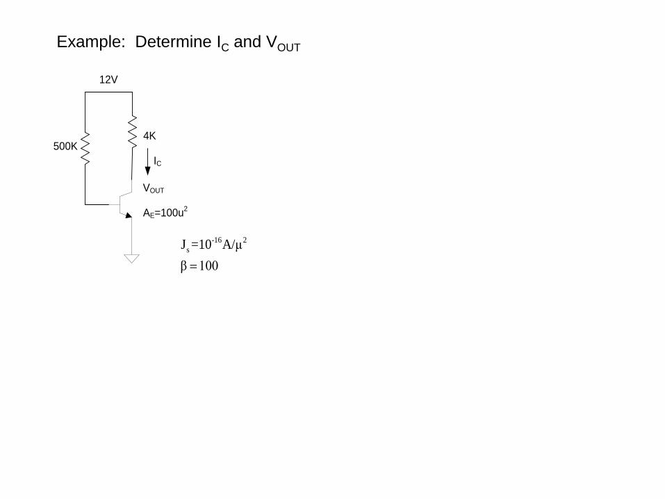
Example: Determine IC and VOUT

12V

4K500K

IC

VOUT

AE=100u2

-16 2

sJ =10 A/μ

β 100

Example: Determine IC and VOUT , assume C is large and VIN is very small.

12V

4K50K

IC

VOUT

AE=100u2

-16 2

sJ =10 A/μ

β 100

Example: Determine IC and VOUT. Assume C is large and VIN is very small.

12V

4K500K

IC

VOUT

AE=100u2

VIN

C

-16 2

sJ =10 A/μ

β 100

End of Lecture 19

Bipolar Device Modeling Bipolar Processclass.ece.iastate.edu/ee330/lectures/EE 330 Lect 19 Spring 2013.pdf · Bipolar transistor can be thought of a current amplifier with a large

Documents