BioUML plug-in for nonlinear parameter estimation using multiple experimental data

Journal InformationJournal ID (publisher-id): vb

Title: Virtual Biology

ISSN (electronic): 2306-8140

Article InformationPublication date (electronic): 25 March 2013

Electronic Location Identifier: e10

DOI: 10.12704/vb/e10

BioUML plug-in for nonlinear parameterestimation using multiple experimental data

Elena Kutumova1, 2 , Anna Ryabova1 , Tagir Valeev1, 3 , Fedor Kolpakov1, 2

[1] Institute of Systems Biology, Ltd, Novosibirsk, Russia

[2] Design Technological Institute of Digital Techniques SB RAS, Novosibirsk, Russia

[3] Institute of Informatics Systems SB RAS, Novosibirsk, Russia

Abstract Motivation: Systems biology deals with many different types of experimental data representingindividual components of biological systems. Behavior of these systems over time could bedescribed using systems of ordinary differential equations (ODE). In order to analyze dynamicsof the ODEs and estimate their parameters based on data obtained in different experimentalconditions, biologists need a flexible framework that allows them to create dynamic models andperform multi-experiment parameter fitting.

Results: We present optimization tools of the BioUML software (http://biouml.org) developedfor modeling and analysis of biochemical systems. We created optimization plug-in to solvenon-linear optimization problems via minimization of the function of deviations betweenexperimental data and model simulation results. Experimental data can be considered as separatesets of time courses or steady states stored in different tab-separated files. BioUML includesseveral deterministic and stochastic optimization methods which find reasonably accuratesolutions faster than the COPASI software. Some of these methods provide constrainedoptimization and some of them were parallelized.

Keywords BioUML, parameter estimation, multi-experiment parameter fitting

IntroductionDevelopment of experimental technologies in molecular biology led to accumulation of huge volumes of data relating tovarious levels of life organization. However, the data alone cannot be used to reconstruct the full organization ofbiological systems. Therefore, the interests of bioinformatics are now focused on the problems of data processing,including the problems of integration and systematization of primary experimental data and the problems of knowledgeproduction based on mathematics and modern information technologies. The challenge of systems biology isconstruction of mathematical models to describe dynamic behavior of biological systems based on experimental data.Such problems involve studying a large volume of data and require software for their processing and interpreting.

The standard tools for working with biological data include access to biological databases, formalized description ofbiological systems, as well as visualization, simulation, parameter fitting and analysis of ODE models representing thesesystems. The BioUML software is an integrated environment that was developed to span all of these capabilities. Here wepresent optimization tools of this software intended for multi-experiment training of the models created using BioUMLnotation or imported in the SBML format [Hucka et al, 2003]. These tools are available both in the desktop and webeditions of BioUML.

Optimization problem in BioUMLThe general nonlinear optimization problem [Runarsson and Yao, 2000] can be formulated as follows: find a minimum ofthe objective function ϕ(x), where x lies in the intersection of the N-dimensional search space

Ω = {y ∈ ℝN || yi

≤ yi ≤ yi , yi

, yi ∈ ℝ, i = 1, …, N},

and the admissible region ℱ ⊆ ℝN defined by a set of equality and/or inequality constraints on x. Since the equalitygs(x) = 0 can be replaced by two inequalities gs(x) ≤ 0 and – gs(x) ≤ 0, the admissible region can be defined withoutloss of generality as

1

ℱ = {y ∈ ℝN || gs(y) ≤ 0, s = 1, …, p} .

In order to get solution situated inside ℱ, we minimize the penalty function

ψ(x) = ∑i= 1

s

max{0, gs(x)}2 .

The problem could be solved by different optimization methods. We implemented the following of them in the BioUMLsoftware:

stochastic ranking evolution strategy (SRES) [Runarsson and Yao, 2000];

cellular genetic algorithm MOCell [Nebro et al, 2009];

particle swarm optimization (PSO) [Sierra and Coello, 2005];

deterministic method of global optimization glbSolve [Björkman and Holmström, 1999];

adaptive simulated annealing (ASA) [Ingber, 1996].

Table 1 shows the generic scheme of the optimization process for these methods. SRES, MOCell, PSO and glbSolve run

a predefined number of iterations Nit considering a sequence of sets (populations) P i, i = 0, …, Nit − 1, of potential

solutions (guesses). In the case of the first three methods, the size s ∈ ℕ + of the population is fixed, whereas in glbSolve

the initial population P0 consists of one guess, while the size sk+ 1 of the population Pk+1 is found during the iteration

with the number k = 0, …, Nit − 1. The method ASA considers sequentially generated guesses xk ∈ Ω, k ∈ ℕ + , and

stops if distance between xk and xk+ 1 defined as Euclidean norm xk − xk+ 1 = ∑i = 1

Nxi

k − xik+ 1

2√ becomes less

than a predefined accuracy ε.

Table 1. An overview of the optimization process for methods SRES, MOCell, PSO, glbSolve and ASA.

Step SRES, MOCell, PSO glbSolve ASA

1 Set k = 0.

2

Generate P0 = {xi0 ∈ Ω, i = 1, …, s}, s ∈ ℕ + .

Find the best guess y ∈ P0.

Set xmin = y.

Generate

P0 = {x0 ∈ Ω}.

Set xmin = x0.

Generate x0 ∈ Ω.

Set xmin = x0, err = + ∞.

3 Evaluate values of the functions ϕ and ψ for all guesses P0 . Evaluate ϕx0 and ψx

0.

4If a predefined number of iterations Nit is passed, then go to step 9,

otherwise go to step 5.If err < ε, where ε is a predefined accuracy,then go to step 9, otherwise go to step 6.

5 Set sk+ 1 = s.Find sk+ 1 for the

current iteration.–

6 Generate Pk+ 1 = {xik+ 1 ∈ Ω, i = 1, …, sk+ 1}. Generate xk+ 1 ∈ Ω.

7Evaluate values of the functions ϕ and ψ

for all guesses Pk+ 1 .

Evaluate ϕxk+1

and ψxk+ 1

.

Set err = xk − xk+ 1 .

8 Update xmin . Increment value k by one, go back to step 4.

9 Return xmin as the solution.

All methods, excepting glbSolve, are stochastic and seek global minimum of the function ϕ taking into account theadmissible region ℱ. Thus, a guess x ∈ Ω is more preferable than a guess y ∈ Ω at some iteration of methods, ifψ(x) = 0 and ψ(y) ≠ 0 or ψ(x) < ψ(y). The method glbSolve is suited to solve only the problems with Ω ⊆ ℱ. Valuesof the function ψ are calculated but do not affect on the generation of potential solutions.

Implementing the optimization scheme in BioUML, we designed the OptimizationProblem interface (fig. 1) comprisingthe following procedures:

getParameters specifies a list of parameters to fit including identification of initial values and variation intervals(upper and lower bounds);

testGoodnessOfFit defines type of the functions ϕ and ψ and evaluates their values for a population of guesses;

getEvaluationsNumber returns the number of passed evaluations during optimization process.

An abstract class OptimizationMethod provides the number of subclasses representing implementation of the foregoingmethods. These subclasses involve search of optimal parameters by calling a procedure getSolution depending on thesettings of optimization problem.

2

(1)

(2)

(3)

(4)

(5)

Figure 1. The class diagram representing implementation of the optimization process in BioUML.

Application of non-linear optimization to systems biologyWe assume that a mathematical model of some biological process consists of a set of chemical species S = {S1 , …, Sm}associated with variables C(t) = (C1(t), …, Cm(t)) representing their concentrations, and a set of biochemical reactions

ℛ = {R1 , …, Rn} with rates v(t) = (v1(t), …, vn(t)) depending on a set of kinetic constants K. Reaction rates are modeledby standard laws of chemical kinetics. A Cauchy problem for ordinary differential equations representing a linearcombination of reaction rates is used to describe the model behavior over time:

dC(t)dt

= N ⋅ v(C, K , t), C(0) = C0 .

Here N is a stoichiometric matrix of n by m. We say that C ss is a steady state of the system (1) if

N ⋅ v(C ss , K , t) = 0, limt→∞

Ci(t) = Ciss.

Identification of parameters K and initial concentrations C0 is based on experimental data represented by a set of points

Ci

exp(ti j) defining dynamics of variables C1(t), …, Cl(t), l ≤ m, at given times ti j , j = 1, …, ri, where ri is the number of

such points for the concentration Ci(t), i = 1, …l. The problem of parameter identification consists in minimization of thefunction of deviations defined as the normalized sum of squares [Hoops et al, 2006]:

ϕ(C0 , K) = ∑i = 1

l ∑j = 1

ri ωminωi

⋅ Ci(ti j) − Ci

exp(ti j)2

,

where normalization factors ωmin /ωi with ωmin = mini

ωi are used to make all concentration trajectories have similar

importance. The weights ωi are calculated by one of the formulas on experimentally measured concentrations:

ωi

sq = ri−1 ⋅ ∑

jCi

exp(ti j)2

√ (mean square value), ωimean =

|||ri

−1 ⋅ ∑jCi

exp(ti j)||| (mean value) and

ωist = ω

i

sq⋅ω

i

sq − ωimean ⋅ω

imean√ (standard deviation).

If we want to consider additional constrains

gs(C, K) ≤ 0, s = 1, …, p,

holding for concentrations C(t) and parameters K for some period of time t ∈ tsstart , ts

end, the penalty function is

defined as

ψ(C0 , K) = ∑s = 1

p

∑t = ts

0tsend

max{0, gs(C,K)}

tsend − ts

start + 1

2

.

This function assumes summation of values gs(C, K) in the nodes of grid defined by an ODE solver to find a numericalsolution of the system (1).

In the particular case, experimental data could be represented by steady state values of species concentrations. Thenfunctions ϕ and ψ have the simpler forms:

ϕ(C0 , K) = ∑i = 1

l ωminωi

⋅ Ciss − C

i

exp_ss

2 , ψ(C0 , K) = ∑

s = 1

p

(max{0, gs(C ss , K)})2

where Ci

exp_ss and Ciss, i = 1, …, l, denote experimental and simulated steady state values.

Typically, researchers want to perform evaluation of model parameters using experimental data obtained with different

experimental conditions, i.e. different initial concentrations C01 , …, C0k of species. In such case, we will consider thefunctions

ϕC01 , …, C0k , K = ∑

i= 1

k

ϕ(C0i , K) and ψC01 , …, C0k , K = ∑

i = 1

k

ψ(C0i , K).

3

Implementation of the parameter estimation process in BioUMLInitiation of the parameter estimation process requires definition of many details including specification of the searchspace, the admissible region, settings of numerical methods to solve ODE system and optimization problem, links to thefiles with experimental data and model description, etc. In order to structure this information, we designed an appropriatehierarchy of classes (fig. 2) taking into account the following rules:

experimental data must be represented by time-courses or steady states of chemical species concentrations; in thefirst case, these data may be expressed as percentage values obtained, for example, on the basis of theWestern-blot technology;

an initial state of the Cauchy problem must be specified for each considered file with experimental data (thesestates may be different for some experiments);

parameters to fit may be divided into local and global:

the local parameters can take different values for some groups of experiments (for example, conductedfor different cell lines);

the global parameters have the same value for all experiments.

The main class Optimization in fig. 2 comprises definition of the optimization method and parameters including themodel parameters to fit, parametric constraints holding for given time intervals, and experiments. The following fieldskeep information about each experiment:

cellLine defines an experimental group to evaluate local parameters of the model;

diagramStateName corresponds to the model initial state;

experimentType defines the time-course or steady state type of experimental data;

tableSupport contains the link to the file with experimental data, and specifies a method for calculation of weightsωi in the formula (2);

parameterConnections is a list of correspondences between variable names in the model and in the experimentalfile including information whether data in this file are expressed as exact values or as values related to a given timepoint.

Figure 2. The class diagram of the optimization plug-in in BioUML.

An object of the OptimizationMethod class contains a set of parameters (methodParameters) including links to the filewith the processed model (diagramPath) and the directory to save results when the parameter estimation will becompleted (resultPath). The estimation process begins immediately after the object control gets command doRun.Goodness of the current fit is defined through the object optimizationProblem providing correct simulation of the model.Firstly, evaluation of functions (2) and (4) is performed separately for all initial states of the model by calling a methodtestGoodnessOfFit for each object of the class SingleExperimentParameterEstimation associated with the certainexperiment. Then the total values of these functions are calculated in the class ParameterEstimationProblem by theformulas (5).

The parameter estimation process is optimized using the following technologies:

Acceleration of simulation of the Cauchy problem for different values of fitted parameter is achieved byautomatic generation and compilation of the Java class file at the first iteration of the optimization algorithm. Atthe subsequent iterations, current values are passed to the object of this compiled class and a solution of theCauchy problem is found.

1.

Acceleration of the optimization methods considering a population of guesses is achieved by parallelization ofcalculations. The following task (SimulationTask in fig. 2) is generated for each guess:

2.

4

find a solution or a steady state of the system (1) for the adjustable parameter values;

evaluate values of the objective function (2) and the penalty function (4)When all tasks are generated, they are passed to the executor service, which distributes their performancebetween the predefined threads.

Fig. 3 shows a graphical user interface of optimization methods in the BioUML workbench (desktop edition). The upperleft panel includes a list of methods. Description of the selected method is provided below. The upper right panel definesthe search space. Under it you can find the tab panel with settings of optimization problem. In fig. 3 the selected tabcontains method parameters and fields displaying intermediate values of objective/penalty functions and the number ofpassed evaluations. The next tab includes description of experimental data and specifies settings for all experiment fieldslisted above.

Figure 3. The user interface of the optimization plug-in provided by the BioUML software.

Web edition optimizationBioUML web edition (http://ie.biouml.org/bioumlweb/) is a web application providing access to BioUML tools and datavia the Internet. The user can manipulate the data stored on the BioUML server and run analyses through the webbrowser. The web interface is a set of HTML pages with interactive JavaScript content. Ajax technology is used tocommunicate with the server and process user activities without page reloading.

The web edition provides a set of optimization tools, like in the workbench edition. The user can set up the boundariesand initial values of optimization parameters, select and adjust an optimization method, manage experimental data, set upconstraints. After all parameters are adjusted, optimization process can be launched. Optimization results can be savedand then viewed as a table of fitted parameter values. Graphical representation of the optimization process is alsoavailable.

Analysis of the methods convergenceStochastic methods (SRES, MOCell, PSO and ASA) for global optimization rely on probabilistic approaches and haveweak theoretical guarantees of convergence to the global optimum. However, they can locate its vicinity with relativeefficiency [Moles et al, 2003]. In contrast, deterministic method glbSolve guarantees global optimality, if the objectivefunction is continuous or at least continuous in the neighborhood of a global optimum [Björkman and Holmström, 1999].However, it can not solve general global optimization problems with certainty in finite time.

To analyze convergence rate of the implemented methods, we considered a reaction chain (fig. 4, table 2) extracted fromthe model by L. Neumann et al. [Neumann et al, 2010] and representing activation of caspase-8 triggered by the receptorCD95 (APO-1/Fas).

5

Figure 4. The test model of caspase-8 activation.

Table 2. List of reactions of caspase-8 activation.

№ Reactions Kinetic laws

r1 CD95L + FADD:CD95R → DISC k1 ⋅ CCD95L ⋅ CCD95R :FADD

r2 DISC + pro8 → DISC:pro8 k2 ⋅ CDISC ⋅ Cpro8

r3 DISC:pro8 + pro8 → 2 · p43⁄p41 k3 ⋅ CDISC :pro8 ⋅ Cpro8

r4 2 · p43/p41 → casp8 k4 ⋅ Cp43/p412

r5 casp8 → k5 ⋅ Ccasp8

We performed estimation of parameters using the search space defined as

0 ≤ k1 ≤ 1, 0 ≤ k5 ≤ 0.1, 0 ≤ ki ≤ 10 −3 , i = 2, 3, 4,

where upper bounds were chosen based on the order of magnitude of parameter values proposed by authors of theoriginal model. Initial values of variables were fixed according to [Neumann et al, 2010]:

CCD95L(0) = 113.220, CCD95R :FADD(0) = 91.266, Cpro8(0) = 64.477.

Estimation was based on the experimental data obtained by Neumann et al. for procaspase-8 and its cleaved productsp43/p41 and caspase-8 (table 3).

Table 3. Experimental data obtained by Neumann et al. for total procaspase-8 (pro-8), p43/p41 and caspase-8(casp-8).

Time (min -1 )Concentrations (nM)

p43/p41 pro-8 casp-8

0.0 0.058 59.963 0.000

10.0 0.268 57.565 0.041

20.0 4.760 58.590 0.316

30.0 8.252 59.422 1.397

45.0 16.144 48.190 3.520

60.0 17.021 38.950 3.947

90.0 15.269 23.502 4.871

120.0 12.530 13.127 4.878

150.0 10.335 10.703 4.228

Fig. 5 shows dependence of the objective function mean values on the number of considered guesses for 100 runs of theoptimization process. Statistics of the best, mean and worst values of ϕ, as well as the best guesses found by the

methods after consideration of 107 guesses are listed in the tables 4 and 5 correspondently.

As can be seen from these tables, the best result was obtained by the particle swarm optimization (PSO) and the cellulargenetic algorithm (MOCell). Methods SRES, MOCell and PSO found similar solutions. Methods ASA and glbSolvefound dissimilar values of parameters k1 and k2 resulting in lower efficiency compared to the first three methods.

For comparison, some test cases considered in the study by Moles et al. [Moles et al, 2003] resulted in superiority ofSRES. However, the authors did not explore such methods as genetic algorithms and particle swarm optimization.

6

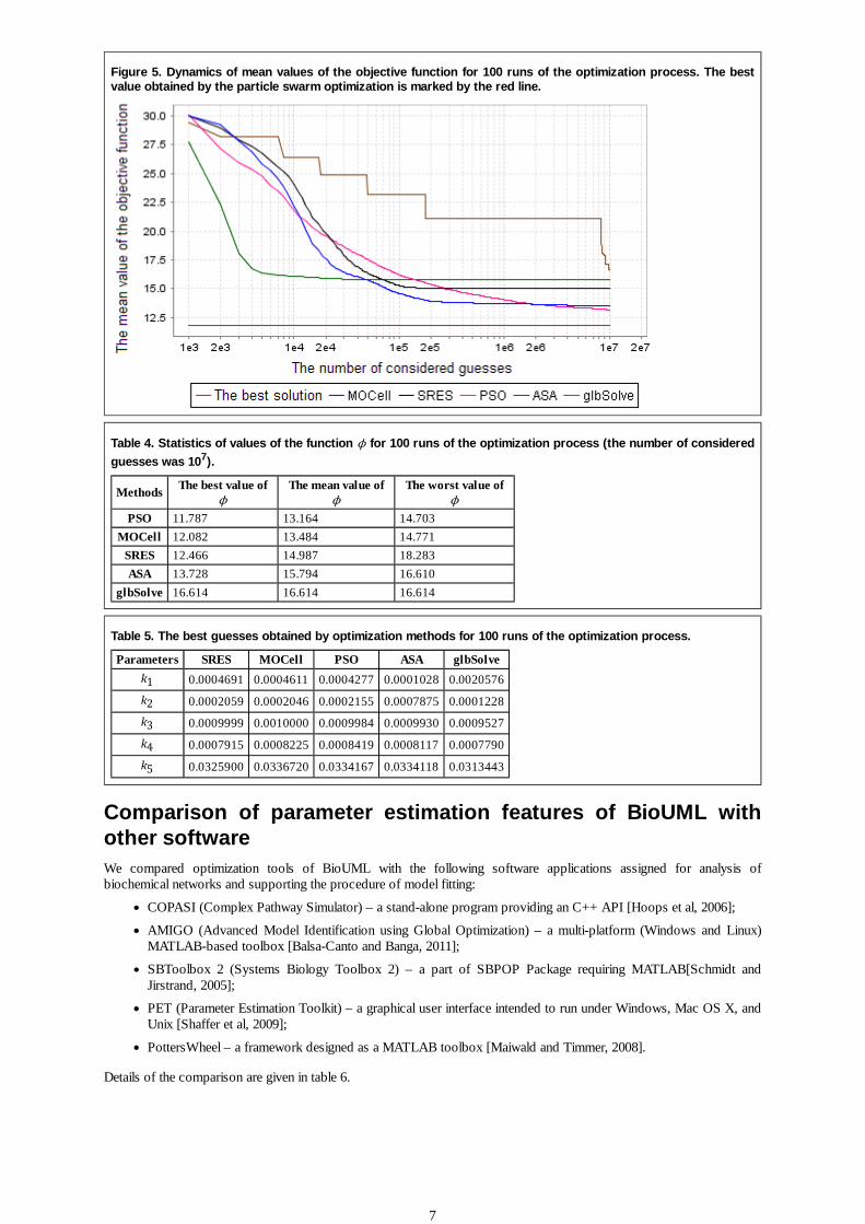
Figure 5. Dynamics of mean values of the objective function for 100 runs of the optimization process. The bestvalue obtained by the particle swarm optimization is marked by the red line.

Table 4. Statistics of values of the function ϕ for 100 runs of the optimization process (the number of considered

guesses was 107).

MethodsThe best value of

ϕ

The mean value ofϕ

The worst value ofϕ

PSO 11.787 13.164 14.703

MOCell 12.082 13.484 14.771

SRES 12.466 14.987 18.283

ASA 13.728 15.794 16.610

glbSolve 16.614 16.614 16.614

Table 5. The best guesses obtained by optimization methods for 100 runs of the optimization process.

Parameters SRES MOCell PSO ASA glbSolve

k1 0.0004691 0.0004611 0.0004277 0.0001028 0.0020576

k2 0.0002059 0.0002046 0.0002155 0.0007875 0.0001228

k3 0.0009999 0.0010000 0.0009984 0.0009930 0.0009527

k4 0.0007915 0.0008225 0.0008419 0.0008117 0.0007790

k5 0.0325900 0.0336720 0.0334167 0.0334118 0.0313443

Comparison of parameter estimation features of BioUML withother softwareWe compared optimization tools of BioUML with the following software applications assigned for analysis ofbiochemical networks and supporting the procedure of model fitting:

COPASI (Complex Pathway Simulator) – a stand-alone program providing an C++ API [Hoops et al, 2006];

AMIGO (Advanced Model Identification using Global Optimization) – a multi-platform (Windows and Linux)MATLAB-based toolbox [Balsa-Canto and Banga, 2011];

SBToolbox 2 (Systems Biology Toolbox 2) – a part of SBPOP Package requiring MATLAB[Schmidt andJirstrand, 2005];

PET (Parameter Estimation Toolkit) – a graphical user interface intended to run under Windows, Mac OS X, andUnix [Shaffer et al, 2009];

PottersWheel – a framework designed as a MATLAB toolbox [Maiwald and Timmer, 2008].

Details of the comparison are given in table 6.

7

Table 6. Comparison of the parameter estimation features for different software applications.

Features BioUML COPASI AMIGOSBToolbox

2PET PottersWheel

Environment Java C++ MATLAB MATLABPerl,Gtk+

MATLAB

Experimental data:

– Multi-experiment fitting + + + + + +

– Experiment types:

– time course + + + + + +

– steady-state + + − − + −

– Individual initial state of the model for eachexperiment

+ − + + + +

– Error bars − − + + − +

– Normalization of data using weights + + + + + +

Local (experiment dependent) and globalparameters

+ − + + − −

Further, we compared computation speed of the optimization methods implemented in BioUML and COPASI. For thispurpose, we considered a series of test cases. A brief description of the models used in these test cases is providedbelow. For more details, including specification of experimental data and fitting parameters, see Additional file 1 of thesupplementary materials.

In the first test case, we analyzed three models of CD95-induced caspase-8 activation constructed on the basis of themodel by Neumann et al. [Neumann et al, 2010] with varying degrees of detail (fig. 6, A-C). The second test case wasproposed by Mendes et al. [Mendes et al, 2009] and corresponded to the model of the MAP kinase cascade (fig. 7)developed by Kholodenko et al. [Kholodenko, 2000]. Finally, we tested the model of Bagci et al. [Bagci et al, 2006]representing the mitochondria-depended apoptosis resulting from the cooperative formation of heptameric apoptosomecomplex and activation of caspase-9 and caspase-3 (fig. 8).

Figure 6. The models of caspase-8 activation constructed based on the model by Neumann et al. with the varyingnumber of species: 7 (A), 13 (B), and 18 (C).

8

Figure 7. The model of the MAP kinase cascade constructed by Kholodenko et al.

Figure 8. The model of the mitochondria-depended apoptosis proposed by Bagci et al.

Analyzing the number of the objective function evaluations per second for these test cases, we found that BioUMLshowed a better result than COPASI (fig. 9).

9

Figure 9. The number of the objective function evaluations per second for different test cases in COPASI andBioUML: the model by Neumann et al. including 7 (A), 13 (B), and 18 (C) species; the model by Kholodenko et al.consisting of 8 species (D); the model of Bagci et al. consisting of 32 species (E).

DiscussionIn this paper, we considered parameter estimation tools of the BioUML software. These tools can be applied tobiological systems characterized with a set of ODEs. The fitting process is based on experimental time course or steadystate measurements, and assumes minimization of the function of error between these measurements and thecorresponding model prediction. We implemented several stochastic and deterministic global optimization methods asnew plug-in for BioUML. None of these methods is effective for all cases. Nevertheless, on the basis of ourobservations, we concluded that adaptive simulated annealing can be used when it is necessary to quickly find the vicinityof the solution. In the case when adequacy of solution is more preferable than the rate of convergence, it is better to usesuch methods as MOCell, PSO and SRES.

Parameter fitting is an important part of the quantitative biological modeling. However, if the model includes moreelements than are necessary to approximate experimental data with the given accuracy, we face the problem of overfitting[Hawkins, 2004]. In this case, there is no overall best solution and it is expedient to find distribution of the parametervalues which are compatible with observed experimental dynamics. For this purpose, we should run parameter estimationprocess many times (it is better with different optimization methods) and evaluate bounds for all parameters.Implementation of this technique in BioUML is a task for the future work.

We successfully applied our optimization plug-in for creation of the combined model of CD95 and NF-κB signalingpathways [Kutumova et al, 2013], where the problem of parameter overfitting was solved using the methodology ofmodel reduction [Gorban et al, 2010].

References

Bagci E Z, Vodovotz Y, Billiar T R, Ermentrout G B, Bahar I, authors. Bistability in apoptosis: roles of bax, bcl-2,and mitochondrial permeability transition pores. Biophys J. 1–3;2006;(5)90:1546–1559.DOI:10.1529/biophysj.105.068122 [PMID:16339882]

Balsa-Canto Eva, Banga Julio R, authors. AMIGO, a toolbox for advanced model identification in systems biologyusing global optimization. Bioinformatics. 17–6;2011;(16)27:2311–2313. DOI:10.1093/bioinformatics/btr370[PMID:21685047]

Björkman M, Holmström K, authors. Global Optimization Using the DIRECT Algorithm in Matlab. AdvancedModeling and Optimization. 1999;(2)1:17–37

Brown Peter N, Byrne George D, Hindmarsh Alan C, authors. VODE: A Variable-Coefficient ODE Solver. SIAM J.Sci. and Stat. Comput. 1989;(5)10:1038–1051. ISSN: 0196-5204 DOI:10.1137/0910062

Dormand J R, Prince P J, authors. A family of embedded Runge-Kutta formulae. Journal of Computational andApplied Mathematics. 1980;(1)6:19–26. ISSN: 03770427 DOI:10.1016/0771-050X(80)90013-3

Gorban A N, Radulescu O, Zinovyev A Y, authors. Asymptotology of chemical reaction networks. ChemicalEngineering Science. 2010;(7)65:2310–2324. ISSN: 00092509 DOI:10.1016/j.ces.2009.09.005

Hairer E, Wanner G, authors. Solving Ordinary Differential Equations II: Stiff and Differential-Algebraic Problems. 1996.

10

2nd revised. Berlin: Springer;

Hawkins Douglas M, author. The problem of overfitting. J Chem Inf Comput Sci. 2004;(1)44:1–12.DOI:10.1021/ci0342472 [PMID:14741005]

Hoops Stefan, Sahle Sven, Gauges Ralph, Lee Christine, Pahle Jürgen, Simus Natalia, Singhal Mudita, Xu Liang, MendesPedro, Kummer Ursula, authors. COPASI--a COmplex PAthway SImulator. Bioinformatics. 10–10;2006;(24)22:3067–3074. DOI:10.1093/bioinformatics/btl485 [PMID:17032683]

Hucka M, Finney A, Sauro H M, Bolouri H, Doyle J C, Kitano H, Arkin A P, Bornstein B J, Bray D, Cornish-Bowden A,Cuellar A A, Dronov S, Gilles E D, Ginkel M, Gor V, Goryanin I I, Hedley W J, Hodgman T C, Hofmeyr J-H, HunterP J, Juty N S, Kasberger J L, Kremling A, Kummer U, Le Novère N , Loew L M, Lucio D, Mendes P, Minch E,Mjolsness E D, Nakayama Y, Nelson M R, Nielsen P F, Sakurada T, Schaff J C, Shapiro B E, Shimizu T S, Spence HD, Stelling J, Takahashi K, Tomita M, Wagner J, Wang J, authors. The systems biology markup language (SBML):a medium for representation and exchange of biochemical network models. Bioinformatics. 1–3;2003;(4)19:524–531. [PMID:12611808]

Ingber L, author. Adaptive simulated annealing (ASA): Lessons learned. Control and Cybernetics. 1996;(1)25:33–54

Kholodenko B N, author. Negative feedback and ultrasensitivity can bring about oscillations in the mitogen-activated protein kinase cascades. Eur J Biochem. 2000;(6)267:1583–1588. [PMID:10712587]

Kutumova Elena, Zinovyev Andrei, Sharipov Ruslan, Kolpakov Fedor, authors. Model composition through modelreduction: a combined model of CD95 and NF-κB signaling pathways. BMC Syst Biol. 15–2;2013;7:13DOI:10.1186/1752-0509-7-13 [PMID:23409788]

Maiwald Thomas, Timmer Jens, authors. Dynamical modeling and multi-experiment fitting with PottersWheel.Bioinformatics. 9–7;2008;(18)24:2037–2043. DOI:10.1093/bioinformatics/btn350 [PMID:18614583]

Mendes Pedro, Hoops Stefan, Sahle Sven, Gauges Ralph, Dada Joseph, Kummer Ursula, authors. Computationalmodeling of biochemical networks using COPASI. Methods Mol Biol. 2009;500:17–59.DOI:10.1007/978-1-59745-525-1_2 [PMID:19399433]

Moles Carmen G, Mendes Pedro, Banga Julio R, authors. Parameter estimation in biochemical pathways: acomparison of global optimization methods. Genome Res. 14–10;2003;(11)13:2467–2474. DOI:10.1101/gr.1262503[PMID:14559783]

Nebro Antonio J, Durillo Juan J, Luna Francisco, Dorronsoro Bernabé, Alba Enrique, authors. MOCell: A cellulargenetic algorithm for multiobjective optimization. Int. J. Intell. Syst. 2009;(7)24:726–746. ISSN: 08848173DOI:10.1002/int.20358

Neumann Leo, Pforr Carina, Beaudouin Joel, Pappa Alexander, Fricker Nicolai, Krammer Peter H, Lavrik Inna N, EilsRoland, authors. Dynamics within the CD95 death-inducing signaling complex decide life and death of cells.Mol Syst Biol. 9–3;2010;6:352 DOI:10.1038/msb.2010.6 [PMID:20212524]

Runarsson T P, Yao Xin, authors. Stochastic ranking for constrained evolutionary optimization. IEEE Trans. Evol.Computat. 2000;(3)4:284–294. ISSN: 1089778X DOI:10.1109/4235.873238

Schmidt Henning, Jirstrand Mats, authors. Systems Biology Toolbox for MATLAB: a computational platform forresearch in systems biology. Bioinformatics. 29–11;2005;(4)22:514–515. DOI:10.1093/bioinformatics/bti799[PMID:16317076]

Shaffer Clifford A, Zwolak Jason W, Randhawa Ranjit, Tyson John J, authors. Modeling molecular regulatorynetworks with JigCell and PET. Methods Mol Biol. 2009;500:81–111. DOI:10.1007/978-1-59745-525-1_4[PMID:19399431]

Sierra Margarita R, Coello Carlos A Coello, authors. Improving PSO-Based Multi-objective Optimization UsingCrowding, Mutation and ∈∈∈∈-Dominance. Evolutionary Multi-Criterion Optimization. 2005. p. 505–519. Berlin,Heidelberg: Springer Berlin Heidelberg; DOI:10.1007/978-3-540-31880-4_35

11