. . . . . . . . . . . . . . . . Complete Statistics . . . . . . . . . Basu’s Theorem . Summary . . Biostatistics 602 - Statistical Inference Lecture 06 Basu’s Theorem Hyun Min Kang January 29th, 2013 Hyun Min Kang Biostatistics 602 - Lecture 07 January 29th, 2013 1 / 21

Welcome message from author
This document is posted to help you gain knowledge. Please leave a comment to let me know what you think about it! Share it to your friends and learn new things together.
Transcript
. . . . . .
. . . . . . . . . .Complete Statistics
. . . . . . . . .Basu’s Theorem
.Summary
.
......
Biostatistics 602 - Statistical InferenceLecture 06
Basu’s Theorem
Hyun Min Kang
January 29th, 2013
Hyun Min Kang Biostatistics 602 - Lecture 07 January 29th, 2013 1 / 21
. . . . . .
. . . . . . . . . .Complete Statistics
. . . . . . . . .Basu’s Theorem
.Summary
Last Lecture
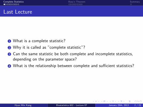
..1 What is a complete statistic?
..2 Why it is called as ”complete statistic”?
..3 Can the same statistic be both complete and incomplete statistics,depending on the parameter space?
..4 What is the relationship between complete and sufficient statistics?
..5 Is a minimal sufficient statistic always complete?
Hyun Min Kang Biostatistics 602 - Lecture 07 January 29th, 2013 2 / 21
. . . . . .
. . . . . . . . . .Complete Statistics
. . . . . . . . .Basu’s Theorem
.Summary
Last Lecture
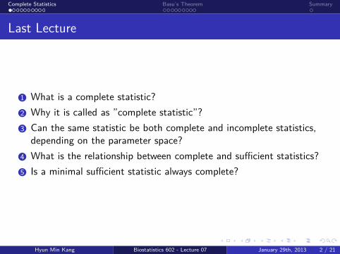
..1 What is a complete statistic?
..2 Why it is called as ”complete statistic”?
..3 Can the same statistic be both complete and incomplete statistics,depending on the parameter space?
..4 What is the relationship between complete and sufficient statistics?
..5 Is a minimal sufficient statistic always complete?
Hyun Min Kang Biostatistics 602 - Lecture 07 January 29th, 2013 2 / 21
. . . . . .
. . . . . . . . . .Complete Statistics
. . . . . . . . .Basu’s Theorem
.Summary
Last Lecture
..1 What is a complete statistic?
..2 Why it is called as ”complete statistic”?
..3 Can the same statistic be both complete and incomplete statistics,depending on the parameter space?
..4 What is the relationship between complete and sufficient statistics?
..5 Is a minimal sufficient statistic always complete?
Hyun Min Kang Biostatistics 602 - Lecture 07 January 29th, 2013 2 / 21
. . . . . .
. . . . . . . . . .Complete Statistics
. . . . . . . . .Basu’s Theorem
.Summary
Complete Statistics
.Definition..
......
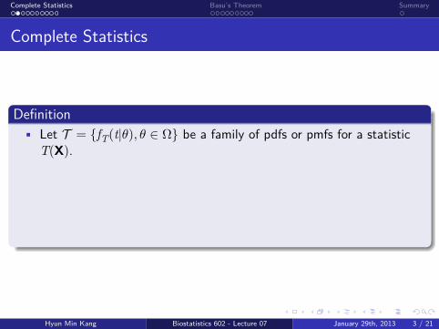
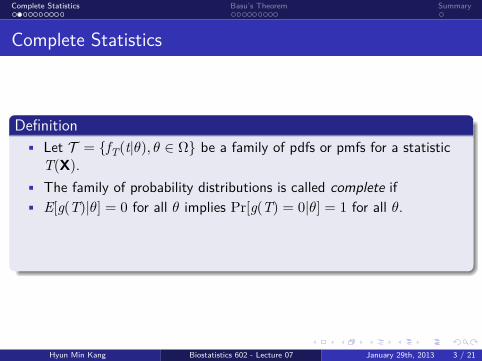
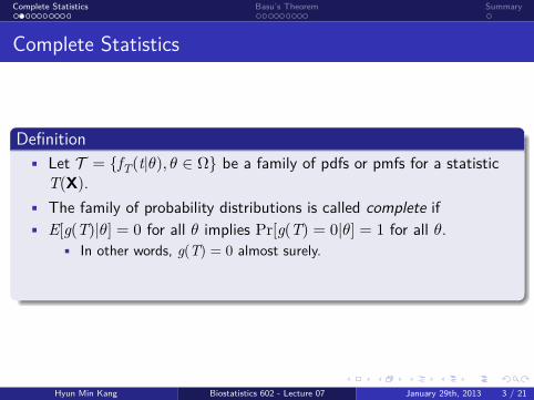
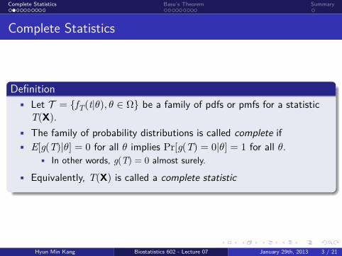
• Let T = fT(t|θ), θ ∈ Ω be a family of pdfs or pmfs for a statisticT(X).
• The family of probability distributions is called complete if• E[g(T)|θ] = 0 for all θ implies Pr[g(T) = 0|θ] = 1 for all θ.
• In other words, g(T) = 0 almost surely.• Equivalently, T(X) is called a complete statistic
Hyun Min Kang Biostatistics 602 - Lecture 07 January 29th, 2013 3 / 21
. . . . . .
. . . . . . . . . .Complete Statistics
. . . . . . . . .Basu’s Theorem
.Summary
Complete Statistics
.Definition..
......
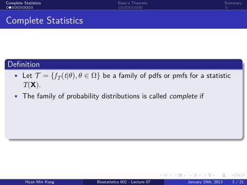
• Let T = fT(t|θ), θ ∈ Ω be a family of pdfs or pmfs for a statisticT(X).
• The family of probability distributions is called complete if
• E[g(T)|θ] = 0 for all θ implies Pr[g(T) = 0|θ] = 1 for all θ.• In other words, g(T) = 0 almost surely.
• Equivalently, T(X) is called a complete statistic
Hyun Min Kang Biostatistics 602 - Lecture 07 January 29th, 2013 3 / 21
. . . . . .
. . . . . . . . . .Complete Statistics
. . . . . . . . .Basu’s Theorem
.Summary
Complete Statistics
.Definition..
......
• Let T = fT(t|θ), θ ∈ Ω be a family of pdfs or pmfs for a statisticT(X).
• The family of probability distributions is called complete if• E[g(T)|θ] = 0 for all θ implies Pr[g(T) = 0|θ] = 1 for all θ.
• In other words, g(T) = 0 almost surely.• Equivalently, T(X) is called a complete statistic
Hyun Min Kang Biostatistics 602 - Lecture 07 January 29th, 2013 3 / 21
. . . . . .
. . . . . . . . . .Complete Statistics
. . . . . . . . .Basu’s Theorem
.Summary
Complete Statistics
.Definition..
......
• Let T = fT(t|θ), θ ∈ Ω be a family of pdfs or pmfs for a statisticT(X).
• The family of probability distributions is called complete if• E[g(T)|θ] = 0 for all θ implies Pr[g(T) = 0|θ] = 1 for all θ.
• In other words, g(T) = 0 almost surely.
• Equivalently, T(X) is called a complete statistic
Hyun Min Kang Biostatistics 602 - Lecture 07 January 29th, 2013 3 / 21
. . . . . .
. . . . . . . . . .Complete Statistics
. . . . . . . . .Basu’s Theorem
.Summary
Complete Statistics
.Definition..
......
• Let T = fT(t|θ), θ ∈ Ω be a family of pdfs or pmfs for a statisticT(X).
• The family of probability distributions is called complete if• E[g(T)|θ] = 0 for all θ implies Pr[g(T) = 0|θ] = 1 for all θ.
• In other words, g(T) = 0 almost surely.• Equivalently, T(X) is called a complete statistic
Hyun Min Kang Biostatistics 602 - Lecture 07 January 29th, 2013 3 / 21
. . . . . .
. . . . . . . . . .Complete Statistics
. . . . . . . . .Basu’s Theorem
.Summary
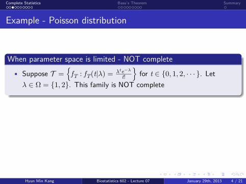
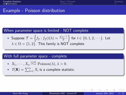
Example - Poisson distribution
.When parameter space is limited - NOT complete..
......
• Suppose T =
fT : fT(t|λ) = λte−λ
t!
for t ∈ 0, 1, 2, · · · . Let
λ ∈ Ω = 1, 2. This family is NOT complete
.With full parameter space - complete..
......
• X1, · · · ,Xni.i.d.∼ Poisson(λ), λ > 0.
• T(X) =∑n
i=1 Xi is a complete statistic.
Hyun Min Kang Biostatistics 602 - Lecture 07 January 29th, 2013 4 / 21
. . . . . .
. . . . . . . . . .Complete Statistics
. . . . . . . . .Basu’s Theorem
.Summary
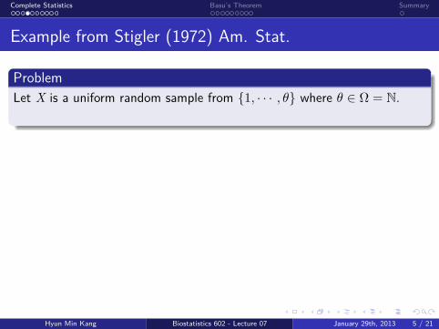
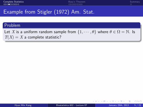
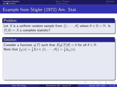
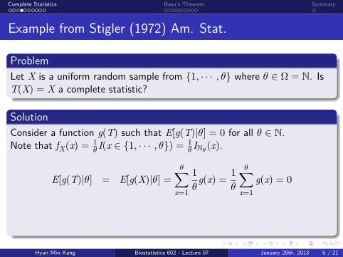
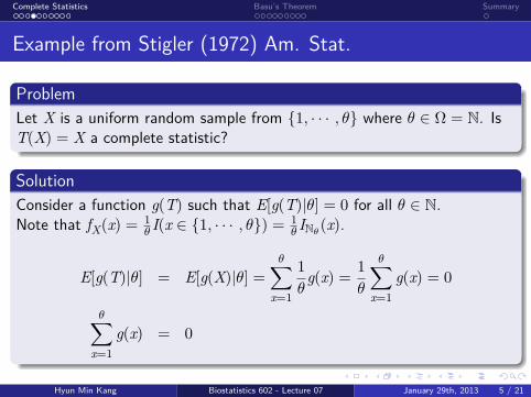
Example from Stigler (1972) Am. Stat..Problem..
......Let X is a uniform random sample from 1, · · · , θ where θ ∈ Ω = N.
IsT(X) = X a complete statistic?
.Solution..
......
Consider a function g(T) such that E[g(T)|θ] = 0 for all θ ∈ N.Note that fX(x) = 1
θ I(x ∈ 1, · · · , θ) = 1θ INθ
(x).
E[g(T)|θ] = E[g(X)|θ] =θ∑
x=1
1
θg(x) = 1
θ
θ∑x=1
g(x) = 0
θ∑x=1
g(x) = 0
Hyun Min Kang Biostatistics 602 - Lecture 07 January 29th, 2013 5 / 21
. . . . . .
. . . . . . . . . .Complete Statistics
. . . . . . . . .Basu’s Theorem
.Summary
Example from Stigler (1972) Am. Stat..Problem..
......Let X is a uniform random sample from 1, · · · , θ where θ ∈ Ω = N. IsT(X) = X a complete statistic?
.Solution..
......
Consider a function g(T) such that E[g(T)|θ] = 0 for all θ ∈ N.Note that fX(x) = 1
θ I(x ∈ 1, · · · , θ) = 1θ INθ
(x).
E[g(T)|θ] = E[g(X)|θ] =θ∑
x=1
1
θg(x) = 1
θ
θ∑x=1
g(x) = 0
θ∑x=1
g(x) = 0
Hyun Min Kang Biostatistics 602 - Lecture 07 January 29th, 2013 5 / 21
. . . . . .
. . . . . . . . . .Complete Statistics
. . . . . . . . .Basu’s Theorem
.Summary
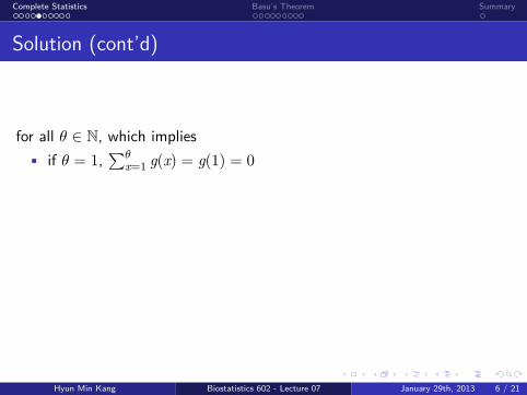
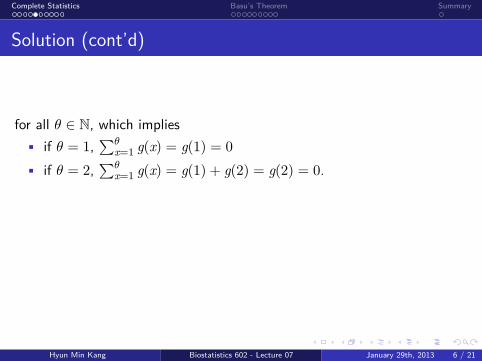
Solution (cont’d)
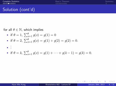
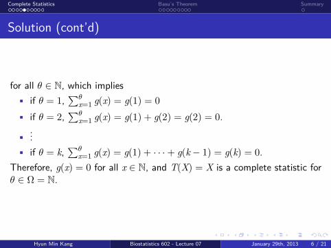
for all θ ∈ N, which implies• if θ = 1,
∑θx=1 g(x) = g(1) = 0
• if θ = 2,∑θ
x=1 g(x) = g(1) + g(2) = g(2) = 0.
•...
• if θ = k,∑θ
x=1 g(x) = g(1) + · · ·+ g(k − 1) = g(k) = 0.Therefore, g(x) = 0 for all x ∈ N, and T(X) = X is a complete statistic forθ ∈ Ω = N.
Hyun Min Kang Biostatistics 602 - Lecture 07 January 29th, 2013 6 / 21
. . . . . .
. . . . . . . . . .Complete Statistics
. . . . . . . . .Basu’s Theorem
.Summary
Solution (cont’d)
for all θ ∈ N, which implies• if θ = 1,
∑θx=1 g(x) = g(1) = 0
• if θ = 2,∑θ
x=1 g(x) = g(1) + g(2) = g(2) = 0.
•...
• if θ = k,∑θ
x=1 g(x) = g(1) + · · ·+ g(k − 1) = g(k) = 0.
Therefore, g(x) = 0 for all x ∈ N, and T(X) = X is a complete statistic forθ ∈ Ω = N.
Hyun Min Kang Biostatistics 602 - Lecture 07 January 29th, 2013 6 / 21
. . . . . .
. . . . . . . . . .Complete Statistics
. . . . . . . . .Basu’s Theorem
.Summary
Solution (cont’d)
for all θ ∈ N, which implies• if θ = 1,
∑θx=1 g(x) = g(1) = 0
• if θ = 2,∑θ
x=1 g(x) = g(1) + g(2) = g(2) = 0.
•...
• if θ = k,∑θ
x=1 g(x) = g(1) + · · ·+ g(k − 1) = g(k) = 0.Therefore, g(x) = 0 for all x ∈ N, and T(X) = X is a complete statistic forθ ∈ Ω = N.
Hyun Min Kang Biostatistics 602 - Lecture 07 January 29th, 2013 6 / 21
. . . . . .
. . . . . . . . . .Complete Statistics
. . . . . . . . .Basu’s Theorem
.Summary
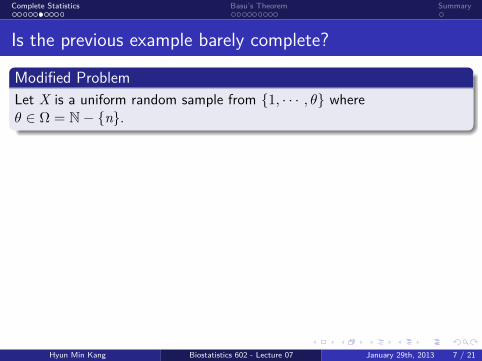
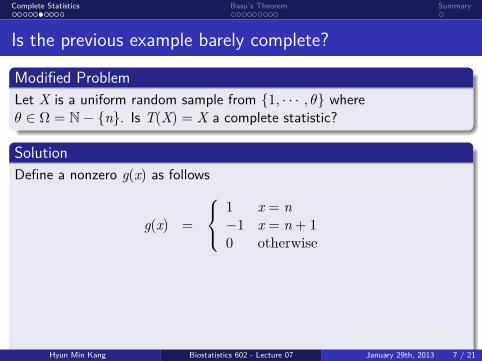
Is the previous example barely complete?.Modified Problem..
......Let X is a uniform random sample from 1, · · · , θ whereθ ∈ Ω = N− n.
Is T(X) = X a complete statistic?.Solution..
......
Define a nonzero g(x) as follows
g(x) =
1 x = n−1 x = n + 10 otherwise
E[g(T)|θ] =1
θ
θ∑x=1
g(x) =
0 θ = n1θ θ = n
Because Ω does not include n, g(x) = 0 for all θ ∈ Ω = N− n, andT(X) = X is not a complete statistic.
Hyun Min Kang Biostatistics 602 - Lecture 07 January 29th, 2013 7 / 21
. . . . . .
. . . . . . . . . .Complete Statistics
. . . . . . . . .Basu’s Theorem
.Summary
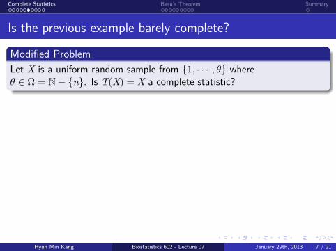
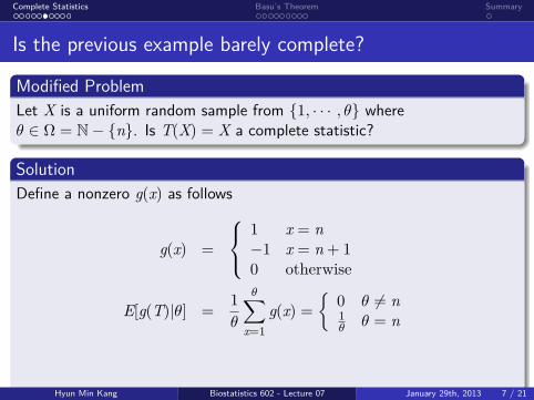
Is the previous example barely complete?.Modified Problem..
......Let X is a uniform random sample from 1, · · · , θ whereθ ∈ Ω = N− n. Is T(X) = X a complete statistic?
.Solution..
......
Define a nonzero g(x) as follows
g(x) =
1 x = n−1 x = n + 10 otherwise
E[g(T)|θ] =1
θ
θ∑x=1
g(x) =
0 θ = n1θ θ = n
Because Ω does not include n, g(x) = 0 for all θ ∈ Ω = N− n, andT(X) = X is not a complete statistic.
Hyun Min Kang Biostatistics 602 - Lecture 07 January 29th, 2013 7 / 21
. . . . . .
. . . . . . . . . .Complete Statistics
. . . . . . . . .Basu’s Theorem
.Summary
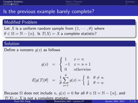
Is the previous example barely complete?.Modified Problem..
......Let X is a uniform random sample from 1, · · · , θ whereθ ∈ Ω = N− n. Is T(X) = X a complete statistic?.Solution..
......
Define a nonzero g(x) as follows
g(x) =
1 x = n−1 x = n + 10 otherwise
E[g(T)|θ] =1
θ
θ∑x=1
g(x) =
0 θ = n1θ θ = n
Because Ω does not include n, g(x) = 0 for all θ ∈ Ω = N− n, andT(X) = X is not a complete statistic.
Hyun Min Kang Biostatistics 602 - Lecture 07 January 29th, 2013 7 / 21
. . . . . .
. . . . . . . . . .Complete Statistics
. . . . . . . . .Basu’s Theorem
.Summary
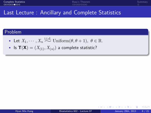
Last Lecture : Ancillary and Complete Statistics
.Problem..
......
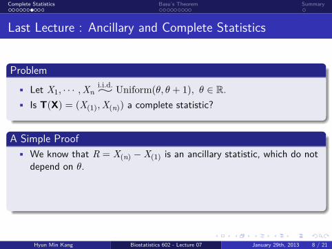
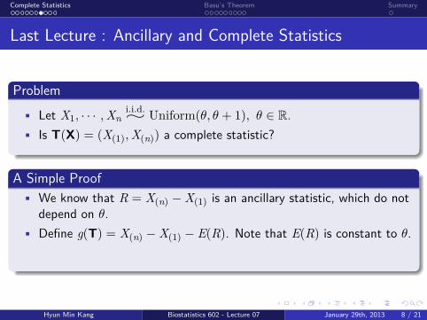
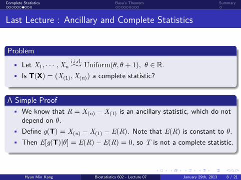
• Let X1, · · · ,Xni.i.d.∼ Uniform(θ, θ + 1), θ ∈ R.
• Is T(X) = (X(1),X(n)) a complete statistic?
.A Simple Proof..
......
• We know that R = X(n) − X(1) is an ancillary statistic, which do notdepend on θ.
• Define g(T) = X(n) − X(1) − E(R). Note that E(R) is constant to θ.• Then E[g(T)|θ] = E(R)− E(R) = 0, so T is not a complete statistic.
Hyun Min Kang Biostatistics 602 - Lecture 07 January 29th, 2013 8 / 21
. . . . . .
. . . . . . . . . .Complete Statistics
. . . . . . . . .Basu’s Theorem
.Summary
Last Lecture : Ancillary and Complete Statistics
.Problem..
......
• Let X1, · · · ,Xni.i.d.∼ Uniform(θ, θ + 1), θ ∈ R.
• Is T(X) = (X(1),X(n)) a complete statistic?
.A Simple Proof..
......
• We know that R = X(n) − X(1) is an ancillary statistic, which do notdepend on θ.
• Define g(T) = X(n) − X(1) − E(R). Note that E(R) is constant to θ.
• Then E[g(T)|θ] = E(R)− E(R) = 0, so T is not a complete statistic.
Hyun Min Kang Biostatistics 602 - Lecture 07 January 29th, 2013 8 / 21
. . . . . .
. . . . . . . . . .Complete Statistics
. . . . . . . . .Basu’s Theorem
.Summary
Last Lecture : Ancillary and Complete Statistics
.Problem..
......
• Let X1, · · · ,Xni.i.d.∼ Uniform(θ, θ + 1), θ ∈ R.
• Is T(X) = (X(1),X(n)) a complete statistic?
.A Simple Proof..
......
• We know that R = X(n) − X(1) is an ancillary statistic, which do notdepend on θ.
• Define g(T) = X(n) − X(1) − E(R). Note that E(R) is constant to θ.• Then E[g(T)|θ] = E(R)− E(R) = 0, so T is not a complete statistic.
Hyun Min Kang Biostatistics 602 - Lecture 07 January 29th, 2013 8 / 21
. . . . . .
. . . . . . . . . .Complete Statistics
. . . . . . . . .Basu’s Theorem
.Summary
Useful Fact 1 : Ancillary and Complete Statistics
.Fact..
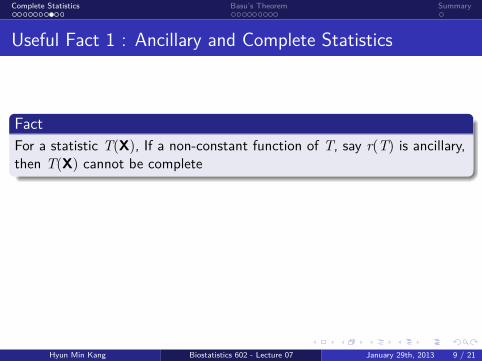
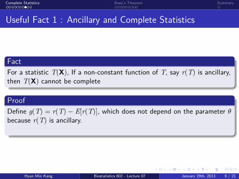
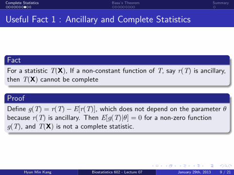
......For a statistic T(X), If a non-constant function of T, say r(T) is ancillary,then T(X) cannot be complete
.Proof..
......
Define g(T) = r(T)− E[r(T)], which does not depend on the parameter θbecause r(T) is ancillary. Then E[g(T)|θ] = 0 for a non-zero functiong(T), and T(X) is not a complete statistic.
Hyun Min Kang Biostatistics 602 - Lecture 07 January 29th, 2013 9 / 21
. . . . . .
. . . . . . . . . .Complete Statistics
. . . . . . . . .Basu’s Theorem
.Summary
Useful Fact 1 : Ancillary and Complete Statistics
.Fact..
......For a statistic T(X), If a non-constant function of T, say r(T) is ancillary,then T(X) cannot be complete
.Proof..
......
Define g(T) = r(T)− E[r(T)], which does not depend on the parameter θbecause r(T) is ancillary.
Then E[g(T)|θ] = 0 for a non-zero functiong(T), and T(X) is not a complete statistic.
Hyun Min Kang Biostatistics 602 - Lecture 07 January 29th, 2013 9 / 21
. . . . . .
. . . . . . . . . .Complete Statistics
. . . . . . . . .Basu’s Theorem
.Summary
Useful Fact 1 : Ancillary and Complete Statistics
.Fact..
......For a statistic T(X), If a non-constant function of T, say r(T) is ancillary,then T(X) cannot be complete
.Proof..
......
Define g(T) = r(T)− E[r(T)], which does not depend on the parameter θbecause r(T) is ancillary. Then E[g(T)|θ] = 0 for a non-zero functiong(T), and T(X) is not a complete statistic.
Hyun Min Kang Biostatistics 602 - Lecture 07 January 29th, 2013 9 / 21
. . . . . .
. . . . . . . . . .Complete Statistics
. . . . . . . . .Basu’s Theorem
.Summary
Useful Fact 2 : Arbitrary Function of Complete Statistics
.Fact..
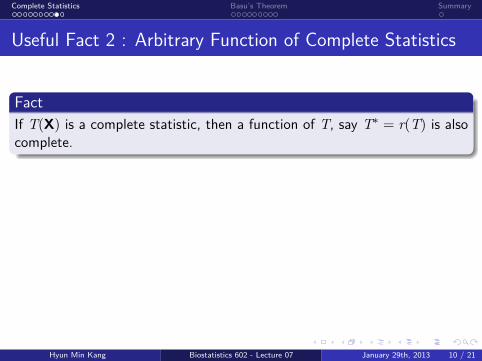
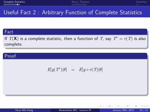
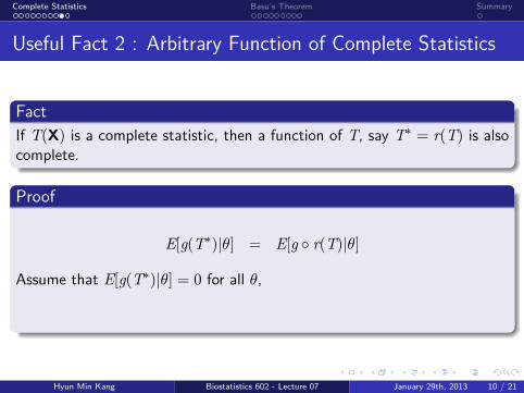
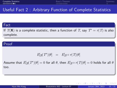
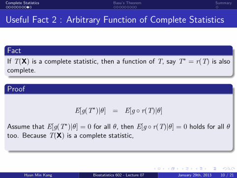
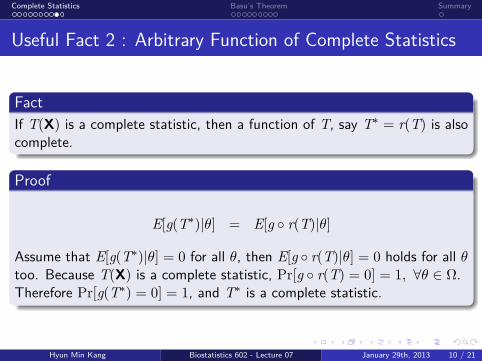
......If T(X) is a complete statistic, then a function of T, say T∗ = r(T) is alsocomplete.
.Proof..
......
E[g(T∗)|θ] = E[g r(T)|θ]
Assume that E[g(T∗)|θ] = 0 for all θ, then E[g r(T)|θ] = 0 holds for all θtoo. Because T(X) is a complete statistic, Pr[g r(T) = 0] = 1, ∀θ ∈ Ω.Therefore Pr[g(T∗) = 0] = 1, and T∗ is a complete statistic.
Hyun Min Kang Biostatistics 602 - Lecture 07 January 29th, 2013 10 / 21
. . . . . .
. . . . . . . . . .Complete Statistics
. . . . . . . . .Basu’s Theorem
.Summary
Useful Fact 2 : Arbitrary Function of Complete Statistics
.Fact..
......If T(X) is a complete statistic, then a function of T, say T∗ = r(T) is alsocomplete.
.Proof..
......
E[g(T∗)|θ] = E[g r(T)|θ]
Assume that E[g(T∗)|θ] = 0 for all θ,
then E[g r(T)|θ] = 0 holds for all θtoo. Because T(X) is a complete statistic, Pr[g r(T) = 0] = 1, ∀θ ∈ Ω.Therefore Pr[g(T∗) = 0] = 1, and T∗ is a complete statistic.
Hyun Min Kang Biostatistics 602 - Lecture 07 January 29th, 2013 10 / 21
. . . . . .
. . . . . . . . . .Complete Statistics
. . . . . . . . .Basu’s Theorem
.Summary
Useful Fact 2 : Arbitrary Function of Complete Statistics
.Fact..
......If T(X) is a complete statistic, then a function of T, say T∗ = r(T) is alsocomplete.
.Proof..
......
E[g(T∗)|θ] = E[g r(T)|θ]
Assume that E[g(T∗)|θ] = 0 for all θ, then E[g r(T)|θ] = 0 holds for all θtoo.
Because T(X) is a complete statistic, Pr[g r(T) = 0] = 1, ∀θ ∈ Ω.Therefore Pr[g(T∗) = 0] = 1, and T∗ is a complete statistic.
Hyun Min Kang Biostatistics 602 - Lecture 07 January 29th, 2013 10 / 21
. . . . . .
. . . . . . . . . .Complete Statistics
. . . . . . . . .Basu’s Theorem
.Summary
Useful Fact 2 : Arbitrary Function of Complete Statistics
.Fact..
......If T(X) is a complete statistic, then a function of T, say T∗ = r(T) is alsocomplete.
.Proof..
......
E[g(T∗)|θ] = E[g r(T)|θ]
Assume that E[g(T∗)|θ] = 0 for all θ, then E[g r(T)|θ] = 0 holds for all θtoo. Because T(X) is a complete statistic,
Pr[g r(T) = 0] = 1, ∀θ ∈ Ω.Therefore Pr[g(T∗) = 0] = 1, and T∗ is a complete statistic.
Hyun Min Kang Biostatistics 602 - Lecture 07 January 29th, 2013 10 / 21
. . . . . .
. . . . . . . . . .Complete Statistics
. . . . . . . . .Basu’s Theorem
.Summary
Useful Fact 2 : Arbitrary Function of Complete Statistics
.Fact..
......If T(X) is a complete statistic, then a function of T, say T∗ = r(T) is alsocomplete.
.Proof..
......
E[g(T∗)|θ] = E[g r(T)|θ]
Assume that E[g(T∗)|θ] = 0 for all θ, then E[g r(T)|θ] = 0 holds for all θtoo. Because T(X) is a complete statistic, Pr[g r(T) = 0] = 1, ∀θ ∈ Ω.Therefore Pr[g(T∗) = 0] = 1, and T∗ is a complete statistic.
Hyun Min Kang Biostatistics 602 - Lecture 07 January 29th, 2013 10 / 21
. . . . . .
. . . . . . . . . .Complete Statistics
. . . . . . . . .Basu’s Theorem
.Summary
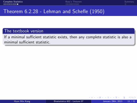
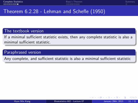
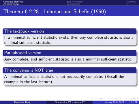
Theorem 6.2.28 - Lehman and Schefle (1950)
.The textbook version..
......If a minimal sufficient statistic exists, then any complete statistic is also aminimal sufficient statistic.
.Paraphrased version..
......Any complete, and sufficient statistic is also a minimal sufficient statistic
.The converse is NOT true..
......A minimal sufficient statistic is not necessarily complete. (Recall theexample in the last lecture).
Hyun Min Kang Biostatistics 602 - Lecture 07 January 29th, 2013 11 / 21
. . . . . .
. . . . . . . . . .Complete Statistics
. . . . . . . . .Basu’s Theorem
.Summary
Theorem 6.2.28 - Lehman and Schefle (1950)
.The textbook version..
......If a minimal sufficient statistic exists, then any complete statistic is also aminimal sufficient statistic..Paraphrased version........Any complete, and sufficient statistic is also a minimal sufficient statistic
.The converse is NOT true..
......A minimal sufficient statistic is not necessarily complete. (Recall theexample in the last lecture).
Hyun Min Kang Biostatistics 602 - Lecture 07 January 29th, 2013 11 / 21
. . . . . .
. . . . . . . . . .Complete Statistics
. . . . . . . . .Basu’s Theorem
.Summary
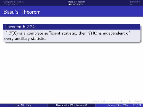
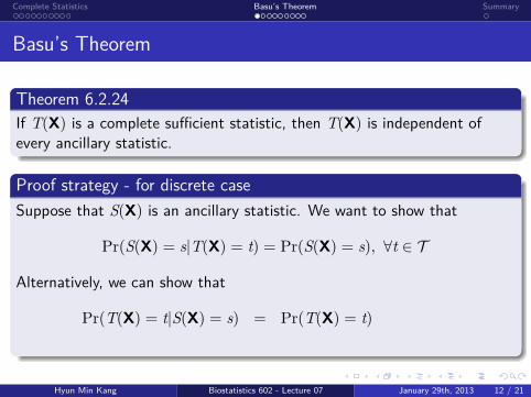
Basu’s Theorem
.Theorem 6.2.24..
......If T(X) is a complete sufficient statistic, then T(X) is independent ofevery ancillary statistic.
.Proof strategy - for discrete case..
......
Suppose that S(X) is an ancillary statistic. We want to show that
Pr(S(X) = s|T(X) = t) = Pr(S(X) = s), ∀t ∈ T
Alternatively, we can show that
Pr(T(X) = t|S(X) = s) = Pr(T(X) = t)Pr(T(X) = t ∧ S(X) = s) = Pr(T(X) = t)Pr(S(X) = s)
Hyun Min Kang Biostatistics 602 - Lecture 07 January 29th, 2013 12 / 21

. . . . . .
. . . . . . . . . .Complete Statistics
. . . . . . . . .Basu’s Theorem
.Summary
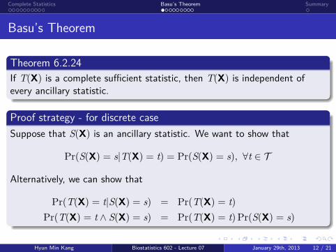
Basu’s Theorem
.Theorem 6.2.24..
......If T(X) is a complete sufficient statistic, then T(X) is independent ofevery ancillary statistic.
.Proof strategy - for discrete case..
......
Suppose that S(X) is an ancillary statistic. We want to show that
Pr(S(X) = s|T(X) = t) = Pr(S(X) = s), ∀t ∈ T
Alternatively, we can show that
Pr(T(X) = t|S(X) = s) = Pr(T(X) = t)Pr(T(X) = t ∧ S(X) = s) = Pr(T(X) = t)Pr(S(X) = s)
Hyun Min Kang Biostatistics 602 - Lecture 07 January 29th, 2013 12 / 21
. . . . . .
. . . . . . . . . .Complete Statistics
. . . . . . . . .Basu’s Theorem
.Summary
Basu’s Theorem
.Theorem 6.2.24..
......If T(X) is a complete sufficient statistic, then T(X) is independent ofevery ancillary statistic.
.Proof strategy - for discrete case..
......
Suppose that S(X) is an ancillary statistic. We want to show that
Pr(S(X) = s|T(X) = t) = Pr(S(X) = s), ∀t ∈ T
Alternatively, we can show that
Pr(T(X) = t|S(X) = s) = Pr(T(X) = t)
Pr(T(X) = t ∧ S(X) = s) = Pr(T(X) = t)Pr(S(X) = s)
Hyun Min Kang Biostatistics 602 - Lecture 07 January 29th, 2013 12 / 21
. . . . . .
. . . . . . . . . .Complete Statistics
. . . . . . . . .Basu’s Theorem
.Summary
Basu’s Theorem
.Theorem 6.2.24..
......If T(X) is a complete sufficient statistic, then T(X) is independent ofevery ancillary statistic.
.Proof strategy - for discrete case..
......
Suppose that S(X) is an ancillary statistic. We want to show that
Pr(S(X) = s|T(X) = t) = Pr(S(X) = s), ∀t ∈ T
Alternatively, we can show that
Pr(T(X) = t|S(X) = s) = Pr(T(X) = t)Pr(T(X) = t ∧ S(X) = s) = Pr(T(X) = t)Pr(S(X) = s)
Hyun Min Kang Biostatistics 602 - Lecture 07 January 29th, 2013 12 / 21
. . . . . .
. . . . . . . . . .Complete Statistics
. . . . . . . . .Basu’s Theorem
.Summary
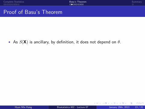
Proof of Basu’s Theorem
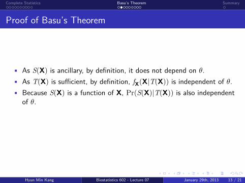
• As S(X) is ancillary, by definition, it does not depend on θ.
• As T(X) is sufficient, by definition, fX(X|T(X)) is independent of θ.• Because S(X) is a function of X, Pr(S(X)|T(X)) is also independent
of θ.• We need to show that
Pr(S(X) = s|T(X) = t) = Pr(S(X) = s), ∀t ∈ T .
Hyun Min Kang Biostatistics 602 - Lecture 07 January 29th, 2013 13 / 21
. . . . . .
. . . . . . . . . .Complete Statistics
. . . . . . . . .Basu’s Theorem
.Summary
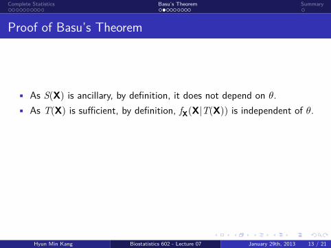
Proof of Basu’s Theorem
• As S(X) is ancillary, by definition, it does not depend on θ.• As T(X) is sufficient, by definition, fX(X|T(X)) is independent of θ.
• Because S(X) is a function of X, Pr(S(X)|T(X)) is also independentof θ.
• We need to show thatPr(S(X) = s|T(X) = t) = Pr(S(X) = s), ∀t ∈ T .
Hyun Min Kang Biostatistics 602 - Lecture 07 January 29th, 2013 13 / 21
. . . . . .
. . . . . . . . . .Complete Statistics
. . . . . . . . .Basu’s Theorem
.Summary
Proof of Basu’s Theorem
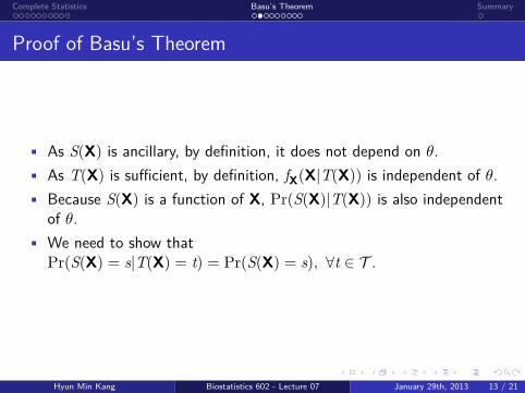
• As S(X) is ancillary, by definition, it does not depend on θ.• As T(X) is sufficient, by definition, fX(X|T(X)) is independent of θ.• Because S(X) is a function of X, Pr(S(X)|T(X)) is also independent
of θ.
• We need to show thatPr(S(X) = s|T(X) = t) = Pr(S(X) = s), ∀t ∈ T .
Hyun Min Kang Biostatistics 602 - Lecture 07 January 29th, 2013 13 / 21
. . . . . .
. . . . . . . . . .Complete Statistics
. . . . . . . . .Basu’s Theorem
.Summary
Proof of Basu’s Theorem
• As S(X) is ancillary, by definition, it does not depend on θ.• As T(X) is sufficient, by definition, fX(X|T(X)) is independent of θ.• Because S(X) is a function of X, Pr(S(X)|T(X)) is also independent
of θ.• We need to show that
Pr(S(X) = s|T(X) = t) = Pr(S(X) = s), ∀t ∈ T .
Hyun Min Kang Biostatistics 602 - Lecture 07 January 29th, 2013 13 / 21
. . . . . .
. . . . . . . . . .Complete Statistics
. . . . . . . . .Basu’s Theorem
.Summary
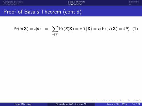
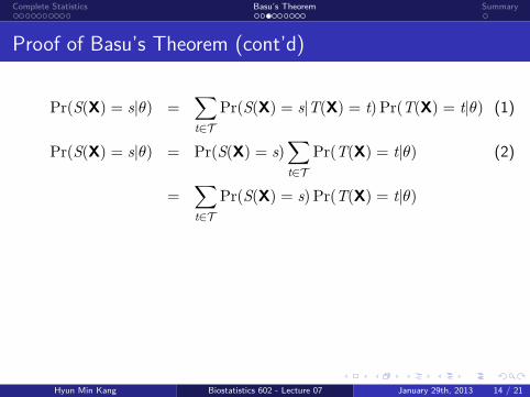
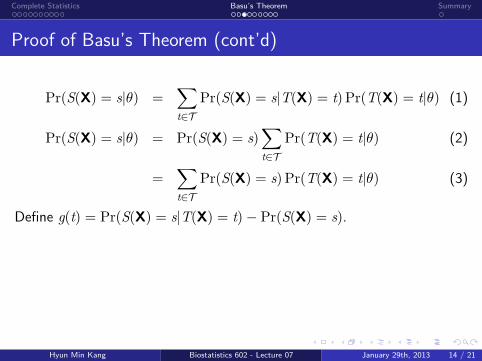
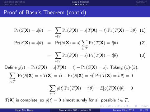
Proof of Basu’s Theorem (cont’d)
Pr(S(X) = s|θ) =∑t∈T
Pr(S(X) = s|T(X) = t)Pr(T(X) = t|θ) (1)
Pr(S(X) = s|θ) = Pr(S(X) = s)∑t∈T
Pr(T(X) = t|θ) (2)
=∑t∈T
Pr(S(X) = s)Pr(T(X) = t|θ) (3)
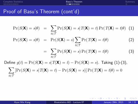
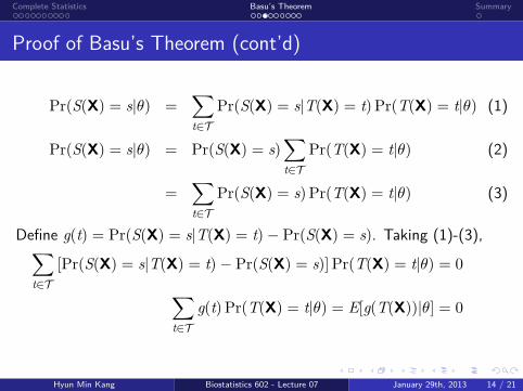
Define g(t) = Pr(S(X) = s|T(X) = t)− Pr(S(X) = s). Taking (1)-(3),∑t∈T
[Pr(S(X) = s|T(X) = t)− Pr(S(X) = s)]Pr(T(X) = t|θ) = 0∑t∈T
g(t)Pr(T(X) = t|θ) = E[g(T(X))|θ] = 0
T(X) is complete, so g(t) = 0 almost surely for all possible t ∈ T .Therefore, S(X) is independent of T(X).
Hyun Min Kang Biostatistics 602 - Lecture 07 January 29th, 2013 14 / 21
. . . . . .
. . . . . . . . . .Complete Statistics
. . . . . . . . .Basu’s Theorem
.Summary
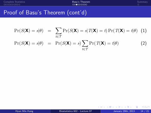
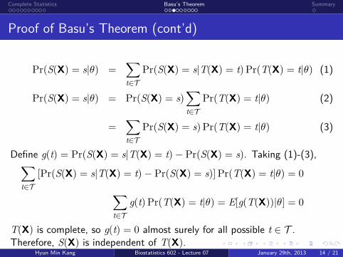
Proof of Basu’s Theorem (cont’d)
Pr(S(X) = s|θ) =∑t∈T
Pr(S(X) = s|T(X) = t)Pr(T(X) = t|θ) (1)
Pr(S(X) = s|θ) = Pr(S(X) = s)∑t∈T
Pr(T(X) = t|θ) (2)
=∑t∈T
Pr(S(X) = s)Pr(T(X) = t|θ) (3)
Define g(t) = Pr(S(X) = s|T(X) = t)− Pr(S(X) = s). Taking (1)-(3),∑t∈T
[Pr(S(X) = s|T(X) = t)− Pr(S(X) = s)]Pr(T(X) = t|θ) = 0∑t∈T
g(t)Pr(T(X) = t|θ) = E[g(T(X))|θ] = 0
T(X) is complete, so g(t) = 0 almost surely for all possible t ∈ T .Therefore, S(X) is independent of T(X).
Hyun Min Kang Biostatistics 602 - Lecture 07 January 29th, 2013 14 / 21
. . . . . .
. . . . . . . . . .Complete Statistics
. . . . . . . . .Basu’s Theorem
.Summary
Proof of Basu’s Theorem (cont’d)
Pr(S(X) = s|θ) =∑t∈T
Pr(S(X) = s|T(X) = t)Pr(T(X) = t|θ) (1)
Pr(S(X) = s|θ) = Pr(S(X) = s)∑t∈T
Pr(T(X) = t|θ) (2)
=∑t∈T
Pr(S(X) = s)Pr(T(X) = t|θ)
(3)
Define g(t) = Pr(S(X) = s|T(X) = t)− Pr(S(X) = s). Taking (1)-(3),∑t∈T
[Pr(S(X) = s|T(X) = t)− Pr(S(X) = s)]Pr(T(X) = t|θ) = 0∑t∈T
g(t)Pr(T(X) = t|θ) = E[g(T(X))|θ] = 0
T(X) is complete, so g(t) = 0 almost surely for all possible t ∈ T .Therefore, S(X) is independent of T(X).
Hyun Min Kang Biostatistics 602 - Lecture 07 January 29th, 2013 14 / 21
. . . . . .
. . . . . . . . . .Complete Statistics
. . . . . . . . .Basu’s Theorem
.Summary
Proof of Basu’s Theorem (cont’d)
Pr(S(X) = s|θ) =∑t∈T
Pr(S(X) = s|T(X) = t)Pr(T(X) = t|θ) (1)
Pr(S(X) = s|θ) = Pr(S(X) = s)∑t∈T
Pr(T(X) = t|θ) (2)
=∑t∈T
Pr(S(X) = s)Pr(T(X) = t|θ) (3)
Define g(t) = Pr(S(X) = s|T(X) = t)− Pr(S(X) = s).
Taking (1)-(3),∑t∈T
[Pr(S(X) = s|T(X) = t)− Pr(S(X) = s)]Pr(T(X) = t|θ) = 0∑t∈T
g(t)Pr(T(X) = t|θ) = E[g(T(X))|θ] = 0
T(X) is complete, so g(t) = 0 almost surely for all possible t ∈ T .Therefore, S(X) is independent of T(X).
Hyun Min Kang Biostatistics 602 - Lecture 07 January 29th, 2013 14 / 21
. . . . . .
. . . . . . . . . .Complete Statistics
. . . . . . . . .Basu’s Theorem
.Summary
Proof of Basu’s Theorem (cont’d)
Pr(S(X) = s|θ) =∑t∈T
Pr(S(X) = s|T(X) = t)Pr(T(X) = t|θ) (1)
Pr(S(X) = s|θ) = Pr(S(X) = s)∑t∈T
Pr(T(X) = t|θ) (2)
=∑t∈T
Pr(S(X) = s)Pr(T(X) = t|θ) (3)
Define g(t) = Pr(S(X) = s|T(X) = t)− Pr(S(X) = s). Taking (1)-(3),∑t∈T
[Pr(S(X) = s|T(X) = t)− Pr(S(X) = s)]Pr(T(X) = t|θ) = 0
∑t∈T
g(t)Pr(T(X) = t|θ) = E[g(T(X))|θ] = 0
T(X) is complete, so g(t) = 0 almost surely for all possible t ∈ T .Therefore, S(X) is independent of T(X).
Hyun Min Kang Biostatistics 602 - Lecture 07 January 29th, 2013 14 / 21
. . . . . .
. . . . . . . . . .Complete Statistics
. . . . . . . . .Basu’s Theorem
.Summary
Proof of Basu’s Theorem (cont’d)
Pr(S(X) = s|θ) =∑t∈T
Pr(S(X) = s|T(X) = t)Pr(T(X) = t|θ) (1)
Pr(S(X) = s|θ) = Pr(S(X) = s)∑t∈T
Pr(T(X) = t|θ) (2)
=∑t∈T
Pr(S(X) = s)Pr(T(X) = t|θ) (3)
Define g(t) = Pr(S(X) = s|T(X) = t)− Pr(S(X) = s). Taking (1)-(3),∑t∈T
[Pr(S(X) = s|T(X) = t)− Pr(S(X) = s)]Pr(T(X) = t|θ) = 0∑t∈T
g(t)Pr(T(X) = t|θ) = E[g(T(X))|θ] = 0
T(X) is complete, so g(t) = 0 almost surely for all possible t ∈ T .Therefore, S(X) is independent of T(X).
Hyun Min Kang Biostatistics 602 - Lecture 07 January 29th, 2013 14 / 21
. . . . . .
. . . . . . . . . .Complete Statistics
. . . . . . . . .Basu’s Theorem
.Summary
Proof of Basu’s Theorem (cont’d)
Pr(S(X) = s|θ) =∑t∈T
Pr(S(X) = s|T(X) = t)Pr(T(X) = t|θ) (1)
Pr(S(X) = s|θ) = Pr(S(X) = s)∑t∈T
Pr(T(X) = t|θ) (2)
=∑t∈T
Pr(S(X) = s)Pr(T(X) = t|θ) (3)
Define g(t) = Pr(S(X) = s|T(X) = t)− Pr(S(X) = s). Taking (1)-(3),∑t∈T
[Pr(S(X) = s|T(X) = t)− Pr(S(X) = s)]Pr(T(X) = t|θ) = 0∑t∈T
g(t)Pr(T(X) = t|θ) = E[g(T(X))|θ] = 0
T(X) is complete, so g(t) = 0 almost surely for all possible t ∈ T .
Therefore, S(X) is independent of T(X).
Hyun Min Kang Biostatistics 602 - Lecture 07 January 29th, 2013 14 / 21
. . . . . .
. . . . . . . . . .Complete Statistics
. . . . . . . . .Basu’s Theorem
.Summary
Proof of Basu’s Theorem (cont’d)
Pr(S(X) = s|θ) =∑t∈T
Pr(S(X) = s|T(X) = t)Pr(T(X) = t|θ) (1)
Pr(S(X) = s|θ) = Pr(S(X) = s)∑t∈T
Pr(T(X) = t|θ) (2)
=∑t∈T
Pr(S(X) = s)Pr(T(X) = t|θ) (3)
Define g(t) = Pr(S(X) = s|T(X) = t)− Pr(S(X) = s). Taking (1)-(3),∑t∈T
[Pr(S(X) = s|T(X) = t)− Pr(S(X) = s)]Pr(T(X) = t|θ) = 0∑t∈T
g(t)Pr(T(X) = t|θ) = E[g(T(X))|θ] = 0
T(X) is complete, so g(t) = 0 almost surely for all possible t ∈ T .Therefore, S(X) is independent of T(X).
Hyun Min Kang Biostatistics 602 - Lecture 07 January 29th, 2013 14 / 21
. . . . . .
. . . . . . . . . .Complete Statistics
. . . . . . . . .Basu’s Theorem
.Summary
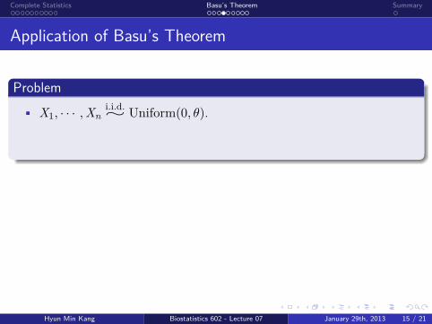
Application of Basu’s Theorem
.Problem..
......
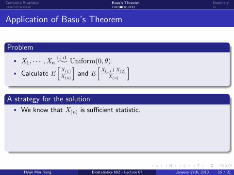
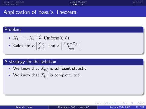
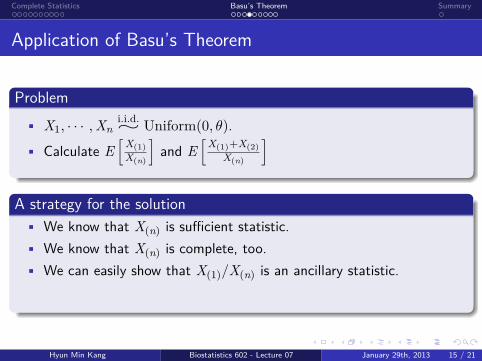
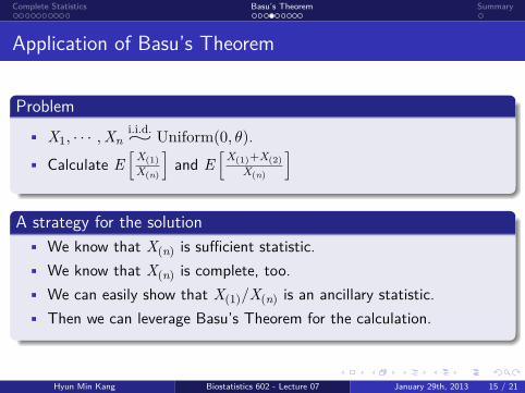
• X1, · · · ,Xni.i.d.∼ Uniform(0, θ).
• Calculate E[X(1)
X(n)
]and E
[X(1)+X(2)
X(n)
].A strategy for the solution..
......
• We know that X(n) is sufficient statistic.• We know that X(n) is complete, too.• We can easily show that X(1)/X(n) is an ancillary statistic.• Then we can leverage Basu’s Theorem for the calculation.
Hyun Min Kang Biostatistics 602 - Lecture 07 January 29th, 2013 15 / 21
. . . . . .
. . . . . . . . . .Complete Statistics
. . . . . . . . .Basu’s Theorem
.Summary
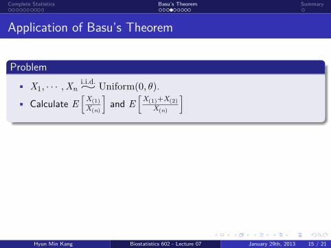
Application of Basu’s Theorem
.Problem..
......
• X1, · · · ,Xni.i.d.∼ Uniform(0, θ).
• Calculate E[X(1)
X(n)
]and E
[X(1)+X(2)
X(n)
]
.A strategy for the solution..
......
• We know that X(n) is sufficient statistic.• We know that X(n) is complete, too.• We can easily show that X(1)/X(n) is an ancillary statistic.• Then we can leverage Basu’s Theorem for the calculation.
Hyun Min Kang Biostatistics 602 - Lecture 07 January 29th, 2013 15 / 21
. . . . . .
. . . . . . . . . .Complete Statistics
. . . . . . . . .Basu’s Theorem
.Summary
Application of Basu’s Theorem
.Problem..
......
• X1, · · · ,Xni.i.d.∼ Uniform(0, θ).
• Calculate E[X(1)
X(n)
]and E
[X(1)+X(2)
X(n)
].A strategy for the solution..
......
• We know that X(n) is sufficient statistic.
• We know that X(n) is complete, too.• We can easily show that X(1)/X(n) is an ancillary statistic.• Then we can leverage Basu’s Theorem for the calculation.
Hyun Min Kang Biostatistics 602 - Lecture 07 January 29th, 2013 15 / 21
. . . . . .
. . . . . . . . . .Complete Statistics
. . . . . . . . .Basu’s Theorem
.Summary
Application of Basu’s Theorem
.Problem..
......
• X1, · · · ,Xni.i.d.∼ Uniform(0, θ).
• Calculate E[X(1)
X(n)
]and E
[X(1)+X(2)
X(n)
].A strategy for the solution..
......
• We know that X(n) is sufficient statistic.• We know that X(n) is complete, too.
• We can easily show that X(1)/X(n) is an ancillary statistic.• Then we can leverage Basu’s Theorem for the calculation.
Hyun Min Kang Biostatistics 602 - Lecture 07 January 29th, 2013 15 / 21
. . . . . .
. . . . . . . . . .Complete Statistics
. . . . . . . . .Basu’s Theorem
.Summary
Application of Basu’s Theorem
.Problem..
......
• X1, · · · ,Xni.i.d.∼ Uniform(0, θ).
• Calculate E[X(1)
X(n)
]and E
[X(1)+X(2)
X(n)
].A strategy for the solution..
......
• We know that X(n) is sufficient statistic.• We know that X(n) is complete, too.• We can easily show that X(1)/X(n) is an ancillary statistic.
• Then we can leverage Basu’s Theorem for the calculation.
Hyun Min Kang Biostatistics 602 - Lecture 07 January 29th, 2013 15 / 21
. . . . . .
. . . . . . . . . .Complete Statistics
. . . . . . . . .Basu’s Theorem
.Summary
Application of Basu’s Theorem
.Problem..
......
• X1, · · · ,Xni.i.d.∼ Uniform(0, θ).
• Calculate E[X(1)
X(n)
]and E
[X(1)+X(2)
X(n)
].A strategy for the solution..
......
• We know that X(n) is sufficient statistic.• We know that X(n) is complete, too.• We can easily show that X(1)/X(n) is an ancillary statistic.• Then we can leverage Basu’s Theorem for the calculation.
Hyun Min Kang Biostatistics 602 - Lecture 07 January 29th, 2013 15 / 21
. . . . . .
. . . . . . . . . .Complete Statistics
. . . . . . . . .Basu’s Theorem
.Summary
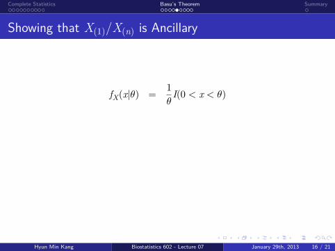
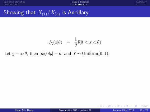
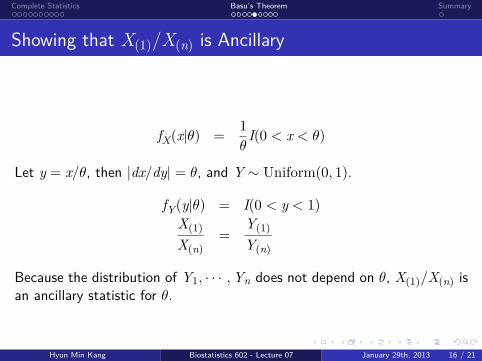
Showing that X(1)/X(n) is Ancillary
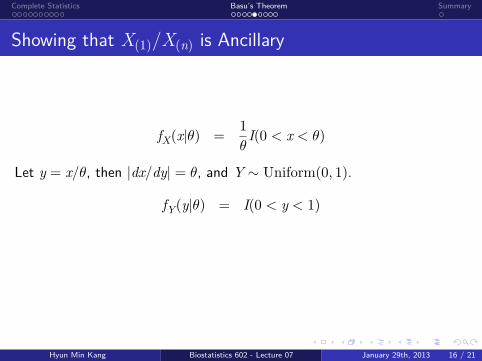
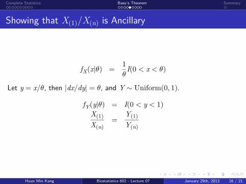
fX(x|θ) =1
θI(0 < x < θ)
Let y = x/θ, then |dx/dy| = θ, and Y ∼ Uniform(0, 1).
fY(y|θ) = I(0 < y < 1)
X(1)
X(n)=
Y(1)
Y(n)
Because the distribution of Y1, · · · ,Yn does not depend on θ, X(1)/X(n) isan ancillary statistic for θ.
Hyun Min Kang Biostatistics 602 - Lecture 07 January 29th, 2013 16 / 21
. . . . . .
. . . . . . . . . .Complete Statistics
. . . . . . . . .Basu’s Theorem
.Summary
Showing that X(1)/X(n) is Ancillary
fX(x|θ) =1
θI(0 < x < θ)
Let y = x/θ, then |dx/dy| = θ, and Y ∼ Uniform(0, 1).
fY(y|θ) = I(0 < y < 1)
X(1)
X(n)=
Y(1)
Y(n)
Because the distribution of Y1, · · · ,Yn does not depend on θ, X(1)/X(n) isan ancillary statistic for θ.
Hyun Min Kang Biostatistics 602 - Lecture 07 January 29th, 2013 16 / 21
. . . . . .
. . . . . . . . . .Complete Statistics
. . . . . . . . .Basu’s Theorem
.Summary
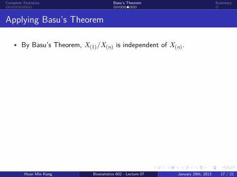
Applying Basu’s Theorem
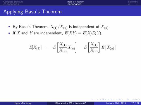
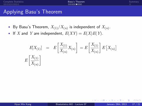
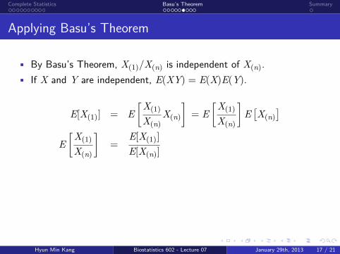
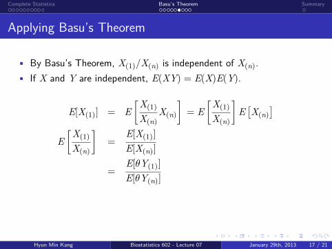
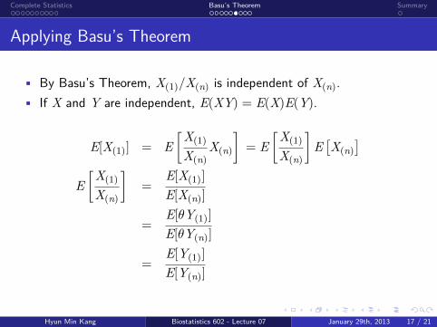
• By Basu’s Theorem, X(1)/X(n) is independent of X(n).
• If X and Y are independent, E(XY) = E(X)E(Y).
E[X(1)] = E[X(1)
X(n)X(n)
]= E
[X(1)
X(n)
]E[X(n)
]E[X(1)
X(n)
]=
E[X(1)]
E[X(n)]
=E[θY(1)]
E[θY(n)]
=E[Y(1)]
E[Y(n)]
Hyun Min Kang Biostatistics 602 - Lecture 07 January 29th, 2013 17 / 21
. . . . . .
. . . . . . . . . .Complete Statistics
. . . . . . . . .Basu’s Theorem
.Summary
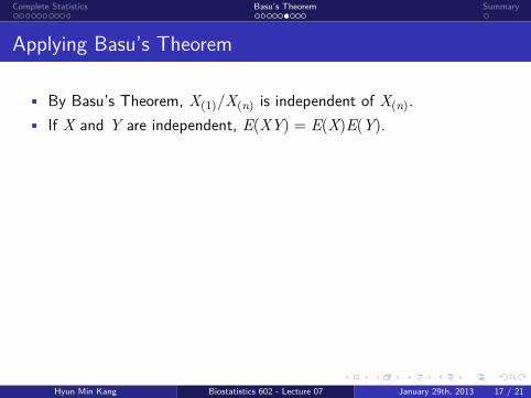
Applying Basu’s Theorem
• By Basu’s Theorem, X(1)/X(n) is independent of X(n).• If X and Y are independent, E(XY) = E(X)E(Y).
E[X(1)] = E[X(1)
X(n)X(n)
]= E
[X(1)
X(n)
]E[X(n)
]E[X(1)
X(n)
]=
E[X(1)]
E[X(n)]
=E[θY(1)]
E[θY(n)]
=E[Y(1)]
E[Y(n)]
Hyun Min Kang Biostatistics 602 - Lecture 07 January 29th, 2013 17 / 21
. . . . . .
. . . . . . . . . .Complete Statistics
. . . . . . . . .Basu’s Theorem
.Summary
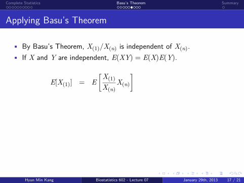
Applying Basu’s Theorem
• By Basu’s Theorem, X(1)/X(n) is independent of X(n).• If X and Y are independent, E(XY) = E(X)E(Y).
E[X(1)] = E[X(1)
X(n)X(n)
]
= E[X(1)
X(n)
]E[X(n)
]E[X(1)
X(n)
]=
E[X(1)]
E[X(n)]
=E[θY(1)]
E[θY(n)]
=E[Y(1)]
E[Y(n)]
Hyun Min Kang Biostatistics 602 - Lecture 07 January 29th, 2013 17 / 21
. . . . . .
. . . . . . . . . .Complete Statistics
. . . . . . . . .Basu’s Theorem
.Summary
Applying Basu’s Theorem
• By Basu’s Theorem, X(1)/X(n) is independent of X(n).• If X and Y are independent, E(XY) = E(X)E(Y).
E[X(1)] = E[X(1)
X(n)X(n)
]= E
[X(1)
X(n)
]E[X(n)
]
E[X(1)
X(n)
]=
E[X(1)]
E[X(n)]
=E[θY(1)]
E[θY(n)]
=E[Y(1)]
E[Y(n)]
Hyun Min Kang Biostatistics 602 - Lecture 07 January 29th, 2013 17 / 21
. . . . . .
. . . . . . . . . .Complete Statistics
. . . . . . . . .Basu’s Theorem
.Summary
Applying Basu’s Theorem
• By Basu’s Theorem, X(1)/X(n) is independent of X(n).• If X and Y are independent, E(XY) = E(X)E(Y).
E[X(1)] = E[X(1)
X(n)X(n)
]= E
[X(1)
X(n)
]E[X(n)
]E[X(1)
X(n)
]
=E[X(1)]
E[X(n)]
=E[θY(1)]
E[θY(n)]
=E[Y(1)]
E[Y(n)]
Hyun Min Kang Biostatistics 602 - Lecture 07 January 29th, 2013 17 / 21
. . . . . .
. . . . . . . . . .Complete Statistics
. . . . . . . . .Basu’s Theorem
.Summary
Applying Basu’s Theorem
• By Basu’s Theorem, X(1)/X(n) is independent of X(n).• If X and Y are independent, E(XY) = E(X)E(Y).
E[X(1)] = E[X(1)
X(n)X(n)
]= E
[X(1)
X(n)
]E[X(n)
]E[X(1)
X(n)
]=
E[X(1)]
E[X(n)]
=E[θY(1)]
E[θY(n)]
=E[Y(1)]
E[Y(n)]
Hyun Min Kang Biostatistics 602 - Lecture 07 January 29th, 2013 17 / 21
. . . . . .
. . . . . . . . . .Complete Statistics
. . . . . . . . .Basu’s Theorem
.Summary
Applying Basu’s Theorem
• By Basu’s Theorem, X(1)/X(n) is independent of X(n).• If X and Y are independent, E(XY) = E(X)E(Y).
E[X(1)] = E[X(1)
X(n)X(n)
]= E
[X(1)
X(n)
]E[X(n)
]E[X(1)
X(n)
]=
E[X(1)]
E[X(n)]
=E[θY(1)]
E[θY(n)]
=E[Y(1)]
E[Y(n)]
Hyun Min Kang Biostatistics 602 - Lecture 07 January 29th, 2013 17 / 21
. . . . . .
. . . . . . . . . .Complete Statistics
. . . . . . . . .Basu’s Theorem
.Summary
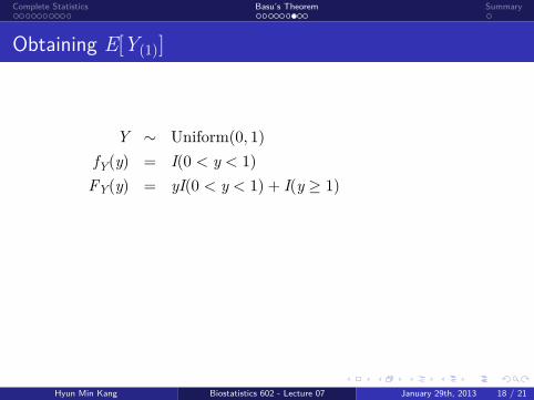
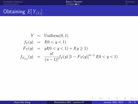
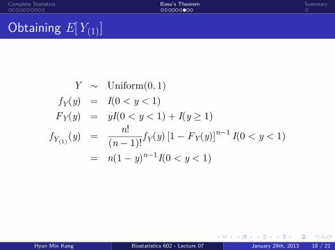
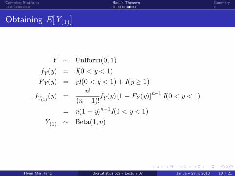
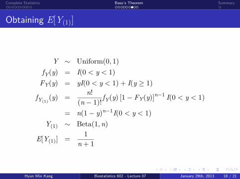
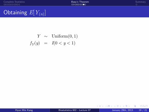
Obtaining E[Y(1)]
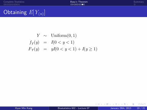
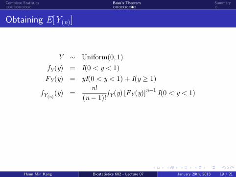
Y ∼ Uniform(0, 1)
fY(y) = I(0 < y < 1)
FY(y) = yI(0 < y < 1) + I(y ≥ 1)
fY(1)(y) =
n!(n − 1)!
fY(y) [1− FY(y)]n−1 I(0 < y < 1)
= n(1− y)n−1I(0 < y < 1)
Y(1) ∼ Beta(1,n)
E[Y(1)] =1
n + 1
Hyun Min Kang Biostatistics 602 - Lecture 07 January 29th, 2013 18 / 21
. . . . . .
. . . . . . . . . .Complete Statistics
. . . . . . . . .Basu’s Theorem
.Summary
Obtaining E[Y(1)]
Y ∼ Uniform(0, 1)
fY(y) = I(0 < y < 1)
FY(y) = yI(0 < y < 1) + I(y ≥ 1)
fY(1)(y) =
n!(n − 1)!
fY(y) [1− FY(y)]n−1 I(0 < y < 1)
= n(1− y)n−1I(0 < y < 1)
Y(1) ∼ Beta(1,n)
E[Y(1)] =1
n + 1
Hyun Min Kang Biostatistics 602 - Lecture 07 January 29th, 2013 18 / 21
. . . . . .
. . . . . . . . . .Complete Statistics
. . . . . . . . .Basu’s Theorem
.Summary
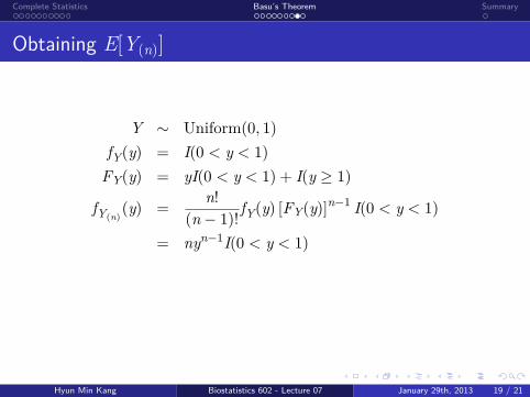
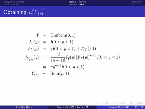
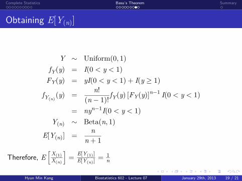
Obtaining E[Y(n)]
Y ∼ Uniform(0, 1)
fY(y) = I(0 < y < 1)
FY(y) = yI(0 < y < 1) + I(y ≥ 1)
fY(n)(y) =
n!(n − 1)!
fY(y) [FY(y)]n−1 I(0 < y < 1)
= nyn−1I(0 < y < 1)
Y(n) ∼ Beta(n, 1)
E[Y(n)] =n
n + 1
Therefore, E[X(1)
X(n)
]=
E[Y(1)]
E[Y(n)]= 1
n
Hyun Min Kang Biostatistics 602 - Lecture 07 January 29th, 2013 19 / 21
. . . . . .
. . . . . . . . . .Complete Statistics
. . . . . . . . .Basu’s Theorem
.Summary
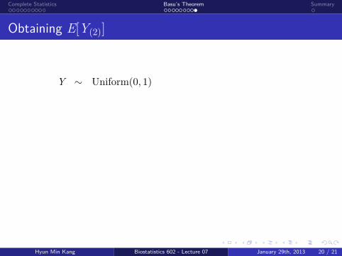
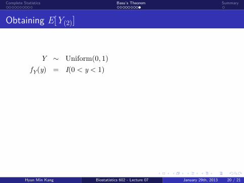
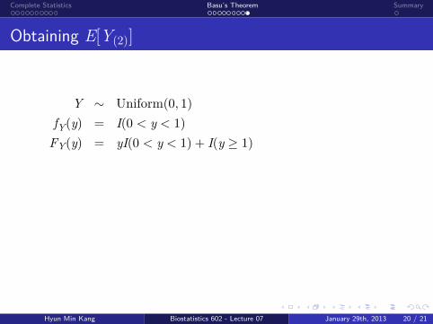
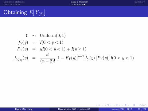
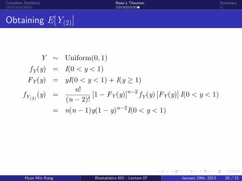
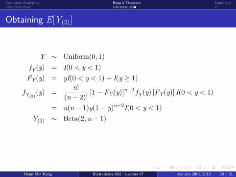
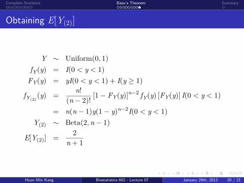
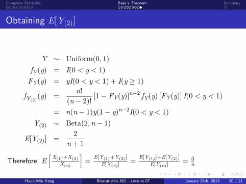
Obtaining E[Y(2)]
Y ∼ Uniform(0, 1)
fY(y) = I(0 < y < 1)
FY(y) = yI(0 < y < 1) + I(y ≥ 1)
fY(2)(y) =
n!(n − 2)!
[1− FY(y)]n−2 fY(y) [FY(y)] I(0 < y < 1)
= n(n − 1)y(1− y)n−2I(0 < y < 1)
Y(2) ∼ Beta(2,n − 1)
E[Y(2)] =2
n + 1
Therefore, E[X(1)+X(2)
X(n)
]=
E[Y(1)+Y(2)]
E[Y(n)]=
E[Y(1)]+E[Y(2)]
E[Y(n)]= 3
n
Hyun Min Kang Biostatistics 602 - Lecture 07 January 29th, 2013 20 / 21
. . . . . .
. . . . . . . . . .Complete Statistics
. . . . . . . . .Basu’s Theorem
.Summary
Summary
.Today..
......
• More on complete statistics• Basu’s Theorem
.Next Lecture..
......• Exponential Family
Hyun Min Kang Biostatistics 602 - Lecture 07 January 29th, 2013 21 / 21
. . . . . .
. . . . . . . . . .Complete Statistics
. . . . . . . . .Basu’s Theorem
.Summary
Summary
.Today..
......
• More on complete statistics• Basu’s Theorem
.Next Lecture..
......• Exponential Family
Hyun Min Kang Biostatistics 602 - Lecture 07 January 29th, 2013 21 / 21
Related Documents