Biosphere-Atmosphere Interactions

Chapter 2Biosphere-Atmosphere InteractionsLead authors: MaryC.Scholes· PatriciaA.Matrai . Meinrat O.Andreae· Keith A. Smith· MartinR.ManningCo-authors: PauloArtaxo . Leonard A. Barrie · TimothyS. Bates · James H. Butler· Paolo Ciccioli . Stanislaw A. Cieslik

Robert J.Delmas· FrankJ.Dentener . Robert A.Duce . David J.Erickson III . IanE. Galbally . Alex B. GuentherRuprecht Jaenicke· Bernd Iahne . Anthony J.Kettle- Ronald P. Kiene· Jean-Pierre Lacaux . Peter S.Liss . G.MalinPamela A. Matson · ArvinR.Mosier · Heinz-Ulrich Neue · HansW. Paerl . UlrichF. Platt · PatriciaK. QuinnWolfgang Seiler . Ray F.Weiss

2.1 Introduction

The contemporary atmosphere was created as a resultof biological activity some two billion years ago. To thisday, its natural composition is supported and modified,mostly through biological processes of trace gas pro­duction and destruction, while also involving physicaland chemical degradation processes. The biosphere hasa major influence on present environmental conditions,both on a regional and global scale. One of the best­documented and most important indicators of globalchange is the progressive increase of a number of tracegases in the atmosphere, among them carbon dioxide(C0 2) , methane (CH4) , and nitrous oxide (N20 ), all ofwhich are of biospheric origin. There is considerableuncertainty, however, regarding the processes that de­termine the concentration and distribution of trace gasesand aerosols in the atmosphere and the causes and con­sequences of atmospheric change (Andreae and Schimel1989). To improve our understanding IGAC created anenvironment for multi-disciplinary collaboration amongbiologists,chemists, and atmospheric scientists. This wasessential to develop analytical methods, to characteriseecosystems, to investigate physiological controls, to de­velop and validate micrometeorological theory, and todesign and develop diagnostic and predictive models(Matson and Ojima 1990) .

Interactions between the biosphere and the atmo­sphere are part of a complex,interconnected system.Theemission and uptake of atmospheric constituents by thebiota influence chemical and physical climate throughinteractions with atmospheric photochemistry andEarth's radiation budget. Comparatively small amountsof CH4 and N20 present in the atmosphere make sub­stantial contributions to the global greenhouse effect.In addition, emissions of hydrocarbons and nitrogenoxides from biomass burning in the Tropics result inthe photochemical production of large amounts ofozone (03) and acidity in the tropical atmosphere. Inturn, climate change and atmospheric pollution alter therates and sometimes even the direction of chemical ex­change between the biosphere and atmosphere throughinfluences at both individual organism and ecosystem

levels. Recent and expected future changes in land useand land management practices provide further impe­tus for closely examining climate-gas flux interactions.Anthropogenic influences, e.g, tropical deforestationand the widespread implementation of agricultural tech­nologies, have and will continue to make significant al­terations in the sources and sinks for the various tracegases.

Ten years ago, at the beginning of IGAC, researcherssought to establish the source and sink strength of gasesin different kinds of ecosystems, in different areas ofthe world. Specific goals of the programme, related tothe biosphere included:

• to understand the interactions between atmosphericchemical composition and biological and climaticprocesses;

• to predict the impact of natural and anthropogenicforcings on the chemical composition of the atmo­sphere ; and

• to provide the necessary knowledge for the propermaintenance of the biosphere and climate.

Earlier extrapolations of gas fluxes over space andtime were often based on a single, or very small , setof measurements, and researchers sought for "repre­sentative" sites at which to make those crucial measure­ments. IGAC brought a new focus to the variabilityamong ecosystems and regions of the world, in order tounderstand better the factors controlling fluxes (Galbally1989) . For example, studies of CH4 flux from wetlandsand rice paddies of N 20 flux from natural and man­aged ecosystems, and of dimethylsulphide (DMS) emis­sions from oceans, consciously spanned gradients oftemperature, hydrological characteristics, soil types,marine systems, management regimes, and nitrogendeposition. One result of this strategy has been the rec­ognition that the same basic processes were responsi­ble for gas fluxes across regions, latitudinal zones, andenvironments. This chapter gives a general overview ofthe progress that has been made in the field as a wholewithin the last decade, with emphasis on research ac­tivities stimulated, initiated, and/or endorsed by theIGACcommunity. It is not our intent to provide current

G. Brasseur et al. (eds.), Atmospheric Chemistry in a Changing World

© Springer-Verlag Berlin Heidelberg 2002

[email protected]

The complete book is available at: http://www.igacproject.org/sites/all/themes/bluemasters/images/2003_Brasseur_AtmosphericChemistryinaChangingWorld.pdf

:!.O M.C.Scholes • P.A.Matrai . M.O.Andreae . K.A.Smith . M.R.Manning

assessments of all trace gas source and sink strengths.as those budgets have been compiled and published(with considerable contributions by IGAC researchers)in recent Intergovernmental Panel on Climate Change(IPCC) documents. Examples of research not conductedwithin the IGAC framework but relevant to the topicare CH4 from landfills. ruminant livestock. and termites;information on these topics can be found in IPCC(1996,1999)·

Exchanges of biogenic trace gases between surfacesand the atmosphere depend on the production and con­sumption of gases by microbial and plant processes. onphysical transport through soils. sediments. and water.and on flux across the surface-air boundaries. Thus, tounderstand and predict fluxes. studies of whole ecosys­tems are required. The goals of research over the pastdecade have been to develop an understanding of thefactors that control flux, organise the measurements sothat they are useful for regional and global scale budg­ets. and use the knowledge to predict how fluxes arelikely to change in the future.

The IGAC Project focussed on issues of specific in­terest over a number of different geographical regionsof Earth. A variety of projects have been conducted overthe last ten years, many of which addressed issues re­lated to exchange between the biosphere and the atmo­sphere. Several field campaigns. using a combination ofmeasurement and modelling techniques. have beenconducted very successfully under the IGAC umbrella,e.g. in southern Africa (SAFARI 1992and 2000) and invarious oceanic regions (ACE-I,ACE-2. and ACE-Asia)(see A.5).

Why certain trace gases were studied together andwhyvarious scientific approaches were adopted to studythem is described in this chapter. Research findings spe­cifically related to the exchange of trace gases and aero­sols between the atmosphere and the terrestrial andmarine biospheres will be given. In the terrestrial sec­tion. special attention is given to biomass burning andwet deposition in the Tropics. because of the significantcontribution made by IGAC to these programmes. Wealso consider some of the anthropogenic activities that

alter biosphere-atmosphere exchange and discuss po­tential feedbacks related to climate change. regional levelair pollution, and deposition. In the marine section,emphasis is on the biogeochemistry of DMS.given thatthe greatest advances were made on this topic. The chap­ter concludes by summarising the major accomplish­ments of the last decade and highlighting some of theremaining research challenges.

2.2 Key Biogenic Gasesor Families and theirRelevance to Atmospheric Chemistry

The study of atmospheric composition has largelyfocussed on trace compounds that affect either theradiative properties of the atmosphere, or the biosphereas nutrients or toxins, or playa key role in atmosphericchemistry. The trace gases that are important in thisregard have been summarised in the preceding chapter.This chapter considers the role of the biosphere in emis­sion or removal of such compounds.

Although CO2 and water (H20 ) are both greenhousegases which are strongly affected by the biosphere. stud­ies of these compounds have generally been conductedin parallel scientific communities, and IGAChas main­tained a focus on the chemically reactive greenhousegases. Thus no attempt is made here to cover the largebody of research on the global carbon cycle and the in­teractions of CO2 with the biosphere.

2.2.1 The Carbon Family of Gases:CH4' Volatile Organic Carbon Compounds(VOCs), and Carbon Monoxide (CO)

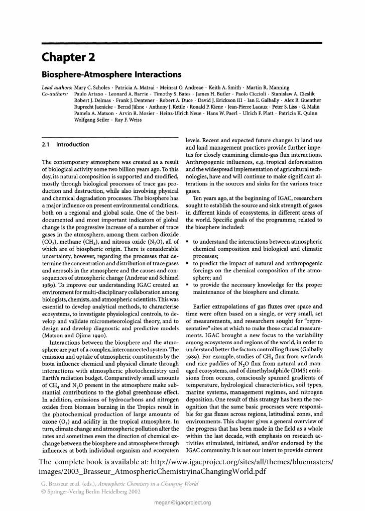
Methane (CH4) is a greenhouse gas with a lifetime inthe atmosphere of about nine years. Its atmosphericconcentration is largely controlled by the biosphere, with70% or more of current emissions and virtually all ofpre-industrial emissions being biogenic (Fig. 2.1; Milich1999). The dominant biogenic production process forCH4 is microbial breakdown of organic compounds in

CIl ue:CIl -c: 0

~ ~~'" w e:a. CIl

8 Eif ~

200

100

0J---L-.l......:.- .:.......J: --:L.....L....L....l.....L........ ..L..J...------ - -- _

~ - 100cc: -200Bc: - 300.Q -400

~ - 500

-600

-enI--

Fig. 2.1.Estimated annual anthropo­genic and natural sources andsinks of methane (thick bars)in millions of tons, and uncer­tainty ranges (thin lines)(Milich 1999)

[email protected]

Fig. 2.2.Methane growth rate s (figurecourtesy of the National Oce­anic and Atmospheric Admin­istration (NOAA), ClimateMonitoring and DiagnosticsLaboratory (CMDLl. and Car­bon Cycle-Greenhouse Gases(CCGG))

0.5

CII"C

.~

.; 0CIIC

Vi

- 0.5

- 1

CHAPTER 2 . Biosphere-Atmosphere Interactions 2 1

CH4 growth rate (nmol mor ' yr· l)

90·

30·

CII"C

o· 3";;",

...J

30·

90·84 85 86 87 88 89 90 91 92 93 94 95 96 97 98 99 00

Year

anaerobic conditions. This occurs in flooded soils suchas natural wetlands and rice paddies, in the rumen ofanimals such as cattle, in landfills, and in anoxic layersin the marine water column and sediments. Methane isalso emitted directly to the atmosphere from burningvegetation as a product of pyrolytic breakdown of or­ganic material.

Changes in land use, particularly increases in num­bers of domestic ruminants, the extent of rice paddies,and biomass burning, have more than doubled biogenicCH4 emissions since the pre-industrial era (Milich 1999;Ehhalt et al. 2001). Fossil fuel related emissions and adecrease in atmospheric oxidation rates (Thompson1992) have further increased CH4 concentrations butthose aspects fall outside the scope of this chapter.

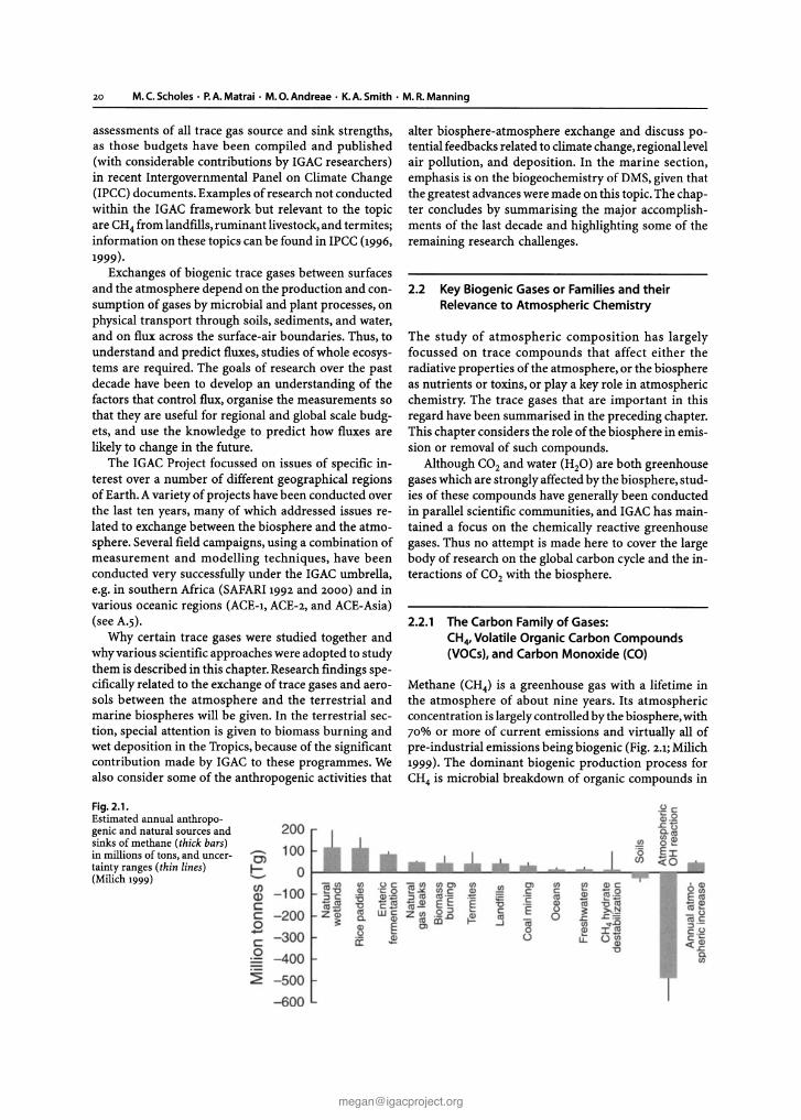
The atmospheric concentration of CH4 is now about1745nmol mol' I , compared to pre-industrial levels ofabout 700 nmol mol'. Growth rates have been observeddirectly in the atmosphere since the 1950S (Rinslandet al.198S;Zander et al.1989) and on an increasingly sys­tematic basis since 1978 (Blake and Rowland 1988;Dlugokencky et al. 1994). Concentrations were increas­ing at about 20 nmol mol:' yr" in the 1970s, but that ratehas generally declined to an average of 5 nmol mol"! yr·1

over the period 1992to 1998.High growth rates of about15nmol mol"! yr·1 occurred in 1991 and 1998 (Fig. 2.2,Dlugokencky et al. 1998; Ehhalt et al. 2001) and appearto be caused by climate related increases in wetland and!or biomass burning emissions (Dlugokencky et al. 2000;Walter and Matthews 2000). IPCC (2001) estimates itsrate of increase at 8.4 nmol mol"! yr".

The evolution of the CH4 budget since the pre-in­dustrial era provides a good example of interactionsbetween land use and atmospheric change. A schematicof the change in total emissions from the 18th century tothe present is shown in Fig. 2.3 (based on Stern andKaufmann 1996,Lelieveldet al.1998,and Houweling et al.

Lifetime 7.6 y r 8.4 yr

Removal g gflux Tg yr-1

Atmospheric ~ 1900 Tg ( 4900 Tg IIbu rden (690 nmo lmol'' ) (1750 nmol mOr l)

Emission g gflux Tg yr-1

Pre - indust rial Current

Fig. 2.3. Schematic of the pre -industrial Holocene and current(1990S) atmospheric methane budget. The mean lifetime derivedfrom the ratio of atmospheric burden to removal rate has increasedby ca. 10%, which is broadly consistent with estimates of the relativedecrease in OH from atmospheric chemistry models (based onStern and Kaufmann (1996), Lelieveld et al. (1998) and Houwelinget al. (1999) (see also Fig. 7.4.)

1999). The removal rates that are required to balancethe source-sink budget at pre-industrial and presentconcentrations imply an increase in the methane life­time. This is consistent with independent estimates of adecrease in atmospheric oxidation rates inferred fromchemistry models.

Plants emit a range of volatile organic carbon (VOCs)compounds, which include hydrocarbons, alcohols,carbonyls, fatty acids, and esters, together with organicsulphur compounds, halocarbons, nitric oxide (NO), CO,and organic particles. Estimates of anthropogenic emis­sions for 1990 are shown in Fig. 2.4. According to cur­rent estimates plants emit up to 1200 Tg C yr- I as VOCs(Guenther et al. 1995).The amount of carbon releasedfrom the biosphere this way may be up to 30% of netecosystem productivity (NEP), i.e, the annual accumu­lation of carbon in an ecosystem before taking account

[email protected]

22 M.C.Scholes· P. A. Matrai . M.O.Andreae· K.A.Smith· M. R. Manning

NMVOC from anthropogen ic so urces in 1990Sources : lEA. UN, FAD, misc.

o

60

30

-60

18090

-30

~

150

150

120

120

90

90

60

60

30

30

o

o

-30

-30

-60

-60

- 90

-90

- 120

- 120

- 150

-150

o

I •

30

- 18090

-60

-90~=~=-_-=-=-_--:-:__ ;;"'-_--:-:__ =--_--:-:-_----:-=--_--:-:-__ :-:-_-=-=_~- 90- 180 180

- 30

Global total : 171 Tg NVOC(min. = 0.0. max . = 1.2 TG)

Tangent cylinde r project ion.

Unit: Gg NMVOClcell

o 2-10_ 0-0 .1 10-50_ 0.1-1 _ 50-100

1-2 _ 100-6200

Calculation : G: NMV·s UM: Anthr. em issions i n 1990Dataset ( AL. EF) : 4:PUBLIC DATAsET·Vers ion

Source : EDGARlRIM+

Fig. 2.4. Anthropogenic yearly non -methane VOC emissions in 1990 from the EDGAR (Emission Database for Global AtmosphericResearch) database (Olivier et a1. 1996)

of ecosystem disturbance (e.g. Valentini et al. 1997;Kesselmeier et al. 1998; Crutzen et al. 1999). Neglect ofVOC and CO terrestrial emissions may cause signifi­cant errors in estimates of NEP and changes in carbonstorage for some ecosystems.

While the oceans are supersaturated with CO andsurface production of VOCs is widespread, the ocean­atmosphere fluxes are small, but less well studied, com­pared with terrestrial emission estimates. VOCsshow awide range of reactivities in the troposphere, with life­times ranging from minutes (e.g. ~-caryophyllene) totwo weeks (e.g, methanol) (Atkinson and Arey 1998).Many are emitted at very low rates, and in some casesare offset by plant uptake, thus having a negligibleimpacton atmospheric chemistry; others impact ozone produc­tion (see Chap. 3), aerosol production (see Chap. 4), andthe global CO budget.

Primary pollutants emitted main ly as a result of hu­man activity include hydrocarbons, CO, and nitrogenoxides. About half the terrestrial surface emissions ofCO are due to direct emissions from vegetation andbiomass burning. In addition about 45%of the total COsource to the atmosphere is due to oxidation of meth-

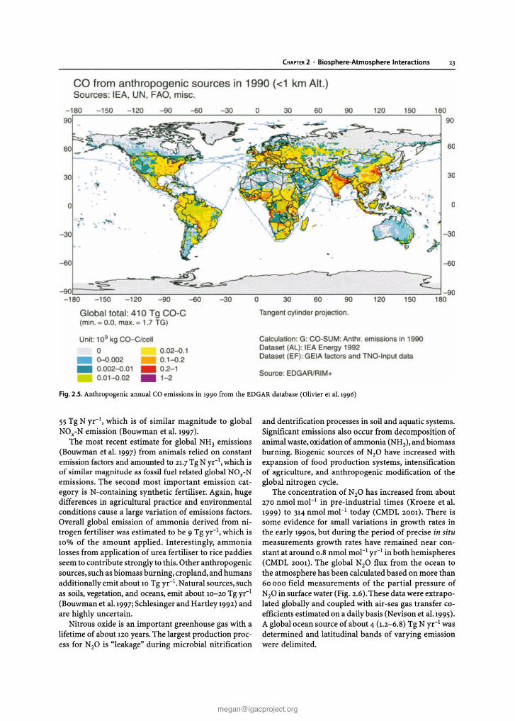
ane and other organics in the atmosphere, which them­selves are predominantly biogenic compounds. BecauseCO is the end product in the methane oxidation chainthe two budgets are closely linked; in addition, CO alsooriginates from the breakdown of VOCs. The concen­trations of CO are temporally and spatially highly vari­able due to the short lifetime of CO and the nature of itsdiscontinuous land based sources. Estimates of anthro­pogenic CO emissions for 1990 are shown in Fig. 2.5.

2.2.2 The Nitrogen Family of Gases:Ammonia (NH3), N20, and NO

Despite its importance for particle formation and cli­mate, relatively little effort has been spent on un­derstanding the sources and removal processes of NH3•

Most work on atmospheric ammonia has been per­formed with respect to eutrophication and acidificationclose to the terrestrial sources; large scale transport andchemistry of NH3 and ammonium (NHt) have receivedmuch less attention, especially over remote marine re­gions. The global source strength of ammonia is about

[email protected]

CHAPTER 2 . Biosphere-Atmosphere Interactions 23

CO from anthropogenic sources in 1990 « 1 km Alt.)Sources : lEA. UN, FAO, misc.

i ' ... ,

- 18090

30

o

- 30

-60

- 150 - 120 - 90 -60 -30 o 30 60 90 120 150 18090

60

30

o

- 30

~-60

150120906030o-30-60- 90- 120- 150-90t==~=- -=- ..::J -90

- 180 180

Global tota l: 410 Tg CO-C(min. =0.0 . max . =1.7 TG )

Tangen t cylinder projection .

Source : EDGARlRIM+

Calculation : G : CO-S UM: Anlhr. emiss ions In 1990Dataset ( AL): lEA Energy 1992Dataset (EF ): GEIA fac tors and TNO-Input data

0.02-0.10.1-0.2

. 0.2- 1

. 1- 2

Unit: 109 kg CQ-C/cell

o. 0-0.002• 0.002-0.01

0.01-0.02

Fi9. 2.5. Anthropogenic annual CO emissions in 1990 from the EDGAR database (Olivier et aJ.1996)

55Tg N yr- I , which is of similar magnitude to globalNOx-N emission (Bouwman et al. 1997).

The most recent estimate for global NH3 emissions(Bouwman et al. 1997) from animals relied on constantemission factors and amounted to 21.7 Tg N yr", which isof similar magnitude as fossil fuel related global NOx-Nemissions. The second most important emission cat­egory is N-containing synthetic fertiliser. Again, hugedifferences in agricultural practice and environmentalconditions cause a large variation of emissions factors.Overall global emission of ammonia derived from ni­trogen fertiliser was estimated to be 9 Tg yr- I

, which is10% of the amount applied. Interestingly, ammonialosses from application of urea fertiliser to rice paddiesseem to contribute strongly to this. Other anthropogenicsources, such as biomass burning, cropland, and humansadditionally emit about 10 Tg yr'". Natural sources, suchas soils, vegetation, and oceans, emit about 10-20 Tg yr-I(Bouwman et al.1997;Schlesinger and Hartley iccz) andare highly uncertain.

Nitrous oxide is an important greenhouse gas with alifetime of about 120years. The largest production proc­ess for N20 is "leakage" during microbial nitrification

and dentrification processes in soil and aquatic systems.Significant emissions also occur from decomposition ofanimal waste, oxidation of ammonia (NH3) , and biomassburning. Biogenic sources of N20 have increased withexpansion of food production systems, intensificationof agriculture, and anthropogenic modification of theglobal nitrogen cycle.

The concentration ofN20 has increased from about270 nmol mol! in pre-industrial times (Kroeze et al.1999) to 314nmol mol:" today (CMDL 2001). There issome evidence for small variations in growth rates inthe early 1990S, but during the period of precise in situmeasurements growth rates have remained near con­stant at around 0.8 nmol mol" yr- I in both hemispheres(CMDL 2001). The global N20 flux from the ocean tothe atmosphere has been calculated based on more than60000 field measurements of the partial pressure ofN20 in surface water (Fig. 2.6).These data were extrapo­lated globally and coupled with air-sea gas transfer co­efficients estimated on a daily basis (Nevison et al.1995).A global ocean source of about 4 (1.2-6.8) Tg N yr'" wasdetermined and latitudinal bands of varying emissionwere delimited.

[email protected]

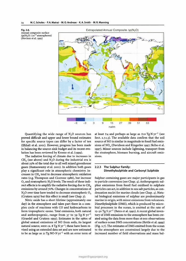
24 M.C.Scholes · P.A.Matrai · M.O.Andreae · K.A.Smith· M.R.Manning

Fig. 2.6.Annual composite surface.1p(N20) (10-9 atmospheres)(Nevison et al. 1995)

1

Extrapolated Annua l Compos ite p(N20)

;

) , I....~ .....)~

I3 9 15 27

natm

39 5 1 63

Quantifying the wide range of N20 sources hasproved difficult and upper and lower bound estimatesfor specific source types can differ by a factor of ten(Ehhalt et al. 2001). However, progress has been madein balancing the source-sink budget and its recent evo­lution has been reviewed by Kroeze et al. (1999).

The radiative forcing of climate due to increases inCH4 (see above) and N20 during the industrial era isabout 25% of the total due to all well mixed greenhousegases (Ramaswamy et al. 2001). In addition both gasesplaya significant role in atmospheric chemistry. In­creases in CH4 tend to decrease atmospheric oxidationrates (e.g, Thompson and Cicerone 1986), but increase03 and stratospheric H20 levels.The result of these indi­rect effects is to amplify the radiative forcing due to CH4emissions by around 70%. Changes in concentrations ofN20 over time have tended to decrease stratospheric 03(Crutzen 1979) but this effect is small (see Chap. 3).

Nitric oxide has a short lifetime (approximately oneday) in the atmosphere and takes part there in a com­plex cycle of reactions with CO and hydrocarbons toform tropospheric ozone. Total emissions, both naturaland anthropogenic, range from 37 to 59 Tg N yr- 1

(Graedel and Crutzen 1993). Estimates in the 1980s ofglobal annual emissions of NO from soils, its largestnatural source, were ca. 8 Tg N yr- 1

; these have been re­vised using an extended data set and are now estimatedto be as large as 21Tg NO-N yr- 1 with an error term of

at least ±4 and perhaps as large as ±10 Tg N yr-1 (seeSect. 2.7.1.3). The available data confirm that the soilsource of NO is similar in magnitude to fossil fuel emis­sions of NOx (Davidson and Kingerlee 1997;Skiba et al.1997). Minor sources include lightning, transport fromthe stratosphere, biomass burning, and aircraft emis­sions.

2.2.3 The Sulphur Family:Dimethylsulphide and Carbonyl Sulphide

Sulphur containing gases are major participants in gasto particle conversion (see Chap. 4). Anthropogenic sul­phur emissions from fossil fuel oxidised to sulphateparticles can act , in addition to sea salt particles, as con­densation nuclei for marine clouds (see Chap. 4). Natu­ral biological emissions of sulphur are predominantlymarine in origin, with minor emissions from volcanoes.Dimethylsulphide (DMS), which is produced by micro­bial processes in the ocean, is emitted at the rate of15-30 Tg S yr- 1 (Bates et aI.1992). A recent global inven­tory of DMS emissions to the atmosphere has been cre­ated using the data from more than 16000 observationsof surface ocean DMS concentrations (Kettle et a1.1999)(Fig. 2.7). The estimates of DMS emitted from the oceanto the atmosphere are constrained largely due to theincreased number of field observations and mass bal-

[email protected]

CHAPTER 2 . Biosphere-Atmosphere Interactions 25

Fig. 2.7.Smoothed field of Januarymean DMS sea surface concen­tration (10-9 mol I"). The origi­nal field was smoothed with ann -point unwe ighted filter toremove discontinuities be­tween biogeochemical prov­inces (Kettle et al. 1999)

.lO· N

.lIT 5

6IT 5

OMS surface concent ration (10 -9 mo l 1- 1)

9 .5

9.0

8.5

8 .0

7.5

7.0

6.0

5.0

< 5

<.0

.l .S

.l.0

2.5

2.0

.5

\.0

0 .5

0 .0

ance of the sulphur budget in the marine boundary layer(Chen et al. 1999; Davis et aI.1999) .

Carbonyl sulphide (COS) in the atmosphere origi­nates predominantly from the outgassing of the upperocean (30%), atmospheric oxidation of carbon disul­phide (unknown), and biomass burning (20%), with atotal emission of about 1Tg S yr" (Andreae and Crutzen1997; Chin and Davis 1993). With the longest tropo­spheric lifetime of all atmospheric sulphur compounds,COS can reach the stratosphere where it is oxidised tosulphate particles, which may impact the radiationbudget of Earth's surface (Crutzen 1976) and influencethe stratospheric ozone cycle.

2.3 A Paleoclimatic Perspective on CH4 and DMS

Information on past concentrations of several trace gasesis preserved in air bubbles trapped when snow is pro ­gressively buried and compacted to form ice in areas ofGreenland and the Antarctic where temperatures arecold enough to prevent surface melting. The archivedair preserved in this way has provided reliable estimatesof changes in atmospheric CH4 and N20 for up to400000 years in the past.

Methane concentration changes are now well de ­picted in both hemispheres and vary from about350 nmol mol"! for glacial to about 700 nmol mol? for

interglacial climatic conditions (Stauffer et al. 1988;Raynaud et al. 1988; Chappellaz et al. 1990). Significantrapid CH4 changes are associated with nearly all abruptclimatic changes that affected the northern hemisphereover the last ice age (Chappellaz et al. 1990, 1993;Brooket al. 1996), indicating a very tight response of the natu­ral CH4 cycle to climate fluctuations.

The Holocene record (U500 B.P. to present) providesthe natural atmospheric CH4 variability in relatively sta­ble climatic conditions (BIunieret al.1995; Chappellaz et al.1997).The early Holocene (11500-9000 B.P.) is a periodof relatively high concentrations (720 nmol mol:'), witha lower mean value (570 nmol mol") centred around5000 B.P. and marked drops of 200-year duration around11300,9700, and 8200 B.P. The mean inter-hemisphericdifference of concentrations,which is mainly a functionof the latitudinal distribution of sources and sinks, hasbeen found to be 45 ±3 nmol mol'", i.e, markedly lowerthan the present-day difference of ca. 140 nmol mol?(Dlugokencky et al. 1994).

A high precision record for CH4 in the Antarctic(Etheridge et al. 1998), shows mixing ratios increasingfrom about 670 nmol mol"i 000 yr ago with an anthro­pogenic increase evident from the second half of the18th century. Similar information is available fromGreenland ice (BIunier et al. 1993). Over the pre-indus­trial period, natural variability is about 70 nmol mol"!around the mean level.

[email protected]

26 M.e.Scholes· P.A.Matrai · M.O.Andreae· K.A.Smith· M.R.Manning

For the last 50 years both concentration and isotopicdata (BC/ 12C and 14C/12C) for CH4 are now becomingavailable from analyses of firn air samples (e.g. Franceyet al.1999).The concentration data indicate a pause in theincrease of anthropogenic emissions during the period1920-1945, probably due to a stabilisation of fossil fuelemissions at that time, whilethe isotopic data haveplacedconstraints on the relative role of natural and anthropo­genic sources and sinks in the 1978 to 1995 period.

Paleo data from ice core studies have had a strongimpact on our understanding of the global CH4 cycle,in particular the latitudinal distribution of wetlandemissions . Changes in monsoon patterns (Chappellazet al. 1990) and the distribution of northern mid- andhighlatitude wetlands (Chappellaz et a1.1993) have beenconsidered. More recently Brook et al. (1996) favoureda boreal control on the CH4 global budget. Changes inmethane removal rates must also be taken into account,and model calculations (Thompson 1992; Thompsonet a1.1993; Crutzen and Briih11993;Martinerie et a1.1995)generally, though not unanimously, suggest that hy­droxyl radical (OH) concentrations were higher in gla­cial conditions than today. The consequent increasedremoval rate explains at most 30% ~f the reduction inconcentration, implying that the larger effect is that dueto lowered emissions .

Ice core data do not support a sudden release to theatmosphere of large amounts of CH4from clathrate (hy­drate) decomposition at the last deglaciation (Thorpeet al. 1996), as proposed by several authors (e.g, Paullet al. 1991; Nisbet 1992).However,more gradual releaseof CH4 from clathrates cannot be discounted as a po­tentially significant factor and there is some isotopic evi­dence for clathrate methane releases synchronous withreorganisation of ocean circulation (Kennett et al.2000).

Global DMSemissions may be modulated by climaticconditions. Could global warming trigger a change ofmarine biogenic activity and consequently of DMSemis­sions?Human-induced atmospheric changes could alsodisturb the oxidation processes of DMS and modify thebranching ratio between methanesulphonic acid (MSA)and non-sea salt (nss) S04 formation. Ice core studiesmay help to elucidate these questions, provided thatDMS or at least a DMS-related compound is recordedin polar ice. In this regard, MSAhas been considered asthe most promising parameter to determine in polarice cores. Over the last decade, a few firn and ice coreshave been analysed in detail for MSA and nssS04,in thehope of finding a correlation between concentrations inice and climate fluctuations on various time scales.Someinteresting results have been obtained, but glaciologicalphenomena have been pointed out recently that obscurethe interpretation of the data.

At Antarctic locations where accumulation is rela­tivelyhigh (>20 g em:" yr-1),MSAconcentration recordsseem to be reliable and decadal variations can be seen

in shallow firn cores. In the Weddell Sea area, Pasteuret al. (1995) found from an icecore covering the last threecenturies that MSA marine production increases atwarmer temperatures, in relation probably to theamount of broken sea ice where phytoplankton can de­velop favourably.MSAconcentration in coastal Antarc­tic snow seems to be linked with sea-ice extent (Welchet al. 1993). On the other hand, the validity of MSA icerecords is questionable inland. A marked decreasingtrend of MSA concentration was found in upper firnlayers (the first 6 m) at Vostok (Wagnon et al.1999). It issuggested that MSA scavenged in the snow crystals isprogressively released from the solid phase by snowmetamorphism. Part of the initially deposited MSAprobably escapes back to the atmosphere. The profileobtained at Dome F (Dome-F Ice Core Research Group1998) shows very low MSA concentrations betweenabout 30 and 70 m depth, thereafter a rise from about70 m up to 110 m. The effect can be attributed tentativelyto the trapping of interstitial gaseous MSA in the airbubbles at the firn-ice transition (pore close-off). Theseobservations, corroborated by MSA measurements atByrd Station (West Antarctica) (Langway et al. 1994),lead to the conclusion that MSA concentration depthprofiles from central Antarctica are most probablystrongly affected by post-deposition phenomena. Sul­phate records are not perturbed.

At Amundsen Scott Station (the South Pole), somedecreasing trend of MSA concentrations with depth isobservable in the firn layers, but it is less steep than atVostok, probably related to the higher snow accumula­tion rate. Interestingly, Legrand and Feniet-Saigne (1991)detected marked spikes of MSA concentration in theupper 12m of firn (i.e. over the last 60 years) at this site.These were attributed to the impact of EI Nino eventson the production rate of MSAin the sub-Antarctic ma­rine areas or on its transport to inner Antarctica. Thechanges are superimposed on the general decreasingtrend of MSAprofiles found in the upper firn layers.

MSA records in Greenland firn cores over the last200 years, on the other hand, show a rise starting fromsurface layers and lasting several decades (Whung et al.1994; Legrand et al. 1997). This surprising trend, oppo­site to what is found at the South Pole, could be attrib­uted to a change in DMS marine productivity duringthis period or to the marked increase of atmosphericacidity caused by anthropogenic sulphur emissions. Inthe latter case, the amount of MSAremaining in the snowcould depend on the pH of the atmosphere or of thesnow.

Long-term changes in DMS-derived compounds canbe seen in both Antarctica and Greenland records. Thecovariance of MSAand nssso, concentrations observedin the Vostok core suggests that both compounds aremainly derived from marine DMSemissions. MSA andnssS04concentrations are both higher in glacial condi-

[email protected]

tions, with higher values of the ratio MSAI nssS0 4 foundfor ice ages. An increase of marine biogenic productiv­ity has been put forward to explain this observation(Legrand et al. 1988, 1991, 1992), but the glaciological ar­tefacts reported above for MSA records in central Ant­arctic firn layers cast some doubt on the proposition.Clearly more work has to be done on the understand­ing of chemical composition changes of ice on the scaleof several glaciations, all the more since Greenland dataarecontradictory to Antarcticobservations.In the Renlandice core (East Greenland), MSA concentration and theMSAI nssS0 4 ratio are markedly lower for cold than forwarm climatic stages (Hansson and Saltzman 1993). Forthe two deep cores recovered at Summit (GRIP andGISP 2), conclusions are similar (Saltzman et al. 1997;Legrand et al.1997).These observations suggest that, forthe sulphur cycle, the cases of the northern and thesouthern hemispheres have to be discussed differently.In particular, the interaction of the primary aerosol(continental dust, sea salt) with acid sulphur compoundshas to be investigated.

2.4 Atmospheric Compounds as Nutrients or Toxins

Deposition of atmospheric trace compounds can actas a significant source of nutrients or toxic substancesto ecosystems, and their effects on these systems mayin turn affect other trace atmospheric constituents.An example is natural fertilisation of the oceans bydust deposition, which leads to increased biologicalproductivity, hence increased uptake of atmosphericCO2 and release of DMS. The effect of dust deposi­tion on community structure in certain marine systemsis currently a key research topic among oceanogra­phers.

Natural biogenic aerosol particles emitted by plantsplay an important role in nutrient cycling in tropicalecosystems. Many tropical systems are limited by nitro­gen and phosphorus and depend on atmospheric inputof certain mineral nutrients to maintain productivity(Vitousek and Sanford 1986). Work conducted in theOkavango Delta in southern Africa showed that in chan­nel fringes water is the dominant source of nutrientsbut that in backswamps aerosols may provide as muchas 50% of the phosphorus requirement of the ecosys­tem (Garstang et al. 1998).Sulphur emissions have beenstudied since the 1970S when their role in acid rain andforest die-back became key environmental issues (see,e.g. reviews by Sehmel 1980; Hosker and Lindenberg1982; Voldner et al. 1986). Other acids (e.g. nitric acid)or anhydrides (e.g. sulphur dioxide) can also be depos­ited in gaseous form.

Ozone is a significant greenhouse gas and in addi­tion plays a major role in the atmospheric chemistry ofboth the troposphere and stratosphere (see Chap. 3). In

CHAPTER 2 • Biosphere -Atmosphere Interactions 27

the stratosphere its role in removing biologically dam­aging UV radiation has received considerable attention.In the troposphere this gas is associated with negativeimpacts to human health and plant physiology and itcan have significant negative impacts on plant produc­tivity in polluted regions. Ozone damage occurs in mostcrop plants at concentrations of 0.05 to 0.3 umol mol" ,with some more sensitive plants being affected at0.01 umol mol'". Ozone directly affects the photosyn­thetic processes, which results in decreases in plant yield(Tingey and Taylor1982). As 03 has a short lifetime andis produced and consumed in the atmosphere, its con­centration is highly variable both spatially and tempo­rally. This makes accurate estimates of the total atmo­spheric burden difficult and estimates of global scaletrends even more so. Surface 03 measurements frombackground stations have shown both positive and nega­tive trends of less than or about 1%yr- I (e.g.Oltmanset al. 1998; Logan 1999).This complex picture may re­flect real re-distribution of 03 abundance due to changesin the emissions of precursors.

2.5 Approaches for Studying Exchange

Abasic organising principle for understanding the fluxesof trace gases to and from the atmosphere is that of asource-sink budget. For each compound, there is a massbalance between the fluxes into the atmosphere(sources), removals from the atmosphere (sinks),includ­ing chemical conversions and changes in the atmo­spheric burden. Budgets provide the conceptual frame­work for bringing together a process-based understand­ing of surface exchange fluxes and atmospheric chem­istry through demonstration of balanced source-sinkbudgets.

Exchanges of biogenic trace gases and particles be­tween surfaces and the atmosphere are typically drivenby the production and consumption of gases by plant,microbial, and chemical processes, and influenced byphysical transport through soils, sediments, water, oracross gas-liquid boundaries.

For many chemical compounds, demonstrating abalanced budget based on process models of these fluxesremains a goal rather than a reality. However, substan­tial progress has been made in the last decade throughcollaborations between a number of disciplines, includ­ing atmospheric chemistry, ecology, biogeochemistry,geochemistry, microbiology, soil science, meteorology,hydrology,and oceanography. One of the hallmarks andgreat successes of IGAC research has been the integra­tion of knowledge from such relevant disciplines towardthe understanding of trace gas sources and sinks.

Understanding the source-sink budget for a trace gasinvolves establishing and validating process modelsacross a range of scales. Most terrestrial process stud-

[email protected]

28 M.C.Scholes . P. A. Matrai • M.O.Andreae· K.A.Smith· M.R.Manning

ies of trace gas fluxes are carried out at small spatialscales, e.g, of the order of 1m, in order to control therelevant environmental factors. Validation at this scaletypically uses flux measurements derived from cham­ber studies. However, process models are also increas­ingly used as extrapolation tools to derive landscape,regional, and even global scale flux estimates. Most mod­els can account for short term changes (minutes tohours) of some compounds but are limited in their abil­ity to predict longer term (days to years) variations (Ot­ter et al. 1999).

This up-scaling provides flux inventories that are rel­evant for environmental management, but requires es­timation of the key inputs to the process model such asmarine plankton speciation, soil or vegetation type, landcover and management, and climatic, radiation, hydro­logical, and marine parameters. Validation of thesescaled-up inventories requires measurement of averagefluxes at the corresponding scale. These may be deter­mined by direct flux measurements near the surface,e.g. using eddy-covariance or relaxed eddy accumulationtechniques, inferred from vertical gradients in the atmo­spheric boundary layer,or derived from regional or glo­bal scale transport models used in an inverse mode tocalculate the flux distribution that reproduces observedconcentration distributions. Coupled land-ocean-atmo­sphere models are only available for CO2and H20 withlittle attention being paid to other chemical compoundsof biogenic origin. A few modelling studies have in­cluded the effects of anthropogenic sulphur (Ericksonet al. 1995; Meehl et al. 1996; Haywood et al. 1997) forexample, on climate and plant growth, but much moreresearch is required to include a very detailed treatmentof sulphur and other aerosol dynamics in on-line climatesimulations. Few global climate models have examinedthe climate response of DMSemissions from the oceansor variability thereof (Bopp et al. 2000). Similar model­ling work is required for the emissions of many othercompounds as well as for deposition to the surface.

Additional validation of budgets or constraints onindividual source and sink terms can be derived fromdual-tracer studies. For example co-variation of 222Rnand CH4or NzO concentrations has been used to deter­mine regional scale terrestrial fluxes of the latter wherethe corresponding 222Rn fluxesare better known (Wilsonet al. 1997; Schmidt et al. 1996). A special case of dual­tracer studies is the use of isotope rat io measurementsin trace gases.Where different source types emit a tracegas with different isotopic ratios, measurement of thoseratios in the atmosphere provides a means of separatingthe influence of each source.Typicalexamples of this arethe use of the BCfraction in methane to place constraintson the biogenic source fraction (e.g , Sugawaraet al.1996;Connyand Curie 1996; Hein et al.1997; Bergamaschi et al.1998; Lassey et al. 2000) and the 14C fraction to placeconstraints on the fossil fuel source (e.g. Loweet a1.1988;

Wahlen et a1.1989; Manning et a1.1990; Quayet a1.1999) .Isotopic studies in marine regions are currently used inthe parameterisation of air-sea exchange. Methodologi­cal difficulties still prevent this approach from fully ex­tending into marine process studies.

Process models, both diagnostic and prognostic, re­quire large data sets for initialisation and validation.Compilation of trace gas emission inventories has beencarried out by the Global Emissions Inventory Activity(GEIA) (http ;llweather.engin.umich.edulgeia). Thiscomponent of IGAC was created in 1990to develop anddistribute scientifically sound and policy-relevant in­ventories of gases and aerosols emitted into the atmo ­sphere from natural and anthropogenic sources. MostGEIA inventories currently available are for emissionsfrom anthropogenic sources. Current inventories fornatural sources include emissions of N20 , NOx' VOCs,and organic halogens. Inventories are in progress fornatural sources of methane, reduced sulphur com­pounds, and some source -specific emissions such asbiomass burning. There is still uncertainty, however,associated with all global emission inventories . The ex­trapolation of space- and time-limited observations toregional and global scales invites many venues for er­ror. For example, coastal regions typically have higherconcentrations than open ocean regions but the patternsare very local; in addition, marine measurements aremore biased towards spring and summer than terres­trial measurements but annual scaling frequently takesplace.

2.6 Terrestrial Highlights

2.6.1 Exchange of Trace Gases and Aerosols fromTerrestrial Ecosystems

A Dahlem workshop was held in 1989 where the del­egates focussed on research needs in the area of ex­change of trace gases between terrestrial ecosystems andthe atmosphere (Andreae and Schimel 1989). Theyfocussed on five priority areas for research:

• Todetermine what processes are involved in produc­tion of CH4,N20 ,and NOin different ecosystems,andif they are constant or change with time, and whydifferent ecosystems have evolved different produc­tion pathways.

• To describe characteristics of soils that influence thearea and depth distributions of production-con­sumption reactions modulating trace gas emissions .

• To develop mechanistic models that include micro­biological and physical-chemical processes applica­ble at the scale of trace gas exchange experimentsand to test these models with field and laboratoryexperiments.

[email protected]

• Todevelop ecosystem scale models for biogenic tracegas fluxes.

• To assess what quantitative changes in CH4, N20, andNO fluxes can be expected in response to physicaland chemical climate changes.

A large number of studies has been conducted in thelast ten years attempting to address these questions.Substantial progress has been made in both expandingthe databases by conducting more measurements, andimproving markedly the level of sophistication withwhich these measurements have been carried out (seeChap. 5), together with the way they are linked to auxil­iary data, e.g. isotopic data. Not only do we now havebetter databases but we also understand better themechanistic processes and controlling factors regulat­ing the fluxes. This has enabled adequate models tobe formulated, although many of them are very limitedin their applicability (see Chap. 6). A significant part ofthe effort has come via the TRAGNETtrace gas network,developed in the US with strong European participa­tion, and the BATGE trace gas exchange programmecentred on the Tropics. The following section sum­marises the progress made in the last decade in the quan­tification of the terrestrial sources and sinks of meth ­ane,volatile organic carbon compounds,and nitrous andnitric oxides, and advances in the understanding of theprocesses controlling their fluxes. Additional sectionsfollow on biomass burning and wet deposition in theTropics.

2.7 Background: Emissions and Deposition

Biogenic emissions from and deposition to vegetationand soils occur in a more or less continuous way overthe year with the magnitude of the exchange controlledby a complex interaction of biotic and abiotic factors.On the other hand, biomass burning releases largeamounts of emissions in pulses varying in frequencydepending on the geographic location, the biome, andthe management. The natural biogenic aerosol com­prises many different types of particles, including pol­len, spores, bacteria, algae, protozoa, fungi, fragmentsof leaves and insects , and excrement. The mechanismsof particle emission are still not well understood, butprobably include mechanical abrasion by wind, biologi­cal activity of microorganisms on plant surfaces andforest litter, and plant physiological processes such astranspiration and guttation. Vegetation has long beenrecognised as an important source of both primary andsecondary aerosol particles. Forest vegetation is theprincipal global source of atmospheric organic parti­cles (Cachier et al. 1985) and tropical forests make amajor contribution to airborne particle concentrations(Andreae and Crutzen 1997). However, only a few stud-

CHAPTER 2 . Biosphere-Atmosphere Interactions 29

ies of natural biogenic aerosols from vegetation in tropi­cal rain forests have been undertaken (Artaxo et al.1988,1990,1994; Echalar et al. 1998).

Gaseous or particulate matter may be removed fromthe atmosphere and transferred to Earth's surface byvarious mechanisms, known under the generic termsof "dry deposition" and "wet deposition". Research find­ings related to the latter in tropical systems are ad ­dressed specifically in Sect. 2.7.3. Dry deposition is theremoval of particles or gases from the atmospherethrough the delivery of mass to the surface by non-pre­cipitation atmospheric processes and the subsequentchemical reaction with, or physical attachment to, veg­etation, soil, or the built environment (Dolske and Gatz1985). Dry deposition isbest described by the surface flux,F,corresponding to an amount of matter cross ing a unitsurface area per unit time. In most modelling work, an­other quantity, called deposition velocity, vd = FIe (fluxdivided by concentration), is preferred for practicalnumerical reasons, because its time variations aresmoother. Deposition velocities are also easier to para­meterise and most data on dry deposition are actuallyexpressed as deposition velocities, usually in em S-I. Apowerful parameterisation of dry deposition is the re­sistance analogy (Chamberlain and Chadwick 1953),where the difference between concentrations in the airand at the surface (Cs) is equal to the product of the fluxand a resistance R, an empirical quantity to be para­meterised. Through parameterisation of resistances,deposition velocities are readily derived. Further, thisscheme may be extended and adapted to the degree ofcomplexity of the surface, e.g. as in the case of a forestcanopy, by using a greater number of resistances, in se­ries or in parallel, according to the rules of an electriccircuit. The most powerful mechanism by which depo­sition occurs over a canopy is penetration into plant tis­sues through the stomata.

Although most pollutants undergo deposition only(downward flux) , some of them show bidirectionalfluxes. An illustration of such behaviour is the case ofnitrogen oxides NO and N02, as shown by Delany et al.(1986) and Wesely et al. (1989). Nitric oxide is emittedby soils (Williams et al. 1992; Wildt et al. 1997). Onceemitted, it can readily be oxidised to nitrogen dioxide,with a resulting upward flux of the latter. If the concen­tration of nitrogen dioxide is high, as in the case of pol­luted air, its flux can be directed downwards.

Contrary to nitrogen oxides, ozone undergoes depo­sition only,since there is no known process which couldproduce ozone at the surface . The deposition velocityof ozone depends mostly on the nature of the surface. Ifvegetation is present, ozone is deposited ("taken up"would be a more appropriate term) by penetration intoplant tissues through the stomatal cavities present onleaves. This process is likely to cause damage, and, inextreme cases, decreases in crop yields . Ozone uptake

[email protected]

30 M.C.Scholes • P.A.Matrai· M. O.Andreae . K.A.Smith· M.R.Manning

by vegetation has been put forward to explain ozonedownward fluxes by Rich et al. (1970), and Turner et al.(1974),and subsequently by many other authors. Anotherozone deposition mechanism occurs on bare soils, whereozone molecules are destroyed by a process similar towall reactions observed in the laboratory, e.g, in a glassvessel. On mixed surfaces, both processes occur. Drydeposition of ozone has been extensively studied overthe last forty years (Regener 1957; Galbally 1971; Galballyand Roy 1980;Wesely et al. 1978,1982;Delany et al. 1986;Guesten and Heinrich 1996; Labatut 1997;Cieslik 1998).

Resistance analysis has been applied to the interpre­tation of ozone flux observations (Massman 1993;Padro1996; Cieslik and Labatut 1996, 1997;Sun and Massman1999), in particular to discriminate between the relativecontributions of stomatal uptake and direct depositionon soil to the overall process. Most authors used an ap­proach in which stomatal resistance for ozone uptakewas deduced from stomatal resistance for evaporation,since both processes depend on stomatal aperture. Com­bining direct ozone deposition measurements and theinferred ozone stomatal resistance, its partial resistancefor deposition on the soil was deduced as a residual.

The diurnal pattern of ozone deposition is governed byboth turbulence and physiological activity of the vegeta­tion. At night, ozone deposition is close to zero. It in­creases during the morning hours, both because air tur­bulence increases, bringing more molecules into contactwith the surface, and because stomata are open for tran­spiration and carbon assimilation. The noon maximumvalue of deposition velocity ranges between 0.2 and0.8 em S-I, depending on the intensity of turbulence andon the state of vegetation: the more active the vegetation,the more ozone is taken up. The daily variation in ozonedeposition generally followsthe pattern of the surface heatflux. For example, rapid deposition of ozone was observedin the lowest layers of a tropical forest canopy in Brazil,with an average flux of -5.6 ±2.5 x lOll molecules cm-zS-I .

This co-occurred with a large NO flux of 5.2±I.7 x 1010

molecules cm-zS-I, which was about three times largerthan the flux of NzO. The rapid destruction of 03 in theforest environment was also manifested by a pronouncedozone deficit in the atmospheric boundary layer. Rapidremoval by the forest clearly plays a role in the regionalozone balance, and, potentially, in the global ozone bal­ance . The location of strong NO sources and sinks in thehumid Tropics makes these ecosystems pivotal in thechemistry of the atmosphere (Kaplan et al. 1988).

2.7.1 Production and Consumption of CH4

The state of understanding of the CH4 budget in 1990was well summarised by Fung et al. (1991) who showedthat the observed seasonal cycles at sites remote fromsources could be reproduced using estimates of sources

and removal rates consistent with the literature at thattime. However, large uncertainties in individual com­ponents of the budget were evident and the atmosphericglobal observation network did not provide sufficientlystrong constraints to reduce these uncertainties.

Since 1990 considerable progress has been made,particularly through studies of CH4 emissions fromwetlands and rice paddies, but also through improvedestimates of oxidation rates, better data on animal andlandfill emissions, and extension of the observationalnetwork. One significant outcome of these studies hasbeen to decrease estimates of rice emissions and in­crease estimates of natural wetland emissions. At theregional scale there has been a reduction in the uncer­tainty of some type of emissions, e.g. from ruminantanimals, with some studies being prompted by require­ments to report national greenhouse gas emission in­ventories under the United Nations Framework Conven­tion for Climate Change (UNFCCC).

Early successes of IGAC included a systematic char­acterisation of CH4 fluxes from wetlands obtained fromfield programs in the ABLE, BOREAS, and related projects.This area has received considerable attention by manygroups during the last decade; although a comprehen­sive literature review is beyond the scope of this chapter,a partial summary follows. A summary of parallel stud­ies of CH4 from rice paddies is given separately (seeBox2.1). Dependencies of CH4 production rates in wetlandsand closely related systems on water table depth, tem­perature, and precipitation, were examined and used todevelop regression-based explanatorymodels (e.g. Wahlenand Reeburgh 1992;Roulet et al. 1993;Frolking and Crill1994). Consumption by methanotrophic communities,which may intercept a substantial fraction of belowground production, was also quantified in a variety ofsituations and related to environmental variables (e.g.Wahlen et al.1992;Koschorreck and Conrad 1993;Benderand Conrad 1994).

As the available data grew,the value of organising themin terms of latitudinal transects and of using consistentmethodologies and reporting formats was recognised. TheUS Trace Gas network (TRAGNET), a component of theIGACBATREX project, was established to meet this need(Ojima et al. 2000) and has created a database of fluxmeasurements covering 29 sites ranging largely, but notexclusively, from 100 N to 680 N on the American conti­nent (see http://www.nrel.colostate.edu/projects/tragnet/).These flux data along with site and climate characteris­tics are stimulating the development and validation ofmore sophisticated models. Recent wetland CH4 mod­els have improved their ability to simulate observationsby explicit treatment of net primary productivity as anunderlying driver of production (Cao et al. 1996;Walterand Heimann 2000) . More sophisticated models of soiloxidation processes have also been developed (DelGrosso et al. 2000) and comparison of models across a

[email protected]

Box 2.1. Case study: Methane emissions from rice

IGAC researchers have been very act ive in studying methaneemissions from r ice paddies and considering mit igation opt ions(RICE Activi ty). This is particularly relevan t given project ionsthat rice production will incre ase from 520 mill ion t today upto 1billion t dur ing this century. Rice agriculture is subdivid­able into dryland, rainfed, deepwater, and wet-paddy produc­tion. The latter three categories have land cont inuously underwater at some time of the year, creat ing anoxic conditions. Theycomprise some 50% of the rice crop area and contribute 70%of total rice production (Minami and Neue 1994).

Emiss ions from rice fields are influenced by many factors , ofwhich the most important are water management, the amountof decomposable organ ic matter (e.g , rice straw) incorporatedinto the soil, and the cult ivar of rice grown (Neue 1997). Otherfactors such as temperature, soil redox potential, soil pH, andthe type and amount of mineral fert iliser appl ied also affectthe emission, which reflects a net balance between gross pro ­duction and microbial oxidation in the rhizosphere.

Substantial CH. emissions occur only during those parts ofthe cult ivation period when rice paddies are flooded, althougha delay of typically two weeks occurs after flooding. The maincontrol of CH. produc tion is the availability of degradable or ­ganic substrates (Yao and Con rad 1999). Readi ly mineralisablecarbon, e.g, in rice straw or green man ure, produces more CH.per unit carbon than humified substrates like compost (Vander Gon and Neue 1995). Higher soil temperature also speedsup the initiation of CH. formation but not necessarily the totalemitted over a growing season.

Earlier estimates that up to 80-90% of the CH. produced ina paddy field is oxid ised (e.g, Sass and Fisher 1995) may be toohigh. The use of a novel gaseous inhibitor, difluoromethane,which is specific for CH. oxidising bacteria in rice fields andwhich does not affect the CH4-producing bacteria, showed thatCH. oxidation was important only during a rather short periodof time at the beg inning of the season, when ca. 40% of theCH4 produced was oxidised before it cou ld enter the atmo­sphere. This fraction then decreased rapidly and for most of theseason the CH4 oxidation was on ly of minor importance (Krugeret al. 2000 ). There is now evidence of a nitrogen lim itation ofthe oxidation process (Bodelier et al. 2000 ). There is also evi­dence of systematic changes during the rice-growing season inthe 6u C value of emitted CH4 due to changes in production ,transport, and oxidat ion (Tyler et al. 1994; Bergamaschi 1997).Th is may have an impac t on the 6u C signa l of atmospheric CH4,

which is relevant for inverse modelling of methane sources.

range of soil sources (wetland, rice paddy, and landfills)now suggests an ability to explain variations over or­ders of magnitude in the net emission result ing fromproduction and oxidation processes involving bothnatural and anthropogenic factors (Bogner et a!' 2000).

As understanding of the CH4 budget has improved,attention has turned to explaining interannual variabil­ity and, in particular, the high growth rates observed in1991 and 1998, which appear to be associated withanomalous climatic conditions. A key factor in this re­spect has been the development of better process mod­els for wetland emissions outlined above. An importantfactor in both the contemporary and pre-industrial glo­bal CH4 budgets is the relative role of tropical vs, tem­perate and boreal wetlands . Recent estimates of currenttotal wetland emissions cover a wide range from about100 Tg yr-1 to over 200 Tg yr- 1 (Hein et a!' 1997; Caoet al. 1996; Houweling et al. 1999; Walter and Matthews

CHAPTER 2 • Biosphere-Atmosphere Interactions 31

Up to 90% of the CH4 emitted from rice fields passes throughthe rice plant. Well-developed intracellular air spaces (aerenchyma )in leaf blades, leaf sheaths, culm, and roots provide a transportsystem for the conduction of CH4 from the bulk soil into theatmosphere (Nouchi et al. 1990). Modern cultivars emit gener­ally less per plant than traditional varieties because the im­proved harvest index often results in less unproductive tiller,root biomass, and root exudates (Neue 1997). Work in China(Lin t993) and the US (Huang et al. 1997) has demonstrated atwo-fold difference in emission rates between rice varietiesgrown under similar conditions. However, under field condi­tions , a comparison of cultivars is more complex because farm­ers adjust planting densities or seed rates to achieve an opti­mum canopy and tiller density.

Existing model approaches are still crude, with low resolu­tion, but they provide good regional estimates within the rangeof observed and extrapolated fluxes. The best estimate of theglobal emission of CH4 from rice fields is likely to be in therange of 30-70 Tg (Neue 1997). Recently Matthews et al. (2000)developed a simu lat ion model describing the main processesinvolved in CH. emission from flooded rice fields by linking anexist ing crop simu lation model (CERES-Rice) to a model de­scribing the steady -state concentrations of CH. and oxygen (Oz)in soils. Experi mental field and laboratory data from five Asiancountries participating in the Inter-regional Research Programwere used to develop, parameterise, and test the model. Fieldmeasurements of CH. emissions were extrapolated to nat ionallevels for various crop ma nagement scenarios using spatialdatabases of requ ired inputs on a province-district level. Lackof geographic information on required inputs at appropriatescales limits application of this model in determining current,and predicting future, source strengths.

Promising candidates for mitigation of rice emissions arechanges in water management. organic amendments, fertilisa­tion.cultural practices, and rice cultivars (Neue et aI.1998).How­ever,while present knowledge of processes controlling fluxes al­lows the development of mitigat ion technologies, information isstill lacking on trade-offs and socio -economic feasibilities. Cli­mate change will tend to extend rice production northwards, es­pecially in Japan and China. Elevated COz concentrations willenhance the production of rice yields. but also increase carbonexudation from roots. enhancing CH. emissions. Breeding ofnew rice cultivars will be the most effective strategy for dealingwith this issue (Milich 1999). However, enh anced temperaturesare likely to limit the potential increases.

2000). Inversion methods tend to favour the upper halfof this range and both inverse estimates and process­model estimates now suggest that tropical emissionsdominate over those at higher latitudes. The best deter­mined biogenic source of CH4, based on the consistencyof different estimates, is that from ruminant animals.Total emissions from this source are estimated in therange 80 to 115 Tg yr- 1 (Mosier et al.1998; Lelieveldet al.1998). In recent years, several studies have produced alarge amount of data on emission factors per animal orper unit of production and related these to models ofrumen physiology (e.g. Lassey and Ulyatt 2000). Emis­sions from rice paddies and biomass burning are cov­ered separately below, and other biogenic sources suchas termites and marine methanogenesis are relativelyminor in significance.

Most CH4 removal occurs through atmospheric oxi­dation by 0 H;however,consumption by methanotrophic

[email protected]

32 M.e .Scholes· P.A.Matrai · M.O.Andreae· K.A.Smith· M.R.Manning

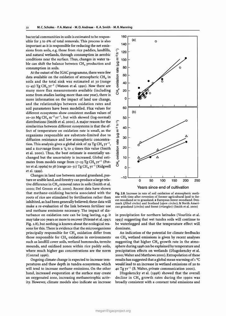
Fig. 2.8. Increase in rate of soil oxidation of atmospheric meth­ane with time after reversion of former agricultural land to for­est-woodland or to grassland. a European forest-woodland: Den­mark (filled circles) and Scotland (open circles); b North Ameri­can grassland (circles) and forest (triangles) (Smith et aI. 2000)

in precipitation for northern latitudes (Vourlitis et al.1993) suggesting that wet tundra soils will continue tobe waterlogged and that the temperature effect willdominate.

An indication of the potential for climate feedbackson CH4 wetland emissions is given by recent analysessuggesting that higher CH4 growth rate in the atmo­sphere during 1998can be explained by temperature andprecipitation effects on wetlands (Dlugokencky et al.2000;Walterand Matthews 2000). Extrapolation of theseresults has suggested that a global mean warming of 1°Cwould lead to an increase in wetland emissions of 20 to40 Tg yr- I (B.Walter,private communication 2000).

Dlugokencky et al. (1998) showed that the overalldecline in CH4 growth rates during the 1990S wasbroadly consistent with a constant total emissions and

250

o

200150100

o

50

Years since end of cultivation

160(a)

140

,. 120s:'1'E 100Ol,2,

~80

c: 600

~'C 40'x0... 20IU

0

60(b)

50~,.s:'1' 40EOl,2, 30

~c: 200

~'C'x 100...IU

0

-100

bacterial communities in soils is estimated to be respon­sible for 3 to 6% of total removals. This process is alsoimportant as it is responsible for reducing the net emis­sions from soils, e.g. those from rice paddies, landfills,and natural wetlands, through consumption in aerobicconditions near the surface. Thus, changes in water ta­ble can shift the balance between CH4 production andconsumption in soils.

At the outset of the IGAC programme, there were fewdata available on the oxidation of atmospheric CH4 insoils and the total sink was estimated at 30 (range15-45)Tg CH4 yr- I (Watson et al. 1990). Now tlIere aremany more flux measurements available (includingsome from studies lasting more than one year), there ismore information on the impact of land use change,and the relationships between oxidation rates andsoil parameters have been modelled. Flux values fordifferent ecosystems show consistent median values of10-20 Mg CH4 m-2yr-l , but with skewed (log-normal)distributions (Smith et al. 2000).A major reason for thesimilarities between different ecosystems is that the ef­fect of temperature on oxidation rate is small, as theorganisms responsible are substrate-limited due todiffusion resistance and low atmospheric concentra­tion. This analysis gives a global sink of 29 Tg CH4 yr- I

,

and a ±wrange from a If.t to 4 times this value (Smithet al. 2000). Thus, the best estimate is essentially un­changed but the uncertainty is increased. Global esti­mates from models range from 17-23 Tg CH4 yr- I (Pot­ter et al.1996a)to 38 (range 20-51)Tg CH4 yr' (Ridgwellet al. 1999).

Changes in land use between natural grassland, pas­ture or arable land, and forestry can produce a large rela­tive difference in CH4 removal rates in soils (Smith et al.2000; Del Grosso et al. 2000). Recent data have shownthat methane-oxidising bacteria associated with theroots of rice are stimulated by fertilisation rather thaninhibited, as had been generally believed; these data willmake a re-evaluation of the link between fertiliser useand methane emissions necessary. The impact of dis­turbance on oxidation rate can be long lasting, e.g. itmay take 100years or more to recover (Prieme et al.1997;Fig. 2.8),but nothing is known about the ecological rea­sons for this. There is evidence that the microorganismsprincipally responsible for CH4 oxidation differ fromthose responsible for CH4 oxidation in environmentssuch as landfill cover soils, wetland hummocks, termitemounds, and oxidised zones within rice paddy soils,where much higher gas concentrations are the norm(Conrad 1996).

Ongoing climate change is expected to increase tem­peratures and thaw depth in tundra ecosystems, whichwill tend to increase methane emissions. On the otherhand, increased evaporation at the surface may createan oxygenated zone, increasing methanotrophic activ­ity. However, climate models also indicate an increase

[email protected]

removal rate and that CH4 concentrations would stabi­lise at a level 4% higher than observed in 1996 if thissituation continued. Alternatively, CH4 could be stabi­lised at 1996 concentrations if the total emissions werereduced by 4%. However,there is some evidence that re­moval rates have been increasing during the last decade(Krol et al. 1998; Karlsdottir and Isaksen 2000) at ca.0.5%yr'". This would imply that total sources were in­creasing at about the same rate and is consistent with ananalysis of trends in the l3C tvc ratios in CH4 (Franceyet al. 1999).

Longer term scenarios for CH4 emissions have notbeen studied in as much detail as those for CO2 emis­sions. One perspective is that emissions will generallyfollow human population because of the connection toagriculture, sewage,and landfill. However,recent trendsindicate a decoupling of emissions from population (D.Etheridge, private communication 2001) and severalauthors have noted that anthropogenic CH4 emissionsare generally associated with inadvertent losses of en­ergy for both animals and fossil fuel use. These lead toan alternative view that abatement of current CH4 emis­sions may be possible at low or negative cost.

2.7.1.1 Production of Volatile Organic CarbonCompounds from Vegetation

Plant growth involves the uptake of CO2, H20 , and nu­trients and the release of particles,water vapour, 02' andreduced carbon compounds to the atmosphere. Thesereduced carbon compounds are usually described asVOCsand consist of a range of short chain organic com­pounds including hydrocarbons, alcohols, carbonyls,fatty acids, and esters. Recent reviews of biogenic VOCresearch have been published in journals of the biologi­cal (Sharkey 1996;Lerdau et al.1997; Harley et al. 1999),chemical (Atkinson and Arey 1998), and atmospheric(Kesselmeier et al. 1998; Guenther et al. 2000) sciencecommunities as well as in a book (Helas et al. 1997)andseveral book chapters (e.g. Fall 1999; Guenther 1999;Steinbrecher and Ziegler 1997). The achievements ofIGACand associated research activities during the lastdecade on VOCemissions from plants and the currentlyidentified research gaps are discussed in the followingsection.

2.7.1.2 New Emission Measurements

The advances in measurement techniques described inChap. 5 have greatly increased capabilities for investi­gating biogenic VOCfluxes at multiple spatial and tem­poral scales. The resulting data have provided a morecomplete and accurate picture of biogenic VOC emis­sions. New analytical methods have extended the range

CHAPTER 2 . Biosphere-Atmosphere Interactions 33

of chemical compounds that can be investigated. En­closures coupled with environmental control systemshave been used to characterise the environmental andgenetic controls over emissions, while above-canopy fluxmeasurements provide an integrated measurement oflandscape-level trace gas exchange. Tower-based fluxmeasurements are particularly useful for investigatingdiurnal and seasonal variations without disturbing theemission source . Aircraft and tethered balloon meas­urement systems can be used to characterise fluxes overscales similar to those used in regional models . Theseregional measurements are especially useful in tropicallandscapes with high plant species diversity.

The measurement database that can be used to char­acterise biogenic emission processes and distributionshas been greatly increased by large international fieldprograms including EXPRESSO, LBA, SAFARI, NARSTOfSOS, EC-BEMA, EC-BIPHOREP, EC-EUSTACH (seeAppendix A.3).Over a thousand plant species have beeninvestigated, for at least a few VOCs, by these studies.Equally important has been the large number of land­scapes that have been studied. IGAC-endorsed researchhas been particularly important for advancing meas­urements in tropical regions . A number of these studieshave investigated emissions on multiple scales result­ing in measurements that can be used to evaluate bio­genic VOC emission model estimates.

Investigations of emission mechanisms, often con­ducted under controlled laboratory conditions, have alsoadded to our understanding of biogenic VOCemissions.These measurements have been used to relate emissionsto both environmental and genetic controls. Althoughthese measurements have not revealed distinct taxo­nomic relationships, some patterns have emerged(Harley et al. 1999; Csiky and Seufert 1999).

2.7.1.3 Newly Identified Compounds

A substantial improvement has been achieved in the lastten years in the identification and accurate quantifica­tion of VOCs emitted by terrestrial ecosystems. Thenumber of components reported as biogenic VOCemis­sions has increased from seven (ethylene, isoprene,a-pinene,{3-pinene, limonene, ~-3-carene, and p-cymene)to more than 50,belonging to ten different classes. Thelist of detected compounds is reported in Table 2.1 to­gether with information on:

• hypothesised biological production pathways occur­ring inside and outside the chloroplast:

• numerical algorithms adopted for describing emis­sion variations;

• relative abundance in vegetation emission; and• degree of removal by OH and 03 attack under cer­

tain atmospheric conditions.

[email protected]

,. M.C. Schol~ · P.A.Matrai . M. O.And reae · K.A.Smith · M. R.Manrdn g

Tabl e 2.1. W I ofVOC so far ident ified an d quantified in te rrestrial vegeta tion emiss ions

• The existence of a pos sible bio synthetic pathway OC , ,0 '" not yet hypothesized c ( 15eccreocsds (sesquiterpenes), '" on'Y hypothesized t-zr-blse bclene z z, '" hypothesised and partly supported byenzyme isola- e -copaene z ,

lion or carbon labelingp -<aryoph y1 lene a a -z

3 '" hypothesi5ed and partly sopporred by both enzymeio;olation andc arton labeling a-humu lene z , -z

The type' of algorilhm followedLongifolene z ,

bValencene z ,, '" light and temperature dependent

Arenes, = temperature depe ndentT~uene

c The relat ive abundance in th e emi ssio n Aldehydes

4 '" high abundant Forma ldehyde z z .,3 = abundant A<:eta ldehyde z .,a = mod e rately abundant n-he i<ilnal, = present at trace level lHlonana l

= ep isodic emission due to injuriesn-decanal

d The production or losses occurring by within-(illlopy processes r-2-hel«.'nal a a-when level s of 0. and OH radical s in airexc eed 60 nmol lllOt"'

Benza ldehyd eand 106 molecules cm-) of OH radicals, respectively

-, '" oarteuossesKetones

-, = complete lossesAceton e a .,.. moderat e p rodu(tioo Camphor '" z

., = strong production 6-me thy!-S-heptene-2-one (MHO) , + 1, - 1

sut anone

OC , ,2,3-butadione

Alkane~ z-centenone

n-he xane 4-met hyl-2-pentanone

Alkenes Ether~

Ethylene , a l,8-< ineo le , t.z a• CS isoprenoids Esters

Isop rene s • Acetyl !HIlidlille

b ClO isoprenoids (mo noterpe nes) Borny! acetate ,Cam phene a Ernio bo rnyl acetate ,p-cvmene , .., , 3-he xeny! acetat e z 3·

as -cereoe , .., a Lynalyl aceta te z ..,rench ene I

"3-methy l-3-bu tenyl acetate ,

d -limonene 3 tz 3 -, Alcohol s

Myrcene 3"

, -, Met hanol a zrp-ocimen e , tz , -, 2-methy l-3-bu ten-2-o 1(MOO) z zc-P-ocimene , tz , -, 3-methy l-a -bote o- 1-01 z ,a- phe lland rene , t.a -, cis-3-he xen· l -o! a 3·

P -phellandrene , '.' , -, uoecor 3 t.a za- p inene s .., 3 a- te rp ineol a

",

p -p inene a .., , r -terp ineol z tzSabnere 3 .., , Acids

c-ter plneoe z .., , -, Form k aci d

r -terpinene , .., , -, Acen c eod

repooere , .., , -, Oxid es

Thujene z t.a , c-linalool o xide z I'Tricyclene , t.z , r-linalool oxide z ..,

[email protected]

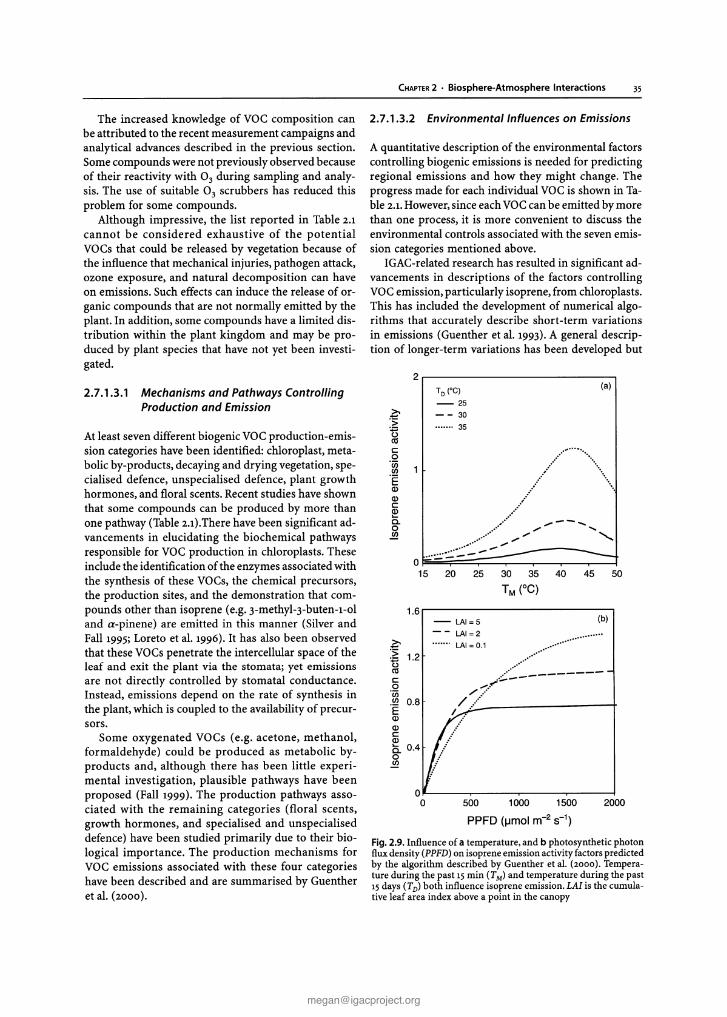
CHAPTER 2 . Biosphere-Atmosphere Interactions 35

The increased knowledge of VOC composition canbe attributed to the recent measurement campaigns andanalytical advances described in the previous section .Some compounds were not previously observed becauseof their reactivity with 0 3 during sampling and analy­sis. The use of suitable 0 3 scrubbers has reduced thisproblem for some compounds.

Although impressive, the list reported in Table 2.1cannot be considered exhaustive of the potentialVOCs that could be released by vegetation because ofthe influence that mechanical injuries, pathogen attack,ozone exposure, and natural decomposition can haveon emissions. Such effects can induce the release of or­ganic compounds that are not normally emitted by theplant. In addition, some compounds have a limited dis­tribution within the plant kingdom and may be pro­duced by plant species that have not yet been investi­gated.

2.7 .1.3.2 Environmental Influences on Emissions

A quantitative description of the environmental factorscontrolling biogenic emissions is needed for predictingregional emissions and how they might change. Theprogress made for each individual VOCis shown in Ta­ble 2.1. However, since each VOCcan be emitted by morethan one process, it is more convenient to discuss theenvironmental controls associated with the seven emis­sion categories mentioned above.

IGAC-relatedresearch has resulted in significant ad­vancements in descriptions of the factors controllingVOCemission, particularly isoprene, from chloroplasts.This has included the development of numerical algo­rithms that accurately describe short-term variationsin emissions (Guenther et al. 1993). A general descrip­tion of longer-term variations has been developed but

2,---------------...,

Fig. 2.9. Influence of a temperature, and b photosynthetic photonflux density (PPFD) on isoprene emission activity factors predictedby the algorithm described by Guenther et al. (2000). Tempera­ture during the past 15min (TM)and temperature during the past15days (TD) both influence isoprene emission. LAI is the cumula­tive leaf area index above a point in the canopy

1.6,---------------...,

500 1000 1500 2000

PPFD (urnol m- 2 S-1)

(a)

(b)

To (OC)

-25

- - 30....... 35

- LAI=5

LAI=2....... LAI= 0.1 ........................................

..;;::----------",:'"

/~....•..I . .,

:.0'

l /...

......!

......

~

:2: 1.2tsCllco'00en 0.8'EQ)

Q)cQ)a. 0.4o!E

.~>

~co'00en'EQ)

Q)c~Cl.o!E

2.7.1.3.1 Mechanisms and Pathways ControllingProduction and Emission

At least seven different biogenic VOCproduction-emis­sion categories have been identified: chloroplast, meta­bolic by-products, decaying and drying vegetation, spe­cialised defence, unspecialised defence, plant growthhormones, and floral scents. Recent studies have shownthat some compounds can be produced by more thanone pathway (Table z.ij.There have been significant ad­vancements in elucidating the biochemical pathwaysresponsible for VOC production in chloroplasts. Theseinclude the identification of the enzymes associated withthe synthesis of these VOCs, the chemical precursors,the production sites, and the demonstration that com­pounds other than isoprene (e.g. 3-methyl-3-buten-1-01and a-pinene) are emitted in this manner (Silver andFall 1995; Loreto et al. 1996). It has also been observedthat these VOCspenetrate the intercellular space of theleaf and exit the plant via the stomata; yet emissionsare not directly controlled by stomatal conductance.Instead, emissions depend on the rate of synthesis inthe plant, which is coupled to the availability of precur­sors.

Some oxygenated VOCs (e.g. acetone, methanol,formaldehyde) could be produced as metabolic by­products and, although there has been little experi­mental investigation, plausible pathways have beenproposed (Fall 1999). The production pathways asso­ciated with the remaining categories (floral scents,growth hormones, and specialised and unspecialiseddefence) have been studied primarily due to their bio­logical importance. The production mechanisms forVOC emissions associated with these four categorieshave been described and are summarised by Guentheret al. (2000).

[email protected]

36 M.C.Scholes . P.A.Matrai· M.O.Andreae· K.A.Smith· M.R.Manning

an improved physiological and biochemical understand­ing is needed (Schnitzler et al. 1997; Guenther et al.2000). It is known that the light response of shade leavesdiffers considerably from sun leaves and that the tem­perature that the plant has been exposed to in the pastcan influence its temperature dependence. This generalunderstanding is illustrated by the response curvesshown in Fig. 2.9.

Emission of stored monoterpenes from specialiseddefence structures results from the diffusion of com­pounds through the cell barrier around the resin ves­sels or ducts. The amount released by this process at agiven temperature is dependent on the nature of thecompound, resistance properties of the cell layers, andother transport resistances within and outside of theleaf.Ascell resistances and vapour pressure of the com­pound are temperature dependent, the emission sourcestrength is strongly dependent on the temperature ofthe leaf. Recent advancements have been made in de­scribing how the exponential increase in emissions withtemperature is dependent on VOCcompounds and theresistance properties of the plant.

The environmental controls over metabolic by-prod­ucts, decaying and drying vegetation, plant hormones,floral scents, and unspecialised defence have not beencharacterised in a manner that is useful for emissionmodelling . Some of the primary controlling factors areknown but there are no quantitative algorithms forsimulating emission variations (Fall 1999; Kirstine et al.1998; Guenther 1999).A significant obstacle to regional­scale extrapolation of these emissions is the need fordatabases of driving variables, e.g, temperature and ir­radiance intensity, which are currently unavailable.

2.7.1.3 .3 Production and Loss Mechanismsin the Plant Canopy

Field experiments carried out within the frame of theEC-BEMA project (Valentini et al. 1997; Ciccioli et al.1999)have shown that within-canopy losses are signifi­cant for VOCs that have atmospheric lifetimes compa­rable to the transport time from the canopy to the at­mospheric boundary layer (ABL). Compounds with at­mospheric lifetimes ranging between one and threeminutes (ranked as -2 in Table 2.1)never reach the ABLwherea s severe losses (>so%) are observed for com­pounds characterised by atmospheric lifetimes rangingbetween three and ten minutes (ranked as -1 in Table2.1)(Ciccioli et al. 1999).

In addition to gas-phase reactions, adsorption andpartition processes can also play an important role inremoving emitted components inside the forest canopy.These effects can be particularly important in the caseof polar compounds (such as alcohols and carboxylicacids) that are three orders of magnitude more solublethan isoprenoids in water droplets and stick on parti-

cles and surfaces. They have been invoked to explainthe reduced flux of linalool from pine-oak forests andorange orchards.

Degradation ofVOCs in the canopy may lead to theformation of secondary organic aerosols (SOA), as men­tioned earlier (see also Chap. 4), or gaseous products(mainly very volatile carbonyls) that can diffuse in theABL. Photochemical degradation ofVOCs has been sus­pected to be the main source of the huge fluxesof acetal­dehyde, formaldehyde, and, partly, acetone from orangeorchards. A substantial contribution to carbonyl fluxescan also arise from heterogeneous ozonolysis of lipidscovering the leaf surface (Fruekilde et al. 1998),whichcan produce acetone, e-methyl-s-hepten-z-one, andgeranyl acetone as a function of the levels of ozone inair. Mesoscale modelling studies applied to a regionnorth of Valencia, Spain (Thunis and Cuvelier 2000)have shown that secondary products formed by within­canopy reactions accounted for more than 70% of theozone formed by biogenic emission from orange or­chards. The complexity of within-canopy processes oc­curring in certain ecosystems can only be assessed byincorporating chemical processes into models describ­ing the transport of VOCsinto the ABL. At the presenttime, development of such models is made difficult bythe fact that degradation pathways of primary productsformed by photochemical reactions of mono- andsesquiterpenes are still unknown and it is not clear towhat extent and in which conditions they can possiblynucleate to form SOA.

2.7.1.3.4 Models of Emissions

The IGAC-GEIA natural VOCproject has compiled andsynthesised the available information on biogenic VOCemissions and their driving variables into a global modelthat has been used to generate inputs for regional andglobal chemistry and transport models. The initial ef­fort described by Guenther et al. (199S) providedmonthly emissions of isoprene and three VOC catego­ries (monoterpenes, other reactive VOC, less reactiveVOC)with a spatial resolution of o.s degree of latitudellongitude.The global distribution of isoprene emissionspredicted by this model for the month of July is illus­trated in Fig. 2.10.

The model was constructed using the following in­formation. Emission factors were based on the resultsof 20 studies that were primarily located at temperateforest field sites. Twoemission types were utilised: iso­prene emissions were estimated using current light andtemperature conditions while all other emissions wereassumed to be dependent on current temperature.Landcover characteristics were primarily based on val­ues assigned to landscape types and a global databaseof current landcover distributions. Satellite (AVHRR)measurements were used to estimate monthly foliar

[email protected]

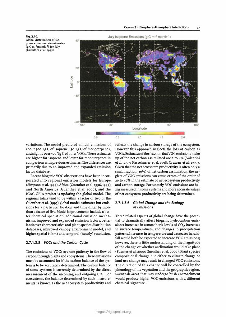
Fig. 2.10 .Global distribution of iso­prene emission rate estimates(g C m-2month-1) for July(Guenther et al. 1995)

30'

CD"0

.~ ff'iii..J

-30'

CHAPTER 2 . Biosphere-Atmosphere Interactions 37

Ju ly Isoprene Em issions ( 9 C m -2 month -I )

0.0 0.5 1.0 1.5 2.0

variations. The model predicted annual emissions ofabout 500 Tg C of isoprene, 130Tg C of monoterpenes,and slightlyover 500 Tg Cof other VOCs.These estimatesare higher for isoprene and lower for monoterpenes incomparison with previous estimates.The differences areprimarily due to an improved and expanded emissionfactor database.

Recent biogenic VOC observations have been incor­porated into regional emission models for Europe(Simpson et aI.1999),Africa (Guenther et a1.1996, 1999)and North America (Guenther et al. 2000), and theIGAC-GEIA project is updating the global model. Theregional totals tend to be within a factor of two of theGuenther et al. (1995) global model estimates but emis­sions for a particular location and time differ by morethan a factor of five.Model improvements include a bet­ter chemical speciation, additional emission mecha­nisms, improved and expanded emission factors, betterlandcover characteristics and plant species distributiondatabases, improved canopy environment model, andhigher spatial (I km) and temporal (hourly) resolution.

2.7.1.3.5 VOCs and the Carbon Cycle

The emissions of VOCs are one pathway in the flow ofcarbon through plants and ecosystems .These emissionsmust be accounted for if the carbon balance of the sys­tem is to be accurately determined. The carbon balanceof some systems is currently determined by the directmeasurement of the incoming and outgoing CO2, Forecosystems, the balance determined by such measure­ments is known as the net ecosystem productivity and

reflects the change in carbon storage of the ecosystem.However this approach neglects the loss of carbon asVOCs.Estimates of the fraction that VOCemissions makeup of the net carbon assimilated are 2 to 4% (Valentiniet al. 1997; Kesselmeier et al. 1998; Crutzen et al. 1999).Given that the net ecosystem productivity is often only asmall fraction (10%) of net carbon assimilation, the ne­glect of VOCemissions can cause errors of the order of20 to 40% in the estimate of net ecosystem productivityand carbon storage. Fortunately, VOCemissions are be­ing measured in some systems and more accurate valuesof net ecosystem productivity are being determined.

2.7.1.3.6 Global Change and the Ecologyof Emissions

Three related aspects of global change have the poten­tial to dramatically affect biogenic hydrocarbon emis­sions: increases in atmospheric levels of CO2, increasesin surface temperatures, and changes in precipitationpatterns. Increases in temperature and decreases in rain­fall would both be expected to increase VOCemissions;however, there is little understanding of the magnitudeof the change or whether acclimation would take place(Fuentes et al. 2000; Guenther et al. 2000). Plant speciescompositional change due either to climate change orland use change may result in changed VOC emissions.The direction of this change will be controlled by thephenology of the vegetation and the geographic region .Savannah areas that may undergo bush encroachmentwould produce higher VOC emissions with a differentchemical signature.

[email protected]

38 M.e.Scholes· P.A.Matrai · M.O.Andreae· K.A.Smith· M.R.Manning

Changes in air temperature, the length of the grow­ing season, precipitation, and atmospheric CO2 concen­trations could lead to large changes in the VOC emis­sions from temperate latitude ecosystems. In tropicalregions, little change may take place because plant leavesalready may be near their optimal temperature for iso­prene emissions .There are some suggestions that plantsadapt to changing temperature regimes and that VOCemissions would also rise in the Tropics. It is also un­clear if cultivating increased areas of genetically modi­fied plants could alter the nature ofVOC emissions sig­nificantly.

Changes in vegetation type can lead to large changesin VOCemissions . For instance, replacing C3grass spe­cieswith C4 types could change the direct emissions andemissions from the plant decay process. Current knowl­edge is inadequate, however, to quantify these changes.Woody plants (shrubs and sun tolerant trees) tend tohave much higher isoprene and monoterpene emissionsrates, compared to annual crops and grasses; thereforedeforestation involving conversion of closed forest tograssland could greatly reduce biogenic VOCemissions .However,there is a tendency for higher emissions fromthe woody plants that replace a closed canopy forest(Klinger et al. 1998); therefore, the effect of conversionof closed forest to open woodland is unknown. Firedominated systems in the more arid areas have sup­pressed woody plants and kept emissions low,but agri­cultural practices of grazing and fire suppression haveallowed shrublands to spread with resultant increasedemissions .The chestnut blight of the late nineteenth andearly twentieth centuries on the US East Coast lowlandforests caused massive change in forest compositionwith oak replacing the chestnut. Unlike oak, chestnutdoes not emit isoprene. The chestnut blight has thusresulted in an approximate doubling of the biomass ofisoprene-emitting species (Lerdau et al. 1997).

2.7.1.4 Ammonia Emissions and Interactionswith Particles

Terrestrial emissions of NH3 are associated with ani­mal waste, fertilisers , biomass combustion, soils, veg­etation, and some other minor sources (Bouwman et al.1997). The microbial breakdown of urea and uric acidpresent in animal waste produces ammonium, whichsubsequently partlyvolatilises as NH3'The overall emis­sion of NH3 from waste is dependent on the specific N­excretion per animal, and the NH310ss during housing,storage of waste outside the stable, grazing, and appli­cation of manure on grassland or arable land. Furtherimportant properties influencing NH3 volatilisation in­volve soil pH and moisture, and temperature. There is apH-dependent equilibrium between NH3 and NHt, withNH3 being emitted from soils when they are alkaline.

Some northern European countries have measured andcalculated country- and animal-specific emission fac­tors. The applications of such emission factors to calcu­late animal related emissions elsewhere may be quiteproblematic, since agricultural practice and climaticfactors may differ substantially from those in northernEurope. In addition, the number of animals per countrymay fluctuate strongly from year to year.

Dry deposition and reactions with acidic particlesand particle precursor gases are the main removalmechanisms for NH3 (see also Sect. 2.7.3). Oxidationchemistry of NH3 is thought to playa relatively minorrole (Dentener and Crutzen 1994). Because NH3 emis­sions occur almost exclusively close to Earth's surface,and because plants utilise nitrogen in their metabolism,dry deposition is a very efficient process that may re­move 40-60% of all emissions. Ammonia that has re­acted with sulphuric or nitric acid to form NHt is re­moved mainly by wet deposition and much less effi­ciently by dry deposition. It has an average residencetime in the atmosphere of up to one week, in contrast tothe much shorter residence time of gas phase ammo­nia, which is less than one day.

The understanding of the atmospheric NH3 cycle isstill limited, because:

• NH3 emissions are estimated for most countries,rather than measured because of the difficulty ofmaking such measurements (Fehsenfeld 1995).

• Emissions of NH3 show a large spatial and temporalvariability (e .g, farm-scale, winter-summer). Trans­port models of NH3 and NHt utilise larger grid scalesand the temporal variability of NH3 emissions is notaccounted for in such models .

• Most models of NH3 chemistry and transport arehighly simplified and parameterised and may there­fore produce results that may be spurious.

• Measurements of particulate NHt are common, al­though their quality is frequently suspect; gas phaseNH3 data are scarcely available.

The comparison of models with such measurementsis difficult since the measurements may not be repre­sentat ive for the model grid scale. This is especially thecase for gas phase NH3, which may have an atmosphericlifetime of hours . In addition, there may be substantialinstrumental problems, e.g. the evaporation of ammo­nium nitrate from filter packs, which makes it difficultto interpret routinely performed aerosol measurements.

Wet deposition measurements of NHt are relativelystraightforward, and there are, at least in Europe and theUS,substantial data sets available. However, these meas­urements may again not be representative for a largermodel region. Also, discrepancies of model results andmeasurements may be due to a host of reasons, such as apoor representation of dry deposition, vertical mixing,

[email protected]

and in- and below-cloud scavenging or emissions. Anevaluation of global model deposition with measure­ments in Europe and the US by Holland et al. (1999) in­deed indicated substantial discrepancies but no singleprocess could be identified as the cause of the problem.

Despite all uncertainties involved, several studies (e.g.Galloway et al. 1995) have indicated the significance ofterrestrial NH3 emissions for the global nitrogen cycle.Recent modelling studies (Adams et al. 1999; Metzgeret al. 1999) indicated the potential significance of NHtand nitrate (NO;) for aerosol burden and composition.These studies were performed using thermodynamicequilibrium models, developed originally for urban smogconditions.Substantial effort has been spent on extendingthese schemes to global modelling (e.g. Nenes et al.1998).

Amajor challenge is presented by the need to increasethe resolution of the models and develop sub-grid para­meterisations that represent the variability of ammo­nia emissions and the resulting effect on particle com­position. Long-term, representative, and reliable meas­urements of NH3, NHt, SO~-, and NO; are needed inconjunction with deposition measurements to constrainthe NHt budget further.

2.7.1.5 Production and Consumption ofNP and NOin Soils

Nitrogen oxides are produced in soils as obligate inter­med iates or by-products of the microbially mediatedprocesses of nitrification and denitrification (Conrad1996). The same environmental factors of soil tempera­ture , nitrogen availability, and soil moisture affect theproduction of both nitrogen oxides. The pathways andenzymatic mechanisms of these processes were not wellunderstood in the 1980s.The development of chemilu­minescence instruments for NO measurement and re­ports in the late 1970S that increased use of nitrogenfertilisers could be one of the main causes of accumula­tion of nitrous oxide in the atmosphere, thus contribut­ing to global warming, stimulated scientists to researchthe mechanisms involved (Firestone and Davidson 1989;Davidson and Kingerlee 1997). The conceptual modeloffered by Firestone and Davidson in 1989,which hassince become known as the "hole-in-the-pipe" (HIP)model, synthesised the information known at that timeabout the microb iological and ecological factors influ­encing soil emissions of NO and N20 . The HIP modellinked the two gases through their common processesof microbial production and consumption. It was abreakthrough in understanding factors controllingemissions and the model has stood the test of time.Ongoing testing of the model over the last decade withnumerous data sets from temperate and tropical agro­ecosystems shows that it provides a sound ecological andmechanistic basis for interpreting temporal and spatial

CHAPTER 2 . Biosphere-Atmosphere Interactions 3 9

variation at all scales of study by neatly encapsulatinginto two functions - nitrogen availability and soil watercontent - a large fraction of the variability caused bynumerous environmental factors that influence the pro­duction and consumption of NO and N20 by nitrifyingand denitrifying bacteria (Davidson et al. 2000b).

Matson et al. (1989)stated that empirical models thatare based on correlation analysis involving easily meas­ured soil variables (e.g, temperature, moisture, texture ,and organic carbon) often predict trace gas fluxes quitewell.Asdata sets became more available, this set of vari­ables has been further reduced to moisture and tem­perature with some corrections needed to take accountof texture differences.Empirical relationships have beenestablished for a number of different ecosystems aroundthe world for both NO and N20 emissions with water­filled pore space values of approximately 35%being theswitch from NO to N20 emissions. The magnitude ofthe emissions varies with substrate availability; the useof 15N labelling techniques to measure the turnover ofthe soil ammonium and nitrate pools has greatly en­hanced our capacity to partition nitrogen gas produc­tion among NO,N20 , and N2• Trace gases are producedand consumed by defined reactions in individual micro­organisms and control must be exerted at this level ini­tially. To date, empirical models based on various physi­cal and chemical parameters have been successful with­out considering the structure of the microbial commu­nity; even those models that differentiate between nitri­fication and denitrification neglect microbial commu­nity structure. It is still unknown whether microbial spe­cies diversity is an important factor especially if one con­siders changes associated with land use (Conrad 1996).

Soil mineral N, resulting from additions of syntheticN fertilisers and N from animal manure, crop residues,etc., and the mineralisation of soil organic matter anddeposition from the atmosphere, is recognised as a ma­jor driver of these emissions. Much work has gone intoestablishing the relationships between the fluxes of N20and NO and the other key drivers, soil moisture and tem­perature. Although some questions remain to be an­swered, significant developments in this direction havebeen achieved. The logarithmic relationship betweenN20 flux and soil water-filled pore space (WFPS) in atropical forest soil is illustrated in Fig. 2.11a (Keller andReiners1994).Aremarkably similar relationship has beenfound for temperate fertilised grassland, when mineralN was not limiting (Dobbie et al. 1999).These data canbe contrasted with NO flux data (Fig. 2.11b) obtainedfrom a semi-arid southern African savannah, where tem­perature and soil moisture are the major controlling fac­tors on emissions. Multiple regression analyses revealthe following sequence of importance of environmen­tal factors on NO flux: soil temperature> water-filledpore space> soil nitrate concentrations> soil ammo­nium concentrations (Otter et al. 1999) (see Box 2.2).

[email protected]

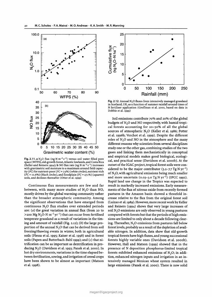
40 M.C.Scholes· P.A.Matrai · M.O.Andreae· K.A.Smith · M.R.Manning

100.0 ~--.,...----r----,---~

Fig. 2.11. a N20 flux (ng N m-2 S- I) versus soil water filled porespace (WFPS),old-growth forest ,Atlantic lowlands ,and Costa Rica(Keller and Reiners 1994) ; b NO flux rate (ng N m-2S- I ) increaseswith gravimetric soil moisture to a maximum around field capac­ity (FC) for nutrient-poor (FC = 7.5%) (wh it eci rcles),nutrient-rich(FC= 10.6%) (black ci rcles), and floodpla in (FC= 27.1%) (squares)soils, and declines thereafter (Otter et al. 1999)

•25

x_ 20::J-_I-ctlQ).L: 15.;:::z10 6::J C\I 10E Z::JClOe.

5

00

Fig. 2.12. Annual N20 fluxes from intensively managed grasslandin Scotland, UK, as a function of summer rain fall around times ofN fertiliser application (Groffman et al. 2000, based on data inDobbie et al. 1999)

50 100 150 200 250

Rainfall (mm)

Soil emissions contribute 70% and 20% of the globalbudgets of N20 and NO respectively, with humid tropi­cal forests accounting for 20-50% of all the globalsources of atmospheric N20 (Keller et al. 1986; Potteret al. 1996b; Verchot et al. 1999). Despite the differentroles of N20 and NO in the atmosphere and the manydifferent reasons why scientists from several disciplinesstudy one or the other gas, combining studies of the twogases and linking them mechanistically in conceptualand empirical models makes good biological, ecologi­cal, and practical sense (Davidson et al. 2000b). At theoutset of the IGAC project,tropical forest soils were con­sidered to be the major contributor (3.2- 7.7 Tg N yr-!)ofN20, with agricultural emissions being much smallerand more uncertain (0.03-3.0 Tg N yr") (IPCC 1992).Rapid land use change in the Tropics was expected toresult in markedly increased emissions. Early measure­ments of the flux of nitrous oxide from recently formedpastures in the Amazon basin showed a threefold in­crease relative to the flux from the original forest soil(Luizao et al.1989).However,more recent work by Kellerand Reiners (1994) shows that very large increases ofsoil N20 emissions are only observed in young pasturescompared with forests but that the periods of high emis­sions are limited to only about a decade following clear­ing. Thereafter, N20 emissions from pastures fall belowforest levels,probably as a result of the depletion of avail­able nitrogen. In addition, data show that old-growthtropical forests have high fluxes,and young successionalforests highly variable ones (Davidson et al. 2000b).However, Hall and Matson (1999) showed that in thepresence of N deposition phosphorus-limited tropicalforests exhibited enhanced emissions of N20; in addi­tion, enhanced nitrogen inputs and irrigat ion in an in­tensively managed Mexican wheat system resulted inlarge emissions (Panek et al. 2000). There is now solid

9060 70 80WFPS (%)

•

(b)

0.150

40 ,--------------,

35

30

~ 25(; 20Z 15

10

5

oo 5 10 15 20 25 30 35 40 45 50

Gravimetric water content (%)

10.0x::J

;:;::::

1.0

Continuous flux measurements are few and farbetween, with many more studies of N20 than NO,mostly driven by the global warming community ratherthan the broader atmospheric community. Amongthe significant observations that have emerged fromcontinuous N20 flux studies over extended periodsare: (a) the great variation in annual flux (from 20 to>200 Mg N20-N m-2 yr-!) that can occur from fertilisedtemperate grassland as a result of variations in the tim­ing and amount of rainfall (Fig. 2.12); (b) the large pro­portion of the annual N20 that can be derived from soilfreezing/thawing events in winter, both in agriculturalsoils (Flessa et al. 1995; Kaiser et al. 1998)and in forestsoils (Papen and Butterbach-Bahl icce): and (c) that ni­trification can be as important as dentrification in pro­ducing Np (Davidson et al. 1993; Panek et al. 2000). Inhot dry environments, variations in the time elapsed be­tween fertilisation, sowing, and irrigation of cereal cropshave been shown to be almost as important (Matsonet al. 1998).

oC\I

Z

[email protected]

CM..... TEII2 • Biosph ere ·Atmosphere Intera ct ions 41

Box 2 .2. Im pa ct of n it rog e n fertilise r and depo si tion on n it rog e n tra ce gas emissions

Worldwide consumption of synthdic N fert ilis..r s has inc reasedac-fcld since 1950 to about 82 Tg N yr- I in 1996 (Bouwman1998). Abo ut 4 0 % of current consumption is in the Tropicsand subtropics, par ticularly in Asia, and is expected to rtseto 60% by 2020 (Hall and Matson '999). Animal was les usedas fert iliser supplied an estimated additional 65 Tg N yr l in1996, compared with )] Tg N yr · 1 in 1950 (Mosie r and Kroeze1999), an d this input is likely to increase in the futu re. Theexpected effect of t he add it ional N use is a furthe r majo rinc rease in N20 from ag ric ult ural sources. These increases inN fert ilise r use are also expected to raise the agricultural con­nibution to soil NO emiss ions to over 50% {Yienger an d Levy' 995). In the IPCC (1999) assessment, di rect emissions of N20from agricultu ral soils were taken to be 1.25±I% of the Nap·plied (Bouwman 1996), but a re-evaluation indicates that theobserved emission factor s are st rongly skewed, giving an un­certainty range from one-fifth to five lim es th e mean vatce.t.e.,from 0.25% to about 6% of the N applied, and suggesting thatthe mean fluxfrom this source may be even high er or lower thanpresently accepted. Recent data (Fig. 2-13) on N,O and NO emis·sions from N fertilised and N_saturated systems in temperateregions give indications as to how global mange and changingland management prac tices may be enhancing emissions. How·ever, Hall an d Matso n (1999), raise the possibility tha t increasingnitrogen deposition in tropical regions is likely to have very dil·ferent effects than nitrogen deposition in the temperate zone, withmum great er feedbacks to the atmos phere (see Sect. 2.7.3).

Figure 2.I}Iland b showa remarkable simi1arityin grar,hs ofN ,Oemission VI. deposition and NlO emission (nmolmc l") vs. ferti­liser ap plication for sites in Sootland. 1n a three-year oontinuousrecord study of nitrogen trace gas!luxes from untreated and limedsoils of a N·Sllturated.sp~ and be«h forest ecosystem in Ger·many (Flg.l.l3Cand d) th<:-re was a significant positive correlationbetween the amount of in situ N inp ut by wet deposition and mag·nitude of in situ N20 and NO emissions (Papen and Butterbech­Bahl I999; Gasche and Plpen '999). At the beech site, 10% of theactual N input was rekased from the soil in the form ofNlO whereasat the spruce site the fraction waS 0.5%, indicating that forest Iypeitself is an important modulator of Np releue from soil How·ever, there is a marked similarity in the NlO data obtained fromScotland and from Germany. Approximately 15% and 7% of theactual N input was lost as NO from the German soils stocked withspruce and beech, respectively. liming resulted in 49% reductionof NO emissions as compared 10 an unlimed sp~ control site.The results indicate tha i the reduction in NO emission was due toan increase in NO consum ption within the limed soil Liming of aspruce site resulted. in a signitirnnt increase in ammonification, ni­trifkal:ioll,and N20emissions ascompared with an untreated sprucecontrol site. On the basis of these results it was concluded that theimpo rtance of temperate and boreal forests for the global N20source strength may have been significantly underestimated in thepastand tha t these forests,in which N deposition ishigh ,mostlikelycont ribule in excess of '.0 Tg N,D-N and 0.3Tg NOx·N yr' (Papenand BUlterbach-BahlI999; Gasche and Papen 1999).

20(.) •

e .,~ 16 •o ~ •~ , 12-2~~ • •8 • •a N£l 4 • •,

• ." •00 100 200 300 400 500

N app lication (kg N ha- 1 yr- I)

6

5(b)

•c _-~ '- 4 •. ~

.~~~ 30

'<.~ 2Z 6 •• ••0 • a

00 20 40 60 80 100N app licatio n (kg N ha - I yr~l )

o $prlJCfl eontrol _ f{xl _72 ,35+81.72x• beech f{xl_26,89+ 41.91x

o

.........~.

•

o

.....

oo

(d)

08 ••• ..~..... .......... ':"~,,~ ;......

3OOr-~~~~~~-

250

200

150

100

50

f: 200 • ••• ! 150E _

o '. ••'<.~ 100 • ••z 2 • •50 • \

0 0 0

00 0.' 1.0 1.5 2.0N in put by we t depos ition (kg N ha - I week - I )

250

c sp ruce f{x} _ 6. 18 + 5.1 2>::: r2. 0. 176• beech f{x} _ 31.2+1 00. 1x:r2 _0. 428

(c

f ig.213. Devialions of N·induced emissions of N20 in Scotland from the IPCC ud"faull~ values, a Mineral N-lndeced emissions from grass(solid blackcircles), ara ble land with cereal crops (open circles), and arable lan d with non-cereal crop s 19rey-sJu,ded circles),together with theIPCC default emission factor ( t.25'!l> of the N applied ) (solid line) (Dobbie eraL1999; Skiba and Smith 20(0); b N deposition-induced emiss ionsfrom forest and moorland soils downwind of poultry and pig farms (soJid bl<lck circles), in large·scaIe acid mist experime nts (open circJes) andin upland areas (grey-shaded circles), togethe r with the lPCCdefaul t emissio n fa£tor (1%of the N applied ) (solid Jine) (Skiba an d Smith 1999);c linear regression analysis between in situ N input by wet deposition and in situ N10 emission rate s from soil of spruce and beech controlsites. For correlation an alysis, data for mean weekly NlO emission rates and mean weeklyN input (da ta from Huber 1997) by wet deposilionmeasured in the thro ughfall were used (l 994-1995) (Papen and Bulterbach ·BahI ' 999); and, d linear regression llDaIysis between weeklymean NO emission rates and weekly amounts of N input (sum of arnmnnium and nitrate) by wet deposition (measured in the throughfall)(Huber 1997) at the . pruce control an d bce<;hsites of the Hllglwald forest ; dat a obtained in the t ime period Jan uary 1994 to Decembe r 1994(sp ruce sites) and Septembe r '994 10 Jun e 1995 (beech sites), respeClively, were used for correlanon analysi s (Gasche and Papen 1999)

[email protected]

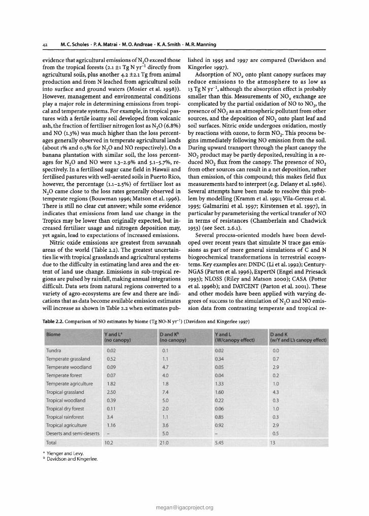
42 M.C.Scholes· P.A.Matrai · M.O.Andreae· K.A.Smith · M.R.Manning

evidence that agricultural emissions ofNzO exceed thosefrom the tropical forests (2.1 ±1Tg N yr" directly fromagricultural soils, plus another 4.2 ±2.1Tg from animalproduction and from N leached from agricultural soilsinto surface and ground waters (Mosier et al. 1998» .However, management and environmental conditionsplaya major role in determining emissions from tropi­cal and temperate systems. For example, in tropical pas­tures with a fertile loamy soil developed from volcanicash, the fraction of fertiliser nitrogen lost as NzO (6.8%)and NO (1.3%) was much higher than the loss percent­ages generally observed in temperate agricultural lands(about 1%and 0.5% for N zO and NO respectively). On abanana plantation with similar soil, the loss percent­ages for N zO and NO were 1.3-2.9% and 5.1-5.7%, re­spectively. In a fertilised sugar cane field in Hawaii andfertilised pastures with well-aerated soils in Puerto Rico,however, the percentage (1.1-2.5%) of fertiliser lost asNzO came close to the loss rates generally observed intemperate regions (Bouwman 1996;Matson et al. 1996).There is still no clear cut answer; while some evidenceindicates that emissions from land use change in theTropics may be lower than originally expected, but in­creased fertiliser usage and nitrogen deposition may,yet again, lead to expectations of increased emissions.

Nitric oxide emissions are greatest from savannahareas of the world (Table 2.2). The greatest uncertain­ties lie with tropical grasslands and agricultural systemsdue to the difficulty in estimating land area and the ex­tent of land use change . Emissions in sub-tropical re­gions are pulsed by rainfall, making annual integrationsdifficult. Data sets from natural regions converted to avariety of agro-ecosystems are few and there are indi­cations that as data become available emission estimateswill increase as shown in Table 2.2when estimates pub-

lished in 1995 and 1997 are compared (Davidson andKingerlee 1997).

Adsorption of NOx onto plant canopy surfaces mayreduce emissions to the atmosphere to as low as13 Tg N yr", although the absorption effect is probablysmaller than this. Measurements of NOx exchange arecomplicated by the partial oxidation of NO to NOz, thepresence ofNOz as an atmospheric pollutant from othersources, and the deposition of NOz onto plant leaf andsoil surfaces. Nitric oxide undergoes oxidation, mostlyby reactions with ozone, to form NO z•This process be­gins immediately following NO emission from the soil.During upward transport through the plant canopy theNOzproduct may be partly deposited, resulting in a re­duced NO z flux from the canopy. The presence of NO zfrom other sources can result in a net deposition, ratherthan emission, of this compound; this makes field fluxmeasurements hard to interpret (e.g. Delanyet aI.1986).Several attempts have been made to resolve this prob­lem by modelling (Kramm et aI. 1991; Vila-Gereau et al.1995; Galmarini et al. 1997; Kirstensen et al. 1997), inparticular by parameterising the vertical transfer of NOin terms of resistances (Chamberlain and Chadwick1953) (see Sect. 2.6.1).

Several process-oriented models have been devel­oped over recent years that simulate N trace gas emis­sions as part of more general simulations of C and Nbiogeochemical transformations in terrestrial ecosys­tems. Keyexamples are: DNDC (Li et al. 1992);Century­NGAS (Parton et al. 1996), ExpertN (Engel and Priesack1993); NLOSS (Riley and Matson 2000); CASA (Potteret al. 1996b); and DAYCENT (Parton et al. 2001).Theseand other models have been applied with varying de­grees of success to the simulation of NzO and NO emis­sion data from contrasting temperate and tropical re-

Table 2.2 . Comparison of NO estimates by biome (Tg NO-N yr- 1) (Davidson and Kingerlee 1997)

Biome Y and L' o and K b Yand L Dand K(no canopy ) (no canopy ) (W/ canopy e ffect) (wlYand L'scanopy effect >

Tundra 0.02 0.1 0.02 0.0

Temperate grassland 0.52 1.1 0.34 0.7

Temperate wood land 0.09 4.7 0.05 2.9

Temperate forest 0.07 4.0 0.04 0.2

Temperate agr icultu re 1.82 1.8 1.33 1.0

Tropic a l grassland 2.50 7.4 1.60 4.3

Tropical woodland 0.39 5.0 0.22 0.3

Tropical dry forest 0.11 2.0 0.06 1.0

Tropical rainforest 3.4 1.1 0 .85 0.3

Tropical agricult ure 1.16 3.6 0.92 2.9

Deserts and sem i-deserts 5.0 0.5

Tota l 10.2 21.0 5.45 13

a Yienger and Levy .b Davidson a nd Kingerlee.

[email protected]

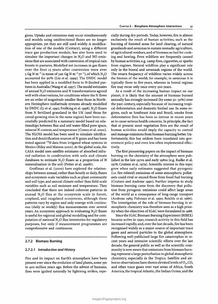
gions. Uptake and emissions may occur simultaneouslyand models using unidirectional fluxes are no longerappropriate, yet they are still used widely. A modifica ­tion of one of the models (Century), using a differenttrace gas production module, has also been used tosimulate the important changes in N20 and NO emis­sions that are associated with conversion of tropical rainforests to pastures. Modelled net increases in gas fluxesover the first 15 years after conversion were over5 Gg N m-2 (a mean of340 Gg N m-2yr-1),ofwhich N20accounted for 90% (Liu et al. 1999). The DNDC modelhas been applied in a modified form to N-limited pas­tures in Australia (Wang et al.1997).The model estimatesof annual N20 emissions and N transformations agreedwellwith observations, for conditions where the N flowsare an order of magnitude smaller than those in North­ern Hemisphere midlatitude systems already modelledby DNDC (Liet al. 1992; Frolking et al.I998). Np fluxesfrom N fertilised grassland in the UK (and those forcereal-growing sites in the same region) have been suc­cessfully predicted by a summary model based on rela­tionships between flux and soil water-filled pore space,mineral N content, and temperature (Conen et al. 2000).The NLOSS model has been used to simulate nitrifica­tion and denitrification sources of N gases and has beentested against 15Ndata from irrigated wheat systems inMexico (Riley and Matson 2000). At the global scale, theCASA model uses satellite estimates of absorbed infra­red rad iation in comb ination with soils and climatedatabases to estimate N20 fluxes as a proportion of Nmineralisation in the soil (Potter et al. 1996b).

Groffman et al. (2000) have explored the relation­ships between annual, rather than hourly or daily, fluxesand ecosystem-scale variables such as plant communityand soil type, and annual climate rather than field-scalevariables such as soil moisture and temperature. Theyconcluded that there are indeed coherent patterns inannual N20 flux at the ecosystem scale in forest,cropland, and rangeland ecosystems, although thesepatterns vary by region and only emerge with continu­ous (daily or weekly) flux measurements over severalyears. An ecosystem approach to evaluating N20 fluxesis useful for regional and global modelling and for com­putation of national N20 flux inventories for regulatorypurposes, but only if measurement programmes arecomprehensive and continuous.

2.7.2 Biomass Burning

2.7.2.1 Introduction and History

Fire and its impact on Earth's atmosphere have beenpresent ever since the evolution of land plants , some 350to 400 million years ago. Before the advent of humans,fires were ignited naturally by lightning strikes, espe-

CHAPTER 2 . Biosphere-Atmosphere Interactions 43

cially during dry periods. Today,however, fire is almostexclusively the result of human activities, such as theburning of forested areas for land clearing, of naturalgrasslands and savannas to sustain nomadic agriculture,of agricultural residues, and of biomass as fuel for cook­ing and heating. Even wildfires are frequently causedby human activities , e.g. camp fires, cigarettes, or sparksfrom engines. Natural wildfires playa significant roleonly in the boreal and savannah regions of the world .The return frequency of wildfires varies widely acrossthe biomes of the world; for example, in savannas it istypically three to five years, whereas in boreal regionsfire may recur only once every 500 years.

As a result of the increasing human impact on ourplanet , it is likely that the amount of biomass burnedannually has strongly increased (by some 30-50%) overthe past century, especially because of increasing tropi­cal deforestation and domestic biofuel use. In some re­gions, such as Southeast Asia and Brazil, smoke fromdeforestation fires has been so intense in recent yearsas to cause serious health concerns . In principle, the factthat at present most vegetation fires are the result ofhuman activities would imply the capacity to controland manage emissions from biomass burning better. Un­fortunately, this has seldom been translated into gov­ernment policy and even less often implemented effec­tively.

The first pioneering papers on the impact of biomassburning on the chemistry of the atmosphere were pub­lished in the late 1970S and early 1980s (e.g, Radke et al.1978; Crutzen et al. 1979). Scientific interest in this topicgrew when early estimates suggested that pyrogenic(i.e. fire-related) emissions of some atmospheric pollut­ants could rival or exceed those from fossil fuel burning(Crutzen and Andreae 1990). Further impetus to studybiomass burning came from the discovery that pollu­tion from pyrogenic emissions could affect large areasof the world as a consequence of long-range transport(Andreae 1983; Fishman et al. 1990; Reichle et al. 1986).The investigation of the role of biomass burning in at­mospheric chemistry was therefore seen as a high prior­itywhen the objectives ofIGAC were formulated in 1988.

Sincethe IGAC Biomass Burning Experiment (BIBEX)became active in 1990, research activity in this field hasincreased rapidly, and ,over the last decade, fire has beenrecognised widely as a major source of important tracegases and aerosol particles to the global atmosphere.Following well-publicised large fire catastrophes in re­cent years and intensive scientific efforts over the lastdecade, the general public as well as the scientific com­munity is now aware that emissions from biomass burn­ing represent a large perturbation to global atmosphericchemistry, especially in the Tropics. Satellite and air­borne observations have shown elevated levelsof 03' CO,and other trace gases over vast areas of Africa, SouthAmerica, the tropical Atlantic, the Indian Ocean, and the

[email protected]

44 M.C.Scholes· P.A.Matrai· M.O.Andreae· K.A.Smith· M.R.Manning

Pacific Ocean. There is now also strong evidence thatsmoke aerosols perturb climate by scattering and ab­sorbing sunlight and by influencing cloud microphysi­cal processes.

We have also learned that the effects of burning arenot limited to the emissions from the fires themselves,but that vegetation fires have pronounced effects ontrace gas emissions from plants and soils. In the case ofCO2, NO,and N20 , post-fire emissions may be more sig­nificant than the immediate pyrogenic release. Fire alsoalters the long-term dynamics of the cycling and stor­age of elements within terrestrial ecosystems, therebychanging their potential as sources or sinks of varioustrace gases. Finally,deposition of pyrogenic compoundsonto tropical ecosystems may affect their compositionand dynamics. In the followingsections,we review someof the results and attempt to put them into the largercontext of global change research.

2.7.2.2 Scientific Approach

Since the early 1990S, BIBEX has designed and carriedout a number of biomass burning experiments in vari­ous ecosystems throughout the world, often in collabo­ration with other international programmes, particu­larly with other IGBPCore Projects. These experimentshave produced extensive local-scale data on vegetationfire characteristics, emissions, and ecology,while simul­taneous regional-scale measurements, using remotesensing and aircraft sampling platforms, have provideda capability to scale results up. Typically, these experi­ments have involved ground measurements on indi­vidual fires, airborne sampling and analysis of smokeplumes, and remote sensing of regional and global fireactivity. Emphasis to date has been placed on tropicalecosystems, but an increasing number of experimentsare now being organised in the boreal zone in responseto climate change concerns.

STARE (Southern Tropical Atlantic Regional Experi­ment), with its two components SAFARI (Southern Af­rica Fire-Atmosphere Research Initiative) (see Box2.3),and TRACE-A (Transport and Chemistry near the Equa­tor) was the first large experiment coordinated byBIBEX. Conducted in 1992, STARE brought together sci­entists from many countries to investigate the chemicalcomposition, transport, and fate of fire emissions origi­nating from South America and southern Africa.

2.7.2.3 Land-Use Fires, Wildfires, and DomesticBiomass Burning: General Trends,Uncertainties, and Possible Changes

In the regional and global research activities on fire ecol­ogy and atmospheric chemistry, keyquestions have been

addressed: What is the current state of vegetation firesat the global scale? Are there quantitative and qualita­tive changes of vegetation fires compared to historictimes? The baseload of natural fires and anthropogenicfires during evolutionary time scales has been deter­mined by several factors : climate and vegetationchanges, changes of land occupation, and cultural prac­tices. The magnitude of historic and prehistoric vegeta­tion burning remains largely unknown, however, be­cause only fragmentary data obtained by case studiesare available (summarised in Clark et al. (1997» . BIBEXresearch and other observations reveal uncertainties,recent changes, and new insights of fire occurrence inthe following main vegetation zones.

Tropical evergreen forest. Deforestation statistics by theFADand others in many studies have provided the base­line data for calculation of pyrogenic emissions due toland use change. While these numbers are useful for es­timating the net releaseof carbon to the atmosphere, theydo not reflect the entire spectrum of fire activities. Re­current fires followingthe initial deforestation burns notonly present additional emission pulses but also lead toimpoverishment of forest ecosystems resulting in re­duced above- and below-ground phytomass (Goldammer1999a; Nepstad et al. 1999).Extreme climate variabilitysuch as the ENSO-related droughts of 1982-1983 and1997-1998 favour the application of fire for land usechange and maintenance of agricultural systems and fa­cilitate the spread of uncontrolled fires (wildfires) inhumid tropical ecosystems that under average climateconditions are subjected to less fire. The area burned bywildfire in the Indonesian and Malaysian provinces onBorneo Island in 1982-1983 covered ca. 5 x 106 ha, and in1997-1998 land use fires and wildfires combined burnedca. 8-9 x 106 ha in Indonesia alone.

Tropical savannas and open seasonal forests. Assess­ments made in the early 1990S on the average annualamount of savannah phytomass burned were in therange of 3-4 Pg yr- I (Andreae 1993). Model predictionson the savannah area annually burned ranged between750 x 1010 m-2yr- 1 (Haoet al.ioco) and 1500x 1010 m-2yr- 1

(Goldammer 1993).More detailed studies on fire re­gimes and fuel loads in Africa point towards lesseramounts of regional and global combustion of sa­vannah phytomass (Menaut et al. 1991; Scholes et al.1996).Recent and ongoing growth of rural populationsand intensity of land use involves landscape fragmen­tation and competitive utilisation of phytomass forgrazing and domestic burning (biofuel use) and mayrepresent a reason for a decrease of fire activities intropical savannas and open forests; desertification in thesub-Saharan Sahelzone of Africaand other regions leadsto a reduction and discontinuity of fuel loads and wild­fire occurrence.

[email protected]

Box 2.3 . C<lISe st udy: SAFARI-92

The following example from the SAFARJ.o;u cam paign (Lindesayet aI.1996) highlights the Kientific approaches used to test hy­po theses and validate models related to biogenic and biomassburning emissions and depo sit ions. It is approaches like thesethat have allowed for an integrated understanding of the magni­tude and controllers of sources, sinks, and exchange processes.During SAFARI-92.,exper imental vegetatio n fires were set andstudied in the Kr uger National Park, South Africa, and at somesites in zambia and Swaziland. These experiments provided abroad set of data on tra ce gases and aerosolemissions,from whichemission (actors (or fires in dry savannas and related biomescould be duived. The relationships be twu n fuel characteristics,burning conditions, and fire behaviour were elucidated.

Regional studieson atmospheric chemis try and air mass tra ns­port showed that savannah fires in southe rn Africa account for asubstantial amount of photochemical oxid ants and haze over thesubcontinent. These studies also showed that the export of smoke­laden air masses cont ributes strongly to the burden of ozone andother trace gases and aerosols over the tropical ocean surround­ingAfrica.How~r, results also sho wed that biogenic soil emis­sions severely impac ted atmospheric chemistry. Investigationson the relationsh ips among rlTe,soil moisture statll.l, and soil tracegas emissions showed tha t soil moistu re played a cr ucial role butth at rITe history also had an important influe nce on the emissionof several trace gases. Figure 1.14a shows the relationship amongdaily NO emissions and nitrate concentrations plotted againstwater·filled pore space. Figure 1.14b desc ribes the relationshipbe tween NO emission rate and nitrifica tinn rate in areas wherefire has bee n excluded and in areas where the vegetation has beenburn ed every two years (Parsnns et aI.1996). These relation shipswere late r incorporated into a simulation model to predict NOemissi ons from semi-and savan nas thereby red ucing the largeunce rtain ty associ ated with the magnitude of previom savan ­nah measurements (Otte r et aI. 1999).

Remote sens ing studies confirmed that Advanced Very HighResolution RadiometerylLand Aerial Cover (AVHRRlLAc'1 km)imagery was a useful too l for fire monitor ing in the region. Incombination with biomass models. the remote sensingdata couldbe used for the estimat ion of the seaso nal and geographical dis­t r ibution of pyrogenic emissions. The results from SAFARI-91confirmed th at it is jus tified to cons ider biomass burning as asignificant contributor to the overall increase in greenhouse gasesth at has occu rred over the last 150years. accoun t ing for some10-15'* of current estimates (Andreae 19'93).

In orde r to est ablis h accurately the global budge ts of tr acegases, reliable source st rength and dist ribution estimates areneeded . At present, the uncertaint ies associated with budget cal­culations are necess arily large, owing to the often-inadequatequant ification of indiv idual sources and the problems associatedwith extr apo lati ng from a number of poorly known sou rces toachieve a globa l estimate. The cont ribu tio n of vegetat ion fires inthe savan nah regio ns of southern Africa has been such a poorlyquantified source, despite the fact that savannas are recognisedas one of the mos t significant biomes in terms of global biomassburning emissions (And reae 1993) and that a large porti on ofthe savannah burns each year. It will now be possible to refinethese esti mates on the basis of results obt ained from SAFARI-91.Modelling studies inco rpo rating the emission data, meteorologi­cal infor mation, and the chemical measurement data obt ainedduring these campaigns indicate that the fires on the African andSouth American cont inents are indeed a major source of the gas-

Areas of Mediterranean and temperate vegetation ,Mediterran ean forest and shrub vegetation, includingCaliforn ian chaparral and South African fynbos, are in­creasingly converted to suburban residential use. Theconsequent suppression of natural and human-causedwildfires results in a buildup of fuels that often cannot

C HAI'TEA 2 • Biosphere -Atmosphere Inter;llC1 ions 45

eeus and p artic ulate po llutants, particula rly ozon e, found in thetroposphe re over the study regions (T hompson et aI. 1996a).Datafrom airborne observations (Fig. 1.15) aboard a DC-3 using acombination of spectrometers and chemiluminescence instru­ments, sho wed that episod ic pyrogenic em issions were not ad­eq uate to acco unt for the buildup of troposphe ric ozone in theregio n but tha t the continuous production of biogenic NO. emis­sions and especially the amounts produced at the star t of therainy seasons have important consequences for regional Kal eozone formation (Harris et aI. 1996). The vertical dist ribu tio n ofN02 and NO as well as that of COl showed markedly d ifferentcharacteristics. All three compounds have a strong gradient tc­ward higher values nea r the ground, and the COl and NO. mix­ing ratios correlated linearl y.The anticorrelation of the profilesof these compounds with that of CO rules out biomass bu rningas a sou rce of the obse rved NO. and COl nea r the gro und, sup ­portin g the field evide nce of no act ive fires in the region. II wasconcluded that the source of the elevated NO. mixing rat ios nearthe surface was biogenic emission from the soil (Harris et a1.1'}96).

SAFARI'92 was an innovative project in many ways. In addi ­tion to being the largest internat iona l, interdisciplinary investi­gation of biomass burning and its atmospheric emissions, it alsorepresented the first time that a large- scale fire emission meas­urement campaign included. as integral compenente the char­acter istics of the biomass, the fire ecology, the fire dynamics inthe area, th e biogenic emissions, and the long-range transpo rt ofthe aerosols and part iculates.

As a fellow-up to SAFARI-92, a much small er experiment,SAFARI·94. was organised by BIBEX to investigate the composi­tion of trace gases in the tropos phere over Africa outside the bu rn­ingseason. EXPRESSO (Experiment for Regional Sources and Sinksof Oxi<1ants),designed primarily to investigate th~ exchange OUl[eSof tra ce gasesbetw~n the trop ical biosp here and atmosphere, tookplace in the Congo Biliin in 19¢>-t997 (Ddmlli el aL1999)· ln '997,AFARI-97 (African Fire-Atm osphere Researclt Init iative) was car­ried out in Kenya, investigating the at mospheric eff« ts of firesoccur ring in the fert ile savannas of East Africa. At the sam~ time,an experime nt designed to quan tify aerosol and trace gas lIUl[eSfrom the Miombo woodl ands of sou thern Africa waS initiated:ZIBBEE (The Zamhian Inter national Biomass Burn ing EmissionsExperiment) began in 1997 and is ongoing. At the present time,BIBEXis hea vily involved in the planning of two large t ropical fire·atmosphere experimen ts: SAFARI-1OOO is studying the transportand climat iceffectof biogenic, pyrogenic,and anthropogenic emis·sions in southe rn Afr ica, while LBA(The Large ScaleBiosphere-At.mosp here Experiment in Amazonia) is investigating the climate­logical, ecological, biogrochemical, and hydrological funct ioningof Amazonia.and the sm tainability of developme nt in this region.

In the bo real zone, BIBEX has bee n involved in the develop'ment of research prog rams addressing the role of fire in bor ealecosystem s and its consequences for the global atmosphere andclima te. F1RESCAN (Fire Research Campaign Asia-Nor th) con 'dacted the first joint Russian-wester n expe rimental fire in cen ­tral Siberi a in 19'93, and continues with the planning of fur thersuch under the auspices of the IGBP Northern Eurasia Study(FIRESCAN Science Team (996). In addition, BIBEXis ac tive inICFME (T he Internat ional Crown Fire Modeling Experiment), aseries of high-intensity experimental crown fires carried out inthe Canadian Northwest Territo ries during the 1 997~ 2000 pe.riod for the pu rpose of d~loping a physical model of crow nfire initia tion and propagat ion.

be burned by prescribed fires. High-intensity wildfiresare an inevitable consequence of fire suppress ion inthese ecosystems. However, there is no indication ofchange in the average area burned in the recent decade.In the industrial countries of the temperate region theapplication of fire in non-forest land use systems has

[email protected]

46 M.C.scholes · P.A.Matrai· M.O.Andreae· K. A.Smith . M.R.Manning

o

(b)

0\ o~(a)o 0 0

Q>o 0

}

Rn> )00 0 '8

o 0

o 0

00 0o

359 360 a 0.5 1 1.5CO 2 N02

(IImOI mor') (nmol mol-I)

500

:§: 400

~ 300::l~ 200

« 100

0li......"""""".......... w.L............................JL.......L.. ............ '-'-'-W-L-'-'--'-'-.L.LJ

76 78 80 82 84 100 110 120 130 29 30 31 3233340 3 CO I Temp ( 'C)

(nmol morl) (nmol mol- )

Fig. 2.15. a Vertical profiles of CO2, N02, and NO and the ratioNOxl NOymeasured in the SAF11 profile dur ing SAFARI 92 (Harriset al.1996); b Vertical profiles of ozone, CO,and temperature meas­ured during SAFARI on September 28, 1992 (Harris et al. 1996)

Temperate-boreal steppe-forest ecotones. A typicalregion representing the steppe-forest fire environmentis central Asia. Recent remotely sensed data from Mon­golia indicate that in the past years political and socio­economic changes in the country were responsible for asharp increase in the area burned by wildfires. In 1996and 1997 more than 10 x 10 10 m-2 and 12 x 10 10 rn ?

burned in the grass steppes and adjoining coniferousforests (Goldammer 1999b).

500

I 400Ql

3001J.a200.,.

0.60 « 1000

0

(a)

(b)

0.48

o

0.24 0.36

O .'.:»: "0.«:.. '

0 .12

Ex. burned

•

~

Ex. unburned

"Bi. unburned

4.5 .----------------,

0.0 L...-....J..::::.....L.__....l-__.L..-_-1.--''--...J

0.00

23.0 ,---------------,

4.6

13.8

9.2

Water-filled pore space

18.4

.'

Ql

~ 4.0c:o'wen'EQl

o 3 .5Z

Nitrification rate

Boreal forest. More than 70% of the global borealforest area is located in Russia. Fire statistics publishedafter the dissolution of the USSR indicate that morethan 650000 ha of forests were burned annually. Thisnumber most likely is still an underestimation. Inthe period 1990-1996, burn areas totalling more than1.12 x 10 10 m-2yr- l were recorded (Stocks et al. 1999,2000). Satellite imagery revealed that a large area wasburning in central Siberia during the 1987 fire season,totalling ca. 10x 1010 m-2 (Cahoon et al.1994).While thefire exclusionpolicyof the USSR reduced the area burnedby natural fires,the scaleofhuman-caused fires increasedover the same period. Current economic problems re­sulting in a weakening of the fire control system in Rus­sia are responsible for a recent increase in area burned.

In Canada, detailed forest fire statistics have beenarchived since 1920 and, within limits, this extensiverecord permits a general analysis of trends in this coun­try (Stocks et al. 1999). Fire occurrence has increasedrather steadily from approximately 6 000 fires annuallyin the 1930-1960 period, to almost 10000 fires during

0.300.240.180.06 0.12

3.0 '---__-'--_----L-__ -'--__ .L...-_--'

0.00

been eliminated (e.g. in Europe) or is subject to legalrestrictions due to air pollution and traffic risks (e.g. inNorth America) . Natural and human-caused wild­fires in temperate forests are usually suppressed. Pre­scribed burning in forestry has been receiving moreattention in the US where it is envisaged to expand theprescribed burned area under the jurisdiction of theUSDA Forest Service to 1.2 X 10 10 m·2 by 2010 (Haineset al. 1998).

Fig. 2.14. a Mean daily NO emissions (ng N-NO m· 2 S·I, circles)and NO:; concentrations (fig N-NO:;s" dry soil, squares) in thefire exclusion plots, plotted against water-filled pore space simu­lated using the HotWet model. Solid and dashed lines representfitted functions to the NO emissions and NO:; concentrations, re­spectively; b Mean NO emissions (ng N-NO m· 2 s') measured byParsons et al. (1996) and Levine et al. (1996) plotted against meannitrification rate (mg N kg'" dry soil) measured in the correspond­ing plots. Linear function: NO emission rate = 0.04 (nitrificationrate) + 0.003, r2 = 0.911, P < 0.030, n =5

[email protected]

the 1980s and 1990S. This is due to a growing popula­tion and increased forest use, but also reflects an ex­panded fire detection capability. During the 1981-1996period an average of 9246 fires annually burned overan average of 2.5 x 10 10 m-z in Can ada, with the annualarea burned fluctuating by an order of magnitude(0 .76-7.28 x 10 10 m -Z). Lightning accounts for 35% ofCanada's fires, yet these fires result in 85% of the total areaburned, due to the fact that lightning fires occur randomlyand therefore present access problems usually not associ­ated with human-caused fires,with the end result that light­ning fires generally grow larger, and detection and con­trol efforts are often delayed. In addition, the practice of"modified" or "selective" protection in remote regionsof Canada results in many large fires in low-priority ar­eas being allowed to perform their natural function.

Domestic biofuel use. Plant biomass provides about 14%of the world's demand of primary energy. Half of the glo­bal population meets an average of 35% of its energy needsby domestic biomass burning. In Africa , for example, thebiomass contribution to the total energy use typicallyranges from 90-100% in poor, 55-65% in middle, and30-40% in high income groups. Unlike free -burning veg­etation fires, which are usually rest ricted to a few monthsduring the dr y season, domestic biofuel combustion takesplace during the whole year (Marufu et al. 2000) .

Summary assessment of trends in global vegetationfire occurrence. The trends of changing fire occurrenceand fire regimes are not uniform. Qualitative and quan­titative data on fire occurrence and fire effects are stillinsufficient to determine reliably the amount of phyto­mass burned in all eco- and land-use systems world­wide. However, improved remote sensing capabilitiesand rigorous fire detection algorithms now provide re­gional fuel load and burning estimates within a muchnarrower range of uncertainty. Fire in boreal and tropi­cal forests and the resulting ecological effects playa po­tentially critical role in determining the rate of globalclimate change (Goldammer and Price 1998;Stocks et al.2000; Nepstad et al. 1999). Changes in the carbon bal­ance of these two fores t biomes could strongly influ­ence global warming through impacts on atmosphericCOz' The implications of regional circumpolar changesof climate and fire regimes on boreal ecosystem prop­erties, permafrost changes, and the release of gas andcarbon stored in organic terrain and ice must be fur­ther addressed by research.

2.7.2.4 Characterisation of Emissions

A central objective of BIBEX was to characterise andquantify the production of chemically and radiatively

CHAPTER 2 . Biosphere-Atmosphere Interactions 4 7

important gases and aerosol compounds from biomassburning. To meet this goal, the BIBEX scientific com­munity has produced a large set of measurements thatdescribe qualitatively and quantitatively the pyrogenicemission of gase s and aerosols. The results show thatthe composition of fire emissions is mainly determinedby two factors: the elemental composition (carbon, ni­trogen, sulphur, halogen, minerals, etc.) of the biomassfuel , and the relative contribution of flaming and smoul­dering combustion in the vegetation fires .

Heating of vegetation fuels produces combustiblegases by pyrolysis and volatilisation of waxes , oils, etc.Sustained flaming conditions are obtained when thevegetation reaches a temperature ofabout 600 K.Smoul­dering combustion involves heterogeneous reactions ofatmospheric oxygen with solid fuel. The combustiontype dominating in a given fire is influenced by the wa­ter content, the density and structure of the fuel, theoxygen availability in intense flaming, and the meteoro­logical conditions prevailing during the fire .

Generally, emissions from fires occurring in naturalvegetation are a mixture of compounds from flamingand smoulder ing combustion, with different propor­tions being typical of the various types of fires. Themajor part of savannah and domestic fuels is consumedin the flaming stage, while charcoal making is a purelysmouldering process; forest biomass is combusted aboutequally by both processes. Lobert et al. (1991) summa­rised the composition of emissions released during thedifferent burning stages. Relatively oxidi sed compounds,such as COz' NO, NOz, SOz' NzO, as well as Nz and el­emental carbon particles are emitted during the flam­ing stage of a fire. The emission of more reduced com­pounds (CO,CH4, nonmethane hydrocarbons, PAH,NH3,

HCN, CH3CN, amines, CH3CI, HzS, COS, OMS, and or­ganic particles) occurs during the smouldering stage(e.g, Lobert et al. 1991;Yokelson et al. 1997).

2.7.2.5 Emission Ratios and Emission Factors forDifferent Chemical Compounds from Fires inVarious Ecological Systems or Vegetation Types

To express the emission of trace gases and aerosols fromfires quantitatively, we use the concept of emission ra­tios and emission factors. These parameters relate theemission of a particular compound of interest to thatof a reference compound, such as COz or CO (emissionratio), or to the amount of fuel burned (emission fac­tor). Emission ratios are obtained by dividing the ex­cess trace compound concentrations measured in a fireplume by the excess concentration of a simultaneouslymeasured reference gas, such as COz or CO. To obtain"excess" concentrations, the ambient background con­centrations mu st be subtracted from the values meas-

[email protected]

48 M.C.Scholes· P.A.Matrai· M.O.Andreae· K.A.Smith· M.R.Manning

ured in the smoke. For example the emission ratio ofmethyl chloride, CH3Cl,relative to CO is:

ElL _ ~CH3Cl _ (CH3Cl)smoke - (CH3Cl)Ambient"cH Cl/CO - -

3 ~CO (CO)Smoke - (CO)Ambient

The various techniques for these calculations and theassociated errors are discussed in Le Canut et al. (1996).For gases, the results are expressed in terms of molarratios. For aerosols, emission ratios are usually given inunits of mass of aerosol per kg carbon in the form ofCO2 (g kg-l C(C0 2».In this chapter,all resultswillbe pre­sented after conversion to emission factors (see below).

The selection of CO or CO2 as reference gas is deter­mined by the ultimate objective of the analysis and onthe fire phase (flaming or smouldering) during whichthe compound is preferentially released. For compoundsemitted predominantly in the smouldering stage of fires,CO is a suitable reference gas as it is also emitted pre­dominantly during this stage. Close correlations be­tween derived-derived gases and CO can usually be ob­tained, which allows fairly accurate estimation of tracegas emissions from fires for which the CO emission isknown . For compounds containing nitrogen or halogenelements, the emission ratio relative to CO is also de­pendent on fuel composition, i.e. the nitrogen or halo­gen element content of the fuel.

Flaming-derived compounds correlate wellwith CO2,

while correlations of derived-derived gases with CO2tend to be relatively poor because the variation in therelative proportion of flaming versus smouldering com­bustion between different fires or even different partsof the same fire results in variable trace gas to CO2 ratios.On the other hand, the emission ratio relative to CO2permits the estimation of trace gas emission from firesbased on the amount of biomass burned, because mostof the biomass carbon is released as CO2, Therefore thisratio is the most suitable for regional or global estima ­tions; however, it is worth noting that when multipleratios are used to estimate emissions, errors are propa­gated making overall estimates quite uncertain.

Another parameter frequently used to characteriseemissions from fires is the emission factor, which is de­fined as the amount of a compound released per amountof fuel consumed (g kg'" dm; dm: dry matter). Calcula­tion of this parameter requires knowledge of the car­bon content of the biomass burned and the carbonbudget of the fire (usually expressed as combustion ef­ficiency, see Ward et al. 1996); both parameters are dif­ficult to establish in the field as opposed to laboratoryexperiments where they are readily determined. Wherefuel and residue data at the ground are not available, afuel carbon content of 45% is usually assumed in orderto derive emission factors from emission ratios .

During the various BIBEX field experiments, and inother studies over the last decade, a large number of

emission ratios/factors have been determined. Recently,these data have been compiled into a coherent set of rec­ommended emission factors (Andreae and Merlet 2001) .In Table 2.3 we present emission data from this compila­tion for selected gaseous and particulate emission prod­ucts and for the most important types of fire regimes(savannas and grasslands, tropical forest, ex-tratropicalforest, domestic biofuel burning, charcoal combustion,and agricultural waste burning). These emission factorsare based on an analysis of some 130 publications, a largefraction of which were produced as a result of BIBEXcampaigns. The values given are means and standarddeviations wherever possible; when only two values foran emission factor are available in the literature, thesetwo values are given as a range, and where only a singlemeasurement is available, it is given without an uncer­tainty estimate. It is evident from this compilation thatonly for savannah fires do we have adequate data for mostcompounds, whereas for other fire types only the emis­sions of some key compounds have been satisfactorilydetermined. The release of compounds for which dataare missing for a given type of fire can, however, be esti­mated by scaling emissions to CO or CO2,

2.7.2.6 Emissions from Global Biomass Burning

Estimation of the amounts of trace substances emittedfrom biomass burning requires knowledge of both theemission factors (i.e. the amount of trace substance peramount of fuel combusted) and the actual amount of fuelburned. We have shown above that the emission factorsfor many important compounds, such as CO and CH4,

are now fairly well known, with a typical uncertainty ofabout 20-30%. In spite of this progress , large uncertain­ties persist for regional and global fire emissions becauseof the difficulties inherent in estimating the amount ofbiomass burned. In particular, there are differences ofas much as an order of magnitude in regional estimatesbased on estimates of typical fire frequencies in the vari­ous vegetation types, and those based on actual firecounts obtained from remote sensing . These issues willbe discussed in more detail in Sect. 2.6.2.7. Table 2.4 pro­vides a summary of estimates made over the last decadeusing the former approach . In the following paragraphs,we discuss global emissions for key compounds basedon the emissions factors in Table 2.3 and the biomassburning estimates of Logan and Yevich (R. Yevich, per­sonal communication 2001) given in Table2.4 (also seeAndreae and Merlet (2001) for further information).

Carbon compounds. CO2 is the major carbon compoundemitted and accounts on average for about 80-90% ofthe mass of carbon burned, ca. 3650 Tg C(C0 2) yr-l .COrepresents around five to eight percent of the carbonburned, ca. 300 Tg C(CO) yr" . Hydrocarbon (methane

[email protected]

CHAPTER2 • Blosph~re-Atmosph~r~ rraerecncns 49

Tabl~ 2.]. Emission factors for se lected gases and ae rosols for di fferent forms of bi om a>s burning (in g s~des p<'r kg dry fue l burned)

CO, 1613 "5 "ao ". 1ses :t131 "50 ,~ 2611 "" 1515 ± 177

CO 65 <20 1~ <20 101 "7 n '" 200 ,~ 91 ".CH. za "'.9 6.8 ±2.0 1.7 ±L9 61 <2, 61 "3 1.7

NMH( l< :t1.0 8.1 :tl O 5.7 H 6 73 :t4} 1.7 ±L9

(,H, 019 "'17 0.21-{1.59 0.27 "'.09 0.51~.90 O.QS--.-\l.B

C,H. 0.79 "''' 1.l>--2,9 1.12 :to.55 1.8 "'6 0<6 :to.33

C,", 0.32 "''' 0.5-1.9 0"" :to.15 11 "'6 0.53 "'''(,H. 0.022 :to.014 0.013 0.~.06

C,", 016 :to.14 0.55 0.59 :to.16 1l.5-1.9 0.13--0.56

(,H, 0.09 :to.03 0.15 0.25 :to.ll 0.2~.8 0.07~.3O

t- butene 0.09 "'.~ O.B 0.09-<l.16 0.1~.5 Q02~.20

i-but ene 0.030 :to.012 0.11 0.05-{1.11 0.1~.5 1l.01~.16

n--bu !ane 0.019 "'09 0,041 0'"' :to.Q38 0.03---{l.13 0,02~.10

Iso prene 0.020 :to.on 0.016 0,10 0.15~A2 0.017

Benzene 0.23 :to.ll 1l.39-0,41 049 "'OS 19 :t1.0 0.3-1.7 0.14

Toluene 0.13 "'~ 0.2H29 0.'" :to.lO 1.1 "'.7 0.1)8~,61 0,026

Metha nol 1.0 ±L4

Formaldehyde 0,2H.44 1.1 "'5 O,B"' ~

Acetaldehyde 0.50 :to.39 0.48-052 0.1 4"'~

Acetone 0.25~.62 0.5H.59 0,01~.04

Benzaldehyde 0.029 0.027 0.Q2--il.03 0.009

Furan 0095 0.40--0.45

2-methyl--furan O.O44-<l.l)48 0.17 0.47 0.012

Furfural 019-0.63 0.22

Aceton itr ile 0.11 0.19

Formic acid 1.9 :t24 0.13 011

Aceticadd 18 ±L8 0.4--1.4 0.8

H, 0.97 "' ~ 3.H ,O 18 "'5NO. (as NO) 19 ±2A 16 "'.7 30 :t1.4 1.1 "'6 19 15 ±LO

N,o 0.21 :tO.10 0.26 :to.07 O.~ 0,07

NH, 0.6-15 1.' "'.HeN 0.025--il.031

so, OJ5 :to,16 0.57 :to.23 10 017 "'.,COS 0.015 "' 009 1l.0:3O---<l.O36 0.065 :to.077

c-,c 0.075 "'019 O.o2~.18 0.050 :to,032 0,~.07 0.012 0.24 :to.14

(H18r 0.0021 :to.OOlO 0,0078 :to,0035 0.0032 rlI,0012

(H II 0.OC05 :to.COOl 0.0068 0""'

PMH S' "5 9.1 "5 13.0 ±7.0 7.1 ±2.3 1.9

TPM 8J '" 6.5-105 17.6 '" 9.' :t6.0 11

TC 17 eu as ±1.5 6.1 -10,4 5.1 :t1.1 63 '.0

OC l< :t1.4 5.1 ±lS 8.6-9.7 '.0 :t1.2 '8 13

Be 018 :to.18 O~ "'31 0." :to.19 059 "'37 15 0,69 :tO,13

K 03' "''' 0.19 :to.22 0.08--{I,41 O.~ :tO.01 0.'" 0,13--0.43

[email protected]

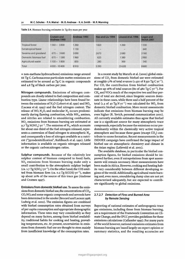
50 M.C.Scholes · P.A.M alrai · M. O.Andn·ae · K. A.Smilh · M. R.Manning

Ta ble 2.4. Biomass burn ing esti mates in Tg dry mass per year

ndreae 1993 lIOano Llu 1994 jcusse ee . 1.1996

Tropical forest 1S60- 3800 "60 1820 " 60 1330

Extratropcat forest 1150 ""Savanna and grassland 610 - 3600 3690 2610 2680 3160

Domestic biomass fuel 670 - 1300 1960 620 13SO 2900

Agricultural waste 1100 - 1800 850 2SO 300 S411

Total 40CKl - l0400 8910 5390 (5620) 8600

+ non-metha ne hydrocarbons) emissions range around66 Tg C.Carbonaceous particulate matter emissions areestimated to be around 4ZTg C in organic compoundsand 4.8 Ig of black carbon per year.

Nitrogen compounds. Emissions of nit ro gen com­pounds are closely related 10 fuel composition and com­bustion type. Linear relat ionships have been found be­tween the emissions ofN 20 (Lobert er a1. 1991)and NO.,(Lacaux et al. 1993) and the fuel nitrogen content. Therelease of NO, N20, and molecular N2occurs predomi­nantly during flaming combustion, while NHl , amines,and nit riles are related to smoulde ring combustion.NO., emissions from biomass burning are estimated at9.7 Tg N(NO.,) yr- ' . The emission of N2, which accountsfor about one-third of the fuel nitrogen released, repre­sents a conversion of fixed nitrogen to atmospheric N2,and consequently a loss of nitrogen available as a nutri­ent ("pyrode nitrification", Kuhlbusch et al. 1991). Littleinformation is available on organic nit rogen releasedor the organic carb onmitrogen ratios.

Sulphur co mpo unds . Beca use of th e relatively lowsulphur content of biomass compared to fossil fuels,S02 em issions from bioma ss burning m ake on ly asmall contr ibution to the atmospheric sulphur budget(ca. I.] Tg 5(50 2) yr-!).O n the other hand, theC05 emit­ted from biomass fires (ca. o.r Tg 5(C05) vr-' ), makesup about 20% of the source of this trace gas (Andreaeand Crutzen 1997).

Emissions from domestic blcfuet use. To assess the emis­sions from domesticbiofueluse,the concentrationsofC02>CO, NO,and some organic compounds and aerosols havebeen determined in the smoke (Brocard and Lacaux 1998;Ludwig et al. 200Z).The emission figures are combinedwith biofuel consumption rates obta ined from surveysof per capita consumption and appropriate demographicinformation. These rates may vary considerably as theydepend on many factors, among them biofuel availabil­ity, traditional habits for cooking and heating, prevail­ing temperatures, etc. At present, uncertainties in emis­sions from domestic fuel use are thought to stem mainlyfrom insufficient knowledge of the consumpt ion rates.

In a recent study by Marufu et al. (2000) global emis­sions of CO2 from domestic biofuel use were estimatedat roughly 17%of total sources (t 4Z0 of 8350 Tg C yr· l

) .

For CO, the con t ribution from biofuel combustionmakes up 16% of total sources (80 of 480 Tg C yr>!). ForCHt and VOCSmuch of the respective two and four per­cent of total are derived, since biogenic sources domi­nate in these cases, while three and a half percent of thetotal (1.4 of 40 Tg N yr- l ) was calculated for NO., fromdome stic biofuel combustion. More recent assessmentsindicate that emissio ns from biomass bu rn ing may beeven higher (R. Yevich, personal communication ZOOt ).

All currently available estimates thus agree that biofucluse is a significant source for many atmospheric tracecompounds, especially because th e emissio ns occur pre­domin antly withi n the chemically very active tropicalatmosphere and because these gases (except Ca l) con­tribute to ozone formation. Recent measurements in theINDOEX campaig n have confirmed the large impact ofbiofuel use on atmosphe ric chem istry and climate inthe Asian region {Lelieveld et al. ZOOt ).

The available database, in particular the biofuel con­sumption figures, for biofuel emissions should be im­proved further,even if extrapolations from spot assess­ments will remain necessar y. Most measurements havebeen made in Africa. However,cooking and heating hab­its vary considerably between different developing re­gions of the world. Add itionally, agricultural wasteburn­ing and, even more, smouldering dump sites are not yetcharacterised adequately, but are expected to contrib­ute significantly to global emissions.

2.7.2.7 Detection ofFires and Burned Areaby Remote Sensing

Report ing of national estimates of anthropogenic tracegas emissions, including those from biomass burning,are a requirement of the Framework Convention on Cli­mate Change, and the IPCC provides guidelines for theseemissions calculations (Callander 1995). For many par tsof the world however,national emissions estimates frombiomass burning are based largely on expert opinion orsummary statistic s, and the resulti ng accuracies are

[email protected]

largely unknown. Synoptic fire information derivedfrom satellites provides a source of information for aug­menting available national fire statistics. Satellite detec­tion of active fire occurrence has been used to identifythe timing and location of fires, and has been used inemission product transport studies, for example. Polarorbiting and geostationary satellite systems have beenused to provide fire information (Elvidge et al. 1996;French et al.1996;Prins et al.1998). The first global dataset of annual satellite fire distributions was developeddirectly as a contribution to BIBEX (Stroppiana et al.2000).

Automated algorithms for direct estimation ofburned area are currently under development with theintent of providing direct input to emissions modelling(Roy et al. 1999). Satellite based techniques for directestimation of emitted energy, fire intensity, atmosphericaerosol loading, and vegetation recovery are also beingdeveloped. Since in most cases the data products are tobe used in numerical modelling, there is a need to pro­vide a quantitative assessment of their accuracy. Forsatellite products, validation using independent datasources needs to be undertaken to determine productaccuracy.

New satellite systems are planned that will improveour current fire monitoring capability (e.g. Kaufmanet al. 1998b).The requirements for these systems comein part from the experience gained from BIBEX. Thesatellite fire research community is working to securethe necessary long-term fire observations from the nextgeneration of operational satellite systems, such as theUSNational Polar Orbiting Environmental Satellite Sys­tem (NPOESS).

With the operational availability of satellite-derivedinformation on the location and timing of fires and onthe area burned, it will be feasible to run an improvedclass of models to estimate emissions on an annual ba­sis. These improved models will require ground-basedestimates of emission factors and modelled estimatesof fuel load and fuel consumed for a given year, ratherthan representative values for a given vegetation type.As new satellite information becomes available on fireintensity, emitted energy, and fuel moisture content,these first order emissions estimates can be improved.Providing robust models that can be used for opera­tional generation of annual emissions estimates anddeveloping approaches to validate them provide the nextchallenge for the fire and global change research com­munity.

2.7.2.8 Impacts ofBurning on Trace Gas Exchangefrom Soils

The process of biomass burning represents a vast real­location of nutrients in cleared tropical forest and sa-

CHAPTER 2 . Biosphere-Atmosphere Interactions 51

vannah systems. Large proportions of system carbon,nitrogen, and sulphur are volatilised. Soils are affectedby changes in nutrient levels, pH, and temperature,with associated changes in microbial communities.Studies conducted during the SAFARI 92 campaignshowed that the mean NO emissions increased afterburning, reaching 15 ng N m-2 S-l from dry sites andexceeding 60 ng N m? S-1 from the wetted sites (Levineet al. 1996).The long-term effect of excluding fire froma savannah is to increase the soil nitrogen contentthrough increased litter inputs, which in turn increasesnitrification rates and soil NO emissions (Parsons et al.1996). Soil emissions of CO2 and CO were increased byan order of magnitude after burning, whereas exchangeof CH4 was not affected. In all cases the increases wereshort lived and dropped back to pre-burn levels withina few days (Zepp et al. 1996).Studies on the impact ofburning on soil carbon pools showed that annual burn­ing in a semi-arid savannah reduced the light-fractioncarbon markedly but did not impact the intermediateor passive carbon pools. This has implications for theamount of soil carbon that can be readily metabolisedby the soil microorganisms. Burning the savannas atlonger time intervals had no effect on the pool size orthe turnover rates of the various soil carbon pools (Ot­ter 1992).

2.7.2.9 Importance to Atmospheric Chemistryand Climate

We have already pointed out that biomass burning is asignificant source of several greenhouse gases, amongthem CO2, CH4, and, to a much lesser extent, N20 . It alsomakes important contributions to the budget of severalgases of stratospheric significance, such as methyl chlo­ride and methyl bromide, N20 , and COS. Of particularimportance to the chemistry and radiative characteris­tics of the atmosphere are the emissions of ozone pre­cursors, particularly NO x' VOC, CO, and CH4• Becausevegetation fires in tropical regions can occur only whenthe vegetation is dry enough to burn, firesare most abun­dant in the dry season, when the trade wind inversionwith its large-scale subsidence and suppression of rain­forming convection prevails over the region.Becausethisinversion prevents convection to heights of more than afew kilometres, it was initially thought that the linkagebetween dry condit ions and subsidence more or lessprecluded the transport of pyrogenic ozone precursorsto the middle and upper troposphere. Recent work hasshown, however, that large amounts of smoke can getswept by low-level circulation, e.g. the trade winds, to­wards convergent regions over the continents or the In­ter-Tropical Convergence Zone, and there become sub­ject to deep convection (Andreae et al. 2000; Chatfieldet al. 1996;Thompson et al. 1996a). This transport pat-

[email protected]

52 M.C.Scholes · P.A.Matrai · M.O.Andreae· K.A.Smith · M.R.Manning

tern can explain the abundance of fire-related 03 and0 3-precursors in the middle and upper troposphere asobserved by remote sensing and in situ measurements(Browell et al. 1996a; Connors et al. 1996; Olson et al.1996).

The aerosols from biomass fires, the most obviousand visible sign of pyrogenic air pollution, may have animportant impact on climate. Biomass burning is thesecond largest source of anthropogenic sub-micrometeraerosol (after sulphates from fossil fuel combustion),and possibly the largest source of black carbon parti­cles.These aerosols influence climate and the hydrologi­cal cycleby scattering and absorbing solar radiation, andby changing the properties of clouds in ways that arejust now being elucidated (Hobbs et al. 1997; Kaufmanet al. 1998a; Ramanathan et al. 2000). Further charac­terisation of the radiative and cloud-nucleating proper­ties of pyrogenic aerosols and their effect on regionaland global climate remains a major challenge to the sci­entific community.

Whether the impact of biomass burning will grow inthe future depends both on climate change and on hu­man factors. The amount of fuel available for burningat a given place and time is a function of ecological fac­tors, e.g. soil fertility, precipitation, and temperature. Italso depends on land use, i.e. if the area has been burnedpreviously,is used for grazing or agriculture, and so on.If climatic variat ions become more extreme, as climatemodels have suggested, we can expect a more frequentoccurrence of drought years following very wet years.This would result in large amounts of fuel ready to burnin the fire season. Furthermore, in a warmer and drierclimate, fire frequency is likely to increase, which wouldreduce biomass carbon storage bychanging the age classstructure of vegetation, as well as causing increasedemissions of ozone precursors. To monitor the regionaland global evolution of pyrogenic emissions, it wouldbe very useful to develop unique tracers for biomassburning, and to set up continuous measurements ofthese tracers at selected sites.

Human activities are of central importance to thefrequency and severity of biomass fires. If large partsof the humid Tropics are deforested further, they willbe transformed from a biome essentially free of fires(the tropical rainforest) to biomes with much more fre­quent fires (grazing lands, agricultural lands, and waste­lands). With a higher human population density, the fre­quency of ignition will go up as well. And finally, theamount of biomass burned for cooking and domesticheating, already a major source of emissions in tropicalcountries, will increase further. Tofollowthese changes,we will need to develop further and validate techniquesto determine the spatial and temporal distribution ofbiomass burning and the amounts of biomass burnedin the various fire regimes.

2.7.3 Wet Deposition in the Tropics

Wetdeposition plays an essential role in controlling theconcentrations of trace gases and aerosol particles inthe atmosphere and in providing the essential nutrientsfor the biological functioning of ecosystems. Wet anddry deposition affect the budgets of key nutrients andtrace gases in both terrestrial and marine ecosystems,as described in other sections of this chapter.

The Tropics are a particularly important region re­garding global atmospheric chemistry. Due to intenseultraviolet radiation and high water vapour concentra­tions, high OH concentrations oxidise inorganic andorganic gases, and induce an efficient removal from theatmosphere of the oxidised products.Strong convectionin the tropical regions results in huge volumes of airbeing drawn out of the sub-cloud layer with the result­ant chemical composition of the precipitation comingfrom the capture of gases and small particles by the liq­uid phases of cloud and rain. Knowledge of the chemi­cal composition of wet deposition allows one to trackseasonal emissions from various ecosystems.

In the 1990S, due to the lack of information on wetdeposition in the Tropics, a cooperative programmewas undertaken, involving the Global AtmosphereWatch (GAW) of the World Meteorological Organisationand the Deposition of Biogeochemically ImportantTrace Species (DEBITS) Activity of IGAC (see A.S),mostly in Asia. It was followed by the Composition andAcidity of the Asian Precipitation (CAAP) programme,later expanded into Africa and South America (Lacaux1999).

In some tropical areas, however, dry deposition is atleast as important as wet deposition and must be con­sidered in the calculation of total deposition. Dry depo­sition of acidic gases impacts soil and plants, as indi­cated in Sect. 2.4 and 2.6.1. High concentrations of sul­phur and nitrogen oxides and nitric and sulphuric ac­ids may increase acidification processes. In many aridor semi-arid regions, transport and deposition of alka­line soil particles to adjacent ecosystems are also im­portant. The deposition of alkaline particles partly miti­gates the effectsof wet and dry deposition of acidic com­pounds.

In addition to acidity, the N content of wet deposi­tion may strongly affect ecosystem properties such as Cstorage, trace gas exchange,cation leaching,biodiversity,and estuarine eutrophication. This has been shown fortemperate regions with altered N inputs (e.g. Howarthet al. 1996; Mansfield et al. 1998 and papers therein).Now, however, 40% of global applications of industrialN fertiliser takes place in the Tropics and subtropics, andover two-thirds is expected to occur in now-developingregions by 2020 (Matthews 1993; Bouwman 1998).Simi-

[email protected]

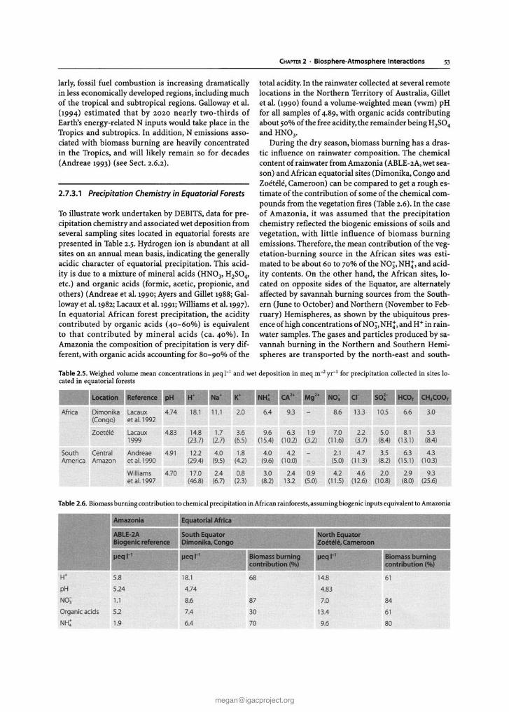
larly, fossil fuel combustion is increasing dram aticallyin less econom ically developed regions , including muchof the tropical and subt ropical regions. Galloway et al.(1994) estimated that by 2020 nearly two -thirds ofEarth's energy-related N inputs would take place in theTr opics and subtropics. In add ition, N em issions asso­ciated with biomass burni ng are heavily concentratedin the Tropics, an d will likely rem ain so for decades(Andreae 1993) (see Sect. 2.6.2).

2.7.3.1 Precipi tation Chemistry in EquQtorial Forests

To illustrate work under taken by DEBITS, data for pre­cipitat ion chemistr y and associated wet deposition fromseveral sampling sites located in equ atorial forests arepresented in Table 2.5. Hydrogen ion is abunda nt at allsites on an annual mean basis , indica ting the generallyacidic character of equa torial precipitation . This acid­ity is due to a mixture of mineral acids (HNO" H2SO"etc.] and organic acids (formic, acetic , propionic, andothers) (Andreae et al. 1990; Ayers and Gillet 1988; Gal­loway et aI. 1982; Lacaux et al. 1991;Williams et al. 1997).In equatorial African forest precipitation, the aciditycontributed by orga nic acids (40-60%) is equiva lentto tha t contr ibuted by mineral acids (ca. 40%). InAmazon ia the composit ion of precipitation is very dif­ferent, with organic acids accounting for 80-90% of the

C.....PT£R 2 • Bio sphere-Atm osphere Inler actions S3

total acidity. In the rainwater collected at several remotelocation s in the North ern Terr itory of Australia, Gilletet al. (1990) found a volume-weighted mean (vwm) pHfor all samples of 4.89, with organic adds contributingabout 50% of the free acidity,the remainder being H2SO,and HNO,.

Dur ing the dry season, biomass burning has a dras­tic influence on rainwater composition. The chem icalcontent of rainwater from Amazonia (ABLE-2A,wet sea­son) and African equatorial sites (Dirnonika, Congo andZoetell!,Cameroon) can be compared to get a rough es­timate of the contribution of some of the chemical com ­pounds from the vegetation fires (Table 2.6). In the caseof Amazonia, it was assumed that the precip itat ionchemistry reflected the biogenic emiss ions of soils andvegetation, with littl e influence of biomass burningemissions. Therefore, the mean contribution of the veg­etatio n-bu rning sou rce in the African sites was est i­mated to be about 60 to 70% of the NO" NH: , and acid­ity contents. On the other hand, the African sites, lo­cated on opposite sides of the Equator, are alternatelyaffected by savannah burning sources from the South­ern (June to Octobe r) and Northern (November to Feb­ruary) Hemispheres, as shown by the ubiquitous pres­ence of high concentrations of Nfj '[ NHt ,and H+in rain­water sam ples. The gases and parti cles produced by sa­vannah bu rning in the Northern and Southern Hemi­sphe res are transported by the nor th -east and south-

•

Table 2.5. Weighed volum e mean concentranom in ~eq I- I and wet depo sit ion in rneq m-2yr-1 for precipitat ion collected in silu lo-cared in equatorial forests- ccencn ereeoce ,< H: " Mg'· NO; r SO~· HCo, CH,C

Af<i<o Dimonika lacauK 4.74 '" 11.1 2.0 ., 93 8 ' 113 105 " 3.0(Congo) etal.l992

zcerae teceux 4" '" ,.7 3' 9' '3 \.9 7.0 2.2 5.0 8.1 5.3

'999 {23.n 0." (6.5) {15.4l (10.2) (3.2) (11.6) (3.n (SA) (13.1l (8 .4)

South Centeal And.eae 4.91 ", ' 0 \.8 ' 0 . ] z .., 35 6.3 '.3America Amazon et al. 1990 {294} (95) (4.2) (9.6l (10.0) (5.0) (11.3) (82) (15.1) (10.3)

Williams 4.70 17.0 2A 0.8 3.0 2.4 0.9 4.2 4.' 2.0 2.9 93et al. I997 (46.8) (6.n (2.3) (8.2) 13.2 (5.0) (11.5) (12.6) (l0.8) (8.0) (25.6)

Table 2.6. Biomass burning contribution to chemical precipitation in African rainfu rests,assuming biogenic inputsequivaient to Amazonia

maz onia ~quatoria l Africa

ABLE-2A South Equator North Equato rBloqenlc referen ce Dimonika,Co~o Zoe te le, Cameroo n

"" ~"" I ~~oma ss bu rning j.leqt ' I~~omass burn ingo nt ribu t ion ('lib) ont ribution ('lib)

W

pH

NO;

Organic acids

NH:

s.e 18.1 se ta.a 61

51 4 4.74 4.83

U 8 ' 87 7.0 84

51 7A 30 13.4 61

\.9 ' 4 70 9.' 80

[email protected]

54 M.C. Scholes • P.A.Matrai · M.O.Andreae· K.A.Smith· M.R.Manning

east Trade Winds, respectively, to the equatorial forestsand progressively scavenged by convective clouds.

The wet deposition measured in the semi-arid andhumid savannas surrounding the forested ecosystemspresents a source of high potential acidity, which maynot result in final strong acidity of the deposition. Forexample, Galy and Modi (1998) have shown that theprecipitation from arid savannas is characterised by aweak acidity (H+=2 fleq 1-1) in spite of a high potentialacidity (nitrate + dissociated formate + dissociatedacetate = 22 fleq 1-1). This result is explained by hetero­geneous interactions occurring between alkaline soildust particles and acidic gases. Many of these mineraldust particles are able to entirely neutralise gaseous ni­tric acid. These gas-particle interactions occur beforethe incorporation of these particles into cloud dropletsor raindrops. Furthermore, high concentrations of or­ganic aerosols (from biomass burning and condensa­tion of biogenic hydrocarbons) and mineral dust (fromdeserts and arid areas) could also promote intense het­erogeneous atmospheric chemistry (e.g. Dentener et al.1996; Carmichael et al. 1996, 1997) (also see Chap. 4).These processes may affect the cycles of nitrogen, sul­phur, and atmospheric oxidants significantly.

2.7.3.2 Effect of Wet Deposition on TropicalTerrestrial Ecosystems

Acidification effects are mainly due to deposition ofmineral sulphur and nitrogen compounds. In tropicalregions, organic acid deposition may contribute as muchas 80%; however, these acids are oxidised in soils andwill not participate directly in soil acidification. Soilparticles exchange alkaline cations with H+and the con­centration of alkaline ions determines the soil base satu­ration. When base saturation is low, acids may releasealuminium ions from soil particles. In spite of its limi­tations, the "critical load" concept, characterising eco­system sensitivity to acidic deposition,has been adoptedas a tool for estimating potential impacts on ecosystems.In order to facilitate the development of strategies tocontrol pollution in tropical countries, the StockholmEnvironment Institute (SEI) has recently proposed aglobal assessment of terrestrial ecosystem sensitivity toacidic deposition that uses soil buffering capacity as akey indicator (Cinderby et al. 1998). This assessmentdepends on two factors: the buffering capacity of thebase layer to identify soils that have high weatheringrate, and the cation exchange capacity to quant ify thecapacity of a soil to buffer acidity.

A global map prepared by SEI (see Fig. 2.16), showsfive classes of sensitivity to acidic deposition, from acritical load of 200 meq m-2 yr- I for the insensitive classto a critical load of 2S meq m-2 yr" for the most sensi­tive class. Some selected wet deposition measurements

of non-sea salt sulphate, nitrate, and organic acids,mainly obtained by the DEBITS Activity, are also in­cluded.These combined measurements provide an over­all view of tropical regions where the potential risk ofacidification is important. All the equatorial rainforestsof South America, Africa, and Asia are classified in themost sensitive classes. For South American soils, whichhave a level of mineral acidity deposition of about10-20 meq m-2 yr- I , future acidification problems maybecome severe if further land use change and indus­trial activities occur in these regions. For tropical Af­rica,due to the high contribution of mineral acidity fromwet deposition from biomass burning sources, the criti­cal load is nearly exceeded in many parts of westernAfrica. For Asia,in some parts of China, Japan, and otherindustrialised and populated zones, the critical load hasalready been exceeded (Fig. 2.16).

Work by IGBPresearchers suggests that there is sub­stantial, although mostly indirect, evidence that the sup­ply of N may not limit plant production in some tropi­cal forests (Hall and Matson 1999).Thus, additions of Nmay have little direct effect on plant production andcarbon storage, but may substantially affect rate and tim­ing of N losses. As indicated above, tropical forest soilsare highly acidic ; additions of anthropogenic N mayincrease that acidity, leading to increased losses of cati­ons and decreased availability of phosphorus and othernutrients,ultimately limiting plant production and otherecosystem functions. Moreover, N additions to tropicalsoils may result in immediate and relatively large pro­portional losses of N in trace gas forms , as discussedabove. On-going work strives to identify the direct andindirect effects of wet deposition on tropical agro-eco­systems, and to determine its implications for ecosys­tem functioning and feed-backs to the atmosphere lo­cally, regionally, and globally.

2.8 Marine Highlights

From its inception, IGAC stimulated and sponsoredresearch on marine aerosol and gas exchange of com­pounds of biological origin through the Marine Aero­sol and Gas Exchange (MAGE) Activity (see A.S),exam­ples of which are given below. Similar to terrestrialbiosphere-atmosphere research, integrated field cam­paigns in marine regions, such as the ACE-I,ACE-2 andASGAIMAGE experiments (see A.s) have been an IGAChallmark. These field research efforts have linked stud­ies of emissions, transformations, and transport in themarine boundary layer. The study of pertinent marinebiogeochemical cycles resulting in sea -air fluxes,however, has yet to be fully integrated into these fieldcampaigns. While research on biosphere-atmosphereinteractions in marine regions has progressed signifi­cantly in the last decade, it remains less advanced than

[email protected]

CHAPTER 2 . Biosphere-Atmosphere Interactions 55

Wet depos ition (meq m -2 year - I)

Fig. 2.16. Wet deposition (meq m-2 yr-1) of nitrate, non-sea-saIt sulphate and organic acids compared with "cr itical load ", a measure ofecosystem sensitivity to acidic depo sit ion. Asia and Ocean ia (Ayers et aI. 1996a); Africa (GaIy and Mod i 1998; Turner et aI. 1996c);Amazonia (Andreae et aI. 1990; Williams et aI. 1997); and ecosystem sensit ivity to acidic deposition (Cinderby et aI.1998 )

that for terrestrial regions due to the higher demands offield logistics as well as, perhaps, a lesser recognition ofthe interaction by the whole of the research communi­ties involved. In the last decade , the greatest advancesoccurred in DMSbiogeochemistry while the marine cy­cling of other compounds (e.g.organohalogens) is lesswell, or not at all, understood. Currently, it is still neces­sary to estimate air-sea fluxes of most gases given exist­ing measurements of the mixing ratios in the atmo­sphere and sea surface waters. The recent establishmentof a new IGBP programme element, Surface Ocean ­LowerAtmosphere Study (SOLAS), hopefully will inspireaccelerated progress in these various research areas .

2.8.1 Air-Water Gas Exchange Parameterisation

The exchange of inert and sparingly soluble gases in­cluding COz' 0z' CH4, and DMSbetween the atmosphereand oceans is controlled by a th in (20-200 urn) bound­ary layer at the top of the ocean. Laboratory and fieldmeasurements show that wind waves significantly in­crease the gas transfer rate and that it may be signifi­cantly influenced by the presence of surfactants. The

mechanisms are still understood only marginally. Em­pirical gas transfer rate/wind speed relations imply anuncertainty of between 50 and 100% .

The transfer across the boundary layer at an inter­face shows characteristic mean properties that can bedescribed by a transfer velocity, k, a boundary layerthickness, z, and time constant, t (Jiihne and HauBecke1998). The flux density divided by the concentration dif­ference between the surface and the bulk at some refer­en ce level is defined as the transfer velocity, k (alsoknown as the piston velocity transfer coefficient). Theequilibrium partitioning between air and water (asmeasured by the Henry's law constant, H) is another keyparameter of air-water gas transfer. A strong partition­ing in favour of the water phase shifts control of thetransfer process to the gas-phase boundary layer, and apartitioning in favour of the air phase moves control tothe aqueous layer. The value of H for a transition atwhich the control shifts from one phase to the otherdepends on the ratio of the transfer velocities. For allsparingly soluble gases only the water-side controlledprocess is relevant (Fig. 2.17). Some environmentallyimportant compounds (e.g, polychlorinated benzenesand some pesticides) lie in a transition zone where it is

[email protected]

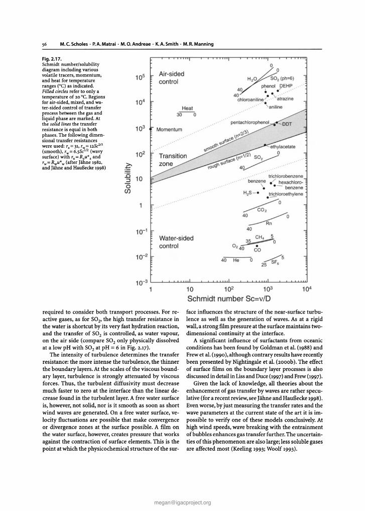
56 M. C.Scholes • P.A.Matrai · M.O.Andreae· K.A.Smith· M.R.Manning

Fig. 2.17.Schmidt number/solubilitydiagram including variousvolatile tracers, momentum,and heat for temperatureranges (OC) as indicated.Filled circlesrefer to only atemperature of 20 °C. Regionsfor air-sided, mixed, and wa­ter-sided control of transferprocess between the gas andliquid phase are marked, Atthe solid lines the transferresistance is equal in bothphases, The following dimen­sional transfer resistanceswere used: Ta =31,Tw=12Sc2/3

(smooth), Tw=6.5SC1l2 (wavysurface) with Ta =Rau' a andTw=Rwu'w(after J1ihne 1982,and Iahne and HauBecke 1998)

105 Air-sidedco ntro l

104

He at3-0- -0

103 Momen tum

102

>-."!::

:c 10:::J(5(j)

Water-sidedcontro l

10-2

oo

S0 2 (ph =6)

phenol DEH P ",~ . .... .... .

40 •• " ,ch loroaniline / , ' " a trazme.. ..•

an iline

- e thylacetate

1l\"'~I'l)SO 0 "l\llc0' 2 , "

~",\l " ,(O\l9 40 ' " '

" ' trich lorobenzene" , " benzene . / he xach loro-

\ . - benzeneH2S - . trichloroe thylene.-~o40 ~O

~40

CH. 5~o

0 2 40 CO40 He 0 ~SF 5

25 e

10 102 103

Schm idt numbe r Sc =v/D

10-3 L..-............J..-jU-l..........._-'--'-'..................._....L..-.......................LLI.._............ l....L-............u.J

1

required to consider both transport processes. For re­active gases, as for S02' the high transfer resistance inthe water is shortcut by its very fast hydration reaction,and the transfer of S02 is controlled, as water vapour,on the air side (compare S02 only physically dissolvedat a low pH with S02 at pH = 6 in Fig. 2.17).

The intensity of turbulence determines the transferresistance: the more intense the turbulence, the thinnerthe boundary layers.At the scales of the viscous bound­ary layer, turbulence is strongly attenuated by viscousforces. Thus, the turbulent diffusivity must decreasemuch faster to zero at the interface than the linear de­crease found in the turbulent layer.A free water surfaceis, however, not solid, nor is it smooth as soon as shortwind waves are generated. On a free water surface, ve­locity fluctuations are possible that make convergenceor divergence zones at the surface possible. A film onthe water surface, however, creates pressure that worksagainst the contraction of surface elements. This is thepoint at which the physicochemical structure of the sur-

face influences the structure of the near-surface turbu­lence as well as the generation of waves. As at a rigidwall,a strong film pressure at the surface maintains two­dimensional continuity at the interface.

A significant influence of surfactants from oceanicconditions has been found by Goldman et al. (1988) andFrewet al.(1990),although contrary results have recentlybeen presented by Nightingale et al. (2000b). The effectof surface films on the boundary layer processes is alsodiscussed in detail in Lissand Duce (1997) and Frew(1997).

Given the lack of knowledge, all theories about theenhancement of gas transfer by waves are rather specu­lative (for a recent review,see Iahne and Hauflecke1998).Evenworse, by just measuring the transfer rates and thewave parameters at the current state of the art it is im­possible to verify one of these models conclusively.Athigh wind speeds, wave breaking with the entrainmentof bubbles enhances gas transfer further.The uncertain­ties of this phenomenon are also large; less soluble gasesare affected most (Keeling 1993; Woolf 1993).

[email protected]

Fig. 2.18. Summary of gas exchange coefficients normalised toa Schmidt number of 600 and plotted versus wind speed (10 mabove sea level), plus two empirical relationships (Iahne andHaussecker 1998)

A collection of field data is shown in Fig. 2.18. Al­though the data show a clear increase of the transfervelocity with wind speed, there is significant scatter inthe data that can only partly be attributed to uncertain­ties and systematic errors in the measurements. The gastransfer velocity is not simply a function of the windspeed . The scatter mainly reflects the additional influ­ence of the wind wave field, which may vary with allparameters that modify the microturbulence in theboundary layer such as the viscoelastic properties of thesurface films present and the wind wave field.

Part of the data shown in Fig. 2.18 is based on geo­chemical tracers such as the 14C, 3He/ T,or 222Rn / 226Ra

methods. The transfer velocities obtained in this wayare only mean values. Thus a parameterisation is onlypossible under steady state conditions over extendedperiods; it is questionable under changing conditions.The changes of the parameters (e.g. wind speed) aresome orders of magnitude faster. Thus mass balancemethods are not suitable for a study of the mechanismsof air-water gas transfer. This is also true for the tracerinjection techniques pioneered by Wanninkhof et a1.(1985,1987) in lakes, and Watson et a1. (1991a) and Night­ingale et a1. (2000a) in oceans. Progress in better un­derstanding the mechanisms of air-water gas exchangehas been hindered by inadequate measuring technol­ogy.Promising new techniques are now available (Jiihneand Hauflecke 1998; McGillis et al. 1999) but there arecurrently too few measurements using them for defi­nite conclusions to be drawn. Thus, empirical gas ex­change-wind speed relationships (see Fig. 2.17) must stillbe applied with caution since they have an uncertaintyof up to a factor of two.

80 .70

---- Wanninkhof relationship

-- Liss-Merlivat relationship

60 'V 14C:

.--. 0 SF s -3He

.!: 50 .- 0 222Rn .E ...o 40 • Heat (CFT) ....... .

0 0 ..0 30 ..CD~

20

5 10 15Wind speed u 10 [m/s]

20

CHAPTER 2 . Biosphere-Atmosphere Interactions 57

2.8.2 Marine Biogenic Emissions: A Few Examples

2.8.2.1 Methane

The ocean is a small source of methane to the atmos­phere. Open Pacific Ocean saturation ratios (ratio ofseawater CH4 partial pressure to the overlying atmo­spheric CH4 partial pressure) range from 0.95 to 1.17.Large areas of the PacificOcean are undersaturated withrespect to atmospheric CH4partial pressures during thefall and winter.On a seasonal time scale,the driving forcecontrolling saturation ratios outside the Tropics appearsto be the change in sea surface temperature. Saturationratios in the equatorial region have always been posi­tive and appear to be driven by the strength of the equa­torial upwelling. Extrapolating the Pacific data globallyand regionally into ten zones, the calculated average fluxof CH4to the atmosphere is 0.4 Tg yr-l (0.2-0.6 Tg yr")(Bates et a1. 1996). This is approximately an order ofmagnitude less than previous estimates, which lackedfall and winter data . Thus the open ocean is a very mi­nor source of methane to the atmosphere «0.1%)com­pared with other sources (IPCC 1996). However, thecoastal ocean and marginal seas appear to be a muchlarger source (Owens et a1. 1991; Kvenvolden et a1. 1993;Bange et a1. 1994; Lammers et a1. 1995; Scranton andMcShane 1991) due to CH4 emissions from bottomsediments; this definitely warrants further investigation .

2.8.2.2 Carbon Monoxide

The ocean is ubiquitously supersaturated with CO withrespect to the atmosphere, resulting in a net flux to theatmosphere ranging seasonally and regionally from 0.25to 13 umol m-2d-1. However, the total annual emissionto the atmosphere (13 Tg; see Table 3.1) is small com­pared to current estimates from both terrestrial natu­ral and anthropogenic sources (1150 Tg yr'") (Bateset a1.1995; WMO 1999). Even in the Southern Hemisphere,which accounts for two-thirds of the oceanic emissions,the ocean source is relatively small «1%), since bothmethane oxidation and biomass burning are largesources of CO (Bates et al. 1995).

2.8.2.3 Volatile Organic Carbon Compounds

Volatileorganic carbon (VOC)compounds, or non-meth­ane hydrocarbons, are produced in surface seawater pos­sibly by photochemical mechanisms, phytoplankton ac­tivity, and/or microbial breakdown of organic matter(Plass-Diilmer et al.1995; Ratte et al.1995; Broadgate et al.1997). Oceanic concentrations show a strong seasonalcycle (Broadgate et a1. 1997). The ocean-atmosphere flux

[email protected]

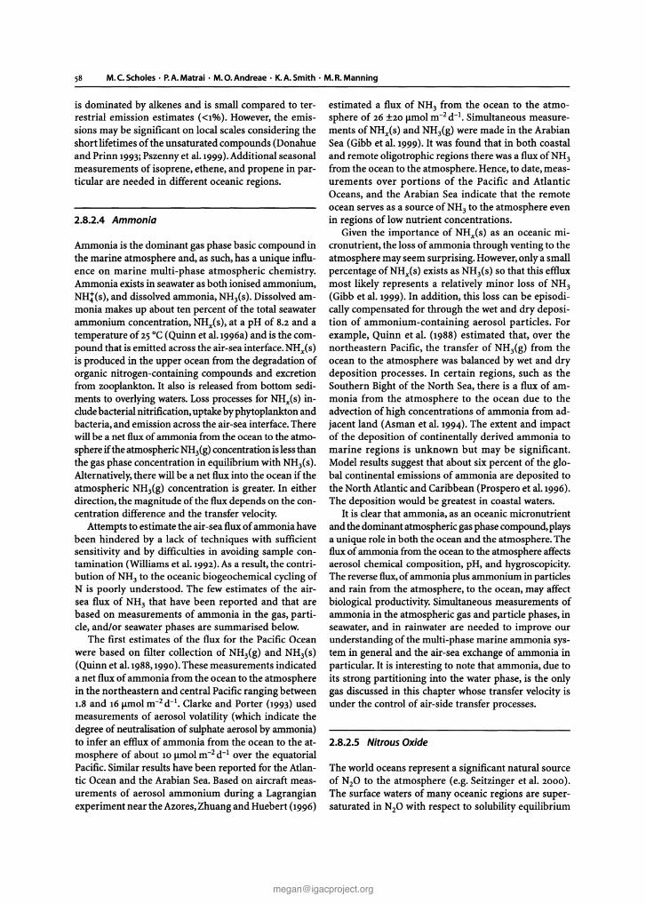
58 M.e.Scholes· P.A.Matrai . M.O.Andreae · K.A.Smith . M.R.Manning

is dominated by alkenes and is small compared to ter­restrial emission estimates «1%). However, the emis­sions may be significant on local scales considering theshort lifetimes of the unsaturated compounds (Donahueand Prinn 1993; Pszenny et al.1999).Additional seasonalmeasurements of isoprene, ethene, and propene in par­ticular are needed in different oceanic regions.

2.8.2.4 Ammonia

Ammonia is the dominant gas phase basic compound inthe marine atmosphere and, as such, has a unique influ­ence on marine multi-phase atmospheric chemistry.Ammonia exists in seawater as both ionised ammonium,NHt(s), and dissolved ammonia, NH3(s). Dissolved am­monia makes up about ten percent of the total seawaterammonium concentration, NHx(s),at a pH of 8.2 and atemperature of 25°C (Quinn et al.1996a)and is the com­pound that is emitted across the air-sea interface. NHx(s)is produced in the upper ocean from the degradation oforganic nitrogen-containing compounds and excretionfrom zooplankton. It also is released from bottom sedi­ments to overlying waters. Loss processes for NHx(s) in­cludebacterial nitrification, uptake byphytoplankton andbacteria, and emission across the air-sea interface.Therewill be a net fluxof ammonia from the ocean to the atmo­sphere ifthe atmospheric NH3(g) concentration is lessthanthe gas phase concentration in equilibrium with NH3(s).Alternatively,there will be a net flux into the ocean if theatmospheric NH3(g) concentration is greater. In eitherdirection, the magnitude of the flux depends on the con­centration difference and the transfer velocity.

Attempts to estimate the air-sea fluxof ammonia havebeen hindered by a lack of techniques with sufficientsensitivity and by difficulties in avoiding sample con­tamination (Williams et al. 1992).As a result, the contri­bution of NH3 to the oceanic biogeochemical cycling ofN is poorly understood. The few estimates of the air­sea flux of NH3 that have been reported and that arebased on measurements of ammonia in the gas, parti­cle, and/or seawater phases are summarised below.

The first estimates of the flux for the Pacific Oceanwere based on filter collection of NH3(g) and NH3(s)(Quinn et al.1988,1990).These measurements indicateda net flux of ammonia from the ocean to the atmospherein the northeastern and central Pacific ranging between1.8 and 16 pmol m-2 d- 1• Clarke and Porter (1993) usedmeasurements of aerosol volatility (which indicate thedegree of neutralisation of sulphate aerosol by ammonia)to infer an efflux of ammonia from the ocean to the at­mosphere of about 10 umol m-2 d- 1 over the equatorialPacific. Similar results have been reported for the Atlan­tic Ocean and the Arabian Sea. Based on aircraft meas­urements of aerosol ammonium during a Lagrangianexperiment near the Azores,Zhuang and Huebert (1996)

estimated a flux of NH3 from the ocean to the atmo ­sphere of 26 ±20 umol m-2 d-1• Simultaneous measure­ments ofNHx(s) and NH3(g) were made in the ArabianSea (Gibb et al. 1999). It was found that in both coastaland remote oligotrophic regions there was a flux of NH3from the ocean to the atmosphere. Hence, to date, meas­urements over portions of the Pacific and AtlanticOceans, and the Arabian Sea indicate that the remoteocean serves as a source ofNH3 to the atmosphere evenin regions of low nutrient concentrations.

Given the importance of NHx(s) as an oceanic mi­cronutrient, the loss of ammonia through venting to theatmosphere may seem surprising. However, only a smallpercentage ofNHx(s) exists as NH3(s) so that this effluxmost likely represents a relatively minor loss of NH3

(Gibb et al. 1999). In addition, this loss can be episodi­cally compensated for through the wet and dry deposi­tion of ammonium-containing aerosol particles. Forexample, Quinn et al. (1988) estimated that, over thenortheastern Pacific, the transfer of NH3(g) from theocean to the atmosphere was balanced by wet and drydeposition processes. In certain regions, such as theSouthern Bight of the North Sea, there is a flux of am­monia from the atmosphere to the ocean due to theadvection of high concentrations of ammonia from ad­jacent land (Asman et al. 1994). The extent and impactof the deposition of continentally derived ammonia tomarine regions is unknown but may be significant.Model results suggest that about six percent of the glo­bal continental emissions of ammonia are deposited tothe North Atlantic and Caribbean (Prospero et al.1996).The deposition would be greatest in coastal waters.

It is clear that ammonia, as an oceanic micronutrientand the dominant atmospheric gasphase compound, playsa unique role in both the ocean and the atmosphere. Thefluxof ammonia from the ocean to the atmosphere affectsaerosol chemical composition, pH, and hygroscopicity.The reverse flux,of ammonia plus ammonium in particlesand rain from the atmosphere, to the ocean, may affectbiological productivity. Simultaneous measurements ofammonia in the atmospheric gas and particle phases, inseawater, and in rainwater are needed to improve ourunderstanding of the multi-phase marine ammonia sys­tem in general and the air-sea exchange of ammonia inparticular. It is interesting to note that ammonia, due toits strong partitioning into the water phase, is the onlygas discussed in this chapter whose transfer velocity isunder the control of air-side transfer processes.

2.8.2.5 Nitrous Oxide

The world oceans represent a significant natural sourceof N20 to the atmosphere (e.g. Seitzinger et al. 2000).The surface waters of many oceanic regions are super­saturated in N20 with respect to solubility equilibrium

[email protected]

with the atmosphere, giving rise to a net air-sea gas ex­change flux of N20 to the atmosphere. Nitrous oxide isproduced in subsurface waters both as an intermediateof denitrification, the reduction of nitrate ion (NO;) tonitrogen (N2) , and as a trace by-product of nitrification,the oxidation of NHt to NO;. Denitrification occursunder suboxic to anoxic conditions, and is thought totake place mainly in restricted low-oxygen regions suchas the eastern tropical Pacific and the Arabian Sea, andin the sediments of continental shelves. The distribu­tion of nitrificat ion is thought to be more widespread,since it occurs under aerobic conditions in associationwith the internal recycling of fixed nitrogen.

During the past decade there have been significantimprovements in our understanding of oceanic proc­esses of N20 production, of the distribution of N20 inthe surface and subsurface ocean, and of the magnitudeof the oceanic N20 source to the global atmosphere.Therelative roles of nitrification and denitrification proc­esses have been addressed by measuring nitrogen sta­ble isotopes and their fractionation between N20 andother dissolved nitrogen-bearing compounds. The in­terpretation of these difficult measurements is compli­cated by the likelihood that both nitrification anddenitrification are coupled in many oceanic systems,andno clear picture has yet emerged. There have also beenrecent advances in the study of air-sea gas exchangeprocesses, as indicated in Sect. 2.8.1, which will lead toimprovements in the quantification of exchange coeffi­cients as a function of wind speed.

Finally, our understanding of the large-scale distri­bution ofN20 in the oceans has been improved througha number of shipboard measurement programs, suchas those associated with the World Ocean CirculationExperiment (WOCE)and Joint Global Ocean FluxStudy(JGOFS) programs. These have generally reinforced ourview that open ocean upwelling regions along easternocean boundaries and in equatorial and coastal regions,represent major sources of atmospheric N20 . By con­trast, the great subtropical gyres, which represent a largeportion of the surface area of the oceans, are relativelyclose to atmospheric equilibrium for N20 . In recentyears, some extremely high N20 concentrations havebeen found in the eastern Arabian Sea, in suboxic wa­ters over the Indian Shelf (Naqvi et al. 2000). Since an­thropogenic impingements on the coastal ocean maycause an increase in hypoxia, suboxia, and anoxia insome areas, these recent observations from the ArabianSea are provocative. By modelling these distributionstogether with the wind field (e.g. Nevison et al. 1995),we have come to believe that the global oceans consti­tute a net source to the atmosphere of about 4-5 Tg ofN20 , or about one third of the global natural sourcestrength. This value may increase as more is learnedabout the diverse distribution of N20 in coastal waters(e.g. Seitzinger and Kroeze 1998).

CHAPTER 2 . Biosphere-Atmosphere Interactions 59

2.8.2.6 Dimethylsulphide

2.8.2 .6.1 Introduction

Dimethylsulphide was discovered in ocean waters some30 years ago by Lovelock et al. (1972). However, it re­mained a compound of marginal scientific interest forabout a decade, until it was established that DMSis themain volatile sulphur compound emanating from theoceans and therefore plays a major role in the atmo ­spheric sulphur cycle (e.g. Nguyen et al. 1978; Leek andRodhe 1991). Interest in the biogeochemical cycle ofDMS increased sharply again in the late 1980s, whenCharlson et al. (1987) proposed a hypothesis linking bio­genic DMS emission and global climate. In short, thishypothesis states that DMS released by marine phyto­plankton enters the troposphere and is oxidised thereto sulphate particles, which then act as cloud condensa­tion nuclei (CCN) for marine clouds (see Box 4.3,how­ever,regarding the utility of the CCNconcept) . Changesin CCN concentration affect the cloud droplet numberconcentration, which influences cloud albedo and con­sequently climate. Large-scale climate change, in turn,affects the phytoplankton number and speciation in theoceans and thereby completes, but does not necessarilyclose, a feedback loop. Recent assessments of the DMS­climate link can be found in Watson and Liss (1998) andBigg and Leek (2001) (also see Chap. 4).

In the years since publication of the DMS-CCN-cli­mate hypothesis, almost 1000 papers have been pub­lished discussing the distribution and biogeochemistryof DMS(and its precursors) and its link to climate. Sev­eral IGAC-inspired studies have addressed aspects ofthe DMS-aerosol-climate connection, most prominentlyamong them ASTEXIMAGE (e.g. Huebert et al. 1996),ACE-l (e.g, Bates et al. 1998),and AOE-91, 96 (e.g, Leeket al. 1996,2001). As a result of these projects, and thelarge number of independently conducted studies re­lated to the DMS-climatehypothesis,we now understandmany of the details of DMS production in the oceans,its transfer to the atmosphere, and the atmospheric oxi­dation processes (see Chap. 3) that lead to the forma­tion of aerosols (see Chap. 4) that can act as CCN. How­ever, in spite of this progress , fundamental gaps remainin our understanding of key issues in this biosphere­climate interaction, in particular with regard to the proc­esses that regulate the concentration of DMSin seawater.While the basic processes have been identified, and evenquantified in specific locations (e.g, Bates et al. 1994;Simo and Pedro-Alio 1999),generally applicable mod­els of DMS-plankton relationships are still in their in­fancy (e.g. Gabric et al.1993; Jodwaliset al.2000).There­fore, we are still not able to represent the DMS-CCN­climate hypothesis in the form of a process-based, quan­titative, and predictive model. Even the overall sign ofthe feedback cannot be deduced with certainty, since it

[email protected]

60 M.C.Scholes . P.A.Matrai · M.O.Andreae· K.A.smith · M.R.Manning

is not known yet if a warming climate would result inan increase or decrease of DMS emissions . Glacial-to­interglacial changes in the amounts of DMS oxidationproducts in polar ice cores cannot answer this questionunambiguously, as they may reflect variations in atmo ­spheric transport patterns as much as differences inDMSproduction (e.g, Whung et aI.1994),as is discussedin detail in Sect. 2.3.

Early,limited data sets had suggested a possible cor­relation between DMS and phytoplankton concentra­tion (e.g. Andreae and Barnard 1984).This correlationis particularly evident in vertical profiles of DMS andchlorophyll a, which in most instances show a sharpdrop of both parameters around the depth correspond­ing to a light penetration of one percent of the surfacelight flux. Close correlations between DMS and phyto­plankton densities were also found in situations wherea single species accounted for much of the DMS pro­duction or phytoplankton biomass (e.g. Barnard et al.1984; Matrai and Keller 1994).These findings led to thehope that global DMS distributions could be estimatedfrom chlorophyll concentrations obtained by remotesensing, but experimental investigations of this proposalwere not encouraging (e.g. Matrai et al. 1993),except infrontal regions (e.g. Holligan et al. 1993; Belviso et al.2000) . Furthermore, a statistical analysis of almost16000 measurements of DMSin surface seawater failedto show any useful correlations between DMSand chlo­rophyll or other chemical or physical parameters (Ket­tle et al. 1999).One reason for the absence of a generalcorrelation between plankton biomass and DMSis thatthe intracellular concentration of its metabolic precur­sor, dimethylsulphoniopropionate (DMSP), varies be­tween different phytoplankton species over a range offiveorders of magnitude.While it is clear that some taxo­nomic groups typically contain higher amounts ofDMSP, these relationships are by no means clear-cut(e.g. Keller et al. 1989). At least as important, however,are the complexities of DMS cycling by biological andabiotic processes in the surface ocean , which will beaddressed below.

2.8.2.6.2 Physiological and Ecological Controlsof DMS Production

The pathways of DMSP biosynthesis in phytoplanktonhave been studied and have shed light on potential regu­lating mechanisms such as nitrogen nutrition (e.g,Groneand Kirst1992; Kelleret al.1999a,b),temperature (Baumannet al.1994), and light (Vetter and Sharp 1993; Matrai et al.1995). While DMSP, and sometimes DMS,is directly re­leased by phytoplankton, zooplankton also playa roleby grazing, or avoiding, DMSP-rich cells (e.g. Dacey andWakeham 1986; Wolfeet al.1997;Tang 2000).

Very high concentrations of DMS and dissolvedDMSP have been reported from several coastal and/or

high latitude areas, especially where blooms of DMSP­producing phytoplankton such as the coccolithophoreEmiliania huxleyi and the prymnesiophyte Phaeocyst ispouchetii occur (e .g, Malin et al. 1993; Barnard et al.1984).In this context, it is interesting to note that Kettleet al.s (1999) DMSdatabase revealed that high DMS re­gions corresponded roughly to the coccolithophoridbloom areas derived by Brown and Yoder (1994) fromremotely sensed ocean colour data . Prymnesiophytes(including coccolithophores) and dinoflagellates arephytoplankton groups that tend to have high DMSPcellquotas (Keller et al. 1989)and, not surprisingly, DMS isoften relatively high when these groups dominate thephytoplankton assemblage. Diatoms, on the other hand,tend to have low intracellular DMSPconcentrations andit is generally observed that diatoms are less importantDMSPproducers in the field (e.g. Keller et al.1989). Pre­dicting DMS concentrations from the algal assemblageis not straightforward, however.For example, Matrai andVernet (1997) reported that DMS concentrations wereas high in diatom -dominated, Arctic waters as they werein those dominated by Phaeocystis sp. It is now recog­nised that some phytoplankton species not only pro­duce high intracellular concentrations ofDMSP,but theyalso have cell-surface (Stefelsand Dijkhuizen 1996)andintracellular (Steinke et al. 1996) DMSP lyase enzymesthat may be involved actively in DMS production,thereby contributing further to the elevated DMS con­centrations associated with these organisms. The eco­logical roles of these lyase enzymes are not well under­stood but several recent studies have pointed to veryinteresting functions such as in grazing deterrence, car­bon acquisition, and bacterial inhibition (Noordkampet al. 1998;Wolfeand Steinke 1996; Wolfeet al. 1997).

Blooms of marine phytoplankton provide convenientnatural "laboratories" for investigating the productionof DMS in relation to phytoplankton community dy­namics and species succession and associated processes,including grazing and bacterial turnover. However, thisapparent focus on "hotspots" ofDMS production in rela­tively nutrient rich areas can be criticised in thatoligotrophic areas of the oceans, which generally haverelatively low levels of DMS and DMSP throughout theyear, make up a large fraction of the total ocean areaand so must contribute significantly to the total globalflux of DMS (Bates et al. 1992). These pioneering stud­ies established the link between phytoplankton and DMSlevels, but failed to account for a large part of the natu­ral variability in DMSconcentrations. There have beenrather few actual DMS time-series studies (Leek et al.1990; Turner et al.1996a; Dacey et aI.1998), all of whichnoted seasonal periods of elevated DMSconcentrations.

We now realise that bacterial processes are also veryimportant in the overall DMScycle.More isolates ofbac­teria are availablewith which to study biochemical path­ways and physiology of DMSP and DMS metabolism

[email protected]

(e.g, Ledyardand Dacey1994;Yochet al.1997). Newmeth­ods, including use of 35S tracers, improved inhibitors, andmolecular genetics techniques have allowed ever moresensitive analyses ofDMSP-DMS cycling rates and fates,and have permitted more detailed examination of thecomplex microbial communities involved (e.g. Gonzalezet al.1999; Wolfeand Kiene 1993).The potential for DMSproduction from dissolved DMSPis quite large (e.g.Kiene1996b;van Duyl et al. 1998),but recent studies indicatethat most of the DMSPin the sea is not converted to DMS.A demethylation-demethiolation pathway leading toproduction of methanethiol (MeSH) can account for70-95% of DMSP metabolism in situ thereby divertingsulphur away from DMS (Kiene 1996a). The predomi­nance of this non-DMS producing demethylation­demethiolation pathway is explained by the fact thatbacteria use it to assimilate the sulphur from DMSPintoprotein amino acids (Kiene et al. 1999). Further under­standing of this DMSP-DMS-MeSH-bacteria interactionis critical because a relatively small change in the yieldof DMS from DMSP could have a major impact on thegross production of DMS, which would then be avail­able for sea-air exchange.

Removal of DMS from the water column by biologi­cal and photochemical mechanisms also exerts a greatinfluence on the net accumulations of DMS in surfacewaters. Slow biological degradation of DMS may par­tially explain the rise in DMS concentrations observedat the peak and initial decline phases of phytoplanktonblooms (e.g, Matrai and Keller 1993; Nguyen et aI.1988).Net consumption of DMS appears to occur in the laterstages of blooms after DMS-consuming bacteria havehad time to develop (Kwint et al. 1996; van Duyl et al.1998). The photochemistry of DMS in seawater remainspoorly understood, despite the fact that it has been iden­tified as a major removal mechanism under some cir­cumstances (e.g. Kieber et al. 1996; Sakka et al. 1997;Brugger et al. 1998). DMS photooxidation appears todepend on photosensitisers in seawater, which are mostlikely part of the coloured dissolved organic matter(CDOM) (Dacey et al. 1998). In the open ocean CDOMoriginates from autochthonous primary productivityand food web processes so the interaction with DMS isprobably complex. Add to this the fact that DMS pro­ducing and consuming bacterial populations are likelyto be strongly influenced by UV-Bin surface waters, andone can easily see the importance of understandingphotophysical effects on the DMS cycle. Recently, it hasbeen shown that viruses are significant agents in the con­trol of bacteria and phytoplankton. Viral infections cancause a total release of intracellular DMSP (Hill et al.1998)and viruses are known to infect DMSP-containingbloom organisms such as Emiliania huxleyi (Brussaardet al.1996)and Phaeocystis sp, (Malin et al.1998).It seemsclear from studies such as these that the overall food webdynamics, including macro- and microzooplankton graz-

CHAPTER 2 • Biosphere-Atmosphere Interactions 61

ing, bacterial, and viral activities, as well as the physico­chemical dynamics of the upper ocean (e.g, incomingsolar radiation, mixing, temperature, air-sea exchange)are important factors governing DMS accumulation.

Modelling efforts have expanded our understandingof DMSproduction,both for field situations (e.g. Gabricet al.1999) and laboratory systems (Laroche et al.1999).However, our current knowledge base is not sufficientto develop and constrain predictive DMS productionmodels for diverse biogeographic regions, in order toallow interpretation of the role ofDMS in climate change,for example. Future research will need to focus on(1) gain ing a full understanding of the processes thatcontrol DMSproduction and allowthe prediction ofDMSemissions, and (2) obtaining much more data concern­ing spatial, temporal, and interannual variation in theconcentration of DMS and related compounds. Empha­sis on undersampled areas and seasons would be valu­able. For process studies, there is an increasing need tocross disciplinary and international boundaries to bringtogether experts on different aspects of DMSand relatedcompounds for integrated field campaigns. For analysisof variability, "remote" sampling systems could be con­sidered (such as attempted in ACE-I). It might be possibleto develop a buoy-mounted monitoring system wherebysamples were stored on a carousel for later analysis.Alter­natively,we might followthe example of the pCOz meas­uring community, who have demonstrated that it is fea­sible to employ unmanned instruments on merchantships (Cooper et al. 1998a). This would enable the col­lection oflarge data sets during long passage routes, cov­ering diverse biogeographic areas, and different seasons,and the chance to investigate interannual variability atrelatively low cost. New techniques will be needed to cir­cumvent the present lack of a reliable storage methodfor DMS samples. In the first instance , it might be morerealistic to concentrate on DMSP analyses.

2.8.2.7 Carbonyl Sulphide

The oceans represent approximately 30% of the totalatmospheric source of COS, and much of the oceano­graphic work on COSover the last decade has focussedon assessing the spatial and temporal distributions ofCOS concentration and understanding the processesthat control its temporal and spatial distribution. Thephotochemical source of COS was first recognised byFerek and Andreae (1984), who demonstrated a cleardiurnal cycle in the sea surface concentration of thecompound.A mechanism of formation of COSwas pro­posed by Pos et al. (1998)who suggested that the photo­chemical production of COSand carbon monoxide pro­ceeds along a coupled pathway which first involves thephotochemical formation of an acyl radical from col­oured dissolved organic matter (CDOM). Plock et al.

[email protected]

62 M.e.Scholes · P.A.Matrai · M.O.Andreae· K.A.Smith· M.R.Manning

(1997)and Ulshofer et a1. (1996) suggested that cysteineis probably implicated in the reaction mechanism ofCOS formation as the result of its reactivity and abun­dance in the oceans. The photochemical COS produc­tion in natural seawater is probably not limited by theconcentration of a precursor sulphur compound butrather by the concentration of CDOM represented byits ultraviolet attenuation coefficient (Ulshofer et a1.1996;Uher and Andreae 1997).Zepp and Andreae (1994)and Weiss et aI. (1995) quantified the wavelength de­pendence of COS photoproduction from CDOM andfound that quantum efficiency of photoproduction de­creases monotonically with increasing wavelength. Thedark (or non-photochemical) production of COS hasbeen proposed on the basis of the non-zero COS con­centration observed at ocean depths where there is nophotochemical production and where there is no mix­ing from the surface (Radford-Knoery and Cutter 1994;Flock and Andreae 1996) and also on the basis of care­ful interpretation of sea surface COS concentrationmeasurements using inverse models (Ulshofer 1995).COShydrolysis varies as a function of temperature andpH and has been evaluated several times over the lastdecade (Elliott et al. 1989; Radford-Knoery and Cutter1994; Uher and Andreae 1997).

Recent models have used laboratory results for thephotoproduction and hydrolysis rate constants to ex­plain COS sea surface measurements obtained duringexpeditions made in the 1980s and 1990S (see Ulshofer(1995)for a review of recent sea surface COS concentra­tion measurements). Andreae and Ferek (1992) devel­oped the first chemical box model to explain the diur­nal variation of COS in terms of photochemical forma­tion and hydrolysis destruction. Ulshofer (1995)adoptedan optimisation scheme based on the coupled photo­chemical-mixed layer used by Kettle (1994) to calculatethe photoproduction and dark production constants forCOS from a series of sea surface measurements madebetween 1992and 1994 in the North Atlantic Ocean. vonHobe (1999) extended this work for other models andexpedition measurements. Najjar et a1. (1995) general­ised a simplified coupled physical-chemical model on aglobal scale to investigate the sensitivity of COSsea sur­face concentration on ozone reduction and troposphericincreases of carbon dioxide. Kettle and Andreae (1998)and Preiswerk and Najjar (1998) have used existingmeasurements of the CDOM absorption coefficient ofseawater to predict a seasonal variation in the absoluteCOS concentration, with maximum values at high lati­tudes in the summer of either hemisphere.

Future work on COS should aim to quantify moreaccurately the role of the oceans as a source or sink ofthe gas to the atmosphere. The global application of thephotochemical production model for COS is currentlylimited by the absence of an algorithm to predict theglobal CDOM absorption coefficient and by the sugges-

tion that the apparent quantum yield of COS formationmay vary by more than an order of magnitude in differ­ent regions of the ocean . The scarcity of profile meas­urements of COS concentration has been problematicfor modelling efforts which have so far been developedto explain only the surface COS concentration distribu­tions. Finally, the precise quantification of the sea-airflux of all gases produced in the upper ocean (includingCOS) is currently limited by the absence of an effectivegas exchange parameterisation based on wind speed,average wave slope, or other measure of upper oceanturbulence, as already indicated.

2.8.2.8 The Ocean's Role as Source and Sink ofAtmospheric Methyl Bromide andother Methyl Halides

Methyl halides are produced and consumed biologically(CH3Br) (Moore and Webb1996;Baker et al.1999);(CH3I)(Moore and Groszko 1999); photochemically (CH3I)(Happell and Wallace 1996);and in surface ocean waters(CH3CI) (Moore et al, 1996). Recent measurements haveshown that the fluxof CH3CI is significantly less than earlyestimates (Moore et al. 1996) and that the open ocean isa net sink, rather than a source, for CH3Br (see below).

Methyl bromide (CH3Br) in the environment beganto receive considerable attention in the early1990Swhenit was being evaluated as an ozone-depleting gas, alongwith chlorofluorocarbons, chlorocarbons, and halons.First-order calculations indicated that methyl bromidewas likely to be a significant contributor to stratosphericozone depletion. Before then, only a fewstudies of CH3Br

in the ocean and atmosphere had been conducted.Lovelock (1975) detected CH3Br in coastal waters ofEngland and suggested that this gas could have a largenatural source. Singh et al, (1983) later reported wide­spread supersaturations greater than 200% off the westcoast of North America, lending support to the oceanas a large natural source of CH3Br. Khalil et a1. (1993)suggested that the open ocean was supersaturated inmethyl bromide by 40-80%. However, prompted in partby calculations showing that the ocean simultaneouslyhad to be a large sink for CH3Br because of reactionwith CI- in seawater (Elliott and Rowland 1995; Jeffersand Wolfe 1996; King and Saltzman 1997), numerousinvestigations, using in situ mass spectrometry-gaschromatography, demonstrated that the ocean on aver­age was a net sink for atmospheric CH3Br, with tropicaland subtropical waters of the open ocean highlyundersaturated and coastal waters often supersaturatedin this gas (Lobert et al.1995,1996,1997; Moore and Webb1996; Groszko and Moore 1998). Certain species ofphytoplankton produce CH3Br, but apparently not atrates sufficient to explain the observed saturation lev­els (Saemundsdottir and Matrai 1998; Moore et a1. 1995;

[email protected]

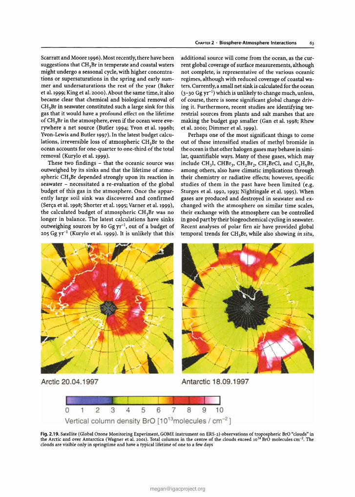
Scarratt and Moore 1996).Most recently, there have beensuggestions that CH3Br in temperate and coastal watersmight undergo a seasonal cycle, with higher concentra­tions or supersaturations in the spring and early sum­mer and undersaturations the rest of the year (Bakeret al. 1999;King et al. 2000) .About the same time , it alsobecame clear that chemical and biological removal ofCH3Br in seawater constituted such a large sink for thisgas that it would have a profound effect on the lifetimeof CH3Br in the atmosphere, even if the ocean were eve­rywhere a net source (Butler 1994; Yvon et al. 1996b;Yvon-Lewis and Butler 1997).In the latest budget calcu­lations, irreversible loss of atmospheric CH3Br to theocean accounts for one-quarter to one-third of the totalremoval (Kurylo et al. 1999).

These two findings - that the oceanic source wasoutweighed by its sinks and that the lifetime of atmo­spheric CH3Br depended strongly upon its reaction inseawater - necessitated a re-evaluation of the globalbudget of this gas in the atmosphere. Once the appar­ently large soil sink was discovered and confirmed(Serca et al. 1998;Shorter et al. 1995; Varner et al. 1999),the calculated budget of atmospheric CH3Br was nolonger in balance. The latest calculat ions have sinksoutweighing sources by 80 Gg yr-1, out of a budget of205 Gg yr-1 (Kurylo et al. 1999). It is unlikely that this

Arctic 20 .04. 1997

CHAPTER 2 . Biosphere-Atmosphere Interactions 63

additional source will come from the ocean, as the cur­rent global coverage of surface measurements, althoughnot complete, is representative of the various oceanicregimes , although with reduced coverage of coastal wa­ters. Currently, a small net sink is calculated for the ocean(3-30 Gg yr-1) which is unlikely to change much , unless,of course , there is some significant global change driv­ing it. Furthermore, recent studies are identifying ter­restrial sources from plants and salt marshes that aremaking the budget gap smaller (Gan et al. 1998; Rhewet al. 2000; Dimmer et al. 1999).

Perhaps one of the most significant things to comeout of these intensified studies of methyl bromide inthe ocean is that other halogen gases may behave in simi­lar, quantifiable ways. Many of these gases, which mayinclude CH3I, CHBr3, CH2Br2, CH2BrCI, and C2HsBr,among others, also have climatic implications throughtheir chemistry or radiative effects; however, specificstudies of them in the past have been lim ited (e.g,Sturges et al. 1992, 1993; Nightingale et al. 1995). Whengases are produced and destroyed in seawater and ex­changed with the atmosphere on similar time scales,their exchange with the atmosphere can be controlledin good part by their biogeochemical cycling in seawater.Recent analyses of polar firn air have prov ided globaltemporal trends for CH3Br, while also showing in situ,

Antarct ic 18 .09 .1997

o 1 2 3 4 5 6 7 8 9 10

Vertical column dens ity BrO [1013molecules / cm -2]

Fig. 2.19 . Satellite (Global Ozone Monitor ing Experiment, GaME instrument on ERS-2) observations of trop ospheric Bra "clouds" inthe Arctic and over Antarctica (Wagner et aI. 2001) . Total column s in the centre of the clouds exceed 10 14 Bra molecules cm-2• Theclouds are visible only in spr ingt ime and have a typical lifetime of one to a few days

[email protected]

64 M.e.Scholes· P.A.Matrai · M.O.Andreae· K.A.Smith · M.R.Manning

seasonal production for other organohalogens (Butleret al. 1999;Sturges et al. 2001).

Large amounts of reactive bromine (and smalleramounts of chlorine) are also found in polar regions andnear salt pans likely due to oxidation of halides by inor­ganic reactions (see also Table3.4). However, the sourceof iodine compounds in the coastal marine air and ofbromine in the free troposphere is much more likely tobe the photochemical degradation of organohalogencompounds (like CH2I 2, or CH3Br, respectively) of ma­rine biogenic origin, as indicated above.

In field campaigns of the IGAC'sPolar Air and SnowChemistry (PASC) activity, it was discovered in the late1980sand early 1990S (Barrie et al. 1988, 1992; Barrie andPlatt 1997) that surface ozone depletion chemistry oc­curring in spring over the Arctic Ocean is a troposphericanalogue of stratospheric ozone chemistry, with a dif­ference. It is driven by sea salt halogens from heteroge­neous reactions occurring in sunlight on surface snowand ice,rather than by halogens from photolysis of spraycan propellants. The existence of BrO and ClO as well asCl and Br reactions with hydrocarbons was well docu­mented in numerous measurements in air just above thesurface of frozen marine areas. In spring, BrOwas foundin the Arctic (Hausmann and Platt 1994; Tuckermannet al.1997) and Antarctic marine boundary layer (Kreheret al. 1997) by ground based and satellite observations(Fig.2.19) (Wagnerand Platt1998;Richteret al.1998; Hegelset al.1998;Wagner et al.2001).In addition, measurementsmade by chemical amplification (Perner et al. 1999),DOAS (Tuckermann et al. 1997), and by the "hydrocarbonclock" technique (Jobson et al. 1994,Solberg et al. 1996;Ramacher et al.1999) suggest ClOlevelsin the pmol mol"!range in the Arctic marine boundary layer.An unexpectedlink to the mercury cycle was discovered to result in en­hanced inputs of mercury to the biosphere in these regions,when long lived elemental mercury is converted to shorterlived particulate and reactive gaseous forms of mercury(Schroeder et al.1998).Halogen reactions are suspected tobe the cause of this conversion of mercury.

As a result of these polar discoveries as well as mod­elling studies (e.g. Vogt et al. 1996;Sander and Crutzen1996) (see also Chap. 3), researchers have begun to seekand confirm the occurrence of reactive halogen com­pounds (10 , BrO,ClO) from air-surface exchange proc­esses in other regions (e.g. remote mid- and lowlatitudemarine sites, midlatitudes coastal sites, Dead Sea basin,and the free troposphere).

2.8.2.9 Primary Marine Aerosols

Primary aerosols are also emitted directlyfrom tiIeoceans.The work of Blanchard and colleagues (Blanchard 1983)has shown that bubble bursting at the air-water inter­face injects aerosols into the atmosphere from two

sources . One is from fragments of the bubble film (filmdrops), the other from a jet of water that follows thebubble burst. Bubbles selectively scavenge high molecu­lar weight surface-active compounds (Gershey 1983) andviable particulate material from the water such as bac­teria and viruses (Blanchard 1983), leading to a consid ­erable enrichment of these organic components in theaerosol relative to the water. As a result, primary parti­cles in the marine environment will usually contain awide range of biogenic compounds. Long-chain fattyacids, alcohols, esters, and soluble proteins have all beenfound in marine aerosols . Proteinaceous material andfree amino acids are present in marine rain (Mopperand Zika 1987).In the atmosphere some of these com­pounds are degraded to form secondary aerosols, suchas the fatty acids which may break down to short chainforms such as oxalic acid. Others, like the amino acid L­methionine, are oxidised. Bacteria and remains of or­ganisms have been observed to become separated fromthe other aerosol components in Arctic conditions (Biggand Leck 2001). Estimates of the organic componentsof marine aerosols in relatively unpolluted environ­ments vary widely, the order of magnitude being around10-20% by number, but this may include secondaryaerosols as well as those transported from continents(Mathias-Maser 1998) (see Chap. 4).

2.8.3 Biological and Chemical Impactsof Atmospheric Deposition on Marineand Estuarine Systems

2.8.3.1 Atmospheric Iron Input to the Oceanand its Role in Marine Biogeochemistry

2.8.3.1.1 Introduction

It is now recognised that a primary transport path foriron found in the ocean is through the atmosphere.Among the first papers to address the importance ofatmospherically derived iron were those of Moore et al.(1984) and Duce (1986). These authors calculated theaeolian transport of mineral matter into many areas ofthe ocean, and pointed out that some fraction of the ironfrom the mineral matter dissolved into seawater afterthe dust was deposited to the ocean surface. Duce andTindale (1991) and, more recently, Iickells and Spokes(2001) have reviewed this topic.

The major reason why atmospheric dust transporthas received considerable research effort over the lastdecade is because of the role iron has been hypothesisedto play in controlling marine primary productivity overlarge areas of the oceans remote from land. Because ofthe ir distance from riverine and shelf inputs in theseregions (e.g, Southern Oceans, North and EquatorialPacific) one of the primary ways in which "new" iron

[email protected]

CHAPTER 2 • Biosphere-Atmosphere Interactions 65

gets into the system is via deposition from the atmo­sphere of terrestrially derived material. The idea of ironbeing a major control on ocean production is not new.In the early decades of the 20th century it was hypoth­esised that the reason why large areas of the SouthernOceans contained significant amounts of residual con­ventional plant nutrients (nitrate and phosphate), whenlight and other conditions for plant growth were favour­able (the HNLC,high nutrient-low chlorophyll, regions),was because of iron deficiency in the water (see, for ex­ample, Gran 1931; Harvey 1933;Hart 1934; and the recentreview by DeBaar and Boyd 2000). However, it is onlyin the last decade that analytical techniques for iron andfield-going experimental approaches have been goodenough to begin to test the hypothesis critically.

2.8.3.1.2 Sourcesand Transport of Mineral Aerosolto the Oceans

The primary sources of mineral aerosol are arid andsemi-arid continental regions (e.g. Tegenand Fung 1994;Duce 1995; IPCC 1996) (see also Chap. 4). The atmo­spheric concentrations of dust and the deposition of dustto the ocean surface are both very episodic and are pri­marily associated with the transport of aerosol fromdust storms or major dust outbreaks. The typical dura­tion of such dust pulses over the ocean may range fromone to four days, and the transport and deposition mayalso vary seasonally. Due to the episodic character ofboth the atmospheric dust concentrations and localrainfall, the primary removal process for dust (Duce1995) input to the ocean in a particular region can oftenoccur during a few events covering a relatively shortperiod of time. For example, the results of one multi­year study showed that half of the annual deposition ofdust to the ocean at Midway Island in the central Pacificoccurred during only two weeks (Prospero et al. 1989).In Bermuda, Arimoto et al. (1992) found that mineralaerosol concentrations ranged over four orders of mag­nitude, from 0.001 to 11 flgm-3•

We have very few data sets of marine surface dustconcentrations collected over long periods of time. Ingeneral, the highest atmospheric concentrations of dustin marine areas are found over the North Pacific andthe tropical Atlantic. Other high concentration areas arefound in the Arabian Sea and the northern Indian Ocean,but there are very limited data in these regions. Accu­rate estimation or calculation of dust deposition is stillquite difficult. An estimate of the geographical distri­bution of the flux of mineral matter to the global oceanis presented in Fig. 2.20 (Duce et al. 1991). Note that byfar the major fraction of mineral dust is deposited inthe Northern Hemisphere. The atmospheric depositionhas clearly fluctuated significantly in the past, as seenin ice core and deep sea sediment samples (see, for ex­ample, Rea1994; Andersen et al. 1998; Maher and Houns­low 1999). Numerical simulations of the mineral dustcycle are attempting to improve global data sets by link­ing soil types, particle emissions, gas-particle heteroge­neous chemistry, and wind transport in the tropospherewith aerosol satellite measurements (e.g. Marticorenaand Bergametti 1995; Phadnis and Carmichael 2000)(also see Chap. 6).

2.8.3.1.3 Iron in Mineral Aerosol over the Oceans

The atmospheric deposition of iron is associated withthe eroded mineral aerosol particles, and the iron isprimarily bound in their aluminosilicate matrices. It isthus possible to convert mineral aerosol concentrationsor fluxes to an iron concentration or flux by knowingthe abundance of iron in the earth's crust. This rangesfrom -3 to 5% (Taylor and McClennan 1985). Typicallya value of 3.5% is used. With a mineral aerosol fluxof 500-2000 Tg yr", the input of iron would be ca.15-100 Tg yr- 1. However,before the iron deposited fromthe atmosphere can be utilised by phytoplankton, it mustbe in a form that is available to these organisms. Proc­esses that change the solubility or lability of the iron inthe atmosphere will then have potential for influencing

0°60 0W120 0W180 0 E120 0E

30 0S

60 0 N

30 0N

Fig. 2.20.Calculated global fluxes ofatmospheric mineral matterto the ocean (Duce et al. 1991)

600S 1-------.......----_

[email protected]

66 M. C. Scholes . P.A.Matrai· M.O.Andreae· K.A.Smith· M.R.Manning

the availability of the iron when the atmospheric mate­rial enters the ocean. Iickells and Spokes (2001) havecarefully reviewed the information to date on the mecha­nisms that may control the distribution of dissolved and/or particulate iron in the material entering the oceanfrom the atmosphere.Some studies have observed Fe(II)in aerosol iron and its formation is postulated to occurvia photochemical reduction of Fe(III) hydroxides. Cer­tain organic compounds such as oxalate, acetate, andformate can facilitate this photoreduction. It has beensuggested by several authors that the low pH (0-5) char­acteristic of the cloud cycling process produces acidic,hygroscopic aerosols.This combined with possible pho­tochemical reactions results in an increase in the labilityof crustally derived metals, such as iron, in the atmo­sphere over that seen in the parent material. In turn, thiswill playa role in the availability of the iron when theaerosol enters the ocean (e.g. Jickells and Spokes 2001;Zhu et al.1992). In addition, high ionic strength solutionsand alternating wet and dry cycles during cloud forma­tion and evaporation would be common. There are likelyto be many such cycles before the particles ultimatelyenter the ocean by dry deposition or precipitation.

Iickells and Spokes (2001, and references therein)state, in summary, that it is likely that the overall ironsolubility of dry deposited mineral aerosol is <1% at aseawater pH of 8, and that a significant proportion ofthis iron is photoreduced to Fe(II),which is bioavailable.The solubility of iron in marine rains with a pH of 4-7is generally 14%. Thus the input of soluble atmosphericiron to the oceans is apparently dominated by wet depo­sition. These estimates , based on laboratory studies , aresomewhat lower than those made earlier by other au­thors . However, Iickells and Spokes (2001) made otheroceanographic approaches to estimate the solubility ofatmospheric iron. All of these approaches result in lowoverall iron solubility,probably less than 2%. Their finalconclusion is that approximately 0.8 to 2.1% of the totaliron deposited in the ocean is soluble. With a total inputof 15 to 100Tg yr-1, this would result in a total solubleiron atmospheric input of from 0.12 to 2.1 Tg yr- 1•

2.8.3.1.4 Iron and Marine Biogeochemistry

Once the atmospheric iron has entered the oceans byeither wet or dry deposition, it is hypothesised to playpotentially important roles in the primary productivityof surface waters in substantial areas remote from land.These HNLC regions are estimated to cover -20-25%of the area of the oceans. An up-to-date and detailedassessment of the chemical form of iron in seawater andhow this relates to its uptake by marine organisms is tobe found in several chapters in the book edited byTurnerand Hunter (2001).

John Martin and his colleagues made some of the firstreliable measurements of iron in the oceans and con-

ducted shipboard incubation studies in flasks and car­boys of HNLC seawater that had been amended withsoluble iron (Martin et al.1994).The results were prom­ising (e.g. Martin and Fitzwater1988) and clearlyshowedthat addition of iron (normally added as ferrous sul­phate or other simple inorganic salts) could lead to sub­stantial increases in plankton growth, as indicated byincreasing chlorophyll concentrations with time in theexperimental flasks. An interesting variant on this ba­sic experiment, which is particularly relevant in thepresent context, was a study conducted in the equato­rial Pacific by Johnson et al. (1994). They added the ironin a variety of inorganic and organically complexedforms, but they also used natural Asian dust aerosolparticles (collected in Hawaii) and added them to oneof the carboys of seawater. In this carboy the rate ofplankton growth was found to be the most rapid andattained the highest chlorophyll levels, indicating thatthe aerosol particles were more effective at promotinggrowth than artificial iron supplements.

Other avenues have been explored to attack the prob­lem in a more direct way. Younget al. (1991) monitorednatural dust inputs to the North Pacific and examinedany resulting change in productivity in the receivingwater. Several dust deposition events appeared to becorrelated with increases in primary productivity meas­ured in on-deck incubators, but with a four day lag be­tween the dust input and the peak in productivity. Al­though suggestive of a relationship, the results were toofew and insufficiently clear-cut to be totally convincing.In addition, interpretation was complicated becauseproductivity change was measured in a deck incubator,not in the ocean itself. Also, when deposition occurred,meteorological conditions changed, with greater stirringof near-surface water,which itself may have changed theproductivity. However, this experiment represents anovel and potentially powerful tool since it uses thenatural atmospheric input and examines the responseof the real oceanic system.

A different approach to testing the iron hypothesis isthat of adding inorganic iron (FeSO4) directly to a smallpatch (of the order of 100 krn-) of the oceans. In orderto be able to track the iron enriched patch as it movesin the ocean, the gas sulphur hexafluoride is added alongwith the iron. Sulphur hexafluoride can be easily meas­ured at tracer (femtomolar) concentrations in almostreal time from the research vessel,enabling the enrichedpatch to be tracked . The principles underlying this ap­proach are outlined in Watson et al. (1991a). It has beenutilised three times to date; twice in the equatorial Pa­cific (IronEx I: Martin et al. (1994) and IronEx II: Coaleet al. (1996» and very recently in the southern oceans(SOIREE:Boydet al. (2000». On all three occasions,rais­ing the iron level in the water by a few nanomoles perlitre produced a significant enhancement in phyto­plankton activity, as measured by chlorophyll concen-

[email protected]

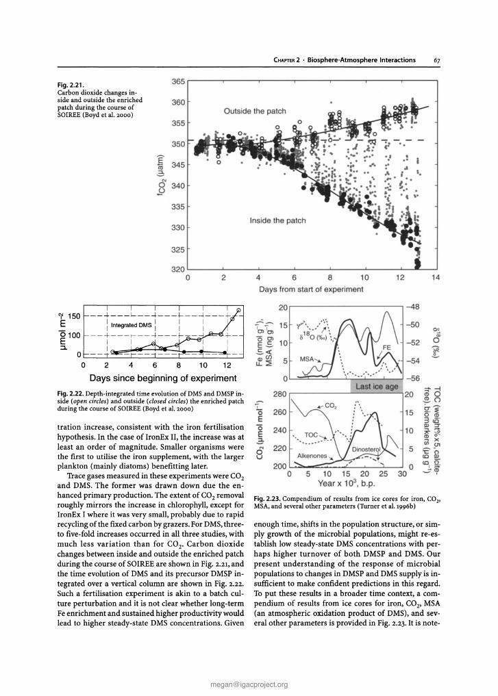
CHAPTER 2 . Biosphere-Atmosphere Interactions 67

5

- 54

10

15

o30

12 14

-48

- 50C>l

C;;

- 52 0

?

'.

... •.,... ., ..I I.

I: .....•• ,.

108

5 10 15 20 25Year x 10 3

, b .p.

't"'" .....\o18~·('J.o) \:.

6

5

Days from start of exper iment

20 ,--- - - - - - - - - --,

4

'i(5 260E

(5 240E3-

N 2200u

'77 15ClCl

'0 ~ 10E ~

.s et:<Denu.~

Fig. 2.23. Compendium of results from ice cores for iron . CO2,

MSA,and several other parameters (Thrner et al. 1996b)

enough time, shifts in the population structure, or sim­ply growth of the microbial populations, might re-es­tablish low steady-state DMS concentrations with per­haps higher turnover of both DMSP and DMS. Ourpresent understanding of the response of microbialpopulations to changes in DMSPand DMSsupply is in­sufficient to make confident predictions in this regard.To put these results in a broader time context, a com­pendium of results from ice cores for iron, CO2, MSA(an atmospheric oxidation product of DMS), and sev­eral other parameters is provided in Fig. 2.23. It is note-

oL....=::::i:::=::::::L--L,~L..:---l----l - 56

280 ,....-- - - - -----'=---;20

Inside the patch

Outs ide the patch

2

325

320 L...-__ --'-__ ---l. ...L-_ _ --'- L.-__ --'---"'L.----'

o

365

360

355

350

E 345iii2:

'"0 340.Y

335

330

2 4 6 8 10 12

Days since beginning of experiment

Fig. 2.21.Carbon dioxide changes in­side and outside the enrichedpatch during the course ofSOIREE(Boyd et al. 2000)

Fig. 2.22. Depth- integrated time evolution of DMSand DMSPin­side (open circles) and outside (closedcircles) the enriched patchduring the course of SOIREE(Boyd et al. 2000)

tration increase, consistent with the iron fertilisationhypothesis. In the case of IronEx II, the increase was atleast an order of magnitude. Smaller organisms werethe first to utilise the iron supplement, with the largerplankton (mainly diatoms) benefitting later.

Tracegases measured in these experiments were CO2and DMS. The former was drawn down due the en­hanced primary production. The extent of CO2 removalroughly mirrors the increase in chlorophyll, except forIronEx I where it was very small, probably due to rapidrecycling of the fixed carbon by grazers .For DMS,three­to five-fold increases occurred in all three studies, withmuch less variation than for CO2, Carbon dioxidechanges between inside and outside the enriched patchduring the course of SOIREE are shown in Fig. 2.21, andthe time evolution of DMSand its precursor DMSP in­tegrated over a vertical column are shown in Fig. 2.22.

Such a fertilisation experiment is akin to a batch cul­ture perturbation and it is not clear whether long-termFeenrichment and sustained higher productivity wouldlead to higher steady-state DMSconcentrations. Given

')' 150E"0100E:l.

O'--_--'-_---'- __ -'--_-'-_----J'-_---L-----J

o

[email protected]

68 M.C. Scholes • P.A.Matrai · M.D. Andreae • K.A.Smith· M.R.Manning

5.0 .---------------------,

Paerl 1997).Although the composition of atmosphericON is poorlyknown, recent work (Peierls and Paerl1997;Seitzinger and Sanders 1999)indicates that constituentsof this pool are biologically utilised and, hence, shouldbe included in eutrophication assessments.

In situ bioassays and field surveys show that enrich­ment with the major deposition constituents NHt andNO; at natural dilutions and atmospherically deriveddissolved organic nitrogen (DON) results in enhancedphytoplankton primary production and increasedbiomass (Paerl 1985; Willey and Paerl 1993; Paerl andFogel 1994; Peierls and PaerlI997). Atmospheric DONmay selectively stimulate growth of specific types ofmarine phytoplankton (Neilson and Lewin 1974; Antiaet al. 1991). These selective phytoplankton responses tospecific nitrogen inputs, and changes in stoichiometricC:N ratios resulting from these inputs may inducechanges at the zooplankton, invertebrate, herbivorousfish, and higher trophic levels.

•

••

•

•

4.0 f-

".........,-................. .... ..... .....

.......... ...................

1.0 f- .....

0.0 !---'-..............l...-............ ....J................-L....o...-...........--'-...........J............--'-.L......!

0.4 - NH!/N0"3

2.0 f-

3.0 f-

co

:;:::;'woa­Q)

o

2.8.3 .2.1 Coastal Regions

worthy that the elevated iron and MSAand lowered CO2

levels during the last glacial period are consistent witha scenario wherein ocean productivity was higher thendue to enhanced atmospheric inputs of iron. For fur­ther discussion of the use of ice core records to exam­ine the overall sulphur cycle see Sect. 2.3.

There is now widespread evidence that atmospheric fixednitrogen compounds contribute to enrichment and in someareas probably to coastal and estuarine eutrophication(Jaworskiet al.1997; Howarth et al.1996).Current estimatesof the percentage of total (natural + anthropogenic) newN loading attributed to direct atmospheric depositionat a number of North American and European locationsrange from 5% to over 50% (Duce 1991; Fisher andOppenheimer 1991; Valigura et al. 1996; Dennis 1997;Holland et al. 1999). Inputs of N to estuarine systemsthat result from direct atmospheric deposition by-passmuch of the estuarine N "filter" (Kennedy 1983; Paerl1995, 1997). Thus, atmospheric deposition assumes anincreasingly important role as a new N source in lowerestuarine and coastal waters below the biological N fil­tering zone (Fig. 2.24).

Dry and wet atmospheric deposition introduces intoestuaries a variety of biologically available inorganic(NO;, NHt, DON) compounds, most of which resultfrom human activities (Likens et al. 1974; Gallowayet al.1994). In addition, organic nitrogen (ON) comprises asignificant fraction (from 15 to over 30%) of wet and dryatmospheric deposition in coastal watersheds (Correlland Ford 1982; Scudlark and Church 1993; Peierls and

2.8.3.2 TheInput ofAtmospheric Nitrogen to the Ocean

Fig. 2.24. Schematic repres entation of airsh ed, upper estuarine,and lower estuarine processes

•

•

0.0 ............--'--J.......L.--'-............-J......l...- ............ -'--............. ...J.............. --L.....I

1977 1980 1983 1986 1989 1992 1995

Year

.................................................

0.2 - • . . ........ .... ......

,....fY

0.3 -

0.1 -

Fig. 2.2S. Trends in annual atmospheric deposition (wet deposi­tion as NHt and NOi, expressed in kg N ha? yr") collected dur­ing a 20 year period at the National Atmospheric Deposition Pro­gram (NADP)site NC-35 in Sampson County, North Carolina (datare-plotted from NADP information)

co:;:::;'woa­Q)

o

~Advection .

rruxrnq

Su n

New N inputs

Upper and lowerestuar ine pro cesses

Sedimen t recycling of N

Airshed processes

Wa tershedprocesses

Wind

~N~~~CAo-V

t ttl I I- _ IndifeCI

Ermssions d Wet and dry di rect depos .noneposmon 1 1t ttl

P omt a nd non-po int run -off

[email protected]

Atmospheric nitrogen inputs have been examinedrecently in North Carolina's Albemarle-Pamlico SoundSystem (APSS) (PaerlI995, 1997). Within the APSS, theNeuse River Estuary receives N inputs from a mosaic ofupstream and upwind agricultural, urban, and indus­trial sources. Fossil fuel combustion and agriculturaland industrial N emissions represent a significant andgrowing source of new N to this system (Paerl and Fogel1994),reflecting a national and world-wide trend (Duce1986; Luke and Dickerson 1987; Asman 1994; Paerl1995;Holland et al. 1999).Depending on the relationship be­tween watershed-estuary surface areas, degree of wa­tershed N retention, seasonal rainfall, discharge and flowpatterns, and proximity of atmospheric sources, an im­portant fraction of nitrogen from atmospheric deposi­tion is directly deposited on the estuary. In the case ofthe APSS, recent estimates are on the order of 20% (forits estuarine tributaries) to 40% (for the downstreamwaters of Pamlico Sound) (Paerl and Fogel 1994; Paerl1995,1997) of the N being directly deposited.

Atmospheric N generated from expanding intensiveanimal farming is of particular concern. Examinationof the long-term record of atmospheric NHt and NO}deposition in Sampson County, eastern North Carolina,shows a nearly three-fold increase in annual NHt depo­sition (also relative to NO}) since 1977. with a particu­larly precipitous rise since the late 1980s(Fig. 2.25). Thereason for this may be that unlike human waste, swinewaste is stored in open lagoons and remains largelyuntreated, and substantial amounts (30 to >80%) of Nare lost via NH3 volatilisation alone (O'Halloran 1993).

2.8.3.2.2 The Open Ocean

There is also growing concern about the increasing in­put of human-derived nitrogen compounds to the openocean. This is especially important in parts of the openocean where nitrogen is the nutrient that limits biologi­cal growth . This is the case in the nutrient-poor watersof the large central oceanic gyres in the North and SouthPacificand AtlanticOceansand the southern Indian Ocean.Current estimates suggest that, at present , atmosphericnitrogen accounts for only a few percent of the total newnitrogen delivered to surface waters in these regions,withupwelling from deep waters being the pr imary source ofnew surface nitrogen. It is recognised , however, that theatmospheric input to the ocean is highly episodic, oftencoming in large pulses extending over a fewdays.Atsuchtimes, atmospheric input plays a much more importantrole as a source for nitrogen in surface waters. A recentestimate of the current input of fixed nitrogen to the glo­bal ocean from rivers, the atmosphere, and nitrogen fixa­tion indicates that all three sources are important(Cornell et al.1995). Paerl and Whitall (1999) estimate that46-57% of the total human-mobilised nitrogen enteringthe North Atlantic Ocean is coming via the atmosphere.

CHAPTER 2 • Biosphere-Atmosphere Interactions 6 9

In addition, the atmospheric organic nitrogen flux maybe equal to or perhaps greater than the inorganic (i.e.ammonium and nitrate) nitrogen flux in open ocean re­gions. The source of the organic nitrogen is not known,but a large fraction of it is likelyto be human-derived.Thisform of atmospheric nitrogen input to the open ocean hadnot been considered in detail until very recently.

Not only will the input of atmospheric fixed nitro­gen to the open ocean increase significantly in the fu­ture as a result of increasing human activities, but thegeographical locations of much of this input will prob­ably change as well. Galloway et al. (1994, 1995) haveevaluated pre-industrial nitrogen fixation (formation ofthe so-called reactive nitrogen) on the continents; thenear-current (1990) reactive nitrogen generated fromhuman activities such as energy production (primarilyas nitrogen oxides), fertiliser use, and legume growth;and the estimated reactive nitrogen that will be pro­duced in 2020 as a result of human activities .

The most highly developed regions in the world arepredicted to show relatively little increase in the forma­tion of reactive nitrogen, with none of these areas con­tributing more than a few per cent to the overall globalincrease . However, other areas will contribute very sig­nificantly to increased human-derived reactive nitro­gen formation in 2020. For example, it is predicted thatAsia will account for -40% of the global increase inenergy-derived reactive nitrogen, while Africa will havea six-fold increase accounting for 15% of the total glo­bal increase. It is predicted that production of reactivenitrogen from the use of fertilisers in Asia will accountfor -87% of the global increase from this source. Bothenergy sources (nitrogen oxides and ultimately nitrate)and fertiliser (ammonia, urea) result in the extensiverelease of reactive nitrogen to the atmosphere. Thus,these predictions indicate very significant potential in­creases in the atmospheric deposition of nutrient ni­trogen compounds to the ocean downwind of such re­gions as Asia, Central and South America, Africa, andthe former Soviet Union (see Fig. 2.26).

The potential problem outlined above was high­lighted by a computer modelling study undertaken byGalloway et al. (1994), who generated maps of the re­cent (1980) and expected (2020) annual deposition ofreactive nitrogen compounds from the atmosphere tothe global ocean. Figure 2.26 is a map of the projectedratio of the estimated deposition of oxidised forms ofnitrogen in 2020 to the values for 1980.It appears thatfrom one and a half to three, and in some limited areasup to four, times the 1980rate will occur over large areasof the oceans. This increased nitrogen deposition willprovide new sources of nutrient nitrogen to some regionsof the ocean where biological production is currently lim­ited by nitrogen. There is thus the possibility of impor­tant impacts on regional biological production and themarine carbon cycle in these regions of the open ocean.

[email protected]

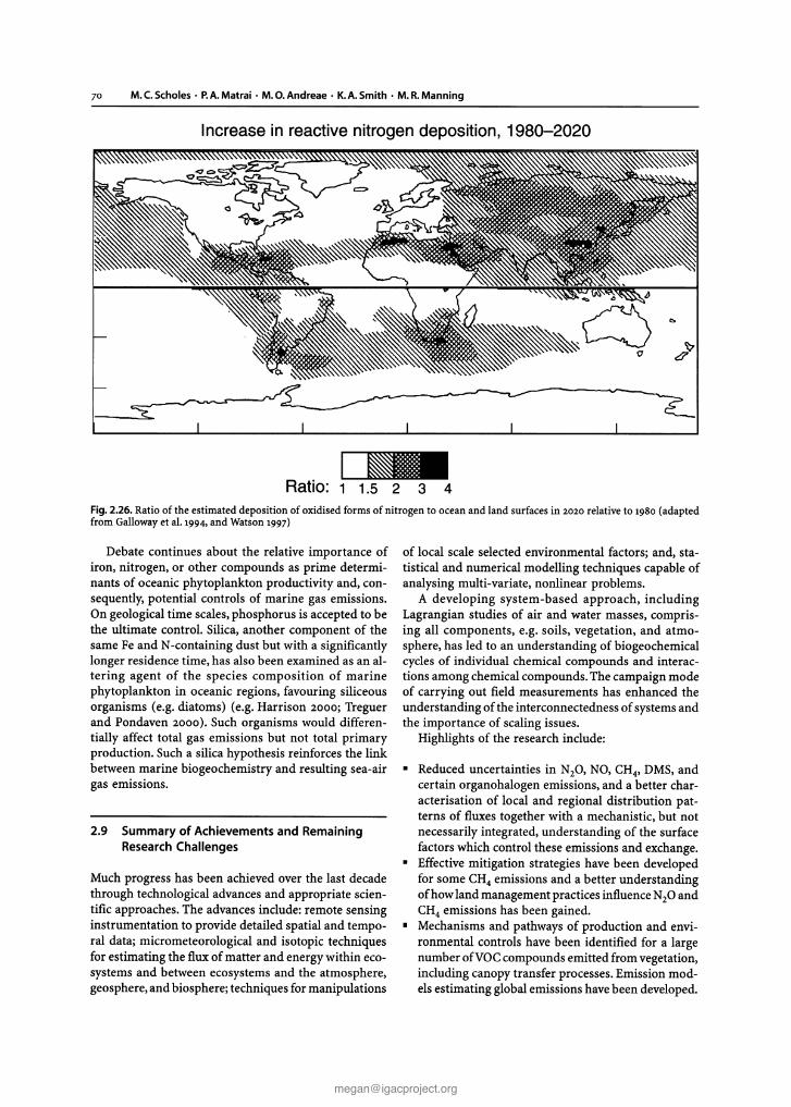
70 M.C. Scholes · P.A.Matrai . M.O.Andreae· K.A. Smith· M. R. Manning

Increase in reactive nitrogen deposition, 1980-2020

Ratio:c-.1 1.5 2 3 4

Fig. 2.26. Ratio of the estimated depos ition of oxidised forms of nitrogen to ocean and land surfaces in 2020 relative to 1980 (adaptedfrom Galloway et aI.1994, and Watson 1997)

Debate continues about the relative importance ofiron, nitrogen, or other compounds as prime determi­nants of oceanic phytoplankton productivity and, con­sequently, potential controls of marine gas emissions.On geological time scales, phosphorus is accepted to bethe ultimate control. Silica, another component of thesame Fe and N-containing dust but with a significantlylonger residence time, has also been examined as an al­tering agent of the species composition of marinephytoplankton in oceanic regions, favouring siliceousorganisms (e.g, diatoms) (e.g, Harrison 2000; Treguerand Pondaven 2000). Such organisms would differen­tially affect total gas emissions but not total primaryproduction. Such a silica hypothesis reinforces the linkbetween marine biogeochemistry and resulting sea-airgas emissions.

2.9 Summary of Achievements and RemainingResearch Challenges

Much progress has been achieved over the last decadethrough technological advances and appropriate scien­tific approaches. The advances include: remote sensinginstrumentation to provide detailed spatial and tempo­ral data; micrometeorological and isotopic techniquesfor estimating the flux of matter and energy within eco­systems and between ecosystems and the atmosphere,geosphere, and biosphere; techniques for manipulations

of local scale selected environmental factors; and, sta­tist ical and numerical modelling techniques capable ofanalys ing multi-variate, nonlinear problems.

A developing system-based approach, includingLagrangian studies of air and water masses, compris­ing all components, e.g. soils, vegetation. and atmo­sphere, has led to an understanding of biogeochemicalcycles of individual chemical compounds and interac­tions among chemical compounds.The campaign modeof carrying out field measurements has enhanced theunderstanding of the interconnectedness of systems andthe importance of scaling issues.

Highlights of the research include:

• Reduced uncertainties in N20, NO, CH4, DMS, andcertain organohalogen emissions, and a better char­acterisation of local and regional distribut ion pat­terns of fluxes together with a mech anistic, but notnecessarily integrated, understanding of the surfacefactors which control these emissions and exchange.

• Effective mitigation strategies have been developedfor some CH4 emiss ions and a better understandingof how land management practices influence N20 andCH4 emissions has been gained.

• Mechanisms and pathways of production and envi­ronmental controls have been identified for a largenumber ofVOC compounds emitted from vegetation,including canopy transfer pro cesses. Emission mod­els estimating global emissions have been developed.

[email protected]

• VOCemissions can account for a loss of two to fourpercent of C taken up by photosynthesis, which hasimplications for understanding and quantifying theC cycle.

• Improved understanding of atmospheric input ofinorganic N and Fe,mainly of anthropogenic and soilorigin, into coastal and open ocean environmentsrepresenting 5-70% of total input in the case of ni­trogen and the subsequent impacts on the C uptakeof the oceans and the C and S cycles.

• The acidic nature of wet deposition, which differs bysource and region, has been characterised.

• Improved understanding of the partitioning of drydeposition (particularly 03 and N02) on leaves andsoil surfaces and related physiological mechanismshas been developed.

• Emission ratios for biomass burning are well de­scribed for savannas, but less well described for hu­mid forests and biofuels. Broad databases are avail­able of emission factors for a large number of sub­stances .

Toachieve more plausible and quantitatively reliableanswers, several key issues remain :

• Toinvestigate mechanisms (chemical and biological)responsible for trace gas cycling (emission and depo­sition) in oceans, soils, and plants, and to establishlong-term sites/studies to provide that information,undertaking field experiments to determine, quan­tify, and discriminate among driving variables.

• To study the exchange of VOCsbetween vegetation,oceans, and the atmosphere along with the exchangeof other trace gases.

• Tounderstand and quantify the effectof soil-releasedNO and its oxidation product N02, under differentmanagement practices, to the atmosphere includinginteraction of these gases both within and above thecanopy.

CHAPTER 2 . Biosphere-Atmosphere Interactions 71

• To determine whether changes in the marine emis­sions of trace gases and particles are likely to have asignificant influence on atmospheric chemistry andvice-versa, resulting from climatic (e .g, rainfall, tem­perature; perhaps small), elevated CO2 (perhapslarge), and/or land use changes. Key areas may in­clude the greenhouse effect (tropospheric 0 3)'strato­spheric ozone (CH3Br), radiation and clouds (DMS),VOCs,tropospheric chemistry (dust-FE-DMS-C02) ,

and other unpredicted impacts (e.g, the change inmarine phytoplankton communities coupled withchanges in N and Fe deposition), especially in theTropics and high latitudes.

• To understand how the hydrological cycle will be af­fected in various regions with climate change and thesubsequent impacts on emissions.

• Toimprove the parameterisation of air-sea exchangeand its links to biogeochemical cycling in surfacewaters as well as improve Lagrangian studies in wa­ter, air, and the combined ocean-atmospheric front,including international participation in order to over­come the intrinsic organisational and logistical dif­ficulties.

• To promote the establishment, wherever possible, oflong-term sites for flux measurements, to investigatethe magnitude of interannual variation and thusachieve more robust estimates of mean annual fluxesand global budgets .

• Todesign experiments that will bring synthesis fromemission-type studies, regional means of fire detec­tion and prediction, spatially and temporally re­solved, and chemical transport models (see Chap. 6)in order to determine the impact of burning on at­mospheric chemistry.

• To develop more realistic biological and depositionprocess-oriented models with interaction and feed­back among process-oriented, regional models andglobal models in order to provide improved estimatesof emission and deposition fluxes.

[email protected]