Bioinformatics analysis and consensus ranking for biological ...

HAL Id: tel-01207489https://tel.archives-ouvertes.fr/tel-01207489

Submitted on 1 Oct 2015

HAL is a multi-disciplinary open accessarchive for the deposit and dissemination of sci-entific research documents, whether they are pub-lished or not. The documents may come fromteaching and research institutions in France orabroad, or from public or private research centers.

L’archive ouverte pluridisciplinaire HAL, estdestinée au dépôt et à la diffusion de documentsscientifiques de niveau recherche, publiés ou non,émanant des établissements d’enseignement et derecherche français ou étrangers, des laboratoirespublics ou privés.

Bioinformatics analysis and consensus ranking forbiological high throughput data

Bo Yang

To cite this version:Bo Yang. Bioinformatics analysis and consensus ranking for biological high throughput data. Bioin-formatics [q-bio.QM]. Université Paris Sud - Paris XI; Université de Wuhan (Chine), 2014. English.�NNT : 2014PA112250�. �tel-01207489�

UNIVERSITÉ PARIS-SUD

ÉCOLE DOCTORALE 427 :INFORMATIQUE PARIS SUD

Laboratoire : Laboratoire de Recherche en Informatique

THÈSE DE DOCTORAT

INFORMATIQUE

par

Bo YANG

Analyses bioinformatiques et classements consensus

pour les données biologiques à haut débit

Date de soutenance : 30/09/2014

Composition du jury :

Directeur de thèse : Alain DENISE Co-directeur de thèse Co-directeur de thèse : Xiang-Dong Fu Co-directeur de thèse

Rapporteurs : Daowen WANG ExaminateurExaminateurs : Sarah COHEN-BOULAKIA Examinatrice

Stéphane VIALETTE ExaminateurMin Wu Examinateur

I

Content

Content ............................................................................................................................................. I

Résumé .......................................................................................................................................... III

Abstract ........................................................................................................................................... V

Chapter 1: Introduction ................................................................................................................. 1

Chapter 2: Genome-wide Analysis of U2AF Functions in pre-mRNA Splicing ........................ 5

2.1 Introduction ......................................................................................................................... 5

2.1.1 RNA splicing ............................................................................................................ 5

2.1.2 Alternative splicing ................................................................................................ 11

2.1.3 Splicing regulation ................................................................................................. 13

2.1.4 Splicing and disease ............................................................................................... 16

2.1.5 Motivation .............................................................................................................. 18

2.2 Methods ............................................................................................................................. 21

2.2.1 High throughput sequencing .................................................................................. 21

2.2.2 Bioinformatics analysis .......................................................................................... 27

2.3 Results ............................................................................................................................... 38

2.3.1 Genome-wide mapping of U2AF-RNA interactions .............................................. 38

2.3.2 U2AF recognition of ~88% functional 3’ splice sites in the human genome ......... 44

2.3.3 Additional U2AF binding events beyond functional 3’ splice sites ....................... 47

2.3.4 Critical roles of U2AF in regulated splicing .......................................................... 49

2.3.5 Multiple mechanisms underlying U2AF-regulated alternative splicing ................. 52

2.3.6 Polar effect of U2AF65 binding on downstream 3’ splice site recognition............ 56

2.3.7 Coordinated action of U2AF65 and U2AF35 in regulated splicing ....................... 59

2.3.8 U2AF65 binding scores .......................................................................................... 63

2.4 Discussion ......................................................................................................................... 66

Chapter 3: Consistent-Pivot: A New effective Pivot Algorithms for Ranking Aggregation

Problem .......................................................................................................................................... 69

3.1 Introduction ....................................................................................................................... 69

II

3.2 Notations ........................................................................................................................... 73

3.2.1 Ranking with ties.................................................................................................... 73

3.2.2 Unifying a set of partial rankings ........................................................................... 73

3.2.3 Distance measures .................................................................................................. 74

3.2.4 Kemeny optimal aggregations ................................................................................ 76

3.3 Previous algorithms ........................................................................................................... 78

3.3.1 Some heuristics and approximation algorithms ..................................................... 78

3.3.2 Other algorithms..................................................................................................... 82

3.3.3 Pivot Algorithms .................................................................................................... 82

3.4 Methods ............................................................................................................................. 91

3.4.1 Consistent-Pivot algorithm ..................................................................................... 91

3.4.2 Experiments on the algorithms ............................................................................... 94

3.5 Results ............................................................................................................................... 98

3.5.1 Results on real biological data ............................................................................... 98

3.5.2 Results on WebSearch data .................................................................................. 100

3.5.3 Results on synthetic data ...................................................................................... 103

3.6 Discussion ....................................................................................................................... 105

Reference ..................................................................................................................................... 106

Appendix : List of the publications............................................................................................ 120

Acknowledgement ....................................................................................................................... 121 

III

Résumé Cette thèse aborde deux problèmes relatifs à l’analyse et au traitement des données

biologiques à haut débit: le premier touche l’analyse bioinformatique des génomes à

grande échelle, le deuxième est consacré au développement d’algorithmes pour le

problème de la recherche d’un classement consensus de plusieurs classements.

L’épissage des ARN est un processus cellulaire qui modifie un ARN pré-messager

en en supprimant les introns et en raboutant les exons. L’hétérodimère U2AF a été très

étudié pour son rôle dans processus d’épissage lorsqu’il se fixe sur des sites d’épissage

fonctionnels. Cependant beaucoup de problèmes critiques restent en suspens,

notamment l’impact fonctionnel des mutations de ces sites associées à des cancers. Par

une analyse des interactions U2AF-ARN à l’échelle génomique, nous avons déterminé

qu’U2AF a la capacité de reconnaître environ 88% des sites d’épissage fonctionnels

dans le génome humain. Cependant on trouve de très nombreux autres sites de fixation

d’U2AF dans le génome. Nos analyses suggèrent que certains de ces sites sont

impliqués dans un processus de régulation de l’épissage alternatif. En utilisant une

approche d’apprentissage automatique, nous avons développé une méthode de

prédiction des sites de fixation d’UA2F, dont les résultats sont en accord avec notre

modèle de régulation. Ces résultats permettent de mieux comprendre la fonction

d’U2AF et les mécanismes de régulation dans lesquels elle intervient.

Le classement des données biologiques est une nécessité cruciale. Nous nous

sommes intéressés au problème du calcul d’un classement consensus de plusieurs

classements de données, dans lesquels des égalités (ex-aequo) peuvent être présentes.

Plus précisément, il s’agit de trouver un classement dont la somme des distances aux

classements donnés en entrée est minimale. La mesure de distance utilisée le plus

fréquemment pour ce problème est la distance de Kendall-tau généralisée. Or, il a été

montré que, pour cette distance, le problème du consensus est NP-difficile dès lors qu’il

y a plus de quatre classements en entrée. Nous proposons pour le résoudre une

heuristique qui est une nouvelle variante d’algorithme à pivot. Cette heuristique,

IV

appelée Consistent-pivot, s’avère à la fois plus précise et plus rapide que les algorithmes

à pivot qui avaient été proposés auparavant.  

V

Abstract

It is thought to be more and more important to solve biological questions using

Bioinformatics approaches in the post-genomic ear. This thesis focuses on the

Bioinformatics analysis and algorithms development of consensus ranking for

biological high throughput data.

In molecular biology and genetics, RNA splicing is a modification of the nascent

pre-messenger RNA (pre-mRNA) transcript in which introns are removed and exons

are joined. The U2AF heterodimer has been well studied for its role in defining

functional 3’ splice sites in pre-mRNA splicing, but multiple critical problems are still

outstanding, including the functional impact of their cancer-associated mutations.

Through genome-wide analysis of U2AF-RNA interactions, we report that U2AF has

the capacity to define ~88% of functional 3’ splice sites in the human genome.

Numerous U2AF binding events also occur in other genomic locations and metagene

and minigene analysis suggests that upstream intronic binding events interfere with the

immediate downstream 3’ splice site associated with either the alternative exon to cause

exon skipping or competing constitutive exon to induce inclusion of the alternative

exon. We further build up a U2AF65 scoring scheme for prediction its target sites base

on the high throughput sequencing data using a Maximum Entropy machine learning

method, and the scores on the up and down regulated cases are consistent with our

regulation model. These findings reveal the genomic function and regulatory

mechanism of U2AF, which facilitates us understanding those associated diseases.

Ranking biological data is a crucial need. Instead of developing new ranking

methods, Cohen-Boulakia and her colleagues proposed to generate a consensus ranking

to highlight the common points of a set of rankings while minimizing their

disagreements to combat the noise and error for biological data. However, it is a NP-

hard question even for only four rankings based on the Kendall-tau distance. In this

thesis, we propose a new variant of pivot algorithms named as Consistent-Pivot. It uses

a new strategy of pivot selection and other elements assignment, which performs better

VI

both on computation time and accuracy than previous pivot algorithms.

Key words: Bioinformatics analysis; High throughput sequencing; U2AF; RNA

splicing; Algorithm; Consensus ranking;

1

Chapter 1: Introduction

As said by Eric Green who is the director of American National Human Genome

Research Institute, “Generating the data is not the bottleneck…… The bottleneck is

analyzing the data”, it is thought to be more and more important to solve biological

questions using Bioinformatics approaches in the post-genomic ear. Bioinformatics is

an interdisciplinary scientific field of computer and biology sciences. It uses computer

to better understand biology, especially important in this biological big data era (see

Figure 1.1).

Figure 1.1. The amount of base pairs and users in GenBank database in twenty three years. Many

important events are also indicated. Figure from (http://www.nlm.nih.gov/about/2014CJ.html).

Bioinformatics starts from sequencing alignment and annotation, while it appears

in every aspect in biological research now (see Figure 1.2), as shown in below:

2

Figure 1.2. Overview of various of subfields of bioinformatics

1. Sequence analysis: Genome annotation to predict unknown genes;

comparative genomics to understand gene function and evolution; genome

wide associate study (GWAS) to find disease genes or mutation sites.

2. High throughput sequencing analysis: Data analysis of ChIP-seq, CLIP-seq,

RNA-seq, Ribo-Seq and so on, to reveal the gene and protein expression

profiles, protein and DNA/RNA interaction and regulation.

3. Structure prediction: Structures of RNAs and proteins are always related

with their functions. Structure prediction helps to understand the function,

and then guides drug design

4. Network and systems biology: Attempts to integrate many different data

types, to understand biology process in a network view.

5. Software and tools: Rang from simple tools to design PCR primer, to

complex platform or web-server for searching various types of data.

Algorithm Development

Software Development

Database Construction

Sequence Database Searching

Sequence Allgnment

Genome Comparision

Gene & PromoterPrediction

Motif Discovery

Phylogeny

Gene Expression Profiling

Metabolic PathwayModeling

Protein InteractionPrediction

Protein SubcellularLocalizationPrediction

Nucleic AcidStructure Prediction

Protein StructurePrediction

Protein StructureClassification

Protein StructureComparision

SequenceAnalysis

FunctionAnalysis

StructureAnalysis

App

licat

ion

Com

puta

tion

3

6. Algorithms development: Big data means a large amount of calculation. It

cannot be accepted, if it should run for a long time. Developing an effective

algorithm to correctly solve problem in a short time, is also a big challenge.

7. Databases: It is very important for biological research, because it is mainly

based on a large amount of knowledge. Storing in database facilitate

searching, modification and utilization.

Bioinformatics has become an important part of many areas of biology. In

experimental molecular biology, bioinformatics techniques such as image and signal

processing allow extraction of useful results from large amounts of raw data. In the field

of genetics and genomics, it aids in sequencing and annotating genomes and their

observed mutations. It plays a role in the text mining of biological literature and the

development of biological and gene ontologies to organize and query biological data.

It also plays a role in the analysis of gene and protein expression and regulation.

Bioinformatics tools aid in the comparison of genetic and genomic data and more

generally in the understanding of evolutionary aspects of molecular biology. At a more

integrative level, it helps analyze and catalogue the biological pathways and networks

that are an important part of systems biology. In structural biology, it aids in the

simulation and modeling of DNA, RNA, and protein structures as well as molecular

interactions.

This thesis focuses on the Bioinformatics data analysis in Chapter 2 and algorithms

development of consensus ranking for biological high throughput data in Chapter 3, to

to solve biological questions.

In molecular biology and genetics, RNA splicing is a modification of the nascent

pre-messenger RNA (pre-mRNA) transcript in which introns are removed and exons

are joined. The U2AF heterodimer has been well studied for its role in defining

functional 3’ splice sites in pre-mRNA splicing, but multiple critical problems are still

outstanding, including the functional impact of their cancer-associated mutations. In

Chapter 2, we aim to find out the function of U2AF65 to define 3’ splice sites and

4

regulate alternative splicing using high throughput sequencing data, to facilitate the

research of related disease.

Ranking biological data is a crucial need. For example, in the research of RNA

alternative splicing regulation, we always want to know which splice site is weaker or

stranger. There have been many tools for scoring the splice sites signal strength. But

the rankings of these tools are always very different. Instead of developing new ranking

methods, Cohen-Boulakia and her colleagues proposed to generate a consensus ranking

to highlight the common points of a set of rankings while minimizing their

disagreements to combat the noise and error for biological data. However, it is a NP-

hard question even for only four rankings based on the Kendall-tau distance. In Chapter

3, we propose a new variant of pivot algorithms named as Consistent-Pivot. It uses a

new strategy of pivot selection and other elements assignment, which performs better

both on computation time and accuracy than previous pivot algorithms.

5

Chapter 2: Genome-wide Analysis of U2AF Functions in pre-mRNA Splicing

2.1 Introduction

The genetic information is stored in DNA, which is transferred from one generation

to the next generation. During the life of a cell, the DNA information is transferred as

RNA, and then the RNA is translated as protein. This is the central dogma of molecular

biology, describing the flow of genetic information within a biological system (Crick,

1970). However, RNA does not simply copy the genetic information, as the primary

RNA transcript generated from DNA should undergo processing.

2.1.1 RNA splicing

As we know, the DNA coding sequence of a protein-coding gene is a series of three-

nucleotide codons, which specifies the linear sequence of amino acids in its polypeptide

product. In the vast majority of cases in bacteria and their phages, the coding sequence

is contiguous: the codon for one amino acid is immediately adjacent to the codon for

the next amino acid in the polypeptide chain. But it is rarely so for eukaryotic genes. In

those cases, the coding sequence is periodically interrupted by stretches of non-coding

sequence.

Most eukaryotic genes are thus mosaics, consisting of blocks of coding sequences

separated from each other by blocks of non-coding sequences. The coding sequences

are called exons, and the intervening sequences are called introns. Once DNA is

transcribed into an RNA transcript, the introns must be removed and the exons are

joined together to create the messenger RNA (mRNA) for that gene, which is then

exported into the cytoplasm. So the term exon technically names for exported regions,

6

and applies to any region retained in a mature RNA, whether or not it is coding. Non-

coding exons include the 5’ and 3’ untranslated regions of an mRNA.

Figure 2.1.1. A typical eukaryotic gene. The depicted gene contains four coding exons separated by

three introns. Transcription from the promoter generates a pre-mRNA, shown in the middle line,

which contains all of the exons and introns. Splicing removes the introns and fuses the exons to

generate the mature mRNA. Technically, the 5’ and 3’ untranslated regions are also exons because

they are retained in the mature mRNA. They are shown here in light purple to indicate their status

as non-coding exons.

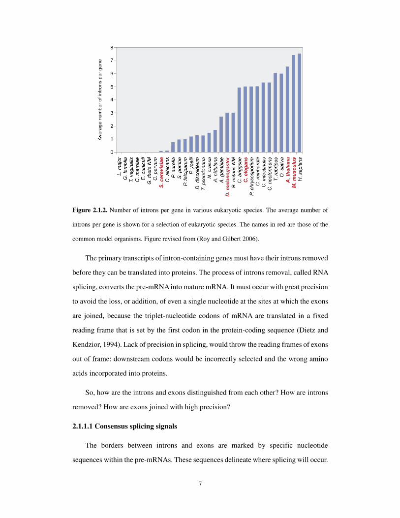
Figure 2.1.1 shows a typical eukaryotic gene in which the coding region is

interrupted by three introns, splitting it into four exons. The number of introns found

within a gene varies enormously, from one in the case of most intron-containing yeast

genes (and a few human genes), to as many as 363 in the case of the Titin gene of

humans. Figure 2.1.2 shows the average number of introns per gene for a range of

organisms. Interestingly, the average number increases as one looks from simple single-

celled eukaryotes, such as yeast, through higher organisms such as worms and flies, all

the way up to humans (Roy and Gilbert, 2006).

Genomic DNA

Promoter region

Intron 1

exon 1 2

2

3

3

4

Pre-mRNA 5'

5' UTR1 2 3 4

3'

3' UTR

5' 3'

1 2 3 4Spliced mRNA

Transcription

Splicing

7

Figure 2.1.2. Number of introns per gene in various eukaryotic species. The average number of

introns per gene is shown for a selection of eukaryotic species. The names in red are those of the

common model organisms. Figure revised from (Roy and Gilbert 2006).

The primary transcripts of intron-containing genes must have their introns removed

before they can be translated into proteins. The process of introns removal, called RNA

splicing, converts the pre-mRNA into mature mRNA. It must occur with great precision

to avoid the loss, or addition, of even a single nucleotide at the sites at which the exons

are joined, because the triplet-nucleotide codons of mRNA are translated in a fixed

reading frame that is set by the first codon in the protein-coding sequence (Dietz and

Kendzior, 1994). Lack of precision in splicing, would throw the reading frames of exons

out of frame: downstream codons would be incorrectly selected and the wrong amino

acids incorporated into proteins.

So, how are the introns and exons distinguished from each other? How are introns

removed? How are exons joined with high precision?

2.1.1.1 Consensus splicing signals

The borders between introns and exons are marked by specific nucleotide

sequences within the pre-mRNAs. These sequences delineate where splicing will occur.

8

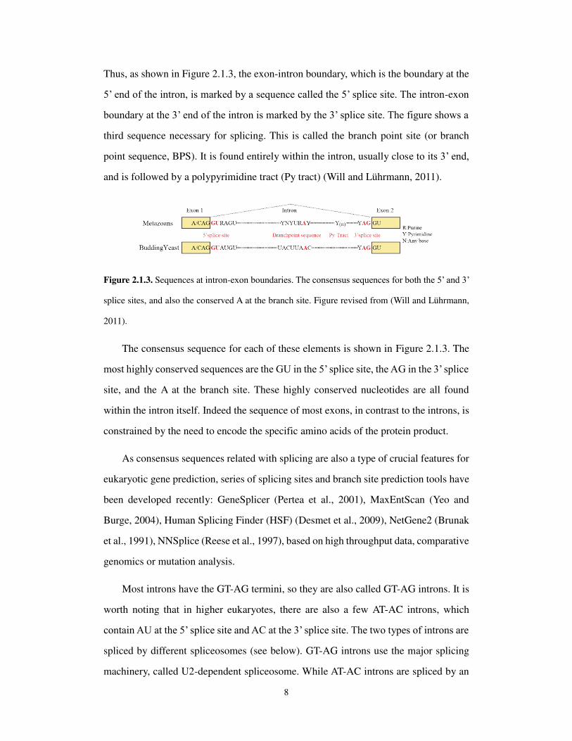
Thus, as shown in Figure 2.1.3, the exon-intron boundary, which is the boundary at the

5’ end of the intron, is marked by a sequence called the 5’ splice site. The intron-exon

boundary at the 3’ end of the intron is marked by the 3’ splice site. The figure shows a

third sequence necessary for splicing. This is called the branch point site (or branch

point sequence, BPS). It is found entirely within the intron, usually close to its 3’ end,

and is followed by a polypyrimidine tract (Py tract) (Will and Lührmann, 2011).

Figure 2.1.3. Sequences at intron-exon boundaries. The consensus sequences for both the 5’ and 3’

splice sites, and also the conserved A at the branch site. Figure revised from (Will and Lührmann,

2011).

The consensus sequence for each of these elements is shown in Figure 2.1.3. The

most highly conserved sequences are the GU in the 5’ splice site, the AG in the 3’ splice

site, and the A at the branch site. These highly conserved nucleotides are all found

within the intron itself. Indeed the sequence of most exons, in contrast to the introns, is

constrained by the need to encode the specific amino acids of the protein product.

As consensus sequences related with splicing are also a type of crucial features for

eukaryotic gene prediction, series of splicing sites and branch site prediction tools have

been developed recently: GeneSplicer (Pertea et al., 2001), MaxEntScan (Yeo and

Burge, 2004), Human Splicing Finder (HSF) (Desmet et al., 2009), NetGene2 (Brunak

et al., 1991), NNSplice (Reese et al., 1997), based on high throughput data, comparative

genomics or mutation analysis.

Most introns have the GT-AG termini, so they are also called GT-AG introns. It is

worth noting that in higher eukaryotes, there are also a few AT-AC introns, which

contain AU at the 5’ splice site and AC at the 3’ splice site. The two types of introns are

spliced by different spliceosomes (see below). GT-AG introns use the major splicing

machinery, called U2-dependent spliceosome. While AT-AC introns are spliced by an

9

alternative, low-abundance spliceosome, called U12-dependent spliceosome (Levine

and Durbin, 2001).

2.1.1.2 Spliceosome

An intron is removed through two successive transesterification reactions in which

phosphodiester linkages within the pre-mRNA are broken and new ones are formed.

Figure 2.1.4. Schematic representation of the two-step mechanism of pre-mRNA splicing. Boxes

and solid lines represent the exons (E1, E2) and the intron, respectively. The branch site adenosine

is indicated by the letter A and the phosphate groups (p) at the 5′ and 3′ splice sites, which are

conserved in the splicing products, are also shown. Figure from (Will and Lührmann, 2011)

The transesterification reactions are mediated by a huge molecular machine called

the spliceosome. This complex comprises about 150 proteins and five RNAs. The five

RNAs (U1, U2, U4, U5, and U6) are collectively called small nuclear RNAs (snRNAs).

Each of these RNAs is between 100 and 300 nucleotides long in most eukaryotes and

is complexed with several proteins. These RNA-protein complexes are called small

nuclear ribonuclear proteins (snRNPs). The spliceosome is the large complex made up

of these snRNPs and also many other proteins, but the exact makeup differs at different

stages of the splicing reaction: different snRNPs come and go at different times, each

performing particular functions in the reaction.

10

Figure 2.1.5. Canonical cross-intron assembly and disassembly pathway of the U2-dependent

spliceosome. For simplicity, the ordered interactions of the snRNPs (indicated by circles) are shown,

but not those of non-snRNP proteins. The various spliceosomal complexes are named according to

the metazoan nomenclature. Exon and intron sequences are indicated by boxes and lines,

respectively. The stages at which the evolutionarily conserved DExH/D-box RNA

ATPases/helicases Prp5, Sub2/UAP56, Prp28, Brr2, Prp2, Prp16, Prp22 and Prp43, or the GTPase

Snu114, act to facilitate conformational changes are indicated. Figure from (Will and Lührmann,

2011)

As shown in Figure 2.1.5, initially the 5’ splice site is recognized by the U1 snRNP,

using base pairing between its snRNA and the pre-mRNA. U2AF is made up of two

subunits, the larger of which, called U2AF65, binds to the Py tract and the smaller,

called U2AF35, binds to the 3’ splice site. The former subunit interacts with BBP (SF1)

and helps that protein bind to the branch site. This arrangement of proteins and RNA is

called the early (E) complex. U2 snRNP then binds to the branch site, aided by U2AF

and displacing BBP (SF1). This arrangement is called the A complex. Binding of the

U4/U6-U5 tri-snRNP then forms the B complex. Several structural rearrangements in

the B complex lead to loss of the U1 and U4 snRNPs, resulting in the C complex. Here

11

the U6 snRNA is base-paired to the 5’splice site, and the base-pairing between the

U4/U6 snRNAs is replaced with a U2-U6 snRNA interaction. This creates the active

conformation of the spliceosome, and the two-transesterification reactions of splicing

occur in it (Will and Lührmann, 2011).

2.1.2 Alternative splicing

Most pre-mRNAs in higher eukaryotes can be spliced in more than one way. Thus,

mRNAs containing different selections of exons can be generated from a given pre-

mRNA. Called alternative splicing (AS), this strategy enables a gene to give rise to

more than one polypeptide product. These alternative products are called isoforms.

There are several different types of alternative splicing events, which can be

classified into four main subgroups. The first type is exon skipping, in which a type of

exon known as a cassette exon is spliced out of the transcript together with its flanking

introns (see the Figure 2.1.6, Cassette exon). Exon skipping accounts for nearly 40% of

alternative splicing events in higher eukaryotes (Alekseyenko et al., 2007 and Sugnet

et al., 2004), but is extremely rare in lower eukaryotes. The second and third types are

alternative 3’ splice site (3’ SS) and 5’ SS selection. These types of AS events occur

when two or more splice sites are recognized at one end of an exon. Alternative 3’ SS

and 5’ SS selection account for 18.4% and 7.9% of all AS events in higher eukaryotes,

respectively. The fourth type is intron retention, in which an intron remains in the

mature mRNA transcript. This is the rarest AS event in vertebrates and invertebrates,

accounting for less than 5% of known events (Alekseyenko et al., 2007; Kim et al.,

2008; and Sugnet et al., 2004). By contrast, intron retention is the most prevalent type

of AS in plants, fungi and protozoa (Kim et al., 2008). Less frequent, complex events

that give rise to alternative transcript variants include mutually exclusive exons,

alternative promoter usage and alternative polyadenylation (Black, 2003).

12

Figure 2.1.6. Types of alternative splicing events. Constitutive exons are shown in yellow and

alternatively spliced regions in red or blue. Introns are represented by solid lines, and dashed lines

indicate splicing options. Figure revised from (Keren, Lev-Maor and Ast, 2010).

Alternative splicing is a major cellular mechanism in metazoans for generating

proteomic diversity (Nilsen and Graveley, 2010). A large proportion of protein-coding

genes in multicellular organisms undergo alternative splicing, and in humans, it has

been estimated that nearly 90 % of protein-coding genes-much larger than expected-are

subject to alternative splicing (Black, 2003; Pan et al., 2008; Chen and Manley, 2009).

Genomic analyses of alternative splicing have illuminated its universal role in shaping

the evolution of genomes, in the control of developmental processes, and in the dynamic

regulation of the transcriptome to influence phenotype. Disruption of the splicing

machinery has been found to drive pathophysiology, and indeed reprogramming of

aberrant splicing can provide novel approaches to the development of molecular therapy.

13

2.1.3 Splicing regulation

Splicing is regulated by trans-acting proteins (repressors and activators) and

corresponding cis-acting regulatory sites (silencers and enhancers) on the pre-mRNA.

However, as part of the complexity of alternative splicing, it is noted that the effects of

a splicing factor are frequently position-dependent. It means that a splicing factor that

serves as splicing activator when bound to an intronic enhancer element may serve as

a repressor when bound to its splicing element in the context of an exon, and vice versa

(Lim et al., 2011).

Figure 2.1.7. Schematic representation of core spliceosomal components that bind to the canonical

splicing signals (5’ splice site, branch point, polypyrimidine tract, and 3’ splice site). Additional cis-

acting elements in exons and introns that control splice site recognition are also shown. Although

the diagram depicts positive and negative acting roles for SR and hnRNP proteins, respectively,

depending on the location of the binding sites of these factors, they can also act in the opposite

manner. Similarly, various tissue-dependent splicing factors can either promote or repress splice

site selection depending on the location of their binding sites with respect to splicing signals. ISE,

intronic splicing enhancer; ISS, intronic splicing silencer; ESE, exonic splicing enhancer; ESS,

exonic splicing silencer; SR, Ser/Arg-repeat containing protein; hnRNP, heterogeneous

ribonucleoprotein (hnRNP); and U2AF, U2 snRNP auxiliary factor. Figure from (Irimia and

14

Blencowe, 2012).

There are two major types of cis-acting RNA sequence elements present in pre-

mRNAs and they have corresponding trans-acting RNA-binding proteins (see Figure

2.1.7). Splicing silencers are sites to which splicing repressor proteins bind, reducing

the probability that a nearby site will be used as a splice junction. These can be located

in the intron (intronic splicing silencers, ISS) or in a neighboring exon (exonic splicing

silencers, ESS). They vary in sequence, as well as in the types of proteins that bind to

them. The majority of splicing repressors are heterogeneous nuclear ribonucleoproteins

(hnRNPs) such as hnRNPA1 and polypyrimidine tract binding protein (PTB) (Matlin,

Clark and Smith, 2005; Wang and Burge, 2008).

Splicing enhancers are sites to which splicing activator proteins bind, increasing

the probability that a nearby site will be used as a splice junction. These also may locate

in the intron (intronic splicing enhancers, ISE) or exon (exonic splicing enhancers,

ESE). Most of the activator proteins that bind to ISEs and ESEs are members of the SR

protein family. Such proteins contain RNA recognition motifs and arginine and serine-

rich (RS) domains (Matlin, Clark and Smith, 2005; Wang and Burge, 2008).

The secondary structure of the pre-mRNA transcript also plays a role in regulating

splicing, such as by bringing together splicing elements or by masking a sequence that

would otherwise serve as a binding element for a splicing factor (Warf and Berglund,

2010; Reid et al., 2009).

Mechanisms of alternative splicing are highly variable, and new examples are

constantly being found, particularly through the use of high-throughput techniques.

Researchers hope to fully elucidate the regulatory systems involved in splicing, so that

alternative splicing products from a given gene under particular conditions could be

predicted by a “splicing code” (Matlin, Clark and Smith, 2005; David and Manley,

2008).

15

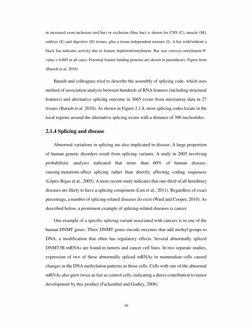
Figure 2.1.8. Graphical depiction of the splicing code. The region-specific activity of each feature

16

in increased exon inclusion (red bar) or exclusion (blue bar) is shown for CNS (C), muscle (M),

embryo (E) and digestive (D) tissues, plus a tissue-independent mixture (I). A bar with/without a

black hat indicates activity due to feature depletion/enrichment. Bar size conveys enrichment P-

value < 0.005 in all cases. Potential feature binding proteins are shown in parentheses. Figure from

(Barash et al. 2010)

Barash and colleagues tried to describe the assembly of splicing code, which uses

method of association analysis between hundreds of RNA features (including structural

features) and alternative splicing outcome in 3665 exons from microarray data in 27

tissues (Barash et al. 2010). As shown in Figure 2.1.8, most splicing codes locate in the

local regions around the alternative splicing exons with a distance of 300 nucleotides.

2.1.4 Splicing and disease

Abnormal variations in splicing are also implicated in disease. A large proportion

of human genetic disorders result from splicing variants. A study in 2005 involving

probabilistic analyses indicated that more than 60% of human disease-

causing mutations affect splicing rather than directly affecting coding sequences

(López-Bigas et al., 2005). A more recent study indicates that one-third of all hereditary

diseases are likely to have a splicing component (Lim et al., 2011). Regardless of exact

percentage, a number of splicing-related diseases do exist (Ward and Cooper, 2010). As

described below, a prominent example of splicing-related diseases is cancer.

One example of a specific splicing variant associated with cancers is in one of the

human DNMT genes. Three DNMT genes encode enzymes that add methyl groups to

DNA, a modification that often has regulatory effects. Several abnormally spliced

DNMT3B mRNAs are found in tumors and cancer cell lines. In two separate studies,

expression of two of these abnormally spliced mRNAs in mammalian cells caused

changes in the DNA methylation patterns in those cells. Cells with one of the abnormal

mRNAs also grew twice as fast as control cells, indicating a direct contribution to tumor

development by this product (Fackenthal and Godley, 2008).

17

Figure 2.1.9. Components of the splicing E/A complex mutated in myelodysplasia. RNA splicing

is initiated by the recruitment of U1 snRNP to the 5’ SS. SF1 and the larger subunit of the U2

auxiliary factor (U2AF), U2AF65, bind the branch point sequence (BPS) and its downstream

polypyrimidine tract, respectively. The smaller subunit of U2AF (U2AF35) binds to the AG

dinucleotide of the 3’ SS, interacting with both U2AF65 and a SR protein, such as SRSF2, through

its UHM and RS domain, comprising the earliest splicing complex (E complex). ZRSR2 also

interacts with U2AF and SR proteins to perform essential functions in RNA splicing. After the

recognition of the 3’ SS, U2 snRNP, together with SF3A1 and SF3B1, is recruited to the 3’ SS to

generate the splicing complex A. The mutated components in myelodysplasia are indicated by

arrows. Figure from (Yoshida et al., 2011).

Single-nucleotide alterations in splice sites or cis-acting splicing regulatory sites

may lead to differences in splicing of a single gene, while changes in the RNA

processing machinery may lead to mis-splicing of multiple transcripts. Yoshida and his

colleagues report whole-exome sequencing of 29 myelodysplasia specimens, which

unexpectedly revealed novel pathway mutations involving multiple components of the

RNA splicing machinery, including U2AF35, ZRSR2, SRSF2 and SF3B1. In a large

series analysis, these splicing pathway mutations were frequent (~45 to 85%), and

highly specific to myeloid neoplasms showing features of myelodysplasia (see Figure

2.1.9). Conspicuously, most of the mutations affect genes involved in the 3’ splice site

recognition during pre-mRNA processing, which may induce abnormal RNA splicing

18

and compromised haematopoiesis (Yoshida et al., 2011).

2.1.5 Motivation

Pre-mRNA splicing takes place in the multi-component RNA machinery known as

the spliceosome, which is assembled in a step-wise fashion through the sequential

addition of U1, U2, and U4/U6/U5 small nuclear ribonucleoprotein particles to the pre-

mRNA (Wahl et al., 2009). U1 defines the functional 5’ splice site largely through base-

pairing interactions, whereas U2 recognizes the functional 3’ splice site, which also

involves base pairing with the branch point sequence. Because the BPS (branch point

site) is quite degenerate in higher eukaryotic cells (see Figure 2.1.3), the addition of U2

snRNP requires multiple auxiliary factors, the most important one being the U2AF

heterodimer consisting of a 65kD and 35kD subunit (Zamore et al., 1992; Zhang et al.,

1992). Numerous biochemical experiments on model pre-mRNAs have established

sequence-specific binding of U2AF65 to the polypyrimidine tract (Py-tract) immediate

downstream of the BPS and direct contact of U2AF35 with the AG dinucleotide, which

together defines functional 3’ splice sites (Singh et al., 1995; Valcárcel et al., 1996).

Upon definition of the functional 5’ and 3’ splice sites by U1 and U2 snRNPs and

following a series of ATP-dependent steps, the U4/U6/U5 tri-snRNP complex joins the

initial pre-spliceosome to convert it into the mature spliceosome (Wahl et al., 2009).

While the vital role of the U2AF heterodimer in defining 3’ splice sites has widely

been appreciated, it has been unclear whether it is required for the recognition of all

functional 3’ splice sites, especially in mammalian cells. In budding yeast, Mud2 has

been characterized as the U2AF65 ortholog, but Mud2 is a non-essential gene, likely

because of highly invariant BPS in this lower eukaryotic organism (Abovich et al., 1994;

Abovich et al., 1997). Similarly, in fission yeast, a significant fraction of intron-

containing genes seem to lack typical Py-tract, and indeed, multiple U2AF-independent

introns have been reported (Sridharan et al., 2011; Sridharan and Singh, 2007). In

mammals, the presence of high levels of splicing enhancer factors, such as SR proteins,

appears to be capable of bypassing the requirement for U2AF to initiate spliceosome

19

assembly (MacMillan et al., 1997). In addition, mammalian genomes also encode for

multiple genes with related functions to both U2AF65 (Imai et al., 1993; Hastings et

al., 2007; Page-McCaw et al., 1999) and U2AF35 (Tronchre et al., 1997; Shepard et al.,

2002; Mollet et al., 2006). Therefore, the functional requirement for U2AF may be

bypassed by multiple mechanisms, raising a general question with respect to the degree

of the involvement of the U2AF65/35 heterodimer in 3’ splice site definition in

mammalian genomes. This fundamental question has remained unaddressed despite the

availability of genome-wide U2AF65-RNA interaction data (Zarnack et al., 2013).

Secondly, the RNA binding specificity of U2AF65 has been well characterized at

the biochemical levels. Introns that contain a strong Py-tract are able to support

spliceosome assembly in an AG-independent manner (Reed, 1989), and U2AF65

appears to be sufficient to support splicing of such AG-independent introns, at least in

vitro (Zamore and Green, 1991). However, the U2AF35 subunit is responsible for

directly contacting the AG dinucleotide on typical functional 3’ splice sites and this

partnership is enforced by U2AF65-dependent stability control of U2AF35 (Pacheco et

al., 2006). Functioning as a heterodimer, U2AF65/35 is thought to provide strong

discrimination against pyrimidine-rich exonic as well as intronic sequences that are not

part of the functional 3’ splice sites in mammalian genomes. Specific RNA binding

proteins, such as DEK and hnRNP A1, have been implicated in improving the RNA

binding specificity in mammalian genomes (Soares et al., 2006; Tavanez et al., 2012).

However, it remains to be directly demonstrated whether the U2AF heterodimer indeed

binds preferentially to the Py-tract followed by the AG dinucleotide from genome-wide

analysis.

Thirdly, besides the critical role of U2AF in constitutive splicing, both U2AF65

and U2AF35 have been implicated in regulated splicing (Park et al., 2004; Moore et al.,

2010). In theory, alternative splice sites are weak in general, and as a result, suboptimal

binding may render them particularly sensitive to levels of U2AF, which may be further

subjected to such PTB, TIA-1/TIAR, and more recently, hnRNP C (Zarnack et al., 2013;

Le Guiner et al., 2001; Xue et al., 2009; Wang et al., 2010). While these mechanisms

20

appear to readily explain U2AF-dependent exon inclusion, it has been largely unknown

why and how depletion of U2AF could also induce a large number of exon inclusion

events in vivo (Park et al., 2004). Engineered U2AF binding on exon was recently

shown to inhibit the inclusion of the exon (Lim et al., 2011), but it has been unclear

how widely this mechanism is used to regulate alternative splicing of endogenous genes.

Last, but not least, multiple mutations in both U2AF65 and U2AF35 have been

reported to associate with myelodysplasia (MDS) and related blood disorders (Yoshida

et al., 2011; Thol et al., 2012; Cazzola et al., 2013). However, it is unclear how such

mutations might affect the normal function of U2AF in regulated splicing, which further

underscores the importance in mechanistic understanding of the regulatory role of

U2AF in mammalian cells.

Given such a long range of mechanistic issues that remain to be addressed, we have

embarked on genome-wide analysis of U2AF-RNA interactions in the human genome.

By defining the genomic landscape of U2AF binding and the functional requirement

for both U2AF65 and U2AF35 in regulated splicing, we provide a series of mechanistic

insights into the function of U2AF in normal and disease states.

21

2.2 Methods

To reveal the target site of U2AF, my colleagues use UV radiation to link the

protein to RNA molecules in vivo. U2AF65 is then precipitated by using a specific

antibody. With the protein, target RNA attached to the protein is isolated and high

throughput sequenced.

On the other hand, RNA-seq or RASL-seq could give us the insights into all the

alternative splicing change regulated by knockdown the trans-acting splicing regulatory

protein.

I then developed serials of bioinformatics analysis pipelines to parse the rules

coding in the high throughput sequencing data.

2.2.1 High throughput sequencing

“It could be argued that the greatest transformative aspect of the Human Genome

Project has been not the sequencing of the genome itself, but the resultant development

of new technologies”, just as said by Kahvejian in 2008, high throughput sequencing

has dramatically changed the way of life sciences research (Kahvejian et al., 2008).

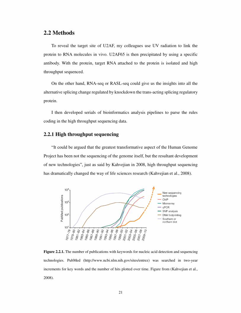
Figure 2.2.1. The number of publications with keywords for nucleic acid detection and sequencing

technologies. PubMed (http://www.ncbi.nlm.nih.gov/sites/entrez) was searched in two-year

increments for key words and the number of hits plotted over time. Figure from (Kahvejian et al.,

2008).

22

As shown in Figure 2.2.1, traditional biological nucleic acid detection methods are

used less and less, while high throughput sequencing starts to be widely used from 2008.

Consistent with it, the amount of genetic sequencing data stored at the European

Bioinformatics Institute takes less than a year to double in size (Marx, 2013) (see Figure

2.2.2).

Figure 2.2.2. Data explosion. The amount of genetic sequencing data stored at the European

Bioinformatics Institute takes less than a year to double in size. Figure from (Marx, 2013)

In the other hand, the high demand for sequencing has driven the development of

several types of efficient high throughput sequencers. There are four platforms

dominating the high throughput sequencing field now: 454, illumina, Ion Torrent and

PacBio (Quiñones-Mateu et al., 2014). All those four sequencers could generate high

quality sequence information, while they each have their own advantages and

disadvantages (see Figure 2.2.3).

23

Figure 2.2.3. Principal characteristics of the four most used deep sequencing platforms now: 454

(GS Junior and GS FLX+ systems), Illumina (MiSeq v2 and HiSeq 2500 systems), Ion Torrent (Ion

Personal Genome Machine, 318 v2 chip and Ion Proton), and Pacific Biosciences (PacBio RS II

SMRT). Figure from (Quiñones-Mateu et al., 2014)

Along with the remarkable improvements in DNA sequencing technologies, the

cost of sequencing is decreasing (see Figure 2.2.4). White line in the figure reflects

Moore's Law, which describes a long-term trend in the computer hardware industry that

involves the doubling of compute power every two years. As shown in the figure, the

cost of sequencing a human genome is consistent with the Moore’s Law before 2008,

while the trend of cost decreasing surpasses the Moore’s Law later. Now it only cost

4000 dollars to sequencing a genome.

24

Figure 2.2.4. Total cost of sequencing a human genome over time as calculated by the National

Human Genome Research Institute (NHGRI). Figure from

(http://www.genome.gov/sequencingcosts/).

Biological scientists develop a lot of types of methods base on high throughput

sequencing technologies, to get insights of biological molecular’ expression and

regulation in a large scale. Various high throughput sequencing methods can precisely

map and quantify chromatin features, DNA modifications and several specific steps in

the cascade of information from transcription to translation (see Figure 2.2.5 and Table

2.2.1).

25

Feature Method Description Refernce

Transcripts, small RNA and transcribed regions

RNA-seq Isolate RNA followed by HT sequencing (Waern et al, 2011)

CAGE HT sequencing of 5’-methylated RNA (Kodzius et al, 2006)

RNA-PET CAGE combined with HT sequencing of poly-A tail (Fullwood et al, 2009c)

ChIRP-Seq Antibody-based pull down of DNA bound to lncRNAs followed by HT sequencing (Chu et al, 2011)

GRO-Seq HT sequencing of bromouridinated RNA to identify transcriptionally engaged Pol II and determine direction of transcription

(Core et al, 2008)

NET-Seq Deep sequencing of 3’ ends of nascent transcripts associated with RNA polymerase, to monitor transcription at nucleotide resolution

(Churchman and Weissman, 2011)

Ribo-Seq Quantification of ribosome-bound regions revealed uORFs and non-ATG codons (Ingolia et al,2009)

Transcriptional machinery and protein-DNA interactions

ChIP-seq Antibody-based pull down of DNA bound to protein followed by HT sequencing (Robertson et al, 2007)

DNAse footprinting HT sequencing of regions protected from DNAsel by presence of proteins on the DNA (Hesselberth et al, 2009)

DNAse-seq HT sequencing of hypersensitive non-methylated regions cut by DNAsel (Crawford et al, 2006)

FAIRE Open regions of chromatin that is sensitive to formaldehyde is isolated and sequenced (Giresi et al, 2007)

Histone modification

ChIP-seq to identify various methylation marks (Wang et al, 2009a)

DNA methylation

RRBS Bisulfite treatment creates C to U modification that is a marker for methylation (Smith et al, 2009)

Chromosome-interacting sites

5C HT sequencing of ligated chromosomal regions (Dostie et al. 2006)

ChIA-PET Chromatin-IP of formaldehyde cross-linked chromosomal regions, followed by HT sequencing

(Fullwood et al, 2009a)

Table 2.2.1. The various high throughput sequencing assays. Table from (Soon et al., 2013).

26

Figure 2.2.5. Sequencing technologies and their uses. Figure from (Soon et al., 2013)

These technologies can be applied in a variety of medically relevant settings,

including uncovering regulatory mechanisms and expression profiles that distinguish

normal and cancer cells, and identifying disease biomarkers, particularly regulatory

variants that fall outside of protein coding regions. Together, these methods can be used

for integrated personal omics profiling to map all regulatory and functional elements in

an individual. Using this basal profile, dynamics of the various components can be

studied in the context of disease, infection, treatment options, and so on. Such studies

27

will be the cornerstone of personalized and predictive medicine (see Figure 2.2.5).

2.2.2 Bioinformatics analysis

To examine the function of U2AF in pre-mRNA splicing, my colleagues get a high

quality library of the protein-RNA interaction by CLIP-seq, and two RNA-seq data for

Hela cells with or without U2AF65 knockdown. In addition, several RASL-seq

experiments were done to reveal the cooperative relationship. All these high throughput

data are analyzed as below.

The scripts for the analysis were mainly written in Perl or R. All the analysis was

done under Linux Ubuntu 10.04.

2.2.2.1 FastQ format

Height throughput sequencing result are mostly storied in a text-based format. It is

proposed by the Welcome Trust Sanger Institute. The format includes both the

biological sequence and sequencing quality which is encoded as a single American

Standard Code for Information Interchange (ASCII) character (Cock et al., 2010).

It uses four lines for one sequence: line 1 and line 3 usually are the identifier of the

sequence, which line 1 must begin with a character “@” and line 2 should begin with a

character “+”; Only line 2 and line 4 are useful information that line 2 is the raw

sequence letters and line 4 is the Phred quality score which is encoded with a ASCII

letter (see Figure 2.2.8).

Figure 2.2.6. An example of a sequence data in FastQ format out of high throughput sequencers.

The Phred quality score Q is used to measure the sequencing accurate of each

nucleotide base of a sequence. It is defined as property which is logarithmically related

to the base-calling error probabilities P (Li et al., 2008).

28

1010(log )Q P

So, if the error ratio is 0.001, the quality score would be 30. In common, only

sequences with an average Phred quality score of 20 or above could be used.

2.2.2.2 Sequencing quality control

Before analyzing the high throughput sequencing data, we always should check the

quality of it to make sure there are no problems or biases in data which may affect the

way we use it.

Figure 2.2.7. An interface of the FastQC. It could find out that the quality in the end of the data is

bad, mainly because of the sequencing procedure. Figure from

(http://www.bioinformatics.babraham.ac.uk/projects/fastqc/)

We use a tool named FastQC (Andrews, 2010). The report of it include a lot of

summary information of all the sequences: sequence base quality at each position,

average quality distribution for all the sequences, nucleotide frequency at each position,

and over presented sequence (see Figure 2.2.9). It can be run in a non-interactive mode.

So it would be suitable for integrating into a larger analysis pipeline for the systematic

29

processing of large numbers of files.

2.2.2.3 Mapping

Finding the best alignment of two sequences is an ancient problem. And almost all

the books about algorithm would introduce it, because it is a classical application of the

algorithm of dynamic programming. Setting reasonable scoring parameters, algorithm

of dynamic programming could map the sequencing reads to the genome very well.

However, it is still much too slow for mapping, especially for millions of short reads.

Figure 2.2.8. Burrows-Wheeler transform. (a) The Burrows-Wheeler matrix and transformation for

'acaacg'. (b) Steps taken by EXACTMATCH to identify the range of rows, and thus the set of

reference suffixes, prefixed by 'aac'. (c) UNPERMUTE repeatedly applies the last first (LF)

mapping to recover the original text (in red on the top line) from the Burrows-Wheeler transform

(in black in the rightmost column). Figure from (Langmead et al., 2009)

There are two mostly used for short-reads sequence alignment: Bowtie (Langmead

et al., 2009) and BWA (Li and Durbin, 2009). They are both based on a algorithms

called Burrows-Wheeler transform to create a compressed, reusable index (table) form

genome sequence first (see Figure 2.2.10). Then a new version of Bowtie named

Bowtie2 was developed. It allows indels in alignment (Langmead and Salzberg, 2012).

As for UV crosslinking would induce deletion in the reads (Zhang and Darnell, 2011),

we use Bowtie2 to map our reads to the genome.

For RNA-seq data, we firstly make an index of mRNA, but not genome sequence.

30

After mapping the pair-end reads separately, we join them together and recalculate the

coordinate in the genome.

2.2.2.4 Peak calling

Biological experiments cannot avoid inducing noise. High throughput sequencing

also would read out some noisy signals for non-specific binding or sequencing error.

So we should find out the real binding site out of the background, called peak calling.

Figure 2.2.9. The double peak pattern in Watson strand and Crick strand around protein binding site

from ChIP-Seq data. Figure from (Zhang et al., 2008).

A famous peak calling algorithm for ChIP-seq data is developed by Liu group

(Zhang et al., 2008). It is based on a pattern that reads of ChIP-seq are always forming

a separate peak in each strand around the binding site with a reasonable distance (see

Figure 2.2.11). The center of the peaks is accurately the binding site of proteins. While

RNA is single strand, the signal cannot appear a two-peak mode. So it is more difficult

to peak calling for the CLIP-seq data. There are mainly two types of methods.

One is developed by Yeo and colleagues (Yeo et al., 2009; Xue et al., 2009). It is

based on an intuition that real peaks would have a significant higher height than noise

in each gene region. The background frequency of the height for overlapped reads at

31

every nucleotide was computed by randomly placing the same number of reads within

the gene. Based on the sampling background, a threshold peak height could be found

out with a pre-set FDR.

Figure 2.2.10. An example of peak calling base on kurtosis. The black line is the real signal of high

throughput sequencing. After cubic spline interpolation, we get a smooth and derivative line (red

line).

The other one is proposed by Darnell group (Chi et al., 2008). It is based on the

shape value that real peaks always like a mountain that has a bigger kurtosis value.

After using cubic spline interpolation, all the potential peaks could be seek out base on

derivative value, and then the excess kurtosis could be computed and the threshold

kurtosis value for peaks could be find out with a pre-set FDR (see Figure 2.2.12).

In this study, we code and try both the two methods, and find that each method

have advantages and disadvantages. Height based method is more reliable, but it can

not be used in regions without any annotation gene. Kurtosis based method could be

used anywhere, but it perform not well in regions with lots of continuous peaks.

32

2.2.2.5 Annotation and plotting distribution

Annotation and plotting distribution could directly release a lot of information,

including data quality, binding pattern and function. Beside the well-known genes, there

are a lot of genes are predicted by varies of algorithms. Corresponding to it, there are

several annotation data from different groups for using. The widely used are: UCSC

genes (Hsu et al., 2006), RefSeq genes (Pruitt et al., 2007), Ensemble genes (Hubbard

et al., 2002), GENCODE genes (Harrow et al., 2006), Genscan genes (Burge and Karlin,

1997) and so on.

2.2.2.6 Motif finding

All of the reads sequences from CLIP experiment were supposed to bind with the

protein in vivo, although there may exist some non-specific tags. Motif finding is to

identify the RNA sequence pattern which is bound with the protein. In short, it tries to

find out the overrepresented sequence. It usually calculates the k-mer (like 2-mer, 3-

mer, 4-mer, 5-mer) frequency, and find out the most enriched sequence than

background.

Here, Motif finding was implemented using RSA tools oligo analysis algorithm

(http://rsat.ulb.ac.be/) with input U2AF65 peaks (van Helden et al., 1998).

2.2.2.7 Visualization

Pictures contain more information than a serial of numbers, and they are more

intuitionist than numbers. People also always like to look at picture but not pure

numbers. It is the same for biological data. Many platforms are developed for storing

and visualization the high throughput data. Two of those are widely used.

33

Figure 2.2.11. The interface of Integrative Genomics Viewer. 1: tool bar; 2 and 3: chromosome is

displayed; 4: data displays in horizontal rows called tracks; 5: annotation features also display, such

as genes, in tracks; 6: track names; 7: attribute names. Figure from

(https://www.broadinstitute.org/software/igv/MainWindow)

The Integrative Genomics Viewer (IGV) is a high-performance visualization tool

for interactive exploration of large, integrated genomic datasets (see Figure 2.2.13). It

supports a wide variety of data types, including array-based and next-generation

sequence data, and genomic annotations.

Figure 2.2.12. The interface of UCSC genome browser. The track names are on the right site.

Chromosome and genes structure are showed on the up side. Data track could be showed in four

34

types of ways. Figure from (https://genome.ucsc.edu/cgi-bin/hgGateway).

The other one is UCSC genome browser. It is an interactive web server build by

University of California, Santa Cruz (UCSC), offering access to genome sequence data

from a variety of vertebrate and invertebrate species and major model organisms.

Above all, there are a large collection of aligned annotations integrated in the database,

and all could be easily used (see Figure 2.2.14).

2.2.2.8 Regulation pattern analysis

Plotting the RNA-map on up- and down-regulated cases is a common way to dig

the regulation pattern. However, it is very tricky because of the normalization. Different

types of data should be normalized in a commensurate level, and cases in a same type

also should be normalized. If not, the final result would be dominant by only few cases.

2.2.2.9 Machine learning and prediction of U2AF65 binding sites

Motif finding only state a general intuition of U2AF65 binding preference, because

it just finds out the most frequency k-mer sequence. The base frequency at each position,

the neighboring and nonneighboring dependencies of the pattern are all crucial, and

should be taken into account for prediction binding site.

As we known, a weight matrix could present the likes and dislikes for nucleotides

at each position, and the product of all the probability at each position could be used as

a criterion for prediction. More complicated, the first- or higher-order Markov model

could reflect the dependencies between neighboring bases in a positional or

nonpositional way. All the possibility model cannot contain all the potential patterns,

and the nonneighboring dependencies are much more complex (Durbin, 1998).

Yeo and Burge proposed a framework for modeling sequence patterns based on the

maximum entropy principle (MEP), which could consider all constraints together, and

give insight into the relative importance of different dependencies at different positions

(Yeo and Burge, 2004). The Shannon entropy, H , is given by the expression

2( ) ( ) log ( ( ))H p p x p x .

35

Where the sum is taken over all possible sequences, x . It is a measure of the average

uncertainty in the random variable X . For example, a rolling of an unbiased dice

would get every number from 1 to 6 in a probability 1/ 6 . So the uncertainty for this

thing would be 2log 6 .

The principle of maximum entropy states that, the probability distribution which

best represents the current state of knowledge is the one with largest entropy. People

always automatically use this principle. When we have no prior information of a dice,

we would think that every side would appear in a same probability 1/ 6 , but not other

possible. Interestingly, this is just the maximum entropy state in this situation.

The maximum entropy model (MEM) aim to learn two distributions for all kinds

of sequences X (the number is 4n , if the length of target sites is n ). They are a signal

model ( ( )P X) learning from positive training data and a negative probability

distribution ( ( )P X) learning from negative training data. Given a new sequence, the

MEM could be used to judge if it is a real binding site based on the likelihood ratio,

L

( )( )

( )P X x

L X xP X x

If ( )L X x is not smaller than a threshold which achieved based on a setting

FDR, it would be predicted as a true target site.

How to learn the distribution of training data? We begin with a uniform possibility

distribution for all the sequences X .

( ) 4 np x

In this study, we set the length of predicted binding sequences as 12 nucleotides

based on the results of motif finding (see below). And then the technique of iterative

scaling is used to learn the positive or negative training data with a set of constraints

circularly one by one, to reach a convergence which simultaneously satisfy all the list

36

of constrains as far as possible.

In detail, represent each member of the ordered list of constraints as iQ , where i

is the order in the list. The sequences relevant to the constraint at the j th step of

iteration have the form

11( ) ( )j j i

ji

QP X x P X x

Q

Where 1( )jP X x is the probability of the sequence at the ( 1j )th step in the

iteration. 1jiQ is the sum of probabilities of the sequences accord with constraint iQ

determined from the distribution at the ( 1j )th step. For example, when calculate a

nonadjacent constraint ( )iQ X ANA at the j th step, for all the sequences satisfy the

constrains:

11( ) ( )j j i

ji

QP X ANA P X ANA

Q

, { , , , }N A C G T .

1 1

{ , , , }

( )j ji

N A C G T

Q P X ANA

.

While all the sequences not matching ANA are iterated as follows:

11

1( ) ( )

1j j i

ji

QP X ANA P X ANA

Q

, { , , , }N A C G T .

As the iterations proceed, the entropy H for all the sequences X decreases. For our

purposes, we say the entropy has converged when the scope of decreases between

iterations becomes very small (7| H| 10 ).

True binding sites False binding sites

Train 113090 198946

Test 56514 99955

Total 169604 300000

37

Table 2.2.2. Number of sequences in training and test sets.

We use a total of 169604 real U2AF65 binding sites with crosslink induced deletion

sites, taking 3 nucleotides (nt) before, 8 nt after the deletion site and the deletion site

itself (12 nt in total) as the target sites. 300000 false binding sites are randomly selected

from intronic regions without any U2AF65 binding reads in the genes having U2AF65

binding peaks (see Table 2.2.2).

38

2.3 Results

2.3.1 Genome-wide mapping of U2AF-RNA interactions

To map the interaction of U2AF65 with RNA in the human genome, my colleagues

initially employed the standard CLIP-seq procedure to construct the library (Xue et al.,

2009). While we could not efficiently ligate the 3’ RNA linker to IPed RNA on the

U2AF complex, resulted in a useless high throughput sequencing data full of non-

specific PCR product. Reasoning that the U2AF35 subunit might had caused steric

hindrance for enzymatic reactions at the 3’ end of nuclease-trimmed RNA under our

conditions, we modified the CLIP procedure by first ligating the 5’ linker to 32P-labeled

RNA on the complex (see Figure 2.3.1).

39

Figure 2.3.1. Schematic illustration of U2AF65 CLIP-seq. U2AF65 was immunoprecipitated with

MC3 mAb before Micrococcal Nuclease (MNase) treatment on beads. The associated RNA were

dephosphorylated and 5’-labeled with 32P by T4 kinase. Because the 3’ end of RNA appears to be

protected by U2AF35, we first ligated the RNA linker to the 5’ RNA. After SDS-PAGE followed

by transfer to nitrocellulose, the isolated U2AF-RNA complexes were deproteinized, and recovered

RNA was ligated to the 3’ RNA linker, reverse transcribed, amplified by PCR, and analyzed by deep

sequencing.

This resulted in U2AF65-RNA complexes that were readily detectable by

autoradiography (see Figure 2.3.2). Recovered RNA was next ligated to the 3’ linker

followed by reverse transcription, PCR amplification, and deep sequencing. This

modified CLIP procedure effectively prevented primer dimer formation because both

5’ and 3’ linkers contain the 5’-OH group.

Figure 2.3.2. The U2AF65-RNA complexes trimmed by two different concentration of MNase

(1:2,000,000 or 1:10,000 dilution) was detected by autoradiography. The positions of U2AF65 and

U2AF35 were determined by Western blotting. * indicates the IgG heavy chain. Bracketed RNA-

protein adducts were recovered for CLIP library construction.

We included a randomized barcode in our libraries to help remove PCR products

during library amplification. Out of a total of 19.5 million sequenced tags, 12.1 million

could be mapped and 9.3 million could be uniquely mapped to the human genome (see

Table 2.3.1).

40

U2AF65 CLIP-Seq data

total reads 19513772

mapped reads 12088822

mapped ratio 61.95%

uniquely mapped reads 9329565

uniquely mapped ratio 77.18%

crosslink reads 1482140

Table 2.3.1. Mapping result of U2AF65 CLIP-Seq data. Cross-linked reads are reads with deletion

site which induced by UV crosslinking.

Figure 2.3.3. A reads number correlation of two separate CLIP-seq data. Reads number was counted

in windows by 5000 nt length.

Since another iCILP-seq of U2AF65 work was reported in a recent study (Zarnack

et al., 2013), We should examine the overlap of read tags between two works to see

whether these two dataset are consistent to each other. It is revealing that R=0.58, p-

value<2.2e-16 (see Figure 2.3.3). In consideration of the difference of the experiment

methods (iCLIP and CLIP) and sequencing depth, the data show a highly reasonable

correlation.

41

After peak calling, we find out that U2AF65 binding was mostly detected in

intronic regions of pre-mRNA (80.74%) with an additional fraction (13.24%)

corresponding to exon-intron boundaries, which together accounts for 94% of mapped

U2AF65 binding events in the human genome (see Figure 2.3.4). We also detected

U2AF65 binding to exons (2.3%) and 3’UTRs (2.7%), consistent with the negative

impact of exon-bound U2AF65 on splicing (Lim et al., 2011) and with the positive role

of U2AF65 in 3’ end formation (Danckwardt et al., 2007).

Figure 2.3.4. Genomic distribution of U2AF65 CLIP-seq peaks, the majority of which are located

in introns or at exon-intron boundaries.

Chi and his colleagues developed a useful methods to calculate the footprint of a

RNA binding protein using CLIP-seq data in 2009 (Chi et al., 2009). We made a similar

estimate on the footprint of the U2AF heterodimer. By compiling a set of frequent

U2AF65 binding events (8111 tags on 200 top clusters), we estimated the average

U2AF65 footprint to be ~36nt (see Figure 2.3.5).

42

Figure 2.3.5. U2AF65 footprint on RNA. A set of high-density clusters (clusters=200; tags=8111)

was used to derive the footprint. The peaks of top 200 robust clusters (peak height > 30, with single

peaks) were determined, and the position of tags (brown graph) and width of individual clusters

(colour lines and fraction plotted as green graph) are shown relative to the peaks (Chi et al., 2009).

The minimum region of overlap of all clusters (100%) was within -18 and +18 nucleotides of cluster

peaks, suggesting that the U2AF footprint on mRNA spans stringently 36 nucleotides.

Based on crosslinking-induced mutation sites (CIMS), as described earlier (Zhang

et al., 2011), which displays characteristic distribution of base deletions, but not

insertions or substitutions with uridine (U) being the most frequently deleted base

within U2AF65 bound regions (see Figure 2.3.6).

43

Figure 2.3.6. Preferential deletion mutation on uridine residues in CIMS.

Meta-gene analysis demonstrated prevalent U2AF65 binding at the 3’ splice site

of a composite pre-mRNA (see Figure 2.3.7), which is also illustrated on the SNRPA1

gene based on both mapped tags and identified CIMS (see Figure 2.3.8).

Figure 2.3.7. Meta-gene analysis of U2AF65-RNA interactions on a composite pre-mRNA.

Figure 2.3.8. U2AF65 binding on a gene example (SNRPA1), showing raw tags, peaks and

identified Crosslinking-induced Mutation Sites (CIMS).

These data demonstrated high fidelity mapping results for U2AF65-RNA

interactions in the human genome.

44

2.3.2 U2AF recognition of ~88% functional 3’ splice sites in the human

genome

Consistent with the biochemically defined binding specificity of U2AF (Singh et

al., 1995), motif analysis showed highly pyrimidine-enriched sequences on mapped

U2AF65 binding sites (see Figure 2.3.9 ).

Figure 2.3.9. Enriched motifs for U2AF65 binding. Top 3 motifs were shown and top 50 motifs

were used to deduce the consensus in the insert.

Figure 2.3.10. Percentage of U2AF65 binding sites that contain one or more top 50 motifs (red),

compared with randomly selected 50 hexamers (blue).

45

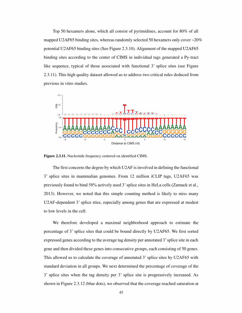
Top 50 hexamers alone, which all consist of pyrimidines, account for 80% of all

mapped U2AF65 binding sites, whereas randomly selected 50 hexamers only cover ~20%

potential U2AF65 binding sites (See Figure 2.3.10). Alignment of the mapped U2AF65

binding sites according to the center of CIMS in individual tags generated a Py-tract

like sequence, typical of those associated with functional 3’ splice sites (see Figure

2.3.11). This high quality dataset allowed us to address two critical rules deduced from

previous in vitro studies.

Figure 2.3.11. Nucleotide frequency centered on identified CIMS.

The first concerns the degree by which U2AF is involved in defining the functional

3’ splice sites in mammalian genomes. From 12 million iCLIP tags, U2AF65 was

previously found to bind 58% actively used 3’ splice sites in HeLa cells (Zarnack et al.,

2013). However, we noted that this simple counting method is likely to miss many

U2AF-dependent 3’ splice sties, especially among genes that are expressed at modest

to low levels in the cell.

We therefore developed a maximal neighborhood approach to estimate the

percentage of 3’ splice sites that could be bound directly by U2AF65. We first sorted

expressed genes according to the average tag density per annotated 3’ splice site in each

gene and then divided these genes into consecutive groups, each consisting of 50 genes.

This allowed us to calculate the coverage of annotated 3’ splice sites by U2AF65 with

standard deviation in all groups. We next determined the percentage of coverage of the

3’ splice sites when the tag density per 3’ splice site is progressively increased. As

shown in Figure 2.3.12 (blue dots), we observed that the coverage reached saturation at

46

~88% with increasing levels of U2AF65 binding at annotated 3’ splice sites, indicating

the existence of ~12% U2AF65-independent introns in the human genome.

Figure 2.3.12. U2AF65 has the capacity to bind ~88% of annotated 3’ splice sites in the human

genome based on the maximal neighborhood analysis. Each blue dot represents averaged occupancy

of group of 50 genes, which were sorted according to the averaged tag density at 3’ splice sites; each

orange dot shows the average of 3’ splice site score among those in each group of 100 genes that

exhibited no U2AF65 binding peaks.

We next asked whether those U2AF65 unbound 3’ splice sites are drifted from

U2AF65 binding consensus. For this purpose, we similarly sorted expressed genes

according to the average tag density per 3’ splice site and then group those splice sites

without U2AF65 peak into consecutive groups, each consisting of a total of 50 introns.

We next calculated the averaged 3’ splice site score of U2AF65 unbound 3’ splice sites

in each group according to Yeo and Burge36. As shown in Figure 2.3.12 (orange dots),

we detected progressive decease in the averaged 3’ splice site score with U2AF65

unbound introns. These data indicate that, among genes that show less efficient U2AF

binding in general, the lack of U2AF binding in unoccupied introns is likely due to

limited expression, but among genes that show extensive U2AF binding, the lack of

47

U2AF binding in the remaining introns likely results from poor consensus in their 3’

splice sites. Therefore, coupled with the maximal neighborhood analysis, our data

suggest that a significant fraction (~12%) of functional 3’ splice sites may indeed

represent U2AF-independent ones.

2.3.3 Additional U2AF binding events beyond functional 3’ splice sites

The second rule concerns the ability of the U2AF heterodimer to discriminate Py-

tracts with or without a flanking AG dinucleotide in mammalian genomes. In vitro

binding studies suggest that U2AF efficiently binds Py-tracts followed by AG, but

much less to Py-tracts without ending with an AG dinucleotide (Wu et al., 1999;

Merendino et al., 1999), and such specificity appears to be enhanced by additional RNA

binding factors, such as DEK and hnRNP A1 (Soares et al., 2006; Tavanez et al., 2012).

Because U2AF65 functions as a heterodimer with U2AF35 based on their tight

interactions in co-IP experiments, it is likely that the mapped genomic U2AF65 binding

events largely reflect the action of the U2AF65/35 heterodimer in vivo, which now

affords us to directly test whether the U2AF heterodimer indeed prefer for Py tracts

each followed by an AG dinucleotide in the human genome.

48

Figure 2.3.13. S65 scores of U2AF65 binding sites in 3’splice sites and non-3’splice sites.

Comparing between U2AF65 binding events on canonical 3’ spice sites and other

regions, we found that both U2AF65-bound 3’ splice sites and non-3' splice sites

exhibited a similar profile of the S65 score, a measure of U2AF65 binding affinity based

on SELEX experiments (Murray et al., 2008) (see Figure 2.3.13). We next segregated

U2AF65 binding events on non-3’ splice sites into two classes. The first contains

potential decoy exons (those with flanking sequences that resemble a 3’ or 5’ splice site)

or pseudo exons (those with flanking potential 3’ and 5’ splice sites separated by a

sequence up to 250nt) (Danckwardt et al., 2007), and the other has no obvious evidence

for any splicing signals. We found that U2AF65 binding at functional 3’ splice sites are

strongly associated with a downstream AG dinucleotide; its binding near decoy and

pseudo exons shows less, but still significant, link to a downstream AG; and the

remaining U2AF65 binding events in other intronic locations exhibit no selective

enrichment with a downstream AG dinucleotide (see Figure 2.3.14).

Figure 2.3.14. The frequency of the AG dinucleotide from the mapped U2AF65 binding sites on

49

annotated 3’ splice sites (red), deduced decoy and pseudo exons (blue), or other intronic regions

(green).

These data suggest that, despite the presence of other specificity enhancing factors

to prevent U2AF65 from binding to other pyrimidine-rich sequences, a significant

fraction of U2AF65 is still able to bind other locations in pre-mRNA besides functional

3’ splice sties. These U2AF65 binding events may interfere with functional definition

of adjacent bone fide 3’ splice sites as a mechanism to modulate alternative splice site

selection (see below) and/or reflect a role of U2AF65 in other RNA metabolism steps,

such as mRNA export (Gama-Carvalho et al., 2006; Xiao et al., 2012).

2.3.4 Critical roles of U2AF in regulated splicing

U2AF65 has been implicated as a regulator of alternative splicing besides its role

in constitutive splicing (Hastings et al., 2007; Pacheco et al., 2006), but it has been

unclear how extensively U2AF65 is involved in regulated splicing in mammalian cells.

To determine this question, we performed RNA-seq, generating 14.1 and 16.8 million

uniquely mapped tags before and after knockdown of U2AF65 in HeLa cells,

respectively (see Table 2.3.2).

Table 2.3.2. Summary information of RNA-seq data.

RNA-Seq data

Ctrl Knock down U2AF65

total reads 28228751 25595461

mapped reads 14384722 17183922

mapped ratio 50.96% 67.14%

uniquely mapped reads 14119360 16834141

uniquely mapped ratio 91.16% 97.96%

50

Figure 2.3.15. Altered alternative splicing events determined by RNA-seq, showing significantly

induced (blue) or repressed (red) splicing events in U2AF65 knockdown cells.

We analyze the RNA-seq data to deduce altered splicing events in an unbiased

manner. Taking advantage of 75nt sequences from both ends of our libraries, we

generated sequence contigs that cover alternative splice junctions, which permitted

calculation of the splicing ratio (Percentage of Splice In or PSI) of individual annotated

cassette exons, as described (Zhou et al., 2012). The data revealed 102 and 343 (out of

a total of 6915) cassette exons that showed significantly increased and decreased

inclusion, respectively, in response to U2AF65 depletion (see Figure 2.3.15).

51

Figure 2.3.16. Splicing of two representative genes in response to U2AF65 knockdown. RNA-seq

data were validated by RT-PCR in HeLa cells treated with two independent U2AF65 RNAi.

Most identified alternative splicing events are evident even from RNA-seq tags

mapped on the alternative and flanking exons (see examples in Figure 2.3.16). We

validated 70 randomly selected alternative splicing events by semi-quantitative RT-

PCR and found that the induced exon inclusion or skipping events detected by RNA-

seq were well correlated with the RT-PCR results (R2=0.65, p-value<2.2e-16, see

Figure 2.3.17).

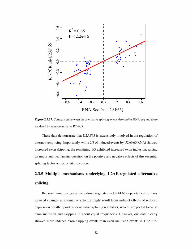
52

Figure 2.3.17. Comparison between the alternative splicing events detected by RNA-seq and those

validated by semi-quantitative RT-PCR.

These data demonstrate that U2AF65 is extensively involved in the regulation of

alternative splicing. Importantly, while 2/3 of induced events by U2AF65 RNAi showed

increased exon skipping, the remaining 1/3 exhibited increased exon inclusion, raising

an important mechanistic question on the positive and negative effects of this essential

splicing factor on splice site selection.

2.3.5 Multiple mechanisms underlying U2AF-regulated alternative

splicing

Because numerous genes were down regulated in U2AF65-depeleted cells, many

induced changes in alternative splicing might result from indirect effects of reduced

expression of either positive or negative splicing regulators, which is expected to cause

exon inclusion and skipping in about equal frequencies. However, our data clearly

showed more induced exon skipping events than exon inclusion events in U2AF65-

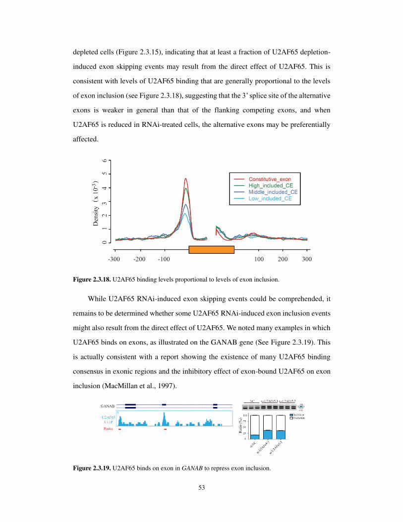
53

depleted cells (Figure 2.3.15), indicating that at least a fraction of U2AF65 depletion-

induced exon skipping events may result from the direct effect of U2AF65. This is

consistent with levels of U2AF65 binding that are generally proportional to the levels

of exon inclusion (see Figure 2.3.18), suggesting that the 3’ splice site of the alternative

exons is weaker in general than that of the flanking competing exons, and when

U2AF65 is reduced in RNAi-treated cells, the alternative exons may be preferentially

affected.

Figure 2.3.18. U2AF65 binding levels proportional to levels of exon inclusion.

While U2AF65 RNAi-induced exon skipping events could be comprehended, it

remains to be determined whether some U2AF65 RNAi-induced exon inclusion events

might also result from the direct effect of U2AF65. We noted many examples in which

U2AF65 binds on exons, as illustrated on the GANAB gene (See Figure 2.3.19). This

is actually consistent with a report showing the existence of many U2AF65 binding

consensus in exonic regions and the inhibitory effect of exon-bound U2AF65 on exon

inclusion (MacMillan et al., 1997).

Figure 2.3.19. U2AF65 binds on exon in GANAB to repress exon inclusion.

54

The mechanism for the inhibitory role of U2AF65 via direct binding on the

alternative exon, however, could not explain numerous other U2AF65 RNAi-induced

exon inclusion events. To aid in mechanistic dissection, we constructed the U2AF65

RNA map based on detected exon inclusion or skipping events in response to U2AF65

RNAi (see Figure 2.3.20).

Figure 2.3.20. Normalized U2AF65 binding events on unaffected cassette exons (black), up-

regulated (blue) or down-regulated (red) cassette exons in U2AF65 knockdown cells. U2AF65

binding appears higher upstream of the alternative cassette exons that were up regulated in response

to U2AF65 knockdown.

However, we could not see any obvious trend for U2AF65-dependent exon

inclusion or skipping, except some additional intronic binding events upstream of

functional 3’ splice sites associated with U2AF65-repressed alternative exons (blue line

in Figure 2.3.20), comparing with the upstream of functional 3’ splice site associated

with the downstream exons.

It is real that the difference in U2AF65 binding in Figure 2. 3.20 are modest. This

is because the size of introns varies greatly. As we displayed U2AF65 intronic binding

events in a lineage fashion, the figure misses many intronic binding events that are

beyond the adjacent regions from 5’ and 3’ splice sites.

55

Figure 2.3.21. Ratio of upstream and downstream intronic binding events on down- and up-

regulated exons

To solve this problem, we choose to keep the original Figure 2.3.20 to illustrate

our points. One of the key features of U2AF-regulated alternative splicing events is

elevated binding of U2AF65 in the upstream intronic region in many up-regulated cases,

which is not evident with down-regulated ones. To further emphasize this point, we

display the ratio of upstream and downstream intronic binding events on down- and up-

regulated exons (see Figure 2.3.21).

It is significant that, among down-regulated exons, the ratio is evenly distributed

between 0 and 1, indicating that the dominant regulatory mode for these events is

selective weakening of U2AF binding at the alternative 3’ splice site relative to the

downstream 3’ splice site. In contrast, we observe that most ratios are >0.5 among up-

regulated exons, indicating that prevalent upstream intronic binding events interfere

with the function of U2AF65 at the 3’ splice site of the alternative exon, and as a result,

removal of such interference induces the inclusion of the alternative exon. This is next

validated by mutational analysis in the following panels, which additionally show that

the same regulatory principle also holds for some strong downstream intronic binding

events where they interfere with the function of U2AF65 at the 3’ splice site of the

56

downstream exon, thus producing the opposite functional consequence.

Figure 2.3.22. CU content levels proportional to levels of exon inclusion.

This is highly consistent with levels of CU content (U2AF65 binding sequence) in

the upstream region of 3’ splice site of cassette exon (the bigger box regions in Figure

2.3.22) that are generally inversely proportional to the levels of exon inclusion (see

Figure 2.3.22), suggesting that the more CU content, or the more U2AF65 binds in the

upstream region of functional 3’ splice site, the less cassette exons included.

This finding raises an intriguing possibility that these additional U2AF65 binding

events may interfere with normal recognition of adjacent functional 3’ splice sites.

2.3.6 Polar effect of U2AF65 binding on downstream 3’ splice site

recognition

We chose three representative genes to perform mutational analysis on their

minigenes, which could avoid potential indirect effects of U2AF65 depletion, and to

compare between the effect of deletion mutations and response to U2AF RNAi.

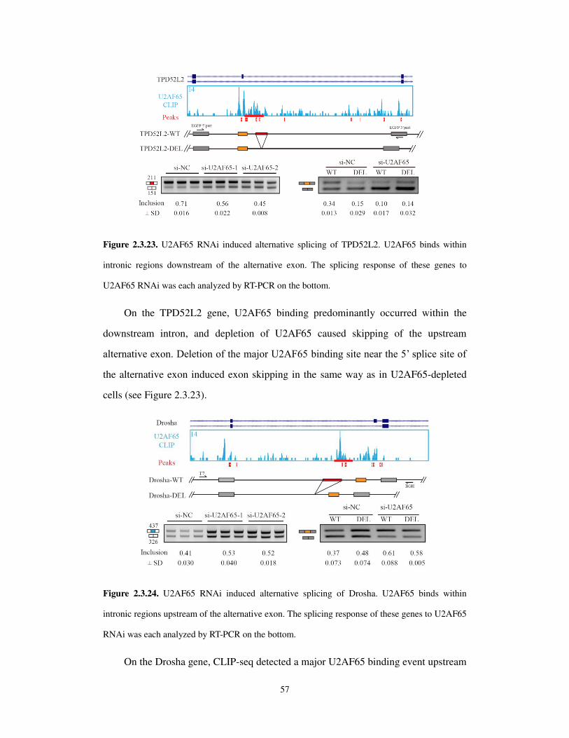
57

Figure 2.3.23. U2AF65 RNAi induced alternative splicing of TPD52L2. U2AF65 binds within

intronic regions downstream of the alternative exon. The splicing response of these genes to

U2AF65 RNAi was each analyzed by RT-PCR on the bottom.

On the TPD52L2 gene, U2AF65 binding predominantly occurred within the

downstream intron, and depletion of U2AF65 caused skipping of the upstream

alternative exon. Deletion of the major U2AF65 binding site near the 5’ splice site of

the alternative exon induced exon skipping in the same way as in U2AF65-depleted

cells (see Figure 2.3.23).

Figure 2.3.24. U2AF65 RNAi induced alternative splicing of Drosha. U2AF65 binds within

intronic regions upstream of the alternative exon. The splicing response of these genes to U2AF65

RNAi was each analyzed by RT-PCR on the bottom.

On the Drosha gene, CLIP-seq detected a major U2AF65 binding event upstream

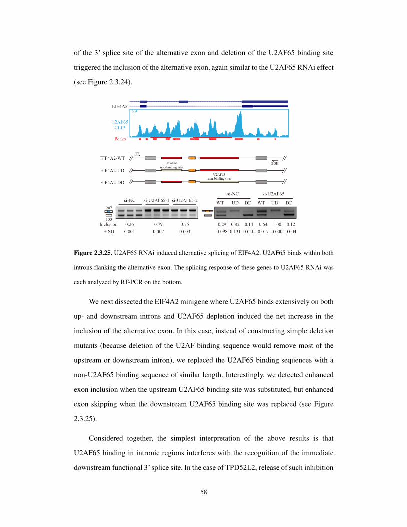
58

of the 3’ splice site of the alternative exon and deletion of the U2AF65 binding site

triggered the inclusion of the alternative exon, again similar to the U2AF65 RNAi effect

(see Figure 2.3.24).

Figure 2.3.25. U2AF65 RNAi induced alternative splicing of EIF4A2. U2AF65 binds within both

introns flanking the alternative exon. The splicing response of these genes to U2AF65 RNAi was

each analyzed by RT-PCR on the bottom.

We next dissected the EIF4A2 minigene where U2AF65 binds extensively on both

up- and downstream introns and U2AF65 depletion induced the net increase in the

inclusion of the alternative exon. In this case, instead of constructing simple deletion

mutants (because deletion of the U2AF binding sequence would remove most of the

upstream or downstream intron), we replaced the U2AF65 binding sequences with a

non-U2AF65 binding sequence of similar length. Interestingly, we detected enhanced

exon inclusion when the upstream U2AF65 binding site was substituted, but enhanced

exon skipping when the downstream U2AF65 binding site was replaced (see Figure

2.3.25).

Considered together, the simplest interpretation of the above results is that

U2AF65 binding in intronic regions interferes with the recognition of the immediate

downstream functional 3’ splice site. In the case of TPD52L2, release of such inhibition

59

increases the competitiveness of the flanking 3’ splice site, thereby suppressing the

selection of the upstream 3’ splice site associated with the alternative exon. This is also

the case with U2AF65 binding in the downstream intron of the EIF4A2 gene. On the

other hand, the removal of U2AF65 competition from the upstream intron in both

Drosha and EIF4A2 genes likely increases the competitiveness of the 3’ splice site of

the alternative exon, allowing it to be included more efficiently in each case. When both

competing events are operating in the same alternative splicing unit, a strong one would

win, as in the case the EIF4A2 gene, thus generating a net effect of exon inclusion in

U2AF65-depleted cells.

Figure 2.3.26. Proposed polar effect model for the effect of intronically bound U2AF65 to interfere

with the recognition of the immediate downstream 3’ splice site in regulated splicing.

Based on these findings, we propose a polar mechanism for intronic U2AF65

binding to interfere with the recognition of the downstream 3’ splice site (see Figure

2.3.26).

2.3.7 Coordinated action of U2AF65 and U2AF35 in regulated splicing

It has been unclear thus far whether U2AF65 predominantly acts alone or in

conjunction with U2AF35 or with other U2AF35-related molecules in the regulation of

alternative splicing. Because the vast majority of U2AF65 appears to exist as the

heterodimer with U2AF35 in the cell, it is likely that the U2AF65/35 heterodimer may

play a dominant role in both constitutive and regulated splicing. To directly test this

hypothesis, we used alternative splicing as a functional readout to compare the cellular

response to U2AF65 and U2AF35 RNAi. As previously reported (Pacheco et al., 2006),

U2AF35 RNAi only reduced the expression of U2AF35 while U2AF65 RNAi reduced

the levels of both subunits of the U2AF heterodimer (see Figure 2.3.27).

60

Figure 2.3.27. Western blotting analysis of RNAi-mediated U2AF65 and U2AF35 knockdown.

Note reduced U2AF35 in U2AF65 RNAi-treated cells.

To determine how the reduction of U2AF35 alone or the U2AF65/35 heterodimer

might affect alternative splicing from a global prospective, we employed the RASL-seq

based technology we recently developed (Wei et al., 2012) to conduct a cost-effective

survey of alternative splicing events in U2AF65 and U2AF35 RNAi-treated HeLa cells.

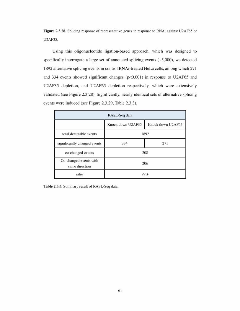
61

Figure 2.3.28. Splicing response of representative genes in response to RNAi against U2AF65 or

U2AF35.

Using this oligonucleotide ligation-based approach, which was designed to

specifically interrogate a large set of annotated splicing events (~5,000), we detected

1892 alternative splicing events in control RNAi-treated HeLa cells, among which 271

and 334 events showed significant changes (p<0.001) in response to U2AF65 and

U2AF35 depletion, and U2AF65 depletion respectively, which were extensively

validated (see Figure 2.3.28). Significantly, nearly identical sets of alternative splicing

events were induced (see Figure 2.3.29, Table 2.3.3).

RASL-Seq data

Knock down U2AF35 Knock down U2AF65

total detectable events 1892

significantly changed events 334 271

co-changed events 208

Co-changed events with same direction

206

ratio 99%

Table 2.3.3. Summary result of RASL-Seq data.

62

Figure 2.3.29. Global concordance of U2AF65 and U2AF35 dependent splicing revealed by RASL-

seq.

While since depletion of U2AF65 also decreases the levels of U2AF35 (see Figure

2.3.27), it cannot be concluded that U2AF35 largely functions in conjunction with

U2AF65 in the regulation of AS in mammalian cells. It could be that the effects seen in

both experiments are due to a decreased level of U2AF35. So we should overexpress

U2AF35 in cells that are subject to siRNA against U2AF65. If then, U2AF35 reach

levels similar to the control, then they will be able to control effects of depleting

U2AF35 and U2AF65.

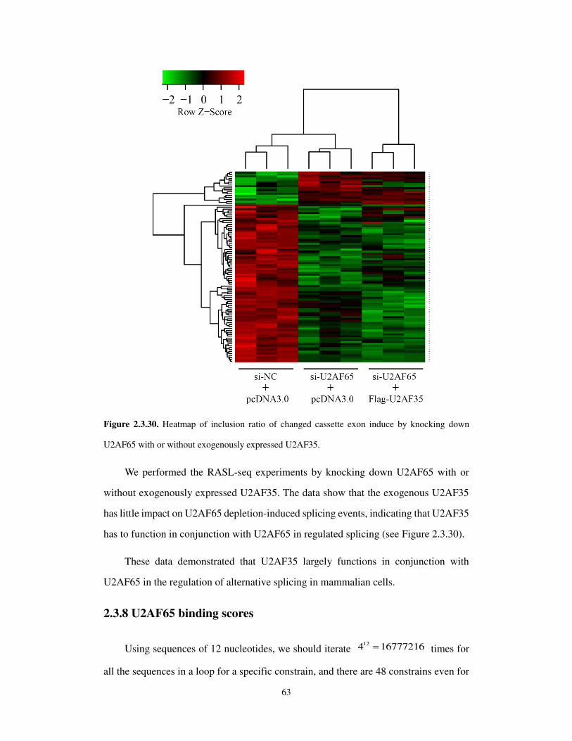
63

Figure 2.3.30. Heatmap of inclusion ratio of changed cassette exon induce by knocking down

U2AF65 with or without exogenously expressed U2AF35.

We performed the RASL-seq experiments by knocking down U2AF65 with or

without exogenously expressed U2AF35. The data show that the exogenous U2AF35

has little impact on U2AF65 depletion-induced splicing events, indicating that U2AF35

has to function in conjunction with U2AF65 in regulated splicing (see Figure 2.3.30).

These data demonstrated that U2AF35 largely functions in conjunction with

U2AF65 in the regulation of alternative splicing in mammalian cells.

2.3.8 U2AF65 binding scores

Using sequences of 12 nucleotides, we should iterate 124 16777216 times for

all the sequences in a loop for a specific constrain, and there are 48 constrains even for

64

the simplest type of pattern. Being limited of our computers’ performance, we have

only tried three kinds of patterns now. Latter, we could try to break the long target

sequences into smaller ones to predict, and then join them together. In this way, we

could test more complex pattern and mixed pattern of them.

The three patterns just present the weight matrix model (me1s0), the first-order

Markov model (me2s0) and a simplest nonadjacent dependence model (me2s1) (see

Figure 2.3.31). As shown in Figure 2.3.31, there are not too much difference among

them, indicating that the adjacent and nonadjacent dependencies between nucleotides

maybe not be used so much by U2AF65 to recognize it target sites. And all the patterns

do not perform very well. We think that there are two reasons at least: There are many

assistant factors (U2AF35, hnRNPA1) could help U2AF65 to recognize target sites, as

described previously; RNA structures in the intronic regions may also affect U2AF65

binding on the target patterns.

Figure 2.3.31. Receiver operating characteristic (ROC) curve of three type of constrains performing

on test data sets. ‘me’ stands for maximum entropy model; ‘s’ stands for skipping. For example,

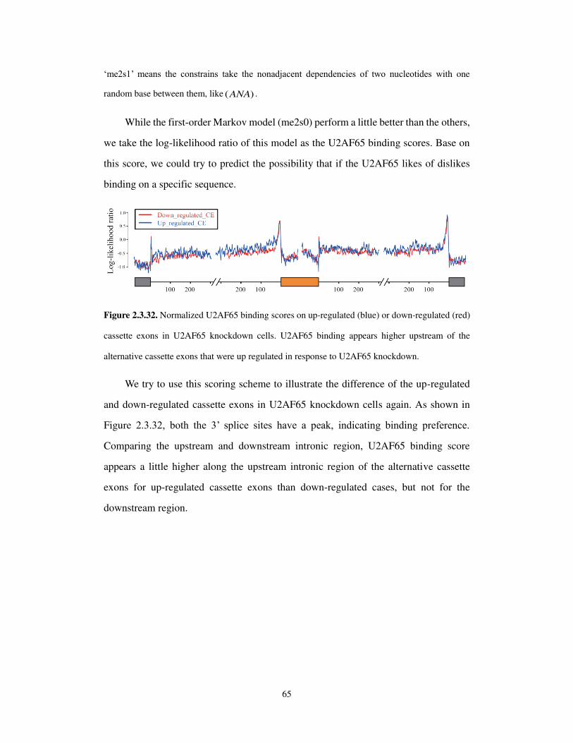
65

‘me2s1’ means the constrains take the nonadjacent dependencies of two nucleotides with one

random base between them, like ( )ANA .

While the first-order Markov model (me2s0) perform a little better than the others,

we take the log-likelihood ratio of this model as the U2AF65 binding scores. Base on

this score, we could try to predict the possibility that if the U2AF65 likes of dislikes

binding on a specific sequence.

Figure 2.3.32. Normalized U2AF65 binding scores on up-regulated (blue) or down-regulated (red)

cassette exons in U2AF65 knockdown cells. U2AF65 binding appears higher upstream of the

alternative cassette exons that were up regulated in response to U2AF65 knockdown.

We try to use this scoring scheme to illustrate the difference of the up-regulated

and down-regulated cassette exons in U2AF65 knockdown cells again. As shown in

Figure 2.3.32, both the 3’ splice sites have a peak, indicating binding preference.

Comparing the upstream and downstream intronic region, U2AF65 binding score

appears a little higher along the upstream intronic region of the alternative cassette

exons for up-regulated cassette exons than down-regulated cases, but not for the

downstream region.

66

2.4 Discussion

Our current genome-wide study demonstrates that U2AF65 plays a predominant

role in functional definition of 3’ splice sites and is required for efficient expression of

most intron-containing genes in the human genome. Interestingly, however, our data

also suggest the existence of ~12% U2AF65-independent introns because they lack

evidence for U2AF65 binding and their Py tracts are considerably degenerate from the

pyrimidine-rich consensus. It is important to point out that the functional requirement

for U2AF is not strictly determined by the consensus, as many poor 3’ splice sites could

be aided in by other intronic splicing enhancer factors, such as YB1 (Shen et al., 2010).

However, the existence of a fraction of U2AF-independent introns is fully consistent

with the observations made in fission yeast (Sridharan et al., 2011; Sridharan et al.,

2007), which begs the question of which specific splicing factors fulfill such role in

defining various untypical 3’ splice sites. Although several RNA binding splicing

factors have structures related to U2AF65 or U2AF35 (Mollet et al., 2006), the

available functional evidence suggests that most of them function in synergy with,

rather than independently from, U2AF (Page-McCaw et al., 1999; Tronchere et al.,

1997; Shepard et al., 2002; Han et al., 2011b). Therefore, it remains to be understood

how U2AF-independent introns are recognized in mammalian genomes.

The preferential binding of U2AF65 to functional 3’ splice sites over other

pyrimidine-rich sequences in the genome appears to be enforced by the U2AF35

subunit. Other factors have also been suggested to provide the proofreading function of

the U2AF heterodimer in the genome (Soares et al., 2006; Tavanez et al., 2012).

However, our genome-wide binding data clearly show that U2AF65 can also bind to

various locations that are not part of annotated 3’ splice sites and these binding events

do not seem to depend on a downstream AG dinucleotide. This is consistent with the

proposed function of U2AF65 in promoting nuclear export of intronless transcripts in

Drosophila (Gama-Carvalho et al., 2006) and with binding of U2AF65 on some spliced

mRNAs (Xiao et al., 2012). A more recent study showed that hnRNP C is able to

prevent U2AF65 from binding to many Alu-containing transcripts to suppress

67

exonization of those Alu elements (Zarnack et al., 2013). Therefore, U2AF binding

appears to be a highly regulated process in mammalian genomes.

Besides its role in constitutive splicing, U2AF has been implicated in the

regulation of alternative splicing. Our metagene analysis indicates that U2AF binding

on the 3’ splice site of alternative exons generally tracks the level of exon inclusion.

This has been generally perceived as a predominant mechanism for U2AF-regulated

splicing. However, we also found that U2AF65 exhibits other modes of binding in the

human genome, one corresponding to its binding to exonic regions to interfere with the

selection of nearby 3’ splice site, which has been demonstrated on engineered

minigenes (Lim et al., 2011). A more widespread mode of U2AF65 binding appears to

occur in various intronic locations.

By mutational analysis, we found that those intronic U2AF65 binding events

appear to selectively interfere with the recognition of the immediate downstream 3’

splice site, and thus, the competition between the alternative and flanking constitutive

splice sites dictates the splicing outcome. This splice site competition model provides

a universal mechanism for the regulation of alternative splicing by both sequence-

specific RNA binding proteins and core components of the splicing machinery (Zhou

et al., 2012). The observed polar effect may underlie the positional effect of many other

splicing regulators whose binding on the upstream intron may inhibit the inclusion of

the alternative exon, whereas their interaction with the downstream intron may induce

the skipping of the alternative exon (Przychodzen et al., 2013).

One of the most important advances in the field is the identification of specific

mutations in multiple splicing factors, including U2AF65 and U2AF35, in specific

types of myeloid leukemia. Because of the prevalence of those mutations in the disease,

they are generally considered driver mutations, which actually remain to be functionally

defined.

Therefore, although our current study was not carried out in a disease-relevant cell

type, our findings provide critical insights into the nature of specific mutations in the

68

splicing regulators. The challenge ahead is to link specific molecular defects in right

cell types, likely hemopoietic stem cells, to the etiology of the disease.

69

Chapter 3: Consistent-Pivot: A New effective Pivot

Algorithms for Ranking Aggregation Problem

3.1 Introduction

With the increasing development of high throughput technologies, very high

amounts of data are produced and stored in public databases to make them available to

the scientific community, for example, Gene Expression Omnibus (GEO) which is a

public functional high-throughput sequencing genomics data repository (Barrett et al.,

2013) (see Figure 3.1.1).

Figure 3.1.1. Distribution of the number and types of selected studies released by GEO each year

since inception. Users can explore and download historical submission numbers using the ‘history’

page, as well as constructing GEO DataSet database queries for specific data types and date ranges

using the ‘DataSet type’ and ‘publication date’ fields. Figure from (Barrett et al., 2013)

70

From the biological Big Data, vast amounts of genes lists of expression, regulation,

interaction, correlation could be extracted from the data mining results, such as cell

expressed microRNAs, gene regulated genes, protein-protein interaction, disease

related genes, or just gene association from text mining (Metzker, 2010). Facing these

kinds of lists, it is very difficult to exploit them if they are not ranked. However,

rankings of biological data on a same query are always very different between different

processing methods, algorithms or datasets, especially for biological data mostly with

noise, fuzziness, biases and errors (Brusic et al., 1998). Based on all these issues, how

to get a convincible ranking result from biological data becomes an important task

in post-genome era.

Instead of developing new ranking methods, Cohen-Boulakia and her colleagues

proposed to generate a consensus ranking to highlight the common points of a set of

rankings while minimizing their disagreements to combat the noise and error for

biological data (Cohen-Boulakia et al., 2011). This idea had already been used for

combining results of microarray data (DeConde et al., 2006), microRNA targets

prediction algorithms (Sengupta et al., 2013), Comparison ligand-binding site

prediction methods (Gao et al., 2012), and so on.

There has been also a lot of interest in this problem in the computer science

community in recent years which arises when building meta-search engines for Web

search, where one wants to combine the rankings obtained by different algorithms into

a representative ranking. For example, Dwork combines the rankings of individual

search engines to get more robust rankings that are not sensitive to the various

shortcomings and biases of individual search engines (for instance, “paid placement”

and “paid inclusion” among search engines) (Dwork et al., 2001).

The process of generating a consensus ranking is based on the concept of ranking

aggregation, originating in social choice theory, machine learning, and theoretical

computer science (Ali et al., 2012), defined on rankings: Given m rankings of n

elements and a distance function, the ranking aggregation problem is to find a ranking

of all the elements that is the closest of the m given rankings.

71

It could be easily thought of a kind of a ranking aggregation method, where the

order of each element is determined by taking simple average of positions of it from

different rankings. This method was firstly proposed by Borda as a voting system for

elections in the late eighteenth century (Young, 1974). Condorcet proposed a more

reasonable method of pairwise majority voting known as Condorcet’s criterion, which

permits A to be ranked higher than B if the majority vote for A over B in

pairwise comparison, even if the average of positions of A is after B (De Grazia,

1953).

Obeying to extended Condorcet criterion, Kemeny proposed the Kemeny optimal

aggregation for determining the best aggregate ranking based on the Kendall-tau

distance which counts the number of pairwise disagreements between orderings of

elements (Kemeny et al., 1962).

However, Kemeny optimal aggregation is unfortunately a computational challenge,

because the problem is NP-hard even for only four rankings (Dwork et al., 2001; Blin

et al., 2011). Since the problem is important across a variety of fields, many researchers

across these fields have converged on finding good, practical algorithms for its solution.

There are formulations that lead to exact algorithms, of course without polynomial

running time guarantees. There are also a large number of heuristic and approximation

algorithms.

Among these, a group of algorithms are thought to be very prospective, named

pivot algorithms (Ailon et al., 2008; Van Zuylen et al., 2009). In common, they

recursively generate a solution by choosing an elements as pivot and ordering all the

other elements with respect to the pivot according to some criterion. It divides the

problem into smaller ones and conquers separately, and uses the transitive property (see

below) which is right in most situations, especially for the rankings with high agreement.

So the pivot algorithms are always fast in time and not bad in accuracy.

In this chapter, we propose a new variant of pivot algorithms named as Consistent-

Pivot. It uses a new strategy of pivot selection and other elements assignment which

72

performs much better both on computation time and accuracy than previous pivot

algorithms.

73

3.2 Notations

In this section, we introduce the definition of ranking and the distance used to

compare two rankings, then we provide the general statement of the problem of

Kemeny optimal aggregation with ties under generalized Kendall-tau distance.

3.2.1 Ranking with ties

Following the definition of Fagin and his colleagues, given a universe set U , a

ranking with ties ( or bucket order) of a subset S U , r is a transitive binary relation

represented as set of non-empty buckets 1,..., kB B that form a disjoint partition of

the elements of S , such that x y if and only if there are i , j with i j such

that ix B and jy B (Fagin, 2004). We may assume without loss of generality that

a ranking with ties on [ ]n is defined as 1[ ,..., ]kr B B , and let ( )r x i if ix B

which denotes the rank of x .

If r contains all the elements in U , then it is said to be a full ranking. There are

situations where full rankings are not possible. For instance, the ranking result of target

genes of a miRNA from a prediction tool usually cannot include all the targets. Such

rankings that rank only some of the elements in U are called partial rankings.

3.2.2 Unifying a set of partial rankings

Aiming to penalize the fact that one element is considered in a ranking but not in

another one, Cohen-Boulakia and her colleagues present a unifying preprocess for sets

of partial rankings to append the set of elements belonging to the other rankings to the

end in a same bucket.

Example 1 For instance, let us consider three different ranking methods which outputs

are the following:

74

1

2

3

[{1},{7},{2},{3}]

[{2,4,5},{7},{3}]

[{1,2,3},{4,5},{6,7}]

r

r

r

Here we have {1,2,3, ,7}U , 1\ {4,5,6}U r , 2\ {1,6}U r and 3\U r .

The rankings processed using the unifying preprocess are then the followings:

'1

'2

'3

[{1},{7},{2},{3},{4,5,6}]

[{2,4,5},{7},{3},{1,6}]

[{1,2,3},{4,5},{6,7}]

r

r

r

This is a normalized method to facilitate the comparison between the rankings and

the consensus ranking, especially for comparing the performance of the different

ranking methods. In the remainder of this chapter, the unifying preprocess is applied

before running the ranking aggregation algorithm.

3.2.3 Distance measures

How do we define a distance between two full rankings with respect to a set S ?

In the last century, this problem has been studied and defined from a mathematical

perspective (Kendall, 1938).

3.2.3.1 The Spearman footrule distance

For all elements i S , the Spearman footrule distance is the sum of the absolute

difference between the rank level of i according to the two rankings. Formally, given

two full rankings 1r and 2r , the distance is given by:

1 2 1 21

( , ) [ ] [ ]s

i

F r r r i r i

So if based on the Spearman footrule distance, the consensus ranking of m

rankings with smallest distance is just the median value of the set of positions of every

element in the m rankings, because only in this way, the footrule distance is the

smallest (Dwork et al., 2007).

75

3.2.3.2 Kendall-tau distance

A good dissimilarity measure for comparing two rankings without ties is the

Kendall-tau distance which counts the number of pairwise disagreements between

positions of elements in these rankings (Kendall, 1938). The larger the distance, the

more dissimilar the two rankings are. Kendall-tau distance is also called bubble-sort

distance since it is equivalent to the number of swaps that the bubble sort algorithm

would make to place one ranking in the same order as the other ranking.

A strict ranking without ties, or permutation, r is a bijection of [ ] {1,2..., }n n

on to itself. It represents a strict total order of the elements of [ ]n . The Kendall-tau

distance, denoted K , counts the number of pairwise disagreements between two

permutations. For permutations 1r and 2r of [ ]n , it is defined as:

1 2 1 1 2 2

1 1 2 2

( , ) #{( , ) : and [( [ ] [ ] and [ ] [ ]) or

( [ ] [ ] and [ ] [ ])]}

K r r i j i j r i r j r i r j

r i r j r i r j

where [ ]r i denotes the position of integer i in permutation r and # S the

cardinality of set S . For example, if

1 [{1},{2},{3},{4}]r ,

2 [{2},{3},{1},{4}]r ,

then 1 2( , ) 2K r r since elements 1 and 2 appear in different orders in the two

rankings as do elements 1 and 3, but not others.

3.2.3.3 Generalized Kendall-tau distance for rankings with ties

Following the definition of Fagin et al., the generalized Kendall-tau distance,

denoted ( )pK (or simply K , when parameter 1p ), is defined according to a

parameter p , 0 1p :

76

( )1 2 1 1 2 2

1 1 2 2

1 1 2

( , ) #{( , ) : and [( [ ] [ ] and [ ] [ ]) or

( [ ] [ ] and [ ] [ ])]}

#{( , ) : and [( [ ] [ ] and

pK r r i j i j r i r j r i r j

r i r j r i r j

p i j i j r i r j r

2

1 1 2 2

[ ] [ ]) or

( [ ] [ ] and [ ] [ ])]}

i r j

r i r j r i r j

In other words, the generalized Kendall-tau distance considers the number of

disagreements between two rankings with ties: a disagreement can be either two

elements that are in different buckets in each ranking, where the order of the buckets

disagree, and each such disagreement counts for 1 in the distance; or two elements that

are in the same bucket in one ranking and in different buckets in the other, and each

such disagreement counts for p , 0 1p . For example, if

1 [{1},{2,3,4}]r

2 [{2,3},{1,4}]r ,

then 1 2( , ) 2 3K r r p since two pairs of elements 1 and 2, 1 and 3 appear in

different orders in the two rankings, and three pair of elements 1 and 4, 2 and 4, 3 and

4 appear in different buckets in one ranking while in a same bucket in the other ranking.

3.2.4 Kemeny optimal aggregations

Based on the definition of Kendall-tau distance, Kemeny proposed a precise

criterion for determining the “best” aggregate ranking (Kemeny and James, 1962).

Given n elements and m rankings of the elements, a Kemeny optimal ranking of

the elements is a ranking *r that minimizes the sum of distances, 1

( *, )m

ii

K r r . In

other words a Kemeny optimal ranking minimizes the number of pairwise

disagreements with the given m rankings, corresponding to the geometric median of

the inputs (Farah and Vanderpooten, 2007).

More formally, let nRank be the set of all possible rankings with ties over [ ]n .

Given any subset nR Rank and a ranking r , we define

77

( ) ( )( , ) ( , )i

p pi

r R

K r R K r r

A Kemeny optimal ranking of a set of rankings with ties nR Rank under the

generalized Kendall-tau distance is a ranking with ties *r such as

( ) * ( )( , ) ( , ), for all p pnK r R K r R r Rank

Kemeny optimal aggregations have maximum likelihood interpretation. Suppose

there is an underlying “correct” ordering *r of S , and each order, 1r , 2r … ir , is

obtained from *r by swapping two elements with some probability less than 1/ 2 .

Thus, the ( ir )s are “noisy” versions of *r . A Kemeny optimal aggregation of 1r , 2r …

ir , is one that is maximally likely to have produced the ( ir )s, so it is just *r . Viewed in

this way, Kemeny optimal aggregation has the property of eliminating noise from

various different ranking schemes (Dwork et al., 2007).

However finding a Kemeny optimal ranking is NP-hard and remains NP-hard even

when there are only four input rankings to aggregate (Dwork et al., 2001; Blin et al.,

2011). This motivates the problem of finding a ranking that approximately minimizes

the number of disagreements with the given input rankings.

78

3.3 Previous algorithms

As for the Kemeny optimal aggregation problem, Conitzer et al have provided a

integer linear programming scheme for treating strict rankings (Conitzer et al., 2006)

and Blin expands it generally for rankings with ties (Brancotte et al., in preparation).

However, of course solving the integer linear programming problem is also NP-hard.

Another exact algorithm was proposed by Meila et al. It is a branch and bound

algorithm (B&B). Each node in the search tree corresponds to a prefix

1 2[ , , , ]jx x x of *r , so that level j in the tree contains all possible prefixes of

length j ; branching is on the item to be added in rank 1j which is one of the other

elements. The cost and cost-to-go at a node are computed for bounding. A brute force

search tree has !n paths if there are no ties, while if the lower bound of some nodes

A is greater than the upper bound of some other nodes B , branch and bound

algorithm could safely discard A from the search, what is called pruning. However

in bad cases, as aggregation of strong disagreement rankings, pruning can not always

be effective. So, branch and bound algorithm, limiting the available memory leads to a

family of approximate algorithms in which memory and runtime can be traded off for

accuracy.

So, many heuristic and approximate algorithms were developed.

3.3.1 Some heuristics and approximation algorithms

Heuristics and approximation algorithms are techniques designed for solving a

problem more quickly when classic methods are too slow, or when classic methods fail

to find any exact solution, especially for NP-hard problems. However, more than

heuristics algorithms, approximation algorithms want provable solution quality and

provable run-time bounds. For example, a -approximation algorithm A is defined

to be an algorithm for which it is proven that the result of the approximation algorithm

( )A x will not be more (or less, depending on the situation) than a factor times the

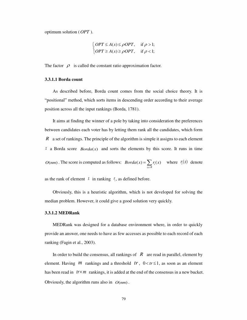
79

optimum solution ( OPT ).

( ) , if 1;( ) , if 1;

OPT A x OPT

OPT A x OPT

The factor is called the constant ratio approximation factor.

3.3.1.1 Borda count

As described before, Borda count comes from the social choice theory. It is

“positional” method, which sorts items in descending order according to their average

position across all the input rankings (Borda, 1781).

It aims at finding the winner of a pole by taking into consideration the preferences

between candidates each voter has by letting them rank all the candidates, which form

R a set of rankings. The principle of the algorithm is simple it assigns to each element

x a Borda score ( )Borda x and sorts the elements by this score. It runs in time

( )O nm . The score is computed as follows: ( ) ( )i

ir R

Borda x r x

where ( )ir x denote

as the rank of element x in ranking ir , as defined before.

Obviously, this is a heuristic algorithm, which is not developed for solving the

median problem. However, it could give a good solution very quickly.

3.3.1.2 MEDRank

MEDRank was designed for a database environment where, in order to quickly

provide an answer, one needs to have as few accesses as possible to each record of each

ranking (Fagin et al., 2003).

In order to build the consensus, all rankings of R are read in parallel, element by

element. Having m rankings and a threshold tr , 0 1tr , as soon as an element

has been read in tr m rankings, it is added at the end of the consensus in a new bucket.

Obviously, the algorithm runs also in ( )O nm .

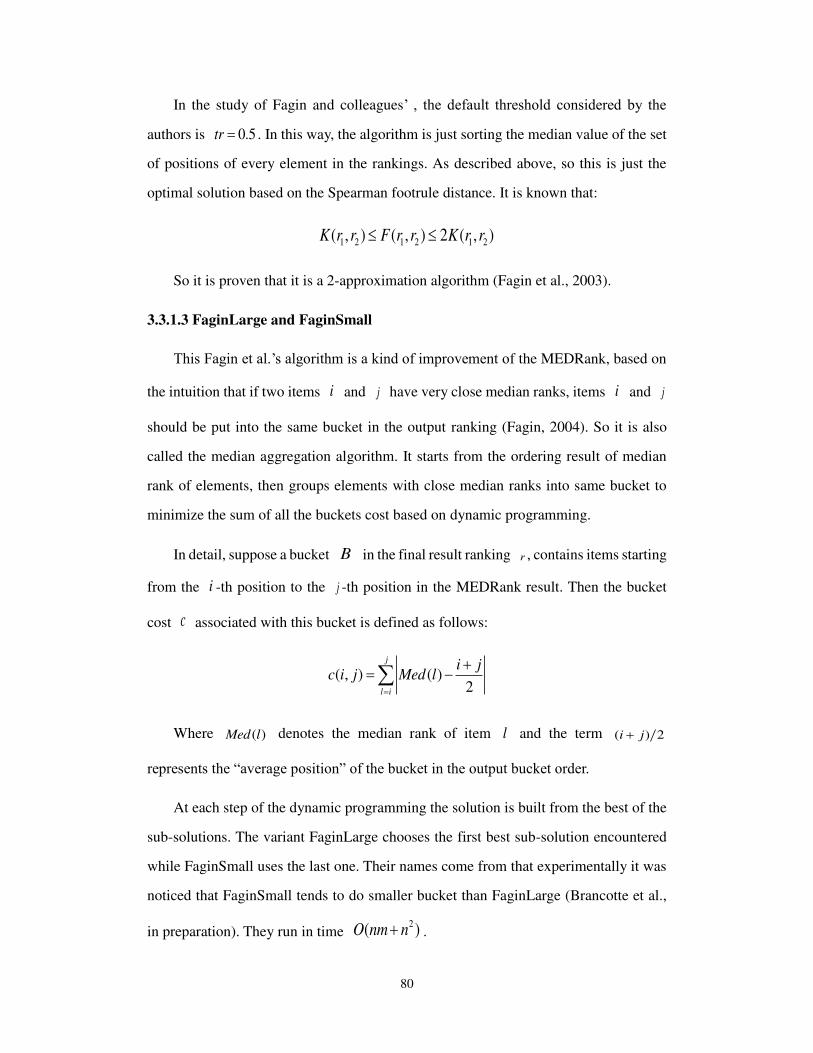
80

In the study of Fagin and colleagues’ , the default threshold considered by the

authors is 0.5tr . In this way, the algorithm is just sorting the median value of the set

of positions of every element in the rankings. As described above, so this is just the

optimal solution based on the Spearman footrule distance. It is known that:

1 2 1 2 1 2( , ) ( , ) 2 ( , )K r r F r r K r r

So it is proven that it is a 2-approximation algorithm (Fagin et al., 2003).

3.3.1.3 FaginLarge and FaginSmall

This Fagin et al.’s algorithm is a kind of improvement of the MEDRank, based on

the intuition that if two items i and j have very close median ranks, items i and j

should be put into the same bucket in the output ranking (Fagin, 2004). So it is also

called the median aggregation algorithm. It starts from the ordering result of median

rank of elements, then groups elements with close median ranks into same bucket to

minimize the sum of all the buckets cost based on dynamic programming.

In detail, suppose a bucket B in the final result ranking r , contains items starting

from the i -th position to the j -th position in the MEDRank result. Then the bucket

cost c associated with this bucket is defined as follows:

( , ) ( )2

j

l i

i jc i j Med l

Where ( )Med l denotes the median rank of item l and the term ( ) 2i j

represents the “average position” of the bucket in the output bucket order.

At each step of the dynamic programming the solution is built from the best of the

sub-solutions. The variant FaginLarge chooses the first best sub-solution encountered

while FaginSmall uses the last one. Their names come from that experimentally it was

noticed that FaginSmall tends to do smaller bucket than FaginLarge (Brancotte et al.,

in preparation). They run in time 2( )O nm n .

81

It has been proven that this algorithm is a constant factor approximation both full

rankings and partial rankings. For full rankings, the median aggregation algorithm gives

a near-optimal full ranking, with an approximation factor of two (Fagin, 2004).

3.3.1.4 BioConsert

BioConsert was proposed by Cohen-Boulakia and her colleagues. It works by

iteratively trying to move a element to another bucket or a new bucket from an input

ranking to reduce the sum of Kendall-tau distance which improves the input ranking

step by step. If none of the elements are changed from their buckets, then the algorithm

terminates (see Algorithm 1) (Cohen-Boulakia et al., 2011).

Algorithm 1. BioConsert

In contrast to the two previous one, this heuristic is an anytime algorithm, as the

82

input ranking is iteratively improved and interrupting the algorithm at any time will

return a proper result. This heuristic can be implemented with a time complexity of

3( )O n m . BioConsert is a kind of local search algorithm. At each step, the BioConsert

algorithm is only looking for a better neighbor. So it would falls in to a local best

solution, which can be the global best one sometimes.

3.3.2 Other algorithms

There are some other algorithms for the ranking aggregation problem. Dwork et al.

introduced a Markov chain based algorithm (Dwork et al., 2001). Qin and colleagues

developed a posibility based algorithm (Qin et al., 2010). In addition, the attempts of

combinations of several algorithm to give a better result were also reported (Ailon et

al., 2008; Schalekamp and van Zuylen, 2009; Ali and Marina, 2012). For example, the

combination of KwikSort and Pick-A-Perm could get a 117

-factor approximation

algorithm, which is a little better than KwikSort algorithm (2-factor approximation

algorithm).

3.3.3 Pivot Algorithms

Previous pivot algorithms are all published for rankings without ties, but they all

could be expanded to the rankings with ties. Besides the two relationships for two

elements ( i j , i is before j ; i j , i is after j ), rankings with ties allow elements

in a same level. So, it is a little more complex for rankings with ties. Here for simple

description, we follow the same situations described in the papers before for the

previous pivot algorithms.

3.3.3.1 Transitive property and conflicts

We define the weight that element i is before element j as ijw , which is how

many times the element i is before element j in the m rankings. So if ij jiw w ,

we would say that the situation where element i is before element j ( i j ) is

83

dominant.

We have stated that sets of rankings usually have transitive property for elements.

It means that if i j and j k are dominant for the set of rankings, we could usually

see that i k in most time (or, i j k ), especially for the rankings with high

agreement. Let us illustrate this property in an example, for the three rankings below:

1

2

3

[{1},{3},{4},{2}];

[{4},{2},{3},{1}];

[{1},{2},{3},{4}].

r

r

r

Here we try to illustrate the positional relationship of all the elements in a weighted

directed graph (see Figure 3.3.1). The relationship of “before” is plotted on the upside,

and “after” is plotted on the underside. In this weighted directed graph, all the thicker

lines have a weight of 2, while the thinner lines have a weight of 1. As shown in the

figure, element 1 is before element 2 in two rankings ( 1r and 3r ), so there is a thicker

line (weight of 2 in this figure) linking the element 1 to the element 2. At the same time,

element 1 is after element 2 in the ranking 2r , so there is also a thinner line (weight of

1 in this figure) linking the element 2 to the element 1. Here it is the dominant positional

relationship between the two elements that element 1 is before element 2 (1 2 )

Figure 3.3.1. A weighted digraph to describe the positional relationship of all the elements. The

relationship of “before” is plotted on the upside, and “after” is plotted on the underside. In this

weighted digraph, all the thicker lines have a weight of 2, while the thinner lines have a weight of

1 2 3 4

Before

After

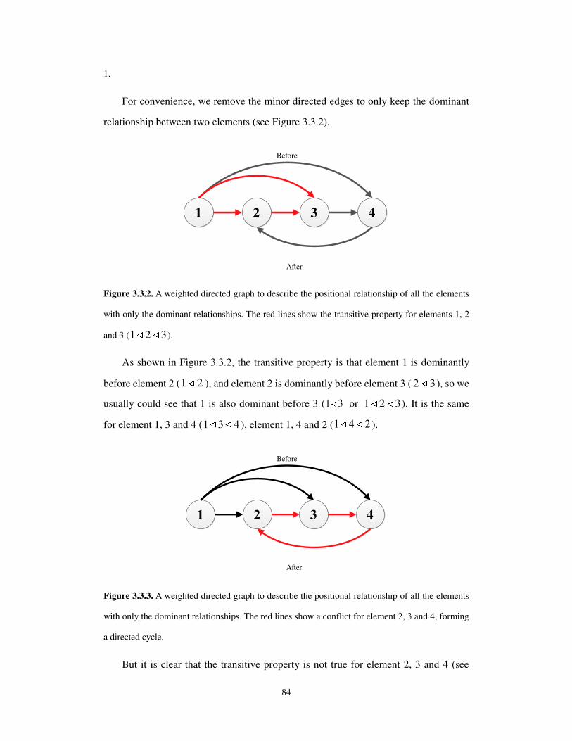
84

1.

For convenience, we remove the minor directed edges to only keep the dominant

relationship between two elements (see Figure 3.3.2).

Figure 3.3.2. A weighted directed graph to describe the positional relationship of all the elements

with only the dominant relationships. The red lines show the transitive property for elements 1, 2

and 3 (1 2 3).

As shown in Figure 3.3.2, the transitive property is that element 1 is dominantly

before element 2 (1 2 ), and element 2 is dominantly before element 3 ( 2 3), so we

usually could see that 1 is also dominant before 3 (1 3 or 1 2 3). It is the same

for element 1, 3 and 4 (1 3 4), element 1, 4 and 2 (1 4 2 ).

Figure 3.3.3. A weighted directed graph to describe the positional relationship of all the elements

with only the dominant relationships. The red lines show a conflict for element 2, 3 and 4, forming

a directed cycle.

But it is clear that the transitive property is not true for element 2, 3 and 4 (see

1 2 3 4

Before

After

1 2 3 4

Before

After

85

Figure 3.3.3). element 2 is before 3 ( 2 3), and element 3 is before 4 ( 3 4 ). While

we could not see that element 2 is before element 4, but it is just the opposite that

element 2 is after element 4. In this way, they form a directed cycle. We also call it a

conflict in the set of rankings, because it could not simultaneously be satisfied in a

linear ordering.

Ranking aggregation is just aiming to set up a compatible positional relationship

(or a linear ordering) by removing a set of conflicting edges with a sum of smallest

weight. It is worth mentioning that this is just the definition of the minimum feedback

arc set problem. And in fact it has been stated that the problem of Kemeny optimal

aggregation of rankings can be cast as a special case of the minimum feedback arc set

problem (Ailon et al., 2008). It is easy for this example that we could get three different

results by removing any edge in the directed cycle, because they are all same weighted

(see Figure 3.3.4).

1 3 4 2 1 4 2 3 1 2 3 4

Figure 3.3.4. The three types of answers for the problem are all right.

3.3.3.2 KwikSort

Based on the transitive property of the elements in rankings, Ailon, Charikar and

Newman developed a 2-factor approximation algorithm for rankings without ties,

KwikSort. It was named KwikSort, mainly because the algorithm looks like a type of

sorting algorithm, Quicksort. It was defined for the feedback arc set problem (Ailon et

al., 2008). Here we describe it for the ranking aggregation problem without ties.

Let ( , )G V W be a directed graph of a set of rankings, where V indicates all

the elements, and W is the weight table between any two elements ( ijw and jiw ). The

1 2 3 4

Before

After

1 2 3 4

Before

After

1 2 3 4

Before

After

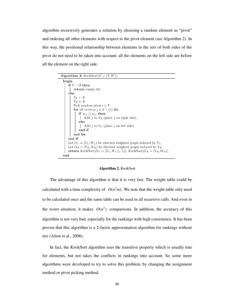
86

algorithm recursively generates a solution by choosing a random element as “pivot”

and ordering all other elements with respect to the pivot element (see Algorithm 2). In

this way, the positional relationship between elements in the sets of both sides of the

pivot do not need to be taken into account: all the elements on the left side are before

all the element on the right side.

Algorithm 2. KwikSort

The advantage of this algorithm is that it is very fast. The weight table could be

calculated with a time complexity of 2( )O n m . We note that the weight table only need

to be calculated once and the same table can be used in all recursive calls. And even in

the worst situation, it makes 2( )O n comparisons. In addition, the accuracy of this

algorithm is not very bad, especially for the rankings with high consistence. It has been

proven that this algorithm is a 2-factor approximation algorithm for rankings without

ties (Ailon et al., 2008).

In fact, the KwikSort algorithm uses the transitive property which is usually true

for elements, but not takes the conflicts in rankings into account. So some more

algorithms were developed to try to solve this problem, by changing the assignment

method or pivot picking method.

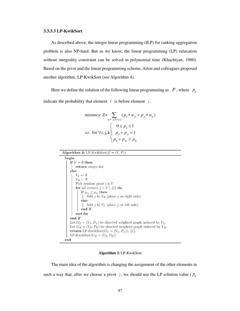
87

3.3.3.3 LP-KwikSort

As described above, the integer linear programming (ILP) for ranking aggregation

problem is also NP-hard. But as we know, the linear programming (LP) relaxation

without integrality constraint can be solved in polynomial time (Khachiyan, 1980).

Based on the pivot and the linear programming scheme, Ailon and colleagues proposed

another algorithm, LP-KwikSort (see Algorithm 4).

Here we define the solution of the following linear programming as P , where ijp

indicate the probability that element i is before element j .

, \{i}

Z= ( )

0 1. . for , j, k 1

ij ji ji iji V j V

ij

ij ji

ij jk ki

minimize p w p w

p

s t i p p

p p p

Algorithm 3. LP-KwikSort

The main idea of the algorithm is changing the assignment of the other elements in

such a way that, after we choose a pivot j , we should use the LP solution value ( ijp

88

and jip ) to decide where to put all the other elements, instead of deciding greedily.

Ailon and colleagues proved that this algorithm is a 43

-approximation algorithm

for rankings without ties, which is better than KwikSort algorithm (Ailon et al., 2008).

Based on the same scheme, Ailon introduced a 32

-approximation algorithm for partial

rankings (Ailon, 2010).

3.3.3.4 DerandLP-Pivot

Another modified pivot algorithm called DerandLP-Pivot, was proposed by Van

Zuylen and colleagues (Van Zuylen et al., 2009). It is a deterministic pivot algorithm,

instead of randomly picking pivot. And this algorithm directly faces up the conflicts in

rankings.

Figure 3.3.5. A schematic figure of conflict between elements for picking k as the pivot.

For a pivot k , let ( )kT G be the set of combination of two elements with conflicts.

( ) {( , ) | , , , }kT G i j k j k k i i j . They define a budget for element i and

element j as min( , )ij ij jic w w . As shown in Figure 3.3.5, for a pivot k and a

conflict between i and j , ijw is the cost for picking k as the pivot for this conflict,

and ijc is just the earning of picking k as the pivot for this conflict.

So in every recursive call, we choose the pivot k that minimizes the cost-earning

ratio:

j ik

ijw

ij jic w

89

( , ) ( )

( , ) ( )

( ) k

k

iji j T G

iji j T G

wPivot k

c

.

In this way, the choice of k costs as little as possible, and earns as much as possible.

In addition, this algorithm also improves the method of assignment of all the other

elements based on the solution of linear programming without integrality constraint

(see Algorithm 5). It also involves comparing of a type of cost-earning ratios of placing

the element on the left sides or right sides:

( ) | ,( )

( ) | ,k L R

Lk L R

W V V i VRatio i V

C V V i V

( ) | ,( )

( ) | ,k L R

Rk L R

W V V V iRatio i V

C V V V i

Where

\{ } ( , ) ( )

( ) | , ( ) | ,L R k

k L R ki ik ik ki ki ik ij L Ri V i V i V k i j T V

W V V V w w p w p w w V V

\{ } ( , ) ( )

( ) | , | ,k

k L R ik ij L Ri V k i j T V

C V V V c c V V

And

( , ) ( ) , { , } \{ } \{ }, \{ },

| , ( )k L R R L

ij L R ij ji ij ij ji jk ij ki iji j T V j V i V i j V k j V k i V i V k j V

w V V w p w p w p w p w

( , ) ( ) , { , } \{ } \{ }, \{ },

| , ( )k L R R L

ij L R ij ji ij ij ji jk ij ki iji j T V j V i V i j V k j V k i V i V k j V

c V V c p c p c p c p c

90

Algorithm 4. DerandLP-Pivot

Compared to Ailon et al.’s KwikSort algorithm, the running time of DerandLP-

Pivot is approximately a factor of n slower, because the pivot picking method should

be implemented in 3( )O n time (Van Zuylen et al., 2009).

91

3.4 Methods

3.4.1 Consistent-Pivot algorithm

Here we propose a new pivot algorithm, called Consistent-Pivot. It is based on a

novel method of pivot picking and assignment of all the other elements. We think that

this algorithm is more suitable for the transitive property of the data of ranking

aggregation problem.

In this part, we introduce this algorithm for rankings with ties. Besides the two

positional relationships for two elements ( i j , i is before j ; i j , i is after j ),

rankings with ties allow elements in a same level ( i j ). In addition, there are three

types of weight between two elements, ijw (for i is before j )， jiw (for i is after

j ) and i jw ( i is the same as j ). For ranking aggregation problem, we usually want

to choose the positional relationship with highest weight. We define the earning of this

kind of choosing as:

( , ) max( , , )ij ji i jearning i j w w w

And accordingly, the cost of this kind of choosing is

, ( )

( , ) , ( )

, ( )

ji i j

ij i j

ij ji

w w if i j

cost i j w w if i j

w w if i j

This is the minimum cost for every two elements without taking the relationships

with the other elements into account. This value reflects the consistency of the

positional relationship between the two elements in the rankings. The smaller the value

is, the more agreement for the two elements in the set rankings shows. If ( , ) 0cost i j ,

it means that the relationships for the two elements in all the rankings are all the same,

without disagreement.

92

In what follows, we define a consistent score for element i as the sum of the costs

between the element and all the other elements:

\{ }

( ) ( , )j V i

Consistent i cost i j

This score reflect the positional certainty of the element in the rankings. The

element with smaller consistent score is more stable. As a well-known landmark in a

city for the other buildings, the positional relationships are clear, the element with the

smallest consistent score could also be a marker to position all the other elements.

With the intuition above, we propose that the element with the smallest consistent

score should be picked as the pivot.

For example, here are four rankings of 15 elements:

1

2

3

4

=[{7},{3, 2},{31, 41, 4, 5, 1},{8},{27, 43},{42},{40},{6},{17}];

=[{7},{31, 41, 4, 5, 1, 3, 2},{8},{6, 17},{27, 40, 42, 43}];

=[{7},{31, 41, 4, 5, 1, 2},{3},{27},{8},{42, 6, 43},{40},{17}];

=[{7}

r

r

r

r ,{3, 2},{31, 41, 4, 5, 1},{8},{6},{17, 27, 40, 43},{42}].

In the first recursive cycle, element 7 is picked as the pivot ( (7) 0Consistent ). It

is worth noting that in the second recursive cycle, element 8 is picked as the pivot

( (8) 1Consistent ). Based on the element 8, all the other elements can be easily

assigned into the two sides. And in fact, the two groups of elements beside the element

8 really have little interaction between groups, but have complex positional relationship

in the groups.

Continuing to use the principle, we assign all the other elements not randomly but

in an order of the consistent score from small to large. As for the method of assignment

of all the other elements, we do not directly use the positional relationship between the

element and the pivot, instead of using a cost function that the position with the smallest

cost is chosen (see Algorithm 5).

93

Algorithm 5. Consistent-Pivot

For a given pivot k , the costs of element i to be placed before, after or the same

as the pivot are defined as:

1 1 1\{ }

( | ) ( , ) ( ) ( )

min( ( , ) | , ( ) | , ( ) | );

( | ) ( ) ( ) ( )

L S R

jk kjj k

L S R

ji jii j i jj V j V j V

x ji x ji xi j i jj V i

ij ji ij jii j i jj V j V j V

Cost i before cost i j w w w w

cost i j w w w w

Cost i same w w w w w w

1 1 1\{ }

1 1\{ }

min(( ) | , ( ) | , ( ) | );

( | ) ( ) ( ) ( , )

min(( ) | , ( ) | , ( , )

jk kjj k

L S R

jk j k

ij x ji ij x ji xi j i jj V i

ij iji j i jj V j V j V

ij x ij xi j i jj V i

w w w w w w

Cost i after w w w w cost i j

w w w w cost i j

1| ).kjx

Where 1jkx , 1kjx and 1j kx are the best positional result for the element

in the unassigned set V and the pivot k . Sometimes, there are two or three best

94

positional relationships between the element and pivot. In this situation, the cost

function should take the minimum value among them.

Both the weight table (W ) and best positional relationships table ( X ) between any

two elements can be simultaneously calculated in a time of 2( )O n m . The processes of

sorting of the elements, picking a pivot and assignment of all the others are much

quicker. So the time complexity of this algorithm is 2( )O n m , the same as KwikSort,

and faster than DerandLP-Pivot.

Figure 3.4.1. A tree structure of implementation of the Consistent-Pivot algorithm on the example.

The elements are all sorted with the green one in the front which is selected as the pivot (in red) in

the next recursive cycle.

The algorithm is implemented in a ternary tree structure. Figure 3.4.1 shows the

structure of the result of the real example given above in this section.

3.4.2 Experiments on the algorithms

In the work of Cohen-Boulakia and colleagues, the BioConsert algorithm performs

much better than Fagin et al.’s algorithm and the two pivot algorithms of Ailon et al. in

accuracy (Cohen-Boulakia et al., 2011). In addition, Brancotte et al. shows that the

95

BioConsert algorithm is the best one in most cases (Brancotte et al., in preparation). So,

in this section, we focus on the comparison of the results of the Consistent-Pivot

algorithm with all the previous pivot algorithms and the BioConsert algorithm.

The experiments have been conducted on a personal computer with an Intel Core

2 Duo CPU, 2 GB memory and Fedora 11 system. We used the GLPK 4.45 (GNU

Linear Programming Kit) package to solve large-scale linear programming problems

(Makhorin, 2008). All the Algorithms were coded in C.

3.4.2.1 Experiment Settings

To measure the accuracy of the algorithms, we should set a standard. But without

the best aggregation result, it is difficult to value a relative accuracy for different data

sets. Based on the definition of consistent score, we propose a strict lower bound

( IdealDis ) of the best Kendall-tau distance between the Kemeny optimal ranking *r

and the set of rankings R :

1( )

2 i V

IdealDis Consistent i

( ) *( , )pIdealDis K r R

Where ( )i V

Consistent i is the sum of the consistent scores of all the elements,

which is also twice the sum of the minimum cost for every two elements.

The IdealDis can be calculated easily. It is just the Kemeny distance between the

Kemeny optimal ranking ( *r ) with the sets of rankings ( R ), if and only if there is no

conflict (or directed cycles) between elements:

( ) *( , )pK r R IdealDis

Based on the lower bound of the best result, we define a normalized gap function

to measure the performance in accuracy:

96

( ) ( , )presultK r R IdealDis

GapIdealDis

It is a relative value to the ideal distance. Clearly, the more the gap is, the less the

accuracy shows.

3.4.2.2 Data sets

We firstly test the performance on real biological data (Cohen-Boulakia et al.,

2011). It is query results from four ranking methods of rankings for genes known to be

possibly associated with some kinds of diseases: Breast cancer, Prostate cancer,

Neuroblastoma, Bladder cancer, Retinoblastoma, Attention Deficit Hyperactivity

Disorder (ADHD), and Long QT syndrome (LQT) (see Table 3.4.1).

Query number of elements IdealDis

ADHD_reduced 15 48

LQT 35 350

Retinoblastoma_reduced 37 653

ADHD 45 670

Bladdercancer_reduced 115 3881

Prostatecancer_reduced 218 26313

Bladdercancer 308 38159

Breastcancer_reduced 386 78892

Retinoblastom 402 75032

Neuroblastoma_reduced 431 56536

Table 3.4.1. The real biological data set. The 10 sets of rankings used in the work of Cohen-Boulakia

et al. are all listed. The number of elements and IdealDis are shown.

We also did the experiment on the WebSearch dataset, which was widely used in

comparison of various algorithms for ranking aggregation (Dwork et al., 2001;

Schalekamp and van Zuylen, 2009; Ali et al., 2012). It is extracted from search results

of queries for 37 keywords from four search engines.

To systematically compare the algorithms, we also use a group of synthetic data

97

sets. We generated dataset of 4m , {4...20}n and [20;100]n stepping 10 by 10

and then [200;1000]n stepping 100. We generate 500 datasets for each n , which

gives a total of 15000 datasets. They were produced by putting n elements randomly

into n buckets independently, and then sorting them by the bucket order.

98

3.5 Results

3.5.1 Results on real biological data

Query IdealDis CP BC KS LK DLP

ADHD_reduced 48 48 48 55 48 48

LQT 350 352 352 392 352 352

Retinoblastoma_reduced 653 653 653 653 653 653

ADHD 670 682 682 747 682 682

Bladdercancer_reduced 3881 3881 3881 3899 - -

Prostatecancer_reduced 26313 26388 26386 27676 - -

Bladdercancer 38159 38159 38159 38245 - -

Breastcancer_reduced 78892 79023 79057 80089 - -

Retinoblastom 75032 75456 75073 75111 - -

Neuroblastoma_reduced 56536 56859 57192 58709 - -

Table 3.5.1. Results on real biological data with ( 1p ). “CP” stands for the Consistent-Pivot

algorithm; “BC” stands for BioConsert; “KS” stands for KwikSort; “LK” stands for LP-KwikSort;

“DLP” stands for DerandLP-Pivot.

As shown in Table 3.5.1, The Consistent-Pivot algorithm performs as well as the

BioConsert algorithm, with two results better than the BioConsert algorithm (in red),

and two worse results (in blue). As for the three previous pivot algorithms, the

KwikSort algorithm is fast, but it is mostly worse than the Consistent-Pivot algorithm

in accuracy; In another way, both the LP-KwikSort algorithm and the DerandLP-Pivot

algorithm cannot finish running all the rest 6 datasets ( 100n ) in one hour, so we

stopped the programs and cannot get the results.

99

Figure 3.5.1. Gap and running time on real biological data with ( 1p ).

The normalized gap and running time are also shown in the Figure 3.5.1. Clearly,

with the similar performance in accuracy, the running time of the Consistent-Pivot

algorithm is much less than the BioConsert algorithm. The result is nearly the same for

0.5p , which gives a less weight of disagreement for two elements that are in the same

bucket in one ranking and in different buckets in another ranking (see Figure 3.5.2).

100

Figure 3.5.2. Results of gap and running time on real biological data with ( 0.5p )

3.5.2 Results on WebSearch data

To value the performance of the two pivot algorithms based on linear

programming, we firstly generate a dataset with less elements for all the 37 queries.

The average number of elements per query is 36.2, with a standard deviation of 4.4

( 36.2 4.4n ).

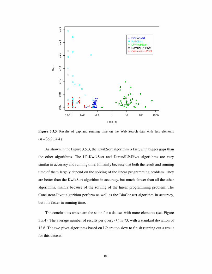
101

Figure 3.5.3. Results of gap and running time on the Web Search data with less elements

( 36.2 4.4n ).

As shown in the Figure 3.5.3, the KwikSort algorithm is fast, with bigger gaps than

the other algorithms. The LP-KwikSort and DerandLP-Pivot algorithms are very

similar in accuracy and running time. It mainly because that both the result and running

time of them largely depend on the solving of the linear programming problem. They

are better than the KwikSort algorithm in accuracy, but much slower than all the other

algorithms, mainly because of the solving of the linear programming problem. The

Consistent-Pivot algorithm perform as well as the BioConsert algorithm in accuracy,

but it is faster in running time.

The conclusions above are the same for a dataset with more elements (see Figure

3.5.4). The average number of results per query ( n ) is 73, with a standard deviation of

12.6. The two pivot algorithms based on LP are too slow to finish running out a result

for this dataset.

102

Figure 3.5.4. Results of gap and running time on the Web Search data with more elements

( 73 12.6n ).

103

3.5.3 Results on synthetic data

Figure 3.5.5. Result of gap and running time on the synthetic data.

As shown in Figure 3.5.5, the running time of the LP-KwikSort, DerandLP-Pivot

and BioConsert algorithm growths rapidly. So we just run the two pivot algorithm based

on LP for datasets with 40n , and run the BioConsert algorithm for datasets with

400n . Comparatively, the Consistent-Pivot and KwikSort algorithm are much faster,

and even for 1000n , they could finish running in 1 second.

104

Figure 3.5.6. Enlarged figure of the result of gap on the synthetic data for the number of elements

range from 4 to 40.

As for the accuracy, the DerandLP-Pivot algorithm perform best for the synthetic

data with elements from 4 to 40 (see the enlarged figure in Figure 3.5.6), followed by

the LP-KwikSort algorithm. The KwikSort algorithm is much worse than all the other

algorithms.

It is worth noting that the BioConsert algorithms perform significantly better than

the Consistent-Pivot algorithm for this synthetic data, which is not the same as the result

from both the real data. However the Consistent-Pivot algorithm perform not too bad,

with less than 6% relative distance to the IdealDis even for datasets 1000n .

We think it is mainly because of the synthetic datasets which are produced randomly

without agreement information between the four rankings. It is not the same as the real

data that have much transitive property in the rankings.

105

3.6 Discussion

In summary, the Consistent-Pivot algorithm is an efficient algorithm for real data

both in accuracy and running time. It is much faster than the BioConsert, LP-KwikSort,

DerandLP-Pivot algorithms, and performs almost as well as the BioConsert for real

data.

However, there is still a lot of work to do for this project. The experiments on the

algorithms are not sufficient. We could test them systematically on more real data and

synthetic data, to study how the agreement in rankings affects the performance of the

Consistent-Pivot algorithm. And we would try to find an improvement of the

Consistent-Pivot algorithm to deal with the datasets with not so much agreement in

rankings.

All the algorithms have advantages with shortcomings. The thinking of

combination of several algorithms to get better performance is a good idea (Schalekamp

and van Zuylen, 2009). The Consistent-Pivot followed by the better search of the

BioConsert algorithm in a local range, maybe a good combined algorithm for the

ranking aggregation problem.

106

Reference

1. Crick, F. (1970). Central dogma of molecular biology. Nature, 227(5258), 561-563.

2. Roy, S. W., & Gilbert, W. (2006). The evolution of spliceosomal introns: patterns, puzzles and

progress. Nature Reviews Genetics, 7(3), 211-221.

3. Dietz, H. C., & Kendzior, R. J. (1994). Maintenance of an open reading frame as an additional

level of scrutiny during splice site selection. Nature genetics, 8(2), 183-188.

4. Will, C. L., & Lührmann, R. (2011). Spliceosome structure and function. Cold Spring Harbor

perspectives in biology, 3(7), a003707.

5. Yeo, G., & Burge, C. B. (2004). Maximum entropy modeling of short sequence motifs with

applications to RNA splicing signals. Journal of Computational Biology, 11(2-3), 377-394.

6. Desmet, F. O., Hamroun, D., Lalande, M., Collod-Béroud, G., Claustres, M., & Béroud, C.

(2009). Human Splicing Finder: an online bioinformatics tool to predict splicing

signals. Nucleic acids research, 37(9), e67-e67.

7. Pertea, M., Lin, X., & Salzberg, S. L. (2001). GeneSplicer: a new computational method for

splice site prediction. Nucleic acids research, 29(5), 1185-1190.

8. Brunak, S., Engelbrecht, J., & Knudsen, S. (1991). Prediction of human mRNA donor and

acceptor sites from the DNA sequence. Journal of molecular biology, 220(1), 49-65.

9. Reese, M. G., Eeckman, F. H., Kulp, D., & Haussler, D. (1997). Improved splice site detection

in Genie. Journal of computational biology, 4(3), 311-323.

10. Levine, A., & Durbin, R. (2001). A computational scan for U12-dependent introns in the human

genome sequence. Nucleic acids research, 29(19), 4006-4013.

11. Alekseyenko, A. V., Kim, N., & Lee, C. J. (2007). Global analysis of exon creation versus loss

and the role of alternative splicing in 17 vertebrate genomes. Rna, 13(5), 661-670.

12. Sugnet, C. W., Kent, W. J., Ares, M., & Haussler, D. (2004). Transcriptome and genome

conservation of alternative splicing events in humans and mice. InPacific Symposium on

107

Biocomputing (Vol. 9, pp. 66-77).

13. Kim, E., Goren, A., & Ast, G. (2008). Alternative splicing: current

perspectives.Bioessays, 30(1), 38-47.

14. Black, D. L. (2003). Mechanisms of alternative pre-messenger RNA splicing. Annual review of

biochemistry, 72(1), 291-336.

15. Keren, H., Lev-Maor, G., & Ast, G. (2010). Alternative splicing and evolution: diversification,

exon definition and function. Nature Reviews Genetics, 11(5), 345-355.

16. Nilsen, T. W., & Graveley, B. R. (2010). Expansion of the eukaryotic proteome by alternative

splicing. Nature, 463(7280), 457-463.

17. Pan, Q., Shai, O., Lee, L. J., Frey, B. J., & Blencowe, B. J. (2008). Deep surveying of alternative

splicing complexity in the human transcriptome by high-throughput sequencing. Nature

genetics, 40(12), 1413-1415.

18. Chen, M., & Manley, J. L. (2009). Mechanisms of alternative splicing regulation: insights from

molecular and genomics approaches. Nature Reviews Molecular Cell Biology, 10(11), 741-754.

19. Lim, K. H., Ferraris, L., Filloux, M. E., Raphael, B. J., & Fairbrother, W. G. (2011). Using

positional distribution to identify splicing elements and predict pre-mRNA processing defects

in human genes. Proceedings of the National Academy of Sciences, 108(27), 11093-11098.

20. Irimia, M., & Blencowe, B. J. (2012). Alternative splicing: decoding an expansive regulatory

layer. Current opinion in cell biology, 24(3), 323-332.

21. Matlin, A. J., Clark, F., & Smith, C. W. (2005). Understanding alternative splicing: towards a

cellular code. Nature Reviews Molecular Cell Biology, 6(5), 386-398.

22. Wang, Z., & Burge, C. B. (2008). Splicing regulation: from a parts list of regulatory elements

to an integrated splicing code. Rna, 14(5), 802-813.

23. Warf, M. B., & Berglund, J. A. (2010). Role of RNA structure in regulating pre-mRNA

splicing. Trends in biochemical sciences, 35(3), 169-178.

24. Reid, D. C., Chang, B. L., Gunderson, S. I., Alpert, L., Thompson, W. A., & Fairbrother, W. G.

108

(2009). Next-generation SELEX identifies sequence and structural determinants of splicing

factor binding in human pre-mRNA sequence. RNA, 15(12), 2385-2397.

25. David, C. J., & Manley, J. L. (2008). The search for alternative splicing regulators: new

approaches offer a path to a splicing code. Genes & development, 22(3), 279-285.

26. Barash, Y., Calarco, J. A., Gao, W., Pan, Q., Wang, X., Shai, O., ... & Frey, B. J. (2010).

Deciphering the splicing code. Nature, 465(7294), 53-59.

27. López-Bigas, N., Audit, B., Ouzounis, C., Parra, G., & Guigó, R. (2005). Are splicing mutations

the most frequent cause of hereditary disease?. FEBS letters, 579(9), 1900-1903.

28. Ward, A. J., & Cooper, T. A. (2010). The pathobiology of splicing. The Journal of

pathology, 220(2), 152-163.

29. Fackenthal, J. D., & Godley, L. A. (2008). Aberrant RNA splicing and its functional

consequences in cancer cells. Disease models & mechanisms, 1(1), 37-42.

30. Yoshida, K., Sanada, M., Shiraishi, Y., Nowak, D., Nagata, Y., Yamamoto, R., ... & Ogawa, S.

(2011). Frequent pathway mutations of splicing machinery in

myelodysplasia. Nature, 478(7367), 64-69.

31. Wahl, M. C., Will, C. L., & Lührmann, R. (2009). The spliceosome: design principles of a

dynamic RNP machine. Cell, 136(4), 701-718.

32. Zamore, P. D., Patton, J. G., & Green, M. R. (1992). Cloning and domain structure of the

mammalian splicing factor U2AF. Nature, 355(6361), 609-614.

33. Zhang, M., Zamore, P. D., Carmo-Fonseca, M., Lamond, A. I., & Green, M. R. (1992). Cloning

and intracellular localization of the U2 small nuclear ribonucleoprotein auxiliary factor small

subunit. Proceedings of the National Academy of Sciences, 89(18), 8769-8773.

34. Singh, R., Valcarcel, J., & Green, M. R. (1995). Distinct binding specificities and functions of

higher eukaryotic polypyrimidine tract-binding proteins. Science, 268(5214), 1173-1176.

35. Valcárcel, J., Gaur, R. K., Singh, R., & Green, M. R. (1996). Interaction of U2AF65 RS region

with pre-mRNA of branch point and promotion base pairing with U2

109

snRNA. Science, 273(5282), 1706-1709.

36. Abovich, N., Liao, X. C., & Rosbash, M. (1994). The yeast MUD2 protein: an interaction with

PRP11 defines a bridge between commitment complexes and U2 snRNP addition. Genes &

development, 8(7), 843-854.

37. Abovich, N., & Rosbash, M. (1997). Cross-intron bridging interactions in the yeast commitment

complex are conserved in mammals. Cell, 89(3), 403-412.

38. Sridharan, V., Heimiller, J., & Singh, R. (2011). Genomic mRNA profiling reveals

compensatory mechanisms for the requirement of the essential splicing factor U2AF. Molecular

and cellular biology, 31(4), 652-661.

39. Sridharan, V., & Singh, R. (2007). A conditional role of U2AF in splicing of introns with

unconventional polypyrimidine tracts. Molecular and cellular biology, 27(20), 7334-7344.

40. MacMillan, A. M., McCaw, P. S., Crispino, J. D., & Sharp, P. A. (1997). SC35-mediated

reconstitution of splicing in U2AF-depleted nuclear extract. Proceedings of the National

Academy of Sciences, 94(1), 133-136.

41. Imai, H., Chan, E. K., Kiyosawa, K., Fu, X. D., & Tan, E. M. (1993). Novel nuclear autoantigen

with splicing factor motifs identified with antibody from hepatocellular carcinoma. Journal of

Clinical Investigation, 92(5), 2419.

42. Hastings, M. L., Allemand, E., Duelli, D. M., Myers, M. P., & Krainer, A. R. (2007). Control

of pre-mRNA splicing by the general splicing factors PUF60 and U2AF65. PLoS One, 2(6),

e538.

43. Page-McCaw, P. S., Amonlirdviman, K. E. V. I. N., & Sharp, P. A. (1999). PUF60: a novel

U2AF65-related splicing activity. Rna, 5(12), 1548-1560.

44. Tronchre, H., Wang, J., & Fu, X. D. (1997). A protein related to splicing factor U2AF35 that

interacts with U2AF65 and SR proteins in splicing of pre-mRNA. Nature, 388(6640), 397-400.

45. Shepard, J., Reick, M., Olson, S., & Graveley, B. R. (2002). Characterization of U2AF6, a

splicing factor related to U2AF35. Molecular and cellular biology, 22(1), 221-230.

110

46. Mollet, I., Barbosa‐Morais, N. L., Andrade, J., & Carmo‐Fonseca, M. (2006). Diversity of

human U2AF splicing factors. FEBS Journal, 273(21), 4807-4816.

47. Zarnack, K., König, J., Tajnik, M., Martincorena, I., Eustermann, S., Stévant, I., ... & Ule, J.

(2013). Direct competition between hnrnp c and u2af65 protects the transcriptome from the

exonization of Alu elements. Cell, 152(3), 453-466.

48. Reed, R. (1989). The organization of 3'splice-site sequences in mammalian introns. Genes &

development, 3(12b), 2113-2123.

49. Zamore, P. D., & Green, M. R. (1991). Biochemical characterization of U2 snRNP auxiliary

factor: an essential pre-mRNA splicing factor with a novel intranuclear distribution. The EMBO

journal, 10(1), 207.

50. Wu, S., Romfo, C. M., Nilsen, T. W., & Green, M. R. (1999). Functional recognition of the 3′

splice site AG by the splicing factor U2AF35. Nature,402(6763), 832-835.

51. Merendino, L., Guth, S., Bilbao, D., Martínez, C., & Valcárcel, J. (1999). Inhibition of msl-2

splicing by Sex-lethal reveals interaction between U2AF35 and the 3′ splice site

AG. Nature, 402(6763), 838-841.

52. Pacheco, T. R., Coelho, M. B., Desterro, J. M., Mollet, I., & Carmo-Fonseca, M. (2006). In vivo

requirement of the small subunit of U2AF for recognition of a weak 3′ splice site. Molecular

and cellular biology, 26(21), 8183-8190.

53. Soares, L. M. M., Zanier, K., Mackereth, C., Sattler, M., & Valcárcel, J. (2006). Intron removal

requires proofreading of U2AF/3'splice site recognition by DEK. Science, 312(5782), 1961-

1965.

54. Tavanez, J. P., Madl, T., Kooshapur, H., Sattler, M., & Valcárcel, J. (2012). hnRNP A1

proofreads 3′ splice site recognition by U2AF. Molecular cell, 45(3), 314-329.

55. Park, J. W., Parisky, K., Celotto, A. M., Reenan, R. A., & Graveley, B. R. (2004). Identification

of alternative splicing regulators by RNA interference in Drosophila. Proceedings of the

National Academy of Sciences of the United States of America, 101(45), 15974-15979.

111

56. Moore, M. J., Wang, Q., Kennedy, C. J., & Silver, P. A. (2010). An alternative splicing network

links cell-cycle control to apoptosis. Cell, 142(4), 625-636.

57. Le Guiner, C., Lejeune, F., Galiana, D., Kister, L., Breathnach, R., Stévenin, J., & Del Gatto-

Konczak, F. (2001). TIA-1 and TIAR activate splicing of alternative exons with weak 5′ splice

sites followed by a U-rich stretch on their own pre-mRNAs. Journal of Biological

Chemistry, 276(44), 40638-40646.

58. Xue, Y., Zhou, Y., Wu, T., Zhu, T., Ji, X., Kwon, Y. S., ... & Zhang, Y. (2009). Genome-wide

analysis of PTB-RNA interactions reveals a strategy used by the general splicing repressor to

modulate exon inclusion or skipping. Molecular cell, 36(6), 996-1006.

59. Wang, Z., Kayikci, M., Briese, M., Zarnack, K., Luscombe, N. M., Rot, G., ... & Ule, J. (2010).

iCLIP predicts the dual splicing effects of TIA-RNA interactions. PLoS biology, 8(10),

e1000530.

60. Lim, K. H., Ferraris, L., Filloux, M. E., Raphael, B. J., & Fairbrother, W. G. (2011). Using

positional distribution to identify splicing elements and predict pre-mRNA processing defects

in human genes. Proceedings of the National Academy of Sciences, 108(27), 11093-11098.

61. Yoshida, K., Sanada, M., Shiraishi, Y., Nowak, D., Nagata, Y., Yamamoto, R., ... & Ogawa, S.

(2011). Frequent pathway mutations of splicing machinery in

myelodysplasia. Nature, 478(7367), 64-69.

62. Thol, F., Kade, S., Schlarmann, C., Löffeld, P., Morgan, M., Krauter, J., ... & Heuser, M. (2012).

Frequency and prognostic impact of mutations in SRSF2, U2AF1, and ZRSR2 in patients with

myelodysplastic syndromes. Blood, 119(15), 3578-3584.

63. Cazzola, M., Della Porta, M. G., & Malcovati, L. (2013). The genetic basis of myelodysplasia

and its clinical relevance. Blood, 122(25), 4021-4034.

64. Danckwardt, S., Kaufmann, I., Gentzel, M., Foerstner, K. U., Gantzert, A. S., Gehring, N. H., ...

& Kulozik, A. E. (2007). Splicing factors stimulate polyadenylation via USEs at non‐

canonical 3′ end formation signals. The EMBO journal, 26(11), 2658-2669.

65. Zhang, C., & Darnell, R. B. (2011). Mapping in vivo protein-RNA interactions at single-

112

nucleotide resolution from HITS-CLIP data. Nature biotechnology, 29(7), 607-614.

66. Yeo, G., & Burge, C. B. (2004). Maximum entropy modeling of short sequence motifs with

applications to RNA splicing signals. Journal of Computational Biology, 11(2-3), 377-394.

67. Murray, J. I., Voelker, R. B., Henscheid, K. L., Warf, M. B., & Berglund, J. A. (2008).

Identification of motifs that function in the splicing of non-canonical introns. Genome

Biol, 9(6), R97.

68. Huelga, S. C., Vu, A. Q., Arnold, J. D., Liang, T. Y., Liu, P. P., Yan, B. Y., ... & Yeo, G. W.

(2012). Integrative genome-wide analysis reveals cooperative regulation of alternative splicing

by hnRNP proteins. Cell reports, 1(2), 167-178.

69. Aguilera, A. (2005). Cotranscriptional mRNP assembly: from the DNA to the nuclear

pore. Current opinion in cell biology, 17(3), 242-250.

70. Gama-Carvalho, M., Barbosa-Morais, N. L., Brodsky, A. S., Silver, P. A., & Carmo-Fonseca,

M. (2006). Genome-wide identification of functionally distinct subsets of cellular mRNAs

associated with two nucleocytoplasmic-shuttling mammalian splicing factors. Genome

biology, 7(11), R113.

71. Xiao, R., Tang, P., Yang, B., Huang, J., Zhou, Y., Shao, C., ... & Fu, X. D. (2012). Nuclear

matrix factor hnRNP U/SAF-A exerts a global control of alternative splicing by regulating U2

snRNP maturation. Molecular cell, 45(5), 656-668.

72. Zhou, Z., Qiu, J., Liu, W., Zhou, Y., Plocinik, R. M., Li, H., ... & Fu, X. D. (2012). The Akt-

SRPK-SR axis constitutes a major pathway in transducing EGF signaling to regulate alternative

splicing in the nucleus. Molecular cell,47(3), 422-433.

73. Wei, W. J., Mu, S. R., Heiner, M., Fu, X., Cao, L. J., Gong, X. F., ... & Hui, J. (2012). YB-1

binds to CAUC motifs and stimulates exon inclusion by enhancing the recruitment of U2AF to

weak polypyrimidine tracts. Nucleic acids research, 40(17), 8622-8636.

74. Shen, H., Zheng, X., Luecke, S., & Green, M. R. (2010). The U2AF35-related protein Urp

contacts the 3′ splice site to promote U12-type intron splicing and the second step of U2-type

intron splicing. Genes & development, 24(21), 2389-2394.

113

75. Han, J., Ding, J. H., Byeon, C. W., Kim, J. H., Hertel, K. J., Jeong, S., & Fu, X. D. (2011). SR

proteins induce alternative exon skipping through their activities on the flanking constitutive

exons. Molecular and cellular biology, 31(4), 793-802.

76. Han, J., Xiong, J., Wang, D., & Fu, X. D. (2011). Pre-mRNA splicing: where and when in the

nucleus. Trends in cell biology, 21(6), 336-343.

77. Przychodzen, B., Jerez, A., Guinta, K., Sekeres, M. A., Padgett, R., Maciejewski, J. P., &

Makishima, H. (2013). Patterns of missplicing due to somatic U2AF1 mutations in myeloid

neoplasms. Blood, 122(6), 999-1006.

78. van Helden, J., André, B., & Collado-Vides, J. (1998). Extracting regulatory sites from the

upstream region of yeast genes by computational analysis of oligonucleotide

frequencies. Journal of molecular biology, 281(5), 827-842.

79. Kahvejian, A., Quackenbush, J., & Thompson, J. F. (2008). What would you do if you could

sequence everything?. Nature biotechnology, 26(10), 1125-1133.

80. Marx, V. (2013). Biology: The big challenges of big data. Nature, 498(7453), 255-260.

81. Quiñones-Mateu, M. E., Avila, S., Reyes-teran, G., & Martinez, M. A. (2014). Deep sequencing:

Becoming a critical tool in clinical virology. Journal of Clinical Virology.

82. Waern, K., Nagalakshmi, U., & Snyder, M. (2011). RNA sequencing. Yeast Systems Biology (pp.

125-132). Humana Press.

83. Kodzius, R., Kojima, M., Nishiyori, H., Nakamura, M., Fukuda, S., Tagami, M., ... & Carninci,

P. (2006). CAGE: cap analysis of gene expression. Nature methods, 3(3), 211-222.

84. Fullwood, M. J., Wei, C. L., Liu, E. T., & Ruan, Y. (2009). Next-generation DNA sequencing

of paired-end tags (PET) for transcriptome and genome analyses. Genome research, 19(4), 521-

532.

85. Chu, C., Qu, K., Zhong, F. L., Artandi, S. E., & Chang, H. Y. (2011). Genomic maps of long

noncoding RNA occupancy reveal principles of RNA-chromatin interactions. Molecular

cell, 44(4), 667-678.

114

86. Core, L. J., Waterfall, J. J., & Lis, J. T. (2008). Nascent RNA sequencing reveals widespread

pausing and divergent initiation at human promoters. Science, 322(5909), 1845-1848.

87. Churchman, L. S., & Weissman, J. S. (2011). Nascent transcript sequencing visualizes

transcription at nucleotide resolution. Nature, 469(7330), 368-373.

88. Ingolia, N. T., Ghaemmaghami, S., Newman, J. R., & Weissman, J. S. (2009). Genome-wide

analysis in vivo of translation with nucleotide resolution using ribosome

profiling. Science, 324(5924), 218-223.

89. Robertson, G., Hirst, M., Bainbridge, M., Bilenky, M., Zhao, Y., Zeng, T., ... & Jones, S. (2007).

Genome-wide profiles of STAT1 DNA association using chromatin immunoprecipitation and

massively parallel sequencing. Nature methods, 4(8), 651-657.

90. Hesselberth, J. R., Chen, X., Zhang, Z., Sabo, P. J., Sandstrom, R., Reynolds, A. P., ... &

Stamatoyannopoulos, J. A. (2009). Global mapping of protein-DNA interactions in vivo by

digital genomic footprinting. Nature methods, 6(4), 283-289.

91. Crawford, G. E., Holt, I. E., Whittle, J., Webb, B. D., Tai, D., Davis, S., ... & Collins, F. S.

(2006). Genome-wide mapping of DNase hypersensitive sites using massively parallel

signature sequencing (MPSS). Genome research,16(1), 123-131.

92. Giresi, P. G., Kim, J., McDaniell, R. M., Iyer, V. R., & Lieb, J. D. (2007). FAIRE

(Formaldehyde-Assisted Isolation of Regulatory Elements) isolates active regulatory elements

from human chromatin. Genome research, 17(6), 877-885.

93. Wang, Z., Zang, C., Cui, K., Schones, D. E., Barski, A., Peng, W., & Zhao, K. (2009). Genome-

wide mapping of HATs and HDACs reveals distinct functions in active and inactive

genes. Cell, 138(5), 1019-1031.

94. Smith, Z. D., Gu, H., Bock, C., Gnirke, A., & Meissner, A. (2009). High-throughput bisulfite

sequencing in mammalian genomes. Methods, 48(3), 226-232.

95. Dostie, J., Richmond, T. A., Arnaout, R. A., Selzer, R. R., Lee, W. L., Honan, T. A., ... & Dekker,

J. (2006). Chromosome Conformation Capture Carbon Copy (5C): a massively parallel solution

for mapping interactions between genomic elements. Genome research, 16(10), 1299-1309.

115

96. Fullwood, M. J., Liu, M. H., Pan, Y. F., Liu, J., Xu, H., Mohamed, Y. B., ... & Ruan, Y. (2009).

An oestrogen-receptor-&agr;-bound human chromatin interactome. Nature, 462(7269), 58-64.

97. Soon, W. W., Hariharan, M., & Snyder, M. P. (2013). High‐throughput sequencing for biology

and medicine. Molecular systems biology, 9(1).

98. Cock, P. J., Fields, C. J., Goto, N., Heuer, M. L., & Rice, P. M. (2010). The Sanger FASTQ file

format for sequences with quality scores, and the Solexa/Illumina FASTQ variants. Nucleic

acids research, 38(6), 1767-1771.

99. Li, H., Ruan, J., & Durbin, R. (2008). Mapping short DNA sequencing reads and calling variants

using mapping quality scores. Genome research, 18(11), 1851-1858.

100. Andrews, S. (2010). FastQC: A quality control tool for high throughput sequence data.

101. Langmead, B., Trapnell, C., Pop, M., & Salzberg, S. L. (2009). Ultrafast and memory-efficient

alignment of short DNA sequences to the human genome. Genome Biol, 10(3), R25.

102. Li, H., & Durbin, R. (2009). Fast and accurate short read alignment with Burrows–Wheeler

transform. Bioinformatics, 25(14), 1754-1760.

103. Langmead, B., & Salzberg, S. L. (2012). Fast gapped-read alignment with Bowtie 2. Nature

methods, 9(4), 357-359.

104. Zhang, C., & Darnell, R. B. (2011). Mapping in vivo protein-RNA interactions at single-

nucleotide resolution from HITS-CLIP data. Nature biotechnology, 29(7), 607-614.

105. Zhang, Y., Liu, T., Meyer, C. A., Eeckhoute, J., Johnson, D. S., Bernstein, B. E., ... & Liu, X.

S. (2008). Model-based analysis of ChIP-Seq (MACS). Genome Biol, 9(9), R137.

106. Yeo, G. W., Coufal, N. G., Liang, T. Y., Peng, G. E., Fu, X. D., & Gage, F. H. (2009). An RNA

code for the FOX2 splicing regulator revealed by mapping RNA-protein interactions in stem

cells. Nature structural & molecular biology, 16(2), 130-137.

107. Xue, Y., Zhou, Y., Wu, T., Zhu, T., Ji, X., Kwon, Y. S., ... & Zhang, Y. (2009). Genome-wide

analysis of PTB-RNA interactions reveals a strategy used by the general splicing repressor to

modulate exon inclusion or skipping. Molecular cell, 36(6), 996-1006.

116

108. Chi, S. W., Zang, J. B., Mele, A., & Darnell, R. B. (2009). Argonaute HITS-CLIP decodes

microRNA–mRNA interaction maps. Nature, 460(7254), 479-486.

109. Hsu, F., Kent, W. J., Clawson, H., Kuhn, R. M., Diekhans, M., & Haussler, D. (2006). The

UCSC known genes. Bioinformatics, 22(9), 1036-1046.

110. Pruitt, K. D., Tatusova, T., & Maglott, D. R. (2007). NCBI reference sequences (RefSeq): a

curated non-redundant sequence database of genomes, transcripts and proteins. Nucleic acids

research, 35(suppl 1), D61-D65.

111. Hubbard, T., Barker, D., Birney, E., Cameron, G., Chen, Y., Clark, L., ... & Clamp, M. (2002).

The Ensembl genome database project. Nucleic acids research, 30(1), 38-41.

112. Harrow, J., Denoeud, F., Frankish, A., Reymond, A., Chen, C. K., Chrast, J., ... & Guigo, R.

(2006). GENCODE: producing a reference annotation for ENCODE. Genome Biol, 7(Suppl 1),

S4.

113. Burge, C., & Karlin, S. (1997). Prediction of complete gene structures in human genomic

DNA. Journal of molecular biology, 268(1), 78-94.

114. van Helden, J., André, B., & Collado-Vides, J. (1998). Extracting regulatory sites from the

upstream region of yeast genes by computational analysis of oligonucleotide

frequencies. Journal of molecular biology, 281(5), 827-842.

115. Durbin, R. (Ed.). (1998). Biological sequence analysis: probabilistic models of proteins and

nucleic acids. Cambridge university press.

116. Yeo, G., & Burge, C. B. (2004). Maximum entropy modeling of short sequence motifs with

applications to RNA splicing signals. Journal of Computational Biology, 11(2-3), 377-394.

117. Barrett, T., Wilhite, S. E., Ledoux, P., Evangelista, C., Kim, I. F., Tomashevsky, M., ... &

Soboleva, A. (2013). NCBI GEO: archive for functional genomics data sets—update. Nucleic

acids research, 41(D1), D991-D995.

118. Metzker, Michael L. "Sequencing technologies—the next generation." Nature Reviews

Genetics 11.1 (2010): 31-46.

117

119. Brusic, Vladimir, et al. "Data learning: understanding biological data." Knowledge sharing

across biological and medical knowledge based systems: Papers from the 1998 AAAI Workshop.

1998.

120. Cohen-Boulakia, Sarah, Alain Denise, and Sylvie Hamel. "Using medians to generate

consensus rankings for biological data." Scientific and Statistical Database Management.

Springer Berlin Heidelberg, 2011.

121. DeConde, Robert P., et al. "Combining results of microarray experiments: a rank aggregation

approach." Statistical Applications in Genetics and Molecular Biology 5.1 (2006).

122. Gao, Jun, et al. "Comparison of different ranking methods in protein-ligand binding site

prediction." International journal of molecular sciences 13.7 (2012): 8752-8761.

123. Sengupta, Debarka, et al. "Reformulated Kemeny Optimal Aggregation with Application in

Consensus Ranking of microRNA Targets." (2013): 1-1.

124. Dwork, Cynthia, et al. "Rank aggregation methods for the web." Proceedings of the 10th

international conference on World Wide Web. ACM, 2001.

125. Kendall, Maurice G. "A new measure of rank correlation." Biometrika (1938).

126. Fagin, Ronald, Ravi Kumar, and Dandapani Sivakumar. "Efficient similarity search and

classification via rank aggregation." Proceedings of the 2003 ACM SIGMOD international

conference on Management of data. ACM, 2003.

127. Diaconis, P., & Graham, R. L. (1977). Spearman's footrule as a measure of disarray. Journal of

the Royal Statistical Society. Series B (Methodological), 262-268.

128. Fagin, Ronald, et al. "Comparing and aggregating rankings with ties." Proceedings of the

twenty-third ACM SIGMOD-SIGACT-SIGART symposium on Principles of database systems.

ACM, 2004.

129. Kemeny, John G., and James Laurie Snell. Mathematical models in the social sciences. Vol. 9.

Boston: Ginn, 1962.

130. Farah, M., & Vanderpooten, D. (2007, July). An outranking approach for rank aggregation in

118

information retrieval. In Proceedings of the 30th annual international ACM SIGIR conference

on Research and development in information retrieval (pp. 591-598). ACM.

131. Dwork, Cynthia, et al. "System and method for aggregating ranking results from various

sources to improve the results of web searching." U.S. Patent No. 7,188,106. 6 Mar. 2007.

132. Conitzer, Vincent, Andrew Davenport, and Jayant Kalagnanam. "Improved bounds for

computing Kemeny rankings." AAAI. Vol. 6. 2006.

133. Meila, Marina, et al. "Consensus ranking under the exponential model." arXiv preprint

arXiv:1206.5265 (2012).

134. Brusic, Vladimir, et al. "Data learning: understanding biological data." Knowledge sharing

across biological and medical knowledge based systems: Papers from the 1998 AAAI Workshop.

1998.

135. Risse, Mathias. "Why the count de Borda cannot beat the Marquis de Condorcet." Social

Choice and Welfare 25.1 (2005): 95-113.

136. Young, H. Peyton, and Arthur Levenglick. "A consistent extension of Condorcet's election

principle." SIAM Journal on Applied Mathematics 35.2 (1978): 285-300.

137. De Grazia, Alfred. "Mathematical derivation of an election system." Isis 44.1/2 (1953): 42-51.

138. Blin, Guillaume et al. "Medians of an odd number of permutations." Pure Mathematics and

Applications 21, 2 (2011) 161 – 175.

139. Ailon, Nir. "Aggregation of partial rankings, p-ratings and top-m lists." Algorithmica 57.2

(2010): 284-300.

140. Ailon, Nir, Moses Charikar, and Alantha Newman. "Aggregating inconsistent information:

ranking and clustering." Journal of the ACM (JACM) 55.5 (2008): 23.

141. Van Zuylen, Anke, and David P. Williamson. "Deterministic pivoting algorithms for

constrained ranking and clustering problems." Mathematics of Operations Research 34.3

(2009): 594-620.

142. Schalekamp, F., & van Zuylen, A. (2009). Rank Aggregation: Together We're Strong.

119

In ALENEX (pp. 38-51).

143. Qin, T., Geng, X., & Liu, T. Y. (2010). A new probabilistic model for rank aggregation.

In Advances in neural information processing systems (pp. 1948-1956).

144. Ali, Alnur, and Marina Meilă. "Experiments with Kemeny ranking: What works

when?." Mathematical Social Sciences 64.1 (2012): 28-40.

145. Young, H. Peyton. "An axiomatization of Borda's rule." Journal of Economic Theory 9.1

(1974): 43-52.

146. Cohen, William W., Robert E. Schapire, and Yoram Singer. "Learning to order things." arXiv

preprint arXiv:1105.5464 (2011).

147. de Borda, Jean C. "Mémoire sur les élections au scrutin." (1781).

148. Ailon, N. (2010). Aggregation of partial rankings, p-ratings and top-m lists.

Algorithmica, 57(2), 284-300.

149. Khachiyan, L. G. (1980). Polynomial algorithms in linear programming. USSR Computational

Mathematics and Mathematical Physics, 20(1), 53-72.

150. Makhorin, A. (2008). GLPK (GNU linear programming kit).

120

Appendix: List of the publications

Huang, C., Xie, M. H., Liu, W., Yang, B., Yang, F., Huang, J., ... & Zhang, Y. (2011).

A structured RNA in hepatitis B virus post‐ transcriptional regulatory element

represses alternative splicing in a sequence‐independent and position‐dependent

manner. FEBS Journal, 278(9), 1533-1546.

Xiao, R., Tang, P., Yang, B., Huang, J., Zhou, Y., Shao, C., ... & Fu, X. D. (2012).

Nuclear matrix factor hnRNP U/SAF-A exerts a global control of alternative splicing

by regulating U2 snRNP maturation. Molecular cell, 45(5), 656-668.

Wang, Y., Jiang, L., Ji, X., Yang, B., Zhang, Y., & Fu, X. D. (2013). Hepatitis B viral

RNA directly mediates down-regulation of the tumor suppressor microRNA miR-

15a/miR-16-1 in hepatocytes. Journal of Biological Chemistry, 288(25), 18484-18493.

Zhang X., Zuo X., Yang B., Li Z., Xue Y., Zhou Y., Huang J., Zhao X., Zhou J., Yan Y.,

Zhang H., Guo P., Sun H., Guo L., Zhang Y., Fu X. (2014). MicroRNA Directly

Enhances Mitochondrial Translation during Muscle Differentiation. Cell, 158(3), 607-

619.

Shao C., Yang B., Wu T., Huang J., Tang P., Zhou Y., Zhou J., Qiu J., Jiang L., Li H.,

Chen G., Sun H., Zhang Y., Denise A., Zhang D., and Fu X-D. (2014). Mechanisms for

U2AF to Define 3’ Splice Sites and Regulate Alternative Splicing in the Human

Genome. Nature Structure & Molecular Biology. (Co-first author)

121

Acknowledgement

I would have not been able to finish this dissertation without the help and support

of many people through these years.

First, I would like to express my deepest gratitude to my two advisors, Professor

Xiangdong Fu and Professor Alain Denise, for their excellent guidance, enthusiasm,

patience, and immense knowledge. Professor Denise is always so kind, precise and full

of patience to me. He led me into the exciting field of combinatorial algorithms, trained

me on algorithms and programming, taught me how to write and present, and usually

concerned about my life in France. And Professor Fu is full of enthusiasm and

knowledge. He taught me how to think independently in a biological view, and usually

gave me profound insight or advice. I learned a lot from them and I am sure this will

benefit me in the future. I also would like to thank to Yi Zhang, for her guide and kind

help.

I would also like to thank the members of this thesis committee, Stéphane Vialette,

and Jérome Waldispühl, for their reviews of my work and their helpful comments.

Special thanks to all my collaborators: Changwei Shao, Bryan Brancotte, Xiaorong

Zhang, Yanling Wang, Rui Xiao, Chen Huang and Qijia Wu, Peng Tang, Li Jiang. Many

good ideas come out from discussion with them about the details, and they told me a

lot of the experiments with patience.

I wish to thank all of the members of labs in Wuhan and Orsay, for their tremendous

concern and help, as Feng Lou, Cong Zeng and Cécile Pereira usually discussed with

me about our projects in Orsay. I would like to thank Yu Zhou. He taught me a lot and

helps me in many aspects.

Last but not the least I would like to thank my family. Thanks to my parents for

their always supporting and encouraging me with their best wishes. And I would like

to thank my wife, Wei Zhou, for her love and unwavering support through the good

times and bad.