Biofuel policies and the environment: Do climate benefits warrant increased production from biofuel feedstocks?

Ecological Economics 70 (2011) 676–687

Contents lists available at ScienceDirect

Ecological Economics

j ourna l homepage: www.e lsev ie r.com/ locate /eco lecon

Analysis

Biofuel policies and the environment: Do climate benefits warrant increasedproduction from biofuel feedstocks?

Jussi Lankoski a, Markku Ollikainen b,⁎a OECD, Directorate for Trade and Agriculture, Paris, Franceb University of Helsinki, Department of Economics and Management, Helsinki, Finland

⁎ Corresponding author. P.O. Box 27, FI-00014 UniverE-mail addresses: [email protected] (J. Lankos

[email protected] (M. Ollikainen).

0921-8009/$ – see front matter © 2010 Elsevier B.V. Adoi:10.1016/j.ecolecon.2010.11.002

a b s t r a c t

Article history:Received 5 June 2009Received in revised form 14 October 2010Accepted 8 November 2010Available online 21 December 2010

Keywords:Climate benefitsBiofuelsLife cycle analysisNutrient runoffBiodiversityGreenhouse gas emissions

We examine whether climate benefits warrant policies promoting biofuel production from agricultural cropswhen other environmental impacts are accounted for. We develop a general economic–ecological modellingframework for integrated analysis of biofuel policies. An economic model of farmers' decision making iscombined with a biophysical model predicting the effects of farming practices on crop yields and relevantenvironmental impacts. They include GHG emissions over the life cycle, nitrogen and phosphorus runoff, andthe quality of wildlife habitats. We apply our model to crop production in Finland. We find that under currentbiofuel production technology the case for promotion of biofuels is not as evident as has been generallythought. Only reed canary grass for biodiesel is unambiguously desirable, whereas biodiesel from rape seedand ethanol production from wheat and barley cause in most cases negative net impacts on the environment.Suggested policies in the US and the EU tend to improve slightly the environmental performance of biofuelproduction.

sity of Helsinki, Finland.ki),

ll rights reserved.

© 2010 Elsevier B.V. All rights reserved.

1. Introduction

Bioenergy-related policy analyses have gradually shifted the focusfrom the mere output (biofuels and bioenergy) to a more compre-hensive analysis that accounts for the climate impacts of theproduction chain (Farrell et al., 2006; Mäkinen et al., 2006; Edwardset al., 2006). The bulk of bioenergy and biofuels literature has focusedon net energy balances and net greenhouse gas (GHG) emissions ofalternative bioenergy and biofuels options, many extending theirfocus on the life cycle of the production chain. Accounting climateexternalities in the biofuel production process allows one to makebetter decisions regarding biofuel policies.

However, one important step still remains to be taken in bioenergypolicy studies. Bioenergy production has many kinds of environmen-tal impacts, such as the effects on soil, water, biodiversity and thelandscape. What is good for the climate may not be good for waterecosystems. Increasing bioenergy production affects biodiversity andthe landscape, too. Thus, it is important to ask whether pursuingbioenergy policies for climate change entails important environmen-tal trade-offs, for instance, with regard to water quality andbiodiversity. Furthermore, if other environmental impacts exist, it isnecessary to examine if there is a need to revise bioenergy policies tostrike a better balance between all key environmental aspects.

Studies on multiple environmental effects of biofuel productionare still rare. Two recent US biofuel studies focusing on waterprotection are alarming. Both examined environmental effects fromland use change associated with corn-based ethanol production in theUS. Donner and Kucharik (2008) analyse the effects of US ethanoltargets on nitrogen runoff from farmland into the Gulf of Mexico.Their results show that meeting the US ethanol targets set out for2022 will increase nitrogen loading by 10–34%. Using an integratedagronomic and economic model, Marshall (2007) shows thatincreased corn-based ethanol production will lead to a significantincrease in total losses of nutrients from agriculture and an increasedrisk of erosion. From a slightly different angle, Evans and Cohen(2009) examine the competition of selected biofuel crops on land andwater in the Southern States of the US, while de Fraiture et al. (2008)examine the land and water implications in China and India. Muller(2009) discusses the broad aspects of sustainable bioenergy cropproduction. Landis et al. (2008) analyse how increasing corn ethanolproduction reduces diversity of agricultural landscapes and decreasesthe value of biocontrol services to combat weeds and pests. Barneyand DiTomaso (2008) assess the risk that recently favoured bioenergycrops become new invasive species in agricultural landscapes.Emphasizing both spatial and temporal aspects, Sala et al. (2009)provide a discussion on biodiversity, invasive and pollution aspects ofbiofuel crop production.

While all the abovementioned studies stress the complex ecologicaland biological problems associated with bioenergy crop production,they devote less attention to the economic aspects, the potential costsand benefits. There is clearly a need for a comprehensive monetary

677J. Lankoski, M. Ollikainen / Ecological Economics 70 (2011) 676–687

assessment of the climate and other impacts of bioenergy cropproduction. In this paper we examine whether the climate benefitswarrant the current and suggested biofuel support policies when otherenvironmental impacts are accounted for. We provide an integratedeconomic and ecological modelling approach: an economic model offarmers' decision making is combined with a biophysical modelpredicting the effects of biofuel support policies on farming practices,crop yields and the key environmental effects. They include GHGemissions over the life cycle, nitrogen and phosphorus runoff, and thequality of wildlife habitats.1 To facilitate comparison of these diverseimpacts, we express them in monetary terms (utilizing environmentalvaluation studies). Using monetary values as a common measure helpsus to compare and contrast the value of other environmental impactswith the climate benefits of bioenergy production.

The baseline of the analysis consists of the current support programsthat rely mostly on budgetary instruments, such as tax concessions anddirect support, that are complemented with biofuel blending or usemandates and trade restrictions (mainly import tariffs). As regardspolicy analysis we scrutinize two types of biofuel support policyreforms. The first policy reform involves radical elimination of currentsupport policy programs. The second policy reform is formulated in thespirit of two new large programs, the US Energy Act and the EUBioenergy Directive. The US Energy Independence and Security Act(EISA) was enacted in December 2007, and the new EU Directive onRenewable Energy (DRE) is currently in the legislative process. Whilethe former defines a Renewable Fuel Standard (RFS) calling for USbiofuel use to grow to a minimum of 136 billion litres per year by 2022,the latter suggests biofuels will account for at least 10% of all transportfuel consumption.2

Bioenergy policies have profound impacts on commodity markets,land-use patterns and the environment. This requires a comprehen-sive approach. We follow here OECD (2008), which analysed theimplications of biofuel support policies for biofuel supply anddemand, as well as for agricultural commodity markets and land useby using the OECD Aglink simulation model complemented by theFAO-developed Cosimo model.3 We adopt the new equilibrium EUcrop prices taken from Aglink–Cosimo for our policy scenarios andincorporate them into our integrated economic and ecological model.Because comprehensive data on environmental impacts and theirvaluation for the EU is missing, we use Finnish agricultural andenvironmental data.

The rest of the paper is organized as follows. Section 2 develops atheoretical framework for the paper. The empirical application of themodel is presented in Section 3. Finally, the results and discussion arepresented in Section 4.

2. Theoretical Framework

We develop an integrated economic and ecological modellingapproach to bioenergy policies. We first examine the market

1 As regards water, we focus on nutrient runoff only, because in Finland agricultureis rainfed, so that total water use is not a problem. There are many countries wherewater use matters, see for instance, Dominguez-Faus et al. (2009) and Chiu et al.(2009) for discussion.

2 The revised statutory requirements for RFS establish new specific annual volumestandards for cellulosic biofuel, biomass-based diesel, advanced biofuel, and totalrenewable fuel that must be used in transportation fuel. The revised statutoryrequirements also include new definitions and criteria for both renewable fuels andthe feedstocks used to produce them, including new greenhouse gas emission (GHG)thresholds as determined by lifecycle analysis. The regulatory requirements for RFSwill apply to domestic and foreign producers and importers of renewable fuel used inthe US.

3 Aglink–Cosimo-based analysis includes a sequence of scenarios aiming to shedlight on a number of questions related to biofuel markets and biofuel support policiesincluding: (i) the effects of existing policies analysed by simulating an elimination ofbiofuel support policies and (ii) analysing the impacts of two new programs (the USEISA and the EU DRE) on the supply of and demand for biofuels.

equilibriumof bioenergy crop production and use in biofuel production.We then link these decisions to a biophysical model predicting theeffects of farming practices on the environmental effects. The analysedenvironmental effects include GHG emissions over the life cycle,nitrogen and phosphorus runoff, and the quality of wildlife habitats.

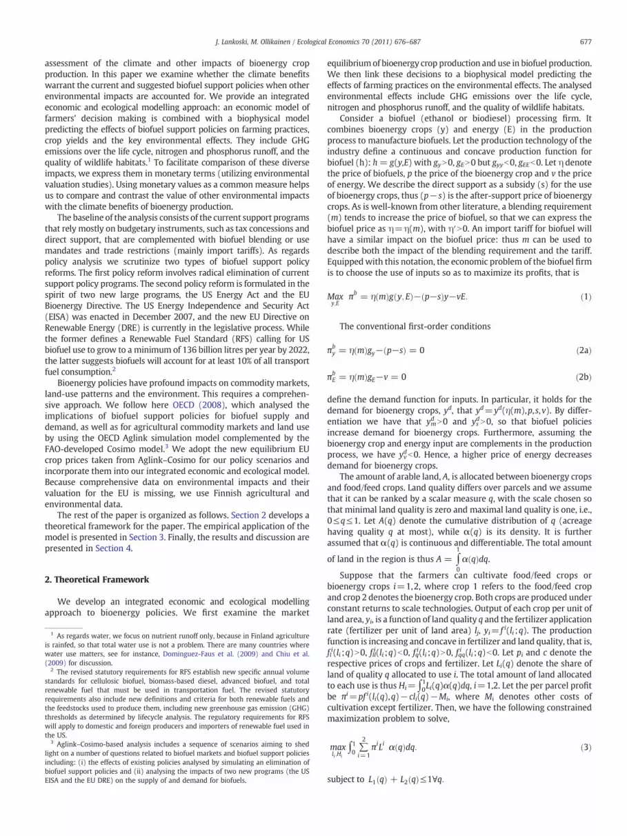
Consider a biofuel (ethanol or biodiesel) processing firm. Itcombines bioenergy crops (y) and energy (E) in the productionprocess to manufacture biofuels. Let the production technology of theindustry define a continuous and concave production function forbiofuel (h): h= g(y,E) with gyN0, gEN0 but gyyb0, gEEb0. Let η denotethe price of biofuels, p the price of the bioenergy crop and v the priceof energy. We describe the direct support as a subsidy (s) for the useof bioenergy crops, thus (p−s) is the after-support price of bioenergycrops. As is well-known from other literature, a blending requirement(m) tends to increase the price of biofuel, so that we can express thebiofuel price as η=η(m), with η′N0. An import tariff for biofuel willhave a similar impact on the biofuel price: thus m can be used todescribe both the impact of the blending requirement and the tariff.Equippedwith this notation, the economic problem of the biofuel firmis to choose the use of inputs so as to maximize its profits, that is

Maxy;E

πb = η mð Þg y; Eð Þ− p−sð Þy−vE: ð1Þ

The conventional first-order conditions

πby = η mð Þgy− p−sð Þ = 0 ð2aÞ

πbE = η mð ÞgE−v = 0 ð2bÞ

define the demand function for inputs. In particular, it holds for thedemand for bioenergy crops, yd, that yd=yd(η(m),p,s,v). By differ-entiation we have that ym

d N0 and ysdN0, so that biofuel policies

increase demand for bioenergy crops. Furthermore, assuming thebioenergy crop and energy input are complements in the productionprocess, we have yv

db0. Hence, a higher price of energy decreasesdemand for bioenergy crops.

The amount of arable land, A, is allocated between bioenergy cropsand food/feed crops. Land quality differs over parcels and we assumethat it can be ranked by a scalar measure q, with the scale chosen sothat minimal land quality is zero and maximal land quality is one, i.e.,0≤q≤1. Let A(q) denote the cumulative distribution of q (acreagehaving quality q at most), while α(q) is its density. It is furtherassumed that α(q) is continuous and differentiable. The total amount

of land in the region is thus A = ∫1

0

α qð Þdq.Suppose that the farmers can cultivate food/feed crops or

bioenergy crops i=1,2, where crop 1 refers to the food/feed cropand crop 2 denotes the bioenergy crop. Both crops are produced underconstant returns to scale technologies. Output of each crop per unit ofland area, yi, is a function of land quality q and the fertilizer applicationrate (fertilizer per unit of land area) lj, yi= f i(li ;q). The productionfunction is increasing and concave in fertilizer and land quality, that is,fli(li ;q)N0, flli(li ;q)b0, fqi(li ;q)N0, fqqi (li ;q)b0. Let pi and c denote therespective prices of crops and fertilizer. Let Li(q) denote the share ofland of quality q allocated to use i. The total amount of land allocatedto each use is thus Hi=∫0

1Li(q)α(q)dq, i=1,2. Let the per parcel profitbe πi=pf i(li(q),q)−cli(q)−Mi, where Mi denotes other costs ofcultivation except fertilizer. Then, we have the following constrainedmaximization problem to solve,

maxli ;Hi

∫10∑2

i=1πiLi α qð Þdq: ð3Þ

subject to L1 qð Þ + L2 qð Þ≤1∀q:

678 J. Lankoski, M. Ollikainen / Ecological Economics 70 (2011) 676–687

At the interior solution the first order conditions defining theoptimal production and allocation of land among alternative uses are:

li : p∂f i

∂li−c

" #= 0 ð4aÞ

q� : π1 = π2: ð4bÞ

The choice of fertilizer intensity is optimal when the value of themarginal product equals the fertilizer price. To determine landallocation it is assumed that crop 2 is more profitable on land ofmaximal quality, crop 1 is more profitable on land of minimal quality,and that crop 2 is more responsive to changes in land quality thancrop 1 on all land qualities. Under these assumptions, condition (4b)defines a unique critical quality, q*, at which the profits from bothcrops become equal and the land allocation switches from one crop toanother (see for example Lichtenberg (2002)). Land of quality0≤qbq* is allocated to crop 1; land of quality q≥q* is allocated tocrop 2.

Drawing on the first-order conditions, output supply functions forboth crops can be obtained. In particular for the bioenergy cropwe have

ys = ∫q�

0

f 2 l�2 p; cð Þ; q� �α qð Þdq. Thus, output supply comes from the

optimized production of all parcels allocated to the bioenergy crop.Finally, the market equilibrium of bioenergy crops is obtained as anequality of demand and supply, that is when yd(η(m),p,s,v)=ys(p,c,q).It is evident, then, that the price of the bioenergy crop becomes afunction of bioenergy policies.

The market equilibrium and the properties of production technol-ogy used determine the environmental impacts as regards climate,water quality and biodiversity. The (net) climate benefits of bioenergycrops are defined by the difference between the replaced fossil fuelsand emissions created during the production process of bioenergycrops. We denote the amount 1 ton of bioenergy crop replaces CO2

from fossil fuels (defined from extraction to production and use, seee.g. Edwards et al. (2006)) by ε, the per ton emissions caused by theproduction process of biofuels by Γ and the social value of climatedamage of 1 ton of CO2-eq emissions by b. Thus, using the definition ofoutput supply and assuming linear benefits, the climate benefits ofbioenergy crop can be given as,

B = b ε−Γð Þ∫q�

0

f 2 l�2 p; cð Þ; q� �α qð Þdq: ð5Þ

Defining the other environmental effects can be made as follows.Total nutrient runoff, Z, depends on fertilizer application intensity,site-dependent exogenous factors (the slope of the field parceltowards the watercourse) φ, and the amount of land allocated tocrops:

Z = ∫1

0∑2

i=1zi li qð Þ;φð ÞLj qð Þα qð Þdq: ð6Þ

In Eq. (6), zi(li(q);φ) is the per parcel runoff. Furthermore, input useintensity and land allocation are determined by themarket equilibrium.Fertilizer use intensity is dependent on land productivity/quality, that isli(q). Furthermore, given that land quality differs between field parcels,the optimal fertilizer intensity differs. Consequently, also the actualnutrient runoff differs between field parcels. Finally, the slope of thefield parcel, φ, towards the watercourse impacts the nutrient runoff;the steeper the slope, the higher the nutrient runoff (see Lankoski andOllikainen (2003) for a detailed discussion).

Finally, biodiversity and landscape benefits depend on land usepatterns in complicated ways,Ω=Ω(H1,H2), which are modelled in adetailed way in the empirical analysis.

3. Empirical Specification of the Model

We apply our model to data from the Uusimaa and Varsinais-Suomi provinces in Southern Finland. The economic data come fromregional economic and employment development centres, whilethe environmental and ecological data come from studies con-ducted on the catchment area that approximately corresponds tothese two provinces. The cultivated agricultural land in the regionwas 475400 hectares in 2006, which represents approximately 20%of cultivated land in Finland. The average farm size in 2006 was42 ha. Agriculture in the region is predominantly crop production.The predominant soil type in this region is clay and thepredominant tillage method is conventional tillage (mouldboardplough tillage). The most representative crops in 2006 were barley(27%), spring wheat (21%), oats (10%), and rape (10%) (Yearbook ofFarm Statistics, 2007).

In addition to the above land use forms, we also include cultivationof reed canary grass (Phalaris arundinacea L.) in our analysis, becauseit is regarded as the most suitable bioenergy crop for the climaticconditions in Scandinavia (Landström et al., 1996). According toFinnish field experiments, reed canary grass (RCG) can be cultivatedon almost any type of soil (textural classes), but the highest yields areobtained on organic soils. In the Finnish climatic and soil conditions,reed canary grass produces 6–8 tons of drymass per hectare for a timeperiod of 10–12 years (Lankoski and Ollikainen, 2008). RCG is mostlyused in combined electricity and heat production, but in thisapplication we assume that it is used as a feedstock for F–T biodiesel(second generation biodiesel) while rape is used as a first generationRME biodiesel. Grains of wheat and barley are used in ethanolprocessing and their straw replaces peat in CHP production.

3.1. Production and Profits

3.1.1. Crop ProductionWe model the per hectare crop yield as a function of nitrogen

fertilization. Farmers use a compound fertilizer that contains nitrogenand phosphorus in fixed proportions and target yield response tonitrogen application. TheMitscherlich yield function is applied to springwheat, barley, and reed canary grass but a quadratic yield function isused for rape:

yi = μ i 1−σ i e−ζiNi� �

and yi = Θi + χiNi + γiN2i ð7Þ

where yi is yield per hectare, Ni is nitrogen use per hectare, and μ i, σi

and ζ, as well as Θi, χi and γi are parameters. The former set ofparameters is estimated by Bäckman et al. (1997) and latter estimatesby Heikkilä (1980) on the basis of Finnish field experiments. Theseparameters were calibrated to match observed crop yields associatedwith known fertilizer application rates on soils of different produc-tivity in Southern and South-Western Finland. In the Mitscherlichyield function land quality differences are incorporated through theparameter μi and in the quadratic yield function they are incorporatedthrough parameters Θi and χi. These parameters are calibrated tomatch the nitrogen response on 42 parcels of differential landproductivity (see Lankoski and Ollikainen (2003) and Lankoski et al.(2008) for additional details).

3.1.2. Farmers' ProfitsFarmers maximize their profits by choosing the optimal rate of

fertilizer application, and on the basis of profits obtained fromalternative crops, allocate each differential land productivity parcel tothe highest profit use.

πi = p̂μ 1−σe−ζN� �

−cN−Λ−K + S ð8aÞ

679J. Lankoski, M. Ollikainen / Ecological Economics 70 (2011) 676–687

πi = p̂ Θ + χN + γN2� �

−cN−Λ−K + S ð8bÞ

Farmers' per hectare profits for spring wheat and barley are givenby Eq. (8a) and per hectare profits for rape are given by Eq. (8b). Theeffective output price is given by p̂ = p−ο−ω, where p is output priceper kg, ο is grain drying costs per kg of output, andω is transportationcost per kg of output. Because this application utilizes life cycleanalysis data the transportation distance T is fixed at 200 km forfertilizer, 100 km for barley and spring wheat and 70 km for rapeand reed canary grass. Following Lankoski and Ollikainen (2008)the following cubic transportation cost function, ω, is applied forreed canary grass (transported as round bales): ωi=ϑ1T

3−ϑ2T2+

ϑ3T+ϑ4. For other crops, the Finnish data suggests a lineartransportation cost: ωi=ς1+ς2T. The price of fertilizer is denotedby c. Λ denotes the other costs of cultivation per ha, which are fixedwith respect to the chosen tillage method (conventional tillage) andinclude seed, fuel, herbicide, lubricants, etc. Capital costs K refer tofixed costs of capital including depreciation, interest, and mainte-nance. Finally, S denotes EU and national support payments (areapayments) for crops. Note that we report farmer's profits both withand without these support payments.

The modelling of reed canary grass cultivation follows Lankoskiand Ollikainen (2008). Unlike other crops, reed canary grass is aperennial crop, which is planted for a 14-year production rotation andthe annual harvests start from the third year. Fertilizer application istechnologically fixed for the first two years. Farmers' profits from reedcanary grass cultivation are given by

πi = ∑n

t=31+ rð Þ− t−1ð Þ pμ 1−σe−ζl

� �−cN−I−K + S

� �h i−C1−C2 1 + rð Þ−1

:

ð8cÞ

In Eq. (8c), C1 = E + K + S and C2 = cN2 + I + K + S comprisethe establishment and some other cost items during the first twoyears, 1 and 2. E is the establishment costs of reed canary grasscomprising fuel and labour costs of primary tillage, secondary tillage,and herbicide application, as well as fertilizer, seed and herbicidecosts. I denotes the variable costs of cultivation, K refers to fixedmachinery costs and the annual crop area payments are S.

3.2. Environmental Effects

Fig. 1 in the Appendix shows the environmental effects taken intoaccount in the empirical application. We focus on three environmen-tal topics: surface water quality, climate impacts, and biodiversity. Asregards CO2-equivalent life cycle effects, the focus is on the wholeproduction chain including manufacture of inputs, agriculturalproduction practices and the conversion of feedstock into the endproduct. Due to a lack of data, some important topics such as healtheffects are omitted from the analysis (see Hill et al. (2009) for a recentdiscussion).

3.2.1. Nutrient RunoffWe examine both nitrogen and phosphorus runoff and in the case

of phosphorus we account for both dissolved reactive phosphorus(DRP) and particulate phosphorus (PP). Because the three mainnutrients in compound fertilizer (NPK) are in fixed proportions,nitrogen fertilizer intensity determines also the amount of phospho-rus used. Part of this phosphorus is taken up by the crop, while the restaccumulates and builds up in soil P. The concentration of dissolvedphosphorus in surface runoff is found to depend linearly on the easilysoluble soil P, and the runoff of particulate phosphorus depends on therate of soil erosion and the P content of eroded soil material.

The following nitrogen runoff function (Simmelsgaard, 1991) isemployed,

ZiN = ϕi exp ι0 + ιNið Þ; ð9Þ

where ZNi = nitrogen runoff at fertilizer intensity level Ni, kg/ha,

ϕi=nitrogen runoff at average nitrogen use, ι0b0 and ιN0 areconstants and Ni=nitrogen fertilization in relation to the normalfertilizer intensity for the crop, 0.5≤N≤1.5. This runoff functionrepresents nitrogen runoff generated by a nitrogen application rate ofNi per hectare and the parameter ϕi reflects differences in bothcultivated crops and slopes of the field parcels.

Drawing on Finnish field experiment studieswe assume that a 1 kgincrease in soil phosphorus reserve increases the soil P status (i.e.,ammonium acetate-extractable P) by 0.01 mg/l soil. Uusitalo andJansson (2002) estimated the following linear equation between soil Pand the concentration of dissolved phosphorus (DRP) in runoff:watersoluble P in runoff (mg/l)=0.021*soil_P (mg/l soil)−0.015 (mg/l). Thesurface runoff of potentially bioavailable particulate phosphorus isapproximated from the rate of soil loss and the concentration ofpotentially bioavailable phosphorus in eroded soil material as follows:potentially bioavailable particulate phosphorus PP (mg/kg erodedsoil)=250*ln [soil_P (mg/l soil)]−150 (Uusitalo, 2004). Thus, theparametric description of surface phosphorus runoff is given by

ZiDRP = ϖi ψi 0:021 Φ + 0:01�Pið Þ−0:015ð �= 100½ ð10aÞ

ZiPP = Δi ξi 250 ln Φ + 0:01�Pið Þ−150f g½ ��10−6 ð10bÞ

where ψi is runoff volume (mm),Φ is soil_P (common to all crops), ξ iserosion kg/ha, and Pi is the phosphorus application rate. As in the caseof nitrogen, the cultivated crop and field parcel slope baseddifferences in the runoff of dissolved and the potentially bioavailableparticulate phosphorus are captured by parameters ϖi and Δi,respectively. soil_ P is fixed at 10.6 mg/l, which is the average forFinnish FADN farms situated in Southern and South-Western Finland(Myyrä et al., 2005).

3.2.2. Greenhouse Gas EmissionsGreenhouse gas emissions are modelled on the basis of life cycle

assessment (LCA) estimates provided by Mäkinen et al. (2006), whoanalysed both bioenergy crops for Combined Heat and Power (CHP)and biofuels (ethanol from barley andwheat, RME biodiesel from rapeand biodiesel from reed canary grass with the Fischer–Tropschprocess) for transportation. They estimated CO2-equivalent emissionsfor the whole chain from the production of inputs to the final use ofbioenergy and biofuels, including the manufacturing of inputs (suchas fertilizer and pesticides), transportation of inputs and outputs,bioenergy crop production, conversion of feedstock to biofuels, etc.

In this application the following aspects are included: (i) CO2-eqemissions related to the transportation of crops, (ii) CO2-eq emissionsrelated to the manufacturing, transportation and application offertilizers, herbicide, and lime, (iii) CO2 emissions from soil (sensitivityanalysis), (iv) CO2-eq emissions from tillage practices, such asploughing, harrowing and planting as well as CO2-eq emissions fromharvest and grain drying, and (v) CO2-eq emissions from feedstockconversion to biofuels, including production, storage and distribution ofbiofuels.

With respect to the transportation of inputs and outputs thefollowing assumptions are made: All transportation takes place with aEURO 3-class (capacity 60 tons) trailer truck (one-way 100% use ofcapacity). On the basis of this assumption the CO2-eq emissions are69.63 g/ton/km. The manufacture, transportation (200 km) andapplication (N2O emissions from soil) of 1 ton of NPK (20-3-8)fertilizer produce 13.563 kg CO2-eq emissions per 1 kg of N fertilizer.The manufacture, transportation and application of pesticides cause

680 J. Lankoski, M. Ollikainen / Ecological Economics 70 (2011) 676–687

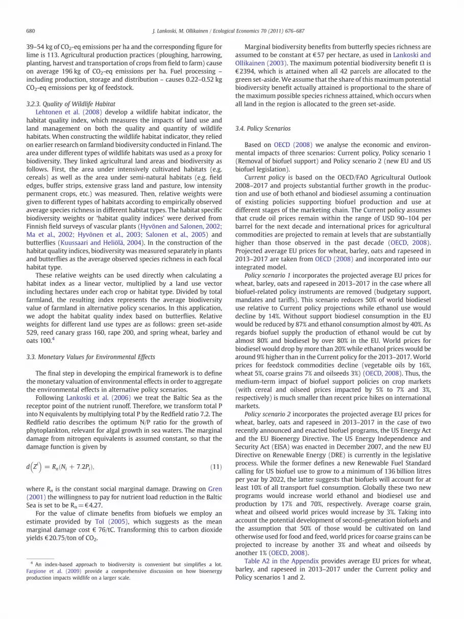
39–54 kg of CO2-eq emissions per ha and the corresponding figure forlime is 113. Agricultural production practices (ploughing, harrowing,planting, harvest and transportation of crops from field to farm) causeon average 196 kg of CO2-eq emissions per ha. Fuel processing –

including production, storage and distribution – causes 0.22–0.52 kgCO2-eq emissions per kg of feedstock.

3.2.3. Quality of Wildlife HabitatLehtonen et al. (2008) develop a wildlife habitat indicator, the

habitat quality index, which measures the impacts of land use andland management on both the quality and quantity of wildlifehabitats. When constructing the wildlife habitat indicator, they reliedon earlier research on farmland biodiversity conducted in Finland. Thearea under different types of wildlife habitats was used as a proxy forbiodiversity. They linked agricultural land areas and biodiversity asfollows. First, the area under intensively cultivated habitats (e.g.cereals) as well as the area under semi-natural habitats (e.g. fieldedges, buffer strips, extensive grass land and pasture, low intensitypermanent crops, etc.) was measured. Then, relative weights weregiven to different types of habitats according to empirically observedaverage species richness in different habitat types. The habitat specificbiodiversity weights or ‘habitat quality indices’ were derived fromFinnish field surveys of vascular plants (Hyvönen and Salonen, 2002;Ma et al., 2002; Hyvönen et al., 2003; Salonen et al., 2005) andbutterflies (Kuussaari and Heliölä, 2004). In the construction of thehabitat quality indices, biodiversity wasmeasured separately in plantsand butterflies as the average observed species richness in each focalhabitat type.

These relative weights can be used directly when calculating ahabitat index as a linear vector, multiplied by a land use vectorincluding hectares under each crop or habitat type. Divided by totalfarmland, the resulting index represents the average biodiversityvalue of farmland in alternative policy scenarios. In this application,we adopt the habitat quality index based on butterflies. Relativeweights for different land use types are as follows: green set-aside529, reed canary grass 160, rape 200, and spring wheat, barley andoats 100.4

3.3. Monetary Values for Environmental Effects

The final step in developing the empirical framework is to definethe monetary valuation of environmental effects in order to aggregatethe environmental effects in alternative policy scenarios.

Following Lankoski et al. (2006) we treat the Baltic Sea as thereceptor point of the nutrient runoff. Therefore, we transform total Pinto N equivalents by multiplying total P by the Redfield ratio 7.2. TheRedfield ratio describes the optimum N/P ratio for the growth ofphytoplankton, relevant for algal growth in sea waters. The marginaldamage from nitrogen equivalents is assumed constant, so that thedamage function is given by

d Zi� �

= Rn Ni + 7:2Pið Þ; ð11Þ

where Rn is the constant social marginal damage. Drawing on Gren(2001) the willingness to pay for nutrient load reduction in the BalticSea is set to be Rn=€4.27.

For the value of climate benefits from biofuels we employ anestimate provided by Tol (2005), which suggests as the meanmarginal damage cost € 76/tC. Transforming this to carbon dioxideyields €20.75/ton of CO2.

4 An index-based approach to biodiversity is convenient but simplifies a lot.Fargione et al. (2009) provide a comprehensive discussion on how bioenergyproduction impacts wildlife on a larger scale.

Marginal biodiversity benefits from butterfly species richness areassumed to be constant at €57 per hectare, as used in Lankoski andOllikainen (2003). The maximum potential biodiversity benefit Ω is€2394, which is attained when all 42 parcels are allocated to thegreen set-aside.We assume that the share of this maximumpotentialbiodiversity benefit actually attained is proportional to the share ofthe maximum possible species richness attained, which occurs whenall land in the region is allocated to the green set-aside.

3.4. Policy Scenarios

Based on OECD (2008) we analyse the economic and environ-mental impacts of three scenarios: Current policy, Policy scenario 1(Removal of biofuel support) and Policy scenario 2 (new EU and USbiofuel legislation).

Current policy is based on the OECD/FAO Agricultural Outlook2008–2017 and projects substantial further growth in the produc-tion and use of both ethanol and biodiesel assuming a continuationof existing policies supporting biofuel production and use atdifferent stages of the marketing chain. The Current policy assumesthat crude oil prices remain within the range of USD 90–104 perbarrel for the next decade and international prices for agriculturalcommodities are projected to remain at levels that are substantiallyhigher than those observed in the past decade (OECD, 2008).Projected average EU prices for wheat, barley, oats and rapeseed in2013–2017 are taken from OECD (2008) and incorporated into ourintegrated model.

Policy scenario 1 incorporates the projected average EU prices forwheat, barley, oats and rapeseed in 2013–2017 in the case where allbiofuel-related policy instruments are removed (budgetary support,mandates and tariffs). This scenario reduces 50% of world biodieseluse relative to Current policy projections while ethanol use woulddecline by 14%. Without support biodiesel consumption in the EUwould be reduced by 87% and ethanol consumption almost by 40%. Asregards biofuel supply the production of ethanol would be cut byalmost 80% and biodiesel by over 80% in the EU. World prices forbiodiesel would drop bymore than 20%while ethanol prices would bearound 9% higher than in the Current policy for the 2013–2017.Worldprices for feedstock commodities decline (vegetable oils by 16%,wheat 5%, coarse grains 7% and oilseeds 3%) (OECD, 2008). Thus, themedium-term impact of biofuel support policies on crop markets(with cereal and oilseed prices impacted by 5% to 7% and 3%,respectively) is much smaller than recent price hikes on internationalmarkets.

Policy scenario 2 incorporates the projected average EU prices forwheat, barley, oats and rapeseed in 2013–2017 in the case of tworecently announced and enacted biofuel programs, the US Energy Actand the EU Bioenergy Directive. The US Energy Independence andSecurity Act (EISA) was enacted in December 2007, and the new EUDirective on Renewable Energy (DRE) is currently in the legislativeprocess. While the former defines a new Renewable Fuel Standardcalling for US biofuel use to grow to a minimum of 136 billion litresper year by 2022, the latter suggests that biofuels will account for atleast 10% of all transport fuel consumption. Globally these two newprograms would increase world ethanol and biodiesel use andproduction by 17% and 70%, respectively. Average coarse grain,wheat and oilseed world prices would increase by 3%. Taking intoaccount the potential development of second-generation biofuels andthe assumption that 50% of those would be cultivated on landotherwise used for food and feed, world prices for coarse grains can beprojected to increase by another 3% and wheat and oilseeds byanother 1% (OECD, 2008).

Table A2 in the Appendix provides average EU prices for wheat,barley, and rapeseed in 2013–2017 under the Current policy andPolicy scenarios 1 and 2.

681J. Lankoski, M. Ollikainen / Ecological Economics 70 (2011) 676–687

4. Results

We solve the model for a given spatial structure and employsensitivity analysis to investigate the impacts of the spatial pattern.We let the biorefinery be located at the centre of a given landscapeand focus on a gradient extending from it. The field parcels are locatedat a distance of 100 km from the biorefinery. Field parcels differ inland productivity and thus in fertilizer intensity for a given crop, sothat their runoff differs even in the case they are identical in theirspatial characteristics (such as slopes of field parcels towardswatercourses). Moreover, we account for retention of nutrient inthe waterways to the sea. In the sensitivity analysis both the locationof the biorefinery and spatial features of the field parcels are changedto examine how the landscape pattern impacts the results.

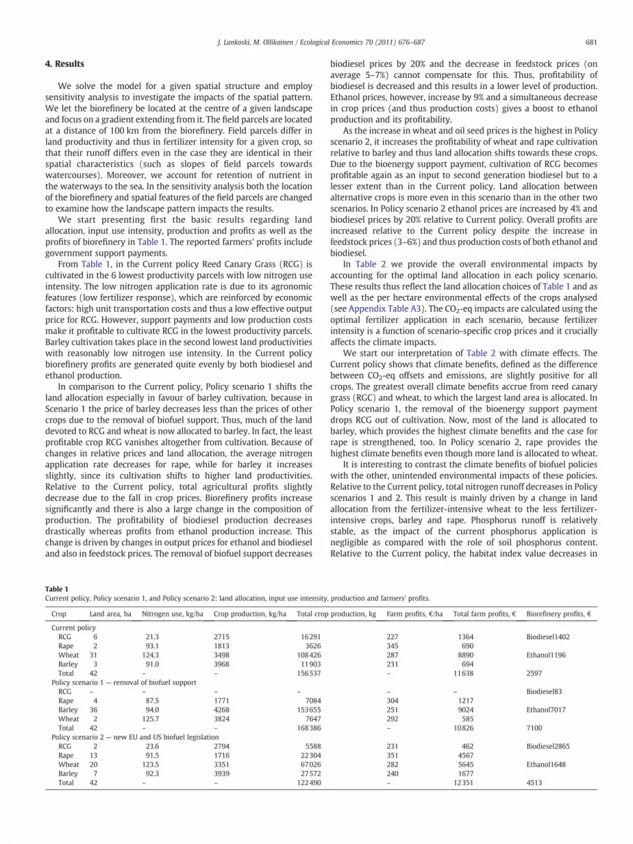
We start presenting first the basic results regarding landallocation, input use intensity, production and profits as well as theprofits of biorefinery in Table 1. The reported farmers' profits includegovernment support payments.

From Table 1, in the Current policy Reed Canary Grass (RCG) iscultivated in the 6 lowest productivity parcels with low nitrogen useintensity. The low nitrogen application rate is due to its agronomicfeatures (low fertilizer response), which are reinforced by economicfactors: high unit transportation costs and thus a low effective outputprice for RCG. However, support payments and low production costsmake it profitable to cultivate RCG in the lowest productivity parcels.Barley cultivation takes place in the second lowest land productivitieswith reasonably low nitrogen use intensity. In the Current policybiorefinery profits are generated quite evenly by both biodiesel andethanol production.

In comparison to the Current policy, Policy scenario 1 shifts theland allocation especially in favour of barley cultivation, because inScenario 1 the price of barley decreases less than the prices of othercrops due to the removal of biofuel support. Thus, much of the landdevoted to RCG and wheat is now allocated to barley. In fact, the leastprofitable crop RCG vanishes altogether from cultivation. Because ofchanges in relative prices and land allocation, the average nitrogenapplication rate decreases for rape, while for barley it increasesslightly, since its cultivation shifts to higher land productivities.Relative to the Current policy, total agricultural profits slightlydecrease due to the fall in crop prices. Biorefinery profits increasesignificantly and there is also a large change in the composition ofproduction. The profitability of biodiesel production decreasesdrastically whereas profits from ethanol production increase. Thischange is driven by changes in output prices for ethanol and biodieseland also in feedstock prices. The removal of biofuel support decreases

Table 1Current policy, Policy scenario 1, and Policy scenario 2: land allocation, input use intensity,

Crop Land area, ha Nitrogen use, kg/ha Crop production, kg/ha Total crop

Current policyRCG 6 21.3 2715 16291Rape 2 93.1 1813 3626Wheat 31 124.3 3498 108426Barley 3 91.0 3968 11903Total 42 – – 156537

Policy scenario 1 — removal of biofuel supportRCG – – – –

Rape 4 87.5 1771 7084Barley 36 94.0 4268 153655Wheat 2 125.7 3824 7647Total 42 – – 168386

Policy scenario 2 — new EU and US biofuel legislationRCG 2 23.6 2794 5588Rape 13 91.5 1716 22304Wheat 20 123.5 3351 67026Barley 7 92.3 3939 27572Total 42 – – 122490

biodiesel prices by 20% and the decrease in feedstock prices (onaverage 5–7%) cannot compensate for this. Thus, profitability ofbiodiesel is decreased and this results in a lower level of production.Ethanol prices, however, increase by 9% and a simultaneous decreasein crop prices (and thus production costs) gives a boost to ethanolproduction and its profitability.

As the increase in wheat and oil seed prices is the highest in Policyscenario 2, it increases the profitability of wheat and rape cultivationrelative to barley and thus land allocation shifts towards these crops.Due to the bioenergy support payment, cultivation of RCG becomesprofitable again as an input to second generation biodiesel but to alesser extent than in the Current policy. Land allocation betweenalternative crops is more even in this scenario than in the other twoscenarios. In Policy scenario 2 ethanol prices are increased by 4% andbiodiesel prices by 20% relative to Current policy. Overall profits areincreased relative to the Current policy despite the increase infeedstock prices (3–6%) and thus production costs of both ethanol andbiodiesel.

In Table 2 we provide the overall environmental impacts byaccounting for the optimal land allocation in each policy scenario.These results thus reflect the land allocation choices of Table 1 and aswell as the per hectare environmental effects of the crops analysed(see Appendix Table A3). The CO2-eq impacts are calculated using theoptimal fertilizer application in each scenario, because fertilizerintensity is a function of scenario-specific crop prices and it cruciallyaffects the climate impacts.

We start our interpretation of Table 2 with climate effects. TheCurrent policy shows that climate benefits, defined as the differencebetween CO2-eq offsets and emissions, are slightly positive for allcrops. The greatest overall climate benefits accrue from reed canarygrass (RGC) and wheat, to which the largest land area is allocated. InPolicy scenario 1, the removal of the bioenergy support paymentdrops RCG out of cultivation. Now, most of the land is allocated tobarley, which provides the highest climate benefits and the case forrape is strengthened, too. In Policy scenario 2, rape provides thehighest climate benefits even though more land is allocated to wheat.

It is interesting to contrast the climate benefits of biofuel policieswith the other, unintended environmental impacts of these policies.Relative to the Current policy, total nitrogen runoff decreases in Policyscenarios 1 and 2. This result is mainly driven by a change in landallocation from the fertilizer-intensive wheat to the less fertilizer-intensive crops, barley and rape. Phosphorus runoff is relativelystable, as the impact of the current phosphorus application isnegligible as compared with the role of soil phosphorus content.Relative to the Current policy, the habitat index value decreases in

production and farmers' profits.

production, kg Farm profits, €/ha Total farm profits, € Biorefinery profits, €

227 1364 Biodiesel1402345 690287 8890 Ethanol1196231 694– 11638 2597

– – Biodiesel83304 1217251 9024 Ethanol7017292 585– 10826 7100

231 462 Biodiesel2865351 4567282 5645 Ethanol1648240 1677– 12351 4513

Table 2Current policy, Policy scenario 1, and Policy scenario 2: total nitrogen and phosphorusrunoff (kg), total CO2-eq offsets and emissions (tons) and habitat index value.

Crop N-runoff,kg

P-runoff,kg

CO2-eq offsets,tons

CO2-eqemissions, tons

Habitat indexvalue

Current policyRCG 23 5 20 7Barley 42 4 14 11Wheat 552 45 143 126Rape 29 3 10 4Total 646 57 187 148 113.3

Policy scenario 1 — removal of biofuel supportBarley 518 51 183 140Wheat 36 3 10 9Rape 55 6 19 8Total 609 60 212 157 109.5

Policy scenario 2 — new EU and US biofuel legislationRCG 8 1 7 3Barley 100 10 33 26Wheat 354 29 89 80Rape 184 18 61 27Total 646 58 190 136 133.8

682 J. Lankoski, M. Ollikainen / Ecological Economics 70 (2011) 676–687

Policy scenario 1, because of a reduction of land allocated to RCG,which is a slightly more valuable habitat for butterflies than cereals. Incontrast, the habitat index value increases in Policy scenario 2.

To facilitate discussion on whether the climate benefits frombiofuel production exceed the costs associated with other environ-mental impacts we use valuation studies to provide Table 3, whichdefines all impacts in monetary terms.

The first two columns in Table 3 indicate the social costs due tonutrient runoff damage. The third and fourth columns define themonetary climate and biodiversity benefits. The fifth columnexpresses the overall net environmental impact in monetary terms.Finally, the last column indicates the net social benefits from biofuelproduction. These net social benefits incorporate the monetary valueof environmental impacts, farmers' short-run profits without subsi-dies and biorefinery profits without subsidies.

Table 3 reports nutrient runoff damage to the Baltic Sea usingnitrogen equivalents as the counting units on the basis of the Redfieldratio. Moreover, for both nitrogen and phosphorus runoff we accountfor nutrient retention (on average 10%), which slightly decreases thenutrient damage. Despite this, Table 3 clearly demonstrates thatnutrient runoff damage from bioenergy crop cultivation is large. Dueto the Redfield ratio the damages from nitrogen and phosphorusrunoff are roughly equal. Biodiversity benefits are determined on the

Table 3Current policy, Policy scenario 1, and Policy scenario 2: money values of total nitrogen ruprofits, €.

Crop N-runoff damage, € P-runoff damage, € Climate benefit, €

Current policyRCG 88 132 259Rape 110 78 116Barley 162 118 64Wheat 2120 1246 353Total 2480 1574 792

Policy scenario 1 — removal of biofuel supportRCG 0 0 0Rape 211 156 229Barley 1991 1413 898Wheat 138 80 33Total 2340 1649 1160

Policy scenario 2 — new EU and US biofuel legislationRCG 30 44 88Rape 706 509 693Barley 382 274 184Wheat 1360 803 145Total 2478 1630 1110

basis of wildlife habitat quality weights for different crops and landallocation between the crops. Higher biodiversity benefits in Policyscenario 2 relative to Policy scenario 1 are due to the larger share ofland allocated to the cultivation of rape and reed canary grass, whichprovide a more valuable habitat for butterflies than cereals do.

Table 3 demonstrates that the case for biofuels under currentbiofuel processing technology is hardly warranted when all environ-mental impacts are taken into account. In the Current policy, only reedcanary grass provides a sum of climate and biodiversity benefits thatexceeds the nutrient runoff damage. Thus, there is a sound basis forthe existing biofuel policy for this crop. The same does not, however,necessarily hold true for wheat, barley and rape. In these cases theeconomic value of all environmental impacts is negative. The samepattern can be found in Policy scenarios 1 and 2. However, bothsuggested policies moderate the negative impacts of the Currentpolicy, that is, the current biofuel policy.

Despite the negative net impacts on the environment the overallsocial benefits are positive for all crops and all scenarios. Moreover,both suggested policy scenarios perform clearly better than currentpolicies as regards overall net social benefits. These results are mainlydriven by increased profitability of biofuel production and to a lesserextent improved environmental performance.

In sum, our analysis of both the Current policy and suggestedpolicies reveals that in the light of peoples' willingness to pay forenvironmental quality, in most cases the harm from production ofbiofuels is greater for other parts of the ecosystem than its benefits arefor the climate. Only for reed canary grass were we able to find a solidbasis for current and suggested policies. These results are based on aset of assumptions, which we find the most plausible. We now turn toexamining how robust the findings are to changes in the values ofsome key parameters.

5. Sensitivity Analysis

Our base case employed a set of assumptions concerning theproduction chain and associated life cycle impacts of biofuel crops in afixed spatial set-up. We now explore in detail how spatial featuresimpact the social returns to biofuel production. The spatial featurescomprise both the environmental characteristics of field parcels(through field slopes) and the location of the fields relative to thebiorefinery.

Unlike location, the slopes of field parcels do not impact theprivately optimal choices of farmers in the absence of e.g. water

noff, total phosphorus runoff, total climate benefits, habitat index value, and farmer's

Biodiversity benefit, € Net environmental impact, € Net social benefit, €

103 142 163943 −30 99132 −183 732

332 −2681 8063510 −2752 11425

0 0 086 −53 1519

386 −2120 1378521 −164 756

493 −2337 16060

34 48 825279 −244 739975 −437 1898

214 −1765 5458602 −2398 15580

683J. Lankoski, M. Ollikainen / Ecological Economics 70 (2011) 676–687

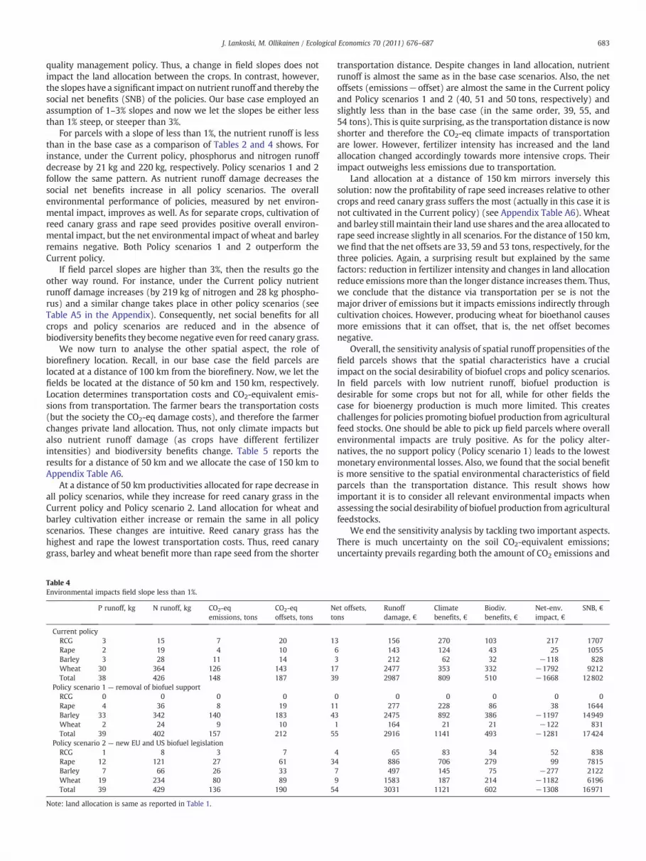
quality management policy. Thus, a change in field slopes does notimpact the land allocation between the crops. In contrast, however,the slopes have a significant impact on nutrient runoff and thereby thesocial net benefits (SNB) of the policies. Our base case employed anassumption of 1–3% slopes and now we let the slopes be either lessthan 1% steep, or steeper than 3%.

For parcels with a slope of less than 1%, the nutrient runoff is lessthan in the base case as a comparison of Tables 2 and 4 shows. Forinstance, under the Current policy, phosphorus and nitrogen runoffdecrease by 21 kg and 220 kg, respectively. Policy scenarios 1 and 2follow the same pattern. As nutrient runoff damage decreases thesocial net benefits increase in all policy scenarios. The overallenvironmental performance of policies, measured by net environ-mental impact, improves as well. As for separate crops, cultivation ofreed canary grass and rape seed provides positive overall environ-mental impact, but the net environmental impact of wheat and barleyremains negative. Both Policy scenarios 1 and 2 outperform theCurrent policy.

If field parcel slopes are higher than 3%, then the results go theother way round. For instance, under the Current policy nutrientrunoff damage increases (by 219 kg of nitrogen and 28 kg phospho-rus) and a similar change takes place in other policy scenarios (seeTable A5 in the Appendix). Consequently, net social benefits for allcrops and policy scenarios are reduced and in the absence ofbiodiversity benefits they become negative even for reed canary grass.

We now turn to analyse the other spatial aspect, the role ofbiorefinery location. Recall, in our base case the field parcels arelocated at a distance of 100 km from the biorefinery. Now, we let thefields be located at the distance of 50 km and 150 km, respectively.Location determines transportation costs and CO2-equivalent emis-sions from transportation. The farmer bears the transportation costs(but the society the CO2-eq damage costs), and therefore the farmerchanges private land allocation. Thus, not only climate impacts butalso nutrient runoff damage (as crops have different fertilizerintensities) and biodiversity benefits change. Table 5 reports theresults for a distance of 50 km and we allocate the case of 150 km toAppendix Table A6.

At a distance of 50 km productivities allocated for rape decrease inall policy scenarios, while they increase for reed canary grass in theCurrent policy and Policy scenario 2. Land allocation for wheat andbarley cultivation either increase or remain the same in all policyscenarios. These changes are intuitive. Reed canary grass has thehighest and rape the lowest transportation costs. Thus, reed canarygrass, barley and wheat benefit more than rape seed from the shorter

Table 4Environmental impacts field slope less than 1%.

P runoff, kg N runoff, kg CO2-eqemissions, tons

CO2-eqoffsets, tons

Nto

Current policyRCG 3 15 7 20 1Rape 2 19 4 10Barley 3 28 11 14Wheat 30 364 126 143 1Total 38 426 148 187 3

Policy scenario 1 — removal of biofuel supportRCG 0 0 0 0Rape 4 36 8 19 1Barley 33 342 140 183 4Wheat 2 24 9 10Total 39 402 157 212 5

Policy scenario 2 — new EU and US biofuel legislationRCG 1 8 3 7Rape 12 121 27 61 3Barley 7 66 26 33Wheat 19 234 80 89Total 39 429 136 190 5

Note: land allocation is same as reported in Table 1.

transportation distance. Despite changes in land allocation, nutrientrunoff is almost the same as in the base case scenarios. Also, the netoffsets (emissions−offset) are almost the same in the Current policyand Policy scenarios 1 and 2 (40, 51 and 50 tons, respectively) andslightly less than in the base case (in the same order, 39, 55, and54 tons). This is quite surprising, as the transportation distance is nowshorter and therefore the CO2-eq climate impacts of transportationare lower. However, fertilizer intensity has increased and the landallocation changed accordingly towards more intensive crops. Theirimpact outweighs less emissions due to transportation.

Land allocation at a distance of 150 km mirrors inversely thissolution: now the profitability of rape seed increases relative to othercrops and reed canary grass suffers the most (actually in this case it isnot cultivated in the Current policy) (see Appendix Table A6). Wheatand barley still maintain their land use shares and the area allocated torape seed increase slightly in all scenarios. For the distance of 150 km,we find that the net offsets are 33, 59 and 53 tons, respectively, for thethree policies. Again, a surprising result but explained by the samefactors: reduction in fertilizer intensity and changes in land allocationreduce emissions more than the longer distance increases them. Thus,we conclude that the distance via transportation per se is not themajor driver of emissions but it impacts emissions indirectly throughcultivation choices. However, producing wheat for bioethanol causesmore emissions that it can offset, that is, the net offset becomesnegative.

Overall, the sensitivity analysis of spatial runoff propensities of thefield parcels shows that the spatial characteristics have a crucialimpact on the social desirability of biofuel crops and policy scenarios.In field parcels with low nutrient runoff, biofuel production isdesirable for some crops but not for all, while for other fields thecase for bioenergy production is much more limited. This createschallenges for policies promoting biofuel production from agriculturalfeed stocks. One should be able to pick up field parcels where overallenvironmental impacts are truly positive. As for the policy alter-natives, the no support policy (Policy scenario 1) leads to the lowestmonetary environmental losses. Also, we found that the social benefitis more sensitive to the spatial environmental characteristics of fieldparcels than the transportation distance. This result shows howimportant it is to consider all relevant environmental impacts whenassessing the social desirability of biofuel production from agriculturalfeedstocks.

We end the sensitivity analysis by tackling two important aspects.There is much uncertainty on the soil CO2-equivalent emissions;uncertainty prevails regarding both the amount of CO2 emissions and

et offsets,ns

Runoffdamage, €

Climatebenefits, €

Biodiv.benefits, €

Net-env.impact, €

SNB, €

3 156 270 103 217 17076 143 124 43 25 10553 212 62 32 −118 8287 2477 353 332 −1792 92129 2987 809 510 −1668 12802

0 0 0 0 0 01 277 228 86 38 16443 2475 892 386 −1197 149491 164 21 21 −122 8315 2916 1141 493 −1281 17424

4 65 83 34 52 8384 886 706 279 99 78157 497 145 75 −277 21229 1583 187 214 −1182 61964 3031 1121 602 −1308 16971

Table 5Distance to biorefinery 50 km.

P runoff, kg N runoff, kg CO2-eqemissions, tons

CO2-eqoffsets, tons

Net offsets,tons

Runoffdamage, €

Climatebenefit, €

Biodiv.benefit, €

Net env.impact, €

SNB, €

Current policyRCG 6 33 11 30 19 325 394 137 206 1881Rape 0 0 0 0 0 0 0 0 0 0Barley 4 43 11 14 3 307 62 32 −212 778Wheat 45 564 129 147 18 3792 374 332 −3086 8543Total 55 640 151 191 40 4424 830 501 −3092 11202

Policy scenario 1 — removal of biofuel supportRCG 0 0 0 0 0 0 0 0 0 0Rape 0 0 0 0 0 0 0 0 0 0Barley 56 570 154 202 48 4156 996 418 −2742 15577Wheat 4 55 13 16 3 358 62 32 −264 1208Total 60 625 167 218 51 4513 1058 450 −3006 16785

Policy scenario 2 — new EU and US biofuel legislationRCG 3 17 6 15 9 165 187 69 91 1870Rape 11 115 17 38 21 829 436 171 −223 4717Barley 10 101 26 34 8 739 166 75 −498 2008Wheat 33 419 94 106 12 2804 249 246 −2309 6775Total 57 652 143 193 50 4536 1038 561 −2939 15370

Note: land allocation is as follows: wheat/barley/rape/reed canary grass: Current policy: 37/3/0/8, Policy scenario 1: 3/39/00 and Policy scenario 2: 23/7/8/4.

684 J. Lankoski, M. Ollikainen / Ecological Economics 70 (2011) 676–687

N2O emissions and the mechanisms by which they are created.Moreover, given that biofuel processing technology is developing, wealso analyse how an increased productivity of biofuel processingimpacts the provision of increased offsets and the returns tobioenergy production. For the soil CO2-equivalent emissions we usean estimate of 1.8 tons/ha for wheat, barley and rape and 0.2 tons/hafor reed canary grass. As regards increased productivity we increasethe biofuel processing efficiency by 20%. The findings are as expected.For higher soil CO2 emissions, the environmental basis for biofuelpolicies worsens significantly and as a result also social net benefits.The increased productivity of biofuel processing improves environ-mental performance of all scenarios but is not enough to make othercrops than reed canary grass and rape positive in their netenvironmental impacts.5

6. Conclusions

We examined how the climate benefits of the current andsuggested biofuel support policies relate to other environmentalimpacts of these policies. We developed a general integratedeconomic and ecological modelling approach and applied it toFinnish agriculture. The key environmental effects include GHGemissions over the life cycle, nitrogen and phosphorus runoff, and thequality of wildlife habitats. We used monetary values as a commonmeasure to contrast the value of other environmental effects toclimate benefits from bioenergy production. The Current policy wasthe current biofuel production support program. In addition to theCurrent policy, two recently suggested biofuel support policies wereanalysed. The first policy scenario entailed a radical elimination ofthe current support policies and the second one followed the twonew large biofuel programs, the US Energy Act and the EU BioenergyDirective.

The case for biofuel production under current feedstock produc-tion practices and biofuel processing technology is hardly warranted.In the Current policy scenario, only reed canary grass provides a sumof climate and biodiversity benefits that exceeds the increasednutrient runoff damage. Thus, there is a basis for the existing biofuelpolicy for this crop. The same does not, however, hold true for wheat,barley, and rape since in these cases the net economic impact on the

5 The detailed results are available from the authors upon request.

environment is negative. Both analysed policy scenarios moderate thenegative impacts of the current biofuel support policies.

Our basic findings can be condensed as follows. In light of thewillingness to pay estimates for environmental quality, both theCurrent policy and the suggested policy scenarios provide negativenet-impacts on the environment, that is, they do more harm to otherparts of the ecosystems than they create benefits for the climate. Onlybiodiesel that is produced from reed canary grass feedstocks providedsome rationale for current and suggested policies.

Sensitivity analysis shows that the spatial environmental char-acteristics have a great impact on the results. Due to lower (higher)nutrient runoff damages the total social net-benefits are increased(decreased) in the case where field parcel slopes are less (more) steepthan average slopes. The impact of increased or decreased transpor-tation distance to biorefinery impacts the profitability of certain cropsrelatively more, namely reed canary grass and rape seed. However,the social net-benefits seem to be more sensitive to spatialenvironmental characteristics of field parcels than transportationdistance. This result shows how important it is to consider all relevantenvironmental impacts when assessing the social desirability ofbiofuel production from agricultural feedstocks.

Our results generally provide biofuel policy analysis conducted inthe EU and the US (see e.g. OECD, 2008). Most of the biofuelproduction chains exhibit high production costs per unit of fuelenergy, so that biofuels in the EU and the US remain highlydependent on public support. Reduction of biofuel support wouldsignificantly reduce the profitability of both ethanol and biodieselproduction in the EU and ethanol production in the US. Environ-mental performance of biofuels varies a lot and requires theconsideration of the full life cycle of these fuels. Reduction of GHGemissions of cereal-based ethanol and of rapeseed-based biodieselare much lower than those of ethanol-based on sugarcane or secondgeneration biofuels. Moreover, if indirect land use changes are takeninto account, then potential reduction of GHG emissionswith the firstgeneration biofuels is even lower. Thus, current and proposedpolicies in the EU and the US have significant implications for globalland use and land use changes.

Our analysis reveals that current biofuel support policy is notespecially well-designed; it was outperformed by both policyalternatives. In net social benefit terms the suggested policies in theEU and the US that reform the existing policy performed best.However, a more important policy conclusion is that while makingbiodiesel from reed canary grass is desirable under current processing

Table A1 (continued)

Parameter Symbol Value

Price of nitrogen fertilizer, €/kg c 1.30Total expenditure for other inputs than fertilizer(seed, herbicide, fuel, machinery, etc.), €/ha

Λ, Κ

Spring wheat 544

685J. Lankoski, M. Ollikainen / Ecological Economics 70 (2011) 676–687

technology, manufacturing biodiesel from rape seed or ethanol fromwheat and barley is not. A shift to no-till cultivation, increasedattention to water protection issues and more efficient biofuelprocessing are probably needed simultaneously to make biofuelproduction socially desirable. This calls for close coordination ofbiofuel policies with agri-environmental policies.

Barley 520Rape 584Reed canary grass 372

Support payments, €/ha SSFP 230LFA 169Agri-environment 117Energy crop payment 45

Mitscherlich nitrogen response function

Acknowledgments

Funding from the Academy of Finland (Grants No. 124480 and131282) is gratefully acknowledged. The authors thank an anony-mous referee for very insightful constructive comments.

Spring wheat μ 3647–4945σ 0.7624ζ 0.0105

Barley μ 4630–5835σ 0.8280ζ 0.0168

Appendix

Table A1Price, cost, support, production and environmental parameters.

Parameter Symbol Value

Effective output price (net of grain drying andtransportation costs) in Current policy, €/kg

p

Spring wheat 0.136Barley 0.089Rape 0.295Reed canary grass 0.028

Grain drying cost, €/kg ο 0.013Transportation cost, €/kg/100 km ω1 0.0065

ω2 0.003

(continued on next page)

Table A2The average EU crop prices (2013–2017) under alternative scenarios.

Crop Current policy Policy scenario 1 Policy scenario 1

Wheat 155.7 146.0 159.9Barley 108.6 107.8 111.8Rape 312.7 292.4 331.7

Fertilizermanufacture

Herbicidemanufacture

Transport Transport

Transport

Cropproduction

- CO2-eq.

- CO2-eq.

- CO2-eq.

- CO2-eq.

- CO2-eq.

- CO2 from soil- CO2-eq. from fertilization- CO2-eq. from tillage practices,

harvesting and grain drying

- N, P runoff

- quality of wildlifehabitat

Biofuel production

Storage and distribution

Fig. A1. Environmental effects covered in the empirical application.

Reed canary grass μ 5021–5864σ 0.7075ζ 0.0197

Quadratic nitrogen response function Θ 690–1100Χ 8.17–11.04γ −0.0354

Nitrogen runoff function ϕi 15.0ι 0.7ι0 −0.7

Phosphorus runoff functions ψi 234Φ 10.9ξ 790

Runoff damage, €/kg of N equivalents Rn 4.27Social value of climate damage, €/CO2-eq b 20.75Maximum biodiversity benefit, € Ω 2394

Table A3Current policy, Policy scenario 1, and Policy scenario 2: per ha environmental effects:nitrogen runoff and phosphorus runoff (kg/ha), CO2-eq emissions and offsets (tons/ha)and CO2-eq net-offsets (tons/ha).

Crop N-runoff,kg/ha

P-runoff,kg/ha

CO2-eqemissions,tons/ha

CO2-eqoffsets,tons/ha

CO2-eq netoffsetstons/ha

Current policyWheat 17.8 1.45 4.1 4.6 0.5Barley 14.1 1.42 3.7 4.7 1.0Rape 14.3 1.42 2.1 4.9 2.8RCG 3.8 0.80 1.2 3.3 2.1

Policy scenario 1 — removal of biofuel supportWheat 18.0 1.45 4.3 5.1 0.8Barley 14.4 1.42 3.9 5.1 1.2Rape 13.7 1.41 2.1 4.8 2.7

Policy scenario 2 — new EU and US biofuel legislationWheat 17.7 1.45 4.0 4.4 0.4Barley 14.2 1.42 3.7 4.7 1.0Rape 14.1 1.42 2.1 4.7 2.6RCG 3.9 0.80 1.3 3.4 2.1

Table A4Sensitivity analysis: total farm profits, biorefinery profits, nitrogen runoff damage, phosphorus runoff damage, and net-environmental impact, €.

Current policy Policy scenario 1 Policy scenario 2

Total farm profits Field slopeb1% 11580 11297 13465Field slopeN3% 11580 11297 13465Biorefinery distance 50 km 11368 11503 13156Biorefinery distance 150 km 12227 10998 13615

Total biorefinery profits Field slopeb1% 2597 7100 4513Field slopeN3% 2597 7100 4513Biorefinery distance 50 km 2575 7849 4747Biorefinery distance 150 km 1874 6677 4105

Nitrogen runoff damage Field slopeb1% 1638 1544 1624Field slopeN3% 3323 3136 3321Biorefinery distance 50 km 2461 2402 2506Biorefinery distance 150 km 2621 2301 2511

Phosphorus runoff damage Field slopeb1% 1040 1082 1073Field slopeN3% 2343 2469 2437Biorefinery distance 50 km 1544 1655 1605Biorefinery distance 150 km 1656 1647 1662

Net environmental impacts Field slopeb1% −1376 −973 −1006Field slopeN3% −4364 −3952 −4045Biorefinery distance 50 km −2741 −2567 −2532Biorefinery distance 150 km −3061 −2222 −2457

Table A5Field slopes more than 3%.

P-runoff, kg N-runoff, kg CO2-eq emissions, tons CO2-eq offsets, tons Runoff damage, € Climate benefits, € Biodiv. benefits, € Net-env. impact, € NSB, €

Current policyRCG 7 31 7 20 348 270 103 25 1554Rape 4 38 4 10 285 125 43 −118 914Barley 6 57 11 14 428 62 32 −334 619Wheat 67 739 126 143 5215 353 332 −4531 6726Total 84 865 148 187 6276 809 510 −4958 9813

Policy scenario 1 — removal of biofuel supportRCG 0 0 0 0 0 0 0 0 –

Rape 8 74 8 19 562 228 86 −248 1369Barley 76 694 140 183 5300 892 386 −4022 12406Wheat 4 48 9 10 328 21 21 −286 669Total 88 816 157 212 6190 1141 493 −4556 14444

Policy scenario 2 — new EU and US biofuel legislationRCG 2 10 3 7 104 83 34 13 797Rape 28 246 27 61 1911 706 279 −927 6906Barley 15 133 26 33 1029 145 75 −809 1631Wheat 43 474 80 89 3346 187 214 −2945 4598Total 88 863 136 190 6390 1120 602 −4668 13932

Land allocation: same as Table 1.

Table A6Location 150 km.

P-runoff, kg N-runoff, kg CO2-eq emissions, tons CO2-eq offsets, tons Runoff damage, € Climate benefits, € Biodiv. benefits, € Net-env. impact, € NSB, €

Current policyRCG 1 3 1 2 44 21 17 −6 160Rape 6 56 8 19 424 228 86 −109 1928Barley 8 83 22 27 600 104 64 −433 1349Wheat 45 540 124 140 3689 −2283 332 −3025 7603Total 60 682 155 188 4754 −1930 499 −3573 11040

Policy scenario 1 — removal of biofuel supportRCG 0 0 0 0 0 0 0 0 0Rape 8 81 12 28 592 332 129 −131 2208Barley 48 482 130 171 3534 851 364 −2319 12524Wheat 3 35 8 10 242 42 21 −179 721Total 59 598 150 209 4367 1224 514 −2629 15453

Policy scenario 2 — new EU and US biofuel legislationRCG 0 0 0 0 0 0 0 0 0Rape 21 209 31 69 1538 789 321 −429 8325Barley 10 98 25 32 726 145 75 −506 1788Wheat 29 346 78 86 2369 166 214 −1989 5150Total 60 653 134 187 4633 1100 611 −2924 15263

Note: Land allocation is as follows: wheat/barley/rape/reed canary grass: Current policy: 31/6/4/1, Policy scenario 1: 2/34/6/0 and Policy scenario 2: 20/7/15/0.

686 J. Lankoski, M. Ollikainen / Ecological Economics 70 (2011) 676–687

687J. Lankoski, M. Ollikainen / Ecological Economics 70 (2011) 676–687

References

Barney, J.N., DiTomaso, J.M., 2008. Nonnative species and bioenergy: are we cultivatingthe next invader? BioScience 58 (1), 64–70.

Bäckman, S.T., Vermeulen, S., Taavitsainen, V.-M., 1997. Long-term fertilizer field trials:comparison of three mathematical response models. Agricultural and Food Sciencein Finland 6, 151–160.

Chiu, Y.-W., Walseth, B., Suh, S., 2009. Water embodies in bioethanol in the UnitedStates. Environmental Science and Technology 43, 2688–2692.

Dominguez-Faus, R., Powers, S., Burken, J., Alvarex, P., 2009. The water footprint ofbiofuels: a drink or drive issue? Environmental Science and Technology 43,3005–3010.

Donner, S.D., Kucharik, C.J., 2008. Corn-based ethanol production compromises goal ofreducing nitrogen runoff by the Mississippi river. Proceedings of the NationalAcademy of Sciences 105, 4513–4518.

Edwards, R., Larivé, J.-F., Mahieu, V., Rouveirolles, P., 2006. Well-to-wheels analysis offuture automotive fuels and powertrains in the European context. Well-to-WheelsReport. Version 2b. EUCAR, CONCAWE & JRC/IES.

Evans, J.M., Cohen, M.J., 2009. Regional water resource implications of bioethanolproduction in the Southeastern United States. Global Change Biology 15,2261–2273. doi:10.1111/j.1365-2486.2009.01868.x.

Fargione, J., Cooper, T., Flaspohler, D., Hill, J., Lehman, C., McCoy, T., McLeod, S., Nelson,E., Oberhauser, K., Tilman, D., 2009. Bioenergy and wildlife: threats andopportunities for grassland conservation. BioScience 59, 767–777.

Farrell, A.E., Plevin, R.J., Turner, B.T., Jones, A.D., O'Hare, M., Kammen, D.M., 2006.Ethanol can contribute to energy and environmental goals. Science 311 (5760),506–508.

de Fraiture, C., Giordano, M., Liao, Y., 2008. Biofuels and implications for agriculturalwater use: blue impacts of green energy. Water Policy 10 (Supplement 1), 67–81.

Gren, I-M., 2001. International versus national action against pollution at the Baltic Sea.Environmental and Resource Economics 20, 41–59.

Heikkilä, T., 1980. Economic use of nitrogen drawing on field experiments. ResearchReports No.70. Agricultural Economics Research Institute, Finland (In Finnish).

Hill, J., Polasky, S., Nelson, E., Tilman, D., Huo, H., Ludwig, L., Neuman, J., Zheng, H., Bonta,D., 2009. Climate change and health costs of air emissions from biofuels andgasoline. Proceedings of the National Academy of Sciences of the United States ofAmerica 106, 2077–2082.

Hyvönen, T., Salonen, J., 2002. Weed species diversity and community composition incropping practices at two intensity levels — a six-year experiment. Plant Ecology159, 73–81.

Hyvönen, T., Ketoja, E., Salonen, J., Jalli, H., Tiainen, J., 2003. Weed species diversity andcommunity composition in organic and conventional cropping of spring cereals.Agriculture, Ecosystems & Environment 97, 131–149.

Kuussaari, M., Heliölä, J., 2004. Perhosten monimuotoisuus eteläsuomalaisilla maatalou-salueilla. In: Kuussaari, M., Tiainen, J., Helenius, J., Hietala-Koivu, R., Heliölä, J. (Eds.),Maatalouden ympäristötuen merkitys luonnon monimuotoisuudelle ja maisemalle:MYTVAS-seurantatutkimus 2000–2003: Suomen ympäristö, 709, pp. 44–81.

Landis, D.A., Gardiner, M.M., van der Werf, W., Swinton, S.C., 2008. Increasing corn forbiofuel production reduces biocontrol services in agricultural landscapes. PNAS 105(51), 20552–20557 (published ahead of print December 15, 2008). doi:10.1073/pnas.0804951106.

Landström, S., Lomakka, L., Anderson, S., 1996. Harvest in spring improves yield andquality of reed canary grass as a bioenergy crop. Biomass and Bioenergy 11 (4),333–341.

Lankoski, J., Ollikainen, M., 2003. Agri–environmental externalities: a framework fordesigning targeted policies. European Review of Agricultural Economics 30, 51–75.

Lankoski, J., Ollikainen, M., Uusitalo, P., 2006. No-till technology: benefits to farmers andthe environment? Theoretical analysis and application to Finnish agriculture.European Review of Agricultural Economics 33, 193–221.

Lankoski, J., Lichtenberg, E., Ollikainen, M., 2008. Point/nonpoint effluent trading withspatial heterogeneity. American Journal of Agricultural Economics 90, 1044–1058.

Lankoski, J., Ollikainen, M., 2008. Bioenergy crop production and climate policies: a vonThunen model and case of reed canary grass in Finland. European Review ofAgricultural Economics 35, 519–546.

Lehtonen, H., Kuussaari, M., Hyvönen, T., Lankoski, J., 2008. Use of wildlife habitatindices in agricultural sector modelling. (unpublished manuscript).

Lichtenberg, E., 2002. Agriculture and the environment. In: Gardner, B., Rausser, G.(Eds.), Handbook of Agricultural Economics, vol 2A: Agriculture and its Linkages.Amsterdam, North Holland. pp. 1249–1313.

Ma, M., Tarmi, S., Helenius, J., 2002. Revisiting the species area relationship in a semi-Natural habitat: floral richness in agricultural buffer zones in Finland. Agriculture,Ecosystems and Environment 89, 137–148.

Marshall, L., 2007. Thirst for corn: what 2007 plantings could mean for theenvironment. WRI Policy Note — Energy: Biofuels No. 2. World Resources Institute,Washington.

Muller, A., 2009. Sustainable agriculture and the production of biomass for energy use.Climatic Change 94 (3–4), 319–331. doi:10.1007/s10584-008-9501-2.

Myyrä, S., Ketola, E., Yli-Halla, M., Pietola, K., 2005. Land improvements under landtenure insecurity: the case of pH and phosphate in Finland. Land Economics 81,557–569.

Mäkinen, T., Soimakallio, S., Paappanen, T., Pahkala, K., Mikkola, M., 2006. Liikenteebiopolttoaineiden ja peltoenergian kasvihuonekaasutaseet ja uudet liiketoiminta-konseptit. VTT Tiedotteita 2357. Espoo, Finland (In Finnish with English abstract:Greenhouse gas balances and new business opportunities for biomass-basedtransportation fuels and agribiomass in Finland).

OECD, 2008. Biofuel Support Policies — An Economic Assessment. Paris, France.Sala, O.E., Sax, D., Leslie, H., 2009. Biodiversity consequences of biofuel production. In:

Howarth, R.W., Bringezu, S. (Eds.), Biofuels: environmental consequences andinteractions with changing land use. : Proceedings of the Scientific Committee onProblems of the Environment (SCOPE) International Biofuels Project RapidAssessment, 22–25 September 2008, Gummersbach Germany. Cornell University,Ithaca NY, USA, pp. 127–137 http://cip.cornell.edu/biofuels/.

Salonen, J., Hyvönen, T., Jalli, H., 2005. Weed flora and weed management of field peasIn Finland. Agricultural and Food Science 14, 189–201.

Simmelsgaard, S., 1991. Estimation of nitrogen leakage functions — nitrogen leakage asa function of nitrogen applications for different crops on sand and clay soils. In:Rude, S. (Ed.), Nitrogen Fertilizers in Danish Agriculture — Present and FutureApplication And Leaching, Report 62. Institute of Agricultural Economics,Copenhagen, pp. 135–150 (in Danish: Kvaelstofgödning i landbruget — behov ogudvasking nu og I fremtiden).

Tol, R.S.J., 2005. The marginal damage costs of carbon dioxide emissions: an assessmentof the uncertainties. Energy Policy 33, 2064–2074.

Uusitalo, R., 2004. Potential bioavailability of particular phosphorus in runoff fromarable clayey soils. Agrifood Research Reports 53, Doctoral Dissertation, MTTAgrifood Research Finland. Jokioinen: MTT Agrifood Research Finland.

Uusitalo, R., Jansson, H., 2002. Dissolved reactive phosphorus in runoff assessed by soilextraction with an acetate buffer. Agricultural and Food Science in Finland 11,343–353.

Yearbook of Farm Statistics, 2007. Information Centre of the Ministry of Agriculture andForestry. Helsinki, Finland.