Biodiversity conservation in traditional farming landscapes The future of birds and large carnivores in Transylvania Doctoral thesis by Ine Dorresteijn

Welcome message from author
This document is posted to help you gain knowledge. Please leave a comment to let me know what you think about it! Share it to your friends and learn new things together.
Transcript
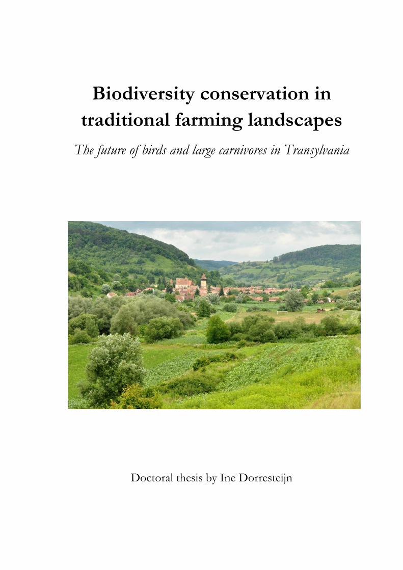
Biodiversity conservation in
traditional farming landscapes
The future of birds and large carnivores in Transylvania
Doctoral thesis by Ine Dorresteijn

Biodiversity conservation in
traditional farming landscapes
The future of birds and large carnivores in Transylvania
Academic dissertation Submitted to the Faculty of Sustainability of Leuphana University
for the award of the degree
‘Doctor of Natural Sciences’
-Dr. rer. nat.-
Submitted by
Ine Dorresteijn
Born on 15.05.1984 in Utrecht (The Netherlands)

Date of submission: 09.01.2015
Doctoral advisor and reviewer: Prof. Dr. Joern Fischer
Reviewer: Prof. Dr. Tobias Kuemmerle
Reviewer: Prof. Dr. Kristoffer Hylander
Date of disputation: 29 May 2015
Copyright notice
Chapters II-IX, and Appendix I & II have either been published or are in preparation for
publication in international scientific journals. Copyright of the text and the illustrations is with the
author or the authors of the respective chapter. The publishers own the exclusive right to publish
or to use the text and illustrations for their purposes. Reprint of any part of this dissertation
requires permission of the copyright holders.
Photo credits: Jan Hanspach (cover page; page 14, Fig 1.2a,b,d), Nathanaël Vetter (page 33), and
Rémi Bigonneau & Anne-Catherine Klein (page 155, 187), all other photos by Ine Dorresteijn
© Ine Dorresteijn (Chapters I, II, V & IX)
© Springer (Chapter III & IV)
© Elsevier (Chapters VI & Appendix II)
© Public Library of Science (Chapters VII & Appendix I)
© International Association for Bear Research and Management (Chapter VIII)
Author΄s address:
Leuphana University, Faculty of Sustainability Science
Scharnhorststrasse 1, 21335 Lueneburg, Germany
e-mail: [email protected]

Acknowledgements
‘Even the woodpecker owes his success to the fact that he uses his head and keeps pecking away
until he finishes the job he starts’ – Coleman Cox
I quite often felt like this woodpecker during my PhD, and I would still be pecking away if it wasn’t
for the many people that helped from the start to the finish of my PhD.
First of all I wish to thank my supervisor Joern Fischer. This PhD would not have been
possible without him. Joern supported, encouraged, and inspired me, and he has given me
irreplaceable guidance and advice at every stage of the PhD. Thanks for sometimes keeping me on
the ground, but also for giving me the space to carry out my ideas, even if that meant more time in
the field.
I am grateful to the entire team for their support during my PhD, but most of all just for
making me part of the team. Jan Hanspach provided important guidance throughout the PhD.
Many thanks for helping, listening, and handling my impatience, especially with R. Also thanks to
Henrik von Wehrden for helping me through several statistical and GIS problems. I learned a lot
about the region from Tibor Hartel, but also had a great time with him during my first month in
the field. Thanks to Dave Abson for proofreading the first chapter of this dissertation, and
together with Julia Leventon and Heike Zimmermann for creating a nice atmosphere and many
serious and not so serious discussions. Thanks to my fellow PhD-students Jacqueline Loos, Andra
Milcu, Friederieke Mikulcak, and Marlene Roellig for sharing all the ups and downs, frustrations
and laughs, invaluable discussions, chocolates and cookies, and for being my friends during the past
years. I also had the pleasure to work with two bright bachelor students. Being able to discover the
world of identifying birds by their song together with Lunja Ernst was incredibly helpful. Thanks to
Lucas Teixeira for helping me with data entry, data analyses, and making fieldwork at night look
easy and fun – it was great having you around for so long.
This dissertation arises from a large amount of data collected in the field. None of this
would have been possible without the help of the most awesome field team, and a big thanks to all
of you! Cathy Klein spent nine months with me in the field and deserves special thanks. Having
such a reliable, hardworking, and funny good friend by my side was the best recipe for two
successful field seasons. Joris Tinnemans was tireless in the field and while sorting camera pictures
and with his humour made both years a lot of fun. Rémi Bigonneau did a fantastic job on the bird
surveys and made the best barbecues for the team. Arpad Szapanyos was indispensable at several
stages during my time in Romania and I could always count on him. Thanks to Cosmin Moga for
helping with the bird surveys when the migrants arrived, but also for the wines in the evenings.
Hans Hedrich did an incredible job with the interviews and translations and had the superb skill of
making people feel comfortable during the interviews. Annamarie Krieg, you were a sunshine in
the field house even after long days of anthill counting in the heat. Ben Scheele and Alexander
Fletcher were crazy enough to spend their holidays counting anthills and I very much appreciate
their efforts. Also thanks to Jenny Long who spent part of her holidays setting out camera traps
and sorting pictures. Martin Bubner and Frank Dietrich were a hardworking and dependable team,
and fortunately also knew how to fix the lights in our field house. Nate Vetter and Frans Meeuwsen
reinforced the team with new energy in the last month of fieldwork and without their help we
would not have been able to finish our ambitious camera trap plan. Thanks to Kuno and
Annemarie Martini for opening their house to us in Sighisoara.
I am especially grateful to all respondents that participated in the interviews, the people
whose land we accessed for our fieldwork, and the people that helped with directions, cars, or any
other problem encountered in the field.
I am also thankful to our partner organizations in Romania. I enjoyed the collaboration
with The Milvus-group in Targu Mures very much, and would like to thank all the people that
collected data on bear activity. In particular, I would like to thank Attila Kecskés, Hana Latková,
Zsófia Mezey, and Szilárd Sugár, with whom I worked closely for Chapter IV of this dissertation.
My thanks also go to the Mihai Eminescu Trust, especially Caroline Fernolend and Oliviu Marian,
for their help and logistical support.
I would like to thank all my co-authors for their help with the preparations of the different
manuscripts. I would especially like to thank Euan Ritchie and Dale Nimmo. Euan made it possible
for me to spend a month in his working group at Deakin University to learn more about trophic
ecology and have an overall amazing experience in Australia. Thanks to Dale for his valuable input
on several manuscripts and also for letting me live in his house while I was in Australia. Thanks to
Laura Kehoe and Tobias Kuemmerle for providing extra camera traps and driving them all the way
down to Romania.
This research would not have been possible without funding. I am grateful to the
Alexander von Humboldt Foundation and the International Association for Bear Research and
Management for funding our research. Most of the research was funded through a Sofja
Kovalevskaja Award by the Alexander von Humboldt Foundation to Joern Fischer. The
International Association for Bear Research and Management funded the interview work and made
this interdisciplinary dissertation possible.
Finally, thanks to all friends and family that reminded me of also having a life next to the
PhD. Thanks to the Schultner family for their interest and support, and for providing me with the
most delicious energy packages when times were busy. A warm thanks go to my brother, sister, and
sister-in-law – Bram, Marleen, and Dorien Dorresteijn – for always showing interest in my work
and their visits to Germany. I am grateful to my parents, Leo and Joyce Dorresteijn for their
support and encouragements, but also for visiting me wherever I decide to go, and for moving my
stuff to those places. A loving thanks to Jannik Schultner who was my rock during my PhD years,
kept me sane at especially more stressful times, let me rant when I wanted too, but also made this
time wonderful!
Preface
This dissertation is presented as a series of manuscripts based on empirical research carried out in
Transylvania, Romania. Chapter I provides a general overview of the dissertation, including the
overarching goal and specific aims, a summary of all included manuscripts, a synthesis of the results
identifying system properties that facilitate biodiversity conservation in traditional farming
landscapes, and finally an outlook for conservation priorities in traditional farming landscapes.
Beyond Chapter I, the manuscripts included in this dissertation (Chapters II-IX) are divided into
three sections (A, B, and C). Section A examines the effects of local and landscape scale land-use
patterns on birds and large carnivores and how these animals may be affected by future land-use
change (Chapters II-V). To gauge the role of traditional land-use elements for biodiversity, in
Section B, I focus on wood pastures as one prominent example of such traditional elements
(Chapters VI-VIII). Lastly, in section C, I use a social-ecological systems approach to understand
social drivers underlying human-bear coexistence (Chapters IV and IX). With the exception of
Chapter II, all manuscripts are either published, in revision, or under review in international
scientific journals. I, the author of this dissertation, conducted the majority of the research
presented in this dissertation and am the lead author of the manuscripts presented in Chapters II-
V, VII, and IX. I provided important contributions to Chapters VI and VIII as a co-author. A
reference to the journal each manuscript is submitted to and the contributing co-authors is
presented on the title page of each chapter. The Appendix contains two published manuscripts that
I co-authored during my PhD. The research of these two manuscripts was conducted in the same
study area but with a focus on butterflies and plants; their similar research context provides
additional insights for the general synthesis of this dissertation.

Table of contents
Abstract 1
Chapter I 3
Biodiversity conservation in traditional farming landscapes:
The future of birds and large carnivores in Transylvania
Section A: Land-use effects on biodiversity 29
Chapter II 31
Maintaining bird diversity in a traditional farming
landscape in Eastern Europe
Chapter III 53
Impact of land cover homogenization on the corncrake
(Crex crex) in traditional farmland
Chapter IV 71
Human-carnivore coexistence in a traditional rural
landscape
Chapter V 105
Incorporating anthropogenic effects into trophic ecology:
Predator-prey interactions in a human-dominated landscape
Section B: Traditional wood pastures 129
Chapter VI 131
Wood-pastures in a traditional rural region of Eastern
Europe: Characteristics, management, and status
Chapter VII 153
The conservation value of traditional rural landscapes:
The case of woodpeckers in Transylvania, Romania
Chapter VIII 169
Brown bear activity in traditional wood-pastures in Southern
Transylvania, Romania
Section C: Human-bear coexistence 183
Chapter IX 185
Social factors mediating human-carnivore coexistence:
Understanding coexistence pathways in Central Romania
(Chapter IV is also part of this Section)
References 213
Appendix I 239
Low-intensity agricultural landscapes in Transylvania
support high butterfly diversity: Implications for conservation
Appendix II 265
Plant diversity in a changing agricultural landscape mosaic
in Southern Transylvania (Romania)

1
Abstract
Traditional farming landscapes typically support exceptional biodiversity. They evolved as tightly
coupled social-ecological systems, in which traditional human land-use shaped highly
heterogeneous landscapes. However, these landscapes are under severe threats of land-use
change, in particular through land-use intensification and land abandonment. Changing land-use
practices fundamentally change the structure of traditional farming landscapes, which implies a
direct threat to the biodiversity they support. Navigating biodiversity conservation in such changing
landscapes requires a thorough understanding of the drivers that maintain the social-ecological
system.
This dissertation aimed to identify system properties that facilitate biodiversity
conservation in traditional farming landscape, focusing specifically on birds and large carnivores in
the rapidly changing traditional farmland region of Southern Transylvania, Romania. In order to
identify these properties, I first examined the effects of local and landscape scale land-use
patterns on birds and large carnivores and how they may be affected by future land-use change.
Bird diversity was supported by the broad gradients of woody vegetation cover and
compositional heterogeneity. Land-use intensification, and hence the loss of woody vegetation
cover and homogenization of land covers, would thus negatively affect biodiversity. This was
especially evident from predictions on the distribution of the corncrake (Crex crex) in response
to potential future land cover homogenization. Here, a moderate reduction of land cover
diversity could drastically reduce the extent of corncrake habitat. Further results showed that
the brown bear (Ursus arctos) would mainly be affected by land-use change through the
fragmentation of large forest blocks, especially if land-use change would reduce habitat
connectivity to the presumed source population in the Carpathian Mountains. Moreover, this
dissertation revealed that large carnivores (brown bear and wolf, Canis lupus) may have
important and often ignored roles in structuring the ecosystem of traditional farming
landscapes by limiting herbivores.
Second, to gauge the role of particular traditional land-use elements for biodiversity
this dissertation focused on the conservation value of traditional wood pastures, as one
prominent example of such traditional elements. Wood pastures were found to have a high
conservation value. The combination of low-intensity used grasslands with old scattered trees
provided important supplementary habitat for different forest species such as woodpeckers
and the brown bear. Worryingly, current management of wood pastures differed from traditional
techniques in several aspects, which may threaten their persistence in the landscape.
Third, this dissertation took a social-ecological systems approach to understand how links
between the social and ecological parts of the system affect human-bear coexistence. The majority
of people had a positive perception on human-bear coexistence. The use of traditional sheep
2
herding techniques combined with the tolerance of some shepherds to occasional livestock
predation facilitated coexistence in a region where both carnivores and livestock are present. More
generally, the genuine links between people and their environment (i.e. where people value their
natural surroundings) were important drivers of people’s positive views on human-bear
coexistence. However, perceived failures of top-down managing institutions could potentially erode
these links and reduce people’s tolerance towards bears.
Through the consideration of two different animal taxa, this dissertation revealed six
important system properties facilitating biodiversity conservation in traditional farming landscapes.
Biodiversity was supported by the heterogeneous character of the traditional farming landscape at
multiple spatial scales. At the scale of the study area, similar proportions of the main land-use types (arable
land, grassland, and forests) support species associated with farmland as well as with forests,
through for example habitat connectivity and continuous spill-over between land-use types.
Heterogeneous landscapes can further support biodiversity through complementation and
supplementation of habitat at the landscape scale, where species can occur outside their considered core
habitat. Gradients of woody vegetation cover and heterogeneity, supported biodiversity at both local and
landscape scales, possibly through the provision of a wide range of resources or by facilitating
cross-habitat movements and spill-over. The heterogeneous character of the landscape is tightly
linked to traditional land-use practices, and thus these practices are key to maintaining biodiversity. In
addition, specific traditional land-use elements such as wood pastures have high conservation value,
while specific practices such is traditional livestock husbandry techniques facilitate human-
carnivore coexistence. Top-down limitation of large carnivores on herbivores may facilitate biodiversity
conservation through for example enhancing vegetation growth and tree regeneration. The genuine
links between humans and nature supported human-bear coexistence, and these links may form the core
of people’s values and sustainable use of natural resources.
Maintaining or preserving these six system properties should be a priority for
biodiversity conservation in traditional farming landscapes. However, to accomplish this, there
is an urgent need to develop more holistic visions for biodiversity conservation in traditional
farming landscapes that integrates the entire social-ecological system. Such a holistic approach may
comprise ‘broad and shallow’ landscape-scale conservation measures targeting the heterogeneous
landscape character of the forest-farmland mosaic at multiple spatial scales. Large scale
conservation measures may be complemented with more ‘deep and narrow’ conservation measures
targeting specific species, land-use types, threats, or traditional practices. Finally, conservation
measures should encourage the integration of the entire social-ecological system by recognizing and
incorporating important links between people and the environment. Traditional farming landscapes
are rapidly disappearing worldwide and developing conservation visions to navigate such landscape
through land-use change are now needed to prevent major biodiversity declines in these landscapes.

3
Chapter I

4
5
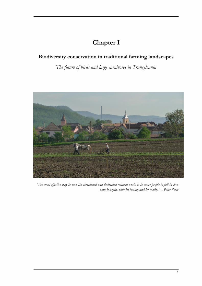
Chapter I
Biodiversity conservation in traditional farming landscapes
The future of birds and large carnivores in Transylvania
‘The most effective way to save the threatened and decimated natural world is to cause people to fall in love
with it again, with its beauty and its reality.’ – Peter Scott

Chapter I
6
Biodiversity conservation in traditional farming landscapes
7
Introduction
Traditional farming landscapes often harbour exceptional biodiversity and have high conservation
value. These landscapes evolved as tightly coupled social-ecological systems, which are now under
severe pressure of land-use change. From a biodiversity conservation perspective this is worrying
because land-use change may potentially erode the high levels of diversity these landscapes support.
Navigating biodiversity conservation in such changing landscapes requires a thorough
understanding of the drivers that maintain the social-ecological system. In this dissertation I focus
on the ecological part of the system and aim to identify system properties that facilitate biodiversity
conservation in traditional farming landscapes, focusing specifically on the traditional farmland
region in Southern Transylvania.
Human impacts on ecosystems
Humans have shaped and impacted the natural environment for tens of thousands of years (Smith
2007). Humanity’s dominance over virtually all ecological systems has created the urgent need to
understand the impacts and consequences of this anthropogenic influence (Vitousek et al. 1997;
Ellis & Ramankutty 2008). Human influences on the environment range from hunting-gathering
activities to the modification of entire ecosystems, most notably through agriculture. Until the
onset of industrialization, relatively low human population densities and limited technological
progress constrained human development. However, with the dramatic population increase and
technological advances of the last 200 years, human influences on the environment are now so
pervasive that they have become the major drivers of environmental change, taking us into a new
geological era, the Anthropocene (Crutzen 2002; Steffen et al. 2007). The Anthropocene is
characterized by a series of rapid biophysical and socio-economic changes (i.e. global change) that
are threatening ecosystems and human well-being. For example, during the last 50 years, the
structure of many ecosystems changed more rapidly than at any time in history (Millennium
Ecosystem Assessment 2005; Steffen et al. 2007). One of the most notable consequence is the
global biodiversity decline, with current rates potentially leading to the sixth mass extinction event
(Pimm et al. 1995; Pereira et al. 2010; Barnosky et al. 2011; Monastersky 2014). This rapid loss of
biodiversity matters not just because of the intrinsic values ascribed to biodiversity, but also
because current rates of biodiversity loss cannot be sustained without substantially eroding
resilience of ecosystems around the world – that is their ability to continue functioning in the face
of external shocks (Folke et al. 2004; Rockström et al. 2009). Ambitious goals to reduce human-
induced biodiversity loss (e.g. the Convention on Biological Diversity) have not yet been reached
(Butchart et al. 2010), and because of this failure, such goals have sometimes simply been
postponed into the future (www.cbd.int). Thus, a central challenge to humanity is to understand,
address and act on the underlying causes of human-induced biodiversity loss to safeguard
biodiversity in the future.
Chapter I
8
Land-use change and biodiversity loss
In terrestrial ecosystems, land-use change has been one of the major drivers of biodiversity loss -
although other drivers such as climate change, pollution, invasive species, and the synergistic
effects between different drivers also significantly contribute to global biodiversity loss (Sala et al.
2000). Land-use change can transform land through the conversion of the natural environment into
farmland or farmland can be transformed through a change in agricultural practices (Foley et al.
2005). Responses of biodiversity to land-use change are complex and dynamic and depend on the
type of land-use change and the ecological setting (DeFries et al. 2004). The conversion of the
natural environment into farmland caused biodiversity loss worldwide (Foley et al. 2005). Cropland
and pasture are now the largest terrestrial biome occupying 40 % of the land surface (Foley et al.
2005), while the area of forests has been halved over the past three centuries (Millennium
Ecosystem Assessment 2005).
Two of the most distinct effects related to the conversion of the natural environment into
agricultural land are habitat loss and habitat fragmentation for many species (reviewed in Fahrig
2003; Fischer & Lindenmayer 2007), especially for birds and mammals (Andrén 1994; Monastersky
2014). The expansion of agricultural land induced a global loss of birds to between a fifth and a
quarter relative to estimates of pre-agricultural numbers (Gaston et al. 2003). For large carnivores,
typical life-history traits such as large body size, large area requirements, slow reproductive rates,
and low population densities make them exceptionally vulnerable to habitat loss and fragmentation
(Crooks 2002). Increased human-carnivore conflicts and a resulting persecution by humans pose
additional threats to large carnivores in modified landscapes (Treves & Karanth 2003). Habitat loss
and fragmentation in combination with human persecution have severely reduced large carnivore
populations worldwide, which on average occupy only 47% of their historical distribution range
(Breitenmoser 1998; Woodroffe 2000; Ripple et al. 2014). However, large carnivores play critical
roles in structuring ecosystems through inducing trophic cascades, and the loss of large carnivores
has caused undesirable changes to a diverse range of ecosystems and its associated biodiversity
(Estes et al. 2011; Ripple et al. 2014).
Farmland biodiversity, in contrast, is to a large degree adapted to and dependent on the
continuation of agricultural management (Tscharntke et al. 2005). Farmland is the dominant
ecosystem in many places (e.g. in Europe) and holds a large part of the world’s biodiversity
(Pimentel et al. 1992). Yet, also farmland biodiversity can be adversely affected by land-use change,
most notably land-use intensification and land abandonment (Tscharntke et al. 2005; Queiroz et al.
2014; Uchida & Ushimaru 2014). Hence, understanding how land-use change affects biodiversity in
agricultural landscapes is important to mitigate global biodiversity loss.
Land-use change in European farmland
In Europe, most forests were cleared for agricultural land before the onset of the Anthropocene
(Kaplan et al. 2009). This historic forest loss, in combination with direct persecution, caused
Biodiversity conservation in traditional farming landscapes
9
dramatic declines of large carnivore populations in large parts of Western Europe during the 18th
and 19th century (Breitenmoser 1998). Biodiversity loss as a consequence of agricultural
intensification and land abandonment, in contrast, occurred mainly over the last decades and are
now the major threats to European farmland biodiversity (Donald et al. 2001; Tilman et al. 2001;
Stoate et al. 2009).
Agricultural intensification, with the aim to increase agricultural production, has caused
declines of farmland biodiversity and resulted in a halving of the European farmland bird
population (Donald et al. 2001; Voříšek et al. 2010). This decline is caused by ecosystem changes
during intensification due to increased mechanization, increased use of agrochemicals (i.e. fertilizers
and pesticides), loss of crop varieties and management techniques such as crop rotation and
intercropping, and the decline of low intensity land-use. Overall, intensification usually entails
homogenization (e.g. decrease in land cover diversity and woody vegetation cover) at multiple
spatial scales, including entire landscapes (Benton et al. 2003; Tscharntke et al. 2005). These
changes lead to decreased food availability and increased habitat loss and fragmentation for a wide
range of species (Hinsley 2000; Weibull et al. 2003; Concepción et al. 2008; Guerrero et al. 2012).
Species persistence in agricultural landscapes is highly dependent on landscape structure (Fischer &
Lindenmayer 2007), and maintaining or restoring heterogeneity in agricultural landscapes has been
suggested as one of the major strategies to halt farmland biodiversity declines (Benton et al. 2003).
For instance, negative effects of habitat loss and fragmentation may be reduced if the landscape
contains elements that provide habitat connectivity for a range of species, including birds and
carnivores (Uezu et al. 2005; Donald & Evans 2006; Crooks et al. 2011).
In addition to intensification, abandonment of farmland is also becoming more pervasive
globally, especially in marginal agricultural areas characterized by low-intensity farming and
generating relatively low yields (MacDonald et al. 2000; Queiroz et al. 2014). Land abandonment
typically changes the landscape by transforming agricultural land into shrubland, which eventually
turns into forest (Rudel et al. 2005). Land abandonment is often viewed as a negative process for
biodiversity because farmland biodiversity in low-intensity farming regions is often higher than in
natural forests (Höchtl et al. 2005; Lindborg et al. 2008). Indeed, especially in Europe, land
abandonment has been reported to negatively affect a range of taxa, with especially detrimental
effects on farmland birds (reviewed by Queiroz et al. 2014). On the other hand, land abandonment
has also been viewed to offer unique opportunities to restore the biodiversity of natural forest
ecosystems including large carnivores (Navarro & Pereira 2012).
Although intensification and more recently also abandonment have been exacerbated by
the European Union’s Common Agricultural Policy (CAP), the recognition of the value of
farmland biodiversity sparked national and international conservation measures to halt biodiversity
loss on farmland (Young et al. 2005; Henle et al. 2008). Despite these measures, farmland
biodiversity continues to decline and their effectiveness is questioned (Kleijn et al. 2011; Pe'er et al.
2014). Ongoing biodiversity decline highlights the need for more effective biodiversity
Chapter I
10
conservation in Europe’s agricultural landscapes. In this context, traditional farming landscapes are
of great interest to conservation because they often harbour exceptional biodiversity (Tscharntke et
al. 2005; Kleijn et al. 2009).
Traditional farming landscapes: values and challenges
Traditional farming landscapes are increasingly valued for their natural and cultural heritage. Their
importance for biodiversity has been noted worldwide (Ranganathan et al. 2008; Takeuchi 2010;
Robson & Berkes 2011; Liu et al. 2013), including in the traditional village systems of Eastern
Europe (Palang et al. 2006; Fischer et al. 2012). Traditional farming landscapes are characterized by
a long history of relatively persistent farming practices. Farming techniques in these landscapes are
often of low-intensity with low levels of agro-chemical input and little mechanization, that is, a high
degree of manual labour (Bignal & McCracken 2000; Plieninger et al. 2006). This way of farming
has created mixed farming landscapes with a mosaic of different land-uses including specific
traditional landscape elements like wood pastures (Plieninger & Schaar 2008), high land cover and
structural heterogeneity, and relatively abundant semi-natural vegetation (Plieninger et al. 2006).
Another distinctive feature of traditional farming landscapes is that they are often tightly
coupled social-ecological systems, that is, systems in which rural communities influence the
ecosystems and vice versa (Folke 2006). Moreover, the long history of interactions within this
system has created the opportunity for the different entities of the system to constantly co-evolve
(Liu et al. 2007). People have shaped the ecosystem through their activities, such as land-use, and
the ecosystem in turn provided people a variety of ecosystem services (i.e. the benefits people
derive from nature; Millennium Ecosystem Assessment 2005). These ecosystem services range
from provisioning services such as crops, water, and firewood, to cultural services such as the
feeling of a ‘sense of place’, and have historically provided direct incentives for sustainable land-use
(Fischer et al. 2012; Hartel et al. 2014). It is these centuries of co-evolving interactions between
humans and the natural environment that created the high cultural and natural value of the
landscape (Bignal & McCracken 2000). Moreover, landscapes shaped by traditional farming
practices harbour many of the habitats and species that are valued for biodiversity today (Halada et
al. 2011).
Despite their unique natural and cultural values, traditional farming landscapes are under
increasing pressure from modernization and globalization. Rapid socio-economic, political, and
cultural changes lead to the cessation of traditional farming practices in exchange for more
intensive practices, or abandonment of farmland altogether (Henle et al. 2008). The persistence of
these landscapes depends on how the social-ecological system navigates these profound changes
while simultaneously fostering biodiversity conservation and human well-being. Nevertheless,
current policies often fail to acknowledge the links between the social and the ecological parts of
the system, and policies usually target either the social or the ecological part exclusively (Fischer et
al. 2012). Such one-sided policies potentially erode the established historical connections between
Biodiversity conservation in traditional farming landscapes
11
people and the land that maintain the character of these landscapes, and hence the structures
supporting biodiversity. In addition, in Europe in particular, existing policies for farmland
biodiversity are often poorly adapted to traditional farmland (Sutcliffe et al. 2014). This can be
partly ascribed to a significant research gap, with the majority of European studies on farmland
biodiversity conducted in (Western European) countries with more intensively used farmland,
while biodiversity patterns in the more low-intensity traditional farmland regions (e.g. in Eastern
Europe) remain poorly understood (Baldi & Batary 2011; Tryjanowski et al. 2011).
Therefore, fostering biodiversity conservation of traditional farming regions requires a
thorough understanding of the drivers that maintain the social-ecological system. While this
dissertation does not aim to understand the entire social-ecological system, it deals with some
important aspects of the ecological system while acknowledging the significance of the other
features. In particular, I aimed to identify system properties that facilitate biodiversity conservation
in traditional farming landscapes, focusing specifically on birds and large carnivores in the rapidly
changing traditional farmland region of Southern Transylvania, Romania.
Transylvania’s traditional farmland region
Southern Transylvania in Central Romania (Fig. 1.1) is one of Europe’s last regions that is
dominated by traditional, small-scale farming systems. The study region was shaped by the culture
and land-use of the Saxons, which settled in Transylvania in the 12th and 13th century. The Saxons
came from different German-speaking European countries, and were the dominating ethnic group
in the study region where Hungarians, Romanians, and Roma were also present. Saxon land tenure
was based on communal management of pastures and forests, with individually owned arable fields
(Sutcliffe et al. 2013). The rise and fall of communism influenced land-use in the region. During
communism, agricultural land became collectivized under state ownership, but intensification was
not severe enough to fundamentally change the landscape and its associated biodiversity. After the
fall of communism in 1989 there was a large exodus of Saxons from the region as many resettled to
Germany. This exodus led to an abandonment of part of the agricultural land, while restitution of
small parcels of arable land to the remaining and new population prevented intensification of
agriculture and stimulated semi-subsistence farming.
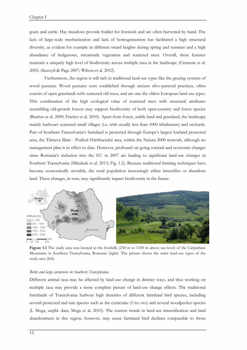
Despite these social changes, the characteristics of Southern Transylvania’s farming
landscape have changed relatively little since pre-industrial times, and traditional semi-subsistence
farming has maintained a land cover mosaic of relatively similar proportions of forest (28%), arable
land (37%), and grassland (24%; Fig. 1.1). Land-use is primarily determined by topography with
forests occupying the hill-tops, arable fields being located mainly in the valleys, and pastures
occurring on the slopes. Forests are dominated by hornbeam (Carpinus betulus), oak (Quercus sp.),
and beech (Fagus sylvatica). Arable lands are characterized by farming techniques that are small-scale
(most fields are smaller than two hectares) and are of low-intensity (most fields have low chemical
input and are tilled manually). The semi-natural pastures are grazed by sheep (dominant livestock),
Chapter I
12
goats and cattle. Hay meadows provide fodder for livestock and are often harvested by hand. The
lack of large-scale mechanization and lack of homogenization has facilitated a high structural
diversity, as evident for example in different sward heights during spring and summer and a high
abundance of hedgerows, streamside vegetation and scattered trees. Overall, these features
maintain a uniquely high level of biodiversity across multiple taxa in the landscape (Cremene et al.
2005; Akeroyd & Page 2007; Wilson et al. 2012).
Furthermore, the region is still rich in traditional land-use types like the grazing systems of
wood pastures. Wood pastures were established through ancient silvo-pastoral practices, often
consist of open grasslands with scattered old trees, and are one the oldest European land-use types.
This combination of the high ecological value of scattered trees with structural attributes
resembling old-growth forests may support biodiversity of both open-country and forest species
(Bauhus et al. 2009; Fischer et al. 2010). Apart from forest, arable land and grassland, the landscape
mainly harbours scattered small villages (i.e. with usually less than 1000 inhabitants) and orchards.
Part of Southern Transylvania’s farmland is protected through Europe’s largest lowland protected
area, the Târnava Mare - Podisul Hârtibaciului area, within the Natura 2000 network, although no
management plan is in effect to date. However, profound on-going societal and economic changes
since Romania’s inclusion into the EU in 2007 are leading to significant land-use changes in
Southern Transylvania (Mikulcak et al. 2013; Fig. 1.2). Because traditional farming techniques have
become economically unviable, the rural population increasingly either intensifies or abandons
land. These changes, in turn, may significantly impact biodiversity in the future.
Figure 1.1 The study area was located in the foothills (230 m to 1100 m above sea level) of the Carpathian
Mountains in Southern Transylvania, Romania (right). The picture shows the main land-use types of the
study area (left).
Birds and large carnivores in Southern Transylvania
Different animal taxa may be affected by land-use change in distinct ways, and thus working on
multiple taxa may provide a more complete picture of land-use change effects. The traditional
farmlands of Transylvania harbour high densities of different farmland bird species, including
several protected and rare species such as the corncrake (Crex crex) and several woodpecker species
(I. Moga, unpbl. data; Moga et al. 2010). The current trends in land-use intensification and land
abandonment in this region, however, may cause farmland bird declines comparable to those
Biodiversity conservation in traditional farming landscapes
13
observed in the more intensified countries of Western Europe (Voříšek et al. 2010). Considering
the effects of land-use change on the entire bird community beyond protected species is highly
necessary since common European birds are declining at high rates while populations of rare
species are slowly increasing (Inger et al. 2015).
Unlike most European countries, Romania sustains large and stable populations of large
carnivores (Salvatori et al. 2002), and the study area harbours relatively high densities of the brown
bear (Ursus arctos) and lower densities of the wolf (Canis lupus). In contrast to birds, large
carnivores may be affected especially by changes in forest cover, and may thus be positively
affected by land abandonment. In addition, large carnivores may not only be affected by land-use
or land-use change, but also by the tolerance levels of the rural population towards carnivores. The
reliance of people on forest products (e.g. firewood; Hartel et al. 2014), and the use of traditional
practices such as shepherding and beekeeping are potential areas of conflicts with carnivores. Thus,
large carnivore conservation in traditional farming landscapes does not only depend on the
biophysical environment, but also on the willingness of people to live with carnivores (Treves &
Karanth 2003; Dickman 2010).
Aims
As described above the overarching goal of this dissertation was to ‘identify system properties that
facilitate biodiversity conservation in traditional farming landscapes’ using birds and large carnivores in the
rapidly changing traditional farmland region of Southern Transylvania as a study system (Fig. 1.3).
In order to identify these properties this dissertation is divided into three sections. In Section A, I
focus on the effects of local and landscape scale land-use patterns on birds and large carnivores.
This Section also provides insights on the effects of potential land-use change on biodiversity. To
gauge the role of traditional land-use elements for biodiversity, in Section B, I focus on wood
pastures as one prominent example of such traditional elements. Here, we examined the structure
of wood pastures, and their use by woodpeckers and bears. Lastly, in section C, I use a social-
ecological systems approach to understand social drivers underlying human-bear coexistence. In
this part, we assessed the level of human-bear conflicts and the factors shaping the willingness of
people to live with bears. Thus, my specific aims were (Fig. 1.3):
A. How do local and landscape scale land-use and land-use change affect biodiversity (Chapters II-V)?
B. How do ancient wood pastures affect biodiversity (Chapters VI-VIII)?
C. How do links between the ecological system and the social system affect human-bear coexistence
(Chapters IV and IX)?
Chapter I
14
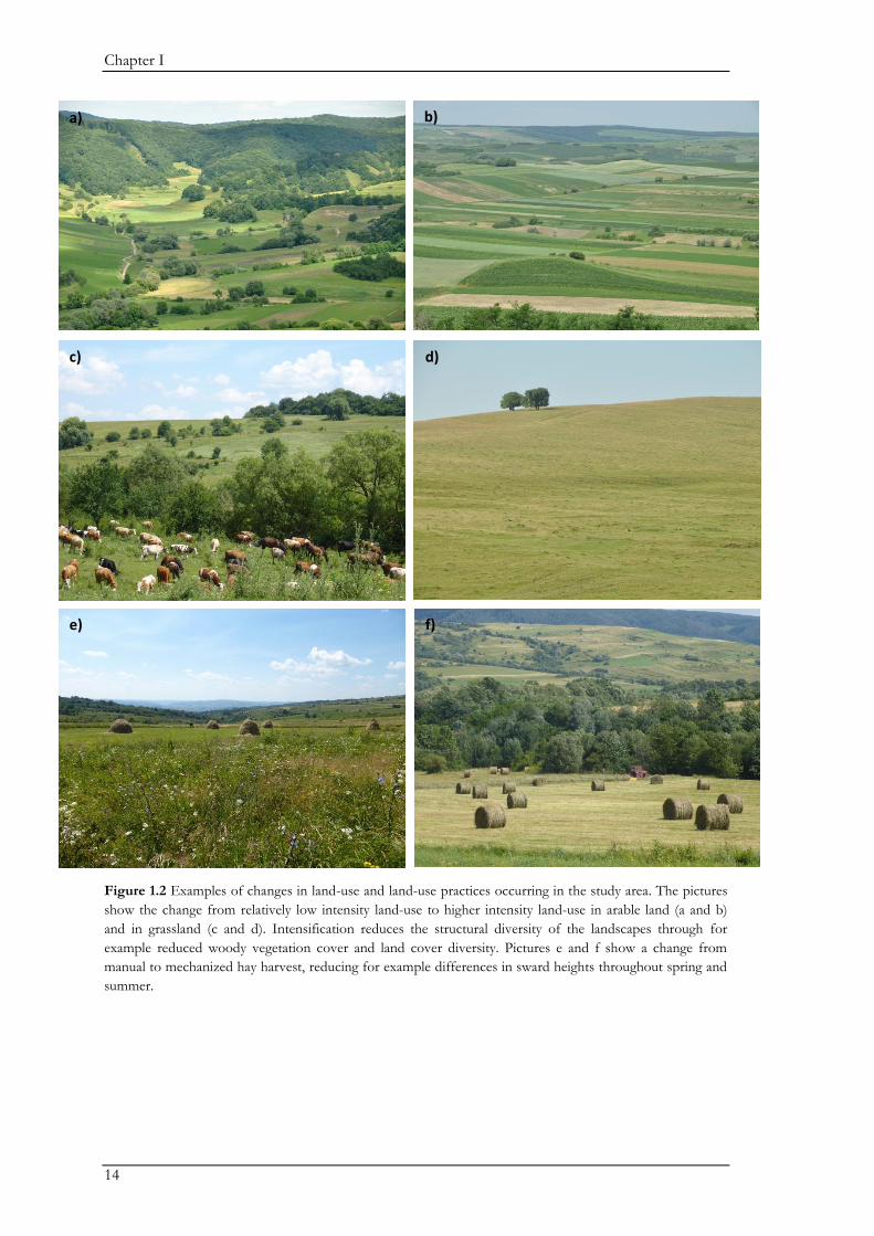
Figure 1.2 Examples of changes in land-use and land-use practices occurring in the study area. The pictures
show the change from relatively low intensity land-use to higher intensity land-use in arable land (a and b)
and in grassland (c and d). Intensification reduces the structural diversity of the landscapes through for
example reduced woody vegetation cover and land cover diversity. Pictures e and f show a change from
manual to mechanized hay harvest, reducing for example differences in sward heights throughout spring and
summer.
a) b)
c) d)
e) f)
Biodiversity conservation in traditional farming landscapes
15
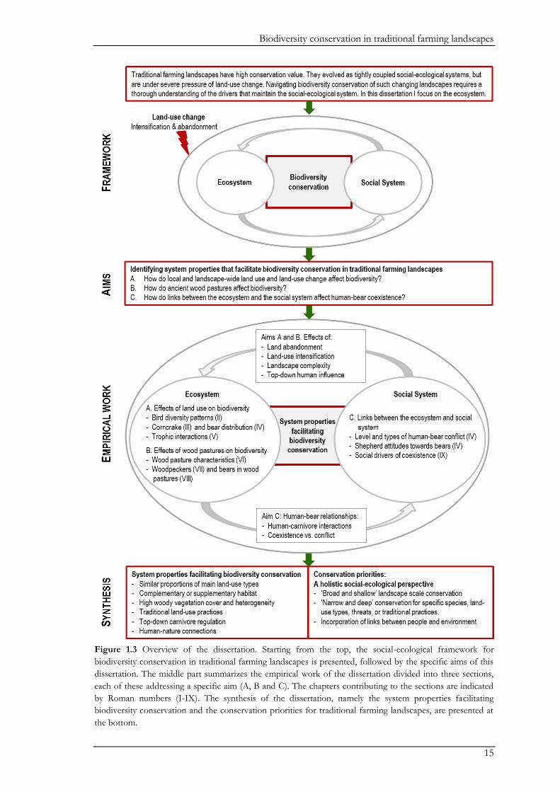
Figure 1.3 Overview of the dissertation. Starting from the top, the social-ecological framework for
biodiversity conservation in traditional farming landscapes is presented, followed by the specific aims of this
dissertation. The middle part summarizes the empirical work of the dissertation divided into three sections,
each of these addressing a specific aim (A, B and C). The chapters contributing to the sections are indicated
by Roman numbers (I-IX). The synthesis of the dissertation, namely the system properties facilitating
biodiversity conservation and the conservation priorities for traditional farming landscapes, are presented at
the bottom.
Chapter I
16
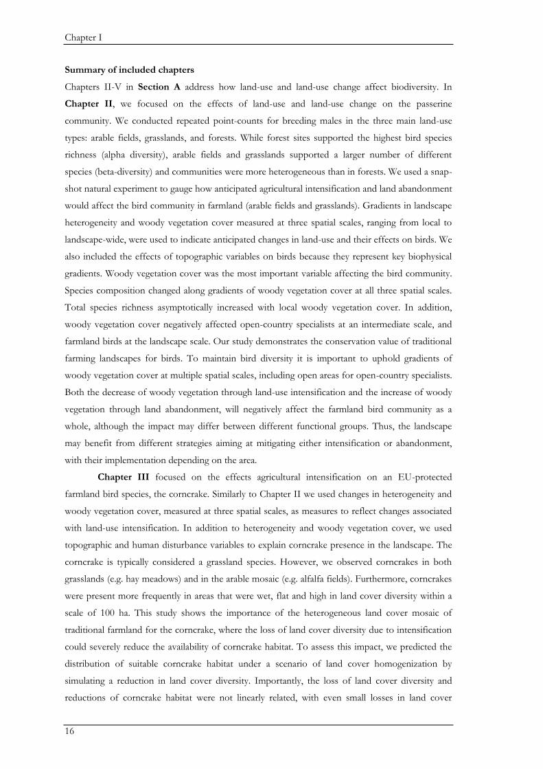
Summary of included chapters
Chapters II-V in Section A address how land-use and land-use change affect biodiversity. In
Chapter II, we focused on the effects of land-use and land-use change on the passerine
community. We conducted repeated point-counts for breeding males in the three main land-use
types: arable fields, grasslands, and forests. While forest sites supported the highest bird species
richness (alpha diversity), arable fields and grasslands supported a larger number of different
species (beta-diversity) and communities were more heterogeneous than in forests. We used a snap-
shot natural experiment to gauge how anticipated agricultural intensification and land abandonment
would affect the bird community in farmland (arable fields and grasslands). Gradients in landscape
heterogeneity and woody vegetation cover measured at three spatial scales, ranging from local to
landscape-wide, were used to indicate anticipated changes in land-use and their effects on birds. We
also included the effects of topographic variables on birds because they represent key biophysical
gradients. Woody vegetation cover was the most important variable affecting the bird community.
Species composition changed along gradients of woody vegetation cover at all three spatial scales.
Total species richness asymptotically increased with local woody vegetation cover. In addition,
woody vegetation cover negatively affected open-country specialists at an intermediate scale, and
farmland birds at the landscape scale. Our study demonstrates the conservation value of traditional
farming landscapes for birds. To maintain bird diversity it is important to uphold gradients of
woody vegetation cover at multiple spatial scales, including open areas for open-country specialists.
Both the decrease of woody vegetation through land-use intensification and the increase of woody
vegetation through land abandonment, will negatively affect the farmland bird community as a
whole, although the impact may differ between different functional groups. Thus, the landscape
may benefit from different strategies aiming at mitigating either intensification or abandonment,
with their implementation depending on the area.
Chapter III focused on the effects agricultural intensification on an EU-protected
farmland bird species, the corncrake. Similarly to Chapter II we used changes in heterogeneity and
woody vegetation cover, measured at three spatial scales, as measures to reflect changes associated
with land-use intensification. In addition to heterogeneity and woody vegetation cover, we used
topographic and human disturbance variables to explain corncrake presence in the landscape. The
corncrake is typically considered a grassland species. However, we observed corncrakes in both
grasslands (e.g. hay meadows) and in the arable mosaic (e.g. alfalfa fields). Furthermore, corncrakes
were present more frequently in areas that were wet, flat and high in land cover diversity within a
scale of 100 ha. This study shows the importance of the heterogeneous land cover mosaic of
traditional farmland for the corncrake, where the loss of land cover diversity due to intensification
could severely reduce the availability of corncrake habitat. To assess this impact, we predicted the
distribution of suitable corncrake habitat under a scenario of land cover homogenization by
simulating a reduction in land cover diversity. Importantly, the loss of land cover diversity and
reductions of corncrake habitat were not linearly related, with even small losses in land cover
Biodiversity conservation in traditional farming landscapes
17
diversity resulting in a high loss of suitable corncrake habitat. Thus, pro-active conservation
measures for the corncrake should include the farmland mosaic beyond grasslands. Here it will be
important to encourage the persistence of mixed farming.
We examined the effects of land-use patterns on bear distribution in Chapter IV. Bear
distribution was indicated through a sign-based metric of bear activity, namely the proportion of
anthills destroyed by bears relative to the total number of anthills in a transect. We were also
interested in identifying specific hotspots for bears in the region, especially with regard to the
Natura 2000 area. We modelled bear activity in relation to anthropogenic, biophysical, and
connectivity variables, and based on this, predicted bear activity for the entire study area. Contrary
to our expectations bears were not influenced by distance to the nearest settlement. Instead,
connectivity to the Carpathian Mountains, where the source population resides, was the most
important variable explaining bear activity. This measure of connectivity was indicated through a
cost-distance metric, where the ‘cost’ for a bear to move through each possible land cover type was
scored by a local bear expert. In contrast, connectivity between forest patches contained within the
study area did not affect bear activity. Connectivity of the different forest patches was indicated
through ‘betweenness centrality’, which represents how well connected a forest patch is within the
forest patch network regardless of the other land covers between these patches. Furthermore, bear
activity was higher in more rugged areas with large forest blocks and low pasture cover. We did not
find particular hotspots of activity in the Natura 2000 area. Rather, predicted bear activity showed a
gradual increase toward the Carpathian Mountains, but was otherwise relatively homogenous
throughout the study. Our results suggest that conservation management for bears should primarily
maintain the connectivity to the Carpathian Mountains, which would require land-use management
beyond the Natura 2000 region. The lack of importance of connectivity between forest patches at
more local scales indicates that forest fragmentation has not yet reached a level that would affect
bears and that high connectivity remains throughout the study area. Therefore, emphasis should be
placed on preserving large connected forest blocks, especially in rugged areas where bears can find
shelter. In contrast to birds, reduced pasture cover and an increase in woody vegetation as result of
land abandonment is likely to positively affect bears.
Chapter V explored the role of large carnivores in a human dominated ecosystem by
analysing trophic interactions between forest mammals, including humans as apex predators. We
aimed at assessing the top-down effects of large carnivores on herbivores and mesopredators in
relation to direct and indirect human top-down effects and bottom-up effects. Wolves, bears,
domestic dogs (Canis familiaris), and humans represented apex predators, red deer (Cervus elaphus)
and roe deer (Capreolus capreolus) represented the herbivores, and the red fox (Vulpes vulpes)
represented the mesopredator. Bottom-up effects were indicated by pasture and forest cover. We
combined data on species encounter rates from camera traps and bear and wolf densities from
hunting records to assess trophic interactions with piecewise structural equation models. We found
that bears and wolves exert top-down control, especially on herbivores, and thus maintain their

Chapter I
18
ecological role in human-dominated landscapes. Nevertheless, direct and indirect human-top down
effects at multiple trophic levels affected species encounter rates more strongly. Furthermore,
herbivores were also limited by dogs brought into the system by humans. The importance of top-
down herbivore control was even more evident through the relatively weak effect of the land cover
(i.e. bottom-up) variables. On the other hand, through their limiting effect on predators, humans
may reduce the predators’ top-down control. Although not accounted for in this study, humans
may further affect trophic cascades by mediating bottom-up effects through landscape
modification. Thus, bears and wolves are important for the regulation of the ecosystem, but human
direct and indirect top-down effects are currently higher. The persistence of bears and wolves
should therefore be ensured in order to conserve the ecological character of these valued traditional
landscapes. We also believe that further understanding of the different human effects on trophic
interactions in modified landscapes should be a major research priority.
Chapters VI-VIII in Section B focus specifically on the conservation value of traditional wood
pastures to gauge the role of particular traditional land-use elements for biodiversity. To gain a
better understanding of wood pastures we first of all explored the characteristics, management, and
status of wood pastures in Chapter VI. Wood pastures were mainly dominated by oak and several
species of fruit trees, which differed from the tree community composition in forests. Wood
pastures also contained more ancient trees (trees of which the age can reach centuries) compared to
forest sites, but were relatively low in dead tree abundance and shrub cover. These characteristics
reflect the traditional management of wood pastures, which were created from forests by grazing
and selective tree removal. Remaining trees were not only valued for their shade, but oaks provided
timber and acorns for livestock, while fruit trees provided fruits. Specific characteristics of wood
pastures were determined by variables such as topography, distance to village, management, and
surrounding forest cover. For example, fruit trees were more prevalent close to villages, while many
dead trees were found in wood pastures surrounded by forests. A detailed study on the biodiversity
of one specific wood pasture showed the high potential of wood pastures to support high levels of
biodiversity. Worryingly, current management of wood pastures differed from traditional
techniques in several aspects, which could potentially threaten their persistence. First, most wood
pastures were grazed by sheep only, whereas mixed livestock grazing used to be the common
management type. Second, many large trees suffered from (anthropogenic) burning. Although
pasture clearing through controlled burning has been used for centuries, the current trend towards
uncontrolled burning is a major threat to wood pastures. Third, we found some evidence of (illegal)
tree cutting, while historically only branches were cut and the trunk remained (‘pollarding’). Wood
pastures are not consistently formally protected within the EU, and our results show that their
persistence in Transylvania is in danger. Therefore, a solid ecological understanding in combination
with knowledge on cultural and human livelihood importance of wood pastures needs to be
developed to further their recognition for formal conservation.
Biodiversity conservation in traditional farming landscapes
19
The role of wood pastures for biodiversity was explored in more detail in Chapters VII
and VIII. In Chapter VII we assessed the habitat value of wood pastures for an assemblage of six
woodpecker species. Woodpeckers are considered to be highly sensitive to changes in forest
management due to their large home ranges and their requirement of large trees and dead wood for
nesting and foraging. Since wood pastures retain elements of natural forests they may provide
additional habitat for the more forest-associated woodpeckers. Indeed, we found that species
richness in wood pastures was similar to forests, although species composition differed slightly.
Wood pastures were especially important for the green woodpecker (Picus viridis), which is
considered an open-country species, while forests were more important for the lesser-spotted
woodpecker (Dendrocopos minor), which typically avoids foraging in open areas. In contrast, the other
four woodpecker species occurred in both wood pastures and forests. Two of the protected species
were especially prevalent in wood pastures with a higher surrounding forest cover. Thus, wood
pastures provide valuable supplementary habitat for woodpeckers. Favourable characteristics of
wood pastures may be high food availability (e.g. ants and insects), nesting cavities in large trees,
and the provision of connectivity between different forest patches.
Chapter VIII showed that wood pastures also provide valuable supplementary habitat for
the brown bear. We found evidence for bear activity in 87% of the surveyed wood pastures
(indicated through destroyed anthills). Similarly to Chapter IV, bear activity was higher at a close
proximity to the Carpathian Mountains and in more rugged and forested areas. Bears may find
wood pastures suitable for foraging because of the availability of multiple food sources and the
shelter provided by woody vegetation. Grassland ant species are not found in forests, but form an
important source of protein for the mainly vegetarian bear. During autumn, wood pastures further
provide fruits and hard mast, although the use of these food sources by bears could not be assessed
within the time-frame of our study. These two studies show the high potential of wood pastures for
biodiversity conservation. We suggest to explicitly consider wood pastures in major EU
conservation policies, for example by stimulating the maintenance of scattered trees in extensively
managed pastures.
Section C takes a social-ecological systems approach to understand how links between the social
and ecological parts of the system affect human-bear coexistence. In Chapter IV we used
questionnaires to obtain an overview on human-bear conflicts in the study area, and correlated
perceived levels of conflicts with observed bear activity. Conflicts with bears occurred across the
study area. People reportedly suffered from damage to crops, orchards, and beehives, as well as
predation on livestock, while attacks on humans were rare. Cow herders had little problems with
bears. In contrast, about half of the shepherds suffered bear attacks on sheep during the past three
years. Interestingly, perceived level of damage to orchards and crops was positively correlated with
bear activity, while bear activity did not correlate to the number of sheep attacks or perceived level
of damage to beehives. These differences may be explained by differences in guarding
Chapter I
20
management. Orchards and crops are often left unguarded, whereas, sheep are actively guarded by
both shepherds and sheep guard dogs. The lack of a correlation between bear activity and
perceived damage to beehives may be more related to the low abundance of this technique among
participants. These results indicate the importance of local factors other than bear activity on the
prevalence of livestock predation and highlight the possibility for conflict mitigation (e.g. through
location of the sheep camp). We asked shepherds several additional questions to examine whether
livestock predation affected their attitudes towards bears. There was some tolerance towards bears,
despite occasional sheep predation. Shepherds suffering from a higher rate of bear attacks
nevertheless expressed a strong dislike of bears more frequently. About half of the shepherds were
unsupportive of immediate killing of bears after a sheep attack. Thus, the use of traditional sheep
herding techniques combined with the tolerance of some shepherds is likely to facilitate human-
bear coexistence in the region.
In Chapter IX, we combined questionnaires with semi-structured interviews for a more
holistic understanding of the social drivers underlying human-bear coexistence. The majority of
participants had a positive perception of coexistence. The questionnaires revealed general patterns
on social drivers underlying coexistence such as past negative interactions, perceived risks of
damage, attitude, and age. The interviews revealed three coexistence pathways highlighting the
causal mechanisms driving people’s willingness to coexist with bears. These pathways show
different ways in which ongoing interactions between the ecological system and the social system
shape the willingness of people to coexist with bears. The three pathways were defined by three
major themes, namely bears, humans, and management. The landscape had important mediating
effects on the pathways centred on bears and humans. For example, in the landscape-bear
coexistence pathway, people’s perceptions and beliefs about bears were largely shaped through
direct interactions and experiences with bears. The importance of direct interactions was further
emphasized in the landscape-human coexistence pathway where people’s tolerance towards bears
increased following positive encounters with bears, while livestock predation by bears decreased
people’s tolerance. Nevertheless, negative perceptions on coexistence were more likely to be
shaped by the perception of a high risk of potential conflicts with bears than by the actual
experience of damage caused by bears. Furthermore, the landscape-human-coexistence pathway
showed that genuine links between people and their environment (i.e. where people value their
natural surroundings) were important drivers of people’s positive attitudes towards bears and an
ascription of non-use values to bears. However, the management coexistence pathway revealed that
perceived inadequate management may erode the rural population’s tolerance for bears.
Management related to bear population management, conflict mitigation and compensation
payments, and trophy hunting was often perceived unsatisfactory by the participants. In addition,
the feeling of distrust towards management bodies and dis-empowerment further widened the gap
between management bodies and local stakeholders. We conclude that to avoid the escalation of
human-human conflicts over bears, where bears represent disagreements between local
Biodiversity conservation in traditional farming landscapes
21
stakeholders and management bodies, coexistence may be maintained or facilitated through: (i)
participation of local stakeholders to enhance the information flow and reduce distrust towards
management bodies; (ii) targeted education programs to address people’s specific beliefs and
concerns regarding bear-related issues; and (iii) the development and increased transparency of
current and alternative solutions for conflict mitigation.
Synthesis: System properties facilitating biodiversity conservation
This dissertation provides important insights on biodiversity drivers and patterns in traditional
farming landscapes. To start with, it demonstrates the large biodiversity value of traditional farming
landscapes in general, and calls for an increased recognition of these systems for biodiversity
conservation. This is especially urgent since anticipated land-use change and the loss of traditional
farming practices may cause significant biodiversity declines in traditional farming landscapes.
Undoubtedly, there are many system properties of traditional farming landscapes that potentially
facilitate biodiversity conservation. Some of these are beyond the focus of this dissertation such as
traditional livestock and crop rotation schemes, diverse crop systems, low agro-chemical input, and
land-use that is not optimized to produce maximum yields. However, through the consideration of
two different animal taxa, this dissertation reveals six important system properties that support high
biodiversity in Transylvania’s traditional farming landscape.
1. Similar proportions of main land-use types
Biodiversity was supported by the heterogeneous character of the traditional farming landscape at
multiple spatial scales. At the scale of the study area, relatively similar proportions of the three main
land-use types likely support high biodiversity. Habitat loss and fragmentation are considered major
drivers of mammal and bird declines (Andrén 1994; Monastersky 2014). However, fragmentation
effects usually become visible below a threshold of 30% of available habitat (Andrén 1994; Hanski
2011), which is close to the proportional cover of the study area’s three main land-use types. The
approximately one-third of forest cover also seemed to provide sufficient habitat connectivity for
the brown bear (Chapter IV). Habitat connectivity at large scales is an important system property as
it can facilitate species’ movements and dispersal in fragmented landscapes and maintain gene flow
and metapopulation dynamics (Fischer & Lindenmayer 2007; Kopatz et al. 2012). For the brown
bear in Southern Transylvania, the existing connectivity between the study area and the source
population in the Carpathian Mountains, provided by configuration and composition of land
covers, was found to be particularly important (Chapter IV). In other parts of the brown bear’s
European range, in contrast, forest connectivity is degraded to a degree that limits the species’
expansion (Fernández et al. 2012).
Within farmland, bird species composition was not determined by land-use per se (e.g.
arable land vs grassland), but was influenced by different environmental gradients (Chapter II). The
availability of both grassland and arable land in relatively large proportions may support the similar
Chapter I
22
species composition of birds (Chapter II) and butterflies (Appendix I) in both land-use types, for
example through constant spill-over (Tscharntke et al. 2012). These processes may prevent the
divergence of distinct grassland and arable land communities but maintain more diverse
communities at the landscape scale. Although plant species composition differed between
grasslands and arable land, a substantial number of species was shared and both land-use types
were important contributors to the total species pool (Appendix II). In addition, a forest-farmland
mosaic facilitates spill-over effects from forests to farmland (Tscharntke et al. 2012), and we
observed a considerable number of forest bird species in farmland (Chapter II). Thus, the observed
proportions of land-use types in the study area support species associated with farmland as well as
with forests, with all three major land-use types contributing to high regional biodiversity.
2. Complementary or supplementary habitat
Heterogeneous landscapes can further support biodiversity through complementation and
supplementation of habitat at the landscape scale (Dunning et al. 1992). Landscape
complementation is provided in landscapes in which species encounter all required spatially
separated habitats containing necessary resources, while landscape supplementation is provided in
landscapes in which species encounter additional habitats that contain similar resources (Dunning
et al. 1992). We observed several species in land-use types outside their core habitat. For example,
wood-pastures were extensively used by different woodpecker species and the brown bear
(Chapters VII and VIII). The retention of forest structures across the landscape in traditional
farming landscapes thus provides supplementary if not complementary habitat for forest species
(Mikusinski & Angelstam 1998). Similarly, the corncrake was present throughout the arable mosaic
despite being considered a grassland species (Chapter III). Uncropped arable land in combination
with field margins or ditches may be important in providing resources similar to grasslands, such as
safe breeding and sheltering sites and high insect availability (Corbett & Hudson 2010; Budka &
Osiejuk 2013; Josefsson et al. 2013).
3. High woody vegetation cover and heterogeneity
At a more specific level, traditional farming landscapes supported biodiversity through the presence
of gradients in woody vegetation cover, including semi-natural vegetation, and through
heterogeneity, measured as the composition and configuration of land cover. High woody
vegetation cover supported bird (Chapter III), butterfly (Appendix 1) and plant (Appendix 2)
species richness locally, possibly by providing a range of resources such as refuge areas, nesting,
sheltering, and foraging sites (e.g. Benton et al. 2003; Ernoult & Alard 2011), or by facilitating
cross-habitat movements and spill-over (Tscharntke et al. 2012). Importantly, not all taxa respond
linearly to woody vegetation cover or heterogeneity. For example, bird richness increased
asymptotically with woody vegetation cover, which was especially evident in grasslands (Chapter II)
which harbours a large number of open-country species that disappear beyond certain levels of
Biodiversity conservation in traditional farming landscapes
23
woody vegetation cover (Sanderson et al. 2013). These findings demonstrate the need to also
maintain relatively homogenous, open areas (Batary et al. 2011b). Another case of important non-
linearity was revealed by the simulated severe reduction of corncrake habitat at relatively modest
levels of land cover homogenization (Chapter III).
We also identified the significance of the landscape context for effects of woody vegetation
cover and heterogeneity. Woody vegetation cover and heterogeneity influenced different species or
groups of species of birds (Chapter II), butterflies (Appendix 1), and plants (Appendix 2) at larger
spatial scales, and sometimes with effects opposite to those at smaller scales. Furthermore, we
found biodiversity to be affected not only by processes at multiple spatial scales, but effects also
differed between species, which may depend on their specific resource needs (Lindenmayer &
Fischer 2006). To conclude, the availability of woody vegetation cover and heterogeneity at
different spatial scales are important drivers of biodiversity in traditional farming landscapes.
Moreover, we demonstrated the need to further understand the scale dependence of different
species and across different taxa.
4. Traditional land-use practices
The presence of high woody vegetation cover and heterogeneity is linked to traditional semi-
subsistence farming practices. Such farming, including high degree of manual labour and few agro-
chemical inputs, is thus key to maintaining biodiversity. The manual cutting of hay in a mosaic
pattern, for example, provides a variety of sward heights throughout the breeding season of
corncrakes, thereby facilitating their presence in agricultural land (Chapter III). Wood pastures were
created by traditional silvo-pastoral practices but current management techniques differ from the
traditional ones and may severely threaten the persistence of wood pastures in the landscape
(Chapter VI). This change in management is likely to have a negative effect on the biodiversity
supported by wood pastures. As another example, the use of traditional livestock husbandry
techniques allowed coexistence between humans and large carnivores (Chapter IV and IX). The
combination of shepherds, livestock guard dogs, and nightly confinement of livestock are
successful in reducing livestock conflicts worldwide (Rigg 2001; Gehring et al. 2010), as well as in
Romania, as demonstrated here. This provides an important insight for European regions into
which large carnivores return after their earlier extirpation, but in which the loss of these husbandry
techniques and resulting conflicts hamper their successful establishment (Enserink & Vogel 2006;
Chapron et al. 2014).
5. Top-down carnivore regulation
The presence of large carnivores in the landscape can benefit biodiversity through top-down
control on mesopredators and herbivores (Estes et al. 2011; Ripple et al. 2014), which induce
trophic cascades that affect species at multiple trophic levels (Letnic et al. 2009). The importance of
trophic cascades for biodiversity have mainly been observed in wilderness areas (Ripple & Beschta
Chapter I
24
2012b), whereas the role of large carnivores in structuring human-dominated ecosystems remains
unclear (Sergio et al. 2014). We found limited evidence for top-down control on a mesopredator
(the red fox; Chapter V), which may be explained by large differences in body size (Donadio &
Buskirk 2006; Ritchie & Johnson 2009), or by densities of wolves and bears too low to effectively
limit foxes. In contrast, we found top-down limitation of wolves and bears on herbivores (Chapter
V), which indicates the importance of their persistence for the ecosystem (for example by limiting
overgrazing, enhancing vegetation growth, and maintaining biodiversity in general; Terborgh et al.
2001; Estes et al. 2011). Still, to fully understand the role of carnivores in traditional farming
landscapes future research should aim to understand (i) the extent and effects of possible trophic
cascades induced by carnivore top-down herbivore control; and (ii) the role of human bottom-up
and top-down effects on trophic cascades in combination with the effects induced by carnivores.
6. Human-nature connections
Large carnivore persistence does not only depend on the biophysical environment, but also on the
degree to which the rural population is willing to coexist with large carnivores (Treves & Karanth
2003). People in our study area had a general positive perception of human-bear coexistence
(Chapter IX). Their ability to tolerate carnivores partly stemmed from genuine links between
humans and nature, with people valuing the natural heritage. People’s culture shapes the landscape,
but the landscape in turn also shapes the culture of people (Pretty 2011). The centuries of co-
occurrence of humans and bears in Southern Transylvania probably shaped human culture to
accept and adapt to living with carnivores (see also Glikman et al. 2012). These strong ties between
people and the landscape possibly form the core of people’s values and sustainable use of natural
resources. Disconnecting these bonds could potentially destroy people’s culture and with it the
associated natural heritage (Pretty 2011). In the case of large carnivores, for example, perceived
failures of top-down managing institutions may harm carnivores through reduced tolerance and
increased poaching (Chapter IX; Bell et al. 2007; Liberg et al. 2012; Gangaas et al. 2013).
Conservation priorities for traditional farming landscapes
Traditional farming landscapes have a high conservation value, and facilitating biodiversity
conservation in these landscapes should be of priority worldwide. The maintenance or preservation
of the six system properties highlighted in this dissertation should be a central part of conservation
measures targeting traditional farming landscapes. Biodiversity was greatly supported through the
heterogeneous character of the forest-farmland mosaic. This heterogeneous character, however, is
tightly linked to the historical multi-functionality of the landscape and the practice of small-scale
semi-subsistence farming. Yet, it is these features that will vanish under anticipated land-use change
in form of agricultural intensification or land abandonment. Agricultural intensification will cause
major declines in biodiversity. Although land abandonment may benefit certain forest species (e.g.
Biodiversity conservation in traditional farming landscapes
25
bears and forest birds), the associated decline of farmland species will significantly reduce the
overall species pool. Moreover, we found that humans and bears can coexist in the landscape at
current conditions, without the need to set additional land aside for carnivore conservation. Thus,
conservation priorities should integrate farming and biodiversity conservation through encouraging
farming that maintain the heterogeneous character of the landscape (i.e. land sharing; Fischer et al.
2008).
Conservation initiatives that prevent biodiversity loss in heterogeneous farmland are
considered to be more (cost-) effective than restoration initiatives after biodiversity declines driven
by land-use change (Kleijn et al. 2011). Yet, current conservation measures in the EU are poorly
adapted to support biodiversity in heterogeneous traditional farming landscapes, which face very
different conservation challenges from more intensified landscapes (Tryjanowski et al. 2011;
Mikulcak et al. 2013; Sutcliffe et al. 2014). The two main measures to mitigate farmland biodiversity
loss in Europe are agri-environment schemes (AES) of the Common Agricultural Policy and the
Natura 2000 network. The effectiveness of AES for farmland biodiversity conservation has been
questioned because biodiversity continues to decline (Kleijn et al. 2006; Kleijn et al. 2011; Pe'er et
al. 2014). Through the voluntary uptake of AES by farmers, implementation of AES is often
restricted to small field or farm scales and may be one of the reasons why AES can be unsuccessful
(Whittingham et al. 2007). Furthermore, local-scale AES are generally considered to be ineffective
in highly heterogeneous landscapes (Tscharntke et al. 2005; Concepción et al. 2008; Batary et al.
2011a). The Natura 2000 network, on the other hand, designates sites at larger scales that protect
specific habitats and species listed under the Habitats and Birds Directives, and can have positive
biodiversity impacts (Gruber et al. 2012; Brodier et al. 2013; Pellissier et al. 2013). Nonetheless,
these measures also may be limited in their effectiveness, due to for example missing cooperation
between EU member states and a lack of trans- and interdisciplinary research to obtain a holistic
social-ecological understanding of the selected sites (Apostolopoulou & Pantis 2009; Albuquerque
et al. 2013; Popescu et al. 2014). In our study area, the implementation of the management plan for
the Natura 2000 area is pending, and it remains unclear how successful the forthcoming plan will
be in maintaining the heterogeneous character of the landscape. Furthermore, the brown bear
(listed under the Habitats Directive) depends on connectivity to the Carpathians Mountains outside
the Natura 2000 area, which is threatened by Romania’s increasing deforestation rates (Knorn et al.
2012; Griffiths et al. 2013), also in places where the Natura 2000 management plan will not apply.
Thus, there is a need to develop more holistic visions for biodiversity conservation in this and
other traditional farming landscapes, which include areas inside and outside protected areas.
Building upon the identified system properties such a holistic approach may firstly
comprise ‘broad and shallow’ landscape-scale conservation strategies targeting the entire forest-
farmland mosaic. Secondly, large scale conservation measures may be complemented with more
‘deep and narrow’ conservation measures targeting specific species, land-use types, threats, or
Chapter I
26
traditional practices. Third, conservation initiatives should encourage the integration of the entire
social-ecological system by recognizing important links between people and the environment.
The application of AES at the landscape scale has already proven beneficial for a range of
species (Merckx et al. 2009; Dallimer et al. 2010). In the case of traditional farming landscapes,
large-scale conservation measurements could provide the more ‘broad and shallow’ landscape
perspective to maintain the heterogeneous landscape character at multiple spatial scales
(Concepción et al. 2008). These measures could focus on maintaining similar proportions of land-
use types, large-scale habitat connectivity, complementary and supplementary habitat of different
species, and the gradients in land cover heterogeneity and woody vegetation cover. Applying this
landscape perspective may, for example, prevent the under-valuation of certain habitats (e.g. wood
pastures) and allow the inclusion of conservation strategies for supplementary species habitat (e.g.
arable land for the corncrake and butterflies).
‘Deep and narrow’ conservation measures need to complement landscape-scale
conservation measures to ensure the persistence of specific species (Koleček et al. 2014). Here, it
seems vital to advance our understanding of scale-dependent responses of different species to
woody vegetation cover and land cover heterogeneity (Pickett & Siriwardena 2011; Tscharntke et
al. 2012). Biodiversity responses in our study also differed between land-use types indicating the
need for distinct and more detailed strategies for grasslands and arable fields. Similarly, biodiversity
may benefit most from policies targeted to mitigate either abandonment or intensification. For
example, abandonment may be more prevalent in remote grasslands on steep slopes and could be
mitigated by providing incentives to maintain rotational livestock grazing to remove shrubs. In
contrast, intensification is more likely to occur in accessible arable land where the retention of
woody vegetation cover should be prioritized. Lastly, these conservation measures could focus on
the preservation of key elements of traditional land-use and practices (e.g. livestock herding
techniques) and on strategies for their future integration in new land-use systems (Plieninger et al.
2006).
The above-mentioned priorities aim to support biodiversity conservation. However,
ultimately, the persistence of biodiversity in traditional farming landscapes will depend on
navigating social-ecological change so that it does not only maintain biodiversity but also benefit
local people. Traditional farming practices have become largely unviable, and standard conservation
policies take a ‘preservation approach’ where financial incentives are provided for people to
maintain traditional farming practices (Fischer et al. 2012; Plieninger & Bieling 2013). These
strategies, however, may only be successful in the short term, because human-environment bonds
are not primarily driven by economic incentives (Milcu et al. 2014). In our study, people did not
tolerate bears for their economic benefits but because of non-use values people ascribed to bears.
Understanding and addressing these values and links between people and the environment could
reduce conflicts between rural populations and conservation initiatives (Ives & Kendal 2014).
Moreover, the links between people, their activities, and the environment could form the base for a
Biodiversity conservation in traditional farming landscapes
27
more integrated ‘transformation approach’ (Fischer et al. 2012). Such an approach should foster
new links between the social and the ecological parts of the system aimed at maintaining the system
properties of traditional farming landscapes that support biodiversity but also fosters human-well-
being. Alternative development pathways could be created through, for example, the uptake of
agro-ecological and organic farming or the development of agro-ecotourism (Hole et al. 2005;
Young et al. 2010). Because people may have aspirations for the future different from those
prioritized by conservation (Milcu et al. 2014), community participation and the support of bottom-
up driven initiatives are essential for the development of holistic conservation strategies.
Importantly, biodiversity conservation of traditional farming landscapes can only be facilitated if
initiatives to support other capitals (e.g. social, human, financial, physical) are developed
simultaneously (Mikulcak et al. 2015). In the end, the future of traditional farming landscapes in a
globalized world will depend on how well people can capitalize on the available opportunities
(Hanspach et al. 2014), and thus successful biodiversity conservation will hinge on the integration
of the entire social-ecological system.
Conclusion
The unique natural heritage of traditional farming landscapes is under severe pressure from the
regional impacts of globalization, with land-use intensification and land abandonment threatening
to erode regional biodiversity. The future of traditional farming landscapes and its associated
biodiversity depends on the navigation route of the social-ecological system through these
profound changes. Using the example of birds and large carnivores in the changing traditional
farming region of Southern Transylvania, this dissertation revealed six important system properties
that facilitate biodiversity conservation. Drawing on the identified properties this dissertation
highlighted several conservation priorities that can help to maintain biodiversity in traditional
farming landscapes. There is a clear need to develop a conservation vision for traditional farming
landscapes that takes a holistic approach and complements ‘broad and shallow’ landscape-scale
conservation of the entire forest-farmland mosaic with more ‘deep and narrow’ conservation
initiatives targeting specific species, land-use types, threats, or traditional practices. More
importantly, integration of the entire social-ecological system within this vision is necessary to
maintain biodiversity and simultaneously foster the well-being of the rural population whose
livelihoods are strongly interconnected with the natural environment. There is an urgent need to
develop visions that navigate traditional farming landscapes through ongoing land-use change
because these landscapes are rapidly disappearing worldwide. Ensuring the persistence of
traditional farming landscapes in the future would contribute considerably to the challenging yet
crucial goal to halt global biodiversity decline.

28
29
Section A: Land-use
effects on biodiversity
This Section includes Chapters II-IV and examines the effects of local and landscape scale land-use
patterns on birds and large carnivores, and how future land-use change may affect them. Chapter II
aims to gauge the likely effects of future land-use change on the passerine community, with
emphasis on land-use intensification and land abandonment. Chapter III aims to assess the
sensitivity of an EU-protected farmland bird species, the corncrake, to possible future land-use
intensification. Chapter IV examines the effects of land-use patterns on brown bear distribution.
Chapter V explores the role of large carnivores in the ecosystem by analyzing the top-down effects
of large carnivores on herbivores and mesopredators in relation to direct and indirect human top-
down effects and land-use bottom-up effects.

30

31
Chapter II

32
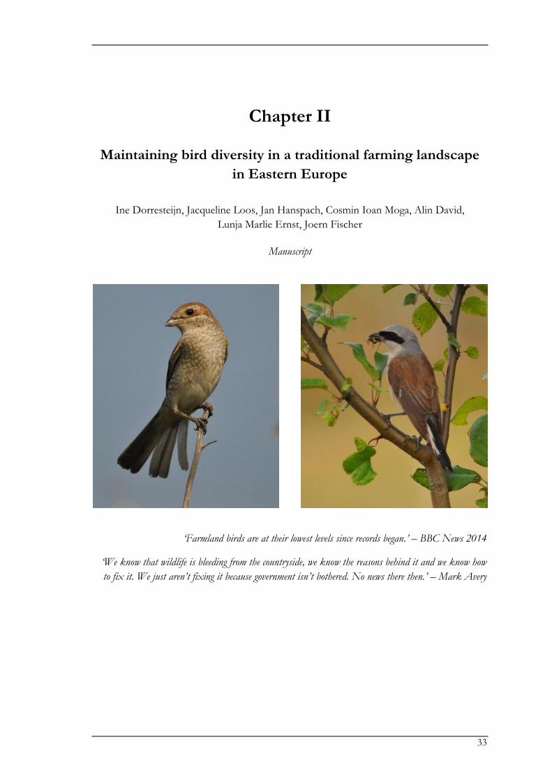
33
Chapter II
Maintaining bird diversity in a traditional farming landscape
in Eastern Europe
Ine Dorresteijn, Jacqueline Loos, Jan Hanspach, Cosmin Ioan Moga, Alin David,
Lunja Marlie Ernst, Joern Fischer
Manuscript
‘Farmland birds are at their lowest levels since records began.’ – BBC News 2014
‘We know that wildlife is bleeding from the countryside, we know the reasons behind it and we know how
to fix it. We just aren’t fixing it because government isn’t bothered. No news there then.’ – Mark Avery

Chapter II
34
Bird diversity in traditional farming landscapes
35
Abstract
Traditional farming landscapes harbor high biodiversity worldwide. However, farmland biodiversity
is increasingly threatened by agricultural intensification and land abandonment. We aimed to assess
the drivers of biodiversity in a traditional farming landscape in order to gauge the likely effects of
agricultural intensification and land abandonment on bird communities. We examined the
responses of species composition, species richness, and richness within functional groups, to
woody vegetation cover, land cover heterogeneity, and topography (each measured at local,
context, and landscape scales). We conducted repeated point counts for breeding birds in a
randomly selected set of 30 forest, 60 grassland, and 60 arable sites, which spanned stratified
gradients in heterogeneity and woody vegetation cover. Species composition in forests differed
from that in grassland and arable land. Species composition in grassland and arable land responded
to gradients of woody vegetation cover at all three scales. Within grassland and arable land, total
species richness, richness of farmland birds, and of forest specialists, asymptotically increased with
local-scale woody vegetation cover. In contrast, richness of open-country species responded
negatively to context-scale woody vegetation cover, and other farmland birds responded negatively
to landscape-scale woody vegetation cover. Our results show that different groups of birds would
be impacted differently by contrasting future land-use change scenarios. The regional bird
community as a whole would benefit from the maintenance of gradients in woody vegetation cover
across multiple scales.
Chapter II
36
Introduction
Agricultural expansion and intensification have caused biodiversity decline worldwide (Tilman et al.
2001; Foley et al. 2005), with the widespread loss of landscape heterogeneity identified as one of
the major drivers (Benton et al. 2003). Agricultural land holds a large part of the world’s
biodiversity (Pimentel et al. 1992) and occupies 40% of Earth’s land surface (Foley et al. 2005).
Growing recognition of the value of farmland biodiversity has sparked major national and
international conservation initiatives, but nevertheless, farmland biodiversity continues to decline
(Kleijn et al. 2011). In contrast, low-intensity land-use systems, such as traditional farming
landscapes, often harbor exceptional biodiversity and are therefore of great conservation
significance (Tscharntke et al. 2005; Kleijn et al. 2009).
Traditional farming landscapes occur in regions where farming practices have changed
little over long periods of time, and are typically characterized by large amounts of semi-natural
vegetation and high heterogeneity in land covers and structural elements (Plieninger et al. 2006).
The value of traditional farming landscapes for biodiversity has been noted worldwide
(Ranganathan et al. 2008; Takeuchi 2010; Robson & Berkes 2011; Liu et al. 2013), including in parts
of Eastern Europe (Fischer et al. 2012). However, traditional farming landscapes have come under
severe pressure from land-use intensification, and in economically marginal areas, from land
abandonment (Lepers et al. 2005; Plieninger et al. 2006). Land-use intensification influences
landscape structure via the loss of non-crop landscape elements (including semi-natural vegetation,
shrub areas, and woodlands) and consequently, homogenization of the landscape (Benton et al.
2003). Land abandonment typically affects landscape structure by transforming agricultural land
into shrubland, which may eventually turn into forest (Rudel et al. 2005; Kuemmerle et al. 2008).
To effectively conserve biodiversity in traditional farmland facing potential land-use changes thus
requires, first of all, a solid understanding of how different species respond to woody vegetation
cover and landscape heterogeneity.
Here, we present a comprehensive, regional-scale case study on the drivers of bird diversity
in a traditional farming landscape that is subject to land-use change. Our study investigated bird
community responses to landscape structure in Southern Transylvania, Romania, and was
specifically designed to cover the entire agricultural mosaic, spanning large gradients in
heterogeneity and woody vegetation cover. Transylvania’s farmland has changed relatively little
since pre-industrial times, and traditional semi-subsistence farming has maintained a species-rich
mosaic of arable fields, grasslands, and forests (Wilkie 2001; Cremene et al. 2005; Akeroyd & Page
2007). In recognition of its biodiversity, Europe’s largest lowland protected area within the Natura
2000 network has been established in Southern Transylvania to conserve its farmland biodiversity.
Yet, the region is undergoing rapid socio-demographic and land-use changes, which may
significantly impact biodiversity in the future (Mikulcak et al. 2013). Traditional farming has
become economically unviable, causing land abandonment by the rural population in some cases,
and agricultural land-use intensification in others (Hanspach et al. 2014).
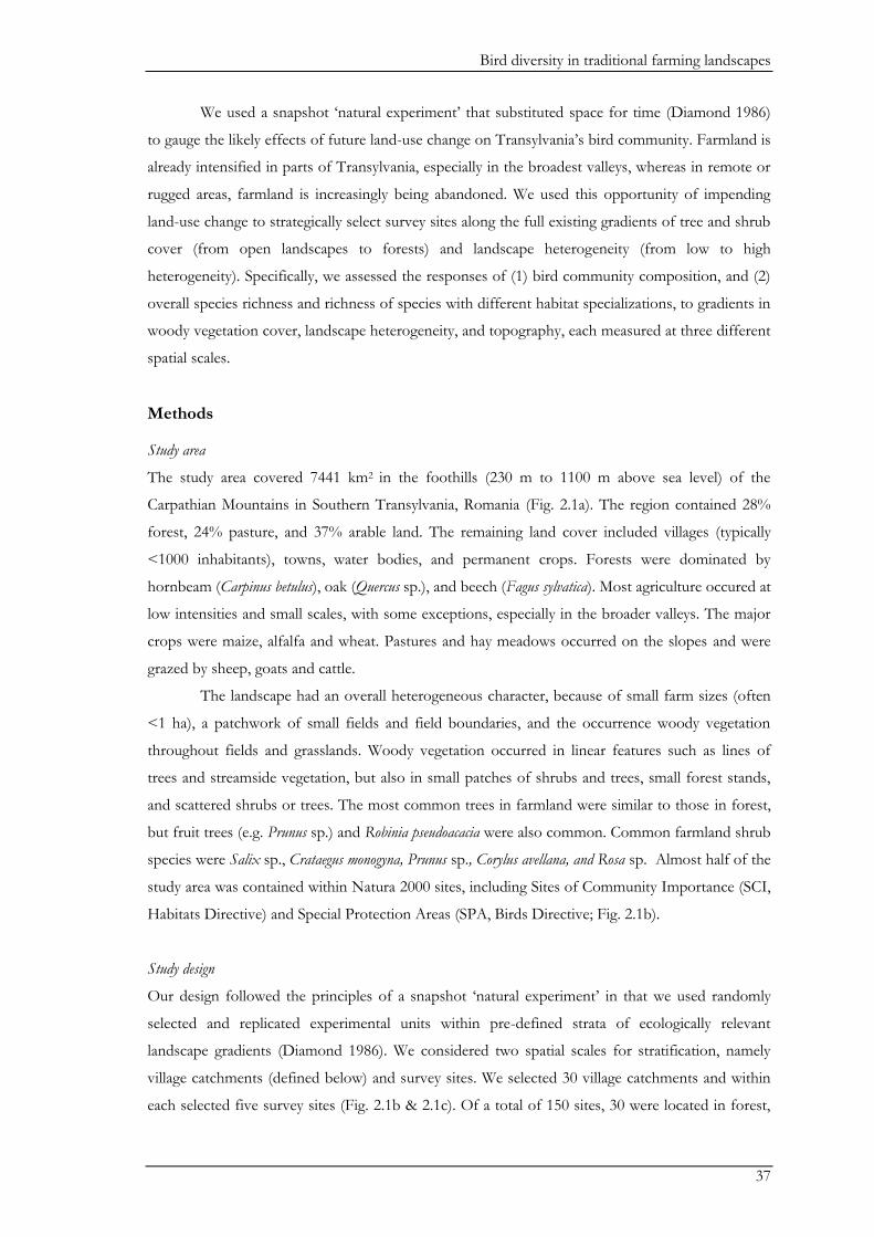
Bird diversity in traditional farming landscapes
37
We used a snapshot ‘natural experiment’ that substituted space for time (Diamond 1986)
to gauge the likely effects of future land-use change on Transylvania’s bird community. Farmland is
already intensified in parts of Transylvania, especially in the broadest valleys, whereas in remote or
rugged areas, farmland is increasingly being abandoned. We used this opportunity of impending
land-use change to strategically select survey sites along the full existing gradients of tree and shrub
cover (from open landscapes to forests) and landscape heterogeneity (from low to high
heterogeneity). Specifically, we assessed the responses of (1) bird community composition, and (2)
overall species richness and richness of species with different habitat specializations, to gradients in
woody vegetation cover, landscape heterogeneity, and topography, each measured at three different
spatial scales.
Methods
Study area
The study area covered 7441 km2 in the foothills (230 m to 1100 m above sea level) of the
Carpathian Mountains in Southern Transylvania, Romania (Fig. 2.1a). The region contained 28%
forest, 24% pasture, and 37% arable land. The remaining land cover included villages (typically
<1000 inhabitants), towns, water bodies, and permanent crops. Forests were dominated by
hornbeam (Carpinus betulus), oak (Quercus sp.), and beech (Fagus sylvatica). Most agriculture occured at
low intensities and small scales, with some exceptions, especially in the broader valleys. The major
crops were maize, alfalfa and wheat. Pastures and hay meadows occurred on the slopes and were
grazed by sheep, goats and cattle.
The landscape had an overall heterogeneous character, because of small farm sizes (often
<1 ha), a patchwork of small fields and field boundaries, and the occurrence woody vegetation
throughout fields and grasslands. Woody vegetation occurred in linear features such as lines of
trees and streamside vegetation, but also in small patches of shrubs and trees, small forest stands,
and scattered shrubs or trees. The most common trees in farmland were similar to those in forest,
but fruit trees (e.g. Prunus sp.) and Robinia pseudoacacia were also common. Common farmland shrub
species were Salix sp., Crataegus monogyna, Prunus sp., Corylus avellana, and Rosa sp. Almost half of the
study area was contained within Natura 2000 sites, including Sites of Community Importance (SCI,
Habitats Directive) and Special Protection Areas (SPA, Birds Directive; Fig. 2.1b).
Study design
Our design followed the principles of a snapshot ‘natural experiment’ in that we used randomly
selected and replicated experimental units within pre-defined strata of ecologically relevant
landscape gradients (Diamond 1986). We considered two spatial scales for stratification, namely
village catchments (defined below) and survey sites. We selected 30 village catchments and within
each selected five survey sites (Fig. 2.1b & 2.1c). Of a total of 150 sites, 30 were located in forest,
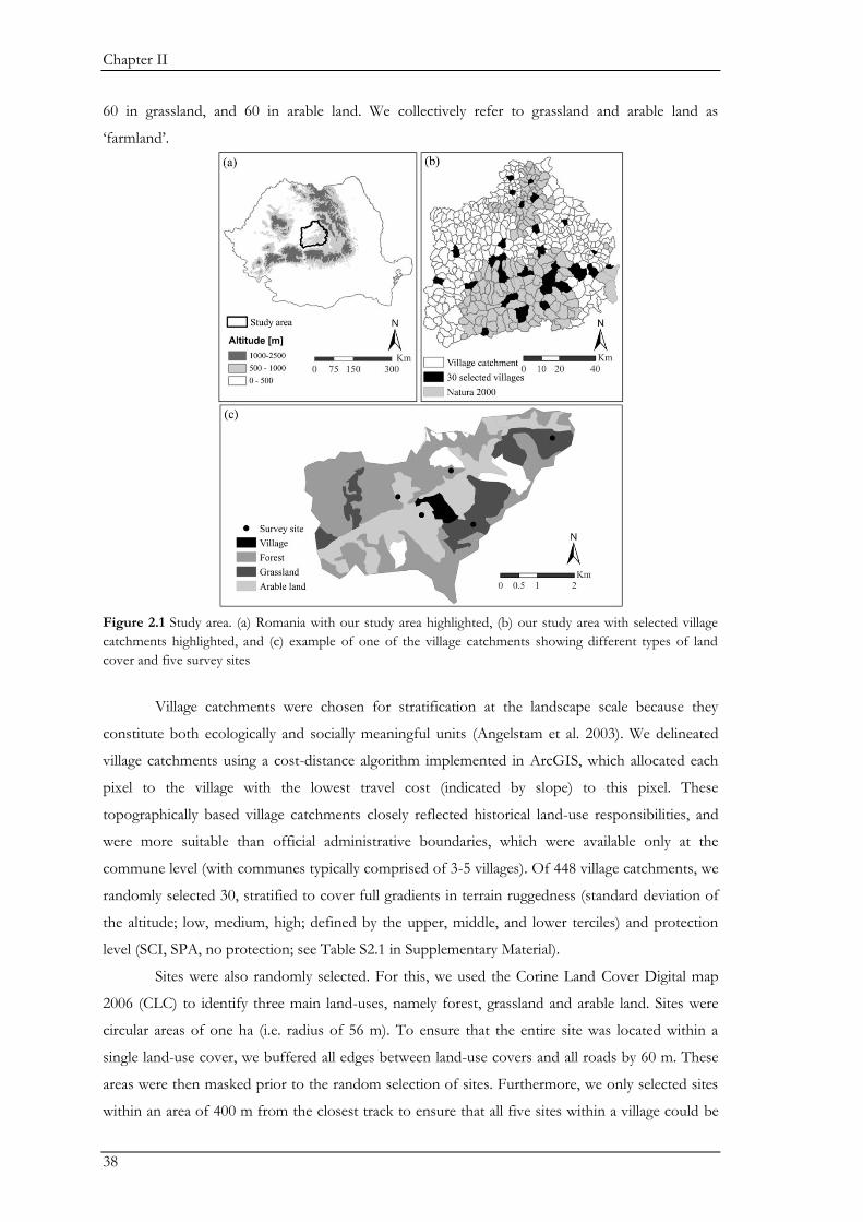
Chapter II
38
60 in grassland, and 60 in arable land. We collectively refer to grassland and arable land as
‘farmland’.
Figure 2.1 Study area. (a) Romania with our study area highlighted, (b) our study area with selected village
catchments highlighted, and (c) example of one of the village catchments showing different types of land
cover and five survey sites
Village catchments were chosen for stratification at the landscape scale because they
constitute both ecologically and socially meaningful units (Angelstam et al. 2003). We delineated
village catchments using a cost-distance algorithm implemented in ArcGIS, which allocated each
pixel to the village with the lowest travel cost (indicated by slope) to this pixel. These
topographically based village catchments closely reflected historical land-use responsibilities, and
were more suitable than official administrative boundaries, which were available only at the
commune level (with communes typically comprised of 3-5 villages). Of 448 village catchments, we
randomly selected 30, stratified to cover full gradients in terrain ruggedness (standard deviation of
the altitude; low, medium, high; defined by the upper, middle, and lower terciles) and protection
level (SCI, SPA, no protection; see Table S2.1 in Supplementary Material).
Sites were also randomly selected. For this, we used the Corine Land Cover Digital map
2006 (CLC) to identify three main land-uses, namely forest, grassland and arable land. Sites were
circular areas of one ha (i.e. radius of 56 m). To ensure that the entire site was located within a
single land-use cover, we buffered all edges between land-use covers and all roads by 60 m. These
areas were then masked prior to the random selection of sites. Furthermore, we only selected sites
within an area of 400 m from the closest track to ensure that all five sites within a village could be
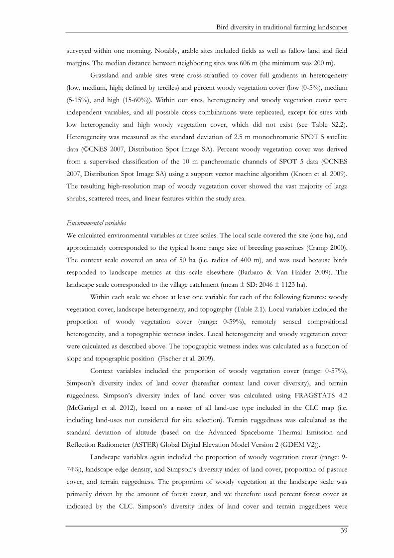
Bird diversity in traditional farming landscapes
39
surveyed within one morning. Notably, arable sites included fields as well as fallow land and field
margins. The median distance between neighboring sites was 606 m (the minimum was 200 m).
Grassland and arable sites were cross-stratified to cover full gradients in heterogeneity
(low, medium, high; defined by terciles) and percent woody vegetation cover (low (0-5%), medium
(5-15%), and high (15-60%)). Within our sites, heterogeneity and woody vegetation cover were
independent variables, and all possible cross-combinations were replicated, except for sites with
low heterogeneity and high woody vegetation cover, which did not exist (see Table S2.2).
Heterogeneity was measured as the standard deviation of 2.5 m monochromatic SPOT 5 satellite
data (©CNES 2007, Distribution Spot Image SA). Percent woody vegetation cover was derived
from a supervised classification of the 10 m panchromatic channels of SPOT 5 data (©CNES
2007, Distribution Spot Image SA) using a support vector machine algorithm (Knorn et al. 2009).
The resulting high-resolution map of woody vegetation cover showed the vast majority of large
shrubs, scattered trees, and linear features within the study area.
Environmental variables
We calculated environmental variables at three scales. The local scale covered the site (one ha), and
approximately corresponded to the typical home range size of breeding passerines (Cramp 2000).
The context scale covered an area of 50 ha (i.e. radius of 400 m), and was used because birds
responded to landscape metrics at this scale elsewhere (Barbaro & Van Halder 2009). The
landscape scale corresponded to the village catchment (mean ± SD: 2046 ± 1123 ha).
Within each scale we chose at least one variable for each of the following features: woody
vegetation cover, landscape heterogeneity, and topography (Table 2.1). Local variables included the
proportion of woody vegetation cover (range: 0-59%), remotely sensed compositional
heterogeneity, and a topographic wetness index. Local heterogeneity and woody vegetation cover
were calculated as described above. The topographic wetness index was calculated as a function of
slope and topographic position (Fischer et al. 2009).
Context variables included the proportion of woody vegetation cover (range: 0-57%),
Simpson’s diversity index of land cover (hereafter context land cover diversity), and terrain
ruggedness. Simpson’s diversity index of land cover was calculated using FRAGSTATS 4.2
(McGarigal et al. 2012), based on a raster of all land-use type included in the CLC map (i.e.
including land-uses not considered for site selection). Terrain ruggedness was calculated as the
standard deviation of altitude (based on the Advanced Spaceborne Thermal Emission and
Reflection Radiometer (ASTER) Global Digital Elevation Model Version 2 (GDEM V2)).
Landscape variables again included the proportion of woody vegetation cover (range: 9-
74%), landscape edge density, and Simpson’s diversity index of land cover, proportion of pasture
cover, and terrain ruggedness. The proportion of woody vegetation at the landscape scale was
primarily driven by the amount of forest cover, and we therefore used percent forest cover as
indicated by the CLC. Simpson’s diversity index of land cover and terrain ruggedness were
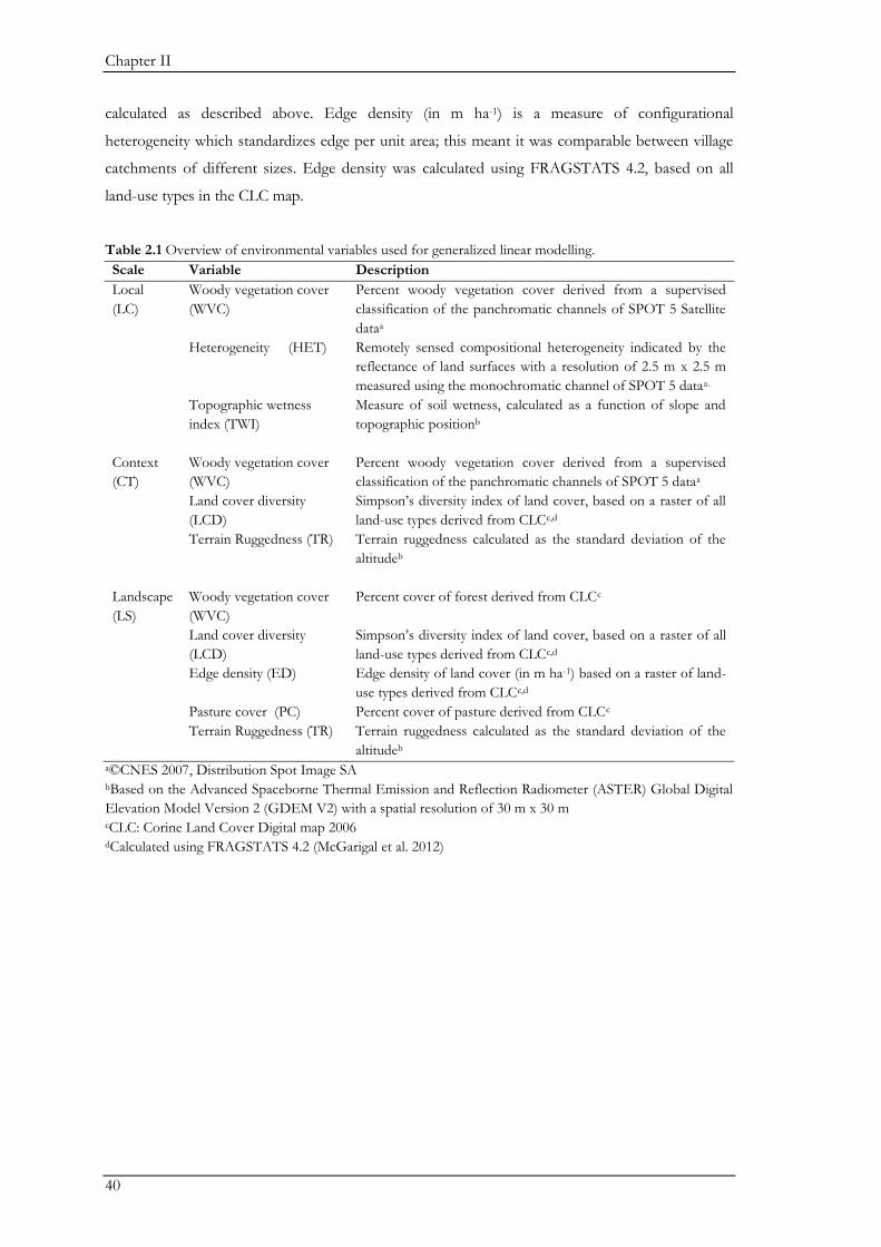
Chapter II
40
calculated as described above. Edge density (in m ha-1) is a measure of configurational
heterogeneity which standardizes edge per unit area; this meant it was comparable between village
catchments of different sizes. Edge density was calculated using FRAGSTATS 4.2, based on all
land-use types in the CLC map.
Table 2.1 Overview of environmental variables used for generalized linear modelling.
Scale Variable Description
Local
(LC)
Woody vegetation cover
(WVC)
Percent woody vegetation cover derived from a supervised
classification of the panchromatic channels of SPOT 5 Satellite
dataa
Heterogeneity (HET) Remotely sensed compositional heterogeneity indicated by the
reflectance of land surfaces with a resolution of 2.5 m x 2.5 m
measured using the monochromatic channel of SPOT 5 dataa.
Topographic wetness
index (TWI)
Measure of soil wetness, calculated as a function of slope and
topographic positionb
Context
(CT)
Woody vegetation cover
(WVC)
Percent woody vegetation cover derived from a supervised
classification of the panchromatic channels of SPOT 5 dataa
Land cover diversity
(LCD)
Simpson’s diversity index of land cover, based on a raster of all
land-use types derived from CLCc,d
Terrain Ruggedness (TR) Terrain ruggedness calculated as the standard deviation of the
altitudeb
Landscape
(LS)
Woody vegetation cover
(WVC)
Percent cover of forest derived from CLCc
Land cover diversity
(LCD)
Simpson’s diversity index of land cover, based on a raster of all
land-use types derived from CLCc,d
Edge density (ED) Edge density of land cover (in m ha-1) based on a raster of land-
use types derived from CLCc,d
Pasture cover (PC) Percent cover of pasture derived from CLCc
Terrain Ruggedness (TR) Terrain ruggedness calculated as the standard deviation of the
altitudeb a©CNES 2007, Distribution Spot Image SA bBased on the Advanced Spaceborne Thermal Emission and Reflection Radiometer (ASTER) Global Digital
Elevation Model Version 2 (GDEM V2) with a spatial resolution of 30 m x 30 m cCLC: Corine Land Cover Digital map 2006 dCalculated using FRAGSTATS 4.2 (McGarigal et al. 2012)
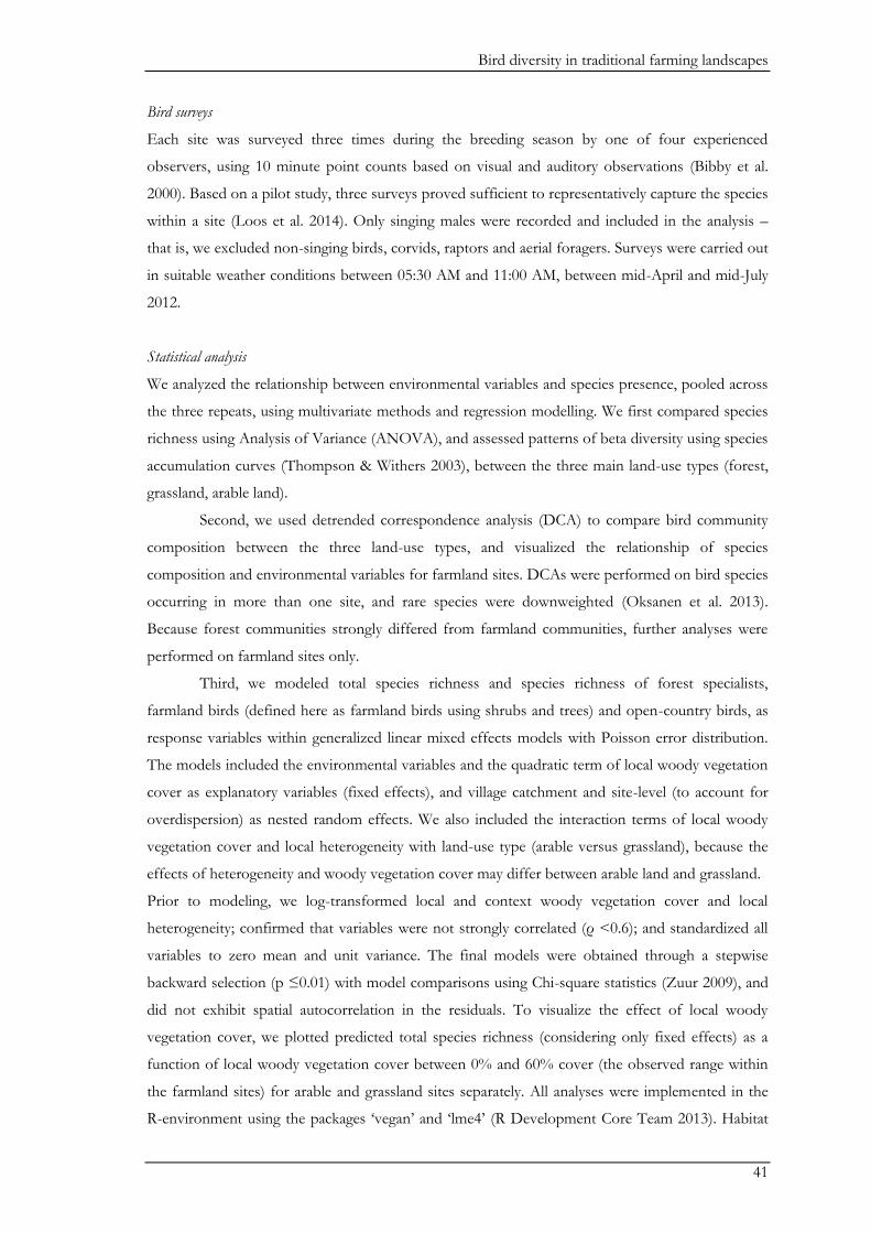
Bird diversity in traditional farming landscapes
41
Bird surveys
Each site was surveyed three times during the breeding season by one of four experienced
observers, using 10 minute point counts based on visual and auditory observations (Bibby et al.
2000). Based on a pilot study, three surveys proved sufficient to representatively capture the species
within a site (Loos et al. 2014). Only singing males were recorded and included in the analysis –
that is, we excluded non-singing birds, corvids, raptors and aerial foragers. Surveys were carried out
in suitable weather conditions between 05:30 AM and 11:00 AM, between mid-April and mid-July
2012.
Statistical analysis
We analyzed the relationship between environmental variables and species presence, pooled across
the three repeats, using multivariate methods and regression modelling. We first compared species
richness using Analysis of Variance (ANOVA), and assessed patterns of beta diversity using species
accumulation curves (Thompson & Withers 2003), between the three main land-use types (forest,
grassland, arable land).
Second, we used detrended correspondence analysis (DCA) to compare bird community
composition between the three land-use types, and visualized the relationship of species
composition and environmental variables for farmland sites. DCAs were performed on bird species
occurring in more than one site, and rare species were downweighted (Oksanen et al. 2013).
Because forest communities strongly differed from farmland communities, further analyses were
performed on farmland sites only.
Third, we modeled total species richness and species richness of forest specialists,
farmland birds (defined here as farmland birds using shrubs and trees) and open-country birds, as
response variables within generalized linear mixed effects models with Poisson error distribution.
The models included the environmental variables and the quadratic term of local woody vegetation
cover as explanatory variables (fixed effects), and village catchment and site-level (to account for
overdispersion) as nested random effects. We also included the interaction terms of local woody
vegetation cover and local heterogeneity with land-use type (arable versus grassland), because the
effects of heterogeneity and woody vegetation cover may differ between arable land and grassland.
Prior to modeling, we log-transformed local and context woody vegetation cover and local
heterogeneity; confirmed that variables were not strongly correlated (ρ <0.6); and standardized all
variables to zero mean and unit variance. The final models were obtained through a stepwise
backward selection (p ≤0.01) with model comparisons using Chi-square statistics (Zuur 2009), and
did not exhibit spatial autocorrelation in the residuals. To visualize the effect of local woody
vegetation cover, we plotted predicted total species richness (considering only fixed effects) as a
function of local woody vegetation cover between 0% and 60% cover (the observed range within
the farmland sites) for arable and grassland sites separately. All analyses were implemented in the
R-environment using the packages ‘vegan’ and ‘lme4’ (R Development Core Team 2013). Habitat
Chapter II
42
specialization was assigned to all bird species by two Romanian experts (CIM and AD), based on
Birds of the Western Palearctic (Cramp 2000) and specific literature from Romania (Linţia 1954,
1955; Ciochia 1992).
Results
Bird diversity
We identified 61 breeding bird species (see Table S2.3). Species richness was higher in forests
(mean ± SE: 10.6 ± 0.53) than grasslands (5.5 ± 0.35) and arable land (5.5 ± 0.52; F2,147 = 28.18,
p<0.001). Despite having the highest alpha diversity, forests had lower beta diversity than arable
and grassland sites (Fig. 2.2).
Figure 2.2 Bird species accumulation curves for forest, grassland and arable sites. Ninety-five percent
confidence intervals are indicated by grey shading.
Community composition
Species composition in forest sites differed from grassland and arable sites, and forest sites were
more homogenous in species composition than grassland and arable sites (Fig. 2.3a). Bird
community composition strongly overlapped in grasslands and arable sites, but exhibited clear
gradients (both axes approximately covered one species turnover; length of gradient first DCA axis
= 5.34, second DCA axis = 3.82; Fig. 2.3b, see Fig. S2.1 for species scores of the ordination). The
gradients of bird composition in farmland were related to environmental variables at all three
scales. The first axis of community composition followed a gradient from high to low cover of
local woody vegetation (Fig. 2.3b). The second axis described a gradient from sites with high
woody vegetation cover at the landscape and context scales, and high context land cover diversity,
to sites in less heterogeneous, pasture-dominated landscapes with low woody vegetation cover (Fig.
2.3b).
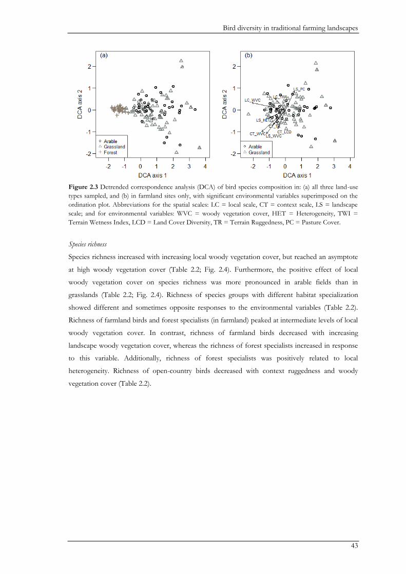
Bird diversity in traditional farming landscapes
43
Figure 2.3 Detrended correspondence analysis (DCA) of bird species composition in: (a) all three land-use
types sampled, and (b) in farmland sites only, with significant environmental variables superimposed on the
ordination plot. Abbreviations for the spatial scales: LC = local scale, CT = context scale, LS = landscape
scale; and for environmental variables: WVC = woody vegetation cover, HET = Heterogeneity, TWI =
Terrain Wetness Index, LCD = Land Cover Diversity, TR = Terrain Ruggedness, PC = Pasture Cover.
Species richness
Species richness increased with increasing local woody vegetation cover, but reached an asymptote
at high woody vegetation cover (Table 2.2; Fig. 2.4). Furthermore, the positive effect of local
woody vegetation cover on species richness was more pronounced in arable fields than in
grasslands (Table 2.2; Fig. 2.4). Richness of species groups with different habitat specialization
showed different and sometimes opposite responses to the environmental variables (Table 2.2).
Richness of farmland birds and forest specialists (in farmland) peaked at intermediate levels of local
woody vegetation cover. In contrast, richness of farmland birds decreased with increasing
landscape woody vegetation cover, whereas the richness of forest specialists increased in response
to this variable. Additionally, richness of forest specialists was positively related to local
heterogeneity. Richness of open-country birds decreased with context ruggedness and woody
vegetation cover (Table 2.2).
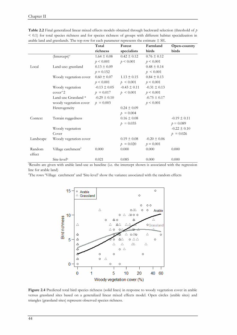
Chapter II
44
Table 2.2 Final generalized linear mixed effects models obtained through backward selection (threshold of p
< 0.1) for total species richness and for species richness of groups with different habitat specialization in
arable land and grasslands. The top row for each parameter represents the estimate ± SE.
Total
richness
Forest
specialists
Farmland
birds
Open-country
birds
(Intercept)a 1.64 ± 0.08
p < 0.001
0.42 ± 0.12
p < 0.001
0.76 ± 0.12
p < 0.001
Local Land-use: grassland 0.13 ± 0.09
p = 0.152
0.48 ± 0.14
p < 0.001
Woody vegetation cover 0.60 ± 0.07
p < 0.001
1.13 ± 0.15
p < 0.001
0.84 ± 0.13
p < 0.001
Woody vegetation
cover^2
-0.13 ± 0.05
p = 0.017
-0.43 ± 0.11
p < 0.001
-0.31 ± 0.13
p < 0.001
Land-use Grassland *
woody vegetation cover
-0.29 ± 0.10
p = 0.003
-0.75 ± 0.17
p < 0.001
Heterogeneity
0.24 ± 0.09
p = 0.004
Context Terrain ruggedness 0.16 ± 0.08
p = 0.035
-0.19 ± 0.11
p = 0.089
Woody vegetation
Cover
-0.22 ± 0.10
p = 0.026
Landscape Woody vegetation cover 0.19 ± 0.08
p = 0.020
-0.20 ± 0.06
p = 0.001
Random
effect
Village catchmentb 0.000 0.000 0.000 0.000
Site-levelb 0.021 0.085 0.000 0.000 aResults are given with arable land-use as baseline (i.e. the intercept shown is associated with the regression
line for arable land) bThe rows ‘Village catchment’ and ‘Site-level’ show the variance associated with the random effects
Figure 2.4 Predicted total bird species richness (solid lines) in response to woody vegetation cover in arable
versus grassland sites based on a generalized linear mixed effects model. Open circles (arable sites) and
triangles (grassland sites) represent observed species richness.
Bird diversity in traditional farming landscapes
45
Discussion
To the best of our knowledge, this is the first regional-scale study on birds in a transforming
traditional farming landscape that is based on a stratified, randomized design with replicated survey
sites spanning the entire agricultural mosaic. Our study shows the high conservation value of
traditional farmland: although alpha diversity of birds was higher in forests than in farmland, the
opposite was the case for beta diversity. That is, forest sites appeared relatively homogenous in bird
community composition, whereas farmland sites showed larger differences between sites. Within
farmland, bird distribution patterns were primarily driven by gradients in woody vegetation cover,
and to a lesser extent by gradients of landscape heterogeneity – rather than by differences in land-
use per se (i.e. grassland versus arable land). In combination, our findings suggest that gradients in
woody vegetation cover (and to a lesser extent in heterogeneity) need to be maintained at multiple
scales to conserve regional bird diversity.
The most important driver of bird community composition in farmland was woody
vegetation cover. As local woody vegetation cover decreased, farmland community composition
changed from birds associated with forest and farmland birds (e.g. the Blue Tit, Parus major, and the
Long-tailed Tit, Aegithalos caudatus), to a community mainly comprising open-country birds (e.g. the
Whinchat, Saxicola rubetra, and the Quail, Coturnix coturnix (see Fig. S2.1)). A similar change in
community composition was observed along the gradient from high context-scale land cover
diversity and woody vegetation cover to less heterogeneous, open pasture-dominated areas (see Fig.
S2.1). Gradients in woody vegetation cover are major drivers of bird community composition
worldwide (Ranganathan et al. 2008; Hanspach et al. 2011), and within Europe, evidence continues
to accumulate that both open farmland and farmland with woody vegetation need to be maintained
and restored to conserve bird diversity in its entirety (Batary et al. 2011b; Fischer et al. 2011).
Species richness followed similar patterns to community composition. Total species
richness was positively related to local woody vegetation cover, although this relationship was less
pronounced in grassland. This difference probably resulted from the greater prominence of several
open-country specialists in grassland (e.g. Saxicola sp.), which avoid woody vegetation (Sanderson et
al. 2013). Bird species richness has been observed to increase with high woody vegetation cover
elsewhere in Europe (e.g. Sanderson et al. 2009), with most research focusing on edges and field
margins (Herzon et al. 2008; Batáry et al. 2010; Wuczynski et al. 2011). The positive response to
woody vegetation typically has been ascribed to a greater diversity of nesting, sheltering and feeding
sites in areas with woody vegetation (Hinsley & Bellamy 2000). The strong effect of local woody
vegetation cover in our study therefore may be related to the small home ranges (<1 to 4 ha, for
most observed birds (Cramp 2000)) of breeding birds, with nesting and foraging site selection likely
determined by fine-scale habitat characteristics. These findings suggest that retaining structures of
woody vegetation at small scales could potentially ameliorate the negative effects of agricultural
intensification on bird richness.
Chapter II
46
Despite the strong effect of local woody vegetation cover on species richness, this effect
was found to level off at high levels of woody vegetation, or become negative in grassland. Land
abandonment, and its subsequent transformation to shrubland and eventually forests, is a major
threat to farmland in Eastern Europe (Kuemmerle et al. 2008) and is expected to expand in the
future (Renwick et al. 2013). This is concerning, because many farmland birds, such as the Red-
backed Shrike (Lanius collurio), need both open areas for foraging and trees or shrubs for breeding,
and thus require landscapes with scattered woody vegetation cover (Brambilla et al. 2010). Thus,
although an increase in woody vegetation might initially enhance bird diversity, a major expansion
of shrubland will likely have negative impacts on farmland bird richness, especially in grasslands.
Context and landscape woody vegetation cover also had significant effects on the richness of birds
with different habitat requirements. Unsurprisingly, open country-specialists were negatively
affected by high woody vegetation cover at the context scale. These species often breed or forage
in open landscapes, and dense cover of woody vegetation could also increase nest predation of
ground nesting birds (Morris & Gilroy 2008). Forest specialists and farmland birds showed
opposite patterns to landscape woody vegetation cover, with farmland birds responding negatively
and forest specialists positively. Thus, besides a general decrease in species richness following local
land abandonment, the abandonment of larger farmland areas would be associated with the
replacement of open-country farmland birds and farmland birds by forest specialists. Such a change
in bird community composition would also encompass the loss of several Species of European
Conservation Concern (Table S2.3). Thus, although extensification through land abandonment may
be a desirable conservation strategy in some intensively managed landscapes (Gregory et al. 2005;
Wretenberg et al. 2007), it could be detrimental to the bird fauna of traditional low-intensity
farming landscapes (Suárez-Seoane et al. 2002; Laiolo et al. 2004; Verhulst et al. 2004; Sirami et al.
2008).
Heterogeneity has been proposed as a major factor underpinning farmland biodiversity
(Benton et al. 2003), and positive effects of land cover diversity and structural landscape features
on bird assemblages have been widely reported (Atkinson et al. 2002; Piha et al. 2007; Sanderson et
al. 2009; Wretenberg et al. 2010; Guerrero et al. 2012). The overall lack of an effect of
heterogeneity in our study (except for the positive response of forest specialists to local
heterogeneity) may therefore be surprising. However, unlike our study, most other studies to date
have not decoupled the effects of woody vegetation cover and land cover heterogeneity. Our
findings suggest that woody vegetation cover may be more important for bird species richness than
other aspects of heterogeneity related to land cover. This possible explanation is consistent with
Sanderson et al. (2009), who found a stronger positive response of bird richness and abundance to
woody edge habitat than to compositional land cover heterogeneity in Poland.
Open-country birds in particular (such as the Skylark, Alauda arvensis) often prefer simpler
landscapes dominated by agriculture and may be expected to respond negatively to heterogeneity
(e.g. Fischer et al. 2011). Nevertheless, within agricultural landscapes, small field sizes, high crop
Bird diversity in traditional farming landscapes
47
diversity, and a high proportion of field margins provide better conditions for foraging, nesting,
and shelter (Vickery et al. 2001; Guerrero et al. 2012; Josefsson et al. 2013; Kuiper et al. 2013). The
lack of a response to heterogeneity in this group might be related to the coarse resolution of the
CLC map, used to derive context and landscape heterogeneity measures, which only distinguishes
between the main land-use types but not individual arable fields. Alternatively, the reduced
invertebrate prey due to simultaneous application of fertilizers and pesticides in intensified
landscapes may partly explain the loss of open-country farmland birds in the more homogenous
intensified landscapes (Verhulst et al. 2004). In contrast, in our study area pesticide and fertilizer
use is very limited even in the more intensified regions, and hence invertebrates may be rich
throughout the landscape and dampen the effect of heterogeneity on open-farmland specialists.
In combination, our findings suggest that the key mechanism underpinning Transylvania’s
bird community is the availability of gradients in woody vegetation cover and, to a lesser extent,
land cover heterogeneity across multiple different scales. Notably, we captured responses of bird
richness and composition only to those landscape features we could readily quantify, namely woody
vegetation cover and heterogeneity. While these features are important, many other characteristics
of Transylvanian farmland may also be relevant. These include a high variety of crops and crop
rotation within small fields (Guerrero et al. 2012), traditional livestock rotation (Söderström et al.
2001), occurrence of fallow land and semi-natural vegetation (Devictor & Jiguet 2007; Sanderson et
al. 2013), low pesticide and fertilizer use (Kleijn et al. 2009; Geiger et al. 2010), a wide variety of
different field margins (Wuczynski et al. 2011), and land-use that is not optimized for a single
performance or to produce maximum yield (Donald et al. 2001). As observed in other regions
(Doxa et al. 2010; Wretenberg et al. 2010; Sanderson et al. 2013), the loss of low-intensity mixed
farmland from Transylvania very likely would have a negative impact on bird diversity.
Conservation implications
Conservation actions in traditional farming landscapes are urgently needed because farmland bird
populations are declining in Central and Eastern Europe (Reif et al. 2008; Voříšek et al. 2010).
Although national conservation efforts improve population trends, decreasing trends are not being
reversed (Koleček et al. 2014). Research on farmland biodiversity in these traditional farming
landscapes is lagging behind research in Western Europe, which is problematic because the
conservation challenges here may be different from those in more intensified landscapes (Baldi &
Batary 2011; Tryjanowski et al. 2011). Our findings suggest that the key to conserve Transylvania’s
bird diversity is to maintain broad gradients of woody vegetation cover across multiple spatial
scales, and to a lesser extent, maintain small-scale compositional heterogeneity.
In Transylvania, land abandonment is most likely to occur in the grasslands of more
remote, forested, and steep areas. Preventing abandonment in these areas could be achieved by
providing incentives to maintain rotational livestock grazing and to remove shrubs in order to
maintain landscapes with little to intermediate woody vegetation cover. Intensification, on the other
Chapter II
48
hand, is more likely to occur in arable land, especially in the broader, accessible valleys. Here,
conservation strategies should prioritize the retention of woody vegetation cover at intermediate
levels, for example by maintaining various types of field margins (Wuczynski et al. 2011), and
encouraging high land cover diversity through mixed farming. Furthermore, care should be taken in
both grasslands and arable fields that larger tracts of open landscape with low woody vegetation
cover remain available for open-country birds.
In conclusion, there is no simple conservation recipe that can be implemented across
traditional farmland, but rather, farmland bird communities will benefit most from policies targeted
to either mitigate land abandonment or land-use intensification, depending on the specific location.
Because traditional farming has become largely unviable, new strategies need to be identified that
not only maintain farmland biodiversity but also benefit local people, thus preventing an exodus of
the rural population and subsequent cessation of farming. In our study area, potential strategies
could include the uptake of modern agro-ecological and organic farming methods instead of
conventional land-use intensification (Hole et al. 2005; Gabriel et al. 2010), or the development of
incentives for smallholder farmers to engage in (agro-)ecotourism (Young et al. 2010).
Acknowledgements
We thank A. Klein and R. Bigonneau for their tremendous efforts in the field. We are also grateful
to many local people and stakeholders, including the Mihai Eminescu Trust and local government
representatives. We thank P. Griffiths, J. Knorn and T. Kuemmerle for their help with creating the
woody vegetation layer, J. Stein for help with the TWI layer, and D. Abson, P. Fust, and H. von
Wehrden for analytical assistance. We thank Dale Nimmo for constructive suggestions on a
previous draft of this manuscript. The project was funded by a Sofja Kovalevskaja Award by the
Alexander von Humboldt Foundation to JF.
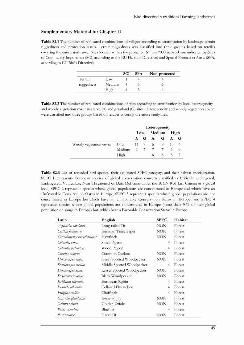
Bird diversity in traditional farming landscapes
49
Supplementary Material for Chapter II
Table S2.1 The number of replicated combinations of villages according to stratification by landscape terrain
ruggedness and protection status. Terrain ruggedness was classified into three groups based on terciles
covering the entire study area. Sites located within the protected Natura 2000 network are indicated by Sites
of Community Importance (SCI, according to the EU Habitats Directive) and Special Protection Areas (SPA,
according to EU Birds Directive).
Table S2.2 The number of replicated combinations of sites according to stratification by local heterogeneity
and woody vegetation cover in arable (A) and grassland (G) sites. Heterogeneity and woody vegetation cover
were classified into three groups based on terciles covering the entire study area.
Table S2.3 List of recorded bird species, their associated SPEC category, and their habitat specialization.
SPEC 1 represents European species of global conservation concern classified as Critically endangered,
Endangered, Vulnerable, Near Threatened or Data Deficient under the IUCN Red List Criteria at a global
level; SPEC 2 represents species whose global populations are concentrated in Europe and which have an
Unfavorable Conservation Status in Europe; SPEC 3 represents species whose global populations are not
concentrated in Europe but which have an Unfavorable Conservation Status in Europe; and SPEC 4
represents species whose global populations are concentrated in Europe (more than 50% of their global
population or range in Europe) but which have a Favorable Conservation Status in Europe.
Latin English SPEC Habitat
Aegithalos caudatus Long-tailed Tit NON Forest
Certhia familiaris Eurasian Treecreeper NON Forest
Coccothraustes coccothraustes Hawfinch NON Forest
Columba oenas Stock Pigeon 4 Forest
Columba palumbus Wood Pigeon 4 Forest
Cuculus canorus Common Cuckoo NON Forest
Dendrocopos major Great Spotted Woodpecker NON Forest
Dendrocopos medius Middle Spotted Woodpecker 4 Forest
Dendrocopos minor Lesser Spotted Woodpecker NON Forest
Dryocopus martius Black Woodpecker NON Forest
Erithacus rubecula European Robin 4 Forest
Ficedula albicollis Collared Flycatcher 4 Forest
Fringilla coelebs Chaffinch 4 Forest
Garrulus glandarius Eurasian Jay NON Forest
Oriolus oriolus Golden Oriole NON Forest
Parus caeruleus Blue Tit 4 Forest
Parus major Great Tit NON Forest
SCI SPA Non-protected
Terrain Low 1 4 4
ruggedness Medium 4 3 3
High 4 3 4
Heterogeneity
Low Medium High
A G A G A G
Woody vegetation cover Low 11 8 6 8 10 6
Medium 6 7 7 7 6 9
High 6 8 8 7
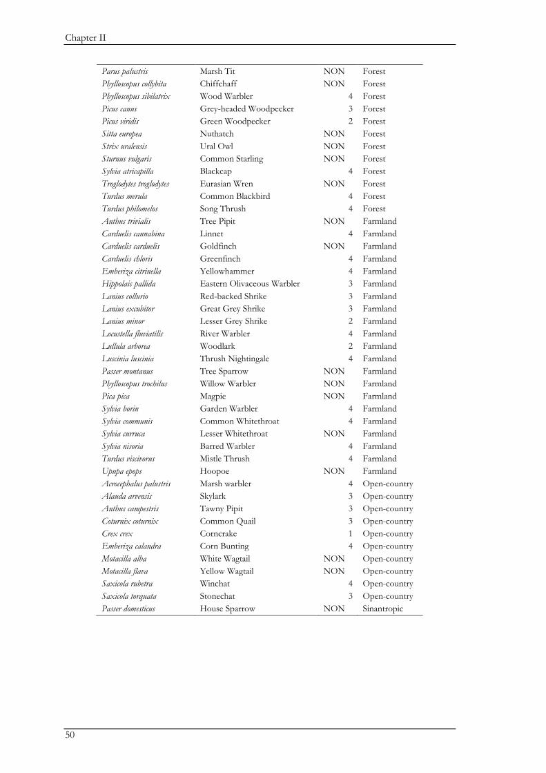
Chapter II
50
Parus palustris Marsh Tit NON Forest
Phylloscopus collybita Chiffchaff NON Forest
Phylloscopus sibilatrix Wood Warbler 4 Forest
Picus canus Grey-headed Woodpecker 3 Forest
Picus viridis Green Woodpecker 2 Forest
Sitta europea Nuthatch NON Forest
Strix uralensis Ural Owl NON Forest
Sturnus vulgaris Common Starling NON Forest
Sylvia atricapilla Blackcap 4 Forest
Troglodytes troglodytes Eurasian Wren NON Forest
Turdus merula Common Blackbird 4 Forest
Turdus philomelos Song Thrush 4 Forest
Anthus trivialis Tree Pipit NON Farmland
Carduelis cannabina Linnet 4 Farmland
Carduelis carduelis Goldfinch NON Farmland
Carduelis chloris Greenfinch 4 Farmland
Emberiza citrinella Yellowhammer 4 Farmland
Hippolais pallida Eastern Olivaceous Warbler 3 Farmland
Lanius collurio Red-backed Shrike 3 Farmland
Lanius excubitor Great Grey Shrike 3 Farmland
Lanius minor Lesser Grey Shrike 2 Farmland
Locustella fluviatilis River Warbler 4 Farmland
Lullula arborea Woodlark 2 Farmland
Luscinia luscinia Thrush Nightingale 4 Farmland
Passer montanus Tree Sparrow NON Farmland
Phylloscopus trochilus Willow Warbler NON Farmland
Pica pica Magpie NON Farmland
Sylvia borin Garden Warbler 4 Farmland
Sylvia communis Common Whitethroat 4 Farmland
Sylvia curruca Lesser Whitethroat NON Farmland
Sylvia nisoria Barred Warbler 4 Farmland
Turdus viscivorus Mistle Thrush 4 Farmland
Upupa epops Hoopoe NON Farmland
Acrocephalus palustris Marsh warbler 4 Open-country
Alauda arvensis Skylark 3 Open-country
Anthus campestris Tawny Pipit 3 Open-country
Coturnix coturnix Common Quail 3 Open-country
Crex crex Corncrake 1 Open-country
Emberiza calandra Corn Bunting 4 Open-country
Motacilla alba White Wagtail NON Open-country
Motacilla flava Yellow Wagtail NON Open-country
Saxicola rubetra Winchat 4 Open-country
Saxicola torquata Stonechat 3 Open-country
Passer domesticus House Sparrow NON Sinantropic
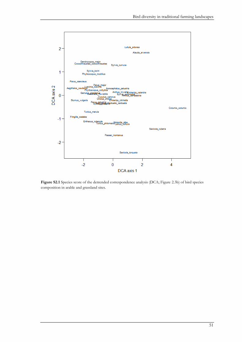
Bird diversity in traditional farming landscapes
51
Figure S2.1 Species score of the detrended correspondence analysis (DCA; Figure 2.3b) of bird species
composition in arable and grassland sites.

52

53
Chapter III

54
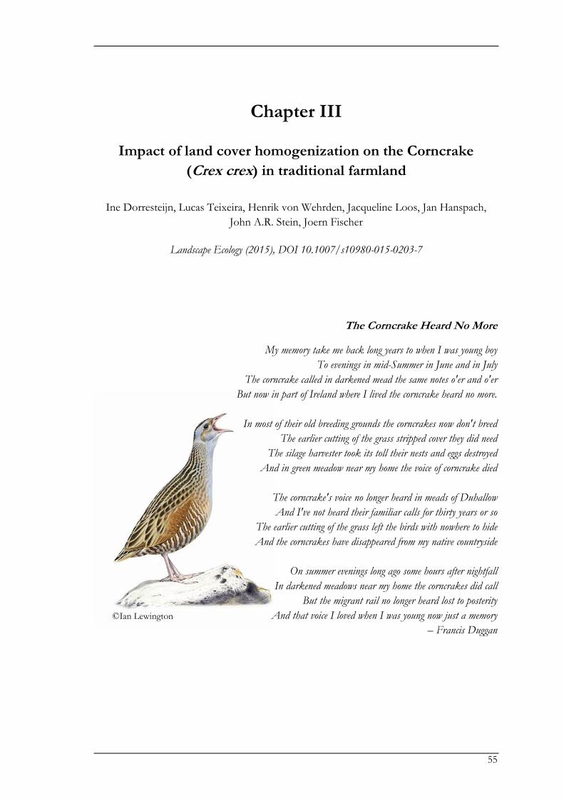
55
©Ian Lewington
Chapter III
Impact of land cover homogenization on the Corncrake
(Crex crex) in traditional farmland
Ine Dorresteijn, Lucas Teixeira, Henrik von Wehrden, Jacqueline Loos, Jan Hanspach,
John A.R. Stein, Joern Fischer
Landscape Ecology (2015), DOI 10.1007/s10980-015-0203-7
The Corncrake Heard No More
My memory take me back long years to when I was young boy
To evenings in mid-Summer in June and in July
The corncrake called in darkened mead the same notes o'er and o'er
But now in part of Ireland where I lived the corncrake heard no more.
In most of their old breeding grounds the corncrakes now don't breed
The earlier cutting of the grass stripped cover they did need
The silage harvester took its toll their nests and eggs destroyed
And in green meadow near my home the voice of corncrake died
The corncrake's voice no longer heard in meads of Duhallow
And I've not heard their familiar calls for thirty years or so
The earlier cutting of the grass left the birds with nowhere to hide
And the corncrakes have disappeared from my native countryside
On summer evenings long ago some hours after nightfall
In darkened meadows near my home the corncrakes did call
But the migrant rail no longer heard lost to posterity
And that voice I loved when I was young now just a memory
– Francis Duggan

Chapter III
56
Corncrakes in traditional farming landscapes
57
Abstract
Context.
The loss of landscape heterogeneity is causing declines of farmland biodiversity around the world.
Traditional farmland regions are often highly heterogeneous and harbor high biodiversity, but are
under threat of land cover homogenization due to changing agricultural practices. One species
potentially affected by landscape homogenization is the Corncrake (Crex crex), which is threatened
in Western Europe but remains widespread in the traditional farmland regions of Eastern Europe.
Objectives.
In this study we present a case study aiming to assess the potential threat of landscape
homogenization for the Corncrake in Romania. We first examined current Corncrake distribution
in relation to woody vegetation cover, landscape heterogeneity, and topography (measured at three
different spatial scales), as well as human disturbance, throughout the existing agricultural mosaic.
Second, we predicted potential future distribution of suitable Corncrake habitat in response to land
cover homogenization by simulating a reduction in land cover diversity.
Results.
Corncrakes were present in grassland and arable fields, and preferentially occupied remote areas
that were wet and flat, and had high land cover diversity at the 100 ha scale. The simulation of land
cover diversity loss revealed that even a moderate reduction of land cover diversity could drastically
reduce the extent of suitable Corncrake habitat.
Conclusions.
Our findings show the high conservation value of traditional heterogeneous farmland for the
Corncrake. Therefore, to protect the Corncrake in traditional farmland, pro-active policy measures
should encourage the continuation of mixed farming practices to maintain a diversity of land
covers.
Chapter III
58
Introduction
Agricultural intensification since the mid-1900s has caused worldwide declines of farmland
biodiversity (Donald et al. 2001; Tilman et al. 2001; Stoate et al. 2009). The process of agricultural
intensification typically involves a combination of changes in management practices to increase
production, such as increased mechanization and use of agrochemicals, loss of crop varieties and
crop rotation, and the decrease of fallow land, non-cropped areas, and natural and semi-natural
vegetation (e.g. Tilman et al. 2002; Tscharntke et al. 2005) . One of the defining consequences of
agricultural intensification is the homogenization of the agricultural mosaic at multiple spatial
scales, for instance through the loss of land cover diversity and structural heterogeneity (Benton et
al. 2003; Tscharntke et al. 2005). Such land cover homogenization has severely reduced the
suitability of farmland for numerous species across multiple taxa through reducing (nesting) habitat,
food availability, and causing habitat fragmentation (Hinsley 2000; Weibull et al. 2003; Concepción
et al. 2008; Guerrero et al. 2012; Tscharntke et al. 2012).
To mitigate the loss of farmland biodiversity, a range of national and international
conservation policies are being implemented. In the European Union, agri-environment schemes
(AES) of the European Common Agricultural Policy (CAP; Pillar 2) are a particularly prominent
strategy (Skogstad and Verdun 2010). Farmers can take up AES voluntarily and receive financial
support to improve habitat quality and promote certain species. However, the effectiveness of AES
for biodiversity conservation has been questioned, and European farmland biodiversity continues
to decline (Kleijn et al. 2006; Kleijn et al. 2011; Pe'er et al. 2014). The apparent ineffectiveness of
AES partly could be explained by the lack of effective tools to assess the outcomes of AES (Kleijn
& Sutherland 2003), or by a poor fit of AES to the ecological requirements of specific farmland
bird species (Princé et al. 2012). Moreover, the effectiveness of AES is likely to be dependent on
context conditions, including levels of land-use intensification (Princé et al. 2012) and landscape
complexity. For example, local-scale AES may be more effective in relatively homogenous
landscapes than in highly heterogeneous landscapes (Tscharntke et al. 2005; Concepción et al. 2008;
Batary et al. 2011a). However, highly heterogeneous landscapes are threatened as a whole
(Tscharntke et al. 2005). To more effectively protect the ecological values of heterogeneous
landscapes, a key challenge therefore is to scale up AES, from local-level measures to landscape-
level measures (Concepción et al. 2008).
The increasing shift in focus from local to larger scale agri-environment measures (e.g.
Dallimer et al. 2010; McKenzie et al. 2013) could thus be of particular interest for heterogeneous
landscapes, such as the traditional farming landscapes in Eastern Europe (Fischer et al. 2012).
Traditional farmland is typically characterized by high heterogeneity in land cover and structural
elements (Plieninger et al. 2006), and subsequently often harbors high levels of biodiversity,
including threatened species (Tscharntke et al. 2005; Kleijn et al. 2009). However, traditional
farming landscapes are under severe pressure of landscape homogenization from changes
associated with agricultural intensification (Lepers et al. 2005). Nevertheless, empirical research to
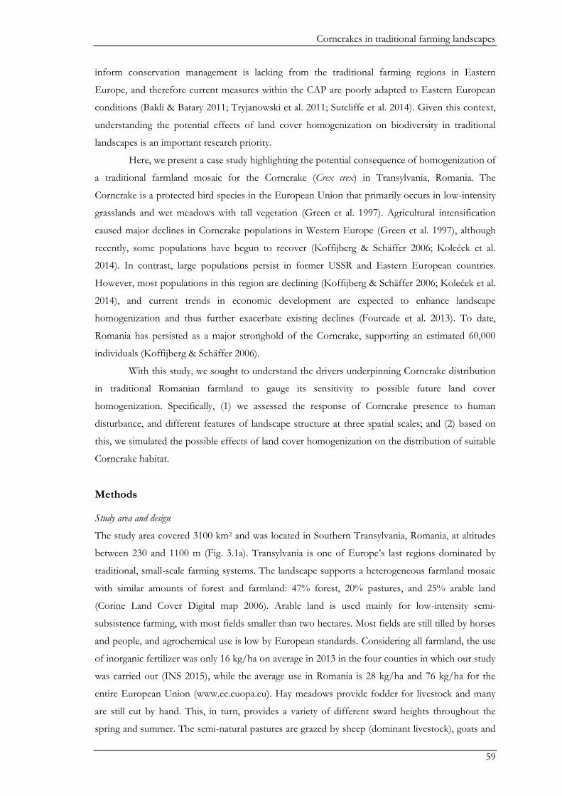
Corncrakes in traditional farming landscapes
59
inform conservation management is lacking from the traditional farming regions in Eastern
Europe, and therefore current measures within the CAP are poorly adapted to Eastern European
conditions (Baldi & Batary 2011; Tryjanowski et al. 2011; Sutcliffe et al. 2014). Given this context,
understanding the potential effects of land cover homogenization on biodiversity in traditional
landscapes is an important research priority.
Here, we present a case study highlighting the potential consequence of homogenization of
a traditional farmland mosaic for the Corncrake (Crex crex) in Transylvania, Romania. The
Corncrake is a protected bird species in the European Union that primarily occurs in low-intensity
grasslands and wet meadows with tall vegetation (Green et al. 1997). Agricultural intensification
caused major declines in Corncrake populations in Western Europe (Green et al. 1997), although
recently, some populations have begun to recover (Koffijberg & Schäffer 2006; Koleček et al.
2014). In contrast, large populations persist in former USSR and Eastern European countries.
However, most populations in this region are declining (Koffijberg & Schäffer 2006; Koleček et al.
2014), and current trends in economic development are expected to enhance landscape
homogenization and thus further exacerbate existing declines (Fourcade et al. 2013). To date,
Romania has persisted as a major stronghold of the Corncrake, supporting an estimated 60,000
individuals (Koffijberg & Schäffer 2006).
With this study, we sought to understand the drivers underpinning Corncrake distribution
in traditional Romanian farmland to gauge its sensitivity to possible future land cover
homogenization. Specifically, (1) we assessed the response of Corncrake presence to human
disturbance, and different features of landscape structure at three spatial scales; and (2) based on
this, we simulated the possible effects of land cover homogenization on the distribution of suitable
Corncrake habitat.
Methods
Study area and design
The study area covered 3100 km2 and was located in Southern Transylvania, Romania, at altitudes
between 230 and 1100 m (Fig. 3.1a). Transylvania is one of Europe’s last regions dominated by
traditional, small-scale farming systems. The landscape supports a heterogeneous farmland mosaic
with similar amounts of forest and farmland: 47% forest, 20% pastures, and 25% arable land
(Corine Land Cover Digital map 2006). Arable land is used mainly for low-intensity semi-
subsistence farming, with most fields smaller than two hectares. Most fields are still tilled by horses
and people, and agrochemical use is low by European standards. Considering all farmland, the use
of inorganic fertilizer was only 16 kg/ha on average in 2013 in the four counties in which our study
was carried out (INS 2015), while the average use in Romania is 28 kg/ha and 76 kg/ha for the
entire European Union (www.ec.euopa.eu). Hay meadows provide fodder for livestock and many
are still cut by hand. This, in turn, provides a variety of different sward heights throughout the
spring and summer. The semi-natural pastures are grazed by sheep (dominant livestock), goats and
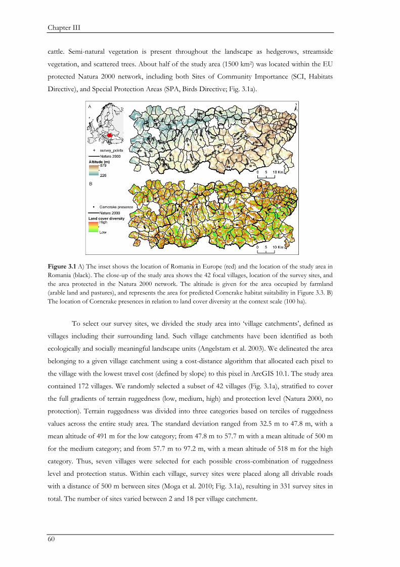
Chapter III
60
cattle. Semi-natural vegetation is present throughout the landscape as hedgerows, streamside
vegetation, and scattered trees. About half of the study area (1500 km2) was located within the EU
protected Natura 2000 network, including both Sites of Community Importance (SCI, Habitats
Directive), and Special Protection Areas (SPA, Birds Directive; Fig. 3.1a).
Figure 3.1 A) The inset shows the location of Romania in Europe (red) and the location of the study area in
Romania (black). The close-up of the study area shows the 42 focal villages, location of the survey sites, and
the area protected in the Natura 2000 network. The altitude is given for the area occupied by farmland
(arable land and pastures), and represents the area for predicted Corncrake habitat suitability in Figure 3.3. B)
The location of Corncrake presences in relation to land cover diversity at the context scale (100 ha).
To select our survey sites, we divided the study area into ‘village catchments’, defined as
villages including their surrounding land. Such village catchments have been identified as both
ecologically and socially meaningful landscape units (Angelstam et al. 2003). We delineated the area
belonging to a given village catchment using a cost-distance algorithm that allocated each pixel to
the village with the lowest travel cost (defined by slope) to this pixel in ArcGIS 10.1. The study area
contained 172 villages. We randomly selected a subset of 42 villages (Fig. 3.1a), stratified to cover
the full gradients of terrain ruggedness (low, medium, high) and protection level (Natura 2000, no
protection). Terrain ruggedness was divided into three categories based on terciles of ruggedness
values across the entire study area. The standard deviation ranged from 32.5 m to 47.8 m, with a
mean altitude of 491 m for the low category; from 47.8 m to 57.7 m with a mean altitude of 500 m
for the medium category; and from 57.7 m to 97.2 m, with a mean altitude of 518 m for the high
category. Thus, seven villages were selected for each possible cross-combination of ruggedness
level and protection status. Within each village, survey sites were placed along all drivable roads
with a distance of 500 m between sites (Moga et al. 2010; Fig. 3.1a), resulting in 331 survey sites in
total. The number of sites varied between 2 and 18 per village catchment.
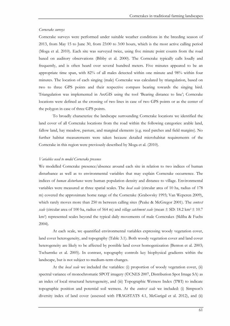
Corncrakes in traditional farming landscapes
61
Corncrake surveys
Corncrake surveys were performed under suitable weather conditions in the breeding season of
2013, from May 15 to June 30, from 23:00 to 3:00 hours, which is the most active calling period
(Moga et al. 2010). Each site was surveyed twice, using five minute point counts from the road
based on auditory observations (Bibby et al. 2000). The Corncrake typically calls loudly and
frequently, and is often heard over several hundred meters. Five minutes appeared to be an
appropriate time span, with 82% of all males detected within one minute and 98% within four
minutes. The location of each singing (male) Corncrake was calculated by triangulation, based on
two to three GPS points and their respective compass bearing towards the singing bird.
Triangulation was implemented in ArcGIS using the tool ‘Bearing distance to line’; Corncrake
locations were defined as the crossing of two lines in case of two GPS points or as the center of
the polygon in case of three GPS points.
To broadly characterize the landscape surrounding Corncrake locations we identified the
land cover of all Corncrake locations from the road within the following categories: arable land,
fallow land, hay meadow, pasture, and marginal elements (e.g. reed patches and field margins). No
further habitat measurements were taken because detailed microhabitat requirements of the
Corncrake in this region were previously described by Moga et al. (2010).
Variables used to model Corncrake presence
We modelled Corncrake presence/absence around each site in relation to two indices of human
disturbance as well as to environmental variables that may explain Corncrake occurrence. The
indices of human disturbance were human population density and distance to village. Environmental
variables were measured at three spatial scales. The local scale (circular area of 10 ha, radius of 178
m) covered the approximate home range of the Corncrake (Grabovsky 1993; Van Weperen 2009),
which rarely moves more than 250 m between calling sites (Peake & McGregor 2001). The context
scale (circular area of 100 ha, radius of 564 m) and village catchment scale (mean ± SD: 18.2 km2 ± 10.7
km2) represented scales beyond the typical daily movements of male Corncrakes (Sklíba & Fuchs
2004).
At each scale, we quantified environmental variables expressing woody vegetation cover,
land cover heterogeneity, and topography (Table 3.1). Both woody vegetation cover and land cover
heterogeneity are likely to be affected by possible land cover homogenization (Benton et al. 2003;
Tscharntke et al. 2005). In contrast, topography controls key biophysical gradients within the
landscape, but is not subject to medium-term changes.
At the local scale we included the variables: (i) proportion of woody vegetation cover, (ii)
spectral variance of monochromatic SPOT imagery (©CNES 2007, Distribution Spot Image SA) as
an index of local structural heterogeneity, and (iii) Topographic Wetness Index (TWI) to indicate
topographic position and potential soil wetness. At the context scale we included: (i) Simpson’s
diversity index of land cover (assessed with FRAGSTATS 4.1, McGarigal et al. 2012), and (ii)
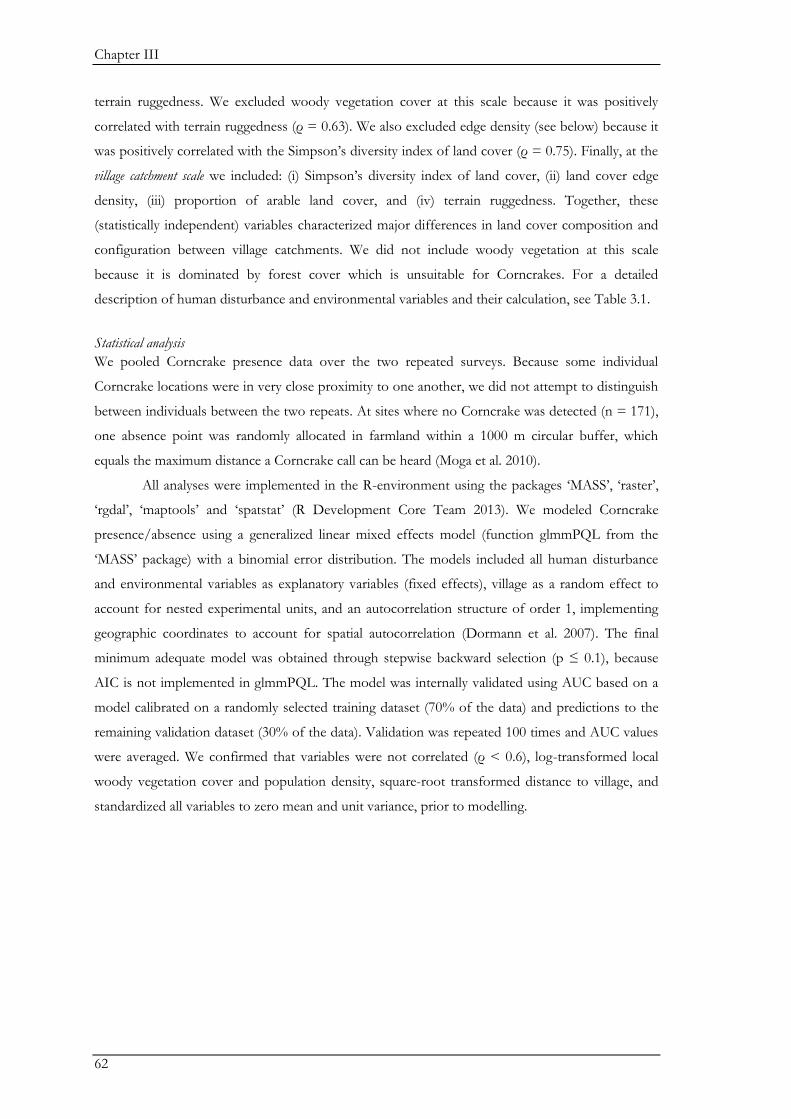
Chapter III
62
terrain ruggedness. We excluded woody vegetation cover at this scale because it was positively
correlated with terrain ruggedness (ρ = 0.63). We also excluded edge density (see below) because it
was positively correlated with the Simpson’s diversity index of land cover (ρ = 0.75). Finally, at the
village catchment scale we included: (i) Simpson’s diversity index of land cover, (ii) land cover edge
density, (iii) proportion of arable land cover, and (iv) terrain ruggedness. Together, these
(statistically independent) variables characterized major differences in land cover composition and
configuration between village catchments. We did not include woody vegetation at this scale
because it is dominated by forest cover which is unsuitable for Corncrakes. For a detailed
description of human disturbance and environmental variables and their calculation, see Table 3.1.
Statistical analysis
We pooled Corncrake presence data over the two repeated surveys. Because some individual
Corncrake locations were in very close proximity to one another, we did not attempt to distinguish
between individuals between the two repeats. At sites where no Corncrake was detected (n = 171),
one absence point was randomly allocated in farmland within a 1000 m circular buffer, which
equals the maximum distance a Corncrake call can be heard (Moga et al. 2010).
All analyses were implemented in the R-environment using the packages ‘MASS’, ‘raster’,
‘rgdal’, ‘maptools’ and ‘spatstat’ (R Development Core Team 2013). We modeled Corncrake
presence/absence using a generalized linear mixed effects model (function glmmPQL from the
‘MASS’ package) with a binomial error distribution. The models included all human disturbance
and environmental variables as explanatory variables (fixed effects), village as a random effect to
account for nested experimental units, and an autocorrelation structure of order 1, implementing
geographic coordinates to account for spatial autocorrelation (Dormann et al. 2007). The final
minimum adequate model was obtained through stepwise backward selection (p ≤ 0.1), because
AIC is not implemented in glmmPQL. The model was internally validated using AUC based on a
model calibrated on a randomly selected training dataset (70% of the data) and predictions to the
remaining validation dataset (30% of the data). Validation was repeated 100 times and AUC values
were averaged. We confirmed that variables were not correlated (ρ < 0.6), log-transformed local
woody vegetation cover and population density, square-root transformed distance to village, and
standardized all variables to zero mean and unit variance, prior to modelling.
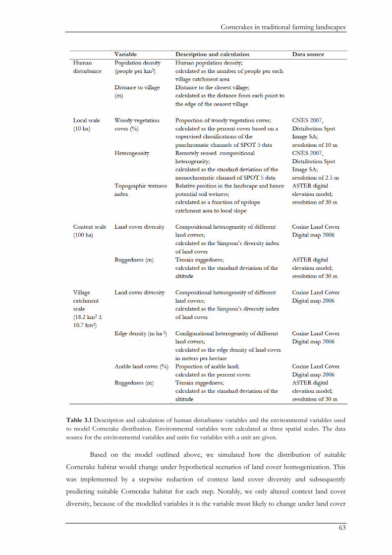
Corncrakes in traditional farming landscapes
63
Table 3.1 Description and calculation of human disturbance variables and the environmental variables used
to model Corncrake distribution. Environmental variables were calculated at three spatial scales. The data
source for the environmental variables and units for variables with a unit are given.
Based on the model outlined above, we simulated how the distribution of suitable
Corncrake habitat would change under hypothetical scenarios of land cover homogenization. This
was implemented by a stepwise reduction of context land cover diversity and subsequently
predicting suitable Corncrake habitat for each step. Notably, we only altered context land cover
diversity, because of the modelled variables it is the variable most likely to change under land cover
Chapter III
64
homogenization. Other variables that influenced Corncrake occurrence are either not influenced by
land cover change (e.g. ruggedness), or would change in unpredictable ways (e.g. human population
density). We reduced land cover diversity incrementally by values of 0.01 for a given pixel in a given
step (original dataset: min = 0, max = 0.84). Pixels with a value of zero were not reduced further.
After each homogenization step, we predicted the probability of suitable Corncrake habitat in
farmland (grassland and arable land) of the whole study area using the fixed effects estimates from
the above described Corncrake model. Finally, the predicted probabilities of occurrence were
converted into presence/absence data using a probability threshold of 0.5 to define suitable
Corncrake habitat.
Based on the results of this simulation, we calculated percent loss in land cover diversity as
the proportion of land cover diversity in a given step relative to the current situation and
standardized to 100%. Similarly, we calculated the remaining proportion of suitable Corncrake
habitat based on the area of predicted suitable Corncrake habitat in a given simulation step relative
to the total area of suitable Corncrake habitat in the region. To visualize the effects of reducing
land cover diversity, we plotted percent loss of land cover diversity against the percent of available
suitable Corncrake habitat. Additionally, land cover diversity and Corncrake suitable habitat were
mapped, both for current conditions and for habitat losses of 33 % and 66 %, corresponding to the
loss of a third or two thirds of the available suitable habitat, respectively.
Results
We found 114 Corncrake presences pooled over the two repeats, of which 71 were located in the
Natura 2000 area (Fig. 3.1b). Corncrakes occurred most frequently in arable land (n = 36; 25 in
Alfalfa fields, Medicago sativa subsp. sativa), marginal elements (n = 31; mostly reed (Phragmites
australis)), and hay meadows (n = 25), followed by fallow land (n = 13) and pastures (n = 9).
Corncrake presence was predicted by human disturbance variables and by environmental
variables at the local and context scales (Table 3.2). The Corncrake was more likely to occupy
remote locations at large distances from villages, and village catchments with a low human
population density. Moreover, the species was more likely to occur in areas with low terrain
ruggedness and high land cover diversity at the context scale, and a high topographic wetness index
at the local scale (Table 3.2; Fig. 3.1b). Model validation indicated a good overall model
performance (AUC mean ± SD: 0.84 ± 0.04).
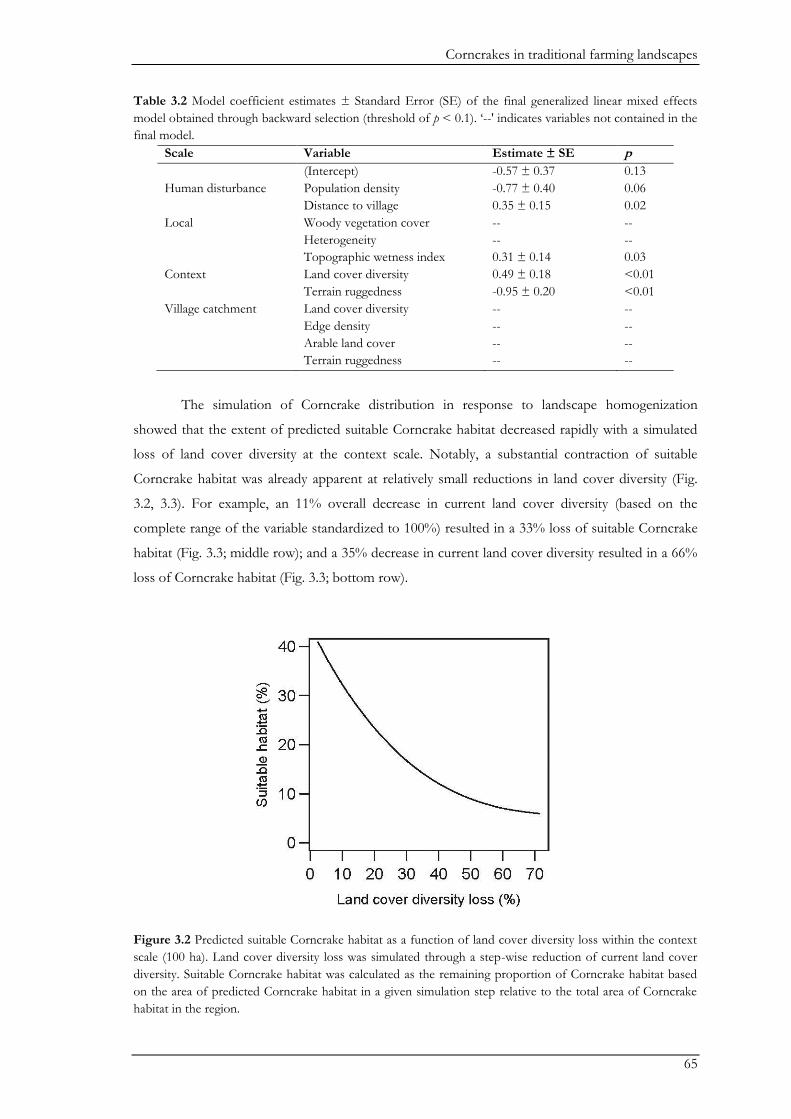
Corncrakes in traditional farming landscapes
65
Table 3.2 Model coefficient estimates ± Standard Error (SE) of the final generalized linear mixed effects
model obtained through backward selection (threshold of p < 0.1). ‘--' indicates variables not contained in the
final model.
Scale Variable Estimate ± SE p
(Intercept) -0.57 ± 0.37 0.13
Human disturbance Population density -0.77 ± 0.40 0.06
Distance to village 0.35 ± 0.15 0.02
Local Woody vegetation cover -- --
Heterogeneity -- --
Topographic wetness index 0.31 ± 0.14 0.03
Context Land cover diversity 0.49 ± 0.18 <0.01
Terrain ruggedness -0.95 ± 0.20 <0.01
Village catchment Land cover diversity -- --
Edge density -- --
Arable land cover -- --
Terrain ruggedness -- --
The simulation of Corncrake distribution in response to landscape homogenization
showed that the extent of predicted suitable Corncrake habitat decreased rapidly with a simulated
loss of land cover diversity at the context scale. Notably, a substantial contraction of suitable
Corncrake habitat was already apparent at relatively small reductions in land cover diversity (Fig.
3.2, 3.3). For example, an 11% overall decrease in current land cover diversity (based on the
complete range of the variable standardized to 100%) resulted in a 33% loss of suitable Corncrake
habitat (Fig. 3.3; middle row); and a 35% decrease in current land cover diversity resulted in a 66%
loss of Corncrake habitat (Fig. 3.3; bottom row).
Figure 3.2 Predicted suitable Corncrake habitat as a function of land cover diversity loss within the context
scale (100 ha). Land cover diversity loss was simulated through a step-wise reduction of current land cover
diversity. Suitable Corncrake habitat was calculated as the remaining proportion of Corncrake habitat based
on the area of predicted Corncrake habitat in a given simulation step relative to the total area of Corncrake
habitat in the region.
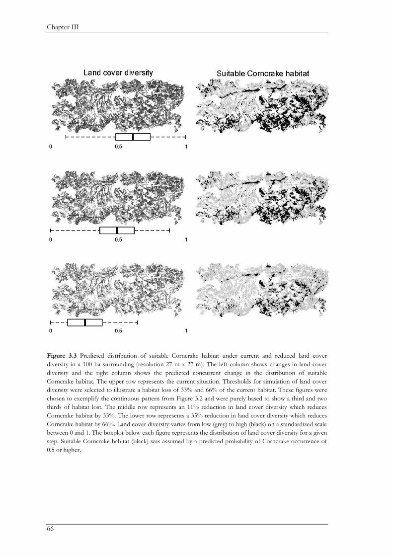
Chapter III
66
Figure 3.3 Predicted distribution of suitable Corncrake habitat under current and reduced land cover
diversity in a 100 ha surrounding (resolution 27 m x 27 m). The left column shows changes in land cover
diversity and the right column shows the predicted concurrent change in the distribution of suitable
Corncrake habitat. The upper row represents the current situation. Thresholds for simulation of land cover
diversity were selected to illustrate a habitat loss of 33% and 66% of the current habitat. These figures were
chosen to exemplify the continuous pattern from Figure 3.2 and were purely based to show a third and two
thirds of habitat lost. The middle row represents an 11% reduction in land cover diversity which reduces
Corncrake habitat by 33%. The lower row represents a 35% reduction in land cover diversity which reduces
Corncrake habitat by 66%. Land cover diversity varies from low (grey) to high (black) on a standardized scale
between 0 and 1. The boxplot below each figure represents the distribution of land cover diversity for a given
step. Suitable Corncrake habitat (black) was assumed by a predicted probability of Corncrake occurrence of
0.5 or higher.
Corncrakes in traditional farming landscapes
67
Discussion
Our study adds to a growing body of knowledge on the effects of heterogeneity on farmland
biodiversity, suggesting that the loss of heterogeneity, typically associated with land-use
intensification, can negatively impact biodiversity (e.g. Stein et al. 2014). Furthermore, substantial
losses of Corncrake habitat are likely to result from relatively small losses in land cover diversity,
indicating a non-linear relationship between habitat loss and loss in land cover diversity. These
findings have important implications for the management of heterogeneous farming landscapes. In
Europe, the majority of studies on the effects of landscape homogenization on farmland
biodiversity have been performed in countries with more intensively used farmland (Devictor &
Jiguet 2007; Pickett & Siriwardena 2011), while more heterogeneous, low-intensity regions remain
poorly understood (Baldi & Batary 2011; Tryjanowski et al. 2011). Our findings suggest that land
cover homogenization in a traditional farming landscape could drastically reduce suitable habitat
for farmland species such as the Corncrake. This underlines the need for conservation strategies
that consider land cover diversity across entire landscape mosaics, and that are specifically geared
towards traditional farmland supporting large populations of rare or threatened species.
Agricultural landscapes are increasingly recognized for their value for biodiversity
conservation (Mendenhall et al. 2014). This is especially important for European landscapes, which
reflect centuries of interactions between people and the natural environment (Bignal & McCracken
2000). Long-established traditional agriculture has created many of the habitats and niches for
species valued for biodiversity today (Bignal & McCracken 2000). Nevertheless, traditional
agricultural landscapes have declined dramatically over the last decades (Foley et al. 2005). The few
remaining examples are under considerable threat from changes in agricultural management and
their continued existence hinges on both national and international conservation policies (Henle et
al. 2008).
Our study shows that land cover heterogeneity is a key feature to be addressed in
conservation measures targeting traditional farmland. The positive effects of heterogeneity on
biodiversity, including farmland birds, have been well-documented (e.g. Weibull et al. 2000; Benton
et al. 2003; Diacon-Bolli et al. 2012; Stein et al. 2014). In particular, land cover diversity appears to
positively affect bird richness and abundance in farmland (Sanderson et al. 2009; Pickett &
Siriwardena 2011), suggesting that different land-use covers provide complementary resources,
such as feeding, nesting, and sheltering sites. However, responses of farmland birds to
heterogeneity are species-specific; especially ground nesting birds and open farmland specialists
often prefer relatively homogenous landscapes (Filippi-Codaccioni et al. 2010; Fischer et al. 2011;
Pickett & Siriwardena 2011; Guerrero et al. 2012). For such specialist species, management
practices to increase heterogeneity may therefore reduce their populations, especially in low-
intensity farmland (Batary et al. 2011b).
Also the Corncrake is a ground-nesting species in open farmland, and similar to other
grassland species, it has been observed to occur in extensive areas of relatively homogenous,
Chapter III
68
uncultivated meadows (Keišs 2005; Berg & Hiron 2012; Quinn et al. 2012). Nevertheless, a
traditional farmland mosaic such as the one we studied evidently can provide important additional
habitat for the Corncrake. Land cover homogenization at the context scale as consequence of
intensification would have a substantial negative impact on the Corncrake in currently
heterogeneous landscapes. To protect the Corncrake in traditional farmland, it is therefore
important to ensure the persistence of mixed farming practices.
While the use of low-intensity grasslands and hay meadows by the Corncrake is well
documented (Berg & Gustafson 2007; Budka & Osiejuk 2013), less is known about the
complementary values of other land-use types to the species (but see e.g. Berg & Hiron 2012). For
example, in a diverse land cover mosaic, uncropped arable land, and the high density of edges
between different land covers (e.g. field margins or ditches) provide safe breeding or sheltering sites
for the Corncrake (Green et al. 1997; Corbett & Hudson 2010; Budka & Osiejuk 2013). Such
structures are especially important during the early breeding season when the height of
surrounding spring-vegetation is short (Budka & Osiejuk 2013). In addition, field margins are often
rich in invertebrates (Josefsson et al. 2013), and thus a higher abundance of field margins may
increase food availability for the Corncrake.
Some studies have found that the Corncrake tends to avoid annually cropped arable fields
(Keišs 2005; Berg & Hiron 2012; Budka & Osiejuk 2013). However, we found a considerable
number of Corncrakes in arable fields, and in particular in Alfalfa fields. Corncrakes and other
grassland species have also been observed in grass or clover fields used for silage and hay in other
regions (Corbett & Hudson 2010; Berg & Hiron 2012; Quinn et al. 2012). Although this suggests
that arable fields sown with grass or leguminous plants can provide important additional habitat for
Corncrakes, care should be taken for appropriate management because hayed crops can create
population sinks (Perlut et al. 2006). In contrast, pastures appeared to have little habitat value for
the Corncrake, and similarly to other regions, the Corncrake was more likely to be present in hay
meadows than pastures (Wettstein et al. 2001; Keišs 2005). The Corncrake may avoid grazed
pastures for several reasons. For example, they are typically located on better drained, steeper
slopes, whereas the Corncrake preferentially uses moist flat areas. In addition, the reduced
vegetation height in pastures caused by grazing may reduce habitat suitability (Berg & Gustafson
2007).
Loss of hay meadows and the intensification of grassland management are currently
viewed as the main threats to Corncrake populations (Koffijberg & Schäffer 2006). Therefore,
current conservation strategies (including AES schemes) for the Corncrake relate primarily to the
maintenance of hay meadows and low-intensity grasslands, with emphasis on specified mowing
regimes (Koffijberg & Schäffer 2006; Berg & Gustafson 2007) and leaving unmown refuge strips
(Tyler et al. 1998). These methods have been successful (Koffijberg & Schäffer 2006), and have
also provided wider biodiversity benefits in countries with relatively intensive agriculture
(Wilkinson et al. 2012). However, our results suggest that the implementation of grassland-focused
Corncrakes in traditional farming landscapes
69
strategies alone may not be sufficient for Corncrake conservation in Transylvania’s traditional
farmland. Moreover, at present, farmers in Transylvania mow their land in a way that creates a
heterogeneous vegetation structure, including numerous unmown patches until late in the season.
Delayed mowing regimes could potentially be counter-productive, because they may result in the
synchronization of management and thus homogenization of vegetation height (Dahlström et al.
2013), which has negatively affected Corncrakes elsewhere (Brambilla & Pedrini 2013). Other
specific CAP measures in Romania, such as sheep premium payments, also may pose a threat to the
Corncrake. This is because such incentives may inadvertently encourage the conversion of hay
meadows to pastures (Demeter & Kelemen 2012). These examples highlight the need to carefully
adjust agri-environment schemes and other CAP measures to traditional farmland. Moreover,
schemes particularly related to the Corncrake should primarily target core Corncrake habitat, such
as remote, flat and wet areas, which are especially at risk of conversion to homogenous, intensified
farmland.
Our findings thus underline that agri-environment management needs to be adapted to the
context of the landscape (Batary et al. 2011a), and schemes designed for high-intensity landscapes
cannot be readily transferred to traditional farmland (Sutcliffe et al. 2014). Given the affinity of the
Corncrake with the heterogeneous farmland mosaic, there could be major benefits in agri-
environment schemes specifically aiming at maintaining the heterogeneous character of low-
intensity landscapes (Kleijn et al. 2011). Without pro-active policy measures to maintain land cover
heterogeneity in traditional farmland, homogenization of the landscape will have negative effects
on biodiversity in general, and on already threatened species such as the Corncrake in particular.
The successful implementation of measures that maintain land cover heterogeneity across
entire landscapes will hinge on finding ways to coordinate actions across multiple farmers, rather
than relying on local measures alone (McKenzie et al. 2013). Moreover, high heterogeneity in
traditional farmland is tightly linked to the multi-functionality of semi-subsistence farm holdings of
relatively small size (Tryjanowski et al. 2011). Thus, landscape-scale governance may be challenging
because it depends on the involvement of many individual farmers (McKenzie et al. 2013). In
traditional farmland, AESs could be used to support collaborations of specific target groups (Pe'er
et al. 2014), such as small-scale farm holders which create the heterogeneous mosaic but are also
particularly susceptible to selling land to large-scale farmers.
Conclusions
Our study showed that heterogeneous farmland has high complementary conservation value for
the Corncrake, in addition to their core habitat of large areas of wet meadows. Furthermore, our
simulations highlighted that in heterogeneous low-intensity farmland, conservation measures
implemented on small scales by single farmers should be complemented with landscape-scale
measures to maintain land cover heterogeneity. Although we highlighted the importance of
landscape-scale conservation for a single protected species, a similar pattern appears to be emerging
Chapter III
70
more generally (Merckx et al. 2009; Dallimer et al. 2010). More research is needed on the
effectiveness of landscape-scale conservation in farmland; however, research should also focus on
how conservation measures targeting whole landscapes rather than single farms can be
implemented. This is especially important in traditional farming landscapes, many of which are
complex but rapidly changing social-ecological systems that are threatened by land cover
homogenization.
Acknowledgements
We thank A. Klein and J. Tinnemans for their tremendous effort in the field. We thank P. Griffiths,
J. Knorn and T. Kümmerle for their help with creating the woody vegetation layer, and D. Abson
and P. Fust for analytical assistance. We thank two anonymous reviewers for constructive
suggestions on a previous draft of this manuscript. The project was funded by a Sofja Kovalevskaja
Award by the Alexander von Humboldt Foundation to JF.

71
Chapter IV

72
73
Chapter IV
Human-carnivore coexistence in a traditional rural landscape
Ine Dorresteijn, Jan Hanspach, Attila Kecskés, Hana Latková, Zsófia Mezey, Szilárd Sugár,
Henrik von Wehrden, Joern Fischer
Landscape Ecology (2014), 29:1145-1155
‘There is no conservation without conservation.’ – Luigi Boitani

Chapter IV
74
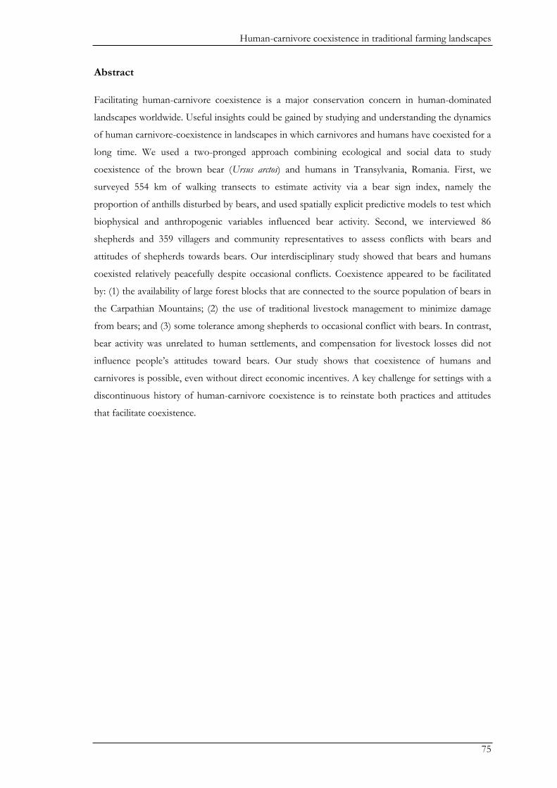
Human-carnivore coexistence in traditional farming landscapes
75
Abstract
Facilitating human-carnivore coexistence is a major conservation concern in human-dominated
landscapes worldwide. Useful insights could be gained by studying and understanding the dynamics
of human carnivore-coexistence in landscapes in which carnivores and humans have coexisted for a
long time. We used a two-pronged approach combining ecological and social data to study
coexistence of the brown bear (Ursus arctos) and humans in Transylvania, Romania. First, we
surveyed 554 km of walking transects to estimate activity via a bear sign index, namely the
proportion of anthills disturbed by bears, and used spatially explicit predictive models to test which
biophysical and anthropogenic variables influenced bear activity. Second, we interviewed 86
shepherds and 359 villagers and community representatives to assess conflicts with bears and
attitudes of shepherds towards bears. Our interdisciplinary study showed that bears and humans
coexisted relatively peacefully despite occasional conflicts. Coexistence appeared to be facilitated
by: (1) the availability of large forest blocks that are connected to the source population of bears in
the Carpathian Mountains; (2) the use of traditional livestock management to minimize damage
from bears; and (3) some tolerance among shepherds to occasional conflict with bears. In contrast,
bear activity was unrelated to human settlements, and compensation for livestock losses did not
influence people’s attitudes toward bears. Our study shows that coexistence of humans and
carnivores is possible, even without direct economic incentives. A key challenge for settings with a
discontinuous history of human-carnivore coexistence is to reinstate both practices and attitudes
that facilitate coexistence.
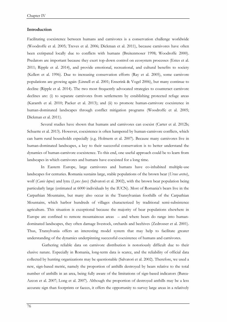
Chapter IV
76
Introduction
Facilitating coexistence between humans and carnivores is a conservation challenge worldwide
(Woodroffe et al. 2005; Treves et al. 2006; Dickman et al. 2011), because carnivores have often
been extirpated locally due to conflicts with humans (Breitenmoser 1998; Woodroffe 2000).
Predators are important because they exert top-down control on ecosystem processes (Estes et al.
2011; Ripple et al. 2014), and provide emotional, recreational, and cultural benefits to society
(Kellert et al. 1996). Due to increasing conservation efforts (Ray et al. 2005), some carnivore
populations are growing again (Linnell et al. 2001; Enserink & Vogel 2006), but many continue to
decline (Ripple et al. 2014). The two most frequently advocated strategies to counteract carnivore
declines are: (i) to separate carnivores from settlements by establishing protected refuge areas
(Karanth et al. 2010; Packer et al. 2013); and (ii) to promote human-carnivore coexistence in
human-dominated landscapes through conflict mitigation programs (Woodroffe et al. 2005;
Dickman et al. 2011).
Several studies have shown that humans and carnivores can coexist (Carter et al. 2012b;
Schuette et al. 2013). However, coexistence is often hampered by human-carnivore conflicts, which
can harm rural households especially (e.g. Holmern et al. 2007). Because many carnivores live in
human-dominated landscapes, a key to their successful conservation is to better understand the
dynamics of human-carnivore coexistence. To this end, one useful approach could be to learn from
landscapes in which carnivores and humans have coexisted for a long time.
In Eastern Europe, large carnivores and humans have co-inhabited multiple-use
landscapes for centuries. Romania sustains large, stable populations of the brown bear (Ursus arctos),
wolf (Canis lupus) and lynx (Lynx lynx) (Salvatori et al. 2002), with the brown bear population being
particularly large (estimated at 6000 individuals by the IUCN). Most of Romania’s bears live in the
Carpathian Mountains, but many also occur in the Transylvanian foothills of the Carpathian
Mountains, which harbor hundreds of villages characterized by traditional semi-subsistence
agriculture. This situation is exceptional because the majority of bear populations elsewhere in
Europe are confined to remote mountainous areas – and where bears do range into human-
dominated landscapes, they often damage livestock, orchards and beehives (Zedrosser et al. 2001).
Thus, Transylvania offers an interesting model system that may help to facilitate greater
understanding of the dynamics underpinning successful coexistence of humans and carnivores.
Gathering reliable data on carnivore distribution is notoriously difficult due to their
elusive nature. Especially in Romania, long-term data is scarce, and the reliability of official data
collected by hunting organizations may be questionable (Salvatori et al. 2002). Therefore, we used a
new, sign-based metric, namely the proportion of anthills destroyed by bears relative to the total
number of anthills in an area, being fully aware of the limitations of sign-based indicators (Barea-
Azcon et al. 2007; Long et al. 2007). Although the proportion of destroyed anthills may be a less
accurate sign than footprints or faeces, it offers the opportunity to survey large areas in a relatively
Human-carnivore coexistence in traditional farming landscapes
77
short time, which we believe more than compensates the risks of potentially higher methodological
uncertainty.
To understand long-term coexistence in multiple-use landscapes, both ecological and social
variables are important (Treves & Karanth 2003; Treves et al. 2006; Carter et al. 2012a). Although
the need for interdisciplinary work on human-wildlife coexistence has repeatedly been
acknowledged (Redpath et al. 2012), few studies have combined ecological studies on habitat
preferences of carnivores with social data on human-carnivore conflicts and tolerance levels
towards carnivores (Glikman and Frank, 2011; but see Schuette et al. 2013). The overarching goal
of our study was to assess how humans and bears coexist in Southern Transylvania. Our study had
two specific objectives. First, we sought to understand spatial patterns of bear activity in response
to anthropogenic variables, biophysical variables, as well as local connectivity between forest
patches and regional connectivity to the Carpathian Mountains. Second, we examined the nature of
human-bear conflicts in the region and related it to the spatial distribution of bear activity.
Methods
Study area and design
Our 7441 km2 study area was located within a 50 km radius around the town of Sighisoara, in the
foothills of the Carpathian Mountains in Southern Transylvania (Fig. 4.1a). Recently, one of the
largest sets of non-mountainous EU protected Natura 2000 sites was established in this area (Fig.
4.1b). We selected transects inside and outside this protected area to provide data for the
foundations of the brown bear management plan, and to provide reference data so the
management plan can later be evaluated. A detailed description of the area is provided in
Supplementary Material Text S4.1.
To quantify bear activity, we used the proportion of anthills destroyed by bears relative to
the total number of anthills in each pasture transect. Destroyed anthills and other signs are rare in
forests and therefore we walked transects on pasture adjacent to forest. Anthills are available on
pastures across the entire landscape which allowed us to cover a large area in a standardized way.
Ants form an important food source of protein for the brown bear (Dahle et al. 1998; Swenson et
al. 1999). Ant larvae are particularly sought after by bears in spring and summer, and the incidence
of destroyed anthills has been used in previous sign surveys for bear presence (Munro et al. 2006;
Ciarniello et al. 2007). Anthills destroyed by bears are readily distinguishable from those destroyed
by other animals (e.g. cattle) and humans because they have a characteristic ‘crater’ dug out of the
top.
Our choice of transects was guided by three design considerations. First, we sought to
obtain a broad overview of bear activity in the study area. We surveyed bear activity in 30 focal
villages and their surrounding land, because villages have been identified as both ecologically and
socially meaningful ‘landscape’ units (Angelstam et al. 2003). We delineated the area belonging to a
Chapter IV
78
given village using a cost-distance algorithm that allocated each pixel to the village with the lowest
travel cost to this pixel (slope-penalized distance, implemented in ArcGIS, mean area ± SD: 20.5 ±
11.2 km2). We randomly selected 30 villages from 448 villages in the study area, stratified to cover
the full gradient in terrain ruggedness and to include Natura 2000 areas as well as unprotected areas
(Fig. 4.1b). With few exceptions arising from logistical obstacles we surveyed four transects around
each village (n = 113; described in detail below).
Second, we covered the focal conservation area (2675 km2) in detail to inform the new
management plan. We divided the Natura 2000 area into grid cells of 2 km x 2 km (n = 759). We
surveyed one transect in each grid cell with more than 15% forest cover (n = 417), and we surveyed
one transect per grid cell for 100 additional, randomly chosen cells with less than 15% forest cover.
For these two considerations, all transects were chosen to cover the full gradient of available
distances to the nearest village and amount of surrounding forest cover within a radius of 1500 m.
Third, to assess the connectivity from our study area to the assumed source population of brown
bears in the Carpathian Mountains, we compared alternative cost-distance metrics to the
mountains, so that the best cost-distance metric could be used in later analyses (see the section on
variables used to model bear activity below). For this, we specifically surveyed 59 transects within
15-20 km from the mountains (Fig. 4.1b). These transects were chosen to cover a gradient from
likely low cost to high cost by varying the sets of land cover types available between a given
transect and the mountains.
All transects were walked once at the forest-pasture interface at approximately 10 m
distance from the forest edge. Each transect was 800 m long and 6 m wide. All destroyed and
undestroyed anthills within a transect were counted. We included both fresh (this year) and old
(previous years but clearly visible) destroyed anthills. In total, we walked 692 transects (554 km)
between April 28 and August 10, 2012. Three transects were excluded from analysis because they
had no anthills. The mean number of anthills per transect was 139. All transects for the cost-
distance analysis were surveyed in May and June, 2012.
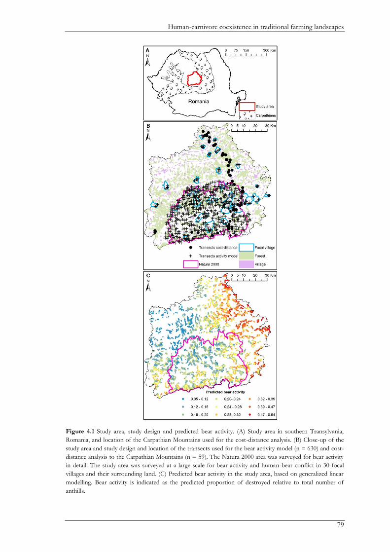
Human-carnivore coexistence in traditional farming landscapes
79
Figure 4.1 Study area, study design and predicted bear activity. (A) Study area in southern Transylvania,
Romania, and location of the Carpathian Mountains used for the cost-distance analysis. (B) Close-up of the
study area and study design and location of the transects used for the bear activity model (n = 630) and cost-
distance analysis to the Carpathian Mountains (n = 59). The Natura 2000 area was surveyed for bear activity
in detail. The study area was surveyed at a large scale for bear activity and human-bear conflict in 30 focal
villages and their surrounding land. (C) Predicted bear activity in the study area, based on generalized linear
modelling. Bear activity is indicated as the predicted proportion of destroyed relative to total number of
anthills.
Chapter IV
80
Variables used to model bear activity
We used four sets of variables to explain patterns in bear activity. First, anthropogenic disturbance
was indicated by distance to settlements. Second, the biophysical environment within a radius of
1000 m from the midpoint of each transect was indicated by (i) terrain ruggedness calculated as the
standard deviation of the altitude; (ii) percent pasture cover; and (iii) the shape and size of forest
patches indicated by the forest edge to forest interior ratio. We did not include forest cover because
it was correlated with forest edge to interior ratio (ρ = - 0.71). Third, local connectivity between
forest patches within the study area was indicated by betweenness centrality. Betweenness centrality
is an index of how well connected a given forest patch is within the network of forest patches
regardless of land-use between the different forest patches. Fourth, connectivity to the Carpathian
Mountains (the presumed source population) was indicated by the cost-distance of each transect to
the mountains. Cost-distance was based on a matrix with a resolution of 10 m x 10 m and
combined distance to the mountains with weights between 1-10, assigned by experts to the
different land-use types. Detailed descriptions of these variables are provided in Supplementary
Material Text S4.1.
We accounted for possible effects of the total number of anthills per transect and survey
date (bears might be more attracted to pastures with more anthills; and the number of destroyed
anthills by definition accumulates with time) by including them as variables in the model. Because
the effects of number of anthills and survey date were not necessarily linear, we included their
quadratic terms (e.g. the number of destroyed anthills might level off before the end of the field
season if bears shift to other food sources such as fruit). Protection level was not included in the
models, because the recent establishment of the Natura 2000 area has not yet resulted in different
natural resource use that could affect bear activity.
Statistical modelling
All analyses were performed with the proportion of destroyed vs. total number of anthills as the
response variable within generalized linear models (GLM) with a quasi-binomial error structure to
account for overdispersion. This model specification took into account that the precision of the
response variable increased with an increasing total number of anthills found along a given transect
(e.g. one destroyed anthill out of two total anthills is less precise information than 50 destroyed out
of 100). The final GLM was obtained by using model averaging based on a 10-fold cross-validation
(Fielding & Bell 1997). Validation was done by relating the predicted activity (based on a model
using nine tenths of the data) with the activity observed in the remaining tenth via a binomial GLM
(see Table S4.1 for the estimates and explained deviance for each of the validation steps). We
calculated the amount of deviance explained as a measure of predictive performance of each of the
ten models. We averaged the parameter estimates over the 10 models, weighting the estimates from
each model by its predictive performance. The averaged estimates were used to predict bear activity
in forest edges bordering pastures across the entire study area, at a resolution of 800 m, equalling
Human-carnivore coexistence in traditional farming landscapes
81
the transect length of the field surveys. All statistical analysis were implemented in the ‘R’
environment (R Development Core Team 2013). Further details on statistical modelling and
predictive mapping are provided in Supplementary Material Text S4.1.
Human-bear conflicts
Human-bear conflicts were assessed using questionnaires in the same 30 villages targeted for bear
transects (Fig. 4.1b). We used a detailed questionnaire for shepherds that addressed attacks on
livestock, attitudes towards bears, and the current compensation schedule; and a shorter one for
villagers that addressed the types of damage caused by bears. To assess attitudes among different
stakeholder groups relevant to coexistence dynamics, we used the same short questionnaire for
mayors, hunters and local councillors. These groups are in charge of compensation payments after
carnivore damage, and we therefore included several questions regarding compensation
(questionnaires are available as Supplementary Material Text S4.2-4.4). We aimed to interview
approximately three shepherds (on average a village had between one and four shepherds), ten
villagers, one mayor and one hunter or councillor per village, but not everyone was available in all
villages. Ultimately, we obtained questionnaires from 86 shepherds (73 sheep-herders, 13 cow-
herders), 302 villagers, 22 mayors or vice-mayors, 20 local councillors and 15 hunters. (For ethical
considerations see Supplementary Material Text S4.1.)
We expected a significant relationship between bear activity and perceived number of
conflicts (e.g. higher bear activity could increase bear-related impacts), as well as livestock
management (e.g. proactive measures prevent attacks by bears). To test for a possible relationship
between bear activity and conflicts, we first averaged predicted bear activity within the land
associated with each village. We then calculated Spearman rank correlations between average
predicted bear activity and: (i) the mean number of bear attacks on sheep in the last three years; and
(ii) perceived damage to orchards, crops and beehives. For the latter we used the proportion of
local people who stated that bears caused damage to local orchards, crops or beehives. To assess
whether certain herding techniques were more or less prone to attacks we used Spearman rank
correlations between number of bear attacks on sheep and (i) the number of sheep in the herd; (ii)
the number of sheep per guarding dog; (iii) total number of dogs, and (iv) the number of sheep per
shepherd.
Results
Predictive model of bear activity
Bear activity was recorded in 52% of the 630 transects. Cost-distance to the Carpathian Mountains
had the largest effect on bear activity (Table 4.1), which decreased with increasing cost-distance.
Biophysical variables also were strongly related to bear activity (Table 4.1). Bear activity was highest
in rugged terrain, near large forest patches with a low edge to interior ratio, and in areas with low
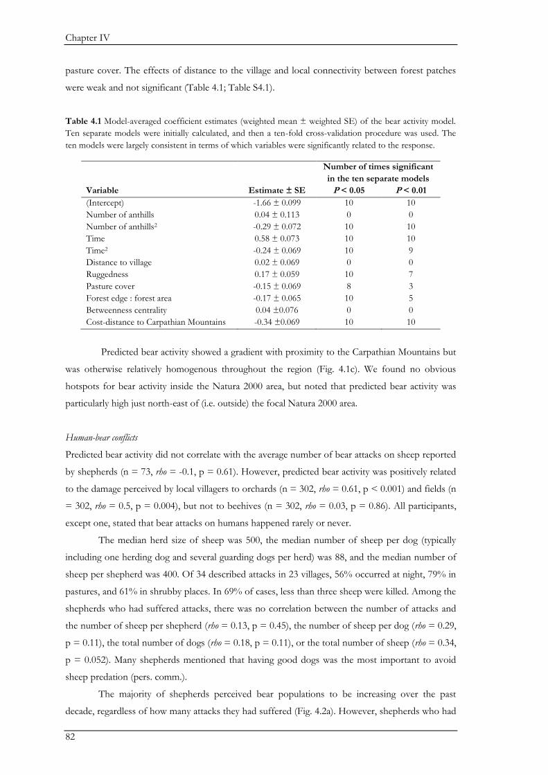
Chapter IV
82
pasture cover. The effects of distance to the village and local connectivity between forest patches
were weak and not significant (Table 4.1; Table S4.1).
Table 4.1 Model-averaged coefficient estimates (weighted mean ± weighted SE) of the bear activity model.
Ten separate models were initially calculated, and then a ten-fold cross-validation procedure was used. The
ten models were largely consistent in terms of which variables were significantly related to the response.
Number of times significant
in the ten separate models
Variable Estimate ± SE P < 0.05 P < 0.01
(Intercept) -1.66 ± 0.099 10 10
Number of anthills 0.04 ± 0.113 0 0
Number of anthills2 -0.29 ± 0.072 10 10
Time 0.58 ± 0.073 10 10
Time2 -0.24 ± 0.069 10 9
Distance to village 0.02 ± 0.069 0 0
Ruggedness 0.17 ± 0.059 10 7
Pasture cover -0.15 ± 0.069 8 3
Forest edge : forest area -0.17 ± 0.065 10 5
Betweenness centrality 0.04 ±0.076 0 0
Cost-distance to Carpathian Mountains -0.34 ±0.069 10 10
Predicted bear activity showed a gradient with proximity to the Carpathian Mountains but
was otherwise relatively homogenous throughout the region (Fig. 4.1c). We found no obvious
hotspots for bear activity inside the Natura 2000 area, but noted that predicted bear activity was
particularly high just north-east of (i.e. outside) the focal Natura 2000 area.
Human-bear conflicts
Predicted bear activity did not correlate with the average number of bear attacks on sheep reported
by shepherds (n = 73, rho = -0.1, p = 0.61). However, predicted bear activity was positively related
to the damage perceived by local villagers to orchards (n = 302, rho = 0.61, p < 0.001) and fields (n
= 302, rho = 0.5, p = 0.004), but not to beehives (n = 302, rho = 0.03, p = 0.86). All participants,
except one, stated that bear attacks on humans happened rarely or never.
The median herd size of sheep was 500, the median number of sheep per dog (typically
including one herding dog and several guarding dogs per herd) was 88, and the median number of
sheep per shepherd was 400. Of 34 described attacks in 23 villages, 56% occurred at night, 79% in
pastures, and 61% in shrubby places. In 69% of cases, less than three sheep were killed. Among the
shepherds who had suffered attacks, there was no correlation between the number of attacks and
the number of sheep per shepherd (rho = 0.13, p = 0.45), the number of sheep per dog (rho = 0.29,
p = 0.11), the total number of dogs (rho = 0.18, p = 0.11), or the total number of sheep (rho = 0.34,
p = 0.052). Many shepherds mentioned that having good dogs was the most important to avoid
sheep predation (pers. comm.).
The majority of shepherds perceived bear populations to be increasing over the past
decade, regardless of how many attacks they had suffered (Fig. 4.2a). However, shepherds who had
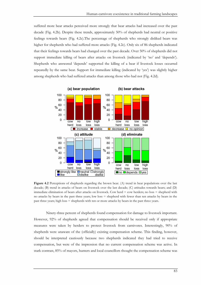
Human-carnivore coexistence in traditional farming landscapes
83
suffered more bear attacks perceived more strongly that bear attacks had increased over the past
decade (Fig. 4.2b). Despite these trends, approximately 50% of shepherds had neutral or positive
feelings towards bears (Fig. 4.2c).The percentage of shepherds who strongly disliked bears was
higher for shepherds who had suffered more attacks (Fig. 4.2c). Only six of 86 shepherds indicated
that their feelings towards bears had changed over the past decade. Over 50% of shepherds did not
support immediate killing of bears after attacks on livestock (indicated by ‘no’ and ‘depends’).
Shepherds who answered ‘depends’ supported the killing of a bear if livestock losses occurred
repeatedly by the same bear. Support for immediate killing (indicated by ‘yes’) was slightly higher
among shepherds who had suffered attacks than among those who had not (Fig. 4.2d).
Figure 4.2 Perceptions of shepherds regarding the brown bear. (A) trend in bear populations over the last
decade; (B) trend in attacks of bears on livestock over the last decade; (C) attitudes towards bears; and (D)
immediate elimination of bears after attacks on livestock. Cow herd = cow herders; no loss = shepherd with
no attacks by bears in the past three years; low loss = shepherd with fewer than ten attacks by bears in the
past three years; high loss = shepherds with ten or more attacks by bears in the past three years.
Ninety-three percent of shepherds found compensation for damage to livestock important.
However, 92% of shepherds agreed that compensation should be received only if appropriate
measures were taken by herders to protect livestock from carnivores. Interestingly, 90% of
shepherds were unaware of the (officially) existing compensation scheme. This finding, however,
should be interpreted cautiously because two shepherds indicated they had tried to receive
compensation, but were of the impression that no current compensation scheme was active. In
stark contrast, 85% of mayors, hunters and local councillors thought the compensation scheme was
Chapter IV
84
readily accessible; but only 43% of mayors, hunter and councillors believed that the majority of the
community was aware of the scheme.
Discussion
There is growing recognition of the need to conserve large carnivores outside protected areas (e.g.
Athreya et al. 2013; Schuette et al. 2013), however, insights from human-dominated landscapes are
still limited (e.g. Ghosal et al. 2013). Our approach drawing on both ecological and social data
suggests an apparent balance between humans and bears in Southern Transylvania. The main
factors contributing to this appeared to be: (i) the availability of large forest blocks connected to the
presumed source population of bears in the Carpathian Mountains; (ii) the use of traditional
livestock husbandry techniques to minimize damage from bears; and (iii) some tolerance among
shepherds to occasional conflict with bears. Unlike elsewhere, avoidance of human settlements by
bears (Posillico et al. 2004; Preatoni et al. 2005; Nellemann et al. 2007) and financial incentives
(Maclennan et al. 2009; Banerjee et al. 2013) appeared to play negligible roles in facilitating human-
bear coexistence.
Explaining coexistence
The Carpathian Mountains support the largest extant populations of the brown bear in Europe
(Zedrosser et al. 2001). Consistent with this, the most important predictor of bear activity was
proximity to the Carpathians. Higher bear activity was also found in rugged areas and near large
blocks of forest, which is most likely related to better shelter and den sites in rough terrain, and
potentially a wider variety of food resources (Nellemann et al. 2007; May et al. 2008; Güthlin et al.
2011). Local connectivity between forest patches, however, was unrelated to bear activity,
suggesting that forest patches are well-connected throughout the region. Indeed, forest cover in
our study area was close to the presumed 30% threshold below which the effects of habitat loss
may be exacerbated by isolation effects (Andrén 1994). Alternatively, local connectivity may be
related to shrub cover which was not accounted for in our analyses, and this may partly explain the
lack of statistical significance of local connectivity. In contrast to other studies (Posillico et al. 2004;
Preatoni et al. 2005; Nellemann et al. 2007), bears were not affected by distance to human
settlements. This may be because, at present, vehicle traffic does not increase strongly near
settlements, and major agricultural machinery is also relatively uncommon, although agricultural
intensification is likely in the future (Mikulcak et al. 2013). In addition, human presence per se may
not deter bears because local people are not a major threat, given that bears are protected by law
and hunting is prohibited. Finally, retaliation killing is probably uncommon in the study area,
though better knowledge on this would be useful to more fully understand human-bear
coexistence.
Interestingly, observed bear activity was not related to the frequency of attacks on sheep,
but was negatively related to perceived damage to orchards and fields. Unlike sheep, fields and
Human-carnivore coexistence in traditional farming landscapes
85
orchards are often guarded less carefully and most lack (effective) fences, suggesting that the
livestock husbandry techniques used by shepherds may effectively prevent bear attacks. The use of
guarding dogs and nightly confinement appears to reduce livestock attacks worldwide (Gehring et
al. 2010; Rigg et al. 2011). Indeed, most of the reported bear attacks occurred on the pasture, and
not in the well-guarded sheepfolds. Similar to observations in the Romanian mountains (Mertens &
Schneider 2005), we found no relationship between the frequency of bear attacks and the number
of sheep per dog. This is surprising, given the shepherds’ emphasis on the importance of good
guarding dogs. The lack of a relationship between attacked and the number of dogs could arise
from: (i) the use of an appropriately large number of dogs by the majority of shepherds; (ii) our
sample size being too small to detect a significant relationship; or (iii) our model for bear activity
only explaining bear distribution in spring and summer, while bear attacks occurred year-round.
The lack of a relationship between bear activity and frequency of attacks further suggests
that local conditions may be more important than actual carnivore densities in determining rates of
attack (Kaczensky 1999; Rigg et al. 2011). This supports the notion that human-carnivore
coexistence is possible, but knowledge of local conditions is necessary for effective, proactive
conflict management. In our case, relevant local conditions may include the quality of guarding
dogs and vigilance of shepherds, but also the prevalence of woody vegetation in pastures. Because
local conditions can, in principle, be managed, our findings indicate opportunities for proactive
conflict mitigation.
Public attitudes towards carnivores are typically most positive in areas without carnivores
(Kellert et al. 1996), or where people and carnivores have coexisted for a long time (Boitani 1995).
The long-term coexistence of bears and shepherds may have led to the acceptance of occasional
livestock loss by some shepherds, however, as observed elsewhere (Kaczensky et al. 2004),
shepherds that were heavily affected by bears were also less tolerant to livestock loss. Tolerance
could be further enhanced via compensation measures (Dickman et al. 2011) or the availability of
lethal measures to local authorities to take care of occasional ‘problem bears’ (Lescureux & Linnell
2010). At present, coexistence was not artificially upheld by economic incentives, suggesting that in
the absence of effective payment schemes, relatively cheap traditional, non-lethal methods can help
facilitate coexistence. Thus, the key to successful human-bear coexistence could lie in limiting
livestock losses to levels that are acceptable to a large proportion of the shepherd community,
while also establishing an understanding between local authorities and people that authorities will
increase efforts to prevent damage by bears. Developing such an understanding might be a difficult
challenge in Romania, where trust between local people and authorities is low due to historical
suppression, corruption and poverty (Hartel et al. 2014).
Chapter IV
86
Local management priorities
To facilitate the ongoing coexistence of bears and humans in southern Transylvania, conservation
measures should aim to maintain or improve: (i) connectivity between the foothills and the
Carpathian Mountains; (ii) availability of large blocks forest; and (iii) acceptance of occasional losses
to bears within the rural population. Maintaining regional connectivity and large forest blocks could
be challenging because of increasing pressure on forests from illegal logging activities (Knorn et al.
2012), and because of new major highways planned to cut through the study area. Highways can
negatively impact bear populations by causing habitat fragmentation and increasing the risk of
collisions with vehicles (Kaczensky et al. 2003; Karamanlidis et al. 2012). Wildlife crossing
structures could partly counteract these impacts, but research is needed to identify suitable
locations for such structures (Clevenger & Waltho 2001). Furthermore, there is the danger that
conservation efforts will focus on the protected Natura 2000 area, which does not extend all the
way to the Carpathian Mountains, and does not capture all of the most important areas for the
brown bear (Fig. 4.1c).
Compensation payments are often used to increase tolerance levels of people negatively
affected by carnivores (Dickman et al. 2011). In Romania, damage caused by protected species
should be compensated through the central public authority for environmental protection (law
407/2006). Yet, most shepherds indicated they found compensation payments important but did
not know about the existence of the compensation scheme. Many officials dealing with
compensation thought the scheme was still relatively unknown, but overall, despite a complicated
application process (Mertens & Promberger 2001), they believed that the scheme was readily
accessible. This suggests that the compensation payments need to be more transparent and
accessible to local people. Importantly, monetary compensation is not the only plausible policy
option. Proactive payments for preventive measures may be more successful in improving
conditions for coexistence (Swenson & Andrén 2005), and subsidizing electric fences along forest
edges and around sheepfolds could help reduce sheep predation. Moreover, given widespread
mistrust in authorities, bottom-up compensation payments organized by local groups could be
more effective. For example, contributions to a local livestock insurance program (Mishra et al.
2003) or replacements of lost livestock from a communal compensation herd may be worth
considering.
Limitations
The proportion of destroyed anthills to total anthills turned out to be a low-cost and pragmatic, but
evidently useful, index of bear activity. However, this metric has several limitations. First, bear use
of anthills in a given pasture might be influenced by overall levels of anthill availability and by other
pasture characteristics. Our large sample size and stratification of transects should minimize
systematic biases caused by general pasture characteristics, and the availability of anthills was
accounted for in the model. Therefore, we are confident that our indicator measured actual bear
Human-carnivore coexistence in traditional farming landscapes
87
activity rather than bear exploitation of anthills. Second, ant larvae are a seasonal food source, and
thus, other variables may explain bear distribution patterns in other seasons. The seasonal nature of
our surveys could partly explain the lack of a correlation between bear activity and self-reported
attacks of bears on sheep, which occurred year round. That said, we did find significant correlations
between bear activity and perceived damage to orchards and fields, suggesting a certain level of
cross-validation of methods – by definition, it is highly unlikely that a statistical significant
correlation between our activity index and perceived damage would have arisen by chance if there
was in fact no relationship between these two variables. Third, our data on damage caused by bears
was based on the perceptions of shepherds and local people, and was not validated by official
damage reports. Interview data therefore should be interpreted with care. While these limitations
should be kept in mind, we do not believe they fundamentally undermine the validity of our overall
findings.
Future research and conclusion
Although coexistence of humans and carnivores is a socially desired goal in many landscapes
around the world, most research takes place in protected areas with few people (Ghosal et al.
2013). Our interdisciplinary approach demonstrated the usefulness of combining ecological and
social data to highlight conservation priorities in carnivore conservation. Arguably, framing
carnivore conservation in a social-ecological context would also be useful in other human-
dominated landscapes.
Our study indicates that coexistence of humans and carnivores is possible, even without
direct economic incentives. Continuous coexistence with large carnivores appears to foster the
development of management tools and attitudes that effectively reduce conflicts. Nevertheless, this
shared history of relationships between humans and bears has been eroded in many regions
worldwide. Thus, a key challenge for settings with a broken history of human-carnivore co-
occurrence is to reinstate both practices and attitudes that facilitate coexistence. While a history of
continuous coexistence cannot be re-created in places where carnivores have been extirpated, it is
noteworthy that in areas were carnivores are slowly re-colonizing landscapes, initially negative
attitudes can become more neutral as people once again become accustomed to living with
carnivores (Majić & Bath 2010).
Although our study indicates that coexistence is possible, the functional mechanisms
facilitating this remain poorly understood. One recently discussed mechanism is that of behavioural
adjustment on behalf of the carnivores, who may adjust temporal activity patterns (Martin et al.
2010; Carter et al. 2012b). Our study suggests that ‘behavioural’ mechanisms on behalf of people –
that is, social mechanisms – also deserve more attention. Social mechanisms underpinning human-
carnivore coexistence are acknowledged by several authors (e.g. Carter et al. 2012a; Athreya et al.
2013), but still remain poorly accounted for in many studies on human-carnivore conflicts, as well
as in many mitigation programs (Dickman 2010; Glikman & Frank 2011). Future research should
Chapter IV
88
investigate the drivers of human attitudes towards carnivores, which may vary substantially in
relation to the behaviour and ecology of the species in question, the prevalence of traditional
ecological knowledge, dominant cultural values and beliefs, differences in social equity and
distribution of carnivore impacts, and political context (Dickman 2010; Lescureux & Linnell 2010).
Acknowledgments
We thank Z. Aczél-Fridrich, R. Bigonneau, M. Brix, K. Delille, L. A. Dénes, A. Fletcher, T. Fülöp,
F. Helissandre, C. Klein, I. Kósa, A. Krieg, C. Moga, N. Moraru, M. Roellig, B. Scheele, J.
Schultner, A. Szapanyos, L. Teixeira, and J. Tinnemans for field efforts and data entry. We thank
the shepherds and local people, and O. Bodin for advice on connectivity analyses. We thank two
anonymous reviewers and the handling editor for constructive suggestions on a previous draft of
this manuscript. The project was funded by a grant of the International Association for Bear
Research and Management to ID and a Sofja Kovalevskaja Award by the Alexander von Humboldt
Foundation to JF. Part of the data collection was supported by the European Regional
Development Fund (ERDF) through Sectorial Operational Plan - Environment (POS Mediu)
under the project ‘For nature and local communities - the basis for a Natura 2000 integrated
management in the Hârtibaciu - Târnava Mare - Olt area’.
Human-carnivore coexistence in traditional farming landscapes
89
Supplementary Material for Chapter IV
Text S4.1. Additional information on the study area and bear activity model.
Study area
The overall character of Transylvanian villages and the surrounding land has changed relatively
little for decades (Wilkie 2001; Akeroyd & Page 2007). The on-going practice of low-intensity semi-
subsistence farming has maintained exceptional levels of biodiversity (Cremene et al. 2005;
Akeroyd & Page 2007). The study area had approximately equal amounts of the main land-use
types forests (28%), pasture (24%), and arable land (37%), and altitudes ranged between 230 and
1100 m above sea level. Most forests are deciduous and dominated by hornbeam (Carpinus betulus),
oak (Quercus sp.), and beech (Fagus sylvatica). Pastures occur on the slopes and are grazed by sheep
(dominant livestock), goats and cattle. Forest edges usually abut pastures. Low-intensity small scale
farming occupies the valleys. Recently, one of the largest sets of non-mountainous Natura 2000
sites in the EU has been established in the study area, including both Sites of Community
Importance (SCI, Habitats Directive), and Special Protection Areas (SPA, Birds Directive; Fig.
4.1b).
Details on the variables used to model bear activity
Distance to the nearest settlement was measured as the distance from the midpoint of a given
transect to the edge of the nearest village (min = 30 m, max = 4368.7 m, median = 1505.8 m) and
was included because human activities often negatively affect bear presence (Nellemann et al. 2007;
Fernández et al. 2012). We did not include the distance to roads nor human population density,
because there are few big roads, and population density was relatively uniform across the region.
The biophysical variables were calculated within a radius of 1000 m from the midpoint of a
given transect, which is slightly larger than the straight line daily distance travelled by brown bears
in Croatia (Huber & Roth 1993). Variables included: (i) terrain ruggedness calculated as the
standard deviation of the altitude (Advanced Spaceborne Thermal Emission and Reflection
Radiometer (ASTER) Global Digital Elevation Model Version 2 (GDEM V2)), because more
rugged areas may offer more and better resting and sheltering sites (Naves et al. 2003); (ii) percent
pasture cover as a general indicator of the extent to which the landscape was used for livestock
grazing; and (iii) forest edge to forest interior ratio as an indication of the shapes and sizes of forest
patches (patches with lower edge to interior ratios were both rounder and larger). We first
calculated forest cover for the entire study area within a moving window with a radius of 1000 m.
Second, we extracted all forest edges as polylines in ArcGIS, and converted them into pixels of 10
x 10 m to create a measure of forest-edge cover. Third, we used these two variables to calculate the
forest edge to forest interior ration. Hence, no artificial forest edges were created by the circle itself.
Forest and pasture variables were derived from the Corine Land Cover digital map 2006 (CLC). All
variables were calculated and mapped for the entire study area with a resolution of 10 m x 10 m.
Chapter IV
90
Due to the large home range of the brown bear (58 km2 – 128 km2; Huber & Roth 1993),
habitat characteristics probably influence bear activity beyond a 1000 m radius. Therefore, we
included a measure of local connectivity between forest patches, indicated by the betweenness
centrality of the forest patch k that was closest to a given transect. Betweenness centrality is the
sum of all shortest pathways between all pairs of patches that go through patch k: it measures how
much patch k is involved in potential movements between other pairs of patches by serving as an
intermediate stepping stone patch (Bodin & Saura 2010). Betweenness centrality was calculated
with Conefor Sensinode 2.2 (Saura & Torne 2009), between the edges of individual forest patches
using a dispersal distance of 2000 m (Huber & Roth 1993).
The presumed source population of brown bears resides in the Carpathian Mountains and
thus proximity to the mountains is likely to affect bear activity. We used the cost-distance from the
midpoint of a given transect to the mountains in our models, which we calculated using the cost-
distance analysis tool in ArcGIS 10.0 at a resolution of 10 m x 10 m. Expert opinions are widely
used in animal habitat suitability models and corridor analyses (e.g. Rathore et al. 2012), and
therefore we asked two local bear experts in Romania to weight the different main land-use types
of the Corine Land Cover Map 2006 on a scale from 1-10 with regard to their effects on bear
movement (Table S4.2). Expert 1 has approximately 20 years of working experience with bears in
Transylvania including basic research on bears, monitoring movement activities with radio-collars,
conflict mitigation and non-invasive genetic monitoring. Expert 2 has approximately 10 years of
working experience with bears in Transylvania including basic research on bears and conflict
mitigation. Based on the weights provided by these experts, we developed two alternative cost
surfaces for the cost-distance analysis in ArcGIS. To decide which cost-distance matrix performed
best we compared three generalized linear models with a quasi-binomial error structure and the
proportion of destroyed anthills as response variable. For this procedure, we used only those 59
transects at an approximately constant distance of 15-20 km from the Carpathians. The three
different models included the same variables as the model used to predict bear activity; however,
they differed in their cost-distance measures. Model 1 and 2 each reflected a cost-distance measure
according to either of the experts, while model 3 did not include a cost-distance measure. In the
latter case, we could have used ‘raw distance’ as an alternative (with no weightings for land cover
types), but we did not deem this meaningful because raw distance to the mountains was held
approximately constant during this calibration. The cost-distance measure associated with the
model that explained most deviance was used in further analyses (Table S4.3).
Human-carnivore coexistence in traditional farming landscapes
91
Details on statistical modelling
Prior to modelling we log-transformed the number of anthills, distance to village, and forest edge
to interior ratio; we confirmed that variables were not correlated (allowing only Pearson's r < 0.5);
and we standardized all variables to zero mean and unit variance. We pooled transect data from the
30 villages with data from the Natura 2000 site. We used principal components analysis to confirm
that the environmental variables spanned similar gradients in these two datasets to ensure they
could be meaningfully combined.
All analyses were performed with the proportion of destroyed vs. total number of anthills as
the response variable within generalized linear models (GLM) with a quasi-binomial error structure
to account for overdispersion. We first included all data into a global model to check model
assumptions and test for spatial autocorrelation. We found spatial autocorrelation in the first five
bins using an increment of 4000 m, however, the correlation was low (first bin correlation = 0.13, p
< 0.001). To correct for this (relatively mild) autocorrelation, we ran a mixed effects model
(glmmPQL) with an exponential spatial correlation structure, using the R packages ‘MASS’.
Although the mixed model diminished spatial autocorrelation of the data, the model estimates were
very similar to the estimates in the quasi-binomial GLM (Table S4.4). Therefore, we chose to
present the modelling results from the simpler quasi-binomial generalized linear model, and also
used it to predict bear activity for the whole study area.
The final GLM was obtained by using model averaging with a 10-fold cross-validation
(Fielding & Bell 1997). This means we randomly divided our data into ten equally-sized groups,
successively left out one tenth of the data to calibrate the models, and predicted and tested bear
activity for the omitted tenth. Validation was done by relating the predicted activity (obtained from
a model using nine tenths of the data) with the activity observed in the remaining tenth via a
binomial GLM. We calculated the amount of deviance explained as a measure of predictive
performance of each of the ten models. Finally, we averaged the parameter estimates over the 10
models, weighting each model by its predictive performance. The averaged parameter estimates
then were used to predict bear activity. Table S4.1 shows the estimates and explained deviance used
for each of the validation steps.
We predicted bear activity for all 800 m segments (n = 7536) of forest-pasture interface in the
entire study area. We first extracted all forest-pasture interfaces as a polyline from the Corine Land
Cover Map 2006 using ArcGIS 10.0. We divided all forest-pasture polylines into segments of 800
m, because this was equal to the length of our transects. Then we extracted the middle point from
each segment. We used these points to extract the values for all variables used in the bear activity
model to predict bear activity across the study area. To extract the variables we used the same maps
(resolution 10 m x 10 m) we created for our bear activity model described above. The total number
of anthills presumed to exist at any given forest edge was set to the mean observed, and time was
set to the time when observed bear activity peaked. All statistical analysis were implemented in the
‘R’ environment (R Development Core Team 2013).

Chapter IV
92
Ethical considerations for the interviews
Prior to all interviews, informed voluntary consent was obtained orally by all interviewees.
Interviewees were provided with information about the research project before the interview.
Interviewees had the opportunity to withdraw from interview at any time if they felt uncomfortable
with the questions. The privacy of the interviewees was protected by keeping them anonymous.
Data were not of a personal nature, and no interviewees expressed concerns.

Human-carnivore coexistence in traditional farming landscapes
93
Text S4.2. The questionnaire for the personal interviews with 86 shepherds (original in Romanian).
With this questionnaire we would like to learn more about the problems between people and bears and wolves.
Date: Village: GPS point: Please indicate how often you encounter:
Never or very rarely
About once a year
Several times a year
About once a month
About once a week
Bears
Wolves
The following questions will ask about your experience with damage by bears and wolves
1. Have you ever lost livestock due to bears? a) yes b) no
2. How many times did bears attack your livestock in the last 3 years:
3. Have you ever lost livestock due to wolves?
a) yes b) no
4. How many times did wolves attack your livestock in the last 3 years: If you have ever suffered an attack by bears and/or wolves answer the following questions regarding the last attack for each species. Bears
5. Date of the attack o Year: o Month:
6. Which livestock was present and approximately how many of each?
o Sheep: present: a) yes b) no c) number: o Cows: present: a) yes b) no c) number: o Goat: present: a) yes b) no c) number: o Horse: present: a) yes b) no c) number: o Donkey: present: a) yes b) no c) number:
7. What were the losses?
o Animal species 1: o Loss in numbers:
o Animal species 2: o Loss in numbers:
o Animal species 3: o Loss in numbers:
8. When did the attack happen? a) day b) night
9. Where did the attack happen?
a) in the sheepfold c) in the forest b) on the pasture d) other, namely:

Chapter IV
94
10. Did the attack happen in the location of this sheepfold? a) yes b) no, in another location, namely:
11. What did the surroundings look like?
a) open landscape c) other, namely: b) shrubby landscape
12. How many shepherds were present?
13. What was the behavior of the shepherds present? ______________________________________________________________________ ______________________________________________________________________ ______________________________________________________________________ ______________________________________________________________________ ______________________________________________________________________
14. How many dogs were present?
15. What was the behavior of the dogs present?
______________________________________________________________________ ______________________________________________________________________ ______________________________________________________________________ ______________________________________________________________________ ______________________________________________________________________
16. Would you like to add anything else that could explain why the attack was successful or
unsuccessful? ______________________________________________________________________ ______________________________________________________________________ ______________________________________________________________________ ______________________________________________________________________ ______________________________________________________________________
Wolves
17. Date of the attack o Year: o Month:
18. Which livestock was present and approximately how many of each?
o Sheep: present: a) yes b) no c) number: o Cows: present: a) yes b) no c) number: o Goat: present: a) yes b) no c) number: o Horse: present: a) yes b) no c) number: o Donkey: present: a) yes b) no c) number:
19. What were the losses? o Animal species 1: o Loss in numbers:
o Animal species 2: o Loss in numbers:
o Animal species 3: o Loss in numbers:
20. When did the attack happen? a) day b) night

Human-carnivore coexistence in traditional farming landscapes
95
21. Where did the attack happen?
c) in the sheepfold c) in the forest d) on the pasture d) other, namely:
22. Did the attack happen in the location of this sheepfold? b) yes b) no, in another location, namely:
23. What did the surrounding look like? a) open landscape c) other, namely: b) shrubby landscape
24. How many shepherds were present?
25. What was the behavior of the shepherds present? ______________________________________________________________________ ______________________________________________________________________ ______________________________________________________________________ ______________________________________________________________________ ______________________________________________________________________
26. How many dogs were present?
27. What was the behavior of the dogs present?
______________________________________________________________________ ______________________________________________________________________ ______________________________________________________________________ ______________________________________________________________________ ______________________________________________________________________
28. Would you like to add anything else that could explain why the attack was successful or
unsuccessful? ______________________________________________________________________ ______________________________________________________________________ ______________________________________________________________________ ______________________________________________________________________ ______________________________________________________________________
This section will ask for your opinion about a list of statements on bears and wolves. In your opinion:
29. Bear populations over the last 10 years have: a) increased b) remained stable c) decreased d) don’t know
30. Wolf populations over the last 10 years have: a) increased b) remained stable c) decreased d) don’t know
31. Sheep populations in my region over the last 10 years have: a) increased b) remained stable c) decreased d) don’t know
32. Cow populations in my region over the last 10 years have: a) increased b) remained stable c) decreased d) don’t know

Chapter IV
96
33. Bear attacks on livestock over the last 10 years have:
a) increased b) remained stable c) decreased d) don’t know
34. Wolf attacks on livestock over the last 10 years have: a) increased b) remained stable c) decreased d) don’t know
35. Which of the following describes your feeling towards bears?
a) do not like at all b) do not like c) neutral d) I rather like e) I like very much
36. Has your attitude towards bears changed over the last 10 years? a) yes b) no
37. If yes, have you become a) more negative b) more positive
38. Why has your attitude changed?
______________________________________________________________________ ______________________________________________________________________ ______________________________________________________________________ ______________________________________________________________________ ______________________________________________________________________
39. Which of the following describes your feeling towards wolves?
a) do not like at all b) do not like c) neutral d) I rather like e) I like very much
40. Has your attitude towards wolves changed over the last 10 years? a) yes b) no
41. If yes, have you become a) more negative b) more positive
42. Why has your attitude changed?
______________________________________________________________________ ______________________________________________________________________ ______________________________________________________________________ ______________________________________________________________________ ______________________________________________________________________
The following questions are about bear attacks on humans.
43. Bear attacks on humans happen: a) never b) rarely c) regularly d) very often
44. Bears only attack humans when they feel threatened by humans: a) yes b) no
45. I am afraid to be attacked by a bear: a) yes b) no
The following questions are about compensation schemes.
46. It is important to receive compensation for livestock losses:
a) yes b) no

Human-carnivore coexistence in traditional farming landscapes
97
47. Compensation should only be paid when livestock is properly guarded, e.g. by dogs or
fences
a) yes b) no
48. Bears and wolves should be eliminated after damaging livestock:
a) yes b) no
49. Compensation is currently being paid for livestock losses:
a) yes b) no c) don’t know
48. Have you ever asked for compensation for livestock losses: a) yes; b) no
If yes:
a. Was it easy to receive the compensation: a) yes b) no
b. What did you need to do to receive compensation:
______________________________________________________________________ ______________________________________________________________________ ______________________________________________________________________ ______________________________________________________________________ ______________________________________________________________________
The following questions are about you.
48. Gender: a) M b) F
49. Age:______years
50. Ethnicity: a) Romanian b) Hungarian c) Roma d) Saxon e) Other, namely:
51. Which animals do you have in your camp and how many of each? o Sheep number: o Cows number: o Goat number: o Horse number: o Donkey number: o Dogs number:
Thank you very much for your participation!

Chapter IV
98
Text S4.3. The questionnaire used for interviews with 302 local people, 15 hunters and 20 local
councillors (original in Romanian).
With this questionnaire we would like to learn more about the problems between people and bears and wolves.
Date: Village: The following questions will ask about your experience with damage by bears and wolves. Please indicate how often you encounter:
Never or very rarely
About once a year
Several times a year
About once a month
About once a week
Bears
Wolves
Please indicate if you agree or disagree.
1. My village suffers great damage to fields by bears? a) yes b) no
2. My village suffers great damage to orchards by bears? a) yes b) no
3. My village suffers great damage to beehives by bears? a) yes b) no
4. My village suffers great damage to livestock by bears? a) yes b) no
5. My village suffers great damage to livestock by wolves? a) yes b) no
The following questions are about bear attacks on humans.
6. Bear attacks on humans happen: a) never b) rarely c) regularly d) very often
7. Bears only attack humans when they feel threatened by humans: a) yes b) no
8. I am afraid to be attacked by a bear: a) yes b) no
9. Do you have anything you would like to add regarding your opinion about bears or
wolves? ______________________________________________________________________ ______________________________________________________________________ ______________________________________________________________________ ______________________________________________________________________
The following questions are about compensation schemes and should only be filled in for members of the local council and hunters.
10. It is important that compensation is paid for livestock losses and/or damage to crops by wolves and bears a) yes b) no c) don’t know
11. In my village compensation for damage to livestock by bears and/or wolves is frequently
requested a) yes b) no c) don’t know

Human-carnivore coexistence in traditional farming landscapes
99
12. In my village compensation for damage to crops by bears is often requested
a) yes b)no c) don’t know
13. Most people in my village are aware of the existing compensation scheme for damage caused by bears and wolves a) yes b)no c) don’t know
14. Most applications for compensations are successful
a) yes b)no c) don’t know
15. Could you briefly describe the steps that need to be taken to receive compensation for damage inflicted by bears and wolves? ______________________________________________________________________ ______________________________________________________________________ ______________________________________________________________________ ______________________________________________________________________
16. Do you think the procedure you described is accessible to everybody? a) yes b) no c) don’t know
The following questions are about you.
17. Gender: a) M b) F
18. Age:______years
19. Profession
20. Ethnicity: a) Romanian b) Hungarian c) Roma d)Saxon e) Other, namely:
21. Do you have: i) Land with crops a) yes b) no ii) Orchards a) yes b) no iii) Beehives a) yes b) no iv) Livestock a) yes b) no
Thank you very much for your participation!

Chapter IV
100
Text S4.4. The questionnaire used for interviews with 22 mayors or vice-mayors (original in
Romanian).
Date: Commune: In this questionnaire we would like to know about the problems between humans and bears/wolves in your commune.
The following questions are about damage caused by bears and wolves. Please indicate if you agree or disagree.
22. My commune suffers great damage to fields by bears? a) yes b) no
23. My commune suffers great damage to orchards by bears? a) yes b) no
24. My commune suffers great damage to beehives by bears? a) yes b) no
25. My commune suffers great damage to livestock by bears? a) yes b) no
26. My commune suffers great damage to livestock by wolves? a) yes b) no 27. Bear attacks on humans in my commune happen:
a) rarely b) regularly c) very often d) never
The following questions are about compensation schemes.
I. It is important that compensation is paid for livestock losses and/or damage to crops by wolves and bears a) yes b) no c) don’t know
II. In my village compensation for damage to livestock by bears and/or wolves is frequently
requested a) yes b) no c) don’t know
III. In my village compensation for damage to crops by bears is often requested a) yes b)no c) don’t know
IV. Most people in my village are aware of the existing compensation scheme for damage caused by bears and wolves a) yes b)no c) don’t know
V. Most applications for compensations are successful
a) yes b)no c) don’t know VI. Could you briefly describe the steps that need to be taken to receive compensation for
damage inflicted by bears and wolves : ______________________________________________________________________ ______________________________________________________________________ ______________________________________________________________________ ______________________________________________________________________
VII. Do you think the procedure you described is accessible to everybody? a) yes b) no c) don’t know

Human-carnivore coexistence in traditional farming landscapes
101
VIII. Do you have anything you would like to add regerading your opinion about bears or wolves? ______________________________________________________________________ ______________________________________________________________________ ______________________________________________________________________ ______________________________________________________________________
The following questions are about you.
8. Gender: a) M b) F
9. Age:______years
10. Ethnicity: a) Romanian b) Hungarian c) Roma d)Saxon e) Other, namely:
Thank you very much for your participation!
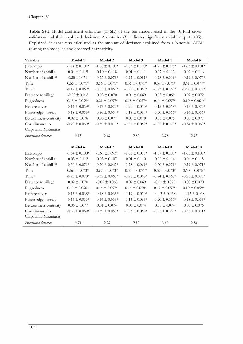
Chapter IV
102
Table S4.1 Model coefficient estimates (± SE) of the ten models used in the 10-fold cross-
validation and their explained deviance. An asterisk (*) indicates significant variables (p < 0.05).
Explained deviance was calculated as the amount of deviance explained from a binomial GLM
relating the modelled and observed bear activity.
Variable Model 1 Model 2 Model 3 Model 4 Model 5
(Intercept) -1.74 ± 0.101* -1.68 ± 0.100* -1.63 ± 0.100* -1.72 ± 0.098* -1.63 ± 0.101*
Number of anthills 0.04 ± 0.115 0.10 ± 0.118 0.01 ± 0.111 0.07 ± 0.113 0.02 ± 0.116
Number of anthills2 -0.28 ±0.071* -0.35 ± 0.078* -0.25 ± 0.081* -0.28 ± 0.069* -0.29 ± 0.073*
Time 0.55 ± 0.071* 0.56 ± 0.071* 0.56 ± 0.071* 0.58 ± 0.071* 0.61 ± 0.077*
Time2 -0.17 ± 0.069* -0.23 ± 0.067* -0.27 ± 0.069* -0.23 ± 0.069* -0.28 ± 0.072*
Distance to village -0.02 ± 0.068 0.03 ± 0.070 0.06 ± 0.069 0.03 ± 0.069 0.02 ± 0.072
Ruggedness 0.15 ± 0.059* 0.21 ± 0.057* 0.18 ± 0.057* 0.16 ± 0.057* 0.19 ± 0.061*
Pasture cover -0.14 ± 0.069* -0.17 ± 0.070* -0.20 ± 0.070* -0.15 ± 0.068* -0.15 ± 0.070*
Forest edge : forest
area
-0.18 ± 0.065* -0.20 ± 0.064* -0.15 ± 0.064* -0.20 ± 0.066* -0.16 ± 0.066*
Betweenness centrality 0.02 ± 0.076 0.08 ± 0.077 0.00 ± 0.078 0.03 ± 0.075 0.03 ± 0.077
Cost-distance to
Carpathian Mountains
-0.29 ± 0.069* -0.39 ± 0.070* -0.38 ± 0.069* -0.32 ± 0.070* -0.34 ± 0.069*
Explained deviance 0.35 0.12 0.19 0.24 0.27
Model 6 Model 7 Model 8 Model 9 Model 10
(Intercept) -1.64 ± 0.100* -1.61 ±0.093* -1.62 ± 0.097* -1.67 ± 0.100* -1.65 ± 0.100*
Number of anthills 0.03 ± 0.112 0.03 ± 0.107 0.01 ± 0.110 0.09 ± 0.114 0.06 ± 0.115
Number of anthills2 -0.30 ± 0.071* -0.30 ± 0.067* -0.28 ± 0.069* -0.30 ± 0.071* -0.29 ± 0.071*
Time 0.56 ± 0.073* 0.67 ± 0.073* 0.57 ± 0.071* 0.57 ± 0.073* 0.60 ± 0.075*
Time2 -0.23 ± 0.070* -0.32 ± 0.068* -0.26 ± 0.068* -0.24 ± 0.068* -0.25 ± 0.070*
Distance to village 0.02 ± 0.070 -0.02 ± 0.068 0.07 ± 0.069 -0.01 ± 0.070 0.03 ± 0.070
Ruggedness 0.17 ± 0.060* 0.14 ± 0.057* 0.14 ± 0.058* 0.17 ± 0.057* 0.19 ± 0.059*
Pasture cover -0.15 ± 0.068* -0.18 ± 0.065* -0.19 ± 0.070* -0.13 ± 0.068 -0.12 ± 0.068
Forest edge : forest
area
-0.16 ± 0.066* -0.16 ± 0.063* -0.13 ± 0.065* -0.20 ± 0.067* -0.18 ± 0.065*
Betweenness centrality 0.06 ± 0.077 0.01 ± 0.074 0.06 ± 0.074 0.05 ± 0.074 0.05 ± 0.076
Cost-distance to
Carpathian Mountains
-0.36 ± 0.069* -0.39 ± 0.065* -0.33 ± 0.068* -0.35 ± 0.068* -0.33 ± 0.071*
Explained deviance 0.28 0.02 0.39 0.19 0.36
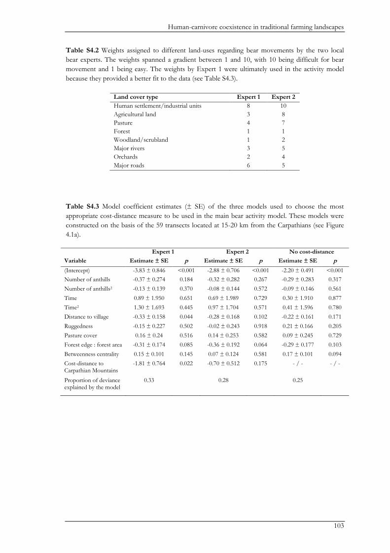
Human-carnivore coexistence in traditional farming landscapes
103
Table S4.2 Weights assigned to different land-uses regarding bear movements by the two local
bear experts. The weights spanned a gradient between 1 and 10, with 10 being difficult for bear
movement and 1 being easy. The weights by Expert 1 were ultimately used in the activity model
because they provided a better fit to the data (see Table S4.3).
Land cover type Expert 1 Expert 2
Human settlement/industrial units 8 10
Agricultural land 3 8
Pasture 4 7
Forest 1 1
Woodland/scrubland 1 2
Major rivers 3 5
Orchards 2 4
Major roads 6 5
Table S4.3 Model coefficient estimates (± SE) of the three models used to choose the most
appropriate cost-distance measure to be used in the main bear activity model. These models were
constructed on the basis of the 59 transects located at 15-20 km from the Carpathians (see Figure
4.1a).
Expert 1 Expert 2 No cost-distance
Variable Estimate ± SE p Estimate ± SE p Estimate ± SE p
(Intercept) -3.83 ± 0.846 <0.001 -2.88 ± 0.706 <0.001 -2.20 ± 0.491 <0.001
Number of anthills -0.37 ± 0.274 0.184 -0.32 ± 0.282 0.267 -0.29 ± 0.283 0.317
Number of anthills2 -0.13 ± 0.139 0.370 -0.08 ± 0.144 0.572 -0.09 ± 0.146 0.561
Time 0.89 ± 1.950 0.651 0.69 ± 1.989 0.729 0.30 ± 1.910 0.877
Time2 1.30 ± 1.693 0.445 0.97 ± 1.704 0.571 0.41 ± 1.596 0.780
Distance to village -0.33 ± 0.158 0.044 -0.28 ± 0.168 0.102 -0.22 ± 0.161 0.171
Ruggedness -0.15 ± 0.227 0.502 -0.02 ± 0.243 0.918 0.21 ± 0.166 0.205
Pasture cover 0.16 ± 0.24 0.516 0.14 ± 0.253 0.582 0.09 ± 0.245 0.729
Forest edge : forest area -0.31 ± 0.174 0.085 -0.36 ± 0.192 0.064 -0.29 ± 0.177 0.103
Betweenness centrality 0.15 ± 0.101 0.145 0.07 ± 0.124 0.581 0.17 ± 0.101 0.094
Cost-distance to Carpathian Mountains
-1.81 ± 0.764 0.022 -0.70 ± 0.512 0.175 - / - - / -
Proportion of deviance explained by the model
0.33 0.28 0.25
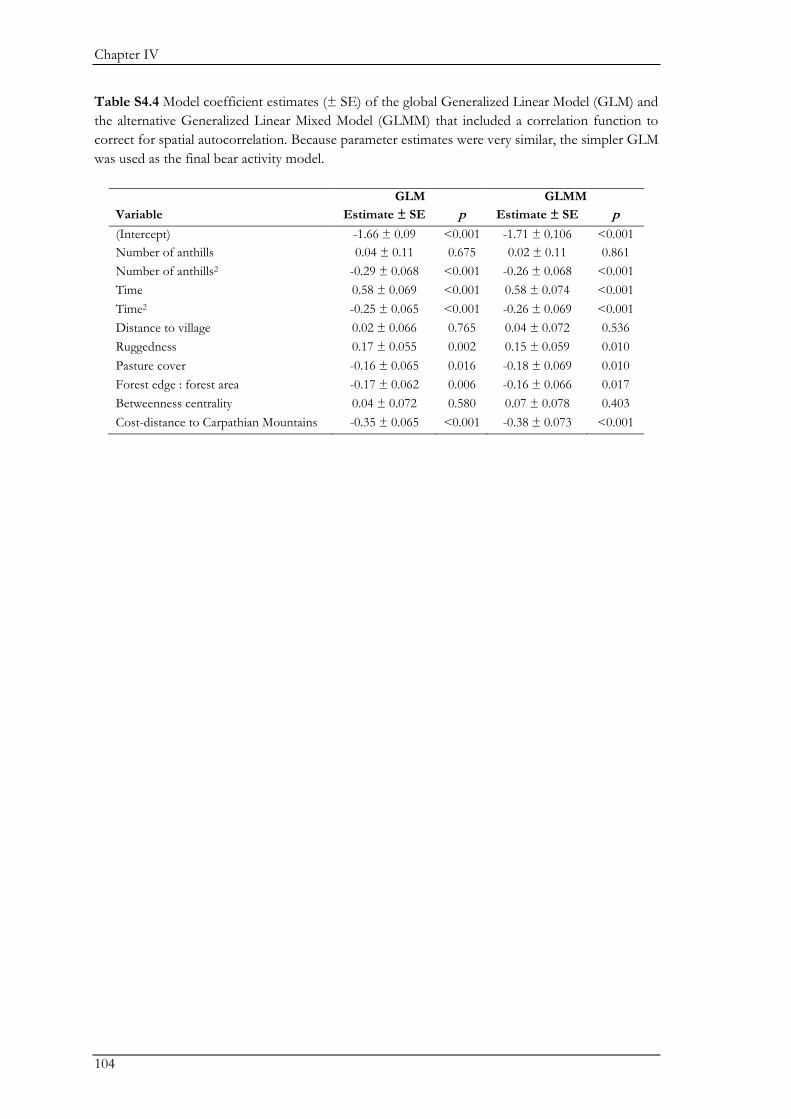
Chapter IV
104
Table S4.4 Model coefficient estimates (± SE) of the global Generalized Linear Model (GLM) and
the alternative Generalized Linear Mixed Model (GLMM) that included a correlation function to
correct for spatial autocorrelation. Because parameter estimates were very similar, the simpler GLM
was used as the final bear activity model.
GLM GLMM
Variable Estimate ± SE p Estimate ± SE p
(Intercept) -1.66 ± 0.09 <0.001 -1.71 ± 0.106 <0.001
Number of anthills 0.04 ± 0.11 0.675 0.02 ± 0.11 0.861
Number of anthills2 -0.29 ± 0.068 <0.001 -0.26 ± 0.068 <0.001
Time 0.58 ± 0.069 <0.001 0.58 ± 0.074 <0.001
Time2 -0.25 ± 0.065 <0.001 -0.26 ± 0.069 <0.001
Distance to village 0.02 ± 0.066 0.765 0.04 ± 0.072 0.536
Ruggedness 0.17 ± 0.055 0.002 0.15 ± 0.059 0.010
Pasture cover -0.16 ± 0.065 0.016 -0.18 ± 0.069 0.010
Forest edge : forest area -0.17 ± 0.062 0.006 -0.16 ± 0.066 0.017
Betweenness centrality 0.04 ± 0.072 0.580 0.07 ± 0.078 0.403
Cost-distance to Carpathian Mountains -0.35 ± 0.065 <0.001 -0.38 ± 0.073 <0.001

105
Chapter V

106
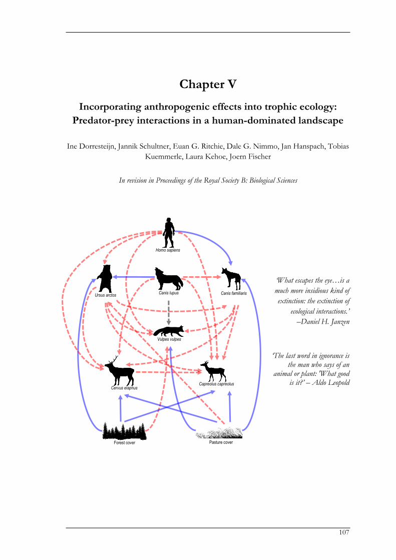
107
Chapter V
Incorporating anthropogenic effects into trophic ecology:
Predator-prey interactions in a human-dominated landscape
Ine Dorresteijn, Jannik Schultner, Euan G. Ritchie, Dale G. Nimmo, Jan Hanspach, Tobias
Kuemmerle, Laura Kehoe, Joern Fischer
In revision in Proceedings of the Royal Society B: Biological Sciences
‘What escapes the eye…is a
much more insidious kind of
extinction: the extinction of
ecological interactions.’
–Daniel H. Janzen
‘The last word in ignorance is the man who says of an
animal or plant: 'What good is it?’ – Aldo Leopold
Forest cover
Cervus elaphus
Pasture cover
Canis lupus Ursus arctos Canis familiaris
Capreolus capreolus
Homo sapiens
Vulpes vulpes

Chapter V
108
Human influence on trophic interactions
109
Abstract
Apex predators perform important functions that regulate ecosystems worldwide. However, little is
known about how ecosystem regulation by predators is influenced by human activities. In
particular, how important are top-down effects of predators relative to direct and indirect human-
mediated bottom-up and top-down processes? Combining data on species’ encounter rates from
camera traps and hunting records, we aimed to understand and quantify the relative effects of top-
down and bottom-up processes in shaping predator and prey distributions in a human-dominated
landscape in Transylvania, Romania. By global standards this system is diverse, including apex
predators (brown bear and wolf), mesopredators (red fox) and large herbivores (roe and red deer).
Furthermore, humans and free-ranging dogs represent additional predators in the system. Using
structural equation modelling we found that apex predators maintained their ecological role by
suppressing lower trophic levels, especially herbivores. However, direct and indirect human top-
down effects at multiple trophic levels affected the ecosystem more strongly, influencing species at
all trophic levels. Our study highlights the need to explicitly embed humans and their influences
within trophic cascade theory. This will greatly expand our understanding of species interactions
and ecosystem dynamics in human-modified landscapes, which compose the majority of Earth’s
terrestrial surface.
Chapter V
110
Introduction
There is increasing recognition of the critical role apex predators play in structuring ecosystems
globally (Estes et al. 2011; Ripple et al. 2014). They do so by killing or instilling fear in competitors
and prey (Creel & Christianson 2008; Ritchie & Johnson 2009), thereby inducing trophic cascades
that flow through entire ecosystems (Letnic et al. 2009). Despite 40% of the Earth’s terrestrial
surface being dominated by agriculture (Foley et al. 2005) and human’s effects permeating into
more natural areas (Sanderson et al. 2002), most research on trophic cascades has focused on
relatively intact wilderness and conservation reserves. However, top-down processes (i.e. the
structuring of the ecosystem by high trophic levels) and bottom-up processes (i.e. control through
productivity and low trophic levels) in largely pristine areas may differ substantially from those in
human-dominated landscapes. Thus, a key question remains: what role do humans play in the
trophic networks of modified ecosystems (Sergio et al. 2014)? Answering this question is important
for a number of reasons. Firstly, many large carnivore populations exist outside protected areas and
are embedded within human-dominated landscapes (Crooks et al. 2011; Carter et al. 2012b; Vanak
et al. 2013). Secondly, there is increased focus on using large carnivores in the context of ecosystem
restoration (Ritchie et al. 2012). And thirdly, in parts of the world such as Europe and North
America, large carnivores are returning through active rewilding efforts and conservation initiatives
(Enserink & Vogel 2006; Navarro & Pereira 2012; Morell 2013). Together this highlights the urgent
need to better understand relationships between apex predators, people, and ecosystem
components in human-dominated landscapes.
In terrestrial ecosystems, apex predators have been linked to two major trophic cascades.
First, apex predators limit herbivores through direct predation and behaviourally mediated changes
in habitat use, thereby promoting vegetation growth (i.e. tri-trophic cascades; Beschta & Ripple
2009; Ripple & Beschta 2012b; Kuijper et al. 2013). Second, apex predators limit smaller predators
through interference competition, including in its most extreme form, intraguild predation (Polis &
Holt 1992; Palomares & Caro 1999; Brook et al. 2012). Mesopredator suppression by apex
predators can thereby increase the abundance of small mammals and birds (i.e. mesopredator
cascades; Crooks & Soulé 1999; Ritchie & Johnson 2009). Such cascading effects could differ in
human-dominated landscapes in at least two main ways. For example, humans influence species
abundances through bottom up processes such as land-use, agriculture, and forestry, which may
translate into a wide range of changes in ecosystem properties and functions (Foley et al. 2005),
including ecosystem productivity (Haberl et al. 2007), or food and habitat availability (Muhly et al.
2013). Such changes in productivity can significantly modify predator-prey relationships (i.e., the
Ecosystem Exploitation Hypothesis; Oksanen & Oksanen 2000). Also, humans directly (e.g.
harvesting of both predators and prey; Barnosky et al. 2004) or indirectly (e.g. by creating an
anthropogenic landscape of fear; Ordiz et al. 2013) affect top-down processes and it remains
unclear if apex predators can achieve high enough densities outside wilderness areas and protected
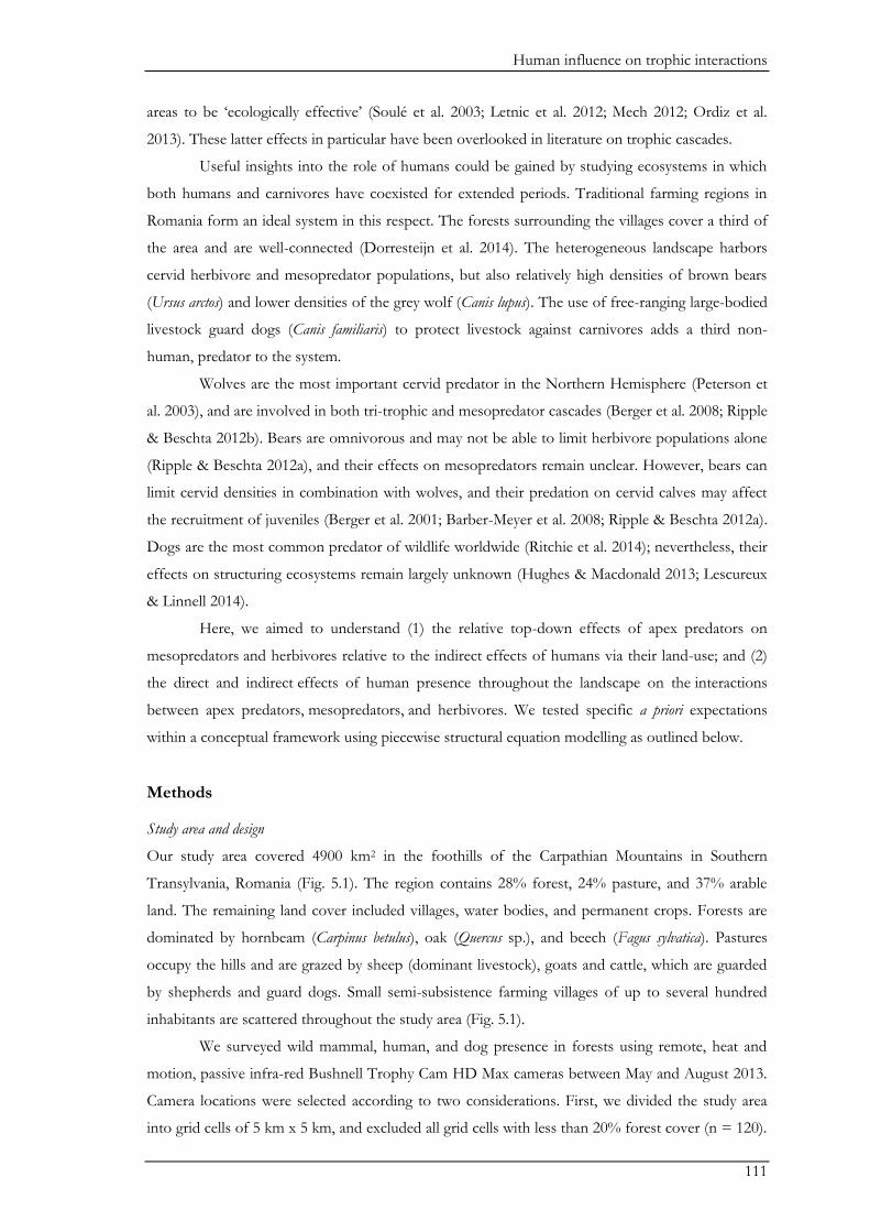
Human influence on trophic interactions
111
areas to be ‘ecologically effective’ (Soulé et al. 2003; Letnic et al. 2012; Mech 2012; Ordiz et al.
2013). These latter effects in particular have been overlooked in literature on trophic cascades.
Useful insights into the role of humans could be gained by studying ecosystems in which
both humans and carnivores have coexisted for extended periods. Traditional farming regions in
Romania form an ideal system in this respect. The forests surrounding the villages cover a third of
the area and are well-connected (Dorresteijn et al. 2014). The heterogeneous landscape harbors
cervid herbivore and mesopredator populations, but also relatively high densities of brown bears
(Ursus arctos) and lower densities of the grey wolf (Canis lupus). The use of free-ranging large-bodied
livestock guard dogs (Canis familiaris) to protect livestock against carnivores adds a third non-
human, predator to the system.
Wolves are the most important cervid predator in the Northern Hemisphere (Peterson et
al. 2003), and are involved in both tri-trophic and mesopredator cascades (Berger et al. 2008; Ripple
& Beschta 2012b). Bears are omnivorous and may not be able to limit herbivore populations alone
(Ripple & Beschta 2012a), and their effects on mesopredators remain unclear. However, bears can
limit cervid densities in combination with wolves, and their predation on cervid calves may affect
the recruitment of juveniles (Berger et al. 2001; Barber-Meyer et al. 2008; Ripple & Beschta 2012a).
Dogs are the most common predator of wildlife worldwide (Ritchie et al. 2014); nevertheless, their
effects on structuring ecosystems remain largely unknown (Hughes & Macdonald 2013; Lescureux
& Linnell 2014).
Here, we aimed to understand (1) the relative top-down effects of apex predators on
mesopredators and herbivores relative to the indirect effects of humans via their land-use; and (2)
the direct and indirect effects of human presence throughout the landscape on the interactions
between apex predators, mesopredators, and herbivores. We tested specific a priori expectations
within a conceptual framework using piecewise structural equation modelling as outlined below.
Methods
Study area and design
Our study area covered 4900 km2 in the foothills of the Carpathian Mountains in Southern
Transylvania, Romania (Fig. 5.1). The region contains 28% forest, 24% pasture, and 37% arable
land. The remaining land cover included villages, water bodies, and permanent crops. Forests are
dominated by hornbeam (Carpinus betulus), oak (Quercus sp.), and beech (Fagus sylvatica). Pastures
occupy the hills and are grazed by sheep (dominant livestock), goats and cattle, which are guarded
by shepherds and guard dogs. Small semi-subsistence farming villages of up to several hundred
inhabitants are scattered throughout the study area (Fig. 5.1).
We surveyed wild mammal, human, and dog presence in forests using remote, heat and
motion, passive infra-red Bushnell Trophy Cam HD Max cameras between May and August 2013.
Camera locations were selected according to two considerations. First, we divided the study area
into grid cells of 5 km x 5 km, and excluded all grid cells with less than 20% forest cover (n = 120).
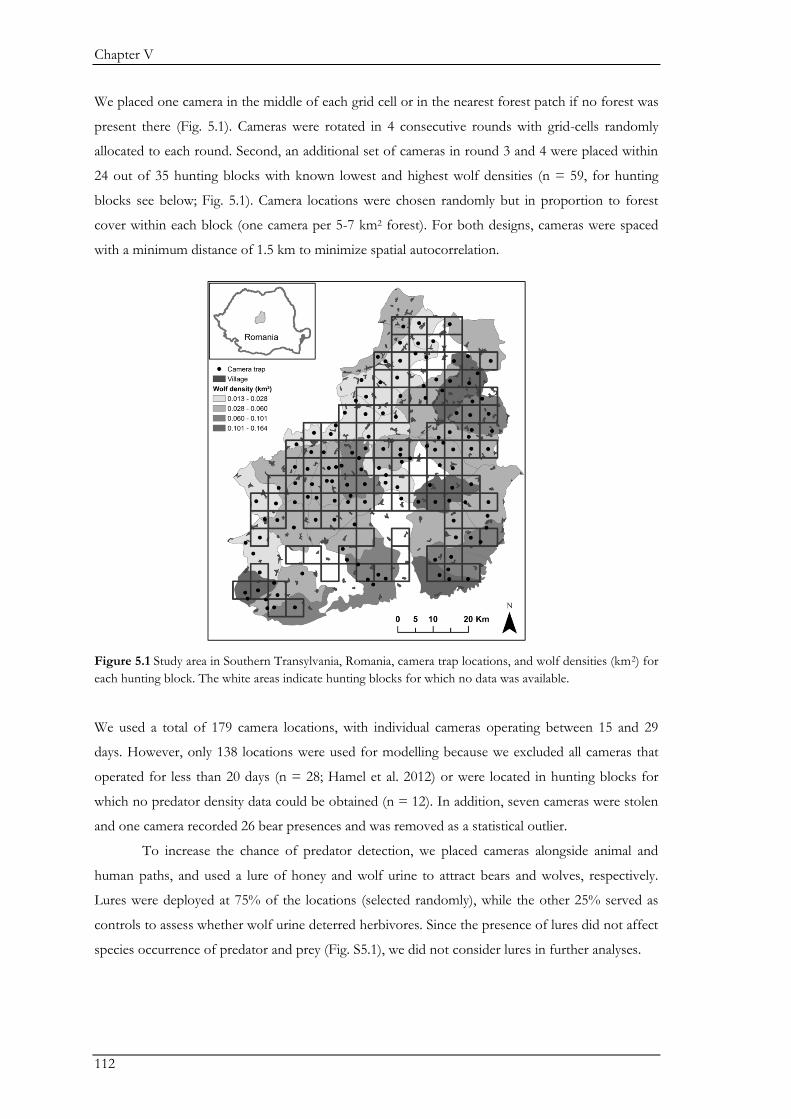
Chapter V
112
We placed one camera in the middle of each grid cell or in the nearest forest patch if no forest was
present there (Fig. 5.1). Cameras were rotated in 4 consecutive rounds with grid-cells randomly
allocated to each round. Second, an additional set of cameras in round 3 and 4 were placed within
24 out of 35 hunting blocks with known lowest and highest wolf densities (n = 59, for hunting
blocks see below; Fig. 5.1). Camera locations were chosen randomly but in proportion to forest
cover within each block (one camera per 5-7 km2 forest). For both designs, cameras were spaced
with a minimum distance of 1.5 km to minimize spatial autocorrelation.
Figure 5.1 Study area in Southern Transylvania, Romania, camera trap locations, and wolf densities (km2) for
each hunting block. The white areas indicate hunting blocks for which no data was available.
We used a total of 179 camera locations, with individual cameras operating between 15 and 29
days. However, only 138 locations were used for modelling because we excluded all cameras that
operated for less than 20 days (n = 28; Hamel et al. 2012) or were located in hunting blocks for
which no predator density data could be obtained (n = 12). In addition, seven cameras were stolen
and one camera recorded 26 bear presences and was removed as a statistical outlier.
To increase the chance of predator detection, we placed cameras alongside animal and
human paths, and used a lure of honey and wolf urine to attract bears and wolves, respectively.
Lures were deployed at 75% of the locations (selected randomly), while the other 25% served as
controls to assess whether wolf urine deterred herbivores. Since the presence of lures did not affect
species occurrence of predator and prey (Fig. S5.1), we did not consider lures in further analyses.
Human influence on trophic interactions
113
Variables used for modelling
We modelled the occurrence of five species in relation to top-down and bottom-up variables: bears
and dogs (apex predators), foxes (mesopredator; Vulpes vulpes), and red and roe deer (herbivores;
Cervus elaphus and Capreolus capreolus, respectively). Species occurrence was derived from data
collected by the cameras, and calculated as a cumulative abundance index or encounter rate by
summing all individuals for each species at each camera location, and corrected for camera days
during modelling (see below). Due to insufficient wolf records (two presences), wolves were not
included as a response variable.
Explanatory variables included (i) top-down variables which were represented by apex
predators (wolves, bears, dogs) and humans; and (ii) bottom-up variables which were represented
by land-use variables (forest and pasture cover). Bear and dog variables were calculated from the
camera data as the number of presences per camera day. Because of insufficient wolf records and
surprisingly little spatial variation in bear presences across camera locations, we obtained additional
information on large-scale wolf and bear densities within the 35 hunting blocks from 2010
(http://www.mmediu.ro/paduri/vanatoare.htm-accessed 01.02.2014). Although absolute densities
are most likely overestimated (Salvatori et al. 2002), this data provided a useful general indicator for
regional-scale differences in predator pressure. Notably, reported predator densities had been
largely stable between 2006 and 2010 (Supplementary Material Fig. S5.2, S5.3), suggesting that the
2010 data was likely to be indicative of bear and wolf densities, despite not being from the same
year as our camera data. The local density of humans near camera traps was calculated as the
number of presences per camera day. As an additional approximation of human pressure, we also
calculated the total number of people within the three nearest villages to each camera location. For
bears, we used either reported hunting block bear density or bear encounter rate from the camera as
an explanatory variable, and for humans, nearby village population size or human encounter rate
from the camera. The choice between these two variables was based on which provided the better
fit for a given response variable, based on Akaike information criterion, AIC (i.e. lower AIC
values). Pasture cover (range 0 - 50%; median: 13%) and forest cover (range 15 - 100%; median:
59.5%) were derived from the Corine Land Cover map (2006) within a radius of 1000 m around
camera locations. Forest cover also indicated fragmentation because it was highly correlated with
the forest edge to area ratio (ρ = -0.83).
Modelling
We used piecewise structural equation modelling (SEM) to model the importance of top-down and
bottom-up effects for the five target species. SEMs are used to analyse both direct and indirect
relationships in ecosystem processes, where a priori knowledge of relationships between
components is available (Grace 2006). In contrast to classical SEM, a piecewise approach does not
calculate global estimates for the entire network of relationships, but calculates local estimates for
Chapter V
114
each ‘node’ or response variable (Grace et al. 2012). This approach has been applied in recent
studies of trophic cascades (Pasanen-Mortensen et al. 2013; Colman et al. 2014).
First, generalized linear mixed-effect models with a Poisson error distribution were built
for each species. Depending on the species, fixed effects included human variables, natural
predators and competitors, and bottom-up variables (see Model description). All fixed variables were
scaled, and log-transformed where transformation led to a better explanation of the response
variable (based on Akaike information criterion, AIC). Random effects included hunting block,
study round, and – in cases of overdispersion (i.e. φ >1.5) – individual site identity (Elston et al.
2001). We included camera days as an offset in all models to account for differences in exposure
time for response variables.
Next, we performed model averaging across the set of models with all possible
combinations of fixed variables. We calculated averaged parameter estimates, averaged standard
errors, and the relative importance of explanatory variables (i.e. the sum of AIC weights over all
models including the explanatory variable) on the subset of models within dAIC<4 of the best
model. We also calculated marginal R2 for the full model to assess the explained variance of the
fixed factors (Nakagawa & Schielzeth 2013). Finally, composite graphs of all local estimates were
generated to visualize the relative importance of relationships between ecosystem components. All
statistical analyses were performed in R using the packages lme4 and MuMIn (R Core Team 2013).
Model description
The pathways between top-down and bottom-up variables were determined by a priori knowledge
on trophic cascade theory and included the following assumptions (Fig. 5.2). Apex predators
(brown bear, wolf, dog) were assumed to potentially limit the main mesopredator, the red fox,
through interference competition or intraguild predation (Elmhagen & Rushton 2007; Ritchie &
Johnson 2009), as well as to limit red deer and roe deer through direct predation (Peterson et al.
2003; Ripple & Beschta 2012a). Bottom-up factors were assumed to be strong for the brown bear
with an expected positive effect of forest cover and a negative effect of pasture cover (Dorresteijn
et al. 2014). We did not assume a relationship between dogs and forest cover, but expected a strong
positive link with pasture cover because dogs are commonly used for shepherding in our study
area. We assumed bottom-up factors would play a role in mesopredator and herbivore encounter
rate, but that top-down would be stronger than bottom-up effects as expected for productive
ecosystems (Ecosystem Exploitation Hyoptthesis; Oksanen & Oksanen 2000). We expected the
fox encounter rate to be negatively affected by forest cover and positively affected by pasture
cover since this species prefers fragmented and open farmland (Kurki et al. 1998; Panek &
Bresiński 2002). Herbivores were expected to be positively affected by both forest and pasture
cover (Godvik et al. 2009; Morellet et al. 2011). We assumed that there would be no intraguild
competition between wolves and bears due to different diets, but that wolves would positively
affect bear encounter rate through increasing carrion (Wilmers et al. 2003). In contrast, we assumed
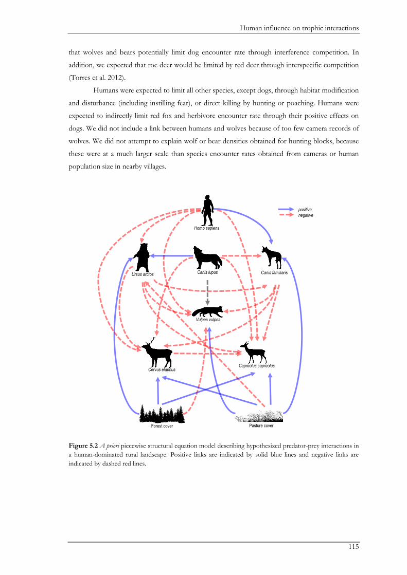
Human influence on trophic interactions
115
that wolves and bears potentially limit dog encounter rate through interference competition. In
addition, we expected that roe deer would be limited by red deer through interspecific competition
(Torres et al. 2012).
Humans were expected to limit all other species, except dogs, through habitat modification
and disturbance (including instilling fear), or direct killing by hunting or poaching. Humans were
expected to indirectly limit red fox and herbivore encounter rate through their positive effects on
dogs. We did not include a link between humans and wolves because of too few camera records of
wolves. We did not attempt to explain wolf or bear densities obtained for hunting blocks, because
these were at a much larger scale than species encounter rates obtained from cameras or human
population size in nearby villages.
Figure 5.2 A priori piecewise structural equation model describing hypothesized predator-prey interactions in
a human-dominated rural landscape. Positive links are indicated by solid blue lines and negative links are
indicated by dashed red lines.
Forest cover
Cervus elaphus
Pasture cover
Canis lupus Ursus arctos Canis familiaris
Capreolus capreolus
Homo sapiens
Vulpes vulpes
positive
negative

Chapter V
116
Results
Across 3042 camera days at 138 locations we obtained 2197 detections of roe deer, 388 of red
foxes, 275 of humans, 120 of dogs, 94 of red deer, 76 of bears, and 2 of wolves.
Top-down and bottom-up effects on species encounter rates
In accordance with our a priori SEM, wolves and bears had a negative effect on foxes (Fig.
5.3a). Bottom-up effects were similar in strength as top-down effects on fox encounter rates
with the strongest negative effect found for forest cover (Fig. 5.3a). Nevertheless, both top-
down and bottom-up effects were fairly weak with standard errors indicating a high degree of
uncertainty, and explained less variance as compared to all other species (Fig. 5.3a). Positive
bottom-up effects of forest cover and negative effects of pasture cover were strong
determinants of bear encounter rates (Fig. 5.3a). Within the apex predator guild, bears were
negatively related to wolves (Fig. 5.3a).
Figure 5.3 Final structural equation models showing top-down and bottom-up pathways for encounter rates
of (A) predators, and (B) herbivores. Co-efficient estimates and standard errors are presented for each
interaction and marginal R2 are given for all response variables (i.e. brown bear, domestic dog, red fox, red
deer, and roe deer). The line thickness of the arrows refers to the Akaike weights and can therefore only be
compared within a species and not between species. Positive links are indicated by solid lines and negative
links are indicated by dashed lines. The * indicates log-transformed variables
Forest cover
Cervus elaphus
Pasture cover
Canis lupus Ursus arctos Canis familiaris
Capreolus capreolus
Homo sapiens
Vulpes vulpes
Forest cover
Cervus elaphus
Pasture cover
Canis lupus Ursus arctos Canis familiaris
Capreolus capreolus
Homo sapiens
Vulpes vulpes
Predators Herbivores
(A)
-0.31±0.13* -0.28±0.19* -0.16±
0.10*
-0.12±0.06*
0.01
±0.
14* 0.05±
0.06*
[R 2 = 0.13] [R
2 = 0.31]
[R2 = 0.09]
[R2 = 0.24] [R
2 = 0.76]
(B)
positive negative
Human influence on trophic interactions
117
For herbivores, we also found a negative effect of wolves on red deer and of bears on roe
deer. In contrast, a positive effect was found for wolves on roe deer and bears on red deer (Fig.
5.3b). Bottom-up effects were positive (except for forest cover on roe deer) and very weak with a
larger degree of uncertainty compared to top-down effects for both red deer and roe deer (Fig.
5.3b). For example, the negative coefficient indicating the effect of wolves on red deer was 2.6
times larger than the positive coefficients of pasture cover. Roe deer appeared further limited
through competition with red deer with its coefficient similar to the coefficients of top-down
predator effects (Fig. 5.3b).
Top-down control by humans and their dogs
As predicted, humans limited all other species (Fig. 5.3a, b). While the effect was negligible for
foxes, human top-down control on bears, dogs, and herbivores was relatively strong (Fig. 5.3a, b).
For example, the coefficient describing the effect of humans on bears was 5.6 to 8.3 times larger
than the coefficients of the bottom-up effects. Human effects on red deer and roe deer were also
larger than top-down predator effects (red deer coefficients were 1.7 - 2.5 times larger; roe deer
coefficients were 1.1 - 1.6 times larger) and much larger than the very weak bottom-up effects.
Additionally, humans had significant indirect effects on species’ encounter rates due to a
strong positive effect on dogs and their subsequent flow-on effects (Fig. 5.3a). The top-down
limiting effect of dogs on red deer and roe deer was only slightly weaker than that of natural
predators but stronger than bottom-up processes (Fig. 5.3b). In contrast, dogs were positively
correlated with fox encounter rates; however, the SEM showed a negative effect of wolves on both
dogs and foxes (Fig. 5.3a). All model selection tables are available in Supplementary Material Tables
S5.1- S5.5
Discussion
Despite growing interest in using apex predators for ecological restoration (Ritchie et al. 2012), and
although agriculture covers 40% of the world’s ice-free land surface (Foley et al. 2005), few studies
have examined and quantified the ecological role of apex predators in human-dominated
landscapes. Our study addressed (1) the relative contributions of top-down limitation by apex
predators and (2) direct and indirect human bottom-up and top-down processes on mesopredator
and herbivore encounter rates in a multiple-predator, human-dominated landscape. In accordance
with trophic cascade theory, apex predators appeared to be important in structuring the ecosystem,
particularly through the suppression of herbivores. However, the extent of human direct and
indirect top-down effects at multiple trophic levels notably had a stronger effect on the ecosystem
than apex predators. Our results suggest that human factors need far greater consideration in
trophic ecology research and associated theory, because excluding humans could lead to incomplete
understanding of ecosystem structure and function.
Chapter V
118
Mesopredator limitation by apex predators and human-mediated bottom-up effects
The mesopredator release hypothesis predicts top-down control of mesopredators by apex
predators, with bottom-up factors mediating mesopredator abundance, but not regulating it
(Crooks & Soulé 1999; Elmhagen et al. 2010). We found limited evidence of suppression of foxes
by wolves and bears in our study, therefore questioning the mesopredator release hypothesis in this
human-dominated landscape. The suppressive effects of apex predators, although present, were
generally weak, and similar in strength to bottom-up control. There are large differences in body-
size and diet between foxes, omnivorous bears, and large ungulate-predating wolves, and body size
differences may be too pronounced to provide ecological benefits to bears and wolves by killing
foxes (Donadio & Buskirk 2006; Ritchie & Johnson 2009). Similarly, foxes were not suppressed by
wolves in Europe (Pasanen-Mortensen et al. 2013), but were limited by the smaller-sized dingo,
Canis lupus dingo, in Australia (Johnson & VanDerWal 2009), and lynx, Lynx lynx, in Europe
(Elmhagen et al. 2010; Pasanen-Mortensen et al. 2013). An alternative explanation is that, at
currently low apex predator densities, mesopredators may not be significantly suppressed. Indirect
effects of interference competition, such as restricting habitat use and prey availability by instilling
fear, could also have contributed to the limiting effects of apex predators but were unaccounted for
in this study (Creel & Christianson 2008; Shirley et al. 2009; Brook et al. 2012).
Human-mediated bottom-up effects were apparent through a preference of foxes for less
forested areas that are more fragmented (see also Kurki et al. 1998). Nevertheless, this effect was
also weak, probably because generalist foxes can thrive in both forested and open landscapes
(Panek & Bresiński 2002; Payne et al. 2014), and their densities increase along a natural-urban
environmental gradient (Šálek et al. 2014). Thus, our gradients in land-use may not have been
strong enough to capture fox habitat preferences, or fox distribution may be more affected by
other human-mediated bottom-up effects such as the presence of anthropogenic food sources
(Panek & Bresiński 2002). Furthermore, increased spatial heterogeneity in more complex habitats
could have mediated interference competition and dampened top-down suppression of foxes
through reduced encounter rates (McGee et al. 2006; Ritchie & Johnson 2009). More importantly,
bottom-up effects influenced foxes and bears, and most likely wolves (Jedrzejewski et al. 2004), in
opposite ways and thus, human-mediated bottom-up processes could further reduce interference
competition between foxes and apex predators through increasing forest loss and fragmentation in
Romania (Knorn et al. 2012; Griffiths et al. 2013).
Herbivore limitation by apex predators and human-mediated bottom-up effects
Despite human presence, apex predators still exerted substantial top-down limitation on
herbivores. This is consistent with the Ecosystem Exploitation Hypothesis for systems with tri-
trophic-cascades, where herbivores should be top-down limited and apex predators bottom-up
limited (Oksanen & Oksanen 2000). Top-down control of wolves and bears on red deer and roe
deer showed varying patterns. The observed negative effect on red deer and not on the roe deer
Human influence on trophic interactions
119
encounter rate by wolves can be explained by wolves’ preference for red deer over roe deer when
both species are present (Jȩdrzejewski et al. 2000). Wolf extirpation caused eruptions of deer
populations in European and American national parks (Jedrzejewski et al. 2002; Ripple & Beschta
2012b), and our results suggest that similar wolf reductions and extirpations could have led to
increased red deer populations elsewhere in Europe (Lovari et al. 2007). By contrast, roe deer
populations were only suppressed by apex predators in unproductive landscapes, and were more
affected by foraging needs and competition for food in Europe (Melis et al. 2009; Samelius et al.
2013).
In contrast, bears had a negative effect on roe deer and not on red deer. Bears are known
to predate young cervids (Berger et al. 2001; Swenson et al. 2007), and may either have predated
preferentially on fawns of roe deer over those of red deer, or the positive relationship between
bears and red deer is a likely indirect effect of the strong negative impact of humans on both
species. However, since the diet of bears in our region does not include a lot of meat (Bojarska &
Selva 2012), deer could alternatively have been suppressed by apex predators through a landscape
of fear where deer alter their behaviour in response to predation risk (Laundré et al. 2001; Creel &
Christianson 2008).
Although our results confirm theoretical predictions of weak bottom-up effects on deer
species, they contrast with a recent study where human-mediation of forage quality influenced
herbivores more strongly than top-down predator effects (Muhly et al. 2013). A lack of bottom-up
effects may be due to the present land cover composition, which features forest and pasture cover
close to the 30% threshold below which fragmentation effects become severe (Andrén 1994).
Alternatively, the resolution of the Corine Land Cover (25 ha minimum mapping unit) may have
been too coarse to pick up deer habitat preferences. Although human-mediated processes through
land-use may not determine deer encounter rates in our study area; other human-mediated bottom-
up processes such as supplemental feeding of deer may affect their populations (Schmidt & Hoi
2002). Moreover, similar to mesopredators, an increase in deforestation in the area would reduce
apex predator presence and ultimately reduce top-down control of deer.
Humans as apex predators in the system
Direct and indirect human top-down impacts were more important in shaping patterns of species
encounter rates compared to the effects of apex predators and human-mediated bottom-up effects.
Thus, our study shows that humans themselves are an apex predator in the system, indicating that
they should not be ignored in predator-prey studies (Sergio et al. 2014), particularly given the
pervasive impacts of humans across the globe (Steffen et al. 2007; Goudie 2013). Humans are
perhaps unique amongst apex predators in their ability to influence ecosystems through
simultaneously directly reducing large carnivore, mesopredator and herbivore populations and,
impacting their behaviour by creating a landscape of fear for all three trophic levels (Ordiz et al.
2013).
Chapter V
120
Direct human effects on foxes were negligible in our study. This is consistent with Baker &
Harris (2006) who showed that fox culling through hunting does not necessarily reduce fox
numbers. In contrast, direct human negative effects on deer were relatively large. Hunting of deer
could have directly reduced deer populations (see e.g. Jȩdrzejewski et al. 2000), however, the
observed pattern could also be a response to an anthropogenic landscape of fear where deer avoid
areas where hunting and other human activities are prevalent (Theuerkauf & Rouys 2008). In
addition, humans also suppressed deer through the use of livestock guard dogs, which are kept on
the pasture and thus in proximity to preferred deer foraging areas. Although the effects of dogs on
wildlife are relatively unknown, they can reduce herbivore populations through the same
mechanisms of direct predation and behaviourally induced changes as other apex predators (Ritchie
et al. 2014).
Indirectly, humans suppression of bears and possibly wolves (Jedrzejewski et al. 2004;
Llaneza et al. 2012) could lift top-down control and lead to increased herbivore populations and
possibly further mesopredator release. Herbivore and mesopredator population increases after
anthropogenic extirpations of apex predators are widely documented (Terborgh & Estes 2010). For
example, in Europe, the loss of lynx due to a combination of anthropogenic pressures
(Breitenmoser et al. 2000), caused large scale mesopredator release in Europe (Elmhagen et al.
2010), perhaps even in our study area. However, here we found that in a system where both
humans and other apex predators are present, top-down control by humans and predators and
indirect release due to human suppression of apex predators act simultaneously, particularly on
herbivore populations. Further studies that disentangle the effects of humans and predators on
lower trophic levels will be key to advancing our understanding of the drivers and dynamics of
ecosystems, trophic cascade theory, and ultimately how these affect biodiversity conservation. This
is especially important since humans may not replicate the exact nature of indirect effects caused by
other apex predators, highlighting that the ecological roles of apex predators are not always
interchangeable (Ordiz et al. 2013). This may explain in part why humans are often unsuccessful at
preventing or reversing negative impacts such as overgrazing, reduced vegetation recruitment, and
biodiversity loss caused by altered predator-herbivore-plant trophic cascades or mesopredator
release (e.g. Terborgh et al. 2001; Estes et al. 2011; Kuijper 2011; Ripple et al. 2013).
Conclusions
To date, ecological theory on trophic cascades has not explicitly included human effects, despite
humanity’s pervasive impacts on the globe (Sanderson et al. 2002). Our study adds to a growing
recognition that humans play vital roles in influencing ecosystems through mediating and altering
trophic cascades as well as through direct landscape modification. Apex predators maintained their
ecological role by suppressing lower trophic levels in a human-dominated landscape, but both
direct and indirect anthropogenic top-down effects dominated over natural processes. Improving
our understanding of human impacts on trophic cascades in human-dominated landscapes is
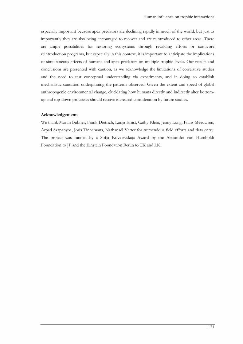
Human influence on trophic interactions
121
especially important because apex predators are declining rapidly in much of the world, but just as
importantly they are also being encouraged to recover and are reintroduced to other areas. There
are ample possibilities for restoring ecosystems through rewilding efforts or carnivore
reintroduction programs, but especially in this context, it is important to anticipate the implications
of simultaneous effects of humans and apex predators on multiple trophic levels. Our results and
conclusions are presented with caution, as we acknowledge the limitations of correlative studies
and the need to test conceptual understanding via experiments, and in doing so establish
mechanistic causation underpinning the patterns observed. Given the extent and speed of global
anthropogenic environmental change, elucidating how humans directly and indirectly alter bottom-
up and top-down processes should receive increased consideration by future studies.
Acknowledgements
We thank Martin Bubner, Frank Dietrich, Lunja Ernst, Cathy Klein, Jenny Long, Frans Meeuwsen,
Arpad Szapanyos, Joris Tinnemans, Nathanaël Vetter for tremendous field efforts and data entry.
The project was funded by a Sofja Kovalevskaja Award by the Alexander von Humboldt
Foundation to JF and the Einstein Foundation Berlin to TK and LK.
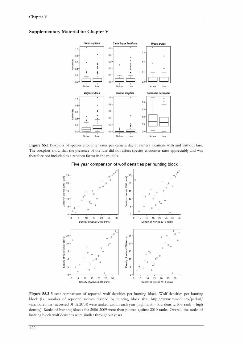
Chapter V
122
Supplementary Material for Chapter V
Figure S5.1 Boxplots of species encounter rates per camera day at camera locations with and without lure.
The boxplots show that the presence of the lure did not affect species encounter rates appreciably and was
therefore not included as a random factor in the models.
Figure S5.2 5 year comparison of reported wolf densities per hunting block. Wolf densities per hunting
block (i.e. number of reported wolves divided by hunting block size; http://www.mmediu.ro/paduri/
vanatoare.htm - accessed 01.02.2014) were ranked within each year (high rank = low density, low rank = high
density). Ranks of hunting blocks for 2006-2009 were then plotted against 2010 ranks. Overall, the ranks of
hunting block wolf densities were similar throughout years.
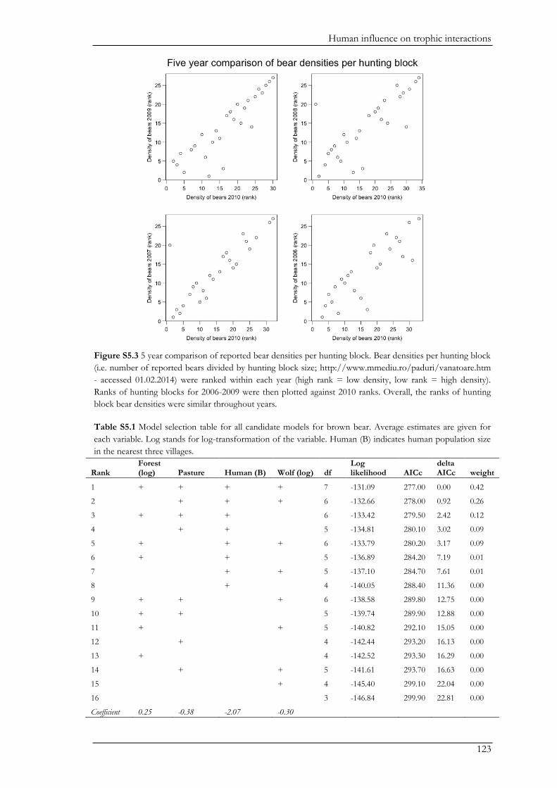
Human influence on trophic interactions
123
Figure S5.3 5 year comparison of reported bear densities per hunting block. Bear densities per hunting block
(i.e. number of reported bears divided by hunting block size; http://www.mmediu.ro/paduri/vanatoare.htm
- accessed 01.02.2014) were ranked within each year (high rank = low density, low rank = high density).
Ranks of hunting blocks for 2006-2009 were then plotted against 2010 ranks. Overall, the ranks of hunting
block bear densities were similar throughout years.
Table S5.1 Model selection table for all candidate models for brown bear. Average estimates are given for
each variable. Log stands for log-transformation of the variable. Human (B) indicates human population size
in the nearest three villages.
Rank Forest (log) Pasture Human (B) Wolf (log) df
Log likelihood AICc
delta AICc weight
1 + + + + 7 -131.09 277.00 0.00 0.42
2
+ + + 6 -132.66 278.00 0.92 0.26
3 + + +
6 -133.42 279.50 2.42 0.12
4
+ +
5 -134.81 280.10 3.02 0.09
5 +
+ + 6 -133.79 280.20 3.17 0.09
6 +
+
5 -136.89 284.20 7.19 0.01
7
+ + 5 -137.10 284.70 7.61 0.01
8
+
4 -140.05 288.40 11.36 0.00
9 + +
+ 6 -138.58 289.80 12.75 0.00
10 + +
5 -139.74 289.90 12.88 0.00
11 +
+ 5 -140.82 292.10 15.05 0.00
12
+
4 -142.44 293.20 16.13 0.00
13 +
4 -142.52 293.30 16.29 0.00
14
+
+ 5 -141.61 293.70 16.63 0.00
15
+ 4 -145.40 299.10 22.04 0.00
16
3 -146.84 299.90 22.81 0.00
Coefficient 0.25 -0.38 -2.07 -0.30
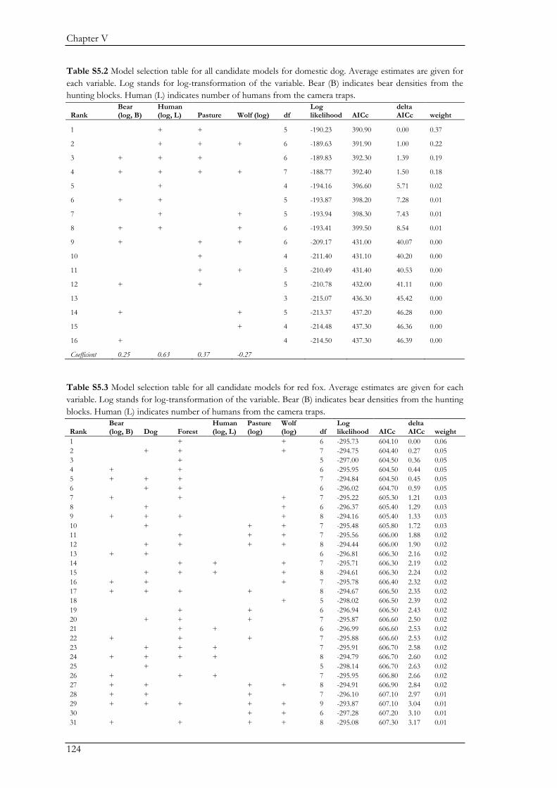
Chapter V
124
Table S5.2 Model selection table for all candidate models for domestic dog. Average estimates are given for
each variable. Log stands for log-transformation of the variable. Bear (B) indicates bear densities from the
hunting blocks. Human (L) indicates number of humans from the camera traps.
Rank Bear (log, B)
Human (log, L) Pasture Wolf (log) df
Log likelihood AICc
delta AICc weight
1
+ +
5 -190.23 390.90 0.00 0.37
2
+ + + 6 -189.63 391.90 1.00 0.22
3 + + +
6 -189.83 392.30 1.39 0.19
4 + + + + 7 -188.77 392.40 1.50 0.18
5
+
4 -194.16 396.60 5.71 0.02
6 + +
5 -193.87 398.20 7.28 0.01
7
+
+ 5 -193.94 398.30 7.43 0.01
8 + +
+ 6 -193.41 399.50 8.54 0.01
9 +
+ + 6 -209.17 431.00 40.07 0.00
10
+
4 -211.40 431.10 40.20 0.00
11
+ + 5 -210.49 431.40 40.53 0.00
12 +
+
5 -210.78 432.00 41.11 0.00
13
3 -215.07 436.30 45.42 0.00
14 +
+ 5 -213.37 437.20 46.28 0.00
15
+ 4 -214.48 437.30 46.36 0.00
16 +
4 -214.50 437.30 46.39 0.00
Coefficient 0.25 0.63 0.37 -0.27
Table S5.3 Model selection table for all candidate models for red fox. Average estimates are given for each
variable. Log stands for log-transformation of the variable. Bear (B) indicates bear densities from the hunting
blocks. Human (L) indicates number of humans from the camera traps.
Rank Bear (log, B) Dog Forest
Human (log, L)
Pasture (log)
Wolf (log) df
Log likelihood AICc
delta AICc weight
1
+
+ 6 -295.73 604.10 0.00 0.06
2
+ +
+ 7 -294.75 604.40 0.27 0.05
3
+
5 -297.00 604.50 0.36 0.05
4 +
+
6 -295.95 604.50 0.44 0.05
5 + + +
7 -294.84 604.50 0.45 0.05
6
+ +
6 -296.02 604.70 0.59 0.05
7 +
+
+ 7 -295.22 605.30 1.21 0.03
8
+
+ 6 -296.37 605.40 1.29 0.03
9 + + +
+ 8 -294.16 605.40 1.33 0.03
10
+
+ + 7 -295.48 605.80 1.72 0.03
11
+
+ + 7 -295.56 606.00 1.88 0.02
12
+ +
+ + 8 -294.44 606.00 1.90 0.02
13 + +
6 -296.81 606.30 2.16 0.02
14
+ +
+ 7 -295.71 606.30 2.19 0.02
15
+ + +
+ 8 -294.61 606.30 2.24 0.02
16 + +
+ 7 -295.78 606.40 2.32 0.02
17 + + +
+
8 -294.67 606.50 2.35 0.02
18
+ 5 -298.02 606.50 2.39 0.02
19
+
+
6 -296.94 606.50 2.43 0.02
20
+ +
+
7 -295.87 606.60 2.50 0.02
21
+ +
6 -296.99 606.60 2.53 0.02
22 +
+
+
7 -295.88 606.60 2.53 0.02
23
+ + +
7 -295.91 606.70 2.58 0.02
24 + + + +
8 -294.79 606.70 2.60 0.02
25
+
5 -298.14 606.70 2.63 0.02
26 +
+ +
7 -295.95 606.80 2.66 0.02
27 + +
+ + 8 -294.91 606.90 2.84 0.02
28 + +
+
7 -296.10 607.10 2.97 0.01
29 + + +
+ + 9 -293.87 607.10 3.04 0.01
30
+ + 6 -297.28 607.20 3.10 0.01
31 +
+
+ + 8 -295.08 607.30 3.17 0.01
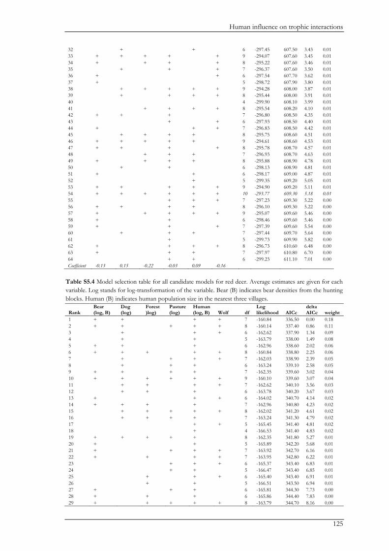
Human influence on trophic interactions
125
32
+
+
6 -297.45 607.50 3.43 0.01
33 + + + +
+ 9 -294.07 607.60 3.45 0.01
34 +
+ +
+ 8 -295.22 607.60 3.46 0.01
35
+
+
+ 7 -296.37 607.60 3.50 0.01
36 +
+ 6 -297.54 607.70 3.62 0.01
37 +
5 -298.72 607.90 3.80 0.01
38
+ + + + + 9 -294.28 608.00 3.87 0.01
39
+
+ + + 8 -295.44 608.00 3.91 0.01
40
4 -299.90 608.10 3.99 0.01
41
+ + + + 8 -295.54 608.20 4.10 0.01
42 + +
+
7 -296.80 608.50 4.35 0.01
43
+
+ 6 -297.93 608.50 4.40 0.01
44 +
+ + 7 -296.83 608.50 4.42 0.01
45
+ + + +
8 -295.75 608.60 4.51 0.01
46 + + + + +
9 -294.61 608.60 4.53 0.01
47 + +
+
+ 8 -295.78 608.70 4.57 0.01
48
+ + +
7 -296.93 608.70 4.63 0.01
49 +
+ + +
8 -295.88 608.90 4.78 0.01
50
+
+
6 -298.13 608.90 4.81 0.01
51 +
+
6 -298.17 609.00 4.87 0.01
52
+
5 -299.35 609.20 5.05 0.01
53 + +
+ + + 9 -294.90 609.20 5.11 0.01
54 + + + + + + 10 -293.77 609.30 5.18 0.01
55
+ + + 7 -297.23 609.30 5.22 0.00
56 + +
+ +
8 -296.10 609.30 5.22 0.00
57 +
+ + + + 9 -295.07 609.60 5.46 0.00
58 +
+
6 -298.46 609.60 5.46 0.00
59 +
+
+ 7 -297.39 609.60 5.54 0.00
60
+
+ +
7 -297.44 609.70 5.64 0.00
61
+
5 -299.73 609.90 5.82 0.00
62 +
+ + + 8 -296.73 610.60 6.48 0.00
63 +
+ +
7 -297.97 610.80 6.70 0.00
64
+ +
6 -299.23 611.10 7.01 0.00
Coefficient -0.13 0.15 -0.22 -0.03 0.09 -0.16
Table S5.4 Model selection table for all candidate models for red deer. Average estimates are given for each
variable. Log stands for log-transformation of the variable. Bear (B) indicates bear densities from the hunting
blocks. Human (B) indicates human population size in the nearest three villages.
Rank Bear (log, B)
Dog (log)
Forest )log)
Pasture (log)
Human (log, B) Wolf df
Log likelihood AICc
delta AICc weight
1 + +
+ + 7 -160.84 336.50 0.00 0.18
2 + +
+ + + 8 -160.14 337.40 0.86 0.11
3
+
+ + 6 -162.62 337.90 1.34 0.09
4
+
+
5 -163.79 338.00 1.49 0.08
5 + +
+
6 -162.96 338.60 2.02 0.06
6 + + +
+ + 8 -160.84 338.80 2.25 0.06
7
+
+ + + 7 -162.03 338.90 2.39 0.05
8
+
+ +
6 -163.24 339.10 2.58 0.05
9 + +
+ +
7 -162.35 339.60 3.02 0.04
10 + + + + + + 9 -160.10 339.60 3.07 0.04
11
+ +
+ + 7 -162.62 340.10 3.56 0.03
12
+ +
+
6 -163.78 340.20 3.67 0.03
13 +
+ + 6 -164.02 340.70 4.14 0.02
14 + + +
+
7 -162.96 340.80 4.23 0.02
15
+ + + + + 8 -162.02 341.20 4.61 0.02
16
+ + + +
7 -163.24 341.30 4.79 0.02
17
+ + 5 -165.45 341.40 4.81 0.02
18
+
4 -166.53 341.40 4.83 0.02
19 + + + + +
8 -162.35 341.80 5.27 0.01
20 +
+
5 -165.89 342.20 5.68 0.01
21 +
+ + + 7 -163.92 342.70 6.16 0.01
22 +
+
+ + 7 -163.95 342.80 6.22 0.01
23
+ + + 6 -165.37 343.40 6.83 0.01
24
+ +
5 -166.47 343.40 6.85 0.01
25
+
+ + 6 -165.40 343.40 6.91 0.01
26
+
+
5 -166.51 343.50 6.94 0.01
27 +
+ +
6 -165.81 344.30 7.73 0.00
28 +
+
+
6 -165.86 344.40 7.83 0.00
29 +
+ + + + 8 -163.79 344.70 8.16 0.00
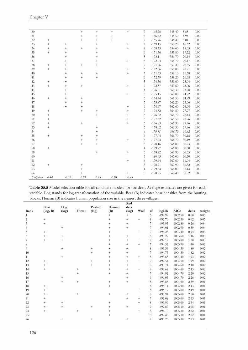
Chapter V
126
30
+ + + + 7 -165.28 345.40 8.88 0.00
31
+ + +
6 -166.42 345.50 8.94 0.00
32 +
+ + +
7 -165.76 346.40 9.84 0.00
33 + +
+
+ 7 -169.15 353.20 16.62 0.00
34 + + + +
+ 8 -168.73 354.60 18.03 0.00
35 + +
+
6 -171.56 355.80 19.22 0.00
36
+
+
5 -173.11 356.70 20.14 0.00
37
+
+
+ 6 -172.04 356.70 20.17 0.00
38 + + + +
7 -171.26 357.40 20.85 0.00
39 + +
+ 6 -172.56 357.80 21.21 0.00
40
+ + +
+ 7 -171.63 358.10 21.58 0.00
41
+ + +
6 -172.79 358.20 21.68 0.00
42 + +
5 -174.56 359.60 23.04 0.00
43 + + +
+ 7 -172.37 359.60 23.06 0.00
44
+
4 -176.01 360.30 23.78 0.00
45
+
+ 5 -175.15 360.80 24.22 0.00
46 + + +
6 -174.44 361.50 24.99 0.00
47
+ +
5 -175.87 362.20 25.66 0.00
48
+ +
+ 6 -174.97 362.60 26.04 0.00
49 +
+ +
+ 7 -174.82 364.50 27.97 0.00
50 +
+
+ 6 -176.02 364.70 28.14 0.00
51 +
+ 5 -177.52 365.50 28.96 0.00
52 +
+
+ 6 -176.83 366.30 29.76 0.00
53 +
+
5 -178.02 366.50 29.96 0.00
54
+
4 -179.18 366.70 30.12 0.00
55 +
+ +
6 -177.04 366.70 30.18 0.00
56
+ +
+ 6 -177.04 366.70 30.19 0.00
57
+ +
5 -178.16 366.80 30.23 0.00
58 +
4 -179.27 366.80 30.30 0.00
59
+
+ 5 -178.22 366.90 30.35 0.00
60
3 -180.43 367.00 30.50 0.00
61
+ 4 -179.64 367.60 31.04 0.00
62 +
+
5 -178.71 367.90 31.32 0.00
63
+
4 -179.84 368.00 31.44 0.00
64
+
+ 5 -178.95 368.40 31.82 0.00
Coefficient 0.44 -0.32 0.01 0.18 -0.84 -0.48
Table S5.5 Model selection table for all candidate models for roe deer. Average estimates are given for each
variable. Log stands for log-transformation of the variable. Bear (B) indicates bear densities from the hunting
blocks. Human (B) indicates human population size in the nearest three villages.
Rank Bear (log, B)
Dog (log) Forest
Pasture (log)
Human (B)
Red deer (log) Wolf df logLik AICc delta weight
1
+ +
6 -494.92 1002.50 0.00 0.05
2 +
+ + + 8 -492.70 1002.50 0.02 0.05
3 +
+ +
7 -493.95 1002.80 0.26 0.04
4
+
+ +
7 -494.01 1002.90 0.39 0.04
5 +
+
+ 7 -494.28 1003.40 0.94 0.03
6 + +
+ +
8 -493.27 1003.60 1.16 0.03
7 + +
+ + + 9 -492.19 1003.80 1.30 0.03
8
+ + + 7 -494.52 1003.90 1.40 0.02
9
+
+ + +
8 -493.59 1004.30 1.80 0.02
10
+ + +
7 -494.73 1004.30 1.82 0.02
11
+
+ + + 8 -493.65 1004.40 1.93 0.02
12 +
+ + + + 9 -492.54 1004.50 1.99 0.02
13 +
+ + +
8 -493.74 1004.60 2.10 0.02
14 +
+
+ + + 9 -492.62 1004.60 2.15 0.02
15
+
+ +
7 -494.92 1004.70 2.20 0.02
16
+
+
6 -496.05 1004.70 2.26 0.02
17
+ +
+ +
8 -493.88 1004.90 2.39 0.01
18 +
+
6 -496.14 1004.90 2.43 0.01
19 +
+ 6 -496.17 1005.00 2.49 0.01
20 +
+
+ +
8 -493.94 1005.00 2.50 0.01
21 +
+ + 7 -495.08 1005.00 2.53 0.01
22 + +
+
+ 8 -493.96 1005.00 2.54 0.01
23 + +
+ + +
9 -492.87 1005.10 2.65 0.01
24 +
+
+
+ 8 -494.10 1005.30 2.82 0.01
25
+
5 -497.43 1005.30 2.82 0.01
26
+
+
+
7 -495.23 1005.30 2.83 0.01
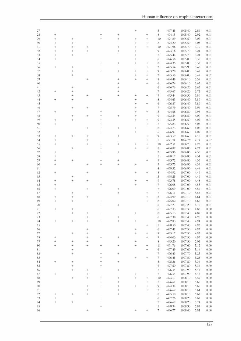
Human influence on trophic interactions
127
27
+
5 -497.45 1005.40 2.86 0.01
28 +
+ +
+ 8 -494.15 1005.40 2.92 0.01
29 + +
+ + + + 10 -491.89 1005.50 3.02 0.01
30 + +
+ + 8 -494.20 1005.50 3.03 0.01
31 + + +
+ + + 10 -491.96 1005.70 3.16 0.01
32 + + +
+ +
9 -493.16 1005.70 3.24 0.01
33 + +
+
7 -495.44 1005.70 3.24 0.01
34 +
+
6 -496.58 1005.80 3.30 0.01
35
+ + + + 8 -494.35 1005.80 3.32 0.01
36 + +
+ 7 -495.54 1005.90 3.45 0.01
37
+
+ + + + 9 -493.28 1006.00 3.47 0.01
38
+
+ + 7 -495.56 1006.00 3.49 0.01
39
+
+ + + 8 -494.48 1006.10 3.59 0.01
40
+
+ 6 -496.74 1006.10 3.63 0.01
41
+
+
6 -496.76 1006.20 3.67 0.01
42 + +
+
7 -495.67 1006.20 3.72 0.01
43
+ +
+ + + 9 -493.44 1006.30 3.80 0.01
44 + +
+
+
8 -494.63 1006.40 3.89 0.01
45
+ + 6 -496.87 1006.40 3.89 0.01
46
+ +
+
7 -495.79 1006.40 3.94 0.01
47 +
+
+ + 8 -494.68 1006.50 3.98 0.01
48
+ + + + +
9 -493.54 1006.50 4.00 0.01
49 + +
+
+ + 9 -493.55 1006.50 4.02 0.01
50 +
+
+ 7 -495.83 1006.50 4.03 0.01
51
+ + + +
8 -494.73 1006.60 4.08 0.01
52
+
+
6 -496.97 1006.60 4.09 0.01
53 + + +
+
+ 9 -493.59 1006.60 4.10 0.01
54 +
+
+ 7 -495.91 1006.70 4.19 0.01
55 +
+ + + + + 10 -492.51 1006.70 4.26 0.01
56
+
+
+ + 8 -494.82 1006.80 4.27 0.01
57 +
+ +
7 -495.96 1006.80 4.30 0.01
58 +
5 -498.17 1006.80 4.31 0.01
59 + +
+ +
+ 9 -493.72 1006.80 4.36 0.01
60 +
+ + + +
9 -493.73 1006.90 4.39 0.01
61
4 -499.32 1006.90 4.44 0.01
62 +
+
+ + 8 -494.92 1007.00 4.46 0.01
63
+
5 -498.25 1007.00 4.46 0.01
64 + + +
+ + 9 -493.78 1007.00 4.48 0.01
65 +
+
+
7 -496.08 1007.00 4.53 0.01
66 +
+
+
7 -496.09 1007.00 4.56 0.01
67
+
+
+ 7 -496.11 1007.10 4.58 0.01
68 + + +
+ 8 -494.99 1007.10 4.61 0.01
69 + +
+
+ 8 -495.02 1007.10 4.66 0.01
70
+ +
6 -497.27 1007.20 4.70 0.01
71 + +
6 -497.33 1007.30 4.82 0.00
72
+ + +
+
8 -495.13 1007.40 4.89 0.00
73
+
+
6 -497.38 1007.40 4.90 0.00
74 + + + + + +
10 -492.83 1007.40 4.91 0.00
75
+ 5 -498.50 1007.40 4.96 0.00
76
+
+
6 -497.41 1007.50 4.97 0.00
77
+ +
+ + 8 -495.17 1007.50 4.97 0.00
78 +
+ + +
+ 9 -494.03 1007.50 4.97 0.00
79 + + +
+
8 -495.20 1007.50 5.02 0.00
80 + + + + + + + 11 -491.76 1007.60 5.12 0.00
81
+
+ 6 -497.49 1007.60 5.14 0.00
82
+
+ +
7 -496.43 1007.70 5.23 0.00
83
+
+ + 7 -496.45 1007.80 5.28 0.00
84 + +
+ +
8 -495.36 1007.80 5.34 0.00
85
+
+
6 -497.60 1007.80 5.36 0.00
86
+ +
+
7 -496.54 1007.90 5.44 0.00
87 +
+
+
7 -496.54 1007.90 5.45 0.00
88
+ + + + + + 10 -493.17 1008.10 5.59 0.00
89
+ +
+ 7 -496.61 1008.10 5.60 0.00
90
+ + + + + 9 -494.34 1008.10 5.60 0.00
91
+
+
+ 7 -496.62 1008.10 5.61 0.00
92 + + +
+
8 -495.50 1008.10 5.62 0.00
93 +
+
6 -497.76 1008.20 5.67 0.00
94 + +
+
7 -496.69 1008.20 5.74 0.00
95
+
5 -498.94 1008.30 5.84 0.00
96
+
+ + 7 -496.77 1008.40 5.91 0.00
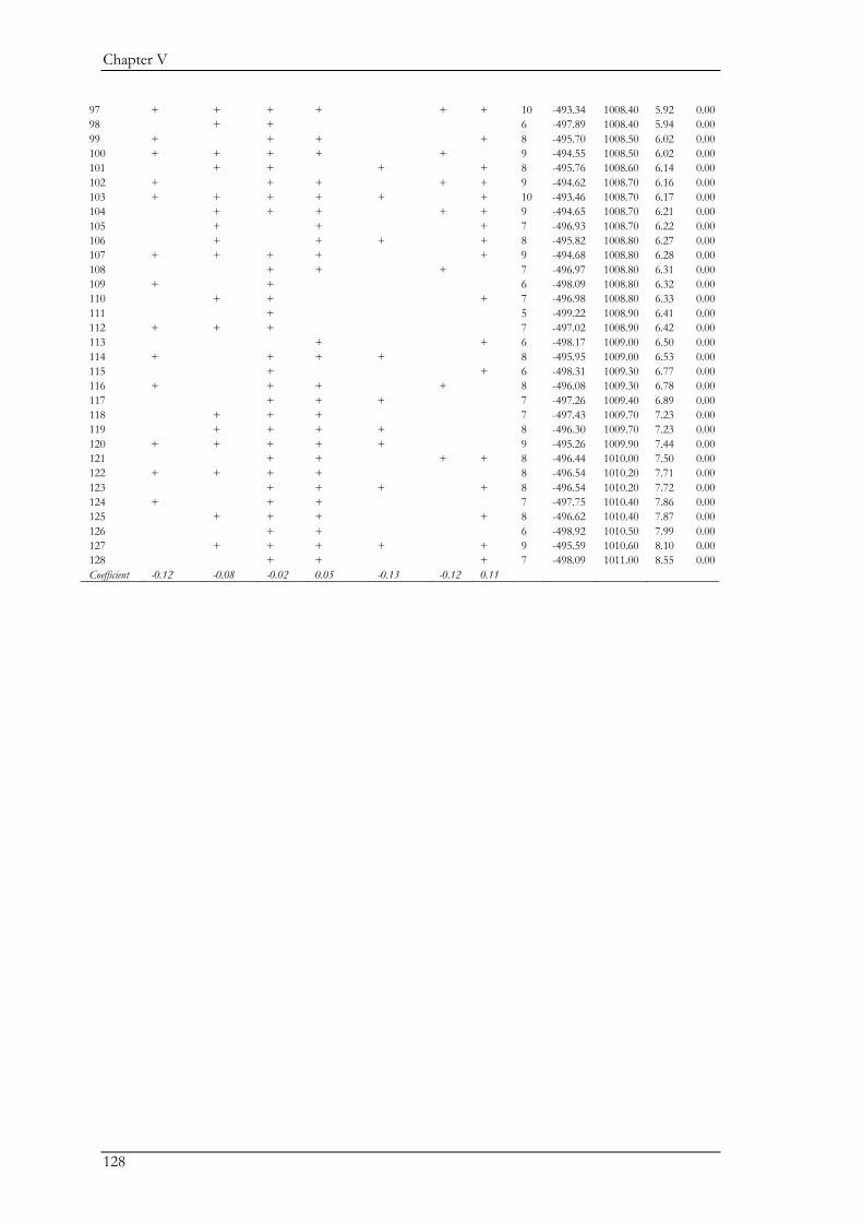
Chapter V
128
97 + + + +
+ + 10 -493.34 1008.40 5.92 0.00
98
+ +
6 -497.89 1008.40 5.94 0.00
99 +
+ +
+ 8 -495.70 1008.50 6.02 0.00
100 + + + +
+
9 -494.55 1008.50 6.02 0.00
101
+ +
+
+ 8 -495.76 1008.60 6.14 0.00
102 +
+ +
+ + 9 -494.62 1008.70 6.16 0.00
103 + + + + +
+ 10 -493.46 1008.70 6.17 0.00
104
+ + +
+ + 9 -494.65 1008.70 6.21 0.00
105
+
+
+ 7 -496.93 1008.70 6.22 0.00
106
+
+ +
+ 8 -495.82 1008.80 6.27 0.00
107 + + + +
+ 9 -494.68 1008.80 6.28 0.00
108
+ +
+
7 -496.97 1008.80 6.31 0.00
109 +
+
6 -498.09 1008.80 6.32 0.00
110
+ +
+ 7 -496.98 1008.80 6.33 0.00
111
+
5 -499.22 1008.90 6.41 0.00
112 + + +
7 -497.02 1008.90 6.42 0.00
113
+
+ 6 -498.17 1009.00 6.50 0.00
114 +
+ + +
8 -495.95 1009.00 6.53 0.00
115
+
+ 6 -498.31 1009.30 6.77 0.00
116 +
+ +
+
8 -496.08 1009.30 6.78 0.00
117
+ + +
7 -497.26 1009.40 6.89 0.00
118
+ + +
7 -497.43 1009.70 7.23 0.00
119
+ + + +
8 -496.30 1009.70 7.23 0.00
120 + + + + +
9 -495.26 1009.90 7.44 0.00
121
+ +
+ + 8 -496.44 1010.00 7.50 0.00
122 + + + +
8 -496.54 1010.20 7.71 0.00
123
+ + +
+ 8 -496.54 1010.20 7.72 0.00
124 +
+ +
7 -497.75 1010.40 7.86 0.00
125
+ + +
+ 8 -496.62 1010.40 7.87 0.00
126
+ +
6 -498.92 1010.50 7.99 0.00
127
+ + + +
+ 9 -495.59 1010.60 8.10 0.00
128
+ +
+ 7 -498.09 1011.00 8.55 0.00
Coefficient -0.12 -0.08 -0.02 0.05 -0.13 -0.12 0.11
129
Section B: Traditional
wood pastures
This Section includes Chapters VI-VIII and focuses specifically on the conservation value of
traditional wood pastures to gain insights on the role of particular traditional land-use elements for
biodiversity. Wood pastures are one of the oldest land-use types in Europe. They were established
through ancient silvo-pastoral practices and often consist of open grasslands with scattered old
trees. Chapter VI explores the characteristics, management, and status of wood pastures, but also
the current threats to wood pastures. The role of wood pastures for biodiversity is assessed in more
detail in Chapters VII and VIII: Chapter VII examines the habitat value of woodpeckers for an
assemblage of six woodpecker species, Chapter VIII aims to assess the extent of wood pastures use
by the brown bear.

130

131
Chapter VI

132
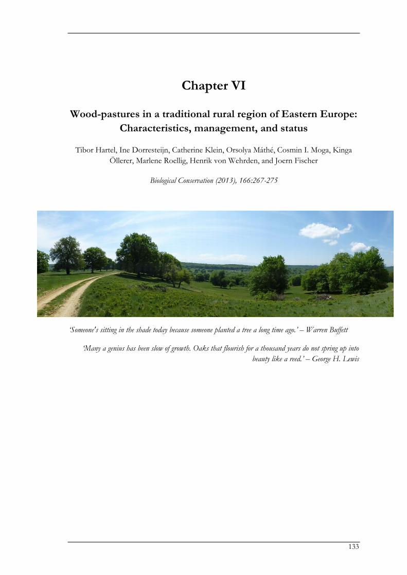
133
Chapter VI
Wood-pastures in a traditional rural region of Eastern Europe:
Characteristics, management, and status
Tibor Hartel, Ine Dorresteijn, Catherine Klein, Orsolya Máthé, Cosmin I. Moga, Kinga
Öllerer, Marlene Roellig, Henrik von Wehrden, and Joern Fischer
Biological Conservation (2013), 166:267-275
‘Someone's sitting in the shade today because someone planted a tree a long time ago.’ – Warren Buffett
‘Many a genius has been slow of growth. Oaks that flourish for a thousand years do not spring up into
beauty like a reed.’ – George H. Lewis

Chapter VI
134
Wood pasture characteristics, management and status
135
Abstract
Wood-pastures are among the oldest land-use types in Europe and have high ecological and
cultural importance. They are under rapid decline all over Europe because of changes in land-use,
tree cutting, and lack of regeneration. In this study we characterized the structure, condition and
threats of wood-pastures in a traditional rural region in Romania. Forty-two wood-pastures were
surveyed, as well as 15 forest sites for comparison. All wood-pasture sites were described via four
groups of variables: condition, management, site, and landscape context. Forest sites were
dominated by Hornbeam (Carpinus betulus) and Beech (Fagus sylvatica), whereas wood-pastures were
dominated by Oak (Quercus sp.) and various species of fruit trees. Most wood-pastures contained
trees classified as ‘ancient’ but no such trees were found in forests. The proportion of dead trees
was positively related to forest cover within 300 m around the wood-pasture. Models that included
management, site and landscape-related variables best explained the prelevance of Oak, Beech,
Hornbeam and Pear trees in wood-pastures. Large oaks and hornbeams were more likely to be
dead or affected by uncontrolled pasture burning than small oaks and other tree species. Our
results show that ancient wood-pastures are common in this rural region, and they may be more
common in Eastern Europe than previously thought. There is an urgent need for research, legal
recognition and conservation management of wood-pastures as distinct landscape elements for
their cultural, ecological and agricultural importance.
Chapter VI
136
Introduction
Wood-pastures represent an important part of European cultural–natural heritage (Bergmeier et al.
2010), and are one of the oldest land-use types in Europe, being known since the Neolithic (Luick
2008). Although the concept of wood-pastures is broad (Spencer & Kirby 1992; Caledonian
Partnership 2003; Goldberg et al. 2007), it characteristically refers to environments that are defined
by trees scattered through an open area, generally grassland. Appropriate livestock grazing regimes
applied through centuries have been crucial for the formation of wood-pastures and will be
important for their further persistence (Quelch 2002).
Ancient wood-pastures bring together several important components that make them
attractive for ecologists and conservationists. First, wood-pastures contain scattered trees. The age
of these trees can reach centuries; such trees are sometimes referred to as ‘veteran’ or ‘ancient’ trees
(Read 2000; Quelch 2002). Old, scattered trees provide a broad range of habitat features such as
dead branches or hollows (Gibbons & Lindenmayer 2003). For this reason, old trees represent
local ‘biodiversity hotspots’ in ecosystems around the world (Fischer et al. 2010; Lindenmayer et al.
2014). Moreover, scattered trees (regardless of their age) significantly influence microclimatic
conditions and soil humidity, and consequently vegetation structure (Manning et al. 2006) and may
help to facilitate adaptation to anthropogenic climate change in the future (Manning et al. 2009).
Second, the open habitat throughout which trees are scattered is managed mostly as pasture
(Quelch 2002; Mountford & Peterken 2003; Bergmeier et al. 2010). Traditional pasture
management has typically been low in intensity, thus supporting a rich flora and fauna, including
many species of conservation interest (Rosenthal et al. 2012). Low intensity grazing, together with
scattered, often old trees, makes many wood-pastures regional hotspots of biodiversity (Bugalho et
al. 2011).
Wood-pastures have received increasing scientific attention throughout Europe in recent
years. Studies on the biodiversity of wood-pastures and the ecological value of old trees have been
conducted in the Czech Republic (Vojta & Drhovská 2012; Horák & Rébl 2013), Portugal
(Gonçalves et al. 2012), Romania (Moga et al. 2009; Dorresteijn et al. 2013), and Sweden (Paltto et
al. 2011; Widerberg et al. 2012). Vegetation dynamics and landscape change related to management
regimes are available, for example, from the Swiss Jura Mountains (Buttler et al. 2008), the Italian
Alps (Garbarino et al. 2011), Belgium (Van Uytvanck et al. 2008), the Netherlands (Smit & Ruifrok
2011; Smit & Verwijmeren 2011), Spain (Plieninger & Schaar 2008) and Sweden (Brunet et al.,
2011). Studies exploring the recruitment of trees in wood-pastures are available from Spain
(Plieninger 2007); and research about the vegetation structure and conservation status of wood-
pastures is available from Romania (Öllerer 2012, 2013), Turkey (Uğurlu et al. 2012), and Greece
(Chaideftou et al. 2011). Finally, the crucial importance of low intensity human use for the
maintenance of biodiversity and ecosystem services in Mediterranean wood-pastures and their
provisioning ecosystem services was reported by Bugalho et al. (2011).
Wood pasture characteristics, management and status
137
Existing studies highlight that wood-pastures have been undergoing major changes in the
past few decades. These changes threaten the existence of wood-pastures and are mostly driven by
changing land-use (e.g. land abandonment and changing farming practices), policies, changing
attitudes toward old trees, and lack of tree regeneration (reviewed in Bergmeier et al. 2010).
While until recently Britain was considered as one of the main locations in Europe for
large (veteran) trees in wood-pastures (Rackham 1998; Mountford & Peterken 2003), information
from Central and Eastern European (CEE) countries about ancient wood-pastures is scarce. Some
national level evaluations exist for example in Hungary (e.g Haraszthy et al. 1997), suggesting that
wood-pastures are among the most threatened ecosystems in this country.
Here, we present research on wood-pastures in a traditional rural region of Central
Romania. Our study had three aims: (i) to compare the structure of tree communities and tree sizes
between forests and wood-pastures, (ii) to describe the main characteristics and current
management of wood-pastures and (iii) to model wood-pasture condition using a number of site,
landscape and management related variables. Although our study has a regional focus and is partly
descriptive in nature, we discuss our findings broadly in the context of international wood-pasture
conservation. Drawing on our findings, we argue that some Eastern European wood-pastures have
particularly high, but largely unrecognised, conservation values.
Methods
Study area
The study was conducted in Southern Transylvania, Romania and covered ca 3600 km2, of which
ca 860 km2 were covered by Natura 2000 regulations (Site of Community Importance, hereafter
SCI) (Fig. 6.1). The region is dominated by traditional land-use practices and has low levels of
infrastructure development. The most important land cover types based on CORINE land cover
classes (see Table 6.1 for reference) are forest (ca. 30%), pasture (ca. 26%), heterogeneous
agricultural areas (including agro-forestry areas; ca. 15%) and arable fields (ca. 14%). The urban
area cover is low (ca. 3%). Other minor land covers include wetlands and vineyards. The climate in
the region is continental and moderate. Annual temperature averages 8.2 ºC, with an average
temperature of -4.3 ºC in January and 18.6 ºC in July. The yearly mean amount of precipitation is
between 650 and 700 mm (Hartel and Moga, 2010).
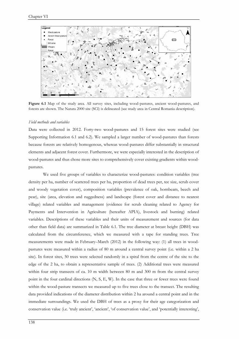
Chapter VI
138
Figure 6.1 Map of the study area. All survey sites, including wood-pastures, ancient wood-pastures, and
forests are shown. The Natura 2000 site (SCI) is delineated (see study area in Central Romania description).
Field methods and variables
Data were collected in 2012. Forty-two wood-pastures and 15 forest sites were studied (see
Supporting Information 6.1 and 6.2). We sampled a larger number of wood-pastures than forests
because forests are relatively homogenous, whereas wood-pastures differ substantially in structural
elements and adjacent forest cover. Furthermore, we were especially interested in the description of
wood-pastures and thus chose more sites to comprehensively cover existing gradients within wood-
pastures.
We used five groups of variables to characterize wood-pastures: condition variables (tree
density per ha, number of scattered trees per ha, proportion of dead trees per, tee size, scrub cover
and woody vegetation cover), composition variables (prevalence of oak, hornbeam, beech and
pear), site (area, elevation and ruggedness) and landscape (forest cover and distance to nearest
village) related variables and management (evidence for scrub cleaning related to Agency for
Payments and Intervention in Agriculture (hereafter APIA), livestock and burning) related
variables. Descriptions of these variables and their units of measurement and sources (for data
other than field data) are summarized in Table 6.1. The tree diameter at breast height (DBH) was
calculated from the circumference, which we measured with a tape for standing trees. Tree
measurements were made in February–March (2012) in the following way: (1) all trees in wood-
pastures were measured within a radius of 80 m around a central survey point (i.e. within a 2 ha
site). In forest sites, 50 trees were selected randomly in a spiral from the centre of the site to the
edge of the 2 ha, to obtain a representative sample of trees. (2) Additional trees were measured
within four strip transects of ca. 10 m width between 80 m and 300 m from the central survey
point in the four cardinal directions (N, S, E, W). In the case that three or fewer trees were found
within the wood-pasture transects we measured up to five trees close to the transect. The resulting
data provided indications of the diameter distribution within 2 ha around a central point and in the
immediate surroundings. We used the DBH of trees as a proxy for their age categorization and
conservation value (i.e. ‘truly ancient’, ‘ancient’, ‘of conservation value’, and ‘potentially interesting’,
Wood pasture characteristics, management and status
139
following Read (2000) and Farm Environment Plan Guide (2006)). We also recorded if the
measured trees were burned (i.e. the tree showed signs of fire but was alive), dead (for standing
dead trees), healthy (no visible injury on the trunk of the tree) and injured (when the trunk was
injured by cutting – coppicing and pollarding were not considered as injuries).
Tree density within 2 ha was assessed in wood-pastures as the count of all trees within 80
m of the central survey point. All dead trees from the two hectare sites were counted, both in
wood-pastures and forests. Trees were identified to genus level. According to a previous study
(Hartel & Moga 2010), the vast majority of the Oaks in wood-pastures in this region belong to the
species Quercus robur (90% out of 339 Oaks measured), or to Q. petraea and hybrids between the two
species. Due to the similarities of the ecology and habit of these two oaks, we believe that
considering them together was reasonable and facilitated meaningful comparison with the other
dominant tree genera.
Scrub cover was assessed for the entire wood-pasture using 400 m long and 6 m wide
transects which were placed subjectively so that they covered all representative locations of the
wood-pasture. This assessment was made in the period of May-July. The number of transects in
each wood-pasture was chosen according to the size of the wood-pasture: two transects were used
in wood-pastures with an area of up to 30 ha, three transects in those measuring 30–80 ha, four
transects in those of 80–130 ha area, five transects in those of 130–180 ha area, and six in those
measuring more than 180 ha. On average there were 3.7 transects per site. In each transect, the
percent of scrub cover was assessed visually every 100 m. Scrub cover values were averaged for the
entire wood-pasture to obtain a single representative estimate.
Furthermore we recorded the presence/absence of livestock based on direct observation
of the animals and/or their faeces. Pasture burning was recorded in March–April period (when this
activity usually takes place as management intervention to remove excessive biomass from
pastures), and the presence of scrub removal was recorded in March–July (Table 6.1). We further
recorded if we observed tree cutting activities in wood-pastures in 2012.
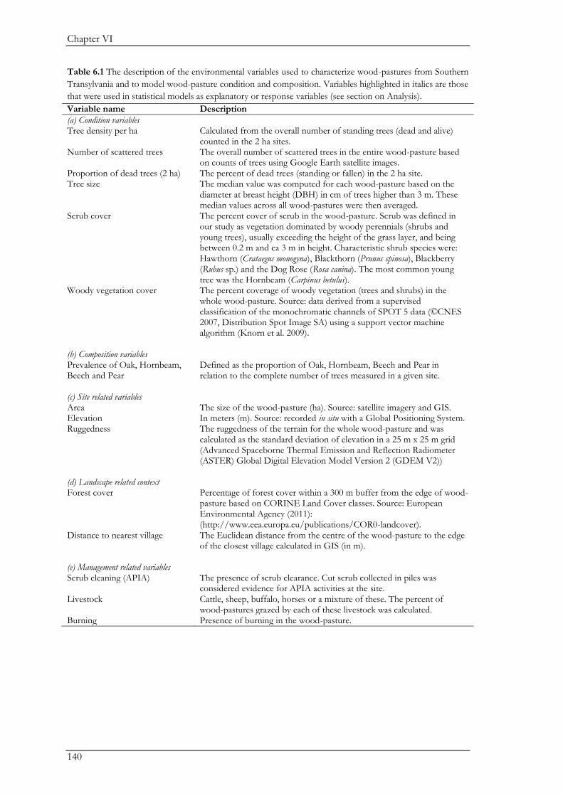
Chapter VI
140
Table 6.1 The description of the environmental variables used to characterize wood-pastures from Southern
Transylvania and to model wood-pasture condition and composition. Variables highlighted in italics are those
that were used in statistical models as explanatory or response variables (see section on Analysis).
Variable name Description
(a) Condition variables Tree density per ha Calculated from the overall number of standing trees (dead and alive)
counted in the 2 ha sites. Number of scattered trees The overall number of scattered trees in the entire wood-pasture based
on counts of trees using Google Earth satellite images. Proportion of dead trees (2 ha) The percent of dead trees (standing or fallen) in the 2 ha site. Tree size The median value was computed for each wood-pasture based on the
diameter at breast height (DBH) in cm of trees higher than 3 m. These median values across all wood-pastures were then averaged.
Scrub cover The percent cover of scrub in the wood-pasture. Scrub was defined in our study as vegetation dominated by woody perennials (shrubs and young trees), usually exceeding the height of the grass layer, and being between 0.2 m and ca 3 m in height. Characteristic shrub species were: Hawthorn (Crataegus monogyna), Blackthorn (Prunus spinosa), Blackberry (Rubus sp.) and the Dog Rose (Rosa canina). The most common young tree was the Hornbeam (Carpinus betulus).
Woody vegetation cover The percent coverage of woody vegetation (trees and shrubs) in the whole wood-pasture. Source: data derived from a supervised classification of the monochromatic channels of SPOT 5 data (©CNES 2007, Distribution Spot Image SA) using a support vector machine algorithm (Knorn et al. 2009).
(b) Composition variables Prevalence of Oak, Hornbeam, Beech and Pear
Defined as the proportion of Oak, Hornbeam, Beech and Pear in relation to the complete number of trees measured in a given site.
(c) Site related variables Area The size of the wood-pasture (ha). Source: satellite imagery and GIS. Elevation In meters (m). Source: recorded in situ with a Global Positioning System. Ruggedness The ruggedness of the terrain for the whole wood-pasture and was
calculated as the standard deviation of elevation in a 25 m x 25 m grid (Advanced Spaceborne Thermal Emission and Reflection Radiometer (ASTER) Global Digital Elevation Model Version 2 (GDEM V2))
(d) Landscape related context Forest cover Percentage of forest cover within a 300 m buffer from the edge of wood-
pasture based on CORINE Land Cover classes. Source: European Environmental Agency (2011): (http://www.eea.europa.eu/publications/COR0-landcover).
Distance to nearest village The Euclidean distance from the centre of the wood-pasture to the edge of the closest village calculated in GIS (in m).
(e) Management related variables Scrub cleaning (APIA) The presence of scrub clearance. Cut scrub collected in piles was
considered evidence for APIA activities at the site. Livestock Cattle, sheep, buffalo, horses or a mixture of these. The percent of
wood-pastures grazed by each of these livestock was calculated. Burning Presence of burning in the wood-pasture.
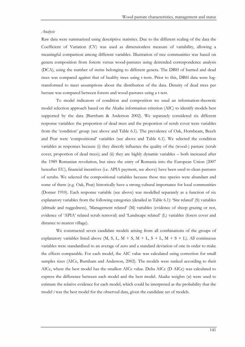
Wood pasture characteristics, management and status
141
Analysis
Raw data were summarized using descriptive statistics. Due to the different scaling of the data the
Coefficient of Variation (CV) was used as dimensionless measure of variability, allowing a
meaningful comparison among different variables. Illustration of tree communities was based on
genera composition from forests versus wood-pastures using detrended correspondence analysis
(DCA), using the number of stems belonging to different genera. The DBH of burned and dead
trees was compared against that of healthy trees using t-tests. Prior to this, DBH data were log-
transformed to meet assumptions about the distribution of the data. Density of dead trees per
hectare was compared between forests and wood-pastures using a t-test.
To model indicators of condition and composition we used an information-theoretic
model selection approach based on the Akaike information criterion (AIC) to identify models best
supported by the data (Burnham & Anderson 2002). We separately considered six different
response variables: the proportion of dead trees and the proportion of scrub cover were variables
from the ‘condition’ group (see above and Table 6.1). The prevalence of Oak, Hornbeam, Beech
and Pear were ‘compositional’ variables (see above and Table 6.1). We selected the condition
variables as responses because (i) they directly influence the quality of the (wood-) pasture (scrub
cover, proportion of dead trees); and (ii) they are highly dynamic variables – both increased after
the 1989 Romanian revolution, but since the entry of Romania into the European Union (2007
hereafter EU), financial incentives (i.e. APIA payment, see above) have been used to clean pastures
of scrubs. We selected the compositional variables because these tree species were abundant and
some of them (e.g. Oak, Pear) historically have a strong cultural importance for local communities
(Dorner 1910). Each response variable (see above) was modelled separately as a function of six
explanatory variables from the following categories (detailed in Table 6.1): ‘Site related’ (S) variables
(altitude and ruggedness), ‘Management related’ (M) variables (evidence of sheep grazing or not,
evidence of ‘APIA’ related scrub removal) and ‘Landscape related’ (L) variables (forest cover and
distance to nearest village).
We constructed seven candidate models arising from all combinations of the groups of
explanatory variables listed above (M, S, L, M + S, M + L, S + L, M + S + L). All continuous
variables were standardized to an average of zero and a standard deviation of one in order to make
the effects comparable. For each model, the AIC value was calculated using correction for small
samples sizes (AICc, Burnham and Anderson, 2002). The models were ranked according to their
AICc, where the best model has the smallest AICc value. Delta AICc (D AICc) was calculated to
express the difference between each model and the best model. Akaike weights (w) were used to
estimate the relative evidence for each model, which could be interpreted as the probability that the
model i was the best model for the observed data, given the candidate set of models.
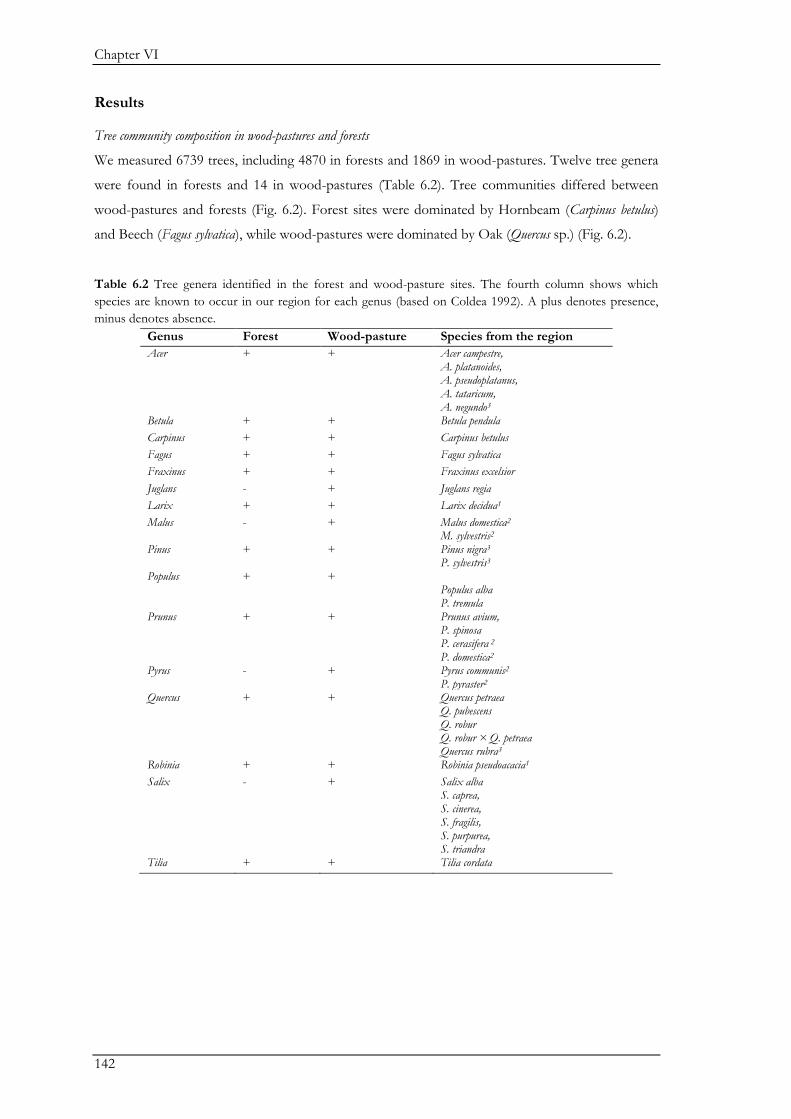
Chapter VI
142
Results
Tree community composition in wood-pastures and forests
We measured 6739 trees, including 4870 in forests and 1869 in wood-pastures. Twelve tree genera
were found in forests and 14 in wood-pastures (Table 6.2). Tree communities differed between
wood-pastures and forests (Fig. 6.2). Forest sites were dominated by Hornbeam (Carpinus betulus)
and Beech (Fagus sylvatica), while wood-pastures were dominated by Oak (Quercus sp.) (Fig. 6.2).
Table 6.2 Tree genera identified in the forest and wood-pasture sites. The fourth column shows which
species are known to occur in our region for each genus (based on Coldea 1992). A plus denotes presence,
minus denotes absence.
Genus Forest Wood-pasture Species from the region
Acer + + Acer campestre, A. platanoides, A. pseudoplatanus, A. tataricum, A. negundo3
Betula + + Betula pendula
Carpinus + + Carpinus betulus
Fagus + + Fagus sylvatica
Fraxinus + + Fraxinus excelsior
Juglans - + Juglans regia
Larix + + Larix decidua1
Malus - + Malus domestica2
M. sylvestris2
Pinus + + Pinus nigra3
P. sylvestris3
Populus + +
Populus alba P. tremula
Prunus + + Prunus avium, P. spinosa P. cerasifera 2 P. domestica2
Pyrus - + Pyrus communis2
P. pyraster2
Quercus + + Quercus petraea Q. pubescens Q. robur Q. robur × Q. petraea Quercus rubra3
Robinia + + Robinia pseudoacacia1
Salix - + Salix alba S. caprea, S. cinerea, S. fragilis, S. purpurea, S. triandra
Tilia + + Tilia cordata
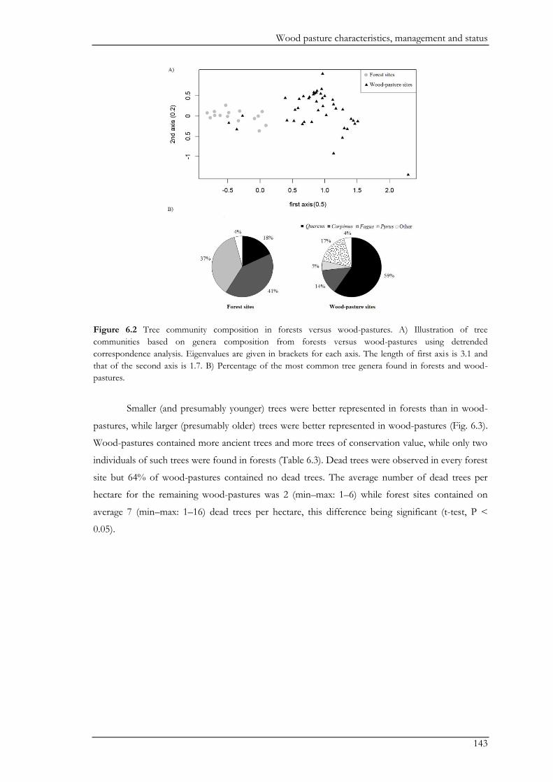
Wood pasture characteristics, management and status
143
Figure 6.2 Tree community composition in forests versus wood-pastures. A) Illustration of tree
communities based on genera composition from forests versus wood-pastures using detrended
correspondence analysis. Eigenvalues are given in brackets for each axis. The length of first axis is 3.1 and
that of the second axis is 1.7. B) Percentage of the most common tree genera found in forests and wood-
pastures.
Smaller (and presumably younger) trees were better represented in forests than in wood-
pastures, while larger (presumably older) trees were better represented in wood-pastures (Fig. 6.3).
Wood-pastures contained more ancient trees and more trees of conservation value, while only two
individuals of such trees were found in forests (Table 6.3). Dead trees were observed in every forest
site but 64% of wood-pastures contained no dead trees. The average number of dead trees per
hectare for the remaining wood-pastures was 2 (min–max: 1–6) while forest sites contained on
average 7 (min–max: 1–16) dead trees per hectare, this difference being significant (t-test, P <
0.05).
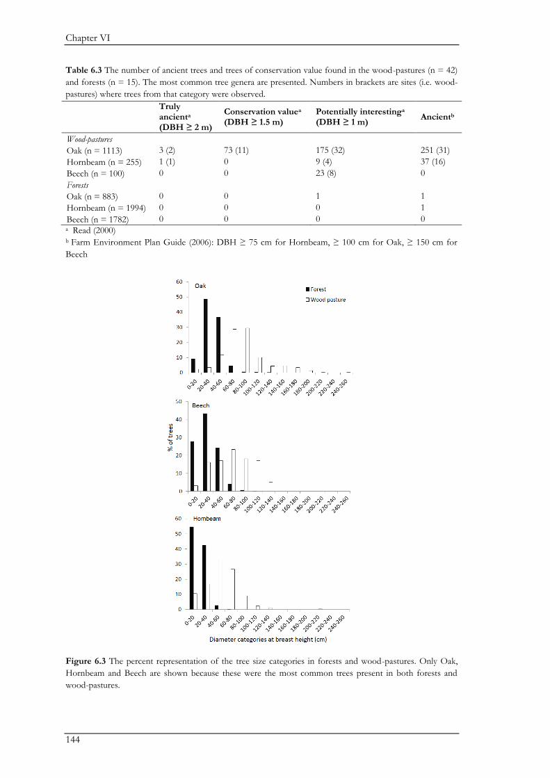
Chapter VI
144
Table 6.3 The number of ancient trees and trees of conservation value found in the wood-pastures (n = 42)
and forests (n = 15). The most common tree genera are presented. Numbers in brackets are sites (i.e. wood-
pastures) where trees from that category were observed.
Truly ancienta (DBH ≥ 2 m)
Conservation valuea (DBH ≥ 1.5 m)
Potentially interestinga
(DBH ≥ 1 m) Ancientb
Wood-pastures
Oak (n = 1113) 3 (2) 73 (11) 175 (32) 251 (31)
Hornbeam (n = 255) 1 (1) 0 9 (4) 37 (16)
Beech (n = 100) 0 0 23 (8) 0
Forests
Oak (n = 883) 0 0 1 1
Hornbeam (n = 1994) 0 0 0 1
Beech (n = 1782) 0 0 0 0 a Read (2000) b Farm Environment Plan Guide (2006): DBH ≥ 75 cm for Hornbeam, ≥ 100 cm for Oak, ≥ 150 cm for
Beech
Figure 6.3 The percent representation of the tree size categories in forests and wood-pastures. Only Oak,
Hornbeam and Beech are shown because these were the most common trees present in both forests and
wood-pastures.
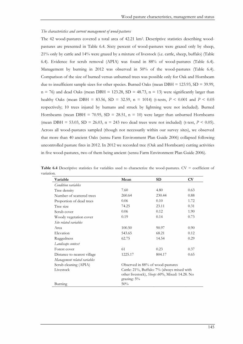
Wood pasture characteristics, management and status
145
The characteristics and current management of wood-pastures
The 42 wood-pastures covered a total area of 42.21 km2. Descriptive statistics describing wood-
pastures are presented in Table 6.4. Sixty percent of wood-pastures were grazed only by sheep,
21% only by cattle and 14% were grazed by a mixture of livestock (i.e. cattle, sheep, buffalo) (Table
6.4). Evidence for scrub removal (APIA) was found in 88% of wood-pastures (Table 6.4).
Management by burning in 2012 was observed in 50% of the wood-pastures (Table 6.4).
Comparison of the size of burned versus unburned trees was possible only for Oak and Hornbeam
due to insufficient sample sizes for other species. Burned Oaks (mean DBH = 123.93, SD = 39.99,
n = 76) and dead Oaks (mean DBH = 123.28, SD = 48.73, n = 13) were significantly larger than
healthy Oaks (mean DBH = 83.56, SD = 32.59, n = 1014) (t-tests, P < 0.001 and P < 0.05
respectively; 10 trees injured by humans and struck by lightning were not included). Burned
Hornbeams (mean DBH = 70.95, SD = 28.51, n = 10) were larger than unburned Hornbeams
(mean DBH = 53.03, SD = 26.03, n = 243 two dead trees were not included) (t-test, P < 0.05).
Across all wood-pastures sampled (though not necessarily within our survey sites), we observed
that more than 40 ancient Oaks (sensu Farm Environment Plan Guide 2006) collapsed following
uncontrolled pasture fires in 2012. In 2012 we recorded tree (Oak and Hornbeam) cutting activities
in five wood-pastures, two of them being ancient (sensu Farm Environment Plan Guide 2006).
Table 6.4 Descriptive statistics for variables used to characterize the wood-pastures. CV = coefficient of
variation.
Variable Mean SD CV
Condition variables Tree density 7.60 4.80 0.63
Number of scattered trees 260.64 230.44 0.88
Proportion of dead trees 0.06 0.10 1.72
Tree size 74.25 23.11 0.31
Scrub cover 0.06 0.12 1.90
Woody vegetation cover 0.19 0.14 0.73
Site related variables Area 100.50 90.97 0.90
Elevation 543.65 68.21 0.12
Ruggedness 62.75 14.54 0.29
Landscape context Forest cover 61 0.23 0.37
Distance to nearest village 1225.17 804.17 0.65
Management related variables Scrub cleaning (APIA) Observed in 88% of wood-pastures
Livestock Cattle: 21%, Buffalo: 7% (always mixed with
other livestock), Sheep: 60%, Mixed: 14.28. No grazing: 5%
Burning 50%
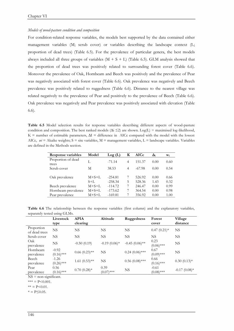
Chapter VI
146
Models of wood-pasture condition and composition
For condition-related response variables, the models best supported by the data contained either
management variables (M; scrub cover) or variables describing the landscape context (L;
proportion of dead trees) (Table 6.5). For the prevalence of particular genera, the best models
always included all three groups of variables (M + S + L) (Table 6.5). GLM analysis showed that
the proportion of dead trees was positively related to surrounding forest cover (Table 6.6).
Moreover the prevalence of Oak, Hornbeam and Beech was positively and the prevalence of Pear
was negatively associated with forest cover (Table 6.6). Oak prevalence was negatively and Beech
prevalence was positively related to ruggedness (Table 6.6). Distance to the nearest village was
related negatively to the prevalence of Pear and positively to the prevalence of Beech (Table 6.6).
Oak prevalence was negatively and Pear prevalence was positively associated with elevation (Table
6.6).
Table 6.5 Model selection results for response variables describing different aspects of wood-pasture
condition and composition. The best ranked models (∆i ≤2) are shown. Log(L) = maximised log-likelihood,
K = number of estimable parameters, ∆I = difference in AICc compared with the model with the lowest
AICc, wi = Akaike weights; S = site variables, M = management variables, L = landscape variables. Variables
are defined in the Methods section.
Table 6.6 The relationship between the response variables (first column) and the explanatory variables,
separately tested using GLMs.
Livestock type
APIA clearing
Altitude Ruggedness Forest cover
Village distance
Proportion of dead trees
NS NS NS NS 0.47 (0.21)* NS
Scrub cover NS NS NS NS NS NS Oak prevalence
NS -0.50 (0.19) -0.19 (0.06)* -0.45 (0.06)** 0.23 (0.06)***
NS
Hornbeam prevalence
-0.92 (0.16)***
0.66 (0.23)** NS 0.24 (0.06)*** 0.67 (0.09)***
NS
Beech prevalence
-1.26 (0.26)***
1.61 (0.53)** NS 0.56 (0.08)*** 0.66 (0.16)***
0.30 (0.13)*
Pear prevalence
0.56 (0.16)***
0.70 (0.28)* 0.39 (0.07)***
NS -0.61 (0.08)***
-0.17 (0.08)*
NS = non-significant.
*** = P<0.001.
** = P<0.01.
* = P≤0.05.
Response variables Model Log (L) K AICc Δi wi
Proportion of dead trees
L -71.14 4 151.37 0.00 0.60
Scrub cover M 38.53 4 -67.98 0.00 0.54
Oak prevalence M+S+L
-254.81
7
526.92
0.00
0.66
S+L -258.34 5 528.36 1.43 0.32 Beech prevalence M+S+L -114.72 7 246.47 0.00 0.99 Hornbeam prevalence M+S+L -173.62 7 364.54 0.00 0.98 Pear prevalence M+S+L -169.81 7 356.92 0.00 1.00
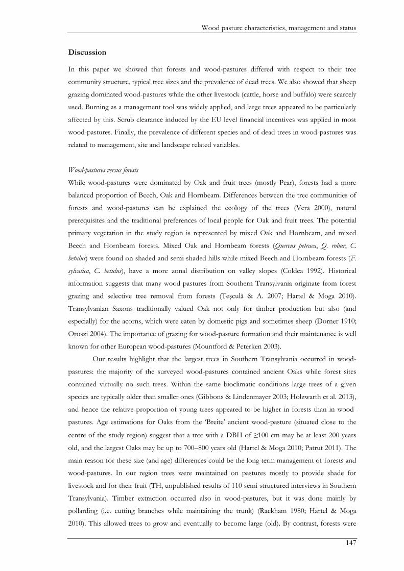
Wood pasture characteristics, management and status
147
Discussion
In this paper we showed that forests and wood-pastures differed with respect to their tree
community structure, typical tree sizes and the prevalence of dead trees. We also showed that sheep
grazing dominated wood-pastures while the other livestock (cattle, horse and buffalo) were scarcely
used. Burning as a management tool was widely applied, and large trees appeared to be particularly
affected by this. Scrub clearance induced by the EU level financial incentives was applied in most
wood-pastures. Finally, the prevalence of different species and of dead trees in wood-pastures was
related to management, site and landscape related variables.
Wood-pastures versus forests
While wood-pastures were dominated by Oak and fruit trees (mostly Pear), forests had a more
balanced proportion of Beech, Oak and Hornbeam. Differences between the tree communities of
forests and wood-pastures can be explained the ecology of the trees (Vera 2000), natural
prerequisites and the traditional preferences of local people for Oak and fruit trees. The potential
primary vegetation in the study region is represented by mixed Oak and Hornbeam, and mixed
Beech and Hornbeam forests. Mixed Oak and Hornbeam forests (Quercus petraea, Q. robur, C.
betulus) were found on shaded and semi shaded hills while mixed Beech and Hornbeam forests (F.
sylvatica, C. betulus), have a more zonal distribution on valley slopes (Coldea 1992). Historical
information suggests that many wood-pastures from Southern Transylvania originate from forest
grazing and selective tree removal from forests (Teşculă & A. 2007; Hartel & Moga 2010).
Transylvanian Saxons traditionally valued Oak not only for timber production but also (and
especially) for the acorns, which were eaten by domestic pigs and sometimes sheep (Dorner 1910;
Oroszi 2004). The importance of grazing for wood-pasture formation and their maintenance is well
known for other European wood-pastures (Mountford & Peterken 2003).
Our results highlight that the largest trees in Southern Transylvania occurred in wood-
pastures: the majority of the surveyed wood-pastures contained ancient Oaks while forest sites
contained virtually no such trees. Within the same bioclimatic conditions large trees of a given
species are typically older than smaller ones (Gibbons & Lindenmayer 2003; Holzwarth et al. 2013),
and hence the relative proportion of young trees appeared to be higher in forests than in wood-
pastures. Age estimations for Oaks from the ‘Breite’ ancient wood-pasture (situated close to the
centre of the study region) suggest that a tree with a DBH of ≥100 cm may be at least 200 years
old, and the largest Oaks may be up to 700–800 years old (Hartel & Moga 2010; Patrut 2011). The
main reason for these size (and age) differences could be the long term management of forests and
wood-pastures. In our region trees were maintained on pastures mostly to provide shade for
livestock and for their fruit (TH, unpublished results of 110 semi structured interviews in Southern
Transylvania). Timber extraction occurred also in wood-pastures, but it was done mainly by
pollarding (i.e. cutting branches while maintaining the trunk) (Rackham 1980; Hartel & Moga
2010). This allowed trees to grow and eventually to become large (old). By contrast, forests were
Chapter VI
148
traditionally managed for timber production (see Oroszi 2004 for and overview of forest
managament by Transylvanian Saxons), and the economic value (in a monetary sense) of trees was
and still is important in determining management actions. Old trees were and are removed from
forests because their economic value is decreasing as the amount of dead elements and hollows
increase with age. Assuring sustainability of the forests by regeneration (naturally ‘from seed’ or by
replanting the cleared parcels) was important both traditionally (Oroszi 2004) and continues to be
common practice nowadays (Codul Silvic (Forest Code of Romania), Law 46/2008). However, no
mechanisms to re-plant trees (or otherwise support their regeneration) occur in the vast majority of
wood-pastures.
Management of wood-pastures
Sixty percent of wood-pastures surveyed in 2012 were grazed only by sheep and 14% by a mixture
of livestock (Table 6.4). This is in sharp contrast with traditional grazing systems: Saxons preferred
cattle, horses, buffalo and pigs, and typically each of these had its own pastures with specific
management practices around a given village (Dorner 1910; and also Heinlein et al. 2005 for
selected areas of Bavaria, Germany). Pig grazing stopped in the late 1940s and 1950s, and the
number of buffalo dropped after the Romanian revolution in 1989, partly because of mass
emigration of Saxons and partly for economic reasons. Cattle grazing also declined sharply in many
wood-pastures after 1989 (although less so than for buffalo), and the number of sheep is now
higher than ever before in the Saxon region of Transylvania (TH, unpublished results of 110 semi
structured interviews in Southern Transylvania). Changes to the traditional grazing systems also
have been reported from many European wood-pastures throughout Europe (Plieninger & Schaar
2008; Bergmeier et al. 2010; Costa et al. 2011; Garbarino et al. 2011; Chételat et al. 2013).
Half of the wood-pastures were burned in 2012, and large trees (Oak and Hornbeam)
appeared to be most likely to be permanently damaged from this. Fire has been used as a method
for pasture clearing in the region since the 16th century (Dorner 1910). However, uncontrolled
pasture burning appears to have increased in recent years, even in protected areas, despite being
illegal (TH, personal observation).
Wood-pasture condition
Our model selection approach showed that the prevalence of Oak, Beech, Hornbeam and Pear
trees in wood-pastures was best explained by models containing management, site and landscape
related variables. Oak dominated in wood-pastures with low terrain ruggedness while Beech
dominated in areas with high ruggedness. This result can be explained partly by the ecology of
these species (see above) and partly by human influence. For example, it is possible that Oak was
retained in flatter terrain where accessibility for livestock was high and which contained wet areas
often preferred by these animals (especially cattle, domestic pigs and buffalo). Fruit trees (especially
Pear) dominated in wood-pastures close to villages (suggesting that accessibility for people was
Wood pasture characteristics, management and status
149
important in creating them) with little forest cover in their surroundings. By contrast, forest cover
was an important positive predictor for the abundance of all three forest tree species. A likely
explanation is that many, if not most, thinning existing forests created wood-pastures in our region.
The pear prevalence was positively associated with the elevation; this is most likely a result of the
slight increase of the average elevation toward the Eastern part of the region, where this tree is
more abundant. Our result regarding the significant relationship found between the management
related variables and prevalence of different tree genera (Table 6.5) is not straightforward: the
relationship is likely caused by the fact that local conditions shaped human activity (this being
recorded in 2012) and not the other way round. For example, it is possible that wood-pastures
where beech and hornbeam dominated were less attractive for grazing, possibly because of steeper
slopes or higher woody vegetation density. The grazing system in our region is undergoing rapid
changes, and therefore this relationship is likely to change in the future.
The percentage of dead trees was significantly related to forest cover around the wood-
pasture. Wood-pastures surrounded by forests may be less accessible for people than the wood-
pastures from open landscapes. Traditional rural communities from this region carefully cleared the
pastures of dead wood and scrub to maintain pasture quality (Dorner 1910; TH, unpublished
results of 110 semi structured interviews in Southern Transylvania). Based on this, it is reasonable
to assume that wood-pastures in traditional societies contained dead wood only accidentally and if
the scrub was present, it was deliberately maintained (e.g. as occasional firewood or as source of
fruits). It is possible that the increase of the dead wood on pastures is the result of the
abandonment of pastures, which was very pronounced after the 1989 Romanian revolution. As the
continuation of use of pastures and hay meadows is promoted by EU agro-environment incentives,
it is likely that abundance of dead wood will decline again in the future in most of wood-pastures
from this region.
The biodiversity of the ‘Breite’ ancient wood-pasture
In the context of wood-pasture conservation, it is important to note that some wood-pastures in
our study area have been shown to support a very rich diversity of plants and animals. A wide
range of studies have been conducted on one of the wood-pastures also surveyed by us for this
paper, namely the ‘Breite’ wood-pasture, situated near the centre of our study area, near the town
Sighisoara. The Breite measures 133 ha and is completely surrounded by deciduous forest. It is
dominated by Oaks (mostly Q. robur), many of which are over 200 years old (Patrut 2011). Overall,
476 species of vascular plants (Öllerer, 2012), 121 species of macromycetes (from which over 50
species were found on ancient Oaks - Bucşa 2007; Bucşa & Tăuşan 2010), 281 species of
Lepidoptera, 40 species of xylophagous beetles (i.e. insects to which wood represents the primary
diet), eight species of amphibians, four species of reptiles, 27 species of nesting birds and 38 species
of mammals (including Gray Wolf, Canis lupus, and Brown Brear, Ursus arctos) have been identified
in this wood-pasture (synthesized in Hartel & Moga 2010; Hartel et al. 2011). The overall number
Chapter VI
150
of species considered rare or protected at national (e.g. Red List) and international (e.g. IUCN,
Habitats and Birds Directives) level exceeds 50.
Conclusions and conservation implications
We showed that there were differences between the tree communities in wood-pastures and
forests. Ancient trees were found only in wood-pastures, and most of the surveyed wood-pastures
contained ancient trees. Historical and current management, traditional preferences of local people,
and natural environmental gradients are likely explanations for these differences. Fire appears to be
regularly used in pasture management, but our data suggest that uncontrolled fires can negatively
affect (or even kill) trees, especially large ones. Further, our data, in combination with historical
records, suggest that major changes are underway regarding patterns of livestock grazing in
Southern Transylvania, implying that the management of wood-pastures is shifting from traditional
practices. Demographic and economic factors are the likely drivers of these recent shifts. Data
from one of the wood-pastures in the centre of our study area suggest that the presence of
scattered, old trees, in combination with dead trees, scrub and extensively managed grassland,
results in a high biodiversity, with species rich communities of woodland and grassland related
organisms. To maintain the ecological value of wood-pastures, at least some of the dead trees and
scrub need to be maintained - although this runs counter to both traditional practices and current
policy incentives. Wood-pastures are currently managed as pastures (or occasionally as hay
meadows) and are formally recognized as such at the national level (Romanian Law No. 214/2011).
While tree cutting from wood-pastures without a formal institutional agreement is illegal in
Romania (Law 214/2011), there is no legal framework that specifically targets the maintenance and
regeneration of wood-pastures and the conservation of old (including ancient and veteran) trees.
With very few exceptions, wood-pastures are not recognized in the nature conservation policies of
the EU and are not protected as distinct land cover types with special management
history, ecological and cultural value. Therefore their maintenance as such is not promoted at
policy level. Our study shows that ancient wood-pastures are common in our region, and we
suggest that they also may be common in other CEE countries. We urge for more wood-pasture
inventories and research in other parts of CEE, to develop the knowledge base that is needed for
their formal recognition and legal protection.
Wood pasture characteristics, management and status
151
Acknowledgements
The early stages (i.e. 2010 and before) of wood-pasture research in Southern Transylvania were
founded by the Mihai Eminescu Trust, EEA Grants through the project ‘Conservation of the
biodiversity of the Breite Ancient Oak tree nature reserve, Sighisoara’ and ‘The implication of local
communities in the conservation of wood-pasture habitats from the Saxon villages of
Transylvania’. The present research and the research stay of TH in Germany were supported by
Alexander von Humboldt Foundation. JF was funded by Alexander von Humboldt Foundation via
a Sofja Kovalevskaja Award. We thank Árpád Szapanyos for his help with the tree measurements.
Appendix A. Supplementary material
Figure 1. KML-file of the surveyed wood-pasture sites shown in Google Earth Map
Figure 2. KML-file of the surveyed forest sites shown in Google Earth Map

152

153
Chapter VII

154
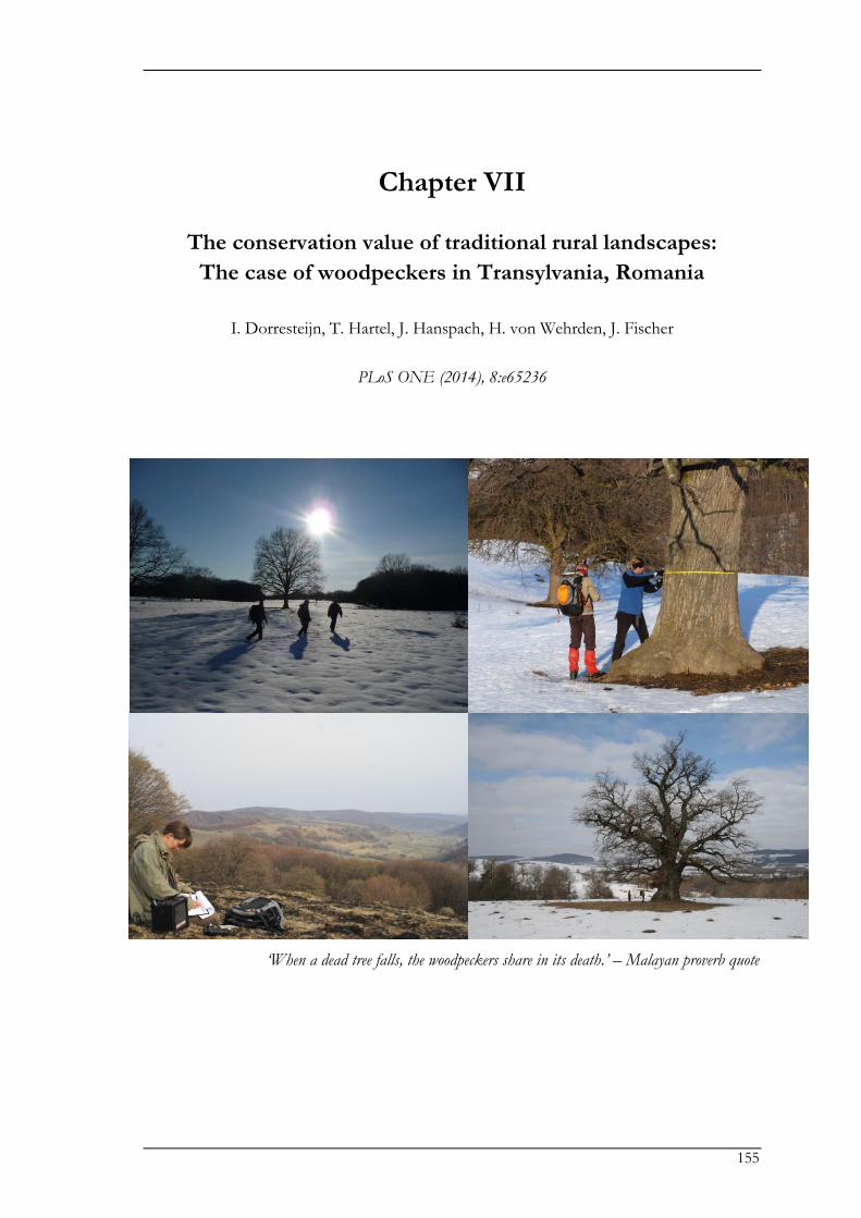
155
Chapter VII
The conservation value of traditional rural landscapes:
The case of woodpeckers in Transylvania, Romania
I. Dorresteijn, T. Hartel, J. Hanspach, H. von Wehrden, J. Fischer
PLoS ONE (2014), 8:e65236
‘When a dead tree falls, the woodpeckers share in its death.’ – Malayan proverb quote

Chapter VII
156
Woodpeckers in wood pastures
157
Abstract
Land-use change is a major threat to global biodiversity. Forest species face the dual threats of
deforestation and intensification of forest management. In regions where forests are under threat,
rural landscapes that retain structural components of mature forests potentially provide valuable
additional habitat for some forest species. Here, we illustrate the habitat value of traditional wood
pastures for a woodpecker assemblage of six species in southern Transylvania, Romania. Wood
pastures are created by long-term stable silvo-pastoral management practices, and are composed of
open grassland with scattered large, old trees. Because of their demanding habitat requirements,
woodpeckers share habitat with many other bird species, and have been considered as possible
indicator species for bird species diversity. We first compared woodpecker assemblages between
forests and wood pastures. Second, we grouped features of wood pastures into three spatial
contexts and addressed how these features related to the occurrence of three woodpecker species
that are formally protected. Woodpecker species composition, but not the number of species,
differed between forests and wood pastures, with the green woodpecker occurring more commonly
in wood pastures, and the lesser spotted woodpecker more commonly in forests. Within wood
pastures, the intermediate context (especially surrounding forest cover) best explained the presence
of the grey-headed and middle spotted woodpecker. By contrast, variables describing local
vegetation structure and characteristics of the surrounding landscape did not affect woodpecker
occurrence in wood pastures. In contrast to many other parts of Europe, in which several species
of woodpeckers have declined, the traditional rural landscape of Transylvania continues to provide
habitat for several woodpecker species, both in forests and wood pastures. Given the apparent
habitat value of wood pastures for woodpeckers we recommend wood pastures be explicitly
considered in relevant policies of the European Union, namely the Habitats Directive and the EU
Common Agricultural Policy.
Chapter VII
158
Introduction
Human-induced landscape change poses a major threat to global biodiversity (Fahrig 2003; Foley et
al. 2005). Forest species face the dual threat of deforestation and intensification of forest
management. Woodpeckers are especially sensitive to these changes because they require large
home ranges and depend on large trees for nesting and dead wood for foraging (Angelstam &
Mikusinski 1994). Consequently, changes in forest structure and cover have caused woodpecker
declines worldwide (Conner & Rudolph 1991; Roberge et al. 2008; Lammertink et al. 2009).
Because of their demanding habitat requirements, woodpeckers share habitat requirements with
many other bird species. Therefore, woodpeckers have been considered as potential indicator
species for bird species diversity (Roberge & Angelstam 2006).
In Europe, six out of ten species of woodpeckers are protected under the EU Birds
Directive Annex I. While several woodpecker species have declined in Western Europe, Eastern
European woodpecker assemblages have remained diverse and stable due to the persistence of
large forest tracts (Mikusinski & Angelstam 1998). However, Eastern European forest landscapes
are increasingly coming under pressure from more intensive and widespread logging operations
(Knorn et al. 2012). Against this background, it is important to understand to what extent the
landscape context surrounding forest patches could provide complementary habitat for
woodpeckers in Eastern Europe. Many agricultural landscapes in Eastern Europe are characterized
by low-intensity subsistence farming that still contain semi-natural vegetation cover, including
transitional elements between forest patches such as scattered trees (Tryjanowski et al. 2011). Such
relatively complex landscapes have the potential to support high biodiversity. However, the links
between biodiversity and land-use are still relatively poorly understood in Eastern Europe
(Tryjanowski et al. 2011). Mikusinski and Angelstam (1998) proposed that rural landscapes
retaining remnant structures of natural forests could provide valuable additional habitat for species
otherwise confined to forests, but little work has specifically tested this claim to date.
One of the most intact traditional rural landscapes in lowland Europe occurs in southern
Transylvania (Romania). In this area, traditional wood pastures are of particular interest in terms of
their potential habitat value for woodpeckers. Many wood pastures in southern Transylvania are
several centuries old; they are composed of open grassland with scattered trees and result from
ancient silvo-pastoral management practices. Wood pastures bring together three ecologically
important components. First, scattered trees have a disproportionate ecological value, that is their
effect on ecosystem functioning is disproportionately large relative to the small area occupied by an
individual tree, both locally (Fischer et al. 2010) and at a landscape scale (Manning et al. 2006;
Manning et al. 2009). Second, many wood pastures contain large and old trees (Robles et al. 2007;
Hartel & Moga 2010), and therefore incorporate structural attributes that support biodiversity
elements typical of old-growth forests (Bauhus et al. 2009). Third, wood pastures can provide
habitat for both open-country and forest species. Despite their high potential to support
biodiversity, the ecological importance of wood pastures, especially in Eastern Europe, remains
Woodpeckers in wood pastures
159
poorly understood (but see e.g. Mountford & Peterken 2003; Taboada et al. 2006; Bergmeier et al.
2010). However, existing evidence from Western Europe suggests that wood pastures can provide
habitat for a range of bird species including woodpeckers and secondary cavity-nesting birds
(Robles et al. 2007; Robles et al. 2011).
Here, we document the habitat value of wood pastures for an assemblage of six
woodpecker species in Transylvania, Romania. Our specific objectives were to (1) compare
woodpecker communities between wood pastures and forests; and (2) assess which features of a
wood pasture are particularly important for different woodpecker species. Our findings highlight
the conservation value of wood pastures in traditional rural landscapes in Eastern Europe.
Methods
Ethics statement
All necessary permits were obtained for the described study. Permission to survey woodpeckers
within the EU Natura 2000 network was granted by Progresul Silvic, the organisation officially
entrusted with the custody of the protected area by the Romanian government. The survey
procedure, including the use of playback calls for protected species, was cleared by the ethics
committee of Leuphana University Lueneburg.
Woodpeckers were surveyed in 28 wood pastures and 12 forests in Southern Transylvania,
Romania (Fig. 7.1a). We sampled a larger number of wood pastures than forests because forests are
relatively homogenous, whereas wood pastures differ substantially in structural elements and
adjacent forest cover. Furthermore, we were especially interested in which features of a wood
pasture affected woodpecker presence and thus chose more sites to comprehensively cover existing
gradients within wood pastures. Wood pastures were chosen on the basis of availability and access,
and to cover a gradient in surrounding forest cover (min. = 3.3%; max. = 96.8%; mean ± SE =
59.7 ± 4.8%). Within each wood pasture we choose one survey site, located approximately in the
centre of the wood pasture, for woodpecker point counts. Forests were chosen on the basis of
accessibility, and each forest site was located randomly at a distance of at least 600 m from the
forest edge. Wood pastures and forests differed in tree species composition: forests were
dominated by oak (Quercus robur and Q. petrea), hornbeam (Carpinus betulus) and beech (Fagus
sylvatica), whereas wood pastures were dominated by oak and had more fruit trees (mainly pear,
Pyrus pyraster) (Table 7.1). Trees were larger (and typically older) and occurred at a lower density in
wood pastures than in forests (Table 7.1).
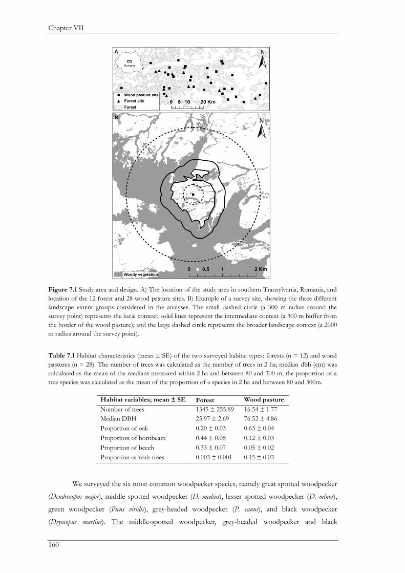
Chapter VII
160
Figure 7.1 Study area and design. A) The location of the study area in southern Transylvania, Romania, and
location of the 12 forest and 28 wood pasture sites. B) Example of a survey site, showing the three different
landscape extent groups considered in the analyses. The small dashed circle (a 300 m radius around the
survey point) represents the local context; solid lines represent the intermediate context (a 300 m buffer from
the border of the wood pasture); and the large dashed circle represents the broader landscape context (a 2000
m radius around the survey point).
Table 7.1 Habitat characteristics (mean ± SE) of the two surveyed habitat types: forests (n = 12) and wood
pastures (n = 28). The number of trees was calculated as the number of trees in 2 ha; median dbh (cm) was
calculated as the mean of the medians measured within 2 ha and between 80 and 300 m; the proportion of a
tree species was calculated as the mean of the proportion of a species in 2 ha and between 80 and 300m.
We surveyed the six most common woodpecker species, namely great spotted woodpecker
(Dendrocopos major), middle spotted woodpecker (D. medius), lesser spotted woodpecker (D. minor),
green woodpecker (Picus viridis), grey-headed woodpecker (P. canus), and black woodpecker
(Dryocopus martius). The middle-spotted woodpecker, grey-headed woodpecker and black
Habitat variables; mean ± SE Forest Wood pasture
Number of trees 1345 ± 255.89 16.54 ± 1.77
Median DBH 25.97 ± 2.69 76.52 ± 4.86
Proportion of oak 0.20 ± 0.03 0.63 ± 0.04
Proportion of hornbeam 0.44 ± 0.05 0.12 ± 0.03
Proportion of beech 0.33 ± 0.07 0.05 ± 0.02
Proportion of fruit trees 0.003 ± 0.001 0.15 ± 0.03
Woodpeckers in wood pastures
161
woodpecker are protected under the EU Birds Directive Annex I. We did not include the Syrian
woodpecker (Dendrocopos syriacus) and white-backed woodpecker (Dendrocopos leucotos) into our study
because they are very rare in our study area, and we did not encounter these species during our
surveys. We used unlimited point counts enhanced by the use of playbacks of woodpecker
drummings and/or calls with an audible range of approximately 150 m. Following 5 minutes of
initial listening, playbacks were used in a sequence from smallest to largest species (Kumar & Singh
2010). For each species, a sequence of drummings and/or calls was played three times for 15
seconds, with 15 seconds of silence between playbacks and 1.5 minutes of silence between species.
All sites were surveyed three times during appropriate weather conditions between 10 March and 6
April 2012.
To characterize the structure of sites, we recorded the species and diameter at breast height
(dbh) of: (1) within 80 m of the survey point (= 2 ha), all trees in wood pastures (1 to 34 trees) or
50 trees in forests (selected randomly in a spiral from the survey point to the edge of 2 ha); and (2)
in four strip transects of 10 m width between 80 and 300 m from the survey point in the four
cardinal directions (N, S, E, W). In case that no or too few trees were found on a transect we
measured between one and four trees close to the transect. For forest sites, we estimated tree
density in 2 ha by doubling the count of all trees in two opposite quarters of a 2 ha circle; in wood
pastures we counted all trees within 2 ha around the survey point.
All analyses were performed on presence/absence data, pooled across the three repeats,
and implemented in the ‘R’ environment (R Development Core Team 2013). First, we assessed
differences in woodpecker species composition and the number of species between forest sites and
wood pastures. We conducted nonmetric multi-dimensional scaling based on Sørensen dissimilarity
to assess the differences in woodpecker composition between forests and wood pastures using the
R package ‘Vegan’. We used analysis of similarity (ANOSIM; Sørensen dissimilarities) with 1000
permutations to test for differences in woodpecker composition between forests and wood
pastures. In a last step, we modelled the number of woodpecker species as a function of site type
using a generalized linear model with Poisson error structure. Although using playbacks and three
repeat surveys presumably decreased the incidence of false absences, they cannot be ruled out. This
is especially the case for the species that were relatively uncommon (number of times a species was
observed at least twice compared to total number of sites present: great spotted woodpecker:
21/33; middle spotted woodpecker: 7/15; lesser spotted woodpecker: 1/9; grey-headed
woodpecker: 9/22; green woodpecker: 23/30; black woodpecker: 4/10). Importantly, however, we
are confident that detectability did not differ between forests and wood pastures. Potential
differences in visibility between forests and wood pastures were of minor importance because: (1)
most woodpeckers were identified using calls; and (2) trees did not yet have leaves and visibility in
forests was therefore good.
Second, we assessed which features of a wood pasture were important for different species
of woodpeckers. The response of the three species protected under the EU Birds Directive to
Chapter VII
162
environmental variables was analysed using generalized linear models with a binomial error
structure. We did not include the forest sites in these analyses because their habitat characteristics
were very different from wood pastures (Table 7.1), and we were specifically interested in which
features of wood pastures affected woodpecker occurrence. We did not analyse the three
unprotected species because they occurred too rarely or too frequently to be modelled (site
occurrence of great spotted woodpecker: 23/28; green woodpecker: 26/28; lesser spotted
woodpecker: 5/28)
We hypothesized that different site-specific and landscape variables might influence
woodpecker presence, and we therefore grouped our explanatory variables as follows: local context
(L) represented by a circle with a 300 m radius around a site; intermediate context (I) represented as
an irregular buffer of 300 m around a particular wood pasture; and broader landscape context (B)
represented by a circle with a 2000 m radius around a site (Fig. 7.1b). Scales were selected both to
match the scale of the wood pastures and to be ecologically meaningful to woodpeckers.
Local variables included the proportion of oak, median dbh, and percent woody vegetation
cover. Woodpeckers generally prefer older trees for nesting, with several species showing a
particular preference for oak (Kosiński & Kempa 2007; Barrientos 2010). Proportion of oak was
estimated by calculating the mean of the proportion of oak in 2 ha and between 80 and 300 m, and
median dbh was estimated by calculating the mean of the median diameters measured within 2 ha
and between 80 and 300 m. Percent woody vegetation was derived from a supervised classifications
of the panchromatic channels of SPOT 5 data (©CNES 2007, Distribution Spot Image SA) using a
support vector machine algorithm (Knorn et al. 2009).
Intermediate context variables were related to specific structures of the wood pasture and
included the area of the wood pasture and percent woody vegetation cover within a 300 m buffer
from the edge of the wood pasture (as a measure of how much of the perimeter of a given wood
pasture was adjacent to forest). Adjacency to forest cover was considered important because it may
positively or negatively affect the use of wood pastures by woodpeckers.
Landscape variables related to compositional heterogeneity and terrain ruggedness within a
radius of 2000 m around the survey point. This radius corresponds to the approximate average
valley width of the study area. Birds occurring in farmland mosaics have been observed to respond
strongly to landscape heterogeneity (Benton et al. 2003). Compositional heterogeneity was
calculated as the standard deviation of the monochromatic channel of SPOT 5 data (©CNES 2007,
Distribution Spot Image SA). Terrain ruggedness was calculated as the standard deviation of the
elevation. It indicated the geomorphology of the surrounding landscape, and also functioned as a
proxy for forest cover because highly rugged landscapes tended to be densely forested.
Prior to modelling we log transformed percent woody vegetation within 300 m of the
survey point, as well as area of the wood pasture; we standardized all variables by subtracting their
mean and dividing by their standard deviation; and we confirmed that variables were not correlated.
We then used an information theoretic approach for model selection to identify models that best
Woodpeckers in wood pastures
163
explained woodpecker presence (Burnham & Anderson 2002). We constructed eight alternative
candidate models arising from all possible combinations of the three groups of variables (I, I+L,
I+B, I+L+B, L, L+B, B) and the null model. We used the R package ‘AICmodavg’ to rank the
candidate models, based on AICc values to account for small-sample bias (Burnham & Anderson
2002). Models considered best had an AICc difference (∆AICc) of less than two from the model
with the lowest AICc.
Results
We found differences in species composition between wood pastures and forests in the ordination
and the analysis of similarity (NMDS: two axes, stress = 15.1, see Fig. 7.2; ANOSIM: R = 0.141, P
= 0.009). The R-statistic from the analysis of similarity was only slightly larger than zero indicating
that compositional dissimilarity between groups was only slightly larger than within groups. Only
two species showed a clear habitat preference: the green woodpecker for wood pastures and the
lesser spotted woodpecker for forests (Fig. 7.2). The number of species ranged from two to six in
wood pastures, and from zero to four in forests. The mean number of species did not differ
significantly between wood pastures (mean: 3.14 ± 0.25) and forests (mean: 2.58 ±0.38) (GLM, z =
0.91, P = 0.34).
We detected the middle-spotted woodpecker in 11, the grey-headed woodpecker in 16, and
the black woodpecker in 7 of our 28 wood pasture sites. The best ranked models for individual
species included the intermediate context group and the null model for the middle spotted
woodpecker, and the intermediate context and broader landscape context groups for the grey-
headed woodpecker (Table 7.2). Within the intermediate context, the amount of woody vegetation
within 300 m from the edge of the wood pasture (i.e. a proxy of the amount of perimeter that was
forested) had the largest effect on both species, with both responding positively to a more forested
perimeter (Table 7.3). For the black woodpecker only the null model was selected as the best-
ranked model (Table 7.2).
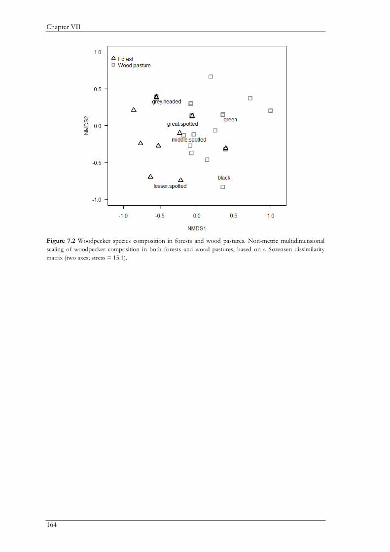
Chapter VII
164
Figure 7.2 Woodpecker species composition in forests and wood pastures. Non-metric multidimensional
scaling of woodpecker composition in both forests and wood pastures, based on a Sørensen dissimilarity
matrix (two axes; stress = 15.1).
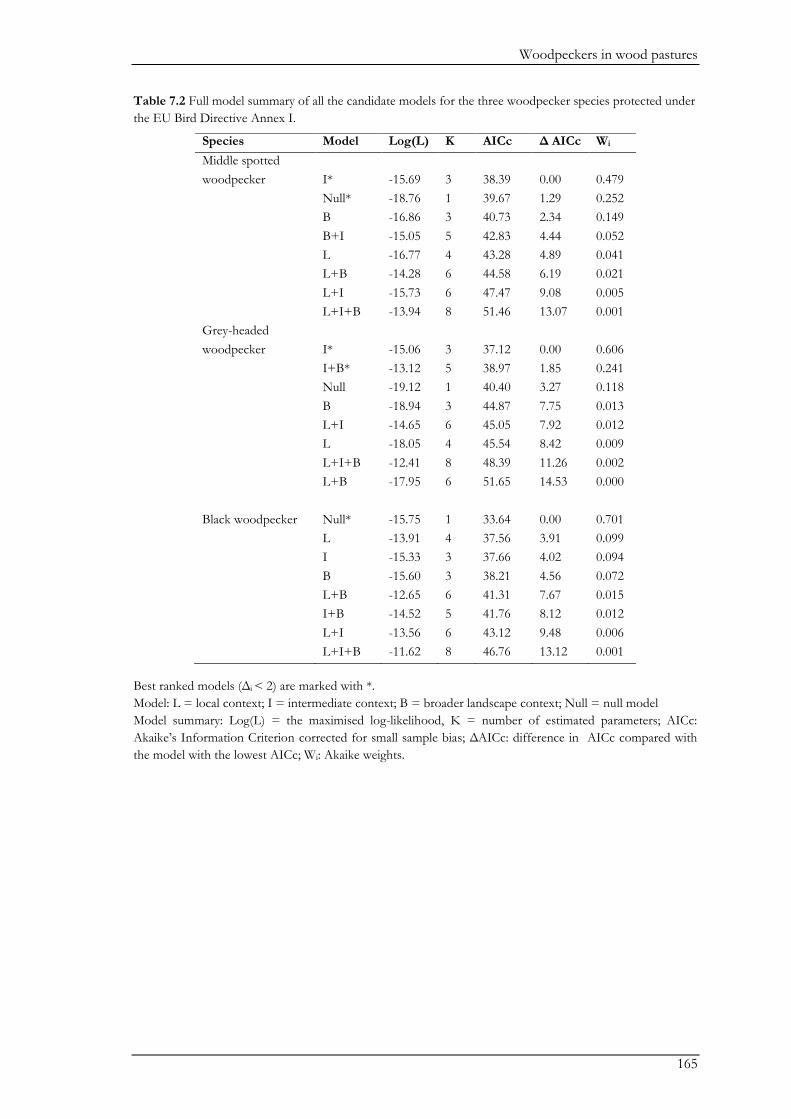
Woodpeckers in wood pastures
165
Table 7.2 Full model summary of all the candidate models for the three woodpecker species protected under
the EU Bird Directive Annex I.
Best ranked models (Δi < 2) are marked with *. Model: L = local context; I = intermediate context; B = broader landscape context; Null = null model
Model summary: Log(L) = the maximised log-likelihood, K = number of estimated parameters; AICc:
Akaike’s Information Criterion corrected for small sample bias; ΔAICc: difference in AICc compared with
the model with the lowest AICc; Wi: Akaike weights.
Species Model Log(L) K AICc Δ AICc Wi
Middle spotted
woodpecker I* -15.69 3 38.39 0.00 0.479
Null* -18.76 1 39.67 1.29 0.252
B -16.86 3 40.73 2.34 0.149
B+I -15.05 5 42.83 4.44 0.052
L -16.77 4 43.28 4.89 0.041
L+B -14.28 6 44.58 6.19 0.021
L+I -15.73 6 47.47 9.08 0.005
L+I+B -13.94 8 51.46 13.07 0.001
Grey-headed
woodpecker I* -15.06 3 37.12 0.00 0.606
I+B* -13.12 5 38.97 1.85 0.241
Null -19.12 1 40.40 3.27 0.118
B -18.94 3 44.87 7.75 0.013
L+I -14.65 6 45.05 7.92 0.012
L -18.05 4 45.54 8.42 0.009
L+I+B -12.41 8 48.39 11.26 0.002
L+B -17.95 6 51.65 14.53 0.000
Black woodpecker Null* -15.75 1 33.64 0.00 0.701
L -13.91 4 37.56 3.91 0.099
I -15.33 3 37.66 4.02 0.094
B -15.60 3 38.21 4.56 0.072
L+B -12.65 6 41.31 7.67 0.015
I+B -14.52 5 41.76 8.12 0.012
L+I -13.56 6 43.12 9.48 0.006
L+I+B -11.62 8 46.76 13.12 0.001
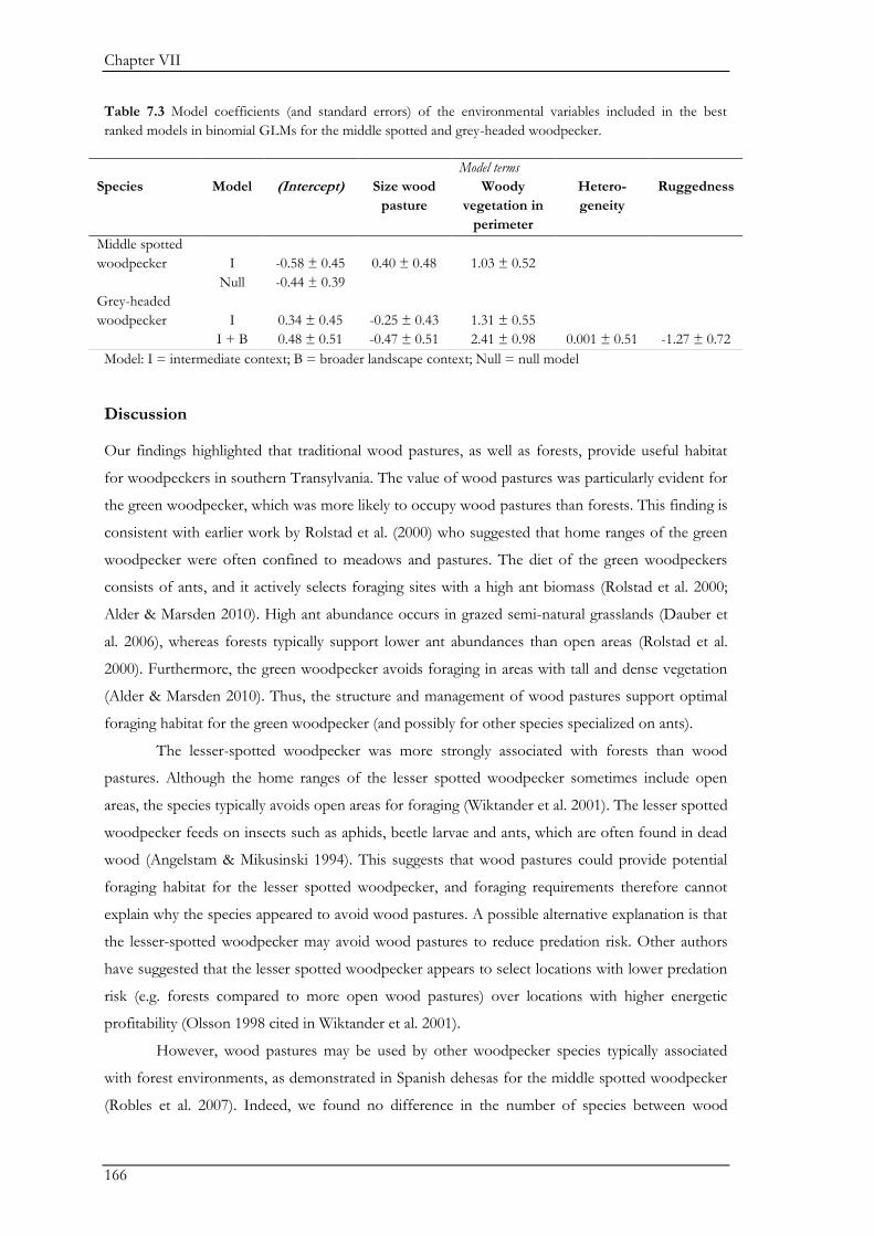
Chapter VII
166
Table 7.3 Model coefficients (and standard errors) of the environmental variables included in the best
ranked models in binomial GLMs for the middle spotted and grey-headed woodpecker.
Model: I = intermediate context; B = broader landscape context; Null = null model
Discussion
Our findings highlighted that traditional wood pastures, as well as forests, provide useful habitat
for woodpeckers in southern Transylvania. The value of wood pastures was particularly evident for
the green woodpecker, which was more likely to occupy wood pastures than forests. This finding is
consistent with earlier work by Rolstad et al. (2000) who suggested that home ranges of the green
woodpecker were often confined to meadows and pastures. The diet of the green woodpeckers
consists of ants, and it actively selects foraging sites with a high ant biomass (Rolstad et al. 2000;
Alder & Marsden 2010). High ant abundance occurs in grazed semi-natural grasslands (Dauber et
al. 2006), whereas forests typically support lower ant abundances than open areas (Rolstad et al.
2000). Furthermore, the green woodpecker avoids foraging in areas with tall and dense vegetation
(Alder & Marsden 2010). Thus, the structure and management of wood pastures support optimal
foraging habitat for the green woodpecker (and possibly for other species specialized on ants).
The lesser-spotted woodpecker was more strongly associated with forests than wood
pastures. Although the home ranges of the lesser spotted woodpecker sometimes include open
areas, the species typically avoids open areas for foraging (Wiktander et al. 2001). The lesser spotted
woodpecker feeds on insects such as aphids, beetle larvae and ants, which are often found in dead
wood (Angelstam & Mikusinski 1994). This suggests that wood pastures could provide potential
foraging habitat for the lesser spotted woodpecker, and foraging requirements therefore cannot
explain why the species appeared to avoid wood pastures. A possible alternative explanation is that
the lesser-spotted woodpecker may avoid wood pastures to reduce predation risk. Other authors
have suggested that the lesser spotted woodpecker appears to select locations with lower predation
risk (e.g. forests compared to more open wood pastures) over locations with higher energetic
profitability (Olsson 1998 cited in Wiktander et al. 2001).
However, wood pastures may be used by other woodpecker species typically associated
with forest environments, as demonstrated in Spanish dehesas for the middle spotted woodpecker
(Robles et al. 2007). Indeed, we found no difference in the number of species between wood
Model terms
Species Model (Intercept) Size wood
pasture
Woody
vegetation in
perimeter
Hetero-
geneity
Ruggedness
Middle spotted
woodpecker I -0.58 ± 0.45 0.40 ± 0.48 1.03 ± 0.52
Null -0.44 ± 0.39
Grey-headed
woodpecker I 0.34 ± 0.45 -0.25 ± 0.43 1.31 ± 0.55
I + B 0.48 ± 0.51 -0.47 ± 0.51 2.41 ± 0.98 0.001 ± 0.51 -1.27 ± 0.72
Woodpeckers in wood pastures
167
pastures and forests, and all three woodpecker species protected by the EU Bird Directive Annex I
(and typically considered to be forest-associated) were present in both types of sites.
Surprisingly, environmental variables at different spatial scales had little effect on the
presence of protected woodpecker species. The only environmental variable positively related to
the presence of two species was surrounding forest cover (especially evident for the grey-headed
woodpecker; Table 7.3). The grey-headed woodpecker may preferentially occupy forest stands
containing beech (Shurulinkov et al. 2012), which in our study area more frequently occurred in
forests rather than wood pastures. It is possible, therefore, that the grey-headed woodpecker selects
nest sites in beech trees within forest patches (Kosiński & Kempa 2007) but uses nearby wood
pastures for foraging. We observed the grey-headed woodpecker twice or more in only 9 out of the
22 sites in which it was ultimately detected, which may support the notion that it uses wood
pastures for foraging rather than breeding. The grey-headed woodpecker forages on ants, although
it is less specialized compared to the green woodpecker (Angelstam & Mikusinski 1994) – it is
primarily a ground feeder when the ground is free of snow or forages on bark-dwelling insects on
dead trees during winter (Rolstad & Rolstad 1995). While it appears that wood pastures should
provide good foraging habitat for the grey-headed woodpecker, data on breeding locations would
be required to further scrutinize this explanation of occurrence patterns.
Similarly to the grey-headed woodpecker, the black woodpecker also may preferentially
select beech trees for nesting (Kosiński & Kempa 2007), and its diet also includes ants (Angelstam
& Mikusinski 1994). However, the black woodpecker is likely to use the landscape at a different
spatial scale compared to the other two species. It moves over larger areas (Tjernberg et al. 1993)
and the intermediate spatial scale chosen in our study may have been too small for this species to
show an effect of adjacent forest cover.
Local vegetation structure, including the availability of large trees, is known to influence
woodpecker presence elsewhere (e.g. Pasinelli 2000). The lack of association of woodpecker species
with local variables in our study may reflect that wood pastures contain enough old trees to provide
critical habitat elements such as dead wood and food resources (Angelstam & Mikusinski 1994) -
the amount of old-growth elements thus apparently did not limit woodpecker distribution.
Habitat fragmentation by loss of forests has been hypothesized to be one of the major
causes of forest bird declines (Robinson et al. 1995). Because woodpeckers have large home ranges,
they may be highly sensitive to forest fragmentation (Pettersson 1985; Wiktander et al. 1992).
Given the widespread occurrence of woodpeckers throughout our study area, our results suggest
that woodpeckers are likely to perceive the landscape as largely unfragmented: (1) we found no
difference in the number of species between forests and wood pastures; and (2) environmental
variables such as ruggedness (a proxy for landscape level forest cover) had little effect on the three
threatened woodpecker species. Broad-leaved forest cover in our study area is approximately 42%,
and existing evidence suggests that fragmentation effects becomes severe only well below this
threshold (Tjernberg et al. 1993; Andrén 1994; Wiktander et al. 2001). For example, the black
Chapter VII
168
woodpecker was largely insensitive to fragmentation in a highly fragmented landscape with only
26% of forest cover (Tjernberg et al. 1993). Moreover, scattered trees are available throughout the
agricultural mosaic, very likely providing effective functional connectivity between forest patches
(Manning et al. 2006). Because we lack information on reproductive performance of woodpeckers
in wood pastures compared to forests, we cannot make inferences about the quality of wood
pastures as breeding habitat for woodpeckers. Nevertheless, our results suggest that wood pastures
provide important feeding habitat for woodpeckers and probably provide connectivity between
different forest patches.
Conservation implications
Despite their high cultural and natural values, wood pastures are declining rapidly throughout
Europe (Bergmeier et al. 2010). Considering their important values for a range of species (Taboada
et al. 2006; Paltto et al. 2011; Robles et al. 2011; Horák & Rébl 2013), the conservation of wood
pastures should be addressed in relevant policies and directives. For woodpecker conservation
specifically, we recommend that conservation policies focus not only on maintaining mature forests
but also recognize the complementary value of wood pastures that have retained old-growth
structures. There are a few national conservation policies for wood pastures (e.g. Goldberg et al.
2007), but to date there is no pan-European conservation policy (Bergmeier et al. 2010).
To improve the conservation status of European wood pastures we suggest they should be
considered explicitly in two major EU policies: (1) the EU Habitats Directive; and (2) the EU
Common Agricultural Policy, specifically with respect to agri-environment payments. Currently,
wood pastures are inconsistently considered in the EU Habitats Directive, and the Directive does
not include Romanian wood pastures (Bergmeier et al. 2010). Although the ecological effect of
some agri-environment payments is still debated (Kleijn et al. 2006), when appropriately targeted,
they can provide a useful tool for farmland biodiversity conservation (Donald & Evans 2006). In
many member states of the EU, agri-environment payments exist for management of extensive
pastures, which typically provide subsidies for clearing woody vegetation to maintain extensive
grassland environments. However, such payments may inadvertently pose a threat to wood
pastures, because scattered tress can fall victim to the clearing process (legally or accidentally, pers.
obs.; (Blom 2012)). More carefully specified agri-environment schemes could stimulate the
conservation of trees in extensively managed pastures, thereby recognizing their keystone role for a
wide range of organisms (Manning et al. 2006).
Acknowledgements
We thank Arpad Szapanyos and Anne-Catherine Klein for their tremendous effort in the field. We
thank Patrick Griffiths, Jan Knorn and Tobias Kümmerle for their help with creating the woody
vegetation layer. We thank four anonymous reviewers for constructive suggestions on a previous
draft of this manuscript.

169
Chapter VIII

170
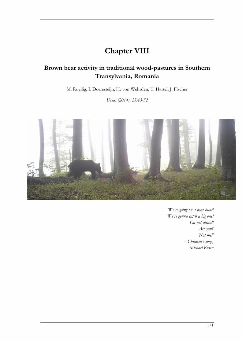
171
Chapter VIII
Brown bear activity in traditional wood-pastures in Southern
Transylvania, Romania
M. Roellig, I. Dorresteijn, H. von Wehrden, T. Hartel, J. Fischer
Ursus (2014), 25:43-52
‘We're going on a bear hunt!
We're gonna catch a big one!
I'm not afraid!
Are you?
Not me!’
– Children’s song,
Michael Rosen

Chapter VIII
172
Brown bear activity in wood pastures
173
Abstract
During the past century, habitat fragmentation and increased human impacts have reduced
populations of large carnivores throughout the world. Although bears have been extirpated from
human-dominated landscape in most parts of Europe, they still occur in multiuse cultural
landscapes in Southern Transylvania, Romania. Wood-pastures - grazed permanent grasslands with
scattered or clumped trees and shrubs - are important elements of these cultural landscapes and
provide habitat for a wide range of species. However, wood-pastures are under threat from land-
use change, including intensified agricultural use and land abandonment. In 2012 we assessed the
level of activity of brown bears (Ursus arctos) and environmental factors influencing bear activity in
54 wood-pastures in Southern Transylvania. As an index of bear activity, we measured the
proportion of anthills that were destroyed by bears. The variables were combined in 3 groups
(anthropogenic effects, local variables, and landscape context) to test which group most strongly
influenced bear activity. Bear activity was found in 47 (87%) wood-pastures. Bear activity was best
explained by variables describing the landscape context, with proximity to the Carpathian
Mountains, terrain ruggedness, and amount of surrounding woody vegetation positively related to
bear activity. Local variables (distance to forest edge and anthill density) had no effect, and
surprisingly, variables related to anthropogenic features (distance to major roads, distance to
villages) were positively related to bear activity (albeit weakly). Most of the wood-pastures in
Southern Transylvania were used by bears for foraging on ant larvae. For the conservation of
brown bears in Southern Transylvania, it is important to maintain large areas of forest but also
consider cultural landscape elements such as wood-pastures. To conserve European wood-
pastures, we suggest they be explicitly considered in national nature conservation policies and in
major European Union (EU) policies such as the EU Habitats Directive.
Chapter VIII
174
Introduction
Habitat fragmentation and increased human impact have reduced populations of large carnivores
throughout the world (Breitenmoser 1998; Woodroffe 2000). The brown bear (Ursus arctos) is
Europe’s largest carnivore, but has been displaced from human-dominated landscapes in most
parts of Europe (Swenson et al. 1995; Zedrosser et al. 2011; Kopatz et al. 2012). Most remaining
populations are confined to mountainous regions and heavily depend on major conservation
efforts (Swenson et al. 2000; Zedrosser et al. 2001). Thus, the need to protect the brown bear in
Europe remains a priority (Zedrosser et al. 2011; Krofel et al. 2012), even though the species has
been listed in Annex II and Annex IV of the European Union (EU) Habitats Directive
(92/43/EEC) since 1992. Although bear populations are now increasing in some areas (Zedrosser
et al. 2011), agricultural intensification and habitat fragmentation, resource extraction, road
development, recreation development, and urban expansion still threaten Europe’s remaining bear
populations (Swenson et al. 1995; Breitenmoser 1998; Zedrosser et al. 2001).
Romania has the largest national brown bear population in Europe (excluding Russia;
Chestin 1999; Spassov & Spiridonov 1999), estimated by the International Union for Conservation
of Nature, to be stable at approximately 6,000 individuals (Huber 2007). In Transylvania, bears
occur not only in large forest patches, but also in multi-use cultural landscapes. However, potential
landscape changes such as intensified agriculture, deforestation, and planned new highways could
negatively affect Transylvania’s bear population (Swenson et al. 2000; Ministry of Agriculture
Forestry and Rural Development and the Ministry of Environment and Water Management
[MAPDR and MMGA] 2005).
Changes in land-use also pose a major threat in multi-use cultural landscapes such as the
traditional grazing systems of wood-pastures (Plieninger 2007; Bergmeier et al. 2010). Wood-
pastures are grazed permanent grasslands with scattered trees and shrubs or with groups of trees
and shrubs, and important elements of cultural landscapes in Europe (Bergmeier et al. 2010).
Wood-pastures are used by a wide range of species, including many threatened species (Tucker &
Evans 1997; Wegener 1998; Olea & San Miguel-Ayanz 2006; Bergmeier et al. 2010; Dorresteijn et
al. 2013). Plants, invertebrates, and birds are the most commonly studied species in wood-pastures
but, apart from some publications mentioning use of the Spanish dehesas by Iberian lynx (Lynx
pardinus; Olea & San Miguel-Ayanz 2006; Bergmeier et al. 2010), relatively little is known about the
use of wood-pastures by large carnivores. To our knowledge, this is the first ecological study
focusing on the use of wood-pastures by large carnivores.
Wood-pastures in Southern Transylvania (Fig. 8.1) are generally open, with a density of
approximately 8 trees/ha (Hartel et al. 2013). Some wood-pastures are surrounded by forest, while
others are situated within open pastures or, more rarely, arable fields. Wood-pastures in Southern
Transylvania are mainly grazed by sheep, cattle, and sometimes goats and buffalos in moving herds.
The main tree species are oak (Quercus spp.) and beech (Fagus sylvatica), but also fruit trees such as
wild pear (Pyrus silvestris) and hornbeam (Carpinus betulus). Characteristic shrub species are hawthorn
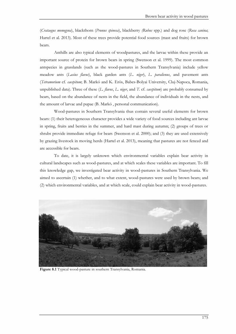
Brown bear activity in wood pastures
175
(Crataegus monogyna), blackthorn (Prunus spinosa), blackberry (Rubus spp.) and dog rose (Rosa canina;
Hartel et al. 2013). Most of these trees provide potential food sources (mast and fruits) for brown
bears.
Anthills are also typical elements of woodpastures, and the larvae within these provide an
important source of protein for brown bears in spring (Swenson et al. 1999). The most common
antspecies in grasslands (such as the wood-pastures in Southern Transylvania) include yellow
meadow ants (Lasius flavus), black garden ants (L. niger), L. paralienus, and pavement ants
(Tetramorium cf. caespitum; B. Markó and K. Erös, Babes-Bolyai University, Cluj-Napoca, Romania,
unpublished data). Three of these (L. flavus, L. niger, and T. cf. caespitum) are probably consumed by
bears, based on the abundance of nests in the field, the abundance of individuals in the nests, and
the amount of larvae and pupae (B. Markó , personal communication).
Wood-pastures in Southern Transylvania thus contain several useful elements for brown
bears: (1) their heterogeneous character provides a wide variety of food sources including ant larvae
in spring, fruits and berries in the summer, and hard mast during autumn; (2) groups of trees or
shrubs provide immediate refuge for bears (Swenson et al. 2000); and (3) they are used extensively
by grazing livestock in moving herds (Hartel et al. 2013), meaning that pastures are not fenced and
are accessible for bears.
To date, it is largely unknown which environmental variables explain bear activity in
cultural landscapes such as wood-pastures, and at which scales these variables are important. To fill
this knowledge gap, we investigated bear activity in wood-pastures in Southern Transylvania. We
aimed to ascertain (1) whether, and to what extent, wood-pastures were used by brown bears; and
(2) which environmental variables, and at which scale, could explain bear activity in wood-pastures.
Figure 8.1 Typical wood-pasture in southern Transylvania, Romania.
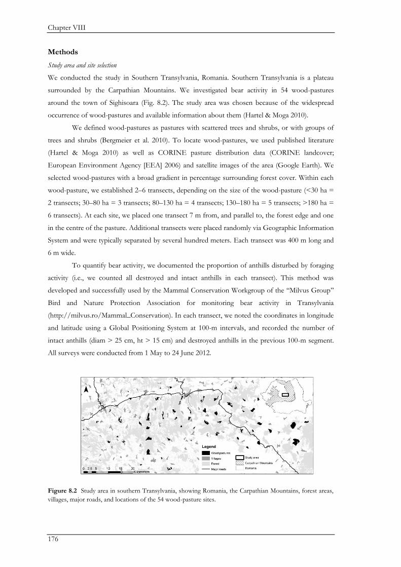
Chapter VIII
176
Methods
Study area and site selection
We conducted the study in Southern Transylvania, Romania. Southern Transylvania is a plateau
surrounded by the Carpathian Mountains. We investigated bear activity in 54 wood-pastures
around the town of Sighisoara (Fig. 8.2). The study area was chosen because of the widespread
occurrence of wood-pastures and available information about them (Hartel & Moga 2010).
We defined wood-pastures as pastures with scattered trees and shrubs, or with groups of
trees and shrubs (Bergmeier et al. 2010). To locate wood-pastures, we used published literature
(Hartel & Moga 2010) as well as CORINE pasture distribution data (CORINE landcover;
European Environment Agency [EEA] 2006) and satellite images of the area (Google Earth). We
selected wood-pastures with a broad gradient in percentage surrounding forest cover. Within each
wood-pasture, we established 2–6 transects, depending on the size of the wood-pasture (<30 ha =
2 transects; 30–80 ha = 3 transects; 80–130 ha = 4 transects; 130–180 ha = 5 transects; >180 ha =
6 transects). At each site, we placed one transect 7 m from, and parallel to, the forest edge and one
in the centre of the pasture. Additional transects were placed randomly via Geographic Information
System and were typically separated by several hundred meters. Each transect was 400 m long and
6 m wide.
To quantify bear activity, we documented the proportion of anthills disturbed by foraging
activity (i.e., we counted all destroyed and intact anthills in each transect). This method was
developed and successfully used by the Mammal Conservation Workgroup of the ‘‘Milvus Group’’
Bird and Nature Protection Association for monitoring bear activity in Transylvania
(http://milvus.ro/Mammal_Conservation). In each transect, we noted the coordinates in longitude
and latitude using a Global Positioning System at 100-m intervals, and recorded the number of
intact anthills (diam > 25 cm, ht > 15 cm) and destroyed anthills in the previous 100-m segment.
All surveys were conducted from 1 May to 24 June 2012.
Figure 8.2 Study area in southern Transylvania, showing Romania, the Carpathian Mountains, forest areas,
villages, major roads, and locations of the 54 wood-pasture sites.
Brown bear activity in wood pastures
177
Environmental variables
Bears are known to react to both human activity (e.g. Clevenger et al. 1992; Nellemann et al. 2007;
May et al. 2008) and environmental conditions (Slobodyan 1974; Swenson et al. 2000), and we
assumed based on their large range size (Preatoni et al. 2005) that they are sensitive to multiple
spatial scales. Therefore, to investigate which combination of variables best explained bear activity
in wood-pastures, we grouped our explanatory variables as follows: (1) anthropogenic variables
(AV), (2) local variables (LV), and (3) variables describing the (broader) landscape context (LC).
Each of the variables was calculated based on the midpoints of each 100-m segment.
We used anthropogenic variables to describe disturbance, measured as the shortest
distance to village limits and major roads, based on each midpoint. For local variables, we estimated
the proportion of woody vegetation cover within a 300-m-radius circle and measured the distance
to forest edge (using CORINE forest data from 2006 [EEA 2006]), as a proxy for distance to
shelter, from each segment’s middle point. We also accounted for possible effects of the total
number of anthills/100 m by including them as a local variable, because bears might be more
attracted to pastures with more anthills. Finally, landscape-context variables included woody
vegetation cover and terrain ruggedness within a 3-km radius around each segment’s midpoint, as
well as distance to the Carpathian Mountains, measured from each segment’s midpoint to the edge
of the Carpathian Mountains. Both woody vegetation cover and ruggedness may be important with
respect to the availability of sheltering habitat and a wider variety of food for bears. Woody
vegetation and distance to the Carpathian Mountains may be important for connectivity to a larger
(source) population and to dens at the higher altitudes. We derived woody vegetation from a
supervised classification of the monochromatic channels of SPOT 5 data (ECNES 2007;
Distribution Spot Image SA, Toulouse, France) using a support vector machine algorithm (Knorn
et al. 2009). We calculated terrain ruggedness as the standard deviation of the elevation (Advanced
Spaceborne Thermal Emission and Reflection Radiometer [ASTER] Global Digital Elevation
Model Version 2 [GDEM V2]; Land Processes Distribution Active Archive Center, Sioux Falls,
South Dakota, USA).
Modelling bear activity
As an index of bear activity, we quantified the proportion of destroyed anthills relative to the total
number of anthills in each 100-m segment of each transect. The resulting data structure therefore
was nested, with 4 segments/transect, and several transects per site (i.e., pasture). Thus, we
modelled activity at the transect level to simplify the structure of random effects to 2 nested levels
(transect/site). We used a binomial error distribution for the response data. All statistical analyses
were implemented in the R environment (R Development Core Team 2013), and generalized linear
mixed models were fitted using the package ‘lme4’ (Bates et al. 2014).
To account for the nested data structure, we initially included site as a random intercept in
the model, while in a second model we accounted for potential changes in activity over time by
Chapter VIII
178
including Julian date as a random slope. Using both date and site as random factors at the same
time was not meaningful because they were redundant, meaning each site was sampled on a specific
date. Because site explained a greater amount of variance and arrived at more parsimonious models
based on initial Akaike Information Criterion (AIC) comparisons, we used the model that included
site only as a random intercept.
Distance to forest and anthill density were strongly skewed; therefore, we log-transformed
these variables before modelling. Furthermore, we standardized all predictors by subtracting their
mean and dividing by their standard deviation to make the estimates comparable. Because of a
strong correlation between distance to forest edge and woody vegetation within a 300-m-radius
circle (Spearman rank correlation; r = -0.68), we removed woody vegetation from the group of
local variables.
We used an information theoretic approach for model selection to identify models that
best explained bear activity (Burnham & Anderson 2002). We constructed 7 alternative candidate
models, which considered all possible combinations of the 3 groups of variables (AV, LV, LC). We
used the R package AICmodavg (Mazerolle 2012) to rank the candidate models, based on AICc
values to account for small-sample bias (Burnham & Anderson 2002). The AICc values of the best
models were compared with the AICc values of the null model (which only included the random
effects). Marginal and conditional R2 values were calculated following the procedure outlined by
Nakagawa and Schielzeth (2013), using the package ‘arm’ (Gelman et al. 2013).
Results
The size of wood-pastures ranged from approximately 11 ha to 475 ha, but most were 30 - 130 ha
(<30 ha, n = 8; 30–80 ha, n = 19; 80–130 ha, n = 15; 130–180 ha, n = 6; >180 ha, n = 6). We
surveyed 199 transects, with a mean of 3.6 transects/wood-pasture. Anthills were found in all
pastures; only 1 of the transects and 21 of the 100-m segments contained no anthills.
We detected destroyed anthills in 87% of wood-pastures and in 42% of transects. We
found 29,236 total anthills, including 1,771 destroyed anthills (6%). Within a given 100-m segment,
we recorded up to 300 anthills, and up to 127 destroyed anthills (mean total no./100 m ≈ 37; mean
destroyed/100 m ≈ 2).
Mean distance to nearest village was 2 km (range = approx. 150 m to approx. 5 km). The
distance to the major roads averaged 35 km (120 m to 100 km). The average distance to the
Carpathian Mountains was 30 km (11 - 64 km) and average distance to forest edge was 0.2 km (7 m
to 1.8 km). The woody vegetation cover within 3,000 m averaged 44% (7% - 84%). Terrain
ruggedness averaged 57 m (32 - 105 m). All models including explanatory variables performed
better than the null model (Table 8.1). The best supported model (wi = 0.66) included
anthropogenic variables (AV) and landscape context variables (LC). Despite the low difference in
AIC values (<2) between the best supported and the second-ranked model, we selected the most
parsimonious one (i.e., containing AV and LC), because the contribution of the third group of
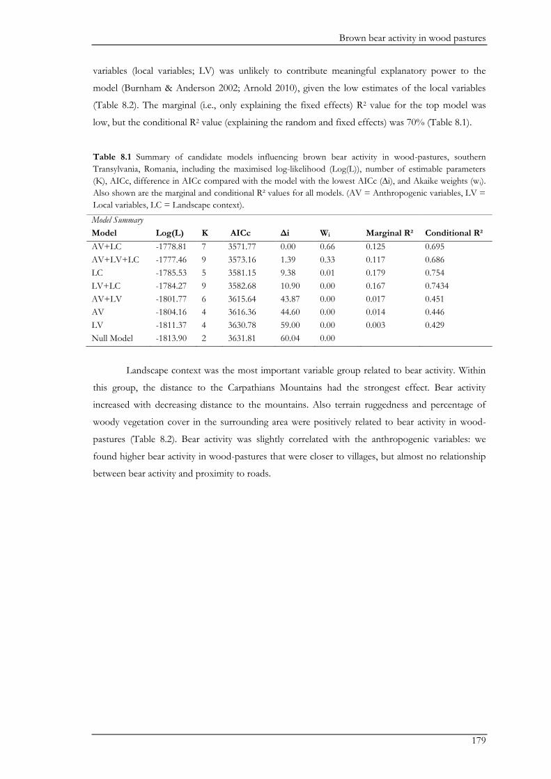
Brown bear activity in wood pastures
179
variables (local variables; LV) was unlikely to contribute meaningful explanatory power to the
model (Burnham & Anderson 2002; Arnold 2010), given the low estimates of the local variables
(Table 8.2). The marginal (i.e., only explaining the fixed effects) R2 value for the top model was
low, but the conditional R2 value (explaining the random and fixed effects) was 70% (Table 8.1).
Table 8.1 Summary of candidate models influencing brown bear activity in wood-pastures, southern
Transylvania, Romania, including the maximised log-likelihood (Log(L)), number of estimable parameters
(K), AICc, difference in AICc compared with the model with the lowest AICc (∆i), and Akaike weights (w i).
Also shown are the marginal and conditional R² values for all models. (AV = Anthropogenic variables, LV =
Local variables, LC = Landscape context).
Landscape context was the most important variable group related to bear activity. Within
this group, the distance to the Carpathians Mountains had the strongest effect. Bear activity
increased with decreasing distance to the mountains. Also terrain ruggedness and percentage of
woody vegetation cover in the surrounding area were positively related to bear activity in wood-
pastures (Table 8.2). Bear activity was slightly correlated with the anthropogenic variables: we
found higher bear activity in wood-pastures that were closer to villages, but almost no relationship
between bear activity and proximity to roads.
Model Summary
Model Log(L) K AICc Δi Wi Marginal R² Conditional R²
AV+LC -1778.81 7 3571.77 0.00 0.66 0.125 0.695
AV+LV+LC -1777.46 9 3573.16 1.39 0.33 0.117 0.686
LC -1785.53 5 3581.15 9.38 0.01 0.179 0.754
LV+LC -1784.27 9 3582.68 10.90 0.00 0.167 0.7434
AV+LV -1801.77 6 3615.64 43.87 0.00 0.017 0.451
AV -1804.16 4 3616.36 44.60 0.00 0.014 0.446
LV -1811.37 4 3630.78 59.00 0.00 0.003 0.429
Null Model -1813.90 2 3631.81 60.04 0.00
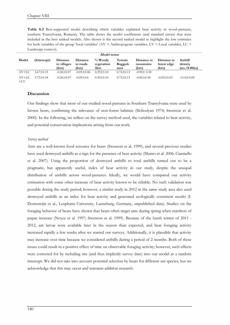
Chapter VIII
180
Table 8.2 Best-supported model describing which variables explained bear activity in wood-pastures,
southern Transylvania, Romania. The table shows the model coefficients (and standard errors) that were
included in the best ranked models. Also shown is the second ranked model to highlight the low estimates
for both variables of the group ‘local variables’ (AV = Anthropogenic variables, LV = Local variables, LC =
Landscape context).
Discussion
Our findings show that most of our studied wood-pastures in Southern Transylvania were used by
brown bears, confirming the relevance of non-forest habitats (Slobodyan 1974; Swenson et al.
2000). In the following, we reflect on the survey method used, the variables related to bear activity,
and potential conservation implications arising from our work.
Survey method
Ants are a well-known food resource for bears (Swenson et al. 1999), and several previous studies
have used destroyed anthills as a sign for the presence of bear activity (Munro et al. 2006; Ciarniello
et al. 2007). Using the proportion of destroyed anthills to total anthills turned out to be a
pragmatic, but apparently useful, index of bear activity in our study, despite the unequal
distribution of anthills across wood-pastures. Ideally, we would have compared our activity
estimation with some other measure of bear activity known to be reliable. No such validation was
possible during the study period; however, a similar study in 2012 in the same study area also used
destroyed anthills as an index for bear activity and generated ecologically consistent results (I.
Dorresteijn et al., Leuphana University, Lueneburg, Germany, unpublished data). Studies on the
foraging behavior of bears have shown that bears often target ants during spring when numbers of
pupae increase (Noyce et al. 1997; Swenson et al. 1999). Because of the harsh winter of 2011 -
2012, ant larvae were available later in the season than expected, and bear foraging activity
increased rapidly a few weeks after we started our surveys. Additionally, it is plausible that activity
may increase over time because we considered anthills during a period of 2 months. Both of these
issues could result in a positive effect of time on observable foraging activity; however, such effects
were corrected for by including site (and thus implicitly survey date) into our model as a random
intercept. We did not take into account potential selection by bears for different ant species, but we
acknowledge that this may occur and warrants addition research.
Model terms
Model (Intercept) Distance to villages (km)
Distance to roads (km)
% Woody vegetation 3km
Terrain Rugged-ness
Distance to mountains (km)
Distance to forest edge (km)
Anthill density (no./0.06ha)
AV+LC 3.67±0.33 -0.26±0.07 -0.05±0.06 0.29±0.10 0.74±0.11 -0.90± 0.30
AV+LC+LV
3.72±0.34 -0.26±0.07 -0.05±0.6 0.30±0.10 0.72±0.11 -0.82±0.30 -0.02±0.03 -0.14±0.09
Brown bear activity in wood pastures
181
Variables influencing bear activity in wood-pastures
Bear activity in wood pastures was primarily driven by environmental variables at the landscape
level and to a lesser extent by anthropogenic variables. The importance of the landscape variables is
consistent with previous studies, which also identified mountainous regions (Posillico et al. 2004),
as well as rugged and forested areas, as being preferred by bears for shelter, denning sites, and food
(Clevenger et al. 1992; Preatoni et al. 2005; Nellemann et al. 2007; May et al. 2008). The relative
lack of importance of local variables was surprising because we hypothesized that distance to the
forest edge could be an important element of escape over (Swenson et al. 2000) and expected
higher bear activity closer to forests. However, the relatively small size and complex shape of many
of the studied wood-pastures may have ensured that the forest edge was generally within close
proximity. Alternatively, the structurally rich wood-pastures could have provided adequate shelter.
Anthill density also did not appear to influence bear activity; fewer anthills than were available in
our study area are potentially still sufficient in number to attract bears.
Bear occurrence has been shown to be negatively affected by human presence (Clevenger
et al. 1992; Preatoni et al. 2005; Nellemann et al. 2007; May et al. 2008). However, bear activity in
our study was slightly positively associated with the anthropogenic variables we measured. This
unexpected finding may be explained by most villages in Southern Transylvania being small and
characterized by low human density (approx. 34 inhabitants/km2; Arion et al. 2011). Elsewhere in
Europe, bears inhabit areas with human densities up to 80 people/km2 (Linnell et al. 2001). In
Scandinavia, female brown bears avoided human activity, but used human-dominated landscapes
for foraging when human density was low, especially at night (Martin et al. 2010). Such temporal
niche partitioning between humans and bears may also occur in Southern Transylvania. Major
roads were generally several kilometers from the wood-pastures we studied, which may explain
their lack of influence on bear activity.
Conservation and management implications
Although bears typically require large, relatively undisturbed areas, we showed that they also use
wood-pastures within the cultural landscapes of Southern Transylvania. This is likely because they
represent a source of protein (ants), which is critically important in the otherwise mainly vegetarian
diet of the brown bear in temperate latitudes (Bojarska & Selva 2012). Wood-pastures likely
provide fruits and hard mast as food sources for brown bears in summer and autumn, but our
investigations were confined to the spring season when ants and their larvae were most abundant
and sought after by bears.
Wood-pastures in Southern Transylvania face several threats. Land abandonment leads to
forest succession, which will eventually displace species linked to the semi-open character of wood-
pastures, including fruit trees and invertebrates such as the grassland ant species (both food sources
for bears). On the other hand, intensified agricultural use, including clearing of tree cover or
fertilization, will destroy the semi-open and semi-natural character of the wood-pastures, which is
Chapter VIII
182
also a threat to animal and plant species (Manning et al. 2006). Additional threats to wood-pastures
are illegal burning in spring, which often leads to the destruction of trees, and legal and illegal
cutting of trees. These factors, in combination with occasional overgrazing and clearing the
pastures of shrubs as part of the requirements for EU agricultural subsidies, leads to a lack of
regeneration (Hartel et al. 2013). Within Europe, some types of wood-pastures (such as the dehesas
in Spain and the Fennoscandia wooded pastures in Scandinavia) are protected under the EU
Habitats Directive, but there is no consistent conservation approach across Europe (Bergmeier et
al. 2010). A loss of Transylvania’s wood-pastures could mean the loss of some food sources for
bears, but also the loss of a buffer between forest patches and villages, which could increase
conflicts between people and bears. The protection and management of wood-pastures in Southern
Transylvania thus could make a positive contribution to bear conservation.
Finally, a critical aspect of bear conservation in Southern Transylvania is the maintenance
of a network of large and well-connected forest patches. Southern Transylvania has approximately
30% forest cover, which offers several potential corridors to nearby mountains and source
populations. We did not observe a negative effect of roads on bear use of wood-pastures.
However, other studies have shown the negative impact of highways, and newly planned major
highways could negatively impact bear activity by causing habitat fragmentation (Kaczensky et al.
2003; Karamanlidis et al. 2011). Further research is needed on the importance of connectivity of
forest patches to the mountains and how it may be affected by improvements and/or alterations to
the local road network.
Zedrosser et al. (2011) suggested that bear conservation in Europe should not be restricted
to only wild and remote areas, because few such areas remain (Linnell et al. 2005), and because
other landscape elements can provide useful complementary conservation opportunities. Our
findings suggest this is the case for our study area, where bears also use wood-pastures within
multi-use cultural landscapes.
Acknowledgements
We are deeply grateful to the team of the Milvus Mammal Conservation group, especially A.
Kecskés, H. Latková, S. Szilárd, and Z. Mezey for establishing and sharing with us the survey
method described in this paper. For creating the woody-vegetation layer we thank P. Griffiths, J.
Knorn, and T. Kümmerle. For his opinion on ant consumption by bears we thank Balint Markó.
We thank also A. Szapanyos and M. Solomon for their efforts in the field, and L. Sutcliffe for
providing language assistance and for proof reading the manuscript. Lastly we thank the
anonymous reviewers for constructive suggestions on a previous draft of this manuscript. The
project was funded by the Alexander von Humboldt Foundation through a postdoctoral fellowship
to T.H. and a Sofja Kovalevskaja Award to J.F.
183
Section C: Human-
bear coexistence
This Section includes Chapters IV (see Section A) and IX and takes a social-ecological systems
approach to understand how links between the social and ecological parts of the system affect
human-bear coexistence. Chapter IV aims to obtain an overview on human-bear conflicts in the
study region. Chapter IV also examines whether the level of perceived conflict relates to bear
activity and whether it influences attitudes of shepherds towards bears. Chapter IX aims to gain a
more holistic understanding on the social drivers shaping the willingness of people to coexist with
bears.

184

185
Chapter IX

186
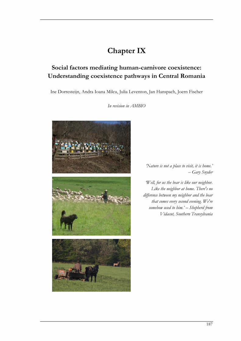
187
Chapter IX
Social factors mediating human-carnivore coexistence:
Understanding coexistence pathways in Central Romania
Ine Dorresteijn, Andra Ioana Milcu, Julia Leventon, Jan Hanspach, Joern Fischer
In revision in AMBIO
‘Nature is not a place to visit, it is home.’
– Gary Snyder
‘Well, for us the bear is like our neighbor.
Like the neighbor at home. There's no
difference between my neighbor and the bear
that comes every second evening. We're
somehow used to him.’ – Shepherd from
Vidacut, Southern Transylvania

Chapter IX
188
Drivers of human-carnivore coexistence
189
Abstract
Successful carnivore conservation depends on the degree to which humans and carnivores can
coexist. Facilitating human-carnivore coexistence does not only depend on the biophysical
environment but also on understanding the social factors that shape human-carnivore coexistence.
Focusing on Central Romania, we aimed to understand social drivers of coexistence by applying a
combined approach of questionnaires (n = 252) and inductive semi-structured interviews (n = 70)
to examine human-bear (Ursus arctos) coexistence. The majority of respondents had a positive
perception of coexistence. The questionnaires revealed general patterns on the most important
social drivers, and highlighted four distinct groups of respondents. Perceptions of coexistence were
negatively influenced by negative attitudes towards bears, past negative interactions with bears, and
perceived risks of damage. Qualitative content analysis of interviews identified three coexistence
pathways. These pathways showed different (but not mutually exclusive) ways in which ongoing
interactions between the ecological system and the social system shape the willingness of people to
coexist with bears. While the connection between humans and the landscape had important
mediating effects on perceived coexistence, the generally positive perception of coexistence could
be undermined by perceived flaws in official bear management. We suggest that the concept of
coexistence pathways, coupled with a comprehensive approach to their analysis, can help landscape
managers identify drivers that facilitate or hinder coexistence, and thus target interventions
accordingly. This conceptual framework, in turn, may help facilitate human-carnivore coexistence
worldwide.
Chapter IX
190
Introduction
Where humans and large carnivores share the same landscape, there are inevitable conflicts:
humans experience attacks and predation on livestock, with resultant economic impacts (Thirgood
et al. 2005; Holmern et al. 2007); and carnivore populations decline as a result of persecution and
growing human pressure on carnivore habitat (Woodroffe 2000; Ripple et al. 2014). Therefore,
successful carnivore conservation depends not only on the biophysical environment but also on
understanding the social factors that shape human-carnivore coexistence (Treves & Karanth 2003).
Importantly, human tolerance towards carnivores is not only shaped by the experience of damage
(Hazzah et al. 2009; Dickman et al. 2014; Kansky et al. 2014). Rather, it is constructed through a
variety of factors related to economic, aesthetic, ecological, cultural, religious, and intrinsic values
ascribed to carnivores (Zinn et al. 2000; Dickman 2010). For example, traditional and cultural
differences between pastoralist and agriculturalists lead to differences in their tolerance towards
lions in South Africa (Gusset et al. 2008; Lagendijk & Gusset 2008). Moreover, in many places the
political environment has added an additional factor influencing human-carnivore interactions, for
example through the implementation of top-down conservation management, financial incentives,
or tight legislation (Redpath et al. 2012), which may clash with the priorities of rural populations
(Skogen et al. 2008; Majić et al. 2011).
To design effective tools that facilitate coexistence, studies need to account for the
complexity of social factors that shape it (Dickman 2010). Despite an increasing recognition of the
need to integrate social science into understanding the extent of human-carnivore conflicts (Carter
et al. 2012a; Inskip et al. 2014), the majority of studies to date have described conflicts or patterns
of attitudes towards carnivores, whereas fewer studies have focused on the underlying drivers and
impacts of conflict, or on conflict resolution and coexistence (Lescureux & Linnell 2010; Barua et
al. 2013; Can et al. 2014). In Europe, such knowledge is particularly important because recent
expansions of brown bear (Ursus arctos) populations have caused conflicts (Enserink & Vogel 2006;
Can et al. 2014), and illegal killing could undermine the recovery of bear populations (Ciucci &
Boitani 2008; Kaczensky et al. 2011). To understand coexistence, regions where humans and
carnivores have successfully co-occurred for a long time could provide particularly useful case
studies (Boitani 1995).
In this study, we aimed to elicit the social drivers of coexistence by taking a combined
approach of questionnaires and inductive semi-structured interviews to examine human-brown
bear coexistence. We focused on the foothills of the Carpathian Mountains in Transylvania,
Romania. Here, people and bears have co-occurred for extended periods of time, and the close
proximity of the forest to villages and farmland, as well as the reliance of people on forest
ecosystem services (e.g. firewood) provide ample opportunities for human-bear interactions.
Furthermore, traditional practices such as shepherding and bee keeping are potential areas of
conflict with bears (Zedrosser et al. 2001).
Drivers of human-carnivore coexistence
191
Our specific objectives were (i) to obtain a general overview of how social drivers affect
people’s perception of human-bear coexistence; and (ii) to generate a deeper understanding of the
mechanisms and causal factors underlying people’s perceptions of coexistence. One of our key
outcomes is the concept of coexistence pathways, which show how ongoing interactions between
elements of the ecological system and the social system shape the willingness of people to coexist
with carnivores. We outline specific coexistence pathways for our case study, and discuss their
potential general relevance for carnivore conservation. In addition, we discuss how the concept of
co-existence pathways could be extended to other species and locations by providing a general
framework for unpacking the social factors mediating human-carnivore co-existence.
Methods
Our research design was based on a sociological triangulation approach which combined
quantitative and qualitative methods to broaden understanding rather than to validate each other
(Olsen 2004). In particular, we used quantitative questionnaires to identify general patterns, and
inductive, semi-structured qualitative interviews to gain a deeper understanding of the social factors
mediating human-carnivore coexistence. We used an inductive approach to generate insights on
human-carnivore coexistence, rather than a deductive approach to test specific theories or
hypotheses (Pratt 2009). This approach was chosen to construct a holistic framework of
understanding that would account for a wide range of social factors that shape co-existence.
Indeed, inductive research has previously been useful in gathering detailed information for
understanding human-carnivore relationships (Inskip et al. 2014).
Questionnaires for an overview
We used questionnaires to identify general patterns in the social drivers underlying coexistence
(objective i), by assessing how combinations of predefined social factors influenced people’s
perception of current and future coexistence. Questionnaires are useful when the researchers know
what they are seeking, give the opportunity to sample many individuals and thereby obtain an
impression of average opinions, and simplify the comparison between respondents by enabling
quantitative analyses (Huntington 2000). We utilised these strengths by basing questions on social
factors we deemed relevant to our study area, including socio-demographic factors, interactions and
conflicts with bears, general attitudes, knowledge acquisition and culture, perceived benefits and
disadvantages of bears, and bear management (e.g. Kaczensky et al. 2004; Dickman 2010; Redpath
et al. 2012; Dickman et al. 2014). For all questions on perceptions we used a 5-point Likert scale
(from strongly disagree to strongly agree), whereas for all other questions we either used multiple
choice or yes/no answers (46 questions total; Supplementary Material Text S9.1). Questions that
could not be answered by the respondent were noted as ‘don’t know’.
We randomly selected 30 villages of the over 400 villages scattered throughout the 7441
km2 study area spanning the full range of biophysical and social conditions (Dorresteijn et al. 2014).
Chapter IX
192
The average number of inhabitants per village was 584 (min–max cc. 30–1900) (INS 2011). We
aimed to ask 7-10 persons per village for the questionnaires in all 30 villages, based on chance
encounters, and obtained 252 responses.
General patterns on how social drivers influenced people’s perception of coexistence were
analysed using hierarchical agglomerative cluster analysis (Wards clustering based on Euclidean
distances: agglomerative coefficient of 0.95) and principal component analyses (PCA). First, we
used a cluster analysis to identify groups of people that were similar in their perceptions of the
importance of different social factors (questions based on a 5-point Likert scale). We characterized
these groups based on their perceptions of coexistence, interactions and conflicts with bears, and
socio-demographic factors. Second, we used PCA to extract the main social drivers of coexistence
and related these to four groups previously obtained from the cluster analysis. We calculated four
separate PCAs for each of the following themes: (i) attitudes towards bears; (ii) cultural values and
bear knowledge acquisition; (iii) benefits and disadvantages related to bears; and (iv) bear
management (Supporting information Fig. S9.1-S9.4). For each theme, we plotted the first two axes
and overlayed them with the four groups from the cluster analysis. Twenty individuals missed one
question, and their responses were replaced with imputed values (i.e. the average of the total
sample pool). All questions that were answered with ‘don’t know’ where scored with a 3 (neutral
opinion about a statement). All statistical analysis were implemented in the ‘R’ environment (R
Core Team 2013).
Semi-structured interviews for in-depth analysis
In contrast to questionnaires, semi-structured interviews give the opportunity to go deeper into
certain topics by guiding participants into discussions but allowing the interview to follow the
thoughts of the participant (Huntington 2000). Therefore, interviews can generate insights into the
mechanisms and causal factors underlying people’s perception of human-bear coexistence
(objective ii), and can help interpret the patterns derived from questionnaires. Although the
interviews were guided to prompt discussions, we allowed for discussions on unanticipated themes.
The themes covered were the same as in the questionnaire (Supplementary Material Text S9.2). All
interviews were conducted by a local Romanian and Hungarian speaker, digitally recorded, and later
transcribed and translated into English.
We aimed to interview 3-4 people per village in a total of 20 villages, and selected the 10
villages with the highest and 10 with the lowest perceived human-bear conflicts as indicated by
previous research (Dorresteijn et al. 2014) to ensure a broad gradient in perceived conflicts, and
thus a broad range of responses on conflict and coexistence. We purposefully sampled for
shepherds, foresters and hunters to obtain a wide variety in human-bear interactions. In total, we
conducted 70 interviews.
We analysed the interview transcripts by first grouping all interview participants into three
groups regarding their perception of human-bear coexistence (positive, negative and neutral). For
Drivers of human-carnivore coexistence
193
ease of communication we only show the results here for people with positive or negative
perceptions. We applied qualitative content analysis by coding the interviews for themes using
‘NVivo 10’ (QSR International Pty ltd 2012). Coding was conducted in an exploratory way to
extract themes that related to those covered in the interview guide as well as to unprompted
content or emerging themes. To gain a deeper understanding of the mechanisms driving
coexistence, we combined themes in an emergent conceptual framework that included three
coexistence pathways. These coexistence pathways reflected how different elements of the social
and ecological systems interacted to create mechanisms that shaped human-bear coexistence
according to local people. Each coexistence pathway consisted of different themes, and in a second
round of coding, we categorized the statements of the participants to the different themes within
each pathway.
Results
Social drivers affecting perceptions, based on questionnaires
The cluster analysis revealed four distinct groups of respondents (Fig. 9.1), which differed in their
perception of coexistence, interactions with bears, and socio-demographic factors (Table 9.1). The
majority of people clustered in groups 1 and 2 and had a more positive perception of current and
future human-bear coexistence compared to groups 3 and 4. Respondents from group 1 had the
fewest interactions with bears, and respondents from groups 3 and 4 most frequently experienced
damage to crops and predation on livestock. The largest proportion of women was in group 1 and
the largest proportion of men was in group 2. Respondents in group 4 were oldest on average.
The identified groups revealed that attitudes towards bears, culture and knowledge
acquisition, perception of damages and threats, and opinion of management, may be important
social drivers influencing people’s perceptions of human-bear coexistence. The four groups of
respondents were characterized by their position along the main gradients of the four themes (see
PCAs in Fig. 9.1; full ordinations can be found in Supporting Information, Fig. S9.1-S9.4). Overall
patterns were more similar between groups 1 and 2, who had a more positive attitude towards
bears and between groups 3 and 4, who held a more negative attitude (Fig. 9.1). Similarly, groups 1
and 2 perceived bears to be less harmful than groups 3 and 4, while in contrast different beliefs
regarding the benefits provided by bears were not reflected in the grouping (Fig. 9.1). Also,
responses on the influence of culture, knowledge acquisition, and management had relatively little
influence on the grouping. However, group 4 ascribed low cultural importance to bears, and group
3 acquired most knowledge through experience (Fig. 9.1). Opinions on management most
importantly were characterized by the desire to be more actively involved, which was especially
high for group 2, whereas the overall satisfaction with bear management differed only slightly
between the groups (Fig. 9.1).
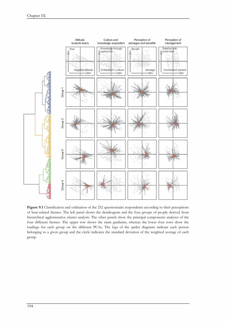
Chapter IX
194
Figure 9.1 Classification and ordination of the 252 questionnaire respondents according to their perceptions
of bear-related themes. The left panel shows the dendrogram and the four groups of people derived from
hierarchical agglomerative cluster analysis. The other panels show the principal components analyses of the
four different themes. The upper row shows the main gradients, whereas the lower four rows show the
loadings for each group on the different PCAs. The legs of the spider diagrams indicate each person
belonging to a given group and the circle indicates the standard deviation of the weighted average of each
group.
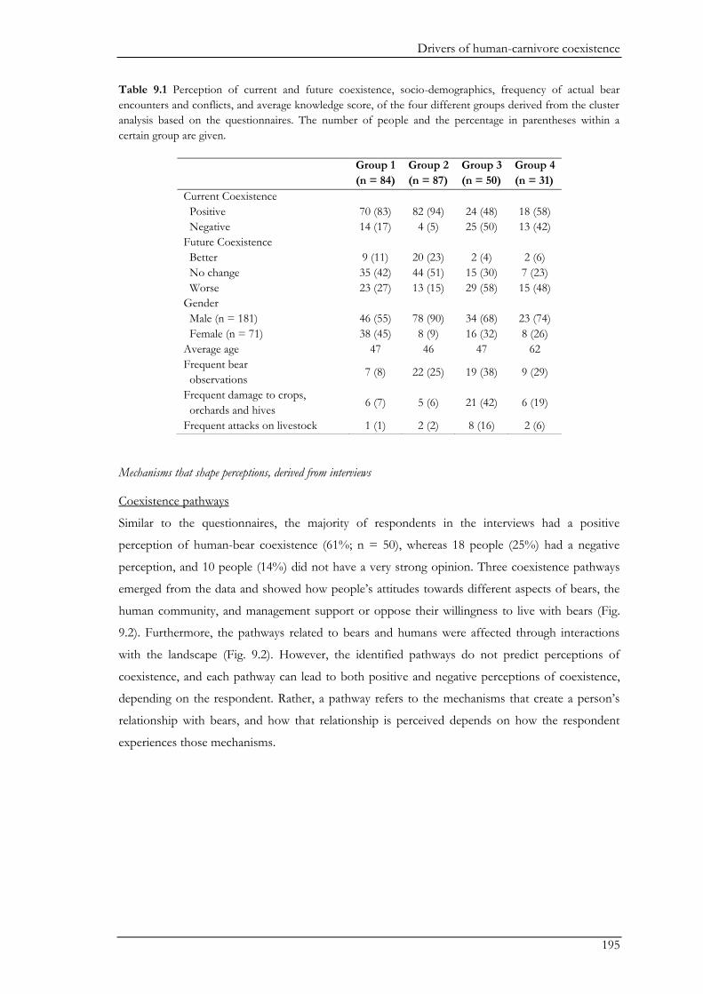
Drivers of human-carnivore coexistence
195
Table 9.1 Perception of current and future coexistence, socio-demographics, frequency of actual bear
encounters and conflicts, and average knowledge score, of the four different groups derived from the cluster
analysis based on the questionnaires. The number of people and the percentage in parentheses within a
certain group are given.
Mechanisms that shape perceptions, derived from interviews
Coexistence pathways
Similar to the questionnaires, the majority of respondents in the interviews had a positive
perception of human-bear coexistence (61%; n = 50), whereas 18 people (25%) had a negative
perception, and 10 people (14%) did not have a very strong opinion. Three coexistence pathways
emerged from the data and showed how people’s attitudes towards different aspects of bears, the
human community, and management support or oppose their willingness to live with bears (Fig.
9.2). Furthermore, the pathways related to bears and humans were affected through interactions
with the landscape (Fig. 9.2). However, the identified pathways do not predict perceptions of
coexistence, and each pathway can lead to both positive and negative perceptions of coexistence,
depending on the respondent. Rather, a pathway refers to the mechanisms that create a person’s
relationship with bears, and how that relationship is perceived depends on how the respondent
experiences those mechanisms.
Group 1
(n = 84)
Group 2
(n = 87)
Group 3
(n = 50)
Group 4
(n = 31)
Current Coexistence
Positive
Negative
70 (83)
14 (17)
82 (94)
4 (5)
24 (48)
25 (50)
18 (58)
13 (42)
Future Coexistence
Better
No change
Worse
9 (11)
35 (42)
23 (27)
20 (23)
44 (51)
13 (15)
2 (4)
15 (30)
29 (58)
2 (6)
7 (23)
15 (48)
Gender
Male (n = 181)
Female (n = 71)
46 (55)
38 (45)
78 (90)
8 (9)
34 (68)
16 (32)
23 (74)
8 (26)
Average age 47 46 47 62
Frequent bear
observations 7 (8) 22 (25) 19 (38) 9 (29)
Frequent damage to crops,
orchards and hives 6 (7) 5 (6) 21 (42) 6 (19)
Frequent attacks on livestock 1 (1) 2 (2) 8 (16) 2 (6)
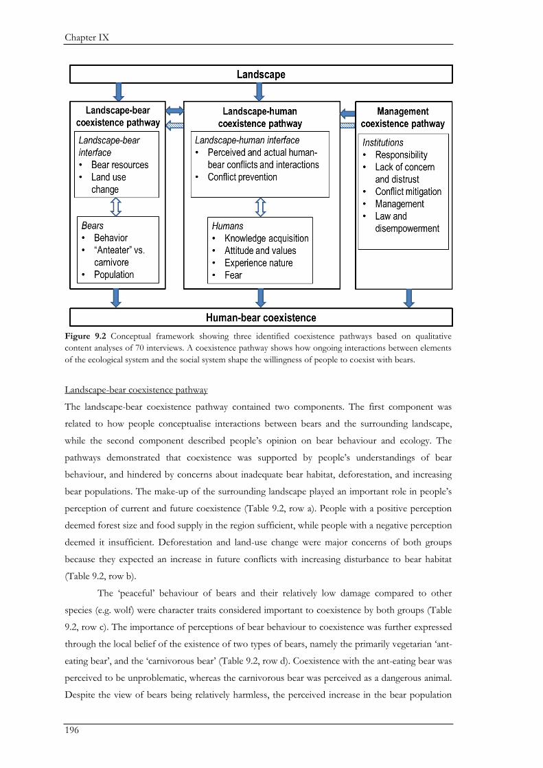
Chapter IX
196
Figure 9.2 Conceptual framework showing three identified coexistence pathways based on qualitative
content analyses of 70 interviews. A coexistence pathway shows how ongoing interactions between elements
of the ecological system and the social system shape the willingness of people to coexist with bears.
Landscape-bear coexistence pathway
The landscape-bear coexistence pathway contained two components. The first component was
related to how people conceptualise interactions between bears and the surrounding landscape,
while the second component described people’s opinion on bear behaviour and ecology. The
pathways demonstrated that coexistence was supported by people’s understandings of bear
behaviour, and hindered by concerns about inadequate bear habitat, deforestation, and increasing
bear populations. The make-up of the surrounding landscape played an important role in people’s
perception of current and future coexistence (Table 9.2, row a). People with a positive perception
deemed forest size and food supply in the region sufficient, while people with a negative perception
deemed it insufficient. Deforestation and land-use change were major concerns of both groups
because they expected an increase in future conflicts with increasing disturbance to bear habitat
(Table 9.2, row b).
The ‘peaceful’ behaviour of bears and their relatively low damage compared to other
species (e.g. wolf) were character traits considered important to coexistence by both groups (Table
9.2, row c). The importance of perceptions of bear behaviour to coexistence was further expressed
through the local belief of the existence of two types of bears, namely the primarily vegetarian ‘ant-
eating bear’, and the ‘carnivorous bear’ (Table 9.2, row d). Coexistence with the ant-eating bear was
perceived to be unproblematic, whereas the carnivorous bear was perceived as a dangerous animal.
Despite the view of bears being relatively harmless, the perceived increase in the bear population
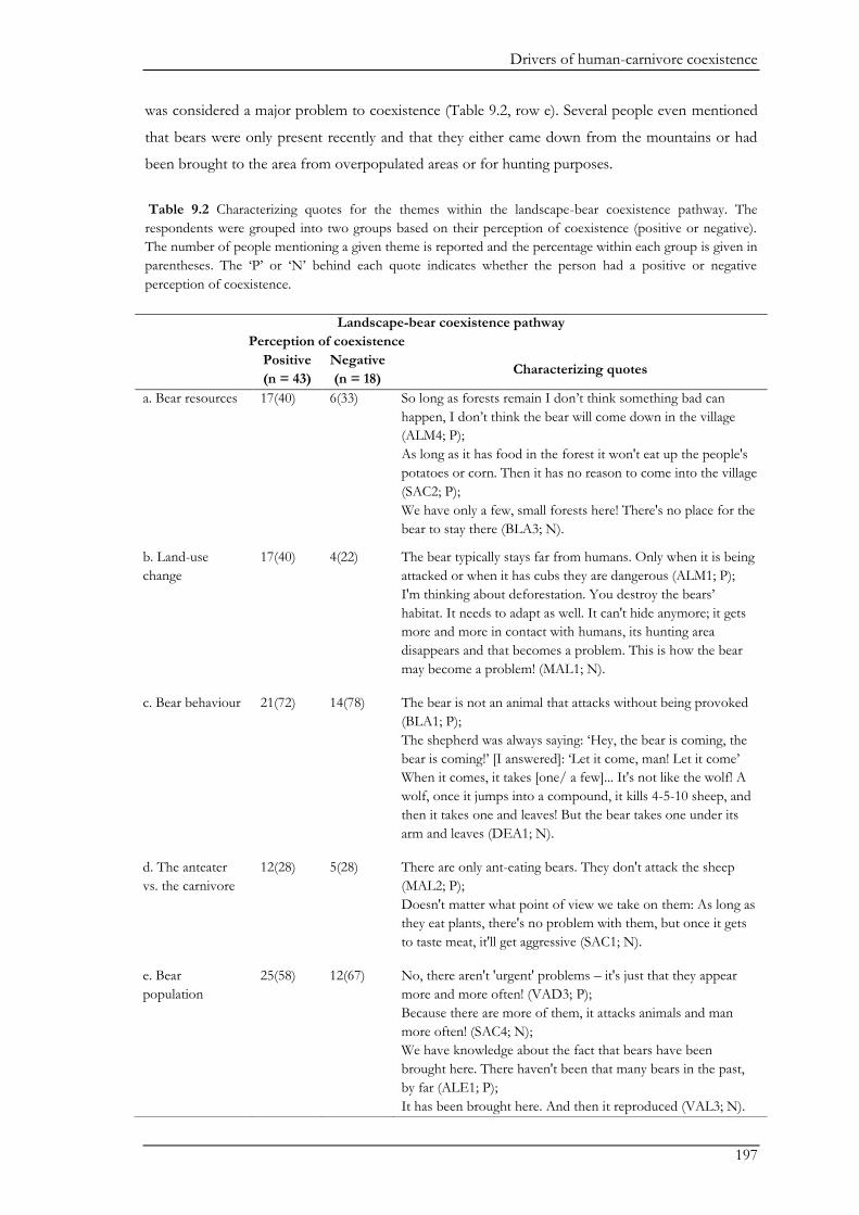
Drivers of human-carnivore coexistence
197
was considered a major problem to coexistence (Table 9.2, row e). Several people even mentioned
that bears were only present recently and that they either came down from the mountains or had
been brought to the area from overpopulated areas or for hunting purposes.
Table 9.2 Characterizing quotes for the themes within the landscape-bear coexistence pathway. The
respondents were grouped into two groups based on their perception of coexistence (positive or negative).
The number of people mentioning a given theme is reported and the percentage within each group is given in
parentheses. The ‘P’ or ‘N’ behind each quote indicates whether the person had a positive or negative
perception of coexistence.
Landscape-bear coexistence pathway
Perception of coexistence
Positive
(n = 43)
Negative
(n = 18) Characterizing quotes
a. Bear resources 17(40) 6(33) So long as forests remain I don’t think something bad can
happen, I don’t think the bear will come down in the village
(ALM4; P);
As long as it has food in the forest it won't eat up the people's
potatoes or corn. Then it has no reason to come into the village
(SAC2; P);
We have only a few, small forests here! There's no place for the
bear to stay there (BLA3; N).
b. Land-use
change
17(40) 4(22) The bear typically stays far from humans. Only when it is being
attacked or when it has cubs they are dangerous (ALM1; P);
I'm thinking about deforestation. You destroy the bears’
habitat. It needs to adapt as well. It can't hide anymore; it gets
more and more in contact with humans, its hunting area
disappears and that becomes a problem. This is how the bear
may become a problem! (MAL1; N).
c. Bear behaviour 21(72) 14(78) The bear is not an animal that attacks without being provoked
(BLA1; P);
The shepherd was always saying: ‘Hey, the bear is coming, the
bear is coming!’ [I answered]: ‘Let it come, man! Let it come’
When it comes, it takes [one/ a few]... It's not like the wolf! A
wolf, once it jumps into a compound, it kills 4-5-10 sheep, and
then it takes one and leaves! But the bear takes one under its
arm and leaves (DEA1; N).
d. The anteater
vs. the carnivore
12(28) 5(28) There are only ant-eating bears. They don't attack the sheep
(MAL2; P);
Doesn't matter what point of view we take on them: As long as
they eat plants, there's no problem with them, but once it gets
to taste meat, it'll get aggressive (SAC1; N).
e. Bear
population
25(58) 12(67) No, there aren't 'urgent' problems – it's just that they appear
more and more often! (VAD3; P);
Because there are more of them, it attacks animals and man
more often! (SAC4; N);
We have knowledge about the fact that bears have been
brought here. There haven't been that many bears in the past,
by far (ALE1; P);
It has been brought here. And then it reproduced (VAL3; N).
Chapter IX
198
Landscape-human coexistence pathway
The landscape-human coexistence pathway also contained two components. The first component
described the relationships between people and the landscape (including interactions with bears),
while the second component related to people’s values. Experiencing bears and nature, and the
values ascribed to them, were key in shaping people’s perceptions of coexistence. The perception
of coexistence was especially positive for people that had positive interactions with bears, while
negative perceptions were related to higher livestock predation and the levels of perceived damage
and danger by bears (Fig. 9.3a). Interestingly, such damage beliefs appeared to have more influence
on coexistence than actual conflict (Fig. 9.3a). In contrast, crop damage and indirect knowledge of
conflicts had little effect on the perception of coexistence (Fig. 9.3a). Moreover, preventing
conflicts by adjusting human behaviour or using traditional shepherding techniques was seen as an
integral component of coexistence by both groups and was mentioned in 62% and 23% of the
cases respectively.
Family, community members, and education all played a role in acquiring knowledge on
how to live with bears, but people with a positive perception mentioned more often that they
learned through experience (Fig. 9.3b). Attitudes towards bears were especially positive for people
with a positive perception of coexistence (88% positive attitude; 0% negative attitude), compared
to people with a negative perception (19% positive attitude; 28% negative attitude). Non-use
values, such as cultural, existence, and historical values, were more often associated with bears than
use values by both groups, although these values were more prominent among people with a
positive perception (Fig. 9.3c). The genuine and continuous relations between people and nature,
where they experience and value nature, seemed to be more important to support coexistence than
financial incentives or other use-values: ‘Well, for us the bear is like our neighbour. (…) like the
neighbour at home. There's no difference between my neighbour and the bear that comes every
second evening. We're somehow used to it. (VID4)’; ‘When you love nature I don't think that you
need a lesson, necessarily, to live with them [bears] (CIN3)’; You don’t want to see a dead forest
[without animals], right? It's different when you see a bird on a tree, a bear, a deer. ‘That makes the
difference! You see life in nature! Dead nature is like a village without inhabitants (LAS4)’. Fear was
one of the emergent themes but only mentioned by several people (afraid: n = 6; not afraid n= 9),
without large differences between the two groups.
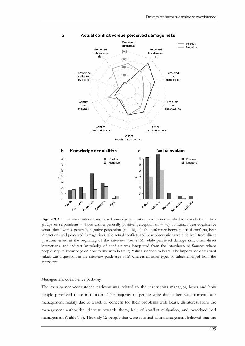
Drivers of human-carnivore coexistence
199
Figure 9.3 Human-bear interactions, bear knowledge acquisition, and values ascribed to bears between two
groups of respondents – those with a generally positive perception (n = 43) of human bear-coexistence
versus those with a generally negative perception (n = 18). a) The difference between actual conflicts, bear
interactions and perceived damage risks. The actual conflicts and bear observations were derived from direct
questions asked at the beginning of the interview (see S9.2), while perceived damage risk, other direct
interactions, and indirect knowledge of conflicts was interpreted from the interviews. b) Sources where
people acquire knowledge on how to live with bears. c) Values ascribed to bears. The importance of cultural
values was a question in the interview guide (see S9.2) whereas all other types of values emerged from the
interviews.
Management coexistence pathway
The management-coexistence pathway was related to the institutions managing bears and how
people perceived these institutions. The majority of people were dissatisfied with current bear
management mainly due to a lack of concern for their problems with bears, disinterest from the
management authorities, distrust towards them, lack of conflict mitigation, and perceived bad
management (Table 9.3). The only 12 people that were satisfied with management believed that the

Chapter IX
200
provision of supplemental or divisionary feeding was enough to prevent conflict (Table 9.3, row c).
However, the majority of people believed that authorities and hunting organizations failed to
mitigate conflict by not feeding the bears (enough), by not controlling the bear population, and by
not providing compensation after damage (Table 9.3, rows i-k). Furthermore, six people expressed
concerns about trophy hunting, indicating that common people carried the burden of living with
bears so that hunting organizations could earn money from trophy hunting (Table 9.3, row l).
Although the law and protection status was perceived to aid coexistence by people with a positive
perception of coexistence, people with a negative perception viewed it as an artificial tool that they
could not influence or even felt disempowered by, because they were not able to take care of
problem animals themselves (Table 9.3, row g and m).
Table 9.3 Characterizing quotes for the themes within the management coexistence pathway. The
respondents were first grouped into two groups based on their perception of coexistence (positive or
negative), and second, based on their opinion whether they were satisfied with current bear management. The
number of people mentioning a given theme is reported and the percentage within each group is given in
parentheses. The ‘P’ or ‘N’ behind each quote indicates whether the person had a positive or negative
perception of coexistence.
Management coexistence pathway
Perception of coexistence
Positive
(n = 11)
Negative
(n = 1) Characterizing quotes
Satisfied with current bear management
a. Lack of
concern and
distrust
b. Conflict
mitigation:
compensation
1(9) Yes, there is the principle when an animal caused damage,
the person affected will be compensated. (…)There is this
principle of compensation at local level (BLA1;P).
c. Conflict
mitigation:
feeding
9(82) 1(100) Yes, they feed them – the ‘paznic de vanatoare’. This has
been done in the past as well, when they brought them dead
animals in a big open pit (CIN1; P).
e. Management:
control bear
population
1(9) I'm against their killing and wiping them out, but I think that
their population growth should be controlled a bit, as well as
their spreading (CIN3; P).
f. Management:
legal and illegal
hunting
6(55) Every year we shoot one bear which is pretty ok. That's the
money of the hunting association. They pay something to
the state as well. Don't know if they pay something to the
local community (VAN2; P).
g. Law and
disempowerment
5(45) They'd almost disappeared and [you can shoot them today]
only with a special permit where the cause big damage. The
wolf, the wild cat, the bear – they're all protected (GRA1; P).
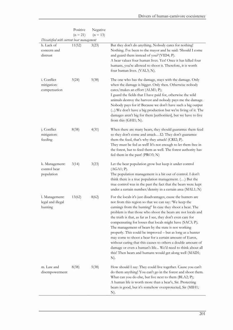
Drivers of human-carnivore coexistence
201
Positive
(n = 21)
Negative
(n = 13)
Dissatisfied with current bear management
h. Lack of
concern and
distrust
11(52) 3(23) But they don't do anything. Nobody cares for nothing!
Nothing. I've been to the mayor and he said: ‘Should I come
and guard them instead of you?’(VID4; P).
A bear values four human lives. Yes! Once it has killed four
humans, you're allowed to shoot it. Therefore, it is worth
four human lives. (VAL3; N).
i. Conflict
mitigation:
compensation
5(24) 5(38) The one who has the damage, stays with the damage. Only
when the damage is bigger. Only then. Otherwise nobody
cares/makes an effort (ALM1; P);
I guard the fields that I have paid for, otherwise the wild
animals destroy the harvest and nobody pays me the damage.
Nobody pays for it! Because we don't have such a big output
(...).We don't have a big production but we're living of it. The
damages aren't big for them [authorities], but we have to live
from this (GHI1; N).
j. Conflict
mitigation:
feeding
8(38) 4(31) When there are many bears, they should guarantee them feed
so they don't come and attack…I2: They don't guarantee
them the feed, that's why they attack! (CRI2; P).
They must be fed as well! It's not enough to let them free in
the forest, but to feed them as well. The forest authority has
fed them in the past! (PRO3; N)
k. Management:
control bear
population
3(14) 3(23) Let the bear population grow but keep it under control
(AGA1; P).
The population management is a bit out of control. I don't
think there is a true population management. (…) But the
true control was in the past the fact that the bears were kept
under a certain number/density in a certain area (MAL1; N)
l. Management:
legal and illegal
hunting
13(62) 8(62) For the locals it's just disadvantages, cause the hunters are
not from this region so that we can say: ‘We keep the
earnings from the hunting!’ In case they shoot a bear. The
problem is that those who shoot the bears are not locals and
the truth is that, as far as I see, they don't even care for
compensating for losses that locals might have (SAC3; P);
The management of bears by the state is not working
properly. This could be improved – but as long as a hunter
may come to shoot a bear for a certain amount of Euros,
without caring that this causes to others a double amount of
damage or even a human's life... We'd need to think about all
this! Then bears and humans would get along well (MAD1;
N).
m. Law and
disempowerment
8(38) 5(38) How should I say: They could live together. Cause you can't
do them anything! You can't go in the forest and shoot them.
What can you do else, but live next to them (BLA2; P);
A human life is worth more than a bear's, Sir. Protecting
bears is good, but it's somehow overprotected, Sir (MIH1;
N).
Chapter IX
202
Discussion
Our methodological approach provided two different perspectives on the social drivers to human-
bear coexistence. First, questionnaires revealed general patterns of the most important drivers
within groups of people. Grouping people with similar perceptions may be beneficial for the design
of more specific conservation programs targeted at different groups or societal concerns. Second,
semi-structured interviews identified coexistence pathways highlighting the causal mechanisms
driving people’s willingness to coexist with bears. Our research showed that perceptions of
coexistence were negatively influenced by negative attitudes, past negative interactions with bears,
perceived risks of damage, and respondents’ age, which is in line with previous studies (e.g.
Naughton-Treves et al. 2003; Kaczensky et al. 2004; Carter et al. 2012a). Nevertheless, other factors
such as culture and management were also found to be important.
Our study showed that human-carnivore coexistence is possible, and we identified three
major pathways consisting of different social drivers that influenced human-carnivore coexistence
from the perspective of the rural population. These pathways serve as a framework for identifying
the drivers that shape co-existence and how they interact. Identifying such drivers is essential in
shaping management approaches, but also to linking the drivers to broader theoretical and research
areas that help to understand how these factors are shaped. Thus the concept of coexistence
pathways and the research approach to elicit them offers a conceptual framework to assist in
facilitating human-carnivore facilitation worldwide.
Factors mediating coexistence
The two landscape-mediated coexistence pathways showed that conservation management geared
towards facilitating coexistence needs to address the beliefs shaping people’s tolerance towards
carnivores, and maintain or re-establish people’s connections to carnivores and nature. Similar to
other regions (Lescureux et al. 2011), direct interaction with bears and experiential knowledge
acquisition was particularly important in shaping perceptions and beliefs about bears (e.g.
behaviour, anteater vs. carnivore, population size).
The importance of direct interactions was further emphasized through reduced tolerance
of people that experienced livestock predation, while positive direct interactions were distinctively
higher among people with a positive perception of coexistence. Nevertheless, beliefs about bear-
related conflicts and damage risk more strongly determined people’s perception of coexistence than
the actual negative experiences, which has also been observed elsewhere (Kaczensky et al. 2004;
Carter et al. 2012a). More importantly, a stronger impact of affective risk perceptions compared to
cognitive risk perceptions can influence human behaviour and has been associated to motivations
of tiger killing (Inskip et al. 2014). To fully comprehend human-carnivore coexistence therefore
requires an understanding of the links between beliefs and risk perceptions.
The landscape-human coexistence pathway also showed that key social drivers for people’s
perceptions of human-bear coexistence were landscape-mediated attitudes and non-use values.
Drivers of human-carnivore coexistence
203
These were constructed through the existence of genuine links between people and nature, where
people valued their surrounding landscape and considered bears as part of their natural heritage.
Thus, human-carnivore coexistence may be influenced by factors such as sense of place, and
understanding which specific dimensions of sense of place affect human-carnivore coexistence
could be an important domain for further research (Williams & Stewart 1998). Such values may be
more important drivers of people’s perceptions towards carnivores than damage risks (Lagendijk &
Gusset 2008; Glikman et al. 2012; Dickman et al. 2014). Tolerance may have been further
facilitated by low fear levels, most likely resulting from sharing the landscape with bears (Roskaft et
al. 2003; Majić et al. 2011). Moreover, in intact social-ecological systems cultural tolerance to
carnivores is not uncommon (Lagendijk & Gusset 2008) and can reduce carnivore extinction risk
(Karanth et al. 2010). Such a genuine link to nature is perhaps facilitated by the continuous
coexistence with large carnivores over long periods of time. Such long-term coexistence most likely
also influenced human behaviour to avoid conflict with bears and prevent livestock predation by
using traditional livestock husbandry techniques. Thus, the continuous coexistence with large
carnivores presumably shaped the emotional component of human culture to accept and adapt to
human-bear coexistence (Glikman et al. 2012). While a history of continuous coexistence cannot be
re-created in places where carnivores were once extirpated, a key conservation challenge for
settings without a continuous history of human-carnivore coexistence is to (re-)connect people to
nature and carnivores.
The management coexistence pathway underlined the perceived gaps in current
management and showed that perceptions of (mis-)management could become a major obstacle to
coexistence. Consistent with the varying responses to management in the questionnaire, strong
negative opinions about current management did not necessarily lead to a negative perception of
coexistence. Nevertheless, people’s negative opinions on various aspect of current bear
management and the feeling of being treated unfairly have the potential to erode the build-up
tolerance towards carnivores through human-human conflicts. For example, a perception of
inadequate governance can compel people to retaliatory killing (Treves et al. 2002), and poaching in
Greece is partly motivated by a desire to defy the authorities (Bell et al. 2007). The approach of
seeking coexistence pathways was particularly useful to detect where people perceived mitigation as
necessary, which strategies were culturally accepted, and whether current efforts were satisfactory.
For example, the beliefs and concerns around an increasing bear population and its control should
receive high priority because increasing carnivore populations, rumours about ‘secret’ carnivore
introductions, and inequality over benefits and disadvantages, could reduce people’s tolerance
towards carnivores (Skogen et al. 2008).
Chapter IX
204
Managing coexistence
To avoid such disagreements between management bodies and local stakeholders, management
may facilitate coexistence through participation and education. Distrust and the feeling of
disempowerment can be reduced by including people in carnivore management through
participatory processes or active management (Treves et al. 2006), and conflicts could be reduced
through a holistic set of mitigation strategies geared towards the needs of both humans and bears
(Can et al. 2014). Although the interviewed respondents did not express the wish to be involved in
bear management, several respondents to the questionnaires showed this aspiration. This potential
for co-management of different local stakeholders may increase or maintain tolerance through
shared responsibilities, accepted management and good relationships between local people and
management bodies (Treves et al. 2006; Lagendijk & Gusset 2008).
Such participation or collaboration could also provide an education component or
function. Under the landscape-mediated pathways, experience and education were mentioned as
the most important sources to acquire knowledge about bears, and conservation could use these
tools to address people’s beliefs and concerns to facilitate coexistence. For example, by fostering
positive interactions with bears, people may feel less threatened and their tolerance towards bears
may increase (Majić et al. 2011). Education can help to foster tolerance towards large carnivores by
targeting specific (local) beliefs (Zinn et al. 2008).
Finally, direct actions such as well-regulated and managed options for local people to react
against certain ‘carnivorous’ problem animals could increase empowerment of people (Lescureux &
Linnell 2010; Majić et al. 2011). Yet, non-lethal interventions are still more effective in reducing
livestock predation rates (Bergstrom et al. 2014), and socially accepted methods like divisionary
feeding need more attention. The anger around compensation payments may be harder to resolve
when it is governed by perceived ‘weak’ institutions (Ferraro & Kiss 2002). Although compensation
payments or other financial benefits can aid conservation (Dickman et al. 2011), they often do not
improve tolerance (Naughton-Treves et al. 2003; Hazzah et al. 2009) or are distributed unequally
among society (Hemson et al. 2009). Therefore it could be worthwhile to explore other alternatives
for social-ecological systems to manage human-carnivore conflicts such as bottom-up community
organized payments like contributions to a local livestock insurance program (Mishra et al. 2003).
Conservation implications
Facilitating human-carnivore coexistence is a conservation goal worldwide. By highlighting the
existence of coexistence pathways, and then unpacking these pathways, it is possible to derive
meaningful recommendations for approaches to manage coexistence. In our case study, the content
of conservation programs should be designed to target these mechanisms in a way that
meaningfully engages with people’s coexistence perceptions, both in terms of content and how it is
delivered. In particular, we advocate for a more collaborative, participatory approach to carnivore
management in this area. The approach should foster people’s connection to their landscape,
Drivers of human-carnivore coexistence
205
provide education on bears and management approaches, and provide transparency around
management.
More broadly, we believe that our approach of combining questionnaires for large scale
patterns with the concept of coexistence pathways could be extended to regions worldwide. In
particular, the inductive approach of generating an understanding of coexistence pathways could be
used to understand human-carnivore coexistence for different regions and species. Whether the
specific pathways and their outcomes are transferable to other regions remains yet to be tested in
future studies. However, by constructing co-existence pathways through inductive research, a
broad range of factors that influence co-existence can be identified, and how these factors interact
with each other can be understood. We therefore encourage scientists to use interdisciplinary
research to obtain a comprehensive understanding of social drivers to human-carnivore
coexistence, and thus to work towards holistic conservation efforts. Through the framework
concept of coexistence pathways, and a comprehensive analysis of such pathways, landscape
managers can identify factors that facilitate or hinder coexistence, and thus target interventions
accordingly.
Acknowledgements
We are grateful to Hans Hedrich for conducting and translating all the interviews and we thank all
respondents for their participation. The survey procedure was cleared by the ethics committee of
Leuphana University Lueneburg. The project was funded by a grant of the International
Association for Bear Research and Management to ID and a Sofja Kovalevskaja Award by the
Alexander von Humboldt Foundation to JF.

Chapter IX
206
Supplementary Material for Chapter IX
Text S9.1. The questionnaire used for 252 people (original in Romanian).
Please indicate how often: 1. You see a bear
a) never b) rarely c) several times a year d) often
2. A bear damages your fields/orchards/beehives a) never b) rarely c) several times a year d) often e) not applicable
3. A bear attacks your animals a) never b) rarely c) several times a year d) often e) not applicable
The following questions will ask if you use any protective measures against bears Please indicate:
4. Do you use protective measures to prevent damage to fields/orchards/beehives a) no b) occasional c) yes d) not applicable
5. Do you use protective measures to prevent bear attacks on your animals
a) no b) occasional c) yes d) not applicable
6. I go into areas where bears are present a) no b) occasional c) yes
7. In my daily life I try to prevent getting into conflict with bears
a) no b) occasional c) yes The following questions are general questions about bears Please answer the following statements to your best knowledge:
8. Bears mainly feed on meat a) yes b) no
9. Female bears have young every year a) yes b) no
10. Most bears weigh more than 150 kg a) yes b) no
11. Bear cubs leave the mother in their first year of their life a) yes b) no
12. Bears are protected animals in Romania a) yes b) no The following questions will ask about how you achieve knowledge about bears Please indicate the extent to which you disagree or agree with the following statements: 1 = strongly disagree; 2= disagree; 3 = neutral; 4 = agree; 5 = strongly agree
13. My parents told me how to live in a landscape with bears 1 2 3 4 5
14. At school we learned about bears and how to live with them 1 2 3 4 5
15. Local authorities provide information on how to live with bears 1 2 3 4 5
16. Local NGO’s provide information on how to live with bears 1 2 3 4 5

Drivers of human-carnivore coexistence
207
17. What I know about bears, I learned from experience 1 2 3 4 5
The following questions will ask about bears in your culture Please indicate the extent to which you disagree or agree with the following statements
18. Bears are important in our culture 1 2 3 4 5
19. Hunting bears is important in our culture 1 2 3 4 5
20. I grew up hearing stories about bears 1 2 3 4 5
21. In the stories I know, bears mainly have a positive character 1 2 3 4 5
22. It is important for our culture that bears persist in the landscape 1 2 3 4 5
The following questions are regarding your feelings towards bears in general Please indicate the extent to which you disagree or agree with the following statements
23. I generally like bears 1 2 3 4 5
24. It is bad to have bears in Transylvania 1 2 3 4 5
25. Bears should remain part of our landscape in the future 1 2 3 4 5
26. I am afraid to meet a bear 1 2 3 4 5
27. Bears do not have the same rights as humans to exist in the landscape 1 2 3 4 5
The following questions are regarding the usefulness of bears in the landscape Please indicate the extent to which you disagree or agree with the following statements
28. Bears have a negative impact on hunting opportunities 1 2 3 4 5
29. In areas where there are bears and sheep, bears kill a lot of sheep 1 2 3 4 5
30. Bears damage a lot of orchards and fields 1 2 3 4 5
31. Bears are dangerous to humans 1 2 3 4 5
32. Bears increase the value of a hunting area 1 2 3 4 5
33. Having bears increases tourism in the area 1 2 3 4 5
34. Bears keep the forest clean of dead and sick animals 1 2 3 4 5
35. Bears keep nature in balance 1 2 3 4 5

Chapter IX
208
The following questions are regarding the management of bears Please indicate the extent to which you disagree or agree with the following statements
36. Bears should be completely protected 1 2 3 4 5
37. Local authorities put in enough effort to prevent damage by bears 1 2 3 4 5
38. Hunting associations put in enough effort to prevent damage by bears 1 2 3 4 5
39. I would like to be involved in the management of bears in the area 1 2 3 4 5
40. We receive compensation for damage by bears 1 2 3 4 5
41. Trophy hunting benefits the entire community 1 2 3 4 5
42. Hunting bears should be possible to everybody in the community 1 2 3 4 5
The following questions are about your opinion on how humans and bears share the landscape
43. In your opinion, how do bears and humans live together in this region a. Peacefully without conflicts b. Relatively peacefully with tolerance for occasional conflicts c. Relatively unpeacefully due to occasional conflicts d. Unpeacefully due to escalating conflicts
44. In your opinion, how do you see the relationship between humans and bears in the future?
a. Better b. Worse c. No change
45. Explain shortly your answer under question 44
___________________________________________________________________ ___________________________________________________________________ ___________________________________________________________________
46. Would you like to add any additional information about bears?
___________________________________________________________________ ___________________________________________________________________ ___________________________________________________________________
The following questions are with respect to you IX. Gender: a) M b) F X. Age:______years
XI. Profession XII. Ethnicity: a) Romanian b) Hungarian c) Roma d)Saxon e) Other, namely:
XIII. Where did you grow up: a) this region b) a different region, but with bears present c) a different region without any bears present
Thank you very much for your participation!

Drivers of human-carnivore coexistence
209
Text S9.2. The interview guide used for semi-structured interviews with 70 people (original in
Romanian).
1. The following questions will ask about your experience with bears
Please indicate how often:
1.1 You see a bear
a) never b) rarely c) several times a year d) often
1.2 A bear damages your fields and/or orchards, and/or beehives
a) never b) rarely c) several times a year d) often e) not applicable (no
fields/orhards/beehives)
1.3 A bear attacks your animals
a) never b) rarely c) several times a year d) often e) not applicable (no
animals)
1.4 Which other animals cause problems in the village? Do you think these problems are worse
than the problems caused by bears?
___________________________________________________________________
___________________________________________________________________
___________________________________________________________________
2. (Traditional ecological) knowledge on how to live with bears
Romania is a special country regarding bears because it has one of the largest populations in
Europe. Furthermore, Transylvania is especially unique, because people and bears live alongside
each other and share the same landscapes. This is very different from Western Europe. There are
few bears in Western Europe, and in many places they have been hunted to extinction. However, at
the moment in many places bears are returning to Western Europe. Therefore, we would like to
know and learn more on how you manage to live together with bears in Transylvania.
2.1 How do you manage to live together with bears?
2.2 Where and how do you learn to share a landscape with bears?
3. Which factors could disturb human-bear relationships
The Transylvanian country side has changed rapidly over the last years. For example, tourism from
foreign countries has increased and the architecture of the houses has changed. In your opinion,
are there certain changes that have changed or might change the relationships between humans and
bears?
3.1 Do you think the way people and bears live together now is different from the past?
3.2 Do you think people and bears can live together in this region in the future?
3.3 What do you think are the major factors that could change the way people currently live
with bears?

Chapter IX
210
4. Cultural values and attitudes towards bears
In some countries bears are important for their culture and there are stories and believes around
bears. For example, Sleeping Bear Dunes, a huge sand dune in America, is named after a Native
American legend. A female bear and her cub swam across a big lake (Lake Michigan). Exhausted
from their journey, the bears rested on the shoreline and fell sound asleep. Over the years, the sand
covered them up, creating a huge sand dune. Or for example, in Finland and Russia the bear is the
national animal. In your opinion, does the bear play an important role in your culture?
4.1 Are bears an important part of your culture?
4.2 Can you remember any particular stories that include bears? Which one and what kind of
character did the bear have?
Germany and Switzerland have had similar recent experiences with bears. In both countries one
bear came back and lived in the country for a while. However, in both countries they decided to
shoot the bear as it was classified as a problem bear and a threat to human safety. How do you feel
about this approach?
4.3 What would you do in this case? What are your feelings in general towards bears?
4.4 Do you think it is important that bears persist in the Transylvanian landscape in the future?
5. Management of bears
Not everybody in a country, region or village is affected in the same way by sharing the landscape
with bears. Do you think that there are any benefits or disadvantages of sharing the landscape with
bears?
5.1 Are these benefits or disadvantages equally distributed between community members?
5.2 Do local authorities/hunting associations help to prevent damage caused by bears? Do
they take care to close the difference in the distributions of benefits/disadvantages
indicated in the previous question?
People living in countries that lack large carnivores such as bears are often very impressed by the
presence of these animals. Therefore, many countries have developed tourism based on large
carnivores. This includes guiding tourists around the landscape with the chance to see and
photograph carnivores, or tourists pay for a license to hunt for carnivores and they can take home
the fur and parts of the skeleton (trophy hunting). Are there any of these examples present in your
village?
5.3a If yes, are they managed well and does the community benefit from this? Who benefits?
5.3b If no, do you see a future for tourism based on bears in this region?
The following questions are with respect to you
I. Gender: a) M b) F
II. Age:
III. Profession
IV. Ethnicity: a) Romanian b) Hungarian c) Roma d)Saxon
V. Where did you grow up: a) this region b) a different region, but with bears present
c) a different region without any bears present
Thank you very much for your participation!
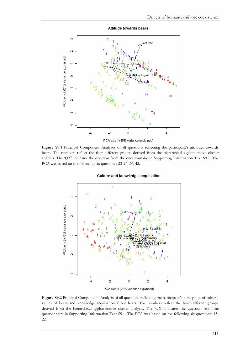
Drivers of human-carnivore coexistence
211
Figure S9.1 Principal Component Analyses of all questions reflecting the participant’s attitudes towards
bears. The numbers reflect the four different groups derived from the hierarchical agglomerative cluster
analysis. The ‘QX’ indicates the question from the questionnaire in Supporting Information Text S9.1. The
PCA was based on the following six questions: 23-26, 36, 42.
Figure S9.2 Principal Components Analysis of all questions reflecting the participant’s perception of cultural
values of bears and knowledge acquisation about bears. The numbers reflect the four different groups
derived from the hierarchical agglomerative cluster analysis. The ‘QX’ indicates the question from the
questionnaire in Supporting Information Text S9.1. The PCA was based on the following six questions: 13-
22.
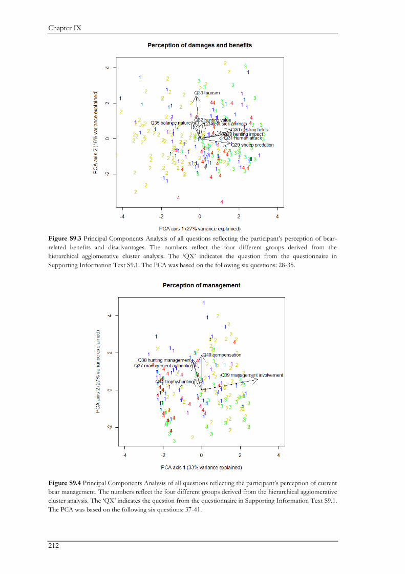
Chapter IX
212
Figure S9.3 Principal Components Analysis of all questions reflecting the participant’s perception of bear-
related benefits and disadvantages. The numbers reflect the four different groups derived from the
hierarchical agglomerative cluster analysis. The ‘QX’ indicates the question from the questionnaire in
Supporting Information Text S9.1. The PCA was based on the following six questions: 28-35.
Figure S9.4 Principal Components Analysis of all questions reflecting the participant’s perception of current
bear management. The numbers reflect the four different groups derived from the hierarchical agglomerative
cluster analysis. The ‘QX’ indicates the question from the questionnaire in Supporting Information Text S9.1.
The PCA was based on the following six questions: 37-41.

213
References

214
References
215
References
Akeroyd, J. R., and N. Page. 2007. The Saxon villages of southern Transylvania: conserving
biodiversity in a historic landscape. In: D. Gafta, and J. Akeroyd (eds). Nature
conservation: concepts and practice, Springer, New York, pp 199-210.
Albuquerque, F. S., M. J. T. Assunção-Albuquerque, L. Cayuela, R. Zamora, and B. M. Benito.
2013. European bird distribution is “well” represented by Special Protected Areas: mission
accomplished? Biological Conservation 159:45-50.
Alder, D., and S. Marsden. 2010. Characteristics of feeding‐site selection by breeding Green
Woodpeckers Picus viridis in a UK agricultural landscape. Bird Study 57:100-107.
Andrén, H. 1994. Effects of habitat fragmentation on birds and mammals in landscapes with
different proportions of suitable habitat: a review. Oikos 71:355-366.
Angelstam, P., L. Boresjö-Bronge, G. Mikusiński, U. Sporrong, and A. Wästfelt. 2003. Assessing
village authenticity with satellite images: a method to identify intact cultural landscapes in
Europe. Ambio 32:594-604.
Angelstam, P., and G. Mikusinski. 1994. Woodpecker assemblages in natural and managed boreal
and hemiboreal forest: a review. Annales Zoologici Fennici 31:157-172.
Apostolopoulou, E., and J. D. Pantis. 2009. Conceptual gaps in the national strategy for the
implementation of the European Natura 2000 conservation policy in Greece. Biological
Conservation 142:221-237.
Arion, F. H., I. Mures ̧an, and L. Balint. 2011. Compiling a visitors profile in Tarnava Mare area.
Bulletin of University of Agricultural Sciences and Veterinary Medicine Cluj-Napoca.
Horticulture 68:16-22.
Arnold, T. W. 2010. Uninformative parameters and model selection using Akaike's information
criterion. The Journal of wildlife management 74:1175-1178.
Athreya, V., M. Odden, J. D. C. Linnell, J. Krishnaswamy, and U. Karanth. 2013. Big cats in our
backyards: persistence of large carnivores in a human dominated landscape in India. PLoS
ONE 8:e57872.
Atkinson, P. W., R. J. Fuller, and J. A. Vickery. 2002. Large-scale patterns of summer and winter
bird distribution in relation to farmland type in England and Wales. Ecography 25:466-
480.
Baker, P. J., and S. Harris. 2006. Does culling reduce fox (Vulpes vulpes) density in commercial
forests in Wales, UK? European Journal of Wildlife Research 52:99-108.
Baldi, A., and P. Batary. 2011. Spatial heterogeneity and farmland birds: different perspectives in
Western and Eastern Europe. Ibis 153:875-876.
Banerjee, K., Y. V. Jhala, K. S. Chauhan, and C. V. Dave. 2013. Living with lions: the economics of
coexistence in the Gir Forests, India. PLoS ONE 8:e49457.
Barbaro, L., and I. Van Halder. 2009. Linking bird, carabid beetle and butterfly life-history traits to
habitat fragmentation in mosaic landscapes. Ecography 32:321-333.
Barber-Meyer, S. M., L. D. Mech, and P. J. White. 2008. Elk calf survival and mortality following
wolf restoration to Yellowstone National Park. Wildlife Monographs 169:1-30.
Barea-Azcon, J. M., E. Virgos, E. Ballesteros-Duperon, M. Moleon, and M. Chirosa. 2007.
Surveying carnivores at large spatial scales: a comparison of four broad-applied methods.
Biodiversity and Conservation 16:1213-1230.
Barnosky, A. D., P. L. Koch, R. S. Feranec, S. L. Wing, and A. B. Shabel. 2004. Assessing the
causes of Late Pleistocene extinctions on the continents. Science 306:70-75.
Barnosky, A. D., N. Matzke, S. Tomiya, G. O. Wogan, B. Swartz, T. B. Quental, C. Marshall, J. L.
McGuire, E. L. Lindsey, and K. C. Maguire. 2011. Has the Earth's sixth mass extinction
already arrived? Nature 471:51-57.
References
216
Barrientos, R. 2010. Retention of native vegetation within the plantation matrix improves its
conservation value for a generalist woodpecker. Forest Ecology and Management 260:595-
602.
Barua, M., S. A. Bhagwat, and S. Jadhav. 2013. The hidden dimensions of human-wildlife conflict:
health impacts, opportunity and transaction costs. Biological Conservation 157:309-316.
Batary, P., B. Andras, D. Kleijn, and T. Tscharntke. 2011a. Landscape-moderated biodiversity
effects of agri-environmental management: a meta-analysis. Proceedings of the Royal
Society B: Biological Sciences 278:1894-1902.
Batary, P., J. Fischer, A. Baldi, T. O. Crist, and T. Tscharntke. 2011b. Does habitat heterogeneity
increase farmland biodiversity? Frontiers in Ecology and the Environment 9:152-153.
Batáry, P., T. Matthiesen, and T. Tscharntke. 2010. Landscape-moderated importance of hedges in
conserving farmland bird diversity of organic vs. conventional croplands and grasslands.
Biological Conservation 143:2020-2027.
Bates, D., M. Maechler, B. Bolker, and S. Walker. 2014. lme4: Linear mixed-effects models using
Eigen and S4. R package version 1.0-4.
Bauhus, J., K. Puettmann, and C. Messier. 2009. Silviculture for old-growth attributes. Forest
Ecology and Management 258:525-537.
Bell, S., K. Hampshire, and S. Topalidou. 2007. The political culture of poaching: a case study from
northern Greece. Biodiversity and Conservation 16:399-418.
Benton, T. G., J. A. Vickery, and J. D. Wilson. 2003. Farmland biodiversity: is habitat heterogeneity
the key? Trends in Ecology & Evolution 18:182-188.
Berg, Å., and T. Gustafson. 2007. Meadow management and occurrence of corncrake (Crex crex).
Agriculture, Ecosystems & Environment 120:139-144.
Berg, Å., and M. Hiron. 2012. Occurrence of Corncrakes Crex crex in mosaic farmland landscapes
in south-central Sweden: effects of habitat and landscape structure. Bird Conservation
International 22:234-245.
Berger, J., P. B. Stacey, L. Bellis, and M. P. Johnson. 2001. A mammalian predator-prey imbalance:
grizzly bear and wolf extinction affect avian neotropical migrants. Ecological Applications
11:947-960.
Berger, K. M., E. M. Gese, and J. Berger. 2008. Indirect effects and traditional trophic cascades: a
test involving wolves, coyotes, and pronghorn. Ecology 89:818-828.
Bergmeier, E., J. Petermann, and E. Schroeder. 2010. Geobotanical survey of wood-pasture
habitats in Europe: diversity, threats and conservation. Biodiversity and Conservation
19:2995-3014.
Bergstrom, B. J., L. C. Arias, A. D. Davidson, A. W. Ferguson, L. A. Randa, and S. R. Sheffield.
2014. License to kill: reforming federal wildlife control to restore biodiversity and
ecosystem function. Conservation Letters 7:131-142.
Beschta, R. L., and W. J. Ripple. 2009. Large predators and trophic cascades in terrestrial
ecosystems of the western United States. Biological Conservation 142:2401-2414.
Bibby, C. J., N. D. Burgess, D. A. Hill, and S. Mustoe 2000. Bird census techniques. Academic
Press, London, 302 pp.
Bignal, E. M., and D. I. McCracken. 2000. The nature conservation value of European traditional
farming systems. Environmental Reviews 8:149-171.
Blom, S. 2012. Hur påverkas natur- och kulturvärden av en striktare betesmarksdefinition?,
Jordbruksverket rapport 20, available at http://www2.jordbruksverket.se/
webdav/files/SJV/trycksaker/Pdf_rapporter/ra12_20.pdf. Accessed in October 2012.
Bodin, Ö., and S. Saura. 2010. Ranking individual habitat patches as connectivity providers:
integrating network analysis and patch removal experiments. Ecological Modelling
221:2393-2405.
References
217
Boitani, L. 1995. Ecological and cultural diversities in the evolution of wolf-human relationships.
In: L. N. Carbyn, and D. R. Seip (eds). Ecology and conservation of wolves in a changing
world. Canadian Circumpolar Institute, Alberta, pp 3-11.
Bojarska, K., and N. Selva. 2012. Spatial patterns in brown bear Ursus arctos diet: the role of
geographical and environmental factors. Mammal Review 42:120-143.
Brambilla, M., F. Casale, V. Bergero, G. Bogliani, G. M. Crovetto, R. Falco, M. Roati, and I. Negri.
2010. Glorious past, uncertain present, bad future? Assessing effects of land-use changes
on habitat suitability for a threatened farmland bird species. Biological Conservation
143:2770-2778.
Brambilla, M., and P. Pedrini. 2013. The introduction of subsidies for grassland conservation in the
Italian Alps coincided with population decline in a threatened grassland species, the
Corncrake Crex crex. Bird Study 60:404-408.
Breitenmoser, U. 1998. Large predators in the Alps: the fall and rise of man's competitors.
Biological Conservation 83:279-289.
Breitenmoser, U., C. Breitenmoser-Würsten, H. Okarma, T. Kaphegyi, U. Kaphygyi-Wallmann, U.
M. Müller. 2000. Action plan for the conservation of the Eurasian lynx in Europe (Lynx
lynx). Council of Europe, Strasbourg, 69 pp.
Brodier, S., S. Augiron, T. Cornulier, and V. Bretagnolle. 2013. Local improvement of skylark and
corn bunting population trends on intensive arable landscape: a case study of the
conservation tool Natura 2000. Animal Conservation 17:204-216.
Brook, L. A., C. N. Johnson, and E. G. Ritchie. 2012. Effects of predator control on behaviour of
an apex predator and indirect consequences for mesopredator suppression. Journal of
Applied Ecology 49:1278-1286.
Bucşa, C. and I. Tăuşan. 2010. Preliminary data on the sylophagous beetles (Insecta: Coleoptera)
from the "Breite ancient oak trees" nature reserve (Sighişoara, Romania). Brukenthal Acta
Musei 5:593-606.
Bucşa, L. 2007. Macromycetes of the Breite nature reserve of ancient oaks (Transylvania, Romania).
Transylvanian Review of Systematical and Ecological Research 4:33-42.
Budka, M., and T. S. Osiejuk. 2013. Habitat preferences of Corncrake (Crex crex) males in
agricultural meadows. Agriculture, Ecosystems & Environment 171:33-38.
Bugalho, M. N., M. C. Caldeira, J. S. Pereira, J. Aronson, and J. G. Pausas. 2011. Mediterranean
cork oak savannas require human use to sustain biodiversity and ecosystem services.
Frontiers in Ecology and the Environment 9:278-286.
Burnham, K. P., and D. R. Anderson. 2002. Model selection and multimodel inference. Springer,
New York, 488 pp.
Butchart, S. H., M. Walpole, B. Collen, A. van Strien, J. P. Scharlemann, R. E. Almond, J. E. Baillie,
B. Bomhard, C. Brown, and J. Bruno. 2010. Global biodiversity: indicators of recent
declines. Science 328:1164-1168.
Buttler, A., F. Kohler, and F. Gillet. 2009. The Swiss mountain wooded pastures: patterns and
processes. In: A. Rigueiro-Rodríguez, J. McAdam, M. R. Mosquera-Losada (eds).
Agroforestry in Europe: current status and future prospects. Springer, Dordrecht, pp 377-
396.
Caledonian Partnership. 2003. Restoring Natura Forest Habitats. Highland Birchwoods, Munlochy,
56 pp.
Can, Ö. E., N. D'Cruze, D. L. Garshelis, J. Beecham, and D. W. Macdonald. 2014. Resolving
human‐bear conflict: a global survey of countries, experts and key factors. Conservation
Letters 7:501-513.
Carter, N. H., S. J. Riley, and J. Liu. 2012a. Utility of a psychological framework for carnivore
conservation. Oryx 46:525-535.
References
218
Carter, N. H., B. K. Shrestha, J. B. Karki, N. M. B. Pradhan, and J. Liu. 2012b. Coexistence
between wildlife and humans at fine spatial scales. Proceedings of the National Academy
of Sciences 109:15360-15365.
Chaideftou, E., C. A. Thanos, E. Bergmeier, A. S. Kallimanis, and P. Dimopoulos. 2011. The herb
layer restoration potential of the soil seed bank in an overgrazed oak forest. Journal of
Biological Research 15:47-57.
Chapron, G., P. Kaczensky, J. D. Linnell, M. von Arx, D. Huber, H. Andrén, J. V. López-Bao, M.
Adamec, F. Álvares, and O. Anders. 2014. Recovery of large carnivores in Europe’s
modern human-dominated landscapes. Science 346:1517-1519.
Chestin, I. 1999. The management of the brown bear in Romania. In: C. Servheen, S. Herrero, and
B. Peyton (eds). Bears: status survey and conservation action plan. International Union for
the Conservation of Nature and Natural Resources, Gland, pp 136-143.
Chételat, J., M. Kalbermatten, K. S. Lannas, T. Spiegelberger, J.-B. Wettstein, F. Gillet, A. Peringer,
and A. Buttler. 2013. A contextual analysis of land-use and vegetation changes in two
wooded pastures in the Swiss Jura Mountains. Ecology and Society 18:39.
Ciarniello, L. M., M. S. Boyce, D. C. Heard, and D. R. Seip. 2007. Components of grizzly bear
habitat selection: density, habitats, roads, and mortality risk. The Journal of Wildlife
Management 71:1446-1457.
Ciochia, V. 1992. Păsările clocitoare din România. Editura Ştiintifică, Bucharest, 386 pp.
Ciucci, P., and L. Boitani. 2008. The Apennine brown bear: a critical review of its status and
conservation problems. Ursus 19:130-145.
Clevenger, A. P., F. J. Purroy, and M. R. Pelton. 1992. Food habits of brown bears (Ursus arctos) in
the Cantabrian Mountains, Spain. Journal of Mammalogy 73:415-421.
Clevenger, A. P., and N. Waltho. 2001. Factors influencing the effectiveness of wildlife underpasses
in Banff National Park, Alberta, Canada. Conservation Biology 14:47-56.
Coldea, G. 1992. The vegetation of Transylvania and Maramureş. In: D. Ivan (ed). Vegetaţia
României. Editura Technică Agricolă, Bucharest, pp. 162-183 (in Romanian).
Colman, N., C. Gordon, M. Crowther, and M. Letnic. 2014. Lethal control of an apex predator has
unintended cascading effects on forest mammal assemblages. Proceedings of the Royal
Society B: Biological Sciences 281:20133094.
Concepción, E. D., M. Díaz, and R. A. Baquero. 2008. Effects of landscape complexity on the
ecological effectiveness of agri-environment schemes. Landscape Ecology 23:135-148.
Conner, R. N., and D. C. Rudolph. 1991. Forest habitat loss, fragmentation, and red-cockaded
woodpecker populations. Wilson Bulletin 103:446-457.
Corbett, P. E., and M. D. Hudson. 2010. Management of cover areas may increase numbers of
breeding Corncrakes Crex crex. Bird Study 57:553-559.
Costa, A., M. Madeira, J. Lima Santos, and Â. Oliveira. 2011. Change and dynamics in
Mediterranean evergreen oak woodlands landscapes of Southwestern Iberian Peninsula.
Landscape and Urban Planning 102:164-176.
Cramp, S. 2000. The complete birds of the western palearctic. CD-ROM edition. Oxford
University Press. Oxford.
Creel, S., and D. Christianson. 2008. Relationships between direct predation and risk effects.
Trends in Ecology & Evolution 23:194-201.
Cremene, C., G. Groza, L. Rakosy, A. A. Schileyko, A. Baur, A. Erhardt, and B. Baur. 2005.
Alterations of steppe-like grasslands in Eastern Europe: a threat to regional biodiversity
hotspots. Conservation Biology 19:1606-1618.
Crooks, K. R. 2002. Relative sensitivities of mammalian carnivores to habitat fragmentation.
Conservation Biology 16:488-502.
References
219
Crooks, K. R., C. L. Burdett, D. M. Theobald, C. Rondinini, and L. Boitani. 2011. Global patterns
of fragmentation and connectivity of mammalian carnivore habitat. Philosophical
Transactions of the Royal Society B: Biological Sciences 366:2642-2651.
Crooks, K. R., and M. E. Soulé. 1999. Mesopredator release and avifaunal extinctions in a
fragmented system. Nature 400:563-566.
Crutzen, P. J. 2002. Geology of mankind. Nature 415:23-23.
Dahle, B., O. J. Sørensen, E. H. Wedul, J. E. Swenson, and F. Sandegren. 1998. The diet of brown
bears Ursus arctos in central Scandinavia: effect of access to free-ranging domestic sheep
Ovis aries. Wildlife Biology 4:147-158.
Dahlström, A., A. Iuga, and T. Lennartsson. 2013. Managing biodiversity rich hay meadows in the
EU: a comparison of Swedish and Romanian grasslands. Environmental Conservation
40:194-205.
Dallimer, M., K. J. Gaston, A. M. J. Skinner, N. Hanley, S. Acs, and P. R. Armsworth. 2010. Field-
level bird abundances are enhanced by landscape-scale agri-environment scheme uptake.
Biology Letters 6:643-646.
Dauber, J., J. Bengtsson, and L. Lenoir. 2006. Evaluating effects of habitat loss and land‐use
continuity on ant species richness in seminatural grassland remnants. Conservation Biology
20:1150-1160.
DeFries, R. S., J. A. Foley, and G. P. Asner. 2004. Land-use choices: balancing human needs and
ecosystem function. Frontiers in Ecology and the Environment 2:249-257.
Demeter, L., and A. Kelemen. 2012. Quantifying the abandonment of mountain hay meadows in
the Eastern Carpathians. European Forum on Nature Conservation and Pastoralism,
Hamsterley Vale, 21 pp.
Devictor, V., and F. Jiguet. 2007. Community richness and stability in agricultural landscapes: the
importance of surrounding habitats. Agriculture, Ecosystems & Environment 120:179-184.
Diacon-Bolli, J., T. Dalang, R. Holderegger, and M. Bürgi. 2012. Heterogeneity fosters biodiversity:
linking history and ecology of dry calcareous grasslands. Basic and Applied Ecology
13:641-653.
Diamond, J. 1986. Overview: laboratory experiments, field experiments, and natural experiments.
In: J. M. Diamond, and T. J. Case (eds). Community ecology. Harper & Row, New York,
pp 3-22.
Dickman, A. J. 2010. Complexities of conflict: the importance of considering social factors for
effectively resolving human-wildlife conflict. Animal Conservation 13:458-466.
Dickman, A. J., L. Hazzah, C. Carbone, and S. M. Durant. 2014. Carnivores, culture and
‘contagious conflict’: Multiple factors influence perceived problems with carnivores in
Tanzania’s Ruaha landscape. Biological Conservation 178:19-27.
Dickman, A. J., E. A. Macdonald, and D. W. Macdonald. 2011. A review of financial instruments
to pay for predator conservation and encourage human-carnivore coexistence. Proceedings
of the National Academy of Sciences 108:13937-13944.
Donadio, E., and S. W. Buskirk. 2006. Diet, morphology, and interspecific killing in Carnivora.
American Naturalist 167:524-536.
Donald, P., R. Green, and M. Heath. 2001. Agricultural intensification and the collapse of Europe's
farmland bird populations. Proceedings of the Royal Society of London Series B:
Biological Sciences 268:25-29.
Donald, P. F., and A. D. Evans. 2006. Habitat connectivity and matrix restoration: the wider
implications of agri-environment schemes. Journal of Applied Ecology 43:209-218.
Dormann, C. F., J. M. McPherson, M. B. Araújo, R. Bivand, J. Bolliger, G. Carl, R. G. Davies, A.
Hirzel, W. Jetz, W. Daniel Kissling, I. Kühn, R. Ohlemüller, P. R. Peres-Neto, B.
Reineking, B. Schröder, F. M. Schurr, and R. Wilson. 2007. Methods to account for spatial
References
220
autocorrelation in the analysis of species distributional data: a review. Ecography 30:609-
628.
Dorner, B. 1910. The agriculture of the Transylvanian Saxons. Győr, 336 pp (in Hungarian).
Dorresteijn, I., J. Hanspach, A. Kecskés, H. Latková, Z. Mezey, S. Sugár, H. von Wehrden, and J.
Fischer. 2014. Human-carnivore coexistence in a traditional rural landscape. Landscape
Ecology 29:1145-1155.
Dorresteijn, I., T. Hartel, J. Hanspach, H. von Wehrden, and J. Fischer. 2013. The conservation
value of traditional rural landscapes: the case of woodpeckers in Transylvania, Romania.
PLoS ONE 8:e65236.
Doxa, A., Y. Bas, M. L. Paracchini, P. Pointereau, J.-M. Terres, and F. Jiguet. 2010. Low-intensity
agriculture increases farmland bird abundances in France. Journal of Applied Ecology
47:1348-1356.
Dunning, J. B., B. J. Danielson, and H. R. Pulliam. 1992. Ecological processes that affect
populations in complex landscapes. Oikos:169-175.
Ellis, E. C., and N. Ramankutty. 2008. Putting people in the map: anthropogenic biomes of the
world. Frontiers in Ecology and the Environment 6:439-447.
Elmhagen, B., G. Ludwig, S. Rushton, P. Helle, and H. Lindén. 2010. Top predators,
mesopredators and their prey: interference ecosystems along bioclimatic productivity
gradients. Journal of Animal Ecology 79:785-794.
Elmhagen, B., and S. P. Rushton. 2007. Trophic control of mesopredators in terrestrial ecosystems:
top‐down or bottom‐up? Ecology Letters 10:197-206.
Elston, D., R. Moss, T. Boulinier, C. Arrowsmith, and X. Lambin. 2001. Analysis of aggregation, a
worked example: numbers of ticks on red grouse chicks. Parasitology 122:563-569.
Enserink, M., and G. Vogel. 2006. Wildlife conservation: the carnivore comeback. Science 314:746-
749.
Ernoult, A., and D. Alard. 2011. Species richness of hedgerow habitats in changing agricultural
landscapes: are α and γ diversity shaped by the same factors? Landscape Ecology 26:683-
696.
Estes, J. A., J. Terborgh, J. S. Brashares, M. E. Power, J. Berger, W. J. Bond, S. R. Carpenter, T. E.
Essington, R. D. Holt, J. B. C. Jackson, R. J. Marquis, L. Oksanen, T. Oksanen, R. T.
Paine, E. K. Pikitch, W. J. Ripple, S. A. Sandin, M. Scheffer, T. W. Schoener, J. B. Shurin,
A. R. E. Sinclair, M. E. Soule, R. Virtanen, and D. A. Wardle. 2011. Trophic downgrading
of planet Earth. Science 333:301-306.
European Environment Agency [EEA]. 2006. Corine land use cover 2006 seamless vector data
base. Copenhagen. www.eea.europa.eu/data-and-maps/data/clc-2006-vector-data-version-
2. Accessed 12 March 2014.
Fahrig, L. 2003. Effects of habitat fragmentation on biodiversity. Annual Review of Ecology
Evolution and Systematics 34:487-515.
Farm Environment Plan Guide. 2006. Identifying ancient trees. Rural Development Service,
London, 2 pp.
Fernández, N., N. Selva, C. Yuste, H. Okarma, and Z. Jakubiec. 2012. Brown bears at the edge:
Modeling habitat constrains at the periphery of the Carpathian population. Biological
Conservation 153:134-142.
Ferraro, P. J., and A. Kiss. 2002. Direct payments to conserve biodiversity. Science 298:1718-1719.
Fielding, A. H., and J. F. Bell. 1997. A review of methods for the assessment of prediction errors in
conservation presence/absence models. Environmental Conservation 24:38-49.
Filippi-Codaccioni, O., V. Devictor, Y. Bas, J. Clobert, and R. Julliard. 2010. Specialist response to
proportion of arable land and pesticide input in agricultural landscapes. Biological
Conservation 143:883-890.
References
221
Fischer, C., A. Flohre, L. W. Clement, P. Batary, W. W. Weisser, T. Tscharntke, and C. Thies. 2011.
Mixed effects of landscape structure and farming practice on bird diversity. Agriculture
Ecosystems & Environment 141:119-125.
Fischer, J., B. Brosi, G. C. Daily, P. R. Ehrlich, R. Goldman, J. Goldstein, D. B. Lindenmayer, A.
D. Manning, H. A. Mooney, and L. Pejchar. 2008. Should agricultural policies encourage
land sparing or wildlife-friendly farming? Frontiers in Ecology and the Environment 6:380-
385.
Fischer, J., T. Hartel, and T. Kuemmerle. 2012. Conservation policy in traditional farming
landscapes. Conservation Letters 5:167-175.
Fischer, J., and D. B. Lindenmayer. 2007. Landscape modification and habitat fragmentation: a
synthesis. Global Ecology and Biogeography 16:265-280.
Fischer, J., K. Sherren, J. Stott, A. Zerger, G. Warren, and J. Stein. 2009. Toward landscape-wide
conservation outcomes in Australia's temperate grazing region. Frontiers in Ecology and
the Environment 8:69-74.
Fischer, J., J. Stott, and B. S. Law. 2010. The disproportionate value of scattered trees. Biological
Conservation 143:1564-1567.
Foley, J. A., R. DeFries, G. P. Asner, C. Barford, G. Bonan, S. R. Carpenter, F. S. Chapin, M. T.
Coe, G. C. Daily, H. K. Gibbs, J. H. Helkowski, T. Holloway, E. A. Howard, C. J.
Kucharik, C. Monfreda, J. A. Patz, I. C. Prentice, N. Ramankutty, and P. K. Snyder. 2005.
Global consequences of land use. Science 309:570-574.
Folke, C. 2006. Resilience: the emergence of a perspective for social-ecological systems analyses.
Global Environmental Change 16:253-267.
Folke, C., S. Carpenter, B. Walker, M. Scheffer, T. Elmqvist, L. Gunderson, and C. Holling. 2004.
Regime shifts, resilience, and biodiversity in ecosystem management. Annual Review of
Ecology, Evolution, and Systematics 35:557-581.
Fourcade, Y., J. O. Engler, A. G. Besnard, D. Rödder, and J. Secondi. 2013. Confronting expert-
based and modelled distributions for species with uncertain conservation status: a case
study from the corncrake (Crex crex). Biological Conservation 167:161-171.
Gabriel, D., S. M. Sait, J. A. Hodgson, U. Schmutz, W. E. Kunin, and T. G. Benton. 2010. Scale
matters: the impact of organic farming on biodiversity at different spatial scales. Ecology
Letters 13:858-869.
Gangaas, K. E., B. P. Kaltenborn, and H. P. Andreassen. 2013. Geo-spatial aspects of acceptance
of illegal hunting of large carnivores in Scandinavia. PLoS ONE 8:e68849.
Garbarino, M., E. Lingua, M. M. Subira, and R. Motta. 2011. The larch wood pasture: structure and
dynamics of a cultural landscape. European Journal of Forest Research 130:491-502.
Gaston, K. J., T. M. Blackburn, and K. K. Goldewijk. 2003. Habitat conversion and global avian
biodiversity loss. Proceedings of the Royal Society B: Biological Sciences 270:1293-1300.
Gehring, T. M., K. C. VerCauteren, and J.-M. Landry. 2010. Livestock protection dogs in the 21st
century: is an ancient tool relevant to modern conservation challenges? BioScience 60:299-
308.
Geiger, F., J. Bengtsson, F. Berendse, W. W. Weisser, M. Emmerson, M. B. Morales, P. Ceryngier,
J. Liira, T. Tscharntke, and C. Winqvist. 2010. Persistent negative effects of pesticides on
biodiversity and biological control potential on European farmland. Basic and Applied
Ecology 11:97-105.
Gelman, A., Y. S. SU, V. Dorie, and M. Y. S. SU. 2013. Package ‘arm’. R package version 1.7-7.
Ghosal, S., V. Athreya, J. C. Linnell, and P. Vedeld. 2013. An ontological crisis? A review of large
felid conservation in India. Biodiversity and Conservation 22:2665-2681.
Gibbons, P., and D. Lindenmayer 2003. Tree hollows and wildlife conservation in Australia.
CSIRO, Collingwood, 240 pp.
References
222
Glikman, J. A., and B. Frank. 2011. Human dimensions of wildlife in Europe: the Italian way.
Human Dimensions of Wildlife 16:368-377.
Glikman, J. A., J. J. Vaske, A. J. Bath, P. Ciucci, and L. Boitani. 2012. Residents’ support for wolf
and bear conservation: the moderating influence of knowledge. European Journal of
Wildlife Research 58:295-302.
Godvik, I. M. R., L. E. Loe, J. O. Vik, V. Veiberg, R. Langvatn, and A. Mysterud. 2009. Temporal
scales, trade-offs, and functional responses in red deer habitat selection. Ecology 90:699-
710.
Goldberg, E., K. Kirby, J. Hall, and J. Latham. 2007. The ancient woodland concept as a practical
conservation tool in Great Britain. Journal for Nature Conservation 15:109-119.
Gonçalves, P., S. Alcobia, L. Simões, and M. Santos-Reis. 2012. Effects of management options on
mammal richness in a Mediterranean agro-silvo-pastoral system. Agroforestry Systems
85:383-395.
Goudie, A. S. 2013. The human impact on the natural environment: past, present, and future.
Wiley-Blackwell, Malden, 422 pp.
Grabovsky, V. 1993. Spatial distribution and spacing behaviour of males in a Russian Corncrake
(Crex crex) population. Gibier faune sauvage 10:259-279.
Grace, J. B. 2006. Structural equation modeling and natural systems. Cambridge University Press,
Cambridge, 378 pp.
Grace, J. B., D. R. Schoolmaster Jr, G. R. Guntenspergen, A. M. Little, B. R. Mitchell, K. M. Miller,
and E. W. Schweiger. 2012. Guidelines for a graph-theoretic implementation of structural
equation modeling. Ecosphere 3:art73.
Green, R. E., G. Rocamora, and N. Schaffer. 1997. Populations, ecology and threats to the
Corncrake Crex crex in Europe. Vogelwelt Berlin 118:117-134.
Gregory, R. D., A. Van Strien, P. Vorisek, A. W. G. Meyling, D. G. Noble, R. P. Foppen, and D.
W. Gibbons. 2005. Developing indicators for European birds. Philosophical Transactions
of the Royal Society B: Biological Sciences 360:269-288.
Griffiths, P., T. Kuemmerle, M. Baumann, V. C. Radeloff, I. V. Abrudan, J. Lieskovsky, C.
Munteanu, K. Ostapowicz, and P. Hostert. 2013. Forest disturbances, forest recovery, and
changes in forest types across the Carpathian ecoregion from 1985 to 2010 based on
Landsat image composites. Remote Sensing of Environment 151: 72-88.
Gruber, B., D. Evans, K. Henle, B. Bauch, D. Schmeller, F. Dziock, P.-Y. Henry, S. Lengyel, C.
Margules, and C. Dormann. 2012. ‘Mind the gap!’: how well does Natura 2000 cover
species of European interest? Nature Conservation 3:45-62.
Guerrero, I., M. B. Morales, J. J. Oñate, F. Geiger, F. Berendse, G. d. Snoo, S. Eggers, T. Pärt, J.
Bengtsson, L. W. Clement, W. W. Weisser, A. Olszewski, P. Ceryngier, V. Hawro, J. Liira,
T. Aavik, C. Fischer, A. Flohre, C. Thies, and T. Tscharntke. 2012. Response of ground-
nesting farmland birds to agricultural intensification across Europe: landscape and field
level management factors. Biological Conservation 152:74-80.
Gusset, M., A. H. Maddock, G. J. Gunther, M. Szykman, R. Slotow, M. Walters, and M. J. Somers.
2008. Conflicting human interests over the re-introduction of endangered wild dogs in
South Africa. Biodiversity and Conservation 17:83-101.
Güthlin, D., F. Knauer, T. Kneib, H. Küchenhoff, P. Kaczensky, G. Rauer, M. Jonozovič, A.
Mustoni, and K. Jerina. 2011. Estimating habitat suitability and potential population size
for brown bears in the Eastern Alps. Biological Conservation 144:1733-1741.
Haberl, H., K. H. Erb, F. Krausmann, V. Gaube, A. Bondeau, C. Plutzar, S. Gingrich, W. Lucht,
and M. Fischer-Kowalski. 2007. Quantifying and mapping the human appropriation of net
primary production in Earth's terrestrial ecosystems. Proceedings of the National Academy
of Sciences 104:12942-12947.
References
223
Halada, L., D. Evans, C. Romão, and J. E. Petersen. 2011. Which habitats of European importance
depend on agricultural practices? Biodiversity and Conservation 20:2365-2378.
Hamel, S., S. T. Killengreen, J. A. Henden, N. E. Eide, L. Roed‐Eriksen, R. A. Ims, and N. G.
Yoccoz. 2012. Towards good practice guidance in using camera‐traps in ecology: influence
of sampling design on validity of ecological inferences. Methods in Ecology and Evolution
4:105-113.
Hanski, I. 2011. Habitat loss, the dynamics of biodiversity, and a perspective on conservation.
Ambio 40:248-255.
Hanspach, J., J. Fischer, J. Stott, and K. Stagoll. 2011. Conservation management of eastern
Australian farmland birds in relation to landscape gradients. Journal of Applied Ecology
48:523-531.
Hanspach, J., T. Hartel, A. I. Milcu, F. Mikulcak, I. Dorresteijn, J. Loos, H. von Wehrden, T.
Kuemmerle, D. Abson, A. Kovács-Hostyánszki, A. Báldi, and J. Fischer. 2014. A holistic
approach to studying social-ecological systems and its application to southern
Transylvania. Ecology and Society 19:32.
Haraszthy, L., F. Márkus, and L. Bank. 1997. The nature conservation of wood-pastures. WWF-
füzetek 12, 23 pp (in Hungarian).
Hartel, T., R. Bancila, and D. Cogalniceanu. 2011. Spatial and temporal variability of aquatic habitat
use by amphibians in a hydrologically modified landscape. Freshwater Biology 56:2288-
2298.
Hartel, T., I. Dorresteijn, C. Klein, O. Máthé, C. I. Moga, K. Öllerer, M. Roellig, H. von Wehrden,
and J. Fischer. 2013. Wood-pastures in a traditional rural region of Eastern Europe:
characteristics, management and status. Biological Conservation 166:267-275.
Hartel, T., J. Fischer, C. Câmpeanu, A. I. Milcu, J. Hanspach, and I. Fazey. 2014. The importance
of ecosystem services for rural inhabitants in a changing cultural landscape in Romania.
Ecology and Society 19:42.
Hartel, T., and C. I. Moga. 2010. Good practice management of wood-pasture habitats. Fundatia
Mihai Eminescu Trust, Sighisoara (in Romanian).
Hazzah, L., M. Borgerhoff Mulder, and L. Frank. 2009. Lions and warriors: social factors
underlying declining African lion populations and the effect of incentive-based
management in Kenya. Biological Conservation 142:2428-2437.
Heinlein, K., R. Schöller, M. Scholz, and R. Wölfel 2005. Hutanger: Natur- und Kulturerbe mit
Zukunft. Pfeifer, 224 pp (in German).
Hemson, G., S. Maclennan, G. Mills, P. Johnson, and D. Macdonald. 2009. Community, lions,
livestock and money: a spatial and social analysis of attitudes to wildlife and the
conservation value of tourism in a human-carnivore conflict in Botswana. Biological
Conservation 142:2718-2725.
Henle, K., D. Alard, J. Clitherow, P. Cobb, L. Firbank, T. Kull, D. McCracken, R. F. A. Moritz, J.
Niemelae, M. Rebane, D. Wascher, A. Watt, and J. Young. 2008. Identifying and managing
the conflicts between agriculture and biodiversity conservation in Europe: A review.
Agriculture Ecosystems & Environment 124:60-71.
Herzon, I., A. Auninš, J. Elts, and Z. Preikša. 2008. Intensity of agricultural land-use and farmland
birds in the Baltic States. Agriculture, Ecosystems & Environment 125:93-100.
Hinsley, S., and P. Bellamy. 2000. The influence of hedge structure, management and landscape
context on the value of hedgerows to birds: a review. Journal of Environmental
Management 60:33-49.
Hinsley, S. A. 2000. The costs of multiple patch use by birds. Landscape Ecology 15:765-775.
References
224
Höchtl, F., S. Lehringer, and W. Konold. 2005. “Wilderness”: what it means when it becomes a
reality—a case study from the southwestern Alps. Landscape and Urban Planning 70:85-
95.
Hole, D., A. Perkins, J. Wilson, I. Alexander, P. Grice, and A. Evans. 2005. Does organic farming
benefit biodiversity? Biological Conservation 122:113-130.
Holmern, T., J. Nyahongo, and E. Røskaft. 2007. Livestock loss caused by predators outside the
Serengeti National Park, Tanzania. Biological Conservation 135:518-526.
Holzwarth, F., A. Kahl, J. Bauhus, and C. Wirth. 2013. Many ways to die: partitioning tree mortality
dynamics in a near‐natural mixed deciduous forest. Journal of Ecology 101:220-230.
Horák, J., and K. Rébl. 2013. The species richness of click beetles in ancient pasture woodland
benefits from a high level of sun exposure. Journal of Insect Conservation 17:307-318.
Huber, D. 2007. Ursus arctos. The IUCN Red List of Threathened Species, version 2013.2.
International Union for Conservation of Nature and Natural Resources.
www.iucnredlist.org. Accessed 12 Mar 2014.
Huber, D., and H. U. Roth. 1993. Movements of European brown bears in Croatia. Acta
Theriologica 38:151-159.
Hughes, J., and D. W. Macdonald. 2013. A review of the interactions between free-roaming
domestic dogs and wildlife. Biological Conservation 157:341-351.
Huntington, H. P. 2000. Using traditional ecological knowledge in science: methods and
applications. Ecological Applications 10:1270-1274.
Inger, R., R. Gregory, J. P. Duffy, I. Stott, P. Voříšek, and K. J. Gaston. 2015. Common European
birds are declining rapidly while less abundant species' numbers are rising. Ecology Letters
18:28-36.
INS [Institutul National de Statistica; Romanian National Institute of Statistics]. 2011. The 2011
population and housing census (database at the level of administrative units). Bucharest.
Received 6 February 2012.
Inskip, C., Z. Fahad, R. Tully, T. Roberts, and D. MacMillan. 2014. Understanding carnivore killing
behaviour: exploring the motivations for tiger killing in the Sundarbans, Bangladesh.
Biological Conservation 180:42-50.
Ives, C. D., and D. Kendal. 2014. The role of social values in the management of ecological
systems. Journal of Environmental Management 144:67-72.
Jȩdrzejewski, W., B. Jȩdrzejewska, H. Okarma, K. Schmidt, K. Zub, and M. Musiani. 2000. Prey
Selection and predation by wolves in Bialowieza Primeval Forest, Poland. Journal of
Mammalogy 81:197-212.
Jedrzejewski, W., M. Niedzialkowska, S. Nowak, and B. Jedrzejewska. 2004. Habitat variables
associated with wolf (Canis lupus) distribution and abundance in northern Poland. Diversity
and Distributions 10:225-233.
Jedrzejewski, W., K. Schmidt, J. Theuerkauf, B. Jedrzejewska, N. Selva, K. Zub, and L. Szymura.
2002. Kill rates and predation by wolves on ungulate populations in Bialowieza Primeval
Forest (Poland). Ecology 83:1341-1356.
Johnson, C. N., and J. VanDerWal. 2009. Evidence that dingoes limit abundance of a
mesopredator in eastern Australian forests. Journal of Applied Ecology 46:641-646.
Josefsson, J., Å. Berg, M. Hiron, T. Pärt, and S. Eggers. 2013. Grass buffer strips benefit
invertebrate and breeding skylark numbers in a heterogeneous agricultural landscape.
Agriculture, Ecosystems & Environment 181:101-107.
Kaczensky, P. 1999. Large carnivore depredation on livestock in Europe. Ursus 11:59-71.
Kaczensky, P., M. Blazic, and H. Gossow. 2004. Public attitudes towards brown bears (Ursus arctos)
in Slovenia. Biological Conservation 118:661-674.
References
225
Kaczensky, P., K. Jerina, M. Jonozovič, M. Krofel, T. Skrbinšek, G. Rauer, I. Kos, and B. Gutleb.
2011. Illegal killings may hamper brown bear recovery in the Eastern Alps. Ursus 22:37-46.
Kaczensky, P., F. Knauer, B. Krze, M. Jonozovic, M. Adamic, and H. Gossow. 2003. The impact
of high speed, high volume traffic axes on brown bears in Slovenia. Biological
Conservation 111:191-204.
Kansky, R., M. Kidd, and A. T. Knight. 2014. Meta‐analysis of attitudes toward damage‐causing
mammalian wildlife. Conservation Biology 28:924-938.
Kaplan, J. O., K. M. Krumhardt, and N. Zimmermann. 2009. The prehistoric and preindustrial
deforestation of Europe. Quaternary Science Reviews 28:3016-3034.
Karamanlidis, A. A., A. Sanopoulos, L. Georgiadis, and A. Zedrosser. 2011. Structural and
economic aspects of human-bear conflicts in Greece. Ursus 22:141-151.
Karamanlidis, A. A., M. Straka, E. Drosopoulou, M. de Gabriel Hernando, I. Kocijan, L. Paule, and
Z. Scouras. 2012. Genetic diversity, structure, and size of an endangered brown bear
population threatened by highway construction in the Pindos Mountains, Greece.
European Journal of Wildlife Research 58:511-522.
Karanth, K. K., J. D. Nichols, K. U. Karanth, J. E. Hines, and N. L. Christensen. 2010. The
shrinking ark: patterns of large mammal extinctions in India. Proceedings of the Royal
Society B: Biological Sciences 277:1971-1979.
Keišs, O. 2005. Impact of changes in agricultural land use on the Corncrake Crex crex population in
Latvia. Acta Univ Latv 691:93-109.
Kellert, S. R., M. Black, C. R. Rush, and A. J. Bath. 1996. Human culture and large carnivore
conservation in North America. Conservation Biology 10:977-990.
Kleijn, D., R. A. Baquero, Y. Clough, M. Díaz, J. De Esteban, F. Fernández, D. Gabriel, F. Herzog,
A. Holzschuh, R. Jöhl, E. Knop, A. Kruess, E. J. P. Marshall, I. Steffan-Dewenter, T.
Tscharntke, J. Verhulst, T. M. West, and J. L. Yela. 2006. Mixed biodiversity benefits of
agri-environment schemes in five European countries. Ecology Letters 9:243-254.
Kleijn, D., F. Kohler, A. Baldi, P. Batary, E. D. Concepcion, Y. Clough, M. Diaz, D. Gabriel, A.
Holzschuh, E. Knop, A. Kovacs, E. J. P. Marshall, T. Tscharntke, and J. Verhulst. 2009.
On the relationship between farmland biodiversity and land-use intensity in Europe.
Proceedings of the Royal Society B: Biological Sciences 276:903-909.
Kleijn, D., M. Rundlof, J. Scheper, H. G. Smith, and T. Tscharntke. 2011. Does conservation on
farmland contribute to halting the biodiversity decline? Trends in Ecology & Evolution
26:474-481.
Kleijn, D., and W. J. Sutherland. 2003. How effective are European agri-environment schemes in
conserving and promoting biodiversity? Journal of Applied Ecology 40:947-969.
Knorn, J., T. Kuemmerle, V. C. Radeloff, A. Szabo, M. Mindrescu, W. S. Keeton, I. Abrudan, P.
Griffiths, V. Gancz, and P. Hostert. 2012. Forest restitution and protected area
effectiveness in post-socialist Romania. Biological Conservation 146:204-212.
Knorn, J., A. Rabe, V. C. Radeloff, T. Kuemmerle, J. Kozak, and P. Hostert. 2009. Land cover
mapping of large areas using chain classification of neighboring Landsat satellite images.
Remote Sensing of Environment 113:957-964.
Koffijberg, K., and N. Schäffer 2006. International single species action plan for the conservation
of the corncrake Crex crex. CMS Technical Series 14 & AEWA Technical Series 9, Bonn,
53 pp.
Koleček, J., M. Schleuning, I. J. Burfield, A. Báldi, K. Böhning-Gaese, V. Devictor, J. M.
Fernández-García, D. Hořák, C. A. Van Turnhout, and O. Hnatyna. 2014. Birds protected
by national legislation show improved population trends in Eastern Europe. Biological
Conservation 172:109-116.
References
226
Kopatz, A., H. G. Eiken, S. B. Hagen, M. Ruokonen, R. Esparza-Salas, J. Schregel, I. Kojola, M. E.
Smith, I. Wartiainen, and P. E. Aspholm. 2012. Connectivity and population subdivision at
the fringe of a large brown bear (Ursus arctos) population in North Western Europe.
Conservation Genetics 13:681-692.
Kosiński, Z., and M. Kempa. 2007. Density, distribution and nest-sites of woodpeckers picidae, in a
managed forest of Western Poland. Polish Journal of Ecology 55:519-533.
Krofel, M., M. Jonozovič, and K. Jerina. 2012. Demography and mortality patterns of removed
brown bears in a heavily exploited population. Ursus 23:91-103.
Kuemmerle, T., P. Hostert, V. Radeloff, S. Linden, K. Perzanowski, and I. Kruhlov. 2008. Cross-
border comparison of post-socialist farmland abandonment in the Carpathians.
Ecosystems 11:614-628.
Kuijper, D. 2011. Lack of natural control mechanisms increases wildlife-forestry conflict in
managed temperate European forest systems. European Journal of Forest Research
130:895-909.
Kuijper, D. P. J., C. de Kleine, M. Churski, P. van Hooft, J. Bubnicki, and B. Jędrzejewska. 2013.
Landscape of fear in Europe: wolves affect spatial patterns of ungulate browsing in
Białowieża Primeval Forest, Poland. Ecography 36:1263-1275.
Kuiper, M. W., H. J. Ottens, L. Cenin, A. P. Schaffers, J. van Ruijven, B. J. Koks, F. Berendse, and
G. R. de Snoo. 2013. Field margins as foraging habitat for skylarks (Alauda arvensis) in the
breeding season. Agriculture, Ecosystems & Environment 170:10-15.
Kumar, R., and P. Singh. 2010. Determining woodpecker diversity in the sub-Himalayan forests of
northern India using call playbacks. Journal of Field Ornithology 81:215-222.
Kurki, S., A. Nikula, P. Helle, and H. Lindén. 1998. Abundances of red fox and pine marten in
relation to the composition of boreal forest landscapes. Journal of Animal Ecology 67:874-
886.
Lagendijk, D. G., and M. Gusset. 2008. Human-carnivore coexistence on communal land
bordering the Greater Kruger Area, South Africa. Environmental management 42:971-976.
Laiolo, P., F. Dondero, E. Ciliento, and A. Rolando. 2004. Consequences of pastoral abandonment
for the structure and diversity of the alpine avifauna. Journal of Applied Ecology 41:294-
304.
Lammertink, M., D. M. Prawiradilaga, U. Setiorini, T. Z. Naing, J. W. Duckworth, and S. B. J.
Menken. 2009. Global population decline of the great slaty woodpecker (Mulleripicus
pulverulentus). Biological Conservation 142:166-179.
Laundré, J. W., L. Hernández, and K. B. Altendorf. 2001. Wolves, elk, and bison: reestablishing the
‘landscape of fear’ in Yellowstone National Park, USA. Canadian Journal of Zoology
79:1401-1409.
Lepers, E., E. F. Lambin, A. C. Janetos, R. DeFries, F. Achard, N. Ramankutty, and R. J. Scholes.
2005. A Synthesis of information on rapid land-cover change for the period 1981–2000.
BioScience 55:115-124.
Lescureux, N., J. Linnell, S. Mustafa, D. Melovski, A. Stojanov, G. Ivanov, and V. Avukatov. 2011.
The king of the forest: local knowledge about European brown bears (Ursus arctos) and
implications for their conservation in contemporary Western Macedonia. Conservation
and Society 9:189.
Lescureux, N., and J. D. Linnell. 2010. Knowledge and perceptions of Macedonian hunters and
herders: the influence of species specific ecology of bears, wolves, and lynx. Human
Ecology 38:389-399.
Lescureux, N., and J. D. Linnell. 2014. Warring brothers: the complex interactions between wolves
(Canis lupus) and dogs (Canis familiaris) in a conservation context. Biological Conservation
171:232-245.
References
227
Letnic, M., F. Koch, C. Gordon, M. S. Crowther, and C. R. Dickman. 2009. Keystone effects of an
alien top-predator stem extinctions of native mammals. Proceedings of the Royal Society
B: Biological Sciences 276:3249-3256.
Letnic, M., E. G. Ritchie, and C. R. Dickman. 2012. Top predators as biodiversity regulators: the
dingo Canis lupus dingo as a case study. Biological Reviews 87:390-413.
Liberg, O., G. Chapron, P. Wabakken, H. C. Pedersen, N. T. Hobbs, and H. Sand. 2012. Shoot,
shovel and shut up: cryptic poaching slows restoration of a large carnivore in Europe.
Proceedings of the Royal Society B: Biological Sciences 279:910-915.
Lindborg, R., J. Bengtsson, Å. Berg, S. A. O. Cousins, O. Eriksson, T. Gustafsson, K. P. Hasund,
L. Lenoir, A. Pihlgren, E. Sjödin, and M. Stenseke. 2008. A landscape perspective on
conservation of semi-natural grasslands. Agriculture, Ecosystems & Environment 125:213-
222.
Lindenmayer, D. B., and J. Fischer 2006. Habitat fragmentation and landscape change: an
ecological and conservation synthesis. Island Press, Washington DC, 352 pp.
Lindenmayer, D. B., W. F. Laurance, J. F. Franklin, G. E. Likens, S. C. Banks, W. Blanchard, P.
Gibbons, K. Ikin, D. Blair, and L. McBurney. 2014. New policies for old trees: averting a
global crisis in a keystone ecological structure. Conservation Letters 7:61-69.
Linnell, J. D., C. Promberger, L. Boitani, J. E. Swenson, U. Breitenmoser, and R. Andersen. 2005.
The linkage between conservation strategies for large carnivores and biodiversity: the view
from the ‘half-full’ forests of Europe. In: J. C. Ray, K. H. Redford, R. Steneck, J. Berger
Large carnivores and the conservation of biodiversity. Island Press, Washington DC, pp
381-398.
Linnell, J. D. C., J. E. Swenson, and R. Anderson. 2001. Predators and people: conservation of
large carnivores is possible at high human densities if management policy is favourable.
Animal Conservation 4:345-349.
Linţia, D. 1954. Păsările din R.P.R., vol II. Ed. Acad. R.P.R., Bucharest, 298 pp.
Linţia, D. 1955. Păsările din R.P.R., vol III. Ed. Acad. R.P.R., Bucharest, 487 pp.
Liu, J. G., T. Dietz, S. R. Carpenter, M. Alberti, C. Folke, E. Moran, A. N. Pell, P. Deadman, T.
Kratz, J. Lubchenco, E. Ostrom, Z. Ouyang, W. Provencher, C. L. Redman, S. H.
Schneider, and W. W. Taylor. 2007. Complexity of coupled human and natural systems.
Science 317:1513-1516.
Liu, Y., M. Duan, and Z. Yu. 2013. Agricultural landscapes and biodiversity in China. Agriculture,
Ecosystems & Environment 166:46-54.
Llaneza, L., J. V. López‐Bao, and V. Sazatornil. 2012. Insights into wolf presence in human‐
dominated landscapes: the relative role of food availability, humans and landscape
attributes. Diversity and Distributions 18:459-469.
Long, R. A., T. M. Donovan, P. Mackay, W. J. Zielinski, and J. S. Buzas. 2007. Comparing scat
detection dogs, cameras, and hair snares for surveying carnivores. Journal of Wildlife
Management 71:2018-2025.
Loos, J., J. Hanspach, H. von Wehrden, M. Beldean, C. I. Moga, and J. Fischer. 2014. Developing
robust field survey protocols in landscape ecology: a case study on birds, plants and
butterflies. Biodiversity and Conservation, doi: 10.1007/s10531-014-0786-3.
Lovari, S., J. Herrero, J. Conroy, T. Maran, G. Giannatos, M. Stubbe, and S. Aulagnier. 2007. Cervus
elaphus. The IUCN Red List of Threatened Species. Version 2014.2. www.iucnredlist.org.
Accessed 04 November 2014.
Luick, R. 2008. Transhumance in Germany. Report to European Forum on Nature Conservation
and Pastoralism, Lampeter, 16 pp.

References
228
MacDonald, D., J. Crabtree, G. Wiesinger, T. Dax, N. Stamou, P. Fleury, J. Gutierrez Lazpita, and
A. Gibon. 2000. Agricultural abandonment in mountain areas of Europe: environmental
consequences and policy response. Journal of Environmental Management 59:47-69.
Maclennan, S. D., R. J. Groom, D. W. Macdonald, and L. G. Frank. 2009. Evaluation of a
compensation scheme to bring about pastoralist tolerance of lions. Biological Conservation
142:2419-2427.
Majić, A., and A. J. Bath. 2010. Changes in attitudes toward wolves in Croatia. Biological
Conservation 143:255-260.
Majić, A., A. Marino Taussig de Bodonia, Đ. Huber, and N. Bunnefeld. 2011. Dynamics of public
attitudes toward bears and the role of bear hunting in Croatia. Biological Conservation
144:3018-3027.
Manning, A. D., J. Fischer, and D. B. Lindenmayer. 2006. Scattered trees are keystone structures:
implications for conservation. Biological Conservation 132:311-321.
Manning, A. D., P. Gibbons, and D. B. Lindenmayer. 2009. Scattered trees: a complementary
strategy for facilitating adaptive responses to climate change in modified landscapes?
Journal of Applied Ecology 46:915-919.
Martin, J. M. J., M. B. M. Basille, B. Bram Van Moorter, V. Moorter, J. K. J. Kindberg, D. A. D.
Allainé, and J. E. S. J. Swenson. 2010. Coping with human disturbance: spatial and
temporal tactics of the brown bear (Ursus arctos). Canadian Journal of Zoology 88:875-883.
May, R., J. Van Dijk, P. Wabakken, J. E. Swenson, J. D. Linnell, B. Zimmermann, J. Odden, H. C.
Pedersen, R. Andersen, and A. Landa. 2008. Habitat differentiation within the large‐
carnivore community of Norway's multiple‐use landscapes. Journal of Applied Ecology
45:1382-1391.
Mazerolle, M. J. 2012. AICcmodavg: model selection and multimodel inference based on
(Q)AIC(c). R package version 1.24.
McGarigal, K., S. A. Cushman, and E. Ene. 2012. FRAGSTATS v4: spatial pattern analysis
program for categorical and continuous maps. Software, University of Massachusetts,
Amherst. www.umass.edu/landeco/research/fragstats/fragstats.html.
McGee, B. K., W. B. Ballard, K. L. Nicholson, B. L. Cypher, P. R. Lemons, and J. F. Kamler. 2006.
Effects of artificial escape dens on swift fox populations in northwest Texas. Wildlife
Society Bulletin 34:821-827.
McKenzie, A. J., S. B. Emery, J. R. Franks, and M. J. Whittingham. 2013. Landscape-scale
conservation: collaborative agri-environment schemes could benefit both biodiversity and
ecosystem services, but will farmers be willing to participate? Journal of Applied Ecology
50:1274-1280.
Mech, D. L. 2012. Is science in danger of sanctifying the wolf? Biological Conservation 150:143-
149.
Melis, C., B. Jędrzejewska, M. Apollonio, K. A. Bartoń, W. Jędrzejewski, J. D. Linnell, I. Kojola, J.
Kusak, M. Adamic, and S. Ciuti. 2009. Predation has a greater impact in less productive
environments: variation in roe deer, Capreolus capreolus, population density across Europe.
Global Ecology and Biogeography 18:724-734.
Mendenhall, C. D., D. S. Karp, C. F. Meyer, E. A. Hadly, and G. C. Daily. 2014. Predicting
biodiversity change and averting collapse in agricultural landscapes. Nature 509:213-217.
Merckx, T., R. E. Feber, P. Riordan, M. C. Townsend, N. A. D. Bourn, M. S. Parsons, and D. W.
Macdonald. 2009. Optimizing the biodiversity gain from agri-environment schemes.
Agriculture, Ecosystems & Environment 130:177-182.
Mertens, A., and C. Promberger. 2001. Economic aspects of large carnivore-livestock conflicts in
Romania. Ursus 12:173-180.
References
229
Mertens, A., and H. Schneider. 2005. What is wrong with Romanian livestock guarding dogs? A
discussion. Carnivore Damage Prevention News 9:9-14.
Mikulcak, F., J. L. Haider, D. J. Abson, J. Newig, and J. Fischer. 2015. Applying a capitals approach
to understand rural development traps: a case study from post-socialist Romania. Land Use
Policy 43:248-258.
Mikulcak, F., J. Newig, A. I. Milcu, T. Hartel, and J. Fischer. 2013. Integrating rural development
and biodiversity conservation in Central Romania. Environmental Conservation 40:1-9.
Mikusinski, G., and P. Angelstam. 1998. Economic geography, forest distribution, and woodpecker
diversity in central Europe. Conservation Biology 12:200-208.
Milcu, A. I., K. Sherren, J. Hanspach, D. Abson, and J. Fischer. 2014. Navigating conflicting
landscape aspirations: application of a photo-based Q-method in Transylvania (Central
Romania). Land Use Policy 41:408-422.
Millennium Ecosystem Assessment 2005. Ecosystems and human well-being: synthesis. Island
Press Washington, DC, 155 pp.
Ministry of Agriculture Forestry and Rural Development and the Ministry of Environment and
Water Management [MAPDR and MMGA]. 2005. Management and action plan for the
bear population in Romania. MAPDR and MMGA, Bucharest, 84 pp.
Mishra, C., P. Allen, T. McCarthy, M. Madhusudan, A. Bayarjargal, and H. H. Prins. 2003. The role
of incentive programs in conserving the snow leopard. Conservation Biology 17:1512-
1520.
Moga, C., T. Hartel, and K. Öllerer. 2009. Ancient oak wood-pasture as a habitat for the
endangered tree pipit Anthus trivialis. Biologia 64:1011-1015.
Moga, C. I., T. Hartel, and K. Öllerer. 2010. Status, microhabitat use and distribution of the
corncrake Crex crex in a Southern Transylvanian rural landscape, Romania. North-Western
Journal of Zoology 6:63-70.
Monastersky, R. 2014. Biodiversity: Life a status report. Nature 516:158-161.
Morell, V. 2013. Predators in the ‘hood. Science 341:1332-1335.
Morellet, N., B. Van Moorter, B. Cargnelutti, J.-M. Angibault, B. Lourtet, J. Merlet, S. Ladet, and A.
M. Hewison. 2011. Landscape composition influences roe deer habitat selection at both
home range and landscape scales. Landscape Ecology 26:999-1010.
Morris, A. J., and J. J. Gilroy. 2008. Close to the edge: predation risks for two declining farmland
passerines. Ibis 150:168-177.
Mountford, E. P., and G. E. Peterken. 2003. Long-term change and implications for the
management of woodpastures: experience over 40 years from Denny Wood, New Forest.
Forestry 76:19-43.
Muhly, T. B., M. Hebblewhite, D. Paton, J. A. Pitt, M. S. Boyce, and M. Musiani. 2013. Humans
strengthen bottom-up effects and weaken trophic cascades in a terrestrial food web. PLoS
ONE 8:e64311.
Munro, R. H. M., S. Nielsen, M. Price, G. Stenhouse, and M. Boyce. 2006. Seasonal and diel
patterns of grizzly bear diet and activity in west-central Alberta. Journal of Mammalogy
87:1112-1121.
Nakagawa, S., and H. Schielzeth. 2013. A general and simple method for obtaining R2 from
generalized linear mixed‐effects models. Methods in Ecology and Evolution 4:133-142.
Naughton-Treves, L., R. Grossberg, and A. Treves. 2003. Paying for tolerance: rural citizens'
attitudes toward wolf depredation and compensation. Conservation Biology 17:1500-1511.
Navarro, L. M., and H. M. Pereira. 2012. Rewilding abandoned landscapes in Europe. Ecosystems
15:900-912.
References
230
Naves, J., T. Wiegand, E. Revilla, and M. Delibes. 2003. Endangered species constrained by natural
and human factors: the case of brown bears in northern Spain. Conservation Biology
17:1276-1289.
Nellemann, C., O.-G. Støen, J. Kindberg, J. E. Swenson, I. Vistnes, G. Ericsson, J. Katajisto, B. P.
Kaltenborn, J. Martin, and A. Ordiz. 2007. Terrain use by an expanding brown bear
population in relation to age, recreational resorts and human settlements. Biological
Conservation 138:157-165.
Noyce, K. V., P. B. Kannowski, and M. R. Riggs. 1997. Black bears as ant-eaters: seasonal
associations between bear myrmecophagy and ant ecology in north-central Minnesota.
Canadian Journal of Zoology 75:1671-1686.
Oksanen, J., F. Guillaume, B. Kindt, R. Kindt, P. Legendre, P. R. Minchin, R. B. O'Hara, G. L.
Simpson, P. Solymos, M. H. H. Stevens, and H. Wagner. 2013. vegan: Community ecology
package. R package version 2.0-9.
Oksanen, L., and T. Oksanen. 2000. The logic and realism of the hypothesis of exploitation
ecosystems. American Naturalist 155:703-723.
Olea, L., and A. San Miguel-Ayanz. 2006. The Spanish dehesa: a traditional Mediterranean
silvopastoral system linking production and nature conservation. Grassland Science in
Europe 11:3-13.
Öllerer, K. 2012. The flora of the Breite wood-pasture (Sighisoara, Romania). Brukenthal Acta
Musei 7:589-604.
Öllerer, K. 2013. The vegetation of the Breite wood-pasture (Sighisoara, Romania): history, current
status and prospects. Brukenthal Acta Musei 8:547-566.
Olsen, W. 2004. Triangulation in social research: qualitative and quantitative methods can really be
mixed. Developments in Sociology 20:103-118.
Ordiz, A., R. Bischof, and J. E. Swenson. 2013. Saving large carnivores, but losing the apex
predator? Biological Conservation 168:128-133.
Oroszi, S. 2004. The forest management of Transylvanian Saxons/Erdészeti Egyesület.
Erdészettörténeti közlemények 63: 1-153 (in Hungarian).
Packer, C., A. Loveridge, S. Canney, T. Caro, S. T. Garnett, M. Pfeifer, K. K. Zander, A. Swanson,
D. MacNulty, G. Balme, H. Bauer, C. M. Begg, K. S. Begg, S. Bhalla, C. Bissett, T.
Bodasing, H. Brink, A. Burger, A. C. Burton, B. Clegg, S. Dell, A. Delsink, T. Dickerson,
S. M. Dloniak, D. Druce, L. Frank, P. Funston, N. Gichohi, R. Groom, C. Hanekom, B.
Heath, L. Hunter, H. H. DeIongh, C. J. Joubert, S. M. Kasiki, B. Kissui, W. Knocker, B.
Leathem, P. A. Lindsey, S. D. Maclennan, J. W. McNutt, S. M. Miller, S. Naylor, P. Nel, C.
Ng'weno, K. Nicholls, J. O. Ogutu, E. Okot-Omoya, B. D. Patterson, A. Plumptre, J.
Salerno, K. Skinner, R. Slotow, E. A. Sogbohossou, K. J. Stratford, C. Winterbach, H.
Winterbach, and S. Polasky. 2013. Conserving large carnivores: dollars and fence. Ecology
Letters 16:635-641.
Palang, H., A. Printsmann, E. K. Gyuro, M. Urbanc, E. Skowronek, and W. Woloszyn. 2006. The
forgotten rural landscapes of Central and Eastern Europe. Landscape Ecology 21:347-357.
Palomares, F., and T. M. Caro. 1999. Interspecific killing among mammalian carnivores. The
American Naturalist 153:492-508.
Paltto, H., A. Nordberg, B. Nordén, and T. Snäll. 2011. Development of secondary woodland in
oak wood pastures reduces the richness of rare epiphytic lichens. PLoS ONE 6:e24675.
Panek, M., and W. Bresiński. 2002. Red fox Vulpes vulpes density and habitat use in a rural area of
western Poland in the end of 1990s, compared with the turn of 1970s. Acta Theriologica
47:433-442.
Pasanen-Mortensen, M., M. Pyykönen, and B. Elmhagen. 2013. Where lynx prevail, foxes will fail:
limitation of a mesopredator in Eurasia. Global Ecology and Biogeography 22:868-877.
References
231
Pasinelli, G. 2000. Oaks (Quercus sp.) and only oaks? Relations between habitat structure and home
range size of the middle spotted woodpecker (Dendrocopos medius). Biological Conservation
93:227-235.
Patrut, A. 2011. Age estimation of ancient oaks in the Breite reserve. Report to the Mihai Eminescu
Trust (in Romanian).
Payne, C. J., E. G. Ritchie, L. T. Kelly, and D. G. Nimmo. 2014. Does fire influence the landscape-
scale distribution of an invasive mesopredator? PLoS ONE 9:e107862.
Pe'er, G., L. Dicks, P. Visconti, R. Arlettaz, A. Báldi, T. Benton, S. Collins, M. Dieterich, R.
Gregory, and F. Hartig. 2014. EU agricultural reform fails on biodiversity. Science
344:1090-1092.
Peake, T., and P. McGregor. 2001. Corncrake Crex crex census estimates: a conservation application
of vocal. Animal Biodiversity and Conservation 24:81-90.
Pellissier, V., J. Touroult, R. Julliard, J. Siblet, and F. Jiguet. 2013. Assessing the Natura 2000
network with a common breeding birds survey. Animal Conservation 16:566-574.
Pereira, H. M., P. W. Leadley, V. Proença, R. Alkemade, J. P. Scharlemann, J. F. Fernandez-
Manjarrés, M. B. Araújo, P. Balvanera, R. Biggs, and W. W. Cheung. 2010. Scenarios for
global biodiversity in the 21st century. Science 330:1496-1501.
Perlut, N. G., A. M. Strong, T. M. Donovan, and N. J. Buckley. 2006. Grassland songbirds in a
dynamic management landscape: behavioral responses and management strategies.
Ecological Applications 16:2235-2247.
Peterson, R. O., J. A. Vucetich, R. E. Page, and A. Chouinard. 2003. Temporal and spatial aspects
of predator-prey dynamics. Alces 39:215-232.
Pettersson, B. 1985. Relative importance of habitat area, isolation and quality for the occurrence of
middle spotted woodpecker Dendrocopos medius (L.) in Sweden. Ecography 8:53-58.
Pickett, S. R., and G. M. Siriwardena. 2011. The relationship between multi‐scale habitat
heterogeneity and farmland bird abundance. Ecography 34:955-969.
Piha, M., J. Tiainen, J. Holopainen, and V. Vepsäläinen. 2007. Effects of land-use and landscape
characteristics on avian diversity and abundance in a boreal agricultural landscape with
organic and conventional farms. Biological Conservation 140:50-61.
Pimentel, D., U. Stachow, D. A. Takacs, H. W. Brubaker, A. R. Dumas, J. J. Meaney, D. E. Onsi,
and D. B. Corzilius. 1992. Conserving biological diversity in agricultural/forestry systems.
BioScience 42:354-362.
Pimm, S. L., G. J. Russell, J. L. Gittleman, and T. M. Brooks. 1995. The future of biodiversity.
Science 269:347-349.
Plieninger, T. 2007. Compatibility of livestock grazing with stand regeneration in Mediterranean
holm oak parklands. Journal for Nature Conservation 15:1-9.
Plieninger, T., and C. Bieling. 2013. Resilience-based perspectives to guiding high nature value
farmland through socio-economic change. Ecology and Society 18:20.
Plieninger, T., F. Höchtl, and T. Spek. 2006. Traditional land-use and nature conservation in
European rural landscapes. Environmental Science & Policy 9:317-321.
Plieninger, T., and M. Schaar. 2008. Modification of land cover in a traditional agroforestry system
in Spain: processes of tree expansion and regression. Ecology and Society 13:25.
Polis, G. A., and R. D. Holt. 1992. Intraguild predation: the dynamics of complex trophic
interactions. Trends in Ecology & Evolution 7:151-154.
Popescu, V. D., L. Rozylowicz, I. M. Niculae, A. L. Cucu, and T. Hartel. 2014. Species, habitats,
society: an evaluation of research supporting EU's Natura 2000 Network. PLoS ONE
9:e113648.
References
232
Posillico, M., A. Meriggi, E. Pagnin, S. Lovari, and L. Russo. 2004. A habitat model for brown bear
conservation and land use planning in the central Apennines. Biological Conservation
118:141-150.
Pratt, M. G. 2009. For the lack of a boilerplate: tips on writing up (and reviewing) qualitative
research. Academy of Management Journal 52:856-862.
Preatoni, D., A. Mustoni, A. Martinoli, E. Carlini, B. Chiarenzi, S. Chiozzini, S. Van Dongen, L. A.
Wauters, and G. Tosi. 2005. Conservation of brown bear in the Alps: space use and
settlement behavior of reintroduced bears. Acta Oecologica 28:189-197.
Pretty, J. 2011. Interdisciplinary progress in approaches to address social-ecological and ecocultural
systems. Environmental Conservation 38:127-139.
Princé, K., J.-P. Moussus, and F. Jiguet. 2012. Mixed effectiveness of French agri-environment
schemes for nationwide farmland bird conservation. Agriculture, Ecosystems &
Environment 149:74-79.
Queiroz, C., R. Beilin, C. Folke, and R. Lindborg. 2014. Farmland abandonment: threat or
opportunity for biodiversity conservation? A global review. Frontiers in Ecology and the
Environment 12:288-296.
Quelch, P. R. 2002. An illustrated guide to ancient wood-pasture in Scotland. Forestry
Commission, Lochgilphead, 54 pp.
Quinn, J. E., J. R. Brandle, and R. J. Johnson. 2012. The effects of land sparing and wildlife-friendly
practices on grassland bird abundance within organic farmlands. Agriculture, Ecosystems
& Environment 161:10-16.
R Development Core Team. 2013. R: a language and environment for statistical computing. R
Foundation for Statistical Computing, Vienna, Austria.
Rackham, O. 1980. Ancient woodland, its history, vegetation and uses in England. Edward Arnold,
London, 402 pp.
Rackham, O. 1998. Savanna in Europe. In: K. J. Kirby, and C. Watkins (eds). The ecological history
of European forests, CAB International, Wallingford, pp 1-24.
Ranganathan, J., R. J. R. Daniels, M. D. S. Chandran, P. R. Ehrlich, and G. C. Daily. 2008.
Sustaining biodiversity in ancient tropical countryside. Proceedings of the National
Academy of Sciences 105:17852-17854.
Rathore, C. S., Y. Dubey, A. Shrivastava, P. Pathak, and V. Patil. 2012. Opportunities of habitat
connectivity for tiger (Panthera tigris) between Kanha and Pench National Parks in Madhya
Pradesh, India. PLoS ONE 7:e39996.
Ray, J. C., K. H. Redford, R. S. Steneck, and J. Berger. 2005. Large carnivores and the conservation
of biodiversity. Island Press, Washington DC, 526 pp.
Read, H. 2000. Veteran trees: a guide to good management. English Nature, Peterborough, 169 pp.
Redpath, S. M., J. Young, A. Evely, W. M. Adams, W. J. Sutherland, A. Whitehouse, A. Amar, R. A.
Lambert, J. D. Linnell, and A. Watt. 2012. Understanding and managing conservation
conflicts. Trends in Ecology & Evolution 28:100-109.
Reif, J., P. Voříšek, V. Bejcek, and J. Petr. 2008. Agricultural intensification and farmland birds:
new insights from a central European country. Ibis 150:596-605.
Renwick, A., T. Jansson, P. H. Verburg, C. Revoredo-Giha, W. Britz, A. Gocht, and D.
McCracken. 2013. Policy reform and agricultural land abandonment in the EU. Land Use
Policy 30:446-457.
Rigg, R. 2001. Livestock guarding dogs: their current use world wide. IUCN/SSC Canid Specialist
Group Occasional Paper No 1, 133 pp.
Rigg, R., S. Findo, M. Wechselberger, M. L. Gorman, C. Sillero-Zubiri, and D. W. Macdonald.
2011. Mitigating carnivore-livestock conflict in Europe: lessons from Slovakia. Oryx
45:272-280.
References
233
Ripple, W. J., and R. L. Beschta. 2012a. Large predators limit herbivore densities in northern forest
ecosystems. European Journal of Wildlife Research 58:733-742.
Ripple, W. J., and R. L. Beschta. 2012b. Trophic cascades in Yellowstone: the first 15 years after
wolf reintroduction. Biological Conservation 145:205-213.
Ripple, W. J., J. A. Estes, R. L. Beschta, C. C. Wilmers, E. G. Ritchie, M. Hebblewhite, J. Berger, B.
Elmhagen, M. Letnic, and M. P. Nelson. 2014. Status and ecological effects of the world’s
largest carnivores. Science 343:1241484.
Ripple, W. J., A. J. Wirsing, C. C. Wilmers, and M. Letnic. 2013. Widespread mesopredator effects
after wolf extirpation. Biological Conservation 160:70-79.
Ritchie, E. G., C. R. Dickman, M. Letnic, and A. T. Vanak. 2014. Dogs as predators and trophic
regulators. In: M. Gommper (ed). Free-ranging dogs and wildlife conservation. Oxford
University Press, Oxford, 55-68 pp.
Ritchie, E. G., B. Elmhagen, A. S. Glen, M. Letnic, G. Ludwig, and R. A. McDonald. 2012.
Ecosystem restoration with teeth: what role for predators? Trends in Ecology & Evolution
27:265-271.
Ritchie, E. G., and C. N. Johnson. 2009. Predator interactions, mesopredator release and
biodiversity conservation. Ecology Letters 12:982-998.
Roberge, J. M., and P. Angelstam. 2006. Indicator species among resident forest birds: a cross-
regional evaluation in northern Europe. Biological Conservation 130:134-147.
Roberge, J. M., P. Angelstam, and M. A. Villard. 2008. Specialised woodpeckers and naturalness in
hemiboreal forests: deriving quantitative targets for conservation planning. Biological
Conservation 141:997-1012.
Robinson, S. K., F. R. Thompson, T. M. Donovan, D. R. Whitehead, and J. Faaborg. 1995.
Regional forest fragmentation and the nesting success of migratory birds. Science
267:1987-1990.
Robles, H., C. Ciudad, and E. Matthysen. 2011. Tree-cavity occurrence, cavity occupation and
reproductive performance of secondary cavity-nesting birds in oak forests: the role of
traditional management practices. Forest Ecology and Management 261:1428-1435.
Robles, H., C. Ciudad, R. Vera, P. P. Olea, F. J. Purroy, and E. Matthysen. 2007. Sylvopastoral
management and conservation of the middle spotted woodpecker at the south-western
edge of its distribution range. Forest Ecology and Management 242:343-352.
Robson, J. P., and F. Berkes. 2011. Exploring some of the myths of land use change: can rural to
urban migration drive declines in biodiversity? Global Environmental Change 21:844-854.
Rockström, J., W. Steffen, K. Noone, Å. Persson, F. S. Chapin, E. F. Lambin, T. M. Lenton, M.
Scheffer, C. Folke, and H. J. Schellnhuber. 2009. A safe operating space for humanity.
Nature 461:472-475.
Rolstad, J., B. Løken, and E. Rolstad. 2000. Habitat selection as a hierarchical spatial process: the
green woodpecker at the northern edge of its distribution range. Oecologia 124:116-129.
Rolstad, J., and E. Rolstad. 1995. Seasonal patterns in home range and habitat use of the grey-
headed woodpecker Picus canus as influenced by the availability of food. Ornis Fennica
72:1-13.
Rosenthal, G., J. Schrautzer, and C. Eichberg. 2012. Low-intensity grazing with domestic
herbivores: a tool for maintaining and restoring plant diversity in temperate Europe.
Teuxenia 32:167-205.
Roskaft, E., T. Bjerke, B. Kaltenborn, J. D. C. Linnell, and R. Andersen. 2003. Patterns of self-
reported fear towards large carnivores among the Norwegian public. Evolution and
Human Behavior 24:184-198.
References
234
Rudel, T. K., O. T. Coomes, E. Moran, F. Achard, A. Angelsen, J. Xu, and E. Lambin. 2005. Forest
transitions: towards a global understanding of land use change. Global Environmental
Change 15:23-31.
Sala, O. E., F. S. Chapin, J. J. Armesto, E. Berlow, J. Bloomfield, R. Dirzo, E. Huber-Sanwald, L. F.
Huenneke, R. B. Jackson, and A. Kinzig. 2000. Global biodiversity scenarios for the year
2100. Science 287:1770-1774.
Šálek, M., L. Drahníková, and E. Tkadlec. 2014. Changes in home range sizes and population
densities of carnivore species along the natural to urban habitat gradient. Mammal Review
45:1-14.
Salvatori, V., H. Okarma, O. Ionescu, Y. Dovhanych, S. Find'o, and L. Boitani. 2002. Hunting
legislation in the Carpathian Mountains: implications for the conservation and
management of large carnivores. Wildlife Biology 8:3-10.
Samelius, G., H. Andrén, P. Kjellander, and O. Liberg. 2013. Habitat selection and risk of
predation: re-colonization by lynx had limited impact on habitat selection by roe deer.
PLoS ONE 8:e75469.
Sanderson, E. W., M. Jaiteh, M. A. Levy, K. H. Redford, A. V. Wannebo, and G. Woolmer. 2002.
The human footprint and the last of the wild. BioScience 52:891-904.
Sanderson, F. J., A. Kloch, K. Sachanowicz, and P. F. Donald. 2009. Predicting the effects of
agricultural change on farmland bird populations in Poland. Agriculture, Ecosystems &
Environment 129:37-42.
Sanderson, F. J., M. Kucharz, M. Jobda, and P. F. Donald. 2013. Impacts of agricultural
intensification and abandonment on farmland birds in Poland following EU accession.
Agriculture, Ecosystems & Environment 168:16-24.
Saura, S., and J. Torne. 2009. Conefor Sensinode 2.2: a software package for quantifying the
importance of habitat patches for landscape connectivity. Environmental Modelling &
Software 24:135-139.
Schmidt, K. T., and H. Hoi. 2002. Supplemental feeding reduces natural selection in juvenile red
deer. Ecography 25:265-272.
Schuette, P., S. Creel, and D. Christianson. 2013. Coexistence of African lions, livestock, and
people in a landscape with variable human land use and seasonal movements. Biological
Conservation 157:148-154.
Sergio, F., O. J. Schmitz, C. J. Krebs, R. D. Holt, M. R. Heithaus, A. J. Wirsing, W. J. Ripple, E.
Ritchie, D. Ainley, D. Oro, Y. Jhala, F. Hiraldo, and E. Korpimäki. 2014. Towards a
cohesive, holistic view of top predation: a definition, synthesis and perspective. Oikos
123:1234-1243.
Shirley, M. D., B. Elmhagen, P. W. Lurz, S. P. Rushton, and A. Angerbjörn. 2009. Modelling the
spatial population dynamics of arctic foxes: the effects of red foxes and microtine cycles.
Canadian Journal of Zoology 87:1170-1183.
Shurulinkov, P., G. Stoyanov, E. Komitov, G. Daskalova, and A. Ralev. 2012. Contribution to the
knowledge on distribution, number and habitat preferences of rare and endangered birds
in western Rhodopes Mountains, southern Bulgaria. Strigiformes and Piciformes. Acta
Zoologica Bulgarica 64:43-56.
Sirami, C., L. Brotons, I. Burfield, J. Fonderflick, and J.-L. Martin. 2008. Is land abandonment
having an impact on biodiversity? A meta-analytical approach to bird distribution changes
in the north-western Mediterranean. Biological Conservation 141:450-459.
Sklíba, J., and R. Fuchs. 2004. Male Corncrakes Crex crex extend their home ranges by visiting the
territories of neighbouring males: capsule radiotracked male Corncrake often intruded on
the territories of neighbouring males. Bird Study 51:113-118.
Skogen, K., I. Mauz, and O. Krange. 2008. Cry wolf!: narratives of wolf recovery in France and
Norway. Rural Sociology 73:105-133.
References
235
Skogstad G, A.Verdun. 2010. The Common Agricultural Policy: Policy Dynamics in a Changing
Context. Routledge, London, 176 pp.
Slobodyan, A. A. 1974. The European brown bear in the Carpathians. International Conference on
Bear Research and Management 3:313-319.
Smit, C., and J. L. Ruifrok. 2011. From protege to nurse plant: establishment of thorny shrubs in
grazed temperate woodlands. Journal of Vegetation Science 22:377-386.
Smit, C., and M. Verwijmeren. 2011. Tree-shrub associations in grazed woodlands: first rodents,
then cattle? Plant Ecology 212:483-493.
Smith, B. D. 2007. The ultimate ecosystem engineers. Science 315:1797-1798.
Söderström, B., T. Pärt, and E. Linnarsson. 2001. Grazing effects on between-year variation of
farmland bird communities. Ecological Applications 11:1141-1150.
Soulé, M. E., J. A. Estes, J. Berger, and C. M. Del Rio. 2003. Ecological effectiveness: conservation
goals for interactive species. Conservation Biology 17:1238-1250.
Spassov, N., and G. Spiridonov. 1999. The management of the brown bear in Romania. In: C.
Servheen, S. Herrero, and B. Peyton (eds). Bears: status survey and conservation action
plan. International Union for the Conservation of Nature and Natural Resources, Gland,
pp 59-63.
Spencer, J., and K. Kirby. 1992. An inventory of ancient woodland for England and Wales.
Biological Conservation 62:77-93.
Steffen, W., P. J. Crutzen, and J. R. McNeill. 2007. The Anthropocene: are humans now
overwhelming the great forces of nature? Ambio 36:614-621.
Stein, A., K. Gerstner, and H. Kreft. 2014. Environmental heterogeneity as a universal driver of
species richness across taxa, biomes and spatial scales. Ecology Letters 17:866-880.
Stoate, C., A. Báldi, P. Beja, N. D. Boatman, I. Herzon, A. van Doorn, G. R. de Snoo, L. Rakosy,
and C. Ramwell. 2009. Ecological impacts of early 21st century agricultural change in
Europe: a review. Journal of Environmental Management 91:22-46.
Suárez-Seoane, S., P. E. Osborne, and J. Baudry. 2002. Responses of birds of different
biogeographic origins and habitat requirements to agricultural land abandonment in
northern Spain. Biological Conservation 105:333-344.
Sutcliffe, L. M., P. Batáry, U. Kormann, A. Báldi, L. V. Dicks, I. Herzon, D. Kleijn, P. Tryjanowski,
I. Apostolova, and R. Arlettaz. 2014. Harnessing the biodiversity value of Central and
Eastern European farmland. Diversity and Distributions, doi:10.1111/ddi.12288.
Sutcliffe, L. M., I. Paulini, G. Jones, R. Marggraf, and N. Page. 2013. Pastoral commons use in
Romania and the role of the Common Agricultural Policy. International Journal of the
Commons 7:58-72.
Swenson, J., and H. Andrén. 2005. A tale of two countries: large carnivore depredation and
compensation schemes in Sweden and Norway. In: R. Woodroffe, S. Thirgood, and A.
Rabinowitz (eds). People and wildlife: conflict or co-existence? Cambridge University
Press, Cambridge, pp 323-339.
Swenson, J. E., B. Dahle, H. Busk, O. Opseth, T. Johansen, A. Söderberg, K. Wallin, and G.
Cederlund. 2007. Predation on moose calves by European brown bears. Journal of Wildlife
Management 71:1993-1997.
Swenson, J. E., N. Gerstl, B. Dahle, and A. Zedrosser. 2000. Action plan for the conservation of
the brown bear in Europe (Ursus arctos). Council of Europe, Strasbourg, 68 pp.
Swenson, J. E., A. Jansson, R. Riig, and F. Sandegren. 1999. Bears and ants: myrmecophagy by
brown bears in central Scandinavia. Canadian Journal of Zoology 77:551-561.
Swenson, J. E., P. Wabakken, F. Sandegren, A. Bjärvall, R. Franzén, and A. Söderberg. 1995. The
near extinction and recovery of brown bears in Scandinavia in relation to the bear
management policies of Norway and Sweden. Wildlife Biology 1:11-25.
References
236
Taboada, A., D. J. Kotze, R. Tárrega, and J. M. Salgado. 2006. Traditional forest management: do
carabid beetles respond to human-created vegetation structures in an oak mosaic
landscape? Forest Ecology and Management 237:436-449.
Takeuchi, K. 2010. Rebuilding the relationship between people and nature: the Satoyama Initiative.
Ecological Research 25:891-897.
Terborgh, J., and J. A. Estes 2010. Trophic cascades: predators, prey, and the changing dynamics of
nature. Island Press, Washington DC, 488 pp.
Terborgh, J., L. Lopez, P. Nunez, M. Rao, G. Shahabuddin, G. Orihuela, M. Riveros, R. Ascanio,
G. H. Adler, and T. D. Lambert. 2001. Ecological meltdown in predator-free forest
fragments. Science 294:1923-1926.
Teşculă, N., and G. A. 2007. The history of the protected area. In: Mihai Eminescu Trust (ed). The
Management plan of the Breite Reserve. Mihai Eminescu Trust, Sighisoara, pp 51-55 (in
Romanian).
Theuerkauf, J., and S. Rouys. 2008. Habitat selection by ungulates in relation to predation risk by
wolves and humans in the Białowieża Forest, Poland. Forest Ecology and Management
256:1325-1332.
Thirgood, S., R. Woodroffe, and A. Rabinowitz 2005. The impact of human-wildlife conflict on
human lives and livelihoods. In: R. Woodroffe, S. Thirgood, and A. Rabinowitz (eds).
People and wildlife: conflict or coexistence? Cambridge University Press, Cambridge, pp
13-26.
Thompson, G. G., and P. C. Withers. 2003. Effect of species richness and relative abundance on
the shape of the species accumulation curve. Austral Ecology 28:355-360.
Tilman, D., J. Fargione, B. Wolff, C. D'Antonio, A. Dobson, R. Howarth, D. Schindler, W. H.
Schlesinger, D. Simberloff, and D. Swackhamer. 2001. Forecasting agriculturally driven
global environmental change. Science 292:281-284.
Tilman D, K.G. Cassman, P. A. Matson, R. Naylor, S. Polasky. 2002. Agricultural sustainability and
intensive production practices. Nature 418(6898):671-677.
Tjernberg, M., K. Johnsson, and S. Nilsson. 1993. Density variation and breeding success of the
black woodpecker Dryocopus martius in relation to forest fragmentation. Ornis Fennica
70:155-155.
Torres, R. T., E. Virgós, J. Santos, J. D. Linnell, and C. Fonseca. 2012. Habitat use by sympatric red
and roe deer in a Mediterranean ecosystem. Animal Biology 62:351-366.
Treves, A., R. R. Jurewicz, L. Naughton-Treves, R. A. Rose, R. C. Willging, and A. P. Wydeven.
2002. Wolf depredation on domestic animals in Wisconsin, 1976-2000. Wildlife Society
Bulletin 30:231-241.
Treves, A., and K. U. Karanth. 2003. Human‐carnivore conflict and perspectives on xarnivore
management worldwide. Conservation Biology 17:1491-1499.
Treves, A., R. B. Wallace, L. Naughton-Treves, and A. Morales. 2006. Co-managing human–
wildlife conflicts: a review. Human Dimensions of Wildlife 11:383-396.
Tryjanowski, P., T. Hartel, A. Báldi, P. Szymański, M. Tobolka, I. Herzon, A. Goławski, M.
Konvička, M. Hromada, L. Jerzak, K. Kujawa, M. Lenda, G. Orłowski, M. Panek, P.
Skórka, T. H. Sparks, S. Tworek, A. Wuczyński, and M. Żmihorski. 2011. Conservation of
farmland birds faces different challenges in Western and Central-Eastern Europe. Acta
Ornithologica 46:1-12.
Tscharntke, T., A. M. Klein, A. Kruess, I. Steffan-Dewenter, and C. Thies. 2005. Landscape
perspectives on agricultural intensification and biodiversity: ecosystem service
management. Ecology Letters 8:857-874.
References
237
Tscharntke, T., J. M. Tylianakis, T. A. Rand, R. K. Didham, L. Fahrig, P. Batary, J. Bengtsson, Y.
Clough, T. O. Crist, and C. F. Dormann. 2012. Landscape moderation of biodiversity
patterns and processes: eight hypotheses. Biological Reviews 87:661-685.
Tucker, G. M., and M. I. Evans 1997. Habitats for birds in Europe: a conservation strategy for the
wider environment. Birdlife International, Cambridge, 464 pp.
Tyler, G. A., R. E. Green, and C. Casey. 1998. Survival and behaviour of Corncrake Crex crex chicks
during the mowing of agricultural grassland. Bird Study 45:35-50.
Uchida, K., and A. Ushimaru. 2014. Biodiversity declines due to abandonment and intensification
of agricultural lands: patterns and mechanisms. Ecological Monographs 84:637-658.
Uezu, A., J. P. Metzger, and J. M. Vielliard. 2005. Effects of structural and functional connectivity
and patch size on the abundance of seven Atlantic Forest bird species. Biological
Conservation 123:507-519.
Uğurlu, E., J. Roleček, and E. Bergmeier. 2012. Oak woodland vegetation of Turkey: a first
overview based on multivariate statistics. Applied Vegetation Science 15:590-608.
Van Uytvanck, J., D. Maes, D. Vandenhaute, and M. Hoffmann. 2008. Restoration of woodpasture
on former agricultural land: The importance of safe sites and time gaps before grazing for
tree seedlings. Biological Conservation 141:78-88.
Van Weperen, M. 2009. Habitat selection of the Corncrake (Crex crex) in floodplains along the
Dutch Rhine River branches. MSc thesis, Radboud Universiteit Nijmegen, 65 pp.
Vanak, A. T., C. R. Dickman, E. A. Silva-Rodriguez, J. R. Butler, and E. G. Ritchie. 2013. Top-dogs
and under-dogs: competition between dogs and sympatric carnivores. In: M. E. Gompper
(ed). Free-Ranging Dogs and Wildlife Conservation. Oxford University Press, Oxford, pp
69-93.
Vera, F. W. M. 2000. Grazing ecology and forest history. CAB International, Wallingford, 506 pp.
Verhulst, J., A. Báldi, and D. Kleijn. 2004. Relationship between land-use intensity and species
richness and abundance of birds in Hungary. Agriculture, Ecosystems & Environment
104:465-473.
Vickery, J., J. Tallowin, R. Feber, E. Asteraki, P. Atkinson, R. Fuller, and V. Brown. 2001. The
management of lowland neutral grasslands in Britain: effects of agricultural practices on
birds and their food resources. Journal of Applied Ecology 38:647-664.
Vitousek, P. M., H. A. Mooney, J. Lubchenco, and J. M. Melillo. 1997. Human domination of
Earth's ecosystems. Science 277:494-499.
Vojta, J., and L. Drhovská. 2012. Are abandoned wooded pastures suitable refugia for forest
species? Journal of Vegetation Science 23:880-891.
Voříšek, P., F. Jiguet, A. van Strien, J. Škorpilová, A. Klvaňová, and R. Gregory. 2010. Trends in
abundance and biomass of widespread European farmland birds: how much have we lost.
BOU Proceedings–Lowland Farmland Birds III, 24 pp.
Wegener, U. 1998. Naturschutz in der Kulturlandschaft: Schutz und Pflege von Lebensräumen.
Gustav Fischer, Jena, 456 pp (in German.).
Weibull, A.-C., Ö. Östman, and Å. Granqvist. 2003. Species richness in agroecosystems: the effect
of landscape, habitat and farm management. Biodiversity & Conservation 12:1335-1355.
Weibull, A. C., J. Bengtsson, and E. Nohlgren. 2000. Diversity of butterflies in the agricultural
landscape: the role of farming system and landscape heterogeneity. Ecography 23:743-750.
Wettstein, W., T. Szép, and M. Kéry. 2001. Habitat selection of Corncrakes (Crex crex L.) in
Szatmár-Bereg (Hungary) and implications for further monitoring. Ornis Hungarica 11:9-
18.
Whittingham, M. J., J. R. Krebs, R. D. Swetnam, J. A. Vickery, J. D. Wilson, and R. P. Freckleton.
2007. Should conservation strategies consider spatial generality? Farmland birds show
regional not national patterns of habitat association. Ecology Letters 10:25-35.
References
238
Widerberg, M. K., T. Ranius, I. Drobyshev, U. Nilsson, and M. Lindbladh. 2012. Increased
openness around retained oaks increases species richness of saproxylic beetles. Biodiversity
and Conservation 21:3035-3059.
Wiktander, U., I. Nilsson, S. Nilsson, and O. Olsson. 1992. Occurrence of the lesser spotted
woodpecker Dendrocopos minor in relation to area of deciduous forest. Ornis Fennica 69:113-
113.
Wiktander, U., O. Olsson, and S. G. Nilsson. 2001. Seasonal variation in home-range size, and
habitat area requirement of the lesser spotted woodpecker (Dendrocopos minor) in southern
Sweden. Biological Conservation 100:387-395.
Wilkie, K. 2001. The Saxon villages of Transylvania, Romania: a future for mediaeval landscape.
Report to HRH The Prince of Wales and Mihai Eminescu Trust, United Kingdom, 33 pp.
Wilkinson, N. I., J. D. Wilson, and G. Q. Anderson. 2012. Agri-environment management for
corncrake Crex crex delivers higher species richness and abundance across other taxonomic
groups. Agriculture, Ecosystems & Environment 155:27-34.
Williams, D. R., and S. I. Stewart. 1998. Sense of place: an elusive concept that is finding a home in
ecosystem management. Journal of Forestry 96:18-23.
Wilmers, C. C., R. L. Crabtree, D. W. Smith, K. M. Murphy, and W. M. Getz. 2003. Trophic
facilitation by introduced top predators: grey wolf subsidies to scavengers in Yellowstone
National Park. Journal of Animal Ecology 72:909-916.
Wilson, J. B., R. K. Peet, J. Dengler, and M. Partel. 2012. Plant species richness: the world records.
Journal of Vegetation Science 23:796-802.
Woodroffe, R. 2000. Predators and people: using human densities to interpret declines of large
carnivores. Animal Conservation 3:165-173.
Woodroffe, R., S. Thirgood, and A. Rabinowitz 2005. People and wildlife: conflict or co-existence?
Cambridge University Press, Cambridge, 516 pp.
Wretenberg, J., Å. Lindstrom, S. Svensson, and T. Pärt. 2007. Linking agricultural policies to
population trends of Swedish farmland birds in different agricultural regions. Journal of
Applied Ecology 44:933-941.
Wretenberg, J., T. Pärt, and Å. Berg. 2010. Changes in local species richness of farmland birds in
relation to land-use changes and landscape structure. Biological Conservation 143:375-381.
Wuczynski, A., K. Kujawa, Z. Dajdok, and W. Grzesiak. 2011. Species richness and composition of
bird communities in various field margins of Poland. Agriculture Ecosystems &
Environment 141:202-209.
Young, J., A. Watt, P. Nowicki, D. Alard, J. Clitherow, K. Henle, R. Johnson, E. Laczko, D.
McCracken, S. Matouch, J. Niemela, and C. Richards. 2005. Towards sustainable land use:
identifying and managing the conflicts between human activities and biodiversity
conservation in Europe. Biodiversity and Conservation 14:1641-1661.
Young, J. C., M. Marzano, R. M. White, D. I. McCracken, S. M. Redpath, D. N. Carss, C. P. Quine,
and A. D. Watt. 2010. The emergence of biodiversity conflicts from biodiversity impacts:
characteristics and management strategies. Biodiversity and Conservation 19:3973-3990.
Zedrosser, A., B. Dahle, J. E. Swenson, and N. Gerstl. 2001. Status and management of the brown
bear in Europe. Ursus 12:9-20.
Zedrosser, A., S. M. J. G. Steyaert, H. Gossow, and J. E. Swenson. 2011. Brown bear conservation
and the ghost of persecution past. Biological Conservation 144:2163-2170.
Zinn, H. C., M. J. Manfredo, and D. J. Decker. 2008. Human conditioning to wildlife: steps toward
theory and research. Human Dimensions of Wildlife 13:388-399.
Zinn, H. C., M. J. Manfredo, and J. J. Vaske. 2000. Social psychological bases for stakeholder
acceptance capacity. Human Dimensions of Wildlife 5:20-33.
Zuur, A., E.N. Ieno, N. Walker, A. A. Saveliev, G. M. Smith. 2009. Mixed effects models and
extensions in ecology with R. Springer, New York, 574 pp.

239
Appendix I

240
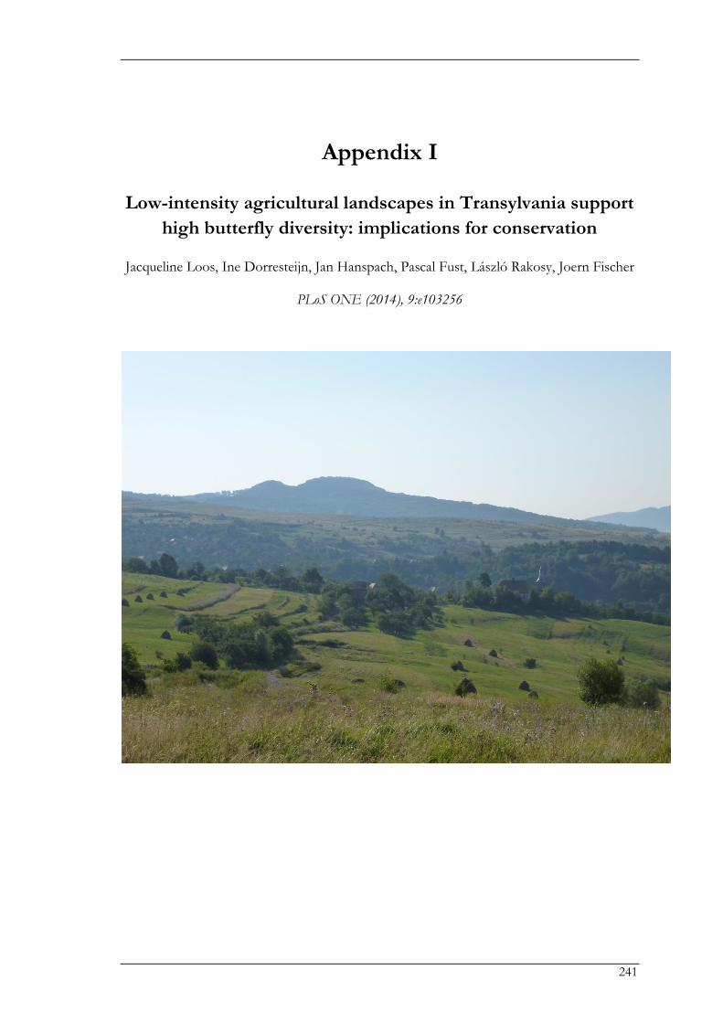
241
Appendix I
Low-intensity agricultural landscapes in Transylvania support
high butterfly diversity: implications for conservation
Jacqueline Loos, Ine Dorresteijn, Jan Hanspach, Pascal Fust, László Rakosy, Joern Fischer
PLoS ONE (2014), 9:e103256

Appendix I
242
Butterfly diversity in traditional farming landscapes
243
Abstract
European farmland biodiversity is declining due to land-use changes towards agricultural
intensification or abandonment. Some Eastern European farming systems have sustained
traditional forms of use, resulting in high levels of biodiversity. However, global markets and
international policies now imply rapid and major changes to these systems. To effectively protect
farmland biodiversity, understanding landscape features which underpin species diversity is crucial.
Focusing on butterflies, we addressed this question for a cultural-historic landscape in Southern
Transylvania, Romania. Following a natural experiment, we randomly selected 120 survey sites in
farmland, 60 each in grassland and arable land. We surveyed butterfly species richness and
abundance by walking transects with four repeats in summer 2012. We analysed species
composition using Detrended Correspondence Analysis. We modelled species richness, richness of
functional groups, and abundance of selected species in response to topography, woody vegetation
cover and heterogeneity at three spatial scales, using generalised linear mixed effects models.
Species composition widely overlapped in grassland and arable land. Composition changed along
gradients of heterogeneity at local and context scales, and of woody vegetation cover at context and
landscape scales. The effect of local heterogeneity on species richness was positive in arable land,
but negative in grassland. Plant species richness, and structural and topographic conditions at
multiple scales explained species richness, richness of functional groups and species abundances.
Our study revealed high conservation value of both grassland and arable land in low-intensity
Eastern European farmland. Besides grassland, also heterogeneous arable land provides important
habitat for butterflies. While butterfly diversity in arable land benefits from heterogeneity by small-
scale structures, grasslands should be protected from fragmentation to provide sufficiently large
areas for butterflies. These findings have important implications for EU agricultural and
conservation policy. Most importantly, conservation management needs to consider entire
landscapes, and implement appropriate measures at multiple spatial scales.
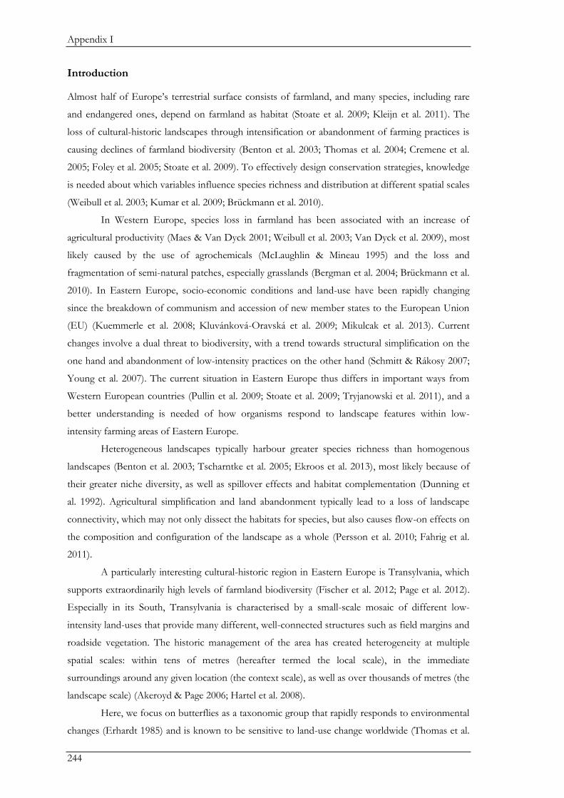
Appendix I
244
Introduction
Almost half of Europe’s terrestrial surface consists of farmland, and many species, including rare
and endangered ones, depend on farmland as habitat (Stoate et al. 2009; Kleijn et al. 2011). The
loss of cultural-historic landscapes through intensification or abandonment of farming practices is
causing declines of farmland biodiversity (Benton et al. 2003; Thomas et al. 2004; Cremene et al.
2005; Foley et al. 2005; Stoate et al. 2009). To effectively design conservation strategies, knowledge
is needed about which variables influence species richness and distribution at different spatial scales
(Weibull et al. 2003; Kumar et al. 2009; Brückmann et al. 2010).
In Western Europe, species loss in farmland has been associated with an increase of
agricultural productivity (Maes & Van Dyck 2001; Weibull et al. 2003; Van Dyck et al. 2009), most
likely caused by the use of agrochemicals (McLaughlin & Mineau 1995) and the loss and
fragmentation of semi-natural patches, especially grasslands (Bergman et al. 2004; Brückmann et al.
2010). In Eastern Europe, socio-economic conditions and land-use have been rapidly changing
since the breakdown of communism and accession of new member states to the European Union
(EU) (Kuemmerle et al. 2008; Kluvánková-Oravská et al. 2009; Mikulcak et al. 2013). Current
changes involve a dual threat to biodiversity, with a trend towards structural simplification on the
one hand and abandonment of low-intensity practices on the other hand (Schmitt & Rákosy 2007;
Young et al. 2007). The current situation in Eastern Europe thus differs in important ways from
Western European countries (Pullin et al. 2009; Stoate et al. 2009; Tryjanowski et al. 2011), and a
better understanding is needed of how organisms respond to landscape features within low-
intensity farming areas of Eastern Europe.
Heterogeneous landscapes typically harbour greater species richness than homogenous
landscapes (Benton et al. 2003; Tscharntke et al. 2005; Ekroos et al. 2013), most likely because of
their greater niche diversity, as well as spillover effects and habitat complementation (Dunning et
al. 1992). Agricultural simplification and land abandonment typically lead to a loss of landscape
connectivity, which may not only dissect the habitats for species, but also causes flow-on effects on
the composition and configuration of the landscape as a whole (Persson et al. 2010; Fahrig et al.
2011).
A particularly interesting cultural-historic region in Eastern Europe is Transylvania, which
supports extraordinarily high levels of farmland biodiversity (Fischer et al. 2012; Page et al. 2012).
Especially in its South, Transylvania is characterised by a small-scale mosaic of different low-
intensity land-uses that provide many different, well-connected structures such as field margins and
roadside vegetation. The historic management of the area has created heterogeneity at multiple
spatial scales: within tens of metres (hereafter termed the local scale), in the immediate
surroundings around any given location (the context scale), as well as over thousands of metres (the
landscape scale) (Akeroyd & Page 2006; Hartel et al. 2008).
Here, we focus on butterflies as a taxonomic group that rapidly responds to environmental
changes (Erhardt 1985) and is known to be sensitive to land-use change worldwide (Thomas et al.
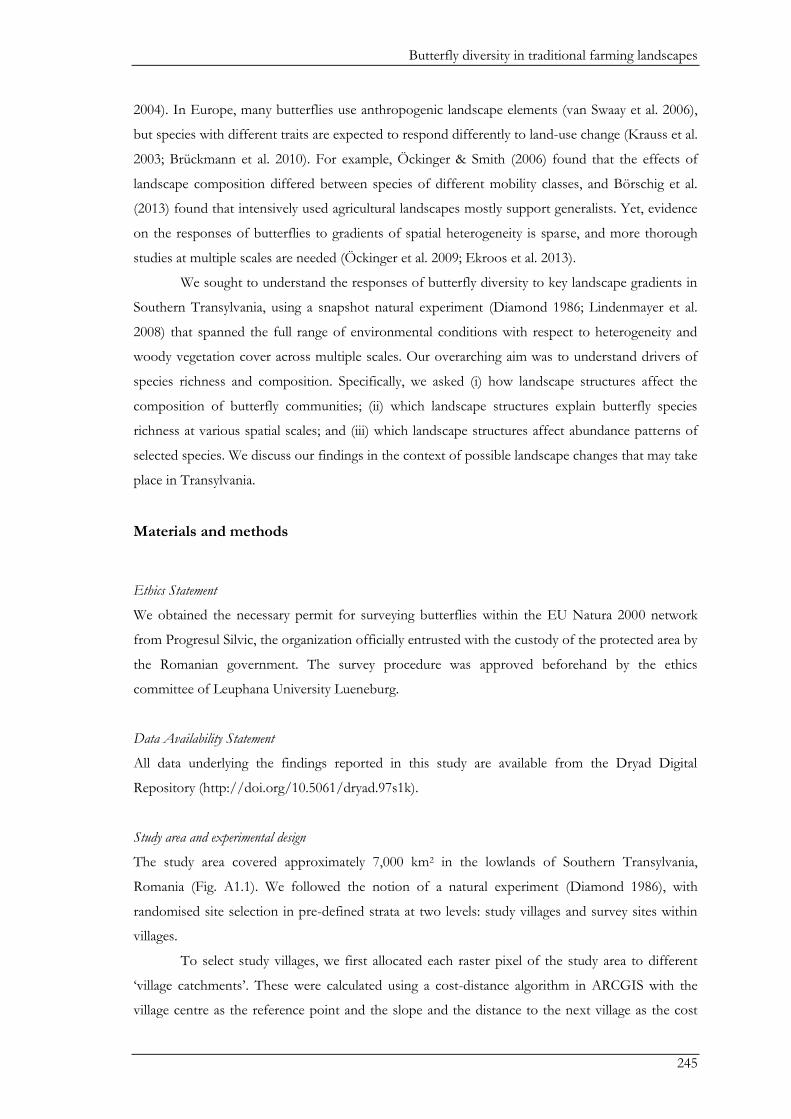
Butterfly diversity in traditional farming landscapes
245
2004). In Europe, many butterflies use anthropogenic landscape elements (van Swaay et al. 2006),
but species with different traits are expected to respond differently to land-use change (Krauss et al.
2003; Brückmann et al. 2010). For example, Öckinger & Smith (2006) found that the effects of
landscape composition differed between species of different mobility classes, and Börschig et al.
(2013) found that intensively used agricultural landscapes mostly support generalists. Yet, evidence
on the responses of butterflies to gradients of spatial heterogeneity is sparse, and more thorough
studies at multiple scales are needed (Öckinger et al. 2009; Ekroos et al. 2013).
We sought to understand the responses of butterfly diversity to key landscape gradients in
Southern Transylvania, using a snapshot natural experiment (Diamond 1986; Lindenmayer et al.
2008) that spanned the full range of environmental conditions with respect to heterogeneity and
woody vegetation cover across multiple scales. Our overarching aim was to understand drivers of
species richness and composition. Specifically, we asked (i) how landscape structures affect the
composition of butterfly communities; (ii) which landscape structures explain butterfly species
richness at various spatial scales; and (iii) which landscape structures affect abundance patterns of
selected species. We discuss our findings in the context of possible landscape changes that may take
place in Transylvania.
Materials and methods
Ethics Statement
We obtained the necessary permit for surveying butterflies within the EU Natura 2000 network
from Progresul Silvic, the organization officially entrusted with the custody of the protected area by
the Romanian government. The survey procedure was approved beforehand by the ethics
committee of Leuphana University Lueneburg.
Data Availability Statement
All data underlying the findings reported in this study are available from the Dryad Digital
Repository (http://doi.org/10.5061/dryad.97s1k).
Study area and experimental design
The study area covered approximately 7,000 km2 in the lowlands of Southern Transylvania,
Romania (Fig. A1.1). We followed the notion of a natural experiment (Diamond 1986), with
randomised site selection in pre-defined strata at two levels: study villages and survey sites within
villages.
To select study villages, we first allocated each raster pixel of the study area to different
‘village catchments’. These were calculated using a cost-distance algorithm in ARCGIS with the
village centre as the reference point and the slope and the distance to the next village as the cost
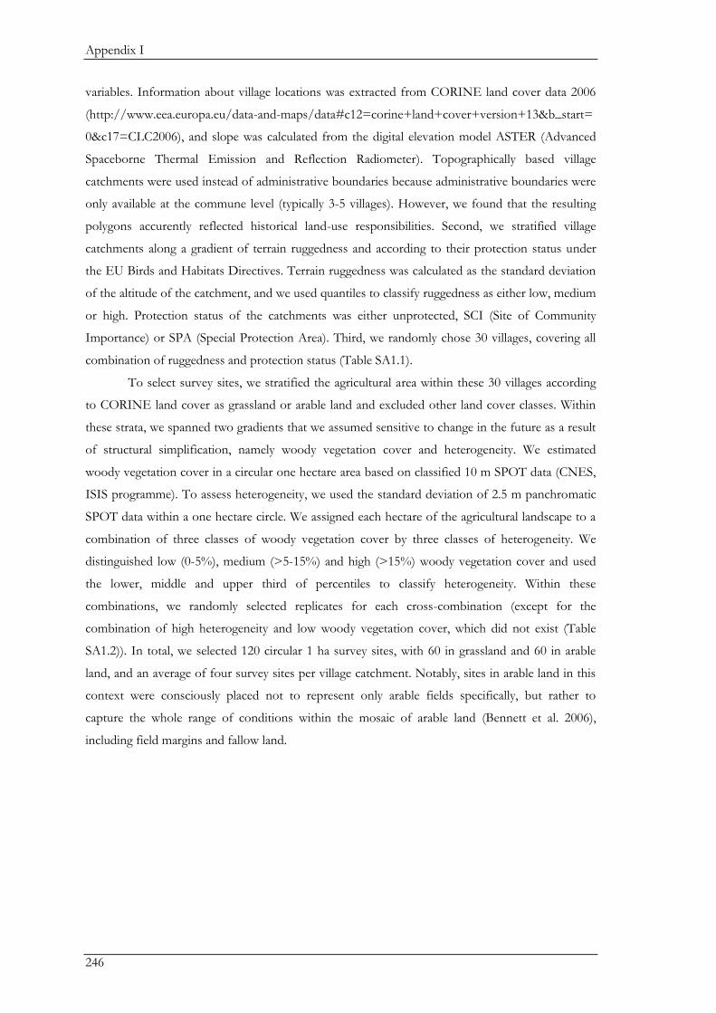
Appendix I
246
variables. Information about village locations was extracted from CORINE land cover data 2006
(http://www.eea.europa.eu/data-and-maps/data#c12=corine+land+cover+version+13&b_start=
0&c17=CLC2006), and slope was calculated from the digital elevation model ASTER (Advanced
Spaceborne Thermal Emission and Reflection Radiometer). Topographically based village
catchments were used instead of administrative boundaries because administrative boundaries were
only available at the commune level (typically 3-5 villages). However, we found that the resulting
polygons accurently reflected historical land-use responsibilities. Second, we stratified village
catchments along a gradient of terrain ruggedness and according to their protection status under
the EU Birds and Habitats Directives. Terrain ruggedness was calculated as the standard deviation
of the altitude of the catchment, and we used quantiles to classify ruggedness as either low, medium
or high. Protection status of the catchments was either unprotected, SCI (Site of Community
Importance) or SPA (Special Protection Area). Third, we randomly chose 30 villages, covering all
combination of ruggedness and protection status (Table SA1.1).
To select survey sites, we stratified the agricultural area within these 30 villages according
to CORINE land cover as grassland or arable land and excluded other land cover classes. Within
these strata, we spanned two gradients that we assumed sensitive to change in the future as a result
of structural simplification, namely woody vegetation cover and heterogeneity. We estimated
woody vegetation cover in a circular one hectare area based on classified 10 m SPOT data (CNES,
ISIS programme). To assess heterogeneity, we used the standard deviation of 2.5 m panchromatic
SPOT data within a one hectare circle. We assigned each hectare of the agricultural landscape to a
combination of three classes of woody vegetation cover by three classes of heterogeneity. We
distinguished low (0-5%), medium (>5-15%) and high (>15%) woody vegetation cover and used
the lower, middle and upper third of percentiles to classify heterogeneity. Within these
combinations, we randomly selected replicates for each cross-combination (except for the
combination of high heterogeneity and low woody vegetation cover, which did not exist (Table
SA1.2)). In total, we selected 120 circular 1 ha survey sites, with 60 in grassland and 60 in arable
land, and an average of four survey sites per village catchment. Notably, sites in arable land in this
context were consciously placed not to represent only arable fields specifically, but rather to
capture the whole range of conditions within the mosaic of arable land (Bennett et al. 2006),
including field margins and fallow land.
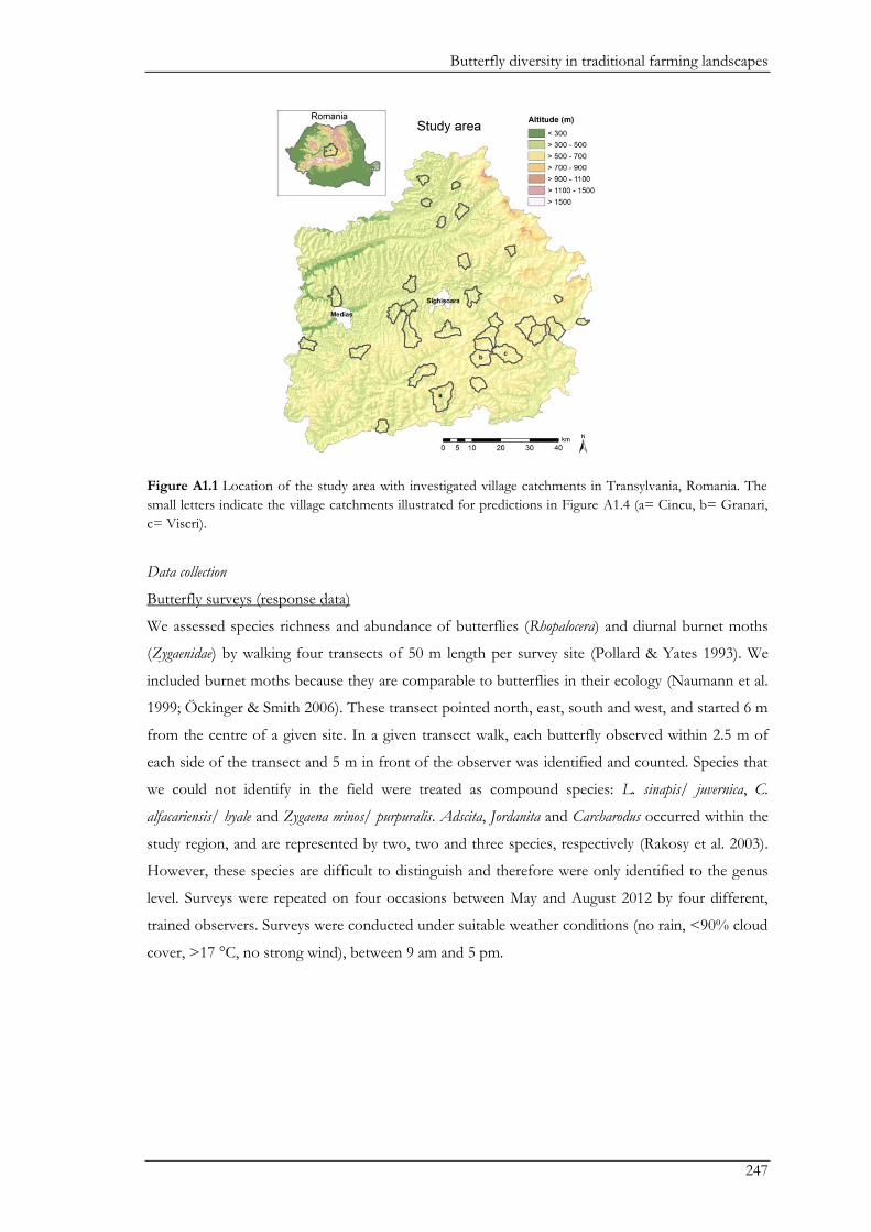
Butterfly diversity in traditional farming landscapes
247
Figure A1.1 Location of the study area with investigated village catchments in Transylvania, Romania. The
small letters indicate the village catchments illustrated for predictions in Figure A1.4 (a= Cincu, b= Granari,
c= Viscri).
Data collection
Butterfly surveys (response data)
We assessed species richness and abundance of butterflies (Rhopalocera) and diurnal burnet moths
(Zygaenidae) by walking four transects of 50 m length per survey site (Pollard & Yates 1993). We
included burnet moths because they are comparable to butterflies in their ecology (Naumann et al.
1999; Öckinger & Smith 2006). These transect pointed north, east, south and west, and started 6 m
from the centre of a given site. In a given transect walk, each butterfly observed within 2.5 m of
each side of the transect and 5 m in front of the observer was identified and counted. Species that
we could not identify in the field were treated as compound species: L. sinapis/ juvernica, C.
alfacariensis/ hyale and Zygaena minos/ purpuralis. Adscita, Jordanita and Carcharodus occurred within the
study region, and are represented by two, two and three species, respectively (Rakosy et al. 2003).
However, these species are difficult to distinguish and therefore were only identified to the genus
level. Surveys were repeated on four occasions between May and August 2012 by four different,
trained observers. Surveys were conducted under suitable weather conditions (no rain, <90% cloud
cover, >17 °C, no strong wind), between 9 am and 5 pm.
Appendix I
248
Environmental data (explanatory variables)
We followed a multi-scale approach and included explanatory variables that could potentially
explain butterfly distribution at the local (1 ha), context (50 ha) and landscape scale (i.e. village
catchments, ranging from 430 to 4963 ha). An overview of all variables included in the analysis is
presented in Table A1.1.
At the local scale, we collected data on vascular plant species richness in eight randomized
quadrants (1x1 m). We used cumulative plant species richness per site as an explanatory variable.
We also calculated indices for heatload (after Parker 1991) and terrain wetness as a measure of
potential soil wetness, and included heterogeneity assessed by the spectral variance of SPOT data
(see Table A1 for details). We calculated percent woody vegetation cover at local and context
scales, and used CORINE land cover to calculate percent forest at the landscape scale. For the
context and landscape scales, we calculated the terrain ruggedness as the standard deviation of
altitude. We also quantified compositional or configurational heterogeneity of the different land
covers grassland, arable land and forest as provided by CORINE land cover data. At the context
scale, our chosen heterogeneity measures (Simpson index of land cover diversity, edge density)
were correlated (ρ = 0.76). Hence, we included only edge density as an explanatory variable
(following Kumar et al. 2009). At the landscape scale, we used both edge density and the Simpson
index of diversity and added the amount of pasture and forest per village catchment, based on
CORINE land cover data. Variables on compositional and configurational heterogeneity were
calculated using FRAGSTATS v4.2 (McGarigal et al. 2012) and all other variables using ARCGIS
10.1 (ESRI Inc., Redland, CA).
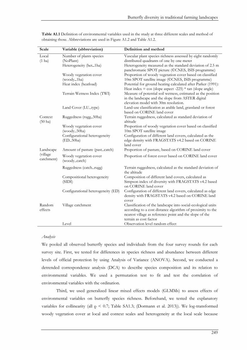
Butterfly diversity in traditional farming landscapes
249
Table A1.1 Definition of environmental variables used in the study at three different scales and method of
obtaining those. Abbreviations are used in Figure A1.2 and Table A1.2.
Scale Variable (abbreviation) Definition and method
Local (1 ha)
Number of plants species (NoPlant)
Vascular plant species richness assessed by eight randomly distributed quadrants of one by one meter
Heterogeneity (het_1ha) Heterogeneity measured as the standard deviation of 2.5 m panchromatic SPOT picture (©CNES, ISIS programme)
Woody vegetation cover (woody_1ha)
Proportion of woody vegetation cover based on classified 10m SPOT satellite image (©CNES, ISIS programme)
Heat index (heatload) Potential for ground heating calculated after Parker (1991): Heat index = cos (slope aspect -225) * tan (slope angle)
Terrain Wetness Index (TWI) Measure of potential soil wetness, estimated as the position in the landscape and the slope from ASTER digital elevation model with 30m resolution.
Land Cover (LU_type) Land-use classification as arable land, grassland or forest based on CORINE land cover
Context (50 ha)
Ruggedness (rugg_50ha) Terrain ruggedness, calculated as standard deviation of altitude
Woody vegetation cover (woody_50ha)
Proportion of woody vegetation cover based on classified 10m SPOT satellite image
Configurational heterogeneity (ED_50ha)
Configuration of different land covers, calculated as the edge density with FRAGSTATS v4.2 based on CORINE land cover
Landscape (village catchment)
Amount of pasture (past_catch) Proportion of pasture, based on CORINE land cover
Woody vegetation cover (woody_catch)
Proportion of forest cover based on CORINE land cover
Ruggedness (catch_rugg) Terrain ruggedness, calculated as the standard deviation of the altitude
Compositional heterogeneity (SIDI)
Composition of different land covers, calculated as Simpson index of diversity with FRAGSTATS v4.2 based on CORINE land cover
Configurational heterogeneity (ED) Configuration of different land covers, calculated as edge density with FRAGSTATS v4.2 based on CORINE land cover
Random effects
Village catchment Classification of the landscape into social-ecological units according to a cost distance algorithm of proximity to the nearest village as reference point and the slope of the terrain as cost factor
Level Observation level random effect
Analysis
We pooled all observed butterfly species and individuals from the four survey rounds for each
survey site. First, we tested for differences in species richness and abundance between different
levels of official protection by using Analysis of Variance (ANOVA). Second, we conducted a
detrended correspondence analysis (DCA) to describe species composition and its relation to
environmental variables. We used a permutation test to fit and test the correlation of
environmental variables with the ordination.
Third, we used generalized linear mixed effects models (GLMMs) to assess effects of
environmental variables on butterfly species richness. Beforehand, we tested the explanatory
variables for collinearity (all ρ < 0.7; Table SA1.3; (Dormann et al. 2013)). We log-transformed
woody vegetation cover at local and context scales and heterogeneity at the local scale because
Appendix I
250
these variables were highly skewed. All numerical explanatory variables were scaled to mean zero
and unit variance. We included the variables listed in Table A1.1 to model species richness of
butterflies. To test for a unimodal relationship in response to woody vegetation cover, we included
a quadratic term of local woody vegetation cover. We furthermore expected that the effect of
heterogeneity may differ between grassland and arable land and therefore included an interaction
term between land cover type and heterogeneity. Grasslands are also interesting to look at
separately because they are among the most species rich biotopes for butterflies in Europe (van
Swaay et al. 2011). We assessed the variance inflation factor (VIF) of the generalized linear model
(GLM) and tested for spatial auto-correlation in the residuals. We included the village catchment as
a random effect and corrected for overdispersion by adding an observation level random effect. We
simplified the model by stepwise backwards selection retaining all variables with p<0.1. For
GLMMs, significance levels are only approximations, hence many statisticians suggest using a
significance level of p<0.1 (Bolker et al. 2009).
Likewise, we modelled species richness of functional groups. To this end, we distinguished
between species of low mobility (Bink´s mobility classes 1 and 2) and high mobility (Bink´s
mobility classes 7, 8 and 9; Bink 1992)). Highly mobile species were Colias crocea, Pieris brassicae,
Vanessa atalanta and Vanessa cardui. Low-mobility species were Brenthis daphne, Brenthis ino,
Coenonympha glycerion, Cupido minimus, Euphydryas aurinia, Hamaeris lucina, Heteropterus morpheus, Lopinga
achine, Melitaea britomartis, Melitaea diamina and Satyrium acaciae. As a third group we modelled the
richness of grassland specialists, namely Euphydryas aurinia, Polyommatus coridon, Cyaniris semiargus,
Lysandra bellargus, Phengaris arion, Cupido minimus and Erynnis tages (van Swaay et al. 2013).
We also modelled the abundance of individual species considered to be declining in
Western and Northern Europe, but that are widespread or even increasing in Eastern Europe (van
Swaay & Warren 1999; Konvicka et al. 2003; Franzén & Ranius 2004; van Swaay et al. 2013). We
only used species that were common enough in the study area to obtain reliable models, namely
Maniola jurtina, Coenonympha pamphilus, Polyommatus Icarus, Lycaena dispar and Glaucopsyche alexis. We
performed all statistical analyses in R (R Core Team 2013), using the packages MASS, ade4, vegan,
gdata and lme4.
Results
In total, we counted 19,878 individuals of 112 species of butterflies (Table SA1.4). Site-level species
richness varied between three and 45, and the number of individuals between seven and 452.
Eighty-five percent of all individuals belonged to 12 species: Colias alfacariensis/hyale, Minois dryas,
Aphantopus hyperantus, Pieris rapae, Everes argiades, Coenonympha glycerion, Leptidea sinapis/juvernica,
Melanargia galathea, Coenonympha pamphilus, Maniola jurtina, Polyommatus icarus, and Plebeius argus. SCI,
SPA and unprotected sites did not differ in species richness (F=0.54, p=0.58) but SCI sites
appeared to have a slightly lower abundance of individuals than unprotected sites (F=2.37, p=0.09).
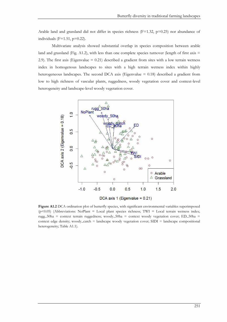
Butterfly diversity in traditional farming landscapes
251
Arable land and grassland did not differ in species richness (F=1.32, p=0.25) nor abundance of
individuals (F=1.51, p=0.22).
Multivariate analysis showed substantial overlap in species composition between arable
land and grassland (Fig. A1.2), with less than one complete species turnover (length of first axis =
2.9). The first axis (Eigenvalue = 0.21) described a gradient from sites with a low terrain wetness
index in homogenous landscapes to sites with a high terrain wetness index within highly
heterogeneous landscapes. The second DCA axis (Eigenvalue = 0.18) described a gradient from
low to high richness of vascular plants, ruggedness, woody vegetation cover and context-level
heterogeneity and landscape-level woody vegetation cover.
Figure A1.2 DCA ordination plot of butterfly species, with significant environmental variables superimposed
(p<0.05) (Abbreviations: NoPlant = Local plant species richness; TWI = Local terrain wetness index;
rugg_50ha = context terrain ruggedness; woody_50ha = context woody vegetation cover; ED_50ha =
context edge density; woody_catch = landscape woody vegetation cover; SIDI = landscape compositional
heterogeneity; Table A1.1).
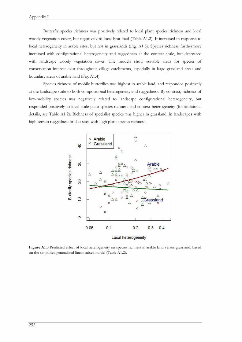
Appendix I
252
Butterfly species richness was positively related to local plant species richness and local
woody vegetation cover, but negatively to local heat load (Table A1.2). It increased in response to
local heterogeneity in arable sites, but not in grasslands (Fig. A1.3). Species richness furthermore
increased with configurational heterogeneity and ruggedness at the context scale, but decreased
with landscape woody vegetation cover. The models show suitable areas for species of
conservation interest exist throughout village catchments, especially in large grassland areas and
boundary areas of arable land (Fig. A1.4).
Species richness of mobile butterflies was highest in arable land, and responded positively
at the landscape scale to both compositional heterogeneity and ruggedness. By contrast, richness of
low-mobility species was negatively related to landscape configurational heterogeneity, but
responded positively to local-scale plant species richness and context heterogeneity (for additional
details, see Table A1.2). Richness of specialist species was higher in grassland, in landscapes with
high terrain ruggedness and at sites with high plant species richness.
Figure A1.3 Predicted effect of local heterogeneity on species richness in arable land versus grassland, based
on the simplified generalized linear mixed model (Table A1.2).
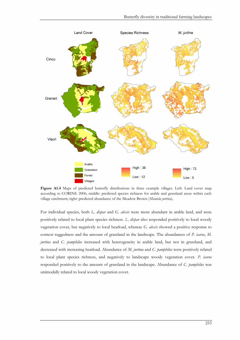
Butterfly diversity in traditional farming landscapes
253
Figure A1.4 Maps of predicted butterfly distributions in three example villages. Left: Land cover map
according to CORINE 2006; middle: predicted species richness for arable and grassland areas within each
village catchment; right: predicted abundance of the Meadow Brown (Maniola jurtina).
For individual species, both L. dispar and G. alexis were more abundant in arable land, and were
positively related to local plant species richness. L. dispar also responded positively to local woody
vegetation cover, but negatively to local heatload, whereas G. alexis showed a positive response to
context ruggedness and the amount of grassland in the landscape. The abundances of P. icarus, M.
jurtina and C. pamphilus increased with heterogeneity in arable land, but not in grassland, and
decreased with increasing heatload. Abundance of M. jurtina and C. pamphilus were positively related
to local plant species richness, and negatively to landscape woody vegetation cover. P. icarus
responded positively to the amount of grassland in the landscape. Abundance of C. pamphilus was
unimodally related to local woody vegetation cover.
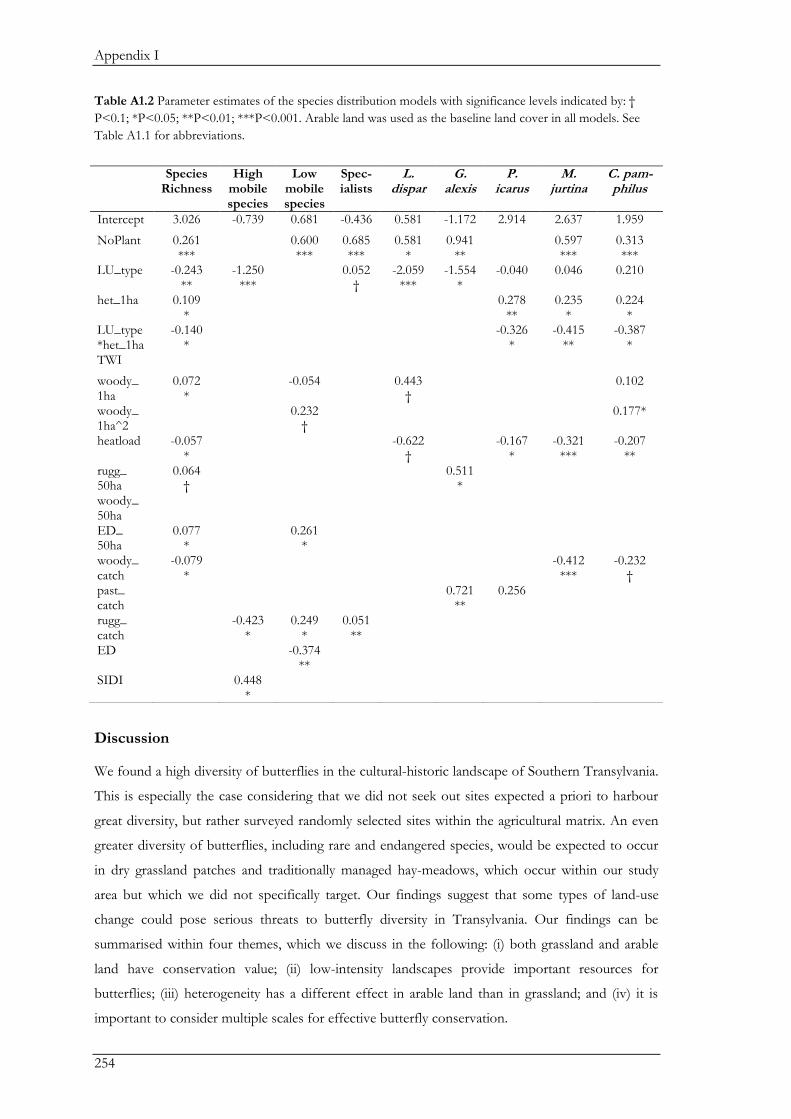
Appendix I
254
Table A1.2 Parameter estimates of the species distribution models with significance levels indicated by: †
P<0.1; *P<0.05; **P<0.01; ***P<0.001. Arable land was used as the baseline land cover in all models. See
Table A1.1 for abbreviations.
Discussion
We found a high diversity of butterflies in the cultural-historic landscape of Southern Transylvania.
This is especially the case considering that we did not seek out sites expected a priori to harbour
great diversity, but rather surveyed randomly selected sites within the agricultural matrix. An even
greater diversity of butterflies, including rare and endangered species, would be expected to occur
in dry grassland patches and traditionally managed hay-meadows, which occur within our study
area but which we did not specifically target. Our findings suggest that some types of land-use
change could pose serious threats to butterfly diversity in Transylvania. Our findings can be
summarised within four themes, which we discuss in the following: (i) both grassland and arable
land have conservation value; (ii) low-intensity landscapes provide important resources for
butterflies; (iii) heterogeneity has a different effect in arable land than in grassland; and (iv) it is
important to consider multiple scales for effective butterfly conservation.
Species Richness
High mobile species
Low mobile species
Spec-ialists
L. dispar
G. alexis
P. icarus
M. jurtina
C. pam-philus
Intercept 3.026 -0.739 0.681 -0.436 0.581 -1.172 2.914 2.637 1.959
NoPlant 0.261 ***
0.600 ***
0.685 ***
0.581 *
0.941 **
0.597 ***
0.313 ***
LU_type -0.243 **
-1.250 ***
0.052 †
-2.059 ***
-1.554 *
-0.040 0.046 0.210
het_1ha 0.109 *
0.278 **
0.235 *
0.224 *
LU_type *het_1ha
-0.140 *
-0.326 *
-0.415 **
-0.387 *
TWI
woody_ 1ha
0.072 *
-0.054 0.443 †
0.102
woody_ 1ha^2
0.232 †
0.177*
heatload -0.057 *
-0.622 †
-0.167 *
-0.321 ***
-0.207 **
rugg_ 50ha
0.064 †
0.511 *
woody_ 50ha
ED_ 50ha
0.077 *
0.261 *
woody_ catch
-0.079 *
-0.412 ***
-0.232 †
past_ catch
0.721 **
0.256
rugg_ catch
-0.423 *
0.249 *
0.051 **
ED -0.374 **
SIDI 0.448 *
Butterfly diversity in traditional farming landscapes
255
Both grassland and arable land have conservation value
Our findings revealed a high conservation value for butterflies of the small-scale farming system in
the lowlands of Transylvania. Interestingly, butterfly species richness and abundance were similar in
arable land and grassland. This is a surprising result and suggests a need to broaden the emphasis of
conservation activities from grassland protection towards the maintenance of heterogeneous
mosaic farmland, including cropland (Bennett et al. 2006). This is particularly important in the
context of criticisms that the recent reform of the European Union’s Common Agricultural Policy,
for example, falls far short of what is needed in terms of biodiversity conservation (Pe'er et al.
2014). Throughout Europe, grasslands are considered most important for butterfly conservation
(e.g. Brückmann et al. 2010; van Swaay et al. 2011). Arable land, on the other hand, has received far
less attention. In Western Europe, arable land has been found to support lower species richness
and more homogenous butterfly communities than grassland (Weibull & Ostman 2003; Weibull et
al. 2003). Our results indicate that this situation may be different in Eastern Europe, and that
certain types of arable land can in fact support similar levels of butterfly diversity as grasslands. A
possible explanation for the similar species richness in arable land and grassland in Transylvania
may be spillover effects (Dunning et al. 1992), which may be more likely in small-scale mosaics of
land covers. The mosaic character of the landscape also could explain the strong overlap in
butterfly communities between arable land and grassland.
Low-intensity landscapes provide important resources for butterflies
The fine-grained mosaic nature of arable land and the low-intensity nature of grassland in Southern
Transylvania emphasize that low-intensity land-use practices have major benefits for butterfly
conservation. Semi-natural elements occur throughout the landscape, and are a likely reason why
species richness is high throughout different land covers (Ekroos et al. 2013). Furthermore, species
richness of vascular plants can be high in field margins, which in turn may indicate high quality
habitat for butterflies (Steffan-Dewenter & Tscharntke 2000). Consistent with the findings of
Kumar, Simonson & Stohlgren (2009), we found plant species richness strongly related to butterfly
species richness. Currently, Transylvania contains some of the world’s most species rich areas for
plants (Wilson et al. 2012), which is partly linked to the low use of fertilizers (Jones 2009).
Agricultural intensification, by contrast, would likely lead to increased use of fertilizers and hence
reduced plant species richness (Zechmeister et al. 2003; Van Landuyt et al. 2008; Kleijn et al. 2009).
Furthermore, intensification is typically associated with the use of fewer, high yielding crop
varieties. Interestingly, many butterflies in Transylvania use the common crop Medicago sativa ssp.
sativa (Alfalfa), a leguminous species that provides nectar and that we also observed to serve as a
host plant for several butterfly species (e.g. Glaucopsyche alexis). Alfalfa is grown in small parcels, is
primarily used as winter fodder for livestock, and may easily be lost as a result of intensification.
However, high amounts of floral resources are critically important to maintain butterfly diversity.
Similarly, woody vegetation offers important resources for butterflies, including shelter and space
Appendix I
256
for thermoregulation (Dover et al. 1997). At present, Transylvania contains many scattered trees
and hedgerows, and we found that butterfly species richness responded positively to these
structures at the local scale. By contrast, a large amount of woody vegetation at the landscape scale
may lead to decreased species richness, probably due to a lack of open habitat.
Heterogeneity has a different effect in arable land than in grassland
We considered heterogeneity and woody vegetation cover at the local scale as two potentially
important gradients describing the structure of the landscape. Interestingly, our results showed that
the effect of local heterogeneity on species richness depended on land cover. In arable land, species
richness increased with heterogeneity, supporting our hypothesis that small-scale farming benefits
biodiversity by providing a range of different resources for butterflies. Notably, our land-use class
of ‘arable land’ reflected the highly heterogeneous nature of traditional farmland, and included
cropped areas as well as fallows and uncultivated field margins. These non-cropped areas are likely
to be particularly important to maintain butterfly diversity in arable land. By contrast, in grassland,
high heterogeneity was associated with reduced butterfly diversity. A possible explanation for this
pattern is that heterogeneity of grassland may correspond to a higher degree of fragmentation of
butterfly habitat, with likely negative consequences for species diversity (Krauss et al. 2004). Our
study thus confirms that heterogeneity per se is not universally beneficial for species richness (see
also Ekroos et al. 2008), although most work to date has focused on its positive effects (e.g. Kerr et
al. 2001).
The importance of considering multiple scales
To date, results from studies investigating multiple scales have been disparate and difficult to
generalize (Flick et al. 2012). We included three spatial scales in our study which we considered
relevant for butterfly diversity and distribution. Our study revealed that all investigated scales
affected butterfly community composition. Previous studies found local factors affecting butterfly
species composition, with local heterogeneity in land cover being a good predictor for species
composition in Canada (Kerr et al. 2001; Weibull & Ostman 2003). Butterfly species composition
in Transylvania also showed a significant correlation with local factors, but was explained by
heterogeneity and woody vegetation cover only at the two larger scales. Butterfly species richness
also responded to variables at all different spatial scales, especially at the local scale, but also at the
two larger scales (see also Weibull et al. 2003). This suggests that local habitat conditions are
particularly important, yet these cannot be considered in isolation from the surrounding landscape
(Steffan-Dewenter et al. 2002; Öckinger & Smith 2006).
Our models also showed that the different functional groups of butterflies were affected
by variables from different spatial scales. For example, landscape heterogeneity appeared to benefit
mobile species but not low-mobility species. Furthermore, we found that woody vegetation cover
was related to species richness. Land abandonment induces natural succession, whereas

Butterfly diversity in traditional farming landscapes
257
intensification leads to loss of scattered woody vegetation, and both have negative effects on
butterfly richness in the long term (Baur et al. 2006). Both processes decrease structural
heterogeneity, which is important for viable butterfly populations in agricultural landscapes. In our
study, only Coenonympha pamphilus showed a unimodal relationship to local woody vegetation cover.
For such low-mobile species, presence of woody vegetation is crucial for wind shield and
thermoregulation. C. pamphilus is abundant in Transylvania, however its population state in other
European countries is declining (Conrad et al. 2007). Habitat heterogeneity from different spatial
scales, including the presence of woody vegetation, should be further investigated as possible key
elements in landscapes to halt biodiversity loss in farmland.
Conclusion
Collapse of communism and accession of Romania to the European Union have accelerated land-
use change in the rural areas of Transylvania, in particular towards land abandonment and
agricultural intensification. The two key gradients considered in this study, namely woody
vegetation cover and heterogeneity, would fundamentally change as a result of these two land-use
change processes. Along the gradients of woody vegetation cover and heterogeneity, we were able
to show that butterfly abundance and distribution were affected by a range of different variables
operating at multiple spatial scales. Not only local conditions, but the composition and
configuration of the landscape as a whole need to be considered for effective conservation
management of butterflies in low-intensively managed farming landscapes such as in Transylvania.
Our results showed that, unlike in Western Europe, species richness of butterflies was not
only high in grassland, but also in arable land. This suggests that more emphasis needs to be placed
on low-intensity farming practices and management of the landscape mosaic, and that arable land
needs to be actively considered in butterfly conservation strategies. In our study area, butterfly
richness would likely benefit from (1) the continuation of small-scale farming; (2) the production of
a variety of crops, including legume species; and (3) the maintenance of broad field margins and
uncultivated ruderal areas. New payment schemes under the Common Agricultural Policy have
recently been criticised as grossly inadequate (Pe'er et al. 2014). Our findings suggest that even
measures considered adequate in Western Europe may not be directly transferable to Transylvania
– in low-intensity landscapes, it will be particularly important to consider the high nature value that
entire agro-ecosystems provide, both inside and outside of protected areas (see also González-
Estébanez et al. 2011). Ultimately, the continued existence of historic-cultural landscapes such as
those in Transylvania hinges on the successful transfer of its appreciation and historic management
to future generations of farmers. Substantial efforts are therefore needed in environmental
education and in developing alternative ways for local people to make a living, for example through
the development of cultural and ecological tourism.

Appendix I
258
Acknowledgements
We warmly thank Rémi Bigonneau, Paul Kirkland, Joerg Steiner, Kimberley Pope, and Elek Telek
for help in the field. Sincere thanks to the farmers, landowners, mayors and the Mihai Eminescu
Trust for their support. We are grateful for analytical support by Henrik von Wehrden and Dave
Abson. Comments by two anonymous reviewers greatly helped to improve an earlier version of
this manuscript.
Butterfly diversity in traditional farming landscapes
259
References
Akeroyd, J. R., and J. N. Page. 2006. The Saxon villages of southern Transylvania: Conserving
biodiversity in a historic landscape. In: D. Gafta, and J. Akeroyd (eds). Nature
conservation: concepts and practice, Springer, New York, pp 199-210.
Baur, B., C. Cremene, G. Groza, L. Rakosy, A. A. Schileyko, A. Baur, P. Stoll, and A. Erhardt.
2006. Effects of abandonment of subalpine hay meadows on plant and invertebrate
diversity in Transylvania, Romania. Biological Conservation 132:261-273.
Bennett, A. F., J. Q. Radford, and A. Haslem. 2006. Properties of land mosaics: implications for
nature conservation in agricultural environments. Biological Conservation 133:250-264.
Benton, T. G., J. A. Vickery, and J. D. Wilson. 2003. Farmland biodiversity: is habitat heterogeneity
the key? Trends in Ecology & Evolution 18:182-188.
Bergman, K. O., J. Askling, O. Ekberg, H. Ignell, H. Wahlman, and P. Milberg. 2004. Landscape
effects on butterfly assemblages in an agricultural region. Ecography 27:619-628.
Bink, F. A. 1992. Ecologische atlas van de dagvlinders van Noordwest-Europa. Schuyt & Co,
Haarlem, 512 pp.
Bolker, B. M., M. E. Brooks, C. J. Clark, S. W. Geange, J. R. Poulsen, M. H. H. Stevens, and J. S. S.
White. 2009. Generalized linear mixed models: a practical guide for ecology and evolution.
Trends in Ecology & Evolution 24:127-135.
Börschig, C., A.-M. Klein, H. von Wehrden, and J. Krauss. 2013. Traits of butterfly communities
change from specialist to generalist characteristics with increasing land-use intensity. Basic
and Applied Ecology 14:547-554.
Brückmann, S. V., J. Krauss, and I. Steffan-Dewenter. 2010. Butterfly and plant specialists suffer
from reduced connectivity in fragmented landscapes. Journal of Applied Ecology 47:799-
809.
Conrad, K. F., R. Fox, and I. P. Woiwod. 2007. Monitoring biodiversity: measuring long-term
changes in insect abundance. In: A. J. A. Stewart, T. R. New, and O. T. Lewis (eds). Insect
Conservation Biology. CAB International, Wallingford, pp 203-225.
Cremene, C., G. Groza, L. Rakosy, A. A. Schileyko, A. Baur, A. Erhardt, and B. Baur. 2005.
Alterations of steppe-like grasslands in Eastern Europe: a threat to regional biodiversity
hotspots. Conservation Biology 19:1606-1618.
Diamond, J. M. 1986. Overview: laboratory experiments, field experiments, and natural
experiments. In: J. M. Diamond, and T. J. Case (eds). Community Ecology. Harper & Row,
New York, pp 3-22.
Dormann, C. F., J. Elith, S. Bacher, C. Buchmann, G. Carl, G. Carre, J. R. G. Marquez, B. Gruber,
B. Lafourcade, P. J. Leitao, T. Munkemuller, C. McClean, P. E. Osborne, B. Reineking, B.
Schroder, A. K. Skidmore, D. Zurell, and S. Lautenbach. 2013. Collinearity: a review of
methods to deal with it and a simulation study evaluating their performance. Ecography
36:27-46.
Dover, J., T. Sparks, and J. Greatorex-Davies. 1997. The importance of shelter for butterflies in
open landscapes. Journal of Insect Conservation 1:89-97.
Dunning, J. B., B. J. Danielson, and H. R. Pulliam. 1992. Ecological processes that affect
populations in complex landscapes. Oikos 65:169-175.
Ekroos, J., M. Piha, and J. Tiainen. 2008. Role of organic and conventional field boundaries on
boreal bumblebees and butterflies. Agriculture, Ecosystems & Environment 124:155-159.
Ekroos, J., M. Rundlöf, and H. G. Smith. 2013. Trait-dependent responses of flower-visiting
insects to distance to semi-natural grasslands and landscape heterogeneity. Landscape
Ecology 28:1283-1292.
Appendix I
260
Erhardt, A. 1985. Diurnal lepidoptera: sensitive indicators of cultivated and abandoned grassland.
Journal of Applied Ecology 22:849-861.
Fahrig, L., J. Baudry, L. Brotons, F. G. Burel, T. O. Crist, R. J. Fuller, C. Sirami, G. M. Siriwardena,
and J. L. Martin. 2011. Functional landscape heterogeneity and animal biodiversity in
agricultural landscapes. Ecology Letters 14:101-112.
Fischer, J., T. Hartel, and T. Kuemmerle. 2012. Conservation policy in traditional farming
landscapes. Conservation Letters 5:167-175.
Flick, T., S. Feagan, and L. Fahrig. 2012. Effects of landscape structure on butterfly species
richness and abundance in agricultural landscapes in eastern Ontario, Canada. Agriculture
Ecosystems & Environment 156:123-133.
Foley, J. A., R. DeFries, G. P. Asner, C. Barford, G. Bonan, S. R. Carpenter, F. S. Chapin, M. T.
Coe, G. C. Daily, H. K. Gibbs, J. H. Helkowski, T. Holloway, E. A. Howard, C. J.
Kucharik, C. Monfreda, J. A. Patz, I. C. Prentice, N. Ramankutty, and P. K. Snyder. 2005.
Global consequences of land use. Science 309:570-574.
Franzén, M., and T. Ranius. 2004. Occurrence patterns of butterflies (Rhopalocera) in semi-natural
pastures in southeastern Sweden. Journal for Nature Conservation 12:121-135.
González-Estébanez, F. J., S. García-Tejero, P. Mateo-Tomás, and P. P. Olea. 2011. Effects of
irrigation and landscape heterogeneity on butterfly diversity in Mediterranean farmlands.
Agriculture, Ecosystems & Environment 144:262-270.
Hartel, T., C. I. Moga, K. Öllerer, I. Sas, L. Demeter, D. Rusti, and A. Balog. 2008. A proposal
towards the incorporation of spatial heterogeneity into animal distribution studies in
Romanian landscapes. North-Western Journal of Zoology 4:67-74.
Jones, A. 2009. Wildflower species indicators for lowland grassland habitat conservation in
Transylvania (Romania). Contributii Botanice 44:57-66.
Kerr, J. T., T. R. E. Southwood, and J. Cihlar. 2001. Remotely sensed habitat diversity predicts
butterfly species richness and community similarity in Canada. Proceedings of the National
Academy of Sciences 98:11365-11370.
Kleijn, D., F. Kohler, A. Baldi, P. Batary, E. D. Concepcion, Y. Clough, M. Diaz, D. Gabriel, A.
Holzschuh, E. Knop, A. Kovacs, E. J. P. Marshall, T. Tscharntke, and J. Verhulst. 2009.
On the relationship between farmland biodiversity and land-use intensity in Europe.
Proceedings of the Royal Society B: Biological Sciences 276:903-909.
Kleijn, D., M. Rundlöf, J. Scheper, H. G. Smith, and T. Tscharntke. 2011. Does conservation on
farmland contribute to halting the biodiversity decline? Trends in Ecology & Evolution
26:474-481.
Kluvánková-Oravská, T., V. Chobotová, I. Banaszak, L. Slavikova, and S. Trifunovova. 2009. From
government to governance for biodiversity: the perspective of central and Eastern
European transition countries. Environmental Policy & Governance 19:186-196.
Konvicka, M., M. Maradova, J. Benes, Z. Fric, and P. Kepka. 2003. Uphill shifts in distribution of
butterflies in the Czech Republic: effects of changing climate detected on a regional scale.
Global Ecology and Biogeography 12:403-410.
Krauss, J., A. M. Klein, I. Steffan-Dewenter, and T. Tscharntke. 2004. Effects of habitat area,
isolation, and landscape diversity on plant species richness of calcareous grasslands.
Biodiversity and Conservation 13:1427-1439.
Krauss, J., I. Steffan-Dewenter, and T. Tscharntke. 2003. How does landscape context contribute
to effects of habitat fragmentation on diversity and population density of butterflies?
Journal of Biogeography 30:889-900.
Kuemmerle, T., D. Muller, P. Griffiths, and M. Rusu. 2008. Land use change in Southern Romania
after the collapse of socialism. Regional Environmental Change 9:1-12.
Butterfly diversity in traditional farming landscapes
261
Kumar, S., S. E. Simonson, and T. J. Stohlgren. 2009. Effects of spatial heterogeneity on butterfly
species richness in Rocky Mountain National Park, CO, USA. Biodiversity and
Conservation 18:739-763.
Lindenmayer, D. B., R. B. Cunningham, C. MacGregor, M. Crane, D. Michael, J. Fischer, R.
Montague-Drake, A. Felton, and A. Manning. 2008. Temporal changes in vertebrates
during landscape transformation: a large-scale “natural experiment”. Ecological
Monographs 78:567-590.
Maes, D., and H. Van Dyck. 2001. Butterfly diversity loss in Flanders (north Belgium): Europe's
worst case scenario? Biological Conservation 99:263-276.
McGarigal, K., S. Cushman, and E. Ene. 2012. FRAGSTATS v4: spatial pattern analysis program
for categorical and continuous maps. Software, University of Massachusetts, Amherst.
www.umass.edu/landeco/research/fragstats/fragstats.html.
McLaughlin, A., and P. Mineau. 1995. The impact of agricultural practices on biodiversity.
Agriculture, Ecosystems & Environment 55:201-212.
Mikulcak, F., J. Newig, A. I. Milcu, T. Hartel, and J. Fischer. 2013. Integrating rural development
and biodiversity conservation in Central Romania. Environmental Conservation 40:129-
137.
Naumann, C. M., G. M. Tarmann, and W. G. Tremewan 1999. The Western Palaearctic Zygaenidae
(Lepidoptera). Apollo Books, Stenstrup, 304 pp.
Öckinger, E., M. Franzen, M. Rundlof, and H. G. Smith. 2009. Mobility-dependent effects on
species richness in fragmented landscapes. Basic and Applied Ecology 10:573-578.
Öckinger, E., and H. G. Smith. 2006. Landscape composition and habitat area affects butterfly
species richness in semi-natural grasslands. Oecologia 149:526-534.
Page, N., A. Bălan, S. Huband, R. Popa, L. Rákosy, and L. Sutcliffe. 2012. Romania. In: R.
Oppermann, G. Beaufoy, and G. Jones (eds). High Nature Value Farming in Europe.
Regionalkultur, Ubstadt-Weiher, pp 346-358.
Parker, K. C. 1991. Topography, substrate, and vegetation patterns in the Northern Sonoran
Desert. Journal of Biogeography 18:151-163.
Pe'er, G., L. V. Dicks, P. Visconti, R. Arlettaz, A. Báldi, T. G. Benton, S. Collins, M. Dieterich, R.
D. Gregory, F. Hartig, K. Henle, P. R. Hobson, D. Kleijn, R. K. Neumann, T. Robijns, J.
Schmidt, A. Shwartz, W. J. Sutherland, A. Turbé, F. Wulf, and A. V. Scott. 2014. EU
agricultural reform fails on biodiversity. Science 344:1090-1092.
Persson, A. S., O. Olsson, M. Rundlöf, and H. G. Smith. 2010. Land use intensity and landscape
complexity: analysis of landscape characteristics in an agricultural region in Southern
Sweden. Agriculture Ecosystems & Environment 136:169-176.
Pollard, E., and T. J. Yates 1993. Monitoring butterflies for ecology and conservation: the British
butterfly monitoring scheme. Chapman & Hall, London, 274 pp.
Pullin, A. S., A. Baldi, O. E. Can, M. Dieterich, V. Kati, B. Livoreil, G. Lovei, B. Mihok, O. Nevin,
N. Selva, and I. Sousa-Pinto. 2009. Conservation focus on Europe: major conservation
policy issues that need to be informed by conservation science. Conservation Biology
23:818-824.
R Core Team. 2013. R: a language and environment for statistical computing. R Foundation for
Statistical Computing, Vienna, Austria.
Rakosy, L., M. Goia, and Z. Kovács. 2003. Catalogul Lepidopterelor Romaniei/Verzeichnis der
Schmetterlinge Rumäniens. S. L. Romana, Cluj-Napoca, 79 pp.
Schmitt, T., and L. Rákosy. 2007. Changes of traditional agrarian landscapes and their conservation
implications: a case study of butterflies in Romania. Diversity and Distributions 13:855-
862.
Appendix I
262
Steffan-Dewenter, I., U. Munzenberg, C. Burger, C. Thies, and T. Tscharntke. 2002. Scale-
dependent effects of landscape context on three pollinator guilds. Ecology 83:1421-1432.
Steffan-Dewenter, I., and T. Tscharntke. 2000. Butterfly community structure in fragmented
habitats. Ecology Letters 3:449-456.
Stoate, C., A. Baldi, P. Beja, N. D. Boatman, I. Herzon, A. van Doorn, G. R. de Snoo, L. Rakosy,
and C. Ramwell. 2009. Ecological impacts of early 21st century agricultural change in
Europe: a review. Journal of Environmental Management 91:22-46.
Thomas, J. A., M. G. Telfer, D. B. Roy, C. D. Preston, J. J. D. Greenwood, J. Asher, R. Fox, R. T.
Clarke, and J. H. Lawton. 2004. Comparative losses of British butterflies, birds, and plants
and the global extinction crisis. Science 303:1879-1881.
Tryjanowski, P., T. Hartel, A. Baldi, P. Szymanski, M. Tobolka, I. Herzon, A. Golawski, M.
Konvicka, M. Hromada, L. Jerzak, K. Kujawa, M. Lenda, G. Orlowski, M. Panek, P.
Skorka, T. H. Sparks, S. Tworek, A. Wuczynski, and M. Zmihorski. 2011. Conservation of
farmland birds faces different challenges in Western and Central-Eastern Europe. Acta
Ornithologica 46:1-12.
Tscharntke, T., A. M. Klein, A. Kruess, I. Steffan-Dewenter, and C. Thies. 2005. Landscape
perspectives on agricultural intensification and biodiversity: ecosystem service
management. Ecology Letters 8:857-874.
Van Dyck, H., A. J. Van Strien, D. Maes, and C. A. M. Van Swaay. 2009. Declines in common,
widespread butterflies in a landscape under intense human use. Conservation Biology
23:957-965.
Van Landuyt, W., L. Vanhecke, I. Hoste, F. Hendrickx, and D. Bauwens. 2008. Changes in the
distribution area of vascular plants in Flanders (northern Belgium): eutrophication as a
major driving force. Biodiversity and Conservation 17:3045-3060.
van Swaay, C., D. Maes, S. Collins, M. L. Munguira, M. Sasic, J. Settele, R. Verovnik, M. Warren,
M. Wiemers, I. Wynhoff, and A. Cuttelod. 2011. Applying IUCN criteria to invertebrates:
How red is the Red List of European butterflies? Biological Conservation 144:470-478.
van Swaay, C., A. v. Strien, A. Harpke, B. Fontaine, C. Stefanescu, D. Roy, D. Maes, E. Kühn, E.
Õunap, E. Regan, G. Švitra, I. Prokofev, J. Heliölä, J. Settele, L. Pettersson, M. Botham,
M. Musche, N. Titeux, N. Cornish, P. Leopold, R. Julliard, R. Verovnik, S. Öberg, S.
Popov, S. Collins, S. Goloshchapova, T. Brereton, and M. Warren. 2013. The european
grassland butterfly indicator: 1990-2011. EEA Technical report. European Environment
Agency, Copenhagen, 36 pp.
van Swaay, C., M. Warren, and G. Lois. 2006. Biotope use and trends of European butterflies.
Journal of Insect Conservation 10:305-306.
van Swaay, C., and M. S. Warren 1999. Red data book of European butterflies (Rhopalocera).
Council of Europe, Strasbourg, 260 pp.
Weibull, A. C., and O. Ostman. 2003. Species composition in agroecosystems: the effect of
landscape, habitat, and farm management. Basic and Applied Ecology 4:349-361.
Weibull, A. C., O. Ostman, and A. Granqvist. 2003. Species richness in agroecosystems: the effect
of landscape, habitat and farm management. Biodiversity and Conservation 12:1335-1355.
Wilson, J. B., R. K. Peet, J. Dengler, and M. Partel. 2012. Plant species richness: the world records.
Journal of Vegetation Science 23:796-802.
Young, J., C. Richards, A. Fischer, L. Halada, T. Kull, A. Kuzniar, U. Tartes, Y. Uzunov, and A.
Watt. 2007. Conflicts between biodiversity conservation and human activities in the central
and eastern European countries. Ambio 36:545-550.
Zechmeister, H. G., I. Schmitzberger, B. Steurer, J. Peterseil, and T. Wrbka. 2003. The influence of
land-use practices and economics on plant species richness in meadows. Biological
Conservation 114:165-177.
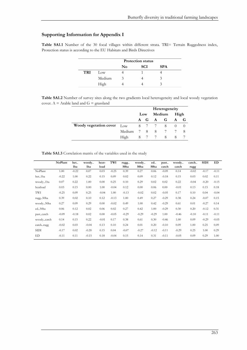
Butterfly diversity in traditional farming landscapes
263
Supporting Information for Appendix I
Table SA1.1 Number of the 30 focal villages within different strata. TRI= Terrain Ruggedness index,
Protection status is according to the EU Habitats and Birds Directives
Table SA1.2 Number of survey sites along the two gradients local heterogeneity and local woody vegetation
cover. A = Arable land and G = grassland Heterogeneity
Low Medium High
A G A G A G
Woody vegetation cover Low 8 7 7 8 0 0
Medium 7 8 8 7 7 8
High 8 7 7 8 8 7
Table SA1.3 Correlation matrix of the variables used in the study
Protection status
No SCI SPA
TRI Low 4 1 4
Medium 3 4 3
High 4 4 3
NoPlant het_
1ha
woody_
1ha
heat-
load
TWI rugg_
50ha
woody_
50ha
ed_
50ha
past_
catch
woody_
catch
catch_
rugg
SIDI ED
NoPlant 1.00 -0.22 0.07 0.03 -0.25 0.39 0.27 0.06 -0.09 0.14 -0.02 -0.17 -0.11
het_1ha -0.22 1.00 0.22 0.15 0.09 0.02 0.09 0.12 -0.18 0.15 0.03 0.02 0.11
woody_1ha 0.07 0.22 1.00 0.00 0.25 0.10 0.29 0.02 0.02 0.22 -0.04 -0.20 -0.15
heatload 0.03 0.15 0.00 1.00 -0.04 0.12 0.00 0.06 0.00 -0.01 0.13 0.15 0.18
TWI -0.25 0.09 0.25 -0.04 1.00 -0.13 -0.02 0.02 -0.05 0.17 0.10 0.04 -0.04
rugg_50ha 0.39 0.02 0.10 0.12 -0.13 1.00 0.49 0.27 -0.29 0.38 0.24 -0.07 0.15
woody_50ha 0.27 0.09 0.29 0.00 -0.02 0.49 1.00 0.42 -0.29 0.61 0.01 -0.27 0.14
ed_50ha 0.06 0.12 0.02 0.06 0.02 0.27 0.42 1.00 -0.29 0.30 0.20 -0.12 0.31
past_catch -0.09 -0.18 0.02 0.00 -0.05 -0.29 -0.29 -0.29 1.00 -0.46 -0.10 -0.11 -0.11
woody_catch 0.14 0.15 0.22 -0.01 0.17 0.38 0.61 0.30 -0.46 1.00 0.09 -0.29 -0.05
catch_rugg -0.02 0.03 -0.04 0.13 0.10 0.24 0.01 0.20 -0.10 0.09 1.00 0.25 0.09
SIDI -0.17 0.02 -0.20 0.15 0.04 -0.07 -0.27 -0.12 -0.11 -0.29 0.25 1.00 0.29
ED -0.11 0.11 -0.15 0.18 -0.04 0.15 0.14 0.31 -0.11 -0.05 0.09 0.29 1.00
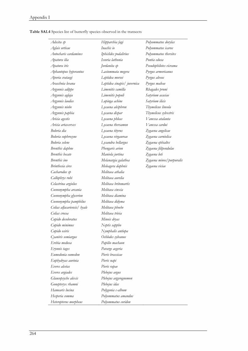
Appendix I
264
Table SA1.4 Species list of butterfly species observed in the transects
Adscita sp Hipparchia fagi Polyommatus dorylas
Aglais urticae Inachis io Polyommatus icarus
Antocharis cardamines Iphiclides podalirius Polyommatus thersites
Apatura ilia Issoria lathonia Pontia edusa
Apatura iris Jordanita sp Pseudophilotes vicrama
Aphantopus hyperantus Lasiommata megera Pyrgus armoricanus
Aporia crataegi Leptidea morsei Pyrgus alveus
Araschnia levana Leptidea sinapis/ juvernica Pyrgus malvae
Argynnis adippe Limenitis camilla Rhagades pruni
Argynnis aglaja Limenitis populi Satyrium acaciae
Argynnis laodice Lopinga achine Satyrium ilicis
Argynnis niobe Lycaena alciphron Thymelicus lineola
Argynnis paphia Lycaena dispar Thymelicus sylvestris
Aricia agestis Lycaena phleas Vanessa atalanta
Aricia artaxerxes Lycaena thersamon Vanessa cardui
Boloria dia Lycaena tityrus Zygaena angelicae
Boloria euphrosyne Lycaena virgaureae Zygaena carniolica
Boloria selene Lysandra bellargus Zygaena ephialtes
Brenthis daphne Phengaris arion Zygaena filipendulae
Brenthis hecate Maniola jurtina Zygaena loti
Brenthis ino Melanargia galathea Zygaena minos/purpuralis
Brinthesia circe Meleagera daphnis Zygaena viciae
Cacharodus sp Melitaea athalia
Callophrys rubi Melitaea aurelia
Celastrina argiolus Melitaea britomartis
Coenonympha arcania Melitaea cinxia
Coenonympha glycerion Melitaea diamina
Coenonympha pamphilus Melitaea didyma
Colias alfacariensis/ hyale Melitaea phoebe
Colias crocea Melitaea trivia
Cupido decoloratus Minois dryas
Cupido minimus Neptis sappho
Cupido osiris Nymphalis antiopa
Cyaniris semiargus Ochlodes sylvanus
Erebia medusa Papilio machaon
Erynnis tages Pararge aegeria
Eumedonia eumedon Pieris brassicae
Euphydryas aurinia Pieris napi
Everes alcetas Pieris rapae
Everes argiades Plebejus argus
Glaucopsyche alexis Plebejus argyrognomon
Gonepteryx rhamni Plebejus idas
Hamearis lucina Polygonia c-album
Hesperia comma Polyommatus amandus
Heteropterus morpheus Polyommatus coridon

265
Appendix II

266
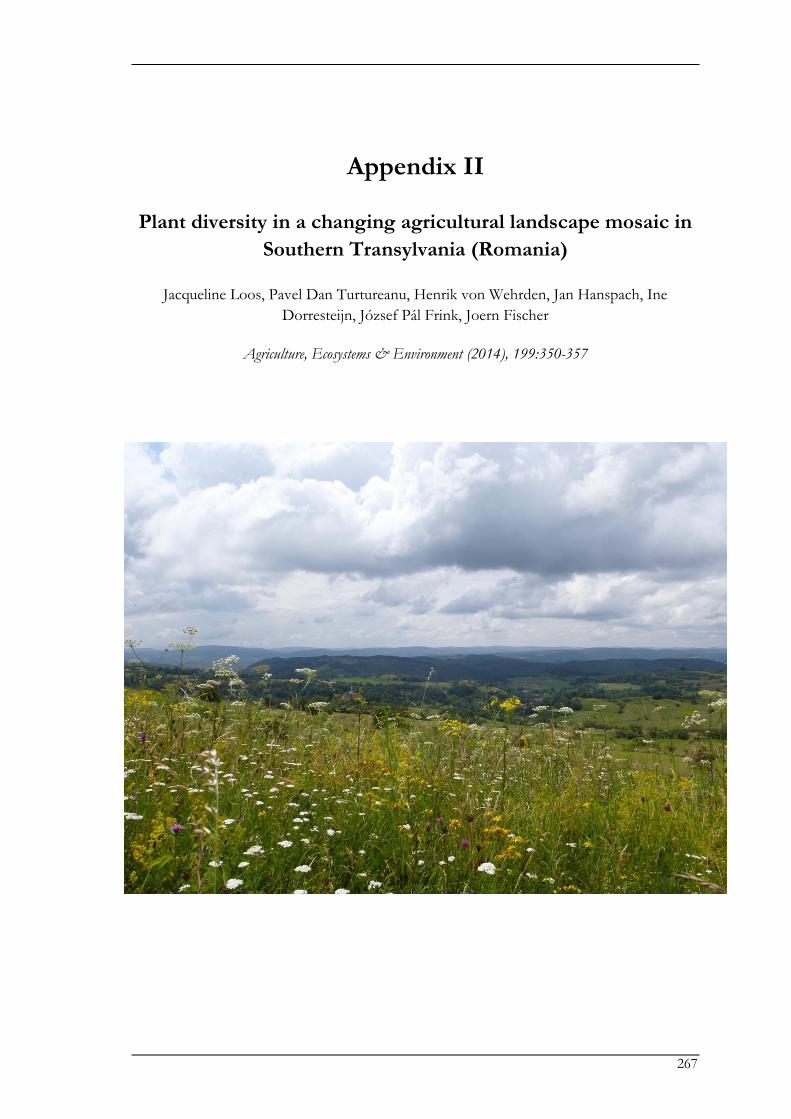
267
Appendix II
Plant diversity in a changing agricultural landscape mosaic in
Southern Transylvania (Romania)
Jacqueline Loos, Pavel Dan Turtureanu, Henrik von Wehrden, Jan Hanspach, Ine
Dorresteijn, József Pál Frink, Joern Fischer
Agriculture, Ecosystems & Environment (2014), 199:350-357

Appendix II
268
Plant diversity in traditional farming landscapes
269
Abstract
Traditional agricultural landscapes represent mosaics of land-use covers that often support high
species diversity. Many Eastern European countries contain large areas of High Nature Value
(HNV) farmland. However, these landscapes are likely to change under current EU regulations and
global market pressure, with potentially negative consequences for biodiversity. The conservation
value of Romania’s grasslands is widely recognized, but the potential conservation value of other
parts of the landscape mosaic has not been assessed to date. For this reason, we sought to assess
patterns of plant diversity across the entire landscape mosaic. We sampled vascular plants at 139
sites (comprising 8 plots of 1m2/ha) in forest (n = 23), grassland (n = 57) and within the arable
mosaic (n = 59). To examine potential differences in species richness and composition between
these land cover types, we used Analysis of Variance and Detrended Correspondence Analysis. We
also modeled total species richness, richness of HNV indicator plants and richness of arable weeds
in response to variables representing topography as well as structural and configurational
heterogeneity. Species composition differed strongly between grassland, the arable mosaic and
forests. Richness was highest in grasslands, but surprisingly, the arable mosaic and grassland
contributed similarly to the cumulative number of recorded species. Models of species richness
revealed a wide range of responses of plant groups to topographical conditions and to structural
and configurational heterogeneity, which often differed between land-use types. Plants were
affected by conditions measured at both local (1 ha) and landscape (50 ha) scales. Noting the
substantial, and hitherto under-recognised, contribution of the agricultural mosaic to regional-scale
plant diversity, we recommend consideration of the entire landscape mosaic in future conservation
schemes.
Appendix II
270
Introduction
Many agricultural landscapes around the world are characterized by a mosaic of land covers
(Forman 1995). With their various patches of land-use types and structures, mosaic landscapes
often host a wide range of species (Bennett et al. 2006). However, unprecedented changes in
agricultural mosaic landscapes are causing major biodiversity loss worldwide (Tscharntke et al.
2005). Moreover, patterns of species richness and distribution in agricultural landscapes are
affected by processes operating at multiple spatial scales, including both local and landscape-level
variables (Vandvik & Birks 2002; Rundlöf et al. 2010; Costanza et al. 2011). Hence, effective
management of biodiversity in agricultural landscapes requires an assessment of the drivers of
species diversity across multiple spatial scales.
In many Eastern European countries, such as Romania, traditional practices have created
small-scale mosaic landscapes. For example, 72% of farms in Romania are smaller than 1 ha
(Fundatia Adept 2012), and individual fields are typically smaller than that. However, Romania’s
farmland has been undergoing drastic changes since the collapse of communism in 1990
(Kuemmerle et al. 2008) and accession to the European Union (EU) in 2007. Ongoing land-use
changes comprise both intensification of land-use in some areas, and land abandonment in others
(Government of Romania 2010; Dahlström et al. 2013; Mikulcak et al. 2013). At present, twenty
percent of Romanian farmland is considered to be High Nature Value (HNV) farmland, and ten
percent is protected under the EU Birds and Habitats Directives (Natura 2000) (European
Environment Agency 2010). Despite official recognition of the ecological values of large areas of
farmland, the future of Romania’s agricultural landscapes and their biodiversity is uncertain.
Some of Romania’s most notable mosaic landscapes occur in the region of Southern
Transylvania. A large part of Transylvania was recently designated one of the largest continuous
(lowland) Natura 2000 sites in Europe (i.e. Târnavelor Plateau), partly in recognition of its
outstanding grassland diversity (Jones et al. 2010; Akeroyd & Page 2011). The region´s biodiversity
includes various taxa that are rare or endangered in other parts of Europe, such as the yellow-
bellied toad (Bombina variegata) (Hartel & von Wehrden 2013), Maculinea butterflies (Vodă et al.
2010) and several rare species of woodpeckers (Dorresteijn et al. 2013). Moreover, Transylvanian
dry grasslands hold the world record for vascular plant species richness at the scales of 0.1 m2 and
10 m2 (Wilson et al. 2012). However, land-use change is likely in Transylvania, and would pose
major threats to its biodiversity. Modifications of land-use will most likely consist of increasing
cropland area, increasing the use of agrochemicals, structural homogenization, and conversion of
traditional hay meadows to pastures, thus mirroring the patterns already apparent in Western
Europe (McLaughlin & Mineau 1995; Benton et al. 2003; Billeter et al. 2008; Ernoult & Alard
2011).
In this study we focus on vascular plants and their distribution throughout the entire
landscape mosaic in Southern Transylvania. Plants respond relatively slowly to environmental
changes (Helm et al. 2006), but in agricultural landscapes, specialized species are highly prone to
Plant diversity in traditional farming landscapes
271
rapid decline (Davies et al. 2004; Clavel et al. 2010). Plant communities in agricultural landscapes
are at risk of homogenization in composition because of nutrient inputs, which many species, and
especially grassland specialists, are sensitive to. For Transylvania, a specific set of sensitive grassland
specialists has been proposed to indicate High Nature Value (HNV) grassland (Akeroyd & Bădărău
2012). Furthermore, arable weeds are of particular interest. Many such weeds have persisted in
Transylvania to date, but are under worldwide decline, and may react quickly to changes in the
environment, both at local and landscape scales (Gabriel et al. 2005; Armengot et al. 2012; Storkey
et al. 2012).
We sought to understand the responses of vascular plant diversity to key landscape
features. To that end, we used a snapshot natural experiment (Diamond 1986; Lindenmayer et al.
2008) that spanned a wide range of environmental conditions with respect to heterogeneity and
woody vegetation cover across local and landscape scales. We sampled vegetation and
environmental conditions throughout the landscape mosaic and asked: (i) how current land-use was
associated with vascular plant diversity and species composition; and (ii) how landscape structure
was related to total richness, richness of HNV indicator plants and richness of arable weeds.
Methods
Study area
Our study area covered approximately 7,000 km2 in the lowlands of Southern Transylvania,
Romania. The area consists of undulating terrain with altitudes from 300 to 700 m above sea level,
and its climate is subcontinental-temperate. The area comprises a mosaic of land-use types,
including arable fields (40% according to CORINE land cover), secondary grasslands and ancient
dry steppe-like grasslands (30%) and deciduous forests (30%) (Dengler et al. 2012). The natural
vegetation consists of oak-hornbeam forests (Quercus petraea-Carpinus betulus; Bohn et al. 2004).
Site selection
We followed the notion of a natural experiment (Diamond 1986), with randomised site selection in
pre-defined strata at two levels: (i) village catchments and (ii) survey sites within village catchments.
We delineated the study area into village catchments using a cost-distance algorithm that allocated
each pixel to the village with the lowest travel cost to this pixel (slope-penalized distance,
implemented in ArcGIS 10.1). We randomly selected a subset of 30 village catchments within three
different strata cross-combined by a gradient of terrain ruggedness (low, medium, high; defined by
quantiles) and protection status according to EU Birds and Habitats Directives (Site of Community
Importance (SCI), Special Protection Area (SPA) and unprotected; Table SA2.1). Within each
village catchment, we assigned land to three different land-use types using the CORINE land cover
map (EEA 2006), namely forest, grassland or arable land. By ‘arable land’, we refer to the mosaic of
arable land in its entirety, including semi-natural vegetation occurring within the mosaic, such as
Appendix II
272
field margins, road verges, hedges and old fields. Throughout grassland and arable land (collectively
termed ‘farmland’), we identified gradients of heterogeneity and woody vegetation cover. We
quantified heterogeneity as the standard deviation of panchromatic SPOT 5 data (©CNES 2007,
Distribution Spot Image SA) within a 1 ha moving window. We calculated the percentage of woody
vegetation within a 1 ha moving window by supervised classifications of the panchromatic channels
of SPOT 5, using a support vector machine algorithm (Knorn et al. 2009). We used the upper,
middle and lower thirds of these gradients to randomly select cross-replicated circular 1 ha survey
sites – 59 within arable land and 57 within grassland (Table SA2.2). An additional 23 sites (also
measuring 1 ha) were randomly selected in forest without further stratification.
Vegetation surveys
We conducted vegetation surveys between 26 May and 26 August 2012. We sampled eight plots
measuring 1 m x 1 m within each site, placed at a random distance from the center, and distributed
every 45 degrees. We alternated between random distances >40m and <40m from the center to
cover the inner and the outer 0.5 ha of the site equally. In each plot, we identified vascular plants to
species level and recorded their percent cover.
Environmental parameters
We considered variables that were potentially related to plant species richness within circles of one
hectare (henceforth: local level) and circles of 50 hectare (henceforth: landscape level) around a
given site. At the local level, we considered heterogeneity, altitude, woody vegetation cover, a heat
index (after Parker (1991): cos (slope aspect -225) * tan (slope angle)), a terrain wetness index (after
Fischer et al. 2010), and land cover type. At the landscape level, we considered terrain ruggedness,
woody vegetation cover, edge density to account for configurational heterogeneity (Fahrig et al.
2011), and a Simpson index of heterogeneity to account for compositional heterogeneity. Variables
were calculated using ArcGIS 10.1 and Fragstats 4.1, and are described in more detail in Table
A2.1.
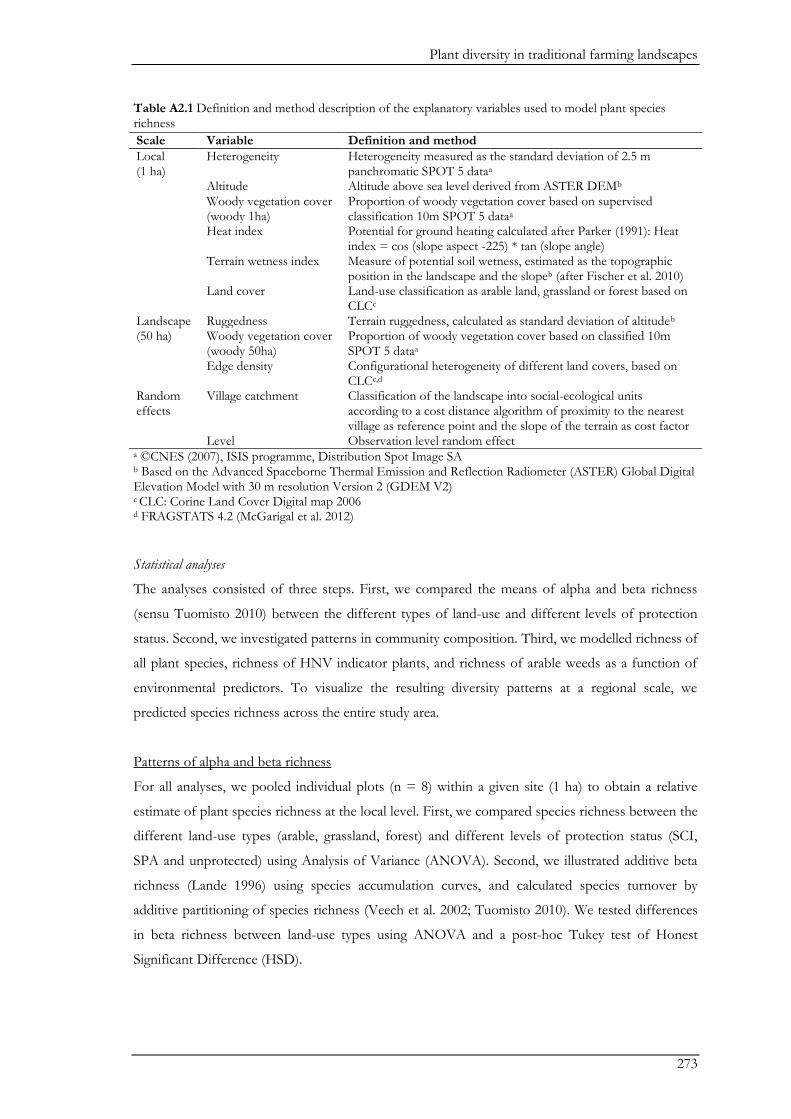
Plant diversity in traditional farming landscapes
273
Table A2.1 Definition and method description of the explanatory variables used to model plant species richness
a ©CNES (2007), ISIS programme, Distribution Spot Image SA b Based on the Advanced Spaceborne Thermal Emission and Reflection Radiometer (ASTER) Global Digital Elevation Model with 30 m resolution Version 2 (GDEM V2) c CLC: Corine Land Cover Digital map 2006 d FRAGSTATS 4.2 (McGarigal et al. 2012)
Statistical analyses
The analyses consisted of three steps. First, we compared the means of alpha and beta richness
(sensu Tuomisto 2010) between the different types of land-use and different levels of protection
status. Second, we investigated patterns in community composition. Third, we modelled richness of
all plant species, richness of HNV indicator plants, and richness of arable weeds as a function of
environmental predictors. To visualize the resulting diversity patterns at a regional scale, we
predicted species richness across the entire study area.
Patterns of alpha and beta richness
For all analyses, we pooled individual plots (n = 8) within a given site (1 ha) to obtain a relative
estimate of plant species richness at the local level. First, we compared species richness between the
different land-use types (arable, grassland, forest) and different levels of protection status (SCI,
SPA and unprotected) using Analysis of Variance (ANOVA). Second, we illustrated additive beta
richness (Lande 1996) using species accumulation curves, and calculated species turnover by
additive partitioning of species richness (Veech et al. 2002; Tuomisto 2010). We tested differences
in beta richness between land-use types using ANOVA and a post-hoc Tukey test of Honest
Significant Difference (HSD).
Scale Variable Definition and method
Local (1 ha)
Heterogeneity Heterogeneity measured as the standard deviation of 2.5 m panchromatic SPOT 5 dataa
Altitude Altitude above sea level derived from ASTER DEMb Woody vegetation cover (woody 1ha)
Proportion of woody vegetation cover based on supervised classification 10m SPOT 5 dataa
Heat index Potential for ground heating calculated after Parker (1991): Heat index = cos (slope aspect -225) * tan (slope angle)
Terrain wetness index
Measure of potential soil wetness, estimated as the topographic position in the landscape and the slopeb (after Fischer et al. 2010)
Land cover Land-use classification as arable land, grassland or forest based on CLCc
Landscape (50 ha)
Ruggedness Terrain ruggedness, calculated as standard deviation of altitudeb Woody vegetation cover (woody 50ha)
Proportion of woody vegetation cover based on classified 10m SPOT 5 dataa
Edge density Configurational heterogeneity of different land covers, based on CLCc,d
Random effects
Village catchment Classification of the landscape into social-ecological units according to a cost distance algorithm of proximity to the nearest village as reference point and the slope of the terrain as cost factor
Level Observation level random effect
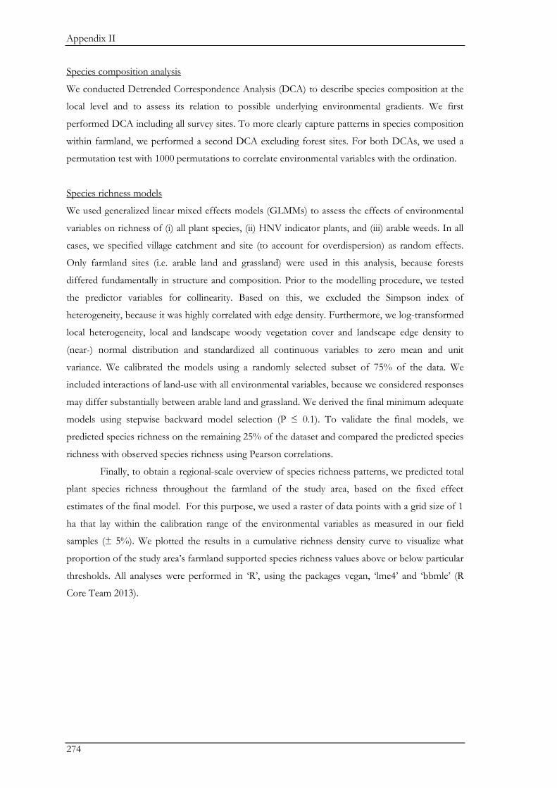
Appendix II
274
Species composition analysis
We conducted Detrended Correspondence Analysis (DCA) to describe species composition at the
local level and to assess its relation to possible underlying environmental gradients. We first
performed DCA including all survey sites. To more clearly capture patterns in species composition
within farmland, we performed a second DCA excluding forest sites. For both DCAs, we used a
permutation test with 1000 permutations to correlate environmental variables with the ordination.
Species richness models
We used generalized linear mixed effects models (GLMMs) to assess the effects of environmental
variables on richness of (i) all plant species, (ii) HNV indicator plants, and (iii) arable weeds. In all
cases, we specified village catchment and site (to account for overdispersion) as random effects.
Only farmland sites (i.e. arable land and grassland) were used in this analysis, because forests
differed fundamentally in structure and composition. Prior to the modelling procedure, we tested
the predictor variables for collinearity. Based on this, we excluded the Simpson index of
heterogeneity, because it was highly correlated with edge density. Furthermore, we log-transformed
local heterogeneity, local and landscape woody vegetation cover and landscape edge density to
(near-) normal distribution and standardized all continuous variables to zero mean and unit
variance. We calibrated the models using a randomly selected subset of 75% of the data. We
included interactions of land-use with all environmental variables, because we considered responses
may differ substantially between arable land and grassland. We derived the final minimum adequate
models using stepwise backward model selection (P ≤ 0.1). To validate the final models, we
predicted species richness on the remaining 25% of the dataset and compared the predicted species
richness with observed species richness using Pearson correlations.
Finally, to obtain a regional-scale overview of species richness patterns, we predicted total
plant species richness throughout the farmland of the study area, based on the fixed effect
estimates of the final model. For this purpose, we used a raster of data points with a grid size of 1
ha that lay within the calibration range of the environmental variables as measured in our field
samples (± 5%). We plotted the results in a cumulative richness density curve to visualize what
proportion of the study area’s farmland supported species richness values above or below particular
thresholds. All analyses were performed in ‘R’, using the packages vegan, ‘lme4’ and ‘bbmle’ (R
Core Team 2013).
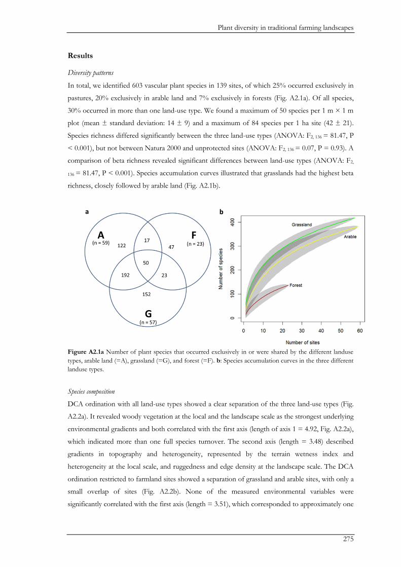
Plant diversity in traditional farming landscapes
275
Results
Diversity patterns
In total, we identified 603 vascular plant species in 139 sites, of which 25% occurred exclusively in
pastures, 20% exclusively in arable land and 7% exclusively in forests (Fig. A2.1a). Of all species,
30% occurred in more than one land-use type. We found a maximum of 50 species per 1 m × 1 m
plot (mean ± standard deviation: 14 ± 9) and a maximum of 84 species per 1 ha site (42 ± 21).
Species richness differed significantly between the three land-use types (ANOVA: F2, 136 = 81.47, P
< 0.001), but not between Natura 2000 and unprotected sites (ANOVA: F2, 136 = 0.07, P = 0.93). A
comparison of beta richness revealed significant differences between land-use types (ANOVA: F2,
136 = 81.47, P < 0.001). Species accumulation curves illustrated that grasslands had the highest beta
richness, closely followed by arable land (Fig. A2.1b).
Figure A2.1a Number of plant species that occurred exclusively in or were shared by the different landuse
types, arable land (=A), grassland (=G), and forest (=F). b: Species accumulation curves in the three different
landuse types.
Species composition
DCA ordination with all land-use types showed a clear separation of the three land-use types (Fig.
A2.2a). It revealed woody vegetation at the local and the landscape scale as the strongest underlying
environmental gradients and both correlated with the first axis (length of axis 1 = 4.92, Fig. A2.2a),
which indicated more than one full species turnover. The second axis (length = 3.48) described
gradients in topography and heterogeneity, represented by the terrain wetness index and
heterogeneity at the local scale, and ruggedness and edge density at the landscape scale. The DCA
ordination restricted to farmland sites showed a separation of grassland and arable sites, with only a
small overlap of sites (Fig. A2.2b). None of the measured environmental variables were
significantly correlated with the first axis (length = 3.51), which corresponded to approximately one
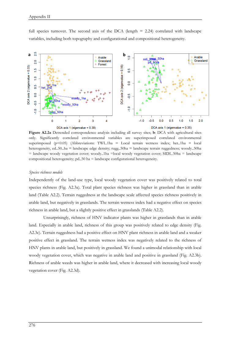
Appendix II
276
full species turnover. The second axis of the DCA (length = 2.24) correlated with landscape
variables, including both topography and configurational and compositional heterogeneity.
Figure A2.2a Detrended correspondence analysis including all survey sites; b: DCA with agricultural sites
only. Significantly correlated environmental variables are superimposed correlated environmental
superimposed (p<0.05) (Abbreviations: TWI_1ha = Local terrain wetness index; het_1ha = local
heterogeneity, ed_50_ha = landscape edge density; rugg_50ha = landscape terrain ruggedness; woody_50ha
= landscape woody vegetation cover; woody_1ha =local woody vegetation cover; SIDI_50ha = landscape
compositional heterogeneity; pd_50 ha = landscape configurational heterogeneity.
Species richness models
Independently of the land-use type, local woody vegetation cover was positively related to total
species richness (Fig. A2.3a). Total plant species richness was higher in grassland than in arable
land (Table A2.2). Terrain ruggedness at the landscape scale affected species richness positively in
arable land, but negatively in grasslands. The terrain wetness index had a negative effect on species
richness in arable land, but a slightly positive effect in grasslands (Table A2.2).
Unsurprisingly, richness of HNV indicator plants was higher in grasslands than in arable
land. Especially in arable land, richness of this group was positively related to edge density (Fig.
A2.3c). Terrain ruggedness had a positive effect on HNV plant richness in arable land and a weaker
positive effect in grassland. The terrain wetness index was negatively related to the richness of
HNV plants in arable land, but positively in grassland. We found a unimodal relationship with local
woody vegetation cover, which was negative in arable land and positive in grassland (Fig. A2.3b).
Richness of arable weeds was higher in arable land, where it decreased with increasing local woody
vegetation cover (Fig. A2.3d).
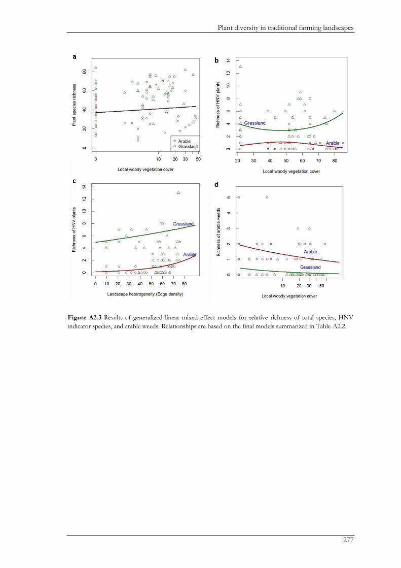
Plant diversity in traditional farming landscapes
277
Figure A2.3 Results of generalized linear mixed effect models for relative richness of total species, HNV
indicator species, and arable weeds. Relationships are based on the final models summarized in Table A2.2.
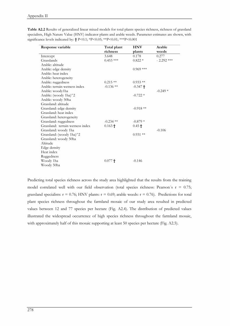
Appendix II
278
Table A2.2 Results of generalized linear mixed models for total plants species richness, richness of grassland
specialists, High Nature Value (HNV) indicator plants and arable weeds. Parameter estimates are shown, with
significance levels indicated by: † P<0.1; *P<0.05; **P<0.01; ***P<0.001
Predicting total species richness across the study area highlighted that the results from the training
model correlated well with our field observation (total species richness: Pearson´s r = 0.75;
grassland specialists: r = 0.76; HNV plants: r = 0.69; arable weeds: r = 0.76). Predictions for total
plant species richness throughout the farmland mosaic of our study area resulted in predicted
values between 12 and 77 species per hectare (Fig. A2.4). The distribution of predicted values
illustrated the widespread occurrence of high species richness throughout the farmland mosaic,
with approximately half of this mosaic supporting at least 50 species per hectare (Fig. A2.5).
Response variable Total plant richness
HNV plants
Arable weeds
Intercept 3.648 0.178 0.277 Grasslands 0.453 *** 0.822 * - 2.292 *** Arable: altitude Arable: edge density 0.969 *** Arable: heat index Arable: heterogeneity Arable: ruggedness 0.215 ** 0.933 ** Arable: terrain wetness index -0.136 ** -0.347 † Arable: woody1ha -0.249 * Arable: (woody 1ha)^2 -0.722 * Arable: woody 50ha Grassland: altitude Grassland: edge density -0.918 ** Grassland: heat index Grassland: heterogeneity Grassland: ruggedness -0.234 ** -0.879 * Grassland: terrain wetness index 0.163 † 0.45 † Grassland: woody 1ha -0.106 Grassland: (woody 1ha)^2 0.931 ** Grassland: woody 50ha Altitude Edge density Heat index Ruggedness Woody 1ha 0.077 † -0.146 Woody 50ha
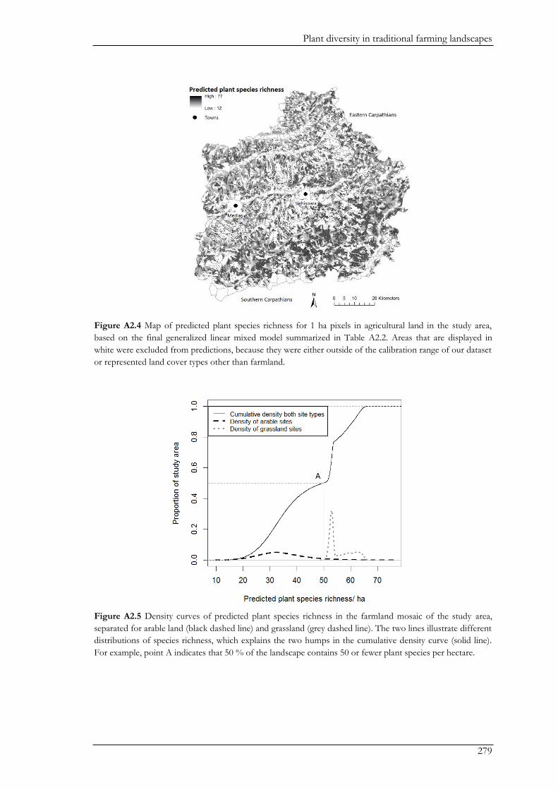
Plant diversity in traditional farming landscapes
279
Figure A2.4 Map of predicted plant species richness for 1 ha pixels in agricultural land in the study area,
based on the final generalized linear mixed model summarized in Table A2.2. Areas that are displayed in
white were excluded from predictions, because they were either outside of the calibration range of our dataset
or represented land cover types other than farmland.
Figure A2.5 Density curves of predicted plant species richness in the farmland mosaic of the study area,
separated for arable land (black dashed line) and grassland (grey dashed line). The two lines illustrate different
distributions of species richness, which explains the two humps in the cumulative density curve (solid line).
For example, point A indicates that 50 % of the landscape contains 50 or fewer plant species per hectare.
Appendix II
280
Discussion
Besides notable exceptions (Wagner et al. 2000; Waldhardt et al. 2004; Simmering et al. 2006), this
work is one of few studies on plant diversity patterns in Europe applying a sampling approach that
covers a large extent of an agricultural landscape, and at the same time investigates environmental
variables at different spatial scales. Our results illustrate the considerable contribution of arable
land to total vascular plant diversity in a low-intensity traditional agricultural landscape. Our case
study may well reflect a situation that is typical for other Eastern European countries whose
agricultural landscapes are still structurally complex and rich in biodiversity (Young et al. 2007).
Based on our findings, we argue that maintaining the extraordinary plant diversity of low-intensity
farming landscapes calls for a conservation vision and for management plans that consider the
entire farmland mosaic.
To date, biodiversity conservation in Europe has often targeted specific sites or local
‘hotspots’ of biodiversity, instead of considering species pools across entire landscapes (Tscharntke
et al., 2012). In Romania, such hotspots are represented by extensively and traditionally managed
grasslands (Jones et al. 2010; Akeroyd & Page 2011; Dahlström et al. 2013). Some of these are
among the world’s most species-rich biotopes (Wilson et al. 2012), and often support a range of
species that are rare or endangered especially in Western European countries (Cremene et al. 2005;
Peter et al. 2009). Hence, it is not surprising that in our case study, we found 69% of all observed
plant species in grasslands. However, we also found 63% of all species were present within the
arable mosaic of our study area. Although site-level species richness was significantly lower in
arable land than in grassland, arable land also supported a considerable amount of species.
Furthermore, plant communities in arable land differed strongly from those in grasslands and
forests. In combination, these findings suggest that grassland, small-scale arable land and forests all
make important contributions to the landscape species pool. Hence, conservation management in
farmland would be most effective if it considers both arable land and grassland as integral parts of
the landscape (Matson & Vitousek 2006; Perfecto & Vandermeer 2010).
Our study unraveled several key drivers of species richness, which occasionally differed
between grassland and in arable land. In both land-use types, total species richness responded
positively to woody vegetation at the local scale. Woody vegetation may provide relatively
undisturbed refuge areas, which provide niches for several species (Ernoult & Alard 2011). Woody
vegetation therefore is an important part of structural heterogeneity, which is often lost as a result
of land-use intensification.
In grasslands, species richness was higher in locations with low ruggedness, higher terrain
wetness and higher woody vegetation cover. This might indicate the importance of continuous
areas of grasslands on species richness. Reasons why we may find lower species richness on rugged
terrain might be that (i) rugged land is vulnerable to erosion if the grazing pressure is high; and (ii)
rugged land is prone to land abandonment, because it is less accessible and less valuable for
agriculture than flat areas. Typically, abandonment induces re-growth of woody vegetation. While
Plant diversity in traditional farming landscapes
281
the positive effect of a certain amount of shrub encroachment on species richness is known (and is
consistent with our findings; see above), later successional stages that are dominated by woody
vegetation do not support high grassland species diversity (Baur et al. 2006; Ruprecht et al. 2010).
Consistently with this, our findings indicate the importance of land cover heterogeneity on species
richness of HNV indicator plants. For woody vegetation and edge density, we found contrasting
effects for HNV indicator plants between arable land and grassland. Specifically, greater
heterogeneity appeared to be more beneficial in arable land than in grassland. This indicates the
importance of maintaining structural elements within the arable mosaic while simultaneously
keeping grasslands free from woody encroachment and fragmentation in order to maintain the
richness of specialized and sensitive species (see also: Zulka et al. 2014).
We presume that high plant diversity at the landscape scale in our study area results from
agricultural practices that are still dominated by semi-subsistence farming and labor-intensive,
traditional techniques, with low levels of agrochemical inputs (van Elsen 2000; Oppermann et al.
2012). In Southern Transylvania, arable land in particular contains many semi-natural elements,
including woody vegetation, which create high heterogeneity and provide different niches for a
variety of species. However, these traditional systems are being lost rapidly, and EU legislation is
likely to inadvertently foster the abandonment of traditional systems and intensification of land-use
(Kleijn & Baldi 2005; Strijker 2005; Fischer et al. 2012). It is well known from Western Europe that
modernization in the agricultural sector, including farm consolidation and agrochemical application,
has caused a drastic declines of plant species richness in arable land, with flow-on effects of other
taxa and areas (Feest et al. 2014). Application of nitrogen, for example, has been known for
decades to affect plant communities, and its negative impacts on species richness are sometimes
irreversible (Strengbom et al. 2001; Stevens et al. 2004). Given existing trends towards rural exodus,
it is likely that traditionally used grasslands in Southern Transylvania will also decrease in extent
(Government of Romania 2010). In the long term, both abandonment and intensification imply
structural simplification of the landscape, and typically cause declines in species richness in many
different taxa (Weibull et al. 2000; Benton et al. 2003; Diacon-Bolli et al. 2012; Sanderson et al.
2013).
Preventing biodiversity loss is at the core of Romania’s national rural development plan
(Government of Romania 2010). It is not only an important goal in its own right, but also
necessary to secure the delivery of important ecosystem services and maintain landscape multi-
functionality (Tscharntke et al. 2012). Moreover, protection of biodiversity in farmland is
economically far more effective than expensive restoration management in hindsight, which is
being applied in many more intensively used farmland areas in Western Europe (Kleijn et al. 2011).
To counteract loss of species diversity in agricultural landscapes, the Common Agriculture Policy
includes a series of agri-environment schemes, which provide opportunities to promote HNV
farming practices, especially in semi-natural grasslands (Page et al. 2010). Existing agri-environment
Appendix II
282
schemes, however, are largely derived from experiences in Western Europe, and their effectiveness
in new EU member states is questionable (Gorton et al. 2009; Dahlström et al. 2013).
At the moment, 20% of Romania´s farmland is of High Nature Value (European
Environment Agency 2010), and 10% is protected under Natura 2000 regulations. In our study
area, a management plan for the Natura 2000 area ‘Tarnava Mare’ is currently being developed, but
to date, it remains unclear how much effective support there will be for small-scale farmers and
other decision makers to use land in a way that promotes biodiversity. Our results indicate that
management strategies are needed that account for a range of different and contrasting effects of
environmental conditions on species richness and particular species groups. The diversity of plants
across the landscape thus appears to result from there being a wide range of different conditions
available that suit different plant species – suggesting that the mosaic character of the region as a
whole is important.
Conclusions
Despite many initiatives to conserve biodiversity in agricultural landscapes, it is highly likely that
existing policy settings, coupled with rural exodus, will cause land-use changes in many parts of
Eastern Europe. The negative effects of land-use intensification, in particular, are known to be
especially pronounced in species-rich, extensively managed agricultural landscapes (Kleijn et al.
2009), such as in Southern Transylvania. Our study showed that plants responded in a range of
different ways to variables representing structural heterogeneity, as represented by woody
vegetation cover at the local and the landscape scale, and to land-use heterogeneity at the landscape
scale. To effectively safeguard the extraordinary biodiversity of this and other biodiverse farming
landscapes of Eastern Europe, we suggest it would be useful to broaden the focus of conservation
strategies to encompass entire agricultural mosaics. Such strategies should be developed both
within and outside protected areas, and need to consider different management measures for
grassland and arable land.
Acknowledgements
The study was funded through a Sofja Kovalevskaja Award by the Alexander von Humboldt
Foundation to Joern Fischer, financed by the German Ministry for Research and Education.
Sincere thanks to the farmers, landowners, mayors and the Mihai Eminescu Trust for their support.
We warmly thank Doreen Hoffmann and Laura Sutcliffe for help in the field, Dave Abson and
Pascal Fust for analytical support and Tibor Hartel for valuable discussions.
Plant diversity in traditional farming landscapes
283
References
Akeroyd, J., and S. Bădărău. 2012. Indicator plants of the High Nature Value dry grasslands of
Transylvania. Fundatia Adept, Saschiz, 16 pp.
Akeroyd, J. R., and N. Page. 2011. Conservation of High Nature Value (HNV) grassland in a
farmed landscape in Transylvania, Romania. Contributii Botanice 46:57-71.
Armengot, L., F. X. Sans, C. Fischer, A. Flohre, L. Jose-Maria, T. Tscharntke, and C. Thies. 2012.
The beta-diversity of arable weed communities on organic and conventional cereal farms
in two contrasting regions. Applied Vegetation Science 15:571-579.
Baur, B., C. Cremene, G. Groza, L. Rakosy, A. A. Schileyko, A. Baur, P. Stoll, and A. Erhardt.
2006. Effects of abandonment of subalpine hay meadows on plant and invertebrate
diversity in Transylvania, Romania. Biological Conservation 132:261-273.
Bennett, A. F., J. Q. Radford, and A. Haslem. 2006. Properties of land mosaics: implications for
nature conservation in agricultural environments. Biological Conservation 133:250-264.
Benton, T. G., J. A. Vickery, and J. D. Wilson. 2003. Farmland biodiversity: is habitat heterogeneity
the key? Trends in Ecology and Evolution 18:182-188.
Billeter, R., J. Liira, D. Bailey, R. Bugter, P. Arens, I. Augenstein, S. Aviron, J. Baudry, R. Bukacek,
F. Burel, M. Cerny, G. De Blust, R. De Cock, T. Diekötter, H. Dietz, J. Dirksen, C.
Dormann, W. Durka, M. Frenzel, R. Hamersky, F. Hendrickx, F. Herzog, S. Klotz, B.
Koolstra, A. Lausch, D. Le Coeur, J. P. Maelfait, P. Opdam, M. Roubalova, A. Schermann,
N. Schermann, T. Schmidt, O. Schweiger, M. J. M. Smulders, M. Speelmans, P. Simova, J.
Verboom, W. K. R. E. Van Wingerden, M. Zobel, and P. J. Edwards. 2008. Indicators for
biodiversity in agricultural landscapes: a pan-European study. Journal of Applied Ecology
45:141-150.
Bohn, U., G. Gollub, C. Hettwer, Z. Neuhäuslová, T. Raus, H. Schlüter, H. Weber, and S.
Hennekens,. 2004. Interactive CD-ROM map of the natural vegetation of Europe. Scale
1:2500000. Bundesamt für Naturschutz, Bonn.
Clavel, J., R. Julliard, and V. Devictor. 2010. Worldwide decline of specialist species: toward a
global functional homogenization? Frontiers in Ecology and the Environment 9:222-228.
Costanza, J. K., A. Moody, and R. K. Peet. 2011. Multi-scale environmental heterogeneity as a
predictor of plant species richness. Landscape Ecology 26:851-864.
Cremene, C., G. Groza, L. Rakosy, A. A. Schileyko, A. Baur, A. Erhardt, and B. Baur. 2005.
Alterations of steppe-like grasslands in Eastern Europe: a threat to regional biodiversity
hotspots. Conservation Biology 19:1606-1618.
Dahlström, A., A. Iuga, and T. Lennartsson. 2013. Managing biodiversity rich hay meadows in the
EU: a comparison of Swedish and Romanian grasslands. Environmental Conservation
40:194-205.
Davies, K. F., C. R. Margules, and J. F. Lawrence. 2004. A synergistic effect puts rare, specialized
species at greater risk of extinction. Ecology 85:265-271.
Dengler, J., T. Becker, E. Ruprecht, A. Szabó, U. Becker, M. Beldean, C. Bita-Nicolae, C. Dolnik, I.
Goia, and J. Peyrat. 2012. Festuco-Brometea communities of the Transylvanian Plateau
(Romania): a preliminary overview on syntaxonomy, ecology, and biodiversity. Tuexenia
32:319-359.
Diacon-Bolli, J., T. Daland, R. Holderegger, and M. Bürgi. 2012. Heterogeneity fosters biodiversity:
linking history and ecology of dry calcareous grasslands. Journal of Applied Ecology
13:641-653.
Diamond, J. M. 1986. Overview: laboratory experiments, field experiments, and natural
experiments. In: J. M. Diamond, and T. J. Case (eds). Community Ecology. Harper & Row,
New York, pp 3-22.
Appendix II
284
Dorresteijn, I., T. Hartel, J. Hanspach, H. von Wehrden, and J. Fischer. 2013. The conservation
value of traditional rural landscapes: the case of woodpeckers in Transylvania, Romania.
PloS ONE 8: e65236.
Ernoult, A., and D. Alard. 2011. Species richness of hedgerow habitats in changing agricultural
landscapes: are alpha and gamma diversity shaped by the same factors? Landscape Ecology
26:683-696.
European Environment Agency. 2010. Approximate distribution of HNV farmland in EU-27.
European Environment Agency, Copenhagen, Denmark.
Fahrig, L., J. Baudry, L. Brotons, F. G. Burel, T. O. Crist, R. J. Fuller, C. Sirami, G. M. Siriwardena,
and J. L. Martin. 2011. Functional landscape heterogeneity and animal biodiversity in
agricultural landscapes. Ecology Letters 14:101-112.
Feest, A., C. van Swaay, and A. van Hinsberg. 2014. Nitrogen deposition and the reduction of
butterfly biodiversity quality in the Netherlands. Ecological Indicators 39:115-119.
Fischer, J., T. Hartel, and T. Kuemmerle. 2012. Conservation policy in traditional farming
landscapes. Conserv Letters 5:167-175.
Fischer, J., K. Sherren, J. Stott, A. Zerger, G. Warren, and J. Stein. 2010. Toward landscape-wide
conservation outcomes in Australia's temperate grazing region. Frontiers in Ecology and
the Environment 8:69-74.
Forman, R. T. 1995. Land mosaics: the ecology of landscapes and regions. Cambridge University
Press, Cambridge, 656 pp.
Fundatia Adept. 2012. Agri-environment schemes in Romania: a success story. Fundatia Adept,
Saschiz, 21 pp.
Gabriel, D., C. Thies, and T. Tscharntke. 2005. Local diversity of arable weeds increases with
landscape complexity. Perspectives in Plant Ecology Evolution and Systematics 7:85-93.
Gorton, M., C. Hubbard, and L. Hubbard. 2009. The folly of european union policy transfer: why
the common agricultural policy (CAP) does not fit Central and Eastern Europe. Regional
Studies 43:1305-1317.
Government of Romania. 2010. National rural development programme 2007-2013. Ministry of
Agriculture and Development, Bukarest, 832 pp.
Hartel, T., and H. von Wehrden. 2013. Farmed areas predict the distribution of amphibian ponds
in a traditional rural landscape. PLoS ONE 8:e63649.
Helm, A., I. Hanski, and M. Pärtel. 2006. Slow response of plant species richness to habitat loss
and fragmentation. Ecology Letters 9:72-77.
Jones, A., J. Akeroyd, M. Beldean, and D. Turtureanu. 2010. Characterization and conservation of
xeric grasslands in the Târnava Mare area of Transylvania (Romania). Tuexenia 30:445-456.
Kleijn, D., and A. Baldi. 2005. Effects of set‐aside land on farmland biodiversity: comments on
Van Buskirk and Willi. Conservation Biology 19:963-966.
Kleijn, D., F. Kohler, A. Baldi, P. Batary, E. D. Concepcion, Y. Clough, M. Diaz, D. Gabriel, A.
Holzschuh, E. Knop, A. Kovacs, E. J. P. Marshall, T. Tscharntke, and J. Verhulst. 2009.
On the relationship between farmland biodiversity and land-use intensity in Europe.
Proceedings of the Royal Society B: Biological Sciences 276:903-909.
Kleijn, D., M. Rundlof, J. Scheper, H. G. Smith, and T. Tscharntke. 2011. Does conservation on
farmland contribute to halting the biodiversity decline? Trends in Ecology & Evolution
26:474-481.
Knorn, J., A. Rabe, V. C. Radeloff, T. Kuemmerle, J. Kozak, and P. Hostert. 2009. Land cover
mapping of large areas using chain classification of neighboring Landsat satellite images.
Remote Sensing of Environment 113:957-964.
Kuemmerle, T., D. Muller, P. Griffiths, and M. Rusu. 2008. Land use change in Southern Romania
after the collapse of socialism. Regional Environmental Change 9:1-12.
Plant diversity in traditional farming landscapes
285
Lande, R. 1996. Statistics and partitioning of species diversity, and similarity among multiple
communities. Oikos 76:5-13.
Lindenmayer, D. B., R. B. Cunningham, C. MacGregor, M. Crane, D. Michael, J. Fischer, R.
Montague-Drake, A. Felton, and A. Manning. 2008. Temporal changes in vertebrates
during landscape transformation: a large-scale “natural experiment”. Ecological
Monographs 78:567-590.
Matson, P. A., and P. M. Vitousek. 2006. Agricultural intensification: will land spared from farming
be land spared for nature? Conservation Biology 20:709-710.
McGarigal, K., S. Cushman, and E. Ene. 2012. FRAGSTATS v4: spatial pattern analysis program
for categorical and continuous maps. Software, University of Massachusetts, Amherst.
www.umass.edu/landeco/research/fragstats/fragstats.html.
McLaughlin, A., and P. Mineau. 1995. The impact of agricultural practices on biodiversity.
Agriculture, Ecosystems & Environment 55:201-212.
Mikulcak, F., J. Newig, A. I. Milcu, T. Hartel, and J. Fischer. 2013. Integrating rural development
and biodiversity conservation in Central Romania. Environmental Conservation 40:129-
137.
Oppermann, R., G. Beaufoy, and G. Jones 2012. High nature value farming in Europe.
Regionalkultur, Ubstadt-Weiher, 544 pp.
Page, N., R. Popa, J. Akeroyd, C. Stanciu, B. Mehedin, G. Beaufoy, K. Larkham, and L. Sutcliffe.
2010. High Nature Value grasslands: securing the ecosystem services of European farming
post 2013. Fundaţia Adept, Saschiz, 32 pp.
Parker, K. C. 1991. Topography, substrate, and vegetation patterns in the Northern Sonoran
Desert. Journal of Biogeography 18:151-163.
Perfecto, I., and J. Vandermeer. 2010. The agroecological matrix as alternative to the land-
sparing/agriculture intensification model. Proceedings of the National Academy of
Sciences 107:5786-5791.
Peter, M., A. Gigon, P. Edwards, and A. Lüscher. 2009. Changes over three decades in the floristic
composition of nutrient-poor grasslands in the Swiss Alps. Biodiversity and Conservation
18:547-567.
R Development Core Team 2013. R: a language and environment for statistical computing. R
Foundation for Statistical Computing, Vienna, Austria.
Rundlöf, M., M. Edlund, and H. G. Smith. 2010. Organic farming at local and landscape scales
benefits plant diversity. Ecography 33:514-522.
Ruprecht, E., M. Z. Enyedi, R. L. Eckstein, and T. W. Donath. 2010. Restorative removal of plant
litter and vegetation 40 years after abandonment enhances re-emergence of steppe
grassland vegetation. Biological Conservation 143:449-456.
Sanderson, F. J., M. Kucharz, M. Jobda, and P. F. Donald. 2013. Impacts of agricultural
intensification and abandonment on farmland birds in Poland following EU accession.
Agriculture, Ecosystems & Environment 168:16-24.
Simmering, D., R. Waldhardt, and A. Otte. 2006. Quantifying determinants contributing to plant
species richness in mosaic landscapes: a single- and multi-patch perspective. Landscape
Ecology 21:1233-1251.
Stevens, C. J., N. B. Dise, J. O. Mountford, and D. J. Gowing. 2004. Impact of nitrogen deposition
on the species richness of grasslands. Science 303:1876-1879.
Storkey, J., S. Meyer, K. S. Still, and C. Leuschner. 2012. The impact of agricultural intensification
and land-use change on the European arable flora. Proceedings of the Royal Society B:
Biological Sciences 279:1421-1429.
Strengbom, J., A. Nordin, T. Nasholm, and L. Ericson. 2001. Slow recovery of boreal forest
ecosystem following decreased nitrogen input. Functional Ecology 15:451-457.
Appendix II
286
Strijker, D. 2005. Marginal lands in Europe: causes of decline. Basic and Applied Ecology 6:99-106.
Tscharntke, T., A. M. Klein, A. Kruess, I. Steffan-Dewenter, and C. Thies. 2005. Landscape
perspectives on agricultural intensification and biodiversity: ecosystem service
management. Ecology Letters 8:857-874.
Tscharntke, T., J. M. Tylianakis, T. A. Rand, R. K. Didham, L. Fahrig, P. Batary, J. Bengtsson, Y.
Clough, T. O. Crist, C. F. Dormann, R. M. Ewers, J. Frund, R. D. Holt, A. Holzschuh, A.
M. Klein, D. Kleijn, C. Kremen, D. A. Landis, W. Laurance, D. Lindenmayer, C. Scherber,
N. Sodhi, I. Steffan-Dewenter, C. Thies, W. H. van der Putten, and C. Westphal. 2012.
Landscape moderation of biodiversity patterns and processes: eight hypotheses. Biological
Reviews 87:661-685.
Tuomisto, H. 2010. A consistent terminology for quantifying species diversity? Yes, it does exist.
Oecologia 164:853-860.
van Elsen, T. 2000. Species diversity as a task for organic agriculture in Europe. Agriculture,
Ecosystems & Environment 77:101-109.
Vandvik, V., and H. J. B. Birks. 2002. Partitioning floristic variance in Norwegian upland grasslands
into within-site and between-site components: are the patterns determined by environment
or by land-use? Plant Ecology 162:233-245.
Veech, J. A., K. S. Summerville, T. O. Crist, and J. C. Gering. 2002. The additive partitioning of
species diversity: recent revival of an old idea. Oikos 99:3-9.
Vodă, R., N. Timuș, I. Paulini, R. Popa, C. Mihali, A. Crișan, and L. Rákosy. 2010. Demographic
parameters of two sympatric Maculinea species in a Romanian site (Lepidoptera:
Lycaenidae). Entomologica Romanica 15:25-32.
Wagner, H. H., O. Wildi, and K. C. Ewald. 2000. Additive partitioning of plant species diversity in
an agricultural mosaic landscape. Landscape Ecology 15:219-227.
Waldhardt, R., D. Simmering, and A. Otte. 2004. Estimation and prediction of plant species
richness in a mosaic landscape. Landscape Ecology 19:211-226.
Weibull, A. C., J. Bengtsson, and E. Nohlgren. 2000. Diversity of butterflies in the agricultural
landscape: the role of farming system and landscape heterogeneity. Ecography 23:743-750.
Wilson, J. B., R. K. Peet, J. Dengler, and M. Partel. 2012. Plant species richness: the world records.
Journal of Vegetation Science 23:796-802.
Young, J., C. Richards, A. Fischer, L. Halada, T. Kull, A. Kuzniar, U. Tartes, Y. Uzunov, and A.
Watt. 2007. Conflicts between biodiversity conservation and human activities in the central
and eastern European countries. Ambio 36:545-550.
Zulka, K. P., M. Abensperg-Traun, N. Milasowszky, G. Bieringer, B.-A. Gereben-Krenn, W.
Holzinger, G. Hölzler, W. Rabitsch, A. Reischütz, P. Querner, N. Sauberer, I.
Schmitzberger, W. Willner, T. Wrbka, and H. Zechmeister. 2014. Species richness in dry
grassland patches of eastern Austria: a multi-taxon study on the role of local, landscape and
habitat quality variables. Agriculture, Ecosystems & Environment 182:25-36.
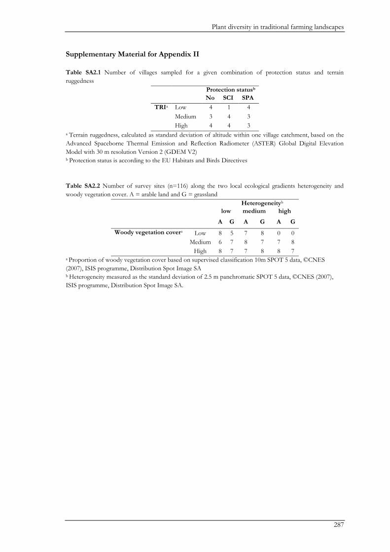
Plant diversity in traditional farming landscapes
287
Supplementary Material for Appendix II
Table SA2.1 Number of villages sampled for a given combination of protection status and terrain
ruggedness
Protection statusb
No SCI SPA
TRIa Low 4 1 4
Medium 3 4 3
High 4 4 3
a Terrain ruggedness, calculated as standard deviation of altitude within one village catchment, based on the
Advanced Spaceborne Thermal Emission and Reflection Radiometer (ASTER) Global Digital Elevation
Model with 30 m resolution Version 2 (GDEM V2) b Protection status is according to the EU Habitats and Birds Directives
Table SA2.2 Number of survey sites (n=116) along the two local ecological gradients heterogeneity and
woody vegetation cover. A = arable land and G = grassland
Heterogeneityb low medium high
A G A G A G
Woody vegetation covera Low 8 5 7 8 0 0
Medium 6 7 8 7 7 8
High 8 7 7 8 8 7 a Proportion of woody vegetation cover based on supervised classification 10m SPOT 5 data, ©CNES
(2007), ISIS programme, Distribution Spot Image SA b Heterogeneity measured as the standard deviation of 2.5 m panchromatic SPOT 5 data, ©CNES (2007),
ISIS programme, Distribution Spot Image SA.
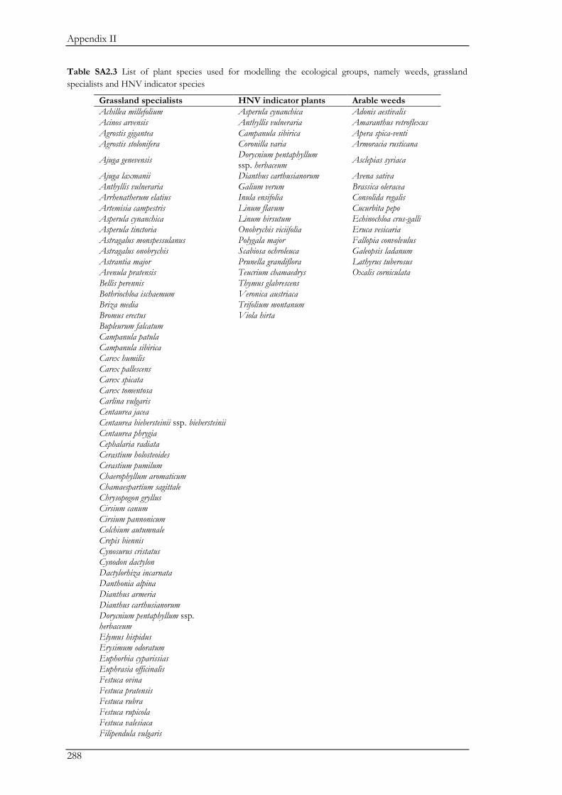
Appendix II
288
Table SA2.3 List of plant species used for modelling the ecological groups, namely weeds, grassland
specialists and HNV indicator species
Grassland specialists HNV indicator plants Arable weeds
Achillea millefolium Asperula cynanchica Adonis aestivalis Acinos arvensis Anthyllis vulneraria Amaranthus retroflexus Agrostis gigantea Campanula sibirica Apera spica-venti Agrostis stolonifera Coronilla varia Armoracia rusticana
Ajuga genevensis Dorycnium pentaphyllum ssp. herbaceum
Asclepias syriaca
Ajuga laxmanii Dianthus carthusianorum Avena sativa Anthyllis vulneraria Galium verum Brassica oleracea Arrhenatherum elatius Inula ensifolia Consolida regalis Artemisia campestris Linum flavum Cucurbita pepo Asperula cynanchica Linum hirsutum Echinochloa crus-galli Asperula tinctoria Onobrychis viciifolia Eruca vesicaria Astragalus monspessulanus Polygala major Fallopia convolvulus Astragalus onobrychis Scabiosa ochroleuca Galeopsis ladanum
Astrantia major Prunella grandiflora Lathyrus tuberosus Avenula pratensis Teucrium chamaedrys Oxalis corniculata Bellis perennis Thymus glabrescens Bothriochloa ischaemum Veronica austriaca Briza media Trifolium montanum
Bromus erectus Viola hirta
Bupleurum falcatum
Campanula patula
Campanula sibirica
Carex humilis
Carex pallescens
Carex spicata
Carex tomentosa
Carlina vulgaris
Centaurea jacea
Centaurea biebersteinii ssp. biebersteinii
Centaurea phrygia
Cephalaria radiata
Cerastium holosteoides
Cerastium pumilum
Chaerophyllum aromaticum
Chamaespartium sagittale
Chrysopogon gryllus
Cirsium canum
Cirsium pannonicum
Colchium autumnale
Crepis biennis
Cynosurus cristatus
Cynodon dactylon
Dactylorhiza incarnata
Danthonia alpina
Dianthus armeria
Dianthus carthusianorum
Dorycnium pentaphyllum ssp. herbaceum Elymus hispidus
Erysimum odoratum
Euphorbia cyparissias
Euphrasia officinalis
Festuca ovina
Festuca pratensis
Festuca rubra
Festuca rupicola
Festuca valesiaca
Filipendula vulgaris
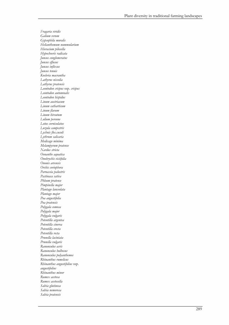
Plant diversity in traditional farming landscapes
289
Fragaria viridis
Galium verum
Gypsophila muralis
Helianthemum nummularium
Hieracium pilosella
Hypochoeris radicata
Juncus conglomeratus
Juncus effusus
Juncus inflexus
Juncus tenuis
Koeleria macrantha
Lathyrus nissolia
Lathyrus pratensis
Leontodon crispus ssp. crispus
Leontodon autumnalis
Leontodon hispidus
Linum austriacum
Linum catharticum
Linum flavum
Linum hirsutum
Lolium perenne
Lotus corniculatus
Luzula campestris
Lychnis flos.cuculi
Lythrum salicaria
Medicago minima
Melampyrum pratense
Nardus stricta
Oenanthe aquatica
Onobrychis viciifolia
Ononis arvensis
Orchis coriophora
Parnassia palustris
Pastinaca sativa
Phleum pratense
Pimpinella major
Plantago lanceolata
Plantago major
Poa angustifolia
Poa pratensis
Polygala comosa
Polygala major
Polygala vulgaris
Potentilla argentea
Potentilla cinerea
Potentilla erecta
Potentilla recta
Prunella laciniata
Prunella vulgaris
Ranunculus acris
Ranunculus bulbosus
Ranunculus polyanthemos
Rhinanthus rumelicus
Rhinanthus angustifolius ssp. angustifolius Rhinanthus minor
Rumex acetosa
Rumex acetosella
Salvia glutinosa
Salvia nemorosa
Salvia pratensis
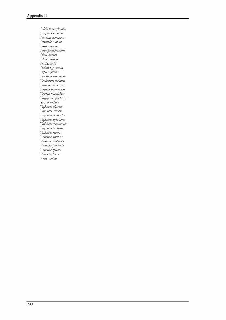
Appendix II
290
Salvia transsylvanica
Sanguisorba minor
Scabiosa ochroleuca
Serratula radiata
Seseli annuum
Seseli peucedanoides
Silene nutans
Silene vulgaris
Stachys recta
Stellaria graminea
Stipa capillata
Teucrium montanum
Thalictrum lucidum
Thymus glabrescens
Thymus pannonicus
Thymus pulegioides
Tragopogon pratensis ssp. orientalis Trifolium alpestre
Trifolium arvense
Trifolium campestre
Trifolium hybridum
Trifolium montanum
Trifolium pratense
Trifolium repens
Veronica arvensis
Veronica austriaca
Veronica prostrata
Veronica spicata
Vinca herbacea
Viola canina

291
Declaration
I hereby certify that the submitted dissertation entitled ‘Biodiversity conservation in traditional
farming landscapes: The future of birds and large carnivores in Transylvania’ has been written by
me without using unauthorized aids. I did not use any aids and writings other than those indicated.
All passages taken from other writings either verbatim or in substance have been marked by me
accordingly.
I hereby confirm that in carrying out my dissertation project I have not employed the services of a
professional broker of dissertation projects, nor will I do so in the future.
This dissertation, in its present or any other version, has not yet been submitted to any other
university for review. I have not taken or registered to take another doctoral examination.
Lüneburg, 09.01.2015
_________________________________________
Ine Dorresteijn


Related Documents


![Patient education for preventing diabetic foot ulceration … · [Intervention Review] Patient education for preventing diabetic foot ulceration Johannes AN Dorresteijn 1, Didi MW](https://static.cupdf.com/doc/110x72/5ecb99029d0d2c34515c80a4/patient-education-for-preventing-diabetic-foot-intervention-review-patient.jpg)
