i BIOMEDICAL DIGITAL SIGNAL PROCESSING C-Language Examples and Laboratory Experiments for the IBM ® PC WILLIS J. TOMPKINS Editor University of Wisconsin-Madison © 2000 by Willis J. Tompkins This book was previously printed by: PRENTICE HALL, Upper Saddle River, New Jersey 07458

Bio Medical Signal Processing Tompkins
Dec 03, 2014
Welcome message from author
This document is posted to help you gain knowledge. Please leave a comment to let me know what you think about it! Share it to your friends and learn new things together.
Transcript

i
BIOMEDICALDIGITALSIGNALPROCESSINGC-Language Examplesand Laboratory Experimentsfor the IBM® PC
WILLIS J. TOMPKINSEditor
University of Wisconsin-Madison
© 2000 by Willis J. Tompkins
This book was previously printed by: PRENTICE HALL, UpperSaddle River, New Jersey 07458
ii Contents
Contents
LIST OF CONTRIBUTORS x
PREFACE xi
1 INTRODUCTION TO COMPUTERS IN MEDICINE 1
1.1 Characteristics of medical data 11.2 What is a medical instrument? 21.3 Iterative definition of medicine 41.4 Evolution of microprocessor-based systems 51.5 The microcomputer-based medical instrument 131.6 Software design of digital filters 161.7 A look to the future 221.8 References 221.9 Study questions 23
2 ELECTROCARDIOGRAPHY 24
2.1 Basic electrocardiography 242.2 ECG lead systems 392.3 ECG signal characteristics 432.4 Lab: Analog filters, ECG amplifier, and QRS detector 442.5 References 532.6 Study questions 53
3 SIGNAL CONVERSION 55
3.1 Sampling basics 553.2 Simple signal conversion systems 593.3 Conversion requirements for biomedical signals 603.4 Signal conversion circuits 613.5 Lab: Signal conversion 743.6 References 753.7 Study questions 75
Contents iii
4 BASICS OF DIGITAL FILTERING 78
4.1 Digital filters 784.2 The z transform 794.3 Elements of a digital filter 814.4 Types of digital filters 844.5 Transfer function of a difference equation 854.6 The z-plane pole-zero plot 854.7 The rubber membrane concept 894.8 References 984.9 Study questions 98
5 FINITE IMPULSE RESPONSE FILTERS 100
5.1 Characteristics of FIR filters 1005.2 Smoothing filters 1035.3 Notch filters 1115.4 Derivatives 1115.5 Window design 1175.6 Frequency sampling 1195.7 Minimax design 1205.8 Lab: FIR filter design 1215.9 References 1235.10 Study questions 123
6 INFINITE IMPULSE RESPONSE FILTERS 125
6.1 Generic equations of IIR filters 1256.2 Simple one-pole example 1266.3 Integrators 1306.4 Design methods for two-pole filters 1366.5 Lab: IIR digital filters for ECG analysis 1446.6 References 1456.7 Study questions 145
7 INTEGER FILTERS 151
7.1 Basic design concept 1517.2 Low-pass integer filters 1577.3 High-pass integer filters 1587.4 Bandpass and band-reject integer filters 1607.5 The effect of filter cascades 1617.6 Other fast-operating design techniques 1627.7 Design examples and tools 1647.8 Lab: Integer filters for ECG analysis 1707.9 References 1717.10 Study questions 171
iv Contents
8 ADAPTIVE FILTERS 174
8.1 Principal noise canceler model 1748.2 60-Hz adaptive canceling using a sine wave model 1758.3 Other applications of adaptive filtering 1808.4 Lab: 60-Hz adaptive filter 1818.5 References 1828.6 Study questions 182
9 SIGNAL AVERAGING 184
9.1 Basics of signal averaging 1849.2 Signal averaging as a digital filter 1899.3 A typical averager 1899.4 Software for signal averaging 1909.5 Limitations of signal averaging 1909.6 Lab: ECG signal averaging 1929.7 References 1929.8 Study questions 192
10 DATA REDUCTION TECHNIQUES 193
10.1 Turning point algorithm 19410.2 AZTEC algorithm 19710.3 Fan algorithm 20210.4 Huffman coding 20610.5 Lab: ECG data reduction algorithms 21110.6 References 21210.7 Study questions 213
11 OTHER TIME- AND FREQUENCY-DOMAIN TECHNIQUES 216
11.1 The Fourier transform 21611.2 Correlation 22211.3 Convolution 22611.4 Power spectrum estimation 23011.5 Lab: Frequency-domain analysis of the ECG 23311.6 References 23511.7 Study questions 235
12 ECG QRS DETECTION 236
12.1 Power spectrum of the ECG 23612.2 Bandpass filtering techniques 23712.3 Differentiation techniques 24112.4 Template matching techniques 242
Contents v
12.5 A QRS detection algorithm 24612.6 Lab: Real-time ECG processing algorithm 26212.7 References 26312.8 Study questions 263
13 ECG ANALYSIS SYSTEMS 265
13.1 ECG interpretation 26513.2 ST-segment analyzer 27113.3 Portable arrhythmia monitor 27213.4 References 28013.5 Study questions 281
14 VLSI IN DIGITAL SIGNAL PROCESSING 283
14.1 Digital signal processors 28314.2 High-performance VLSI signal processing 28614.3 VLSI applications in medicine 29014.4 VLSI sensors for biomedical signals 29114.5 VLSI tools 29314.6 Choice of custom, ASIC, or off-the-shelf components 29314.7 References 29314.8 Study questions 294
A CONFIGURING THE PC FOR UW DIGISCOPE 295
A.1 Installing the RTD ADA2100 in an IBM PC 297A.2 Configuring the Motorola 68HC11EVBU 299A.3 Configuring the Motorola 68HC11EVB 303A.4 Virtual input/output device (data files) 305A.5 Putting a header on a binary file: ADDHEAD 305A.6 References 306
B DATA ACQUISITION AND CONTROL ROUTINES 307
B.1 Data structures 308B.2 Top-level device routines 309B.3 Internal I/O device (RTD ADA2100) 309B.4 External I/O device (Motorola 68HC11EVBU) 311B.5 Virtual I/O device (data files) 313B.6 References 316
C DATA ACQUISITION AND CONTROL—SOME HINTS 317
C.1 Internal I/O device (RTD ADA2100) 318C.2 External I/O device (Motorola 68HC11EVBU) 320C.3 Virtual I/O device (data files) 324
vi Contents
C.4 Writing your own interface software 327C.5 References 331
D UW DIGISCOPE USER’S MANUAL 332
D.1 Getting around in UW DigiScope 332D.2 Overview of functions 334
E SIGNAL GENERATION 342
E.1 Signal generation methods 342E.2 Signal generator program (GENWAVE) 343
F FINITE-LENGTH REGISTER EFFECTS 346
F.1 Quantization noise 346F.2 Limit cycles 348F.3 Scaling 351F.4 Roundoff noise in IIR filters 352F.5 Floating-point register filters 353F.6 Summary 354F.7 Lab: Finite-length register effects in digital filters 355F.8 References 355
G COMMERCIAL DSP SYSTEMS 356
G.1 Data acquisition systems 356G.2 DSP software 357G.3 Vendors 359G.4 References 360
INDEX 361

vii
List of Contributors
Valtino X. AfonsoDavid J. BeebeAnnie P. FoongKok Fung Lai
Danial J. NeebelJesse D. OlsonDorin PanescuJon D. Pfeffer
Pradeep M. TagareSteven J. TangThomas Y. Yen
Ren Zhou

viii
Preface
There are many digital filtering and pattern recognition algorithms used in process-ing biomedical signals. In a medical instrument, a set of these algorithms typicallymust operate in real time. For example, an intensive care unit computer must ac-quire the electrocardiogram of a patient, recognize key features of the signal, de-termine if the signal is normal or abnormal, and report this information in a timelyfashion.
In a typical biomedical engineering course, students have limited real-world de-sign opportunity. Here at the University of Wisconsin-Madison, for example, thelaboratory setups were designed a number of years ago around single board com-puters. These setups run real-time digital signal processing algorithms, and the stu-dents can analyze the operation of these algorithms. However, the hardware can beprogrammed only in the assembly language of the embedded microprocessor and isnot easily reprogrammed to implement new algorithms. Thus, a student has limitedopportunity to design and program a processing algorithm.
In general, students in electrical engineering have very limited opportunity tohave hands-on access to the operation of digital filters. In our current digital filter-ing courses, the filters are designed noninteractively. Students typically do nothave the opportunity to implement the filters in hardware and observe real-timeperformance. This approach certainly does not provide the student with significantunderstanding of the design constraints of such filters nor their actual performancecharacteristics. Thus, the concepts developed here are adaptable to other areas ofelectrical engineering in addition to the biomedical area, such as in signal process-ing courses.
We developed this book with its set of laboratories and special software to pro-vide a mechanism for anyone interested in biomedical signal processing to studythe field without requiring any other instrument except an IBM PC or compatible.For those who have signal conversion hardware, we include procedures that willprovide true hands-on laboratory experiences.
We include in this book the basics of digital signal processing for biomedicalapplications and also C-language programs for designing and implementing simpledigital filters. All examples are written in the Turbo C (Borland) programming lan-guage. We chose the C language because our previous approaches have had limitedflexibility due to the required knowledge of assembly language programming. Therelationship between a signal processing algorithm and its assembly languageimplementation is conceptually difficult. Use of the high-level C language permits
Preface ix
students to better understand the relationship between the filter and the programthat implements it.
In this book, we provide a set of laboratory experiments that can be completedusing either an actual analog-to-digital converter or a virtual (i.e., simulated withsoftware) converter. In this way, the experiments may be done in either a fully in-strumented laboratory or on almost any IBM PC or compatible. The only restric-tions on the PC are that it must have at least 640 kbytes of RAM and VGA (orEGA or monochrome) graphics. This graphics requirement is to provide for a highresolution environment for visualizing the results of signal processing. For someapplications, particularly frequency domain processing, a math coprocessor is use-ful to speed up the computations, but it is optional.
The floppy disk provided with the book includes the special program calledUW DigiScope which provides an environment in which the student can do the labexperiments, design digital filters of different types, and visualize the results ofprocessing on the display. This program supports the virtual signal conversion de-vice as well as two different physical signal conversion devices. The physical de-vices are the Real Time Devices ADA2100 signal conversion board which plugsinto the internal PC bus and the Motorola 68HC11EVB board (chosen because stu-dents can obtain their own device for less than $100). This board sits outside thePC and connects through a serial port. The virtual device simulates signal conver-sion with software and reads data files for its input waveforms. Also on the floppydisk are some examples of sampled signals and a program that permits users to puttheir own data in a format that is readable by UW DigiScope. We hope that thisprogram and the standard file format will stimulate the sharing of biomedical sig-nal files by our readers.
The book begins in Chapter 1 with an overview of the field of computers inmedicine, including a historical review of the evolution of the technologies impor-tant to this field. Chapter 2 reviews the field of electrocardiography since the elec-trocardiogram (ECG) is the model biomedical signal used for demonstrating thedigital signal processing techniques throughout the book. The laboratory in thischapter teaches the student about analog signal acquisition and preprocessing bybuilding circuitry for amplifying his/her own ECG. Chapter 3 provides a traditionalreview of signal conversion techniques and provides a lab that gives insight intothe techniques and potential pitfalls of digital signal acquisition.
Chapters 4, 5, and 6 cover the principles of digital signal processing found inmost texts on this subject but use a conceptual approach to the subject as opposedto the traditional equation-laden theoretical approach that is difficult for many stu-dents. The intent is to get the students involved in the design process as quickly aspossible with minimal reliance on proving the theorems that form the foundation ofthe techniques. Two labs in these chapters give the students hands-on experience indesigning and running digital filters using the UW DigiScope software platform.
Chapter 7 covers a special class of integer coefficient filters that are particularlyuseful for real-time signal processing because these filters do not require floating-point operations. This topic is not included in most digital signal processing books.A lab helps to develop the student’s understanding of these filters through a designexercise.
x Preface
Chapter 8 introduces adaptive filters that continuously learn the characteristicsof their processing environment and change their filtering characteristics to opti-mally perform their intended functions. Chapter 9 reviews the technique and appli-cation of signal averaging.
Chapter 10 covers data reduction techniques, which are important for reducingthe amount of data that must be stored, processed, or transmitted. The ability tocompress signals into smaller file sizes is becoming more important as more sig-nals are being archived and handled digitally. A lab provides an experience in datareduction and reconstruction of signals using techniques provided in the book.
Chapter 11 summarizes additional important techniques for signal processingwith emphasis on frequency domain techniques and illustrates frequency analysisof the ECG with a special lab.
Chapter 12 presents a diversity of techniques for detecting the principal featuresof the ECG with emphasis on real-time algorithms that are demonstrated with alab. Then Chapter 13 shows how many of these techniques are used in actual medi-cal monitoring systems.
Chapter 14 concludes with a summary of the emerging integrated circuit tech-nologies for digital signal processing with a look to the trends in this field for thefuture.
Appendices A, B, and C provide details of interfacing and use of the two physi-cal signal conversion devices supported as well as the virtual signal conversiondevice that can be used on any PC.
Appendix D is the user’s manual for the special UW DigiScope program that isused for the lab experiments. Appendix E describes the signal generator function inUW DigiScope that lets the student create simulated signals with controlled noiseand sampling rates and store them in disk files for processing by the virtual signalconversion device.
Appendix F covers special problems that can occur due to the finite length of acomputer’s internal registers when implementing digital signal processing algo-rithms.
Appendix G reviews some of the commercial software in the market that facili-tates digital signal acquisition and processing.
I would especially like to thank the students who attended my class, Computersin Medicine (ECE 463), in Fall 1991 for helping to find many small (and somelarge problems) in the text material and in the software. I would also like toparticularly thank Jesse Olson, author of Chapter 5, for going the extra mile toensure that the UW DigiScope program is a reliable teaching tool.
The interfaces and algorithms in the labs emphasize real-time digital signal pro-cessing techniques that are different from the off-line approaches to digital signalprocessing taught in most digital signal processing courses. We hope that the useof PC-based real-time signal processing workstations will greatly enhance thestudent’s hands-on design experience.
Willis J. TompkinsDepartment of Electrical
and Computer EngineeringUniversity of Wisconsin-Madison
1
1
Introduction to Computers in Medicine
Willis J. Tompkins
The field of computers in medicine is quite broad. We can only cover a small partof it in this book. We choose to emphasize the importance of real-time signal pro-cessing in medical instrumentation. This chapter discusses the nature of medicaldata, the general characteristics of a medical instrument, and the field of medicineitself. We then go on to review the history of the microprocessor-based system be-cause of the importance of the microprocessor in the design of modern medical in-struments. We then give some examples of medical instruments in which the mi-croprocessor has played a key role and in some cases has even empowered us todevelop new instruments that were not possible before. The chapter ends with adiscussion of software design and the role of the personal computer indevelopment of medical instruments.
1.1 CHARACTERISTICS OF MEDICAL DATA
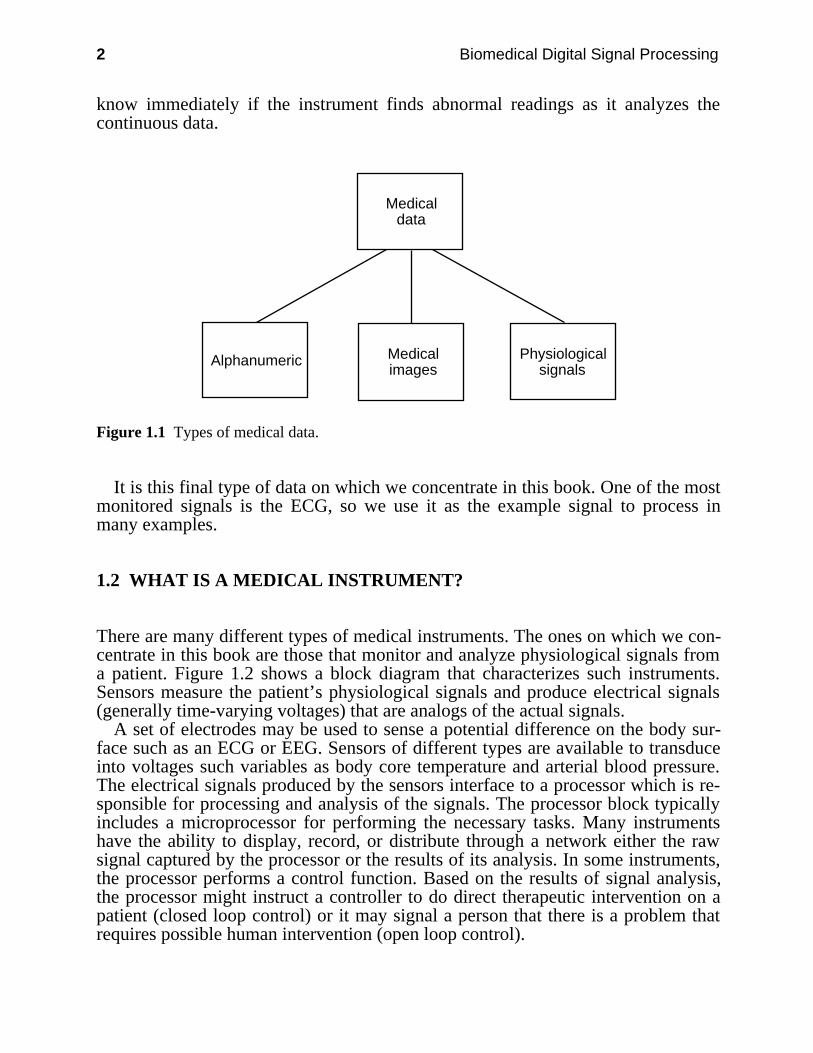
Figure 1.1 shows the three basic types of data that must be acquired, manipulated,and archived in the hospital. Alphanumeric data include the patient’s name andaddress, identification number, results of lab tests, and physicians’ notes. Imagesinclude Xrays and scans from computer tomography, magnetic resonance imaging,and ultrasound. Examples of physiological signals are the electrocardiogram(ECG), the electroencephalogram (EEG), and blood pressure tracings.
Quite different systems are necessary to manipulate each of these three types ofdata. Alphanumeric data are generally managed and organized into a databaseusing a general-purpose mainframe computer.
Image data are traditionally archived on film. However, we are evolving towardpicture archiving and communication systems (PACS) that will store images indigitized form on optical disks and distribute them on demand over a high-speedlocal area network (LAN) to very high resolution graphics display monitors locatedthroughout a hospital.
On the other hand, physiological signals like those that are monitored duringsurgery in the operating room require real-time processing. The clinician must
2 Biomedical Digital Signal Processing
know immediately if the instrument finds abnormal readings as it analyzes thecontinuous data.
Alphanumeric
Medical data
Medical images
Physiological signals
Figure 1.1 Types of medical data.
It is this final type of data on which we concentrate in this book. One of the mostmonitored signals is the ECG, so we use it as the example signal to process inmany examples.
1.2 WHAT IS A MEDICAL INSTRUMENT?
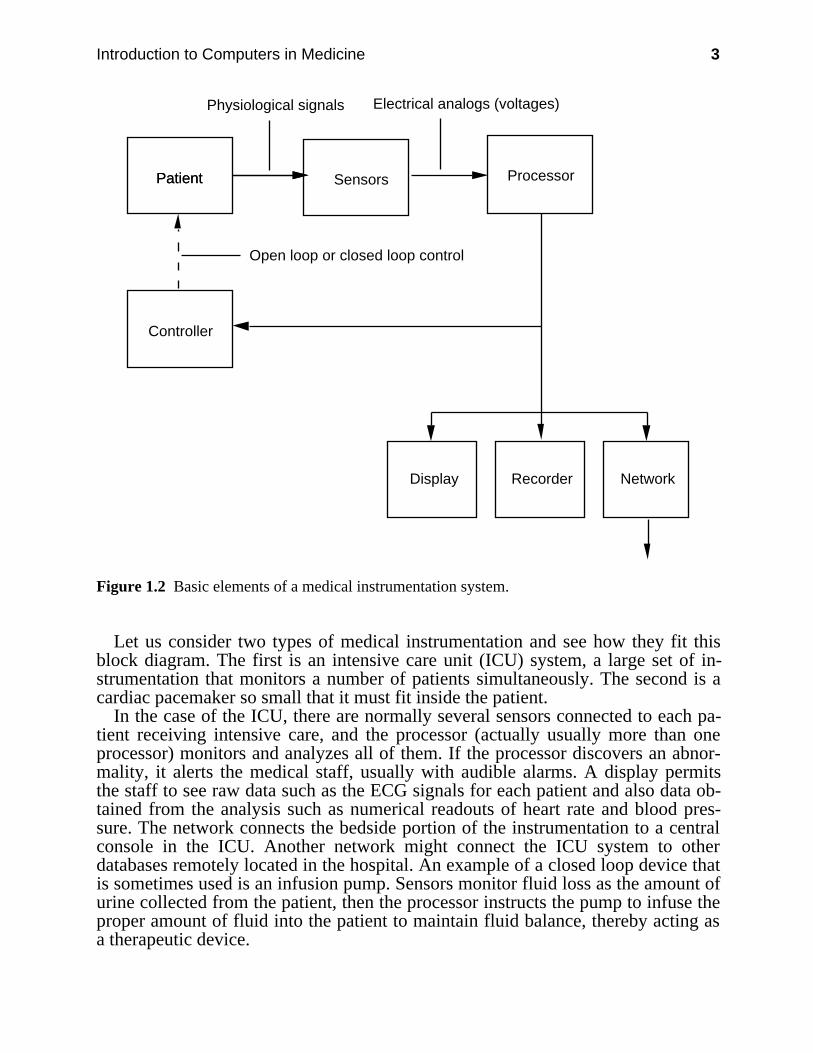
There are many different types of medical instruments. The ones on which we con-centrate in this book are those that monitor and analyze physiological signals froma patient. Figure 1.2 shows a block diagram that characterizes such instruments.Sensors measure the patient’s physiological signals and produce electrical signals(generally time-varying voltages) that are analogs of the actual signals.
A set of electrodes may be used to sense a potential difference on the body sur-face such as an ECG or EEG. Sensors of different types are available to transduceinto voltages such variables as body core temperature and arterial blood pressure.The electrical signals produced by the sensors interface to a processor which is re-sponsible for processing and analysis of the signals. The processor block typicallyincludes a microprocessor for performing the necessary tasks. Many instrumentshave the ability to display, record, or distribute through a network either the rawsignal captured by the processor or the results of its analysis. In some instruments,the processor performs a control function. Based on the results of signal analysis,the processor might instruct a controller to do direct therapeutic intervention on apatient (closed loop control) or it may signal a person that there is a problem thatrequires possible human intervention (open loop control).
Introduction to Computers in Medicine 3
Patient SensorsPatient
Controller
Processor
Physiological signals Electrical analogs (voltages)
Open loop or closed loop control
NetworkRecorderDisplay
Figure 1.2 Basic elements of a medical instrumentation system.
Let us consider two types of medical instrumentation and see how they fit thisblock diagram. The first is an intensive care unit (ICU) system, a large set of in-strumentation that monitors a number of patients simultaneously. The second is acardiac pacemaker so small that it must fit inside the patient.
In the case of the ICU, there are normally several sensors connected to each pa-tient receiving intensive care, and the processor (actually usually more than oneprocessor) monitors and analyzes all of them. If the processor discovers an abnor-mality, it alerts the medical staff, usually with audible alarms. A display permitsthe staff to see raw data such as the ECG signals for each patient and also data ob-tained from the analysis such as numerical readouts of heart rate and blood pres-sure. The network connects the bedside portion of the instrumentation to a centralconsole in the ICU. Another network might connect the ICU system to otherdatabases remotely located in the hospital. An example of a closed loop device thatis sometimes used is an infusion pump. Sensors monitor fluid loss as the amount ofurine collected from the patient, then the processor instructs the pump to infuse theproper amount of fluid into the patient to maintain fluid balance, thereby acting asa therapeutic device.
4 Biomedical Digital Signal Processing
Now consider Figure 1.2 for the case of the implanted cardiac pacemaker. Thesensors are electrodes mounted on a catheter that is placed inside the heart. Theprocessor is usually a specialized integrated circuit designed specifically for thisultra-low-power application rather than a general-purpose microprocessor. Theprocessor monitors the from the heart and analyzes it to determine if the heart isbeating by itself. If it sees that the heart goes too long without its own stimulussignal, it fires an electrical stimulator (the controller in this case) to inject a largeenough current through the same electrodes as those used for monitoring. Thisstimulus causes the heart to beat. Thus this device operates as a closed loop therapydelivery system. The early pacemakers operated in an open loop fashion, simplydriving the heart at some fixed rate regardless of whether or not it was able to beatin a normal physiological pattern most of the time. These devices were far lesssatisfactory than their modern intelligent cousins. Normally a microprocessor-based device outside the body placed over a pacemaker can communicate with itthrough telemetry and then display and record its operating parameters. Such a de-vice can also set new operating parameters such as amplitude of current stimulus.There are even versions of such devices that can communicate with a central clinicover the telephone network.
Thus, we see that the block diagram of a medical instrumentation system servesto characterize many medical care devices or systems.
1.3 ITERATIVE DEFINITION OF MEDICINE
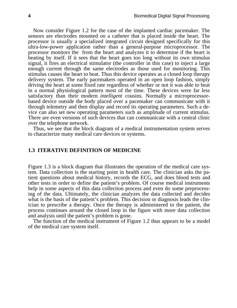
Figure 1.3 is a block diagram that illustrates the operation of the medical care sys-tem. Data collection is the starting point in health care. The clinician asks the pa-tient questions about medical history, records the ECG, and does blood tests andother tests in order to define the patient’s problem. Of course medical instrumentshelp in some aspects of this data collection process and even do some preprocess-ing of the data. Ultimately, the clinician analyzes the data collected and decideswhat is the basis of the patient’s problem. This decision or diagnosis leads the clin-ician to prescribe a therapy. Once the therapy is administered to the patient, theprocess continues around the closed loop in the figure with more data collectionand analysis until the patient’s problem is gone.
The function of the medical instrument of Figure 1.2 thus appears to be a modelof the medical care system itself.
Introduction to Computers in Medicine 5
PatientCollection of data
Decisionmaking
Analysis of data
Therapy
Figure 1.3 Basic elements of a medical care system.
1.4 EVOLUTION OF MICROPROCESSOR-BASED SYSTEMS
In the last decade, the microcomputer has made a significant impact on the designof biomedical instrumentation. The natural evolution of the microcomputer-basedinstrument is toward more intelligent devices. More and more computing powerand memory are being squeezed into smaller and smaller spaces. The commercial-ization of laptop PCs with significant computing power has accelerated the tech-nology of the battery-powered, patient-worn portable instrument. Such an instru-ment can be truly a personal computer looking for problems specific to a given pa-tient during the patient’s daily routines. The ubiquitous PC itself evolved fromminicomputers that were developed for the biomedical instrumentation laboratory,and the PC has become a powerful tool in biomedical computing applications. Aswe look to the future, we see the possibility of developing instruments to addressproblems that could not be previously approached because of considerations ofsize, cost, or power consumption.
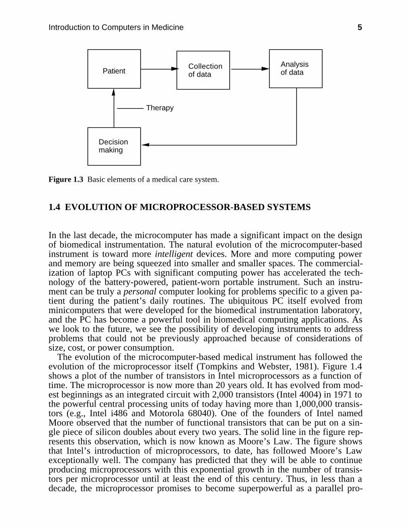
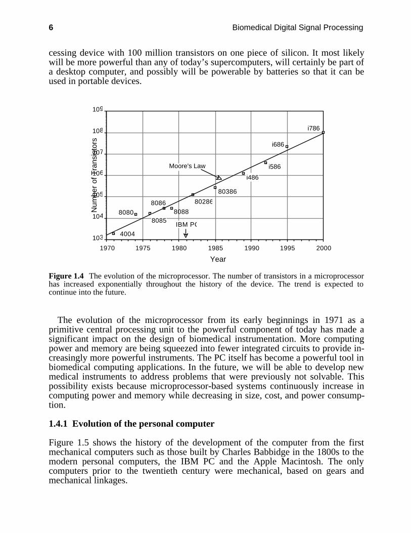
The evolution of the microcomputer-based medical instrument has followed theevolution of the microprocessor itself (Tompkins and Webster, 1981). Figure 1.4shows a plot of the number of transistors in Intel microprocessors as a function oftime. The microprocessor is now more than 20 years old. It has evolved from mod-est beginnings as an integrated circuit with 2,000 transistors (Intel 4004) in 1971 tothe powerful central processing units of today having more than 1,000,000 transis-tors (e.g., Intel i486 and Motorola 68040). One of the founders of Intel namedMoore observed that the number of functional transistors that can be put on a sin-gle piece of silicon doubles about every two years. The solid line in the figure rep-resents this observation, which is now known as Moore’s Law. The figure showsthat Intel’s introduction of microprocessors, to date, has followed Moore’s Lawexceptionally well. The company has predicted that they will be able to continueproducing microprocessors with this exponential growth in the number of transis-tors per microprocessor until at least the end of this century. Thus, in less than adecade, the microprocessor promises to become superpowerful as a parallel pro-
6 Biomedical Digital Signal Processing
cessing device with 100 million transistors on one piece of silicon. It most likelywill be more powerful than any of today’s supercomputers, will certainly be part ofa desktop computer, and possibly will be powerable by batteries so that it can beused in portable devices.
2000199519901985198019751970
103
104
105
106
107
108
109
Year
Num
ber
of T
rans
isto
rs
4004
80808085
80868088
80286
80386
i486
i586
i686
i786
IBM PC
Moore's Law
Figure 1.4 The evolution of the microprocessor. The number of transistors in a microprocessorhas increased exponentially throughout the history of the device. The trend is expected tocontinue into the future.
The evolution of the microprocessor from its early beginnings in 1971 as aprimitive central processing unit to the powerful component of today has made asignificant impact on the design of biomedical instrumentation. More computingpower and memory are being squeezed into fewer integrated circuits to provide in-creasingly more powerful instruments. The PC itself has become a powerful tool inbiomedical computing applications. In the future, we will be able to develop newmedical instruments to address problems that were previously not solvable. Thispossibility exists because microprocessor-based systems continuously increase incomputing power and memory while decreasing in size, cost, and power consump-tion.
1.4.1 Evolution of the personal computer
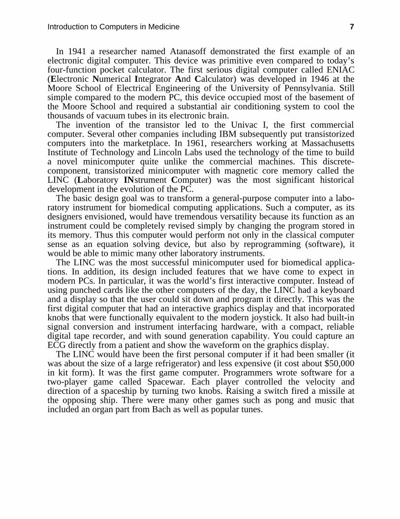
Figure 1.5 shows the history of the development of the computer from the firstmechanical computers such as those built by Charles Babbidge in the 1800s to themodern personal computers, the IBM PC and the Apple Macintosh. The onlycomputers prior to the twentieth century were mechanical, based on gears andmechanical linkages.
Introduction to Computers in Medicine 7
In 1941 a researcher named Atanasoff demonstrated the first example of anelectronic digital computer. This device was primitive even compared to today’sfour-function pocket calculator. The first serious digital computer called ENIAC(Electronic Numerical Integrator And Calculator) was developed in 1946 at theMoore School of Electrical Engineering of the University of Pennsylvania. Stillsimple compared to the modern PC, this device occupied most of the basement ofthe Moore School and required a substantial air conditioning system to cool thethousands of vacuum tubes in its electronic brain.
The invention of the transistor led to the Univac I, the first commercialcomputer. Several other companies including IBM subsequently put transistorizedcomputers into the marketplace. In 1961, researchers working at MassachusettsInstitute of Technology and Lincoln Labs used the technology of the time to builda novel minicomputer quite unlike the commercial machines. This discrete-component, transistorized minicomputer with magnetic core memory called theLINC (Laboratory INstrument Computer) was the most significant historicaldevelopment in the evolution of the PC.
The basic design goal was to transform a general-purpose computer into a labo-ratory instrument for biomedical computing applications. Such a computer, as itsdesigners envisioned, would have tremendous versatility because its function as aninstrument could be completely revised simply by changing the program stored inits memory. Thus this computer would perform not only in the classical computersense as an equation solving device, but also by reprogramming (software), itwould be able to mimic many other laboratory instruments.
The LINC was the most successful minicomputer used for biomedical applica-tions. In addition, its design included features that we have come to expect inmodern PCs. In particular, it was the world’s first interactive computer. Instead ofusing punched cards like the other computers of the day, the LINC had a keyboardand a display so that the user could sit down and program it directly. This was thefirst digital computer that had an interactive graphics display and that incorporatedknobs that were functionally equivalent to the modern joystick. It also had built-insignal conversion and instrument interfacing hardware, with a compact, reliabledigital tape recorder, and with sound generation capability. You could capture anECG directly from a patient and show the waveform on the graphics display.
The LINC would have been the first personal computer if it had been smaller (itwas about the size of a large refrigerator) and less expensive (it cost about $50,000in kit form). It was the first game computer. Programmers wrote software for atwo-player game called Spacewar. Each player controlled the velocity anddirection of a spaceship by turning two knobs. Raising a switch fired a missile atthe opposing ship. There were many other games such as pong and music thatincluded an organ part from Bach as well as popular tunes.
8 Biomedical Digital Signal Processing
Figure 1.5 The evolution of the personal computer.
The LINC was followed by the world’s first commercial minicomputer, whichwas also made of discrete components, the Digital Equipment Corporation PDP-8.Subsequently Digital made a commercial version of the LINC by combining theLINC architecture with the PDP-8 to make a LINC-8. Digital later introduced amore modern version of the LINC-8 called the PDP-12. These computers werephased out of Digital’s product line some time in the early 1970s. I have a specialfondness for the LINC machines since a LINC-8 was the first computer that I pro-grammed that was interactive, could display graphics, and did not require the useof awkward media like punched cards or punched paper tape to program it. One ofthe programs that I wrote on the LINC-8 in the late 1960s computed and displayedthe vectorcardiogram loops of patients (see Chapter 2). Such a program is easy toimplement today on the modern PC using a high-level computing language such asPascal or C.
Although invented in 1971, the first microprocessors were poor central process-ing units and were relatively expensive. It was not until the mid-1970s when useful
Introduction to Computers in Medicine 9
8-bit microprocessors such as the Intel 8080 were readily available. The first ad-vertised microcomputer for the home appeared on the cover of Popular ElectronicsMagazine in January 1975. Called the Altair 8800, it was based on the Intel 8080microprocessor and could be purchased as a kit. The end of the decade was full ofexperimentation and new product development leading to the introduction of PCslike the Apple II and microcomputers from many other companies.
1.4.2 The ubiquitous PC
A significant historical landmark was the introduction of the IBM PC in 1981. Onthe strength of its name alone, IBM standardized the personal desktop computer.Prior to the IBM PC, the most popular computers used the 8-bit Zilog Z80microprocessor (an enhancement of the Intel 8080) with an operating system calledCP/M (Control Program for Microprocessors). There was no standard way toformat a floppy disk, so it was difficult to transfer data from one company’s PC toanother. IBM singlehandedly standardized the world almost overnight on the 16-bitIntel 8088 microprocessor, Microsoft (Disk Operating System), and a uniformfloppy disk format that could be used to carry data from machine to machine. Theyalso stimulated worldwide production of IBM PC compatibles by manyinternational companies. This provided a standard computing platform for whichsoftware developers could write programs. Since so many similar computers werebuilt, inexpensive, powerful application programs became plentiful. This con-trasted to the minicomputer marketplace where there are relatively few similarcomputers in the field, so a typical program is very expensive and the evolution ofthe software is relatively slow.
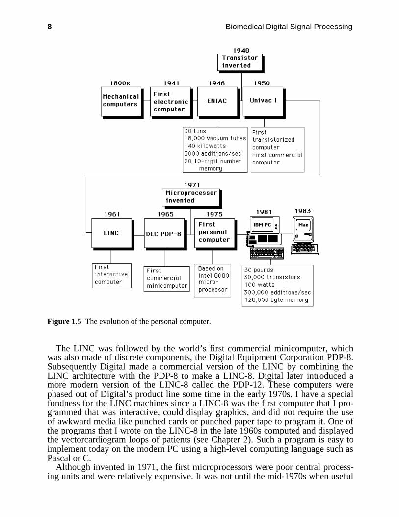
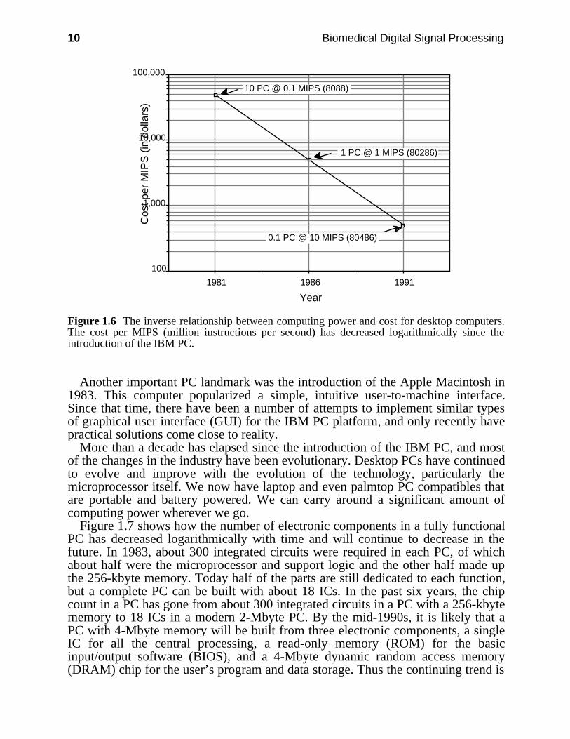
Figure 1.6 shows how the evolution of the microprocessor has improved theperformance of desktop computers. The figure is based on the idea that a completePC at any given time can be purchased for about $5,000. For this cost, the numberof MIPS (million instructions per second) increases with every new model becauseof the increasing power of the microprocessor. The first IBM PC introduced in1981 used the Intel 8088 microprocessor, which provided 0.1 MIPS. Thus, it re-quired 10 PCs at $5,000 each or $50,000 to provide one MIPS of computationalpower. With the introduction of the IBM PC/AT based on the Intel 80286 micro-processor, a single $5,000 desktop computer provided one MIPS. The most recentIBM PS computers using the Intel i486 microprocessor deliver 10 MIPS for thatsame $5,000. A basic observation is that the cost per MIPS of computing power isdecreasing logarithmically in desktop computers.
10 Biomedical Digital Signal Processing
1981 1986 1991
100
1,000
10,000
100,000
Year
10 PC @ 0.1 MIPS (8088)
1 PC @ 1 MIPS (80286)
0.1 PC @ 10 MIPS (80486)
Cos
t per
MIP
S (
in d
olla
rs)
Figure 1.6 The inverse relationship between computing power and cost for desktop computers.The cost per MIPS (million instructions per second) has decreased logarithmically since theintroduction of the IBM PC.
Another important PC landmark was the introduction of the Apple Macintosh in1983. This computer popularized a simple, intuitive user-to-machine interface.Since that time, there have been a number of attempts to implement similar typesof graphical user interface (GUI) for the IBM PC platform, and only recently havepractical solutions come close to reality.
More than a decade has elapsed since the introduction of the IBM PC, and mostof the changes in the industry have been evolutionary. Desktop PCs have continuedto evolve and improve with the evolution of the technology, particularly themicroprocessor itself. We now have laptop and even palmtop PC compatibles thatare portable and battery powered. We can carry around a significant amount ofcomputing power wherever we go.
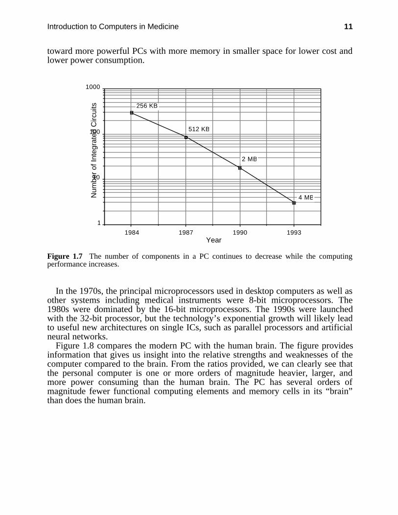
Figure 1.7 shows how the number of electronic components in a fully functionalPC has decreased logarithmically with time and will continue to decrease in thefuture. In 1983, about 300 integrated circuits were required in each PC, of whichabout half were the microprocessor and support logic and the other half made upthe 256-kbyte memory. Today half of the parts are still dedicated to each function,but a complete PC can be built with about 18 ICs. In the past six years, the chipcount in a PC has gone from about 300 integrated circuits in a PC with a 256-kbytememory to 18 ICs in a modern 2-Mbyte PC. By the mid-1990s, it is likely that aPC with 4-Mbyte memory will be built from three electronic components, a singleIC for all the central processing, a read-only memory (ROM) for the basicinput/output software (BIOS), and a 4-Mbyte dynamic random access memory(DRAM) chip for the user’s program and data storage. Thus the continuing trend is
Introduction to Computers in Medicine 11
toward more powerful PCs with more memory in smaller space for lower cost andlower power consumption.
1984 1987 1990 1993
1
10
100
1000
Year
Num
ber
of In
tegr
ated
Circ
uits 256 KB
512 KB
2 MB
4 MB
Figure 1.7 The number of components in a PC continues to decrease while the computingperformance increases.
In the 1970s, the principal microprocessors used in desktop computers as well asother systems including medical instruments were 8-bit microprocessors. The1980s were dominated by the 16-bit microprocessors. The 1990s were launchedwith the 32-bit processor, but the technology’s exponential growth will likely leadto useful new architectures on single ICs, such as parallel processors and artificialneural networks.
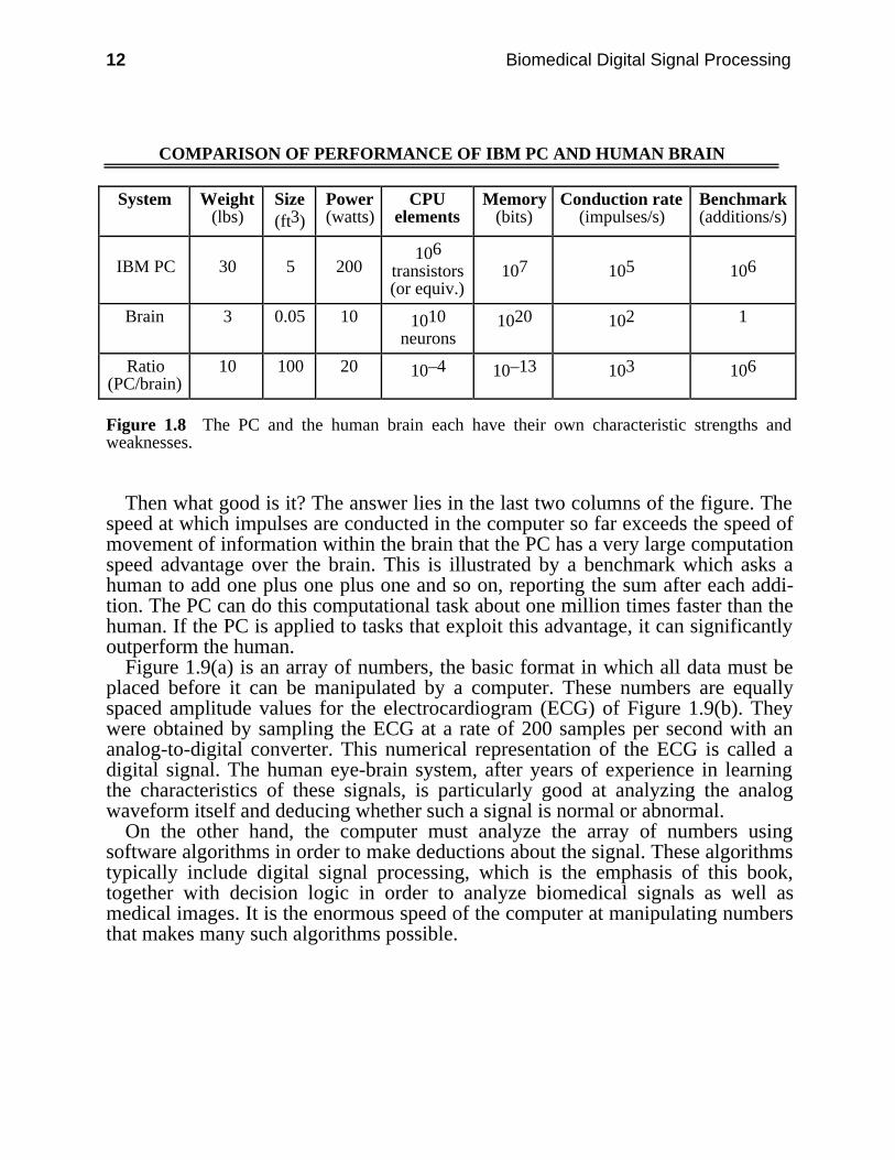
Figure 1.8 compares the modern PC with the human brain. The figure providesinformation that gives us insight into the relative strengths and weaknesses of thecomputer compared to the brain. From the ratios provided, we can clearly see thatthe personal computer is one or more orders of magnitude heavier, larger, andmore power consuming than the human brain. The PC has several orders ofmagnitude fewer functional computing elements and memory cells in its “brain”than does the human brain.
12 Biomedical Digital Signal Processing
COMPARISON OF PERFORMANCE OF IBM PC AND HUMAN BRAIN
System Weight(lbs)
Size(ft3)
Power(watts)
CPUelements
Memory(bits)
Conduction rate(impulses/s)
Benchmark(additions/s)
IBM PC 30 5 200106
transistors(or equiv.)
107 105 106
Brain 3 0.05 10 1010neurons
1020 102 1
Ratio(PC/brain)
10 100 20 10–4 10–13 103 106
Figure 1.8 The PC and the human brain each have their own characteristic strengths andweaknesses.
Then what good is it? The answer lies in the last two columns of the figure. Thespeed at which impulses are conducted in the computer so far exceeds the speed ofmovement of information within the brain that the PC has a very large computationspeed advantage over the brain. This is illustrated by a benchmark which asks ahuman to add one plus one plus one and so on, reporting the sum after each addi-tion. The PC can do this computational task about one million times faster than thehuman. If the PC is applied to tasks that exploit this advantage, it can significantlyoutperform the human.
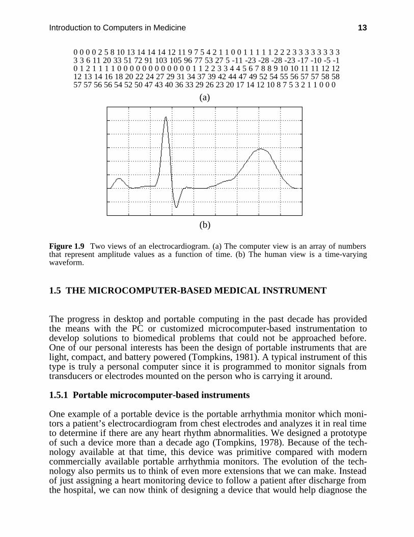
Figure 1.9(a) is an array of numbers, the basic format in which all data must beplaced before it can be manipulated by a computer. These numbers are equallyspaced amplitude values for the electrocardiogram (ECG) of Figure 1.9(b). Theywere obtained by sampling the ECG at a rate of 200 samples per second with ananalog-to-digital converter. This numerical representation of the ECG is called adigital signal. The human eye-brain system, after years of experience in learningthe characteristics of these signals, is particularly good at analyzing the analogwaveform itself and deducing whether such a signal is normal or abnormal.
On the other hand, the computer must analyze the array of numbers usingsoftware algorithms in order to make deductions about the signal. These algorithmstypically include digital signal processing, which is the emphasis of this book,together with decision logic in order to analyze biomedical signals as well asmedical images. It is the enormous speed of the computer at manipulating numbersthat makes many such algorithms possible.
Introduction to Computers in Medicine 13
0 0 0 0 2 5 8 10 13 14 14 14 12 11 9 7 5 4 2 1 1 0 0 1 1 1 1 1 2 2 2 3 3 3 3 3 3 3 33 3 6 11 20 33 51 72 91 103 105 96 77 53 27 5 -11 -23 -28 -28 -23 -17 -10 -5 -10 1 2 1 1 1 1 0 0 0 0 0 0 0 0 0 0 0 0 1 1 2 2 3 3 4 4 5 6 7 8 8 9 10 10 11 11 12 1212 13 14 16 18 20 22 24 27 29 31 34 37 39 42 44 47 49 52 54 55 56 57 57 58 5857 57 56 56 54 52 50 47 43 40 36 33 29 26 23 20 17 14 12 10 8 7 5 3 2 1 1 0 0 0
(a)
(b)
Figure 1.9 Two views of an electrocardiogram. (a) The computer view is an array of numbersthat represent amplitude values as a function of time. (b) The human view is a time-varyingwaveform.
1.5 THE MICROCOMPUTER-BASED MEDICAL INSTRUMENT
The progress in desktop and portable computing in the past decade has providedthe means with the PC or customized microcomputer-based instrumentation todevelop solutions to biomedical problems that could not be approached before.One of our personal interests has been the design of portable instruments that arelight, compact, and battery powered (Tompkins, 1981). A typical instrument of thistype is truly a personal computer since it is programmed to monitor signals fromtransducers or electrodes mounted on the person who is carrying it around.
1.5.1 Portable microcomputer-based instruments
One example of a portable device is the portable arrhythmia monitor which moni-tors a patient’s electrocardiogram from chest electrodes and analyzes it in real timeto determine if there are any heart rhythm abnormalities. We designed a prototypeof such a device more than a decade ago (Tompkins, 1978). Because of the tech-nology available at that time, this device was primitive compared with moderncommercially available portable arrhythmia monitors. The evolution of the tech-nology also permits us to think of even more extensions that we can make. Insteadof just assigning a heart monitoring device to follow a patient after discharge fromthe hospital, we can now think of designing a device that would help diagnose the
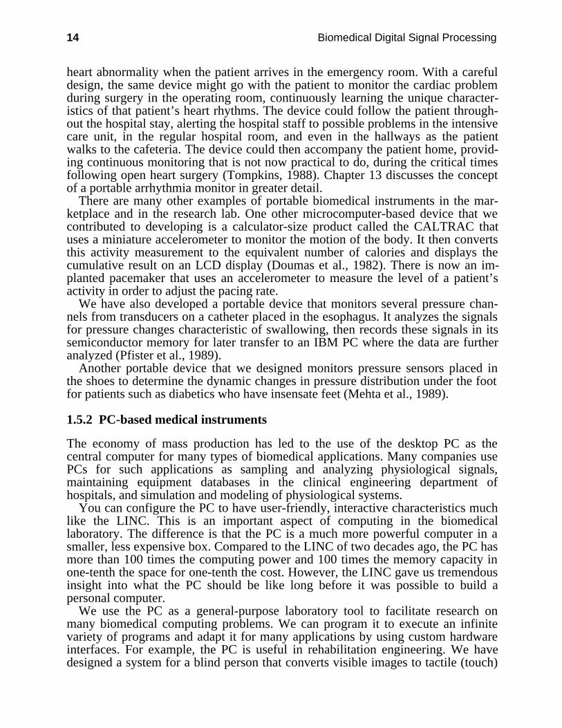
14 Biomedical Digital Signal Processing
heart abnormality when the patient arrives in the emergency room. With a carefuldesign, the same device might go with the patient to monitor the cardiac problemduring surgery in the operating room, continuously learning the unique character-istics of that patient’s heart rhythms. The device could follow the patient through-out the hospital stay, alerting the hospital staff to possible problems in the intensivecare unit, in the regular hospital room, and even in the hallways as the patientwalks to the cafeteria. The device could then accompany the patient home, provid-ing continuous monitoring that is not now practical to do, during the critical timesfollowing open heart surgery (Tompkins, 1988). Chapter 13 discusses the conceptof a portable arrhythmia monitor in greater detail.
There are many other examples of portable biomedical instruments in the mar-ketplace and in the research lab. One other microcomputer-based device that wecontributed to developing is a calculator-size product called the CALTRAC thatuses a miniature accelerometer to monitor the motion of the body. It then convertsthis activity measurement to the equivalent number of calories and displays thecumulative result on an LCD display (Doumas et al., 1982). There is now an im-planted pacemaker that uses an accelerometer to measure the level of a patient’sactivity in order to adjust the pacing rate.
We have also developed a portable device that monitors several pressure chan-nels from transducers on a catheter placed in the esophagus. It analyzes the signalsfor pressure changes characteristic of swallowing, then records these signals in itssemiconductor memory for later transfer to an IBM PC where the data are furtheranalyzed (Pfister et al., 1989).
Another portable device that we designed monitors pressure sensors placed inthe shoes to determine the dynamic changes in pressure distribution under the footfor patients such as diabetics who have insensate feet (Mehta et al., 1989).
1.5.2 PC-based medical instruments
The economy of mass production has led to the use of the desktop PC as thecentral computer for many types of biomedical applications. Many companies usePCs for such applications as sampling and analyzing physiological signals,maintaining equipment databases in the clinical engineering department ofhospitals, and simulation and modeling of physiological systems.
You can configure the PC to have user-friendly, interactive characteristics muchlike the LINC. This is an important aspect of computing in the biomedicallaboratory. The difference is that the PC is a much more powerful computer in asmaller, less expensive box. Compared to the LINC of two decades ago, the PC hasmore than 100 times the computing power and 100 times the memory capacity inone-tenth the space for one-tenth the cost. However, the LINC gave us tremendousinsight into what the PC should be like long before it was possible to build apersonal computer.
We use the PC as a general-purpose laboratory tool to facilitate research onmany biomedical computing problems. We can program it to execute an infinitevariety of programs and adapt it for many applications by using custom hardwareinterfaces. For example, the PC is useful in rehabilitation engineering. We havedesigned a system for a blind person that converts visible images to tactile (touch)
Introduction to Computers in Medicine 15
images. The PC captures an image from a television camera and stores it in itsmemory. A program presents the image piece by piece to the blind person’sfingertip by activating an array of tactors (i.e., devices that stimulate the sense oftouch) that are pressed against his/her fingertip. In this way, we use the PC to studythe ability of a blind person to “see” images with the sense of touch (Kaczmarek etal., 1985; Frisken-Gibson et al., 1987).
One of the applications that we developed based on an Apple Macintosh II com-puter is electrical impedance tomography—EIT (Yorkey et al., 1987; Woo et al.,1989; Hua et al., 1991). Instead of the destructive radiation used for the familiarcomputerized tomography techniques, we inject harmless high-frequency currentsinto the body through electrodes and measure the resistances to the flow of elec-tricity at numerous electrode sites. This idea is based on the fact that body organsdiffer in the amount of resistance that they offer to electricity. This technology at-tempts to image the internal organs of the human body by measuring impedancethrough electrodes placed on the body surface.
The computer controls a custom-built 32-channel current generator that injectspatterns of high-frequency (50-kHz) currents into the body. The computer thensamples the body surface voltage distribution resulting from these currents throughan analog-to-digital converter. Using a finite element resistivity model of thethorax and the boundary measurements, the computer then iteratively calculates theresistivity profile that best satisfies the measured data. Using the standard graphicsdisplay capability of the computer, an image is then generated of the transversebody section resistivity. Since the lungs are high resistance compared to the heartand other body tissues, the resistivity image provides a depiction of the organsystem in the body. In this project the Macintosh does all the instrumentation tasksincluding control of the injected currents, measurement of the resistivities, solvingthe computing-intensive algorithms, and presenting the graphical display of thefinal image.
There are many possible uses of PCs in medical instrumentation (Tompkins,1986). We have used the IBM PC to develop signal processing and artificial neuralnetwork (ANN) algorithms for analysis of the electrocardiogram (Pan andTompkins, 1985; Hamilton and Tompkins, 1986; Xue et al., 1992). These studieshave also included development of techniques for data compression to reduce theamount of storage space required to save ECGs (Hamilton and Tompkins, 1991a,1991b).
1.6 SOFTWARE DESIGN OF DIGITAL FILTERS
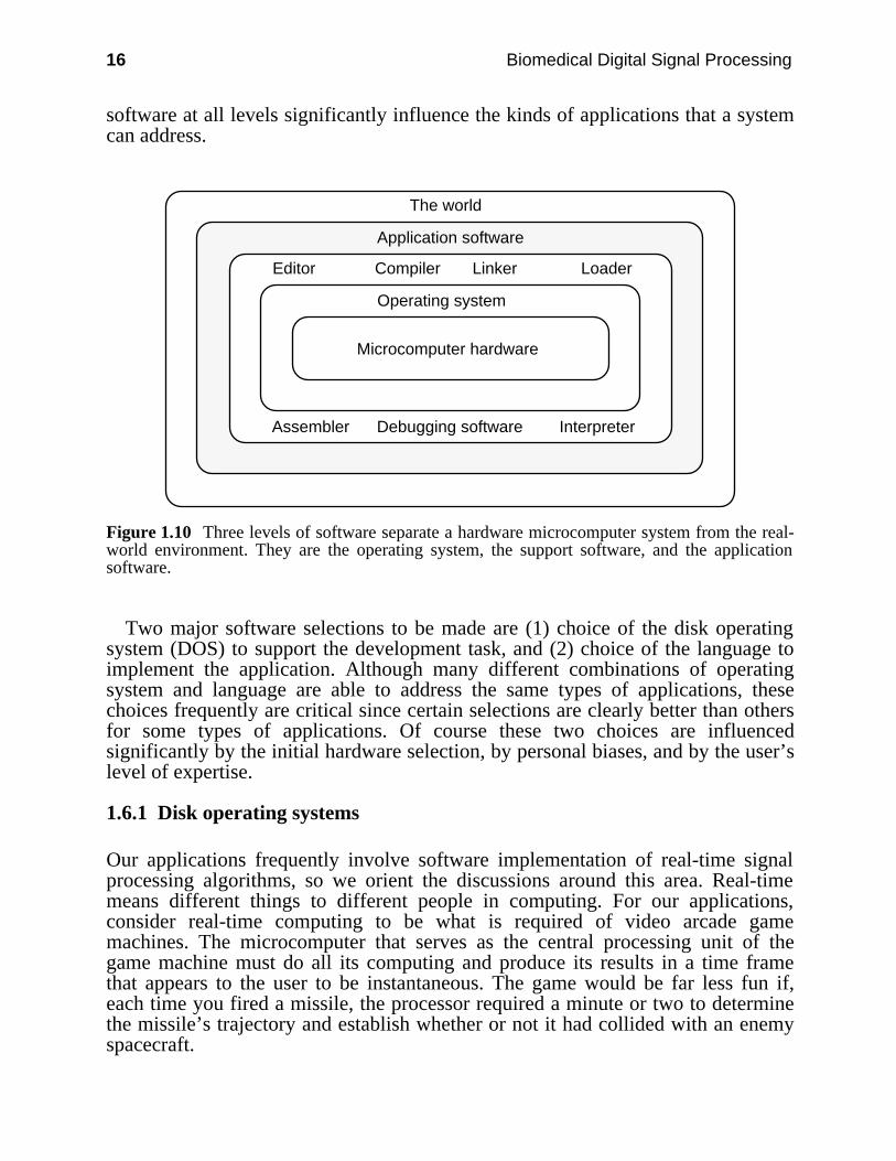
In addition to choosing a personal computer hardware system for laboratory use,we must make additional software choices. The types of choices are frequentlyclosely related and limited by the set of options available for a specific hardwaresystem. Figure 1.10 shows that there are three levels of software between thehardware and the real-world environment: the operating system, the supportsoftware, and the application software (the shaded layer). It is the applicationsoftware that makes the computer behave as a medical instrument. Choices of
16 Biomedical Digital Signal Processing
software at all levels significantly influence the kinds of applications that a systemcan address.
The world
Editor Compiler Linker Loader
Assembler Debugging software Interpreter
Application software
Microcomputer hardware
Operating system
Figure 1.10 Three levels of software separate a hardware microcomputer system from the real-world environment. They are the operating system, the support software, and the applicationsoftware.
Two major software selections to be made are (1) choice of the disk operatingsystem (DOS) to support the development task, and (2) choice of the language toimplement the application. Although many different combinations of operatingsystem and language are able to address the same types of applications, thesechoices frequently are critical since certain selections are clearly better than othersfor some types of applications. Of course these two choices are influencedsignificantly by the initial hardware selection, by personal biases, and by the user’slevel of expertise.
1.6.1 Disk operating systems
Our applications frequently involve software implementation of real-time signalprocessing algorithms, so we orient the discussions around this area. Real-timemeans different things to different people in computing. For our applications,consider real-time computing to be what is required of video arcade gamemachines. The microcomputer that serves as the central processing unit of thegame machine must do all its computing and produce its results in a time framethat appears to the user to be instantaneous. The game would be far less fun if,each time you fired a missile, the processor required a minute or two to determinethe missile’s trajectory and establish whether or not it had collided with an enemyspacecraft.

Introduction to Computers in Medicine 17
A typical example of the need for real-time processing in biomedical computingis in the analysis of electrocardiograms in the intensive care unit of the hospital. Inthe typical television medical drama, the ailing patient is connected to a monitorthat beeps every time the heart beats. If the monitor’s microcomputer required aminute or two to do the complex pattern recognition required to recognize eachvalid heartbeat and then beeped a minute or so after the actual event, the devicewould be useless. The challenge in real-time computing is to develop programs toimplement procedures (algorithms) that appear to occur instantaneously (actually agiven task may take several milliseconds).
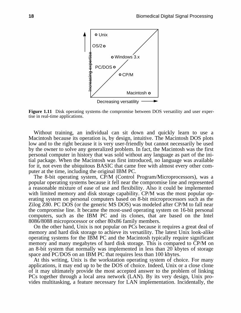
One DOS criterion to consider in the real-time environment is the compromisebetween flexibility and usability. Figure 1.11 is a plot illustrating this compromisefor several general-purpose microcomputer DOSs that are potentially useful in de-veloping solutions to many types of problems including real-time applications. Asthe axes are labeled, the most user-friendly, flexible DOS possible would plot atthe origin. Any DOS with an optimal compromise between usability and flexibilitywould plot on the 45-degree line.
A DOS like Unix has a position on the left side of the graph because it is veryflexible, thereby permitting the user to do any task characteristic of an operatingsystem. That is, it provides the capability to maximally manipulate a hard-ware/software system with excellent control of input/output and other facilities. Italso provides for multiple simultaneous users to do multiple simultaneous tasks(i.e., it is a multiuser, multitasking operating system). Because of this greatflexibility, Unix requires considerable expertise to use all of its capabilities.Therefore it plots high on the graph.
On the other hand, the Macintosh is a hardware/software DOS designed for easeof use and for graphics-oriented applications. Developers of the Macintoshimplemented the best user-to-machine interface that they could conceive of bysacrificing a great deal of the direct user control of the hardware system. Theconcept was to produce a personal computer that would be optimal for runningapplication programs, not a computer to be used for writing new applicationprograms. In fact Apple intended that the Lisa would be the development systemfor creating new Macintosh programs.
18 Biomedical Digital Signal Processing
Unix
PC/DOS
CP/M
Macintosh
OS/2
Decreasing versatility
Incr
easi
ng e
xper
tise
o
o
o
o
o
o
Windows 3.x
Figure 1.11 Disk operating systems–the compromise between DOS versatility and user exper-tise in real-time applications.
Without training, an individual can sit down and quickly learn to use aMacintosh because its operation is, by design, intuitive. The Macintosh DOS plotslow and to the right because it is very user-friendly but cannot necessarily be usedby the owner to solve any generalized problem. In fact, the Macintosh was the firstpersonal computer in history that was sold without any language as part of the ini-tial package. When the Macintosh was first introduced, no language was availablefor it, not even the ubiquitous BASIC that came free with almost every other com-puter at the time, including the original IBM PC.
The 8-bit operating system, CP/M (Control Program/Microprocessors), was apopular operating systems because it fell near the compromise line and representeda reasonable mixture of ease of use and flexibility. Also it could be implementedwith limited memory and disk storage capability. CP/M was the most popular op-erating system on personal computers based on 8-bit microprocessors such as theZilog Z80. PC DOS (or the generic MS DOS) was modeled after CP/M to fall nearthe compromise line. It became the most-used operating system on 16-bit personalcomputers, such as the IBM PC and its clones, that are based on the Intel8086/8088 microprocessor or other 80x86 family members.
On the other hand, Unix is not popular on PCs because it requires a great deal ofmemory and hard disk storage to achieve its versatility. The latest Unix look-alikeoperating systems for the IBM PC and the Macintosh typically require significantmemory and many megabytes of hard disk storage. This is compared to CP/M onan 8-bit system that normally was implemented in less than 20 kbytes of storagespace and PC/DOS on an IBM PC that requires less than 100 kbytes.
At this writing, Unix is the workstation operating system of choice. For manyapplications, it may end up to be the DOS of choice. Indeed, Unix or a close cloneof it may ultimately provide the most accepted answer to the problem of linkingPCs together through a local area network (LAN). By its very design, Unix pro-vides multitasking, a feature necessary for LAN implementation. Incidentally, the
Introduction to Computers in Medicine 19
fact that Unix is written in the C language gives it extraordinary transportability,facilitating its implementation on computers ranging from PCs to supercomputers.
For real-time digital filtering applications, Unix is not desirable because of itsoverhead compared to PC/DOS. In order to simultaneously serve multiple tasks, itmust use up some computational speed. For the typical real-time problem, there isno significant speed to spare for this overhead. Real-time digital signal processingrequires a single-user operating system. You must be able to extract the maximalperformance from the computer and be able to manipulate its lowest level re-sources such as the hardware interrupt structure.
The trends for the future will be toward Macintosh-type operating systems suchas Windows and OS/2. These user-friendly systems sacrifice a good part of thegeneralized computing power to the human-to-machine interface. Each DOS willbe optimized for its intended application area and will be useful primarily for thatarea. Fully implemented versions of OS/2 will most likely require such large por-tions of the computing resources that they will have similar liabilities to those ofUnix in the real-time digital signal processing environment.
Unfortunately there are no popular operating systems available that are specifi-cally designed for such real-time applications as digital signal processing. Atypical DOS is designed to serve the largest possible user base; that is, to be asgeneral purpose as possible. In an IBM PC, the DOS is mated to firmware in theROM BIOS (Basic Input/Output System) to provide a general, orderly way toaccess the system hardware. Use of high-level language calls to the BIOS to do atask such as display of graphics reduces software development time becauseassembly language is not required to deal directly with the specific integrated cir-cuits that control the graphics. A program developed with high-level BIOS callscan also be easily transported to other computers with similar resources. However,the BIOS firmware is general purpose and has some inefficiencies. For example, toimprove the speed of graphics refresh of the screen, you can use assemblylanguage to bypass the BIOS and write directly to the display memory. Howeverthis speed comes at the cost of added development time and loss oftransportability.
Of course, computers like the NEXT computer are attempting to address some ofthese issues. For example, the NEXT has a special shell for Unix designed to makeit more user-friendly. It also includes a built-in digital signal processing (DSP) tofacilitate implementation of signal processing applications.
1.6.2 Languages
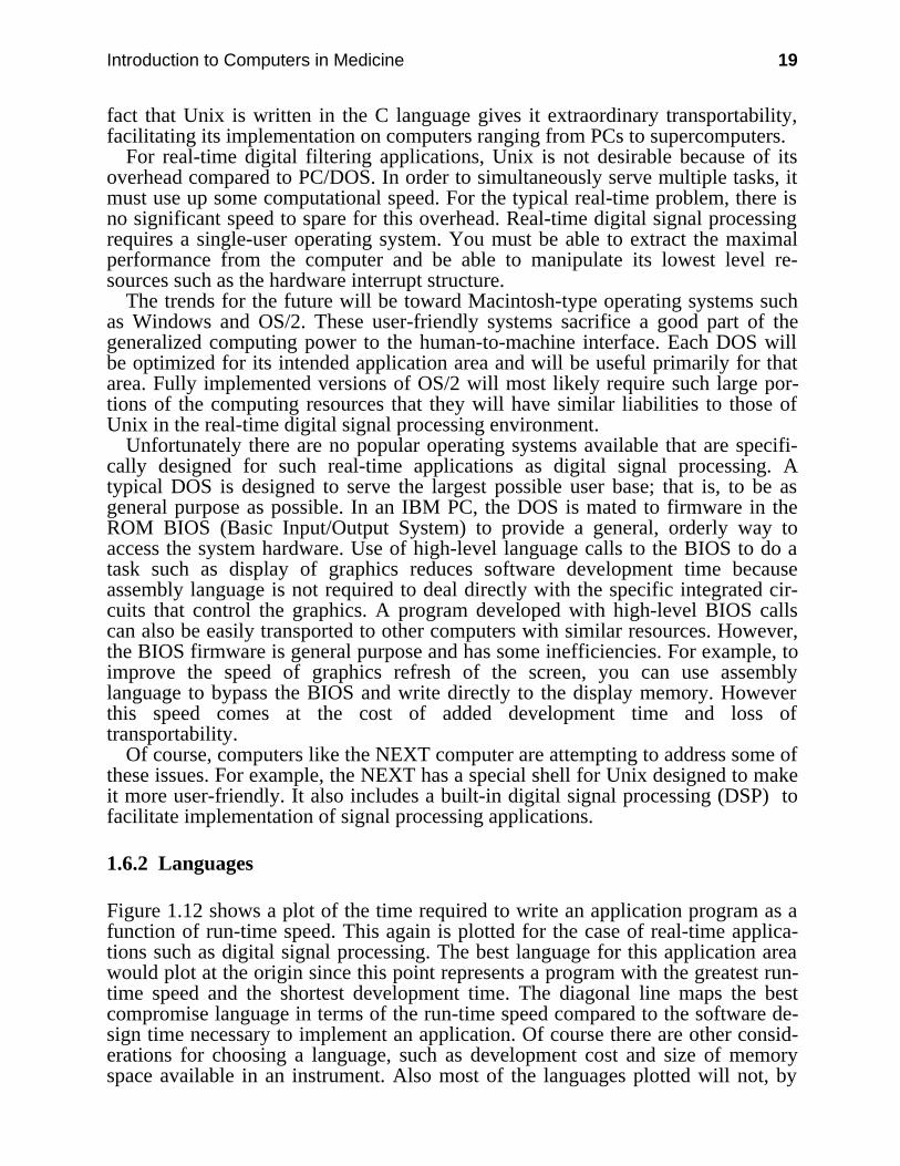
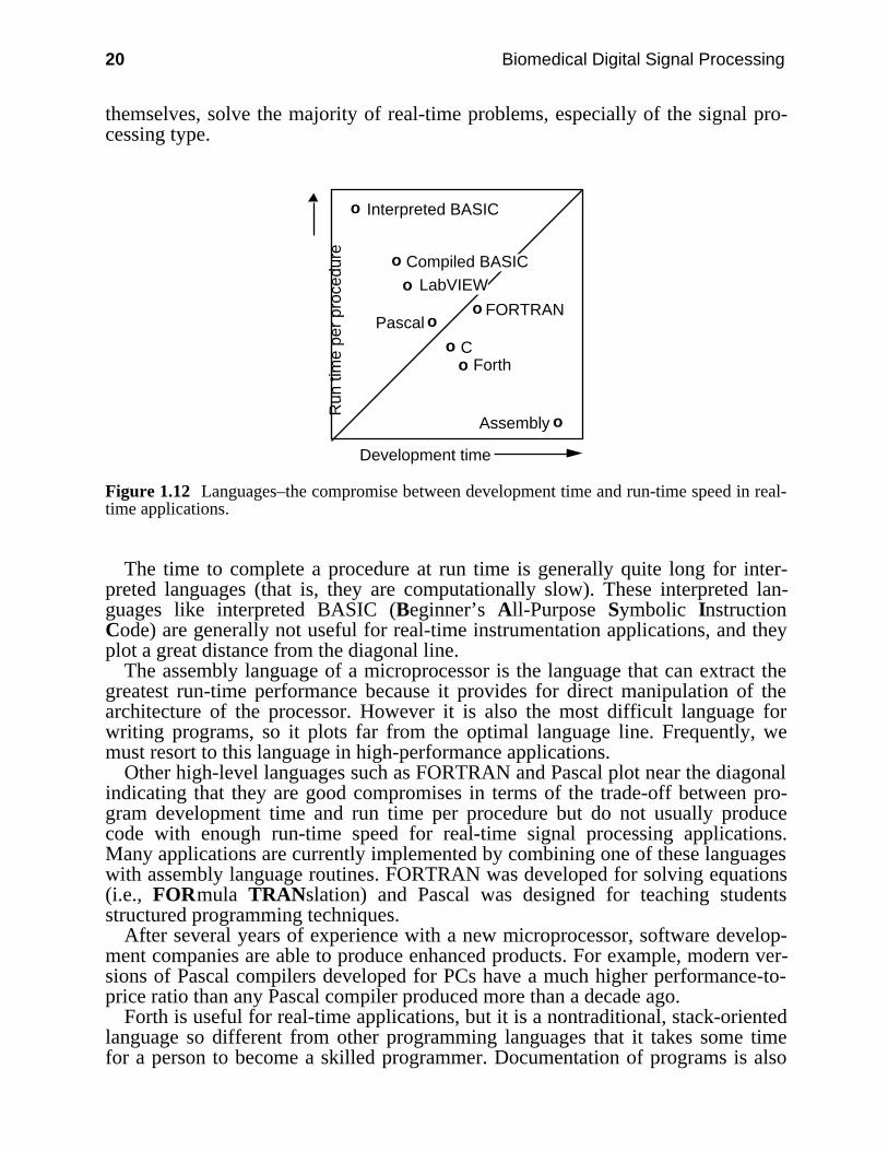
Figure 1.12 shows a plot of the time required to write an application program as afunction of run-time speed. This again is plotted for the case of real-time applica-tions such as digital signal processing. The best language for this application areawould plot at the origin since this point represents a program with the greatest run-time speed and the shortest development time. The diagonal line maps the bestcompromise language in terms of the run-time speed compared to the software de-sign time necessary to implement an application. Of course there are other consid-erations for choosing a language, such as development cost and size of memoryspace available in an instrument. Also most of the languages plotted will not, by
20 Biomedical Digital Signal Processing
themselves, solve the majority of real-time problems, especially of the signal pro-cessing type.
Interpreted BASIC
C
FORTRAN
Assembly
Pascal
Development time
Run
tim
e pe
r pr
oced
ure
o
o
o
o
o
o
Fortho
oCompiled BASIC
LabVIEW
Figure 1.12 Languages–the compromise between development time and run-time speed in real-time applications.
The time to complete a procedure at run time is generally quite long for inter-preted languages (that is, they are computationally slow). These interpreted lan-guages like interpreted BASIC (Beginner’s All-Purpose Symbolic InstructionCode) are generally not useful for real-time instrumentation applications, and theyplot a great distance from the diagonal line.
The assembly language of a microprocessor is the language that can extract thegreatest run-time performance because it provides for direct manipulation of thearchitecture of the processor. However it is also the most difficult language forwriting programs, so it plots far from the optimal language line. Frequently, wemust resort to this language in high-performance applications.
Other high-level languages such as FORTRAN and Pascal plot near the diagonalindicating that they are good compromises in terms of the trade-off between pro-gram development time and run time per procedure but do not usually producecode with enough run-time speed for real-time signal processing applications.Many applications are currently implemented by combining one of these languageswith assembly language routines. FORTRAN was developed for solving equations(i.e., FORmula TRANslation) and Pascal was designed for teaching studentsstructured programming techniques.
After several years of experience with a new microprocessor, software develop-ment companies are able to produce enhanced products. For example, modern ver-sions of Pascal compilers developed for PCs have a much higher performance-to-price ratio than any Pascal compiler produced more than a decade ago.
Forth is useful for real-time applications, but it is a nontraditional, stack-orientedlanguage so different from other programming languages that it takes some timefor a person to become a skilled programmer. Documentation of programs is also
Introduction to Computers in Medicine 21
difficult due to the flexibility of the language. Thus, a program developed in Forthtypically is a one-person program. However, there are several small versions of theForth compiler built into the same chip with a microprocessor. These im-plementations promote its use particularly for controller applications.
LabVIEW (National Instruments) is a visual computing language available onlyfor the Macintosh that is optimized for laboratory applications. Programming is ac-complished by interconnecting functional blocks (i.e., icons) that represent pro-cesses such as Fourier spectrum analysis or instrument simulators (i.e., virtual in-struments). Thus, unlike traditional programming achieved by typing commandstatements, LabVIEW programming is purely graphical, a block diagram language.Although it is a relatively fast compiled language, LabVIEW is not optimized forreal-time applications; its strengths lie particularly in the ability to acquire and pro-cess data in the laboratory environment.
The C language, which is used to develop modern versions of the Unix operatingsystem, provides a significant improvement over assembly language for imple-menting most applications (Kernighan and Ritchie, 1978). It is the currentlanguage of choice for real-time programming. It is an excellent compromisebetween a low-level assembly language and a high-level language. C isstandardized and structured. There are now several versions of commercial C++compilers available for producing object-oriented software.
C programs are based on functions that can be evolved independently of one an-other and put together to implement an application. These functions are to softwarewhat black boxes are to hardware. If their I/O properties are carefully specified inadvance, functions can be developed by many different software designers workingon different aspects of the same project. These functions can then be linked to-gether to implement the software design of a system.
Most important of all, C programs are transportable. By design, a program de-veloped in C on one type of processor can be relatively easily transported to an-other. Embedded machine-specific functions such as those written in assembly lan-guage can be separated out and rewritten in the native code of a new architecture towhich the program has been transported.
1.7 A LOOK TO THE FUTURE
As the microprocessor and its parent semiconductor technologies continue toevolve, the resulting devices will stimulate the development of many new types ofmedical instruments. We cannot even conceive of some of the possibleapplications now, because we cannot easily accept and start designing for thesignificant advances that will be made in computing in the next decade. With the100-million-transistor microprocessor will come personal supercomputing. Onlyfuturists can contemplate ways that we individually will be able to exploit suchcomputing power. Even the nature of the microprocessor as we now know it mightchange more toward the architecture of the artificial neural network, which wouldlead to a whole new set of pattern recognition applications that may be morereadily solvable than with today’s microprocessors.

22 Biomedical Digital Signal Processing
The choices of a laboratory computer, an operating system, and a language for atask must be done carefully. The IBM-compatible PC has emerged as a clear com-puter choice because of its widespread acceptance in the marketplace. The fact thatso many PCs have been sold has produced many choices of hardware add-ons de-veloped by numerous companies and also a wide diversity of software applicationprograms and compilers. By default, IBM produced not only a hardware standardbut also the clear-cut choice of the PC DOS operating system for the first decade ofthe use of this hardware. Although there are other choices now, DOS is still alive.Many will choose to continue using DOS for some time to come, adding to it agraphical user interface (GUI) such as that provided by Windows (Microsoft).
This leaves only the choice of a suitable language for your application area. Mychoice for biomedical instrumentation applications is C. In my view this is aclearly superior language for real-time computing, for instrumentation softwaredesign, and for other biomedical computing applications.
The hardware/software flexibility of the PC is permitting us to do research in ar-eas that were previously too difficult, too expensive, or simply impossible. Wehave come a long way in biomedical computing since those innovators put togetherthat first PC-like LINC almost three decades ago. Expect the PC and its descen-dants to stimulate truly amazing accomplishments in biomedical research in thenext decade.
1.8 REFERENCES
Doumas, T. A., Tompkins, W. J., and Webster, J. G. 1982. An automatic calorie measuringdevice. IEEE Frontiers of Eng. in Health Care, 4: 149–51.
Frisken-Gibson, S., Bach-y-Rita, P., Tompkins, W. J., and Webster, J. G. 1987. A 64-solenoid,4-level fingertip search display for the blind. IEEE Trans. Biomed. Eng., BME-34(12):963–65.
Hamilton, P. S., and Tompkins, W. J. 1986. Quantitative investigation of QRS detection rulesusing the MIT/BIH arrhythmia database. IEEE Trans. Biomed. Eng., BME-33(12): 1157–65.
Hua, P., Woo, E. J., Webster, J. G., and Tompkins, W. J. 1991. Iterative reconstruction methodsusing regularization and optimal current patterns in electrical impedance tomography. IEEETrans. Medical Imaging, 10(4): 621–28.
Kaczmarek, K., Bach-y-Rita, P., Tompkins, W. J., and Webster, J. G. 1985. A tactile visionsubstitution system for the blind: computer-controlled partial image sequencing. IEEE Trans.Biomed. Eng., BME-32(8):602–08.
Kernighan, B. W., and Ritchie, D. M. 1978. The C programming language. Englewood Cliffs,NJ: Prentice Hall.
Mehta, D., Tompkins, W. J., Webster, J. G., and Wertsch, J. J. 1989. Analysis of foot pressurewaveforms. Proc. Annual International Conference of the IEEE Engineering in Medicine andBiology Society, pp. 1487–88.
Pan, J. and Tompkins, W. J. 1985. A real-time QRS detection algorithm. IEEE Trans. Biomed.Eng., BME-32(3): 230–36.
Pfister, C., Harrison, M. A., Hamilton, J. W., Tompkins, W. J., and Webster, J. G. 1989.Development of a 3-channel, 24-h ambulatory esophageal pressure monitor. IEEE Trans.Biomed. Eng., BME-36(4): 487–90.
Tompkins, W. J. 1978. A portable microcomputer-based system for biomedical applications.Biomed. Sci. Instrum., 14: 61–66.

Introduction to Computers in Medicine 23
Tompkins, W. J. 1981. Portable microcomputer-based instrumentation. In H. S. Eden andM. Eden (eds.) Microcomputers in Patient Care. Park Ridge, NJ: Noyes Medical Publications,pp. 174–81.
Tompkins, W. J. 1985. Digital filter design using interactive graphics on the Macintosh. Proc. ofIEEE EMBS Annual Conf., pp. 722–26.
Tompkins, W. J. 1986. Biomedical computing using personal computers. IEEE Engineering inMedicine and Biology Magazine, 5(3): 61–64.
Tompkins, W. J. 1988. Ambulatory monitoring. In J. G. Webster (ed.) Encyclopedia of MedicalDevices and Instrumentation. New York: John Wiley, 1:20–28.
Tompkins, W. J. and Webster, J. G. (eds.) 1981. Design of Microcomputer-based MedicalInstrumentation. Englewood Cliffs, NJ: Prentice Hall.
Woo, E. J., Hua, P., Tompkins, W. J., and Webster, J. G. 1989. 32-electrode electrical impedancetomograph – software design and static images. Proc. Annual International Conference of theIEEE Engineering in Medicine and Biology Society, pp. 455–56.
Xue, Q. Z., Hu, Y. H. and Tompkins, W. J. 1992. Neural-network-based adaptive matchedfiltering for QRS detection. IEEE Trans. Biomed. Eng., BME-39(4): 317–29.
Yorkey, T., Webster, J. G., and Tompkins, W. J. 1987. Comparing reconstruction algorithms forelectrical impedance tomography. IEEE Trans. Biomed. Eng., BME-34(11):843–52.
1.9 STUDY QUESTIONS
1.1 Compare operating systems for support in developing real-time programs. Explain the rela-tive advantages and disadvantages of each for this type of application.
1.2 Explain the differences between interpreted, compiled, and integrated-environment com-piled languages. Give examples of each type.
1.3 List two advantages of the C language for real-time instrumentation applications. Explainwhy they are important.

24
2
Electrocardiography
Willis J. Tompkins
One of the main techniques for diagnosing heart disease is based on the electrocar-diogram (ECG). The electrocardiograph or ECG machine permits deduction ofmany electrical and mechanical defects of the heart by measuring ECGs, which arepotentials measured on the body surface. With an ECG machine, you can deter-mine the heart rate and other cardiac parameters.
2.1 BASIC ELECTROCARDIOGRAPHY
There are three basic techniques used in clinical electrocardiography. The mostfamiliar is the standard clinical electrocardiogram. This is the test done in a physi-cian’s office in which 12 different potential differences called ECG leads arerecorded from the body surface of a resting patient. A second approach uses an-other set of body surface potentials as inputs to a three-dimensional vector modelof cardiac excitation. This produces a graphical view of the excitation of the heartcalled the vectorcardiogram (VCG). Finally, for long-term monitoring in the inten-sive care unit or on ambulatory patients, one or two ECG leads are monitored orrecorded to look for life-threatening disturbances in the rhythm of the heartbeat.This approach is called arrhythmia analysis. Thus, the three basic techniques usedin electrocardiography are:
1. Standard clinical ECG (12 leads)2. VCG (3 orthogonal leads)3. Monitoring ECG (1 or 2 leads)
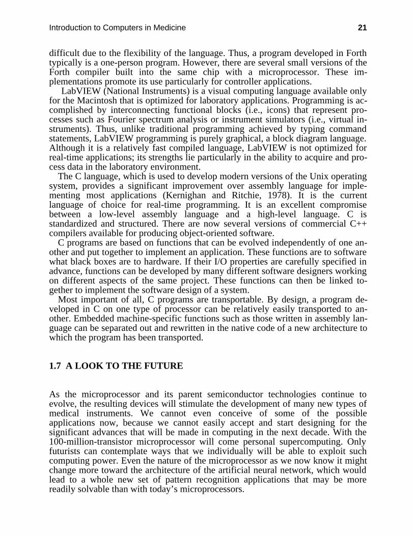
Figure 2.1 shows the basic objective of electrocardiography. By looking at elec-trical signals recorded only on the body surface, a completely noninvasive proce-dure, cardiologists attempt to determine the functional state of the heart. Althoughthe ECG is an electrical signal, changes in the mechanical state of the heart lead tochanges in how the electrical excitation spreads over the surface of the heart,thereby changing the body surface ECG. The study of cardiology is based on therecording of the ECGs of thousands of patients over many years and observing the
Electrocardiography 25
relationships between various waveforms in the signal and different abnormalities.Thus clinical electrocardiography is largely empirical, based mostly on experientialknowledge. A cardiologist learns the meanings of the various parts of the ECG sig-nal from experts who have learned from other experts.
Condition of the heart
Body surface potentials
(electrocardiograms)
Empirical
Figure 2.1 The object of electrocardiography is to deduce the electrical and mechanicalcondition of the heart by making noninvasive body surface potential measurements.
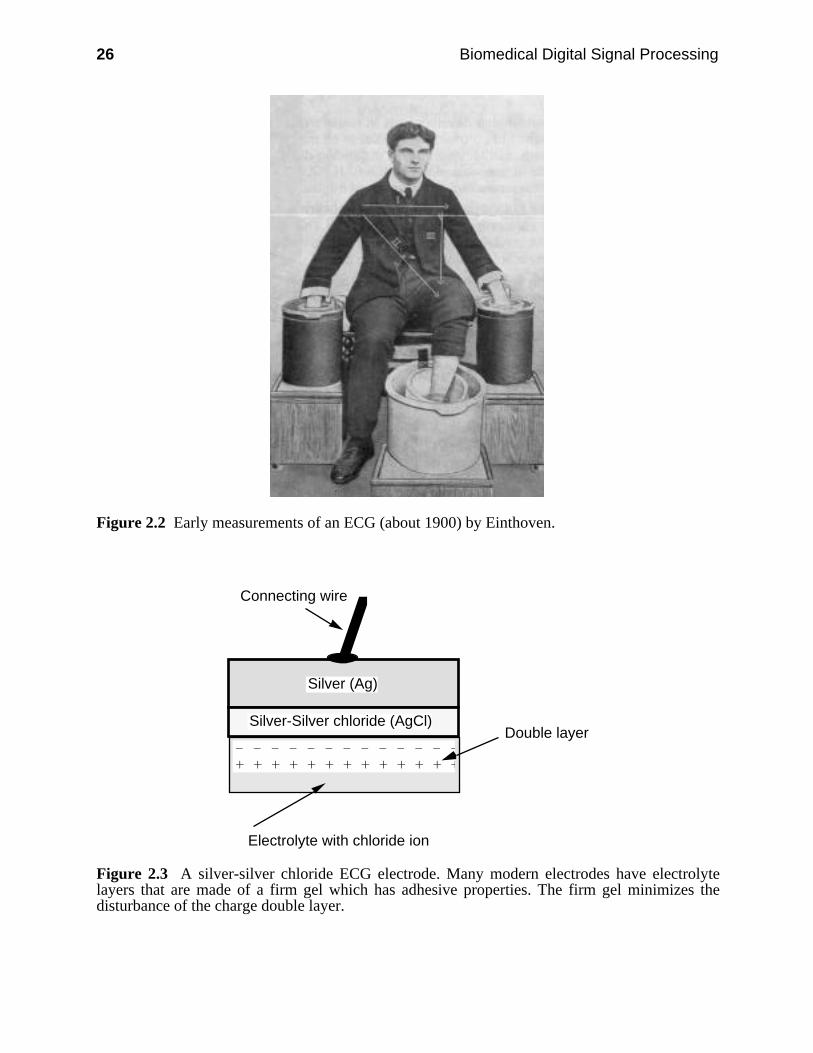
Figure 2.2 shows how the earliest ECGs were recorded by Einthoven at aroundthe turn of the century. Vats of salt water provided the electrical connection to thebody. The string galvanometer served as the measurement instrument for recordingthe ECG.
2.1.1 Electrodes
As time went on, metallic electrodes were developed to electrically connect to thebody. An electrolyte, usually composed of salt solution in a gel, forms the electri-cal interface between the metal electrode and the skin. In the body, currents areproduced by movement of ions whereas in a wire, currents are due to the move-ment of electrons. Electrode systems do the conversion of ionic currents to electroncurrents.
Conductive metals such as nickel-plated brass are used as ECG electrodes butthey have a problem. The two electrodes necessary to acquire an ECG togetherwith the electrolyte and the salt-filled torso act like a battery. A dc offset potentialoccurs across the electrodes that may be as large or larger than the peak ECGsignal. A charge double layer (positive and negative ions separated by a distance)occurs in the electrolyte. Movement of the electrode such as that caused by motionof the patient disturbs this double layer and changes the dc offset. Since this offsetpotential is amplified about 1,000 times along with the ECG, small changes giverise to large baseline shifts in the output signal. An electrode that behaves in thisway is called a polarizable electrode and is only useful for resting patients.
26 Biomedical Digital Signal Processing
Figure 2.2 Early measurements of an ECG (about 1900) by Einthoven.
Silver (Ag)
Silver-Silver chloride (AgCl)
Connecting wire
– – – – – – – – – – – – – + + + + + + + + + + + + +
Electrolyte with chloride ion
Double layer
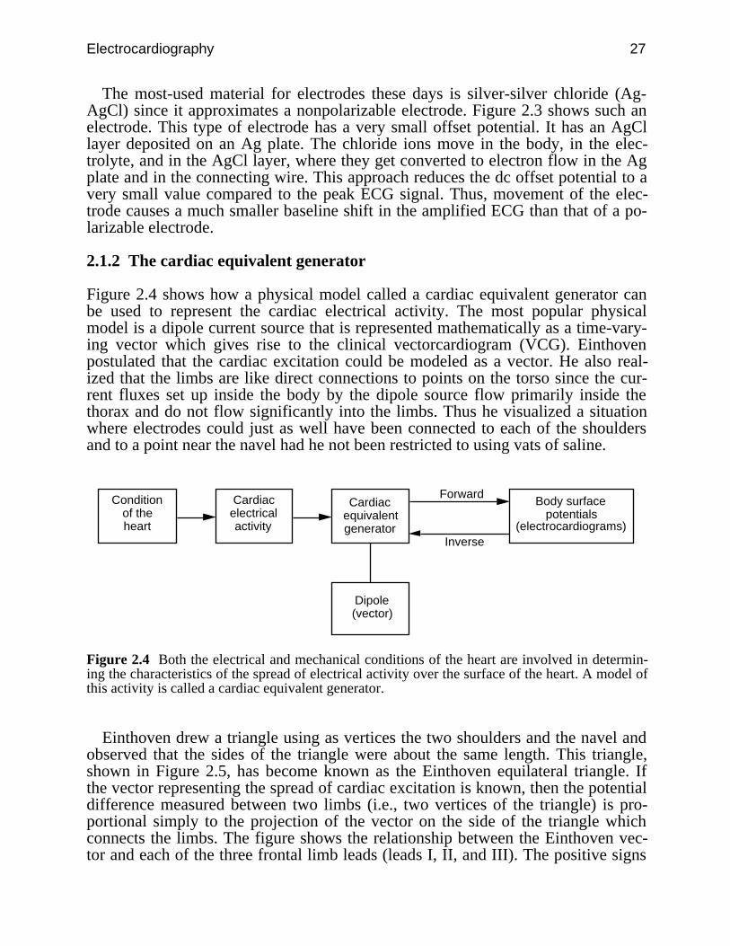
Figure 2.3 A silver-silver chloride ECG electrode. Many modern electrodes have electrolytelayers that are made of a firm gel which has adhesive properties. The firm gel minimizes thedisturbance of the charge double layer.
Electrocardiography 27
The most-used material for electrodes these days is silver-silver chloride (Ag-AgCl) since it approximates a nonpolarizable electrode. Figure 2.3 shows such anelectrode. This type of electrode has a very small offset potential. It has an AgCllayer deposited on an Ag plate. The chloride ions move in the body, in the elec-trolyte, and in the AgCl layer, where they get converted to electron flow in the Agplate and in the connecting wire. This approach reduces the dc offset potential to avery small value compared to the peak ECG signal. Thus, movement of the elec-trode causes a much smaller baseline shift in the amplified ECG than that of a po-larizable electrode.
2.1.2 The cardiac equivalent generator
Figure 2.4 shows how a physical model called a cardiac equivalent generator canbe used to represent the cardiac electrical activity. The most popular physicalmodel is a dipole current source that is represented mathematically as a time-vary-ing vector which gives rise to the clinical vectorcardiogram (VCG). Einthovenpostulated that the cardiac excitation could be modeled as a vector. He also real-ized that the limbs are like direct connections to points on the torso since the cur-rent fluxes set up inside the body by the dipole source flow primarily inside thethorax and do not flow significantly into the limbs. Thus he visualized a situationwhere electrodes could just as well have been connected to each of the shouldersand to a point near the navel had he not been restricted to using vats of saline.
Condition of the heart
Body surface potentials
(electrocardiograms)
Cardiac electrical activity
Cardiac equivalent generator
Dipole (vector)
Forward
Inverse
Figure 2.4 Both the electrical and mechanical conditions of the heart are involved in determin-ing the characteristics of the spread of electrical activity over the surface of the heart. A model ofthis activity is called a cardiac equivalent generator.
Einthoven drew a triangle using as vertices the two shoulders and the navel andobserved that the sides of the triangle were about the same length. This triangle,shown in Figure 2.5, has become known as the Einthoven equilateral triangle. Ifthe vector representing the spread of cardiac excitation is known, then the potentialdifference measured between two limbs (i.e., two vertices of the triangle) is pro-portional simply to the projection of the vector on the side of the triangle whichconnects the limbs. The figure shows the relationship between the Einthoven vec-tor and each of the three frontal limb leads (leads I, II, and III). The positive signs
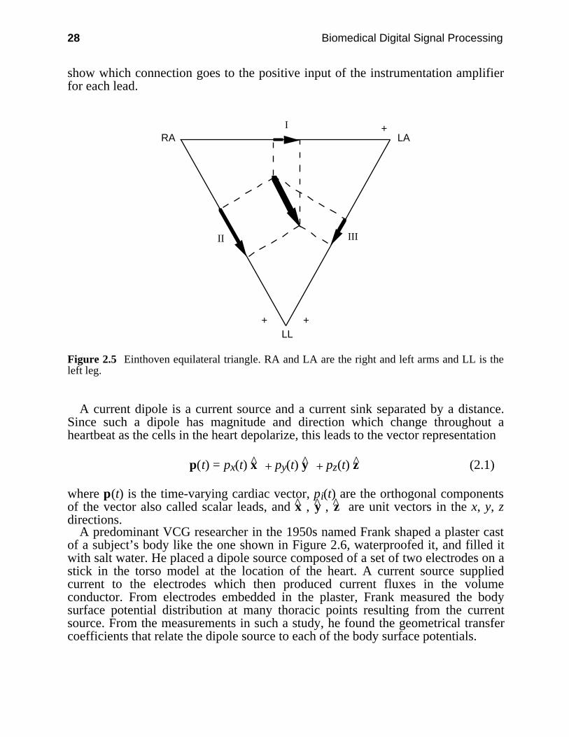
28 Biomedical Digital Signal Processing
show which connection goes to the positive input of the instrumentation amplifierfor each lead.
+
++
I
IIIII
LARA
LL
Figure 2.5 Einthoven equilateral triangle. RA and LA are the right and left arms and LL is theleft leg.
A current dipole is a current source and a current sink separated by a distance.Since such a dipole has magnitude and direction which change throughout aheartbeat as the cells in the heart depolarize, this leads to the vector representation
p(t) = px(t) x + py(t) y + pz(t) z (2.1)
where p(t) is the time-varying cardiac vector, pi(t) are the orthogonal componentsof the vector also called scalar leads, and x , y , z are unit vectors in the x, y, zdirections.
A predominant VCG researcher in the 1950s named Frank shaped a plaster castof a subject’s body like the one shown in Figure 2.6, waterproofed it, and filled itwith salt water. He placed a dipole source composed of a set of two electrodes on astick in the torso model at the location of the heart. A current source suppliedcurrent to the electrodes which then produced current fluxes in the volumeconductor. From electrodes embedded in the plaster, Frank measured the bodysurface potential distribution at many thoracic points resulting from the currentsource. From the measurements in such a study, he found the geometrical transfercoefficients that relate the dipole source to each of the body surface potentials.
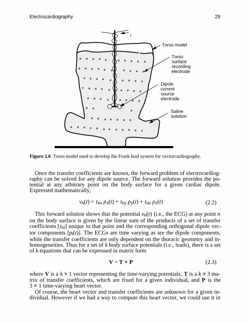
Electrocardiography 29
i
Torso model
Torso surface recording electrode
Dipole current source electrode
Saline solution
Figure 2.6 Torso model used to develop the Frank lead system for vectorcardiography.
Once the transfer coefficients are known, the forward problem of electrocardiog-raphy can be solved for any dipole source. The forward solution provides the po-tential at any arbitrary point on the body surface for a given cardiac dipole.Expressed mathematically,
vn(t) = tnx px(t) + tny py(t) + tnz pz(t) (2.2)
This forward solution shows that the potential vn(t) (i.e., the ECG) at any point non the body surface is given by the linear sum of the products of a set of transfercoefficients [tni] unique to that point and the corresponding orthogonal dipole vec-tor components [pi(t)]. The ECGs are time varying as are the dipole components,while the transfer coefficients are only dependent on the thoracic geometry and in-homogeneities. Thus for a set of k body surface potentials (i.e., leads), there is a setof k equations that can be expressed in matrix form
V = T × P (2.3)
where V is a k × 1 vector representing the time-varying potentials, T is a k × 3 ma-trix of transfer coefficients, which are fixed for a given individual, and P is the3 × 1 time-varying heart vector.
Of course, the heart vector and transfer coefficients are unknown for a given in-dividual. However if we had a way to compute this heart vector, we could use it in
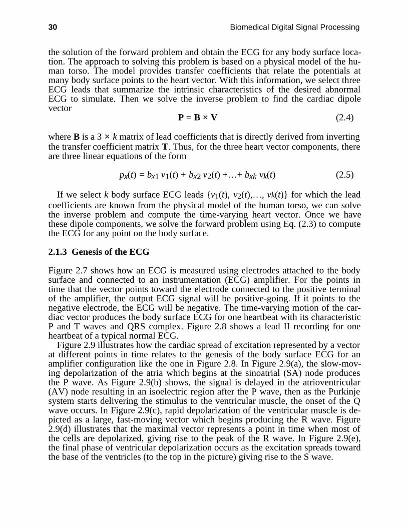
30 Biomedical Digital Signal Processing
the solution of the forward problem and obtain the ECG for any body surface loca-tion. The approach to solving this problem is based on a physical model of the hu-man torso. The model provides transfer coefficients that relate the potentials atmany body surface points to the heart vector. With this information, we select threeECG leads that summarize the intrinsic characteristics of the desired abnormalECG to simulate. Then we solve the inverse problem to find the cardiac dipolevector
P = B × V (2.4)
where B is a 3 × k matrix of lead coefficients that is directly derived from invertingthe transfer coefficient matrix T. Thus, for the three heart vector components, thereare three linear equations of the form
px(t) = bx1 v1(t) + bx2 v2(t) +…+ bxk vk(t) (2.5)
If we select k body surface ECG leads v1(t), v2(t),…, vk(t) for which the leadcoefficients are known from the physical model of the human torso, we can solvethe inverse problem and compute the time-varying heart vector. Once we havethese dipole components, we solve the forward problem using Eq. (2.3) to computethe ECG for any point on the body surface.
2.1.3 Genesis of the ECG
Figure 2.7 shows how an ECG is measured using electrodes attached to the bodysurface and connected to an instrumentation (ECG) amplifier. For the points intime that the vector points toward the electrode connected to the positive terminalof the amplifier, the output ECG signal will be positive-going. If it points to thenegative electrode, the ECG will be negative. The time-varying motion of the car-diac vector produces the body surface ECG for one heartbeat with its characteristicP and T waves and QRS complex. Figure 2.8 shows a lead II recording for oneheartbeat of a typical normal ECG.
Figure 2.9 illustrates how the cardiac spread of excitation represented by a vectorat different points in time relates to the genesis of the body surface ECG for anamplifier configuration like the one in Figure 2.8. In Figure 2.9(a), the slow-mov-ing depolarization of the atria which begins at the sinoatrial (SA) node producesthe P wave. As Figure 2.9(b) shows, the signal is delayed in the atrioventricular(AV) node resulting in an isoelectric region after the P wave, then as the Purkinjesystem starts delivering the stimulus to the ventricular muscle, the onset of the Qwave occurs. In Figure 2.9(c), rapid depolarization of the ventricular muscle is de-picted as a large, fast-moving vector which begins producing the R wave. Figure2.9(d) illustrates that the maximal vector represents a point in time when most ofthe cells are depolarized, giving rise to the peak of the R wave. In Figure 2.9(e),the final phase of ventricular depolarization occurs as the excitation spreads towardthe base of the ventricles (to the top in the picture) giving rise to the S wave.
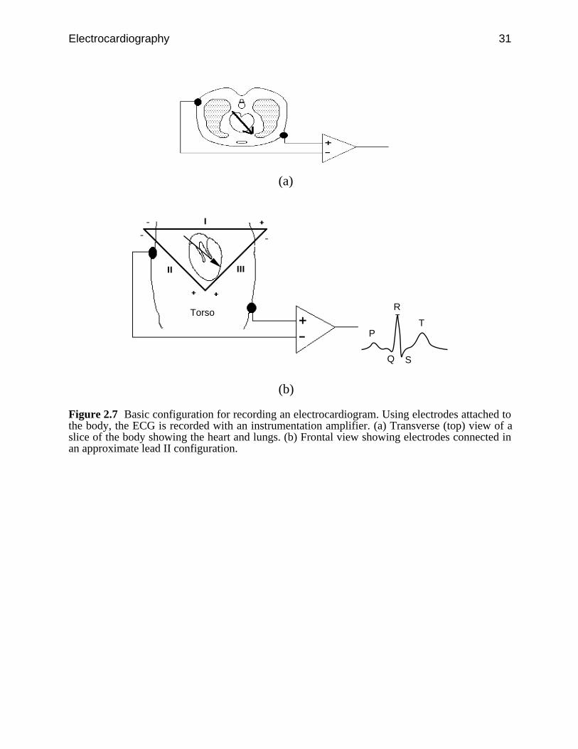
Electrocardiography 31
(a)
Torso
P
Q
R
S
T
(b)
Figure 2.7 Basic configuration for recording an electrocardiogram. Using electrodes attached tothe body, the ECG is recorded with an instrumentation amplifier. (a) Transverse (top) view of aslice of the body showing the heart and lungs. (b) Frontal view showing electrodes connected inan approximate lead II configuration.
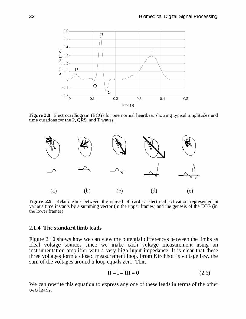
32 Biomedical Digital Signal Processing
-0.2
-0.1
0
0.1
0.2
0.3
0.4
0.5
0.6
0 0.1 0.2 0.3 0.4 0.5
Time (s)
Am
plitu
de (
mV
)
P
Q
R
S
T
Figure 2.8 Electrocardiogram (ECG) for one normal heartbeat showing typical amplitudes andtime durations for the P, QRS, and T waves.
(a) (b) (c) (d) (e)
Figure 2.9 Relationship between the spread of cardiac electrical activation represented atvarious time instants by a summing vector (in the upper frames) and the genesis of the ECG (inthe lower frames).
2.1.4 The standard limb leads
Figure 2.10 shows how we can view the potential differences between the limbs asideal voltage sources since we make each voltage measurement using aninstrumentation amplifier with a very high input impedance. It is clear that thesethree voltages form a closed measurement loop. From Kirchhoff’s voltage law, thesum of the voltages around a loop equals zero. Thus
II – I – III = 0 (2.6)
We can rewrite this equation to express any one of these leads in terms of the othertwo leads.
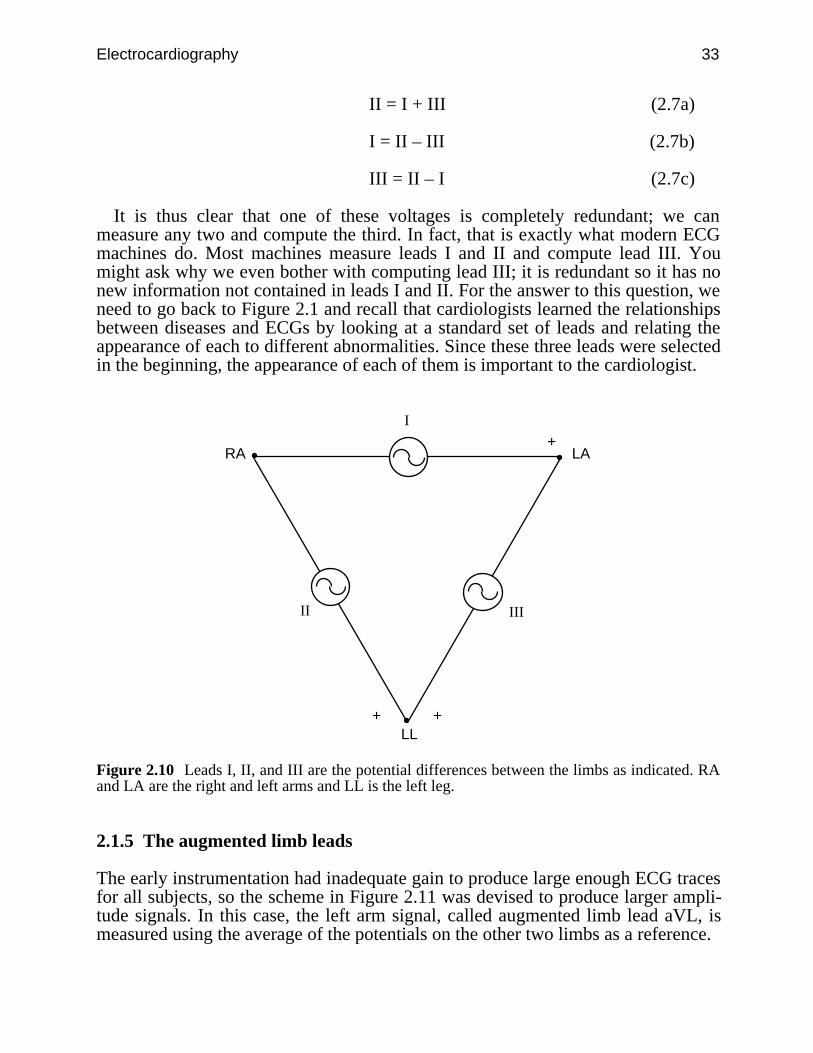
Electrocardiography 33
II = I + III (2.7a)
I = II – III (2.7b)
III = II – I (2.7c)
It is thus clear that one of these voltages is completely redundant; we canmeasure any two and compute the third. In fact, that is exactly what modern ECGmachines do. Most machines measure leads I and II and compute lead III. Youmight ask why we even bother with computing lead III; it is redundant so it has nonew information not contained in leads I and II. For the answer to this question, weneed to go back to Figure 2.1 and recall that cardiologists learned the relationshipsbetween diseases and ECGs by looking at a standard set of leads and relating theappearance of each to different abnormalities. Since these three leads were selectedin the beginning, the appearance of each of them is important to the cardiologist.
+
++
I
IIIII
LARA
LL
Figure 2.10 Leads I, II, and III are the potential differences between the limbs as indicated. RAand LA are the right and left arms and LL is the left leg.
2.1.5 The augmented limb leads
The early instrumentation had inadequate gain to produce large enough ECG tracesfor all subjects, so the scheme in Figure 2.11 was devised to produce larger ampli-tude signals. In this case, the left arm signal, called augmented limb lead aVL, ismeasured using the average of the potentials on the other two limbs as a reference.

34 Biomedical Digital Signal Processing
We can analyze this configuration using standard circuit theory. From the bot-tom left loop
i × R + i × R – II = 0 (2.8)or
i × R = II2 (2.9)
From the bottom right loop–i × R + III + aVL = 0 (2.10)
oraVL = i × R – III (2.11)
Combining Eqs. (2.9) and (2.11) gives
aVL = II2 – III =
II – 2 × III2 (2.12)
+
++
I
IIIII
LARA
LL R
R
+
–aVL
i
Figure 2.11 The augmented limb lead aVL is measured as shown.
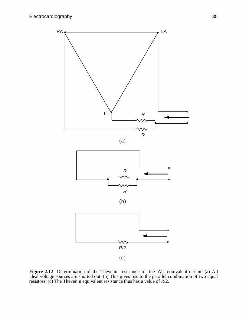
Electrocardiography 35
LARA
LL R
R
(a)
R
R
(b)
R/2
(c)
Figure 2.12 Determination of the Thévenin resistance for the aVL equivalent circuit. (a) Allideal voltage sources are shorted out. (b) This gives rise to the parallel combination of two equalresistors. (c) The Thévenin equivalent resistance thus has a value of R/2.
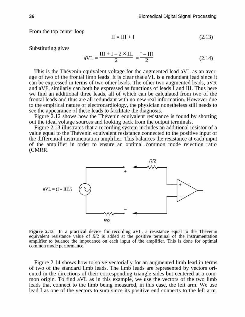
36 Biomedical Digital Signal Processing
From the top center loopII = III + I (2.13)
Substituting gives
aVL = III + I – 2 × III
2 = I – III
2 (2.14)
This is the Thévenin equivalent voltage for the augmented lead aVL as an aver-age of two of the frontal limb leads. It is clear that aVL is a redundant lead since itcan be expressed in terms of two other leads. The other two augmented leads, aVRand aVF, similarly can both be expressed as functions of leads I and III. Thus herewe find an additional three leads, all of which can be calculated from two of thefrontal leads and thus are all redundant with no new real information. However dueto the empirical nature of electrocardiology, the physician nonetheless still needs tosee the appearance of these leads to facilitate the diagnosis.
Figure 2.12 shows how the Thévenin equivalent resistance is found by shortingout the ideal voltage sources and looking back from the output terminals.
Figure 2.13 illustrates that a recording system includes an additional resistor of avalue equal to the Thévenin equivalent resistance connected to the positive input ofthe differential instrumentation amplifier. This balances the resistance at each inputof the amplifier in order to ensure an optimal common mode rejection ratio(CMRR.
+
–
R/2
R/2
+
–
aVL = (I – III)/2
Figure 2.13 In a practical device for recording aVL, a resistance equal to the Théveninequivalent resistance value of R/2 is added at the positive terminal of the instrumentationamplifier to balance the impedance on each input of the amplifier. This is done for optimalcommon mode performance.
Figure 2.14 shows how to solve vectorially for an augmented limb lead in termsof two of the standard limb leads. The limb leads are represented by vectors ori-ented in the directions of their corresponding triangle sides but centered at a com-mon origin. To find aVL as in this example, we use the vectors of the two limbleads that connect to the limb being measured, in this case, the left arm. We uselead I as one of the vectors to sum since its positive end connects to the left arm.
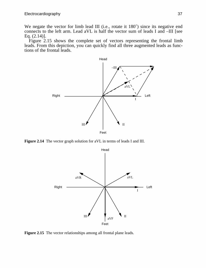
Electrocardiography 37
We negate the vector for limb lead III (i.e., rotate it 180˚) since its negative endconnects to the left arm. Lead aVL is half the vector sum of leads I and –III [seeEq. (2.14)].
Figure 2.15 shows the complete set of vectors representing the frontal limbleads. From this depiction, you can quickly find all three augmented leads as func-tions of the frontal leads.
I
IIIII
–III
aVL
Head
Feet
LeftRight
Figure 2.14 The vector graph solution for aVL in terms of leads I and III.
I
IIIII
aVL
Head
Feet
LeftRight
aVR
aVF
Figure 2.15 The vector relationships among all frontal plane leads.
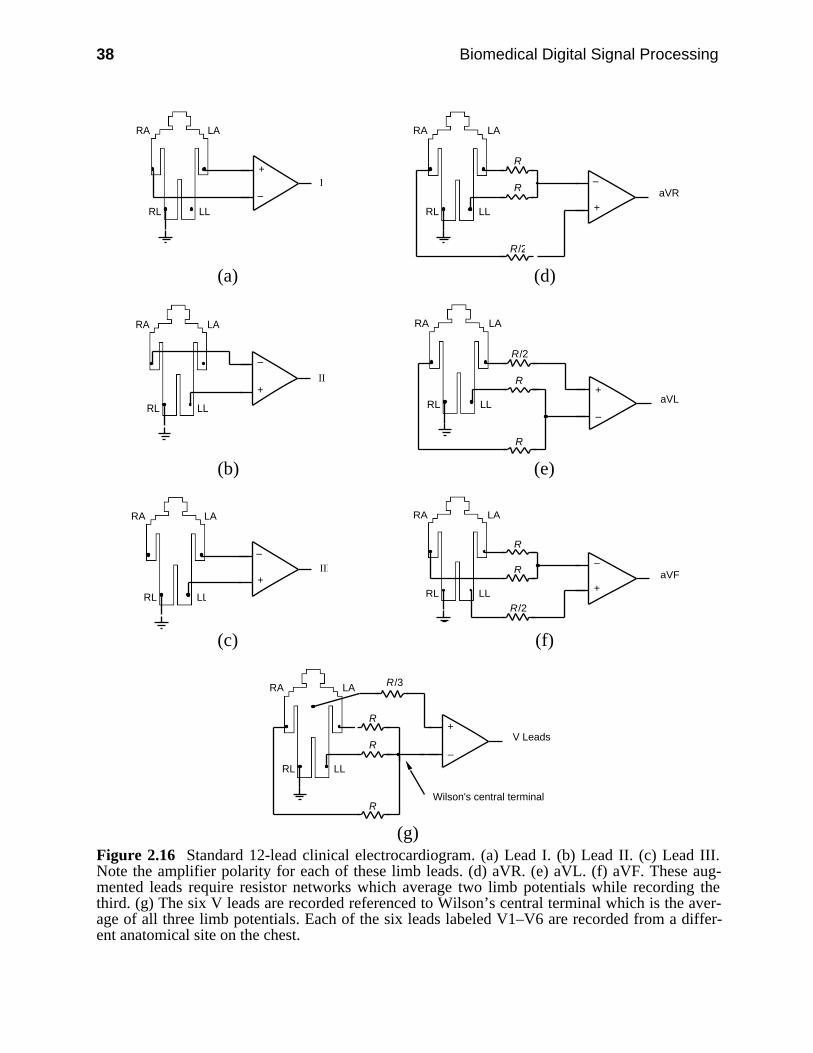
38 Biomedical Digital Signal Processing
+
–I
LARA
RL LL +
–
LARA
RL LL
R
R/2
R aVR
(a) (d)
+
–
II
LARA
RL LL
+
–
LARA
RL LL
R
R/2
R
aVL
(b) (e)
+
–III
LARA
RL LL+
–
LARA
RL LL
R
R/2
R aVF
(c) (f)
LARA
RL LL
+
–
R
RV Leads
R
R/3
Wilson's central terminal
(g)Figure 2.16 Standard 12-lead clinical electrocardiogram. (a) Lead I. (b) Lead II. (c) Lead III.Note the amplifier polarity for each of these limb leads. (d) aVR. (e) aVL. (f) aVF. These aug-mented leads require resistor networks which average two limb potentials while recording thethird. (g) The six V leads are recorded referenced to Wilson’s central terminal which is the aver-age of all three limb potentials. Each of the six leads labeled V1–V6 are recorded from a differ-ent anatomical site on the chest.

Electrocardiography 39
2.2 ECG LEAD SYSTEMS
There are three basic lead systems used in cardiology. The most popular is the 12-lead approach, which defines the set of 12 potential differences that make up thestandard clinical ECG. A second lead system designates the locations of electrodesfor recording the VCG. Monitoring systems typically analyze one or two leads.
2.2.1 12-lead ECG
Figure 2.16 shows how the 12 leads of the standard clinical ECG are recorded, andFigure 2.17 shows the standard 12-lead ECG for a normal patient. The instrumen-tation amplifier is a special design for electrocardiography like the one shown inFigure 2.23. In modern microprocessor-based ECG machines, there are eight simi-lar ECG amplifiers which simultaneously record leads I, II, and V1–V6. They thencompute leads III, aVL, aVR, and aVF for the final report.
Figure 2.17 The 12-lead ECG of a normal male patient. Calibration pulses on the left sidedesignate 1 mV. The recording speed is 25 mm/s. Each minor division is 1 mm, so the majordivisions are 5 mm. Thus in lead I, the R-wave amplitude is about 1.1 mV and the time betweenbeats is almost 1 s (i.e., heart rate is about 60 bpm).
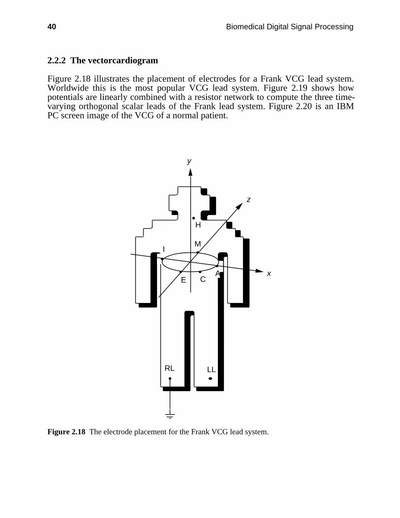
40 Biomedical Digital Signal Processing
2.2.2 The vectorcardiogram
Figure 2.18 illustrates the placement of electrodes for a Frank VCG lead system.Worldwide this is the most popular VCG lead system. Figure 2.19 shows howpotentials are linearly combined with a resistor network to compute the three time-varying orthogonal scalar leads of the Frank lead system. Figure 2.20 is an IBMPC screen image of the VCG of a normal patient.
LL
x
z
y
RL
H
I
E CA
M
Figure 2.18 The electrode placement for the Frank VCG lead system.
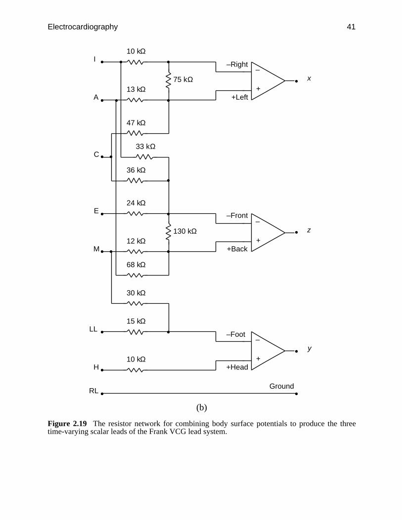
Electrocardiography 41
+
–
10 kΩ
13 kΩ
68 kΩ
30 kΩ
47 kΩ
33 kΩ
36 kΩ
75 kΩ
+
–
24 kΩ
12 kΩ 130 kΩ
+
–
15 kΩ
10 kΩ
–Right
+Left
–Front
+Back
–Foot
+Head
Ground
I
A
C
E
M
LL
H
RL
x
z
y
(b)
Figure 2.19 The resistor network for combining body surface potentials to produce the threetime-varying scalar leads of the Frank VCG lead system.
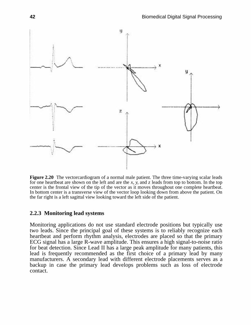
42 Biomedical Digital Signal Processing
Figure 2.20 The vectorcardiogram of a normal male patient. The three time-varying scalar leadsfor one heartbeat are shown on the left and are the x, y, and z leads from top to bottom. In the topcenter is the frontal view of the tip of the vector as it moves throughout one complete heartbeat.In bottom center is a transverse view of the vector loop looking down from above the patient. Onthe far right is a left sagittal view looking toward the left side of the patient.
2.2.3 Monitoring lead systems
Monitoring applications do not use standard electrode positions but typically usetwo leads. Since the principal goal of these systems is to reliably recognize eachheartbeat and perform rhythm analysis, electrodes are placed so that the primaryECG signal has a large R-wave amplitude. This ensures a high signal-to-noise ratiofor beat detection. Since Lead II has a large peak amplitude for many patients, thislead is frequently recommended as the first choice of a primary lead by manymanufacturers. A secondary lead with different electrode placements serves as abackup in case the primary lead develops problems such as loss of electrodecontact.
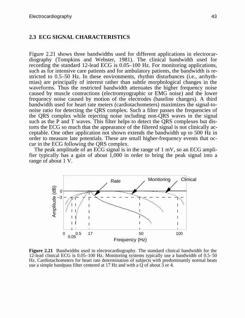
Electrocardiography 43
2.3 ECG SIGNAL CHARACTERISTICS
Figure 2.21 shows three bandwidths used for different applications in electrocar-diography (Tompkins and Webster, 1981). The clinical bandwidth used forrecording the standard 12-lead ECG is 0.05–100 Hz. For monitoring applications,such as for intensive care patients and for ambulatory patients, the bandwidth is re-stricted to 0.5–50 Hz. In these environments, rhythm disturbances (i.e., arrhyth-mias) are principally of interest rather than subtle morphological changes in thewaveforms. Thus the restricted bandwidth attenuates the higher frequency noisecaused by muscle contractions (electromyographic or EMG noise) and the lowerfrequency noise caused by motion of the electrodes (baseline changes). A thirdbandwidth used for heart rate meters (cardiotachometers) maximizes the signal-to-noise ratio for detecting the QRS complex. Such a filter passes the frequencies ofthe QRS complex while rejecting noise including non-QRS waves in the signalsuch as the P and T waves. This filter helps to detect the QRS complexes but dis-torts the ECG so much that the appearance of the filtered signal is not clinically ac-ceptable. One other application not shown extends the bandwidth up to 500 Hz inorder to measure late potentials. These are small higher-frequency events that oc-cur in the ECG following the QRS complex.
The peak amplitude of an ECG signal is in the range of 1 mV, so an ECG ampli-fier typically has a gain of about 1,000 in order to bring the peak signal into arange of about 1 V.
0
0
50 100
Frequency (Hz)
Am
plitu
de (
dB)
MonitoringRate
170.05
0.5
–3
Clinical
Figure 2.21 Bandwidths used in electrocardiography. The standard clinical bandwidth for the12-lead clinical ECG is 0.05–100 Hz. Monitoring systems typically use a bandwidth of 0.5–50Hz. Cardiotachometers for heart rate determination of subjects with predominantly normal beatsuse a simple bandpass filter centered at 17 Hz and with a Q of about 3 or 4.
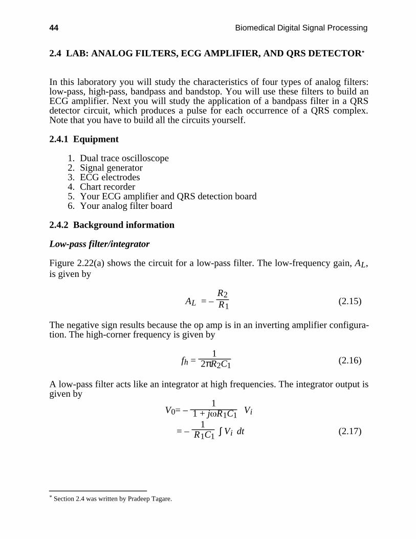
44 Biomedical Digital Signal Processing
2.4 LAB: ANALOG FILTERS, ECG AMPLIFIER, AND QRS DETECTOR*
In this laboratory you will study the characteristics of four types of analog filters:low-pass, high-pass, bandpass and bandstop. You will use these filters to build anECG amplifier. Next you will study the application of a bandpass filter in a QRSdetector circuit, which produces a pulse for each occurrence of a QRS complex.Note that you have to build all the circuits yourself.
2.4.1 Equipment
1. Dual trace oscilloscope2. Signal generator3. ECG electrodes4. Chart recorder5. Your ECG amplifier and QRS detection board6. Your analog filter board
2.4.2 Background information
Low-pass filter/integrator
Figure 2.22(a) shows the circuit for a low-pass filter. The low-frequency gain, AL,is given by
AL = – R2 R1
(2.15)
The negative sign results because the op amp is in an inverting amplifier configura-tion. The high-corner frequency is given by
fh = 1
2πR2C1 (2.16)
A low-pass filter acts like an integrator at high frequencies. The integrator output isgiven by
V0= – 1
1 + j R1C1 Vi
= – 1
R1C1 ∫ Vi dt (2.17)
* Section 2.4 was written by Pradeep Tagare.
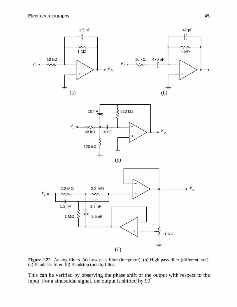
Electrocardiography 45
+
–10 kΩ
1 MΩ
1.5 nF
oViV
+
–10 kΩ
1 MΩ
47 pF
iV470 nF
(a) (b)
+
–
68 kΩ oViV
10 nF
820 kΩ10 nF
120 kΩ
(c)
+
–2.2 MΩ o
V
iV
1.3 nF
1 MΩ 2.5 nF
10 kΩ+
–
2.2 MΩ
1.3 nF
(d)
Figure 2.22 Analog filters. (a) Low-pass filter (integrator). (b) High-pass filter (differentiator).(c) Bandpass filter. (d) Bandstop (notch) filter.
This can be verified by observing the phase shift of the output with respect to theinput. For a sinusoidal signal, the output is shifted by 90˚
46 Biomedical Digital Signal Processing
⌡⌠ v sin t = – v
cos t = v
sin( t + π2 ) (2.18)
Thus the gain of the integrator falls at high frequencies. Also note that if R2 werenot included in the integrator, the gain would become infinite at dc. Thus at dc theop amp dc bias current charges the integrating capacitor C1 and saturates theamplifier.
High-pass filter/differentiator
In contrast to the low-pass filter which acts as an integrator at high frequencies, thehigh-pass filter acts like a differentiator at low frequencies. Referring to Figure2.22(b), we get the high-frequency gain Ah and the low-corner frequency fL as
Ah = – R2 R1
(2.19)
fL = 1
2πR1C1 (2.20)
The differentiating behavior of the high-pass filter at low frequencies can be veri-fied by deriving equations as was done for the integrator. Capacitor C2 is added toimprove the stability of the differentiator. The differentiator gain increases withfrequency, up to the low-corner frequency.
Bandpass filter
The circuit we will use is illustrated in Figure 2.22(c). The gain of a bandpass filteris maximum at the center frequency and falls off on either side of the centerfrequency. The bandwidth of a bandpass filter is defined as the difference betweenthe two corner frequencies. The Q of a bandpass filter is defined as
Q = center frequency
bandwidth (2.21)
Bandstop/notch filter
Line frequency noise is a major source of interference. Sometimes a 60-Hz band-stop (notch) filter is used to reject this interference. Basically such a filter rejectsone particular frequency while passing all other frequencies. Figure 2.22(d) showsthe bandstop filter that we will use. For the 60-Hz notch filter shown, the 60-Hz re-jection factor is defined as
60-Hz rejection factor = output voltage of the filter at 100 Hz output voltage of the filter at 60 Hz (2.22)
Electrocardiography 47
for the same input voltage.
ECG amplifier
An ECG signal is usually in the range of 1 mV in magnitude and has frequencycomponents from about 0.05–100 Hz. To process this signal, it has to be amplified.Figure 2.23 shows the circuit of an ECG amplifier. The typical characteristics of anECG amplifier are high gain (about 1,000), 0.05–100 Hz frequency response, highinput impedance, and low output impedance. Derivation of equations for the gainand frequency response are left as an exercise for the reader.
QRS detector
Figures 2.24 and 2.25 show the block diagram and complete schematic for theQRS detector. The QRS detector consists of the following five units:
1. QRS filter. The power spectrum of a normal ECG signal has the greatest signal-to-noise ratio at about 17 Hz. Therefore to detect the QRS complex, the ECG ispassed through a bandpass filter with a center frequency of 17 Hz and a band-width of 6 Hz. This filter has a large amount of ringing in its output.
2. Half-wave rectifier. The filtered QRS is half-wave rectified, to be subsequentlycompared with a threshold voltage generated by the detector circuit.
3. Threshold circuit. The peak voltage of the rectified and filtered ECG is storedon a capacitor. A fraction of this voltage (threshold voltage) is compared withthe filtered and rectified ECG output.
4. Comparator. The QRS pulse is detected when the threshold voltage is exceeded.The capacitor recharges to a new threshold voltage after every pulse. Hence anew threshold determined from the past history of the signal is generated afterevery pulse.
5. Monostable. A 200-ms pulse is generated for every QRS complex detected.This pulse drives a LED.
Some patients have a cardiac pacemaker. Since sharp pulses of the pacemakercan cause spurious QRS pulse detection, a circuit is often included to reject pace-maker pulses. The rejection is achieved by limiting the slew rate of the amplifier.

48 Biomedical Digital Signal Processing
+
–
+
–
+
–
+
–
43 kΩ
10 kΩ
10 kΩ
10 kΩ
22 pF
10 kΩ
10 kΩ
10 kΩ
22 kΩ
22 kΩ
47 kΩ
4.7 kΩ
150 kΩ
1 µF
3.3 MΩ
Vo
RA
LA
RL10 kΩ
22 pF
Reset
0.01 µF
3.3 MΩ
Figure 2.23 Circuit diagram of an ECG amplifier.
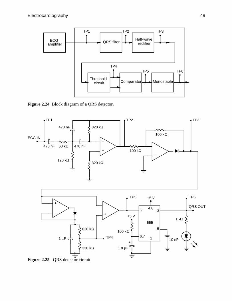
Electrocardiography 49
ECG amplifier
QRS filter
Threshold circuit Comparator Monostable
TP1 TP2 TP3
Half-wave rectifier
TP6TP5TP4
Figure 2.24 Block diagram of a QRS detector.
+
–
68 kΩ 470 nF
820 kΩ470 nF
120 kΩ
470 nF
ECG IN
820 kΩ
TP1
100 kΩ
TP2
+
–
100 kΩ
+
– +
–
820 kΩ
330 kΩ
1 µF
TP3
TP4
TP5
QRS OUT
TP6
10 nF
+5 V
+5 V
1.8 µF
+
100 kΩ
16,7
34,82
5
5551 kΩ
Figure 2.25 QRS detector circuit.
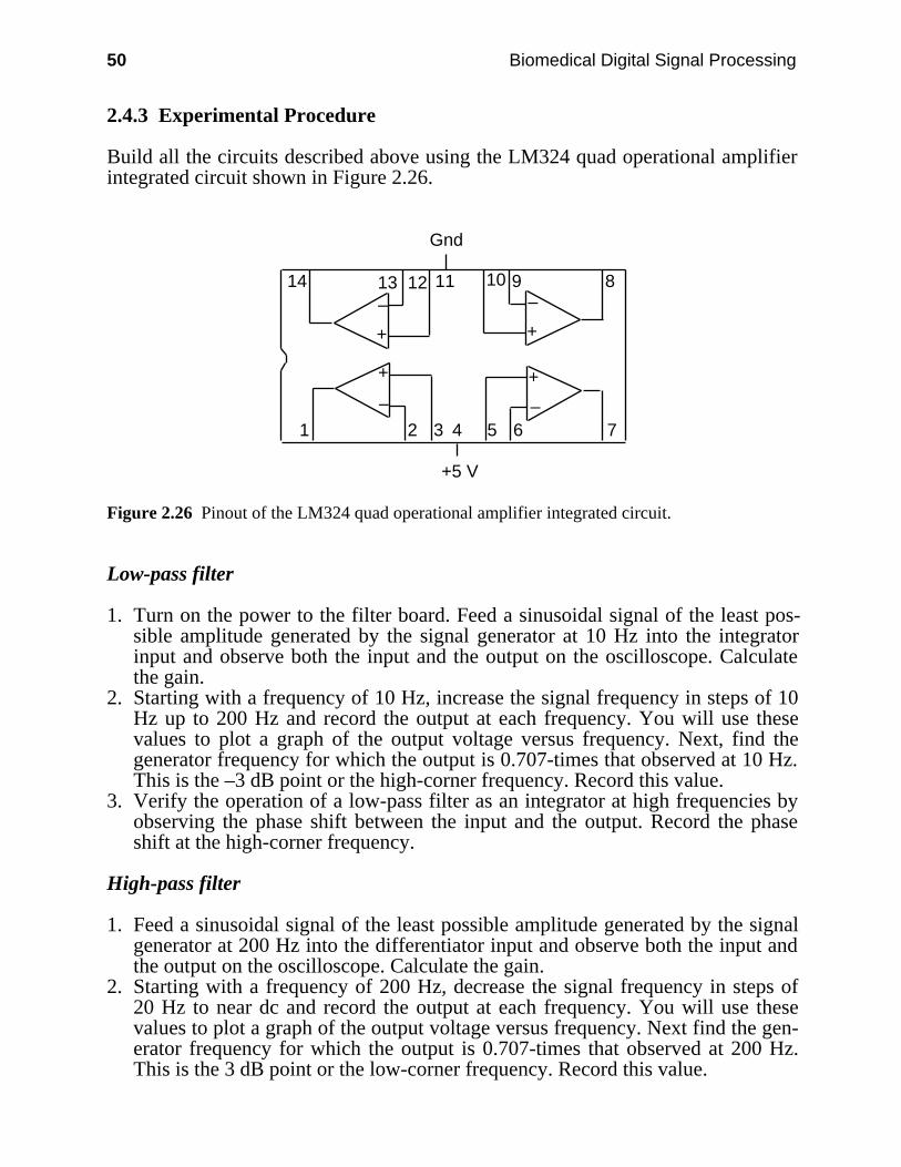
50 Biomedical Digital Signal Processing
2.4.3 Experimental Procedure
Build all the circuits described above using the LM324 quad operational amplifierintegrated circuit shown in Figure 2.26.
2 3 4 5 6 7
8910111214 13
+ +
++
+5 V
Gnd
1––
––
Figure 2.26 Pinout of the LM324 quad operational amplifier integrated circuit.
Low-pass filter
1. Turn on the power to the filter board. Feed a sinusoidal signal of the least pos-sible amplitude generated by the signal generator at 10 Hz into the integratorinput and observe both the input and the output on the oscilloscope. Calculatethe gain.
2. Starting with a frequency of 10 Hz, increase the signal frequency in steps of 10Hz up to 200 Hz and record the output at each frequency. You will use thesevalues to plot a graph of the output voltage versus frequency. Next, find thegenerator frequency for which the output is 0.707-times that observed at 10 Hz.This is the –3 dB point or the high-corner frequency. Record this value.
3. Verify the operation of a low-pass filter as an integrator at high frequencies byobserving the phase shift between the input and the output. Record the phaseshift at the high-corner frequency.
High-pass filter
1. Feed a sinusoidal signal of the least possible amplitude generated by the signalgenerator at 200 Hz into the differentiator input and observe both the input andthe output on the oscilloscope. Calculate the gain.
2. Starting with a frequency of 200 Hz, decrease the signal frequency in steps of20 Hz to near dc and record the output at each frequency. You will use thesevalues to plot a graph of the output voltage versus frequency. Next find the gen-erator frequency for which the output is 0.707-times that observed at 200 Hz.This is the 3 dB point or the low-corner frequency. Record this value.
Electrocardiography 51
3. Verify the operation of a high-pass filter as a differentiator at low frequenciesby observing the phase shift between the input and the output. Record the phaseshift at the low-corner frequency. Another simple way to observe the differenti-ating behavior is to feed a 10-Hz square wave into the input and observe thespikes at the output.
Bandpass filter
For a 1-V p-p sinusoidal signal, vary the frequency from 10–150 Hz. Record thehigh- and low-corner frequencies. Find the center frequency and the passbandgain of this filter.
Bandstop/notch filter
Feed a 1-V p-p 60-Hz sinusoidal signal into the filter, and measure the outputvoltage. Repeat the same for a 100-Hz sinusoid. Record results.
ECG amplifier
1. Connect LA and RA inputs of the amplifier to ground and observe the output.Adjust the 100-kΩ pot to null the offset voltage.
2. Connect LA and RA inputs to the signal high and the RL input to signal high(60 Hz) and RL to signal low. This is the common mode operation. Calculatethe common mode gain.
3. Connect the LA input to the signal high (30 Hz) and the RA input to the signallow (through an attenuator to avoid saturation). This is the differential modeoperation. Calculate the differential mode gain.
4. Find the frequency response of the amplifier.5. Connect three electrodes to your body. Connect these electrodes to the amplifier
inputs. Observe the amplifier output. If the signal is very noisy, try twisting theleads together. When you get a good signal, get a recording on the chartrecorder.
QRS detector
1. Apply three ECG electrodes. Connect the electrodes to the input of the ECGamplifier board. Turn on the power to the board and observe the output of theECG amplifier on the oscilloscope. Try pressing the electrodes if there is ex-cessive noise.
2. Connect the output of the ECG amplifier to the input of the QRS detector board.Observe the following signals on the oscilloscope and then record them on astripchart recorder with the ECG (TP1) on one channel and each of the othertest signals (TP2–TP6) on the other channel. Use a reasonably fast paper speed(e.g., 25 mm/s).

52 Biomedical Digital Signal Processing
Signals to be observed:
Test point Signal
TP1 Your ECGTP2 Filtered outputTP3 Rectified outputTP4 Comparator inputTP5 Comparator outputTP6 Monostable output
The LED should flash for every QRS pulse detected.
2.4.4 Lab report
1. Using equations described in the text, determine the values of AL and fh for thelow-pass filter. Compare these values with the respective values obtained inthe lab and account for any differences.
2. Plot the graph of the filter output voltage versus frequency. Show the –3 dBpoint on this graph.
3. What value of phase shift did you obtain for the low-pass filter?4. Using equations described in the text, determine the values of AH and fL for
the high-pass filter. Compare these values with the respective values obtainedin the lab and account for any differences.
5. Plot the graph of the filter output voltage versus frequency. Show the –3 dBpoint on this graph.
6. What value of phase shift did you obtain for the high-pass filter?7. For the bandpass amplifier, list the values that you got for the following:
(a) center frequency(b) passband gain(c) bandwidth(d) QShow all calculations.
8. What is the 60-Hz rejection factor for the bandstop filter you used?9. What are the upper and lower –3 dB frequencies of your ECG amplifier? How
do they compare with the theoretical values?10. What is the gain of your ECG amplifier? How does it compare with the
theoretical value?11. What is the CMRR of your ECG amplifier?12. How would you change the –3 dB frequencies of this amplifier?13. Explain the waveforms you recorded on the chart recorder. Are these what
you would expect to obtain?14. Will the QRS detector used in this lab work for any person’s ECG? Justify
your answer.
Include all chart recordings with your lab report and show calculations whereverappropriate.

Electrocardiography 53
2.5 REFERENCES
Tompkins, W. J. and Webster, J. G. (eds.) 1981. Design of Microcomputer-based MedicalInstrumentation. Englewood Cliffs, NJ: Prentice-Hall.
2.6 STUDY QUESTIONS
2.1 What is a cardiac equivalent generator? How is it different from the actual cardiac electricalactivity? Give two examples.
2.2 What is the vectorcardiogram and how is it recorded?2.3 The heart vector of a patient is oriented as shown below at one instant of time. At this time,
which of the frontal leads (I, II, and III) are positive-going for:
II
I
III
+ +
+RA LA
LL
II
I
III
+ +
+RA LA
LL
(a) (b)
2.4 A certain microprocessor-based ECG machine samples and stores only leads I and II. Whatother standard leads can it compute from these two?
2.5 It is well known that all six frontal leads of the ECG can be expressed in terms of any twoof them. Express the augmented lead at the right arm (i.e., aVR) in terms of leads I and II.
2.6 Express Lead II in terms of aVF and aVL.2.7 Is it possible to express lead V6 in terms of two other leads? Is there any way to calculate
V6 from a larger set of leads?2.8 There are four different bandwidths that are used in electrocardiography. Describe the
principal applications for each of these bandwidths.2.9 What is the frequency range of the standard 3-dB bandwidth used in (a) clinical electro-
cardiography, (b) electrocardiography monitoring applications such as in the intensive careunit? (c) Why are the clinical and monitoring bandwidths different?
2.10 A cardiologist records a patient’s ECG on a machine that is suspected of being defective.She notices that the QRS complex of a normal patient’s ECG has a lower peak-to-peakamplitude than the one recorded on a good machine. Explain what problems in instrumentbandwidth might be causing this result.
2.11 A cardiologist notices that the T wave of a normal patient’s ECG is distorted so that itlooks like a biphasic sine wave instead of a unipolar wave. Explain what problems in in-strument bandwidth might be causing this problem.
2.12 What is the electrode material that is best for recording the ECG from an ambulatorypatient?
2.13 A cardiotachometer uses a bandpass filter to detect the QRS complex of the ECG. What isits center frequency (in Hz)? How was this center frequency determined?
2.14 An engineer designs a cardiotachometer that senses the occurrence of a QRS complex witha simple amplitude threshold. It malfunctions in two patients. (a) One patient’s ECG has
54 Biomedical Digital Signal Processing
baseline drift and electromyographic noise. What ECG preprocessing step would providethe most effective improvement in the design for this case? (b) Another patient has a Twave that is much larger than the QRS complex. This false triggers the thresholding circuit.What ECG preprocessing step would provide the most effective improvement in the designfor this case?
2.15 What is included in the design of an averaging cardiotachometer that prevents it from re-sponding instantaneously to a heart rate change?
2.16 A typical modern microprocessor-based ECG machine samples and stores leads I, II, V1,V2, V3, V4, V5, and V6. From this set of leads, calculate (a) lead III, (b) augmentedlead aVF.
55
3
Signal Conversion
David J. Beebe
The power of the computer to analyze and visually represent biomedical signals isof little use if the analog biomedical signal cannot be accurately captured and con-verted to a digital representation. This chapter discusses basic sampling theory andthe fundamental hardware required in a typical signal conversion system. Section3.1 discusses sampling basics in a theoretical way, and section 3.2 describes thecircuits required to implement a real signal conversion system. We examine theoverall system requirements for an ECG signal conversion system and discuss thepossible errors involved in the conversion. We review digital-to-analog andanalog-to-digital converters and other related circuits including amplifiers, sample-and-hold circuits, and analog multiplexers.
3.1 SAMPLING BASICS*
The whole concept of converting a continuous time signal to a discrete representa-tion usable by a microprocessor, lies in the fact that we can represent a continuoustime signal by its instantaneous amplitude values taken at periodic points in time.More important, we are able to reconstruct the original signal perfectly with justthese sampled points. Such a concept is exploited in movies, where individualframes are snapshots of a continuously changing scene. When these individualframes are played back at a sufficiently fast rate, we are able to get an accuraterepresentation of the original scene (Oppenheim and Willsky, 1983).
3.1.1 Sampling theorem
The sampling theorem initially developed by Shannon, when obeyed, guaranteesthat the original signal can be reconstructed from its samples without any loss ofinformation. It states that, for a continuous bandlimited signal that contains no fre-quency components higher than fc, the original signal can be completely recovered
* Section 3.1 was written by Annie Foong.
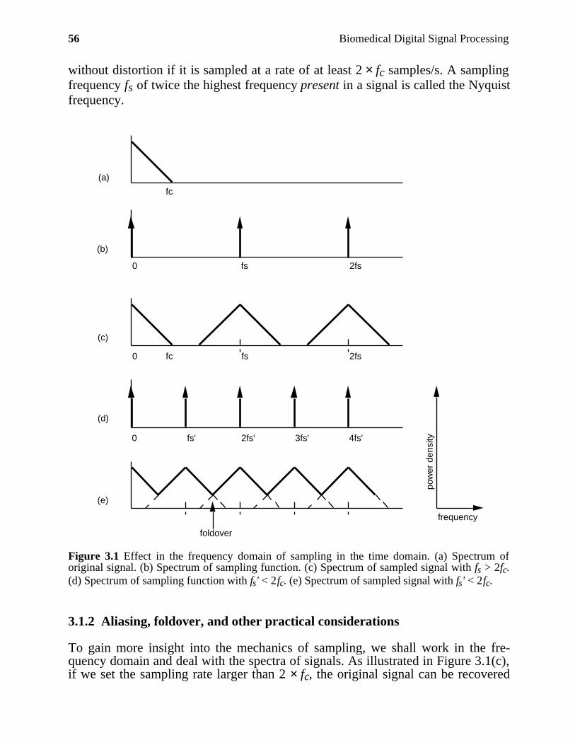
56 Biomedical Digital Signal Processing
without distortion if it is sampled at a rate of at least 2 × fc samples/s. A samplingfrequency fs of twice the highest frequency present in a signal is called the Nyquistfrequency.
(a)
(b)
(c)
(d)
(e)
pow
er d
ensi
ty
frequency
fc
0 fs 2fs
0 fc fs 2fs
foldover
0 fs' 2fs' 3fs' 4fs'
Figure 3.1 Effect in the frequency domain of sampling in the time domain. (a) Spectrum oforiginal signal. (b) Spectrum of sampling function. (c) Spectrum of sampled signal with fs > 2fc.(d) Spectrum of sampling function with fs' < 2fc. (e) Spectrum of sampled signal with fs' < 2fc.
3.1.2 Aliasing, foldover, and other practical considerations
To gain more insight into the mechanics of sampling, we shall work in the fre-quency domain and deal with the spectra of signals. As illustrated in Figure 3.1(c),if we set the sampling rate larger than 2 × fc, the original signal can be recovered
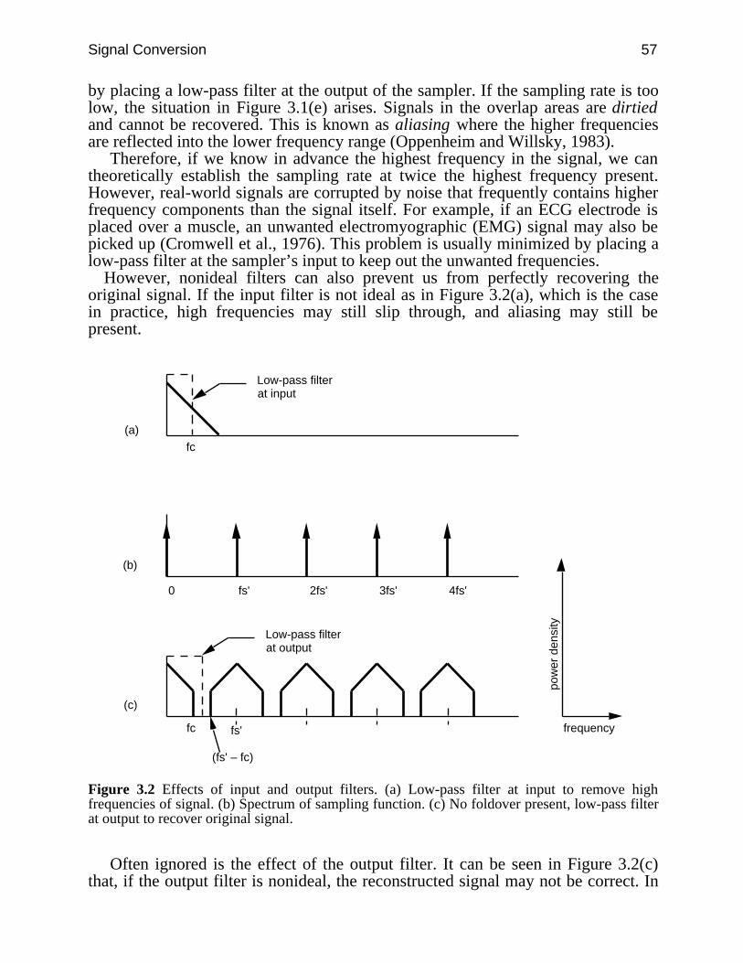
Signal Conversion 57
by placing a low-pass filter at the output of the sampler. If the sampling rate is toolow, the situation in Figure 3.1(e) arises. Signals in the overlap areas are dirtiedand cannot be recovered. This is known as aliasing where the higher frequenciesare reflected into the lower frequency range (Oppenheim and Willsky, 1983).
Therefore, if we know in advance the highest frequency in the signal, we cantheoretically establish the sampling rate at twice the highest frequency present.However, real-world signals are corrupted by noise that frequently contains higherfrequency components than the signal itself. For example, if an ECG electrode isplaced over a muscle, an unwanted electromyographic (EMG) signal may also bepicked up (Cromwell et al., 1976). This problem is usually minimized by placing alow-pass filter at the sampler’s input to keep out the unwanted frequencies.
However, nonideal filters can also prevent us from perfectly recovering theoriginal signal. If the input filter is not ideal as in Figure 3.2(a), which is the casein practice, high frequencies may still slip through, and aliasing may still bepresent.
(a)
(b)
(c)
pow
er d
ensi
ty
frequency
fc
0 fs' 2fs' 3fs' 4fs'
Low-pass filterat input
fc fs'
Low-pass filterat output
(fs' – fc)
Figure 3.2 Effects of input and output filters. (a) Low-pass filter at input to remove highfrequencies of signal. (b) Spectrum of sampling function. (c) No foldover present, low-pass filterat output to recover original signal.
Often ignored is the effect of the output filter. It can be seen in Figure 3.2(c)that, if the output filter is nonideal, the reconstructed signal may not be correct. In
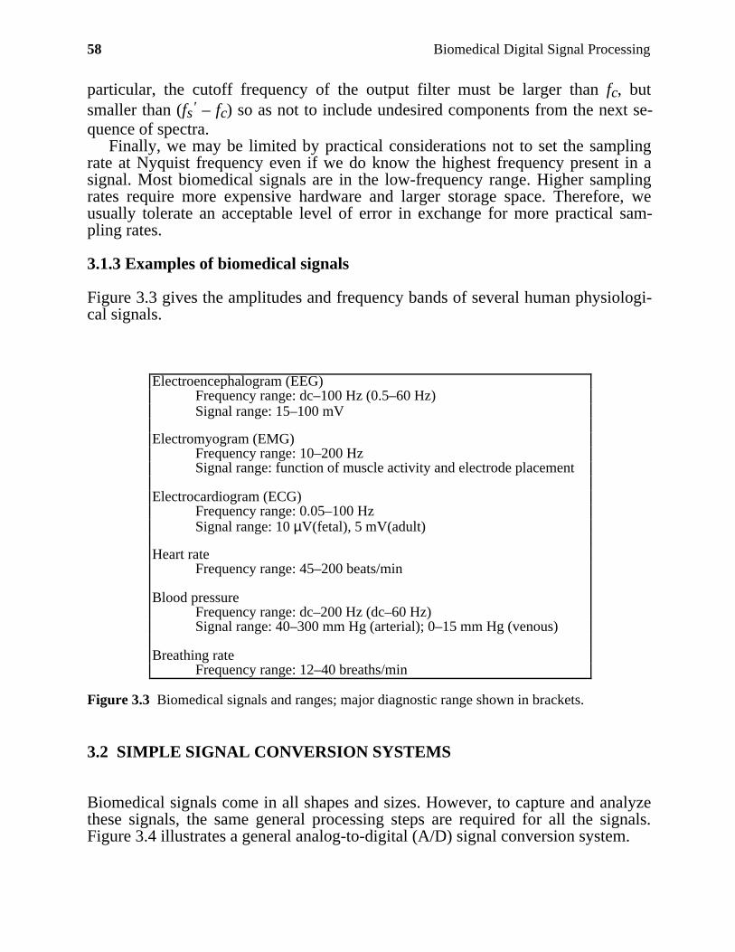
58 Biomedical Digital Signal Processing
particular, the cutoff frequency of the output filter must be larger than fc, butsmaller than (fs' – fc) so as not to include undesired components from the next se-quence of spectra.
Finally, we may be limited by practical considerations not to set the samplingrate at Nyquist frequency even if we do know the highest frequency present in asignal. Most biomedical signals are in the low-frequency range. Higher samplingrates require more expensive hardware and larger storage space. Therefore, weusually tolerate an acceptable level of error in exchange for more practical sam-pling rates.
3.1.3 Examples of biomedical signals
Figure 3.3 gives the amplitudes and frequency bands of several human physiologi-cal signals.
Electroencephalogram (EEG)Frequency range: dc–100 Hz (0.5–60 Hz)Signal range: 15–100 mV
Electromyogram (EMG)Frequency range: 10–200 HzSignal range: function of muscle activity and electrode placement
Electrocardiogram (ECG)Frequency range: 0.05–100 HzSignal range: 10 µV(fetal), 5 mV(adult)
Heart rateFrequency range: 45–200 beats/min
Blood pressureFrequency range: dc–200 Hz (dc–60 Hz)Signal range: 40–300 mm Hg (arterial); 0–15 mm Hg (venous)
Breathing rateFrequency range: 12–40 breaths/min
Figure 3.3 Biomedical signals and ranges; major diagnostic range shown in brackets.
3.2 SIMPLE SIGNAL CONVERSION SYSTEMS
Biomedical signals come in all shapes and sizes. However, to capture and analyzethese signals, the same general processing steps are required for all the signals.Figure 3.4 illustrates a general analog-to-digital (A/D) signal conversion system.
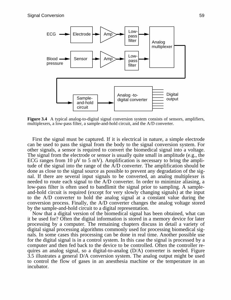
Signal Conversion 59
ECG
Analogmultiplexer
Sample-and-hold circuit
Analog -to-digital converter
Electrode Amp
Bloodpressure
AmpSensor
Digitaloutput
Low-passfilter
Low-passfilter
Figure 3.4 A typical analog-to-digital signal conversion system consists of sensors, amplifiers,multiplexers, a low-pass filter, a sample-and-hold circuit, and the A/D converter.
First the signal must be captured. If it is electrical in nature, a simple electrodecan be used to pass the signal from the body to the signal conversion system. Forother signals, a sensor is required to convert the biomedical signal into a voltage.The signal from the electrode or sensor is usually quite small in amplitude (e.g., theECG ranges from 10 µV to 5 mV). Amplification is necessary to bring the ampli-tude of the signal into the range of the A/D converter. The amplification should bedone as close to the signal source as possible to prevent any degradation of the sig-nal. If there are several input signals to be converted, an analog multiplexer isneeded to route each signal to the A/D converter. In order to minimize aliasing, alow-pass filter is often used to bandlimit the signal prior to sampling. A sample-and-hold circuit is required (except for very slowly changing signals) at the inputto the A/D converter to hold the analog signal at a constant value during theconversion process. Finally, the A/D converter changes the analog voltage storedby the sample-and-hold circuit to a digital representation.
Now that a digital version of the biomedical signal has been obtained, what canit be used for? Often the digital information is stored in a memory device for laterprocessing by a computer. The remaining chapters discuss in detail a variety ofdigital signal processing algorithms commonly used for processing biomedical sig-nals. In some cases this processing can be done in real time. Another possible usefor the digital signal is in a control system. In this case the signal is processed by acomputer and then fed back to the device to be controlled. Often the controller re-quires an analog signal, so a digital-to-analog (D/A) converter is needed. Figure3.5 illustrates a general D/A conversion system. The analog output might be usedto control the flow of gases in an anesthesia machine or the temperature in anincubator.
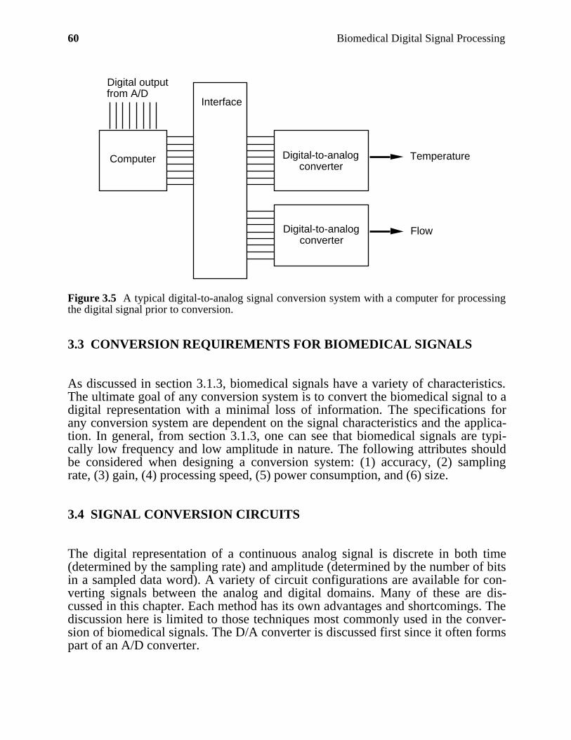
60 Biomedical Digital Signal Processing
Digital-to-analog converter
Digital outputfrom A/D
Computer
Interface
Digital-to-analog converter
Flow
Temperature
Figure 3.5 A typical digital-to-analog signal conversion system with a computer for processingthe digital signal prior to conversion.
3.3 CONVERSION REQUIREMENTS FOR BIOMEDICAL SIGNALS
As discussed in section 3.1.3, biomedical signals have a variety of characteristics.The ultimate goal of any conversion system is to convert the biomedical signal to adigital representation with a minimal loss of information. The specifications forany conversion system are dependent on the signal characteristics and the applica-tion. In general, from section 3.1.3, one can see that biomedical signals are typi-cally low frequency and low amplitude in nature. The following attributes shouldbe considered when designing a conversion system: (1) accuracy, (2) samplingrate, (3) gain, (4) processing speed, (5) power consumption, and (6) size.
3.4 SIGNAL CONVERSION CIRCUITS
The digital representation of a continuous analog signal is discrete in both time(determined by the sampling rate) and amplitude (determined by the number of bitsin a sampled data word). A variety of circuit configurations are available for con-verting signals between the analog and digital domains. Many of these are dis-cussed in this chapter. Each method has its own advantages and shortcomings. Thediscussion here is limited to those techniques most commonly used in the conver-sion of biomedical signals. The D/A converter is discussed first since it often formspart of an A/D converter.
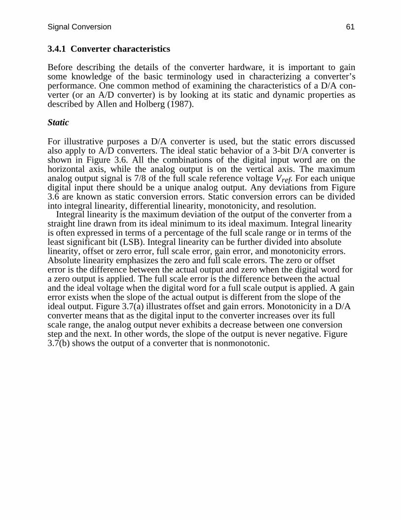
Signal Conversion 61
3.4.1 Converter characteristics
Before describing the details of the converter hardware, it is important to gainsome knowledge of the basic terminology used in characterizing a converter’sperformance. One common method of examining the characteristics of a D/A con-verter (or an A/D converter) is by looking at its static and dynamic properties asdescribed by Allen and Holberg (1987).
Static
For illustrative purposes a D/A converter is used, but the static errors discussedalso apply to A/D converters. The ideal static behavior of a 3-bit D/A converter isshown in Figure 3.6. All the combinations of the digital input word are on thehorizontal axis, while the analog output is on the vertical axis. The maximumanalog output signal is 7/8 of the full scale reference voltage Vref. For each uniquedigital input there should be a unique analog output. Any deviations from Figure3.6 are known as static conversion errors. Static conversion errors can be dividedinto integral linearity, differential linearity, monotonicity, and resolution.
Integral linearity is the maximum deviation of the output of the converter from astraight line drawn from its ideal minimum to its ideal maximum. Integral linearityis often expressed in terms of a percentage of the full scale range or in terms of theleast significant bit (LSB). Integral linearity can be further divided into absolutelinearity, offset or zero error, full scale error, gain error, and monotonicity errors.Absolute linearity emphasizes the zero and full scale errors. The zero or offseterror is the difference between the actual output and zero when the digital word fora zero output is applied. The full scale error is the difference between the actualand the ideal voltage when the digital word for a full scale output is applied. A gainerror exists when the slope of the actual output is different from the slope of theideal output. Figure 3.7(a) illustrates offset and gain errors. Monotonicity in a D/Aconverter means that as the digital input to the converter increases over its fullscale range, the analog output never exhibits a decrease between one conversionstep and the next. In other words, the slope of the output is never negative. Figure3.7(b) shows the output of a converter that is nonmonotonic.
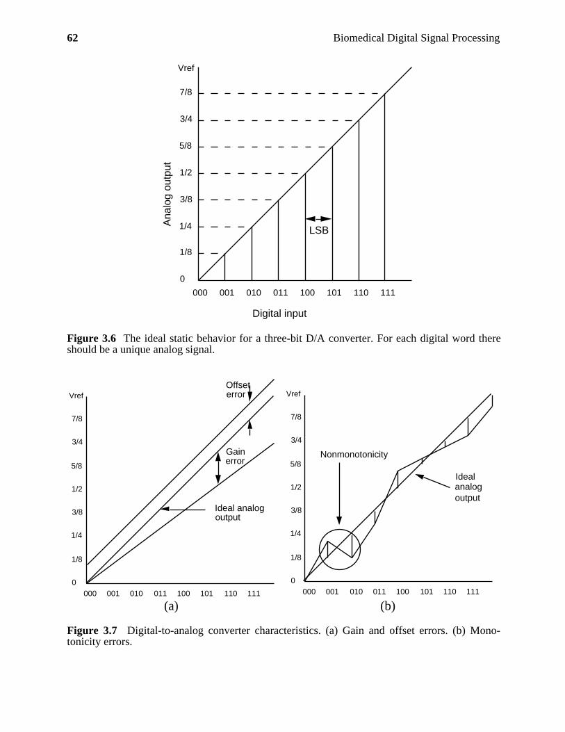
62 Biomedical Digital Signal Processing
000 001 010 011 100 101 110 111
0
1/8
1/4
3/8
1/2
5/8
3/4
7/8
Digital input
Ana
log
outp
ut
LSB
Vref
Figure 3.6 The ideal static behavior for a three-bit D/A converter. For each digital word thereshould be a unique analog signal.
000 001 010 011 100 101 110 111
Gainerror
Offseterror
Ideal analogoutput
Vref
0
1/8
1/4
3/8
1/2
5/8
3/4
7/8
000 001 010 011 100 101 110 111
Vref
0
1/8
1/4
3/8
1/2
5/8
3/4
7/8
Nonmonotonicity
Idealanalogoutput
(a) (b)
Figure 3.7 Digital-to-analog converter characteristics. (a) Gain and offset errors. (b) Mono-tonicity errors.

Signal Conversion 63
Differential linearity differs from integral linearity in that it is a measure of theseparation between adjacent levels (Allen and Holberg, 1987). In other words, dif-ferential linearity measures bit-to-bit deviations from the ideal output step size of 1LSB. Figure 3.8 illustrates the differences between integral and differentiallinearity.
000 001 010 011 100 101 110 111
(b)
Idealanalogoutput
0.5 LSB
2 LSB1.5 LSB
Vref
0
1/8
1/4
3/8
1/2
5/8
3/4
7/8
Figure 3.8 A D/A converter with ±2 LSB integral linearity and ±0.5 LSB differential linearity.
Resolution is defined as the smallest input digital code for which a unique analogoutput level is produced. Theoretically the resolution of an n-bit D/A converter is2n discrete analog output levels. In reality, the resolution is often less due to noiseand component drift.
Dynamic
Settling time, for a D/A converter, is defined as the time it takes for the converterto respond to an input change. More explicitly, settling time is the time betweenthe time a new digital signal is received at the converter input and the time whenthe output has reached its final value (within some specified tolerance). Manyfactors affect the settling time, so the conditions under which the settling time wasfound must be clearly stated if comparisons are to be made. Factors to note includethe magnitude of the input change applied and the load on the output. Settling timein D/A converters is important as it relates directly to the speed of the conversion.The output must settle sufficiently before it can be used in any further processing.
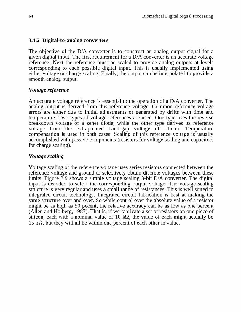
64 Biomedical Digital Signal Processing
3.4.2 Digital-to-analog converters
The objective of the D/A converter is to construct an analog output signal for agiven digital input. The first requirement for a D/A converter is an accurate voltagereference. Next the reference must be scaled to provide analog outputs at levelscorresponding to each possible digital input. This is usually implemented usingeither voltage or charge scaling. Finally, the output can be interpolated to provide asmooth analog output.
Voltage reference
An accurate voltage reference is essential to the operation of a D/A converter. Theanalog output is derived from this reference voltage. Common reference voltageerrors are either due to initial adjustments or generated by drifts with time andtemperature. Two types of voltage references are used. One type uses the reversebreakdown voltage of a zener diode, while the other type derives its referencevoltage from the extrapolated band-gap voltage of silicon. Temperaturecompensation is used in both cases. Scaling of this reference voltage is usuallyaccomplished with passive components (resistors for voltage scaling and capacitorsfor charge scaling).
Voltage scaling
Voltage scaling of the reference voltage uses series resistors connected between thereference voltage and ground to selectively obtain discrete voltages between theselimits. Figure 3.9 shows a simple voltage scaling 3-bit D/A converter. The digitalinput is decoded to select the corresponding output voltage. The voltage scalingstructure is very regular and uses a small range of resistances. This is well suited tointegrated circuit technology. Integrated circuit fabrication is best at making thesame structure over and over. So while control over the absolute value of a resistormight be as high as 50 pecent, the relative accuracy can be as low as one percent(Allen and Holberg, 1987). That is, if we fabricate a set of resistors on one piece ofsilicon, each with a nominal value of 10 kΩ, the value of each might actually be15 kΩ, but they will all be within one percent of each other in value.
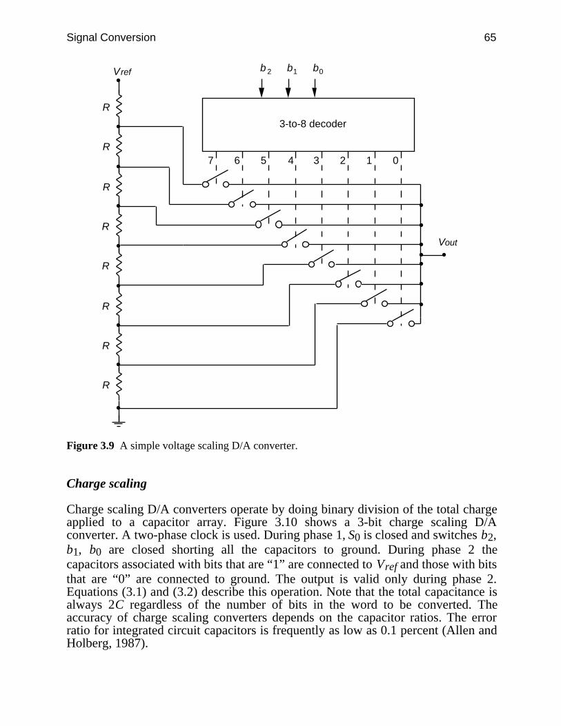
Signal Conversion 65
3-to-8 decoder
b 2 b 1 b 0Vref
R
R
R
R
R
R
R
R
Vout
7 6 5 4 3 2 1 0
Figure 3.9 A simple voltage scaling D/A converter.
Charge scaling
Charge scaling D/A converters operate by doing binary division of the total chargeapplied to a capacitor array. Figure 3.10 shows a 3-bit charge scaling D/Aconverter. A two-phase clock is used. During phase 1, S0 is closed and switches b2,b1, b0 are closed shorting all the capacitors to ground. During phase 2 thecapacitors associated with bits that are “1” are connected to Vref and those with bitsthat are “0” are connected to ground. The output is valid only during phase 2.Equations (3.1) and (3.2) describe this operation. Note that the total capacitance isalways 2C regardless of the number of bits in the word to be converted. Theaccuracy of charge scaling converters depends on the capacitor ratios. The errorratio for integrated circuit capacitors is frequently as low as 0.1 percent (Allen andHolberg, 1987).
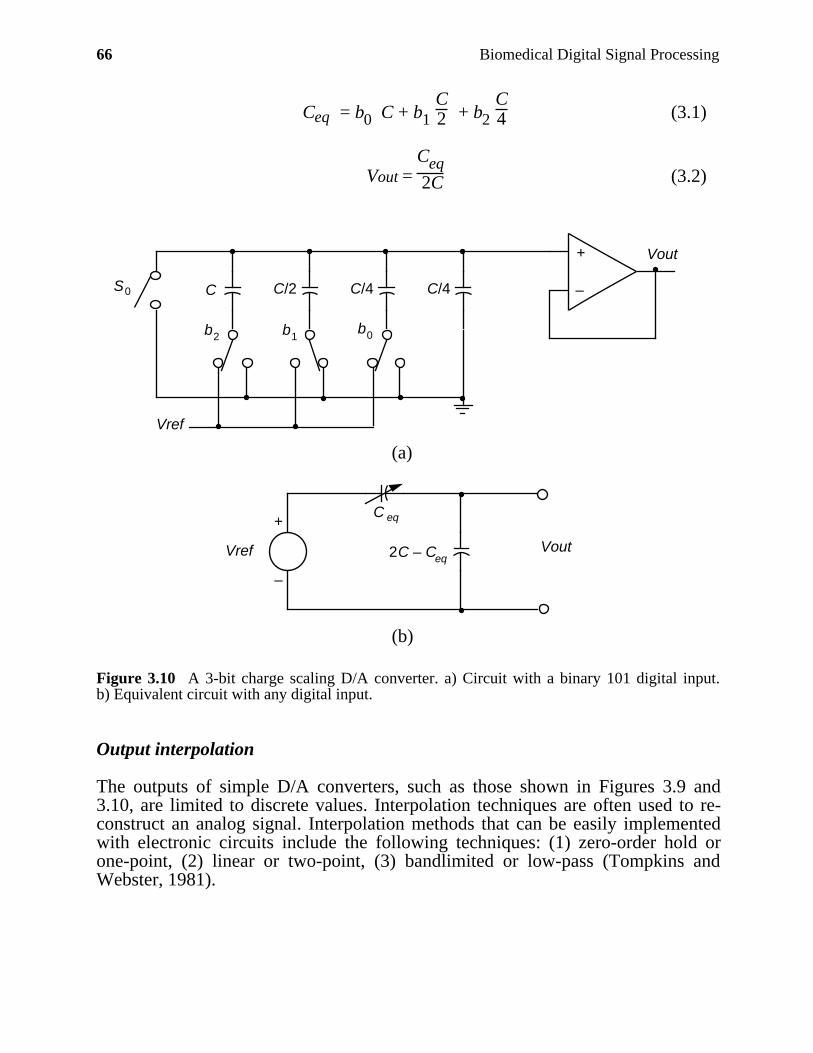
66 Biomedical Digital Signal Processing
Ceq = b0 C + b1 C2 + b2
C4 (3.1)
Vout = Ceq 2C (3.2)
+
–
Vref
C C/2 C/4 C/4
b0b1b2
S0
Vout
(a)
Vref 2C – Ceq
C eq
Vout
+
–
(b)
Figure 3.10 A 3-bit charge scaling D/A converter. a) Circuit with a binary 101 digital input.b) Equivalent circuit with any digital input.
Output interpolation
The outputs of simple D/A converters, such as those shown in Figures 3.9 and3.10, are limited to discrete values. Interpolation techniques are often used to re-construct an analog signal. Interpolation methods that can be easily implementedwith electronic circuits include the following techniques: (1) zero-order hold orone-point, (2) linear or two-point, (3) bandlimited or low-pass (Tompkins andWebster, 1981).
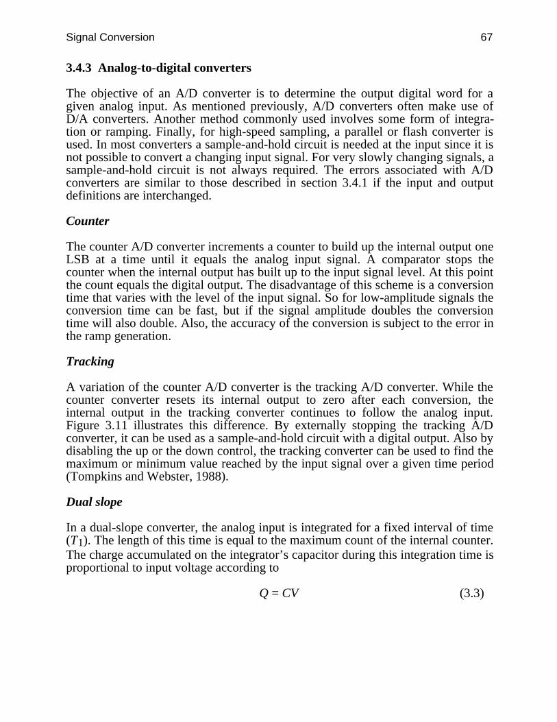
Signal Conversion 67
3.4.3 Analog-to-digital converters
The objective of an A/D converter is to determine the output digital word for agiven analog input. As mentioned previously, A/D converters often make use ofD/A converters. Another method commonly used involves some form of integra-tion or ramping. Finally, for high-speed sampling, a parallel or flash converter isused. In most converters a sample-and-hold circuit is needed at the input since it isnot possible to convert a changing input signal. For very slowly changing signals, asample-and-hold circuit is not always required. The errors associated with A/Dconverters are similar to those described in section 3.4.1 if the input and outputdefinitions are interchanged.
Counter
The counter A/D converter increments a counter to build up the internal output oneLSB at a time until it equals the analog input signal. A comparator stops thecounter when the internal output has built up to the input signal level. At this pointthe count equals the digital output. The disadvantage of this scheme is a conversiontime that varies with the level of the input signal. So for low-amplitude signals theconversion time can be fast, but if the signal amplitude doubles the conversiontime will also double. Also, the accuracy of the conversion is subject to the error inthe ramp generation.
Tracking
A variation of the counter A/D converter is the tracking A/D converter. While thecounter converter resets its internal output to zero after each conversion, theinternal output in the tracking converter continues to follow the analog input.Figure 3.11 illustrates this difference. By externally stopping the tracking A/Dconverter, it can be used as a sample-and-hold circuit with a digital output. Also bydisabling the up or the down control, the tracking converter can be used to find themaximum or minimum value reached by the input signal over a given time period(Tompkins and Webster, 1988).
Dual slope
In a dual-slope converter, the analog input is integrated for a fixed interval of time(T1). The length of this time is equal to the maximum count of the internal counter.The charge accumulated on the integrator’s capacitor during this integration time isproportional to input voltage according to
Q = CV (3.3)
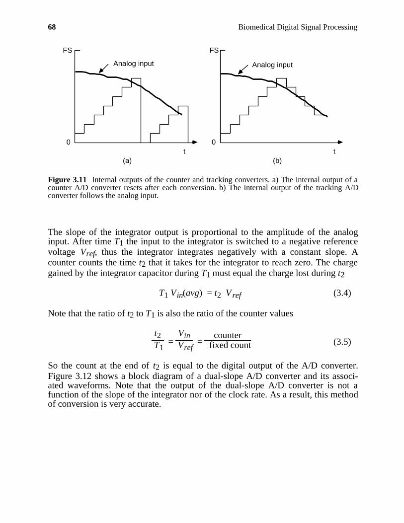
68 Biomedical Digital Signal Processing
t t0 0
FS FS
(a) (b)
Analog input Analog input
Figure 3.11 Internal outputs of the counter and tracking converters. a) The internal output of acounter A/D converter resets after each conversion. b) The internal output of the tracking A/Dconverter follows the analog input.
The slope of the integrator output is proportional to the amplitude of the analoginput. After time T1 the input to the integrator is switched to a negative referencevoltage Vref, thus the integrator integrates negatively with a constant slope. Acounter counts the time t2 that it takes for the integrator to reach zero. The chargegained by the integrator capacitor during T1 must equal the charge lost during t2
T1 Vin(avg) = t2 V ref (3.4)
Note that the ratio of t2 to T1 is also the ratio of the counter values
t2 T1
= Vin
Vref =
counter fixed count (3.5)
So the count at the end of t2 is equal to the digital output of the A/D converter.Figure 3.12 shows a block diagram of a dual-slope A/D converter and its associ-ated waveforms. Note that the output of the dual-slope A/D converter is not afunction of the slope of the integrator nor of the clock rate. As a result, this methodof conversion is very accurate.
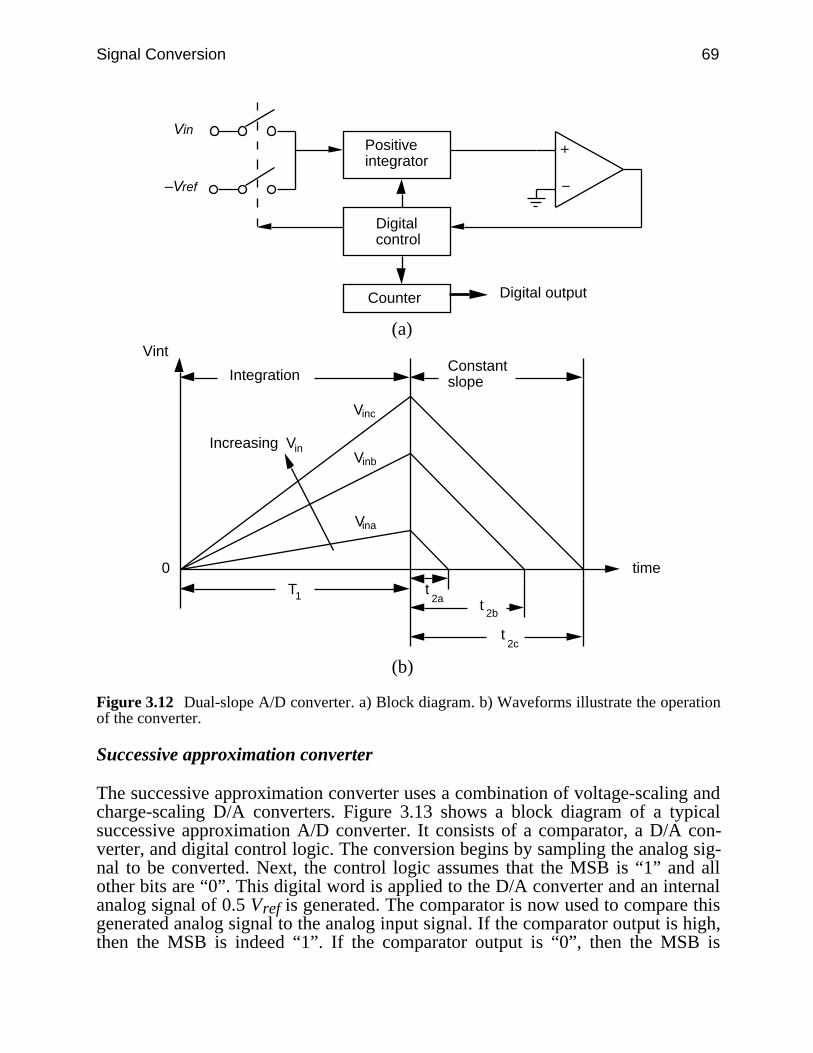
Signal Conversion 69
Positiveintegrator
Digitalcontrol
Counter
Vin
–Vref
Digital output
(a)
T1 t2a t
2b
t2c
Vinb
Vinc
Vina
0
Vint
time
IntegrationConstantslope
Increasing Vin
(b)
Figure 3.12 Dual-slope A/D converter. a) Block diagram. b) Waveforms illustrate the operationof the converter.
Successive approximation converter
The successive approximation converter uses a combination of voltage-scaling andcharge-scaling D/A converters. Figure 3.13 shows a block diagram of a typicalsuccessive approximation A/D converter. It consists of a comparator, a D/A con-verter, and digital control logic. The conversion begins by sampling the analog sig-nal to be converted. Next, the control logic assumes that the MSB is “1” and allother bits are “0”. This digital word is applied to the D/A converter and an internalanalog signal of 0.5 Vref is generated. The comparator is now used to compare thisgenerated analog signal to the analog input signal. If the comparator output is high,then the MSB is indeed “1”. If the comparator output is “0”, then the MSB is
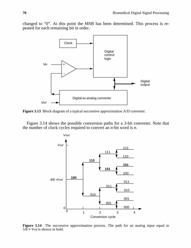
70 Biomedical Digital Signal Processing
changed to “0”. At this point the MSB has been determined. This process is re-peated for each remaining bit in order.
Vref
Vin
Clock
Digital-to-analog converter
Digital control logic
Digitaloutput
–
+
Figure 3.13 Block diagram of a typical successive approximation A/D converter.
Figure 3.14 shows the possible conversion paths for a 3-bit converter. Note thatthe number of clock cycles required to convert an n-bit word is n.
4/8 ×Vref
Vref
Vout
00 1 2 3 4
Conversion cycle
110
101101
100
111111
110
010
011011
010
000
001
100
001
Figure 3.14 The successive approximation process. The path for an analog input equal to5/8 × Vref is shown in bold.
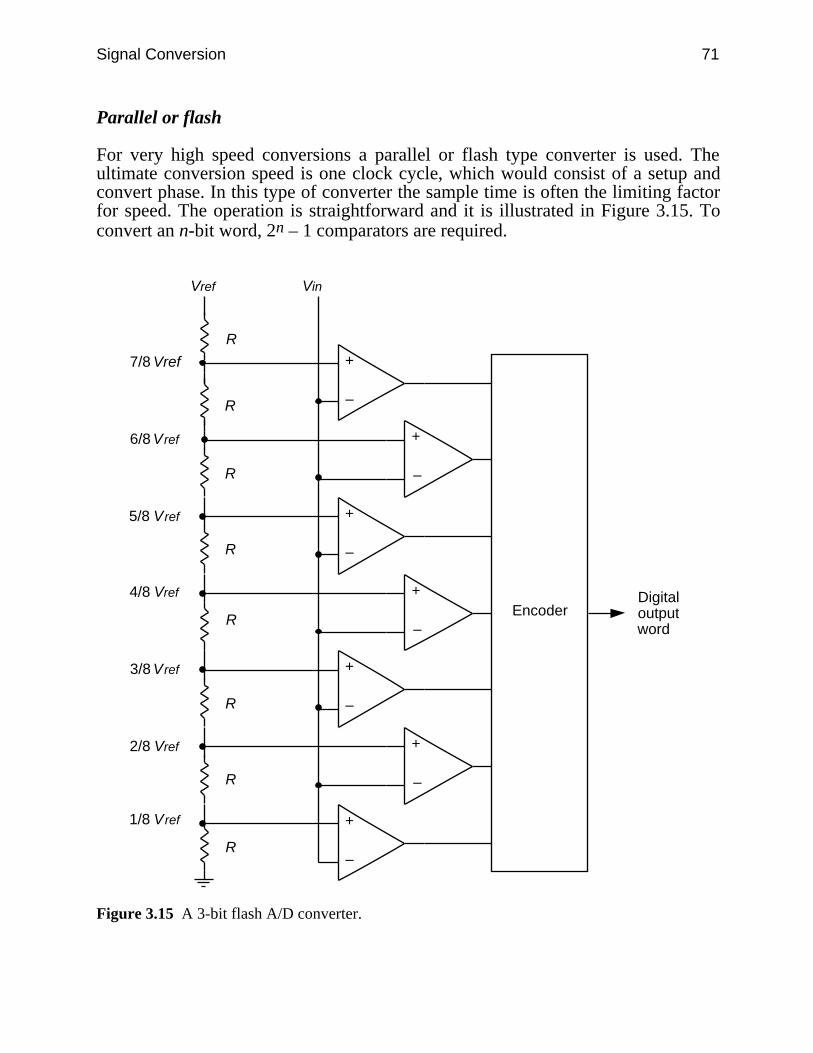
Signal Conversion 71
Parallel or flash
For very high speed conversions a parallel or flash type converter is used. Theultimate conversion speed is one clock cycle, which would consist of a setup andconvert phase. In this type of converter the sample time is often the limiting factorfor speed. The operation is straightforward and it is illustrated in Figure 3.15. Toconvert an n-bit word, 2n – 1 comparators are required.
2/8 Vref +
–
+
–
+
–
+
–
+
–
+
–
+
–
R
R
R
R
R
R
R
R
Vref Vin
7/8 Vref
6/8 Vref
5/8 Vref
4/8 Vref
3/8 Vref
Encoder
1/8 Vref
Digitaloutput word
Figure 3.15 A 3-bit flash A/D converter.
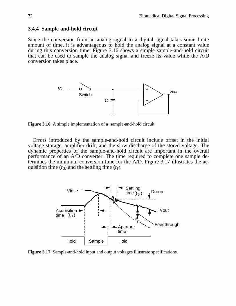
72 Biomedical Digital Signal Processing
3.4.4 Sample-and-hold circuit
Since the conversion from an analog signal to a digital signal takes some finiteamount of time, it is advantageous to hold the analog signal at a constant valueduring this conversion time. Figure 3.16 shows a simple sample-and-hold circuitthat can be used to sample the analog signal and freeze its value while the A/Dconversion takes place.
+
–
Vout Vin
C
Switch
Figure 3.16 A simple implementation of a sample-and-hold circuit.
Errors introduced by the sample-and-hold circuit include offset in the initialvoltage storage, amplifier drift, and the slow discharge of the stored voltage. Thedynamic properties of the sample-and-hold circuit are important in the overallperformance of an A/D converter. The time required to complete one sample de-termines the minimum conversion time for the A/D. Figure 3.17 illustrates the ac-quisition time (ta) and the settling time (ts).
Hold Sample Hold
Vin
Vout
Aperturetime
Settlingtime Droop
Feedthrough
Acquisitiontime (t )a
(t )s
Figure 3.17 Sample-and-hold input and output voltages illustrate specifications.
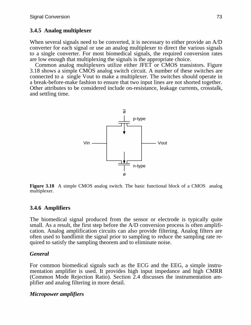
Signal Conversion 73
3.4.5 Analog multiplexer
When several signals need to be converted, it is necessary to either provide an A/Dconverter for each signal or use an analog multiplexer to direct the various signalsto a single converter. For most biomedical signals, the required conversion ratesare low enough that multiplexing the signals is the appropriate choice.
Common analog multiplexers utilize either JFET or CMOS transistors. Figure3.18 shows a simple CMOS analog switch circuit. A number of these switches areconnected to a single Vout to make a multiplexer. The switches should operate ina break-before-make fashion to ensure that two input lines are not shorted together.Other attributes to be considered include on-resistance, leakage currents, crosstalk,and settling time.
ø
ø
Vin Vout
p-type
n-type
Figure 3.18 A simple CMOS analog switch. The basic functional block of a CMOS analogmultiplexer.
3.4.6 Amplifiers
The biomedical signal produced from the sensor or electrode is typically quitesmall. As a result, the first step before the A/D conversion process is often amplifi-cation. Analog amplification circuits can also provide filtering. Analog filters areoften used to bandlimit the signal prior to sampling to reduce the sampling rate re-quired to satisfy the sampling theorem and to eliminate noise.
General
For common biomedical signals such as the ECG and the EEG, a simple instru-mentation amplifier is used. It provides high input impedance and high CMRR(Common Mode Rejection Ratio). Section 2.4 discusses the instrumentation am-plifier and analog filtering in more detail.
Micropower amplifiers
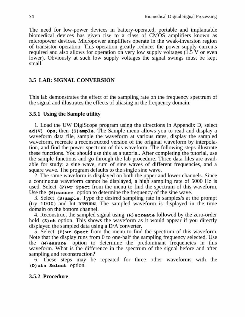
74 Biomedical Digital Signal Processing
The need for low-power devices in battery-operated, portable and implantablebiomedical devices has given rise to a class of CMOS amplifiers known asmicropower devices. Micropower amplifiers operate in the weak-inversion regionof transistor operation. This operation greatly reduces the power-supply currentsrequired and also allows for operation on very low supply voltages (1.5 V or evenlower). Obviously at such low supply voltages the signal swings must be keptsmall.
3.5 LAB: SIGNAL CONVERSION
This lab demonstrates the effect of the sampling rate on the frequency spectrum ofthe signal and illustrates the effects of aliasing in the frequency domain.
3.5.1 Using the Sample utility
1. Load the UW DigiScope program using the directions in Appendix D, selectad(V) Ops, then (S)ample. The Sample menu allows you to read and display awaveform data file, sample the waveform at various rates, display the sampledwaveform, recreate a reconstructed version of the original waveform by interpola-tion, and find the power spectrum of this waveform. The following steps illustratethese functions. You should use this as a tutorial. After completing the tutorial, usethe sample functions and go through the lab procedure. Three data files are avail-able for study: a sine wave, sum of sine waves of different frequencies, and asquare wave. The program defaults to the single sine wave.
2. The same waveform is displayed on both the upper and lower channels. Sincea continuous waveform cannot be displayed, a high sampling rate of 5000 Hz isused. Select (P)wr Spect from the menu to find the spectrum of this waveform.Use the (M)easure option to determine the frequency of the sine wave.
3. Select (S)ample. Type the desired sampling rate in samples/s at the prompt(try 1000) and hit RETURN. The sampled waveform is displayed in the timedomain on the bottom channel.
4. Reconstruct the sampled signal using (R)ecreate followed by the zero-orderhold (Z)oh option. This shows the waveform as it would appear if you directlydisplayed the sampled data using a D/A converter.
5. Select (P)wr Spect from the menu to find the spectrum of this waveform.Note that the display runs from 0 to one-half the sampling frequency selected. Usethe (M)easure option to determine the predominant frequencies in thiswaveform. What is the difference in the spectrum of the signal before and aftersampling and reconstruction?
6. These steps may be repeated for three other waveforms with the(D)ata Select option.
3.5.2 Procedure
Signal Conversion 75
1. Load the sine wave and measure its period. Sample this wave at a frequencymuch greater than the Nyquist frequency (e.g., 550 samples per second) and re-construct the waveform using the zero-order hold command. What do you expectthe power spectrum of the sampled wave to look like? Perform (P)wr Spect onthe sampled data and explain any differences from your expectations. Measure thefrequencies at which the peak magnitudes occur.
2. Sample at sampling rates 5–10 percent above, 5–10 percent below, and just atthe Nyquist frequency. Describe the appearance of the sampled data and its powerspectrum. Measure the frequencies at which peaks in the response occur. Samplethe sine wave at the Nyquist frequency several times. What do you notice? Can thesignal be perfectly reproduced?
3. Recreate the original data by interpolation using zero-order hold, linear andsinusoidal interpolation. What are the differences between these methods? What doyou expect the power spectrum of the recreated data will look like?
4. Repeat the above steps 1–3 using the data of the sum of two sinusoids.5. Repeat the above steps 1–3 using the square wave data.
3.6 REFERENCES
Allen, P. E. and Holberg, D. R. 1987. CMOS Analog Circuit Design. New York: Holt, Rinehartand Winston.
Cromwell, L., Arditti, M., Weibel, F. J., Pfeiffer, E. A., Steele, B., and Labok, J. 1976. MedicalInstrumentation for Health Care. Englewood Cliffs, NJ: Prentice Hall.
Oppenheim, A. V. and Willsky, A. S. 1983. Signals and Systems. Englewood Cliffs, NJ: PrenticeHall.
Tompkins, W. J., and Webster, J. G. (eds.) 1981. Design of microcomputer-based medicalinstrumentation. Englewood Cliffs, NJ: Prentice Hall.
Tompkins, W. J., and Webster, J. G. (eds.) 1988. Interfacing sensors to the IBM PC. EnglewoodCliffs, NJ: Prentice Hall.
3.7 STUDY QUESTIONS
3.1 What is the purpose of using a low-pass filter prior to sampling an analog signal?3.2 Draw D/A converter characteristics that illustrate the following errors: (1) offset error of
one LSB, (2) integral linearity of ±1.5 LSB, (3) differential linearity of ±1 LSB.3.3 Design a 4-bit charge scaling D/A converter. For Vref = 5 V, what is Vout for a digital input
of 1010?3.4 Why is a dual-slope A/D converter considered an accurate method of conversion? What
will happen to the output if the integrator drifts over time?3.5 Show the path a 4-bit successive approximation A/D converter will make to converge given
an analog input of 9/16 Vref.3.6 Discuss reasons why each attribute listed in section 3.3 is important to consider when de-
signing a biomedical conversion system. For example, size would be important if the de-vice was to be portable.
3.7 List the specifications for an A/D conversion system that is to be used for an EEG device.3.8 Draw a block diagram of a counter-type A/D converter.

76 Biomedical Digital Signal Processing
3.9 Explain Shannon’s sampling theorem. If only two samples per cycle of the highest fre-quency in a signal is obtained, what sort of interpolation strategy is needed to reconstructthe signal?
3.10 A 100-Hz-bandwidth ECG signal is sampled at a rate of 500 samples per second. (a) Drawthe approximate frequency spectrum of the new digital signal obtained after sampling, andlabel important points on the axes. (b) What is the bandwidth of the new digital signal ob-tained after sampling this analog signal? Explain.
3.11 In order to minimize aliasing, what sampling rate should be used to sample a 400-Hz trian-gular wave? Explain.
3.12 A 100-Hz full-wave-rectified sine wave is sampled at 200 samples/s. The samples are usedto directly reconstruct the waveform using a digital-to-analog converter. Will the resultingwaveform be a good representation of the original signal? Explain.
3.13 An A/D converter has an input signal range of 10 V. What is the minimum signal that it canresolve (in mV) if it is (a) a 10-bit converter, (b) an 11-bit converter?
3.14 A 10-bit analog-to-digital converter can resolve a minimum signal level of 10 mV. What isthe approximate full-scale voltage range of this converter (in volts)?
3.15 A 12-bit D/A converter has an output signal range of ±5 V. What is the approximate mini-mal step size that it produces at its output (in mV)?
3.16 For an analog-to-digital converter with a full-scale input range of +5 V, how many bits arerequired to assure resolution of 0.5-mV signal levels?
3.17 A normal QRS complex is about 100 ms wide. (a) What is the American HeartAssociation’s (AHA) specified sampling rate for clinical electrocardiography? (b) If yousample an ECG at the AHA standard sampling rate, about how many sampled data pointswill define a normal QRS complex?
3.18 An ECG with a 1-mV peak-to-peak QRS amplitude is passed through a filter with a verysharp cutoff, 100-Hz passband, and sampled at 200 samples/s. The ECG is immediately re-constructed with a digital-to-analog converter (DAC) followed by a low-pass reconstruc-tion filter. Comparing the DAC output with the original signal, comment on any differencesin appearance due to (a) aliasing, (b) the sampling process itself, (c) the peak-to-peak am-plitude, and (d) the clinical acceptability of such a signal.
3.19 An ECG with a 1-mV peak-to-peak QRS amplitude and a 100-ms duration is passedthrough an ideal low-pass filter with a 100-Hz cutoff. The ECG is then sampled at 200samples/s. Due to a lack of memory, every other data point is thrown away after the sam-pling process, so that 100 data points per second are stored. The ECG is immediately re-constructed with a digital-to-analog converter followed by a low-pass reconstruction filter.Comparing the reconstruction filter output with the original signal, comment on any differ-ences in appearance due to (a) aliasing, (b) the sampling process itself, (c) the peak-to-peakamplitude, and (d) the clinical acceptability of such a signal.
3.20 An IBM PC signal acquisition board with an 8-bit A/D converter is used to sample anECG. An ECG amplifier provides a peak-to-peak signal of 1 V centered in the 0-to-5-Vinput range of the converter. How many bits of the A/D converter are used to represent thesignal?
3.21 A commercial 12-bit signal acquisition board with a ±10-V input range is used to sample anECG. An ECG amplifier provides a peak-to-peak signal of ±1 V. How many discrete am-plitude steps are used to represent the ECG signal?
3.22 Explain the relationship between the frequencies present in a signal and the samplingtheorem.
3.23 Describe the effects of having a nonideal (a) input filter; (b) output filter.3.24 What sampling rate and filter characteristics (e.g., cutoff frequency) would you use to
sample an ECG signal?3.25 What type of A/D converter circuit provides the fastest sampling speed?3.26 What type of A/D converter circuit tends to average out high-frequency noise?3.27 In an 8-bit successive-approximation A/D converter, what is the initial digital approxima-
tion to a signal?
Signal Conversion 77
3.28 A 4-bit successive-approximation A/D converter gets a final approximation to a signal of0110. What approximation did it make just prior to this final result?
3.29 In a D/A converter design, what are the advantages of an R-2R resistor network over a bi-nary-weighted resistor network?
3.30 For an 8-bit successive approximation analog-to-digital converter, what will be the nextapproximation made by the converter (in hexadecimal) if the approximation of (a) 0x90 tothe input signal is found to be too low, (b) 0x80 to the input signal is found to be too high?
3.31 For an 8-bit successive-approximation analog-to-digital converter, what are the possible re-sults of the next approximation step (in hexadecimal) if the approximation at a certain stepis a) 0x10, b) 0x20?
3.32 An 8-bit analog-to-digital converter has a clock that drives the internal successive approxi-mation circuitry at 80 kHz. (a) What is the fastest possible sampling rate that could beachieved by this converter? (b) If 0x80 represents a signal level of 1 V, what is the mini-mum signal that this converter can resolve (in mV)?
3.33 What circuit is used in a signal conversion system to store analog voltage levels? Draw aschematic of such a circuit and explain how it works.
3.34 The internal IBM PC signal acquisition board described in Appendix A is used to samplean ECG. An amplifier amplifies the ECG so that a 1-mV level uses all 12 bits of the con-verter. What is the smallest ECG amplitude that can be resolved (in µV)?
3.35 An 8-bit successive-approximation analog-to-digital converter is used to sample an ECG.An amplifier amplifies the ECG so that a 1-mV level uses all 8 bits of the converter. Whatis the smallest ECG amplitude that can be resolved (in µV)?
3.36 The Computers of Wisconsin (COW) A/D converter chip made with CMOS technologyincludes an 8-bit successive-approximation converter with a 100-µs sampling period. Anon-chip analog multiplexer provides for sampling up to 8 channels. (a) With this COWchip, how fast could you sample a single channel (in samples per s)? (b) How fast couldyou sample each channel if you wanted to use all eight channels? (c) What is the minimalexternal clock frequency necessary to drive the successive-approximation circuitry for themaximal sampling rate? (d) List two advantages that this chip has over an equivalent onemade with TTL technology.
78
4
Basics of Digital Filtering
Willis J. Tompkins and Pradeep Tagare
In this chapter we introduce the concept of digital filtering and look at the advan-tages, disadvantages, and differences between analog and digital filters. Digitalfilters are the discrete domain counterparts of analog filters. Implementation ofdifferent types of digital filters is covered in later chapters. There are many goodbooks that expand on the general topic of digital filtering (Antoniou, 1979; Bognerand Constantinides, 1985; Gold and Rader, 1969; Rabiner and Rader, 1972;Stearns, 1975).
4.1 DIGITAL FILTERS
The function of a digital filter is the same as its analog counterpart, but its imple-mentation is very different. Analog filters are implemented using either active orpassive electronic circuits, and they operate on continuous waveforms. Digital fil-ters, on the other hand, are implemented using either a digital logic circuit or acomputer program and they operate on a sequence of numbers that are obtained bysampling the continuous waveform. The use of digital filters is widespread todaybecause of the easy availability of computers. A computer program can be writtento implement almost any kind of digital filter.
There are several advantages of digital filters over analog filters. A digital filteris highly immune to noise because of the way it is implemented (software/digitalcircuits). Accuracy is dependent only on round-off error, which is directly deter-mined by the number of bits that the designer chooses for representing the vari-ables in the filter. Also it is generally easy and inexpensive to change a filter’s op-erating characteristics (e.g., cutoff frequency). Unlike an analog filter, performanceis not a function of factors such as component aging, temperature variation, andpower supply voltage. This characteristic is important in medical applicationswhere most of the signals have low frequencies that might be distorted due to thedrift in an analog circuit.
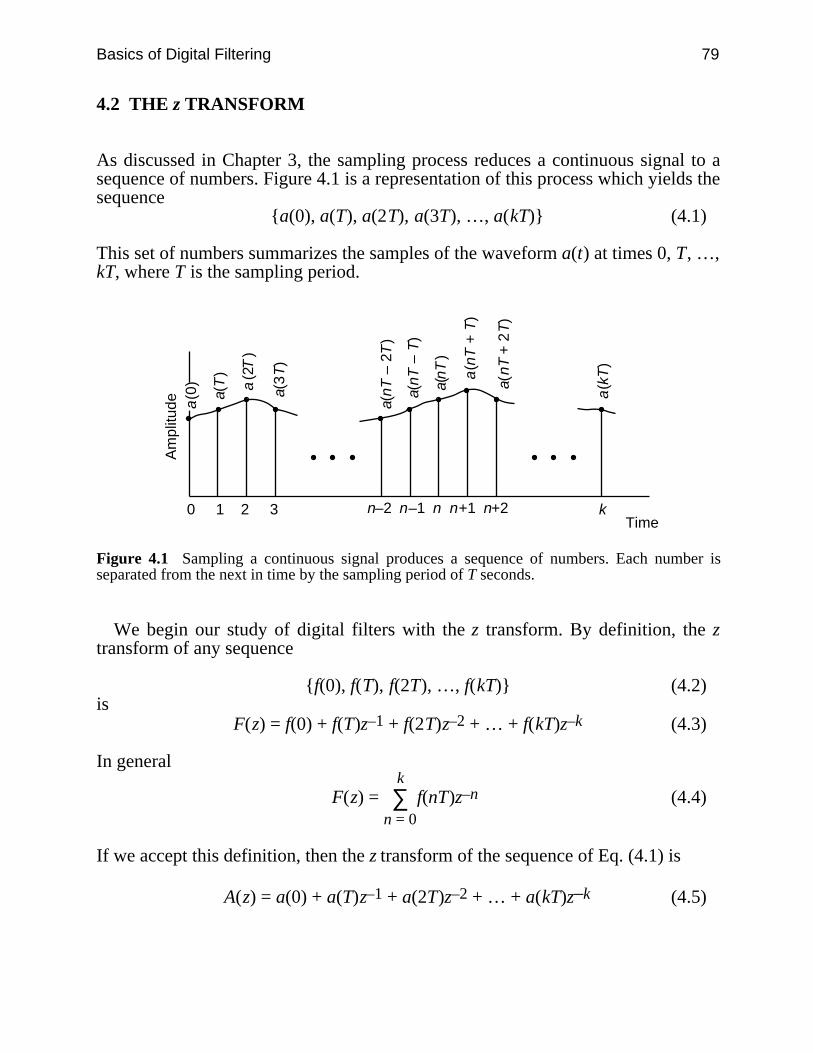
Basics of Digital Filtering 79
4.2 THE z TRANSFORM
As discussed in Chapter 3, the sampling process reduces a continuous signal to asequence of numbers. Figure 4.1 is a representation of this process which yields thesequence
a(0), a(T), a(2T), a(3T), …, a(kT) (4.1)
This set of numbers summarizes the samples of the waveform a(t) at times 0, T, …,kT, where T is the sampling period.
a(T
)
a(0
) a(2
T)
a(3
T)
a(n
T –
2T
)
a(n
T –
T)
a(n
T)
a(n
T +
2T
)
a(n
T +
T)
a(k
T)
0 1 2 3
Am
plitu
de
k n–2 n–1 n n+1 n+2Time
Figure 4.1 Sampling a continuous signal produces a sequence of numbers. Each number isseparated from the next in time by the sampling period of T seconds.
We begin our study of digital filters with the z transform. By definition, the ztransform of any sequence
f(0), f(T), f(2T), …, f(kT) (4.2)is
F(z) = f(0) + f(T)z–1 + f(2T)z–2 + … + f(kT)z–k (4.3)
In general
F(z) = ∑n = 0
k f(nT)z–n (4.4)
If we accept this definition, then the z transform of the sequence of Eq. (4.1) is
A(z) = a(0) + a(T)z–1 + a(2T)z–2 + … + a(kT)z–k (4.5)
80 Biomedical Digital Signal Processing
or
A(z) = ∑n = 0
k a(nT)z–n (4.6)
Suppose we want to find the z transform of a signal represented by any sequence,for example
1, 2, 5, 3, 0, 0, … (4.7)
From Eq. (4.4), we can write the z transform at once as
X(z) = 1 + 2z–1 + 5z–2 + 3z–3 (4.8)
Since the sequence represents an array of numbers, each separated from the nextby the sampling period, we see that the variable z–1 in the z transform represents aT-s time separation of one term from the next. The numerical value of the negativeexponent of z tells us how many sample periods after the beginning of thesampling process when the sampled data point, which is the multiplier of the zterm, occurred. Thus by inspection, we know, for example, that the first sampleddata value, which was obtained at t = 0, is 1 and that the sample at clock tick 2(i.e., t = 2 × T s) is 5.
The z transform is important in digital filtering because it describes the samplingprocess and plays a role in the digital domain similar to that of the Laplace trans-form in analog filtering. Figure 4.2 shows two examples of discrete-time signalsanalogous to common continuous time signals. The unit impulse of Figure 4.2(a),which is analogous to a Dirac delta function, is described by
f(nT) = 1 for n = 0f(nT) = 0 for n > 0 (4.9)
This corresponds to a sequence of
1, 0, 0, 0, 0, 0, … (4.10)
Therefore, the z transform of the unit impulse function is
F(z) = 1 (4.11)
This is an important finding since we frequently use the unit impulse as the inputfunction to study the performance of a filter.
For the unit step function in Figure 4.2(b)
f(nT) = 1 for n ≥ 0
giving a sequence of1, 1, 1, 1, 1, 1, … (4.12)
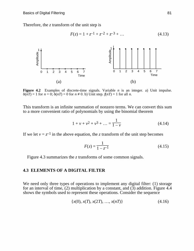
Basics of Digital Filtering 81
Therefore, the z transform of the unit step is
F(z) = 1 + z–1 + z–2 + z–3 + … (4.13)
0 1 2 3 4 5 6 7
Am
plitu
de
1
Time0 1 2 3 4 5 6 7
Am
plitu
de
1
Time
(a) (b)
Figure 4.2 Examples of discrete-time signals. Variable n is an integer. a) Unit impulse.(nT) = 1 for n = 0; (nT) = 0 for n ≠ 0. b) Unit step. f(nT) = 1 for all n.
This transform is an infinite summation of nonzero terms. We can convert this sumto a more convenient ratio of polynomials by using the binomial theorem
1 + v + v2 + v3 + … = 1
1 – v (4.14)
If we let v = z–1 in the above equation, the z transform of the unit step becomes
F(z) = 1
1 – z–1 (4.15)
Figure 4.3 summarizes the z transforms of some common signals.
4.3 ELEMENTS OF A DIGITAL FILTER
We need only three types of operations to implement any digital filter: (1) storagefor an interval of time, (2) multiplication by a constant, and (3) addition. Figure 4.4shows the symbols used to represent these operations. Consider the sequence
x(0), x(T), x(2T), …, x(nT) (4.16)
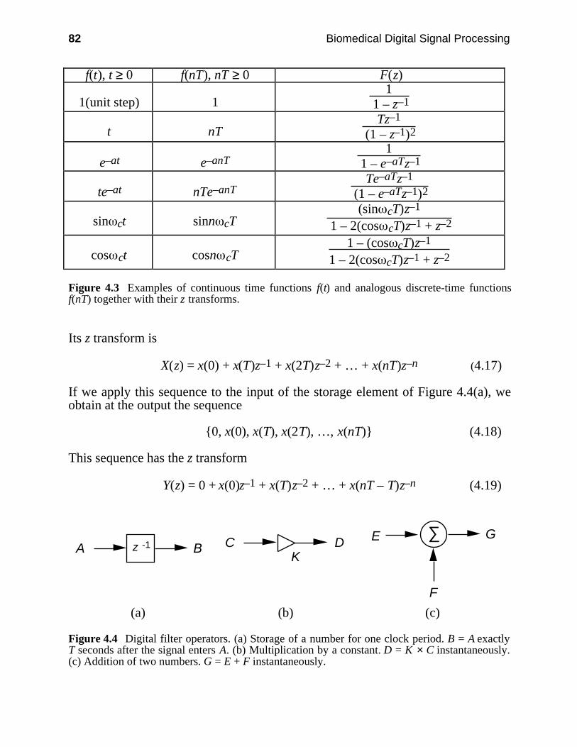
82 Biomedical Digital Signal Processing
f(t), t ≥ 0 f(nT), nT ≥ 0 F(z)
1(unit step) 11
1 – z–1
t nTTz–1
(1 – z–1)2
e–at e–anT1
1 – e–aTz–1
te–at nTe–anTTe–aTz–1
(1 – e–aTz–1)2
sin ct sinn cT(sin cT)z–1
1 – 2(cos cT)z–1 + z–2
cos ct cosn cT1 – (cos cT)z–1
1 – 2(cos cT)z–1 + z–2
Figure 4.3 Examples of continuous time functions f(t) and analogous discrete-time functionsf(nT) together with their z transforms.
Its z transform is
X(z) = x(0) + x(T)z–1 + x(2T)z–2 + … + x(nT)z–n (4.17)
If we apply this sequence to the input of the storage element of Figure 4.4(a), weobtain at the output the sequence
0, x(0), x(T), x(2T), …, x(nT) (4.18)
This sequence has the z transform
Y(z) = 0 + x(0)z–1 + x(T)z–2 + … + x(nT – T)z–n (4.19)
z -1A BK
C D∑E
F
G
(a) (b) (c)
Figure 4.4 Digital filter operators. (a) Storage of a number for one clock period. B = A exactlyT seconds after the signal enters A. (b) Multiplication by a constant. D = K × C instantaneously.(c) Addition of two numbers. G = E + F instantaneously.
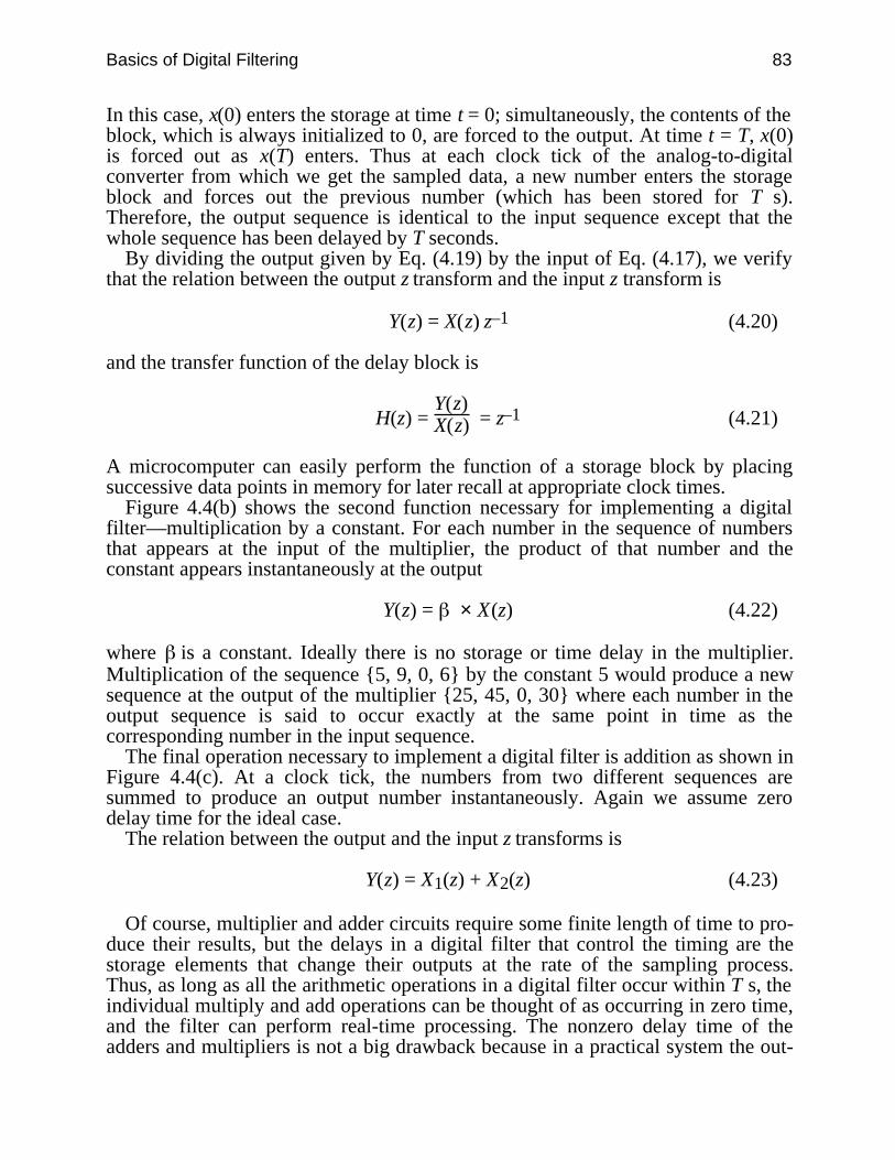
Basics of Digital Filtering 83
In this case, x(0) enters the storage at time t = 0; simultaneously, the contents of theblock, which is always initialized to 0, are forced to the output. At time t = T, x(0)is forced out as x(T) enters. Thus at each clock tick of the analog-to-digitalconverter from which we get the sampled data, a new number enters the storageblock and forces out the previous number (which has been stored for T s).Therefore, the output sequence is identical to the input sequence except that thewhole sequence has been delayed by T seconds.
By dividing the output given by Eq. (4.19) by the input of Eq. (4.17), we verifythat the relation between the output z transform and the input z transform is
Y(z) = X(z) z–1 (4.20)
and the transfer function of the delay block is
H(z) = Y(z)X(z) = z–1 (4.21)
A microcomputer can easily perform the function of a storage block by placingsuccessive data points in memory for later recall at appropriate clock times.
Figure 4.4(b) shows the second function necessary for implementing a digitalfilter—multiplication by a constant. For each number in the sequence of numbersthat appears at the input of the multiplier, the product of that number and theconstant appears instantaneously at the output
Y(z) = × X(z) (4.22)
where is a constant. Ideally there is no storage or time delay in the multiplier.Multiplication of the sequence 5, 9, 0, 6 by the constant 5 would produce a newsequence at the output of the multiplier 25, 45, 0, 30 where each number in theoutput sequence is said to occur exactly at the same point in time as thecorresponding number in the input sequence.
The final operation necessary to implement a digital filter is addition as shown inFigure 4.4(c). At a clock tick, the numbers from two different sequences aresummed to produce an output number instantaneously. Again we assume zerodelay time for the ideal case.
The relation between the output and the input z transforms is
Y(z) = X1(z) + X2(z) (4.23)
Of course, multiplier and adder circuits require some finite length of time to pro-duce their results, but the delays in a digital filter that control the timing are thestorage elements that change their outputs at the rate of the sampling process.Thus, as long as all the arithmetic operations in a digital filter occur within T s, theindividual multiply and add operations can be thought of as occurring in zero time,and the filter can perform real-time processing. The nonzero delay time of theadders and multipliers is not a big drawback because in a practical system the out-
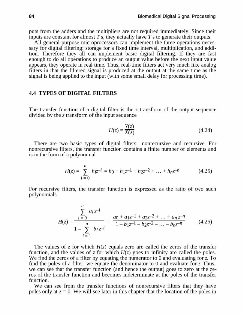
84 Biomedical Digital Signal Processing
puts from the adders and the multipliers are not required immediately. Since theirinputs are constant for almost T s, they actually have T s to generate their outputs.
All general-purpose microprocessors can implement the three operations neces-sary for digital filtering: storage for a fixed time interval, multiplication, and addi-tion. Therefore they all can implement basic digital filtering. If they are fastenough to do all operations to produce an output value before the next input valueappears, they operate in real time. Thus, real-time filters act very much like analogfilters in that the filtered signal is produced at the output at the same time as thesignal is being applied to the input (with some small delay for processing time).
4.4 TYPES OF DIGITAL FILTERS
The transfer function of a digital filter is the z transform of the output sequencedivided by the z transform of the input sequence
H(z) = Y(z)X(z) (4.24)
There are two basic types of digital filters—nonrecursive and recursive. Fornonrecursive filters, the transfer function contains a finite number of elements andis in the form of a polynomial
H(z) = ∑i = 0
n hiz–i = h0 + h1z–1 + h2z–2 + … + hnz–n (4.25)
For recursive filters, the transfer function is expressed as the ratio of two suchpolynomials
H(z) =
∑i = 0
n ai z–i
1 – ∑i = 1
n bi z–i
= a0 + a1z–1 + a2z–2 + … + an z–n
1 – b1z–1 – b2z–2 – … – bnz–n (4.26)
The values of z for which H(z) equals zero are called the zeros of the transferfunction, and the values of z for which H(z) goes to infinity are called the poles.We find the zeros of a filter by equating the numerator to 0 and evaluating for z. Tofind the poles of a filter, we equate the denominator to 0 and evaluate for z. Thus,we can see that the transfer function (and hence the output) goes to zero at the ze-ros of the transfer function and becomes indeterminate at the poles of the transferfunction.
We can see from the transfer functions of nonrecursive filters that they havepoles only at z = 0. We will see later in this chapter that the location of the poles in

Basics of Digital Filtering 85
the z plane determines the stability of the filter. Since nonrecursive filters havepoles only at z = 0, they are always stable.
4.5 TRANSFER FUNCTION OF A DIFFERENCE EQUATION
Once we have the difference equation representing the numerical algorithm forimplementing a digital filter, we can quickly determine the transfer equation thattotally characterizes the performance of the filter. Consider the difference equation
y(nT) = x(nT) + 2x(nT – T) + x(nT – 2T) (4.27)
Recognizing that x(nT) and y(nT) are points in the input and output sequencesassociated with the current sample time, they are analogous to the undelayed z-domain variables, X(z) and Y(z) respectively. Similarly x(nT – T), the input valueone sample point in the past, is analogous to the z-domain input variable delayedby one sample point, or X(z)z–1. We can then write an equation for output Y(z) as afunction of input X(z)
Y(z) = X(z) + 2X(z)z–1 + X(z)z–2 (4.28)
Thus the transfer function of this difference equation is
H(z) = Y(z)X(z) = 1 + 2z–1 + z–2 (4.29)
From this observation of the relationship between discrete-time variables and z-domain variables, we can quickly write the transfer function if we know the differ-ence equation and vice versa.
4.6 THE z-PLANE POLE-ZERO PLOT
We have looked at the z transform from a practical point of view. However themathematics of the z transform are based on the definition
z = esT (4.30)
where the complex frequency iss = + j (4.31)
Thereforez = e Tej T (4.32)
By definition, the magnitude of z is|z| = e T (4.33)
and the phase angle is∠z = T (4.34)
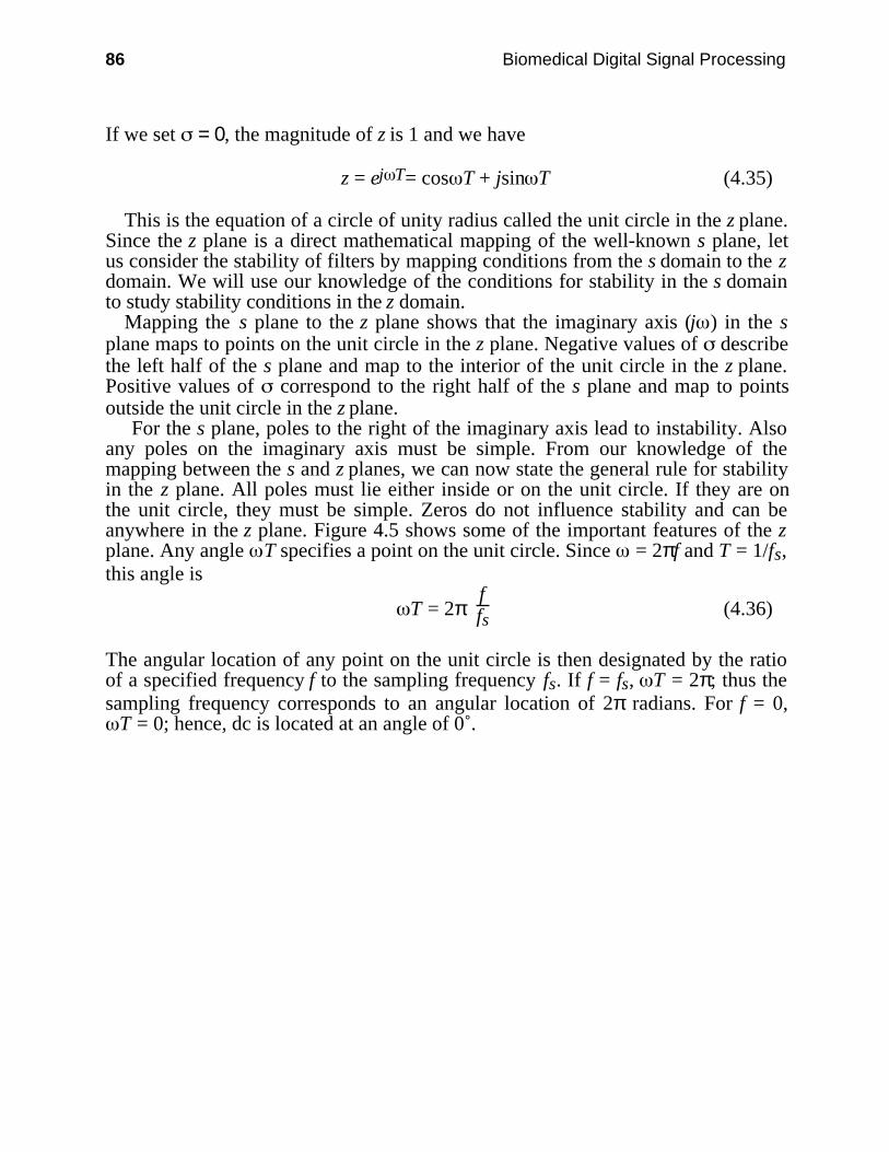
86 Biomedical Digital Signal Processing
If we set = 0, the magnitude of z is 1 and we have
z = ej T= cos T + jsin T (4.35)
This is the equation of a circle of unity radius called the unit circle in the z plane.Since the z plane is a direct mathematical mapping of the well-known s plane, letus consider the stability of filters by mapping conditions from the s domain to the zdomain. We will use our knowledge of the conditions for stability in the s domainto study stability conditions in the z domain.
Mapping the s plane to the z plane shows that the imaginary axis (j ) in the splane maps to points on the unit circle in the z plane. Negative values of describethe left half of the s plane and map to the interior of the unit circle in the z plane.Positive values of correspond to the right half of the s plane and map to pointsoutside the unit circle in the z plane.
For the s plane, poles to the right of the imaginary axis lead to instability. Alsoany poles on the imaginary axis must be simple. From our knowledge of themapping between the s and z planes, we can now state the general rule for stabilityin the z plane. All poles must lie either inside or on the unit circle. If they are onthe unit circle, they must be simple. Zeros do not influence stability and can beanywhere in the z plane. Figure 4.5 shows some of the important features of the zplane. Any angle T specifies a point on the unit circle. Since = 2πf and T = 1/fs,this angle is
T = 2π ffs (4.36)
The angular location of any point on the unit circle is then designated by the ratioof a specified frequency f to the sampling frequency fs. If f = fs, T = 2π; thus thesampling frequency corresponds to an angular location of 2π radians. For f = 0,
T = 0; hence, dc is located at an angle of 0˚.
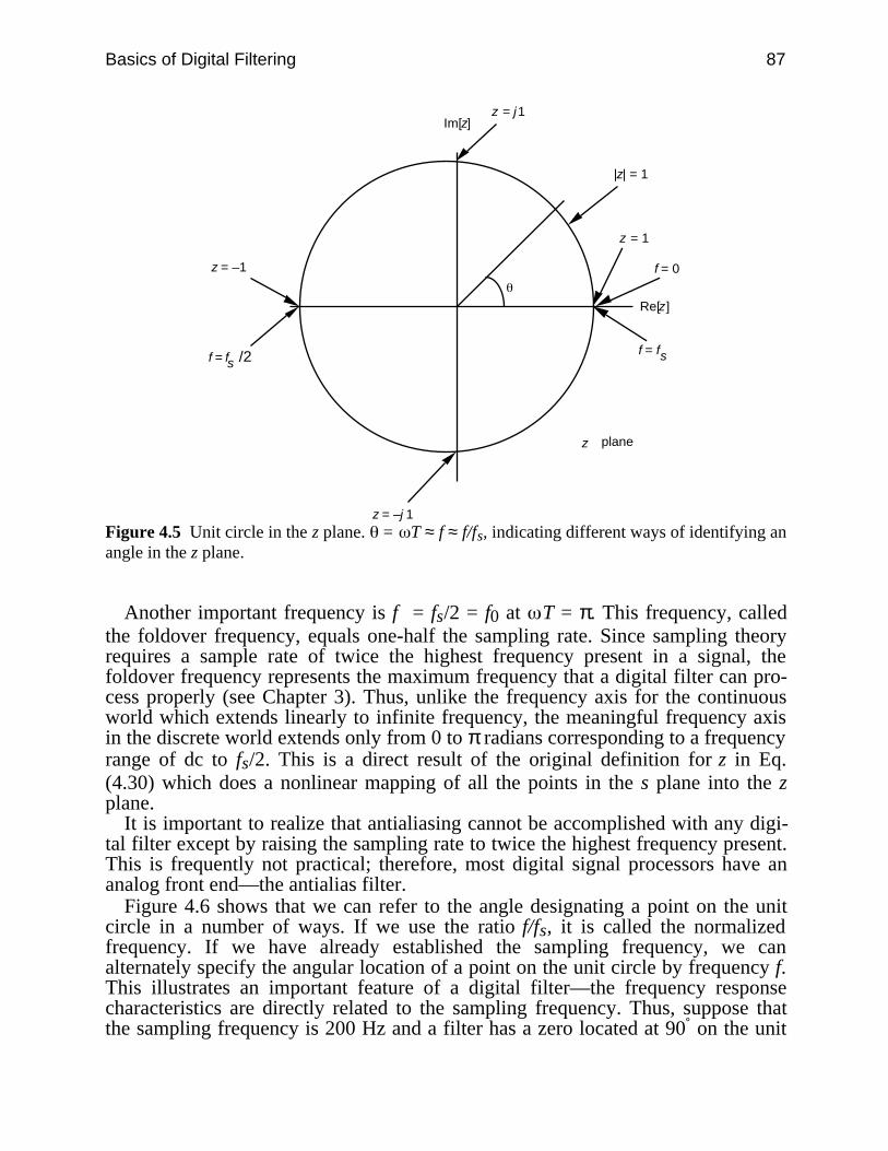
Basics of Digital Filtering 87
z = –1
z = j 1Im[z]
|z| = 1
z = –j 1
Re[z]
z = 1
f = 0
z plane
f = fs /2 sf = f
Figure 4.5 Unit circle in the z plane. = T ≈ f ≈ f/fs, indicating different ways of identifying anangle in the z plane.
Another important frequency is f = fs/2 = f0 at T = π. This frequency, calledthe foldover frequency, equals one-half the sampling rate. Since sampling theoryrequires a sample rate of twice the highest frequency present in a signal, thefoldover frequency represents the maximum frequency that a digital filter can pro-cess properly (see Chapter 3). Thus, unlike the frequency axis for the continuousworld which extends linearly to infinite frequency, the meaningful frequency axisin the discrete world extends only from 0 to π radians corresponding to a frequencyrange of dc to fs/2. This is a direct result of the original definition for z in Eq.(4.30) which does a nonlinear mapping of all the points in the s plane into the zplane.
It is important to realize that antialiasing cannot be accomplished with any digi-tal filter except by raising the sampling rate to twice the highest frequency present.This is frequently not practical; therefore, most digital signal processors have ananalog front end—the antialias filter.
Figure 4.6 shows that we can refer to the angle designating a point on the unitcircle in a number of ways. If we use the ratio f/fs, it is called the normalizedfrequency. If we have already established the sampling frequency, we canalternately specify the angular location of a point on the unit circle by frequency f.This illustrates an important feature of a digital filter—the frequency responsecharacteristics are directly related to the sampling frequency. Thus, suppose thatthe sampling frequency is 200 Hz and a filter has a zero located at 90˚ on the unit
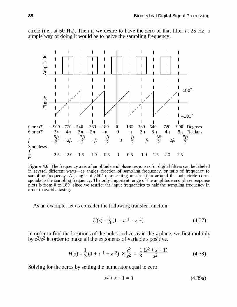
88 Biomedical Digital Signal Processing
circle (i.e., at 50 Hz). Then if we desire to have the zero of that filter at 25 Hz, asimple way of doing it would be to halve the sampling frequency.
Am
plitu
deP
hase
180˚
–180˚
or T –900 –720 –540 –360 –180 0 180 360 540 720 900 Degrees or T –5π –4π –3π –2π –π 0 π 2π 3π 4π 5π Radians
f –5fs2 –2fs –
3fs2 –fs –
fs2 0
fs2 fs
3fs2 2fs
5fs2
Samples/sffs –2.5 –2.0 –1.5 –1.0 –0.5 0 0.5 1.0 1.5 2.0 2.5
Figure 4.6 The frequency axis of amplitude and phase responses for digital filters can be labeledin several different ways—as angles, fraction of sampling frequency, or ratio of frequency tosampling frequency. An angle of 360˚ representing one rotation around the unit circle corre-sponds to the sampling frequency. The only important range of the amplitude and phase responseplots is from 0 to 180˚ since we restrict the input frequencies to half the sampling frequency inorder to avoid aliasing.
As an example, let us consider the following transfer function:
H(z) = 13 (1 + z–1 + z–2) (4.37)
In order to find the locations of the poles and zeros in the z plane, we first multiplyby z2/z2 in order to make all the exponents of variable z positive.
H(z) = 13 (1 + z–1 + z–2) ×
z2
z2 = 13
(z2 + z + 1)z2 (4.38)
Solving for the zeros by setting the numerator equal to zero
z2 + z + 1 = 0 (4.39a)

Basics of Digital Filtering 89
We find that there are two complex conjugate zeros located at
z = –0.5 ± j0.866 (4.39b)
The two zeros are located on the unit circle at = ±2π/3 (±120˚). If the samplingfrequency is 180 Hz, the zero at +120˚ will completely eliminate any signal at60 Hz. Solving for the poles by setting the denominator equal to zero
z2 = 0 (4.39c)
We find that there are two poles, both located at the origin of the z plane
z = 0 (4.39d)
These poles are equally distant from all points on the unit circle, so they influencethe amplitude response by an equal amount at all frequencies. Because of this, wefrequently do not bother to show them on pole-zero plots.
4.7 THE RUBBER MEMBRANE CONCEPT
To get a practical feeling of the pole-zero concept, imagine the z plane to be aninfinitely large, flat rubber membrane “nailed” down around its edges at infinitybut unconstrained elsewhere. The pole-zero pattern of a filter determines the pointsat which the membrane is pushed up to infinity (i.e., poles) or is “nailed” to theground (i.e., zeros). Figure 4.7(a) shows this z-plane rubber membrane with theunit circle superimposed. The magnitude of the transfer function |H(z)| is plottedorthogonal to the x and y axes.
Consider the following transfer function, which represents a pole located in the zplane at the origin, z = 0
H(z) = z–1 = 1z (4.40)
Imagine making a tent by placing an infinitely long tent pole under the rubbermembrane located at z = 0. Figure 4.7(b) illustrates how this pole appears in a pole-zero plot. Figure 4.7(c) is a view from high above the z plane that shows how thepole stretches the membrane. In Figure 4.7(d) we move our observation locationfrom a distant point high above the rubber membrane to a point just above themembrane since we are principally interested in the influence of the pole directlyon the unit circle. Notice how the membrane is distorted symmetrically in alldirections from the location of the pole at z = 0.
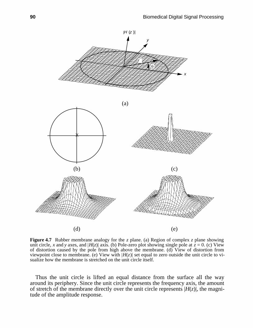
90 Biomedical Digital Signal Processing
y
x
|H (z )|
r
(a)
X
(b) (c)
(d) (e)
Figure 4.7 Rubber membrane analogy for the z plane. (a) Region of complex z plane showingunit circle, x and y axes, and |H(z)| axis. (b) Pole-zero plot showing single pole at z = 0. (c) Viewof distortion caused by the pole from high above the membrane. (d) View of distortion fromviewpoint close to membrane. (e) View with |H(z)| set equal to zero outside the unit circle to vi-sualize how the membrane is stretched on the unit circle itself.
Thus the unit circle is lifted an equal distance from the surface all the wayaround its periphery. Since the unit circle represents the frequency axis, the amountof stretch of the membrane directly over the unit circle represents |H(z)|, the magni-tude of the amplitude response.
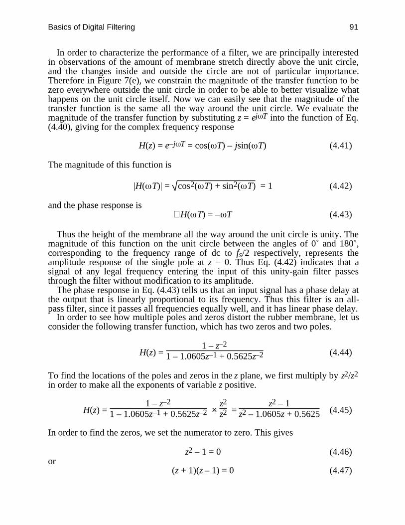
Basics of Digital Filtering 91
In order to characterize the performance of a filter, we are principally interestedin observations of the amount of membrane stretch directly above the unit circle,and the changes inside and outside the circle are not of particular importance.Therefore in Figure 7(e), we constrain the magnitude of the transfer function to bezero everywhere outside the unit circle in order to be able to better visualize whathappens on the unit circle itself. Now we can easily see that the magnitude of thetransfer function is the same all the way around the unit circle. We evaluate themagnitude of the transfer function by substituting z = ej T into the function of Eq.(4.40), giving for the complex frequency response
H(z) = e–j T = cos( T) – jsin( T) (4.41)
The magnitude of this function is
|H( T)| = cos2( T) + sin2( T) = 1 (4.42)
and the phase response is∠H( T) = – T (4.43)
Thus the height of the membrane all the way around the unit circle is unity. Themagnitude of this function on the unit circle between the angles of 0˚ and 180˚,corresponding to the frequency range of dc to fs/2 respectively, represents theamplitude response of the single pole at z = 0. Thus Eq. (4.42) indicates that asignal of any legal frequency entering the input of this unity-gain filter passesthrough the filter without modification to its amplitude.
The phase response in Eq. (4.43) tells us that an input signal has a phase delay atthe output that is linearly proportional to its frequency. Thus this filter is an all-pass filter, since it passes all frequencies equally well, and it has linear phase delay.
In order to see how multiple poles and zeros distort the rubber membrane, let usconsider the following transfer function, which has two zeros and two poles.
H(z) = 1 – z–2
1 – 1.0605z–1 + 0.5625z–2 (4.44)
To find the locations of the poles and zeros in the z plane, we first multiply by z2/z2
in order to make all the exponents of variable z positive.
H(z) = 1 – z–2
1 – 1.0605z–1 + 0.5625z–2 × z2
z2 = z2 – 1
z2 – 1.0605z + 0.5625 (4.45)
In order to find the zeros, we set the numerator to zero. This gives
z2 – 1 = 0 (4.46)or
(z + 1)(z – 1) = 0 (4.47)
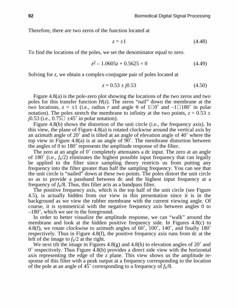
92 Biomedical Digital Signal Processing
Therefore, there are two zeros of the function located at
z = ±1 (4.48)
To find the locations of the poles, we set the denominator equal to zero.
z2 – 1.0605z + 0.5625 = 0 (4.49)
Solving for z, we obtain a complex-conjugate pair of poles located at
z = 0.53 ± j0.53 (4.50)
Figure 4.8(a) is the pole-zero plot showing the locations of the two zeros and twopoles for this transfer function H(z). The zeros “nail” down the membrane at thetwo locations, z = ±1 (i.e., radius r and angle of 1∠0˚ and –1∠180˚ in polarnotation). The poles stretch the membrane to infinity at the two points, z = 0.53 ±j0.53 (i.e., 0.75∠ ±45˚ in polar notation).
Figure 4.8(b) shows the distortion of the unit circle (i.e., the frequency axis). Inthis view, the plane of Figure 4.8(a) is rotated clockwise around the vertical axis byan azimuth angle of 20˚ and is tilted at an angle of elevation angle of 40˚ where thetop view in Figure 4.8(a) is at an angle of 90˚. The membrane distortion betweenthe angles of 0 to 180˚ represents the amplitude response of the filter.
The zero at an angle of 0˚ completely attenuates a dc input. The zero at an angleof 180˚ (i.e., fs/2) eliminates the highest possible input frequency that can legallybe applied to the filter since sampling theory restricts us from putting anyfrequency into the filter greater than half the sampling frequency. You can see thatthe unit circle is “nailed” down at these two points. The poles distort the unit circleso as to provide a passband between dc and the highest input frequency at afrequency of fs/8. Thus, this filter acts as a bandpass filter.
The positive frequency axis, which is the top half of the unit circle (see Figure4.5), is actually hidden from our view in this presentation since it is in thebackground as we view the rubber membrane with the current viewing angle. Ofcourse, it is symmetrical with the negative frequency axis between angles 0 to–180˚, which we see in the foreground.
In order to better visualize the amplitude response, we can “walk” around themembrane and look at the hidden positive frequency side. In Figures 4.8(c) to4.8(f), we rotate clockwise to azimuth angles of 60˚, 100˚, 140˚, and finally 180˚respectively. Thus in Figure 4.8(f), the positive frequency axis runs from dc at theleft of the image to fs/2 at the right.
We next tilt the image in Figures 4.8(g) and 4.8(h) to elevation angles of 20˚ and0˚ respectively. Thus Figure 4.8(h) provides a direct side view with the horizontalaxis representing the edge of the z plane. This view shows us the amplitude re-sponse of this filter with a peak output at a frequency corresponding to the locationof the pole at an angle of 45˚ corresponding to a frequency of fs/8.
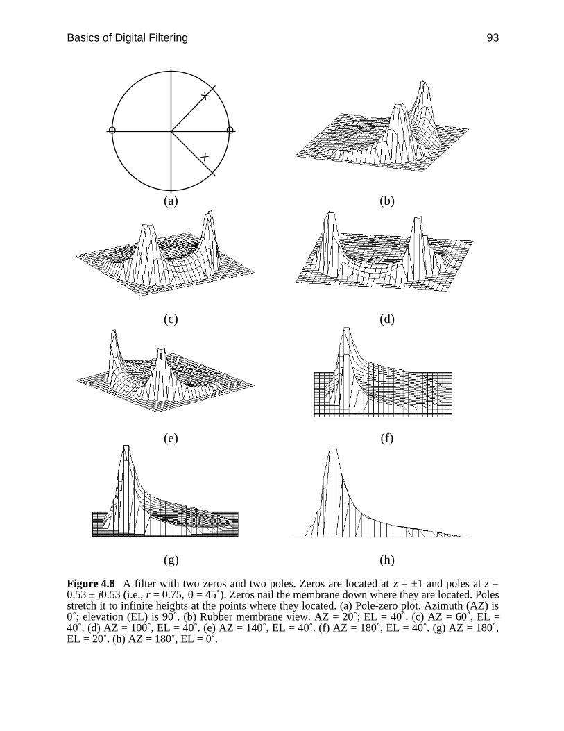
Basics of Digital Filtering 93
X
X
O O
(a) (b)
(c) (d)
(e) (f)
(g) (h)
Figure 4.8 A filter with two zeros and two poles. Zeros are located at z = ±1 and poles at z =0.53 ± j0.53 (i.e., r = 0.75, = 45˚). Zeros nail the membrane down where they are located. Polesstretch it to infinite heights at the points where they located. (a) Pole-zero plot. Azimuth (AZ) is0˚; elevation (EL) is 90˚. (b) Rubber membrane view. AZ = 20˚; EL = 40˚. (c) AZ = 60˚, EL =40˚. (d) AZ = 100˚, EL = 40˚. (e) AZ = 140˚, EL = 40˚. (f) AZ = 180˚, EL = 40˚. (g) AZ = 180˚,EL = 20˚. (h) AZ = 180˚, EL = 0˚.
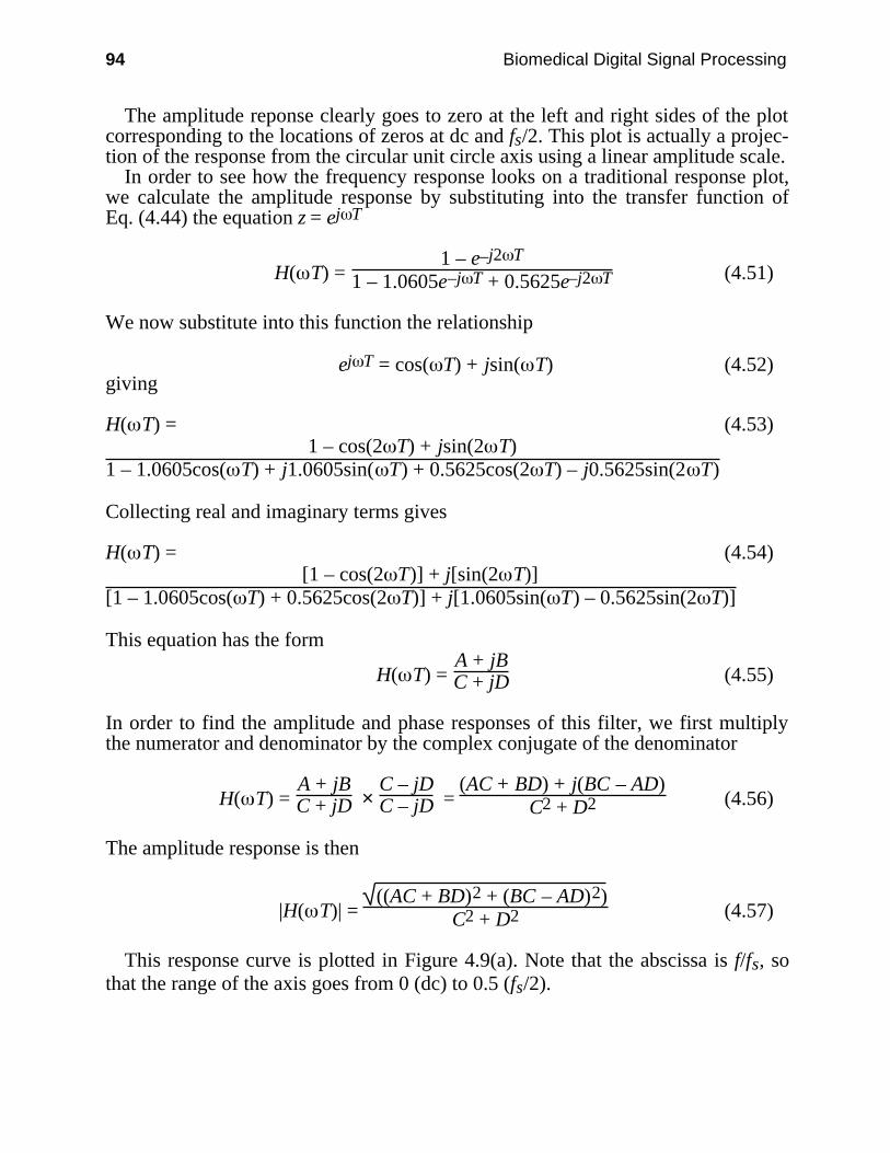
94 Biomedical Digital Signal Processing
The amplitude reponse clearly goes to zero at the left and right sides of the plotcorresponding to the locations of zeros at dc and fs/2. This plot is actually a projec-tion of the response from the circular unit circle axis using a linear amplitude scale.
In order to see how the frequency response looks on a traditional response plot,we calculate the amplitude response by substituting into the transfer function ofEq. (4.44) the equation z = ej T
H( T) = 1 – e–j2 T
1 – 1.0605e–j T + 0.5625e–j2 T (4.51)
We now substitute into this function the relationship
ej T = cos( T) + jsin( T) (4.52)giving
H( T) = (4.53)1 – cos(2 T) + jsin(2 T)
1 – 1.0605cos( T) + j1.0605sin( T) + 0.5625cos(2 T) – j0.5625sin(2 T)
Collecting real and imaginary terms gives
H( T) = (4.54)[1 – cos(2 T)] + j[sin(2 T)]
[1 – 1.0605cos( T) + 0.5625cos(2 T)] + j[1.0605sin( T) – 0.5625sin(2 T)]
This equation has the form
H( T) = A + jBC + jD (4.55)
In order to find the amplitude and phase responses of this filter, we first multiplythe numerator and denominator by the complex conjugate of the denominator
H( T) = A + jBC + jD ×
C – jDC – jD =
(AC + BD) + j(BC – AD)C2 + D2 (4.56)
The amplitude response is then
|H( T)| = ((AC + BD)2 + (BC – AD)2)
C2 + D2 (4.57)
This response curve is plotted in Figure 4.9(a). Note that the abscissa is f/fs, sothat the range of the axis goes from 0 (dc) to 0.5 (fs/2).
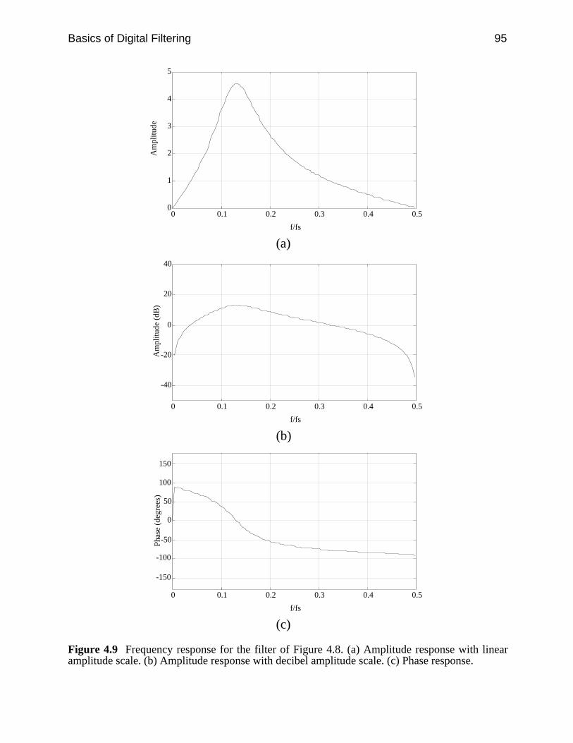
Basics of Digital Filtering 95
0
1
2
3
4
5
0 0.1 0.2 0.3 0.4 0.5
f/fs
Am
plitu
de
(a)
-40
-20
0
20
40
0 0.1 0.2 0.3 0.4 0.5
f/fs
Am
plitu
de (
dB)
(b)
-150
-100
-50
0
50
100
150
0 0.1 0.2 0.3 0.4 0.5
f/fs
Pha
se (
degr
ees)
(c)
Figure 4.9 Frequency response for the filter of Figure 4.8. (a) Amplitude response with linearamplitude scale. (b) Amplitude response with decibel amplitude scale. (c) Phase response.

96 Biomedical Digital Signal Processing
Compare this response to Figure 4.8(h) which shows the same information as aprojection of the response from the circular unit circle axis. Figure 4.9(b) showsthe same amplitude response plotted as a more familiar decibel (dB) plot.
Figure 4.10 shows how the radial locations of the poles influence the distortionof the rubber membrane. Note how moving the poles toward the unit circle makesthe peaks appear sharper. The closer the poles get to the unit circle, the sharper therolloff of the filter.
X
X
O O
(a)
X
X
O O
(b)
X
X
O O
(c)
Figure 4.10 Pole-zero and rubber membrane plots of bandpass filter. Angular frequency of polelocations is fs/8. (a) r = 0.5. (b) r = 0.75. (c) r = 0.9.
The phase response for this filter, which is plotted in Figure 4.9(c), is
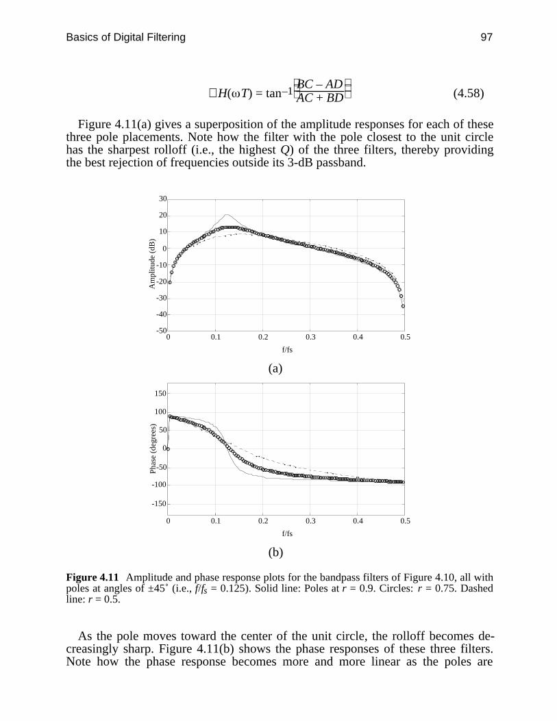
Basics of Digital Filtering 97
∠H( T) = tan–1
BC – AD
AC + BD (4.58)
Figure 4.11(a) gives a superposition of the amplitude responses for each of thesethree pole placements. Note how the filter with the pole closest to the unit circlehas the sharpest rolloff (i.e., the highest Q) of the three filters, thereby providingthe best rejection of frequencies outside its 3-dB passband.
-50
-40
-30
-20
-10
0
10
20
30
0 0.1 0.2 0.3 0.4 0.5
f/fs
Am
plitu
de (
dB)
(a)
-150
-100
-50
0
50
100
150
0 0.1 0.2 0.3 0.4 0.5
f/fs
Pha
se (
degr
ees)
(b)
Figure 4.11 Amplitude and phase response plots for the bandpass filters of Figure 4.10, all withpoles at angles of ±45˚ (i.e., f/fs = 0.125). Solid line: Poles at r = 0.9. Circles: r = 0.75. Dashedline: r = 0.5.
As the pole moves toward the center of the unit circle, the rolloff becomes de-creasingly sharp. Figure 4.11(b) shows the phase responses of these three filters.Note how the phase response becomes more and more linear as the poles are

98 Biomedical Digital Signal Processing
moved toward the center of the unit circle. We will see in the next chapter that thephase response becomes completely piecewise linear when all the poles are at thecenter of the unit circle (i.e., at r = 0).
Thus, the rubber membrane concept helps us to visualize the behavior of anydigital filter and can be used as an important tool in the design of digital filters.
4.8 REFERENCES
Antoniou, A. 1979. Digital Filters: Analysis and Design, New York: McGraw-Hill.Bogner, R. E. and Constantinides, A. G. 1985. Introduction to Digital Filtering, New York: John
Wiley and Sons.Gold, B. and Rader, C. 1969. Digital Processing of Signals, New York: Lincoln Laboratory
Publications, McGraw-Hill.Rabiner, L. R. and Rader, C. M. 1972. Digital Signal Processing New York: IEEE Press.Stearns, S. D. 1975. Digital Signal Analysis. Rochelle Park, NJ: Hayden.
4.9 STUDY QUESTIONS
4.1 What are the differences between an analog filter and a digital filter?4.2 If the output sequence of a digital filter is 1, 0, 0, 2, 0, 1 in response to a unit impulse,
what is the transfer function of this filter?4.3 Draw the pole-zero plot of the filter described by the following transfer function:
H(z) = 14 +
12 z–1 +
14 z–2
4.4 Suppose you are given a filter with a zero at 30˚ on the unit circle. You are asked to use thisfilter as a notch filter to remove 60-Hz noise. How will you do this? Can you use the samefilter as a notch filter, rejecting different frequencies?
4.5 What is the z transform of a step function having an amplitude of five i.e., 5, 5, 5, 5, …?4.6 A function e–at is to be applied to the input of a filter. Derive the z transform of the discrete
version of this function.4.7 Application of a unit impulse to the input of a filter whose performance is unknown
produces the output sequence 1, –2, 0, 0, …. What would the output sequence be if a unitstep were applied?
4.8 A digital filter has the transfer function: H(z) = z–1 + 6z–4 – 2z–7. What is the differenceequation for the output, y(nT)?
4.9 A digital filter has the output sequence 1, 2, –3, 0, 0, 0, … when its input is the unitimpulse 1, 0, 0, 0, 0, …. If its input is a unit step, what is its output sequence?
4.10 A unit impulse applied to a digital filter results in the output sequence: 3, 2, 3, 0, 0, 0, ….A unit step function applied to the input of the same filter would produce what outputsequence?
4.11 The z transform of a filter is: H(z) = 2 – 2z–4 . What is its (a) amplitude response, (b) phaseresponse, (c) difference equation?
4.12 The transfer function of a filter designed for a sampling rate of 800 samples/s is:
H(z) = (1 – 0.5z–1)(1 + 0.5z–1)

Basics of Digital Filtering 99
A 200-Hz sine wave with a peak amplitude of 4 is applied to the input. What is the peakvalue of the output signal?
4.13 A unit impulse applied to a digital filter results in the following output sequence: 1, 2, 3, 4,0, 0, …. A unit step function applied to the input of the same filter would produce whatoutput sequence?
4.14 The transfer function of a filter designed for a sampling rate of 600 samples/s is:
H(z) = 1 – 2z–1
A sinusoidal signal is applied to the input: 10 sin(628t). What is the peak value of theoutput signal?
100
5
Finite Impulse Response Filters
Jesse D. Olson
A finite impulse response (FIR) filter has a unit impulse response that has a limitednumber of terms, as opposed to an infinite impulse response (IIR) filter whichproduces an infinite number of output terms when a unit impulse is applied to itsinput. FIR filters are generally realized nonrecursively, which means that there isno feedback involved in computation of the output data. The output of the filterdepends only on the present and past inputs. This quality has several importantimplications for digital filter design and applications. This chapter discussesseveral FIR filters typically used for real-time ECG processing, and also gives anoverview of some general FIR design techniques.
5.1 CHARACTERISTICS OF FIR FILTERS
5.1.1 Finite impulse response
Finite impulse response implies that the effect of transients or initial conditions onthe filter output will eventually die away. Figure 5.1 shows a signal-flow graph(SFG) of a FIR filter realized nonrecursively. The filter is merely a set of “tapweights” of the delay stages. The unit impulse response is equal to the tap weights,so the filter has a difference equation given by Eq. (5.1), and a transfer functionequation given by Eq. (5.2).
y(nT) = ∑k = 0
N bk x(nT – kT) (5.1)
H(z) = b0 + b1z–1 + b2z–2 + … + bNz–N (5.2)

Finite Impulse Response Filters 101
X (z)
Y (z)
z -1
∑
b 1
b 2
b 3
b N
∑∑∑
b 0
z -1 z -1 z -1
Figure 5.1 The output of a FIR filter of order N is the weighted sum of the values in the storageregisters of the delay line.
5.1.2 Linear phase
In many biomedical signal processing applications, it is important to preservecertain characteristics of a signal throughout the filtering operation, such as theheight and duration of the QRS pulse. A filter with linear phase has a pure timedelay as its phase response, so phase distortion is minimized. A filter has linearphase if its frequency response H(ej ) can be expressed as
H(ej ) = H1( ) e j( + ) (5.3)
where H1( ) is a real and even function, since the phase of H(ej ) is
∠H(ej ) = − − ; H1( ) > 0− − − π ; H1( ) < 0 (5.4)
FIR filters can easily be designed to have a linear phase characteristic. Linearphase can be obtained in four ways, as combinations of even or odd symmetry(defined as follows) with even or odd length.
h(N – 1 – k) = h(k), even symmetryh(N – 1 – k) = –h(k), odd symmetry for 0 ≤ k ≤ N (5.5)
5.1.3 Stability
Since a nonrecursive filter does not use feedback, it has no poles except those thatare located at z = 0. Thus there is no possibility for a pole to exist outside the unitcircle. This means that it is inherently stable. As long as the input to the filter isbounded, the output of the filter will also be bounded. This contributes to ease ofdesign, and makes FIR filters especially useful for adaptive filtering where filtercoefficients change as a function of the input data. Adaptive filters are discussed inChapter 8.
5.1.4 Desirable finite-length register effects
102 Biomedical Digital Signal Processing
When data are converted from analog form to digital form, some information islost due to the finite number of storage bits. Likewise, when coefficient values fora filter are calculated, digital implementation can only approximate the desiredvalues. The limitations introduced by digital storage are termed finite-lengthregister effects. Although we will not treat this subject in detail in this book, finite-length register effects can have significant negative impact on a filter design. Theseeffects include quantization error, roundoff noise, limit cycles, conditionalstability, and coefficient sensitivity. In FIR filters, these effects are much lesssignificant and easier to analyze than in IIR filters since the errors are not fed backinto the filter. See Appendix F for more details about finite-length register effects.
5.1.5 Ease of design
All of the above properties contribute to the ease in designing FIR filters. There aremany straightforward techniques for designing FIR filters to meet arbitrary fre-quency and phase response specifications, such as window design or frequencysampling. Many software packages exist that automate the FIR design process, of-ten computing a filter realization that is in some sense optimal.
5.1.6 Realizations
There are three methods of realizing an FIR filter (Bogner and Constantinides,1985). The most common method is direct convolution, in which the filter’s unitimpulse sequence is convolved with the present input and past inputs to computeeach new output value. FIR filters attenuate the signal very gradually outside thepassband (i.e., they have slow rolloff characteristics). Since they have significantlyslower rolloff than IIR filters of the same length, for applications that require sharprolloffs, the order of the FIR filter may be quite large. For higher-order filters thedirect convolution method becomes computationally inefficient.
For FIR filters of length greater than about 30, the “fast convolution” realizationoffers a computational savings. This technique takes advantage of the fact thattime-domain multiplication, the frequency-domain dual of convolution, is compu-tationally less intensive. Fast convolution involves taking the FFT of a block ofdata, multiplying the result by the FFT of the unit impulse sequence, and finallytaking the inverse FFT. The process is repeated for subsequent blocks of data. Thismethod is discussed in detail in section 11.3.2.
The third method of realizing FIR filters is an advanced, recursive technique in-volving a comb filter and a bank of parallel digital resonators (Rabiner and Rader,1972). This method is advantageous for frequency sampling designs if a largenumber of the coefficients in the desired frequency response are zero, and can beused for filters with integer-valued coefficients, as discussed in Chapter 7. For theremainder of this chapter, only the direct convolution method will be considered.
5.2 SMOOTHING FILTERS
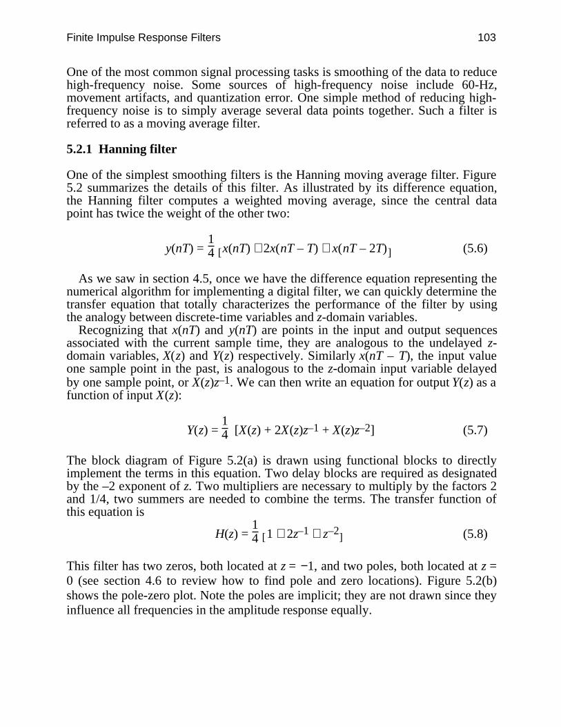
Finite Impulse Response Filters 103
One of the most common signal processing tasks is smoothing of the data to reducehigh-frequency noise. Some sources of high-frequency noise include 60-Hz,movement artifacts, and quantization error. One simple method of reducing high-frequency noise is to simply average several data points together. Such a filter isreferred to as a moving average filter.
5.2.1 Hanning filter
One of the simplest smoothing filters is the Hanning moving average filter. Figure5.2 summarizes the details of this filter. As illustrated by its difference equation,the Hanning filter computes a weighted moving average, since the central datapoint has twice the weight of the other two:
y(nT) = 14 [ ]x(nT) + 2x(nT – T) + x(nT – 2T) (5.6)
As we saw in section 4.5, once we have the difference equation representing thenumerical algorithm for implementing a digital filter, we can quickly determine thetransfer equation that totally characterizes the performance of the filter by usingthe analogy between discrete-time variables and z-domain variables.
Recognizing that x(nT) and y(nT) are points in the input and output sequencesassociated with the current sample time, they are analogous to the undelayed z-domain variables, X(z) and Y(z) respectively. Similarly x(nT – T), the input valueone sample point in the past, is analogous to the z-domain input variable delayedby one sample point, or X(z)z–1. We can then write an equation for output Y(z) as afunction of input X(z):
Y(z) = 14 [X(z) + 2X(z)z–1 + X(z)z–2] (5.7)
The block diagram of Figure 5.2(a) is drawn using functional blocks to directlyimplement the terms in this equation. Two delay blocks are required as designatedby the –2 exponent of z. Two multipliers are necessary to multiply by the factors 2and 1/4, two summers are needed to combine the terms. The transfer function ofthis equation is
H(z) = 14 [ ]1 + 2z–1 + z–2 (5.8)
This filter has two zeros, both located at z = −1, and two poles, both located at z =0 (see section 4.6 to review how to find pole and zero locations). Figure 5.2(b)shows the pole-zero plot. Note the poles are implicit; they are not drawn since theyinfluence all frequencies in the amplitude response equally.
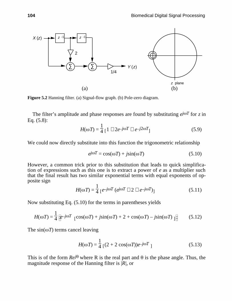
104 Biomedical Digital Signal Processing
X (z)
Y (z)
z -1
∑∑
z -1
2
1/4
z plane
(a) (b)
Figure 5.2 Hanning filter. (a) Signal-flow graph. (b) Pole-zero diagram.
The filter’s amplitude and phase responses are found by substituting ej T for z inEq. (5.8):
H( T) = 14 [ ]1 + 2e–j T + e–j2 T (5.9)
We could now directly substitute into this function the trigonometric relationship
ej T = cos( T) + jsin( T) (5.10)
However, a common trick prior to this substitution that leads to quick simplifica-tion of expressions such as this one is to extract a power of e as a multiplier suchthat the final result has two similar exponential terms with equal exponents of op-posite sign
H( T) = 14 [ ]e–j T (ej T + 2 + e–j T) (5.11)
Now substituting Eq. (5.10) for the terms in parentheses yields
H( T) = 14
e–j T [ ]cos( T) + jsin( T) + 2 + cos( T) – jsin( T) (5.12)
The sin( T) terms cancel leaving
H( T) = 14 [ ](2 + 2 cos( T))e–j T (5.13)
This is of the form Rej where R is the real part and is the phase angle. Thus, themagnitude response of the Hanning filter is |R|, or
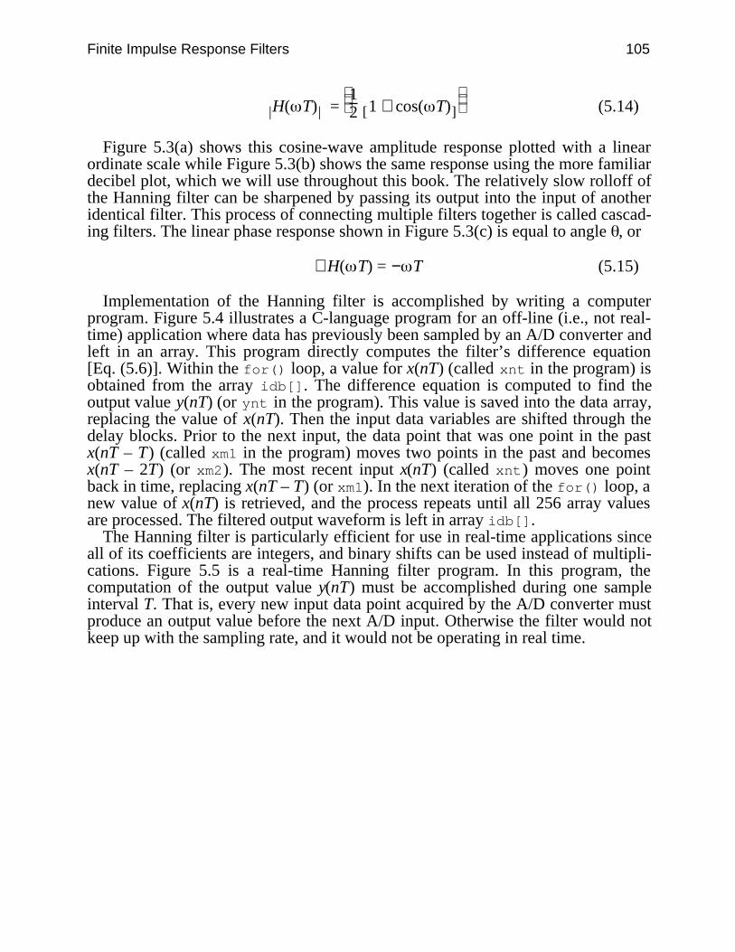
Finite Impulse Response Filters 105
| |H( T) =
1
2 [ ]1 + cos( T) (5.14)
Figure 5.3(a) shows this cosine-wave amplitude response plotted with a linearordinate scale while Figure 5.3(b) shows the same response using the more familiardecibel plot, which we will use throughout this book. The relatively slow rolloff ofthe Hanning filter can be sharpened by passing its output into the input of anotheridentical filter. This process of connecting multiple filters together is called cascad-ing filters. The linear phase response shown in Figure 5.3(c) is equal to angle , or
∠H( T) = − T (5.15)
Implementation of the Hanning filter is accomplished by writing a computerprogram. Figure 5.4 illustrates a C-language program for an off-line (i.e., not real-time) application where data has previously been sampled by an A/D converter andleft in an array. This program directly computes the filter’s difference equation[Eq. (5.6)]. Within the for() loop, a value for x(nT) (called xnt in the program) isobtained from the array idb[]. The difference equation is computed to find theoutput value y(nT) (or ynt in the program). This value is saved into the data array,replacing the value of x(nT). Then the input data variables are shifted through thedelay blocks. Prior to the next input, the data point that was one point in the pastx(nT – T) (called xm1 in the program) moves two points in the past and becomesx(nT – 2T) (or xm2). The most recent input x(nT) (called xnt) moves one pointback in time, replacing x(nT – T) (or xm1). In the next iteration of the for() loop, anew value of x(nT) is retrieved, and the process repeats until all 256 array valuesare processed. The filtered output waveform is left in array idb[].
The Hanning filter is particularly efficient for use in real-time applications sinceall of its coefficients are integers, and binary shifts can be used instead of multipli-cations. Figure 5.5 is a real-time Hanning filter program. In this program, thecomputation of the output value y(nT) must be accomplished during one sampleinterval T. That is, every new input data point acquired by the A/D converter mustproduce an output value before the next A/D input. Otherwise the filter would notkeep up with the sampling rate, and it would not be operating in real time.
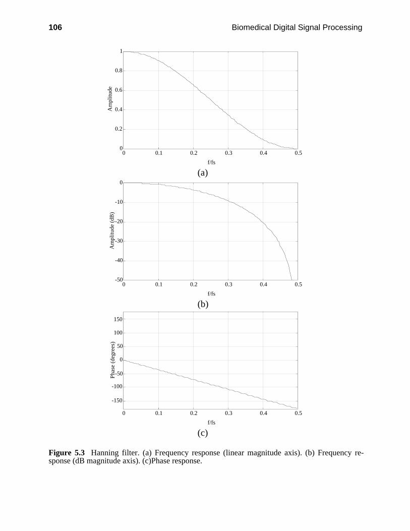
106 Biomedical Digital Signal Processing
0
0.2
0.4
0.6
0.8
1
0 0.1 0.2 0.3 0.4 0.5
f/fs
Am
plitu
de
(a)
-50
-40
-30
-20
-10
0
0 0.1 0.2 0.3 0.4 0.5
f/fs
Am
plitu
de (
dB)
(b)
-150
-100
-50
0
50
100
150
0 0.1 0.2 0.3 0.4 0.5
f/fs
Pha
se (
degr
ees)
(c)
Figure 5.3 Hanning filter. (a) Frequency response (linear magnitude axis). (b) Frequency re-sponse (dB magnitude axis). (c)Phase response.

Finite Impulse Response Filters 107
In this program, sampling from the A/D converter, computation of the results,and sending the filtered data to a D/A converter are all accomplished within afor() loop. The wait() function is designed to wait for an interrupt caused by anA/D clock tick. Once the interrupt occurs, a data point is sampled with theadget() function and set equal to xnt. The Hanning filter’s difference equation isthen computed using C-language shift operators to do the multiplicationsefficiently. Expression <<1 is a binary shift to the left by one bit positioncorresponding to multiplication by a factor of two, and >>2 is a binary shift right oftwo bit positions representing division by four.
/* Hanning filter Difference equation: y(nT) = (x(nT) + 2*x(nT - T) + x(nT - 2T))/4 C language implementation equation: ynt = (xnt + 2*xm1 + xm2)/4;*/
main() int i, xnt, xm1, xm2, ynt, idb[256];
xm2 = 0; xm1 = 0;
for(i = 0; i <= 255; i++) xnt = idb[i]; ynt = (xnt + 2*xm1 + xm2)/4; idb[i] = ynt; xm2 = xm1; xm1 = xnt;
Figure 5.4 C-language code to implement the Hanning filter. Data is presampled by an ADCand stored in array idb[]. The filtered signal is left in idb[].
The computed output value is sent to a D/A converter with function daput().Then the input data variables are shifted through the delay blocks as in theprevious program. For the next input, the data point that was one point in the pastx(nT – T) (called xm1 in the program) moves two points in the past and becomesx(nT – 2T) (or xm2). The most recent input x(nT) (called xnt) moves one pointback in time, replacing x(nT – T) (or xm1). Then the for() loop repeats with thewait() function waiting until the next interrupt signals that a new sampled datapoint is available to be acquired by adget() as the new value for x(nT).
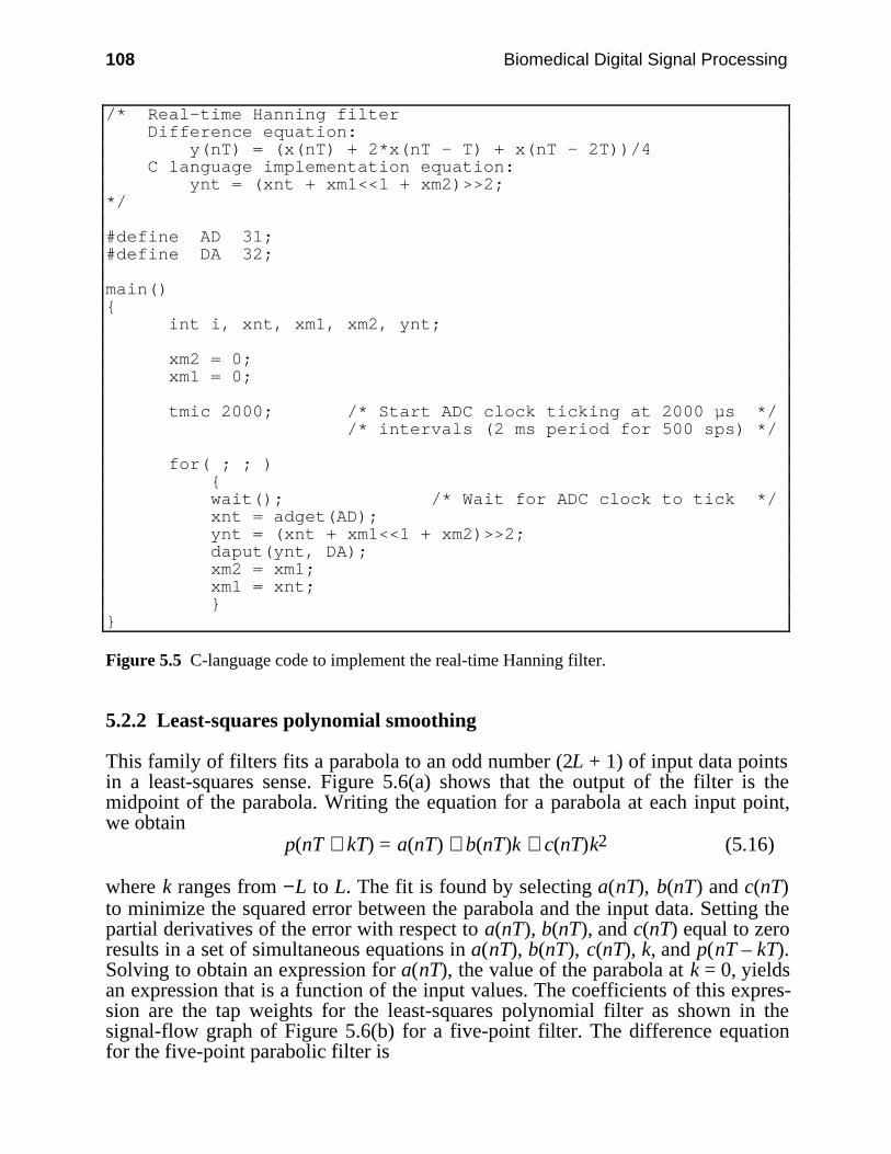
108 Biomedical Digital Signal Processing
/* Real-time Hanning filter Difference equation: y(nT) = (x(nT) + 2*x(nT - T) + x(nT - 2T))/4 C language implementation equation: ynt = (xnt + xm1<<1 + xm2)>>2;*/
#define AD 31;#define DA 32;
main() int i, xnt, xm1, xm2, ynt;
xm2 = 0; xm1 = 0;
tmic 2000; /* Start ADC clock ticking at 2000 µs */ /* intervals (2 ms period for 500 sps) */
for( ; ; ) wait(); /* Wait for ADC clock to tick */ xnt = adget(AD); ynt = (xnt + xm1<<1 + xm2)>>2; daput(ynt, DA); xm2 = xm1; xm1 = xnt;
Figure 5.5 C-language code to implement the real-time Hanning filter.
5.2.2 Least-squares polynomial smoothing
This family of filters fits a parabola to an odd number (2L + 1) of input data pointsin a least-squares sense. Figure 5.6(a) shows that the output of the filter is themidpoint of the parabola. Writing the equation for a parabola at each input point,we obtain
p(nT + kT) = a(nT) + b(nT)k + c(nT)k2 (5.16)
where k ranges from −L to L. The fit is found by selecting a(nT), b(nT) and c(nT)to minimize the squared error between the parabola and the input data. Setting thepartial derivatives of the error with respect to a(nT), b(nT), and c(nT) equal to zeroresults in a set of simultaneous equations in a(nT), b(nT), c(nT), k, and p(nT – kT).Solving to obtain an expression for a(nT), the value of the parabola at k = 0, yieldsan expression that is a function of the input values. The coefficients of this expres-sion are the tap weights for the least-squares polynomial filter as shown in thesignal-flow graph of Figure 5.6(b) for a five-point filter. The difference equationfor the five-point parabolic filter is
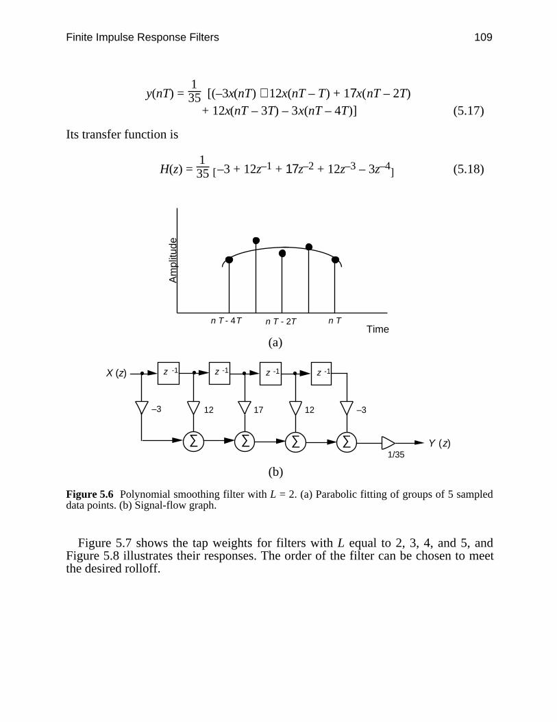
Finite Impulse Response Filters 109
y(nT) = 135 [(–3x(nT) + 12x(nT – T) + 17x(nT – 2T)
+ 12x(nT – 3T) – 3x(nT – 4T)] (5.17)
Its transfer function is
H(z) = 135 [ ]–3 + 12z–1 + 17z–2 + 12z–3 – 3z–4 (5.18)
n T n T - 2T n T - 4T Time
Am
plitu
de
(a)
X (z)
Y (z)
z -1
∑∑
–3
z -1
–312
1/35
z -1
∑
17
z -1
∑
12
(b)
Figure 5.6 Polynomial smoothing filter with L = 2. (a) Parabolic fitting of groups of 5 sampleddata points. (b) Signal-flow graph.
Figure 5.7 shows the tap weights for filters with L equal to 2, 3, 4, and 5, andFigure 5.8 illustrates their responses. The order of the filter can be chosen to meetthe desired rolloff.
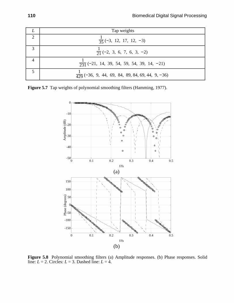
110 Biomedical Digital Signal Processing
L Tap weights
2 135 (−3, 12, 17, 12, −3)
3 121 (−2, 3, 6, 7, 6, 3, −2)
4 1231 (−21, 14, 39, 54, 59, 54, 39, 14, −21)
5 1429 (−36, 9, 44, 69, 84, 89, 84, 69, 44, 9, −36)
Figure 5.7 Tap weights of polynomial smoothing filters (Hamming, 1977).
-50
-40
-30
-20
-10
0
0 0.1 0.2 0.3 0.4 0.5
f/fs
Am
plitu
de (
dB)
(a)
-150
-100
-50
0
50
100
150
0 0.1 0.2 0.3 0.4 0.5
f/fs
Pha
se (
degr
ees)
(b)
Figure 5.8 Polynomial smoothing filters (a) Amplitude responses. (b) Phase responses. Solidline: L = 2. Circles: L = 3. Dashed line: L = 4.
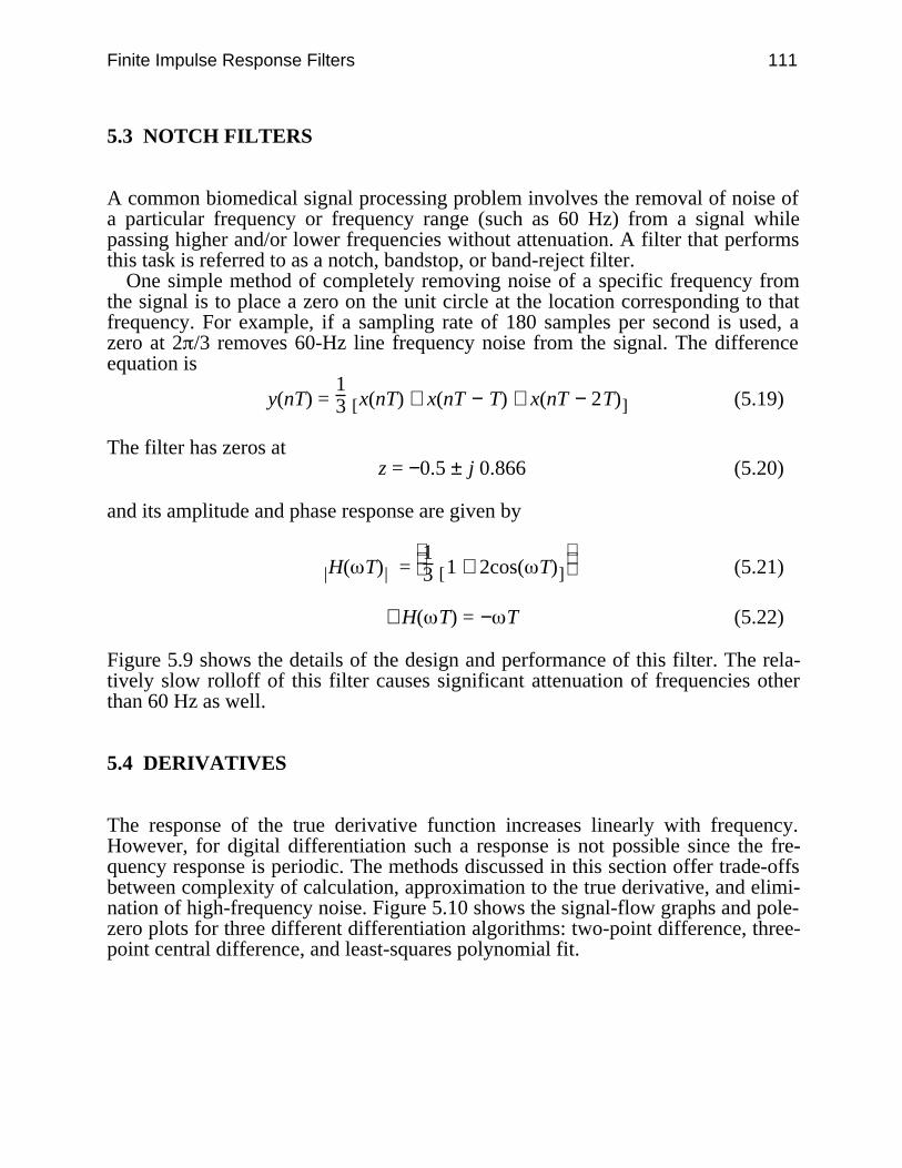
Finite Impulse Response Filters 111
5.3 NOTCH FILTERS
A common biomedical signal processing problem involves the removal of noise ofa particular frequency or frequency range (such as 60 Hz) from a signal whilepassing higher and/or lower frequencies without attenuation. A filter that performsthis task is referred to as a notch, bandstop, or band-reject filter.
One simple method of completely removing noise of a specific frequency fromthe signal is to place a zero on the unit circle at the location corresponding to thatfrequency. For example, if a sampling rate of 180 samples per second is used, azero at 2 /3 removes 60-Hz line frequency noise from the signal. The differenceequation is
y(nT) = 13 [ ]x(nT) + x(nT − T) + x(nT − 2T) (5.19)
The filter has zeros atz = −0.5 ± j 0.866 (5.20)
and its amplitude and phase response are given by
| |H( T) =
1
3 [ ]1 + 2cos( T) (5.21)
∠H( T) = − T (5.22)
Figure 5.9 shows the details of the design and performance of this filter. The rela-tively slow rolloff of this filter causes significant attenuation of frequencies otherthan 60 Hz as well.
5.4 DERIVATIVES
The response of the true derivative function increases linearly with frequency.However, for digital differentiation such a response is not possible since the fre-quency response is periodic. The methods discussed in this section offer trade-offsbetween complexity of calculation, approximation to the true derivative, and elimi-nation of high-frequency noise. Figure 5.10 shows the signal-flow graphs and pole-zero plots for three different differentiation algorithms: two-point difference, three-point central difference, and least-squares polynomial fit.
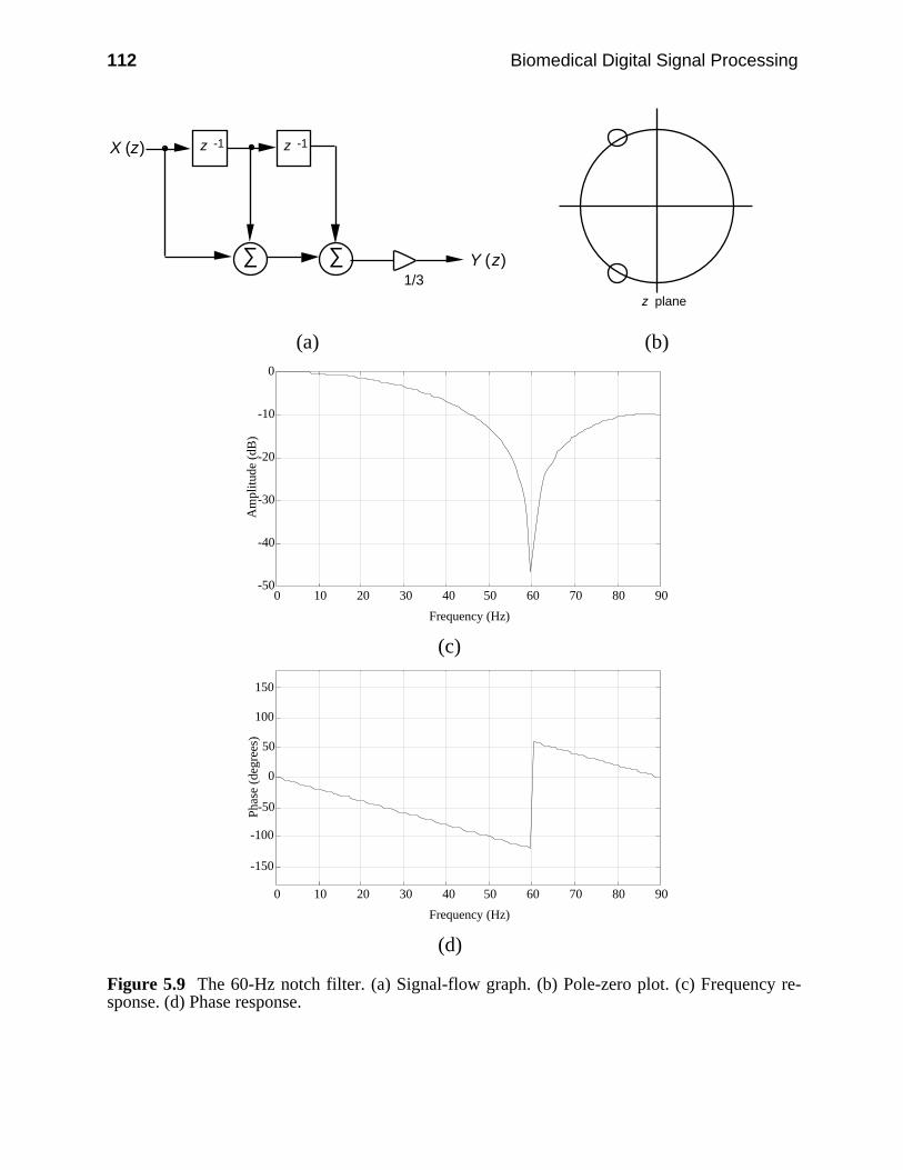
112 Biomedical Digital Signal Processing
X (z)
Y (z)
z -1
∑∑
z -1
1/3z plane
(a) (b)
-50
-40
-30
-20
-10
0
0 10 20 30 40 50 60 70 80 90
Frequency (Hz)
Am
plitu
de (
dB)
(c)
-150
-100
-50
0
50
100
150
0 10 20 30 40 50 60 70 80 90
Frequency (Hz)
Pha
se (
degr
ees)
(d)
Figure 5.9 The 60-Hz notch filter. (a) Signal-flow graph. (b) Pole-zero plot. (c) Frequency re-sponse. (d) Phase response.
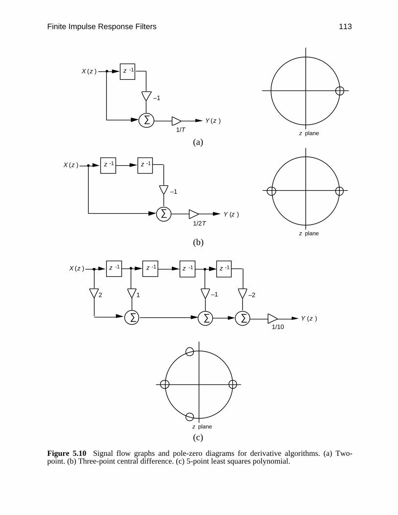
Finite Impulse Response Filters 113
X (z )
Y (z )∑
z -1
–1
1/T z plane
(a)
X (z )
Y (z )
z -1
∑
z -1
–1
1/2T
z plane
(b)
X (z )
Y (z )
z -1
∑∑
z -1
2
1/10
z -1 z -1
∑
1
–1 –2
z plane
(c)
Figure 5.10 Signal flow graphs and pole-zero diagrams for derivative algorithms. (a) Two-point. (b) Three-point central difference. (c) 5-point least squares polynomial.
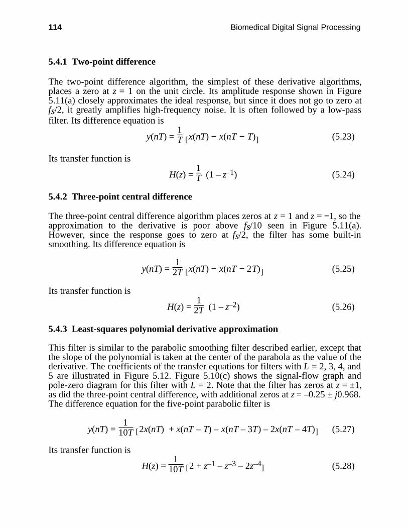
114 Biomedical Digital Signal Processing
5.4.1 Two-point difference
The two-point difference algorithm, the simplest of these derivative algorithms,places a zero at z = 1 on the unit circle. Its amplitude response shown in Figure5.11(a) closely approximates the ideal response, but since it does not go to zero atfs/2, it greatly amplifies high-frequency noise. It is often followed by a low-passfilter. Its difference equation is
y(nT) = 1T [ ]x(nT) − x(nT − T) (5.23)
Its transfer function is
H(z) = 1T (1 – z–1) (5.24)
5.4.2 Three-point central difference
The three-point central difference algorithm places zeros at z = 1 and z = −1, so theapproximation to the derivative is poor above fs/10 seen in Figure 5.11(a).However, since the response goes to zero at fs/2, the filter has some built-insmoothing. Its difference equation is
y(nT) = 1
2T [ ]x(nT) − x(nT − 2T) (5.25)
Its transfer function is
H(z) = 1
2T (1 – z–2) (5.26)
5.4.3 Least-squares polynomial derivative approximation
This filter is similar to the parabolic smoothing filter described earlier, except thatthe slope of the polynomial is taken at the center of the parabola as the value of thederivative. The coefficients of the transfer equations for filters with L = 2, 3, 4, and5 are illustrated in Figure 5.12. Figure 5.10(c) shows the signal-flow graph andpole-zero diagram for this filter with L = 2. Note that the filter has zeros at z = ±1,as did the three-point central difference, with additional zeros at z = –0.25 ± j0.968.The difference equation for the five-point parabolic filter is
y(nT) = 1
10T [ ]2x(nT) + x(nT – T) – x(nT – 3T) – 2x(nT – 4T) (5.27)
Its transfer function is
H(z) = 1
10T [ ]2 + z–1 – z–3 – 2z–4 (5.28)

Finite Impulse Response Filters 115
As Figure 5.11(a) shows, the response only approximates the true derivative at lowfrequencies, since the smoothing nature of the parabolic fit attenuates highfrequencies significantly.
-50
-40
-30
-20
-10
0
10-3 10-2 10-1 100
f/fs
Am
plitu
de (d
B)
(a)
-150
-100
-50
0
50
100
150
0 0.1 0.2 0.3 0.4 0.5
f/fs
Pha
se (
degr
ees)
(b)Figure 5.11 Derivatives. (a) Amplitude response. (b) Phase response. Solid line: Two-point.Circles: Three-point central difference. Dashed line: Least-squares parabolic approximation forL = 2.
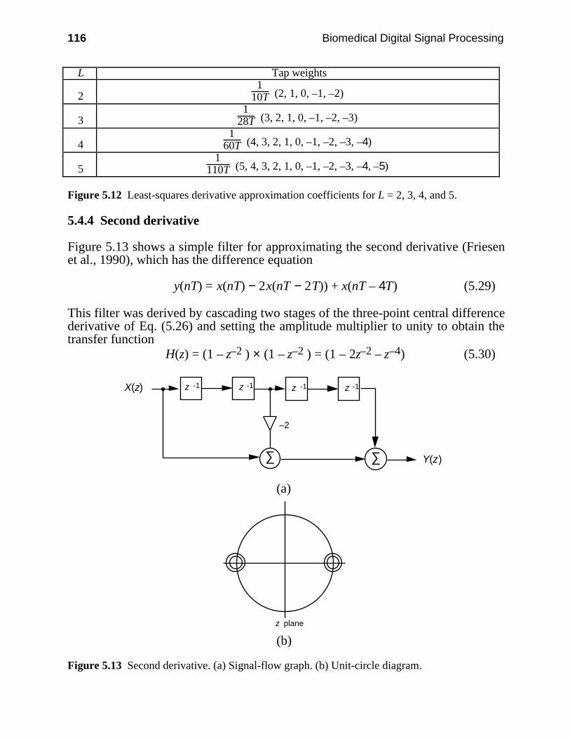
116 Biomedical Digital Signal Processing
L Tap weights
21
10T (2, 1, 0, –1, –2)
31
28T (3, 2, 1, 0, –1, –2, –3)
41
60T (4, 3, 2, 1, 0, –1, –2, –3, –4)
51
110T (5, 4, 3, 2, 1, 0, –1, –2, –3, –4, –5)
Figure 5.12 Least-squares derivative approximation coefficients for L = 2, 3, 4, and 5.
5.4.4 Second derivative
Figure 5.13 shows a simple filter for approximating the second derivative (Friesenet al., 1990), which has the difference equation
y(nT) = x(nT) − 2x(nT − 2T)) + x(nT – 4T) (5.29)
This filter was derived by cascading two stages of the three-point central differencederivative of Eq. (5.26) and setting the amplitude multiplier to unity to obtain thetransfer function
H(z) = (1 – z–2 ) × (1 – z–2 ) = (1 – 2z–2 – z–4) (5.30)
X(z)
Y(z)
z -1
∑
z -1z -1
∑
–2
z -1
(a)
z plane
(b)
Figure 5.13 Second derivative. (a) Signal-flow graph. (b) Unit-circle diagram.
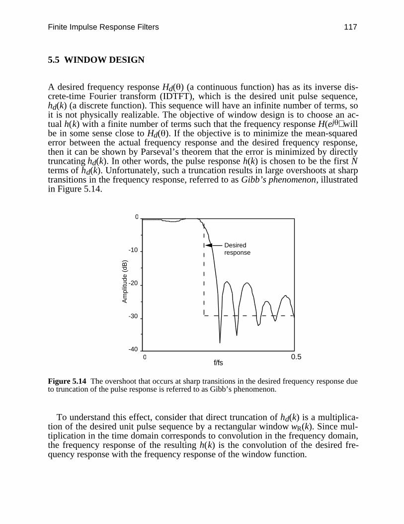
Finite Impulse Response Filters 117
5.5 WINDOW DESIGN
A desired frequency response Hd( ) (a continuous function) has as its inverse dis-crete-time Fourier transform (IDTFT), which is the desired unit pulse sequence,hd(k) (a discrete function). This sequence will have an infinite number of terms, soit is not physically realizable. The objective of window design is to choose an ac-tual h(k) with a finite number of terms such that the frequency response H(ej ) willbe in some sense close to Hd( ). If the objective is to minimize the mean-squarederror between the actual frequency response and the desired frequency response,then it can be shown by Parseval’s theorem that the error is minimized by directlytruncating hd(k). In other words, the pulse response h(k) is chosen to be the first Nterms of hd(k). Unfortunately, such a truncation results in large overshoots at sharptransitions in the frequency response, referred to as Gibb’s phenomenon, illustratedin Figure 5.14.
-40
-30
-20
-10
0
Am
plitu
de (
dB)
0 0.5
Desiredresponse
f/fs
Figure 5.14 The overshoot that occurs at sharp transitions in the desired frequency response dueto truncation of the pulse response is referred to as Gibb’s phenomenon.
To understand this effect, consider that direct truncation of hd(k) is a multiplica-tion of the desired unit pulse sequence by a rectangular window wR(k). Since mul-tiplication in the time domain corresponds to convolution in the frequency domain,the frequency response of the resulting h(k) is the convolution of the desired fre-quency response with the frequency response of the window function.
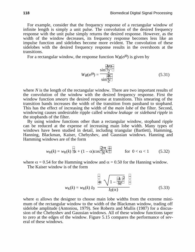
118 Biomedical Digital Signal Processing
For example, consider that the frequency response of a rectangular window ofinfinite length is simply a unit pulse. The convolution of the desired frequencyresponse with the unit pulse simply returns the desired response. However, as thewidth of the window decreases, its frequency response becomes less like animpulse function and sidelobes become more evident. The convolution of thesesidelobes with the desired frequency response results in the overshoots at thetransitions.
For a rectangular window, the response function WR(ej ) is given by
WR(ej ) = sin
N
2
sin
2
(5.31)
where N is the length of the rectangular window. There are two important results ofthe convolution of the window with the desired frequency response. First thewindow function smears the desired response at transitions. This smearing of thetransition bands increases the width of the transition from passband to stopband.This has the effect of increasing the width of the main lobe of the filter. Second,windowing causes undesirable ripple called window leakage or sideband ripple inthe stopbands of the filter.
By using window functions other than a rectangular window, stopband ripplecan be reduced at the expense of increasing main lobe width. Many types ofwindows have been studied in detail, including triangular (Bartlett), Hamming,Hanning, Blackman, Kaiser, Chebyshev, and Gaussian windows. Hanning andHamming windows are of the form
wH(k) = wR(k)
+ (1 – )cos
2π
N k for 0 < < 1 (5.32)
where = 0.54 for the Hamming window and = 0.50 for the Hanning window.The Kaiser window is of the form
wK(k) = wR(k) I0
1 –
k
M2
I0( ) (5.33)
where allows the designer to choose main lobe widths from the extreme mini-mum of the rectangular window to the width of the Blackman window, trading offsidelobe amplitude (Antoniou, 1979). See Roberts and Mullis (1987) for a discus-sion of the Chebyshev and Gaussian windows. All of these window functions taperto zero at the edges of the window. Figure 5.15 compares the performance of sev-eral of these windows.
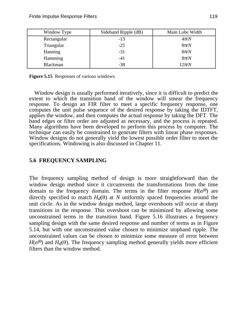
Finite Impulse Response Filters 119
Window Type Sideband Ripple (dB) Main Lobe Width
Rectangular -13 4π/NTriangular -25 8π/NHanning -31 8π/NHamming -41 8π/NBlackman -38 12π/N
Figure 5.15 Responses of various windows.
Window design is usually performed iteratively, since it is difficult to predict theextent to which the transition band of the window will smear the frequencyresponse. To design an FIR filter to meet a specific frequency response, onecomputes the unit pulse sequence of the desired response by taking the IDTFT,applies the window, and then computes the actual response by taking the DFT. Theband edges or filter order are adjusted as necessary, and the process is repeated.Many algorithms have been developed to perform this process by computer. Thetechnique can easily be constrained to generate filters with linear phase responses.Window designs do not generally yield the lowest possible order filter to meet thespecifications. Windowing is also discussed in Chapter 11.
5.6 FREQUENCY SAMPLING
The frequency sampling method of design is more straightforward than thewindow design method since it circumvents the transformations from the timedomain to the frequency domain. The terms in the filter response H(ej ) aredirectly specified to match Hd( ) at N uniformly spaced frequencies around theunit circle. As in the window design method, large overshoots will occur at sharptransitions in the response. This overshoot can be minimized by allowing someunconstrained terms in the transition band. Figure 5.16 illustrates a frequencysampling design with the same desired response and number of terms as in Figure5.14, but with one unconstrained value chosen to minimize stopband ripple. Theunconstrained values can be chosen to minimize some measure of error betweenH(ej ) and Hd( ). The frequency sampling method generally yields more efficientfilters than the window method.
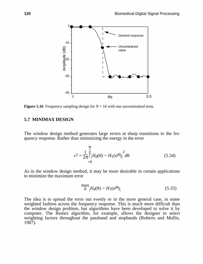
120 Biomedical Digital Signal Processing
-40
-30
-20
-10
0
Am
plitu
de (
dB)
0 0.5
Desired response
Unconstrainedvalue
f/fs
Figure 5.16 Frequency sampling design for N = 16 with one unconstrained term.
5.7 MINIMAX DESIGN
The window design method generates large errors at sharp transitions in the fre-quency response. Rather than minimizing the energy in the error
2 = 1
2π ⌡⌠
-π
π
| |Hd( ) − H1(ej )2d (5.34)
As in the window design method, it may be more desirable in certain applicationsto minimize the maximum error
max| |Hd( ) − H1(ej ) (5.35)
The idea is to spread the error out evenly or in the more general case, in someweighted fashion across the frequency response. This is much more difficult thanthe window design problem, but algorithms have been developed to solve it bycomputer. The Remez algorithm, for example, allows the designer to selectweighting factors throughout the passband and stopbands (Roberts and Mullis,1987).
Finite Impulse Response Filters 121
5.8 LAB: FIR FILTER DESIGN
The UW DigiScope software allows the user to experiment with several FIRdesign techniques, including direct specification of the pulse response, frequencysampling, window design, and placement of the zeros of the transfer equation. Thislab studies some basic FIR filters such as the Hanning filter. It also usesspecification of the pulse response and placement of the zeros of the transferequation as design tools. Refer to Appendix D for information about using UWDigiScope.
5.8.1 Smoothing filters
Generate an ECG file with some random noise with the (G)enwave function, thenrun the Hanning filter by selecting (F)ilters, then (L)oad filter , then choos-ing hanning.fil. This function loads and immediately executes the filterfunction. By choosing (R)un filter, you can see the effect of cascading anotherHanning filter with the first. The filter always operates on the data in the bottomchannel.
The filters poly2.fil, poly3.fil, and poly4.fil are the least-squaressmoothing filters with L = 2, 3, and 4 respectively. To test each of these three fil-ters on the ECG data, first move the original signal from the top channel to thebottom channel with the (C)opy data command. Then use (L)oad filter toload and run the filters on ECG data. Observe the frequency and phase responsesof each filter. How does changing the sampling rate of the ECG data affect theperformance of the filters? Load poly4.fil and measure the time differencebetween the peak of the QRS complex in the unfiltered data and in the filtered datausing the (M)easure command. You will need to change channels using(A)ctive channel to make the measurements. How do you account for thedelay?
5.8.2 Derivatives
Experiment with the various derivative filters deriv2.fil, deriv3.fil, andderiv5.fil (which are the two-point, three-point central limit, and least-squareswith L = 2 derivative filters respectively) on ECG and square wave data. Whichfilter is least suited for use with noisy signals?
5.8.3 Pulse Response
Create a filter that calculates the second derivative by selecting (F)ilters, then(D)esign, then (F)IR. Choose (P)ulse resp, and specify a filter length equal to5. Enter the appropriate coefficients for the transfer equation and observe the fre-quency response. After saving the filter, return to the main menu, create a triangu-lar wave with the (G)enwave function, and then use (R)un filter to observe theeffects of the filter.
122 Biomedical Digital Signal Processing
Create a linear phase filter with odd length (even order) and odd symmetry bysatisfying Eq. (5.4). Observe its phase response.
5.8.4 Zero placement
The user may arbitrarily place zeros around the unit circle. The program automati-cally creates complex-conjugate pairs for values off the real axis. It then calculatesthe frequency, phase, and unit impulse responses for the filter.
Place zeros at z = −0.5 ± j0.866 using the (Z)ero place function for a second-order filter, and comment on the frequency response. Run this filter on ECG datawith and without 60-Hz noise sampled at 180 samples/s, and summarize the re-sults.
5.8.5 Unit pulse sequence
There is a data file in the STDLIB called ups.dat. It consists of a single pulse.Reading this file and running an FIR filter will generate the unit impulse output se-quence of the filter. Executing (P)wr Spect on this resulting output signal willgive the magnitude response of the filter. In this way, the frequency response of fil-ter can be measured more accurately than by the graph generated in the filter de-sign utility. Use this method to find the 3-dB frequency of the Hanning filter (i.e.,file hanning.fil).
5.8.6 Frequency sampling
Study the effect of increasing the width of the transition band by comparing thefrequency response FIR filters of length 13 designed using frequency sampling byentering the following sets of values for the responses around the unit circle: 0, 0,–40, –40, –40, –40, –40 and 0, 0, –6, –40, –40, –40, –40. Optimize thetransition value (the third term in the sequence) for minimum stopband ripple.
Design a 60-Hz notch filter with length 21 by using frequency sampling. Run thefilter on ECG data with and without 60-Hz noise. Does the filter perform betterthan notch60.fil? Optimize the filter for minimal gain at 60 Hz and minimal at-tenuation of other frequencies.
5.8.7 Window design
Compare the frequency response of low-pass filters designed with the various win-dows of the (W)indow function. Design the filters to have a cutoff frequency at 25Hz with a sampling rate of 200 Hz. Make a table comparing main lobe widthversus sideband ripple for the various windows. Measure the main lobe width atthe first minimum in the frequency response.
5.8.8 Linear versus piecewise-linear phase response
Compare the phase response of the Hanning filter with that of the least-squaresderivative filter with L = 2 (deriv5.fil). Why is the phase response of the least-

Finite Impulse Response Filters 123
squares filter not true linear? What causes the discontinuity? See Chapter 7 for ad-ditional information.
5.9 REFERENCES
Antoniou, A. 1979. Digital Filters: Analysis and Design. New York: McGraw-Hill.Bogner, R. E. and Constantinides, A. G. 1985. Introduction to Digital Filtering, New York: John
Wiley and Sons.Friesen, G. M. et al. 1990. A comparison of the noise sensitivity of nine QRS detection algo-
rithms, IEEE Trans. Biomed. Eng., BME-37(1): 85–98.Hamming, R. W. 1977. Digital Filters. Englewood Cliffs, NJ: Prentice Hall.Rabiner, L. R. and Rader, C. M. 1972. Digital Signal Processing New York: IEEE Press.Roberts, R. A. and Mullis, R. T. 1987. Digital Signal Processing. Reading, MA: Addison-
Wesley.
5.10 STUDY QUESTIONS
5.1 What are the main differences between FIR and IIR filters?5.2 What is the difference between direct convolution and “fast convolution”?5.3 Why are finite-length register effects less significant in FIR filters than in IIR filters?5.4 Compute and sketch the frequency response of a cascade of two Hanning filters. Does the
cascade have linear phase?5.5 Derive the phase response for an FIR filter with zeros located at r∠± and r–1∠± .
Comment.5.6 What are the trade-offs to consider when choosing the order of a least-squares polynomial
smoothing filter?5.7 Complete the derivation of coefficient values for the parabolic smoothing filter for L = 2.5.8 Give some of the disadvantages of the simple 60-Hz notch filter described in section 5.3.1.5.9 What are the main differences between the two-point difference and three-point central
difference algorithms for approximating the derivative?5.10 What are the three steps to designing a filter using the window method?5.11 Explain the relationship between main-lobe width and sideband ripple for various windows.5.12 How do the free parameters in the transition band of a frequency sampling design affect the
performance of the filter?5.13 What is the fundamental difference between minimax design and the window design
method?5.14 Design an FIR filter of length 15 with passband gain of 0 dB from 0 to 50 Hz and stopband
attenuation of 40 dB from 100 to 200 Hz using the window design method. Compare theHanning and rectangular windows. (Use a sampling rate of 400 sps.)
5.15 Repeat question 5.14 using frequency sampling.5.16 The transfer function of the Hanning filter is
H1(z) = 1 + 2z–1 + z–2
4
(a) What is its gain at dc? (b) Three successive stages of this filter are cascaded together togive a new transfer function [that is, H(z) = H1(z) × H1(z) × H1(z)]. What is the overall gainof this filter at dc? (c) A high-pass filter is designed by subtracting the output of the

124 Biomedical Digital Signal Processing
Hanning filter from an all-pass filter with zero phase delay. How many zeros does the re-sulting filter have? Where are they located?
5.17 Two filters are cascaded. The first has the transfer function: H1(z) = 1 + 2z–1 – 3z–2. Thesecond has the transfer function: H2(z) = 1 – 2 z–1. A unit impulse is applied to the input ofthe cascaded filters. (a) What is the output sequence? (b) What is the magnitude of theamplitude response of the cascaded filter 1. at dc? 2. at 1/2 the foldover frequency? 3. at thefoldover frequency?
5.18 Two filters are cascaded. The first has the transfer function: H1(z) = 1 + 2z–1 + z–2. Thesecond has the transfer function: H2(z) = 1 – z–1. (a) A unit impulse is applied to the inputof the cascaded filters. What is the output sequence? (b) What is the magnitude of theamplitude response of this cascaded filter at dc?
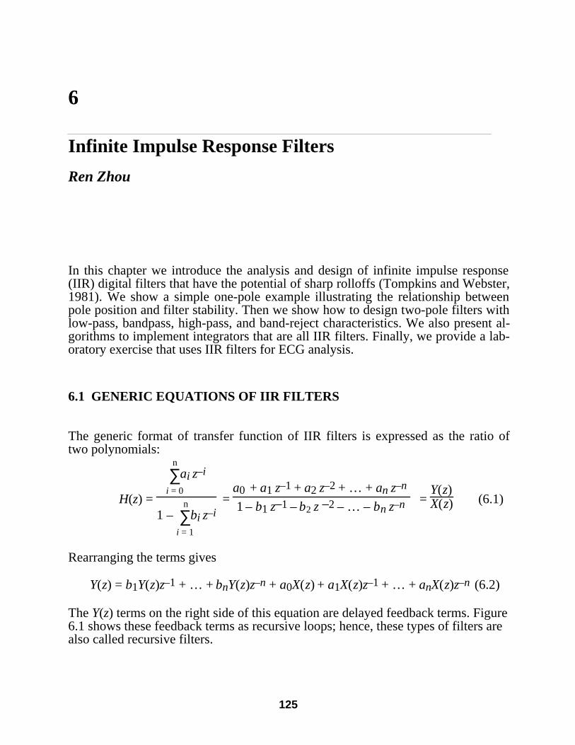
125
6
Infinite Impulse Response Filters
Ren Zhou
In this chapter we introduce the analysis and design of infinite impulse response(IIR) digital filters that have the potential of sharp rolloffs (Tompkins and Webster,1981). We show a simple one-pole example illustrating the relationship betweenpole position and filter stability. Then we show how to design two-pole filters withlow-pass, bandpass, high-pass, and band-reject characteristics. We also present al-gorithms to implement integrators that are all IIR filters. Finally, we provide a lab-oratory exercise that uses IIR filters for ECG analysis.
6.1 GENERIC EQUATIONS OF IIR FILTERS
The generic format of transfer function of IIR filters is expressed as the ratio oftwo polynomials:
H(z) =
∑i = 0
nai z–i
1 – ∑i = 1
nbi z–i
= a0 + a1 z–1 + a2 z–2 + … + an z–n
1 – b1 z–1 – b2 z –2 – … – bn z–n = Y(z)X(z) (6.1)
Rearranging the terms gives
Y(z) = b1Y(z)z–1 + … + bnY(z)z–n + a0X(z) + a1X(z)z–1 + … + anX(z)z–n (6.2)
The Y(z) terms on the right side of this equation are delayed feedback terms. Figure6.1 shows these feedback terms as recursive loops; hence, these types of filters arealso called recursive filters.

126 Biomedical Digital Signal Processing
.
.
.
Σ
-1-1z -1-1z
-1-1z
-1-1z
-1-1z
-1-1z
X (z )
Y (z )
b1
b2
bna0
a1
a2
an
.
.
.
Figure 6.1 The output of an IIR filter is delayed and fed back.
6.2 SIMPLE ONE-POLE EXAMPLE
Let us consider the simple filter of Figure 6.2(a). We find the transfer function byapplying a unit impulse sequence to the input X(z). Figure 6.2(b) shows thesequences at various points in the filter for a feedback coefficient equal to 1/2.Sequence (1) defines the unit impulse. From output sequence (2), we write thetransfer function
H(z) = 1 + 12 z–1 +
14 z–2 +
18 z–3 + … (6.3)
Using the binomial theorem, we write the infinite sum as a ratio of polynomials
H(z) = Y(z)X(z) =
1
1 – 12 z–1
(6.4)
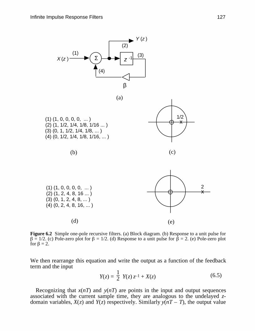
Infinite Impulse Response Filters 127
Σ(1)
(2)
(3)
(4)
β
(a)
(1) (1, 0, 0, 0, 0, ... )(2) (1, 1/2, 1/4, 1/8, 1/16 ... )(3) (0, 1, 1/2, 1/4, 1/8, ... ) (4) (0, 1/2, 1/4, 1/8, 1/16, ... )
(b)
x1/2
(c)
-1-1z
(1) (1, 0, 0, 0, 0, ... )(2) (1, 2, 4, 8, 16 ... )(3) (0, 1, 2, 4, 8, ... )(4) (0, 2, 4, 8, 16, ... )
(d) (e)
x2
X (z )
Y (z )
Figure 6.2 Simple one-pole recursive filters. (a) Block diagram. (b) Response to a unit pulse for = 1/2. (c) Pole-zero plot for = 1/2. (d) Response to a unit pulse for = 2. (e) Pole-zero plot
for = 2.
We then rearrange this equation and write the output as a function of the feedbackterm and the input
Y(z) = 12 Y(z) z–1 + X(z) (6.5)
Recognizing that x(nT) and y(nT) are points in the input and output sequencesassociated with the current sample time, they are analogous to the undelayed z-domain variables, X(z) and Y(z) respectively. Similarly y(nT – T), the output value
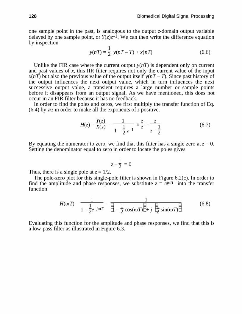
128 Biomedical Digital Signal Processing
one sample point in the past, is analogous to the output z-domain output variabledelayed by one sample point, or Y(z)z–1. We can then write the difference equationby inspection
y(nT) = 12 y(nT – T) + x(nT) (6.6)
Unlike the FIR case where the current output y(nT) is dependent only on currentand past values of x, this IIR filter requires not only the current value of the inputx(nT) but also the previous value of the output itself y(nT – T). Since past history ofthe output influences the next output value, which in turn influences the nextsuccessive output value, a transient requires a large number or sample pointsbefore it disappears from an output signal. As we have mentioned, this does notoccur in an FIR filter because it has no feedback.
In order to find the poles and zeros, we first multiply the transfer function of Eq.(6.4) by z/z in order to make all the exponents of z positive.
H(z) = Y(z)X(z) =
1
1 – 12 z–1
× zz =
z
z – 12
(6.7)
By equating the numerator to zero, we find that this filter has a single zero at z = 0.Setting the denominator equal to zero in order to locate the poles gives
z – 12 = 0
Thus, there is a single pole at z = 1/2.The pole-zero plot for this single-pole filter is shown in Figure 6.2(c). In order to
find the amplitude and phase responses, we substitute z = ej T into the transferfunction
H( T) = 1
1 – 12e–j T
= 1
1 – 12 cos( T) + j
1
2 sin( T) (6.8)
Evaluating this function for the amplitude and phase responses, we find that this isa low-pass filter as illustrated in Figure 6.3.
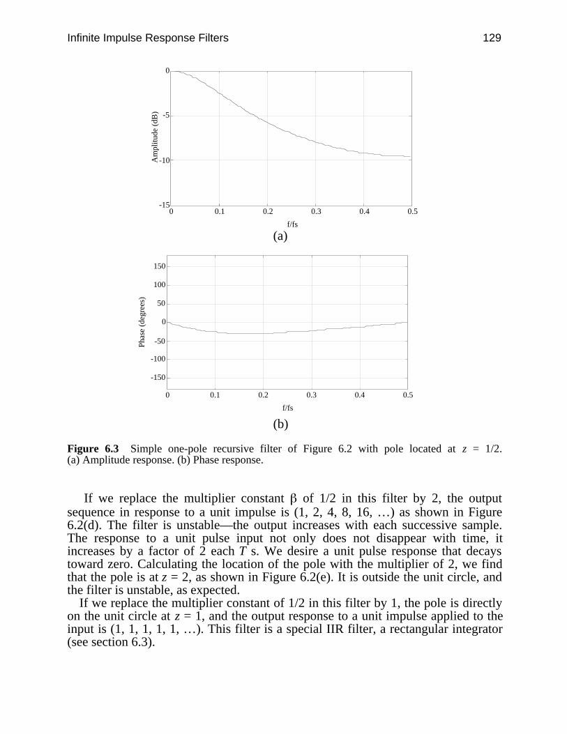
Infinite Impulse Response Filters 129
-15
-10
-5
0
0 0.1 0.2 0.3 0.4 0.5
f/fs
Am
plitu
de (
dB)
(a)
-150
-100
-50
0
50
100
150
0 0.1 0.2 0.3 0.4 0.5
f/fs
Phas
e (d
egre
es)
(b)
Figure 6.3 Simple one-pole recursive filter of Figure 6.2 with pole located at z = 1/2.(a) Amplitude response. (b) Phase response.
If we replace the multiplier constant of 1/2 in this filter by 2, the outputsequence in response to a unit impulse is (1, 2, 4, 8, 16, …) as shown in Figure6.2(d). The filter is unstable—the output increases with each successive sample.The response to a unit pulse input not only does not disappear with time, itincreases by a factor of 2 each T s. We desire a unit pulse response that decaystoward zero. Calculating the location of the pole with the multiplier of 2, we findthat the pole is at z = 2, as shown in Figure 6.2(e). It is outside the unit circle, andthe filter is unstable, as expected.
If we replace the multiplier constant of 1/2 in this filter by 1, the pole is directlyon the unit circle at z = 1, and the output response to a unit impulse applied to theinput is (1, 1, 1, 1, 1, …). This filter is a special IIR filter, a rectangular integrator(see section 6.3).

130 Biomedical Digital Signal Processing
6.3 INTEGRATORS
The general form of the integral is
A = ⌡⌠
t1t2
f(t)dt (6.9)
where A is the area under the function between the limits t1 to t2. The digital im-plementation for the determination of integral solutions is done by approximatingthe function using curve fitting techniques at a finite number of points, where
A = ∑n = t1
t2 f(n) t (6.10)
The Laplace transform of an integrator is
H(s) = 1s (6.11)
The amplitude and phase responses are found by substituting into the transferfunction the relation, s = j , giving
H(j ) = 1
j (6.12)
Thus, the ideal amplitude response is inversely proportional to frequency
|H(j )| =
1
(6.13)
and the phase response is
∠H(j ) = tan–1
–1/ω
0 = – π2 (6.14)
A number of numerical techniques exist for digital integration. Unlike the analogintegrator, a digital integrator has no drift problems because the process is a com-puter program, which is not influenced in performance by residual charge on ca-pacitors. We discuss here three popular digital integration techniques—rectangularsummation, trapezoidal summation, and Simpson’s rule.
6.3.1 Rectangular integration
This algorithm performs the simplest integration. It approximates the integral as asum of rectangular areas. Figure 6.4(a) shows that each rectangle has a base equalin length to one sample period T and in height to the value of the most recently

Infinite Impulse Response Filters 131
sampled input x(nT – T). The area of each rectangle is Tx(nT – T). The differenceequation is
y(nT) = y(nT – T) + T x(nT) (6.15)
where y(nT – T) represents the sum of all the rectangular areas prior to adding themost recent one. The error in this approximation is the difference between the areaof the rectangle and actual signal represented by the sampled data. The z transformof Eq. (6.15) is
Y(z) = Y(z) z–1 + T X(z) (6.16)and
H(z) = Y(z)X(z) = T
1
1 – z–1 (6.17)
Figure 6.4(a) shows that this transfer function has a pole at z = 1 and a zero atz = 0. The amplitude and phase responses are
|H( T)| =
T
2 sin( T/2) (6.18)
and
∠H( T) = T
2 – π2 (6.19)
Figure 6.5 shows the amplitude response. We can reduce the error of this filterby increasing the sampling rate significantly higher than the highest frequency pre-sent in the signal that we are integrating. This has the effect of making the width ofeach rectangle small compared to the rate of change of the signal, so that the areaof each rectangle better approximates the input data. Increasing the sampling ratealso corresponds to using only the portion of amplitude response at the lower fre-quencies, where the rectangular response better approximates the ideal response.Unfortunately, higher than necessary sampling rates increase computation time andwaste memory space by giving us more sampled data than are necessary to charac-terize a signal. Therefore, we select other digital integrators for problems wherehigher performance is desirable.
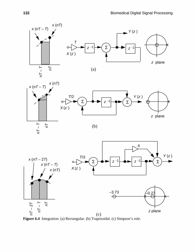
132 Biomedical Digital Signal Processing
X (z )
Y (z )
T
z plane
x (nT – T)x (nT)
nT
– T
nT
(a)
z -1 z -1
X (z )
T/3 Y (z )
4
z plane
–0.27
x (nT – T)x (nT)
nT
– T
nT
nT
– 2
T
x (nT – 2T)
–3.73
(c)
z -1 z -1
X (z )
T/2 Y (z )
z plane
x (nT – T)x (nT)
nT
– T
nT
(b)
z -1
x x
x
x
Σ
Σ
Σ
Σ
Σ
Figure 6.4 Integration. (a) Rectangular. (b) Trapezoidal. (c) Simpson’s rule.
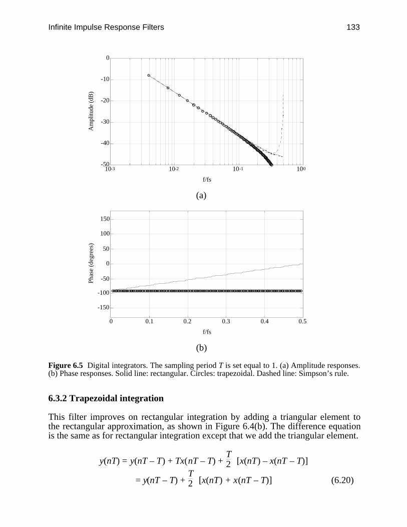
Infinite Impulse Response Filters 133
-50
-40
-30
-20
-10
0
10-3 10-2 10-1 100
f/fs
Am
plitu
de (d
B)
(a)
-150
-100
-50
0
50
100
150
0 0.1 0.2 0.3 0.4 0.5
f/fs
Phas
e (d
egre
es)
(b)
Figure 6.5 Digital integrators. The sampling period T is set equal to 1. (a) Amplitude responses.(b) Phase responses. Solid line: rectangular. Circles: trapezoidal. Dashed line: Simpson’s rule.
6.3.2 Trapezoidal integration
This filter improves on rectangular integration by adding a triangular element tothe rectangular approximation, as shown in Figure 6.4(b). The difference equationis the same as for rectangular integration except that we add the triangular element.
y(nT) = y(nT – T) + Tx(nT – T) + T2 [x(nT) – x(nT – T)]
= y(nT – T) + T2 [x(nT) + x(nT – T)] (6.20)
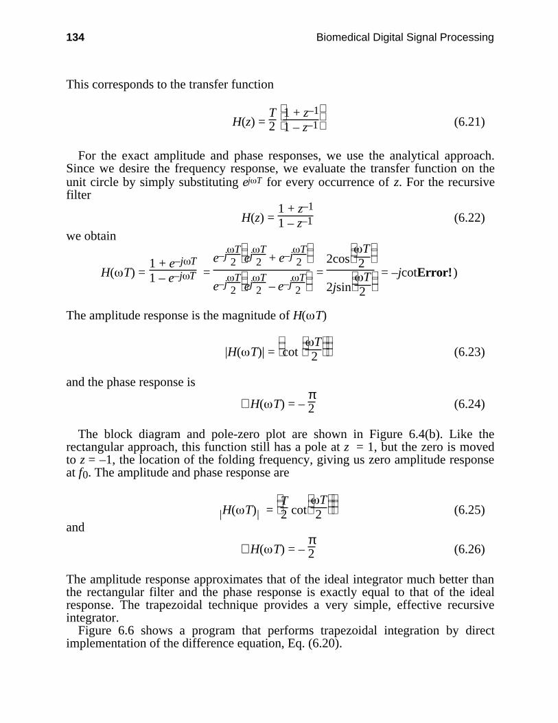
134 Biomedical Digital Signal Processing
This corresponds to the transfer function
H(z) = T2
1 + z–1
1 – z–1 (6.21)
For the exact amplitude and phase responses, we use the analytical approach.Since we desire the frequency response, we evaluate the transfer function on theunit circle by simply substituting ej T for every occurrence of z. For the recursivefilter
H(z) = 1 + z–1
1 – z–1 (6.22)
we obtain
H( T) = 1 + e–j T
1 – e–j T = e–j
T2
ejT
2 + e–j
T2
e–jT
2
ejT
2 – e–j
T2
= 2cos
T
2
2jsin
T
2
= –jcotError!)
The amplitude response is the magnitude of H( T)
|H( T)| =
cot
T
2 (6.23)
and the phase response is
∠H( T) = – π2 (6.24)
The block diagram and pole-zero plot are shown in Figure 6.4(b). Like therectangular approach, this function still has a pole at z = 1, but the zero is movedto z = –1, the location of the folding frequency, giving us zero amplitude responseat f0. The amplitude and phase response are
| |H( T) =
T
2 cot
T
2 (6.25)and
∠H( T) = – π2 (6.26)
The amplitude response approximates that of the ideal integrator much better thanthe rectangular filter and the phase response is exactly equal to that of the idealresponse. The trapezoidal technique provides a very simple, effective recursiveintegrator.
Figure 6.6 shows a program that performs trapezoidal integration by directimplementation of the difference equation, Eq. (6.20).

Infinite Impulse Response Filters 135
/*************************************************************** * Turbo C source code implementing a trapezoidal integrator * * Assume sampling period is 2 ms, the difference equation is: * * y(nT) = y(nT – T) + 0.001x(nT) + 0.001x(nT – T) * **************************************************************/float Trapezoid(signal)float signal; /* x[nT] */static float x[2], y[2];int count;
x[1]=x[0]; /* x[1]=x(nT–T) */x[0]=signal; /* x[0]=x(nT) */
y[0]=y[1]+0.001*x[0]+0.001*x[1];/* difference equation */
y[1]=y[0]; /* y[1]=y(nT – T) */
return y[0];
Figure 6.6 A trapezoidal integrator written in the C language.
6.3.3 Simpson’s rule integration
Simpson’s rule is the most widely used numerical integration algorithm. Figure6.4(c) shows that this approach approximates the signal corresponding to threeinput sequence points by a polynomial fit. The incremental area added for eachnew input point is the area under this polynomial. The difference equation is
y(nT) = y(nT – 2T) + T3 [x(nT) + 4x(nT – T) + x(nT – 2T)] (6.27)
The transfer function is
H(z) = T3
1 + 4z–1 + z–2
1 – z –2 (6.28)
Figure 6.4(c) shows the block diagram and pole-zero plot for this filter. The ampli-tude and phase responses are
| |H( T) =
T
2
2 + cos T
sin T (6.29)
and

136 Biomedical Digital Signal Processing
∠H( T) = – π2 (6.30)
Figure 6.5 shows the amplitude response of the Simpson’s rule integrator. Likethe trapezoidal technique, the phase response is the ideal –π/2. Simpson’s ruleapproximates the ideal integrator for frequencies less than about fs/4 better than theother techniques. However, it amplifies high-frequency noise near the foldoverfrequency. Therefore, it is a good approximation to the integral but is dangerous touse in the presence of noise. Integration of noisy signals can be accomplishedbetter with trapezoidal integration.
6.4 DESIGN METHODS FOR TWO-POLE FILTERS
IIR filters have the potential for sharp rolloffs. Unlike the design of an FIR filter,which frequently is based on approximating an input sequence numerically, IIRfilter design frequently starts with an analog filter that we would like to approxi-mate. Their transfer functions can be represented by an infinite sum of terms or ra-tio of polynomials. Since they use feedback, they may be unstable if improperlydesigned. Also, they typically do not have linear phase response.
6.4.1 Selection method for r and
The general design equation has a standard recursive form for the four types offilters: low-pass, bandpass, high-pass, and band-reject:
H(z) = 1 + a1z–1 + a2z–2
1 – b1z–1 + b2z–2 (6.31)
where the zero locations are
z = –a1 ± a12 – 4a2
2 (6.32)and the pole locations are
z = b1 ± b12 – 4b2
2 (6.33)where
b1 = 2rcos and b2 = r2 (6.34)Also
= 2π
fc
fs (6.35)
Figure 6.7 shows the structure of the two-pole filter. Assigning values to the nu-merator coefficients, a1 and a2, as shown in Figure 6.8 establishes the placement of
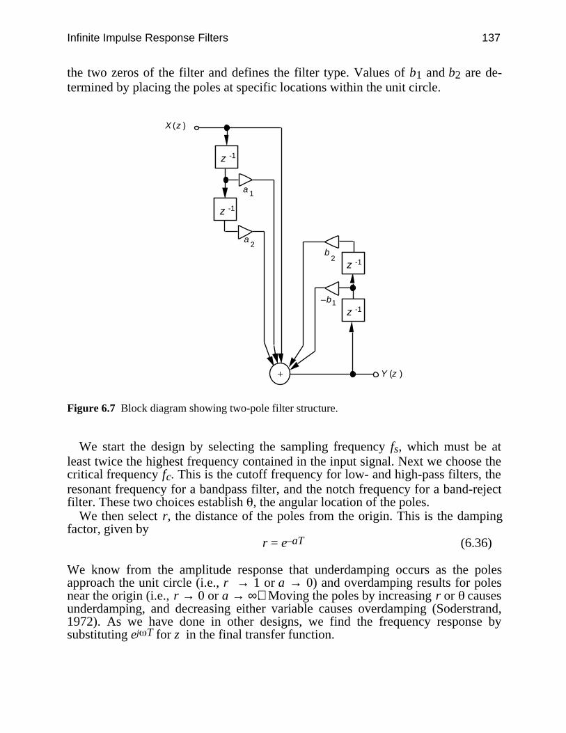
Infinite Impulse Response Filters 137
the two zeros of the filter and defines the filter type. Values of b1 and b2 are de-termined by placing the poles at specific locations within the unit circle.
a
a
+
–b
b
-1-1z
-1-1z
-1-1z
-1-1z
X (z )
Y (z )
1
2
1
2
Figure 6.7 Block diagram showing two-pole filter structure.
We start the design by selecting the sampling frequency fs, which must be atleast twice the highest frequency contained in the input signal. Next we choose thecritical frequency fc. This is the cutoff frequency for low- and high-pass filters, theresonant frequency for a bandpass filter, and the notch frequency for a band-rejectfilter. These two choices establish , the angular location of the poles.
We then select r, the distance of the poles from the origin. This is the dampingfactor, given by
r = e–aT (6.36)
We know from the amplitude response that underdamping occurs as the polesapproach the unit circle (i.e., r → 1 or a → 0) and overdamping results for polesnear the origin (i.e., r → 0 or a → ∞). Moving the poles by increasing r or causesunderdamping, and decreasing either variable causes overdamping (Soderstrand,1972). As we have done in other designs, we find the frequency response bysubstituting ej T for z in the final transfer function.
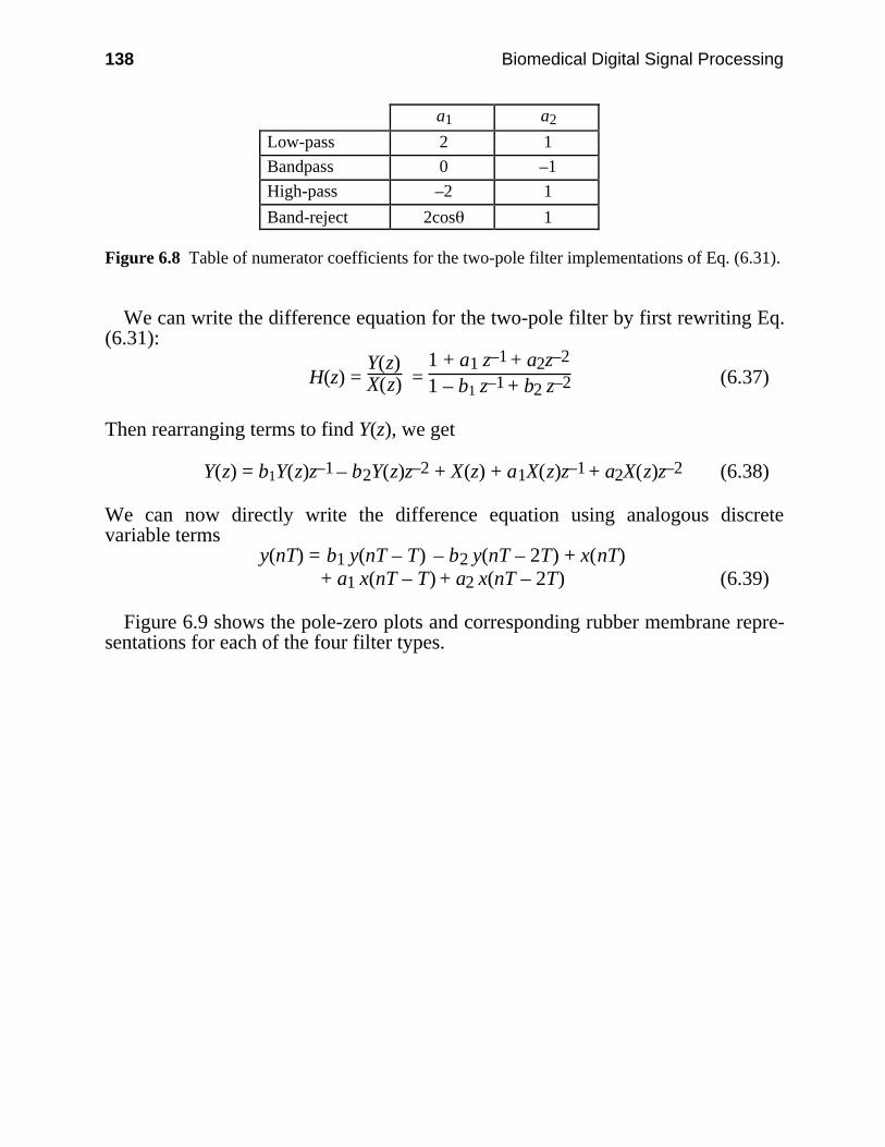
138 Biomedical Digital Signal Processing
a1 a2
Low-pass 2 1
Bandpass 0 –1
High-pass –2 1
Band-reject 2cos 1
Figure 6.8 Table of numerator coefficients for the two-pole filter implementations of Eq. (6.31).
We can write the difference equation for the two-pole filter by first rewriting Eq.(6.31):
H(z) = Y(z)X(z) =
1 + a1 z–1 + a2z–2
1 – b1 z–1 + b2 z–2 (6.37)
Then rearranging terms to find Y(z), we get
Y(z) = b1Y(z)z–1 – b2Y(z)z–2 + X(z) + a1X(z)z–1 + a2X(z)z–2 (6.38)
We can now directly write the difference equation using analogous discretevariable terms
y(nT) = b1 y(nT – T) – b2 y(nT – 2T) + x(nT)+ a1 x(nT – T) + a2 x(nT – 2T) (6.39)
Figure 6.9 shows the pole-zero plots and corresponding rubber membrane repre-sentations for each of the four filter types.
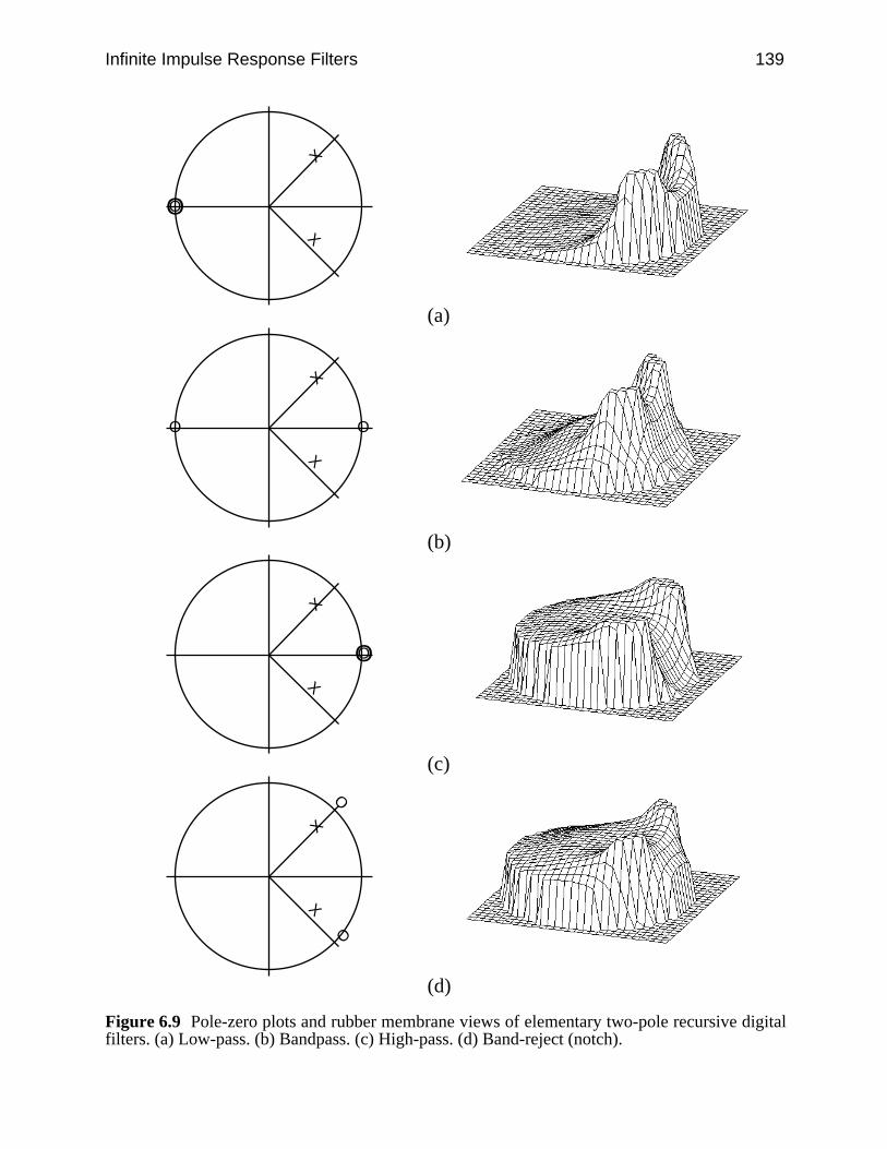
Infinite Impulse Response Filters 139
OOX
X
(a)
O O
X
X
(b)
OOX
X
(c)
O
O
X
X
(d)
Figure 6.9 Pole-zero plots and rubber membrane views of elementary two-pole recursive digitalfilters. (a) Low-pass. (b) Bandpass. (c) High-pass. (d) Band-reject (notch).

140 Biomedical Digital Signal Processing
Let us now design a filter and write a C-language program to implement it. Firstwe choose a low-pass filter. This establishes the locations of the two zeros andestablish the values for a1 = 2 and a2 = 1 (see Figure 6.8). Then we decide on thelocations of the poles. For this design, we choose locations at r = 0.5 and = ±45˚.This establishes the values for b1 = 0.707 and b2 = 0.25 [see Eq. (6.34)].
Software implementation of this digital filter is now fairly straightforward. Wewrite a filter subroutine directly from the difference equation. Figure 6.10 showshow this low-pass filter is executed in five steps:
1. Pass in the current input signal.2. Shift array elements to get delays of past input signal and store them.3. Accumulate all past and/or current input and past output terms with multiplying
coefficients.4. Shift array elements to get delays of past output signal and store them.5. Return with output signal.
/*************************************************************** * Turbo C source code for implementing an IIR low-pass filter * * Assume we use the r and q method where r = 0.5, q = 45°. * The difference equation is: * * y(nT) = 0.707y(nT–T)–0.25y(nT–2T)+x(nT)+2x(nT–T)+x(nT–2T) * y(nT) = 0.707*y[1] – 0.25*y[2] + x[0] + 2*x[1] + x[2] * **************************************************************/float LowPass(signal)float signal; /* x[nT] */static float x[3], y[3];int count;
for ( count=2; count>0; count–– ) x[count]=x[count–1]; /* shift for x term delays */
x[0]=signal; /* x[0] = x[nT] */ /* difference equation */
y[0]=0.707*y[1]–0.25*y[2]+x[0]+2.0*x[1]+x[2];
for( count = 2; count > 0; count––) y[count]=y[count–1]; /* shift for y term delays */
return y[0];
Figure 6.10 An IIR low-pass filter written in the C language.
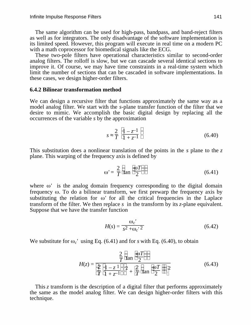
Infinite Impulse Response Filters 141
The same algorithm can be used for high-pass, bandpass, and band-reject filtersas well as for integrators. The only disadvantage of the software implementation isits limited speed. However, this program will execute in real time on a modern PCwith a math coprocessor for biomedical signals like the ECG.
These two-pole filters have operational characteristics similar to second-orderanalog filters. The rolloff is slow, but we can cascade several identical sections toimprove it. Of course, we may have time constraints in a real-time system whichlimit the number of sections that can be cascaded in software implementations. Inthese cases, we design higher-order filters.
6.4.2 Bilinear transformation method
We can design a recursive filter that functions approximately the same way as amodel analog filter. We start with the s-plane transfer function of the filter that wedesire to mimic. We accomplish the basic digital design by replacing all theoccurrences of the variable s by the approximation
s ≈ 2T
1 – z–1
1 + z–1 (6.40)
This substitution does a nonlinear translation of the points in the s plane to the zplane. This warping of the frequency axis is defined by
' = 2T
tan
T
2 (6.41)
where ' is the analog domain frequency corresponding to the digital domainfrequency . To do a bilinear transform, we first prewarp the frequency axis bysubstituting the relation for ' for all the critical frequencies in the Laplacetransform of the filter. We then replace s in the transform by its z-plane equivalent.Suppose that we have the transfer function
H(s) = c'
s2 + c' 2 (6.42)
We substitute for c' using Eq. (6.41) and for s with Eq. (6.40), to obtain
H(z) = 2T
tan
T
2
2
T
1 – z 1
1 + z–1 2 +
2
T
tan
T
2 2 (6.43)
This z transform is the description of a digital filter that performs approximatelythe same as the model analog filter. We can design higher-order filters with thistechnique.
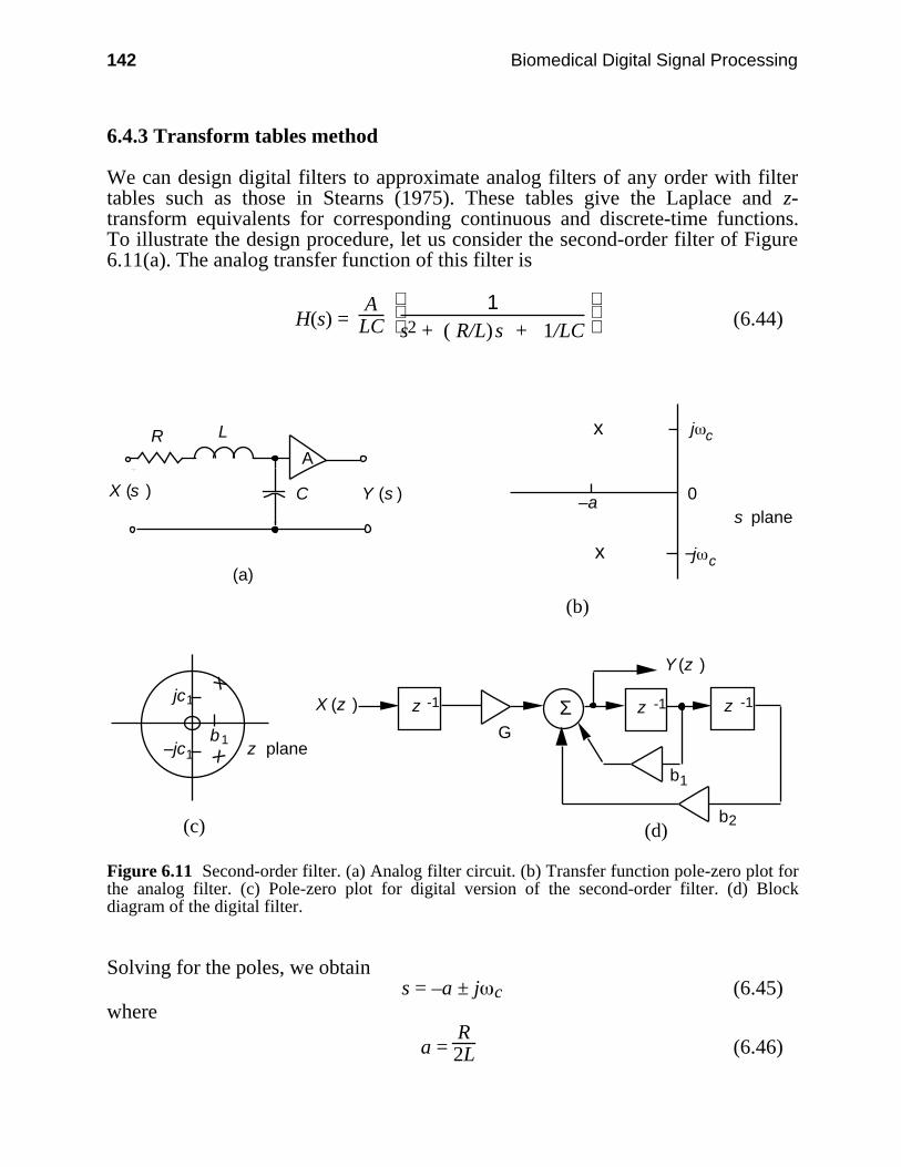
142 Biomedical Digital Signal Processing
6.4.3 Transform tables method
We can design digital filters to approximate analog filters of any order with filtertables such as those in Stearns (1975). These tables give the Laplace and z-transform equivalents for corresponding continuous and discrete-time functions.To illustrate the design procedure, let us consider the second-order filter of Figure6.11(a). The analog transfer function of this filter is
H(s) = A
LC
1
s2 + ( R/L)s + 1/LC (6.44)
R L
C Y (s )X (s )
A
(a)
0s plane
–a
j c
j c–
(b)
(c)
b1
1jc
1– z plane
b1
b2
G
(d)
z -1 z -1 z -1X (z )
Y (z )x
x
x
x
Σ
jc
Figure 6.11 Second-order filter. (a) Analog filter circuit. (b) Transfer function pole-zero plot forthe analog filter. (c) Pole-zero plot for digital version of the second-order filter. (d) Blockdiagram of the digital filter.
Solving for the poles, we obtains = –a ± j c (6.45)
where
a = R2L (6.46)
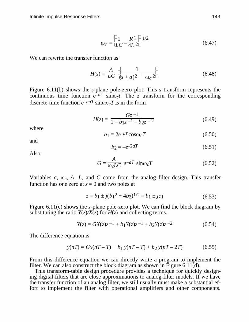
Infinite Impulse Response Filters 143
c =
1
LC – R 24L 2
1/2
(6.47)
We can rewrite the transfer function as
H(s) = A
LC
1
(s + a)2 + c 2 (6.48)
Figure 6.11(b) shows the s-plane pole-zero plot. This s transform represents thecontinuous time function e–at sin ct. The z transform for the correspondingdiscrete-time function e–naT sinn cT is in the form
H(z) = Gz –1
1 – b1z –1 – b2z – 2 (6.49)
whereb1 = 2e–aT cos cT (6.50)
andb2 = –e–2aT (6.51)
Also
G = AcLC e–aT sin cT (6.52)
Variables a, c, A, L, and C come from the analog filter design. This transferfunction has one zero at z = 0 and two poles at
z = b1 ± j(b12 + 4b2)1/2 = b1 ± jc1 (6.53)
Figure 6.11(c) shows the z-plane pole-zero plot. We can find the block diagram bysubstituting the ratio Y(z)/X(z) for H(z) and collecting terms.
Y(z) = GX(z)z –1 + b1Y(z)z –1 + b2Y(z)z –2 (6.54)
The difference equation is
y(nT) = Gx(nT – T) + b1 y(nT – T) + b2 y(nT – 2T) (6.55)
From this difference equation we can directly write a program to implement thefilter. We can also construct the block diagram as shown in Figure 6.11(d).
This transform-table design procedure provides a technique for quickly design-ing digital filters that are close approximations to analog filter models. If we havethe transfer function of an analog filter, we still usually must make a substantial ef-fort to implement the filter with operational amplifiers and other components.

144 Biomedical Digital Signal Processing
However, once we have the z transform, we have the complete filter design speci-fied and only need to write a straightforward program to implement the filter.
6.5 LAB: IIR DIGITAL FILTERS FOR ECG ANALYSIS
This lab provides experience with the use of IIR filters for processing ECGs. In or-der to design integrators and two-pole filters using UW DigiScope, select(F)ilters from the main menu, choose (D)esign, then (I)IR.
6.5.1 Integrators
This chapter reviewed three different integrators (rectangular, trapezoidal, andSimpson’s rule). Which of these filters requires the most computation time? Whatdo the unit-circle diagrams of these three filters have in common?
Run the rectangular integrator on an ECG signal (e.g., ecg105.dat). Explainthe result. Design a preprocessing filter to solve any problem observed. Comparethe output of the three integrators on appropriately processed ECG data with andwithout random noise. Which integrator is best to use for noisy signals?
6.5.2 Second-order recursive filters
Design three two-pole bandpass filters using r = 0.7, 0.9, and 0.95 for a critical fre-quency of 17 Hz (sampling rate of 200 sps). Measure the Q for the three filters. Qis defined as the ratio of critical frequency to the 3-dB bandwidth (difference be-tween the 3-dB frequencies). Run the three filters on an ECG file and contrast theoutputs. What trade-offs must be considered when selecting the value of r?
6.5.3 Transfer function (Generic)
The (G)eneric tool allows you to enter coefficients of a transfer function of theform
H(z) = a0 + a1z–1 + a2z–2 +…+ anz–n
1 + b1z–1 + b2z–2 +…+ bmz–m where m <= n
Using the example from the transform tables method discussed in section 6.4.3with R = 10 Ω, L = 10 mH, and C = 1 µF, calculate and enter the coefficients of theresulting H(z). Use a sampling rate of 200 sps. What is the Q of this filter?
6.5.4 Pole-zero placement
Create a 60-Hz notch FIR filter for a sampling rate of 180 sps by placing two zeroson the unit circle (i.e., r = 1.0) at angles of ±120˚ as shown in Figure 6.12(a).Create an IIR filter by adding poles inside the circle at angles of ±110˚ and ±130˚

Infinite Impulse Response Filters 145
at r = 0.9, as shown in Figure 6.12(b). Compare the amplitude response of this fil-ter with that of the FIR filter. Measure the Q of both filters. Can you further in-crease the Q of the IIR filter? What happens to the phase response?
(a) (b)
Figure 6.12 Notch filters. (a) FIR filter. (b) IIR filter.
6.6 REFERENCES
Soderstrand, M. A. 1972. On-line digital filtering using the PDP-8 or PDP-12. Computers in theNeurophysiology Laboratory, 1: 31-49. Maynard, MA: Digital Equipment Corporation.
Stearns, S. D. 1975. Digital Signal Analysis. Rochelle Park, NJ: Hayden.Tompkins, W. J. and Webster, J. G. (eds.) 1981. Design of Microcomputer-based Medical
Instrumentation. Englewood Cliffs, NJ: Prentice Hall.
6.7 STUDY QUESTIONS
6.1 Describe the characteristics of the generic transfer function of recursive filters.6.2 What is the difference between IIR filters and recursive filters?6.3 How do you derive the frequency response of a recursive filter?6.4 How do you write the difference equation from the transfer function of a recursive filter?6.5 Design a low-pass recursive filter using the r and method.6.6 Design a high-pass filter using bilinear transformation method.6.7 Design a filter using transform tables method.6.8 A digital filter has a unit impulse output sequence i.e., 1, 0, 0,… when a unit step i.e., 1,
1, 1, 1,… is applied at its input. What is the transfer function of the filter?6.9 Write a rectangular integrator in C.6.10 Using the difference equation from the result of question 6.5, run the filtering program
provided in section 6.4.6.11 Draw the z-plane pole-zero plot for a filter with the z transform:
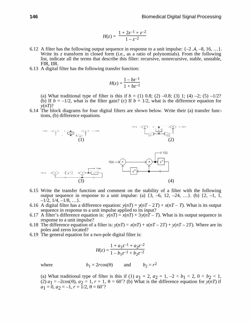
146 Biomedical Digital Signal Processing
H(z) = 1 + 2z–1 + z–2
1 – z–2
6.12 A filter has the following output sequence in response to a unit impulse: –2 ,4, –8, 16, ….Write its z transform in closed form (i.e., as a ratio of polynomials). From the followinglist, indicate all the terms that describe this filter: recursive, nonrecursive, stable, unstable,FIR, IIR.
6.13 A digital filter has the following transfer function:
H(z) = 1 – bz–1
1 + bz–1
(a) What traditional type of filter is this if b = (1) 0.8; (2) –0.8; (3) 1; (4) –2; (5) –1/2?(b) If b = –1/2, what is the filter gain? (c) If b = 1/2, what is the difference equation fory(nT)?
6.14 The block diagrams for four digital filters are shown below. Write their (a) transfer func-tions, (b) difference equations.
(1) (2)
(3) (4)
6.15 Write the transfer function and comment on the stability of a filter with the followingoutput sequence in response to a unit impulse: (a) 3, –6, 12, –24, …. (b) 2, –1, 1,–1/2, 1/4, –1/8, ….
6.16 A digital filter has a difference equation: y(nT) = y(nT – 2T) + x(nT – T). What is its outputsequence in response to a unit impulse applied to its input?
6.17 A filter’s difference equation is: y(nT) = x(nT) + 3y(nT – T). What is its output sequence inresponse to a unit impulse?
6.18 The difference equation of a filter is: y(nT) = x(nT) + x(nT – 2T) + y(nT – 2T). Where are itspoles and zeros located?
6.19 The general equation for a two-pole digital filter is:
H(z) = 1 + a1z–1 + a2z–2
1 – b1z–1 + b2z–2
where b1 = 2rcos( ) and b2 = r2
(a) What traditional type of filter is this if (1) a1 = 2, a2 = 1, –2 < b1 < 2, 0 < b2 < 1,(2) a1 = –2cos( ), a2 = 1, r = 1, = 60˚? (b) What is the difference equation for y(nT) ifa1 = 0, a2 = –1, r = 1/2, = 60˚?
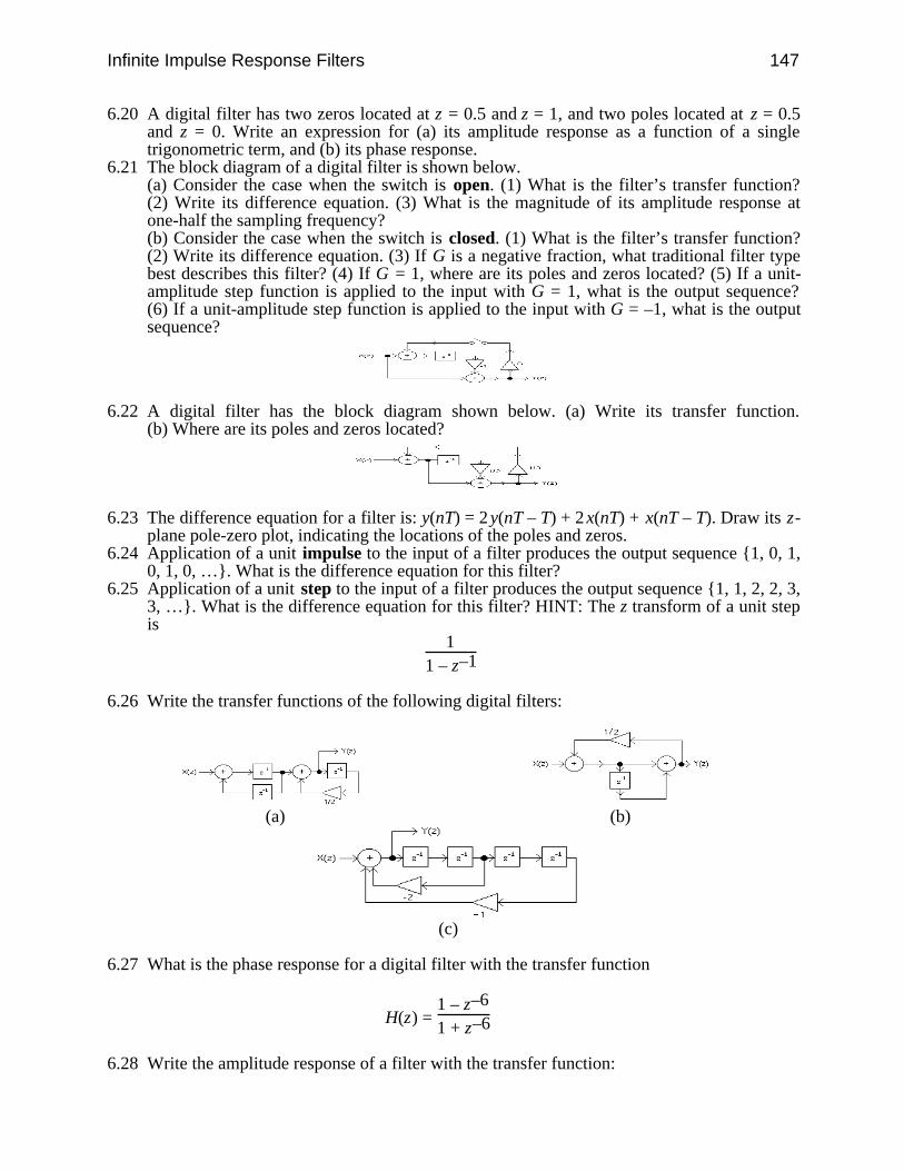
Infinite Impulse Response Filters 147
6.20 A digital filter has two zeros located at z = 0.5 and z = 1, and two poles located at z = 0.5and z = 0. Write an expression for (a) its amplitude response as a function of a singletrigonometric term, and (b) its phase response.
6.21 The block diagram of a digital filter is shown below.(a) Consider the case when the switch is open. (1) What is the filter’s transfer function?(2) Write its difference equation. (3) What is the magnitude of its amplitude response atone-half the sampling frequency?(b) Consider the case when the switch is closed. (1) What is the filter’s transfer function?(2) Write its difference equation. (3) If G is a negative fraction, what traditional filter typebest describes this filter? (4) If G = 1, where are its poles and zeros located? (5) If a unit-amplitude step function is applied to the input with G = 1, what is the output sequence?(6) If a unit-amplitude step function is applied to the input with G = –1, what is the outputsequence?
6.22 A digital filter has the block diagram shown below. (a) Write its transfer function.(b) Where are its poles and zeros located?
6.23 The difference equation for a filter is: y(nT) = 2 y(nT – T) + 2 x(nT) + x(nT – T). Draw its z-plane pole-zero plot, indicating the locations of the poles and zeros.
6.24 Application of a unit impulse to the input of a filter produces the output sequence 1, 0, 1,0, 1, 0, …. What is the difference equation for this filter?
6.25 Application of a unit step to the input of a filter produces the output sequence 1, 1, 2, 2, 3,3, …. What is the difference equation for this filter? HINT: The z transform of a unit stepis
1
1 – z–1
6.26 Write the transfer functions of the following digital filters:
(a) (b)
(c)
6.27 What is the phase response for a digital filter with the transfer function
H(z) = 1 – z–6
1 + z–6
6.28 Write the amplitude response of a filter with the transfer function:

148 Biomedical Digital Signal Processing
H(z) = z–2
1 – z–2
6.29 A filter has two poles at z = 0.5 ± j0.5 and two zeros at z = 0.707 ± j0.707. What traditionalfilter type best describes this filter?
6.30 A filter operating at a sampling frequency of 1000 samples/s has a pole at z = 1/2 and azero at z = 3. What is the magnitude of its amplitude response at dc?
6.31 A filter is described by the difference equation: y(nT) = x(nT) + x(nT – T) – 0.9y(nT – T).What is its transfer function?
6.32 A filter has the difference equation: y(nT) = y(nT – 2T) + x(nT) + x(nT – T). Whattraditional filter type best describes this filter?
6.33 In response to a unit impulse applied to its input, a filter has the output sequence: 1, 1/2,1/4, 1/8,…. What is its transfer function?
6.34 The difference equation for a digital filter is: y(nT) = x(nT) – ax(nT – T) – by(nT – T).Variables a and b are positive integers. What traditional type of filter is this if a = 1 and(a) b = 0.8, (b) b > 1?
6.35 Write the (a) amplitude response, (b) phase response, and (c) difference equation for a filterwith the transfer function:
H(z) = 1 – z–1
1 + z–1
6.36 Write the (a) amplitude response, (b) phase response, and (c) difference equation for a filterwith the transfer function:
H(z) = z – 12z + 1
6.37 A filter operating at a sampling frequency of 1000 samples/s has a pole at z = 1 and a zeroat z = 2. What is the magnitude of its amplitude response at 500 Hz?
6.38 A filter operating at a sampling frequency of 200 samples/s has poles at z = ±j/2 and zerosat z = ±1. What is the magnitude of its amplitude response at 50 Hz?
6.39 A filter is described by the difference equation: 2y(nT) + y(nT – T) = 2x(nT). What is itstransfer function H(z)?
6.40 A filter has the difference equation: y(nT) = y(nT – T) – y(nT – 2T) + x(nT) + x(nT – T).What is its transfer function?
6.41 In response to a unit impulse applied to its input, a filter has the output sequence:1, 1, 1/2, 1/4, 1/8,…. What is its transfer function?
6.42 A filter has a transfer function that is identical to the z transform of a unit step. A unit stepis applied at its input. What is its output sequence?
6.43 A filter has a transfer function that is equal to the z transform of a ramp. A unit impulse isapplied at its input. What is its output sequence? HINT: The equation for a ramp is x(nT) =nT, and its z transform is
X(z) = Tz–1
(1 – z–1)2
6.44 A ramp applied to the input of digital filter produces the output sequence: 0, T, T, T, T,…. What is the transfer function of the filter?
6.45 A digital filter has a unit step i.e., 1, 1, 1, 1, …) output sequence when a unit impulse i.e.,1, 0, 0, … is applied at its input. How is this filter best described?
6.46 A discrete impulse function is applied to the inputs of four different filters. For each of theoutput sequences that follow, state whether the filter is recursive or nonrecursive.(a) 1, 2, 3, 4, 5, 6, 0, 0, 0,…, (b) 1, –1, 1, –1, 1, –1,…, (c) 1, 2, 4, 8, 16,…,(d) 1, 0.5, 0.25, 0.125,….

Infinite Impulse Response Filters 149
6.47 What similarities are common to all three integrator algorithms discussed in the text (i.e.,rectangular, trapezoidal, and Simpson’s rule)?
6.48 A differentiator is cascaded with an integrator. The differentiator uses the two-pointdifference algorithm:
H1(z) = 1 – z–1
T
The integrator uses trapezoidal integration:
H2(z) = T2
1 + z–1
1 – z–1
A unit impulse is applied to the input. What is the output sequence?6.49 A differentiator is cascaded with an integrator. The differentiator uses the three-point
central difference algorithm:
H1(z) = 1 – z–2
2T
The integrator uses rectangular integration:
H2(z) = T
1
1 – z–1
(a) A unit impulse is applied to the input. What is the output sequence? (b) What traditionalfilter type best describes this filter?
6.50 A digital filter has two zeros located at z = 0.5 and z = 1, and a single pole located at z =0.5. Write an expression for (a) its amplitude response as a function of a single trigonomet-ric term, and (b) its phase response.
6.51 In response to a unit impulse applied to its input, a filter has the output sequence: 2, –1, 1,–1/2, 1/4, –1/8,…. What is its transfer function?
6.52 The difference equation for a filter is: y(nT – T) = x(nT – T) + 2x(nT – 4T) + 4 x(nT – 10T).What is its transfer function, H(z)?
6.53 What is the transfer function H(z) of a digital filter with the difference equation
y(nT – 2T) = y(nT – T) + x(nT – T) + x(nT – 4T) + x(nT – 10T)
6.54 A digital filter has the following output sequence in response to a unit impulse:1, –2, 4, –8,…. Where are its poles located?
6.55 A digital filter has a single zero located at z = 0.5 and a single pole located at z = 0.5. Whatare its amplitude and phase responses?
6.56 The difference equation for a filter is: y(nT) = 2y(nT – T) + 2x(nT) + x(nT – T). What arethe locations of its poles and zeros?
6.57 What traditional filter type best describes the filter with the z transform:
H(z) = z2 – 1z2 + 1
6.58 A discrete impulse function is applied to the inputs of four different filters. The outputsequences of these filters are listed below. Which one of these filters has a pole outside theunit circle? (a) 1, 2, 3, 4, 5, 6, 0, 0, 0,… (b) 1, –1, 1, –1, 1, –1,… (c) 1, 2, 4, 8,16,… (d) 1, 0.5, 0.25, 0.125,…
6.59 Draw the block diagram of a filter that has the difference equation:

150 Biomedical Digital Signal Processing
y(nT) = y(nT – T) + y(nT – 2T) + x(nT) + x(nT – T)
6.60 What is the transfer function H(z) of a filter described by the difference equation:
y(nT) + 0.5y(nT – T) = x(nT)
6.61 A filter has an output sequence of 1, 5, 3, –9, 0, 0,… in response to the input sequence of1, 3, 0, 0,…. What is its transfer function?
151
7
Integer Filters
Jon D. Pfeffer
When digital filters must operate in a real-time environment, many filter designsbecome unsatisfactory due to the amount of required computation time. A consid-erable reduction in computation time is achieved by replacing floating-point coeffi-cients with small integer coefficients in filter equations. This increases the speed atwhich the resulting filter program executes by replacing floating-point multiplica-tion instructions with integer bit-shift and add instructions. These instructions re-quire fewer clock cycles than floating-point calculations.
Integer filters are a special class of digital filters that have only integer coeffi-cients in their defining equations. This characteristic leads to some design con-straints that can often make it difficult to achieve features such as a sharp cutofffrequency. Since integer filters can operate at higher speeds than traditional de-signs, they are often the best type of filter for high sampling rates or when using aslow microprocessor.
This chapter discusses basic design concepts of integer filters. It also reviewswhy these filters display certain characteristics, such as linear phase, and how toderive the transfer functions. Next this theory is extended to show how to designlow-pass, high-pass, bandpass, and band-reject integer filters by appropriate selec-tion of pole and zero locations. Then a discussion shows how certain aspects offilter performance can be improved by cascading together integer filters. Next a re-cent design method is summarized which is more complicated but adds flexibilityto the design constraints. Finally, a lab provides hands-on experience in the designand use of integer filters.
7.1 BASIC DESIGN CONCEPT
Lynn (1977) presented the best known techniques for integer filter design used to-day by showing a methodology to design low-pass, high-pass, bandpass, and band-reject filters with integer coefficients. This method is summarized in several steps.First place a number of evenly spaced zeros around the unit circle. These zeroscompletely attenuate the frequencies corresponding to their locations. Next choose

152 Biomedical Digital Signal Processing
poles that also lie on the unit circle to exactly cancel some of the zeros. When apole cancels a zero, the frequency corresponding to this location is no longer atten-uated. Since each point on the unit circle is representative of a frequency, the loca-tions of the poles and zeros determine the frequency response of the filter. Thesefilters are restricted types of recursive filters.
7.1.1 General form of transfer function
The general form of the filter transfer function used by Lynn for this application is:
H1(z) = [1 – z–m]p
[1 – 2cos( )z–1 + z–2]t (7.1a)
H2(z) = [1 + z–m]p
[1 – 2cos( )z–1 + z–2]t (7.1b)
The m exponent represents how many evenly spaced zeros to place around theunit circle. The angle represents the angular locations of the poles. The powers pand t represent the order of magnitude of the filter, which has a direct bearing onits gain and on the attenuation of the sidelobes. Raising p and t by equal integralamounts has the effect of cascading identical filters. If the filter is to be useful andphysically realizable, p and t must both be nonnegative integers. The effects ofraising p and t to values greater than one are further described in section 7.5.
7.1.2 Placement of poles
The denominator of this transfer function comes from the multiplication of a pairof complex-conjugate poles that always lie exactly on the unit circle. Euler’s rela-tion, ej = cos( ) + j sin( ), shows that all values of ej lie on the unit circle. Thuswe can derive the denominator as follows:
Denominator = (z – ej )(z – e–j ) (7.2a)
Multiplying the two factors, we get
Denominator = z2 – (ej + e–j )z + (ej e–j ) (7.2b)Using the identity,
cos( ) = ej + e–j
2 (7.2c)We arrive at
Denominator = 1 – 2cos( )z–1 + z–2 (7.2d)
The pair of complex-conjugate poles from the denominator of this transfer func-tion provides integer multiplier and divisor coefficient values only when 2cos( ) isan integer as shown in Figure 7.1(a). Such integer values result only when is
Integer Filters 153
equal to 0˚, ± 60˚, ± 90˚, ±120˚, and 180˚ respectively, as shown in Figure 7.1(b).When the coefficients are integers, a multiplication step is saved in the calculationsbecause the multiplication of small integers is done by using bit-shift C-languageinstructions instead of multiplication instructions.
The poles in these positions are guaranteed to exactly lie on the unit circle. It isimpossible to “exactly” cancel a zero on the unit circle unless the pole has integercoefficients. All other locations, say = 15˚, have a small region of instability dueto round-off error in the floating-point representation of numbers.
These filters have the added benefit of true-linear phase characteristics. Thismeans that all the frequency components in the signal experience the same trans-mission delay through the filter (Lynn, 1972). This is important when it is desiredto preserve the relative timing of the peaks and features of an output waveform.For example, it is crucial for a diagnostic quality ECG waveform to have P waves,T waves, and QRS complexes that remain unchanged in shape or timing. Changesin phase could reshape normal ECG waveforms to appear as possible arrhythmias,which is, of course, unacceptable.
7.1.3 Placement of zeros
We have seen that poles with integer coefficients that lie on the unit circle are re-stricted to five positions. This places constraints on the placement of zeros and alsolimits choices for the sampling rate when a designer wants to implement a specificcutoff frequency. To place zeros on the unit circle, one of two simple factors isused in the numerator of the filter’s transfer function
(1 – z–m) (7.3a)or
(1 + z–m) (7.3b)
For both equations, m is a positive integer equal to the number of zeros evenlyspaced around the unit circle. Equation (7.3a) places a zero at 0˚ with the rest ofthe zeros evenly displaced by angles of (360/m)˚. To prove this statement, set
(1 – z–m) = 0
Placing the z term on the right-hand side of the equation
z–m = 1or equivalently
zm = 1
You can see that, if z is on the unit circle, it is only equal to 1 at the point z = (1, 0),which occurs every 2π radians. Thus, we can say
zm = ejn2π = 1Solving for z, we arrive at
z = ej(n/m)2π
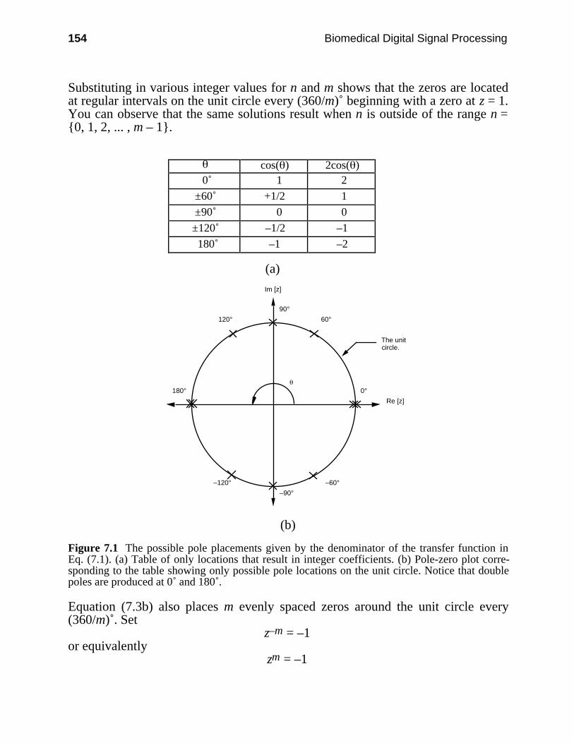
154 Biomedical Digital Signal Processing
Substituting in various integer values for n and m shows that the zeros are locatedat regular intervals on the unit circle every (360/m)˚ beginning with a zero at z = 1.You can observe that the same solutions result when n is outside of the range n =0, 1, 2, ... , m – 1.
cos( ) 2cos( ) 0˚ 1 2
±60˚ +1/2 1
±90˚ 0 0
±120˚ –1/2 –1
180˚ –1 –2
(a)
Re [z]
Im [z]
The unitcircle.
60°
0°
90°
120°
180°
–120°
–90°
–60°
(b)
Figure 7.1 The possible pole placements given by the denominator of the transfer function inEq. (7.1). (a) Table of only locations that result in integer coefficients. (b) Pole-zero plot corre-sponding to the table showing only possible pole locations on the unit circle. Notice that doublepoles are produced at 0˚ and 180˚.
Equation (7.3b) also places m evenly spaced zeros around the unit circle every(360/m)˚. Set
z–m = –1or equivalently
zm = –1
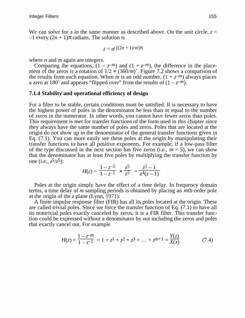
Integer Filters 155
We can solve for z in the same manner as described above. On the unit circle, z =–1 every (2n + 1)π radians. The solution is
z = ej [(2n + 1)/m]π
where n and m again are integers.Comparing the equations, (1 – z–m) and (1 + z–m), the difference in the place-
ment of the zeros is a rotation of 1/2 × (360/m)˚. Figure 7.2 shows a comparison ofthe results from each equation. When m is an odd number, (1 + z–m) always placesa zero at 180˚ and appears “flipped over” from the results of (1 – z–m).
7.1.4 Stability and operational efficiency of design
For a filter to be stable, certain conditions must be satisfied. It is necessary to havethe highest power of poles in the denominator be less than or equal to the numberof zeros in the numerator. In other words, you cannot have fewer zeros than poles.This requirement is met for transfer functions of the form used in this chapter sincethey always have the same number of poles and zeros. Poles that are located at theorigin do not show up in the denominator of the general transfer functions given inEq. (7.1). You can more easily see these poles at the origin by manipulating theirtransfer functions to have all positive exponents. For example, if a low-pass filterof the type discussed in the next section has five zeros (i.e., m = 5), we can showthat the denominator has at least five poles by multiplying the transfer function byone (i.e., z5/z5):
H(z) = 1 – z–5
1 – z–1 × z5
z5 = z5 – 1
z4(z – 1)
Poles at the origin simply have the effect of a time delay. In frequency domainterms, a time delay of m sampling periods is obtained by placing an mth-order poleat the origin of the z plane (Lynn, 1971).
A finite impulse response filter (FIR) has all its poles located at the origin. Theseare called trivial poles. Since we force the transfer function of Eq. (7.1) to have allits nontrivial poles exactly canceled by zeros, it is a FIR filter. This transfer func-tion could be expressed without a denominator by not including the zeros and polesthat exactly cancel out. For example
H(z) = 1 – z–m
1 – z–1 = 1 + z1 + z2 + z3 + … + zm+1 = Y(z)X(z) (7.4)

156 Biomedical Digital Signal Processing
Solutions for: 1 – z = 0–m
1 – z = 0–1
z – 1 = 0
z = 1
1 – z = 0–2
z – 1 = 02
z = 12
z = 1, –1
1 – z = 0–3
z – 1 = 03
z + 1 = 0m
z = 13
z = 1, –0.5 + j0.866, –0.5 – j0.866
1 – z = 0–4
z – 1 = 04
z = 14
z = 1, –1, +j, –j
1 – z = 0–m
z – 1 = 0m
z = 1 = em j2πn
z = ej2π(n/m)
places m zeros displacedby angles of (360/m)°
1 + z = 0–m
1 + z = 0–1
z + 1 = 0
z = –1
1 + z = 0–2
z + 1 = 02
z = –12
z = +j, –j
1 + z = 0–3
z = –13
z + 1 = 03
z = –1, +0.5 + j0.866, +0.5 – j0.866
1 + z = 0–4
z + 1 = 04
z = –14
z = +0.707 + j0.707 +0.707 – j0.707 –0.707 + j0.707 –0.707 – j0.707
z = ej[(2n + 1)/m]π
m z = –1 = e
j(2n + 1)π
places m zeros displacedby angles of (360/m)°
Solutions for: 1 + z = 0–m
Figure 7.2 A comparison between the factors (1 – z–m) and (1 + z–m) for different values of m.When m is odd, the zeros appear “flipped over” from each other.
However, this is not done since expressing filters in recursive form is computa-tionally more efficient. If m is large, the nonrecursive transfer function requires m
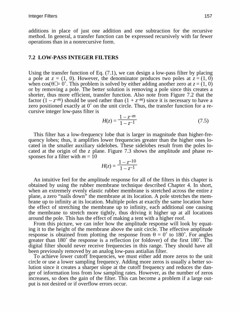
Integer Filters 157
additions in place of just one addition and one subtraction for the recursivemethod. In general, a transfer function can be expressed recursively with far feweroperations than in a nonrecursive form.
7.2 LOW-PASS INTEGER FILTERS
Using the transfer function of Eq. (7.1), we can design a low-pass filter by placinga pole at z = (1, 0). However, the denominator produces two poles at z = (1, 0)when cos( ) = 0˚. This problem is solved by either adding another zero at z = (1, 0)or by removing a pole. The better solution is removing a pole since this creates ashorter, thus more efficient, transfer function. Also note from Figure 7.2 that thefactor (1 – z–m) should be used rather than (1 + z–m) since it is necessary to have azero positioned exactly at 0˚ on the unit circle. Thus, the transfer function for a re-cursive integer low-pass filter is
H(z) = 1 – z–m
1 – z–1 (7.5)
This filter has a low-frequency lobe that is larger in magnitude than higher-fre-quency lobes; thus, it amplifies lower frequencies greater than the higher ones lo-cated in the smaller auxiliary sidelobes. These sidelobes result from the poles lo-cated at the origin of the z plane. Figure 7.3 shows the amplitude and phase re-sponses for a filter with m = 10
H(z) = 1 – z–10
1 – z–1
An intuitive feel for the amplitude response for all of the filters in this chapter isobtained by using the rubber membrane technique described Chapter 4. In short,when an extremely evenly elastic rubber membrane is stretched across the entire zplane, a zero “nails down” the membrane at its location. A pole stretches the mem-brane up to infinity at its location. Multiple poles at exactly the same location havethe effect of stretching the membrane up to infinity, each additional one causingthe membrane to stretch more tightly, thus driving it higher up at all locationsaround the pole. This has the effect of making a tent with a higher roof.
From this picture, we can infer how the amplitude response will look by equat-ing it to the height of the membrane above the unit circle. The effective amplituderesponse is obtained from plotting the response from = 0˚ to 180˚. For anglesgreater than 180˚ the response is a reflection (or foldover) of the first 180˚. Thedigital filter should never receive frequencies in this range. They should have allbeen previously removed by an analog low-pass antialias filter.
To achieve lower cutoff frequencies, we must either add more zeros to the unitcircle or use a lower sampling frequency. Adding more zeros is usually a better so-lution since it creates a sharper slope at the cutoff frequency and reduces the dan-ger of information loss from low sampling rates. However, as the number of zerosincreases, so does the gain of the filter. This can become a problem if a large out-put is not desired or if overflow errors occur.
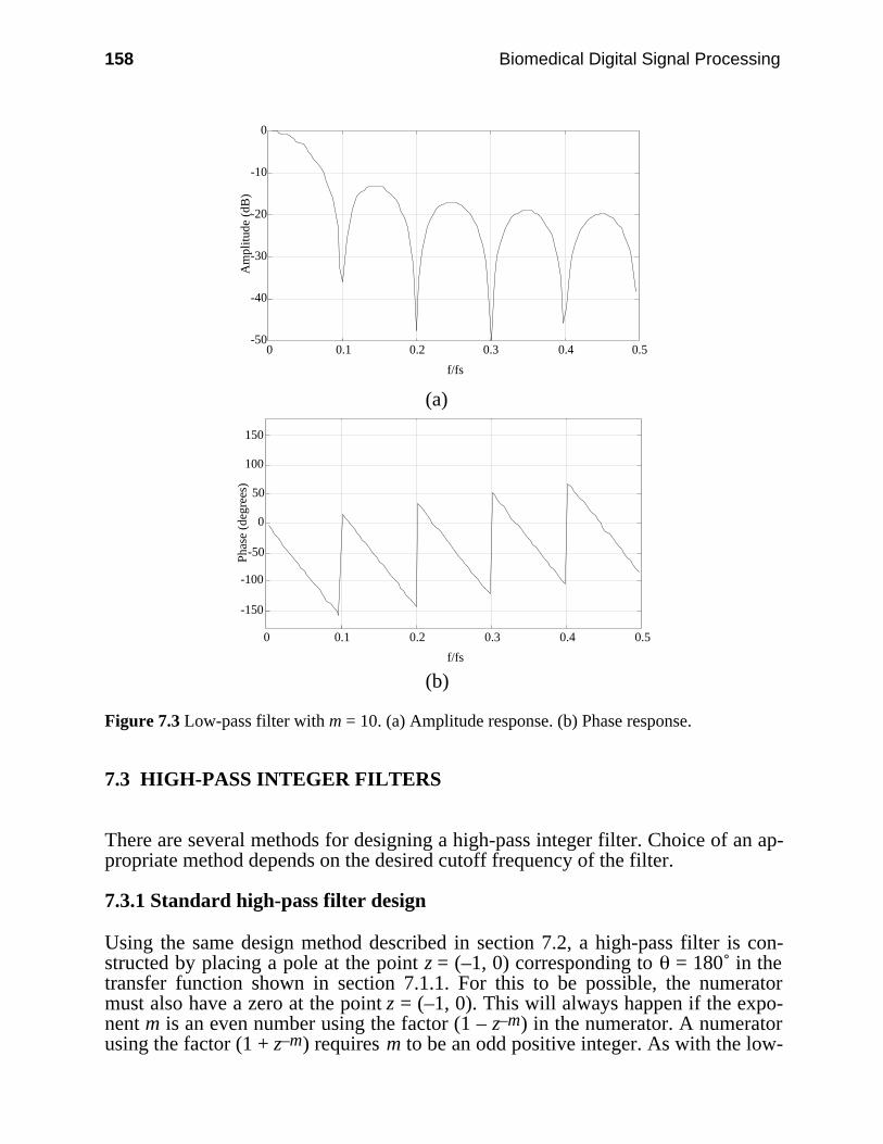
158 Biomedical Digital Signal Processing
-50
-40
-30
-20
-10
0
0 0.1 0.2 0.3 0.4 0.5
f/fs
Am
plit
ude
(dB
)
(a)
-150
-100
-50
0
50
100
150
0 0.1 0.2 0.3 0.4 0.5
f/fs
Pha
se (
degr
ees)
(b)
Figure 7.3 Low-pass filter with m = 10. (a) Amplitude response. (b) Phase response.
7.3 HIGH-PASS INTEGER FILTERS
There are several methods for designing a high-pass integer filter. Choice of an ap-propriate method depends on the desired cutoff frequency of the filter.
7.3.1 Standard high-pass filter design
Using the same design method described in section 7.2, a high-pass filter is con-structed by placing a pole at the point z = (–1, 0) corresponding to = 180˚ in thetransfer function shown in section 7.1.1. For this to be possible, the numeratormust also have a zero at the point z = (–1, 0). This will always happen if the expo-nent m is an even number using the factor (1 – z–m) in the numerator. A numeratorusing the factor (1 + z–m) requires m to be an odd positive integer. As with the low-
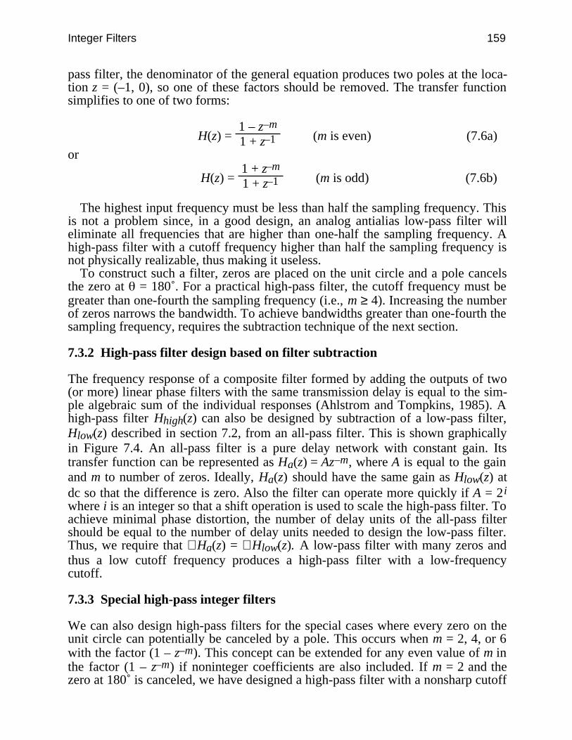
Integer Filters 159
pass filter, the denominator of the general equation produces two poles at the loca-tion z = (–1, 0), so one of these factors should be removed. The transfer functionsimplifies to one of two forms:
H(z) = 1 – z–m
1 + z–1 (m is even) (7.6a)
or
H(z) = 1 + z–m
1 + z–1 (m is odd) (7.6b)
The highest input frequency must be less than half the sampling frequency. Thisis not a problem since, in a good design, an analog antialias low-pass filter willeliminate all frequencies that are higher than one-half the sampling frequency. Ahigh-pass filter with a cutoff frequency higher than half the sampling frequency isnot physically realizable, thus making it useless.
To construct such a filter, zeros are placed on the unit circle and a pole cancelsthe zero at = 180˚. For a practical high-pass filter, the cutoff frequency must begreater than one-fourth the sampling frequency (i.e., m ≥ 4). Increasing the numberof zeros narrows the bandwidth. To achieve bandwidths greater than one-fourth thesampling frequency, requires the subtraction technique of the next section.
7.3.2 High-pass filter design based on filter subtraction
The frequency response of a composite filter formed by adding the outputs of two(or more) linear phase filters with the same transmission delay is equal to the sim-ple algebraic sum of the individual responses (Ahlstrom and Tompkins, 1985). Ahigh-pass filter Hhigh(z) can also be designed by subtraction of a low-pass filter,Hlow(z) described in section 7.2, from an all-pass filter. This is shown graphicallyin Figure 7.4. An all-pass filter is a pure delay network with constant gain. Itstransfer function can be represented as Ha(z) = Az–m, where A is equal to the gainand m to number of zeros. Ideally, Ha(z) should have the same gain as Hlow(z) atdc so that the difference is zero. Also the filter can operate more quickly if A = 2i
where i is an integer so that a shift operation is used to scale the high-pass filter. Toachieve minimal phase distortion, the number of delay units of the all-pass filtershould be equal to the number of delay units needed to design the low-pass filter.Thus, we require that ∠Ha(z) = ∠Hlow(z). A low-pass filter with many zeros andthus a low cutoff frequency produces a high-pass filter with a low-frequencycutoff.
7.3.3 Special high-pass integer filters
We can also design high-pass filters for the special cases where every zero on theunit circle can potentially be canceled by a pole. This occurs when m = 2, 4, or 6with the factor (1 – z–m). This concept can be extended for any even value of m inthe factor (1 – z–m) if noninteger coefficients are also included. If m = 2 and thezero at 180˚ is canceled, we have designed a high-pass filter with a nonsharp cutoff
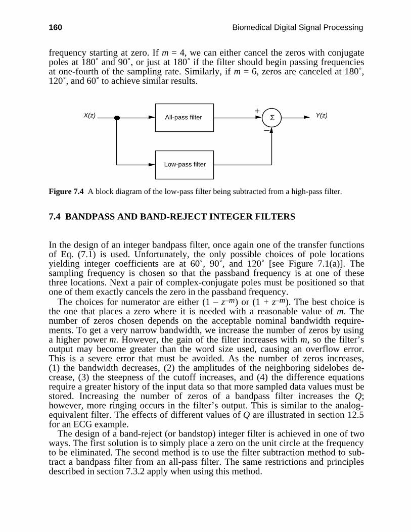
160 Biomedical Digital Signal Processing
frequency starting at zero. If m = 4, we can either cancel the zeros with conjugatepoles at 180˚ and 90˚, or just at 180˚ if the filter should begin passing frequenciesat one-fourth of the sampling rate. Similarly, if m = 6, zeros are canceled at 180˚,120˚, and 60˚ to achieve similar results.
All-pass filter
Low-pass filter
X(z) Y(z) +
–Σ
Figure 7.4 A block diagram of the low-pass filter being subtracted from a high-pass filter.
7.4 BANDPASS AND BAND-REJECT INTEGER FILTERS
In the design of an integer bandpass filter, once again one of the transfer functionsof Eq. (7.1) is used. Unfortunately, the only possible choices of pole locationsyielding integer coefficients are at 60˚, 90˚, and 120˚ [see Figure 7.1(a)]. Thesampling frequency is chosen so that the passband frequency is at one of thesethree locations. Next a pair of complex-conjugate poles must be positioned so thatone of them exactly cancels the zero in the passband frequency.
The choices for numerator are either (1 – z–m) or (1 + z–m). The best choice isthe one that places a zero where it is needed with a reasonable value of m. Thenumber of zeros chosen depends on the acceptable nominal bandwidth require-ments. To get a very narrow bandwidth, we increase the number of zeros by usinga higher power m. However, the gain of the filter increases with m, so the filter’soutput may become greater than the word size used, causing an overflow error.This is a severe error that must be avoided. As the number of zeros increases,(1) the bandwidth decreases, (2) the amplitudes of the neighboring sidelobes de-crease, (3) the steepness of the cutoff increases, and (4) the difference equationsrequire a greater history of the input data so that more sampled data values must bestored. Increasing the number of zeros of a bandpass filter increases the Q;however, more ringing occurs in the filter’s output. This is similar to the analog-equivalent filter. The effects of different values of Q are illustrated in section 12.5for an ECG example.
The design of a band-reject (or bandstop) integer filter is achieved in one of twoways. The first solution is to simply place a zero on the unit circle at the frequencyto be eliminated. The second method is to use the filter subtraction method to sub-tract a bandpass filter from an all-pass filter. The same restrictions and principlesdescribed in section 7.3.2 apply when using this method.
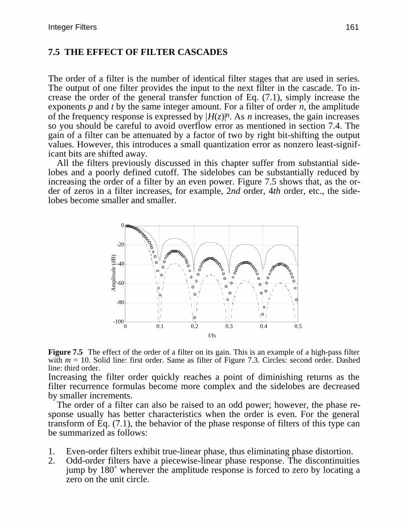
Integer Filters 161
7.5 THE EFFECT OF FILTER CASCADES
The order of a filter is the number of identical filter stages that are used in series.The output of one filter provides the input to the next filter in the cascade. To in-crease the order of the general transfer function of Eq. (7.1), simply increase theexponents p and t by the same integer amount. For a filter of order n, the amplitudeof the frequency response is expressed by |H(z)|n. As n increases, the gain increasesso you should be careful to avoid overflow error as mentioned in section 7.4. Thegain of a filter can be attenuated by a factor of two by right bit-shifting the outputvalues. However, this introduces a small quantization error as nonzero least-signif-icant bits are shifted away.
All the filters previously discussed in this chapter suffer from substantial side-lobes and a poorly defined cutoff. The sidelobes can be substantially reduced byincreasing the order of a filter by an even power. Figure 7.5 shows that, as the or-der of zeros in a filter increases, for example, 2nd order, 4th order, etc., the side-lobes become smaller and smaller.
-100
-80
-60
-40
-20
0
0 0.1 0.2 0.3 0.4 0.5
f/fs
Am
plitu
de (
dB)
Figure 7.5 The effect of the order of a filter on its gain. This is an example of a high-pass filterwith m = 10. Solid line: first order. Same as filter of Figure 7.3. Circles: second order. Dashedline: third order.Increasing the filter order quickly reaches a point of diminishing returns as thefilter recurrence formulas become more complex and the sidelobes are decreasedby smaller increments.
The order of a filter can also be raised to an odd power; however, the phase re-sponse usually has better characteristics when the order is even. For the generaltransform of Eq. (7.1), the behavior of the phase response of filters of this type canbe summarized as follows:
1. Even-order filters exhibit true-linear phase, thus eliminating phase distortion.2. Odd-order filters have a piecewise-linear phase response. The discontinuities
jump by 180˚ wherever the amplitude response is forced to zero by locating azero on the unit circle.
162 Biomedical Digital Signal Processing
A piecewise-linear phase response is acceptable if the filter displays significantattenuation in the regions where the phase response has changed to a new value. Ifthe stopband is not well attenuated, phase distortions will occur whenever the sig-nals that are being filtered have significant energy in those regions. The concept ofphase distortions caused by linear phase FIR filters is thoroughly explained in apaper by Kohn (1987).
It is also possible to combine nonidentical filters together. Often complicatedfilters are crafted from simple subfilters. Examples of these include the high-passand band-reject filters described in previous sections that were derived from filtersubtraction. Lynn (1983) also makes use of this principle when he expands the de-sign method described in this chapter to include resonator configurations. Lynnuses these resonator configurations to expand the design format to include 11 polelocations which add to design flexibility; however, this concept is not covered inthis chapter.
7.6 OTHER FAST-OPERATING DESIGN TECHNIQUES
Principe and Smith (1986) used a method slightly different from Lynn’s fordesigning digital filters to operate on electroencephalographic (EEG) data. Theirmethod is a dual to the frequency sampling technique described in section 5.6.They construct the filter’s transfer function in two steps. First zeros are placed onthe unit circle creating several passbands, one of which corresponds to the desiredpassband. Next zeros are placed on the unit circle in the unwanted passbands tosquelch gain and to produce stopbands.
An example of this is shown in Figure 7.6. Since all the poles are located at theorigin, these FIR filters are guaranteed to be stable. Placing zeros to attenuate gainis more flexible than placing poles to cancel zeros on the unit circle. Zeros areplaced in conjugate pairs by using the factor 1 – 2cos( ) z–1 + z–2 in the numeratorof the transfer function.

Integer Filters 163
-50
-40
-30
-20
-10
0
10
0 0.1 0.2 0.3 0.4 0.5
f/fs
Am
plitu
de (d
B)
(a)
-50
-40
-30
-20
-10
0
10
0 0.1 0.2 0.3 0.4 0.5
f/fs
Am
plitu
de (
dB)
(b)
-50
-40
-30
-20
-10
0
10
0 0.1 0.2 0.3 0.4 0.5
f/fs
Am
plitu
de (d
B)
(c)
Figure 7.6 An example using only zeros to create a high-pass filter. The outputs of magnitude(a) plus magnitude (b) are summed to create magnitude (c).
If a zero is needed at a location that involves multiplication to calculate the co-efficient, it is acceptable to place it at a nearby location that only requires a few bi-
164 Biomedical Digital Signal Processing
nary-shift and add instructions so as to reduce computation time. A 3-bit approxi-mation for 2cos( ) which uses at most two shifts and two additions can place azero at every location that the factors (1 – z–m) or (1 + z–m) do with an error of lessthan 6.5 percent if m is less than 8. This is a common technique to save multiplica-tions. The zero can be slightly moved to an easy-to-calculate location at the cost ofslightly decreasing the stopband attenuation.
This technique of squelching the stopband by adding more zeros could also beused with Lynn’s method described in all of the previous sections. Adding zeros atspecific locations can make it easier to achieve desired nominal bandwidths forbandpass filters, remove problem frequencies in the stopband (such as 60-Hznoise), or eliminate sidelobes without increasing the filter order.
All the previously discussed filters displayed a true-linear or piecewise-linearphase response. Sometimes situations demand a filter to have a sharp cutoff fre-quency, but phase distortion is irrelevant. For these cases, placing interior polesnear zeros on the unit circle has the effect of amplifying the passband frequenciesand attenuating the stopband frequencies. Whenever nontrivial poles remain un-canceled by zeros, an IIR rather than an FIR filter results. IIR filters have sharpercutoff slopes at the price of a nonlinear phase response. However, we do not wishto express the pole’s coefficients, which have values between 0 and 1, usingfloating-point representation.
Thakor and Moreau (1987) solved this problem in a paper about the use of“quantized coefficients.” To place poles inside the unit circle, they use a less re-strictive method that retains some of the advantages of integer coefficients. Theyallow coefficients of the poles to have values of x/2y where x is an integer between1 and (2y – 1) and y is a nonnegative integer called the quantization value.Quantization y is the designer’s choice, but is limited by the microprocessor’s wordlength (e.g., y = 8 for an 8-bit microprocessor). Using these values, fractional coef-ficients, such as 1/8, can be implemented with right shift instructions. A coeffi-cient, such as 17/32, will not show much speed improvement over a multiplicationinstruction since many shifts and adds are required for its calculation. Thakor andMoreau give an excellent description of the use of these coefficients in filters andanalyze the possible quantization, truncation, roundoff, filter-coefficient represen-tation, and overflow errors that can occur.
7.7 DESIGN EXAMPLES AND TOOLS
This chapter includes enough material to design a wide variety of fast-operatingdigital filters. It would require many example problems to provide a feeling for allof the considerations needed to design an “optimal” filter for a certain application.However, the following design problems adequately demonstrate several of themethods used to theoretically analyze some of the characteristics of integer filters.We also demonstrate how a filter’s difference equation is converted into Clanguage so that it can be quickly implemented.
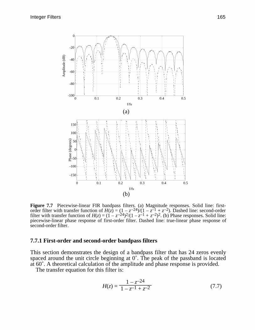
Integer Filters 165
-100
-80
-60
-40
-20
0
0 0.1 0.2 0.3 0.4 0.5
f/fs
Am
plitu
de (d
B)
(a)
-150
-100
-50
0
50
100
150
0 0.1 0.2 0.3 0.4 0.5
f/fs
Pha
se (
degr
ees)
(b)
Figure 7.7 Piecewise-linear FIR bandpass filters. (a) Magnitude responses. Solid line: first-order filter with transfer function of H(z) = (1 – z–24)/(1 – z–1 + z–2). Dashed line: second-orderfilter with transfer function of H(z) = (1 – z–24)2/(1 – z–1 + z–2)2. (b) Phase responses. Solid line:piecewise-linear phase response of first-order filter. Dashed line: true-linear phase response ofsecond-order filter.
7.7.1 First-order and second-order bandpass filters
This section demonstrates the design of a bandpass filter that has 24 zeros evenlyspaced around the unit circle beginning at 0˚. The peak of the passband is locatedat 60˚. A theoretical calculation of the amplitude and phase response is provided.
The transfer equation for this filter is:
H(z) = 1 – z–24
1 – z–1 + z–2 (7.7)

166 Biomedical Digital Signal Processing
Substitute ej T for z and rearrange to produce positive and negative exponents ofequal magnitude:
H( T) = 1 – e–j24 T
1 – e–j T + e–j2 T = e–j12 T (ej12 T – e–j12 T )
e–j T (ej T – 1 + e–j T) (7.8)
Substituting inside the parentheses the relation
ej T = cos( T) + j sin( T) (7.9)gives
H( T) = e–j12 T [cos(12 T) + j sin(12 T) – cos(12 T) + j sin(12 T)]
e–j T [cos( T) + j sin( T) –1 + cos( T) – j sin( T)] (7.10)
Combining terms
H( T) = j2sin(12 T)2cos( T) – 1 × e–j11 T (7.11)
Substituting j = ejπ/2 gives
H( T) = 2sin(12 T)
2cos( T) – 1 × ej(π/2 – 11 T) (7.12)
Thus, the magnitude response shown in Figure 7.7(a) as a solid line is
|H( T)| =
2sin(12 T)
2cos( T) – 1 (7.13)
and the phase response shown in Figure 7.7(b) as a solid line is
∠H( T) = π/2 –11 T (7.14)
Next we cascade the filter with itself and calculate the amplitude and phase re-sponses. This permits a comparison between the first-order and second-orderfilters.
The transfer equation now becomes
H(z) = (1 – z–24)2
(1 – z–1 + z–2)2 (7.15)
Again we substitute ej T for z. The steps are similar to those for the first-orderfilter until we arrive at the squared form of Eq. (7.12). The transfer equation of thesecond-order example is
H( T) =
2 sin(12 T)
2 cos( T) – 1 × ej(π/2 – 11 T) 2

Integer Filters 167
=
2sin(12 T)
2 cos( T) – 1 2 × ej(π – 22 T) (7.16)
The magnitude response of this second-order bandpass filter shown in Figure7.7(a) as a dashed line is
|H( T)| =
2sin(12 T)
2 cos( T) – 1 2 (7.17)
and the phase response shown in Figure 7.7(b) as a dashed line is
∠H( T) = π – 22 T (7.18)
Comparing the phase responses of the two filters, we see that the first-order filter ispiecewise linear, whereas the second-order filter has a true-linear phase response.A true-linear phase response is recognized on these plots when every phase linehas the same slope and travels from 360˚ to –360˚.
To calculate the gain of the filter, substitute into the magnitude equation thecritical frequency. For this bandpass filter, this frequency is located at an angle of60˚. Substituting this value into the magnitude response equation gives an inde-terminate result
|H( T)| =
2sin(12 T)
2 cos( T) – 1 2 =
2sin(60˚)
2 cos(60˚) – 1 2
T=60˚ =
30 (7.17)
Thus, to find the gain, L’Hôpital’s Rule must be used. This method requires differ-entiation of the numerator and differentiation of the denominator prior to evalua-tion at 60˚.
This procedure yields
d(|H( T)|)d( T) =
24cos(12 T)
–2sin( T) 2
T=60˚ =
24
– 3 2
= 192 (7.19)
Thus, the gain for the second-order filter is 192 compared to 13.9 for the first-orderfilter. Increasing the order of a filter also increases the filter’s gain. However,Figure 7.7(a) shows that the sidelobes are more attenuated than the passband lobefor the second-order filter.
We use the filter’s difference equation to write a C-language function thatimplements this filter:
y(nT) = 2y(nT – T) – 3y(nT – 2T) + 2y(nT – 3T) – y(nT – 4T)+ x(nT) – 2x(nT – 24T) + x(nT – 48T) (7.20)
Figure 7.8 shows the C-language program for a real-time implementation of thesecond-order bandpass filter. This code segment is straightforward; however, it is
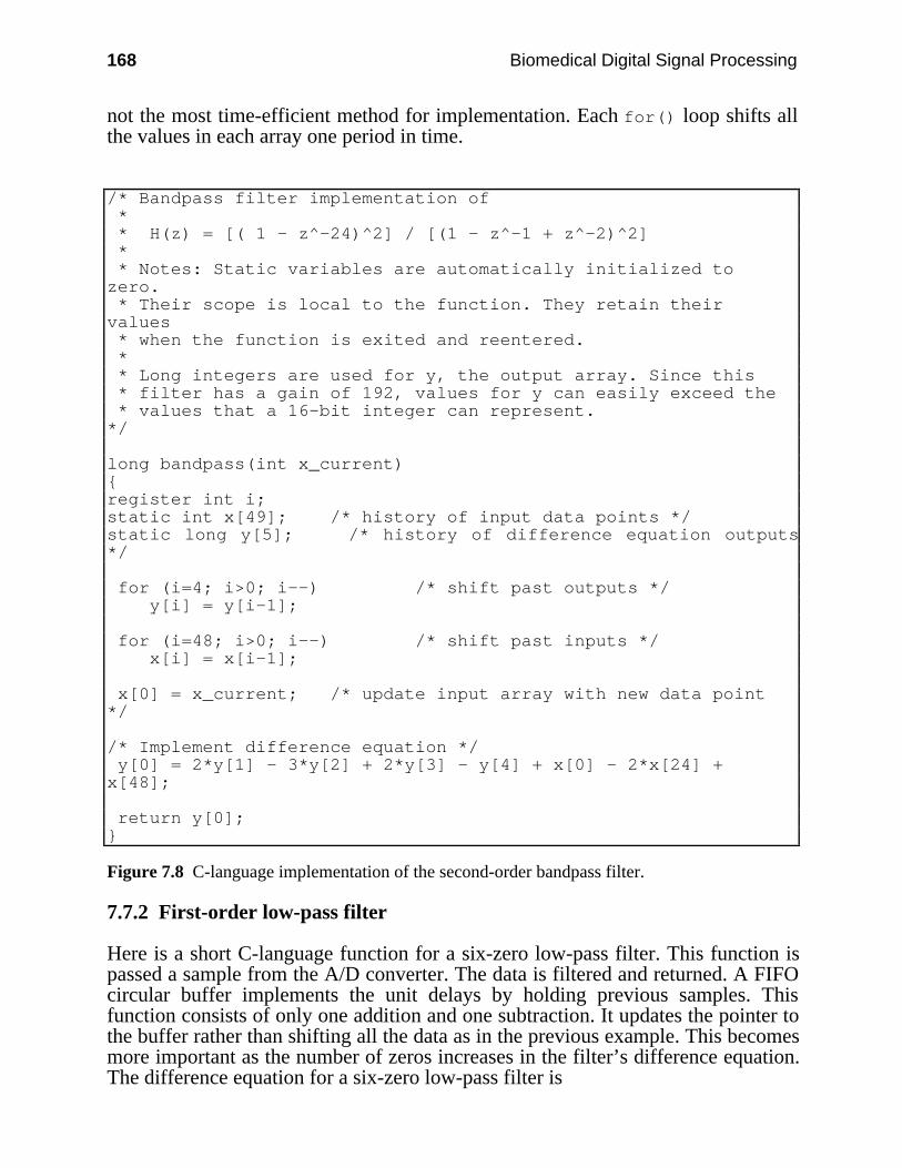
168 Biomedical Digital Signal Processing
not the most time-efficient method for implementation. Each for() loop shifts allthe values in each array one period in time.
/* Bandpass filter implementation of * * H(z) = [( 1 - z^-24)^2] / [(1 - z^-1 + z^-2)^2] * * Notes: Static variables are automatically initialized tozero. * Their scope is local to the function. They retain theirvalues * when the function is exited and reentered. * * Long integers are used for y, the output array. Since this * filter has a gain of 192, values for y can easily exceed the * values that a 16-bit integer can represent.*/
long bandpass(int x_current)register int i;static int x[49]; /* history of input data points */static long y[5]; /* history of difference equation outputs*/
for (i=4; i>0; i--) /* shift past outputs */ y[i] = y[i–1];
for (i=48; i>0; i--) /* shift past inputs */ x[i] = x[i-1];
x[0] = x_current; /* update input array with new data point*/
/* Implement difference equation */ y[0] = 2*y[1] - 3*y[2] + 2*y[3] - y[4] + x[0] - 2*x[24] +x[48];
return y[0];
Figure 7.8 C-language implementation of the second-order bandpass filter.
7.7.2 First-order low-pass filter
Here is a short C-language function for a six-zero low-pass filter. This function ispassed a sample from the A/D converter. The data is filtered and returned. A FIFOcircular buffer implements the unit delays by holding previous samples. Thisfunction consists of only one addition and one subtraction. It updates the pointer tothe buffer rather than shifting all the data as in the previous example. This becomesmore important as the number of zeros increases in the filter’s difference equation.The difference equation for a six-zero low-pass filter is
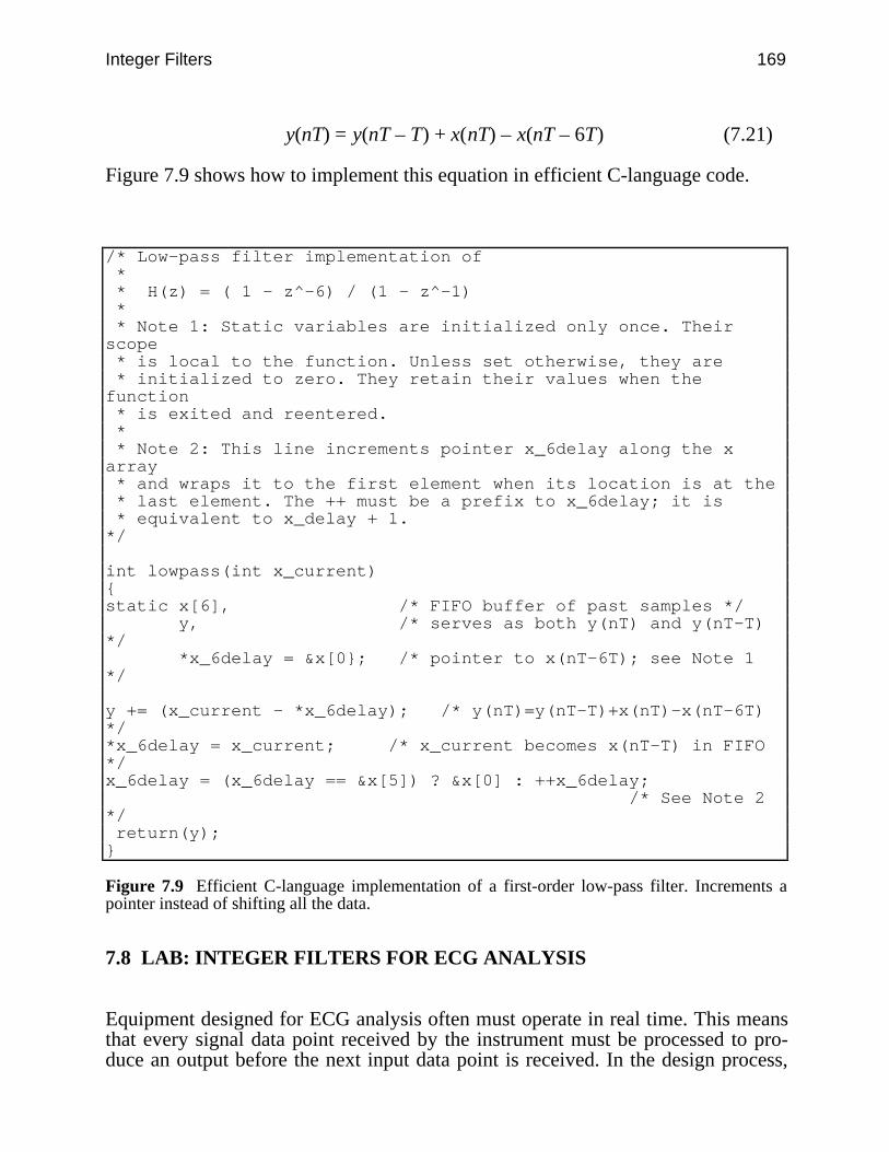
Integer Filters 169
y(nT) = y(nT – T) + x(nT) – x(nT – 6T) (7.21)
Figure 7.9 shows how to implement this equation in efficient C-language code.
/* Low-pass filter implementation of * * H(z) = ( 1 - z^-6) / (1 - z^-1) * * Note 1: Static variables are initialized only once. Theirscope * is local to the function. Unless set otherwise, they are * initialized to zero. They retain their values when thefunction * is exited and reentered. * * Note 2: This line increments pointer x_6delay along the xarray * and wraps it to the first element when its location is at the * last element. The ++ must be a prefix to x_6delay; it is * equivalent to x_delay + 1.*/
int lowpass(int x_current)static x[6], /* FIFO buffer of past samples */ y, /* serves as both y(nT) and y(nT-T)*/ *x_6delay = &x[0; /* pointer to x(nT-6T); see Note 1*/
y += (x_current - *x_6delay); /* y(nT)=y(nT-T)+x(nT)-x(nT-6T)*/*x_6delay = x_current; /* x_current becomes x(nT-T) in FIFO*/x_6delay = (x_6delay == &x[5]) ? &x[0] : ++x_6delay; /* See Note 2*/ return(y);
Figure 7.9 Efficient C-language implementation of a first-order low-pass filter. Increments apointer instead of shifting all the data.
7.8 LAB: INTEGER FILTERS FOR ECG ANALYSIS
Equipment designed for ECG analysis often must operate in real time. This meansthat every signal data point received by the instrument must be processed to pro-duce an output before the next input data point is received. In the design process,
170 Biomedical Digital Signal Processing
cost constraints often make it desirable to use smaller, low-performance micropro-cessors to control a device. If the driver for an instrument is a PC, many times it isnot equipped with a math coprocessor or a high-performance microprocessor. Forthis lab, you will design and implement several of the filters previously discussedto compare their performance in several situations.
Execute (F)ilters, (D)esign, then i(N)teger to enter the integer filter de-sign shell.
1. Use the (G)enwave function to generate a normal ECG from template 1 andan abnormal ECG from template 5, both with a sampling rate of 100 sps and anamplitude resolution of eight bits.
(a) Design a bandpass filter for processing these signals with six zeros and acenter frequency of 16.7 Hz. This type of filter is sometimes used in cardiota-chometers to find the QRS complex determine heart rate.
(b) Filter the two ECGs with these filters. Since this filter has gain, you willprobably need to adjust the amplitudes with the (Y) Sens function. Sketch the re-sponses.
(c) Read the unit impulse signal file ups.dat from the STDLIB directory, andfilter it. Sketch the response. Take the power spectrum of the impulse response us-ing (P)wr Spect. The result is the amplitude response of the filter, which is thesame as the response that you obtained when you designed the filter except that thefrequency axis is double that of your design because the unit impulse signal wassampled at 200 sps instead of the 100 sps for which you designed your filter. Usethe cursors of the (M)easure function to locate the 3-dB points, and find thebandwidth. Note that the actual bandwidth is half the measurement because ofdoubling of the frequency axis. Calculate the Q of the filter.
(d) Design two bandpass filters similar to the one in part (a) except with 18 and48 zeros. Repeat parts (b) and (c) using these filters. As the number of zeros in-creases, the gain of these filters also increases, so you may have an overflow prob-lem with some of the responses, particularly for the unit impulse. If this occurs, theoutput will appear to have discontinuities, indicating that the 16-bit representationof data in DigiScope has overflowed. In this case, attenuate the amplitude of theunit impulse signal prior to filtering it. Which of these three filter designs is mostappropriate for detecting the QRS complexes? Why?
2. Design a low-pass filter with 10 zeros. Filter the normal ECG from part 1,and sketch the output. Which waves are attenuated and which are amplified? Whatis the 3-dB passband?
3. Generate a normal ECG with a sampling rate of 180 sps. Include 10% 60-Hznoise and 10% random noise in the signal. Design a single low-pass filter that(a) has a low-pass bandwidth of about 15 Hz to attenuate random noise, and(b) completely eliminates 60-Hz noise. Measure the actual 3-dB bandwidth.Comment on the performance of your design.
Integer Filters 171
7.9 REFERENCES
Ahlstrom, M. L., and Tompkins, W. J. 1985. Digital filters for real-time ECG signal processingusing microprocessors. IEEE Trans. Biomed. Eng., BME-32(9): 708–13.
Kohn, A. F. 1987. Phase distortion in biological signal analysis caused by linear phase FIRfilters. Med. & Biol. Eng. & Comput. 25: 231–38.
Lynn, P. A. 1977. Online digital filters for biological signals: some fast designs for a smallcomputer. Med. & Biol. Eng. & Comput. 15: 534–40.
Lynn, P. A. 1971. Recursive digital filters for biological signals. Med. & Biol. Eng. & Comput.9: 37–44.
Lynn, P. A. 1972. Recursive digital filters with linear-phase characteristics. Comput. J. 15:337–42.
Lynn, P. A. 1983. Transversal resonator digital filters: fast and flexible online processors forbiological signals. Med. & Biol. Eng. & Comput. 21: 718–30.
Principe, J. C., and Smith, J. R. 1986. Design and implementation of linear phase FIR filters forbiological signal processing. IEEE Trans. Biomed. Eng. BME-33(6):550–59.
Thakor, N. V., and Moreau, D. 1987. Design and analysis of quantised coefficient digital filters:application to biomedical signal processing with microprocessors. Med. & Biol. & Comput.25: 18–25.
7.10 STUDY QUESTIONS
7.1 Why is it advantageous to use integer coefficients in a digital filter’s difference equation?7.2 Explain why it is more difficult to design a digital filter when all coefficients are restricted
to having integer values.7.3 Show how the denominator of Eq. (7.1) will always place two poles on the unit circle for
all values of . What values of produce integer coefficients? Why should values of thatyield floating-point numbers be avoided?
7.4 Show mathematically why the numerators (1 + z–m) and (1 – z–m) place zeros on the unitcircle. Both numerators produce evenly spaced zeros. When would it be advantageous touse (1 – z–m) instead of (1 + z–m)?
7.5 When does Eq. (7.1) behave as a FIR filter? How can this equation become unstable? Whatare the advantages of expressing a FIR filter in recursive form?
7.6 When does Eq. (7.1) behave as a low-pass filter? Discuss what characteristics of filterbehavior a designer must consider when a filter is to have a low cutoff frequency.
7.7 What is the difference between a true-linear phase response and a piecewise-linear phaseresponse? When is a linear phase response essential? Can a filter with a piecewise-linearphase response behave as one with a true-linear phase response?
7.8 Name four ways in which an integer digital filter’s magnitude and phase response changewhen the filter is cascaded with itself. Why or why not are these changes helpful?
7.9 If poles and zeros are placed at noninteger locations, how can a digital filter still remaincomputationally efficient? Describe two methods that use this principle.
7.10 Calculate expressions for the amplitude and phase response of a filter with the z transform
H(z) = 1 – z–6
7.11 The numerator of a transfer function is (1 – z–10). Where are its zeros located?7.12 A filter has 12 zeros located on the unit circle starting at dc and equally spaced at 30˚
increments (i.e., 1 – z–12). There are three poles located at z = +0.9, and z = ±j. The

172 Biomedical Digital Signal Processing
sampling frequency is 360 samples/s. (a) At what frequency is the output at its maximalamplitude? (b) What is the gain at this frequency?
7.13 A digital filter has the following transfer function. (a) What traditional filter type bestdescribes this filter? (b) What is its gain at dc?
H(z) = 1 – z–6
(1 – z–1)(1 – z–1 + z–2)
7.14 For a filter with the following transfer function, what is the (a) amplitude response,(b) phase response, (c) difference equation?
H(z) = 1 – z–8
1 + z–2
7.15 A digital filter has the following transfer function. (a) What traditional filter type bestdescribes this filter? (b) Draw its pole-zero plot. (c) Calculate its amplitude response.(d) What is its difference equation?
H(z) = (1 – z–8)2
(1 + z–2)2
7.16 What is the gain of a filter with the transfer function
H(z) = 1 – z–6
1 – z–1
7.17 What traditional filter type best describes a filter with the transfer function
H(z) = 1 – z–256
1 – z–128
7.18 What traditional filter type best describes a filter with the transfer function
H(z) = 1 – z–200
1 – z–2
7.19 A digital filter has four zeros located at z = ±1 and z = ±j and four poles located at z = 0,z = 0, and z = ±j. The sampling frequency is 800 samples/s. The maximal output amplitudeoccurs at what frequency?
7.20 For a sampling rate of 100 samples/s, a digital filter with the following transfer function hasits maximal gain at approximately what frequency (in Hz)?
H(z) = 1 – z–36
1 – z–1 + z–2
7.21 The z transform of a filter is:H(z) = 1 – z–360
The following sine wave is applied at the input: x(t) = 100 sin(2π10t). The sampling rate is720 samples/s. (a) What is the peak-to-peak output of the filter? (b) If a unit step input is

Integer Filters 173
applied, what will the output amplitude be after 361 samples? (c) Where could poles beplaced to convert this to a bandpass filter with integer coefficients?
7.22 What is the phase delay (in milliseconds) through the following filter which operates at 200samples/sec?
H(z) = 1 – z–100
1 – z–2
7.23 A filter has 8 zeros located on the unit circle starting at dc and equally spaced at 45˚increments. There are two poles located at z = ±j. The sampling frequency is 360 samples/s.What is the gain of the filter?
174
8
Adaptive Filters
Steven Tang
This chapter discusses how to build adaptive digital filters to perform noise cancel-lation and signal extraction. Adaptive techniques are advantageous because they donot require a priori knowledge of the signal or noise characteristics as do fixed fil-ters. Adaptive filters employ a method of learning through an estimated synthesisof a desired signal and error feedback to modify the filter parameters. Adaptivetechniques have been used in filtering of 60-Hz line frequency noise from ECGsignals, extracting fetal ECG signals, and enhancing P waves, as well as for remov-ing other artifacts from the ECG signal. This chapter provides the basic principlesof adaptive digital filtering and demonstrates some direct applications.
In digital signal processing applications, frequently a desired signal is corruptedby interfering noise. In fixed filter methods, the basic premise behind optimal fil-tering is that we must have knowledge of both the signal and noise characteristics.It is also generally assumed that the statistics of both sources are well behaved orwide-sense stationary. An adaptive filter learns the statistics of the input sourcesand tracks them if they vary slowly.
8.1 PRINCIPAL NOISE CANCELER MODEL
In biomedical signal processing, adaptive techniques are valuable for eliminatingnoise interference. Figure 8.1 shows a general model of an adaptive filter noisecanceler. In the discrete time case, we can model the primary input as s(nT) +n0(nT). The noise is additive and considered uncorrelated with the signal source. Asecondary reference input to the filter feeds a noise n1(nT) into the filter to produceoutput (nT) that is a close estimate of n0(nT). The noise n1(nT) is correlated in anunknown way to n0(nT).
The output (nT) is subtracted from the primary input to produce the systemoutput y(nT). This output is also the error (nT) that is used to adjust the taps of theadaptive filter coefficients w(1,…, p).
y(nT) = s(nT) + n0(nT) – (nT) (8.1)
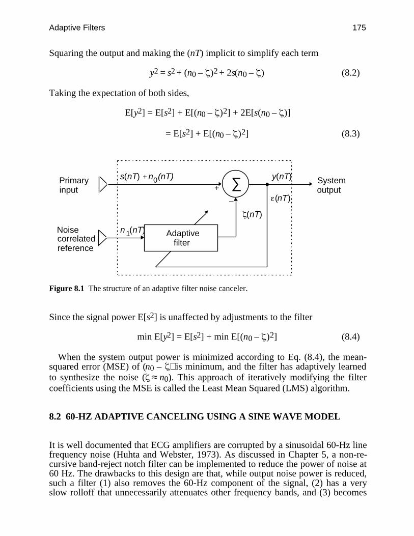
Adaptive Filters 175
Squaring the output and making the (nT) implicit to simplify each term
y2 = s2 + (n0 – )2 + 2s(n0 – ) (8.2)
Taking the expectation of both sides,
E[y2] = E[s2] + E[(n0 – )2] + 2E[s(n0 – )]
= E[s2] + E[(n0 – )2] (8.3)
∑+
–
Adaptive filter
Primaryinput
Noise correlated reference
System output
(nT)
n (nT)
(nT)
y(nT)s(nT) + n (nT)0
1
Figure 8.1 The structure of an adaptive filter noise canceler.
Since the signal power E[s2] is unaffected by adjustments to the filter
min E[y2] = E[s2] + min E[(n0 – )2] (8.4)
When the system output power is minimized according to Eq. (8.4), the mean-squared error (MSE) of (n0 – ) is minimum, and the filter has adaptively learnedto synthesize the noise ( ≈ n0). This approach of iteratively modifying the filtercoefficients using the MSE is called the Least Mean Squared (LMS) algorithm.
8.2 60-HZ ADAPTIVE CANCELING USING A SINE WAVE MODEL
It is well documented that ECG amplifiers are corrupted by a sinusoidal 60-Hz linefrequency noise (Huhta and Webster, 1973). As discussed in Chapter 5, a non-re-cursive band-reject notch filter can be implemented to reduce the power of noise at60 Hz. The drawbacks to this design are that, while output noise power is reduced,such a filter (1) also removes the 60-Hz component of the signal, (2) has a veryslow rolloff that unnecessarily attenuates other frequency bands, and (3) becomes
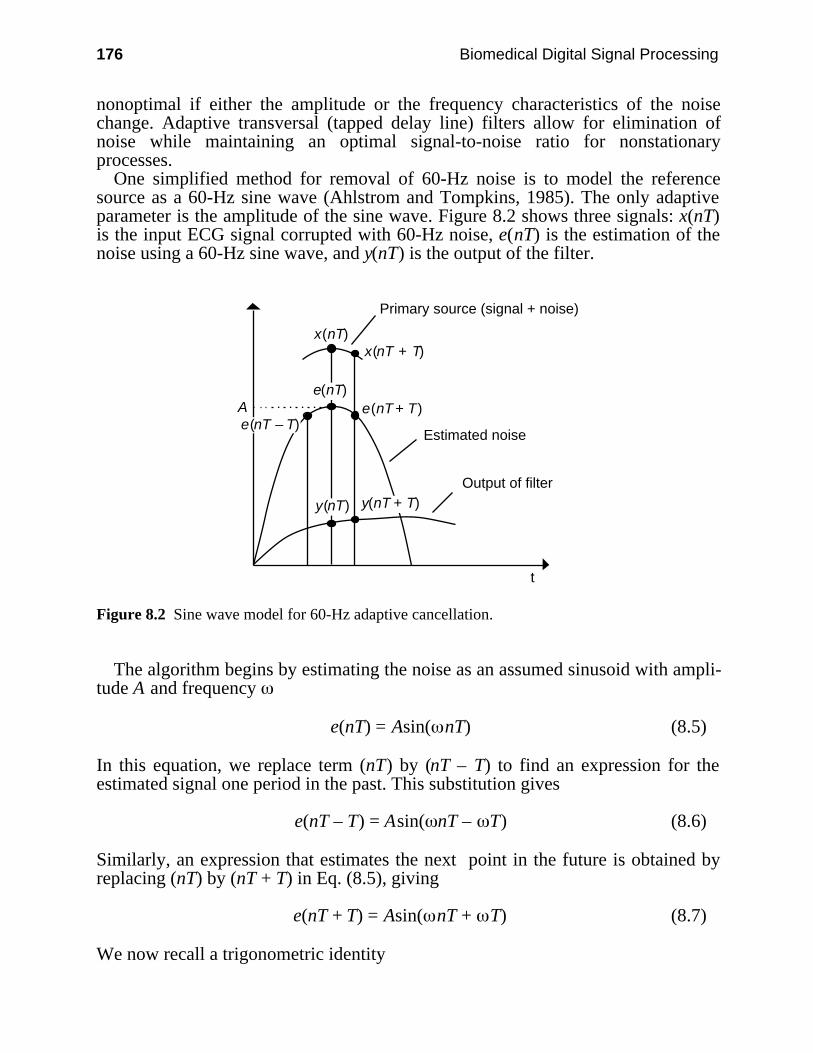
176 Biomedical Digital Signal Processing
nonoptimal if either the amplitude or the frequency characteristics of the noisechange. Adaptive transversal (tapped delay line) filters allow for elimination ofnoise while maintaining an optimal signal-to-noise ratio for nonstationaryprocesses.
One simplified method for removal of 60-Hz noise is to model the referencesource as a 60-Hz sine wave (Ahlstrom and Tompkins, 1985). The only adaptiveparameter is the amplitude of the sine wave. Figure 8.2 shows three signals: x(nT)is the input ECG signal corrupted with 60-Hz noise, e(nT) is the estimation of thenoise using a 60-Hz sine wave, and y(nT) is the output of the filter.
Output of filter
A
Estimated noise
Primary source (signal + noise)
x(nT + T)
e(nT – T)
e(nT)e(nT + T)
y(nT + T)
t
x(nT)
y(nT)
Figure 8.2 Sine wave model for 60-Hz adaptive cancellation.
The algorithm begins by estimating the noise as an assumed sinusoid with ampli-tude A and frequency
e(nT) = Asin( nT) (8.5)
In this equation, we replace term (nT) by (nT – T) to find an expression for theestimated signal one period in the past. This substitution gives
e(nT – T) = Asin( nT – T) (8.6)
Similarly, an expression that estimates the next point in the future is obtained byreplacing (nT) by (nT + T) in Eq. (8.5), giving
e(nT + T) = Asin( nT + T) (8.7)
We now recall a trigonometric identity
Adaptive Filters 177
sin( + ) = 2sin( ) cos( ) – sin( – ) (8.8)Now let
= nT and = T (8.9)
Expanding the estimate for the future estimate of Eq. (8.7) using Eqs. (8.8) and(8.9) gives
e(nT + T) = 2 Asin( nT) cos( T) – Asin( nT – T) (8.10)
Note that the first underlined term is the same as the expression for e(nT) in Eq.(8.5), and the second underlined term is the same as the expression for e(nT – T) inEq. (8.6). The term, cos( T), is a constant determined by the frequency of thenoise to be eliminated and by the sampling frequency, fs= 1/T:
N = cos( T) = cos
2πf
fs (8.11)
Thus, Eq. (8.10) is rewritten, giving a relation for the future estimated point on asampled sinusoidal noise waveform based on the values at the current and pastsample times.
e(nT + T) = 2Ne(nT) – e(nT – T) (8.12)
The output of the filter is the difference between the input and the estimatedsignals
y(nT + T) = x(nT + T) – e(nT + T) (8.13)
Thus, if the input were only noise and the estimate were exactly tracking (i.e.,modeling) it, the output would be zero. If an ECG were superimposed on the inputnoise, it would appear noise-free at the output.
The ECG signal is actually treated as a transient, while the filter iteratively at-tempts to change the “weight” or amplitude of the reference input to match the de-sired signal, the 60-Hz noise. The filter essentially learns the amount of noise thatis present in the primary input and subtracts it out. In order to iteratively adjust thefilter to adapt to changes in the noise signal, we need feedback to adjust the sinu-soidal amplitude of the estimate signal for each sample period.
We define the difference function
f(nT + T) = [x(nT + T) – e(nT + T)] – [x(nT) – e(nT)] (8.14)
In order to understand this function, consider Figure 8.3. Our original model of thenoise e(nT) in Eq. (8.5) assumed a simple sine wave with no dc component asshown. Typically, however, there is a dc offset represented by Vdc in the inputx(nT) signal. From the figure
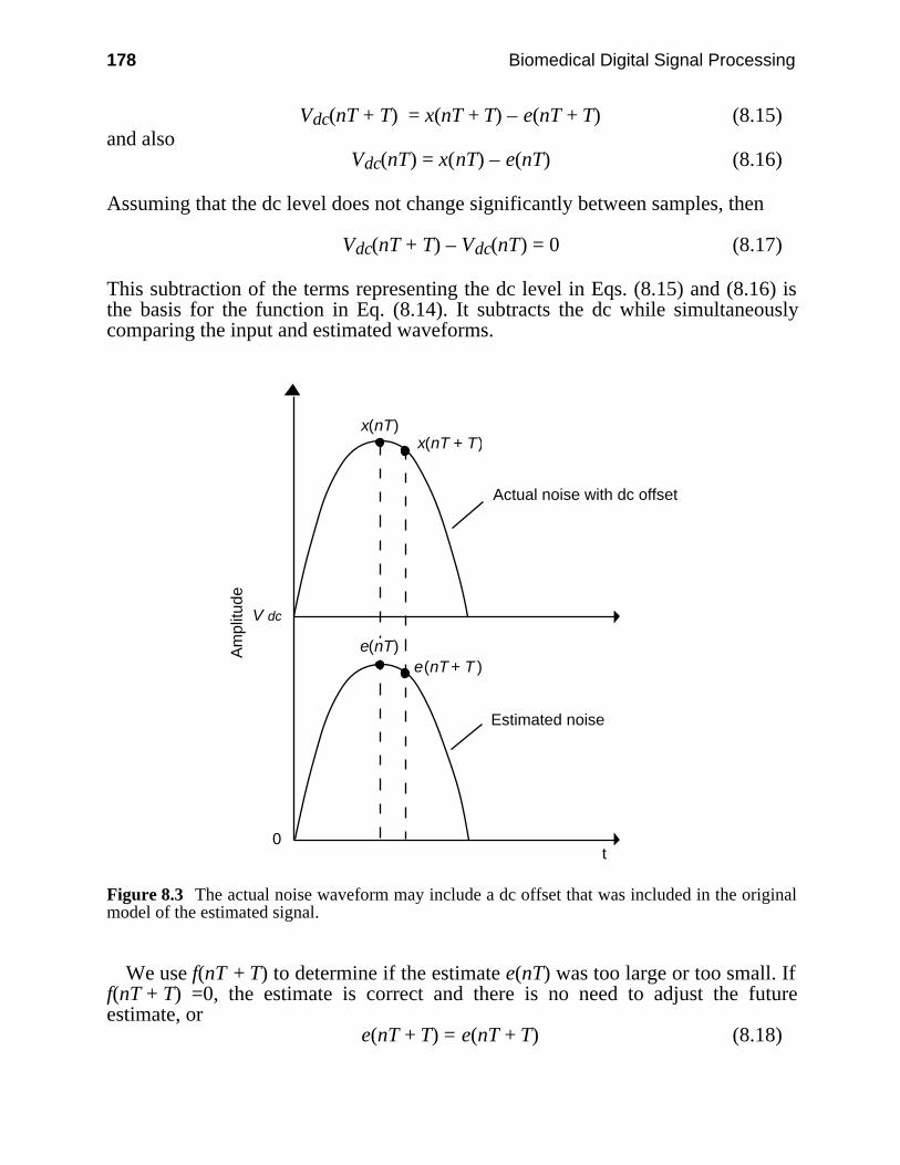
178 Biomedical Digital Signal Processing
Vdc(nT + T) = x(nT + T) – e(nT + T) (8.15)and also
Vdc(nT) = x(nT) – e(nT) (8.16)
Assuming that the dc level does not change significantly between samples, then
Vdc(nT + T) – Vdc(nT) = 0 (8.17)
This subtraction of the terms representing the dc level in Eqs. (8.15) and (8.16) isthe basis for the function in Eq. (8.14). It subtracts the dc while simultaneouslycomparing the input and estimated waveforms.
Estimated noise
Actual noise with dc offset
x(nT + T)
e(nT)e(nT + T )
t
x(nT)
V dc
0
Am
plitu
de
Figure 8.3 The actual noise waveform may include a dc offset that was included in the originalmodel of the estimated signal.
We use f(nT + T) to determine if the estimate e(nT) was too large or too small. Iff(nT + T) =0, the estimate is correct and there is no need to adjust the futureestimate, or
e(nT + T) = e(nT + T) (8.18)
Adaptive Filters 179
If f(nT + T) > 0, the estimate is low, and the estimate is adjusted upward by a smallstep size d
e(nT + T) = e(nT + T) + d (8.19)
If f(nT + T) < 0, the estimate is high and the estimate is adjusted downward by asmall step size d
e(nT + T) = e(nT + T) – d (8.20)
The choice of d is empirically determined and depends on how quickly the filterneeds to adapt to changes in the interfering noise. If d is large, then the filterquickly adjusts its coefficients after the onset of 60-Hz noise. However, if d is toolarge, the filter will not be able to converge exactly to the noise. This results insmall oscillations in the estimated signal once the correct amplitude has beenfound. With a smaller d, the filter requires a longer learning period but providesmore exact tracking of the noise for a smoother output. If the value of d is too largeor too small, the filter will never converge to a proper noise estimate.
A typical value of d is less than the least significant bit value of the integers usedto represent a signal. For example, if the full range of numbers from an 8-bit A/Dconverter is 0–255, then an optimal value for d might be 1/4.
Producing the estimated signal of Eq. (8.12) requires multiplication by a fractionN given in Eq. (8.11). For a sampling rate of 500 sps and 60-Hz power line noise
N = cos
2π × 60
500 = 0.7289686 (8.21)
Such a multiplier requires floating-point arithmetic, which could considerably slowdown the algorithm. In order to approximate such a multiplier, we might choose touse a summation of power-of-two fractions, which could be implemented with bit-shift operations and may be faster than floating-point multiplication in some hard-ware environments. In this case
N = 12 +
18 +
116 +
132 +
1128 +
1512 +
12048 = 0.72900 (8.22)
8.3 OTHER APPLICATIONS OF ADAPTIVE FILTERING
Adaptive filtering is not only used to suppress 60-Hz interference but also forsignal extraction and artifact cancellation. The adaptive technique is advantageousfor generating a desired signal from one that is uncorrelated with it.
8.3.1 Maternal ECG in fetal ECG
Prenatal monitoring has made it possible to detect the heartbeat of the unborn childnoninvasively. However, motion artifact and the maternal ECG make it verydifficult to perceive the fetal ECG since it is a low-amplitude signal. Adaptive
180 Biomedical Digital Signal Processing
filtering has been used to eliminate the maternal ECG. Zhou et al. (1985) describean algorithm that uses a windowed LMS routine to adapt the tap weights. Theabdominal lead serves as the primary input and the chest lead from the mother isused as the reference noise input. Subtracting the best matched maternal ECG fromthe abdominal ECG which contains both the fetal and maternal ECGs produces aresidual signal that is the fetal ECG.
8.3.2 Cardiogenic artifact
The area of electrical impedance pneumography has used adaptive filtering tosolve the problem of cardiogenic artifact (ZCG). Such artifact can arise fromelectrical impedance changes due to blood flow and heart-volume changes. Thiscan lead to a false interpretation of breathing. When monitoring for infant apnea,this might result in a failure to alarm. Sahakian and Kuo (1985) proposed using anadaptive LMS algorithm to extract the cardiogenic impedance component so as toachieve the best estimate of the respiratory impedance component. To model thecardiogenic artifact, they created a template synchronized to the QRS complex inan ECG that included sinus arrhythmia. Cardiogenic artifact is synchronous withbut delayed from ventricular systole, so the ECG template can be used to deriveand eliminate the ZCG.
8.3.3 Detection of ventricular fibrillation and tachycardia
Ventricular fibrillation detection has generally used frequency-domain techniques.This is computationally expensive and cannot always be implemented in real time.Hamilton and Tompkins (1987) describe a unique method of adaptive filtering tolocate the poles corresponding to the frequency spectrum formants. By running asecond-order IIR filter, the poles derived from the coefficients give a fairly goodestimate of the first frequency peak.
The corresponding z transform of such a filter is
H(z) = 1
1 – b1z–1 – b2z–2
We can solve for the pole radius and angle by noting that, for all poles not on thereal axis
b1 = 2rcos and b2 = –r2
Using the fact that fibrillation produces a prominent peak in the 3–7 Hz fre-quency band, we can determine whether the poles fall in the “detection region” ofthe z plane. An LMS algorithm updates the coefficients of the filter. Figure 8.4shows the z-plane pole-zero diagram of the adaptive filter. The shaded region indi-cates that the primary peak in the frequency spectrum of the ECG is in a“dangerous” area. The only weakness of the algorithm is that it creates false detec-tions for rhythm rates greater than 100 bpm with frequent PVCs, atrial fibrillation,and severe motion artifact.
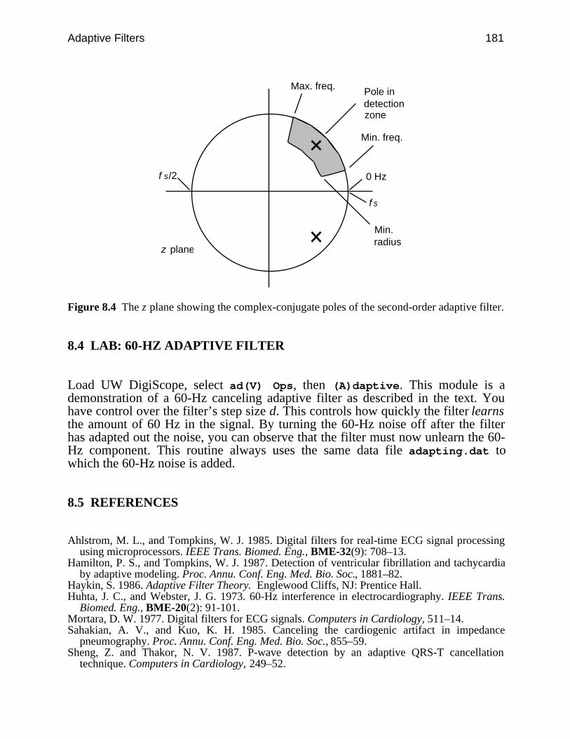
Adaptive Filters 181
0 Hzf s/2
z plane
Pole indetectionzone
Max. freq.
Min. freq.
Min.radius
fs
Figure 8.4 The z plane showing the complex-conjugate poles of the second-order adaptive filter.
8.4 LAB: 60-HZ ADAPTIVE FILTER
Load UW DigiScope, select ad(V) Ops, then (A)daptive. This module is ademonstration of a 60-Hz canceling adaptive filter as described in the text. Youhave control over the filter’s step size d. This controls how quickly the filter learnsthe amount of 60 Hz in the signal. By turning the 60-Hz noise off after the filterhas adapted out the noise, you can observe that the filter must now unlearn the 60-Hz component. This routine always uses the same data file adapting.dat towhich the 60-Hz noise is added.
8.5 REFERENCES
Ahlstrom, M. L., and Tompkins, W. J. 1985. Digital filters for real-time ECG signal processingusing microprocessors. IEEE Trans. Biomed. Eng., BME-32(9): 708–13.
Hamilton, P. S., and Tompkins, W. J. 1987. Detection of ventricular fibrillation and tachycardiaby adaptive modeling. Proc. Annu. Conf. Eng. Med. Bio. Soc., 1881–82.
Haykin, S. 1986. Adaptive Filter Theory. Englewood Cliffs, NJ: Prentice Hall.Huhta, J. C., and Webster, J. G. 1973. 60-Hz interference in electrocardiography. IEEE Trans.
Biomed. Eng., BME-20(2): 91-101.Mortara, D. W. 1977. Digital filters for ECG signals. Computers in Cardiology, 511–14.Sahakian, A. V., and Kuo, K. H. 1985. Canceling the cardiogenic artifact in impedance
pneumography. Proc. Annu. Conf. Eng. Med. Bio. Soc., 855–59.Sheng, Z. and Thakor, N. V. 1987. P-wave detection by an adaptive QRS-T cancellation
technique. Computers in Cardiology, 249–52.

182 Biomedical Digital Signal Processing
Widrow, B., Glover, J. R., John, M., Kaunitz, J., Charles, S. J., Hearn, R. H., Zeidler, J. R.,Dong, E., and Goodlin, R. C. 1975. Adaptive noise canceling: principles and applications.Proc. IEEE, 63(12): 1692–1716.
Zhou, L., Wei, D., and Sun, L. 1985. Fetal ECG processing by adaptive noise cancellation. Proc.Annu. Conf. Eng. Med. Bio. Soc., 834–37.
8.6 STUDY QUESTIONS
8.1 What are the main advantages of adaptive filters over fixed filters?8.2 Explain the criterion that is used to construct a Wiener filter.8.3 Why is the error residual of a Wiener filter normal to the output?8.4 Design an adaptive filter using the method of steepest-descent.8.5 Design an adaptive filter using the LMS algorithm.8.6 Why are bounds necessary on the step size of the steepest-descent and LMS algorithms?8.7 What are the costs and benefits of using different step sizes in the 60-Hz sine wave
algorithm?8.8 Explain how the 60-Hz sine wave algorithm adapts to the phase of the noise.8.9 The adaptive 60-Hz filter calculates a function
f(nT + T) = [ ]x(nT + T) – e(nT + T) – [ ]x(nT) – e(nT)
If this function is less than zero, how does the algorithm adjust the future estimate,e(nT + T)?
8.10 The adaptive 60-Hz filter uses the following equation to estimate the noise:
e(nT + T) = 2Ne(nT) – e(nT – T)
If the future estimate is found to be too high, what adjustment is made to (a) e(nT – T),(b) e(nT + T). (c) Write the equation for N and explain the terms of the equation.
8.11 The adaptive 60-Hz filter calculates the function
f(nT + T) = [ ]x(nT + T) – e(nT + T) – [ ]x(nT) – e(nT)
It adjusts the future estimate e(nT + T) based on whether this function is greater than, lessthan, or equal to zero. Use a drawing and explain why the function could not be simplifiedto
f(nT + T) = x(nT + T) – e(nT + T)

Adaptive Filters 183
184
9
Signal Averaging
Pradeep Tagare
Linear digital filters like those discussed in previous chapters perform very wellwhen the spectra of the signal and noise do not significantly overlap. For example,a low-pass filter with a cutoff frequency of 100 Hz generally works well for atten-uating noise frequencies greater than 100 Hz in ECG signals. However, if high-level noise frequencies were to span the frequency range from 50–100 Hz, attempt-ing to remove them using a 50–Hz low-pass filter would attenuate some of thecomponents of the ECG signal as well as the noise. High-amplitude noise corrup-tion within the frequency band of the signal may completely obscure the signal.Thus, conventional filtering schemes fail when the signal and noise frequencyspectra significantly overlap. Signal averaging is a digital technique for separatinga repetitive signal from noise without introducing signal distortion (Tompkins andWebster, 1981). This chapter describes the technique of signal averaging forincreasing the signal-to-noise ratio and discusses several applications.
9.1 BASICS OF SIGNAL AVERAGING
Figure 9.1(a) shows the spectrum of a signal that is corrupted by noise. In this case,the noise bandwidth is completely separated from the signal bandwidth, so thenoise can easily be discarded by applying a linear low-pass filter. On the otherhand, the noise bandwidth in Figure 9.1(b) overlaps the signal bandwidth, and thenoise amplitude is larger than the signal. For this situation, a low-pass filter wouldneed to discard some of the signal energy in order to remove the noise, thereby dis-torting the signal.
One predominant application area of signal averaging is in electroencephalogra-phy. The EEG recorded from scalp electrodes is difficult to interpret in part be-cause it consists of a summation of the activity of the billions of brain cells. It isimpossible to deduce much about the activity of the visual or auditory parts of thebrain from the EEG. However, if we stimulate a part of the brain with a flash oflight or an acoustical click, an evoked response occurs in the region of the brainthat processes information for the sensory system being stimulated. By summing
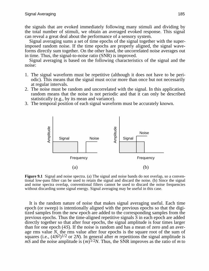
Signal Averaging 185
the signals that are evoked immediately following many stimuli and dividing bythe total number of stimuli, we obtain an averaged evoked response. This signalcan reveal a great deal about the performance of a sensory system.
Signal averaging sums a set of time epochs of the signal together with the super-imposed random noise. If the time epochs are properly aligned, the signal wave-forms directly sum together. On the other hand, the uncorrelated noise averages outin time. Thus, the signal-to-noise ratio (SNR) is improved.
Signal averaging is based on the following characteristics of the signal and thenoise:
1. The signal waveform must be repetitive (although it does not have to be peri-odic). This means that the signal must occur more than once but not necessarilyat regular intervals.
2. The noise must be random and uncorrelated with the signal. In this application,random means that the noise is not periodic and that it can only be describedstatistically (e.g., by its mean and variance).
3. The temporal position of each signal waveform must be accurately known.
Am
plitu
de
Frequency
Am
plitu
de
Frequency
Signal Noise Signal
Noise
(a) (b)
Figure 9.1 Signal and noise spectra. (a) The signal and noise bands do not overlap, so a conven-tional low-pass filter can be used to retain the signal and discard the noise. (b) Since the signaland noise spectra overlap, conventional filters cannot be used to discard the noise frequencieswithout discarding some signal energy. Signal averaging may be useful in this case.
It is the random nature of noise that makes signal averaging useful. Each timeepoch (or sweep) is intentionally aligned with the previous epochs so that the digi-tized samples from the new epoch are added to the corresponding samples from theprevious epochs. Thus the time-aligned repetitive signals S in each epoch are addeddirectly together so that after four epochs, the signal amplitude is four times largerthan for one epoch (4S). If the noise is random and has a mean of zero and an aver-age rms value N, the rms value after four epochs is the square root of the sum ofsquares (i.e., (4N2)1/2 or 2N). In general after m repetitions the signal amplitude ismS and the noise amplitude is (m)1/2N. Thus, the SNR improves as the ratio of m to

186 Biomedical Digital Signal Processing
m1/2 (i.e., m1/2). For example, averaging 100 repetitions of a signal improves theSNR by a factor of 10. This can be proven mathematically as follows.
The input waveform f(t) has a signal portion S(t) and a noise portion N(t). Then
f(t) = S(t) + N(t) (9.1)
Let f(t) be sampled every T seconds. The value of any sample point in the timeepoch (i = 1, 2,…, n) is the sum of the noise component and the signal component.
f(iT) = S(iT) + N(iT) (9.2)
Each sample point is stored in memory. The value stored in memory location iafter m repetitions is
∑k=1
m f(iT) = ∑
k=1
m S(iT) + ∑
k=1
m N(iT) for i = 1, 2, …, n (9.3)
The signal component for sample point i is the same at each repetition if the signalis stable and the sweeps are aligned together perfectly. Then
∑k=1
mS(iT) = mS(iT) (9.4)
The assumptions for this development are that the signal and noise are uncorrelatedand that the noise is random with a mean of zero. After many repetitions, N(iT) hasan rms value of n.
∑k=1
mN(iT) = m n2 = m n (9.5)
Taking the ratio of Eqs. (9.4) and (9.5) gives the SNR after m repetitions as
SNRm = mS(iT)
m n = m SNR (9.6)
Thus, signal averaging improves the SNR by a factor of m . Figure 9.2 is a graphillustrating the results of Eq. (9.6).

Signal Averaging 187
5004003002001000
1
10
100
Number of sweeps
Incr
ease
in S
NR
Figure 9.2 Increase in SNR as a function of the number of sweeps averaged.
Figure 9.3 illustrates the problem of signal averaging. The top trace is the ECGof the middle trace after being corrupted by random noise. Since the noise isbroadband, there is no way to completely remove it with a traditional linear filterwithout also removing some of the ECG frequency components, thereby distortingthe ECG. Signal averaging of this noisy signal requires a way to time align each ofthe QRS complexes with the others. By analyzing a heavily filtered version of thewaveform, it is possible to locate the peaks of the QRS complexes and use themfor time alignment. The lower trace shows these timing references (fiducial points)that are required for signal processing.
Figure 9.4 shows how the QRS complexes, centered on the fiducial points, areassembled and summed to produce the averaged signal. The time-aligned QRScomplexes sum directly while the noise averages out to zero. The fiducial marksmay also be located before or after the signal to be averaged, as long as they haveaccurate temporal relationships to the signals.
One research area in electrocardiography is the study of late potentials that re-quire an ECG amplifier with a bandwidth of 500 Hz. These small, high-frequencysignals of possible clinical significance occur after the QRS complex in body sur-face ECGs of abnormals. These signals are so small compared to the other wave-forms in the ECG that they are hidden in the noise and are not observable withoutsignal averaging. In this application, the fiducial points are derived from the QRScomplexes, and the averaging region is the time following each QRS complex.
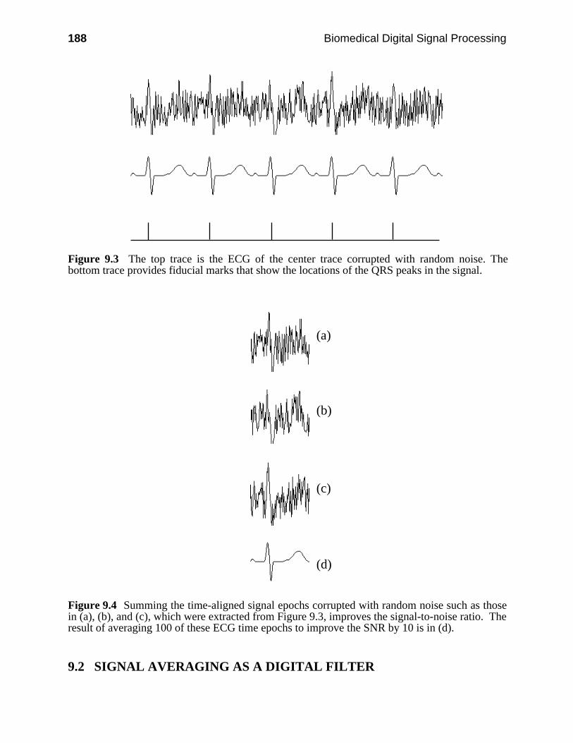
188 Biomedical Digital Signal Processing
Figure 9.3 The top trace is the ECG of the center trace corrupted with random noise. Thebottom trace provides fiducial marks that show the locations of the QRS peaks in the signal.
(a)
(b)
(c)
(d)
Figure 9.4 Summing the time-aligned signal epochs corrupted with random noise such as thosein (a), (b), and (c), which were extracted from Figure 9.3, improves the signal-to-noise ratio. Theresult of averaging 100 of these ECG time epochs to improve the SNR by 10 is in (d).
9.2 SIGNAL AVERAGING AS A DIGITAL FILTER
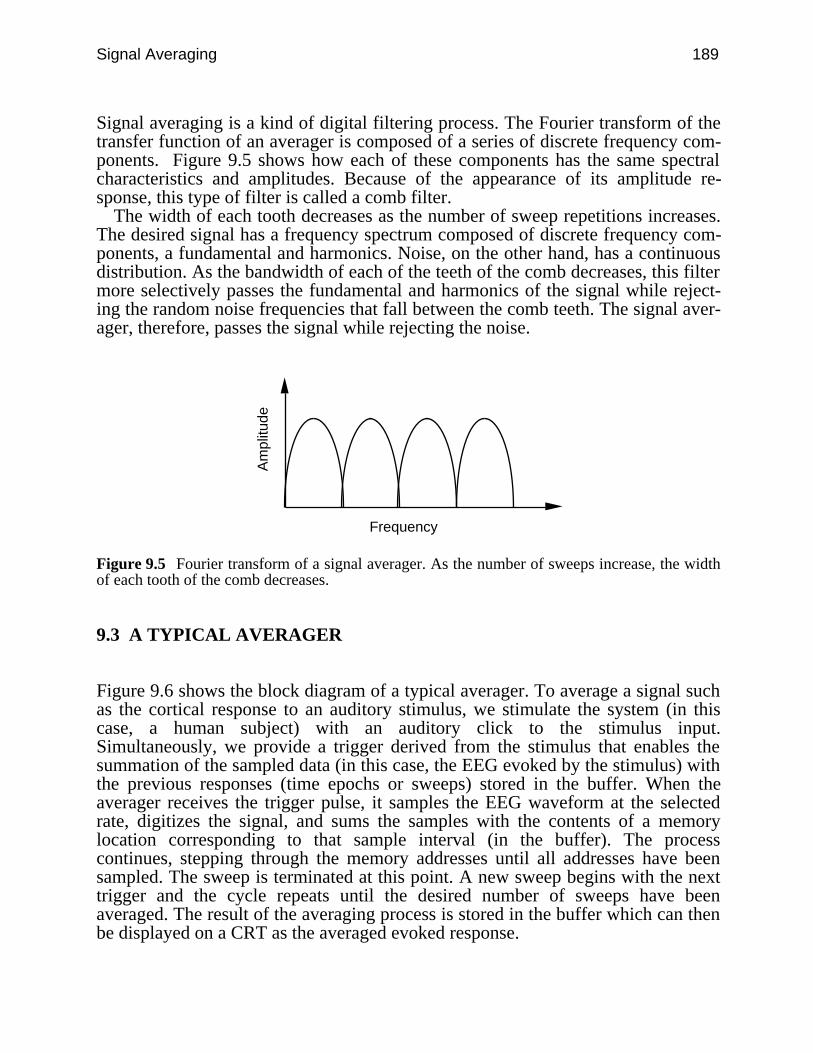
Signal Averaging 189
Signal averaging is a kind of digital filtering process. The Fourier transform of thetransfer function of an averager is composed of a series of discrete frequency com-ponents. Figure 9.5 shows how each of these components has the same spectralcharacteristics and amplitudes. Because of the appearance of its amplitude re-sponse, this type of filter is called a comb filter.
The width of each tooth decreases as the number of sweep repetitions increases.The desired signal has a frequency spectrum composed of discrete frequency com-ponents, a fundamental and harmonics. Noise, on the other hand, has a continuousdistribution. As the bandwidth of each of the teeth of the comb decreases, this filtermore selectively passes the fundamental and harmonics of the signal while reject-ing the random noise frequencies that fall between the comb teeth. The signal aver-ager, therefore, passes the signal while rejecting the noise.
Am
plitu
de
Frequency
Figure 9.5 Fourier transform of a signal averager. As the number of sweeps increase, the widthof each tooth of the comb decreases.
9.3 A TYPICAL AVERAGER
Figure 9.6 shows the block diagram of a typical averager. To average a signal suchas the cortical response to an auditory stimulus, we stimulate the system (in thiscase, a human subject) with an auditory click to the stimulus input.Simultaneously, we provide a trigger derived from the stimulus that enables thesummation of the sampled data (in this case, the EEG evoked by the stimulus) withthe previous responses (time epochs or sweeps) stored in the buffer. When theaverager receives the trigger pulse, it samples the EEG waveform at the selectedrate, digitizes the signal, and sums the samples with the contents of a memorylocation corresponding to that sample interval (in the buffer). The processcontinues, stepping through the memory addresses until all addresses have beensampled. The sweep is terminated at this point. A new sweep begins with the nexttrigger and the cycle repeats until the desired number of sweeps have beenaveraged. The result of the averaging process is stored in the buffer which can thenbe displayed on a CRT as the averaged evoked response.
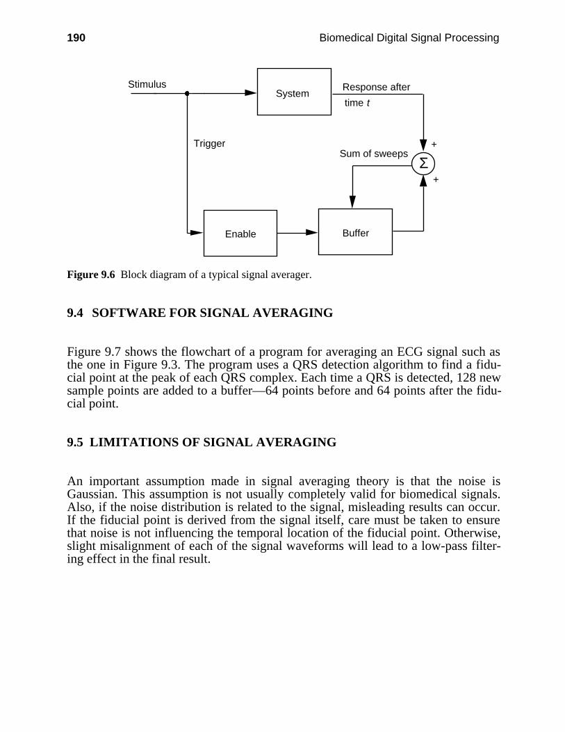
190 Biomedical Digital Signal Processing
System
Sum of sweeps
Response after
time t
Stimulus
Trigger
Enable Buffer
Σ+
+
Figure 9.6 Block diagram of a typical signal averager.
9.4 SOFTWARE FOR SIGNAL AVERAGING
Figure 9.7 shows the flowchart of a program for averaging an ECG signal such asthe one in Figure 9.3. The program uses a QRS detection algorithm to find a fidu-cial point at the peak of each QRS complex. Each time a QRS is detected, 128 newsample points are added to a buffer—64 points before and 64 points after the fidu-cial point.
9.5 LIMITATIONS OF SIGNAL AVERAGING
An important assumption made in signal averaging theory is that the noise isGaussian. This assumption is not usually completely valid for biomedical signals.Also, if the noise distribution is related to the signal, misleading results can occur.If the fiducial point is derived from the signal itself, care must be taken to ensurethat noise is not influencing the temporal location of the fiducial point. Otherwise,slight misalignment of each of the signal waveforms will lead to a low-pass filter-ing effect in the final result.
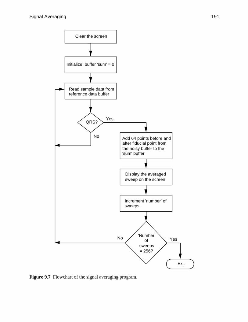
Signal Averaging 191
Clear the screen
Read sample data fromnoisy data bufferRead sample data fromreference data buffer
Initialize: buffer 'sum' = 0
QRS?
Add 64 points before and after fiducial point from the noisy buffer to the 'sum' buffer
Display the averagedsweep on the screen
Increment 'number' of sweeps
'Number' of
sweeps= 256?
Yes
No
Exit
YesNo
Figure 9.7 Flowchart of the signal averaging program.
192 Biomedical Digital Signal Processing
9.6 LAB: ECG SIGNAL AVERAGING
Load UW DigiScope, select ad(V) Ops, then A(V)erage. This module is ademonstration of the use of signal averaging. The source file is always aver-age.dat to which random, gaussian-distributed noise is added. A clean version ofthe data is preserved to use as a trigger signal. The averaged version of the data,displayed in the output channel, will build in size as successive waveforms areadded. A summation of the accumulated signal traces is displayed, not the average.Thus you need to scale down the amplitude of the resultant signal in order to seethe true average at the same amplitude scale factor as the original signal. Scaling ofthe output channel can be controlled as the traces are acquired. The down arrowkey divides the amplitude by two each time it is struck. For example, while adding16 heartbeats, you would need to strike the down arrow four times to divide theoutput by 16 so as to obtain the proper amplitude scale.
9.7 REFERENCES
Tompkins, W. J. and Webster, J. G. (eds.) 1981. Design of Microcomputer-based MedicalInstrumentation. Englewood Cliffs, NJ: Prentice Hall.
9.8 STUDY QUESTIONS
9.1 Under what noise conditions will signal averaging fail to improve the SNR?9.2 In a signal averaging application, the amplitude of uncorrelated noise is initially 16 times as
large as the signal amplitude. How many sweeps must be averaged to give a resultingsignal-to-noise ratio of 4:1?
9.3 After signal averaging 4096 EEG evoked responses, the signal-to-noise ratio is 4.Assuming that the EEG and noise sources are uncorrelated, what was the SNR beforeaveraging?
9.4 In a signal averaging application, the noise amplitude is initially 4 times as large as the sig-nal amplitude. How many sweeps must be averaged to give a resulting signal-to-noise ratioof 4:1?
9.5 In a signal averaging application, the signal caused by a stimulus and the noise are slightlycorrelated. The frequency spectra of the signal and noise overlap. Averaging 100 responseswill improve the signal-to-noise ratio by what factor?
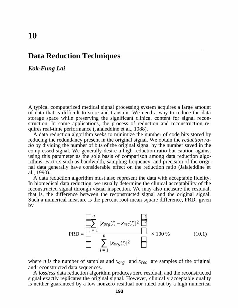
193
10
Data Reduction Techniques
Kok-Fung Lai
A typical computerized medical signal processing system acquires a large amountof data that is difficult to store and transmit. We need a way to reduce the datastorage space while preserving the significant clinical content for signal recon-struction. In some applications, the process of reduction and reconstruction re-quires real-time performance (Jalaleddine et al., 1988).
A data reduction algorithm seeks to minimize the number of code bits stored byreducing the redundancy present in the original signal. We obtain the reduction ra-tio by dividing the number of bits of the original signal by the number saved in thecompressed signal. We generally desire a high reduction ratio but caution againstusing this parameter as the sole basis of comparison among data reduction algo-rithms. Factors such as bandwidth, sampling frequency, and precision of the origi-nal data generally have considerable effect on the reduction ratio (Jalaleddine etal., 1990).
A data reduction algorithm must also represent the data with acceptable fidelity.In biomedical data reduction, we usually determine the clinical acceptability of thereconstructed signal through visual inspection. We may also measure the residual,that is, the difference between the reconstructed signal and the original signal.Such a numerical measure is the percent root-mean-square difference, PRD, givenby
PRD =
∑
i = 1
n
[xorg(i) – xrec(i)]2
∑i = 1
n
[xorg(i)]2
12
× 100 % (10.1)
where n is the number of samples and xorg and xrec are samples of the originaland reconstructed data sequences.
A lossless data reduction algorithm produces zero residual, and the reconstructedsignal exactly replicates the original signal. However, clinically acceptable qualityis neither guaranteed by a low nonzero residual nor ruled out by a high numerical
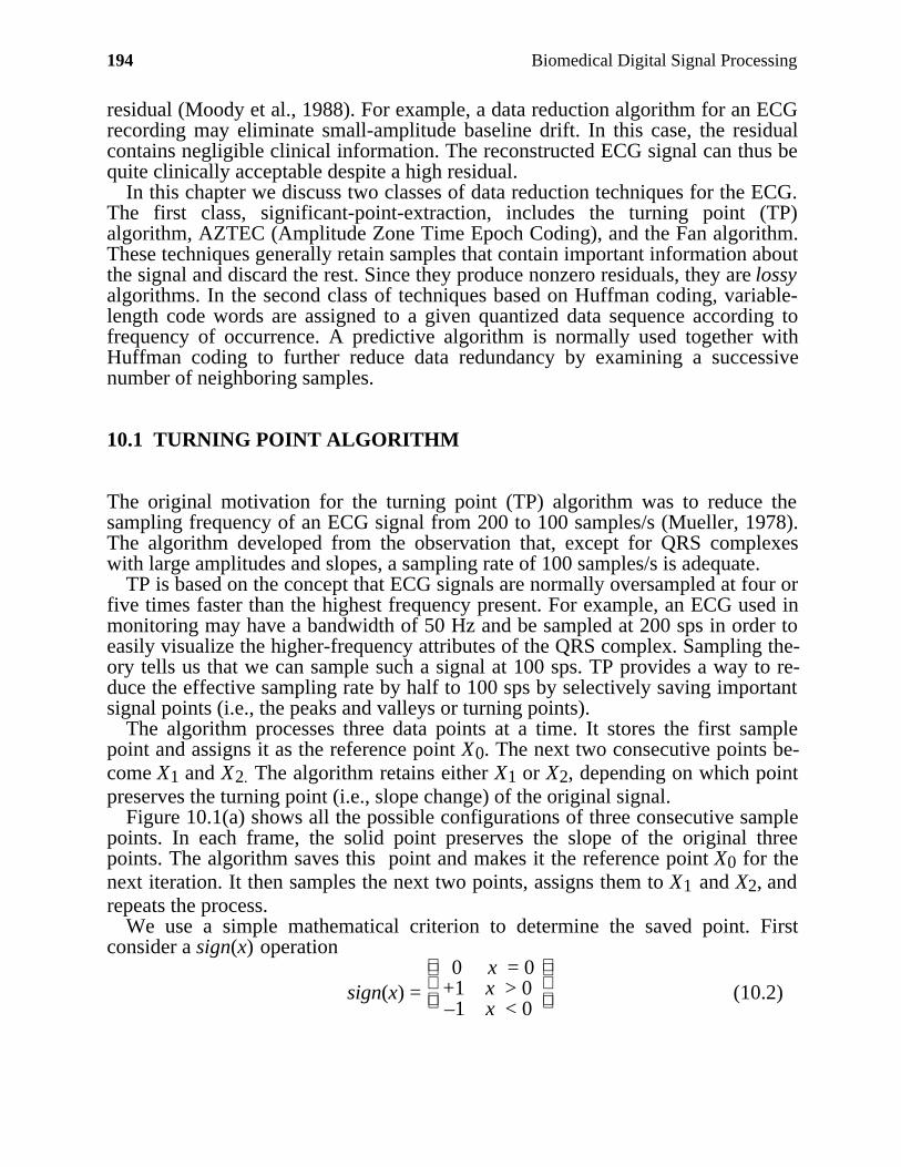
194 Biomedical Digital Signal Processing
residual (Moody et al., 1988). For example, a data reduction algorithm for an ECGrecording may eliminate small-amplitude baseline drift. In this case, the residualcontains negligible clinical information. The reconstructed ECG signal can thus bequite clinically acceptable despite a high residual.
In this chapter we discuss two classes of data reduction techniques for the ECG.The first class, significant-point-extraction, includes the turning point (TP)algorithm, AZTEC (Amplitude Zone Time Epoch Coding), and the Fan algorithm.These techniques generally retain samples that contain important information aboutthe signal and discard the rest. Since they produce nonzero residuals, they are lossyalgorithms. In the second class of techniques based on Huffman coding, variable-length code words are assigned to a given quantized data sequence according tofrequency of occurrence. A predictive algorithm is normally used together withHuffman coding to further reduce data redundancy by examining a successivenumber of neighboring samples.
10.1 TURNING POINT ALGORITHM
The original motivation for the turning point (TP) algorithm was to reduce thesampling frequency of an ECG signal from 200 to 100 samples/s (Mueller, 1978).The algorithm developed from the observation that, except for QRS complexeswith large amplitudes and slopes, a sampling rate of 100 samples/s is adequate.
TP is based on the concept that ECG signals are normally oversampled at four orfive times faster than the highest frequency present. For example, an ECG used inmonitoring may have a bandwidth of 50 Hz and be sampled at 200 sps in order toeasily visualize the higher-frequency attributes of the QRS complex. Sampling the-ory tells us that we can sample such a signal at 100 sps. TP provides a way to re-duce the effective sampling rate by half to 100 sps by selectively saving importantsignal points (i.e., the peaks and valleys or turning points).
The algorithm processes three data points at a time. It stores the first samplepoint and assigns it as the reference point X0. The next two consecutive points be-come X1 and X2. The algorithm retains either X1 or X2, depending on which pointpreserves the turning point (i.e., slope change) of the original signal.
Figure 10.1(a) shows all the possible configurations of three consecutive samplepoints. In each frame, the solid point preserves the slope of the original threepoints. The algorithm saves this point and makes it the reference point X0 for thenext iteration. It then samples the next two points, assigns them to X1 and X2, andrepeats the process.
We use a simple mathematical criterion to determine the saved point. Firstconsider a sign(x) operation
sign(x) =
0 x = 0
+1 x > 0–1 x < 0
(10.2)
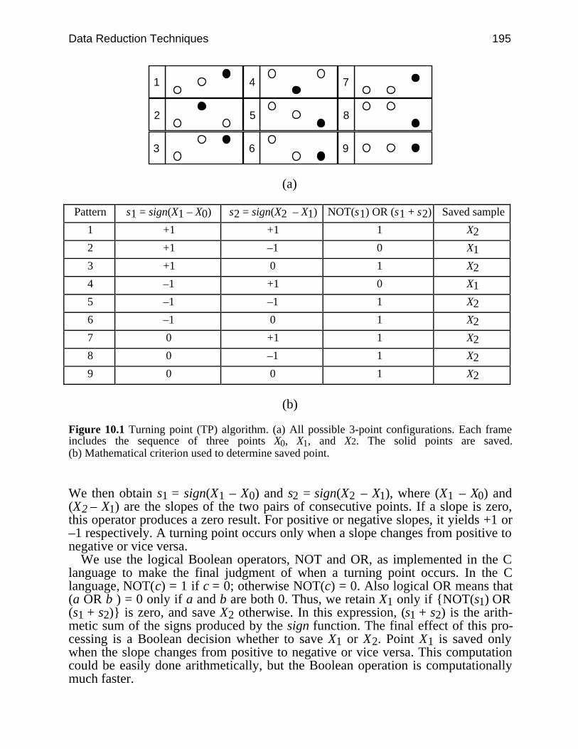
Data Reduction Techniques 195
1
2
3
4
5
6
7
8
9
(a)
Pattern s1 = sign(X1 – X0) s2 = sign(X2 – X1) NOT(s1) OR (s1 + s2) Saved sample
1 +1 +1 1 X2
2 +1 –1 0 X1
3 +1 0 1 X2
4 –1 +1 0 X1
5 –1 –1 1 X2
6 –1 0 1 X2
7 0 +1 1 X2
8 0 –1 1 X2
9 0 0 1 X2
(b)
Figure 10.1 Turning point (TP) algorithm. (a) All possible 3-point configurations. Each frameincludes the sequence of three points X0, X1, and X2. The solid points are saved.(b) Mathematical criterion used to determine saved point.
We then obtain s1 = sign(X1 – X0) and s2 = sign(X2 – X1), where (X1 – X0) and(X2 – X1) are the slopes of the two pairs of consecutive points. If a slope is zero,this operator produces a zero result. For positive or negative slopes, it yields +1 or–1 respectively. A turning point occurs only when a slope changes from positive tonegative or vice versa.
We use the logical Boolean operators, NOT and OR, as implemented in the Clanguage to make the final judgment of when a turning point occurs. In the Clanguage, NOT(c) = 1 if c = 0; otherwise NOT(c) = 0. Also logical OR means that(a OR b ) = 0 only if a and b are both 0. Thus, we retain X1 only if NOT(s1) OR(s1 + s2) is zero, and save X2 otherwise. In this expression, (s1 + s2) is the arith-metic sum of the signs produced by the sign function. The final effect of this pro-cessing is a Boolean decision whether to save X1 or X2. Point X1 is saved onlywhen the slope changes from positive to negative or vice versa. This computationcould be easily done arithmetically, but the Boolean operation is computationallymuch faster.
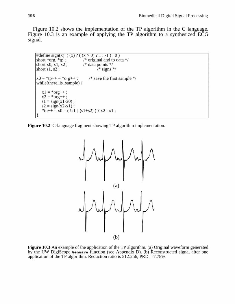
196 Biomedical Digital Signal Processing
Figure 10.2 shows the implementation of the TP algorithm in the C language.Figure 10.3 is an example of applying the TP algorithm to a synthesized ECGsignal.
#define sign(x) ( (x) ? ( (x > 0) ? 1 : -1 ) : 0 )short *org, *tp ; /* original and tp data */short x0, x1, x2 ; /* data points */short s1, s2 ; /* signs */
x0 = *tp++ = *org++ ; /* save the first sample */while(there_is_sample)
x1 = *org++ ;x2 = *org++ ;s1 = sign(x1-x0) ;s2 = sign(x2-x1) ;*tp++ = x0 = ( !s1 || (s1+s2) ) ? x2 : x1 ;
Figure 10.2 C-language fragment showing TP algorithm implementation.
(a)
(b)
Figure 10.3 An example of the application of the TP algorithm. (a) Original waveform generatedby the UW DigiScope Genwave function (see Appendix D). (b) Reconstructed signal after oneapplication of the TP algorithm. Reduction ratio is 512:256, PRD = 7.78%.
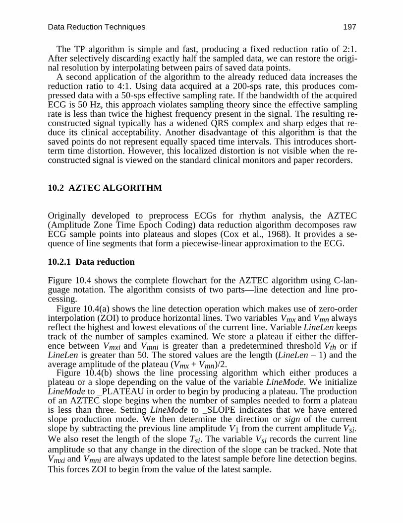
Data Reduction Techniques 197
The TP algorithm is simple and fast, producing a fixed reduction ratio of 2:1.After selectively discarding exactly half the sampled data, we can restore the origi-nal resolution by interpolating between pairs of saved data points.
A second application of the algorithm to the already reduced data increases thereduction ratio to 4:1. Using data acquired at a 200-sps rate, this produces com-pressed data with a 50-sps effective sampling rate. If the bandwidth of the acquiredECG is 50 Hz, this approach violates sampling theory since the effective samplingrate is less than twice the highest frequency present in the signal. The resulting re-constructed signal typically has a widened QRS complex and sharp edges that re-duce its clinical acceptability. Another disadvantage of this algorithm is that thesaved points do not represent equally spaced time intervals. This introduces short-term time distortion. However, this localized distortion is not visible when the re-constructed signal is viewed on the standard clinical monitors and paper recorders.
10.2 AZTEC ALGORITHM
Originally developed to preprocess ECGs for rhythm analysis, the AZTEC(Amplitude Zone Time Epoch Coding) data reduction algorithm decomposes rawECG sample points into plateaus and slopes (Cox et al., 1968). It provides a se-quence of line segments that form a piecewise-linear approximation to the ECG.
10.2.1 Data reduction
Figure 10.4 shows the complete flowchart for the AZTEC algorithm using C-lan-guage notation. The algorithm consists of two parts—line detection and line pro-cessing.
Figure 10.4(a) shows the line detection operation which makes use of zero-orderinterpolation (ZOI) to produce horizontal lines. Two variables Vmx and Vmn alwaysreflect the highest and lowest elevations of the current line. Variable LineLen keepstrack of the number of samples examined. We store a plateau if either the differ-ence between Vmxi and Vmni is greater than a predetermined threshold Vth or ifLineLen is greater than 50. The stored values are the length (LineLen – 1) and theaverage amplitude of the plateau (Vmx + Vmn)/2.
Figure 10.4(b) shows the line processing algorithm which either produces aplateau or a slope depending on the value of the variable LineMode. We initializeLineMode to _PLATEAU in order to begin by producing a plateau. The productionof an AZTEC slope begins when the number of samples needed to form a plateauis less than three. Setting LineMode to _SLOPE indicates that we have enteredslope production mode. We then determine the direction or sign of the currentslope by subtracting the previous line amplitude V1 from the current amplitude Vsi.We also reset the length of the slope Tsi. The variable Vsi records the current lineamplitude so that any change in the direction of the slope can be tracked. Note thatVmxi and Vmni are always updated to the latest sample before line detection begins.This forces ZOI to begin from the value of the latest sample.

198 Biomedical Digital Signal Processing
Figure 10.4(a) Flowchart for the line detection operation of the AZTEC algorithm.
Start
Vmxi = Vmni = ECGtLineMode = _PLATEAULineLen = 1cAZT = 1
Wait for next
sample
V = ECGtVmx = VmxlVmn = VmnlLineLen += 1
LineLen > 50
Vmxi = V
Vmni = VVmn > V
Vmxi - Vmni < Vth
T1 = NUM - 1V1 = (Vmx + Vmn)/2
B
Vmx < V
A
N
N
N
N
Y
Y
Y
Y
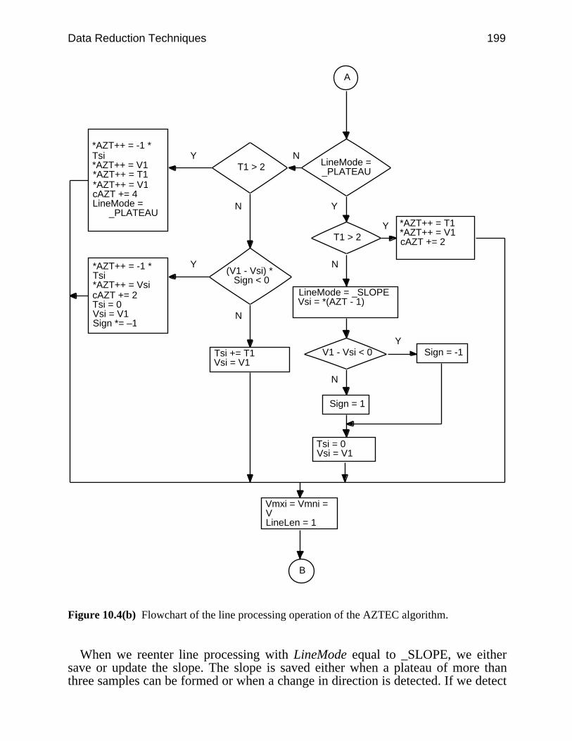
Data Reduction Techniques 199
Figure 10.4(b) Flowchart of the line processing operation of the AZTEC algorithm.
When we reenter line processing with LineMode equal to _SLOPE, we eithersave or update the slope. The slope is saved either when a plateau of more thanthree samples can be formed or when a change in direction is detected. If we detect
A
LineMode = _PLATEAU
T1 > 2
T1 > 2
(V1 - Vsi) * Sign < 0
*AZT++ = T1*AZT++ = V1cAZT += 2
LineMode = _SLOPEVsi = *(AZT - 1)
*AZT++ = -1 * Tsi*AZT++ = V1*AZT++ = T1*AZT++ = V1cAZT += 4LineMode = _PLATEAU
*AZT++ = -1 * Tsi*AZT++ = VsicAZT += 2Tsi = 0Vsi = V1Sign *= –1
Tsi += T1Vsi = V1
B
Y
Y
Y
Y
N
N
N
N
V1 - Vsi < 0
Sign = 1
Sign = -1
Tsi = 0Vsi = V1
Vmxi = Vmni = VLineLen = 1
N
Y
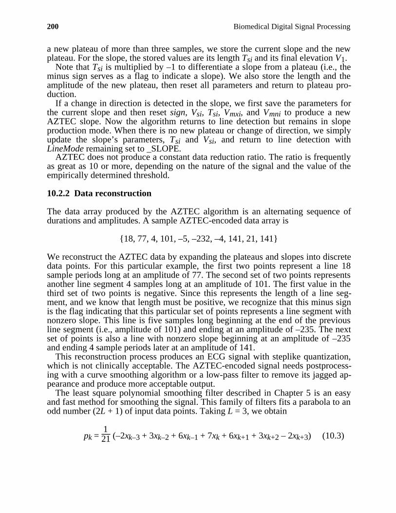
200 Biomedical Digital Signal Processing
a new plateau of more than three samples, we store the current slope and the newplateau. For the slope, the stored values are its length Tsi and its final elevation V1.
Note that Tsi is multiplied by –1 to differentiate a slope from a plateau (i.e., theminus sign serves as a flag to indicate a slope). We also store the length and theamplitude of the new plateau, then reset all parameters and return to plateau pro-duction.
If a change in direction is detected in the slope, we first save the parameters forthe current slope and then reset sign, Vsi, Tsi, Vmxi, and Vmni to produce a newAZTEC slope. Now the algorithm returns to line detection but remains in slopeproduction mode. When there is no new plateau or change of direction, we simplyupdate the slope’s parameters, Tsi and Vsi, and return to line detection withLineMode remaining set to _SLOPE.
AZTEC does not produce a constant data reduction ratio. The ratio is frequentlyas great as 10 or more, depending on the nature of the signal and the value of theempirically determined threshold.
10.2.2 Data reconstruction
The data array produced by the AZTEC algorithm is an alternating sequence ofdurations and amplitudes. A sample AZTEC-encoded data array is
18, 77, 4, 101, –5, –232, –4, 141, 21, 141
We reconstruct the AZTEC data by expanding the plateaus and slopes into discretedata points. For this particular example, the first two points represent a line 18sample periods long at an amplitude of 77. The second set of two points representsanother line segment 4 samples long at an amplitude of 101. The first value in thethird set of two points is negative. Since this represents the length of a line seg-ment, and we know that length must be positive, we recognize that this minus signis the flag indicating that this particular set of points represents a line segment withnonzero slope. This line is five samples long beginning at the end of the previousline segment (i.e., amplitude of 101) and ending at an amplitude of –235. The nextset of points is also a line with nonzero slope beginning at an amplitude of –235and ending 4 sample periods later at an amplitude of 141.
This reconstruction process produces an ECG signal with steplike quantization,which is not clinically acceptable. The AZTEC-encoded signal needs postprocess-ing with a curve smoothing algorithm or a low-pass filter to remove its jagged ap-pearance and produce more acceptable output.
The least square polynomial smoothing filter described in Chapter 5 is an easyand fast method for smoothing the signal. This family of filters fits a parabola to anodd number (2L + 1) of input data points. Taking L = 3, we obtain
pk = 121 (–2xk–3 + 3xk–2 + 6xk–1 + 7xk + 6xk+1 + 3xk+2 – 2xk+3) (10.3)
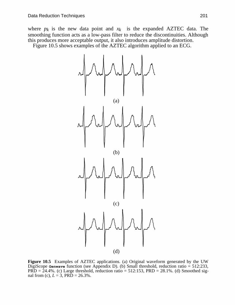
Data Reduction Techniques 201
where pk is the new data point and xk is the expanded AZTEC data. Thesmoothing function acts as a low-pass filter to reduce the discontinuities. Althoughthis produces more acceptable output, it also introduces amplitude distortion.
Figure 10.5 shows examples of the AZTEC algorithm applied to an ECG.
(a)
(b)
(c)
(d)
Figure 10.5 Examples of AZTEC applications. (a) Original waveform generated by the UWDigiScope Genwave function (see Appendix D). (b) Small threshold, reduction ratio = 512:233,PRD = 24.4%. (c) Large threshold, reduction ratio = 512:153, PRD = 28.1%. (d) Smoothed sig-nal from (c), L = 3, PRD = 26.3%.
202 Biomedical Digital Signal Processing
10.2.3 CORTES algorithm
The CORTES (Coordinate Reduction Time Encoding System) algorithm is a hy-brid of the TP and AZTEC algorithms (Abenstein and Tompkins, 1982; Tompkinsand Webster, 1981). It attempts to exploit the strengths of each while sidesteppingthe weaknesses. CORTES uses AZTEC to discard clinically insignificant data inthe isoelectric region with a high reduction ratio and applies the TP algorithm tothe clinically significant high-frequency regions (QRS complexes). It executes theAZTEC and TP algorithms in parallel on the incoming ECG data.
Whenever an AZTEC line is produced, the CORTES algorithm decides, basedon the length of the line, whether the AZTEC data or the TP data are to be saved. Ifthe line is longer than an empirically determined threshold, it saves the AZTECline. Otherwise it saves the TP data points. Since TP is used to encode the QRScomplexes, only AZTEC plateaus, not slopes, are implemented.
The CORTES algorithm reconstructs the signal by expanding the AZTECplateaus and interpolating between each pair of the TP data points. It then appliesparabolic smoothing to the AZTEC portions to reduce discontinuities.
10.3 FAN ALGORITHM
Originally used for ECG telemetry, the Fan algorithm draws lines between pairs ofstarting and ending points so that all intermediate samples are within some speci-fied error tolerance, ε (Bohs and Barr, 1988). Figure 10.6 illustrates the principlesof the Fan algorithm. We start by accepting the first sample X0 as the nonredundantpermanent point. It functions as the origin and is also called the originating point.We then take the second sample X1 and draw two slopes U1, L1. U1 passesthrough the point (X0, X1 + ε), and L1 passes through the point (X0, X1 – ε). If thethird sample X2 falls within the area bounded by the two slopes, we generate twonew slopes U2, L2 that pass through points (X0, X2 + ε) and (X0, X2 – ε). Wecompare the two pairs of slopes and retain the most converging (restrictive) slopes(i.e., U1, L2 in our example). Next we assign the value of X2 to X1 and read thenext sample into X2. As a result, X2 always holds the most recent sample and X1holds the sample immediately preceding X2. We repeat the process by comparingX2 to the values of the most convergent slopes. If it falls outside this area, we savethe length of the line T and its final amplitude X1 which then becomes the neworiginating point X0, and the process begins anew. The sketch of the slopes drawnfrom the originating sample to future samples forms a set of radial lines similar to afan, giving this algorithm its name.
When adapting the Fan algorithm to C-language implementation, we create thevariables, XU1, XL1, XU2, and XL2, to determine the bounds of X2. From Figure10.6(b), we can show that
XU2 = XU1 – X0
T + XU1 (10.4a)
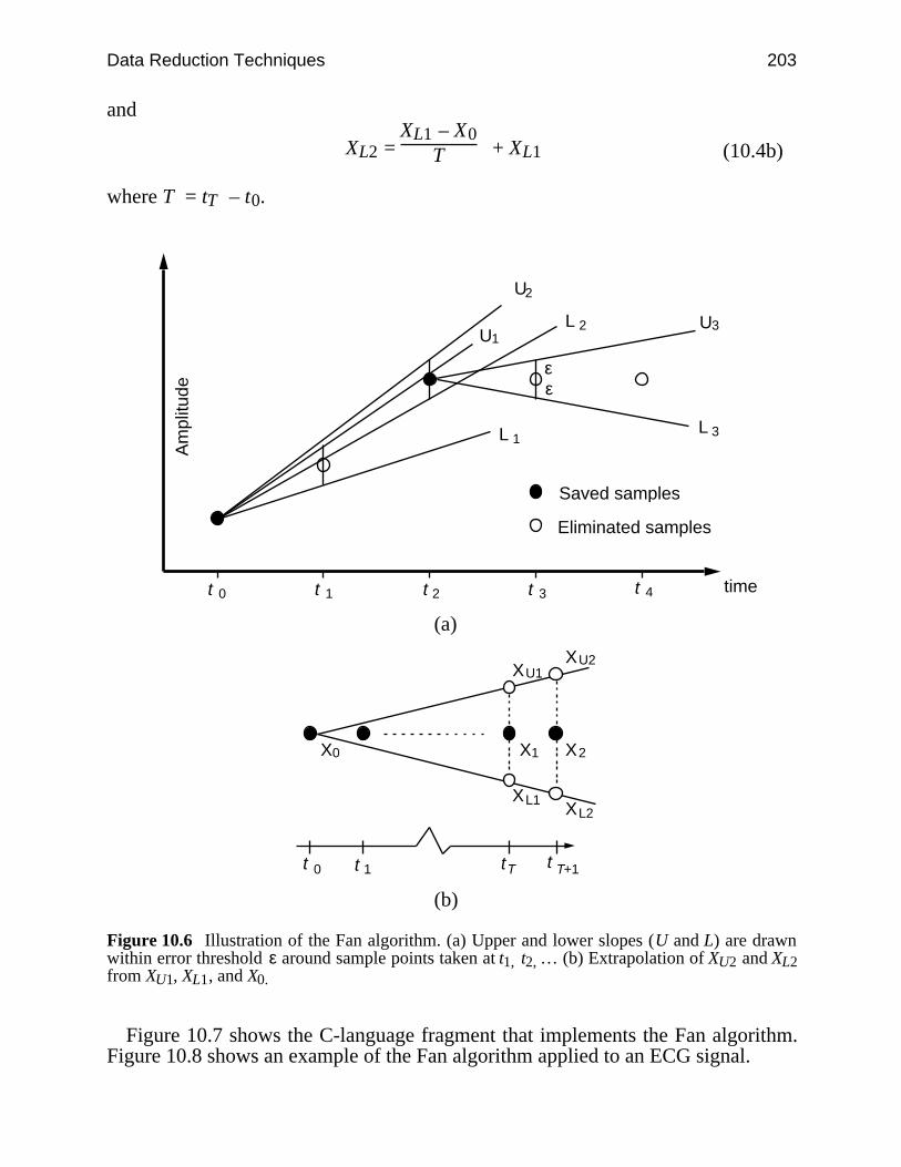
Data Reduction Techniques 203
and
XL2 = XL1 – X0
T + XL1 (10.4b)
where T = tT – t0.
t 1
L 1 3
U2
time
Am
plitu
de
Saved samples
Eliminated samples
L 2
L
U1U3
εε
t 2 t 3 t 4t 0
(a)
X0 X1 X2
XL1XL2
XU2XU1
t 0 t T t T+1t 1
(b)
Figure 10.6 Illustration of the Fan algorithm. (a) Upper and lower slopes (U and L) are drawnwithin error threshold ε around sample points taken at t1, t2, … (b) Extrapolation of XU2 and XL2from XU1, XL1, and X0.
Figure 10.7 shows the C-language fragment that implements the Fan algorithm.Figure 10.8 shows an example of the Fan algorithm applied to an ECG signal.
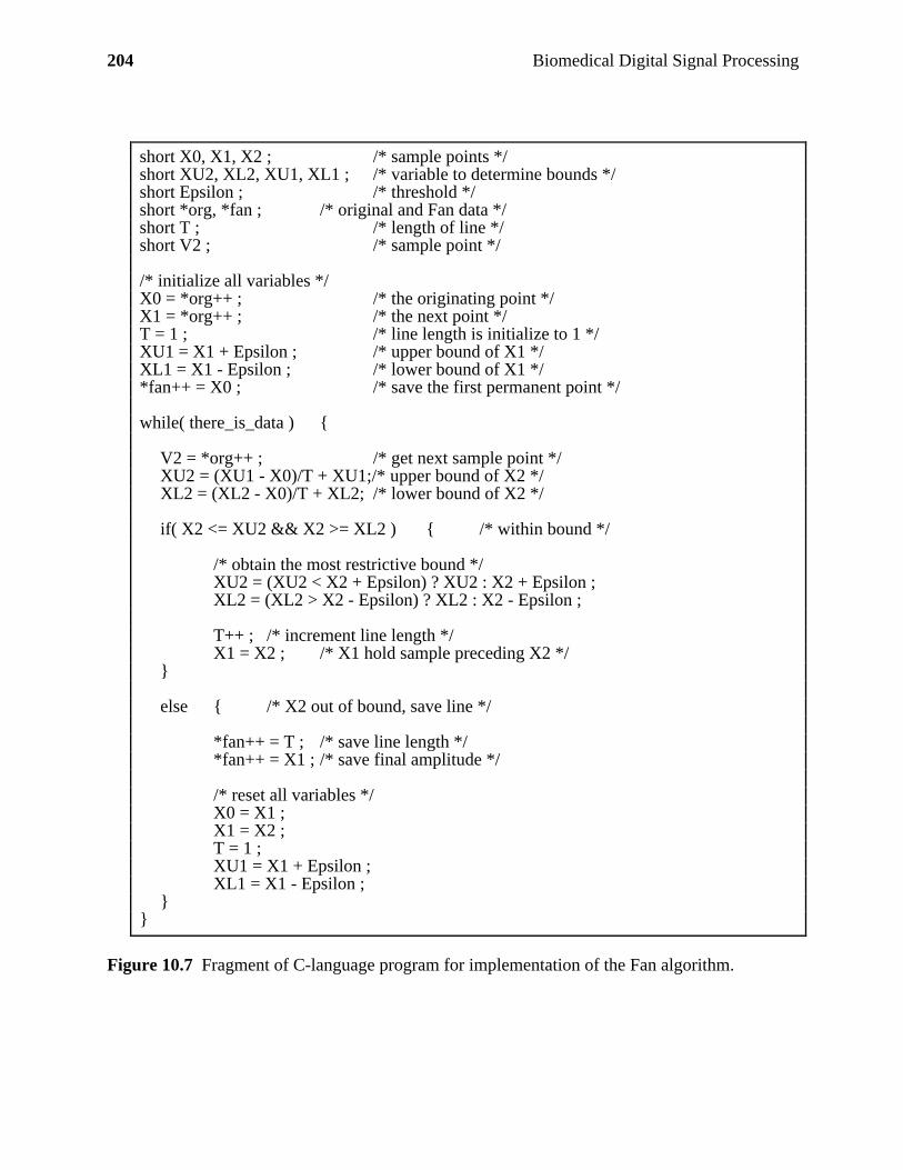
204 Biomedical Digital Signal Processing
short X0, X1, X2 ; /* sample points */short XU2, XL2, XU1, XL1 ; /* variable to determine bounds */short Epsilon ; /* threshold */short *org, *fan ; /* original and Fan data */short T ; /* length of line */short V2 ; /* sample point */
/* initialize all variables */X0 = *org++ ; /* the originating point */X1 = *org++ ; /* the next point */T = 1 ; /* line length is initialize to 1 */XU1 = X1 + Epsilon ; /* upper bound of X1 */XL1 = X1 - Epsilon ; /* lower bound of X1 */*fan++ = X0 ; /* save the first permanent point */
while( there_is_data )
V2 = *org++ ; /* get next sample point */XU2 = (XU1 - X0)/T + XU1;/* upper bound of X2 */XL2 = (XL2 - X0)/T + XL2; /* lower bound of X2 */
if( X2 <= XU2 && X2 >= XL2 ) /* within bound */
/* obtain the most restrictive bound */XU2 = (XU2 < X2 + Epsilon) ? XU2 : X2 + Epsilon ;XL2 = (XL2 > X2 - Epsilon) ? XL2 : X2 - Epsilon ;
T++ ; /* increment line length */X1 = X2 ; /* X1 hold sample preceding X2 */
else /* X2 out of bound, save line */
*fan++ = T ; /* save line length */*fan++ = X1 ; /* save final amplitude */
/* reset all variables */X0 = X1 ;X1 = X2 ;T = 1 ;XU1 = X1 + Epsilon ;XL1 = X1 - Epsilon ;
Figure 10.7 Fragment of C-language program for implementation of the Fan algorithm.
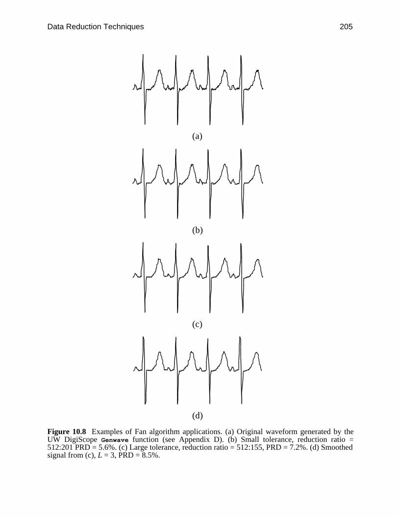
Data Reduction Techniques 205
(a)
(b)
(c)
(d)
Figure 10.8 Examples of Fan algorithm applications. (a) Original waveform generated by theUW DigiScope Genwave function (see Appendix D). (b) Small tolerance, reduction ratio =512:201 PRD = 5.6%. (c) Large tolerance, reduction ratio = 512:155, PRD = 7.2%. (d) Smoothedsignal from (c), L = 3, PRD = 8.5%.
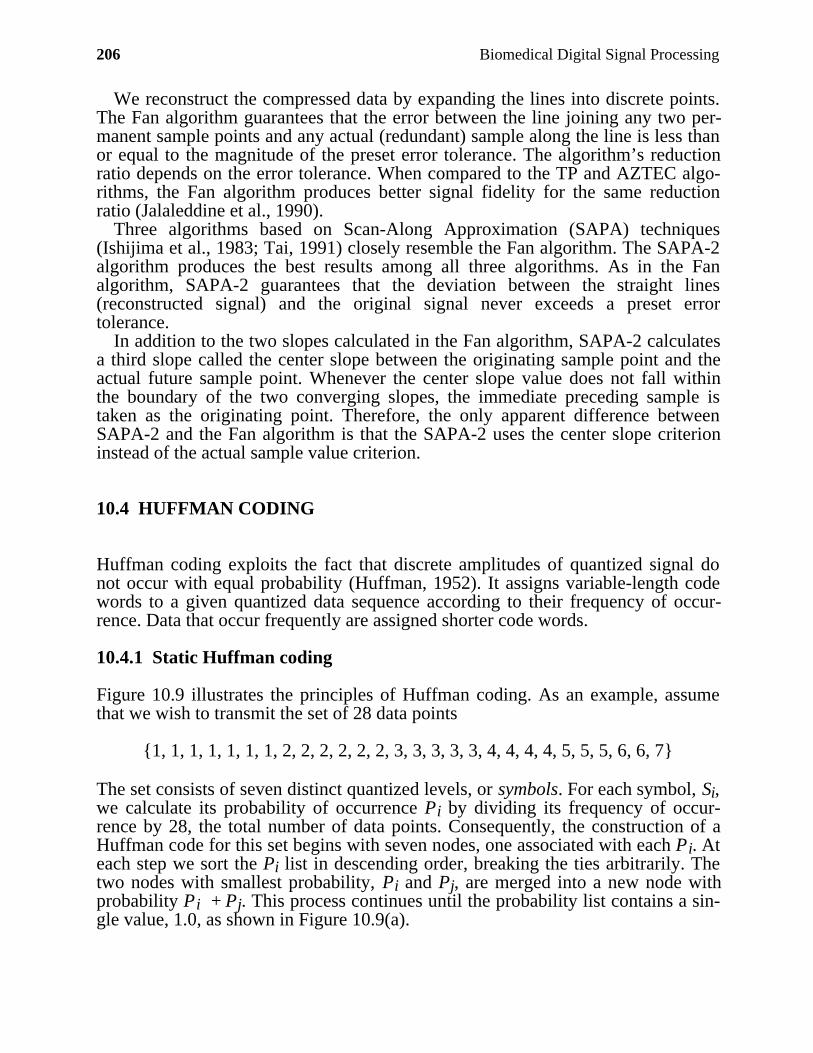
206 Biomedical Digital Signal Processing
We reconstruct the compressed data by expanding the lines into discrete points.The Fan algorithm guarantees that the error between the line joining any two per-manent sample points and any actual (redundant) sample along the line is less thanor equal to the magnitude of the preset error tolerance. The algorithm’s reductionratio depends on the error tolerance. When compared to the TP and AZTEC algo-rithms, the Fan algorithm produces better signal fidelity for the same reductionratio (Jalaleddine et al., 1990).
Three algorithms based on Scan-Along Approximation (SAPA) techniques(Ishijima et al., 1983; Tai, 1991) closely resemble the Fan algorithm. The SAPA-2algorithm produces the best results among all three algorithms. As in the Fanalgorithm, SAPA-2 guarantees that the deviation between the straight lines(reconstructed signal) and the original signal never exceeds a preset errortolerance.
In addition to the two slopes calculated in the Fan algorithm, SAPA-2 calculatesa third slope called the center slope between the originating sample point and theactual future sample point. Whenever the center slope value does not fall withinthe boundary of the two converging slopes, the immediate preceding sample istaken as the originating point. Therefore, the only apparent difference betweenSAPA-2 and the Fan algorithm is that the SAPA-2 uses the center slope criterioninstead of the actual sample value criterion.
10.4 HUFFMAN CODING
Huffman coding exploits the fact that discrete amplitudes of quantized signal donot occur with equal probability (Huffman, 1952). It assigns variable-length codewords to a given quantized data sequence according to their frequency of occur-rence. Data that occur frequently are assigned shorter code words.
10.4.1 Static Huffman coding
Figure 10.9 illustrates the principles of Huffman coding. As an example, assumethat we wish to transmit the set of 28 data points
1, 1, 1, 1, 1, 1, 1, 2, 2, 2, 2, 2, 2, 3, 3, 3, 3, 3, 4, 4, 4, 4, 5, 5, 5, 6, 6, 7
The set consists of seven distinct quantized levels, or symbols. For each symbol, Si,we calculate its probability of occurrence Pi by dividing its frequency of occur-rence by 28, the total number of data points. Consequently, the construction of aHuffman code for this set begins with seven nodes, one associated with each Pi. Ateach step we sort the Pi list in descending order, breaking the ties arbitrarily. Thetwo nodes with smallest probability, Pi and Pj, are merged into a new node withprobability Pi + Pj. This process continues until the probability list contains a sin-gle value, 1.0, as shown in Figure 10.9(a).
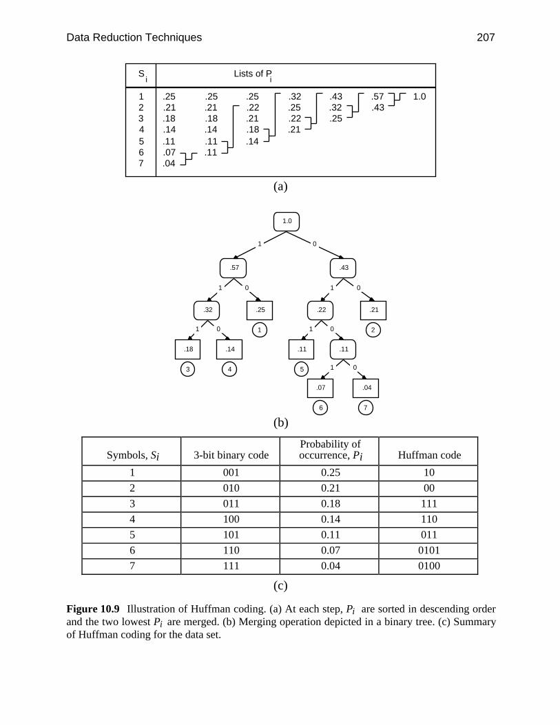
Data Reduction Techniques 207
.25
.21
.18
.14
.11
.07
.04
.25
.21
.18
.14
.11
.11
.25
.22
.21
.18
.14
.32
.25
.22
.21
.43
.32
.25
.57
.431.01
234567
S Lists of Pi i
(a)
1.0
.57 .43
.32
.11
.22.25
.18 .14 .11
.07 .04
01
1 0 1
1 0 1 0
.21
0
1 0
1
3 4 5
6
2
7
(b)
Symbols, Si 3-bit binary codeProbability ofoccurrence, Pi Huffman code
1 001 0.25 10
2 010 0.21 00
3 011 0.18 111
4 100 0.14 110
5 101 0.11 011
6 110 0.07 0101
7 111 0.04 0100
(c)
Figure 10.9 Illustration of Huffman coding. (a) At each step, Pi are sorted in descending orderand the two lowest Pi are merged. (b) Merging operation depicted in a binary tree. (c) Summaryof Huffman coding for the data set.
208 Biomedical Digital Signal Processing
The process of merging nodes produces a binary tree as in Figure 10.9(b). Whenwe merge two nodes with probability Pi + Pj, we create a parent node with twochildren represented by Pi and Pj. The root of the tree has probability 1.0. We ob-tain the Huffman code of the symbols by traversing down the tree, assigning 1 tothe left child and 0 to the right child. The resulting code words have the prefixproperty (i.e., no code word is a proper prefix of any other code word). This prop-erty ensures that a coded message is uniquely decodable without the need forlookahead. Figure 10.9(c) summarizes the results and shows the Huffman codes forthe seven symbols. We enter these code word mappings into a translation table anduse the table to pad the appropriate code word into the output bit stream in the re-duction process.
The reduction ratio of Huffman coding depends on the distribution of the sourcesymbols. In our example, the original data requires three bits to represent the sevenquantized levels. After Huffman coding, we can calculate the expected code wordlength
E[l] = ∑i = 1
7 li Pi (10.5)
where li represents the length of Huffman code for the symbols. This value is 2.65in our example, resulting in an expected reduction ratio of 3:2.65.
The reconstruction process begins at the root of the tree. If bit 1 is received, wetraverse down the left branch, otherwise the right branch. We continue traversinguntil we reach a node with no child. We then output the symbol corresponding tothis node and begin traversal from the root again.
The reconstruction process of Huffman coding perfectly recovers the originaldata. Therefore it is a lossless algorithm. However, a transmission error of a singlebit may result in more than one decoding error. This propagation of transmissionerror is a consequence of all algorithms that produce variable-length code words.
10.4.2 Modified Huffman coding
The implementation of Huffman coding requires a translation table, where eachsource symbol is mapped to a unique code word. If the original data werequantized into 16-bit numbers, the table would need to contain 216 records. A tableof this size creates memory problems and processing inefficiency.
In order to reduce the size of the translation table, the modified Huffman codingscheme partitions the source symbols into a frequent set and an infrequent set. Forall the symbols in the frequent set, we form a Huffman code as in the staticscheme. We then use a special code word as a prefix to indicate any symbol fromthe infrequent set and attach a suffix corresponding to the ordinary binary encodingof the symbol.
Assume that we are given a data set similar to the one before. Assume also thatwe anticipate quantized level 0 to appear in some future transmissions. We maydecide to partition the quantized levels 0, 7 into the infrequent set. We thenapply Huffman coding as before and obtain the results in Figure 10.10. Note thatquantized levels in the infrequent set have codes with prefix 0100, making their
Data Reduction Techniques 209
code length much longer than those of the frequent set. It is therefore important tokeep the probability of the infrequent set sufficiently small to achieve a reasonablereduction ratio.
Some modified Huffman coding schemes group quantized levels centered about0 into the frequent set and derive two prefix codes for symbols in the infrequentset. One prefix code denotes large positive values and the other denotes largenegative values.
10.4.3 Adaptive coding
Huffman coding requires a translation table for encoding and decoding. It isnecessary to examine the entire data set or portions of it to determine the datastatistics. The translation table must also be transmitted or stored for correctdecoding.
An adaptive coding scheme attempts to build the translation table as data arepresented. A dynamically derived translation table is sensitive to the variation inlocal statistical information. It can therefore alter its code words according to localstatistics to maximize the reduction ratio. It also achieves extra space savingbecause there is no need for a static table.
An example of an adaptive scheme is the Lempel-Ziv-Welch (LZW) algorithm.The LZW algorithm uses a fixed-size table. It initializes some positions of the tablefor some chosen data sets. When it encounters new data, it uses the uninitializedpositions so that each unique data word is assigned its own position. When thetable is full, the LZW algorithm reinitializes the oldest or least-used positionaccording to the new data. During data reconstruction, it incrementally rebuilds thetranslation table from the encoded data.
Symbols, Si 3-bit binary codeProbability ofoccurrence, Pi Huffman code
0 000 0.00 0100000
1 001 0.25 10
2 010 0.21 00
3 011 0.18 111
4 100 0.14 110
5 101 0.11 011
6 110 0.07 0101
7 111 0.04 0100111
Figure 10.10 Results of modified Huffman coding. Quantized levels 0, 7 are grouped into theinfrequent set.
210 Biomedical Digital Signal Processing
10.4.4 Residual differencing
Typically, neighboring signal amplitudes are not statistically independent.Conceptually we can decompose a sample value into a part that is correlated withpast samples and a part that is uncorrelated. Since the intersample correlation cor-responds to a value predicted using past samples, it is redundant and removable.We are then left with the uncorrelated part which represents the prediction error orresidual signal. Since the amplitude range of the residual signal is smaller than thatof the original signal, it requires less bits for representation. We can further reducethe data by applying Huffman coding to the residual signal. We briefly describetwo ECG reduction algorithms that make use of residual differencing.
Ruttimann and Pipberger (1979) applied modified Huffman coding to residualsobtained from prediction and interpolation. In prediction, sample values are ob-tained by taking a linearly weighted sum of an appropriate number of past samples
x'(nT) = ∑k = 1
p ak x(nT – kT) (10.6)
where x(nT) are the original data, x'(nT) are the predicted samples, and p is thenumber of samples employed in prediction. The parameters ak are chosen to min-imize the expected mean squared error E[(x – x')2]. When p = 1, we choose a1 = 1and say that we are taking the first difference of the signal. Preliminary investiga-tions on test ECG data showed that there was no substantial improvement by usingpredictors higher than second order (Ruttimann et al., 1976). In interpolation, theestimator of the sample value consists of a linear combination of past and futuresamples. The results for the predictor indicated a second-order estimator to be suf-ficient. Therefore, the interpolator uses only one past and one future sample
x'(n) = ax(nT – T) + bx(nT + T) (10.7)
where the coefficients a and b are determined by minimizing the expected meansquared error. The residuals of prediction and interpolation are encoded using amodified Huffman coding scheme, where the frequent set consists of somequantized levels centered about zero. Encoding using residuals from interpolationresulted in higher reduction ratio of approximately 7.8:1.
Hamilton and Tompkins (1991a, 1991b) exploited the fact that a typical ECGsignal is composed of a repeating pattern of beats with little change from beat tobeat. The algorithm calculates and updates an average beat estimate as data arepresented. When it detects a beat, it aligns and subtracts the detected beat from theaverage beat. The residual signal is Huffman coded and stored along with a recordof the beat locations. Finally, the algorithm uses the detected beat to update theaverage beat estimate. In this scheme, the estimation of beat location and quantizerlocation can significantly affect reduction performance.

Data Reduction Techniques 211
10.4.5 Run-length encoding
Used extensively in the facsimile technology, run-length encoding exploits thehigh degree of correlation that occurs in successive bits in the facsimile bit stream.A bit in the facsimile output may either be 1 or 0, depending on whether it is ablack or white pixel. On a typical document, there are clusters of black and whitepixels that give rise to this high correlation. Run-length encoding simplytransforms the original bit stream into the string v1, l1, v2, l2, … where vi are thevalues and li are the lengths. The observant reader will quickly recognize that bothAZTEC and the Fan algorithm are special cases of run-length encoding.
Take for example the output stream 1, 1, 1, 1, 1, 3, 3, 3, 3, 0, 0, 0 with 12elements. The output of run-length encoding 1, 5, 3, 4, 0, 3 contains only sixelements. Further data reduction is possible by applying Huffman coding to theoutput of run-length encoding.
10.5 LAB: ECG DATA REDUCTION ALGORITHMS
This lab explores the data reduction techniques reviewed in this chapter. Load UWDigiScope according to the directions in Appendix D.
10.5.1 Turning point algorithm
From the ad(V) Ops menu, select C(O)mpress and then (T)urn pt. Theprogram compresses the waveform displayed on the top channel using the TPalgorithm, then decompresses, reconstructs using interpolation, and displays theresults on the bottom channel. Perform the TP algorithm on two different ECGsread from files and on a sine wave and a square wave. Observe
1. Quality of the reconstructed signal2. Reduction ratio3. Percent root-mean-square difference (PRD)4. Power spectra of original and reconstructed signals.
Tabulate and summarize all your observations.
10.5.2 AZTEC algorithm
Repeat section 10.5.1 for the AZTEC algorithm by selecting (A)ztec from theCOMPRESS menu. Using at least three different threshold values (try 1%, 5%, and15% of the full-scale peak-to-peak value), observe and comment on the items inthe list in section 10.5.1. In addition, summarize the quality of the reconstructedsignals both before and after applying the smoothing filter. Tabulate and summa-rize all your observations.
10.5.3 Fan algorithm
212 Biomedical Digital Signal Processing
Repeat section 10.5.2 for the Fan algorithm by selecting (F)an from the COMPRESSmenu. What can you deduce from comparing the performance of the Fan algorithmwith that of the AZTEC algorithm? Tabulate and summarize all your observations.
10.5.4 Huffman coding
Select (H)uffman from the COMPRESS menu. Select (R)un in order to Huffman en-code the signal that is displayed on the top channel. Do not use first differencing atthis point in the experiment. Record the reduction ratio. Note that this reduction ra-tio does not include the space needed for the translation table which must be storedor transmitted. What can you deduce from the PRD? Select (W)rite table towrite the Huffman data into a file. You may view the translation table later withthe DOS type command after exiting from SCOPE.
Load a new ECG waveform and repeat the steps above. When you select (R)un,the program uses the translation table derived previously to code the signal. Whatcan you deduce from the reduction ratio? After deriving a new translation tableusing (M)ake from the menu, select (R)un again and comment on the new reduc-tion ratio.
Select (M)ake again and use first differencing to derive a new Huffman code. Isthere a change in the reduction ratio using this newly derived code? Select(W)rite table to write the Huffman data into a file. Now reload the first ECGwaveform that you used. Without deriving a new Huffman code, observe the re-duction ratio obtained. Comment on your observations.
Exit from the SCOPE program to look at the translation tables that you generated.What comments can you make regarding the overhead involved in storing a trans-lation table?
10.6 REFERENCES
Abenstein, J. P. and Tompkins, W. J. 1982. New data-reduction algorithm for real-time ECGanalysis, IEEE Trans. Biomed. Eng., BME-29: 43–48.
Bohs, L. N. and Barr, R. C. 1988. Prototype for real-time adaptive sampling using the Fanalgorithm, Med. & Biol. Eng. & Comput., 26: 574–83.
Cox, J. R., Nolle, F. M., Fozzard, H. A., and Oliver, G. C. Jr. 1968. AZTEC: a preprocessingprogram for real-time ECG rhythm analysis. IEEE Trans. Biomed. Eng., BME-15: 128–29.
Hamilton, P. S., and Tompkins, W. J. 1991a. Compression of the ambulatory ECG by averagebeat subtraction and residual differencing. IEEE Trans. Biomed. Eng., BME-38(3): 253–59.
Hamilton, P. S., and Tompkins, W. J. 1991b. Theoretical and experimental rate distortion perfor-mance in compression of ambulatory ECGs. IEEE Trans. Biomed. Eng., BME-38(3): 260–66.
Huffman, D. A. 1952. A method for construction of minimum-redundancy codes. Proc. IRE , 40:1098–1101.
Ishijima, M., Shin, S. B., Hostetter, G. H., and Skalansky, J. 1983. Scan-along polygonalapproximation for data compression of electrocardiograms, IEEE Trans. Biomed. Eng., BME-30: 723–29.
Jalaleddine, S. M. S., Hutchens, C. G., Coberly, W. A., and Strattan, R. D. 1988. Compression ofHolter ECG data. Biomedical Sciences Instrumentation, 24: 35–45.
Jalaleddine, S. M. S., Hutchens. C. G., and Strattan, R. D. 1990. ECG data compressiontechniques — A unified approach. IEEE Trans. Biomed. Eng., BME-37: 329–43.
Data Reduction Techniques 213
Moody, G. B., Soroushian., and Mark, R. G. 1988. ECG data compression for tapelessambulatory monitors. Computers in Cardiology, 467–70.
Mueller, W. C. 1978. Arrhythmia detection program for an ambulatory ECG monitor. Biomed.Sci. Instrument., 14: 81–85.
Ruttimann, U. E. and Pipberger, H. V. 1979. Compression of ECG by prediction or interpolationand entropy encoding. IEEE Trans. Biomed. Eng., BME-26: 613–23.
Ruttimann, U. E., Berson, A. S., and Pipberger, H. V. 1976. ECG data compression by linearprediction. Proc. Comput. Cardiol., 313–15.
Tai, S. C. 1991. SLOPE — a real-time ECG data compressor. Med. & Biol. Eng. & Comput.,175–79.
Tompkins, W. J. and Webster, J. G. (eds.) 1981. Design of Microcomputer-based MedicalInstrumentation. Englewood Cliffs, NJ: Prentice Hall.
10.7 STUDY QUESTIONS
10.1 Explain the meaning of lossless and lossy data compression. Classify the four datareduction algorithms described in this chapter into these two categories.
10.2 Given the following data: 15, 10, 6, 7, 5, 3, 4, 7, 15, 3, produce the data points that arestored using the TP algorithm.
10.3 Explain why an AZTEC reconstructed waveform is unacceptable to a cardiologist.Suggest ways to alleviate the problem.
10.4 The Fan algorithm can be applied to other types of biomedical signals. List the desirablecharacteristics of the biomedical signal that will produce satisfactory results using this al-gorithm. Give an example of such a signal.
10.5 Given the following data set: a, a, a, a, b, b, b, b, b, c, c, c, d, d, e, derive the codewords for the data using Huffman coding. What is the average code word length?
10.6 Describe the advantages and disadvantages of modified Huffman coding.10.7 Explain why it is desirable to apply Huffman coding to the residuals obtained by subtract-
ing the estimated sample points from the original sample points.10.8 Data reduction can be performed using parameter extraction techniques. A particular
characteristic or parameter of the signal is extracted and transmitted in place of the origi-nal signal. Draw a block diagram showing the possible configuration for such a system.Your block diagram should include the compression and the reconstruction portions.What are the factors governing the success of these techniques?
10.9 Does the TP algorithm (a) produce significant time-base distortion over a very long time,(b) save every turning point (i.e., peak or valley) in a signal, (c) provide data reduction of4-to-1 if applied twice to a signal without violating sampling theory, (d) provide for ex-actly reconstructing the original signal, (e) perform as well as AZTEC for electroen-cephalography (EEG)? Explain your answers.
10.10 Which of the following are characteristic of a Huffman coding algorithm? (a) Guaranteesmore data reduction on an ECG than AZTEC; (b) Cannot perfectly reconstruct thesampled data points (within some designated error range); (c) Is a variable-length code;(d) Is derived directly from Morse code; (e) Uses ASCII codes for the most frequent A/Dvalues; (f) Requires advance knowledge of the frequency of occurrence of data patterns;(g) Includes as part of the algorithm self-correcting error checks.
10.11 After application of the TP algorithm, what data sequence would be saved if the datasampled by an analog-to-digital converter were: (a) 20, 40, 20, 40, 20, 40, 20, 40,(b) 50, 40, 50, 20, 30, 40, (c) 50, 50, 40, 30, 40, 50, 40, 30, 40, 50, 50, 40,(d) 50, 25, 50, 25, 50, 25, 50, 25?
10.12 After application of the TP algorithm on a signal, the data points saved are 50, 70, 30,40. If you were to reconstruct the original data set, what is the data sequence that wouldbest approximate it?
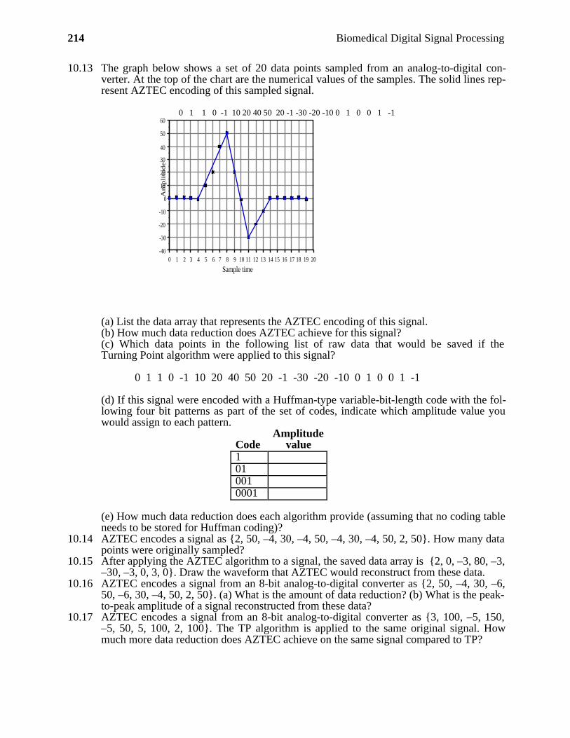
214 Biomedical Digital Signal Processing
10.13 The graph below shows a set of 20 data points sampled from an analog-to-digital con-verter. At the top of the chart are the numerical values of the samples. The solid lines rep-resent AZTEC encoding of this sampled signal.
0 1 1 0 -1 10 20 40 50 20 -1 -30 -20 -10 0 1 0 0 1 -1
20191817161514131211109876543210-40
-30
-20
-10
0
10
20
30
40
50
60
Sample time
Am
pli
tude
(a) List the data array that represents the AZTEC encoding of this signal.(b) How much data reduction does AZTEC achieve for this signal?(c) Which data points in the following list of raw data that would be saved if theTurning Point algorithm were applied to this signal?
0 1 1 0 -1 10 20 40 50 20 -1 -30 -20 -10 0 1 0 0 1 -1
(d) If this signal were encoded with a Huffman-type variable-bit-length code with the fol-lowing four bit patterns as part of the set of codes, indicate which amplitude value youwould assign to each pattern.
CodeAmplitude
value1010010001
(e) How much data reduction does each algorithm provide (assuming that no coding tableneeds to be stored for Huffman coding)?
10.14 AZTEC encodes a signal as 2, 50, –4, 30, –4, 50, –4, 30, –4, 50, 2, 50. How many datapoints were originally sampled?
10.15 After applying the AZTEC algorithm to a signal, the saved data array is 2, 0, –3, 80, –3,–30, –3, 0, 3, 0. Draw the waveform that AZTEC would reconstruct from these data.
10.16 AZTEC encodes a signal from an 8-bit analog-to-digital converter as 2, 50, –4, 30, –6,50, –6, 30, –4, 50, 2, 50. (a) What is the amount of data reduction? (b) What is the peak-to-peak amplitude of a signal reconstructed from these data?
10.17 AZTEC encodes a signal from an 8-bit analog-to-digital converter as 3, 100, –5, 150,–5, 50, 5, 100, 2, 100. The TP algorithm is applied to the same original signal. Howmuch more data reduction does AZTEC achieve on the same signal compared to TP?
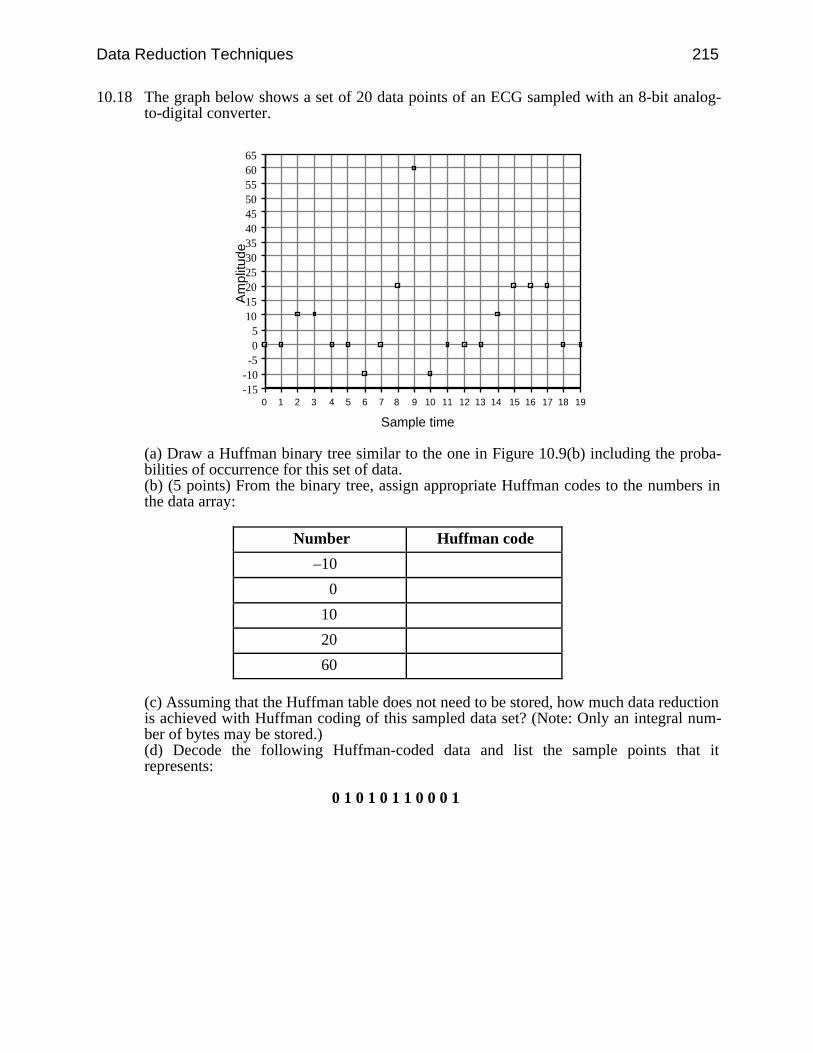
Data Reduction Techniques 215
10.18 The graph below shows a set of 20 data points of an ECG sampled with an 8-bit analog-to-digital converter.
191817161514131211109876543210-15-10-505
101520253035404550556065
Sample time
Am
plitu
de
(a) Draw a Huffman binary tree similar to the one in Figure 10.9(b) including the proba-bilities of occurrence for this set of data.(b) (5 points) From the binary tree, assign appropriate Huffman codes to the numbers inthe data array:
Number Huffman code
–10
0
10
20
60
(c) Assuming that the Huffman table does not need to be stored, how much data reductionis achieved with Huffman coding of this sampled data set? (Note: Only an integral num-ber of bytes may be stored.)(d) Decode the following Huffman-coded data and list the sample points that itrepresents:
0 1 0 1 0 1 1 0 0 0 1
216
11
Other Time- and Frequency-Domain Techniques
Dorin Panescu
A biomedical signal is often corrupted by noise (e.g., powerline interference, mus-cle or motion artifacts, RF interference from electrosurgery or diathermy appara-tus). Therefore, it is useful to know the frequency spectrum of the corrupting signalin order to be able to design a filter to eliminate it. If we want to find out, for ex-ample, how well the patient’s cardiac output is correlated with the area of the QRScomplex, then we need to use proper correlation techniques. This chapter presentstime and frequency-domain techniques that might be useful for situations such asthose exemplified above.
11.1 THE FOURIER TRANSFORM
The digital computer algorithm for Fourier analysis called the fast Fourier trans-form (FFT) serves as a basic tool for frequency-domain analysis of signals.
11.1.1 The Fourier transform of a discrete nonperiodic signal
Assuming that a discrete-time aperiodic signal exists as a sequence of data sampledfrom an analog prototype with a sampling period of T, the angular samplingfrequency being s = 2π/T, we can write this signal in the time domain as a seriesof weighted Dirac functions. Thus
x(t) = ∑n = –∞
∞ x(n) (t – nT) (11.1)
The Fourier transform of this expression is
X( ) = ⌡⌠
–∞
∞ x(t) e–j tdt (11.2)
Other Time- and Frequency-Domain Techniques 217
orX( ) = ⌡⌠
–∞
∞
∑n = –∞
∞ x(n) (t – nT) e–j tdt (11.3a)
The ordering of integration and summation can be changed to give
X( ) = ∑n = –∞
∞ x(n) ⌡⌠
–∞
∞ (t – nT) e–j t dt (11.3b)
Thus we obtain
X( ) = ∑n = –∞
∞ x(n) e–j nT (11.3c)
And similarly, we can find that the inverse Fourier transform is
x(n) = T2π ⌡⌠
0
s
X( ) ej nT d (11.4)
One of the important properties of the Fourier transform, which is shown inFigure 11.1(b), is its repetition at intervals of the sampling frequency in both posi-tive and negative directions. Also it is remarkable that the components in the inter-val 0 < < s/2 are the complex conjugates of the components in the interval
s/2 < < s. It is modern practice to use normalized frequencies, which meansthat the sampling period T is taken to be 1. Therefore, the Fourier transform pairfor discrete signals, considering normalized frequencies, is
X( ) = ∑n = –∞
∞ x(n) e–j n (11.5a)
x(n) = 1
2π ⌡⌠
–π
π X( ) ej n d (11.5b)
We observe that this kind of Fourier transform is continuous, and it repeats at in-tervals of the sampling frequency.

218 Biomedical Digital Signal Processing
t
Discrete signal
− s
Modulus
−2 s s 0 2 s
(a) (b)
Figure 11.1 (a) A discrete-time signal, and (b) the modulus of its Fourier transform. Symmetryabout s/2, due to the sampling process, is illustrated.
11.1.2 The discrete Fourier transform for a periodic signal
The discrete Fourier transform (DFT) is the name given to the calculation of theFourier series coefficients for a discrete periodic signal. The operations are similarto the calculation of Fourier coefficients for a periodic signal, but there are alsocertain marked differences. The first is that the integrals become summations in thediscrete time domain. The second difference is that the transform evaluates only afinite number of complex coefficients, the total being equal to the original numberof data points in one period of original signal. Because of this, each spectral line isregarded as the k-th harmonic of the basic period in the data rather than identifyingwith a particular frequency expressed in Hz or radian/s. Algebraically, the forwardand reverse transforms are expressed as
X(k) = ∑n = 0
N – 1 x(n) e
–jkn 2πN (11.6a)
x(n) = 1N ∑
k = 0
N – 1 X(k) e
jkn 2πN (11.6b)
Figure 11.2 shows a discrete periodic signal and the real and imaginary parts ofits DFT. The first spectral line (k = 0) gives the amplitude of the dc component inthe signal, and the second line corresponds to that frequency which represents onecycle in N data points. This frequency is 2π/N. The N-th line corresponds to thesampling frequency of the discrete N-sample data sequence per period and thek = N/2-th line corresponds to the Nyquist frequency. Using the symmetry of theDFT, algorithms for fast computation have been developed. Also, the symmetryhas two important implications. The first is that the transformation will yield Nunique complex spectral lines. The second is that half of these are effectively re-dundant because all of the information contained in a real time domain signal is
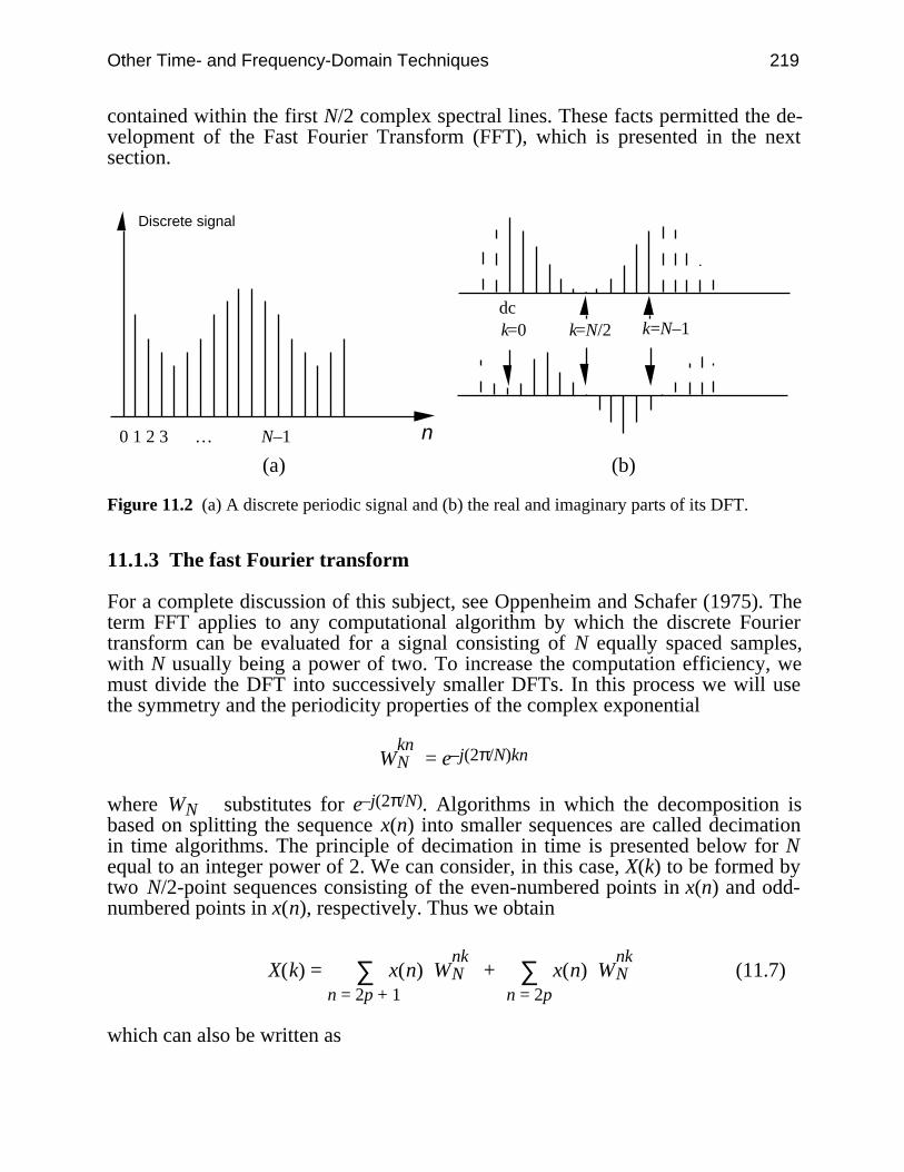
Other Time- and Frequency-Domain Techniques 219
contained within the first N/2 complex spectral lines. These facts permitted the de-velopment of the Fast Fourier Transform (FFT), which is presented in the nextsection.
Discrete signal
n 0 1 2 3 … N–1
dck=0 k=N/2 k=N–1
(a) (b)
Figure 11.2 (a) A discrete periodic signal and (b) the real and imaginary parts of its DFT.
11.1.3 The fast Fourier transform
For a complete discussion of this subject, see Oppenheim and Schafer (1975). Theterm FFT applies to any computational algorithm by which the discrete Fouriertransform can be evaluated for a signal consisting of N equally spaced samples,with N usually being a power of two. To increase the computation efficiency, wemust divide the DFT into successively smaller DFTs. In this process we will usethe symmetry and the periodicity properties of the complex exponential
WknN = e–j(2π/N)kn
where WN substitutes for e–j(2π/N). Algorithms in which the decomposition isbased on splitting the sequence x(n) into smaller sequences are called decimationin time algorithms. The principle of decimation in time is presented below for Nequal to an integer power of 2. We can consider, in this case, X(k) to be formed bytwo N/2-point sequences consisting of the even-numbered points in x(n) and odd-numbered points in x(n), respectively. Thus we obtain
X(k) = ∑n = 2p + 1
x(n) W
nkN + ∑
n = 2p
x(n) W
nkN (11.7)
which can also be written as
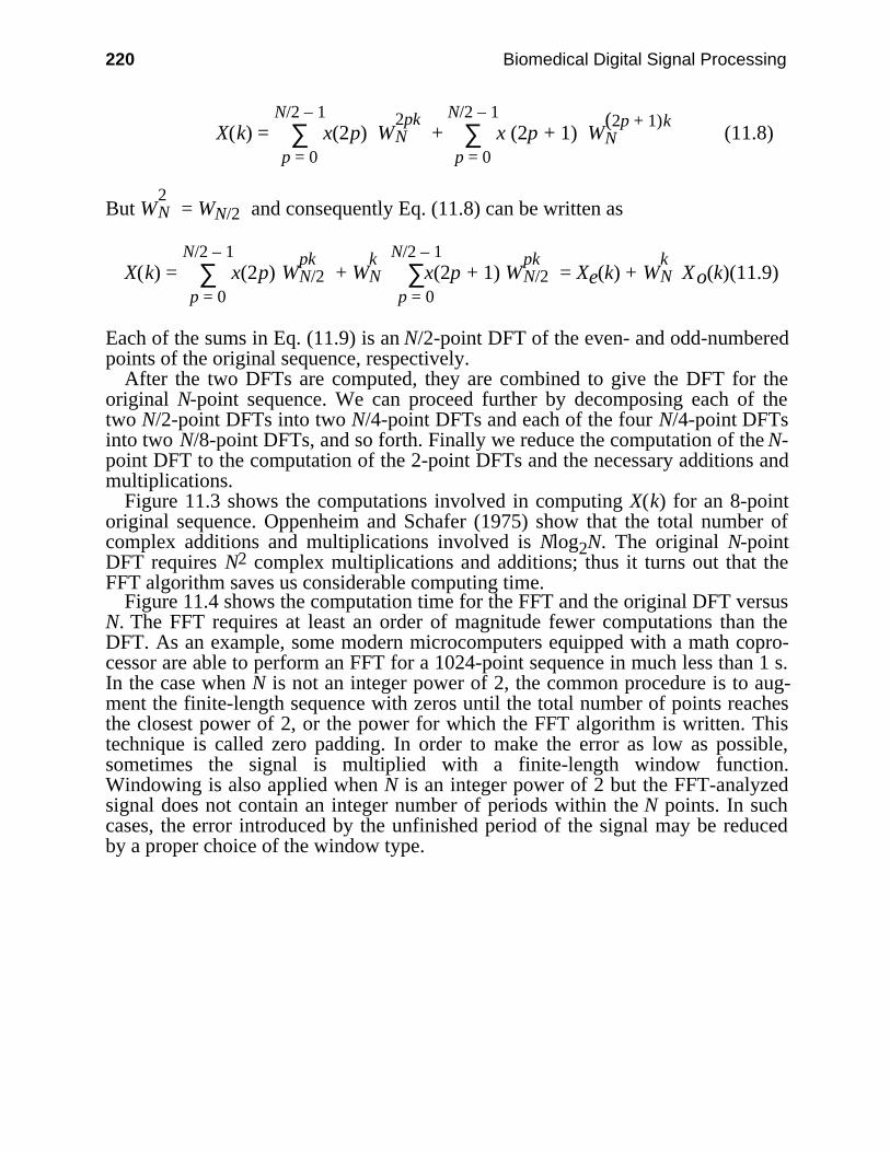
220 Biomedical Digital Signal Processing
X(k) = ∑p = 0
N/2 – 1 x(2p) W
2pkN + ∑
p = 0
N/2 – 1 x (2p + 1) W
(2p + 1)kN (11.8)
But W2N = WN/2 and consequently Eq. (11.8) can be written as
X(k) = ∑p = 0
N/2 – 1 x(2p) W
pkN/2 + W
kN ∑
p = 0
N/2 – 1x(2p + 1) W
pkN/2 = Xe(k) + W
kN Xo(k)(11.9)
Each of the sums in Eq. (11.9) is an N/2-point DFT of the even- and odd-numberedpoints of the original sequence, respectively.
After the two DFTs are computed, they are combined to give the DFT for theoriginal N-point sequence. We can proceed further by decomposing each of thetwo N/2-point DFTs into two N/4-point DFTs and each of the four N/4-point DFTsinto two N/8-point DFTs, and so forth. Finally we reduce the computation of the N-point DFT to the computation of the 2-point DFTs and the necessary additions andmultiplications.
Figure 11.3 shows the computations involved in computing X(k) for an 8-pointoriginal sequence. Oppenheim and Schafer (1975) show that the total number ofcomplex additions and multiplications involved is Nlog2N. The original N-pointDFT requires N2 complex multiplications and additions; thus it turns out that theFFT algorithm saves us considerable computing time.
Figure 11.4 shows the computation time for the FFT and the original DFT versusN. The FFT requires at least an order of magnitude fewer computations than theDFT. As an example, some modern microcomputers equipped with a math copro-cessor are able to perform an FFT for a 1024-point sequence in much less than 1 s.In the case when N is not an integer power of 2, the common procedure is to aug-ment the finite-length sequence with zeros until the total number of points reachesthe closest power of 2, or the power for which the FFT algorithm is written. Thistechnique is called zero padding. In order to make the error as low as possible,sometimes the signal is multiplied with a finite-length window function.Windowing is also applied when N is an integer power of 2 but the FFT-analyzedsignal does not contain an integer number of periods within the N points. In suchcases, the error introduced by the unfinished period of the signal may be reducedby a proper choice of the window type.
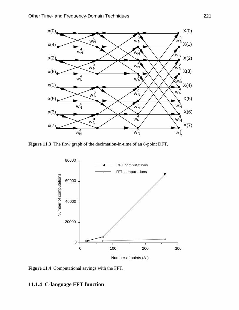
Other Time- and Frequency-Domain Techniques 221
wN2
x(0)
x(4)
x(2)
x(6)
x(1)
x(5)
x(3)
x(7)
wN0
wN4
w N0
w N0
wN4
wN4
wN4
wN0
w N0
wN0
wN4
wN4
wN4
wN6
wN2
wN6
wN1
wN2
wN3
wN5
w N6
w N7
X(0)
X(1)
X(2)
X(3)
X(4)
X(5)
X(6)
X(7)wN
0
Figure 11.3 The flow graph of the decimation-in-time of an 8-point DFT.
3002001000
0
20000
40000
60000
80000DFT computations
FFT computations
Number of points (N )
Num
ber
of c
ompu
tatio
ns
Figure 11.4 Computational savings with the FFT.
11.1.4 C-language FFT function

222 Biomedical Digital Signal Processing
The computational flow graph presented in Figure 11.3 describes an algorithm forthe computation of the FFT of finite-length signal applicable when the number ofpoints is an integer power of 2. When implementing the computations depicted inthis figure, we can imagine the use of two arrays of storage registers, one for thearray being computed and one for the data being used in computation. Forexample, in computing the first array, one set of storage registers would contain theinput data and the second set of storage registers would contain the computedresults for the first stage.
In order to perform the computation based on the “butterfly” graph, the inputdata must be stored in a nonsequential order. In fact, the order in which the inputdata must be stored is the bit-reversed order.
To show what is meant by this, we write the index of the output data and theindex of the corresponding input data using three binary digits.
X(000) — x(000)X(001) — x(100)X(010) — x(010)X(011) — x(110)X(100) — x(001)X(101) — x(101)X(110) — x(011)X(111) — x(111)
If (n2 n1 n0) is the binary representation of the index of the sequence x(n), which isthe input data, then x(n) must be rearranged such that the new position ofx(n2 n1 n0) is x(n0 n1 n2).
Figure 11.5 shows a C-language fragment for the FFT computation, whichreorders the input array, x[nn]. The FFT function in UW DigiScope allows the userto zero-pad the signal or to window it with the different windows.
11.2 CORRELATION
We now investigate the concept of correlation between groups of data or betweensignals. Correlation between groups of data implies that they move or change withrespect to each other in a structured way. To study the correlation between signals,we will consider signals that have been digitized and that therefore form groups ofdata.
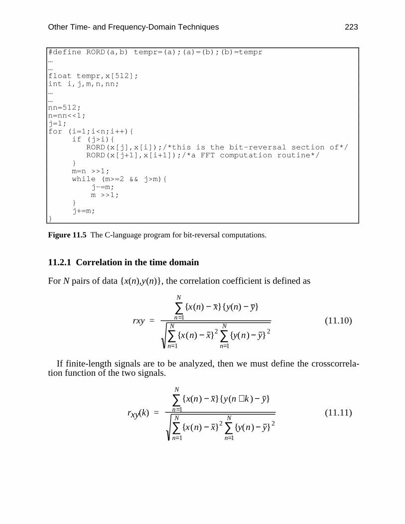
Other Time- and Frequency-Domain Techniques 223
#define RORD(a,b) tempr=(a);(a)=(b);(b)=tempr……float tempr,x[512];int i,j,m,n,nn;……nn=512;n=nn<<1;j=1;for (i=1;i<n;i++) if (j>i) RORD(x[j],x[i]);/*this is the bit-reversal section of*/ RORD(x[j+1],x[i+1]);/*a FFT computation routine*/ m=n >>1; while (m>=2 && j>m) j-=m; m >>1; j+=m;
Figure 11.5 The C-language program for bit-reversal computations.
11.2.1 Correlation in the time domain
For N pairs of data x(n),y(n), the correlation coefficient is defined as
rxy =
x(n) − x y(n) − y n=1
N
∑
x(n) − x 2
n=1
N
∑ y(n) − y 2
n=1
N
∑(11.10)
If finite-length signals are to be analyzed, then we must define the crosscorrela-tion function of the two signals.
rxy(k) =
x(n) − x y(n + k ) − y n=1
N
∑
x(n) − x 2
n=1
N
∑ y(n) − y 2
n=1
N
∑(11.11)
224 Biomedical Digital Signal Processing
In the case when the two input signals are the same, the crosscorrelation functionbecomes the autocorrelation function of that signal. Thus, the autocorrelation func-tion is defined as
rxx(k) =
x(n) − x x(n + k) − x n=1
N
∑
x(n) − x 2
n=1
N
∑(11.12)
Figure 11.6 presents the crosscorrelation of respiratory signals recorded simulta-neously from a human subject using impedance pneumography. In Figure 11.6(a),the signals were acquired at different points along the midaxillary line of the sub-ject. The subject was breathing regularly at the beginning of the recording, movingwithout breathing in the middle of the recording, and breathing regularly again atthe end. In Figure 11.6(b), each combination of two recorded channels were cross-correlated in order to try to differentiate between movement and regular breathing.
11.2.2 Correlation in the frequency domain
The original definition for the crosscorrelation was for continuous signals. Thus ifh(t) and g(t) are two continuous signals, then their crosscorrelation function isdefined as
cgh(t) = ⌡⌠
–∞
∞ g( ) h(t + )d (11.13)
The Fourier transform of the crosscorrelation function satisfies
Corr ( ) = G( )* H( ) (11.14)
where G( )* is the complex conjugate of G( ).Thus if we consider h and g to be digitized, we may approximate the crosscorre-
lation function as
cgh(m) = 1N ∑
n = 0
N – 1 g(n ) h(m + n) (11.15)
This equation is also known as the biased estimator of the crosscorrelation func-tion. Between the DFTs of the two input discrete signals and the DFT of the biasedestimator, we have the relationship
Corr (k) = G(k)* H(k) (11.16)
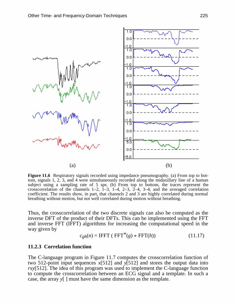
Other Time- and Frequency-Domain Techniques 225
(a) (b)
Figure 11.6 Respiratory signals recorded using impedance pneumography. (a) From top to bot-tom, signals 1, 2, 3, and 4 were simultaneously recorded along the midaxillary line of a humansubject using a sampling rate of 5 sps. (b) From top to bottom, the traces represent thecrosscorrelation of the channels 1–2, 1–3, 1–4, 2–3, 2–4, 3–4, and the averaged correlationcoefficient. The results show, in part, that channels 2 and 3 are highly correlated during normalbreathing without motion, but not well correlated during motion without breathing.
Thus, the crosscorrelation of the two discrete signals can also be computed as theinverse DFT of the product of their DFTs. This can be implemented using the FFTand inverse FFT (IFFT) algorithms for increasing the computational speed in theway given by
cgh(n) = IFFT ( FFT*(g) * FFT(h)) (11.17)
11.2.3 Correlation function
The C-language program in Figure 11.7 computes the crosscorrelation function oftwo 512-point input sequences x[512] and y[512] and stores the output data intorxy[512]. The idea of this program was used to implement the C-language functionto compute the crosscorrelation between an ECG signal and a template. In such acase, the array y[ ] must have the same dimension as the template.
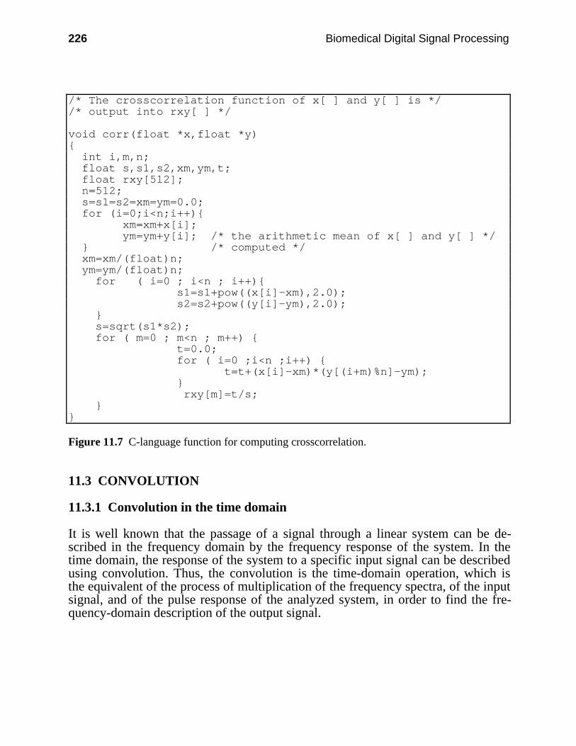
226 Biomedical Digital Signal Processing
/* The crosscorrelation function of x[ ] and y[ ] is *//* output into rxy[ ] */
void corr(float *x,float *y) int i,m,n; float s,s1,s2,xm,ym,t; float rxy[512]; n=512; s=s1=s2=xm=ym=0.0; for (i=0;i<n;i++) xm=xm+x[i]; ym=ym+y[i]; /* the arithmetic mean of x[ ] and y[ ] */ /* computed */ xm=xm/(float)n; ym=ym/(float)n; for ( i=0 ; i<n ; i++) s1=s1+pow((x[i]-xm),2.0); s2=s2+pow((y[i]-ym),2.0); s=sqrt(s1*s2); for ( m=0 ; m<n ; m++) t=0.0; for ( i=0 ;i<n ;i++) t=t+(x[i]-xm)*(y[(i+m)%n]-ym); rxy[m]=t/s;
Figure 11.7 C-language function for computing crosscorrelation.
11.3 CONVOLUTION
11.3.1 Convolution in the time domain
It is well known that the passage of a signal through a linear system can be de-scribed in the frequency domain by the frequency response of the system. In thetime domain, the response of the system to a specific input signal can be describedusing convolution. Thus, the convolution is the time-domain operation, which isthe equivalent of the process of multiplication of the frequency spectra, of the inputsignal, and of the pulse response of the analyzed system, in order to find the fre-quency-domain description of the output signal.
Other Time- and Frequency-Domain Techniques 227
If a continuous signal x(t) is applied at the input of an analogous system whichhas the impulse response h(t), then the equation for the output signal y(t) is knownas the convolution equation.
y(t) = ⌡⌠
–∞
∞ x(t – ) h( ) d (11.18)
For discrete signals, the convolution equation becomes
y(m) = ∑n = 0
N – 1 x(m – n) h(n) (11.19)
where x(n) is the input signal, h(n) is the sampled impulse response of the system,and y(n) is the output signal. Equation (11.19) can be used for implementing finiteimpulse response digital filters. In this case, h(n) would be a finite-length sequencewhich represents, in fact, the coefficients of the FIR filter.
Figure 11.8 shows the input and output signals for a low-pass FIR filter withnine coefficients used for filtering the cardiogenic artifact from respiratory signalsrecorded using impedance pneumography. The corner frequency of this filter is 0.7Hz, and the attenuation in the stopband is about 20 dB.
11.3.2 Convolution in the frequency domain
Time-domain convolution is often expressed in a shorthand notation using a ‘*’operator, thus
y(t) = x(t) * h(t) = h(t) * x(t)
or for discrete signalsy(n) = x(n) * h(n) = h(n)*x(n)
The following relates the DFTs:Y(k ) = X(k) H(k)
If the FFT is used for computing time-domain convolution, this method is called“fast convolution.” We obtain
x(n) *h(n) = IFFT(X(k) H(k)) (11.20)
where X(k) and H(k) are computed using the FFT algorithm.
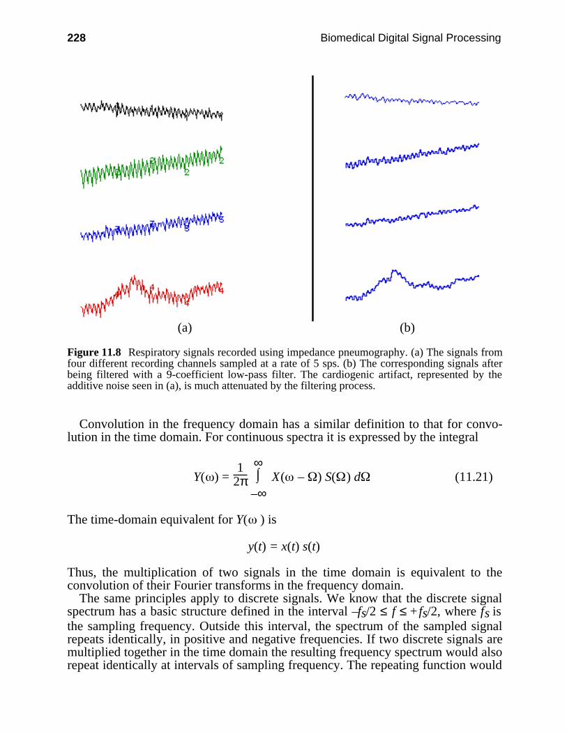
228 Biomedical Digital Signal Processing
(a) (b)
Figure 11.8 Respiratory signals recorded using impedance pneumography. (a) The signals fromfour different recording channels sampled at a rate of 5 sps. (b) The corresponding signals afterbeing filtered with a 9-coefficient low-pass filter. The cardiogenic artifact, represented by theadditive noise seen in (a), is much attenuated by the filtering process.
Convolution in the frequency domain has a similar definition to that for convo-lution in the time domain. For continuous spectra it is expressed by the integral
Y( ) = 1
2π ⌡⌠
–∞
∞ X( – ) S( ) d (11.21)
The time-domain equivalent for Y( ) is
y(t) = x(t) s(t)
Thus, the multiplication of two signals in the time domain is equivalent to theconvolution of their Fourier transforms in the frequency domain.
The same principles apply to discrete signals. We know that the discrete signalspectrum has a basic structure defined in the interval –fs/2 ≤ f ≤ + fs/2, where fs isthe sampling frequency. Outside this interval, the spectrum of the sampled signalrepeats identically, in positive and negative frequencies. If two discrete signals aremultiplied together in the time domain the resulting frequency spectrum would alsorepeat identically at intervals of sampling frequency. The repeating function would
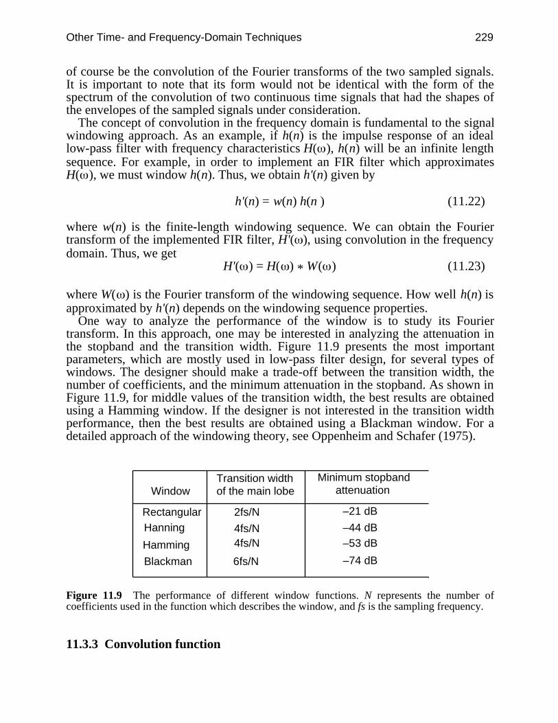
Other Time- and Frequency-Domain Techniques 229
of course be the convolution of the Fourier transforms of the two sampled signals.It is important to note that its form would not be identical with the form of thespectrum of the convolution of two continuous time signals that had the shapes ofthe envelopes of the sampled signals under consideration.
The concept of convolution in the frequency domain is fundamental to the signalwindowing approach. As an example, if h(n) is the impulse response of an ideallow-pass filter with frequency characteristics H( ), h(n) will be an infinite lengthsequence. For example, in order to implement an FIR filter which approximatesH( ), we must window h(n). Thus, we obtain h'(n) given by
h'(n) = w(n) h(n ) (11.22)
where w(n) is the finite-length windowing sequence. We can obtain the Fouriertransform of the implemented FIR filter, H'( ), using convolution in the frequencydomain. Thus, we get
H'( ) = H( ) * W( ) (11.23)
where W( ) is the Fourier transform of the windowing sequence. How well h(n) isapproximated by h'(n) depends on the windowing sequence properties.
One way to analyze the performance of the window is to study its Fouriertransform. In this approach, one may be interested in analyzing the attenuation inthe stopband and the transition width. Figure 11.9 presents the most importantparameters, which are mostly used in low-pass filter design, for several types ofwindows. The designer should make a trade-off between the transition width, thenumber of coefficients, and the minimum attenuation in the stopband. As shown inFigure 11.9, for middle values of the transition width, the best results are obtainedusing a Hamming window. If the designer is not interested in the transition widthperformance, then the best results are obtained using a Blackman window. For adetailed approach of the windowing theory, see Oppenheim and Schafer (1975).
WindowTransition widthof the main lobe
Minimum stopband attenuation
RectangularHanning
Hamming
Blackman
2fs/N
4fs/N4fs/N
6fs/N
–21 dB
–44 dB–53 dB
–74 dB
Figure 11.9 The performance of different window functions. N represents the number ofcoefficients used in the function which describes the window, and fs is the sampling frequency.
11.3.3 Convolution function
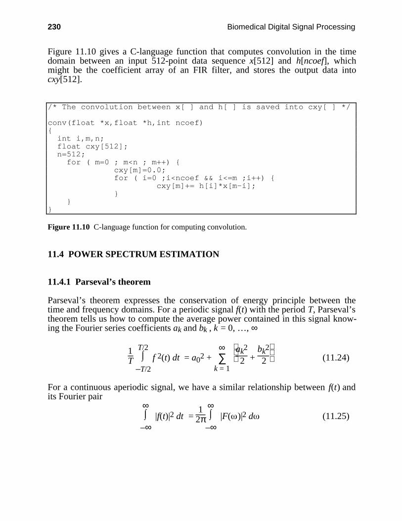
230 Biomedical Digital Signal Processing
Figure 11.10 gives a C-language function that computes convolution in the timedomain between an input 512-point data sequence x[512] and h[ncoef], whichmight be the coefficient array of an FIR filter, and stores the output data intocxy[512].
/* The convolution between x[ ] and h[ ] is saved into cxy[ ] */
conv(float *x,float *h,int ncoef) int i,m,n; float cxy[512]; n=512; for ( m=0 ; m<n ; m++) cxy[m]=0.0; for ( i=0 ;i<ncoef && i<=m ;i++) cxy[m]+= h[i]*x[m-i];
Figure 11.10 C-language function for computing convolution.
11.4 POWER SPECTRUM ESTIMATION
11.4.1 Parseval’s theorem
Parseval’s theorem expresses the conservation of energy principle between thetime and frequency domains. For a periodic signal f(t) with the period T, Parseval’stheorem tells us how to compute the average power contained in this signal know-ing the Fourier series coefficients ak and bk , k = 0, …, ∞
1T ⌡⌠
–T/2
T/2 f 2(t) dt = a02 + ∑
k = 1
∞
ak2
2 + bk2
2 (11.24)
For a continuous aperiodic signal, we have a similar relationship between f(t) andits Fourier pair
⌡⌠
–∞
∞ |f(t)|2 dt =
12π ⌡⌠
–∞
∞ |F( )|2 d (11.25)

Other Time- and Frequency-Domain Techniques 231
Similarly, for the Fourier transform of real discrete signals
∑–∞
∞ f2(n ) =
12π ⌡⌠
2π
|F( )|2 d (11.26)
In the case of the DFT we assume that the time-domain signal repeats identicallywith a period of N points, thus the DFT will repeat at intervals of samplingfrequency. Parseval’s theorem is expressed under these conditions as
∑n = 0
N – 1 x2(n) =
1N ∑
k = 0
N – 1 |X(k)|2 (11.27)
To estimate the average power of the signal, we compute the mean squared ampli-tude and make the approximation
1T ⌡⌠
–T/2
T/2 f 2(t) dt ≈
1N ∑
n = 0
N – 1 f 2(n) (11.28)
The method for power spectrum estimation (PSE) used in this section is based onthe periodogram concept. Thus, if we sample a function c(t) and use the FFT tocompute its DFT, we get
Ck = ∑n = 0
N – 1 c(n) e
–jkn 2πN
Then the periodogram estimate for the power spectrum is defined for N/2 + 1 fre-quencies as
P(0) = 1
N2 |C0|2
P(k) = 1
N2 (|Ck|2 + |CN – k|2) for k = 1,…, N/2 – 1 (11.29)
P(N/2) = 1
N2 |CN/2|2
By Parseval’s theorem, we see that the mean squared amplitude is equal to the sumof the N/2 + 1 values of P. We must ask ourselves how accurate this estimator isand how it can be improved. The following sections provide two methods for im-proving the performance of the estimator.
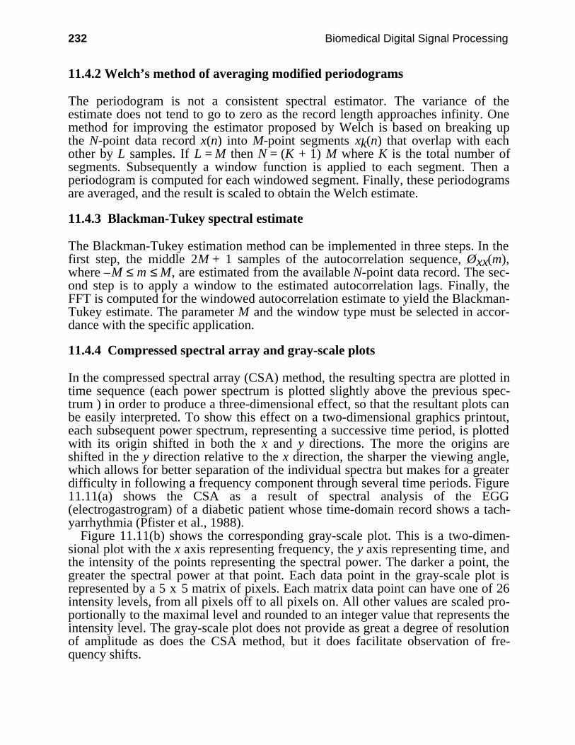
232 Biomedical Digital Signal Processing
11.4.2 Welch’s method of averaging modified periodograms
The periodogram is not a consistent spectral estimator. The variance of theestimate does not tend to go to zero as the record length approaches infinity. Onemethod for improving the estimator proposed by Welch is based on breaking upthe N-point data record x(n) into M-point segments xk(n) that overlap with eachother by L samples. If L = M then N = (K + 1) M where K is the total number ofsegments. Subsequently a window function is applied to each segment. Then aperiodogram is computed for each windowed segment. Finally, these periodogramsare averaged, and the result is scaled to obtain the Welch estimate.
11.4.3 Blackman-Tukey spectral estimate
The Blackman-Tukey estimation method can be implemented in three steps. In thefirst step, the middle 2M + 1 samples of the autocorrelation sequence, Øxx(m),where –M ≤ m ≤ M, are estimated from the available N-point data record. The sec-ond step is to apply a window to the estimated autocorrelation lags. Finally, theFFT is computed for the windowed autocorrelation estimate to yield the Blackman-Tukey estimate. The parameter M and the window type must be selected in accor-dance with the specific application.
11.4.4 Compressed spectral array and gray-scale plots
In the compressed spectral array (CSA) method, the resulting spectra are plotted intime sequence (each power spectrum is plotted slightly above the previous spec-trum ) in order to produce a three-dimensional effect, so that the resultant plots canbe easily interpreted. To show this effect on a two-dimensional graphics printout,each subsequent power spectrum, representing a successive time period, is plottedwith its origin shifted in both the x and y directions. The more the origins areshifted in the y direction relative to the x direction, the sharper the viewing angle,which allows for better separation of the individual spectra but makes for a greaterdifficulty in following a frequency component through several time periods. Figure11.11(a) shows the CSA as a result of spectral analysis of the EGG(electrogastrogram) of a diabetic patient whose time-domain record shows a tach-yarrhythmia (Pfister et al., 1988).
Figure 11.11(b) shows the corresponding gray-scale plot. This is a two-dimen-sional plot with the x axis representing frequency, the y axis representing time, andthe intensity of the points representing the spectral power. The darker a point, thegreater the spectral power at that point. Each data point in the gray-scale plot isrepresented by a 5 x 5 matrix of pixels. Each matrix data point can have one of 26intensity levels, from all pixels off to all pixels on. All other values are scaled pro-portionally to the maximal level and rounded to an integer value that represents theintensity level. The gray-scale plot does not provide as great a degree of resolutionof amplitude as does the CSA method, but it does facilitate observation of fre-quency shifts.
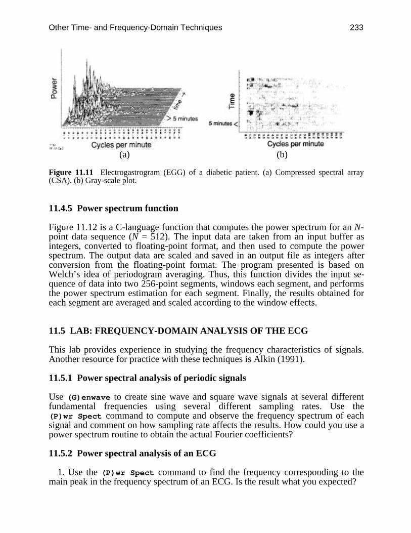
Other Time- and Frequency-Domain Techniques 233
(a) (b)
Figure 11.11 Electrogastrogram (EGG) of a diabetic patient. (a) Compressed spectral array(CSA). (b) Gray-scale plot.
11.4.5 Power spectrum function
Figure 11.12 is a C-language function that computes the power spectrum for an N-point data sequence (N = 512). The input data are taken from an input buffer asintegers, converted to floating-point format, and then used to compute the powerspectrum. The output data are scaled and saved in an output file as integers afterconversion from the floating-point format. The program presented is based onWelch’s idea of periodogram averaging. Thus, this function divides the input se-quence of data into two 256-point segments, windows each segment, and performsthe power spectrum estimation for each segment. Finally, the results obtained foreach segment are averaged and scaled according to the window effects.
11.5 LAB: FREQUENCY-DOMAIN ANALYSIS OF THE ECG
This lab provides experience in studying the frequency characteristics of signals.Another resource for practice with these techniques is Alkin (1991).
11.5.1 Power spectral analysis of periodic signals
Use (G)enwave to create sine wave and square wave signals at several differentfundamental frequencies using several different sampling rates. Use the(P)wr Spect command to compute and observe the frequency spectrum of eachsignal and comment on how sampling rate affects the results. How could you use apower spectrum routine to obtain the actual Fourier coefficients?
11.5.2 Power spectral analysis of an ECG
1. Use the (P)wr Spect command to find the frequency corresponding to themain peak in the frequency spectrum of an ECG. Is the result what you expected?
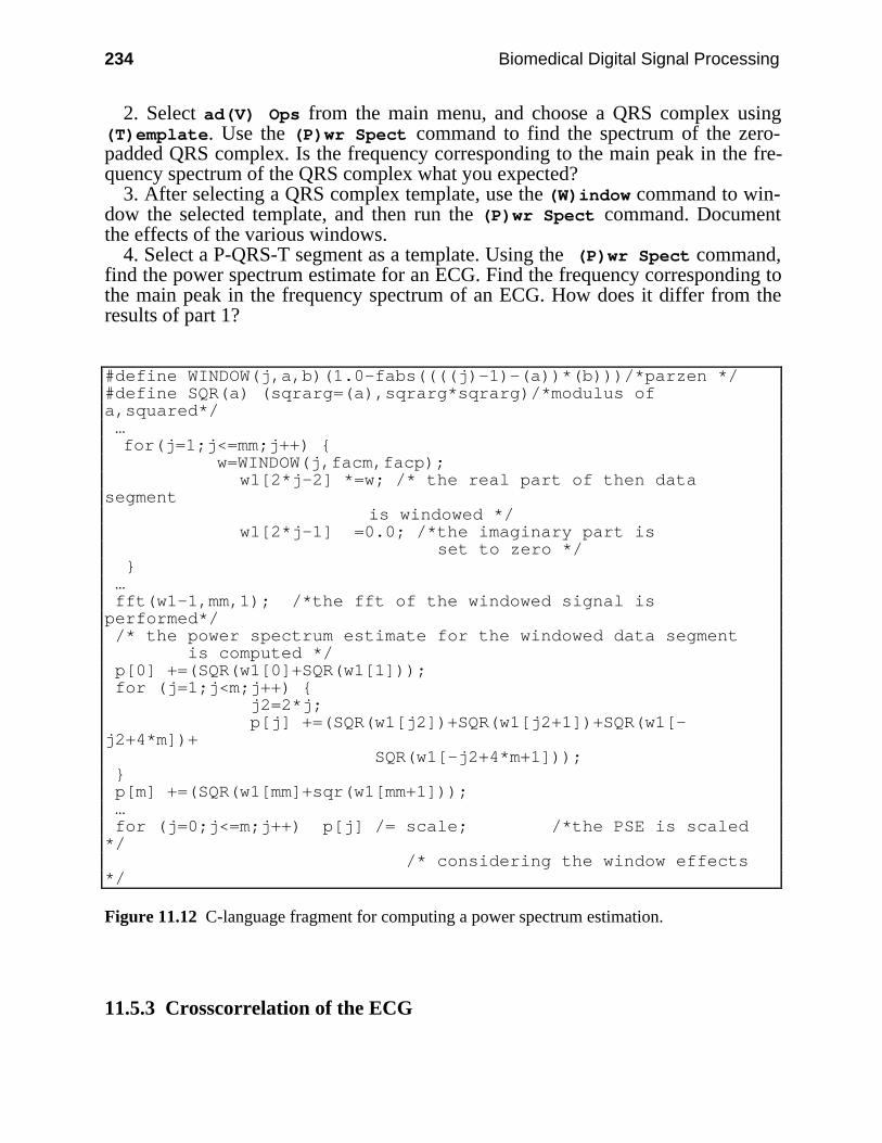
234 Biomedical Digital Signal Processing
2. Select ad(V) Ops from the main menu, and choose a QRS complex using(T)emplate. Use the (P)wr Spect command to find the spectrum of the zero-padded QRS complex. Is the frequency corresponding to the main peak in the fre-quency spectrum of the QRS complex what you expected?
3. After selecting a QRS complex template, use the (W)indow command to win-dow the selected template, and then run the (P)wr Spect command. Documentthe effects of the various windows.
4. Select a P-QRS-T segment as a template. Using the (P)wr Spect command,find the power spectrum estimate for an ECG. Find the frequency corresponding tothe main peak in the frequency spectrum of an ECG. How does it differ from theresults of part 1?
#define WINDOW(j,a,b)(1.0-fabs((((j)-1)-(a))*(b)))/*parzen */#define SQR(a) (sqrarg=(a),sqrarg*sqrarg)/*modulus ofa,squared*/ … for(j=1;j<=mm;j++) w=WINDOW(j,facm,facp); w1[2*j-2] *=w; /* the real part of then datasegment is windowed */ w1[2*j-1] =0.0; /*the imaginary part is
set to zero */ … fft(w1-1,mm,1); /*the fft of the windowed signal isperformed*/ /* the power spectrum estimate for the windowed data segment is computed */ p[0] +=(SQR(w1[0]+SQR(w1[1])); for (j=1;j<m;j++) j2=2*j; p[j] +=(SQR(w1[j2])+SQR(w1[j2+1])+SQR(w1[-j2+4*m])+ SQR(w1[-j2+4*m+1])); p[m] +=(SQR(w1[mm]+sqr(w1[mm+1])); … for (j=0;j<=m;j++) p[j] /= scale; /*the PSE is scaled*/ /* considering the window effects*/
Figure 11.12 C-language fragment for computing a power spectrum estimation.
11.5.3 Crosscorrelation of the ECG
Other Time- and Frequency-Domain Techniques 235
Select a QRS complex using the (T)emplate command. Use the (C)orrelationcommand to correlate this QRS with the ECG. Explain the relationship betweenthe output of the crosscorrelation function and the size of the selected template.What is the time delay between the peak of the crosscorrelation function and theselected QRS? Read a different ECG from a disk file, and crosscorrelate thetemplate with the new ECG. Explain all your observations.
11.6 REFERENCES
Alkin, O. 1991. PC-DSP, Englewood Cliffs, NJ: Prentice Hall.Oppenheim, A. V., and Schafer, R. W. 1975. Digital Signal Processing. Englewood Cliffs, NJ:
Prentice Hall.Pfister, C. J., Hamilton, J. W., Bass, P., Webster, J. G., and Tompkins, W. J. 1988. Use of
spectral analysis in detection of frequency differences in electrogastrograms of normal anddiabetic subjects. IEEE Trans. Biomed. Eng. 935–41.
11.7 STUDY QUESTIONS
11.1 Derive Eqs. (11.24) and (11.27) considering x(n) to be a digital periodic signal containingN samples in a period.
11.2 If x(n) = 1.0 + cos(2πn/4.0), find the DFT of this signal for n = 0, …, 7. Write a C-languageprogram that creates a data file with the values of this signal. Read this data file with theUW DigiScope program, and pad it with the corresponding number of zeros. Take thepower spectrum of the zero-padded signal using the (P)wr Spect command withoutwindowing it, and compare the result with your hand analysis. Explain the differences.
11.3 Create a file that has the values of x(n) = sin(2πn/512.0), n = 0, …, 511. Take the powerspectrum of this signal without windowing it. Replace the last 10 samples of this signalwith zeros. Take the power spectrum of the padded signal with and without a window.Explain the differences.
11.4 Select one period of the signal created in question 11.2 as a template. Crosscorrelate thistemplate with the created signal. Explain the shape of the crosscorrelation function.Compute the amplitude of the peak and compare it with the result of your experiment.
11.5 A 100-Hz-bandwidth ECG signal is sampled at a rate of 500 samples/s. (a) Draw the ap-proximate frequency spectrum of the new digital signal obtained after sampling, and labelimportant points on the axes. (b) On the same graph, draw the approximate spectrum thatwould be averaged from a set of normal QRS complexes.
236
12
ECG QRS Detection
Valtino X. Afonso
Over the past few years, there has been an increased trend toward processing of theelectrocardiogram (ECG) using microcomputers. A survey of literature in this re-search area indicates that systems based on microcomputers can perform neededmedical services in an extremely efficient manner. In fact, many systems have al-ready been designed and implemented to perform signal processing tasks such as12-lead off-line ECG analysis, Holter tape analysis, and real-time patient monitor-ing. All these applications require an accurate detection of the QRS complex of theECG. For example, arrhythmia monitors for ambulatory patients analyze the ECGin real time (Pan and Tompkins, 1985), and when an arrhythmia occurs, the moni-tor stores a time segment of the abnormal ECG. This kind of monitor requires anaccurate QRS recognition capability. Thus, QRS detection is an important part ofmany ECG signal processing systems.
This chapter discusses a few of the many techniques that have been developed todetect the QRS complex of the ECG. It begins with a discussion of the powerspectrum of the ECG and goes on to review a variety of QRS detection algorithms.
12.1 POWER SPECTRUM OF THE ECG
The power spectrum of the ECG signal can provide useful information about theQRS complex. This section reiterates the notion of the power spectrum presentedearlier, but also gives an interpretation of the power spectrum of the QRS complex.The power spectrum (based on the FFT) of a set of 512 sample points that containapproximately two heartbeats results in a series of coefficients with a maximalvalue near a frequency corresponding to the heart rate.
The heart rate can be determined by multiplying together the normalized fre-quency and the sampling frequency. We can also get useful information about thefrequency spectrum of the QRS complex. In order to obtain this information, theQRS complex of the ECG signal must be selected as a template and zero-paddedprior to the power spectrum analysis. The peak of the frequency spectrum obtainedcorresponds to the peak energy of the QRS complex.
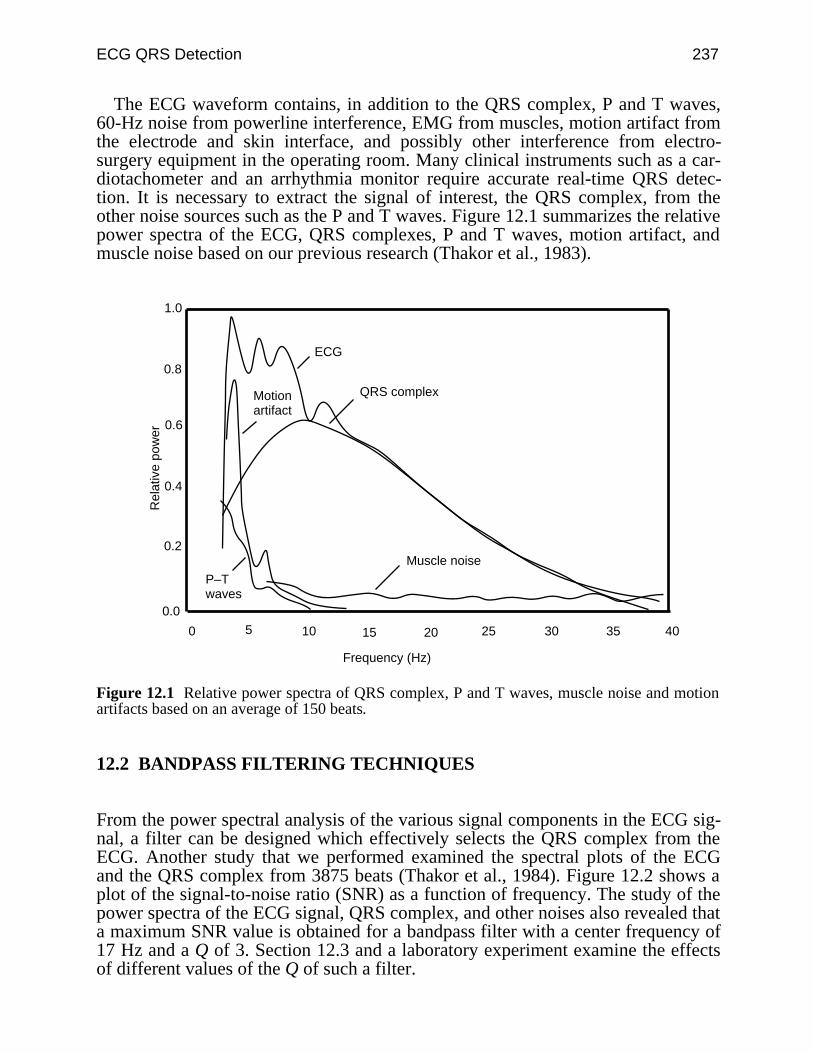
ECG QRS Detection 237
The ECG waveform contains, in addition to the QRS complex, P and T waves,60-Hz noise from powerline interference, EMG from muscles, motion artifact fromthe electrode and skin interface, and possibly other interference from electro-surgery equipment in the operating room. Many clinical instruments such as a car-diotachometer and an arrhythmia monitor require accurate real-time QRS detec-tion. It is necessary to extract the signal of interest, the QRS complex, from theother noise sources such as the P and T waves. Figure 12.1 summarizes the relativepower spectra of the ECG, QRS complexes, P and T waves, motion artifact, andmuscle noise based on our previous research (Thakor et al., 1983).
Motionartifact
QRS complex
P–Twaves
Muscle noise
1.0
0.8
0.6
0.4
0.2
0.0
0 5 10 15 20 25 30 35 40
Rel
ativ
e po
wer
Frequency (Hz)
ECG
Figure 12.1 Relative power spectra of QRS complex, P and T waves, muscle noise and motionartifacts based on an average of 150 beats.
12.2 BANDPASS FILTERING TECHNIQUES
From the power spectral analysis of the various signal components in the ECG sig-nal, a filter can be designed which effectively selects the QRS complex from theECG. Another study that we performed examined the spectral plots of the ECGand the QRS complex from 3875 beats (Thakor et al., 1984). Figure 12.2 shows aplot of the signal-to-noise ratio (SNR) as a function of frequency. The study of thepower spectra of the ECG signal, QRS complex, and other noises also revealed thata maximum SNR value is obtained for a bandpass filter with a center frequency of17 Hz and a Q of 3. Section 12.3 and a laboratory experiment examine the effectsof different values of the Q of such a filter.
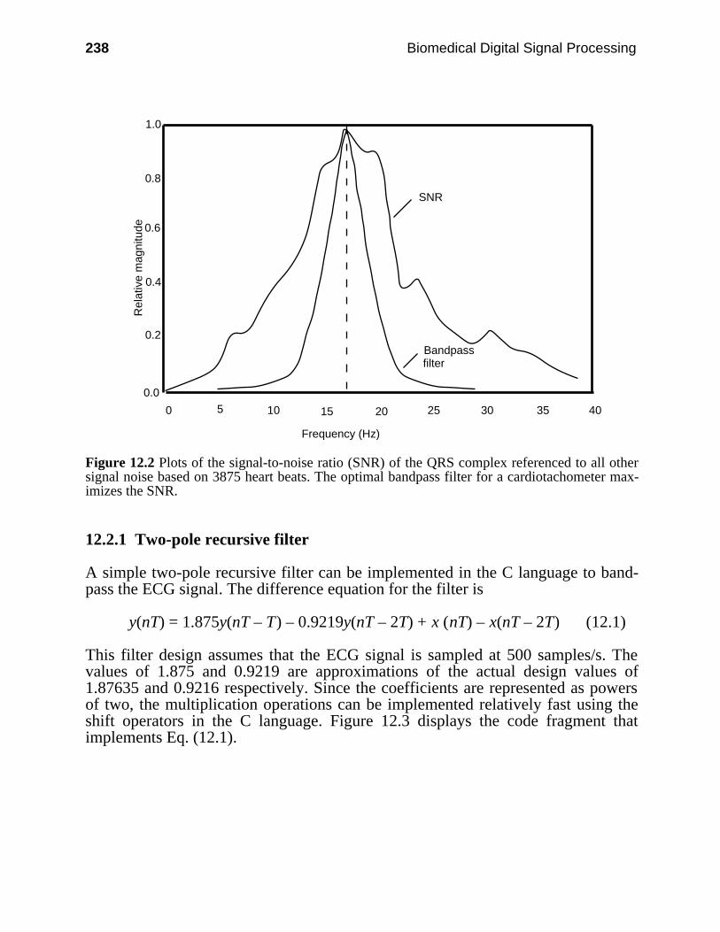
238 Biomedical Digital Signal Processing
1.0
0.8
0.6
0.4
0.2
0.0
0 5 10 15 20 25 30 35 40
Rel
ativ
e m
agni
tude
Frequency (Hz)
SNR
Bandpassfilter
Figure 12.2 Plots of the signal-to-noise ratio (SNR) of the QRS complex referenced to all othersignal noise based on 3875 heart beats. The optimal bandpass filter for a cardiotachometer max-imizes the SNR.
12.2.1 Two-pole recursive filter
A simple two-pole recursive filter can be implemented in the C language to band-pass the ECG signal. The difference equation for the filter is
y(nT) = 1.875y(nT – T) – 0.9219y(nT – 2T) + x (nT) – x(nT – 2T) (12.1)
This filter design assumes that the ECG signal is sampled at 500 samples/s. Thevalues of 1.875 and 0.9219 are approximations of the actual design values of1.87635 and 0.9216 respectively. Since the coefficients are represented as powersof two, the multiplication operations can be implemented relatively fast using theshift operators in the C language. Figure 12.3 displays the code fragment thatimplements Eq. (12.1).
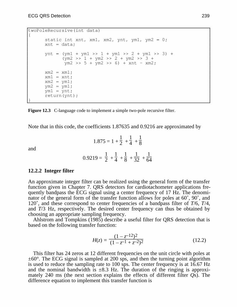
ECG QRS Detection 239
twoPoleRecursive(int data) static int xnt, xm1, xm2, ynt, ym1, ym2 = 0; xnt = data;
ynt = (ym1 + ym1 >> 1 + ym1 >> 2 + ym1 >> 3) + (ym2 >> 1 + ym2 >> 2 + ym2 >> 3 + ym2 >> 5 + ym2 >> 6) + xnt - xm2;
xm2 = xm1; xm1 = xnt; xm2 = ym1; ym2 = ym1; ym1 = ynt; return(ynt);
Figure 12.3 C-language code to implement a simple two-pole recursive filter.
Note that in this code, the coefficients 1.87635 and 0.9216 are approximated by
1.875 = 1 + 12 +
14 +
18
and
0.9219 = 12 +
14 +
18 +
132 +
164
12.2.2 Integer filter
An approximate integer filter can be realized using the general form of the transferfunction given in Chapter 7. QRS detectors for cardiotachometer applications fre-quently bandpass the ECG signal using a center frequency of 17 Hz. The denomi-nator of the general form of the transfer function allows for poles at 60˚, 90˚, and120˚, and these correspond to center frequencies of a bandpass filter of T/6, T/4,and T/3 Hz, respectively. The desired center frequency can thus be obtained bychoosing an appropriate sampling frequency.
Ahlstrom and Tompkins (1985) describe a useful filter for QRS detection that isbased on the following transfer function:
H(z) = (1 – z–12)2
(1 – z–1 + z–2)2 (12.2)
This filter has 24 zeros at 12 different frequencies on the unit circle with poles at±60°. The ECG signal is sampled at 200 sps, and then the turning point algorithmis used to reduce the sampling rate to 100 sps. The center frequency is at 16.67 Hzand the nominal bandwidth is ±8.3 Hz. The duration of the ringing is approxi-mately 240 ms (the next section explains the effects of different filter Qs). Thedifference equation to implement this transfer function is
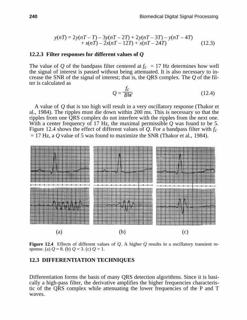
240 Biomedical Digital Signal Processing
y(nT) = 2y(nT – T) – 3y(nT – 2T) + 2y(nT – 3T) – y(nT – 4T)+ x(nT) – 2x(nT – 12T) + x(nT – 24T) (12.3)
12.2.3 Filter responses for different values of Q
The value of Q of the bandpass filter centered at fc = 17 Hz determines how wellthe signal of interest is passed without being attenuated. It is also necessary to in-crease the SNR of the signal of interest; that is, the QRS complex. The Q of the fil-ter is calculated as
Q = fc
BW (12.4)
A value of Q that is too high will result in a very oscillatory response (Thakor etal., 1984). The ripples must die down within 200 ms. This is necessary so that theripples from one QRS complex do not interfere with the ripples from the next one.With a center frequency of 17 Hz, the maximal permissible Q was found to be 5.Figure 12.4 shows the effect of different values of Q. For a bandpass filter with fc = 17 Hz, a Q value of 5 was found to maximize the SNR (Thakor et al., 1984).
(a) (b) (c)
Figure 12.4 Effects of different values of Q. A higher Q results in a oscillatory transient re-sponse. (a) Q = 8. (b) Q = 3. (c) Q = 1.
12.3 DIFFERENTIATION TECHNIQUES
Differentiation forms the basis of many QRS detection algorithms. Since it is basi-cally a high-pass filter, the derivative amplifies the higher frequencies characteris-tic of the QRS complex while attenuating the lower frequencies of the P and Twaves.
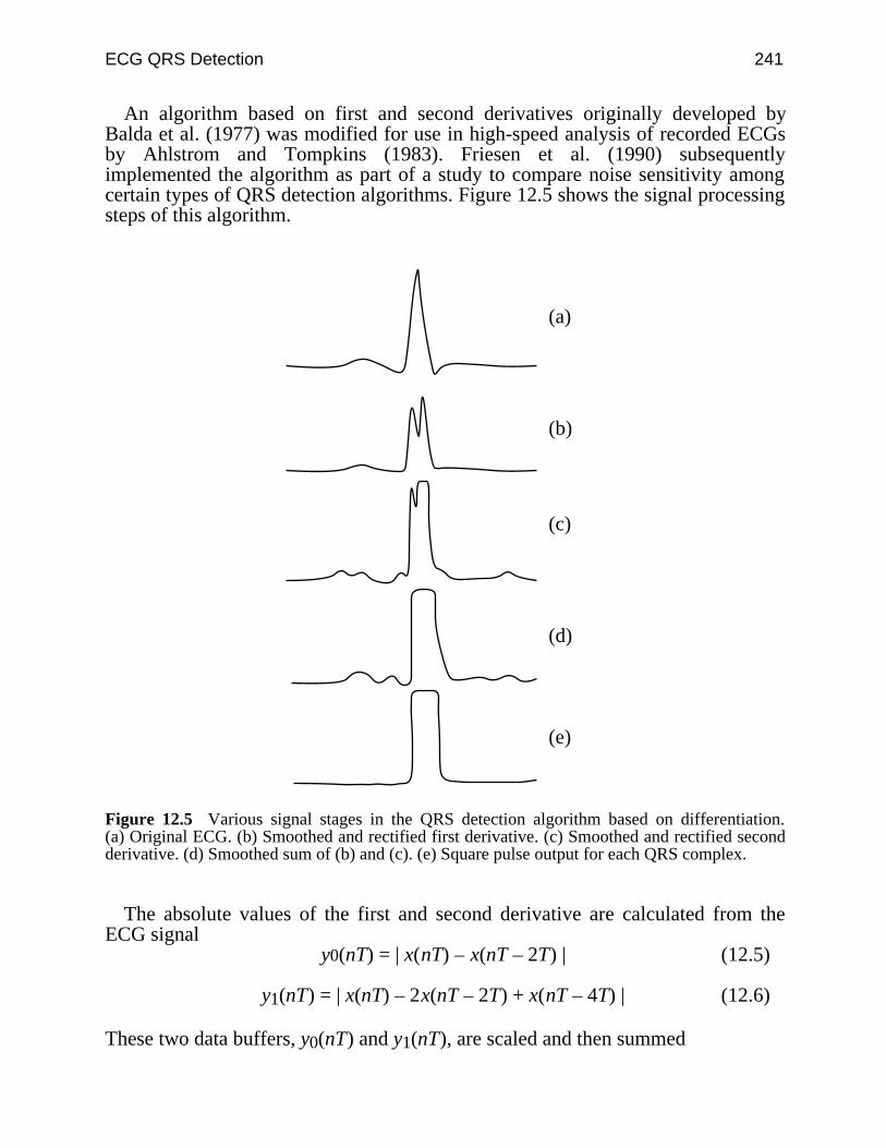
ECG QRS Detection 241
An algorithm based on first and second derivatives originally developed byBalda et al. (1977) was modified for use in high-speed analysis of recorded ECGsby Ahlstrom and Tompkins (1983). Friesen et al. (1990) subsequentlyimplemented the algorithm as part of a study to compare noise sensitivity amongcertain types of QRS detection algorithms. Figure 12.5 shows the signal processingsteps of this algorithm.
(a)
(b)
(c)
(d)
(e)
Figure 12.5 Various signal stages in the QRS detection algorithm based on differentiation.(a) Original ECG. (b) Smoothed and rectified first derivative. (c) Smoothed and rectified secondderivative. (d) Smoothed sum of (b) and (c). (e) Square pulse output for each QRS complex.
The absolute values of the first and second derivative are calculated from theECG signal
y0(nT) = | x(nT) – x(nT – 2T) | (12.5)
y1(nT) = | x(nT) – 2x(nT – 2T) + x(nT – 4T) | (12.6)
These two data buffers, y0(nT) and y1(nT), are scaled and then summed
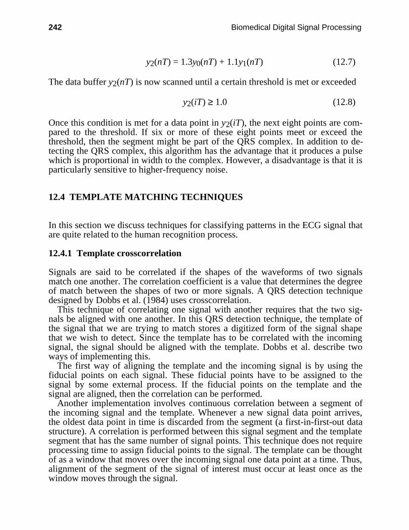
242 Biomedical Digital Signal Processing
y2(nT) = 1.3y0(nT) + 1.1y1(nT) (12.7)
The data buffer y2(nT) is now scanned until a certain threshold is met or exceeded
y2(iT) ≥ 1.0 (12.8)
Once this condition is met for a data point in y2(iT), the next eight points are com-pared to the threshold. If six or more of these eight points meet or exceed thethreshold, then the segment might be part of the QRS complex. In addition to de-tecting the QRS complex, this algorithm has the advantage that it produces a pulsewhich is proportional in width to the complex. However, a disadvantage is that it isparticularly sensitive to higher-frequency noise.
12.4 TEMPLATE MATCHING TECHNIQUES
In this section we discuss techniques for classifying patterns in the ECG signal thatare quite related to the human recognition process.
12.4.1 Template crosscorrelation
Signals are said to be correlated if the shapes of the waveforms of two signalsmatch one another. The correlation coefficient is a value that determines the degreeof match between the shapes of two or more signals. A QRS detection techniquedesigned by Dobbs et al. (1984) uses crosscorrelation.
This technique of correlating one signal with another requires that the two sig-nals be aligned with one another. In this QRS detection technique, the template ofthe signal that we are trying to match stores a digitized form of the signal shapethat we wish to detect. Since the template has to be correlated with the incomingsignal, the signal should be aligned with the template. Dobbs et al. describe twoways of implementing this.
The first way of aligning the template and the incoming signal is by using thefiducial points on each signal. These fiducial points have to be assigned to thesignal by some external process. If the fiducial points on the template and thesignal are aligned, then the correlation can be performed.
Another implementation involves continuous correlation between a segment ofthe incoming signal and the template. Whenever a new signal data point arrives,the oldest data point in time is discarded from the segment (a first-in-first-out datastructure). A correlation is performed between this signal segment and the templatesegment that has the same number of signal points. This technique does not requireprocessing time to assign fiducial points to the signal. The template can be thoughtof as a window that moves over the incoming signal one data point at a time. Thus,alignment of the segment of the signal of interest must occur at least once as thewindow moves through the signal.
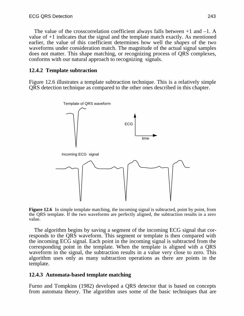
ECG QRS Detection 243
The value of the crosscorrelation coefficient always falls between +1 and –1. Avalue of +1 indicates that the signal and the template match exactly. As mentionedearlier, the value of this coefficient determines how well the shapes of the twowaveforms under consideration match. The magnitude of the actual signal samplesdoes not matter. This shape matching, or recognizing process of QRS complexes,conforms with our natural approach to recognizing signals.
12.4.2 Template subtraction
Figure 12.6 illustrates a template subtraction technique. This is a relatively simpleQRS detection technique as compared to the other ones described in this chapter.
Template of QRS waveform
Incoming ECG signal
time
ECG
Figure 12.6 In simple template matching, the incoming signal is subtracted, point by point, fromthe QRS template. If the two waveforms are perfectly aligned, the subtraction results in a zerovalue.
The algorithm begins by saving a segment of the incoming ECG signal that cor-responds to the QRS waveform. This segment or template is then compared withthe incoming ECG signal. Each point in the incoming signal is subtracted from thecorresponding point in the template. When the template is aligned with a QRSwaveform in the signal, the subtraction results in a value very close to zero. Thisalgorithm uses only as many subtraction operations as there are points in thetemplate.
12.4.3 Automata-based template matching
Furno and Tompkins (1982) developed a QRS detector that is based on conceptsfrom automata theory. The algorithm uses some of the basic techniques that are
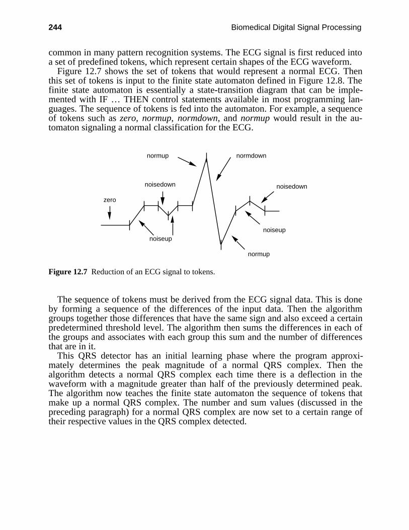
244 Biomedical Digital Signal Processing
common in many pattern recognition systems. The ECG signal is first reduced intoa set of predefined tokens, which represent certain shapes of the ECG waveform.
Figure 12.7 shows the set of tokens that would represent a normal ECG. Thenthis set of tokens is input to the finite state automaton defined in Figure 12.8. Thefinite state automaton is essentially a state-transition diagram that can be imple-mented with IF … THEN control statements available in most programming lan-guages. The sequence of tokens is fed into the automaton. For example, a sequenceof tokens such as zero, normup, normdown, and normup would result in the au-tomaton signaling a normal classification for the ECG.
normup normdown
noisedown
normup
noiseupnoiseup
noisedown
zero
Figure 12.7 Reduction of an ECG signal to tokens.
The sequence of tokens must be derived from the ECG signal data. This is doneby forming a sequence of the differences of the input data. Then the algorithmgroups together those differences that have the same sign and also exceed a certainpredetermined threshold level. The algorithm then sums the differences in each ofthe groups and associates with each group this sum and the number of differencesthat are in it.
This QRS detector has an initial learning phase where the program approxi-mately determines the peak magnitude of a normal QRS complex. Then thealgorithm detects a normal QRS complex each time there is a deflection in thewaveform with a magnitude greater than half of the previously determined peak.The algorithm now teaches the finite state automaton the sequence of tokens thatmake up a normal QRS complex. The number and sum values (discussed in thepreceding paragraph) for a normal QRS complex are now set to a certain range oftheir respective values in the QRS complex detected.
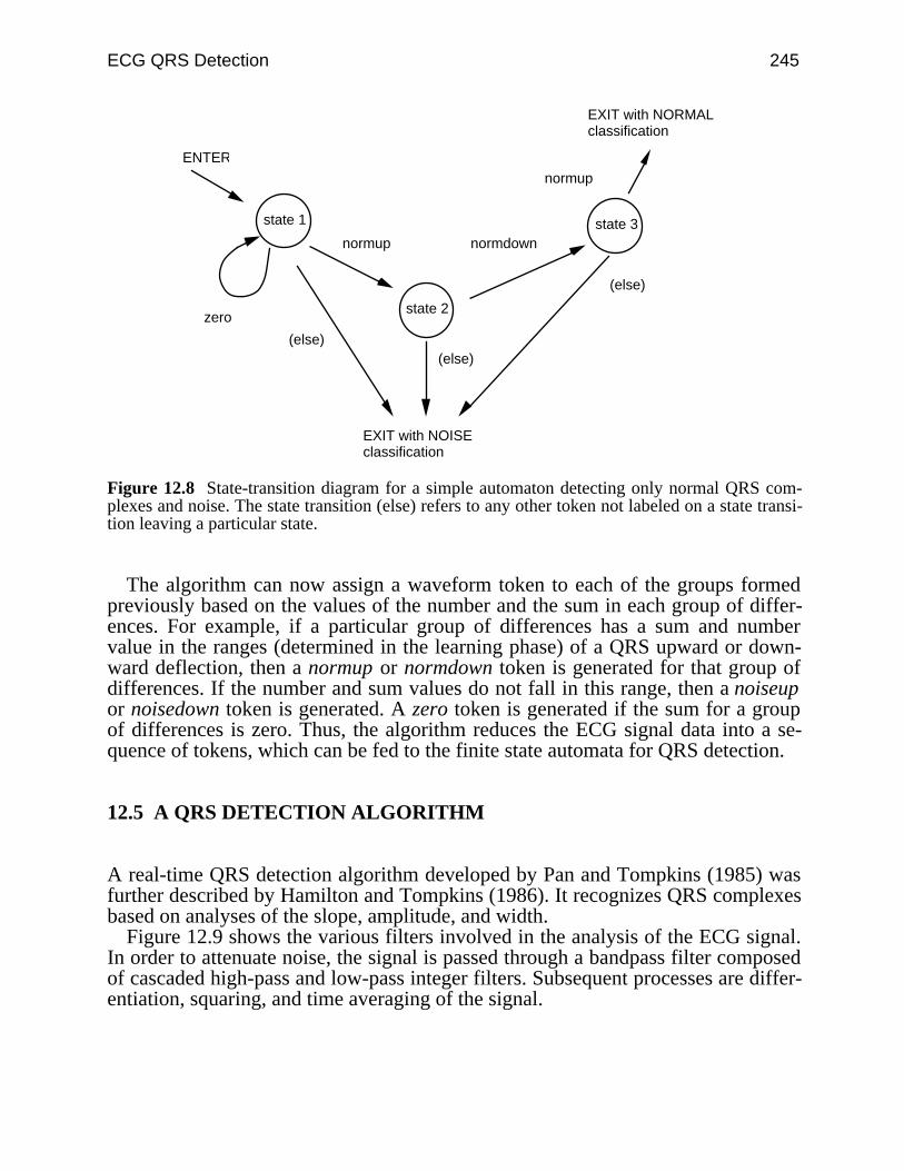
ECG QRS Detection 245
ENTER
state 1
EXIT with NORMALclassification
EXIT with NOISEclassification
normup normdown
normup
zero
(else)(else)
(else)
state 2
state 3
Figure 12.8 State-transition diagram for a simple automaton detecting only normal QRS com-plexes and noise. The state transition (else) refers to any other token not labeled on a state transi-tion leaving a particular state.
The algorithm can now assign a waveform token to each of the groups formedpreviously based on the values of the number and the sum in each group of differ-ences. For example, if a particular group of differences has a sum and numbervalue in the ranges (determined in the learning phase) of a QRS upward or down-ward deflection, then a normup or normdown token is generated for that group ofdifferences. If the number and sum values do not fall in this range, then a noiseupor noisedown token is generated. A zero token is generated if the sum for a groupof differences is zero. Thus, the algorithm reduces the ECG signal data into a se-quence of tokens, which can be fed to the finite state automata for QRS detection.
12.5 A QRS DETECTION ALGORITHM
A real-time QRS detection algorithm developed by Pan and Tompkins (1985) wasfurther described by Hamilton and Tompkins (1986). It recognizes QRS complexesbased on analyses of the slope, amplitude, and width.
Figure 12.9 shows the various filters involved in the analysis of the ECG signal.In order to attenuate noise, the signal is passed through a bandpass filter composedof cascaded high-pass and low-pass integer filters. Subsequent processes are differ-entiation, squaring, and time averaging of the signal.
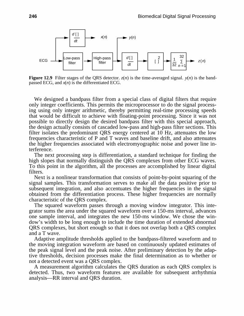
246 Biomedical Digital Signal Processing
ECG [ ] z(n)
x(n) y(n)
1 ∑d [ ]
dt
Low-passfilter
High-passfilter
32
32
2
d [ ]
dt
n =1
Figure 12.9 Filter stages of the QRS detector. z(n) is the time-averaged signal. y(n) is the band-passed ECG, and x(n) is the differentiated ECG.
We designed a bandpass filter from a special class of digital filters that requireonly integer coefficients. This permits the microprocessor to do the signal process-ing using only integer arithmetic, thereby permitting real-time processing speedsthat would be difficult to achieve with floating-point processing. Since it was notpossible to directly design the desired bandpass filter with this special approach,the design actually consists of cascaded low-pass and high-pass filter sections. Thisfilter isolates the predominant QRS energy centered at 10 Hz, attenuates the lowfrequencies characteristic of P and T waves and baseline drift, and also attenuatesthe higher frequencies associated with electromyographic noise and power line in-terference.
The next processing step is differentiation, a standard technique for finding thehigh slopes that normally distinguish the QRS complexes from other ECG waves.To this point in the algorithm, all the processes are accomplished by linear digitalfilters.
Next is a nonlinear transformation that consists of point-by-point squaring of thesignal samples. This transformation serves to make all the data positive prior tosubsequent integration, and also accentuates the higher frequencies in the signalobtained from the differentiation process. These higher frequencies are normallycharacteristic of the QRS complex.
The squared waveform passes through a moving window integrator. This inte-grator sums the area under the squared waveform over a 150-ms interval, advancesone sample interval, and integrates the new 150-ms window. We chose the win-dow’s width to be long enough to include the time duration of extended abnormalQRS complexes, but short enough so that it does not overlap both a QRS complexand a T wave.
Adaptive amplitude thresholds applied to the bandpass-filtered waveform and tothe moving integration waveform are based on continuously updated estimates ofthe peak signal level and the peak noise. After preliminary detection by the adap-tive thresholds, decision processes make the final determination as to whether ornot a detected event was a QRS complex.
A measurement algorithm calculates the QRS duration as each QRS complex isdetected. Thus, two waveform features are available for subsequent arrhythmiaanalysis—RR interval and QRS duration.
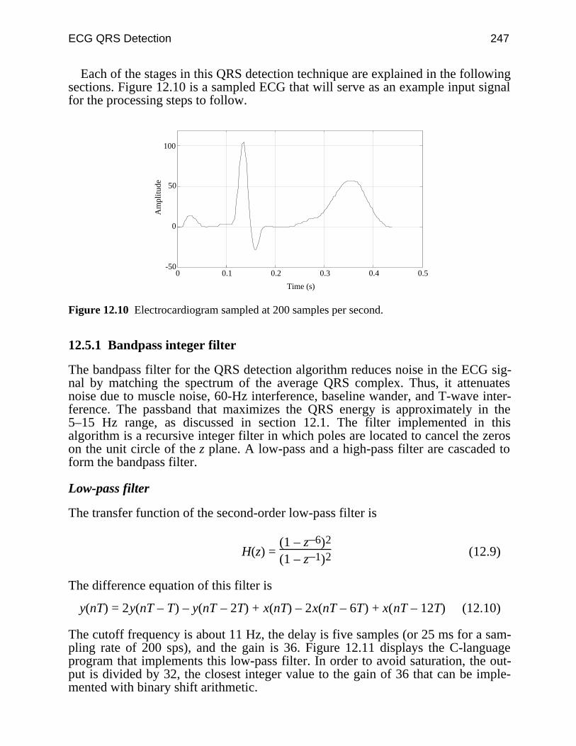
ECG QRS Detection 247
Each of the stages in this QRS detection technique are explained in the followingsections. Figure 12.10 is a sampled ECG that will serve as an example input signalfor the processing steps to follow.
-50
0
50
100
0 0.1 0.2 0.3 0.4 0.5
Time (s)
Am
plit
ude
Figure 12.10 Electrocardiogram sampled at 200 samples per second.
12.5.1 Bandpass integer filter
The bandpass filter for the QRS detection algorithm reduces noise in the ECG sig-nal by matching the spectrum of the average QRS complex. Thus, it attenuatesnoise due to muscle noise, 60-Hz interference, baseline wander, and T-wave inter-ference. The passband that maximizes the QRS energy is approximately in the5–15 Hz range, as discussed in section 12.1. The filter implemented in thisalgorithm is a recursive integer filter in which poles are located to cancel the zeroson the unit circle of the z plane. A low-pass and a high-pass filter are cascaded toform the bandpass filter.
Low-pass filter
The transfer function of the second-order low-pass filter is
H(z) = (1 – z–6)2
(1 – z–1)2 (12.9)
The difference equation of this filter is
y(nT) = 2y(nT – T) – y(nT – 2T) + x(nT) – 2x(nT – 6T) + x(nT – 12T) (12.10)
The cutoff frequency is about 11 Hz, the delay is five samples (or 25 ms for a sam-pling rate of 200 sps), and the gain is 36. Figure 12.11 displays the C-languageprogram that implements this low-pass filter. In order to avoid saturation, the out-put is divided by 32, the closest integer value to the gain of 36 that can be imple-mented with binary shift arithmetic.
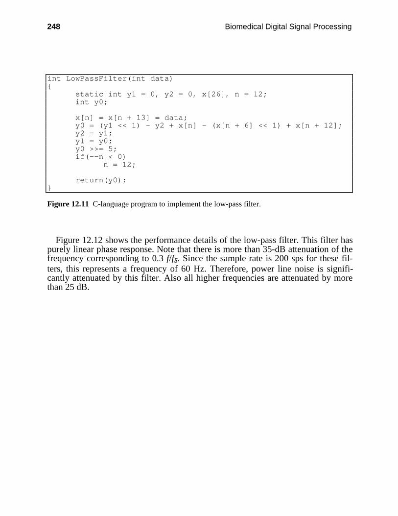
248 Biomedical Digital Signal Processing
int LowPassFilter(int data) static int y1 = 0, y2 = 0, x[26], n = 12; int y0;
x[n] = x[n + 13] = data; y0 = (y1 << 1) - y2 + x[n] - (x[n + 6] << 1) + x[n + 12]; y2 = y1; y1 = y0; y0 >>= 5; if(--n < 0) n = 12;
return(y0);
Figure 12.11 C-language program to implement the low-pass filter.
Figure 12.12 shows the performance details of the low-pass filter. This filter haspurely linear phase response. Note that there is more than 35-dB attenuation of thefrequency corresponding to 0.3 f/fs. Since the sample rate is 200 sps for these fil-ters, this represents a frequency of 60 Hz. Therefore, power line noise is signifi-cantly attenuated by this filter. Also all higher frequencies are attenuated by morethan 25 dB.
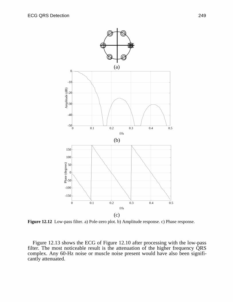
ECG QRS Detection 249
(a)
-50
-40
-30
-20
-10
0
0 0.1 0.2 0.3 0.4 0.5
f/fs
Am
plit
ude
(dB
)
(b)
-150
-100
-50
0
50
100
150
0 0.1 0.2 0.3 0.4 0.5
f/fs
Pha
se (
degr
ees)
(c)Figure 12.12 Low-pass filter. a) Pole-zero plot. b) Amplitude response. c) Phase response.
Figure 12.13 shows the ECG of Figure 12.10 after processing with the low-passfilter. The most noticeable result is the attenuation of the higher frequency QRScomplex. Any 60-Hz noise or muscle noise present would have also been signifi-cantly attenuated.
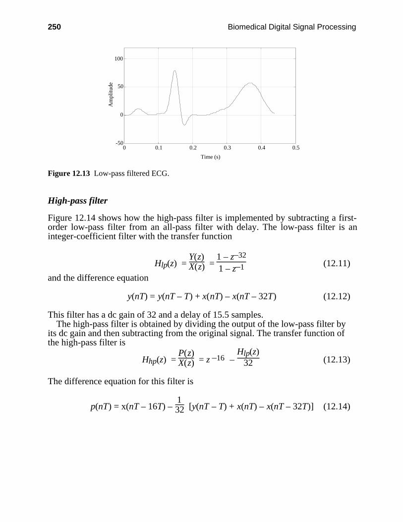
250 Biomedical Digital Signal Processing
-50
0
50
100
0 0.1 0.2 0.3 0.4 0.5
Time (s)
Am
plit
ude
Figure 12.13 Low-pass filtered ECG.
High-pass filter
Figure 12.14 shows how the high-pass filter is implemented by subtracting a first-order low-pass filter from an all-pass filter with delay. The low-pass filter is aninteger-coefficient filter with the transfer function
Hlp(z) = Y(z)X(z) =
1 – z–32
1 – z–1 (12.11)
and the difference equation
y(nT) = y(nT – T) + x(nT) – x(nT – 32T) (12.12)
This filter has a dc gain of 32 and a delay of 15.5 samples.The high-pass filter is obtained by dividing the output of the low-pass filter by
its dc gain and then subtracting from the original signal. The transfer function ofthe high-pass filter is
Hhp(z) = P(z)X(z) = z –16 –
Hlp(z)32 (12.13)
The difference equation for this filter is
p(nT) = x(nT – 16T) – 132 [y(nT – T) + x(nT) – x(nT – 32T)] (12.14)
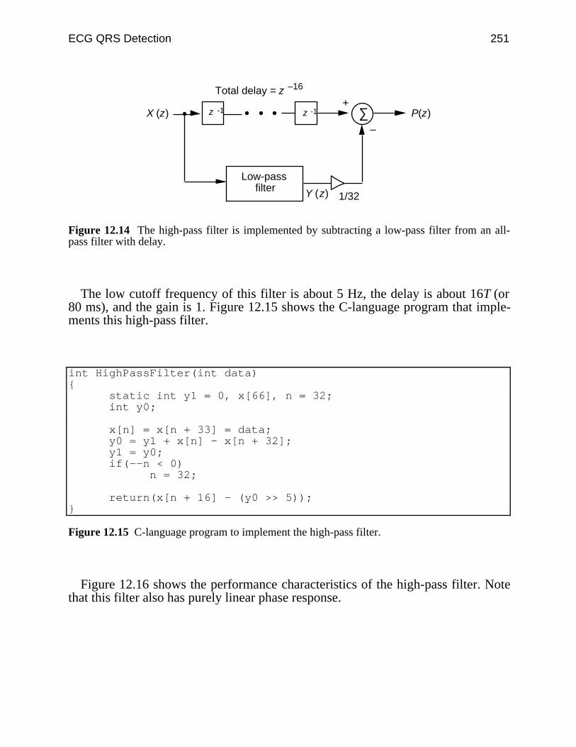
ECG QRS Detection 251
X (z)
Y (z)
z -1 z -1
1/32
∑ P(z)
Low-pass filter
Total delay = z –16
+
–
Figure 12.14 The high-pass filter is implemented by subtracting a low-pass filter from an all-pass filter with delay.
The low cutoff frequency of this filter is about 5 Hz, the delay is about 16T (or80 ms), and the gain is 1. Figure 12.15 shows the C-language program that imple-ments this high-pass filter.
int HighPassFilter(int data) static int y1 = 0, x[66], n = 32; int y0;
x[n] = x[n + 33] = data; y0 = y1 + x[n] - x[n + 32]; y1 = y0; if(--n < 0) n = 32;
return(x[n + 16] - (y0 >> 5));
Figure 12.15 C-language program to implement the high-pass filter.
Figure 12.16 shows the performance characteristics of the high-pass filter. Notethat this filter also has purely linear phase response.
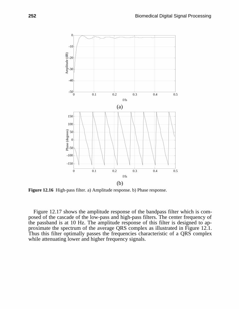
252 Biomedical Digital Signal Processing
-50
-40
-30
-20
-10
0
0 0.1 0.2 0.3 0.4 0.5
f/fs
Am
plitu
de (
dB)
(a)
-150
-100
-50
0
50
100
150
0 0.1 0.2 0.3 0.4 0.5
f/fs
Pha
se (
degr
ees)
(b)Figure 12.16 High-pass filter. a) Amplitude response. b) Phase response.
Figure 12.17 shows the amplitude response of the bandpass filter which is com-posed of the cascade of the low-pass and high-pass filters. The center frequency ofthe passband is at 10 Hz. The amplitude response of this filter is designed to ap-proximate the spectrum of the average QRS complex as illustrated in Figure 12.1.Thus this filter optimally passes the frequencies characteristic of a QRS complexwhile attenuating lower and higher frequency signals.
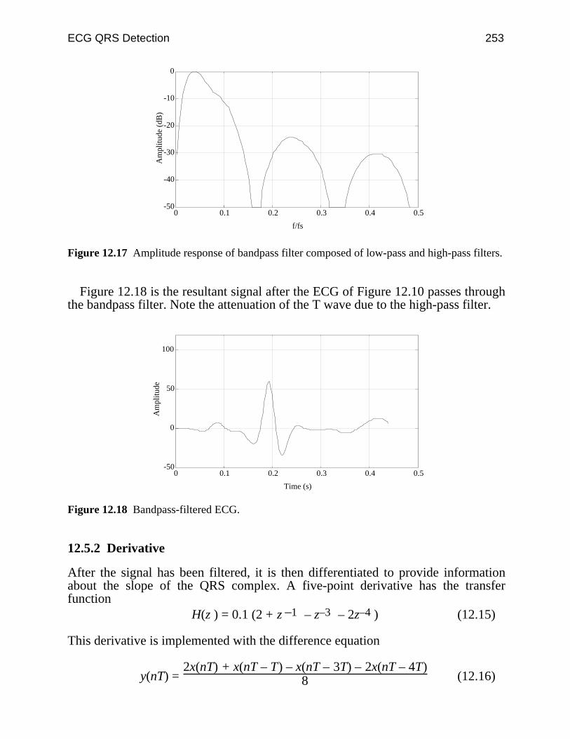
ECG QRS Detection 253
-50
-40
-30
-20
-10
0
0 0.1 0.2 0.3 0.4 0.5
f/fs
Am
plitu
de (
dB)
Figure 12.17 Amplitude response of bandpass filter composed of low-pass and high-pass filters.
Figure 12.18 is the resultant signal after the ECG of Figure 12.10 passes throughthe bandpass filter. Note the attenuation of the T wave due to the high-pass filter.
-50
0
50
100
0 0.1 0.2 0.3 0.4 0.5
Time (s)
Am
plitu
de
Figure 12.18 Bandpass-filtered ECG.
12.5.2 Derivative
After the signal has been filtered, it is then differentiated to provide informationabout the slope of the QRS complex. A five-point derivative has the transferfunction
H(z ) = 0.1 (2 + z –1 – z–3 – 2z–4 ) (12.15)
This derivative is implemented with the difference equation
y(nT) = 2x(nT) + x(nT – T) – x(nT – 3T) – 2x(nT – 4T)
8 (12.16)
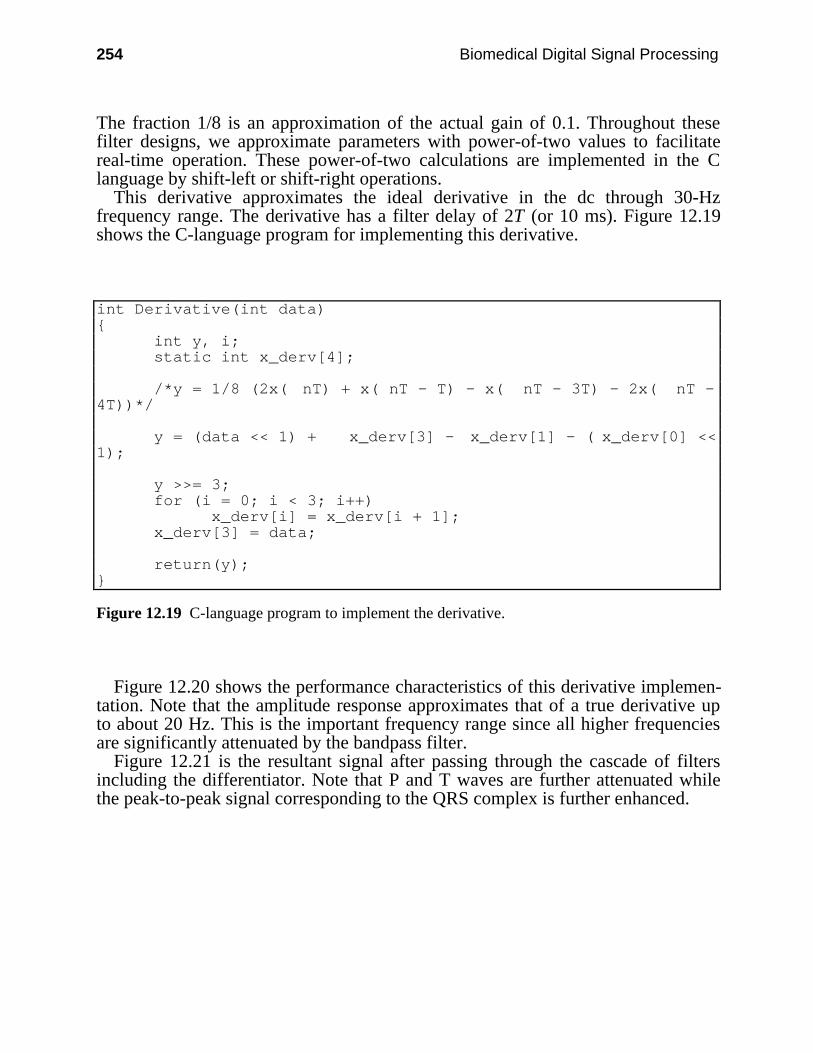
254 Biomedical Digital Signal Processing
The fraction 1/8 is an approximation of the actual gain of 0.1. Throughout thesefilter designs, we approximate parameters with power-of-two values to facilitatereal-time operation. These power-of-two calculations are implemented in the Clanguage by shift-left or shift-right operations.
This derivative approximates the ideal derivative in the dc through 30-Hzfrequency range. The derivative has a filter delay of 2T (or 10 ms). Figure 12.19shows the C-language program for implementing this derivative.
int Derivative(int data) int y, i; static int x_derv[4];
/*y = 1/8 (2x( nT) + x( nT - T) - x( nT - 3T) - 2x( nT -4T))*/
y = (data << 1) + x_derv[3] - x_derv[1] - ( x_derv[0] <<1);
y >>= 3; for (i = 0; i < 3; i++) x_derv[i] = x_derv[i + 1]; x_derv[3] = data;
return(y);
Figure 12.19 C-language program to implement the derivative.
Figure 12.20 shows the performance characteristics of this derivative implemen-tation. Note that the amplitude response approximates that of a true derivative upto about 20 Hz. This is the important frequency range since all higher frequenciesare significantly attenuated by the bandpass filter.
Figure 12.21 is the resultant signal after passing through the cascade of filtersincluding the differentiator. Note that P and T waves are further attenuated whilethe peak-to-peak signal corresponding to the QRS complex is further enhanced.
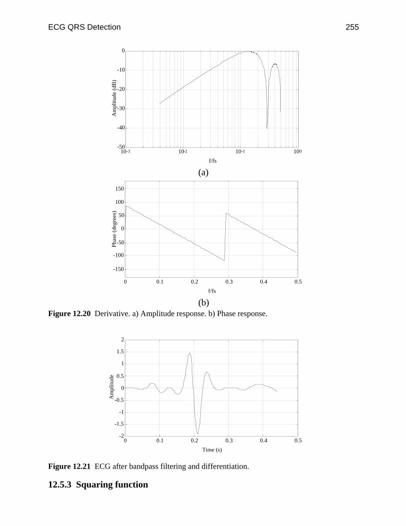
ECG QRS Detection 255
-50
-40
-30
-20
-10
0
10-3 10-2 10-1 100
f/fs
Am
plitu
de (
dB)
(a)
-150
-100
-50
0
50
100
150
0 0.1 0.2 0.3 0.4 0.5
f/fs
Pha
se (
degr
ees)
(b)Figure 12.20 Derivative. a) Amplitude response. b) Phase response.
-2
-1.5
-1
-0.5
0
0.5
1
1.5
2
0 0.1 0.2 0.3 0.4 0.5
Time (s)
Am
plitu
de
Figure 12.21 ECG after bandpass filtering and differentiation.
12.5.3 Squaring function
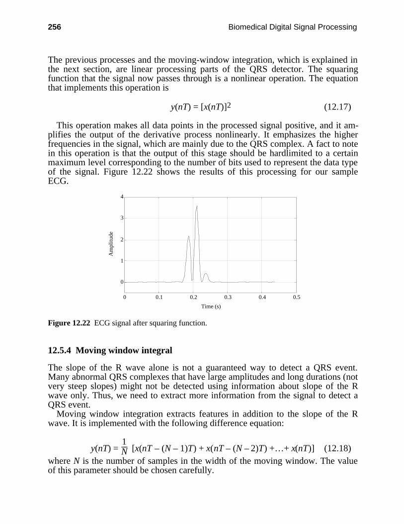
256 Biomedical Digital Signal Processing
The previous processes and the moving-window integration, which is explained inthe next section, are linear processing parts of the QRS detector. The squaringfunction that the signal now passes through is a nonlinear operation. The equationthat implements this operation is
y(nT) = [x(nT)]2 (12.17)
This operation makes all data points in the processed signal positive, and it am-plifies the output of the derivative process nonlinearly. It emphasizes the higherfrequencies in the signal, which are mainly due to the QRS complex. A fact to notein this operation is that the output of this stage should be hardlimited to a certainmaximum level corresponding to the number of bits used to represent the data typeof the signal. Figure 12.22 shows the results of this processing for our sampleECG.
0
1
2
3
4
0 0.1 0.2 0.3 0.4 0.5
Time (s)
Am
plitu
de
Figure 12.22 ECG signal after squaring function.
12.5.4 Moving window integral
The slope of the R wave alone is not a guaranteed way to detect a QRS event.Many abnormal QRS complexes that have large amplitudes and long durations (notvery steep slopes) might not be detected using information about slope of the Rwave only. Thus, we need to extract more information from the signal to detect aQRS event.
Moving window integration extracts features in addition to the slope of the Rwave. It is implemented with the following difference equation:
y(nT) = 1N [x(nT – (N – 1)T) + x(nT – (N – 2)T) +…+ x(nT)] (12.18)
where N is the number of samples in the width of the moving window. The valueof this parameter should be chosen carefully.
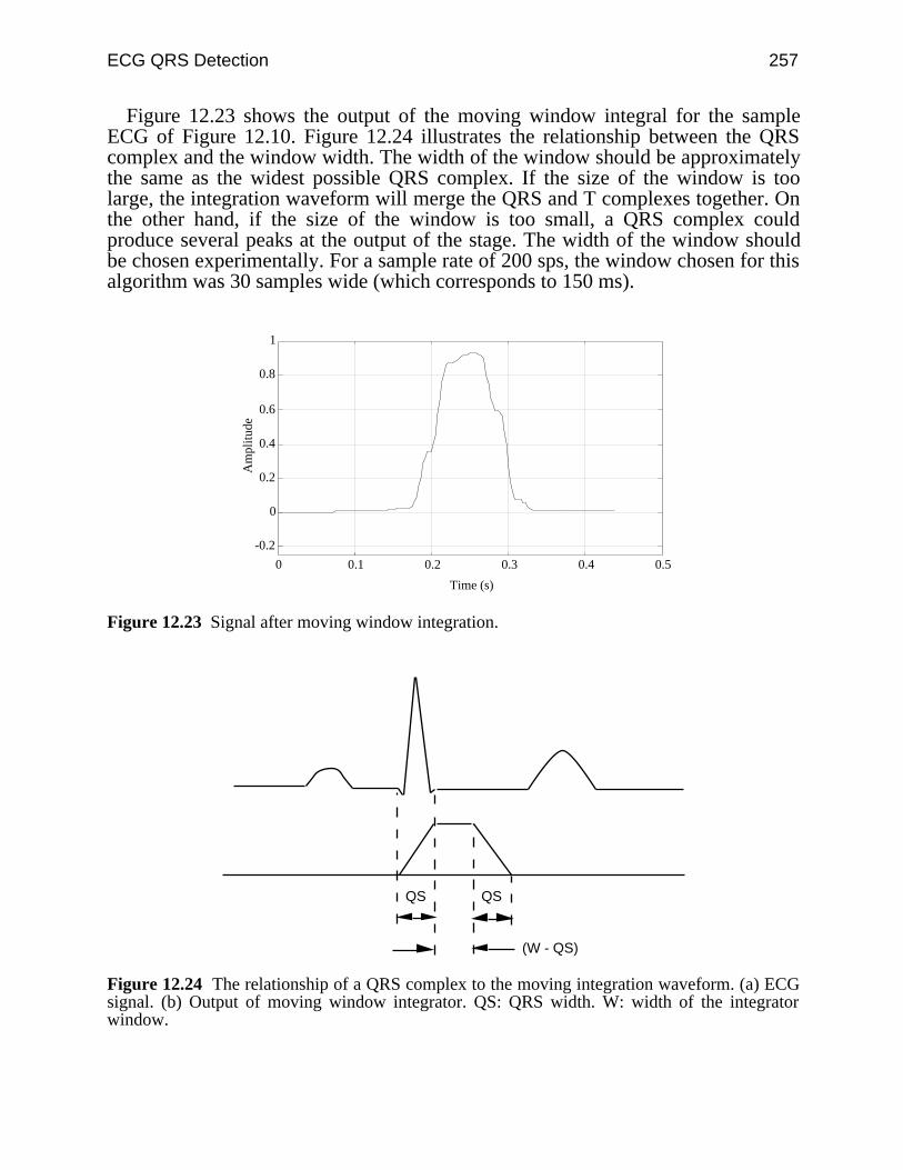
ECG QRS Detection 257
Figure 12.23 shows the output of the moving window integral for the sampleECG of Figure 12.10. Figure 12.24 illustrates the relationship between the QRScomplex and the window width. The width of the window should be approximatelythe same as the widest possible QRS complex. If the size of the window is toolarge, the integration waveform will merge the QRS and T complexes together. Onthe other hand, if the size of the window is too small, a QRS complex couldproduce several peaks at the output of the stage. The width of the window shouldbe chosen experimentally. For a sample rate of 200 sps, the window chosen for thisalgorithm was 30 samples wide (which corresponds to 150 ms).
-0.2
0
0.2
0.4
0.6
0.8
1
0 0.1 0.2 0.3 0.4 0.5
Time (s)
Am
plitu
de
Figure 12.23 Signal after moving window integration.
QS QS
(W - QS)
Figure 12.24 The relationship of a QRS complex to the moving integration waveform. (a) ECGsignal. (b) Output of moving window integrator. QS: QRS width. W: width of the integratorwindow.
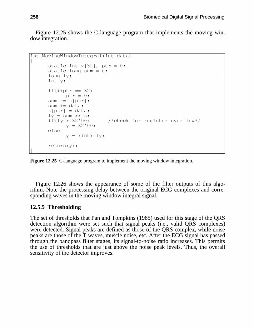
258 Biomedical Digital Signal Processing
Figure 12.25 shows the C-language program that implements the moving win-dow integration.
int MovingWindowIntegral(int data) static int x[32], ptr = 0; static long sum = 0; long ly; int y;
if(++ptr == 32) ptr = 0; sum -= x[ptr]; sum += data; x[ptr] = data; ly = sum >> 5; if(ly > 32400) /*check for register overflow*/ y = 32400; else y = (int) ly;
return(y);
Figure 12.25 C-language program to implement the moving window integration.
Figure 12.26 shows the appearance of some of the filter outputs of this algo-rithm. Note the processing delay between the original ECG complexes and corre-sponding waves in the moving window integral signal.
12.5.5 Thresholding
The set of thresholds that Pan and Tompkins (1985) used for this stage of the QRSdetection algorithm were set such that signal peaks (i.e., valid QRS complexes)were detected. Signal peaks are defined as those of the QRS complex, while noisepeaks are those of the T waves, muscle noise, etc. After the ECG signal has passedthrough the bandpass filter stages, its signal-to-noise ratio increases. This permitsthe use of thresholds that are just above the noise peak levels. Thus, the overallsensitivity of the detector improves.
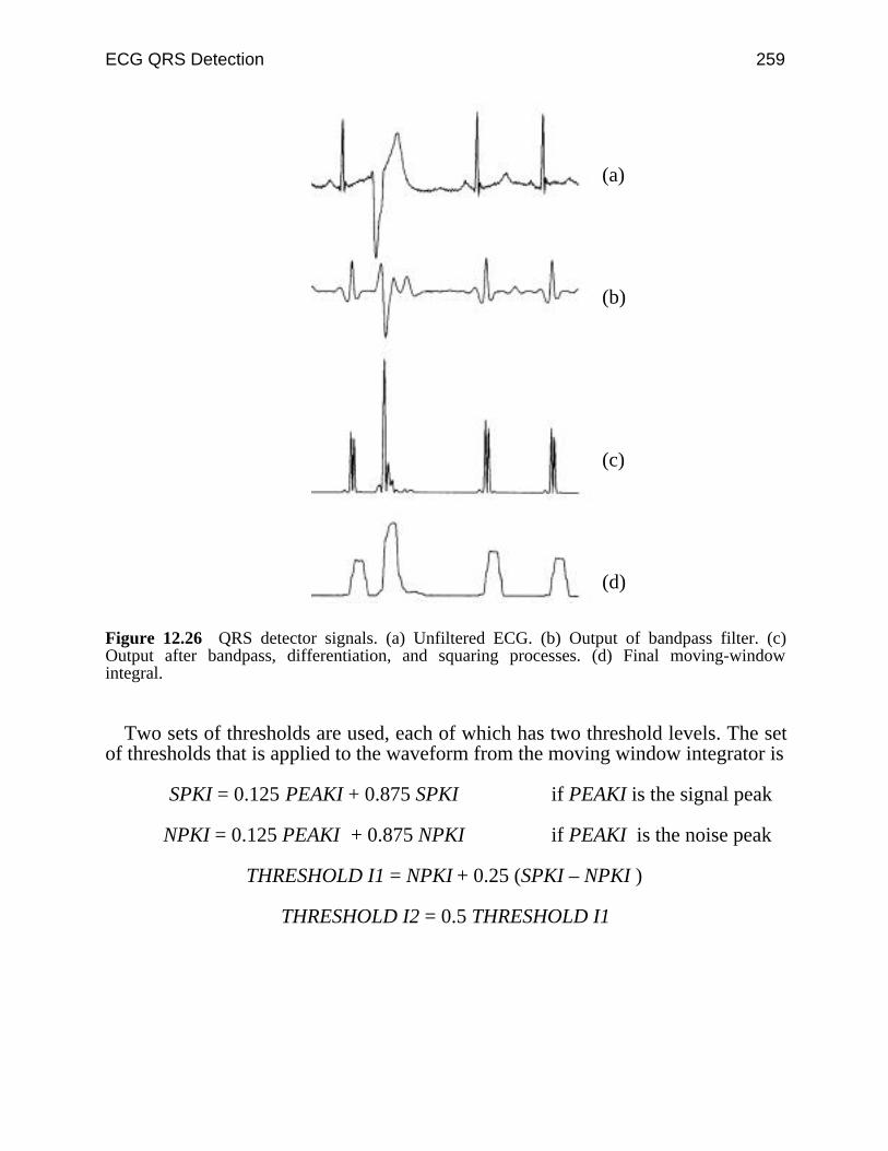
ECG QRS Detection 259
(a)
(b)
(c)
(d)
Figure 12.26 QRS detector signals. (a) Unfiltered ECG. (b) Output of bandpass filter. (c)Output after bandpass, differentiation, and squaring processes. (d) Final moving-windowintegral.
Two sets of thresholds are used, each of which has two threshold levels. The setof thresholds that is applied to the waveform from the moving window integrator is
SPKI = 0.125 PEAKI + 0.875 SPKI if PEAKI is the signal peak
NPKI = 0.125 PEAKI + 0.875 NPKI if PEAKI is the noise peak
THRESHOLD I1 = NPKI + 0.25 (SPKI – NPKI )
THRESHOLD I2 = 0.5 THRESHOLD I1
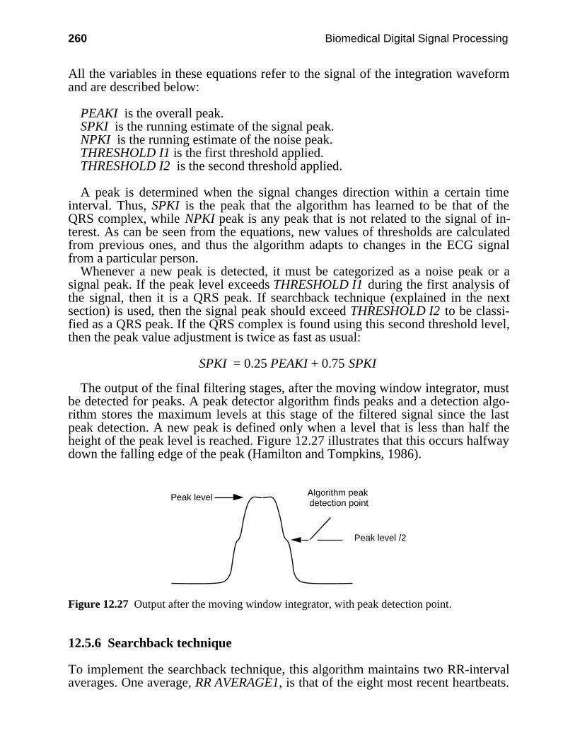
260 Biomedical Digital Signal Processing
All the variables in these equations refer to the signal of the integration waveformand are described below:
PEAKI is the overall peak.SPKI is the running estimate of the signal peak.NPKI is the running estimate of the noise peak.THRESHOLD I1 is the first threshold applied.THRESHOLD I2 is the second threshold applied.
A peak is determined when the signal changes direction within a certain timeinterval. Thus, SPKI is the peak that the algorithm has learned to be that of theQRS complex, while NPKI peak is any peak that is not related to the signal of in-terest. As can be seen from the equations, new values of thresholds are calculatedfrom previous ones, and thus the algorithm adapts to changes in the ECG signalfrom a particular person.
Whenever a new peak is detected, it must be categorized as a noise peak or asignal peak. If the peak level exceeds THRESHOLD I1 during the first analysis ofthe signal, then it is a QRS peak. If searchback technique (explained in the nextsection) is used, then the signal peak should exceed THRESHOLD I2 to be classi-fied as a QRS peak. If the QRS complex is found using this second threshold level,then the peak value adjustment is twice as fast as usual:
SPKI = 0.25 PEAKI + 0.75 SPKI
The output of the final filtering stages, after the moving window integrator, mustbe detected for peaks. A peak detector algorithm finds peaks and a detection algo-rithm stores the maximum levels at this stage of the filtered signal since the lastpeak detection. A new peak is defined only when a level that is less than half theheight of the peak level is reached. Figure 12.27 illustrates that this occurs halfwaydown the falling edge of the peak (Hamilton and Tompkins, 1986).
Peak level Algorithm peak detection point
Peak level /2
Figure 12.27 Output after the moving window integrator, with peak detection point.
12.5.6 Searchback technique
To implement the searchback technique, this algorithm maintains two RR-intervalaverages. One average, RR AVERAGE1, is that of the eight most recent heartbeats.
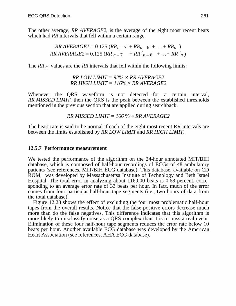
ECG QRS Detection 261
The other average, RR AVERAGE2, is the average of the eight most recent beatswhich had RR intervals that fell within a certain range.
RR AVERAGE1 = 0.125 (RRn – 7 + RRn – 6 + … + RRn )RR AVERAGE2 = 0.125 (RR'n – 7 + RR 'n – 6 + …+ RR 'n )
The RR'n values are the RR intervals that fell within the following limits:
RR LOW LIMIT = 92% × RR AVERAGE2RR HIGH LIMIT = 116% × RR AVERAGE2
Whenever the QRS waveform is not detected for a certain interval,RR MISSED LIMIT, then the QRS is the peak between the established thresholdsmentioned in the previous section that are applied during searchback.
RR MISSED LIMIT = 166 % × RR AVERAGE2
The heart rate is said to be normal if each of the eight most recent RR intervals arebetween the limits established by RR LOW LIMIT and RR HIGH LIMIT.
12.5.7 Performance measurement
We tested the performance of the algorithm on the 24-hour annotated MIT/BIHdatabase, which is composed of half-hour recordings of ECGs of 48 ambulatorypatients (see references, MIT/BIH ECG database). This database, available on CDROM, was developed by Massachusettsa Institute of Technology and Beth IsraelHospital. The total error in analyzing about 116,000 beats is 0.68 percent, corre-sponding to an average error rate of 33 beats per hour. In fact, much of the errorcomes from four particular half-hour tape segments (i.e., two hours of data fromthe total database).
Figure 12.28 shows the effect of excluding the four most problematic half-hourtapes from the overall results. Notice that the false-positive errors decrease muchmore than do the false negatives. This difference indicates that this algorithm ismore likely to misclassify noise as a QRS complex than it is to miss a real event.Elimination of these four half-hour tape segments reduces the error rate below 10beats per hour. Another available ECG database was developed by the AmericanHeart Association (see references, AHA ECG database).
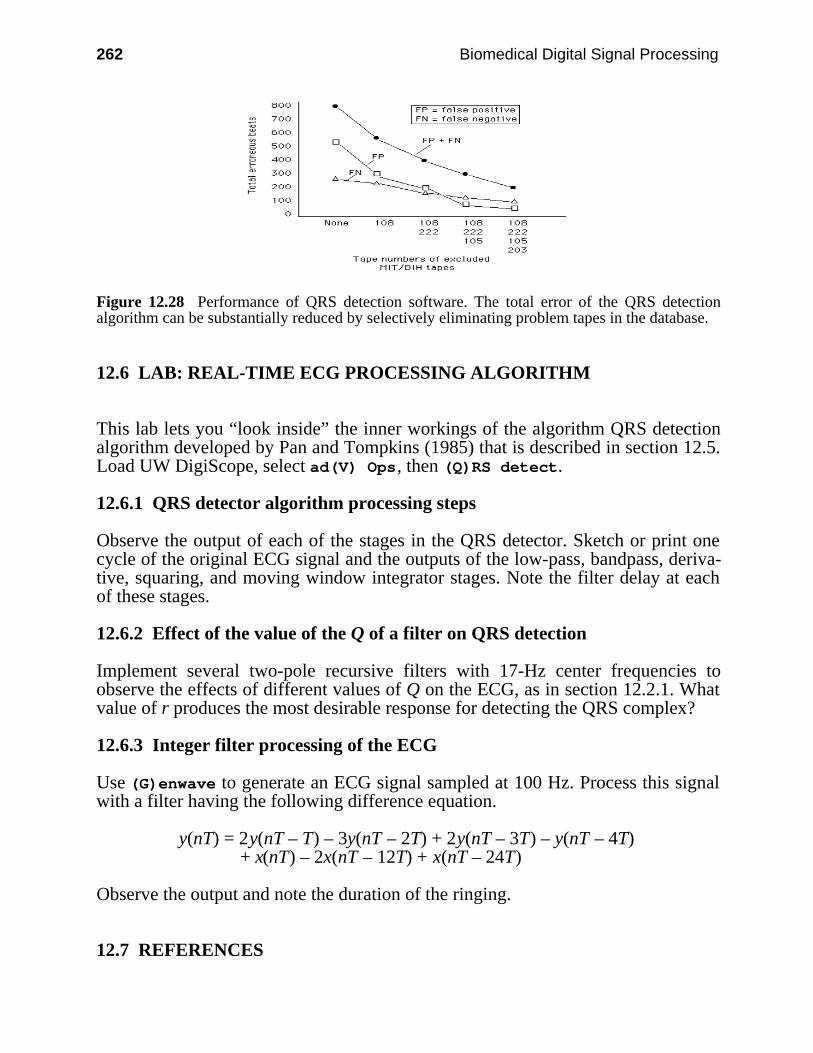
262 Biomedical Digital Signal Processing
Figure 12.28 Performance of QRS detection software. The total error of the QRS detectionalgorithm can be substantially reduced by selectively eliminating problem tapes in the database.
12.6 LAB: REAL-TIME ECG PROCESSING ALGORITHM
This lab lets you “look inside” the inner workings of the algorithm QRS detectionalgorithm developed by Pan and Tompkins (1985) that is described in section 12.5.Load UW DigiScope, select ad(V) Ops, then (Q)RS detect.
12.6.1 QRS detector algorithm processing steps
Observe the output of each of the stages in the QRS detector. Sketch or print onecycle of the original ECG signal and the outputs of the low-pass, bandpass, deriva-tive, squaring, and moving window integrator stages. Note the filter delay at eachof these stages.
12.6.2 Effect of the value of the Q of a filter on QRS detection
Implement several two-pole recursive filters with 17-Hz center frequencies toobserve the effects of different values of Q on the ECG, as in section 12.2.1. Whatvalue of r produces the most desirable response for detecting the QRS complex?
12.6.3 Integer filter processing of the ECG
Use (G)enwave to generate an ECG signal sampled at 100 Hz. Process this signalwith a filter having the following difference equation.
y(nT) = 2y(nT – T) – 3y(nT – 2T) + 2y(nT – 3T) – y(nT – 4T)+ x(nT) – 2x(nT – 12T) + x(nT – 24T)
Observe the output and note the duration of the ringing.
12.7 REFERENCES

ECG QRS Detection 263
AHA ECG database. Available from Emergency Care Research Institute, 5200 Butler Pike,Plymouth Meeting, PA 19462.
Ahlstrom, M. L. and Tompkins, W. J. 1983. Automated high-speed analysis of Holter tapes withmicrocomputers. IEEE Trans. Biomed. Eng., BME-30: 651–57.
Ahlstrom, M. L. and Tompkins, W. J. 1985. Digital filters for real-time ECG signal processingusing microprocessors. IEEE Trans. Biomed. Eng., BME-32: 708–13.
Balda R. A., Diller, G., Deardorff, E., Doue, J., and Hsieh, P. 1977. The HP ECG analysisprogram. Trends in Computer-Processed Electrocardiograms. J. H. vanBemnel and J. L.Willems, (eds.) Amsterdam, The Netherlands: North Holland, 197–205.
Dobbs, S. E., Schmitt, N. M., Ozemek, H. S. 1984. QRS detection by template matching usingreal-time correlation on a microcomputer. Journal of Clinical Engineering, 9: 197–212.
Friesen, G. M., Jannett, T. C., Jadallah, M. A., Yates, S. L., Quint, S. R., Nagle, H. T. 1990.A comparison of the noise sensitivity of nine QRS detection algorithms. IEEE Trans. Biomed.Eng., BME-37: 85–97.
Furno, G. S. and Tompkins, W. J. 1982. QRS detection using automata theory in a battery-powered microprocessor system. IEEE Frontiers of Engineering in Health Care, 4: 155–58.
Hamilton, P. S. and Tompkins, W. J. 1986. Quantitative investigation of QRS detection rulesusing the MIT/BIH arrhythmia database. IEEE Trans. Biomed. Eng. BME-33: 1157–65.
MIT/BIH ECG database. Available from: MIT-BIH Database Distribution, MassachusettsInstitute of Technology, 77 Massachusetts Avenue, Room 20A-113, Cambridge, MA 02139.
Pan, J. and Tompkins, W. J. 1985. A real-time QRS detection algorithm. IEEE Trans. Biomed.Eng. BME-32: 230–36,.
Thakor, N. V., Webster, J. G., and Tompkins, W. J. 1983. Optimal QRS detector. Medical andBiological Engineering, 343–50.
Thakor, N. V., Webster, J. G., and Tompkins, W. J. 1984. Estimation of QRS complex powerspectra for design of a QRS filter. IEEE Trans. Biomed. Eng., BME-31: 702–05.
12.8 STUDY QUESTIONS
12.1 How can ectopic beats be detected using the automata approach to QRS detection?12.2 How can QRS complexes in abnormal waveforms be detected using the crosscorrelation
method?12.3 In the moving window integrator of the algorithm in section 12.5, how should the width
of the window be chosen? What are the effects of choosing a window width that is toolarge or too small?
12.4 In the QRS detection algorithm explained in section 12.5, how should the first thresholdin each set of thresholds be changed so as to increase the detection sensitivity of irregularheart rates?
12.5 What are the effects of bandpass filter Q on the QRS-to-noise ratio in the ECG?12.6 Design an algorithm that obtains the fiducial point on the ECG.12.7 As an implementation exercise write a program using the C language, to detect QRS
complexes in the ECG signal using any of the techniques described in this chapter.12.8 Suggest a QRS detection algorithm, based on some of the techniques explained in this
chapter or in other related literature, that can detect QRS complexes from the ECG in realtime.
12.9 Experiments to determine the frequency characteristics of the average QRS complex haveshown that the largest spectral energy of the QRS complex occurs at approximately whatfrequency?
12.10 A filter with the difference equation, y(nT) = (y(nT – T))2 + x(nT), is best described aswhat traditional filter type?
264 Biomedical Digital Signal Processing
12.11 The center frequency of the optimal QRS bandpass filter is not at the location of themaximal spectral energy of the QRS complex. (a) What function is maximized for the op-timal filter? (b) What is the center frequency of the optimal QRS filter for cardiotachome-ters? (c) If this filter has the proper center frequency and a Q = 20, will it work properly?If not, why not?
12.12 In addition to heart rate information, what QRS parameter is provided by the QRSdetection algorithm that is based on the first and second derivatives?
12.13 The derivative algorithm used in a real-time QRS detector has the difference equation:y(nT) = 2x(nT) + x(nT – T) – x(nT – 3T) – 2x(nT – 4T). (a) Draw its block diagram.(b) What is its output sequence in response to a unit step input? Draw the outputwaveform.
12.14 Write the equations for the amplitude and phase responses of the derivative algorithmused in a real-time QRS detector that has the transfer function
H(z) = –2z–2 – z–1 + z1 + 2z2
8
12.15 A moving window integrator integrates over a window that is 30 samples wide and has anoverall amplitude scale factor of 1/30. If a unit impulse (i.e., 1, 0, 0, 0, …) is applied tothe input of this integrator, what is the output sequence?
12.16 A moving window integrator is five samples wide and has a unity amplitude scale factor.A pacemaker pulse is described by the sequence: (1, 1, 1, 1, 0, 0, 0, 0, …). Application ofthis pulse to the input of the moving window integrator will produce what output se-quence?
12.17 The transfer function of a filter used in a real-time QRS detection algorithm is
H(z) = (1 – z–6)2
(1 – z–1)2
For a sample rate of 200 sps, this filter eliminates input signals of what frequencies?

265
13
ECG Analysis Systems
Willis J. Tompkins
This chapter covers the techniques for analysis and interpretation of the 12-leadECG. Then it discusses ST-level analysis that is used in cardiac stress test systems.Finally, there is a summary of the hardware and software design of a portable ECGarrhythmia monitor.
13.1 ECG INTERPRETATION
Computer interpretation of the 12-lead ECG uses algorithms to determine whethera patient is normal or abnormal. It also provides written description of any abnor-malities discovered.
13.1.1 Historical review of ECG interpretation by computer
ECG interpretation techniques were initially developed and used on mainframecomputers in the early 1960s (Pordy et al., 1968). In those days, mainframe com-puters centrally located in computing centers performed the ECG analysis and in-terpretation. The ECGs were transmitted to the computer from remote hospitalsites using a specially designed ECG acquisition cart that could be rolled to thepatient’s bedside. The cart had three ECG amplifiers, so three leads were acquiredsimultaneously and transmitted over the voice-grade telephone network using athree-channel analog FM modem. The interpretation program running in themainframe computer consisted of several hundred thousand lines of FORTRANcode.
As technology evolved, minicomputers located within hospitals took over therole of the remote mainframes. The ECG acquisition carts began to include embed-ded microprocessors in order to facilitate ECG capture. Also, since the interpreta-tion algorithms had increased failure rates if the ECG was noisy, the microproces-sors increased the signal-to-noise ratio by performing digital signal preprocessingalgorithms to remove baseline drift and to attenuate powerline interference.
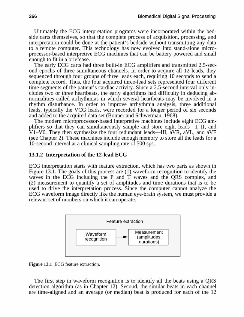
266 Biomedical Digital Signal Processing
Ultimately the ECG interpretation programs were incorporated within the bed-side carts themselves, so that the complete process of acquisition, processing, andinterpretation could be done at the patient’s bedside without transmitting any datato a remote computer. This technology has now evolved into stand-alone micro-processor-based interpretive ECG machines that can be battery powered and smallenough to fit in a briefcase.
The early ECG carts had three built-in ECG amplifiers and transmitted 2.5-sec-ond epochs of three simultaneous channels. In order to acquire all 12 leads, theysequenced through four groups of three leads each, requiring 10 seconds to send acomplete record. Thus, the four acquired three-lead sets represented four differenttime segments of the patient’s cardiac activity. Since a 2.5-second interval only in-cludes two or three heartbeats, the early algorithms had difficulty in deducing ab-normalities called arrhythmias in which several heartbeats may be involved in arhythm disturbance. In order to improve arrhythmia analysis, three additionalleads, typically the VCG leads, were recorded for a longer period of six secondsand added to the acquired data set (Bonner and Schwetman, 1968).
The modern microprocessor-based interpretive machines include eight ECG am-plifiers so that they can simultaneously sample and store eight leads—I, II, andV1–V6. They then synthesize the four redundant leads—III, aVR, aVL, and aVF(see Chapter 2). These machines include enough memory to store all the leads for a10-second interval at a clinical sampling rate of 500 sps.
13.1.2 Interpretation of the 12-lead ECG
ECG interpretation starts with feature extraction, which has two parts as shown inFigure 13.1. The goals of this process are (1) waveform recognition to identify thewaves in the ECG including the P and T waves and the QRS complex, and(2) measurement to quantify a set of amplitudes and time durations that is to beused to drive the interpretation process. Since the computer cannot analyze theECG waveform image directly like the human eye-brain system, we must provide arelevant set of numbers on which it can operate.
Feature extraction
Waveform recognition
Measurement (amplitudes, durations)
Figure 13.1 ECG feature extraction.
The first step in waveform recognition is to identify all the beats using a QRSdetection algorithm (as in Chapter 12). Second, the similar beats in each channelare time-aligned and an average (or median) beat is produced for each of the 12
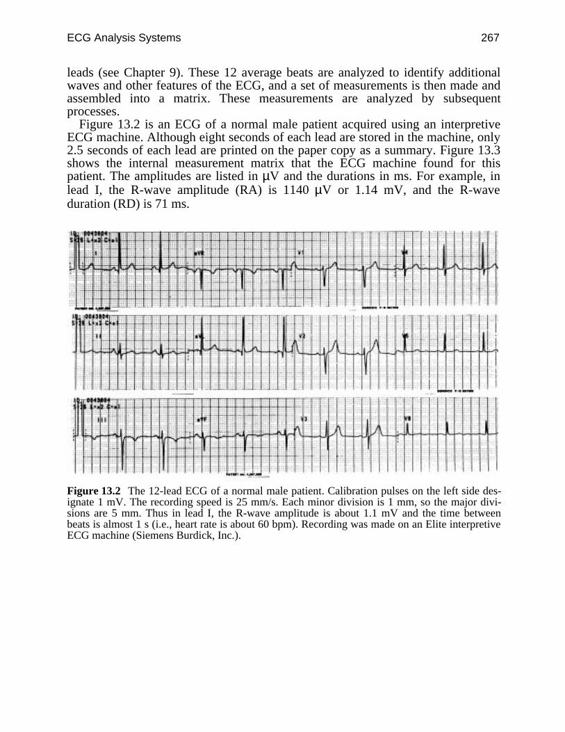
ECG Analysis Systems 267
leads (see Chapter 9). These 12 average beats are analyzed to identify additionalwaves and other features of the ECG, and a set of measurements is then made andassembled into a matrix. These measurements are analyzed by subsequentprocesses.
Figure 13.2 is an ECG of a normal male patient acquired using an interpretiveECG machine. Although eight seconds of each lead are stored in the machine, only2.5 seconds of each lead are printed on the paper copy as a summary. Figure 13.3shows the internal measurement matrix that the ECG machine found for thispatient. The amplitudes are listed in µV and the durations in ms. For example, inlead I, the R-wave amplitude (RA) is 1140 µV or 1.14 mV, and the R-waveduration (RD) is 71 ms.
Figure 13.2 The 12-lead ECG of a normal male patient. Calibration pulses on the left side des-ignate 1 mV. The recording speed is 25 mm/s. Each minor division is 1 mm, so the major divi-sions are 5 mm. Thus in lead I, the R-wave amplitude is about 1.1 mV and the time betweenbeats is almost 1 s (i.e., heart rate is about 60 bpm). Recording was made on an Elite interpretiveECG machine (Siemens Burdick, Inc.).
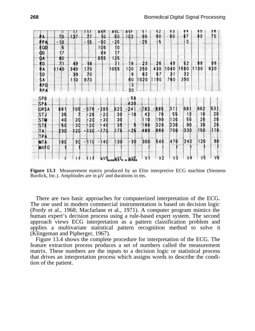
268 Biomedical Digital Signal Processing
Figure 13.3 Measurement matrix produced by an Elite interpretive ECG machine (SiemensBurdick, Inc.). Amplitudes are in µV and durations in ms.
There are two basic approaches for computerized interpretation of the ECG.The one used in modern commercial instrumentation is based on decision logic(Pordy et al., 1968; Macfarlane et al., 1971). A computer program mimics thehuman expert’s decision process using a rule-based expert system. The secondapproach views ECG interpretation as a pattern classification problem andapplies a multivariate statistical pattern recognition method to solve it(Klingeman and Pipberger, 1967).
Figure 13.4 shows the complete procedure for interpretation of the ECG. Thefeature extraction process produces a set of numbers called the measurementmatrix. These numbers are the inputs to a decision logic or statistical processthat drives an interpretation process which assigns words to describe the condi-tion of the patient.
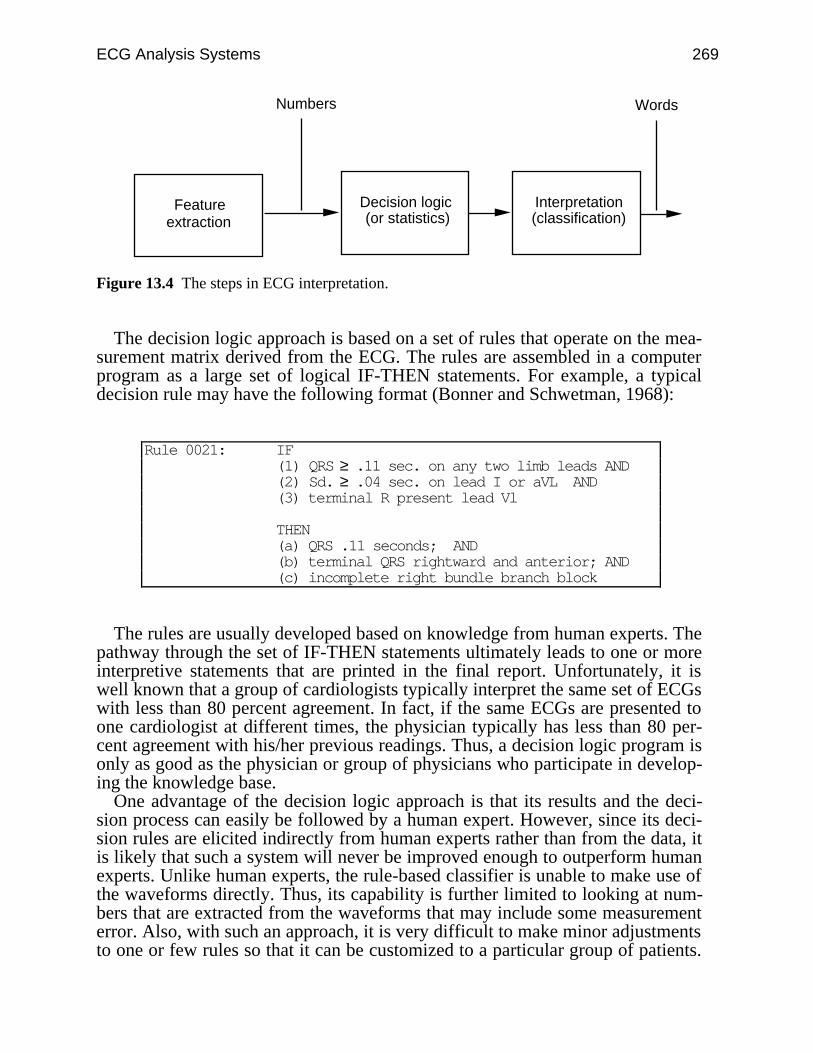
ECG Analysis Systems 269
Decision logic (or statistics)
Numbers
Interpretation (classification)
Words
Feature extraction
Figure 13.4 The steps in ECG interpretation.
The decision logic approach is based on a set of rules that operate on the mea-surement matrix derived from the ECG. The rules are assembled in a computerprogram as a large set of logical IF-THEN statements. For example, a typicaldecision rule may have the following format (Bonner and Schwetman, 1968):
Rule 0021: IF(1) QRS ≥ .11 sec. on any two limb leads AND(2) Sd. ≥ .04 sec. on lead I or aVL AND(3) terminal R present lead Vl
THEN(a) QRS .11 seconds; AND(b) terminal QRS rightward and anterior; AND(c) incomplete right bundle branch block
The rules are usually developed based on knowledge from human experts. Thepathway through the set of IF-THEN statements ultimately leads to one or moreinterpretive statements that are printed in the final report. Unfortunately, it iswell known that a group of cardiologists typically interpret the same set of ECGswith less than 80 percent agreement. In fact, if the same ECGs are presented toone cardiologist at different times, the physician typically has less than 80 per-cent agreement with his/her previous readings. Thus, a decision logic program isonly as good as the physician or group of physicians who participate in develop-ing the knowledge base.
One advantage of the decision logic approach is that its results and the deci-sion process can easily be followed by a human expert. However, since its deci-sion rules are elicited indirectly from human experts rather than from the data, itis likely that such a system will never be improved enough to outperform humanexperts. Unlike human experts, the rule-based classifier is unable to make use ofthe waveforms directly. Thus, its capability is further limited to looking at num-bers that are extracted from the waveforms that may include some measurementerror. Also, with such an approach, it is very difficult to make minor adjustmentsto one or few rules so that it can be customized to a particular group of patients.
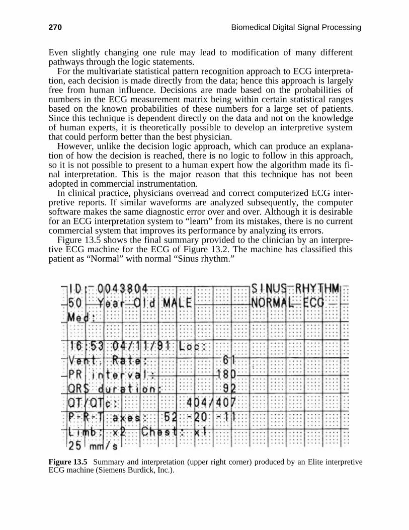
270 Biomedical Digital Signal Processing
Even slightly changing one rule may lead to modification of many differentpathways through the logic statements.
For the multivariate statistical pattern recognition approach to ECG interpreta-tion, each decision is made directly from the data; hence this approach is largelyfree from human influence. Decisions are made based on the probabilities ofnumbers in the ECG measurement matrix being within certain statistical rangesbased on the known probabilities of these numbers for a large set of patients.Since this technique is dependent directly on the data and not on the knowledgeof human experts, it is theoretically possible to develop an interpretive systemthat could perform better than the best physician.
However, unlike the decision logic approach, which can produce an explana-tion of how the decision is reached, there is no logic to follow in this approach,so it is not possible to present to a human expert how the algorithm made its fi-nal interpretation. This is the major reason that this technique has not beenadopted in commercial instrumentation.
In clinical practice, physicians overread and correct computerized ECG inter-pretive reports. If similar waveforms are analyzed subsequently, the computersoftware makes the same diagnostic error over and over. Although it is desirablefor an ECG interpretation system to “learn” from its mistakes, there is no currentcommercial system that improves its performance by analyzing its errors.
Figure 13.5 shows the final summary provided to the clinician by an interpre-tive ECG machine for the ECG of Figure 13.2. The machine has classified thispatient as “Normal” with normal “Sinus rhythm.”
Figure 13.5 Summary and interpretation (upper right corner) produced by an Elite interpretiveECG machine (Siemens Burdick, Inc.).
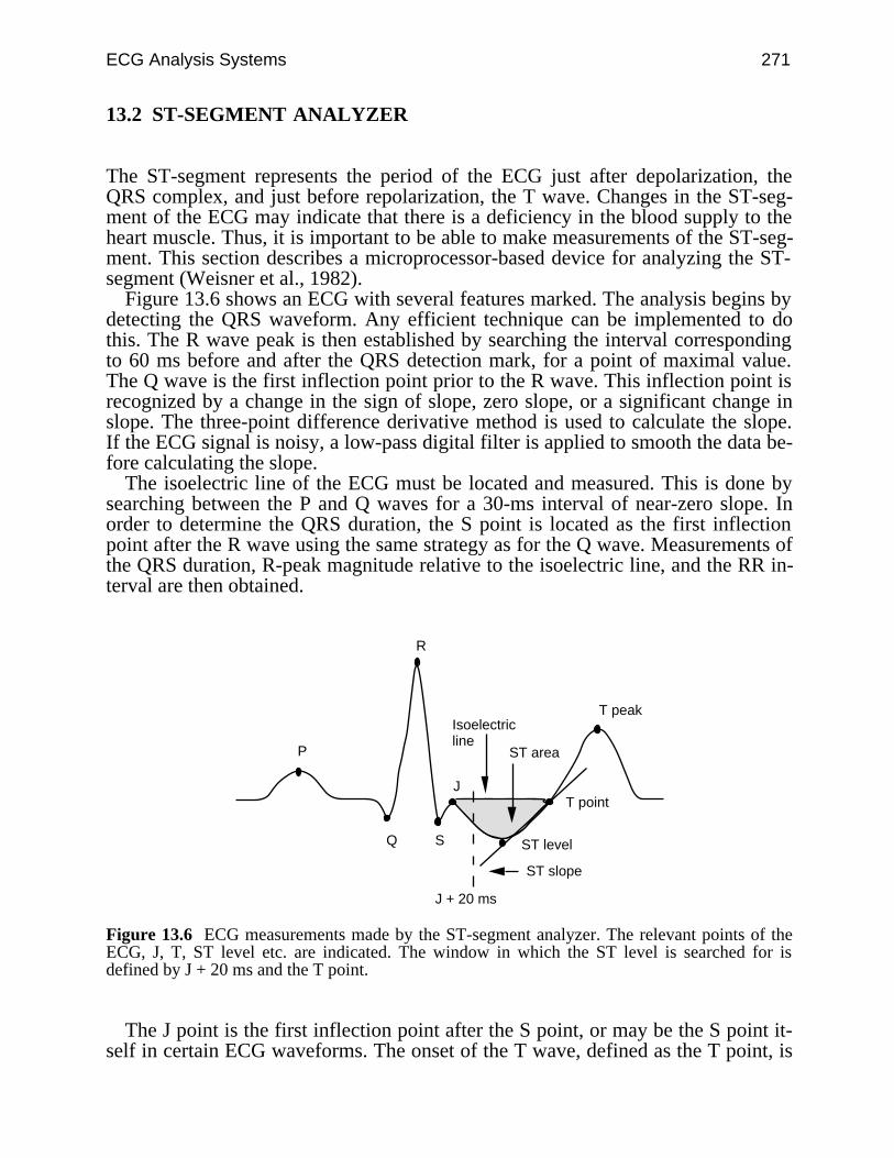
ECG Analysis Systems 271
13.2 ST-SEGMENT ANALYZER
The ST-segment represents the period of the ECG just after depolarization, theQRS complex, and just before repolarization, the T wave. Changes in the ST-seg-ment of the ECG may indicate that there is a deficiency in the blood supply to theheart muscle. Thus, it is important to be able to make measurements of the ST-seg-ment. This section describes a microprocessor-based device for analyzing the ST-segment (Weisner et al., 1982).
Figure 13.6 shows an ECG with several features marked. The analysis begins bydetecting the QRS waveform. Any efficient technique can be implemented to dothis. The R wave peak is then established by searching the interval correspondingto 60 ms before and after the QRS detection mark, for a point of maximal value.The Q wave is the first inflection point prior to the R wave. This inflection point isrecognized by a change in the sign of slope, zero slope, or a significant change inslope. The three-point difference derivative method is used to calculate the slope.If the ECG signal is noisy, a low-pass digital filter is applied to smooth the data be-fore calculating the slope.
The isoelectric line of the ECG must be located and measured. This is done bysearching between the P and Q waves for a 30-ms interval of near-zero slope. Inorder to determine the QRS duration, the S point is located as the first inflectionpoint after the R wave using the same strategy as for the Q wave. Measurements ofthe QRS duration, R-peak magnitude relative to the isoelectric line, and the RR in-terval are then obtained.
R
Q S ST level
T point
T peak
ST area
J
ST slope
Isoelectricline
J + 20 ms
P
Figure 13.6 ECG measurements made by the ST-segment analyzer. The relevant points of theECG, J, T, ST level etc. are indicated. The window in which the ST level is searched for isdefined by J + 20 ms and the T point.
The J point is the first inflection point after the S point, or may be the S point it-self in certain ECG waveforms. The onset of the T wave, defined as the T point, is
272 Biomedical Digital Signal Processing
found by first locating the T-wave peak which is the maximal absolute value, rela-tive to the isoelectric line, between J + 80 ms and R + 400 ms. The onset of the Twave, the T point, is then found by looking for a 35-ms period on the R side of theT wave, which has values within one sample unit of each other. The T point isamong the most difficult features to identify. If this point is not detected, it is as-sumed to be J + 120 ms.
Having identified various ECG features, ST-segment measurements are madeusing a windowed search method. Two boundaries, the J + 20 ms and the T point,define the window limits. The point of maximal depression or elevation in the win-dow is then identified. ST-segment levels can be expressed as the absolute changerelative to the isoelectric line.
In addition to the ST-segment level, several other parameters are calculated. TheST slope is defined as the amplitude difference between the ST-segment point andthe T point divided by the corresponding time interval. The ST area is calculatedby summing all sample values between the J and T points after subtracting the iso-electric-line value from each point. An ST index is calculated as the sum of the ST-segment level and one-tenth of the ST slope.
13.3 PORTABLE ARRHYTHMIA MONITOR
There is a great deal of interest these days in home monitoring of patients, particu-larly due to cost considerations. If the same diagnostic information can be obtainedfrom an ambulatory patient as can be found in the hospital, it is clearly more costeffective to do the monitoring in the home. Technological evolution has led to ahigh-performance computing capacity that is manifested in such devices as com-pact, lap-sized versions of the personal computer. Such battery-powered systemsprovide us with the ability to do computational tasks in the home or elsewhere thatwere previously possible only with larger, nonportable, line-powered computers.
This increase in computing capability, with its concurrent decrease in size andpower consumption, has led to the possibility of designing intelligent biomedicalinstrumentation that is small and light enough to be worn by an ambulatory patient(Tompkins, 1978; Webster, 1978; Webster et al., 1978; Tompkins et al., 1979;Tompkins, 1980; Tompkins, 1981a; Tompkins, 1981b; Tompkins, 1982;Tompkins, 1983). In addition, instrumentation can now be designed that was notcontemplated previously, because microcomputer technology had not yet evolvedfar enough to support such applications (Sahakian et al., 1978; Tompkins et al.,1980; Weisner et al., 1982a; Weisner et al., 1982b; Chen and Tompkins, 1982;Tompkins et al., 1983). Portable instrumentation will ultimately perform monitor-ing functions previously done only within the confines of the hospital.
13.3.1 Holter recording
An initial goal is to replace the functions of the Holter tape recorder, the currentdevice of choice for determining if an ambulatory patient has a potential cardiacproblem. An optimal replacement device would be a microprocessor-based,
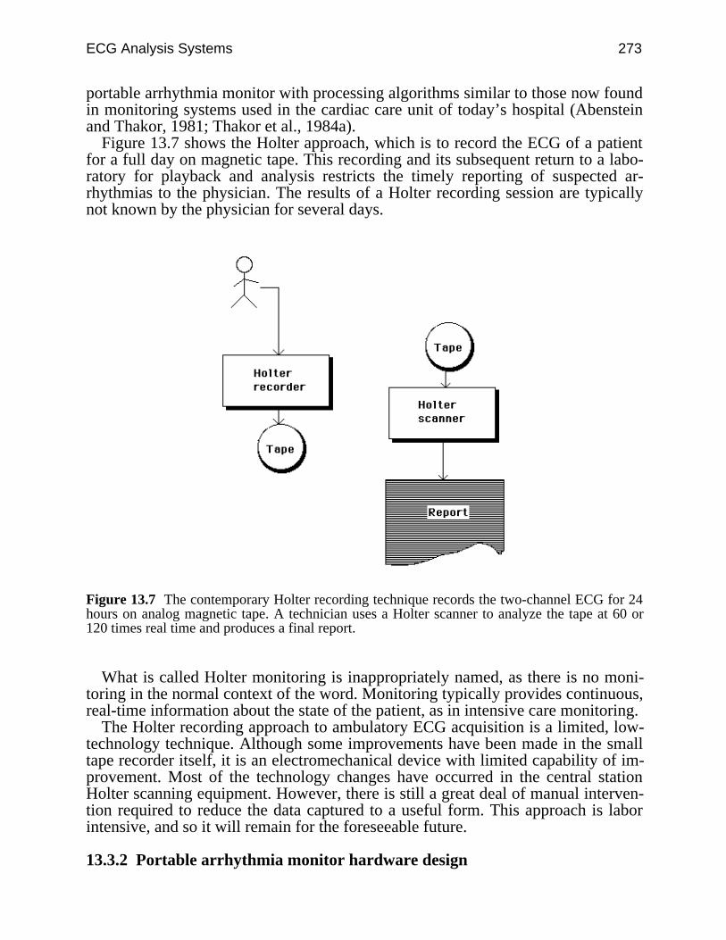
ECG Analysis Systems 273
portable arrhythmia monitor with processing algorithms similar to those now foundin monitoring systems used in the cardiac care unit of today’s hospital (Abensteinand Thakor, 1981; Thakor et al., 1984a).
Figure 13.7 shows the Holter approach, which is to record the ECG of a patientfor a full day on magnetic tape. This recording and its subsequent return to a labo-ratory for playback and analysis restricts the timely reporting of suspected ar-rhythmias to the physician. The results of a Holter recording session are typicallynot known by the physician for several days.
Figure 13.7 The contemporary Holter recording technique records the two-channel ECG for 24hours on analog magnetic tape. A technician uses a Holter scanner to analyze the tape at 60 or120 times real time and produces a final report.
What is called Holter monitoring is inappropriately named, as there is no moni-toring in the normal context of the word. Monitoring typically provides continuous,real-time information about the state of the patient, as in intensive care monitoring.
The Holter recording approach to ambulatory ECG acquisition is a limited, low-technology technique. Although some improvements have been made in the smalltape recorder itself, it is an electromechanical device with limited capability of im-provement. Most of the technology changes have occurred in the central stationHolter scanning equipment. However, there is still a great deal of manual interven-tion required to reduce the data captured to a useful form. This approach is laborintensive, and so it will remain for the foreseeable future.
13.3.2 Portable arrhythmia monitor hardware design
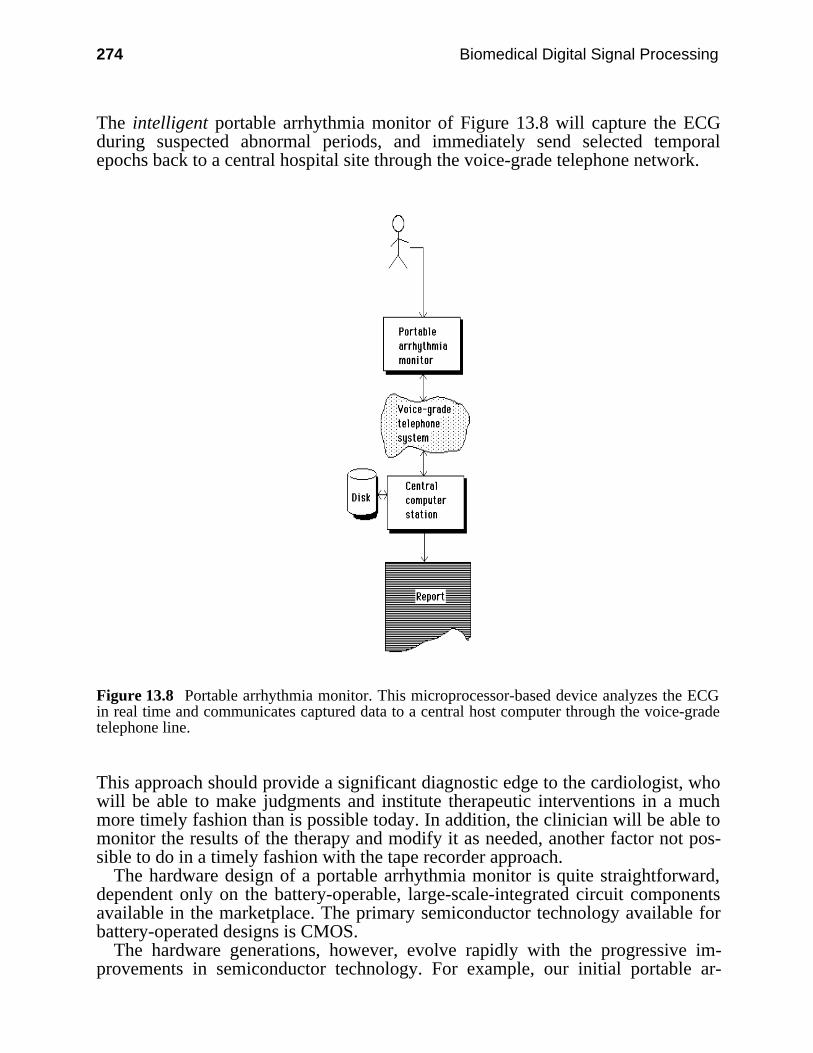
274 Biomedical Digital Signal Processing
The intelligent portable arrhythmia monitor of Figure 13.8 will capture the ECGduring suspected abnormal periods, and immediately send selected temporalepochs back to a central hospital site through the voice-grade telephone network.
Figure 13.8 Portable arrhythmia monitor. This microprocessor-based device analyzes the ECGin real time and communicates captured data to a central host computer through the voice-gradetelephone line.
This approach should provide a significant diagnostic edge to the cardiologist, whowill be able to make judgments and institute therapeutic interventions in a muchmore timely fashion than is possible today. In addition, the clinician will be able tomonitor the results of the therapy and modify it as needed, another factor not pos-sible to do in a timely fashion with the tape recorder approach.
The hardware design of a portable arrhythmia monitor is quite straightforward,dependent only on the battery-operable, large-scale-integrated circuit componentsavailable in the marketplace. The primary semiconductor technology available forbattery-operated designs is CMOS.
The hardware generations, however, evolve rapidly with the progressive im-provements in semiconductor technology. For example, our initial portable ar-

ECG Analysis Systems 275
rhythmia monitor designs in 1977 were based on the COSMAC microprocessor(RCA CDP1802), a primitive central processing unit by today’s standards. Moderncommercial devices use the 80C86 microprocessor (Intel), a CMOS chip that isfrom the family of parts that make up the models of the IBM PC and compatibles.
Figure 13.9 shows a block diagram of one of our prototype monitors. In additionto the microprocessor, a portable arrhythmia monitor requires analog and digitalsupport electronics. Analog amplifiers do the front-end ECG amplification and sig-nal conditioning. An analog-to-digital (A/D) converter integrated circuit changesthe analog ECG to the digital signal representation needed by the microprocessor.
Figure 13.9 Block diagram of portable arrhythmia monitor.
ROM memory holds the program that directs the performance of all the func-tions of the instrument, and RAM memory stores the captured ECG signal.Input/output (I/O) ports interface audio and visual displays and switch interactionsin the device. A modem circuit provides for communication with a remote com-puter so that captured ECG signals can be transmitted back to a central site(Thakor et al., 1982).
All these technologies are changing rapidly, so we must constantly consider im-proving the hardware design. Newer designs permit devices with (1) fewer compo-nents, (2) greater reliability, (3) smaller size and weight, (4) less power consump-tion, and (5) greater computational power (thereby permitting more complex signalprocessing and interpretive algorithms). Thus, there is a technological force drivingus to continually improve the hardware design. In industry, an engineering com-promise must come into play at some point, and the design must be frozen to pro-duce a viable product. However, we are in a university environment, and so can af-ford to indulge ourselves by continual iteration of the design.
276 Biomedical Digital Signal Processing
13.3.3 Portable arrhythmia monitor software design
Unfortunately, the frequent hardware changes lead to equally frequent software re-design. The software for an instrument is very hardware dependent. Each new mi-croprocessor has its own unique machine language. Thus, we end up rewriting thesame programs for different processors, and thereby waste considerable program-ming time. This software problem has led us to explore higher-level languages thatare transportable from one kind of microprocessor to another.
We have settled on the C language, conceived at Bell Laboratories, as the mostnearly ideal language now available for this type of real-time instrumentation ap-plication. Its primary advantages are (1) a programming level low enough toachieve the requisite machine control, and (2) transportability from one type of mi-croprocessor to another. Providing that we follow a few software design rules, areal-time program written in the C language for one type of microprocessor can beeasily reconfigured to run on a different one. Although it is not perfect, the C lan-guage considerably reduces the programming time necessary to rewrite the soft-ware when changing microprocessors. We then use our programming time to con-centrate on improving the algorithms.
For a portable arrhythmia monitor, the two major software design tasks are(1) QRS detection and (2) arrhythmia analysis (Abenstein, 1978; Mueller, 1978).The QRS detection must be nearly perfect, otherwise the arrhythmia analysis algo-rithms will be fooled too often by false reports of beats that are not really there(i.e., false positives) or lack of reporting of beats that are missed (i.e., false nega-tives). An additional software design task important in these devices with limitedmemory is a data reduction algorithm (Tompkins and Abenstein, 1979; Abensteinand Tompkins, 1982).
QRS detection algorithm
Included in the various techniques that are used to implement a QRS detector arelinear digital filters, nonlinear transformations, decision processes, and templatematching (Thakor, 1978; Thakor et al., 1980; Ahlstrom and Tompkins, 1981;Furno and Tompkins, 1982; Thakor et al., 1983; Thakor et al., 1984b; Tompkinsand Pan, 1985). Typically two or more of these techniques are combined togetherin a detector algorithm.
The most common approach in contemporary commercial ECG instrumentationis based on template matching. A model of the normal QRS complex, called a tem-plate, is extracted from the ECG during a learning period on a particular patient.This template is compared with the subsequent incoming real-time ECG to look fora possible match, using a mathematical criterion for goodness of fit. A closeenough match to the template represents a detected QRS complex. If a waveformcomes along that does not match but is a suspected abnormal QRS complex, it istreated as a separate template, and future suspected QRS complexes are comparedwith it. We have elected not to use this technique for the detection process, since itrequires considerable memory for saving the templates (depending on how manyyou use; at least one system permits 40) and significant computational power formatching the templates to the real-time signal.
ECG Analysis Systems 277
Instead, we use an algorithm based entirely on digital filters. Section 12.5 sum-marizes the QRS detection algorithm that we have developed for this application.
Arrhythmia analysis
From the QRS detector, the QRS duration and the RR intervals are determined.The ECG signal is then classified based on the QRS duration and the RR interval.Figure 13.10 is a conceptual drawing of an arrhythmia analysis algorithm based onthe two parameters, RR interval and QRS duration (Ahlstrom and Tompkins,1983). In this two-parameter mapping, we establish a region called normal bypermitting the algorithm to first learn on a set of eight QRS complexes defined bya clinician as having normal rhythm and morphology for the specific patient. Thislearning process establishes the initial center of the normal region in the two-di-mensional mapping space.
Boundaries of all the other regions in the map, except for region “0”, are com-puted as percentages of the location of the center of the normal region. Region “0”has fixed boundaries based on physiological limits. Any point mapped into region“0” is considered to be noise because it falls outside what we normally expect to bethe physiological limits of the smallest possible RR interval or QRS duration.
An abnormality such as tachycardia causes clusters of beats to fall in region “1”which represents very short RR intervals. Bradycardia beats fall in region “6”.Typically, abnormalities must be classified by considering sequences of beats. Forexample, a premature ventricular contraction with a full compensatory pausewould be characterized by a short RR interval coupled with a long QRS duration,followed by a long RR interval coupled with a normal QRS duration. This wouldbe manifested as a sequence of two points on the map, the first in region “3” andthe second in region “5”. Thus, arrhythmia analysis consists of analyzing the waysin which the beats fall onto the mapping space.

278 Biomedical Digital Signal Processing
0 1.0 1.5 2.0 2.50.50
50
100
150
200
Normal
(0)
(1)
(2)
(3) (5)(4) (6)
RR interval (seconds)
QR
S d
urat
ion
(ms)
0.2s -64% -14% +14% +84%
+20%
-20%
Figure 13.10 Arrhythmia analysis algorithm based on mapping the RR interval and QRS dura-tion into two-dimensional space.
The center of the normal region is continuously updated, based on the averageRR interval of the eight most-recent beats classified as normal. This approachpermits the normal region to move in the two-dimensional space with normalchanges in heart rate that occur with exercise and other physiological changes. Theboundaries of other regions are modified beat-by-beat, since they are based on thelocation of the normal region. Thus, this algorithm adapts to normal changes inheart rate.
The classification of the waveforms can be made by noting the regions in whichsuccessive beats fall. Figure 13.11 lists some of the algorithms to detect differentarrhythmias. The technique described is an efficient method for extracting RR in-terval and QRS duration information from an ECG signal. Based on the acquiredinformation, different arrhythmias can be classified.
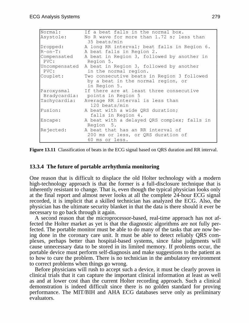
ECG Analysis Systems 279
Normal: If a beat falls in the normal box.Asystole: No R wave for more than 1.72 s; less than 35 beats/minDropped: A long RR interval; beat falls in Region 6.R-on-T: A beat falls in Region 2.Compensated A beat in Region 3, followed by another in PVC: Region 5.Uncompensated A beat in Region 3, followed by another PVC: in the normal region.Couplet: Two consecutive beats in Region 3 followed by a beat in the normal region, or in Region 5.Paroxysmal If there are at least three consecutive Bradycardia: points in Region 5Tachycardia: Average RR interval is less than 120 beats/minFusion: A beat with a wide QRS duration; falls in Region 4.Escape: A beat with a delayed QRS complex; falls in Region 5.Rejected: A beat that has an RR interval of 200 ms or less, or QRS duration of 60 ms or less.
Figure 13.11 Classification of beats in the ECG signal based on QRS duration and RR interval.
13.3.4 The future of portable arrhythmia monitoring
One reason that is difficult to displace the old Holter technology with a modernhigh-technology approach is that the former is a full-disclosure technique that isinherently resistant to change. That is, even though the typical physician looks onlyat the final report and almost never looks at all the complete 24-hour ECG signalrecorded, it is implicit that a skilled technician has analyzed the ECG. Also, thephysician has the ultimate security blanket in that the data is there should it ever benecessary to go back through it again.
A second reason that the microprocessor-based, real-time approach has not af-fected the Holter market as yet is that the diagnostic algorithms are not fully per-fected. The portable monitor must be able to do many of the tasks that are now be-ing done in the coronary care unit. It must be able to detect reliably QRS com-plexes, perhaps better than hospital-based systems, since false judgments willcause unnecessary data to be stored in its limited memory. If problems occur, theportable device must perform self-diagnosis and make suggestions to the patient asto how to cure the problem. There is no technician in the ambulatory environmentto correct problems when things go wrong.
Before physicians will rush to accept such a device, it must be clearly proven inclinical trials that it can capture the important clinical information at least as wellas and at lower cost than the current Holter recording approach. Such a clinicaldemonstration is indeed difficult since there is no golden standard for provingperformance. The MIT/BIH and AHA ECG databases serve only as preliminaryevaluators.
280 Biomedical Digital Signal Processing
Our current device does not attempt to make an interpretation of the patient’sECG. Instead it is designed to separate out suspicious waveforms from those thatare considered normal for an individual patient. It then transmits the suspiciousdata by telephone to a clinician for a diagnostic judgment. Thus, it is a type ofscreening device. This approach as a first design step is simpler than a comprehen-sive ICU approach where critical clinical decisions must be made rapidly.
No portable arrhythmia monitor (or real-time Holter monitor as it is sometimescalled) has yet been successful in the medical instrumentation marketplace. Part ofthe reason for this is that real-time QRS detection and arrhythmia analysis algo-rithms are not yet good enough for this application. However, there is steadyprogress in improvement of these algorithms, as microprocessors are being usedmore and more in bedside monitoring systems.
There is no doubt that Holter recording will be displaced, at some time, by mi-croprocessor-based portable monitors. When that time comes, it will lead to lowerdiagnostic costs, greater device reliability, better clinical research capabilities, andcontinually evolving performance. The utility of these devices will evolve with thetechnology, just as the early four-function calculator has evolved into the lap-sized,high-performance portable computer of today.
13.4 REFERENCES
Abenstein, J. P. 1978. Algorithms for real-time ambulatory ECG monitoring. Biomed. Sci.Instrum., 14: 73–79.
Abenstein, J. P. and Thakor, N. V. 1981. A detailed design example—ambulatory ECGmonitoring. In Tompkins, W. J. and Webster, J. G. (eds) Design of Microcomputer-BasedMedical Instrumentation. Englewood Cliffs, NJ: Prentice Hall.
Abenstein, J. P. and Tompkins, W. J. 1982. A new data reduction algorithm for real-time ECGanalysis. IEEE Trans Biomed Eng., BME-29: 43–48.
Ahlstrom, M. L. and Tompkins, W. J. 1981. An inexpensive microprocessor system for highspeed QRS width detection. Proc. 1st Annual IEEE Compmed. Conf., 81–83.
Ahlstrom, M. L. and Tompkins, W. J. 1983. Automated high-speed analysis of Holter tapes withmicrocomputers. IEEE Trans. Biomed. Eng., BME-30: 651–57.
Bonner, R. E. and Schwetman, H. D. 1968. Computer diagnosis of the electrocardiogram II.Comp. Biomed. Res., 1: 366.
Furno, G. S. and Tompkins, W. J. 1982. QRS detection using automata theory in a battery-powered microprocessor system. IEEE Frontiers of Eng. in Health Care, 4: 155–58.
Klingeman, J., and Pipberger, H. V. 1967. Computer classification of electrocardiograms. Comp.Biomed. Res., 1: 1.
Macfarlane, P. W., Lorimer, A. R., and Lowrie, T. D. V. 1971. 3 and 12 lead electrocardiograminterpretation by computer. A comparison in 1093 patients. Br. Heart J., 33: 226.
Mueller, W. C. 1978. Arrhythmia detection program for an ambulatory ECG monitor. Biomed.Sci. Instrum., 14: 81–85.
Pan, J. and Tompkins, W. J. 1985. A real-time QRS detection algorithm. IEEE Trans. Biomed.Eng., BME-32(3): 230–36.
Pordy, L., Jaffe,H., Chesky, K. et al. 1968. Computer diagnosis of electrocardiograms, IV, acomputer program for contour analysis with clinical results of rhythm and contourinterpretation. Comp. Biomed. Res., 1: 408–33.
Thakor, N. V. 1978. Reliable R-wave detection from ambulatory subjects. Biomed. Sci. Instrum.,14: 67–72.
ECG Analysis Systems 281
Thakor, N. V., Webster, J. G., and Tompkins, W. J. 1980. Optimal QRS filter. Proc. IEEE Conf.on Frontiers of Eng. in Health Care, 2: 190–95.
Thakor, N. V., Webster, J. G., and Tompkins, W. J. 1982. A battery-powered digital modem fortelephone transmission of ECG data. IEEE Trans. Biomed. Eng., BME-29: 355–59.
Thakor, N. V., Webster, J. G., and Tompkins, W. J. 1983. Optimal QRS detector. Med. & Biol.Eng. & Comput., 21: 343–50.
Thakor, N. V., Webster, J. G., and Tompkins, W. J. 1984a. Design, implementation, and evalua-tion of a microcomputer-based portable arrhythmia monitor. Med. & Biol. Eng. & Comput.,22: 151–59.
Thakor, N. V., Webster, J. G., and Tompkins, W. J. 1984b. Estimation of QRS complex powerspectra for design of a QRS filter. IEEE Trans. Biomed. Eng. BME-31: 702–706.
Tompkins, W. J. 1978. A portable microcomputer-based system for biomedical applications.Biomed. Sci. Instrum., 14: 61–66.
Tompkins, W. J. 1980. Modular design of microcomputer-based medical instruments. Med.Instrum., 14: 315–18.
Tompkins, W. J. 1981a. Portable microcomputer-based instrumentation. In Eden, M. S. andEden, M. (eds) Microcomputers in Patient Care, Park Ridge, NJ: Noyes Medical Publications,174–81.
Tompkins, W. J. 1981b. Role of microprocessors in ambulatory monitoring. Proc. AAMI, 99.Tompkins, W. J. 1982. Trends in ambulatory electrocardiography. IEEE Frontiers of Eng. in
Health Care, 4: 201–04.Tompkins, W. J. 1983. Arrhythmia detection and capture from ambulatory outpatients using mi-
croprocessors. Proc. AAMI, 122.Tompkins, W. J. and Abenstein, J. P. 1979. CORTES—A data reduction algorithm for electro-
cardiography. Proc. AAMI, 277.Tompkins, W. J., Tompkins, B. M., and Weisner, S. J. 1983. Microprocessor-based device for
real-time ECG processing in the operating room. Proc. AAMI, 122.Tompkins, W. J., Webster, J. G., Sahakian, A. V., Thakor, N. V., and Mueller, W. C. 1979.
Long-term, portable ECG arrhythmia monitoring. Proc. AAMI, 278.Webster, J. G. 1978. An intelligent monitor for ambulatory ECGs. Biomed. Sci. Instrum., 14:
55–60.Webster, J. G., Tompkins, W. J., Thakor, N. V., Abenstein, J. P., and Mueller, W. C. 1978.
A portable, microcomputer-based ECG arrhythmia monitor. Proc. 31st ACEMB, 60.Weisner, S. J., Tompkins, W. J., and Tompkins, B. M. 1982a. A compact, microprocessor-based
ECG ST-segment monitor for the operating room. IEEE Trans. Biomed. Eng., BME-29:642–49.
Weisner, S. J., Tompkins, W. J., and Tompkins, B. M. 1982b. Microprocessor-based, portableanesthesiology ST-segment analyzer. Proc. Northeast Bioeng. Conf., 222–26.
13.5 STUDY QUESTIONS
13.1 In the modern version of the portable arrhythmia monitor, the arrhythmia analysis is basedon mapping what two variables into two-dimensional space?
13.2 Current real-time QRS detection algorithms developed at the UW can correctly detectapproximately what percentage of the QRS complexes in a standard 24-hour database?
13.3 In arrhythmia analysis, the RR interval and QRS duration for each beat are mapped into atwo-dimensional space. How is the location of the center of the box marked Normalestablished?
13.4 Which of the following best describe the portable arrhythmia monitor developed at UW:(a) is a distributed processing approach, (b) selects important signals and stores them onmagnetic tape for subsequent playback to a central computer over the telephone, (c) storesRR intervals and QRS durations in its memory so that a 24-hour trend plot can be made for
282 Biomedical Digital Signal Processing
these variables, (d) uses ST-segment levels as part of the arrhythmia analysis algorithm,(e) saves 30 16-second ECG segments in its memory, (f) transmits over the telephone usinga separate modem that fits in a shirt pocket, (g) currently uses an CMOS 8088 microproces-sor but will be updated soon, (h) always stores the ECG segment that preceded an alarm,(i) is being designed as a replacement for a Holter recorder, (j) uses the new medical satel-lite network to send its data to the central computer by telemetry, (k) has a built-in ac-celerometer for monitoring the patient's activity level, (l) includes 256 kbytes of RAM tostore ECG signals, (m) uses two features extracted from the ECG in the arrhythmia analy-sis, (n) does near-optimal QRS detection so it will be produced commercially by a com-pany early next year, (o) saves all the sampled two-channel ECG data for 24 hours,(p) stores the single ECG segment that caused an alarm, (q) analyzes the 12-lead ECG.
13.5 Which of the following best describe the portable arrhythmia monitor developed byHewlett Packard: (a) a CMOS Z80 is the microprocessor, (b) the signal is transmitted to thecentral PC over the telephone, (c) sampled ECG waveforms are saved in RAM memory,(d) a 12-lead ECG is analyzed.
13.6 Describe the QRS detection technique that is used most in high-performance commercialarrhythmia monitors such as in the intensive care unit.
13.7 Explain how you would approach the problem of writing software to do 12-lead ECG in-terpretation by computer so that it would be commercially accepted.
13.8 What are some other techniques of measuring the ST-segment level? Give any advantagesor disadvantages as compared to the windowed search method.

283
14
VLSI in Digital Signal Processing
David J. Beebe
The hardware used to implement the digital techniques discussed previously is themain focus of this chapter. We will first discuss digital signal processors (DSPs)and the functions they must perform. Next, two commercially available DSPs aredescribed. Current high-performance VLSI architectures for signal processing areintroduced including parallel processing, bit-serial processing, systolic arrays, andwavefront arrays. A portable ECG and a digital hearing aid are used as examplesof VLSI applications in medicine. Finally, the emerging integration of VLSI andbiomedical sensors is briefly discussed.
14.1 DIGITAL SIGNAL PROCESSORS
Until about 25 years ago, most signal processing was performed using specializedanalog processors. As digital systems became available and digital processing al-gorithms could be implemented, the digital processing of signals became morewidespread. Initially, digital signal processing was performed on general-purposemicroprocessors such as the Intel 8088. While this certainly allowed for more so-phisticated signal analysis, it was quite slow and was not useful for real-time appli-cations. A more specialized design was needed.
14.1.1 Processor requirements and elements
Digital signal processors are really just specialized microprocessors. Micro-processors are typically built to be used for a wide range of general-purpose appli-cations. In addition, microprocessors normally run large blocks of software, suchas operating systems, and usually are not used for real-time computation.
A digital signal processor, on the other hand, is designed to perform a fairly lim-ited number of functions, but at very high speeds. The digital signal processor mustbe capable of performing the computations necessary to carry out the techniquesdescribed in previous chapters. These include transformation to the frequency
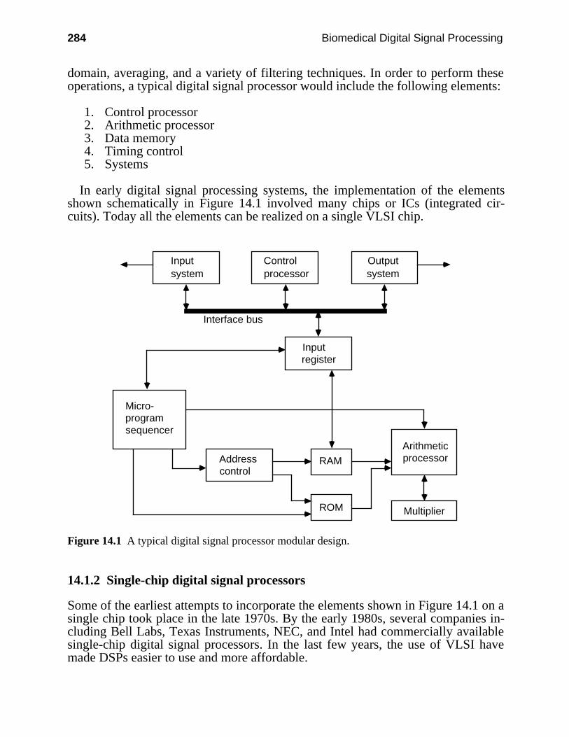
284 Biomedical Digital Signal Processing
domain, averaging, and a variety of filtering techniques. In order to perform theseoperations, a typical digital signal processor would include the following elements:
1. Control processor2. Arithmetic processor3. Data memory4. Timing control5. Systems
In early digital signal processing systems, the implementation of the elementsshown schematically in Figure 14.1 involved many chips or ICs (integrated cir-cuits). Today all the elements can be realized on a single VLSI chip.
Addresscontrol
RAM
ROM Multiplier
Arithmeticprocessor
Inputsystem
Outputsystem
Controlprocessor
Inputregister
Micro-programsequencer
Interface bus
Figure 14.1 A typical digital signal processor modular design.
14.1.2 Single-chip digital signal processors
Some of the earliest attempts to incorporate the elements shown in Figure 14.1 on asingle chip took place in the late 1970s. By the early 1980s, several companies in-cluding Bell Labs, Texas Instruments, NEC, and Intel had commercially availablesingle-chip digital signal processors. In the last few years, the use of VLSI havemade DSPs easier to use and more affordable.
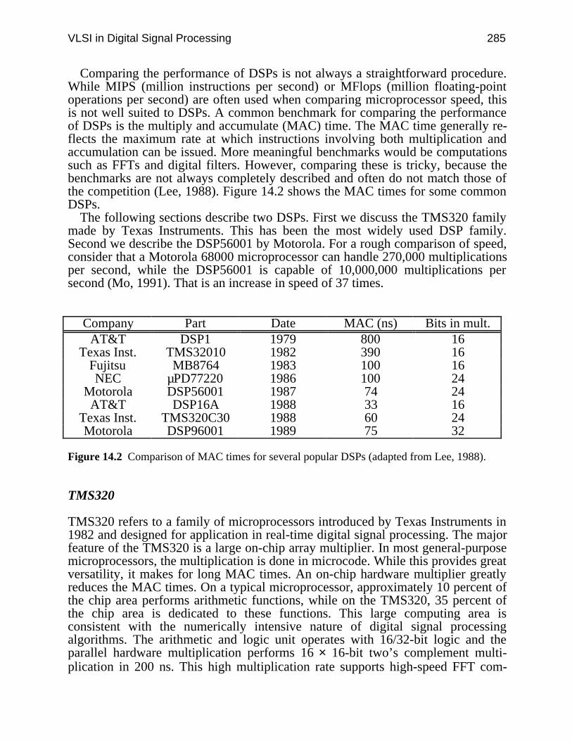
VLSI in Digital Signal Processing 285
Comparing the performance of DSPs is not always a straightforward procedure.While MIPS (million instructions per second) or MFlops (million floating-pointoperations per second) are often used when comparing microprocessor speed, thisis not well suited to DSPs. A common benchmark for comparing the performanceof DSPs is the multiply and accumulate (MAC) time. The MAC time generally re-flects the maximum rate at which instructions involving both multiplication andaccumulation can be issued. More meaningful benchmarks would be computationssuch as FFTs and digital filters. However, comparing these is tricky, because thebenchmarks are not always completely described and often do not match those ofthe competition (Lee, 1988). Figure 14.2 shows the MAC times for some commonDSPs.
The following sections describe two DSPs. First we discuss the TMS320 familymade by Texas Instruments. This has been the most widely used DSP family.Second we describe the DSP56001 by Motorola. For a rough comparison of speed,consider that a Motorola 68000 microprocessor can handle 270,000 multiplicationsper second, while the DSP56001 is capable of 10,000,000 multiplications persecond (Mo, 1991). That is an increase in speed of 37 times.
Company Part Date MAC (ns) Bits in mult.AT&T DSP1 1979 800 16
Texas Inst. TMS32010 1982 390 16Fujitsu MB8764 1983 100 16NEC µPD77220 1986 100 24
Motorola DSP56001 1987 74 24AT&T DSP16A 1988 33 16
Texas Inst. TMS320C30 1988 60 24Motorola DSP96001 1989 75 32
Figure 14.2 Comparison of MAC times for several popular DSPs (adapted from Lee, 1988).
TMS320
TMS320 refers to a family of microprocessors introduced by Texas Instruments in1982 and designed for application in real-time digital signal processing. The majorfeature of the TMS320 is a large on-chip array multiplier. In most general-purposemicroprocessors, the multiplication is done in microcode. While this provides greatversatility, it makes for long MAC times. An on-chip hardware multiplier greatlyreduces the MAC times. On a typical microprocessor, approximately 10 percent ofthe chip area performs arithmetic functions, while on the TMS320, 35 percent ofthe chip area is dedicated to these functions. This large computing area isconsistent with the numerically intensive nature of digital signal processingalgorithms. The arithmetic and logic unit operates with 16/32-bit logic and theparallel hardware multiplication performs 16 × 16-bit two’s complement multi-plication in 200 ns. This high multiplication rate supports high-speed FFT com-
286 Biomedical Digital Signal Processing
putations. Programming is done in assembly language. The maximum clock rate is20 MHz (Quarmby, 1985; Yuen et al., 1989).
DSP56001
The DSP56001 was introduced in 1987 and has quickly gained widespread use inaudio equipment, scientific instrumentation, and other applications. The chip is ca-pable of 10 million multiplications, 10 million additions, 20 million data move-ments, and 10 million loop operations per second. To achieve these high speeds,the chip has a highly parallel architecture with a hardware array multiplier, twoALUs (arithmetic logic units), two independent on-chip memory spaces, and anon-chip program memory. Most important, the DSP56001 utilizes a parallel andpipelined architecture in which several independent units operate simultaneously(Mo, 1991). The Motorola DSP is also unique in its ability to perform a MAC injust one cycle, with the result available by the next cycle. Its features include 512words of on-chip program RAM, 24-bit data paths providing a dynamic range of144 dB, a data ALU, address arithmetic units and program controller operating inparallel, and a MAC time of 74 ns (Lee, 1988; Motorola, 1988).
14.2 HIGH-PERFORMANCE VLSI SIGNAL PROCESSING
Only recently has it become feasible to perform digital signal processing in realtime. This is because the implementation of digital processing techniques requireshigh levels of computational throughput, particularly for real-time applications.This demand combined with the continually increasing levels of performance ofVLSI has led to the development of VLSI digital signal processors such as theTMS320 and the DSP56001 discussed above. The trend in DSP design is towardmore algorithm-based architectures. In other words, the ease with which VLSI de-sign can be done today leads the designer to more specialized architectures.
As discussed previously, the most useful digital signal processing techniques in-clude FFT computing, FIR and IIR digital filters. The implementation of thesetechniques requires only three types of operations. The required operations arestorage, multiplication, and addition. The small number of operations required sug-gest the use of a repetitive modular architecture. This is indeed the case. The lim-ited number of different operations required and the way in which VLSI technol-ogy is fabricated have led to several VLSI-oriented special-purpose architecturesfor digital signal processing applications. These architectures use multiprocessingand parallel processing, array processors, reduced instruction set computer (RISC),and pipelining to achieve very high-speed processing rates.
The terminology used to describe and classify VLSI architectures is by no meansstandard. Various attempts have been made to establish a useful taxonomy, includ-ing Flynn’s terminology based on instruction and data streams (Flynn, 1966). Inthe following discussion, we have tried to use the most commonly used terms.However, be aware that the literature is peppered with various terminology used todescribe the similar architectures.
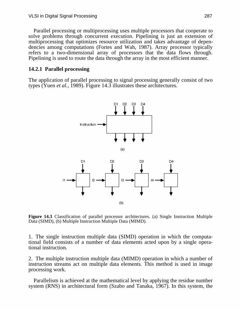
VLSI in Digital Signal Processing 287
Parallel processing or multiprocessing uses multiple processors that cooperate tosolve problems through concurrent execution. Pipelining is just an extension ofmultiprocessing that optimizes resource utilization and takes advantage of depen-dencies among computations (Fortes and Wah, 1987). Array processor typicallyrefers to a two-dimensional array of processors that the data flows through.Pipelining is used to route the data through the array in the most efficient manner.
14.2.1 Parallel processing
The application of parallel processing to signal processing generally consist of twotypes (Yuen et al., 1989). Figure 14.3 illustrates these architectures.
Figure 14.3 Classification of parallel processor architectures. (a) Single Instruction MultipleData (SIMD), (b) Multiple Instruction Multiple Data (MIMD).
1. The single instruction multiple data (SIMD) operation in which the computa-tional field consists of a number of data elements acted upon by a single opera-tional instruction.
2. The multiple instruction multiple data (MIMD) operation in which a number ofinstruction streams act on multiple data elements. This method is used in imageprocessing work.
Parallelism is achieved at the mathematical level by applying the residue numbersystem (RNS) in architectural form (Szabo and Tanaka, 1967). In this system, the
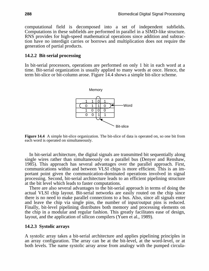
288 Biomedical Digital Signal Processing
computational field is decomposed into a set of independent subfields.Computations in these subfields are performed in parallel in a SIMD-like structure.RNS provides for high-speed mathematical operations since addition and subtrac-tion have no interdigit carries or borrows and multiplication does not require thegeneration of partial products.
14.2.2 Bit-serial processing
In bit-serial processors, operations are performed on only 1 bit in each word at atime. Bit-serial organization is usually applied to many words at once. Hence, theterm bit-slice or bit-column arose. Figure 14.4 shows a simple bit-slice scheme.
1 1 0 10 1 1 01 0 0 00 0 1 1
Memory
Word
Bit-slice
Figure 14.4 A simple bit-slice organization. The bit-slice of data is operated on, so one bit fromeach word is operated on simultaneously.
In bit-serial architecture, the digital signals are transmitted bit sequentially alongsingle wires rather than simultaneously on a parallel bus (Denyer and Renshaw,1985). This approach has several advantages over the parallel approach. First,communications within and between VLSI chips is more efficient. This is an im-portant point given the communication-dominated operations involved in signalprocessing. Second, bit-serial architecture leads to an efficient pipelining structureat the bit level which leads to faster computations.
There are also several advantages to the bit-serial approach in terms of doing theactual VLSI chip layout. Bit-serial networks are easily routed on the chip sincethere is no need to make parallel connections to a bus. Also, since all signals enterand leave the chip via single pins, the number of input/output pins is reduced.Finally, bit-level pipelining distributes both memory and processing elements onthe chip in a modular and regular fashion. This greatly facilitates ease of design,layout, and the application of silicon compilers (Yuen et al., 1989).
14.2.3 Systolic arrays
A systolic array takes a bit-serial architecture and applies pipelining principles inan array configuration. The array can be at the bit-level, at the word-level, or atboth levels. The name systolic array arose from analogy with the pumped circula-
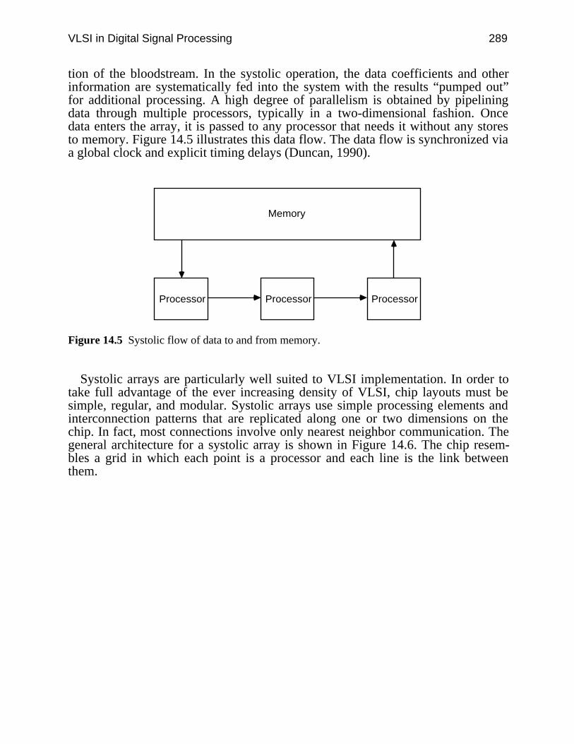
VLSI in Digital Signal Processing 289
tion of the bloodstream. In the systolic operation, the data coefficients and otherinformation are systematically fed into the system with the results “pumped out”for additional processing. A high degree of parallelism is obtained by pipeliningdata through multiple processors, typically in a two-dimensional fashion. Oncedata enters the array, it is passed to any processor that needs it without any storesto memory. Figure 14.5 illustrates this data flow. The data flow is synchronized viaa global clock and explicit timing delays (Duncan, 1990).
Processor Processor Processor
Memory
Figure 14.5 Systolic flow of data to and from memory.
Systolic arrays are particularly well suited to VLSI implementation. In order totake full advantage of the ever increasing density of VLSI, chip layouts must besimple, regular, and modular. Systolic arrays use simple processing elements andinterconnection patterns that are replicated along one or two dimensions on thechip. In fact, most connections involve only nearest neighbor communication. Thegeneral architecture for a systolic array is shown in Figure 14.6. The chip resem-bles a grid in which each point is a processor and each line is the link betweenthem.
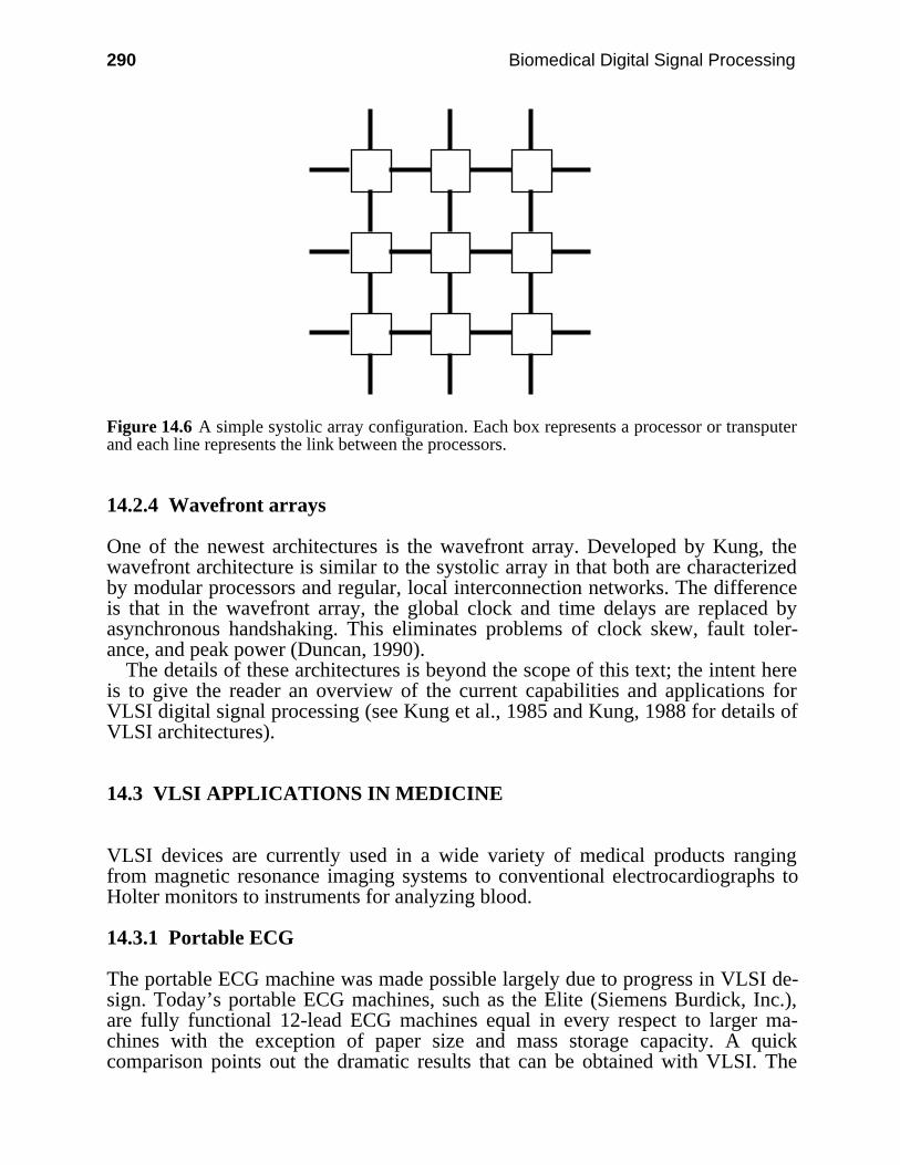
290 Biomedical Digital Signal Processing
Figure 14.6 A simple systolic array configuration. Each box represents a processor or transputerand each line represents the link between the processors.
14.2.4 Wavefront arrays
One of the newest architectures is the wavefront array. Developed by Kung, thewavefront architecture is similar to the systolic array in that both are characterizedby modular processors and regular, local interconnection networks. The differenceis that in the wavefront array, the global clock and time delays are replaced byasynchronous handshaking. This eliminates problems of clock skew, fault toler-ance, and peak power (Duncan, 1990).
The details of these architectures is beyond the scope of this text; the intent hereis to give the reader an overview of the current capabilities and applications forVLSI digital signal processing (see Kung et al., 1985 and Kung, 1988 for details ofVLSI architectures).
14.3 VLSI APPLICATIONS IN MEDICINE
VLSI devices are currently used in a wide variety of medical products rangingfrom magnetic resonance imaging systems to conventional electrocardiographs toHolter monitors to instruments for analyzing blood.
14.3.1 Portable ECG
The portable ECG machine was made possible largely due to progress in VLSI de-sign. Today’s portable ECG machines, such as the Elite (Siemens Burdick, Inc.),are fully functional 12-lead ECG machines equal in every respect to larger ma-chines with the exception of paper size and mass storage capacity. A quickcomparison points out the dramatic results that can be obtained with VLSI. The
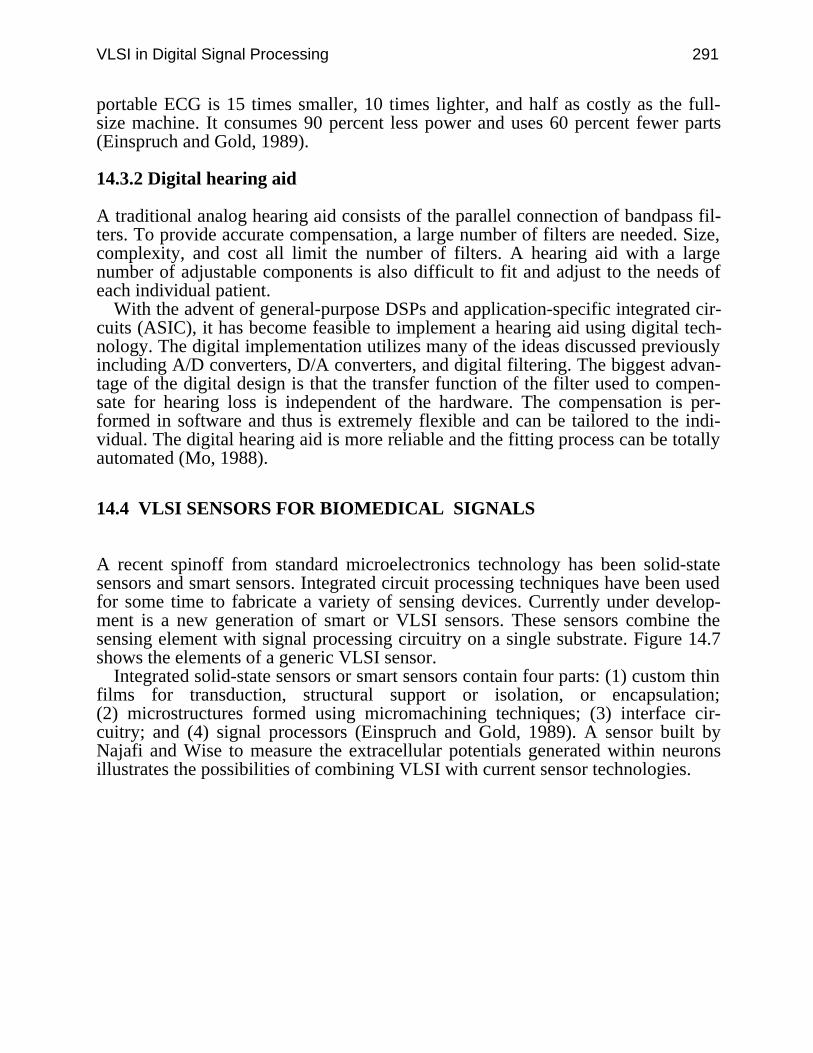
VLSI in Digital Signal Processing 291
portable ECG is 15 times smaller, 10 times lighter, and half as costly as the full-size machine. It consumes 90 percent less power and uses 60 percent fewer parts(Einspruch and Gold, 1989).
14.3.2 Digital hearing aid
A traditional analog hearing aid consists of the parallel connection of bandpass fil-ters. To provide accurate compensation, a large number of filters are needed. Size,complexity, and cost all limit the number of filters. A hearing aid with a largenumber of adjustable components is also difficult to fit and adjust to the needs ofeach individual patient.
With the advent of general-purpose DSPs and application-specific integrated cir-cuits (ASIC), it has become feasible to implement a hearing aid using digital tech-nology. The digital implementation utilizes many of the ideas discussed previouslyincluding A/D converters, D/A converters, and digital filtering. The biggest advan-tage of the digital design is that the transfer function of the filter used to compen-sate for hearing loss is independent of the hardware. The compensation is per-formed in software and thus is extremely flexible and can be tailored to the indi-vidual. The digital hearing aid is more reliable and the fitting process can be totallyautomated (Mo, 1988).
14.4 VLSI SENSORS FOR BIOMEDICAL SIGNALS
A recent spinoff from standard microelectronics technology has been solid-statesensors and smart sensors. Integrated circuit processing techniques have been usedfor some time to fabricate a variety of sensing devices. Currently under develop-ment is a new generation of smart or VLSI sensors. These sensors combine thesensing element with signal processing circuitry on a single substrate. Figure 14.7shows the elements of a generic VLSI sensor.
Integrated solid-state sensors or smart sensors contain four parts: (1) custom thinfilms for transduction, structural support or isolation, or encapsulation;(2) microstructures formed using micromachining techniques; (3) interface cir-cuitry; and (4) signal processors (Einspruch and Gold, 1989). A sensor built byNajafi and Wise to measure the extracellular potentials generated within neuronsillustrates the possibilities of combining VLSI with current sensor technologies.
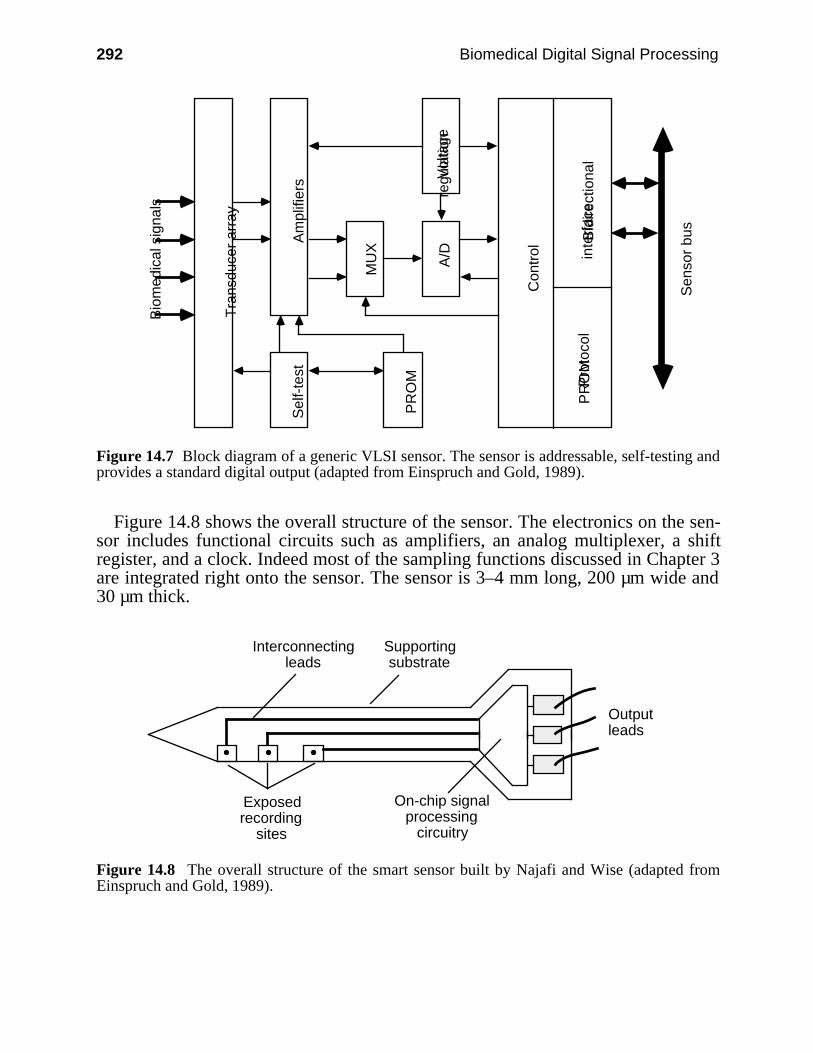
292 Biomedical Digital Signal Processing
Vol
tage
regu
latio
n
PR
OM
Sel
f-te
stA
mpl
ifier
s
MU
X
A/D
Tra
nsdu
cer
arra
y
Con
trol
Pro
toco
lP
RO
MB
idire
ctio
nal
inte
rfac
e
Sen
sor
bus
Bio
med
ical
sig
nals
Figure 14.7 Block diagram of a generic VLSI sensor. The sensor is addressable, self-testing andprovides a standard digital output (adapted from Einspruch and Gold, 1989).
Figure 14.8 shows the overall structure of the sensor. The electronics on the sen-sor includes functional circuits such as amplifiers, an analog multiplexer, a shiftregister, and a clock. Indeed most of the sampling functions discussed in Chapter 3are integrated right onto the sensor. The sensor is 3–4 mm long, 200 µm wide and30 µm thick.
On-chip signal processing
circuitry
Supporting substrate
Interconnecting leads
Exposed recording
sites
Output leads
Figure 14.8 The overall structure of the smart sensor built by Najafi and Wise (adapted fromEinspruch and Gold, 1989).
VLSI in Digital Signal Processing 293
14.5 VLSI TOOLS
The most commonly used VLSI design tools in the academic environment are theBerkeley VLSI tools. The system allows the designer to lay out the design at thedevice level and simulate the design for correct operation. A typical design wouldbegin with a functional block diagram. One next moves progressively lower andlower toward the actual device layout. The device level layout is done in MAGIC,a VLSI layout editor. MAGIC is analogous to a mechanical CAD program. Thedesigner actually draws each and every transistor in the design just as it will befabricated. Obviously this can be a painstaking task since a typical chip maycontain several hundred thousand transistors. MAGIC contains many features thatsimplify the design and often portions of the layout are redundant. As portions ofthe design are completed, programs such as CRYSTAL (a VLSI timing analyzer)and ESIM (an event-driven switch level simulator) are used to test the logic andtiming operation of that portion of the design. This is an important point! It isimportant to thoroughly test each portion of the layout as it is completed ratherthan waiting until the whole design is done. Continual testing will help ensure thatthe design will be functional when all the pieces are connected together in the finallayout.
Once the entire layout is complete and it has been successfully simulated, it isfabricated. The MOSIS (MOS implementation system) fabrication facility at theUniversity of Southern California is often used for low-volume experimental work.Finally, the device is tested and revised as necessary.
14.6 CHOICE OF CUSTOM, ASIC, OR OFF-THE-SHELF COMPONENTS
When approaching an instrument design, one must decide between simply usingoff-the-shelf chips, ASIC (application specific integrated circuits), or fully customchips. In reality, the finished design will usually contain some combination ofthese approaches. Ten years ago, using off-the-shelf chips was the only option.However, in recent years it has become feasible for even small companies todesign their own ASIC or fully custom chips via tools similar to those discussedabove. The design choices are based on the needs of the particular project and theavailability of suitable off-the-shelf chips. The design time and cost generallyincrease as one moves from a design containing only off-the-shelf chips to a fullycustom design.
14.7 REFERENCES
Denyer, P. and Renshaw, D. 1985. VLSI Signal Processing: A Bit-serial Approach. Reading,MA: Addison-Wesley.
Duncan, R. 1990. A survey of parallel computer architectures. Computer, 23(2): 5–16.Einspruch, N. G. and Gold, R. D. 1989. VLSI in Medicine. San Diego: Academic Press.
294 Biomedical Digital Signal Processing
Flynn, M. J. 1966. Very high speed computing systems. Proc. IEEE, 54: 1901–09.Fortes, J. A. B. and Wah, B. W. 1987. Systolic arrays—from concept to implementation.
Computer, 20(7) :12–17.Kung, S. Y. 1988. VLSI Array Processors. Englewood Cliffs, NJ: Prentice Hall.Kung, S. Y., Whitehouse, H. J., and Kailath, T. 1985. VLSI and Modern Signal Processing.
Englewood Cliffs, NJ: Prentice Hall.Lee, E. A. 1988. Programmable DSP architectures: Part 1. IEEE ASSP Magazine. 4–19.Mo, F. 1991. Basic digital signal processing concepts for medical applications. Biomedical
Science and Technology. 1(1): 12–18.Motorola. 1988. Technical Data #DSP56001/D, Motorola Literature Distribution, P.O. Box
20912, Phoenix, Arizona, 85036.Quarmby, D. (ed.) 1985. Signal Processor Chips. Englewood Cliffs, NJ: Prentice Hall.Szabo, N. S. and Tanaka, R. I. 1967. Residue Arithmetic and Its Applications to Computer
Technology. New York: McGraw-Hill.Yuen, C. K., Beauchamp, K.G., and Fraser, D. 1989. Microprocessor Systems in Signal
Processing. San Diego: Academic Press.
14.8 STUDY QUESTIONS
14.1 Describe the difference between general-purpose microprocessors and DSPs.14.2 Why are MAC times used as benchmarks for DSPs instead of the usual MIPS or MFlops?14.3 Discuss why VLSI is well suited to the design of DSPs.14.4 Define the following terms: (1) parallel processing, (2) pipelining, (3) array processors,
(4) SIMD, (5) MIMD.14.5 Describe the difference between systolic arrays and wavefront arrays. Which would operate
more efficiently?14.6 List at least four advantages of using VLSI-based designs for medical applications.
Related Documents