Bio-economic Development of Floodplains - AgEcon …ageconsearch.umn.edu/bitstream/22084/1/sp03is01.pdfBio-economic Development of Floodplains: Farming versus Fishing in Bangladesh

Bio-economic Development of Floodplains: Farming versus Fishing in Bangladesh †

Mursaleena Islam EconOne Research, Inc. 601 W. 5th Street, Fifth Floor, Los Angeles, CA 90403. Email: [email protected]. Corresponding author.

John B. Braden Professor, Department of Agricultural and Consumer Economics University of Illinois, 1301 W. Gregory Drive, Rm. 431, Urbana, IL 61801. Email: [email protected]. Paper prepared for presentation at the American Agricultural Economics Association meeting, Montreal, Canada, July 27-30, 2003.

†Acknowledgements: This research was supported in part by the National Science Foundation through grant number DEB-9613562, the Illinois Agricultural Experiment Station, University of Illinois, and the Cooperative States Research, Education, and Extension Service, U.S. Department of Agriculture through project 05-305 ACE, the Graduate College and the program in Environmental and Resource Economics of the University of Illinois, and the Social Sciences Research Council. The authors are grateful for assistance received from Munir Ahmed, Mustafa Alam, Mahbub Ali, Md. Shawkat Ali, Kingsley Allen, Lee Alston, Peter Bayley, Richard Brazee, Sharifuzzaman Choudhury, Mike Demissie, Ashley Halls, Mujibul Huq, Anisul Islam, Mustafa Kamal, Madhu Khanna, Roger Koenker, Syed Iqbal Khosru, Hayri Önal, Mokhlesur Rahman, Salim Rashid, Salimullah, Quazi Shahabuddin, Richard Sparks, and David White. The analysis and conclusions are the authors’ alone and are not attributable to these individuals and sponsors. Copyright 2003 by Mursaleena Islam and John B. Braden. All rights reserved. Readers may make verbatim copies of this document for non-commercial purposes by any means, provided that this copyright notice appears on all such copies.

Bio-economic Development of Floodplains:

Farming versus Fishing in Bangladesh

Abstract

This paper explores the linkages of environment and economic development in the floodplain of

large rivers. There is considerable evidence that even the most vital floodplains in the world are not

being managed efficiently and both economic and ecological factors need to be considered for

effective management. Floodplain management policies in Bangladesh emphasize structural

changes to enhance agricultural production. However, these structural changes reduce fisheries

production, where the fishery is an important natural resource sector and a source of subsistence for

the rural poor. We develop a model where net returns to agriculture and fisheries are jointly

maximized taking into account the effect of flooding depth and timing on production. Results for a

region in Bangladesh show that optimal production in a natural floodplain yields higher net returns

compared to a floodplain modified by flood control structures. This finding has important

implications for management policies -- neglecting the bio-economic relationship between fisheries

and land use may significantly affect the long-run economic role of a river floodplain, particularly

in a poor country.

JEL classification: Q2, O13, Q22

1

Bio-economic Development of Floodplains:

Farming versus Fishing in Bangladesh

I. Introduction Traditional development planning has focused primarily on commercial uses of natural resources,

such as agriculture, and has failed to take into account the broader environmental effects of policies,

particularly those affecting non-commercial resources, such as subsistence floodplain fisheries.

Rural communities in developing countries depend heavily on natural resources, both for

commercial production and subsistence consumption. Agriculture, forestry, fisheries, and many

other economic activities often depend simultaneously on both the exploitation and conservation of

natural resources. These competing needs have to be balanced in order to maximize returns from

development in the long run. For low-income countries that depend heavily on primary production,

such as, agriculture, fisheries and forestry, it is particularly important to understand the economic

importance of the environmental resource base that supports such production. Degradation of the

environmental resource base affects the quantity and quality of services that are produced by

ecosystems, as well as the resilience of these systems (Dasgupta and Mäler, 1997). These effects

can, over time, significantly diminish the economic value of productive activities dependant on the

natural system.

In this paper, we explore the linkages of environment and economic development in an

important natural system, the floodplain of large rivers. Large river floodplains around the world

support large population settlements, where development goals most often include improved

navigation, enhanced agricultural production and flood protection. Floodplain development

policies, such as building levees, appear to offer these desired benefits. However, by altering the

annual hydrologic regime, many development programs also have undesirable effects on the

ecosystem. There is now considerable evidence that even the most vital floodplains in the world are

2

not being managed efficiently and both economic and ecological factors need to be considered for

more effective management (Rogers et al., 1989; Interagency Floodplain Management Review

Committee, 1994; Naiman et al., 1995; Sparks, 1995).

Our focus is on Bangladesh, where eighty percent of the country is the floodplains of the

Ganges, Brahmaputra, Meghna and other rivers (Clarke, 2003). Floodplain fisheries are an

important natural resource sector in the country, where both commercial and subsistence fishing are

important (Tsai and Ali, 1997). Seventy-five percent of rural households engage in part-time

fishing from floodplains, rivers and beels1 (FAP 16, 1995; UNDP, 1995). Fish also constitute an

important source of nutrition for the rural poor; it is estimated to provide up to eighty percent of

animal protein consumed by rural households (UNDP, 1995). Despite the importance of floodplain

fisheries, the value of this sector is not adequately accounted for in traditional development

planning because much of it takes place in the informal economy.

This paper studies agriculture and fisheries production in an integrated bio-economic

framework in order to understand the tradeoffs between these sectors and to quantify the economic

impacts of structural changes in the floodplain. The policy challenge is to manage the floodplain

such that the value of both agriculture and fisheries are taken into account. This work is distinct in

that we explicitly account for productivity linkages between agriculture and fisheries and apply

econometric tools to characterize the hydrology that drives both systems. We develop a floodplain

land use model where land is allocated to either agriculture or fisheries based on the highest net

returns to land. This is an optimization model where the objective is to maximize joint returns from

agriculture and fisheries production subject to a set of production and flooding constraints. We

model the trade-offs between agriculture and fisheries production in different land types where land

types are classified based on the exposure to flooding. Agriculture and fisheries production are then

1 Beels are permanent backwater lakes in the floodplain, which support fish year-round.

3

modeled to vary with the area of land in each flood exposure class or flood land type. The model is

used to study the effect of alternate management policies. Management policies include levees

which affect the hydrology of the floodplain and thus change the distribution of areas in each flood

land type. By changing the distribution of areas in each land type, we can study the economic effect

of alternate floodplain management policies.

II. Floodplain Systems Floodplains are wetland ecosystems and are defined as areas that are periodically inundated by the

lateral overflow of rivers and lakes (Junk, Bayley, and Sparks, 1989). In their natural state,

floodplains support diverse wildlife habitats, fisheries and forests, whose productivity depend

critically on the annual flood cycle. The pulsing of the river flow or the flood pulse is considered to

be the principal driving force responsible for the existence, productivity, and interaction of the

major biota in river-floodplain systems (Junk, Bayley and Sparks, 1989). Economic development in

river floodplains often imposes external losses on renewable resource production, such as fisheries,

by altering the natural hydrologic regime of the floodplain (Sparks, 1995; Welcomme, 1985).

Economic development is pursued in floodplains around the world primarily through the

installation of dams, embankments or levees2, and through river channelization. In Bangladesh, the

trend has been to construct large-scale Flood Control, Drainage and Irrigation (FCDI) projects--

systems of embankments. FCD/I3 projects are designed to reduce flooding and enhance agriculture

production. These projects change the intensity, timing and duration of flooding. The area flooded

and depth of routine flooding are reduced so as to make more land available for agriculture and to

increase agricultural productivity. Floodplain management policies in Bangladesh target the

agriculture sector, with the goal of increasing productivity and achieving self-sufficiency in rice

2 The terms embankments and levees are used interchangeably here. 3 The notation FCD/I is used to imply either a FCD or a FCDI project. FCD projects are Flood Control and Drainage projects with no irrigation component.

4

production. While floodplain rice production has boomed, however, some areas have noted

declines in fish population and species diversity. As floodplain lands are reduced by FCD/I

projects, so is the potential for floodplain fish production (World Bank, 1991). Changes in the

hydrological cycle caused by FCD/I projects affect floodplain fisheries in several ways. First, a

decrease in flooded area during the monsoon results in a loss of fisheries habitat and reduced

spawning grounds. Second, the influx of riverine fish and hatchlings at the beginning of the flood

season is diminished due to the blockage of lateral migratory paths. Finally, dry season habitat is

reduced as beels are drained to provide irrigation water and/or to create open more land for

agriculture. All of these factors result in a decline in floodplain fish production both in the wet and

dry seasons (FAP 20, 1994; Halls, 1998).

Hydrologic Cycle and Tradeoffs between Agriculture and Fisheries Production The annual flood season in Bangladesh is from July to October, with early flooding possible in May

and June. Water recedes from the plains in October and November. The dry season covers

December through June.

Agricultural productivity, the choice of crops grown, and the cropping pattern in the

floodplain are largely determined by hydrologic conditions (MPO, 1987). Most important of these

are the depth, timing and duration of flooding, the rainfall pattern, and the availability of dry season

drainage and irrigation. Depending on the water regime, from one to three crops are grown in the

floodplain each year. Rice is the dominant crop and several varieties may be grown in a given year.

Other crops include wheat, jute, mustard, and pulses. There are three main seasons for the

floodplain crops, the pre-monsoon season (March-June), the monsoon season (July to October) and

the winter dry season (November to March).

5

The life cycle of fish is also based on the annual hydrologic cycle. Spawning takes place

during the pre-monsoon and early monsoon seasons. Some species breed in the rivers while others

breed in the floodplains. Lateral migration to the floodplains occurs with the early floods as the

water level in the rivers rise. Adult fish are carried into the floodplains with the water in July. They

spawn during the early monsoon months and the fingerlings grow rapidly in the floodplain during

the monsoon flood season. As the floods recede, some fish move back to the rivers, while others

remain in the floodplain beels.

The physical trade-offs between agriculture and fisheries production occur in some flood

land types, based on land elevation. In a natural floodplain, crop production is feasible in higher

elevation lands with shallow to medium seasonal flooding, while it is not feasible in lowlands and in

beels where flooding is deeper and longer-lived. Fish production is feasible in medium to deeply

flooded lands and in beels. High-yield crop varieties are produced in shallow to medium flooded

lands and farmers attempt to keep flood waters out of areas where these crops are planted. The loss

of flood coverage reduces fish production for reasons discussed earlier.

During the flood season, the floodplain fishery is an open-access resource. The rural poor

and the landless harvest fish for household consumption (Ali, 1997) as well as for sale in local

markets. This is also the time of the year where the tradeoff with agriculture production occurs in

the floodplain. Since landowners make cropping decisions, the fisheries sector is generally ignored

in their land-use decisions. A primary source of conflict between farmers and fishers is over the

controlled timing of flooding, particularly during the pre-monsoon season in May and June. Fishers

often cut embankments (or open sluice gates, where present) to allow pre-monsoon floodwaters

(and accompanying fish) to enter the floodplain. Farmers resist this, particularly if their rice crop is

yet to be harvested. The property rights structure in the floodplain is such that farmers benefit

directly from the flood control structures, even though they do not have to bear any costs associated

6

with these structures. The open access approach to the fishery in this case reduces potential gains

from the fishing sector. It gives individual subsistence fishers little bargaining power with the

landowners.

In the dry season, farmers often drain beels to grow a winter rice crop. This results in a

reduction of water area and fish productivity, causing conflict with fishers. Most professional

fishers in the region are landless. During the dry season, they work as wage laborers or

shareworkers for fisheries leaseholders to fish in the beels. Lost fish production in the beels directly

cuts into their primary source of income, causing conflict with the farmers.

III. Floodplain Management Model A floodplain land-use model permits systematic analysis of the economic tradeoffs between

agriculture and fisheries production. In our model, land is allocated either to crop production or to

maintain fish habitat based on the highest return to land. The social objective is to determine the

floodplain management plan and the land allocation that maximizes net returns from both

agriculture and fisheries production in the floodplain, given expected flooding conditions.

Management plans here include any measures that directly affect the total area of land exposed to

flooding and the area of land in each flood land type. We study four management options: a

natural (unmodified) floodplain and three types of structural changes in the form of low, medium,

and high embankments. The planner observes a range of economic and hydrologic factors that

affect the use of floodplain land for agriculture or fish production. These factors include prices and

production costs, crop yields, fish productivity and the suitability of land for agriculture or fish

production. The planner determines the management plan such that net returns from agriculture and

fisheries are maximized given an optimal allocation of land between agriculture and fishing

activities. A prime factor affecting the suitability of floodplain land for agriculture or fisheries and

the productivity in each sector is the timing, duration and depth of flooding. The land use model

7

here incorporates the differences in productivity based on flood land type, as categorized by the

average depth of flooding in each month. The flood land types are as defined in Table 1.

The theoretical foundation for the analysis is derived from theories of natural resource

development and renewable resource exploitation (Clark and Munro, 1975; Dasgupta and Mäler,

1997; Swallow, 1994). It also draws from the body of literature that stresses the value and optimal

use of environmental resources as inputs into production (Barbier, 1998; Dasgupta, 1990; Mäler,

1991; Serafy, 1993). This approach allows us to determine the best use of resources, such as land

and water, in recognition of their economic value through their support of natural production as well

as of agriculture. In our case, floodplain area can be thought of as a stock of environmental

resource that can be used as a direct input in agriculture or to support fisheries. There are indirect

uses of the floodplain resource also, such as, providing breeding grounds and nurseries for river

fisheries or for sediment and nutrient retention, which ultimately enhances the productivity of the

resource.

Our floodplain management model (FMM) is designed to maximize net returns from

agriculture and fisheries by solving for the optimal allocation of land between agriculture and

fishing activities for any given management plan. The FMM builds on comparable models focusing

on the tradeoff between land development and preservation (Barbier and Strand, 1998; Parks and

Bonifaz, 1994; Shahabuddin, 1987; Stavins and Jaffe, 1990; Swallow, 1990 and 1994). The area of

land allocated to crop i in flood land type l at time t is Ailt, the area maintained for the fishery is

Aflt, and the total land available in each flood land type is Alt. Fish stock is given by Slt, fish catch

by Qlt and the fishing effort expended is given by Elt. Crop yield is given by yilt. Prices and costs

are given by pf, cf and pi, ci for fish and crops respectively.

8

Fisheries Model

An important component of the FMM is the empirical fisheries model. We develop a model of

fisheries production that associates output to floodplain characteristics, such as area and depth of

flooding, and stresses the importance of this relationship. Given evidence that fish production is

dependent upon floodplain for habitat and nurseries (Welcomme and Hagborg, 1977; FAP 20,

1994), we model explicitly the effect of flooded area on fish production. We do not model fish

stock dynamics explicitly here. To the extent that fish growth and stock dynamics may affect

fishing seasons and seasonal production outcomes, our model will fail to capture that. Thus, the

model is useful only for studying annual optimal production levels, which was our primary goal.

This approach is appropriate for the study context in Bangladesh, where recruitment occurs

predominately from stocks outside the floodplain in the form of seasonal migrations of fish (Halls,

1998). Fishing practices in Bangladesh do not leave much of the floodplain fish stock for the

following year. Thus, an annual fishery can be modeled with an initial stock dependent on available

floodplain land and its flooding condition.

We start with the Schaefer specification, which is commonly used in the fisheries literature

(Clark, 1976; Barbier and Strand, 1998). The fish harvest or catch function is given by:

Q aS Et t t= (1)

where, a > 0. This specification assumes constant marginal returns to both stock, S, and effort, E.

However, it has been shown that the production function of a fishery eventually exhibits decreasing

marginal returns to both input factors. Decreasing returns with respect to effort can be explained

well by the effect of congestion, where, beyond a certain level of E, any further increases in effort

lowers catch per unit effort, due to congestion. Decreasing returns with respect to stock can be

explained by gear saturation, where catch increases proportionately with stock up to a certain

9

capacity level of fishing gear, such as nets, beyond which gear saturation reduces catchability

(Clark, 1976). We thus have:

δφttt EaSQ = (2)

where, a > 0, 0 < φ < 1 and 0 < δ < 1. That is, catch Q is increasing in both stock and effort but

exhibits decreasing marginal returns to both input factors. Finally, for simplicity, the units of the

production function are normalized so that E is equal to one:

φtt bSq = (3)

where, b > 0.

Next, we introduce the stock function. Typically, fisheries stock is modeled as a dynamic

function of growth and harvest. The change in stock at any time, t, is given by the growth in stock

minus the harvest. The growth function gives the natural rate of increase of stock, S, and can be

thought of as the “natural” production function. Since our purpose here is to measure total annual

fish production under different hydrological management scenarios we use a simple static model of

fish production in order to measure the “economic” value of fish. We model fish stock, S, simply as

a function of floodplain area, A, given that the area of the floodplain in each flood land type that is

available to the fishery is an important determinant of fish stock at any given time (Halls, 1998;

Welcomme, 1979). Using the area of land in each flood land type captures the effects of both the

intensity and the duration of flooding. Evidence from other floodplains suggests that stock is an

increasing function of the area flooded but stock per unit area is a decreasing function of the area

flooded (FAP 20, 1994; Welcomme and Hagborg, 1977). Thus we have the general form stock

function:

S F At ft= ( ) (4)

where, ′ > ′′ < =F F and F0 0 0 0, , ( ) . For the empirical analysis we use a common non-linear

specification:

10

S cAt ft= θ (5)

where, c > 0 and θ < 1. Combining equations (3) and (5), we get:

βα ftt Aq = (6)

where, α > 0 and β < 1.

Next, we need to account for the fact that higher intensity floods will lead to higher initial

stocks and thus higher productivity. This can be done simply by specifying equation (6) for each of

the flood land types, l. Since for different intensity floods we have not only different flooded areas,

but also different distributions of l, this would lead to different fish outputs in the various flood land

types. So accounting for l leads to:

βα fltlt Aq = (7)

where β < 1 for floodplain lands l1 to l4 and β = 1 for beels, i.e., flood land type l5. Fishing is not

feasible in land type l0, since that is dry land. Equation (7) is the fish production function, which is

modeled here explicitly as a function of floodplain area maintained for the fishery. Fish output

increases at a decreasing rate with an increase in flooded area. Output for floodplain lakes or beels

is assumed to exhibit constant returns to scale (land type l5). This is because flood depth in beels is

close to constant across the beel area and thus output per unit area is assumed to be constant over

the area.

Next, we add a parameter, µ, which measures the effect of structural changes on fish

productivity, as given by catch per unit area. Halls (1998) finds that flood control structures not

only reduce fish production because they reduce the area flooded, but that they also reduce overall

fish productivity. This reflects the partial inaccessibility of the floodplains inside the embankment

by migratory fish species. Halls’ study area is the Pabna Irrigation and Rural Development Project

(PIRDP), which is an FCDI project. Halls’ results suggest that floodplain fish productivity is

11

reduced by as much as 50 percent due to the embankments.

Finally, a variable, θ, is added to reflect the portion of fish catch which is valued at the

market price. When θ is equal to one, all fish harvested are valued at market price. That is, we

assume that even subsistence fish consumption is valued at market prices. The analysis here does

not attempt to estimate the value that households place on fish for subsistence consumption but

rather attempts to measure the total value of all fish produced in the floodplain, whether for the

market or for household consumption. In this case, using the market price of fish, as a shadow

value for domestic use, is the best measure we have for the use value. When θ is less than one, only

the marketed portion of fish catch is valued at market price. The rest of the fish catch, which is

used for subsistence consumption, is valued at an alternate nutritional value. This alternate value is

measured by computing the price of an equivalent protein supply from another source, pulses, in the

region.

Agriculture and the Full Empirical Model

For computational ease, the agriculture sector is modeled using simple production technologies.

These are characterized by linear input-output coefficients that vary by crop. Eleven agricultural

crops are specified in the empirical model. These are the most common varieties of crops and fish

produced in the floodplain. These include wheat, jute, pulses, mustard and seven varieties of rice:

High Yielding Variety (HYV) Aus, Local Aus, HYV T. Aman, DW T. Aman, DW B. Aman, HYV

Boro and Local Boro. Crops are specified based on their suitability to different land types and

seasons. We assume that there are constant returns to scale in agriculture. We also assume that

irrigation water is available as needed during the dry season. This is reasonable since groundwater

irrigation is common in the study area and water is usually not scarce. However, individual farmers

might face other constraints in determining crop choice, such as credit, capital costs, labor, etc.,

12

which are not explicitly modeled here. This abstraction might lead certain crops, particularly the

high-cost high-yielding varieties of rice, to be chosen more often in the model than in practice. This

is not necessarily a problem if we are interested in finding the maximum potential returns from the

floodplain, as long as we realize that the agriculture returns will always be somewhat inflated across

all model scenarios.

The full empirical floodplain management model is:

∑∑ −−′++−tlf

fltffltffltftli

iltiiltiAAAcqpqpAcypMax

fltilt ,,,,,))1(()( µθµθ (8)

subject to,

A A A for all l and tilti

fltf

lt∑ ∑+ ≤ (9)

40 ,..., llforAq fltfltβα= (10)

5lforkAq fltflt = (11)

The objective is to maximize the sum of net returns from agriculture and fisheries (equation (8)).

The first term is crop returns per hectare multiplied by the area allocated to that crop. This is

summed across all crops, land types, and time. The second term is the net returns from fisheries

which is given by the revenue from all catch minus the cost. Revenues are reduced to the extent the

parameters µ and θ take on values less than one. The total cost is given by the cost per hectare of

fishing multiplied by the total area allocated to fishing.

Equation (9), is the land constraint. It ensures that the sum of optimal lands allocated to

agriculture and fisheries production is no greater than the available land in each flood land type in

each time period. Equations (10) and (11) are the fish production functions for the floodplain and

beels, respectively, as explained earlier. Several other conditions are specified for the empirical

model such as production parameters and feasibility conditions. These include:

• crop suitability by months/season

13

• crop suitability by flood land type

• fishing season

• fishing feasibility by flood land type

• area matrix - for total available area by flood land type and month

• vector of crop yields

• vector of production costs

• vector of crop and fish prices

All economic values, including net returns, are expressed as annualized equivalents. All input cost

and price data and results are in 1995 Taka.4 For analytical convenience, an annual model is used

with discrete monthly time increments, t. For agriculture, cropping decisions are made on a

seasonal basis, whereas, fish catch can vary daily. A monthly time increment was chosen as a

reasonable middle-ground. An annual model is used for both of these sectors. Crop choice and

cropping pattern are based on the expected net returns and the available area of land in each flood

land type in each season, which is then aggregated up to a year. Floodplain fisheries are assumed to

follow an annual cycle, where new recruits migrate from the river to the floodplain at the beginning

of each flood season and the adults leave with the receding floods.

IV. Model Calibration The study area is in the Tangail region of North-Central Bangladesh. An area of 143,640 hectares

(ha) was selected in the Bangshi-Dhaleswari floodplain, which is part of the larger Brahmaputra

River floodplain. Detailed data on agriculture and fisheries in the study area were available from

several other ongoing research studies in the area. These data include fish catch, fishing effort,

cropping pattern, growing season, water tolerance, crop yields, as well as costs and prices. Islam

4 1 US$ equals 57.95 Bangladeshi Taka in April 2003.

14

(2001) provides further details. The data on fish catch were not detailed enough for econometric

estimation of equation (10); instead, we numerically estimated the parameters of the fish production

function, α and β, using data from a fish catch survey conducted by the Center for Natural Resource

Studies in Dhaka (CNRS, 1997). Catch data and approximate floodplain area data were used to

estimate the parameters by setting one parameter value and solving for the other. With fish

production exhibiting only slightly decreasing returns to scale (Welcomme, 1985), we expected β to

be close to 1. So, we started by setting the value for β and solving for α, and repeated the process

until there was convergence.

Hydrology Simulation

As mentioned earlier, flood season hydrology is an important input into the floodplain

management model. We use properties of historical water level data to simulate a series of water

levels, which are then inputs to the optimization model. Figure 1 shows sample historical

hydrographs. Historical water level data were provided by the Surface Water Modelling Centre in

Bangladesh (SWMC, 1997). A novel approach based on a branch of time-series econometrics

called Fourier (harmonic) analysis is developed here to simulate flood levels. Fourier analysis

decomposes periodic data into a sum of sinusoidal components (Bloomfield, 1976). The procedure

describes or measures the fluctuations in a time series by comparing them with sinusoids. This

approach provides a realistic series of simulated hydrographs by accounting for both the

fluctuations and the random component in annual floods. There are several steps to this analysis.

First, econometric analysis is used to fit the best curve to the historical data. Next, residuals from

the fitted model are tested for heteroscedasticity and autoregressive processes. Finally, the fitted

values are combined with fitted residuals in order to randomly generate a new water level series.

For our purposes, one hundred years of daily water level series were simulated (Islam, 2001).

15

The simulated hydrographs were then used to generate monthly average water levels and to

calculate the associated areas in each flood land type. The area-types are inputs into the floodplain

management model. The annual distribution of areas in each flood land type is calculated by

combining the simulated hydrographs with area-elevation data from a digital elevation model

(DEM) of the study area (Environment and GIS Support Project for Water Sector Planning, 1997a).

The area-elevation data is first fitted to a generalized logistic function. Then this fitted function

together with the simulated water level is used to calculate the area in each flood land type, based

on the depth of flooding. This provides a stochastic distribution of flood land types, an input into

the FMM.

Figure 2 presents a schematic of how the different model components come together. The

figure reflects the sequencing of the empirical model. Outputs from the DEM and the hydrology

components from the simulation model are combined to give the site-specific flooding pattern, that

is, the distribution of areas in each flood land type in each month. These are used to solve the

floodplain management model, producing a distribution of optimal net returns for each specified

model scenario.

V. Results This section presents results from the four management scenarios. The optimization model is

solved for each of the scenarios using non-linear programming techniques.

The base model is for the natural (unmodified) floodplain. It is run with parameter values of

α=20, β=0.8, θ=1, and µ=1 (see Appendix A for sensitivity of model results to changes in these

parameter values). Results show that crops are grown in land types L0, L1, and L2 with no crops

grown in L3, where the optimal land use is for fisheries. Table 2 shows the cropping pattern for a

typical year of the model run – it shows the percentage of total floodplain land devoted to each crop

in each month and in each land type. Different varieties of rice are found to be optimal in each

16

season. This cropping pattern is comparable to what we find in the floodplain. Rice is the

dominant crop in the region where the traditional rice crops of Aus, Aman and Boro are grown in

the Kharif-I (pre-monsoon), Kharif-II (monsoon) and Rabi (winter) seasons respectively (EGIS,

1997b; FAP 20, 1992). Our results reflect this, although local varieties of rice are not always found

to be optimal since HYV crops yield higher returns. The absence of credit constraints may account

for the over-representation of HYV crops that require more costly inputs. Another factor is that the

different varieties of rice taste different and there may be some preference for traditional local

varieties over HYVs, although the trend has been toward planting more HYV crops (FAP 20, 1992).

Jute is also grown in the region, but is not reflected in our optimal cropping pattern. The acreage of

jute has been decreasing due to low market prices (FAP 20, 1992).

Since the base model results correspond well to current practice in most respects, the slight

differences in cropping pattern are not of serious concern. These results indicate the highest

possible returns given the production constraints in the floodplain and are consistent across the

different scenarios. This suggests that the model is appropriate for making counterfactual

predictions and we can apply it to this end.

The optimal fishing pattern in the base model includes some fishing in all feasible land

types, L1 to L5. Table 3 shows the optimal fishing pattern for a typical year of the model run – it

shows the percentage of total floodplain land devoted to fisheries in each month and in each land

type. Land types L4 (low-lying land) and L5 (floodplain beels) are not suited to agriculture. As

expected, the model allocates all of L4 and L5 areas are allocated to fisheries. What is interesting is

that there is some land in L1, L2 and L3 allocated to fisheries, thus indicating that returns from

fisheries are higher compared to agriculture for some of these areas. This is in contrast to

traditional planning models that fully allocate these land types to crop production. Optimal

floodplain fish catch per unit area (CPUA) in the base model ranges from 83 kg/ha/year to 128

17

kg/ha/year, with an average of 104 kg/ha/year. Data on actual floodplain CPUA is sparse and

variable in time and place. A study in the PIRDP floodplain found CPUA to be 104 kg/ha/yr in

1995 and 130 kg/ha/yr in 1996 (MRAG, 1997). A survey in the Tangail region found CPUA of90

kg/ha/year in 1992/93 to 403 kg/ha/year in 1993/94, including beel catch (FAP 20, 1994). The

official national Fish Catch Statistics report 130 kg/ha/year for the 1994-1995 water year (DOF,

1995). Thus, the optimal CPUA from our FMM is at the low end of observed conditions. This is

true for all of the counterfactuals studied, and therefore does not affect the comparison between

them. But, it does mean that fisheries are disadvantaged relative to agriculture in all scenarios.

Comparison of Alternate Management Scenarios

The three alternative management scenarios involve the installation, respectively, of low, medium

and high embankments. These scenarios offer increasing levels of flood protection to land behind

the embankments but decreasing access of fish to the floodplain. In all three cases, the optimal

cropping patterns are very similar to the base model. For the models with low and medium

embankments, the cropping patterns are identical to the base model. The shift in flood land types

brought about by these embankments was not sufficient to change the optimal cropping pattern. For

the model with high embankments, more land of type L0 is allocated to agriculture compared to the

base model. This is what we would expect since there would be more L0 land with high

embankments management scenario and all of that land would be devoted to cropping since it is not

feasible for fisheries.

The fishing patterns for the low and medium embankment models are also close to the base

model (note that µ is equal to one here). For the first year, they are identical. There are slight

variations in other years. For the high embankment model, less land is optimal for fisheries as

compared to the base model. This is particularly true in land types L1 and L2 where the tradeoff

18

between agriculture and fisheries is greatest. This is expected given that there is typically less land

in L1 and L2 and more land in L0 for the high embankment scenario.

Next, net returns under the alternate management plans are lower than in the base model for

all years. We calculate net returns by subtracting annualized capital and O&M costs of each

management scenario from the total returns (Islam, 2001 provides further details). For the base

model, net returns are equal to the total returns since there are no structural changes for which costs

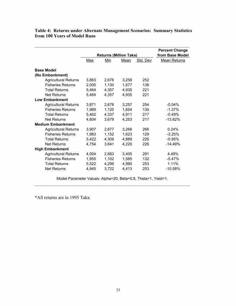
have to be taken into account. Table 4 presents summary statistics of agriculture, fisheries, and net

returns from the different models based on the 100 years of model runs. Figure 3 plots the net

returns for all 100 years of model results. Net returns from the high embankment are almost always

higher compared to the other two scenarios of structural change. This implies that even though the

cost of the high embankment management plan is the highest, the benefits of reduced flooding

under this plan are higher than the other management plans. However, the higher costs are not

justified when compared to the base model. This is clearer when we compare the two components

of returns, one agriculture and the other fisheries. We expect returns from agriculture to be greater

and fisheries returns to be less under the alternate management plans as compared to the base

model. Results from model runs bear this out for the most part. Agriculture returns increase with

the medium and high embankment models, but change little with the low embankment scenario (see

Table 4). Fisheries returns decrease under each management plan, with the largest decline of 5.5

percent under the high embankment model. It is important to note that fisheries productivity is

assumed not to change under these management plans; that is, the parameter, µ, is equal to 1. Fish

production changes only to the extent that areas flooded change with the different structural

changes. In reality, we would expect productivity to change beyond this since structural changes

block migration routes of fish and delay the timing of flooding. This is addressed below in

Appendix A.

19

The decrease in fisheries returns is not made up by an increase in agricultural returns under

the low and medium embankment plans. Thus, total returns are lower than the base model, without

accounting for the cost of the management plan. In the case of high embankment, the increase in

agriculture returns offsets the decrease in fisheries returns. This shows a slight increase in operating

returns of about one percent when compared to the base model. However, when the capital cost is

taken into account, the net return is 10.6 percent lower than in the base model (see Table 4).

Next, we examined the sensitivity of model outputs to the key input parameters, α, β, θ and

µ. We find that model results are not sensitive to realistic ranges of the parameters, α and β, the

parameters of the fish production function. Results are very sensitive to the parameters θ and µ, as

expected. Appendix A presents details of our sensitivity analysis.

Finally, we carried out a stochastic dominance analysis which confirms that the base model

dominates over other the models by first-degree stochastic dominance. Appendix B presents details

of the stochastic dominance analysis.

VI. Policy Implications and Conclusions Our results provide two important conclusions. First, we find that the optimal resource use in the

base case (that of a natural floodplain) allocates less land to agriculture than is currently observed in

the floodplain and allocates some additional land to fisheries in several flood land types. Second,

we find that net returns from the base scenario are higher than the other management scenarios and

that the base model dominates the other models by first-order stochastic dominance.

An important assumption of our conceptual model is that producers make optimal land-use

decisions given the policy choice made by the planner, while the planner in turn chooses the optimal

floodplain management policy assuming optimal land-use decisions are made by floodplain

producers. Thus, to the extent our results from the base scenario diverge from actual observed

20

conditions in the floodplain, we can conclude that floodplain producers currently do not make

socially optimal land-use decisions in the study area. This finding, that more than optimal areas of

land are currently being allocated to agriculture, is not surprising. Fisheries production is not

adequately valued by agricultural land-owners since much of the floodplain fish production is used

for subsistence consumption by the landless.

The second key result shows that the base model, solved for a natural floodplain, dominates

the other management scenarios of low, medium, and high embankment.5 This is true even under

different values of key parameters. The finding that the base model always yields higher net returns

than the three structural management scenarios is rather surprising, given the dominance of these

structural changes in traditional development planning. Our results give tentative support to the

hypothesis that structural changes in the floodplain, as represented by these scenarios, would not

always provide higher returns if the economic value of fisheries production were accounted for,

along with agriculture. In fact, our results may even be conservative in that the fisheries sector may

be undervalued. Our results depend critically on the value placed on fish production. To the extent

that the market price of fish we use does not fully reflect the true social value of fish, this would be

true. The market price may be too low because much of the fishery is open access and fish harvest

may be too high in the flood season. In this case we would want to use a shadow price of floodplain

fish that takes into account the scarcity value of the fish and reflects the future loss of the resource

due to changes in the management regime. Another issue is how we value the non-marketed

portion of fish production. We use a value associated with an alternate protein source, which does

not fully value fish as an important food source. A better measure would be to value the fish at its

full replacement cost for nutritional intake. That is, find a complete bundle of foods that will

provide an equivalent nutritional supplement and estimate the market value of that bundle. This

5 This key result also holds when structural changes with sluice gates were studied. That study was part of a project commissioned by UK’s Department for International Development and is not reported here.

21

would be the nutritional replacement value for any fish lost. We believe these adjustments would

further strengthen our results.

These results suggest that traditional development policies that emphasize structural changes

in the floodplain and target agricultural growth have been misdirected in their oversight of the

fisheries sector. The floodplain fisheries sector is not taken into account since it is not a

commercially important sector. However, recent emphasis on the fisheries sector in Bangladesh,

brought about by concerns over reduction in fish stocks and the subsequent effect on rural poor who

depend on fish for subsistence consumption, will hopefully stimulate further research in this area

and inform future planning. For the rural poor, environmental resources, such as fisheries, can

supplement income and consumption especially in times of economic stress. Degradation of the

environmental resource base can make certain communities destitute even while the economy on

average is growing (Dasgupta and Mäler, 1997).

This paper is one of the first attempts at quantifying the effects of floodplain economic

development policies in Bangladesh on two key sectors, agriculture and fisheries, in an integrated

bio-economic framework. The primary contribution is the empirical floodplain management model

developed here to study both agriculture and fisheries sectors in one framework. This allows us to

quantify floodplain production tradeoffs in a way that was not possible before. Although similar

land use models exist in the literature, what is unique here is the integration with hydrology and

physical characteristics of the floodplain. Our work is distinct in that we take explicit account of

the productivity linkages between agriculture and fisheries production for different flooding

conditions. The model we develop here is flexible enough that we can study the effects of different

policy options for different input conditions. Both the floodplain land use model and the simulation

methodology developed here can be used in other studies of wetland management.

22

In modeling the effects of floodplain management policies, we have not attempted to include

all possible effects of these policies. Further research needs to take into account several factors that

we have not incorporated. First, we have not made any attempt to measure the reduction in flood

damages brought about by structural changes in the floodplain, such as embankments. In normal

flood years, the primary functions of embankments are to reduce flooding and delay the start of the

flood, which greatly benefits agricultural production. There is very little damage to property in

normal flood years since most rural roads and homes are built on naturally or artificially elevated

lands. Also, life in rural Bangladesh is well adapted to normal annual floods, and thus the benefits

of these structural changes beyond agriculture are small. Severe damages to property do occur

during years of high floods. This is when flood control structures are most useful, but only to an

extent. These structures are typically breached or topped during particularly high floods and their

failure may exacerbate the resulting damages. Thus, it is important not to over-value the flood

control benefits of these structures.6

The FMM also does not take into account externalities that occur over time and space.

Externalities over space include changes in river channel structure and the effect on downstream

flooding. For fisheries, the effect of flood control structures over time would be to reduce overall

populations of river fish and thus further decrease productivity of the fisheries, both in the

floodplain and in the river. This is because flood control structures erode the floodplain nursery and

feeding habitats of river fish, although the extent of this effect is not well understood. Fewer

recruits would remain from one year to the next to repopulate fished-out areas. For agriculture,

flood control structures may reduce productivity over time for two reasons. First, flood control

structures reduce nutrient-rich sediment deposition on floodplains. Second, the flood pulse is

important for groundwater recharge and this may be reduced with flood control structures, thus

6 Note that our analysis focuses on rural floodplains only. Reducing flood damages is an important consideration for urban areas, which we do not address here.

23

reducing irrigation water available for agriculture (Clarke, 2003). Both effects could potentially

reduce agriculture productivity over time, although the extents of these effects are not well

understood. A more detailed model, one that incorporates these various externalities of flood

control projects, could provide results that further support ours.

Our results suggest that flood control projects may not be the best development option for

many floodplains and it will thus be important to better account for the different effects of these

projects, rather than focus only on the agriculture sector. These results cannot be ignored as natural

river floodplains are important wetland ecosystems with extraordinary biological potential.

Seasonal flood cycles are the principal driving force responsible for the existence, productivity, and

interaction of the major biota in these systems (Junk, Bayley and Sparks, 1989). Our analysis

shows that the advantages of a free-flowing river connected to its floodplain are not only biological,

but also economic.

Better management of river floodplains, where fisheries are considered alongside

agricultural development, will be essential for realizing the long-term economic benefits of these

ecosystems, particularly in low-income countries like Bangladesh. Better integrated management

will also require specific understanding of the interactions between land, water and the people

dependant on the floodplains. Of particular importance is the institutional structure in place,

including an understanding of current property rights structures and the key winners and losers of

floodplain development. Without such integrated management, the true goals of development will

not be reached.

24

References

Ali, M. Y. 1997. “Management of Inland Openwater Capture Fisheries,” in Fish, Water and People:

Reflections on Inland Openwater Fisheries Resources of Bangladesh. Dhaka: The University Press

Limited.

Barbier, E.B. 1998. “Environmental Project Evaluation in Developing Countries: Valuing the

Environment as Input” Paper prepared for the Resource Policy Consortium Panel, World Congress

of Environmental and Resource Economists, Venice, 25-27 June 1998.

Barbier, E.B. and Strand, I. 1998. “Valuing Mangrove-Fishery Linkages: A Case Study of Campeche,

Mexico.” Environmental and Resource Economics 12(2):151-166.

Bayley, P.B. 1991. “The Flood Pulse Advantage and the Restoration of River-Floodplain Systems.”

Regulated Rivers: Research & Management 6:75-86.

Bloomfield, P. 1976. Fourier Analysis of Time Series: An Introduction. New York: John Wiley & Sons.

Clark, C. 1976. Mathematical Bioeconomics: The Optimal Management of Renewable Resources. New

York: John Wiley & Sons.

Clark, C.W. and G.R. Munro. 1975. “The Economics of Fishing and Modern Capital Theory: A

Simplified Approach” Journal of Environmental Economics and Management 2: 92-106.

Clarke, T. 2003. “Delta Blues” Nature 422 (March 20, 2003): 254 – 256.

CNRS, 1997. Community-based Fisheries Management and Habitat Restoration Project Annual and

Report and Database. Dhaka: Center for Natural Resource Studies.

Dasgupta, P. 1990. “The Environment as a Commodity” Oxford Review of Economic Policy 6(1): 51-

67.

Dasgupta, P. and K-G. Mäler. 1997. “The Resource-Basis of Production and Consumption: An

Economic Analysis” in The Environment and Emerging Development Issues Volume 1. A Study

25

Prepared for the World Institute for Development Economics Research of the United Nations

University. New York: Oxford University Press.

DOF. 1995. Fish Catch Statistics of Bangladesh 1994-1995. Dhaka: Department of Fisheries,

Government of the People’s Republic of Bangladesh.

Environment and GIS Support Project for Water Sector Planning, 1997a. Digital Elevation Model for

the North-Central Region. Dhaka.

Environment and GIS Support Project for Water Sector Planning, 1997b. Regional Environmental

Profile: Bangshi-Dhaleswari-Kaliganga Region. Report prepared for the Water Resources Planning

Organization. February 1997. Dhaka: Environment and GIS Support Project for Water Sector

Planning.

FAP 16. 1995. Potential Impacts of Flood Control on the Biological Diversity and Nutritional Value of

Subsistence Fisheries in Bangladesh. Report prepared by ISPAN. April 1995. Bangladesh.

FAP 20. 1992. Annex 2: Agriculture. Tangail Compartmentalization Pilot Project, Interim Report.

September 1992. Dhaka, Bangladesh.

FAP 20. 1994. Special Fisheries Study. Tangail Compartmentalization Pilot Project, Final Report. June

1994. Dhaka, Bangladesh.

Halls, A. 1998. An assessment of the impact of hydraulic engineering on floodplain fisheries and

species assemblages in Bangladesh. Ph.D. Thesis. London: University of London.

Interagency Floodplain Management Review Committee. 1994. Sharing the Challenge: Floodplain

Management into the 21st Century. Washington DC: U.S. Government Printing Office.

Islam, M. 2001. Floodplain Resource Management: An Economic Analysis of Policy Issues in

Bangladesh. Unpublished Dissertation. Champaign: University of Illinois.

Junk, E., P.B. Bayley, and R.E. Sparks. 1989. “The Flood Pulse Concept in River-Floodplain Systems.”

Canada Special Publication of Fisheries and Aquatic Sciences. 106:110-127.

26

Johnson, A.K.L. and R.A. Cramb. 1996. “Integrated Land Evaluation to Generate Risk-efficient

Land-use Options in a Coastal Catchment.” Agricultural Systems 50(3):287-305.

Mäler, K-G. 1991. “The Production Function Approach” in J.R. Vincent, E.W. Crawford and J.P.

Hoehn eds. Valuing Environmental Benefits in Developing Countries. Special Report 29. East

Lansing: Michigan State University.

MPO, 1987. Agricultural Production Systems. Technical Report No. 14. April 1987. Dhaka: Master

Plan Organization.

MRAG, 1997. Fisheries Dynamics of Modified Floodplains in Southern Asia. Final Technical

Report. London: ODA.

Naiman, R.J., J.J. Magnuson, D.M. McKnight, and J.A. Stanford. 1995. The Freshwater

Imperative: A Research Agenda. Covelo, CA: Island Press.

Parks, P.J. and M. Bonifaz. 1994. “Nonsustainable Use of Renewable Resources: Mangrove

Deforestation and Mariculture in Ecuador.” Marine Resource Economics 9: 1-18.

Rogers, P. P. Lydon and D. Seckler. 1989. Eastern Waters Study: Strategies to Manage Flood and

Drought in the Ganges-Brahmaputra Basin. Washington DC: USAID.

Serafy, S. E. 1993. “The Environment as Capital” in E. Lutz ed. Toward Improved Accounting for

the Environment. An UNSTAT-World Bank Symposium Washington, D.C.: The World Bank.

Shahabuddin, Q. 1987. “The Investment Analysis Model: An Application to Water Resources

Planning in Bangladesh.” The Bangladesh Development Studies 15(3): 63-81.

Sparks, R.E. 1995. “Need for Ecosystem Management of Large Rivers and Their Floodplains.”

BioScience 45:168-182.

Stavins, R.N. and A.B. Jaffe. 1990. “Unintended Impacts of Public Investments on Private

Decisions: The Depletion of Forested Wetlands.” American Economic Review 80:337-52.

27

Swallow, S.K. 1990. “Depletion of the Environmental Basis for Renewable Resources: The

Economics of Interdependent Renewable and Nonrenewable Resources.” Journal of

Environmental Economics and Management 19: 281-296.

Swallow, S.K. 1994. “Renewable and Nonrenewable Resource Theory Applied to Coastal

Agriculture, Forest, Wetland, and Fishery Linkages.” Marine Resource Economics 9: 291-310.

SWMC, 1997. Water level database including daily water level data from 1964 to 1992 recorded at

the Porabari station on the Brahmaputra-Jamuna river. Dhaka: Surface Water Modelling

Centre.

Tsai, C. and M.Y. Ali. 1997. Openwater Fisheries of Bangladesh. Dhaka: The University Press

Limited.

UNDP. 1995. Environment. UNDP’s 1995 Report on Human Development in Bangladesh.

Dhaka: UNDP.

Welcomme, R.L. and D. Hagborg. 1977. “Towards a Model of Floodplain Fish Population and its

Fishery.” Environmental Biology of Fishes 2(1): 7-24.

Welcomme, R.L. 1979. Fisheries ecology of floodplain rivers. London: Longman.

Welcomme, R.L. 1985. River fisheries. FAO Technical Paper No. 262. Rome: FAO.

World Bank. 1991. Bangladesh Fisheries Sector Review. Report of the Agriculture Operations

Division. Washington DC: The World Bank.

28

Table 1: Flood Land Types Defined on the Basis of Flood Depth Flood Land

Type Flood Depth Flooding Condition Note: Type of crop grown in wet

season

L0 0-30 cm Intermittent High Yield Variety (HYV) rice

L1 30-90 cm Seasonal Local and HYV rice

L2 90-180 cm Seasonal Local varieties of rice

L3 180-300 cm Seasonal Local varieties of rice

L4 Greater than 300 cm

Seasonal deepwater body No crops grown in the wet season.

L5 Greater than 300 cm

Perennial deepwater body; permanent backwater lakes (beels).

No crops grown in the wet season. Some areas may be drained for agriculture in the dry season.

Note: This is based on the land classification, F0-F4, used in Bangladesh. For our purposes we have separated out beels

from F4 and classified it separately as L5.

Source: MPO, 1987.

29

Figure 1: Annual Hydrographs showing Daily Water Levels for 1988-1992 Water Years

Source: SWMC, 1997.

0.000

2.000

4.000

6.000

8.000

10.000

12.000

14.000

4/1/88

7/1/88

10/1/

881/1

/894/1

/897/1

/89

10/1/

891/1

/904/1

/907/1

/90

10/1/

901/1

/914/1

/917/1

/91

10/1/

911/1

/924/1

/927/1

/92

10/1/

921/1

/93

Water Years

Wat

er L

evel

(m)

30

Figure 2: Floodplain Management Model Schematic - Systems and Linkages

GIS Modeling

Floodplain Physical Characteristic• elevation from a DEM

Flood Simulation

River Behavior • river stage hydrograph

Modeling Management Options

Social Planner’s Problem Objective:

• maximize joint net returns from floodplain agriculture and fisheries production

Policy Options:

• structural changes - flood control projects

Constraints:

• agriculture and fisheries production functions

• area of floodplain land in each flood land type

Site-specific Flooding Pattern Area-Elevation Analysis

• areas in each flood land type based on the depth of flooding

Modeling Floodplain Production Tradeoffs

Agriculture Fisheries Decision Crop Choice Fishing Effort Variables: Cropping Pattern Fish Catch Constraints: Production Cost Harvest Cost Input-Output Coeffs. Production Function Land and Water Availability

Net Returns in each sector

31

Table 2: Optimal Cropping Pattern in the Base Model (no embankment)

Optimal land use by crop and by land type

(percent of total floodplain area) Month Crop L0 L1 L2 L3 December Pulses 67.35 January HYV Boro rice 29.65 January Pulses 67.35 February HYV Boro rice 29.65 February Pulses 67.35 March HYV Boro rice 29.65 March Pulses 67.35 April HYV Aus rice 55.23 April HYV Boro rice 29.65 May HYV Aus rice 55.23 May HYV Boro rice 29.65 June HYV Aus rice 55.23 July HYV T. Aman rice 9.30 7.52 July DW T. Aman rice 15.90 August HYV T. Aman rice 9.30 7.52 August DW T. Aman rice 15.90 September HYV T. Aman rice 9.30 7.52 September DW T. Aman rice 15.90 October HYV T. Aman rice 9.30 7.52 October DW T. Aman rice 15.90

Model Parameter Values: Alpha=20, Beta=0.8, Theta=1, Yield=1. Results for one sample year, Y1.

32

Table 3: Optimal Fishing Pattern in the Base Model (no embankment)

Optimal land use for fisheries by land type

(percent of total floodplain area) Month L1 L2 L3 L4 L5 April 8.60May 8.60June 12.98 14.58 8.60 8.60July 0.98 27.72 29.97 8.60August 0.34 1.46 27.68 28.46 8.60September 2.87 4.18 25.96 18.62 8.60October 6.55 2.11 15.97 8.60November 3.91 8.60December 5.25 8.60January 3.00February 0.55March 0.40

Model Parameter Values: Alpha=20, Beta=0.8, Theta=1, Yield=1. Results for one sample year, Y1.

33

Table 4: Returns under Alternate Management Scenarios: Summary Statistics from 100 Years of Model Runs Percent Change Returns (Million Taka) from Base Model Max Min Mean Std. Dev Mean Returns Base Model (No Embankment) Agricultural Returns 3,863 2,676 3,258 252 Fisheries Returns 2,005 1,130 1,677 138 Total Returns 5,464 4,357 4,935 221 Net Returns 5,464 4,357 4,935 221 Low Embankment Agricultural Returns 3,871 2,678 3,257 254 -0.04% Fisheries Returns 1,989 1,120 1,654 135 -1.37% Total Returns 5,462 4,337 4,911 217 -0.49% Net Returns 4,804 3,679 4,253 217 -13.82% Medium Embankment Agricultural Returns 3,907 2,677 3,266 266 0.24% Fisheries Returns 1,983 1,152 1,623 129 -3.25% Total Returns 5,422 4,309 4,889 226 -0.95% Net Returns 4,754 3,641 4,220 226 -14.49% High Embankment Agricultural Returns 4,004 2,683 3,405 291 4.49% Fisheries Returns 1,955 1,102 1,585 132 -5.47% Total Returns 5,522 4,299 4,990 253 1.11% Net Returns 4,945 3,722 4,413 253 -10.58%

Model Parameter Values: Alpha=20, Beta=0.8, Theta=1, Yield=1. *All returns are in 1995 Taka.

34

Figure 3: Net Returns under Alternate Management Plans

0

1000

2000

3000

4000

5000

6000

Y1 Y6Y11 Y16 Y21 Y26 Y31 Y36 Y41 Y46 Y51 Y56 Y61 Y66 Y71 Y76 Y81 Y86 Y91 Y96

Years of Model Runs

Taka

(Mill

ions

)

Base High Medium Low

Model Parameter Values: Alpha=20, Beta=0.8, Theta=1, Yield=1.

All returns are in 1995 Taka.

35

Appendix A

This appendix presents further details of the sensitivity analysis mentioned in Section V.

Table A1 reports the parameter values for which the sensitivity analysis is carried out.

We find the floodplain management model to be relatively insensitive to different values

of α and β (the two parameters of the fisheries production function) within realistic

ranges. Tables A2 and A3 show the model runs with different values of these parameters

for all the management scenarios. For the two values of α that were used, 15 and 25,

fisheries returns changed by less than 10 percent as compared to the initial model with an

α of 20. The change in net returns is even smaller, about 2 percent in either direction.

This is because fisheries returns make up a smaller share of the total returns than

agriculture. We used a twenty-five percent change from the initial case in the parameter

value of α (15 and 25 compared to 20) since smaller changes made very little difference

in fisheries returns. For the parameter, β, we compared values of 0.9, 0.85 and 0.75 to

0.8 in the base case. Two values higher than 0.8 were chosen, compared to one lesser

value, because we believe that fisheries production exhibits only slight decreasing returns

with respect to increased floodplain area. Results show that fisheries returns change by

about two percent or less, although the change is bigger for lower values of β. We would

expect this since a lower β indicates more pronounced decreasing returns, thus increasing

the trade-off with agricultural production. Nevertheless, the models are not very sensitive

to this parameter. Net returns in all the scenarios change by less than one percent for the

alternate parameter values of β (see Table A3).

Table A4 presents model results from sensitivity analysis on the parameter, θ,

which is the share of fisheries production that is valued at market price. A θ of 1.0

36

implies all of the fish catch is valued at market price, regardless of how much of the fish

caught is for subsistence consumption and how much is actually sold in the market. A θ

less than 1 implies that θ x 100 percent of the catch is valued at market price while the (1-

θ) x 100 percent of fish caught for subsistence consumption are valued at less than the

market price. The alternate value is based on the price of pulses with comparable protein

content (see Islam 2001 for details of the calculation.) The model results are very

sensitive to this parameter for all the management scenarios. Fisheries returns decrease

by about 30 percent for θ = 0.7 as compared to θ = 1, for all the scenarios. Net returns

decrease by about 11 percent for the three flood control scenarios and by 10 percent for

the base scenarios (see Table A4). This shows the importance of adequately valuing the

fish production.

Table A5 presents model results from sensitivity analysis on µ for all the

management scenarios. The parameter, µ, represents how much fish productivity or yield

is decreased due to structural change in the floodplain, above and beyond the effect of

reduced flooded areas (that is, reflecting additional productivity loss due to the structures

blocking key migratory paths). A value of 1 indicates that productivity is 100 percent

and any change in fish production is due only to the fact that less area is flooded under a

given flood control structure. On the other hand, a value of 0.5 indicates that 50 percent

of fisheries productivity is lost due to structural changes alone. In this case, any

reduction in total production will reflect both this loss in productivity as well as the fact

that less area is flooded for a given structural change. The model is very sensitive to µ.

For a parameter value of 0.9, indicating a 10 percent reduction in productivity, fisheries

returns decrease by about 15 percent and net returns are 5 percent less compared to a µ of

37

1. Compared to the base model, fisheries returns decrease by about 17 percent in the low

embankment scenario to about 19 percent in the high embankment scenario (see Table

A5). For a parameter value of 0.5, indicating a 50 percent reduction in productivity,

fisheries returns decrease by about 70 percent, while net returns decrease by about 35

percent, for all the model scenarios. It is clear from these results that we need a better

understanding of how fisheries productivity is affected by alternate management plans,

above and beyond the simple effect of reduced flooded areas.

38

Table A1: Parameter Values Used in the Floodplain Management Model

Parameter Base Value Sensitivity Tests

α 20 15, 25 β 0.8 0.9, 0.85, 0.75 θ 1 0.9, 0.8, 0.7 µ 1 0.9-0.5

39

Table A2: Mean Returns under Different Parameter Values – Alpha (α) Percent Change Mean Returns (Million Taka*) from Alpha=20 Agriculture Fisheries Net Returns Agriculture Fisheries Net Returns Base Model (No Embankment) Alpha 15 3310 1529 4839 1.59% -8.82% -1.95% 20 3258 1677 4935 0.00% 0.00% 0.00% 25 3231 1814 5045 -0.85% 8.18% 2.22% Low Embankment Alpha 15 3309 1507 4158 1.58% -8.90% -2.25% 20 3257 1654 4253 25 3230 1791 4362 -0.84% 8.26% 2.56% Medium Embankment Alpha 15 3312 1482 4125 1.40% -8.68% -2.25% 20 3266 1623 4220 25 3240 1756 4328 -0.80% 8.21% 2.54% High Embankment Alpha 15 3412 1483 4318 0.22% -6.47% -2.16% 20 3405 1585 4413 25 3392 1696 4511 -0.38% 6.98% 2.22%

Model Parameter Values: Beta=0.8, Theta=1, Yield=1. *All returns are in 1995 Taka.

40

Table A3: Mean Returns under Different Parameter Values – Beta (β) Percent Change Mean Returns (Million Taka*) from Beta=0.8 Agriculture Fisheries Net Returns Agriculture Fisheries Net Returns Base Model (No Embankment) Beta 0.9 3256 1715 4971 -0.07% 2.26% 0.72% 0.85 3255 1697 4953 -0.09% 1.21% 0.35% 0.8 3258 1677 4935 0.75 3282 1640 4921 0.72% -2.24% -0.28% Low Embankment Beta 0.9 3255 1692 4289 -0.07% 2.29% 0.84% 0.85 3254 1674 4271 -0.09% 1.23% 0.40% 0.8 3257 1654 4253 0.75 3281 1617 4239 0.72% -2.27% -0.33% Medium Embankment Beta 0.9 3264 1660 4256 -0.06% 2.32% 0.85% 0.85 3264 1642 4238 -0.08% 1.23% 0.41% 0.8 3266 1623 4220 0.75 3287 1588 4206 0.63% -2.15% -0.34% High Embankment Beta 0.9 3405 1620 4449 0.02% 2.21% 0.81% 0.85 3405 1602 4430 0.01% 1.07% 0.39% 0.8 3405 1585 4413 0.75 3407 1567 4397 0.07% -1.16% -0.36%

Model Parameter Values: Beta=0.8, Theta=1, Yield=1. *All returns are in 1995 Taka.

41

Table A4: Mean Returns under Different Parameter Values – Theta (θ) Percent Change Mean Returns (Million Taka*) from Theta=1 Agriculture Fisheries Net Returns Agriculture Fisheries Net Returns Base Model (No Embankment) Theta 1 3258 1677 4935 0.9 3280 1488 4768 0.66% -11.27% -3.39% 0.8 3298 1304 4603 1.23% -22.23% -6.74% 0.7 3308 1131 4438 1.52% -32.58% -10.07% Low Embankment Theta 1 3257 1654 4253 0.9 3279 1467 4088 0.66% -11.28% -3.88% 0.8 3297 1286 3925 1.22% -22.26% -7.72% 0.7 3306 1115 3763 1.51% -32.61% -11.52% Medium Embankment Theta 1 3266 1623 4220 0.9 3285 1441 4058 0.58% -11.17% -3.84% 0.8 3302 1265 3898 1.08% -22.07% -7.64% 0.7 3310 1097 3739 1.34% -32.39% -11.42% High Embankment Theta 1 3405 1585 4413 0.9 3408 1423 4253 0.09% -10.27% -3.62% 0.8 3411 1260 4094 0.17% -20.51% -7.23% 0.7 3412 1100 3935 0.21% -30.63% -10.84%

Model Parameter Values: Alpha=20, Beta=0.8, Yield=1. *All returns are in 1995 Taka.

42

Table A5: Mean Returns under Different Parameter Values – Yield (µ) Percent Change Mean Returns (Million Taka*) from Base Model Agriculture Fisheries Net Returns Agriculture Fisheries Net Returns Base Model (No Embankment) Yield 1.0 3258 1677 4935 Low Embankment Yield 1.0 3257 1654 4253 -0.04% -1.37% -13.82% 0.9 3287 1395 4024 0.88% -16.83% -18.47% 0.8 3305 1151 3798 1.43% -31.39% -23.05% 0.5 3312 471 3125 1.64% -71.91% -36.68% Medium Embankment Yield 1.0 3266 1623 4220 0.24% -3.25% -14.49% 0.9 3293 1371 3995 1.05% -18.26% -19.05% 0.8 3309 1132 3773 1.54% -32.49% -23.56% 0.5 3315 464 3110 1.73% -72.35% -36.98% High Embankment Yield 1.0 3405 1585 4413 4.49% -5.47% -10.58% 0.9 3409 1359 4191 4.63% -18.99% -15.09% 0.8 3412 1134 3969 4.71% -32.38% -19.59% 0.5 3413 468 3304 4.73% -72.08% -33.06%

Model Parameter Values: Alpha=20, Beta=0.8, Theta=1.

*All returns are in 1995 Taka.

43

Appendix B

This appendix reports on the results of our stochastic dominance analysis. Stochastic

dominance analysis allows us to identify scenarios that dominate or rank over others on

economic grounds. As presented earlier, the floodplain management model is run one

hundred times for each management scenario, based on one hundred years of simulated

flood hydrographs. The resulting net returns and standard deviations provide the basis

for stochastic dominance analysis. Stochastic dominance analysis involves pair-wise

comparisons of cumulative probability distribution functions (CDF). In our case, we

would compare the CDFs of net returns for the different management strategies. First-

degree stochastic dominance (FSD) is the simplest and most widely applicable efficiency

criterion (Johnson and Cramb, 1996). The basic assumption for FSD is that marginal

utility is always positive, that is, the decision-maker always prefers more to less. For

FSD, the CDF of the dominant strategy lies entirely to the right of all other alternatives.

In cases where the CDFs are completely separated, choosing the dominant strategy using

FSD is simple. If we allow for decreasing marginal utility, then the second-order

stochastic dominance (SSD) rule must be applied. An SSD strategy discriminates only

when the CDFs of the relevant strategies cross each other. Thus, SSD rules often fail to

order distributions.

With the results presents earlier, we derived the CDFs of net returns for the

alternate management scenarios. The CDF of net returns from the base FMM lies clearly

to the right of the CDFs of the other models. Thus the base model dominates over the

other models by the FSD rule. The CDFs of the low, medium, and high embankment

models do not cross but are tangent to each other at different points. Thus, we cannot

44

conclusively use the SSD rule to rank the three flood control strategies. The mean and

standard deviation of net returns and the degree of stochastic dominance of each

management strategy are presented in Table B1.

45

Table B1: Returns under Alternate Management Scenarios

Degree of Management Scenario Net Returns (Million Taka*) Stochastic Dominance Mean Std. Dev Floodplain Management Model Base - No Embankment 4935.40 221.36 FSD over all other scenarios

Low Embankment 4253.34 217.33 FSD over Medium Embankment; FSD by Base Model

Medium Embankment 4220.48 225.80 FSD by Base Model

High Embankment 4413.02 252.50 FSD by Base Model

Traditional Planning Model Base - No Embankment 3313.31 236.15

FSD over 'other scenarios

Low Embankment 2654.09 238.18

FSD over Medium Embankment; FSD by Base Model

Medium Embankment 2646.49 249.64 FSD by Base Model

High Embankment 2835.52 284.01 FSD by Base Model

Model Parameter Values: Alpha=20, Beta=0.8, Theta=1, Yield=1.

*All returns are in 1995 Taka.