HAL Id: tel-03434565 https://tel.archives-ouvertes.fr/tel-03434565 Submitted on 18 Nov 2021 HAL is a multi-disciplinary open access archive for the deposit and dissemination of sci- entific research documents, whether they are pub- lished or not. The documents may come from teaching and research institutions in France or abroad, or from public or private research centers. L’archive ouverte pluridisciplinaire HAL, est destinée au dépôt et à la diffusion de documents scientifiques de niveau recherche, publiés ou non, émanant des établissements d’enseignement et de recherche français ou étrangers, des laboratoires publics ou privés. Binaural Synthesis Individualization based on Listener Perceptual Feedback Corentin Guezenoc To cite this version: Corentin Guezenoc. Binaural Synthesis Individualization based on Listener Perceptual Feedback. Signal and Image processing. CentraleSupélec, 2021. English. NNT : 2021CSUP0004. tel-03434565

Welcome message from author
This document is posted to help you gain knowledge. Please leave a comment to let me know what you think about it! Share it to your friends and learn new things together.
Transcript
HAL Id: tel-03434565https://tel.archives-ouvertes.fr/tel-03434565
Submitted on 18 Nov 2021
HAL is a multi-disciplinary open accessarchive for the deposit and dissemination of sci-entific research documents, whether they are pub-lished or not. The documents may come fromteaching and research institutions in France orabroad, or from public or private research centers.
L’archive ouverte pluridisciplinaire HAL, estdestinée au dépôt et à la diffusion de documentsscientifiques de niveau recherche, publiés ou non,émanant des établissements d’enseignement et derecherche français ou étrangers, des laboratoirespublics ou privés.
Binaural Synthesis Individualization based on ListenerPerceptual Feedback
Corentin Guezenoc
To cite this version:Corentin Guezenoc. Binaural Synthesis Individualization based on Listener Perceptual Feedback.Signal and Image processing. CentraleSupélec, 2021. English. NNT : 2021CSUP0004. tel-03434565

THÈSE DE DOCTORAT DE
CENTRALESUPÉLECCOMUE UNIVERSITÉ BRETAGNE LOIRE
ÉCOLE DOCTORALE NO 601Mathématiques et Sciences et Technologiesde l’Information et de la CommunicationSpécialité : Traitement du signal
Par
Corentin GuezenocIndividualisation de la synthèse binauralepar retours perceptifs d’auditeurBinaural Synthesis Individualization based on Listener PerceptualFeedback
Thèse présentée et soutenue à CentraleSupélec à Rennes, le 11 juin 2021Unité de recherche : FAST / IETR, UMR CNRS 6164Thèse No : 2021CSUP0004
Rapporteurs avant soutenance :
Étienne Parizet Professeur des Universités INSA LyonBrian FG Katz Direction de Recherche CNRS Sorbonne Université, Paris
Composition du Jury :
Président : Étienne Parizet Professeur des Universités INSA LyonRapporteurs : Étienne Parizet Professeur des Universités INSA Lyon
Brian FG Katz Directeur de Recherche CNRS Sorbonne Université, ParisExaminateurs : Nancy Bertin Chargée de Recherche CNRS IRISA/INRIA Rennes
Antoine Deleforge Chargé de Recherche INRIA NancyXavier Bonjour Responsable produit MICROOLED, Grenoble
Dir. de thèse : Renaud Séguier Professeur CentraleSupélec, Rennes


– Voilà ! C’est tout ce qu’y a ! Unisson, quarte, quinte et c’est marre ! Tousles autres intervalles, c’est de la merde ! Le prochain que je chope en train desiffler un intervalle païen, je fais un rapport au pape !
Père Blaise, interprété par Jean-Robert Lombard,Kaamelott, Livre II, Épisode 55, « La Quinte juste », par Alexandre Astier.
iii


Scarlet sun, golden skies,The scorching heat recedes.Scarlet sun, golden skies,The ground throbs beneath your feet.The warm breeze ruffles the vultures feathersWhile they fly for cover,Scarlet sun, golden skies,The scorching heat recedes.
[...]
Is it you, Electric Woman?A being of power and steel...Is it you, Electric Woman?Oh god I cannot believe my eyes!
“Electric Woman”, Mind Trip EP, 2021, by Electric Mistress.
v

Remerciements
Si le doctorat est une aventure très personnelle, le travail qui en résulte est un édifice quirepose sur de nombreuses fondations : les travaux des collègues, les publications scienti-fiques de divers chercheurs, les idées qui émergent au cours d’une conversation, le soutienmoral de proches... Je ne suis et ne serai pas en mesure de remercier à leur juste mesuretoutes les personnes qui ont contribué à l’aboutissement de cette thèse. C’est néanmoinsce que je vais tâcher de faire dans ces lignes. À ceux que je pourrais avoir omis, sachezque je vous suis infiniment reconnaissant.
En premier lieu, je tiens à remercier Renaud Séguier, mon directeur de thèse, pourson encadrement, pour nos nombreux échanges enrichissants, et pour son soutien tout aulong de la thèse, y compris à travers la fermeture de 3D Sound Labs. Merci également àmes anciens patrons à 3D Sound Labs, Xavier Bonjour et Dimitri Singer, d’avoir acceptéque je passe de mon rôle d’ingénieur R&D à celui de doctorant, toujours au sein del’entreprise. En particulier, merci à Xavier pour nos discussions souvent passionnées ettoujours fructueuses.
Merci aux rapporteurs de cette thèse, Brian FG Katz et Étienne Parizet pour leursretours sur mon manuscrit. Leurs suggestions ont très certainement permis d’accroîtrela pertinence et la qualité de ces travaux. Merci une fois de plus aux rapporteurs, maiségalement aux examinateurs Nancy Bertin, Antoine Deleforge et Xavier Bonjour, pour larichesse et la qualité de la séance de questions lors de la soutenance.
Merci à mes collègues de l’équipe R&D de 3D Sound Labs, Adrien Leman, PierreBerthet et Slim Ghorbal. Mes travaux de thèse reposent très largement sur notre travaild’équipe, que je tiens à saluer ici. Par ailleurs, merci à vous pour les nombreuses discussionsenrichissantes qui m’ont permis d’orienter mes travaux de thèse. Enfin, merci à Adrien etPierre qui ont, à l’occasion, gentiment pris du temps pour me donner un coup de mainsur des développements spécifiques à la thèse. De manière générale, ce fut un plaisir devous fréquenter, au travail et ailleurs.
Merci à la direction de la recherche de CentraleSupélec de m’avoir permis de poursuivrema thèse dans de bonne conditions malgré la fermeture de 3D Sound Labs. En particulier,merci à Karine Bernard pour son soutien précieux durant cette période d’incertitude, etsans qui je n’aurai jamais trouvé ce financement. Merci à elle aussi pour l’assistanceinestimable qu’elle fournit à tous les doctorants du campus rennais pour qu’ils trouventleur chemin parmi les méandres des procédures administratives liées au doctorat.
vii

Aux collègues, amis, parents, frère, sœur et beau-frère qui ont participé et supportémes fastidieux tests d’écoute (souvent en plein confinement), je tiens à vous témoignermon immense gratitude.
À mes chers collègues de CentraleSupélec, Adrien, Bastien, Morgane, Esteban, Eloïseet Lilian, merci à vous et kenavo ar wech all ! Sans vous, les pauses cafés, déjeuners, pausesjardinage et autres afterworks auraient été bien fades.
Merci également à mes amis, rennais ou autre, pour leur écoute et leur patience lorsqueque je déblatérais encore et encore sur ma thèse et, plus généralement, pour leur amitié.
Merci à ma famille pour leur soutien dans une entreprise qui leur a probablement paruun peu floue, si ce n’est ésotérique. J’ai bon espoir qu’avoir assisté à ma soutenance (pourceux qui l’ont pu) vous a permis d’y voir plus clair.
Ces années de thèse ont coïncidé avec une période fantastique pour moi en tant quemusicien, et cela m’a grandement porté tout au long du doctorat. Elles seront pour moitoujours associées à mon groupe de stoner rock préféré, Electric Mistress, à ses innom-brables répétitions, ses séances de composition, ses nombreux concerts et ses deux opus.Un énorme merci à vous les gars, Emmanuel, Julien et Alex, pour l’aventure musicalemais aussi pour votre amitié.
Enfin, il aurait été difficile de tenir la distance sans le soutien et la confiance indéfec-tibles de ma chère et tendre, Andréa. Je pense que tu connais l’étendue de ma gratitude :)
viii

ix


Abstract
In binaural synthesis, providing individual HRTFs (head-related transfer functions)to the end user is a key matter, which is addressed in this thesis. On the one hand, wepropose a method that consists in the automatic tuning of the weights of a principal com-ponent analysis (PCA) statistical model of the HRTF set based on listener localizationperformance. After having examined the feasibility of the proposed approach under vari-ous settings by means of psycho-acoustic simulations of the listening tests, we test it on12 listeners. We find that it allows considerable improvement in localization performanceover non-individual conditions, up to a performance comparable to that reported in theliterature for individual HRTF sets. On the other hand, we investigate an underlying ques-tion: the dimensionality reduction of HRTF sets. After having compared the PCA-baseddimensionality reduction of 9 contemporary HRTF and PRTF (pinna-related transferfunction) databases, we propose a dataset augmentation method that relies on randomlygenerating 3-D pinna meshes and calculating the corresponding PRTFs by means of theboundary element method.
xi

Résumé
En synthèse binaurale, fournir à l’auditeur des HRTFs (fonctions de transfert rela-tives à la tête) personnalisées est un problème clef, traité dans cette thèse. D’une part,nous proposons une méthode d’individualisation qui consiste à régler automatiquement lespoids d’un modèle statistique ACP (analyse en composantes principales) de jeu d’HRTFà partir des performances de localisation de l’auditeur. Nous examinons la faisabilitéde l’approche proposée sous différentes configurations grâce à des simulations psycho-acoustiques des tests d’écoute, puis la testons sur 12 auditeurs. Nous constatons qu’ellepermet une amélioration considérable des performances de localisation comparé à desconditions d’écoute non-individuelles, atteignant des performances comparables à cellesrapportées dans la littérature pour des HRTF individuelles. D’autre part, nous examinonsune question sous-jacente : la réduction de dimensionnalité des jeux d’HRTF. Après avoircomparé la réduction de dimensionalité par ACP de 9 bases de données contemporainesd’HRTF et de PRTF (fonctions de transfert relatives au pavillon de l’oreille), nous propo-sons une méthode d’augmentation de données basée sur la génération aléatoire de formesd’oreilles 3D et sur la simulation des PRTF correspondantes par méthode des élémentsfrontières.
xiii


Diverradenn
Evit ar sintezenn divskouarnel, pourchas d’ar selaouer HRTF (head-related transferfunctions e saozneg, da lavaret eo kevreizhennoù treuzdoug e diazalc’h ar penn) persone-laet a zo ur gudenn a-ziazez, a zo kaoz outi en tezenn-mañ. Eus un tu, kinnig a reompun hentenn personeladur, a dalvez da gefluniañ, en un doare emgefreek, pouezioù ur pa-trom statistikel PCA (principal component analysis e saozneg, da lavaret eo analizenn dreelfennoù pennañ) HRTF. Ensellet a reomp greadusted an hentenn-mañ e meur a geflu-niadur a-drugarez da zrevezadennoù psiko-klevedoniel, hag he amprouiñ a reomp gant 12selaouerien. Stadañ a reomp eo gwellaet kalz o barregezh war al lec’hiadur klevedoniele-keñver doareoù selaou ha n’int ket hiniennek, betek barregezhioù damheñvel ouzh redanevellet el lennegezh evit doareoù selaou hiniennek. Eus un tu all, ensellet a reompar gudenn a-zindan-mañ : reduadur mentelezh ar strolloù HRTF. Da c’houde bezañ keñ-veriet ganeomp reduadur mentelezh dre PCA 9 stlennvonioù kempred HRTF ha PRTF(pinna-related transfer functions, da lavaret eo kevreizhennoù treuzdoug e diazalc’h arskouarn), kinnig a reomp un hentenn evit pinvidikaat ar stlennoù hag a zo diazezet warganedigezh dargouezhek stummoù skouarn 3D ha war drevezadur ar strolloù PRTF ken-glot a-drugarez da hentenn an elfennoù bevenn (boundary element method, pe BEM, esaozneg).


Résumé substantiel
Ces travaux de thèse ont été réalisés à Rennes au sein de l’entreprise 3D Sound Labset de l’équipe de recherche FAST (Facial Analysis, Synthesis and Tracking) de l’Institutd’Électronique et de Télécommunications de Rennes (IETR, UMR CNRS 6164), située àCentraleSupélec. Ces travaux s’inscrivent dans le projet principal de recherche et dévelop-pement de cette première : apporter la synthèse binaurale individualisée au grand public.Quand l’aventure 3D Sound Labs prit fin en février 2019 (à mi-chemin du doctorat), lesprésents travaux de thèse furent poursuivis au sein de l’équipe FAST.
Notre système auditif nous permet de localiser les sources sonores environnantes grâceà seulement deux canaux audio, perçus aux tympans gauche et droit. Pour ce faire, lesystème auditif utilise divers indices de localisation : spectraux, temporels ou liés auniveau sonore, monauraux ou interauraux. Ces indices proviennent des réflexions et dela diffraction des ondes sonores entre leur émission et leur arrivée à nos tympans. Entred’autres termes, notre tête, torse et pavillons d’oreille effectuent un filtrage directionnel dessons incidents. En reproduisant ces indices de manière adéquate dans les canaux droite etgauche d’un casque ou d’écouteurs, il est possible de donner l’illusion d’une scène sonorevirtuelle (SSV) tri-dimensionnelle. Contrairement à la stéréo, cette technique, appeléereproduction binaurale, permet la perception de sons provenant de toutes les directionsde l’espace, y compris en élévation.
D’autres techniques, telles que la synthèse de front d’onde ou l’ambisonie, permettentle rendu de SSV 3D grâce à des haut-parleurs. Cependant, elles en nécessitent un grandnombre, positionnés avec précision. De plus, comme pour toute technique de restitutionbasée sur des haut-parleurs, le rendu est souvent dégradé par les réverbérations dues à lasalle environnante. En ce sens, la reproduction binaurale présente un avantage considé-rable : elle n’a besoin que d’équipement courant et peu coûteux pour fonctionner, c’est-à-dire un casque ou des écouteurs ordinaires. Ces derniers permettent de plus de s’affranchirde l’effet de salle.
L’approche historique à la restitution binaurale, toujours d’usage, est d’enregistrer unescène sonore au travers d’une paire de microphones placés dans les canaux auditifs d’unepersonne ou d’un mannequin. Le signal audio bicanal est ensuite rejoué au casque. Lalimitation majeure de cette technique est que le point de vue de l’auditeur sur la scènesonore est déterminé par la position ou trajectoire de la paire de microphones durantl’enregistrement, et ne peut être modifié après coup. Par exemple, lors de la restitution,
iii
si l’auditeur tourne la tête, la SSV suit ce mouvement (alors qu’une scène fixe serait plusimmersive).
Néanmoins, une autre approche, la synthèse binaurale, pallie à ce défaut en effectuantle rendu de la SSV au moment de la restitution. L’idée est, pour chaque source sonorevirtuelle, de filtrer le signal mono par la paire de fonctions de transfert relatives à la tête(d’acronyme anglophone HRTF1) adéquate, qui contient les indices de localisation cor-respondant à la direction souhaitée. Grâce à cette technique, une SSV peut être adaptéeen temps réel aux mouvements de l’auditeur par le biais d’un système de suivi de la tête.Mieux, une SSV complètement synthétique, c’est-à-dire constituée d’un certain nombrede sources sonores virtuelles en mouvement dans l’espace 3D, peut être l’objet d’une resti-tution binaurale. Cet aspect est primordial pour les jeux vidéos, et tout particulièrementadapté aux contextes de réalités virtuelle et augmentée, dans lesquelles l’utilisateur porteun casque et recherche l’immersion dans un environnement virtuel par la vision, le son etle mouvement.
Les HRTF, issues du filtrage acoustique effectué par la tête, le torse et les oreilles,dépendent non seulement de la position de la source sonore mais aussi de la morphologiede l’auditeur, ce qui leur confèrent un caractère individuel. Cependant, la synthèse binau-rale est généralement effectuée à partir d’un jeu d’HRTF générique, donc non-individuel.Cela peut causer diverses dégradations dans la perception de la SSV, tels que des in-versions avant-arrière, une perception erronée de l’élévation et/ou une faible impressiond’externalisation (cf Section 1.3.2, [Wenzel93 ; Kim05]).
En effet, comme nous le verrons en Section 2.3 du Chapitre 2, l’obtention d’HRTFindividuelles est loin d’être triviale. En particulier, la mesure acoustique, qui est la mé-thode historique et état-de-l’art, est fastidieuse, coûteuse et inappropriée pour le grandpublic. En effet, elle repose sur un dispositif de mesure coûteux et encombrant, installéen chambre anéchoïque quand c’est possible. Alternativement, il est possible de simulernumériquement ces sessions d’enregistrement à partir de scans 3D des pavillons d’oreille,de la tête et du torse. Bien que de qualité professionnelle, les scanners sont en général faci-lement transportables, et les sessions d’acquisition relativement courtes – de l’ordre de 15minutes. Cependant, entre l’acquisition et le traitement des maillages 3D et la simulationnumérique, le procédé dans son ensemble prend un certain temps (de l’ordre de plusieursheures) et nécessite une puissance de calcul importante. De plus, la qualité objective etsurtout perceptive d’HRTF calculées ainsi reste à démontrer.
1Head-related transfer function
iv
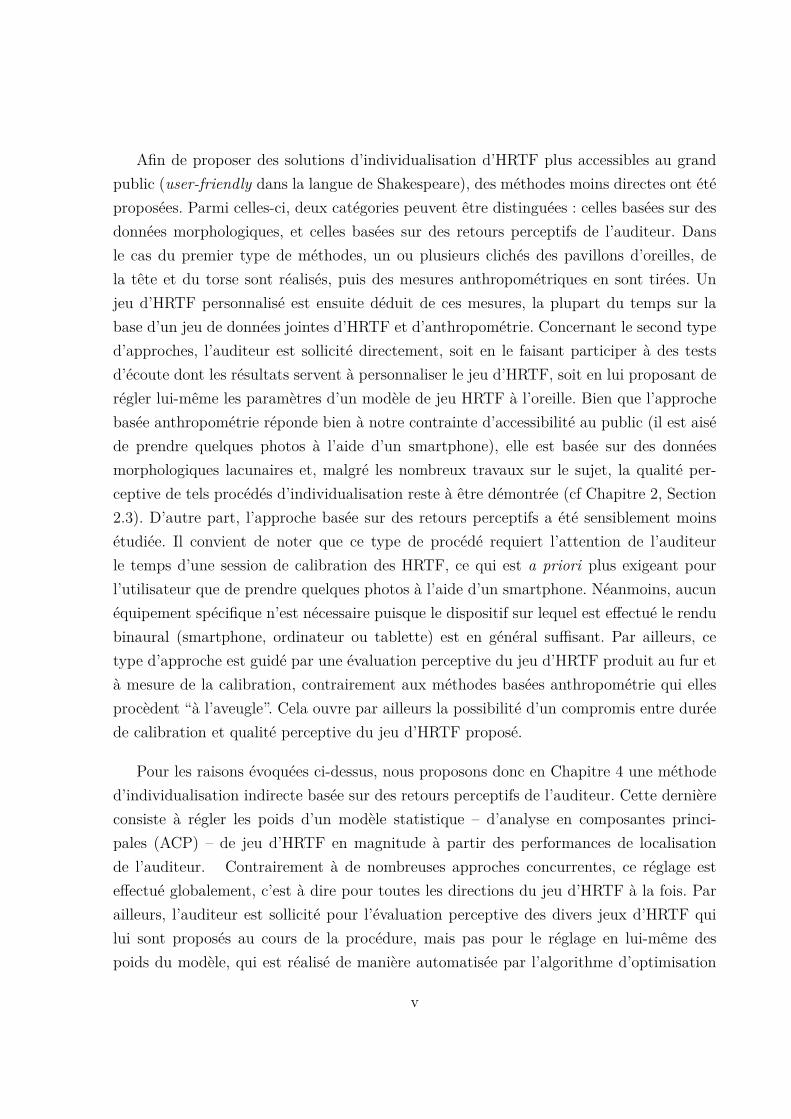
Afin de proposer des solutions d’individualisation d’HRTF plus accessibles au grandpublic (user-friendly dans la langue de Shakespeare), des méthodes moins directes ont étéproposées. Parmi celles-ci, deux catégories peuvent être distinguées : celles basées sur desdonnées morphologiques, et celles basées sur des retours perceptifs de l’auditeur. Dansle cas du premier type de méthodes, un ou plusieurs clichés des pavillons d’oreilles, dela tête et du torse sont réalisés, puis des mesures anthropométriques en sont tirées. Unjeu d’HRTF personnalisé est ensuite déduit de ces mesures, la plupart du temps sur labase d’un jeu de données jointes d’HRTF et d’anthropométrie. Concernant le second typed’approches, l’auditeur est sollicité directement, soit en le faisant participer à des testsd’écoute dont les résultats servent à personnaliser le jeu d’HRTF, soit en lui proposant derégler lui-même les paramètres d’un modèle de jeu HRTF à l’oreille. Bien que l’approchebasée anthropométrie réponde bien à notre contrainte d’accessibilité au public (il est aiséde prendre quelques photos à l’aide d’un smartphone), elle est basée sur des donnéesmorphologiques lacunaires et, malgré les nombreux travaux sur le sujet, la qualité per-ceptive de tels procédés d’individualisation reste à être démontrée (cf Chapitre 2, Section2.3). D’autre part, l’approche basée sur des retours perceptifs a été sensiblement moinsétudiée. Il convient de noter que ce type de procédé requiert l’attention de l’auditeurle temps d’une session de calibration des HRTF, ce qui est a priori plus exigeant pourl’utilisateur que de prendre quelques photos à l’aide d’un smartphone. Néanmoins, aucunéquipement spécifique n’est nécessaire puisque le dispositif sur lequel est effectué le rendubinaural (smartphone, ordinateur ou tablette) est en général suffisant. Par ailleurs, cetype d’approche est guidé par une évaluation perceptive du jeu d’HRTF produit au fur età mesure de la calibration, contrairement aux méthodes basées anthropométrie qui ellesprocèdent “à l’aveugle”. Cela ouvre par ailleurs la possibilité d’un compromis entre duréede calibration et qualité perceptive du jeu d’HRTF proposé.
Pour les raisons évoquées ci-dessus, nous proposons donc en Chapitre 4 une méthoded’individualisation indirecte basée sur des retours perceptifs de l’auditeur. Cette dernièreconsiste à régler les poids d’un modèle statistique – d’analyse en composantes princi-pales (ACP) – de jeu d’HRTF en magnitude à partir des performances de localisationde l’auditeur. Contrairement à de nombreuses approches concurrentes, ce réglage esteffectué globalement, c’est à dire pour toutes les directions du jeu d’HRTF à la fois. Parailleurs, l’auditeur est sollicité pour l’évaluation perceptive des divers jeux d’HRTF quilui sont proposés au cours de la procédure, mais pas pour le réglage en lui-même despoids du modèle, qui est réalisé de manière automatisée par l’algorithme d’optimisation
v
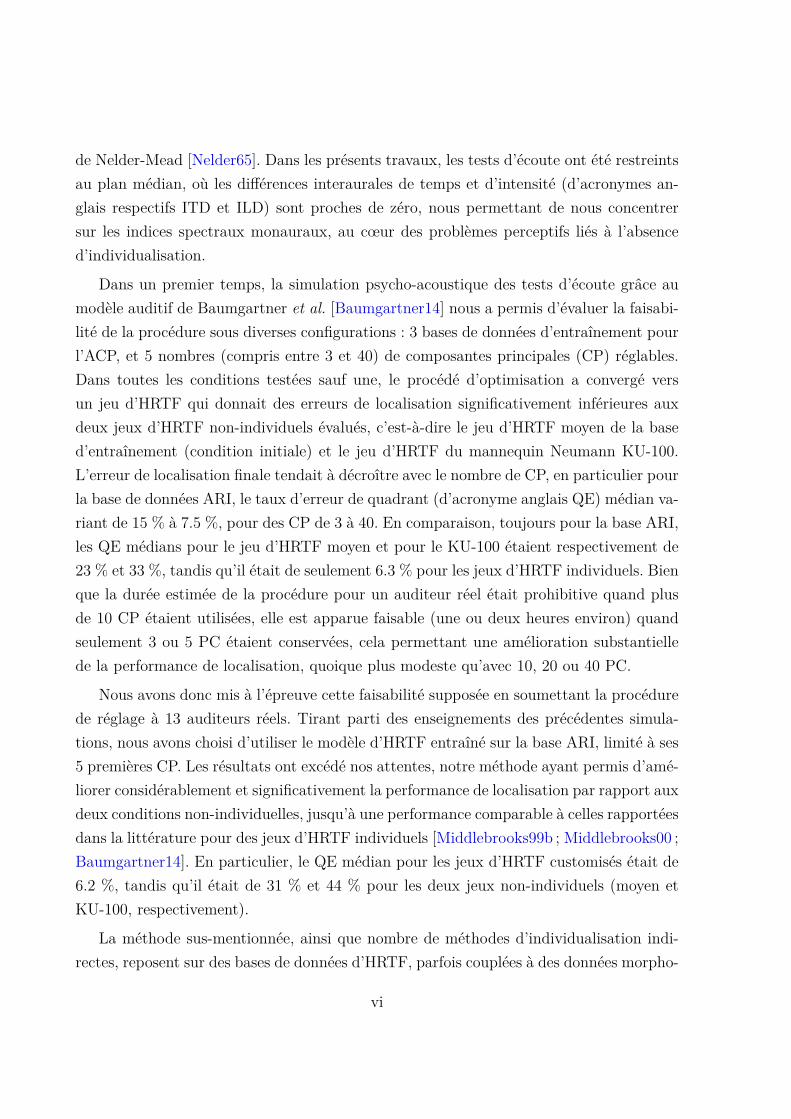
de Nelder-Mead [Nelder65]. Dans les présents travaux, les tests d’écoute ont été restreintsau plan médian, où les différences interaurales de temps et d’intensité (d’acronymes an-glais respectifs ITD et ILD) sont proches de zéro, nous permettant de nous concentrersur les indices spectraux monauraux, au cœur des problèmes perceptifs liés à l’absenced’individualisation.
Dans un premier temps, la simulation psycho-acoustique des tests d’écoute grâce aumodèle auditif de Baumgartner et al. [Baumgartner14] nous a permis d’évaluer la faisabi-lité de la procédure sous diverses configurations : 3 bases de données d’entraînement pourl’ACP, et 5 nombres (compris entre 3 et 40) de composantes principales (CP) réglables.Dans toutes les conditions testées sauf une, le procédé d’optimisation a convergé versun jeu d’HRTF qui donnait des erreurs de localisation significativement inférieures auxdeux jeux d’HRTF non-individuels évalués, c’est-à-dire le jeu d’HRTF moyen de la based’entraînement (condition initiale) et le jeu d’HRTF du mannequin Neumann KU-100.L’erreur de localisation finale tendait à décroître avec le nombre de CP, en particulier pourla base de données ARI, le taux d’erreur de quadrant (d’acronyme anglais QE) médian va-riant de 15 % à 7.5 %, pour des CP de 3 à 40. En comparaison, toujours pour la base ARI,les QE médians pour le jeu d’HRTF moyen et pour le KU-100 étaient respectivement de23 % et 33 %, tandis qu’il était de seulement 6.3 % pour les jeux d’HRTF individuels. Bienque la durée estimée de la procédure pour un auditeur réel était prohibitive quand plusde 10 CP étaient utilisées, elle est apparue faisable (une ou deux heures environ) quandseulement 3 ou 5 PC étaient conservées, cela permettant une amélioration substantiellede la performance de localisation, quoique plus modeste qu’avec 10, 20 ou 40 PC.
Nous avons donc mis à l’épreuve cette faisabilité supposée en soumettant la procédurede réglage à 13 auditeurs réels. Tirant parti des enseignements des précédentes simula-tions, nous avons choisi d’utiliser le modèle d’HRTF entraîné sur la base ARI, limité à ses5 premières CP. Les résultats ont excédé nos attentes, notre méthode ayant permis d’amé-liorer considérablement et significativement la performance de localisation par rapport auxdeux conditions non-individuelles, jusqu’à une performance comparable à celles rapportéesdans la littérature pour des jeux d’HRTF individuels [Middlebrooks99b ; Middlebrooks00 ;Baumgartner14]. En particulier, le QE médian pour les jeux d’HRTF customisés était de6.2 %, tandis qu’il était de 31 % et 44 % pour les deux jeux non-individuels (moyen etKU-100, respectivement).
La méthode sus-mentionnée, ainsi que nombre de méthodes d’individualisation indi-rectes, reposent sur des bases de données d’HRTF, parfois couplées à des données morpho-
vi
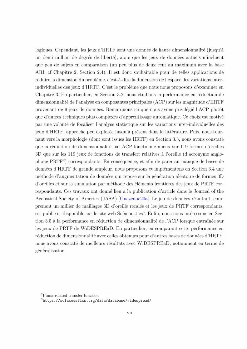
logiques. Cependant, les jeux d’HRTF sont une donnée de haute dimensionnalité (jusqu’àun demi million de degrés de liberté), alors que les jeux de données actuels n’incluentque peu de sujets en comparaison (un peu plus de deux cent au maximum avec la baseARI, cf Chapitre 2, Section 2.4). Il est donc souhaitable pour de telles applications deréduire la dimension du problème, c’est-à-dire la dimension de l’espace des variations inter-individuelles des jeux d’HRTF. C’est le problème que nous nous proposons d’examiner enChapitre 3. En particulier, en Section 3.2, nous étudions la performance en réduction dedimensionnalité de l’analyse en composantes principales (ACP) sur les magnitude d’HRTFprovenant de 9 jeux de données. Remarquons ici que nous avons privilégié l’ACP plutôtque d’autres techniques plus complexes d’apprentissage automatique. Ce choix est motivépar une volonté de focaliser l’analyse statistique sur les variations inter-individuelles desjeux d’HRTF, approche peu explorée jusqu’à présent dans la littérature. Puis, nous tour-nant vers la morphologie (dont sont issues les HRTF) en Section 3.3, nous avons constatéque la réduction de dimensionnalité par ACP fonctionne mieux sur 119 formes d’oreilles3D que sur les 119 jeux de fonctions de transfert relatives à l’oreille (d’acronyme anglo-phone PRTF2) correspondants. En conséquence, et afin de parer au manque de bases dedonnées d’HRTF de grande ampleur, nous proposons et implémentons en Section 3.4 uneméthode d’augmentation de données qui repose sur la génération aléatoire de formes 3Dd’oreilles et sur la simulation par méthode des éléments frontières des jeux de PRTF cor-respondants. Ces travaux ont donné lieu à la publication d’article dans le Journal of theAcoustical Society of America (JASA) [Guezenoc20a]. Le jeu de données résultant, com-prenant un millier de maillages 3D d’oreille recalés et les jeux de PRTF correspondants,est public et disponible sur le site web Sofacoustics3. Enfin, nous nous intéressons en Sec-tion 3.5 à la performance en réduction de dimensionnalité de l’ACP lorsque entraînée surles jeux de PRTF de WiDESPREaD. En particulier, en comparant cette performance enréduction de dimensionnalité avec celles obtenues pour d’autres bases de données d’HRTF,nous avons constaté de meilleurs résultats avec WiDESPREaD, notamment en terme degénéralisation.
2Pinna-related transfer function3https://sofacoustics.org/data/database/widespread/
vii


TABLE OF CONTENTS
Introduction 1
1 Background 51.1 Human Auditory Localization . . . . . . . . . . . . . . . . . . . . . . . . . 5
1.1.1 Coordinate System . . . . . . . . . . . . . . . . . . . . . . . . . . . 51.1.2 Interaural Cues . . . . . . . . . . . . . . . . . . . . . . . . . . . . . 71.1.3 Monaural Spectral Cues . . . . . . . . . . . . . . . . . . . . . . . . 91.1.4 Dynamic Cues . . . . . . . . . . . . . . . . . . . . . . . . . . . . . . 111.1.5 Perceptual Sensitivity and Accuracy . . . . . . . . . . . . . . . . . 11
1.2 Modeling the Localization Cues . . . . . . . . . . . . . . . . . . . . . . . . 131.2.1 Head-Related Transfer Function . . . . . . . . . . . . . . . . . . . . 131.2.2 Pinna-Related Transfer Function . . . . . . . . . . . . . . . . . . . 151.2.3 Directional Transfer Function . . . . . . . . . . . . . . . . . . . . . 16
1.3 Binaural Synthesis . . . . . . . . . . . . . . . . . . . . . . . . . . . . . . . 191.3.1 Binaural Reproduction Techniques . . . . . . . . . . . . . . . . . . 191.3.2 Individualization - Impact on Perception . . . . . . . . . . . . . . . 20
2 State of the Art 232.1 HRTF Modeling . . . . . . . . . . . . . . . . . . . . . . . . . . . . . . . . . 23
2.1.1 Filters . . . . . . . . . . . . . . . . . . . . . . . . . . . . . . . . . . 242.1.2 Spatial Frequency Response Surfaces . . . . . . . . . . . . . . . . . 272.1.3 Statistical Modeling . . . . . . . . . . . . . . . . . . . . . . . . . . 30
2.2 Evaluation of HRTF Sets . . . . . . . . . . . . . . . . . . . . . . . . . . . . 342.2.1 Objective Metrics . . . . . . . . . . . . . . . . . . . . . . . . . . . . 342.2.2 Subjective Evaluation . . . . . . . . . . . . . . . . . . . . . . . . . . 352.2.3 Localization Prediction . . . . . . . . . . . . . . . . . . . . . . . . . 39
2.3 HRTF Individualization Techniques . . . . . . . . . . . . . . . . . . . . . . 432.3.1 Acoustic Measurement . . . . . . . . . . . . . . . . . . . . . . . . . 432.3.2 Numerical Simulation . . . . . . . . . . . . . . . . . . . . . . . . . . 48
ix
TABLE OF CONTENTS
2.3.3 Indirect Individualization based on Morphological Data . . . . . . . 572.3.4 Indirect Individualization based on Perceptual Feedback . . . . . . 62
2.4 HRTF Databases . . . . . . . . . . . . . . . . . . . . . . . . . . . . . . . . 692.4.1 Acoustically Measured . . . . . . . . . . . . . . . . . . . . . . . . . 692.4.2 Numerically Simulated . . . . . . . . . . . . . . . . . . . . . . . . . 72
3 Dimensionality Reduction and Data Augmentation of Head-Related Trans-fer Functions 753.1 The FAST Dataset: 119 Ear Meshes and Matching Simulated Pinna-Related
Transfer Functions . . . . . . . . . . . . . . . . . . . . . . . . . . . . . . . 763.1.1 Ear Meshes . . . . . . . . . . . . . . . . . . . . . . . . . . . . . . . 763.1.2 PRTFs: Numerical Simulations . . . . . . . . . . . . . . . . . . . . 81
3.2 Dimensionality Reduction of HRTFs . . . . . . . . . . . . . . . . . . . . . . 893.2.1 Principal Component Analysis of Log-Magnitude HRTFs . . . . . . 903.2.2 Cumulative Percentage of Total Variation of 9 Datasets . . . . . . . 953.2.3 Reconstruction Error Distribution . . . . . . . . . . . . . . . . . . . 101
3.3 Compared Dimensionality Reductions of EarShapes and Matching PRTF Sets . . . . . . . . . . . . . . . . . . . . . . . 1073.3.1 Principal Component Analysis of Ear Shapes . . . . . . . . . . . . . 1073.3.2 Comparison of Both PCA Models . . . . . . . . . . . . . . . . . . . 111
3.4 Dataset Augmentation . . . . . . . . . . . . . . . . . . . . . . . . . . . . . 1133.4.1 Random Generation of Ear Meshes . . . . . . . . . . . . . . . . . . 1133.4.2 Numerical Simulations . . . . . . . . . . . . . . . . . . . . . . . . . 1163.4.3 Visualization of the Augmented Dataset . . . . . . . . . . . . . . . 117
3.5 Dimensionality Reduction of the AugmentedPRTF Dataset . . . . . . . . . . . . . . . . . . . . . . . . . . . . . . . . . . 1193.5.1 Cumulative Percentage of Total Variation . . . . . . . . . . . . . . 1193.5.2 Cross-Validation . . . . . . . . . . . . . . . . . . . . . . . . . . . . 121
3.6 Conclusion & Perspectives . . . . . . . . . . . . . . . . . . . . . . . . . . . 125
4 Individualization of Head-Related Transfer Functions based on Percep-tual Feedback 1294.1 Introduction . . . . . . . . . . . . . . . . . . . . . . . . . . . . . . . . . . . 1294.2 Method . . . . . . . . . . . . . . . . . . . . . . . . . . . . . . . . . . . . . 131
4.2.1 HRTF Model . . . . . . . . . . . . . . . . . . . . . . . . . . . . . . 131
x

TABLE OF CONTENTS
4.2.2 Cost Function . . . . . . . . . . . . . . . . . . . . . . . . . . . . . . 1334.2.3 Optimization Algorithm . . . . . . . . . . . . . . . . . . . . . . . . 134
4.3 Simulated Listening Tests . . . . . . . . . . . . . . . . . . . . . . . . . . . 1364.3.1 Auditory Model . . . . . . . . . . . . . . . . . . . . . . . . . . . . . 1364.3.2 Configurations . . . . . . . . . . . . . . . . . . . . . . . . . . . . . . 1364.3.3 Results . . . . . . . . . . . . . . . . . . . . . . . . . . . . . . . . . . 137
4.4 Actual Listening Tests . . . . . . . . . . . . . . . . . . . . . . . . . . . . . 1514.4.1 Localization Task . . . . . . . . . . . . . . . . . . . . . . . . . . . . 1524.4.2 Results . . . . . . . . . . . . . . . . . . . . . . . . . . . . . . . . . . 155
4.5 Conclusion & Perspectives . . . . . . . . . . . . . . . . . . . . . . . . . . . 165
Conclusion & Perspectives 169Summary . . . . . . . . . . . . . . . . . . . . . . . . . . . . . . . . . . . . . . . 169Perspectives . . . . . . . . . . . . . . . . . . . . . . . . . . . . . . . . . . . . . . 172One Last Perceptual Experiment . . . . . . . . . . . . . . . . . . . . . . . . . . 174
Bibliography 179
A Abbreviations 211
B Publications 213
xi

INTRODUCTION
This PhD was carried out in Rennes within the 3D Sound Labs company and the FacialAnalysis, Synthesis and Tracking (FAST) research team of the Institute of Electronics andTelecommunications of Rennes (IETR, UMR CNRS 6164) located at CentraleSupélec.It falls within the principal research and development project of the former: providingindividualized binaural synthesis to the public. After 3D Sound Labs closed its doors inFebruary 2019 (halfway through the PhD), this work was carried on within the FASTteam.
Our auditory system allows us to localize sound sources thanks to two audio signalsperceived at the left and right ear drums. To achieve that, the human auditory systemrelies on monaural and interaural, spectrum-, time- and level-based auditory cues. Thesecues originate in the reflections and diffraction of sound on its path from the sound sourceto the ear drums. In other words, our head, torso and pinnae4 perform a directionalacoustic filtering of incoming sounds. By reproducing these cues appropriately in the leftand right channel of a headphone or earbuds, the brain can be fooled into perceiving athree-dimensional virtual auditory scene (VAS). Unlike stereo, this technique, called bin-aural reproduction, allows the perception of sound from every direction in space, includingalong the vertical dimension.
Other techniques render 3-D VASs over loudspeakers, such as wave field synthesis orhigh-order Ambisonics [Furness90]. However, these require a large number of carefullypositioned loudspeakers and, as any loudspeaker-based restitution, are often degraded bythe surrounding room. In this regard, binaural rendition has a considerable advantage: itonly requires a common and inexpensive piece of equipment to work, i.e. a standard pairof headphones or earbuds. Moreover, room effect is ruled out of the equation.
The historical approach to binaural reproduction, still well-used to this day, is torecord a sound scene through a pair of microphones placed in a person or an anthropo-morphic manikin’s ear canals. The two-channel audio signal is then played-back throughheadphones. The main limitation of this technique is that the listener’s point of view onthe sound scene is determined by the position or trajectory of the pair of microphones at
4Pinna: latin for external ears.
1
Introduction
recording time, and cannot be modified afterwards. For instance, at the time of play-back,if the listener turns his head, the VAS follows that movement (while a stationary scenewould be more immersive).
However, another approach called binaural synthesis overcomes this limitation, byrendering the VAS at the time of play-back. The idea is, for every virtual sound source,to filter the mono signal by the adequate pair of head-related transfer functions (HRTFs)which include the localization cues that correspond to the desired sound direction. Usingthis technique, a VAS can be adapted in real time to the listener’s orientation thanks toa head-tracker device. More importantly, a completely synthetic VAS, i.e. constitutedof a number of virtual sound sources moving around the 3-D space, can be renderedbinaurally. This aspect is essential for video games, and is particularly suited for virtualand augmented realities, contexts in which the user wears headphones and seeks 3-Dimmersion through vision, sound and movement.
HRTFs, deriving from the acoustic filtering effect of one’s head, torso and pinnae,depend not only on sound source position but on morphology, which makes them specificto each listener. Nevertheless, binaural synthesis is generally performed using a generic(non-individualized) HRTF set, which can cause discrepancies such as front-back inver-sions, erroneous perception of the elevation and weak externalization (see Section 1.3.2,[Wenzel93; Kim05]).
Indeed, as we will see in Section 2.3 of Chapter 2, the obtention of individual HRTFsis far from trivial. For instance, the historical and state-of-the-art method to acquireindividual HRTFs, acoustic measurement, is cumbersome and unsuitable for an end-userapplication. Indeed, it requires a heavy apparatus and an anechoic room, which makesthe setup untransportable. As an alternative, it has been proposed to numerically simu-late these measurement sessions from 3-D scans of the listener’s pinnae, head and torso.While professional-grade, the scanning equipment is generally easily transportable, andthe measurement session reasonably short – in the order of 15 minutes. However, be-tween the scanning session, the processing of the 3-D meshes, and the simulation itself,the process in its entirety takes a long time (in the order of several hours) and requiresconsiderable computing power. More importantly, the quality of such computed HRTFsis still to be demonstrated.
Focusing on the user-friendly aspect of HRTF individualization, less direct methodshave been proposed to obtain individual HRTFs. Among these, two categories can bedistinguished: those based on morphological information, and those based on subjective
2
Introduction
feedback from the listener. In the first one, one or several pictures of the pinnae and/orhead and torso are taken and anthropometric measurements derived from them. Then,a personalized HRTF set is inferred from the anthropometric data, most often based ona dataset of both HRTFs and anthropometry. In the second category, the listener eithertunes the parameters of an HRTF set model while listening to it, or he participates inlistening experiments whose outcomes serve to personalize the HRTF set. While theanthropometry-based approach answers well our constraint of user-friendliness – it isindeed easy to take a few pictures with a smartphone, it is based on sparse morphologicalinformation and, despite the quantity of work on the subject, the perceptual quality ofsuch individualization processes remains to be established (see Chapter 2, Section 2.3).On the other hand, approaches based on perceptual feedback from the listener have beenless studied. Such individualization processes require the listener to be attentive for theduration of a tuning session, which may be less practical than taking a few pictures with asmartphone. They however require no specific equipment (a smartphone, a PC, a tablet:any device on which the binaural synthesis is performed) and are actually based on aperceptual evaluation of the resulting HRTFs. In other words, this family of approachesdo not go blindly about individualizing the HRTFs, they do it from some knowledge ofthe perceptual result. Furthermore, a trade-off is possible between the cumbersomenessof the process and the perceptual quality of the resulting HRTF set. In that sense, thisless-explored approach is particularly interesting, which is why we propose and evaluatesuch a method in Chapter 4.
These user-friendly methods generally rely on databases of HRTFs, sometimes coupledwith morphological data. For instance, in the approach that we present in Chapter 4, wepropose to tune the parameters of a statistical model of HRTF set based on evaluations ofthe listener’s localization performance. However, HRTF sets are a high-dimensional data(up to half a million degrees of freedom), whereas current datasets include few subjectsin comparison (up to two hundred, see Chapter 2, Section 2.4). It is thus desirable forsuch applications to reduce the dimensionality of the problem – that is the variations ofHRTF sets across individuals.
As a consequence, in Chapter 3, we explore the matter of reducing the dimensionalityof magnitude HRTF sets. In particular, in Section 3.2, we investigate the dimensionalityreduction performance of principal component analysis (PCA) on magnitude HRTFs fromvarious datasets. Let us point out that we chose PCA over more complex techniquesbecause we wanted to perform statistical modeling in a way that focuses on the inter-
3
Introduction
subject variations of HRTF sets, which has barely been studied in the literature so far. InSection 3.3 we compare the dimensionality reduction performance of PCA on 119 pinna3-D shapes with that of 119 matching sets of pinna-related transfer functions (PRTFs).In Section 3.4, in order to alleviate the lack of large-scale HRTF datasets, we propose andimplement a data augmentation method that relies on random generations of ear shapesand numerical simulations of the matching PRTF sets. This work has been published inan article of the Journal of the Acoustical Society of America (JASA) [Guezenoc20a]. Theresulting dataset, comprising over a thousand 3-D ear meshes and matching PRTF sets,was made available on-line on the Sofacoustics website5. In Section 3.5, we investigate theimpact on dimensionality reduction performance of using this augmented PRTF dataset,which was published and presented at the 148th convention of the Audio EngineeringSociety (AES) [Guezenoc20b].
This manuscript is organized as follows. In Chapter 1 and Chapter 2, we cover back-ground notions regarding binaural synthesis and establish a state-of-the-art of HRTFindividualization techniques and databases. In Chapter 3, we deal with the statisticalmodeling and dimensionality reduction of magnitude HRTF sets. Contributions in thisrespect are five-fold. First, we present the constitution of a dataset of 119 3-D ear meshesand matching simulated PRTF sets, named FAST. Second, we look into the capacityof PCA to reduce the dimensionality of magnitude HRTF sets for FAST and 8 publicdatasets. Third, focusing on FAST, we compare the dimensionality reduction perfor-mance of PCA on its ear point clouds and on its matching magnitude PRTF sets. Fourth,based on the results of these two studies, we present a data augmentation method thatrelies on random generations of pinna meshes and numerical simulations of the correspond-ing PRTF sets. Fifth, we study the impact on dimensionality reduction performance ofusing this augmented PRTF dataset for training. Finally, in Chapter 4, we present alow-cost HRTF individualization method which consists in tuning the weights of a PCAmodel of magnitude HRTF set based on localization performance. First, we investigateits feasibility under various configurations by simulating the localization tasks thanks toan auditory model [Baumgartner14]. Second, the tuning procedure is submitted to 12actual listeners.
5https://sofacoustics.org/data/database/widespread/
4
Chapter 1
BACKGROUND
Thanks to only two audio signals perceived at the eardrums, the human brain is ableto capture the spatial characteristics of surrounding sound sources. This psycho-acousticprocess relies on auditory cues created by the alterations of sound on its acoustic path tothe eardrums. Such cues depend not only on the room and the position of the acousticsource, but also on the listener’s morphology. By reproducing them over headphones orear-buds, it is possible, thanks to a process called binaural synthesis, to create a virtualauditory environment that imitates natural sound localization.
In this chapter, we go over the fundamentals of human auditory localization andbinaural reproduction over headphone. First, we look into the mechanisms and auditorycues involved in sound localization. Second, we introduce signal processing concepts usedto model these cues, namely the head-related transfer function (HRTF) and its derivatives,the pinna-related and directional transfer functions (PRTFs and DTFs, respectively).Third, we present binaural synthesis and discuss why it can and should be individualized.Finally, several important HRTF models are reviewed.
1.1 Human Auditory Localization
The human brain relies on various auditory cues to localize surrounding sound. Afterdefining a listener-related coordinate system, we go over these interaural, monaural anddynamic cues. Finally, we discuss the sensitivity and accuracy of the human auditorylocalization system.
1.1.1 Coordinate System
Throughout this thesis, we will discuss the location of incoming sound sources relativeto listener perception. Hence, before going on, let us introduce tools and terminology todescribe spatial positions relative to the listener.
5

Chapter 1 – Background
Figure 1.1 – The head-related coordinate system used throughout this thesis and theplanes of interest named after standard anatomical terminology (source: [Richter19]). θand ϕ denote the azimuth and elevation angles, respectively.
The axis that goes through both ears is referred to as the interaural axis. The centerof the head and origin of the head-related coordinate system is usually defined as themiddle point of the interaural segment. In coherence with the standard anatomical termsof location [Behnke12, Chap. 2], the vertical and horizontal planes that contain this axisare called the frontal and horizontal planes, respectively. The vertical plane, orthogonalto the interaural axis, that crosses it in the center of the head is called the median plane.A plane parallel to the median plane is called sagittal plane.
The Cartesian axes used throughout this thesis are the following. The x-axis standsfor the front-back axis, defined by the intersection of the horizontal and median plane andoriented frontward. The y-axis is the interaural axis, oriented towards the listener’s left.Finally, the z-axis represents the up-down direction and is orthogonal to the horizontalplane, oriented upward.
Several egocentric coordinate systems have been used in the literature that deals withauditory localization. The most widespread one is the spherical system, which uses az-imuth and elevation angles θ and ϕ and a distance parameter r defined by the distancefrom sound source to origin. The convention adopted in this thesis is that azimuths rangefrom -180 to 180 (back to back) and elevations from -90 to 90 (bottom to top). The
6
1.1. Human Auditory Localization
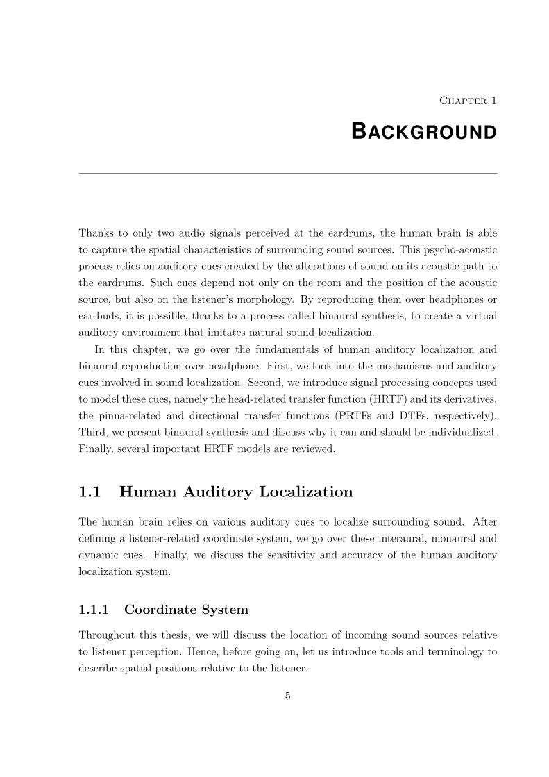
Figure 1.2 – The interaural-polar coordinate system (source: [Morimoto84]). S: soundsource, O: center of the head / origin, r: distance between sound source and origin, θ:azimuth, ϕ: elevation, α: interaural angle, β: rising or polar angle.
direction of zero azimuth and zero elevation is located in front of the listener.An alternative is the interaural-polar system introduced by Morimoto and Aokata
[Morimoto84], deemed more adequate to sound localization. While the distance parameteris the same as in the spherical system, the rising or polar angle β is defined as the anglefrom the horizontal plane to the plane that contains the sound source and the interauralaxis. As for the lateral angle α, it is defined as the angle from the median plane to thesagittal plane that contains the source.
1.1.2 Interaural Cues
Although early experiments on binaural hearing can be traced back to the late XVIIIth
century with Venturi (1796) and Wells (1792) [Wade08]1, Lord Rayleigh has arguablylaid the foundations of our modern understanding of sound localization at the end of theXIXth century, with his “duplex” theory [Rayleigh07]. Experimenting with pure tones, hedetermined that left-right discrimination can be imputed to two types of cues: interauraltime differences (ITDs) and interaural level differences (ILDs).
Interaural time difference For most directions, incoming sound waves reach one earbefore the other due to the distance between both ears and head diffraction. ITD varieswith source direction, starting at zero in the median plane area and reaching a maximum
1For a detailed account of the history of the study of binaural hearing, we advise to read Wade andDeutsch’s work [Wade08].
7

Chapter 1 – Background
on the left and right sides. This maximal value is of 709 µs on average, with a standarddeviation of 32 µs, for a population of 33 adult subjects [Middlebrooks99a].
ITD can be well approximated using geometric models. One of the first well-knownones is the one by Woodworth [Woodworth54, Chap. 12]. Assuming a hard spherical headand a far sound source located in the horizontal plane, the ITD is modeled as
ITD(θ) = ∆d(θ)c
= r(θ + sin(θ))c
, (1.1)
where ∆d is the path difference, r is the head radius, c the velocity of sound and θ ∈[0, π2 ] is the azimuth. Other models have been proposed in order to generalize the modelto other frequency ranges [Kuhn77], sound source directions [Larcher97; Savioja99], ormore complex geometrical models such as a variable position of the pinnae [Busson06;Ziegelwanger14a] and an ellipsoidal head shape [Bomhardt16c]. A more thorough state-of-the-art of ITD models can be found in Baumhardt’s PhD thesis [Bomhardt17].
Interaural level difference For most incoming sound directions, acoustic pressure isgreater at the ipsilateral2 ear than at the contralateral3 one. The phenomenon is mostlydue to head diffraction. As the wavelength decreases (and frequency increases), the headis more and more of an obstacle to sound waves, leading to larger ILDs. ILD varies withsound direction, starting at zero in the median plane area and reaching maximal values inlateral positions. For instance, Middlebrooks and Green report a maximal ILD of 20 dBat 4 kHz and 35 dB at 10 kHz for an azimuth of θ = 90 [Middlebrooks90].
Perceptual importance of both cues The respective roles of ITD and ILD in lat-eral perception vary with frequency. For frequencies below approximately 1.5 kHz, i.e.wavelengths lower than the head width (14.5 cm on average4), ILDs are small and ITDis the predominant cue [Rayleigh07; Wightman92; Macpherson02]. Above 1.5 kHz, ILDbecomes the predominant cue, as listener sensitivity to ITD decreases and ILD ampli-tude increases (diffraction is stronger for smaller wavelengths) [Rayleigh07; Kulkarni99;Macpherson02]. While the decrease in phase sensitivity is easily explainable in the caseof pure tones, where the interaural phase difference is ambiguous for small wavelengths
2On the same side of the head as the incoming sound source.3On the side of the head opposite to the incoming sound source.4Source: The DINBelg 2005 campaign of anthropometric measurements of the Belgian population
http://dinbelg.be/anthropometrie.htm.
8
1.1. Human Auditory Localization
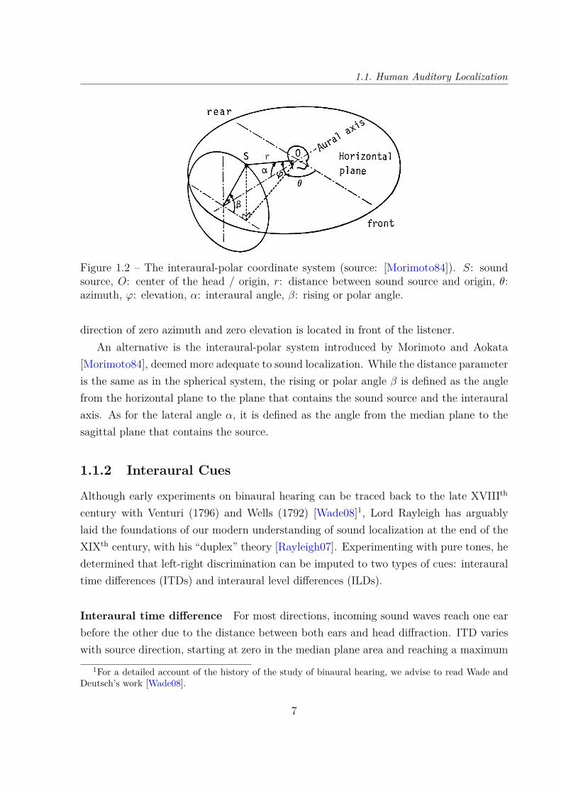
Figure 1.3 – Iso-ITD (in µs) and iso-ILD (in dB) contours of one human listener, on aglobe that represents the directions of incidence (source: [Wightman99]). The direction ofzero longitude/azimuth and zero latitude/elevation is faced by the listener, and the middleof the interaural axis coincides with the origin (same head-related coordinate system asin Figure 1.1).
[Rayleigh07], the psycho-acoustic mechanism remains unclear for signals with a largerband. However, ITD seems to be more important than ILD for localization as long aslow-frequency phase information is present [Wightman92; Macpherson02].
1.1.3 Monaural Spectral Cues
While the perception of laterality is based on ITD and ILD, these cues are ambiguousin certain directions. As can be seen in Figure 1.3, iso-ITD and iso-ILD curves looselycorrespond to circles contained by a sagittal plane, forming with the center of the head theso-called “cones of confusion” [Blauert97, Chap. 2, Sec. 5]. As a consequence, elevationand front-back discrimination can not be derived from ITD and ILD.
This information is provided to the human auditory system by monaural spectral cues.More particularly, high-frequency content (> 4 kHz) is critical for sound localization alongthe cones of confusion [Morimoto84; Hebrank74; Asano90].
At these frequencies, the peaks and notches caused by constructive and destructiveinterference in the external ear are predominant spectral features, and vary considerablywith sound direction [Shaw68; Takemoto12] (see Figure 1.4) and pinna morphology. Usingnumerical simulations, Takemoto et al. [Takemoto12] establishes a thorough analysis ofthe link between resonances in the pinna and spectral patterns perceived at the ear canalentrance.
9

Chapter 1 – Background
Figure 1.4 – Figure reproduced from [Takemoto12], illustrating resonances and anti-resonances in the pinna responsible for notches in the magnitude spectra of PRTFs, foran exemplary subject. The upper panel shows magnitude PRTFs in the median plane,in dB. The lower panels show the matching distribution patterns of pressure nodes andanti-nodes on the pinna. Arrows represent the source direction.
10

1.1. Human Auditory Localization
To a lesser extent, low-frequency features generated by the head and torso (< 3 kHz)can also sometimes convey useful cues for intra-conic localization [Asano90; Algazi01a].
1.1.4 Dynamic Cues
A complementary way to dispel the confusions that can occur on the sagittal planesis movement. Indeed, when the listener turns his head relatively to the sound source(or the other way around), the auditory cues are perceived for various subsequent posi-tions, yielding precious additional information [Wallach40; Wightman99]. This is partic-ularly useful to make up for poor spectral content or simply to improve localization (in astatic set-up, front-back confusions sometimes occur even with broadband spectral cues[Bronkhorst95]). Furthermore, it would seem that dynamic cues override the monauralspectral ones [Blauert97, Chap. 2, Sec. 5].
1.1.5 Perceptual Sensitivity and Accuracy
Now that we have identified the mechanisms and cues used by the human auditory local-ization system, let us discuss its perceptual sensitivity and accuracy.
Interaural time difference In [Blauert97], Blauert summarizes the results of previouslateralization studies. He reports just noticeable difference (JND) ITD values between2 and 62 µs, depending on the sound level, stimulus and experimental protocol. Inaddition, the JND in ITD has been found to increase with the azimuth. In a recent study,using a protocol carefully selected based on previous work [Simon16], Andreopoulou etal. [Andreopoulou17] report JND values ranging from 40 µs at an azimuth of 0 to 85 µsat an azimuth of 90, in good agreement with previous research.
Interaural level difference In a study using pulse tones as stimuli, Mills [Mills60]reports median thresholds for ILD between 0.5 and 1 dB depending on the frequency(between 250 Hz and 10 kHz).
Spatial accuracy Many studies investigate the just noticeable difference in sound di-rection, or “localization blur”, as summarized in [Blauert97, Chap. 2, Sec. 1].
In the horizontal plane, localization accuracy is best in the frontal position, steadilydecreases exponentially towards the sides, and increases again towards the rear [Mills58;
11
Chapter 1 – Background
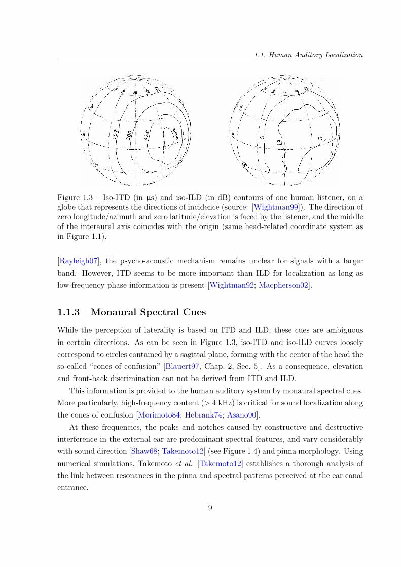
Figure 1.5 – Frequency response of a bank of 41 1-ERB-spaced 4th-order gammatone filtersbetween 20 Hz and 20 kHz.
Blauert97; Carlile97]. The order of magnitude of the localization blur in front, left-rightand back is of 4, 10 and 6 (according to Figure 2.2 of [Blauert97]).
In a study that includes various elevations, Carlile et al. report an average localizationerror of 3 in azimuth and 4 in elevation for short broadband stimuli [Carlile97]. Theyalso notice that the errors are smaller in the anterior hemisphere.
Additionally, localization blur depends on frequency in both horizontal and medianplanes, as reported by Mills in the case of pure tones [Mills58]. More generally, it de-pends greatly on the stimulus: for instance, vertical imprecision in the frontal directionis reported in studies mentioned in [Blauert97, Chap. 2, Sec. 1] to increase from 4 to 17
by changing the stimulus from a white noise to an unfamiliar voice.
Frequency resolution Due to how the cochlea treats sound, the frequency resolutionof the human auditory system is not uniform across the audible frequency range. Indeed,each hair cell along the organ of Corti is tuned to a certain frequency that depends on itslocation along the cochlea, resulting in higher sensitivity at low frequencies than at highones [Ehret78].
This processing effect of the cochlea can be approximated by the so-called “Patterson-Holdsworth” filter bank [Patterson92], a bank of fourth-order gammatone filters whosebandwidths follow the equivalent rectangular bandwidth (ERB) scale introduced by Glas-berg and Moore [Glasberg90]. This filter bank is plotted in Figure 1.5.
In the case of auditory localization, Breebaart and Kohlrausch [Breebaart01] reportthat smoothing non-individual spectral cues with a Patterson-Holdsworth filter bank does
12

1.2. Modeling the Localization Cues
not produce audible artifacts, even when using first-order gammatone filters (which areless selective than the fourth order ones). Furthermore, results from a study by Xieand Zhang [Xie10], in which the magnitude of individual spectral cues of six subjects atfrequencies above 5 kHz is smoothed using a moving frequency window, suggest that a pre-cision of 3.5 ERB for contralateral directions and 2 ERB elsewhere is sufficient. However,in their 2010 study, Breebaart and Nater argue that magnitude spectral cues smoothed us-ing a bank of overlapping 1-ERB spaced filters are advisable as a safe frequency resolutionfor accurate sound localization [Breebaart10].
In the case of non-overlapping filters, the spacing must however be finer. Indeed,according to the same study by Breebart and Nater, using non-overlapping 1-ERB spacedfilters instead of overlapping ones deteriorates the localization results. This is in accordwith results from a study by Rugeles and Emerit [Rugeles Ospina14], in which non-individual magnitude spectral cues are filtered using a bank of non-overlapping filters.Indeed, the results of the subjective evaluation with 12 subjects suggest that the 1
6th-octave
scale (roughly equivalent to 0.7 ERB) is too coarse. In contrast, a bank of non-overlapping112
th-octave filters seems not to produce audible alterations.
1.2 Modeling the Localization Cues
1.2.1 Head-Related Transfer Function
In the previous section, we presented different auditory cues used by the human auditorysystem to localize sound. These cues were identified in early experiments and associatedto a corresponding spatial and/or frequency domain of perceptual influence. However,taking a step back, these cues can be viewed as the result of the alterations of sound onits path from the sound source to the left and right ear drums.
Under the traditional assumption of a linear and time-invariant system, these alter-ations can be described by a left and a right transfer function, commonly called head-related transfer functions (HRTFs) [Møller92, Chap. 2, Sec. 2]. A widely used definitionis the one proposed by Blauert in the case of a free-field environment:
“The free-field transfer function relates sound pressure at a point of mea-surement in the auditory canal of the experimental subject to the sound pres-sure that would be measured, using the same sound source, at a point corre-sponding to the center of the head (i.e. at the origin of the coordinate system)while the subject is not present.” [Blauert97, Chap. 2, Sec. 2]
13

Chapter 1 – Background
In the Fourier domain, this definition translates to the following equation:
HRTFfree−field(f) ∆= P (f)Pref(f) , (1.2)
where P (f) refers to the Fourier transform of the sound pressure in the auditory canal,and Pref(f) refers to the Fourier transform of the reference pressure defined by Blauerti.e. the pressure at the origin in the absence of the head.
Throughout this thesis the term HRTF refers to this free-field definition. Its time-domain equivalent is referred to as the head-related impulse response (HRIR):
HRIR = F−1(HRTF ), (1.3)
where F−1 denotes the inverse Fourier transform.The fact that HRTFs are a function of frequency, sound source location, ear side and
listener can be a source of ambiguity in what is meant by terms such as HRTF, HRTFsor HRTF set. Let us clarify the terminology employed in this thesis:
• HRTF : a filter, for a given sound source location, ear side and listener,
• Pair of HRTFs / HRTF pair : the left- and righ-ear filters for a given sound sourcelocation and listener,
• Set of HRTFs / HRTF set: a collection of filters for a given listener, for varioussound source locations and ears.
The corresponding HRIR-related terms are to be understood in the same fashion.Further on, HRTFs are denoted
H(λ)(f, r, θ, ϕ) ∈ C,
where λ ∈ L,R denotes the left or right ear, (r, θ, ϕ) ∈ R+ × [0, 2π] × [−π2 ,
π2 ] is the
position of the sound source in the azimuth/elevation coordinate system, and f ∈ R+ isthe frequency.
However, most often the dependency to distance r is not considered
H(λ)(f, θ, ϕ) = H(λ)(f, r0, θ, ϕ).
14

1.2. Modeling the Localization Cues
0.2 1 10 18
-50
0
0.2 1 10 18-200
-100
0
0 1 2 3 4 5 6-0.05
0
0.05
Figure 1.6 – Exemplary HRTFs and HRIRs. Magnitude (top) and phase (middle) of theHRTFs and corresponding HRIRs (bottom) of subject NH8 of the ARI dataset, for 3horizontal directions of azimuths −90, 0 and 90.
Indeed, while range dependency can be simulated thanks to reverberation and/or atten-uation, rotations in a virtual acoustical space (VAS) rely completely on the directionalvariations of HRTFs. Furthermore, it is possible to extrapolate near-field HRTFs fromfar-field (r0 & 1.5 m) measurements [Pollow14].
For simplicity, when the ear side is irrelevant, an HRTF H(λ)(f, r, θ, ϕ) is denotedH(f, r, θ, ϕ).
1.2.2 Pinna-Related Transfer Function
As discussed in Section 1.1.3, the pinna is at the origin of complex acoustic resonances athigh frequencies that largely contribute to intra-conic5 localization.
5Intra-conic: within a cone of confusion.
15
Chapter 1 – Background
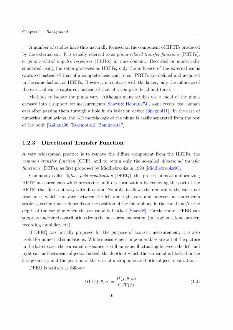
A number of studies have thus naturally focused on the component of HRTFs producedby the external ear. It is usually referred to as pinna-related transfer functions (PRTFs),or pinna-related impulse responses (PRIRs) in time-domain. Recorded or numericallysimulated using the same processes as HRTFs, only the influence of the external ear iscaptured instead of that of a complete head and torso. PRTFs are defined and acquiredin the same fashion as HRTFs. However, in contrast with the latter, only the influence ofthe external ear is captured, instead of that of a complete head and torso.
Methods to isolate the pinna vary. Although many studies use a mold of the pinnaencased into a support for measurements [Shaw68; Hebrank74], some record real humanears after passing them through a hole in an isolation device [Spagnol11]. In the case ofnumerical simulations, the 3-D morphology of the pinna is easily separated from the restof the body [Kahana06; Takemoto12; Bomhardt17].
1.2.3 Directional Transfer Function
A very widespread practice is to remove the diffuse component from the HRTFs, thecommon transfer function (CTF), and to retain only the so-called directional transferfunctions (DTFs), as first proposed by Middlebrooks in 1990 [Middlebrooks90].
Commonly called diffuse field equalization (DFEQ), this process aims at uniformizingHRTF measurements while preserving auditory localization by removing the part of theHRTFs that does not vary with direction. Notably, it allows the removal of the ear canalresonance, which can vary between the left and right ears and between measurementssessions, seeing that it depends on the position of the microphone in the canal and/or thedepth of the ear plug when the ear canal is blocked [Shaw68]. Furthermore, DFEQ cansuppress undesired contributions from the measurement system (microphone, loudspeaker,recording amplifier, etc).
If DFEQ was initially proposed for the purpose of acoustic measurement, it is alsouseful for numerical simulations. While measurement imponderables are out of the picturein the latter case, the ear canal resonance is still an issue, fluctuating between the left andright ear and between subjects. Indeed, the depth at which the ear canal is blocked in the3-D geometry and the position of the virtual microphone are both subject to variation.
DFEQ is written as follows:
DTF(f, θ, ϕ) = H(f, θ, ϕ)CTF(f) . (1.4)
16
1.2. Modeling the Localization Cues
0.2 1 10 18-40
-30
-20
0.2 1 10 18-1
0
1
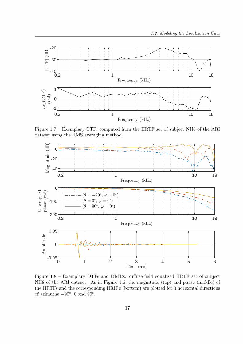
Figure 1.7 – Exemplary CTF, computed from the HRTF set of subject NH8 of the ARIdataset using the RMS averaging method.
0.2 1 10 18
-40
-20
0
0.2 1 10 18-200
-100
0
0 1 2 3 4 5 6-0.05
0
0.05
Figure 1.8 – Exemplary DTFs and DRIRs: diffuse-field equalized HRTF set of subjectNH8 of the ARI dataset. As in Figure 1.6, the magnitude (top) and phase (middle) ofthe HRTFs and the corresponding HRIRs (bottom) are plotted for 3 horizontal directionsof azimuths −90, 0 and 90.
17
Chapter 1 – Background
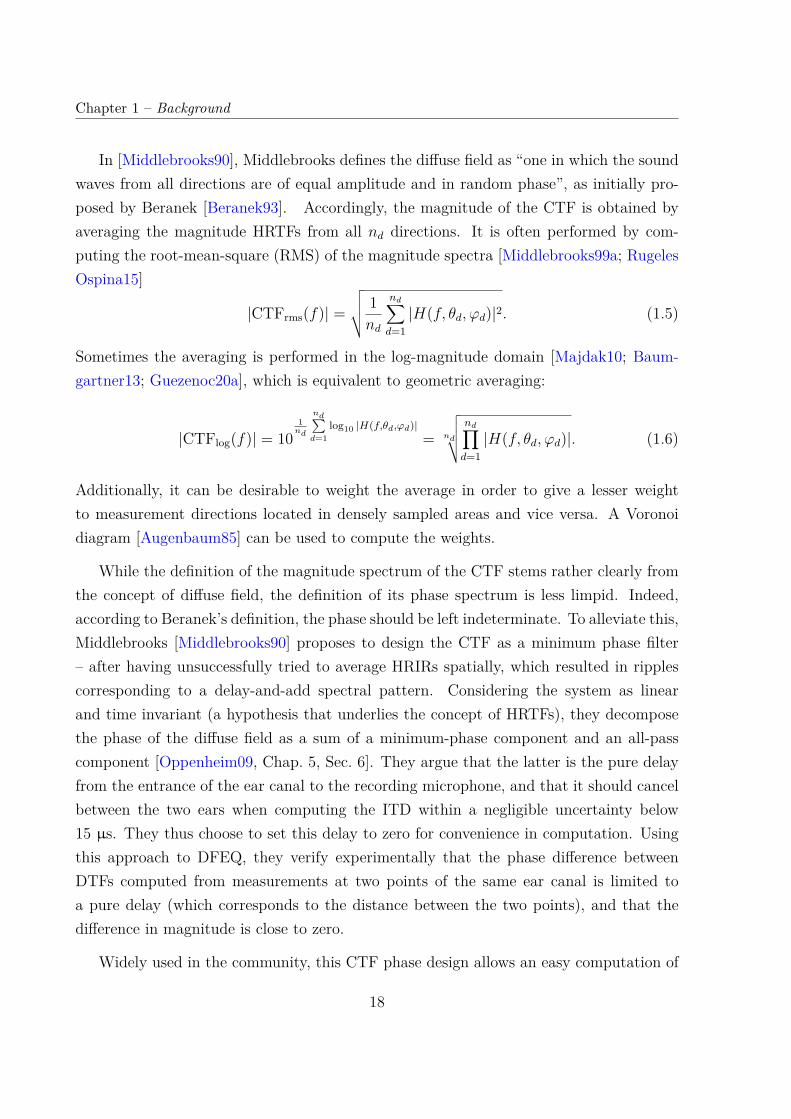
In [Middlebrooks90], Middlebrooks defines the diffuse field as “one in which the soundwaves from all directions are of equal amplitude and in random phase”, as initially pro-posed by Beranek [Beranek93]. Accordingly, the magnitude of the CTF is obtained byaveraging the magnitude HRTFs from all nd directions. It is often performed by com-puting the root-mean-square (RMS) of the magnitude spectra [Middlebrooks99a; RugelesOspina15]
|CTFrms(f)| =√√√√ 1nd
nd∑d=1|H(f, θd, ϕd)|2. (1.5)
Sometimes the averaging is performed in the log-magnitude domain [Majdak10; Baum-gartner13; Guezenoc20a], which is equivalent to geometric averaging:
|CTFlog(f)| = 101nd
nd∑d=1
log10 |H(f,θd,ϕd)|= nd
√√√√ nd∏d=1|H(f, θd, ϕd)|. (1.6)
Additionally, it can be desirable to weight the average in order to give a lesser weightto measurement directions located in densely sampled areas and vice versa. A Voronoidiagram [Augenbaum85] can be used to compute the weights.
While the definition of the magnitude spectrum of the CTF stems rather clearly fromthe concept of diffuse field, the definition of its phase spectrum is less limpid. Indeed,according to Beranek’s definition, the phase should be left indeterminate. To alleviate this,Middlebrooks [Middlebrooks90] proposes to design the CTF as a minimum phase filter– after having unsuccessfully tried to average HRIRs spatially, which resulted in ripplescorresponding to a delay-and-add spectral pattern. Considering the system as linearand time invariant (a hypothesis that underlies the concept of HRTFs), they decomposethe phase of the diffuse field as a sum of a minimum-phase component and an all-passcomponent [Oppenheim09, Chap. 5, Sec. 6]. They argue that the latter is the pure delayfrom the entrance of the ear canal to the recording microphone, and that it should cancelbetween the two ears when computing the ITD within a negligible uncertainty below15 µs. They thus choose to set this delay to zero for convenience in computation. Usingthis approach to DFEQ, they verify experimentally that the phase difference betweenDTFs computed from measurements at two points of the same ear canal is limited toa pure delay (which corresponds to the distance between the two points), and that thedifference in magnitude is close to zero.
Widely used in the community, this CTF phase design allows an easy computation of
18

1.3. Binaural Synthesis
the phase spectrum of the CTF from its magnitude by means of the Hilbert transform H:
arg (CTF(f)) = H (− ln |CTF(f)|) . (1.7)
1.3 Binaural Synthesis
1.3.1 Binaural Reproduction Techniques
As we have seen above, certain auditory cues allow the listener to localize sound. Byincorporating these cues into the audio signals perceived at his ear drums, a two-channelaudio system is able to generate the illusion of a spatial sound scene.
Binaural recording and play-back The most direct manner to achieve this is binauralrecording and play-back: a sound scene is recorded through a pair of microphones placedinside the ear canals of a person or of an artificial head. Later on, the recording is playedback through headphones or ear-buds. First experiments with binaural play-back dateback to as early as the late XIXth century. Nowadays, the process is used in a varietyof applications such as radio-phonic documentaries6, music recordings 7 or experimentalmusical creations8.
Such recordings naturally include the spatial cues due to the propagation of soundfrom its points of emission to the ear drums. However, the trajectory and orientation ofthe listener in his virtual environment is immutable. Worse, if he rotates his head whilelistening, the virtual auditory scene rotates with it, which is a major drawback in termsof immersion (see Section 1.1.4). Furthermore, the auditory cues are tailored to the headused for measurement whose morphology can be quite different from the listener’s. Thisis cause to perceptual discrepancies, as we will see in Section 1.3.2.
Binaural synthesis An alternative approach made possible by last century’s techno-logical advances is to incorporate the spatial auditory cues into the binaural signals not atthe time of recording but at the time of play-back, thus opening a new world of possibili-ties. This process, called binaural synthesis [Wightman89b; Møller92], consists in filtering
6Example of audio documentary: [Casadamont18].7Example of binaural music recording: [Rueff20].8Example of experimental music creation: [KRoll18].
19
Chapter 1 – Background
the sound emitted by a given virtual sound source with the pair of HRTFs that corre-sponds to its position. This allows the synthesis of whole audio scenes by placing varioussound sources at different locations in a virtual environment. This is an indispensablequality for video games, and virtual and augmented reality applications, for instance.
In contrast with binaural recording, the HRTFs and thus the spatial auditory cuescan be adapted to the context of play-back. The HRTFs at play can be adjusted to thelistener’s position in real time, thus providing precious dynamic cues (see Section 1.1.4)and/or individual HRTFs can be used instead of an artificial head’s (see Section 1.3.2 onthe importance of individualization).
Extension to loudspeakers: transaural Both binaural techniques can be adapted forbroadcast on loudspeakers thanks to transaural corrections. First proposed by Schroederin 1970 [Schroeder70] and refined later by Cooper and Bauck [Cooper89], the fundamentalprinciple is to cancel the cross-talk between the loudspeakers so that each ear drumreceives its own spatial cues without interference from the opposite ear’s. However, thespatial auditory image is very sensitive to the listener’s position and orientation relativelyto the loudspeakers. Corrective strategies have been developed such as using more thantwo loudspeakers [Baskind12] and/or adapt to the listener’s position via head-tracking[Gardner97]. Transaural reproduction is out of the scope of this thesis.
1.3.2 Individualization - Impact on Perception
By definition (see Section 1.2.1), HRTFs describe the transformation of a sound wave onits path from the free field to the ear drums. In free field, this transformation is due to theinteraction of the sound wave with the listener’s pinnae, head and torso. Hence, HRTFsare in principle specific to each individual, due to their morphological origin.
In practice, using non-individual HRTFs instead of individual ones in binaural synthe-sis has indeed adverse effects on the perceptual quality of a VAS. In particular, localizationwithin cones of confusion – based on monaural spectral cues – is subject to deterioration,whereas lateral localization – based on ILD and ITD – is less affected.
Indeed, in a study where 16 subjects participated in localization tests with non-individual static and free-field binaural synthesis, Wenzel et al. [Wenzel93] report adeterioration in the capacity to resolve location along the cones of confusion, with higherfront-back and up-down confusion. In contrast, they note that lateral perception is morerobust to non-individual cues.
20
1.3. Binaural Synthesis
Similar observations are made by Møller et al. [Møller96] when studying the lo-calization performance of 8 subjects with real sound sources and both individual andnon-individual binaural recordings. They observe increased median-plane errors for non-individual reproduction in comparison with individual reproduction – the latter beingreported to be on a par with real life. In particular, they identify a general trend forfrontal sources to be heard in the rear.
While the aforementioned work studied the impact of using either an individual or non-individual HRTF set on localization performance, it did not attempt to isolate the variouslocalization cues involved. Romigh et al. [Romigh14] thus propose to decompose theHRTFs into an ITD component and average, lateral and intraconic spectral components.One by one, they replace each component of an individual HRTF set with its matchfrom a non-individual HRTF set (that of the KEMAR manikin) and study the resultinglocalization performances. 9 subjects participated in the listening experiments. Theyfind that the intraconic spectral component encodes the most important cues for HRTFindividualization. In contrast, localization is only minimally affected by introducing non-individualized cues into the other HRTF components.
Besides front-back confusions and erroneous elevation perception, non-individual bin-aural synthesis can also cause discrepancies in the perception of externalization. In astudy where 5 subjects were asked to report the perceived direction and distance of avirtual sound source synthesized (in the horizontal plane) thanks to both non-individualand individual binaural synthesis, Kim et al. reports higher front-back confusion rate andintra-cranial perception when using non-individual HRTFs [Kim05]. In contrast, no intra-cranial perception is observed by Møller et al. in [Møller96]. However, these experimentsdiffer in the stimuli used for the listening experiments: Kim et al. use a wide-band whitenoise whereas Møller et al. use a female voice. Indeed, using a narrow-band signal isknown to deteriorate localization performance compared to a wider-band signal, seeingthat the monaural spectral cues are then restricted to its frequency range.
21


Chapter 2
STATE OF THE ART
2.1 HRTF Modeling
In this section, we review various ways of modeling HRTFs, distinguishing three categories.The first category concerns spectral models i.e. models related to the representation ofHRTFs as filters. In addition to understanding which spectral features are useful for soundlocalization, these models were generally motivated by a concern for the reduction of thecomputational load and latency of binaural engines. Indeed, generating a convincingVAS potentially requires a large number of virtual sources, everyone of which needs to beconvoluted with a pair of HRTFs. In that context, reducing the size of the finite impulseresponses (FIRs) is critical.
The second category of models are related to the representation of HRTFs as frequency-dependent directivity responses, typically called spatial frequency response surfaces (SF-RSs) [Guillon08]. Rather than the variations of HRTFs along the frequency axis, it is theirvariations with sound source position that are modeled. Such models are typically mo-tivated by the need to generate continuously moving virtual sound sources, while HRTFmeasurement grids are discrete and their resolution often below human localization ac-curacy. Another motivation is to be able to recover a spatially dense HRTF set from asparse one, thus facilitating the acquisition of individual HRTF sets by means of acousticmeasurement.
The third category is statistical modeling. In particular, PCA has been widely usedin the community, although other machine learning techniques have been used as well.As we will see, statistical modeling has been used as an alternative to more conventionaltechniques in both cases reviewed above, modeling HRTFs as filters or as SFRSs. In ad-dition, statistical modeling can be used to learn the inter-individual variations of HRTFs,which is particularly relevant in a context of HRTF individualization.
23

Chapter 2 – State of the Art
2.1.1 Filters
Minimum-phase filter and interaural time delay
A widespread and key HRTF model is the combination of a minimum-phase filter and apure delay often called time of arrival (TOA).
Principle For linear time-invariant systems – a hypothesis that underlies the concept ofHRTF, a transfer function can be decomposed into a minimum-phase and a unitary-gainexcess-phase component [Oppenheim09, Chap. 5, Sec. 6]. The latter can be decomposedfurther into two unitary gain components: a linear phase one i.e. a pure delay, and anall-pass one that contains the remaining phase information.
H = Hmin phase ·Hexc phase (2.1)= Hmin phase ·Hlin phase ·Hall-pass. (2.2)
The minimum phase component Hmin phase is determined by the magnitude spectrum ofthe all-phase filter H. While, by construction, its magnitude spectrum is that of theoriginal filter, its phase can conveniently be derived from the magnitude spectrum bycomputing the Hilbert transform of the additive inverse of its logarithm [Smith07]:
|Hmin phase| = |H|,
arg (Hmin phase) = H (− ln (|H|)) .(2.3)
The so-called minimum-phase processing concentrates a filter’s energy into the early partof its impulse response (see Figure 2.1) while faithfully preserving the magnitude spectralresponse.
In an objective study of measured HRIRs of 20 subjects in 30 directions of the hori-zontal and median planes, Mehrgardt and Mellert [Mehrgardt77] observe that HRTFs arenearly minimum phase up to 10 kHz. Following that early work, it has been very commonin the literature to approximate HRTFs as a combination of minimum-phase filters andpure delays, hence neglecting the all-pass component. According to that approximation,an HRTF H(f, θ, ϕ) is decomposed as follows:
H(f, θ, ϕ) = Hmp(f, θ, ϕ) · exp [−2πjf · τ(θ, ϕ)] , (2.4)
24

2.1. HRTF Modeling
0 1 2 3 4 5 6-0.05
0
0.05
0 1 2 3 4 5 6-0.05
0
0.05
Figure 2.1 – Exemplary HRIR (above) and matching minimum-phase impulse response(below). The exemplary HRIR is that of the left ear of subject NH8 of the ARI dataset,in the ipsilateral direction of 90 azimuth and 0 elevation).
where Hmp(f, θ, ϕ) is the minimum-phase filter and τ(θ, ϕ) is a pure delay, for all frequen-cies f ∈ R+, azimuths θ ∈ [0, 2π] and elevations ϕ ∈
[−π
2 ,π2
].
This approximation presents two major advantages. First, it permits a compact rep-resentation of HRIR data as a combination of short finite impulse responses (FIRs) andpure delays, thus reducing the computational load of binaural rendering. Second, it ishighly convenient on a psychoacoustic level: the magnitude spectra and the pure delays re-spectively correspond to the spectral and ITD localization cues, allowing for independentanalysis and manipulation of both types of cues [Hoffmann08].
Perceptual relevance The perceptual relevance of this model is investigated in severalstudies. Kistler et al. [Kistler92] compare the localization performances of 5 listeners withtheir own HRTF sets in 36 virtual source directions, with or without minimum-phase-plus-delay approximation. The similarity of the localization results between both conditionslead them to conclude that the approximation is perceptually valid.
Rather than performing localization experiments, Hammershøi et al. [Sandvad94]study directly the ability of 7 listeners to detect differences between measured and minimum-phase-plus-delay HRTFs in a multiple choice experiment in 17 virtual source directions.Their results show that some minimum-phase HRTFs are detected by some listeners,without further insight about dependency on direction or listener.
25
Chapter 2 – State of the Art
In another multiple choice experiment, Kulkarni et al. [Kulkarni99] compare thecapacity of 4 listeners to hear the difference between measured and minimum-phase-plus-delay HRTFs, at 4 horizontal positions of azimuths 0, ±90 and 180. In agreementwith the results of [Kistler92], they find that some of the listeners were able to hearthe difference between some of the HRTFs, in particular in lateral directions. Indeed,while no subject was able to discriminate between both HRTF sets at 0 and 180, thediscrimination rate was significantly greater than chance at ±90 for 2 of the 4 listeners.
Let us note that this is coherent with the observation by several authors [Algazi02;Katz14] that HRIRs are bimodal in contralateral positions close to the interaural axis,due to multiple-path propagation around the head. Such HRIRs are thus, to some extent,non-causal and contradict the minimum-phase assumption.
Plogsties et al. [Plogsties00] confirm, by means of a multiple choice experiment with 12listeners, that the removal of the all-pass component is inaudible for most HRTFs but canbe detected for some, in particular those that correspond to lateral directions. However,with further scrutiny and work on the way the ITD is derived from the excess-phasecomponent, they show that the minimum-phase-plus-delay approximation is perceptuallytransparent for every HRTF, provided that the ITD is properly calculated.
ITD estimation ITD estimation from measured HRIRs has indeed been the subjectof much work in the literature. While we shall not delve further into this question here,we encourage the curious reader to refer to [Katz14] for a thorough comparative studyof the degree of variability between many of the most common ITD estimation methods,and to [Andreopoulou17] for a perceptual assessment of which of these methods are themost relevant for use in the minimum-phase-plus-delay approximation.
Further on, for simplicity, we use the terms “mag-HRTF”, “mag-DTF” or “mag-PRTF”and to refer to the magnitude spectrum of an HRTF, DTF or PRTF, respectively.
Pole-zero modeling
In coherence with the physical interpretation of HRTFs as containing resonances andreflections, the overall structure of mag-HRTFs exhibits several narrow-band peaks andnotches. Based on this observation, it has been proposed to approximate HRTFs usingpole-zero parameterizations [Asano90; Blommer97; Haneda99].
26

2.1. HRTF Modeling
In particular, Haneda et al. approximate the horizontal HRTFs of a dummy-headusing the so-called common acoustical poles and zeros (CAPZ) approach: each HRTF ismodeled thanks to 20 direction-independent poles and 40 zeros [Haneda99]. All-pole orall-zero modeling have been used as well to avoid mutual cancellations of poles and zeros[Sandvad94; AlSheikh09].
Spectral smoothing
Based on prior knowledge of the frequency resolution of the human auditory localizationsystem (see Section 1.1.5 for more details), the magnitude spectrum of an HRTF canin principle be represented thanks to magnitude coefficients distributed in a logarithmicmanner along frequencies [Breebaart10].
Although most studies suggest that a magnitude value per ERB band is sufficient (i.e.about 30 magnitude coefficients) [Breebaart10], other results tend to indicate that whenusing non-overlapping filters the frequency scale should be as fine as a 1
12th of octave which
is equivalent to about a third of ERB, i.e. about 120 magnitude coefficients.
2.1.2 Spatial Frequency Response Surfaces
So far, we have reviewed approaches to model magnitude HRTFs as filters, without lookingat their directional variations. An HRTF set, i.e. the set of HRTFs from all directions,can however be viewed as a directivity response that depends on frequency. This modeof representation is referred to as spatial frequency response surface (SFRS) [Guillon08]:
SFRS(f) =H(f, θ, ϕ) | θ ∈ [0, 2π] , ϕ ∈
[−π2 ,
π
2
]. (2.5)
Spherical harmonics
Spherical harmonics decomposition (SHD) is a popular method to model and approximateSFRSs. Similarly to the Fourier transform in 1-D, SHD expands a function g : [0, 2π] ×[−π
2 ,π2
]7→ C into an infinite sum of weighted orthonormal basis functions called spherical
harmonics.
Continous SHD The SHD of SFRSs relies on the fact that, by applying the reciprocityprinciple, HRTFs can be formulated as an acoustical radiation problem [Pollow14]. As-suming that the Sommerfeld radiation condition is satisfied, the solution of the Helmholtz
27

Chapter 2 – State of the Art
equation in spherical coordinates results in the expansion of the acoustic pressure field,and thus of the HRTF H(f, r, θ, ϕ) at frequency f and position (r, θ, ϕ) as follows.
H(f, r, θ, ϕ) =+∞∑p=1
p∑q=−p
apq(r, k)Y qp (θ, ϕ) (2.6)
where k = 2πfc0
is the wavenumber. Y qp denotes the complex SH function of order p and
degree q, defined as
Y qp (θ, ϕ) = (−1)q
√√√√(2p+ 1)4π
(p− |q|)!(p+ |q|)!P
|q|p (cos θ)ejqϕ, (2.7)
where P |q|p is the associated Legendre polynomial. apq denotes the spherical expansioncoefficients
apq(r, k) = bpq(k)hp(kr), (2.8)
where hp(kr) is the spherical Hankel function of the first kind.hp can be used for range extrapolation which allows to derive HRTFs for any given
distance r from measurements at a fixed distance r0 (usually r0 & 1.5 m) [Pollow14]. Thefirst spherical harmonic functions are plotted in Figure 2.2.
In practical applications, the infinite sum is truncated to a finite number of SHsnsh ∈ N∗:
H(f, r, θ, ϕ) 'nsh∑p=1
p∑q=−p
apq(r, k)Y qp (θ, ϕ). (2.9)
In order to avoid spatial aliasing, nsh must be limited to an upper bound nshmax , determinedby the number nd and distribution of the measurement points on the sphere of possibledirections:
nshmax =⌊√
ndγ− 1
⌋, (2.10)
where γ = 4 for an equiangular spatial sampling, γ = 2 for a Gaussian one and γ = 1 foran hyper-interpolation one [Bomhardt17, Chap. 2, Sec. 5].
Due to the analytical definition of the SHs, SHD provides a continuous representationof the HRTFs on the sphere. This characteristic facilitates real-time rotation of the VAS isbinaural synthesis. Additionally, it permits the spatial interpolation of sparsely measuredHRTF sets [Duraiswami04; Pollow14].
Depending on nsh, SHD can be used provide a compact representation of the spatial
28
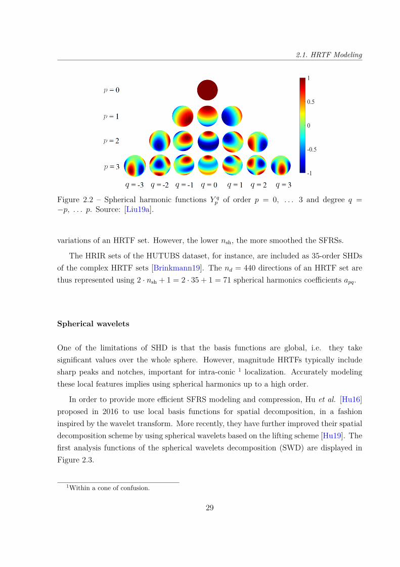
2.1. HRTF Modeling
Figure 2.2 – Spherical harmonic functions Y qp of order p = 0, . . . 3 and degree q =
−p, . . . p. Source: [Liu19a].
variations of an HRTF set. However, the lower nsh, the more smoothed the SFRSs.
The HRIR sets of the HUTUBS dataset, for instance, are included as 35-order SHDsof the complex HRTF sets [Brinkmann19]. The nd = 440 directions of an HRTF set arethus represented using 2 · nsh + 1 = 2 · 35 + 1 = 71 spherical harmonics coefficients apq.
Spherical wavelets
One of the limitations of SHD is that the basis functions are global, i.e. they takesignificant values over the whole sphere. However, magnitude HRTFs typically includesharp peaks and notches, important for intra-conic 1 localization. Accurately modelingthese local features implies using spherical harmonics up to a high order.
In order to provide more efficient SFRS modeling and compression, Hu et al. [Hu16]proposed in 2016 to use local basis functions for spatial decomposition, in a fashioninspired by the wavelet transform. More recently, they have further improved their spatialdecomposition scheme by using spherical wavelets based on the lifting scheme [Hu19]. Thefirst analysis functions of the spherical wavelets decomposition (SWD) are displayed inFigure 2.3.
1Within a cone of confusion.
29
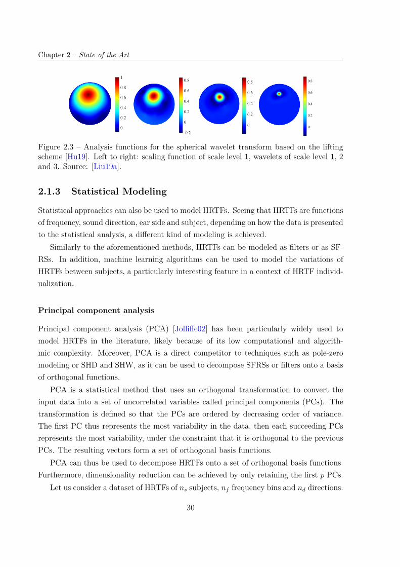
Chapter 2 – State of the Art
Figure 2.3 – Analysis functions for the spherical wavelet transform based on the liftingscheme [Hu19]. Left to right: scaling function of scale level 1, wavelets of scale level 1, 2and 3. Source: [Liu19a].
2.1.3 Statistical Modeling
Statistical approaches can also be used to model HRTFs. Seeing that HRTFs are functionsof frequency, sound direction, ear side and subject, depending on how the data is presentedto the statistical analysis, a different kind of modeling is achieved.
Similarly to the aforementioned methods, HRTFs can be modeled as filters or as SF-RSs. In addition, machine learning algorithms can be used to model the variations ofHRTFs between subjects, a particularly interesting feature in a context of HRTF individ-ualization.
Principal component analysis
Principal component analysis (PCA) [Jolliffe02] has been particularly widely used tomodel HRTFs in the literature, likely because of its low computational and algorith-mic complexity. Moreover, PCA is a direct competitor to techniques such as pole-zeromodeling or SHD and SHW, as it can be used to decompose SFRSs or filters onto a basisof orthogonal functions.
PCA is a statistical method that uses an orthogonal transformation to convert theinput data into a set of uncorrelated variables called principal components (PCs). Thetransformation is defined so that the PCs are ordered by decreasing order of variance.The first PC thus represents the most variability in the data, then each succeeding PCsrepresents the most variability, under the constraint that it is orthogonal to the previousPCs. The resulting vectors form a set of orthogonal basis functions.
PCA can thus be used to decompose HRTFs onto a set of orthogonal basis functions.Furthermore, dimensionality reduction can be achieved by only retaining the first p PCs.
Let us consider a dataset of HRTFs of ns subjects, nf frequency bins and nd directions.
30
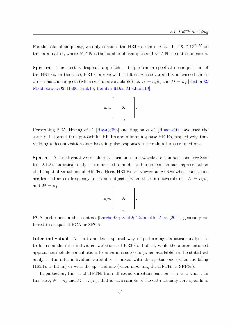
2.1. HRTF Modeling
For the sake of simplicity, we only consider the HRTFs from one ear. Let X ∈ CN×M bethe data matrix, where N ∈ N is the number of examples andM ∈ N the data dimension.
Spectral The most widespread approach is to perform a spectral decomposition ofthe HRTFs. In this case, HRTFs are viewed as filters, whose variability is learned acrossdirections and subjects (when several are available) i.e. N = ndns andM = nf [Kistler92;Middlebrooks92; Hu06; Fink15; Bomhardt16a; Mokhtari19]:
ndns
X
nf
.
Performing PCA, Hwang et al. [Hwang08b] and Hugeng et al. [Hugeng10] have used thesame data formatting approach for HRIRs and minimum-phase HRIRs, respectively, thusyielding a decomposition onto basis impulse responses rather than transfer functions.
Spatial As an alternative to spherical harmonics and wavelets decompositions (see Sec-tion 2.1.2), statistical analysis can be used to model and provide a compact representationof the spatial variations of HRTFs. Here, HRTFs are viewed as SFRSs whose variationsare learned across frequency bins and subjects (when there are several) i.e. N = nfns
and M = nd:
nfns
X
nd
.
PCA performed in this context [Larcher00; Xie12; Takane15; Zhang20] is generally re-ferred to as spatial PCA or SPCA.
Inter-individual A third and less explored way of performing statistical analysis isto focus on the inter-individual variations of HRTFs. Indeed, while the aforementionedapproaches include contributions from various subjects (when available) in the statisticalanalysis, the inter-individual variability is mixed with the spatial one (when modelingHRTFs as filters) or with the spectral one (when modeling the HRTFs as SFRSs).
In particular, the set of HRTFs from all sound directions can be seen as a whole. Inthis case, N = ns and M = nfnd, that is each sample of the data actually corresponds to
31
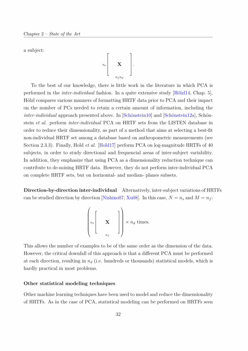
Chapter 2 – State of the Art
a subject:
ns
X
nfnd
.
To the best of our knowledge, there is little work in the literature in which PCA isperformed in the inter-individual fashion. In a quite extensive study [Hölzl14, Chap. 5],Hölzl compares various manners of formatting HRTF data prior to PCA and their impacton the number of PCs needed to retain a certain amount of information, including theinter-individual approach presented above. In [Schönstein10] and [Schönstein12a], Schön-stein et al. perform inter-individual PCA on HRTF sets from the LISTEN database inorder to reduce their dimensionality, as part of a method that aims at selecting a best-fitnon-individual HRTF set among a database based on anthropometric measurements (seeSection 2.3.3). Finally, Hold et al. [Hold17] perform PCA on log-magnitude HRTFs of 40subjects, in order to study directional and frequencial areas of inter-subject variability.In addition, they emphasize that using PCA as a dimensionality reduction technique cancontribute to de-noising HRTF data. However, they do not perform inter-individual PCAon complete HRTF sets, but on horizontal- and median- planes subsets.
Direction-by-direction inter-individual Alternatively, inter-subject variations of HRTFscan be studied direction by direction [Nishino07; Xu08]. In this case, N = ns andM = nf :ns
X
nf
× nd times.
This allows the number of examples to be of the same order as the dimension of the data.However, the critical downfall of this approach is that a different PCA must be performedat each direction, resulting in nd (i.e. hundreds or thousands) statistical models, which ishardly practical in most problems.
Other statistical modeling techniques
Other machine learning techniques have been used to model and reduce the dimensionalityof HRTFs. As in the case of PCA, statistical modeling can be performed on HRTFs seen
32

2.1. HRTF Modeling
either as filters, SFRSs or HRTF sets.
Independent component analysis Among linear techniques, let us mention indepen-dent component analysis (ICA) [Larcher00; Liu19b] or high-order singular value decom-position [Li13]. While Larcher et al. use it to model complex SFRSs [Larcher00], bothLiu et al. [Liu19b] and Li et al. [Li13] use it to reduce the dimensionality of HRTFs –seen as HRTF sets – in a context of HRTF individualization based on regression fromanthropometric measurements.
Non-linear techniques Regarding non-linear approaches, Isomap [Grijalva16; Kapra-los08] and locally linear embedding (LLE) [Duraiswami05; Kapralos08] have been appliedto SFRSs.
Local tangent space alignment (LTSA) has been used as well on binaural acousticdata, with the aim of retrieving the latent two-dimensional manifold that corresponds tosound source direction and/or head orientation. In that way, Aytekin et al. [Aytekin08]reduce the dimensionality of HRTFs of human beings2 and echolocating bats, in orderto simulate the process of learning auditory localization for a living organism. Cuesbased on head movement are also used. With the aim of providing a means for soundlocalization for a two-ear robot, Deleforge et al. [Deleforge15], perform LTSA on a datasetof binaural recordings of a human-like manikin head. Based on interaural level and phasedifferences, they identify a two-dimensional non-linear manifold that corresponds to thehead’s orientation (or sound source direction, conversely).
Neural networks have come up recently in unsupervised HRTF modeling. In [Ya-mamoto17] , Yamamoto et al. train a variational autoencoder on HRTFs seen as filters,associated with directional information and personalization weights. For compressionpurposes, Chen et al. [Chen20] propose to use a different approach and to train a convo-lutional network on median-plane HRTF subsets, thus focusing on inter-individual varia-tions.
Overall, as in the case of PCA, other machine learning techniques have rarely beenperformed in a way that focuses on the inter-individual variations of HRTF sets. Hereas well, a likely cause is the small number of examples in currently available datasetscompared to the dimensionality of a whole HRTF set. The scarcity of data may even bemore of a problem with these more complex techniques.
2The 45 HRTF sets from the CIPIC dataset (see Section 2.4, [Algazi01c]).
33
Chapter 2 – State of the Art
2.2 Evaluation of HRTF Sets
In a context of HRTF individualization, we seek to improve the quality of binaural syn-thesis by modifying the HRTF set used for rendering. It is thus desirable to be able toevaluate and compare HRTF sets objectively and subjectively.
2.2.1 Objective Metrics
Due to the time and cost of performing perceptual evaluations, objective metrics are anecessity. They are however as diverse as there are ways of representing the signal (time-or frequency-domain, magnitude or complex spectra, linear or logarithmic scale, cepstralcoefficients...). We herein present two metrics that have been commonly used in theliterature. For an extensive review of HRTF metrics, we advise the curious reader to referto [Bahu16a, Chap. 5].
Spectral distortion A rather widespread metric, the spectral distortion (SD) [Inoue05]is the RMS of the difference between log-magnitude HRTFs and is expressed in dB. Thismetric is sometimes referred to as spectral distance [Inoue05].
Let there be HB and HA two HRTF sets, and ∆GdB = 20 log10
(|HB||HA|
)the difference
between the corresponding log-magnitudes.
SD(θ, ϕ) =
√√√√√ 1Nf
Nf∑k=1|∆GdB(fk, θ, ϕ)|2, (2.11)
where (θ, ϕ) is a direction, designated here by its azimuth and elevation.In order to compare two HRTF sets, the SD is typically extended to all directions by
computing its RMS across directions
SDglobal =
√√√√ 1Nd
Nd∑d=1
SD(θd, ϕd)2 =
√√√√√ 1Nd
1Nf
Nd∑d=1
Nf∑k=1|∆GdB(fk, θd, ϕd)|2. (2.12)
Prior to computing the SD, some [Huopaniemi99] resample the HRTFs to a logarithmicfrequency scale in order to better fit human perception.
Inter-subject spectral difference In order not to account for gain differences, Mid-dlebrooks et al. [Middlebrooks99a] proposed a metric termed inter-subject spectral dif-
34
2.2. Evaluation of HRTF Sets
ference (ISSD), expressed in dB2. At each direction (θ, ϕ), the HRTF is passed througha filter-bank of Nb = 64 bands ranging from 3.7 to 12.9 kHz whose center frequencies arelogarithmically distributed. The ISSD is then computed as the variance of the differencebetween the log-magnitude HRTFs in this logarithmic frequency scale:
ISSD(θ, ϕ) = 1Nb
Nb∑b=1
∆GdB(b, θ, ϕ)− 1Nb
Nb∑b=1
∆GdB(b, θ, ϕ)2
. (2.13)
The ISSD is typically extended to all directions by averaging the local ISSD
ISSDglobal = 1Nd
Nd∑d=1
ISSD(θd, ϕd). (2.14)
There are some variants of the ISSD in the literature. For instance, it can be computedfrom a linear frequency scale [Guillon08]. Additionally, a weighting of the contributionsof each frequency can be applied [Durant02].
2.2.2 Subjective Evaluation
Objective metrics can however not account for the full complexity of human auditory lo-calization, and perceptual experiments are the ultimate test of binaural rendering quality.
Perceptual experiments are however far from trivial to implement. For instance, sub-jective judgments are subject to inter- and intra-subject variability [Schönstein12b; An-dreopoulou16]. As a result, subjective evaluations generally include many repetitionsof the same stimuli in order to be able to extract statistically significant information.
On another level, there is no absolute answer as to which type of criterion is to be usedto evaluate the perceptual quality of a binaural reproduction system in a given context.The criteria found in the literature can however be divided into two categories: spatialones such as localization accuracy or sensation of externalization, and timbral ones suchas coloration or naturalness [Le Bagousse10].
We hereon provide a summarized state-of-the-art of the two main types of subjectiveevaluations found in the literature: judgment and localization experiments. For an exten-sive discussion on perceptual assessment of the quality of binaural spatial reproduction,we encourage the reader to read [Katz19].
35
Chapter 2 – State of the Art
Judgment experiments
A first type of approach is judgment experiments. Presented with one or several VASs,the listener is asked to rate the renderings [Katz12; Brinkmann19] or to indicate a pref-erence [Yamamoto17] in an A/B comparison, based on attributes defined by the exper-imenters. These attributes can be global, or related to one of two categories: spectralcontent (i.e. timbre, coloration) or sound source location [Le Bagousse10]. Brinkmannet al. [Brinkmann19], for instance, asks 46 subjects to rate their measured and numer-ical computed HRTF sets according to 12 criteria such as difference, low-, mid- andhigh-frequency coloration, crispness, horizontal and vertical direction, distance, external-ization and source extension. It is not trivial, however, to define the attributes so that theunderlying concepts are understood by the listener as the experimenters intended. Muchresearch has been carried out to establish a set of such attributes, which is reviewedextensively in [Katz19, pp. 380-386].
Sometimes, the test is simply a discrimination task: the listener is asked to indicateif he is able to hear a difference between two VASs. This is the case for instance in[Langendijk99], where binaural synthesis is compared with real sound sources.
Overall, this approach has the advantage of being able to explore various perceptualdimensions in spatial audio rendering quality. Moreover, the experiments can be shorterand less tiring than localization ones. However, they are highly dependent on the definitionof the attributes and of the rating scales.
Localization experiments
In a context of spatial audio, it is only natural to test for localization accuracy i.e. theaccuracy of the perceived position of a given sound source. In that case, the listeneris presented with one or several sound sources in a virtual environment and is asked toreport the position at which he perceives them. In most cases, only the direction of thesound source is evaluated, although sometimes it is rather the distance to the listenerthat is under test [Kim05]. The historical and perhaps most widespread mannerin which binaural rendering has been evaluated is localization experiments, especiallyin work related to HRTF individualization [Wightman89a; Mokhtari08; Middlebrooks00;Seeber03; Shin08; Majdak10; Fink15; Liu19b].
This approach allows for a quantified and absolute evaluation of the perceptual results.Furthermore, unlike some of the criteria used in judgment experiments, there is little
36
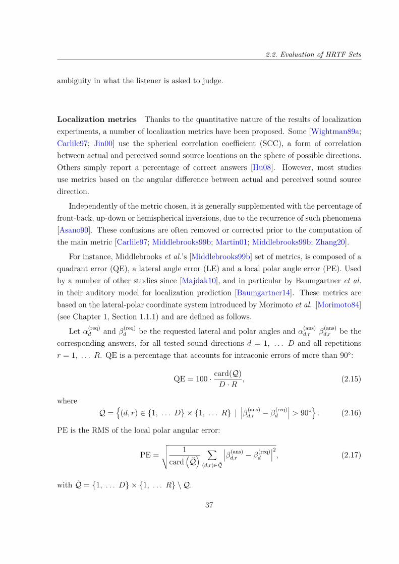
2.2. Evaluation of HRTF Sets
ambiguity in what the listener is asked to judge.
Localization metrics Thanks to the quantitative nature of the results of localizationexperiments, a number of localization metrics have been proposed. Some [Wightman89a;Carlile97; Jin00] use the spherical correlation coefficient (SCC), a form of correlationbetween actual and perceived sound source locations on the sphere of possible directions.Others simply report a percentage of correct answers [Hu08]. However, most studiesuse metrics based on the angular difference between actual and perceived sound sourcedirection.
Independently of the metric chosen, it is generally supplemented with the percentage offront-back, up-down or hemispherical inversions, due to the recurrence of such phenomena[Asano90]. These confusions are often removed or corrected prior to the computation ofthe main metric [Carlile97; Middlebrooks99b; Martin01; Middlebrooks99b; Zhang20].
For instance, Middlebrooks et al.’s [Middlebrooks99b] set of metrics, is composed of aquadrant error (QE), a lateral angle error (LE) and a local polar angle error (PE). Usedby a number of other studies since [Majdak10], and in particular by Baumgartner et al.in their auditory model for localization prediction [Baumgartner14]. These metrics arebased on the lateral-polar coordinate system introduced by Morimoto et al. [Morimoto84](see Chapter 1, Section 1.1.1) and are defined as follows.
Let α(req)d and β(req)
d be the requested lateral and polar angles and α(ans)d,r β
(ans)d,r be the
corresponding answers, for all tested sound directions d = 1, . . . D and all repetitionsr = 1, . . . R. QE is a percentage that accounts for intraconic errors of more than 90:
QE = 100 · card(Q)D ·R
, (2.15)
whereQ =
(d, r) ∈ 1, . . . D × 1, . . . R |
∣∣∣β(ans)d,r − β
(req)d
∣∣∣ > 90. (2.16)
PE is the RMS of the local polar angular error:
PE =√√√√ 1
card(Q) ∑
(d,r)∈Q
∣∣∣β(ans)d,r − β
(req)d
∣∣∣2, (2.17)
with Q = 1, . . . D × 1, . . . R \ Q.
37
Chapter 2 – State of the Art
As to the LE, it accounts for errors along the lateral dimension:
LE =
√√√√ 1D ·R
D∑d=1
R∑r=1
(α
(ans)d,r − α
(req)d
)2. (2.18)
As a variant, the polar error can be computed without excluding the intraconic errorsa priori – which we do in Chapter 4. Implemented by Baumgartner et al. [Baumgart-ner14] as part of their auditory modeling toolbox [Søndergaard13], the absolute polarerror (APE) is defined as follows:
APE =
√√√√ 1D ·R
D∑d=1
R∑r=1
∣∣∣β(ans)d,r − β
(req)d
∣∣∣2. (2.19)
Localization versus judgment
In [Zagala20], Zagala et al. point out that there is a considerable lack of cross-comparisonof localization and judgment tasks in the literature. In order to alleviate that, they studythe link between rankings of 8 representative HRTF sets from the LISTEN database (pre-viously identified in [Katz12]) according to two different types of perceptual evaluations:a localization task, and a judgment task – similar to that of [Katz12] – in which thelisteners evaluate the overall rendering quality of two virtual trajectories, horizontal andvertical. For each type of test, various metrics are covered. 28 subjects participated inthe experiment.
Overall, they observe that localization performances across HRTF sets are correlatedto overall quality of experience judgments. Notably, the best HRTF set selected accordingto perceptual metrics for one given method exhibit a rating score better than a randomselection in the alternate method.
Looking into the various metrics related to each task, they report that some of themetrics from the localization method correlated better to metrics from the quality evalu-ation method than others: metrics such as the mean great circle error and mean unsignedpolar error should be preferred over the confusion rate or mean unsigned lateral error topredict overall quality of experience.
Finally, studying the repeatability of the listeners’ answers, they find that raters whowere consistent in one task tended to be consistent in the other. What is more, consistentraters tended to score best with the same HRTF sets in both methods, whereas incon-sistent raters were more likely to score differently with each HRTF set depending on the
38
2.2. Evaluation of HRTF Sets
method.
2.2.3 Localization Prediction
As we have seen, although subjective experiments are indispensable when evaluating anHRTF set, they are delicate to implement due to several problems such as headphonecalibration, listener fatigue and variability of subjective answers. Furthermore, manyrepetitions are needed to establish statistical significance, which is costly in time andmoney. As to objective metrics, they allow for an inexpensive comparison of HRTF setsbut cannot account for the complexity of the human auditory system.
A compromise is reached thanks to auditory models that mimic the mechanisms ofsound localization to predict localization performance. While there were previous at-tempts at modeling sound localization [Middlebrooks92; Langendijk02], we herein focuson the widely popular Baumgartner model [Baumgartner14] which we use intensively inChapter 4.
The Baumgartner model
The Baumgartner model aims at predicting localization performance inside a sagittalplane. It has been used in a large number of studies by different research teams [Geron-azzo18; Brinkmann17; Braren19; Spagnol20; Zhang20]. One of the reasons for this popu-larity is the fact that its Matlab code is freely available online in the Auditory ModelingToolbox3 (AMT) [Søndergaard13]. Another one is the fact that the results of this auditorymodel have been verified against real localization experiments.
This function model is based on the hypothesis that a listener constructs an internaltemplate of his own HRTFs as the result of a lifelong learning process. The structure of themodel is displayed in Figure 2.4. For a given sagittal plane, the internal representation ofthe spectral features is associated to matching corresponding polar angles. When listeningto a sound signal, its internal spectral representation is compared to the internal template.The more similar the input signal is to the cues associated with a given direction, thehigher is the probability of perceiving sound coming from that direction. When listeningto a new target HRTF set, the input signal is created by convoluting a reference stimulus(impulse) with the target HRTF.
3https://amtoolbox.sourceforge.net/
39
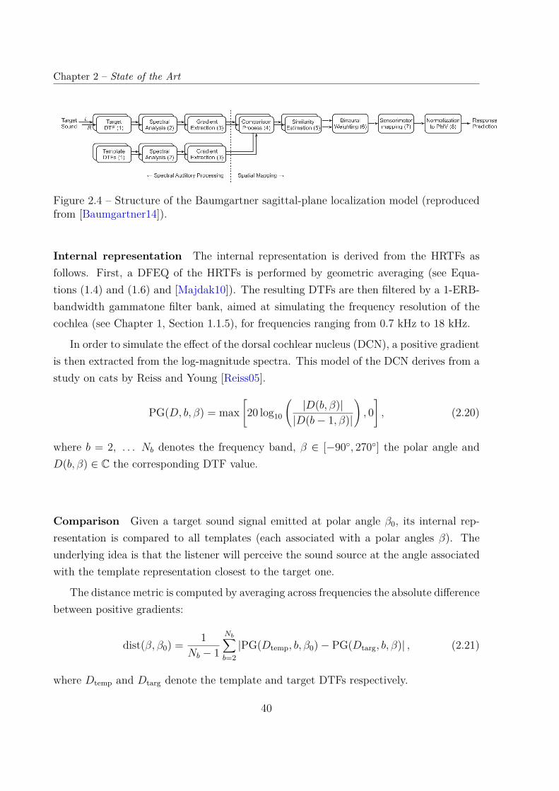
Chapter 2 – State of the Art
Figure 2.4 – Structure of the Baumgartner sagittal-plane localization model (reproducedfrom [Baumgartner14]).
Internal representation The internal representation is derived from the HRTFs asfollows. First, a DFEQ of the HRTFs is performed by geometric averaging (see Equa-tions (1.4) and (1.6) and [Majdak10]). The resulting DTFs are then filtered by a 1-ERB-bandwidth gammatone filter bank, aimed at simulating the frequency resolution of thecochlea (see Chapter 1, Section 1.1.5), for frequencies ranging from 0.7 kHz to 18 kHz.
In order to simulate the effect of the dorsal cochlear nucleus (DCN), a positive gradientis then extracted from the log-magnitude spectra. This model of the DCN derives from astudy on cats by Reiss and Young [Reiss05].
PG(D, b, β) = max[20 log10
(|D(b, β)||D(b− 1, β)|
), 0], (2.20)
where b = 2, . . . Nb denotes the frequency band, β ∈ [−90, 270] the polar angle andD(b, β) ∈ C the corresponding DTF value.
Comparison Given a target sound signal emitted at polar angle β0, its internal rep-resentation is compared to all templates (each associated with a polar angles β). Theunderlying idea is that the listener will perceive the sound source at the angle associatedwith the template representation closest to the target one.
The distance metric is computed by averaging across frequencies the absolute differencebetween positive gradients:
dist(β, β0) = 1Nb − 1
Nb∑b=2|PG(Dtemp, b, β0)− PG(Dtarg, b, β)| , (2.21)
where Dtemp and Dtarg denote the template and target DTFs respectively.
40

2.2. Evaluation of HRTF Sets
Similarity estimation The distance is then translated into a similarity index (SI) SIin a non-linear fashion by means of a sigmoid function:
SI(β, β0) = 1− 11 + exp (−Γ [dist(β, β0)− Sl])
, (2.22)
where Γ denote the degree of selectivity and Sl the sensitivity. These two parameters arelater tuned based on real localization results. The sensitivity parameter, in particular,is designed to be individual, and accounts for inter-subject variability in localizationperformance. The lower Γ and the higher Sl, the more sensitive the listener to spectralvariations and the more precise his localization.
Binaural weighting At this point of the process, spectral features were compared inde-pendently for the right and left pinnae. Then, left and right similarity indices are combinedwith binaural weighting. The weights vary with the lateral angle α ∈ [−90, 90] accord-ing to sigmoid functions, based empirically on two studies [Morimoto01; Macpherson07]:
wL(α) = 1
1+e−αΩ,
wR(α) = 1− wL(α),(2.23)
where Ω is a parameter set to 13 in order to fit the experimental results of the aforemen-tioned studies.
The SIs are then interpolated to match a regular sampling of the polar angles.
Sensorimotor mapping Between auditory perception and source source pointing, acomplex sensorimotor process takes place, which results in pointing hazards [Bahu16b].These pointing hazards are modeled by Baumgartner et al. as a centered Gaussian scatterwhich “smears” the answers. This scattering effect is defined in the elevation dimension(coherent with the body frame) with a constant concentration. Projected into the polardimension, the concentration depends on the interaural angle and is expressed as follows:
κ(α) = cos2 α
ε2, (2.24)
where α ∈ [−90, 90] is the lateral angle and ε is the scatter parameter defined in theelevation dimension.
41
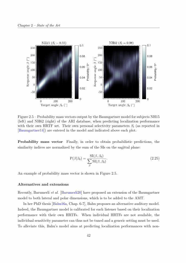
Chapter 2 – State of the Art
Figure 2.5 – Probability mass vectors output by the Baumgartner model for subjects NH15(left) and NH62 (right) of the ARI database, when predicting localization performancewith their own HRTF set. Their own personal selectivity parameters Sl (as reported in[Baumgartner14]) are entered in the model and indicated above each plot.
Probability mass vector Finally, in order to obtain probabilistic predictions, thesimilarity indices are normalized by the sum of the SIs on the sagittal plane:
P(β|β0) = SI(β, β0)∑β
SI(β, β0). (2.25)
An example of probability mass vector is shown in Figure 2.5.
Alternatives and extensions
Recently, Barumerli et al. [Barumerli20] have proposed an extension of the Baumgartnermodel to both lateral and polar dimensions, which is to be added to the AMT.
In her PhD thesis [Bahu16a, Chap. 6-7], Bahu proposes an alternative auditory model.Indeed, the Baumgartner model is calibrated for each listener based on their localizationperformance with their own HRTFs. When individual HRTFs are not available, theindividual sensitivity parameter can thus not be tuned and a generic setting must be used.To alleviate this, Bahu’s model aims at predicting localization performances with non-
42
2.3. HRTF Individualization Techniques
individual HRTFs as well as individual ones, without having to tune the model parametersindividually. Furthermore, the model handles both angular dimensions.
2.3 HRTF Individualization Techniques
As we have seen in Chapter 1, using individual HRTFs in binaural synthesis is key to re-producing accurate localization cues. Nevertheless, in most current applications a genericHRTF set is used. Indeed, the historical and state-of-the-art method to capture individualHRTFs, i.e. acoustic measurement, is cumbersome and inaccessible to the public. Hence,a lot of work has been done over the course of the last decades to provide an alternativeto acoustic measurement.
In this section, we provide a survey of the various ways of obtaining individualizedHRTFs. Four categories are distinguished: acoustic measurement, numerical simulationand indirect methods either based on morphological data or perceptual feedback. We payattention, in particular, to the perceptual assessment of the methods (see Table 2.1 for anoverview) and their user-friendliness, according to criteria such as user comfort, requiredequipment and process duration.
2.3.1 Acoustic Measurement
As mentioned above, acoustic measurement is the historical and most straightforwardmethod to acquire HRTFs. It consists in placing microphones in the subject’s ear canalsand to record impulse responses from every direction of interest. Ideally, the measure-ments are performed in an anechoic or semi-anechoic environment in order to acquirefree-field auditory cues. Indeed, HRTFs are by definition free-field transfer functions (seeChapter 1). Furthermore, it is easier to control room reverberation a posteriori in a VASif the HRTFs are anechoic in the first place.
Measurement setup
A state-of-the-art measurement setup [Bomhardt16b; Rugeles Ospina16; Carpentier14;Enzner08; Mokhtari08] typically features loudspeakers on one or several vertical arcs anda turntable on which the subject stands or sits, though a variety of measurement setupscan be read of in the literature such as one or several loudspeakers moving around astill subject [Langendijk99]. This is the main shortcoming of the method: the equipment
43
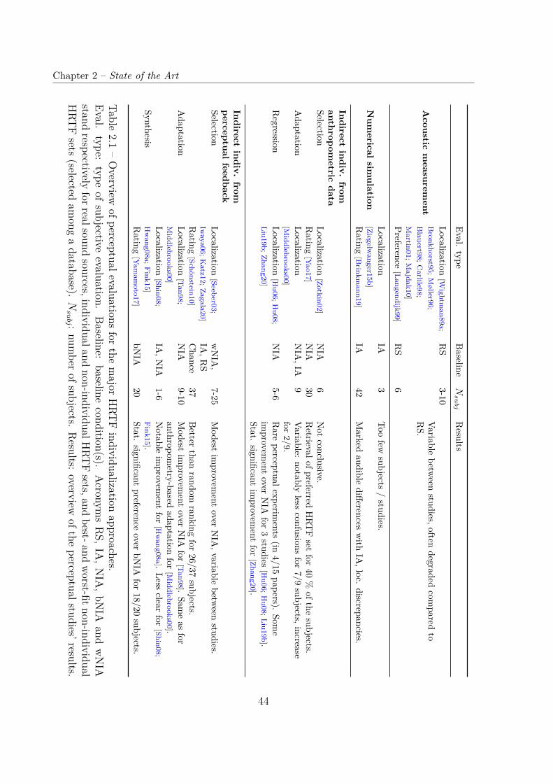
Chapter 2 – State of the ArtEval.
typeBaseline
Nsu
bj
Results
Acoustic
measurem
ent
Localization[W
ightman89a;
Bronkhorst95;M
øller96;B
lauert98;Carlile98;
Martin01;M
ajdak10]
RS
3-10Variable
between
studies,oftendegraded
compared
toRS.
Preference[Langendijk99]
RS
6
Num
ericalsim
ulationLocalization[Ziegelw
anger15b]IA
3Too
fewsubjects
/studies.
Rating
[Brinkm
ann19]IA
42Marked
audibledifferences
with
IA,loc.
discrepancies.
Indirectindiv.
fromanthropom
etricdata
SelectionLocalization
[Zotkin02]NIA
6Not
conclusive.Rating
[Yao17]
NIA
30Retrievalofpreferred
HRT
Fset
for40
%ofthe
subjects.Adaptation
Localization[M
iddlebrooks00]NIA
,IA9
Variable:notably
lessconfusions
for7/9
subjects,increasefor
2/9.Regression
Localization[H
u06;Hu08;
Liu19b;Zhang20]NIA
5-6Rare
perceptualexperiments
(in4/15
papers).Som
eim
provement
overNIA
for3studies
[Hu06;H
u08;Liu19b].Stat.
significantim
provement
for[Zhang20].
Indirectindiv.
fromperceptual
feedbackSelection
Localization[Seeber03;
Iwaya06;K
atz12;Zagala20]wNIA
,IA
,RS
7-25Modest
improvem
entover
NIA
,variablebetw
eenstudies.
Rating
[Schönstein10]Chance
37Better
thanrandom
rankingfor
26/37subjects.
Adaptation
Localization[Tan98;
Middlebrooks00]
NIA
9-10Modest
improvem
entover
NIA
for[Tan98].
Sameas
foranthropom
etry-basedadaptation
for[M
iddlebrooks00].
SynthesisLocalization
[Shin08;H
wang08a;F
ink15]IA
,NIA
1-6Notable
improvem
entfor
[Hw
ang08a].Less
clearfor
[Shin08;F
ink15].Rating
[Yam
amoto17]
bNIA
20Stat.
significantpreference
overbN
IAfor
18/20subjects.
Table2.1
–Overview
ofperceptualevaluationsfor
themajor
HRT
Findividualization
approaches.Eval.
type:type
ofsubjective
evaluation.Baseline:
baselinecondition(s).
Acronym
sRS,IA
,NIA
,bNIA
andwNIA
standrespectively
forrealsoundsources,individualand
non-individualHRT
Fsets,and
best-andworst-fitnon-individual
HRT
Fsets(selected
among
adatabase).
Nsubj :num
berofsubjects.Results:overview
oftheperceptualstudies’results.
44

2.3. HRTF Individualization Techniques
Figure 2.6 – HRTF measurement setup used at Orange Labs: two vertical arcs and aturntable on which the subject is seated. Picture reproduced from [Rugeles Ospina16].
is expensive and hardly transportable. A more detailed presentation of measurementsetups and their respective benefits and constraints can be found in Rugeles’s PhD Thesis[Rugeles Ospina16, Chap. 3, Sec. 1].
Measurement time
Another major disadvantage of the method is the time needed to measure the HRTFs forthousands of directions. Indeed, between a few minutes and a couple of hours dependingon the method, the subject is supposed to remain still for that duration, which is difficultand highly uncomfortable.
The historical approach, which consists in measuring the HRIRs one direction at atime, takes up to 1h45 on a modern setup such as the IRCAM’s [Carpentier14]. Itis however often sped up by means of interleaved multiple sweep sines, as proposed byMajdak et al. in 2007 [Majdak07]. Using this method, Rugeles [Rugeles Ospina16] reportsa recording duration of 20 min on Orange Labs’ setup.
To further reduce the measurement time, Zotkin et al. [Zotkin06] propose in 2006 toswap microphones and loudspeakers based on the acoustic reciprocity principle in order tospeed up the measurement session. Although this approach shows good agreement with
45
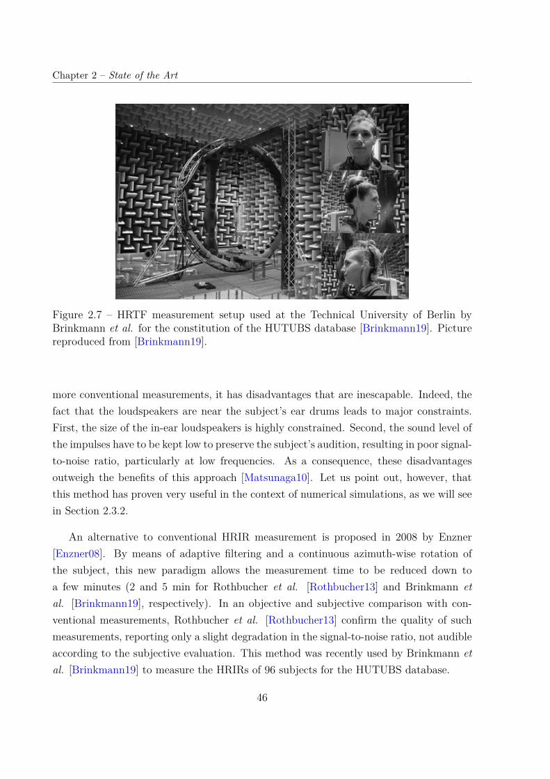
Chapter 2 – State of the Art
Figure 2.7 – HRTF measurement setup used at the Technical University of Berlin byBrinkmann et al. for the constitution of the HUTUBS database [Brinkmann19]. Picturereproduced from [Brinkmann19].
more conventional measurements, it has disadvantages that are inescapable. Indeed, thefact that the loudspeakers are near the subject’s ear drums leads to major constraints.First, the size of the in-ear loudspeakers is highly constrained. Second, the sound level ofthe impulses have to be kept low to preserve the subject’s audition, resulting in poor signal-to-noise ratio, particularly at low frequencies. As a consequence, these disadvantagesoutweigh the benefits of this approach [Matsunaga10]. Let us point out, however, thatthis method has proven very useful in the context of numerical simulations, as we will seein Section 2.3.2.
An alternative to conventional HRIR measurement is proposed in 2008 by Enzner[Enzner08]. By means of adaptive filtering and a continuous azimuth-wise rotation ofthe subject, this new paradigm allows the measurement time to be reduced down toa few minutes (2 and 5 min for Rothbucher et al. [Rothbucher13] and Brinkmann etal. [Brinkmann19], respectively). In an objective and subjective comparison with con-ventional measurements, Rothbucher et al. [Rothbucher13] confirm the quality of suchmeasurements, reporting only a slight degradation in the signal-to-noise ratio, not audibleaccording to the subjective evaluation. This method was recently used by Brinkmann etal. [Brinkmann19] to measure the HRIRs of 96 subjects for the HUTUBS database.
46

2.3. HRTF Individualization Techniques
Directional imprecision due to subject movement
Measurement time exacerbates another issue: as reported in 2010 by Hirahara et al.[Hirahara10] the subject cannot stay completely still all the way through the measurementsession, which is a source of errors about the actual direction of the measured HRTFs.
Nevertheless, studies from 2010 and 2017 [Majdak10; Denk17] seem to have success-fully limited the subject’s movements by giving him a visual feedback. Denk et al.[Denk17], in particular, report the directional error to be imperceptible with HRTFsmeasured using their setup.
Using the same principle of adaptive filtering as the one used for continuous-azimuthHRIR measurements, Ranjan et al. [Ranjan16] propose an experimental method that aimsat avoiding this issue altogether by recording the HRIRs in a context of unconstrainedhead rotations. However, the method was only tested on synthetic data derived from theCIPIC dataset.
Reproducibility
Although acoustic measurement is the state-of-the-art method, it should not be consideredas perfectly accurate. Indeed, potential inaccuracies become apparent when looking intothe reproducibility of HRIR measurements.
Intra-database Measurements are subject to variations from one occurrence to theother, even when the setup and the subject stay the same. In [Riederer98], Riedererinvestigates thoroughly the influence of various factors on the repeatability of HRIR mea-surements in a well-controlled environment. The factors under test include reflectionsfrom the equipment, microphone placement, head position, clothes and hair. In idealconditions, i.e. a dummy head with built-in microphones, the author reports an excellentagreement between two independent measurements (spectral differences below 1 dB). Incontrast, the factors under study are reported to induce non-negligible variations: up to2 dB below 6 kHz and between 3 and 5 dB below 10 kHz. Moreover, as this factorswere studied one by one, larger variations are to be expected when they combine in realmeasurement sessions.
Inter-database Much larger variations are observed between databases. For instance,as part of the “Club Fritz” project, Andreopoulou et al. [Andreopoulou15] compare 12different measurements from 10 laboratories of the HRTF set of the Neumann KU-100
47
Chapter 2 – State of the Art
manikin. The same pair of microphones, built in the artificial head, was used in all themeasurements. Looking at the ITD, they report worrisome variations of up to 235 µs, wellabove the JND (about 10 µs, see Chapter 1, Section 1.1.5). As to the magnitude spectrum,considerable variations are observed: between 1.4 and 22 dB for the frontal position, andbetween 2.5 and 19 dB for the rear one. Additionally, left-right asymmetries are noted aswell.
Perceptual assessment
For the last 30 years binaural synthesis with individual measured HRTFs has been exten-sively compared with real free-field sound sources. The vast majority of studies on thesubject consist in localization experiments.
While some of such studies [Møller96; Langendijk99; Martin01] report equivalent lo-calization performances, a number of others [Wightman89a; Bronkhorst95; Blauert98;Carlile98] report worse localization performance with virtual sources than with real ones.First, the confusion rate increases by a factor 2 with virtual sources [Wightman89a;Bronkhorst95; Blauert98; Carlile98]. For instance, it goes from 6 % to 11 % for Wightmanet al. [Wightman89a], and from 21 % to 41 % for Bronkhorst [Bronkhorst95]. Second,somewhat poorer vertical localization is observed with virtual sources than real ones[Bronkhorst95; Blauert98]. For instance, Bronkhorst [Bronkhorst95] reports the verticalvariability to have increased from 8 to 13. In contrast, provided that confusions areresolved, the horizontal accuracy – only related to the ITD – is equivalent with virtualand real sources [Wightman89a; Bronkhorst95].
As to the cause of the observed degradations, no definite answer was found. AsWightman et al. [Wightman89a] suggest, small dynamic clues (absent from their bin-aural synthesis condition) could impact the real-source condition favorably. Bronkhorst[Bronkhorst95], on the other hand, tends to attribute it to microphone positioning andsound source position variability. Indeed, as we have seen in the two previous sections,some inaccuracies are inevitable when measuring HRTFs, due to various factors includingmicrophone positioning or accidental movement from the subject.
2.3.2 Numerical Simulation
An alternative to measurements is to simulate numerically the propagation of acousticwaves. Its main advantages over HRTF measurement are mobility and user comfort. In-
48
2.3. HRTF Individualization Techniques
deed, only a 3D scan of the listener is needed for individualization, which results in amuch less tedious acquisition session than acoustic measurement. Moreover, once the 3Dgeometry is acquired, the simulation procedure is completely repeatable and free of mea-surement noise. Thus, it holds a large potential to better understand the inter-individualvariations in HRTFs. Furthermore, a low-cost version can be made available to the enduser by using 2D-to-3D reconstruction techniques, thus reducing the acquisition require-ments to a set of consumer-grade 2-D pictures [Kaneko16b; Ghorbal16; Mäkivirta20].
Methods
Thanks to the technological advances in terms of computing power, several research teamsproposed to numerically simulate HRTFs in the early 2000s. Three approaches can bedistinguished: the boundary element method (BEM) [Kahana99; Katz01; Otani03; Gr-eff07] and the finite element method (FEM) [Kahana99; Huttunen07; Farahikia17] inthe harmonic domain, and the finite difference time domain method (FDTD) [Xiao03;Mokhtari07; Prepelit,ă16] in the time domain.
To this day, the most popular technique is the fast-multipole-accelerated boundaryelement method (FM-BEM) [Gumerov07; Kreuzer09; Huttunen13; Rui13; Jin14; Ghor-bal17]. Introduced in 2007 by Gumerov et al. [Gumerov07], it owes its popularity tocompetitive computing times and to the release in 2015 of the Mesh2HRTF open-sourcesimulation software by the Acoustics Research Institute (ARI) [Ziegelwanger15a]. Thisis the technique used for numerical simulations in the present thesis (see Chapter 3, Sec-tion 3.1).
Alternative approaches include a sped-up version of the FDTD called the adaptiverectangular decomposition (ARD) [Meshram14], and the more exotic differential pressuresynthesis (DPS) [Tao03] and ray-tracing techniques [Röber06].
3D geometry acquisition
A major topic of interest for HRTF calculation is the accuracy of the 3D geometry of thehead, pinnae and torso, starting with acquisition. Let us note that the problem of 3-Dsurface accuracy lies mostly in the pinnae. Indeed, their shape is complex – with variousconvolutions and occlusions, and have an important impact on perceptually-sensitive high-frequency HRTF content. In contrast, the head and torso are much simpler shapes andare easier to acquire.
49
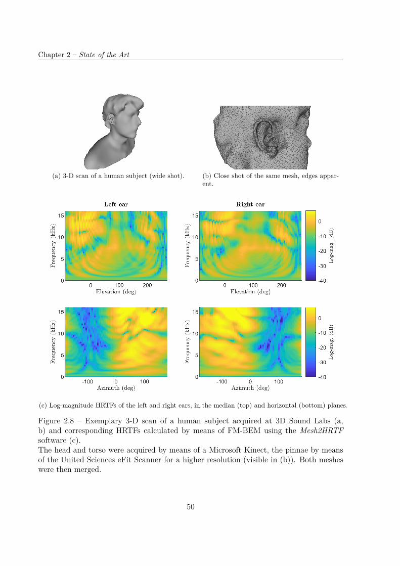
Chapter 2 – State of the Art
(a) 3-D scan of a human subject (wide shot). (b) Close shot of the same mesh, edges appar-ent.
(c) Log-magnitude HRTFs of the left and right ears, in the median (top) and horizontal (bottom) planes.
Figure 2.8 – Exemplary 3-D scan of a human subject acquired at 3D Sound Labs (a,b) and corresponding HRTFs calculated by means of FM-BEM using the Mesh2HRTFsoftware (c).The head and torso were acquired by means of a Microsoft Kinect, the pinnae by meansof the United Sciences eFit Scanner for a higher resolution (visible in (b)). Both mesheswere then merged.
50

2.3. HRTF Individualization Techniques
Often, the pinnae are scanned separately and more precisely than the rest of themorphology, then combined with a rougher scan of the head and/or torso by a humanoperator [Ziegelwanger14b; Kaneko16a; Brinkmann19]. In our experience, this step cantake up to dozens of minutes of manual labor.
MRI & CT Magnetic resonance imagery (MRI) [Mokhtari07; Jin14] and computerizedtomography (CT) scan [Turku08] have often been used to acquire pinnae, head and torsogeometries for HRTF calculation, especially in early work. While these methods have theadvantage of not being sensitive to occlusions, the 3-D surface is deduced from the data bymeans of a segmentation process which may be a source of errors. In order to attain betteraccuracy, some [Reichinger13; Ziegelwanger14b; Kaneko16a] have performed CT scans ofnegative impressions of the pinnae. These silicone or plaster molds being constituted ofhigh-contrast material, it is then easier to extract an accurate 3-D surface. Reichinger etal. [Reichinger13] use this method as ground truth in their comparison of various scanningmethods.
Although interesting for research purposes, these hospital-grade scanning methods arenot suited for an end-user purpose, for obvious reasons of cost and accessibility.
Structured light & laser scanners Structured light- or laser- based devices are a goodalternative. Indeed, they are much more practical, some of them being hand-held. Amongthe numerous commercial options that exist, let us quote the eFit Scanner by United Sci-ences4 – which we used in this thesis (see Chapter 3) – and the Artec Space SpiderScanner5 (used to build the HUTUBS dataset [Brinkmann19]) regarding hand-held de-vices, and the GOM ATOS-I6 Scanner (used to build the FABIAN dataset [Brinkmann17])regarding stationary ones.
Photogrammetry Finally, benefiting from technical advances in the domain of pho-togrammetry, a recent trend has been to reconstruct 3-D morphology from 2-D pictures.Although, as we will see below, this technique is not very inaccurate, its holds an in-escapable potential in its practicality: being able to acquire one’s 3-D shape thanks toa few pictures or a video clip taken by means of a smartphone. Commercial applica-tions have already emerged at Genelec [Mäkivirta20] and 3D Sound Labs [Ghorbal20],
4http://www.unitedsciences.com/efit-scanner/5https://www.artec3d.com/portable-3d-scanners/artec-spider6https://www.gom.com/
51
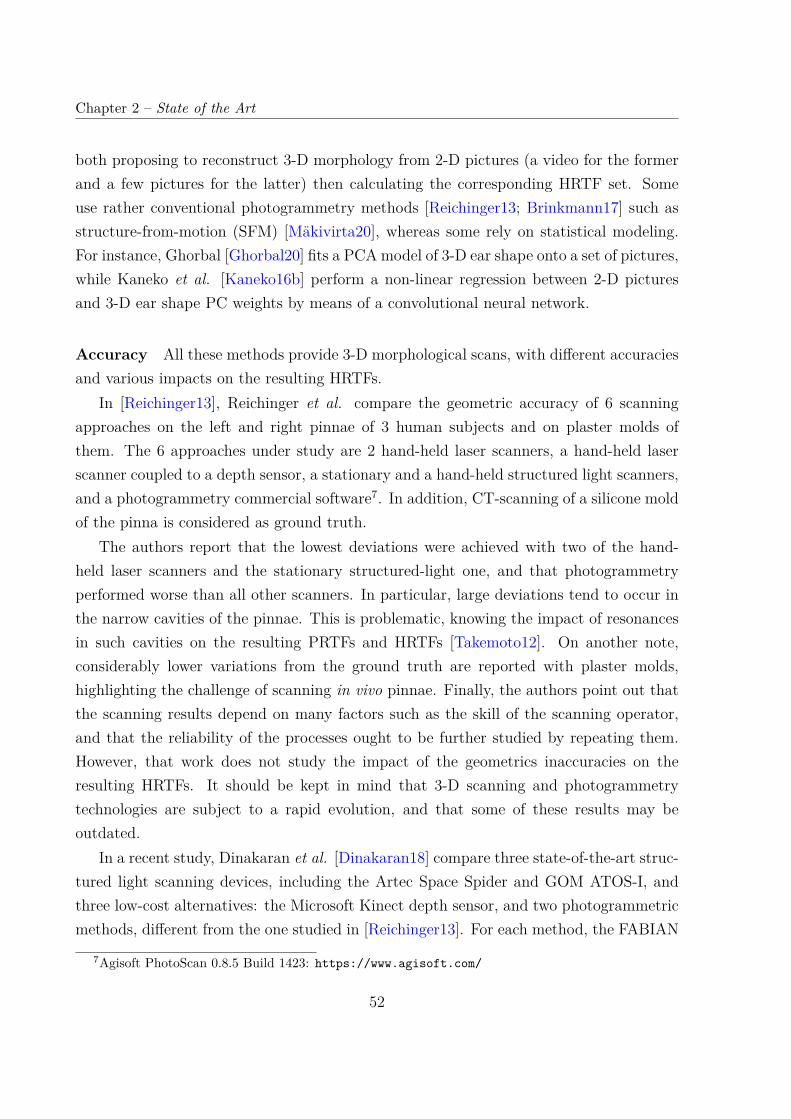
Chapter 2 – State of the Art
both proposing to reconstruct 3-D morphology from 2-D pictures (a video for the formerand a few pictures for the latter) then calculating the corresponding HRTF set. Someuse rather conventional photogrammetry methods [Reichinger13; Brinkmann17] such asstructure-from-motion (SFM) [Mäkivirta20], whereas some rely on statistical modeling.For instance, Ghorbal [Ghorbal20] fits a PCA model of 3-D ear shape onto a set of pictures,while Kaneko et al. [Kaneko16b] perform a non-linear regression between 2-D picturesand 3-D ear shape PC weights by means of a convolutional neural network.
Accuracy All these methods provide 3-D morphological scans, with different accuraciesand various impacts on the resulting HRTFs.
In [Reichinger13], Reichinger et al. compare the geometric accuracy of 6 scanningapproaches on the left and right pinnae of 3 human subjects and on plaster molds ofthem. The 6 approaches under study are 2 hand-held laser scanners, a hand-held laserscanner coupled to a depth sensor, a stationary and a hand-held structured light scanners,and a photogrammetry commercial software7. In addition, CT-scanning of a silicone moldof the pinna is considered as ground truth.
The authors report that the lowest deviations were achieved with two of the hand-held laser scanners and the stationary structured-light one, and that photogrammetryperformed worse than all other scanners. In particular, large deviations tend to occur inthe narrow cavities of the pinnae. This is problematic, knowing the impact of resonancesin such cavities on the resulting PRTFs and HRTFs [Takemoto12]. On another note,considerably lower variations from the ground truth are reported with plaster molds,highlighting the challenge of scanning in vivo pinnae. Finally, the authors point out thatthe scanning results depend on many factors such as the skill of the scanning operator,and that the reliability of the processes ought to be further studied by repeating them.However, that work does not study the impact of the geometrics inaccuracies on theresulting HRTFs. It should be kept in mind that 3-D scanning and photogrammetrytechnologies are subject to a rapid evolution, and that some of these results may beoutdated.
In a recent study, Dinakaran et al. [Dinakaran18] compare three state-of-the-art struc-tured light scanning devices, including the Artec Space Spider and GOM ATOS-I, andthree low-cost alternatives: the Microsoft Kinect depth sensor, and two photogrammetricmethods, different from the one studied in [Reichinger13]. For each method, the FABIAN
7Agisoft PhotoScan 0.8.5 Build 1423: https://www.agisoft.com/
52
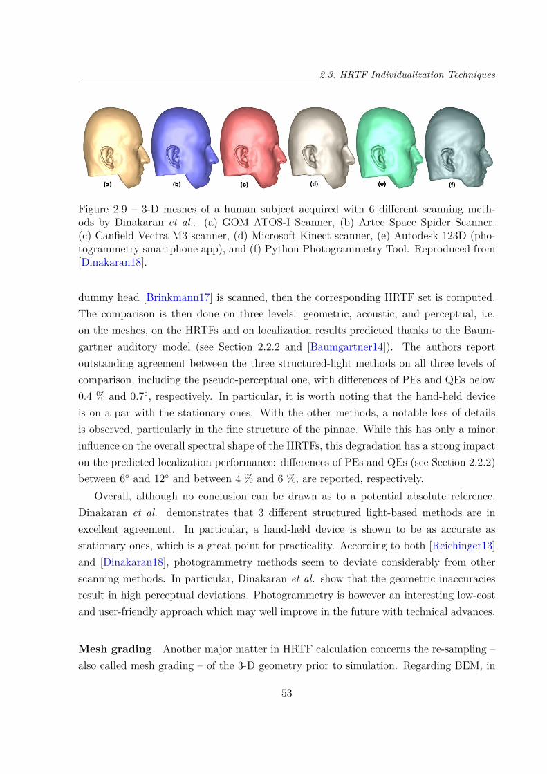
2.3. HRTF Individualization Techniques
Figure 2.9 – 3-D meshes of a human subject acquired with 6 different scanning meth-ods by Dinakaran et al.. (a) GOM ATOS-I Scanner, (b) Artec Space Spider Scanner,(c) Canfield Vectra M3 scanner, (d) Microsoft Kinect scanner, (e) Autodesk 123D (pho-togrammetry smartphone app), and (f) Python Photogrammetry Tool. Reproduced from[Dinakaran18].
dummy head [Brinkmann17] is scanned, then the corresponding HRTF set is computed.The comparison is then done on three levels: geometric, acoustic, and perceptual, i.e.on the meshes, on the HRTFs and on localization results predicted thanks to the Baum-gartner auditory model (see Section 2.2.2 and [Baumgartner14]). The authors reportoutstanding agreement between the three structured-light methods on all three levels ofcomparison, including the pseudo-perceptual one, with differences of PEs and QEs below0.4 % and 0.7, respectively. In particular, it is worth noting that the hand-held deviceis on a par with the stationary ones. With the other methods, a notable loss of detailsis observed, particularly in the fine structure of the pinnae. While this has only a minorinfluence on the overall spectral shape of the HRTFs, this degradation has a strong impacton the predicted localization performance: differences of PEs and QEs (see Section 2.2.2)between 6 and 12 and between 4 % and 6 %, are reported, respectively.
Overall, although no conclusion can be drawn as to a potential absolute reference,Dinakaran et al. demonstrates that 3 different structured light-based methods are inexcellent agreement. In particular, a hand-held device is shown to be as accurate asstationary ones, which is a great point for practicality. According to both [Reichinger13]and [Dinakaran18], photogrammetry methods seem to deviate considerably from otherscanning methods. In particular, Dinakaran et al. show that the geometric inaccuraciesresult in high perceptual deviations. Photogrammetry is however an interesting low-costand user-friendly approach which may well improve in the future with technical advances.
Mesh grading Another major matter in HRTF calculation concerns the re-sampling –also called mesh grading – of the 3-D geometry prior to simulation. Regarding BEM, in
53

Chapter 2 – State of the Art
Figure 2.10 – Reference 3-D mesh (a), uniform grading with an average edge length of2 mm (b), and progressive grading with an edge length ranging from 1 to 25 mm (c).Reproduced from [Ziegelwanger14c].
particular, the surface mesh must be re-arranged so that it is regular enough and so theedge lengths are small enough in regard to the simulation’s wavelength. As computingtime increases considerably with the number of mesh elements, the re-meshing resolutionis a trade-off between numerical accuracy and computing time.
Although the use of the six-elements-per-wavelength rule [Marburg02] has been widespread,the Acoustics Research Institute has recently well contributed to the subject. Indeed, bystudying the effect of various average edge lengths (AEL) on the resulting HRTFs, objec-tively and subjectively, Ziegelwanger et al. [Ziegelwanger15b] determine that the optimalresolution for uniform re-meshing is an AEL of 1 mm.
Going further, in their 2016 study [Ziegelwanger16], they implement and comparevarious re-meshing methods, demonstrating that a progressive approach is appropriateand desirable. Indeed, making the mesh fine (AEL ' 1 mm) near the ear canal andcoarser the further away from it allows a factor-10 decrease in the computing cost ofFM-BEM simulation while maintaining HRTF accuracy. Their code was made availableon-line along with their HRTF simulation software Mesh2HRTF 8 [Ziegelwanger15a]. Theeffect of both uniform and progressive mesh gradings are shown in Figure 2.10.
In the case of FDTD simulation, similar work has been carried out through the study ofthe impact of the voxelization of a subject’s volumetric geometry on the resulting HRTFs[Prepelit,ă16].
8https://sourceforge.net/projects/mesh2hrtf/.
54
2.3. HRTF Individualization Techniques
Computing time
Computing time used to be the main drawback of HRTF calculation. Indeed, up until 2007[Huttunen07; Mokhtari07], computations of HRTFs on the whole audible frequency rangewere scarce. For instance, in pioneering work by Katz et al. [Katz01] in 2001, the BEMcalculation of HRTF set is limited to a frequency range of 1 kHz to 5.4 kHz, and took 28hours for 54 regularly-spaced frequencies and a single ear. The author extrapolates that,using his setup, it would take more than 5 years to compute an HRTF set for frequenciesup to 20 kHz for both ears.
Computing times have however greatly been reduced since then. While the exponentialdecrease in the cost of CPU power and RAM is certainly a major factor, several technicaladvances have had a major part in this reduction.
One of these advances was the introduction by Gumerov et al. of FM-BEM in 2007[Gumerov07]. In their 2010 study, Gumerov et al. [Gumerov10] report that the FM-BEMcomputation of a single-ear HRTF set of a mesh that includes the torso takes 30 h for 117frequencies ranging from 172 Hz to 20.155 kHz.
The work by Ziegelwanger et al. [Ziegelwanger16] on progressive mesh grading con-stitutes another major step forward, as it reported to permit a factor-10 decrease in thecomputing load (see previous paragraph).
The democratization of distributed computing on clusters over the last decade andthe constant increase in available computing power have further decreased the computingtimes. Indeed, simulations in the harmonic domain such as the FEM or BEM are highlydistributable, as each frequency is simulated independently. Although in theory hundredsof frequencies could be computed simultaneously, parallelization is generally limited byhigh memory requirements (especially at high frequencies), as the memory is often sharedby the parallel threads. As early as 2007, Huttunen et al. [Huttunen07] distribute FEMsimulations on a PC cluster of 22 CPU cores and 44 GB total RAM. They report comput-ing times ranging from a few tens of seconds at 20 Hz to 2.5 h at 20 kHz, and extrapolatethat a complete HRTF set with relatively low high-frequency resolution (500 Hz steps forfrequencies above 13 kHz) could be computed in a few days. By distributing FM-BEMcomputations on a cluster of 5 PCs with 2-core CPUs, Kreuzer et al. [Kreuzer09] reportin 2009 to have computed a complete single-ear HRTF set in 5 hours for 100 frequen-cies ranging from 200 Hz to 20 kHz. Recently, Fan et al. [Fan19] have implemented aGPU-distributed version of conventional BEM and used it to compute HRTFs. Due tolimitations in global GPU memory, computations for a mesh with torso were limited to
55
Chapter 2 – State of the Art
an upper frequency of 12 kHz. The authors report computation times of 5 to 7.5 secondsper frequency and of 12.8 to 21.5 seconds per frequency for a mesh without and withtorso, respectively. It is however unclear whether these per-frequency computation timesare averaged over all frequencies, or if they correspond to a specific frequency.
With our own numerical simulation setup (see Chapter 3), the calculation of a completePRTF set by means of FM-BEM was distributed over 10 cores of a desktop workstation of12 CPU cores and 32 GB of RAM. Not all 12 cores could be exploited due to limitations inthe memory, shared by all threads. The computation of one PRTF set from a pinna mesh(up to about 55000 triangular faces at the highest frequency i.e. 16 kHz) was achieved in1 hour, with computing times ranging from 4 s to 5 min per frequency. For a completetorso – a substantially larger mesh (up to about 110000 triangular faces at the highestfrequency i.e. 16 kHz), using the same setup, the calculation of an HRTF set is distributedon only 5 CPU cores and takes about 10 hours, with computing times ranging from 40 sto 45 min per frequency.
Comparison with measurements
Several studies compare calculated HRTF sets to acoustically measured ones [Greff07;Kreuzer09; Gumerov10; Ziegelwanger13; Brinkmann19] and agree on the following. Whilethe shapes of the spectral patterns are overall coherent and while there is good agreementbelow 5 to 7 kHz, large mismatches are observed at higher frequencies. In particular, localspatial-spectral features such as notches and peaks – known to be important featuresfor elevation perception – are impacted, being displaced (in space and/or frequency),attenuated and sometimes absent [Greff07; Kreuzer09; Gumerov10].
Greff et al. [Greff07] compare two different calculations (carried out by different teams)and a measurement of the HRTF set of a dummy-head manikin. They find that, in thefrontal position, the two calculated HRTF show minimal spectral variations between eachother, but both exhibit a frequency shift above 5 kHz compared to the measurement. Interms of ITD, good agreement is obtained between all three methods.
Such deviations are also reported by Brinkmann et al. [Brinkmann19] in a larger-scalestudy, in which the calculated and measured HRTF sets of 96 human subjects of theHUTUBS database are compared. The authors report an average spectral difference ofless than 1 dB below 5 kHz and of up to 7 dB at 17.1 kHz. Differences in ITD are reportedto be lower than the JND of 20 µs for most sound source positions and subjects. Goingfurther, the authors asked 46 subjects to participate in a rating experiment which aimed
56
2.3. HRTF Individualization Techniques
at comparing both types of HRTF sets based on 12 criteria. The listeners were generallywere able to discriminate computed and measured HRTFs. In particular, large differencesin coloration were perceived, with emphasized high- and attenuated low-frequencies forcomputed HRTFs. The authors note that, indeed, simulated HRTFs contain on averagemore high-frequency energy than measured ones. Regarding localization, an elevationshift of 12 upwards and an azimuth shift of 2 clockwise were reported. According to theauthors, the former might be partially explained by the high-frequency boost.
Beside [Brinkmann19], a few studies evaluate computed HRTFs perceptually [Turku08;Ziegelwanger15b; Fan19]. However, among them, only one [Ziegelwanger15b] concerns in-dividual HRTF sets of human subjects. In that study, Ziegelwanger et al. study varioussimulation settings such as mesh grading or source position. They evaluate the local-ization performance in the horizontal and median planes of 3 subjects presented withtheir computed own HRTF set and their own acoustically measured one (from the ARIdatabase). With the setting that performed best, they report localization performanceswith computed HRTF sets to be on a par with measured ones. However, these resultsshould be taken with caution seeing that only 3 subjects participated in the study.
Overall, the perceptual relevance of computed HRTFs remains to be demonstrated.Indeed, notable spectral mismatches are generally observed between computed and mea-sured HRTFs, potentially affecting features that are useful for vertical localization. Never-theless, acoustic measurement is no absolute reference (see Section 2.3.1) and perceptualassessment ought to be the ultimate criteria. However, perceptual studies are conspic-uous by their scarcity and present mitigated results. While Ziegelwanger et al. [Ziegel-wanger15b] report localization performances with computed HRTFs to be as good as withmeasured ones, the study includes too few subjects to be really conclusive. Furthermore,according to Brinkmann et al.’s [Brinkmann19] 46-subject rating experiment, listenersconsistently discriminate computed and measured HRTF, localize differently and reporta different timbre colorations.
2.3.3 Indirect Individualization based on Morphological Data
Though more convenient than acoustic measurement, HRTF calculation still requiresspecialized equipment and non-negligible mesh processing and computing time. Hence,based on the idea that the individual character of HRTFs derives from morphologicaldifferences, many studies have explored the idea of a low-cost HRTF individualizationbased on simple morphological data such as anthropometric measurements.
57
Chapter 2 – State of the Art
Selection
One way to tackle the problem is to select the most suited non-individual HRTF setamong a database.
Using the 46-subject CIPIC database (see Section 2.4, [Algazi01c]), Zotkin et al.[Zotkin02] propose to select the HRTF set associated with the anthropometric nearestneighbor. The latter is determined based on 7 morphological parameters measured on apicture of the pinna. According to their 6-subject localization experiment, for 4 of thesubjects, the elevation error is lower by 15-20 % with the best-fit HRTF set than with ageneric one (the HRTF set of a listener who did not participate in the experiment). How-ever, for the 2 remaining subjects, the error is either lower by only 5 % or considerablyhigher (by 73 %), highlighting highly variable performances. Averaging the results overthe 6 subjects ourselves, we find an elevation error decrease of only 0.7 with a standarddeviation of 3.1. Regarding the azimuthal dimension, we find a notable degradation,with an average error increase of 3.3 (with a standard deviation of 3.3). The latter isnot commented by the authors but is somewhat expected, seeing that the HRTF selectionprocess relies on the dimensions of the pinna but not of the head. Overall, the localizationresults are hardly conclusive and, as the authors point out, a larger-scale perceptual studywould be needed.
In [Schönstein10] Schönstein et al. propose to select an HRTF set among 37 fromthe LISTEN database (see Section 2.4, [Warusfel03]) based on a set of 5 anthropomet-ric parameters. To do so, a multilinear regression is performed between the 37 sets ofmorphological measurements and a compact representation of the matching HRTF sets.Two methods are considered to create this compact representation: PCA of linear mag-nitude HRTF sets performed in the inter-individual fashion (see Section 2.1.3), and MDS(multidimensional scaling) of global frequency scaling factors which are used to character-ize spectral dissimilarity between HRTF sets as in [Middlebrooks99a]. To evaluate theirmethod, they compare its rankings of HRTF sets to a rating (bad/ok/excellent) of the46 LISTEN HRTF sets established in a previous study [Katz12] by 45 of the subjects bymeans of listening tests. In particular, they look at the proportion of excellent ratings inthe HRTF sets ranked among the first 10 by the method. With regard to that metric,they find that their method outperforms the random selection of 10 HRTF sets for 26 outof 37 subjects.
Recently, Yao et al. [Yao17] have proposed a concurrent method that relies on aneural network trained to predict a perceptual score from anthropometric measurements.
58
2.3. HRTF Individualization Techniques
30 subjects were asked to rate 18 HRTF sets of the CIPIC database on a scale from 1 to 5according to two criteria: front-back and elevation discrimination. The two rating scoresare then combined into one by computing the mean, thus giving a perceptual score for eachsubject and HRTF set. A single- or double-hidden-layer neural network was then trainedto predict this localization score from 10 anthropometric measurements of the head andpinnae. Thus, when presenting the neural network with a new set of anthropometricmeasurements, one or several best-fit non-individual HRTF sets are presented to the userbased on the predicted perceptual score. Evaluating the method by means of a leave-one-out cross-validation, they compare the performance of both neural networks with thatof Zotkin et al.’s approach. They find that the two former outperform the latter. Inparticular, the “target” HRTF set (i.e. the one with the best perceptual score) is found tobe among the 3 predicted best-fit HRTF sets for 40 % of the 18 subjects for both neuralnetwork methods, against 23.3 % for Zotkin et al.’s.
Adaptation
Complementary to the selection of a best-fit non-individual HRTF set in a database, ageneric HRTF set can be adapted to the user by means of rudimentary transformations.
Based on the idea that a variation in pinna size results in a frequency scaling ofthe corresponding spectral features in the HRTFs from all directions, Middlebrooks etal. [Middlebrooks99a; Middlebrooks00] propose a rough adaptation of a generic HRTFset by means of a global frequency scaling. Three methods of determining the optimalscaling factor are compared: best spectral match in terms of ISSD (see Section 2.2.1),linear regression from 9 morphological measurements of the head and pinna, and tuningby the listener. In [Middlebrooks99a], an objective comparison between the two former ispresented, for 33 subjects of a proprietary database. The authors report that the acousticoptimal scaling factor could be retrieved from only pinna height and head width with acorrelation factor of 0.89 and RMS error of 0.069. In addition to a frequency scaling,the ISSD can be further reduced by applying a head tilt to the HRTF set. On averageover all 990 pairwise comparisons, average ISSDs of 8.29 dB2, 6.18 dB2 and 5.37 dB2 arereported for HRTF sets without adaptation, with scaling, and with scaling and head tilt,respectively.
In the companion paper [Middlebrooks00], the listener-driven method is presented andcompared to the two former by means of localization experiments with 5 subjects. Threenon-individual HRTF sets are used for this comparison, chosen so as to span the range of
59

Chapter 2 – State of the Art
optimal frequency scalings observed in their dataset of 33 measured HRTF sets. Regardingthe subjective tuning procedure, the listeners were randomly presented with virtual soundsources located in the median plane. During each of 240 trials, knowing the sound source’sposition, they elected in an A/B comparison one of two scaled HRTFs according to criteriaof front-back discrimination, primarily, and elevation accuracy, secondarily. The processlasted about one hour. A good agreement was obtained between the scaling factorsobtained via tuning and the acoustic ones, with a correlation of 0.89 and a RMS errorof 0.069. Regarding the perceptual assessment of scaled generic HRTF sets, a notabledecrease in quadrant error (QE, see Section 2.2.2) of more than half the difference betweenown and raw generic is reported in 7 cases out of 9 (each of the 5 listeners listened to oneor two non-individual HRTF sets for a total of 9 cases). However, for the two remainingsubjects, the QE increases. Local angular accuracy is not evaluated.
Later on, other researchers [Maki05; Guillon08] also propose to apply a combination offrequency scaling and rotation to adapt a generic HRTF set. In particular, Guillon et al.[Guillon08] derives the frequency scaling and rotation parameters from 3-D scans of thehead and pinnae for 6 subjects. However, neither study include a perceptual evaluationof the resulting HRTF sets.
Regression
The methods reviewed above aim at reducing perceptual discrepancies due to non-individualHRTF sets by rudimentary means which do not embrace the full complexity of the inter-individual variations of HRTFs. They thus cannot pretend to provide an HRTF set whoseperceptual quality would come close to individual conditions. Hence, a lot of work hasrelied on statistical modeling and regression to synthesize individualized HRTF sets fromanthropometric measurements.
To this end, an approach that has widely been used since the early 2000s is to performa regression between a set of 8 to 93 heuristically-chosen morphological measurementsand the corresponding HRTF sets.
While most – especially early – work use multiple linear regression [Jin00; Hu06;Huang09b; Hugeng10; Bomhardt16a; Liu19b] or other linear methods [Bilinski14] to linkthe anthropometric and acoustic spaces, others use non-linear techniques such as sup-port vector regression (SVR) [Huang09b] and neural networks [Hu08; Li13; Grijalva14;Fayek17; Qi18; Zhang20]. Due to their high dimensionality, the HRTF sets are typi-cally “compressed” prior to regression, by means of PCA [Jin00; Hu06; Hu08; Huang09a;
60
2.3. HRTF Individualization Techniques
Hugeng10; Bomhardt16a; Fayek17; Zhang20], independent component analysis (ICA)[Huang09b; Liu19b], sparsity-constrained weight mapping (SWM) [Qi18], high-order sin-gular value decomposition [Li13] or Isomap [Grijalva14].
Often, a subset of “key” morphological measurements is selected based on their statis-tical relevance [Hu08; Huang09a; Zhang20] prior to regression. Sometimes, they are rep-resented as weights of a statistical model such as PCA [Jin00] or factor analysis [Liu19b].However, the number and choice of the parameters is limited by the dataset. In the vastmajority of cases, the dataset is CIPIC, which includes 27 heuristically-defined anthropo-metric features, measured from a 2-D picture. It thus seems legitimate to question theaccuracy of these measurements and the choice of only 27 parameters, in particular fora complex 3-D shape such as the pinna. This issue is however barely addressed in theliterature, although sometimes mentioned in the few studies in which a different dataset isused: [Bilinski14] and [Bomhardt16a] and their respective 96 and 12 measurements madefrom 3-D meshes, and [Jin00] and their 20 measurements made with a 3D stylus pen.
Regarding perceptual assessment, among the 15 aforementioned studies, 4 providelocalization experiments. In their first study based on multiple linear regression, Hu et al.[Hu06] compare the localization performance of 5 subjects presented with their customizedHRTF set and with a non-individual HRTF set, that of CIPIC’s subject 003. The resultsshow a modest advantage for the customized condition, with an average rate of correctanswers of 79.2 % against 61 % and an average rate of front-back confusions of 10.8 %and 11.7 %. The variance of these results is however not reported and only horizontalpositions are under test. In their later study based on a three-layer neural network, Huet al. [Hu08] perform a similar 5-subject localization experiment. They report a slightlybetter result than the previous study, with average rates of correct answers of 75.2 % and56.1 %, and front-back confusion rates of 9.7 % and 12.2 % for the customized and CIPIC003 HRTF sets, respectively. In this study as well, the variance is not reported and onlyhorizontal positions are under test. Liu et al. [Liu19b] perform a 6-subject localizationexperiment in 6 directions of the median plane for the customized and the KEMARHRTF sets. They report an improvement in localization with the customized conditionover the KEMAR one, with respective front-back confusion rates of 5.1 % and 10.6 % andrespective up-down confusion rates of 6.9 % and 10.2 %. Finally, Zhang et al. [Zhang20]perform a localization experiment with 5 subjects for 3 directions of the median plane.For all 3 directions, a statistically significant decrease in angular error is observed betweenKEMAR and customized HRTF sets. A statistically significant difference in front-back
61
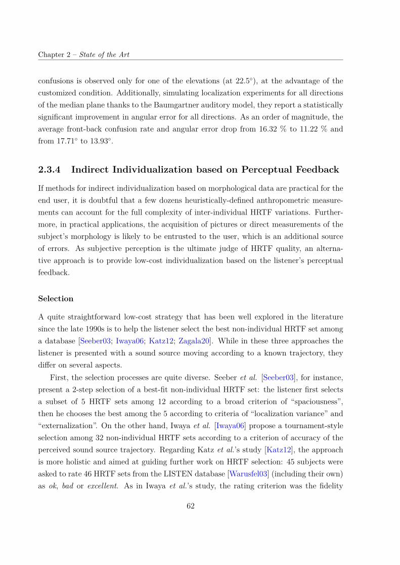
Chapter 2 – State of the Art
confusions is observed only for one of the elevations (at 22.5), at the advantage of thecustomized condition. Additionally, simulating localization experiments for all directionsof the median plane thanks to the Baumgartner auditory model, they report a statisticallysignificant improvement in angular error for all directions. As an order of magnitude, theaverage front-back confusion rate and angular error drop from 16.32 % to 11.22 % andfrom 17.71 to 13.93.
2.3.4 Indirect Individualization based on Perceptual Feedback
If methods for indirect individualization based on morphological data are practical for theend user, it is doubtful that a few dozens heuristically-defined anthropometric measure-ments can account for the full complexity of inter-individual HRTF variations. Further-more, in practical applications, the acquisition of pictures or direct measurements of thesubject’s morphology is likely to be entrusted to the user, which is an additional sourceof errors. As subjective perception is the ultimate judge of HRTF quality, an alterna-tive approach is to provide low-cost individualization based on the listener’s perceptualfeedback.
Selection
A quite straightforward low-cost strategy that has been well explored in the literaturesince the late 1990s is to help the listener select the best non-individual HRTF set amonga database [Seeber03; Iwaya06; Katz12; Zagala20]. While in these three approaches thelistener is presented with a sound source moving according to a known trajectory, theydiffer on several aspects.
First, the selection processes are quite diverse. Seeber et al. [Seeber03], for instance,present a 2-step selection of a best-fit non-individual HRTF set: the listener first selectsa subset of 5 HRTF sets among 12 according to a broad criterion of “spaciousness”,then he chooses the best among the 5 according to criteria of “localization variance” and“externalization”. On the other hand, Iwaya et al. [Iwaya06] propose a tournament-styleselection among 32 non-individual HRTF sets according to a criterion of accuracy of theperceived sound source trajectory. Regarding Katz et al.’s study [Katz12], the approachis more holistic and aimed at guiding further work on HRTF selection: 45 subjects wereasked to rate 46 HRTF sets from the LISTEN database [Warusfel03] (including their own)as ok, bad or excellent. As in Iwaya et al.’s study, the rating criterion was the fidelity
62
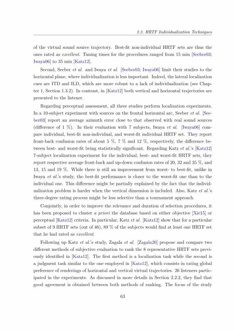
2.3. HRTF Individualization Techniques
of the virtual sound source trajectory. Best-fit non-individual HRTF sets are thus theones rated as excellent. Tuning times for the procedures ranged from 15 min [Seeber03;Iwaya06] to 35 min [Katz12].
Second, Seeber et al. and Iwaya et al. [Seeber03; Iwaya06] limit their studies to thehorizontal plane, where individualization is less important. Indeed, the lateral localizationcues are ITD and ILD, which are more robust to a lack of individualization (see Chap-ter 1, Section 1.3.2). In contrast, in [Katz12] both vertical and horizontal trajectories arepresented to the listener.
Regarding perceptual assessment, all three studies perform localization experiments.In a 10-subject experiment with sources on the frontal horizontal arc, Seeber et al. [See-ber03] report an average azimuth error close to that observed with real sound sources(difference of 1 %). In their evaluation with 7 subjects, Iwaya et al. [Iwaya06] com-pare individual, best-fit non-individual, and worst-fit individual HRTF set. They reportfront-back confusion rates of about 5 %, 7 % and 12 %, respectively, the difference be-tween best- and worst-fit being statistically significant. Regarding Katz et al.’s [Katz12]7-subject localization experiment for the individual, best- and worst-fit HRTF sets, theyreport respective average front-back and up-down confusion rates of 20, 32 and 35 %, and13, 15 and 19 %. While there is still an improvement from worst- to best-fit, unlike inIwaya et al.’s study, the best-fit performance is closer to the worst-fit one than to theindividual one. This difference might be partially explained by the fact that the individ-ualization problem is harder when the vertical dimension is included. Also, Katz et al.’sthree-degree rating process might be less selective than a tournament approach.
Conjointly, in order to improve the relevance and duration of selection procedures, ithas been proposed to cluster a priori the database based on either objective [Xie15] orperceptual [Katz12] criteria. In particular, Katz et al. [Katz12] show that for a particularsubset of 9 HRTF sets (out of 46), 89 % of the subjects would find at least one HRTF setthat he had rated as excellent.
Following up Katz et al.’s study, Zagala et al. [Zagala20] propose and compare twodifferent methods of subjective evaluation to rank the 8 representative HRTF sets previ-ously identified in [Katz12]. The first method is a localization task while the second isa judgment task similar to the one employed in [Katz12], which consists in rating globalpreference of renderings of horizontal and vertical virtual trajectories. 26 listeners partic-ipated in the experiments. As discussed in more details in Section 2.2.2, they find thatgood agreement is obtained between both methods of ranking. The focus of the study
63
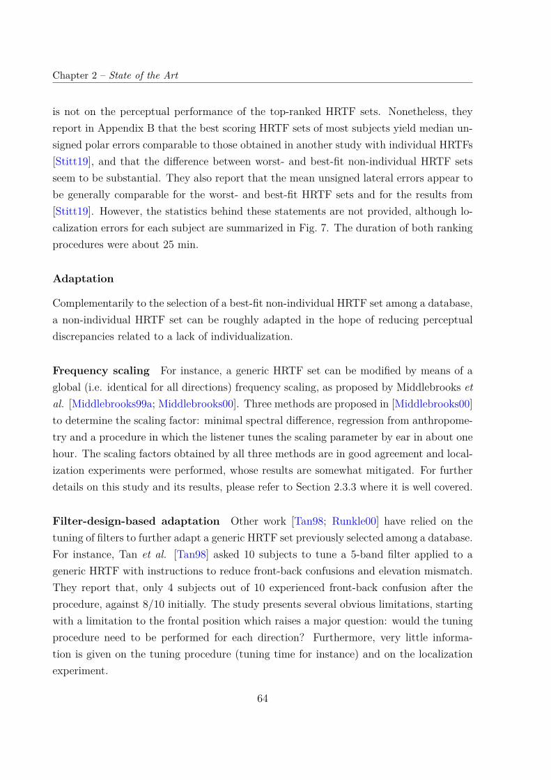
Chapter 2 – State of the Art
is not on the perceptual performance of the top-ranked HRTF sets. Nonetheless, theyreport in Appendix B that the best scoring HRTF sets of most subjects yield median un-signed polar errors comparable to those obtained in another study with individual HRTFs[Stitt19], and that the difference between worst- and best-fit non-individual HRTF setsseem to be substantial. They also report that the mean unsigned lateral errors appear tobe generally comparable for the worst- and best-fit HRTF sets and for the results from[Stitt19]. However, the statistics behind these statements are not provided, although lo-calization errors for each subject are summarized in Fig. 7. The duration of both rankingprocedures were about 25 min.
Adaptation
Complementarily to the selection of a best-fit non-individual HRTF set among a database,a non-individual HRTF set can be roughly adapted in the hope of reducing perceptualdiscrepancies related to a lack of individualization.
Frequency scaling For instance, a generic HRTF set can be modified by means of aglobal (i.e. identical for all directions) frequency scaling, as proposed by Middlebrooks etal. [Middlebrooks99a; Middlebrooks00]. Three methods are proposed in [Middlebrooks00]to determine the scaling factor: minimal spectral difference, regression from anthropome-try and a procedure in which the listener tunes the scaling parameter by ear in about onehour. The scaling factors obtained by all three methods are in good agreement and local-ization experiments were performed, whose results are somewhat mitigated. For furtherdetails on this study and its results, please refer to Section 2.3.3 where it is well covered.
Filter-design-based adaptation Other work [Tan98; Runkle00] have relied on thetuning of filters to further adapt a generic HRTF set previously selected among a database.For instance, Tan et al. [Tan98] asked 10 subjects to tune a 5-band filter applied to ageneric HRTF with instructions to reduce front-back confusions and elevation mismatch.They report that, only 4 subjects out of 10 experienced front-back confusion after theprocedure, against 8/10 initially. The study presents several obvious limitations, startingwith a limitation to the frontal position which raises a major question: would the tuningprocedure need to be performed for each direction? Furthermore, very little informa-tion is given on the tuning procedure (tuning time for instance) and on the localizationexperiment.
64
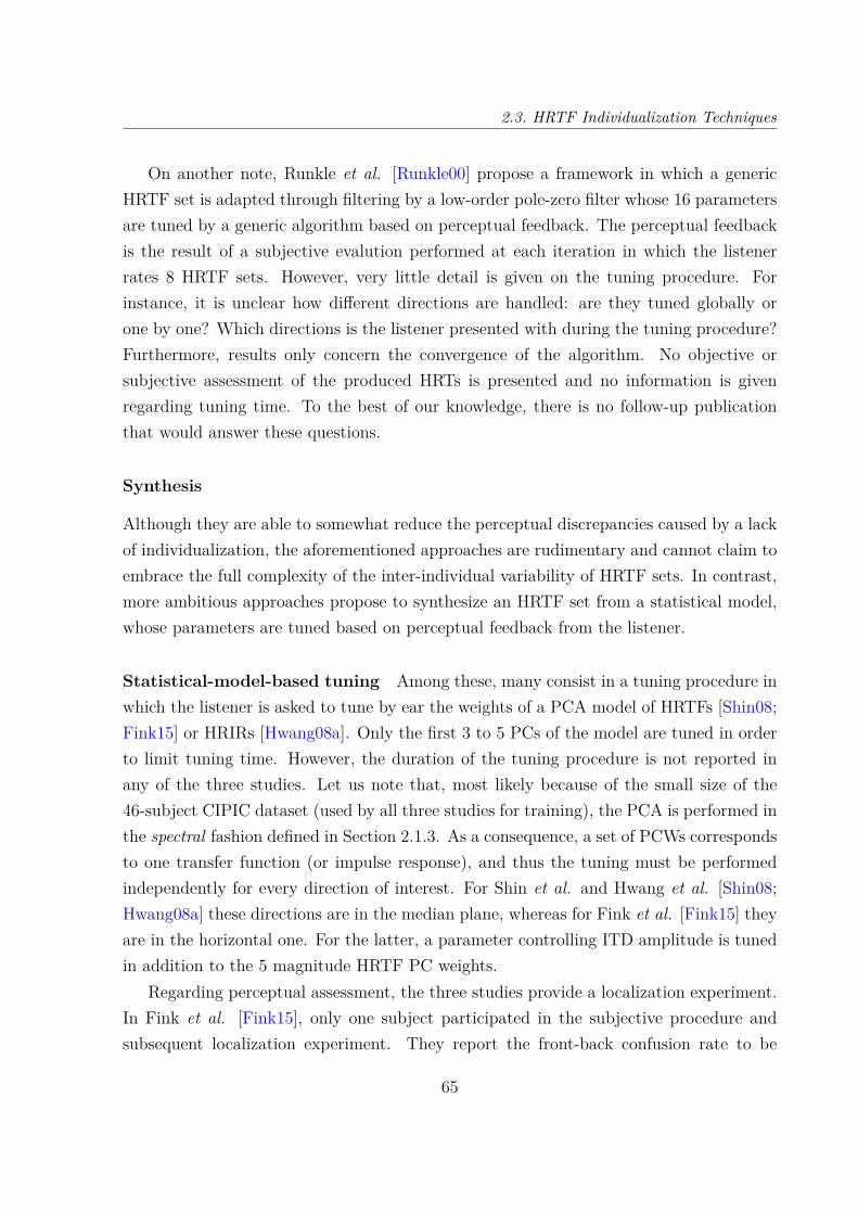
2.3. HRTF Individualization Techniques
On another note, Runkle et al. [Runkle00] propose a framework in which a genericHRTF set is adapted through filtering by a low-order pole-zero filter whose 16 parametersare tuned by a generic algorithm based on perceptual feedback. The perceptual feedbackis the result of a subjective evalution performed at each iteration in which the listenerrates 8 HRTF sets. However, very little detail is given on the tuning procedure. Forinstance, it is unclear how different directions are handled: are they tuned globally orone by one? Which directions is the listener presented with during the tuning procedure?Furthermore, results only concern the convergence of the algorithm. No objective orsubjective assessment of the produced HRTs is presented and no information is givenregarding tuning time. To the best of our knowledge, there is no follow-up publicationthat would answer these questions.
Synthesis
Although they are able to somewhat reduce the perceptual discrepancies caused by a lackof individualization, the aforementioned approaches are rudimentary and cannot claim toembrace the full complexity of the inter-individual variability of HRTF sets. In contrast,more ambitious approaches propose to synthesize an HRTF set from a statistical model,whose parameters are tuned based on perceptual feedback from the listener.
Statistical-model-based tuning Among these, many consist in a tuning procedure inwhich the listener is asked to tune by ear the weights of a PCA model of HRTFs [Shin08;Fink15] or HRIRs [Hwang08a]. Only the first 3 to 5 PCs of the model are tuned in orderto limit tuning time. However, the duration of the tuning procedure is not reported inany of the three studies. Let us note that, most likely because of the small size of the46-subject CIPIC dataset (used by all three studies for training), the PCA is performed inthe spectral fashion defined in Section 2.1.3. As a consequence, a set of PCWs correspondsto one transfer function (or impulse response), and thus the tuning must be performedindependently for every direction of interest. For Shin et al. and Hwang et al. [Shin08;Hwang08a] these directions are in the median plane, whereas for Fink et al. [Fink15] theyare in the horizontal one. For the latter, a parameter controlling ITD amplitude is tunedin addition to the 5 magnitude HRTF PC weights.
Regarding perceptual assessment, the three studies provide a localization experiment.In Fink et al. [Fink15], only one subject participated in the subjective procedure andsubsequent localization experiment. They report the front-back confusion rate to be
65

Chapter 2 – State of the Art
notably better with the customized HRTF set than with the average HRTF set of thedatabase: 36.25 % against 16.25 %. However, it should be noted that the average HRTFset is somewhat unrealistic: the peaks and notches are smoothed out compared to a“real” HRTF set, likely degrading useful spectral localization cues. Regarding Shin etal. and Hwang et al. [Shin08; Hwang08a], the customized HRTF set is compared tothe individual one and to that of the KEMAR manikin. In the former study, for twosubjects out of 4, the front-back confusion rate is notably lower with the two formerHRTF conditions (between 6 % and 14 %) than with the latter (between 29 % and 43 %).However, for the 2 remaining subjects, there is no clear trend. The latter study by Hwanget al. shows a clearer trend regarding the front-back confusion rates of the KEMAR andindividual conditions. Indeed, for all 3 subjects, they are in the order of 20 % and 0-1 %respectively. Regarding the customized condition, they report front-back confusion ratesclose to the individual condition for two subjects (in the order of 1 % to 3 %), whereasfor the remaining subject it is quite high (13.3 %).
In these studies, the tuning is local, in the sense that it is performed independentlyat each direction of interest. This poses a problem of tuning time, seeing that a high-resolution HRTF set typically contains HRTFs for several hundreds of directions. Toalleviate this, in his Master’s thesis, Hölzl [Hölzl14] proposes a method to tune an HRTFset globally. Like in the three aforementioned studies, the listener tunes by ear the weightsof a PCA model – built in the spectral fashion – of magnitude HRTFs. However, insteadof tuning the PCWs directly, the listener is asked to tune the coefficients of a sphericalharmonics representation (see Section 2.1.2) of the PCWs. Three training sets are usedin turn to build the PCA model: LISTEN, CIPIC and ARI.
This global approach was however not put in practice and thus there is no perceptualassessment of the method. Let us note that, although this approach allows a globaltuning of an HRTF set, there is no guarantee that these tuning parameters (i.e. SHs ofPCWs) result in plausible HRTF spatial patterns. As mentioned by the author, if the SHcoefficients are tuned by the user with regard to certain directions, it is unknown whetherthe tuning will be appropriate for other areas of the sphere.
Recently, in 2017, Yamamoto and Igarashi [Yamamoto17] propose a method that relieson the modeling of HRTF sets thanks to a variational autoencoder neural network. Thetuning procedure consists in a gradient descent optimization of the network’s weightswhere, at every iteration, the cost is derived from the user’s A/B rating of two HRTF setspresented to him by the algorithm. Here as well, the database used to train the statistical
66

2.3. HRTF Individualization Techniques
model is CIPIC. In contrast with the aforementioned approaches, the parameters thatare tuned correspond to a complete HRTF set (all directions). The optimization thusexplores the space of the inter-individual variations of HRTF sets. The tuning procedureis reported to last 20 to 35 min with about 100-200 pairwise comparisons.
In guise of perceptual assessment, after tuning, the 20 participants are asked to rateHRTF sets pair by pair in a double-blind manner. The baseline condition is a best fitnon-individual HRTF set for each participant, selected among the database by means ofa previous rating test procedure. The authors report a statistically significant preferenceof the customized HRTF set over the best-fit non-individual HRTF set for 18 participantsout of 20.
Conclusion
Overall, acoustic measurement remains the reference in individual HRTFs acquisition.Indeed, it is the historical approach and the resulting HRTFs have been well comparedto real-life sound localization over the years. However, HRTF measurement is far frombeing flawless. Indeed, it suffers from a lack of reproducibility which translates to largevariations in both ITD and magnitude spectra between different measurements setups,but also between repetitions of the same measurements. In particular, when evaluatinga VAS generated thanks to individual measured HRTFs, a number of studies observe adegradation of the localization performance compared to a real auditory environment. Inthese studies, confusion rates are reported to increase by a factor 2 and elevation accuracyto be somewhat degraded. Furthermore, this approach can not be proposed to the enduser: besides the uncomfortable nature of the acquisition process for the subject, themeasurement setup is delicate, expensive and, most of all, untransportable.
As an alternative, individual HRTFs can be computed from 3-D scans of the listener’spinnae, head and torso by means of numerical simulations of acoustic propagation. Unlikemeasurement, the data acquisition step can be performed anywhere, in particular whenreconstructing 3-D morphology from 2-D pictures. Moreover, it allows to work around, orat least to displace, the reproducibility issue: once the 3-D mesh is acquired, the rest ofthe simulation process is deterministic. Be that as it may, the quality of computed HRTFsremains to be demonstrated. Indeed, perceptual studies have been scarce and mismatcheshave been reported in objective comparisons with measured HRTFs. Furthermore, be-tween acquisition, 3-D shape preparation and the simulation itself, the process takes aconsiderable amount of time (in the order of hours), which may be a serious limitation in
67
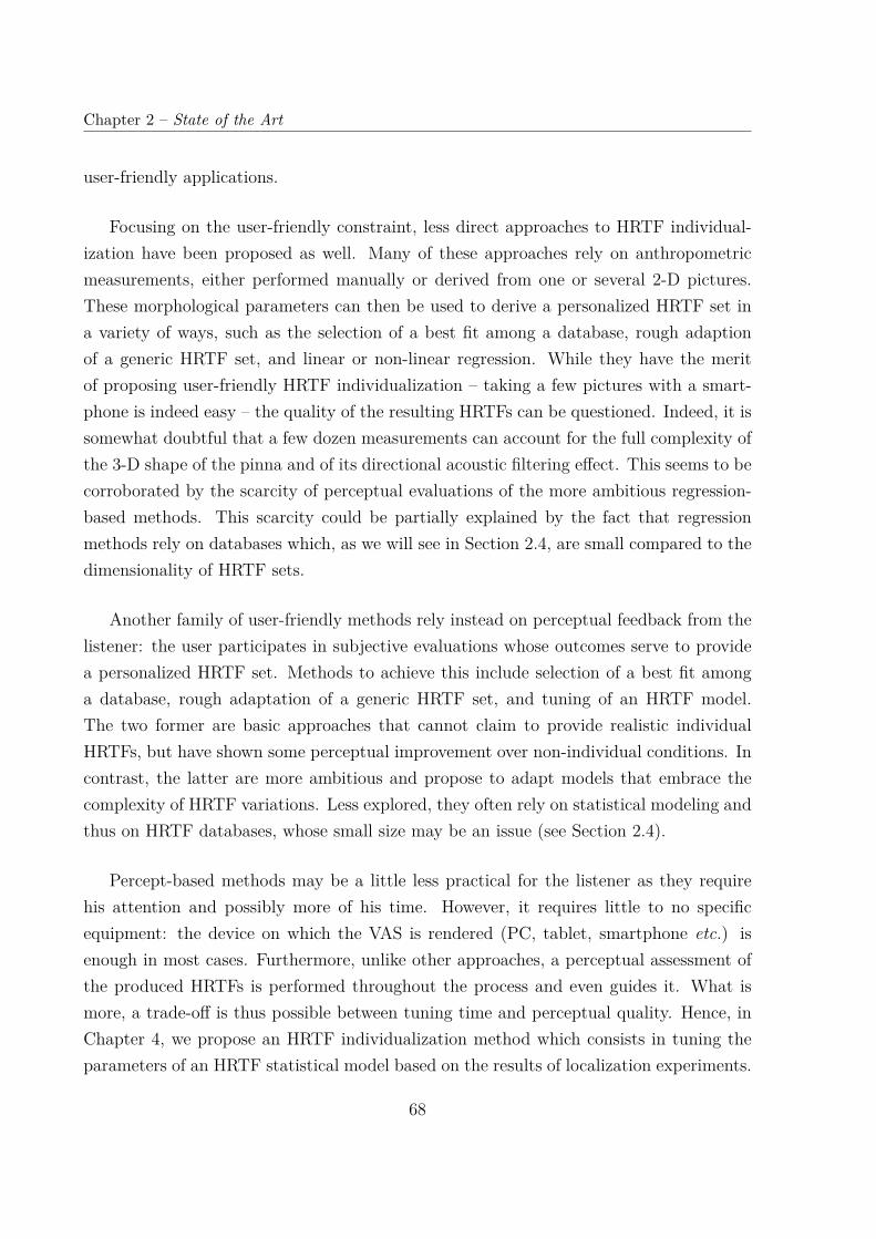
Chapter 2 – State of the Art
user-friendly applications.
Focusing on the user-friendly constraint, less direct approaches to HRTF individual-ization have been proposed as well. Many of these approaches rely on anthropometricmeasurements, either performed manually or derived from one or several 2-D pictures.These morphological parameters can then be used to derive a personalized HRTF set ina variety of ways, such as the selection of a best fit among a database, rough adaptionof a generic HRTF set, and linear or non-linear regression. While they have the meritof proposing user-friendly HRTF individualization – taking a few pictures with a smart-phone is indeed easy – the quality of the resulting HRTFs can be questioned. Indeed, it issomewhat doubtful that a few dozen measurements can account for the full complexity ofthe 3-D shape of the pinna and of its directional acoustic filtering effect. This seems to becorroborated by the scarcity of perceptual evaluations of the more ambitious regression-based methods. This scarcity could be partially explained by the fact that regressionmethods rely on databases which, as we will see in Section 2.4, are small compared to thedimensionality of HRTF sets.
Another family of user-friendly methods rely instead on perceptual feedback from thelistener: the user participates in subjective evaluations whose outcomes serve to providea personalized HRTF set. Methods to achieve this include selection of a best fit amonga database, rough adaptation of a generic HRTF set, and tuning of an HRTF model.The two former are basic approaches that cannot claim to provide realistic individualHRTFs, but have shown some perceptual improvement over non-individual conditions. Incontrast, the latter are more ambitious and propose to adapt models that embrace thecomplexity of HRTF variations. Less explored, they often rely on statistical modeling andthus on HRTF databases, whose small size may be an issue (see Section 2.4).
Percept-based methods may be a little less practical for the listener as they requirehis attention and possibly more of his time. However, it requires little to no specificequipment: the device on which the VAS is rendered (PC, tablet, smartphone etc.) isenough in most cases. Furthermore, unlike other approaches, a perceptual assessment ofthe produced HRTFs is performed throughout the process and even guides it. What ismore, a trade-off is thus possible between tuning time and perceptual quality. Hence, inChapter 4, we propose an HRTF individualization method which consists in tuning theparameters of an HRTF statistical model based on the results of localization experiments.
68

2.4. HRTF Databases
2.4 HRTF Databases
As we have seen in Section 2.3, many user-friendly HRTF individualization approachesrely on HRTF statistical modeling and thus on databases. In this section, we reviewthe major HRTF databases. While we take a particular interest into the number ofsubjects available, we review other important characteristics as well, such as the spatialresolution of the measurements and the morphological data included. First, datasets ofacoustically measured HRIRs are presented. Then, datasets of numerically simulated onesare reviewed. Finally, these surveys are discussed.
2.4.1 Acoustically Measured
Most HRIR datasets were built thanks to acoustic measurements (see Section 2.3.1 formore details on the technique). In the following, we go over ten of them and theircharacteristics, such as the number of subjects, their spatial resolution and the type ofmorphological data included (if present).
In the early 2000s, one of the first freely available HRIR datasets was created bythe Center for Image Processing and Integrated Computing (CIPIC)9 [Algazi01c]. Itfeatures HRIRs of 45 human subjects, measured in a regular room whose walls werecovered with absorbing materials. The spatial resolution of the measurements is of 5.6
in elevation, and 5 in azimuth for azimuth ranging from −45 to 45 and from 135 to225 and of 10, 15 or 20 for more lateral positions. The dataset innovated by including27 anthropometric measurements of the pinnae, head and torso for 43 subjects, measuredfrom pictures. Consequently, since then this dataset has been used in a wide variety ofwork on HRTF individualization, particularly in the context of morphology-based low-costpersonalization processes. Subsequent anthropometric datasets have for the major partfollowed the lead, using a set of measurements identical or similar to the one proposed inCIPIC.
In the same period, another HRTF database named LISTEN was built at the Institutde Recherche et Coordination Acoustique/Musique (IRCAM), [Warusfel03]. It comprisesHRIRs of 51 subjects that were recorded in a fully anechoic room with a lesser spatialresolution of about 15 both in azimuth and elevation.
More recently, i.e. during the last half-decade, a number of datasets of measured HRTF9The CIPIC dataset is available at https://www.ece.ucdavis.edu/cipic/spatial-sound/
hrtf-data/.
69
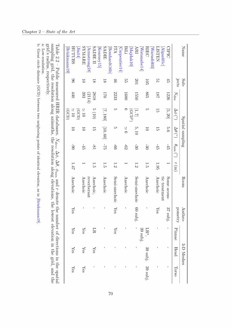
Chapter 2 – State of the Art
Nam
eSub-jects
Spatialsampling
Room
Anthro-
pometry
3-DMeshes
Ndirs
∆φ
( )∆θ( )
θmin ( )
r(m)
PinnaeHead
Torso
CIPIC
[Algazi01c]
451226
[5,20]5.6
-451
Someacous-
tictreatm
ent37
subj.-
--
LISTEN
[Warusfel03]
51187
1515
-451.95
Anechoic
Yes-
--
RIEC
[Watanabe14]
105865
510
-301.5
Anechoic
-LR
a,39
subj.39
subj.39
subj.
ARI
[Majdak10]
2011550
[1,7](G
CD
b)5,10
-301.2
Semi-anechoic
60subj.
--
-
BiLi
[Carpentier14]
551680
6'
6-62
1Anechoic
--
--
ITA[Bom
hardt16b]46
22335
5-66
1.2
Semi-anechoic
YesYes
--
SADIE
[Kearney15]
18170
[7,180][10,60]
-751.5
Anechoic
--
--
SADIE
II[A
rmstrong18]
182818(2114)
5(10)
15-81
1.5
Anechoic,
reverberant-
LRYes
-
SYMARE
[Jin14]10
393'
10(G
CD)
10-45
1Anechoic
-Yes
YesYes
HUTUBS
[Brinkm
ann19]96
440'
10(G
CD)
10-90
1.47
Anechoic
YesYes
YesYes
Table2.2
–Public
measured
HRIR
databases.Ndirs ,∆
φ,∆θ,φmin
andrdenote
thenum
berofdirections
inthe
spatialsam
plinggrid,the
resolutionalong
azimuths,the
resolutionalong
elevations,thelowest
elevationin
thegrid,and
thegrid’s
radius,respectively.a:
Low-resolution.
b:Great
circledistance
(GCD)betw
eentw
oneigboring
pointsofidenticalelevation,as
in[Brinkm
ann19].
70
2.4. HRTF Databases
sets have been issued. For instance, RIEC, a database with twice as many subjects (105)as CIPIC and ARI, was published in 2014 by the Advanced Acoustic Information SystemsLaboratory at Tohoku University, and features HRIRs measured for 865 directions at adistance of 1.5 m with azimuth and elevation resolutions of 5 and 10, respectively. Thedataset includes anthropometric measurements for 39 subjects as well as scans of the headand torso. However, no detailed scans of the pinnae were provided.
The same year, a database of HRIR sets measured in a semi-anechoic room was intro-duced by the Acoustics Research Institute (ARI) database [Majdak10], featuring a higherspatial resolution than RIEC (azimuth resolution between 2.5 and 5 and elevation res-olution of 5) and a comparable initial number of subjects. It has however been suppliedwith new subjects ever since, reaching 201 in December 2019, thus making it the largestHRTF database available to this day. CIPIC-like anthropometric measurements of 60subjects are provided.
In 2014 as well, another high-resolution HRTF database, named BiLi10 (BinauralListening) [Carpentier14; Rugeles Ospina15], was released as the result of a collaborationbetween IRCAM and Orange. It features HRIRs measured for 54 human subjects in ananechoic chamber on a 1680-point Gaussian grid of radius 2.06 m. The Gaussian grid waschosen for its convenience for measurements (practical with a vertical ark of loudspeakersand an azimuth-wise rotating subject) and its adequateness to high-order Ambisonics, i.e.SHD (see Section 2.1.2). Using that setup, the measurement of a complete HRIR set tookabout 20 minutes, thanks to the use of overlapping exponential sweeps [Majdak07].
Another database of high-resolution HRIR sets, ITA [Bomhardt16b], was published in2016 by a team from the University of Aachen. HRIRs were measured in a semi-anechoicenvironment for 2304 points of a 1.2-meter-radius spherical azimuth/elevation equiangulargrid whose resolution was 5. The dataset includes high-resolution 3-D scans of the pinna(obtained by MRI), 4 measurements of the head and 8 CIPIC-like pinna anthropometricmeasurements made on the scans.
The SADIE dataset11 [Kearney15] includes HRIR sets of 18 subjects, measured in ananechoic room at the University of York. However, as these measurements were intendedfor the specific needs of 5th-order Ambisonics, the spatial resolution is quite low, withonly 170 directions across the 1.5 m-radius sphere.
More recently, in 2018, a new iteration was issued, the SADIE II dataset12 [Arm-10The BiLi dataset is available at http://bili2.ircam.fr.11The SADIE dataset is available at https://www.york.ac.uk/sadie-project/database_old.html.12The SADIE II dataset is available at https://www.york.ac.uk/sadie-project/.
71
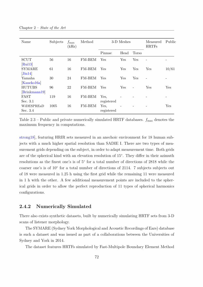
Chapter 2 – State of the Art
Name Subjects fmax(kHz)
Method 3-D Meshes MeasuredHRTFs
Public
Pinnae Head Torso
SCUT[Rui13]
56 16 FM-BEM Yes Yes Yes - -
SYMARE[Jin14]
61 16 FM-BEM Yes Yes Yes Yes 10/61
Yamaha[Kaneko16a]
30 24 FM-BEM Yes Yes Yes - -
HUTUBS[Brinkmann19]
96 22 FM-BEM Yes Yes - Yes Yes
FASTSec. 3.1
119 16 FM-BEM Yes,registered
- - - -
WiDESPREaDSec. 3.4
1005 16 FM-BEM Yes,registered
- - - Yes
Table 2.3 – Public and private numerically simulated HRTF databases. fmax denotes themaximum frequency in computations.
strong18], featuring HRIR sets measured in an anechoic environment for 18 human sub-jects with a much higher spatial resolution than SADIE I. There are two types of mea-surement grids depending on the subject, in order to adapt measurement time. Both gridsare of the spherical kind with an elevation resolution of 15. They differ in their azimuthresolutions as the finest one’s is of 5 for a total number of directions of 2818 while thecoarser one’s is of 10 for a total number of directions of 2114. 7 subjects subjects outof 18 were measured in 1.25 h using the first grid while the remaining 11 were measuredin 1 h with the other. A few additional measurement points are included to the spher-ical grids in order to allow the perfect reproduction of 11 types of spherical harmonicsconfigurations.
2.4.2 Numerically Simulated
There also exists synthetic datasets, built by numerically simulating HRTF sets from 3-Dscans of listener morphology.
The SYMARE (Sydney York Morphological and Acoustic Recordings of Ears) databaseis such a dataset and was issued as part of a collaborations between the Universities ofSydney and York in 2014.
The dataset features HRTFs simulated by Fast-Multipole Boundary Element Method
72
2.4. HRTF Databases
(FM-BEM) for 61 subjects as well as 3-D scans of the pinnae, head and torso used forthe simulations. Simulations were performed for frequencies up to 20 kHz when usingthe head and pinnae, and up to 16 kHz when including the torso. Spatial resolution isnot an issue here. Indeed, as the reciprocity principle [Zotkin06] is easily applicable tosimulations, virtually any measurement grid can be chosen with only a marginal increasein computing cost. The dataset also includes HRIRs measured in an anechoic chamberwith a low spatial resolution, on a grid of radius 1.2 m and average azimuth and elevationresolutions of 10 in both cases. Only a sample of 10 subjects is freely available. In spiteof this, this dataset has been the reference of databases gathering both measured andsimulated HRTFs, up until very recently.
A team from the Technical University of Berlin, Huawei Technologies and SennheiserElectronic has issued the HUTUBS database13 [Brinkmann19] in 2019. It features bothmeasured and simulated HRTFs for 96 subjects, as well as pinnae and head 3-D meshesand anthropometric measurements. The spatial resolution of the measurements is notparticularly high, with 440 directions on a 1.47 m-radius grid with average azimuth andelevation resolutions of 10. The choice of measurement grid accounted for compatibilitywith SHD up to the 17th order. Acoustical simulations were performed on shoulder-lessheads for frequencies up to 22 kHz.
There exists other databases of simulated HRTFs that are not accessible to the public.For example, an article published by a team from the South China University of Technol-ogy (SCUT) in 2013 [Rui13] presents the simulation by FM-BEM of the HRTF sets of 56human subjects including near-field HRTFs, with distances ranging from 10 cm to 1.2 m.
Another example is the dataset mentioned by a research team from Yamaha in a 2016article [Kaneko16a], which features the HRTF sets of 30 subjects, simulated by FM-BEMbased on a combination of high-resolution pinnae 3-D scans and rougher head-and-torsoones.
Discussion
Over the past twenty years, a number of datasets have been built by measuring the HRIRsof various human subjects, particularly in the last half-decade, period during which eightout of the ten datasets mentioned above were issued.
While some of them (SADIE, LISTEN, SYMARE, HUTUBS) have a rather low spa-
13The HUTUBS database is available at https://depositonce.tu-berlin.de/handle/11303/9429.
73
Chapter 2 – State of the Art
tial resolution (compared to the localization blur presented in Section 1.1.5), others canbe considered as having a high spatial resolution (SADIE II, ITA, BiLi). Sets of mea-surements of the human morphology are included in several of them (CIPIC, LISTEN,ARI, ITA and HUTUBS), a trend that was initiated by CIPIC and kick-started the activefield of user-friendly HRTF individualization based on anthropometry (see Section 2.3.3).Sometimes, morphological information is included in the form of 3-D scans of the head,torso and/or pinna as in RIEC, ITA, SADIE II, SYMARE and HUTUBS. However RIECand SADIE II do not include detailed scans of the pinnae and, while ITA does, it doesnot feature head or torso meshes.
Independently of their quality, due to the heavy apparatus and time that are requiredto make acoustic measurements, these databases are rather limited in terms of numberof subjects. Indeed, the largest one, ARI, features 201 which is twice more than its twoclosest competitors in this area, RIEC and HUTUBS, who feature 105 and 96, respectively.Most of the other datasets mentioned above comprise data for about 50 listeners (CIPIC,LISTEN, BiLi, ITA) while both SADIE sets feature 18 and the public section of SYMAREfeatures only 10.
When studying the inter-individual variations of HRTF sets, this may be problem-atic as the order of magnitude of the dimensionality of a high-resolution HRTF set[Bomhardt16b] is half a million (129 frequencies× 2300 directions× 2 ears ' 6 · 105).
One could imagine turning to numerical simulations to create larger datasets of syn-thetic HRTFs. While a few such datasets exist (SYMARE, HUTUBS, Yamaha andSCUT), they are mostly private, HUTUBS being the only fully public one. Moreover,none of them features more subjects than measured HRTF databases. Indeed, the largestone, HUTUBS, includes simulated HRTFs for 96 subjects while ARI, RIEC and HUTUBSinclude measured HRTFs for 201, 105 and 96 subjects, respectively. The fact that syn-thetic datasets do not present more subjects than acoustical ones can be explained by thefact that they still rely on the acquisition and edition of 3-D morphology of the subjects,which is largely manual and time-consuming, and that simulations requires non-negligiblecomputing resources. An additional problem is the uncertainty of the perceptual rele-vance of simulated HRTFs, making it possibly unworthy of the effort of building a largedatabase.
74

Chapter 3
DIMENSIONALITY REDUCTION AND DATA
AUGMENTATION OF HEAD-RELATED
TRANSFER FUNCTIONS
As we have seen in Section 2.3 of Chapter 2, an interesting approach to the matter ofuser-friendly HRTF individualization consists in tuning the parameters of a statisticalmodel of HRTFs, either based on anthropometry or on perceptual feedback from thelistener – the latter being further explored in Chapter 4. Seeing that HRTF sets are adata with hundreds of thousands of degrees of freedom (see Section 3.2 and Table 3.1),it is important in that context to reduce the dimensionality of the problem. Indeed, inthe case of a perceptual feedback-based approach, for instance, a lower number of tuningparameters allows for a more efficient exploration of the inter-individual variations ofHRTFs and thus a shorter and more comfortable tuning session for the listener.
However, currently available datasets are small compared to the dimensionality of thedata: the largest one, ARI [Majdak10], includes data for 201 subjects (see Chapter 2,Section 2.4 for a review of HRTF databases). Furthermore, while work has been donetowards combining existing databases [Andreopoulou11; Tsui18; Spagnol20], such com-posite databases can hardly attain the same level of homogeneity as a database made ina single campaign.
In this chapter, we investigate the matter of the dimensionality reduction of magnitudeHRTF sets. To this end, we used principal component analysis (PCA). Choosing PCA overmore complex machine learning techniques, was motivated by the fact that we performedthe statistical modeling in a way that focuses on the inter-individual variations of HRTFsets, which has barely been addressed in the literature (see Chapter 2, Section 2.1.3 formore details).
Thus, we investigate in Section 3.2 the capacity of this inter-individual approach toPCA to reduce the dimensionality of magnitude HRTF sets for 9 different datasets. These
75
Chapter 3 – Dimensionality Reduction and Data Augmentation of Head-Related TransferFunctions
9 datasets include 8 public datasets and a proprietary dataset of 119 3-D ear meshesand matching simulated PRTF sets, named FAST, which we present in Section 3.1. InSection 3.3, we compare the dimensionality reduction performance of PCA on FASTmagnitude PRTF sets to that of matching ear point clouds. Based on the results ofthis study, and in order to alleviate the aforementioned lack of large-scale datasets, wepresent in Section 3.4 a data augmentation method that relies on random generations ofpinna meshes and on numerical simulations of corresponding PRTF sets. The resulting1005-example dataset, named WiDESPREaD (Wide Dataset of Ear Shapes and Pinna-related transfer functions generated by Random Ear Drawings) was made public andavailable online1. Finally, in Section 3.5 we study the impact on dimensionality reductionperformance of training PCA with this augmented PRTF dataset.
3.1 The FAST Dataset: 119 Ear Meshes and Match-ing Simulated Pinna-Related Transfer Functions
Most work presented in this chapter is based on a proprietary dataset of n = 119 3-Dscans of human left pinnae and matching 119 numerically simulated PRTF sets. Wehereon refer to it as the FAST dataset, after our research team.
In this section, we present the constitution of this dataset. First, we introduce abasis dataset of 123 registered left ear meshes which was constituted in previous work byGhorbal et al. [Ghorbal19]. Then, we go over corrections that were applied to that firstdataset, including the removal of 4 problematic subjects. Finally, we describe in detailhow we complemented the n = 119 pinna meshes with matching PRTF sets by means ofboundary element method (BEM) simulations.
3.1.1 Ear Meshes
Acquisition & registration
For the major part, the dataset of ear meshes was constituted in previous work by Ghorbalet al. [Ghorbal19]. First, 3-D scans of the left pinna of 123 human subjects were acquiredusing a commercial structured-light based scanner, eFit by United Sciences. The acqui-sition of one pinna took about 20 min. Then, the meshes were rigidly aligned by means
1https://sofacoustics.org/data/database/widespread/
76
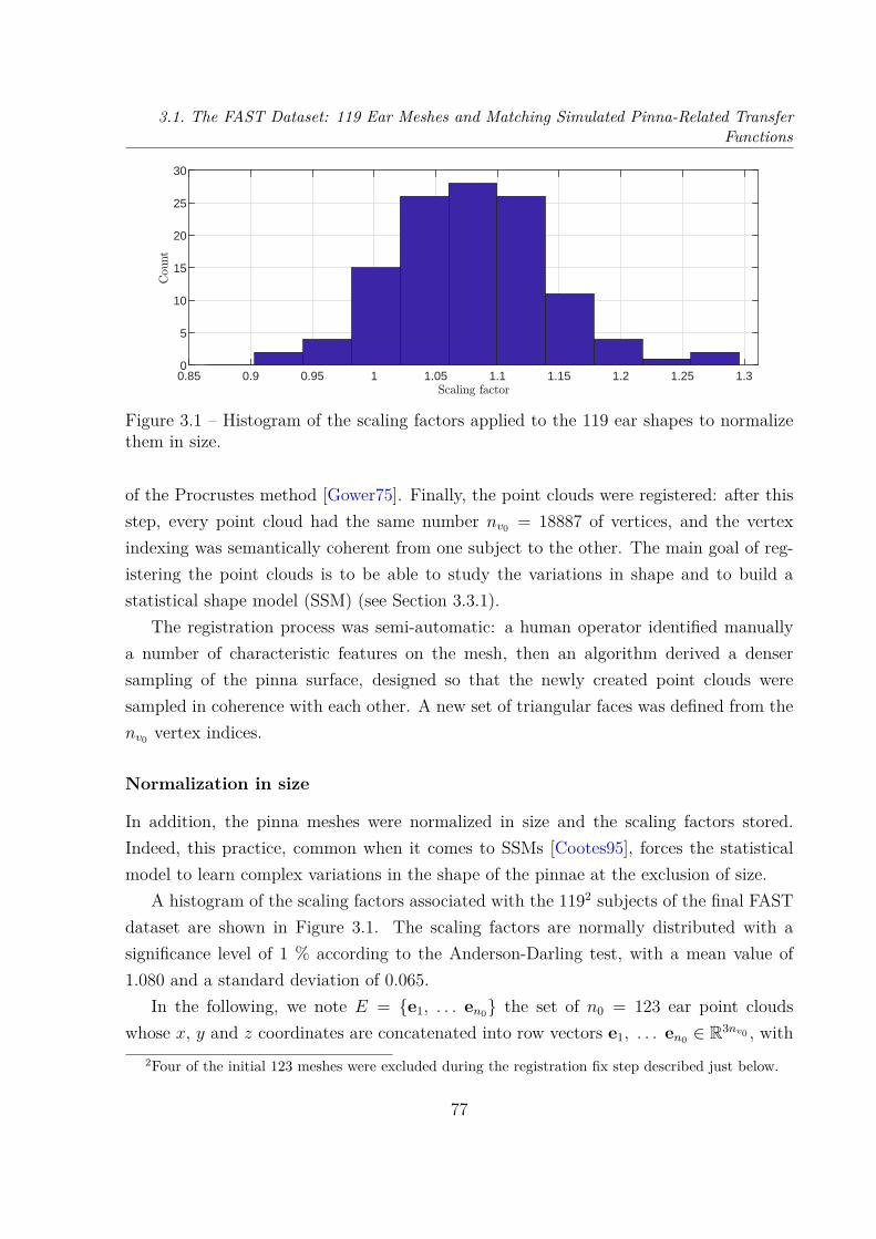
3.1. The FAST Dataset: 119 Ear Meshes and Matching Simulated Pinna-Related TransferFunctions
0.85 0.9 0.95 1 1.05 1.1 1.15 1.2 1.25 1.30
5
10
15
20
25
30
Figure 3.1 – Histogram of the scaling factors applied to the 119 ear shapes to normalizethem in size.
of the Procrustes method [Gower75]. Finally, the point clouds were registered: after thisstep, every point cloud had the same number nv0 = 18887 of vertices, and the vertexindexing was semantically coherent from one subject to the other. The main goal of reg-istering the point clouds is to be able to study the variations in shape and to build astatistical shape model (SSM) (see Section 3.3.1).
The registration process was semi-automatic: a human operator identified manuallya number of characteristic features on the mesh, then an algorithm derived a densersampling of the pinna surface, designed so that the newly created point clouds weresampled in coherence with each other. A new set of triangular faces was defined from thenv0 vertex indices.
Normalization in size
In addition, the pinna meshes were normalized in size and the scaling factors stored.Indeed, this practice, common when it comes to SSMs [Cootes95], forces the statisticalmodel to learn complex variations in the shape of the pinnae at the exclusion of size.
A histogram of the scaling factors associated with the 1192 subjects of the final FASTdataset are shown in Figure 3.1. The scaling factors are normally distributed with asignificance level of 1 % according to the Anderson-Darling test, with a mean value of1.080 and a standard deviation of 0.065.
In the following, we note E = e1, . . . en0 the set of n0 = 123 ear point cloudswhose x, y and z coordinates are concatenated into row vectors e1, . . . en0 ∈ R3nv0 , with
2Four of the initial 123 meshes were excluded during the registration fix step described just below.
77
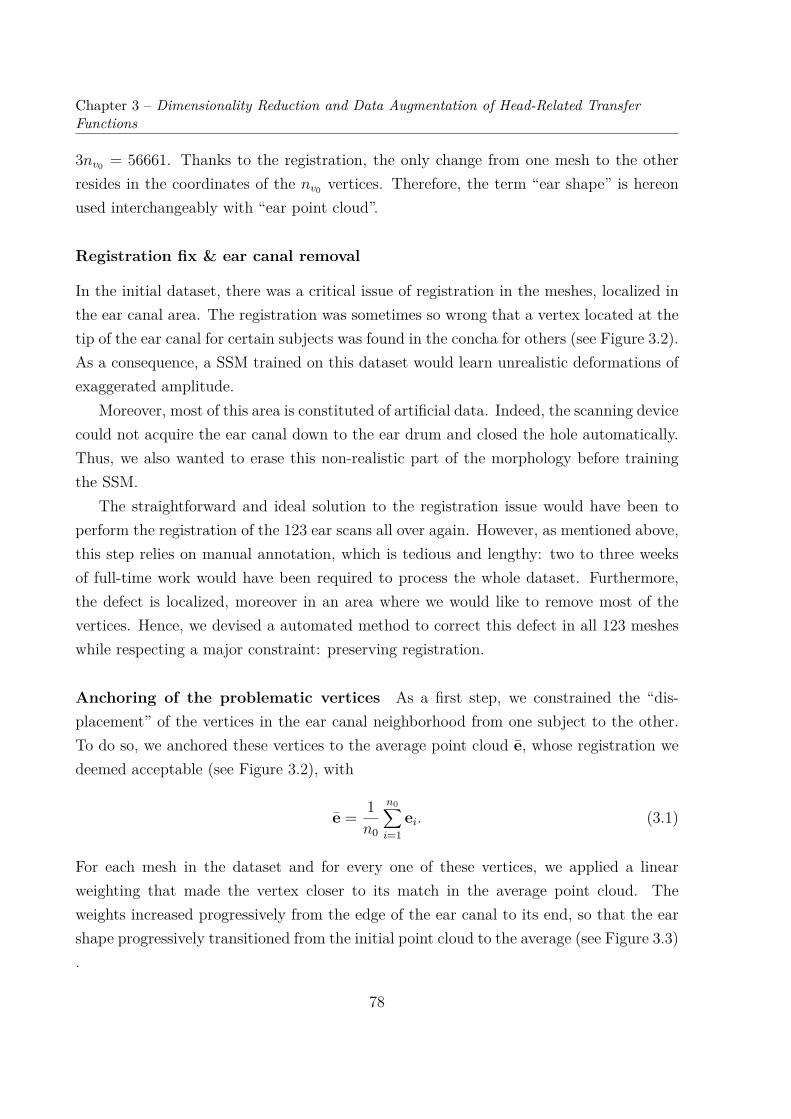
Chapter 3 – Dimensionality Reduction and Data Augmentation of Head-Related TransferFunctions
3nv0 = 56661. Thanks to the registration, the only change from one mesh to the otherresides in the coordinates of the nv0 vertices. Therefore, the term “ear shape” is hereonused interchangeably with “ear point cloud”.
Registration fix & ear canal removal
In the initial dataset, there was a critical issue of registration in the meshes, localized inthe ear canal area. The registration was sometimes so wrong that a vertex located at thetip of the ear canal for certain subjects was found in the concha for others (see Figure 3.2).As a consequence, a SSM trained on this dataset would learn unrealistic deformations ofexaggerated amplitude.
Moreover, most of this area is constituted of artificial data. Indeed, the scanning devicecould not acquire the ear canal down to the ear drum and closed the hole automatically.Thus, we also wanted to erase this non-realistic part of the morphology before trainingthe SSM.
The straightforward and ideal solution to the registration issue would have been toperform the registration of the 123 ear scans all over again. However, as mentioned above,this step relies on manual annotation, which is tedious and lengthy: two to three weeksof full-time work would have been required to process the whole dataset. Furthermore,the defect is localized, moreover in an area where we would like to remove most of thevertices. Hence, we devised a automated method to correct this defect in all 123 mesheswhile respecting a major constraint: preserving registration.
Anchoring of the problematic vertices As a first step, we constrained the “dis-placement” of the vertices in the ear canal neighborhood from one subject to the other.To do so, we anchored these vertices to the average point cloud e, whose registration wedeemed acceptable (see Figure 3.2), with
e = 1n0
n0∑i=1
ei. (3.1)
For each mesh in the dataset and for every one of these vertices, we applied a linearweighting that made the vertex closer to its match in the average point cloud. Theweights increased progressively from the edge of the ear canal to its end, so that the earshape progressively transitioned from the initial point cloud to the average (see Figure 3.3).
78

3.1. The FAST Dataset: 119 Ear Meshes and Matching Simulated Pinna-Related TransferFunctions
(a) Average, front view (b) Subject HF, front view (c) Subject PB, front view
(d) Average, rear view (e) Subject HF, rear view (f) Subject PB, rear view
Figure 3.2 – Illustration of the registration issue, and the variability of the registration inthe ear canal area. Vertices expected to be at the tip of the ear canal are circled in redfor three exemplary meshes. The average shape (a, d) illustrates the expected behavior,with the circled vertices well located at the end of the ear canal. Subject HF (b, e), incontrast, constitutes an extreme example of the issue: the circled vertices are not evenlocated in the ear canal, but are in the concha. For subject PB (c, f) the registration issueis present but milder, with the circled vertices slightly on the side of the ear canal.
79
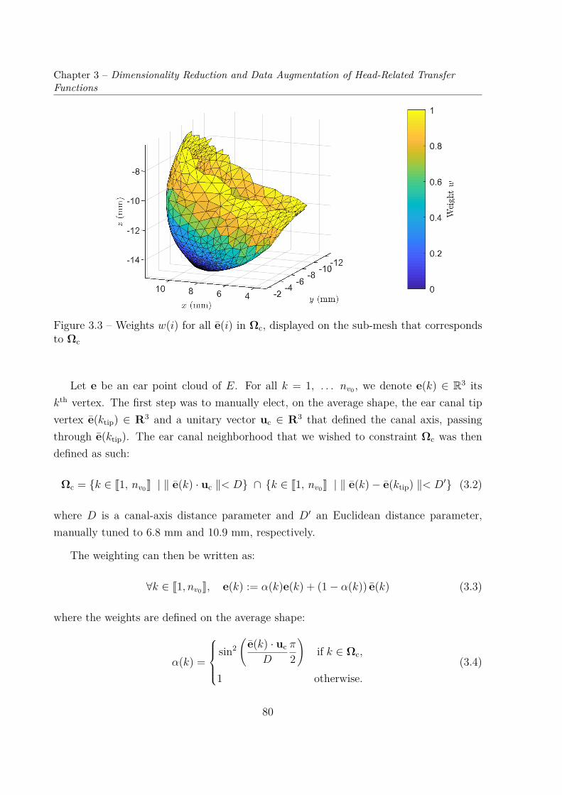
Chapter 3 – Dimensionality Reduction and Data Augmentation of Head-Related TransferFunctions
Figure 3.3 – Weights w(i) for all e(i) in Ωc, displayed on the sub-mesh that correspondsto Ωc
Let e be an ear point cloud of E. For all k = 1, . . . nv0 , we denote e(k) ∈ R3 itskth vertex. The first step was to manually elect, on the average shape, the ear canal tipvertex e(ktip) ∈ R3 and a unitary vector uc ∈ R3 that defined the canal axis, passingthrough e(ktip). The ear canal neighborhood that we wished to constraint Ωc was thendefined as such:
Ωc = k ∈ J1, nv0K | ‖ e(k) · uc ‖< D ∩ k ∈ J1, nv0K | ‖ e(k)− e(ktip) ‖< D′ (3.2)
where D is a canal-axis distance parameter and D′ an Euclidean distance parameter,manually tuned to 6.8 mm and 10.9 mm, respectively.
The weighting can then be written as:
∀k ∈ J1, nv0K, e(k) := α(k)e(k) + (1− α(k)) e(k) (3.3)
where the weights are defined on the average shape:
α(k) =
sin2
(e(k) · uc
D
π
2
)if k ∈ Ωc,
1 otherwise.(3.4)
80
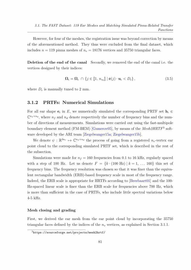
3.1. The FAST Dataset: 119 Ear Meshes and Matching Simulated Pinna-Related TransferFunctions
However, for four of the meshes, the registration issue was beyond correction by meansof the aforementioned method. They thus were excluded from the final dataset, whichincludes n = 119 pinna meshes of nv = 18176 vertices and 35750 triangular faces.
Deletion of the end of the canal Secondly, we removed the end of the canal i.e. thevertices designed by their indices:
Ωt = Ωc ∩ j ∈ J1, nv0K | e(j) · uc < De , (3.5)
where De is manually tuned to 2 mm.
3.1.2 PRTFs: Numerical Simulations
For all ear shape ei in E, we numerically simulated the corresponding PRTF set hi ∈Cnf×nd , where nf and nd denote respectively the number of frequency bins and the num-ber of directions of measurements. Simulations were carried out using the fast-multipoleboundary element method (FM-BEM) [Gumerov05], by means of the Mesh2HRTF 3 soft-ware developed by the ARI team [Ziegelwanger15a; Ziegelwanger15b].
We denote ψ : R3nv 7→ Cnf×nd the process of going from a registered nv-vertex earpoint cloud to the corresponding simulated PRTF set, which is described in the rest ofthe subsection.
Simulations were made for nf = 160 frequencies from 0.1 to 16 kHz, regularly spacedwith a step of 100 Hz. Let us denote F = k · (100 Hz) | k = 1, . . . 160 this set offrequency bins. The frequency resolution was chosen so that it was finer than the equiva-lent rectangular bandwidth (ERB)-based frequency scale in most of the frequency range.Indeed, the ERB scale is appropriate for HRTFs according to [Breebaart01] and the 100-Hz-spaced linear scale is finer than the ERB scale for frequencies above 700 Hz, whichis more than sufficient in the case of PRTFs, who include little spectral variations below4-5 kHz.
Mesh closing and grading
First, we derived the ear mesh from the ear point cloud by incorporating the 35750triangular faces defined by the indices of the nv vertices, as explained in Section 3.1.1.
3https://sourceforge.net/projects/mesh2hrtf/
81
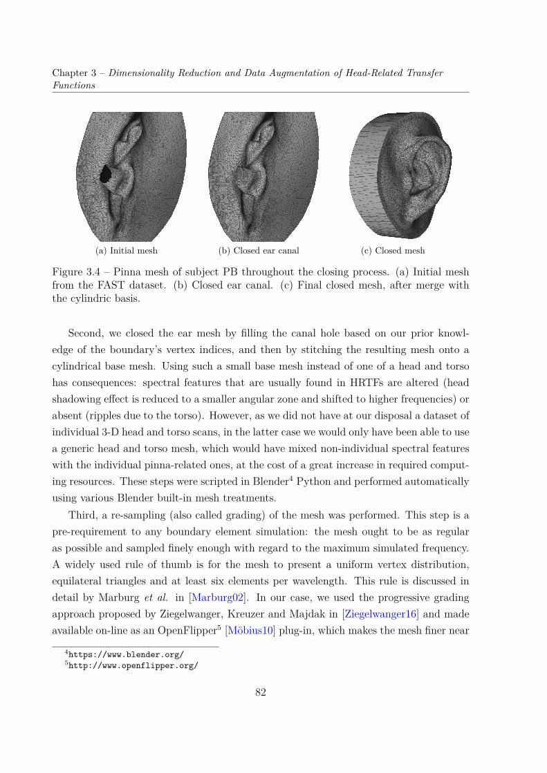
Chapter 3 – Dimensionality Reduction and Data Augmentation of Head-Related TransferFunctions
(a) Initial mesh (b) Closed ear canal (c) Closed mesh
Figure 3.4 – Pinna mesh of subject PB throughout the closing process. (a) Initial meshfrom the FAST dataset. (b) Closed ear canal. (c) Final closed mesh, after merge withthe cylindric basis.
Second, we closed the ear mesh by filling the canal hole based on our prior knowl-edge of the boundary’s vertex indices, and then by stitching the resulting mesh onto acylindrical base mesh. Using such a small base mesh instead of one of a head and torsohas consequences: spectral features that are usually found in HRTFs are altered (headshadowing effect is reduced to a smaller angular zone and shifted to higher frequencies) orabsent (ripples due to the torso). However, as we did not have at our disposal a dataset ofindividual 3-D head and torso scans, in the latter case we would only have been able to usea generic head and torso mesh, which would have mixed non-individual spectral featureswith the individual pinna-related ones, at the cost of a great increase in required comput-ing resources. These steps were scripted in Blender4 Python and performed automaticallyusing various Blender built-in mesh treatments.
Third, a re-sampling (also called grading) of the mesh was performed. This step is apre-requirement to any boundary element simulation: the mesh ought to be as regularas possible and sampled finely enough with regard to the maximum simulated frequency.A widely used rule of thumb is for the mesh to present a uniform vertex distribution,equilateral triangles and at least six elements per wavelength. This rule is discussed indetail by Marburg et al. in [Marburg02]. In our case, we used the progressive gradingapproach proposed by Ziegelwanger, Kreuzer and Majdak in [Ziegelwanger16] and madeavailable on-line as an OpenFlipper5 [Möbius10] plug-in, which makes the mesh finer near
4https://www.blender.org/5http://www.openflipper.org/
82

3.1. The FAST Dataset: 119 Ear Meshes and Matching Simulated Pinna-Related TransferFunctions
Figure 3.5 – Simulation-ready meshes derived from ear point cloud e1 for four mesh gradingconfigurations, each corresponding to a frequency band. Left to right: [0.1, 0.4 kHz], [0.5,2.0 kHz], [2.1, 3.5 kHz] and [3.6, 16 kHz].
the ear canal (where the sound source is positioned) and progressively coarser elsewhere.This considerably decreases the computing cost of the FM-BEM simulation compared touniform re-sampling, while maintaining numerical accuracy. In this case, we used thecosine-based approach with the grading factor set to 10.
Additionally, in order to further reduce the computational cost, we adapted the meshgrading step to each of four different frequency bands. At low frequencies, a uniformre-sampling was enough due to the low number of required elements. It was performedwith target edge lengths of 10 and 5 mm, in the frequency bands [0.1, 0.4 kHz] and [0.5,2.0 kHz], respectively. At higher frequencies, the re-sampling was progressive, with targetminimum and maximum edge lengths of 2 and 5 mm, and 0.7 and 5 mm, in the frequencybands [2.1, 3.5 kHz] and [3.6, 16 kHz], respectively. An example of simulation-readymeshes (each corresponding to a mesh grading configuration) is displayed in Figure 3.5.
Simulation settings
Reciprocity principle According to the reciprocity principle in acoustics, given twopoints in space A and B, the pressure in B due a sound source located in A, pA→B is equalto the pressure that would be observed in A if the sound source was located in B pB→A:
pA→B = pB→A. (3.6)
This is particularly interesting in the case of HRIR measurements. Instead of sequen-tially measuring the responses in the ear canal to sound sources located in nd locations,
83
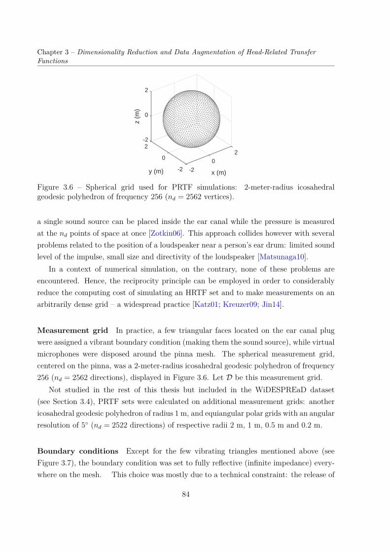
Chapter 3 – Dimensionality Reduction and Data Augmentation of Head-Related TransferFunctions
-22
0
2
z (m
)
y (m)
0
x (m)
2
0-2 -2
Figure 3.6 – Spherical grid used for PRTF simulations: 2-meter-radius icosahedralgeodesic polyhedron of frequency 256 (nd = 2562 vertices).
a single sound source can be placed inside the ear canal while the pressure is measuredat the nd points of space at once [Zotkin06]. This approach collides however with severalproblems related to the position of a loudspeaker near a person’s ear drum: limited soundlevel of the impulse, small size and directivity of the loudspeaker [Matsunaga10].
In a context of numerical simulation, on the contrary, none of these problems areencountered. Hence, the reciprocity principle can be employed in order to considerablyreduce the computing cost of simulating an HRTF set and to make measurements on anarbitrarily dense grid – a widespread practice [Katz01; Kreuzer09; Jin14].
Measurement grid In practice, a few triangular faces located on the ear canal plugwere assigned a vibrant boundary condition (making them the sound source), while virtualmicrophones were disposed around the pinna mesh. The spherical measurement grid,centered on the pinna, was a 2-meter-radius icosahedral geodesic polyhedron of frequency256 (nd = 2562 directions), displayed in Figure 3.6. Let D be this measurement grid.
Not studied in the rest of this thesis but included in the WiDESPREaD dataset(see Section 3.4), PRTF sets were calculated on additional measurement grids: anothericosahedral geodesic polyhedron of radius 1 m, and equiangular polar grids with an angularresolution of 5 (nd = 2522 directions) of respective radii 2 m, 1 m, 0.5 m and 0.2 m.
Boundary conditions Except for the few vibrating triangles mentioned above (seeFigure 3.7), the boundary condition was set to fully reflective (infinite impedance) every-where on the mesh. This choice was mostly due to a technical constraint: the release of
84
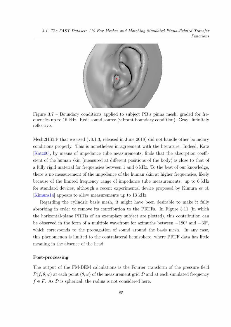
3.1. The FAST Dataset: 119 Ear Meshes and Matching Simulated Pinna-Related TransferFunctions
Figure 3.7 – Boundary conditions applied to subject PB’s pinna mesh, graded for fre-quencies up to 16 kHz. Red: sound source (vibrant boundary condition). Gray: infinitelyreflective.
Mesh2HRTF that we used (v0.1.3, released in June 2018) did not handle other boundaryconditions properly. This is nonetheless in agreement with the literature. Indeed, Katz[Katz00], by means of impedance tube measurements, finds that the absorption coeffi-cient of the human skin (measured at different positions of the body) is close to that ofa fully rigid material for frequencies between 1 and 6 kHz. To the best of our knowledge,there is no measurement of the impedance of the human skin at higher frequencies, likelybecause of the limited frequency range of impedance tube measurements: up to 6 kHzfor standard devices, although a recent experimental device proposed by Kimura et al.[Kimura14] appears to allow measurements up to 13 kHz.
Regarding the cylindric basis mesh, it might have been desirable to make it fullyabsorbing in order to remove its contribution to the PRTFs. In Figure 3.11 (in whichthe horizontal-plane PRIRs of an exemplary subject are plotted), this contribution canbe observed in the form of a multiple wavefront for azimuths between −180 and −30,which corresponds to the propagation of sound around the basis mesh. In any case,this phenomenon is limited to the contralateral hemisphere, where PRTF data has littlemeaning in the absence of the head.
Post-processing
The output of the FM-BEM calculations is the Fourier transform of the pressure fieldP (f, θ, ϕ) at each point (θ, ϕ) of the measurement grid D and at each simulated frequencyf ∈ F . As D is spherical, the radius is not considered here.
85
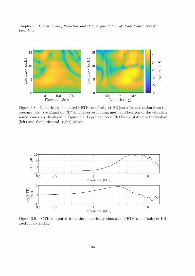
Chapter 3 – Dimensionality Reduction and Data Augmentation of Head-Related TransferFunctions
Figure 3.8 – Numerically simulated PRTF set of subject PB just after derivation from thepressure field (see Equation (3.7)). The corresponding mesh and location of the vibratingsound source are displayed in Figure 3.7. Log-magnitude PRTFs are plotted in the median(left) and the horizontal (right) planes.
0.1 0.2 1 10-5
0
5
10
0.1 0.2 1 10-1
0
1
Figure 3.9 – CTF computed from the numerically simulated PRTF set of subject PB,used for its DFEQ.
86
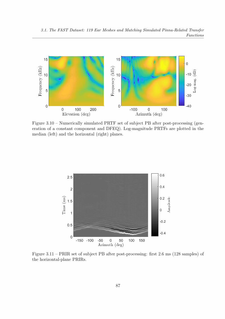
3.1. The FAST Dataset: 119 Ear Meshes and Matching Simulated Pinna-Related TransferFunctions
Figure 3.10 – Numerically simulated PRTF set of subject PB after post-processing (gen-eration of a constant component and DFEQ). Log-magnitude PRTFs are plotted in themedian (left) and the horizontal (right) planes.
Figure 3.11 – PRIR set of subject PB after post-processing: first 2.6 ms (128 samples) ofthe horizontal-plane PRIRs.
87
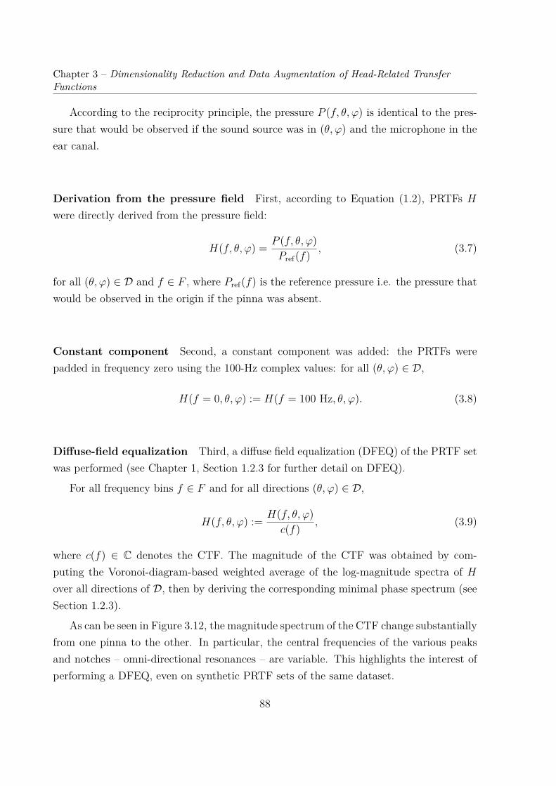
Chapter 3 – Dimensionality Reduction and Data Augmentation of Head-Related TransferFunctions
According to the reciprocity principle, the pressure P (f, θ, ϕ) is identical to the pres-sure that would be observed if the sound source was in (θ, ϕ) and the microphone in theear canal.
Derivation from the pressure field First, according to Equation (1.2), PRTFs Hwere directly derived from the pressure field:
H(f, θ, ϕ) = P (f, θ, ϕ)Pref(f) , (3.7)
for all (θ, ϕ) ∈ D and f ∈ F , where Pref(f) is the reference pressure i.e. the pressure thatwould be observed in the origin if the pinna was absent.
Constant component Second, a constant component was added: the PRTFs werepadded in frequency zero using the 100-Hz complex values: for all (θ, ϕ) ∈ D,
H(f = 0, θ, ϕ) := H(f = 100 Hz, θ, ϕ). (3.8)
Diffuse-field equalization Third, a diffuse field equalization (DFEQ) of the PRTF setwas performed (see Chapter 1, Section 1.2.3 for further detail on DFEQ).
For all frequency bins f ∈ F and for all directions (θ, ϕ) ∈ D,
H(f, θ, ϕ) := H(f, θ, ϕ)c(f) , (3.9)
where c(f) ∈ C denotes the CTF. The magnitude of the CTF was obtained by com-puting the Voronoi-diagram-based weighted average of the log-magnitude spectra of Hover all directions of D, then by deriving the corresponding minimal phase spectrum (seeSection 1.2.3).
As can be seen in Figure 3.12, the magnitude spectrum of the CTF change substantiallyfrom one pinna to the other. In particular, the central frequencies of the various peaksand notches – omni-directional resonances – are variable. This highlights the interest ofperforming a DFEQ, even on synthetic PRTF sets of the same dataset.
88
3.2. Dimensionality Reduction of HRTFs
0.1 1 10
0
5
10
Figure 3.12 – Magnitude CTFs of three exemplary PRTF sets of the FAST dataset (priorto DFEQ), each computed from a different pinna.
Conclusion
In this section, we have presented the FAST dataset, a dataset of 119 3-D pinna meshesand matching PRTF sets computed by means of BEM simulations.
This dataset has the advantage of including both auditory and morphological data.Furthermore, the pinna meshes are registered, which makes them particularly suited forvarious applications such as statistical analysis, easy extraction of anthropometric mea-surements and/or regression between morphology and transfer functions. Finally, it in-cludes data for more subjects than most public HRTF datasets, being surpassed only byARI’s 201 (see Chapter 2, Section 2.4).
However, the dataset does not include head and torso 3-D morphologies nor theirauditory filtering contributions to HRTFs. Yet, the pinnae have a vast influence on thespectral features involved in the perceptual problems that arise from a lack of individ-ualization [Asano90]. Furthermore, they are arguably the most complex component ofHRTF-impacting morphology (i.e. pinnae, head and torso) in terms of shape, inter-individual variability and influence of physical changes on auditory filtering.
Finally, let us note that the pinnae were normalized in size and that the PRTF setswere derived from them. However, as we stored the scaling factors, the ear meshes caneasily be re-scaled. Additionally, a close approximation of the corresponding PRTFs setscan be obtained by applying matching frequency scalings to the PRTF sets.
3.2 Dimensionality Reduction of HRTFs
In this section, we investigate how PCA performs at reducing the dimensionality of mag-nitude HRTF sets from 9 different datasets, including FAST. We start by explaining
89
Chapter 3 – Dimensionality Reduction and Data Augmentation of Head-Related TransferFunctions
how we performed PCA to learn inter-subject variations and reduce their dimensionality.Then, we compare the various datasets under the light of how PCA performed at reducingdimensionality. In particular, we compare some of these results to the literature.
3.2.1 Principal Component Analysis of Log-Magnitude HRTFs
We focus hereon on the magnitude spectra of HRTFs, leaving the matter of ITD indi-vidualization out of the scope of this work. Indeed, lateral perception is more robustto a lack of individualization [Wenzel93]. Furthermore, a set of ITDs is a data of lowerdimensionality, as it corresponds to one value per direction, against at least a few dozensfor the magnitude spectra. For a state-of-the-art on approximating and modeling ITDs,the curious reader can refer to Bomhardt’s PhD thesis [Bomhardt17].
In matters of dimensionality reduction, PCA is usually an indispensable first step.Indeed, it is a statistical analysis tool that can help better understand the dataset beforemoving on to more complex approaches. Furthermore, it is a simple, low-complexitytechnique that has proved its usefulness in a wide variety of dimensionality reductionproblems. Its main limitation lies in its inability to describe non-linear manifolds.
Looking into the literature, PCA is effectively the most popular machine learningapproach to model HRTFs. Yet, let us mention that other techniques have been usedas well, such as independent component analysis (ICA) [Larcher00; Huang09b; Liu19b],High-Order SVD [Li13] for linear techniques, and Isomap [Kapralos08; Grijalva16] andlocally linear embedding (LLE) [Duraiswami05; Kapralos08] for non-linear ones. Neuralnetworks have only come up very recently for unsupervised HRTF modeling [Yamamoto17;Chen20]. However, these approaches rarely learn inter-subject variations only, often mix-ing in directional variations.
In Section 2.1.3, we discussed the various ways in which HRTF data can be formattedprior to PCA. Regarding our HRTF individualization problem, the inter-individual oneseems most adequate as, in that case, PCA only learns variations between subjects. How-ever, it is worth noting that it has rarely been used in the literature [Hölzl14; Hold17],likely because of the limited size of currently available datasets (≤ 201) compared to thedimensionality of the data (order of magnitude between 104 and 106, see Table 3.1).
In the following, we detail how we used PCA to reduce the dimensionality of magnitudeHRTF sets.
90
3.2. Dimensionality Reduction of HRTFs
Pre-processing
Prior to PCA, all HRTF sets went through a small pre-processing step. First, we re-sampled the HRIRs to a sampling frequency of 32 kHz, that is a maximum frequency of16 kHz. Indeed, most listeners cannot hear content at higher frequencies. Second, weperformed a diffuse-field equalization of the HRTF sets. The magnitude spectrum of theCTF was computed by performing a Voronoi-diagram-based average of the log-magnitudeHRTF sets (see Section 1.2.3).
The spatial grids of 3 HRTF sets from the ARI database differed slightly from thatof the other 198 HRTF sets. Rather than tampering with the data by interpolating theHRTFs, we cast aside these 3 HRTF sets.
Data formatting
Let us consider a dataset of n DTF sets measured or simulated on a spherical or hemi-spherical grid D of nd directions and on a frequency range F of nf bins
H
(λ)i (f, θ, ϕ) | i = 1, . . . n, λ ∈ L,R, f ∈ F, (θ, ϕ) ∈ D
(3.10)
the dataset of DTFs. In the case of PRTFs (i.e. for the FAST dataset), data in thecontralateral hemisphere has little meaning due to the unrealistic contribution of thecylindric basis mesh in that area. Yet, we are dealing here with the matter of reducingthe very high dimensionality of HRTF sets. Hence, in order to emulate the more generalmatter of HRTFs, in what follows PRTF and HRTF sets are not restricted to the ipsilateralhemisphere, unless indicated otherwise.
Following the aforementioned pre-processing step, we focused on the magnitude spec-tra of HRTFs. The logarithmic scale was chosen for its coherence with human perception.Furthermore, considering that HRTFs from left and right ears are largely symmetrical,and that the FAST dataset only contains left-ear data, we restricted this study to left-earHRTFs. For all i = 1, . . . n, f ∈ F and (θ, ϕ) ∈ D, let there be such a mag-HRTF
Gi(f, θ, ϕ) = 20 · log10
∣∣∣H(L)i (f, θ, ϕ)
∣∣∣ (3.11)
andG = Gi(f, θ, ϕ) | i = 1, . . . n, f ∈ F, (θ, ϕ) ∈ D (3.12)
the corresponding mag-HRTF dataset.
91
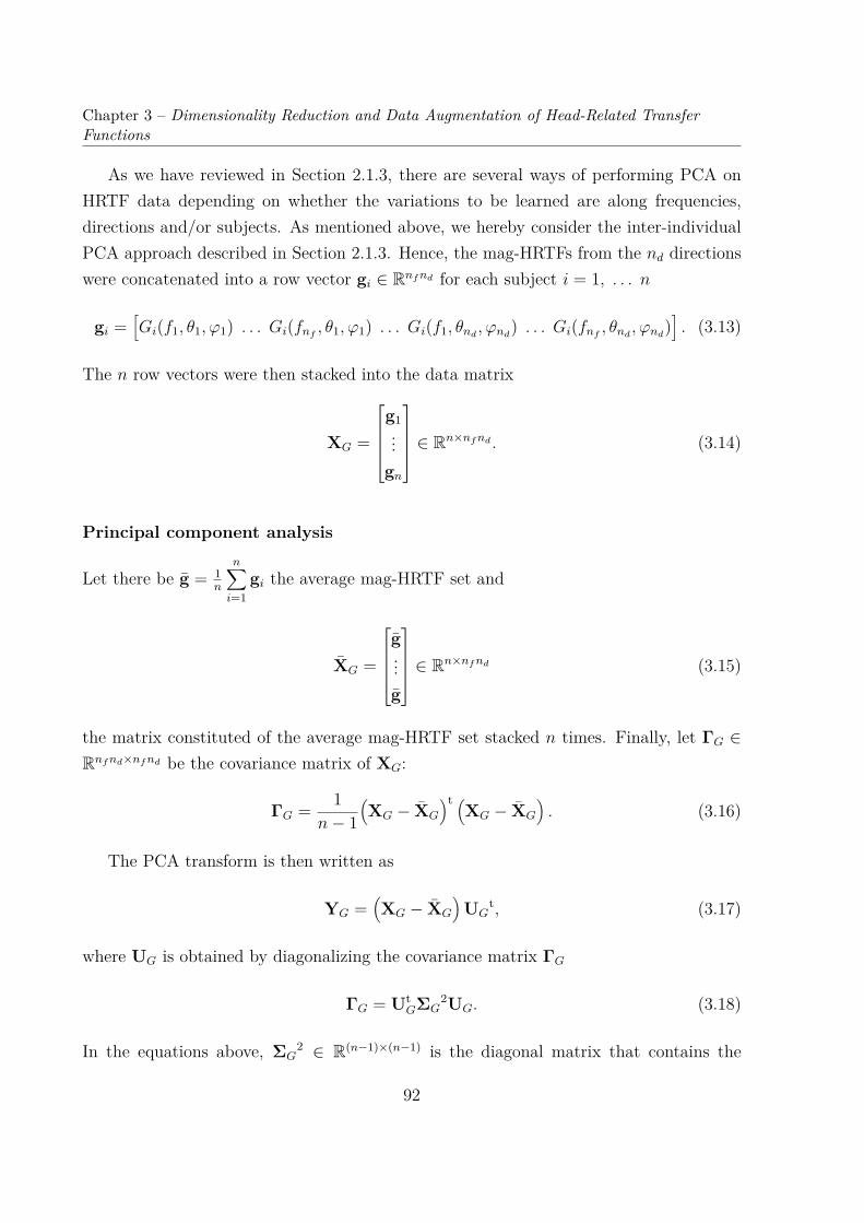
Chapter 3 – Dimensionality Reduction and Data Augmentation of Head-Related TransferFunctions
As we have reviewed in Section 2.1.3, there are several ways of performing PCA onHRTF data depending on whether the variations to be learned are along frequencies,directions and/or subjects. As mentioned above, we hereby consider the inter-individualPCA approach described in Section 2.1.3. Hence, the mag-HRTFs from the nd directionswere concatenated into a row vector gi ∈ Rnfnd for each subject i = 1, . . . n
gi =[Gi(f1, θ1, ϕ1) . . . Gi(fnf , θ1, ϕ1) . . . Gi(f1, θnd , ϕnd) . . . Gi(fnf , θnd , ϕnd)
]. (3.13)
The n row vectors were then stacked into the data matrix
XG =
g1...
gn
∈ Rn×nfnd . (3.14)
Principal component analysis
Let there be g = 1n
n∑i=1
gi the average mag-HRTF set and
XG =
g...g
∈ Rn×nfnd (3.15)
the matrix constituted of the average mag-HRTF set stacked n times. Finally, let ΓG ∈Rnfnd×nfnd be the covariance matrix of XG:
ΓG = 1n− 1
(XG − XG
)t (XG − XG
). (3.16)
The PCA transform is then written as
YG =(XG − XG
)UG
t, (3.17)
where UG is obtained by diagonalizing the covariance matrix ΓG
ΓG = UtGΣG
2UG. (3.18)
In the equations above, ΣG2 ∈ R(n−1)×(n−1) is the diagonal matrix that contains the
92

3.2. Dimensionality Reduction of HRTFs
eigenvalues of ΓG, σG12, σG2
2, . . . σGn−12, ordered so that σG1
2 ≥ σG22 ≥ · · · ≥ σGn−1
2
ΣG2 =
σG1
2
. . .σGn−1
2
, (3.19)
and UG ∈ R(n−1)×nfnd is an orthogonal matrix that contains the corresponding eigenvec-tors uG1 , uG2 , . . . uGn−1 ∈ Rnfnd
UG =
uG1...
uGn−1
. (3.20)
The eigenvalues denote how much variance in the input data is explained by the corre-sponding eigenvectors.
In the equations above, we implicitly set the number of principal components (PCs)to n− 1, because all PCs after the (n− 1)th are trivial, i.e. of null associated eigenvalue.Indeed, the number of examples n is lower than the data dimension nfnd and the data iscentered, thus
r = rank(XG − XG
)≤ n− 1. (3.21)
Hence, the rank of the covariance matrix does not exceed n− 1 either:
rank (ΓG) ≤ min (r, r) = r ≤ n− 1. (3.22)
Dimensionality reduction
PCA can be used as a dimensionality reduction technique by retaining only the first p PCsand setting the weights of the discarded PCs to zero [Jolliffe02], where p ∈ 0, . . . n−1:
Y(p)G =
yG1,1 . . . yG1,p 0 . . . 0... . . . ... ... . . . ...
yGn,1 . . . yGn,p 0 . . . 0
, (3.23)
where yGi,j is the value of matrix YG at the ith row and jth column for all i = 1, . . . nand j = 1, . . . n− 1.
The choice of the p first PCs (rather than another subset of p PCs) is motivated by
93
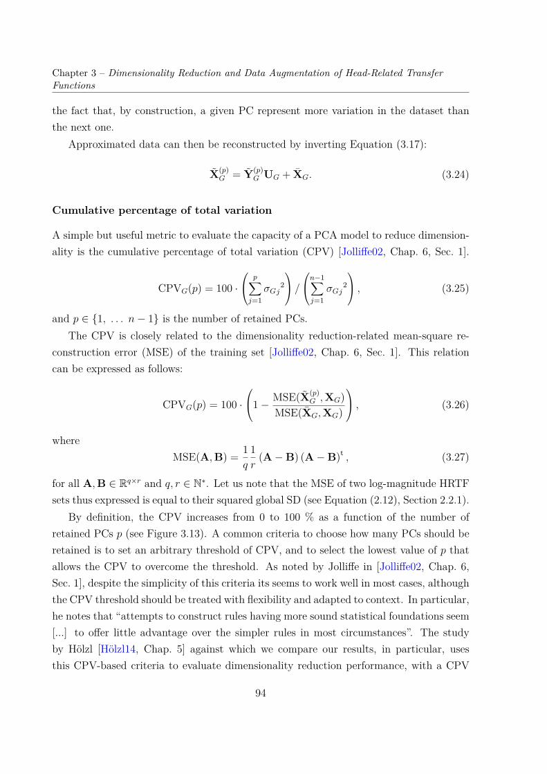
Chapter 3 – Dimensionality Reduction and Data Augmentation of Head-Related TransferFunctions
the fact that, by construction, a given PC represent more variation in the dataset thanthe next one.
Approximated data can then be reconstructed by inverting Equation (3.17):
X(p)G = Y(p)
G UG + XG. (3.24)
Cumulative percentage of total variation
A simple but useful metric to evaluate the capacity of a PCA model to reduce dimension-ality is the cumulative percentage of total variation (CPV) [Jolliffe02, Chap. 6, Sec. 1].
CPVG(p) = 100 · p∑j=1
σGj2
/n−1∑j=1
σGj2
, (3.25)
and p ∈ 1, . . . n− 1 is the number of retained PCs.The CPV is closely related to the dimensionality reduction-related mean-square re-
construction error (MSE) of the training set [Jolliffe02, Chap. 6, Sec. 1]. This relationcan be expressed as follows:
CPVG(p) = 100 ·1− MSE(X(p)
G ,XG)MSE(XG,XG)
, (3.26)
whereMSE(A,B) = 1
q
1r
(A−B) (A−B)t , (3.27)
for all A,B ∈ Rq×r and q, r ∈ N∗. Let us note that the MSE of two log-magnitude HRTFsets thus expressed is equal to their squared global SD (see Equation (2.12), Section 2.2.1).
By definition, the CPV increases from 0 to 100 % as a function of the number ofretained PCs p (see Figure 3.13). A common criteria to choose how many PCs should beretained is to set an arbitrary threshold of CPV, and to select the lowest value of p thatallows the CPV to overcome the threshold. As noted by Jolliffe in [Jolliffe02, Chap. 6,Sec. 1], despite the simplicity of this criteria its seems to work well in most cases, althoughthe CPV threshold should be treated with flexibility and adapted to context. In particular,he notes that “attempts to construct rules having more sound statistical foundations seem[...] to offer little advantage over the simpler rules in most circumstances”. The studyby Hölzl [Hölzl14, Chap. 5] against which we compare our results, in particular, usesthis CPV-based criteria to evaluate dimensionality reduction performance, with a CPV
94
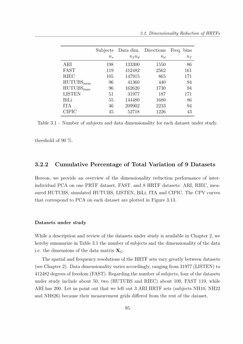
3.2. Dimensionality Reduction of HRTFs
Subjectsns
Data dim.nfnd
Directionsnd
Freq. binsnf
ARI 198 133300 1550 86FAST 119 412482 2562 161RIEC 105 147915 865 171HUTUBSmeas 96 41360 440 94HUTUBSsimu 96 162620 1730 94LISTEN 51 31977 187 171BiLi 55 144480 1680 86ITA 46 209902 2233 94CIPIC 45 52718 1226 43
Table 3.1 – Number of subjects and data dimensionality for each dataset under study.
threshold of 90 %.
3.2.2 Cumulative Percentage of Total Variation of 9 Datasets
Hereon, we provide an overview of the dimensionality reduction performance of inter-individual PCA on one PRTF dataset, FAST, and 8 HRTF datasets: ARI, RIEC, mea-sured HUTUBS, simulated HUTUBS, LISTEN, BiLi, ITA and CIPIC. The CPV curvesthat correspond to PCA on each dataset are plotted in Figure 3.13.
Datasets under study
While a description and review of the datasets under study is available in Chapter 2, wehereby summarize in Table 3.1 the number of subjects and the dimensionality of the datai.e. the dimensions of the data matrix XG.
The spatial and frequency resolutions of the HRTF sets vary greatly between datasets(see Chapter 2). Data dimensionality varies accordingly, ranging from 31977 (LISTEN) to412482 degrees of freedom (FAST). Regarding the number of subjects, four of the datasetsunder study include about 50, two (HUTUBS and RIEC) about 100, FAST 119, whileARI has 200. Let us point out that we left out 3 ARI HRTF sets (subjects NH10, NH22and NH826) because their measurement grids differed from the rest of the dataset.
95
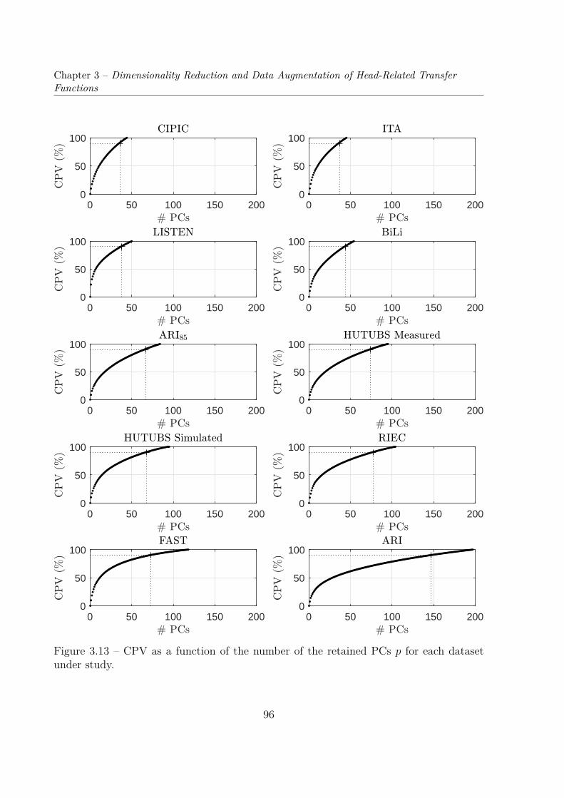
Chapter 3 – Dimensionality Reduction and Data Augmentation of Head-Related TransferFunctions
0 50 100 150 2000
50
100
0 50 100 150 2000
50
100
0 50 100 150 2000
50
100
0 50 100 150 2000
50
100
0 50 100 150 2000
50
100
0 50 100 150 2000
50
100
0 50 100 150 2000
50
100
0 50 100 150 2000
50
100
0 50 100 150 2000
50
100
0 50 100 150 2000
50
100
Figure 3.13 – CPV as a function of the number of the retained PCs p for each datasetunder study.
96
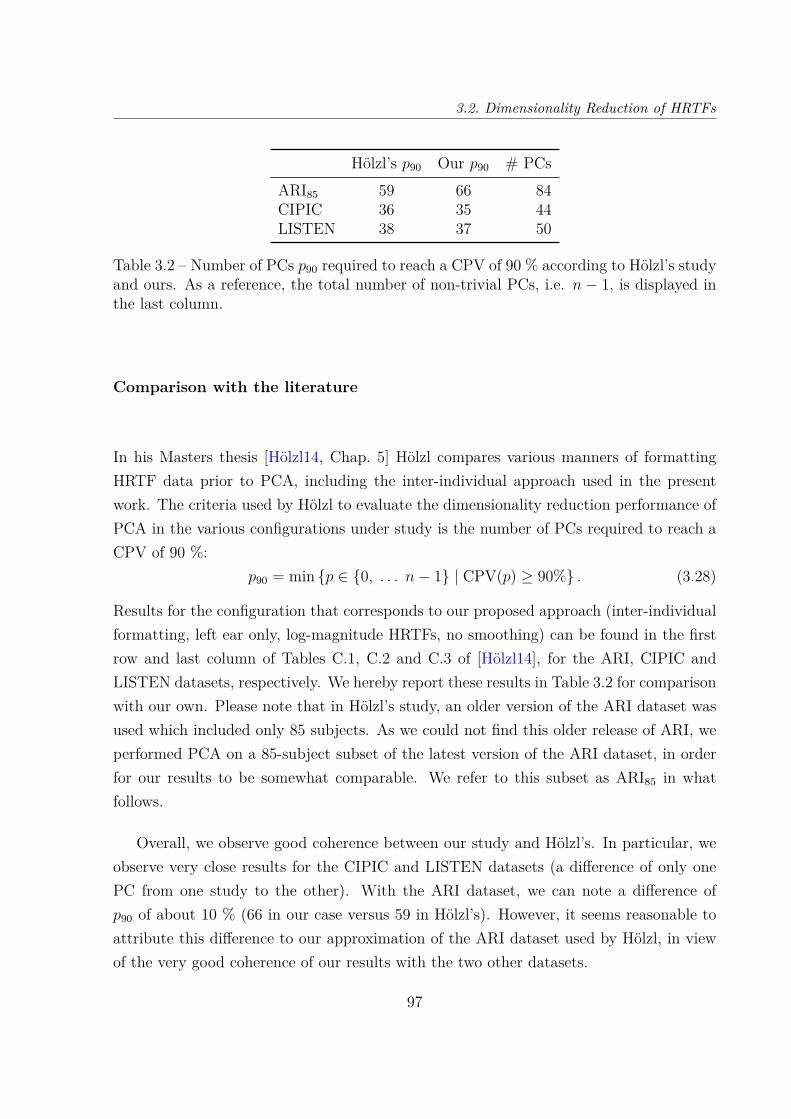
3.2. Dimensionality Reduction of HRTFs
Hölzl’s p90 Our p90 # PCsARI85 59 66 84CIPIC 36 35 44LISTEN 38 37 50
Table 3.2 – Number of PCs p90 required to reach a CPV of 90 % according to Hölzl’s studyand ours. As a reference, the total number of non-trivial PCs, i.e. n − 1, is displayed inthe last column.
Comparison with the literature
In his Masters thesis [Hölzl14, Chap. 5] Hölzl compares various manners of formattingHRTF data prior to PCA, including the inter-individual approach used in the presentwork. The criteria used by Hölzl to evaluate the dimensionality reduction performance ofPCA in the various configurations under study is the number of PCs required to reach aCPV of 90 %:
p90 = min p ∈ 0, . . . n− 1 | CPV(p) ≥ 90% . (3.28)
Results for the configuration that corresponds to our proposed approach (inter-individualformatting, left ear only, log-magnitude HRTFs, no smoothing) can be found in the firstrow and last column of Tables C.1, C.2 and C.3 of [Hölzl14], for the ARI, CIPIC andLISTEN datasets, respectively. We hereby report these results in Table 3.2 for comparisonwith our own. Please note that in Hölzl’s study, an older version of the ARI dataset wasused which included only 85 subjects. As we could not find this older release of ARI, weperformed PCA on a 85-subject subset of the latest version of the ARI dataset, in orderfor our results to be somewhat comparable. We refer to this subset as ARI85 in whatfollows.
Overall, we observe good coherence between our study and Hölzl’s. In particular, weobserve very close results for the CIPIC and LISTEN datasets (a difference of only onePC from one study to the other). With the ARI dataset, we can note a difference ofp90 of about 10 % (66 in our case versus 59 in Hölzl’s). However, it seems reasonable toattribute this difference to our approximation of the ARI dataset used by Hölzl, in viewof the very good coherence of our results with the two other datasets.
97
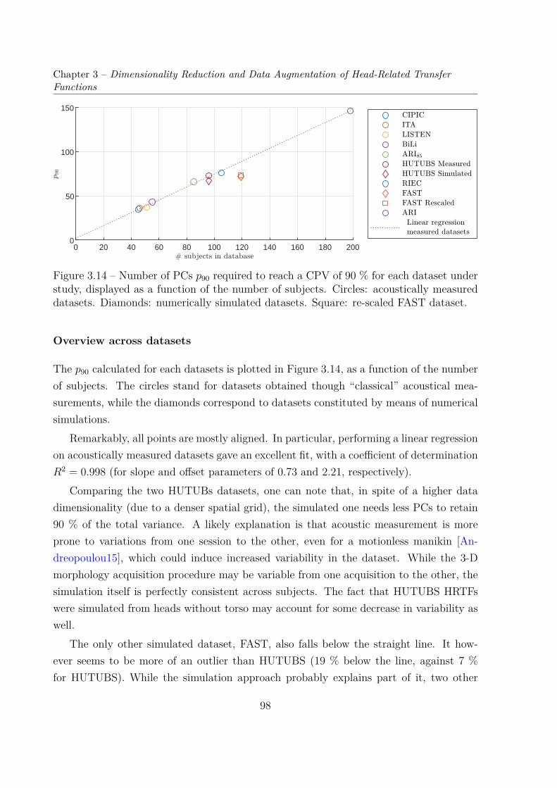
Chapter 3 – Dimensionality Reduction and Data Augmentation of Head-Related TransferFunctions
0 20 40 60 80 100 120 140 160 180 2000
50
100
150
Figure 3.14 – Number of PCs p90 required to reach a CPV of 90 % for each dataset understudy, displayed as a function of the number of subjects. Circles: acoustically measureddatasets. Diamonds: numerically simulated datasets. Square: re-scaled FAST dataset.
Overview across datasets
The p90 calculated for each datasets is plotted in Figure 3.14, as a function of the numberof subjects. The circles stand for datasets obtained though “classical” acoustical mea-surements, while the diamonds correspond to datasets constituted by means of numericalsimulations.
Remarkably, all points are mostly aligned. In particular, performing a linear regressionon acoustically measured datasets gave an excellent fit, with a coefficient of determinationR2 = 0.998 (for slope and offset parameters of 0.73 and 2.21, respectively).
Comparing the two HUTUBs datasets, one can note that, in spite of a higher datadimensionality (due to a denser spatial grid), the simulated one needs less PCs to retain90 % of the total variance. A likely explanation is that acoustic measurement is moreprone to variations from one session to the other, even for a motionless manikin [An-dreopoulou15], which could induce increased variability in the dataset. While the 3-Dmorphology acquisition procedure may be variable from one acquisition to the other, thesimulation itself is perfectly consistent across subjects. The fact that HUTUBS HRTFswere simulated from heads without torso may account for some decrease in variability aswell.
The only other simulated dataset, FAST, also falls below the straight line. It how-ever seems to be more of an outlier than HUTUBS (19 % below the line, against 7 %for HUTUBS). While the simulation approach probably explains part of it, two other
98
3.2. Dimensionality Reduction of HRTFs
hypotheses are plausible. The first one is the fact that the ear shapes used for simulationwere normalized in size, which corresponds to a normalization in frequency scaling ofthe PRTF sets. However, by re-introducing the frequency scaling factors in the PRTFsets, and performing PCA on this rescaled version of the FAST dataset, we found thatthe p90 is higher only by 1 PC. A second one is that contributions from the head andtorso are absent from the PRTFs, thus reducing variability compared to full-morphologymeasurements or simulations. This reduced variability should be more prominent in thecontralateral hemisphere and at low frequencies. Thus, we look below into the impactof leaving out these particular spatial and frequency ranges from PCA on the p90 of alldatasets.
Despite the considerable variety in data dimensionality (spatial sampling, notably)and HRTF acquisition conditions, the number of PCs required to retain 90 % of totalvariation, p90, increases in an approximately linear fashion with the number of subjectscontained in the datasets. The measured datasets fit very well this linear trend, while theFAST and, to a lesser extent, the simulated HUTUBS datasets, lie slightly out of it. Bothof them were simulated instead of measured, and were generated from 3-D geometriesthat excluded the torso (HUTUBS) or both the torso and head (FAST).
Effect of restricting the spatial and frequency ranges
As we have seen above, the magnitude PRTF sets from the FAST dataset seem to presenta lesser inter-individual variability than other HRTF datasets. This difference is likely dueto the absence of contribution from the head and torso in the PRTFs. We herein studythe effect on the p90 of leaving out of PCA spatial or frequency ranges where contributionfrom the pinna is less prominent: the contralateral hemisphere and frequencies below4 kHz.
Frequency range Restricting the frequency range to frequencies above 4 kHz had littleto no effect on the p90. The p90 remained identical for most datasets and decreased onlyby 1 for the three datasets which exhibited change, that is ARI, ARI85 and LISTEN.
It appears that data in the lower frequency range (where only the torso and headcontribute to directional filtering) correspond to a very small proportion of the variabilitybetween magnitude HRTF sets of a given dataset. This is coherent with the fact thatspectral features of HRTFs at these low frequencies are rather “smooth”, unlike the sharppeaks and notches caused by the pinna, whose central frequencies and gains are very
99
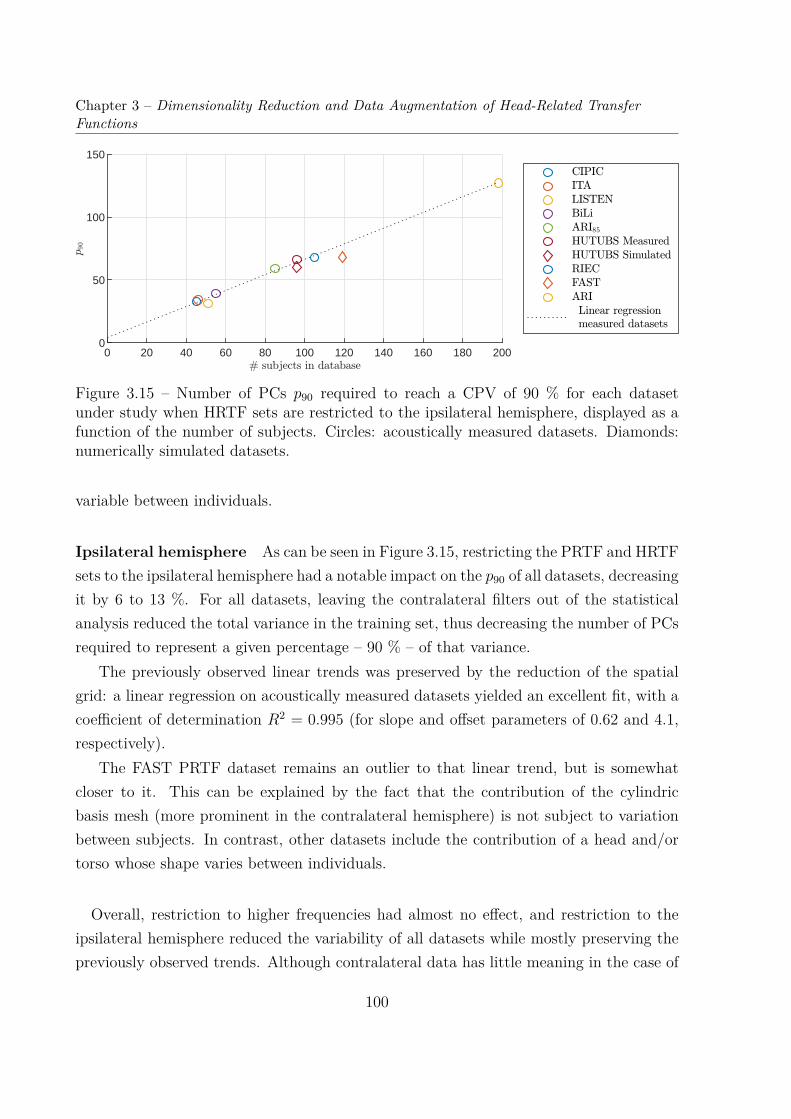
Chapter 3 – Dimensionality Reduction and Data Augmentation of Head-Related TransferFunctions
0 20 40 60 80 100 120 140 160 180 2000
50
100
150
Figure 3.15 – Number of PCs p90 required to reach a CPV of 90 % for each datasetunder study when HRTF sets are restricted to the ipsilateral hemisphere, displayed as afunction of the number of subjects. Circles: acoustically measured datasets. Diamonds:numerically simulated datasets.
variable between individuals.
Ipsilateral hemisphere As can be seen in Figure 3.15, restricting the PRTF and HRTFsets to the ipsilateral hemisphere had a notable impact on the p90 of all datasets, decreasingit by 6 to 13 %. For all datasets, leaving the contralateral filters out of the statisticalanalysis reduced the total variance in the training set, thus decreasing the number of PCsrequired to represent a given percentage – 90 % – of that variance.
The previously observed linear trends was preserved by the reduction of the spatialgrid: a linear regression on acoustically measured datasets yielded an excellent fit, with acoefficient of determination R2 = 0.995 (for slope and offset parameters of 0.62 and 4.1,respectively).
The FAST PRTF dataset remains an outlier to that linear trend, but is somewhatcloser to it. This can be explained by the fact that the contribution of the cylindricbasis mesh (more prominent in the contralateral hemisphere) is not subject to variationbetween subjects. In contrast, other datasets include the contribution of a head and/ortorso whose shape varies between individuals.
Overall, restriction to higher frequencies had almost no effect, and restriction to theipsilateral hemisphere reduced the variability of all datasets while mostly preserving thepreviously observed trends. Although contralateral data has little meaning in the case of
100

3.2. Dimensionality Reduction of HRTFs
PRTFs, removing the contralateral hemisphere reduces for all datasets the dimensionalityof the data by half and removes a substantial part of the variability (p90 decreased by 7 %for the FAST PRTF dataset). Thus, in order to stay close to the more general matterof reducing the dimensionality of HRTF sets, we hereon consider PCA models built onunrestricted spatial and frequency grids.
3.2.3 Reconstruction Error Distribution
In the previous section, we looked into the number of PCs required to retain 90 % of thevariance of 9 datasets of HRTF or PRTF sets. However, the CPV does not inform uson the type of information that is lost when reducing the dimensionality of magnitudeHRTF sets. Thus, we herein look into the distribution of that loss of information (i.e. thereconstruction error) over the frequency and spatial domains for two models: the FASTPRTF model and the ARI HRTF model.
Frequency dependency The dimensionality-reduced magnitude mag-HRTF set of ex-emplary subjects from the FAST and ARI datasets are plotted in Figure 3.16, along withthe original mag-HRTF set and the difference between them in the dB domain. As canbe seen in that figure, the magnitude HRTF sets are somewhat “smoothed” by the di-mensionality reduction process: progressive changes in gain across frequency bins anddirections are better reconstructed than sharper ones.
For both HRTF sets, reconstruction errors are low below 1 kHz, and at their largestbeyond 4-5 kHz, which is coherent with the average behavior observed in Figure 3.18.Indeed, the root-mean-squared reconstruction error (across all subjects and directions)increases with frequency. In contrast with the ARI HRTF model, this error is almost zerofor the FAST PRTF model for frequencies up to 4 kHz. This is coherent with the factthat the pinna has little effect on HRTFs and PRTFs in that frequency range, and that inthe meshes used to compute the FAST PRTFs, only the pinna varies from one “subject”to the other. There is a large increase of this error around 16 kHz, which is a side effectof our pre-processing: re-sampling the HRTFs independently at each direction causedthem to have little coherence between directions and subjects at these high frequencies.The data beyond 15 kHz thus has little meaning but, due to the aforementioned lack ofdirectional coherence, is “seen” as noise by the PCA i.e. associated to the very last PCs.
Finally, the reconstruction error for the FAST PRTF model is lower than that ofthe ARI HRTF model, regardless of the frequency. This was expected, seeing that the
101
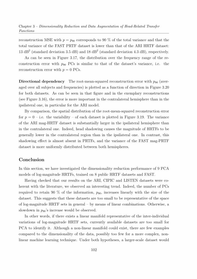
Chapter 3 – Dimensionality Reduction and Data Augmentation of Head-Related TransferFunctions
reconstruction MSE with p = p90 corresponds to 90 % of the total variance and that thetotal variance of the FAST PRTF dataset is lower than that of the ARI HRTF dataset:13 dB2 (standard deviation 3.5 dB) and 18 dB2 (standard deviation 4.3 dB), respectively.
As can be seen in Figure 3.17, the distribution over the frequency range of the re-construction error with p90 PCs is similar to that of the dataset’s variance, i.e. thereconstruction error with p = 0 PCs.
Directional dependency The root-mean-squared reconstruction error with p90 (aver-aged over all subjects and frequencies) is plotted as a function of direction in Figure 3.20for both datasets. As can be seen in that figure and in the exemplary reconstructions(see Figure 3.16), the error is more important in the contralateral hemisphere than in theipsilateral one, in particular for the ARI model.
By comparison, the spatial distribution of the root-mean-squared reconstruction errorfor p = 0 – i.e. the variability – of each dataset is plotted in Figure 3.19. The varianceof the ARI mag-HRTF dataset is substantially larger in the ipsilateral hemisphere thanin the contralateral one. Indeed, head shadowing causes the magnitude of HRTFs to begenerally lower in the contralateral region than in the ipsilateral one. In contrast, thisshadowing effect is almost absent in PRTFs, and the variance of the FAST mag-PRTFdataset is more uniformly distributed between both hemispheres.
Conclusion
In this section, we have investigated the dimensionality reduction performance of 9 PCAmodels of log-magnitude HRTFs, trained on 8 public HRTF datasets and FAST.
Having checked that our results on the ARI, CIPIC and LISTEN datasets were co-herent with the literature, we observed an interesting trend. Indeed, the number of PCsrequired to retain 90 % of the information, p90, increases linearly with the size of thedataset. This suggests that these datasets are too small to be representative of the spaceof log-magnitude HRTF sets in general – by means of linear combinations. Otherwise, aslowdown in p90’s increase would be observed.
In other words, if there exists a linear manifold representative of the inter-individualvariations of log-magnitude HRTF sets, currently available datasets are too small forPCA to identify it. Although a non-linear manifold could exist, there are few examplescompared to the dimensionality of the data, possibly too few for a more complex, non-linear machine learning technique. Under both hypotheses, a larger-scale dataset would
102
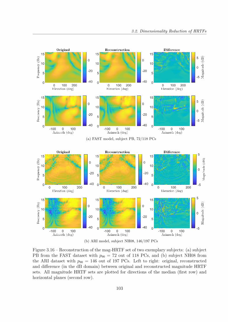
3.2. Dimensionality Reduction of HRTFs
(a) FAST model, subject PB, 72/118 PCs
(b) ARI model, subject NH08, 146/197 PCs
Figure 3.16 – Reconstruction of the mag-HRTF set of two exemplary subjects: (a) subjectPB from the FAST dataset with p90 = 72 out of 118 PCs, and (b) subject NH08 fromthe ARI dataset with p90 = 146 out of 197 PCs. Left to right: original, reconstructedand difference (in the dB domain) between original and reconstructed magnitude HRTFsets. All magnitude HRTF sets are plotted for directions of the median (first row) andhorizontal planes (second row).
103
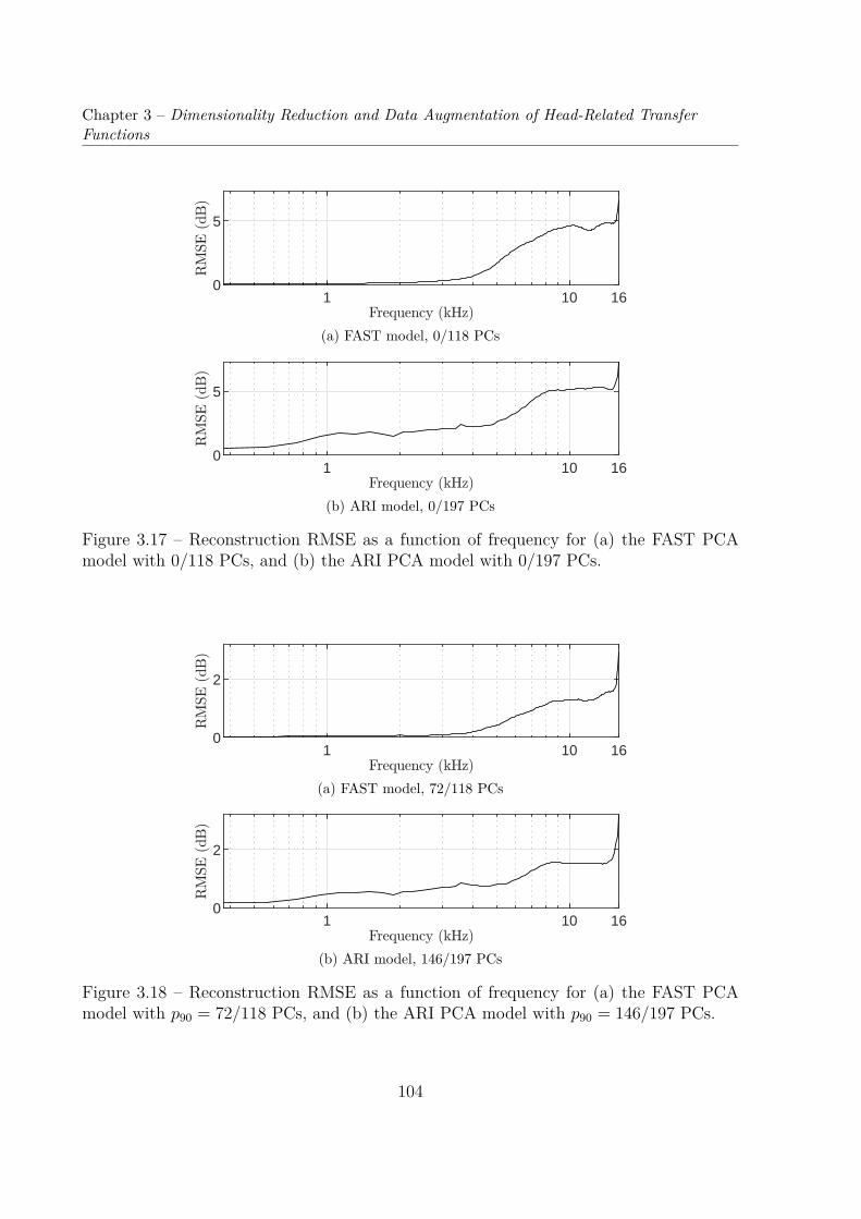
Chapter 3 – Dimensionality Reduction and Data Augmentation of Head-Related TransferFunctions
1 10 160
5
(a) FAST model, 0/118 PCs
1 10 160
5
(b) ARI model, 0/197 PCs
Figure 3.17 – Reconstruction RMSE as a function of frequency for (a) the FAST PCAmodel with 0/118 PCs, and (b) the ARI PCA model with 0/197 PCs.
1 10 160
2
(a) FAST model, 72/118 PCs
1 10 160
2
(b) ARI model, 146/197 PCs
Figure 3.18 – Reconstruction RMSE as a function of frequency for (a) the FAST PCAmodel with p90 = 72/118 PCs, and (b) the ARI PCA model with p90 = 146/197 PCs.
104

3.2. Dimensionality Reduction of HRTFs
(a) FAST model, 0/118 PCs
(b) ARI model, 0/197 PCs
Figure 3.19 – Reconstruction RMSE as a function of direction for (a) the FAST PCAmodel with 0/118 PCs, and (b) the ARI PCA model with 0/197 PCs.
105

Chapter 3 – Dimensionality Reduction and Data Augmentation of Head-Related TransferFunctions
(a) FAST model, 72/118 PCs
(b) ARI model, 146/197 PCs
Figure 3.20 – Reconstruction RMSE as a function of direction for (a) the FAST PCAmodel with p90 = 72/118 PCs, and (b) the ARI PCA model with p90 = 146/197 PCs.
106
3.3. Compared Dimensionality Reductions of EarShapes and Matching PRTF Sets
be desirable.
3.3 Compared Dimensionality Reductions of EarShapes and Matching PRTF Sets
In the previous section, we studied the dimensionality reduction performance of PCAon log-magnitude HRTF sets from various datasets, including the FAST one. Resultssuggested that current datasets include too few examples for PCA to be able to find alinear subspace representative of log-magnitude HRTF sets in general.
In this section, we deal with the preliminary study of the FAST dataset that led todesigning a data augmentation method. Taking advantage of the fact that the FASTdataset includes registered pinna meshes, we investigated whether PCA performs betterat reducing the dimensionality of 3-D ear morphology than of matching computed PRTFsets.
First, we study the ability of PCA to reduce the dimensionality of the 119 log-magnitude PRTF sets. Second, we present how we performed PCA on the corresponding119 ear point clouds. Third, we compare the dimensionality reduction performances ofboth PCA models, as well as the statistical distribution of their respective PCs. Finally,we draw the conclusions that led us to propose the data augmentation scheme.
3.3.1 Principal Component Analysis of Ear Shapes
Let E = e1, . . . en be the set of n = 119 ear point clouds from the FAST datasetwhose x, y and z coordinates are concatenated into row vectors e1, . . . en ∈ R3nv , with3nv = 54528.
In order to build a statistical shape model of the pinna, the ear point clouds were
gathered into a data matrix as follows. Let there be XE =
e1...
en
∈ Rn×3nv the data
107

Chapter 3 – Dimensionality Reduction and Data Augmentation of Head-Related TransferFunctions
matrix, e = 1n
n∑i=1
ei the average ear shape and
XE =
e...e
∈ Rn×3nv (3.29)
the matrix constituted of the average shape stacked n times. Finally, let ΓE ∈ R3nv×3nv
be the covariance matrix of XE:
ΓE = 1n− 1
(XE − XE
)t (XE − XE
). (3.30)
Similarly to the case of magnitude PRTF sets (see Section 3.2), we performed PCAon the data matrix XE according to Equations (3.17), (3.18) and (3.20). The number ofnon-trivial PCs is (n− 1) in this case as well, due to the fact that n < 3nv. From the setof ear point clouds E described in Section 3.1.1, we classically constructed a statistical3-D shape model of the pinna using PCA [Rajamani07].
Behavior of the first principal components
The behavior of the first principal components can be observed as follows.For each PC of index j ∈ 1, 2, 3, we set the jth PC weight to λσEj and all other PC
weights to zero, with λ ∈ −5, −3, −1, +1, +3, +5 and reconstructed the correspondingear point cloud evj(λ) by inverting Equation (3.17)
evj(λ) =(0 . . . 0 λσEj 0 . . . 0
)UE + e. (3.31)
Meshes derived from these ear point clouds are displayed in Figure 3.21, colored with thevertex-to-vertex euclidean distance to the average shape.
The first one seems to control vertical pinna elongation including concha height andlobe length up to disappearance, as well as some pinna vertical axis rotation. The secondone seems to encode the intensity of some topography features such as triangular fossadepth or helix prominence. It also has an impact on concha shape and vertical axisrotation. The third PC seems to have a strong influence on concha depth, triangularfossa depth as well as upper helix shape.
108
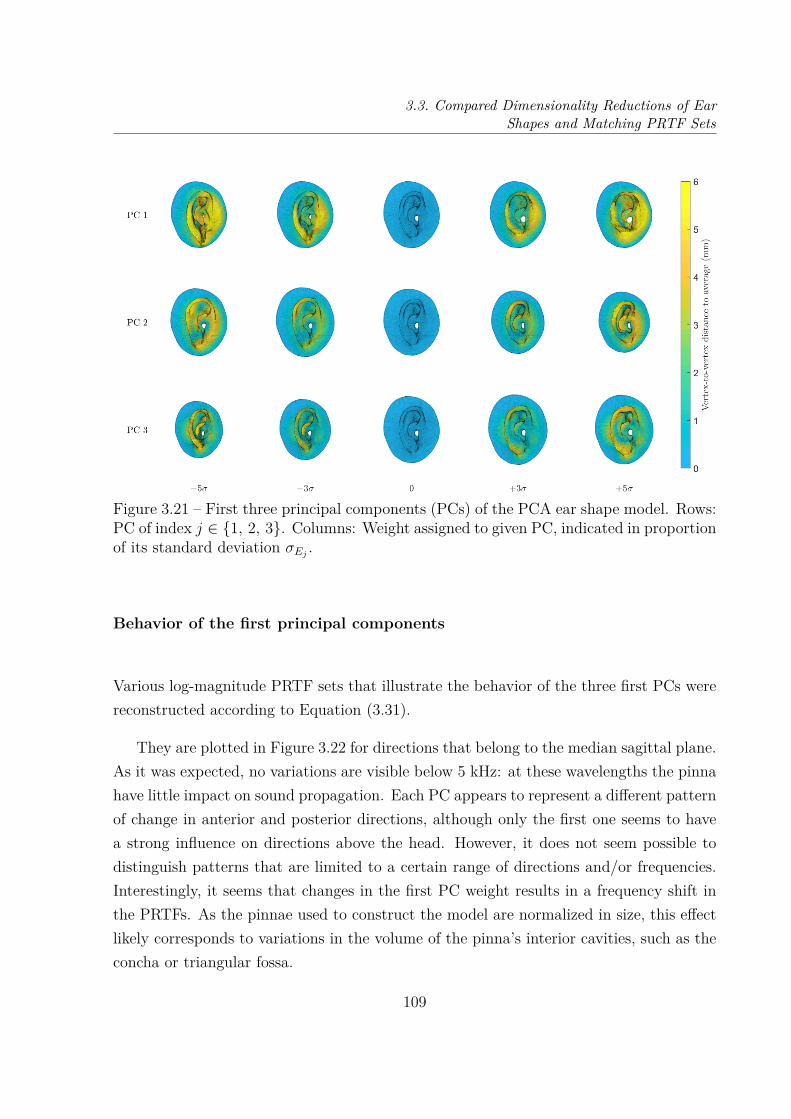
3.3. Compared Dimensionality Reductions of EarShapes and Matching PRTF Sets
Figure 3.21 – First three principal components (PCs) of the PCA ear shape model. Rows:PC of index j ∈ 1, 2, 3. Columns: Weight assigned to given PC, indicated in proportionof its standard deviation σEj .
Behavior of the first principal components
Various log-magnitude PRTF sets that illustrate the behavior of the three first PCs werereconstructed according to Equation (3.31).
They are plotted in Figure 3.22 for directions that belong to the median sagittal plane.As it was expected, no variations are visible below 5 kHz: at these wavelengths the pinnahave little impact on sound propagation. Each PC appears to represent a different patternof change in anterior and posterior directions, although only the first one seems to havea strong influence on directions above the head. However, it does not seem possible todistinguish patterns that are limited to a certain range of directions and/or frequencies.Interestingly, it seems that changes in the first PC weight results in a frequency shift inthe PRTFs. As the pinnae used to construct the model are normalized in size, this effectlikely corresponds to variations in the volume of the pinna’s interior cavities, such as theconcha or triangular fossa.
109
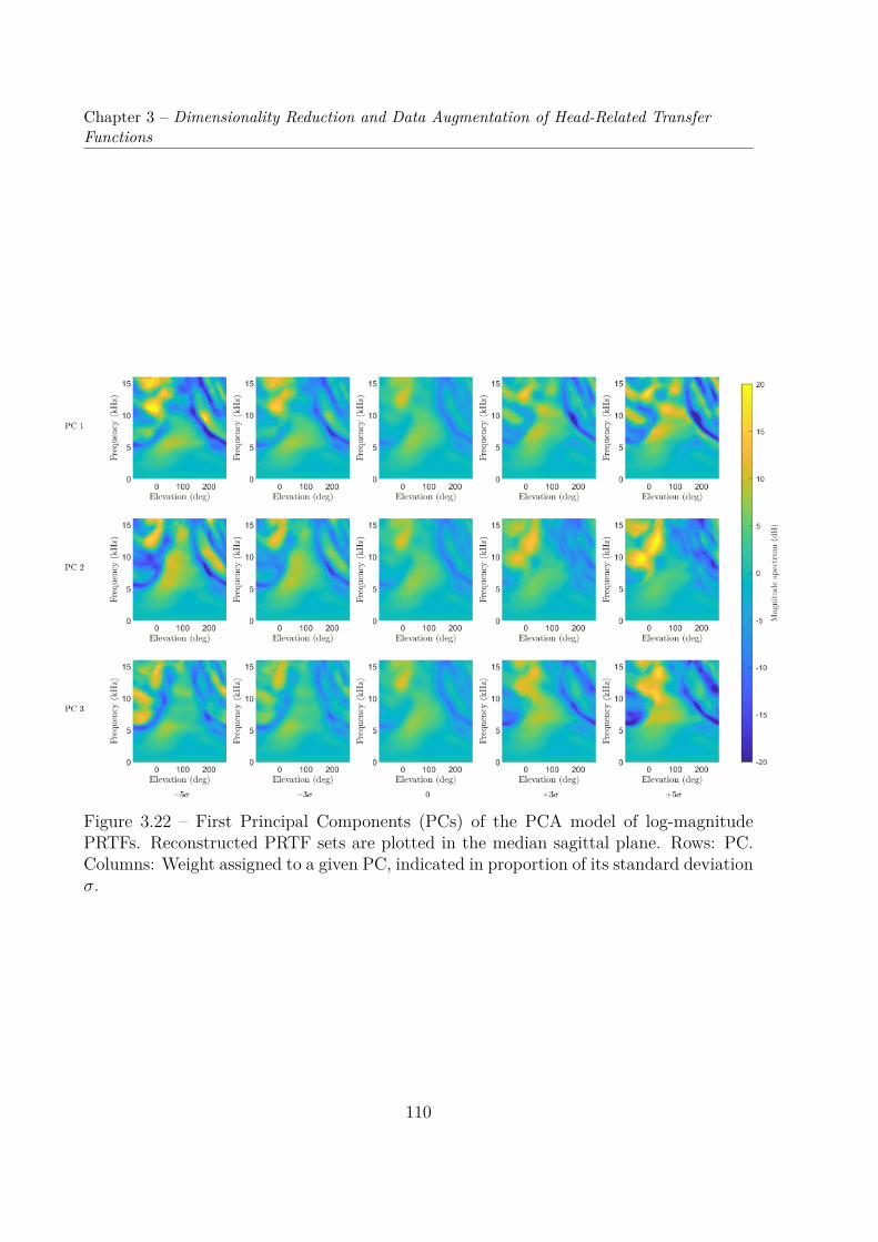
Chapter 3 – Dimensionality Reduction and Data Augmentation of Head-Related TransferFunctions
Figure 3.22 – First Principal Components (PCs) of the PCA model of log-magnitudePRTFs. Reconstructed PRTF sets are plotted in the median sagittal plane. Rows: PC.Columns: Weight assigned to a given PC, indicated in proportion of its standard deviationσ.
110

3.3. Compared Dimensionality Reductions of EarShapes and Matching PRTF Sets
Figure 3.23 – CPVS(p) as a function of the number of retained PCs p ∈ 0, . . . n−1 foreither PCA model. Circles: ear shape model (S = E). Dots: PRTF set model (S = Q).
3.3.2 Comparison of Both PCA Models
For all ear shapes ei ∈ E, let us denote hi = ψ (ei) ∈ Cnf×nd the corresponding PRTFset, computed according to the process described in Section 3.1.
Additionally, let gi ∈ Rnfnd be the log-magnitude PRTF set derived from hi accordingto the pre-processing step described in Section 3.2. Accordingly, let Ψ : R3nv 7→ Rnf×nd ,defined by e 7−→ g = 20 · log10 (|ψ(e)|), be the process of deriving a log-magnitude PRTFset from an ear point cloud, and let G = g1, . . . gn = Ψ(e1) . . . Ψ(en).
PCA was performed on the 119 log-magnitude PRTF sets from the FAST dataset inthe inter-individual fashion described in Section 3.2. The number of non-trivial PCs is(n− 1) in this case as well, due to the fact that n < nfnd.
Dimensionality reduction performance
As in Section 3.2, we use CPV to compare the dimensionality reduction performances ofboth PCA models. CPVs for both models are plotted in Figure 3.23. While we previouslyused a CPV threshold of 90 % as a basis for comparison with the literature, we hereonprefer a more selective threshold of 99 %.
A first notable result is that, for the ear shape model, the 99 %-of-total-variancethreshold is reached for p = 80 retained PCs, i.e. only p
n−1 = 80118 = 67.8 % of the
maximum number of PCs.In other words, the 118-dimensional linear subspace of R3nv = R56661 defined by the
n = 119 pinnae of our database can be described using only 80 parameters while main-taining a ‘reasonable’ reconstruction accuracy, in the sense of a vertex-to-vertex MSE. Inthe present example of a CPV of 99 %, this accuracy corresponds to a MSE of 1 % of its
111

Chapter 3 – Dimensionality Reduction and Data Augmentation of Head-Related TransferFunctions
maximum value. Indeed, for a CPV of 99 %, Equation (3.26) gives us:
MSE(X(p99)E ,XE) =
(1− CPVE(p99)
100
)·MSE(XE,XE)
= 0.01 ·MSE(XE,XE).(3.32)
More importantly, PCA appears to be largely more successful at reducing the dimen-sion of ear shapes ei than that of magnitude PRTF sets calculated from the same earshapes gi = Ψ(ei). Indeed, the PRTF CPV is substantially lower than the ear shapeCPV for any number of retained PCs. For instance, the 99 %-of-total-variance thresholdis reached for 112 PCs out of 118 for the PRTF model against 80 out of 118 for the earshape one.
Statistical distribution
Going further in our comparison of both PCA models, we looked into the statisticaldistribution of the data in both 118-dimensional PCA subspaces.
To do so, we tested the PCs of each model for multivariate normal distribution usingRoyston’s test [Royston83], performed on the columns of the PC weights matrix YS,where S ∈ E,G denotes the dataset.
The outcome of the test was an associated p-value of 0.037 in the case of ear pointclouds, and 0.000 in the case of mag-PRTF sets, where the p-value refers to the nullhypothesis that the distribution is not multivariate normal. In other words, the earmodel’s PC weights can be considered to be multivariate-normally distributed with asignificance level of 3.7 %, while its PRTF counterpart’s fail the test for any significancelevel.
Conclusion
We found that PCA performs largely better at reducing the dimensionality of the 1193-D ear shapes than of the log-magnitude PRTF sets derived from them. In particular,in contrast with the case of log-magnitude PRTF sets, PCA allowed us to identify an80-dimensional linear subspace in which the 119 training examples can be representedwhile retaining 99 % of the information. Moreover, the ear point cloud PC weights followa multivariate normal distribution.
112

3.4. Dataset Augmentation
Overall, the ear shape PCA model seems more suited than its PRTF counterpart forthe random generation of new data.
3.4 Dataset Augmentation
Based on the conclusions drawn in Section 3.3, we devised and implemented a method toaugment the FAST dataset that uses the space of 3-D ear morphology as a back door torandomly generate new examples (see Figure 3.24 for an overview). This method allowsthe generation of new data (pinna meshes and matching PRTF sets) from existing data,based on the statistical distribution of the latter. Such a process is commonly referredto as “data augmentation” in the field of machine learning, and is used to overcomethe recurring problem of limited dataset size in applications that require a lot of data –generally neural-network-based.
In the present section, we introduce this process and the resulting dataset, namedWiDESPREaD (a wide dataset of ear shapes and pinna-related transfer functions). First,we explain how we used the PCA model of ear shapes presented in Section 3.3 to randomlygenerate over a thousand ear meshes. Then, we go over how PRTF sets were derived fromthose meshes by means of FM-BEM calculations. Finally, we take a look at a few examplesfrom the augmented dataset.
3.4.1 Random Generation of Ear Meshes
The statistical ear shape model learned from dataset E and presented in Section 3.3.1 canbe used as a generative model. By construction, the model’s PCs (i.e. the columns of YE)are of zero mean and are mutually uncorrelated, i.e. statistically independent up to thesecond order. Furthermore, as we have shown in Section 3.3, the columns of YE follow amultivariate normal distribution. They are thus mutually statistically independent (up toany order) and follow respective normal probability laws of zero mean and σEj standarddeviation N (0, σEj), where j ∈ 1, . . . n−1 represents the PC index. As a consequence,a new statistically realistic ear point cloud can be conveniently generated by randomlydrawing a vector of PC weights according to the distribution of probability observed inthe FAST dataset.
To constitute the WiDESPREaD dataset, an arbitrarily large number N of ear shapese′1, . . . e′N ∈ R3nv were thus randomly generated as follows. First, for all i = 1, . . . N ,
113
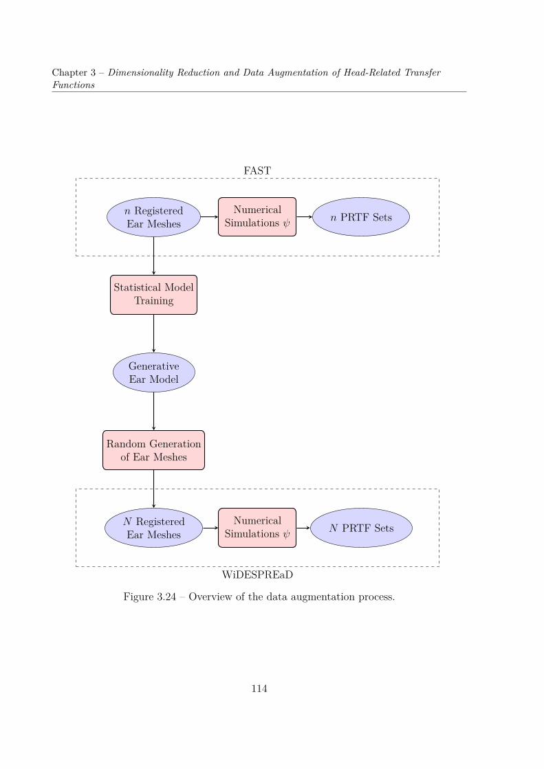
Chapter 3 – Dimensionality Reduction and Data Augmentation of Head-Related TransferFunctions
n RegisteredEar Meshes
Statistical ModelTraining
NumericalSimulations ψ n PRTF Sets
GenerativeEar Model
Random Generationof Ear Meshes
N RegisteredEar Meshes
NumericalSimulations ψ N PRTF Sets
FAST
WiDESPREaD
Figure 3.24 – Overview of the data augmentation process.
114
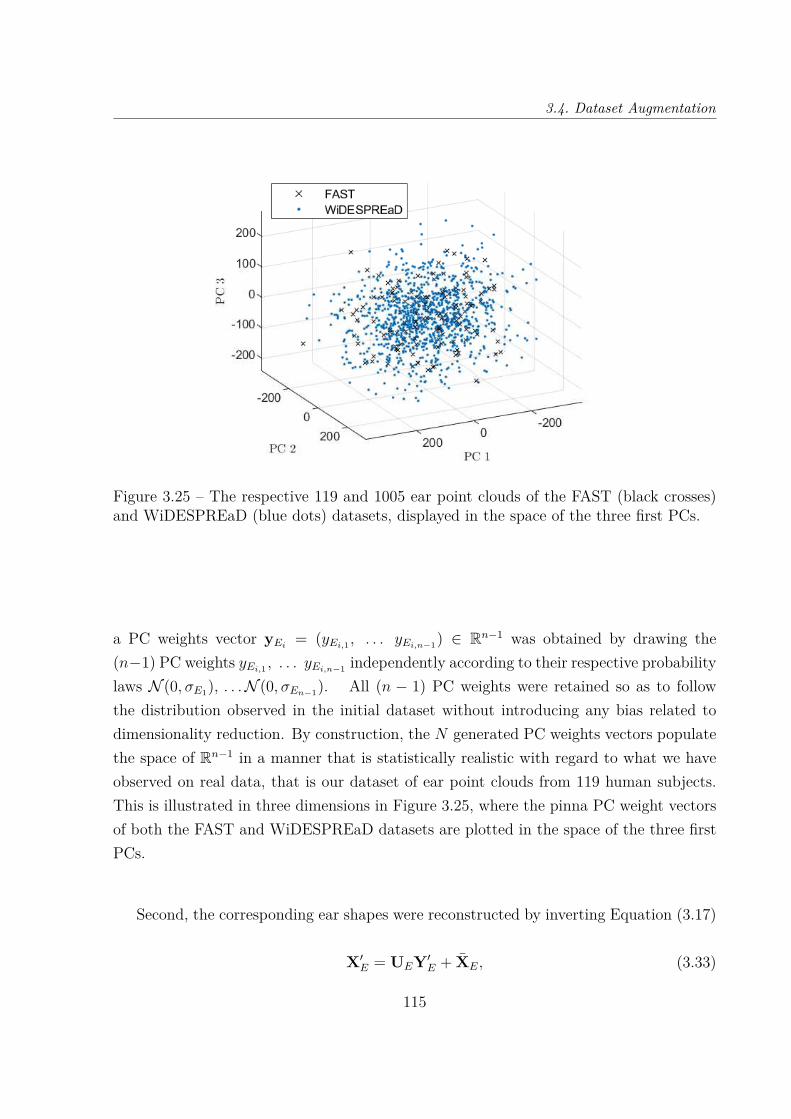
3.4. Dataset Augmentation
Figure 3.25 – The respective 119 and 1005 ear point clouds of the FAST (black crosses)and WiDESPREaD (blue dots) datasets, displayed in the space of the three first PCs.
a PC weights vector yEi = (yEi,1 , . . . yEi,n−1) ∈ Rn−1 was obtained by drawing the(n−1) PC weights yEi,1 , . . . yEi,n−1 independently according to their respective probabilitylaws N (0, σE1), . . .N (0, σEn−1). All (n − 1) PC weights were retained so as to followthe distribution observed in the initial dataset without introducing any bias related todimensionality reduction. By construction, the N generated PC weights vectors populatethe space of Rn−1 in a manner that is statistically realistic with regard to what we haveobserved on real data, that is our dataset of ear point clouds from 119 human subjects.This is illustrated in three dimensions in Figure 3.25, where the pinna PC weight vectorsof both the FAST and WiDESPREaD datasets are plotted in the space of the three firstPCs.
Second, the corresponding ear shapes were reconstructed by inverting Equation (3.17)
X′E = UEY′E + XE, (3.33)
115

Chapter 3 – Dimensionality Reduction and Data Augmentation of Head-Related TransferFunctions
where Y′E ∈ RN×(n−1) is the matrix whose rows are the N PC weights vectors
Y′E =
y′E1...
y′EN
=
y′E1,1 . . . y′E1,n−1... . . . ...
y′EN,1 . . . y′EN,n−1
, (3.34)
and X′E ∈ RN×3nv is the data matrix whose rows are the N ear shapes e′1, . . . e′N ∈ R3nv
X′E =
e′1...
e′N
. (3.35)
Quality check
At the end of the ear shape generation process, meshes were derived from the pointclouds as in the case of the FAST dataset (see Section 3.1.1). We then verified that themeshes were not aberrant and that they were fit for numerical simulation: any mesh thatpresented at least one self-intersecting face was left out.
In total, 24 % (320 out of 1325) of the meshes were discarded. Performing the Roys-ton’s multivariate normality test on the 1325 randomly drawn ear PC weights then on the1005 remaining ones, we observed a decrease in the significance level of the test from 4.8 %to 0.8 %: it appears that the statistical distribution of the ear PC weights was somewhatdegraded by the selection process. However, when looking into the distribution of eachPC of the selected ear shapes separately (using the Shapiro-Wilk univariate normalitytest with a significance level of 5 %), we observe that the 9 rejected PCs account only for3.7 % of the total variance.
For simplicity, we consider further on that N is the number of retained meshes i.e.N = 1005.
3.4.2 Numerical Simulations
Finally, PRTF sets were numerically simulated from the ear shapes of the new set E ′
according to the process described in Section 3.1.2
h′i = ψ (e′i) , ∀ i = 1, . . . N. (3.36)
116
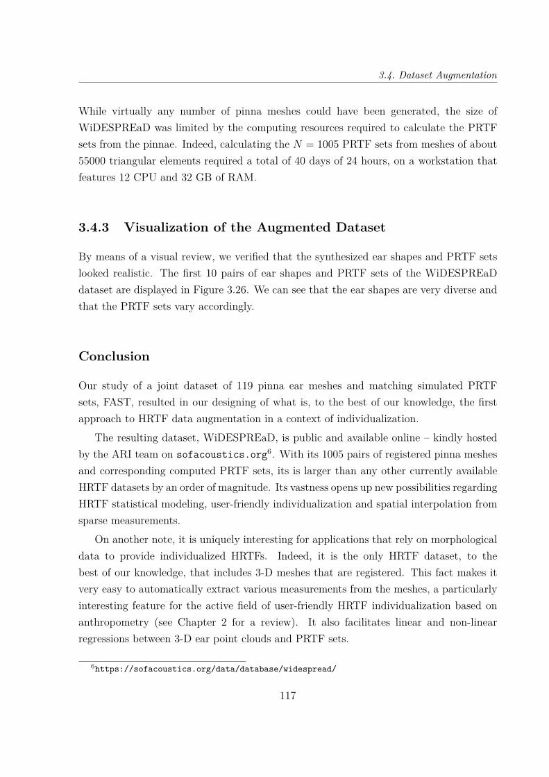
3.4. Dataset Augmentation
While virtually any number of pinna meshes could have been generated, the size ofWiDESPREaD was limited by the computing resources required to calculate the PRTFsets from the pinnae. Indeed, calculating the N = 1005 PRTF sets from meshes of about55000 triangular elements required a total of 40 days of 24 hours, on a workstation thatfeatures 12 CPU and 32 GB of RAM.
3.4.3 Visualization of the Augmented Dataset
By means of a visual review, we verified that the synthesized ear shapes and PRTF setslooked realistic. The first 10 pairs of ear shapes and PRTF sets of the WiDESPREaDdataset are displayed in Figure 3.26. We can see that the ear shapes are very diverse andthat the PRTF sets vary accordingly.
Conclusion
Our study of a joint dataset of 119 pinna ear meshes and matching simulated PRTFsets, FAST, resulted in our designing of what is, to the best of our knowledge, the firstapproach to HRTF data augmentation in a context of individualization.
The resulting dataset, WiDESPREaD, is public and available online – kindly hostedby the ARI team on sofacoustics.org6. With its 1005 pairs of registered pinna meshesand corresponding computed PRTF sets, its is larger than any other currently availableHRTF datasets by an order of magnitude. Its vastness opens up new possibilities regardingHRTF statistical modeling, user-friendly individualization and spatial interpolation fromsparse measurements.
On another note, it is uniquely interesting for applications that rely on morphologicaldata to provide individualized HRTFs. Indeed, it is the only HRTF dataset, to thebest of our knowledge, that includes 3-D meshes that are registered. This fact makes itvery easy to automatically extract various measurements from the meshes, a particularlyinteresting feature for the active field of user-friendly HRTF individualization based onanthropometry (see Chapter 2 for a review). It also facilitates linear and non-linearregressions between 3-D ear point clouds and PRTF sets.
6https://sofacoustics.org/data/database/widespread/
117
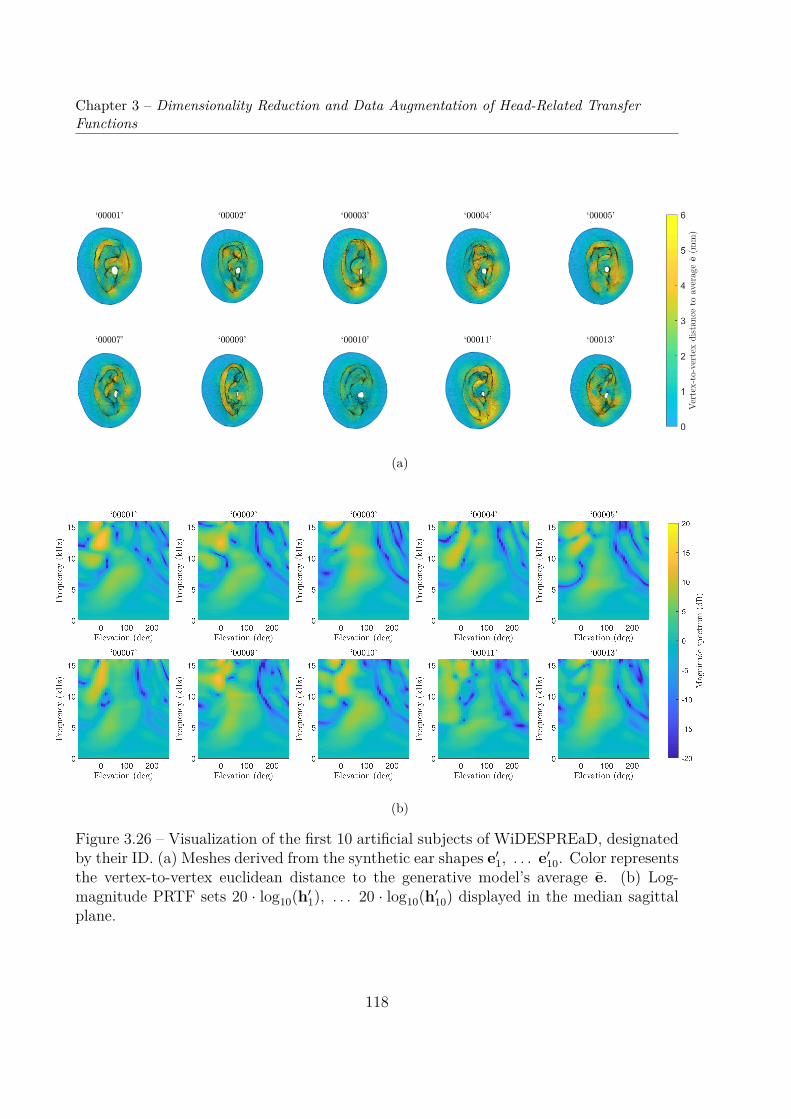
Chapter 3 – Dimensionality Reduction and Data Augmentation of Head-Related TransferFunctions
(a)
(b)
Figure 3.26 – Visualization of the first 10 artificial subjects of WiDESPREaD, designatedby their ID. (a) Meshes derived from the synthetic ear shapes e′1, . . . e′10. Color representsthe vertex-to-vertex euclidean distance to the generative model’s average e. (b) Log-magnitude PRTF sets 20 · log10(h′1), . . . 20 · log10(h′10) displayed in the median sagittalplane.
118

3.5. Dimensionality Reduction of the AugmentedPRTF Dataset
3.5 Dimensionality Reduction of the AugmentedPRTF Dataset
In this section, we investigate how using the augmented dataset, WiDESPREaD, to traina PCA model of log-magnitude PRTF sets impacts dimensionality reduction performance.We start by comparing its CPV with that of 10 PCA models from Section 3.2, trained onvarious HRTF datasets including FAST. Going further, we then compare the results of20-fold cross-validations performed respectively on the FAST and WiDESPREaD PCAmodels.
3.5.1 Cumulative Percentage of Total Variation
Pre-processing and PCA of the WiDESPREaD log-magnitude PRTF sets was performedas for the other HRTF datasets (see Section 3.2). Let us look into its CPV, as we havedone for other PCA models throughout this chapter, and compare it with that of otherHRTF datasets.
Comparison with FAST
In particular, let us compare the CPV of the WiDESPREaD model with that of FAST,dataset from which it derives. CPVs of both log-magnitude PRTF PCAmodels are plottedin Figure 3.27.
A first observation that can be made is that, for equal numbers of retained PCs, theFAST CPV is lower than the WiDESPREaD one. In other words, to achieve a givenCPV, the WiDESPREaD model requires more PCs than the FAST one. For instance, toretain 90 % of the variability, p90 = 321 PCs are required for the former, against p90 = 72for the latter (see Figure 3.27). In that sense, this could be seen as a regression: morePCs are needed to achieve a CPV of 90 %.
Yet, it actually corroborates our choice of augmenting the FAST dataset. Indeed, theaim of our dataset augmentation method was to produce a large yet statistically realisticpopulation of PRTF sets, by using the more PCA-compatible ear shape space as a backdoor. According to the aforementioned observation, the WiDESPREaD PCA model hascaptured variations in magnitude PRTF sets that were not present in the initial dataset.If that was not the case, using the space of ear shapes to generate new data by means ofPCA would have had little interest.
119
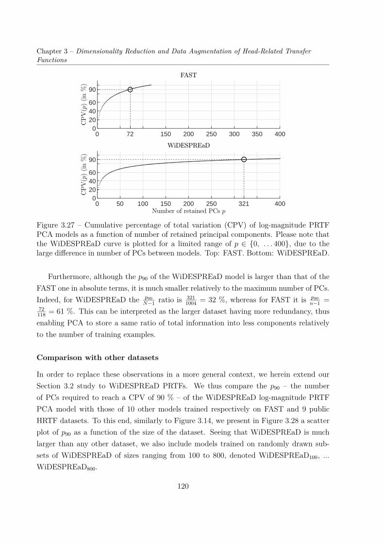
Chapter 3 – Dimensionality Reduction and Data Augmentation of Head-Related TransferFunctions
0 72 150 200 250 300 350 4000
204060
90
0 50 100 150 200 250 321 4000
204060
90
Figure 3.27 – Cumulative percentage of total variation (CPV) of log-magnitude PRTFPCA models as a function of number of retained principal components. Please note thatthe WiDESPREaD curve is plotted for a limited range of p ∈ 0, . . . 400, due to thelarge difference in number of PCs between models. Top: FAST. Bottom: WiDESPREaD.
Furthermore, although the p90 of the WiDESPREaD model is larger than that of theFAST one in absolute terms, it is much smaller relatively to the maximum number of PCs.Indeed, for WiDESPREaD the p90
N−1 ratio is 3211004 = 32 %, whereas for FAST it is p90
n−1 =72118 = 61 %. This can be interpreted as the larger dataset having more redundancy, thusenabling PCA to store a same ratio of total information into less components relativelyto the number of training examples.
Comparison with other datasets
In order to replace these observations in a more general context, we herein extend ourSection 3.2 study to WiDESPREaD PRTFs. We thus compare the p90 – the numberof PCs required to reach a CPV of 90 % – of the WiDESPREaD log-magnitude PRTFPCA model with those of 10 other models trained respectively on FAST and 9 publicHRTF datasets. To this end, similarly to Figure 3.14, we present in Figure 3.28 a scatterplot of p90 as a function of the size of the dataset. Seeing that WiDESPREaD is muchlarger than any other dataset, we also include models trained on randomly drawn sub-sets of WiDESPREaD of sizes ranging from 100 to 800, denoted WiDESPREaD100, ...WiDESPREaD800.
120

3.5. Dimensionality Reduction of the AugmentedPRTF Dataset
0 200 400 600 800 1000 12000
100
200
300
400
500
600
700
800
Figure 3.28 – Number of PCs p90 required to reach a CPV of 90 % for WiDESPREaD,5 WiDESPREaD subsets, FAST and 9 public HRTF datasets, displayed as a function ofthe number of subjects. Circles: acoustically measured datasets. Diamonds: numericallysimulated datasets. Dots: WiDESPREaD subsets.
We can see in Figure 3.28 that WiDESPREaD’s p90 falls largely below the linear trendfollowed by the smaller datasets: the p90 (301) is worth less than half the linear prediction(731). As hoped, augmenting the FAST dataset has allowed us to reach a number ofsubjects high enough to observe a slowdown in p90’s increase.
Overall, studying the CPV of WiDESPREaD and comparing it to that of FAST andother HRTF datasets has given us indications that the WiDESPREaD model may performbetter at representing log-magnitude PRTF sets in general.
3.5.2 Cross-Validation
In order to assess and compare the capacity of the WiDESPREaD and FAST PCA modelsto generalize to new examples, we performed a 20-fold cross-validation on each one ofthem.
Method
Let us denote g(F)1 , . . . g(F)
n ∈ Rnfnd , and g(W)1 , . . . g(W)
N ∈ Rnfnd the log-magnitudePRTF sets from the FAST and WiDESPREaD datasets, respectively. Additionally, let
121
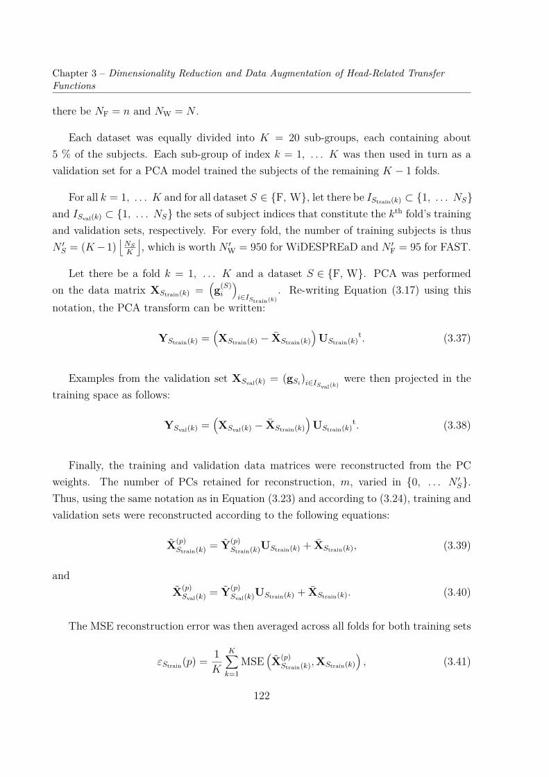
Chapter 3 – Dimensionality Reduction and Data Augmentation of Head-Related TransferFunctions
there be NF = n and NW = N .
Each dataset was equally divided into K = 20 sub-groups, each containing about5 % of the subjects. Each sub-group of index k = 1, . . . K was then used in turn as avalidation set for a PCA model trained the subjects of the remaining K − 1 folds.
For all k = 1, . . . K and for all dataset S ∈ F, W, let there be IStrain(k) ⊂ 1, . . . NSand ISval(k) ⊂ 1, . . . NS the sets of subject indices that constitute the kth fold’s trainingand validation sets, respectively. For every fold, the number of training subjects is thusN ′S = (K−1)
⌊NSK
⌋, which is worth N ′W = 950 for WiDESPREaD and N ′F = 95 for FAST.
Let there be a fold k = 1, . . . K and a dataset S ∈ F, W. PCA was performedon the data matrix XStrain(k) =
(g(S)i
)i∈IStrain(k)
. Re-writing Equation (3.17) using thisnotation, the PCA transform can be written:
YStrain(k) =(XStrain(k) − XStrain(k)
)UStrain(k)
t. (3.37)
Examples from the validation set XSval(k) = (gSi)i∈ISval(k)were then projected in the
training space as follows:
YSval(k) =(XSval(k) − XStrain(k)
)UStrain(k)
t. (3.38)
Finally, the training and validation data matrices were reconstructed from the PCweights. The number of PCs retained for reconstruction, m, varied in 0, . . . N ′S.Thus, using the same notation as in Equation (3.23) and according to (3.24), training andvalidation sets were reconstructed according to the following equations:
X(p)Strain(k) = Y(p)
Strain(k)UStrain(k) + XStrain(k), (3.39)
andX(p)Sval(k) = Y(p)
Sval(k)UStrain(k) + XStrain(k). (3.40)
The MSE reconstruction error was then averaged across all folds for both training sets
εStrain(p) = 1K
K∑k=1
MSE(X(p)Strain(k),XStrain(k)
), (3.41)
122
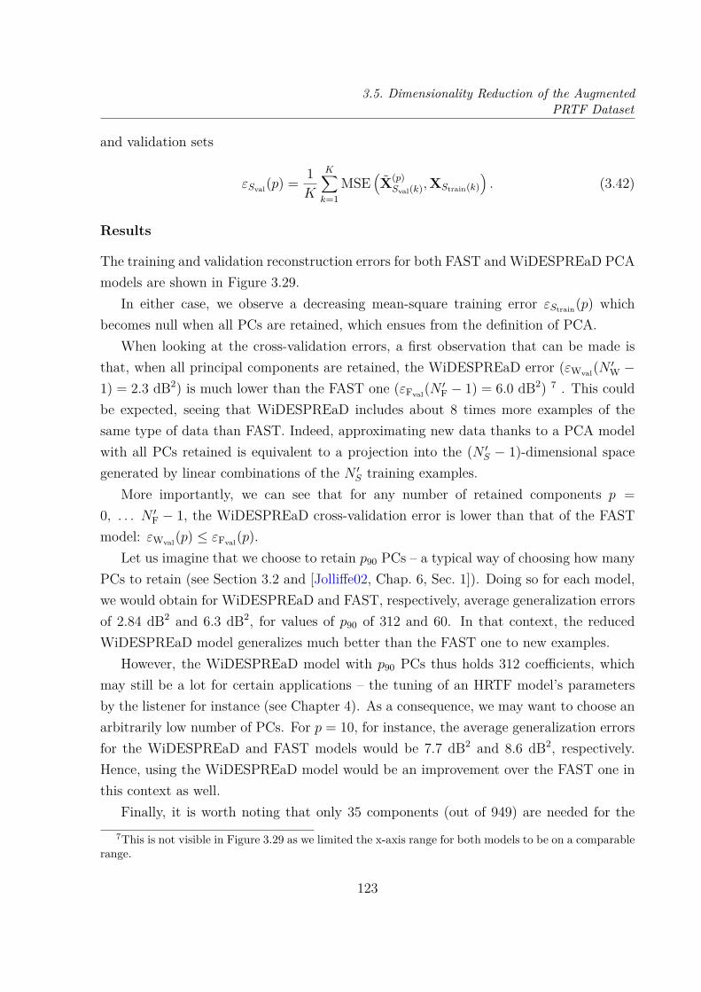
3.5. Dimensionality Reduction of the AugmentedPRTF Dataset
and validation sets
εSval(p) = 1K
K∑k=1
MSE(X(p)Sval(k),XStrain(k)
). (3.42)
Results
The training and validation reconstruction errors for both FAST and WiDESPREaD PCAmodels are shown in Figure 3.29.
In either case, we observe a decreasing mean-square training error εStrain(p) whichbecomes null when all PCs are retained, which ensues from the definition of PCA.
When looking at the cross-validation errors, a first observation that can be made isthat, when all principal components are retained, the WiDESPREaD error (εWval(N ′W −1) = 2.3 dB2) is much lower than the FAST one (εFval(N ′F − 1) = 6.0 dB2) 7 . This couldbe expected, seeing that WiDESPREaD includes about 8 times more examples of thesame type of data than FAST. Indeed, approximating new data thanks to a PCA modelwith all PCs retained is equivalent to a projection into the (N ′S − 1)-dimensional spacegenerated by linear combinations of the N ′S training examples.
More importantly, we can see that for any number of retained components p =0, . . . N ′F − 1, the WiDESPREaD cross-validation error is lower than that of the FASTmodel: εWval(p) ≤ εFval(p).
Let us imagine that we choose to retain p90 PCs – a typical way of choosing how manyPCs to retain (see Section 3.2 and [Jolliffe02, Chap. 6, Sec. 1]). Doing so for each model,we would obtain for WiDESPREaD and FAST, respectively, average generalization errorsof 2.84 dB2 and 6.3 dB2, for values of p90 of 312 and 60. In that context, the reducedWiDESPREaD model generalizes much better than the FAST one to new examples.
However, the WiDESPREaD model with p90 PCs thus holds 312 coefficients, whichmay still be a lot for certain applications – the tuning of an HRTF model’s parametersby the listener for instance (see Chapter 4). As a consequence, we may want to choose anarbitrarily low number of PCs. For p = 10, for instance, the average generalization errorsfor the WiDESPREaD and FAST models would be 7.7 dB2 and 8.6 dB2, respectively.Hence, using the WiDESPREaD model would be an improvement over the FAST one inthis context as well.
Finally, it is worth noting that only 35 components (out of 949) are needed for the7This is not visible in Figure 3.29 as we limited the x-axis range for both models to be on a comparable
range.
123
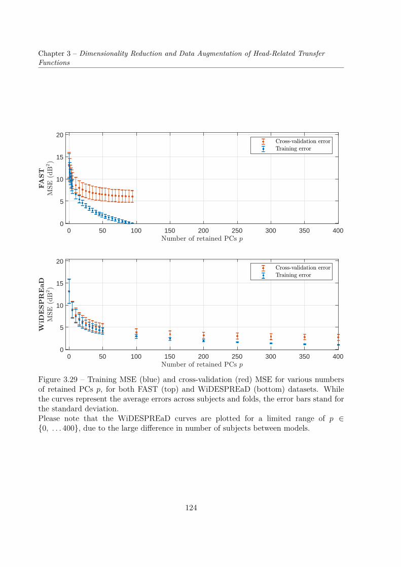
Chapter 3 – Dimensionality Reduction and Data Augmentation of Head-Related TransferFunctions
0 50 100 150 200 250 300 350 4000
5
10
15
20
0 50 100 150 200 250 300 350 4000
5
10
15
20
Figure 3.29 – Training MSE (blue) and cross-validation (red) MSE for various numbersof retained PCs p, for both FAST (top) and WiDESPREaD (bottom) datasets. Whilethe curves represent the average errors across subjects and folds, the error bars stand forthe standard deviation.Please note that the WiDESPREaD curves are plotted for a limited range of p ∈0, . . . 400, due to the large difference in number of subjects between models.
124
3.6. Conclusion & Perspectives
WiDESPREaD cross-validation reconstruction error to subceed the lowest cross-validationerror ever attained in the case of the FAST dataset (εFval(N ′F−1) = 6.0 dB2), that is with94 retained PCs (out of 94).
Conclusion
In this section, in order to investigate WiDESPREaD’s potential for PRTF dimension-ality reduction, we have performed PCA on its log-magnitude PRTFs and compared itsdimensionality reduction performance with that of other PCA models of log-magnitudeHRTFs.
By comparing the CPV of the WiDESPREaD model with that of 10 log-magnitudeHRTF PCA models (previously studied in Section 3.2), we corroborated our choice ofaugmenting the FAST dataset. Indeed, we seem to have sufficiently increased the numberof subject for PCA to be able to compress more observed variability into fewer PCs.WiDESPREaD is thus the only dataset of the 10 models under study that is able toclearly escape the linear trend observed with the smaller datasets.
These results suggest that the WiDESPREaD PCA model is more representative oflog-magnitude PRTF sets in general. Thus, in order to confirm it, we performed 20-cross-validations of the FAST and WiDESPREaD models. We find that, indeed, much bettergeneralization is obtained with the WiDESPREaD model, regardless of the number ofretained PCs.
3.6 Conclusion & Perspectives
The contributions in this chapter are five-fold. First, we presented the constitution of ajoint dataset of 119 3-D registered meshes of human pinnae and matching simulated PRTFsets. Second, choosing an inter-individual approach to the PCA of HRTFs – one that hasbarely been covered in the literature, we studied and compared the dimensionality reduc-tion performance of PCA on log-magnitude HRTF sets from 9 datasets including FAST.This led us to the conclusion that current datasets are too small to be representative oflog-magnitude HRTF sets in general. Third, focusing on the FAST dataset, we comparedthe dimensionality reduction performance of PCA on the ear point clouds and that of thecorresponding log-magnitude PRTF sets. We found that PCA-based dimensionality re-duction performed considerably better in the space of 3-D ear morphology. Fourth, based
125
Chapter 3 – Dimensionality Reduction and Data Augmentation of Head-Related TransferFunctions
on this result, we presented a data augmentation process that allows the generation of anarbitrarily large synthetic PRTF database by means of random ear shape generations andFM-BEM calculations. The resulting dataset of 1005 ear meshes and matching PRTFsets, named WiDESPREaD, is public and freely available online8. Fifth and finally, wecompared the dimensionality reduction performance of PCA on log-magnitude PRTFsfrom WiDESPREaD with that of other HRTF datasets, both on training and test data.We found that the WiDESPREaD seems to generalize better to new data than any otherHRTF PCA model under study. In particular, much better generalization is obtained withthe WiDESPREaD model that with the FAST one, regardless of the number of retainedPCs.
Increasing the number of PRTF sets by generating new data in the ear shape space,where linear modeling seems adequate, may allow us to better understand the complex-ity of the link between morphology and HRTFs, as well as improve supervised and un-supervised HRTF statistical modeling. In particular, non-linear machine-learning tech-niques such as neural networks can benefit from the scalability of this synthetic datasetgeneration, as they generally require a large amount of data. As it is, WiDESPREaD isthe first database, to our knowledge, with over a thousand PRTF sets and matching reg-istered ear meshes. Although PRTFs are not complete HRTFs, they include an importantpart of the information relevant to HRTF individualization and, as the dataset includesabout 5 times more subjects than any available HRTF dataset, it has great potentialto help develop and improve methods for HRTF modeling, dimensionality reduction andmanifold learning, as well as spatial interpolation of sparsely measured HRTFs.
Going further, it would be interesting to look for a potential non-linear manifold amongWiDESPREaD magnitude PRTF sets. For that purpose, non-linear machine learningtechniques such as locally linear embedding or neural networks could be used. Indeed,thanks to its size, WiDESPREaD is more suitable such techniques than any other dataset.
The dataset augmentation process itself could be improved on several aspects. Inparticular, including the contributions of a head and torso is an indispensable next step,as it would allow us to produce complete HRTFs instead of PRTFs. This could be done byrandomly generating head and torso meshes in parallel of the pinnae, combining them thennumerically simulating the corresponding HRTF set. This would however considerablyincrease the computing cost. Another option is to approximate complete HRTF sets byincluding the acoustic filtering effect of the head and torso a posteriori into the PRTFs
8https://www.sofacoustics.org/data/database/widespread
126

3.6. Conclusion & Perspectives
by means of structural composition [Algazi01b].On another note, there is the pending question of the validity of numerically simulated
HRTFs (see Chapter 2). However, the simulation process being completely deterministic,any upgrade could be easily included in the dataset augmentation method.
Finally, our generative ear model is quite rudimentary and may be further improvedeither using a simple trick such as probabilistic PCA [Tipping99] or a more complexmachine learning technique altogether, although our work suggests that PCA fares ratherwell on ear point clouds.
127

Chapter 4
INDIVIDUALIZATION OF HEAD-RELATED
TRANSFER FUNCTIONS BASED ON
PERCEPTUAL FEEDBACK
4.1 Introduction
In Chapter 2, Section 2.3, we established a state of the art of HRTF individualization tech-niques. In particular, we underlined how direct methods such as acoustic measurementsand numerical simulations are ill-suited for an end-user application. On the contrary, wereported that indirect methods – either based on sparse morphological data or on per-ceptual feedback from the listener – are designed to be user-friendly. In this thesis, wefocus on the second – and less-explored – kind of indirect methods: the ones based onperceptual feedback. Indeed, they have the advantage of relying on a perceptual assess-ment of the quality of the produced HRTF set throughout the individualization process.Furthermore, they require no specific equipment and can allow a trade-off between tuningtime and perceptual quality.
As detailed in our state of the art, a popular approach among such methods is to selecta best-fit non-individual HRTF set among a database [Seeber03; Iwaya06; Katz12] and/orto adapt a non-individual HRTF set so as to improve localization performance [Tan98;Middlebrooks00; Runkle00]. These methods are however rudimentary and cannot claimto embrace the full complexity of the inter-individual variations of HRTF sets. In contrastwith these, a more ambitious alternative has been to synthesize an HRTF set by meansof a statistical model whose parameters are tuned based on perceptual feedback [Shin08;Hwang08a; Hölzl14; Fink15; Yamamoto17].
In this chapter, we present and evaluate such a method, which consists in tuning theparameters of a PCA model of magnitude HRTF set based on the outcome of listening ex-periments. The parameters are optimized by means of a Nelder-Mead simplex algorithm,
129

Chapter 4 – Individualization of Head-Related Transfer Functions based on Perceptual Feedback
Optimization HRTFmodel Φ Listening test
Modelparameters w
HRTF seth = Φ(w)
Cost derived from perceptual score J(h)
Figure 4.1 – General architecture of the HRTF tuning method.
based on a cost function directly derived from localization error.
Optimization Rather than letting the listener tune the model parameters himself asin [Shin08; Hwang08a; Hölzl14; Fink15], an optimization of the model parameters isperformed by an algorithm – as in [Yamamoto17]. The listener is only prompted forsubjective evaluation. While the former has the advantage of letting the listener decidewhat the best tuning duration/HRTF quality trade-off is, the latter gives us more controlon the optimization scheme, seeing that it is performed by the algorithm instead of beingentrusted to a human subject whose behavior is hardly predictable.
HRTFmodel In most similar work, the underlying model of HRTFs [Shin08; Hwang08a;Hölzl14; Fink15] is PCA-based. Interestingly, Yamamoto et al. [Yamamoto17] differedand used a variational autoencoder neural network to model the magnitude HRTFs. In thepresent work, we model the magnitude HRTFs by means of the inter-individual approachto PCA introduced in Chapter 2, Section 2.1.3 – which focuses on the inter-individualvariations of magnitude HRTFs. Indeed, PCA was not performed in this fashion in any ofthe aforementioned PCA-based studies. Thus, for the same reasons as the ones invokedin Chapter 3, we use PCA to model magnitude HRTF sets, before potentially moving onto more complex unsupervised learning techniques.
With this particular way of performing PCA on HRTF data, a set of parameters (thePC weights) corresponds to a collection of magnitude HRTFs over the whole sphere – amag-HRTF set as per the definition proposed in Chapter 1, Section 1.2.1. What is more,the PCs encode the inter-individual variations of HRTF sets. In our proposed method, themag-HRTF set is thus tuned globally, as in [Hölzl14] or [Yamamoto17]. However, unlikeHölzl [Hölzl14], who used a SHD of the PC weights of a spectral PCA model of magnitudeHRTFs, here the spatial patterns that underly our model’s PCs were statistically inferred
130
4.2. Method
from the training data.
Listening tests In the present work, the listening tests are localization tasks and thecost is derived from a localization error metric. Indeed, localization tasks allow for anabsolute and quantitative rating of the perceptual quality of an HRTF set, as opposedto judgment tasks were an HRTF set is rated relatively to other HRTF sets accordingto a certain set of criteria (see Chapter 2, Section 2.2.2). This absolute character isparticularly convenient in the present context: it allows to carry out independently theperceptual evaluation of every new HRTF set presented to the listener throughout theoptimization process. Furthermore, according to Zagala et al. [Zagala20], localizationperformance appear to be also a good predictor of overall preference based on virtualsound trajectories.
The perceptual evaluations were restricted to directions of the median-plane, whereILD and ITD are almost null, allowing us to focus on monaural spectral auditory cues,which are the core problem in HRTF individualization (see Chapter 1).
The present chapter is laid out as follows. First, we detail the HRTF individualizationmethod. Second, we present a preliminary experiment, in which the localization taskswere simulated by means of an auditory model. Third, the HRTF tuning method isevaluated in an actual listening experiment with 12 participants.
4.2 Method
The general architecture of the tuning algorithm is laid out in Figure 4.1. At each itera-tion, an HRTF set is generated by the HRTF model. Then, the HRTF set is presented tothe listener for a listening test which yields a perceptual score. Based on that score, theoptimization algorithm then updates the model’s parameters.
4.2.1 HRTF Model
As mentioned above, the HRTF model used in our implementation was a PCA modeltrained in the inter-individual fashion, as in the work presented in Chapter 3. In thissub-section, we go over the process Φ of reconstructing a complex two-ear HRTF seth ∈ R2nfnd from a set of PC weights w ∈ Rp.
131
Chapter 4 – Individualization of Head-Related Transfer Functions based on Perceptual Feedback
Let N be the number of training subjects and
X =
g1...
gN
∈ RN×nfnd
the training data matrix. The PCA transform is expressed according to Equation (3.37)(see Section 3.3 for more detail):
Y =(X− X
)Ut, (4.1)
where U ∈ R(N−1)×nfnd is the transform matrix. The rows of U are the (N − 1) eigenvectors u1, . . . uN−1 ∈ Rnfnd that correspond to the PCs:
U =
u1...
uN−1.
(4.2)
Log-magnitude HRTF set
Conversely, let there be a row vector w ∈ Rp of weights for the first p ∈ 0, . . . N − 1PCs. The corresponding log-mag-HRTF set g ∈ Rnfnd is reconstructed as follows
g = wU(p) + g, (4.3)
where
U(p) =
u1...
up
(4.4)
is the sub-set of the transform matrix U that corresponds to the p first eigen vectors.
Complex two-ear PRTF set
By construction, g contains left-ear log-magnitude HRTFs G(L)dB (fi, θj, ϕj) for all frequen-
cies fi = f1, . . . fnf and all directions (θj, ϕj) = (θ1, ϕ1), . . . (θnd , ϕnd):
g =[G
(L)dB (f1, θ1, ϕ1) . . . G(L)
dB (f1, θnd , ϕnd) . . . G(L)dB (fnf , θ1, ϕ1) . . . G(L)
dB (fnf , θnd , ϕnd)]. (4.5)
132
4.2. Method
Corresponding left-ear minimal phase HRTFs H(L) were obtained by deriving minimalphase filters from the magnitude spectra
H(L)(f, θ, ϕ) = G(L)(f, θ, ϕ) · exp[jH
(− ln
(G(L)(f, θ, ϕ)
))], (4.6)
where G(L)(f, θ, ϕ) = 10G(L)dB (f,θ,ϕ) is the linear magnitude.
The left-ear HRTFs were then mirrored with regard to the median plane to constituteright-ear HRTFs
H(R)(f, θ, ϕ) = H(L)(f,−θ, ϕ). (4.7)
Although in a more general context ITD would need to be tuned along with themagnitude HRTF model and the corresponding TOAs combined with the minimum-phasefilters, it is irrelevant here, in the case of median-plane localization tests – where the ITDis close to zero.
Overall, Φ(w) = h ∈ C2nfnd , with
h = [H(L)(f1, θ1, ϕ1) . . . H(L)(f1, θnd , ϕnd) . . . H(L)(fnf , θ1, ϕ1) . . . H(L)(fnf , θnd , ϕnd) . . .H(R)(f1, θ1, ϕ1) . . . H(R)(f1, θnd , ϕnd) . . . H(R)(fnf , θ1, ϕ1) . . . H(R)(fnf , θnd , ϕnd)].
(4.8)
4.2.2 Cost Function
The tuning process can be formulated as an optimization problem, where we seek tominimize a localization-error-based cost function J :
w = argminw∈Rp
[J(Φ(w))] , (4.9)
where p ∈ N∗ is the number of model parameters.The cost function was composed of two components Jloc and Jreg:
J = Jloc + Jreg. (4.10)
Localization error cost
The former, Jloc, is directly related to the localization error.For the present application, we use the absolute polar error (APE) which is the ex-
133
Chapter 4 – Individualization of Head-Related Transfer Functions based on Perceptual Feedback
pectation of the absolute error in elevation
ε(h) = 1Nϕ
Nϕ∑k=1
Nϕ∑l=1
Ph(ϕk | ϕl) · |ϕk − ϕl|. (4.11)
The cost was then computed by normalizing the APE, by dividing it by the APE thatwould be observed for random answers εchance
Jloc(w) = ε (h)εchance
= ε (Φ(w))εchance
. (4.12)
Regularization cost
The second term, Jreg, is a regularization cost that encourages the PCWs to be in a“plausible” range, i.e. that discourages extreme values.
We based the cost on a multivariate normal probability density function whose meanin the null vector and whose covariance matrix is the diagonal matrix composed of thevariances associated with each PC Σ2
G′ , multiplied by a factor α ∈ R+, used to controlthe harshness of the constraint.
The probability density is then normalized by its maximum value, i.e. its value in thenull vector.
Jreg(w) = 1−ρ0,(αΣG′ )
2(w)ρ0,Σ2
G′(0) , (4.13)
where ρµ,Σ2 : Rp 7→ [0, 1] designates the multivariate probability density function of meanµ ∈ Rp and covariance Σ2 ∈ Rp×p, defined by
ρµ,Σ2(x) = 1(2π) p2
exp[−1
2(x− µ)tΣ−2(x− µ)]. (4.14)
In the following experiments, α was tuned manually to 6.
4.2.3 Optimization Algorithm
To solve the optimization problem, we used the Nelder-Mead simplex method [Nelder65].This general-purpose approach is appropriate to the present case, where the cost
function is provided by a black box system, that is a human subject participating in
134

4.2. Method
Figure 4.2 – Regularization cost Jreg in two dimensions (p = 2) for α = 6 and Σ =1 0
0 1
.
a localization experiment. Indeed, the Nelder-Mead algorithm is aimed at minimizing ascalar-valued non-linear cost function of Rp without any derivative information, explicitor implicit.
Furthermore, according to Lagarias et al. [Lagarias98], the method is parsimoniousin cost function evaluations, a desirable trait in our case where limiting the number ofsubjective evaluations is desirable in order to limit the duration of the tuning procedure.
Initialization The optimization process was initiated with PC weights set to zero,which corresponds to the average log-magnitude HRTF set g.
Convergence The optimization process was considered to have converged when theabsolute difference of two subsequent evaluations of the cost function subceeded a lowerbound of 10−3:
|J(w[n+ 1])− J(w[n])| < 10−3, (4.15)
where n ∈ N+ denotes the iteration. If that criterion was not reached before, the processstopped at 500 iterations. These parameters were tuned manually after a number of trialsand errors.
135
Chapter 4 – Individualization of Head-Related Transfer Functions based on Perceptual Feedback
4.3 Simulated Listening Tests
4.3.1 Auditory Model
To simulate localization tasks, we used the Baumgartner auditory model for median-planelocalization [Baumgartner14], described in more details in Section 2.2.3 of Chapter 2.Given two sets of median-plane HRTFs, e.g. the listener’s own h0 and the one listenedto h, the model outputs a map of response probabilities. The result is a probabilitymass vector (PMV). This PMV contains, for all elevations ϕ and ϕreq, the probabilitythat the listener’s answer is ϕ given that the requested elevation is ϕreq. We denote thisprobability Ph(ϕ|ϕreq).
The code, included in the freely available Auditory Modeling Toolbox1, also includestools to compute common localization error metrics from the probabilities, such as thequadrant error (QE) and polar error (PE) presented in Section 2.2.2 of Chapter 2.
4.3.2 Configurations
Several configurations of the tuning method were explored.
Datasets
Three of the HRTF datasets studied in Chapter 3, WiDESPREaD, FAST and ARI, wereused in turn to build the model of HRTF magnitudes. Each time, approximately 95%of the log-magnitude HRTF sets were used to train the PCA model. The remaining 5%were then used as targets for the tuning process.
The WiDESPREaD dataset was chosen because of its large number of examples. Aswe have seen in Chapter 3, it allows the PCA model to generalize well compared to otherdatasets. As WiDESPREaD was generated by augmenting the FAST dataset, the latter isa good comparison point. Finally, the FAST and WiDESPREaD datasets are composed ofsynthetic PRTF sets, simulated from pinnae normalized in size. It thus seemed desirableto also perform the tuning procedure on a more conventional dataset, made of acousticallymeasured HRTFs. We chose ARI in particular for its size, the good spatial accuracy ofits HRTF sets, and its popularity among the community.
1http://amtoolbox.sourceforge.net/
136
4.3. Simulated Listening Tests
Number of principal components
Different numbers of tuning PCs were studied. The higher the number of parameters to betuned by the Nelder-Mead optimization algorithm, the higher the number of evaluationsof the cost function and thus of virtual localization experiments. With in mind thegoal of simulating real localization experiments and thus to keep the tuning time as lowas possible, the number of PCs was kept arbitrarily low. Hence, we tested the tuningprocedure for 3, 5, 10, 20 and 40 retained PCs.
4.3.3 Results
In Figures 4.3, 4.4 and 4.5, we report the localization errors (the APEs, QEs and PEs,respectively) obtained at the beginning and at the end of the tuning process for eachdataset and for the various numbers of PCs under test. In addition, we include a groundtruth (GT) localization error which corresponds to the case where the “virtual listener”(VL) is presented with his own HRTF set. Finally, for each number of PCs under study,we also provide a reduced ground truth localization error which corresponds to the VLbeing presented with the approximation by the reduced PCA model of his own HRTFset. This log-magnitude HRTF set is also the best fit of the reduced PCA model to thetarget in terms of MSE. A baseline condition is included as well for the ARI dataset case:the HRTF set of a Neumann KU-100 manikin, commonly used in the literature to generatea generic non-individual VAS. For coherence with the ARI dataset, the KU-100 HRTFset measurement used in this work is the one made at the ARI as part of the Club Fritzproject [Andreopoulou15]. Seeing that the baseline, initial and ground truth localizationerrors do not depend on the number of PCs, they are plotted only once. The results arereported as box plots in order to represent statistical variation across test subjects.
Additionally, an exemplary outcome of the optimization process is displayed in Fig-ure 4.6. For ARI subject NH825 and p = 20 tuning PCs, the initial, final, reduced-GTand GT mag-HRTF sets are plotted for directions of the median plane, as well as thecorresponding localization PMVs output by the Baumgartner model.
Ground truth – comparison with the literature
Before going on, let us compare the GT localization errors that we obtained in the ARIcase to those reported in [Baumgartner14]. In that work, Baumgartner et al. used theauditory model to predict the localization performance of 23 listeners from the ARI dataset
137
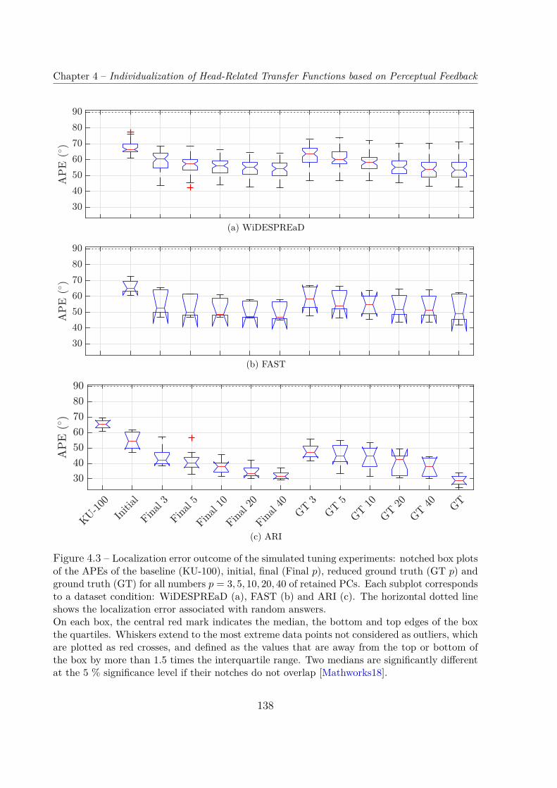
Chapter 4 – Individualization of Head-Related Transfer Functions based on Perceptual Feedback
(a) WiDESPREaD
(b) FAST
(c) ARI
Figure 4.3 – Localization error outcome of the simulated tuning experiments: notched box plotsof the APEs of the baseline (KU-100), initial, final (Final p), reduced ground truth (GT p) andground truth (GT) for all numbers p = 3, 5, 10, 20, 40 of retained PCs. Each subplot correspondsto a dataset condition: WiDESPREaD (a), FAST (b) and ARI (c). The horizontal dotted lineshows the localization error associated with random answers.On each box, the central red mark indicates the median, the bottom and top edges of the boxthe quartiles. Whiskers extend to the most extreme data points not considered as outliers, whichare plotted as red crosses, and defined as the values that are away from the top or bottom ofthe box by more than 1.5 times the interquartile range. Two medians are significantly differentat the 5 % significance level if their notches do not overlap [Mathworks18].
138
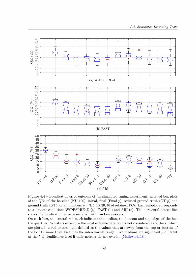
4.3. Simulated Listening Tests
(a) WiDESPREaD
(b) FAST
(c) ARI
Figure 4.4 – Localization error outcome of the simulated tuning experiment: notched box plotsof the QEs of the baseline (KU-100), initial, final (Final p), reduced ground truth (GT p) andground truth (GT) for all numbers p = 3, 5, 10, 20, 40 of retained PCs. Each subplot correspondsto a dataset condition: WiDESPREaD (a), FAST (b) and ARI (c). The horizontal dotted lineshows the localization error associated with random answers.On each box, the central red mark indicates the median, the bottom and top edges of the boxthe quartiles. Whiskers extend to the most extreme data points not considered as outliers, whichare plotted as red crosses, and defined as the values that are away from the top or bottom ofthe box by more than 1.5 times the interquartile range. Two medians are significantly differentat the 5 % significance level if their notches do not overlap [Mathworks18].
139
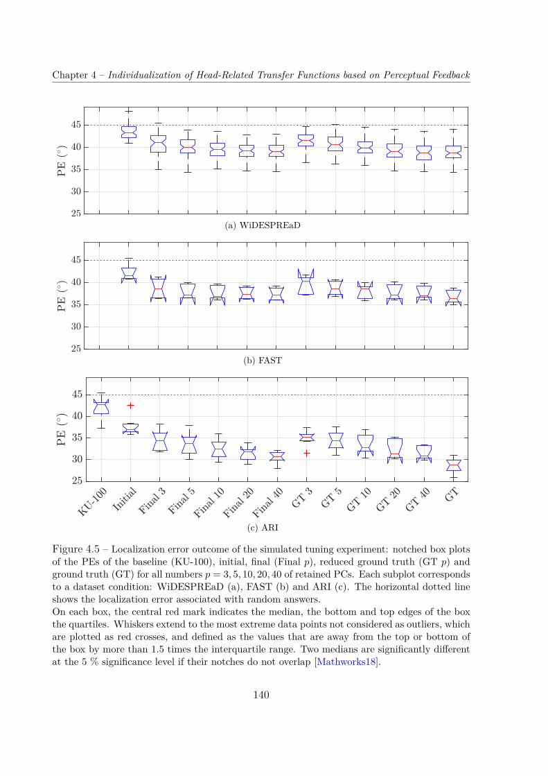
Chapter 4 – Individualization of Head-Related Transfer Functions based on Perceptual Feedback
(a) WiDESPREaD
(b) FAST
(c) ARI
Figure 4.5 – Localization error outcome of the simulated tuning experiment: notched box plotsof the PEs of the baseline (KU-100), initial, final (Final p), reduced ground truth (GT p) andground truth (GT) for all numbers p = 3, 5, 10, 20, 40 of retained PCs. Each subplot correspondsto a dataset condition: WiDESPREaD (a), FAST (b) and ARI (c). The horizontal dotted lineshows the localization error associated with random answers.On each box, the central red mark indicates the median, the bottom and top edges of the boxthe quartiles. Whiskers extend to the most extreme data points not considered as outliers, whichare plotted as red crosses, and defined as the values that are away from the top or bottom ofthe box by more than 1.5 times the interquartile range. Two medians are significantly differentat the 5 % significance level if their notches do not overlap [Mathworks18].
140
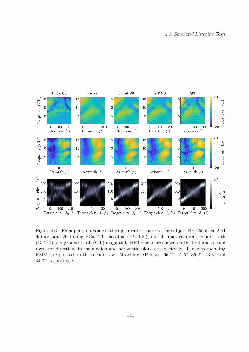
4.3. Simulated Listening Tests
Figure 4.6 – Exemplary outcome of the optimization process, for subject NH825 of the ARIdataset and 20 tuning PCs. The baseline (KU-100), initial, final, reduced ground truth(GT 20) and ground truth (GT) magnitude HRTF sets are shown on the first and secondrows, for directions in the median and horizontal planes, respectively. The correspondingPMVs are plotted on the second row. Matching APEs are 66.1, 61.5, 39.2, 43.3 and34.0, respectively.
141

Chapter 4 – Individualization of Head-Related Transfer Functions based on Perceptual Feedback
who were presented with their own HRTF sets, which they compare to the outcome ofactual localization experiments.
We report in Figure 4.7, in the form of notched boxplots, the simulated and actualQEs and PEs from Table I of [Baumgartner14], alongside our own ARI GT QEs andPEs, simulated for a random ARI subset of 9 virtual listeners presented with their ownHRTF set – also reported in subplot (c) of Figure 4.4 and Figure 4.5. Our own simulatedmedian QE and PE (6.3 % and 29, respectively) are somewhat lower than the simulatedQE and PE from [Baumgartner14] (9.7 % and 32). The difference in medians appearsto be significant for local angular errors (PEs), but it is not the case for quadrant errors.Possible explanations for this modest mismatch include the fact that we used a fixedsensitivity parameter in the auditory model, while they tuned it for each individual.Also, we considered a different and smaller subset of the ARI dataset.
Compared to actual localization errors with individual HRTF sets found in the lit-erature, our simulated GT for ARI virtual listeners is in rather good agreement. In astudy by Middlebrooks [Middlebrooks99b, Figure 13], in which 11 listeners participatedin actual localization experiments, the author reports a median QE of about 4 % and amedian PE of about 27 with individual HRTF sets. In a similar study by Middlebrookset al. [Middlebrooks00], the QEs for 5 listeners having listened once or twice to their ownHRTF set (for a total of 9 cases) are reported in Figure 3 and correspond to a medianQE of about 8 %. In [Baumgartner14], Baumgartner et al. report median QE and PEfor the actual localization experiments of 9.6 % and 34, respectively (see Figure 4.7). Itis worth noting that the outcome of these experiments are, by construction, in excellentagreement with the aforementioned simulated localization errors from the same study: thesensitivity parameter of the auditory model had been tuned individually for each listenerin order to fit the results of the actual experiments. Our median QE in the simulatedARI GT condition is comprised between the median QEs reported in [Middlebrooks99b]on the one hand, and [Middlebrooks99b] and [Baumgartner14] on the other hand, andour median PE is comparable to that of [Middlebrooks99b] and slightly lower than thatof [Baumgartner14].
Differences between datasets
When comparing datasets, we can see that all localization errors are higher in the FASTand WiDESPREaD cases than in the ARI case. In particular, the median ground truthAPEs are largely and significantly higher for FAST and WiDESPREaD (49 and 54)
142
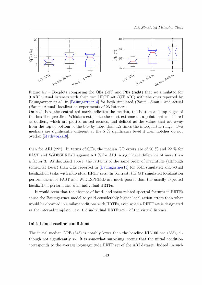
4.3. Simulated Listening Tests
Figure 4.7 – Boxplots comparing the QEs (left) and PEs (right) that we simulated for9 ARI virtual listeners with their own HRTF set (GT ARI) with the ones reported byBaumgartner et al. in [Baumgartner14] for both simulated (Baum. Simu.) and actual(Baum. Actual) localization experiments of 23 listeners.On each box, the central red mark indicates the median, the bottom and top edges ofthe box the quartiles. Whiskers extend to the most extreme data points not consideredas outliers, which are plotted as red crosses, and defined as the values that are awayfrom the top or bottom of the box by more than 1.5 times the interquartile range. Twomedians are significantly different at the 5 % significance level if their notches do notoverlap [Mathworks18].
than for ARI (29). In terms of QEs, the median GT errors are of 20 % and 22 % forFAST and WiDESPREaD against 6.3 % for ARI, a significant difference of more thana factor 3. As discussed above, the latter is of the same order of magnitude (althoughsomewhat lower) than QEs reported in [Baumgartner14] for both simulated and actuallocalization tasks with individual HRTF sets. In contrast, the GT simulated localizationperformances for FAST and WiDESPREaD are much poorer than the usually expectedlocalization performance with individual HRTFs.
It would seem that the absence of head- and torso-related spectral features in PRTFscause the Baumgartner model to yield considerably higher localization errors than whatwould be obtained in similar conditions with HRTFs, even when a PRTF set is designatedas the internal template – i.e. the individual HRTF set – of the virtual listener.
Initial and baseline conditions
The initial median APE (54) is notably lower than the baseline KU-100 one (66), al-though not significantly so. It is somewhat surprising, seeing that the initial conditioncorresponds to the average log-magnitude HRTF set of the ARI dataset. Indeed, in such
143
Chapter 4 – Individualization of Head-Related Transfer Functions based on Perceptual Feedback
an HRTF set the spectral features are smoothed and the peaks and notches useful toelevation perception and front-back disambiguation are shallower and less sharp than theones found in a measured HRTF set, such as the KU-100 one (see Figure 4.14).
As we have seen above, simulated ARI GT localization tasks seem to yield localiza-tion errors that are in good agreement with the outcome of actual localization tasks withindividual HRTFs found in the literature. In Figure 13 of [Middlebrooks99b], in additionto localization errors with individual HRTF sets, Middlebrooks reports the outcome oflocalization tasks with non-individual HRTF sets (those of other participants in the ex-periment): the median QE in the latter condition is about 19 % and the median PE about41. Similarly, in [Middlebrooks00], Middlebrooks et al. report in Figure 3 the QEs of5 subjects having listened to the HRTF sets of one or two other participants, for a totalof 9 non-individual conditions, and a median QE of about 33 %. Our initial condition,a non-individualized VAS based on an average HRTF set, yields simulated localizationperformance comparable to the first study with a median QE of 23 % and a median PEof 37. In contrast, our baseline KU-100 condition, a generic non-individualized VASbased on the HRTF set of a manikin, results in significantly poorer simulated localizationperformance, with a median QE and a median PE of 31 % and 43, respectively. Thismedian QE is nevertheless comparable to that of the second study.
Regarding the FAST and WiDESPREaD datasets, the initial localization perfor-mances are much poorer than with the ARI dataset, with median QEs and PEs of 31 %and 41 for the former and 31 % and 43 for the latter, all significantly lower than theARI initial median QE and PE.
Optimization outcome
General trends For all datasets, we observe that the tuning procedure significantlydecreased the median APE and QE compared to initialization (training set’s average log-magnitude HRTF set). The only exception occurred with FAST and 3 tuning PCs, inwhich case the standard deviation is very high, although the median is indeed lower thanthe initial APE by 19 %. In the case of the ARI HRTF model, for instance, the QEdecreased in median from 23 % to between 7.5 % (for p = 40) and 15 % (for p = 3),depending on the number of PCs p – against a ground truth median QE of 6.3 %.
For all datasets, the localization errors – APE, QE and PE – tend to decrease withthe number of PCs. The decrease is the most important between the Initial and Final 3conditions, and is significant in terms of APE and QE for the WiDESPREaD and ARI
144

4.3. Simulated Listening Tests
datasets. The decrease gets however more modest when more PCs are retained. Inparticular, there seems to be a plateau for FAST and WiDESPREaD when the numberof PCs exceeds 5.
Nevertheless, for all datasets, when at least p = 20 PCs are retained (p ≥ 10 forWiDESPREaD, p ≥ 3 for FAST), the difference between the median final APE (re-spectively QE) and the median ground truth APE (respectively QE) is not statisticallysignificant. In the particular case of the FAST dataset, due the high variability of thelocalization error results in all conditions, the difference between the median Final p andground truth APE, QE and PE is not significant for any p ∈ 3, 5, 10, 20, 40.
Interestingly, the median final APE for a given p is generally lower than the APE ofthe corresponding projected GT – excepted for the WiDESPREaD dataset when p ≥ 20,where the difference in median APEs is lower than 0.5. This difference is not significantfor any p or dataset. Nevertheless, it seems to exhibit some capacity of the optimizationprocess to overcome – in terms of localization performance – the projection of the listener’sown HRTF set in the space of the p first PCs.
Number of iterations and cost function evaluations
The number of iterations required to converge for all three datasets and all 5 numbers ofPCs are reported in box plots in Figure 4.8. The corresponding number of evaluationsof the cost function – i.e. the number of virtual localization tasks – are reported in thesame fashion in Figure 4.9.
A first observation that we can make is that the number of iterations needed to con-verge is very consistent from one dataset to the other, for all numbers of PCs. Moreover,the number of iterations increases with the number of tuning parameters, which could beexpected seeing that more tuning parameters means more dimensions to explore for theoptimization algorithm.
Before going on, let us establish a rough estimate of the time that one cost functionevaluation could take in real life, i.e. with a human subject participating in a localizationexperiment. Let us say that reporting the perceived direction for one stimulus (binaural-ized at a given direction) would take 2 seconds. Then, for 27 positions in the median plane(elevations between −45 and 225 with a 10 step) and 2 repetitions at each position,one localization experiment would take 27× 2× 2 s = 108 s = 1.8 min.
As mentioned above, in order for the difference between the final and ground truthmedian APE (or QE) to be non-significant, at least 20 PCs are needed in the ARI case.
145
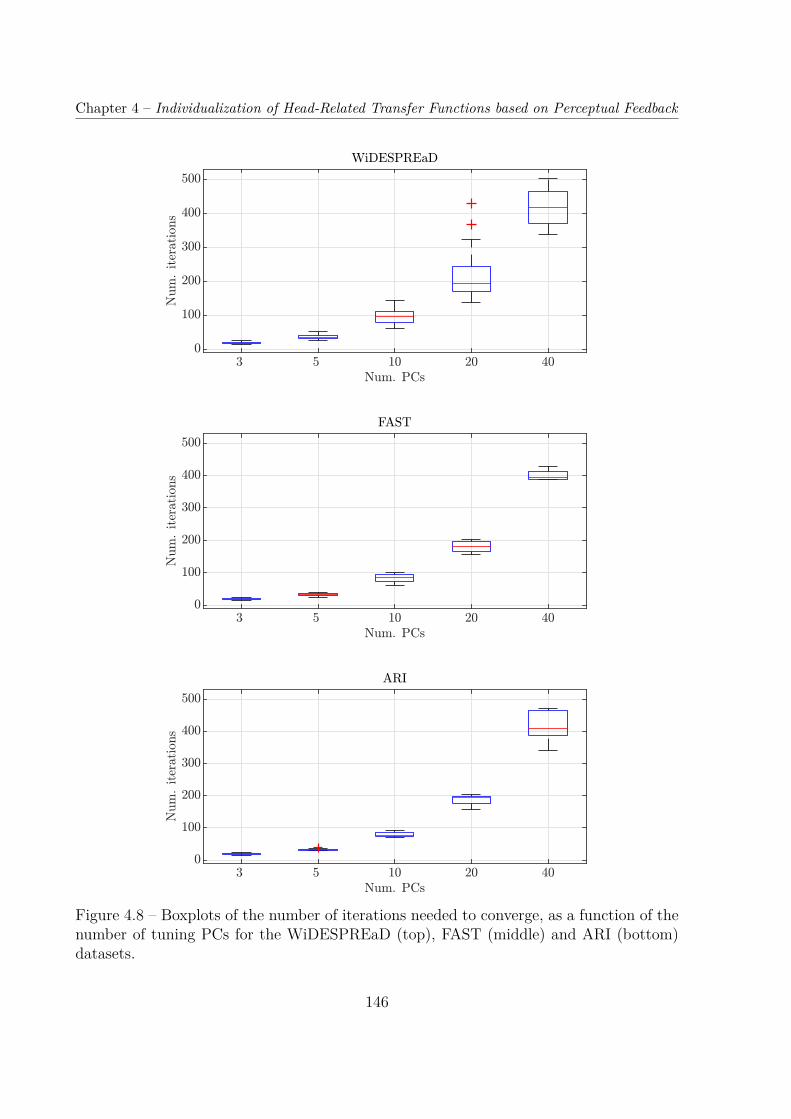
Chapter 4 – Individualization of Head-Related Transfer Functions based on Perceptual Feedback
Figure 4.8 – Boxplots of the number of iterations needed to converge, as a function of thenumber of tuning PCs for the WiDESPREaD (top), FAST (middle) and ARI (bottom)datasets.
146

4.3. Simulated Listening Tests
Figure 4.9 – Boxplots of the number of cost function evaluations needed to converge, as afunction of the number of tuning PCs for the WiDESPREaD (top), FAST (middle) andARI (bottom) datasets.
147
Chapter 4 – Individualization of Head-Related Transfer Functions based on Perceptual Feedback
However, the conditions with 20 and 40 PCs require many iterations to converge: themedian numbers of iterations are about 200 (193, 180 and 194) and about 400 (407, 427and 418), respectively. The matching median numbers of cost function evaluations areabout 300 (308, 305 and 305) and about 600 (620, 616 and 620), which would roughlycorrespond to tuning times of 300× 1.8 min ' 9 h and 600× 1.8 min ' 18 h, which arehighly impractical.
In contrast, for the conditions with 3 and 5 PCs, convergence is reached in about 20(medians of 20, 22 and 20) and 40 (medians of 38, 38 and 41) iterations, respectively. Thiscorresponds to about 30 (medians of 34, 34.5 and 34) and 70 (medians of 68.5, 68 and 37.5)cost function evaluations, i.e. respective total tuning time estimates of 30×1.8 min ' 1 hand 70 × 1.8 min ' 2 h. Despite being long, such sessions of localization experimentsmay be feasible for a real listener, in particular if less than 27 positions are tested in thelocalization task.
As discussed above, the final median APE, QE and PE in those conditions are sig-nificantly higher that the ground truth ones. However, the final median APE, QE andPE are also significantly lower than the initial and baseline conditions. It thus appearsthat such tuning sessions would offer partial but substantial individualization in termsof localization performance. In the ARI case with p = 5 PCs, for instance, the distanceto the median ground truth APE (29) is reduced by more than half (56 % = 40−54
29−54 )between initialization (median of 54) and convergence (median of 40). When looking atthe baseline KU-100 condition (median APE of 66) which corresponds to a standard non-individualized VAS, the distance to the median ground truth APE is even more largelyreduced, by 70 % = 40−66
29−66 . Regarding quadrant errors, the improvement rates are verysimilar: 54 % = 14%−23%
6.3%−23% between the Initial and Final 5 conditions, and 69 % = 14%−31%6.3%−31%
between the KU-100 and Final 5 conditions.
Evolution throughout optimization
The evolution of the APE (QE, respectively) throughout the optimization process isshown for all test virtual listeners in Figure 4.10 (Figure 4.11, respectively). In general,the median APE and QE decrease with the number of iterations. However, sometimesthe APE and QE can slightly increase, due to the regularization scheme having found asolution less extreme in terms of PCWs at the cost of a small increase in APE. This hasa particularly strong impact on the median behavior of the APE and QE in the FASTcase, due to the small number (5) of virtual listeners and large inter-individual difference
148
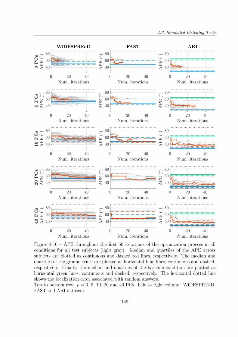
4.3. Simulated Listening Tests
Figure 4.10 – APE throughout the first 50 iterations of the optimization process in allconditions for all test subjects (light gray). Median and quartiles of the APE acrosssubjects are plotted as continuous and dashed red lines, respectively. The median andquartiles of the ground truth are plotted as horizontal blue lines, continuous and dashed,respectively. Finally, the median and quartiles of the baseline condition are plotted ashorizontal green lines, continuous and dashed, respectively. The horizontal dotted lineshows the localization error associated with random answers.Top to bottom row: p = 3, 5, 10, 20 and 40 PCs. Left to right column: WiDESPREaD,FAST and ARI datasets.
149

Chapter 4 – Individualization of Head-Related Transfer Functions based on Perceptual Feedback
Figure 4.11 – QE throughout the first 50 iterations of the optimization process in all con-ditions for all test subjects (light gray). Median and quartiles of the QE across subjectsare plotted as continuous and dashed red lines, respectively. The median and quartiles ofthe ground truth are plotted as horizontal blue lines, continuous and dashed, respectively.Finally, the median and quartiles of the baseline condition are plotted as horizontal greenlines, continuous and dashed, respectively. The horizontal dotted line shows the localiza-tion error associated with random answers.Top to bottom row: p = 3, 5, 10, 20 and 40 PCs. Left to right column: WiDESPREaD,FAST and ARI datasets.
150

4.4. Actual Listening Tests
in localization error from initialization to convergence. The decrease in median APE andQE appears to be slower for WiDESPREaD than for the other datasets, due to an earlystagnation phase whose duration varies from subject to subject. For WiDESPREaD, thedecrease gets slower when the number of PCs increases, but this behavior is not clear forthe other datasets.
In the case of the ARI dataset, the median APE and QE decrease quickly within thefirst dozen iterations before pursuing the decrease more slowly. For instance, after 10iterations the median QE is between 12 % and 14 % for any number of PCs p, i.e. aboutor below the median QEs of the Final 3 and Final 5 conditions. As a consequence, even if20 or 40 PCs were to be retained for the tuning process, similar localization performancewould be obtained after 10 iterations than with only 3 or 5 PCs.
At first glance, using many PCs thus appears to be desirable for practical HRTF tuningapplications: it provides similar localization performance as with 3 or 5 PCs within thefirst dozen iterations of the optimization process, but allows the listener to spend moretuning time to further improve the rendering if he desires. However, a given number ofiterations does not correspond to the same tuning time depending on the number of PCsp. The latter corresponds in fact to an offset in the number of localization tasks to beperformed. Indeed, by construction, the Nelder-Mead’s algorithm performs during thefirst iteration p + 1 cost function evaluations. For instance, for p = 40 PCs, 35 morelocalization tasks are to be performed during the first iteration than for p = 5 PCs. Inour simulations, in the ARI case, 10 iterations corresponded to about 19 (between 18 and20) localization tasks for p = 5 PCs, against about 50 (between 49 and 51) for p = 40PCs. The corresponding estimated tuning times are 34 min and 90 min, respectively, aconsiderable difference for comparable localization performances.
4.4 Actual Listening Tests
For the tuning experiments with actual listening tests, we used the HRTF model trainedon the ARI dataset, previously used in the tuning simulations (see Section 4.3). In-deed, unlike WiDESPREaD and FAST which are PRTF datasets, it includes the filteringcontributions of the head and torso.
Aiming at a tuning session of about one hour, we set the number of tuning PCs to5. As a reminder, we roughly estimated in Section 4.3 that the time needed to reachconvergence with 5 PCs was 2 hours in median. With 5 PCs and the ARI HRTF model,
151
Chapter 4 – Individualization of Head-Related Transfer Functions based on Perceptual Feedback
the localization performance was substantially and significantly improved compared toinitialization and to the baseline condition, although it remained significantly higher thanground truth performance. After some informal trials of the tuning procedure, in order toreduce the duration of each localization task, we limited the median-plane test positionsto 8 polar angles, at roughly every 30 and all present in the measurement grids of theARI HRTF sets: −30, 0, 30, 60, 120, 150, 180, 210.
4.4.1 Localization Task
Subjects
12 listeners (5 female and 7 male) participated in the experiment and were aged between24 and 37 years old (28 on average). 9 were naive listeners with no experience withlistening tests and 2 were experienced with localization experiments. All participantsreported having normal hearing.
Localization task
Each listener participated in a rather large number of localization tasks (between 20 and88). Due to the iterative nature of the tuning process, the listener is presented with asingle HRTF set by localization task.
For the localization task, the listener was presented with each one of the 16 stimuli.After listening to a given stimulus as many times as he wanted, he reported his answerthen moved on to the next one. There was no time limit for answering, although swiftanswers were encouraged due to the large numbers of HRTF sets to be evaluated in onesession.
The participant was asked to report the perceived angle on a 2-D interface (see Fig-ure 4.12). Such an exocentric method is known to be less accurate and less intuitive thanan egocentric one [Bahu16a, Chap. 4; Katz19, pp. 359-361]. However, all directions areequally easy to report, while with egocentric methods the rear positions are more difficultto evaluate accurately, due to bio-mechanical limitations. Furthermore, it is materiallyeasier to set up, as it does not require an additional tracking device for the head, handsor any other object used for pointing. Finally, this allowed us to use as is a user interfacepreviously developed at 3D Sound Labs.
152
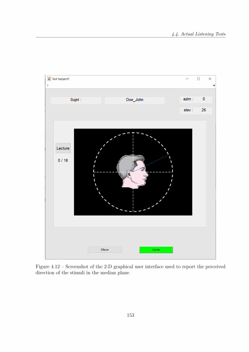
4.4. Actual Listening Tests
Figure 4.12 – Screenshot of the 2-D graphical user interface used to report the perceiveddirection of the stimuli in the median plane.
153

Chapter 4 – Individualization of Head-Related Transfer Functions based on Perceptual Feedback
Stimuli presentation
The test stimuli that we used were a sequence of three white noise bursts of 40 ms,separated by silences of 30 ms [Andreopoulou17; Zagala20]. To avoid artifacts, each noiseburst was faded in and out linearly in 2 ms. While white noise was chosen in order toinclude spectral cues over the whole audible frequency range, the bursts were kept shortin order to limit the duration of the tests, to limit auditory fatigue and to encourageintuitive answers.
During each localization task – which corresponded to one HRTF set, and one costfunction evaluation in the optimization scheme – the virtual sound source was presentedat 8 different polar angles (−30, 0, 30, 60, 120, 150, 180 and 210), twice each, fora total of 16 stimuli, presented in random order.
The binauralized stimuli were played over a pair of Sennheiser HD 650 open circum-aural headphones, via an Alesis iO2 sound card, and at a sampling rate of 48 kHz.
We performed no headphone equalization (HpEq) before presenting the binauralizedstimuli. Indeed, while it is generally admitted in the literature that performing individualHpEq yields better VAS quality, such an equalization is independent of sound direction,thus being equivalent to source filtering, and has not been shown to have a significantimpact on sound localization [Engel19].
Protocol
A session of localization experiments went as follows. After welcoming the participant,an operator (the author) read them instructions for the series of localization tasks. Theseinstructions were also provided in the form of a written document.
It was explained to the listener that he or she was about to participate in about twentylistening tests. In each listening test, he or she would be prompted 16 times to indicatethe perceived direction of an auditory stimulus.
Each stimulus was presented once by the software, and the listener could replay it anynumber of times before giving his answer. The user interface allowed to cancel an answerand go back to a previous one – if the participant had clicked by error, for instance.
The participant was asked to perform localization tasks during one hour, but couldperform longer if he or she wanted. He or she was strongly encouraged to take breaks tolimit auditory fatigue, at the end of every localization tasks if needed. In practice, mostparticipants took one long break of about 10-15 min.
154

4.4. Actual Listening Tests
Orally, the operator indicated that it was normal to feel that the task was difficultand to not be able to localize some of the stimuli – free-field median-plane localizationis harduous, especially with non-individual HRTF sets. In such cases, the listeners couldgive a random answer. Informally, intuitive responses were encouraged.
The sound level was set for listener comfort prior to the localization tasks, then re-mained untouched for the rest of the session.
In addition to the localization tasks that were part of the optimization scheme, local-ization performance with the baseline HRTF set (that of the Neumann KU-100 manikin,as measured by the ARI team) was evaluated by means of a localization task before thetuning session itself.
4.4.2 Results
Localization performance
We herein compare the localization performances in three HRTF set conditions: baseline,initial and final. The baseline is the HRTF set of the KU-100 manikin as measured by theARI. The initial condition is the HRTF set that was evaluated at the initialization of thetuning process. It corresponds to the average of the training set for the PCA HRTF model(all PC weights set to zero). The final HRTF set is the customized HRTF set providedby the proposed method. It corresponds to the solution retained by the Nelder-Meadsimplex algorithm based on the various cost function evaluations throughout the tuningsession.
The order of these evaluations was fixed for all subjects and not randomized, due tothe constraints of the tuning method. Indeed, the perceptual evaluation of the baselinewas performed before the start of the tuning session, and that of the initial conditionwas performed just after, when the tuning process started. As to the final condition, itsperceptual evaluation occurred later throughout the tuning session.
Initial and baseline conditions Similarly to what was observed and discussed in thecase of the simulated localization tasks (see Section 4.3), the initial median APE (71) islower than the KU-100 one (76). However, the difference between both median APEsis here not significant and is only of 76 − 71 = 5, against 66 − 54 = 12 in simulations.The difference between initial and baseline median APEs is mostly explained by the –non-significant – difference in quadrant error: the initial and KU-100 QEs are 34 % and
155
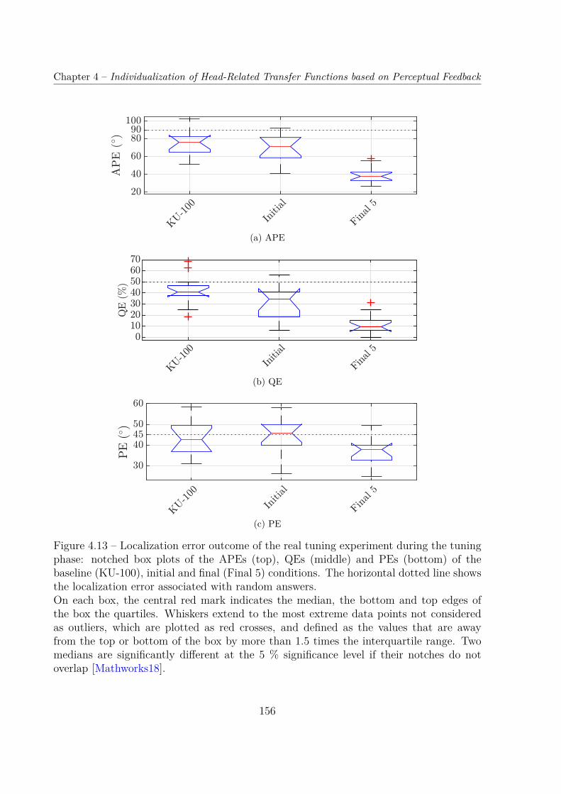
Chapter 4 – Individualization of Head-Related Transfer Functions based on Perceptual Feedback
(a) APE
(b) QE
(c) PE
Figure 4.13 – Localization error outcome of the real tuning experiment during the tuningphase: notched box plots of the APEs (top), QEs (middle) and PEs (bottom) of thebaseline (KU-100), initial and final (Final 5) conditions. The horizontal dotted line showsthe localization error associated with random answers.On each box, the central red mark indicates the median, the bottom and top edges ofthe box the quartiles. Whiskers extend to the most extreme data points not consideredas outliers, which are plotted as red crosses, and defined as the values that are awayfrom the top or bottom of the box by more than 1.5 times the interquartile range. Twomedians are significantly different at the 5 % significance level if their notches do notoverlap [Mathworks18].
156
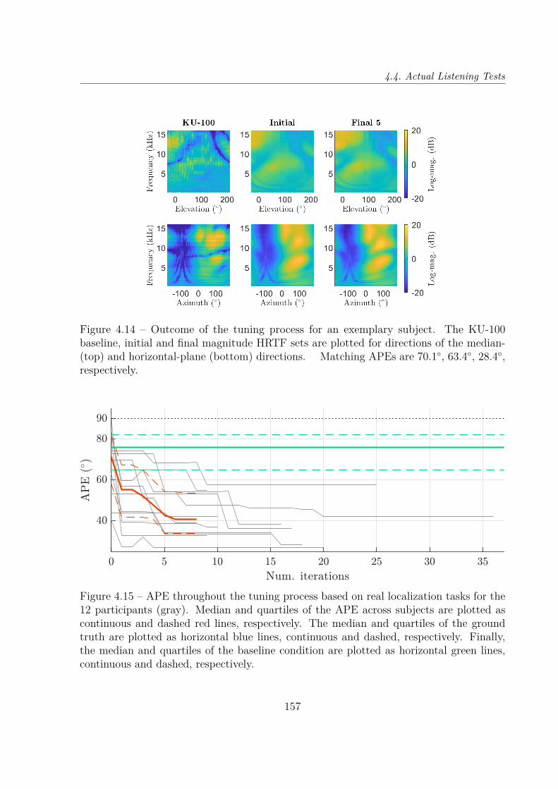
4.4. Actual Listening Tests
Figure 4.14 – Outcome of the tuning process for an exemplary subject. The KU-100baseline, initial and final magnitude HRTF sets are plotted for directions of the median-(top) and horizontal-plane (bottom) directions. Matching APEs are 70.1, 63.4, 28.4,respectively.
Figure 4.15 – APE throughout the tuning process based on real localization tasks for the12 participants (gray). Median and quartiles of the APE across subjects are plotted ascontinuous and dashed red lines, respectively. The median and quartiles of the groundtruth are plotted as horizontal blue lines, continuous and dashed, respectively. Finally,the median and quartiles of the baseline condition are plotted as horizontal green lines,continuous and dashed, respectively.
157

Chapter 4 – Individualization of Head-Related Transfer Functions based on Perceptual Feedback
Figure 4.16 – QE throughout the tuning process based on real localization tasks for the12 participants (gray). Median and quartiles of the QE across subjects are plotted ascontinuous and dashed red lines, respectively. The median and quartiles of the groundtruth are plotted as horizontal blue lines, continuous and dashed, respectively. Finally,the median and quartiles of the baseline condition are plotted as horizontal green lines,continuous and dashed, respectively.
41 %, respectively. On the other hand, the tendency is reversed with the local angularerrors (PEs). Indeed, the median initial PE of 46 is greater than the KU-100 one of 43,although not significantly so. Neither median PE differs significantly from the chance PE.Let us note that the pointing method employed in these experiments is not very accurate,and that the results in terms of local polar error, PE, are thus to be considered in thislight.
The initial and baseline localization errors were in general higher that those fromthe simulations. Indeed, in both conditions, the median APE is significantly greater inthe actual experiments than in the simulated ones: 76 against 66 for KU-100, and 71
against 54 for the average HRTF set (initial condition). This trend is also found in QEs,with 41 % against 31 % for KU-100 (significant), and 34 % against 24 % for the initialHRTF set. Following the same trend, the actual median initial PE (46) is significantlylarger than the simulated one (37). In contrast, the actual median KU-100 PE (43) isequal to that of the simulations.
While the median QE of our initial condition (34 %) is comparable to the resultsof [Middlebrooks00] with non-individual human-subject HRTF sets (about 33 %), it ishigher than the median QE reported in [Middlebrooks99b] in similar conditions (19 %).
158
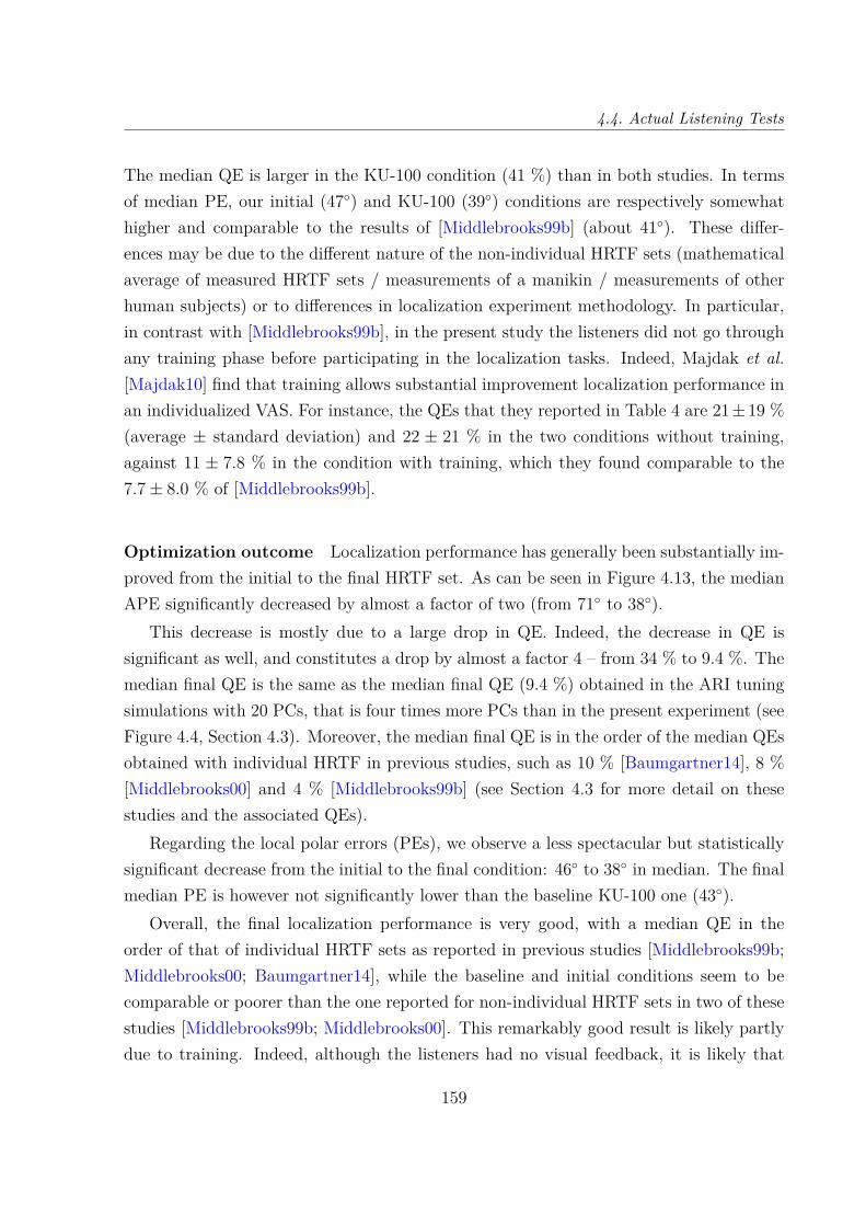
4.4. Actual Listening Tests
The median QE is larger in the KU-100 condition (41 %) than in both studies. In termsof median PE, our initial (47) and KU-100 (39) conditions are respectively somewhathigher and comparable to the results of [Middlebrooks99b] (about 41). These differ-ences may be due to the different nature of the non-individual HRTF sets (mathematicalaverage of measured HRTF sets / measurements of a manikin / measurements of otherhuman subjects) or to differences in localization experiment methodology. In particular,in contrast with [Middlebrooks99b], in the present study the listeners did not go throughany training phase before participating in the localization tasks. Indeed, Majdak et al.[Majdak10] find that training allows substantial improvement localization performance inan individualized VAS. For instance, the QEs that they reported in Table 4 are 21±19 %(average ± standard deviation) and 22 ± 21 % in the two conditions without training,against 11 ± 7.8 % in the condition with training, which they found comparable to the7.7± 8.0 % of [Middlebrooks99b].
Optimization outcome Localization performance has generally been substantially im-proved from the initial to the final HRTF set. As can be seen in Figure 4.13, the medianAPE significantly decreased by almost a factor of two (from 71 to 38).
This decrease is mostly due to a large drop in QE. Indeed, the decrease in QE issignificant as well, and constitutes a drop by almost a factor 4 – from 34 % to 9.4 %. Themedian final QE is the same as the median final QE (9.4 %) obtained in the ARI tuningsimulations with 20 PCs, that is four times more PCs than in the present experiment (seeFigure 4.4, Section 4.3). Moreover, the median final QE is in the order of the median QEsobtained with individual HRTF in previous studies, such as 10 % [Baumgartner14], 8 %[Middlebrooks00] and 4 % [Middlebrooks99b] (see Section 4.3 for more detail on thesestudies and the associated QEs).
Regarding the local polar errors (PEs), we observe a less spectacular but statisticallysignificant decrease from the initial to the final condition: 46 to 38 in median. The finalmedian PE is however not significantly lower than the baseline KU-100 one (43).
Overall, the final localization performance is very good, with a median QE in theorder of that of individual HRTF sets as reported in previous studies [Middlebrooks99b;Middlebrooks00; Baumgartner14], while the baseline and initial conditions seem to becomparable or poorer than the one reported for non-individual HRTF sets in two of thesestudies [Middlebrooks99b; Middlebrooks00]. This remarkably good result is likely partlydue to training. Indeed, although the listeners had no visual feedback, it is likely that
159
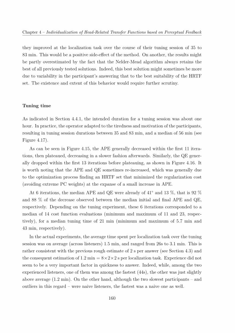
Chapter 4 – Individualization of Head-Related Transfer Functions based on Perceptual Feedback
they improved at the localization task over the course of their tuning session of 35 to83 min. This would be a positive side-effect of the method. On another, the results mightbe partly overestimated by the fact that the Nelder-Mead algorithm always retains thebest of all previously tested solutions. Indeed, this best solution might sometimes be moredue to variability in the participant’s answering that to the best suitability of the HRTFset. The existence and extent of this behavior would require further scrutiny.
Tuning time
As indicated in Section 4.4.1, the intended duration for a tuning session was about onehour. In practice, the operator adapted to the tiredness and motivation of the participants,resulting in tuning session durations between 35 and 83 min, and a median of 56 min (seeFigure 4.17).
As can be seen in Figure 4.15, the APE generally decreased within the first 11 itera-tions, then plateaued, decreasing in a slower fashion afterwards. Similarly, the QE gener-ally dropped within the first 13 iterations before plateauing, as shown in Figure 4.16. Itis worth noting that the APE and QE sometimes re-increased, which was generally dueto the optimization process finding an HRTF set that minimized the regularization cost(avoiding extreme PC weights) at the expanse of a small increase in APE.
At 6 iterations, the median APE and QE were already of 41 and 13 %, that is 92 %and 88 % of the decrease observed between the median initial and final APE and QE,respectively. Depending on the tuning experiment, these 6 iterations corresponded to amedian of 14 cost function evaluations (minimum and maximum of 11 and 23, respec-tively), for a median tuning time of 21 min (minimum and maximum of 5.7 min and43 min, respectively).
In the actual experiments, the average time spent per localization task over the tuningsession was on average (across listeners) 1.5 min, and ranged from 26s to 3.1 min. This israther consistent with the previous rough estimate of 2 s per answer (see Section 4.3) andthe consequent estimation of 1.2 min = 8×2×2 s per localization task. Experience did notseem to be a very important factor in quickness to answer. Indeed, while, among the twoexperienced listeners, one of them was among the fastest (44s), the other was just slightlyabove average (1.2 min). On the other hand, although the two slowest participants – andoutliers in this regard – were naive listeners, the fastest was a naive one as well.
160
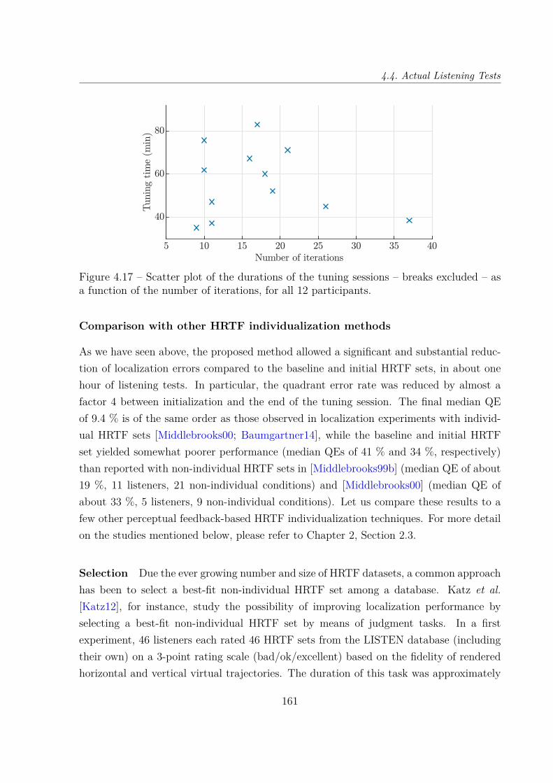
4.4. Actual Listening Tests
Figure 4.17 – Scatter plot of the durations of the tuning sessions – breaks excluded – asa function of the number of iterations, for all 12 participants.
Comparison with other HRTF individualization methods
As we have seen above, the proposed method allowed a significant and substantial reduc-tion of localization errors compared to the baseline and initial HRTF sets, in about onehour of listening tests. In particular, the quadrant error rate was reduced by almost afactor 4 between initialization and the end of the tuning session. The final median QEof 9.4 % is of the same order as those observed in localization experiments with individ-ual HRTF sets [Middlebrooks00; Baumgartner14], while the baseline and initial HRTFset yielded somewhat poorer performance (median QEs of 41 % and 34 %, respectively)than reported with non-individual HRTF sets in [Middlebrooks99b] (median QE of about19 %, 11 listeners, 21 non-individual conditions) and [Middlebrooks00] (median QE ofabout 33 %, 5 listeners, 9 non-individual conditions). Let us compare these results to afew other perceptual feedback-based HRTF individualization techniques. For more detailon the studies mentioned below, please refer to Chapter 2, Section 2.3.
Selection Due the ever growing number and size of HRTF datasets, a common approachhas been to select a best-fit non-individual HRTF set among a database. Katz et al.[Katz12], for instance, study the possibility of improving localization performance byselecting a best-fit non-individual HRTF set by means of judgment tasks. In a firstexperiment, 46 listeners each rated 46 HRTF sets from the LISTEN database (includingtheir own) on a 3-point rating scale (bad/ok/excellent) based on the fidelity of renderedhorizontal and vertical virtual trajectories. The duration of this task was approximately
161
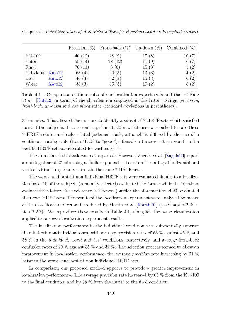
Chapter 4 – Individualization of Head-Related Transfer Functions based on Perceptual Feedback
Precision (%) Front-back (%) Up-down (%) Combined (%)KU-100 46 (12) 28 (9) 17 (8) 10 (7)Initial 55 (14) 28 (12) 11 (9) 6 (7)Final 76 (11) 8 (6) 15 (8) 1 (2)Individual [Katz12] 63 (4) 20 (3) 13 (3) 4 (2)Best [Katz12] 46 (3) 32 (3) 15 (3) 6 (2)Worst [Katz12] 38 (3) 35 (3) 19 (2) 8 (2)
Table 4.1 – Comparison of the results of our localization experiments and that of Katzet al. [Katz12] in terms of the classification employed in the latter: average precision,front-back, up-down and combined rates (standard deviations in parentheses).
35 minutes. This allowed the authors to identify a subset of 7 HRTF sets which satisfiedmost of the subjects. In a second experiment, 20 new listeners were asked to rate these7 HRTF sets in a closely related judgment task, although it differed by the use of acontinuous rating scale (from “bad” to “good”). Based on these results, a worst- and abest-fit HRTF set was identified for each subject.
The duration of this task was not reported. However, Zagala et al. [Zagala20] reporta ranking time of 27 min using a similar approach – based on the rating of horizontal andvertical virtual trajectories – to rate the same 7 HRTF sets.
The worst- and best-fit non-individual HRTF sets were evaluated thanks to a localiza-tion task. 10 of the subjects (randomly selected) evaluated the former while the 10 othersevaluated the latter. As a reference, 4 listeners (outside the aforementioned 20) evaluatedtheir own HRTF sets. The results of the localization experiment were analyzed by meansof the classification of errors introduced by Martin et al. [Martin01] (see Chapter 2, Sec-tion 2.2.2). We reproduce these results in Table 4.1, alongside the same classificationapplied to our own localization experiment results.
The localization performance in the individual condition was substantially superiorthan in both non-individual ones, with average precision rates of 63 % against 46 % and38 % in the individual, worst and best conditions, respectively, and average front-backconfusion rates of 20 % against 35 % and 32 %. The selection process seemed to allow animprovement in localization performance, the average precision rate increasing by 21 %between the worst- and best-fit non-individual HRTF sets.
In comparison, our proposed method appears to provide a greater improvement inlocalization performance. The average precision rate increased by 65 % from the KU-100to the final condition, and by 38 % from the initial to the final condition.
162
4.4. Actual Listening Tests
The localization experiments in [Katz12] seem to have yielded higher localization errorsthan our own in general – i.e. regardless of the various conditions. In particular, theworst of our non-individual conditions, KU-100, is comparable to the precision rate ofthe best-fit HRTF set in [Katz12], while our final precision rate (77 %) is notably greateron average than that of the individual condition in [Katz12] (63 %). The authors noteas well than their individual condition presented poorer localization performance than aprevious study by Wightman et al. [Wightman89b].
Frequency scaling In [Middlebrooks00], Middlebrooks et al. propose a procedure inwhich a non-individual HRTF set is adjusted by means of a frequency scaling (identicalfor all directions), based on successive A/B judgments by the listener of various scaledHRTF sets in terms of localization accuracy of median-plane virtual sources. The resultingadapted non-individual HRTF sets were evaluated by means of a localization experimentfor 5 participants (out of 20), each listening to one or two non-individual HRTF sets, fora total of 9 non-individual and scaled non-individual cases.
The tuning procedure took about one hour (including a 15-min training phase), andthe resulting median QE was of about 13 %, against 8 % and 33 % in the individual andnon-individual conditions.
In comparison, the proposed method seems to produce HRTF sets that provide betterlocalization performance (median QE of 9.4 %) in a similar amount of time. The medianQE obtained by Middlebrooks et al. is more comparable to the median QE that weobserved after 6 iterations of the optimization process, that is a median tuning time of21 min.
Synthesis Finally, let us compare our proposed method to more closely related ap-proaches, which aim at synthesizing a customized HRTF set based on perceptual feedbackfrom the listener.
Hwang et al. [Hwang08a] propose that the listener tune himself 3 PCWs of a spectral(see Chapter 2, Section 2.1.3) PCA model of HRIRs. This is a local approach, in the sensethat the PCA model generates individual filters rather complete HRTF sets. The tuningwas thus performed independently at each of 7 directions of interest – in the median plane.The tuning procedure was tested on three listeners, then its outcome was evaluated bymeans of a localization experiment. Three HRTF sets were under study: the customizedone – produced by the individualization method, the listener’s own, and that of the
163

Chapter 4 – Individualization of Head-Related Transfer Functions based on Perceptual Feedback
Front-back (%)KU-100 40 (12)Initial 39 (14)Final 12 (6)KEMAR [Hwang08a] 23 (3)Custom [Hwang08a] 6 (7)Individual [Hwang08a] 0.4 (0.6)KEMAR [Shin08] 29 (14)Custom [Shin08] 10 (3)Individual [Shin08] 12 (4)
Table 4.2 – Comparison of the results of our localization experiments and that of Hwanget al. [Hwang08a, Table VII] and Shin et al. [Shin08, Table 1] in terms of average front-back confusion rates (standard deviation in parentheses), as per the traditional definitionof front-back confusions by Wightman et al. [Wightman89b].
KEMAR manikin – a standard non-individual condition. Shin et al. [Shin08] propose aclosely related approach in which the listener tunes himself 5 PCWs of a spectral PCAmodel of HRIRs. The performance of the resulting customized HRTF set is comparedto that of their own and KEMAR HRTF sets by means of a localization experiment inwhich four listeners participated.
In both studies, front-back confusions were identified using the conventional definitionby Wightman et al. [Wightman89b]. We report these results in Table 4.2, alongside thefront-back confusion rates of our own localization experiments, calculated according tothe same definition. In both studies, the customized HRTF set yields a rate of front-backconfusion that is, on average, lower than the non-individual KEMAR condition by about70 % (74 % = 100 · 23−6
23 for [Hwang08a], and 66 % = 100 · 29−1029 for [Shin08]). According
to Hwang et al., the difference between the custom and KEMAR condition is significant.This is comparable to the difference between both our non-individual conditions (bothKU-100 and initial) and our final condition, with reductions in the average front-backconfusion rate of 70 % = 100 · 40−12
40 and 69 % = 100 · 39−1239 , respectively. In [Hwang08a],
the average front-back confusion rate with the custom HRTF set (6 %) is higher thanwith the listener’s own HRTF set (0.4 %), but Hwang et al. report that the differenceis not statistically significant, while in [Shin08] the custom average front-back confusionrate (10 %) is slightly lower than the individual one (12 %). While both studies presentcomparable results for the KEMAR and custom conditions, there is a notable mismatch for
164

4.5. Conclusion & Perspectives
the individual condition. Finally, the front-back confusion rates of both our non-individualconditions (40 and 39 %) are notably higher on average than that of the KEMAR conditionof [Hwang08a] and [Shin08], possibly suggesting that our localization experiment protocolyielded overall higher localization error.
Unfortunately, none of these studies reported the duration of the HRTF tuning pro-cedure, although Hwang et al. indicated that they chose only 3 PCs precisely to keepit reasonable – after having determined in a first experiment that reconstructing HRTFsfrom 12 PCs yielded a localization performance indistinguishable from the original HRTFs.Furthermore, in both studies the tuning procedure needs to be performed at each direc-tion of interest, which would likely result in an unpractical total duration for the tuningof even a sparsely spatially sampled HRTF set.
4.5 Conclusion & Perspectives
In this chapter, we proposed a method for low-cost HRTF individualization based onperceptual feedback. It consists in tuning the parameters of a statistical model of magni-tude HRTF set based on the localization performance of the listener. Unlike most othersimilar approaches, the tuning is done globally, i.e. for all sound directions at once – acritical feature if we are to achieve reasonable tuning times. Furthermore, the optimiza-tion itself is performed by means of a Nelder-Mead simplex algorithm. The listener isthus solicited for localization performance evaluation only, not for tuning of the HRTFmodel’s parameters.
As a first step, simulated localization experiments by means of the Baumgartner audi-tory model [Baumgartner14] allowed us to evaluate the proposed method under variousconfigurations – three different datasets (FAST, WiDESPREaD and ARI) and five dif-ferent numbers of tuning parameters from 3 to 40. In all conditions except one, theoptimization process converged to a mag-HRTF set that significantly decreased localiza-tion errors (APE, QE and PE) compared to the training set’s average HRTF set and toa baseline: the Neumann KU-100 manikin HRTF set. When more than 20 PCs wereretained, the final localization errors (APE and QE) were not significantly different fromthe ground truth. For example, in the case of the ARI dataset, the median QE was re-duced from 23 % (with the initial average HRTF set) to between 7.5 % and 15 % (with40 and 3 PCs, respectively) with the customized HRTF sets. Comparatively, the baseline
165

Chapter 4 – Individualization of Head-Related Transfer Functions based on Perceptual Feedback
non-individual (KU-100) and the individual HRTF sets yielded respective median QEs of33 % and 6.3 %.
A large difference was observed between the FAST and WiDESPREaD PRTF datasetson the one hand and the ARI dataset on the other hand: the simulated localization per-formance were considerably higher in median in the former case in all conditions. Yet,results for ARI in the ground truth and in the non-individual (average and KU-100) con-ditions were consistent with localization errors reported in the literature with individualand non-individual HRTF sets, respectively [Middlebrooks99b; Middlebrooks00; Baum-gartner14]. It seems likely that the absence of head- and torso- spectral features in PRTFsresulted in higher localization errors in the auditory model. As a consequence, we usedthe HRTF model based on the ARI dataset in the subsequent tuning experiments withactual listeners.
Regarding the duration of the procedure, the number of iterations required to convergeincreased with the number of tuning parameters, quickly reaching values impractical fora real-subject application: up to more than 500 iterations for 40 PCs, for a roughlyestimated tuning time of 18 hours for a real listener. With only 3 or 5 PCs, however, theestimated tuning session duration was limited to one or two hours, whereas substantialimprovement in localization performance was achieved – although more modest than whenmore PCs were retained. For example, with p = 5 PCs, the median APE was reduced by56 % of the difference between initialization and ground truth.
While long, such sessions appeared to be feasible for a real listener, particularly ifthe number of test directions were to be reduced compared to the 27 considered in ourestimation of total tuning time.
We put to the test this alleged feasibility as a second step by submitting the tuningprocedure to 12 real listeners. As a compromise between expected final localization per-formance and tuning session duration, we retained 5 PCs for these experiments. Theresults somewhat differed from the simulations. Indeed, the customized HRTF sets pro-duced by the procedure yielded substantial improvement of the localization performancecompared to both non-individual conditions (average and KU-100 HRTF sets) in one hourof listening tests in median, thus confirming the feasibility of the procedure in that timeframe. In particular, the median QE was reduced by nearly a factor 4 as a result ofthe tuning procedure, for a final value of 9.4 %. This is a good rate of quadrant errors,comparable to values reported in the literature for individual HRTF sets (10 %, 8 %,
166
4.5. Conclusion & Perspectives
4 %) [Baumgartner14; Middlebrooks00; Middlebrooks99b]. Yet, it does not appear thatthis particularly low final QE is due to a general underestimation of localization errorsrelated to our localization experiment protocol. Indeed, the baseline and initial conditionsyielded comparable or poorer localization performance (median QEs of 41 % and 34 %,respectively) than Middlebrooks et al. reported for non-individual HRTF sets (medianQEs of 19 % and 33 %) [Middlebrooks99b; Middlebrooks00].
This notably large reduction in localization errors may be partly due to some trainingof the listener throughout the tuning session, which would represent a positive side-effectof the method. It is also possible that the final localization performance is somewhatoverestimated due to the fact that the Nelder-Mead optimization algorithm systematicallyretains the lowest evaluation of the cost function, which may be due not only to HRTFset customization, but also to variation in the listener’s answering.
Although the tuning sessions were quite long (one hour in median), we observed thatmost of the decrease in localization error (88 % and 92 % of total median decrease in QEand APE, respectively) occurred within the first 6 iterations: in about 20 min, a finalmedian QE of 13 % was achieved. The present method thus offers flexibility in the formof a trade-off between HRTF tuning duration and localization performance.
Comparing our results to that of other HRTF individualization techniques, it appearsthat our proposed method improves localization performance substantially more thanthe selection of a best-fit non-individual HRTF set among 7 representatives HRTF sets[Katz12]. It however takes longer: one hour against 25 min [Zagala20]. The proposedapproach also appears to reduce localization errors more than the self-tuning of a globalfrequency scaling parameter (in order to adapt a non-individual HRTF set to the user)[Middlebrooks00] in a comparable amount of time. Finally, our procedure yields a reduc-tion in front-back confusions comparable to that of a related method which consists intuning by ear the parameters of an HRTF PCA model in the median plane [Hwang08a;Shin08]. The duration of the tuning procedure was not reported in either study. It shouldbe expected, however, to be substantially higher than ours, in particular when extendedbeyond the median plane. Indeed, in contrast with our global approach, their tuningprocedure must be performed at each direction of the HRTF set.
Overall, in this chapter we proposed a method for low-cost HRTF individualizationbased on localization tasks, allowing considerable improvement in localization perfor-mance compared to non-individual conditions, up to a performance comparable to that
167

Chapter 4 – Individualization of Head-Related Transfer Functions based on Perceptual Feedback
of individual HRTF sets found in the literature. Its main disadvantage is the length of atuning session – one hour in median in the present experiments. In particular, extendingthe method to directions beyond the median plane is likely to lengthen the localizationtasks. However, it offers flexibility in the form of a compromise between localization per-formance and tuning time: in the present experiments, most of the decrease in localizationerror occurred during the first 6 iterations, that is a median tuning time of 20 min.
As mentioned earlier, the large improvement in localization performance observed withthe proposed method may be partly due to factors other than HRTF set customizationitself, such as training for the localization task throughout the procedure. While thiswould be a positive side-effect, it may be interesting in the future to investigate theexistence and part of such an effect in localization performance improvement throughoutthe tuning session. Future work also includes evaluating the customized HRTF sets ina separate listening test, so as to gain further understanding of their perceptual quality,while escaping potential biases such as the aforementioned selection bias of the Nelder-Mead algorithm. Moreover, sound source directions other than the ones used for tuningshould be evaluated.
Going further, the proposed approach ought to be extended to positions beyond themedian plane. While it already produces a whole-sphere magnitude HRTF set, it does soonly based on median-plane localization performance. ITD thus needs to be included inthe HRTF model. For instance, an ITD model could be tuned alongside the magnitudeHRTF set model. This would allow, on the one hand, the production of an HRTF set thatincludes ITD and, on the other hand, the tuning of the HRTF set based on localizationtasks at positions throughout the whole sphere. In order to limit tuning time, an impor-tant subject of study would be the identification of a minimal viable spatial sampling ofthe sphere for the tuning procedure to work.
168
CONCLUSION & PERSPECTIVES
Summary
The work presented in this thesis falls within the context of binaural synthesis, a technol-ogy that allows the rendering of immersive audio in headphones or earbuds. In contrastwith loudspeaker-based techniques (such as wave field synthesis), an inescapable advan-tage of binaural synthesis lies in its simplicity of implementation. Indeed, only a standardpair of headphones and a little computing power are needed to summon a convincing vir-tual audio scene (VAS). Thanks to the omnipresence of smartphones, tablets and laptops,and to the democratization of virtual and augmented realities (VR and AR), binauralsynthesis has known a growing popularity. Providing an optimal experience to the lis-tener, which involves using individual head-related transfer functions (HRTFs), is thusmore and more important. However, in most applications a generic set of HRTFs is used.Indeed, providing individualized HRTFs to the public has proved challenging and remainsan open issue, which this thesis addresses.
Background / state of the art
In Chapter 1 and Chapter 2, we provided background knowledge to the work presentedin this thesis. In the former, notions regarding human auditory localization, localizationcues and binaural synthesis were introduced. In the latter, we laid down a state of the arton various subjects such as HRTF modeling, evaluation, individualization and databases.In particular, we established in Section 2.4 a state of the art of contemporary HRTFdatabases, noting that they include very few subjects (less than 201) compared to the di-mensionality of an HRTF set (in the order of 104 to 105 degrees of freedom, see Table 3.1).Furthermore, we presented in Section 2.3 a survey of HRTF individualization techniques,which was the subject of an article presented at the 145th Audio Engineering SocietyConvention [Guezenoc18]. Four approaches were distinguished: acoustic measurement,numerical simulation, and less direct yet user-friendly methods either based on morpho-logical data or perceptual feedback. We remarked that, with respect to constraints ofuser-friendliness and perceptual assessment of the resulting HRTFs, the latter approach
169
represents a particularly interesting option.
HRTF Individualization based on perceptual feedback
In Chapter 4, we presented such a method which consists in tuning the weights of a PCAmodel of magnitude HRTF set based on listener localization performance. Unlike manyapproaches, the tuning is performed globally i.e. for all directions at once. Furthermore,the listener is prompted for subjective evaluation but is not asked to tune the model, theoptimization being performed by a Nelder-Mead simplex algorithm [Nelder65]. In thepresent work, the listening tests were restricted to the median plane, where the ITD andILD are almost zero, thus focusing on the monaural spectral cues which are the mostcrucial for HRTF individualization (see Chapter 1, Section 1.3.2).
As a first step, psycho-acoustic simulation of the listening tests by means of an audi-tory model (see Chapter 2, Section 2.2.3 and [Baumgartner14]) allowed us to perform apreliminary evaluation of the proposed method under various settings: 3 different trainingdatasets for the PCA model, and 5 different numbers of tuning parameters ranging from 3to 40. Testing these different configurations would have represented a prohibitive amountof time with actual subjective evaluation. In all conditions except one, the optimizationprocess converged to a mag-HRTF set that yielded localization errors significantly lowerthan the two non-individual HRTF sets under test, i.e. the training set’s average andthe HRTF set of the Neumann KU-100 manikin. The final localization error tended todecrease with the number of PCs, notably for the ARI dataset: the final median QEvaried from 15 % to 7.5 % for 3 to 40 PCs. In comparison, for the same dataset, themedian QEs for the average and KU-100 HRTF sets were 23 % and 33 %, respectively,whereas it was 6.3 % for the individual HRTF sets. While the estimated duration ofthe tuning procedure was prohibitive when many PCs were used for tuning, it appearedfeasible (about one or two hours) when only 3 or 5 were retained, while substantial yetmore modest localization performance improvement could be obtained.
We thus put to the test this alleged feasibility by submitting the tuning procedureto 12 actual listeners. Based on the results of the previous tuning simulations, we usedthe mag-HRTF model trained on the ARI dataset, limited to its first 5 PCs. The resultssomewhat differed from the simulations. Indeed, we found that the proposed methodallowed considerable and significant improvement in localization performance over non-individual conditions, up to a performance comparable to that of individual HRTF setsreported in the literature [Middlebrooks99b; Middlebrooks00; Baumgartner14], with a
170
median quadrant error rate of 9.4 % for the customized HRTF sets. In comparison, thetwo non-individual conditions, i.e. the average and KU-100 HRTF sets, yielded respectivemedian QEs of 34 % and 41 %, respectively.
Comparing our results to that of other HRTF individualization techniques, it appearsthat our proposed method improves localization performance substantially more thanthe selection of a best-fit non-individual HRTF set among 7 representatives HRTF sets[Katz12]. It however takes longer: one hour (in median) against 25 min [Zagala20]. Theproposed approach also appears to reduce localization errors more than the self-tuningof a global frequency scaling parameter (in order to adapt a non-individual HRTF setto the user) [Middlebrooks00] in a comparable amount of time. Finally, our procedureyields a reduction in front-back confusions comparable to that of a related method whichconsists in tuning by ear the parameters of an HRTF PCA model in the median plane[Hwang08a; Shin08]. The duration of the tuning sessions was not reported in the latterstudies, but should be expected to be considerably higher than ours: in contrast withour global approach, their tuning procedure must be performed at each direction of theHRTF set.
Although the main weakness of the proposed approach is the duration of a tuningsession – one hour is far too high for a practical consumer-grade application, it can belargely decreased at the cost of a minimal increase in localization error. Indeed, withinthe first 20 minutes (in median), 88 % of the total decrease in median QE and and 92 %of the total decrease in APE was already achieved. Even though such a duration is notnegligible, a playful calibration phase (in the form of a small video game, for instance)may very well make it acceptable, if not fun, to the end-user. Furthermore, this durationis of the same order as that of one of the simplest perceptual-feedback-based methods,i.e. selecting a non-individual HRTF set among a representative subset, while yieldingsubstantially better localization performance.
Dimensionality reduction and data augmentation of HRTFs
As mentioned above, HRTF sets are a high-dimensionality data. It is thus highly desirablefor the aforementioned approach – and many other statistical model-based ones – toreduce the dimensionality of the problem, i.e. the inter-individual variations of HRTFsets. In Chapter 3, we investigated this matter of HRTF dimensionality reduction anddata augmentation.
In particular, in Section 3.2, we studied the dimensionality reduction performance
171

of PCA on log-magnitude HRTF sets from 9 datasets including FAST, using an inter-individual approach that has barely been touched on in the literature. Corroborating theinitial observation that current HRTF datasets are small compared to the dimensionalityof the data, we found that they are indeed too small to be representative of log-magnitudeHRTF sets in general, which constitutes another contribution of this thesis.
In Section 3.3, we turned to 3-D morphology, and compared the respective dimension-ality reduction performances of PCA on ear point clouds and on log-magnitude PRTFsets computed from them. We found that PCA performs considerably better at reduc-ing the dimensionality of the former. Based on this, we presented in Section 3.4 a dataaugmentation process that allows the generation of an arbitrarily large synthetic datasetof PRTFs by means of random 3-D ear shapes generations and FM-BEM numerical sim-ulations. The resulting dataset, named WiDESPREaD2, comprises over a thousand reg-istered pinna meshes and matching computed PRTF sets, and is freely available online3.This work constitutes one of the major contributions of this thesis and was published inthe Journal of the Acoustical Society of America [Guezenoc20a].
In Section 3.5, the dimensionality reduction performance of PCA on WiDESPREaDlog-magnitude PRTF sets was compared to that of other datasets. We found that sucha model generalizes much better to new data, suggesting that a satisfactory numberof examples was reached by means of 3-D morphology-based data augmentation. Thisfinal contribution was published and presented at the 148th Audio Engineering SocietyConvention [Guezenoc20b].
Perspectives
Despite the progress that has been made during this thesis, much work remains to bedone towards HRTF individualization for the public. In particular, the approach that weproposed in Chapter 4 – tuning a statistical model of HRTF set based on localizationperformance – is a proof of concept that ought to be taken further.
Beyond the median plane Firstly, for the HRTF sets produced by our proposedmethod to be audible at directions beyond the median plane, it needs to include ITD.This could be done, for example, by tuning an ITD model based on lateral localization
2A Wide Dataset of Ear Shapes and Pinna-related transfer functions based on Random Ear Drawings3https://sofacoustics.org/data/database/widespread/
172
error, alongside the magnitude HRTF model.Furthermore, while the proposed approach produces a whole-sphere magnitude HRTF
set, it does so based only on median-plane localization performance. It thus remainsto be determined if and how well these magnitude HRTFs generalize to other cones ofconfusions in terms of intra-conic localization performance.
Regardless, in the future, the tuning should be based on positions beyond the medianplane, in order to tune an ITD model and to possibly improve localization performancewithin lateral cones of confusions. Hence, in order to limit tuning time, an importantsubject of study should be the identification of a minimal viable spatial sampling of thesphere for the tuning procedure to work.
Further perceptual assessment To further establish the relevance of our proposedmethod, performing a separate subjective study may be desirable. Indeed, the localizationtasks performed throughout the procedure were constrained in terms of duration andallowed a limited number of repetitions of the stimuli and test directions. Furthermore,this would allow us to evaluate the customized HRTF sets at positions other than the onesthe tuning was based on. In particular, as discussed in the previous paragraph, providedthat we include the listener’s ITD, we could evaluate how the tuning generalizes to lateralcones of confusions.
On another level, the large improvement in localization performance that we observedin this work may be partly due to factors other than HRTF set customization itself, such aslistener training throughout the tuning procedure. While this would constitute a positiveside-effect, it may be interesting to investigate the existence and part of such an effectin localization performance improvement throughout the tuning session. Furthermore,evaluating the customized HRTF sets in a separate subjective study might allow us toavoid potential biases due, for example, to the Nelder-Mead algorithm.
HRTF model Finally, the model of magnitude HRTF set may be further improved.For instance, auto-encoder neural networks may be able to encode the inter-individualvariations of magnitude HRTF sets into fewer parameters than PCA, resulting in a lowertuning duration. This would be the case, for instance, if the magnitude HRTF setsspanned a non-linear manifold of their high-dimensional space.
A secondary but nonetheless interesting advantage of neural networks is that there isa lot of freedom in the choice of the error metric that underlies their training – unlike
173
PCA which is inherently based on the mean squared error. One could thus imagineusing an HRTF metric that is based on psycho-acoustics, such as the average differencebetween positive gradients of magnitude spectra that underlies the Baumgartner model(see Section 2.2.3), for example.
However, neural networks generally require a lot of data and, as we have seen inChapter 3, currently available HRTF datasets are small compared to the dimensional-ity of the data. In this regard, the method that we proposed for randomly generatingPRTF sets – and the resulting 1000-example dataset – may prove useful. However, inthe future, supplementing the PRTFs with the contribution of a head and torso remainsan indispensable next step in order to obtain “listenable” HRTFs. Although this couldbe approximated a posteriori by means of structural composition [Algazi01b], the idealsolution would be to include a statistical shape model of the head and torso into the datageneration process (at the cost of much additional computing power). Finally, seeingthat the quality of state-of-the-art computed HRTFs is still in question (see Chapter 2,Section 2.3), potential upgrades to HRTF numerical simulation ought to be included inthe approach.
One Last Perceptual Experiment
In order to address some of the points we raised concerning the perceptual evaluation ofour HRTF individualization method in the perspectives, we carried out a final campaignof listening tests six months after the tuning experiment presented in Section 4.4 of Chap-ter 4. 11 subjects out of the 12 from the first experiment participated in this new roundof perceptual evaluations.
Method
We performed a double-blind evaluation of the three HRTF set conditions: Initial (averageHRTF set), KU-100 and Final 5 i.e. customized HRTF set.
In order to be able to test sound source directions beyond the median plane, theITDs of the KU-100 HRTF set were injected into the two other HRTF sets – whichwere minimum-phase. These ITDs were estimated using a threshold of -10 dB relativeto the maximum peak of the low-passed HRIRs (with a cut-off frequency of 3 kHz), anapproach among the most perceptually relevant according to the work by Andreopoulouet al. [Andreopoulou17]. After this step, the three HRTF sets shared the same ITDs.
174
In this experiment, the HRTF sets were evaluated at 16 sound source directions, whichwere different from ones used in the tuning experiment, at the exception of the frontaland rear directions (elevations of 0 and respective azimuths of 0 and 180). 8 were locatedin the median plane, with elevations of −15, 0, 20, 70, 110, 160, 180 and 195, whilethe other 8 were slightly lateralized, in the ±10 later-angle cones of confusion, equallydistributed to the left and to the right of the listener. Their elevations (identical for bothleft and right cones of confusion) were −30, 40, 140 and 210. Listeners were askedto report the slightly lateralized positions onto the median plane, using the same 2-Dinterface as in the first experiment.
In one localization task, 32 stimuli – two repetitions for each one of the 16 positions– were presented in random order. In each of two successive blocks of evaluation, the 3HRTF set conditions were presented in random order.
Results
The localization errors for the three HRTF sets are reported in box plots in Figure 4.18.A first observation we can make is that the localization performances associated with
both non-individual conditions are in overall coherence with the results of the tuningexperiment. Indeed, the median KU-100 and initial APEs are 73 and 74, against 76
and 71 in the first experiment. Regarding QEs, the median QE of the initial conditionis identical in both experiments (34 %), while the median QE of the KU-100 HRTF set islower (not significantly) in the second experiment (30 % against 41 %). As to the medianPEs, they are comparable to chance in all cases, which was somewhat expected since theexocentric method that we used for sound localization reporting is not the most accurate(see Section 4.4.1 of Chapter 4 and [Bahu16a, Chap. 4; Katz19, pp. 359-361]). Overall,it seems that there was little to no effect of training between the first experiment (inwhich the KU-100 and initial conditions were evaluated at the beginning of the tuningprocedure) and the second experiment.
In contrast, when looking at the customized HRTF set condition, we observe thatthe median APE and QE (65 and 30 %, respectively) are significantly larger in thesecond experiment than in the first one (38 and 9.4 %, respectively). Furthermore, themedian PE for the customized condition is significantly lower than chance in the firstexperiment, while it is close to chance (like the KU-100 and initial conditions in bothexperiments) in the second experiment. It thus seems that the systematic selection bythe Nelder-Mead simplex algorithm of the solution with the lowest localization error led
175
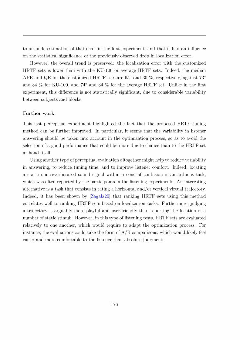
to an underestimation of that error in the first experiment, and that it had an influenceon the statistical significance of the previously observed drop in localization error.
However, the overall trend is preserved: the localization error with the customizedHRTF sets is lower than with the KU-100 or average HRTF sets. Indeed, the medianAPE and QE for the customized HRTF sets are 65 and 30 %, respectively, against 73
and 34 % for KU-100, and 74 and 34 % for the average HRTF set. Unlike in the firstexperiment, this difference is not statistically significant, due to considerable variabilitybetween subjects and blocks.
Further work
This last perceptual experiment highlighted the fact that the proposed HRTF tuningmethod can be further improved. In particular, it seems that the variability in listeneranswering should be taken into account in the optimization process, so as to avoid theselection of a good performance that could be more due to chance than to the HRTF setat hand itself.
Using another type of perceptual evaluation altogether might help to reduce variabilityin answering, to reduce tuning time, and to improve listener comfort. Indeed, locatinga static non-reverberated sound signal within a cone of confusion is an arduous task,which was often reported by the participants in the listening experiments. An interestingalternative is a task that consists in rating a horizontal and/or vertical virtual trajectory.Indeed, it has been shown by [Zagala20] that ranking HRTF sets using this methodcorrelates well to ranking HRTF sets based on localization tasks. Furthermore, judginga trajectory is arguably more playful and user-friendly than reporting the location of anumber of static stimuli. However, in this type of listening tests, HRTF sets are evaluatedrelatively to one another, which would require to adapt the optimization process. Forinstance, the evaluations could take the form of A/B comparisons, which would likely feeleasier and more comfortable to the listener than absolute judgments.
176
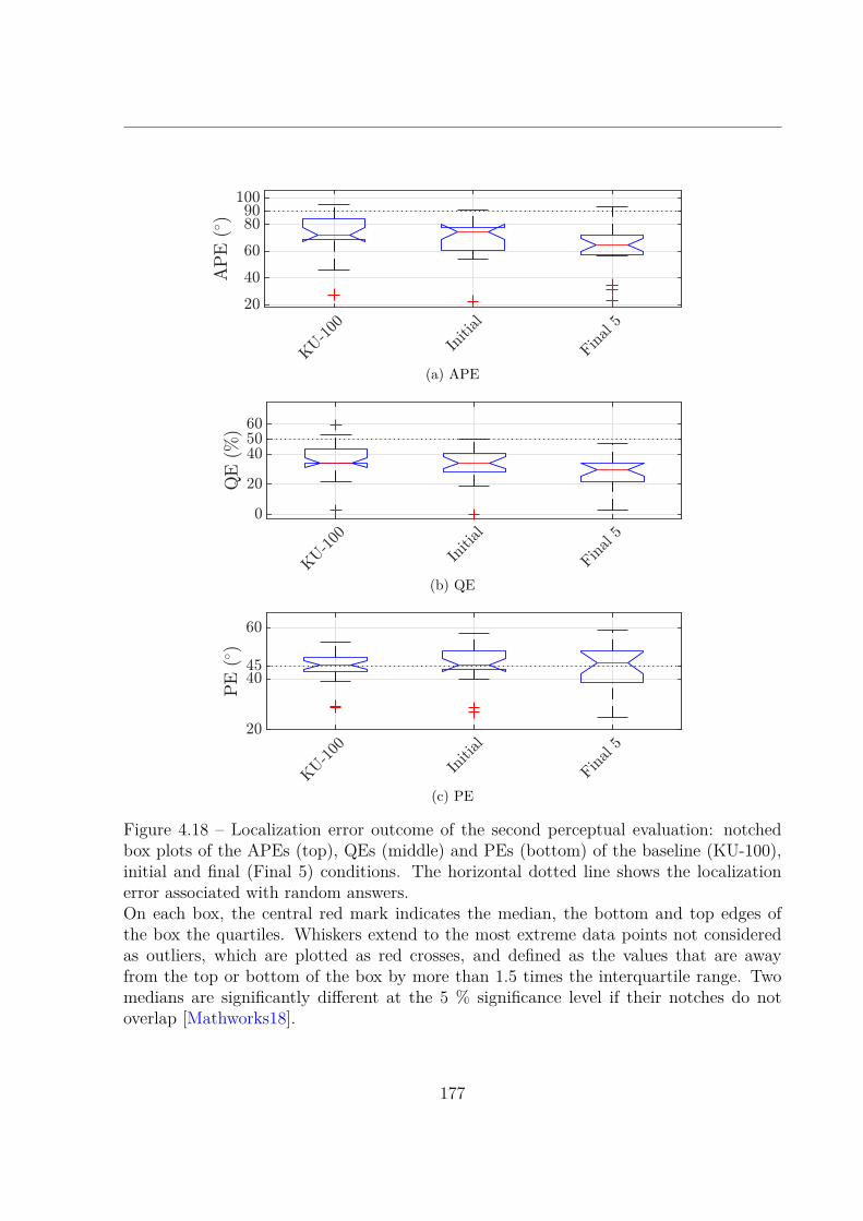
(a) APE
(b) QE
(c) PE
Figure 4.18 – Localization error outcome of the second perceptual evaluation: notchedbox plots of the APEs (top), QEs (middle) and PEs (bottom) of the baseline (KU-100),initial and final (Final 5) conditions. The horizontal dotted line shows the localizationerror associated with random answers.On each box, the central red mark indicates the median, the bottom and top edges ofthe box the quartiles. Whiskers extend to the most extreme data points not consideredas outliers, which are plotted as red crosses, and defined as the values that are awayfrom the top or bottom of the box by more than 1.5 times the interquartile range. Twomedians are significantly different at the 5 % significance level if their notches do notoverlap [Mathworks18].
177

BIBLIOGRAPHY
[Algazi01a] V. Ralph Algazi, Carlos Avendano, and Richard O. Duda. “ElevationLocalization and Head-Related Transfer Function Analysis at LowFrequencies”. In: The Journal of the Acoustical Society of America109.3 (Feb. 27, 2001), pp. 1110–1122. doi: 10.1121/1.1349185.
[Algazi01b] V. Ralph Algazi, Richard O. Duda, Reed P. Morrison, and Dennis M.Thompson. “Structural Composition and Decomposition of HRTFs”.In: Proceedings of the 2001 IEEE Workshop on the Applications ofSignal Processing to Audio and Acoustics (WASPAA). New Paltz,NY, USA: IEEE, Oct. 20, 2001, pp. 103–106. doi: 10.1109/ASPAA.2001.969553.
[Algazi01c] V. Ralph Algazi, Richard O. Duda, Dennis M. Thompson, and Car-los Avendano. “The CIPIC HRTF Database”. In: Proceedings of the2001 IEEE Workshop on the Applications of Signal Processing to Au-dio and Acoustics (WASPAA). New Platz, NY, USA, 2001, pp. 99–102. doi: 10.1109/ASPAA.2001.969552.
[Algazi02] V. Ralph Algazi, Richard O. Duda, Ramani Duraiswami, NailA. Gumerov, and Zhihui Tang. “Approximating the Head-RelatedTransfer Function Using Simple Geometric Models of the Head andTorso”. In: The Journal of the Acoustical Society of America 112.5(Oct. 25, 2002), pp. 2053–2064. doi: 10.1121/1.1508780.
[AlSheikh09] Bahaa W. Al-Sheikh, Mohammad A. Matin, and Daniel J. Tollin.“All-Pole and All-Zero Models of Human and Cat Head RelatedTransfer Functions”. In: Proceedings of SPIE 7444. Vol. 7444. SanDiego, CA, USA: International Society for Optics and Photonics,Aug. 2009, p. 74440X. doi: 10.1117/12.829872.
[Andreopoulou11] Areti Andreopoulou and Agnieszka Roginska. “Towards the Cre-ation of a Standardized HRTF Repository”. In: Proceedings of the
179
131th Audio Engineering Society Convention. New York, NY, USA:Audio Engineering Society, 2011.
[Andreopoulou15] Areti Andreopoulou, Durand R. Begault, and Brian F. G. Katz.“Inter-Laboratory Round Robin HRTF Measurement Comparison”.In: IEEE Journal of Selected Topics in Signal Processing 9.5 (Aug.2015), pp. 895–906. doi: 10.1109/JSTSP.2015.2400417.
[Andreopoulou16] Areti Andreopoulou and Brian F. G. Katz. “Investigation on Subjec-tive HRTF Rating Repeatability”. In: Proceedings of the 140th AudioEngineering Society Convention. Paris, France: Audio EngineeringSociety, June 4, 2016.
[Andreopoulou17] Areti Andreopoulou and Brian F. G. Katz. “Identification of Per-ceptually Relevant Methods of Inter-Aural Time Difference Estima-tion”. In: The Journal of the Acoustical Society of America 142.2(Aug. 1, 2017), pp. 588–598. doi: 10.1121/1.4996457.
[Armstrong18] Cal Armstrong, Lewis Thresh, Damian Murphy, and Gavin Kearney.“A Perceptual Evaluation of Individual and Non-Individual HRTFs:A Case Study of the SADIE II Database”. In: Applied Sciences 8.11(Nov. 2018), p. 2029. doi: 10.3390/app8112029.
[Asano90] Futoshi Asano, Yoiti Suzuki, and Toshio Sone. “Role of SpectralCues in Median Plane Localization”. In: The Journal of the Acous-tical Society of America 88.1 (1990), pp. 159–168. doi: 10.1121/1.399963.
[Augenbaum85] Jeffrey M. Augenbaum and Charles S. Peskin. “On the Constructionof the Voronoi Mesh on a Sphere”. In: Journal of ComputationalPhysics 59.2 (1985), pp. 177–192. doi: 10.1016/0021-9991(85)90140-8.
[Aytekin08] Murat Aytekin, Cynthia F. Moss, and Jonathan Z. Simon. “A Senso-rimotor Approach to Sound Localization”. In: Neural Computation20.3 (Mar. 1, 2008), pp. 603–635. doi: 10.1162/neco.2007.12-05-094.
180
[Bahu16a] Hélène Bahu. « Localisation auditive en contexte de synthèse bi-naurale non-individuelle [Auditory Localization in the Context ofNon-Individual Binaural Synthesis] ». PhD Thesis. Universite Pierreet Marie Curie / IRCAM, 14 déc. 2016.
[Bahu16b] Hélène Bahu, Thibaut Carpentier, Markus Noisternig, and OlivierWarusfel. “Comparison of Different Egocentric Pointing Methods for3D Sound Localization Experiments”. In: Acta Acustica united withAcustica 102.1 (Jan. 1, 2016), pp. 107–118. doi: 10.3813/AAA.918928.
[Barumerli20] Roberto Barumerli, Piotr Majdak, Jonas Reijniers, Robert Baum-gartner, and Michele Geronazzo and Federico Avanzini. “PredictingDirectional Sound-Localization of Human Listeners in Both Hori-zontal and Vertical Dimensions”. In: Proceedings of the 148th AudioEngineering Society Convention. Vienna, Austria: Audio Engineer-ing Society, May 28, 2020.
[Baskind12] Alexis Baskind, Thibaut Carpentier, Markus Noisternig, OlivierWarusfel, and Jean-Marc Lyzwa. “Binaural and Transaural Spatial-ization Techniques in Multichannel 5.1 Production”. In: Proceedingsof the 27th Tonmeistertagung, VDT International Convention. Köln,Germany, Nov. 2012.
[Baumgartner13] Robert Baumgartner, Piotr Majdak, and Bernhard Laback. “Assess-ment of Sagittal-Plane Sound Localization Performance in Spatial-Audio Applications”. In: The Technology of Binaural Listening. Ed.by Jens Blauert. Springer, 2013, pp. 93–119. isbn: 978-3-642-37761-7.
[Baumgartner14] Robert Baumgartner, Piotr Majdak, and Bernhard Laback. “Mod-eling Sound-Source Localization in Sagittal Planes for Human Lis-teners”. In: The Journal of the Acoustical Society of America 136.2(Aug. 2014), pp. 791–802. doi: 10.1121/1.4887447.
[Behnke12] Robert S. Behnke. Kinetic Anatomy. 3rd Edition. Human Kinetics,2012. 329 pp. isbn: 978-1-4504-1055-7.
[Beranek93] Leo L. Beranek. Acoustical Measurements. Revised Edition. Acous-tical Society of America, 1993. 850 pp. isbn: 0-88318-590-3.
181

[Bilinski14] Piotr Bilinski, Jens Ahrens, Mark R. P. Thomas, Ivan J. Tashev, andJohn C. Platt. “HRTF Magnitude Synthesis via Sparse Representa-tion of Anthropometric Features”. In: Proceedings of the 2014 IEEEInternational Conference on Acoustics, Speech and Signal Processing(ICASSP). Florence, Italy, 2014, pp. 4468–4472.
[Blauert97] Jens Blauert. Spatial Hearing: The Psychophysics of Human SoundLocalization. MIT Press, 1997. 514 pp. isbn: 978-0-262-02413-6.
[Blauert98] Jens Blauert, Marc Brueggen, Adelbert W. Bronkhorst, Rob Drull-man, Gerard Reynaud, Lionel Pellieux, Winfried Krebber, andRoland Sottek. “The AUDIS Catalog of Human HRTFs”. In: TheJournal of the Acoustical Society of America 103.5 (May 1, 1998),pp. 3082–3082. doi: 10.1121/1.422910.
[Blommer97] Michael A. Blommer and Gregory H. Wakefield. “Pole-Zero Approx-imations for Head-Related Transfer Functions Using a LogarithmicError Criterion”. In: IEEE Transactions on Speech and Audio Pro-cessing 5.3 (1997), pp. 278–287.
[Bomhardt16a] Ramona Bomhardt, Hark Braren, and Janina Fels. “Individualiza-tion of Head-Related Transfer Functions Using Principal ComponentAnalysis and Anthropometric Dimensions”. In: Proceedings of the172nd Meeting on Acoustics. Vol. 29. Honolulu, HI, USA: AcousticalSociety of America, Dec. 2016, p. 050007. doi: 10.1121/2.0000562.
[Bomhardt16b] Ramona Bomhardt, Matias de la Fuente Klein, and Janina Fels.“A High-Resolution Head-Related Transfer Function and Three-Dimensional Ear Model Database”. In: Proceedings of the 172ndMeeting on Acoustics. Vol. 29. Honolulu, HI, USA: Acoustical Soci-ety of America, Nov. 28, 2016, p. 050002. doi: 10.1121/2.0000467.
[Bomhardt16c] Ramona Bomhardt, Marcia Lins, and Janina Fels. “Analytical Ellip-soidal Model of Interaural Time Differences for the Individualizationof Head-Related Impulse Responses”. In: Journal of the Audio En-gineering Society 64.11 (2016), pp. 882–894.
[Bomhardt17] Ramona Bomhardt. “Anthropometric Individualization of Head-Related Transfer Functions Analysis and Modeling”. PhD Thesis.Aachen, Germany: Aachener Beiträge zur Akustik, 2017. 143 pp.
182

[Braren19] Hark Braren and Janina Fels. “Objective Differences between Indi-vidual HRTF Datasets of Children and Adults”. In: Proceedings ofthe 23rd International Congress on Acoustics (ICA). Aachen, Ger-many, Sept. 9, 19, pp. 5220–5224.
[Breebaart01] Jeroen Breebaart and Armin Kohlrausch. “The Perceptual(Ir)Relevance of HRTF Magnitude and Phase Spectra”. In: Proceed-ings of the 110th Audio Engineering Society Convention. Amster-dam, Netherlands: Audio Engineering Society, May 12, 2001.
[Breebaart10] Jeroen Breebaart, Fabian Nater, and Armin Kohlrausch. “Spec-tral and Spatial Parameter Resolution Requirements for Parametric,Filter-Bank-Based HRTF Processing”. In: Journal of the Audio En-gineering Society 58.3 (Apr. 3, 2010), pp. 126–140.
[Brinkmann17] Fabian Brinkmann, Alexander Lindau, Stefan Weinzerl, Steven vande Par, Markus Müller-Trapet, Rob Opdam, and Michael Vorlän-der. “A High Resolution and Full-Spherical Head-Related TransferFunction Database for Different Head-Above-Torso Orientations”.In: Journal of the Audio Engineering Society 65.10 (Oct. 30, 2017),pp. 841–848. doi: 10.17743/jaes.2017.0033.
[Brinkmann19] Fabian Brinkmann, Manoj Dinakaran, Robert Pelzer, Peter Grosche,Daniel Voss, and Stefan Weinzierl. “A Cross-Evaluated Databaseof Measured and Simulated HRTFs Including 3D Head Meshes,Anthropometric Features, and Headphone Impulse Responses”. In:Journal of the Audio Engineering Society 67.9 (Sept. 21, 2019),pp. 705–718. doi: 10.17743/jaes.2019.0024.
[Bronkhorst95] Adelbert W. Bronkhorst. “Localization of Real and Virtual SoundSources”. In: The Journal of the Acoustical Society of America 98.5(Nov. 1, 1995), pp. 2542–2553. doi: 10.1121/1.413219.
[Busson06] Sylvain Busson. « Individualisation d’indices acoustiques pour lasynthèse binaurale [Individualization of Acoustic Cues for Binau-ral Synthesis] ». PhD Thesis. Université de la Méditerranée-Aix-Marseille II, 2006.
183
[Carlile97] Simon Carlile, Philip Leong, and Stephanie Hyams. “The Nature andDistribution of Errors in Sound Localization by Human Listeners”.In: Hearing Research 114.1 (Dec. 1, 1997), pp. 179–196. doi: 10.1016/S0378-5955(97)00161-5.
[Carlile98] Simon Carlile, Craig Jin, and Vaughn Harvey. “The Generation andValidation of High Fidelity Virtual Auditory Space”. In: Proceedingsof the 20th Annual International Conference of the IEEE Engineer-ing in Medicine and Biology Society. Vol. 20. Hong Kong, China:IEEE, Nov. 1, 1998, pp. 1090–1095. doi: 10.1109/IEMBS.1998.747061.
[Carpentier14] Thibaut Carpentier, Hélène Bahu, Markus Noisternig, and OlivierWarusfel. “Measurement of a Head-Related Transfer FunctionDatabase with High Spatial Resolution”. In: Proceedings of the 7thForum Acusticum. Kraków, Poland: European Acoustics Associa-tion, Sept. 7, 2014.
[Casadamont18] Amandine Casadamont et Alexandre Plank. Welcome to NayPyi Taw. Hyperradio, France Culture / Deutschlandradio Kultur.20 avr. 2018. url : https://hyperradio.radiofrance.fr/son-3d/welcome-to-nay-pyi-taw/.
[Chen20] Wei Chen, Ruimin Hu, Xiaochen Wang, and Dengshi Li. “HRTFRepresentation with Convolutional Auto-Encoder”. In: Proceed-ings of the 26th International Conference on Multimedia Modeling(MMM). Ed. by Yong Man Ro, Wen-Huang Cheng, Junmo Kim,Wei-Ta Chu, Peng Cui, Jung-Woo Choi, Min-Chun Hu, and WesleyDe Neve. Lecture Notes in Computer Science. Seoul, South Korea:Springer International Publishing, Jan. 5, 2020, pp. 605–616. doi:10.1007/978-3-030-37731-1_49.
[Cooper89] Duane H. Cooper and Jerald L. Bauck. “Prospects for TransauralRecording”. In: Journal of the Audio Engineering Society 37.1/2(1989), pp. 3–19.
[Cootes95] Timothy F. Cootes, Christopher J. Taylor, David H. Cooper, andJim Graham. “Active Shape Models - Their Training and Applica-
184
tion”. In: Computer Vision and Image Understanding 61.1 (1995),pp. 38–59. doi: 10.1006/cviu.1995.1004.
[Deleforge15] Antoine Deleforge, Florence Forbes, and Radu Horaud. “AcousticSpace Learning for Sound-Source Separation and Localization onBinaural Manifolds”. In: International Journal of Neural Systems25.1 (Feb. 1, 2015), 21p. doi: 10.1142/S0129065714400036.
[Denk17] Florian Denk, Jan Heeren, Stephan D. Ewert, Birger Kollmeier, andStephan M.A. Ernst. “Controlling the Head Position During Indi-vidual HRTF Measurements and Its Effect on Accuracy”. In: Pro-ceedings of the Annual German Conference on Acoustics (DAGA).Kiel, Germany, 2017.
[Dinakaran18] Manoj Dinakaran, Fabian Brinkmann, Stine Harder, Robert Pelzer,Peter Grosche, Rasmus R. Paulsen, and Stefan Weinzierl. “Percep-tually Motivated Analysis of Numerically Simulated Head-RelatedTransfer Functions Generated By Various 3D Surface Scanning Sys-tems”. In: Proceedings of the 2018 IEEE International Conferenceon Acoustics, Speech and Signal Processing (ICASSP). Calgary, AB,Canada: IEEE, Apr. 2018, pp. 551–555. doi: 10.1109/ICASSP.2018.8461789.
[Duraiswami04] Ramani Duraiswami, Dmitry N. Zotkin, and Nail A. Gumerov. “In-terpolation and Range Extrapolation of HRTFs”. In: Proceedings ofthe 2004 IEEE International Conference on Acoustics, Speech andSignal Processing (ICASSP). Vol. 4. Montréal, QE, Canada, May 17,2004, pp. 45–48. doi: 10.1109/ICASSP.2004.1326759.
[Duraiswami05] Ramani Duraiswami and Vikas C. Raykar. “The Manifolds of SpatialHearing”. In: Proceedings of the 2005 IEEE International Confer-ence on Acoustics, Speech and Signal Processing (ICASSP). Vol. 3.Philadelphia, PA, USA: IEEE, 2005, pp. iii/285–iii/288. doi: 10.1109/ICASSP.2005.1415702.
[Durant02] E. A. Durant and G. H. Wakefield. “Efficient Model Fitting Us-ing a Genetic Algorithm: Pole-Zero Approximations of HRTFs”.In: IEEE Transactions on Speech and Audio Processing 10.1 (Jan.2002), pp. 18–27. doi: 10.1109/89.979382.
185
[Ehret78] Günter Ehret. “Stiffness Gradient along the Basilar Membrane as aBasis for Spatial Frequency Analysis within the Cochlea”. In: TheJournal of the Acoustical Society of America 64.6 (Dec. 1, 1978),pp. 1723–1726. doi: 10.1121/1.382153.
[Engel19] Isaac Engel, David Lou Alon, Philip W. Robinson, and RavishMehra. “The Effect of Generic Headphone Compensation on Bin-aural Renderings”. In: Proceedings of the 2019 AES InternationalConference on Immersive and Interactive Audio. York, UK: AudioEngineering Society, Mar. 17, 2019.
[Enzner08] Gerald Enzner. “Analysis and Optimal Control of LMS-Type Adap-tive Filtering for Continuous-Azimuth Acquisition of Head RelatedImpulse Responses”. In: Proceedings of the 2008 IEEE InternationalConference on Acoustics, Speech and Signal Processing (ICASSP).Las Vegas, NV, USA: IEEE, 2008, pp. 393–396. doi: 10 . 1109 /ICASSP.2008.4517629.
[Fan19] Ziqi Fan, Terek Arce, Chenshen Lu, Kai Zhang, T. W. Wu, and KylaMcMullen. “Computation of Head-Related Transfer Functions UsingGraphics Processing Units and a Perceptual Validation of the Com-puted HRTFs against Measured HRTFs”. In: Proceedings of the 2019Audio Engineering Society International Conference on HeadphoneTechnology. San Francisco, CA, USA: Audio Engineering Society,Aug. 27, 2019.
[Farahikia17] Mahdi Farahikia and Quang T. Su. “Optimized Finite ElementMethod for Acoustic Scattering Analysis With Application to Head-Related Transfer Function Estimation”. In: Journal of Vibration andAcoustics 139.3 (June 2017), p. 034501. doi: 10.1115/1.4035813.
[Fayek17] Haytham Fayek, Laurens van der Maaten, Griffin Romigh, and Rav-ish Mehra. “On Data-Driven Approaches to Head-Related-TransferFunction Personalization”. In: Proceedings of the 143rd Audio Engi-neering Society Convention. New York, NY, USA: Audio Engineer-ing Society, Oct. 8, 2017.
186
[Fink15] Kimberly J. Fink and Laura Ray. “Individualization of Head Re-lated Transfer Functions Using Principal Component Analysis”. In:Applied Acoustics 87 (Jan. 2015), pp. 162–173. doi: 10.1016/j.apacoust.2014.07.005.
[Furness90] Roger K. Furness. “Ambisonics - An Overview”. In: Proceedingsof the 8th AES International Conference on The Sound of Audio.Washington D.C., USA: Audio Engineering Society, May 1, 1990.
[Gardner97] William Grant Gardner. “3-D Audio Using Loudspeakers”. PhDThesis. Massachusetts Institute of Technology, Sept. 1997.
[Geronazzo18] M. Geronazzo, S. Spagnol, and F. Avanzini. “Do We Need Individ-ual Head-Related Transfer Functions for Vertical Localization? TheCase Study of a Spectral Notch Distance Metric”. In: IEEE/ACMTransactions on Audio, Speech, and Language Processing (Apr. 2,2018), pp. 1247–1260. doi: 10.1109/TASLP.2018.2821846.
[Ghorbal16] Slim Ghorbal, Renaud Séguier, and Xavier Bonjour. “Process ofHRTF Individualization by 3D Statistical Ear Model”. In: Proceed-ings of the 141st Audio Engineering Society Convention. Los Ange-les, CA, USA: Audio Engineering Society, Sept. 20, 2016.
[Ghorbal17] Slim Ghorbal, Théo Auclair, Catherine Soladié, and Renaud Séguier.“Pinna Morphological Parameters Influencing HRTF Sets”. In: Pro-ceedings of the 20th International Conference on Digital Audio Ef-fects (DAFx-17). Edinburgh, UK, Sept. 9, 2017.
[Ghorbal19] Slim Ghorbal, Renaud Séguier, and Xavier Bonjour. “Method forEstablishing a Deformable 3D Model of an Element, and AssociatedSystem”. U.S. pat. Patent 16/300, 044. May 16, 2019.
[Ghorbal20] Slim Ghorbal. « Personnalisation de l’écoute binaurale par mo-dèle déformable d’oreille [Personnalization of Binaural Listening bymeans of a Deformable Ear Model] ». PhD Thesis. To be published :CentraleSupélec, 2020.
[Glasberg90] Brian R. Glasberg and Brian C. J. Moore. “Derivation of AuditoryFilter Shapes from Notched-Noise Data”. In: Hearing Research 47.1-2 (Aug. 1990), pp. 103–138. doi: 10.1016/0378-5955(90)90170-T.
187

[Gower75] John C. Gower. “Generalized Procrustes Analysis”. In: Psychome-trika 40.1 (Mar. 1975), pp. 33–51.
[Greff07] Raphaël Greff and Brian F. G. Katz. “Round Robin Comparison ofHRTF Simulation Systems: Preliminary Results”. In: Proceedings ofthe 123rd Audio Engineering Society Convention. New York, NY,USA: Audio Engineering Society, Oct. 1, 2007.
[Grijalva14] Felipe Grijalva, Luiz Martini, Siome Goldenstein, and Dinei Floren-cio. “Anthropometric-Based Customization of Head-Related Trans-fer Functions Using Isomap in the Horizontal Plane”. In: Proceedingsof the 2014 IEEE International Conference on Acoustics, Speech andSignal Processing (ICASSP). Florence, Italy: IEEE, 2014, pp. 4473–4477. doi: 10.1109/ICASSP.2014.6854448.
[Grijalva16] F. Grijalva, L. Martini, D. Florencio, and S. Goldenstein. “A Man-ifold Learning Approach for Personalizing HRTFs from Anthropo-metric Features”. In: IEEE/ACM Transactions on Audio, Speech,and Language Processing 24.3 (Mar. 2016), pp. 559–570. doi: 10.1109/TASLP.2016.2517565.
[Guezenoc18] Corentin Guezenoc and Renaud Séguier. “HRTF Individualization:A Survey”. In: Proceedings of the 145th Audio Engineering SocietyConvention. New York, NY, USA: Audio Engineering Society, Oct. 7,2018. doi: 10.17743/aesconv.2018.978-1-942220-25-1.
[Guezenoc20a] Corentin Guezenoc and Renaud Séguier. “A Wide Dataset of EarShapes and Pinna-Related Transfer Functions Generated by Ran-dom Ear Drawings”. In: The Journal of the Acoustical Society ofAmerica 147.6 (June 23, 2020), pp. 4087–4096. doi: 10.1121/10.0001461.
[Guezenoc20b] Corentin Guezenoc and Renaud Séguier. “Dataset Augmentationand Dimensionality Reduction of Pinna-Related Transfer Func-tions”. In: Proceedings of the 148th Audio Engineering Society Con-vention. Vienna, Austria: Audio Engineering Society, May 28, 2020.doi: 10.17743/aesconv.2020.978-1-942220-32-9.
188

[Guillon08] Pierre Guillon, Rozenn Nicol, and Laurent Simon. “Head-RelatedTransfer Functions Reconstruction from Sparse Measurements Con-sidering a Priori Knowledge from Database Analysis: A PatternRecognition Approach”. In: Proceedings of the 125th Audio Engi-neering Society Convention. San Francisco, CA, USA: Audio Engi-neering Society, Oct. 1, 2008.
[Gumerov05] Nail A. Gumerov and Ramani Duraiswami. Fast Multipole Methodsfor the Helmholtz Equation in Three Dimensions. Elsevier Series inElectromagnetism. Elsevier Science, Jan. 27, 2005. 426 pp. isbn:978-0-08-053159-5.
[Gumerov07] Nail A. Gumerov, Ramani Duraiswami, and Dmitry N. Zotkin. “FastMultipole Accelerated Boundary Elements for Numerical Computa-tion of the Head Related Transfer Function”. In: Proceedings of the2007 IEEE International Conference on Acoustics, Speech and Sig-nal Processing (ICASSP). Honolulu, HI, USA: IEEE, 2007, pp. I-165–I-168. doi: 10.1109/ICASSP.2007.366642.
[Gumerov10] Nail A. Gumerov, Adam E. O’Donovan, Ramani Duraiswami, andDmitry N. Zotkin. “Computation of the Head-Related TransferFunction via the Fast Multipole Accelerated Boundary ElementMethod and Its Spherical Harmonic Representation”. In: The Jour-nal of the Acoustical Society of America 127.1 (Jan. 2010), pp. 370–386. doi: 10.1121/1.3257598.
[Haneda99] Y. Haneda, S. Makino, Y. Kaneda, and N. Kitawaki. “Common-Acoustical-Pole and Zero Modeling of Head-Related Transfer Func-tions”. In: IEEE Transactions on Speech and Audio Processing 7.2(Mar. 1999), pp. 188–196. doi: 10.1109/89.748123.
[Hebrank74] Jack Hebrank and Donald Wright. “Spectral Cues Used in the Lo-calization of Sound Sources on the Median Plane”. In: The Journalof the Acoustical Society of America 56.6 (Dec. 1, 1974), pp. 1829–1834. doi: 10.1121/1.1903520.
189

[Hirahara10] Tatsuya Hirahara, Hiroyuki Sagara, Iwaki Toshima, and MakotoOtani. “Head Movement during Head-Related Transfer FunctionMeasurements”. In: Acoustical Science and Technology 31.2 (2010),pp. 165–171. doi: 10.1250/ast.31.165.
[Hoffmann08] Pablo F. Hoffmann and Henrik Møller. “Audibility of Differencesin Adjacent Head-Related Transfer Functions”. In: Acta Acusticaunited with Acustica 94.6 (Nov. 1, 2008), pp. 945–954. doi: 10 .3813/AAA.918111.
[Hold17] Christoph Hold, Fabian Seipel, Fabian Brinkmann, AthanasiosLykartsis, and Stefan Weinzierl. “Eigen-Images of Head-RelatedTransfer Functions”. In: Proceedings of the 143rd Audio Engineer-ing Society Convention. New York, NY, USA: Audio EngineeringSociety, Oct. 8, 2017.
[Hölzl14] Josef Hölzl. “A Global Model for HRTF Individualization by Ad-justment of Principal Component Weights”. Master Thesis. Graz,Austria: Institute of Electronic Music and Acoustics, University ofMusic and Performing Arts Graz, Graz University of Technology,2014. 135 pp.
[Hu06] Hongmei Hu, Lin Zhou, Jie Zhang, Hao Ma, and Zhenyang Wu.“Head Related Transfer Function Personalization Based on Multi-ple Regression Analysis”. In: Proceedings of the 2006 InternationalConference on Computational Intelligence and Security. Vol. 2.Guangzhou, China, Nov. 2006, pp. 1829–1832. doi: 10 . 1109 /ICCIAS.2006.295380.
[Hu08] Hongmei Hu, Lin Zhou, Hao Ma, and Zhenyang Wu. “HRTF Person-alization Based on Artificial Neural Network in Individual VirtualAuditory Space”. In: Applied Acoustics 69.2 (Feb. 2008), pp. 163–172. doi: 10.1016/j.apacoust.2007.05.007.
[Hu16] Shichao Hu, Jorge Trevino, Cesar Salvador, Shuichi Sakamoto, Jun-feng Li, and Yôiti Suzuki. “A Local Representation of the Head-Related Transfer Function”. In: The Journal of the Acoustical Soci-ety of America 140.3 (Sept. 21, 2016), EL285–EL290. doi: 10.1121/1.4962805.
190

[Hu19] Shichao Hu, Jorge Trevino, César Salvador, Shuichi Sakamoto,and Yôiti Suzuki. “Modeling Head-Related Transfer Functions withSpherical Wavelets”. In: Applied Acoustics 146 (Mar. 1, 2019),pp. 81–88. doi: 10.1016/j.apacoust.2018.10.026.
[Huang09a] Qinghua Huang and Yong Fang. “Modeling Personalized Head-Related Impulse Response Using Support Vector Regression”. In:Journal of Shanghai University (English Edition) 13.6 (2009), p. 428.doi: 10.1007/s11741-009-0602-2.
[Huang09b] Qinghua Huang and Qi-lei Zhuang. “HRIR Personalisation UsingSupport Vector Regression in Independent Feature Space”. In: Elec-tronics Letters 45.19 (Sept. 2009), pp. 1002–1003. doi: 10.1049/el.2009.1865.
[Hugeng10] Hugeng Hugeng, Wahab Wahidin, and Dadag Gunawan. “A NovelIndividualization of Head-Related Impulse Responses on MedianPlane Using Listener’s Anthropometries Based On Multiple Regres-sion Analysis”. In: Jurnal Penelitian dan Pengembangan Telekomu-nikasi 15.1 (June 2010).
[Huopaniemi99] Jyri Huopaniemi, Nick Zacharov, and Matti Karjalainen. “Objectiveand Subjective Evaluation of Head-Related Transfer Function FilterDesign”. In: Journal of the Audio Engineering Society 47.4 (Apr. 1,1999), pp. 218–239.
[Huttunen07] Tomi Huttunen, Eira T. Seppälä, Ole Kirkeby, Asta Kärkkäinen, andLeo Kärkkäinen. “Simulation of the Transfer Function for a Head-and-Torso Model over the Entire Audible Frequency Range”. In:Journal of Computational Acoustics 15.04 (Dec. 1, 2007), pp. 429–448. doi: 10.1142/S0218396X07003469.
[Huttunen13] Tomi Huttunen, Kimmo Tuppurainen, Antti Vanne, Pasi Ylä-Oijala,Seppo Järvenpää, Asta Kärkkäinen, and Leo Kärkkäinen. “Simula-tion of the Head-Related Transfer Functions Using Cloud Comput-ing”. In: Proceedings of the 21st International Congress on Acoustics(ICA). Vol. 19. Montréal, QE, Canada: Acoustical Society of Amer-ica, June 2, 2013, p. 050168. doi: 10.1121/1.4800138.
191
[Hwang08a] Sungmok Hwang, Youngjin Park, and Youn-sik Park. “Modeling andCustomization of Head-Related Impulse Responses Based on Gen-eral Basis Functions in Time Domain”. In: Acta Acustica united withAcustica 94.6 (Nov. 1, 2008), pp. 965–980. doi: 10 . 3813 / AAA .918113.
[Hwang08b] Sungmok Hwang, Youngjin Park, and Youn-sik Park. “Modeling andCustomization of Head-Related Transfer Functions Using Princi-pal Component Analysis”. In: Proceedings of the 2008 InternationalConference on Control, Automation and Systems (ICCAS 2008).Seoul, South Korea: IEEE, 2008, pp. 227–231. doi: 10.1109/ICCAS.2008.4694554.
[Inoue05] Naoya Inoue, Toshiyuki Kimura, Takanori Nishino, Katsunobu Itou,and Kazuya Takeda. “Evaluation of HRTFs Estimated Using Phys-ical Features”. In: Acoustical Science and Technology 26.5 (Apr. 6,2005), pp. 453–455. doi: 10.1250/ast.26.453.
[Iwaya06] Yukio Iwaya. “Individualization of Head-Related Transfer Functionswith Tournament-Style Listening Test: Listening with Other’s Ears”.In: Acoustical Science and Technology 27.6 (2006), pp. 340–343. doi:http://dx.doi.org/10.1250/ast.27.340.
[Jin00] Craig Jin, Philip H. W. Leong, Johahn Leung, Anna Corderoy, andSimon Carlile. “Enabling Individualized Virtual Auditory Space Us-ing Morphological Measurements”. In: Proceedings of the 1st IEEEPacific-Rim Conference on Multimedia. Sydney, NSW, Australia:IEEE, 2000, pp. 235–238.
[Jin14] Craig Jin, Pierre Guillon, Nicolas Epain, Reza Zolfaghari, André vanSchaik, Anthony I. Tew, Carl Hetherington, and Jonathan Thorpe.“Creating the Sydney York Morphological and Acoustic Recordingsof Ears Database”. In: IEEE Transactions on Multimedia 16.1 (Jan.2014), pp. 37–46. doi: 10.1109/TMM.2013.2282134.
[Jolliffe02] Ian T. Jolliffe. Principal Component Analysis. 2nd ed. Springer Se-ries in Statistics. Springer-Verlag, 2002. isbn: 978-0-387-95442-4.
192
[Kahana06] Yuvi Kahana and Philip A. Nelson. “Numerical Modelling of theSpatial Acoustic Response of the Human Pinna”. In: Journal ofSound and Vibration 292.1-2 (Oct. 2006), pp. 148–178. doi: 10.1016/j.jsv.2005.07.048.
[Kahana99] Yuvi Kahana, Philip A. Nelson, Maurice Petyt, and Sunghoon Choi.“Numerical Modelling of the Transfer Functions of a Dummy-Headand of the External Ear”. In: Proceedings of the 16th AES Interna-tional Conference on Spatial Sound Reproduction. Rovaniemi, Fin-land: Audio Engineering Society, Apr. 10, 1999.
[Kaneko16a] Shoken Kaneko, Tsukasa Suenaga, Mai Fujiwara, Kazuya Kume-hara, Futoshi Shirakihara, and Satoshi Sekine. “Ear Shape Modelingfor 3D Audio and Acoustic Virtual Reality: The Shape-Based Aver-age HRTF”. In: Proceedings of the 61st AES International Confer-ence on Audio for Games. London, UK: Audio Engineering Society,Feb. 10, 2016. isbn: 978-1-942220-08-4.
[Kaneko16b] Shoken Kaneko, Tsukasa Suenaga, and Satoshi Sekine. “DeepEar-Net: Individualizing Spatial Audio with Photography, Ear ShapeModeling, and Neural Networks”. In: Proceedings of the 2016 AESInternational Conference on Audio for Virtual and Augmented Re-ality. Los Angeles, CA, USA: Audio Engineering Society, Sept. 30,2016.
[Kapralos08] Bill Kapralos, Nathan Mekuz, Agnieszka Kopinska, and Saad Khat-tak. “Dimensionality Reduced HRTFs: A Comparative Study”. In:Proceedings of the 2008 International Conference on Advances inComputer Entertainment Technology (ACE). Yokohama, Japan: As-sociation for Computing Machinery, Dec. 5, 2008, pp. 59–62. doi:10.1145/1501750.1501763.
[Katz00] Brian F. G. Katz. “Acoustic Absorption Measurement of HumanHair and Skin within the Audible Frequency Range”. In: The Journalof the Acoustical Society of America 108.5 (Nov. 1, 2000), pp. 2238–2242. doi: 10.1121/1.1314319.
193

[Katz01] Brian F. G. Katz. “Boundary Element Method Calculation of Indi-vidual Head-Related Transfer Function. I. Rigid Model Calculation”.In: The Journal of the Acoustical Society of America 110.5 (Oct. 29,2001), pp. 2440–2448. doi: 10.1121/1.1412440.
[Katz12] Brian F. G. Katz and Gaëtan Parseihian. “Perceptually Based Head-Related Transfer Function Database Optimization”. In: The Journalof the Acoustical Society of America 131.2 (Jan. 13, 2012), EL99–EL105. doi: 10.1121/1.3672641.
[Katz14] Brian F. G. Katz and Markus Noisternig. “A Comparative Study ofInteraural Time Delay Estimation Methods”. In: The Journal of theAcoustical Society of America 135.6 (June 1, 2014), pp. 3530–3540.doi: 10.1121/1.4875714.
[Katz19] Brian F. G. Katz and Rozenn Nicol. “Binaural Spatial Reproduc-tion”. In: Sensory Evaluation of Sound. Ed. by Nick Zacharov. CRCPress, 2019. isbn: 978-0-429-76991-7.
[Kearney15] Gavin Kearney and Tony Doyle. “An HRTF Database for VirtualLoudspeaker Rendering”. In: Proceedings of the 139th Audio Engi-neering Society Convention. New York, NY, USA: Audio Engineer-ing Society, Oct. 2015.
[Kim05] Sang-Myeong Kim and Wonjae Choi. “On the Externalization ofVirtual Sound Images in Headphone Reproduction: A Wiener FilterApproach”. In: The Journal of the Acoustical Society of America117.6 (May 31, 2005), pp. 3657–3665. doi: 10.1121/1.1921548.
[Kimura14] Masateru Kimura, Jason Kunio, Andreas Schuhmacher, and Yun-seon Ryu. “A New High-Frequency Impedance Tube for MeasuringSound Absorption Coefficient and Sound Transmission Loss”. In:Proceedings of Inter-Noise. Melbourne, Australia: Institute of NoiseControl Engineering, Nov. 16, 2014.
[Kistler92] Doris J. Kistler and Frederic L. Wightman. “A Model of Head-Related Transfer Functions Based on Principal Components Anal-ysis and Minimum-Phase Reconstruction”. In: The Journal of theAcoustical Society of America 91.3 (Mar. 1, 1992), pp. 1637–1647.doi: 10.1121/1.402444.
194
[Kreuzer09] Wolfgang Kreuzer, Piotr Majdak, and Zhengsheng Chen. “Fast Mul-tipole Boundary Element Method to Calculate Head-Related Trans-fer Functions for a Wide Frequency Range”. In: The Journal of theAcoustical Society of America 126.3 (Sept. 1, 2009), pp. 1280–1290.doi: 10.1121/1.3177264.
[KRoll18] Kristoff K.Roll. Petite Suite A l’Ombre des Ondes. Avec la coll.de Valérie Lavallart, Laure Jung-Lancrey, Francesco Cameli,Claire Bergerault, Isabelle Duthoit, Patrice Soletti, DidierAschour et Edward Perraud. Hyperradio, Radio France. 10 déc.2018. url : https : / / hyperradio . radiofrance . fr / son - 3d /creation - mondiale - kristoff - k - roll - petites - suites - a -lombres- des- ondes- dans- la- bibliotheque- de- recits- de-reves/.
[Kuhn77] George F. Kuhn. “Model for the Interaural Time Differences inthe Azimuthal Plane”. In: The Journal of the Acoustical Society ofAmerica 62.1 (July 1, 1977), pp. 157–167. doi: 10.1121/1.381498.
[Kulkarni99] Abhijit Kulkarni, Scott K. Isabelle, and H. Steven Colburn. “Sensi-tivity of Human Subjects to Head-Related Transfer-Function PhaseSpectra”. In: The Journal of the Acoustical Society of America 105.5(1999), pp. 2821–2840. doi: 10.1121/1.426898.
[Lagarias98] Jeffrey C. Lagarias, James A. Reeds, Margaret H. Wright, and PaulE. Wright. “Convergence Properties of the Nelder-Mead SimplexMethod in Low Dimensions”. In: SIAM Journal on Optimization9.1 (Jan. 1, 1998), pp. 112–147. doi: 10.1137/S1052623496303470.
[Langendijk02] Erno H. A. Langendijk and Adelbert W. Bronkhorst. “Contributionof Spectral Cues to Human Sound Localization”. In: The Journal ofthe Acoustical Society of America 112.4 (Sept. 27, 2002), pp. 1583–1596. doi: 10.1121/1.1501901.
[Langendijk99] Erno H. A. Langendijk and Adelbert W. Bronkhorst. “Fidelity ofThree-Dimensional-Sound Reproduction Using a Virtual AuditoryDisplay”. In: The Journal of the Acoustical Society of America 107.1(Dec. 29, 1999), pp. 528–537. doi: 10.1121/1.428321.
195
[Larcher00] Véronique Larcher, Olivier Warusfel, Jean-Marc Jot, and JéromeGuyard. “Study and Comparison of Efficient Methods for 3D Au-dio Spatialization Based on Linear Decomposition of HRTF Data”.In: Proceedings of the 108th Audio Engineering Society Convention.Paris, France: Audio Engineering Society, Feb. 19, 2000.
[Larcher97] Véronique Larcher et Jean-Marc Jot. « Techniquesd’interpolation de filtres audio-numériques : Application à lareproduction spatiale des sons sur écouteurs [Interpolation Tech-niques for Audio-Digital Filters : Application to Sound SpatialReproduction through Ear-buds] ». In : Actes du Congrès Françaisd’Acoustique (CFA) 1997. Marseille, France, avr. 1997, p. 97-100.
[Le Bagousse10] Sarah Le Bagousse, Catherine Colomes, and Mathieu Paquier.“State of the Art on Subjective Assessment of Spatial Sound Qual-ity”. In: Proceedings of the 38th AES International Conference onSound Quality Evaluation. Piteå, Sweden: Audio Engineering Soci-ety, June 13, 2010.
[Li13] Lin Li and Qinghua Huang. “HRTF Personalization Modeling Basedon RBF Neural Network”. In: Proceedings of the 2013 IEEE In-ternational Conference on Acoustics, Speech and Signal Processing(ICASSP). Vancouver, BC, Canada, 2013, pp. 3707–3710. doi: 10.1109/ICASSP.2013.6638350.
[Liu19a] Huaping Liu, Yong Fang, and Qinghua Huang. “Efficient Repre-sentation of Head-Related Transfer Functions With Combination ofSpherical Harmonics and Spherical Wavelets”. In: IEEE Access 7(June 27, 2019), pp. 78214–78222. doi: 10.1109/ACCESS.2019.2921388.
[Liu19b] Xuejie Liu, Hao Song, and Xiaoli Zhong. “A Hybrid Algorithm forPredicting Median-Plane Head-Related Transfer Functions from An-thropometric Measurements”. In: Applied Sciences 9.11 (11 Jan.2019), p. 2323. doi: 10.3390/app9112323.
[Macpherson02] Ewan A. Macpherson and John C. Middlebrooks. “Listener Weight-ing of Cues for Lateral Angle: The Duplex Theory of Sound Localiza-
196
tion Revisited”. In: The Journal of the Acoustical Society of America111.5 (May 1, 2002), pp. 2219–2236. doi: 10.1121/1.1471898.
[Macpherson07] Ewan A. Macpherson and Andrew T. Sabin. “Binaural Weightingof Monaural Spectral Cues for Sound Localization”. In: The Journalof the Acoustical Society of America 121.6 (June 1, 2007), pp. 3677–3688. doi: 10.1121/1.2722048.
[Majdak07] Piotr Majdak, Peter Balazs, and Bernhard Laback. “Multiple Expo-nential Sweep Method for Fast Measurement of Head-Related Trans-fer Functions”. In: Journal of the Audio Engineering Society 55.7/8(July 2007), pp. 623–637.
[Majdak10] Piotr Majdak, Matthew J. Goupell, and Bernhard Laback. “3-D Lo-calization of Virtual Sound Sources: Effects of Visual Environment,Pointing Method, and Training”. In: Attention, Perception & Psy-chophysics 72.2 (Feb. 1, 2010), pp. 454–469. doi: 10.3758/APP.72.2.454.
[Maki05] Katuhiro Maki and Shigeto Furukawa. “Reducing Individual Dif-ferences in the External-Ear Transfer Functions of the MongolianGerbil”. In: The Journal of the Acoustical Society of America 118.4(Oct. 1, 2005), pp. 2392–2404. doi: 10.1121/1.2033571.
[Mäkivirta20] Aki Mäkivirta, Matti Malinen, Jaan Johansson, Ville Saari, andAapo Karjalainen and Poorang Vosough. “Accuracy of Photogram-metric Extraction of the Head and Torso Shape for Personal Acous-tic HRTF Modeling”. In: Proceedings of the 148th Audio Engineer-ing Society Convention. Vienna, Austria: Audio Engineering Society,May 28, 2020.
[Marburg02] Steffen Marburg. “Six Boundary Elements per Wavelength: Is ThatEnough?” In: Journal of Computational Acoustics 10.01 (Mar. 1,2002), pp. 25–51. doi: 10.1142/S0218396X02001401.
[Martin01] Russell L. Martin, Ken I. McAnally, and Melis A. Senova. “Free-Field Equivalent Localization of Virtual Audio”. In: Journal of theAudio Engineering Society 49.1/2 (Feb. 1, 2001), pp. 14–22.
197

[Mathworks18] Mathworks. MATLAB Statistics and Machine Learning Toolbox Re-lease 2018b: User’s Guide. 2018. url: https://fr.mathworks.com/help/stats/boxplot.html.
[Matsunaga10] Noriyuki Matsunaga and Tatsuya Hirahara. “Reexamination ofFast Head-Related Transfer Function Measurement by Recipro-cal Method”. In: Acoustical Science and Technology 31.6 (2010),pp. 414–416. doi: 10.1250/ast.31.414.
[Mehrgardt77] S. Mehrgardt and V. Mellert. “Transformation Characteristics ofthe External Human Ear”. In: The Journal of the Acoustical Societyof America 61.6 (June 1, 1977), pp. 1567–1576. doi: 10.1121/1.381470.
[Meshram14] Alok Meshram, Ravish Mehra, Hongsheng Yang, Enrique Dunn,Jan-Michael Franm, and Dinesh Manocha. “P-HRTF: Efficient Per-sonalized HRTF Computation for High-Fidelity Spatial Sound”. In:Proceedings of the 2014 IEEE International Symposium on Mixedand Augmented Reality (ISMAR). Munich, Germany: IEEE, Sept.2014, pp. 53–61. doi: 10.1109/ISMAR.2014.6948409.
[Middlebrooks00] John C. Middlebrooks, Ewan A. Macpherson, and Zekiye A. On-san. “Psychophysical Customization of Directional Transfer Func-tions for Virtual Sound Localization”. In: The Journal of the Acous-tical Society of America 108.6 (Nov. 21, 2000), pp. 3088–3091. doi:10.1121/1.1322026.
[Middlebrooks90] John C. Middlebrooks and David M. Green. “Directional Depen-dence of Interaural Envelope Delays”. In: The Journal of the Acous-tical Society of America 87.5 (May 1, 1990), pp. 2149–2162. doi:10.1121/1.399183.
[Middlebrooks92] John C. Middlebrooks and David M. Green. “Observations on aPrincipal Components Analysis of Head-related Transfer Functions”.In: The Journal of the Acoustical Society of America 92.1 (July 1,1992), pp. 597–599. doi: 10.1121/1.404272.
198
[Middlebrooks99a] John C. Middlebrooks. “Individual Differences in External-EarTransfer Functions Reduced by Scaling in Frequency”. In: The Jour-nal of the Acoustical Society of America 106.3 (Aug. 23, 1999),pp. 1480–1492. doi: 10.1121/1.427176.
[Middlebrooks99b] John C. Middlebrooks. “Virtual Localization Improved by ScalingNonindividualized External-Ear Transfer Functions in Frequency”.In: The Journal of the Acoustical Society of America 106.3 (Aug. 23,1999), pp. 1493–1510. doi: 10.1121/1.427147.
[Mills58] A. W. Mills. “On the Minimum Audible Angle”. In: The Journal ofthe Acoustical Society of America 30.4 (Apr. 1, 1958), pp. 237–246.doi: 10.1121/1.1909553.
[Mills60] A. W. Mills. “Lateralization of High-Frequency Tones”. In: TheJournal of the Acoustical Society of America 32.1 (Jan. 1, 1960),pp. 132–134. doi: 10.1121/1.1907864.
[Möbius10] Jan Möbius and Leif Kobbelt. “OpenFlipper: An Open Source Ge-ometry Processing and Rendering Framework”. In: Proceedings ofCurves and Surfaces 2010. Ed. by Jean-Daniel Boissonnat, PatrickChenin, Albert Cohen, Christian Gout, Tom Lyche, Marie-LaurenceMazure, and Larry Schumaker. Lecture Notes in Computer Science.Berlin, Germany: Springer, 2010, pp. 488–500. doi: 10.1007/978-3-642-27413-8_31.
[Mokhtari07] Parham Mokhtari, Hironori Takemoto, Ryouichi Nishimura, and Hi-roaki Kato. “Comparison of Simulated and Measured HRTFs: FDTDSimulation Using MRI Head Data”. In: Proceedings of the 123rd Au-dio Engineering Society Convention. New York, NY, USA: AudioEngineering Society, Oct. 5, 2007.
[Mokhtari08] Parham Mokhtari, Ryouichi Nishimura, and Hironori Takemoto.“Toward HRTF Personalization: An Auditory-Perceptual Evalua-tion of Simulated and Measured HRTFs”. In: Proceedings of the 14thInternational Conference on Auditory Display. Paris, France, 2008.
199
[Mokhtari19] Parham Mokhtari, Hiroaki Kato, Hironori Takemoto, RyouichiNishimura, Seigo Enomoto, Seiji Adachi, and Tatsuya Kitamura.“Further Observations on a Principal Components Analysis of Head-Related Transfer Functions”. In: Scientific Reports 9.7477 (May 16,2019). doi: 10.1038/s41598-019-43967-0.
[Møller92] Henrik Møller. “Fundamentals of Binaural Technology”. In: AppliedAcoustics 36.3 (Jan. 1, 1992), pp. 171–218. doi: 10.1016/0003-682X(92)90046-U.
[Møller96] Henrik Møller, Michael Friis Sørensen, Clemen Boje Jensen, andDorte Hammershøi. “Binaural Technique: Do We Need IndividualRecordings?” In: Journal of the Audio Engineering Society 44.6(June 1, 1996), pp. 451–469.
[Morimoto01] Masayuki Morimoto. “The Contribution of Two Ears to the Percep-tion of Vertical Angle in Sagittal Planes”. In: The Journal of theAcoustical Society of America 109.4 (Mar. 30, 2001), pp. 1596–1603.doi: 10.1121/1.1352084.
[Morimoto84] Masayuki Morimoto and Hitoshi Aokata. “Localization Cues ofSound Sources in the Upper Hemisphere”. In: Journal of the Acous-tical Society of Japan 5.3 (1984), pp. 165–173. doi: 10.1250/ast.5.165.
[Nelder65] John A. Nelder and Roger Mead. “A Simplex Method for Func-tion Minimization”. In: The Computer Journal 7.4 (Jan. 1, 1965),pp. 308–313. doi: 10.1093/comjnl/7.4.308.
[Nishino07] Takanori Nishino, Naoya Inoue, Kazuya Takeda, and FumitadaItakura. “Estimation of HRTFs on the Horizontal Plane Using Phys-ical Features”. In: Applied Acoustics 68.8 (Aug. 1, 2007), pp. 897–908. doi: 10.1016/j.apacoust.2006.12.010.
[Oppenheim09] Alan V. Oppenheim, Ronald W. Schafer, and John R. Buck.Discrete-Time Signal Processing. 3rd Edition. Prentice Hall, 2009.1108 pp. isbn: 978-0-13-198842-2.
200

[Otani03] Makoto Otani and Shiro Ise. “A Fast Calculation Method of theHead-Related Transfer Functions for Multiple Source Points Basedon the Boundary Element Method”. In: Acoustical Science and Tech-nology 24.5 (2003), pp. 259–266. doi: 10.1250/ast.24.259.
[Patterson92] R. D. Patterson, K. Robinson, J. Holdsworth, D. McKeown, C.Zhang, and M. Allerhand. “Complex Sounds and Auditory Images”.In: Proceedings of the 9th International Symposium on Hearing. Ed.by Y. Cazals, K. Horner, and L. Demany. Carcens, France, Jan. 1,1992, pp. 429–446. doi: 10.1016/B978-0-08-041847-6.50054-X.
[Plogsties00] Jan Plogsties, Pauli Minnaar, S. Krarup Olesen, Flemming Chris-tensen, and Henrik Møller. “Audibility of All-Pass Components inHead-Related Transfer Functions”. In: Proceedings of the 108th Au-dio Engineering Society Convention. Paris, France: Audio Engineer-ing Society, Feb. 19, 2000.
[Pollow14] Martin Pollow and Michael Vorländer. “Efficient Quality Assessmentof Spatial Audio Data of High Resolution”. In: Proceedings of the40th German Annual Conference on Acoustics (DAGA). Oldenburg,Germany, 2014.
[Prepelit,ă16] Sebastian Prepelit,ă, Michele Geronazzo, Federico Avanzini, andLauri Savioja. “Influence of Voxelization on Finite Difference TimeDomain Simulations of Head-Related Transfer Functions”. In: TheJournal of the Acoustical Society of America 139.5 (May 1, 2016),pp. 2489–2504. doi: 10.1121/1.4947546.
[Qi18] Xiaoke Qi and Jianhua Tao. “Sparsity-Constrained Weight Mappingfor Head-Related Transfer Functions Individualization from Anthro-pometric Features”. In: Proceedings of Interspeech 2018. Hyderabad,India, Sept. 2, 2018, pp. 841–845. doi: 10.21437/Interspeech.2018-1615.
[Rajamani07] Kumar T. Rajamani, Martin A. Styner, Haydar Talib, GuoyanZheng, Lutz P. Nolte, and Miguel A. González Ballester. “Statis-tical Deformable Bone Models for Robust 3D Surface Extrapolationfrom Sparse Data”. In: Medical Image Analysis 11.2 (Apr. 1, 2007),pp. 99–109. doi: 10.1016/j.media.2006.05.001.
201

[Ranjan16] Rishabh Ranjan, JianJun He, and Woon-Seng Gan. “Fast Continu-ous Acquisition of HRTF for Human Subjects with UnconstrainedRandom Head Movements in Azimuth and Elevation”. In: Pro-ceedings of the 2016 AES International Conference on HeadphoneTechnology. Aalborg, Denmark: Audio Engineering Society, Aug. 19,2016.
[Rayleigh07] Lord Rayleigh. “On Our Perception of Sound Direction”. In: TheLondon, Edinburgh, and Dublin Philosophical Magazine and Journalof Science. Series 6 13.74 (1907), pp. 214–232.
[Reichinger13] Andreas Reichinger, Piotr Majdak, Robert Sablatnig, and StefanMaierhofer. “Evaluation of Methods for Optical 3-D Scanning ofHuman Pinnas”. In: Proceedings of the 2013 International Confer-ence on 3D Vision (3DV). Seattle, WA, USA: IEEE, June 2013,pp. 390–397. doi: 10.1109/3DV.2013.58.
[Reiss05] Lina A. J. Reiss and Eric D. Young. “Spectral Edge Sensitivityin Neural Circuits of the Dorsal Cochlear Nucleus”. In: Journal ofNeuroscience 25.14 (Apr. 6, 2005), pp. 3680–3691. doi: 10.1523/JNEUROSCI.4963-04.2005. pmid: 15814799.
[Richter19] Jan-Gerrit Richter. “Fast Measurement of Individual Head-RelatedTransfer Functions”. PhD Thesis. Aachen, Germany: AachenerBeiträge zur Akustik, 2019. 172 pp.
[Riederer98] Klaus A. J. Riederer. “Repeatability Analysis of Head-RelatedTransfer Function Measurements”. In: Proceedings of the 105th Au-dio Engineering Society Convention. San Francisco, CA, USA: AudioEngineering Society, Sept. 26, 1998.
[Röber06] Niklas Röber, Sven Andres, and Maic Masuch. HRTF Simulationsthrough Acoustic Raytracing. Technical Report 4. Fakultät für Infor-matik, Otto-von-Guericke Universität: Magdeburg Germany, 2006,2006.
[Romigh14] Griffin D. Romigh and Brian D. Simpson. “Do You Hear Where IHear?: Isolating the Individualized Sound Localization Cues”. In:Frontiers in Neuroscience 8 (2014). doi: 10.3389/fnins.2014.00370.
202
[Rothbucher13] Martin Rothbucher, Kajetan Veprek, Philipp Paukner, Tim Habigt,and Klaus Diepold. “Comparison of Head-Related Impulse ResponseMeasurement Approaches”. In: The Journal of the Acoustical Societyof America 134.2 (July 15, 2013), EL223–EL229. doi: 10.1121/1.4813592.
[Royston83] J. Patrick Royston. “Some Techniques for Assessing MultivarateNormality Based on the Shapiro-Wilk W”. In: Journal of the RoyalStatistical Society. Series C (Applied Statistics) 32.2 (1983), pp. 121–133. doi: 10.2307/2347291. JSTOR: 2347291.
[Rueff20] Pascal Rueff. Barrow-Madec-Turnbull Trio. 3D Radio. 2020. url:https://www.binaural.fr/binaural?p=1533.
[Rugeles Ospina14] Felipe Rugeles Ospina, Marc Emerit et Brian F. G. Katz.« Évaluation Objective et Subjective de Différentes méthodes deLissage des HRTF [Objective and Subjective Evaluation of Va-rious HRTF Smoothing Methods] ». In : Actes du Congrès Françaisd’Acoustique (CFA). Poitiers, France, 25 avr. 2014.
[Rugeles Ospina15] Felipe Rugeles Ospina, Marc Emerit, and Jérôme Daniel. “A FastMeasurement of High Spatial Resolution Head Related TransferFunctions for the BiLi Project”. In: Proceedings of the 3rd Inter-national Conference on Spatial Audio (ICSA). Graz, Austria, Sept.2015.
[Rugeles Ospina16] Felipe Rugeles Ospina. « Individualisation de l’écoute binaurale :création et transformation des indices spectraux et des morpholo-gies des individus [Individualization of Binaural Listening : Creationand Transformation of the Spectral Cues and Morphologies of Indi-viduals] ». PhD Thesis. Universite Pierre et Marie Curie / OrangeLabs, juil. 2016. 207 p.
[Rui13] Yuanqing Rui, Guangzheng Yu, Bosun Xie, and Yu Liu. “Calcula-tion of Individualized Near-Field Head-Related Transfer FunctionDatabase Using Boundary Element Method”. In: Proceedings of the134th Audio Engineering Society Convention. Rome, Italy: AudioEngineering Society, May 4, 2013.
203
[Runkle00] Paul Runkle, Anastasia Yendiki, and Gregory H. Wakefield. “ActiveSensory Tuning for Immersive Spatialized Audio”. In: Proceedingsof the 2000 International Conference on Auditory Display (ICAD).Atlanta, GA, USA, Apr. 2000.
[Sandvad94] Jesper Sandvad and Dorte Hammershøi. “Binaural Auralization,Comparison of FIR and IIR Filter Representation of HIRs”. In: Pro-ceedings of the 96th Audio Engineering Society Convention. Amster-dam, Netherlands: Audio Engineering Society, Feb. 26, 1994.
[Savioja99] Lauri Savioja, Jyri Huopaniemi, Tapio Lokki, and Ritta Väänänen.“Creating Interactive Virtual Acoustic Environments”. In: Journalof the Audio Engineering Society 47.9 (1999), pp. 675–705.
[Schönstein10] David Schönstein and Brian F. G. Katz. “HRTF Selection for Bin-aural Synthesis from a Database Using Morphological Parameters”.In: International Congress on Acoustics (ICA). 2010.
[Schönstein12a] David Schönstein. “Individualisation of Spectral Cues for Applica-tions in Virtual Auditory Space: Study of Inter-Subject Differencesin Head-Related Transfer Functions Using Perceptual Judgementsfrom Listening Tests”. PhD Thesis. Université Pierre et Marie Curie- Paris VI, Sept. 2012.
[Schönstein12b] David Schönstein and Brian F. G. Katz. “Variability in PerceptualEvaluation of HRTFs”. In: Journal of the Audio Engineering Society60.10 (Nov. 26, 2012), pp. 783–793.
[Schroeder70] M. R. Schroeder. “Digital Simulation of Sound Transmission inReverberant Spaces”. In: The Journal of the Acoustical Society ofAmerica 47 (2A Feb. 1, 1970), pp. 424–431. doi: 10 . 1121 / 1 .1911541.
[Seeber03] Bernhard U. Seeber and Hugo Fastl. “Subjective Selection of Non-Individual Head-Related Transfer Functions”. In: Proceedings of the2003 International Conference on Auditory Display (ICAD). Boston,MA, USA, July 6, 2003.
204
[Shaw68] E. A. G. Shaw and R. Teranishi. “Sound Pressure Generated inan External-Ear Replica and Real Human Ears by a Nearby PointSource”. In: The Journal of the Acoustical Society of America 44.1(July 1, 1968), pp. 240–249. doi: 10.1121/1.1911059.
[Shin08] Ki Hoon Shin and Youngjin Park. “Enhanced Vertical Perceptionthrough Head-Related Impulse Response Customization Based onPinna Response Tuning in the Median Plane”. In: IEICE Transac-tions on Fundamentals of Electronics, Communications and Com-puter Sciences E91-A.1 (Jan. 1, 2008), pp. 345–356. doi: 10.1093/ietfec/e91-a.1.345.
[Simon16] Laurent S. R. Simon, Areti Andreopoulou, and Brian F. G. Katz.“Investigation of Perceptual Interaural Time Difference EvaluationProtocols in a Binaural Context”. In: Acta Acustica united withAcustica 102.1 (2016), pp. 129–140.
[Smith07] Julius O. Smith. Introduction to Digital Filters with Audio Applica-tions. http://ccrma.stanford.edu/ jos/filters, online book, 2007.
[Søndergaard13] P. L. Søndergaard and P. Majdak. “The Auditory Modeling Tool-box”. In: The Technology of Binaural Listening. Ed. by Jens Blauert.Springer, 2013, pp. 33–56. isbn: 978-3-642-37761-7.
[Spagnol11] Simone Spagnol, Marko Hiipakka, and Ville Pulkki. “A Single-Azimuth Pinna-Related Transfer Function Database”. In: Proceed-ings of the 14th International Conference on Digital Audio Effects(DAFx-11). Paris, France, Sept. 19, 2011, pp. 209–212.
[Spagnol20] Simone Spagnol. “Auditory Model Based Subsetting of Head-Related Transfer Function Datasets”. In: Proceedings of the 2020IEEE International Conference on Acoustics, Speech and SignalProcessing (ICASSP). May 2020, pp. 391–395. doi: 10 . 1109 /ICASSP40776.2020.9053360.
[Stitt19] Peter Stitt, Lorenzo Picinali, and Brian F. G. Katz. “Auditory Ac-commodation to Poorly Matched Non-Individual Spectral Localiza-tion Cues Through Active Learning”. In: Scientific Reports 9.1 (1Jan. 31, 2019), p. 1063. doi: 10.1038/s41598-018-37873-0.
205
[Takane15] Shouichi Takane. “Effect of Domain Selection for Compact Repre-sentation of Spatial Variation of Head-Related Transfer Function inAll Directions Based on Spatial Principal Components Analysis”.In: Applied Acoustics 101 (Aug. 24, 2015), pp. 64–77. doi: 10.1016/j.apacoust.2015.07.018.
[Takemoto12] Hironori Takemoto, Parham Mokhtari, Hiroaki Kato, RyouichiNishimura, and Kazuhiro Iida. “Mechanism for Generating Peaksand Notches of Head-Related Transfer Functions in the MedianPlane”. In: The Journal of the Acoustical Society of America 132.6(Dec. 1, 2012), pp. 3832–3841. doi: 10.1121/1.4765083.
[Tan98] Chong-Jin Tan and Woon-Seng Gan. “User-Defined Spectral Manip-ulation of HRTF for Improved Localisation in 3D Sound Systems”.In: Electronics Letters 34.25 (Dec. 10, 1998), pp. 2387–2389. doi:10.1049/el:19981629.
[Tao03] Yufei Tao, Anthony I. Tew, and Stuart J. Porter. “The DifferentialPressure Synthesis Method for Efficient Acoustic Pressure Estima-tion”. In: Journal of the Audio Engineering Society 51.7/8 (July 15,2003), pp. 647–656.
[Tipping99] Michael E. Tipping and Christopher M. Bishop. “Probabilistic Prin-cipal Component Analysis”. In: Journal of the Royal Statistical So-ciety: Series B (Statistical Methodology) 61.3 (1999), pp. 611–622.doi: 10.1111/1467-9868.00196.
[Tsui18] Benjamin Tsui and Gavin Kearney. “A Head-Related Transfer Func-tion Database Consolidation Tool For High Variance Machine Learn-ing Algorithms”. In: Proceedings of the 145th Audio Engineering So-ciety Convention. New York, NY, USA: Audio Engineering Society,2018.
[Turku08] Julia Turku, Miikka Vilermo, Eira Seppälä, Monika Pölönen, OleKirkeby, Asta Kärkkäinen, and Leo Kärkkäinen. “Perceptual Eval-uation of Numerically Simulated Head-Related Transfer Functions”.In: Proceedings of the 124th Audio Engineering Society Convention.Amsterdam, Netherlands: Audio Engineering Society, May 1, 2008.
206

[Wade08] Nicholas J. Wade and Diana Deutsch. “Binaural Hearing – Beforeand After the Stethophone”. In: Acoustics Today 4.3 (July 2008),pp. 16–27.
[Wallach40] Hans Wallach. “The Role of Head Movements and Vestibular andVisual Cues in Sound Localization.” In: Journal of ExperimentalPsychology 27.4 (1940), p. 339. doi: 10.1037/h0054629.
[Warusfel03] Olivier Warusfel. Listen HRTF Database. IRCAM and AK. 2003.url: http://recherche.ircam.fr/equipes/salles/listen/index.html.
[Watanabe14] Kanji Watanabe, Yukio Iwaya, Yôiti Suzuki, Shouichi Takane, andSojun Sato. “Dataset of Head-Related Transfer Functions Measuredwith a Circular Loudspeaker Array”. In: Acoustical Science andTechnology 35.3 (Mar. 1, 2014), pp. 159–165. doi: 10.1250/ast.35.159.
[Wenzel93] Elizabeth M. Wenzel, Marianne Arruda, Doris J. Kistler, and Fred-eric L. Wightman. “Localization Using Nonindividualized Head-related Transfer Functions”. In: The Journal of the Acoustical Soci-ety of America 94.1 (July 1, 1993), pp. 111–123. doi: 10.1121/1.407089.
[Wightman89a] Frederic L. Wightman and Doris J. Kistler. “Headphone Simulationof Free-field Listening. I: Stimulus Synthesis”. In: The Journal of theAcoustical Society of America 85.2 (Feb. 1, 1989), pp. 858–867. doi:10.1121/1.397557.
[Wightman89b] Frederic L. Wightman and Doris J. Kistler. “Headphone Simulationof Free-field Listening. II: Psychophysical Validation”. In: The Jour-nal of the Acoustical Society of America 85.2 (Feb. 1, 1989), pp. 868–878. doi: 10.1121/1.397558.
[Wightman92] Frederic L. Wightman and Doris J. Kistler. “The Dominant Role ofLow-frequency Interaural Time Differences in Sound Localization”.In: The Journal of the Acoustical Society of America 91.3 (Mar. 1,1992), pp. 1648–1661. doi: 10.1121/1.402445.
207
[Wightman99] Frederic L. Wightman and Doris J. Kistler. “Resolution of Front-Back Ambiguity in Spatial Hearing by Listener and Source Move-ment”. In: The Journal of the Acoustical Society of America 105.5(Apr. 27, 1999), pp. 2841–2853. doi: 10.1121/1.426899.
[Woodworth54] Robert Woodworth and Harold Schlosberg. Experimental Psychol-ogy. Revised Edition. Holt, Rinehart and Winston, 1954. isbn:030074401.
[Xiao03] Tian Xiao and Qing Huo Liu. “Finite Difference Computation ofHead-Related Transfer Function for Human Hearing”. In: The Jour-nal of the Acoustical Society of America 113.5 (May 1, 2003),pp. 2434–2441. doi: 10.1121/1.1561495.
[Xie10] Bosun Xie and Tingting Zhang. “The Audibility of Spectral Detailof Head-Related Transfer Functions at High Frequency”. In: ActaAcustica united with Acustica 96.2 (Mar. 1, 2010), pp. 328–339. doi:10.3813/AAA.918282.
[Xie12] Bo-Sun Xie. “Recovery of Individual Head-Related Transfer Func-tions from a Small Set of Measurements”. In: The Journal of theAcoustical Society of America 132.1 (July 1, 2012), pp. 282–294.doi: 10.1121/1.4728168.
[Xie15] Bosun Xie, Xiaoli Zhong, and Nana He. “Typical Data and Clus-ter Analysis on Head-Related Transfer Functions from Chinese Sub-jects”. In: Applied Acoustics 94 (July 1, 2015), pp. 1–13. doi: 10.1016/j.apacoust.2015.01.022.
[Xu08] Song Xu, Zhizhong Li, and Gavriel Salvendy. “Improved Methodto Individualize Head-Related Transfer Function Using Anthropo-metric Measurements”. In: Acoustical Science and Technology 29.6(2008), pp. 388–390.
[Yamamoto17] Kazuhiko Yamamoto and Takeo Igarashi. “Fully Perceptual-Based3D Spatial Sound Individualization with an Adaptive VariationalAutoencoder”. In: Association for Computing Machinery (ACM)Transactions on Graphics 36.6 (Nov. 20, 2017), pp. 1–13. doi: 10.1145/3130800.3130838.
208

[Yao17] Shu-Nung Yao, Tim Collins, and Chaoyun Liang. “Head-RelatedTransfer Function Selection Using Neural Networks”. In: Archives ofAcoustics 42.3 (2017), pp. 365–373. doi: 10.1515/aoa-2017-0038.
[Younes20] Lara Younes, Corentin Guezenoc, and Renaud Séguier. “Method forProducing a 3D Scatter Plot Representing a 3D Ear of an Individual,and Associated System”. U.S. pat. 10,818,100. 3D Sound Labs, MimiHearing Technologies GmbH. Feb. 13, 2020.
[Zagala20] Franck Zagala, Markus Noisternig, and Brian F. G. Katz. “Compar-ison of Direct and Indirect Perceptual Head-Related Transfer Func-tion Selection Methods”. In: The Journal of the Acoustical Societyof America 147.5 (May 1, 2020), pp. 3376–3389. doi: 10.1121/10.0001183.
[Zhang20] Mengfan Zhang, Zhongshu Ge, Tiejun Liu, Xihong Wu, and Tian-shu Qu. “Modeling of Individual HRTFs Based on Spatial Prin-cipal Component Analysis”. In: IEEE/ACM Transactions on Au-dio, Speech, and Language Processing 28 (2020), pp. 785–797. doi:10.1109/TASLP.2020.2967539.
[Ziegelwanger13] Harald Ziegelwanger, Andreas Reichinger, and Piotr Majdak. “Cal-culation of Listener-Specific Head-Related Transfer Functions: Effectof Mesh Quality”. In: Proceedings of the 21st International Congresson Acoustics (ICA). Vol. 19. Montréal, QE, Canada: Acoustical So-ciety of America, June 2, 2013, p. 050017. doi: 10.1121/1.4799868.
[Ziegelwanger14a] Harald Ziegelwanger and Piotr Majdak. “Modeling the Direction-Continuous Time-of-Arrival in Head-Related Transfer Functions”.In: The Journal of the Acoustical Society of America 135.3 (Mar. 1,2014), pp. 1278–1293. doi: 10.1121/1.4863196.
[Ziegelwanger14b] Harald Ziegelwanger, Piotr Majdak, and Wolfgang Kreuzer. “Effi-cient Numerical Calculation of Head-Related Transfer Functions”.In: Proceedings of the 7th Forum Acusticum. Kraków, Poland: Eu-ropean Acoustics Association, Sept. 7, 2014.
209
[Ziegelwanger14c] Harald Ziegelwanger, Piotr Majdak, and Wolfgang Kreuzer. “Non-Uniform Sampling of Geometry for the Numeric Simulation of Head-Related Transfer Functions”. In: Proceedings of the 21st Interna-tional Congress on Sound and Vibration (ICSV). Beijing, China,July 13, 2014.
[Ziegelwanger15a] Harald Ziegelwanger, Wolfgang Kreuzer, and Piotr Majdak.“Mesh2HRTF: Open-Source Software Package for the NumericalCalculation of Head-Related Transfer Functions”. In: Proceedingsof the 22nd International Congress on Sound and Vibration (ICSV).Florence, Italy, July 16, 2015.
[Ziegelwanger15b] Harald Ziegelwanger, Piotr Majdak, and Wolfgang Kreuzer. “Nu-merical Calculation of Listener-Specific Head-Related Transfer Func-tions and Sound Localization: Microphone Model and Mesh Dis-cretization”. In: The Journal of the Acoustical Society of America138.1 (July 1, 2015), pp. 208–222. doi: 10.1121/1.4922518.
[Ziegelwanger16] Harald Ziegelwanger, Wolfgang Kreuzer, and Piotr Majdak. “A Pri-ori Mesh Grading for the Numerical Calculation of the Head-RelatedTransfer Functions”. In: Applied Acoustics 114 (Dec. 15, 2016),pp. 99–110. doi: 10.1016/j.apacoust.2016.07.005.
[Zotkin02] Dmitry N. Zotkin, Ramani Duraiswami, and Larry S. Davis. “Cus-tomizable Auditory Displays”. In: Proceedings of the 2002 Inter-national Conference on Auditory Display (ICAD). Kyoto, Japan,July 2, 2002.
[Zotkin06] Dmitry N. Zotkin, Ramani Duraiswami, Elena Grassi, and Nail A.Gumerov. “Fast Head-Related Transfer Function Measurement viaReciprocity”. In: The Journal of the Acoustical Society of America120.4 (Oct. 1, 2006), pp. 2202–2215. doi: 10.1121/1.2207578.
210
Appendix A
ABBREVIATIONS
APE Absolute polar errorBEM Boundary element methodCAPZ Common acoustical poles and zerosCTF Common transfer functionDFEQ Diffuse-field equalizationDTF Directional transfer functionERB Equivalent rectangular bandwidthFDTD Finite difference time domainFEM Finite element methodFM-BEM Fast-multipole boundary element methodHRTF Head-related transfer functionHRIR Head-related impulse responseICA Independent component analysisILD Interaural level differenceITD Interaural time differenceJND Just-noticeable differencePCA Principal component analysisPRTF Pinna-related transfer functionPRIR Pinna-related impulse responseQE Quadrant errorPE Polar errorSFRS Spatial frequency response surfaceSH Spherical harmonicSHD Spherical harmonics decompositionSWD Spherical wavelets decompositionTOA Time of arrivalVAS Virtual acoustic scene
211

WiDESPREaD Wide dataset of ear shapes and pinna-related transfer functions gene-rated by random ear drawings
212
Appendix B
PUBLICATIONS
Peer-Reviewed Journals
• Corentin Guezenoc and Renaud Séguier. “AWide Dataset of Ear Shapes and Pinna-Related Transfer Functions Generated by Random Ear Drawings”. In: The Journalof the Acoustical Society of America 147.6 (June 23, 2020), pp. 4087–4096. doi:10.1121/10.0001461
Peer-Reviewed International Conferences
• Corentin Guezenoc and Renaud Séguier. “Dataset Augmentation and Dimension-ality Reduction of Pinna-Related Transfer Functions”. In: Proceedings of the 148thAudio Engineering Society Convention. Vienna, Austria: Audio Engineering Soci-ety, May 28, 2020. isbn: 978-1-942220-32-9. doi: 10.17743/aesconv.2020.978-1-942220-32-9.
• Corentin Guezenoc and Renaud Séguier. “HRTF Individualization: A Survey”. In:Proceedings of the 145th Audio Engineering Society Convention. New York, NY,USA: Audio Engineering Society, Oct. 7, 2018. doi: 10.17743/aesconv.2018.978-1-942220-25-1.
Patents
• Lara Younes, Corentin Guezenoc, and Renaud Séguier. “Method for Producing a3D Scatter Plot Representing a 3D Ear of an Individual, and Associated System”.U.S. pat. 10,818,100. 3D Sound Labs, Mimi Hearing Technologies GmbH. Feb. 13,2020.
213


Titre : Individualisation de la synthèse binaurale par retours perceptifs d’auditeur
Mot clés : audio spatiale, synthèse binaurale, individualisation, HRTF
Résumé : En synthèse binaurale, fournirà l’auditeur des HRTFs (fonctions de trans-fert relatives à la tête) personnalisées est unproblème clef, traité dans cette thèse. D’unepart, nous proposons une méthode d’indivi-dualisation qui consiste à régler automatique-ment les poids d’un modèle statistique ACP(analyse en composantes principales) de jeud’HRTF à partir des performances de locali-sation de l’auditeur. Nous examinons la fai-sabilité de l’approche proposée sous diffé-rentes configurations grâce à des simulationspsycho-acoustiques des tests d’écoute, puisla testons sur 12 auditeurs. Nous constatonsqu’elle permet une amélioration considérabledes performances de localisation comparé
à des conditions d’écoute non-individuelles,atteignant des performances comparables àcelles rapportées dans la littérature pour desHRTF individuelles. D’autre part, nous exami-nons une question sous-jacente : la réductionde dimensionnalité des jeux d’HRTF. Aprèsavoir comparé la réduction de dimensionalitépar ACP de 9 bases de données contem-poraines d’HRTF et de PRTF (fonctions detransfert relatives au pavillon de l’oreille), nousproposons une méthode d’augmentation dedonnées basée sur la génération aléatoire deformes d’oreilles 3D et sur la simulation desPRTF correspondantes par méthode des élé-ments frontières.
Title: Binaural Synthesis Individualization based on Listener Perceptual Feedback
Keywords: spatial audio, binaural synthesis, individualization, HRTF
Abstract: In binaural synthesis, providingindividual HRTFs (head-related transfer func-tions) to the end user is a key matter, whichis addressed in this thesis. On the one hand,we propose a method that consists in the au-tomatic tuning of the weights of a principalcomponent analysis (PCA) statistical model ofthe HRTF set based on listener localizationperformance. After having examined the fea-sibility of the proposed approach under vari-ous settings by means of psycho-acoustic sim-ulations of the listening tests, we test it on12 listeners. We find that it allows consider-able improvement in localization performance
over non-individual conditions, up to a per-formance comparable to that reported in theliterature for individual HRTF sets. On theother hand, we investigate an underlying ques-tion: the dimensionality reduction of HRTFsets. After having compared the PCA-baseddimensionality reduction of 9 contemporaryHRTF and PRTF (pinna-related transfer func-tion) databases, we propose a dataset aug-mentation method that relies on randomly gen-erating 3-D pinna meshes and calculating thecorresponding PRTFs by means of the bound-ary element method.
Related Documents