Binary Tomography for Triplane Cardiography

Binary Tomography for Triplane Cardiography

Bruno M. Carvalho1, Gabor T. Herman1, Samuel Matej1,Claudia Salzberg1, and Eilat Vardi2

1 University of Pennsylvania, Department of Radiology, Medical Image ProcessingGroup, Blockley Hall, Fourth Floor, 423 Guardian Drive, Philadelphia, PA

19104-6021, USA{carvalho, gabor, matej, claudia}@mipg.upenn.edu

2 Technion - Technical Institute of Israel, P.O. Box 41, Haifa 32000, [email protected]

Abstract. The problem of reconstructing a binary image (usually animage in the plane and not necessarily on a Cartesian grid) from a fewprojections translates into the problem of solving a system of equationswhich is very underdetermined and leads in general to a large class ofsolutions. It is desirable to limit the class of possible solutions, by usingappropriate prior information, to only those which are reasonably typicalof the class of images which contains the unknown image that we wish toreconstruct. One may indeed pose the following hypothesis: if the imageis a typical member of a class of images having a certain distribution,then by using this information we can limit the class of possible solu-tions to only those which are close to the given unknown image. Thishypothesis is experimentally validated for the specific case of a class ofbinary images representing cardiac cross-sections, where the probabilityof the occurrence of a particular image of the class is determined by aGibbs distribution and reconstruction is to be done from the three noisyprojections.

1 Introduction

The subject matter of this paper is the recovery of binary images from theirprojections. A binary image is a rectangular array of pixels, each one of whichis either black or white. In the case of cardiac angiography, we can represent asection through the heart as a binary image in which white is assigned to thosepixels which contain contrast material. A projection of a binary image is definedas a data set, which for every line (in a set of parallel lines, each of which goesthrough the center of every pixel which it intersects at all) tells us, at leastapproximately, how many white pixels are intersected by that line. Accordingto this definition there can be only four projections: one horizontal, one verticaland two diagonal. There exist more general definitions of projections in theliterature [1], but it is typical for many applications that only a few projectionsare available [2,3].

The problem of binary tomography is the recovery of a binary image fromits projections. This problem can be represented by a system of equations which

A. Kuba et al. (Eds.): IPMI’99, LNCS 1613, pp. 29–41, 1999.c© Springer-Verlag Berlin Heidelberg 1999

30 B.M. Carvalho et al.

is very underdetermined and leads typically to a large class of solutions. It isdesirable to reduce the class of possible solutions to only those which are reason-ably “close” to the (unknown) image which gave rise to the measurement data.Appropriate prior information on the image may be useful for this task [4]. Inaddition to the inherent information in binary tomography that there are onlytwo possible values, Gibbs priors [5,6] describing the local behavior/character ofthe image can also provide useful information. We pose the hypothesis that, forcertain Gibbs distributions, knowledge that the image is a random element fromthe distribution is sufficient for limiting the class of possible solutions to onlythose which are close to the (unknown) image which gave rise to the measure-ment data.

Binary images can be described in many applications by the following simpli-fied characterization: a set of objects - “white” regions - are located in a “black”background. (We adopt the convention that 1 represents white and 0 representsblack.) This can be easily translated into Gibbs distributions by using a set ofconfigurations of neighboring image elements and assigning a value (which is anindicator of the likelihood of occurrence) to each of these configurations.

One type of test presented in this paper is motivated by the task of recon-structing semiconductor surface layers from a few projections. Fishburn et al. [3]designed three test phantoms for assessing the suitability of binary tomographyfor that task. These phantoms have been recently used in the binary tomographyliterature by the several other researchers (see, e.g., [1]). The common experi-ence reported by these researchers is that knowing the horizontal, vertical andone diagonal projection is not sufficient for exact recovery of such phantoms.However, it is shown in [7] that an algorithm, which makes use of an appropriateGibbs prior, correctly recovers the test phantoms of [3] from three projections.

The following section introduces Gibbs distributions and discusses their def-inition using a look-up table. A reconstruction algorithm based on two givenperfect projections and a Gibbs prior is presented in the third section, where itis also illustrated for the phantoms of [3] that the algorithm (while achieving itsmathematical aim) fails to recover the original object. Since three projections aresufficient to recover these test phantoms based on semiconductor surface layers,it appears possible that three projections would also be sufficient for the recoveryof cardiac cross-sections. An algorithm to do this is presented in Section 4; thisalgorithm does not assume that the projections are noiseless. Its performance isinvestigated in Section 5, where the influence of noise is also demonstrated. Thefinal section presents our conclusions.

2 Gibbs Distributions Associated with Binary Images

Local properties of a given binary image ω defined on H pixels (each pixel isindexed by an integer h, 1 ≤ h ≤ H, and ω(h) is either black or white) can becharacterized by a Gibbs distribution of the form

Π(ω) =1Z

eβ∑H

h=1 Ih(ω) , (1)

Binary Tomography for Triplane Cardiography 31

where Π(ω) is the probability of occurrence of the image ω, Z is the normalizingfactor (which insures that Π is a probability density function; i.e. that the sumof Π(ω) over all possible binary images is 1), β is a parameter defining the“peakedness” of the Gibbs distribution (this is one of the parameters controllingthe appearance of the typical images), and Ih(ω) is the “local energy function”for the pixel indexed by h, 1 ≤ h ≤ H. The local energy function is defined insuch a way that it encourages certain local configurations, such as uniform whiteor black clusters of pixels and configurations forming edges or corners. Each ofthese configurations can be encouraged to a different extent by assigning tothem a specific value. In this paper we have adopted the convention that thelocal energy function at a pixel depends only on its own color and those of itseight neighbors. Thus, the color of a particular pixel influences the value of thelocal energy function of only itself and its eight neighbors.

Appropriate definition of the local energy function plays an important rolein successful image recovery. The definition should reflect the characteristics ofa typical image of the particular application area. There are many possible waysof defining the local energy function. One of them is to use a look-up tablewhich contains a value for each possible configuration. (In our case, there are512 possible configurations.) Given an ensemble of typical images for a particularapplication (a training set), the look-up table can be created by counting thenumber of times each particular configuration appears in the images. Then theIh(ω) of (1) is defined as ln(q+1), where q is the value in the look-up table of thelocal configuration in the image ω at the pixel h. The usefulness of the resultingprior depends on the size of the training set (the larger, the better) and on howrepresentative the images in the training set are for the application area.

3 Biplane Tomography: Preliminary Experiments

Ryser showed in the 1950’s [8] that if one matrix of 0’s and 1’s has the samerow and column sums as another such matrix then the first matrix can be trans-formed into the second by a finite sequence of simple switching operations eachof which changes two 1’s to 0’s and two 0’s to 1’s and leaves the row and columnsums unaltered. This can be regarded as a result of binary tomography, sincematrices of 0’s and 1’s can be viewed as binary images; two matrices that havethe same row and column sums correspond to two binary images which havethe same horizontal and vertical projections. We refer to such images as beingtomographically equivalent. The simple switching operation described above willbe referred to as a rectangular 4-switch.

Let C be any tomographic equivalence class of binary images. Consider thegraph whose vertices are in 1 – 1 correspondence with the binary images in C,in which two vertices are adjacent if and only if the image corresponding toone vertex can be obtained from the image corresponding to the other by asingle rectangular 4-switch. We will call this the Ryser graph of the tomographicequivalence class C.

32 B.M. Carvalho et al.

The Ryser graph is a finite graph since each tomographic equivalence classis finite. In view of Ryser’s result [8], the Ryser graph is connected.

We now give an application of the Ryser graph. Let P be the set of all binaryimages. Consider the following problem: Given a binary image ω ∈ P, find animage in ω’s tomographic equivalence class for which Π(ω) of (1) has a relativelyhigh value. (Ideally, we would like to find an image that maximizes Π(ω), butwe do not expect to always achieve this.)

Kong and Herman [9] describe (two versions of) an iterative stochastic al-gorithm to do this. The algorithm is a typical instance of a class of algorithmsknown in the literature as Metropolis algorithms [10]. Since such algorithms areoften time consuming, [9] devotes a considerable amount of space to the achieve-ment of a relatively efficient implementation. The essential idea is to first find asingle binary image which satisfies the two given projections and then iterativelyinvestigate the effect on Π(ω) of making a random rectangular 4-switch.

Roughly speaking, a single step in the Metropolis procedure starts with “ran-domly picking” a possible rectangular 4-switch for the current image ω1. Let ω2be the image that is obtained by performing this rectangular 4-switch on ω1.Let p be the ratio of Π(ω2) to Π(ω1). The single step of the iterative procedureis completed by replacing ω1 by ω2 if p is greater than 1, and replacing ω1 byω2 with probability p (and hence retaining ω1 with probability 1− p) if p is lessthan 1. As explained in [9], properties of Ryser graphs and of the Metropolisalgorithms guarantee that the procedure just described will produce images ωwith relatively high values of Π(ω); for a precise statement (as well as for adiscussion of implementational concerns), see [9].

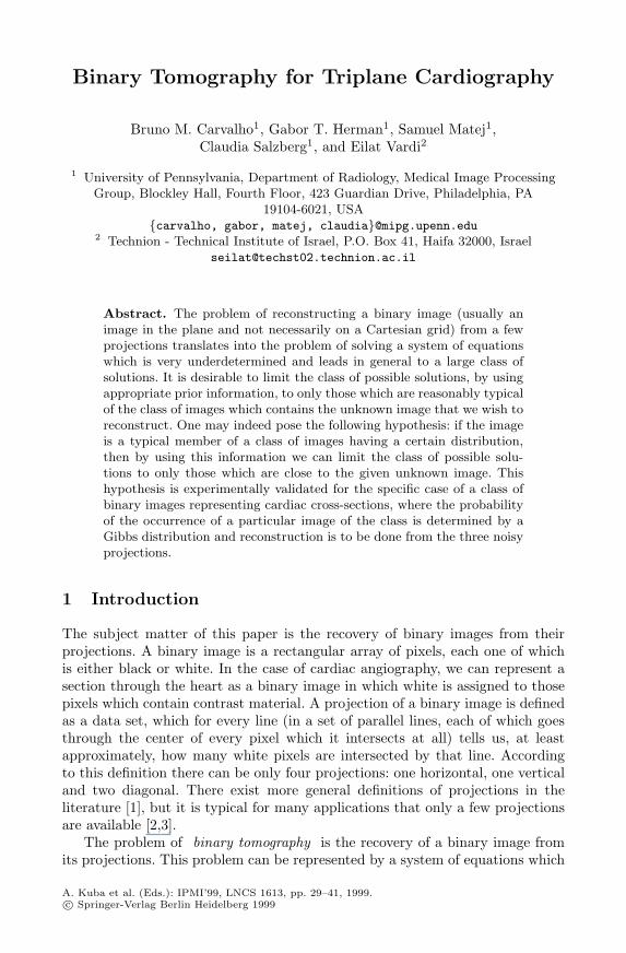
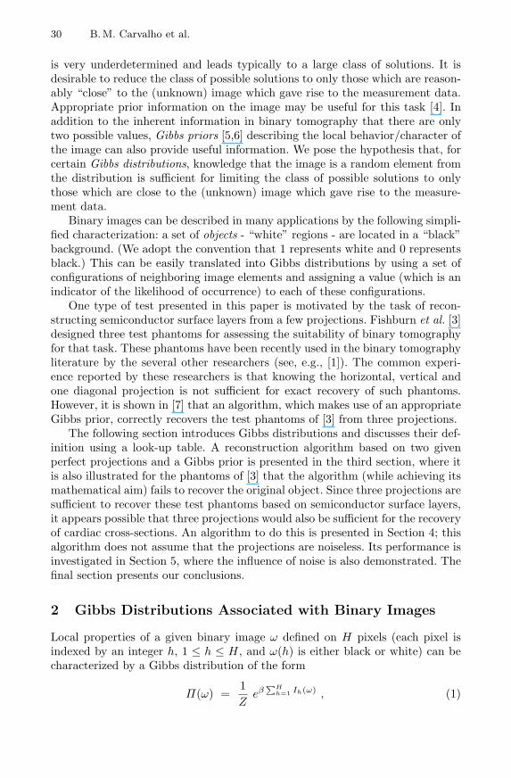
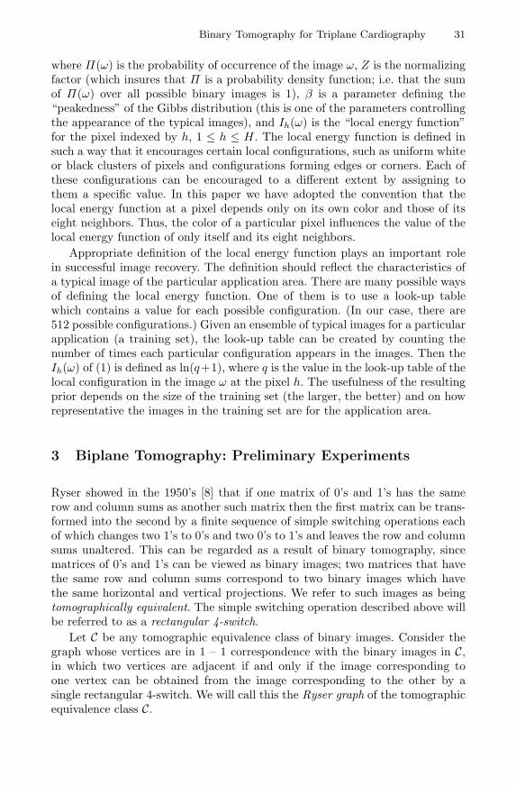
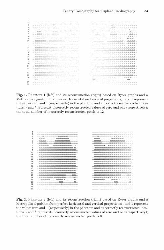
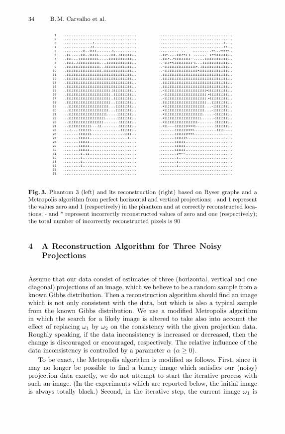
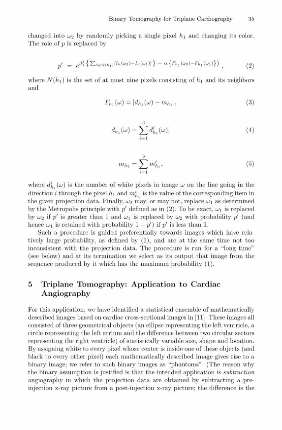
In order to test out our ideas on reconstructions from two projections, weimplemented the algorithms described in [9] and applied them to the binaryimages in [3] representing semiconductor surface layers. (For these experiments,the lookup-table was created using the three phantoms of [3].) For all threephantoms (these are shown on the left of Figs. 1, 2 and 3, respectively), thealgorithms of [9] performed “too well” in the sense that the reconstructed images(these are shown on the right of Figs. 1, 2 and 3, respectively) have a highervalue of Π(ω) than the originals. One might say after looking at these figuresthat the reconstructions are versions of the original binary images in which theboundaries have been smoothed.

As a result of these preliminary experiments combined with the fact thatall three phantoms of [3] were perfectly recovered when Gibbs priors were com-bined with three perfect projections [7], we decided to investigate the efficacy oftriplane rather than biplane cardio-angiography.

Binary Tomography for Triplane Cardiography 33

1 .............................................. ..............................................2 .............................................. ..............................................3 ....................11........................ ....................11........................4 ....................1111...................... ....................1111......................5 .....11.............11111.............1....... ....*11.............11111.............-.......6 ....1111............11111.............111..... ....1111............11111.............111.....7 ....11111..........1111111...........11111.... ...*11111..........1111111...........-1111....8 ...1111111.........1111111...........11111.... ...1111111.........1111111...........11111....9 ...11111111.......11111111..111.....1111111... ..*11111111.......11111111..111.....-111111...

10 ..11111111111...1111111111111111....11111111.. ..11111111111...1111111111111111....11111111..11 ..1111111111111111111111111111111...11111111.. ..1111111111111111111111111111111...11111111..12 ..11111111111111111111111111111111..11111111.. ..11111111111111111111111111111111..11111111..13 ..111111111111111111111111111111111111111111.. ..111111111111111111111111111111111111111111..14 ..111111111111111111111111111111111111111111.. ..111111111111111111111111111111111111111111..15 ..111111111111111111111111111111111111111111.. ..111111111111111111111111111111111111111111..16 ..111111111111111111111111111111111111111111.. ..111111111111111111111111111111111111111111..17 ..111111111111111111111111111111111111111111.. ..111111111111111111111111111111111111111111..18 ..111111111111111111111111111111111111111111.. ..111111111111111111111111111111111111111111..19 ..111111111111111111111111111111111111111111.. ..111111111111111111111111111111111111111111..20 ..111111111111111111111111111111111111111111.. ..111111111111111111111111111111111111111111..21 ..111111111111111111111111111111111111111111.. ..111111111111111111111111111111111111111111..22 ..111111111111111111111111111111111111111111.. ..111111111111111111111111111111111111111111..23 ..111111111111111111111111111111111111111111.. ..111111111111111111111111111111111111111111..24 ..111111111111111111111111111111111111111111.. ..111111111111111111111111111111111111111111..25 ..1111111111111111111111111111111111111111.... ..1111111111111111111111111111111111111111....26 ..11111111111111111111111........11111111..... ..11111111111111111111111........11111111.....27 ..111......................................... ..---...............................***.......28 .............................................. ..............................................29 .............................................. ..............................................

Fig. 1. Phantom 1 (left) and its reconstruction (right) based on Ryser graphs and aMetropolis algorithm from perfect horizontal and vertical projections; . and 1 representthe values zero and 1 (respectively) in the phantom and at correctly reconstructed loca-tions; - and * represent incorrectly reconstructed values of zero and one (respectively);the total number of incorrectly reconstructed pixels is 12

1 ......................................... .........................................2 ......................................... .........................................3 .....11..............1111111111.......... .....11..............1111111111..........4 ..111111...........1111111111111......... ..111111...........1111111111111.........5 ..1111111.........111111111111111........ ..1111111.........111111111111111........6 ..11111111.......11111111111111111....... ..11111111.......11111111111111111.......7 ..1111111111....1111111111111111111...1.. ..1111111111*...-111111111111111111...1..8 ..1111111111111111111111111111111111.11.. ..-111111111111111111111111111111111*11..9 ..1111111111111111111111111111111111111.. ..1111111111111111111111111111111111111..

10 ..1111111111111111111111111111111111111.. ..1111111111111111111111111111111111111..11 ..1111111111111111111111111111111111111.. ..1111111111111111111111111111111111111..12 ..1111111111111111111111111111111111111.. ..1111111111111111111111111111111111111..13 ..1111111111111111111111111111111111111.. ..1111111111111111111111111111111111111..14 ..1111111111111111111111111111111111111.. ..1111111111111111111111111111111111111..15 ..1111111111111111111111111111111111111.. ..1111111111111111111111111111111111111..16 ..1111111111111111111111111111111111111.. ..1111111111111111111111111111111111111..17 ..1111111111111111111111111111111111111.. ..1111111111111111111111111111111111111..18 ..1111111111111111111111111111111111111.. ..1111111111111111111111111111111111111..19 ..1111111111111111111111111111111111111.. ..1111111111111111111111111111111111111..20 ..111111111111111111111111111......1111.. ..111111111111111111111111111......1111..21 ..11111111111111.111111111111.......111.. ..11111111111111*111111111111.......-11..22 ...1111111111......1111111.1.........11.. ..*111111111-......1111111.1.........11..23 ......................1111...........11.. ......................1111...........11..24 ........................1................ ........................1................25 ......................................... .........................................26 ......................................... .........................................

Fig. 2. Phantom 2 (left) and its reconstruction (right) based on Ryser graphs and aMetropolis algorithm from perfect horizontal and vertical projections; . and 1 representthe values zero and 1 (respectively) in the phantom and at correctly reconstructed loca-tions; - and * represent incorrectly reconstructed values of zero and one (respectively);the total number of incorrectly reconstructed pixels is 8

34 B.M. Carvalho et al.

1 .......................................... ..........................................2 .......................................... ..........................................3 .................1........................ .................-...................*....4 ................11........................ ................--...................**...5 ...........11..1111.........1............. ...........--..----.........-.**...*****..6 ..11......111..11111.......111..11111111.. ..11*.....111**1-1--.......--1**11111111..7 ..111....11111111111......11111111111111.. ..111*..*111111111--......11111111111111..8 ..1111..1111111111111....111111111111111.. ..-111**11111111111-1....111111111111111..9 ..1111111111111111111...1111111111111111.. ..-111111111111111111*..1111111111111111..

10 ..11111111111111111111.11111111111111111.. ..-1111111111111111111*11111111111111111..11 ..11111111111111111111111111111111111111.. ..11111111111111111111111111111111111111..12 ..11111111111111111111111111111111111111.. ..11111111111111111111111111111111111111..13 ..11111111111111111111111111111111111111.. ..11111111111111111111111111111111111111..14 ..11111111111111111111111111111111111111.. ..11111111111111111111111111111111111111..15 ..1111111111111111111111111.111111111111.. ..-111111111111111111111111*111111111111..16 ..1111111111111111111111111..11111111111.. ..-111111111111111111111111.*11111111111..17 ..1111111111111111111111111..11111111111.. ..-111111111111111111111111.*11111111111..18 ..1111111111111111111111111...1111111111.. ..1111111111111111111111111...1111111111..19 ...11111111111111111111111....1111111111.. ..*11111111111111111111111....-111111111..20 ...11111111111111111111111....1111111111.. ..*11111111111111111111111....-111111111..21 ...1111111111111111111111......111111111.. ..*1111111111111111111111......-11111111..22 ...111111111111111111111.......111111111.. ..*111111111111111111111.......-11111111..23 ...11111111111111111111.........11111111.. ..*1111111111111111111-.........11111111..24 ...1111111111111....11..........11111111.. ..*11----1111111****1-..........11111111..25 ....1....1111111.................1111111.. ....-....1111111****.............1111---..26 .........1111111...................1111... .........1111111****...............----...27 .........111111......................1.... .........111111*.....................-....28 .........111111........................... .........111111...........................29 .........111111........................... .........111111...........................30 .........111111........................... .........111111...........................31 ..........1..11........................... ..........1**--...........................32 ..........1............................... ..........1...............................33 ..........1............................... ..........1...............................34 ..........1............................... ..........1...............................35 .......................................... ..........................................36 .......................................... ..........................................

Fig. 3. Phantom 3 (left) and its reconstruction (right) based on Ryser graphs and aMetropolis algorithm from perfect horizontal and vertical projections; . and 1 representthe values zero and 1 (respectively) in the phantom and at correctly reconstructed loca-tions; - and * represent incorrectly reconstructed values of zero and one (respectively);the total number of incorrectly reconstructed pixels is 90

4 A Reconstruction Algorithm for Three NoisyProjections

Assume that our data consist of estimates of three (horizontal, vertical and onediagonal) projections of an image, which we believe to be a random sample from aknown Gibbs distribution. Then a reconstruction algorithm should find an imagewhich is not only consistent with the data, but which is also a typical samplefrom the known Gibbs distribution. We use a modified Metropolis algorithmin which the search for a likely image is altered to take also into account theeffect of replacing ω1 by ω2 on the consistency with the given projection data.Roughly speaking, if the data inconsistency is increased or decreased, then thechange is discouraged or encouraged, respectively. The relative influence of thedata inconsistency is controlled by a parameter α (α ≥ 0).

To be exact, the Metropolis algorithm is modified as follows. First, since itmay no longer be possible to find a binary image which satisfies our (noisy)projection data exactly, we do not attempt to start the iterative process withsuch an image. (In the experiments which are reported below, the initial imageis always totally black.) Second, in the iterative step, the current image ω1 is

Binary Tomography for Triplane Cardiography 35

changed into ω2 by randomly picking a single pixel h1 and changing its color.The role of p is replaced by

p′ = eβ({∑h∈N(h1)[Ih(ω2)−Ih(ω1)]} − α{Fh1 (ω2)−Fh1 (ω1)}) , (2)

where N(h1) is the set of at most nine pixels consisting of h1 and its neighborsand

Fh1(ω) = |dh1(ω)−mh1 |, (3)

dh1(ω) =3∑

i=1

dih1

(ω), (4)

mh1 =3∑

i=1

mih1

, (5)

where dih1

(ω) is the number of white pixels in image ω on the line going in thedirection i through the pixel h1 and mi

h1is the value of the corresponding item in

the given projection data. Finally, ω2 may, or may not, replace ω1 as determinedby the Metropolis principle with p′ defined as in (2). To be exact, ω1 is replacedby ω2 if p′ is greater than 1 and ω1 is replaced by ω2 with probability p′ (andhence ω1 is retained with probability 1− p′) if p′ is less than 1.

Such a procedure is guided preferentially towards images which have rela-tively large probability, as defined by (1), and are at the same time not tooinconsistent with the projection data. The procedure is run for a “long time”(see below) and at its termination we select as its output that image from thesequence produced by it which has the maximum probability (1).

5 Triplane Tomography: Application to CardiacAngiography

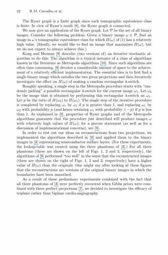
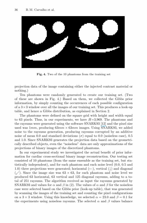
For this application, we have identified a statistical ensemble of mathematicallydescribed images based on cardiac cross-sectional images in [11]. These images allconsisted of three geometrical objects (an ellipse representing the left ventricle, acircle representing the left atrium and the difference between two circular sectorsrepresenting the right ventricle) of statistically variable size, shape and location.By assigning white to every pixel whose center is inside one of these objects (andblack to every other pixel) each mathematically described image gives rise to abinary image; we refer to such binary images as “phantoms”. (The reason whythe binary assumption is justified is that the intended application is subtractionangiography in which the projection data are obtained by subtracting a pre-injection x-ray picture from a post-injection x-ray picture; the difference is the

36 B.M. Carvalho et al.

Fig. 4. Two of the 10 phantoms from the training set

projection data of the image containing either the injected contrast material ornothing.)

Ten phantoms were randomly generated to create our training set. (Twoof these are shown in Fig. 4.) Based on them, we collected the Gibbs priorinformation, by simply counting the occurrences of each possible configurationof a 3×3 window over all the images of our training set. This produces a look-uptable, and hence a Gibbs distribution, as explained in Section 2.

The phantoms were defined on the square grid with height and width equalto 63 pixels. Thus, in our experiments, we have H=3,969. The phantoms andthe raysums were generated using the software SNARK93 [12] and the pixel sizeused was 1mm, producing 63mm × 63mm images. Using SNARK93, we addednoise to the raysums generation, producing raysums corrupted by an additivenoise of mean 0.0 and standard deviations (σ) equal to 0.0 (noiseless case), 0.5and 1.0. Since SNARK93 generates the projection data based on the geometri-cally described objects, even the “noiseless” data are only approximations of theprojections of binary images of the discretized phantoms.

In our experimental study we investigated the actual benefit of prior infor-mation for cardiac cross-sectional binary image reconstruction. Our testing setconsisted of 10 phantoms (from the same ensemble as the training set, but sta-tistically independent), and for each phantom and each noise level (0.0, 0.5 and1.0) three projections were generated; horizontal (←), vertical (↓) and diagonal(↙). Since the image size was 63 × 63, for each phantom and noise level weproduced 63 horizontal, 63 vertical and 125 diagonal raysums, adding to a to-tal of 251 raysums. The algorithm received as input the raysums generated bySNARK93 and values for α and β in (2). The values of α and β for the noiselesscase were selected based on the Gibbs prior (look-up table), that was generatedby scanning the images of the training set and counting the pixel configurationson a 3× 3 window. Using this knowledge, we selected α = 23.0 and β = 0.1 forthe experiments using noiseless raysums. The selected α and β values balance

Binary Tomography for Triplane Cardiography 37

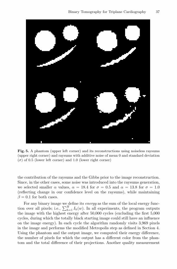
Fig. 5. A phantom (upper left corner) and its reconstructions using noiseless raysums(upper right corner) and raysums with additive noise of mean 0 and standard deviation(σ) of 0.5 (lower left corner) and 1.0 (lower right corner)

the contribution of the raysums and the Gibbs prior to the image reconstruction.Since, in the other cases, some noise was introduced into the raysums generation,we selected smaller α values, α = 18.4 for σ = 0.5 and α = 13.8 for σ = 1.0(reflecting change in our confidence level on the raysums), while maintainingβ = 0.1 for both cases.

For any binary image we define its energy as the sum of the local energy func-tion over all pixels; i.e.,

∑Hh=1 Ih(w). In all experiments, the program outputs

the image with the highest energy after 50,000 cycles (excluding the first 5,000cycles, during which the totally black starting image could still have an influenceon the image energy). In each cycle the algorithm randomly visits 3,969 pixelsin the image and performs the modified Metropolis step as defined in Section 4.Using the phantom and the output image, we computed their energy difference,the number of pixels for which the output has a different color from the phan-tom and the total difference of their projections. Another quality measurement

38 B.M. Carvalho et al.

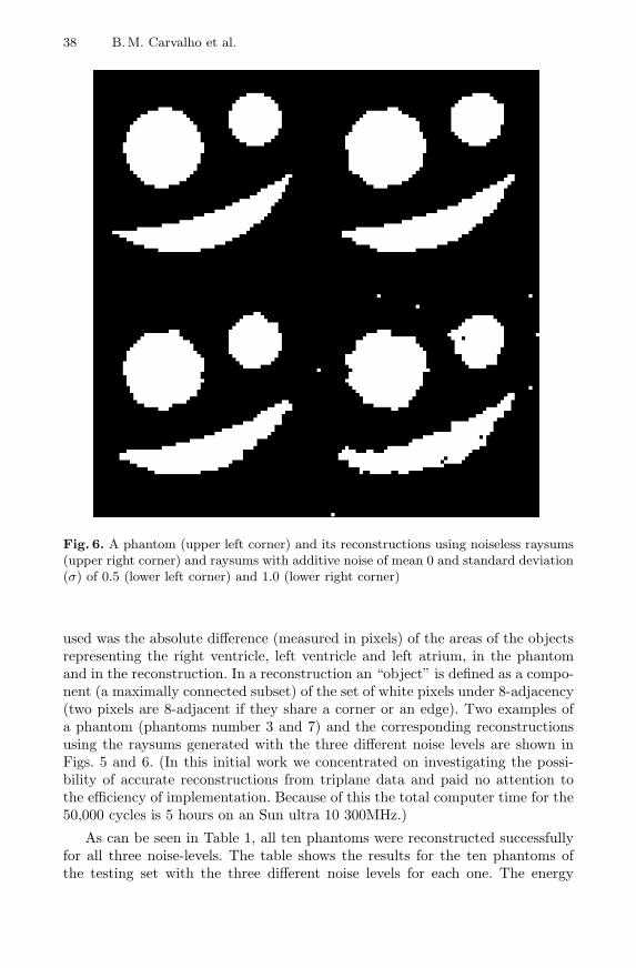
Fig. 6. A phantom (upper left corner) and its reconstructions using noiseless raysums(upper right corner) and raysums with additive noise of mean 0 and standard deviation(σ) of 0.5 (lower left corner) and 1.0 (lower right corner)

used was the absolute difference (measured in pixels) of the areas of the objectsrepresenting the right ventricle, left ventricle and left atrium, in the phantomand in the reconstruction. In a reconstruction an “object” is defined as a compo-nent (a maximally connected subset) of the set of white pixels under 8-adjacency(two pixels are 8-adjacent if they share a corner or an edge). Two examples ofa phantom (phantoms number 3 and 7) and the corresponding reconstructionsusing the raysums generated with the three different noise levels are shown inFigs. 5 and 6. (In this initial work we concentrated on investigating the possi-bility of accurate reconstructions from triplane data and paid no attention tothe efficiency of implementation. Because of this the total computer time for the50,000 cycles is 5 hours on an Sun ultra 10 300MHz.)

As can be seen in Table 1, all ten phantoms were reconstructed successfullyfor all three noise-levels. The table shows the results for the ten phantoms ofthe testing set with the three different noise levels for each one. The energy

Binary Tomography for Triplane Cardiography 39

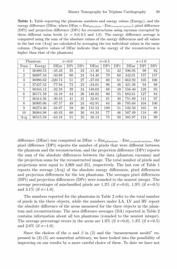
Table 1. Table reporting the phantom numbers and energy values (Energy), and theenergy difference (DEnr, where DEnr = Enrphantom - Enrreconstruction), pixel difference(DPi) and projection difference (DPr) for reconstructions using raysums corrupted bythree different noise levels (σ = 0.0, 0.5 and 1.0). The energy difference average iscomputed using the sum of the absolute values of the energy differences and all valuesin the last row (Avg) are calculated by averaging the ten individual values in the samecolumn. (Negative values of DEnr indicate that the energy of the reconstruction ishigher than that of the phantom)

Phantom σ=0.0 σ=0.5 σ=1.0Num Energy DEnr DPi DPr DEnr DPi DPr DEnr DPi DPr

1 36480.53 -45.43 35 23 -11.40 54 42 596.05 98 822 36087.34 -50.89 60 24 -54.48 79 60 442.01 157 1573 36986.62 -220.74 51 27 -27.03 60 61 662.92 105 1064 37427.52 -77.94 72 23 -34.01 96 46 421.38 94 885 36344.12 -32.58 39 24 149.69 68 49 556.40 128 956 36171.59 16.10 44 26 148.82 80 55 682.61 127 847 36414.56 -30.55 41 31 32.81 61 40 751.89 141 978 36905.06 -97.57 49 24 -62.91 64 46 705.68 104 1009 36273.46 -56.87 59 20 155.52 109 51 532.50 165 9110 36064.98 -40.43 60 26 84.34 77 46 507.49 118 89

Avg 36515.58 -63.18 51 25 38.13 75 50 585.97 124 99

difference (DEnr) was computed as DEnr = Enrphantom - Enrreconstruction, thepixel difference (DPi) reports the number of pixels that were different betweenthe phantom and the reconstruction, and the projection difference (DPr) reportsthe sum of the absolute differences between the data (phantom raysums) andthe projection sums for the reconstructed image. The total number of pixels andprojections were equal to 3,969 and 251, respectively. The last row of Table 1reports the average (Avg) of the absolute energy differences, pixel differencesand projection differences for the ten phantoms. The averages pixel differences(DPi) and projection differences (DPr) were rounded to the nearest integer. Theaverage percentages of misclassified pixels are 1.3% (if σ=0.0), 1.9% (if σ=0.5)and 3.1% (if σ=1.0).

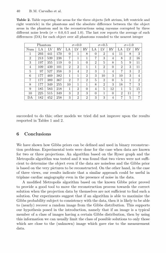
The numbers reported for the phantoms in Table 2 refer to the total numberof pixels in the three objects, while the numbers under LA, LV and RV reportthe absolute difference of the areas measured for the three objects in the phan-tom and reconstructions. The area difference averages (DA) reported in Table 2contains information about all ten phantoms (rounded to the nearest integer).The average percentage errors in the areas are 1.0% (if σ=0.0), 1.3% (if σ=0.5)and 2.6% (if σ=1.0).

Since the choices of the α and β in (2) and the “measurement model” ex-pressed in (3)-(5) are somewhat arbitrary, we have looked into the possibility ofimproving on our results by a more careful choice of these. To date we have not

40 B.M. Carvalho et al.

Table 2. Table reporting the areas for the three objects (left atrium, left ventricle andright ventricle) in the phantoms and the absolute difference between the the objectareas in the phantom and in the reconstructions using raysums corrupted by threedifferent noise levels (σ = 0.0, 0.5 and 1.0). The last row reports the average of suchdifferences (DA) for each object over all phantoms rounded to the nearest integer

Phantom σ=0.0 σ=0.5 σ=1.0Num LA LV RV LA LV RV LA LV RV LA LV RV

1 293 441 170 0 1 8 0 2 4 11 8 32 213 539 238 7 1 1 7 3 4 8 2 163 197 355 119 0 1 0 2 5 8 5 9 114 109 439 101 2 2 1 1 2 0 2 3 115 97 527 358 3 4 2 3 1 4 7 3 26 177 469 382 1 1 2 3 10 3 10 3 47 177 389 367 2 7 2 5 2 0 5 1 28 177 349 255 10 1 1 8 2 3 18 7 39 185 583 218 1 2 0 4 5 12 1 5 1510 225 515 349 3 2 3 0 1 0 2 11 7DA 182 452 258 3 2 2 3 3 4 7 5 7

succeeded to do this; other models we tried did not improve upon the resultsresported in Tables 1 and 2.

6 Conclusions

We have shown how Gibbs priors can be defined and used in binary reconstruc-tion problems. Experimental tests were done for the case when data are knownfor two or three projections. An algorithm based on the Ryser graph and theMetropolis algorithm was tested and it was found that two views were not suffi-cient to determine the object even if the data are noiseless and the Gibbs prioris based on the very pictures to be reconstructed. On the other hand, in the caseof three views, our results indicate that a similar approach could be useful intriplane cardiac angiography even in the presence of noise in the data.

A modified Metropolis algorithm based on the known Gibbs prior provedto provide a good tool to move the reconstruction process towards the correctsolution when the projection data by themselves are not sufficient to find such asolution. Our experiments suggest that if an algorithm is able to maximize theGibbs probability subject to consistency with the data, then it is likely to be ableto (nearly) recover a random image from the Gibbs distribution. This supportsour hypothesis posed in the introduction, namely that if an image is a typicalmember of a class of images having a certain Gibbs distribution, then by usingthis information we can usually limit the class of possible solutions to only thosewhich are close to the (unknown) image which gave rise to the measurementdata.

Binary Tomography for Triplane Cardiography 41

Acknowledgements

This work was supported by the National Science Foundation Grant DMS-9612077, by the National Institutes of Health Grants HL-28438 and CA-54356and by CAPES-BRASILIA-BRAZIL.

References

1. Herman, G.T., Kuba, A. (eds.): Special Issue on Discrete Tomography. Int. J.Imaging Syst. and Technol. 9 No. 2/3 (1998)

2. Chang, S.-K., Chow, C. K.: The Reconstruction of Three-Dimensional Objectsfrom Two Orthogonal Projections and its Application to Cardiac Cineangiography.IEEE Trans. on Computers 22 (1973) 18-28

3. Fishburn, P., Schwander, P., Shepp, L., Vanderbei, R.J.: The Discrete Radon Trans-form and its Approximate Inversion via Linear Programming. Discrete AppliedMathematics 75 (1997) 39-61

4. Chan, M.T., Herman, G.T., Levitan, E.: A Bayesian Approach to PET Recon-struction Using Image-Modeling Gibbs Priors: Implementation and Comparison.IEEE Trans. Nucl. Sci. 44 (1997) 1347-1354

5. Winkler, G.: Image Analysis, Random Fields and Dynamic Monte Carlo Methods.Springer-Verlag, Berlin Heidelberg New York (1995)

6. Levitan, E., Chan, M., Herman, G.T.: Image-Modeling Gibbs Priors. Graph. Mod-els Image Proc. 57 (1995) 117-130

7. Matej, S., Vardi, A., Herman, G.T., Vardi, E.: Binary Tomography Using GibbsPriors. In Herman, G.T., Kuba, A. (eds.): Discrete Tomography: Foundations,Algorithms and Applications. Birkhauser, Boston Cambridge (to appear)

8. Ryser, H.J.: Combinatorial Properties of Matrices of Zeros and Ones. Can. J.Mathematics 9 (1957) 371-377

9. Kong, T.Y., Herman, G.T.: Tomographic Equivalence and Switching Operations.In Herman, G.T., Kuba, A. (eds.): Discrete Tomography: Foundations, Algorithmsand Applications. Birkhauser, Boston Cambridge (to appear)

10. Metropolis, N., Rosenbluth, A.W., Rosenbluth, M.N., Teller, A.H., Teller, E.: Equa-tions of State Calculations by Fast Computing Machines. J. Chem. Phys. 21, (1953)1087-1092

11. Ritman, E.L., Robb, R.A., Harris, L.D.: Imaging Physiological Functions. Praeger,New York (1985)

12. Browne, J.A., Herman, G.T., Odhner, D.: SNARK93: A Programming Systemfor Image Reconstruction from Projections. Technical Report No. 198. MedicalImage Processing Group, Department of Radiology, University of Pennsylvania,Philadelphia (1993)